CONGESTION-DRIVEN DENDRITIC GROWTH

BERTRAND MAURY, AUDE ROUDNEFF-CHUPIN AND FILIPPO SANTAMBROGIO

Abstract. In order to observe growth phenomena in biology where dendriticshapes appear, we propose a simple model where a given population evolvesfeeded by a diffusing nutriment, but is subject to a density constraint. Theparticles (e.g., cells) of the population spontaneously stay passive at rest, andonly move in order to satisfy the constraint ρ ≤ 1, by choosing the minimalcorrection velocity so as to prevent overcongestion. We treat this constraint bymeans of projections in the space of densities endowed with the Wassersteindistance W2, defined through optimal transport. This allows to provide anexistence result and suggests some numerical computations, in the same spiritof what the authors did for crowd motion (but with extra difficulties, essentiallydue to the fact that the total mass may increase). The numerical simulationsshow, according to the values of the parameter and in particular of the diffusioncoefficient of the nutriment, the formation of dendritic patterns in the spaceoccupied by cells.

1. Introduction

Dendritic growth is very common in nature: solidified alloys, snowflake forma-tion, corals, bacterial colonies, and some viscous fluid flows, present similar branch-ing patterns. Those patterns reflect a wide variety of mechanisms. In most cases,branches result from an external supply of a diffusing substance. The simplestmodel for such a phenomenon is the following (Diffusion Limited Aggregation [29]).An initial particle (seed) is located at some point, a second particle is introduced ata large distance from the seed, and is assumed to perform a random walk. When-ever it contacts the seed before escaping to infinity, it is assumed to irreversiblystick to it. A third particle is then introduced, and so on. When a new particleapproaches the cluster, it is more likely to hit a growing part than a part close tothe seed, which tends to generate highly irregular patterns. In the context of cellgrowth, the cluster corresponds to a zone occupied by living cells that grow at arate depending of the local concentration of some nutrient. The latter substancediffuses outside the cluster, so that, like in the DLA process, nutrients are likely tobe eaten before reaching the “fjords”. Thus, the tips receive more nutrients thanunderdeveloped zone, which may tend again to develop branches. Yet, the actualgrowth of a branching cluster necessitates to account for cell motion. Linear diffu-sion for the cells does not lead to dendritic growth, but more sophisticated models(Kitsunezaki [13] or Kawaski [12], see details below) reproduce branching patternsat different scales.

We aim here at investigating the possibility that the motion of cells, and therebythe emergence of branching patterns, may result from a very simple mechanism,namely congestion. We shall focus on the specify situation of Bacillus subtiliscolonies, but the principles are quite general: we shall consider a population ofentities that grow at a rate which depends on the local concentration of a nutrient.

1

2 B. MAURY, A. ROUDNEFF-CHUPIN AND F. SANTAMBROGIO

The nutrient propagates by passive diffusion (linear Fick’s Law), whereas the mainentity does not. The latter is simply subject to a maximal density constraint. Whenthe maximal density is attained, entities push against each other, which induces amotion that ensures that the density constraint is not violated. We shall simply as-sume here that the correction velocity field that advects the entities is the minimalone (in the sense that it minimizes the L2 norm) among those that preserve thedensity constraint. Before detailing this approach, we first give an overview of thedifferent models that have been proposed in the literature to describe the growthof such cells.

Bacterial colonies of Bacillus subtilis develop very different patterns, dependingon the conditions they grow into. Many experiments have been conducted to de-termine the morphological changes arising when the culture parameters are varied(see for instance the work of Matsushita and Fujikawa [9, 16, 10] and Ben-Jacob etal. [4]). In these experiments, bacteria are inoculated in the center of agar plates ofthickness small enough to ensure a two-dimensional evolution of the system. Onlytwo parameters are varied: the concentration of nutrients, denoted by Cn, and thehardness of the medium, controlled by the agar concentration Ca. Other parameterssuch as temperature are kept constant.

Five distinct morphological types have been identified (see Figure 1). In regionA, for low concentrations of nutrients and hard media, bacterial colonies are grow-ing through DLA processes ([29]). It appears that bacteria cannot move at theseconcentrations of agar, and that their evolution is only due to cell-division, thanksto the diffusion of the nutrients towards the colony (see Matsushita et al. [17]). Asthe nutrient concentration increases, colony branches become thicker and finallyform compact patterns (region B). The growth is also faster as Cn increases. Forintermediate hardness of agar, and high levels of nutrients (region C), the evolutionconsists of alternative expanding and consolidating phases, forming concentric ringpatterns. Decreasing again the softness of the medium (region D), bacteria are ableto move on the agar surface. Their evolution is the conjunction of cell-division anddiffusion, and the growth consists of a disk expanding rapidly. Finally, for inter-mediate values of Ca and low levels of nutrients, bacterial colonies develop densebranches, the envelope of which is smooth and circular (region E).

Many models have been proposed to reproduce these morphological changes.Some are microscopic and describe the behavior of each bacteria (see for instancethe communicating walkers models of Ben-Jacob et al. [5] or the cellular-automatonmodel described in [3]), but most of them are macroscopic and study the two-dimensional density of the bacterial colony via a reaction-diffusion equation. Avery simple model to account for the time evolution of the densities of bacteria andnutrients b and n would be

(1)

∂tb = Db∆b + nb

∂tn = Dn∆n− nb.

Unfortunately, system (1) cannot reproduce the emergence of branching patterns.In [13], Kitsunezaki proposes a model of non-linear diffusion, where two differenttypes of cells are considered: active ones (which move actively and perform cell-divisions) of density b, and inactive ones, their density being denoted by a. The

CONGESTION-DRIVEN DENDRITIC GROWTH 3

Figure 1. Morphology diagram of Bacillus subtilis colonies grownby Matsushita et al. [17].

reaction-diffusion equation becomes

(2)

∂tb = D∆(bm+1) + nb− µb

∂tn = ∆n− nb

∂ta = µb.

Branching patterns can be obtained for suitable parameters. Kawaski et al. proposeanother non-linear diffusion model, where the diffusion coefficient is proportionalto nb, pointing out that bacteria are active mostly in the regions where nutrientsare abundant (see [12]). This nutrient-dependent diffusion ensures the creation ofbranches without the need of adding a death term, as it is for instance the case inthe models proposed in [18, 19, 20] by Mimura et al. More precisely, their modelinclude a death term in the bacterial population of the form

− µb

(1 + b)(1 + n).

The numerical simulations reproduce different morphological patterns. Moreover,the authors prove in [8, 23] the existence and uniqueness of the solution of thereaction-diffusion system, and characterize the asymptotic behavior of the totalbacterial population. More complicated models include specific features, such asthe presence of some lubricating fluid produced by the cells (see [11]), the effectsof chemotaxis described for example in [11, 15], or different states of mobility forbacteria, as in [14].

We focus here on the case of hard media (high concentrations Ca), where bacteriacannot move on the agar surface. It has been pointed out in [17] that cell-divisionsare in this case the only cause of growth. However, as explained before, the simplereaction-diffusion system

(3)

∂tb = nb

∂tn = Dn∆n− nb.

4 B. MAURY, A. ROUDNEFF-CHUPIN AND F. SANTAMBROGIO

cannot produce branching patterns, which must be a consequence of other featureswhich are still to be added to this system. In the spirit of the models studied in thecontext of crowd movements (see [21, 22]) and cell-migration (see [7]), we propose totake into account the congestion of the bacterial population throught the constraint

b ≤ 1.

This constraint can be seen as a formal limit of the non-linear diffusion term

∇ · (bm∇b)when m tends to infinity. As a matter of fact, this diffusion term tends to penalizehigh bacterial densities, and can be seen as a form of soft congestion, oppositeto imposing a maximal density constraint, which is usually called hard congestion(see [22] for more details on the different ways of dealing with congestion). Despiteits very simple formulation, this model contains many difficulties, both theoreticaland numerical. In particular, classical methods are inefficient to prove the well-posedness of this type of problems. In [21], we turned to the theory of optimaltransport and gradient flows (see [1, 2, 27, 28]) to prove an existence result.

We detail in Section 2 the rigorous formulation of the model. We prove anexistence result in section 3, adapting the results obtained in [21] to the case wherethe total population is growing. Numerical simulations are presented in section 4.

2. Description of a model driven by congestion

2.1. The congestion model. We propose in this work to take into account thecongestion of the bacterial population through the constraint

b ≤ 1

which has to be satisfied almost everywhere in the bounded domain Ω. Since theexperimental conditions ensure a two-dimensional evolution for the bacteria, thismaximal density constraint makes sense. Here the limit density has been fixed to 1for simplicity, but it can be changed to any other value without loss of generality.The reaction-diffusion system describing our model writes

(4)

∂tb+∇ · (bu) = nb in Ω,

∂tn = Dn∆n− nb in Ω,

where u is the minimal correction velocity (in a mean square sense) ensuring thatthe density b does not exceed 1. This velocity has to counterbalance the growthof the bacterial population, given by the term nb. More precisely, we choose thevelocity which minimizes the L2 norm among the admissible velocities, which areroughly speaking the vector fields v such that ∇ · v ≥ n. More precisely, we definethe set Cb of admissible velocities by

(5) Cb =

v ∈ (L2(Ω))2 :

∫

Ω

v · ∇q ≤ −∫

Ω

nq, ∀q ∈ H1b

.

Here H1b denotes a set of functions acting supported in the saturated area [b = 1] :

(6) H1b =

q ∈ H1(Ω), q ≥ 0, q(1− b) = 0

.

Since the system evolves in a closed medium (the agar plate), we impose no-fluxconditions for the nutrients on the boundary

(7) ∇n · ν = 0 on ∂Ω,

CONGESTION-DRIVEN DENDRITIC GROWTH 5

where ν denotes the outward normal of Ω.Note that this model expresses the basic principles of bacterial growth. The

nutrients diffuse through the medium, and are consumed by the bacteria. Thespatial expansion of the bacterial colony is due to the correction velocity only. Thiscorrection velocity is non-zero whenever there is a sufficient supply of nutrient toinduce a growth that activates the maximal density constraint.

Definition 2.1 (Weak solutions). We shall say that (b, n) is a weak solutionto (4)–(7) for initial data (b0, n0) whenever for all ϕ ∈ C1

c ([0, T [,Ω), for all ψ ∈C1

c ([0, T [,Ω), we have∫ T

0

∫

Ω

(∂tϕ(t, x) +∇ϕ(t, x) · u(t, x) + n(t, x)ϕ(t, x)) b(t, x) dx dt

+

∫

Ω

ϕ(0, x)b0(x) dx = 0

and∫ T

0

∫

Ω

(∂tψ(t, x)n(t, x) −Dn∇ψ(t, x) · ∇n(t, x) − ψ(t, x)n(t, x)b(t, x)) dx dt

+

∫

Ω

ψ(0, x)n0(x) dx = 0.

The set Cb defined by (5) is closed and convex, therefore there is a unique u withminimal L2 norm. We shall use in the proof the saddle-point characterization ofthis minimizer:

Lemma 2.2. If (u, p) ∈ L2(Ω)2 ×H1b is such that

(8)

u+∇p = 0,∫

Ω

u · ∇q ≤ −∫

Ω

nq, ∀q ∈ H1b

and such that (complementary slackness condition)∫

Ω

u · ∇p = −∫

Ω

np,

then u minimizes the L2 norm over Cb.

Proof. The second equation of (8) ensures that u ∈ Cb. Now, from the first equationof (8), u minimizes the quadratic functional

v 7−→ 1

2||v||2L2 +

∫

Ω

(v · ∇p+ np) .

Thanks to the slackness condition, it holds that

1

2||u||2L2 +

∫

Ω

(u · ∇p+ np)

︸ ︷︷ ︸

=0

≤ 1

2||v||2L2 +

∫

Ω

(v · ∇p+ np) .

For any v ∈ Cb, the second term of the right-hand side above is non-positive, thus||u|| ≤ ||v||.

6 B. MAURY, A. ROUDNEFF-CHUPIN AND F. SANTAMBROGIO

Remark 1. The couple (u, p) ∈ L2(Ω)2 ×H1b is a saddle-point for the Lagrangian

L(v, q) =1

2||v||2L2 +

∫

Ω

(v · ∇q + nq) ,

i.e. it holds

L(u, q) ≤ L(u, p) ≤ L(v, p) ∀(v, q) ∈ L2(Ω)2 ×H1b .

Despite its simple formulation, this model arises several difficulties. In particular,the correction velocity has no a priori regularity (else than L2), and depends on bthrough a highly non-linear equation. This prevents us from using classical methodsboth in the theoretical and numerical aspects. We encountered the same difficultiesin [21] in the context of crowd motion. The evolution equation studied there wasvery similar to the present one, since the crowd had also to respect a maximaldensity constraint. In this work, the problem had been reformulated as a gradientflow in the space of Wasserstein. The Wasserstein distance is indeed well-fitted toconsider displacements between measures of same total mass. It is defined (see formore details [27, 28]) as the minimal transport cost from a measure µ to a measureν. More precisely, if µ and ν are absolutely continuous measures, it writes

(9) W 22 (µ, ν) = min

t#µ=ν

∫

Ω

|t(x) − x|2 dµ(x),

where t#µ denotes the push-forward measure of µ by t. In this context, it waspossible to obtain an existence result for the gradient flow problem, and prove thatthis implies a solution to the original system.

We cannot apply straightforwardly these methods to our system. First, the totalmass of the bacterial density grows as time runs by, and this prevents us to considerthe Wasserstein distance between them. Moreover, since System (4) is a coupledreaction-diffusion system, we have to deal with an evolving density of nutrients. Wepresent in the next section a splitting discrete scheme which makes it possible toovercome these two major difficulties.

2.2. Description of an approximation scheme. In order to prove the existenceof a solution, we consider an approximating scheme of system (4). At each timestep, we first let the bacterial density grow thanks to the provision of nutrients,disregarding the congestion constraint. Then we take the nearest bacterial densityamong the densities which obey the constraint b ≤ 1. More precisely, for a timestep τ > 0, starting from initial conditions

b0τ = b0, nτ (0, ·) = n0,

we define discrete densities bkτ thanks to the splitting scheme

(10)

bkτ = bk−1τ exp

(∫ kτ

(k−1)τ

nτ (s, .) ds

)

,

bkτ = PKmkbkτ ,

where nτ is defined by taking, on each interval [(k − 1)τ, kτ ], the solution of

(11) ∂tnτ = Dn∆nτ − nτbk−1τ t ∈ [(k − 1)τ, kτ ],

(more precisely: on each interval [(k − 1)τ, kτ ] the density bk−1τ is considered to be

given, as well as the initial value of nτ at time t = (k − 1)τ , then nτ is computed

CONGESTION-DRIVEN DENDRITIC GROWTH 7

as the solution of the above equation on [(k − 1)τ, kτ ], which makes it possible toupdate the value of bkτ and nτ (kτ, ·) for the next interval).

Here, PKmdenotes the projection for the Wasserstein distance (defined in (9))

on the set of densities of total mass m, which satisfies the congestion constraint:

(12) Km =

b ∈M+(Ω) :

∫

Ω

b = m, b ≤ 1

,

and mk is the total mass of bkτ (and bkτ as well). Here M+(Ω) stands for the set ofpositive finite measures on Ω. The constraint b ≤ 1 means in particular that theyshould be absolutely continuous, and they are therefore confused with their density.

Indeed, it can be established (for details see [22], Proposition 2) that the distancebetween any given density of mass mk and the set Km attains its minimum at aunique point.

Note that bkτ is the solution at time kτ of

∂tb = nτ b,

b((k − 1)τ, .) = bk−1τ ,

and that the equations on nτ and bkτ are no more coupled, since the equation on nτ

only involves bk−1τ .

Our goal is to prove that these discrete densities converge to a solution of Sys-tem (4) as τ tends to 0. With this aim in view, we define two families of interpolatedcurves. The first one will be used to prove that the congestion constraint is satisfied,and is defined by

bτ (t, .) = bkτ , t ∈](k − 1)τ, kτ ],

whereas nτ is simply given as the solution of (11). We also define discrete velocitiesfor the projection step as

(13) vkτ =

id− tkττ

,

where tkτ is the optimal transport from bkτ to bkτ . These velocities are interpolatedthrough

vτ (t, .) = vkτ t ∈](k − 1)τ, kτ ],

and we also define the quantities

Eτ (t, .) = bkτvkτ t ∈](k − 1)τ, kτ ].

The second family of interpolated curves will ensure that the limit densities aresolutions of the reaction-diffusion system. We denote (see Fig. 2)

(14) bτ (t) = (Tkt )#b

kτ (t)

(notice that both sides of this equation are functions - densities of non-negativemeasures of mass mk, actually - of the variable x, but the dependence will be often

omitted in the sequel for similar objects), where Tkt and bkτ (t) are defined by

(15)

Tkt = id+

t− (k − 1)τ

τ(rkτ − id), bkτ (t, .) = bk−1

τ exp

(∫ t

(k−1)τ

nτ (s, .) ds

)

,

and rkτ is the optimal transport from bkτ to bkτ (note that rkτ = (tkτ )−1). The nutrient

density is simply given by

(16) nτ (t, x) = nτ (t, (Tkt )

−1(x)), t ∈](k − 1)τ, kτ ],

8 B. MAURY, A. ROUDNEFF-CHUPIN AND F. SANTAMBROGIO

and we denote by vτ the following interpolated velocity

vτ (t, .) =rkτ − id

τ (Tk

t )−1, t ∈](k − 1)τ, kτ ].

Note that on each interval ](k − 1)τ, kτ ], we have vτ = vτ rkτ (Tkt )

−1. Finally,we define

Eτ = bτ vτ .

We will prove in section 3 that these curves are somehow solutions of the reaction-diffusion equation we consider at a discrete level.

rkτTkt

bkτ

bk−1τ

bτ (t)

bkτ

bkτ (t)

Exponential growth

Projection onto Kmk

Figure 2. Interpolation between bk−1τ and bkτ .

3. Existence result

We prove in this section the existence of a solution for the model of bacterialgrowth including congestion. More precisely, we prove the following theorem.

Theorem 3.1. Let Ω be a convex bounded set of Rd, b0 and n0 given initial admis-sible densities, and (bτ , nτ ) constructed thanks to the approximating scheme definedabove in Section 2.2.Then there exists a family of densities (b(t), n(t))t>0, and a family of velocities(u(t))t>0 such that (bτ (t), nτ (t),Eτ (t)) narrowly converges to

(b(t), n(t), b(t)u(t))

for a.e. t. Moreover, (b, n,u) satisfies the equation:

(17)

∂tb +∇ · (bu) = nb in Ω,

∂tn = Dn∆n− nb in Ω,

∇n · ν = 0 on ∂Ω,

and u satisfies

u(t) ∈ argminv∈Cb(t)

||v||L2 for a.e. t,

where Cb(t) is defined in (5).

CONGESTION-DRIVEN DENDRITIC GROWTH 9

To prove this result, the strategy will be the following (we briefly sketch it heresince the following subsections will be quite technical): we will use the approxima-tion scheme developed in the previous section and

• we prove that bτ , nτ and vτ satisfy the continuity equation;• we prove that vτ is the minimal norm vector field that we consider in themodel thanks to a saddle point argument with a pressure function pτ ;

• we prove a priori bounds on bτ ,Eτ , bτ , Eτ and stronger bounds (suitableH1 bounds) on nτ and pτ ;

• we use the a priori bounds to get the existence of converging subsequencesand we prove that the limits of bτ and bτ , Eτ and Eτ , nτ bτ and nτ bτ arethe same;

• we show, by using the H1 bound on nτ (which implies strong L2 conver-gence), that the limit of nτ bτ is the product of the two limits;

• we show that the minimality of vτ passes to the limit, by taking the limitin the saddle point formulation. The only difficulty is the nonlinear con-dition pτ (1 − bτ ) = 0, which passes also to the limit due to the strongerbounds on pτ , even if this requires some effort since we only have a boundin L2([0, T ];H1(Ω)).

3.1. Technical lemmas. We prove in this section several lemmas that will beneeded in the following. We first focus on the densities bτ and nτ .

Lemma 3.2. The discrete densities bτ , nτ satisfy

(i) bτ (t) ∈ [0, 1] a.e., for a.e. t ;(ii) if n0 ∈ [0, N0] a.e., then nτ (t) ∈ [0, N0] a.e., for a.e. t.

Proof. Property (i) is obvious thanks to the definition of bkτ at (10). To prove (ii),the maximum principle ensures that nτ is positive (since bkτ ∈ [0, 1]). We also provethat nτ ≤ N0 by applying the maximum principle to N0 − nτ .

The following lemma is the discrete equivalent of the saddle point formulation (8).

Lemma 3.3 (Saddle point properties for the velocity vkτ ). There exists pkτ ∈ H1

bkτsuch that

vkτ +∇pkτ = 0 a.e. on b > 0.

Proof. Let us recall that the velocity vkτ is given by

vkτ =

id− tkττ

,

where tkτ is the optimal transport from bkτ to bkτ . Moreover, bkτ is the projection

of bkτ on the set Kmk of densities of same total mass, which satisfy the congestionconstraint. This means that bkτ solves

min W 22 (b, b

kτ ) : b ∈ Kmk .

One can write (following lemma 3.2 p.13 of [21]) the optimality conditions charac-terizing the optimal b. If one consider another admissible measure h ∈ Kmk and

defines b(ε) := (1 − ε)b + εh for ε ∈ [0, 1], we have W 22 (b(ε), b

kτ ) ≥ W 2

2 (b, bkτ ) and

henced

dεW 2

2 (b(ε), bkτ )|ε=0 ≥ 0.

10 B. MAURY, A. ROUDNEFF-CHUPIN AND F. SANTAMBROGIO

Yet, this derivative can be computed in terms of the Kantorovitch potential ψ in

the optimal transport from b to bkτ (see also [25]), thus getting∫

ψ d(h− b) =1

2

d

dεW 2

2 (b(ε), bkτ )|ε=0 ≥ 0.

We recall that ψ is a Lipschitz function satisfying tkτ = id−∇ψ. This implies∫

ψ dh ≥∫

ψ db,

for all other densities h ∈ Kmk , which means that b solves a linearized problemmin

∫ψ dh, h ∈ Kmk . Yet, this solution is easy to compute, since one only needs to

put as much density as he can on a level set ψ < l. More precisely, we must have

b = 1 on ψ < l,

b ∈ [0, 1] on ψ = l,

b = 0 on ψ > l.

It is easy to check that the function p := (l − ψ)+ belongs to H1b (it is Lipshitz,

hence H1, it is positive, and it vanishes where b < 1). Moreover, we have

vkτ =

id− tkττ

=∇ψτ

= −∇pτ, b− a.e.

This gives the required result by taking pkτ := p/τ .

We define again an interpolation of the quantities pkτ thanks to

pτ (t) = pkτ t ∈](k − 1)τ, kτ ].

We switch now to some a priori estimates.

Lemma 3.4 (A priori estimates). We have

(i) vτ is τ-uniformly bounded in L2((0, T ), L2bτ(Ω)) ;

(ii) pτ is τ-uniformly bounded in L2((0, T ), H1(Ω)) ;(iii) Eτ is a τ-uniformly bounded measure.

Proof. (i) Compute∫ T

0

∫

Ω

|vτ |2bτ =∑

k

∫ kτ

(k−1)τ

∫

Ω

∣∣∣∣

id− tkττ

∣∣∣∣

2

bkτ

=1

τ

∑

k

∫

Ω

|id− tkτ |2bkτ

=1

τ

∑

k

W 22 (b

kτ , b

kτ ),

since tkτ is the optimal transport from bkτ to bkτ . Moreover, as nτ is bounded by a

constant N0, bkτ satisfies for τ small enough

bkτ ≤ bk−1τ (1 + 2N0τ),

with bk−1τ ∈ [0, 1] a.e., which implies that there exists a universal constant C such

that

(18) W2(bkτ , b

kτ ) ≤ Cτ

CONGESTION-DRIVEN DENDRITIC GROWTH 11

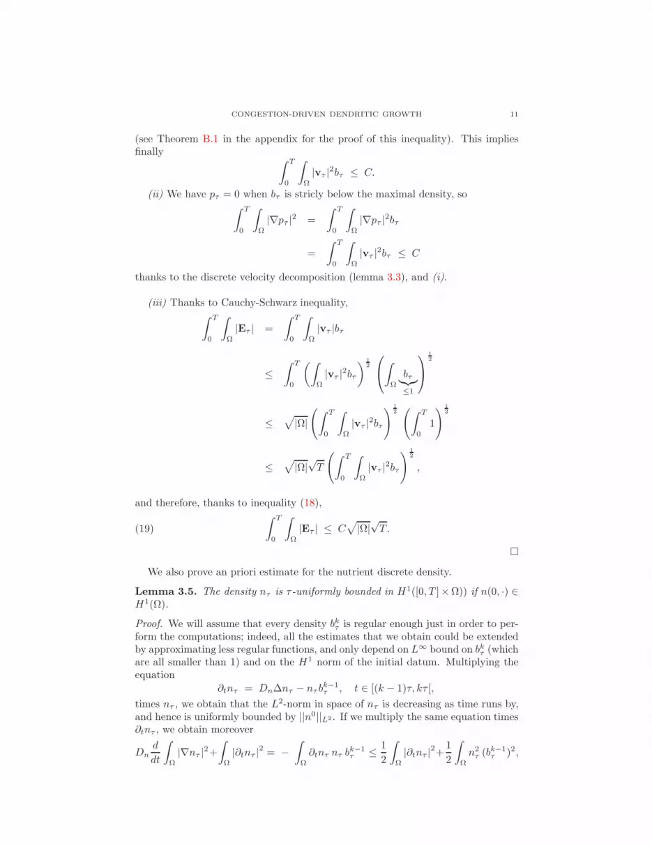
(see Theorem B.1 in the appendix for the proof of this inequality). This impliesfinally

∫ T

0

∫

Ω

|vτ |2bτ ≤ C.

(ii) We have pτ = 0 when bτ is stricly below the maximal density, so∫ T

0

∫

Ω

|∇pτ |2 =

∫ T

0

∫

Ω

|∇pτ |2bτ

=

∫ T

0

∫

Ω

|vτ |2bτ ≤ C

thanks to the discrete velocity decomposition (lemma 3.3), and (i).

(iii) Thanks to Cauchy-Schwarz inequality,∫ T

0

∫

Ω

|Eτ | =

∫ T

0

∫

Ω

|vτ |bτ

≤∫ T

0

(∫

Ω

|vτ |2bτ) 1

2

∫

Ω

bτ︸︷︷︸

≤1

12

≤√

|Ω|(∫ T

0

∫

Ω

|vτ |2bτ) 1

2(∫ T

0

1

) 12

≤√

|Ω|√T

(∫ T

0

∫

Ω

|vτ |2bτ) 1

2

,

and therefore, thanks to inequality (18),

(19)

∫ T

0

∫

Ω

|Eτ | ≤ C√

|Ω|√T .

We also prove an priori estimate for the nutrient discrete density.

Lemma 3.5. The density nτ is τ-uniformly bounded in H1([0, T ]×Ω)) if n(0, ·) ∈H1(Ω).

Proof. We will assume that every density bkτ is regular enough just in order to per-form the computations; indeed, all the estimates that we obtain could be extendedby approximating less regular functions, and only depend on L∞ bound on bkτ (whichare all smaller than 1) and on the H1 norm of the initial datum. Multiplying theequation

∂tnτ = Dn∆nτ − nτ bk−1τ , t ∈ [(k − 1)τ, kτ [,

times nτ , we obtain that the L2-norm in space of nτ is decreasing as time runs by,and hence is uniformly bounded by ||n0||L2 . If we multiply the same equation times∂tnτ , we obtain moreover

Dnd

dt

∫

Ω

|∇nτ |2+∫

Ω

|∂tnτ |2 = −∫

Ω

∂tnτ nτ bk−1τ ≤ 1

2

∫

Ω

|∂tnτ |2+1

2

∫

Ω

n2τ (b

k−1τ )2,

12 B. MAURY, A. ROUDNEFF-CHUPIN AND F. SANTAMBROGIO

which implies

Dnd

dt

∫

Ω

|∇nτ |2 +1

2

∫

Ω

|∂tnτ |2 ≤ 1

2||n0||2L2 .

This gives bounds both on the L2 norm of ∂tnτ and of ∇nτ :

∫

Ω

|∂tnτ |2 ≤ ||n0||2L2 ,

∫

Ω

|∇nτ |2 ≤ ||∇n0||2L2 +T

2Dn||n0||2L2 ,

and finally implies

||nτ ||2H1([0,T ]×Ω) ≤ T

((

1 +T

2Dn

) ∫

Ω

|n0|2 +

∫

Ω

|∇n0|2)

.

We now focus on the densities bτ and nτ . We first prove that they are solutionsof the reaction-diffusion equation.

Lemma 3.6. The densities bτ and nτ are solutions of

∂tbτ +∇ · (bτ vτ ) = bτ nτ .

Proof. For every ϕ ∈ C∞c ([0, T [×Ω), we have

∫ T

0

∫

Ω

(∂tϕ(t, x) +∇ϕ(t, x) · vτ (t, x)) bτ (t, x) dx dt

=∑

k

∫ kτ

(k−1)τ

∫

Ω

(

∂tϕ(t, x) +∇ϕ(t, x) · rkτ − id

τ

((Tk

t )−1(x)

))

(Tkt )#b

kτ (t, x) dx dt

=∑

k

∫ kτ

(k−1)τ

∫

Ω

(

∂tϕ(t,Tkt (x)) +∇ϕ(t,Tk

t (x)) ·rkτ − id

τ(x)

)

bkτ (t, x) dx dt

=∑

k

∫

Ω

[

ϕ(t,Tkt (x))b

kτ (t, x)

]kτ

(k−1)τdx −

∑

k

∫ kτ

(k−1)τ

∫

Ω

ϕ(t,Tkt (x))∂t b

kτ (t, x) dx dt.

The first term writes

∑

k

∫

Ω

[

ϕ(t,Tkt (x))b

kτ (t, x)

]kτ

(k−1)τdx

=∑

k

(∫

Ω

ϕ(kτ, rkτ (x))bkτ (x) dx −

∫

Ω

ϕ((k − 1)τ, x)bk−1τ (x) dx

)

=∑

k

∫

Ω

ϕ(kτ, x) (rkτ )#bkτ (x)

︸ ︷︷ ︸

bkτ (x)

dx −∫

Ω

ϕ((k − 1)τ, x)bk−1τ (x) dx

= −∫

Ω

ϕ(0, x)b0τ (x) dx.

CONGESTION-DRIVEN DENDRITIC GROWTH 13

The second one satisfies

∑

k

∫ kτ

(k−1)τ

∫

Ω

ϕ(t,Tkt (x))∂t b

kτ (t, x) dx dt

=∑

k

∫ kτ

(k−1)τ

∫

Ω

ϕ(t,Tkt (x))nτ (t, x)b

kτ (t, x) dx dt

=∑

k

∫ kτ

(k−1)τ

∫

Ω

ϕ(t, x)nτ (t, (Tkt )

−1(x))(Tkt )#b

kτ (t, x) dx dt

=

∫ T

0

∫

Ω

ϕ(t, x)nτ (x)bτ (x) dx dt.

We finally obtain

∫ T

0

∫

Ω

(∂tϕ(t, x) +∇ϕ(t, x) · vτ (t, x)) bτ (t, x) dx dt

= −∫

Ω

ϕ(0, x)b0τ (x) dx −∫ T

0

∫

Ω

ϕ(t, x)nτ (x)bτ (x) dx dt,

which corresponds to the weak formulation – given in Definition 2.1 – of the aboveequation.

Again, we can prove some a priori estimates.

Lemma 3.7 (A priori estimates). We have

(i) vτ is τ-uniformly bounded in L2((0, T ), L2bτ(Ω)) ;

(iii) Eτ is a τ-uniformly bounded measure.

Proof. (i) We have

∫ T

0

∫

Ω

|vτ |2bτ =∑

k

∫ kτ

(k−1)τ

∫

Ω

∣∣∣∣

rkτ − id

τ (Tk

t )−1

∣∣∣∣

2

(Tkt )#b

kτ (t, .)

=∑

k

∫ kτ

(k−1)τ

∫

Ω

∣∣∣∣

rkτ − id

τ

∣∣∣∣

2

bkτ (t, .).

Moreover, thanks to the definition of bkτ (t, .) (Equation (15)), we have bkτ (t, .) ≤ bkτ ,which implies

∫ T

0

∫

Ω

|vτ |2bτ ≤∑

k

∫ kτ

(k−1)τ

∫

Ω

∣∣∣∣

rkτ − id

τ

∣∣∣∣

2

bkτ

=1

τ

∑

k

W 22 (b

kτ , b

kτ ) ≤ C

thanks to Lemma 3.4 (i).

14 B. MAURY, A. ROUDNEFF-CHUPIN AND F. SANTAMBROGIO

(ii) We have

∫ T

0

∫

Ω

|Eτ | =

∫ T

0

∫

Ω

|vτ |bτ

=∑

k

∫ kτ

(k−1)τ

∫

Ω

∣∣∣∣

rkτ − id

τ (Tk

t )−1

∣∣∣∣(Tk

t )#bkτ (t, .)

=∑

k

∫ kτ

(k−1)τ

∫

Ω

∣∣∣∣

rkτ − id

τ

∣∣∣∣bkτ (t, .)

≤∑

k

∫ kτ

(k−1)τ

∫

Ω

∣∣∣∣

rkτ − id

τ

∣∣∣∣bkτ

=∑

k

∫ kτ

(k−1)τ

∫

Ω

∣∣∣∣

id− tkττ

∣∣∣∣bkτ

=

∫ T

0

∫

Ω

|vτ |bτ ≤ C√

|Ω|√T

thanks to Inequality (19).

3.2. Convergence of the interpolated curves. We can now prove that thecurves defined at section 2.2 converge to a solution of our problem. Notice that,unless differently stated, all the convergences we use in the sequel will be weak-*convergence in the space of finite measures in the duality with continuous functionsover [0, T ]× Ω. We will also refer to this convergence as “weak convergence” andwrite without using any ∗ and without precising any more the space of test func-tions. When extra bounds are available, this convergence will turn into strongerones: in particular both bτ and bτ will actually converge weakly-* in L∞ (due tothe fact that these densities are uniformly bounded by 1) and nτ weakly convergesin H1 (and hence strongly in L2).

Let us start our analysis of the limits of the interpolated curves. Thanks to the apriori estimations given in lemmas 3.4 and 3.7, we know that (bτ ,Eτ ) and (bτ , Eτ )converge (up to subsequences) as τ tends to 0. We prove in the following that theirlimits are the same.

Proposition 1 (Limit of bτ and bτ ). The curves bτ and bτ converge to the samelimit b as τ tends to 0.

CONGESTION-DRIVEN DENDRITIC GROWTH 15

Proof. For every f ∈ C∞c ([0, T ]× Ω), we have

∫ T

0

∫

Ω

f(t, x)(bτ (t, x)− bτ (t, x)) dx dt

=∑

k

∫ kτ

(k−1)τ

∫

Ω

f(t, x)(bkτ (x) − (Tkt )#b

kτ (t, x)) dx dt

=∑

k

∫ kτ

(k−1)τ

(∫

Ω

f(t, x)bkτ (x) dx −∫

Ω

f(t,Tkt (x))b

kτ (t, x)) dx

)

dt

=∑

k

∫ kτ

(k−1)τ

(∫

Ω

f(t, x)(bkτ (x) − bkτ (t, x))) dx

+

∫

Ω

(f(t, x)− f(t,Tkt (x)))b

kτ (t, x)) dx

)

dt.

The first term writes

∑

k

∫ kτ

(k−1)τ

∫

Ω

f(t, x)(bkτ (x)− bkτ (t, x))) dx dt

=∑

k

∫ kτ

(k−1)τ

∫

Ω

f(t, x)(bkτ (x) − bkτ (x))) dx dt

+∑

k

∫ kτ

(k−1)τ

∫

Ω

f(t, x)(bkτ (x)− bkτ (t, x))) dx dt.

On the one hand, we have, thanks to Lemma A.1 and to the estimation onW2(bkτ , b

kτ )

proved at Inequality (18),

∣∣∣∣∣

∑

k

∫ kτ

(k−1)τ

∫

Ω

f(t, x)(bkτ (x) − bkτ (x))) dx dt

∣∣∣∣∣

≤∑

k

∫ kτ

(k−1)τ

||∇f ||L2(Ω)W2(bkτ , b

kτ ) ≤ τ C ||∇f ||L2(Ω) −→

τ→00.

On the other hand, since nτ ∈ [0, N0] a.e.,

∣∣∣∣∣

∑

k

∫ kτ

(k−1)τ

∫

Ω

f(t, x)(bkτ (x) − bkτ (t, x))) dx dt

∣∣∣∣∣

≤∑

k

∫ kτ

(k−1)τ

∫

Ω

||f ||∞ bk−1τ (x)︸ ︷︷ ︸

≤ 1

∣∣∣∣∣exp

(∫ kτ

(k−1)τ

nτ

)

− exp

(∫ t

(k−1)τ

nτ

)∣∣∣∣∣

︸ ︷︷ ︸

≤ τN0eτN0

dx dt

≤ τ ||f ||∞N0 eτN0∑

k

τ |Ω| ≤ τ ||f ||∞N0 eτN0

T |Ω| −→τ→0

0.

16 B. MAURY, A. ROUDNEFF-CHUPIN AND F. SANTAMBROGIO

The second term also tends to 0, since

∣∣∣∣

∫

Ω

(f(t, x)− f(t,Tkt (x)))b

kτ (t, x)) dx dt

∣∣∣∣

≤∑

k

∫ kτ

(k−1)τ

∫

Ω

Lip (f) |x−Tkt (x)|bkt (x)) dx dt

=∑

k

∫ kτ

(k−1)τ

∫

Ω

Lip (f) |t− (k − 1)τ |︸ ︷︷ ︸

≤ τ

∣∣∣∣

rkτ − id

τ

∣∣∣∣bkt (x)) dx dt

≤ Lip (f) τ∑

k

∫ kτ

(k−1)τ

∫

Ω

∣∣∣∣

rkτ − id

τ (Tk

t )−1

∣∣∣∣(Tk

t )#bkt (x)) dx dt

= Lip (f) τ

∫ T

0

∫

Ω

|Eτ |bτ

≤ C√

|Ω|√T Lip (f) τ −→

τ→00.

We can also prove that Eτ and Eτ converge to the same limit.

Proposition 2 (Limit of Eτ and Eτ ). The curves Eτ and Eτ converge to the samelimit E as τ tends to 0.

Proof. For every f ∈ C∞c ([0, T ]× Ω) we have

∫ T

0

∫

Ω

f(t, x)(Eτ (t, x) − Eτ (t, x)) dx dt

=∑

k

∫ kτ

(k−1)τ

(∫

Ω

f(t, x)id− tkττ

(x) bkτ (x)︸ ︷︷ ︸

(rkτ )# bkτ (x)

dx.

−∫

Ω

f(t, x)rkτ − id

τ (Tk

t )−1(x)(Tk

t )#bkτ (t, x)) dx

)

dt

=∑

k

∫ kτ

(k−1)τ

(∫

Ω

f(t, rkτ (x))rkτ − id

τ(x)bkτ (x) dx

−∫

Ω

f(t,Tkt (x))

rkτ − id

τ(x)bkτ (t, x)) dx

)

dt

=∑

k

∫ kτ

(k−1)τ

∫

Ω

(f(t, rkτ (x)) − f(t,Tkt (x)))

rkτ − id

τ(x)bkτ (x) dx dt

+∑

k

∫ kτ

(k−1)τ

∫

Ω

f(t,Tkt (x))

rkτ − id

τ(x)(bkτ (x)− bkτ (t, x)) dx dt.

CONGESTION-DRIVEN DENDRITIC GROWTH 17

The first term writes∣∣∣∣∣

∑

k

∫ kτ

(k−1)τ

∫

Ω

(f(t, rkτ (x))− f(t,Tkt (x)))

rkτ − id

τ(x)bkτ (x) dx dt

∣∣∣∣∣

≤∑

k

∫ kτ

(k−1)τ

∫

Ω

Lip (f) |rkτ (x) −Tkt (x)|

︸ ︷︷ ︸

≤ |rkτ (x)−x|

∣∣∣∣

rkτ − id

τ(x)

∣∣∣∣bkτ (x) dx dt

≤ τ Lip (f)∑

k

∫ kτ

(k−1)τ

∫

Ω

∣∣∣∣

rkτ − id

τ(x)

∣∣∣∣

2

bkτ (x) dx dt

≤ τ Lip (f)C −→τ→0

0,

thanks to Lemma 3.7 (i). The second term also tends to 0 since∣∣∣∣∣

∑

k

∫ kτ

(k−1)τ

∫

Ω

f(t,Tkt (x))

rkτ − id

τ(x)(bkτ (x)− bkτ (t, x)) dx dt

∣∣∣∣∣

≤∑

k

∫ kτ

(k−1)τ

∫

Ω

||f ||∞∣∣∣∣

rkτ − id

τ(x)

∣∣∣∣bkτ (t, x)

∣∣∣∣∣exp

(∫ kτ

t

nτ (s, x) ds

)

− 1

∣∣∣∣∣

︸ ︷︷ ︸

≤ τN0eτN0

dx dt

≤ τ ||f ||∞N0 eτN0

∫ T

0

∫

Ω

|Eτ |bτ ≤ τ ||f ||∞N0 eτN0

C −→τ→0

0

thanks to Lemma 3.7 (ii).

We finally prove that nτ bτ and nτ bτ also converge to the same limit.

Proposition 3 (Limit of nτbτ and nτ bτ ). The curves nτbτ and nτ bτ converge tothe same limit as τ tends to 0.

Proof. For every f ∈ C∞c ([0, T ]× Ω) we have

∫ T

0

∫

Ω

f(t, x)(nτ (t, x)bτ (t, x) − nτ (t, x)bτ (t, x)) dx dt

=∑

k

∫ kτ

(k−1)τ

∫

Ω

f(t, x)(nτ (t, x)bkτ (x) − nτ (t, (T

kt )

−1(x))(Tkt )#b

kτ (t, x)) dx dt

=∑

k

∫ kτ

(k−1)τ

(∫

Ω

f(t, x)nτ (t, x)bkτ (x) dx−

∫

Ω

f(t,Tkt (x))nτ (t, x)b

kτ (t, x)) dx

)

dt.

Since nτ is uniformly bounded with respect to τ , we can prove that these termstend to 0 in the same way as in proposition 1.

3.3. Properties of the limit. We finally prove that the limits (b, n) of the curvesare solutions of our problem. First, the a priori estimates given at lemmas 3.5, 3.4,and 3.7 prove that there exist the limits (in the weak sense of measures) of Eτ ,

bτ and nτ bτ , and that this last limit is given by nb, where n is the limit of nτ inH1([0, T ]× Ω)) and b the limit of bτ , the main difficulty is that the product of thelimits should be equal to the limit of the product, but nτ converges weakly in H1

18 B. MAURY, A. ROUDNEFF-CHUPIN AND F. SANTAMBROGIO

and hence strongly in L2. We can then pass to the limit in the linear equationssatisfied by the discrete curves, and obtain that (b, n) are weak solutions of

∂tb+∇ · (E) = nb in Ω,

∂tn = Dn∆n− nb in Ω,

∇n · ν = 0 on ∂Ω.

We have now to prove that the limit E is of the form bu, where u is the minimalvelocities among the admissible ones, i.e. it satisfies the saddle point formulation (8).

To do so, we will use the limit of Eτ rather than Eτ . Indeed, let us notice thatwe have

Eτ = bτvτ = −bτ∇pτ = −∇pτ ,since pτ = 0 on [bτ < 1]. Lemma 3.4 gives a bound on pτ , hence we can supposethat we have pτ p (up to subsequences and in the weak sense). We need to showthat p ∈ H1

b , which would allow us to write E = −∇p = bu with u = −∇p. Let ussuppose for a while that we have done this, and conclude.

Indeed, the limit equation would give, for a.e. t0, every h > 0, and every q ∈H1

b(t0,.)∫

Ω

(b(t0 + h, x)− b(t0, x)) q(x) dx

=

∫ t0+h

t0

∫

Ω

∇q(x) · u(t, x) b(t, x) dx dt +

∫ t0+h

t0

∫

Ω

n(t, x) b(t, x) q(x) dx dt.

Moreover, since b(t0, x) = 1 wherever q does not vanish, and since b(t0 + h, x) ≤ 1,we have

1

h

∫

Ω

(b(t0 + h, x)− b(t0, x)) q(x) dx ≤ 0,

which implies

1

h

(∫ t0+h

t0

∫

Ω

∇q(x) · u(t, x) b(t, x) dx dt +

∫ t0+h

t0

∫

Ω

n(t, x) b(t, x) q(x) dx dt

)

≤ 0.

Letting h tend to 0, we get∫

Ω

∇q(x) · u(t0, x) b(t0, x) dx ≤ −∫

Ω

n(t0, x) b(t0, x) q(x) dx,

and the reverse inequality can be obtained with h < 0.Thanks to the saddle point formulation (8), this allows to conclude that u is

the desired vector field, the minimal one in Cb. Let us point out that the propertywe obtained is stronger than expected : we have proved that the complementarityrelation holds for every test function in H1

b(t0,.).

The proof is complete once we establish the following lemma.

Lemma 3.8. If b and p are the weak limits (in L∞ and L2((0, T ), H1(Ω)), respec-tively) of bτ and pτ , then we have p(1− b) = 0 and hence p ∈ H1

b .

Proof. We obviously have p ≥ 0, and we must prove that p = 0 on [b < 1]. Followingthe method adopted in [21], let us consider the mean functions

pa,bτ =1

b− a

∫ b

a

pτ (t) dt and pa,b =1

b− a

∫ b

a

p(t) dt.

CONGESTION-DRIVEN DENDRITIC GROWTH 19

The advantage of using pa,bτ is that it is a bounded sequence in H1, converging(weakly in H1, strongly in L2) to pa,b. Since pτ = 0 on [bτ < 1], we have

∫ b

a

∫

Ω

pτ (t, x)(1 − bτ (t, x)) dx dt = 0,

which implies

1

b− a

(∫ b

a

∫

Ω

pτ (t, x)(1 − bτ (a, x)) dx dt +

∫ b

a

∫

Ω

pτ (t, x)(bτ (a, x)− bτ (t, x)) dx dt

)

= 0.

As in [21], for a.e. a, if we take in the first term first the limit as τ → 0 and thenas b→ a, we get convergence to

∫

Ω

p(a, x)(1 − b(a, x)) dx.

Let us prove that the second term converges to 0. Let t ∈ [a, b], and ka, kt suchthat bτ (a, .) = bka

τ and bτ (t) = bktτ . We have

∫ b

a

∫

Ω

pτ (t, x)(bτ (a, x)− bτ (t, x)) dx dt

=

∫ b

a

∫

Ω

pτ (t, x)(bka

τ (x) − bkt

τ (x)) dx dt

=

∫ b

a

kt∑

ka

∫

Ω

pτ (t, x)(bk−1τ (x) − bkτ (x)) dx dt

=

∫ b

a

kt∑

ka

∫

Ω

pτ (t, x)(bk−1τ (x) − bkτ (x)) dx dt

+

∫ b

a

kt∑

ka

∫

Ω

pτ (t, x)(bkτ (x) − bkτ (x)) dx dt.

20 B. MAURY, A. ROUDNEFF-CHUPIN AND F. SANTAMBROGIO

The first term writes∣∣∣∣∣

∫ b

a

kt∑

ka

∫

Ω

pτ (t, x)(bk−1τ (x) − bkτ (x)) dx dt

∣∣∣∣∣

≤∫ b

a

kt∑

ka

∫

Ω

|pτ (t, x)| |bk−1τ (x)|︸ ︷︷ ︸

≤ 1

|1− exp

(∫ kτ

(k−1)τ

nτ (s, x) ds

)

|︸ ︷︷ ︸

≤ τN0eτN0

dx dt

≤ N0eτN0

∫ b

a

∫

Ω

(t− a)|pτ (t, x)| dx dt

≤ N0eτN0

∫

Ω

(∫ b

a

|t− a|2 dt) 1

2(∫ b

a

|pτ (t, x)|2) 1

2

dx

≤ N0eτN0

∫

Ω

((b− a)3

3

) 12

(∫ b

a

|pτ (t, x)|2) 1

2

dx

≤ N0eτN0 (b − a)

32

√3

(∫

Ω

∫ b

a

|pτ (t, x)|2 dx) 1

2 (∫

Ω

dx

) 12

≤ N0eτN0 (b − a)

32

√3

√

|Ω| ||pτ ||L2((0,T ),L2(Ω)).

We have therefore, uniformly in τ ,

limb→a

limτ→0

1

b− a

∫ b

a

kt∑

ka

∫

Ω

pτ (t, x)(bk−1τ (x)− bkτ (x)) dx dt = 0.

Thanks to lemma A.1, the second term satisfies∣∣∣∣∣

∫ b

a

kt∑

ka

∫

Ω

pτ (t, x)(bkτ (x)− bkτ (x)) dx dt

∣∣∣∣∣

≤∫ b

a

kt∑

ka

||∇pτ (t)||L2(Ω)W2(bkτ , b

kτ ) dt

≤∫ b

a

kt∑

ka

||∇pτ (t)||L2(Ω)Cτ (thanks to Inequality (18))

≤ C

∫ b

a

(t− a) ||∇pτ (t)||L2(Ω)

≤ C

(∫ b

a

|t− a|2 dt) 1

2(∫ b

a

||∇pτ (t)||2L2(Ω)

) 12

≤ C(b − a)

32

√3

||∇pτ (t)||L2((0,T ),H1(Ω)).

CONGESTION-DRIVEN DENDRITIC GROWTH 21

This implies that

limb→a

limτ→0

1

b− a

∫ b

a

kt∑

ka

∫

Ω

pτ (t, x)(bkτ (x) − bkτ (x)) dx dt = 0.

The limit is therefore given by∫

Ω

p(a, x)(1 − b(a, x)) dx,

hence p(t) ∈ H1b(t) for a.e. t.

4. Numerical simulations

The numerical study of Problem (4), which we recall is given by∂tb +∇ · (bu) = nb in Ω,

∂tn = Dn∆n− nb in Ω,

arises several difficulties. First of all, the correction velocity u is given as thesolution of a minimization problem on the space of admissible velocities Cb definedat equation (5), which depends on the evolving density b. Its estimation seems tobe out of hand, and even if it could be calculated, it would surely lack regularity.A different approach is therefore needed.

Following the idea exposed in [22], which we already used in the theoreticalwork, we propose to use a splitting scheme to estimate the bacterial density. Moreprecisely, for a time step τ > 0, we define the densities bk thanks to

(20)

bk = bk−1 + τnk−1bk−1 (prediction),

bk = PKmkbk (correction),

where PKmk

is the projection for the Wasserstein distance on the space of densities

of same total mass as bk which respect the congestion constraint b ≤ 1. Noticethat the exponential formula in (10), which was suitable for the theoretical proofof convergence, is now replaced with a simple first order expansion. The density nk

is given as an approximated solution at time kτ of equation

(21)

∂tn = Dn∆n− nbk−1,

n|t=(k−1)τ = nk−1.

The spatial discretization also requires special attention. This kind of problems,which involve unstable interfaces, are indeed very sensitive to anisotropy. Instead ofusing cartesian meshes, we therefore turned to randomly generated Voronoi meshes.An example of such a mesh is presented in Figure 3 on the left.

We chose to discretize equation (21) thanks to a semi-implicit finite volumemethod. On each cell of the mesh, we write

∫

I

nk − nk−1

τ= Dn

∫

I

∆nk −∫

I

nk−1bk−1,

which implies, approximating bk and nk with bki and nki on the cell I,

(22)

(

1 +Dn

∑

J∼I

τ σijai d(xi, xj)

)

nki −Dn

∑

J∼I

τ σijai d(xi, xj)

nkj = nk−1

i (1 + τbk−1i ).

22 B. MAURY, A. ROUDNEFF-CHUPIN AND F. SANTAMBROGIO

xi

xj

I

Jσij ν

Figure 3. Left: example of a random Voronoi mesh. Right: no-tations in one of the Voronoi cells.

Here, xi denotes the center of cell I, σij the length of the edge between cells I andJ , and ai the area of cell I (see Figure 3).

Concerning the bacterial density, the prediction step of equation (20) is easilycomputed through the following scheme

bki = bk−1i + τnk−1

i bk−1i .

However, the correction step is not straightforward. We propose to turn to a stochas-tic method, which has proved to be efficient in the crowd motion context (see [22, 24]for more details). We consider the cells where the density is beyond the conges-tion constraint. For each of these cells, we take the additional mass, and start arandom walk which travels through the neighbor cells. As soon as this randomwalk encounters non-saturated cells, it discharges as much mass as it can, and thisuntil all the additional mass has been redistributed. This method asymptoticallyapproaches the Wasserstein projection, in a sense which is precised in [24], and givesgood numerical results on several examples. Note that we perform a random walkon a non regular mesh. The transition probability from one cell to another musttherefore depend on the geometry of the mesh. The natural coefficients appear tobe the ones that correspond to the discrete Laplacian on the mesh, which write

PI→J =

σij

d(xi,xj)∑

L∼Iσil

d(xi,xl)

.

Note that the transition probabilities are consistent to the finite volume discretiza-tion of the Laplace operator proposed in [26].

Numerical tests have been conducted with different parameters values. Wepresent in Figure 4 three results for a fixed initial bacterial density b0 = 0.7 localizedin a small area at the center of the domain, a fixed diffusion coefficient Dn = 10−6,and three different initial nutrient densities, n0 = 2, n0 = 0.5 and n0 = 0.3. On thefirst case, the evolution is fast and concentric. For lower nutrient densities, however,branches appear and the evolution is slower. This example shows that branchingpatterns can be obtained without the need of adding non-linear diffusion or deathterms.

It is known that the fractal dimension of patterns obtained thanks to diffusion-limited aggregation is of order 1.71 (see [29]). In the present context, the createdpatterns exhibit some fractal character down to a cut off scale (see the end ofthis section). In particular we can estimate some sort of fractal dimension of our

CONGESTION-DRIVEN DENDRITIC GROWTH 23

Figure 4. Evolution of bacteria (left) and nutrients (right) for aninitial nutrient density of 2 (top), 0.5 (center) and 0.3 (bottom).

branching patterns, thanks to the box-counting method. This method consists incounting the number N(r) of boxes of size r which contain some bacteria. The

limit logN(r)log r when r tends to 0 gives the so-called Minkowski-Bouligand dimension,

or Kolmogorov dimension of the pattern. Here, we plot on Figure 5 the curvesr 7→ N(r) in two examples presented in Figure 4. We obtain a slope of 1.96 in thefirst case where n0 = 2, which corresponds to a concentric evolution, and a slope of1.7 in the case where n0 = 0.3, which corresponds to a branching pattern. This fitscorrectly with the estimations of DLA patterns.

Let us finally underline that the branching patterns we obtain are not fractal atevery scale. It seems that there exists a limit scale for the creation of instabilities.More precisely, let us consider a typical situation where the border of the bacterialcolony has irregularities, and where nutrients are less concentrated in the holes than

24 B. MAURY, A. ROUDNEFF-CHUPIN AND F. SANTAMBROGIO

100

101

102

103

102

103

104

105

106

r

N(r

)

Figure 5. Log-log plot of the number of boxes of size r containingsome part of the pattern, in the case of an initial nutrient densityof 2 (dotted black line) and 0.3 (plain blue line).

on the peaks (see Figure 6). In this case, the irregularities will become unstable ifthe characteristic time of the nutrients’ diffusion is slower than the time of growthof the peaks. The diffusion characteristic time can be estimated by L2/Dn, whereL is the length of the peaks, whereas the growth time is given by L/U . This finallygives the following condition for apparition of instabilities

Dn ≤ LU,

where U is the propagation speed of the bacteria, which is of order 1 if the nutrientsconcentration is of order 1. Figure 7 gives the evolution of initial irregularities fortwo different values of Dn. The initial nutrient distribution has been taken uniformwith n0 = 1 on the area free of bacteria. This numerical test confirms the apparitionof instability only for small diffusion coefficients. We have also plotted on Figure 8the evolution of the amplitude of the instabilities for different diffusion coefficients.It appears that the limit scale is indeed attained for diffusion coefficients of order thelength of the irregularities (here 0.5). Finally, Figure 9 gives the bacterial densitiesobtained for two different diffusion coefficients Dn = 10−6 and Dn = 10−5. Itappears that the branches are thicker in the second case.

CONGESTION-DRIVEN DENDRITIC GROWTH 25

n1

n2n2

L

Figure 6. Formation of instabilities in a typical situation wherethe density of nutrients in the holes (n1) is lower than on the peaks(n2).

Figure 7. Initial bacterial density (left), and evolution at time 20for Dn = 10 (center), and Dn = 0.1 (right). In the first case, theirregularities have been smoothed, whereas in the second case, theyhave been amplified.

Figure 8. Evolution of the amplitude of the irregularities for dif-ferent diffusion coefficients Dn. For top to bottom : Dn =0.01, 0.1, 1, 10.

26 B. MAURY, A. ROUDNEFF-CHUPIN AND F. SANTAMBROGIO

Figure 9. Evolution of bacteria for the same nutrient concentra-tion n0 = 0.3 and for Dn = 10−6 (left) and Dn = 10−5 (right).

Appendix A. A technical lemma

We recall here a result, first proved in [21] (Lemma 3.4). We give its proof forthe sake of completeness, since we used it several times.

Lemma A.1. Assume that µ and ν are absolutely continuous measures, whosedensities are bounded by a same constant C. Then, for all function f ∈ H1(Ω), wehave the following inequality:

(23)

∫

Ω

f d(µ− ν) ≤√C ||∇f ||L2(Ω)W2(µ, ν).

Proof. Let µt be the constant speed geodesic between µ and ν, and wt the velocityfield such that (µ,wt) satisfies the continuity equation ∂tµt +∇ · (wtµt) = 0, and||wt||L2(µt) = W2(µ, ν). For all t, µt is absolutely continuous, and its density isbounded by the same constant C a.e.. Therefore:

∫

Ω

f d(µ− ν) =

∫ 1

0

d

dt

(∫

Ω

f(x)dµt(x)

)

dt =

∫ 1

0

∫

Ω

∇f ·wt dµt dt

≤(∫ 1

0

∫

Ω

|∇f |2 dµt dt

)1/2 (∫ 1

0

∫

Ω

|wt|2 dµt dt

)1/2

≤√C ||∇f ||L2(Ω)W2(µ, ν)

Notice that this estimate makes a connection between the distance W2 and thedual norm of H1, exactly as the distance W1 is connected to the dual of W 1,∞. Onthe other hand, it is only valid provided some bound on the densities is supposed,and it is easy to check that (A.1) could not hold without some bounds. In particular,should one be allowed to use atomic measures µ, ν, the existence of an estimate like(A.1) would imply the injection H1 → C0, which is false in higher dimension.

Appendix B. Estimates in the Wasserstein projection

A useful estimate that we needed throughout the paper was the following: con-sider ρ be a probability density on Ω ⊂ R

d satisfying ρ(x) ≤ 1 + τ ≤ 2 a.e. andK = ρ ∈ P(Ω), : ρ(x) ≤ 1 a.e.; then there exists a universal constant such that

minW2(ρ, ρ) : ρ ∈ K ≤ Cτ.

CONGESTION-DRIVEN DENDRITIC GROWTH 27

This fact is quite easy to prove when Ω = Rd.

Indeed, consider the following transport

t(x) = x0 + (1 + τ)1d (x− x0),

where x0 is fixed in Ω. The transported density t#ρ then belongs to K, since it hasthe same total mass as ρ, and its density is given by

t#ρ(x) =ρ

| det∇t| (t−1(x)) ≤ 1.

Therefore, we have

minW 22 (ρ, ρ) : ρ ∈ K ≤ W 2

2 (ρ, t#ρ)

≤∫

Ω

|x− t(x)|2ρ dx

≤ |(1 + τ)1d − 1|2

∫

Ω

|x− x0|2 ρ dx

≤ τ2(1

d+ o(1)

)2 ∫

Ω

|x− x0|2 ρ dx,

which givesminW2(ρ, ρ) : ρ ∈ K ≤ Cτ,

for a constant C only depending on the second moment of ρ.If on the one hand this last constant would become universal in the case of a

bounded domain Ω, on the other hand the same proof could not work, since thedilatation t could fall out of Ω. This is why we develop a different proof in thefollowing theorem.

Theorem B.1. Let Ω ⊂ Rd be a convex and bounded domain with |Ω| > 1, ρ a

probability density on Ω satisfying ρ(x) ≤ 1 + τ ≤ 2 a.e. and K = ρ ∈ P(Ω), :ρ(x) ≤ 1 a.e.. Then it holds

minW2(ρ, ρ) : ρ ∈ K ≤ Cτ

for a constant C only depending on Ω.

Proof. We will select a particular density ρ through a minimization problem, provethat ρ ∈ K, and give an estimate on W2(ρ, ρ). We will suppose that ρ has someextra regularity properties, namely that it is Holder continuous and bounded frombelow by a positive constant. We will remove this assumption later.

Let us solve the following minimization problem

min

(

F (ρ) + ε

∫

f(ρ(x))dx +1

2(1− c)−1τW 2

2 (ρ, ρ)

)

,

where ε is a small parameter that we will send to 0 later on, c < 1 is such thatc|Ω| = 1, f is a given convex function of the form f(t) = 1

t + tp for p > d (so that,

in particular,∫f(ρ) <∞ only if ρ > 0 a.e.) and

F (ρ) =1

2

∫

|∇φ|2dx, where φ is the weak solution of

−∆φ = ρ− c, in Ω,∂φ∂n = 0 on ∂Ω,

(obviously F (ρ) = +∞ if ρ does not belong to the dual of H1).It is easy to see that a solution exists, by semicontinuity, and we can assume that

ρ ∈ Lp, ρ > 0 a.e. and φ ∈ H1.

28 B. MAURY, A. ROUDNEFF-CHUPIN AND F. SANTAMBROGIO

Let us consider the usual optimality conditions (see [6]) for this problem. We get

φ+ εf ′(ρ) +1

(1− c)−1τψ = const ρ− a.e.

(here ψ is the Kantorovitch potential for the quadratic transport from ρ to ρ). Sincewe know that ρ is strictly positive a.e. then we have actually

φ+ εf ′(ρ) +1

(1− c)−1τψ = const a.e.

We want now to prove ρ ≤ 1. To do that we first analyze its regularity. Noticethat ρ ∈ Lp, then φ ∈ W 2,p ⊂ C1,α. Since ψ is Lipschitz continuous, we deducethat f ′(ρ) also is Lipschitz, and hence it is bounded. Since f ′(t) = −1/t2 + ptp−1

explodes near zero, this shows that ρ must be bounded away from 0. Moreover,since (f ′)−1 is Lipschitz (just compute f ′′ and see that it is bounded from below bya positive constant), then ρ is also Lipschitz.

Hence we can apply Caffarelli’s regularity theory since both ρ and ρ are boundedfrom above and below and Holder continuous, and we get that ψ is C2,α. Also φ isC2,α since ρ is C0,α (for the regularity on φ, we must apply standard regularity the-ory with Neumann boundary conditions, which could require some extra regularityon ∂Ω).

We can now look for the maximum point x0 of ρ, which is also a maximum pointfor εf ′(ρ), and hence a minimum point for φ+ 1

(1−c)−1τ ψ. We claim that this point

cannot be on the boundary, unless the gradient of φ + 1(1−c)−1τ ψ vanishes at x0.

Actually, the normal derivative of φ vanishes on the boundary, and that of ψ ispositive, since T (x0) = x0 − ∇ψ(x0) ∈ Ω, which implies ∇ψ(x0) · n ≥ 0. But aminimum point on the boundary cannot have strictly positive normal derivative,so that, even if the minimum is on the boundary, we can anyway prove that thegradient vanishes and, passing to a second order analysis, that the Hessian is positivedefinite. In particular, we get

(24) 0 ≤ ∆φ(x0) +1

(1− c)−1τ∆ψ(x0) = c− ρ(x0) +

1− c

τ∆ψ(x0).

We want to prove ρ(x0) ≤ 1. We know, by Monge-Ampere equation

ρ(x0) = ρ(T (x0)) det(I −D2ψ(x0))

≤ (1 + τ)

(d−∆ψ(x0)

d

)d

=

[

(1 + τ)1/d(

1− ∆ψ(x0)

d

)]d

where we used ρ ≤ 1 + τ but also the geometric-arithmetic mean inequality forthe eigenvalues of the positive matrix I − D2ψ(x0). We also use the inequality(1 + τ)1/d ≤ 1 + τ

d to get

ρ(x0)1/d ≤ (1 + τ)1/d

(

1− ∆ψ(x0)

d

)

≤ 1 +τ −∆ψ(x0)

d− τ∆ψ(x0)

d2.

Assuming by contradiction that ρ(x0) > 1, from the Laplacian inequality (24) weget ∆ψ(x0) ≥ τ > 0 which implies, from the last inequality, ρ(x0) < 1. This provesthat ρ(x0) ≤ 1.

We can also give an estimate onW2(ρ, ρ), since ρ has been chosen as an optimizerand hence it gives a better result than ρ, i.e.

(25)1

2(1− c)−1τW 2

2 (ρ, ρ) + F (ρ) + ε

∫

f(ρ(x))dx ≤ F (ρ) + ε

∫

f(ρ(x))dx.

CONGESTION-DRIVEN DENDRITIC GROWTH 29

First we want to send ε→ 0. What we have proven so far is that, for every ε > 0and for fixed ρ (Holder continuous and bounded away from 0), there is a measureρ = ρε, satisfying the inequality (25). Since ε

∫f(ρ(x))dx → 0 (ρ is fixed and it has

been chosen so that∫f(ρ(x))dx < +∞) and ε

∫f(ρε(x))dx ≥ 0, if ρε ρ (and it

is always possible to assume convergence, up to subsequences), one gets

1

2(1− c)−1τW 2

2 (ρ, ρ) + F (ρ) ≤ F (ρ),

where we used the semicontinuity of F and of W2.Now we want to get rid of the regularity assumption on ρ: if we take an arbi-

trary ρ ≤ 1 + τ and a sequence of densities ρk ρ that are Holder continuous andbounded away from 0, weakly converging in L2 and satisfying all ρk ≤ 1 + τ (theconvergence could be taken in L∞, but we do not need it) to our original measure,we can infer F (ρk) → F (ρ) (actually, weak convergence in L∞, for ρk means H2

weak convergence for the corresponding functions φk, and hence H1 strong conver-gence, which gives

∫|∇φk|2 →

∫|∇φ|2). Moreover, we can also assume that the

corresponding densities ρk converge to some ρ and, by semicontinuity, we still have1

2(1−c)−1τW22 (ρ, ρ) + F (ρ) ≤ F (ρ),.

This inequality is unfortunately not enough, since it gives an estimate of theorder of

√τ if we do not improve it. What we can do is bounding F (ρ)− F (ρ):

F (ρ)− F (ρ) =1

2

∫

|∇φ|2 − 1

2

∫

|∇φ|2

=1

2

∫

(∇φ+∇φ) · (∇φ −∇φ) = −1

2

∫

(φ+ φ)(∆φ −∆φ)

=1

2

∫

(φ+ φ)(ρ − ρ) ≤ C||∇(φ + φ)||L2W2(ρ, ρ) ≤ CW2(ρ, ρ),

where we used both the inequality that we proved in Lemma A.1 (see also Lemma3.4 in [21] for details), which is valid since both measures are bounded by 2, andthe fact that the H1 norm of φ is uniformly bounded as soon as the L∞ norm of ρis bounded.

Finally we get

W 22 (ρ, ρ) ≤ CτW2(ρ, ρ),

which implies the thesis.

References

[1] L. Ambrosio, N. Gigli, G. Savare, Gradient flows in metric spaces and in the space of proba-

bility measures, Lectures in Mathematics, ETH Zurich (2005).[2] L. Ambrosio, G. Savare, Gradient flows of probability measures, Handbook of differential

equations, Evolutionary equations, 3 (ed. by C.M. Dafermos and E. Feireisl, Elsevier, 2007).

[3] M. Badoual, P. Berbez, M. Aubert, B. Grammaticos, Simulating the migration and growthpatterns of Bacillus subtilis, Physica A 388 (2009) 549–559.

[4] E. Ben-Jacob, From Snowflake formation to growth of bacterial colonies II: Cooperative for-mation of complex colonial patterns, Contemporary Physics 38(3) (1997) 205–241.

[5] E. Ben-Jacob, O. Shochet, A. Tenenbaum, I. Cohen, A. Czirok, T. Vicsek, Generic modelingof cooperative growth patterns in bacterial colonies, Nature 368 (2) (1994), 46–49.

[6] G. Buttazzo, F. Santambrogio, A Mass Transportation Model for the Optimal Planning of anUrban Region Siam Review, 51, no 3, 593–610, 2009.

[7] J. Dambrine, B. Maury, N. Meunier, A. Roudneff-Chupin, A congestion model for cell migra-tion, Comm. Pure Appl. Anal. 11(1) (2012) 243–260.

30 B. MAURY, A. ROUDNEFF-CHUPIN AND F. SANTAMBROGIO

[8] E. Feireisl, D. Hilhorst, M. Mimura, R. Weidenfeld, On a nonlinear diffusion system withresource-consumer interaction, Hiroshima Math. J. 33 (2003) 253–295.

[9] H. Fujikawa, M. Matsushita, Fractal growth of Bacillus subtilis on agar plates, J. Phys. Soc.Japan 58 (1989) 3875–3878.

[10] H. Fujikawa, M. Matsushita, Bacterial fractal growth in the concentration field of a nutrient,J. Phys. Soc. Japan 60 (1991) 88–94.

[11] I. Golding, Y. Kozlovsky, I. Cohen, E. Ben-Jacob, Studies of bacterial branching growth usingreaction-diffusion models for colonial development, Physica A 260 (1998) 510–554.

[12] K. Kawasaki, A. Mochizuki, M. Matsushita, T. Umeda, N. Shigesada, Modeling Spatio-Temporal Patterns Generated by Bacillus subtilis, Journal of Theoretical Biology 188 (2)(1997), 177–185.

[13] S. Kitsunezaki, Interface Dynamics for Bacterial Colony Formation, J. Phys. Soc. Japan 66

(1997), 1544–1550.[14] A.M. Lacasta, I.R. Cantalapiedra, C.E. Auguet, A. Penaranda, L. Ramırez-Piscina, Modelling

of spatio-temporal patterns in bacterial colonies, Phys. Rev. E Stat. Phys. Plasmas Fluids

Relat. Interdiscip. Topics 59 (1999) 7036.[15] A. Marrocco, H. Henry, I.B. Holland, M. Plapp, S. J. Seror, B. Perthame, Models of self-

organizing bacterial communities and comparisons with experimental observations, Math.

Model. Nat. Phenom. 5(1) (2010), 148–162.[16] M. Matsushita, H. Fujikawa, Diffusion-limited growth in bacterial colony formation, Physica

A 168 (1990) 498–506.[17] M. Matsushita, F. Hiramatsu, N. Kobayashi, T. Ozawa, Y. Yamasaki, T. Matsuyama, Colony

formation in bacteria, experiments and modeling, Biofilms 1 (2004) 305–317.[18] M. Matsushita, J. Wakita, H. Itoh, I. Rafols, T. Matsuyama, H. Sakaguchi, M. Mimura,

Interface growth and pattern formation in bacterial colonies, Physica A 249 (1998) 517–524.[19] M. Matsushita, J. Wakita, H. Itoh, K. Watanabe, T. Arai, T. Matsuyama, H. Sakaguchi, M.

Mimura, Formation of colony patterns by a bacterial cell population, Physica A 274 (1999)190–199.

[20] M. Mimura, H. Sakaguchi, M. Matsushita, Reaction-diffusion modelling of bacterial colonypatterns, Physica A 282 (2000) 283–303.

[21] B. Maury, A. Roudneff-Chupin, F. Santambrogio, A macroscopic crowd motion model ofgradient flow type, Math. Mod. Meth. Appl. Sci. 20(10) (2010) 1787–1821.

[22] B. Maury, A. Roudneff-Chupin, F. Santambrogio, J. Venel, Handling congestion in crowdmotion models, Netw. Heterog. Media 6(3) (2011) 485–519.

[23] M. Mimura, Pattern formation in consumer-finite resource reaction-diffusion systems, Publ.

RIMS, Kyoto Univ. 40 (2004) 1413–1431.[24] A. Roudneff-Chupin, Modelisation macroscopique de mouvements de foule, PhD thesis, Uni-

versite Paris-Sud XI (2011), available at http://tel.archives-ouvertes.fr/tel-00678596.[25] F. Santambrogio, Gradient flows in Wasserstein spaces and applications to crowd movement,

to appear in the proceedings of the Seminar X-EDP, Ecole Polytechnique, Palaiseau, 2010.[26] N. Sukumar, Voronoi Cell Finite Difference Method for the Diffusion Operator on Arbitrary

Unstructured Grids, Int. J. Numer. Meth. Engng, 2003; 57:1-34.[27] C. Villani, Topics in optimal transportation, Grad. Stud. Math., 58 (AMS, Providence 2003).[28] C. Villani, Optimal transport, old and new, Grundlehren der mathematischen Wissenschaften,

338 (2009).[29] T.A. Witten, L.M. Sander, Diffusion-Limited Aggregation, a Kinetic Critical Phenomenon,

Phys. Rev. Lett., 47 (1981) 1400–1403.

E-mail address: bertrand.maury@math.u-psud.fr

E-mail address: aude.roudneff@math.u-psud.fr

E-mail address: filippo.santambrogio@math.u-psud.fr