Road Traffic Congestion in the Developing World

Vipin JainPolytechnic Institute of NYU

vjain02@students.poly.edu

Ashlesh SharmaNew York University

ashlesh@cs.nyu.edu

LakshminarayananSubramanian

New York Universitylakshmi@cs.nyu.edu

ABSTRACT

Road traffic jams continue to remain a major problem in most citiesaround the world, especially in developing regions resulting in mas-sive delays, increased fuel wastage and monetary losses. Due tothe poorly planned road networks, a common outcome in many de-veloping regions is the presence of small critical areas which arecommon hot-spots for congestion; poor traffic management aroundthese hotspots potentially results in elongated traffic jams. In thispaper, we first present a simple automated image processing mech-anism for detecting the congestion levels in road traffic by process-ing CCTV camera image feeds. Our algorithm is specifically de-signed for noisy traffic feeds with poor image quality. Based onlive CCTV camera feeds from multiple traffic signals in Kenyaand Brazil, we show evidence of this congestion collapse behav-ior lasting long time-periods across multiple locations. To partiallyalleviate this problem, we present a local de-congestion protocol

that coordinates traffic signal behavior within a small area and canlocally prevent congestion collapse sustaining time variant trafficbursts. Based on a simulation based analysis on simple networktopologies, we show that our local de-congestion protocol can en-hance road capacity and prevent congestion collapse in localizedsettings.

Categories and Subject Descriptors

I.4.9 [Computing Methodologies]: Image Processing and Com-puter Vision—Applications; I.6.3 [Computing Methodologies]:Simulation and Modeling—Applications

General Terms

Algorithms, Measurement

Keywords

traffic congestion, traffic detection, congestion collapse, simulation

1. INTRODUCTIONPoor road traffic management is the primary reason for extended

periods of traffic congestion throughout the world. As per Texas

Permission to make digital or hard copies of all or part of this work forpersonal or classroom use is granted without fee provided that copies arenot made or distributed for profit or commercial advantage and that copiesbear this notice and the full citation on the first page. To copy otherwise, torepublish, to post on servers or to redistribute to lists, requires prior specificpermission and/or a fee.DEV ’12, March 11-12, Atlanta, GACopyright c©2012 ACM 978-1-4503-1262-2/12/03 ...$10.00.

Transportation Institute’s 2011 Mobility report [1], congestion inthe US has increased substantially over the last 25 years with mas-sive amounts of losses pertaining to time, fuel and money. São Paulo, Brazil is known to experience the world’s worst trafficjams [32], where people are stuck for two to three hours everydayin traffic jams. The issue of traffic congestion has affected both thedeveloping and developed economies to different degrees irrespec-tive of the measures taken to curb the issue.

A common feature across road networks in many urban regionsin the developing world is the presence of critical congestion ar-eas; we refer to a critical congestion area as one where a networkof roads converge and a large amount of traffic needs to traversethe common congestion area. As per free-flow traffic theory [43], afree flow traffic road segment can be associated with a traffic curvewhere the traffic exit rate is a function of the traffic density in theroad segment. A free-flow road segment is known to exhibit a crit-

ical density point where any traffic input that pushes the densitybeyond the critical value can trigger a “spiralling effect” that re-sults in the road segment operating at a low-capacity equilibriumpoint. Worse still, small traffic bursts over short time periods canpotentially trigger the spiralling effect resulting in a congestion col-lapse. Many critical congestion areas in developing regions havepoor traffic management systems that if any of these critical con-gestion areas hits a congestion collapse, the road network can resultin a massive traffic jam for elongated time periods.

In this paper, our goal is to design mechanisms to detect the stateof traffic congestion in and around critical congestion areas andalso design simple preventive mechanisms to prevent critical con-gestion areas from hitting congestion collapse. In this paper, wedescribe a simple image processing algorithm that can be used toanalyze CCTV video feeds from traffic cameras to detect conges-tion levels in real time. Using this algorithm, we show evidence ofactual congestion collapse across multiple locations in São Paulo,Brazil and Nairobi, Kenya. Specifically, we show congestion col-lapse scenarios that last for multiple hours at important junctions inNairobi and São Paulo. Our congestion detection image processingalgorithms have been specifically designed for highly noisy trafficcamera feeds and differ in spirit from conventional traffic imageprocessing techniques which typically rely on high quality trafficimages [41, 44, 39].

To partially alleviate this problem, we propose a local de-congestion

protocol that coordinates traffic signal behavior within a possiblecritical congestion area to prevent the critical tipping point behav-ior. The goal of the local traffic signal coordination is to maintainthe traffic density in the congestion area below the critical densityvalue. Our local de-congestion protocol coordinates the traffic sig-nals that control the input flow within the congestion area and en-sures that the local traffic density does not cross the critical tipping

point. Based on a simulation-based study across simple real-worldroad network topologies, we show that our local de-congestion pro-tocol can prevent congestion collapse in the face of bursty trafficarrivals and can enhance the road network capacity during suchcongestion. We believe that our local de-congestion protocol canbe deployed around potential congested areas resulting in prevent-ing congestion collapses and thus, maintaining a healthy input andoutput rate during congestion. Our local decongestion protocol isprimarily designed for small congestion areas and is orthogonal indesign to many of the conventional intelligent signaling solutionsproposed in the transportation literature [17, 5, 9, 21, 14, 31, 3].While our solution is by no means optimal, an advantage of a lo-calized approach is that the decongestion protocol is easily deploy-able in critical congestion areas to enhance the operational capacityduring a congestion collapse.

2. POOR TRAFFIC MANAGEMENTCities throughout the world have found themselves at the brink

of massive traffic explosion, hence curtailing their ability to managetraffic. The situation has worsened for developing regions due tothe following reasons:

Unplanned cities: Roads tend to be narrow and poorly built.As cities grow in an ad-hoc manner, no provision is made towardsscaling road capacities, eventually resulting into several bottleneckroads, which remain congested for extended periods of time. Fur-thermore, many developing countries have witnessed an explosivegrowth in their vehicular population resulting in a failure of con-ventional traffic management strategies.

Poor discipline: Drivers often are not trained sufficiently to fol-low lane discipline. The impact of poor lane discipline, especiallyat traffic junctions, deteriorates the already overcrowded junctionsituation. Furthermore, drivers frequently jump red lights and blockthe intersection, causing further traffic congestion. These problemsare compounded by the fact that traffic law enforcement is poor,thereby providing no incentive for drivers to follow the rules.

Alternate traffic means: Countries with fast growing economieshave witnessed a surge in the number of vehicles across majorcities. These cities seldom have efficient mass transit systems, forc-ing people to operate private vehicles. This problem is compoundedby the social stigma, where people view operating a private vehicleas a sign of prosperity, while public transport is viewed as beingused by the lower echelons of society.

Archaic management: Traffic junctions are often unmanned,thereby allowing drivers to drive in a chaotic manner. Even if ajunction is controlled by a cop or a traffic light, the traffic junc-tions are largely independent of any traffic management strategy,only optimizing the respective junction traffic flow, in the direc-tion of maximum traffic build up. Furthermore, these approachesenhances traffic mismanagement in already congested roads, accel-erating congestion collapse (see §3).

Tighter budgets: A significant amount of investment is requiredto set up a traffic management infrastructure which can scale withthe increasing traffic. Such an infrastructure not only involves mea-suring and analyzing real-time traffic data but also focuses towardsenhancing congestion detection, solving real time congestion andforecasting congestion scenarios. In developing countries, ravagedby corruption and bureaucracy, there are multiple hurdles beforethe money actually progresses towards such large initiatives.

In this paper, we specifically make the case that while increas-ing road capacity is useful, it is not the only way to mitigate trafficproblems. By smart flow-control techniques in present infrastruc-ture, it is possible to increase the operational capacity of the existentroad system.

Figure 1: The first picture, taken at 5:15pm shows an empty

road in Rio de Janeiro, Brazil. Barely 5 minutes later, the road

is completely jammed up.

Figure 2: The traffic curve showing the relationship between

traffic density and operational exit rate.

3. CONGESTION COLLAPSEFig.1 shows two pictures from a traffic feed from the Rio-Niteroi

bridge in Brazil. The first picture taken at 5:15pm shows trafficflowing smoothly, with absolutely no congestion. The second pic-ture, taken barely 5 minutes later, shows that congestion has set in,leading to a traffic jam lasting for two hours. This illustrates thebasic fact that once congestion sets in, it takes a long time to beresolved.

To understand why traffic congestion sets in quickly, and alsotakes long to dissipate, we need to understand the concept of a traf-fic curve, as explained next.

3.1 Traffic CurveIn this discussion, the terms road and link are used interchange-

ably. There are several metrics that define traffic characteristicssuch as speed, flow and density of a link. Consider any link withtwo points with traffic free-flowing across them. Each link is asso-ciated with a traffic density representing the number of vehicles inthe link. The operational free-flow exit rate of a link varies with thetraffic density. The traffic curve, illustrated in Fig. 2, captures thevariation between these two parameters. At high traffic densities(signifying traffic jams), links have very low operational exit ratesand at low densities, the exit rate varies linearly with the trafficdensity. Each traffic link reaches an optimal capacity at a corre-sponding optimal operating density.

To formalize this notion, there are a few parameters that describethe state of a link l:

• Capacity: This is the maximum number of vehicles that thelink can hold. It does not vary over time, and is representedas MAXl.

• Buffer size: This is the number of vehicles on the link atany given point of time. However, traffic density is definedas number of vehicles per unit of road. Thus, buffer size issimply a multiple of traffic density(x link length). Hence, theterms buffer size and traffic density are used interchangeably,represented as Bl.

• Exit Rate: This is the rate at vehicles can exit a link, andis represented as Cl. As mentioned earlier, it depends onMAXl, as well as Bl.

The traffic curve behavior has been well documented by the In-telligent Transportation Systems (ITS) community [43]. From thecurve, we see that for low buffer sizes, the exit rate increases as thetraffic density increases. Beyond a certain point, however, conges-tion takes place, and the exit rate of the link reduces. The pointat which this transition takes place has the highest exit rate, de-noted by C∗

l . The corresponding traffic density is denoted by B∗

l .Previous research has shown that B∗

l is approximately equal toMAXl

3[43].

Consider the case when the traffic density is B∗

l , and hence theexit rate is optimal at C∗

l . If a short burst of traffic enters the linkand temporarily pushes the traffic density Bl to be more than B∗

l ,the exit rate Cl will drop below C∗

l ; this decreased exit rate will fur-ther increase Bl. This domino effect leads to the exit rate decayingrapidly, and we call it congestion collapse.

An important point to note is that even if the input rate is greaterthan the maximum exit rate C∗

l , congestion does not take place untilthe traffic density becomes greater than B∗

l . Consider a congestedlink whose Bl value is greater than B∗

l . Even if the input rateis reduced to below C∗

l , we are not guaranteed to get rid of thecongestion in a short period of time, because the exit rate Cl at atraffic density of Bl > B∗

l will be lesser than C∗

l . This is the reasonthat once congestion collapse takes place, it stays that way for longperiods of time.

Thus emphasis of the curve analysis lies in not letting the Bl

value of a link to get greater than B∗

l − ǫ for a small constant ǫ. Asmall burst of traffic ǫ, even for a short period of time, is sufficientto push the link into congestion collapse, as illustrated in Fig.1.

3.2 A simple exampleTo better understand how congestion collapse happens, we con-

sider a simple example of 2:1 merge where two free-flow roadsmerge; this is a common occurrence in road networks. A simpleexample is illustrated in Figure 3 where vehicles in L are merg-ing with the stream of vehicles on H . This simple example canbe viewed at multiple granularity’s: two lanes in the same freewaymerging into a single lane or two separate free-flow roads merging.To visualize this problem from the perspective of traffic curves,consider three links in the setup:(a)Hbef representing,a small seg-ment of H (covering a short distance of up to 0.5 miles) beforethe merge point; (b) a small segment L before the merge point;(c)Haft, representing a small segment of H after the merge point.Each of the links can be associated with their corresponding trafficcurves. Since we are dealing with a discrete version approximationusing traffic curve, we should choose reasonable lengths to havemeaningful buffer values for the links.

We primarily concentrate on two specific parameters of Haft:C∗

l (Haft) and B∗

l (Haft). If the sum total of the exit rates of Hbef

and L is always less than the optimal exit rate C∗

l (Haft), then the

Hbef Haft

L

Figure 3: A sample topology illustrating a 2:1 merge scenario.

merging never faces a congestion problem. If however, the sum ofthe input rates of L and Hbef is larger than C∗

l (Haft), then thebuffer size of Haft grows. If the buffer of Haft grows beyondB∗

l (Haft), then the exit rate of Haft begins to drop thereby, trig-gering the spiralling effect. Figure 3 shows how a small burst intraffic beyond C∗

l (Haft) is sufficient to drive the system to operateat a low-capacity point. Once reached, the system will continue atthis operational point and if the total input rate is greater than theoperational exit rate, the congestion increases and spreads into thelinks Hbef and L.

4. DETECTING TRAFFIC CONGESTIONThe first step in mitigating traffic congestion is to estimate the

amount of traffic on the link at any given point of time. A commonmethod is to place sensors on the road and count the number oftimes they are actuated by the passing wheels of a vehicle. Thisapproach suffers from four main problems: a) it is expensive todeploy, as the sensors need to be partially embedded in the tarmac,b) the sensors on the road are prone to theft, c) sensors need to beplaced at multiple entry and exit points on the road, to maintainaccurate counts, and d) even on a single stretch of road, the sensorsneed to be placed at regular intervals so as to estimate the densityon different segments of the road.

A number of highways constructed in the previous decade con-tain CCTV cameras to monitor the real-time traffic situation alongthe highway. Traditional methods of traffic estimation utilizes theseCCTV camera images for vehicle counting [44] and base front [39]estimation. Although, these techniques are highly problematic anderroneous in such images because of their highly noisy nature anddecreased ability to isolate vehicle characteristics. Along with lowquality CCTV cameras, the process suffer from three major issues,a) low camera resolution resulting in highly noisy images, b) trafficcamera’s limited field of view and c) light illumination from multi-ple reflecting sources distorting vehicle classification capabilities.

The detection mechanism is divided into two parts, a day timeand a night time estimation methodology. Both mechanisms aredifferent due to the high environmental differences, which resultsinto two different image processing techniques. Apart from the en-vironmental differences, vehicle’s headlight and billboard illumina-tion adds considerable noise to the image making vehicle countingdifficult.

4.1 Day Time Congestion DetectionDuring the daytime, the underlying intuition is that when there

is no traffic on the road, it appears gray in color irrespective of thenatural day light. When the road is filled with traffic, the amountof visible gray(empty road) in the picture reduces because of themajority of vehicles attributing a varied level of non gray color.

To perform traffic density estimation, we first use a simple poly-gon to manually mark the road segment area for the image anal-ysis. For a given traffic camera feed on a road segment, this isa one-time operation that explicitly specifies the region of interest

10

20

30

40

50

60

70

80No Congestion

0 50 100 150 200 250

10

20

30

40

50

60

70

80Heavy Congestion

0 50 100 150 200 250

Figure 4: Left: No congestion shot and histogram. Right:

Heavy congestion shot and histogram.

for the analysis. Then, we convert the picture into an 8-bit gray-scale and analyze the pixels within the marked segment area. Foreach value (0-255), we plot a histogram for the number of pixelsthat have each of the 256 different gray-scale values. We have veri-fied that the gray of roads lies in the 135-165 range. Intuitively andbacked by the analysis, if an histogram is constructed for the vary-ing levels of gray in the picture, depending on the level of conges-tion of the road, a histogram would be observed to have a smoothgray level area as compared to a high peak expected in an emptyroad. With increasing traffic, the peaks at 135-165 begins to re-duce and the drop-off at either side is more gradual. By examiningthese histograms, we can easily estimate the traffic density on theroads. Fig.5 shows snapshots from a traffic feed (along with thecorresponding histogram) in Rio de Janeiro (Brazil) The image onthe left shows no congestion, and we observe that the correspond-ing histogram shows peaks in the road gray areas. Similarly, thefigure on the right shows a congested road and the correspondinghistogram. Observe that the histogram is more evenly spread out,and does not peak in the gray areas as much as the case with lowcongestion.

4.2 Night Time Congestion DetectionNight time congestion detection is a harder problem because of

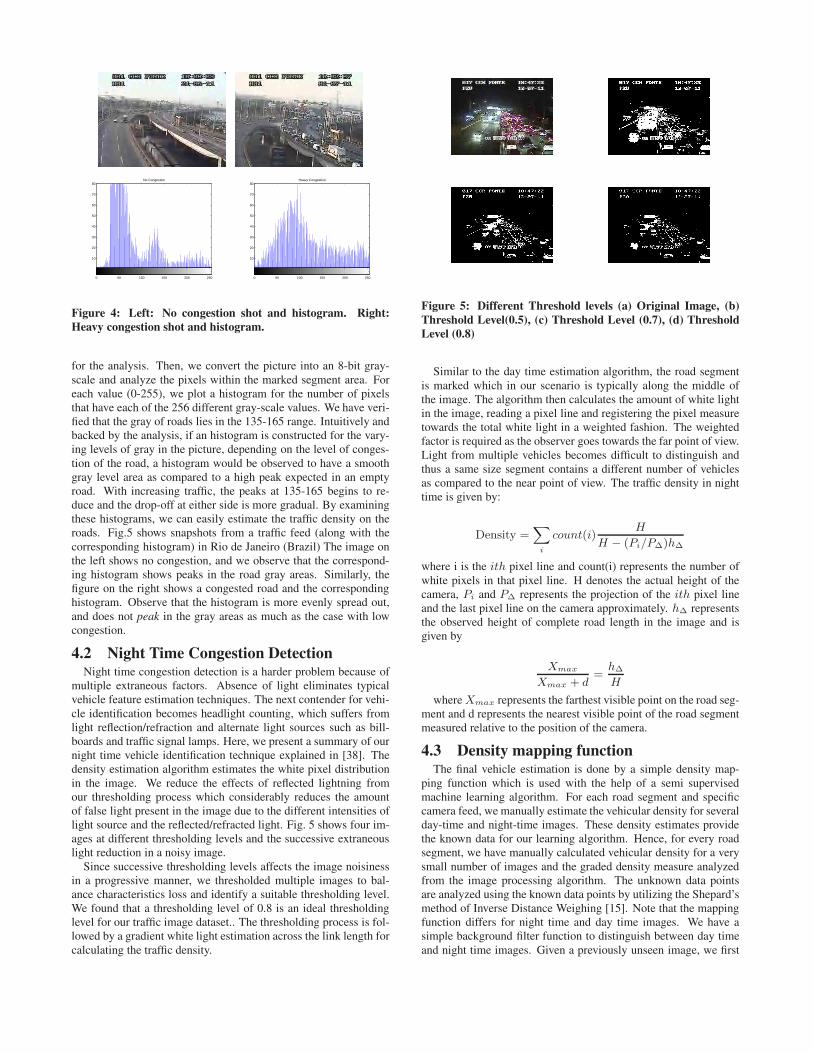
multiple extraneous factors. Absence of light eliminates typicalvehicle feature estimation techniques. The next contender for vehi-cle identification becomes headlight counting, which suffers fromlight reflection/refraction and alternate light sources such as bill-boards and traffic signal lamps. Here, we present a summary of ournight time vehicle identification technique explained in [38]. Thedensity estimation algorithm estimates the white pixel distributionin the image. We reduce the effects of reflected lightning fromour thresholding process which considerably reduces the amountof false light present in the image due to the different intensities oflight source and the reflected/refracted light. Fig. 5 shows four im-ages at different thresholding levels and the successive extraneouslight reduction in a noisy image.

Since successive thresholding levels affects the image noisinessin a progressive manner, we thresholded multiple images to bal-ance characteristics loss and identify a suitable thresholding level.We found that a thresholding level of 0.8 is an ideal thresholdinglevel for our traffic image dataset.. The thresholding process is fol-lowed by a gradient white light estimation across the link length forcalculating the traffic density.

Figure 5: Different Threshold levels (a) Original Image, (b)

Threshold Level(0.5), (c) Threshold Level (0.7), (d) Threshold

Level (0.8)

Similar to the day time estimation algorithm, the road segmentis marked which in our scenario is typically along the middle ofthe image. The algorithm then calculates the amount of white lightin the image, reading a pixel line and registering the pixel measuretowards the total white light in a weighted fashion. The weightedfactor is required as the observer goes towards the far point of view.Light from multiple vehicles becomes difficult to distinguish andthus a same size segment contains a different number of vehiclesas compared to the near point of view. The traffic density in nighttime is given by:

Density =X

i

count(i)H

H − (Pi/P∆)h∆

where i is the ith pixel line and count(i) represents the number ofwhite pixels in that pixel line. H denotes the actual height of thecamera, Pi and P∆ represents the projection of the ith pixel lineand the last pixel line on the camera approximately. h∆ representsthe observed height of complete road length in the image and isgiven by

Xmax

Xmax + d=

h∆

H

where Xmax represents the farthest visible point on the road seg-ment and d represents the nearest visible point of the road segmentmeasured relative to the position of the camera.

4.3 Density mapping functionThe final vehicle estimation is done by a simple density map-

ping function which is used with the help of a semi supervisedmachine learning algorithm. For each road segment and specificcamera feed, we manually estimate the vehicular density for severalday-time and night-time images. These density estimates providethe known data for our learning algorithm. Hence, for every roadsegment, we have manually calculated vehicular density for a verysmall number of images and the graded density measure analyzedfrom the image processing algorithm. The unknown data pointsare analyzed using the known data points by utilizing the Shepard’smethod of Inverse Distance Weighing [15]. Note that the mappingfunction differs for night time and day time images. We have asimple background filter function to distinguish between day timeand night time images. Given a previously unseen image, we first

estimate the graded density measure from the image processing al-gorithm and then use the manual data to analyze the graded trafficdensity. We then compute the final vehicular density as a weightedaverage of the vehicular densities with help from the manually clas-sified images.

5. EVIDENCE OF CONGESTION COLLAPSENumerous sources [32, 2, 7, 46] have reported that traffic con-

gestion is a serious problem in many cities in the developing world,leading to billions of dollars in losses annually. To understand theprevalence of congestion collapse, we have analyzed several daysworth of round-the-clock traffic feeds from several locations.

The traffic feeds used in this evaluation primarily consisted ofCCTV camera feeds. Quite often, video camera feeds consists ofan multi-camera stream where feeds from multiple cameras are dis-played cyclically with a known time period. Since we base ourwork solely using camera images, we convert the video feeds toimages and aggregate them per camera in an automated manner.The process is easy to perform and can be done in real-time, takingan insignificant amount of time per image. The static images nowobtained from the video feeds are fed to the evaluator which utilizesthe configured semantics and performs day/night time estimation toanalyze the vehicle density estimates.

The sources from which traffic data was collected from were:Rio de Janeiro, Brazil: Rio-Niteroi bridge [22, 4], the junction ofAv pres Vargas and Av Rio Branco, Camerino, Rd Santana and RdFrei Caneca.

Mombasa, Kenya: Moi Ave (TSS Bldg), Kengeleni Junction,and Sabasaba Traffic Lights [16].

Nairobi, Kenya: Pushorttam Place (Museum Hill), BarclaysPlaza (Uhuru Highway/Kenyatta Ave Rndbt), Ukulima House (HaileSelassie/Upperhill Road Rndbt), National Bank Building (Haram-bee Avenue), National Bank Building (Railways Roundabout), Na-tion Centre (Kenyatta Ave/Kimathi Street), Heidelberg Building(Mombasa Road), and a few others [16].

In total, we collected traffic image feeds from all three of theabove-mentioned places for a total of 80 hrs during the month ofJuly 2011. Different road segments were identified to exhibit con-gestion on different timings. A bird’s eye view of the source imageset displays high congestion in Brazil region during evening whichcontinues to night primarily near 4:30PM to 8:30 PM. On the otherhand, traffic in Kenya was observed to be highly erratic and burstystarting from 10AM to ending at 2PM. The evening time traffic wasrelatively non congested for the Kenyan region.

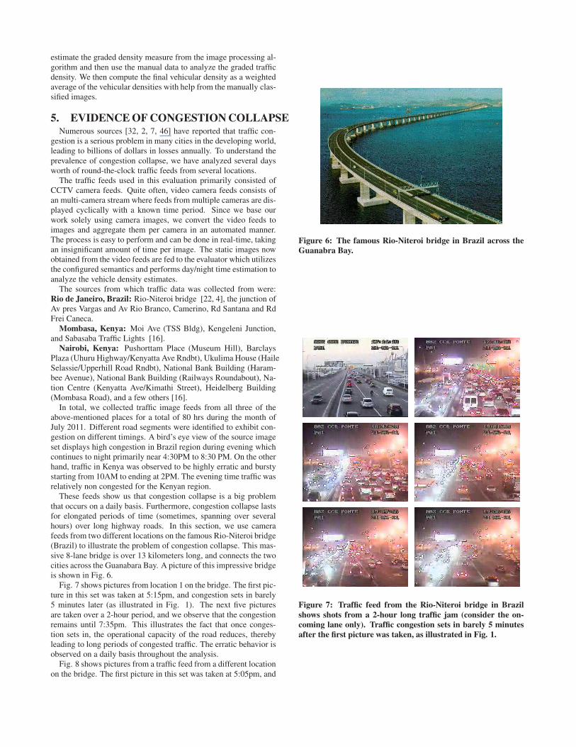
These feeds show us that congestion collapse is a big problemthat occurs on a daily basis. Furthermore, congestion collapse lastsfor elongated periods of time (sometimes, spanning over severalhours) over long highway roads. In this section, we use camerafeeds from two different locations on the famous Rio-Niteroi bridge(Brazil) to illustrate the problem of congestion collapse. This mas-sive 8-lane bridge is over 13 kilometers long, and connects the twocities across the Guanabara Bay. A picture of this impressive bridgeis shown in Fig. 6.

Fig. 7 shows pictures from location 1 on the bridge. The first pic-ture in this set was taken at 5:15pm, and congestion sets in barely5 minutes later (as illustrated in Fig. 1). The next five picturesare taken over a 2-hour period, and we observe that the congestionremains until 7:35pm. This illustrates the fact that once conges-tion sets in, the operational capacity of the road reduces, therebyleading to long periods of congested traffic. The erratic behavior isobserved on a daily basis throughout the analysis.

Fig. 8 shows pictures from a traffic feed from a different locationon the bridge. The first picture in this set was taken at 5:05pm, and

Figure 6: The famous Rio-Niteroi bridge in Brazil across the

Guanabra Bay.

Figure 7: Traffic feed from the Rio-Niteroi bridge in Brazil

shows shots from a 2-hour long traffic jam (consider the on-

coming lane only). Traffic congestion sets in barely 5 minutes

after the first picture was taken, as illustrated in Fig. 1.

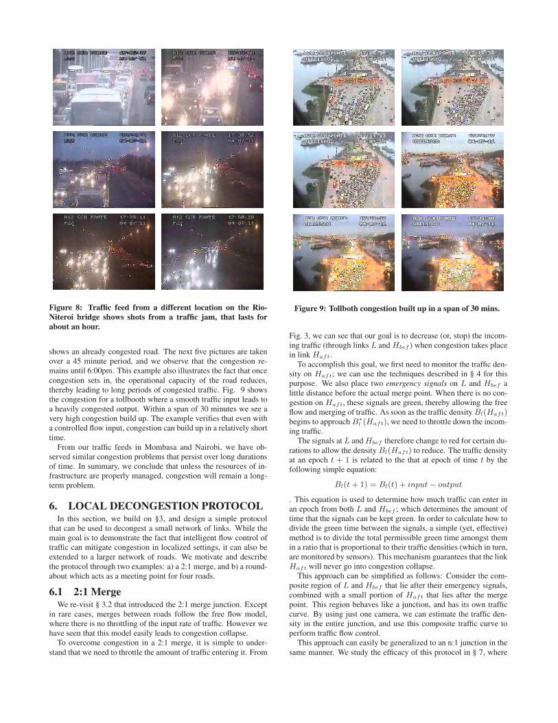
Figure 8: Traffic feed from a different location on the Rio-

Niteroi bridge shows shots from a traffic jam, that lasts for

about an hour.

shows an already congested road. The next five pictures are takenover a 45 minute period, and we observe that the congestion re-mains until 6:00pm. This example also illustrates the fact that oncecongestion sets in, the operational capacity of the road reduces,thereby leading to long periods of congested traffic. Fig. 9 showsthe congestion for a tollbooth where a smooth traffic input leads toa heavily congested output. Within a span of 30 minutes we see avery high congestion build up. The example verifies that even witha controlled flow input, congestion can build up in a relatively shorttime.

From our traffic feeds in Mombasa and Nairobi, we have ob-served similar congestion problems that persist over long durationsof time. In summary, we conclude that unless the resources of in-frastructure are properly managed, congestion will remain a long-term problem.

6. LOCAL DECONGESTION PROTOCOLIn this section, we build on §3, and design a simple protocol

that can be used to decongest a small network of links. While themain goal is to demonstrate the fact that intelligent flow control oftraffic can mitigate congestion in localized settings, it can also beextended to a larger network of roads. We motivate and describethe protocol through two examples: a) a 2:1 merge, and b) a round-about which acts as a meeting point for four roads.

6.1 2:1 MergeWe re-visit § 3.2 that introduced the 2:1 merge junction. Except

in rare cases, merges between roads follow the free flow model,where there is no throttling of the input rate of traffic. However wehave seen that this model easily leads to congestion collapse.

To overcome congestion in a 2:1 merge, it is simple to under-stand that we need to throttle the amount of traffic entering it. From

Figure 9: Tollboth congestion built up in a span of 30 mins.

Fig. 3, we can see that our goal is to decrease (or, stop) the incom-ing traffic (through links L and Hbef ) when congestion takes placein link Haft.

To accomplish this goal, we first need to monitor the traffic den-sity on Haft; we can use the techniques described in § 4 for thispurpose. We also place two emergency signals on L and Hbef alittle distance before the actual merge point. When there is no con-gestion on Haft, these signals are green, thereby allowing the freeflow and merging of traffic. As soon as the traffic density Bl(Haft)begins to approach B∗

l (Haft), we need to throttle down the incom-ing traffic.

The signals at L and Hbef therefore change to red for certain du-rations to allow the density Bl(Haft) to reduce. The traffic densityat an epoch t + 1 is related to the that at epoch of time t by thefollowing simple equation:

Bl(t + 1) = Bl(t) + input − output

. This equation is used to determine how much traffic can enter inan epoch from both L and Hbef ; which determines the amount oftime that the signals can be kept green. In order to calculate how todivide the green time between the signals, a simple (yet, effective)method is to divide the total permissible green time amongst themin a ratio that is proportional to their traffic densities (which in turn,are monitored by sensors). This mechanism guarantees that the linkHaft will never go into congestion collapse.

This approach can be simplified as follows: Consider the com-posite region of L and Hbef that lie after their emergency signals,combined with a small portion of Haft that lies after the mergepoint. This region behaves like a junction, and has its own trafficcurve. By using just one camera, we can estimate the traffic den-sity in the entire junction, and use this composite traffic curve toperform traffic flow control.

This approach can easily be generalized to an n:1 junction in thesame manner. We study the efficacy of this protocol in § 7, where

we show that congestion collapse can be easily prevented.

6.2 Four-way RoundaboutSimilar in spirit to § 6.1, we explain the decongestion of a four-

way roundabout. The roundabout has short segments on its in-put/output links as a composite junction j, with its own trafficcurve. Each of the links that leads into the roundabout has an emer-gency signal that turns red as a reaction to congestion in the round-about. When the traffic density of the junction Bl(j) is lower thanB∗

l (j) − ǫ, all these signals are green.When the junction nears its congestion threshold density B∗

l (j),the signals will have a reduced green time, determined by the actualdensity Bl(j). This green time is divided amongst the input linksin a manner proportional to their traffic densities. As before, thisapproach can be generalized to any junction with n input and outputlinks.

6.3 Localized Congestion AreasThe mechanism described above for the 2:1 merge and round-

about cases can be generalized for local congestion areas. Considera localized congestion area which has a small network of roads anda set of N input/output traffic signal points which dictate the inputand output flow out of this localized area. Based on free flow traffictheory [43], any free flow road segment can be associated with anapproximate traffic curve as described in earlier examples. Giventhat the localized area is a high congestion area, we can assume thatmost road segments are used at high capacity even in the presenceof traffic signals. Hence, there is constant flow across differentdirections within the localized region. In our local de-congestionprotocol, we explicitly model a localized congestion area with anapproximate traffic curve with a tipping point as specified by thetraffic curve. The exact parameters of the traffic curves and thetipping point can be generated using simulation based analysis ofthe road network topology for different arrival patterns.

Consider a local congestion area A with a traffic curve and a tip-ping point ∆ and a set of N input /output signals T1, . . . TN . Ourlocal decongestion protocol works as follows. Consider two smallsafety thresholds ǫ1 > ǫ2 > 0 with a small separation between twovalues. Let δ(A, t) represent the traffic density in the congestionarea A at time t. Our decongestion protocol uses CCTV camerafeeds at each of the input and output points to estimate the inputflow Xi(t) and output flow Yi(t) at each signal i (both are mea-sured in terms of traffic density). Hence, the system measures thenet flow into the congestion area across all the signals at time t asP

iXi(t)−

P

iYi(t) and normalizes the net flow in terms of traf-

fic density change within the area. Using this measure, the protocolconstantly measures δ(A, t) within the traffic area. If the local den-sity is less than ∆ − ǫ1, then the local decongestion protocol doesnot alter traffic signal behavior. The local decongestion protocoltriggers when

δ(A, t) > ∆ − ǫ2

When this event happens, the traffic density is close to the tip-ping point threshold. At this juncture, the local decongestion proto-col provides feedback to the individual signals to increase the "red"signal time and reduce the input flow. The traffic input rate at eachsignal is kept as proportional to the estimated queue size based onthe image feeds from the individual signals. The protocol continu-ously provides feedback to increase the "red" signal time until thedensity drops below ∆ − ǫ1. The two safety thresholds are usedto emulate a simple hysteresis behavior. In practice, ǫ1 and ǫ2 arevery small constants.

7. EVALUATION

In this section, we provide an evaluation of our protocol, to demon-strate the efficacy of the decongestion protocol in alleviating con-gestion collapse in road traffic networks. The specific sample topolo-gies we consider are: a) n:1 merge and b) four-way roundabout.We evaluate our protocol across these topologies, and show howour protocol avoids congestion collapse and provides considerableenhancements to the operational capacity.

7.1 MethodologyThe first step in performing the simulation is identifying the es-

sential parameters, a list of which is given below:

1. The number of links n in the network. Each link l has atraffic curve that is defined by two values: B∗

l and C∗

l . Theminimum delay dmin a vehicle will face in the link is gov-erned by the equation: B∗

l = dmin × C∗

l . Therefore byspecifying dmin and C∗

l , we define all the characteristics ofthe traffic curve. The delay d that a vehicle will face in thelink is calculated using dmin and the current traffic densityBl. Furthermore, the rest of the traffic curve for the link canbe approximated from these values.

2. The number of junctions/merges in the network. Each junc-tion/merge is identified by which input links flow into it, andwhich output links flow out of it. This determines the topol-ogy of the localized network.

3. The number of sources (vehicle generation points) in the net-work. Each source also defines which link it will send all itstraffic into.

4. The number of sinks (end-points of vehicle journeys) in thenetwork. Each sink also defines which link it receives all itsvehicles from.

5. Vehicle routes are determined when a vehicle is generated bya source. Each source is configured with a (possibly large)set of pre-determined routes that a vehicle generated by it cantake. The simulator verifies that these routes are legal (allow-able by the topology) before starting the simulation, and thenrandomly chooses one of these routes for every vehicle upongeneration.

6. Vehicle generation rates (burst rates) can also be configuredfor each of the sources. These rates are set over variablelength epochs of time.

7. The exit rate of free-flow links is determined by its traf-fic curve and current density. Links feeding into a junc-tion/merge can emit vehicles at their maximum rate C∗

l .

Once the various parameters are identified, a parameter file forthe topology is created. The simulator uses this parameter file andsimulates the functioning of the road network. We simulate eachtopology for a period of 40 minutes. In the results presented here,each traffic source generates vehicles uniformly within epochs thatlast 10 minutes each; the burst rate can vary across epochs.

The simulator records the time at which a vehicle was generatedby the source, and the time it was absorbed by the sink. It cantherefore calculate the travel time, along with the throughput (av-erage number of vehicles that reach their destination) at any pointof time. In our graphs, we plot the throughput on the Y-axis, andtime (in seconds) on the X-axis. The throughput at any secondis the total number of vehicles that have reached their respectivedestinations in the 60 second period centered around that second.

0

10

20

30

40

50

60

70

80

0 500 1000 1500 2000 2500

Avera

ge e

xit r

ate

(cars

/min

ute

)

Time (s)

Queue-based Signal Control (Small burst)No Coordination (Small burst)

Queue-based Signal Control (Large burst)No Coordination (Large burst)

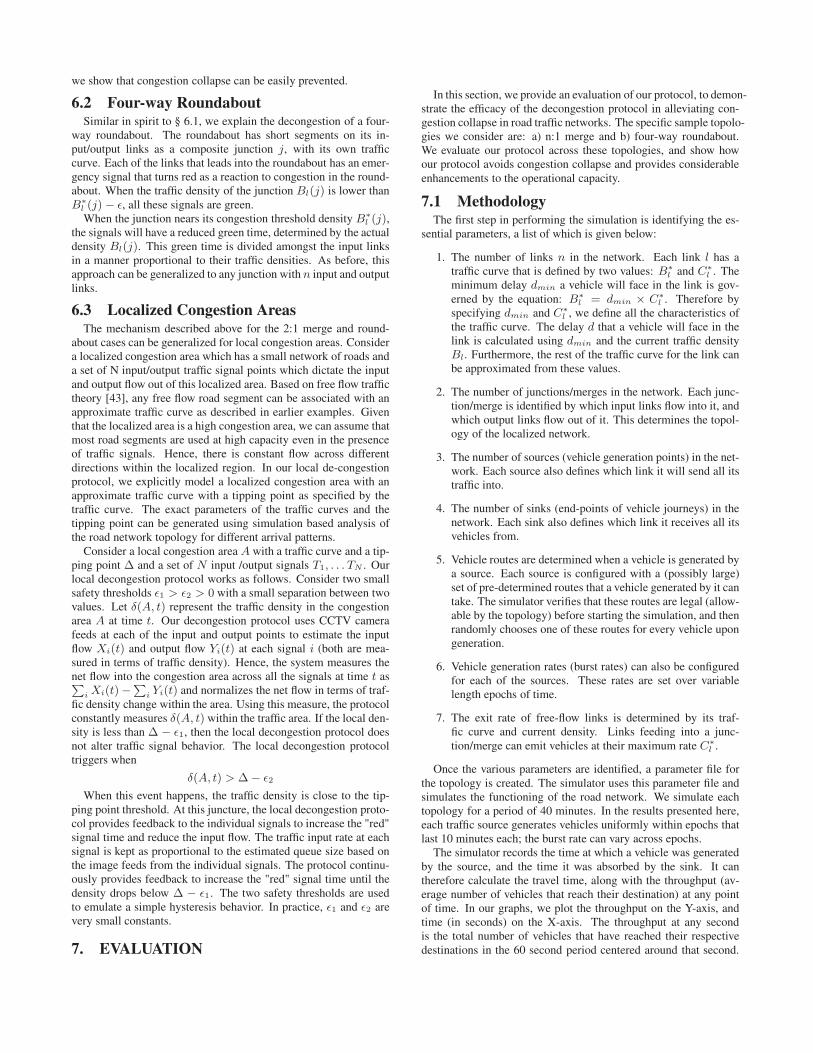
Figure 10: 2 : 1 Merge with d = 300s. Small bursts can lead to

collapse, which can be prevented using intelligent signaling.

Each graph plots two scenarios: a) when no signaling (or, local de-congestion protocol) is used (free-flow model), and b) our protocol(§ 6) is used.

7.2 n:1 MergeThe evaluation was conducted on this topology to examine the

effectiveness of the proposed signaling system in simple scenariosin which merging of traffic across multiple links to a single point ofconfluence. In this study, we repeat the experiments for n = 2, 4.

For the n:1 merge simulations, we set the the n input links tohave d = 160s and C∗

l = 1.0 cars per second. The output link hasC∗

l = 1.0 cars per second. We repeat the simulation for the outputlink having d = 300s and d = 450s. There is a source at each ofthe input links, and each source generates traffic at a constant rateduring the 40 minutes of the experiment. In addition, each sourceinserts an additional burst between t = 10min and t = 20min.We repeat the simulation for two different burst values as described.

7.2.1 2:1 Merge

Each source generates traffic at a constant rate of 30 cars perminute. The additional burst is either 10 cars per minute (largeburst) or 5 cars per minute (small burst). Fig. 10 plots the outputrate when the destination link has d = 300s. Congestion collapseoccurs as soon as the output link density goes above its B∗

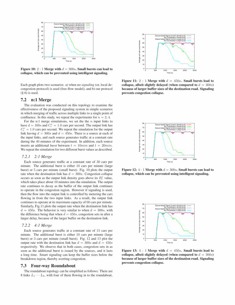
l value,which takes place about 10 minutes into the simulation. The outputrate continues to decay as the buffer of the output link continuesto operate in the congestion region. However if signaling is used,then the flow into the output link is controlled by metering the carsflowing in from the two input links. As a result, the output linkcontinues to operate at its maximum capacity of 60 cars per minute.Similarly, Fig.11 plots the output rate when the destination link hasd = 450s. The behavior is very similar to when d = 300s, withthe difference being that when d = 450s, congestion sets in after alarger delay, because of the larger buffer on the destination link.

7.2.2 4:1 Merge

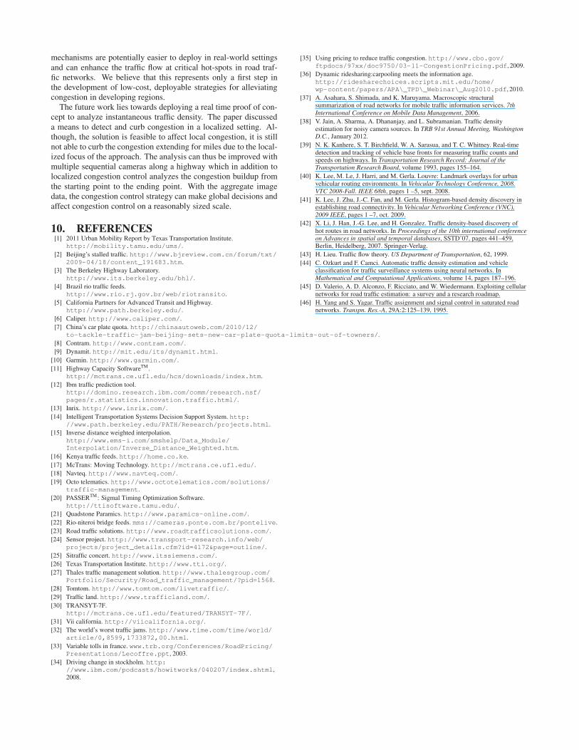
Each source generates traffic at a constant rate of 15 cars perminute. The additional burst is either 10 cars per minute (largeburst) or 3 cars per minute (small burst). Fig. 12 and 13 plot theoutput rate with the destination link has d = 300s and d = 450srespectively. We observe that in both cases, congestion sets in assoon as the additional burst is issued by the sources, and it lastsa long time. Smart signaling can keep the buffer sizes below thebreakdown region, thereby averting congestion.

7.3 Four-way RoundaboutThe roundabout topology can be simplified as follows: There are

8 links L1 · · ·L8, with four of them flowing in to the roundabout,

0

10

20

30

40

50

60

70

80

0 500 1000 1500 2000 2500

Avera

ge e

xit r

ate

(cars

/min

ute

)

Time (s)

Queue-based Signal Control (Small burst)No Coordination (Small burst)

Queue-based Signal Control (Large burst)No Coordination (Large burst)

Figure 11: 2 : 1 Merge with d = 450s. Small bursts lead to

collapse, albeit slightly delayed (when compared to d = 300s)

because of larger buffer sizes of the destination road. Signaling

prevents congestion collapse.

0

10

20

30

40

50

60

70

80

0 500 1000 1500 2000 2500

Avera

ge e

xit r

ate

(cars

/min

ute

)

Time (s)

Queue-based Signal Control (Small burst)No Coordination (Small burst)

Queue-based Signal Control (Large burst)No Coordination (Large burst)

Figure 12: 4 : 1 Merge with d = 300s. Small bursts can lead to

collapse, which can be prevented using intelligent signaling.

0

10

20

30

40

50

60

70

80

0 500 1000 1500 2000 2500

Avera

ge e

xit r

ate

(cars

/min

ute

)

Time (s)

Queue-based Signal Control (Small burst)No Coordination (Small burst)

Queue-based Signal Control (Large burst)No Coordination (Large burst)

Figure 13: 4 : 1 Merge with d = 450s. Small bursts lead to

collapse, albeit slightly delayed (when compared to d = 300s)

because of larger buffer sizes of the destination road. Signaling

prevents congestion collapse.

0

10

20

30

40

50

60

70

80

0 500 1000 1500 2000 2500

Avera

ge e

xit r

ate

(cars

/min

ute

)

Time (s)

Queue-based Signal Control (Small burst)No Coordination (Small burst)

Queue-based Signal Control (Large burst)No Coordination (Large burst)

Figure 14: Roundabout with d = 60s: The small buffer size of

the roundabout leads to congestion quickly taking place, which

can be prevented using signaling.

0

10

20

30

40

50

60

70

80

0 500 1000 1500 2000 2500

Avera

ge e

xit r

ate

(cars

/min

ute

)

Time (s)

Queue-based Signal Control (Small burst)No Coordination (Small burst)

Queue-based Signal Control (Large burst)No Coordination (Large burst)

Figure 15: Roundabout with d = 20s: The extremely small

buffer size of the roundabout leads to congestion immediately

taking place, which can be prevented using signaling.

and the other four flowing out of it. These links have identicaltraffic curves, with d = 160s and C∗

l set to 1.0 cars per second.The roundabout is associated with a traffic curve, with parametersC∗

l = 1.0 cars per second, and the experiment is repeated for d =60s and d = 20s. The four incoming links are each served by asource, while the four outgoing links each flow into a sink. Eachsource generates traffic at the rate of 15 cars per minute during theentire experiment. Each source generates an additional burst fromt = 10min to t = 20min of 10 cars per minute (large burst) or 3cars per minute (small burst).

From Fig. 14 and 15 we observe that if signaling is not used, theroundabout gets congested very quickly. This congestion collapselasts till the end of the simulation. However if we use smart signal-ing to control the flow of traffic from the four input links into theroundabout, we can keep the roundabout operating at its optimal ca-pacity, thereby avoiding congestion collapse. We verified that thisbehavior is repeated with different traffic burst rates, and differenttraffic curves for the links. In particular, we observe that when theroundabout has a smaller buffer capacity (d = 20s, as illustrated inFig.15), even a very small burst over a very small period of time isenough to congest the roundabout.

8. RELATED WORKThe problem of traffic congestion has been prevalent in both de-

veloping and developed countries. Variety of solutions have beendeveloped in the previous decade [23, 19, 25, 27], but as mentionedin § 2, developing countries suffer from an additional set of con-straints hampering these predefined solutions making the problemtougher. Congestion prevention and congestion control are the twoapproaches to solve the traffic congestion problem. Congestion pre-vention focuses on reducing the number of incoming vehicles in

the road traffic networks. Numerous ways have been devised byvarious government authorities like promoting car-pooling systems[36], congestion pricing or time variable toll mechanisms [33, 35,34] and car plate quotas [7]. Congestion control mechanisms in-cludes traffic engineering and monitoring. The available real-timeinformation from deployed road sensors is leveraged and a predic-tive analysis is applied to propose near future traffic patterns anddevelop a situational solution to tackle the current traffic. Nowa-days real-time traffic information is collected from various sourceslike traffic cameras, road sensors and even cellphone providers [29,18, 13]. Advance GPS systems mitigate this problem by find-ing less congested routes [28, 10]. Various mechanisms like vari-able speeding, ramp metering and lane specific signaling are ap-plied on available real-time information to manage traffic conges-tion. [41] proposes the usage of histogram based density discov-ery scheme for road connectivity which is leveraged for LOURVE[40]; LOURVE focuses on global route optimal scheme to calcu-late best paths on its defined overlay network. [42] develops a newalgorithm FlowScan, to cluster road segments instead of clusteringthe moving traffic to identify congested traffic routes.

Texas Transportation Institute (TTI) [26] has developed severalapplications that are widely used in local, state and federal levelsfor controlling the signal timing information [20]. McTrans [17]project at University of Florida provides a host of applications re-lated to road traffic management. HCS+ [11] and Traffic NetworkStudy Tool [30] provides signal timing optimization based on a va-riety of objective functions. Contram [8] is another software whichprovides real time traffic monitoring and optimized real time trafficroutes. It is currently deployed in places like Stockholm, Kent andother large cities. The Sensor Project [24] enables efficient datacollection so that traffic management can be done in a better way,by the use of sensors to collect the data. There are also applicationswhich monitor existing real time traffic and predict traffic mod-els which can prevent traffic congestion. Applications like IBMTraffic prediction tool [12] and the combination of Caliper Prod-ucts [6](Transmodeller and TransCAD) are used to simulate andpredict traffic models.

Use of third party mediums to disseminate traffic information isbeing actively pursued. Danilo [45] explores the idea of cellularnetworks to convey information to users of information. Akinoriet al., [37] proposes creation of well formed maps which could beused by mobile traffic information services. However, in our case,we intend to create monitoring and signaling stations which cantake decisions on their own without user intervention and hence,regulate traffic.

9. CONCLUSION AND FUTURE WORKRoad traffic congestion is a central problem in most developing

regions. Most urban areas have poorly managed traffic networkswith several traffic hot-spots or potential congestion areas. In thispaper, we study the problem of road traffic congestion in high con-gestion hot-spots in developing regions. We first present a simpleimage processing algorithm to estimate traffic density at a hot-spotusing CCTV camera feeds. Based on analysis of traffic imagesfrom live traffic feeds, we show evidence of congestion collapsewhich last for elongated time periods. Based on the free-flow traf-

fic curve behavior of links, critical road segments when exposed toshort bursts in traffic can result in the specific segments operatingat low-capacity levels for long time periods. To partially alleviatethis problem for small congestion areas such as traffic hot-spots, wedevelop a local de-congestion protocol that controls the flow of traf-fic into near-congested regions, thereby preventing collapse causedby short bursts of traffic. Our hope is that localized de-congestion

mechanisms are potentially easier to deploy in real-world settingsand can enhance the traffic flow at critical hot-spots in road traf-fic networks. We believe that this represents only a first step inthe development of low-cost, deployable strategies for alleviatingcongestion in developing regions.

The future work lies towards deploying a real time proof of con-cept to analyze instantaneous traffic density. The paper discusseda means to detect and curb congestion in a localized setting. Al-though, the solution is feasible to affect local congestion, it is stillnot able to curb the congestion extending for miles due to the local-ized focus of the approach. The analysis can thus be improved withmultiple sequential cameras along a highway which in addition tolocalized congestion control analyzes the congestion buildup fromthe starting point to the ending point. With the aggregate imagedata, the congestion control strategy can make global decisions andaffect congestion control on a reasonably sized scale.

10. REFERENCES[1] 2011 Urban Mobility Report by Texas Transportation Institute.

http://mobility.tamu.edu/ums/.

[2] Beijing’s stalled traffic. http://www.bjreview.com.cn/forum/txt/2009-04/18/content_191683.htm.

[3] The Berkeley Highway Laboratory.http://www.its.berkeley.edu/bhl/.

[4] Brazil rio traffic feeds.http://www.rio.rj.gov.br/web/riotransito.

[5] California Partners for Advanced Transit and Highway.http://www.path.berkeley.edu/.

[6] Caliper. http://www.caliper.com/.

[7] China’s car plate quota. http://chinaautoweb.com/2010/12/to-tackle-traffic-jam-beijing-sets-new-car-plate-quota-limits-out-of-towners/.

[8] Contram. http://www.contram.com/.

[9] Dynamit. http://mit.edu/its/dynamit.html.

[10] Garmin. http://www.garmin.com/.

[11] Highway Capacity SoftwareTM .http://mctrans.ce.ufl.edu/hcs/downloads/index.htm.

[12] Ibm traffic prediction tool.http://domino.research.ibm.com/comm/research.nsf/

pages/r.statistics.innovation.traffic.html/.

[13] Inrix. http://www.inrix.com/.

[14] Intelligent Transportation Systems Decision Support System. http://www.path.berkeley.edu/PATH/Research/projects.html.

[15] Inverse distance weighted interpolation.http://www.ems-i.com/smshelp/Data_Module/

Interpolation/Inverse_Distance_Weighted.htm.

[16] Kenya traffic feeds. http://home.co.ke.

[17] McTrans: Moving Technology. http://mctrans.ce.ufl.edu/.

[18] Navteq. http://www.navteq.com/.

[19] Octo telematics. http://www.octotelematics.com/solutions/traffic-management.

[20] PASSERTM : Sigmal Timing Optimization Software.http://ttisoftware.tamu.edu/.

[21] Quadstone Paramics. http://www.paramics-online.com/.

[22] Rio-niteroi bridge feeds. mms://cameras.ponte.com.br/pontelive.

[23] Road traffic solutions. http://www.roadtrafficsolutions.com/.

[24] Sensor project. http://www.transport-research.info/web/projects/project_details.cfm?id=4172&page=outline/.

[25] Sitraffic concert. http://www.itssiemens.com/.

[26] Texas Transportation Institute. http://www.tti.org/.

[27] Thales traffic management solution. http://www.thalesgroup.com/Portfolio/Security/Road_traffic_management/?pid=1568.

[28] Tomtom. http://www.tomtom.com/livetraffic/.

[29] Traffic land. http://www.trafficland.com/.

[30] TRANSYT-7F.http://mctrans.ce.ufl.edu/featured/TRANSYT-7F/.

[31] Vii california. http://viicalifornia.org/.

[32] The world’s worst traffic jams. http://www.time.com/time/world/article/0,8599,1733872,00.html.

[33] Variable tolls in france. www.trb.org/Conferences/RoadPricing/Presentations/Lecoffre.ppt, 2003.

[34] Driving change in stockholm. http://www.ibm.com/podcasts/howitworks/040207/index.shtml,2008.

[35] Using pricing to reduce traffic congestion. http://www.cbo.gov/ftpdocs/97xx/doc9750/03-11-CongestionPricing.pdf, 2009.

[36] Dynamic ridesharing:carpooling meets the information age.http://ridesharechoices.scripts.mit.edu/home/

wp-content/papers/APA\_TPD\_Webinar\_Aug2010.pdf, 2010.

[37] A. Asahara, S. Shimada, and K. Maruyama. Macroscopic structuralsummarization of road networks for mobile traffic information services. 7th

International Conference on Mobile Data Management, 2006.

[38] V. Jain, A. Sharma, A. Dhananjay, and L. Subramanian. Traffic densityestimation for noisy camera sources. In TRB 91st Annual Meeting, Washington

D.C., January 2012.

[39] N. K. Kanhere, S. T. Birchfield, W. A. Sarasua, and T. C. Whitney. Real-timedetection and tracking of vehicle base fronts for measuring traffic counts andspeeds on highways. In Transportation Research Record: Journal of the

Transportation Research Board, volume 1993, pages 155–164.

[40] K. Lee, M. Le, J. Harri, and M. Gerla. Louvre: Landmark overlays for urbanvehicular routing environments. In Vehicular Technology Conference, 2008.

VTC 2008-Fall. IEEE 68th, pages 1 –5, sept. 2008.

[41] K. Lee, J. Zhu, J.-C. Fan, and M. Gerla. Histogram-based density discovery inestablishing road connectivity. In Vehicular Networking Conference (VNC),

2009 IEEE, pages 1 –7, oct. 2009.

[42] X. Li, J. Han, J.-G. Lee, and H. Gonzalez. Traffic density-based discovery ofhot routes in road networks. In Proceedings of the 10th international conference

on Advances in spatial and temporal databases, SSTD’07, pages 441–459,Berlin, Heidelberg, 2007. Springer-Verlag.

[43] H. Lieu. Traffic flow theory. US Department of Transportation, 62, 1999.

[44] C. Ozkurt and F. Camci. Automatic traffic density estimation and vehicleclassification for traffic surveillance systems using neural networks. InMathematical and Computational Applications, volume 14, pages 187–196.

[45] D. Valerio, A. D. Alconzo, F. Ricciato, and W. Wiedermann. Exploiting cellularnetworks for road traffic estimation: a survey and a research roadmap.

[46] H. Yang and S. Yagar. Traffic assignment and signal control in saturated roadnetworks. Transpn. Res.-A, 29A:2:125–139, 1995.