QCN: Quantized Congestion Notification

Rong Pan, Balaji Prabhakar, Ashvin LaxmikanthaHigh PerformanceSwitching and RoutingTelecom Center Workshop: Sept 4, 1997.

2

Overview

• Description the QCN scheme– Pseudocode available with Rong Pan: ropan@cisco.com

• Basic simulations– Infinitely long-lived flows: stability of control loop– Dynamic flows: FCT

• Notes on FCT, heavy-tailed flow size distributions

3

Congestion management loopcomponents

Source ReactionPoint

CongestionPoint 1

CongestionPoint n

ReflectionPoint

Destination

• Reaction Point: Where the rate of injection of a flow (or flows) is changed dueto congestion signals; usually, the place where rate limiters reside.

• Congestion Point: Where resources (buffers/links) exist and can becongested, and where congestion signals are generated; usually, switchbuffers and the links they are attached to.

• Reflection Point: Where congestion signals are reflected back to the source.

• Congestion Management Domain: ReaP -- CPs -- RefP.

4

Summary of QCN• Summary description of mechanisms at the Reaction Points,

Congestion Points and Reflection Points.1. Reaction Points: Insert Fb = 0 in outgoing packets. When congestion message

arrives: perform multiplicative decrease, fast recovery and active probing.2. Congestion Points: Compute Fb, overwrite Fb in packet header, reflect negative

Fb values as “intermediate reflection points”.3. Reflection Points: Reflect Fb values to ReaPs with a probability biased by the Fb

value in the packet.

• We also describe a number of useful enhancements; the details can befound in the pseudocode.1. Extra fast recovery: Helps a reaction point recover from bursty “dings”.2. Positive reinforcement: Helps a reaction point use Fb=0 values to increase rate.3. No queue-length capping: Helps a congestion point use current queue length, even

though this may exceed qeq. This is possible in QCN because Fb is computed at theswitch. It allows the switch to send high Fb values when its queue size is large.This is similar to BCN-MAX.

• Feedback message: Packet generated by a reflection point for a reactionpoint and corresponds to a data packet sampled during congestion.Contains Fb value and flow identification information.

5

Reaction Point

• ReaP Dynamics– Starting rate for every flow equals 10Gbps– Insert Fb = 0 in outgoing packet– Insert a “flowid” into outgoing packet’s header (optional)

• Whenever a ReaP receives a feedback message– Decrease rate from R to Rnew = R(1 - |Fb|xGd), where Gd is a gain– Perform “fast recovery” and “active probing”– Useful refinements: “extra fast recovery” and “positive reinforcement”

• The way refinements are to be incorporated is detailed in the p-code• We give a high-level description at the end of the presentation

6

Fast Recovery and Active Probing

Time

Rat

e

R

Rnew

Congestion message recd

RdRd/2

Rd/4Rd/8

Fast Recovery

Active Probing

7

Reaction Point (cont’d)• Fast recovery

– Let Rd = R |Fb| Gd be the amount of rate decrease– Fast recovery proceeds in cycles, clocked by the “fast recovery timer”– Fast recovery timer

• Resets upon receipt of negative Fb message• Increments for every transmitted byte

– Fast recovery cycles• The FR timer counts out cycles (every so many transmitted bytes)• Cycles numbered 0, 1, 2, 3, 4, 5; the maximum cycle number is 5

– The transmission rate during cycle k equals Rnew + Rd/2 + Rd/4 + … + Rd/2k as longas no further QCN messages are received

– If a congestion message is received, then cut rate as before and restart fast recovery– At the end of fast recovery, the source moves to Active Probing

• Active probing (multiplicative increase) always follows fast recovery– Active probing is clocked by the same byte counting time as fast recovery– When timer expires, the current rate is changed to R + Ri, where Ri is the increase

amount– If a congestion message is received, cut rate as before, perform fast recovery and

then active probing

8

Congestion Point

• At the CP– Sample packets with probability p– Compute: Fb = - [ qoff + w qdelta ]– Overwrite

• If Fb < 0, and if Fb value is smaller (more negative) than Fb value in the packet header, then overwrite Fb value in packet header with computed Fb value

– Reflect• If Fb < 0, then reflect Fb value probabilistically back to the source

with a bias which increases with Fb• Set the “frame-reflected” bit

qoff = q - qeqqdelta = # pkts enqueued - # pkts dequeued between two packet arrivals (or sampling instants)

qeq

9

Reflection Point

• The end reflection point (in the 3-point architecture)– If the incoming frame has the “frame-reflected” bit set, do nothing– Elseif Fb < 0, reflect Fb value to source with a probability which increases with |Fb|– Else Fb=0; reflect this back to source with some small probability, say P0

10

Refinements1. Extra-fast Recovery: Suppose a source gets multiple congestion messages in a

burst, driving its rate down by a lot. Say that the rates of decrease are Rd1, Rd2 andRd3. Fast recovery only uses the last amount of decrease Rd3. UsingRd1+Rd2+Rd3 (or even max(Rd1,Rd2,Rd3)) improves performance. This is doneonly during the first cycle (cycle 0) of Fast Recovery. Negative messages received insubsequent cycles restart Fast Recovery.

2. Positive Reinforcement: If a Reaction Point receives an Fb=0 message, itimmediately advances to the next cycle of Fast Recovery or Active Probing. I.e. itchanges the timer value and transmission rate appropriately.

3. No queue-length capping: Fb is computed as Fb = - [(q-qeq) + w qdelta], where q isnot constrained to be between -qeq and 2qeq. Removing this restriction allows theswitch to compute more negative Fb values if the buffer is congested beyond 2qeq.Of course, these are quantized to the maximum negative value of Fb, should theyexceed the range of Fb. This behavior correctly signals the “congested buffer”condition similarly as BCN-MAX, while retaining “linearity.”

• Note: we have tried not to introduce extra parameters or behaviors so as to avoidextra specification and tuning.

11

Basic Simulations

12

Outline

1. Infinitely long-lived flows• Simultaneous starts• Staggered starts

2. Dynamic heavy-tailed flows• Flow completion times for long flows, short flows• Losses

13

Parameters and settings

• Infinitely long-lived flows: simultaneous starts– Single link, 6 flows on at 10 Gbps at time 0– Link delay (RTT): 40 microseconds– Gd = 1/128– w = 2– Ri = 3 Mbps– Sampling function = linearly increases with |Fb| from 1--25%– Reflection probability = 0 and 2.5%

• Staggered starts: staggered starts– Single link, 6 flows on 500 microseconds apart– Same parameters as above

14

Simultaneous, reflection probability = 0Queue length; # Pkts dropped = 449

15

Simultaneous, reflection probability = 0Rate

16

Simultaneous, reflection probability = 2.5%Queue length; #Pkts dropped = 462

17

Simultaneous, reflection probability = 2.5%Rate

18

Staggered, reflection probability = 0Queue length; #Pkts dropped = 11

19

Staggered, reflection probability = 0Rate

20

Staggered, reflection probability = 2.5%Queue length; #Pkts dropped = 8

21

Staggered, reflection probability = 2.5%Rate

22

Unit step response vs FCT

• Historically, congestion control research has considered the performance of ascheme under infinitely long-lived flows– This gives the unit step response of the scheme– Very useful for control-theoretic analysis and hence for picking the parameters for the

stability of the control loop– But, it does not capture dynamic situation of flows arriving and departing (which is the

actual situation)– It does not have a notion of “load” which can be increased; it is always at 100% load– It does not capture flow completion time (FCT), a quantity users care about

• The recent literature takes a 2-step approach– First study scheme under infinitely long-lived flows– After picking parameters and ensuring stability of control loop, consider FCT– This is consistent with CPU performance under “workloads” consisting of files and

brings the role of algorithms into focus– Key metric: FCT and th related quantity “slowdown”– Slowdown for job or flow of size x = FCT of flow / x = 1 / Bdwdth given to the flow

23

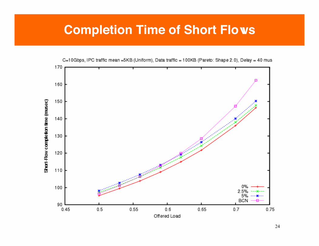
Dynamic flows: FCT and Drops

• Workload– IPC traffic: Mean = 5 KB (uniform distribution)– Data traffic: Pareto, shape 2, mean 100 KB– Parameters (Gd, w, etc): same as before– Reflection probability = 0, 2.5 and 5%

24

Completion Time of Short Flows

25

Completion Time of Long Flows

26

Drops