Forecasting road traffic conditions using a context based random forest algorithm

Jonny Evansa, Ben Watersona and Andrew Hamiltonb

a University of Southampton, Building 176, Boldrewood Innovation Campus, Highfield,

Southampton, Hampshire, U.K.; bSiemens Mobility Limited, Sopers Lane, Poole, Dorset, U.K.

Accepted for publication in Journal of Transportation Planning and Technology

ARTICLE HISTORY Compiled March 27, 2019

ABSTRACT With the ability to accurately forecast road traffic conditions several hours, days and even months ahead of time, both travellers and network managers can take pro-active measures to minimize congestion, saving time, money and emissions. This study evaluates a previously developed random forest algorithm, RoadCast, which was designed to achieve this task. RoadCast incorporates contexts using machine learning to forecast more accurately, contexts such as public holidays, sporting events and school term dates. This study aims to evaluate the potential of RoadCast as a traffic forecasting algorithm for use in Intelligent Transport Systems applications. Tests are undertaken using a number of different forecast horizons and varying amounts of training data, and an implementation procedure is recommended.

KEYWORDS Traffic forecasting, random forest, loop detector, machine learning, context

1. Introduction

Road congestion places a burden on citizens worldwide. In 2016 alone, road congestion cost U.S. drivers more than $295 billion, U.K. drivers £30 billion, and German drivers €69 billion (Cookson 2016). To tackle this, transportation investment has been increasingly directed toward Intelligent Transport Systems (ITS), which aim to make the most of existing transport networks with the use of technology. With the ability to accurately forecast congestion and traffic flow days, weeks or years ahead of time, a number of ITS applications could be improved, such as tolling policies, and route guidance systems.

In a previous study, RoadCast, a random forest algorithm was developed to tackle this task (Evans, Waterson, and Hamilton 2018). Since that study, RoadCast has been iterated on, but the fundamental approach remains the same. RoadCast aims to accurately forecast at a horizon of multiple days by forming an understanding of how contexts affect traffic conditions. Contexts are planned to occur beforehand, and cause variation in a predictable way. RoadCast ‘learns’ from previous occurrences of contexts in a training dataset, then uses schedules of future context occurrences to account for their variation in its forecasts. It was designed to incorporate contexts in an automated way, so that it would be suitable for the ITS applications described. To do this, standardised methods to encode features, and an automatic optimisation algorithm were developed.

CONTACT Jonny Evans. Email: jonny.evans@soton.ac.uk

This study provides an in depth evaluation of RoadCast’s ability to forecast traffic conditions. The aim of this evaluation is to assess RoadCast’s suitability for ITS applications, such as incident detection, context aware route guidance and improved scheduling strategy (planned road works, public transport, congestion charging etc.). To do this, RoadCast will be tested under a number of scenarios with different forecast horizons and amounts of training data, and will be compared to a historical average, which is a commonly used predictor in ITS applications. Based on these tests, an implementation procedure will be recommended for RoadCast’s potential use in ITS applications.

2. Relevant literature

The fields of traffic forecasting and traffic variation are vast, so a complete review has not been included. Instead, the most closely related research on state of the art forecasting algorithms are described, and the gap in literature being filled by RoadCast is identified.

A large portion of the traffic forecasting field is dedicated to short-term forecasting, where algorithms typically have horizons of up to an hour (Vlahogianni, Golias, and Karlaftis 2004; Leshem and Ritov 2007; Zarei, Ghayour, and Hashemi 2013). However, as these algorithms are based on recent observations of traffic conditions, they are incapable of forecasting at a horizon of multiple days. Research using longer horizons typically focus on forecasting aggregated travel behaviour (such as yearly vehicle miles travelled) many years into the future. Little research has been dedicated to forecasting specific traffic conditions (such as five minute flows) at a horizon of multiple hours, days, weeks or years. When such a forecast is required, a form of historical average based on the time of day and day of the week is typically used (Syrjarinne 2016; Chrobok et al. 2000).

Many traffic variation studies found that variation can be caused by contexts, such as weather and sporting events (Thomas, Weijermars, and van Berkum 2008; Stathopoulos and Karlaftis 2001). However, few have built on these studies to create predictive models, and few forecasting algorithms incorporate contextual data. As such, when projects require forecasts of days or weeks ahead of time, variation from contexts is rarely accounted for.

Zhang et al. showed that short-term forecasts can become more accurate when weather and holiday data is incorporated (Zhang et al. 2015). This was shown with a ‘system identification’ method using the average speeds of taxis in Hangzhou, China, from devices with GPS. However, this algorithm’s forecast horizon was at most 10 hours because it relied partly on recent observations. Jia, Wu, and Xu found that accuracies improved when rainfall data was incorporated within their neural network short-term forecasting algorithm, but their forecast horizon was at most 30 minutes (Jia, Wu, and Xu 2017). Both of these algorithm’s horizons were limited as they used recent observations of traffic conditions as inputs.

Chung developed a Small Large Ratio (SLR) clustering algorithm to forecast travel times on ultrasonic detectors on a highway in Tokyo, using rainfall, holiday, and day of the week contexts (Chung 2003). The algorithm clustered similar travel times together, grouped these clusters using the contexts, then used these groups as the base for a historical average predictor. That is, it would classify each time being forecasted into one of its groups, then use the average value of this group’s travel times as the forecast. The predictor was found to be more accurate with contexts by 0.1% mean absolute percentage error. However, this was an unsupervised machine learning algorithm which clustered data based only on the traffic data. The contextual data was only used to explain the outputs of this algorithm. As such, this method did not automatically ‘learn’ the patterns of travel times with respect to contexts, but instead relied on human intuition to interpret the outputs of the algorithm, meaning significant manual calibration would be required for implementation.

2

Of the algorithms presented that were capable of forecasting at a horizon of multiple days, many were forms of historical average (Syrjarinne 2016; Chrobok et al. 2000). Few have incorporated contexts, and none have done so in an automated way. The most similar algorithm to RoadCast presented was a recurrent Jordan neural network for forecasting loop detectors flows (Yasdi 1999). The longest horizon used was one week. First, different types of day were defined manually, ordinary Mondays, Tuesdays/Wednesdays/Thursday, Fridays, Saturdays, Sundays/holidays, and special event days (e.g. football matches, road works etc.). The type of day, along with recent observations of volumes, would be used as the input to the algorithm. This study demonstrated that different types of day can be incorporated within a machine learning traffic forecasting algorithm to improve accuracies. Unfortunately, no results were stated for the algorithm using a one week horizon. This approach differs from RoadCast in that it involved labour intensive and inflexible processes. The creation of different types of day was done manually, which would take time, effort and expertise to replicate for implementation in a new network. It would also be inflexible when different detectors required different groupings. For example, if Sundays had different flows than holidays on detectors near shopping malls, or Saturdays were similar to Sundays at detectors in industrial areas, the algorithm’s presented groupings would be unsuitable. RoadCast differs from this approach in that it uses machine learning to automatically ‘learn’ how different contexts affect each detector.

RoadCast is novel in that it uses contextual data within a machine learning algorithm to forecast traffic conditions at a horizon of multiple days. An advantage of the machine learning approach is that the effect of each context can be ‘learnt’ automatically, so that when implemented in a new location, accurate forecasts can be achieved with minimal manual calibration. As the algorithm does not use recent observations as input, it has a longer horizon than short-term forecasting algorithms, making it better suited to certain ITS applications, such as scheduling road works. To ensure the algorithm would be transferable and easily implemented, an automatic optimisation algorithm was also developed, which automatically selects appropriate contexts, and optimises RoadCast’s parameters at each detector. This differentiates RoadCast from the state of the art in that it allows the calibration of contexts at each detector to be done automatically, reducing the manual time and expertise required for implementation.

3. Methodology

3.1. Approach taken

In order to find the most suitable method for the problem, many types of machine learning and statistical methods were developed and compared in preliminary tests. The random forest algorithm was chosen for use in RoadCast for a number of reasons:

Found to be more accurate than a historical average in terms of mean squared error

during preliminary tests. Capable of stating prediction intervals (Meinshausen 2006). Methods exist to interpret the algorithm’s predictions (Palczewska et al. 2014). Minimal manual calibration required to obtain forecasts for the study test set. Fast training and testing times.

3.2. Random forest theory

Decision trees make splits in training data to create subsets in which messages have similar feature values and similar target variable values. Random forests create many decision trees on various subsets of the training data, and each of which make their own prediction. The random forest prediction is then the average of each of these tree’s predictions. The RoadCast algorithm was developed using the Scikit-learn library in Python (Pedregosa et al. 2011).

3

The random forest algorithm used in RoadCast is formally described in the following algorithms. Algorithm 2 describes how many decision trees (algorithm 1) are combined into the random forest used in RoadCast. Each detector and target variable combination used a separate random forest. Breiman provides further explanation of the random forest method (Breiman 2001). However, the algorithm presented below is a modified version of Breiman’s original random forest method.

Algorithm 1 Decision tree algorithm

1: Training procedure(set of training messages Ztr): 2: Create a node B0 and assign all training messages Ztr to it 3: While every leaf has more than M messages assigned to it: 4: Find the leaf node Bi with the most messages 5: From a random subset of features of size S, find the attribute a to split Bi’s messages

into two subsets such that the sum of the subset’s target variable variances is minimized 6: Create child nodes Bj and Bj+1 from Bi 7: Assign Bi’s messages to Bj and Bj+1 according to their value of a 8: End procedure

Algorithm 2 Random forest algorithm

1: Training procedure(set of training messages Ztr): 2: For a pre defined number of trees K: 3: Create a bootstrap random sample Zr

tr from Ztr of size |Ztr| 4: Create a decision tree Tr with Zr

tr using algorithm 1 5: End procedure 6: Testing procedure(set of testing messages Zts): 7: For each message x in Zts: 8: Predict a value yi for message x using each of the decision trees T1...Tk 9: Return the mean of the predicted values y 10: End procedure

3.3. RoadCast optimisation algorithm

Incorporating contextual data within a complex forecasting algorithm could be an arduous, labour intensive task. But many real-world applications require minimal calibration time, effort and expertise for implementation. For example, a survey regarding the implementation of incident detection algorithms found that Traffic Management Centres (TMCs) require calibration to be achievable either automatically or by TMC staff (Guin 2004). As such, the process of incorporating contextual data within RoadCast was automated as much as possible. As a part of this, an optimisation algorithm, algorithm 3, was developed to automatically select the most relevant contextual features and optimal parameters for each detector and each target variable (flow and average speed). This algorithm improved RoadCast’s accuracy by making it more transferable to different locations, but did not require any manual calibration.

As can be seen in algorithms 1 and 2, the random forest has three tuning parameters, the number of trees grown K, the size of the subset of features used to split on S and the stopping criterion, which in this case was chosen to be the threshold number of messages required at each leaf M. The optimisation algorithm uses a 15-fold cross validation score (herein referred to as ‘score’), which returns 15 scores representing RoadCast’s forecast accuracy on each fold (i.e. subset) of the training data. Throughout the ‘context inclusion’ procedure, RoadCast uses parameters K = 10, M = 1 and S = 1. Once the optimisation algorithm is run on the training data, RoadCast is ready to make forecasts on test data. Algorithm 3 is a psuedocode describing the optimisation algorithm.

4

Algorithm 3 RoadCast optimisation algorithm

1: Context inclusion procedure(set of training messages Ztr, set of features A): 2: For each contextual feature in A: 3: If the context didn’t occur during training: 4: Remove the feature from A 5: Set the benchmark score as the score with ‘time of day’ and ‘day of week’ features

only 6: For each feature in A: 7: Add the feature to the algorithm and find the algorithm’s score 8: If the score improved on the benchmark on at least 14 folds: 9: Keep the feature in A 10: Else: 11: Remove the feature from A 12: Set the benchmark score as the score with the features in A 13: For each feature in A: 14: Remove the feature from the algorithm and find the algorithm’s score 15: If the score improved on the benchmark on at least two folds: 16: Remove the feature from A 17: If the feature ‘Christmas’ is in A: 18: Replace the ‘day of week’ feature with ‘modified day of week’ 19: End procedure 20: Parameter optimisation procedure(set of training messages Ztr, set of features included

in A): 21: For M in [2, 5, 10, 25, 100, 200]: 22: For S = 1 to |A|: 23: Find the cross validation score with parameters M and S 24: Determine the parameters that achieved the best score, M* and S* 25: Retrain the algorithm on all available training data with the features in A, and

parameters M*, S* and K=100 26: End procedure

4. Data

4.1. Traffic data

4.1.1. Location

Southampton City Council provided the traffic data for this study. The problem of congestion comes at a significant cost to Southampton, predominantly in the form of losses in productivity and fuel costs. It was estimated that Southampton drivers spent an average of 24 hours in gridlock in 2016, resulting in a cost to the city of £74 million, or £748 per driver (Cookson 2016).

However, Southampton was ranked as only the 18th most congested in the U.K. Each of the top 25 U.S. cities were found to be more congested than Southampton, and each of the world’s 25 most congested cities (covering 12 countries) were more than twice as congested as Southampton (Cookson 2016). Clearly then, the problem of congestion faced by Southampton is also faced across cities globally. Many ITS applications aim to improve the state of congestion in these cities, and a key part of many of these applications is an accurate traffic forecast.

5

4.1.2. Data description

111 single inductive loop detectors around Southampton were used to collect traffic data for the study. Figure 1 shows the location of the detectors used. 111 single inductive loop detectors around Southampton were used to collect traffic data for the study. 726 days worth of data was collected from 16th March 2015 to 16th March 2017 (5 days of data were missing). In the various tests undertaken in this study, different subsets of this data were used for training and testing. Each detector’s values of flow and estimated average speed of vehicles in each 5 minute period (over the lane of the detector) were used as the target variables in this study. RoadCast would be implemented on each combination of detector and target variable separately.

Figure 1. Locations of the detectors used in this study. This image was created with Google Earth.

4.2. Contextual Data

A wide range of contextual data was collected with the aim of developing contextual features that would improve the accuracy of RoadCast’s forecasts. In a previous study, the first year of the Southampton dataset was used to develop contextual features for RoadCast (Evans, Waterson, and Hamilton 2018). Firstly, influential contexts were identified by observing disruption in traffic conditions on the dates of particular contexts. Then by running preliminary tests on the first year of data, contexts were developed into features if they were found to improve RoadCast’s forecasts.

6

Context type

Encoding method Contexts used in the Southampton network

Time Hour of the day + minutes/60 Time of day Day of week Integer, 0 to 6 (Monday to Sunday) Day of week Modified day of week

Integer, 7 if during Christmas, 0 to 6 otherwise

Modified day of week

Single day events

Number of days + Number of hours/24 + minutes/1440 to the start of the nearest occurrence of the event. 10 if not within a given time-frame of the event occurrence starting.

Football and cricket matches, Southampton marathon, charity event and New Year’s Eve

Multiple day events

Number of days since the start of the nearest occurrence of the event. 10 if not during the event.

Music festival, boat show, public holidays, Easter.

Christmas Number of days since/until the nearest Christmas day. 10 if not during the holiday.

Christmas

Figure 2. Standard method used to encode each type of context, and contexts used in the Southampton network.

A caveat of this study was that the contextual data was collected after the contexts took place, because schedules of contexts from 16th March 2015 were not available. If RoadCast were to make forecasts a year into the future, it would need to use schedules of these contexts. Many of these schedules would not change (such as public holidays and New Year’s Eve), but some may (such as rescheduled football matches). If contexts were rescheduled, RoadCast could account for this by remaking its forecasts with updated contextual features, albeit at a shorter forecasting horizon.

When studying weather contexts for RoadCast, historical weather forecasts were not available. Instead, historical observations were used to understand whether RoadCast’s forecasts would improve with accurate weather data. When forecasting into the future, clearly RoadCast would need to use weather forecasts. These forecasts may differ from observations, particularly when using a forecast horizon of a year. As such, weather contexts were not included in RoadCast in this study.

To minimise the manual time and expertise required to implement RoadCast, standardised methods were developed to define how contextual data can be encoded into features that RoadCast can use as input. These methods were developed by studying the first year of data in Southampton. However, they were designed to be transferable to different locations and data types. Figure 2 defines the methods developed, as well as the features used for the Southampton dataset. These features were used in the tests described in the results section below.

Each event context was given an arbitrary value of 10 if not within a given time-frame of the event starting. These time-frames captured the period in which each type of context could be expected to affect traffic conditions. In this study, each single day event context was given a time-frame of six hours. However, in locations where events may take longer (e.g. American football matches), a longer time frame may be appropriate. This nuance was developed because when developing RoadCast on the training data, over fitting to spurious patterns in some values of contexts would occur occasionally. For example, RoadCast could split a node based on higher/lower than 4.5 days to the nearest football match. One can see that this split wouldn’t truly differentiate traffic patterns at this time. However, RoadCast made splits such as this when there were few samples in a given node, and they happened to be correlated in this way. By giving a value of 10 days to messages that were not within six hours of a football match kickoffs, these messages could not be separated by the ‘football’

7

context. Hence, these spurious patterns in contexts were less likely to be found, and so this overfitting would be reduced. The time-frames of each of the single day event context would need to be defined before implementing RoadCast. ‘Christmas’ had a different encoding method to other multiple day events because the day on which Christmas day falls changes each year, and the proximity of each message to Christmas day was found to be a useful indicator of expected traffic conditions. As such, the context was given a value based on the proximity to Christmas day if during the holiday, 10 otherwise. The holiday was defined as the start of Christmas Eve until the end of the last non-working day after New Year’s Eve.

During preliminary tests, RoadCast’s first split was often by the ‘day of week’ feature, meaning contexts that did not occur on the same day of the week in training and testing sets may not have been accounted for during testing. For example, Christmas occurred on a Friday in 2015, so the algorithm’s decision trees may only have split on the Christmas context over messages that occurred on a Friday. This would mean that when tested on Christmas Sunday in 2016, the ‘Christmas’ context would not have been used. To address this, the ‘modified day of week’ feature was created. This modification tackled the problem above by ensuring all messages during the Christmas holiday would be in the same part of each decision tree. This would then allow the Christmas feature to split messages depending on their date with respect to Christmas, rather than their day of the week. As described in the optimisation algorithm (algorithm 3), the ‘modified day of week’ was used instead of ‘day of week’ when the ‘Christmas’ context was found to improve RoadCast’s accuracy.

5. Results

5.1. Introduction

This section evaluates RoadCast’s ability to forecast traffic conditions in a number of different scenarios. It is tested under different forecast horizons and amounts of training data, and its decision making process is examined. For these tests, the Road-Cast methodology and feature encodings were applied to the Southampton dataset described above. For each test, various subsets of this dataset were used for training and testing. The following subsections describe the findings of these tests, which would be used to make recommendations as to how RoadCast should be implemented in ITS applications.

5.2. Performance metric

In order to evaluate the accuracy of the presented algorithm, the Mean Squared Error (MSE) was used as the performance metric. For a detector d, MSE is defined as:

𝑀𝑆𝐸 𝑑1𝑁

ã 𝑑, 𝑡 𝑎 𝑑, 𝑡

where N is the number of messages in the test dataset, ã is the predicted value at detector d at time tj, and a is the true value.

8

5.3. Historical average predictor

When a traffic forecast of over an hour ahead is required, a form of historical average is typically used. During the development of RoadCast, it was found to be one of the most simple and accurate predictors. The most accurate form of historical average found was to take the mean of subsets of the training data corresponding to each combination of ‘time of day’ and ‘day of week’. That is, to forecast next Monday at 9:05am as the mean of all Mondays at 9:05am in the training data. Periods that had no messages in the training data were predicted as the same day, previous time period. This form of historical average was chosen for comparison with RoadCast because of its commonality of use throughout the literature (Syrjarinne 2016; Chrobok et al. 2000).

5.4. Initial test

5.4.1. Test devised

Firstly, all the available data was used to evaluate RoadCast. The first year of data was used for training (up to 16th March 2016), and the second year for testing (16th March 2016 onwards). A year of training and testing data was used so that every context could be ‘learnt’ from in training, and evaluated in testing. This test can be seen as a preferable scenario for RoadCast being implemented, because a year of training data means that every context will have occurred at least once.

5.4.2. Results

Over all detectors, RoadCast’s flow forecasts had an average MSE of 79.9 vehicles squared, compared to the historical average’s 84.4, a 5.3% improvement. For average speed, RoadCast had an average MSE of 16.36 miles per hour (mph) squared, compared to the historical average’s 17.02, a 3.9% improvement. RoadCast was more accurate than the historical average on 93% and 97% of the detectors when forecasting flow and average speed respectively.

Figure 3 shows the percentage improvement of each detector. Without context, RoadCast forecasted similarly, but slightly more accurately than the historical average (see figure 3). Accuracy improvements came from reducing variance by averaging over similar times of the day and days of the week (such as the similarly low flows on Sunday 23:35-23:55). When contextual data was added, further improvements in both average speed and flow were achieved. More detail on the way in which contexts affected RoadCast’s forecasts was analysed in a previous study (Evans, Waterson, and Hamilton 2018).

Figure 3. RoadCast’s MSE percentage improvement over the historical average at each detector.

9

Notice that the incorporation of contextual data aided the flow forecast accuracy more so than average speed. This is thought to be because the contexts caused more variation in flow than average speed. Every context altered travel demand, and so was seen to cause flow variation. However, this would only lead to average speed variation if flows exceeded the road capacity, and so caused congestion. Variation in average speed may also have come from contexts affecting road capacity, such as road conditions being changed by rainfall, but this variation was found to be negligible in Southampton.

On occasion, RoadCast could forecast less accurately than the historical average. This is thought to be caused by RoadCast training on unrepresentative data. For example, emergency road works caused severe congestion during Easter 2015 in Southampton, which disrupted flow and average speed values at some detectors. Emergency road works cannot be predicted, so the flow values were not representative of what could be expected to occur during future Easters. RoadCast used this data to predict very low average speeds during Easter 2016, which created large MSEs that were not produced by the historical average. Another example of RoadCast training on unrepresentative data was when detectors that had a major change in topology or travel demand nearby, or if a detector broke and hence returned values of the target variable of zero. RoadCast would make inaccurate predictions if such a change occurred during the training or testing period. In practice, if RoadCast were to be retrained regularly, inaccurate forecasts would occur until the training period was entirely after the change. To limit this drawback, manual intervention could be used, or an algorithm to automatically identify such a change, and retrain RoadCast accordingly, could be developed.

6. Sensitivity to the amount of training data used

In the initial test of RoadCast (section 5.4), RoadCast was tested with a year of training data so that all contexts could be ‘learnt’ from in training, and evaluated in testing. However, if RoadCast required one year of data to train, its use in the real world may be limited. If accurate traffic forecasts were needed within a year of data being collected for a particular location, it is unclear whether RoadCast would be suitable. As such, this section evaluates RoadCast’s forecast accuracy when using different amounts of training data.

6.1. Test methodology

The test devised would assess RoadCast’s ability to forecast traffic conditions when using different amounts of training data. The test would use the second year of data for testing (16th March 2016 onwards), but various length periods for training. Training periods would be of the last week, two weeks, month, two months, four months, eight months and one year before the testing period start date. A year of testing data was used so that RoadCast’s ability to forecast every context could be assessed. The same year was used each time so that the results of each test would be directly comparable. The training period was taken as the period before the test start date (rather than 16th March 2015 onwards) because this would be most similar to a real-world implementation of RoadCast. That is, if a certain amount of training data had been collected to date at a particular location, an idea of the accuracy of RoadCast’s forecasts would be gained.

6.2. Flow

Figure 4 shows each predictor’s mean squared error, averaged over all detectors, when forecasting flow while using different amounts of training data. As expected, when each predictor had more training data, forecasts became more accurate. When using only a week of training data, RoadCast had a very similar accuracy with and without contextual data because no event or holiday contexts occurred in the week between 9th and 16th March 2016, and so the optimisation algorithm rarely included any contexts. However, the historical average predictor was much less accurate because it would simply use the message with the same time and day of the week as in the training data. RoadCast would hence forecast with less variance by averaging over messages of similar times and days of

10

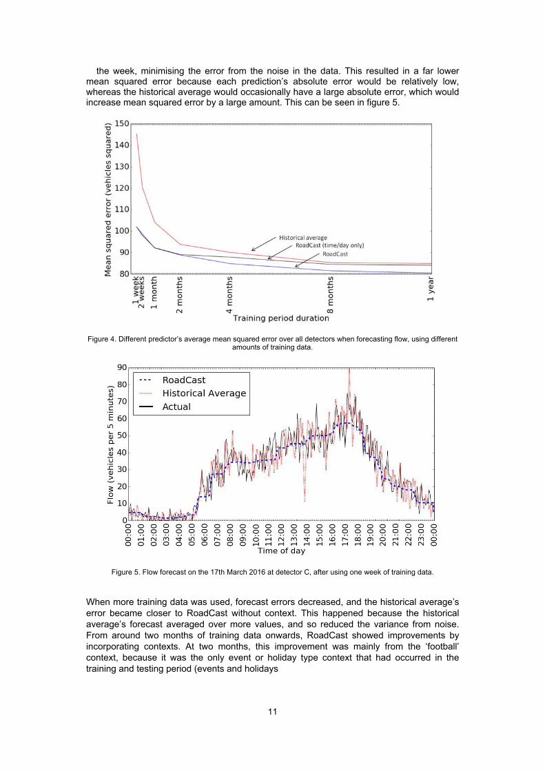
the week, minimising the error from the noise in the data. This resulted in a far lower mean squared error because each prediction’s absolute error would be relatively low, whereas the historical average would occasionally have a large absolute error, which would increase mean squared error by a large amount. This can be seen in figure 5.

Figure 4. Different predictor’s average mean squared error over all detectors when forecasting flow, using different amounts of training data.

Figure 5. Flow forecast on the 17th March 2016 at detector C, after using one week of training data.

When more training data was used, forecast errors decreased, and the historical average’s error became closer to RoadCast without context. This happened because the historical average’s forecast averaged over more values, and so reduced the variance from noise. From around two months of training data onwards, RoadCast showed improvements by incorporating contexts. At two months, this improvement was mainly from the ‘football’ context, because it was the only event or holiday type context that had occurred in the training and testing period (events and holidays

11

had most effect on forecast accuracies). A larger improvement was found at four months because the training period included Christmas (which had very different flows to other days), meaning forecasts of Christmas 2017 were far more accurate. Other days’ forecasts also improved slightly, as they would now be an average of messages that were not during Christmas, meaning the forecast would not be skewed by Christmas’s typically low flows. At eight months, ‘public holiday’ and many other event contexts were also included in the training data. At one year, ‘Easter’ was also included. As such, with more training data, RoadCast continued to improve by incorporating more contexts. The amount of training data required for RoadCast to benefit from particular contexts can be seen as a limitation for implementing RoadCast in a real world implementation. This test showed that if a context doesn’t occur (or rarely occurs) in the available training data, it cannot be accounted for in RoadCast’s forecasts. If a longer time period of training data were to be used, it is unclear how forecast accuracies would change. Accuracy improvements may come from reducing variance further by averaging over more data, but accuracies may worsen if this data is unrepresentative, for example if long term changes, such as population increase, altered traffic patterns. Accuracies of RoadCast without context and the historical average would be expected to converge, because with more data, RoadCast without context would be more likely to use subsets of each combination of time and day of the week. RoadCast with context would be expected to continue to improve relative to the other predictors, by ‘learning’ from more occurrences of rarely occurring contexts, such as ‘Christmas’.

6.3. Average speed

As can be seen in figure 6, the predictors followed a similar trend when forecasting average speed to forecasting flow, but there were some key differences. Firstly, the difference between RoadCast and the historical average was larger with one week of training data, because noise caused more variation in average speed data than flow data. With more data, this difference became proportionally smaller than the difference with flow because the historical average could become more accurate by averaging over more data, but RoadCast improved marginally because there was little to be gained from ‘learning’ from contexts.

Figure 6. Different predictor’s average mean squared error over all detectors when forecasting average speed, using different amounts of training data.

12

7. Sensitivity to the forecast horizon

This test aimed to discover whether RoadCast’s forecast accuracy would degrade when using a greater forecasting horizon. If it did by a large amount, regular re-training of the algorithm would be recommended so that forecasts would be based on representative data. It was clear that RoadCast’s and the historical average’s forecast would not differ greatly when forecasting with different horizons over small time periods, e.g. 5, 10, 15 minutes. This is because both algorithms are based on the patterns found in large periods of historical data, rather than recent observations. However, when forecasting many months into the future, long-term variations in traffic conditions (such as population growth or building construction) could cause lower forecasting accuracies. As such, RoadCast was tested over a variety of long-term forecasting horizons.

7.1. Test methodology

The test devised was to repeatedly test on the last month’s data (from 15th February 2017), using a year of training data from different periods before the test set. That is, a year that ended one day, one week, one month, two months, four months and eleven months before the testing period. Note that five detectors which had no messages during the testing period, due to missing or erroneous data, were not included in the results.

7.2. Flow

Figure 7 shows that as the forecast horizon increased, each predictor became less accurate, but RoadCast remained the most accurate throughout. Each predictor followed a similar trend in terms of the error and the rate of change of error as the forecast horizon increased. The increase in errors observed at greater forecast horizons were likely caused by long term changes in traffic conditions, such as population increase or travel mode change.

Figure 7. Different predictors’ average mean squared error when forecasting flow at different horizons.

13

Although mean squared errors increased by 3.6% as the horizon increased, figure 8 shows how the forecasts at a one year horizon still followed the actual travel conditions closely, and could still use contexts effectively to forecast more accurately. This suggests that the long term variation in Southampton’s traffic conditions between the two years was minor. However, it is expected that if the road network changed significantly, such as a new road was built near to the detector, forecasts would become inaccurate and so retraining would be required. Similarly, significant changes to contexts (such as a football team changing stadium) would result in forecasts of such contexts becoming inaccurate.

Figure 8. Flow forecast at a one year horizon, for Saturday, 4th February 2017, at detector A. Premier League football match against West Ham kicked off at 15:00 at St Mary’s Stadium.

7.3. Average speed

Figure 9 again shows that as the horizon increased, each of the predictors MSE increased, and the difference in MSE between the predictors changed little. However, the difference between the predictors was different for average speed than flow, in that RoadCast without context had a comparatively larger difference to the historical average, but comparatively less difference with and without context. The reasons for these differences were explained in the findings of the initial test (see section 5.4).

14

Figure 9. Different predictor’s average mean squared error when forecasting average speed at different horizons.

8. Implementation procedure

As was previously stated, minimal calibration time, effort and expertise is required for many applications of a traffic forecasting algorithm. As such, RoadCast was designed in such a way that implementation would be simple, quick and as automated as possible. This has meant developing standardised feature encoding methods and an automatic optimisation algorithm, and evaluating RoadCast in a number of different scenarios. Using the results of these tests, this section describes how best RoadCast can be implemented in a new location for an ITS application.

The first step is to identify contexts which may affect road traffic conditions in the network being implemented, and a data source from which their schedules can be collected. This list doesn’t have to be exhaustive, as any relevant context added should only improve the forecasts made. Also, not every context identified has to necessarily affect conditions, because the optimisation algorithm will later rule out contexts that are not relevant to each detector and target variable. This step requires some local knowledge and intuition, which could be expected in many ITS applications, e.g. operators in TMCs to implement an incident detection algorithm. For this study, the author’s local knowledge was relied upon to identify relevant contexts in Southampton. This is the only labour intensive step in implementing RoadCast, and as such increases the time, effort and expertise required to implement RoadCast in real world applications. The next step is to collect historical data for training, both for the traffic variables being forecasted, and the identified contexts. One year of training data is recommended, because this was found to result in the best accuracy as all contexts could be accounted for. However, if less than a year of data was available for training, RoadCast could still be expected to forecast more accurately than the historical average. Single day event contexts also require a start time for each occurrence, and multiple day contexts require a start date and end date for each occurrence. For this study, the data was collected manually from various websites, but for implementation in ITS applications, an automatic web scraper would be recommended.

15

The next step is to encode each context as features to input into RoadCast. To do this, the standardised methods of encoding features, defined in figure 2, should be followed. The only manual step in this process is deciding on a time frame for each context, the time-frame is a period in which the context could be expected to affect traffic conditions.

At this point, the optimisation algorithm should be run. This takes the training data, and returns a trained random forest for each detector and target variable. Finally, RoadCast can make forecasts of future traffic conditions. RoadCast was found to be most accurate at the shortest forecast horizon, one day. As such, retraining is recommended as often as possible. In this study, RoadCast took 8.1 minutes to fully train and test per detector and target variable (30 hours for flow and average speed on all 111 detectors), which was achieved on an Intel(R) Core(TM) i7-6700, 3.40Ghz, 16GB RAM. Considering this training time, retraining every day may not be practical or even possible for implementation in some ITS applications, particularly for large networks or on computer systems with slow processing speeds or low memory capacities. However, RoadCast can be expected to achieve accurate forecasts if retrained just once per year. RoadCast’s MSE increased by 3.6% percent as the horizon increased from one day to 11 months. The retraining frequency is a trade off between accuracy and computation cost and time, which needs to be considered on a case by case basis.

9. Conclusions

This study provides an in depth evaluation of RoadCast, a novel algorithm that forecasts traffic conditions at a horizon of multiple days. The algorithm was compared to a historical average predictor under a number of different forecast horizons and amounts of training data.

In each test, RoadCast was found to be consistently more accurate than the historical average in forecasting both flow and average speed. For low amounts of training data, this came from RoadCast’s ability to minimise the effect of noise by averaging over similar times and day of the week. For high amounts of training data, this came from RoadCast’s ability to ‘learn’ from contexts.

The major limitations of incorporating contexts within RoadCast were found to be the need to identify relevant contexts and their data sources, and acquiring sufficient training data for the contexts to be ‘learnt’ from. Another limitation to RoadCast’s accuracy occurs when the training data includes large amounts of unrepresentative data, such as incidents, erroneous detector values, or major topology or travel demand change.

The tests show that RoadCast is transferable to many different scenarios of fore-casting horizons and amounts of available training data. The findings of these tests were used to form recommendations for how RoadCast could be implemented in ITS applications. Possible applications include:

Varying strategy of public transport and planned road works in response to forecasted traffic conditions.

Varying congestion charges and tolling based on forecasted congestion levels (see

projects such as Stockholm’s congestion charging scheme (Eliasson et al. 2009)).

Incident detection algorithms that could better differentiate incidents from congestion caused by contexts.

Varying logistic companies’ schedules and routes based on congestion forecasts.

16

10. Acknowledgements

This research has been funded by Engineering and Physical Sciences Research Council (EPSRC) and Siemens Mobility Limited. The authors wish to thank Southampton City Council for providing the traffic data used in this research.

17

References

Breiman, Leo. 2001. ‘Random forests’. Machine learning 45 (1): 5-32. Chrobok, Roland, Oliver Kaumann, Joachim Wahle, and Michael Schreckenberg. 2000. ‘Three categories of traffic data: Historical, current, and predictive’. In proceedings of the 9th IFAC Symposium Control in Transportation Systems, 250-255. Chung, Edward. 2003. ‘Classification of traffic pattern’. In proceedings of the 11th World Congress on ITS, 687-694. Cookson, Bob, Graham; Pishue. 2016. ‘INRIX Global Traffic Scorecard’. Technical report. Eliasson, J, L Hultkrantz, L Nerhagen, and L Rosqvist. 2009. ‘The Stockholm congestion charging trial 2006: Overview of effects’. Transportation Research Part A: Policy and Practice 43 (3): 240-250. Evans, Jonny, Ben Waterson, and Andrew Hamilton. 2018. ‘RoadCast: An algorithm to forecast this year’s road traffic." In proceedings of the 97th Annual Meeting of the Transportation Research Board. Guin, Angshuman. 2004. ‘An incident detection algorithm based on a discrete state propagation model of traffic flow’. PhD thesis. Georgia Institute of Technology. Jia, Yuhan, Jianping Wu, and Ming Xu. 2017. ‘Traffic flow prediction with rainfall impact using a deep learning method." Journal of Advanced Transportation 2017: 10. Leshem, Guy, and Yaacov Ritov. 2007. ‘Traffic flow prediction using adaboost algorithm with random forests as a weak learner’. In proceedings of World Academy of Science, Engineering and Technology, Vol. 19, 193-198. Meinshausen, Nicolai. 2006. ‘Quantile regression forests’. Journal of Machine Learning Research 7 (Jun): 983-999. Palczewska, Anna, Jan Palczewski, Richard Marchese Robinson, and Daniel Neagu. 2014. ‘Interpreting random forest classification models using a feature contribution method’. In integration of Reusable Systems, 193-218. Springer. Pedregosa, Fabian, Gael Varoquaux, Alexandre Gramfort, Vincent Michel, Bertrand Thirion, Olivier Grisel, Mathieu Blondel, Peter Prettenhofer, Ron Weiss, and Vincent Dubourg. 2011. ‘Scikit-learn: Machine learning in Python’. Journal of Machine Learning Research 12 (Oct): 2825-2830. Stathopoulos, A., and M. Karlaftis. 2001. ‘Temporal and spatial variations of real-time traffic data in urban areas’. Transportation data and Information Technology (1768): 135-140. Syrjarinne, Paula. 2016. ‘Urban traffic analysis with bus location data’. PhD thesis. University of Tampere. Thomas, T., W. Weijermars, and E. van Berkum. 2008. ‘Variations in urban traffic volumes’. European journal of transport and infrastructure research 3 (8): 71-80. Vlahogianni, Eleni I., John C. Golias, and Matthew G. Karlaftis. 2004. ‘Short-term traffic forecasting: Overview of objectives and methods’. Transport Reviews 24 (5): 533-557. Yasdi, R. 1999. ‘Prediction of road traffic using a neural network approach’. Neural Computing and Applications 8 (2): 135-142. Zarei, Narjes, Mohammad Ali Ghayour, and Sattar Hashemi. 2013. ‘Road traffic prediction using context-aware random forest based on volatility nature of traffic flows’, 196-205. Berlin, Heidelberg: Springer Berlin Heidelberg.

18

Zhang, Rong, Yuanchao Shu, Zequ Yang, Peng Cheng, and Jiming Chen. 2015. ‘Hybrid traffic speed modeling and prediction using real-world data’. In IEEE International Congress on Big Data, 230-237.

19