THE ANALYSIS OF ROAD TRAFFIC ACCIDENT DATA IN THE ...
322
THE ANALYSIS OF ROAD TRAFFIC ACCIDENT DATA IN THE IMPLEMENTATION OF ROAD SAFETY REMEDIAL PROGRAMMES. CALVIN JOHN MOLLETT Thesis presented in partial fulfilment of the requirements for the degree of Master of Engineering at the University of Stellenbosch. Promoter: Professor CJ Bester February 2001
-
Upload
khangminh22 -
Category
Documents
-
view
0 -
download
0
Transcript of THE ANALYSIS OF ROAD TRAFFIC ACCIDENT DATA IN THE ...
THE ANALYSIS OF ROAD TRAFFIC ACCIDENT DATA IN THE
IMPLEMENTATION OF ROAD SAFETY REMEDIAL
PROGRAMMES.
CALVIN JOHN MOLLETT
Thesis presented in partial fulfilment of the requirements for the degree of
Master of Engineering at the University of Stellenbosch.
Promoter: Professor CJ Bester
February 2001

ii
DECLARA TION
I the undersigned hereby declare that the work contained in this thesis is my
own original work and has not previously in its entirety or in part been submitted
at any university for a degree.
DATE
Stellenbosch University http://scholar.sun.ac.za

iii
ABSTRACT
A road safety remedial programme has as an objective the improvement of road
transportation safety by applying road safety engineering remedial measures to
hazardous road network elements in a manner that will be economically
efficient.
Since accident data is the primary manifestation of poor safety levels it must be
analysed in manner that will support the overall objective of economic efficiency.
Three steps in the process of implementing a road safety remedial programme,
that rely on the systematic analysis of accident data, are the identification of
hazardous locations, the ranking of hazardous locations and the evaluation of
remedial measure effectiveness.
The efficiency of a road safety remedial programme can be enhanced by using
appropriate methodologies to measure safety, identify and rank hazardous
locations and to determine the effectiveness of road safety remedial measures.
There are a number of methodologies available to perform these tasks, although
some perform much better than other. Methodologies based on the Empirical
Bayesian approach generally provide better results than the Conventional
methods. Bayesian methodologies are not often used in South Africa. To do so
would require the additional training of students and engineering professionals
as well as more research by tertiary and other research institutions.
The efficiency of a road safety remedial programme can be compromised by
using poor quality accident data. In South Africa the quality of accident data is
generally poor and should more attention be given to the proper management
and control of accident data.
This thesis will report on, investigate and evaluate Bayesian and Conventional
accident data analysis methodologies.
Stellenbosch University http://scholar.sun.ac.za

iv
ABSTRAK
Die doel van 'n padveiligheidsverbeteringsprogram is om op die mees koste
effektiewe manier die veiligheid van onveilige padnetwerkelemente te verbeter
deur die toepassing van ingenieursmaatreëls.
Aangesien padveiligheid direk verband hou met verkeersongelukke vereis die
koste effektiewe implementering van 'n padveiligheidsverbeteringsprogram die
doelgerigte en korrekte ontleding van ongeluksdata.
Om 'n padveiligheidsverbeteringsprogram te implementeer word die ontleding
van ongeluksdata verlang vir die identifisering en priortisering van gevaarkolle,
sowel as om die effektiwiteit van verbeteringsmaatreëls te bepaal.
Die koste effektiwiteit van 'n padveiligheidsverbeteringsprogram kan verbeter
word deur die regte metodes te kies om padveiligheid te meet, gevaarkolle te
identifiseer en te prioritiseer en om die effektiwiteit van verbeteringsmaatreëls te
bepaal. Daar is verskeie metodes om hierdie ontledings te doen, alhoewel
sommige van die metodes beter is as ander. Die 'Bayesian' metodes lewer oor
die algemeen beter resultate as die gewone konvensionele metodes. 'Bayesian'
metodes word nie. in Suid Afrika toegepas nie. Om dit te doen sal addisionele
opleiding van studente en ingenieurs vereis, sowel as addisionele navorsing
deur universiteite en ander navorsing instansies.
Die gebruik van swak kwaliteit ongeluksdata kan die integriteit van 'n
padveiligheidsverbeteringsprogram benadeel. Die kwaliteit van ongeluksdata in
Suid Afrika is oor die algemeen swak en behoort meer aandag gegee te word
aan die bestuur en kontrole van ongeluksdata.
Die doel van hierdie tesis is om verslag te doen oor 'Bayesian' en konvensionele
metodes wat gebruik kan word om ongeluksdata te ontleed, dit te ondersoek en
te evalueer.
Stellenbosch University http://scholar.sun.ac.za

v
There is no such thing as an accident.
What we call by that name is the effect
Of some cause which we do not see.
VOLTAIRE
Carriages without horses shall go,
And accidents fill the world with woe.
Prophecy attributed to Mother Shipton (11h century)
Stellenbosch University http://scholar.sun.ac.za

vi
ACKNOWLEDGEMENTS
I would like to acknowledge the kind support and assistance provided by the
following people and institutions:
• Tina Silva da Camara Pestana Mollett for her kind support, encouragement
and assistance in putting this thesis together.
• Professor CJ Bester, my promoter, for his patience and support.
• Ms E de Beer from the CSIR in Pretoria for assisting me in getting
information from the CSIR library.
• Dr AJ Papenfus from VKE in Pretoria for graciously providing me with a copy
of his PhD dissertation.
• The Provincial Administration of the Western Cape for providing me with a
bursary to do my Masters degree studies at the University of Stellenbosch.
• Professor Bhagwant Persaud from the Ryerson Polytechnic, Toronto,
Canada for kindly providing me with a copy of a paper he delivered at the
Safety on Three Continents conference held in Pretoria during September
2000.
• My colleagues and supervisors at the Branch Transport of the Provincial
Administration of the Western Cape who have shown an interest in my
career development.
Stellenbosch University http://scholar.sun.ac.za
vii
TABLE OF CONTENTS
Page
• ABSTRACT iii
• ABSTRAK iv
• ACKNOWLEDGEMENTS vi
• TABLE OF CONTENTS vii
CHAPTER 1
1. INTRODUCTION
1.1 THE ROAD SAFETY SITUATION IN SOUTH AFRICA 1-1
1.2 ACCIDENT CAUSATION 1-1
1.3 ROAD SAFETY MANAGEMENT 1-3
1.4 THE ROLE OF ROAD SAFETY ENGINEERING 1-4
1.5 ROAD SAFETY REMEDIAL PROGRAMMES 1-6
1.6 THE ROLE OF ACCIDENT DATA ANALYSIS 1-10
1.7 STUDY OBJECTIVES 1-11
Stellenbosch University http://scholar.sun.ac.za

viii
CHAPTER 2
2. INFORMATION REQUIREMENTS
2.1 INTRODUCTION 2-1
2.2 ACCIDENT DATA 2-2
2.2.1 Data quality 2-2
2.2.2 Reportability 2-2
2.2.3 Accident classification 2-4
2.2.4 Accident reporting 2-5
2.3 ROAD NETWORK INFORMATION 2-14
2.4 TRAFFIC VOLUME INFORMATION 2-15
2.4.1 Accuracy of traffic counts 2-16
2.5 INFORMATION MANAGEMENT 2-21
2.5.1 Database design 2-22
2.5.2 Data extraction and reduction 2-25
2.6 SUMMARY and CONCLUSION 2-32
Stellenbosch University http://scholar.sun.ac.za
ix
CHAPTER 3
3. MEASURING SAFETY
3.1 INTRODUCTION 3-1
3.2 DEFINING SAFETY 3-2
3.3 MEASUREMENT THEORY 3-3
3.3.1 Validity and reliability
3.3.2 Measurement error
3-4
3-4
3.4 ACCIDENT MEASURE 3-6
3.5 EXPOSURE 3-9
3.5.1 Road segments
3.5.2 Intersections
3-11
3-13
3.6 AN ALTERNATIVE APPROACH TO SAFETY ESTIMATION 3-14
3.7 SAFETY PERFORMANCE FUNCTIONS 3-15
3.7.1 Road segments 3-16
3.7.2 Intersections 3-22
3.7.3 The argument averaging problem 3-26
3.7.4 The function averaging problem 3-32
3.8 SUMMARY and CONCLUSION 3-34
Stellenbosch University http://scholar.sun.ac.za

x
CHAPTER 4
4. SAFETY MEASUREMENTMETHODOLOGIES
4.1 INTRODUCTION 4-1
4.2 HISTORICAL RATE METHOD 4-2
4.3 GENERIC CLASS METHOD 4-6
4.4 COMBINING THE GENERIC AND HISTORICAL
RATE METHODS 4-7
4.5 THE EMPIRICAL BAYESIAN APPROACH 4-8
4.5.1 Introduction 4-8
4.5.2 Theoretical framework 4-9
4.5.3 Estimating E(m) and VAR(m) 4-10
4.5.4 Applying Bayes theorem 4-15
4.5.5 Performance 4-21
4.5.6 The multivariate regression method without a reference group 4-24
4.5.7 The multivariate regression method - a more coherent approach 4-27
4.5.8 Statistical inference 4-31
4.6 SUMMARY and CONCLUSIONS 4-37
Stellenbosch University http://scholar.sun.ac.za

xi
CHAPTER 5
5. IDENTIFICATION AND RANKING OF HAZARDOUS LOCATIONS
5.1 INTRODUCTION 5-1
5.2 PROGRAMME DESIGN 5-2
5.3 COMPONENTS OF IDENTIFICATION METHODS 5-4
5.3.1 Single sites
5.3.2 Sections/Segments/Routes
5-4
5-6
5.4 IDENTIFICATION OF HAZARDOUS LOCATIONS 5-8
5.4.1 Conventional identification methods
5.4.2 Bayesian identification methods
5.4.3 Comparison of identification methods
5-9
5-25
5-29
5.5 RANKING METHODOLOGIES 5-33
5.5.1 Accident rate/number ranking method 5-33
5.5.2 Bayesian safety estimate method 5-35
5.5.3 Potential Accident Reduction index (PAR) method 5-35
5.5.4 Degree of deviation 5-40
5.5.5 Severity method 5-41
5.6 PERFORMANCE OF IDENTIFICATION AND RANKING
METHODS 5-44
5.7 SUMMARY and CONCLUSION 5-46
Stellenbosch University http://scholar.sun.ac.za

xii
CHAPTER 6
6. THE EVALUATION OF ROAD SAFETY REMEDIAL MEASURES
6.1 INTRODUCTION
6.2 CONCEPTUAL FRAMEWORK
6.2.1 Predicting accidents
6.2.2 Statistical framework
6.2.3 Methodological framework
6.3 SIMPLE BEFORE AND AFTER METHODOLOGY
6.3.1 Statistical analysis
6.3.2 Study design
6.3.3 Performance of before-and-after methodology
6.4 ACCOUNTING FOR THE EXPOSURE EFFECT
6.4.1 Statistical analysis
6-1
6-2
6-3
6-3
6-4
6-5
6-9
6-11
6-17
6-19
6-19
6.5 BEFORE-AND-AFTER WITH COMPARISON GROUP METHOD 6-22
6.5.1 Statistical framework
6.5.2 Study design
6.6 THE EMPIRICAL BAYES APPROACH
6.6.1 The simple before-and-after procedure
6.6.2 Before-and-after with comparison group method
6-23
6-29
6-35
6-35
6-39
Stellenbosch University http://scholar.sun.ac.za
xiii
6.6.3 The multivariate regression 'time-series' approach
6.6.4 Allowing for changes in exposure
6-40
6-44
6.7 THE TREATMENT EFFECT 6-53
6.7.1 Theoretical framework 6-50
6.8 SUMMARY and CONCLUSION 6-52
CHAPTER 7
7. MULTIVARIATE REGRESSION MODELLING
7.1 INTRODUCTION 7-1
7.2 MULTIPLE REGRESSION ANALYSIS - AN INTRODUCTION 7-2
7.3 ORDINARY MULTIPLE LINEAR REGRESSION 7-5
7.3.1 Model form 7-5
7.3.2 Assumptions 7-7
7.3.3 Model estimation 7-7
7.3.4 Performance 7-8
7.4 GENERALISED LINEAR MODELLING 7-9
7.4.1 Theoretical framework 7-9
7.4.2 Poisson model formulation 7-10
7.4.3 Log-linear model estimation 7-15
7.4.4 Estimation techniques 7-17
7.4.5 Estimation tools 7-18
7.4.6 Model evaluation 7-18
Stellenbosch University http://scholar.sun.ac.za

xiv
7.5 SUMMARY and CONCLUSION 7-21
CHAPTER 8
8. SUMMARY AND CONCLUSIONS 8-1
CHAPTER 9
9. RECOMMENDATIONS 9-1
LIST OF REFERENCES
APPENDICES
APPENDIX A1 : Experimental data
APPENDIX A2 : Comparing the ability of the conventional and Bayesian
methods to accurately measure the true level of safety.
APPENDIX A3 : Efficiency assessment of identification methods.
APPENDIX A4 : Assessment of evaluation methods.
APPENDIX 81: The method of sample moments.
APPENDIX 82 : Identification of hazardous locations.
APPENDIX 83 : Ranking of hazardous locations
Stellenbosch University http://scholar.sun.ac.za

xv
LIST OF TABLES
Table 1.1: 1998 South African accident statistics.
Table 1.2: Unit cost of accidents by severity and status.
Table 2.1: Coefficient-of-variation for different stratification methods and
counting periods.
Table 2.2: Coefficient-of variation values for mother/daughter and direct
estimation methods.
Table 2.3: Coefficient-of-variation values per traffic category and counting
period.
Table 2.4: Components of database design.
Table 3.1: Regression parameters of Safety Performance Functions (Persaud
and Musei, 1995).
Table 3.2: Regression parameters of Safety Performance Functions (Persaud
, 1993).
Table 3.3: Regression parameters of SPF's for signalised intersections
(Hauer et al. , 1988).
Table 3.4: Safety Performance Functions (Mountain an Fawaz, 1996).
Table 3.5: Example 3.5 - Expected accident numbers.
Table 4.1 :Table 4.2:Table 4.3:Table 4.4:
Table 4.5 :Table 4.6 :Table 4.7 :Table 4.8 :
Example 4.1 - Calculations.
Example 4.2 - Year 1 data - estimation of mean and variance.
Example 4.3 - Groups of entities - accident number method.
Example 4.7- Summary statistics: Conventional and Bayesian
methods.
Example 4.8 - Calculations.
Example 4.9 - Data and calculations.
Using the GAMMAOIST function of Excel®.
Incomplete Gamma function values (a=1) : 95 % Degree of
Confidence.
Stellenbosch University http://scholar.sun.ac.za

xvi
Table 4.9: Incomplete Gamma function values (a=1) : 5 % Degree of
Confidence.
Table 5.1: Proposed influence areas of intersection at different speeds.
Table 5.2: Accident number method: Efficiency assessment of different
threshold values.
Table 5.3: Probability factor (k) values.
Table 5.4: Cost of accidents in 1988.
Table 5.5: Example 5.3 - Accident data.
Table 5.6: Example 5.4 - Mean, standard deviation and threshold values.
Table 5.7: Example 5.4 - List of hazardous locations from Methods CN1 ,
CR1 and NR.
Table 5.8: Example 5.5 - Method CN2 - theshold values.
Table 5.9: Example 5.5 - Method CN2 - efficiency assessment.
Table 5.10: Example 5.7- Method CP1 - critical values.
Table 5.11 : Example 5.7 - Method CP1 - efficiency assessment.
Table 5.12: Example 5.8 - Method CR2 : Top 10 segments where R > Rcr.
Table 5.13: Example 5.9 - Method B1 - efficiency assessment.
Table 5.14: Example 5.10 - Method B2 - top 10 hazardous locations.
Table 5.15: Example 5.12 - Comparison of CR1, CR2, B1 and B2 identification
methods.
Table 5.16: Example 5.13 - Top 10 sites: Accident Number method.
Table 5.17: Example 5.13 - Top 10 sites: Accident Rate method.
Table 5.18: Example 5.14 - Top 10 sites: Bayesian estimate method.
Table 5.19: Example 5.15 - Top 10 sites according to PAR index.
Table 5.20: Data for comparison of identification and ranking methods
(Persaud et al. 1999b).
Table 6.1: The 4-step process.
Table 6.2: Example 6.1 - Annual average accident frequency data.
Table 6.3: The 4-step process for the simple before-and-after procedure.
Table 6.4: Example 6.2 - Accident data.
Table 6.5: Example 6.2 - The 4-step procedure: Calculations.
Stellenbosch University http://scholar.sun.ac.za
xvii
Table 6.6: Example 6.3 - Before-and-after accident data and calculations.
Table 6.7: Example 6.3 - The 4-step procedure - calculations.
Table 6.8: Minimum expected accidents in before period: 95 % degree of
confidence.
Table 6.9: Minimum expected accidents in before period: 99 % degree of
confidence.
Table 6.10: Example 6.5 - Annual accident data: Hermanus: 1991 to 1998.
Table 6.11 : Example 6.5 - The 4-step procedure - calculations.
Table 6.12: Example 6.5 - The 4-step procedure - calculations.
Table 6.13: Case Study 6.1 - Case study 'before' and 'after' accident data.
Table 6.14: Case Study 6.1 - The 4-step procedure - calculations.
Table 6.15: Example 6.6 - Results of assessment of conventional identification
and evaluation methods.
Table 6.16: The 4-step procedure: Accounting for the exposure effect.
Table 6.17: Example 6.7 - Data and calculations.
Table 6.18: Example 6.7 - The 4-step procedure - calculations.
Table 6.19: Example 6.7 - The 4-step procedure - calculations.
Table 6.20: The 4-step procedure: Comparison group method.
Table 6.21 : Example 6.8 - Treatment and comparison group data.
Table 6.22: Example 6.8 - The 4-step procedure - calculations.
Table 6.23: The 4-step procedure - entities with own comparison ratio.
Table 6.24: Example 6.9 - Data and calculations.
Table 6.25: Example 6.9 - The 4-step procedure - calculations.
Table 6.26: Example 6.10 - Data and calculations.
Table 6.27: Example 6.11 - Data and calculations.
Table 6.28: Example 6.11 - Data and calculations.
Table 6.29: Example 6.11 - The 4-step procedure - calculations.
Table 6.30: Comparison group: Minimum sample size: rd = 1 and var(w)=O.
Table 6.31 : Comparison group: Min. sample size: rd = 0.5 and var(w)=O.
Table 6.32: Comparison group: Minimum sample size: rd= 2 and var(w)=O.
Table 6.33: Case Study 6.1 - Treatment and comparison group data.
Table 6.34: Case Study 6.1 - The 4-step procedure - calculations.
Table 6.35: The 4-step procedure: Bayesian before-and-after method.
Stellenbosch University http://scholar.sun.ac.za
xviii
Table 6.36: Case Study 6.1 - Before-and-after Bayesian estimates
Table 6.37: Example 6.13 - Assessment of simple before-and-after Bayesian
methodology.
Table 6.38: The 4-step procedure: Bayesian before-and-after with comparison
group method.
Table 6.39: Example 6.14 - Data and calculations.
Table 6.40: Example 6.14 - Data and calculations.
Table 6.41 : Example 6.14 - The 4-step procedure - calculations.
Table 6.42: Case Study 6.2 - 'Before' and 'after' data.
Table 6.43: Case Study 6.2 - Results of study.
Table 6.44: Case Study 6.2 - The 4-step procedure - calculations.
Table 6.45: The extended 4-step procedure - estimating treatment effects.
Table 6.46: Case Study 6.1 - Data and calculations.
Table 6.47: Case Study 6.1 - The extended 4-step procedure.
Table 7.1: Case Study 7.1 - Traffic flows for accident pattern 6.
Table 7.2: Case Study 7.2 - Results of multivariate regression analysis.
Table A1.1 : Appendix A1 - Summary statistics
Table A1.2 : Appendix A1 - Listing of data for 1000 experimental sites.
Table A2.1 : Appendix A2 - Conventional and Bayesian estimates and
deviations from the 'true' level of safety (Sites 1 to 50).
Table A2.2 : Appendix A2 - Cumulative frequencies (%) : Conventional, Generic
and Bayesian estimates.
Table A3.1 : Appendix A3 - Methods CP1 and CN2 - Identification of
hazardous locations. (Sites 1 to 50)
Table A3.2 : Appendix A2 - Method B1 -Identification of hazardous locations.
(Sites 1 to 50).
Table A4.1 : Appendix A4 - Hazardous locations - Method CP1 : Period = 3
years.
Stellenbosch University http://scholar.sun.ac.za

xix
Table A4.2 : Appendix A4 - Hazardous locations - Method 81 : Period = 3
years
Table 81.1 : Appendix 81 - Western Cape, Class 1, 2-lane rural road network
and traffic count information - Method of sample moments.
Table 82.1 : Appendix 82 -Identification of hazardous locations.
Table 83.1 : Appendix 83 - Comparison of ranking procedures.
Stellenbosch University http://scholar.sun.ac.za

xx
LIST OF FIGURES
Figure 1.1: Factors contributing to road traffic accidents.
Figure 2.1 : Accuracy vs. degree of accident reporting.
Figure 2.2: A database table.
Figure 2.3: A database table with redundant information.
Figure 2.4: A database table.
Figure 2.5: A database table.
Figure 2.6: Normalised database tables.
Figure 3.1 : Typical categorisation of intersection accidents.
Figure 3.2: Non-linear Safety Performance Function.
Figure 3.3: SPF's for single and multi-vehicle accidents on Michigan freeways.
Figure 3.4: Accident number and rate curves: Exponential SPF.
Figure 3.5: Single vehicle and multi-vehicle accident SPF's.
Figure 3.6: Night-time and day-time accident SPF's.
Figure 3.7: Accident number and rate curves: Quadratic SPF.
Figure 3.8: Accident no. and rate curves: Hoeri's function with k = 1 and 2.
Figure 3.9: Intersection accident patterns (Hauer et al. ; 1988)
Figure 3.10 :The argument averaging problem.
Figure 3.11 :Correction factor (w) - Exponential SPF.
Figure 3.12 :Correction factor (w) - Quadratic SPF.
Figure 3.13 :Correction factor (w) : Hoeri's function: k=1.
Figure 3.14 : Correction factor (w) : Hoeri's function: k=2
Figure 3.15 :The Function Averaging problem.
Figure 4.1: Example 4.1 - Accuracy of different study periods.
Figure 4.2: Example 4.1 - Mean deviations for different study periods.
Figure 4.3: Accident rates at various levels of exposure.
Figure 4.4: Comparison of generic and 5-year historical methods.
Stellenbosch University http://scholar.sun.ac.za

xxi
Figure 4.5: Example 4.7 - Bayesian estimation: comparison of different study
periods.
Figure 4.6: Example 4.7- Degree-of-deviation : Bayesian vs. conventional
methods.
Figure 4.7: Probability density and distribution functions for a Gamma
distribution with a = 1 and j3 = 3.4.
Figure 5.1 : The effect of segment length on P(mj > Ra}.
Figure 5.2: A-False negatives, B - True positives and C - False positives.
Figure 5.3: Example 5.11 - Degree of true positive identifications.
Figure 5.4: Example 5.11 - Degree of false positive identifications.
Figure 6.1: Illustration of the regression-to-mean, treatment and trend effects.
Figure 6.2: Illustration of regression-to-mean effect.
Figure 6.3: Illustration of trend effect.
Figure 7.1 : Case Study 7.1 - Pattern 6 accident freq. vs. left turning flows.
Figure 7.2: Case Study 7.1 - Pattern 6 accident freq. vs. straight thru' flows.
Figure 7.3: Case Study 7.1 -Intersection accident patterns.
Figure A1.1 : Appendix A1 - Fitting of Gamma distribution.
Stellenbosch University http://scholar.sun.ac.za
CHAPTER 1
INTRODUCTION
1.1 THE ROAD SAFETY SITUATION IN SOUTH AFRICA
The number of accidents and casualties reported in South Africa in 1998 are
shown in Table 1.1.
Table 1.1 : 1998 South African accident statistics
Degree Total Fatal Serious Slight Damage
Accidents 511605 7260 21265 52097 430983Casualties 129672 9068 36246 84358 -
Source: CSS Report No. 71·61·01 (1998)
Using the unit cost of accidents compiled by Schutte (2000), as shown Table
1.2, road traffic accidents cost the country approximately R 24817 * 511605 =R 13.7 billion per year (1998 Rands). This figure is about 2 % of the GDP.
Table 1.2 : Unit cost of accidents by severity and status (1998Rand/accident)
STATUS
Accident severity Drivers andPedestrians All
Passengers
Fatal 572386 187562 388487Serious 122415 49189 88248Slight 32793 6455 23723Damage Only 15936 983 15694Average 24163 32897 24817
Source: CSIR Report CR·2000/4 (2000)
1.2 ACCIDENT CAUSATION
According to Austroads (1994) there are three factors that contribute to motor
vehicle accidents:
• Human factors.
Stellenbosch University http://scholar.sun.ac.za

1-2
• Road environment factors.
• Vehicle factors.
Accidents are often caused not by a single factor but by the interaction of two
or more of these factors. Poor driving behaviour in a good vehicle on a good
road will in all likelihood present less of a risk than poor driving behaviour in a
poor quality vehicle on a poor road.
Research (Austroads; 1994) has established the contribution of these factors
to accidents to be as shown in Figure 1.1.
Human factors
67%
24%
Road environment factors
Figure 1.1 : Factors contributing to road traffic accidents ( Austroads ; 1994)
From Figure 1.1 it is evident that the road environment contributes either
direct or indirectly to approximately 28 % of all accidents. In monetary terms
this amounts to about R 3.6 billion per year (1998 Rands).
Stellenbosch University http://scholar.sun.ac.za

1-3
1.3 ROAD SAFETY MANAGEMENT
The philosophy of road safety management in South Africa centres around
the multi-disciplinary approach. This approach advocates that transportation
safety can only be addressed through the integrated efforts of the
Enforcement, Education and Engineering disciplines.
The primary focus of the Enforcement and Education disciplines is to change
road user behaviour in a manner that will lead to an improvement in safety.
These disciplines thus focus on those 92 % of accidents that are attributable
directly or indirectly to human factors. Typically, enforcement and education
campaigns are targeted at high risk behaviours, such as speeding and driving
under the influence of alcohol, and high risk road user groups such as
pedestrians, taxi drivers, children etc.
The Engineering discipline also plays a vital role in influencing driver
behaviour, as engineering measures can influence road user perceptions and
ultimately the way road users behave. One of the primary objectives of the
Engineering discipline is to make the road environment safe to use, taking into
consideration the nature of the interaction between road users and the
environment. The environment can be designed and/or modified to
accommodate the road user and its limitations and to reduce the severity of
accidents should they happen.
According to the United States Department of Transportation's Strategic Plan
: 2000 - 2005, supporting economic growth is one of the most basic purposes
of a national transportation system. Transportation makes possible the
movement of people and goods, fuelling the economy and improving the
quality of life. However, at the same time the transportation system expose
people and property to the risk of accidents and harm. The objective of any
road safety management strategy should be to reduce transportation risk, and
where possible, to enhance mobility in order to maximise the benefits that can
be obtained from a transportation system.
Stellenbosch University http://scholar.sun.ac.za

1-4
1.4 THE ROLEOF ROAD SAFETY ENGINEERING
The Engineering discipline can contribute to improving the efficiency of a
transportation system in a number of ways. These can be divided into two
categories: a) proactive measures, and b) reactive measures.
a) Pro-active approach
One of the main aims of the proactive approach is to 'build' safety into
all aspects of the transportation system. This approach requires a
good understanding of the safety implications of engineering decisions
relating to the planning, design, implementation, operation and
maintenance of road infrastructure elements. In South Africa the Road
Safety Manual (COLTO ; 1999) has been developed to facilitate this
proactive approach to road safety management. The Manual consists
of the following volumes:
• Volume 1 :
• Volume 2:
Principles and Policies
Road Safety Engineering Assessments on Rural
Roads
Road Safety Engineering Assessments on Urban
Roads
• Volume 3 :
• Volume 4: Road Safety Audits
• Volume 5: Remedial Measures and Evaluation
• Volume 6: Roadside Hazard Management
• Volume 7: Design for Safety
The objectives of Volumes 2 and 3 are to provide formal procedures to
examine the quality of traffic flow, accident potential and safety
performance of a road based on a set number of key indicators to
identify hazardous locations and safety deficiencies. A road safety
assessment of a road network would, amongst others, identify those
entities where the accident potential is high.
Stellenbosch University http://scholar.sun.ac.za

1-5
The next proactive step is to subject these locations to detailed road
safety audits, with a view of eventually compiling and implementing a
number of remedial measure reports. Volume 4 of the Manual provides
detailed guidelines and checklists on how to perform these audits. Not
only can road safety audits be performed on existing road safety
infrastructure elements, but also on design projects in various stages of
execution. According to Volume 4 a Road Safety Audit can be
performed during any of the following six stages:
• Stage 1 : Preliminary Stage
• Stage 2 : Draft Design Stage
• Stage 3 : Detailed design Stage
• Stage 4 : During the Construction Stage
• Stage 5 : Pre-opening Stage
• Stage 6 : Existing Road Projects
A Road Safety Audit can be defined as follows (COLTO ; 1999) :
'~ Road Safety Audit is a formal examination of a future or existing
road/traffic project/any project where interaction with road users takes
place, in which an independent, qualified examination team reports on
the accident potential and safety performance of the project."
Volume 6 provides guidelines on how to proactively manage roadside
hazards, while Volume 7 provides guidelines on the safety implications
of geometric design decisions.
b) Reactive approach
Whereas the focus of the proactive approach is on accident potential
the focus of the reactive approach is on actual accident experience.
The assessment procedures of Volume 2 and 3 also consider accident
Stellenbosch University http://scholar.sun.ac.za

1-6
experience and severity but this is done alongside many other
indicators that serve as a measure of accident potential.
The aim of the reactive approach is to identify those road infrastructure
elements which already operate at unacceptable levels of safety, to
investigate these and to apply remedial measures to improve safety.
As far as Road Safety Assessments are concerned the ideal is for an
authority to assess their whole road network on a regular basis in order
to identify those roads with a high accident potential and to apply
preventative measures. The full application of the assessment
procedures as described in Volume 2 and 3 of the South African Road
Safety Manual (COLTO ; 1999) could be very labour intensive and
therefore expensive to implement, especially to road authorities without
proper network management systems. It is a South African reality that
road authorities have limited budgets for road safety studies and
improvements. In light of this reality it would be inappropriate for road
authorities to spent money on assessing roads with possibly low
accident potentials, while existing hazardous locations with poor safety
records continue to operate because of a lack of funds.
Thus in an environment where there are financial and resource
constraints it is advisable to first consider accident experience only, by
implementing road safety remedial programmes, and then if resources
allow it, to consider accident potential by conducting Road Safety
Assessments.
1.5 ROAD SAFETY REMEDIAL PROGRAMMES
The implementation of a road safety remedial programme by a road authority
is a very important strategy to achieve a sustained reduction in accidents and
severity, and to improve the overall efficiency of the road transportation
system.
Stellenbosch University http://scholar.sun.ac.za
1-7
A road safety remedial programme is a process which consists of the
following activities:
a) The identification of hazardous locations.
b) The preliminary ranking of these identified locations for further study.
c) Detailed engineering investigation of hazardous locations.
d) The identification of suitable remedial measures.
e) Economic evaluation of remedial measure options.
f) Final ranking for implementation.
g) Implementation.
h) Monitoring and evaluation.
a) Identification of hazardous locations
This activity involves the statistical analysis of accident data in
combination with road network data and traffic flow information to
identify those locations which experience an abnormally poor level of
safety when compared to similar locations.
b) Preliminary ranking of hazardous locations
The amount of financial, human and physical resources available to a
road authority might be such that it is unable to conduct detailed
investigations of all the identified hazardous locations. To ensure the
efficient allocation of resources is it important to rank sites according to
their expected economic benefit and then to apply resources in
descending order of priority.
c) Detailed investigation
In order to identify the most effective and efficient remedial measures it
is important to have a thorough understanding of the extent, nature and.
causes of the accident problem at a location.
Stellenbosch University http://scholar.sun.ac.za

1-8
An investigation could be one or a combination of the following:
• A further detailed analysis of accident data to reveal accident
types and patterns that fall outside the 'norm'. This information
could provide clues as to the causes of accidents and casualties.
• Detailed analysis of individual accident records - accident
reconstruction and analysis.
• A formal Stage 6 Road Safety Audit according to the guidelines of
Volume 4 of the South African Road Safety Manual (COLTO
1999).
• Conflict studies and analysis
d) The identification of suitable remedial measures
Once all the contributory factors to the safety _problem/s have been
identified the next step is to identify appropriate remedial measures.
Volume 5 : Remedial Measures and Evaluation of the South African
Road Safety Manual (COLTO ; 1999) provides guidance to the road
safety engineer on choosing appropriate remedial measures to address
particular problems.
e) Economic evaluation of remedial measures
To ensure that resources are allocated to those projects that will yield
the best economic returns is it necessary to conduct an engineering
economic study to determine the expected economic return of an
remedial measure 'investment'. Volume 5 : Remedial Measures and
Evaluation of the South African Road Safety Manual (COLTO ; 1999)
provides details on expected accident reductions associated with
different remedial measures and proceeds to show how the expected
Stellenbosch University http://scholar.sun.ac.za

1-9
Net Present Value, Benefit/Cost ratio and Internal Rate of Return can
be estimated.
f) Final ranking and selection for implementation
Once the expected cost and economic returns of each hazardous
location have been determined a decision has to be made on which
locations to select for the implementation of remedial measures. The
number of sites finally selected for treatment will depend on the
available budget. Selecting sites can be a complicated exercise which
falls in the realm of transport economics. Some of these selection
methods are discussed in Volume 5 : Remedial Measures and
Evaluation of the South African Road Safety Manual (COLTO; 1999).
g) Implementation
The identified remedial measures are then designed and implemented
at those locations selected during the previous step.
h) Monitoring and evaluation
After implementation is it imperative that the effectiveness and
efficiency of the remedial measures implemented be evaluated.
The focus of an evaluation study should be on estimating the degree of
change in the level of safety and the economic benefit associated with
this change.
This information is required to :
a) Ensure public accountability with regards to the spending of public
funds.
Stellenbosch University http://scholar.sun.ac.za

1-10
b) Add to the database of knowledge on the effects of different types
of remedial measures in order to provide better quality information
for future road safety studies.
Apart from just evaluating the change in the level of safety it could also
be necessary to evaluate the impact of a remedial measure on social
issues, environmental issues, traffic flow operations, land use and
security issues.
1.6 THE ROLE OF ACCIDENT DATA ANALYSIS
Three of the steps of an road safety remedial programme rely exclusively on
the analysis of accident data - the identification and preliminary ranking of
hazardous locations and the evaluation of road safety remedial measures.
The analysis of accident data can also assist in identifying accident causes
and appropriate remedial measures, however, it is possible (although not
recommended) to perform these steps without analysing accident data.
According to Hauer (1997) accidents are the physical manifestation of
'unsafety' . The proper analysis of accident data is therefore the most
appropriate way to gain an understanding of road safety and all its
dimensions.
When identifying hazardous locations it is important to identify those locations
that are truly hazardous and to 'miss' those locations which are not truly
hazardous. Not identifying 'true' hazardous locations, could cause these
hazardous locations to remain untreated, obviously with potentially severe
consequences in terms of deaths, injury and damage to property. Identifying
'false' hazardous locations could waste potentially scarce resources to
investigate locations which are not really unsafe and whose potential
economic returns are low.
For the sake of the overall efficiency of a road safety remedial programme is it
important that the analysis of accident data to identify hazardous locations
Stellenbosch University http://scholar.sun.ac.za

1-11
use methodologies that are efficient - i.e. methods that maximise the degree
of 'true' identifications and minimise the degree of 'false' identifications.
It is important to use accident data analysis methodologies that will produce
accurate and reliable estimates of the safety effect. The underestimation of
the safety effect could cause a treatment to be discarded in favour treatments
whose 'true' effects are less. It could also cause the expected economic
returns at a location to be underestimated, with the possible consequence that
a perfect viable location remains untreated. Similar principles apply when the
safety effect is overestimated.
1.7 STUDY OBJECTIVES
The objective of this thesis is to report on, investigate and present suitable
accident data analysis methodologies for the efficient identification and
ranking of hazardous locations and the estimation of accurate safety effects of
road safety engineering remedial measures.
Issues relating to the detailed investigation of hazardous locations, the
identification of remedial measures and the economic evaluation of remedial
measures will not be addressed in this thesis.
Chapter 2 will investigate issues relating to the information required to
efficiently identify and rank hazardous locations and to accurately estimate a
treatment effect. Particular attention will be paid to issues affecting the
accuracy and management of data.
Chapter 3 deals with general aspects concerning the measurement of safety.
The concept of measurement error will be explained and steps to reduce the
error associated with a measurement will be presented. The conventional
methods (i.e. accident rates) to express the risk associated with the road
transportation system will be critically evaluated and certain remedial
strategies e.g. using Safety Performance Functions, will be proposed to
overcome certain inherent shortcomings of the conventional approach.
Stellenbosch University http://scholar.sun.ac.za

1-12
Chapter 4 deals with the actual accident data methodologies that can be used
to obtain accurate estimates of the level of safety for an single entity or a
group of entities. The two approaches to road safety measurement, the
Conventional and Bayesian approaches will be presented. The performance
of these methods will be assessed by means of experiments, the details of
which are discussed and presented in Appendix A1 and A2. The use of the
methods will also be illustrated using accident data and traffic flow data on
Class 1 2-lane rural roads in the Province of the Western Cape (AppendixB1).
Chapter 5 will present and evaluate the different Conventional and Bayesian
methodologies available to identify and rank hazardous locations. The
performance of the different methods will also be assessed by means of a
number of experiments, the details of which are contained in Appendix A3.
The use of the methods will also be illustrated using accident data and traffic
flow data on Class 1 rural roads in the Province of the Western Cape
(Appendix B2 and B3).
Chapter 6 will present and evaluate the different Conventional and Bayesian
methodologies to evaluate the effectiveness of road safety remedial
measures. Chapter 6 is largely based on the work of Dr Ezra Hauer as
contained in his authoritative book on the subject - 'Observational Before-
and-After Studies in Road Safety' (Pergamon ; 1997). Once again the
different methods will be assess using a series of experiments, the details of
which are contained in Appendix A4.
Throughout Chapters 3, 4, 5 and 6 it will become evident that multivariate
regression models playa very important role in the Bayesian estimation of
safety, identification and ranking of hazardous locations and the evaluation of
road safety remedial measures. Chapter 6 provides a general overview of
issues relating to the modelling of accident data. The objective is not to make
the reader proficient in developing multivariate regression models, but to
provide general information on how these models are developed and applied.
Stellenbosch University http://scholar.sun.ac.za

CHAPTER 2
INFORMATION REQUIREMENTS
2.1 INTRODUCTION
Apart from information on accident frequencies and severities, the successful
implementation of a road safety remedial programme also require information
on the characteristics of the road network and information on traffic flows. This
information, amongst others, may be required to calculate accident rates, to
identify suitable reference and comparison groups and to develop multivariate
regression models.
The objective of this Chapter is to discuss issues relating to the quality and
management of these information sources - accident data, road network
information and traffic flow information.
Good quality accident data is absolutely essential for the efficient
implementation of a road safety remedial programme. A number of issues
affecting the quality of accident data in South Africa will be reported on. One
of the main issues that could compromise the quality of accident data, namely
the underreporting of accidents will be discussed in detail. It will be shown that
the underreporting of accidents is a widespread which could seriously
compromise the efficiency of a road safety remedial programme. A
methodology will be presented to quantify the effect of underreporting on road
safety measurement and evaluations.
Stellenbosch University http://scholar.sun.ac.za

2-2
2.2 ACCIDENT DATA
2.2.1 DATA QUALITY
According to Q'Day (1993) for accident data the components of quality
include:
• Completeness of coverage - the degree to which the data management
system contain all the accidents as defined by legislation.
• Consistency of coverage - where the degree of reporting varies
geographically or by time, weather or other factors.
• Missing data - the degree to which there are missing data elements for
those accident records that are reported.
• Consistency of interpretation - whether the report elements, for example
the degree of injury, are reported consistently by all persons that
investigate and report on accidents.
• The correct data - whether the correct data are being collected at the
appropriate level of detail.
• Correct data capturing procedure - whether the data as they appear on
the accident report form are taken up correctly and without error in a
computerised database.
2.2.2 REPORT ABILITY
The South African legislated definition of an accident is contained in
Paragraph 61 (1) of the National Road Traffic Act 93 of 1996 :
" The driver of a vehicle on a public road at the time when such vehicle
is involved in or contributes to any accident in which any other person
is killed or injured or suffers damage in respect of any property or
animal shall ... " (Italics added)
Stellenbosch University http://scholar.sun.ac.za

2-3
In Paragraph 61(1f) it is stated:
"....unless he or she is incapable of doing so by reason of injuries
sustained by him or her in the accident, as soon as reasonably
practicable, and in any case within 24 hours after the occurrence of
such accident, report the accident to any police officer at a police
station or at any office set aside by a competent authority for use by atraffic officer .... "malies added)
The Act defines a 'public road' as follows:
'Public road' means any road, street or thoroughfare or any other
place (whether a thoroughfare or not) which is commonly used by the
public or any section thereof or to which the public or any section
thereof has a right of access. And includes -
a) The verge of any such road, street or thoroughfare;
b) Any bridge, ferry or drift traversed by any such road, street or
thoroughfare; and
c) Any other work or object forming part of or connected with or
belonging to such road, street or thoroughfare; (Italics added)
The Act defines a 'driver' as follows:
'Driver' means any person who drives or attempts to drive any vehicle
or who rides or attempts to ride any pedal cycle or who leads any
draught, pack or saddle animal or herd or flock of animals, and 'drive'
or any like word has a corresponding meaning. (Italics added)
Act 93 of 1996 does not specify a definition of the concept 'damage'. In other
words in terms of the Act, for example, two vehicles that collide without any
visible damage and injury to any person would not constitute an accident. A
chipped windscreen as a result of a loose stone on the road would constitute
an accident so would hitting an animal even if it caused no damage to the
Stellenbosch University http://scholar.sun.ac.za
2-4
vehicle. The event of a passenger falling inside a bus because the bus braked
too sharply would constitute an accident in terms of the Act.
In some countries, such as Canada, an accident is only reportable if the
damage to the vehicle exceeds a minimum amount (Hauer; 1997). In 1990
the reportability limit in Ontario was $700. A reportability limit has its
drawbacks in the sense that the cost to fix damage to a car could change from
area to area, and secondly if the threshold is not continually adjusted for
inflation it could cause that more and more damage only accidents are
becoming reportable.
According to Hauer (1997) many countries only keep records of injury
accidents. The injury accident count does not depend on the cost of car
repairs or the value of money.
2.2.3 ACCIDENT CLASSIFICATION
According to the Opperman and Hutton (1991) in South Africa a road traffic
accident can be classified into one of four categories:
• Fatal accident
An accident that results in injuries that cause immediate death, or
death within 6 days as a direct result of the accident.
• Serious injury accident
An accident that results in injuries that include fractures, concussions,
severe cuts and lacerations, shock necessitating medical treatment and
any other injury that requires hospitalisation or confinement to bed.
• Slight injury accident
An accident that results in injuries that include cuts and bruises, sprains
and slight shock not requiring hospital treatment.
• Damage Only accident
An accident in which there is no personal injury but damage to
property.
Stellenbosch University http://scholar.sun.ac.za

2-5
According to Lotter (2000) up to 1975 the official definition of a fatal accident
in South Africa was one where death occurred within three months of an
accident. From January 1975 the definition was changed to death within 6
days of an accident.
Lotter (2000) notes that in South Africa there are no formal follow-up
procedures for tracking the progress of traffic accident casualties en route to
hospitals6 or while undergoing hospital care. The accident report forms are
therefore not updated as far as fatalities are concerned. Consequently fatality
statistics mostly reflect 'dead on the scene' cases. The police reported
fatalities are therefore heavily underreported when compared to actual
fatalities (according to the 6 day definition).
Lotter (2000) found that approximately 76.4 % of fatalities occur at 0 days
after the accident while 14.7 % occur within 1 - 6 days after the accident. It
can therefore be concluded that fatalities could be underreported by as much
as 23.6 %.
2.2.4 ACCIDENT REPORTING
In South Africa the responsible party for the investigation of accidents and the
completion of the accident report form is the South African Police Services.
(SAPS). The law does however provide for duly authorised traffic officers to
complete accident report forms. The traffic departments of certain towns such
as for example, Stellenbosch in the Western Cape, has established their own
traffic accident units which have taken over the function of accident
investigation and reporting from the local SAPS.
Prior to 1999 accident data information was recorded on the SAP352 accident
report form. This form was completed by the SAPS in triplicate. The original
copy was kept by the SAPS for their own records. The 2nd copy was send to
the Central Statistical Services where the information was taken up into the
National Accident Database. The 3rd copy was made available to the relevant
road authority (if any).
Stellenbosch University http://scholar.sun.ac.za

2-6
In the event of a fatal accident or if an accident was caused by an serious
offence ,the SAPS would open a case docket. As information from the
accident report form has to be incorporated into the criminal investigation the
3rd copy was often filed with the case docket without a copy thereof made
available to the relevant traffic authority
It is therefore highly likely that fatal accidents in the accident data
management systems of local, regional and provincial authorities are under
reported.
During 1999 most Provinces changed over to a new accident report form
called the OAR (Officer Accident Report) form. Also in 1999 the responsibility
to operate and maintain a National Accident Register shifted from Stats SA
(Statistics South Africa) to the National Department of Transport. Since there
is only 1 copy of the OAR form as opposed to the 3 copies of the SAP352A
form, large scale changes in the status quo were necessary.
Firstly, it was expected of all the provinces to establish their own provincial
and/or regional databases and to provide accident data electronically to the
National Accident Register. The SAPS is still primarily responsible for
completing the accident form. Each Province in South Africa has their own
strategy for collecting these forms from the SAPS and ensuring that data are
taken up into a provincial accident database, and from there to the National
Accident Register. In the case where the SAPS has to keep the original OAR
form for their case docket they are obliged to make a photocopy of the form
available for collection within 7 days after the accident. In the Western Cape
mechanisms are in place to ensure that all accident forms are collected and
that forms don't 'disappear' into case dockets as was the case with the
SAP352 forms. It is therefore likely that in some instances the number of fatal
accidents will appear to increase as a result of better reporting.
Stellenbosch University http://scholar.sun.ac.za

2-7
2.2.4.1 UNDER REPORTING
According to Hauer and Hakkert (1988) much of what we know and do about
road safety is tied to the use of accident data reported to and by the Police.
For instance if the level of accident reporting was to decrease the ability to
manage road safety will be compromised. Underreporting will result in fewer
accidents being reported with the consequence that it will take longer to
accumulate the same amount of data. Hazardous locations will take longer to
detect, accident patterns will be more difficult to discern, the effect of safety
remedial measures will be less precisely known etc. (Hauer and Hakkert ;
1988).
According to a study done by Hauer and Hakkert (1988) amongst 18 reporting
authorities in North America (USA and Canada), Europe (Netherlands,
Germany) the degree of accident underreporting is substantial and that it
differs widely from one authority to another. They estimated that fatalities
seem to be known to an accuracy of ±5 %. It was also found that 20 % of
injuries that require hospitalisation are underreported and only about 50 % of
all injuries sustained in motor vehicle accidents are reported to the police.
In a detailed comparison of accident reporting levels in 13 different countries
Elvik and Mysen (1999) found that reporting levels varied widely between
different countries and that reporting were incomplete at all levels of injury
severity. They found the mean reporting level for fatalities to be about 95 %
(according to the 30 day rule), for serious injuries 70 % (require
hospitalisation), slight injuries 25 % and very slight injuries 10 %.
According to Hauer and hakkert (1988) and James (1991), for injury accidents
the age of the casualty, type and number of vehicles involved in the accident,
accident location, severity of injury, and consequently mode of transport to
Stellenbosch University http://scholar.sun.ac.za
2-8
medical care and/or length of time before treatment, affected whether or not
an accident was likely to be reported to the police.
It is evident from the studies by Hauer and Hakkert (1988), James (1991) and
Elvik an Mysen (1999) that fatal accidents are reported more fully than serious
accidents and that the reporting of the latter is better than that of slight injury
accidents.
Hauer and Hakkert (1988) states that the probability of reporting an injury
young children is 20 - 30 % and for people over 60 it is 70 %. James (1991)
explains that the low reporting rate for children is related to the type of
accident in which they are most likely to be involved in, namely bicycle
accidents.
Hauer and Hakkert (1988) found that that the probability of reporting an injury
is largest for the driver, less for the passenger and even less for non-
occupants. This was confirmed by Elvik and Mysen (1999) who found that
reporting levels tend to be higher for occupants and lowest for cyclist, and that
this was the pattern for all 13 countries considered in their investigation. They
found that the reporting of single-vehicle bicycle accidents is particularly low -
below 10 % in all the countries studied.
Smith ( in Hauer and Hakkert ; 1988) found that 57 % and 12 % reporting
levels for single-vehicle and damage only accidents respectively ; for multi-
vehicle accidents the corresponding percentages are 96 and 41.
Hauer and Hakkert (1988) argues that most of what is said about road safety
is based on accidents that have been reported and not on estimates of what
actually occurred. Not only do such statements make the safety problem
appear to be smaller than it really is, they also mix and confuse changes and
trends in safety with changes in trends in the inclination to report accidents.
According to Hauer and Hakkert (1988) if the inclination to report an accident
is constant from time period to time period and between sites, comparisons on
Stellenbosch University http://scholar.sun.ac.za

2-9
safety on the basis of reported accidents are legitimate. They do however
argue that this assumption is unrealistic. There are a number of factors that
influence the probability of an accident being reported - factors that can
change over time and from location to location.
Thus if the probability of reporting an accident is not constant across time and
space accurate assessments of safety cannot be made without knowing what
the probabilities are. Without knowing the degree of underreporting a reliable
estimate of the 'true' level of safety at a location cannot be determined.
Hauer and Hakkert (1988) provided the following methodology to assess the
impact of underreporting on the estimation of safety:
Let :-
Xi - The number of accidents of class i reported to the police.
Pi - The probability that an accident of class i will be reported to the police.
mi - The actual number of accidents of class i expected to occur at the site.
The expected number of reported accidents is given by r, :
... [2.1 ]
Therefore
...[2.2]
The value of Pi is an estimate and is surrounded by uncertainty. Two
scenarios will now be investigated, a) Pi is known exactly, and b) Pi is
uncertain.
a) The accuracy of the estimate of mi is described by VAR(mi) :
Stellenbosch University http://scholar.sun.ac.za

2-10
VAR( .) = VAR(lj )m, 2p,
... [2.3]
When the Poisson model is applied to accident data, the variance is
equal to the mean, but when accident reporting is not complete the
variance of the estimate will always be larger than the mean even if pj
is known precisely (Hauer and Hakkert; 1988).
If it is assumed that there are n annual accident counts for some entity
and mj is the expected number of reported accidents per annum then:
rVAR(r) =--'-
I n... [2.4]
Therefore
VAR(r) = miPi andI n
... [2.5]
VAR(m,) = minpi
... [2.6]
The vettenee-te-meen ratio, which serves as a measure of accuracy, is
given by:
VAR(m,) 1--'--= ... [2.7]
m, np,
Stellenbosch University http://scholar.sun.ac.za

2-11
6,- -- --.
0.1 0.2 0.3 0.4 0.5 0.6 0.7 0.8 0.9
P
Figure 2.1 : Accuracy vs. degree of accident reporting
From Figure 2.1 it is evident that if accident reporting is complete (i.e. p
= 1) only 2 years of accident data is required to get a variance that is
half its mean. To keep the same level of accuracy with a50 % reporting
level 4 years of accident data is required.
b) If the reporting probability is known only with some uncertainty i.e. it is
a random variable, it can be shown ( Hauer and Hakkert ; 1988) that
the variance of the expected accident frequency is given by :
VAR(mi) = mi + mi2VA~(p)npi Pi
...[2.8]
It is evident that the number of years for which accident counts are
available (n) affects only one component of the variance of mj and not
the other. Thus for no matter how many years of accident counts are
reported, the uncertainty surrounding Pi puts a limit on how accurately
mi can be measured.
Stellenbosch University http://scholar.sun.ac.za
2-12
If the goal is to obtain estimates of the ratios of the mïe 'before' and the
m'e 'after' treatment the probabilities of reporting during these two
periods should also be considered. If Pi is the same for these two
periods then the net effect of incomplete accident reporting is merely to
reduce the amount of accidents that can be collected per unit time.
Hauer and Hakkert (1988) argue that it is illogical to assume that the Piin the 'before' and the 'after' periods will be the same because remedial
action may change the accident patterns with some type of accidents
having a better probability of being reported than others.
If it can be assumed (however questionable) that Pi is the same for the
'before' and 'after' period the accuracy of the 'after' and 'before' ratio Si
is given by (Hauer and Hakkert; 1988):
VAR(S) =S/[_l_+_!_+ 2VAR~)]-o, lj (p)
...[2.9]
EXAMPLE 2.1
Hauer and Hakkert (1988) provide the following example:
Suppose the number of reported injury accidents changed from 25 before treatment to 20
after treatment then 8 = 20/25 = 0.8 and ARF (Accident Reduction Factor) = 20%.
If P is known exactly and is equal between the 'before' and 'after' periods VAR(8) is given by :
VAR(8) = (0.8)2[1/20 + 1/25] = 0.058
If however if p is a random variable with E(p) = 0.7 and VAR(p) = 0.01 the value of VAR(8) is
given by Equation 2.9:
VAR(8) = (0.8)2[1/20 + 1/25 + 2(0.01 )/(0.7)2] = 0.083
Stellenbosch University http://scholar.sun.ac.za
2-13
2.2.4.2 INCOMPLETE/INCORRECT REPORTING
The problem of non-reporting is compounded by a variety of inaccuracies and
errors recorded by the police on the accident report form. Hauer and Hakkert
(1988) list the following common problems
a) The police often misclassify the severity of injuries. James (1991)
reports on research that estimated that the net effect of police
misclassification caused the number of seriously injury cases to be
under-reported by 13 %. The problem of misclassification was also
identified in Sweden by Thorson and Sande ( in James ; 1991) who
found that 21 % of in-patients were wrongly classified by the police as
slightly injured.
b) Data fields are left uncompleted.
Depending on the nature of an accident study uncompleted data fields
could potentially introduce a serious bias in the analysis. Take for
example the Quality of road surface field on the OAR form. The person
completing the OAR form might a! all times be able to identify when a
road surface is good, but when it is not good he/she might not be able
to choose from the remaining options - bumpy, pothole, cracks,
corrugated, other - and rather choose nothing at all and leave the field
blank. Omitting all records in this case which have blank fields will
introduce a bias in favour of 'good'.
c) Very imprecise location of an accident is given, especially if the
accident did not occur at an intersection.
Having accurate and reliable information on the location of an accident
is a prerequisite for using accident data to identify hazardous locations.
The Provincial Accident Data Centre which collect OAR forms from
more than 120 SAPS stations in the Western Cape are experiencing
Stellenbosch University http://scholar.sun.ac.za
2-14
tremendous problems because of the poor quality of the accident
location description. Problems are especially experienced with Damage
Only type accidents when the driver/s reported the accident directly at
the police station.
The accuracy of the locational description on the accident report form is
a function of the level of motivation of police officers and the
importance that they place on the accuracy of this data item. There
appears to be, in the Western Cape at least, a lack of awareness of the
importance of this data item to overall road safety management. The
South African Police Services are generally understaffed and consider
accident reporting to be of less importance than other policing duties
such as crime prevention.
2.3 ROAD NETWORK INFORMATION
The analysis of accident data often requires the comparison of safety between
different locations, e.g. during the identification of hazardous locations.
According to Hauer (1995) accident rates/number can only be compared if
there exists a reasonable expectation that the accident rate between two
locations should ideally be the same i.e. there exist a reasonable expectancy
of equality.
A major factor that could cause the level of safety between two locations to be
different is the geometric design characteristics of the locations in question.
Bester (1994) found that the following geometric design factors have a
significant influence on the safety of rural roads : Number of lanes, lane
widths, shoulder widths, terrain types, riding quality and the type of shoulder
(paved or unpaved). In addition to the factors identified by Bester (1994),
Milton and Mannering (1998) identified the following additional geometric
factors ; vertical grades, speed limits, horizontal curve radii, horizontal curve
central angles and tangent lengths.
Stellenbosch University http://scholar.sun.ac.za

2-15
The safety of intersections could be a function of the type of intersection
control, traffic signal phasing and timing design, the number of approach
lanes, the presence of median islands, the width of such median islands, the
presence of pedestrian crossings, approach speeds etc.
Other factors that could influence the level of safety is the climate as well as
whether the road is situated in an urban, rural or semi-rural area.
The Empirical Bayesian approach and some of the Conventional methods,
particularly to identify hazardous locations, require a reference group to obtain
an estimate of the safety at a location. Such a reference group should consist
of sites that share similar geometric and environmental characteristics to the
site/s under investigation.
Conventional evaluation methods often require an comparison group to
account for changes in traffic volumes and other external influences over time.
It is possible that the degree and extent of changes in traffic volumes and
other external influences could depend on the geometric and environmental
characteristics of the site in question. In such a case it would be desirable to
have a comparison group of sites that share similar geometric and
environmental characteristics. In order to eliminate the regression-to-mean
effect it is necessary that the comparison group of sites not only share similar
geometric and environmental characteristics but also similar levels of safety
as the site/sites in question.
In conclusion therefore, to implement a road safety remedial programme
sufficient information should be available on the geometric and environmental
characteristics of the whole road network.
2.4 TRAFFIC VOLUME INFORMATION
Another factor that could cause accident rates/numbers between locations to
be different is the traffic volume.
Stellenbosch University http://scholar.sun.ac.za

2-16
Traffic volumes are used to estimate exposure in accident rate calculations. It
is also an important input variable (often the only variable) when developing
accident models (Safety Performance Functions) using regression techniques.
Traffic volumes, especially on rural road networks, are often expressed as an
AADT - Annual Average Daily Traffic. According to Papenfus (1992) the
AADT can be defined as that traffic volume which, if multiplied by the number
of days in a year, will yield the total annual traffic volume on a road.
The extend of a typical rural or urban network makes it impractical for each
link and node to be counted continuously in order to obtain an exact AADT
value. In practice, therefore, traffic counts are collected on a sampling basis
in which counts are collected only for short periods of a year. The estimation
of AADT's from these short term counts and not from a continuous 365 day
count have implications regarding the accuracy of the resultant AADT and
accident rate estimates.
2.4.1 ACCURACY OF TRAFFIC COUNTS
The accuracy of an AADT estimate depends on a number of factors:
• The short term counting period.
• The day /s of the week on which counting was conducted.
• The stratification method.
According to Papenfus (1992) the stratification method is based on the
assumption that the different traffic patterns which occur on the links of a road
network can be divided into different groups or strata. Permanent counting
stations are installed per stratum to determine average expansion factors for
each stratum. These expansion factors are used to convert the observed short
term count to an AADT count.
Stellenbosch University http://scholar.sun.ac.za

2-17
The stratification method refers to how strata are defined and how the
different links are divided into the different strata.
a) No stratification.Only one set of expansion factors is used 'for all roads.
b) Elementary stratification.
Only peak hour traffic is used for stratification.
c) Night-time traffic stratification.The percentage traffic before 06:00 and 18:00 is used to estimate
weekend traffic and for stratification purposes.
d) Full stratification.Stratification is based on both the peak hour traffic and the estimated
weekend traffic.
e) Mother/daughter method.According to Papenfus (1992) this method is based on the assumption
that for each short term or "daughter" counting station, a similar traffic
pattern exists at a permanent or "mother" counting station. Expansion
factors are calculated for the mother station and applied at the
daughter station for the estimation of the AADT.
f) Direct estimation.According to Papenfus (1992) if traffic counts are made over a period
of seven normal days or more, the AADT can be estimated directly
using the 'mother/daughter' method without making use of stratification.
Papenfus (1992) evaluated the accuracy of different stratification methods for
different collection periods. The coefficient-of-variation associated with AADT
estimates based on different counting periods and stratification methods are
shown in Table 2.1 and Table 2.2.
Stellenbosch University http://scholar.sun.ac.za

2-18
The data in Table 2.1 is only applicable to links where the AADT > 500. It is
assumed that a 12 hour count is from 06:00 to 18:00, a 18 hour count from
04:00 to 22:00 and a 24 hour count from 00:00 to 24:00.
Table 2:1 : Coefficient-of-variation for different stratification methods and counting periods
Days counted Hours counted None Elementary Night-time Fullper day
1 12 hr 14.18 12.88 12.88 10.95MON 18 hr 12.39 11.2 10.67 10.21
24 hr 11.32 10.62 10.01 9.881 12 hr 15.83 14.81 14.81 11.54
TUE 18 hr 13.72 12.6 12.21 10.5424 hr 13.04 12.22 11.96 10.56
1 12 hr 15.83 15.04 15.04 11.15WED 18 hr 13.67 12.79 12.31 10.11
24 hr 12.92 12.29 11.75 9.921 12 hr 14.51 13.82 13.82 10.04
THU 18 hr 12.09 11.35 10.86 9.0424 hr 11.32 10.84 10.15 8.83
1 12 hr 12.19 11.83 11.83 10.92FRI 18 hr 9.74 9.83 9.9 9.65
24 hr 9.83 9.9 9.74 9.572 12 hr 14.17 12.97 12.97 9.96
MON-TUE 18 hr 11.61 10.31 9.75 8.624 hr 10.41 11.14 8.86 8.23
2 12 hr 15.3 14.34 14.34 10.2TUE -WED 18 hr 12.87 11.77 11.16 8.83
24 hr 11.95 11.14 10.26 8.52 12 hr 14.76 13.99 13.99 9.88
WED - THU 18 hr 12.31 11.45 10.91 8.724 hr 11.46 11.14 9.97 8.42
2 12 hr 12.18 11.62 11.62 9.44THU - FRI 18 hr 8.86 8.48 8.41 8.17
24 hr 8.21 11.14 8.07 8.027 12 hr 9.69 9.7 9.7 8.34
SUN - SAT 18 hr 7.23 7.14 7.07 7.0524 hr 6.51 6.67 6.67 6.84
Table 2.2 : Coefficient-of variation values
Number of Mother/Daughter Direct Estimation
weeks counted
1 6.91 6.33
2 6.71 6.04
4 5.87 5.15
8 5.06 4.33
Stellenbosch University http://scholar.sun.ac.za

2-19
Sweet and Lockwood (1983) undertook an investigation into the accuracy of
short term traffic counts. They identified 4 main traffic categories:
a) Urban
b) Strategic
c) Recreational
d) Rural low flow
Each one of these categories is characterised by distinctive types of traffic
variation over the year.
a) Group A - Urban
This group have little traffic variation throughout the year, but with
slightly lower flows during holiday periods. This group includes both
urban commuter and non-commuter traffic. The main difference in the
profiles of commuter and non-commuter traffic lies in the weekend
traffic volumes. Commuter traffic has a lower volume over the weekend
than non-commuter traffic.
b) Group B - Strategic
These are primarily interurban routes with a high proportion of heavy
and commercial vehicles. Weekend traffic volumes are high particularly
on Saturdays. The AADT can range from 500 to 8000 vehicles per day.
c) Group C - Recreational
This group is characterised by low to medium traffic volumes : 300 to
3000 vehicles per day. The flows are heavily influenced by recreational
traffic. A site is classified as recreational if the holiday traffic is on
average 50 percent higher than the normal traffic.
Stellenbosch University http://scholar.sun.ac.za

2-20
d) Group 0 - Rural low flow
This group comprises rural low flow routes with little or no recreational
element, and includes most gravel roads and other minor roads. Daily
flows tend to be below 1000 vehicles per day.
Table 2.3 contains coefficients-at-variation for these different traffic categories
for three different common counting periods.
Table 2.3 : Coefficients-of- variation (%).
Traffic categoryCount period
1-day 2-day 7-day
URBAN 9.6 7.9 5.5
STRATEGIC 17.7 14.3 9.0
RECREATIONAL 27.1 22.1 15.2
RURAL LOW FLOW 15.8 12.5 7.3Source: Sweet et al. (1983)
The information in Table 2.3 is based on the assumption that the 1-day and 2-
day counts were conducted for a full 24 hours on normal weekdays i.e. not
during weekends and holiday periods and that the 7-day count was not
conducted during holiday periods.
In conclusion, the reliability and accuracy of road safety estimates that make
use of traffic flow information such as AADT's depends directly on the
accuracy with which the AADT is estimated. Since the accuracy of an AADT is
a function of the collection period, day of the week and stratification method
prior knowledge of these variables is required. Should information on the day
of the week and stratification method not be available it is recommended that
the coefficient-of-variation values in Table 2.3 be used.
Stellenbosch University http://scholar.sun.ac.za

2-21
2.5 INFORMATION MANAGEMENT
In the preceding sections it was emphasised that in order to implement an
efficient and effective accident remedial programme information is required on
accident data, road network data and traffic flow data.
The objective of this section is to show how accident, road network and traffic
flow data could be managed in order to facilitate the efficient and effective
implementation of a road safety remedial programme.
In most road authorities information will be stored in a number of
computerised databases. Typically accident data, road network information
and traffic count information will be stored in separate databases. Each of
these databases are normally operated and maintained by separate
management systems which allow for data input, verification, database
maintenance, data extraction and reporting.
In order to implement a road safety remedial programme and to analyse
accident data according to the procedures set out in this document is it
important to be able to combine the information in these databases in a
manner that will satisfy the needs of an accident data analysis study.
Section 2.5.1 will provide a brief introduction into database design principles
and will discuss the principle of normalised tables and how normalised tables
can be combined to retrieve information. Section 2.5.2 will provide an
introduction to SOL (Structured Ouery language) and will illustrate by means
of numerous examples how SOL can be used to retrieve accident data,
network data and traffic flow information from various database tables in a
format that is suitable for direct analysis or for further manipulation using other
data analysis tools such as spreadsheets.
Stellenbosch University http://scholar.sun.ac.za

2-22
2.5.1 DATABASE DESIGN
2.5.1.1 BASIC PRINCIPLES
Table 2.4 : Components of database design
Table In a relational database data are organised in tables. Fig. 2.2 shows
an example of a table that holds information on accidents.
Rows (Records) A table holds information on an event (or entity) in an horizontal row.
The table in Fig. 2.2 has 4 records i.e. it holds information on 4
different accidents.
Columns (Fields) Information on an event (entity) is stored in columns. In Fig. 2.2
each accident record has 8 attributes: an accident identification
number, a road identification code, the location of the accident, the
date of the accident, the number of fatalities, serious injuries, slight
injuries and magisterial area. Each attribute is defined as a column.
Primary Key A primary key is a column/s that uniquely identify a record. In Fig.
2.2 the 'accnum' column contains information that is unique to each
accident and is therefore the primary key.
Field A field is defined as the intersection of a row and a column. A field
mayor may not contain data. If there is no data in a field it is said to
contain a NULL value.
accNum Road AccKm AccDate Fatal MagArea
Table: accDetail
1234
TR00901TR00101TR01101MR0203
12.334.4514.2045.45
12/11/9913/10/9914/11/9923/10/99
2oo1
BellvilleGeorge
VredendalPaarl
Figure 2.2 : A database table
2.5.1.2 THE RELATIONAL DATABASE CONCEPT
It is desirable that data should be stored in normalised tables, that is tables
that do not contain redundant information. Redundant information is
information that is repeated unnecessarily. The use of normalised tables will
Stellenbosch University http://scholar.sun.ac.za
2-23
lead to less storage space required and that the potential for data errors and
inconsistencies are reduced.
Table: accDetail
accNum Road AccKm AccDate Fatal MagArea Region1 TR00901 12.3 12/11/99 2 Bellville Metro2 TR00101 34.45 13/10/99 0 George S Cape3 TR01101 14.20 14/11/99 0 Vredendal W Coast4 MR0203 45.45 23/10/99 1 Paarl Boland
Figure 2.3 : A database table with redundant information
The Table in Fig. 2.2 could be expanded to include an attribute called Region
- the region in which the accident occurred. This is indicated in Fig 2.3. The
Table in Fig.2.3 is not normalised since it contains redundant information -
Region. Since it is always known in which region a specific magisterial area is
situated it is not necessary to include Region in the accDetail table. This
problem can be overcome by creating a new table, magDe taii, (see Fig. 2.4)
which contains information on in which region a magisterial area is situated. In
order to determine in which region an accident occurred the Tables in Figures
2.2 and 2.4 can be linked. This concept of linking tables is the topic of the
next section.
Table: magDetail
magArea RegionBellvillePaarl
VredendalGeorge
MetroBolandW CoastSCape
Figure 2.4: A database table
Stellenbosch University http://scholar.sun.ac.za

2-24
2.5.1.3 RELATIONSHIPS BETWEEN TABLES
Two or more tables in a database can be linked if they have an attribute/s in
common.
a) One-to-one relationship
If a record from Table A can only be related to one record from Table B
and vice versa there exists a one-ta-one relationship between Table A
and Table B.
b) One-to-many relationship
If any record from Table A is related to zero or more than one record in
Table B and a record in Table B is related to only one record in Table A
there is a one-to-many relationship between Tables Band A. In our
previous example an accident can only be associated with one
magisterial area while a magisterial area can be associated with a large
number of accidents. There is thus a one-to-many relationship between
tables magDetail and aceDe tail.
Even if Tables A and B do not share a
common attribute they can still be
related. If Table A is related to Table C
and Table C is related to Table B then
there is a relationship between Tables
A and B. This can be illustrated by the
addition of a table called regDetail (see
Fig. 2.5). The aceDetail and the magDetail have the magArea attribute
Table: regDetail
Region ProvinceSCapeBolandW CoastMetro
WCapeWCapeWCapeWCape
Figure 2.5 : A database table
in common while the magDetail and the regDetail have the Region in
common. If the magisterial area in which an accident occurred is known
it is possible to determine the region from magDetail, and once the
Stellenbosch University http://scholar.sun.ac.za

2-25
region is known it is possible to determine in which province the
accident happened from the regDetail table. There is an indirect one-to-
many relationship between accDetail and regDetail.
c) Many-to-many relationship
If a record in Table A is related to zero or more than one records in
Table B and vice versa there exist a many-to-many relationship
between Tables A and B.
2.5.2 DATA EXTRACTION and REDUCTION
Having good quality accident data in a well-designed and fully functional
database is worthless unless the data can be accessed, extracted and
reduced in an efficient manner for the purposes of reporting and analysis.
The most common method to extract information from a database is using
Sal (Structured Ouery language).
The objectives of this section are:
• To introduce the reader to Sal.
• To show how Sal can be used to extract information.
• To show how Sal can be used to do basic analysis.
Sal is a 4th generation non-procedural language. It provides tools for a
variety of data management tasks :-
• Ouerying of data
• Inserting, updating and deleting records
Data is queried by formulating and executing, within your software system, a
Sal procedure which in its simplest form has the following general format.
Stellenbosch University http://scholar.sun.ac.za

2-26
Select [column names/ * /expression]
From [table names]
Where Ooin condition/ criteria/expression]
And/Or [criteria/expression]
Group by [column names]
Order by [column names] dese/ase
To illustrate the use of Sal procedures to extract and reduce data the Tables
in Figure 2.6 will be used. Table AccDetails contains details on individual
accident records. Table LinkDetails contain details on geometric and traffic
flow characteristics of link segments. AccDetails and LinkDetails have the
Roadno attribute in common. There exist a many-to-one relationship between
LinkDetails and AccDetails i.e. a record in AccDetails can only be related to
one record in Linkdetails while one record in Linkdetails can be related to
many records in AccDetail. Since a road with a specific Roadno may consist
of more than one link the two tables can only be joined by also specifying in
the joining operation that a record in AccDetails is related to that segment in
LinkDetails for which Acckm falls between Startkm and Endkm.
For the purposes of this exercise is assumed that the Climate (e.g dry,
medium, wet) depends on the magisterial area in which the link fall. Each
magisterial area is associated with one climate type and one only. The
LinkDetails and AreaDetails tables have the magArea (Magisterial area) in
common.
Stellenbosch University http://scholar.sun.ac.za

2-27
AccDetails LinkDetails AreaDetails
Roadno .... Roadno ,--~ MagArea-..Acckm Startkm Region
AccDate Endkm Climate
Fatal AADT
Serious Surfwidth
Slight LShouldW
VehA LShouldType
VehB RShouldW
Severity RShouldType
NumLanesL
NumLanesR
MagArea ~-..
Figure 2.6 : Normalised database tables
a) SELECTstatement
A SELECT statement retrieves information from a database. In its
simplest form it must include
• A SELECT clause which specifies the columns to be retrieved
and/or the expression to be executed
• A FROM clause which specifies the table/s on which these
columns exist.
Ex2.2: To retrieve all attributes of all records in the AccDetails table.
SELECT*
FROM AccDetails;
Stellenbosch University http://scholar.sun.ac.za

2-28
Ex2.3 : To return the road number and accident date attributes of each
record in the AccDetails table.
SELECT RoadNo, AccDate
FROM AccDetails;
Ex2.4 : To return the road number, date and total number of casualties i.e.
the sum of the fatal, serious and slight attributes for all accidents in
the AccDetails table.
SELECT RoadNo, AccDate, (Fatal+Serious+Slight)
FROM AccDetails;
b) WHERE statement
The WHERE clause is optional and is used to i) join two or more tables
ii) or to specify the selection of certain rows.
i) Joining two or more tables
Ex 2.5: To return the AADT and the surfaced width at the location of all
accidents, the AccDetails and LinkDetails can be joined as follows:
SELECT a. *, I.AADT, I.SurfWidth
FROM accDetails a, LinkDetails I
WHERE a.Roadno = I.Roadno;
AND a.Acckm between I.Startkm and l.Endkm;
Ex 2.6: To return the AADT, the surfaced width and the climate for all
accidents, the AccDetails, LinkDetails and AreaDetails can be joined
as follows:
SELECT a. *, I.AADT, I.SurfWidth, r.Climate
FROM accDetails a, LinkDetails I, AreaDetails r
WHERE a.Roadno = I.Roadno
AND I.Area = r.Area
AND a.Acckm between I.Startkm and l.Endkm;
Stellenbosch University http://scholar.sun.ac.za

2-29
In the aboveSal procedures the letters a, I and r are referred to
as aliases.
ii) Specifying the selection of rows
The WHERE statement can be used to limit the display of records by
specifying certain conditions. The WHERE clause consists of three
elements
a) A column name
b) A comparison operator ( <, >, >=, <= or =)
c) A column name, constant or list of values
Ex 2.8: To return all accidents in the AccDetails table where there are 5 or
more fatalities.
SELECTa.*
FROM AccDetails aWHERE a.Fatal >= 5;
Ex 2.9: To return all accidents in the AccDetails table where there are more
fatalities than injuries.
SELECTa.*
FROM AccDetails aWHERE a.fatal > a.serious + a.slight;
Ex 2.10 : To retrieve all accidents in the AccDetails table that occurred on
roads with a surfaced width of greater than 10m and an AADT
greater than 3500 vehicles per day:
SELECTa.*
FROM AccDetails a, LinkDetails I
WHERE = I.Roadno = a.Roadno
AND a.Acckm between I.Startkm and l.Endkm
AND I.AADT >= 3000
AND I.Surf Width >= 10;
Stellenbosch University http://scholar.sun.ac.za

2-30
c) GROUP BY Statement
The GROUP BY statement allows for summary information to be
obtained for groups of rows through the use of aggregate functions. It
divides rows into smaller groups.
The following group functions can be used in the SELECT statement
when using the GROUP BY statement:
AVG[column/expression] - Return the average value of
column/expression over all specified
records.
COUNT[*] - To count all records per group that meet the
specified criteria.
MAX/MIN[column/expression] - Return the maximum/minimum value
of a column/expression per group for
all records that meet the specified
criteria.
SUM[column/expression] - Return the sum of a column/expression per
group for all records that meet the specified
criteria.
The STOOEVand VARIANCE functions are similar to the SUM function
and return the standard deviation and variance of a column/expression
respectively.
Stellenbosch University http://scholar.sun.ac.za

Ex 2.11 :
Ex 2.12 :
Ex 2.13 :
Ex 2.14:
2-31
To determine the total number of accidents per link.
SELECT l.Roadno, I.Startkm, I.Endkm, Count(*)
FROM AccDetails a, UnkDetails I
WHERE I.Roadno = a.Roadno
AND a.Acckm between I.Startkm and l.Endkm
GROUP BY I.Roadno, I.Startkm, l.Endkm;
To determine the number of fatal, serious, slight and damage only
accidents for each link.
SELECT I.Roadno, I.Startkm, I.Endkm, a.Severity, Count(*)
FROM AccDetails a, UnkDetails I
WHERE I.Roadno = a.Roadno
AND a.Acckm between I.Startkm and l.Endkm
GROUP BY I.Roadno, I.Startkm, l.Endkm, a.Severity;
To determine the number of casualties per link that resulted from
accidents involving at least one heavy vehicle.
SELECT I.Roadno, I.Startkm, I.Endkm, Sum(Fatal+Serious+SlightJ
FROM AccDetails a, UnkDetails I
WHERE I.Roadno = a.Roadno
AND a.Acckm between I.Startkm and l.Endkm
AND a. VehA like 'Heavy_ Vehicle' OR a. VehB like 'Heavy_ Vehicle'
GROUP BY I.Roadno, I.Startkm, I.Endkm;
To calculate the accident rate for each link.
SELECT I.Roadno, I.Startkm, l.Endkm, [Endkm-Startkml* AADT*3*
365/106 as E, Count(*) as A, (A)/(E) as R
FROM AccDetails a, UnkDetails I
WHERE a.Roadno and I.Roadno
AND a.Acckm between I.Startkm and a.Endkm
AND a.Accdate between '01-JAN-93' and '31-DEC-95'
GROUP BY I.Roadno, I.Startkm, l.Endkm, [Endkm-Startkml*AADT*3*
365/1if;
Stellenbosch University http://scholar.sun.ac.za

2-32
Ex 2.15: To calculate the total exposure for links with surfaced shoulders and
a surfaced width greater than 11 m (assuming a 3 year period).
SELECT sum[(/. Endkm-I.Startkm] *3*365* I.AADT/1cf)] as E
FROM LinkDetaiII
WHERE I.Surfwidth >= 11
AND I.LShouldType like 'Surfaced'
AND I.RShouldType like 'Surfaced'
Ex 2.16: To calculate the total number of accidents on links with surfaced
shoulders and a surfaced width of >= 11m.
SELECT count(*)
FROM AccDetail a, LinkDetaiIIWHERE I.Roadno = a.Roadno
AND I.LShouldST like 'Surfaced'
AND I. RShouldST like 'Surfaced'
2.6 SUMMARY and CONCLUSION
This Chapter identified three major information sources required to
successfully implement a road safety remedial programme ; accident data,
network and environmental data and, traffic flow information.
Various issues that could affect the quality of accident data in South Africa
were identified. The legislated definition of an accident was presented as well
as other supporting pieces of legislation to show that the legal definition could
be open to misinterpretation which could cause underreporting of accidents.
The issue of under reporting was identified as a major problem that could
seriously impact on the efficiency of a road safety remedial programme. The
results of international research studies on the extent of under reporting
relating to different road user groups and severity classes were presented. A
methodology to quantify the effect of under reporting on the accuracy of safety
estimates was presented.
Stellenbosch University http://scholar.sun.ac.za

2-33
Reference were made to research studies that found that the safety at a
location depends, amongst others, on its geometric and environmental
characteristics. Many accident data methodologies require the use of a
reference group or a comparison group, which necessitate the availability of
road network and environmental characteristics. Without this information it
would not be possible to partition road network elements into reference
groups.
Traffic flow information was identified as important because this type of
information is required to estimate levels of exposure and to develop
multivariate regression models such as Safety Performance Functions. Issues
regarding the accuracy of AADT estimates were discussed . It was reported
that the accuracy of an AADT estimate depends on the stratification method,
day/s of the week counted and the length of the sampling period. The different
stratification methods were discussed and coefficient-of-variation values for
each were presented for the different sampling periods and day/s of the week.
An overview was provided on ways to manage these information sources in a
manner that would ensure that data required for a safety study is readily
available in the desired format. A method to extract data from a number of
relational databases containing accident, network and count data was
presented. A number of illustrated examples were given to show how SQl
(Structured Query language) can be used to extract data, suitable for
analysis, from a number of databases.
Stellenbosch University http://scholar.sun.ac.za

CHAPTER 3
MEASURING SAFETY
3.1 INTRODUCTION
The ability to obtain reliable and valid estimates of safety for a variety of entity
types is fundamentally important for the efficient identification and ranking of
hazardous locations and to successfully determine the effect of various road
safety remedial measures.
The primary objective of this chapter is to investigate and to report on various
issues to consider before subjecting accident data to a formal examination in
order to estimate the safety of various entity types.
Firstly, the issue of what 'safety' is and how it can be defined will be
addressed. In order to facilitate an improved understanding of what is meant
by 'safety' the concepts of reliability, validity and measurement error will be
discussed. Certain recommendations will be made on how to reduce
measurement error and to increase the validity and reliability of a safety
estimate.
One of the most important determinants of the validity of a safety estimate -
the accident measure i.e. what type and kind of accidents to use, will be
discussed in detail.
The validity and reliability of a safety estimate expressed as an accident rate,
in addition to the accident measure, also depends on the measure of
exposure used to calculate the accident rate. For an accident rate to be a
valid and reliable measure of safety it should meet certain requirements.
These requirements will be presented as well as the potential consequences
of violating these requirements. It will be shown that conventional accident
rate expressions commonly used for segments and intersections do not meet
Stellenbosch University http://scholar.sun.ac.za
3-2
the requirements and are therefor not suitable to estimate the safety of road
segments and intersections.
To overcome the shortcomings of using conventional accident rates an
alternative approach to estimating safety will be presented. This approach, it
will be shown, relies heavily on Safety Performance Functions (SPF) i.e.
mathematical functions that relate traffic flows to accidents.
Next, an extensive overview of typical Safety Performance Functions for
segments and intersections will be presented and will be illustrated with -case
studies. It will be shown that using Safety Performance Functions to estimate
safety, in certain circumstances, also has certain shortcomings which could
impact on the validity and reliability of safety estimates. These shortcomings -
the Function Averaging Problem and the Argument Averaging Problem will be
discussed in detail.
3.2 DEFINING SAFETY
According to Hauer (1997) the principle manifestation of safety ( or 'unsafety')
are accidents and the harm they cause i.e. damage to property, loss of life,
injury etc.
Accident data is therefore the primary source of information to make
inferences about road safety.
The analysis of accident data in the planning and evaluation of a road safety
accident remedial programme requires first, the comparison of safety levels to
identify and rank hazardous locations, and secondly to compare the level of
safety between the 'before' and 'after' periods of an entity or a group of
entities.
The quality of the results of such analysis and therefore the overall integrity of
a road safety remedial programme depends directly on the reliability and
validity of the safety estimates used in the analysis.
Stellenbosch University http://scholar.sun.ac.za

3-3
Hauer (1997) provides the following definition of safety at an entity:
"The number of accidents, or accident consequences, by kind and
severity, expected to occur on the entity during a specified period of
time."
Often in practice safety is measured not by expected accident frequency but
by the expected accident rate.
According to Mahalel (1986) a common method of defining the safety of an
entity is by means of risk and exposure. Risk is defined as the possibility of
experiencing a 'negative' event, such as, for example, a road traffic accident.
In statistical terms the risk associated with a transportation system represents
the probability of being involved in an accident while using the system.
Exposure is defined as the amount of risk (expressed as the total number of
opportunities for an event to occur) a road user exposes him or herself to. The
total expected number of accidents to occur at a system during a certain time
period is given by the product of the risk and exposure.
A=R*E ... [3.1]
A - Expected number of accidents in time period T.
R - Risk : The probability of an accident.
E - Exposure: A measure of the total number of opportunities for an
accident to occur during time period T.
The term 'expected' is used here to refer to an estimate that is both reliable
and valid and hence free from measurement error.
3.3 MEASUREMENT THEORY
Leedy (1993) provides the definition of what measurement is :
Stellenbosch University http://scholar.sun.ac.za
3-4
"Measurement is limiting the data of any phenomenon - substantial or
- insubstantial - so that data may be examined mathematically, and
ultimately, according to an acceptable qualitative or quantitative
standard."
In order to research any road safety problem, of whatever nature, the first step
is to identify indicator/s that will provide an acceptably reliable and valid
quantitative measure of the research problem. Such indicator/s form the basis
of the research process. (Leedy; 1993)
3.3.1 VALIDITY AND RELIABILITY
According to Leedy (1993) with any type of measurement validity and
reliability are two very important considerations.
Validity is concerned with the soundness and the effectiveness of the safety
estimate. It raises the question whether an estimate measures what it is
suppose to measure, as well as how comprehensively and accurately. An
important determinant of the validity of a safety estimate is therefore the
chosen 'accident measure' i.e. the type of accidents to consider in the
estimation of safety. Issues relating to 'accident measures' are covered in
more detail in Section 3.4.
Reliability deals with how dependable and accurate an estimate is. A major
determinant of the degree of reliability is the extent to which the estimate
contains any random and systematic errors (see Section 3.3.2). The larger the
degree of these errors the less the reliability of the estimate.
An indicator needs to be reliable for it to be valid. (Leedy; 1993)
3.3.2 MEASUREMENT ERROR
Any measurement (X) or observed value consists of 3 different components:
Stellenbosch University http://scholar.sun.ac.za

3-5
a) True perfect value (T)
b) Systematic Error (8)
c) Random Error ( R)
Where X = T + 8 + R
Under conditions of perfect validity there are no systematic and random errors
i.e. X = T. The validity of a measurement can be improved by focussing on
eliminating 8 and R.
i) RANDOM ERROR
Accidents are discrete random events that according to Abbes et al.
(1981) follow a Poisson distribution around the 'true mean' (T). It is
unlikely therefore that the observed number of accidents X at an entity
will be equal to the true mean (T). Assuming the systematic error = 0,
the difference between T and X represents the random error
associated with a measurement.
ii) SYSTEMATIC ERROR
Whereas random error is a statistical phenomenon, systematic error is
the result of external influences, which distorts a measurement in a
systematic way.
The most common causes of systematic errors relating to accident data
are:
a) The underreporting of accidents.
b) Inaccurate and incorrect accident information.
c) Missing accident information.
The following remedial measures can be taken to minimise systematic
errors:
Stellenbosch University http://scholar.sun.ac.za

3-6
a) Redefine the chosen 'accident measure' so as to exclude those
subsets of data that are normally associated with significant
systematic errors - such as Damage Only accidents.
b) Systematic errors as a result of inaccurate or missing data can really
only be reduced by having a good accident data management
system in place. This issue is covered in more detail in Chapter 2.
3.4 ACCIDENT MEASURE
An accident measure refers primarily to the type/s of accidents to consider
when estimating safety. It refers to what is called primary data - data that lies
closest to the source of 'ultimate truth' - data that will reveal most about the
true nature of the research objective. It refers to that subset of available data
that will have maximum validity and reliability when compared to other
subsets.
When deciding on an appropriate accident measure it is important to consider
the objective of the analysis. As far as road safety accident remedial
programmes are concerned the objectives could be to identify hazardous
locations or to evaluate the effectiveness of road safety remedial measures.
When evaluating road safety treatments it is necessary to identify the kind of
accidents that will be affected by the treatment. Hauer (1997) refers to these
accidents as target accidents.
Hauer (1997) provides the following definition for target accidents:
"The target accidents of a treatment are those accident types the
occurrence of which can be materially affected by the treatment."
Comparison accidents, in contrast, is defined by Hauer (1997) as follows:
Stellenbosch University http://scholar.sun.ac.za

3-7
"Comparison accidents for a treatment are those accidents the
occurrence of which cannot be materially affected by the treatment."
Identifying target accidents require an understanding of the accident
generation process i.e. how the treatment works.
Accidents at an entity can be grouped into different subsets each of which are
associated with a different level of risk. For example research by Persaud and
Musci (1995) has indicate that for rural 2 lane segments in Ontario, Canada,
there are at least 4 distinct accident data types, i) night-time single vehicle
accidents, li) night-time multi-vehicle accidents, iii) day-time single vehicle
accidents and iv) day-time multi-vehicle accidents. Each of these accident
types is associated with significantly different levels of accident risk, with the
risk of night-time accidents being considerably higher than that of day-time
accidents.
The magnitude of an aggregated accident measure which include all day-time
and night-time accidents, will depend on amongst others on the ratio of night-
time to day-time traffic flows. Comparing different entities, each of which might
have a different night-time / day-time traffic ratio, becomes problematic. One
entity, for example, might be identified as more hazardous than another only
because it carries relatively more night-time traffic and not because it is
inherently more unsafe.
There are therefore advantages in using, instead of a single 'aggregated'
'accident measure', a number of 'accident measures' to estimate the safety at
a location.
The guiding principle is that ideally all accidents included in the 'accident
measure' should be associated with the same level of risk.
Stellenbosch University http://scholar.sun.ac.za

3-8
I ALL Accidents I Level1I
I I I IHead-Rear Head-on Right-angle Right-angleAccidents Accidents Accidents Turning
AccidentsLevel2
Figure 3.1 : Typical categorisation of intersection accidents.
Figure 3.1 indicates two levels of data aggregation at an intersection where
Level 1 = ALL accidents and Level 2 = 4 different accident types. Intersections
are often dominated by a specific accident type. Using a Level 1 aggregation
this will not be apparent. The different accident types as identified in
aggregation Level 2 do not necessarily share the same level of risk and the
combination thereof into a single level of safety for an intersection can
produce a result that is not valid nor reliable due to the bias introduced by the
Function Averaging Problem. (See Section 3.7.4)
An important consideration when choosing an 'accident measure' is that
different levels of data aggregation have different information requirements,
especially for developing appropriate exposure measures. For example, in
estimating the safety of an intersection using ALL accidents as an accident
measure only requires information on traffic flows entering the intersection.
However turning movement traffic volumes are required should the objective
be to use Level 2 accident measures to define the safety of an intersection.
At lower levels of aggregation the sub-sets become more homogenous but
this is achieved at the expense of sample size. Because of the of the high
variability inherent in accident data large sample sizes are generally required
to obtain reliable safety estimates. There should be a proper balance between
the demands for homogeneity and sample size requirements,
Stellenbosch University http://scholar.sun.ac.za

3-9
3.5 EXPOSURE
The most widely used means of describing risk is the accident rate. Accident
rates are defined as the number of accidents ( as defined by the 'accident
measure' ) divided by an exposure measure.
The use of accident rates is based on the assumption that there is always a
perfectly linear relationship between A and E. In other words, the accident
rate is completely independent of the level of exposure (E).
The inclusion of an exposure measure in estimating accident risk is required
to equalise for differences in the intensity of use in order to make comparisons
more meaningful. Accident rates determined in this manner are used to
standardise safety with respect to traffic flow. According to Chang (1982)
unless the exposure is known the relative hazards of various situations cannot
be compared.
A valid and reliable measure of exposure should meet the following criteria:
a) It should be a direct measure of the total number of opportunities for
an accident ( as defined by the accident measure) to occur during the
study period.
b) If a 'proxy' measure is used because it is not possible to determine the
total number of opportunities with precision than this 'proxy' measure
should be directly proportional to the total number of accident
opportunities.
c) For it to be a direct measure the exposure measure should be linearly
related to the accident measure. According to Hauer (1995) in order for
exposure to do the job of equalising the Safety Performance Function
(SPF)( i.e. the relationship between the two measures) must be linear.
Stellenbosch University http://scholar.sun.ac.za

3-10
According to Hauer (1995) choosing a measure of exposure that is not
linearly related to the accident measure could have the following
consequences:
a) When the SPF is not a straight line, the accident rate will change as the
amount of traffic (exposure) changes, even if there was no intervention
and the road remained the same. It is possible for the accident rate to
decrease even as the facility becomes less safe. It is even possible
when two facilities are compared with each other for the safer facility to
have a higher accident rate then the other facility.
b) When evaluating the effectiveness of a remedial measure a non-linear
SPF could cause the effectiveness to be over or under estimated. This
is illustrated in Figure 3.2.
c .......--1
c ---2
AADT
Figure 3.2 : Non-linear Safety Performance Function
The accident rate is obtained by the slope of the line connecting the
origin with any particular point on the curve. At exposure level E1 the
accident rate is R1. If the exposure level was to increase to E2 the
accident rate will be R2. It is evident that R2 < R1. In other words in the
absence of any road safety improvements an increase in the exposure
level in this case led to a reduction in the accident rate.
Stellenbosch University http://scholar.sun.ac.za
3-11
In the event of successfully improving the safety of the road the SPF
will shift downwards - from Curve 1 to Curve 2. The improvements
could possibly attract more traffic which would cause the exposure to
increase from E1 to E2. The evaluation of a safety measure requires an
estimate of what the number of accidents would have been had no
improvements been undertaken. Assuming a linear SPF (described by
R1) this estimate would be given by point F1 where in fact the correct
estimate would be given by point F2. The real safety effect would
therefore be given by the difference between F2 and F3 and not by the
difference between F1 and F3. Assuming a linear SPF would cause the
safety effect to be overestimated by the difference between F1and F2.
3.5.1 ROAD SEGMENTS
The most widely used measure of exposure for measuring safety on road
segments is the million-vehicle-kilometres measure that is determined as
follows:
E=AADT*L*n*lO-6 ... [3.2]
n -
Exposure in million-vehicle-kilometers (mvkm)
Average Annual Daily Traffic ( veh/day)
Length of segment in kilometres (km)
Number of days of study period.
E-
AADT-
L-
There is consensus (Hauer ; 1995, Mahalel ; 1986 and Satterwaith ; 1981)
that using this measure of exposure will result in an accident rate that is not
reliable for the following reasons:
a) The relationship between E and most accident measures ( e.g. all
accidents, single vehicle accidents, multi-vehicle accidents etc.) was
found to be non-linear.
Stellenbosch University http://scholar.sun.ac.za
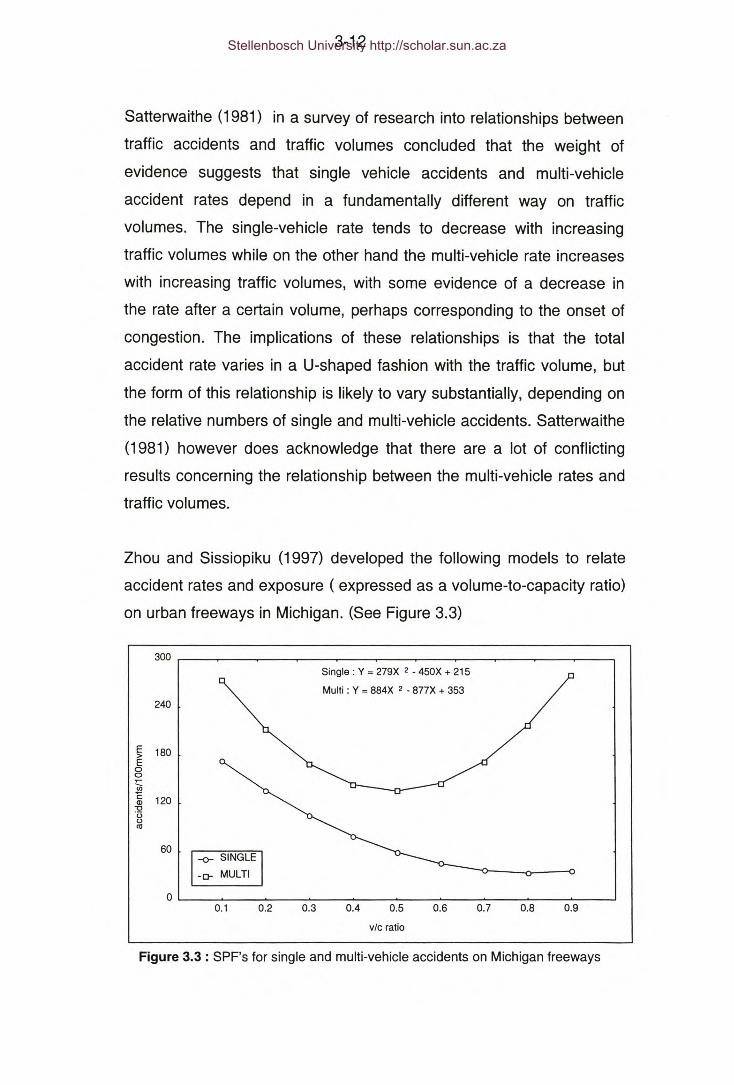
3-12
Satterwaithe (1981) in a survey of research into relationships between
traffic accidents and traffic volumes concluded that the weight of
evidence suggests that single vehicle accidents and multi-vehicle
accident rates depend in a fundamentally different way on traffic
volumes. The single-vehicle rate tends to decrease with increasing
traffic volumes while on the other hand the multi-vehicle rate increases
with increasing traffic volumes, with some evidence of a decrease in
the rate after a certain volume, perhaps corresponding to the onset of
congestion. The implications of these relationships is that the total
accident rate varies in a U-shaped fashion with the traffic volume, but
the form of this relationship is likely to vary substantially, depending on
the relative numbers of single and multi-vehicle accidents. Satterwaithe
(1981) however does acknowledge that there are a lot of conflicting
results concerning the relationship between the multi-vehicle rates and
traffic volumes.
Zhou and Sissiopiku (1997) developed the following models to relate
accident rates and exposure ( expressed as a volume-to-capacity ratio)
on urban freeways in Michigan. (See Figure 3.3)
300 r---~--~--~--~--~--~----~--~--~--~--~Single: Y = 279X 2 - 450X + 215
Multi: Y = 884X 2 - 877X + 353240
~ 180Eoo~U;
].i 120lJ,3uOl
vIc ratio
Figure 3.3 : SPF's for single and multi-vehicle accidents on Michigan freeways
Stellenbosch University http://scholar.sun.ac.za

3-13
Zhou and Sissiopiku (1997) explains the form of these relationships in
the following manner :-. As traffic volumes increase so do vehicle
conflicts and therefore higher accident rates become impossible. To
explain the higher accident rates associated with low traffic flows one
has to consider that low traffic flows generally occur at night where
poor visibility, fatigue and higher rates intoxication are major factors.
Also in low exposure conditions the average driver's attention to
driving tasks is reduced and higher speeds may be selected.
In conclusion, there is therefore sufficient empirical and logical support
to the notion that the relationship between A and E ( as in Equation 3.2)
to be non-linear.
b) In the exposure function a time-average value of traffic flow, the AADT
is used. There exist a causal relationship between traffic flow and
accidents. The effect (accidents) is observed over a long period of time
during which the cause (traffic flows) has assumed widely different
values, but for which only the average value is known. The causal link
between accidents and AADT is therefore indirect. This leads to what is
referred to as the issue of argument averaging which could introduce,
depending on the form of the SPF, a large and significant bias.
(Mensah and Hauer; 1998)
3.5.2 INTERSECTIONS
A common measure of exposure to measure safety at intersections is the
sum-of-flows measure that is determined as follows:
E = d * '" AADT *10-{i~ In
... [3.3]
LAADTin - Sum of incoming flows on all approaches (veh/day).
d - Number of days of study period.
Stellenbosch University http://scholar.sun.ac.za

3-14
The sum-of-flows measure for intersections determines the total number of
vehicles that entered the intersection during the study period. This does not
and cannot account for possible correlation between specific accident types
and certain combinations of vehicle movements. It also implies that all
vehicles entering an intersection have an equal probability of being involved inan accident (Plass et al. ; 1987).
According to Hauer et al. (1988) the assumption that the number of accidents
at an intersection is proportional to the sum of flows that enter the intersection
is logically unsatisfactory and not a suitable basis for engineering analysis
which attempts to link cause and effect. Hauer et al. (1988) suggest that one
could expect, for example, that the number of rear-end accidents at an
intersection approach will strongly depend on the flow on approach A and
depend only weakly on the flow on approaches B, C and D. One would also
expect that accidents between vehicles from traffic streams moving at right-
angles will be related to the product of these flows. To use the sums of these
flows leads to the logical difficulty that one will be able to predict accidents
even if one of the flows is zero.
3.6 AN ALTERNATIVE APPROACH TO SAFETY ESTIMATION
On the basis of the fact that the conventional concept of accident risk, as
determined by the accident rate, is a function of the exposure level - the use
of the accident rate, in some cases, could be an inappropriate measure of
risk. According to Mahalel (1986) the risk level can only be expressed in
relation to a specific exposure level. Using accident rates without relating
them to exposure levels could make the comparison of accident rates for the
purposes of identifying and ranking hazardous locations and evaluating
remedial measures meaningless.
According to Hauer (1995) two accident rates can only be compared with
each other if there exists a reasonable expectation that the two rates should
Stellenbosch University http://scholar.sun.ac.za

3-15
be equal to each other. This expectation is not necessarily valid when two
accident rates were determined using different levels of exposure.
The problems associated with the conventional definition of accident risk can
be overcome by relating it to exposure. This can be achieved by using Safety
Performance Functions.
Mahalel (1986) proposed that the probability of a certain number of accidents
at a given level of exposure to be an alternative definition of accident risk. In
terms of Mahalel's alternative definition of risk, the risk (R) at any location is a
function of the exposure (E), the expected number of accidents (A) and the
probability of A accidents (Pa).
R = j(E,A,P) . .. [3.4]
The fundamental characteristic of this alternative definition of accident risk is
its ability to express the expected number of accidents or the probability of a
certain number of accidents at any exposure level. Accordingly, the risk level
of a system can only be expressed in relation to a specific exposure level.
(Mahalel; 1986)
The role of a SPF can be seen as a 'black box' where exposure is an 'input'
and in which 'output' is accidents and probabilities.
3.7 SAFETY PERFORMANCE FUNCTIONS
Safety Performance Functions are in essence multivariate regression models
that explain how the number of accidents at a location depend on the traffic
flows.
3.7.1 ROAD SEGMENTS
Stellenbosch University http://scholar.sun.ac.za

3-16
Mensah and Hauer (1988) mentions four common forms of SPF's commonly
used to relate accidents to exposure on roadway segments:
a) Type 1 : The Exponential SPF :
A =a(ADT)~ ... [3.5]
This function assumes that the exposure (total number of opportunities)
is proportional to AOJi3 . The value of A will always increase with
increasing values of ADT.
The accident rate (R) at any level of ADT is given by :
R =a(ADT)~-l ... [3.6]
If j3 > 1 then R will always increase with increasing values of ADT, and
if j3 < 1 then R will always decrease with increasing values of ADT.
Please refer to Figure 3.4.
20
/ \b> 1
16
b < 1
12
<
500 1000
ADT
1500 500 15001000
ADT
Figure 3.4 : Accident number and rate curves: Exponential SPF
Stellenbosch University http://scholar.sun.ac.za

3-17
The exponential SPF has been used by Persaud and Musci (1995) to
model the relationship between ADT and accidents on two-lane rural
roads in Ontario, Canada.
Persaud and Musci (1995) used data from Ontario, Canada, for two-
lane rural road segments to develop a series of SPF's using the
Exponential form (Type1).
.A=aQf3 .. .[3.7]
A - accidents/kilometre/year
Q - Average hourly traffic flow
Table 3.1 : Regression parameters of SPF's
Day-time Night-time 24 HoursAccident Type
a {3 a {3 a {3
Single-vehicle 0.0040 0.490 0.0354 0.557 0.0657 0.444
Multi-vehicle 0.0008 1.173 0.0013 1.071 0.0011 1.123
All 0.0194 0.741 0.0468 0.650 0.0415 0.627.
The study by Persaud and Musci (1995) has shown that on 2-lane
roads in Ontario, Canada there exist significantly different SPF's for
day-time single vehicle accidents, day-time multi- vehicle accidents,
night-time single vehicle accidents and night-time multi-vehicle
accidents.
The Safety Performance Functions developed by Persaud and Musci
(1995) are illustrated in Figures 3.5 and 3.6.
Stellenbosch University http://scholar.sun.ac.za

3-18
Multi-vehicle accidents0.8,- ---,
0.6
a . Average hourly traffic flow
Figure 3.5 : Single vehicle and multi-vehicle accident SPF's
From Figure 3.5 it is evident that at similar levels of exposure the risks
associated with single vehicle accidents are considerably worse during
the night than during the day.
Night-time accidents Day-time accidents
1.6 1.6
.I.' " I.',,',.
,.'1.2 .' 1.2."."! "1.0 " 1.0
s " ..' ."'.~ " I,i'.Q
0.8 " 0.8I .».' "... ,":2 ," .~ 0.6 i 0.6 .'"'" ./ ~'
,"/ ,"'
0.' 0.' ,".',/ .""! 0.2 ~
l.-0.0 '
100 150 200 0 100 150 200
a -Average hourly traffic flow a -average hourly traffic flow
Figure 3.6 : Night-time and day-time accident SPF's
Stellenbosch University http://scholar.sun.ac.za
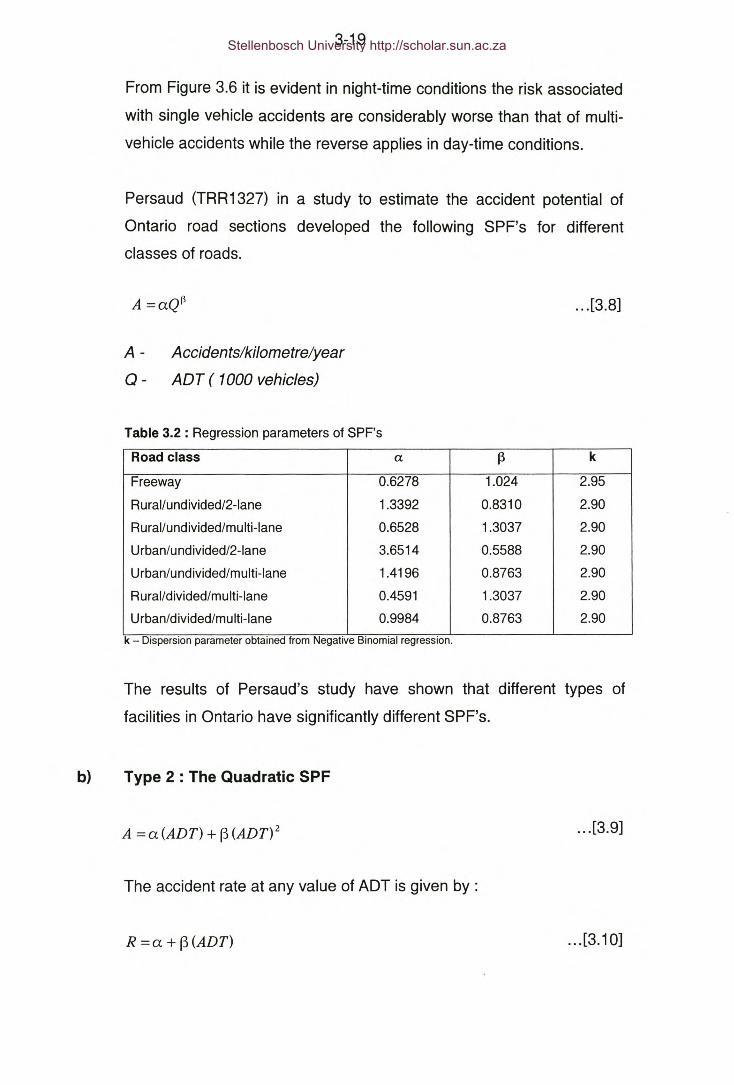
3-19
From Figure 3.6 it is evident in night-time conditions the risk associated
with single vehicle accidents are considerably worse than that of multi-
vehicle accidents while the reverse applies in day-time conditions.
Persaud (TRR1327) in a study to estimate the accident potential of
Ontario road sections developed the following SPF's for different
classes of roads.
A=aQi3 ... [3.8]
A - Accidents/kilometre/year
Q - ADT ( 1000 vehicles)
Table 3.2 : Regression parameters of SPF's
Road class a (3 k
Freeway 0.6278 1.024 2.95
Rural/undivided/2-lane 1.3392 0.8310 2.90
Rural/undivided/multi-Iane 0.6528 1.3037 2.90
Urban/u ndivided/2-lane 3.6514 0.5588 2.90
Urban/undivided/multi-Iane 1.4196 0.8763 2.90
Rural/divided/multi-Iane 0.4591 1.3037 2.90
Urban/divided/multi-Iane 0.9984 0.8763 2.90
k - Dispersion parameter obtained from Negative Binomial regression.
The results of Persaud's study have shown that different types of
facilities in Ontario have significantly different SPF's.
b) Type 2 : The Quadratic SPF
A =a(ADT) + f3 (ADT)2 ... [3.9]
The accident rate at any value of ADT is given by :
R =rz + f3 (ADT) ... [3.10]
Stellenbosch University http://scholar.sun.ac.za

3-20
Figure 3.7 shows the accident number and accident rate curves for the
following quadratic SPF : A = O.0005*Q - 2*10-8*(;2.
0.52
2.8
2.4 0 .. 8
2.0
0.44
1.6 ~II:
i1.2
~0.40
0.8
0.36
0.32'-::-0 ~'OOO::"::"'""::2000~3000~~4000;";:"""::5000~6~OOO~7000~
a . Average Daily Traffic
2000 3000 4000 5000 6000 7000
a . Average Dally Traffic
Figure 3.7 : Accident number and rate curves: Quadratic SPF
The Safety Performance Function developed by Zhou and Sissiopiku
(1997) as shown in Figure 3.3 is of the Quadratic type.
c) Type 3 : Hoeri's Function with k = 1
According to Mensah and Hauer (1998) Hoeri's function is as follows:
... [3.1Ob]
Thus with k = 1, then:
A =a(ADT)e[3(ADT) ... [3.11]
The accident rate at any value of ADT is given by :
R =ae[3(ADT) ... [3.12]
Stellenbosch University http://scholar.sun.ac.za

3-21
With small values of ADT the accident frequency (A) increases
approximately linearly with traffic flow. Mensah and Hauer (1998) noted
that this function may be suitable for single vehicle accidents.
d) Type 4 : Hoeri's function with k = 2
A =a(ADT)2e(3(ADT) ... [3.13]
The accident rate at any value of ADT is given by :
R =a(ADT)e(3(ADT) ... [3.14]
A increases with the square of traffic flow. At large traffic flows the
slope of the function begins to diminish. Eventually a peak is reached
and A will begin to decrease. Mensah and Hauer (1988) noted that this
function may be suitable for two-vehicle accidents.
/k-2
0.8r------------,
2000 3000 4000 5000 6000 7000o . Averaoe Dally Traffic
0.7
00 0~I~OOO~2000~3000~4000~5000~;;:;;6000~7000~
a . Average Daily Tratfic
Figure 3.8: Accident Number and Rate curves: Hoeri's function with k =1 and 2.
Stellenbosch University http://scholar.sun.ac.za

3-22
3.7.2 INTERSECTIONS
Some researchers such as Breunning and Bone, Sunti and Hakkert, and
Mahalel ( in Hauer et al. ; 1988) related accidents to the products of the
conflicting flows.
... [3.15]
Empirical research according to Hauer et al. (1988), has found the above
relationship not to be correct. It was found that accidents are rather related to
the product of flows with each flow raised to a power of less than 1. Tanner (in
Hauer ; 1988) suggested that the square root of the product flows would be
sufficiently accurate as a rule of thumb:
A=a)Q1Q2 ... [3.16]
The 'products-of-flows-to-power' relationship has been used by Bonneson and
McCoy (1993) and Belanger (1994) to relate total accidents to total flows on
the major and minor approaches at two-way stop controlled intersections on
rural highways, while Hauer et al. (1988), in a study to estimate safety at
signalised intersections used the 'products-of-flows-to-power' relation to relate
the frequency of specific accident types to the relevant conflicting flows.
Bonneson and McCoy (1993) developed the following SPF for two-way stop
controlled intersections on rural highways in Minnesota (USA) :
(T JO.2S6( T JO.831A = 0.692 _m_ __c_ k=4
1000 1000... [3.17]
Tm - major road traffic flow (veh/day)
Tc - Minor (cross) road traffic flow (veh/day)
A - Annual expected accident frequency (within 153 m / 500ft of junction)
k - Dispersion parameter from Negative Binomial regression
Stellenbosch University http://scholar.sun.ac.za

3-23
For 4-legged un-signalised intersections in eastern Quebec, Bélanger (1994)
developed the following SPF based on the 'products-of-flows-to-power
relationship.
A = 5 59*10-6F.°.42F 0.51• 1 2 k=2.95... [3.18]
A - Expected daily accident frequency (within 30m of intersection).
Ft - major road traffic flow (veh/day).
F2 - Minor road traffic flows (veh/day).
k - Dispersion parameter from Negative Binomial regression.
Hauer et al. (1988) identified 15 accident patterns in which two vehicles at an
intersection can be involved and developed a SPF for each of the accident
patterns. Accidents in each pattern are defined by the manoeuvres of the
vehicles before the collision. These accident patterns are shown in Figure 3.9.
The form of the model equations was chosen after an exploratory analysis of
the data to determine how accidents would depend on the contributory traffic
flows. The guiding principle was the wish to ensure a satisfactory fit with
parsimony of parameters and without violation of the obvious logical
requirements.
The results of the study by Hauer et al. (1988) are given in Table 3.3.
The study by Hauer et al. (1988) has shown the benefit of using dis-
aggregated accident data to relate these to the traffic flows to which the
colliding vehicles belong. They conclude that the logic of attempting to seek
an aggregate relationship between accident frequencies and some function of
all flows to be unsatisfactory. They also question the suitability of the
-custornary categorisation of accidents by initial impact (rear-end, angle,
turning movement, sideswipe etc.) One cannot assume, for example, that
classification of an accident as a right-angle collision implies that the vehicles
were travelling at right angles to each other or that most accidents involving
left or right turning will be classified as turning accidents.
Stellenbosch University http://scholar.sun.ac.za

3-24
Table 3.3 : Regression parameters of SPF's
Pattern Model Form A b c K
1 A= a(F) 0.2052 * 10.6 4.59
2 A= a(F) 0.1014*10.6 1.97
3 A = a(F2)C 8.6129 * 10.9 1.0682 1.20
4 A = a(F2)C 8.1296 * 10-6 0.3662 5.51
5 A = a(F1)b(F2)C 0.3449 * 10-6 0.1363 0.6013 1.2
6 A = a(F1)(F2)C 0.0418 * 10-6 0.4634 2.1
7 A = a(F1)b(F2)C 0.2113 * 10-6 0.3468 0.4051 1.2
8 A = a(F2)C 2.6792 * 10-6 0.2476 1.2
9 A = a(F1)b 6.9815 * 10-9 1.4892 1.2
10 A = a(F2)C 5.5900 * 10-12 2.7862 1.2
11 A = a(F1)b(F2)C 1.3012 * 10-9 1.1432 0.4353 1.2
12 A = a(F1)b(F2)C 0.0106 * 10-6 0.6135 0.7858 1.2
13 A = a(F1)b(F2)C 0.4846 * 10-6 0.2769 0.4479 1.2
14 A = a(F1)b(F2/ 1.7741 * 10-9 1.1121 0.5467 1.2
15 A = a(F1)b 0.5255 * 10-6 0.4610 1.2
k - Dispersion parameter of Negative Binomial regression.
Models were also developed for AM, PM and off-peak conditions for patterns
1,2,4 and 6.
Table 3.4 show a number of macroscopic models developed by Mountain and
Fawaz (1996) for priority junctions, traffic signals and roundabouts in the UK.
The k value for all three models is 1.65.
Table 3.4 : Safety Performance functions
Junction type Model
Major-minor priority Il = 0.141 t1 0.64t2 0.24
Traffic signals Il = 0.180 t1 0.64t2 0.24
Roundabouts Il = 0.168 t1 0.64t2 0.24
t1 - major road flow (veh/day) and t2 - minor road flow (veh/day)
11- Accident frequency
Stellenbosch University http://scholar.sun.ac.za

3-25
1 2 3 F1
_j L _j L _jl LI)t,IFttl IFI,
4 5 6
_j jb F2_j L _jL~2F;lt~I I IF1tlF1
7 _j L 8 _j L 9 _j L~F2 l~tlF2 I~'IF1tl F1
10 _jLL 11 _j L 12 -.!tLrrr= F2~I~ IIIIF1
13 _j L 14 _j L 15 _j L
IFtIF-F2 jth F
I ril-IF1I 2F
Figure 3.9 : Intersection accident patterns ( Hauer et al. ; 1988) [For traffic drivingon the right hand side of the road.]
Stellenbosch University http://scholar.sun.ac.za

3-26
3.7.3 THE ARGUMENT AVERAGING PROBLEM
Some of the Safety Performance Functions presented in the preceding
section were estimated from using estimates of average traffic flow. According
to Mensah and Hauer (1998) the ideal is for SPF's to represent the cause-
effect relationship between accidents and the actual flows at the time of the
accidents. In practice, mainly because of a lack of sufficient data, average
flows are used for estimation of the SPF and not the actual flows at the time of
the accidents. Relating accidents with average traffic flows forms an indirect
causal link in the sense that the effect is observed over a long period of time
during which the cause has assumed widely different values, but for which
only the average value is known. This is referred to as the 'argument
averaging problem'
To examine the issue of argument averaging consider Figure 3.10 which
shows a non-linear SPF where the accident frequency !l is a function of the
average flow q i.e. !l = !l(q)
Average Flow - Q : (veh/day)
Figure 3.10 : The argument averaging problem.
Stellenbosch University http://scholar.sun.ac.za

3-27
If during one half of a unit of time the flow q = qa and the other half the flow q =qb, then the average flow is given by O.5(qa+qt).
Were the flow to be equal to O.5(qa+qtJ) for the whole unit of time one would
expect t,t[O.5(qa+qt)J accidents per unit time. (Point A in Figure 3.10).
Since the flow qa was for half of the time, and flow qb for half of the time, one
should expect [t,t(a) + t,t(b)]/2 accidents per unit time. (Point B in Figure 3.10).
If the AADT is used a function is fitted through points such as B, instead of
finding the 'true' function that would pass through point A.
According to Mensah and Hauer (1998) one should not be concerned about
errors due to argument averaging when :-
a) the flow during the averaging period is constant, and
b) when the SPF is linear for flows during the averaging period.
These conditions will arise when the period of averaging is short enough that
traffic flows in it can be thought of as nearly constant and if the flow is not
constant then when the segment of the SPF between the largest and the
smallest flows in the period is sufficiently close to a straight line.
According to Mensah and Hauer (1998) considering what is generally known
about how traffic varies over time and the likely shape of the SPF, one should
generally not be concerned about averaging of periods of about an hour and
that periods of longer than an hour need to be considered carefully.
Mensah and Hauer (1998) has developed a methodology to determine a
correction factor w where, from Figure 3.10 :
Aw=-
B... [3.19]
Stellenbosch University http://scholar.sun.ac.za

3-28
The following information is required to determine the value of w:
a) The distribution of traffic flows, in say hourly intervals over the study
period. Information of this kind can be obtained from permanent
counting stations. This information is required to estimate the CV
(coefficient of variation) where:
aCV=-q_E(q)
... [3.20]
Where:
a(q) - The standard deviation of all hourly flows across the
study period.
The average hourly traffic flow over the study period.
The value obtained after substituting E(q) into the SPF.
E(q) -
J;l[E(q)}) -
b) The type and form of the SPF and its parameters.
Mensah and Hauer (1998) presented the following general formula to
determine w from any SPF based on a single flow measure.
W_l+_!_[d2J;l(q) I ] var(q)- 2 dq" E(q) J;l(E{q})
... [3.21]
The section in the square brackets is determined by substituting E(q)
into the second derivative of the SPF. A detailed derivation of this
equation is contained in the paper by Mensah and Hauer (1998).
The above equation leads to several observations ( Mensah and Hauer
; 1998).
i) When over the averaging period the flow varies little, that is
var(q) ---7 0 then w = 1 and no correction is required.
Stellenbosch University http://scholar.sun.ac.za

3-29
ii) When ~(q) is constant, i.e. when the SPF is a straight line then
the second derivative is zero and w = 1 and no correction is
required.
iii) For these values of q for which the slope of ~(q) is decreasing w< 1 i.e. the true level of safety will be underestimated. For values
of q where ~(q) is increasing the true level of safety will be
overestimated.
The following equations are presented by Mensah and Hauer (1998) to
determine the value of w for each of the 4 different types of SPF's mentioned
in Section 3.7.1.
a) Type 1 : The Exponential SPF
w = 1+ 0.5((32 - (3)(CV)2 ... [3.22]
It is evident that the correction factor in this case depends only on the
exponent (3 and the square of the coefficient of variation (cv) of traffic
flow.
1.6
1.5
1.4
:;:: 1.3
01:5
1.2~c0·13
1.1~0CJ
1.0
0.9
0.80.1 0.3 0.5 0.7 0.9 1.1
Bela
cv = 1.0
cv = 0.75
cv = 0.50
cv = 0.25
1.3 1.5 1.7
Figure 3.11 : Correction factor (w) - Exponential SPF
Stellenbosch University http://scholar.sun.ac.za

3-30
b) Type 2 : The Quadratic SPF
1 2w=l+ j3a .(cv)
--+1E(q)
... [3.23]
From Figure 3.12 its is evident that the bias can be very large at high
traffic flows q and high values of cv.
1.1
1.0
0.9
~ 0.8,0 0.7t5<IlLJ..c: 0.60·u~ 0.50o
0.4
0.3
0.20 2000 4000 6000 8000 10000
cv = 0.25
cv = 0.50
cv = 0.75
cv = 1.0
Average Flow - E(q): (veh/day)
Figure 3.12 : Correction factor (w) - Quadratic SPF.
c) Types 3 and 4 : Hoeri's Function ( k = 1 and k = 2)
The correction factor w for Hoeri's function can be estimated from Eqn.
3.24.
w = 1+0.5[j32E(q)2 + 2kj3E(q) +k(k _1)](CV)2 ... [3.24]
Figures 3.13 and 3.14 show how the value of w varies with different
flows and coefficient-ot-variation values.
Stellenbosch University http://scholar.sun.ac.za

3-31
1.1
1.0
0.9~(5t5
0.8~c0U~ 0.7(5o
0.6
0.50 2000 60004000 8000
cv = 0.25
cv = 0.50
cv = 0.75
cv = 1.0
10000
Average Flow - E(q) : (veh/day)
Figure 3.13 : Correction factor (w) : Hoeri's function: k = 1
It is evident from Figures 3.13 and 3.14 that the bias due to the
argument averaging problem when using Hoeri's function could be very
large at large traffic flows with a high coefficient-of- variation.
2.0
1.6
~(5 1.2t5~c0U
0.8~(5o
0.4
0.00
b = -2.0 * 10 ·4
cv = 0.25
cv = 0.50
cv = 0.75
cv = 1.0
10000
Average Flow - E(q) : (veh/day)
Figure 3 .14 : Correction factor (w) : Hoeri's function: k = 2.
Stellenbosch University http://scholar.sun.ac.za
3-32
The bias introduced by developing SPF's using average traffic flows can be
very large. The magnitude of this bias depends on (Mensah and Hauer ;1998) :-
a) The coefficient of variation (cv).
b) The form of the SPF.
c) The parameters of the SPF.
d) The magnitude of the average flow (AADT).
This bias can be removed by dividing the accident counts by w before fitting
the model using regression techniques. Since the determination of an
appropriate value for w depends on the form of the SPF and its parameters
the process must be iterative in nature. (Mensah and Hauer; 1998)
3.7.4 FUNCTION AVERAGING PROBLEM
It is often assumed that one SPF prevailed during the entire study period T. It
is however possible that during T several SPF's may apply. For example, it
has been previously shown by Persaud and Musci (1995) that there exist at
least 4 different SPF's for 2-lane rural roads in Ontario, Canada : 1) Single
vehicle day-time, 2) Single vehicle: night-time, 3) Multi-vehicle: day-time and
4) Multi-vehicle : night-time. Different SPF's could exist for different seasons
of the year, for afternoon and morning peaks etc. The problem of fitting a
single SPF to data where there exist 2 or more distinct SPF's is referred to as
the function averaging problem. (Mensah and Hauer ; 1998) This problem is
illustrated in Figure 3.15.
Stellenbosch University http://scholar.sun.ac.za

3-33
2.8
2.4
2.0n;Ol<:- 1.6E.:.<(ijcoOl 1.2"0'Jo«
0.8
0.4
0.00
!-l1 - Night
500100 200 300 400
It is assumed that !-l1 represent the SPF for night-time conditions and !-l2 the
SPF for daytime conditions.
Average Flow - q : (veh/hr)
With a night-time flow of qa one would expect !-l(qa) accidents, and with a day-
time flow of qb one would expect !-l(qt) accidents. If a flow of qa prevailed for
12 hours and a flow of qb prevailed for 12 hours the average traffic flow is
O.5(qa + qt) and the expected accident frequency is O.5(!-la + !-lJ. (Given by
point A in Figure 3.15).
Figure 3.15 : The Function Averaging Problem
Assuming now the same amount of daily traffic (qa + qb = qc + qd) but a
different ratio of night-time to day-time traffic it can be shown that the
expected number of accidents = O.5(!-lc + !-ld). (given by by Point B in Figure
3.15).
It is evident that even though in both cases the AADT is the same the
expected number of accidents are different because of the different night- to
day traffic ratios.
Stellenbosch University http://scholar.sun.ac.za
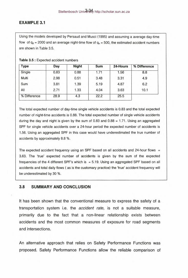
3-34
EXAMPLE 3.1
Using the models developed by Persaud and Musci (1995) and assuming a average day-time
flow of qd = 2000 and an average night-time flow of qn = 500, the estimated accident numbers
are shown in Table 3.5.
Table 3.5 : Expected accident numbers
Type Day Night Sum 24-Hours % Difference
Single 0.83 0.88 1.71 1.56 8.8
Multi 2.98 0.51 3.48 3.31 4.9
Sum 3.81 1.39 5.19 4.87 6.2
All 2.71 1.33 4.04 3.63 10.1
% Difference 28.9 4.3 22.2 25.5
The total expected number of day-time single vehicle accidents is 0.83 and the total expected
number of night-time accidents is 0.88. The total expected number of single vehicle accidents
during the day and night is given by the sum of 0.83 and 0.88 = 1.71. Using an aggregated
SPF for single vehicle accidents over a 24-hour period the expected number of accidents is
1.56. Using an aggregated SPF in this case would have underestimated the true number of
accidents by approximately 8.8 %.
The expected accident frequency using an SPF based on all accidents and 24-hour flows
3.63. The 'true' expected number of accidents is given by the sum of the expected
frequencies of the 4 different SPF's which is = 5.19. Using an aggregated SPF based on all
accidents and total daily flows ( as is the customary practice) the 'true' accident frequency will
be underestimated by 30 %.
3.8 SUMMARY AND CONCLUSION
It has been shown that the conventional measure to express the safety of a
transportation system i.e. the accident rate, is not a suitable measure,
primarily due to the fact that a non-linear relationship exists between
accidents and the most common measures of exposure for road segments
and intersections.
An alternative approach that relies on Safety Performance Functions was
proposed. Safety Performance Functions allow the reliable comparison of
Stellenbosch University http://scholar.sun.ac.za
3-35
safety at equal levels of exposure. Examples of Safety Performance
Functions, suitable to estimate safety on road segments, signalised and un-
signalised intersections were presented.
Due to the fact that often average traffic flows are used in the estimation of
Safety Performance Functions they are susceptible to the Argument
Averaging Problem which could introduce a large and significant bias in the
safety estimates. A methodology was presented on how to estimate the
magnitude of this bias for road segment SPF's.
Using aggregated data, which consists of accident types normally associated
with different levels of risk, the use of Safety Performance Function is also
susceptible to the Function Averaging Problem which could cause the level of
safety either to be over or underestimated. This problem necessitates the use
of different SPF's to define the safety of an entity such as an intersection
which may experience many different accident patterns, each of which are
associated with a different level of risk.
Stellenbosch University http://scholar.sun.ac.za

CHAPTER 4
SAFETY MEASUREMENT METHODOLOGIES
4.1 INTRODUCTION
The objective of this Chapter is to provide methodologies to obtain reliable
safety estimates at site and group-af-sites level taking into consideration some
of the issues identified in the previous chapter.
According to Nembhard and Young (1995) there are two commonly used
methods for providing safety estimates of entities a) the site-specific historical
rate method, and b) the generic class method.
These two methods will be investigated and the disadvantages of each of will
be identified. An alternative methodology, based on the Empirical Bayesian
approach, will be presented, to show how these two methods can be
combined to overcome the shortcomings of each.
The Empirical Bayesian approach and the various methodologies within this
approach will be discussed in detail. Comparisons will be drawn between this
approach and the conventional historical rate method.
Throughout the Chapter use will be made of the experimental data contained
in Appendices A1 and A2 to illustrate some of the concepts and the
differences in the accuracy and performance of the different methods.
Stellenbosch University http://scholar.sun.ac.za

4-2
4.2 HISTORICAL RATE METHOD
This method is based on the conventional definition of risk, where the risk of a
system can be estimated by the accident rate as follows :
R=A ... [4.1]E
R - Accident risk
A - Number of target accidents.
E - Total exposure over study period.
This method has the following disadvantages:
a) RANDOM ERROR
The historical method assumes that the observed accident frequency
(X) at an entity is a reliable measure of the true level of safety at that
location. In other words, it is assumed that the true level of safety (m) is
known precisely and that this is equal to the observed rate/frequency at
an entity. (Abbess et al ; 1981) This assumption is in violation of the
fact that accidents are discrete sporadic events that follow the Poisson
distribution around its true level of safety - m. (AI-Masaeid ; 1993).
Hauer (1986) has shown that X is not a good estimate of m.
The difference between X and m is referred to as the random error
(assuming the systematic error is equal to zero). Because of the
random nature of X this random error could be significant. A
compensating strategy to reduce the random error associated with the
observation X is to increase the size of the observation. This can be
achieved in one of two ways: a) increase the collection period i.e. the
period over which data are collected and, b) include more entities in the
study group if possible.
Stellenbosch University http://scholar.sun.ac.za

4-3
According to Nicholson (1987) a period of at least 5 years is required
for X to be an reliable estimate of m. The problem with using such long
periods for collecting data is the likelihood of significant changes in the
true level of safety (m) over time at an entity, due to the influence of
inevitable changes in the traffic, road and external environment. For
example urban development patterns could cause an increase in
pedestrian traffic or an increased proportion of night-time traffic. Both
scenarios could lead to a decrease in safety.
In order to assess and to quantify the historical rate method's ability to
predict the true level of safety the analysis described in Example 4.1
and Appendix A2 was applied to the experimental data in Appendix A1:
EXAMPLE 4.1
The true level of safety for each of the 1000 entities are known = mti. These were
randomly generated from a Gamma distribution with a mean of 4 accidents/year and
a variance of 2.
For each entity 5 years of accident frequencies were randomly generated assuming a
Poisson distribution with mean = mti. These accident frequencies, X1;, X2i, X3i, X4iand
XSiwere used to estimate mi in the following manner:
Table 4.1 : Calculations
Study period (Years) Expression
1 m1i=X1i-
)(2 = (X1i + X2i)/22 m2i=-
)(3 = (X1i + X2i + X3i)/33 m3i=-
)(4 = (X1i + X2i + X3i+ X4i)/44 m4i=-
)(s = (X1i + X2i + X3i+ X4i + Xsi)/55 mSi=
For each entity and for each study period the degree-of-deviation (D) was computed
as follows:
Continue ...
Stellenbosch University http://scholar.sun.ac.za

4-4
110
100
90
80
70
60
<1< 50
40
30
20
10
00
--0- 1 Year
-0- 2 Year
··0· 3 Year
-6- 4 Year
...... 5 Year
10 20 30 40 50 60 70 80 90 100 110 120 130 140
% Absolute deviation
Figure 4.1 : Accuracy of different study periods
Figure 4.1 shows the cumulative density functions for the degree-at-deviation for the
different study periods. It is evident that the accuracy of the estimates increase with
increasing study periods, with the differences between successive periods gradually
decreasing as the study period increase.
50 r--------------------------------------------------------,I Mean+ 1.96*SE
Mean·1.96*SE
40 -0- Mean
co"'<ii"~
"0 30 .cD"Soen.n<{
<1< 20 -=_~~
10 L- ~ ~ ~ ~ ~ ~
3 Year
Averaging Period
4 Year 5 Year1 Year 2 Year
Figure 4.2 : Mean deviations for different study periods
From Figure 4.2 it is evident that even using a study period of 5 years, as
recommended by Nicholson (1987), still produces an average deviation of 20 %.
Stellenbosch University http://scholar.sun.ac.za
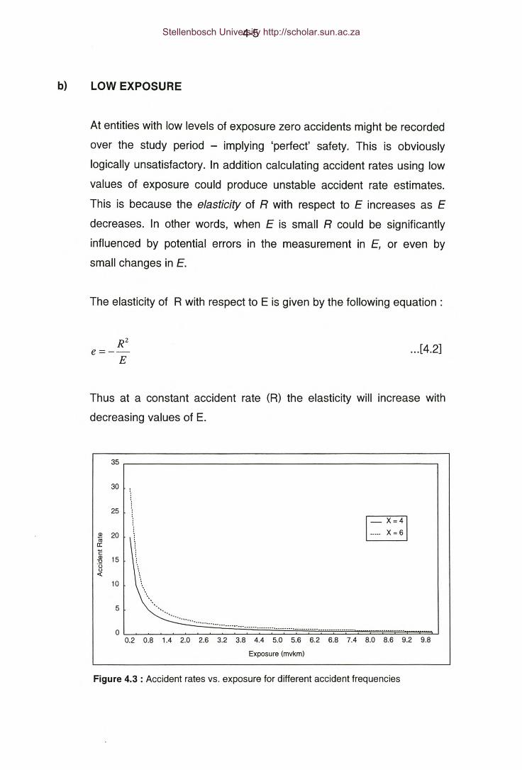
4-5
b) LOW EXPOSURE
At entities with low levels of exposure zero accidents might be recorded
over the study period - implying 'perfect' safety. This is obviously
logically unsatisfactory. In addition calculating accident rates using low
values of exposure could produce unstable accident rate estimates.
This is because the elasticity of R with respect to E increases as E
decreases. In other words, when E is small R could be significantly
influenced by potential errors in the measurement in E, or even by
small changes in E.
The elasticity of R with respect to E is given by the following equation:
R2
e=--E
...[4.2]
Thus at a constant accident rate (R) the elasticity will increase with
decreasing values of E.
35
30
25
Ql 20iiicr:ëQl 15"0'uu-c
10
5
~~
o~ __ ~~===========' =~_'-_~_-_-~~~~~~__~ __=~~~__~~0.2 0.8 1.4 2.0 2_6 3.2 3.8 4.4 5.0 5_6 6.2 6_8 7.4 8.0 8.6 9_2 9_8
Exposure (mvkm)
Figure 4.3 : Accident rates vso exposure for different accident frequencies
Stellenbosch University http://scholar.sun.ac.za

4-6
Figure 4.3 shows how the slope of the accident rate curve increases
with decreasing values of exposure.
EXAMPLE 4.2 .
Consider a gravel road, 10 km in length, which carries 200 vehicles per day. The
average number of accidents is 1 per year. The exposure can be shown to be equal
to 0.73 mvkm and the accident rate equal to 1.37 accidents per mvkm. The elasticity
is equal to -(1.37)2/0.73 = -2.57. In other words a 1 % error in the true value of the
AADT will cause a 2.57 % error in the value of the accident rate.
Consider a road with a similar accident rate, 10 km in length and which carries 600
vehicles per day. The exposure can be shown to be equal to 2.19 mvkm and the
elasticity equal to -0.86. The influence the exposure has on the accident rate when
the AADT is 600 instead of 200 vehicles per day is considerably less.
Thus at very low exposure levels large accident rates can be obtained even at low
accident frequencies and these accident rates can be very sensitive to changes in the
level of exposure.
4.3 THE GENERIC CLASS METHOD
This method assumes that the accident risk of a location is equal to the
accident risk of all locations with similar geometric, traffic and environmental
characteristics - called the reference group. The generic accident risk is
determined as follows:
... [4.3]
The validity of the assumption, on which this method is based, is a function of
the degree of similarity between a group of sites. The more similar the sites
the more valid the assumption. It is however extremely unlikely that two sites
are identical in every respect and that their true level of safety will be the
same. In spite of being similar each site could have its own regional character,
Stellenbosch University http://scholar.sun.ac.za

4-7
driver population, etc. giving it a unique level of safety m. Therefore m varies
from site to site. The distribution of m's between sites in the reference group
can be described by a Gamma density function with mean E(m) and variance
VAR(m). (AI-Masaeid ; 1993)
Figure 4.4 compares the accuracy of the generic and the conventional 5-year
historical method in predicting the true level of safety at the 1000 entities in
the experimental data contained in Appendix A. It is evident that the historical
rate method produces more accurate estimates than the generic estimates.
110
100
90
80
70
~ 60al>.~50:;
E:::l 40 -<r 5 Year historic methodo
30 -0- Generic method
20
10
0o 10 20 30 40 50 60 70 80 90 100 110 120 130 140
% Absolute deviation
Figure 4.4 : Comparison of generic and 5 -year historical methods.
4.4 COMBINING THE GENERIC AND HISTORICAL RATE METHODS
According to Hauer (1997) both these methods, the historic and the generic
method provide clues as to the true level of safety of an entity or a group of
entities. The generic method provide clues as to the safety contained in all
those observed and measurable characteristics that are common to all similar
locations e.g. number of lanes, type of shoulders, shoulder widths etc. The
historical rate method on the other hand provides clues as to the effect of all
those unknown, unobserved and misunderstood characteristics on the level of
safety at an entity i.e. those traits that make an entity absolutely unique.
Stellenbosch University http://scholar.sun.ac.za

4-8
According to Nemhard and Young (1995) and Hauer (1997) the true level of
safety at a location is a combination of the site specific historical rate and the
generic rate, where :
... [4.4]
Rt - True accident rate (level of safety).
Rh - Site specific historical accident rate.
Rg - Generic accident rate for similar sites.
W1 and W2 - Weighting factors where W1 + W2 = 1.
The most common methodology to estimate the weighting factors W1 and W2 is
the empirical Bayesian methodology.( Nembhard and Young; 1995)
4.5 THE EMPIRICAL BAYESIANAPPROACH
4.5.1 INTRODUCTION
The Empirical Bayesian approach uses Bayes Theorem to combine the safety
estimates obtained from the historic and generic methods.
According to AI-Masaeid et al. (1993), the Bayesian approach is a probabilistic
method capable of augmenting the most recent information with the available
historical data or prior knowledge to achieve more accurate safety estimates.
According to Abbess et al. (1981) the Bayesian approach assumes that a
probability distribution can be found before any data becomes available - this
distribution is called the prior distribution of the parameter. Once information
becomes available Bayes theorem can be used to convert the prior
distribution into a posterior distribution. When even more information becomes
available the posterior distribution, using Bayes theorem, can be updated to
obtain even more accurate estimates of the parameter.
Stellenbosch University http://scholar.sun.ac.za

4-9
The objective is to determine the true level of safety E(mIX) at a location. For
this there are two clues - E(m) (from the generic method) and X (the historic
rate method). In order to determine the true level of safety - which is an
unknown parameter, the Bayesian method requires a subjective estimate of
this parameter. This is called the prior estimate. This estimate in itself is in all
likelihood an unreliable estimate of the true level of safety at a location and
has to be augmented with the observed accident experience X to obtain a
more accurate and reliable posterior estimate, E(mIX).
4.5.2 THEORETICAL FRAMEWORK
Unlike the conventional historical rate method which assumes the observed
accident frequency (X) to be a constant and an appropriate measure of safety
the Bayesian approach assumes the observed accident number to be variable
with a Poisson probability distribution with a mean of m - where m is the 'true'
level of safety at the location (Abbess et al. ; 1981).
x -mmeP(xlm} =--
xl ... [4.5]
It is further assumed that m is constant over time and that the observed
accident experience in different years are random variables that are Poisson
distributed about m (Abbess et al. ; 1981)
The Bayesian approach further assumes that m varies between different sites
and that the exact value for any particular site is unknown and is regarded as
a Gamma variable with the following probability density function: (Abbess et
al. ; 1981 and Higle and Witkowski; 1988)
... [4.6]
Where a, 13 are the parameters of the Gamma distribution.
Stellenbosch University http://scholar.sun.ac.za

4-10
From Ang and Tang (1975) and Abbess et al. (1981)
E(m) = _ê_a
... [4.7] VAR(m) = _ê_ = E(m)a2 a
... [4.8]
The Empirical Bayesian method takes E(m) and VAR(m) to be the initial
(prior) estimates of the true level of safety at an entity. In order to obtain a
more reliable estimate of safety the observed accident experience, X, is
combined with E(m) and VAR(m), using Bayes theorem, to obtain the more
reliable posterior estimates, E(mIX) and VAR(mIX).
In order to apply Bayes theorem the following information is required:
• Values of E(m) and VAR(m).
• The Gamma parameters of E(m) - a and j3
• The observed accident experience - X
4.5.3 ESTIMATING E(m) and VAR(m)
According to Hauer (1997) there are two ways to determine E(m) and
VAR(m):
• The method of sample moments
• The multivariate regression method
Both of these methods require a suitable reference population.
4.5.3.1 REFERENCE POPULATION
The Bayesian approach requires a reference group to determine the prior
distribution of m -the true level of safety at a location.
Hauer (1998) provides the following definition of what a reference population
is:
Stellenbosch University http://scholar.sun.ac.za
4-11
"A reference population of entities is the group of entities that share the same
set of traits as the entity in the safety of which we have an interest. "
Accident histories should not be considered in the selection process otherwise
a biased estimate of m will be obtained.
Since the effect of the prior distribution diminishes as it is updated with
observed data to form the posterior distribution the selection criteria for
suitable reference group sites can be relaxed somewhat in order to ensure a
sufficient sample size of sites.
In order to apply the multivariate regression method to estimate the safety of
signalised intersections, Hauer et al. (1988) used a reference group that
consisted of 145 four-legged, fixed time intersections in Metropolitan Toronto
that carried two-way traffic on all approaches and which have no turn
restrictions. All the intersections are on straight level sites with a speed limit of
60 km/h.
Bélanger (1994) used a reference group consisting of 149 four-legged
intersections with stops on the minor approaches to estimate the safety of 4-
legged unsignalised intersections. All the intersections are located in eastern
Quebec. In a similar study to estimate the safety of 2-way stop controlled
intersections on rural highways in Minnesota, Bonneson and McCoy (1993)
used a reference group that consisted of 125 rural, four-legged, two way stop
controlled intersections. In both these studies the multivariate regression
method was used to determine E(m) and VAR(m).
To determine the safety effect of resurfacing operations on rural roads in
Indiana AI-Maseied et al. (1993) used a reference group consisting of 95
undivided rural road segments to estimate E(m) and VAR(m) for the before
and after periods using the method of sample moments.
Stellenbosch University http://scholar.sun.ac.za

4-12
4.5.3.2 THE METHOD OF SAMPLE MOMENTS
Assume there is a reference group consisting of n entities, and that each
entity experienced Xrj accidents during the study period. The mean (Il) and
standard deviation (S2) of the observed accident frequencies are determined
as follows:
2 1 ~ ( )2S =--Li Xri-Il
n -1 i=1
...[4.9] ...[4.10 ]
According to Hauer (1997) the values of E(m) and VAR(m) are estimated as
follows:
E(m) = Il ...[ 4.12]...[4.11 ]
EXAMPLE 4.3
Consider Year 1 of the experimental data contained in Appendix A.
Table 4.2: Year 1 data - estimation of mean and variance.
X n(X) X*n(X)/n (X-Il)'0 40 0.000 0.6551 91 0.091 0.8452 161 0.322 0.6753 164 0.492 0.1804 155 0.620 0.0005 145 0.725 0.1326 87 0.522 0.3327 65 0.455 0.5678 45 0.360 0.7039 25 0.225 0.61310 11 0.110 0.39011 7 0.077 0.33812 4 0.048 0.253
SUM 1000 4.047 5.683
Il = 4.047 and S2 = 5.683.
E(m) = 4.047 accidents/year and VAR(m) = 5.683 - 4.047 = 1.636
Stellenbosch University http://scholar.sun.ac.za
4-13
Allowing for exposure
Assume there is a reference group consisting of n entities, and that each
entity experienced Xr; accidents during the study period and that each entity
has a level of exposure equal to Er;.
Let Rri be the accident rate at reference entity i :
R. = Xr;
n E.n
...[4.13 ]
The mean accident rate for the reference population and its variance can be
estimated as follows:
...[4.14 ] 2 1 f. - 2SR = -L.,; (R -Rr;)
n -1 ;=1
...[4.15]
The harmonic mean of all the normalised traffic volumes can be determined
as follows
lIn 1-,=-I-E n ;=1 Er;
... [4.16]
According to AI-Maseied et al. (1993) E(m) and VAR(m) can be determined as
follows:
E(m) = R ...[2.17] VAR(m) = E's! -RE'
...[2.18 ]
Calculating E(m) and VAR(m) using the above expressions are based on the
assumption that the relationship between X and E for each entity in the
reference group is linear i.e. that the Safety Performance Function is linear. If
Stellenbosch University http://scholar.sun.ac.za
4-14
this assumption of a linear SPF does not hold the multivariate regression
method should be used to estimate E(m) and VAR(m).
4.5.3.3 THE MULTIVARIATE REGRESSION METHOD
It is often necessary to estimate the safety of entities for which a sizeable
reference group population does not or cannot exist. It has been noted before
that if the accident experience at a site is non-linearly related to its exposure
then such a site cannot be compared to sites which do not have the same
level of exposure. Therefore if the objective is, for example, to measure the
safety of a section of a 2-lane rural road that carries 2000 vehicles per day the
reference population should ideally also consist of 2-lane rural roads that carry
2000 vehicles per day. It is obvious that this requirement will in all likelihood
result in a reference population with very few entities, if any (Hauer; 1997).
This problem can be overcome by using multivariate regression models.
Multivariate models, according to Hauer (1998), serve to 'create' an imagined
reference group from which E(m) and VAR(m) can be determined. When a
multivariate model is being fitted to accident data, it is to estimate E(m) as a
function of variables called 'covariates' . These 'covariates' can also be
referred to as the traits or characteristics of an entity.
Hauer (1998) proposed the following procedure to estimate E(m) and VAR(m)
using the multivariate regression method:
1) Develop, using data from a sufficiently large and homogenous group of
reference sites, a set or sets of accident models using multivariate
regression modelling techniques.
...[4.19]
2) For a specific site estimate the values of E(m) and VAR(m) as follows:
Stellenbosch University http://scholar.sun.ac.za

4-15
E(m) = II., r, ...[4.20 ] VAR (m) = [Ei (m) ]2, k ...[4.21 ]
k - Dispersion parameter.
The value of k is obtained as an 'output' from the regression analysis
procedure. (Chapter 7)
4.5.4 APPLYING BAYES THEOREM
The objective of this section is to show how the Bayes Theorem can be used
to estimate the safety of single entities "and groups of entities, with and without
exposure information.
4.5.4.1 SINGLE ENTITY: ACCIDENT NUMBER METHOD
According to Ang and Tang (1975) the Bayesian method can be applied to the
Gamma distribution as follows:
Assume X accidents were observed over a period of n years at an entity and
E(m) is expressed as accidents per year. The posterior gamma parameters
are determined as follows:
a' = a + n
13' = 13 + X
... [4.22]
... [4.23]
With
...[4.24]
VAR(m I X) = E(m I X)a+n
...[4.25]
Stellenbosch University http://scholar.sun.ac.za

4-16
The following equations can be derived by Substituting Equations 4.22 and
4.23 into Equations 4.24 and 4.25.
xE(m I X) = aE(m) + (l-a)-
n...[4.26]
VAR(m I X) = (l-a)E(m I X) ...[4.27]
where
E(m)...[4.28]a=------
E(m) +nVAR(m)
It is evident that Equation 4.26 is similar to Equation 4.4 with WI = a and W2 =t-e.
According to Persaud (1993) if the variance VAR(mIX) is large, i.e. when there
is much unexplained variation then a will be small and the estimate will be
closer to the value of X. This situation could arise when the level of exposure
is quite high. For very high exposure locations therefore the observed
accident count X could be a reasonably accurate safety estimate. When the
amount of unexplained variation is low i.e. when VAR(mIX) is small i.e.
VAR(mIX) « E(mIX) the value of a will become large and the estimate will be
closer to the value of E(m). This situation will typically arise when exposure
levels are low.
Equation 4.26 can be rewritten as follows (Hauer; 1997) :
E(m I X) = X +a[E(m) -Xl ...[4.29]
If the observed accident frequency X is larger than E(m) it means that the
value of X has a large random error associated with it. In this case Equation
4.29 applies a correction factor to X i.e. a[E(m)-X}. Since X is larger than E(m)
Stellenbosch University http://scholar.sun.ac.za

4-17
this correction factor will be negative. Equation 4.29 serves to illustrate the
process by which the Empirical Bayesian approach deals with the random
error inherent in accident number observations (Hauer; 1997).
The use of Equations 4.26, 4.27 and 4.28 to estimate the safety of a location
is illustrated in Example 4.4.
EXAMPLE 4.4
Consider the experimental site with ID = 9. In the 5 year period a total of 17 accidents were
recorded at this site. i.e. X = 17 and n = 5. From Example 4.3 : E(m) = 4.047 and VAR(m) =1.636.
From Eqn 4.28 : a = 4.047/(4.047+5(1.636» = 0.33
From Eqn. 4.26 : E(mgIX) = 0.33(4.047) + (1-0.33)(17)/5 = 3.61 ace/year
From Eqn. 4.27 : VAR(mgIX) = (1-0.33)(3.61) = 2.42
4.5.4.2 GROUP OF ENTITIES: ACCIDENT NUMBER METHOD
According to AI-Maseied et al. (1993) the expected number of accidents at a
group of n similar locations is obtained by using the convolution principle as
follows:
... [4.30]
Where mt has a gamma probability density function with parameters Ll3'i and,
a.
... [4.31]
The expected mean and variance of mt are :
VAR(m ) = L (3';I (a') 2
... [4.33]... [4.32]
Stellenbosch University http://scholar.sun.ac.za
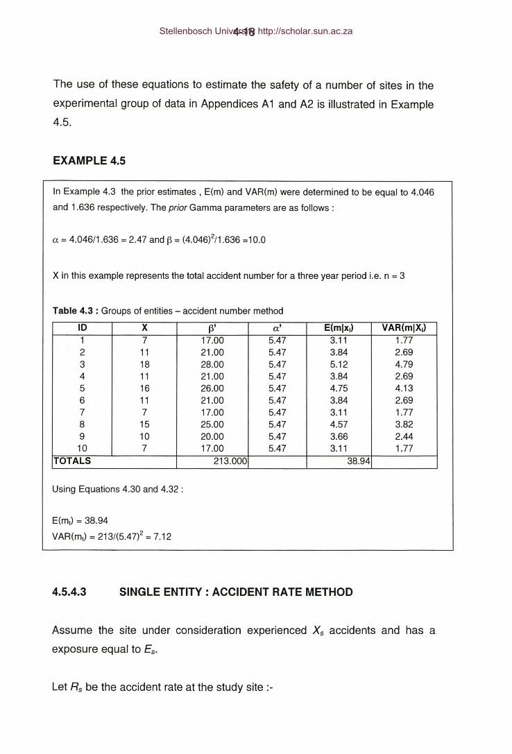
4-18
The use of these equations to estimate the safety of a number of sites in the
experimental group of data in Appendices A1 and A2 is illustrated in Example
4.5.
EXAMPLE 4.5
In Example 4.3 the prior estimates, E(m) and VAR(m) were determined to be equal to 4.046
and 1.636 respectively. The prior Gamma parameters are as follows:
a = 4.046/1.636 = 2.47 and f3 = (4.046)2/1.636 =10.0
X in this example represents the total accident number for a three year period i.e. n = 3
Table 4.3 : Groups of entities - accident number method
ID X f3' a' E(mlxj) VAR(mIX1)
1 7 17.00 5.47 3.11 1.772 11 21.00 5.47 3.84 2.693 18 28.00 5.47 5.12 4.794 11 21.00 5.47 3.84 2.695 16 26.00 5.47 4.75 4.136 11 21.00 5.47 3.84 2.697 7 17.00 5.47 3.11 1.778 15 25.00 5.47 4.57 3.829 10 20.00 5.47 3.66 2.4410 7 17.00 5.47 3.11 1.77
TOTALS 213.000 38.94
Using Equations 4.30 and 4.32 :
E(mt) = 38.94
VAR(mt) = 213/(5.47)2 = 7.12
4.5.4.3 SINGLE ENTITY: ACCIDENT RATE METHOD
Assume the site under consideration experienced X, accidents and has a
exposure equal to Es.
Let Rs be the accident rate at the study site :-
Stellenbosch University http://scholar.sun.ac.za

4-19
R = Xs
s Es
... [4.34]
Where Es = Annual traffic in million vehicles (AADT*365/106).
The estimated prior parameters of the gamma distribution is as follows: (Refer
to Eqn. 4.17 and 4.18]
a= =--=VAR(m) E's;-RE(m) E'R
... [4.35] f3 = [E(m)]2 = RaVAR(m) ... [4.36]
Where E' = Harmonic mean [Eqn. 4. 161, R = Mean accident rate [Eqn. 4. 141
and sl = Variance of accident rates [Eqn. 4. 151.
Once the parameters of prior distribution have been determined, the next step
is to combine the prior information with the site-specific data to obtain the
posterior distribution.
a'=a +E, ... [4.37] . .. [4.38]
E (m I X s ,Es) = ~ = f3 + X sa' a +E,
...[4.39]
f3' f3+XsVAR(m I Xs,E.) = --2 = 2(a') (a+E.) ...[4.40]
Substituting Equations 4.35 and 4.36 into Equations 4.39 and 4.40 will yield
the following equations for E(mIXs, EJ and VAR(mIXs, EJ:
E (m I X s ,Es) = ( Es JRs + ( a JE (m)Es +a Ei +a
... [4.41]
Stellenbosch University http://scholar.sun.ac.za

4-20
VAR(m I Xs,E,) =( Es ]E(m I Xs,E,)Es+a ...[4.42]
where
E'R ... [4.43]a =-~--=E's2 -RR
where E' - the harmonic mean of the exposures (E) of all sites in the
reference group.
The 'true' level of safety at a site is a combination of the observed accident
rate (R) and the underlying Gamma mean, E(m). As mentioned before in
Section 4.2b at low levels of exposure the accident rate R becomes unstable.
In Equation 4.41 the significance of R decreases with decreasing values of E
while the significance of E(m) increases. Thus when a site has a low level of
exposure its 'true' level of safety will be closely related to the average level of
safety for similar locations while the level of safety at a site with a high level of
exposure wi" be closely related to the observed accident rate.
EXAMPLE 4.6
Appendix 81 contains accident and exposure information of a number of road sections in the
Western Cape. All these road sections consist of two 3.7m lanes with 2.4 m wide surfaced
shoulders.
E(m) = R = 0.78 82 = 0.84 E' = 4.44
a = (4.44*0.78)/(4.44*0.84-0.78) = 1.18 and 13 = 1.18*0.78 = 0.92
Consider the section of NR01004 between km 27.78 and km 54.24. During 1994 a total of 8
accidents were recorded on this section of road. During 1994 the AADT = 3085.
Continue ....
Stellenbosch University http://scholar.sun.ac.za

4-21
Example 4.6 (continue)
Xs = 8
Es= (54.24-27.78)*3085 * 365*1000000 = 29.8 mvkm
Rs = 8/29.8 = 0.269 acc/mvkm
13' = 0.92 + 8 = 8.29 and a' = 1.18 + 29.8 = 30.97
E(mIXs,Es) = 8.29/30.97 = 0.29 acc/mvkm
VAR(mIXs,Es) = 0.29/30.97 = 0.009
4.5.4.4 GROUP OF ENTITIES: ACCIDENT RATE METHOD
According to AI-Maseied et al. (1993) at the group of entities level, the total
expected accident rate is given by the sum of the individual accident rates.
The total expected accident rate (rt) for a group of n sites is given by:
... [4.44]
The expected value and variance of rt is given by :
VAR(r ) = {' __ê_J_I LJ 12
i=1 cx i... [4.46]... [4.45]
The Gamma parameters of rt can be estimated as follows:
E(r/)cx = _ __;__/ VAR(r/)
f3 = [E(r/)f/ VAR(~)
... [4.48]... [4.47]
4.5.5 PERFORMANCE
To assess the effect of different study periods on the accuracy of the
Bayesian safety estimates the accident number method was used to perform
the analysis in Example 4.7 and Appendix A2.
Stellenbosch University http://scholar.sun.ac.za
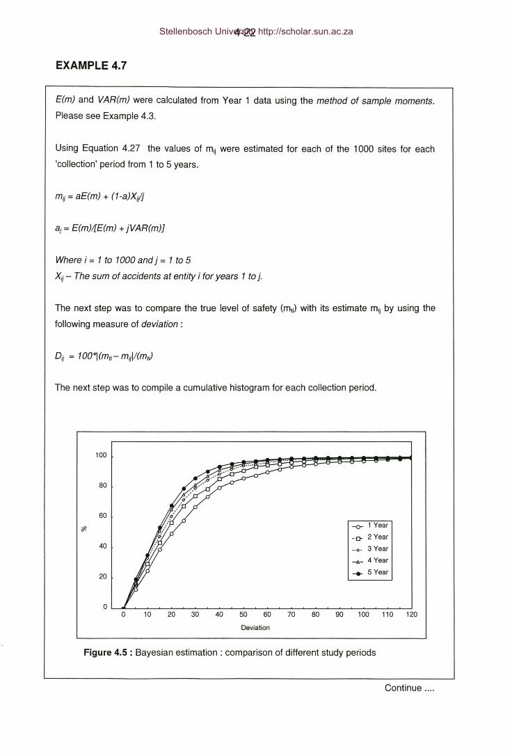
4-22
EXAMPLE 4.7
E(m) and VAR(m) were calculated from Year 1 data using the method of sample moments.
Please see Example 4.3.
Using Equation 4.27 the values of mij were estimated for each of the 1000 sites for each
'collection' period from 1 to 5 years.
mij = aE(m) + (1-a)X;jj
aj = E(m)I[E(m) + jVAR(m)]
Where i = 1 to 1000 and j = 1 to 5
Xij - The sum of accidents at entity i for years 1 to j.
The next step was to compare the true level of safety (mli) with its estimate mij by using the
following measure of deviation:
The next step was to compile a cumulative histogram for each collection period.
100
80
60
<fi. -0- 1 Year
-0- 2 Year40
--00- 3 Year
-d- 4 Year
20 ..... 5 Year
Deviation
Figure 4.5 : Bayesian estimation: comparison of different study periods
Continue ....
Stellenbosch University http://scholar.sun.ac.za
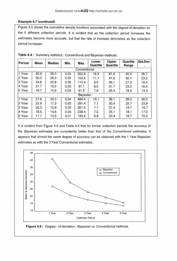
4-23
Example 4.7 (continued)
Figure 4.5 shows the cumulative density functions associated with the degree-at-deviation for
the 5 different collection periods. It is evident that as the collection period increases the
estimates become more accurate, but that the rate of increase diminishes as the collection
period increases.
Table 4.4: Summary statistics: Conventional and Bayesian methods
Period Mean Median Min. Max. Lower Upper Quartile Std.DevQuartile Quartile Range .
Conventional1 Year 42.9 35.0 0.03 302.8 16.3 61.4 45.2 35.72 Year 30.0 26.3 0.03 153.6 11.7 41.8 30.1 23.23 Year 24.6 20.8 0.05 110.4 9.0 36.1 27.0 19.04 Year 21.7 18.0 0.03 97.1 8.5 31.7 23.2 16.45 Year 18.7 15.9 0.03 91.5 7.9 26.4 18.5 14.3
Bayesian1 Year 27.9 20.3 0.04 484.4 10.1 36.1 26.0 30.22 Year 22.9 17.3 0.02 391.4 7.7 30.4 22.7 23.93 Year 20.3 . 15.9 0.03 301.5 7.7 27.4 19.7 19.74 Year 18.5 14.6 0.03 239.4 7.0 25.1 18.1 17.05 Year 17.1 13.9 0.01 193.9 6.8 23.4 16.7 15.2
It is evident from Figure 4.6 and Table 4.4 that for similar collection periods the accuracy of
the Bayesian estimates are consistently better than that of the Conventional estimates. It
appears that almost the same degree of accuracy can be obtained with the 1 Year Bayesian
estimates as with the 3 Year Conventional estimates.
46
42
38c0~ 34's(J)0.l!1 30::l0U).0 26<I:
'*ctil 22(J)
::2:
18
14
-0- Bayesian-o- Conventional
1 Year 2 Year 3 Year
Collection Period
4 Year 5 Year
Figure 4.6: Degree -of-deviation: Bayesian vs. Conventional methods
Stellenbosch University http://scholar.sun.ac.za

4-24
4.5.6 THE MULTIVARIATE REGRESSION METHOD WITHOUT A
REFERENCE GROUP
According to Mountain and Fawaz (1991) there are some practical issues to
consider when applying the multivariate regression method.
The determination of parameters using regression modelling requires a
sufficiently large sample of reference sites in terms of measurable
characteristics. If the size and homogeneity of the reference group is
sacrificed it will increase bias and the variability of the parameters.
In cases where a sufficient group of reference sites is not available it is more
practical to use an existing model suitable for the type of site under
investigation. It is however first necessary to obtain estimates of k, the shape
parameter of the assumed Gamma distribution for the between site variation
in m.
If already developed models are used then k cannot be estimated directly. In
such a case Mountain and Fawaz (1991) propose two possible approaches:
a) Assumean appropriate rangeof values for k.
This approach does not require a reference group of sites to determine
E(m).
According to Mountain and Fawaz (1991) a number of authors have
fitted negative binomial distributions to observed accident frequencies
and obtained k values in the range 0.5 to 2.8. This approach is
considered not preferable because the use of even narrow ranges of k
values can result in wide ranging estimates of safety.
Stellenbosch University http://scholar.sun.ac.za
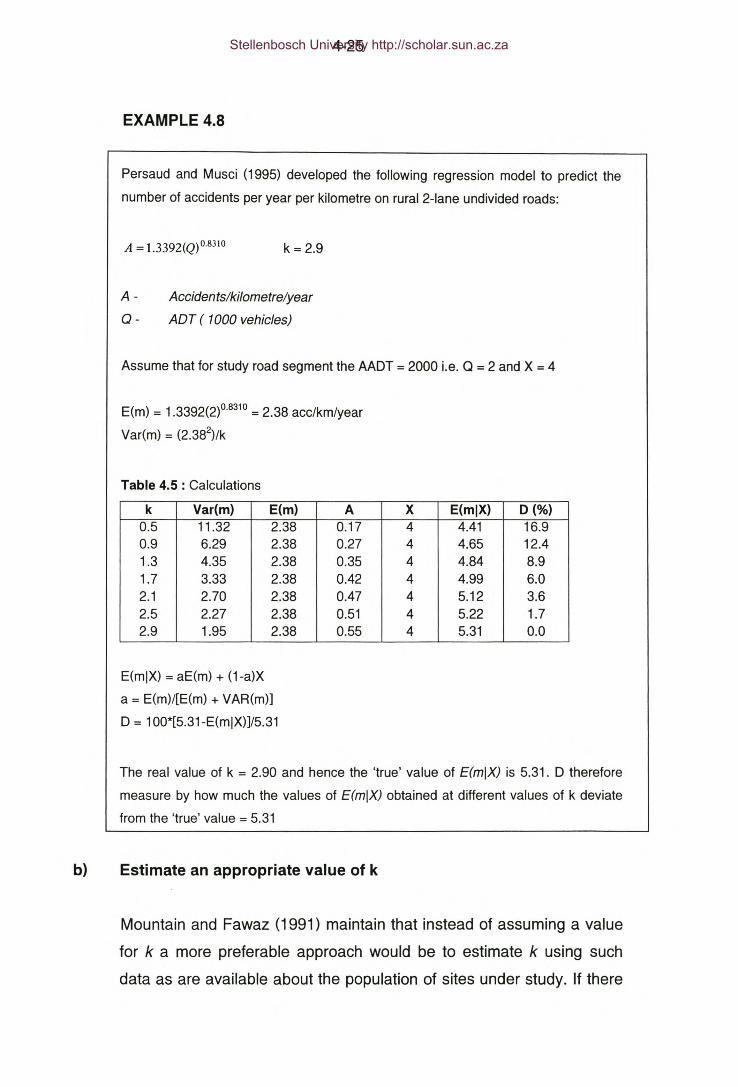
4-25
EXAMPLE 4.8
Persaud and Musci (1995) developed the following regression model to predict the
number of accidents per year per kilometre on rural 2-lane undivided roads:
A = l.3392(Q)08310 k = 2.9
A - Accidents/kilometre/year
Q - ADT ( 1000 vehicles)
Assume that for study road segment the AADT = 2000 i.e. Q = 2 and X = 4
E(m) = 1.3392(2)°·8310= 2.38 acc/km/year
Var(m) = (2.382)/k
Table 4.5 : Calculations
k Var(m) E(m) A X E(mIX) D (%)0.5 11.32 2.38 0.17 4 4.41 16.90.9 6.29 2.38 0.27 4 4.65 12.41.3 4.35 2.38 0.35 4 4.84 8.91.7 3.33 2.38 0.42 4 4.99 6.02.1 2.70 2.38 0.47 4 5.12 3.62.5 2.27 2.38 0.51 4 5.22 1.72.9 1.95 2.38 0.55 4 5.31 0.0
E(mIX) = aE(m) + (1-a)X
a = E(m)/[E(m) + VAR(m)]
D = 100*[5.31-E(mIX)]/5.31
The real value of k = 2.90 and hence the 'true' value of E(mIX) is 5.31. D therefore
measure by how much the values of E(mIX) obtained at different values of k deviate
from the 'true' value = 5.31
b) Estimate an appropriate value of k
Mountain and Fawaz (1991) maintain that instead of assuming a value
for k a more preferable approach would be to estimate k using such
data as are available about the population of sites under study. If there
Stellenbosch University http://scholar.sun.ac.za

4-26
are insufficient data to determine a reliable k for sites similar to the
study site then a broader grouping of sites can be used to generate a
sufficient number of sites.
If a broader grouping of sites is used then k can be estimated asfollows: -
1k =<j>(1+-)8
... [4.49]
Where <j> is determined from fitting a negative binomial distribution to
the observed accident frequencies of each site in the reference group.
The value of <j> can be estimated from the method of moments as
follows:
-2X
<j> = 2 -Sx -x
... [4.50]
The value of 8 can be determined from fitting a Gamma distribution to
the values of y for each site. Where y is the predicted number of
accidents at a site using the prediction model.
-28= Y2 -
_ Sy - Y... [4.51]
Stellenbosch University http://scholar.sun.ac.za

4-27
4.5.7 THE MULTIVARIATE REGRESSION METHOD
COHERENT APPROACHA MORE
The content of this section is based exclusively on the pioneering work done
by Hauer (1997) in his book Observational Before-and-After Studies in Road
Safety (Pergamon).
According to Hauer (1997) one of the major impediments of the 'classical'
multivariate regression method as discussed thus far is that a single estimate
of mj is determined for the whole analysis period. This is based on the
assumption that over the analysis period the 'true' level of safety at a location
(mj) remains unchanged. A further impediment, is that a fixed analysis period
is assumed, based on the notion that accident information prior to this period
contains no useful information.
4.5.7.1 THEORETICAL FRAMEWORK
Assume there is a reference group consisting of n sites. At each site accident
data and covariate values are available for each of the years y = 1, 2, .....Y.
Using multiple regression analysis a multiple regression model can be fitted
to the data for each of the years y = 1, 2, .....Y.
For example:
E(mi) = L,ayQrY
VAR(mi,y) = [E(m,)F / k
...[4.52]
...[4.53]
where
E(mj,y} - Denote the mean of the m/s in year 'y' for all entities in the
imagined reference population of entity i.
VAR(mj,y} - Denote the variance of these mïs
Stellenbosch University http://scholar.sun.ac.za

4-28
k-
0.-I,y
The dispersion parameter obtained from negative binomial
regression analysis.
Traffic flow at entity i in year y.
The length of entity i.
In the above model the purpose of the ay's is to capture the influence of all
factors that change from year to year, except for the change in traffic flow. The
influence of changes in traffic flow is accounted for separately through Qf3. It is
stated that the ay's can be used to account for the joint influences of year-to-
year changes in weather, in economic conditions, the inclination to report
accidents etc. The absence of a subscript 'i' indicates two beliefs. First that
weather, economic conditions and similar factors changed in the same
manner on all road sections in the reference group. Second, that the effect of
a specific change from year-ta-year affects all road sections in the same
manner (Hauer; 1997).
The objective is to estimate mi,y , the expected number of accidents of the
entity i in year y, knowing that the entity experienced Xj,1 , Xj,2 , ... Xj,y
accidents, The different values of mj,y for an entity i are not independent of
one another. According to Hauer (1997) certain characteristics of an entity do
not change from year to year e.g. lane widths, gradient, curvature etc. Some
characteristics do however change from year to year - as quantified by the
a/s, e.g. weather, economic situation, traffic composition etc. One can
therefore expect that there will be some similarity in mi over the years, but that
there will also be some change in mi from year to year.
Hauer (1997) provides a detailed derivation of the following expressions:
m E(m)~= I,y =c.mi,! E(mi,J) I.y
...[4.54]
m. =m.!c.I,y I, I,y...[4.55]
Stellenbosch University http://scholar.sun.ac.za

4-29
...[4.56]
The underlying assumption of these expression is that how the mi of an entity
changes from year to year can be adequately represented by the change in
the covariates over time, and by the model equation. The effect of these
expressions is that mi; and VAR(mi,y) are all a function of m,».
Hauer (1997) provides the following expressions to estimate mi,1 and
VAR(mi,1) :
...[4.57]y=1mi.1 ==r=z:':--+ICiyE(m,) y=1 •
mi•1VAR(mi I) = Y. k--+IciYE (mi•l) y=1 .
.,,[4.58]
The use of these equations to estimate the safety of an entity, as it changes
from year to year, is illustrated in Example 4.9.
Stellenbosch University http://scholar.sun.ac.za

4-30
EXAMPLE 4.9
Consider a hypothetical segment of road with length = 2km that during a 6 year
period experienced the following number of accidents - {4, 1, 3, 4, 2, 5}. Using a
reference group of similar sites a total of 6 multivariate regression models were fitted
to the data, one for each year, - similar in form to the model in Equation 3.5. The f3parameter for all the models = 0.78. The a parameters for six different models are
shown in the Table below. The k value obtained from calibrating the prediction model
for year 1 = 4.5
Table 4.6 : Data and calculations
y ay QI,y E(ml,y) c., X1,y mhy VAR(ml,y)
1 0.00271 1250 1.41 1.000 4 2.49 0.2642 0.00295 1156 1.45 1.024 1 2.55 0.2773 0.00277 1277 1.47 1.039 3 2.59 0.2854 0.00265 1334 1.45 1.029 4 2.56 0.2805 0.00284 1288 1.51 1.073 2 2.67 0.3046 0.00278 1305 1.50 1.061 5 2.64 0.297
TOTALS 6.226 19 15.5
From Eqn. 4.57 and Eqn. 4.58:
m;,1= (4.? + 19)/(4.5/1.41 + 6.226) = 2.49
VAR(m;,1) = 2.49/(4.5/1.41 +6.226) = 0.264
From Eqn. 4.55 and Eqn. 4.56:
m;,2= 2.49 (1.024) = 2.549
VAR(md = (1.024)2(0.264) = 0.277
Stellenbosch University http://scholar.sun.ac.za
4-31
4.5.8 STATISTICAL INFERENCE
Both prior an posterior Bayesian safety estimates follow a Gamma
distribution.
If the parameters of the Gamma distribution are known, using distribution
theory, a number of statistical inferences can be made concerning the safety
estimate of an entity or a group of entities.
The following inferences could be of interest:
• The probability that the safety estimate lies between two values.
• The probability that the safety estimate lies above or below a certain value.
• The values of two-tailed or one-tailed confidence intervals.
• The probability of two Bayesian estimates being different from one
another.
The probability density function of a Gamma distribution is as follows:
...[4.59]
To determine the probability that m is larger than b and smaller than a the
probability distribution function can be used as follows:
b j3a a-I -j3m
P(a < m $, b) = f m e dma r(a)
...[4.60]
Stellenbosch University http://scholar.sun.ac.za

4-32
In Figure 4.7 the probability density function and probability distribution
function of an estimate with parameters a = 1 and f3 = 3.4 is shown.
ProbabilityDensityFunction0.75 r----..-,.-~..,.-~-.__-.....,
0.50 . . .-.--_._ _ ~ _------· .· .· .· .· .· .· .· .· ,, ,, ,, ,, ,, ,, ,, ,, ,, ,, ,, ,, ,, ,· ., ,, ,, ,-.- .. _ -, ,, ,, ,, .· ,, ,, ,· ,, ,, ,, ,, ,· ., ,
ProbabilityDistributionFunction
0.8 . ··1 r I:: :J I: :1--:0.2 1 1 \ ·.0.0 1.....o«.._.......J.._~--'-~_.....__. _ __,
0.0 2.5 5.0 7.5 10.0
0.25
Figure 4.7: Probability density and distribution functions for a Gammadistribution with a = 1 and 13= 3.4.
The integral in Equation 4.59 can be solved using the GAMMADIST function
of Microsoft® Excel® as shown in Table 4.7. In any Excel® function that
refers to the Gamma distribution alpha = f3 and beta = 1lo:
Table 4.7 : Using the GAMMADIST function of Excel®
Prob. Function
P(m:s; b) =GAMMADIST(b,j3, 11a, TRUE)
P(a < rn s b) =GAMMADIST(b,j3, 11a, TRUE) - GAMMADIST(a,j3, 11a, TRUE)
P(m > b) =1- GAMMADIST(b, 13, 1la, TRUE)
To determine the value of merit for which P(m ::; merit)= 0.95 the GAMMAINV
function of Microsoft® Excel® can be used as follows:
=GAMMA IN V(O.95,13, 11a) ...[4.61]
Stellenbosch University http://scholar.sun.ac.za

4-33
The critical values of m at which P(m ~ meriJ = 0.95 or P(m s meriJ = 0.05 can
be obtained from Tables 4.8 and 4.9 respectively. These Tables are used as
follows:
a) Using the f3 parameter of the Gamma distribution locate the
appropriate value of G.
b) Having obtained the G value merit is obtained using the a parameter
as follows:
merit = Gla ...[4.62]
EXAMPLE 4.10
In Example 4.6 the following estimates were obtained for a segment of road:
E(mIXs,Es) = 8.29/30.97 = 0.29 acc/mvkm
VAR(mIXs,Es) = 0.29/30.97 = 0.009
The Gamma parameters are:
f3' = 0.92 + 8 = 8.92
a' = 1.18 + 29.8 = 30.98
To determine the meritsuch that P(m ~ merit)= 0.05 obtain from Table 4.9 the value of G where
f3 = 8.9.
G = 4.84 and merit= 4.84/30.97 = 0.156.
To determine meritsuch that P(m ~ merit)= 0.95 obtain from Table 4.8 the value of G where f3 =8.9.
G = 14.32 and merit= 14.32/30.97 = 0.462.
The 90 % confidence interval of E(mIX,E) is therefore {0.156; 0.462}.
Stellenbosch University http://scholar.sun.ac.za

4-34
AI-Masaeid et al. (1993) provides the derivation for the following expressions
that can be used to determine the probability that two Bayesian estimates are
different from each other:
Assume there are two locations with Bayesian estimates mt and m2respectively. The Gamma parameters of Site 1 are a and f3 while the Gamma
parameters of Site 2 are a' and [3'.
Assuming that m1 and m2 are independent the joint probability density function
is given by :
p'1(l' a'-I -j3'mzIJ mz e ...[4.63]r{a')
P(m1< m2) can be estimated as follows:
a-I [ f3 J[ f3' Ja '+ J r(a '+ j)pim, <mz) =1- ~ IV f3'+f3 r(j+1)r(a')
... [4.64]
The Eqn. 4.64 can be solved using a spreadsheet. E.g. the Gamma function
r(a') can be solved using a combination of the EXP and GAMMALN functions
in Microsoft® Excel®. r(a') = EXP(GAMMALN(a 'J).
EXAMPLE 4.11
Two sites have the following parameters:
Site 1 a = 4.0, 13 = 1.9, E(malxa) = 2.10
Site 2: a' = 3.4 , j3' = 1.2, E(mblxb) = 2.80
lf D . = [_ê_J[-j3'_Ja '+ j l(a '+j)J 13' j3+j3' '['(j+l)l(a')
Then Do = 0.46 and D1 = 0.25
0.9"J- DJ' = DO + 0.9D1 = 0.46 + 0.9(0.25) = 0.685]=1
P(m1 < m2) = 1 - 0.685 = 0.315
Stellenbosch University http://scholar.sun.ac.za

4-35
Table 4.8 : Incomplete Gamma function values (a = 1 ) : 95 % Degree of Confidence
j3 G j3 G j3 G j3 G0.1 0.58 4.1 7.90 8.1 13.28 12.1 18.330.2 1.03 4.2 8.04 8.2 13.41 12.2 18.460.3 1.37 4.3 8.18 8.3 13.54 12.3 18.580.4 1.66 4.4 8.32 8.4 13.66 12.4 18.700.5 1.92 4.5 8.46 8.5 13.79 12.5 18.830.6 2.16 4.6 8.60 8.6 13.92 12.6 18.950.7 2.38 4.7 8.74 8.7 14.05 12.7 19.070.8 2.60 4.8 8.88 8.8 14.18 12.8 19.200.9 2.80 4.9 9.02 8.9 14.31 12.9 19.321.0 3.00 5.0 9.15 9.0 14.43 13.0 19.441.1 3.19 5.1 9.29 9.1 14.56 13.1 19.571.2 3.37 5.2 9.43 9.2 14.69 13.2 19.691.3 3.55 5.3 9.57 9.3 14.82 13.3 19.811.4 3.73 5.4 9.70 9.4 14.94 13.4 19.931.5 3.91 5.5 9.84 9.5 15.07 13.5 20.061.6 4.08 5.6 9.97 9.6 15.20 13.6 20.181.7 4.25 5.7 10.11 9.7 15.33 13.7 20.301.8 4.42 5.8 10.24 9.8 15.45 13.8 20.421.9 4.58 5.9 10.38 9.9 15.58 13.9 20.552.0 4.74 6.0 10.51 10.0 15.71 14.0 20.672.1 4.91 6.1 10.65 10.1 15.83 14.1 20.792.2 5.06 6.2 10.78 10.2 15.96 14.2 20.912.3 5.22 6.3 10.91 10.3 16.08 14.3 21.032.4 5.38 6.4 11.05 10.4 16.21 14.4 21.162.5 5.54 6.5 11.18 10.5 16.34 14.5 21.282.6 5.69 6.6 11.31 10.6 16.46 14.6 21.402.7 5.84 6.7 11.45 10.7 16.59 14.7 21.522.8 5.99 6.8 11.58 10.8 16.71 14.8 21.642.9 6.15 6.9 11.71 10.9 16.84 14.9 21.773.0 6.30 7.0 11.84 11.0 16.96 15.0 21.893.1 6.44 7.1 11.97 11.1 17.09 15.1 22.013.2 6.59 7.2 12.11 11.2 17.21 15.2 22.133.3 6.74 7.3 12.24 11.3 17.34 15.3 22.253.4 6.89 7.4 12.37 11.4 17.46 15.4 22.373.5 7.03 7.5 12.50 11.5 17.59 15.5 22.493.6 7.18 7.6 12.63 11.6 17.71 15.6 22.613.7 7.32 7.7 12.76 11.7 17.84 15.7 22.733.8 7.47 7.8 12.89 11.8 17.96 15.8 22.863.9 7.61 7.9 13.02 11.9 18.08 15.9 22.984.0 7.75 8.0 13.15 12.0 18.21 16.0 23.10
Stellenbosch University http://scholar.sun.ac.za

4-36
Table 4.9 : Incomplete Gamma function values (a = 1): 5 % Degree of Confidence
f3 G f3 G f3 G f3 G0.1 0.00 4.1 1.42 8.1 4.05 12.1 7.000.2 0.00 4.2 1.48 8.2 4.12 12.2 7.080.3 0.00 4.3 1.54 8.3 4.19 12.3 7.150.4 0.00 4.4 1.60 8.4 4.26 12.4 7.230.5 0.00 4.5 1.66 8.5 4.34 12.5 7.310.6 0.01 4.6 1.72 8.6 4.41 12.6 7.380.7 0.01 4.7 1.78 8.7 4.48 12.7 7.460.8 0.02 4.8 1.85 8.8 4.55 12.8 7.540.9 0.03 4.9 1.91 8.9 4.62 12.9 7.61 .1.0 0.05 5.0 1.97 9.0 4.70 13.0 7.691.1 0.07 5.1 2.03 9.1 4.77 13.1 7.771.2 0.09 5.2 2.10 9.2 4.84 13.2 7.841.3 0.12 5.3 2.16 9.3 4.91 13.3 7.921.4 0.15 5.4 2.22 9.4 4.99 13.4 8.001.5 0.18 5.5 2.29 9.5 5.06 13.5 8.081.6 0.21 5.6 2.35 9.6 5.13 13.6 8.151.7 0.24 5.7 2.42 9.7 5.20 13.7 8.231.8 0.28 5.8 2.48 9.8 5.28 13.8 8.311.9 0.32 5.9 2.55 9.9 5.35 13.9 8.392.0 0.36 6.0 2.61 10.0 5.43 14.0 8.462.1 0.40 6.1 2.68 10.1 5.50 14.1 8.542.2 0.44 6.2 2.75 10.2 5.57 14.2 8.622.3 0.48 6.3 2.81 10.3 5.65 14.3 8.702.4 0.53 6.4 2.88 10.4 5.72 14.4 8.782.5 0.57 6.5 2.95 10.5 5.80 14.5 8.852.6 0.62 6.6 3.01 10.6 5.87 14.6 8.932.7 0.67 6.7 3.08 10.7 5.94 14.7 9.012.8 0.72 6.8 3.15 10.8 6.02 14.8 9.092.9 0.77 6.9 3.22 10.9 6.09 14.9 9.173.0 0.82 7.0 3.29 11.0 6.17 15.0 9.253.1 0.87 7.1 3.35 11.1 6.24 15.1 9.323.2 0.92 7.2 3.42 11.2 6.32 15.2 9.403.3 0.98 7.3 3.49 11.3 6.39 15.3 9.483.4 1.03 7.4 3.56 11.4 6.47 15.4 9.563.5 1.08 7.5 3.63 11.5 6.55 15.5 9.643.6 1.14 7.6 3.70 11.6 6.62 15.6 9.723.7 1.19 7.7 3.77 11.7 6.70 15.7 9.803.8 1.25 7.8 3.84 11.8 6.77 15.8 9.883.9 1.31 7.9 3.91 11.9 6.85 15.9 9.964.0 1.37 8.0 3.98 12.0 6.92 16.0 10.04
Stellenbosch University http://scholar.sun.ac.za

4-37
4.6 SUMMARY and CONCLUSION
In this Chapter both the Conventional and Bayesian methodologies were
presented to measure the safety of road infrastructure elements. Certain
shortcomings of the Conventional methods to road safety measurement were
identified and discussed. The Empirical Bayesian methodology was discussed
in detail and it has been shown how Bayesian methods can compensate for
the shortcomings of the Conventional methods.
It has been shown from analysing the experimental data in Appendices A1
and A2 with both the Conventional and Bayesian methodologies that the latter
produce results that are generally more accurate, but that the relative 'benefit'
of using the Bayesian method decreases as the study period increases.
Certain impediments of the 'classical' Bayesian methods, as described in the
Chapter, were identified and a more coherent approach, based on the work of
Hauer (1997), was proposed. This approach acknowledged the fact that the
level of safety at a location may change from year to year.
Stellenbosch University http://scholar.sun.ac.za

CHAPTER 5
THE IDENTIFICATION AND RANKING OF HAZARDOUS LOCATIONS
5.1 INTRODUCTION
A road safety remedial programme requires an effective means of identifying
hazardous locations. Hazardous locations according to Deacon et al. (1997)
are those locations where the accident pattern or the level of safety are
abnormally severe when compared with similar locations elsewhere, and for
which improvements can be made through a variety of engineering measures.
The identification of hazardous locations is the first step in a road safety
remedial programme. In short the procedure is as follows:
a) Identification of hazardous locations.
b) Preliminary ranking of selected locations.
c) Detailed investigation.
d) Final ranking based on cost effectiveness.
e) Design and implementation.
f) Monitoring and evaluation.
Applying an identification procedure is an important first step because it would
be impractical to conduct a road safety investigation on each and every
location in the road network. The detailed investigation of sites as well as the
design and implementation of remedial measures require the application of
potentially scarce resources - money, time, equipment, personnel etc. Road
authorities generally have limited budgets for the purpose of implementing
road safety remedial programmes. It is therefore the road authority's
responsibility and moral obligation to ensure that resources are applied in a
manner, and to those sites, that will yield the maximum possible economic
returns. In identifying hazardous locations it is important that the chosen
Stellenbosch University http://scholar.sun.ac.za

5-2
methodology selects as many of the truly hazardous locations as possible and
discards as many of the non-hazardous locations as possible.
Hauer and Persaud (1984) compare the identification process to a 'sieve' that
retains the hazardous locations and lets the non-hazardous locations through.
The degree of efficiency of an identification process is defined as the degree
to which it retains truly hazardous locations and discards truly non-hazardous
locations.
It is possible that the identification process yields more hazardous locations
than a road authority has the resources to investigate. Ranking the selected
hazardous locations according to the safety benefits that could potentially be
achieved at a site, would ensure that available resources are applied to those
hazardous locations that would yield the best economic returns.
Methods to identify and rank hazardous locations can be divided into two
categories : Conventional methods and Bayesian methods. Conventional
methods rely on conventional safety estimates, and Bayesian methods rely on
Bayesian safety estimates and, in some cases, Safety Performance
Functions.
The objective of this Chapter is to present and to evaluate both the
Conventional and Bayesian methodologies. These two methodologies will be
compared in terms of their efficiency and ability to rank hazardous locations
according to their expected economic benefits.
5.2 PROGRAMME DESIGN
Nicholson (1989) refers to 4 types of plans for accident reduction :-
a) Single site plans
• The treatment of single hazardous locations e.g. intersections, ramps,
bridges, horizontal curves, short segments.
Stellenbosch University http://scholar.sun.ac.za

5-3
b) Route plans
• A whole route or road segments with a poor level of safety is treated
with a remedial measure, such as for example, surfacing gravel
shoulders, widening lanes, resurfacing etc.
c) Area action plans
• A number of remedial measures are implemented in an area that has
been identified as having a particularly poor safety record. For example
the implementation of various traffic calming measures (mini-circles,
speedhumps, street closures etc.) in a town or suburb would constitute
an area action plan.
d) Mass action plans
• A common accident problem is treated by an appropriate remedial
action. An example of a mass action plan would be the wide-scale
resurfacing of intersection approaches to reduce head-rear or right-
angle collisions at intersections.
According to Nicholson (1989) which type of plan is most appropriate to
implement can be determined by evaluating the level and extent to which
accidents are clustered in the study area. A high level of accident clustering
would indicate that a Single-site type plan would be the most appropriate,
while lower levels of clustering would indicate that Route or Area type plans
are more suitable.
Thus with high levels of clustering, in order to maximise the expected accident
reduction and economic benefit, a road authority should commence with a
single-site (blackspot) programme. If the programme is effective the level of
clustering should decrease, after which it may be necessary to adopt a higher
level of aggregation i.e. a Route ('blackroute') programme. Routes may
contain a number of single sites which do not qualify as 'blackspots' but when
considered together give 'blackroutes' .
Stellenbosch University http://scholar.sun.ac.za
5-4
The successful treatment of such routes will lead to a further reduction in the
level of clustering to the extent that even a higher level of aggregation is
required.
Nicholson (1989) provides a number of methods to quantify the level of
accident clustering on a network, but fail to provide threshold values as to
when the different type of plans are more appropriate. The methods proposed
by Nicholson (1989) can however be used to assess whether or not there
were changes in the level of accident clustering.
According to Nicholson (1989) there is a natural progression from single-site
plans to area plans with the expected accident reduction and economic return
declining with the 'law of diminishing returns'.
Even though single-site plans yield the best results in terms of accident
reductions and economic benefits relative to the other type of plans it is not
always the most appropriate course of action to take. Nicholson (1989)
reports that since the mid 80's systematic accident reduction efforts in New
Zealand concentrated primarily on single-site plans, but that subsequently
analysis has shown this to be the wrong approach because of the low levels
of clustering that already existed at the time.
The identification and ranking in this chapter are aimed specifically at single-
site and route action plans.
5.3 COMPONENTS OF IDENTIFICATION METHODS
An important consideration when attempting to identify hazardous locations is
how to define single-sites and routes.
5.3.1 SINGLE SITES
According to Deacon et al. (1975) several considerations are paramount to
determining the appropriate spot length:
Stellenbosch University http://scholar.sun.ac.za
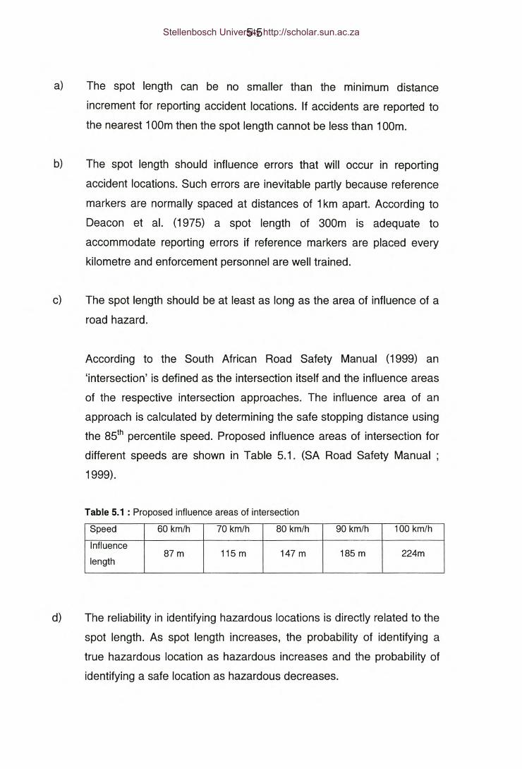
5-5
a) The spot length can be no smaller than the minimum distance
increment for reporting accident locations. If accidents are reported to
the nearest 100m then the spot length cannot be less than 100m.
b) The spot length should influence errors that will occur in reporting
accident locations. Such errors are inevitable partly because reference
markers are normally spaced at distances of 1km apart. According to
Deacon et al. (1975) a spot length of 300m is adequate to
accommodate reporting errors if reference markers are placed every
kilometre and enforcement personnel are well trained.
c) The spot length should be at least as long as the area of influence of a
road hazard.
According to the South African Road Safety Manual (1999) an
'intersection' is defined as the intersection itself and the influence areas
of the respective intersection approaches. The influence area of an
approach is calculated by determining the safe stopping distance using
the 85th percentile speed. Proposed influence areas of intersection for
different speeds are shown in Table 5.1. (SA Road Safety Manual;
1999).
Table 5.1 : Proposed influence areas of intersection
Speed 60 km/h 70 km/h 80 km/h 90 km/h 100 km/h
Influence87m 115 m 147 m 185 m 224m
length
d) The reliability in identifying hazardous locations is directly related to the
spot length. As spot length increases, the probability of identifying a
true hazardous location as hazardous increases and the probability of
identifying a safe location as hazardous decreases.
Stellenbosch University http://scholar.sun.ac.za

5-6
e) If spots are small it becomes increasingly difficult to make meaningful
comparisons between spots because of the low accident counts.
On the basis of these considerations it is desirable that spot lengths be as
long as possible. However if the spot is too long it could become excessively
difficult and time-consuming to locate the hazard/so
Deacon et al. (1975) recommends that a spot should preferably be between
4BOm and BOOmlong.
5.3.2 SECTIONS/SEGMENTS/ROUTES
It is important that sections be defined in a manner that ensures that the
pavement condition, geometric design, traffic volume and other geometric,
traffic and environmental variables etc. are uniform across the whole length of
the section. Sections can be defined as a segment of road between two
nodes, where nodes could be intersections or points where the pavement,
geometric, traffic characteristics etc. change. According to this definition
sections would normally be of variable length.
According to Deacon et al. (1975) observed accident rates are dependent on
section length. High accident rates have been observed on short sections and
low accident rates on long sections of roads. Long sections tend to have lower
traffic volumes and fewer factors of traffic interference such as intersections,
access points and changes in the number of lanes.
The variance of a Bayesian estimate depends amongst others on the
exposure at a site. The longer the length of a section the larger the exposure
and the smaller the variance. A smaller variance makes it easier to detect
whether the estimate exceeds a threshold value.
Stellenbosch University http://scholar.sun.ac.za
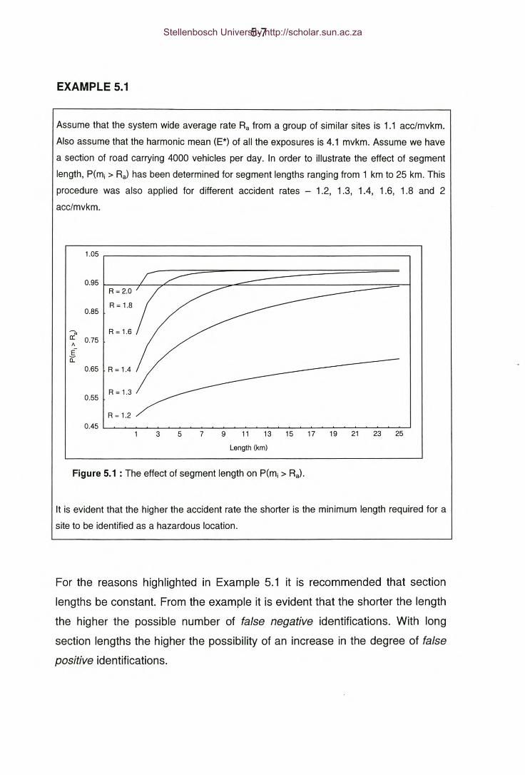
EXAMPLE 5.1
5-7
Assume that the system wide average rate Ra from a group of similar sites is 1.1 acc/mvkm.
Also assume that the harmonic mean (E*) of all the exposures is 4.1 mvkm. Assume we have
a section of road carrying 4000 vehicles per day. In order to illustrate the effect of segment
length, P(mj > Ra) has been determined for segment lengths ranging from 1 km to 25 km. This
procedure was also applied for different accident rates - 1.2, 1.3, 1.4, 1.6, 1.8 and 2
acc/mvkm.
1.05
0.95R = 2.0
R = 1.80.85.. R = 1.6cr: 0.75
A
E-o::
0.65 R = 1.4
0.55R = 1.3
R = 1.2
3 5 9 11 13 15 17 19 21 23 25
Length (km)
7
Figure 5.1 : The effect of segment length on Ptm, > Ra).
It is evident that the higher the accident rate the shorter is the minimum length required for a
site to be identified as a hazardous location.
For the reasons highlighted in Example 5.1 it is recommended that section
lengths be constant. From the example it is evident that the shorter the length
the higher the possible number of false negative identifications. With long
section lengths the higher the possibility of an increase in the degree of false
positive identifications.
Stellenbosch University http://scholar.sun.ac.za
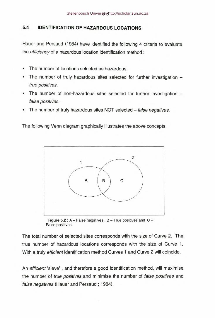
5-8
5.4 IDENTIFICATION OF HAZARDOUS LOCATIONS
Hauer and Persaud (1984) have identified the following 4 criteria to evaluate
the efficiency of a hazardous location identification method :
• The number of locations selected as hazardous.
• The number of truly hazardous sites selected for further investigation -
true positives.
• The number of non-hazardous sites selected for further investigation -
false positives.
• The number of truly hazardous sites NOT selected - false negatives.
The following Venn diagram graphically illustrates the above concepts.
A c
2
Figure 5.2 : A - False negatives, B - True positives and C-False positives
The total number of selected sites corresponds with the size of Curve 2. The
true number of hazardous locations corresponds with the size of Curve 1.
With a truly efficient identification method Curves 1 and Curve 2 will coincide.
An efficient 'sieve' , and therefore a good identification method, will maximise
the number of true positives and minimise the number of false positives and
false negatives (Hauer and Persaud; 1984).
Stellenbosch University http://scholar.sun.ac.za

5-9
It is generally agreed (Higle and Hecht; 1989) that a false negative error is far
more serious than a false positive error. A false negative error would cause a
true hazardous location to go untreated with potentially very severe
consequences. A false postive error on the other hand would cause
potentially scarce resources to be wasted on investigating a site that is not
really a hazardous location, thereby reducing the amount of resources
available to investigate true hazardous locations. According to Higle and
Hecht (1989) a technique that tends to yield a low number of false negatives
is good, as long as its is not accompanied by an excessively large number of
false positives.
The different methods for identifying hazardous locations and for the
preliminary ranking of sites locations can be grouped into two categories:
Conventional methods and Bayesian methods.
5.4.1 CONVENTIONAL IDENTIFICATION METHODS
Palkowski and Menezes (1991) recommend using the following methods to
identify hazardous locations :
a) Accident Number method,
b) Accident Severity method,
c) Accident Rate method,
d) Accident Rate-Number method,
e) Quality Control method.
These methods are called conventional methods because they are based on
the following 'conventional' assumptions:
a) The observed accident rate or number is a reliable and valid measure of
the true level of safety at a location i.e. mi = Xi or mi = R;
b) All sites within a reference group of similar sites have the same 'true' level
of safety.
Stellenbosch University http://scholar.sun.ac.za

5-10
c) The accident rate at a location is a constant irrespective of the level of
exposure at the location i.e. a linear Safety Performance Function.
5.4.1.1 THE ACCIDENT NUMBER METHOD
This method considers only the frequency of accidents at a location. A
location is classified as a hazardous location when the accident frequency
exceeds a predetermined threshold.
This method is considered suitable for small town street systems, local street
systems in larger cities and low volume rural roads. Because of the low and
narrow range of traffic volumes on these types of roads the inclusion of the
exposure factor is not critical (Roy Jorgensen Associates; 1975).
The primary purpose of the threshold value is to control the number of
selected hazardous locations. The threshold value could be different from
authority to authority depending on policy and available resources.
An increase in the threshold value will cause the number of incorrectly
identified sites as well as the number of correctly identified sites to decrease.
It appears that there is a trade off between the two and that a suitable
threshold value will depend on the ability of a road authority to investigate all
identified locations.
Stellenbosch University http://scholar.sun.ac.za

5-11
EXAMPLE 5.2
The experimental data in Appendix A1 was used to illustrate the impact of the chosen
threshold value
The true levels of safety (mt) for each of the 1000 locations were randomly generated from a
Gamma distribution with an annual mean accident frequency of 4. All those locations where
P(mt>4) > 0.95 are assumed to be true hazardous locations.
Using the randomly generated true level of safety mt as the Poisson mean, 5 years of
accident frequencies were randomly generated at each of the 1000 sites, for each of 5 study
years.
For each study period the accident number (X) was determined. If the accident number
exceeded a certain threshold value that location was then flagged as a hazardous location.
The next step was to, for each study period, determine the number of true positives, false
positives, false negatives and true negatives for threshold values (T) of 5, 7 and 9 accidents
per year. The following criteria were used:
True positive:
False negative:
True negative:
False positive:
Pïrn,» 4) > 0.95 AND X ~ T
Pïrn, > 4) > 0.95 AND X < T
P(mt :5: 4) > 0.95 AND X < T
P(mt :5: 4) > 0.95 AND X ~ T
As a measure of efficiency 3 different indicators were calculated. These are the i) number of
sites identified as hazardous locations, ii) the true positive identification rate, and the iii) the
false positive rate. The true positive rate is the % of hazardous locations correctly identified as
hazardous while the false positive rate indicates the % of non-hazardous sites identified as
hazardous.
Continue ....
Stellenbosch University http://scholar.sun.ac.za

5-12
Example 5.2 (continued)
Table 5.2 : Accident no. method: Efficiency assessment of different threshold values.
Collection period 1 Year 2 Year 3 Year 4 Year 5 YearThreshold = 5 Accidents / year
False negative 10 8 5 2 0False positive 345 267 240 226 206True negative 601 679 706 720 740True positive 44 46 49 52 54No. identified 389 313 289 278 260% Incorrectly identified 36.5 28.2 25.4 23.9 21.8% Correctly identified 81.5 85.2 90.7 96.3 100.0
Threshold = 7 Accidents / yearFalse negative 27 25 23 23 20False positive 130 70 50 38 30True negative 816 876 896 908 916True positive 27 29 31 31 34No. identified 157 99 81 69 64% incorrectly identified 13.7 7.4 5.3 4.0 3.2% correctly identified 50.0 53.7 57.4 57.4 63.0
Threshold = 9 Accidents / yearFalse negative 41 42 46 47 48False positive 34 13 5 6 3True negative 912 933 941 940 943True positive 13 12 8 7 6No. identified 47 25 13 13 9% incorrectly identified 3.6 1.4 0.5 0.6 0.3% correctly identified 24.1 22.2 14.8 13.0 11.1
From Table 5.2 it is evident that for the experimental data a low threshold value ( 5 accident /
year) will yield a high % correctly identified as well as a high % incorrectly identified. Since in
practice it is not known which sites were correctly or incorrectly identified all identified sites
will have to be further investigated. If sufficient resources are available to investigate all
identified sites then at least a high number of true hazardous locations will be subjected to an
investigation - along with all the non-hazardous locations.
If a suitable reference group of sites is available a threshold value can be
calculated from Equation 5.1.
METHOD CN1
X: = X +zo ,...[5.1]
where
Stellenbosch University http://scholar.sun.ac.za

5-13
X - The sample mean accident frequency.
ax - Sample standard deviation.
k - A probability factor determined by the desired level of significance.
X T - Threshold value.
A site is flagged as a hazardous location when Xi> XT
The values of k corresponding to various levels of probability are shown in
Table 5.3.
Table 5.3 : k-values
P 0.001 0.005 0.0075 0.05 0.075 0.10
K 3.09 2.576 1.96 1.645 1.440 1.282Source. Palkowski and Menezes, 1991
A probability level is selected to ensure that an accident number/rate is
sufficiently large so that it cannot be reasonably attributed to random
occurrences (Palkowski and Menezes; 1991). The probability level serves the
same function as a threshold value.
Method eNt is based on the assumption that accident frequencies between
sites are distributed according to the Normal distribution. This assumption,
according to Higle and Hecht (1989), causes this method to consistently yield
a high number of false negative identifications.
Since the accident frequency at a site is a function of the traffic volume, the
accident number method tends to favour sites with high traffic volumes.
Two locations with the same amount of accidents, but with different traffic
volumes obviously have different levels of risk. The accident rate method
considers this variable.
Stellenbosch University http://scholar.sun.ac.za
5-14
5.4.1.2 THE ACCIDENT SEVERITY METHOD
This method is a variant of the accident number method, the difference being
that a site is considered a hazardous location if the Equivalent Accident
Number (EAN) exceeds a predetermined threshold level, where:
EAN = w,(F) + ws,(SR) + ws,(SL) + 0 ...[5.2]
Where
w(, WSr, Wsl - The weights associated with fatal, serious injury and slight
injury accidents respectively.
F, SR, SL ,0 - The number of fatal, serious injury, slight injury and damage
only accidents respectively.
The weighting factors represent the average cost of the respective accident
severity classes relative to the cost of a Damage Only accident.
The K21 Manual (Opperman and Hutton ; 1991) proposes the following
weighting factors to be used for the calculation of the EAN :
Fatal accidents 12Injury accidents 3Damage only accidents 1
The average 1998 cost of South African road traffic accidents, according to
Schutte (2000), are shown in Table 5.4.
Stellenbosch University http://scholar.sun.ac.za

5-15
Table 5.4 : Cost of accidents in 1998.
Severity of accident Average cost per collision Weighting factor
Fatal R 388487 25
Serious Injury R 88 248 6
Slight Injury R 23 723 1.5
Damage Only R 15694 1
The total cost of accidents at a location can be obtained by multiplying the
EAN by the cost of a Damage Only accident.
EXAMPLE 5.3
Consider the following two locations:
Table 5.5 : Accident data
Location Fatal Serious Slight Damage Total
A 2 22 25 45 94·B 5 15 18 40 78
The EAN for these sites using the K21 manual weighting factors are:
Location A
Location B
210
199
Using the weighting factors derived from the accident costs the EAN for the two sites are as
follows:
Location A
Location B
265 (Cost = 265 * 15694 = R 4158910)
282 (Cost = 282 * 15694 = R 4 425708)
Using only the accident number method Location A will be considered worse than Location B.
Using the 'K21' factors indicates that Location A is worse than Location B, while using the
'Cost' factors would indicate that Location B is the worst location.
The choice of appropriate weighting factors is critical to this method.
Stellenbosch University http://scholar.sun.ac.za
5-16
The EAN method recognises accident severity as a prime factor in the
identification of hazardous locations.
According to Deacon et al. (1975) the EAN represents not only the accident
number but also the severity of these accidents. The EAN method therefore
favours locations with high accident numbers (i.e. high exposure sites) with a
relatively large proportion of serious and fatal accidents. Deacon et al. (1975)
states that locations selected using the EAN method will be more
economically efficient than sites selected using the accident number method
or the accident rate method.
5.4.1.3 THE ACCIDENT RATE METHOD
This method is very similar to the accident number method. Instead of using
accident frequencies, accident rates are used. A location is identified as
hazardous when its accident rate exceeds some predetermined threshold.
This threshold (Rr) can be determined as follows (Highle and Hecht; 1989 ):
METHOD CR1
RT = R +ka R... [5.4]
where
R - Sample mean of accident rates of all reference group sites.
aR - Sample standard deviation of accident rates.
k - Probability factor.
Location i is flagged as a hazardous location if R, > Rr.
Using this method requires sufficient information to reliably determine the
exposure at each location in the network.
Stellenbosch University http://scholar.sun.ac.za

5-17
According to McGuigan (1982) the accident rate method tends to produce a
set of locations biased towards low accident totals and low traffic usage. By
choosing an appropriate threshold level it is possible to limit the number of
selected sites with low accident numbers. The choice of an appropriate
threshold can be problematic in that a too low level could cause locations with
limited accident reduction potential to be included or too high a level could
cause locations with good accident reduction potential to be excluded. The
identification and ranking of hazardous locations using accident rates
therefore requires a high degree of subjective decision making by the analyst.
5.4.1.4 NUMBER-RATE METHOD
In the preceding section it was stated that the accident number method is
biased towards high volume sites and the accident rate method towards low
volume sites.
The number-rate (NR) method attempts to find a compromise between the
accident number method and the accident rate method.
The NR method is based on the concept that those sites that are flagged as
hazardous locations using the accident number method (e.g. Method CN1)
AND the accident rate method (e.g. Method CR1) can be considered
abnormal and therefore truly hazardous.
The number of sites so identified can be manipulated by adjusting the
threshold values. According to Barbaresso et al.(1982) sites identified by the
NR method can be ranked according to their Severity Indices (SI's), where;
SI = EANN
...[5.5]
SI - Severity Index.
EAN - Equivalent Accident Number ..N - Total number of accidents.
Stellenbosch University http://scholar.sun.ac.za

5-18
EXAMPLE 5.4
The sample means, standard deviations and threshold values (assuming k = 1.645) for
accident numbers (acc/km) and accident rates (acc/mvkm) of all 113 segments in Appendix
81 and 82 are shown below:
Table 5.6 : Mean, standard deviation and threshold values
Safety Measure Mean St. Dev. ThresholdAccident number 5.6 5.4 14.5Accident rate 1.15 1.1 3.0
Table 5.7 indicates all those sites where the accident number threshold OR the accident
frequency threshold are exceeded.
Table 5.7: List of hazardous locations from Methods CN1, CR1 and NR
Road Start End L Ace/km R CN1 CR1 NRNR00205 51.88 52.62 0.74 31.08 7.87 1 1 1MROO027 51.73 52.29 0.56 26.79 4.34 1 1 1MR00165 0 3.63 3.63 8.82 4.02 0 1 0MR00227 5.89 9.66 3.77 5.57 3.43 0 1 0TR02801 0 2.14 2.14 5.61 3.31 0 1 0TR03201 44.35 45.15 0.8 8.75 3.40 0 1 0MROO027 51.15 51.73 0.58 29.31 2.83 1 0 0MROO027 67.19 68.56 1.37 18.25 2.65 1 0 0MR00165 3.63 7.47 3.84 19.79 2.45 1 0 0NR00205 9.85 11.4 1.55 18.71 2.29 1 0 0TR00202 37.09 42.36 5.27 15.75 1.48 1 0 0
It is evident that the RN method only identified two sites as hazardous.
Since both the CNt and CRt methods are associated with a high degree of
false negative identifications, and the RN method tends to identify only those
sites common to methods CNt and CRt, it can be expected that the degree
of false negative identifications using the RN method could be considerably
worse than that of the CNt and CRt methods.
Stellenbosch University http://scholar.sun.ac.za

5-19
5.4.1.5 THE QUALITY CONTROL METHOD
The quality control method calculates, using statistical techniques, a critical
accident rate for each site under consideration. The value of the critical rate is
a function of the system wide average accident number/rate for all reference
groups, the exposure at a site and a probability factor k.
a) THE NUMBER QUALITY CONTROL METHOD
METHOD CN2
...[5.6]
Xcr = Critical accident number.
Xa = Mean (average) accident number for all reference locations
k = Probability factor.
Location i is flagged as a hazardous location if Xi > Xcr.
Method CN2 is based on the assumption that the distribution of
accident numbers between sites follows a Poisson distribution and that
this distribution can be estimated, using the Central Limit Theorem, by
a Normal distribution with mean and variance equal to the system wide
average x,
To illustrate the efficiency of this method the experimental data has
been used to estimate the number of false negatives, false positives,
true negatives and true positives using Equation 5.6 for different study
periods ranging from 1 to 5 years. See Example 5.5 .
Stellenbosch University http://scholar.sun.ac.za

5-20
EXAMPLE 5.5
The threshold value (Xc,) for each study period was estimated from Eqn. 5.6 with k =
1.645.
Table 5.8: Method CN2 - threshold values
Collection Period Xa x,1 Year 4 7.92 Year 8 13.23 Year 12 18.24 Year 16.1 23.25 Year 20.2 28.1
For a location to be flagged as a hazardous location Xi > Xcr.
The next step was to, for each collection period, determine the number of true
positives, false positives, false negatives and true negatives. The following criteria
were used:
True positive:
False negative:
True negative:
False positive:
P(mt> 4) > 0.95 AND X >Xc,
P(mt > 4) > 0.95 AND X < Xc,
P(mt s 4) > 0.95 AND X < Xc,
P(mt s 4) > 0.95 AND X > Xc,
Table 5.9 : Method CN2 - efficiency assessment
Collection period 1 Year 2 Year 3 Year 4 Year 5 YearFalse negatives 37 25 19 9 3False positives 75 70 82 100 114True negative 871 876 864 846 832True positives 17 29 35 45 51No. identified 92 99 117 145 165% Incorrectly identified 7.9 7.4 8.7 10.6 12.1% Correctly Identified 31.5 53.7 64.8 83.3 94.4
It is evident that as the collection period increases the number of true positive
identifications tends to increase. This however is achieved at the expense of an
increased number of false positive identifications.
Stellenbosch University http://scholar.sun.ac.za

5-21
An alternative to using Method CN2 is Method CP1. Method CP1 is
based on the assumption that accident numbers between sites are
Poisson distributed around the system wide average Xa.
METHOD CP1
...[5.7]
A site, which experienced Xi accidents, is considered to be a
hazardous location when P(Xi > Xa) > 0.95. (Assuming a 95 % degree
of confidence.)
With modern computer technology and the use of spreadsheets P(X >
Xa} can be calculated directly using Equation 5.7 without resorting to
the Central Limit Theorem and Method CN2. Generally, because of the
difficulty of solving Equation 5.7 this equation can be approximated by
Equation 5.6.
EXAMPLE 5.6
Assuming Xa = 6 and X = 11.
Then P(X>Xa) can be determined using the following Microsoft® Excel® function:
=POISSON(11 ,6,TRUE) = 0.98.
To illustrate the efficiency of this Method CP1 the experimental data
has been used to estimate the number of false negatives, false
positives, true negatives and true positives using Equation 5.7 for
different study periods ranging from 1 to 5 years. See Example 5.7 and
Appendix A2.
Stellenbosch University http://scholar.sun.ac.za

5-22
EXAMPLE 5.7
The average number (Xa) and the threshold value (Xcr) for each study period are
indicated in Table 5.10. Xcr was determined as the value of Xi in Equation 5.7 for
which P(Xi > Xa).
Table 5.10: Method CP1 - Critical values
Collection Period Xa x,1 Year 4 82 Year 8 133 Year 12 184 Year 16.1 235 Year 20.2 28
For a location to be flagged as a hazardous location: X :?: Xcr.
Table 5.11 : Method CP1 - efficiency assessment
Collection Period 1 Year 2 Year 3 Year 4 Year 5 YearFalse negative 37 23 12 8 2False positive 75 99 117 119 138True negative 871 847 829 827 808True positive 17 31 42 46 52No. identified 92 130 159 165 190% Incorrectly identified 7.93 10.47 12.37 12.58 14.59% Correctly identified 31.5 57.4 77.8 85.2 96.3
Comparing the results of Example 5.6 with the results of this Example it is evident
that Method CPt identifies less sites than method CN2. Take for example Year 3 -
Method CPt will identify all those sites with 18 accidents or more, while method CN2
will only identify those sites with 19 accidents or more. Since only some of the sites
that had 18 accidents are true hazardous locations, method CP1 will identify more of
the truly hazardous locations than method CN2 but also more of the non-hazardous
locations.
Stellenbosch University http://scholar.sun.ac.za
5-23
b) THE RATE QUALITY CONTROL METHOD
METHOD CR2
...[5.8]
Rer (i) = Critical accident rate for site i.
Ra = Average accident rate of reference group
E(i) = Exposure for site i
IX(i)R = I ...[5.9]
a E(i)
A site is identified as a hazardous location if R(i) ~ Reli)
An alternative to Method CR2 is the direct Method CP2.
METHOD CP2
X; (R E.)X; -(RaE;)
P(R. > R ) =" a I eI a ~ 1
;=0 l.
...[5.10]
Method CP2 is based on the assumption that the number of accidents
at a location is Poisson distributed around the mean which is equal to
Ra*E;.
The number and rate quality control methods assume that the
observed accident number at a location has a Poisson distribution
about the system wide average ( X, or Ra*Ej), and that this system
wide average accurately represents the level of safety at a location.
This assumption is not correct, since according to Abbess et al. (1981)
Stellenbosch University http://scholar.sun.ac.za

5-24
the 'true' level of safety at a site between the members of a reference
group generally follow a Gamma distribution around the system wide
average, and that the observed accident number at a location is
Poisson distributed around the 'true' level of safety at a site and not
around the system wide average. Accident frequencies therefore
according to Vogt and Bared (1998) follow a Negative Binomial
distribution between the sites of a reference group. Whereas with the
Poisson distribution the variance is equal to the mean, with the
Negative Binomial distribution the variance is larger than the mean.
The quality control methods therefore use a variance that is
underestimated, with the consequence that the critical (threshold)
values are also underestimated. Although this could cause a high
degree of true positive identification it could also cause a high degree
of false positive identification.
EXAMPLE 5.8
Consider the data in Appendix 81 and 82. The total number of accidents on the 113
segments over a 4 year period = 2433 and the total exposure on all these segments =
3270.3 million-vehicle-kilometres.
Ra = 2433/3270.3 = 0.74 accidents/mvkm
Using the above value of Ra and the level of exposure at each site (Ei) the critical rate
for each segment was determined using Equation 5.8.
Table 5.12: Method CR2: Top 10 segments where R > Rcr
Road Start End AADT E X R RcrNR00205 51.88 52.62 2704 2.92 23 7.87 1.74MROO027 51.73 52.29 4220 3.45 15 4.34 1.65MR00165 0 3.63 1502 7.97 32 4.02 1.31MR00227 5.89 9.66 1111 6.12 21 3.43 1.40TR03201 44.35 45.15 1760 2.06 7 3.40 1.98TR02801 0 2.14 1158 3.62 12 3.31 1.63MROO027 51.15 51.73 7077 6.00 17 2.83 1.41MR00223 6.3 9.63 1618 7.87 21 2.67 1.31TR03201 42.84 44.35 1708 3.77 10 2.65 1.61MROO027 67.19 68.56 4722 9.45 25 2.65 1.26NR00108 2.68 3.61 2530 3.44 9 2.62 1.65
Stellenbosch University http://scholar.sun.ac.za

5-25
5.4.2 BAYESIAN IDENTIFICATION METHODS
According to Persaud et al. (1999b) the conventional methods listed above
are known to have difficulties in identifying hazardous locations because of
the potential bias due to the regression-to-mean phenomenon in which sites
with a randomly high accident count can be wrongly identified as being
hazardous and vice versa.
According to Abbess et al. (1981) the regression-to-mean effect (random
error) has been eliminated from road safety estimates that have been
obtained from using Empirical Bayesian methods. The difficulties associated
with the conventional methods as mentioned by Persaud et al.(1999b) can be
overcome by using Bayesian safety estimates.
Higle and Hecht (1989) investigated and evaluated 4 different Bayesian
methods to identify hazardous locations :
i) METHOD B1
According Higle and Witkowski (1988) location i is hazardous if the
probability is greater than 6 that its true accident rate/number mj,
exceeds the observed average rate/number ( Z ) across the reference
population. ( Z refer to both R and X)
P(mi >Z) >6 ...[5.11]
where
mi - Bayesian estimate of safety.
6 - The desired level of confidence e.g. 0.90, 0.95, 0.99
Z - The sample mean level of all Zïs
Stellenbosch University http://scholar.sun.ac.za
5-26
...[5.12]
Since the Bayesian estimate of safety, mi , has a Gamma distribution:
- _ z !3 a'mal-le-f3,mP{m. >Z) =l-P{m. ~Z) =l-f i dm
I I 0 na)...[5.13]
EXAMPLE 5.9
The experimental data in Appendix A1 was used to illustrate the efficiency of Method
81 in identifying hazardous locations for different study periods. See Appendix A3.
The true levels of safety (mt) for each of the 1000 locations were randomly generated
from a Gamma distribution with an annual mean accident frequency of 4. All those
locations where P(m,>4) are assumed to be true hazardous locations.
Using the randomly generated true level of safety mt as the Poisson mean 5 years of
accident frequencies were randomly generated at each of the 1000 sites. For each
study period ranging from 1 to 5 years, Bayesian estimates (mj) and their gamma
parameters (a, 13) were obtained for each site using the method of sample moments.
The mean accident frequency X was also determined for each collection period. For
each site P(mj > X) was determined using the GAMMADIST function of Microsoft®
Excel® . A site was flagged as hazardous if P(m > X) > 0.95.
The following criteria were used to determine the number of true positive, false
negative, true positive and false positive identifications respectively.
TRUE POSITIVE:
FALSE NEGA TlVE :
TRUE NEGA TIVE :
FALSE POSITIVE:
Ptm,» 4) > 0.95 AND Ptm, > X) > 0.95
P(mt> 4) > 0.95 AND P(mi > YO~ 0.95
P(mt> 4) s 0.95 AND P(mi > X) s 0.95
Pïm,» 4) s 0.95 AND Ptm, > YO> 0.95
Continue ...
Stellenbosch University http://scholar.sun.ac.za

5-27
Example 5.9 (continued)
As a measure of efficiency 3 different indicators were calculated. These are the i)
number of sites identified as hazardous locations, ii) the true positive identification
rate, and the iii) the false positive rate. The true positive rate is the % of hazardous
locations correctly identified as hazardous while the false positive rate indicate the %
of non-hazardous locations identified as hazardous.
Table 5.13 : Method 81 - efficiency assessment
Identification 1 Year 2 Year 3 Year 4 Year 5 YearTrue positive 3 19 31 40 45False negative 51 35 23 14 9True negative 938 915 896 884 876False positive 8 31 50 62 70Total identified 11 50 81 102 115% Correctly identified 5.6 35.2 57.4 74.1 83.3% Incorrectly identified 0.85 3.28 5.29 6.55 7.40
ii) Method 82
According to Higle and Witkowski (1988) location i is hazardous if the
probability is greater than 6 that its true accident rate mi, exceeds the
observed regional accident rate Ra.
...[3.14]
...[3.15]
Since the Bayesian estimate of safety, mi, has a Gamma distribution:
Ra p.. a a·-I -f3.mIJ 'm I e I
P(m > R ) = 1-P(m 'S, R ) = 1- f i dmI a I a 0 r(a)
...[3.16]
Stellenbosch University http://scholar.sun.ac.za

5-28
EXAMPLE 5.10
Consider the data in Appendix B1 and B2.
The mean accident rate for the 113 segments is R = 1.15 acc/mvkm and the area
wide average rate Ra = 0.74 acc/mvkm. The reason for such a large difference
between R and Ra lies in the fact that in the sample of sites used for the estimation
of these rates there is a wide variation in the magnitude of exposures. This is
particularly the case if the road segments in the sample have different lengths.
Table 5.14 shows the P(m > RaJ and Ptm» R) for the top ten sites on the basis of
their Bayesian estimates, mj.
Table 5.14 : Method B2 - top 10 hazardous locations
Road Start End E R m a' W P(m> R) P(m>RJNR00205 51.88 52.62 2.92 7.87 5.98 4.06 24.31 1.000 1.000MR00165 0 3.63 7.97 4.02 3.66 9.11 33.31 1.000 1.000MROO027 51.73 52.29 3.45 4.34 3.55 4.59 16.31 1.000 1.000MR00227 5.89 9.66 6.12 3.43 3.07 7.26 22.31 1.000 1.000TR02801 0 2.14 3.62 3.31 2.80 4.76 13.31 0.997 1.000TR03201 44.35 45.15 2.06 3.40 2.60 3.20 8.31 0.974 0.998MROO027 51.15 51.73 6.00 2.83 2.57 7.14 18.31 0.998 1.000MROO027 67.19 68.56 9.45 2.65 2.48 10.59 26.31 1.000 1.000MR00223 6.3 9.63 7.87 2.67 2.48 9.01 22.31 0.999 1.000MR00165 3.63 7.47 31.02 2.45 2.40 32.17 77.31 1.000 1.000
Pim» R) was determined using the following expression in Microsoft® Excel® :
=t-GAMMAOIST(t.t5,13, t/o; TRUE)
And P(m>RaJ was determined using:
«t. GAMMAOIST(O.74, 13, t/o; TRUE)
Stellenbosch University http://scholar.sun.ac.za
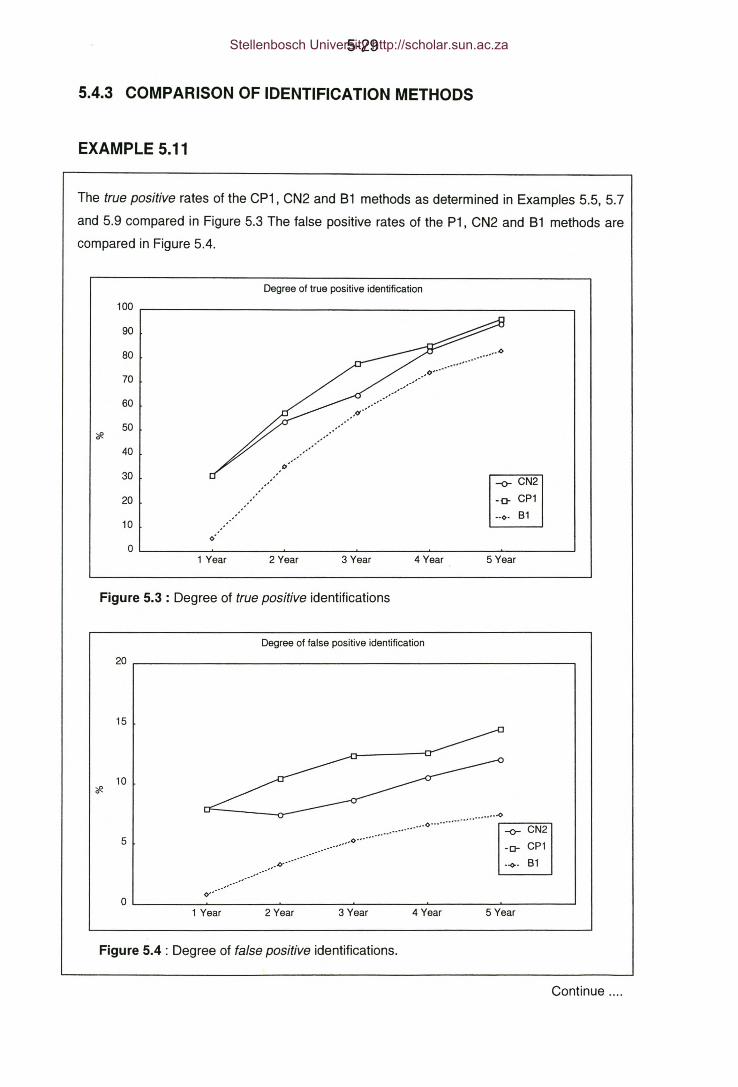
5-29
5.4.3 COMPARISON OF IDENTIFICATION METHODS
EXAMPLE 5.11
Degree of true positive identification
100 r-------------------------------------------------------,90
The true positive rates of the CP1, CN2 and 81 methods as determined in Examples 5.5, 5.7
and 5.9 compared in Figure 5.3 The false positive rates of the P1, CN2 and 81 methods are
compared in Figure 5.4.
80 »>~
70
60
50
40
30-0- CN2
-o- CP1••0. 81
20
10
o L_ ~ ~ ~~------~~----~~------~
2 Year 3 Year 4 Year 5 Year1 Year
Figure 5.3 : Degree of true positive identifications
Degree of false positive identification20 ,- -,
15
10
5 •.•••••0···
•••....••••.•••.•.0.•.... .•..•....0····· r-o----C-=-N:-:-2'"
-0- CP1.~. 81
o L- ~ ~~ ~ ~ ~~--------3 Year 4 Year 5 Year1 Year 2 Year
Figure 5.4 : Degree of false positive identifications.
Continue ....
Stellenbosch University http://scholar.sun.ac.za

5-30
EXAMPLE 5.11 (Continued)
From Figures 5.3 and 5.4 it is evident that for at least the experimental data that method 81
generally has a lower true positive rate than CP1 and CN2, but that this is somewhat
compensated for by a lower rate of false positive identifications. This means that although
method 81 identified less true hazardous locations, it also identified significantly less sites
which are not true hazardous locations.
Although methods CP1 and CN2 have similar rates of true positive identifications, method
CN2 performed better with regards to false positive identifications.
Higle and Witkowski(1988) and Higle and Hecht (1989) conducted a detailed
experimental study to compare the efficiency of the CR1, CR2, 81 and 82
identification methods.
They came to the following conclusions :
a) Methods CR2, 81 and 82 correctly identify a significantly higher
fraction of the truly hazardous sites than does CR1.
b) 8ecause of the underlying assumption of normality in the distribution of
accident rates/numbers method CR1 tends to identify a larger number
of false negatives than methods CR2, 81 and 82.
c) The CR2, 81 and 82 methods tend to be equally efficient. Each yield
low numbers of false negative identifications and are generally
successful in selecting sites that are truly hazardous. This however
comes at the expense of an increase in the number of false positive
identifications, which may be a result of a sensitivity to the traffic
volume at a site.
d) Method 82 is more efficient than CR2 when data are sparse or when
numerous years of comparable data are not available.
Stellenbosch University http://scholar.sun.ac.za

5-31
EXAMPLE 5.12
The CR1, CR2 , B1 and B2 methods of hazardous location identification were applied to the
sample of 113 road segments in Appendix B1 and B2. All the locations that were identified as
a hazardous location of one or more of these methods are listed in Table 5.15
Method CR1 flagged only 6 of the 113 sites as hazardous. This seems to indicate the
likelihood of a high rate of false negative identifications, as was also concluded by Higle and
Hecht (1989) as well as Higle and Witkowski (1988).
Method CR2 identified a total of 48 sites as opposed to the 34 by Method B2. It is likely that
method CR2 identified most of the true hazardous locations but also a large number of non-
hazardous locations, while method B2 might have identified less hazardous locations, but
also less non-hazardous locations.
It appears as if Method B2 is sensitive to the level of exposure at a site. When combining the
prior estimates with the accident frequency and exposure level using Bayes theorem the
larger the level of exposure the smaller the variance of the Bayesian estimate mj. The smaller
the variance, the smaller is the critical threshold value. To illustrate the following two
segments can be compared:
Road Start End E m VAR(m) B2NR00205 40.64 49.34 38.93 1.48 0.037 1NR00205 58.6 59.21 3.14 1.48 0.345 0
Both these locations have the same Bayesian estimates = 1.48 acc/mvkm but only the first
location was flagged as a hazardous location because of its relatively small variance ( =0.037), which in turn is a result of its high exposure level = 38.93 mvkm.
Method B2 therefore favour sites with a potentially high PAR (Potential Accident Reduction). It
also tends to favour sites which are longer than other sites but not necessarily more unsafe. It
is advisable to, when applying the B2 method, to define the locations in a manner which
ensures that they are all of the same length.
Continue ...
Stellenbosch University http://scholar.sun.ac.za

5-32
Example 5.12 (continued)
Table 5.15 : Comparison of CR1, CR2, 81 and 82 identification methods
Road Start End E R m CR1 CR2 81 82NR00205 51.88 52.62 2.92 7.87 5.98 1 1 1 1MR00165 0 3.63 7.97 4.02 3.66 1 1 1 1MROO027 51.73 52.29 3.45 4.34 3.55 1 1 1 1MR00227 5.89 9.66 6.12 3.43 3.07 1 1 1 1TR02801 0 2.14 3.62 3.31 2.80 1 1 1 1TR03201 44.35 45.15 2.06 3.40 2.60 1 1 1 1MROO027 51.15 51.73 6.00 2.83 2.57 0 1 1 1MROO027 67.19 68.56 9.45 2.65 2.48 0 1 1 1MR00223 6.3 9.63 7.87 2.67 2.48 0 1 1 1MR00165 3.63 7.47 31.02 2.45 2.40 0 1 1 1TR03201 42.84 44.35 3.77 2.65 2.31 0 1 1 1NR00108 2.68 3.61 3.44 2.62 2.25 0 1 1 1NR00205 9.85 11.4 12.67 2.29 2.20 0 1 1 1TR03201 0 5.71 14.42 2.22 2.14 0 1 1 1NR00205 49.34 51.8 14.76 2.17 2.10 0 1 1 1TR02801 2.14 3.73 8.74 2.17 2.06 0 1 1 1DR01056 0 1.32 2.14 2.34 1.93 0 1 0 1TR00204 50.54 55.03 17.47 1.95 1.90 0 1 1 1MR00313 1.6 3.1 4.04 1.98 1.80 0 1 0 1TR00204 44.28 45.16 3.15 1.91 1.71 0 1 0 1TR02801 16.37 17.18 4.56 1.76 1.64 0 1 0 1NR00205 52.62 58.6 30.12 1.56 1.55 0 1 1 1TR02801 17.18 19.93 16.19 1.54 1.52 0 1 0 1NR00205 40.64 49.34 38.93 1.49 1.48 0 1 1 1NR00205 58.6 59.21 3.14 1.59 1.48 0 1 0 0TR00202 37.09 42.36 56.21 1.48 1.47 0 1 1 1TR03302 2.74 5.01 4.53 1.55 1.47 0 1 0 0TR02801 19.93 23.6 22.73 1.45 1.44 0 1 0 1NR00205 0 2.02 12.44 1.45 1.42 0 1 0 1DR01101 1.9 5.79 11.25 1.33 1.32 0 1 0 1TR00204 2.84 4.4 6.79 1.32 1.30 0 1 0 0NR00105 29.83 31.89 7.86 1.27 1.26 0 1 0 0DR01105 0 3.99 39.16 1.25 1.25 0 1 0 1TR02801 3.73 9.1 23.78 1.22 1.22 0 1 0 1MR00216 0 3.45 22.78 1.19 1.18 0 1 0 1TR00204 45.16 50.54 19.59 1.17 1.17 0 1 0 1TR02801 23.6 25.83 15.65 1.15 1.15 0 1 0 1DR01101 0 1.9 10.49 1.14 1.14 0 1 0 0TR02901 39.92 45.21 8.08 1.11 1.12 0 1 0 0NR00205 7.12 9.12 18.06 1.00 1.01 0 1 0 0MR00187 6.96 8.03 9.21 0.98 1.00 0 1 0 0NR00208 65.71 67.78 16.38 0.92 0.93 0 1 0 0NR00107 0 34.86 128.65 0.91 0.91 0 1 0 1TR03201 5.71 15.26 21.85 0.87 0.88 0 1 0 0TR03201 15.26 22.79 15.09 0.86 0.88 Q 1 0 0MR00191 16.66 20.2 19.69 0.86 0.88 0 1 0 0NR00108 62 72.44 37.60 0.85 0.86 0 1 0 0TR03102 1.94 9.04 37.92 0.82 0.83 0 1 0 0
TOTAL 6 48 20 34
Stellenbosch University http://scholar.sun.ac.za

5-33
5.5 RANKING METHODOLOGIES
The ranking of hazardous locations is important when a road authority does
not have sufficient resources to investigate and treat all identified hazardous
locations. It could be advantageous to have two levels of ranking, a
preliminary level and a final level of ranking. The objective of the preliminary
level of ranking should be to determine which sites to investigate further,
given the resource constraints. The investigation of the selected sites should
yield an estimate of the expected economic return ( e.g. Benefit/Cost ratio,
Internal Rate of Return etc.) as a result of the selected remedial measures.
The final level of ranking is then based on these economic indicators to
determine which combination of sites, when treated, would provide the best
economic returns. To prevent the unnecessary investigation of hazardous
locations the ranking index used for the preliminary ranking procedure should
provide a good measure of the anticipated economic return.
Some of the ranking methods that will be presented in this section can also be
used as a way to identify locations to apply remedial measures to, without
going through the formal identification procedures as presented in the
preceding sections.
5.5.1 ACCIDENT RATE/NUMBER RANKING METHOD
According to McGuigan (1982) using the accident rate as a ranking criterion
will produce a bias towards sites with low accident totals and low traffic flows.
Using the accident number on the other hand will produce a bias towards
sites with high traffic volumes and high accident numbers.
Stellenbosch University http://scholar.sun.ac.za

5-34
EXAMPLE 5.13
Consider the information in Tables 5.16 and Table 5.17. The road segments in Table 5.16 are
ranked according to their accident numbers while the segments in Table 5.17 are ranked
according to their accident rates. For each site the PAR index has also been determined ( see
Paragraph 5.5.3).
Table 5.16 :Top 10 sites: Accident Number method
Road Start EndKm AADT N N R R E PARKm Rank RankNR2/5 51.88 52.62 2704 31.08 1 7.87 1 2.9 20.84MR27 51.15 51.73 7077 29.31 2 2.83 7 6.0 12.56MR27 51.73 52.29 4220 26.79 3 4.34 2 3.5 12.45MR165 3.63 7.47 5530 19.79 4 2.45 12 31.0 53.04NR2/5 9.85 11.4 5593 18.71 5 2.29 14 12.7 19.63MR27 67.19 68.56 4722 18.25 6 2.65 10 9.5 18.01TR2/2 37.09 42.36 7300 15.75 7 1.48 27 56.2 41.41NR2/5 49.34 51.8 4107 13.01 8 2.17 17 14.8 21.08DR1105 0 3.99 6717 12.28 9 1.25 33 39.2 20.02TR28/1 2.14 3.73 3762 11.95 10 2.17 16 8.7 12.53TOTALS 51732 196.91 29.50 184.4 231.56
Table 5.17:Top 10 sites: Accident Rate method
Road Start EndKm AADT R R N R E PARKm Rank RankNR2/5 51.88 52.62 2704 7.87 1 31.08 1 2.92 20.84MR27 51.73 52.29 4220 4.34 2 26.79 3 3.45 12.45MR165 0 3.63 1502 4.02 3 8.82 17 7.97 26.11MR227 5.89 9.66 1111 3.43 4 5.57 41 6.12 16.47TR32/1 44.35 45.15 1760 3.40 5 8.75 18 2.06 5.48TR28/1 0 2.14 1158 3.31 6 5.61 39 3.62 9.32MR27 51.15 51.73 7077 2.83 7 29.31 2 6.00 12.56MR223 6.3 9.63 1618 2.67 8 6.31 37 7.87 15.17TR32/1 42.84 44.35 1708 2.65 9 6.62 34 3.77 7.21MR27 67.19 68.56 4722 2.65 10 18.25 6 9.45 18.01TOTALS 27580 37.18 147.1 53.23 143.61
The sum of the AADT's for the locations selected using the accident number method is
considerably larger than those selected using the accident rate method, confirming that the
accident rate method is biased towards low volume sites and the accident number method
towards high volume sites. As a result the total number of observed accidents at the sites
selected using the accident number method is also larger than that of the sites selected using
the accident rate method.
Stellenbosch University http://scholar.sun.ac.za

5-35
5.5.2 BAYESIAN SAFETY ESTIMATE METHOD
This method ranks sites according to their Bayesian estimates (m).
EXAMPLE 5.14
In Appendix B1 the Bayesian safety estimates were determined for each of the 113 sites
using the method of sample moments. Table 5.18 shows the top 10 sites ranked according to
their Bayesian safety estimates.
Table 5.18: Top 10 sites - Bayesian estimate method
Road Start End E AADT R R MRank m Rank Wl
NR00205 51.88 52.62 2.92 2704 7.87 1 5.98 1 0.72MROO027 51.73 52.29 3.45 4220 4.34 2 3.55 3 0.75MR00165 0 3.63 7.97 1502 4.02 3 3.66 2 0.87MR00227 5.89 9.66 6.12 1111 3.43 4 3.07 4 0.84TR03201 44.35 45.15 2.06 1760 3.40 5 2.60 6 0.64TR02801 0 2.14 3.62 1158 3.31 6 2.80 5 0.76MROO027 51.15 51.73 6.00 7077 2.83 7 2.57 7 0.84MR00223 6.3 9.63 7.87 1618 2.67 8 2.48 9 0.87TR03201 42.84 44.35 3.77 1708 2.65 9 2.31 11 0.77MROO027 67.19 68.56 9.45 4722 2.65 10 2.48 8 0.89
It is evident that for the sample of 113 segments there is little difference between the ranking
performance of the Accident Rate and Bayesian estimate methods.
The last column Wl represents the weight given to the observed accident rate (R) in the
calculation of the Bayesian estimate. The Wl values are relatively high, which could explain
the similarity in the ranking performance of the Accident Rate and Bayesian estimate
methods.
5.5.3 POTENTIAL ACCIDENT REDUCTION (PAR) INDEX METHOD
5.5.3.1 CONVENTIONAL APPROACH
According to McGuigan (1982) the PAR index provides a significantly better
measure of the potential accident reduction, and hence the potential
economic returns, than the accident number or the accident rate.
Stellenbosch University http://scholar.sun.ac.za
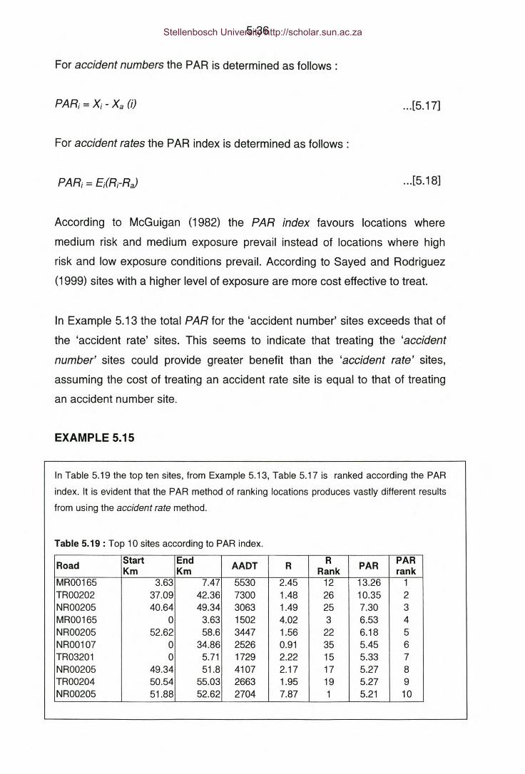
5-36
For accident numbers the PAR is determined as follows:
...[5.17]
For accident rates the PAR index is determined as follows:
...[5.18]
According to McGuigan (1982) the PAR index favours locations where
medium risk and medium exposure prevail instead of locations where high
risk and low exposure conditions prevail. According to Sayed and Rodriguez
(1999) sites with a higher level of exposure are more cost effective to treat.
In Example 5.13 the total PAR for the 'accident number' sites exceeds that of
the 'accident rate' sites. This seems to indicate that treating the 'accident
number' sites could provide greater benefit than the 'accident rate' sites,
assuming the cost of treating an accident rate site is equal to that of treating
an accident number site.
EXAMPLE 5.15
In Table 5.19 the top ten sites, from Example 5.13, Table 5.17 is ranked according the PAR
index. It is evident that the PAR method of ranking locations produces vastly different results
from using the accident rate method.
Table 5.19 : Top 10 sites according to PAR index.
Road Start End AADT R R PARPAR
Km Km Rank rankMR00165 3.63 7.47 5530 2.45 12 13.26 1TR00202 37.09 42.36 7300 1.48 26 10.35 2NR00205 40.64 49.34 3063 1.49 25 7.30 3MR00165 0 3.63 1502 4.02 3 6.53 4NR00205 52.62 58.6 3447 1.56 22 6.18 5NR00107 0 34.86 2526 0.91 35 5.45 6TR03201 0 5.71 1729 2.22 15 5.33 7NR00205 49.34 51.8 4107 2.17 17 5.27 8TR00204 50.54 55.03 2663 1.95 19 5.27 9NR00205 51.88 52.62 2704 7.87 1 5.21 10
Stellenbosch University http://scholar.sun.ac.za
5-37
5.5.3.2 EMPIRICAL BAYESIAN APPROACH
Persaud et al. (1999b) proposed that sites be ranked according to their
potential safety improvement (8), where:
S = (m-P) ...[5.19]
Where
m - The Bayesian estimate of safety
P - The level of safety for similar sites
An important issue to consider is what value to use for P. Persaud et al.
(1999) identified and investigated three different methods.
i) The AADT model method
ST= (m-PT)...[5.20]
The Bayesian estimate m is calculated using the best possible
regression model which incorporates all the available variables which
may contribute to poor safety. PT is based on a model that includes
traffic but no treatable variables. Therefore untreatable variables such
as road classification (freeway/two-lane, urban/rural) for example may
be included in the model to estimate PT. (Persaud et al. ; 1999)
The value of S in this instance is an estimate of the number of treatable
accidents that are caused by all those treatable variables included in
the full model.
This method will be illustrated in Example 5.16.
Stellenbosch University http://scholar.sun.ac.za

5-38
EXAMPLE 5.16
Persaud et al. (1999) used the following model to estimate m , (hereafter referred to
as the tuil model.) :
P = O.000637LQo.8993e-O·08215TW (k = 5.82)
P - Injury accidents per year
L - Length at segment (km)
Q - AADT - Annual Average Daily Traffic
TW - Total pavement width
The AADT model to estimate PT is as follows:
Pr = O.000532LQo.8036
Assume a road segment has the following parameters:
L= 2 km
Q = 4000 veh/day
TW=7m
X = 4 accidents per year
From the tuil model P = 2.2 injury accidents 1 year and from the AADT model PT = 0.8
injury accidents 1year.
E(m) = 2.2 and VAR(m) = (2.2)2/5.82 = 0.83
a = 2.2/(2.2+0.83) = 0.73
m = 0.73(2.2) + (1-0.73)4 = 2.69 injury accidents/year
ST = 2.69 - 0.80 = 1.89 injury accidents/year
Stellenbosch University http://scholar.sun.ac.za

5-39
ii) The BASE model method
Sa = (m-Pa) ...[5.21 ]
PB is for a base condition, reflecting that what is normal can be found in
the predominant values of treatable variables. According to Persaud et
al. (1999) the idea is that roads are built to some desirable standard
from a safety point of view. PB is therefore estimated from a base
model that was calibrated using those sites which represent the ideal
design.
EXAMPLE 5.17
In order to estimate PB, Persaud et al. (1999) calibrated the following model using
only those segments with a lane width of 3.5m and a shoulder width of 1.8m. These
magnitudes were decided on by examining the frequency of various lane width and
shoulder width combinations in their total sample of 2-lane rural road segments. A
review of road safety literature also revealed that these parameters constituted what
could be considered safe design.
PB =O.000826LQo.7448
From the previous example m = 2.69 injury accidents / year and Q = 4000 veh/day.
PB = 0.000826(2)(4000)° 7448 = 0.80 injury accidents / year.
S = 2.69 - 0.80 = 1.89 injury accidents/ year.
It can therefore be expected that increasing the total surfaced width from 7m to 10.3m
will decrease the injury rate by 1.89 accidents per year.
Stellenbosch University http://scholar.sun.ac.za
5-40
iii) The FULL model method
...[5.22]
P is estimated from the full model used for the estimation of m.
SF in this instance provides an estimate of the potential accident
reduction related to those factors that were omitted from the model.
EXAMPLE 5.18
From Example 5.16 m = 2.69 injury accidents /year and P = 2.2 injury accidents /
year.
S = 2.69 - 2.20 = 0.49 injury accidents/year.
Over the 2 km segment there are factors present, treatable or untreatable, that are
causing the injury accident rate to be 0.49 injury accidents / year higher than it should
be. Hypothetically speaking it could be that the quality of road signs and road
markings are inferior when compared to other identical segments, or the segment
carries more nigh-time time traffic, or more heavy vehicles, etc.
5.5.4 DEGREE OF DEVIATION - Ni
R XNi =_1 or Ni =_1e; Xai
...[5.23]
This ranking criterion considers the deviation from the expected values
regardless of the accident number/rate and the level of exposure. According
to Sayed and Rodriguez (1999) this index should be used in conjunction with
the PAR index. They propose that the two ranking criteria be given equal
weights. However if different weights are used a higher weight should be
given to the PAR criterion to achieve higher cost effectiveness.
Stellenbosch University http://scholar.sun.ac.za
5-41
5.5.5 SEVERITY METHOD
5.5.5.1 CONVENTIONAL APPROACH
Sites identified as hazardous locations using the EAN method are often
ranked according to their EAN values.
A Severity Index can be used to rank hazardous locations to favour those
locations where the accidents are relatively severe.
For each selected hazardous location a Severity Index can be determined as
follows:
SI = __ E_:A_N__F +SR+SL+D
...[5.24]
where
F, SR, SL, 0- The number of fatal, serious injury, slight injury and
damage only accidents respectively.
Using the Severity Index as a ranking criterion will favour those sites where
accidents are relatively more severe, irrespective of the number of accidents
or level of exposure at the sites.
Stellenbosch University http://scholar.sun.ac.za

5.5.5.2
5-42
EMPIRICAL BAYESIAN APPROACH
Persaud et al.(1999a) presents a variation of the Bayesian PAR method, in
which PAR indices are determined for each severity class and then combined
with weighting factors to obtain a weighted PAR index.
The weighted Bayesian PAR method requires Safety Performance Functions
for each severity class.
Let
PARfat = mfat-Pfat
PARinj = minj-Pinj
PARdam= mdam- Pdam
...[5.25]
...[5.26]
...[5.27]
where
PARfat -
PARinj -
PARdam-
mfat-
minj -
mdam-
Pfat-
Pinj-
Pdam-
The potential reduction in fatal accidents.
The potential reduction in injury accidents.
The potential reduction in damage only accidents.
The Bayesian safety estimate for fatal accidents.
The Bayesian safety estimate for injury accidents.
The Bayesian safety estimate for damage only accidents.
The fatal accident safety estimate from a suitable SPF.
The injury accident safety estimate from a suitable SPF.
The damage only safety estimate from a suitable SPF.
The weighted PAR Index that can be used to rank and identify locations
potentially suitable for remedial action is determined as follows:
PARindex = wfat*PARfat+ win/PARinj + PARdam ...[5.28]
Stellenbosch University http://scholar.sun.ac.za
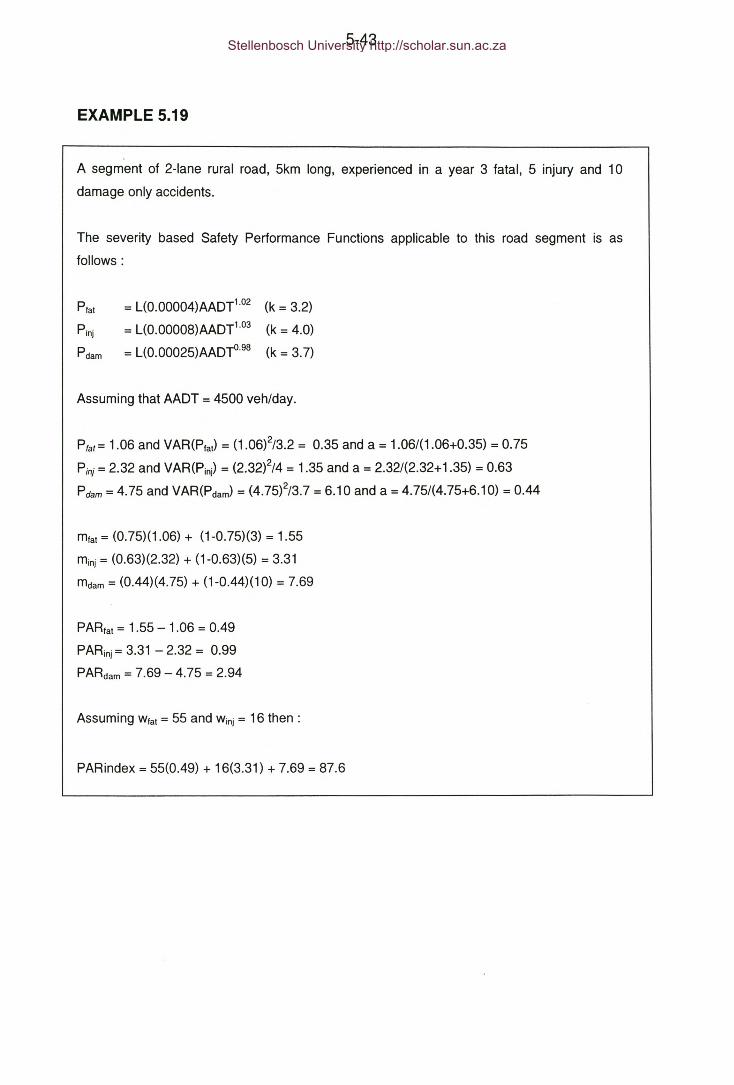
5-43
EXAMPLE 5.19
A segment of 2-lane rural road, 5km long, experienced in a year 3 fatal, 5 injury and 10
damage only accidents.
The severity based Safety Performance Functions applicable to this road segment is as
follows:
Ptat = L(0.00004)AADT1.o2 (k = 3.2)
Pinj = L(0.00008)AADT1.03 (k = 4.0)
Pdam = L(0.00025)AADTo.98 (k = 3.7)
Assuming that AADT = 4500 veh/day.
Ptat= 1.06 and VAR(Ptat) = (1.06)2/3.2 = 0.35 and a = 1.06/(1.06+0.35) = 0.75
Pinj = 2.32 and VAR(Pinj) = (2.32)2/4 = 1.35 and a = 2.32/(2.32+ 1.35) = 0.63
Pdam = 4.75 and VAR(Pdam)= (4.75)2/3.7 = 6.10 and a = 4.75/(4.75+6.10) = 0.44
mtat= (0.75)(1.06) + (1-0.75)(3) = 1.55
minj= (0.63)(2.32) + (1-0.63)(5) = 3.31
mdam= (0.44)(4.75) + (1-0.44)(10) = 7.69
PARtat = 1.55 - 1.06 = 0.49
PARinj= 3.31 - 2.32 = 0.99
PARdam= 7.69 - 4.75 = 2.94
Assuming Wtat= 55 and Winj= 16 then:
PAR index = 55(0.49) + 16(3.31) + 7.69 = 87.6
Stellenbosch University http://scholar.sun.ac.za
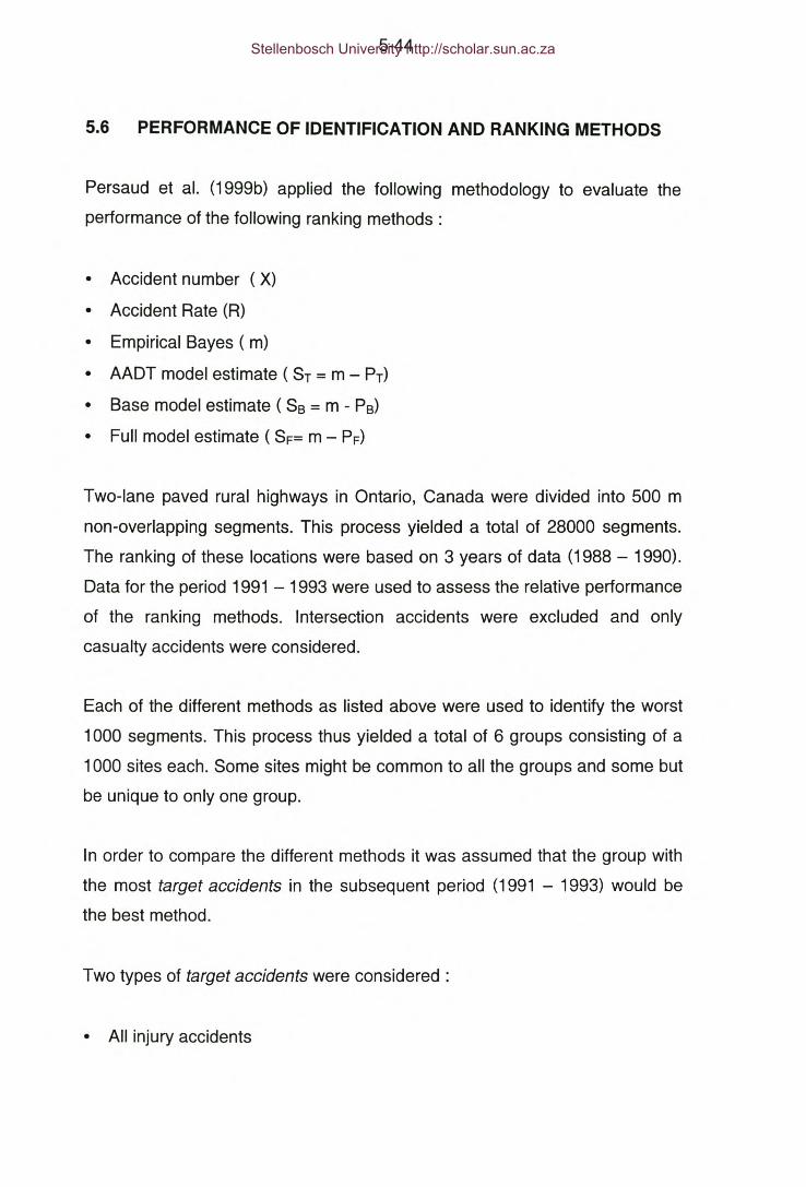
5-44
5.6 PERFORMANCEOF IDENTIFICATIONAND RANKINGMETHODS
Persaud et al. (1999b) applied the following methodology to evaluate the
performance of the following ranking methods:
• Accident number (X)
• Accident Rate (R)
• Empirical Bayes ( m)
• AADT model estimate (ST = m - PT)
• Base model estimate ( Ss = m - Ps)
• Full model estimate ( SF= m - PF)
Two-lane paved rural highways in Ontario, Canada were divided into 500 m
non-overlapping segments. This process yielded a total of 28000 segments.
The ranking of these locations were based on 3 years of data (1988 - 1990).
Data for the period 1991 - 1993 were used to assess the relative performance
of the ranking methods. Intersection accidents were excluded and only
casualty accidents were considered.
Each of the different methods as listed above were used to identify the worst
1000 segments. This process thus yielded a total of 6 groups consisting of a
1000 sites each. Some sites might be common to all the groups and some but
be unique to only one group.
In order to compare the different methods it was assumed that the group with
the most target accidents in the subsequent period (1991 - 1993) would be
the best method.
Two types of target accidents were considered:
• All injury accidents
Stellenbosch University http://scholar.sun.ac.za
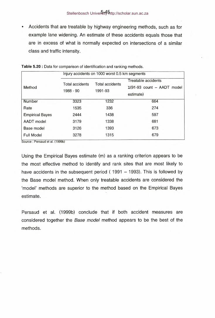
5-45
• Accidents that are treatable by highway engineering methods, such as for
example lane widening. An estimate of these accidents equals those that
are in excess of what is normally expected on intersections of a similar
class and traffic intensity.
Table 5.20 : Data for comparison of identification and ranking methods.
Injury accidents on 1000 worst 0.5 km segments
Treatable accidents
:L(91-93 count - AADT model
estimate)
Total accidents Total accidentsMethod
1988 - 90 1991-93
Number 3323 1232
Rate 1535 336
Empirical Bayes 2444 1438
AADT model 3179 1338
Base model 3126 1393
Full Model 3278 1315
Source: Persaud et al. (1999b)
664
274
597
681
673
679
Using the Empirical Bayes estimate (m) as a ranking criterion appears to be
the most effective method to identify and rank sites that are most likely to
have accidents in the subsequent period ( 1991 - 1993). This is followed by
the Base model method. When only treatable accidents are considered the
'model' methods are superior to the method based on the Empirical Bayes
estimate.
Persaud et al. (1999b) conclude that if both accident measures are
considered together the Base model method appears to be the best of the
methods.
Stellenbosch University http://scholar.sun.ac.za

5-46
5.7 SUMMARY and CONCLUSION
.This Chapter presented a number of Conventional and Bayesian
methodologies to identify and rank hazardous locations or locations that when
treated, would have the potential to produce good benefits in terms of
accident reduction and economic returns.
Generally those Conventional and Bayesian methods that are based on a
measure of potential accident reduction (PAR), according to McGuigan (1982)
and Persaud et al. (1999a and 1999b) appear to produce satisfactory results.
It has been shown how information about the severity of accidents at a
location can be combined with the Bayesian PAR method to favour those
sites with a good potential for accident and severity reduction.
Stellenbosch University http://scholar.sun.ac.za

CHAPTER 6
THE EVALUATION OF ROAD SAFETY REMEDIAL MEASURES
6.1 INTRODUCTION
According to Persaud (1986) the effective management of safety on a system
requires sound knowledge of how the system reacts to the implementation of
measures that affect safety - whether safety increases or decreases and by
how much.
Hauer (1997) states that one of the main reasons for conducting evaluation
studies to determine the safety effect of a treatment/s on an entity or a group
of entities is to have factual guidance for the future. Hauer (1997) also states
that the results of each such evaluation adds to the edifice of professional
knowledge and the quality of professional advice.
The systematic and correct evaluation of road safety remedial measures is
therefore a very important last step in the implementation of an accident
remedial programme, since the results so obtained will add to the quality of
planning and implementation of any future road safety remedial programmes.
Another important reason to have reliable information on the effect of road
safety treatments is to be able to conduct economic feasibility studies. In other
words, to determine how efficiently funds and resources were utilised. The
overall success of a road safety remedial programme is often not measured in
the reduction of accidents but in a comparison of cost and benefits. The cost
component is determined by the amount of resources applied to bring about
improvements in safety, while the benefit component is determined by
expressing the safety effect of a treatment in financial terms using the unit
accident cost in Table 1.2.
Stellenbosch University http://scholar.sun.ac.za

6-2
The objective of this Chapter is to present accident data analysis
methodologies to determine reliable estimates of the effect that road safety
remedial measures may have on the safety of an entity or a group of entities.
As with measurement, identification and ranking methodologies, evaluation
methods can be divided into two categories a) Conventional methods and b)
Bayesian methods.
Although the Conventional methods have been found to be less reliable than
the Bayesian methods especially with regards the regression-to-mean effect
(Hauer; 1997) , for comparison purposes both the Conventional and Bayesian
methods will be presented in this Chapter.
The methodologies presented in this Chapter is based on the work done by Dr
Ezra Hauer in his book - "Observational Before-and-After Studies in Road
Safety" ( Pergamon - 1997).
To evaluate the performance of the Conventional and Bayesian methods and
to compare these methods with one another, use will be made of the
experimental data in Appendix A1. The analyses performed on this data, the
results of which are used in the Chapter, are contained in Appendix A4.
6.2 CONCEPTUAL FRAMEWORK
Estimating the effect of highway and traffic engineering measures on road
safety basically involves three tasks (Hauer; 1997):
a) Predicting what would have been the safety in the 'after' period had
treatment not been applied.
b) Estimating what the safety in the 'after' period was after treatment has
been applied.
c) Comparing the prediction with the estimation in order to estimate the
improvement/decline in safety between the 'before' and 'after' periods.
Stellenbosch University http://scholar.sun.ac.za

6-3
6.2.1 PREDICTING ACCIDENTS
There are a number of ways to predict the expected level of safety in the
'after' period had treatment not been applied. According to Hauer (1997) the
best method is the method that provides the best prediction. The quality of
prediction is determined by (Hauer; 1997) :
a) How the method accounts for those causal factors that affect safety that
are measured and the influence of which is known or can be known, such
as for example traffic flows.
b) How the method accounts for the remaining factors that affect safety,
those that are not measured or of which the influence of safety is
unknown.
c) How the method accounts for the regression-to-mean effect.
d) How the method accounts for changes in the extent of accident reporting.
6.2.2 STATISTICAL FRAMEWORK
According to Hauer (1997) let
Jt - The estimated number of target accidents of a specific entity in the
'after' period had the entity not been treated. I.e. Jt is to be predicted.
A - The expected number of target accidents of the entity in the 'after'
period. I.e. A is to be estimated.
The safety effect of a treatment is determined by comparing Jt and A as
follows:
Stellenbosch University http://scholar.sun.ac.za
6-4
a) Unbiased estimates of the reduction in the number of accidents (6), and
its variance, VAR(6), is given by :
6 = n:-A ... [6.1 ]
...[6.2]VAR(6) = VAR(n:) + VAR(A)
b) Unbiased estimates of the index of effectiveness (8) and its variance,
VAR(8), are given by:
8 = (A/n:)[1 +VAR(n:)/n:2r1VAR(8) = 82[VAR(A)/A2 + VAR(n:)/n:2]/[1 + VAR(n:)/n:2]2
...[6.3]
...[6.4]
For derivations of these expressions the reader is referred to Hauer (1997).
For a treatment to have been effective 6 > 0 and 8 < 1. The accident
reduction factor :
ARF = 100(1-8). ...[6.5]
Equations 6.1, 6.2, 6.3 and 6.4 form the basis for all the evaluation
procedures that will be presented in this Chapter. The difference between the
different evaluation procedures lies in the methods used to obtain Jt ,A,
VAR(Jt) and VAR(A).
6.2.3 METHODOLOGICAL FRAMEWORK
The framework for the statistical analysis of any of the evaluation procedures
in this chapter consists of a simple 4-step process as indicated in Table 6.1.
Stellenbosch University http://scholar.sun.ac.za
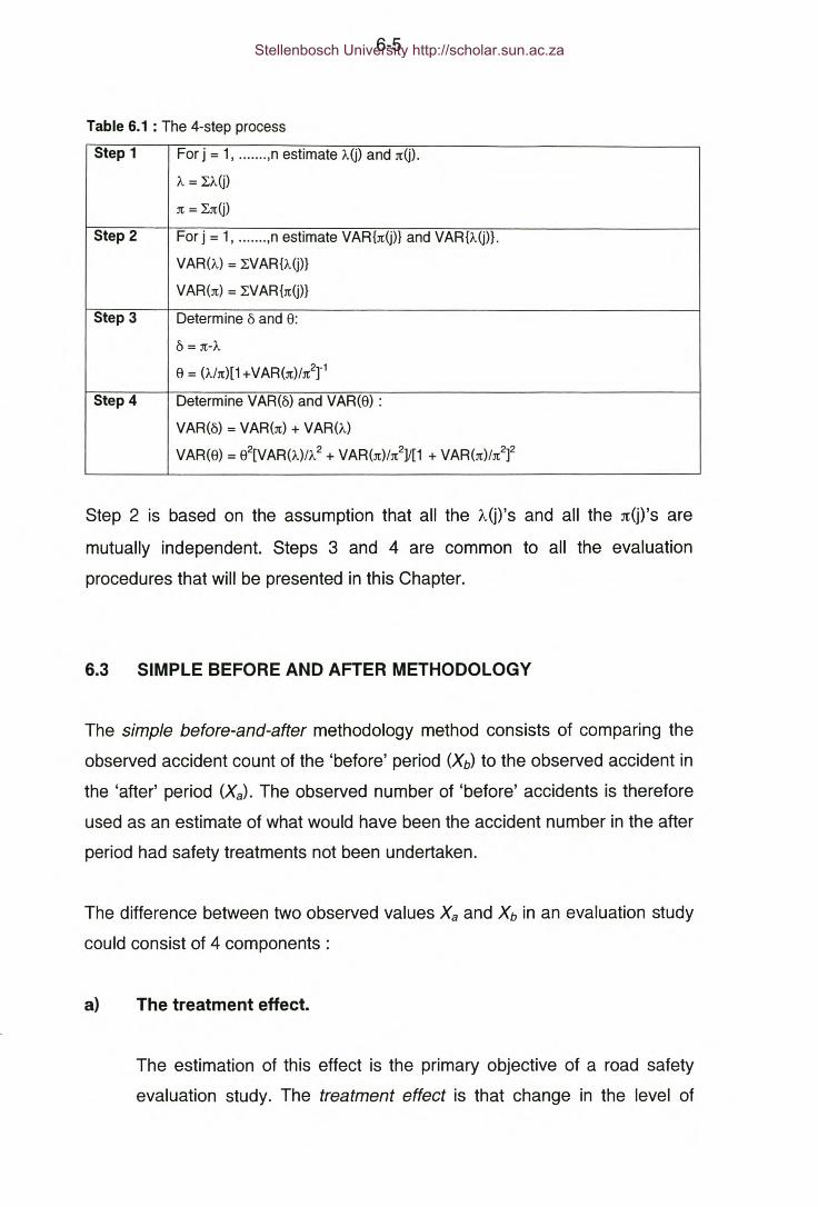
6-5
Table 6.1 : The 4-step process
Step 1 For j = 1, ....... ,n estimate A.G)and JtG).
A.= LA.(j)
Jt = LJt(j)
Step 2 For j = 1, ....... ,n estimate VAR {Jt(j)} and VAR {A.(j)} .
VAR(A.) = LVAR{A.(j)}
VAR(Jt) = LVAR{Jt(j)}
Step 3 Determine 6 and 8:
6 = Jt-A.
8 = (A.JJt)[1+VAR(Jt)JJt2r1Step 4 Determine VAR(6) and VAR(8) :
VAR(6) = VAR(Jt) + VAR(A.)
VAR(8) = 82[VAR(A.)/A.2 + VAR(Jt)/Jt2]J[1 + VAR(Jt)JJt2]2
Step 2 is based on the assumption that all the A(j)'S and all the Jt(j)'s are
mutually independent. Steps 3 and 4 are common to all the evaluation
procedures that will be presented in this Chapter.
6.3 SIMPLE BEFORE AND AFTER METHODOLOGY
The simple before-and-after methodology method consists of comparing the
observed accident count of the 'before' period (Xb) to the observed accident in
the 'after' period (Xa). The observed number of 'before' accidents is therefore
used as an estimate of what would have been the accident number in the after
period had safety treatments not been undertaken.
The difference between two observed values Xa and Xb in an evaluation study
could consist of 4 components:
a) The treatment effect.
The estimation of this effect is the primary objective of a road safety
evaluation study. The treatment effect is that change in the level of
Stellenbosch University http://scholar.sun.ac.za

6-6
safety that was caused by the influence of a safety measure/s, and thatalone.
b) The exposure effect
Between the 'before' and 'after' periods there may be an increase ( or a
decrease) in the traffic volumes. Since higher traffic volumes are
associated with increased accident numbers, an increase in traffic
volumes after the implementation of road safety measures could lead
to a relative increase in accidents. Not accounting for the exposure
effect, when there has been an increase in traffic volumes, could result
in the underestimation of the treatment effect.
c) The trend effect
The trend effect is a function of a number of possible causal factors
which are possibly difficult to identify and measure. Between the
'before' and 'after' periods there may have been changes in the traffic
composition ( i.e. more minibus taxis), changes in the driver
composition ( e.g. more older drivers), changes in law enforcement
activity (e.g. the Arrive Alive campaign), the pedestrian numbers may
have increased, the level of accident reporting may have improved etc.
d) Random effect
Accident counts are random variables which have a Poisson
distribution around a long term mean. (Abbess et al. ; 1981). This long
term mean will hence be referred to as the 'true' level of safety.
Because of the discrete and random nature of accident data is it
unlikely that an observed value will be equal to its 'true' mean. The
difference between the mean and the observed value can be referred
to as the random error. Accident remedial measures are normally
applied to accident sites with a high accident number in the 'before'
period. This introduces what is called selection bias or the regression-
Stellenbosch University http://scholar.sun.ac.za

6-7
to-mean (RTM) effect. (Abbess et al. ; 1981). It can be expected for the
high observed count to decrease (towards the mean) even in the
absence of any remedial measure, thereby creating a false sense of
'success'.
Figure 6.1 : Illustration of the RTM, treatment and trend effects
Figure 6.2 illustrates the regression-to-mean, trend and treatments effects,
assuming there were no changes in the level of exposure between the 'before'
and 'after' periods. If the trend in the 'before' data was not considered in
predicting the expected accident number in the 'after' period the RTM effect
would have been overestimated by the 'trend effect' and the treatment effect
would have been underestimated by the 'trend effect'.
The following example, based on the experimental data of Appendix A1, will
serve to illustrate the regression-to-mean effect.
Stellenbosch University http://scholar.sun.ac.za
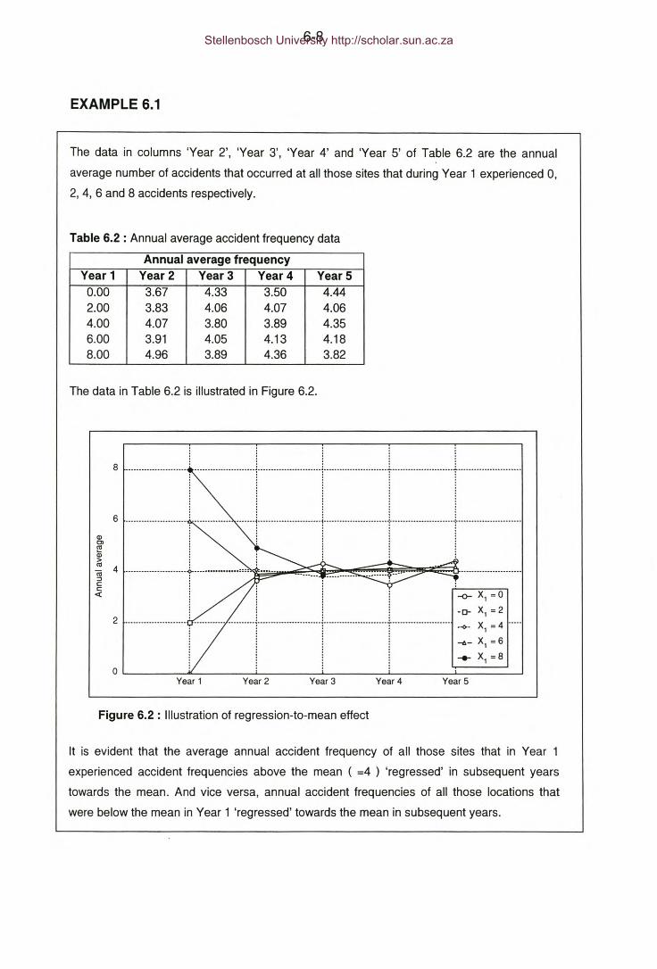
6-8
EXAMPLE 6.1
The data in columns 'Year 2', 'Year 3', 'Year 4' and 'Year 5' of Table 6.2 are the annual
average number of accidents that occurred at all those sites that during Year 1 experienced 0,
2,4,6 and 8 accidents respectively.
Table 6.2 : Annual average accident frequency data
Annual average frequencyYear1 Year2 Year3 Year4 YearS0.00 3.67 4.33 3.50 4.442.00 3.83 4.06 4.07 4.064.00 4.07 3.80 3.89 4.356.00 3.91 4.05 4.13 4.188.00 4.96 3.89 4.36 3.82
The data in Table 6.2 is illustrated in Figure 6.2.
8 r -1 r rt 6 -------------------------------------- 1--------------1--- 1----------------------1------------------------
~
-0- X,=2• .;>. x, =4 .....
-6- X, = 6
...... X, =8
2 . · . ....... --.--- --_ -- -- _- _--_ __ .· . .· . .· . .· . .· . .· . .· . .· . .· . .· . .· . .· . .· . .· . .· . .L ~ _j· _L· 1· J=======~o ::.Year3 Year4 YearSYear 1 Year2
Figure 6.2 : Illustration of regression-to-mean effect
It is evident that the average annual accident frequency of all those sites that in Year 1
experienced accident frequencies above the mean ( =4 ) 'regressed' in subsequent years
towards the mean. And vice versa, annual accident frequencies of all those locations that
were below the mean in Year 1 'regressed' towards the mean in subsequent years.
Stellenbosch University http://scholar.sun.ac.za

6-9
6.3.1 STATISTICAL ANALYSIS
Assume some treatment has been applied to a number of entities numbered
1,2,3 ,j, n.
During the 'before' period the accident counts were Xb(1), Xb(2), ..... Xb(n), and
the 'after' accidents were Xa(1 ),Xa(2), ..... Xa(n).
Since it is possible for the 'before' and the 'after' periods to differ in length
from entity to entity it is necessary to define the 'ratio-of-durations':
...[6.6]
Where
Ta(j} - Duration of after period for entity j.
Tb(j) - Duration of before period for entity j.
Table 6.3 : The 4-step process for the simple before-and-after procedure
STEP 1 STEP2
A = LXaG) VAR(A) = LXaG>
n = Lrd(j)XbG) VAR(1t) =Lr dG>2Xb(j)
STEP 3 STEP4
6 = 1t-A VAR(6) = VAR(1t) + VAR(A)
8 = (Al1t)[1 +VAR(1t)/1t2r1 VAR(8) = 82[VAR(A)/A2 + VAR(Jt)/1t2]/[1 + VAR(1t)/1t2f
The application of this 4 step procedure is illustrated in Example 6.2.
Stellenbosch University http://scholar.sun.ac.za

6-10
EXAMPLE 6.2
During the first 6 months of 1998 a total of 1103 casualty accidents occurred on rural roads in
the province of the Western Cape. The Arrive Alive campaign started on 1 October 1997.
The following example will show the application of the simple before and after methodology in
determining if there was a reduction in the casualty accident number over this period.
The following data is available for the period January to June each year:
Table 6.4 : Accident Data
Year 1994 1995 1996 1997 TOTAL
Accidents 1116 1174 1119 934 4343
Xb = 4343; Xa = 1103; Tb = 4; Ta = 1 ; Rd = 0.25
Table 6.5 : The 4-step procedure; Calculations
STEP 1 STEP2
"A= 1103 VAR("A) = 1103
Jt= 4343 * 0.25 = 1086 VAR(Jt) = 0.252 * 1086 = 68
STEP 2 STEP4
b = 1086 - 1103 = -17 VAR(b) = 1103 + 68 = 1171 = (34.2)"
8 = (1103/1086) / (1 + 68/10862) = 1.015 VAR(8) = (1.015)2 [1/1103 + 68/10862] / [1 +
68/10862f = 0.00099 = (0.0315)2
An approximate 95 % confidence interval for b is -17 ± 2*(34.2) = {-85A ; 51A} .
Note that the shorter the 'before' period the larger rd will become. This will result in larger
values for VAR(Jt) and also for VAR(b) and VAR(8). Larger values of VAR(b) and VAR(8) will
result in less accurate estimates of 8 and b. It will make it more difficult to detect a change in
the accident number with any degree of significance.
In this particular example the calculated effect includes an exposure effect and a trend effect.
It is realistic to assume that rural traffic has grown since 1994 and that there have been many
other causal factors that could have influenced traffic and accident patterns over this period.
Stellenbosch University http://scholar.sun.ac.za

6-11
EXAMPLE 6.3
Assume a treatment has been applied to six entities e.g. intersections.
Table 6.6 : Before-and-After accident data and calculations
Entity Years YearsXb Xa rd(j) rdij)Xb rd(j)2Xbnumber before After
1 3 1 15 4 0.33 5.0 1.72 4 2 23 10 0.50 11.5 5.83 3 3 10 8 1.00 10.0 10.04 2 1 9 3 0.50 4.5 2.35 2 1 12 4 0.50 6.0 3.06 3 2 17 8 0.67 11.3 7.6
TOTAL 37 48.3 30.2
Table 6.7 : The 4-step procedure - calculations
STEP 1 STEP2
'A= 37 VAR('A) = 37
lt = 48.3 VAR(lt) = 30.2
STEP3 STEP4
6 = 48.3 - 37 = 11.3 VAR(6) = 37 + 30.2 = 67.2
8 = (37/48.3)/(1 +30.2/48.32) = 0.75 0(6) = 8.2
ARF = 100(1-0.75) = 25 % VAR(8) = (0.75)2/[1/37 + 30.2/48.32] 1
[1+30.2/48.32f = 0.023
0(8) = 0.15
The approximate 95 % confidence interval of 8 is given by O.75±2(O.15) = {0.45 ; 1.05}. Since
8=1 is contained in this interval there is no certainty that the treatment was indeed effective.
6.3.2 STUDY DESIGN
According to Hauer (1997) there are two important issues to consider when
designing a simple before-and-after study :
a) How many accidents should occur in the before period to estimate a
change in safety with satisfactory precision. For example, how many
Stellenbosch University http://scholar.sun.ac.za

6-12
accidents should occur in the 'before' period in order to detect a 10 %
reduction in the expected number of target accidents?
b) What should be the duration of the 'before' and 'after' periods?
Hauer (1997) derived the following expression that can be used to guide
deliberations about the number of accidents required:
... [6.7]
Where !tXb(j) is the sum of the number of all expected 'before' accidents
across all treated entities.
According to Hauer (1997) the following rule of thumb applies:
"The standard deviation of the estimate has to be 2 - 3 times smaller
than the effect which one expects to detect."
A factor of 2 corresponds with a 95 % degree confidence while a factor of 3
corresponds with a 99 % degree of confidence.
EXAMPLE 6.4
Consider Example 6.2. The question is how many accidents should we have in the 'before'
period, to be able to detect a 10 % reduction as significant at the 95 % degree of confidence?
Rd = 0.25 ; 8 = 0.9 ; 0(8) = 0.10/2 = 0.05 ; VAR(8) = 0.052
Substituting into Equation 6.7 gives:
Xb = (0.9/0.25 + 0.92)/0.0025 = 1764
In the before period we have observed 4343 accidents which implies that one would be able
to detect a 10% reduction between the before and after periods. From Table 6.8 it is evident
that one would not be able to detect a 5% reduction with the available information.
Stellenbosch University http://scholar.sun.ac.za
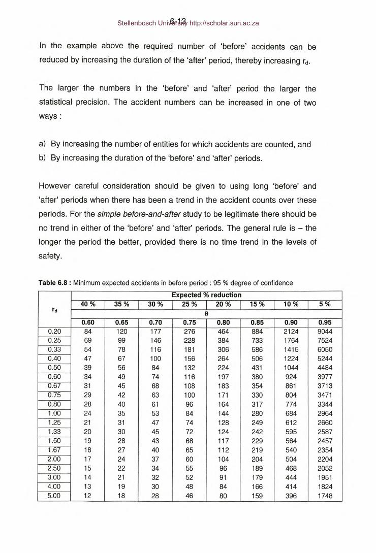
6-13
In the example above the required number of 'before' accidents can be
reduced by increasing the duration of the 'after' period, thereby increasing rd.
The larger the numbers in the 'before' and 'after' period the larger the
statistical precision. The accident numbers can be increased in one of two
ways:
a) By increasing the number of entities for which accidents are counted, and
b) By increasing the duration of the 'before' and 'after' periods.
However careful consideration should be given to using long 'before' and
'after' periods when there has been a trend in the accident counts over these
periods. For the simple before-and-after study to be legitimate there should be
no trend in either of the 'before' and 'after' periods. The general rule is - the
longer the period the better, provided there is no time trend in the levels of
safety.
Table 6.8:Minimum expectedaccidentsinbeforeperiod:95 % degree ofconfidenceExpected % reduction
40% 35% 30% 25% 20% 15% 10 % 5%rd ij
0.60 0.65 0.70 0.75 0.80 0.85 0.90 0.950.20 84 120 177 276 464 884 2124 90440.25 69 99 146 228 384 733 1764 75240.33 54 78 116 181 306 586 1415 60500.40 47 67 100 156 264 506 1224 52440.50 39 56 84 132 224 431 1044 44840.60 34 49 74 116 197 380 924 39770.67 31 45 68 108 183 354 861 37130.75 29 42 63 100 171 330 804 34710.80 28 40 61 96 164 317 774 33441.00 24 35 53 84 144 280 684 29641.25 21 31 47 74 128 249 612 26601.33 20 30 45 72 124 242 595 25871.50 19 28 43 68 117 229 564 24571.67 18 27 40 65 112 219 540 23542.00 17 24 37 60 104 204 504 22042.50 15 22 34 55 96 189 468 20523.00 14 21 32 52 91 179 444 19514.00 13 19 30 48 84 166 414 18245.00 12 18 28 46 80 159 396 1748
Stellenbosch University http://scholar.sun.ac.za
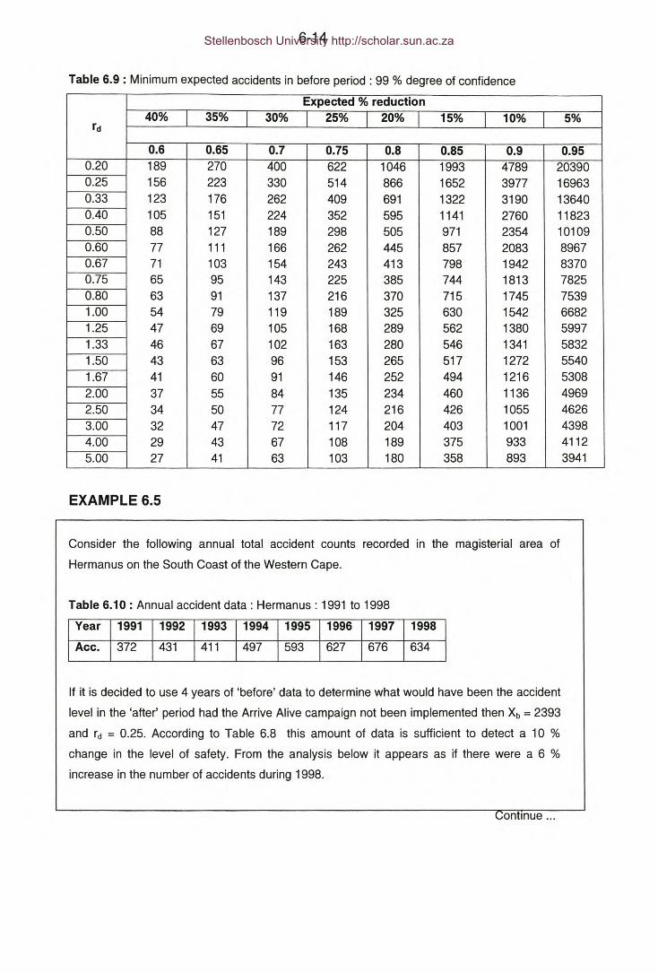
6-14
Table 6.9 : Minimum expected accidents in before period: 99 % degree of confidence
Expected % reduction40% 35% 30% 25% 20% 15% 10% 5%
rd
0.6 0.65 0.7 0.75 0.8 0.85 0.9 0.950.20 189 270 400 622 1046 1993 4789 203900.25 156 223 330 514 866 1652 3977 169630.33 123 176 262 409 691 1322 3190 136400.40 105 151 224 352 595 1141 2760 118230.50 88 127 189 298 505 971 2354 101090.60 77 111 166 262 445 857 2083 89670.67 71 103 154 243 413 798 1942 83700.75 65 95 143 225 385 744 1813 78250.80 63 91 137 216 370 715 1745 75391.00 54 79 119 189 325 630 1542 66821.25 47 69 105 168 289 562 1380 59971.33 46 67 102 163 280 546 1341 58321.50 43 63 96 153 265 517 1272 55401.67 41 60 91 146 252 494 1216 53082.00 37 55 84 135 234 460 1136 49692.50 34 50 77 124 216 426 1055 46263.00 32 47 72 117 204 403 1001 43984.00 29 43 67 108 189 375 933 41125.00 27 41 63 103 180 358 893 3941
EXAMPLE 6.5
Consider the following annual total accident counts recorded in the magisterial area of
Hermanus on the South Coast of the Western Cape.
Table 6.10 : Annual accident data: Hermanus: 1991 to 1998
Year 1991 1992 1993 1994 1995 1996 1997 1998
Acc. 372 431 411 497 593 627 676 634
If it is decided to use 4 years of 'before' data to determine what would have been the accident
level in the 'after' period had the Arrive Alive campaign not been implemented then Xb = 2393
and rd = 0.25. According to Table 6.8 this amount of data is sufficient to detect a 10 %
change in the level of safety. From the analysis below it appears as if there were a 6 %
increase in the number of accidents during 1998.
ontinue ...
Stellenbosch University http://scholar.sun.ac.za

6-15
Example 6.5 (Continued)
Table 6.11 : The 4-step procedure - calculations.
STEP 1 STEP2
'A=634 VAR('A) = 634
Jt = 0.25 * 2393 = 598 VAR(Jt) = 0.252 * 2393 = 150
STEP3 STEP4
6 = 598 - 634 = -36 VAR(6) = 634 + 150 = 784 = 28"
8 = (634/598) / (1+ 150/5982) = 1.060. VAR(8) = (1.06)2[1/634 + 150/5982] / [1+150/59S2f= 0.00224 = 0.0472
Judging from Figure 6.3 it is evident that because of the trend in the accidents the 4 year
average does not provide a good measure of what the level of safety would have been had
the Arrive Alive campaign not been implemented.
The following analysis consider only 1 year in the before period - that is 1997.
Table 6.12 : The 4-step procedure - calculations.
STEP 1 STEP 2
'A= 634 VAR('A) = 634
Jt = 676 VAR(Jt) = 676
STEP3 STEP4
6 = 676 - 634 = 42 VAR('A) = 634 + 676 = 1310 = 36"
8 = (634/676) / (1 + 1/676) = 0.94 VAR(8) = (0.94)2[1/634 + 1/676] / [1 + 1/676]2 = 0.0027
ARF = 6 % = 0.052
It is evident that using a 4-year before period has produced smaller standard deviations for 6
and 8 than using only a 1-year before period i.e. the 4-year period measured 6 and more
precisely, however it measured an' incorrect' effect more precisely. In more human terms - it
is doing the wrong thing well. It is therefore prudent in some instances to use a shorter
'before' or 'after' period even it means a reduction in the accuracy of the estimates.
It is evident from Figure 6.3 that there is still a sizeable trend effect that remains unaccounted
for i.e. the effect estimate above ( - 6 %) is in all likelihood an underestimation. A comparison
group could be used to account for this trend effect.
Continue ...
Stellenbosch University http://scholar.sun.ac.za
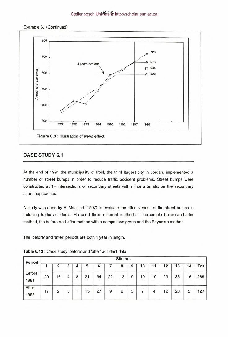
6-16
Example 6. (Continued)
800 r--------------------------------r-----------------,
700..0 728
0°00
4 years average 676
III \ o 634ë 600 598Q)"0IJu'"(ij§ ..-00500(ij
" .."':::>cc~
400..-
3001991 1992 1993 1994 1995 1996 1997 1998
Figure 6.3 : Illustration of trend effect.
CASE STUDY 6.1
At the end of 1991 the municipality of Irbid, the third largest city in Jordan, implemented a
number of street bumps in order to reduce traffic accident problems. Street bumps were
constructed at 14 intersections of secondary streets with minor arterials, on the secondary
street approaches.
A study was done by AI-Masaied (1997) to evaluate the effectiveness of the street bumps in
reducing traffic accidents. He used three different methods - the simple before-and-after
method, the before-and-after method with a comparison group and the Bayesian method.
The 'before' and 'after' periods are both 1 year in length.
Table 6.13: Case study 'before' and 'after' accident data
Site no.Period
1 2 3 4 5 6 7 8 9 10 11 12 13 14 Tot
Before29 16 4 8 21 34 22 13 9 19 19 23 36 16 269
1991
After17 2 0 1 15 27 9 2 3 7 4 12 23 5 127
1992
Stellenbosch University http://scholar.sun.ac.za

6-17
Table 6.14 : The 4-step procedure - calculations
STEP 1 STEP 2
'A= 127 VAR('A) = 127
lt = 269 VAR(lt) = 269
STEP3 STEP4
6 = 269 - 127 = 142 VAR(6) = 127+269 = 396 = 19.9"
8 = (127/269)/(1+1/269) = 0.47 VAR(8) = (0.47)2[1/127+ 1/269]/[1 +1/269f =0.0025 = 0.052
An approximate 95 % confidence interval for 8 is given by 0.47±2(0.05) = {0.37 ; 0.57}. There
appears to have been a significant reduction in the accident number between the before and
after periods.
6.3.3 PERFORMANCE OF BEFORE-AND-AFTER METHODOLOGY
EXAMPLE 6.6
In order to assess the ability of this before-and-after methodology to eliminate the regression-
to-mean effect and to correctly estimate the true safety effect the following analyses were
applied to the hazardous locations identified by conventional methodologies (see Appendix
A4) for the different collection periods. Five sets of hazardous locations were identified -
each set corresponding to a different collection period.
It was assumed that the hazardous locations identified by the Conventional methodologies in
Chapter 3 and Appendix A4 were treated with a treatment that would reduce the accident
frequency by 20 %. The true levels of safety, which were randomly generated from a gamma
distribution for each hazardous location, were reduced by 20 %. This 'after' true level of safety
was then used as the mean to randomly generate 5 years of accident data for each site
according to the Poisson distribution.
If the mb; is the true level of safety at an entity, then ma; = O.8mb;. In the before period Xi -
P(mbi) and in the after period Xi - P(mai).
Xb is the total number of accidents observed at all the hazardous locations during the before
period, mb the sum of all the true levels of safety at all the hazardous locations during the
'before' period and ma the sum of all the true levels of safety during the 'after' period.
The regression-to-mean effect can be determined as follows: RTM = 100*(1-mt/Xt)
Continue ...
Stellenbosch University http://scholar.sun.ac.za
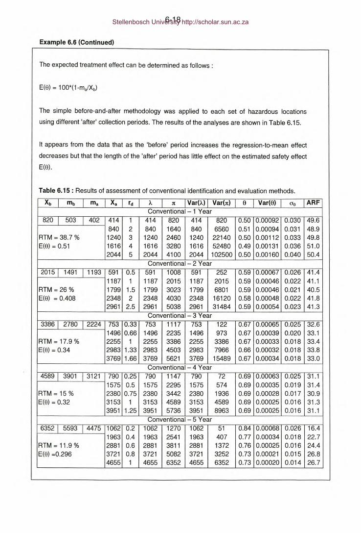
6-18
Example 6.6 (Continued)
The expected treatment effect can be determined as follows:
The simple before-and-after methodology was applied to each set of hazardous locations
using different 'after' collection periods. The results of the analyses are shown in Table 6.15.
It appears from the data that as the 'before' period increases the regression-to-mean effect
decreases but that the length of the 'after' period has little effect on the estimated safety effect
E(8).
Table 6.15 : Results of assessment of conventional identification and evaluation methods.
x, I mb I rna Xa rd 'A. lt Var('A.) Var(lt) 8 Var(8) Oe ARFConventional- 1 Year
820 I 503 I 402 414 1 414 820 414 820 0.50 0.00092 0.030 49.6840 2 840 1640 840 6560 0.51 0.00094 0.031 48.9
RTM = 38.7 % 1240 3 1240 2460 1240 22140 0.50 0.00112 0.033 49.8E(8) = 0.51 1616 4 1616 3280 1616 52480 0.49 0.00131 0.036 51.0
2044 5 2044 4100 2044 102500 0.50 0.00160 0.040 50.4Conventional- 2 Year
2015 I 1491 I 1193 591 0.5 591 1008 591 252 0.59 0.00067 0.026 41.41187 1 1187 2015 1187 2015 0.59 0.00046 0.022 41.1
RTM = 26 % 1799 1.5 1799 3023 1799 6801 0.59 0.00046 0.021 40.5E(8) = 0.408 2348 2 2348 4030 2348 16120 0.58 0.00048 0.022 41.8
2961 2.5 2961 5038 2961 31484 0.59 0.00054 0.023 41.3Conventional - 3 Year
3386 I 2780 I 2224 753 0.33 753 1117 753 122 0.67 0.00065 0.025 32.61496 0.66 1496 2235 1496 973 0.67 0.00039 0.020 33.1
RTM = 17.9 % 2255 1 2255 3386 2255 3386 0.67 0.00033 0.018 33.4E(8) = 0.34 2983 1.33 2983 4503 2983 7966 0.66 0.00032 0.018 33.8
3769 1.66 3769 5621 3769 15489 0.67 0.00034 0.018 33.0Conventional - 4 Year
4589 I 3901 I 3121 790 0.25 790 1147 790 72 0.69 0.00063 0.025 31.11575 0.5 1575 2295 1575 574 0.69 0.00035 0.019 31.4
RTM = 15 % 2380 0.75 2380 3442 2380 1936 0.69 0.00028 0.017 30.9E(8) = 0.32 3153 1 3153 4589 3153 4589 0.69 0.00025 0.016 31.3
3951 1.25 3951 5736 3951 8963 0.69 0.00025 0.016 31.1Conventional - 5 Year
6352 I 5593 I 4475 1062 0.2 1062 1270 1062 51 0.84 0.00068 0.026 16.41963 0.4 1963 2541 1963 407 0.77 0.00034 0.018 22.7
RTM = 11.9 % 2881 0.6 2881 3811 2881 1372 0.76 0.00025 0.016 24.4E(8) =0.296 3721 0.8 3721 5082 3721 3252 0.73 0.00021 0.015 26.8
4655 1 4655 6352 4655 6352 0.73 0.00020 0.014 26.7
Stellenbosch University http://scholar.sun.ac.za
6-19
6.4 ACCOUNTING FOR THE EXPOSURE EFFECT
As mentioned previously a disadvantage of the simple before-and-after
methodology is its inability to separate the treatment effect from the effect
from many other variables that changed between the 'before' and 'after'
periods.
One important measurable causal factor that changes between the 'before'
and 'after' period is traffic flow i.e. exposure. Traffic flow information is
routinely collected by roads authorities for a variety of purposes. The most
common measure of traffic flow for road segments is the AADT - Annual
Average Daily Traffic.
It is often assumed that the exposure effect can be accounted for by using
accident rates ( e.g. accidents / million vehicle kilometres / year). Using
accident rates in this manner is only legitimate if a direct linear relationship
exists between traffic flows and accidents. As has been shown in Chapter 3
AADT based accident rates are in most cases a function of the magnitude of
the AADT i.e. the Safety Performance function is non-linear.
6.4.1 STATISTICAL ANALYSIS
Let
The expected number of accidents when flow = Aa.
The expected number of accidents when flow = Ab.
The traffic flow ratio and its variance is given by (Hauer; 1997) :
In= F(AaJ/F(AJ
VAR(rrJ = r/ [c/VAR(AaJ / f2(AaJ + c/VAR(AJ / f2(AJ]
... [6.8]
... [6.9]
Where CA and Cs denote the derivatives of 'f with respect to traffic flows at A,
and Ab.
Stellenbosch University http://scholar.sun.ac.za

6-20
For a linear Safety Performance Function the values of r« and VAR(rtt) is given
by (Hauer; 1997):
rtf = Aa/Ab
VAR(rtf) = rtf2{v2(Aa) + v2(Ab)}
... [6.10]
... [6.11]
Where
v(AaJ and v(AJ are the coefficients-ot-variation for the 'after' and 'before'
counts respectively. A coefficient-ot-variation is defined as the standard
deviation of a variable divided by its mean.
For a non-linear Safety Performance Function with the following form:
frAY = aAi3 ... [6.12]
the expressions for estimating rtt and VAR(rt,) is (Hauer; 1997):
rtf= (A.lAt)i3
VAR(rtf) = r/f./[';(AaY + ';(At)]
... [6.13]
... [6.14]
Table 6.16: The 4-step procedure - accounting for the exposure effect
STEP 1 STEP 2
A = Xa VAR(A) = Xa
:It = rdrtfXb VAR(:It) = (rr)2 [(rt/Xb + X/VAR(rrJ]
STEP3 STEP4
b = :It-A VAR(b) = VAR(:It) + VAR(A)
8 = (A.I:1t)[1+VAR(:It)/:lt2r1 VAR(8) = 82[VAR(A)/A2 + VAR(:It)/:lt2]/[1 + VAR(:It)/:lt2f
Stellenbosch University http://scholar.sun.ac.za

6-21
• THE ESTIMATION OF v(AJ and v(Ab).
The values of v(Aa) and v(Ab) can be obtained from Tables 2.1, 2.2 and 2.3 in
Chapter 2.
EXAMPLE 6.7
Provincial Trunk Road Number 11 Section 4 connects Citrusdal in the south with Clanwilliam
in the north. It forms part of the N7 route which runs from Cape Town to Namibia. During
1992 the section between kilometre values 57.01 and 76.05 was resurfaced and the road
markings were repainted.
In the 4 years preceding the resurfacing i.e. 1988 to 1991 a total of 71 accidents were
recorded. In the 2 years after the treatment year i.e. 1993 to 1994 a total of 15 accidents were
recorded. The treatment year, 1992, was excluded from the analysis. The AADT for the
'before' period is about 1200 vehicles per day and for the after period it was about 1400
vehicles per day. The former count was obtained from a 2-day (24 hour) count and the latter
from a 1-day (24 hour) count.
Table 6.17 : Data and calculations
Category: Strategic
v(Ab) = 0.177 ( From Table)
v(Aa) = 0.143 ( From Table)
Tb = 4
Ta = 2
rd = 0.5
Xb = 71
Xa = 15
rtt = 1400/1200 = 1.167
VAR(rtt) = (1.167)2 {(0.177)2 + (0.143)2} = 0.071
Table 6.18 : The 4-step procedure - calculations
STEP 1 STEP2
A = 15 VAR(A) = 15
Jt=0.5*1.167*71 =41.4 VAR(Jt) = (0.5)2[(1.167)2*71 + 712*0.071] = 114
STEP 3 STEP4
0= 41.4 - 15 = 26.4 VAR(o) = 15 + 55.2 = 70.2
8 = VAR(8) = (0.35)2[15/152 + 114/41.42] / [1+114/41.42]2=
(15/41.4)/(1 +55.2/41.42)=0.35 0(0) = 8.38
ARF = 100(1-0.35) = 65 % 0(8)=0.105
Continue ...
Stellenbosch University http://scholar.sun.ac.za

6-22
Example 6.7 (Continued)
If it is assumed that the Safety Performance function is non-linear and that X cx: A0.8 then:
rif = (1400/1200)°·8 = 1.13
VAR(rlf) = (1.13)2(O.8)2{(O.098)2+ (O.092)2} = 0.014
Table 6.19 : The 4-step procedure - calculations
STEP 1 STEP2
A = 15 VAR(A) = 15
j[ = 0.5*1.13*71 = 40.1 VAR(j[) = (0.5)2[(1.13)2*71 + 712*0.014] = 40.3
STEP3 STEP4
6 = 40.1 - 15 = 25.1 VAR(6) = 15 + 40.3 = 55.3
8 = (15/40.1 )/(1 +40.3/40.12)=0.36 VAR(8) = (0.36)2[15/152 + 40.3/40.12] 1 [1+40.3/40.12f=ARF = 100(1-0.36) = 64 % 0.011
0(0) = 7.44
0(8)=0.106
The approximate 95 % confidence interval of the ARF is given by 64±2(1 0.6) = {42.8 ; 85.8}. It
can therefore be concluded that the resurfacing operations on TR 1114 were successful in
reducing accidents.
6.5 BEFORE-AND-AFTER WITH COMPARISON GROUP METHOD
According to Hauer (1997) to increase the accuracy of prediction it is required
to account for the influence of causal factors that change with time. In the
previous section the changes in traffic volumes were accounted for. Whereas
the change in traffic volumes can be measured, there are however numerous
causal factors which are not directly measurable or which are very difficult to
measure. Even if all the causal factors could be measured the analytical
procedures could become very complicated and cumbersome. To collectively
account for these causal factors a comparison group is often used.
A comparison group, according to Hauer (1997) is a group of entities that
remained untreated and that are similar to the treated sites.
Stellenbosch University http://scholar.sun.ac.za

6-23
The before-and-after with comparison group procedure is based on two
assumptions:
1. That the causal factors have changed from the 'before' to the 'after' period
in the same manner for both the treatment and the comparison group
2. That the change in these causal factors affects the safety of the treatment
and comparison group in the same way.
6.5.1 STATISTICAL FRAMEWORK
Ca The total observed number of accidents for all entities in the
comparison group during the 'after' period.
Cb- The total observed number of accidents for all entities in the
comparison group during the 'before' period.
f.l- The total expected number of accidents for all entities in the
comparison group during the 'before' period.
v- The total expected number of accidents for all entities in the
comparison group during the 'after' period.
The comparison ratio is defined as :
re = v/f.l ... [6.15]
The equivalent ratio for the treatment group is
rT= xb: ... [6.16]
If the assumptions above holds then re = rT.
The 'odds ratio' is defined as :
(JJ = re/rT ... [6.17]
Stellenbosch University http://scholar.sun.ac.za

6-24
For each group of treatment and comparison entities there is a time series of
(JJ's.Any such sequence of (JJ'shas a mean E«(JJ)and a variance VAR«(JJ).For
a comparison group to be legitimate E«(JJ)= 1.
Table 6.20: The 4-step procedure: Comparison group method
STEP 1 STEP 2
1..= x, VAR(A) = Xa
rT= re = CalCb VAR(rT) = rl [1/Cb + 1/Ca + VAR(w)]
n:= rTXb VAR(n:) = n:2 [1/Xb + VAR(rT)}/rT2]
STEP 3 STEP4
b = n:-A VAR(b) = VAR(Jt) + VAR(A)
8 = (A/Jt)[1+VAR(Jt)/Jt2r1 VAR(8) = 82[VAR(A)/A2 + VAR(Jt)/n:2]/[1 + VAR(Jt)/Jt2f
EXAMPLE 6.8
Assume that during 1996 a municipality converted 6 intersections from 4-way stops to
signalised intersections. Assume that the comparison group consist of all non-treated 4-way
stops in the municipal area. For this exercise assume VAR(w) = o.
Table 6.21 : Treatment and comparison group data
Period Treatment Comparison
Before 73 307
After 59 389
Table 6.22 : The 4-step procedure - calculations
STEP 1 STEP2
1..= 59 VAR(A) = 59
rT= 389/307 = 1.27 VAR(rT) = (1.27)2[1/307 + 1/389] =0.0094
n:= 1.27 * 73 = 92 VAR(n:) = (92)2[1/73 + 0.0094/(1.27)2] = 165
STEP 3 STEP4
b = 92-59 = 33 VAR(b) = 59 + 165 = 224 = 15"
8 = (59/92)/(1 +1/92) = 0.63 VAR(8) = (0.63l[1/59 + 165/922]/[1+165/922f=0.014 = 0.122
ARF = 37 % S(8) = 0.12
The approximate 95 % confidence of the ARF is given by 37±2(12) = {13 ; 61}. The
conversion of the 6 intersections from 4-way stops to signalised installations was therefore
effective in reducing accidents.
Stellenbosch University http://scholar.sun.ac.za

6-25
In Example 6.8 all the entities were situated in the same municipal area.
The procedure above, as illustrated by the example, is not correct for the
case where a treatment was applied to entities which do not have the same
'before' and 'after' periods and that share the same environment. Each entity
therefore has to have a different comparison group. (Hauer; 1997)
Treatments applied to different entities in different years will not have the
same 'before' and 'after' periods. A year which for one entity is in the 'before'
period might be in the 'after' period for another entity. It will therefore be
incorrect to pool the entities because the data for the 'before' and 'after'
periods will not be mutually exclusive.
The way causal factors change between the 'before' and 'after' periods and
their effect of safety could be geographically sensitive. Some areas may have
more rain then others, some areas may have more pedestrians, the growth in
vehicle travel may be higher etc. Therefore entities that are situated in
different environments cannot have a common comparison group. This would
violate the basic assumptions on which the comparison group method is
based on.
In such circumstances each entity should have its own comparison ratio. The
4-step procedure is shown in Table 6.23.
Table 6.23 : The 4 -step procedure: Entities with own comparison ratios
STEP 1 STEP2
A(j) = Xa(j} VAR{AG)} = Xa(j)
rT(j) = rc(j) = Ca(j) ICb(j) VAR{rT(j)} = rT2(j) [1/Cb(j) + 1/Ca(j) + VAR{w(j)]
1t(j) = rT(j)Xb(j) VAR(A) = LVAR{A(j)}
VAR{1t(j)} = 1t2(j) [1/Xb(j) + VAR{rT(j)}/rl(j)]
VAR(1t) = LVAR{1t(j)}
STEP3 STEP4
6 = 1t-A VAR(6) = VAR(1t) + VAR(A)
8 = (A/1t)[1 +VAR(1t)/1t2r1 VAR(8) = 82[VAR(A)/A2 + VAR(1t)/1t2]/[1 + VAR(1t)/1t2f
Stellenbosch University http://scholar.sun.ac.za
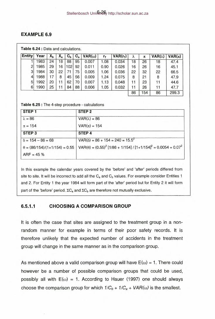
6-26
EXAMPLE 6.9
Table 6.24 : Data and calculations.
Entity Year Xb Xa Cb Ca VAR(w) rT VAR(rT) " :rt VAR(,,) VAR(:rt)1 1983 24 18 88 95 0.007 1.08 0.034 18 26 18 47.42 1985 29 16 102 92 0.011 0.90 0.026 16 26 16 45.13 1984 30 22 71 75 0.005 1.06 0.036 22 32 22 66.54 1988 17 8 45 56 0.009 1.24 0.075 8 21 8 47.95 1992 20 11 62 70 0.007 1.13 0.048 11 23 11 44.66 1990 25 11 84 88 0.006 1.05 0.032 11 26 11 47.7
86 154 86 299.3
Table 6.25 : The 4-step procedure - calculations
STEP 1 STEP2
/...= 86 VAR(/...)= 86
:rt= 154 VAR(:rt) = 154
STEP3 STEP4
o = 154 - 86 = 68 VAR(o) = 86 + 154 = 240 = 15.5"
8 = (86/154)/(1 +1/154) = 0.55 VAR(8) = (0.55)2 [1/86 + 1/154] I [1+11154f = 0.0054 = 0.072
ARF = 45 %
In this example the calendar years covered by the 'before' and 'after' periods differed from
site to site. It will be incorrect to add all the Ca and Cb values. For example consider Entities 1
and 2. For Entity 1 the year 1984 will form part of the 'after' period but for Entity 2 it will form
part of the 'before' period. LCa and LCb are therefore not mutually exclusive.
6.5.1.1 CHOOSING A COMPARISON GROUP
It is often the case that sites are assigned to the treatment group in a non-
random manner for example in terms of their poor safety records. It is
therefore unlikely that the expected number of accidents in the treatment
group will change in the same manner as in the comparison group.
As mentioned above a valid comparison group will have Eko) = 1. There could
however be a number of possible comparison groups that could be used,
possibly all with E(co) = 1. According to Hauer (1997) one should always
choose the comparison group for which 11Gb + 11Ga + VAR(co) is the smallest.
Stellenbosch University http://scholar.sun.ac.za
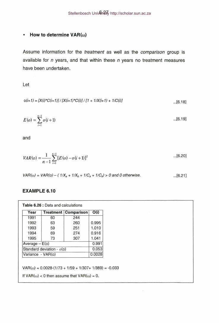
6-27
• How to determine VAR(w)
Assume information for the treatment as well as the comparison group is
available for n years, and that within these n years no treatment measures
have been undertaken.
Let
o(i+ 1) = txarc«. 1)] I txu:1)*C(i)] I [1 + 1IX(i+ 1) + 1/C(i)] ...[6.18]
n-l
£(0) = Lo(i+1)i=l
...[6.19]
and
1 n-l
VAR(o)=-L[£(o)-o(i+l)Yn -1 i=l
...[6.20]
VAR(w) = VAR(o) - ( 11Xa+ 1/Xb + 11Ca+ tlCt) > 0 and 0 otherwise. ...[6.21 ]
EXAMPLE 6.10
Table 6.26 : Data and calculations
Year Treatment Comparison O(i)1991 60 2441992 63 260 0.9951993 59 251 1.0101994 69 274 0.9161995 73 307 1.041
Average - E(o) 0.991Standard deviation - 0(0) 0.053Variance - VAR(o) 0.0028
VAR(w) = 0.0028-(1/73 + 1/59 + 1/307+ 1/389) = -0.033
If VAR(w) < 0 then assume that VAR(w) = O.
Stellenbosch University http://scholar.sun.ac.za
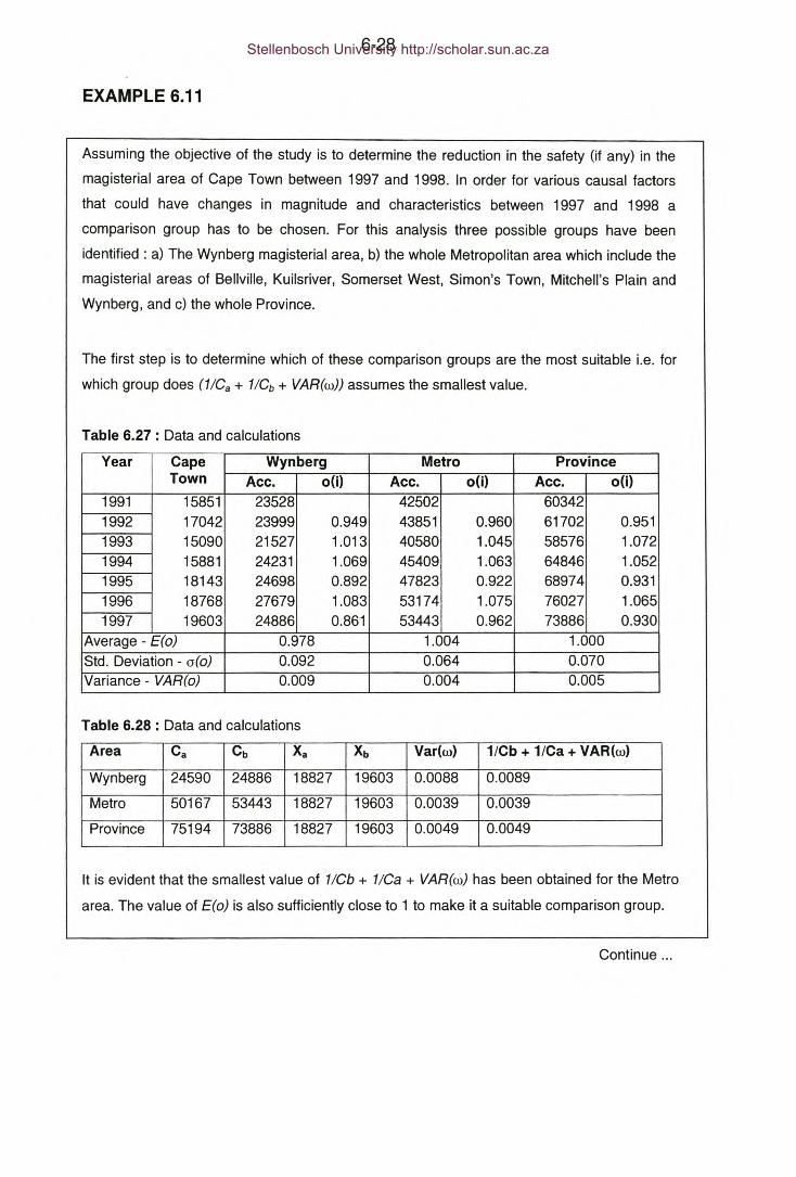
6-28
EXAMPLE 6.11
Assuming the objective of the study is to determine the reduction in the safety (if any) in the
magisterial area of Cape Town between 1997 and 1998. In order for various causal factors
that could have changes in magnitude and characteristics between 1997 and 1998 a
comparison group has to be chosen. For this analysis three possible groups have been
identified: a) The Wynberg magisterial area, b) the whole Metropolitan area which include the
magisterial areas of Bellville, Kuilsriver, Somerset West, Simon's Town, Mitchell's Plain and
Wynberg, and c) the whole Province.
The first step is to determine which of these comparison groups are the most suitable i.e. for
which group does (1IGa + 11Gb+ VAR(w)) assumes the smallest value.
Table 6.27 : Data and calculations
Year Cape Wynberg Metro ProvinceTown Acc. o(i) Acc. o(i) Acc. o(i)
1991 15851 23528 42502 603421992 17042 23999 0.949 43851 0.960 61702 0.9511993 15090 21527 1.013 40580 1.045 58576 1.0721994 15881 24231 1.069 45409 1.063 64846 1.0521995 18143 24698 0.892 47823 0.922 68974 0.9311996 18768 27679 1.083 53174 1.075 76027 1.0651997 19603 24886 0.861 53443 0.962 73886 0.930
Average - E(o) 0.978 1.004 1.000Std. Deviation - 0(0) 0.092 0.064 0.070Variance - VAR(o) 0.009 0.004 0.005
Table 6.28 : Data and calculations
Area Ca Cb Xa Xb Var(w) 1/Cb + 1/Ca + VAR(w)
Wynberg 24590 24886 18827 19603 0.0088 0.0089
Metro 50167 53443 18827 19603 0.0039 0.0039
Province 75194 73886 18827 19603 0.0049 0.0049
It is evident that the smallest value of 11Gb+ 11Ga+ VAR(w) has been obtained for the Metro
area. The value of E(o) is also sufficiently close to 1 to make it a suitable comparison group.
Continue ...
Stellenbosch University http://scholar.sun.ac.za

6-29
Example 6.11 (Continued)
Table 6.29 : The 4-step procedure - calculations
STEP 1 STEP2
VAR().) = 18827 = (137)~
A = 18827 VAR(rT) = (0.94)2 [0.0039] = 0.00345
rT= re= 50167/53443 = 0.94 VAR(Jt) = 184012[1/19603 + 0.00345/(0.94)2 ]=
:rt = 0.94*19603 = 18401 (1157)2
STEP3 STEP4
b = 18401 -18827 = -426 Var(b) =18401 + 1157~ = 1165~
8 = (18827/18401)/(1 + 11572/184012 = VAR(8) = (1.019)2[ 1/18827 + 11572/184012 ] /
1.019 [1 + 11572/184012]2 = 0.0041
Since 8 > 1 it can be concluded that there was no improvement in safety in the magisterial
area of Cape Town between 1997 and 1998.
6.5.2 STUDY DESIGN
Hauer (1997) lists 5 principal choices that have to be made during the design
of a before-and-after with comparison group procedure:
1. Select the size of the treatment group in terms of the expected number of
target accidents.
2. Select the duration of the 'before' period.
3. Decide on an appropriate duration of the 'after' period.
4. Postulate what the anticipated index of effectiveness (8) of the treatment
is.
5. Select the comparison group
Stellenbosch University http://scholar.sun.ac.za
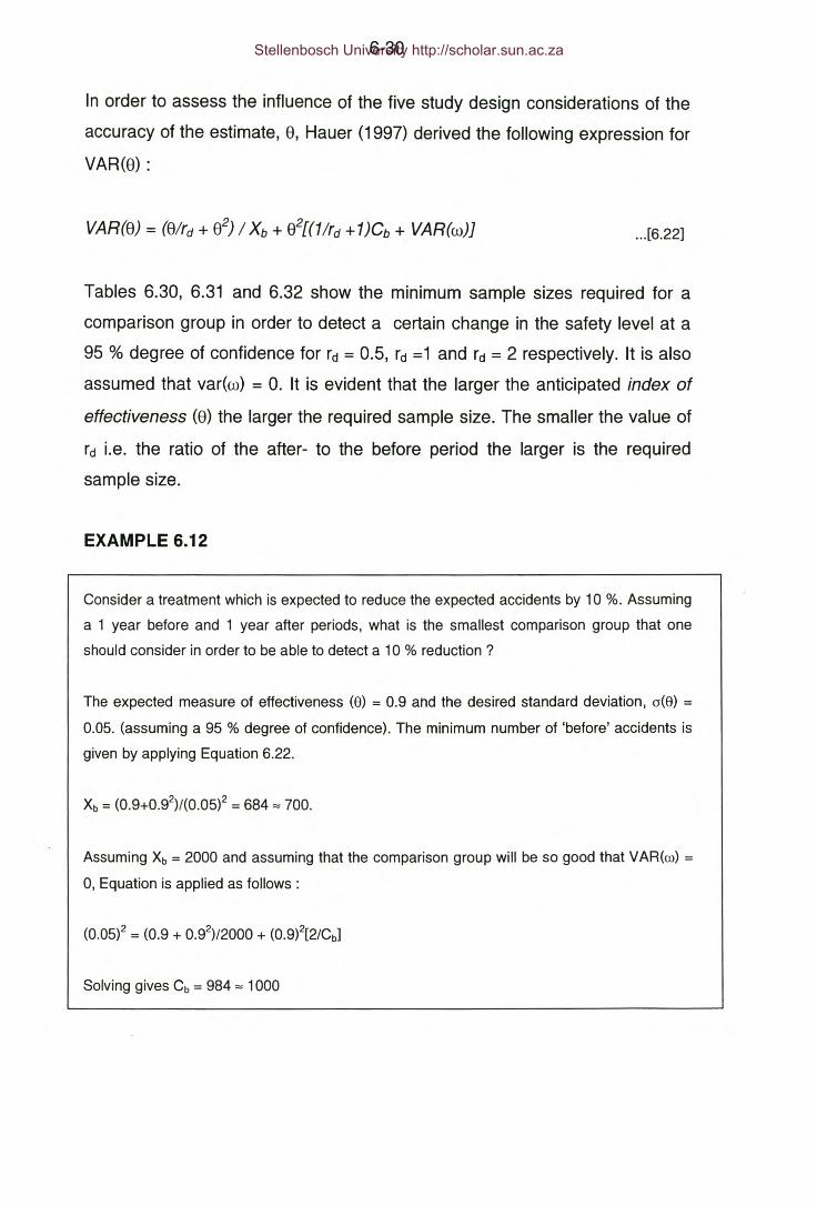
6-30
In order to assess the influence of the five study design considerations of the
accuracy of the estimate, 8, Hauer (1997) derived the following expression for
VAR(8) :
...[6.22]
Tables 6.30, 6.31 and 6.32 show the minimum sample sizes required for a
comparison group in order to detect a certain change in the safety level at a
95 % degree of confidence for rd = 0.5, rd =1 and rd = 2 respectively. It is also
assumed that var(w) = O. It is evident that the larger the anticipated index of
effectiveness (8) the larger the required sample size. The smaller the value of
rd i.e. the ratio of the after- to the before period the larger is the required
sample size.
EXAMPLE 6.12
Consider a treatment which is expected to reduce the expected accidents by 10 %. Assuming
a 1 year before and 1 year after periods, what is the smallest comparison group that one
should consider in order to be able to detect a 10 % reduction?
The expected measure of effectiveness (8) = 0.9 and the desired standard deviation, 0(8) =0.05. (assuming a 95 % degree of confidence). The minimum number of 'before' accidents is
given by applying Equation 6.22.
Assuming Xb = 2000 and assuming that the comparison group will be so good that VAR(w) =0, Equation is applied as follows:
Solving gives Cb = 984 "" 1000
Stellenbosch University http://scholar.sun.ac.za
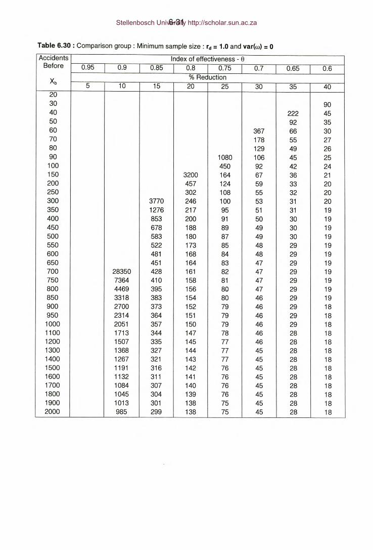
6-31
Table 6.30 : Comparison group: Minimum sample size: rd= 1.0 and var(w) = 0
Accidents Index of effectiveness - 8Before 0.95 0.9 0.85 0.8 0.75 0.7 0.65 0.6Xb
% Reduction5 10 15 20 25 30 35 40
2030 9040 222 4550 92 3560 367 66 3070 178 55 2780 129 49 2690 1080 106 45 25100 450 92 42 24150 3200 164 67 36 21200 457 124 59 33 20250 302 108 55 32 20300 3770 246 100 53 31 20350 1276 217 95 51 31 19400 853 200 91 50 30 19450 678 188 89 49 30 19500 583 180 87 49 30 19550 522 173 85 48 29 19600 481 168 84 48 29 19650 451 164 83 47 29 19700 28350 428 161 82 47 29 19750 7364 410 158 81 47 29 19800 4469 395 156 8Q 47 29 19850 3318 383 154 80 46 29 19900 2700 373 152 79 46 29 18950 2314 364 151 79 46 29 181000 2051 357 150 79 46 29 181100 1713 344 147 78 46 28 181200 1507 335 145 77 46 28 181300 1368 327 144 77 45 28 181400 1267 321 143 77 45 28 181500 1191 316 142 76 45 28 181600 1132 311 141 76 45 28 181700 1084 307 140 76 45 28 181800 1045 304 139 76 45 28 181900 1013 301 138 75 45 28 182000 985 299 138 75 45 28 18
Stellenbosch University http://scholar.sun.ac.za

6-32
Table 6.31 : Comparison group: Minimum sample size: rd = 0.5 and varko) = O.
Accidents Index of effectiveness - eBefore 0.95 0.9 0.85 0.8 0.75 0.7 0.65 0.6
Xb% Reduction
5 10 15 20 25 30 35 40203040 108050 12360 661 7770 211 6180 139 5390 980 110 48100 408 95 44150 900 148 66 36200 318 113 58 34250 1846 229 98 53 32300 758 193 91 51 31350 533 173 86 49 30400 436 161 83 48 30450 8969 382 153 80 47 30500 2779 348 147 79 47 29550 1776 324 142 77 46 29600 1365 306 138 76 46 29650 1142 293 136 75 45 29700 1001 282 133 74 45 29750 905 274 131 74 45 28800 835 267 129 73 45 28850 781 261 128 72 44 28900 739 256 127 72 44 28950 705 251 125 72 44 281000 677 247 124 71 44 281100 19093 633 241 123 71 44 281200 7477 601 236 121 70 43 281300 4936 576 232 120 70 43 281400 3822 557 229 119 70 43 281500 3197 541 226 118 69 43 281600 2797 527 223 118 69 43 281700 2519 516 221 117 69 43 281800 2314 507 219 117 69 43 281900 2157 498 218 116 68 43 282000 2033 491 216 116 68 43 28
Stellenbosch University http://scholar.sun.ac.za

6-33
Table 6.32: Comparison group: Minimum sample size: rd = 2.0 and varke) = 0
Accidents Index of effectiveness - eBefore 0.95 0.9 0.85 0.8 0.75 0.7 0.65 0.6
Xb% Reduction
5 10 15 20 25 30 35 4020 7730 111 3040 490 53 2350 129 40 2060 86 35 1970 378 70 32 1880 216 61 30 1790 162 56 28 17100 135 52 27 16150 313 90 43 25 15200 200 77 40 24 15250 1047 164 71 38 23 14300 602 147 68 37 23 14350 462 137 65 37 22 14400 393 130 64 36 22 14450 352 125 62 36 22 14500 325 121 61 35 22 14550 5811 306 118 61 35 22 14600 3038 292 116 60 35 22 14650 2164 281 114 59 35 22 14700 1736 272 113 59 35 21 14750 1482 265 111 59 34 21 14800 1314 259 110 58 34 21 14850 1194 254 109 58 34 21 14900 1105 249 109 58 34 21 14950 1035 245 108 58 34 21 141000 980 242 107 57 34 21 141100 897 237 106 57 34 21 141200 838 232 105 57 34 21 141300 794 229 104 57 34 21 141400 759 226 104 56 34 21 141500 732 223 103 56 34 21 141600 709 221 103 56 33 21 141700 691 219 102 56 33 21 141800 675 217 102 56 33 21 141900 661 216 102 56 33 21 142000 650 215 101 56 33 21 14
Stellenbosch University http://scholar.sun.ac.za

6-34
CASE STUDY 6.1 (continued)
For the 14 locations where street bumps were implemented in Irbid, Jordan, a total of 21
suitable comparison locations were identified. The comparison locations were selected to be
similar to the locations that have been improved. Similarity included both geometric and
operational characteristics. The 21 sites in the comparison group had 384 and 346 accidents
in the 'before' and 'after' periods respectively.
The value of VAR(w) has not been determined in AI-Maseied's 0 study and will be assumed
to be equal to zero.
Table 6.33: Treatment and comparison group accident data
I Xb~269Xa = 127
I Cb~384Ca = 346
Table 6.34 : The 4-step procedure - calculations
STEP 1 STEP2
A = 127 VAR(A) = 127
rT= 346/384 =0.90 VAR(rT) = (0.90)2[1/384 + 1/346] = 0.0045
lt = 0.9*269 = 242 VAR(lt) = 2422[1/269 + 0.0045/0.902] = 543 = 232
STEP3 STEP4
6 = 242 -127 = 115 VAR(6) = 127 + 543 = 670 = 26"
8 = (127/242)/(1 +1/242) = 0.52 VAR(8) = (0.52)2[1/127+543/2422]/[1 +543/2422f = 0.0046
AFR = 48 % 0(8) = 0.068
The 95 % confidence interval for ARF is approximately {34 % ; 62%}
According to AI-Maseied the mean number of accidents recorded at the 14 treatment sites in
the before period is 19.2 accidents per site, while the mean number recorded at the 21
comparison group sites was 18.3 accidents per site. It is thus evident that on average the
treatment sites and the comparison sites had similar levels of safety. When this is the case
the regression-to-mean effect can be accounted for by the before-and-after with comparison
group procedure.
The regression-to-mean effect can in this case be estimated by the difference between the
result obtained from the simple study and the results obtained from the comparison group
study i.e. RTM = 53 - 48 = 5%.
Stellenbosch University http://scholar.sun.ac.za

6-35
6.6 THE EMPIRICAL BAYES APPROACH
The conventional before-and-after procedures (with or without a comparison
group) assumes that the observed accident numbers Xa and Xb are estimates
of the true level of safety in the 'before' and 'after' periods i.e. mb and ma.
This assumption makes the conventional methods prone to the regression-to-
mean effect as was illustrated in the results shown in Table 6.15.
According to Abbess et al. (1981) one of the advantages of the Empirical
Bayesian approach is that the method is able to eliminate the regression-to-
mean effect, provided that the prior estimates E(m) are sufficiently reliable.
6.6.1 THE SIMPLE BEFORE-AND-AFTER PROCEDURE
6.6.1.1 THE COMPOSITE METHOD
The composite method is suitable to determine the average effect of an
treatment when applied to a number of entities.
Some treatment has been applied to a number of entities numbered 1, 2, 3,
....j, .... n. During the before period the accident counts were Xb(1), Xb(2),
...Xb(n) and during the 'after' period the accident counts were Xa(1), Xa(2),
...Xa(n). The 'before' duration and the 'after' duration may differ from entity to
entity.
For each entity there is a reference population, although several treated
entities may have the same reference group. For each reference population
the prior moments Elm(j)} and VARlm(j)} are known.
The weights for each entity is calculated as follows:
a(j) = [1+VAR{m(j)}lE{m(j)}t ...[6.23]
Stellenbosch University http://scholar.sun.ac.za

6-36
E{mb IXb(j)} = a(j)E{m(j)} + [1-a]Xb(j)
VAR{ mb IXb(j)} =(1-a(j)] E{mb IXb(j)}
...[6.24]
...[6.25]
Table 6.35 : The 4-step procedure: Bayesian before-and-after method
STEP 1 STEP 2
A = LXaU> VAR(A) = L XaG)
n: = LrdG)X(j) VAR(n:) = LrdG)2VAR{xG)}
STEP3 STEP4
0= n:-A VAR(o) = VAR(n:) + VAR(A)
8 = (A/n:)[1 +VAR(n:)/n:2r1 VAR(8) = 82[VAR(A)/A2 + VAR(n:)/n:2]/[1 + VAR(n:)/n:2]2
From Step 2 in Table 6.35 the question may arise as to why LXa(j) is used as
an estimate of the true number of accidents in the 'after' period and not
Lma<DIXa(j) knowing that malXa is a more reliable estimate of safety then Xa ?
The answer is that if all treated sites in the 'after' period also forms the
reference group for the 'after' period then it can be shown, as follows, that for
the treated sites LXa(j) = Lma(j)IXa(j)
Assume that of the n sites that formed the reference group in the 'before'
period a total of k were treated.
k k
IE[m(j} IX(j}] =I {aE(m} + (I-a}X (j)}j=l j=l
...[6.26]
k k
IE[m(j} IX(j}] =ak.E(m} + (I-a) IX(j)j=l j=l
...[6.27]
k
k.E(m} = IX(j}j=l
...[6.28]
k k
IE[m(j} I X (j)] = IX (j)j~ j~
...[6.28]
Stellenbosch University http://scholar.sun.ac.za

6-37
Should the treated sites be too few to form a reference group on their own
E[maIXa(j)] could be estimated for each site using the methods described in
Chapter 4.
CASE STUDY 6.1 (continued)
In the evaluation of the installation of speed humps in the city of Irbid in Jordan, AI-Masaeid
(1997) also used the Empirical Bayes approach to estimate the safety effect of speed hump
installations. For each treated site the method-at-moments (see Chapter 4) was used to
calculate malXa and mblXb i.e. for both the 'before' and 'after' period. The study by AI-
Masaeid (1997) did not provide enough information for the estimation of VAR(maIXa) and
VAR(mbIXb) and this example will be confined to Step 1 and Step 3 of the four step procedure.
Table 6.36 : Before-and-After Bayesian estimates
LocationExpected Accident Frequency
mblXb malXa1 22.35 14.552 14.71 5.463 7.65 4.244 10.00 4.855 17.65 14.556 25.29 20.677 18.24 9.708 12.94 5.459 10.59 6.0610 16.47 8.4911 16.47 6.6712 18.82 11.5213 26.47 18.1814 14.71 7.27TOTAL 232.36 136.60
The (biased) measure of effectiveness 8 = (136.60/232.36) = 0.59 and ARF = 41 %. The
simple before-and-after methodology indicated an ARF of 53 %. The regression-to-mean
effect is thereforee approximately 53 - 41 = 12 %. The before-and-after with comparison
group methodology estimated an ARF of 43 % which is relatively similar the Empirical Bayes
estimate. The reason for this result is that the sites comprising the comparison group shared
similar levels of safety as the 14 sites in the treatment group.
Stellenbosch University http://scholar.sun.ac.za

6-38
6.6.1.2 PERFORMANCE OF BAYESIAN BEFORE AND AFTER
METHODOLOGY
EXAMPLE 6.13
In order to assess the ability of this before-and-after methodology to eliminate the regression-
to-mean effect and to correctly estimate the true safety effect the following analyses were
applied to hazardous locations identified by the Bayesian methodology for the different
collection periods. Five sets of hazardous locations were identified - each set corresponding
to a different collection period
It was assumed that the hazardous locations identified by the Bayesian methodology in
Appendix B4 were treated with a treatment that would reduce the accident frequency by 20
%. The true levels of safety, which were randomly generated from a gamma distribution for
each hazardous location, were reduced by 20 %. This 'after' true level of safety was then
used as the mean to randomly generate 5 years of accident data for each site according to
the Poisson distribution.
If the mb; is the true level of safety at an entity, then ma; = O.8mb;. In the before period Xi -
P(mbi) and in the after period Xi - P(mai).
Xb is the total number of accidents observed at all the hazardous locations during the before
period, mb the sum of all the true levels of safety at all the hazardous locations during the
'before' period and ma the sum of all the true levels of safety during the 'after' period.
The regression-to-mean effect can be determined as follows:
RTM = 100*(1-mtlXt;)
The expected treatment effect can be determined as follows:
The simple before-and-after Bayesian methodology was applied to each set of hazardous
locations using different 'after' collection periods. The results of the analyses are shown in
Table 6.37.
Continue ...
Stellenbosch University http://scholar.sun.ac.za

6-39
Example 6.13 (Continued)
Table 6.37 : Assessment of simple before-and-after Bayesian methodology
Xb I Mb I ma rd ').. :rt VAR(')..) VAR(:rt) 8 0(8) ARFBayesian - 1 Year
68 I 65 I 52 1 58 68 58 68 0.84 0.149 15.62 108 135 108 542 0.77 0.148 22.6
RTM = 4.7 % 3 161 203 161 1829 0.76 0.163 24.1E(8) = 0.76 4 215 271 215 4335 0.75 0.179 25.1
5 271 339 271 8468 0.75 0.193 25.5Bayesian - 2 Year
314 I 316 1 253 1 262 314 262 314 0.83 0.069 16.82 530 627 530 2510 0.84 0.076 16.1
RTM = -0.7 % 3 780 941 780 8470 0.82 0.085 17.9E(8) = 0.81 4 1021 1255 1021 20078 0.80 0.093 19.7
5 1290 1569 1290 39214 0.81 0.103 19.1Bayesian - 3 Year
502 I 512 I 410 1 411 502 411 502 0.82 0.054 18.32 830 1004 830 4017 0.82 0.059 17.7
RTM = -2.0 % 3 1242 1506 1242 13557 0.82 0.067 18.0E(8) = 0.82 4 1636 2008 1636 32134 0.81 0.074 19.2
5 2062 2510 2062 62762 0.81 0.082 18.7Bayesian - 4 Year
634 I 642 I 513 1 518 634 518 634 0.82 0.048 18.42 1052 1268 1052 5073 0.83 0.053 17.3
RTM = -1.2 % 3 1589 1902 1589 17121 0.83 0.061 16.9E(S) = 0.81 4 2099 2536 2099 40582 0.82 0.067 17.8
5 2633 3170 2633 79262 0.82 0.074 17.6Bayesian - 5 Year
713 I 724 I 579 1 684 713 684 713 0.96 0.051 4.22 1283 1427 1283 5707 0.90 0.054 10.3
RTM = -1.5 % 3 1894 2140 1894 19260 0.88 0.060 11.9E(S) = 0.81 4 2451 2853 2451 45654 0.85 0.066 14.6
5 3038 3567 3038 89168 0.85 0.072 15.4
It is evident from the results in Table 6.37 that the Bayesian methodology was effective in
eliminating the regression-to-mean effect completely. There appears to be little difference in
the influence of the length of the 'before' and 'after' periods in estimating the safety effect.
6.6.2 BEFORE-AND-AFTER WITH COMPARISON GROUP METHOD
Treatments may be applied to entities that do not have the same 'before' and
'after' periods and environment. Each entity thereforee has to have a separate
comparison group.
Stellenbosch University http://scholar.sun.ac.za
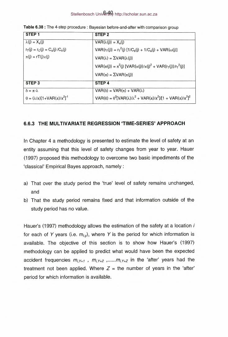
6-40
Table 6.38 : The 4-step procedure: Bayesian before-and-after with comparison group
STEP 1 STEP2
)c(j) = Xa(j) VAR{)cG}} = Xa(j)
rT(j) = rdj) = CaG>ICb(j) VAR{rT(j)} = r/(j) [1/Cb(j) + 1/Ca(j) + VAR{w(j)]
n(j) = rT(j)x(j) VAR()c) = LVAR{)c(j)}
VAR{n(j)} = n2(j) [VAR{x(j)}/x(j)2 + VAR{rT(j)}/rT2(j)]
VAR (n) = LV AR {n(j)}
STEP3 STEP4
6 = n-)c VAR(6) = VAR(n) + VAR()c)
8 = (Aln)[1 +VAR(n)/n2r1 VAR(8) = 82[VAR()C)1)c2+ VAR(n)/n2]/[1 + VAR(n)/n2]2
6.6.3 THE MULTIVARIATE REGRESSION 'TIME-SERIES' APPROACH
In Chapter 4 a methodology is presented to estimate the level of safety at an
entity assuming that this level of safety changes from year to year. Hauer
(1997) proposed this methodology to overcome two basic impediments of the
'classical' Empirical Bayes approach, namely:
a) That over the study period the 'true' level of safety remains unchanged,
andb) That the study period remains fixed and that information outside of the
study period has no value.
Hauer's (1997) methodology allows the estimation of the safety at a location ifor each of Y years (i.e. mi,y),where Y is the period for which information is
available. The objective of this section is to show how Hauer's (1997)
methodology can be applied to predict what would have been the expected
accident frequencies mi,Y+1 , mi,Y+2 , ...... mi,Y+Z in the 'after' years had the
treatment not been applied. Where Z = the number of years in the 'after'
period for which information is available.
Stellenbosch University http://scholar.sun.ac.za

6-41
6.6.3.1 THEORETICAL FRAMEWORK
Assume we have an entity i with Yyears of covariate and accident information
available in the 'before' period and similar information for Z years in the 'after'
period. Assume the treatment has been applied at the end of year Y. Since
the objective is to determine the number of accidents that would have
occurred had treatment not taken place the same reference group should be
used for the 'before' and 'after' periods.
These prediction models can be used to estimate E(mi.1), Etm; v),Etm; Y+1), ..... Etm; y+z} from which Ci.j can be determined as follows:
E(m )c.. = I.JI.J E(m
i)
...[6.29]
where j = 1,2,3 Y+Z.
The predicted number of accidents for each year in the 'after' period can be
estimated from Eqn. 6.30 :
my =Cy mlI, +z I, +z I,
...[6.30]
...[6.31]
where z = 1,2, ......Z.
The value of mi.1 can be determined from Equation 4.57 and VAR(mi.1) from
Equation 4.58.
Stellenbosch University http://scholar.sun.ac.za

6-42
EXAMPLE 6.14
In Example 4.9 the number of accidents on a 2km segment of road was estimated for each of
6 years. Assume now that at the end of year 6 this segment of road underwent major
rehabilitation. The road which had gravel shoulders to start of with now has surfaced
shoulders. For the after period 6 years worth of information is available. Because of
improvements to the road the traffic volumes increased significantly over the 'after' period.
The first step in the evaluation process is to determine what would have been the total
number of accidents in the 'after' had the road not been improved, given the increased traffic
volumes.
In Example 4.9 there was a reference group, consisting of a sufficient number of 2-lane road
segments with gravel shoulders, that was used to develop accident prediction models for
each of the 6 years in the before period. A similar reference group consisting of 2-lane road
segments with gravel shoulders can be used to develop accident prediction models for each
of the 6 years in the after period. For all these models assume j3 = 0.78. The ay+z values are
indicated in the table below.
Table 6.39 : Data and calculations
J aj Q"j E(m"j) c, mhj VAR(mi,j)
1 0.00271 1250 1.41 1.000 2.49 0.2647 0.00283 1410 1.62 1.15 2.86 0.3488 0.00277 1480 1.65 1.17 2.91 0.3609 0.00269 1502 1.62 1.15 2.85 0.34710 0.00280 1493 1.67 1.19 2.96 0.37211 0.00291 1520 1.77 1.25 3.12 0.41412 0.00278 1515 1.68 1.19 2.97 0.376
6 6Jti = Imp(i.Z) =17.66 and VAR(Jt,.) = IVAR(mp(i,z») = 2.22
z=1 z=1
The second step in the evaluation process is to determine the actual number of accidents that
occurred in the 'after' period. Assume the observed accident frequencies in the 'after' period
are - { 2, 1, 2, 0, 3, 3}.
In order to develop prediction models for each of the 6 years in the after period a reference
group consisting of 2-lane segments with surfaced shoulders, each with 6 years' worth of
accident data and traffic flow information, is required. Assume accident models have been
fitted to the data for each year and that the j3 parameter for all 6 models is 0.85.
Continue ...
Stellenbosch University http://scholar.sun.ac.za

6-43
Example 6.14 (Continued)
The a parameters for each year are indicated in the Table below. Assume also that the k
value of the model for the first year of the 'after' period = 5.5.
From Equation 4.57 and 4.58 :
ma(i) = (5.5 +11)/(5.5/1.95 + 5.96) = 1.88
VAR[ma(i,1l] = 1.88/(5.5/1.95 + 5.96) = 0.214
Table 6.40 : Data and calculations
j aj QI,j E[ma(l,j)] C(i,j) XI,j ma(l,j) VAR[(ma(l,j)]7 0.00205 1410 1.95 1.00 2.00 1.88 0.2148 0.00193 1480 1.91 0.98 1.00 1.84 0.2069 0.00185 1502 1.86 0.95 2.00 1.79 0.19410 0.00197 1493 1.97 1.01 0.00 1.90 0.21811 0.00201 1520 2.04 1.05 3.00 1.96 0.23412 0.00188 1515 1.90 0.97 3.00 1.83 0.203
TOTALS 5.96 11.00 11.21 1.270
6 6Ai = Imau.}) = 11.21 and VAR(A) = IVAR[mau.})] = 1.27
}=I }=l
Now applying the 4 step procedure:
Table 6,41 : The 4-Step procedure - calculations
STEP 1 STEP2
'A= 11.21 VAR('A) = 1.27
lt = 17.66 VAR(lt) = 2.22
STEP3 STEP4
6 = 17.66 - 11.21 = 6.45 VAR(6) = 1.27 + 2.22
8 = (11.21/17.66)[1+2.22/17.662]"1 = 0.63 VAR(8) = (0.63f[1.27 /11.212 +
ARF = 100(1-0.63) = 37 % 2.22/17.662]/[1 +2.22/17.662f = 0.00674
0(8) = 0.082
Stellenbosch University http://scholar.sun.ac.za

6-44
6.6.4 ALLOWING FOR CHANGES IN EXPOSURE
Improving the safety of a location may cause traffic volumes to increase
above what is normal. The simple before-and-after Bayesian methodology
estimates what the number of accidents would have been in the 'after' period
using traffic volumes applicable to the 'before' period. This is an acceptable
approach if the policy is to consider the accidents caused by additional traffic,
generated by a treatment, to be included in the estimation of the safety effect.
The assumption is that had the treatment not been undertaken the traffic flows
would not have increased and the additional accidents as result thereof would
not have occurred.
This approach however do not provide accurate estimates of the true (gross)
safety effect of a treatment. To obtain such a 'gross' estimate it is required to
estimate the number of accidents that would have occurred in the before
period if flows were equal to those observed in the 'after' period i.e. after
treatment has been applied. This estimate then becomes what would have
occurred in the after period had no treatment been undertaken.
To illustrate these concepts the following example is presented;
EXAMPLE 6.15
Consider a section of road which during the before period had an accident rate of 2 acc/mvkm
and an exposure of 2 mvkm. The road was then upgraded to the extent that the accident rate
decreased to 1 acc/mvkm and the exposure increased to 3 mvkm.
The number of accidents in the before period = 4. The simple before-and-after methodology
would assume that had the road not been upgraded a total of 4 accidents would have
occurred during the after period. This would give a safety effect 3/4 = 0.75. However if the
section of road in the 'before' period carried the same amount of traffic as in the 'after' period
a total of 6 accidents would have occurred, and since only 3 accidents occurred in the after
period ( at the same level of exposure) the safety effect 8 = 3/6 = 0.5.
Stellenbosch University http://scholar.sun.ac.za

6-45
The multivariate regression 'time-series' method can be adapted to allow for
changes in traffic volumes between the 'before' and 'after' period.
Assume we have a fixed before duration of tb years and a fixed after period of
ta years. In these periods Xb and Xa accidents were observed respectively.
Also assume that during the before and after periods the traffic flows were ab
and Oa respectively.
Using an appropriate regression model, based on a reference group related to
the entity's 'before' condition, the regression estimate of the total annual
number of target accidents for the 'before' (E[ mJ) and 'after' (E[ mP)) periods
can be determined, where E(mb) = f(Ob) and E(mp) = f(OaJ.
The expected annual number of accidents ( mb) can be determined from the
following Equations which can be derived from Equations 4.57 and 4.58 ;
...[6.32]
...[6.33]--+tE(m
b) b
Since the objective is to determine the total number of accidents that would
have occurred in the 'after' period had the treatment not been undertaken it is
necessary to determine the total expected number of accidents in a 'before'
period equal in length to the 'after' period:
...[6.34]
...[6.35]
Stellenbosch University http://scholar.sun.ac.za

6-46
To allow for changes in traffic flows between the 'before' and 'after' periods
Hauer (1997) recommends using a correction factor (C) which is estimated as
follows:
...[6.36]
The total number of accidents that would have occurred in the after period had
the treatment not been undertaken (mp) and its variance can be determined
as follows:
...[6.37]
...[6.38]
For the 4 step process:
Jt = ImpVAR(Jt) = I VAR(mp)
...[6.39]
...[6.40]
CASE STUDY 6.2
This case study is based on research done by Persaud et al. (2000) on crash reductions
following the installation of roundabouts in the United States.
In the states of California, Colorado, Florida, Kansas, Maine, Maryland, South Carolina and
Vermont a total of 24 intersections were converted to modern roundabouts between 1992 and
1997. Of the 24 intersections, 20 were previously controlled by stop signs and 4 were
controlled by traffic signals. Fifteen (15) of the roundabouts were single-lane circulation
designs and 9 had multi-lane designs.
For each intersection accident data were obtained for the periods before and after conversion.
The construction period and the 1st month after conversion were excluded from the analysis.
The lengths of the before and after periods varied in accordance with available accident data.
In no case was a period shorter than 15 months.
Stellenbosch University http://scholar.sun.ac.za
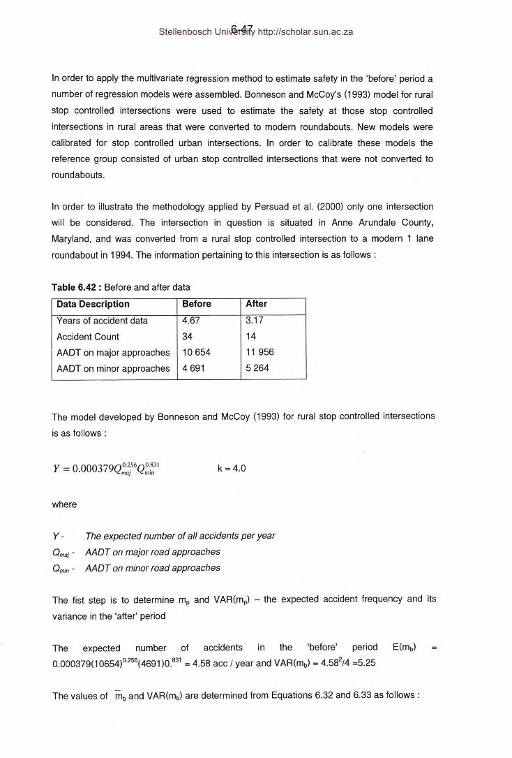
6-47
In order to apply the multivariate regression method to estimate safety in the 'before' period a
number of regression models were assembled. Bonneson and McCoy's (1993) model for rural
stop controlled intersections were used to estimate the safety at those stop controlled
intersections in rural areas that were converted to modern roundabouts. New models were
calibrated for stop controlled urban intersections. In order to calibrate these models the
reference group consisted of urban stop controlled intersections that were not converted to
roundabouts.
In order to illustrate the methodology applied by Persuad et al. (2000) only one intersection
will be considered. The intersection in question is situated in Anne Arundale County,
Maryland, and was converted from a rural stop controlled intersection to a modern 1 lane
roundabout in 1994. The information pertaining to this intersection is as follows:
Table 6.42 : Before and after data
Data Description Before After
Years of accident data 4.67 3.17
Accident Count 34 14
AADT on major approaches 10654 11 956
AADT on minor approaches 4691 5264
The model developed by Bonneson and McCoy (1993) for rural stop controlled intersections
is as follows:
Y = 0 000379Qo.256QO.831• maj mm k = 4.0
where
Y - The expected number of all accidents per year
Omaj - AADT on major road approaches
Omin - AADT on minor road approaches
The fist step is to determine mp and VAR(mp) - the expected accident frequency and its
variance in the 'after' period
The expected number of accidents in the 'before' period E(mb)
0.000379(10654)°·256(4691 )0.831 = 4.58 ace / year and VAR(mb) = 4.582/4 =5.25
The values of mb and VAR(mb) are determined from Equations 6.32 and 6.33 as follows:
Stellenbosch University http://scholar.sun.ac.za
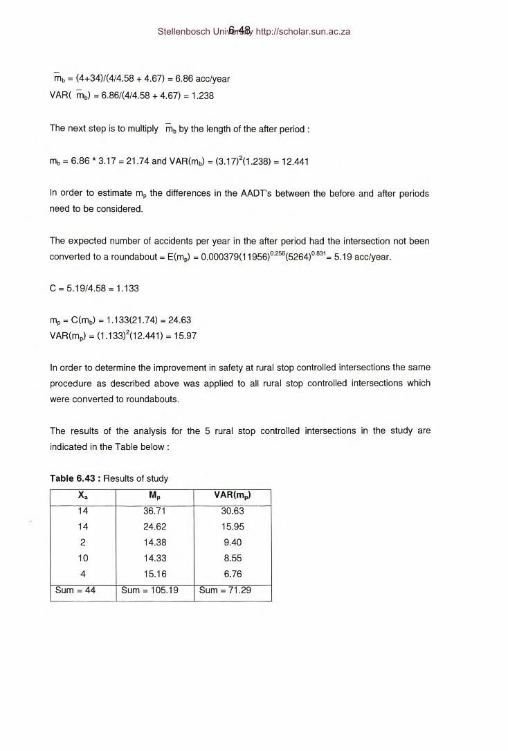
6-48
mb = (4+34)/(4/4.58 + 4.67) = 6.86 ace/year
VAR( mb) = 6.86/(4/4.58 + 4.67) = 1.238
The next step is to multiply mb by the length of the after period:
mb = 6.86 * 3.17 = 21.74 and VAR(mb) = (3.17)2(1.238) = 12.441
In order to estimate mp the differences in the AADT's between the before and after periods
need to be considered.
The expected number of accidents per year in the after period had the intersection not been
converted to a roundabout = E(mp) = 0.000379(11956)°·256(5264)°·831= 5.19 ace/year.
C = 5.19/4.58 = 1.133
mp = C(mb) = 1.133(21.74) = 24.63
VAR(mp) = (1.133)2(12.441) = 15.97
In order to determine the improvement in safety at rural stop controlled intersections the same
procedure as described above was applied to all rural stop controlled intersections which
were converted to roundabouts.
The results of the analysis for the 5 rural stop controlled intersections in the study are
indicated in the Table below:
Table 6.43 : Results of study
Xa Mp VAR(mp)
14 36.71 30.63
14 24.62 15.95
2 14.38 9.40
10 14.33 8.55
4 15.16 6.76
Sum = 44 Sum = 105.19 Sum = 71.29
Stellenbosch University http://scholar.sun.ac.za

6-49
The 4 step procedure can be applied as follows:
Table 6.44 : The 4-step procedure - calculations
STEP 1 STEP2
A = 44 VAR(A) = 44
n:= 105.19 VAR(n:) = 71.29
STEP 3 STEP4
b = 105.19 - 44 = 61.19 VAR(b) = 44 + 71.29 = 115.29
8 = (44/105.19)/[1 +71.29/105.192] VAR(8) = (0.416)2[1/44+71.29/105.192]/
=0.416 __ [1+71.29/1 05.192f = 0.005
ARF = 100(1-0.416) = 58 % 0(8) = 0.07
The approximate 95 % confidence interval of the ARF is 58±2(7) = {34 ; 74}. It can therefore
be concluded that the conversion of the rural stop controlled intersections in the study group
to roundabouts was effective in improving safety.
6.7 THE TREATMENT EFFECT
In the Conventional and Bayesian procedures discussed thus far entities were
lumped together and were treated as if they were one 'composite entity'. Only
the sum of the accident counts of all the entities was used to estimate the
safety effect associated with a treatment. Consider the simple before-and-
after procedure applied to the data of Case Study 6.1. It was estimated that
the average effect of the speed humps was a 53 % reduction with a standard
deviation of 5%. This estimated effect has been determined by considering all
12 sites together. The reduction of 53 % does not apply to any of the sites, nor
does the 5% standard deviation measure how the safety effect varies from
site to site. It represents the uncertainty surrounding the estimated value of
the average effect.
When a treatment is applied to a number of sites the effect of this treatment
will in all likelihood vary from site to site. For these different effects a mean
value as well as a variance can be determined. Should the variance be small
one could expect the treatment to have approximately the same effect on all
Stellenbosch University http://scholar.sun.ac.za

6-50
entities, and should the variance be large the effect of a treatment would be
difficult to predict.
The objective of the following section is to show how the standard 4-step
procedure can be expanded to estimate both the mean and the variance of
the safety effect.
6.7.1 THEORETICAL FRAMEWORK
Assume the same treatment has been applied to n entities that have indices
of effectiveness denoted as 8(1), 8(2), .... 8(n).
The average effect is given by :
...[6.41 ]
The sample variance is given by :
...[6.42]
The expected effect E(8) is determined as follows:
E(8) = ij ...[6.43]
The procedure to determine VAR(8) is as follows (Hauer; 1997):
a) Apply the single entity 4-step procedure to estimate 8(j) and VAR{8(j)} for
each entity.
b) Using the estimates 8(j) compute the sample variance.
c) Determine the average variance for all the entities: avg(V) = LVAR{8(j)}/n
d) VAR(8) can be estimated by : VAR(8) = S2( 8) - avg(V)
Stellenbosch University http://scholar.sun.ac.za

6-51
Table 6.45 : The 5-step procedure - estimating treatment effects
STEP 1 For j = 1 to n estimate AG)and :!tG).
Estimate A and :!t.
STEP2 For j = 1 to n estimate VAR{AG)} and VAR{:!tU)}
Estimate VAR(A) and VAR(:!t)
STEP3 Estimate 6 and 8
STEP4 Estimate VAR( 6) and VAR( 8)
STEPS Determine E(8) and VAR(8)
CASE STUDY 6.1 (continued)
Because of zero accidents in the 'after' period, VAR{8G)} for Site number 3 is not defined and
has this site has been left out of this analysis.
Table 6.46 : Data and calculations
Site :!t(j) AG> 6(j) 8G> ARFij) [%] VAR{6ij)} VAR{8ij)}1 29 17 12 0.57 43 46 0.0282 16 2 14 0.12 88 18 0.0074 8 1 7 0.11 89 9 0.0115 21 15 6 0.68 32 36 0.0486 34 27 7 0.77 23 61 0.0377 22 9 13 0.39 61 31 0.0228 13 2 11 0.14 86 15 0.0109 9 3 6 0.30 70 12 0.032
10 19 7 12 0.35 65 26 0.02211 19 4 15 0.20 80 23 0.01112 23 12 11 0.50 50 35 0.02913 36 23 13 0.62 38 59 0.02614 16 5 11 0.29 71 21 0.020
Sum 265 127 392 0.304Avg. 10.6 0.39 61 0.023Stdev. 3.1 0.22
The calculations to determine E(8) and VAR(8) are shown in Table 6.47.
Stellenbosch University http://scholar.sun.ac.za

6-52
Table 6.47 : The extended 4-step procedure - calculations
STEP 1 STEP 2
A = 127 VAR(A) = 127
Jt= 265 VAR(Jt) = 265
STEP3 STEP4
0= 10.6 VAR( 0)=3.1"=9.6
8 = 0.39 VAR( "8) = 0.222 = 0.048
STEPS
E(8) = 0.39
VAR(8) = 0.048 - 0.023 = 0.025 = 0.052
Avg(ARF) = 61 %
Whereas the 'composite' analysis gave an overall ARF of 53 % in this an average ARF of 61
% has been calculated.
6.8 CONCLUSION
This Chapter presented both Conventional and Bayesian before-and-after
methodologies to evaluate the effectiveness of road safety remedial measures
at entity level as well as at group-of-entity level.
It was stated that any observed change in safety between the 'before' and
'after' periods after the application of a remedial measure could consist of 4
components - the treatment effect, the regression-to-mean effect, the trend
effect and the exposure effect. Conventional and Bayesian methodologies
were presented to account for the trend and exposure effects. It was
concluded after, analysing the experimental data in Appendices A1 and A4,
that the Bayesian method performs considerably better than the Conventional
methods in eliminating the regression-to-mean effect even if short study
periods are used. From the experimental studies it was found that at the
group-of -entity level the length of the 'after' period had little influence on the
magnitude of the estimated treatment effect.
Stellenbosch University http://scholar.sun.ac.za

6-53
A methodology was also presented to determine the effectiveness of a
remedial measure at a location when there is reason to believe that the 'true'
level of safety changed from year to year during both the 'before' and 'after'
periods as a result of changes in traffic volumes and other confounding
factors.
It was shown how each of all these methodologies can be reduced to a simple
4-step procedure to determine measures of effectiveness and their variances.
Stellenbosch University http://scholar.sun.ac.za

CHAPTER 7
MULTIVARIATE REGRESSION MODELS
7.1 INTRODUCTION
From Chapters 3, 4, 5 and 6 it is evident that multivariate regression models
play an important role in applying the Empirical Bayesian methodology to
estimate safety, to identify and rank hazardous locations and to evaluate the
effectiveness of road safety remedial measures.
Multivariate regression models of data from a reference population are the
source of the estimates E(m) and VAR(m) which serve as prior estimates for
the Empirical Bayesian methodology.
An alternative method to estimate E(m) and VAR(m) is the method-ot-sample
moments. This method rest on the assumption that a linear relationship exists
between the number of accidents and traffic flow at a location i.e. that the
accident rate will remain constant irrespective of the traffic flow at a location.
Using multivariate regression models 'release' the Empirical Bayesian
approach from this assumption. The regression model equation can be
specified to allow for any hypothetical relationship between accidents and
traffic flows.
It is often required to estimate the safety of an entity for which a sufficient
reference population does not or cannot exist. Consider the example of a 2
lane rural road with lane widths of 3.55 mand 1.2 m gravel shoulders that has
a traffic flow of 2345 vehicles per day. The ideal reference group, in order to
apply the method-ot-sample moments, would consist of a sufficient number of
entities that share exactly the same geometric characteristics and traffic flows.
It is unlikely that there will be many, or even any, entities that would meet
these requirements.
Stellenbosch University http://scholar.sun.ac.za

7-2
By using a 'wider' reference group that consists perhaps of all 2-lane rural
entities irrespective of lane widths, shoulder widths and traffic volumes a
multivariate regression model can be developed from this reference group
data to estimate precise values of E(m) and VAR(m) for any entity,
irrespective of its geometric characteristics and traffic flows. For each entity
the regression model serves to create, in the words of Hauer (1997), an
'imaginary' reference group.
Multivariate regression models allow for determining how the level of safety at
an entity can expect to change with changing values of the covariates, such
as for example, with changes in traffic flows. This ability of regression models
forms the basis to predict what the level of safety would have been in the
future had no road safety measures been undertaken.
7.2 MULTIPLE REGRESSION ANALYSIS - AN INTRODUCTION
According to Gujarati (1988) the modern interpretation of regression is as
follows:
"Regression analysis is concerned with the study of the dependence of
one variable, the dependent variable, on one or more other variables,
the explanatory variables with a view to estimating and or predicting
the population mean or average value of the former in terms of the
known or fixed ( in repeated sampling) values of the latter. "
The regression process begins with specifying the objectives of the regression
analysis, including the selection of the dependent and independent variables.
The next step is to design the regression analysis, considering such factors as
sample size and the need for variable transformations. With the regression
model formulated the assumptions underlying regression analysis are first
tested for the individual variables. If all the assumptions are met then the
model is estimated. Once results are obtained, diagnostic analyses are
performed to ensure that the overall model meets the regression assumptions
Stellenbosch University http://scholar.sun.ac.za

7-3
and that no observations have undue influence on the results. The next stage
is the interpretation of the modelling results. Finally the results are validated to
ensure generalizability to the population. (Hair et al. ; 1995)
Probably the two most important steps of multivariate regression modelling is
(Hauer; 1997):
a) The choice of model form (model equation).
b) The estimation of parameters.
According to Hauer (1997) when developing a multivariate model these steps
may have to be repeated several times. The results of one cycle of analysis
provide motivation for modifications to the next cycle of analysis. Once
parameters have been estimated and residuals examined, the form of the
model may have to be revised, covariates may have to be added or dropped,
and parameters estimated anew.
Hauer (1997) states that multivariate regression modelling is based on the
belief that accident frequencies are associated in some orderly fashion with
causal factors, and that this belief is embodied in a model equation.
A model equation states in what way accident frequencies are a function of
the various covariate values
According to Hauer (1998) the choice of the model equation is more influential
in determining the quality of the results than is the statistical technique to
estimate the parameter values. The choice of model equation should reflect
prior knowledge and beliefs about the nature of the relationship, and also
insights obtained from an exploratory analysis of the data at hand. Hauer
(1997) states that the choice of model equation reflects beliefs, embodies
assumptions and impose limitations.
For example consider a model equation with the following form:
... [7.1]
Stellenbosch University http://scholar.sun.ac.za
7-4
E(m.) = LaQf3I I I
The expected accident frequency at location i.
The length of location i.
The traffic flow at location i.
The inclusion of Li in the model equation embodies the belief that a road
section along which all characteristics remain constant, will have a constant
expected accident frequency per unit length along the whole length of the
road. According to Hauer (1997) research has indicated that E(m) may not be
proportional to L if intersection accidents are included in the data set.
The inclusion of the a parameter serves the purpose of capturing the effect of
all factors except for the effect of traffic flows. The influence of the traffic flow
is accounted for separately by 0[3. The absence of a subscript i according to
Hauer (1997) reflects the belief that influencing factors such as weather,
economic conditions etc. have the same influence on all entities in the data
set, and by implication, for the entire population which the data set is thought
to represent.
The inclusion of a[3 reflects the belief that differences in 0 make for
differences in E(m). The lack of a subscript i for the f3 parameter reflects the
view that the safety of all entities depend on 0 in the same manner. Using the
form a[3 guarantees that E(m) = 0 as 0 = O. This form however has the
limitation that it cannot represent the scenario where accidents initially
increase with traffic flow, but at some point, as traffic flow increases further
accident frequency begins to diminish.
Data from the reference group used in regression modelling serves to test the
validity of the chosen model equation. If a covariate does not improve the fit of
the model to the data consideration could be given to omitting that variable. If
the introduction of a covariate improves the fit consideration could be given to
Stellenbosch University http://scholar.sun.ac.za

7-5
its inclusion in the model equation. Sometimes a model can be improved by
transforming one or more variables, or even combining one or more variables.
It is important to note that a calibrated model only represents what statistical
associations are present in the set of data at hand and that it does not
necessarily capture plausible cause-effect relationships.
7.3 ORDINARY MULTIPLE LINEAR REGRESSION
7.3.1 MODEL FORM
The most common model form is one where the model is a linear function of
its variables as well as its parameters.
...[7.2]
Y - Level of safety e.g. accident rate or
= 1 for event
= 0 for non-event
E -
Regression parameters
Independent variables e.g. roadway characteristics
Error term
a1- an-1 -
Xt- Xn-
To allow for a possible non-linear relationship between the dependent variable
and an independent variable one or more polynomial terms are included in the
model.
The need to include polynomial terms is generally indicated by means of an
exploratory analysis of the general form of the relationship between a
dependent variable and an independent variable. Constructing and then
evaluating a scatter plot of these two variables is generally a common
method.
Stellenbosch University http://scholar.sun.ac.za

7-6
To allow for the interaction of different driver, vehicle and/or roadway factors
moderator (interaction) effects are often included in the model.
Dummy variables are also used where an independent variable is of a
dichotomous or a categorical nature.
The following examples are presented to illustrate the different models that
have been used to model accidents using linear regression analysis.
Bester (1988) developed the following model to predict the accident rate for all
accidents using data from the Cape Province (now Western Cape, North
West, Eastern Cape and Northern Cape) and the province of KwaZulu-Natal.
TAR = -O.295-0.12S2 +O.710T2 +O.933Rq -O.648T(Rq)... [7.3]
where R2 = 0.278, and
S - Shoulder width (m).
T - Topography: 1= Flat; 2 = Rolling and 3 = Mountainous.
Rq- Riding quality.
The regression model contains two a= degree polynomials (~ and T~ as well
as an interaction term (T*R).
The model shown above has a additive form. A linear regression model can
also take a multiplicative form (Equation 7.4) which can then be linearised
using a logarithmic transformation (Equation 7.5).
Y X a,X a, X an=1= al I 2 . ..... n.. .[7.4]
... [7.5]
Stellenbosch University http://scholar.sun.ac.za
7-7
7.3.2 ASSUMPTIONS
According to Gebers (1998) the multiple linear regression method is based on
the following assumptions:
a) Independence - the Y observations are statistically independent of each
other.
b) Linearity - the value of Y is a linear function of X1, X2, X3 ..... X,
c) Homoscedasticity - the variance of Y is the same for any fixed
combination of X1, X2, X3 ..... Xn •
d) Normality - the errors of prediction (residuals) are normally distributed at
all levels of Y.
e) Measurement infallibility - the variates are free of measurement error.
f) Additivity - the effect terms (coefficient X variable values) of the
parameters can be combined in an additive fashion to estimate Y.
7.3.3 MODEL ESTIMATION
Linear multiple regression models are usually calibrated using the ordinary
least square (OlS) method. The objective is to find the parameters that will
minimise the following function (Gujarati ; 1988):
n
D =I (1'; - I-l) 2
i=1
... [7.6]
When the assumptions of homoscedasticity and/or independence do not hold,
Gujarati (1988) recommends that the weighted least square method be used
to estimate parameters.
Stellenbosch University http://scholar.sun.ac.za

7-8
7.3.4 PERFORMANCE
According to Vogt and Bared (1998) the use of linear regression models have
produced disappointing results because of the following reasons:
a) Accident frequencies and accident rates often do not follow a normal
distribution.
Traffic accidents are random discrete events that are sporadic in
nature. It is widely accepted that accident frequencies generally follow
a Poisson distribution (Miaau et al. ; 1992). Normalising accident
frequencies with exposure estimates to make accident rates appear to
be a continuous random variable, according to Vogt and Bared (1992),
do not change the fundamental discrete nature of accident data.
According to Gebers (1998) highly skewed Poisson-like variables
produce heteroscedastistic residuals, thereby introducing
'inconsistency' into the parameter estimates produced by OlS
techniques. The use of OlS multiple regression in the presence of
heteroscedasticity and non-normality results in regression models that,
although not biased, do not satisfy the property of minimum variance.
b) Accident frequencies for particular locations could be very small or
even zero, even if several years of accident data have been obtained
for those locations. Small integer counts, zero or close to zero do not
typically follow a normal distribution. Using models calibrated using
such small accident counts could predict negative values which is
obviously not possible.
The presence of locations with zero accidents is particularly critical
when using a multiplicative model linearized by a logarithmic
transformation. The logarithm of zero is not defined. locations with
zero observations can therefore not be included in the investigation.
Omitting such locations could be undesirable as traffic situations where
Stellenbosch University http://scholar.sun.ac.za

7-9
no accidents occur could be as important as locations where accidents
occur.
Miaau and Lum (1993) concluded that linear regression models lack the
distributional properties to adequately describe random, discrete, non-
negative and sporadic vehicle accidents. Using linear regression method is
therefore not a suitable method to estimate E(m) and VAR(m).
According to Miaau et al. (1992) the problems associated with the linear
regression approach to modelling accidents can be overcome by using the
Generalised Linear Modelling technique.
7.4 GENERALISED LINEAR MODELLING
According to McCullough and Neider (1989) Generalised Linear Models
(GLM) is a natural generalisation of classical linear models . The class of
generalised linear models includes log-linear models for count data ( such as
accident counts).
The GLM approach allows the analyst to use dependent variables which may
be bounded or which may have a non-continuous or a non-normal distribution.
Accident frequencies for example are bounded in the sense that they can
never be less than zero. As previously stated it also follows a non-normal
distribution.
7.4.1 THEORETICAL FRAMEWORK
According to McCullough and Neider (1989) the GLM approach assumes that
there is a dependent variable Y and one or more independent variables (X/s)
whose values influence the distribution of Y and that the independent
variables influence the distribution of Y through a single linear function only.
This function is called the linear predictor and is written as :
... [7.7]
Stellenbosch University http://scholar.sun.ac.za

7-10
The linear predictor may contain polynomials, moderator effects and/or
dummy variables as long as it remains linear in its coefficients.
The linear prediction function is related to the expected value of an
observation via a link function. There is one link function that is theoretically
related to the error structure of the data on the basis of its underlying
distribution. (Bonneson and McCoy; 1997)
From McCullough and Neider (1989) :
... [7.8]
!li =g-l(l1) =g-l(Lf)kXik)k=l
... [7.9]
The GLM technique relies on the Maximum Likelihood Estimation approach to
estimate the coefficients of the model. This approach involves estimating the
f)-coefficients that will maximise the log-likelihood function.
As with the link function there is a log-likelihood function that is theoretically
related to the error structure of the data on the basis of it underlying
distribution.
In the following section the application of the GLM approach to estimate log-
linear Poisson and Negative Binomial models will be presented.
7.4.2 POISSON MODEL FORMULATION
According to Vogt and Bared (1998) the Poisson regression approach regards
the number of accidents in a given space-time region as a random variable
that takes values 0,1,2 ..... with probabilities obeying the Poisson distribution.
Stellenbosch University http://scholar.sun.ac.za

7-11
Miaou et al. (1992) provides the following formulation of the Poisson
regression model:
Consider a set of n locations. Let Yi be the number of accidents of a
particular type at location i during a year. Assume Ei is the exposure at this
location. Associated with each location i there is a k X 1 covariate vector
denoted by Xi = ( Xi1 = 1, Xi2, , Xi/J', describing its geometric
characteristics, traffic conditions and other relevant attributes. It is postulated
that Yi ( I = 1 to n) are independent and each is Poisson distributed as :
... [7.10]
Where
i = 1,2, nYi = 0,1,2 .....
R, is the accident rate at location i and is expected to vary from one location to
another depending on its covariates Xi. For each location i the Poisson model
implies that the mean is equal to the variance.
If Xi and Ei are given with negligible uncertainties and R, is assumed to be
constant then Equation 7.10 becomes a classical Poisson regression model.
The uncertainties in Ei and R, introduce extra variations (or overdispersion) in
the Poisson model. The consequences of ignoring the extra variations in the
Poisson regression are that the maximum likelihood estimates (MLE's) of the
regression coefficients, (3, under the classical Poisson model are still
consistent; however, variances of the estimated coefficients would tend to be
underestimated. In other words the significance levels of the estimated
coefficients may be overstated (Miaou et al. ;1992).
Stellenbosch University http://scholar.sun.ac.za

7-12
The link function for the Poisson model is (McCullough and Neider; 1989) :
11= lnlul ... [7.11]
... [7.12]
... [7.13]
It is evident that the predicted value I-" will always be greater then zero.
If the dependent variable is a rate which is expressed as accidents per unit of
exposure then the expression above can be modified as follows:
... [7.14]
... [7.15]
The logarithm of exposure is treated as an offset and is subtracted initially
from the logarithm of the number of accidents before fitting the expression.
This approach is based on the assumption that there is a linear relationship
between exposure and accidents.
To allow for a possible non-linear relationship between accidents and
exposure Equation 7.14 can be written as :
... [7.16]
... [7.17]
Stellenbosch University http://scholar.sun.ac.za

7-13
To estimate the safety of two-way stop controlled intersections on rural
highways in Minnesota, USA, Bonneson and McCoy «1993). developed a
model with the following form:
... [7.18]
A - Annual accident frequency.
Tm- Major road traffic demand (veh/day).
Tc - Minor road traffic demand (veh/day).
The linear predictor function for this type of multiplicative model takes the
following form:
... [7.19]
Where n is the number of years of observations and In(n) is termed the offset
variable.
To predict the effect of median treatments on urban arterial safety Bonneson
and McCoy (1997) used a model with the following form:
... [7.20]
where
A - Annual accident frequency.
ADT- Average daily traffic demand.
L - Street segment length.
Xi - Selected traffic and geometric characteristics.
In this case the linear predictor takes the form:
... [7.21]
Stellenbosch University http://scholar.sun.ac.za

7-14
It is often found with the modelling of accidents that the variance of the
dependant variable exceeds its mean. This is due to it not being practical nor
possible to include and account for all variables that could influence accident
occurrence. In such cases Vogt and Bared (1998) recommend that negative
binomial models be used in accident modelling.
7.4.3 NEGATIVE BINOMIAL MODEL FORMULATION
According to Poch and Mannering (1996) Negative Binomial models
generalise the Poisson form by permitting the variance to be overdispersed,
equal to the mean plus a quadratic term in the mean whose coefficient is
called the overdispersion parameter. When the parameter is zero a Poisson
model results. When it is larger than zero, it represents variation above and
beyond that due to the high way variables present in the model.
If accident frequencies are overdispersed the probability density function of Yi
is as follows (Vogt and Bared; 1998):
Where k is the over-dispersion parameter.
... [7.22]
And
var(y.) = Il. + 4,tJ, r, k... [7.23]
If K = 1Ik = 0 then the negative binomial reduces to the Poisson model. The
larger the value of K the more variability there is in the data over and above
that associated with the mean !-l.
Stellenbosch University http://scholar.sun.ac.za
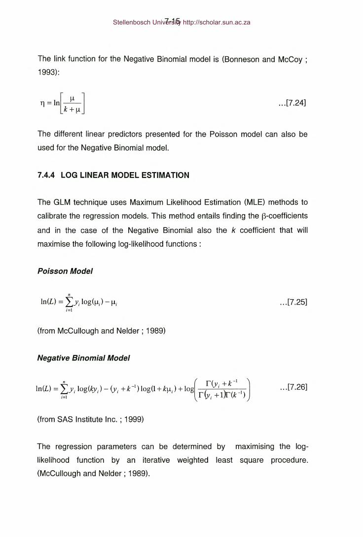
7-15
The link function for the Negative Binomial model is (Bonneson and McCoy;
1993):
Y] = In[-!-t ]k+!-t
... [7.24]
The different linear predictors presented for the Poisson model can also be
used for the Negative Binomial model.
7.4.4 LOG LINEAR MODEL ESTIMATION
The GLM technique uses Maximum Likelihood Estimation (MLE) methods to
calibrate the regression models. This method entails finding the l3-coefficients
and in the case of the Negative Binomial also the k coefficient that will
maximise the following log-likelihood functions:
Poisson Model
n
In(L) = LYi loglu.) - !-tii=1
... [7.25]
(from McCullough and Neider; 1989)
Negative Binomial Model
n ( r(y. +k-I JIn(L)=LYi1og(ky)-(Yi+k-l)log(1+k!-t)+log (y l)r -I
i=1 I" i + 1 (k )... [7.26]
(from SAS Institute Inc. ; 1999)
The regression parameters can be determined by maximising the log-
likelihood function by an iterative weighted least square procedure.
(McCullough and Neider; 1989).
Stellenbosch University http://scholar.sun.ac.za

7-16
According to McCullough and Neider (1989) an equivalent approach to
maximising the log-likelihood function is by minimising the deviance.
The deviance is given by :
... [7.27]
Where
Lf - Log-likelihood value for the 'null' model.
Lm - Log-likelihood value for the model under consideration.
The log-likehood value for the 'null' model can be determined from fitting a
model to the accident data that consist of a constant term only ( no variables
included).
According to McCullough and Neider (1989) the deviance function for a
Poisson model is :
D = 2" (Y In(Y / II .) - (Y - II .)LJ I I r, I rt... [7.28]
Gebers (1998) states that a fundamental assumption underlying ordinary
least squares linear regression analysis is that all random errors have the
same variance at difference values of the explanatory variable. The
homogeneity of residual error assumption is invariably violated with accident
data because of the direct proportional relationship between the means and
variances of the arrays, thereby introducing heteroscedasticity into the
distribution of the residuals. For this reason the OlS technique is not suitable
to calibrate models based on the GlM technique.
Saccomano and Buyco (1988) demonstrated that the weighted least squares
algorithm (WlSA) for calibrating log-linear models produces high residuals for
cells that are characterised by low cell memberships in the contingency table
Stellenbosch University http://scholar.sun.ac.za
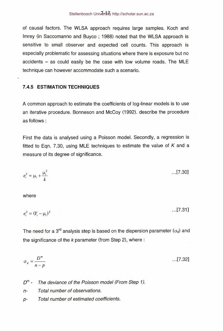
7-17
of causal factors. The WLSA approach requires large samples. Koch and
Imrey (in Saccomanno and Buyco ; 1988) noted that the WLSA approach is
sensitive to small observer and expected cell counts. This approach is
especially problematic for assessing situations where there is exposure but no
accidents - as could easily be the case with low volume roads. The MLE
technique can however accommodate such a scenario.
7.4.5 ESTIMATION TECHNIQUES
A common approach to estimate the coefficients of log-linear models is to use
an iterative procedure. Bonneson and McCoy (1992). describe the procedure
as follows:
First the data is analysed using a Poisson model. Secondly, a regression is
fitted to Eqn. 7.30, using MLE techniques to estimate the value of K and a
measure of its degree of significance.
. .. [7.30]
where
... [7.31]
The need for a 3rd analysis step is based on the dispersion parameter (ad) and
the significance of the k parameter (from Step 2), where:
Dma ---d -
n-p... [7.32]
om - The deviance of the Poisson model (From Step 1J.n- Total number of observations.
p- Total number of estimated coefficients.
Stellenbosch University http://scholar.sun.ac.za
7-18
If the dispersion parameter is greater than 1 and the k parameter is
significant, a 3rd analysis step is conducted using the Negative Binomial
model with the value of k from Step 2. The residuals from this analysis are
then analysed in a 4th step to determine a new k parameter. Steps 3 and 4 are
repeated until convergence on a value of k.
7.4.6 ESTIMATION TOOLS
Generalised linear models can be estimated using specialised statistical
software. The most common software packages used by road safety
researchers to estimate log-linear models are the GLIM software package and
the non-linear regression procedure (NLlN) in the SAS statistical software.
7.4.7 MODEL EVALUATION
According to Vogt and Bared (1998) there are three important tests for an
acceptable model. These are as follows:
a) The estimated regression coefficient for each independent variable should
be statistically significant i.e. one should be able to reject the null
hypothesis that the coefficient is zero.
b) Engineering and intuitive judgements should be able to confirm the validity
and practicality of the sign and rough magnitude of each estimated
coefficient; and
c) Goodness-of-fit measures and statistics should indicate that the variables
do have explanatory and predictive power.
An important assumption of the GLM technique is that there should be no
correlation between different observations. In other words all the observations
should be independent of one another. There are situations in which a
possibly of dependence between observations may arise, for instance treating
Stellenbosch University http://scholar.sun.ac.za

7-19
each year of accident data at a particular site as a separate observation, or
considering the accidents on intersection approaches as separate
observations, where it is quite possible that accident numbers on the
approaches of the same intersection might be correlated with one another.
McCullough and Neider (1989) propose that goodness-of-fit be evaluated on
the basis of the deviance or on the generalised Pearson X2 statistic.
The deviance of a model m is :
... [7.32]
Where Lf is the log-likelihood that would be achieved if the model gave a
perfect fit and Lm is the log-likelihood of the model under consideration.
The overdispersion parameter (ad) is given by :
Dma -_-d -
n-p... [7.33]
where
om - Deviance.
n - Number of observations.
p - Number of coefficients estimated.
According to Vogt and Bared (1998) if the value of the overdispersion
parameter (ad) is larger then 1 then the Poisson model is inappropriate
because of overdispersion due to missing variables and/or measurement
error. In such cases a Negative Binomial models is generally indicated.
The Pearson chi-square statistic is defined by (McCullough and Neider
1989) as:
Stellenbosch University http://scholar.sun.ac.za
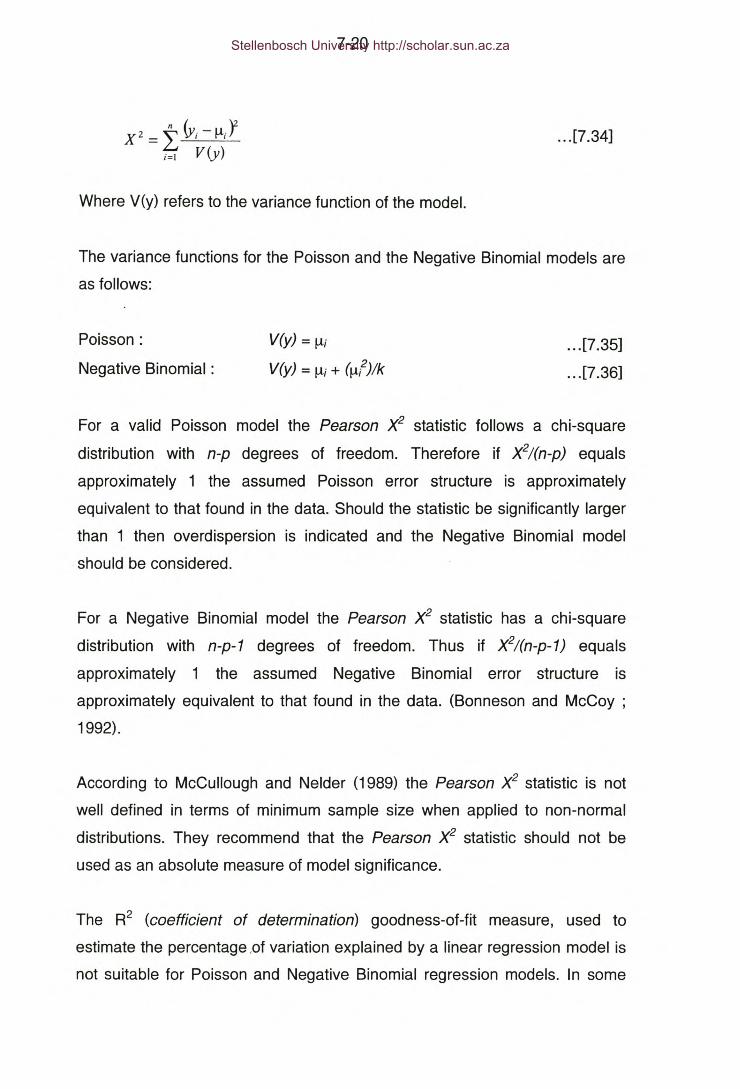
7-20
... [7.34]
Where V(y) refers to the variance function of the model.
The variance functions for the Poisson and the Negative Binomial models are
as follows:
Poisson:
Negative Binomial:
vry) = !-li
vry) = !-li + (!-lP)/k
... [7.35]
... [7.36]
For a valid Poisson model the Pearson X2 statistic follows a chi-square
distribution with n-p degrees of freedom. Therefore if X2/(n-p) equals
approximately 1 the assumed Poisson error structure is approximately
equivalent to that found in the data. Should the statistic be significantly larger
than 1 then overdispersion is indicated and the Negative Binomial model
should be considered.
For a Negative Binomial model the Pearson X2 statistic has a chi-square
distribution with n-p-1 degrees of freedom. Thus if X2/(n-p-1) equals
approximately 1 the assumed Negative Binomial error structure is
approximately equivalent to that found in the data. (Bonneson and McCoy ;
1992).
According to McCullough and Neider (1989) the Pearson X2 statistic is not
well defined in terms of minimum sample size when applied to non-normal
distributions. They recommend that the Pearson X2 statistic should not be
used as an absolute measure of model significance.
The R2 (coefficient of determination) goodness-of-fit measure, used to
estimate the percentage .ot variation explained by a linear regression model is
not suitable for Poisson and Negative Binomial regression models. In some
Stellenbosch University http://scholar.sun.ac.za

7-21
instances the R-square measure may provide values greater then one,
particularly for non-linear models. (Vogt and Bared; 1998)
A more subjective measure of model fit can be obtained from a graphical plot
of prediction ratio vs. the estimate of the expected accident frequency. The
prediction ration is described as the normalised residual (Bonneson and
McCoy; 1992) :
PR = !-li - Y;I ~V(y)
... [7.38]
where V(y) is the variance function.
This type of plot yields a visual assessment of the predictive ability of the
model over the full range of !-li'S. A well fitting model would have the
prediction ratios symmetrically around zero.
7.5 SUMMARY and CONCLUSION
This Chapter provided a brief overview of the processes involved in
developing accident prediction models using multivariate regression
techniques. It was shown that the classical linear regression approach is not a
suitable approach to model accident frequencies and accident rates. An
alternative approach called Generalised Linear Modelling (GLM) was
presented and details on two log linear modelling approaches - Poisson
regression and Negative Binomial were presented. It was shown that these
modelling approaches are suitable to model accident data. To illustrate how
the concepts discussed are applied in practice a case study will be presented
to show how the Negative Binomial modelling approach was used to estimate
the safety of signalised intersections.
Stellenbosch University http://scholar.sun.ac.za

7-22
CASE STUDY 7.1
ESTIMATION OF SAFETY AT SIGNALISED INTERSECTIONS
By Hauer E, Ng JeN and Lovell J (1988)
Introduction
Hauer et al. (1988) developed a number of microscopic and macroscopic
models to measure the safety at signalised intersections if the vehicular flows
using it are known.
Data
They selected for analysis a set of intersections that are similar in most
respects except for traffic flows and accident history. The data set consisted
of accident data and traffic flow information for 145 four-legged, fixed-time,
signalised intersections in Metropolitan Toronto that carry two-way traffic on
all approaches and have no turn restrictions. Most are on straight, level sites
with a speed limit of 60 km/h.
The accident data was collected over a three year period - 1982 to 1984. For
each approach one day manual traffic counts were conducted. Turning and
through moving flows were thus available for each approach for the AM-peak,
the PM-peak and the off-peak periods. All vehicle counts are for weekday
conditions.
The analysis was confined to the AM peak ( 07:00 - 09:00) the PM-peak
(16:00 - 18:00) and the following off-peak period - 10:00 to 15:00. The
periods from 09:00 to 10:00 and 15:00 to 16:00 were excluded because the
signal timings changed during these periods.
Stellenbosch University http://scholar.sun.ac.za
7-23
The accident dataset only contained information on accidents involving two
vehicles. This type of accident accounted for 81 % of the total accidents.
Model development
One of the objectives of the study was to relate accidents to the traffic flows to
which they belong. Fifteen (15) accident patterns were identified and are
shown in Figure 6. Accidents in each pattern were defined by the manoeuvres
of the two vehicles before colliding. The common categorisation by initial
impact type such as rear-end, angle, turning movement, sideswipe etc. was
avoided because of its ambiguity.
The next step was to decide on the model form for each one of these 15
accident patterns. The guiding principle in this process was the wish to
ensure a satisfactory fit with parsimony of parameters and without violation of
the obvious logical requirements.
To determine the most appropriate model form exploratory data analysis was
first undertaken. The following example is presented on how a model form
was developed for Accident Pattern 6.
Table 7.1 gives the average number of accidents per site in 3 years for five
ranges left1 turning flows versus five ranges of the straight-through flow. The
irregular flow ranges were selected so that each row and column would have
approximately one-fifth of all accidents
I 'Left' refers to the Canadian/USA driving convention. This should read 'right' for a SouthAfrican interpretation.
Stellenbosch University http://scholar.sun.ac.za

7-24
Table 7.1 : Traffic flows for accident pattern 6.
Straight- Left turning flow ROW
Through TOTAL
Flow 0-521 522-821 822-1033 1034 -1408 1409 - 4038
0-3525 0.49 0.60 0.63 1.57 0.56 0.643526 - 4825 0.61 1.00 1.91 1.24 1.75 1.164826 - 5941 1.27 1.22 1.44 1.36 2.79 1.635942 - 7771 1.31 1.40 3.10 2.20 1.40 1.787772 - 12091 1.67 2.75 2.63 4.50 3.27 2.73
Total 0.74 1.05 1.56 1.93 1.91 1.26
The relationship between accidents and left-turning flows are shown in Figure
7.1.
2.2
2.0
1.8(il(ij 1.6al>-~en 1.4ëal"Cl'0 1.2o«ëÓ 1.0z
0.8
0.60-521 822-1033 1034-1408 1409-4038522-821
Left Turning flows (F2)
Figure 7.1 : Accident frequency vs. left turning flows.
Stellenbosch University http://scholar.sun.ac.za

7-25
The relationship between straight through flows and accident frequency is
shown in Figure 7.2.
3.2
2.8
ti)2.4
(ijQl>-
2.0~(/)
ëal"Cl 1.6'0u<l:(5
1.2Óz
0.8
0.40-3525 3526-4825 4826-5941 5942-7771 7772-12091
Straight-Through flows (F1)
Figure 7.2 : Accident frequency vs. straight through flows
From Figure 7.2 it appears that accidents are proportional to the through
traffic (F1) i.e. A oe F1 and from Figure 7.1 that the increase of accidents with
the left turning flow (F2) appears to be non-linear i.e. A oe F2b1where b1 < 1.
A suitable model form for accident pattern 6 is thus:
A = af:.F/'
This process of data analysis was applied to all 15 accident patterns and the
subsequent model forms are indicated in Table 7.2.
All these models are mutiplicative in nature and it was assumed they all have
a negative binomial error structure.
Stellenbosch University http://scholar.sun.ac.za

7-26
Coefficient Estimation
The coefficients were estimated using the GLIM ( Generalised Linear
Interactive Mode!). The process of coefficient estimation was iterative. Firstly
a value for k was assumed and then proceeded to estimate the j3-coefficients
using GLIM. The residuals were calculated and from the residuals a new
value of k was determined. This k value was then fed back into the model to
calculate a new set of j3-coefficients. The residuals and a new k value were
calculated again and this process was repeated until convergence.
Interpretation
Hauer et al. (1998) concluded that a closer examination of how the frequency
of accidents depend on traffic flows from which they arise reveals that
preconceived ideas are sometimes not supported by empirical evidence. The
results in Table 7.2 reveal that accident frequencies between vehicles
travelling in the same direction is proportional to the traffic flows in that
direction (Patterns 1 and 2). The frequency of accidents between left turning
and through moving vehicles is proportional to the flow of through traffic but
less than proportional to the flow of left-turning vehicles. (Pattern 6). The
frequency of accidents between right-angle flows (Pattern 4) is not influenced
by the major road flow but by the minor road flow which exerts a great deal of
influence initially, but that this tapers off as flows become larger.
According to Hauer et al. (1988) these observations lead to the conclusion
that the popular assumption that intersection accidents are proportional to the
sum of entering volumes is not supported by empirical evidence for common
accident types. They state it is therefore not correct to use intersection
accident rates calculated on the basis of the sum of entering volumes to
compare the safety of two different intersections, or between 'before' and
'after' periods.
Stellenbosch University http://scholar.sun.ac.za
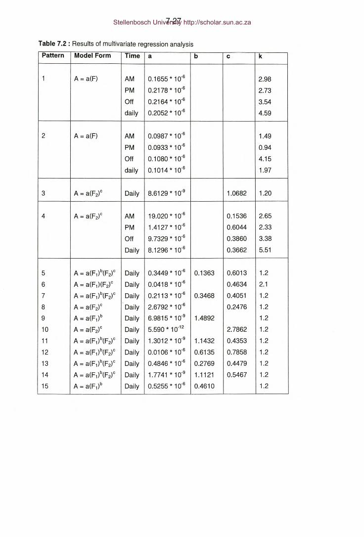
7-27
Table 7.2 : Results of multivariate regression analysis
Pattern Model Form Time a b c k
1 A = a(F) AM 0.1655 * 10.6 2.98
PM 0.2178 * 10.6 2.73
Off 0.2164 * 10.6 3.54
daily 0.2052 * 10-6 4.59
2 A = a(F) AM 0.0987 * 10-6 1.49
PM 0.0933 * 10-6 0.94
Off 0.1080 * 10-6 4.15
daily 0.1014*10-6 1.97
3 A = a(F2)C Daily 8.6129 * 10-9 1.0682 1.20
4 A = a(F2)C AM 19.020 * 10-6 0.1536 2.65
PM 1.4127 * 10-6 0.6044 2.33
Off 9.7329 * 10-6 0.3860 3.38
Daily 8.1296 * 10-6 0.3662 5.51
5 A = a(F1)b(F2)C Daily 0.3449 * 10-6 0.1363 0.6013 1.2
6 A = a(F1)(F2)C Daily 0.0418 * 10-6 0.4634 2.1
7 A = a(F1)b(F2)C Daily 0.2113 * 10-6 0.3468 0.4051 1.2
8 A = a(F2)C Daily 2.6792 * 10-6 0.2476 1.2
9 A = a(F1)b Daily 6.9815 * 10-9 1.4892 1.2
10 A = a(F2)C Daily 5.590 * 10-12 2.7862 1.2
11 A = a(F1)b(F2)C Daily 1.3012 * 10-9 1.1432 0.4353 1.2
12 A = a(F1)b(F2)C Daily 0.0106 * 10-6 0.6135 0.7858 1.2
13 A = a(F1)b(F2)C Daily 0.4846 * 10-6 0.2769 0.4479 1.2
14 A = a(F1)b(F2)C Daily 1.7741 * 10-9 1.1121 0.5467 1.2
15 A = a(F1)b Daily 0.5255 * 10-6 0.4610 1.2
Stellenbosch University http://scholar.sun.ac.za

7-28
1 2 3 F1
_j L ._j L _jl LI)tiIFtti IF!i
4 5 6
_j jb F2_j L _j~2F;lt~, i IF,tiF1
7 _j L 8 _j L 9 _j L~F2 l~tiF2 I~i'F1ti F1
10 _jLL 11 _j L 12 -.JtLi1iF2~I~ Ili'F1
13 _j L 14 _j L 15 _j L
IF!rr-F2 j~FI rriIF, i 2
F
Figure 7.3 : Intersection accident patterns (Right hand driving rule)
Stellenbosch University http://scholar.sun.ac.za
CHAPTER 8
SUMMARY AND CONCLUSIONS
When implementing road safety remedial programmes it is required to analyse
road traffic accident data in a manner that will ensure the effective and
efficient utilisation of often scarce resources.
This thesis has shown how accident data could be analysed to measure
safety at road entities, to identify and rank hazardous locations and how to
determine the effectiveness of road safety remedial measures.
Having valid and reliable estimates of the true level of safety of an entity or a
group of entities is fundamentally important for the efficient identification and
ranking of hazardous locations and determining the effectiveness of remedial
measures.
The methods available to measure safety can be divided into two categories,
a) Conventional methods and b) Bayesian methods. The Conventional
methods are based on the assumption that the level of safety at a location is
fixed and that it can be determined by the observed accident experience,
while the Bayesian methods assume that the true level of safety at a location
is unknown, a variable and that the observed accident experience can
provide a clue as to what the real value is.
It has been shown that the conventional accident rate measure to measure
safety on road segments produces results that are generally not reliable. The
main reason for this is that a non-linear relationship normally exists between
accident frequencies and exposures. It can be concluded therefore that
should the Safety Performance Function be non-linear accident rates should
not be used to compare time periods nor different locations with each other.
Similarly it has been shown that the common sum-ot-flows accident rate
measure to measure the safety of intersections is logically unsatisfactory for a
Stellenbosch University http://scholar.sun.ac.za
8-2
number of reasons. Using a safety measure based on the product of flows is
generally considered to be more appropriate.
Safety Performance Functions can be used to overcome the inherent
shortcomings of the conventional accident rate measures for segments and
intersections. However SPF's are prone to a certain degree of bias if average
traffic flow values such as AADT's are used, or if the SPF serves as an
aggregate function for different accident types, each of which are associated
with significantly different levels of risk. Depending on the form of the SPF, the
chosen accident measure, the variability in traffic flows etc. this bias could be
significantly large.
When identifying hazardous locations it has been shown that it is important to
use methodologies that will maximise the number of true positive
identifications and minimise the number of false positive identifications. As
illustrated in Example 5.11 it could be the case that a large degree of true
positive identification can only be obtained at the expense of the false positive
identification rate. In assessing the overall efficiency of a hazardous location
identification method it becomes necessary to weigh the relative cost and
consequences of false negative and false positive identifications. A false
negative identification would let a true hazardous location continue untreated
with potentially very serious consequences in terms of loss of life, injury and
damage to property, while a false positive identification could cause scarce
resources to be allocated to locations with a low potential for accident
reduction.
The identification methods presented in this work were divided into two
categories, namely : a) Conventional methods, and b) Bayesian methods.
Applying these methods to the experimental data in Appendix A1 revealed
that it appears the Bayesian methods could produce lower true positive
identification rates as well as lower false positive identification rates than the
Conventional methods.
Stellenbosch University http://scholar.sun.ac.za

8-3
It could often be the case that to further investigate all the identified hazardous
locations would require more financial resources than are available. Decisions
are then required on which hazardous locations to investigate and which not
to investigate further. The most common approach is to rank the identified
hazardous locations according to some criteria and then to start investigating
from the 'top' in descending order until the budget for such road investigations
are depleted.
A number of possible criteria to rank hazardous locations were presented.
These criteria can be roughly divided into three groups - those that make use
of Conventional safety estimates, and those make use of Bayesian safety
estimates and regression models, and finally those that combine Conventional
or Bayesian estimates with accident severity information.
Criteria based on accident rates have been shown to produce a bias in favour
of locations with low accident totals and low traffic volumes i.e. sites whose
accident reduction and potential economic returns are low. Criteria based on
accident numbers have been shown to produce a bias in favour of locations
with high accident totals and traffic volumes. Since one of the overall
objectives of a remedial programme is to improve the efficiency of the road
transportation system by reducing accidents, the PAR (Potential Accident
Reduction) index is a popular method of ranking hazardous locations. The
PAR index provides a measure of the expected accident reduction at a
location and therefore also a measure of the expected economic return at a
location.
To quantify the potential accident reduction associated with specific remedial
measures (e.g. shoulder widening) the PAR index can be estimated using the
Bayesian safety estimates and appropriate multivariate regression models.
Research by Persaud et al. (1999b) has shown that this approach generally
produces better results than methods based solely on Conventional and
Bayesian safety estimates. Persaud et al. (1999a) have also shown how this
method of estimating the PAR index can be combined with accident severity
information and accident costs to rank hazardous locations.
Stellenbosch University http://scholar.sun.ac.za

8-4
Evaluating the effectiveness of a remedial measure/s is a very important last
step when implementing a accident remedial programme. This knowledge is
required to determine the actual cost effectiveness of a remedial measure and
to provide factual guidance for the future.
The determination of the effectiveness of a remedial measure basically
involves estimating what would have been the level of safety in the 'after'
period had the remedial measure not been implemented and then to compare
this estimate with the level of safety actually observed in the 'after' period.
The observed number of accidents in the 'before' period are most often used
in procedures to determine the 'what would have been' level of safety in the
'after' period. In doing this a number of factors should be considered and
allowed for, these are - a) the regression-to-mean effect, b) exposure effect
and c) trend effect.
The regression-to-mean effect occurs because of the non-random manner in
which hazardous locations are chosen. Since hazardous locations are
normally selected on the basis of a high number of accidents or accident rate
in the before period it is reasonable to expect that, because of the random
nature of accidents, the accident rate/number in the after period could be less
even in the absence of any remedial measures. The regression-to-mean
effect is particularly relevant when conventional safety estimates are used. It
has been shown however that the magnitude of this effect decreases as the
study period increases.
The regression-to-mean effect can largely be eliminated by using Bayesian
safety estimates.
The exposure effect becomes particularly relevant if there has been an
increase/decrease in the traffic volumes using a location between the 'before'
and 'after' periods. Conventional and Bayesian methodologies were presented
Stellenbosch University http://scholar.sun.ac.za

8-5
on how to eliminate the exposure effect when determining the effectiveness of
a remedial measure.
The trend effect is of importance if there have been changes in the traffic,
road, social environments etc. between the 'before' and 'after' periods.
Changes in the traffic composition, climate, urban structure, law enforcement
quality/quantity etc. could all for example have an impact on the level of safety
at a location. The trend effect is accounted for by using a comparison group. A
methodology is presented on how to choose the most appropriate comparison
group for a before-and-after with comparison group study. Guidelines have
also been provided on how to design such a study and how to interpret the
results.
A Bayesian methodology based on the use of multivariate regression models
for each year in the study period is a suitable methodology to eliminate the
regression-to-mean effect and also to account for any trend and exposure
effects. This methodology as proposed by Hauer (1997) is an improvement on
other Bayesian and Conventional methodologies because it does not assume
that the 'true' level of safety during either the before or after periods remained
constant for the whole period. It is therefore based on the realistic assumption
that the true level of safety of a location may change from year to year for a
variety of reasons.
Many of the methodologies to measure safety, to identify and rank hazardous
locations and to determine the effectiveness of remedial measures rely on the
availability of suitable multivariate regression models. It has been shown that
the ordinary least squares regression technique produce models that are not
suitable. Instead the generalised linear modelling approach was presented as
an alternative.
Stellenbosch University http://scholar.sun.ac.za

CHAPTER 9
RECOMMENDATIONS
It is recommended that road authorities use the Bayesian methodologies in
this thesis to analyse accident data when implementing road safety remedial
programmes. Before this can be undertaken it is recommended that the
following critical issues be addressed:
a) Clarify and/or improve the legal definition of what constitutes an accident
and ensure that all reporting officers interpret and apply the definition
consistently.
b) Improve the management of accident data, particularly focussing on
eliminating underreporting, missing data and incorrect/incomplete
locational information.
c) To ensure that all fatalities that occur within 6 days are recorded as such
and that follow-up procedures for casualties admitted to hospital should be
improved. Attention could be given to linking hospital databases and
accident databases.
d) Bayesian accident data analysis methodologies should be included in the
graduate and/or post graduate civil engineering curricula.
e) Dedicated research should be undertaken by research institutions to
develop appropriate Safety Performance Functions (accident models) for
different road and intersection types.
f) Software systems should be developed to assist local authorities in
implementing the Bayesian methodologies in this thesis.
Stellenbosch University http://scholar.sun.ac.za

LIST OF REFERENCES
ABBESS, C., JARRETI, D., and WRIGHT, C.C. ; 1981 ; Accidents at
blackspots : estimating the effectiveness of remedial treatment, with special
reference to the "regression-to-mean" effect; Traffic Engineering and Control;
Volume 22 No.1 0 ; pp. 535 - 542.
AL-MASAEID, H.R. ; 1997 ; Performance of safety evaluation methods ;
Journal of Transportation Engineering; Volume 123, No.5; pp. 364 - 369.
AL-MASAEID, H.R. and SINHA, K.C. ; 1994 ; Analysis of accident reduction
potentials of pavement markings ; Journal of Transportation Engineering ;
Volume 120, No.5; pp. 723 - 735.
AL-MASAEID, H.R., SINHA, K.C. and KUCZEK, T. ; 1993 ; Evaluation of
safety of safety impact of highway projects; Transportation Research Record
1401 ; TRB, National Research Council, Washington O.C. ; pp. 9 - 16.
ANG, A.H-S and TANG, W.H. ; 1975 ; Probability concepts in engineering,
planning and design; John Wiley and Sons; New York.
AUSTROADS ; 1994 ; Road safety audit; Standards Australia; Sydney.
BARBARESSO, J.C., BAIR, B.O., MANN, C.R. and SMITH, G. ; 1982
Selection process for local highway safety projects ; Transportation Research
Record 847; TRB, National Research Council, Washington O.C. ; pp. 24 - 29.
BéLANGER, C. ; 1994 ; Estimation of safety of four-legged unsignalised
intersections ; Transportation Research Record 1467 ; TRB, National
Research Council, Washington O.C. ; pp. 23 - 29.
Stellenbosch University http://scholar.sun.ac.za
ii
BESTER, C.J. ; 1988 ; The effect of road geometry on accidents on rural
roads in the Cape Province; CSIR Research Report DPVT 24 ; CSIR ;
Pretoria.
BESTER, C.J. ; 1994 ; The effect of various road features on safety; Project
Report PR 93/328 ; Department of Transport; Pretoria.
BONNESON, J.A and McCOY, P.T. ; 1993 ; Estimation of safety at two-way
stop-controlled intersections on rural highways ; Transportation Research
Record 1401 ; TRB, National Research Council, Washington O.C. ; pp. 83 -
89.
BONNESON, J.A. and McCOY, P.T. ; 1997 ; Effect of median treatment on
urban arterial safety - an accident prediction model; Transportation Research
Record 1581 ; TRB, National Research Council, Washington O.C. ; pp. 27 -
36.
CHANG, M.S. ; 1982 ; Conceptual development of exposure measures for
evaluating highway safety. ; Transportation Research Record 847; pp. 37 -
42.
COLTO ; 1999 ; South African Road Safety Manual ; Final Draft ; Pretoria,
South Africa.
DEACON, J.A., ZEGEER, C.V. and DEEN, R.C. ; 1975 ; Identification of
hazardous rural highway locations; Transportation Research Record 543 ;
TRB, National Research Council, Washington O.C. ; pp. 16 - 33.
ELVIK, R. and MYSEN, A.B. ; 1999 ; Incomplete accident reporting - meta
analysis of studies made in 13 countries ; Transportation Research Record
1665; TRB, National Research Council, Washington O.C. ; pp. 133 - 139.
Stellenbosch University http://scholar.sun.ac.za

iii
GEBERS, M.A. ; 1998 ; Exploratory multivariabie analyses of California driver
record accident rates; Transportation Research Record 1635; ; TRB,
National Research Council, Washington O.C.; pp. 72 - 80.
GUJARATI, D.N., ; 1988 ; Basic Econometrics; 2nd Edition McGraw-Hili
Book Company; Singapore.
HAIR, J.F., ANDERSON, R.E., TATHAM, R.L. and BLACK, W.C. ; 1995 ;
Multivariate data analysis with readings ; 4th Edition ; Prentice-Hall
International, Inc. ; New Yersey, USA.
HAUER, E. ; 1986 ; On the estimation of the expected number of accidents;
Accident Analysis and Prevention; Volume 18, No.1; pp. 1-12.
HAUER, E. ; 1995 ; Exposure and accident rate; Traffic Engineering and
Control; Volume 36 , No.3; pp. 134 - 138.
HAUER, E. ; 1997 ; Observational Before-After Studies in Road Safety
Pergamon Press; Elsevier Science Ltd. , Oxford, England.
HAUER, E. And HAKKERT, A.S. ; 1988 ; Extent and some implications if
incomplete accident reporting ; Transportation Research Record 1185 ; TRB,
National Research Council, Washington O.C. ; pp. 1 - 10.
HAUER, E. and PERSAUD, B.N. ; 1984 ; Problem of identifying hazardous
locations using accident data ; Transportation Research Record 975 ; TRB,
National Research Council, Washington O.C. ; pp. 36 - 43.
HAUER, E., NG, J.C.N. and LOVELL, J. ; 1988 ; Estimation of safety at
signalized Intersections ; Transportation Research Record 1185 ; TRB,
National Research Council, Washington O.C. ; pp. 48 - 61.
HAUER, E., TERRY, D. And GRIFFITH, M.S. ; 1995 ; The effect of
resurfacing on the safety of two-lane rural roads in New York State ;
Stellenbosch University http://scholar.sun.ac.za

iv
Transportation Research Record 1467 ; TRB, National Research Council,
Washington O.C. ; pp. 30 - 37.
Highway Strategic Plan 2000 - 2005 ; US Department of Transportation.
HIGLE, J.L. and HECHT, M.B. ; 1989 ; A comparison of techniques for the
identification of hazardous locations; Transportation Research Record 1238 ;
TRB, National Research Council, Washington O.C. ; pp. 10 - 19.
HIGLE, J.L. and WITKOWSKI, J.M. ; 1988 ; Bayesian identification of
hazardous locations; Transportation Research Record 1185 ; TRB, National
Research Council, Washington O.C. ; pp. 24 - 36.
JAMES, H.F. ; 1991 ; Under-reporting of road traffic accidents Traffic
Engineering and Control; Volume 32 ; pp. 574- 583.
LEEDY, P.O. ; 1993 ; Practical Research: Research and Design; Macmillan
Publishing Company; New York.
LoTTER, H.J.S and PEDEN, M.M. ; 2000 ; Towards global standardisation -
redefining fatalities ; Road Safety of Three Continents Conference ; Pretoria,
South Africa; September.
MAHALEL, D. ; 1986 ; A note on accident risk ; Transportation Research
Record 1068 ; TRB, National Research Council, Washington O.C. ; pp. 85 -
89.
McCULLAGH, P. and NELDER, J.A. ; 1989 ; Generalized Linear Models;
Chapman and Hall; London.
McGUIGAN, D.R.D. ; 1982 ; Non-junction accident rates and their use in
'black-spot' identification; Traffic Engineering and Control; Volume 23 No.2;
pp. 60 - 65.
Stellenbosch University http://scholar.sun.ac.za

v
MENSAH, A. and HAUER, E. ; 1998 ; Two problems of averaging arising in
the estimation of the relationship between accidents and traffic flow ;
Transportation Research Record 1635 ; TRB, National Research Council,
Washington O.C. ; pp. 37 - 43.
MIAOU S, HU PS, WRIGHT T, RATHI AK and DAVIS SC ; 1992 ;
Relationship between truck accidents and highway geometric design : A
Poisson Regression Approach; Transportation Research Record 1376 ; TRB,
National Research Council, Washington, D.C ; pp. 10 - 18.
MIAOU, S-P. and LUM, H. ; 1993 ; Modelling vehicle accidents and highway
geometric design relationships ; Accident Analysis and Prevention ; Volume
25, No.6; pp. 689 - 709.
MILTON, J. and MANNERING, F. ; 1998; The relationship among highway
geometrics, traffic-related elements and motor-vehicle accident frequencies
;Transportation; Volume 25, No.4; pp.395 - 413.
MOUNTAIN, L. and FAWAZ, B. ; 1991 ; The accuracy of estimates of
expected accident frequencies obtained using an Empirical Bayes approach ;
Traffic Engineering and Control; Volume 32, No.5; pp.246 - 251.
MOUNTAIN, L. and FAWAZ, B. ; 1996 ; Estimating accidents at junctions
using routinely-available input data; Traffic Engineering and Control; Volume
37, No. 11 ; pp. 624 - 628
National Road Traffic Act 93 of 1996 ; Juta and Co. , Pretoria.
NEMBHARD, O.A. and YOUNG, M.R. ; 1995 ; Parametric Empirical Bayes
estimates of truck accident rates ; Journal of Transportation Engineering ;
Volume 121, NO.4; pp. 359 - 363.
Stellenbosch University http://scholar.sun.ac.za

vi
NICHOLSON, A.J.; 1987 ; The estimation of accident rates and
countermeasure effectiveness. Traffic Engineering and Control; Volume 28
No. 10; pp. 518 - 523.
NICHOLSON, A.J.; 1989; Accident clustering: some simple measures. Traffic
Engineering and Control; Volume 30: pp. 241 - 246.
O'DAY, J. ; 1993 ; Accident data quality : NCHRP Synthesis 192
Transportation Research Board; National Academy Press; Washington DC.
OPPERMAN, R.A. and UPTON, A.H ; 1991 ; The revised K21 : Identification
and improvement of hazardous locations ; Research Report 88109bl2 ; South
African Roads Board; CSIR ; Pretoria.
PALKOKOWSKI R.K. and MENEZES, P.M.G. ; 1991 ; Procedure for
identifying and ranking hazardous locations ; Research Report IR 891901111 ;
South African Roads Board; Pretoria.
PAPENFUS AJ ; 1992 ; A traffic counting strategy for rural roads; Doctoral
Thesis; Faculty of Engineering (Civil) ; University of Pretoria, South Africa.
PERSAUD, B.N ; 1993 ; Estimating Accident Potential of Ontario Road
Sections ; Transportation Research Record 1327 ; TRB, National Research
Council, Washington D.C. ; pp. 47 - 53.
PERSAUD, B.N. and DZBIK, L. ;1993 ; Accident Prediction Models for
Freeways; Transportation Research Record 1401 ; TRB, National Research
Council, Washington D.C. ; pp. 55 - 60.
PERSAUD, B.N. and MUSCl, K. ; 1995 ; Microscopic accident potential
models for two-lane rural roads ; Transportation Research Record 1485 ;
TRB, National Research Council, Washington D.C. ; pp. 134 - 139.
Stellenbosch University http://scholar.sun.ac.za

vii
PERSAUD, B.N. and NGUYEN, T. ; 1998 ; Disaggregate safety performance
models for signalized intersections on Ontario provincial roads ;
Transportation Research Record 1635 ; TRB, National Research Council,
Washington O.C. ; pp. 113 - 120.
PERSAUD, B.N., BAHAR, G.,SMILEY, A., HAUER, E. And PROIEnl, J. ;
1999a ; Applying the science of highway safety to effect highway
improvements - a multi-disciplinary approach ; Canadian Multi-disciplinary
Road Safety Conference XI ; Halifax, Novia Scotia, Canada.
PERSAUD, B.N., LYON, C. and NGUYEN, T. ; 1999b ; Empirical Bayes
procedure for ranking sites for safety investigation by potential for safety
improvement ; Transportation Research Record 1665 ; TRB, National
Research Council, Washington O.C. ; pp. 7 - 12.
PERSAUD, B.N., RETTING, R.A., GARDER, P.E. and LORD, G. ; 2000 ; ..
Crash reductions following installation of roundabouts in the United States ;
Road Safety on Three Continents Conference ; Pretoria, South Africa ;
September.
PLASS, M. and BERG, W.O.; 1987; Evaluation of opportunity-based accident
rate expressions; Transportation Research Record 1111 ; TRB, National
Research Council, Washington D.C. ; pp.42 - 48.
POCH, M. and MANNERING, F. ; 1996 ; Negative binomial analysis of
intersection accident frequencies ; Journal of Transportation Engineering ;
Vol. 122, No.2, March/April 1996 ; pp. 105 - 113.
Road Traffic Collisions, 1998; 1998 ; Report No. 71-61-01 (1998) ; Statistics
South Africa; Pretoria, South Africa.
ROY JORGENSON ASSOSIATES ; 1975 ; Methods for evaluating highway
safety improvements ; National Cooperative Highway Research Program
Report 162; TRB, National Research Council, Washington D.C ..
Stellenbosch University http://scholar.sun.ac.za

viii
SACCOMANNO, F.F. and BUYCO, C.; 1988 ; Generalised loglinear models of
truck accident rates; Transportation Research Record 1172 ; TRB, National
Research Council, Washington D.C. ; 23 - 31.
SATTERWAITHE, S.P. ; 1981 ; A survey of research into relationships
between traffic accidents and traffic volumes; TRRL SP 692. U.K. Transport
and Research Laboratory; Crowthorne, Berkshire, England.
SAS Institute Inc. ; 1999 ; Generalised Linear Models Theory
http://nsit.uchicago.edu/csm/CompOp/sasdoc/stat/chap29/sect27.htm.
SAYED, T. and RODRIGUEZ, F. ; 1999 ; Accident prediction models for urban
unsignalized intersections in British Columbia ; Transportation Research
Record 1665; TRB, National Research Council, Washington D.C. ; pp. 93 -
99.
SCHUTTE, I.C, ; 2000 ; An estimate of the unit cost of road traffic collisions in
South Africa for 1998 ; CSIR Research Report CR-2000/4 ; Pretoria; CSIR .
SILCOCK, D.T., BARRELL, J. and GHEE, C. ; 1991 ; The measurement of
changes in road safety; Traffic Engineering and Control; Volume 32, No.3;
pp. 120 -129.
SWEET, R.J. and LOCKWOOD, D.N. ; 1983 ; The accuracy and estimation of
annual traffic flow; Technical Manual K70 ; National Institute for Transport
and Road Research; Pretoria, South Africa.
SOUTH AFRICAN ROAD SAFETY MANUAL; 1999; Final Draft; Committee
of Land Transport Officials (COLTO) ; Pretoria, South Africa.
VOGT, A. and BARED, J.G. ;1998 ; Accident models for two-lane rural roads
; Segments and intersections ; Report No. FHWA-RD-98-133 ; Federal
Highway Administration; McLean, Virginia, USA.
Stellenbosch University http://scholar.sun.ac.za

ix
ZHOU, M. And SISIOPIKU, V.P. ; 1997 ; Relationship between volume-of-
capacity ratios and accident rates; Transportation Research Record 1581 ;
TRB, National Research Council, Washington D.C. ; pp. 47 - 52.
Stellenbosch University http://scholar.sun.ac.za

APPENDIX A1
EXPERIMENTAL DATA
• Introduction
In order to compare different measurement, identification, ranking and
evaluation methods, and also to assess the influence of different study
periods on the performance of these methods a number of experimental
studies were performed.
These studies were performed using data generated randomly for a total of
1000 sites. The true level of safety at each site (mt) was randomly generated
from a Gamma distribution with mean = 4 ace/year and variance = 2. Based
on the assumption that at each site the observed annual accident frequencies
will follow a Poisson distribution around the true mean (mt), a total of 5 years
of accident frequency data were randomly generated.
The moments of the Gamma distribution were chosen arbitrary. It is assumed
that in practice it is likely that there exist a target accident definition and a
reference group of sites that will follow a similar Gamma distribution. Only 5
years of accident frequency data were generated because in practice more
than 5 years worth of data are seldomly used. To keep the experiment simple
it was assumed that traffic volumes and other possible confounding factors
remained absolutely constant over the 5 year period.
• Procedure
The experimental data was generated using a spreadsheet application -
Microsoft® Excel®.
Below the random numbers, the true level of safety (mt) and the annual
accident frequencies for the first three sites are shown:
Stellenbosch University http://scholar.sun.ac.za

A1-2
1 ! 0.323 0.251 0.098 0.642 . 0.716 0.931 3.24 2 4. 4 6................... ! ..
2! 0.301 0.944f
0.524 0.315 0.850 0.280 3.16 6 3 2: 5 2
31 0.912 0.573 0.381 0.721 0.063 0.347 6.01 6 5 7: 3! 5
The following procedure was followed:
1. Using the »renat) function of Microsoft® Excel® for each of the 1000
sites 6 random numbers were generated - rnd1, rnd2, rnd3, rnd4, rnd5
and rnd6.
2. Random number Rnd1 was used to generate the true level of safety at
a site (mt) assuming it is from a Gamma distribution with mean = 4
ace/year and variance = 2. The Gamma parameters i3 = 8 and a = 2.
The =GAMMAINV function of Excel® was used to generate mt as
follows-
mt = GAMMAINV(rnd1,B,O.5)
In Excel alpha = i3 and beta = 1/a.
3. Using the Microsoft Excel macro below random number Rnd2 was
used to generate X1, Rnd3 to generate X2, Rnd4 to generate X3, Rnd5
to generate X4 and Rnd6 to generate X5. (Refer to Table above)
Sub poissonO
Dim i As Integer
Dim j As Integer
Dim t As Double
Dim to As Double
Dim ts As Double
Dim dum As Integer
Stellenbosch University http://scholar.sun.ac.za
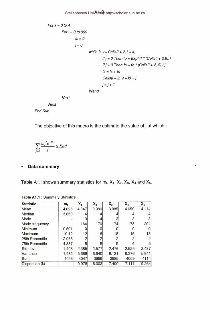
A1-3
For k = 0 to 4
For i = 0 to 999
fs = 0
j = 0
while fs <= Cel/s(i + 2,1 + k)
If j = 0 Then fa = Exp(-1 * (Cel/s(i + 2,8)))
If j > 0 Then fa = fa * (Cel/s(i + 2, 8) / j
ts e ts= toCel/s(i + 2,9 + k) =j
j = j + 1
Wend
Next
Next
End Sub
The objective of this macro is the estimate the value of j at which:
j -m" mt e ' ::;RndL. .,j=O J.
• Data summary
Table A1.1shows summary statistics for mt, X1, X2, X3, X4 and X5.
Table A 1.1 : Summary Statistics
Statistic mt Xl X2 X3 X4 XsMean 4.025 4.047 3.989 3.985 4.059 4.114Median 3.859 4 4 4 4 4Mode - 3 4 3 3 3Mode frequency - 164 170 174 173 204Minimum 0.591 0 0 0 0 0Maximum 10.12 12 16 18 15 1325th Percentile 2.958 2 2 2 2 275th Percentile 4.887 5 5 5 6 5Std.dev. 1.408 2.385 2.577 2.476 2.525 2.437Variance 1.982 5.688 6.640 6.131 6.376 5.941Sum 4025 4047 3989 3985 4059 4114Dispersion (k) - 9.978 6.003 7.400 7.111 9.264
Stellenbosch University http://scholar.sun.ac.za

A1-4
According to Vogt and Bared (1998) if mt has a Gamma distribution between
sites and X is Poisson distributed about mt then the distribution of X between
sites would follow the Negative Binomial distribution, where:
E(X) = Mean and VAR(X) = Mean + (Meani/k
Figure A1.1 shows the fitting of a Gamma distribution to the generated values
of mt.
Gamma distribution mt' 1000 sites
Kolmogorov-Smirnov d = .0158847, P = n.s.
Chi-Square: 18.80982, dl = 12, P = .0932878 (dl adjusted)
180~~~~~~~~~~~~~~~~~~~~~~~~
160 .
140 f••.•••••••..••.
120
............................. alpha = 8.104 .beta = 0.496
100U).Do(5oZ
80
40
20 !-.....••.•.••..
01.-....-'-""""10.0 1.0 2.0 3.0 4.0 5.0 6.0 7.0 8.0 9.0 10.0 11.0
0.5 1.5 2.5 3.5 4.5 5.5 6.5 7.5 8.5 9.5 10.5 11.5
Category (upper limits)
Figure A1.1 : Fitting of Gamma distribution
• Data listing
A complete list of the random numbers used and the generated values for mt,
X1, X2, X3, X4 and X5 for all 1000 sites are shown in Table A2.1
Stellenbosch University http://scholar.sun.ac.za

A1-5
Table A1.2 : Listing of data for experimental sites (Sites 1 to 50)ID rnd1 rnd2 rnd3 rnd4 rnd5 rnd6 mt X1 X2 X3 X4 Xs
1 0.323 0.251 0.098 0.642 0.716 0.931 3.24 2 1 4 4 62 0.301 0.944 0.524 0.315 0.850 0.280 3.16 6 3 2 5 23 0.912 0.573 0.381 0.721 0.063 0.347 6.01 6 5 7 3 54 0.377 0.766 0.376 0.369 0.755 0.982 3.42 5 3 3 5 85 0.631 0.787 0.609 0.711 0.628 0.736 4.31 6 5 5 5 66 0.191 0.725 0.455 0.926 0.548 0.701 2.75 4 2 5 3 37 0.137 0.377 0.775 0.252 0.110 0.785 2.52 2 4 1 1 48 0.504 0.955 0.720 0.388 0.164 0.349 3.85 7 5 3 2 39 0.255 0.716 0.571 0.576 0.204 0.832 3.00 4 3 3 2 5
10 0.073 0.617 0.777 0.630 0.437 0.018 2.16 2 3 2 2 011 0.054 0.783 0.053 0.721 0.741 0.733 2.03 3 0 3 3 312 0.156 0.613 0.466 0.226 0.765 0.567 2.60 3 2 1 4 313 0.162 0.889 0.601 0.448 0.260 0.854 2.63 5 3 2 1 414 0.605 0.010 0.632 0.484 0.228 0.971 4.21 0 5 4 3 815 0.602 0.286 0.528 0.761 0.710 0.204 4.20 3 4 6 5 216 0.063 0.641 0.703 0.722 0.476 0.327 2.09 2 3 3 2 117 0.193 0.121 0.390 0.283 0.551 0.714 2.76 1 2 2 3 418 0.166 0.567 0.608 0.578 0.460 0.899 2.65 3 3 3 2 519 0.797 0.046 0.179 0.281 0.238 0.504 5.10 2 3 4 3 520 0.807 0.105 0.112 0.670 0.939 0.386 5.16 2 2 6 9 421 0.428 0.872 0.450 0.780 0.014 0.773 3.59 6 3 5 0 522 0.186 1.000 0.007 0.194 0.456 0.303 2.73 11 0 1 2 223 0.790 0.386 0.798 0.969 0.464 0.088 5.06 4 7 10 5 224 0.466 0.162 0.752 0.449 0.173 0.819 3.72 2 5 3 2 525 0.662 0.881 0.868 0.470 0.754 0.199 4.44 7 7 4 6 326 0.815 0.833 0.293 0.823 0.415 0.223 5.21 7 4 7 5 327 0.774 0.444 0.989 0.514 0.998 0.041 4.97 4 11 5 12 128 0.212 0.492 0.250 0.780 0.947 0.049 2.84 3 2 4 6 029 0.049 0.486 0.920 0.008 0.030 0.378 1.98 2 4 0 0 130 0.318 0.515 0.581 0.888 0.180 0.975 3.22 3 3 5 2 731 0.535 0.118 0.133 0.115 0.399 0.308 3.96 2 2 2 3 332 0.166 0.007 0.466 0.993 0.192 0.772 2.65 0 2 7 1 433 0.167 0.137 0.978 0.725 0.979 0.489 2.65 1 6 4 6 234 0.693 0.315 0.262 0.208 0.038 0.307 4.57 3 3 3 1 335 0.458 0.024 0.072 0.375 0.628 0.523 3.69 0 1 3 4 436 0.448 0.064 0.002 0.264 0.046 0.107 3.66 1 0 2 1 137 0.657 0.316 0.633 0.593 0.996 0.838 4.42 3 5 5 11 638 0.350 0.331 0.146 0.756 0.843 0.951 3.33 2 1 4 5 739 0.796 0.616 0.584 0.638 0.353 0.836 5.09 6 5 6 4 740 0.447 0.374 0.394 0.273 0.487 0.634 3.65 3 3 2 3 441 0.288 0.236 0.976 0.724 0.669 0.519 3.11 2 7 4 4 342 0.888 0.853 0.612 0.904 0.016 0.104 5.76 8 6 9 1 343 0.947 0.742 0.770 0.030 0.319 0.579 6.52 8 8 2 5 744 0.733 0.227 0.732 0.399 0.034 0.602 4.76 3 6 4 1 545 0.163 0.877 0.761 0.079 0.888 0.815 2.63 5 4 1 5 446 0.604 0.596 0.703 0.419 0.904 0.696 4.21 5 5 4 7 547 0.001 0.169 0.312 0.885 0.398 0.714 1.01 0 0 2 1 148 0.901 0.532 0.972 0.581 0.510 0.566 5.90 6 11 6 6 649 0.633 0.230 0.152 0.068 0.430 0.608 4.32 3 2 1 4 550 0.523 0.733 0.100 0.279 0.743 0.403 3.91 5 2 3 5 3
Stellenbosch University http://scholar.sun.ac.za

APPENDIX A2
COMPARING THE ABILITY OF THE CONVENTIONAL AND BAYESIAN
METHODS TO ACCURATELY MEASURE THE TRUE LEVEL OF SAFETY.
Using the randomly generated accident frequencies from Appendix A1 the
level of safety was estimated at each location for study periods ranging from
1 to 5 years using Conventional as well as Bayesian methods.
1. CONVENTIONAL ESTIMATES
The conventional estimates were determined as follows:
X1 = X1
)(2 = (X1+X2)/2
)(3 = (X1 + X2 + X3)/3
)(4 = (X1 + X2 + X3 + X4)/4
)(5 = (X1 + X2 + X3 + X4 + X5)/5
2. BAYESIAN ESTIMATES
E(m) and VAR(m) were determined from Year 1 data only, using the method-
of-sample-moments: E(m) = 4.05 and VAR(m) = 1.64.
mt = e-Etm) + (1-at)Xt
at = E(m)I[E(m)+VAR(m)]= 0.71
m2 = a2E(m) + (1-a;) X2
a2 = E(m)I[E(m) + 2*VAR(m)] = 0.55
m3 = a3E(m) + (1-a3) X3
a2 = E(m)I[E(m) + 3*VAR(m)] = 0.45
Stellenbosch University http://scholar.sun.ac.za
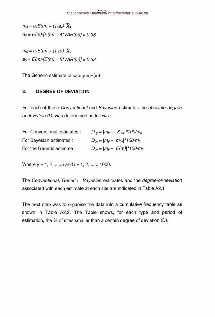
A2-2
m, = a4E(m) + (1-a4) X4tu = E(m)/[E(m) + 4*VAR(m)] = 0.38
ms = asE(m) + (1-as) Xsas = E(m)/[E(m) + S*VAR(m)] = 0.33
The Generic estimate of safety = E(m).
3. DEGREE OF DEVIATION
For each of these Conventional and Bayesian estimates the absolute degree
at deviation (D) was determined as follows:
For Conventional estimates :
For Bayesian estimates:
For the Generic estimate:
Di,y= Imti - X i,yl*1oo/m,Di,y= Imti - mi,yl*1OO/mti
Di,y= Imti - E(m)I*100/mti
Where y = 1, 2, 5 and i = 1, 2, 1000.
The Conventional, Generic , Bayesian estimates and the degree-at-deviation
associated with each estimate at each site are indicated in Table A2.1
The next step was to organise the data into a cumulative frequency table as
shown in Table A2.2. The Table shows, for each type and period of
estimation, the % of sites smaller than a certain degree of deviation (0).
Stellenbosch University http://scholar.sun.ac.za

A2-3
Table A2.1 : Conventional and Bayesian estimates and deviations from the 'true' level of safety (Sites 1 to 50)ID mt X1 D1 X2 D2 X3 D3 X4 D4 Xs Ds Dil m1 Dm1 m2 Dm2 m3 Dm3 m4 Dm4 ms Dms1 3.24 2 38.2 1.5 53.7 2.33 27.9 2.75 15.0 3.4 5.0 25.0 3.46 6.8 2.91 10.2 3.11 4.0 3.24 0.2 3.61 11.62 3.16 6 89.9 4.5 42.4 3.67 16.0 4 26.6 3.6 13.9 28.1 4.61 45.9 4.25 34.5 3.84 21.5 4.02 27.2 3.75 18.63 6.01 6 0.2 5.5 8.5 6 0.2 5.25 12.7 5.2 13.5 32.7 4.61 23.3 4.70 21.9 5.12 14.9 4.79 20.3 4.82 19.94 3.42 5 46.3 4.0 17.0 3.67 7.3 4 17.0 4.8 40.4 18.4 4.32 26.4 4.03 17.8 3.84 12.3 4.02 17.5 4.55 33.15 4.31 6 39.1 5.5 27.5 5.33 23.6 5.25 21.7 5.4 25.2 6.2 4.61 6.9 4.70 8.9 4.75 10.2 4.79 11.1 4.95 14.86 2.75 4 45.3 3.0 9.0 3.67 33.2 3.5 27.2 3.4 23.5 47.0 4.03 46.6 3.58 30.0 3.84 39.5 3.71 34.7 3.61 31.37 2.52 2 20.6 3.0 19.2 2.33 7.3 2 20.6 2.4 4.7 60.8 3.46 37.3 3.58 42.1 3.11 23.4 2.78 10.5 2.94 16.98 3.85 7 81.8 6.0 55.9 5 29.9 4.25 10.4 4.0 3.9 5.1 4.90 27.3 4.92 27.9 4.57 18.7 4.17 8.4 4.02 4.39 3.00 4 33.5 3.5 16.9 3.33 11.3 3 0.2 3.4 13.5 35.1 4.03 34.7 3.80 26.9 3.66 22.0 3.40 13.5 3.61 20.710 2.16 2 7.4 2.5 15.7 2.33 8.0 2.25 4.1 1.8 16.7 87.3 3.46 60.0 3.35 55.2 3.11 43.8 2.94 35.8 2.54 17.711 2.03 3 48.0 1.5 26.0 2 1.4 2.25 11.0 2.4 18.4 99.6 3.74 84.7 2.91 43.3 2.92 44.2 2.94 44.8 2.94 45.212 2.60 3 15.2 2.5 4.0 2 23.2 2.5 4.0 2.6 0.1 55.5 3.74 43.9 3.35 28.9 2.92 12.3 3.09 18.7 3.08 18.213 2.63 5 90.1 4.0 52.1 3.33 26.7 2.75 4.6 3.0 14.1 53.9 4.32 64.3 4.03 53.1 3.66 39.0 3.24 23.4 3.35 27.214 4.21 0 100 2.5 40.7 3 28.8 3 28.8 4.0 5.1 4.0 2.88 31.7 3.35 20.4 3.47 17.6 3.40 19.3 4.02 4.715 4.20 3 28.6 3.5 16.7 4.33 3.1 4.5 7.1 4.0 4.8 3.7 3.74 10.9 3.80 9.5 4.20 0.1 4.33 3.0 4.02 4.416 2.09 2 4.5 2.5 19.4 2.67 27.4 2.5 19.4 2.2 5.1 93.3 3.46 65.1 3.35 60.2 3.29 57.1 3.09 47.6 2.81 34.217 2.76 1 63.8 1.5 45.6 1.67 39.6 2 27.5 2.4 13.0 46.7 3.17 14.8 2.91 5.3 2.74 0.7 2.78 0.8 2.94 6.718 2.65 3 13.3 3.0 13.3 3 13.3 2.75 3.9 3.2 20.9 52.9 3.74 41.5 3.58 35.2 3.47 31.2 3.24 22.6 3.48 31.519 5.10 2 60.8 2.5 51.0 3 41.2 3 41.2 3.4 33.3 20.6 3.46 32.2 3.35 34.2 3.47 31.9 3.40 33.3 3.61 29.120 5.16 2 61.2 2.0 61.2 3.33 35.4 4.75 7.9 4.6 10.8 21.5 3.46 33.0 3.13 39.3 3.66 29.1 4.48 13.1 4.42 14.421 . 3.59 6 67.2 4.5 25.4 4.67 30.1 3.5 2.5 3.8 5.9 12.8 4.61 28.5 4.25 18.4 4.39 22.3 3.71 3.4 3.88 8.222 2.73 11 303 5.5 101 4 46.5 3.5 28.2 3.2 17.2 48.2 6.05 121.7 4.70 72.0 4.02 47.3 3.71 35.8 3.48 27.423 5.06 4 20.9 5.5 8.8 7 38.4 6.5 28.6 5.6 10.8 20.0 4.03 20.2 4.70 7.1 5.67 12.1 5.56 10.1 5.09 0.624 3.72 2 46.2 3.5 5.9 3.33 10.4 3 19.3 3.4 8.6 8.8 3.46 7.1 3.80 2.2 3.66 1.7 3.40 8.6 3.61 2.825 4.44 7 57.6 7.0 57.6 6 35.1 6 35.1 5.4 21.6 8.9 4.90 10.3 5.37 20.9 5.12 15.2 5.26 18.3 4.95 11.5
Continue ....
Stellenbosch University http://scholar.sun.ac.za

A2-4
Table A2.1 (continued)10 mt X1 01 X2 O2 X3 03 X4 04 Xs 05 Og m1 Om1 m2 Om2 m3 Om3 m4 Om4 mS OmS26 5.21 7 34.4 5.5 5.6 6 15.2 5.75 10.4 5.2 0.1 22.3 4.90 5.9 4.70 9.8 5.12 1.7 5.10 2.0 4.82 7.527 4.97 4 19.5 7.5 50.9 6.67 34.2 8 61.0 6.6 32.8 18.6 4.03 18.8 5.59 12.6 5.48 10.4 6.49 30.7 5.76 15.828 2.84 3 5.8 2.5 11.8 3 5.8 3.75 32.2 3.0 5.8 42.7 3.74 32.1 3.35 18.3 3.47 22.4 3.86 36.2 3.35 18.029 1.98 2 1.1 3.0 51.7 2 1.1 1.5 24.2 1.4 29.2 104.6 3.46 74.7 3.58 80.9 2.92 47.8 2.47 24.9 2.27 15.030 3.22 3 6.8 3.0 6.8 3.67 13.9 3.25 0.9 4.0 24.2 25.7 3.74 16.3 3.58 11.1 3.84 19.2 3.55 10.4 4.02 24.731 3.96 2 49.4 2.0 49.4 2 49.4 2.25 43.1 2.4 39.3 2.3 3.46 12.6 3.13 20.9 2.92 26.1 2.94 25.8 2.94 25.632 2.65 0 100 1.0 62.2 3 13.4 2.5 5.5 2.8 5.8 52.9 2.88 8.8 2.68 1.4 3.47 31.2 3.09 16.8 3.21 21.433 2.65 1 62.3 3.5 32.0 3.67 38.2 4.25 60.2 3.8 43.3 52.6 3.17 19.4 3.80 43.3 3.84 44.7 4.17 57.3 3.88 46.334 4.57 3 34.4 3.0 34.4 3 34.4 2.5 45.3 2.6 43.1 11.5 3.74 18.1 3.58 21.8 3.47 24.1 3.09 32.4 3.08 32.735 3.69 0 100.0 0.5 86.5 1.33 63.9 2 45.8 2.4 35.0 9.6 2.88 22.0 2.46 33.4 2.56 30.7 2.78 24.7 2.94 20.336 3.66 1 72.7 0.5 86.3 1 72.7 1 72.7 1.0 72.7 10.7 3.17 13.4 2.46 32.8 2.37 35.1 2.16 40.9 2.01 45.137 4.42 3 32.1 4.0 9.5 4.33 2.0 6 35.7 6.0 35.7 8.4 3.74 15.3 4.03 8.9 4.20 4.9 5.26 18.9 5.36 21.138 3.33 2 39.9 1.5 54.9 2.33 29.9 3 9.8 3.8 14.2 21.7 3.46 3.9 2.91 12.6 3.11 6.6 3.40 2.2 3.88 16.739 5.09 6 17.8 5.5 8.0 5.67 11.3 5.25 3.1 5.6 10.0 20.5 4.61 9.5 4.70 7.7 4.94 3.1 4.79 5.9 5.09 0.140 3.65 3 17.9 3.0 17.9 2.67 27.0 2.75 24.7 3.0 17.9 10.8 3.74 2.5 3.58 2.0 3.29 9.9 3.24 11.2 3.35 8.441 3.11 2 35.8 4.5 44.5 4.33 39.1 4.25 36.4 4.0 28.4 29.9 3.46 11.0 4.25 36.4 4.20 35.0 4.17 34.0 4.02 28.942 5.76 8 38.8 7.0 21.5 7.67 33.0 6 4.1 5.4 6.3 29.8 5.19 10.0 5.37 6.8 6.03 4.7 5.26 8.8 4.95 14.143 6.52 8 22.6 8.0 22.6 6 8.0 5.75 11.9 6.0 8.0 38.0 5.19 20.5 5.82 10.8 5.12 21.5 5.10 21.8 5.36 17.944 4.76 3 36.9 4.5 5.4 4.33 8.9 3.5 26.4 3.8 20.1 14.9 3.74 21.3 4.25 10.6 4.20 11.6 3.71 22.0 3.88 18.445 2.63 5 89.8 4.5 70.8 3.33 26.5 3.75 42.3 3.8 44.2 53.6 4.32 64.0 4.25 61.3 3.66 38.7 3.86 46.6 3.88 47.346 4.21 5 18.8 5.0 18.8 4.67 10.9 5.25 24.7 5.2 23.6 3.8 4.32 2.7 4.47 6.3 4.39 4.2 4.79 13.8 4.82 14.547 1.01 0 100.0 0.0 100.0 0.67 33.9 0.75 25.7 0.8 20.7 301.1 2.88 185.3 2.23 121.4 2.19 117.2 2.01 98.9 1.87 85.648 5.90 6 1.7 8.5 44.1 7.67 30.0 7.25 22.9 7.0 18.7 31.4 4.61 21.8 6.04 2.4 6.03 2.3 6.03 2.2 6.02 2.149 4.32 3 30.6 2.5 42.2 2 53.7 2.5 42.2 3.0 30.6 6.4 3.74 13.4 3.35 22.4 2.92 32.4 3.09 28.5 3.35 22.650 3.91 5 27.7 3.5 10.6 3.33 14.9 3.75 4.2 3.6 8.0 3.4 4.32 10.4 3.80 2.9 3.66 6.6 3.86 1.3 3.75 4.3
Stellenbosch University http://scholar.sun.ac.za

A2-5
Table A2.2 : Cumulative frequencies (%) . Conventional Generic and Bayesian estimates,0 X1 X2 X3 X4 Xs E(m) m1 m2 m3 m4 ms0 0 0 0 0 0 0 0 0 0 0 05 9.4 12.2 13.4 14.5 16.6 10.3 12.8 15.7 15.9 16.9 19.610 16.5 22.0 27.0 28.9 32.7 19.6 24.8 29.6 33.0 35.2 35.515 23.1 30.6 39.8 42.1 48.0 32.8 38.8 43.5 47.5 51.0 53.520 30.0 39.0 48.2 55.0 61.7 43.0 49.4 56.8 60.8 65.2 68.025 37.0 47.6 58.0 64.8 72.4 52.9 58.0 67.4 71.5 75.0 79.130 43.4 56.3 66.7 72.1 80.5 59.7 67.0 74.3 79.2 81.4 86.235 49.9 64.9 73.8 78.9 86.8 66.3 73.6 79.0 84.7 87.2 90.640 55.6 72.1 80.4 84.3 91.2 73.4 79.9 85.4 88.7 91.5 93.845 60.6 78.8 84.7 90.0 95.1 77.2 83.2 88.9 92.0 93.6 95.650 65.9 83.2 89.1 93.1 96.8 80.6 85.9 90.8 94.0 95.5 96.855 70.1 86.6 92.4 95.5 97.9 84.3 87.8 93.5 95.0 96.7 97.560 73.9 89.5 94.8 97.7 98.5 86.4 90.0 94.5 96.5 97.7 98.265 78.1 92.2 96.8 98.7 98.8 88.9 92.1 95.6 97.5 98.3 98.670 81.6 93.8 97.8 99.2 99.5 89.8 93.7 96.6 98.2 98.9 99.075 84.3 95.1 98.5 99.7 99.8 90.6 94.6 97.3 98.5 99.1 99.180 86.6 96.4 99.0 99.8 99.9 91.9 95.4 98.2 98.5 99.2 99.585 88.0 97.3 99.5 99.8 99.9 92.8 96.3 98.3 98.7 99.2 99.590 89.2 98.1 99.5 99.8 99.9 93.8 96.7 98.6 99.0 99.5 99.795 89.9 98.6 99.5 99.9 100.0 94.8 96.9 98.9 99.3 99.6 99.7100 94.7 99.1 99.6 100.0 100.0 95.7 97.5 99.0 99.4 99.7 99.7105 95.3 99.2 99.9 100.0 100.0 96.1 97.9 99.1 99.6 99.7 99.8110 96.5 99.5 99.9 100.0 100.0 96.2 98.3 99.2 99.6 99.8 99.8115 96.9 99.5 100.0 100.0 100.0 96.7 98.8 99.2 99.6 99.9 99.8120 97.3 99.6 100.0 100.0 100.0 96.9 99.0 99.4 99.7 99.9 99.9125 97.5 99.7 100.0 100.0 100.0 97.0 99.1 99.5 99.8 99.9 99.9130 97.8 99.7 100.0 100.0 100.0 97.7 99.1 99.5 99.8 99.9 99.9135 98.0 99.7 100.0 100.0 100.0 98.1 99.1 99.6 99.8 99.9 99.9140 98.6 99.7 100.0 100.0 100.0 98.3 99.2 99.6 99.8 99.9 99.9145 98.7 99.8 100.0 100.0 100.0 98.3 99.4 99.6 99.8 99.9 99.9150 98.9 99.9 100.0 100.0 100.0 98.6 99.4 99.8 99.9 99.9 99.9155 99.0 100.0 100.0 100.0 100.0 98.8 99.5 99.8 99.9 99.9 99.9160 99.0 100.0 100.0 100.0 100.0 98.9 99.5 99.8 99.9 99.9 99.9165 99.2 100.0 100.0 100.0 100.0 99.1 99.5 99.8 99.9 99.9 99.9170 99.3 100.0 100.0 100.0 100.0 99.3 99.5 99.8 99.9 99.9 99.9175 99.3 100.0 100.0 100.0 100.0 99.3 99.5 99.8 99.9 99.9 99.9180 99.4 100.0 100.0 100.0 100.0 99.4 99.5 99.8 99.9 99.9 99.9185 99.4 100.0 100.0 100.0 100.0 99.4 99.5 99.8 99.9 99.9 99.9190 99.5 100.0 100.0 100.0 100.0 99.5 99.6 99.8 99.9 99.9 99.9195 99.5 100.0 100.0 100.0 100.0 99.5 99.8 99.8 99.9 99.9 100.0200 99.6 100.0 100.0 100.0 100.0 99.5 99.8 99.8 99.9 99.9 100.0
Stellenbosch University http://scholar.sun.ac.za

APPENDIX A3
EFFICIENCY ASSESSMENT OF IDENTIFICATION METHODS
In order to assess the efficiency of the CP1, CN2 and 81 identification
methods the following procedures were applied:
• Identifying 'true' hazardous locations.
Previously the random number rnd1 was generated for each of the 1000 sites.
This random number was used to generate the true level of safety (mt) from a
Gamma distribution with mean = 4 ace/year and a variance = 2.
It is assumed that all those sites where rnd1 > 0.95 are 'true' hazardous
locations. All the hazardous locations identified from the CP1, CN2 and 81
identification methods will be compared with these true hazardous locations to
determine the efficiency of the respective methods.
Thus in Tables A3.1 and A3.2 : Ht = 1 of rnd1 > 0.95
• Method CP1
In Table A3.1 the value for Pij ( where j = 1 to 5) represent the probability that
the accident total for a j year period exceeds the average accident total for the
same period across all 1000 sites.
The average accident frequency for the 5 different study periods are shown
below:
Study1 Year 2 Year 3 Year 4 Year 5 Year
Period
Average 4.05 8.04 12.02 16.08 20.2
Stellenbosch University http://scholar.sun.ac.za

A3-2
If Xij is the observed accident number at site i over a period of j years and Xaj
is the average accident number for a period of j years, then:
Xij (Xa.)k e -Xa,p = ,,_-=-J __ij ~ k!
Pij was determined using the following Microsoft® Excel® function:
A site was identified as hazardous if Pj> 0.95. Thus in Table A3.1 : HCj = 1 if
Pj> 0.95.
The efficiency descriptions in the Ej columns were determined as follows:
'tp' - True positive: If Hf = 1 and Hpj = 1'tn' - True negative: If Hf = 0 and Hpj = 0
'tp' - False positive: If Hf = 0 and Hpj = 1
'fn' - False negative: If Hf = 1and Hpj = 1
• Method CN2
Table A3.1 contains the average accident frequency per location for each of
the 5 study periods.
For each study period the critical accident number were estimated as follows:
Xcrj = Xa j +1.64S~Xaj +0.5
These critical values are as follows :
Stellenbosch University http://scholar.sun.ac.za
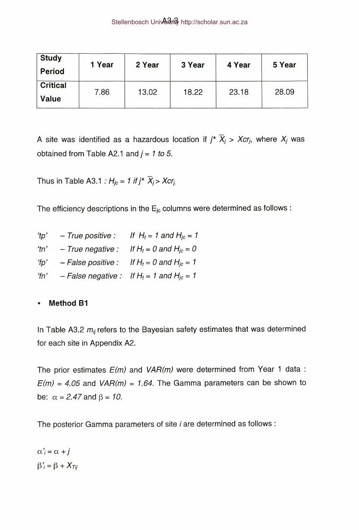
A3-3
Study1 Year 2 Year 3 Year 4 Year 5 Year
Period
Critical7.86 13.02 18.22 23.18 28.09
Value
A site was identified as a hazardous location if j* Xj > xct; where Xj was
obtained from Table A2.1 and j = 1 to 5.
Thus in Table A3.1 : Hjc = 1 ifr X,» XCIj.
The efficiency descriptions in the Eje columns were determined as follows:
'tp' - True positive: If H, = 1 and Hjc = 1
'tn' - True negative: If H, = 0 and Hjc = 0
'fp' - False positive: If Ht = 0 and Hjc = 1
'fn' - False negative: If H, = 1and Hjc = 1
• Method 81
In Table A3.2 mij refers to the Bayesian safety estimates that was determined
for each site in Appendix A2.
The prior estimates E(m) and VAR(m) were determined from Year 1 data:
E(m) = 4.05 and VAR(m) = 1.64. The Gamma parameters can be shown to
be: a = 2.47 and f3 = 10.
The posterior Gamma parameters of site i are determined as follows:
a', = a + j
Stellenbosch University http://scholar.sun.ac.za

A3-4
where
XTij- The total number of accidents at site i over a period of j years.
j - Length of study period : 1 to 5.
A site was identified as a hazardous location if P(mij > E(m)) > 0.95.
Where
E(m) (.l.1(l' a'-l -f3'm-IJ me'
P (m - > E (m)) = 1- f dmlj 0 na')
The following Microsoft® Excel® function was used to calculate P(mij > E(m)):
= 1- GAMMADIST[E(m), [3', 1Ia', TRUE]
Thus in Table A3.2 : Pmj = P(mij > E(m))
Hbj = 1 if Pmj > 0.95
The efficiency descriptions in the Ebj columns were determined as follows:
'tp' - True positive: If H, = 1and Hbj = 1
'tn' - True negative: If Ht = 0 and Hbj = 0
'to' - False positive: If Ht = 0 and Hbj = 1'fn' - False negative: If H, = 1and Hbj = 1
Stellenbosch University http://scholar.sun.ac.za
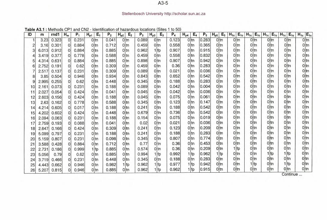
A3-5
Table A3.1 : Methods CP1 and CN2 - Identification of hazardous locations (Sites 1 to 50)ID m rnd1 Hm P1 Hp1 E1 P2 Hp2 E2 P3 Hp3 E3 P4 Hp4 E4 Ps Hps Es H1c E1c H1c E1c H1c E1c H1c E1c H1c E1c
1 3.23 0.323 0 0.231 o tn 0.041 o tn 0.089 o tn 0.123 o tn 0.283 o tn o tn o tn o tn o tn o tn2 3.16 0.301 0 0.884 o tn 0.712 o tn 0.459 o tn 0.558 o tn 0.365 o tn o tn o tn o tn o tn o tn3 6.013 0.912 0 0.884 o tn 0.885 o tn 0.962 1 fp 0.907 o tn 0.915 o tn o tn o tn o tn o tn o tn4 3.419 0.377 0 0.778 o tn 0.588 o tn 0.459 o tn 0.558 o tn 0.832 o tn o tn o tn o tn o tn o tn5 4.314 0.631 0 0.884 o tn 0.885 o tn 0.898 o tn 0.907 o tn 0.942 o tn o tn o tn o tn o tn o tn6 2.752 0.191 0 0.62 o tn 0.309 o tn 0.459 o tn 0.36 o tn 0.283 o tn o tn o tn o tn o tn o tn7 2.517 0.137 0 0.231 o tn 0.309 o tn 0.089 o tn 0.021 o tn 0.036 o tn o tn o tn o tn o tn o tn8 3.85 0.504 0 0.946 o tn 0.934 o tn 0.843 o tn 0.652 o tn 0.542 o tn o tn o tn o tn o tn o tn9 2.995 0.255 0 0.62 o tn 0.448 o tn 0.345 o tn 0.188 o tn 0.283 o tn o tn o tn o tn o tn o tn
10 2.161 0.073 0 0.231 o tn 0.188 o tn 0.089 o tn 0.042 o tn 0.004 o tn o tn o tn o tn o tn o tn11 2.027 0.054 0 0.424 o tn 0.041 o tn 0.045 o tn 0.042 o tn 0.036 o tn o tn o tn o tn o tn o tn12 2.603 0.156 0 0.424 o tn 0.188 o tn 0.045 o tn 0.075 o tn 0.061 o tn o tn o tn o tn o tn o tn13 2.63 0.162 0 0.778 o tn 0.588 o tn 0.345 o tn 0.123 o tn 0.147 o tn o tn o tn o tn o tn o tn
14 4.214 0.605 0 0.017 o tn 0.188 o tn 0.241 o tn 0.188 o tn 0.542 o tn o tn o tn o tn o tn o tn
15 4.202 0.602 0 0.424 o tn 0.448 o tn 0.679 o tn 0.736 o tn 0.542 o tn o tn o tn o tn o tn o tn
16 2.094 0.063 0 0.231 o tn 0.188 o tn 0.154 o tn 0.075 o tn 0.019 o tn o tn o tn o tn o tn o tn
17 2.759 0.193 0 0.088 o tn 0.041 o tn 0.02 o tn 0.021 o tn 0.036 o tn o tn o tn o tn o tn o tn
18 2.647 0.166 0 0.424 o tn 0.309 o tn 0.241 o tn 0.123 o tn 0.209 o tn o tn o tn o tn o tn o tn
19 5.099 0.797 0 0.231 o tn 0.188 o tn 0.241 o tn 0.188 o tn 0.283 o tn o tn o tn o tn o tn o tn
20 5.159 0.807 0 0.231 o tn 0.098 o tn 0.345 o tn 0.807 o tn 0.774 o tn o tn o tn o tn o tn o tn
21 3.588 0.428 0 0.884 o tn 0.712 o tn 0.77 o tn 0.36 o tn 0.453 o tn o tn o tn o tn o tn o tn
22 2.731 0.186 0 0.999 1 fp 0.885 o tn 0.574 o tn 0.36 o tn 0.209 o tn 1 fp o tn o tn o tn o tn
23 5.056 0.79 0 0.62 o tn 0.885 o tn 0.994 1 fp 0.992 1 fp 0.962 1 fp o tn o tn 1 fp 1 fp o tn
24 3.719 0.466 0 0.231 o tn 0.448 o tn 0.345 o tn 0.188 o tn 0.283 o tn o tn o tn o tn o tn o tn
25 4.443 0.662 0 0.946 o tn 0.982 1 fp 0.962 1 fp 0.977 1 fp 0.942 o tn o tn 1 fp o tn 1 fp o tn
26 5.207 0.815 0 0.946 o tn 0.885 o tn 0.962 1 fp 0.962 1 fp 0.915 o tn o tn o tn o tn o tn o tnContinue ...
Stellenbosch University http://scholar.sun.ac.za

A3-6
Table A3.1 (continued)ID m rnd1 Hm P1 Hp1 E1 P2 Hp2 E2 P3 Hp3 E3 P4 Hp4 E4 Ps Hps Es H1c E1c H1c E1c H1c E1c H1c E1c H1c E1c27 4.969 0.774 0 0.62 o tn 0.991 1 fp 0.988 1 fp 1 1 fp 0.997 1 fp o tn 1 fp 1 fp 1 fp 1 fp28 2.836 0.212 0 0.424 o tn 0.188 o tn 0.241 o tn 0.459 o tn 0.147 o tn o tn o tn o tn o tn o tn29 1.978 0.049 0 0.231 o tn 0.309 o tn 0.045 o tn 0.004 o tn 7E-04 o tn o tn o tn o tn o tn o tn30 3.22 0.318 0 0.424 o tn 0.309 o tn 0.459 o tn 0.268 o tn 0.542 o tn o tn o tn o tn o tn o tn31 3.956 0.535 0 0.231 o tn 0.098 o tn 0.045 o tn 0.042 o tn 0.036 o tn o tn o tn o tn o tn o tn32 2.646 0.166 0 0.017 o tn 0.013 o tn 0.241 o tn 0.075 o tn 0.098 o tn o tn o tn o tn o tn o tn33 2.652 0.167 0 0.088 o tn 0.448 o tn 0.459 o tn 0.652 o tn 0.453 o tn o tn o tn o tn o tn o tn34 4.573 0.693 0 0.424 o tn 0.309 o tn 0.241 o tn 0.075 o tn 0.061 o tn o tn o tn o tn o tn o tn35 3.692 0.458 0 0.017 o tn 0.003 o tn 0.007 o tn 0.021 o tn 0.036 o tn o tn o tn o tn o tn o tn36 3.657 0.448 0 0.088 o tn 0.003 o tn 0.002 o tn 4E-04 o tn 6E-05 o tn o tn o tn o tn o tn o tn37 4.42 0.657 0 0.424 o tn 0.588 o tn 0.679 o tn 0.977 1 fp 0.985 1 fp o tn o tn o tn 1 fp 1 fp38 3.326 0.35 0 0.231 o tn 0.041 o tn 0.089 o tn 0.188 o tn 0.453 o tn o tn o tn o tn o tn o tn39 5.092 0.796 0 0.884 o tn 0.885 o tn 0.936 o tn 0.907 o tn 0.962 1 fp o tn o tn o tn o tn o tn40 3.652 0.447 0 0.424 o tn 0.309 o tn 0.154 o tn 0.123 o tn 0.147 o tn o tn o tn o tn o tn o tn41 3.115 0.288 0 0.231 o tn 0.712 o tn 0.679 o tn 0.652 o tn 0.542 o tn o tn o tn o tn o tn o tn42 5.763 0.888 0 0.977 1 fp 0.982 1 fp 0.998 1 fp 0.977 1 fp 0.942 o tn 1 fp 1 fp 1 fp 1 fp o tn43 6.524 0.947 0 0.977 1 fp 0.996 1 fp 0.962 1 fp 0.962 1 fp 0.985 1 fp 1 fp 1 fp o tn o tn 1 fp44 4.756 0.733 0 0.424 o tn 0.712 o tn 0.679 o tn 0.36 o tn 0.453 o tn o tn o tn o tn o tn o tn45 2.635 0.163 0 0.778 o tn 0.712 o tn 0.345 o tn 0.459 o tn 0.453 o tn o tn o tn o tn o tn o tn46 4.209 0.604 0 0.778 o tn 0.812 o tn 0.77 o tn 0.907 o tn 0.915 o tn o tn o tn o tn o tn o tn47 1.009 0.001 0 0.017 o tn 3E-04 o tn 5E-04 o tn 9E-05 o tn 1E-05 o tn o tn o tn o tn o tn o tn48 5.899 0.901 0 0.884 o tn 0.998 1 fp 0.998 1 fp 0.999 1 fp 0.999 1 fp o tn 1 fp 1 fp 1 fp 1 fp49 4.324 0.633 0 0.424 o tn 0.188 o tn 0.045 o tn 0.075 o tn 0.147 o tn o tn o tn o tn o tn o tn50 3.915 0.523 0 0.778 o tn 0.448 o tn 0.345 o tn 0.459 o tn 0.365 o tn o tn o tn o tn o tn o tn
Stellenbosch University http://scholar.sun.ac.za

A3-7
Table A3.2 : Method 81 - Identification of hazardous locations (Sites 1 to 50)ID mt Ht m1 Pm1 Hb1 Eb1 m2 Pm2 Hb2 Eb2 m3 Pm3 Hm3 Em3 m4 Pm4 Hm4 Em4 ms PmS Hms Ems
1 3.24 0 3.46 0.256 o tn 2.91 0.088 o tn 3.11 0.111 o tn 3.24 0.131 o tn 3.61 0.254 o tn2 3.16 0 4.61 0.665 o tn 4.25 0.553 o tn 3.84 0.376 o tn 4.02 0.459 o tn 3.75 0.318 o tn3 6.01 0 4.61 0.665 o tn 4.70 0.723 o tn 5.12 0.871 o tn 4.79 0.803 o tn 4.82 0.832 o tn4 3.42 0 4.32 0.566 o tn 4.03 0.460 o tn 3.84 0.376 o tn 4.02 0.459 o tn 4.55 0.730 o tn5 4.31 0 4.61 0.665 o tn 4.70 0.723 o tn 4.75 0.768 o tn 4.79 0.803 o tn 4.95 0.871 o tn6 2.75 0 4.03 0.459 o tn 3.58 0.279 o tn 3.84 0.376 o tn 3.71 0.308 o tn 3.61 0.254 o tn7 2.52 0 3.46 0.256 o tn 3.58 0.279 o tn 3.11 0.111 o tn 2.78 0.038 o tn 2.94 0.050 o tn8 3.85 0 4.90 0.752 o tn 4.92 0.793 o tn 4.57 0.701 o tn 4.17 0.537 o tn 4.02 0.459 o tn9 3.00 0 4.03 0.459 o tn 3.80 0.367 o tn 3.66 0.296 o tn 3.40 0.181 o tn 3.61 0.254 o tn
10 2.16 0 3.46 0.256 o tn 3.35 0.202 o tn 3.11 0.111 o tn 2.94 0.060 o tn 2.54 0.012 o tn11 2.03 0 3.74 0.354 o tn 2.91 0.088 o tn 2.92 0.073 o tn 2.94 0.060 o tn 2.94 0.050 o tn12 2.60 0 3.74 0.354 o tn 3.35 0.202 o tn 2.92 0.073 o tn 3.09 0.091 o tn 3.08 0.075 o tn13 2.63 0 4.32 0.566 o tn 4.03 0.460 o tn 3.66 0.296 o tn 3.24 0.131 o tn 3.35 0.147 o tn14 4.21 0 2.88 0.107 o tn 3.35 0.202 o tn 3.47 0.224 o tn 3.40 0.181 o tn 4.02 0.459 o tn15 4.20 0 3.74 0.354 o tn 3.80 0.367 o tn 4.20 0.544 o tn 4.33 0.613 o tn 4.02 0.459 o tn16 2.09 0 3.46 0.256 o tn 3.35 0.202 o tn 3.29 0.162 o tn 3.09 0.091 o tn 2.81 0.032 o tn17 2.76 0 3.17 0.172 o tn 2.91 0.088 o tn 2.74 0.045 o tn 2.78 0.038 o tn 2.94 0.050 o tn18 2.65 0 3.74 0.354 o tn 3.58 0.279 o tn 3.47 0.224 o tn 3.24 0.131 o tn 3.48 0.196 o tn19 5.10 0 3.46 0.256 o tn 3.35 0.202 o tn 3.47 0.224 o tn 3.40 0.181 o tn 3.61 0.254 o tn20 5.16 0 3.46 0.256 o tn 3.13 0.138 o tn 3.66 0.296 o tn 4.48 0.684 o tn 4.42 0.669 o tn
21 3.59 0 4.61 0.665 o tn 4.25 0.553 o tn 4.39 0.626 o tn 3.71 0.308 o tn 3.88 0.387 o tn22 2.73 0 6.05 0.951 1 fp 4.70 0.723 o tn 4.02 0.460 o tn 3.71 0.308 o tn 3.48 0.196 o tn
23 5.06 0 4.03 0.459 o tn 4.70 0.723 o tn 5.67 0.957 1 fp 5.56 0.961 1 fp 5.09 0.904 o tn
24 3.72 0 3.46 0.256 o tn 3.80 0.367 o tn 3.66 0.296 o tn 3.40 0.181 o tn 3.61 0.254 o tn
25 4.44 0 4.90 0.752 o tn 5.37 0.895 o tn 5.12 0.871 o tn 5.26 0.919 o tn 4.95 0.871 o tn
26 5.21 0 4.90 0.752 o tn 4.70 0.723 o tn 5.12 0.871 o tn 5.10 0.889 o tn 4.82 0.832 o tn
27 4.97 0 4.03 0.459 o tn 5.59 0.929 o tn 5.48 0.936 o tn 6.49 0.997 1 fp 5.76 0.983 1 fpContinue ...
Stellenbosch University http://scholar.sun.ac.za
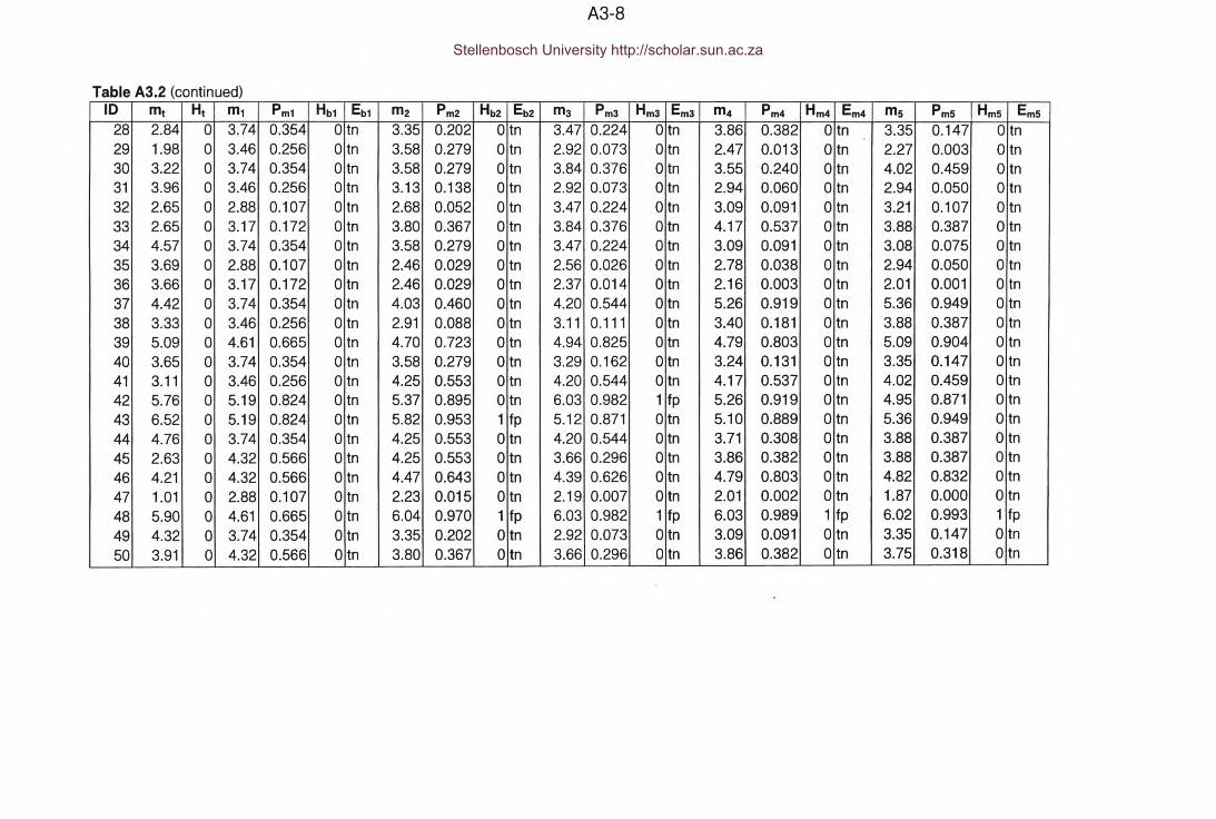
A3-8
Table A3.2 (continued)ID mt Ht m1 Pm1 Hb1 Eb1 m2 Pm2 Hb2 Eb2 m3 Pm3 Hm3 Em3 m4 Pm4 Hm4 Em4 ms PmS HmS EmS28 2.84 0 3.74 0.354 o tn 3.35 0.202 o tn 3.47 0.224 o tn 3.86 0.382 o tn 3.35 0.147 o tn29 1.98 0 3.46 0.256 o tn 3.58 0.279 o tn 2.92 0.073 o tn 2.47 0.013 o tn 2.27 0.003 o tn30 3.22 0 3.74 0.354 o tn 3.58 0.279 o tn 3.84 0.376 o tn 3.55 0.240 o tn 4.02 0.459 o tn31 3.96 0 3.46 0.256 o tn 3.13 0.138 o tn 2.92 0.073 o tn 2.94 0.060 o tn 2.94 0.050 o tn32 2.65 0 2.88 0.107 o tn 2.68 0.052 o tn 3.47 0.224 o tn 3.09 0.091 o tn 3.21 0.107 o tn33 2.65 0 3.17 0.172 o tn 3.80 0.367 o tn 3.84 0.376 o tn 4.17 0.537 o tn 3.88 0.387 o tn34 4.57 0 3.74 0.354 o tn 3.58 0.279 o tn 3.47 0.224 o tn 3.09 0.091 o tn 3.08 0.075 o tn35 3.69 0 2.88 0.107 o tn 2.46 0.029 o tn 2.56 0.026 o tn 2.78 0.038 o tn 2.94 0.050 o tn36 3.66 0 3.17 0.172 o tn 2.46 0.029 o tn 2.37 0.014 o tn 2.16 0.003 o tn 2.01 0.001 o tn37 4.42 0 3.74 0.354 o tn 4.03 0.460 o tn 4.20 0.544 o tn 5.26 0.919 o tn 5.36 0.949 o tn38 3.33 0 3.46 0.256 o tn 2.91 0.088 o tn 3.11 0.111 o tn 3.40 0.181 o tn 3.88 0.387 o tn39 5.09 0 4.61 0.665 o tn 4.70 0.723 o tn 4.94 0.825 o tn 4.79 0.803 o tn 5.09 0.904 o tn40 3.65 0 3.74 0.354 o tn 3.58 0.279 o tn 3.29 0.162 o tn 3.24 0.131 o tn 3.35 0.147 o tn41 3.11 0 3.46 0.256 o tn 4.25 0.553 o tn 4.20 0.544 o tn 4.17 0.537 o tn 4.02 0.459 o tn42 5.76 0 5.19 0.824 o tn 5.37 0.895 o tn 6.03 0.982 1 fp 5.26 0.919 o tn 4.95 0.871 o tn43 6.52 0 5.19 0.824 o tn 5.82 0.953 1 fp 5.12 0.871 o tn 5.10 0.889 o tn 5.36 0.949 o tn44 4.76 0 3.74 0.354 o tn 4.25 0.553 o tn 4.20 0.544 o tn 3.71 0.308 o tn 3.88 0.387 o tn45 2.63 0 4.32 0.566 o tn 4.25 0.553 o tn 3.66 0.296 o tn 3.86 0.382 o tn 3.88 0.387 o tn46 4.21 0 4.32 0.566 o tn 4.47 0.643 o tn 4.39 0.626 o tn 4.79 0.803 o tn 4.82 0.832 o tn47 1.01 0 2.88 0.107 o tn 2.23 0.015 o tn 2.19 0.007 o tn 2.01 0.002 o tn 1.87 0.000 o tn48 5.90 0 4.61 0.665 o tn 6.04 0.970 1 fp 6.03 0.982 1 fp 6.03 0.989 1 fp 6.02 0.993 1 fp49 4.32 0 3.74 0.354 o tn 3.35 0.202 o tn 2.92 0.073 o tn 3.09 0.091 o tn 3.35 0.147 o tn50 3.91 0 4.32 0.566 o tn 3.80 0.367 o tn 3.66 0.296 o tn 3.86 0.382 o tn 3.75 0.318 o tn
Stellenbosch University http://scholar.sun.ac.za

APPENDIX A4
ASSESSMENT OF EVALUATION METHODS
In Appendix A3 the CP1 and 81 methods were used to identify hazardous
locations for study periods from 1 to 5 years.
For each site in a group of identified hazardous locations the true level of
safety in the 'before' period (mtb) was reduced by 20 % - this represents the
'true' effect of a safety treatment. Using the same procedure as in Appendix
A1, 5 years of accident frequencies were randomly generated assuming a
Poisson distribution around the true 'after' level of safety (mta).
Table A4.1 and Table A4.2 contains listings of the hazardous locations
selected by Methods CP1 and 81 using 3 years of data, and information on
the randomly generated accident frequencies for each of 5 years in the 'after'
period.
Stellenbosch University http://scholar.sun.ac.za

A4-2
Table A4.1 : Method CP1 - Hazardous locations· Period = 3 yearsID T3 mbt mat Xa1 Xa2 Xa3 Xê4 Xas3 18 6.01 4.81 4 4 3 6 723 21 5.06 4.04 1 5 2 3 625 18 4.44 3.55 2 3 4 3 326 18 5.21 4.17 3 2 5 6 227 20 4.97 3.98 1 4 6 2 642 23 5.76 4.61 2 5 4 3 443 18 6.52 5.22 6 6 4 7 648 23 5.90 4.72 5 6 5 3 356 19 5.40 4.32 6 2 4 2 578 19 4.56 3.65 4 4 2 3 1080 19 4.78 3.82 3 2 5 2 483 19 5.24 4.19 6 1 1 5 485 27 6.89 5.51 5 5 5 4 695 18 4.53 3.62 5 1 3 5 398 24 7.97 6.38 6 11 3 3 5106 22 5.50 4.40 5 4 7 5 3120 22 5.92 4.73 3 7 5 7 4133 18 5.55 4.44 3 9 7 5 6136 20 4.02 3.22 4 3 5 5 3139 19 4.44 3.55 7 3 4 3 4140 22 6.45 5.16 10 7 6 8 4148 27 7.01 5.60 2 5 7 8 8157 22 7.76 6.21 7 9 3 9 4165 24 7.03 5.63 2 7 7 5 5168 21 6.27 5.02 4 8 6 5 3185 26 5.19 4.15 4 0 4 3 8187 22 4.45 3.56 2 1 2 4 2200 21 6.73 5.39 8 8 6 3 3213 18 7.20 5.76 9 7 7 10 6217 20 5.04 4.03 4 8 2 4 4221 33 6.46 5.17 6 8 7 4 1227 25 7.37 5.89 5 7 7 6 6229 19 5.13 4.11 7 2 2 2 1233 19 5.79 4.64 4 3 7 5 1249 32 9.04 7.23 5 8 7 9 5250 23 5.31 4.24 10 3 6 5 5255 22 4.59 3.67 2 1 4 4 7264 18 6.48 5.19 5 5 2 5 5273 21 5.75 4.60 6 7 3 8 4276 22 5.68 4.55 5 3 2 2 4278 21 4.76 3.81 1 3 0 4 4282 18 6.75 5.40 2 5 6 4 6283 19 6.66 5.33 4 5 8 8 3285 28 7.08 5.66 7 6 10 5 8300 19 5.48 4.38 5 5 2 6 5301 18 6.68 5.34 2 6 9 3 3308 18 3.66 2.93 2 2 2 2 4
Stellenbosch University http://scholar.sun.ac.za

A4-3
Table A4.1 (continued)ID T3 mbt mat Xa1 Xa2 Xa3 X~ Xas327 22 6.93 5.55 8 6 10 3 6334 22 6.08 4.86 8 5 5 4 4341 20 4.95 3.96 7 4 2 5 6344 23 6.65 5.32 6 6 6 4 8349 19 5.55 4.44 5 5 6 9 5354 22 5.95 4.76 4 3 5 7 5355 20 8.70 6.96 3 8 9 5 3361 19 4.63 3.70 2 2 5 4 3370 20 4.85 3.88 6 6 3 3 1371 21 5.31 4.25 4 4 6 3 7389 19 5.81 4.65 2 9 6 4 4392 21 5.96 4.77 5 6 6 7 8397 19 4.39 3.51 6 2 2 4 7398 31 6.81 5.45 6 3 6 5 5402 19 5.66 4.53 2 7 4 6 4403 23 8.18 6.54 10 6 5 7 9409 26 9.05 7.24 6 5 4 7 7413 19 4.15 3.32 5 3 2 4 4418 22 8.10 6.48 10 5 10 5 7421 25 7.27 5.81 7 9 7 5 7428 23 5.64 4.51 4 1 6 5 3435 18 6.03 4.82 6 3 2 3 7436 18 5.58 4.46 4 3 3 3 3437 21 6.76 5.41 7 6 5 5 6443 23 5.64 4.51 4 4 5 3 6450 26 8.64 6.91 8 10 7 3 10456 28 10.12 8.10 8 7 12 5 7460 19 3.64 2.91 2 4 4 4 5463 18 4.30 3.44 3 2 1 2 5468 22 4.84 3.87 5 9 3 7 3477 19 5.27 4.21 4 10 2 6 3481 18 4.01 3.21 3 3 5 2 5491 22 4.87 3.89 7 1 2 6 0493 19 6.59 5.27 7 2 9 3 5497 22 6.91 5.53 6 5 4 4 6503 18 4.03 3.23 3 1 4 1 2506 32 5.36 4.29 2 4 6 3 2516 18 4.39 3.51 4 2 2 2 5520 26 5.25 4.20 3 4 6 2 5523 18 4.44 3.55 3 2 4 5 7535 24 5.65 4.52 3 3 2 9 2539 24 6.67 5.34 4 4 4 7 8543 18 4.25 3.40 2 5 4 4 4548 25 6.98 5.58 7 8 6 3 5559 28 8.84 7.07 8 6 11 4 9560 20 5.28 4.22 4 3 5 2 3573 22 7.46 5.97 8 5 4 7 8581 26 5.92 4.74 2 6 6 4 4
Stellenbosch University http://scholar.sun.ac.za
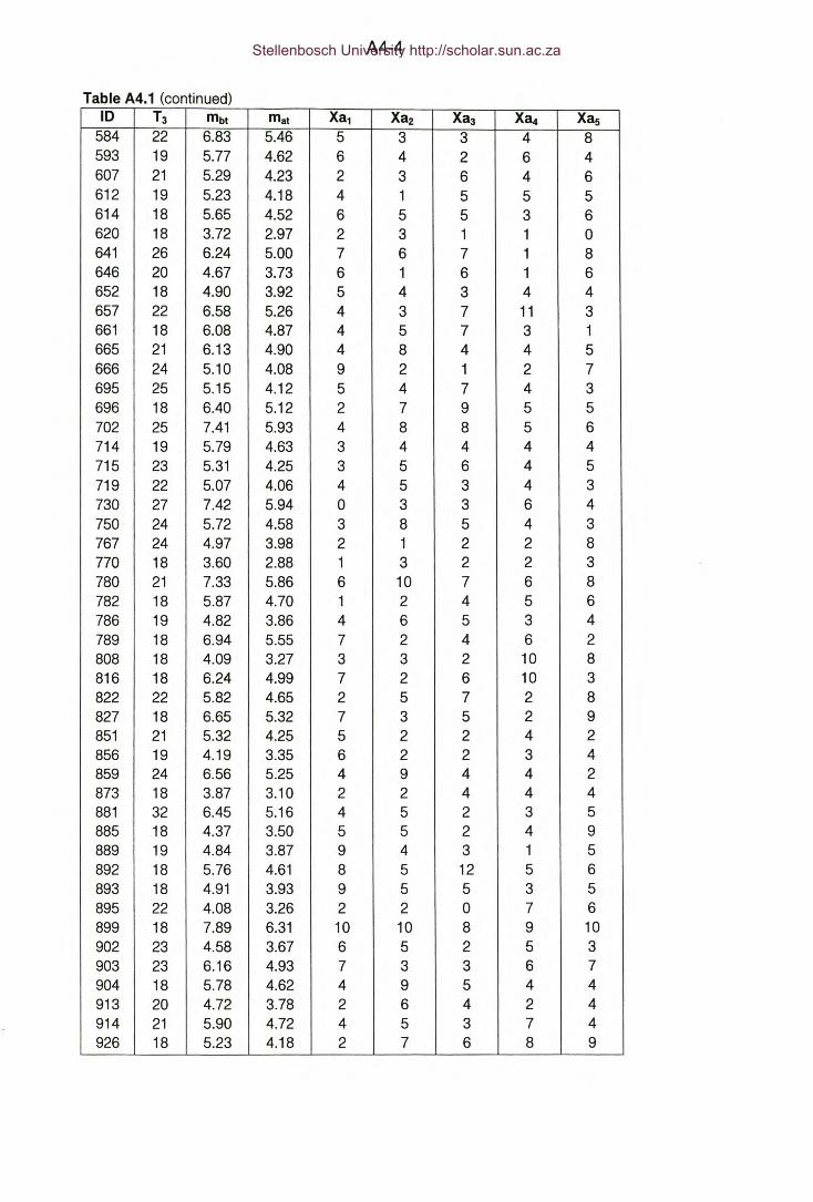
A4-4
Table A4.1 (continued)ID T3 mbt mat Xa1 Xa2 Xa3 Xa4 Xas584 22 6.83 5.46 5 3 3 4 8593 19 5.77 4.62 6 4 2 6 4607 21 5.29 4.23 2 3 6 4 6612 19 5.23 4.18 4 1 5 5 5614 18 5.65 4.52 6 5 5 3 6620 18 3.72 2.97 2 3 1 1 0641 26 6.24 5.00 7 6 7 1 8646 20 4.67 3.73 6 1 6 1 6652 18 4.90 3.92 5 4 3 4 4657 22 6.58 5.26 4 3 7 11 3661 18 6.08 4.87 4 5 7 3 1665 21 6.13 4.90 4 8 4 4 5666 24 5.10 4.08 9 2 1 2 7695 25 5.15 4.12 5 4 7 4 3696 18 6.40 5.12 2 7 9 5 5702 25 7.41 5.93 4 8 8 5 6714 19 5.79 4.63 3 4 4 4 4715 23 5.31 4.25 3 5 6 4 5719 22 5.07 4.06 4 5 3 4 3730 27 7.42 5.94 0 3 3 6 4750 24 5.72 4.58 3 8 5 4 3767 24 4.97 3.98 2 1 2 2 8770 18 3.60 2.88 1 3 2 2 3780 21 7.33 5.86 6 10 7 6 8782 18 5.87 4.70 1 2 4 5 6786 19 4.82 3.86 4 6 5 3 4789 18 6.94 5.55 7 2 4 6 2808 18 4.09 3.27 3 3 2 10 8816 18 6.24 4.99 7 2 6 10 3822 22 5.82 4.65 2 5 7 2 8827 18 6.65 5.32 7 3 5 2 9851 21 5.32 4.25 5 2 2 4 2856 19 4.19 3.35 6 2 2 3 4859 24 6.56 5.25 4 9 4 4 2873 18 3.87 3.10 2 2 4 4 4881 32 6.45 5.16 4 5 2 3 5885 18 4.37 3.50 5 5 2 4 9889 19 4.84 3.87 9 4 3 1 5892 18 5.76 4.61 8 5 12 5 6893 18 4.91 3.93 9 5 5 3 5895 22 4.08 3.26 2 2 0 7 6899 18 7.89 6.31 10 10 8 9 10902 23 4.58 3.67 6 5 2 5 3903 23 6.16 4.93 7 3 3 6 7904 18 5.78 4.62 4 9 5 4 4913 20 4.72 3.78 2 6 4 2 4914 21 5.90 4.72 4 5 3 7 4926 18 5.23 4.18 2 7 6 8 9
Stellenbosch University http://scholar.sun.ac.za
A4-5
Table A4.1 (continue)ID T3 mbt mat Xa1 Xa2 Xa3 Xa4 Xas932 22 6.08 4.86 5 7 5 7 6934 23 8.45 6.76 7 8 5 3 6935 18 6.22 4.98 7 6 8 8 3943 26 7.42 5.94 4 3 6 4 6950 18 6.73 5.38 9 7 4 4 7951 24 6.42 5.13 6 5 3 6 5955 20 6.99 5.59 7 6 9 7 7961 22 4.97 3.97 5 2 7 1 9962 28 6.57 5.25 6 6 7 8 5963 18 5.06 4.05 2 1 6 4 2964 18 5.79 4.63 2 3 4 8 4965 19 4.53 3.63 3 5 4 0 6966 23 6.24 4.99 7 3 4 3 2972 27 4.88 3.90 6 5 6 9 4991 19 4.72 3.77 2 2 2 5 6994 18 5.36 4.28 4 6 5 1 3Total 3386 2779.81 2223.84 753 743 759 728 786
Table A4.2 : Method 81 - hazardous locations: Period = 3 yearsID m3 mbt mat Xa1 Xa2 Xa3 Xa4 Xas
23 5.67 5.06 4.04 1 5 2 3 642 6.03 5.76 4.61 2 5 4 3 448 6.03 5.90 4.72 5 6 5 3 385 6.77 6.89 5.51 5 5 5 4 698 6.22 7.97 6.38 6 11 3 3 5106 5.85 5.50 4.40 5 4 7 5 3120 5.85 5.92 4.73 3 7 5 7 4140 5.85 6.45 5.16 10 7 6 8 4148 6.77 7.01 5.60 2 5 7 8 8157 5.85 7.76 6.21 7 9 3 9 4165 6.22 7.03 5.63 2 7 7 5 5168 5.67 6.27 5.02 4 8 6 5 3185 6.58 5.19 4.15 4 0 4 3 8187 5.85 4.45 3.56 2 1 2 4 2200 5.67 6.73 5.39 8 8 6 3 3221 7.86 6.46 5.17 6 8 7 4 1227 6.40 7.37 5.89 5 7 7 6 6249 7.68 9.04 7.23 5 8 7 9 5250 6.03 5.31 4.24 10 3 6 5 5255 5.85 4.59 3.67 2 1 4 4 7273 5.67 5.75 4.60 6 7 3 8 4276 5.85 5.68 4.55 5 3 2 2 4278 5.67 4.76 3.81 1 3 0 4 4285 6.95 7.08 5.66 7 6 10 5 8327 5.85 6.93 5.55 8 6 10 3 6334 5.85 6.08 4.86 8 5 5 4 4344 6.03 6.65 5.32 6 6 6 4 8354 5.85 5.95 4.76 4 3 5 7 5371 5.67 5.31 4.25 4 4 6 3 7
Stellenbosch University http://scholar.sun.ac.za
A4-6
Table A4.2 (continued)ID m3 mbt mat Xa1 Xa2 Xa3 Xa.. Xas392 5.67 5.96 4.77 5 6 6 7 8398 7.50 6.81 5.45 6 3 6 5 5403 6.03 8.18 6.54 10 6 5 7 9409 6.58 9.05 7.24 6 5 4 7 7418 5.85 8.10 6.48 10 5 10 5 7421 6.40 7.27 5.81 7 9 7 5 7428 6.03 5.64 4.51 4 1 6 5 3437 5.67 6.76 5.41 7 6 5 5 6443 6.03 5.64 4.51 4 4 5 3 6450 6.58 8.64 6.91 8 10 7 3 10456 6.95 10.12 8.10 8 7 12 5 7468- 5.85 4.84 3.87 5 9 3 7 3491 5.85 4.87 3.89 7 1 2 6 0497 5.85 6.91 5.53 6 5 4 4 6506 7.68 5.36 4.29 2 4 6 3 2520 6.58 5.25 4.20 3 4 6 2 5535 6.22 5.65 4.52 3 3 2 9 2539 6.22 6.67 5.34 4 4 4 7 8548 6.40 6.98 5.58 7 8 6 3 5559 6.95 8.84 7.07 8 6 11 4 9573 5.85 7.46 5.97 8 5 4 7 8581 6.58 5.92 4.74 2 6 6 4 4584 5.85 6.83 5.46 5 3 3 4 8607 5.67 5.29 4.23 2 3 6 4 6641 6.58 6.24 5.00 7 6 7 1 8657 5.85 6.58 5.26 4 3 7 11 3665 5.67 6.13 4.90 4 8 4 4 5666 6.22 5.10 4.08 9 2 1 2 7695 6.40 5.15 4.12 5 4 7 4 3702 6.40 7.41 5.93 4 8 8 5 6715 6.03 5.31 4.25 3 5 6 4 5719 5.85 5.07 4.06 4 5 3 4 3730 6.77 7.42 5.94 0 3 3 6 4750 6.22 5.72 4.58 3 8 5 4 3767 6.22 4.97 3.98 2 1 2 2 8780 5.67 7.33 5.86 6 10 7 6 8822 5.85 5.82 4.65 2 5 7 2 8851 5.67 5.32 4.25 5 2 2 4 2859 6.22 6.56 5.25 4 9 4 4 2881 7.68 6.45 5.16 4 5 2 3 5895 5.85 4.08 3.26 2 2 0 7 6902 6.03 4.58 3.67 6 5 2 5 3903 6.03 6.16 4.93 7 3 3 6 7914 5.67 5.90 4.72 4 5 3 7 4932 5.85 6.08 4.86 5 7 5 7 6934 6.03 8.45 6.76 7 8 5 3 6943 6.58 7.42 5.94 4 3 6 4 6951 6.22 6.42 5'.13 6 5 3 6 5
Stellenbosch University http://scholar.sun.ac.za

A4-7
Table A4.2 (continued)ID mJ mbt mat Xa1 Xa2 XaJ Xat Xas961 5.85 4.97 3.97 5 2 7 1 9962 6.95 6.57 5.25 6 6 7 8 5966 6.03 6.24 4.99 7 3 4 3 2972 6.77 4.88 3.90 6 5 6 9 4
Total 502.10 512.18 409.75 411 419 412 394 426
Stellenbosch University http://scholar.sun.ac.za
APPENDIX 81
THE METHOD OF SAMPLE MOMENTS
In Table B1.1 is listed all the road links in the Province of the Western Cape,
South Africa, that meet the following criteria. :
• Number of lanes: 2 lanes ( one in each direction)
• Type of shoulder: Surfaced
• Surfaced width: >= 11 m ( typically 2*3.7 m lanes with shoulder widths>
1.8m)
• Geography: Rural - Province of the Western Cape
• AADT: > 1000 veh/day and < 8000 veh/day
• Segment length: > 500 m
• Accident period: 1993 to 1996 (4 Years)
• Accident type : ALL
This information was obtained from the road network and accident databases of
the Transport Branch of the Department of Economic Affairs, Agriculture and
Tourism of the Provincial Administration of the Western Cape
The method of sample moments has been applied as follows to estimate the
true level of safety at each of these segments:
Mean accident rate ( R) = 1.15
Variance of R «l) = 1.13
Harmonic mean (E*) = 9.60
E(m) = 1.15 and VAR(m) = [9.60(1.13)-1.15]/9.60 = 1.01
a = 9.60(1.15)/[1.13(9.60) -1.15] = 1.14 and (3= 1.14*1.15 = 1.31
a'i = 1.14 + Ei and (3'= 1.31 + Ai
mi = (3'i/a'i and VAR(mi) = (3'/(a'i)2
Stellenbosch University http://scholar.sun.ac.za

81-2
Table 81.1 : Method of sample momentsRoad Start End L AADT E A R a' f3' m VAR(m)NR00205 51.88 52.6 0.74 2704 2.92 23 7.87 4.06 24.31 5.98 1.47MR00165 0 3.63 3.63 1502 7.97 32 4.02 9.11 33.31 3.66 0.40MROO027 51.73 52.3 0.56 4220 3.45 15 4.34 4.59 16.31 3.55 0.77MR00227 5.89 9.66 3.77 1111 6.12 21 3.43 7.26 22.31 3.07 0.42TR02801 0 2.14 2.14 1158 3.62 12 3.31 4.76 13.31 2.80 0.59TR03201 44.35 45.2 0.8 1760 2.06 7 3.40 3.20 8.31 2.60 0.81MROO027 51.15 51.7 0.58 7077 6.00 17 2.83 7.14 18.31 2.57 0.36MROO027 67.19 68.6 1.37 4722 9.45 25 2.65 10.59 26.31 2.48 0.23MR00223 6.3 9.63 3.33 1618 7.87 21 2.67 9.01 22.31 2.48 0.27MR00165 3.63 7.47 3.84 5530 31.02 76 2.45 32.17 77.31 2.40 0.07TR03201 42.84 44.4 1.51 1708 3.77 10 2.65 4.91 11.31 2.31 0.47NR00108 2.68 3.61 0.93 2530 3.44 9 2.62 4.58 10.31 2.25 0.49NR00205 9.85 11.4 1.55 5593 12.67 29 2.29 13.81 30.31 2.20 0.16TR03201 0 5.71 5.71 1729 14.42 32 2.22 15.56 33.31 2.14 0.14NR00205 49.34 51.8 2.46 4107 14.76 32 2.17 15.90 33.31 2.10 0.13TR02801 2.14 3.73 1.59 3762 8.74 19 2.17 9.88 20.31 2.06 0.21TR00204 50.54 55 4.49 2663 17.47 34 1.95 18.61 35.31 1.90 0.10NR00205 52.62 58.6 5.98 3447 30.12 47 1.56 31.26 48.31 1.55 0.05NR00205 40.64 49.3 8.7 3063 38.93 58 1.49 40.07 59.31 1.48 0.04TR00202 37.09 42.4 5.27 7300 56.21 83 1.48 57.35 84.31 1.47 0.03DR01056 0 1.32 1.32 1108 2.14 5 2.34 3.28 6.31 1.93 0.59MR00313 1.6 3.1 1.5 1843 4.04 8 1.98 5.18 9.31 1.80 0.35TR00204 44.28 45.2 0.88 2449 3.15 6 1.91 4.29 7.31 1.71 0.40TR02801 16.37 17.2 0.81 3850 4.56 8 1.76 5.70 9.31 1.64 0.29TR02801 17.18 19.9 2.75 4029 16.19 25 1.54 17.33 26.31 1.52 0.09NR00205 58.6 59.2 0.61 3519 3.14 5 1.59 4.28 6.31 1.48 0.35TR03302 2.74 5.01 2.27 1365 4.53 7 1.55 5.67 8.31 1.47 0.26TR02801 19.93 23.6 3.67 4240 22.73 33 1.45 23.87 34.31 1.44 0.06NR00205 0 2.02 2.02 4214 12.44 18 1.45 13.58 19.31 1.42 0.10DR01101 1.9 5.79 3.89 1980 11.25 15 1.33 12.39 16.31 1.32 0.11TR00204 2.84 4.4 1.56 2981 6.79 9 1.32 7.93 10.31 1.30 0.16NR00105 29.83 31.9 2.06 2610 7.86 10 1.27 9.00 11.31 1.26 0.14DR01105 0 3.99 3.99 6717 39.16 49 1.25 40.30 50.31 1.25 0.03TR02801 3.73 9.1 5.37 3031 23.78 29 1.22 24.92 30.31 1.22 0.05MR00216 0 3.45 3.45 4520 22.78 27 1.19 23.92 28.31 1.18 0.05TR00204 45.16 50.5 5.38 2492 19.59 23 1.17 20.73 24.31 1.17 0.06TR02801 23.6 25.8 2.23 4803 15.65 18 1.15 16.79 19.31 1.15 0.07DR01101 0 1.9 1.9 3779 10.49 12 1.14 11.63 13.31 1.14 0.10TR02901 39.92 45.2 5.29 1045 8.08 9 1.11 9.22 10.31 1.12 0.12MR00279 33.98 34.7 0.67 2016 1.97 2 1.01 3.11 3.31 1.06 0.34TR02901 51.85 55.1 3.23 1060 5.00 5 1.00 6.14 6.31 1.03 0.17MR00279 34.65 35.3 0.68 3142 3.12 3 0.96 4.26 4.31 1.01 0.24NR00205 7.12 9.12 2 6182 18.06 18 1.00 19.20 19.31 1.01 0.05MR00187 6.96 8.03 1.07 5894 9.21 9 0.98 10.35 10.31 1.00 0.10TR03302 1.74 2.74 1 1507 2.20 2 0.91 3.34 3.31 0.99 0.30NR00208 65.71 67.8 2.07 5417 16.38 15 0.92 17.52 16.31 0.93 0.05TR03201 22.79 26.2 3.42 1564 7.81 7 0.90 8.96 8.31 0.93 0.10NR00107 0 34.9 34.86 2526 128.65 117 0.91 129.79 118.31 0.91 0.01TR03201 5.71 15.3 9.55 1566 21.85 19 0.87 22.99 20.31 0.88 0.04
Continue ...
Stellenbosch University http://scholar.sun.ac.za
81-3
Table 81.1 (continued)Road Start End L AADT E A R a' (3' m VAR(m)TR03201 15.26 22.8 7.53 1372 15.09 13 0.86 16.23 14.31 0.88 0.05MR00191 16.66 20.2 3.54 3808 19.69 17 0.86 20.84 18.31 0.88 0.04NR00108 62 72.4 10.44 2465 37.60 32 0.85 38.74 33.31 0.86 0.02MR00227 1 5.89 4.89 1359 9.71 8 0.82 10.85 9.31 0.86 0.08NR00205 9.12 9.85 0.73 5839 6.23 5 0.80 7.37 6.31 0.86 0.12MR00166 3.93 4.71 0.78 1405 1.60 1 0.62 2.74 2.31 0.84 0.31TR03102 1.94 9.04 7.1 3656 37.92 31 0.82 39.06 32.31 0.83 0.02TR00202 54.11 58.2 4.1 3524 21.11 17 0.81 22.25 18.31 0.82 0.04NR00206 35.76 37.2 1.46 3647 7.78 6 0.77 8.92 7.31 0.82 0.09NR00108 56.93 62 5.07 2550 18.89 15 0.79 20.03 16.31 0.81 0.04MROO027 42.91 44.8 1.9 7270 20.18 16 0.79 21.32 17.31 0.81 0.04MR00187 4.36 6.96 2.6 6407 24.34 19 0.78 25.48 20.31 0.80 0.03MROO027 44.81 50.7 5.86 6922 59.26 45 0.76 60.40 46.31 0.77 0.01NR00108 39.85 56.9 17.08 2277 56.82 43 0.76 57.96 44.31 0.76 0.01TR03102 10.78 13.6 2.8 2722 11.14 8 0.72 12.28 9.31 0.76 0.06TR03103 1.9 18.4 16.53 1284 31.01 23 0.74 32.15 24.31 0.76 0.02MR00187 8.03 14.7 6.68 6170 60.22 45 0.75 61.36 46.31 0.75 0.01NR00205 32.72 40.6 7.92 3386 39.18 29 0.74 40.32 30.31 0.75 0.02TR02801 9.1 16.4 7.27 2831 30.07 22 0.73 31.21 23.31 0.75 0.02TR03201 32.73 42.8 10.11 1563 23.09 16 0.69 24.23 17.31 0.71 0.03TR00202 52.64 54.1 1.47 4247 9.12 6 0.66 10.26 7.31 0.71 0.07MROO027 68.56 72.1 3.57 6622 34.54 23 0.67 35.68 24.31 0.68 0.02MR00188 16.54 19.2 2.63 2540 9.76 6 0.61 10.90 7.31 0.67 0.06NR00106 0.42 29.9 29.46 2514 108.21 72 0.67 109.35 73.31 0.67 0.01TR02901 24.03 27.3 3.3 1129 5.44 3 0.55 6.58 4.31 0.66 0.10NR00208 0 6.35 6.35 7379 68.46 44 0.64 69.60 45.31 0.65 0.01MR00344 0 6.2 6.2 2247 20.35 12 0.59 21.49 13.31 0.62 0.03MR00191 20.2 20.7 0.5 3576 2.61 1 0.38 3.75 2.31 0.62 0.16NR00208 46.62 48.6 2.01 5398 15.85 9 0.57 16.99 10.31 0.61 0.04NR00107 61.64 68.3 6.64 2839 27.54 16 0.58 28.68 17.31 0.60 0.02NR00206 25.35 27.7 2.32 3770 12.78 7 0.55 13.92 8.31 0.60 0.04NR00105 81.64 84.5 2.82 2701 11.13 6 0.54 12.27 7.31 0.60 0.05NR00205 2.02 7.12 5.1 6241 46.50 27 0.58 47.64 28.31 0.59 0.01TR00203 26.1 38.2 12.14 2064 36.61 21 0.57 37.75 22.31 0.59 0.02NR00206 16.61 25.4 8.74 2734 34.91 19 0.54 36.05 20.31 0.56 0.02NR00205 59.21 66.8 7.54 3706 40.83 22 0.54 41.97 23.31 0.56 0.01NR00108 3.61 39.9 36.24 2602 137.77 75 0.54 138.91 76.31 0.55 0.00NR00206 58.17 62.4 4.26 3721 23.16 12 0.52 24.30 13.31 0.55 0.02NR00205 70.77 82.1 11.28 4187 69.00 37 0.54 70.14 38.31 0.55 0.01TR00202 58.21 64.3 6.07 4694 41.63 22 0.53 42.77 23.31 0.55 0.01NR00107 34.86 61.6 26.78 2665 104.27 56 0.54 105.41 57.31 0.54 0.01NR00206 46.84 58.2 11.33 4114 68.10 36 0.53 69.24 37.31 0.54 0.01DR01105 3.99 5.12 1.13 4461 7.36 3 0.41 8.51 4.31 0.51 0.06NR00206 38.65 45.1 6.43 3327 31.25 15 0.48 32.40 16.31 0.50 0.02TR07501 29.55 31.5 1.94 2640 7.48 3 0.40 8.62 4.31 0.50 0.06NR00208 63.69 65.7 2.02 6003 17.72 8 0.45 18.86 9.31 0.49 0.03NR00206 45.08 46.8 1.76 3189 8.20 3 0.37 9.34 4.31 0.46 0.05NR00105 31.89 39.8 7.88 2715 31.26 13 0.42 32.40 14.31 0.44 0.01
Continue ...
Stellenbosch University http://scholar.sun.ac.za

81-4
Table 81.1 (continued)Road Start End L AADT E A R a' (3' m VAR(m)NR00104 27.78 54.2 26.46 3609 139.52 60 0.43 140.66 61.31 0.44 0.00MR00177 18.12 22.5 4.39 7495 48.07 20 0.42 49.21 21.31 0.43 0.01NR00105 39.77 81.6 41.87 2617 160.09 68 0.42 161.23 69.31 0.43 0.00MR00200 3.64 11.3 7.7 7465 83.98 34 0.40 85.12 35.31 0.41 0.00MR00223 0 6.3 6.3 4015 36.96 14 0.38 38.10 15.31 0.40 0.01NR00206 12.44 16.6 4.17 2802 17.07 6 0.35 18.21 7.31 0.40 0.02NR00206 62.43 68.3 5.87 3193 27.38 10 0.37 28.52 11.31 0.40 0.01NR00205 66.75 70.8 4.02 3432 20.16 7 0.35 21.30 8.31 0.39 0.02NR00208 48.63 54.9 6.28 6260 57.44 18 0.31 58.58 19.31 0.33 0.01NR00208 8.27 16.8 8.51 5961 74.11 23 0.31 75.25 24.31 0.32 0.00NR00206 68.3 72.9 4.55 4092 27.20 7 0.26 28.34 8.31 0.29 0.01NR00205 11.4 14.7 3.27 5096 24.35 6 0.25 25.49 7.31 0.29 0.01MR00199 19.57 22.5 2.89 3751 15.84 3 0.19 16.98 4.31 0.25 0.01NR00207 43.29 52.1 8.78 7415 95.12 23 0.24 96.26 24.31 0.25 0.00NR00208 59.42 63.7 4.27 6011 37.50 8 0.21 38.64 9.31 0.24 0.01NR00208 34.32 46.6 12.3 6074 109.15 23 0.21 110.29 24.31 0.22 0.00
LEGEND
Road: The number assigned to the road by the provincial roads authority where NR = NationalRoad, TR = Trunk Road and MR = Main Road.Start: The kilometre value (according to the provincial road logs) at which the segment start.End: The kilometre value (according to the provincial road logs) at which the segment end.L : The length of the segment ( End - Start).AADT: Annual Average Daily TrafficE: Exposure in million vehicle kilometres (= L*365*4*AADT*10-6)A : The total number of accidents recorded on the segment between 1993 and 1996 ( 4 years)R : The accident rate (accidents per million vehicle kilometres) : = A/E.a' : The posterior alpha parameter of the Gamma distribution of mj = a + E(3' : The posterior beta parameter of the Gamma distribution of mj = (3 + Aml: The posterior Bayesian estimate = (3'/a'var(ml) : The variance of the posterior Bayesian estimate = (3'/(a,)2
Stellenbosch University http://scholar.sun.ac.za
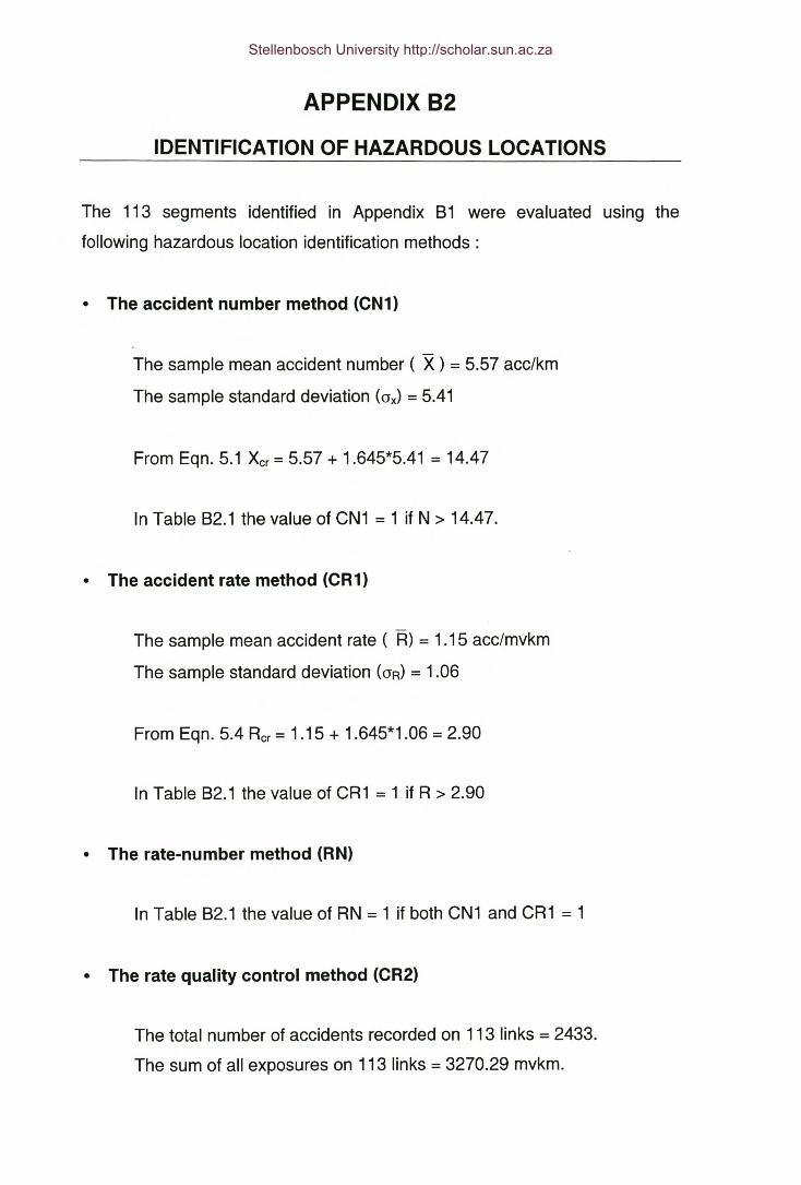
APPENDIX 82
IDENTIFICATION OF HAZARDOUS LOCATIONS
The 113 segments identified in Appendix 81 were evaluated using the
following hazardous location identification methods:
• The accident number method (CN1)
The sample mean accident number ( X ) = 5.57 ace/km
The sample standard deviation (ox) = 5.41
From Eqn. 5.1 Xcr= 5.57 + 1.645*5.41 = 14.47
In Table 82.1 the value of CN1 = 1 if N > 14.47.
• The accident rate method (CR1)
The sample mean accident rate ( R) = 1.15 acc/mvkm
The sample standard deviation (OR) = 1.06
From Eqn. 5.4 Rcr= 1.15 + 1.645*1.06 = 2.90
In Table 82.1 the value of CR1 = 1 if R > 2.90
• The rate-number method (RN)
In Table 82.1 the value of RN = 1 if both CN1 and CR1 = 1
• The rate quality control method (CR2)
The total number of accidents recorded on 113 links = 2433.
The sum of all exposures on 113 links = 3270.29 mvkm.
Stellenbosch University http://scholar.sun.ac.za

82-2
From Eqn 5.9 Ra= 2433/3270.29 = 0.74 acc/mvkm
In Table 82.1 Re= 0.74 + 1.645(0.74/E) + 0.5/E and CR2 = 1 if R > Re.
• The B1 Bayesian method
In Table 82.1 'Pb1 = P(m > 1.15) which was determined using the
following Microsoft® Excel® function:
=1-GAMMADIST(1.15,(3,1/a,TRUE) where a and (3 are the Gamma
parameters determined in Appendix 81.
In Table 82.1 81 = 1 if Pb1> 0.95
• The B2 Bayesian method
In Table 82.1 P21 = P(m > 0.74) which was determined using the
following Microsoft® Excel® function:
=1-GAMMADIST(0.74,(3,1/a,TRUE) where a and (3 are the Gamma
parameters determined in Appendix 81.
In Table 82.1 82 = 1 if Pb2> 0.95
Stellenbosch University http://scholar.sun.ac.za
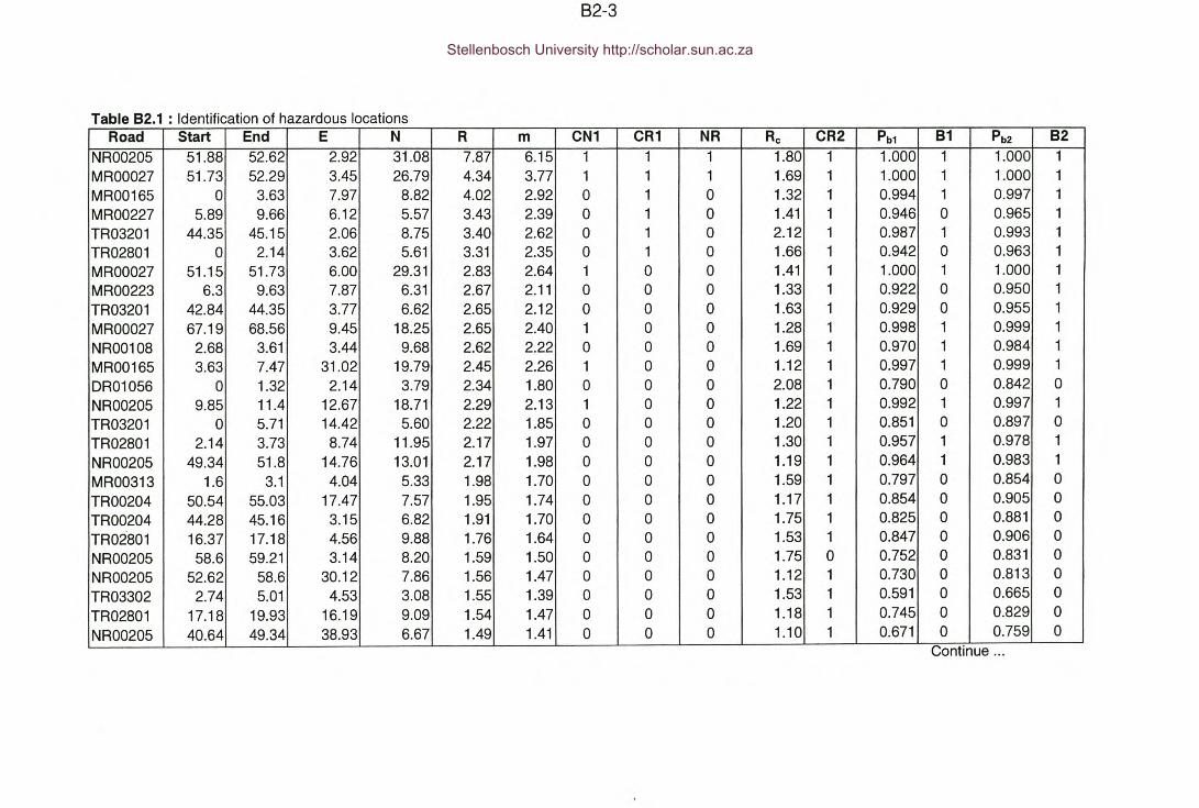
82-3
Table 82.1 : Identification of hazardous locationsRoad Start End E N R m CN1 CR1 NR Rc CR2 Pb1 81 Pb2 82
NR00205 51.88 52.62 2.92 31.08 7.87 6.15 1 1 1 1.80 1 1.000 1 1.000 1MROO027 51.73 52.29 3.45 26.79 4.34 3.77 1 1 1 1.69 1 1.000 1 1.000 1MR00165 0 3.63 7.97 8.82 4.02 2.92 0 1 0 1.32 1 0.994 1 0.997 1MR00227 5.89 9.66 6.12 5.57 3.43 2.39 0 1 0 1.41 1 0.946 0 0.965 1TR03201 44.35 45.15 2.06 8.75 3.40 2.62 0 1 0 2.12 1 0.987 1 0.993 1TR02801 0 2.14 3.62 5.61 3.31 2.35 0 1 0 1.66 1 0.942 0 0.963 1MROO027 51.15 51.73 6.00 29.31 2.83 2.64 1 0 0 1.41 1 1.000 1 1.000 1MR00223 6.3 9.63 7.87 6.31 2.67 2.11 0 0 0 1.33 1 0.922 0 0.950 1TR03201 42.84 44.35 3.77 6.62 2.65 2.12 0 0 0 1.63 1 0.929 0 0.955 1MROO027 67.19 68.56 9.45 18.25 2.65 2.40 1 0 0 1.28 1 0.998 1 0.999 1NR00108 2.68 3.61 3.44 9.68 2.62 2.22 0 0 0 1.69 1 0.970 1 0.984 1MR00165 3.63 7.47 31.02 19.79 2.45 2.26 1 0 0 1.12 1 0.997 1 0.999 1DR01056 0 1.32 2.14 3.79 2.34 1.80 0 0 0 2.08 1 0.790 0 0.842 0NR00205 9.85 11.4 12.67 18.71 2.29 2.13 1 0 0 1.22 1 0.992 1 0.997 1TR03201 0 5.71 14.42 5.60 2.22 1.85 0 0 0 1.20 1 0.851 0 0.897 0TR02801 2.14 3.73 8.74 11.95 2.17 1.97 0 0 0 1.30 1 0.957 1 0.978 1NR00205 49.34 51.8 14.76 13.01 2.17 1.98 0 0 0 1.19 1 0.964 1 0.983 1MR00313 1.6 3.1 4.04 5.33 1.98 1.70 0 0 0 1.59 1 0.797 0 0.854 0TR00204 50.54 55.03 17.47 7.57 1.95 1.74 0 0 0 1.17 1 0.854 0 0.905 0TR00204 44.28 45.16 3.15 6.82 1.91 1.70 0 0 0 1.75 1 0.825 0 0.881 0TR02801 16.37 17.18 4.56 9.88 1.76 1.64 0 0 0 1.53 1 0.847 0 0.906 0NR00205 58.6 59.21 3.14 8.20 1.59 1.50 0 0 0 1.75 0 0.752 0 0.831 0NR00205 52.62 58.6 30.12 7.86 1.56 1.47 0 0 0 1.12 1 0.730 0 0.813 0TR03302 2.74 5.01 4.53 3.08 1.55 1.39 0 0 0 1.53 1 0.591 0 0.665 0TR02801 17.18 19.93 16.19 9.09 1.54 1.47 0 0 0 1.18 1 0.745 0 0.829 0
NR00205 40.64 49.34 38.93 6.67 1.49 1.41 0 0 0 1.10 1 0.671 0 0.759 0Continue ...
Stellenbosch University http://scholar.sun.ac.za
82-4
Table 82.1 (continued)Road Start End E N R m CN1 CR1 NR Rc CR2 Pb1 81 Pb2 82
TR00202 37.09 42.36 56.21 15.75 1.48 1.44 1 0 0 1.08 1 0.791 0 0.882 0TR02801 19.93 23.6 22.73 8.99 1.45 1.40 0 0 0 1.14 1 0.692 0 0.787 0NR00205 0 2.02 12.44 8.91 1.45 1.39 0 0 0 1.22 1 0.688 0 0.784 0DR01101 1.9 5.79 11.25 3.86 1.33 1.28 0 0 0 1.24 1 0.534 0 0.619 0TR00204 2.84 4.4 6.79 5.77 1.32 1.28 0 0 0 1.37 0 0.564 0 0.661 0NR00105 29.83 31.89 7.86 4.85 1.27 1.24 0 0 0 1.33 0 0.521 0 0.615 0DR01105 0 3.99 39.16 12.28 1.25 1.24 0 0 0 1.10 1 0.570 0 0.701 0TR02801 3.73 9.1 23.78 5.40 1.22 1.20 0 0 0 1.14 1 0.494 0 0.594 0MR00216 0 3.45 22.78 7.83 1.19 1.18 0 0 0 1.14 1 0.484 0 0.601 0TR00204 45.16 50.54 19.59 4.28 1.17 1.17 0 0 0 1.16 1 0.458 0 0.550 0TR02801 23.6 25.83 15.65 8.07 1.15 1.15 0 0 0 1.19 0 0.455 0 0.574 0DR01101 0 1.9 10.49 6.32 1.14 1.15 0 0 0 1.26 0 0.446 0 0.554 0TR02901 39.92 45.21 8.08 1.70 1.11 1.13 0 0 0 1.32 0 0.414 0 0.483 0MR00279 33.98 34.65 1.97 2.99 1.01 1.06 0 0 0 2.17 0 0.366 0 0.448 0TR02901 51.85 55.08 5.00 1.55 1.00 1.07 0 0 0 1.49 0 0.374 0 0.442 0NR00205 7.12 9.12 18.06 9.00 1.00 1.02 0 0 0 1.17 0 0.302 0 0.424 0MR00187 6.96 8.03 9.21 8.41 0.98 1.00 0 0 0 1.29 0 0.287 0 0.404 0MR00279 34.65 35.33 3.12 4.41 0.96 1.00 0 0 0 1.76 0 0.316 0 0.408 0NR00208 65.71 67.78 16.38 7.25 0.92 0.95 0 0 0 1.18 0 0.241 0 0.346 0NR00107 0 34.86 128.6 3.36 0.91 0.98 0 0 0 1.06 0 0.298 0 0.380 0TR03302 1.74 2.74 2.20 2.00 0.91 1.00 0 0 0 2.05 0 0.327 0 0.399 0TR03201 22.79 26.21 7.81 2.05 0.90 0.99 0 0 0 1.33 0 0.320 0 0.392 0TR03201 5.71 15.26 21.85 1.99 0.87 0.98 0 0 0 1.15 0 0.308 0 0.379 0MR00191 16.66 20.2 19.69 4.80 0.86 0.92 0 0 0 1.16 0 0.235 0 0.323 0TR03201 15.26 22.79 15.09 1.73 0.86 0.98 0 0 0 1.19 0 0.313 0 0.381 0NR00108 62 72.44 37.60 3.07 0.85 0.93 0 0 0 1.10 0 0.267 0 0.345 0MR00227 1 5.89 9.71 1.64 0.82 0.96 0 0 0 1.27 0 0.299 0 0.365 0
Continue ...
Stellenbosch University http://scholar.sun.ac.za

82-5
Table B2.1 (continued)Road Start End E N R m CN1 CR1 NR Re CR2 Pb1 B1 Pb2 B2
TR03102 1.94 9.04 37.92 4.37 0.82 0.89 0 0 0 1.10 0 0.210 0 0.291 0TR00202 54.11 58.21 21.11 4.15 0.81 0.88 0 0 0 1.15 0 0.206 0 0.286 0NR00205 9.12 9.85 6.23 6.85 0.80 0.85 0 0 0 1.40 0 0.149 0 0.233 0NR00108 56.93 62 18.89 2.96 0.79 0.89 0 0 0 1.16 0 0.233 0 0.307 0MROO027 42.91 44.81 20.18 8.42 0.79 0.83 0 0 0 1.15 0 0.118 0 0.199 0MR00187 4.36 6.96 24.34 7.31 0.78 0.83 0 0 0 1.14 0 0.124 0 0.203 0NR00206 35.76 37.22 7.78 4.11 0.77 0.85 0 0 0 1.33 0 0.183 0 0.258 0MROO027 44.81 50.67 59.26 7.68 0.76 0.81 0 0 0 1.08 0 0.103 0 0.176 0NR00108 39.85 56.93 56.82 2.52 0.76 0.87 0 0 0 1.08 0 0.225 0 0.294 0MR00187 8.03 14.71 60.22 6.74 0.75 0.80 0 0 0 1.08 0 0.109 0 0.180 0TR03103 1.9 18.43 31.01 1.39 0.74 0.91 0 0 0 1.12 0 0.272 0 0.335 0NR00205 32.72 40.64 39.18 3.66 0.74 0.83 0 0 0 1.10 0 0.174 0 0.244 0TR02801 9.1 16.37 30.07 3.03 0.73 0.84 0 0 0 1.12 0 0.189 0 0.258 0TR03102 10.78 13.58 11.14 2.86 0.72 0.83 0 0 0 1.24 0 0.187 0 0.254 0TR03201 32.73 42.84 23.09 1.58 0.69 0.86 0 0 0 1.14 0 0.236 0 0.297 0MROO027 68.56 72.13 34.54 6.44 0.67 0.73 0 0 0 1.11 0 0.063 0 0.113 0NR00106 0.42 29.88 108.2 2.44 0.67 0.80 0 0 0 1.07 0 0.171 0 0.232 0TR00202 52.64 54.11 9.12 4.08 0.66 0.75 0 0 0 1.29 0 0.106 0 0.163 0
NR00208 0 6.35 68.46 6.93 0.64 0.70 0 0 0 1.08 0 0.045 0 0.087 0
MR00166 3.93 4.71 1.60 1.28 0.62 0.84 0 0 0 2.43 0 0.221 0 0.278 0
MR00188 16.54 19.17 9.76 2.28 0.61 0.76 0 0 0 1.27 0 0.148 0 0.204 0
MR00344 0 6.2 20.35 1.94 0.59 0.75 0 0 0 1.15 0 0.152 0 0.207 0
NR00107 61.64 68.28 27.54 2.41 0.58 0.72 0 0 0 1.13 0 0.120 0 0.172 0
NR00205 2.02 7.12 46.50 5.29 0.58 0.65 0 0 0 1.09 0 0.039 0 0.074 0
TR00203 26.1 38.24 36.61 1.73 0.57 0.75 0 0 0 1.11 0 0.157 0 0.210 0
NR00208 46.62 48.63 15.85 4.48 0.57 0.65 0 0 0 1.18 0 0.048 0 0.084 0
TR02901 24.03 27.33 5.44 0.91 0.55 0.82 0 0 0 1.45 0 0.221 0 0.274 0Continue ...
Stellenbosch University http://scholar.sun.ac.za

82-6
Table 82.1 (continued)Road Start End E N R m CN1 CR1 NR Re CR2 Pb1 81 Pb2 82
NR00206 25.35 27.67 12.78 3.02 0.55 0.67 0 0 0 1.22 0 0.076 0 0.118 0NR00108 3.61 39.85 137.7 2.07 0.54 0.70 0 0 0 1.06 0 0.117 0 0.165 0NR00206 16.61 25.35 34.91 2.17 0.54 0.70 0 0 0 1.11 0 0.111 0 0.158 0NR00105 81.64 84.46 11.13 2.13 0.54 0.70 0 0 0 1.24 0 0.110 0 0.158 0NR00205 59.21 66.75 40.83 2.92 0.54 0.66 0 0 0 1.10 0 0.074 0 0.116 0NR00107 34.86 61.64 104.2 2.09 0.54 0.70 0 0 0 1.07 0 0.111 0 0.158 0NR00205 70.77 82.05 69.00 3.28 0.54 0.65 0 0 0 1.08 0 0.061 0 0.099 0NR00206 46.84 58.17 68.10 3.18 0.53 0.64 0 0 0 1.08 0 0.060 0 0.098 0TR00202 58.21 64.28 41.63 3.62 0.53 0.63 0 0 0 1.10 0 0.048 0 0.082 0NR00206 58.17 62.43 23.16 2.82 0.52 0.65 0 0 0 1.14 0 0.067 0 0.106 0NR00206 38.65 45.08 31.25 2.33 0.48 0.63 0 0 0 1.12 0 0.067 0 0.103 0NR00208 63.69 65.71 17.72 3.96 0.45 0.55 0 0 0 1.17 0 0.016 0 0.032 0NR00104 27.78 54.24 139.5 2.27 0.43 0.58 0 0 0 1.06 0 0.046 0 0.074 0NR00105 39.77 81.64 160.0 1.62 0.42 0.62 0 0 0 1.06 0 0.077 0 0.112 0MR00177 18.12 22.51 48.07 4.56 0.42 0.50 0 0 0 1.09 0 0.006 0 0.013 0NR00105 31.89 39.77 31.26 1.65 0.42 0.60 0 0 0 1.12 0 0.070 0 0.104 0DR01105 3.99 5.12 7.36 2.65 0.41 0.54 0 0 0 1.35 0 0.025 0 0.045 0MR00200 3.64 11.34 83.98 4.42 0.40 0.49 0 0 0 1.07 0 0.005 0 0.012 0TR07501 29.55 31.49 7.48 1.55 0.40 0.60 0 0 0 1.34 0 0.069 0 0.102 0MR00191 20.2 20.7 2.61 2.00 0.38 0.54 0 0 0 1.89 0 0.036 0 0.060 0MR00223 0 6.3 36.96 2.22 0.38 0.52 0 0 0 1.10 0 0.027 0 0.047 0NR00206 45.08 46.84 8.20 1.70 0.37 0.54 0 0 0 1.32 0 0.042 0 0.067 0NR00206 62.43 68.3 27.38 1.70 0.37 0.54 0 0 0 1.13 0 0.042 0 0.066 0NR00206 12.44 16.61 17.07 1.44 0.35 0.55 0 0 0 1.17 0 0.051 0 0.077 0NR00205 66.75 70.77 20.16 1.74 0.35 0.52 0 0 0 1.15 0 0.033 0 0.053 0NR00208 48.63 54.91 57.44 2.87 0.31 0.42 0 0 0 1.08 0 0.004 0 0.008 0NR00208 8.27 16.78 74.11 2.70 0.31 0.42 0 0 0 1.07 0 0.004 0 0.010 0
Continue ...
Stellenbosch University http://scholar.sun.ac.za

82-7
Table 82.1 (continued)Road Start End E N R m CN1 CR1 NR Rc CR2 Pb1 81 Pb2 82
NR00206 68.3 72.85 27.20 1.54 0.26 0.42 0 0 0 1.13 0 0.011 0 0.020 0NR00205 11.4 14.67 24.35 1.83 0.25 0.39
,0 0 0 1.14 0 0.004 0 0.009 0
NR00207 43.29 52.07 95.12 2.62 0.24 0.34 0 0 0 1.07 0 0.001 0 0.002 0NR00208 59.42 63.69 37.50 1.87 0.21 0.34 0 0 0 1.10 0 0.001 0 0.003 0NR00208 34.32 46.62 109.1 1.87 0.21 0.34 0 0 0 1.07 0 0.001 0 0.003 0MR00199 19.57 22.46 15.84 1.04 0.19 0.38 0 0 0 1.18 0 0.009 0 0.016 0
Stellenbosch University http://scholar.sun.ac.za
B3-1
APPENDIX 83
COMPARISON OF RANKING METHODS
The 113 segments identified in Appendix B1 were ranked according to the
following criteria :
• Accident number - X (ace/km)
• Accident rate - R (acc/mvkm)
• Bayesian safety estimate - m (acc/mvkm)
• Potential Accident Reduction - PAR ( ace/year)
The results of this ranking study are shown in Table B3.1.
Stellenbosch University http://scholar.sun.ac.za

83-2
Table 83.1 : Comparison of ranking proceduresRoad Start End AADT E N Rank(N) R Rank(R) M Rank(m) PAR Rank(PAR)MR00165 3.63 7.47 5530 31.02 19.8 4 2.45 12 2.40 10 13.23 1TR00202 37.09 42.36 7300 56.21 15.7 7 1.48 27 1.47 26 10.30 2NR00205 40.64 49.34 3063 38.93 6.7 33 1.49 26 1.48 24 7.26 3MR00165 0 3.63 1502 7.97 8.8 17 4.02 3 3.66 2 6.52 4NR00205 52.62 58.6 3447 30.12 7.9 23 1.56 23 1.55 22 6.15 5NR00107 0 34.86 2526 128.65 3.4 61 0.91 46 0.91 48 5.32 6TR03201 0 5.71 1729 14.42 5.6 40 2.22 15 2.14 14 5.32 7NR00205 49.34 51.8 4107 14.76 13.0 8 2.17 17 2.10 15 5.25 8TR00204 50.54 55.03 2663 17.47 7.6 26 1.95 19 1.90 18 5.25 9NR00205 51.88 52.62 2704 2.92 31.1 1 7.87 1 5.98 1 5.21 10DR01105 0 3.99 6717 39.16 12.3 9 1.25 33 1.25 33 4.97 11NR00205 9.85 11.4 5593 12.67 18.7 5 2.29 14 2.20 13 4.89 12MROO027 67.19 68.56 4722 9.45 18.2 6 2.65 10 2.48 8 4.49 13MR00227 5.89 9.66 1111 6.12 5.6 41 3.43 4 3.07 4 4.11 14TR02801 19.93 23.6 4240 22.73 9.0 15 1.45 28 1.44 28 4.02 15MR00223 6.3 9.63 1618 7.87 6.3 37 2.67 8 2.48 9 3.79 16TR02801 17.18 19.93 4029 16.19 9.1 13 1.54 25 1.52 23 3.24 17MROO027 51.15 51.73 7077 6.00 29.3 2 2.83 7 2.57 7 3.13 18TR02801 2.14 3.73 3762 8.74 11.9 10 2.17 16 2.06 16 3.12 19MROO027 51.73 52.29 4220 3.45 26.8 3 4.34 2 3.55 3 3.11 20TR02801 3.73 9.1 3031 23.78 5.4 42 1.22 34 1.22 34 2.83 21MR00216 0 3.45 4520 22.78 7.8 24 1.19 35 1.18 35 2.51 22TR02801 0 2.14 1158 3.62 5.6 39 3.31 6 2.80 5 2.33 23NR00205 0 2.02 4214 12.44 8.9 16 1.45 29 1.42 29 2.19 24TR00204 45.16 50.54 2492 19.59 4.3 52 1.17 36 1.17 36 2.11 25TR03201 42.84 44.35 1708 3.77 6.6 34 2.65 9 2.31 11 1.80 26
Continue ...
Stellenbosch University http://scholar.sun.ac.za

83-3
Table 83.1 (continued)Road Start End AADT E N Rank(N) R Rank(R) M Rank(m) PAR Rank(PAR)DR01101 1.9 5.79 1980 11.25 3.9 57 1.33 30 1.32 30 1.66 27NR00108 2.68 3.61 2530 3.44 9.7 12 2.62 11 2.25 12 1.61 28TR02801 23.6 25.83 4803 15.65 8.1 22 1.15 37 1.15 37 1.59 29TR03201 44.35 45.15 1760 2.06 8.8 18 3.40 5 2.60 6 1.37 30MR00313 1.6 3.1 1843 4.04 5.3 43 1.98 18 1.80 19 1.25 31TR02801 16.37 17.18 3850 4.56 9.9 11 1.76 21 1.64 21 1.15 32NR00205 7.12 9.12 6182 18.06 9.0 14 1.00 42 1.01 43 1.14 33DR01101 0 1.9 3779 10.49 6.3 36 1.14 38 1.14 38 1.05 34NR00105 29.83 31.89 2610 7.86 4.9 45 1.27 32 1.26 32 1.04 35NR00108 62 72.44 2465 37.60 3.1 65 0.85 52 0.86 52 1.01 36TR00204 2.84 4.4 2981 6.79 5.8 38 1.32 31 1.30 31 0.99 37TR00204 44.28 45.16 2449 3.15 6.8 31 1.91 20 1.71 20 0.91 38TR03302 2.74 5.01 1365 4.53 3.1 64 1.55 24 1.47 27 0.91 39DR01056 0 1.32 1108 2.14 3.8 58 2.34 13 1.93 17 0.85 40TR02901 39.92 45.21 1045 8.08 1.7 101 1.11 39 1.12 39 0.75 41NR00208 65.71 67.78 5417 16.38 7.2 28 0.92 45 0.93 46 0.70 42TR03102 1.94 9.04 3656 37.92 4.4 51 0.82 54 0.83 56 0.70 43TR03201 5.71 15.26 1566 21.85 2.0 91 0.87 49 0.88 49 0.69 44NR00205 58.6 59.21 3519 3.14 8.2 21 1.59 22 1.48 25 0.67 45MR00191 16.66 20.2 3808 19.69 4.8 46 0.86 50 0.88 51 0.59 46MR00187 6.96 8.03 5894 9.21 8.4 20 0.98 43 1.00 44 0.54 47
TR03201 15.26 22.79 1372 15.09 1.7 98 0.86 51 0.88 50 0.44 48
TR00202 54.11 58.21 3524 21.11 4.1 53 0.81 55 0.82 57 0.32 49
TR02901 51.85 55.08 1060 5.00 1.5 106 1.00 41 1.03 41 0.32 50
TR03201 22.79 26.21 1564 7.81 2.0 88 0.90 48 0.93 47 0.30 51
MROO027 42.91 44.81 7270 20.18 8.4 19 0.79 58 0.81 60 0.25 52
NR00108 56.93 62 2550 18.89 3.0 69 0.79 57 0.81 59 0.24 53Continue ...
Stellenbosch University http://scholar.sun.ac.za

83-4
Table 83.1 (continued)Road Start End AADT E N Rank(N) R Rank(R) M Rank(m) PAR Rank(PAR)MROO027 44.81 50.67 6922 59.26 7.7 25 0.76 61 0.77 62 0.23 54MR00187 4.36 6.96 6407 24.34 7.3 27 0.78 59 0.80 61 0.22 55MR00227 1 5.89 1359 9.71 1.6 103 0.82 53 0.86 53 0.19 56NR00108 39.85 56.93 2277 56.82 2.5 77 0.76 62 0.76 63 0.18 57MR00279 34.65 35.33 3142 3.12 4.4 50 0.96 44 1.01 42 0.17 58MR00279 33.98 34.65 2016 1.97 3.0 68 1.01 40 1.06 40 0.13 59NR00205 9.12 9.85 5839 6.23 6.8 30 0.80 56 0.86 54 0.09 60TR03302 1.74 2.74 1507 2.20 2.0 89 0.91 47 0.99 45 0.09 61NR00206 35.76 37.22 3647 7.78 4.1 54 0.77 60 0.82 58 0.05 62MR00187 8.03 14.71 6170 60.22 6.7 32 0.75 63 0.75 66 0.05 63TR03103 1.9 18.43 1284 31.01 1.4 110 0.74 64 0.76 65 -0.02 64NR00205 32.72 40.64 3386 39.18 3.7 59 0.74 65 0.75 67 -0.04 65MR00166 3.93 4.71 1405 1.60 1.3 111 0.62 73 0.84 55 -0.05 66TR03102 10.78 13.58 2722 11.14 2.9 72 0.72 67 0.76 64 -0.07 67TR02801 9.1 16.37 2831 30.07 3.0 66 0.73 66 0.75 68 -0.09 68TR00202 52.64 54.11 4247 9.12 4.1 55 0.66 71 0.71 70 -0.20 69MR00191 20.2 20.7 3576 2.61 2.0 90 0.38 100 0.62 77 -0.24 70TR02901 24.03 27.33 1129 5.44 0.9 113 0.55 80 0.66 74 -0.26 71TR03201 32.73 42.84 1563 23.09 1.6 105 0.69 68 0.71 69 -0.29 72MR00188 16.54 19.17 2540 9.76 2.3 81 0.61 74 0.67 72 -0.32 73NR00105 81.64 84.46 2701 11.13 2.1 85 0.54 84 0.60 81 -0.57 74DR01105 3.99 5.12 4461 7.36 2.7 75 0.41 97 0.51 92 -0.62 75NR00206 25.35 27.67 3770 12.78 3.0 67 0.55 81 0.60 80 -0.63 76TR07501 29.55 31.49 2640 7.48 1.5 107 0.40 99 0.50 94 -0.64 77MROO027 68.56 72.13 6622 34.54 6.4 35 0.67 69 0.68 71 -0.67 78NR00208 46.62 48.63 5398 15.85 4.5 48 0.57 79 0.61 78 -0.70 79NR00206 45.08 46.84 3189 8.20 1.7 99 0.37 102 0.46 96 -0.78 80
Continue ...
Stellenbosch University http://scholar.sun.ac.za

83-5
Table 83.1 (continued)Road Start End AADT E N Rank(N) R Rank(R) M Rank(m) PAR Rank(PAR)MR00344 0 6.2 2247 20.35 1.9 92 0.59 75 0.62 76 -0.79 81NR00107 61.64 68.28 2839 27.54 2.4 79 0.58 76 0.60 79 -1.12 82NR00208 63.69 65.71 6003 17.72 4.0 56 0.45 92 0.49 95 -1.30 83NR00206 58.17 62.43 3721 23.16 2.8 73 0.52 90 0.55 87 -1.31 84TR00203 26.1 38.24 2064 36.61 1.7 97 0.57 78 0.59 83 -1.56 85NR00206 12.44 16.61 2802 17.07 1.4 109 0.35 104 0.40 103 -1.68 86NR00208 0 6.35 7379 68.46 6.9 29 0.64 72 0.65 75 -1.73 87NR00206 16.61 25.35 2734 34.91 2.2 84 0.54 83 0.56 84 -1.74 88NR00205 2.02 7.12 6241 46.50 5.3 44 0.58 77 0.59 82 -1.90 89NR00205 66.75 70.77 3432 20.16 1.7 96 0.35 105 0.39 105 -2.00 90NR00206 38.65 45.08 3327 31.25 2.3 80 0.48 91 0.50 93 -2.06 91NR00205 59.21 66.75 3706 40.83 2.9 70 0.54 85 0.56 85 -2.09 92NR00106 0.42 29.88 2514 108.21 2.4 78 0.67 70 0.67 73 -2.13 93MR00199 19.57 22.46 3751 15.84 1.0 112 0.19 113 0.25 110 -2.20 94TR00202 58.21 64.28 4694 41.63 3.6 60 0.53 89 0.55 89 -2.24 95NR00105 31.89 39.77 2715 31.26 1.6 102 0.42 96 0.44 97 -2.56 96NR00206 62.43 68.3 3193 27.38 1.7 100 0.37 103 0.40 104 -2.59 97NR00205 11.4 14.67· 5096 24.35 1.8 95 0.25 109 0.29 109 -3.03 98NR00206 68.3 72.85 4092 27.20 1.5 108 0.26 108 0.29 108 -3.31 99MR00223 0 6.3 4015 36.96 2.2 83 0.38 101 0.40 102 -3.37 100NR00205 70.77 82.05 4187 69.00 3.3 62 0.54 87 0.55 88 -3.58 101NR00206 46.84 58.17 4114 68.10 3.2 63 0.53 88 0.54 91 -3.67 102MR00177 18.12 22.51 7495 48.07 4.6 47 0.42 95 0.43 99 -3.94 103NR00208 59.42 63.69 6011 37.50 1.9 93 0.21 111 0.24 112 -4.97 104NR00107 34.86 61.64 2665 104.27 2.1 86 0.54 86 0.54 90 -5.39 105NR00208 48.63 54.91 6260 57.44 2.9 71 0.31 106 0.33 106 -6.18 106NR00108 3.61 39.85 2602 137.77 2.1 87 0.54 82 0.55 86 -6.87 107
Continue ...
Stellenbosch University http://scholar.sun.ac.za
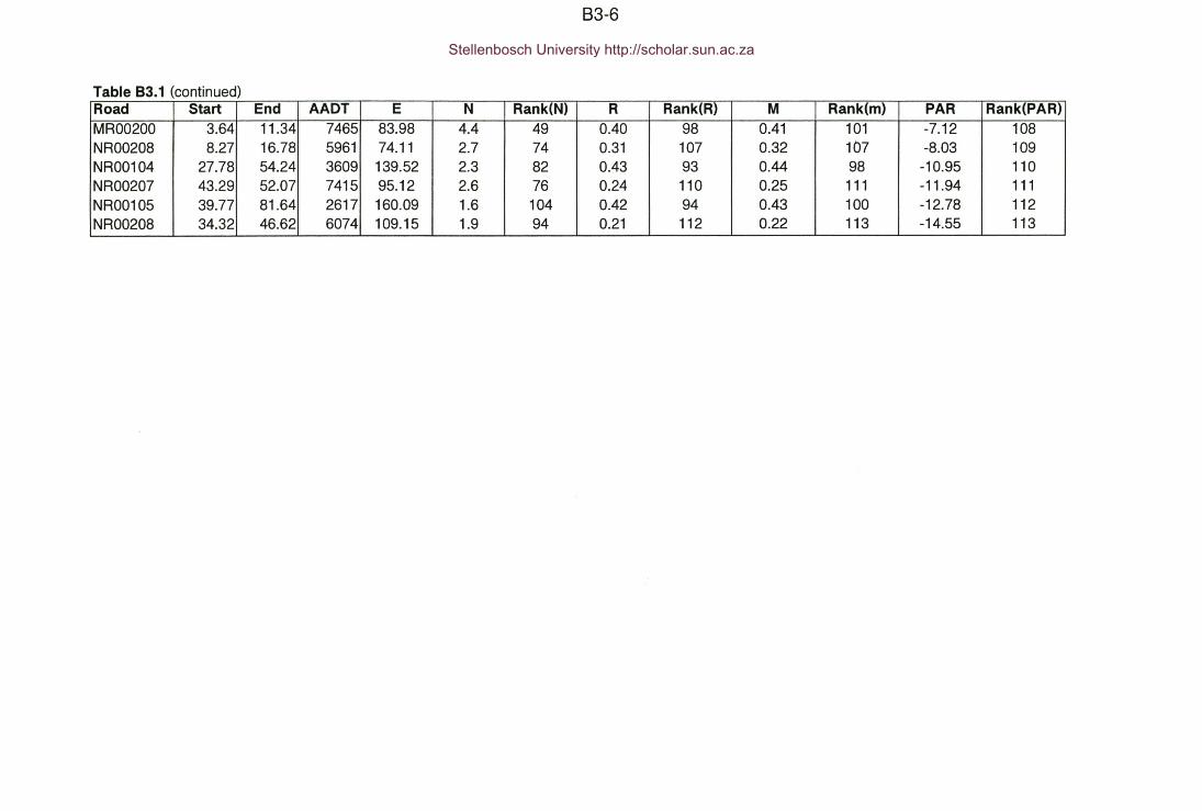
83-6
Table 83.1 (continued)Road Start End AADT E N Rank(N) R Rank(R) M Rank(m) PAR Rank(PAR)MR00200 3.64 11.34 7465 83.98 4.4 49 0.40 98 0.41 101 -7.12 108NR00208 8.27 16.78 5961 74.11 2.7 74 0.31 107 0.32 107 -8.03 109NR00104 27.78 54.24 3609 139.52 2.3 82 0.43 93 0.44 98 -10.95 110NR00207 43.29 52.07 7415 95.12 2.6 76 0.24 110 0.25 111 -11.94 111NR00105 39.77 81.64 2617 160.09 1.6 104 0.42 94 0.43 100 -12.78 112NR00208 34.32 46.62 6074 109.15 1.9 94 0.21 112 0.22 113 -14.55 113
Stellenbosch University http://scholar.sun.ac.za