Measurements of Road Traffic Parameters Using Inductive Loops and Piezoelectric Sensors  Metrology and Measurement Systems, vol. 14, no. 2, pp. 187–203, 2007. 

 

Piotr Burnos (burnos@agh.edu.pl), Janusz Gajda, Piotr Piwowar, Ryszard Sroka, 

Marek Stencel, Tadeusz Zeglen 

AGH – University of Science and Technology, Department of Measurement and Electronics, Poland 

 

ISSN: 0860‐8229  

DOI: 

Keywords: Traffic parameters measurements; Single loop detectors; WIM systems; Multi sensor WIM 

systems; Vehicle classification; Vehicle’s magnetic signature  

Cite as:  

IEEE:  

P. Burnos, J. Gajda, P. Piwowar, R. Sroka, M. Stencel, and T. Zeglen, “Measurements of Road Traffic 

Parameters Using Inductive Loops and Piezoelectric Sensors,” Metrol. Meas. Syst., vol. 14, no. 2, pp. 187–

203, 2007. 

Harvard: 

Burnos, P. et al., 2007. Measurements of Road Traffic Parameters Using Inductive Loops and Piezoelectric Sensors. Metrology and Measurement Systems, 14(2), pp.187–203. 

 

 

 

 

 

 

Licence: 

This work is licensed under the Creative Commons Attribution‐NonCommercial 4.0 

International License. To view a copy of this license, visit 

http://creativecommons.org/licenses/by‐nc/4.0/. 

Measurements of Road Traffic Parameters Using Inductive Loops and Piezoelectric Sensors

Piotr Burnos, Janusz Gajda, Piotr Piwowar, Ryszard Sroka,

Marek Stencel and Tadeusz Żegleń

AGH – University of Science and Technology Department of Measurement and Instrumentation

30-059 Kraków, al. Mickiewicza 30, e-mail: jgajda@agh.edu.pl

Abstract – The basic problems corresponding to the traffic measurements have been presented in the paper. Authors gave the general overview of the parameters and characteristics describing the vehicles and traffic flow. The current sensors’ technologies used in measuring systems has been presented. Moreover the measuring systems used in traffic measurements have been described. Special attention has been paid to the more sophisticated problems like the vehicle’s classification based on the analysis of its magnetic signature and to vehicles’ weigh-in-motion technique. The presented results base on the Authors’ experience in designing and exploitation of the measuring systems equipped with inductive loops and piezoelectric sensors.

Keywords – Traffic parameters measurements, Single loop detectors, WIM systems, Multi sensor WIM systems, Vehicle classification, Vehicle’s magnetic signature.

I. INTRODUCTION

The story of the measurements of road traffic parameters is very long. The first system oriented towards road traffic control has been put into use in London, in the 1868 year. It was a simple traffic light system, equipped with gas lamps. Following attempts in this area have been undertaken in Ohio, USA, in the 1914 year.

Much more advanced control system, called „Green Wave”, whose assignment was to increase traffic continuity, has been employed for the first time in Münich, Germany, in the 1953 year. Since then the number of vehicles participating in the traffic increases rapidly from year to year.

At present, the demand for the information concerning the basic traffic parameters and more sophisticated characteristics is still huge [27]. For example: traffic operators need these data for real-time traffic monitoring, transportation researches need these data to develop real-time incident detection algorithms, traffic engineers need these data as guidance of location of freight-oriented variable message signs, freight modellers need these data to provide calibration information for freight modelling, motor carrier dispatchers need these data for routing information, etc. The source of these data are measuring systems, which differ in their complexity and are equipped with different sensors kinds.

For optimal control the executive systems should be supplied with information - best of all in real time - about the situation taking place on the road. Therefore systems of traffic monitoring are coming into existence. The monitoring includes among others: presence and the number of vehicles in the detection area, speed of individual vehicle (or mean value of speed for specified number of vehicles), vehicle assortment, their load exerted upon road surface, occurrence of traffic jams, weather conditions (which have substantial influence upon traffic safety), etc.

The monitoring assignments are not merely aspects of direct traffic control, but its results may be of service for statistical studies, economic investigations, automatic toll collecting, highway infrastructure planning and reconditioning, as well as for protection against overloaded vehicles.

So monitoring prompts necessity to create measurement systems, capable of data acquisition and traffic parameters estimation. The basis of the latter are measurements of parameters of individual vehicle, participating in the traffic.

This paper addresses the basic problems corresponding to the measurements of the traffic parameters. The presented results base on the Authors’ experience in designing and exploitation of the measuring systems equipped with inductive loops and piezoelectric sensors. The paper is organized as follows. The basic parameters characterising the individual vehicles and characteristics of the traffic stream are presented in chapter 2nd. The overview of sensors used in traffic measurement systems is given in chapter 3rd. In chapter 4th the systems designed for measurements of basic traffic parameters, characterising the individual vehicles are presented. Chapter 5th contains the discussion of the problem of automated vehicle classification. The very nowadays-important problem of weighing of the moving vehicles is discussed in chapter 6th. Chapter 7th presents the research problems corresponding to the control and maintains of the road traffic.

II. BASIC PARAMETERS AND CHARACTERISTICS OF THE ROAD TRAFFIC

The basic parameters, which are the subject of the direct measurement, describe the individual vehicle or the traffic at the specific point on the road. The characteristics describing the traffic system are estimated on the base of the directly measured parameters. These parameters are divided into two groups i.e. transient parameters and fixed parameters. The transient parameters group consists of the following: time of arrival, lane number, speed, time headway, space headway, time gap, space gap, travel direction, acceleration, total mass, axle load (static component), axle load (dynamic component), axle frequency, number of passengers, trailer presence. The group of fixed parameters contains: vehicle’s class, number of axles, total wheel base, axle distances, length, width, area, height, front overhang, rear overhang, suspension height.

Considering individual vehicles, we can say that each vehicle i in a line of a traffic stream has the following informational

variables: a length, denoted by il , a longitudinal position, denoted by ix , a speed, denoted by dt

dxv i

i and acceleration,

denoted by 2

2

dt

xd

dt

dva ii

i . In this first approach, the other spatial characteristics of the vehicle such as its width, height and

line number are neglected [21]. Describing the traffic flow characteristics, we can consider two consecutive vehicles in the same lane in a traffic stream: a

follower i and its leader 1i . The vehicle i has certain space headway sih , to its predecessor, the space gap sig to its leader

and its own length il :

isisi lgh (1)

Taking the rear bumper as a vehicle’s position, the space headway iisi xxh 1 . The space gap is thus measured from

vehicle’s front bumper to its leader’s rear bumper. Analogously to equation (1) each vehicle also has a time headway tih (expressed in seconds), consisting of a time gap tig

and an occupancy time i :

ititi gh (2)

When the vehicle’s speed is constant, the time gap is the amount of time necessary to reach the current position of the leader when traveling at the current speed. Similarly, the occupancy time can be interpreted as the time needed to traverse a distance equal to the vehicle’s own length at the current speed, i.e., iii vl . Both equations (1) and (2) are furthermore linked to the

vehicle’s speed as follows:

ii

i

ti

si

ti

si vl

g

g

h

h

(3)

As the above definitions deal with what is called single-line traffic, we can easily extend them to multi-lane traffic. In some traffic flow literature, other nomenclature is used: space for the space headway, distance or clearance for the space gap, and headway for the time headway.

When considering many vehicles simultaneously, the macroscopic flow characteristics are used to represent all traffic faithfully.

The macroscopic characteristic, called density, allows us to get an idea of how crowded a certain section of a road is. It is typically expressed as the number of vehicles per kilometer. When density can not be exactly measured or computed, it has to be estimated. Using the spatial region sR (corresponding to measurements at a single instant in time), the density k for single-line

traffic is defined as:

K

Nk (4)

with N the number of vehicles presents on the road segment of length K . In general, density can be defined as the total time spent by all the vehicles in the measurement region, divided by the area of this region. This generalization allows us computing the density at a point using the measurement temporal region tR (corresponding to measurements at single fixed location in

space, during a certain time period mpT ):

N

i

N

i impimpmp

N

ii

vTv

dx

dxTdxT

T

k1 1

1 111 (5)

with iT the travel time and iv the speed of the thi vehicle.

Flow can be considered as a temporal measurement and it is typically expressed as a number of vehicles per hour. Sometimes other synonyms such as intensity, flux, throughput, current or volume are used. Measuring the flow q in region tR for single-

line traffic is done using the following equation:

mpT

Nq (6)

with N the number of vehicles that has passed the detector’s site. When using single inductive loop detectors, the vehicle speeds are not available. The detector’s logic therefore resorts to a

temporal measurement called the occupancy , which corresponds to the fraction of time the measurement location was

occupied by a vehicle:

N

iti

mp

oT

1

1 (7)

with tio the on-time of the thi vehicle, i.e., the time period during which it presents above the detector.

The final macroscopic characteristic to be considered is the mean speed of a traffic stream. It is expressed in kilometers per hour. If we base our approach on direct measurements of the individual vehicles’ speed, we can generally obtain the mean speed as the total distance traveled by all the vehicles in the measurement region, divided by the total time spent in this region. This gives the following formulas for the spatial and temporal regions, sR and tR respectively:

)(11

1

)(1

11

1

1

1

1

tN

i i

N

i i

s

N

ii

N

ii

N

ii

N

ii

s

Rregion

vNv

dx

dxN

RregionvNdtN

dtv

T

X

v (8)

with iX and iT the distance, respectively time, traveled by the thi vehicle and N the number of vehicles presents during the

measurement. The mean speed computed by the previous equations, is called the average travel speed, which is more commonly known as the space-mean speed.

It is interesting to see that the spatial measurement is based on an arithmetic average of the vehicles’ instantaneous speeds, whereas the temporal measurement is based on the harmonic average of the vehicles’ spot speed. If we take the arithmetic average of the vehicles’ spot speeds in the temporal measurement region tR instead, this would lead to what is called the time-

mean speed:

)(1

1t

N

iit Rregionv

Nv

(9)

The traffic parameters and characteristics defined above are measured by using specialized measurement systems based on different sensor technologies.

III. TRAFFIC SENSOR TECHNOLOGIES

There are many technologies available for collecting traffic data. Although inductive loop detectors (ILD) have been used more than any other method up to now, the other technologies are beginning to replace or complement loop detectors in many

applications last years. Many of these new technologies are roadside (or vertical sensors), which do not require pavement cuts or the disruption of traffic for installation. Many of the new sensors are cost competitive with ILD systems.

This section provides descriptions of currently available detectors. Road traffic detectors can be divided into two groups [17]:

* Embedded Detectors, * Non-intrusive

Detectors.

An embedded detector system consists of sensors in or below the surface of the roadway. These detectors are currently the most widely used form of vehicle detection. The main detectors being used include the following: rubber tubes, inductive loops, magnetometers, piezoelectric sensors, capacitive sensors, fiber optic sensors, strain gauge sensors, resistive sensors.

Non-intrusive detectors are also known as the above ground detectors. They are mounted on a structure above the surface of the pavement.

Advantages of that non-intrusive detectors over embedded detectors include the following: modifications to pavement are not required for installation, detectors can be moved or replaced more easily, lane closure may not be required during installation and maintenance, detectors can be used during and after any reconstruction or maintenance activities.

A disadvantage of non-intrusive detectors is that they may produce unreliable results during adverse weather conditions. Non-intrusive detectors include the following [17]: microwave radar, laser detector, passive infrared detector, ultrasonic

detector, passive acoustic detector, light curtain, video image processing. The detailed discussion concerning the properties of each kind of traffic detectors exceeds the frames of this paper. The

summarized information on chosen sensors is collect in Table I.

TABLE I ADVANTAGES AND DISADVANTAGES OF SOME TRAFFIC DETECTORS

Detector Type Advantages Disadvantages

Inductive Loop [17, 28,

39]

Flexible design. Wide range of applications. Provides basic traffic parameters (e. g. volume, speed, presence, occu-pancy).

Installation requires pave-ment cuts. Installation and maintenance requires lane closure. Detectors subject to stresses of traffic.

Magnetometer [17, 40]

Can be used in situations where loops are not feasible (e. g., bridge decks). Less sensitive than loops to stresses of traffic.

Installation requires pave-ment cuts. Installation and maintenance require lane closure. Small detection zone. Typically used only to pro-vide count and occupancy.

Microwave Radar [17, 29,

30, 31, 32]

Generally insensitive to weather conditions. Provides day and night operation.

Requires license for operation and maintenance. May lock on to the strongest signal (e. g., large truck).

Infrared [17, 43]

Active detector emits narrow beam allowing for accurate determination of vehicle position. Provides day and night operation. Provides most basic traffic parameters. Passive detectors can be used for strategic loop replacement.

Operation affected by precipitation (e. g., rain, fog, etc.). Difficulty in maintaining alignment on vibrating structures.

Ultrasonic [17, 41,42]

Provides most basic traffic parameters.

Environmental conditions (e. g., temperature, humi-dity, air turbulence, etc.) can affect performance. Snow covered vehicles are difficult to detect. High level of special maintenance capability is required.

Acoustic [17, Completely passive. Relatively new technology

39] Generally insensitive to weather conditions. Provides day and night operation.

for traffic surveillance.

Video Image Processing [17, 33, 34, 35, 36, 37]

Location or addition of detector zones can easily be done. Provides basic traffic para-meters. Provides wide-area detec-tion.

Inclement weather, sha-dows, and poor lighting can affect performance. May require significant processing power and a wide communication band-width.

IV. MEASUREMENTS OF BASIC TRAFFIC PARAMETERS

Figure 1 presents the measuring systems designed for measurement of basic traffic parameters. The systems are equipped with different sensor kinds and are able to measure different sets of parameters.

traffic line

system

inductive loop

"a"

traffic line

system

inductive loop 1

inductive loop 2

"b"

traffic line

system

inductive loop

piezo sensor 1

piezo sensor 2

"c"

Fig. 1. Diagrams of the measuring systems The system equipped with single inductive loop is the most simple one. In general, the measured parameters are as follows:

volume, magnetic signature of the vehicle, that allows the vehicles classification, occupancy, time intervals between successive vehicles. The more sophisticated analysis of the magnetic signature allows estimation of individual vehicle speed, trailer detection, as well as counting the number of axles, their reciprocal distances and vehicle length [1, 5, 6, 9, 10, 24, 27]. Uncertainty of the speed estimation depends on the loop width and vehicle class. In the class of personal cars this uncertainty, measured by standard deviation of the measurement results, is equal to 6% in the velocity range from 20km/h to 90km/h. The problem of vehicle classification, based on the analysis of its magnetic signature, is discussed in chapter 5th.

The second system is classical. It is equipped with two inductive loop sensors, what allows measurement of the following parameters: volume, occupancy, speed, individual vehicle length, trailer presence, time intervals between successive vehicles and vehicles class according to the vehicle length and presence of trailer.

The length measurement uncertainty in this system was tested using the reference vehicle 1250cm long, which traveled 4000 times through the tested measurement site. The standard deviation of the error of length measurement results was estimated as equal to 20cm. The maximum error did not exceed 60cm.

The error analysis of speed measurements in system with two inductive loop sensors was conducted by comparison its results with the reference results obtained in the system with two piezoelectric axle sensors. Than the speed was measured at the same moment by two systems i.e. by tested and reference. The speed of 800 vehicles was measured by compared systems. The mean value of the error was equal to zero and its standard deviation was 1.3 km/h.

The most advanced system is equipped with single inductive loop sensor and two piezoelectric axle sensors. The traffic parameters estimated in this system are as follows: presence detection, volume, occupancy, speed, vehicle length, number of axles, distances between successive axles, magnetic signature, trailer presence, time intervals between successive vehicles. The system is also able to classify vehicles on the base of the number of axles and their distances. Typical measurement signals of the system are presented in Fig. 2. Such a system allows differentiating between 13–14 vehicle classes [25].

0.0 0.2 0.4 0.6 0.8 1.0Time [s]

1 2

34

Fig. 2. Measurement signals from presented in Fig. 1c system, taken from a three-axle vehicle with two-axle trailer. 1 – vehicle presence signal; 2 – trailer presence signal; 3,4 – signals from axle load sensors

The uncertainty of axle counting in this system is very difficult to estimate. In the set of 400 vehicles passed the tested site

under different metrological and traffic conditions none case of erroneous axle counting was detected. The error and uncertainty of the axle distance measurement of the moving vehicles was tested by using the multi-axle

reference vehicle, which distance between first and second axles is equal to 360cm. The mean value of the measured distance was equal to 364 cm with the standard deviation 1.1cm. The mean value of the measured distance between axles number 4 and 5 was equal to 129.1 cm (true value 132cm) with standard deviation 0.83cm.

V. VEHICLE CLASSIFICATION

Classifying an automotive vehicle means determining to which of the selected classes the vehicle belongs. Classification methods are depend on the vehicle parameters that can be determined in a given measuring system and on the classification purpose.

The most simple classification method, often used in practice, is based on measuring the vehicle length. Not more than three classes are defined then. The method can be applied in a very simple measuring system, e.g., in a single-sensor system with inductive loop utilizing only the signal of vehicle occurrence above the sensor (Fig.1a).

When a necessity of defining more (four or five) classes arises, it is possible to use a system with inductive sensor and process the obtained magnetic profile of the vehicle [10, 19, 23]. The shape of a time signal generated by the interaction of a vehicle passing over an induction loop sensor with the magnetic field produced by the sensor is the basis for the recognition of vehicle class. Signals generated by different vehicles differ in their parameters such as e.g. amplitude, frequency spectrum, statistical parameters. These signals are called “vehicle magnetic signature” (or magnetic profile). The exemplary magnetic signatures of basic vehicle classes are presented in Figure 3.

0 0.4 0.8 1.2 1.6Time [s]

0

0.2

0.4

0.6

0.8

1

No

rmal

ized

am

plit

ud

e

1

2 3

4

Fig. 3. Magnetic signatures of the basic vehicle classes. 1 – passenger car, 2 – van, 3 – lorry, 4 – bus

The essence of the problem of the vehicle class recognition lies in the analysis of the recorded measurement signals concerning the above mentioned parameters and the comparison of the results of this analysis to the results of the analysis of the reference signals representing selected vehicle classes. This vehicle class is adopted as a classification result, which is represented by a reference signal the closest one in the sense of the analyzed properties, to the recorded, measured signal generated by the vehicle being identified. Reference signals are generated as a result of averaging many measurement signals corresponding to the selected vehicle.

An essential problem here is to make the measurement signal parameters (and, therefore, the results of classification) independent of the vehicle speed, vehicle suspension height and other disturbing factors. This aspect of the problem was discussed e.g. in [11]. There is also a tendency to ensure the satisfactory selectivity of the classification process in order to differentiate among the required number of vehicle classes.

One method out of the magnetic profile preprocessing methods consists in transforming the profile into the vehicle length domain [11]. This operation results in that, the profile contains the combined information on the shape and length of the primary profile, what enables more selective classification to be made (Fig. 4). To carry out such transformation the information about the vehicle speed is also necessary. In specific cases, amplitude standardization can be abandoned, gaining this way additional information about the vehicle suspension height.

0 2 4 6 8 10 12 14 16 18 20Vehicle length [m]

0.0

0.2

0.4

0.6

0.8

1.0

No

rmal

ized

am

plit

ud

e

Short bus

Bus

City bus

Fig. 4. Bus magnetic profiles in the vehicle length domain Nonparametric classification methods consist in comparing directly the profile generated by the vehicle being classified (after

transformation) with the reference profiles representing each of the defined classes. Depending on vehicle class, the effectiveness of such classification ranges from 67% to 100%.

Parametric methods consist in comparing the profile parameters of the vehicle being classified and reference vehicle. The effectiveness of the classification based on individual profile parameters is unsatisfactory [11, 23] (depending on the selected parameter, the effectiveness gained is 60%–70% for one of the classes and considerable worse for the others).

Combined utilization of various parameters is much more effective: the classification effectiveness in all classes that were under consideration is then increased and equalized [11], [12]. It can be implemented basing on voting or weighted voting methods, or hierarchical methods. Depending on the class, the classification effectiveness of the voting methods is in the interval of 50% to 97%. The classification effectiveness of the hierarchical methods ranges from 77% to 96%.

However, such classification may not be enough selective. It is then necessary to measure the inter-axle distances. Taking into account this parameter improves considerably the classification selectiveness although requires the vehicle speed to be measured. In such a system also vehicle length is measured and a trailer is detected. Such classification is performed in the measuring system equipped with single inductive loop sensor and two piezoelectric axle detectors. For such classification systems used in Europe European Classification of Road Vehicle is recommended, which distinguishes 13 classes. The axle distance measured using the piezoelectric axle sensors is strongly affected by the vehicle mass, because the length of the tire footprint depends on the axle load.

The erroneous classification of the vehicle on the base of its axle distances occurs first of all in the population of two-axle vehicles. The error in the distance measurement may cause the classification of the vehicle to one of the neighbor class, for instance the car is classified as the van and so. The estimated probability of erroneous classification of two-axle vehicles is presented in Table II.

TABLE II ESTIMATED PROBABILITY OF THE ERRONEOUS CLASSIFICATION OF TWO-AXLE VEHICLES, BASING ON THE AXLE DISTANCE MEASUREMENT

Vehicle class Probability of the erro-neous classification

(%)

Car classified as van 0.24 Van classified as car 4.8 Van classified as lorry 0.5 Lorry classified as van 1.2 Lorry classified as bus 5.2 Bus classified as lorry 46.0

VI. WEIGH IN MOTION SYSTEMS (WIM)

The term weigh-in-motion (WIM) means a process of measuring the dynamic wheel forces of a moving vehicle onto the road and estimating the corresponding static loads or/and total vehicle weight. The lack of significant limitations posed on the vehicle speed is a characteristic feature of such weighing systems. At present, the WIM systems complement the static vehicle weighing stations, playing the role of preselection systems. Limited accuracy of these systems is the reason of such situation [4, 7, 26].

Classic WIM preselection systems are based on an inductive sensor and two load sensors (Fig. 1c). Such a system configuration allows estimation of the static loads of individual axles and total weight. Moreover it provides classification of the vehicle, based on the number of its axles. The pavement temperature measurement is necessary for correction of weighing results, which depend on the thermal and mechanical properties of the pavement and sensors.

The basic reasons limiting the accuracy of the WIM systems are as follows: - vertical balancing of the suspended mass (car body) and hopping of the unsuspended mass (wheels), - influence of the temperature on the sensitivity of the piezoelectric load sensors, - changes in sensitivity along the sensors. The load exerted by the wheels of weighed vehicle on the road surface contains both the constant, as well as dynamic

components. The amplitude and spectral properties of the load dynamic component depend on the specific vehicle mechanical parameters, its speed and roughness of the road surface [2, 8]. The load signal is sampled at the moments when the weighed axle is passed over the load sensor (Fig. 5). It means that in preselective WIM systems equipped with two load sensors the axle static load is estimated on the base of two samples only. The High Speed WIM systems equipped with two load sensors allow estimation of the total weight of a moving vehicle with error not less than 10–15%.

Lo

ad

load samples

WIM sensors

wheel path

distance y

Fig. 5. Sampling of the load force on the MS-WIM site The piezoelectric, strip sensors are one of the load sensors frequently used in WIM systems. They are mounted under the

asphalt surface. Than asphalt transfers the load from the wheel to the sensors. Changes in the asphalt mechanical parameters vs. temperature cause correlated changes in the sensor sensitivity. From this point of view the quartz load sensors have better

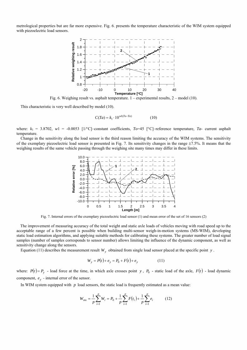
metrological properties but are far more expensive. Fig. 6. presents the temperature characteristic of the WIM system equipped with piezoelectric load sensors.

-20 -10 0 10 20 30 40Temperature [oC]

0.8

1

1.2

1.4

1.6

1.8

2

Rel

ativ

e w

eig

hin

g r

esu

lt1

2

Fig. 6. Weighing result vs. asphalt temperature. 1 – experimental results, 2 – model (10).

This characteristic is very well described by model (10).

)o(11 10)( TaTwkTaC (10)

where: k1 = 3.8702, w1 = -0.0053 [1/C]–constant coefficients, To=45 [C]–reference temperature, Ta- current asphalt temperature.

Change in the sensitivity along the load sensor is the third reason limiting the accuracy of the WIM systems. The sensitivity of the exemplary piezoelectric load sensor is presented in Fig. 7. Its sensitivity changes in the range 7.5%. It means that the weighing results of the same vehicle passing through the weighing site many times may differ in these limits.

0 0.5 1 1.5 2 2.5 3 3.5 4Length [m]

-10.0-8.0-6.0-4.0-2.00.02.04.06.08.0

10.0

Rel

ativ

e er

ror

[%] 1

2

Fig. 7. Internal errors of the exemplary piezoelectric load sensor (1) and mean error of the set of 16 sensors (2) The improvement of measuring accuracy of the total weight and static axle loads of vehicles moving with road speed up to the

acceptable range of a few percent is possible when building multi-sensor weigh-in-motion systems (MS-WIM), developing static load estimation algorithms, and applying suitable methods for calibrating these systems. The greater number of load signal samples (number of samples corresponds to sensor number) allows limiting the influence of the dynamic component, as well as sensitivity change along the sensors.

Equation (11) describes the measurement result yW obtained from single load sensor placed at the specific point y .

yyy etFPetPW 0 (11)

where: yPtP - load force at the time, in which axle crosses point y , 0P - static load of the axle, tF - load dynamic

component, ye - internal error of the sensor.

In WIM system equipped with p load sensors, the static load is frequently estimated as a mean value:

p

ii

p

ii

p

iims e

ptF

pPW

pW

110

1

111 (12)

where: iW - load measured at i-th sensor, ie - internal error of the ith sensor, it - time moment at which weighed axle passes ith

sensor. The mean characteristic of the set of 16 sensors is presented in Fig. 7. The mean error was reduced few times and is in the

range 3%. In the same way proper sampling of the load signal also reduces the dynamic component tF . It is fulfilled under additional

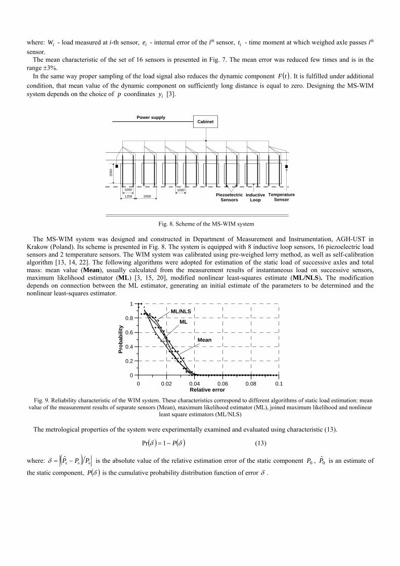
condition, that mean value of the dynamic component on sufficiently long distance is equal to zero. Designing the MS-WIM system depends on the choice of p coordinates iy [3].

1000

1200 2000

1000

TemperatureSensor

InductiveLoop

PiezoelectricSensors

2000

CabinetPower supply

Fig. 8. Scheme of the MS-WIM system The MS-WIM system was designed and constructed in Department of Measurement and Instrumentation, AGH-UST in

Krakow (Poland). Its scheme is presented in Fig. 8. The system is equipped with 8 inductive loop sensors, 16 piezoelectric load sensors and 2 temperature sensors. The WIM system was calibrated using pre-weighed lorry method, as well as self-calibration algorithm [13, 14, 22]. The following algorithms were adopted for estimation of the static load of successive axles and total mass: mean value (Mean), usually calculated from the measurement results of instantaneous load on successive sensors, maximum likelihood estimator (ML) [3, 15, 20], modified nonlinear least-squares estimate (ML/NLS). The modification depends on connection between the ML estimator, generating an initial estimate of the parameters to be determined and the nonlinear least-squares estimator.

0 0.02 0.04 0.06 0.08 0.1Relative error

0

0.2

0.4

0.6

0.8

1

Pro

bab

ility

Mean

ML

ML/NLS

Fig. 9. Reliability characteristic of the WIM system. These characteristics correspond to different algorithms of static load estimation: mean value of the measurement results of separate sensors (Mean), maximum likelihood estimator (ML), joined maximum likelihood and nonlinear

least square estimators (ML/NLS) The metrological properties of the system were experimentally examined and evaluated using characteristic (13).

P 1Pr (13)

where: 000̂ PPP is the absolute value of the relative estimation error of the static component 0P , 0P̂ is an estimate of

the static component, P is the cumulative probability distribution function of error .

This characteristic specifies the probability of occurrence of error greater than and it is called reliability characteristic. The characteristic (13) determined for described MS-WIM system is presented in Fig. 9. The conclusion, which could be draw out from the obtained results says, that none vehicle was weighed with the error greater than 4%.

VII. CONCLUSIONS

The basic problems corresponding to the road traffic measurements have been addressed in the paper. In correlation with the growth of vehicle transport the research projects are still conducted and new technical tools are offered for practical applications in this area. A lot of effort has been put into the solution of the following problems corresponding to the traffic measurements and monitoring during last years:

- new technologies of the traffic detectors and sensors (wireless sensors), - design of the new data processing algorithms, using the classical sensors for obtaining the new traffic parameters, which

were not available in classical solutions (estimation of the individual vehicle speed in the system with single loop detector, counting the axles on the base of vehicle magnetic signature),

- design of the MS-WIM systems allowing to estimate the static axle load and vehicle total mass with uncertainty limited to several percentage (multi-sensor site with uniformly distributed WIM sensors, more sophisticated algorithms of static load estimation),

- automatic weighing and charging of the overloaded vehicles, - design of the traffic monitoring and information system that visually conveys the traffic flow information to general public

through the client/server computer architecture.

REFERENCES

[1] Athol P. „Interdependence of Certain Operational Characteristics Within a Moving Traffic Stream”, Highway Research Record, Vol. 72, 1965.

[2] Cebon D., Handbook of Vehicle-Road Interaction, Swets&Zeitlinger B.V., Lisse, the Netherlands 1999. [3] Cebon D.: “Design of multiple-sensor weigh-in-motion systems”, Journal of Automobile Engineering, Proc. I. Mech. E., 204, 1990, pp.

133 – 144. [4] Cebon D., Winkler CB.; „Multiple-Sensor WIM: Theory and experiments”, Transportation Research Record, TRB, 1311, 1991, pp. 70 -

78. [5] Dailey D.J.; “Travel Time Estimates Using a Series of Single Loop Volume and Occupancy Measurements”, Transport Research Board

76th Annual Meeting, Washington, D.C., 1997. [6] Dailey D.J., Harn P., Lin P.; ITS Data Fusion, Final research report, Research project T9903, Department of Transportation, Washington

State Transportation Commission, April 1996. [7] Dolcemascolo V., Jacob B.: “Multiple sensor Weigh-In-Motion: Optimal Design and Experimental Study”, Pre-proceedings of 2nd

European Conference of Weigh in Motion of Road Vehicles, Lisbon, 14/16 September 1998, pp.129-138. [8] Dukkipati R.V.: Vehicle Dynamics, Alpha Science International Ltd. 2000. [9] Gajda J., Sroka R., Stencel M., Żegleń T.; "Measurement of Road Traffic Parameters Using an Inductive Single-Loop Detector", 9th

International Symposium on Electrical Instruments in Industry, Glasgow 1997. [10] Gajda J., Stencel M.; "Determination of Road Vehicle Types Using an Inductive Loop Detector", XIV IMEKO World Congress,

Tampere, Finland, 1997. [11] Gajda J., Sroka R.: “Vehicle classification by parametric identification of the measured signals”, Proceedings of XVI IMEKO World

Congress, Vienna 2000, vol. IX, pp. 199-204. [12] Gajda J., Sroka R., Stencel M., Wajda A., Zeglen T.: “A vehicle classification based on inductive loop detectors”, Proceedings of the 18th

IEEE, IMTC, Budapest 2001, pp. 460-464. [13] Gajda J.; “Statistical calibration of WIM systems”, Scientific Series of Rzeszów Politechnic, Electrotechnic, nr 27, Rzeszów, 2004r, (in

Polish). [14] Gajda J., Burnos P.: “Self-calibration of the weigh-in-motion systems”. Proceedings of XV Symposium Modelling and Simulation of

Measurement Systems, Krynica 2005, (in Polish). [15] Gonzales A., Papagiannakis A.T., O’Brien E.: Evaluation of an Artificial Neural Network Technique Applied to Multiple Sensor Weigh-

in-Motion Systems, University College Dublin, Ireland. [16] Huhtala M.: Factors Affecting Calibration Effectiveness, Proceedings of the Final Symposium of the Project WAVE, Paris 1999. [17] Klein L.A.: Sensor Technologies and Data Requirements for ITS, Artech House, London 2001. [18] Karlsson B.: “Fuzzy Measures for Sensor Data Fusion in Industrial Recycling”, Measurement Science and Technology, Vol. 9, 1998, pp.

907-912. [19] Ki Y.K., Baik D.K.: “Vehicle Classification Algorithm for Loop Detectors using Neural Network”, IEEE Transactions on Vehicular

Technology, vol. 55, Nr 6, 2006, pp. 1704-1711. [20] Mangeas M., Glaser S., Dolcemascolo V.: “Neural networks estimation of truck static weights by fusing weight-in-motion data”,

Proceedings of Eurofusion 2000. [21] Maerivoet S., De Moor B.; “Traffic Flow Theory”, internet paper, 2006. [22] Stanczyk D.: “New Calibration Procedure by Axle Rank”, Proceedings of the Final Symposium of the Project WAVE, Paris 1999, pp.

307-316.

[23] Sun C., Ritchie G., Tsai K., Jayakrishnan R.,; “Use of vehicle signature analysis and lexicographic optimisation for vehicle reidentification on freeways”. Transportation Research Part C 7 (1999), pp. 167-185.

[24] Wang Y., Nihan N.; „Can Single-Loop Detectors Do the Work of Dual-Loop Detectors?”, internet paper. [25] Weigh-in Motion of Road Vehicle, Final Report of COST 323 action, Ver. 3.0, 1999. [26] Weigh-In-Motion of Axles and Vehicles for Europe (WAVE), General Report of 4th Programme Transport, Laboratoire Central des Pontes

et Chaussees, 2001. [27] Zhang X., Wang Y., Nihan N.; „Monitoring a Freeway Network in Real Time Using Single - Loop . Detectors”, Int. J. Vehicle

Information and Communication Systems, Vol. 1, Nos. 1/2 2005. [28] Gibson D., Tweedy C.; “An Advanced Preformed Inductive Loop Sensor”, NATMEC, Charlotte, USA, 1998. [29] www.rtms-by-eis.com. [30] www.agd-systems.com. [31] www.rtms-by-eis.com. [32] www.wavetronix.com. [33] www.crs-vision.com. [34] www.iteris.com. [35] www.traffipax.com. [36] www.autoscope.com. [37] www.imagesensing.com. [38] www.smarteksys.com. [39] www.orincon.com/itms. [40] Caruso M.J., Withanawasam L.S.; „Vehicle Detection and Compass Application using AMR Magnetic Sensors”, Honeywell (internet

paper). [41] www.mssedeo.com,/TC30.html. [42] Song K., Chen C., Huang C.C.; “Design and Experimental Study of an Ultrasonic Sensor System for Lateral Collision Avoidance at Low

Speeds”, IEEE Intelligent Vehicles Symposium, Parma, 2004. [43] Mustafa H.T.; “Infrared Vehicle Sensor for Traffic Control”, (Ph.D. Thesis – City University of New York, 1994.