Congestion Control and Resource Allocation in Emerging ...

Congestion Control and Resource Allocation in Emerging Wireless Networks

by

Kefan Xiao

A dissertation submitted to the Graduate Faculty ofAuburn University

in partial fulfillment of therequirements for the Degree of

Doctor of Philosophy

Auburn, AlabamaMay 4, 2018

Keywords: Congestion control, Video streaming, Wireless networks, Deep reinforcementlearning

Copyright 2018 by Kefan Xiao

Approved by

Shiwen Mao, Chair, Ginn Distinguished Professor of Electrical and Computer EngineeringXiaowen Gong, Professor of Electrical and Computer Engineering

Robert Mark Nelms, Professor of Electrical and Computer EngineeringJitendra K. Tugnait, James B Davis Professor of Electrical and Computer Engineering

Abstract

With the fast growth of wireless technologies, such as 4G-LTE, cognitive radio networks,

and 5G and beyond, data transportation in the wireless environment is dramatically increasing

and has taken the dominant role over wired networks. The advantage of wireless networks

are obvious: easier deployment, ubiquitous access, etc. However, the traditional transporta-

tion layer protocols, such as Transmission Control Protocol (TCP), are well known to perform

poorly in wireless environments. This is because packets might be dropped due to transmission

errors or broken connection, in addition to congestion caused buffer overflow. Furthermore, the

capacity variation of wireless links also affect the TCP performance.

One of the key applications of TCP nowadays, is video streaming. It has now dominated

the mobile data traffic, i.e., over 60 percent, in 2016, and is expected to account for over 75

percent of the mobile data in 2021. At the same time, rapidly growing overall mobile traffic

(which has increased 18-fold since 2011) and the large number of mobile devices (429 millions

were added in 2016) have made it a great challenge for mobile video streaming. The instabil-

ity nature of wireless link capacity will make the situation even worse. There is a compelling

need now to deal with the problem: how to achieve efficiency and robustness for video deliv-

ery over emerging wireless networks. This problem should be studied from both the wireless

infrastructure and user equipment aspects.

In this thesis, we first conduct research on how to enhance the performance of TCP in

wireless environment, specifically, for cognitive radio networks (CRNs). We investigate the

problem of robust congestion control in infrastructure based cognitive radio networks (CRN).

We develop an active queue management (AQM) algorithm, termed MAQ, which is based on

multiple model predictive control (MMPC). The goal is to stabilize the TCP queue at the base

station (BS) under disturbances from the time-varying service capacity for secondary users

(SU). The proposed MAQ scheme is validated with extensive simulation studies under various

ii

types of background traffic and system/network configurations. It outperforms two benchmark

schemes with considerable gains in all the scenarios considered.

We then further investigate the dynamics of nowadays complicated networking systems

and propose a smart congestion control algorithm based on recent progress of Artificial Intel-

ligence (i.e., Deep reinforcement learning (DRL)). In order to accommodate the wide range of

different types of networks and goals, the general framework of congestion control based on

DRL is first proposed. With the understanding of the congestion control problem, the states,

actions, and reward of the DRL framework are defined. The new progress in deep learning such

as convolutional neural network (CNN) and long short term memory (LSTM) are also utilized

to deal with the challenges in congestion control problem. Extensive NS3 simulation studies

are conducted, which validate the superior of this method over all scenarios.

Finally, the problem of effective and robust delivery of video over orthogonal frequency-

division multiplexing access (OFDMA) wireless network is studied. The measurement of real

network capacity and request interval time is presented as the motivation for the considera-

tion of the estimation of capacity and request interval. The offline cross-layer optimization is

first formulated. Then the online transformation is proposed and proved to be asymptotically

converge to the offline solution. After analyzing the structure of the optimization problem,

we proposed an primal decomposition (DORA) for this DASH bit rate adaption and OFDM

Resource Allocation problem. Further, we introduce the stochastic model predictive control

(SMPC) to achieve better Robustness on bit rate adaption and consider the request Interval time

at resource allocation (DORA-RI). Simulations are conducted and the efficacy and robustness

of the proposed scheme are validated.

iii

Acknowledgments

I would like to express my sincere appreciation to my major advisor Prof. Shiwen Mao

and co-advisor Prof. Tugnait. They provided me the continuous guidance of my Ph.D research

with their excellent expertise and superior research ideology. Prof. Mao spent precious time

and effort to polish my writing of publications and this dissertation. Moreover, with the com-

munication and interaction in the past four and half years, their research methodology, integrity

and curiosity to the world enlightened me how to become a researcher, and most importantly,

how to be a better human-being.

I also would like to thank my dissertation committee:Prof. Mark Nelms, and Prof. Xi-

aowen Gong, for their insightful comments and suggestions to my research works. I am also

indebted to Prof. Tao Shu for serving as the university reader, who reviewed my work.

My sincere thanks also goes to my friends at Auburn University: Dr. Yi Xu, Dr. Zhifeng

He, Dr. Zhefeng Jiang, Dr. Yu Wang, Dr. Xuyu Wang, Dr. Mingjie Feng, Yu Wang, Ningkai

Tang, Lingjun Gao, Wei Sun, Blake A. Jacobs and Brett E. Todd, Chao Yang, Ticao Zhang, for

the support, friendship, happiness and tears we shared these years.

Last but certainly not the least, I would like to give my deep appreciation to my parents.

Their selflessly love and support provide me the courage along the journey.

This work is supported in part by the US NSF under Grants CNS-1320664, CNS-1702957,

and CNS-1822055, and through the Wireless Engineering Research and Education Center

(WEREC) at Auburn University.

iv

Table of Contents

Abstract . . . . . . . . . . . . . . . . . . . . . . . . . . . . . . . . . . . . . . . . . . . ii

Acknowledgments . . . . . . . . . . . . . . . . . . . . . . . . . . . . . . . . . . . . . . iv

List of Abbreviations . . . . . . . . . . . . . . . . . . . . . . . . . . . . . . . . . . . . xii

1 Introduction . . . . . . . . . . . . . . . . . . . . . . . . . . . . . . . . . . . . . . . 1

2 MAQ: A Multiple Model Predictive Congestion Control Scheme for Cognitive RadioNetworks . . . . . . . . . . . . . . . . . . . . . . . . . . . . . . . . . . . . . . . . 6

2.1 Introduction . . . . . . . . . . . . . . . . . . . . . . . . . . . . . . . . . . . . 6

2.2 System Model and Problem Formulation . . . . . . . . . . . . . . . . . . . . . 8

2.2.1 Network Model . . . . . . . . . . . . . . . . . . . . . . . . . . . . . . 8

2.2.2 Fluid Flow Model for TCP Sessions . . . . . . . . . . . . . . . . . . . 10

2.2.3 Linearization and Discretization . . . . . . . . . . . . . . . . . . . . . 11

2.3 MAQ Design . . . . . . . . . . . . . . . . . . . . . . . . . . . . . . . . . . . 14

2.3.1 Estimation . . . . . . . . . . . . . . . . . . . . . . . . . . . . . . . . . 15

2.3.2 Weight Calculation . . . . . . . . . . . . . . . . . . . . . . . . . . . . 16

2.3.3 MMPC Control Law . . . . . . . . . . . . . . . . . . . . . . . . . . . 17

2.3.4 Parameter Tuning . . . . . . . . . . . . . . . . . . . . . . . . . . . . . 20

2.4 Simulation Study . . . . . . . . . . . . . . . . . . . . . . . . . . . . . . . . . 22

2.4.1 Responsive Background Traffic . . . . . . . . . . . . . . . . . . . . . . 23

2.4.2 Non-responsive Background Traffic . . . . . . . . . . . . . . . . . . . 25

2.4.3 Varying Number of FTP Connections . . . . . . . . . . . . . . . . . . 27

v

2.4.4 Different Propagation Delay and Reference Queue Length . . . . . . . 28

2.5 Related Work . . . . . . . . . . . . . . . . . . . . . . . . . . . . . . . . . . . 32

2.5.1 End-to-End Solutions . . . . . . . . . . . . . . . . . . . . . . . . . . . 32

2.5.2 Router-based Solutions . . . . . . . . . . . . . . . . . . . . . . . . . . 33

2.5.3 CRN Congestion Control Schemes . . . . . . . . . . . . . . . . . . . . 33

2.6 Conclusion . . . . . . . . . . . . . . . . . . . . . . . . . . . . . . . . . . . . 34

3 Model Free Congestion Control for Mobile Network based on Deep ReinforcementLearning . . . . . . . . . . . . . . . . . . . . . . . . . . . . . . . . . . . . . . . . . 35

3.1 Introduction . . . . . . . . . . . . . . . . . . . . . . . . . . . . . . . . . . . . 35

3.2 Related Work . . . . . . . . . . . . . . . . . . . . . . . . . . . . . . . . . . . 38

3.2.1 End-to-End Schemes . . . . . . . . . . . . . . . . . . . . . . . . . . . 38

3.2.2 Router based Schemes . . . . . . . . . . . . . . . . . . . . . . . . . . 40

3.2.3 Smart Schemes . . . . . . . . . . . . . . . . . . . . . . . . . . . . . . 40

3.3 Preliminaries of DRL . . . . . . . . . . . . . . . . . . . . . . . . . . . . . . . 41

3.4 System Model, Assumptions and Problem Statement . . . . . . . . . . . . . . 43

3.4.1 Network Architecture . . . . . . . . . . . . . . . . . . . . . . . . . . . 43

3.4.2 Partially Observable Information . . . . . . . . . . . . . . . . . . . . . 44

3.4.3 Basic Assumptions . . . . . . . . . . . . . . . . . . . . . . . . . . . . 45

3.4.4 Network Modeling . . . . . . . . . . . . . . . . . . . . . . . . . . . . 46

3.4.5 Utility Function . . . . . . . . . . . . . . . . . . . . . . . . . . . . . . 47

3.5 TCP-Drinc Design . . . . . . . . . . . . . . . . . . . . . . . . . . . . . . . . . 48

3.5.1 Approach for Multi-agent Situation . . . . . . . . . . . . . . . . . . . 48

3.5.2 Feature Engineering . . . . . . . . . . . . . . . . . . . . . . . . . . . . 49

3.5.3 Definitions of States and Actions . . . . . . . . . . . . . . . . . . . . 49

3.5.4 Reward Calculation . . . . . . . . . . . . . . . . . . . . . . . . . . . . 50

3.5.5 Experience Buffer Formation . . . . . . . . . . . . . . . . . . . . . . . 52

vi

3.5.6 Agent Design . . . . . . . . . . . . . . . . . . . . . . . . . . . . . . . 53


3.6.1 Simulation Setup . . . . . . . . . . . . . . . . . . . . . . . . . . . . . 55

3.6.2 Training Process . . . . . . . . . . . . . . . . . . . . . . . . . . . . . 55

3.6.3 Congestion Control Performance . . . . . . . . . . . . . . . . . . . . . 56

3.7 Conclusions . . . . . . . . . . . . . . . . . . . . . . . . . . . . . . . . . . . . 65

4 DORA: A Cross-layer optimization for Robust QoE-Driven DASH over OFDMANetworks Bit Rate Adaption and Resource Allocation . . . . . . . . . . . . . . . . . 66

4.1 Introduction . . . . . . . . . . . . . . . . . . . . . . . . . . . . . . . . . . . . 66

4.1.1 Motivation . . . . . . . . . . . . . . . . . . . . . . . . . . . . . . . . . 68

4.1.2 Contributions and Organization . . . . . . . . . . . . . . . . . . . . . . 69

4.2 System Model . . . . . . . . . . . . . . . . . . . . . . . . . . . . . . . . . . 71

4.2.1 Network Model . . . . . . . . . . . . . . . . . . . . . . . . . . . . . . 71

4.2.2 Streaming Video Model . . . . . . . . . . . . . . . . . . . . . . . . . . 73

4.2.3 Quality of Experience (QoE) Model . . . . . . . . . . . . . . . . . . . 74

4.3 Problem Formulation . . . . . . . . . . . . . . . . . . . . . . . . . . . . . . . 76

4.3.1 The Offline Optimization Problem . . . . . . . . . . . . . . . . . . . . 77

4.3.2 Online Optimization Formulation . . . . . . . . . . . . . . . . . . . . 78

4.4 Solution Algorithms and Analysis . . . . . . . . . . . . . . . . . . . . . . . . 80

4.4.1 Prob-Online Analysis . . . . . . . . . . . . . . . . . . . . . . . . . . . 80

4.4.2 UE Rate Adaption . . . . . . . . . . . . . . . . . . . . . . . . . . . . 81

4.4.3 Base Station Side Optimization . . . . . . . . . . . . . . . . . . . . . 83


4.5.1 Simulation Scenario and Algorithm Configuration . . . . . . . . . . . . 85

4.5.2 Simulation Results and Discussions . . . . . . . . . . . . . . . . . . . 86

4.6 Related Work . . . . . . . . . . . . . . . . . . . . . . . . . . . . . . . . . . . 90

vii

4.7 Conclusions . . . . . . . . . . . . . . . . . . . . . . . . . . . . . . . . . . . . 92

4.8 Proof for Theorem 4.1 . . . . . . . . . . . . . . . . . . . . . . . . . . . . . . . 92

4.9 Proof for Lemma 1 . . . . . . . . . . . . . . . . . . . . . . . . . . . . . . . . 93



5 Future Work . . . . . . . . . . . . . . . . . . . . . . . . . . . . . . . . . . . . . . . 97

References . . . . . . . . . . . . . . . . . . . . . . . . . . . . . . . . . . . . . . . . . . 99

viii

List of Figures

2.1 Network model of CR network . . . . . . . . . . . . . . . . . . . . . . . . . . 9

2.2 The control system structure. . . . . . . . . . . . . . . . . . . . . . . . . . . . 15

2.3 The CRN downlink capacity over time used in one of the simulations. . . . . . 23

2.4 Queue length dynamics under responsive background traffic. . . . . . . . . . . 24

2.5 Packet queuing delay dynamics under responsive background traffic. . . . . . . 24

2.6 Queue length dynamics under non-responsive background traffic. . . . . . . . . 26

2.7 Packet queuing delay dynamics under non-responsive background traffic. . . . 26

2.8 Change of the number of FTP connections during the simulation period. . . . . 27

2.9 Queue length dynamics under varying number of connections. . . . . . . . . . 27

2.10 Packet queuing delay dynamics under varying number of connections. . . . . . 28

2.11 Queue length dynamics under varying number of connections. . . . . . . . . . 29

2.12 Packet queuing delay dynamics under varying number of connections. . . . . . 29

2.13 Average link utilization under increased propagation delays. . . . . . . . . . . 30

2.14 Link utilization under under increasing reference queue lengths. . . . . . . . . 30

2.15 Average delay and delay STD under increasing propagation delays. . . . . . . . 31

2.16 Average delay and delay STD under increasing reference queue lengths. . . . . 31

3.1 Reinforcement learning design for congestion control. . . . . . . . . . . . . . . 43

3.2 System architecture for TCP over wireless. . . . . . . . . . . . . . . . . . . . . 44

3.3 The TCP-Drinc system architecture. . . . . . . . . . . . . . . . . . . . . . . . 53

3.4 Design of the proposed convolutional neural network (in the figure, “C.” rep-resents the convolutional layer, “S.” represents the down sampling (pooling)layer, “FC” means fully connected). . . . . . . . . . . . . . . . . . . . . . . . 53

ix

3.5 The dynamics of the single agent pre-training. . . . . . . . . . . . . . . . . . . 57

3.6 The training result of single agent distribute training. . . . . . . . . . . . . . . 58

3.7 Throughput and RTT statistics with different propagation delays. . . . . . . . . 60

3.8 Throughput and RTT statistics with different number of users. . . . . . . . . . 61

3.9 Throughput and RTT statistics with different bottleneck capacities. . . . . . . . 62

3.10 Performance of different algorithms over randomly varied parameters. . . . . . 64

3.11 Jain’s index for each algorithm. . . . . . . . . . . . . . . . . . . . . . . . . . . 64

3.12 LTE network simulation results with the dumbell topology and 5 mobile users. . 65

4.1 DASH mobile video streaming system architecture. . . . . . . . . . . . . . . . 68

4.2 The variations of request intervals obtained in our measurement study over anLTE link. . . . . . . . . . . . . . . . . . . . . . . . . . . . . . . . . . . . . . 69

4.3 The variations in the average capacity of an LTE video link. . . . . . . . . . . . 70

4.4 Timeline of the discrete time DASH system. . . . . . . . . . . . . . . . . . . . 73

4.5 Comparison of QoE values for DORA-RI, DORA, and PFWF-RM. . . . . . . . 87

4.6 Comparison of rebuffering ratio for DORA-RI, DORA and PFWF-RM. . . . . 88

4.7 Comparison of QoE score for DORA-RI, DORA-MPC and DORA-no-RI. . . . 88

4.8 Comparison of rebuffering ratio for DORA-RI, DORA-MPC and DORA-no-RI. 89

4.9 Comparison of data-rate standard deviation for DORA-RI, DORA-MPC andDORA-no-RI . . . . . . . . . . . . . . . . . . . . . . . . . . . . . . . . . . . 90

x

List of Tables

2.1 Queue Length, Queueing Delay, and Link Utilization Statistics . . . . . . . . . 25

3.1 Notation . . . . . . . . . . . . . . . . . . . . . . . . . . . . . . . . . . . . . . 39

4.1 Notation . . . . . . . . . . . . . . . . . . . . . . . . . . . . . . . . . . . . . . 71

4.2 Three variations of the proposed scheme . . . . . . . . . . . . . . . . . . . . . 86

xi

List of Abbreviations

Auburn Auburn University

LoA List of Abbreviations

xii

Chapter 1

Introduction

The boom of wireless technologies has driven the prosper of mobile data transmission and

applications. The mobile data has grown 16 folds in the last five years in which the OFDMA

based 4G-LTE traffic accounts for over 60 percent [1]. In the meantime, the mobile video traffic

has experienced a tremendous increasing as well. It has now dominated the mobile data traffic

for over 60 percent in 2016, and is expected to account for over 75 percent in 2021. However,

these dramatic increasings over the mobile usage bring unprecedented challenges to current

wireless networking protocols and applications.

First, the widely adopted mobile applications such as video streaming are in constant

demand of wireless capacity. And the demand is predicted to increase drastically in the near

future. Cognitive radio networking (CRN) is a promising solution for more capacity by exploit-

ing underutilized licensed spectrum [2, 3, 4]. In CRNs, licensed users (or, Primary User (PU))

are the main users for specific spectrum. When they are silence, they share spectrum with

CRN users (or, Secondary User (SU)). With the dynamic spectrum access (DSA) approach,

SUs detect and access unused licensed channels, where the tension between PU protection

and SU capacity gain should be carefully balanced [5, 6]. In particular, the SUs have a lower

priority for channel access and their service capacity usually varies over time as affected by

the PU transmission behavior. Although CRN has been well-studied in the past decade, the

mainstream research effort has been focused on spectrum sensing, access, leasing, and policy

related aspects. The upper layer, such as transportation layer, in the networking of CRN, has

not received much attention. Some important network-level problems, such as TCP congestion

control, have not been well studied. Since most network applications (e.g., video streaming)

1

are based on TCP, supporting TCP in CRNs is critical for enabling such applications in CRNs,

which is also crucial for the success of CRNs.

The Transportation Control Protocol (TCP) provides applications with an end-to-end and

connection-oriented packet transport mechanism that ensures the reliable and ordered delivery

of data. It is an important protocol in transport layer based on which many applications are built.

The HyperText Transfer Protocol (HTTP) for the web and the popular video streaming protocol,

Dynamic streaming over HTTP (DASH), are all built upon TCP. On the other hand, TCP still

has poor performance in wireless environments. Wireless links generally have larger bit error

rate (BER) than their wired counterparts. Also, the disconnection due to handoffs, obstacles and

out-of-coverage is common in wireless networks. It would cause considerable packet drops.

The current TCP lacks the ability to differentiate the packet drops due to congestion from those

due to broken connection or transmission errors. In addition, the constant variation of capacity

of wireless connection would hurt the efficiency of the TCP algorithms. How to design a TCP

variant that works efficiently in different types of emerging wireless networks is still an open

problem.

In this dissertation, we aim to further study the applications such as video streaming that

based on TCP in the wireless environment. The problem is how to achieve efficiency and

robustness for video delivery over emerging wireless networks. It is a problem that should be

studied from the perspectives of both wireless infrastructure and user control algorithms due to

the popularity of video streaming.

Video streaming has drawn great research attention for decades. The early works are

mainly based on User Datagram Protocol (UDP) which can provide timely transmission com-

pared with TCP that is designed for strengthening reliability over timeliness. However, the

deployment of UDP based algorithms is challenging due to the incompatibility with firewalls

and other type of middleboxes. On the other hand, data flows of TCP are supported by most

middleboxes for its reliability and security. The congestion control algorithms facilitate the

timeliness of transmission as well. Therefore, the Hypertext Transfer Protocol (HTTP) based

on video streaming is now the mainstream technique. In particular, Dynamic video stream-

ing over HTTP (DASH), which can adapt to variation of network conditions, is proposed as a

2

promising technique to enhance the user’s quality of experince (QoE). YouTube and Netflix,

which are all based on DASH, have accounted for more than half of the total Internet traffic in

North America in 2016 [7].

Among different generations of mobile transmission techniques, the 3GPP-Long Term

Evolution (LTE) and Wi-Fi (802.11 standard) are the most popular. The Orthogonal frequency-

division multiplexing (OFDM) is the common method of both standards that encode digital

data into different subcarriers of the broadband channel. OFDM is expected to continue serve

the next generation wireless networks for its ability on tackling narrowband interference and

frequency-selective fading, etc. with a low complexity. The broadband is divided into several

subcarriers, which are modulated with conventional modulation schemes. OFDM also intro-

duces flexibility by dynamically assigning subcarriers, time, and power to each user in order to

accommodate their customized QoS requirements.

With the development of different wireless technology and networking algorithms, the

complexity of the entire system is increasing. Now, it is hard to use the simplified mathemat-

ical models to capture the dynamics of the system and then build the corresponding solutions.

With the recent progress of AI technologies, the computer can now achieve super-human per-

formance in video games [8], and even beats top human players in Go [9]. To deal with this

problem, we proposed a smart congestion control framework that is based on deep reinforce-

ment learning (DRL) [8]. The framework is focused on the general congestion control problem

in different kinds of networks and provides the flexibility to accommodate different design

goals.

Motivated by these interesting problems, we investigate the problems of robust congestion

control in CRNs, in general wireless networks, and efficient video streaming in the wireless

environment. The contributions of this thesis are summarized as follows:

1. We exploit active queue management (AQM) to deal with the CRN congestion control

problem. AQM is a class of packet dropping/marking mechanisms implemented at the

router queue to support end-to-end congestion control. We develop a robust AQM mech-

anism to stabilize the queue length at the CRN BS, which can not only yield a rela-

tive stable queueing delay, but also absorb the disturbances caused by busty background

3

traffic or capacity variation. The proposed scheme, termed MAQ, is based on multiple

model predictive control (MMPC) that integrates the estimation and prediction of multi-

ple models with different weights, which can significantly enhance the robustness of the

controller to reject disturbances from the environment [10]. We evaluate the performance

of the proposed scheme with extensive NS2 simulations, such as under responsive and

non-responsive background traffic, varying number of TCP connections, various prop-

agation delays, and various reference queue lengths. The simulation study shows that

MAQ can effectively stabilize the TCP buffer in all the scenarios we simulated, and out-

performs two benchmark schemes with considerable gains.

2. The congestion control problem is further studied in a general network setting. As

wired/wireless networks become more and more complex, the fundamental assumptions

made by many existing TCP variants may not hold true anymore. In this dissertation, we

develop a model free congestion control algorithm based on deep reinforcement learn-

ing (DRL), which has a high potential in dealing with the complex and varying network

environment. We present TCP-Drinc, acronym for Deep ReInforcement learNing based

Congestion Control, which learns from past experience and a set of measured features

to decide the next action on adjusting the congestion window size. We present the TCP-

Drinc design and validate its performance with extensive NS3 simulations and compari-

son with five benchmark schemes.

3. We investigate the problem of effective and robust delivery of DASH videos over an

orthogonal frequency-division multiplexing access (OFDMA) network. Motivated by a

measurement study, we propose to explore the request interval and robust rate prediction

for DASH over OFDMA. We first formulate an offline cross-layer optimization problem

based on a novel QoE model. Then the online reformulation is derived and proved to be

asymptotically optimal. After analyzing the structure of the online problem, we propose

a decomposition approach to obtain a UE rate adaptation problem and a BS resource

allocation problem. We introduce stochastic model predictive control (SMPC) to achieve

high robustness on video rate adaption and consider the request interval for more efficient

4

resource allocation. The efficacy of the proposed DORA-RI scheme is validated with

simulations.

5

Chapter 2

MAQ: A Multiple Model Predictive Congestion Control Scheme for Cognitive RadioNetworks

In this chapter, we investigate the problem of robust congestion control in infrastructure based

cognitive radio networks (CRN). We develop an active queue management (AQM) algorithm,

termed MAQ, which is based on multiple model predictive control (MMPC). The goal is to sta-

bilize the TCP queue at the base station (BS) under disturbances from the time-varying service

capacity for secondary users (SU). The proposed MAQ scheme is validated with extensive sim-

ulation studies under various types of background traffic and system/network configurations. It

outperforms two benchmark schemes with considerable gains in all the scenarios considered.

2.1 Introduction

The wide availability of mobile devices and services has triggered unprecedented demand for

wireless capacity, and the demand is predicted to increase drastically in the near future. In

addition, the emerging wireless sensing techniques [11, 12, 13, 14, 15, 16, 17, 18, 19] requres.

Cognitive radio network (CRN) is a promising solution for more capacity by exploiting under-

utilized licensed spectrum [2]. In CRNs, licensed users (or, Primary User (PU)) share spec-

trum with CRN users (or, Secondary User (SU)). With the dynamic spectrum access (DSA)

approach, SUs detect and access unused licensed channels, where the tension between PU pro-

tection and SU capacity gain should be carefully balanced [5, 20, 21, 22, 23]. In particular, the

SUs have a lower priority for channel access and their service capacity usually varies over time

as affected by the PU transmission behavior.

6

Although CRN has been well-studied in the past decade, the mainstream research effort

has been focused on spectrum sensing, access, leasing, and policy related aspects. Some other

important network-level problems, such as congestion control, have not been well studied.

Since most network applications (e.g., even video streaming from many commercial video-

sharing websites) are based on TCP, supporting TCP in CRNs is critical for enabling such

applications in CRNs, which is also crucial for the success of CRNs. However, this problem

has only been investigated in a few prior works [24, 25, 26]. In [24, 25, 27, 28], the TCP

congestion control mechanism is modified for the CRN environment, while in [26], a partially

observable Markov decision process (POMDP) based approach is proposed to maximize the

SU throughput by jointly adjusting spectrum sensing, access, and the physical-layer modulation

and coding scheme. Although interesting results are derived, the existing schemes are either

offline [26] or based on heuristics [24, 25].

Motivated by these interesting works, we investigate the problem of robust congestion

control in CRNs. It is well-known that TCP does not work well in wireless networks, largely

due to the fact that it does not distinguish between packet loss due to congestion or transmission

errors. Many effective solutions have been proposed in the literature, such as split-TCP or

making the wireless link more reliable [29]. In CRNs, the additional challenge is the time-

varying capacity for SU TCP sessions, which may even be zero during sensing periods when all

the SUs stop transmission to sense the channels. During the transmission period, the capacity

that is available for SU TCP sessions also varies over time due to PU transmissions, and the

variation could be large and occur at various timescales from session to packet levels. These

pose considerable disturbance to the TCP feedback control mechanism. There is a critical need

for robust congestion control mechanisms in such a highly dynamic network environment.

In this chapter, we consider an infrastructure-based CRN, where multiple SUs maintain

TCP connections with various TCP servers in the Internet. The TCP sessions share a buffer

at the CRN base station (BS) and the last hop, and bottleneck, of the TCP connections is the

downlink of the CRN. The BS advertises a zero-size receive window on behalf of the SUs

to inform the TCP senders of the sensing period and to freeze the TCP servers during the

sensing period [24]. Since the classic additive-increase-multiple-decrease (AIMD) algorithm

7

incorporated in TCP does not deal well with the frozen period and capacity variations, we aim

to develop a new congestion control mechanism that is robust to such disturbances.

Specifically, we exploit active queue management (AQM) to deal with the CRN congestion

control problem. AQM is a class of packet dropping/marking mechanisms implemented at the

router queue to support end-to-end congestion control. We develop a robust AQM mechanism

to stabilize the queue length at the CRN BS, which can not only yield a relative stable queueing

delay, but also absorb the disturbances caused by busty background traffic or capacity variation.

The proposed scheme, termed MAQ, is based on multiple model predictive control (MMPC)

that integrates the estimation and prediction of multiple models with different weights, which

can significantly enhance the robustness of the controller to reject disturbances from the en-

vironment [10]. We evaluate the performance of the proposed scheme with extensive NS2

simulations, such as under responsive and non-responsive background traffic, varying number

of TCP connections, various propagation delays, and various reference queue lengths. The

simulation study shows that MAQ can effectively stabilize the TCP buffer in all the scenarios

we simulated, and outperforms two benchmark schemes with considerable gains.

The remainder of this chapter is organized as follows. We present the system model and

problem formulation in Section 2.2. We discuss the MAQ design in Section 2.3 and validate its

performance in Section 4.5. Related work is reviewed in Section 4.6 and Section 4.7 concludes

this chapter.

2.2 System Model and Problem Formulation

2.2.1 Network Model

We consider a primary network with M licensed channels. The primary users transmit on the

licensed channels from time to time, and the availability of each channel (i.e., transmission

opportunities for SUs) follows a certain on-off process [5]. There is a CRN collocated with

the primary network, consisting of a CRN base station (BS) and N active SUs. The CRN BS

and SUs cooperatively sense the licensed channels to identify transmission opportunities for

SUs. Since spectrum sensing is a well-studied problem, we assume that an effective spectrum

8

Channels

1

2

3

.

.

.

L

Primary userPrimary

network base station

CR network

base stationCR user TCP server

Figure 2.1: Network model of CR network

sensing scheme is in force and the sensing results are accurate with a high probability. The

infrastructure-based CRN network model is illustrated in Fig. 2.1.

In the CRN, each active SU maintains a TCP connection with a TCP server in the Internet

cloud (e.g., downloading a large file). We assume the channel bonding/aggregation technique is

used, such that the BS and SUs can transmit and receive on multiple assigned channels simul-

taneously to make use of all the available spectrum [30]. Let the aggregated usable capacity

be C(t), which is time-varying as availability of the licensed channels vary over time. All

the TCP connections share the downlink capacity of the BS with time division multiplexing

(TDM), assuming negligible uplink feedback. Due to the mismatch of capacity between wired

and wireless links, it is reasonable to assume that the CRN BS is the bottleneck of the TCP

connections.

We aim to develop a congestion control mechanism to stabilize the bottleneck queue at the

CRN BS for the TCP connections under time-varying capacity C(t). In addition to the time-

varying capacity C(t), the sensing period of the CRN also poses a challenge for congestion

control, during which C(t) = 0 since the BS and all the SUs stop transmission to sense the

licensed channels. We follow the approach in [24] to freeze the TCP senders during the sensing

period, assuming that the TCP servers obtain the sensing schedule of the CRN during the

9

session setup phase and the zero-size receive window mechanism is used [24]. Thus the sensing

period only has a negligible impact on the congestion control except for a fixed small cost to

the overall throughput.

2.2.2 Fluid Flow Model for TCP Sessions

Ignoring the sensing period of the CRN, during the transmission period, the dynamics of the

multiple-TCP system can be modeled by a fluid flow model [31]. Different from many existing

AQM algorithms, we adopt the drop-from-front mechanism [32], i.e., when there is incipient

congestion, the head-of-line (HOL) packet in the bottleneck queue will be dropped (instead of

the packet at the tail). This way, the TCP server can infer congestion more quickly (i.e., without

the queueing delay) and react faster to congestion as well as the changing capacity in the CRN.

The dynamics of the TCP connections sharing a queue at the CRN BS can be derived by

slightly modifying the model in [31] as follows.

W (t) =1

R(t)− βW (t)

W (t− Tp)R(t− Tp)

p(t− Tp) (2.1)

q(t) =

N(t)W (t)R(t)− C(t), q > 0

max{

0, N(t)W (t)R(t)− C(t)

}, q = 0,

(2.2)

where f(t) donates the time-derivative of a function f(t). The other functions are defined as

follows.

• q(t): the queue length at the CRN BS and q(t) ∈ [0, B], where B is the maximum buffer

size.

• C(t): the downlink capacity of the CRN BS in packets/s.

• R(t): the round trip time (RTT) of a TCP connection.

• p(t): the packet drop probability of AQM.

• Tp: the propagation delay of a TCP connection, i.e., RTT minus queueing delay at the

CRN BS.

10

• N(t): the number of active TCP connections going through the CRN BS.

• W (t): the congestion window size of the TCP source.

• β: the window multiplicative decrease parameter, which a constant and is usually set to

1/2 (sometimes as ln(2)) [33].

This model is based on the fluid flow traffic model and is a system of delayed stochastic dif-

ferential equations. It ignores the TCP time out mechanism to make the problem manageable.

Since drop-from-front is adopted, the drop probability p is actually delayed by a propagation

delay Tp to take effect at the TCP server.

2.2.3 Linearization and Discretization

Linearization

We first build the model bank for the proposed MMPC scheme by choosing multiple operating

points (each corresponding to a model) and linearizing the system around them. It’s obvious

that the more models, the more accurate the representation will be. However, the computational

complexity will also be higher. For practical systems, usually three to five models should be

sufficient. We choose π different reference capacity values denoted as Ci, i = 1, 2, . . . , π, in

descending order as follows.

• When π = 3: C, C ± σC ;

• When π = 5: C, C ± 0.75× σC , C ± 1.5× σC ,

where C = E[C(t)] is the average link capacity and σC is the standard deviation of C(t), which

can be obtained from historical data.

A change in the capacity will cause immediate change of the queue length. The magni-

tude depends on how quickly the TCP source can react to the changing capacity. Given an

expected queuing delay Dq and considering the chosen reference capacities, we choose the

corresponding π reference queue lengths as qi, i = 1, 2, . . . , π, in ascending order as follows.

• When π = 3: q1 = CDq, q1 ± σCDq;

11

• When π = 5: q1 = CDq, q1 ± 0.75× σCDq, q1 ± 1.5× σCDq.

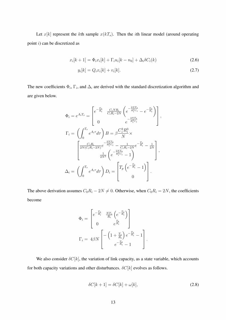
The operating point i of the system, denoted as five-tuples (Wi, qi, pi, Ci, Ri), can be

solved from the system equations (2.1) and (2.2) by setting W = 0 and q = 0, for i =

1, 2, . . . , π. Assuming the system is stabilized at operating point i, we have W (t) = W (t−Tp)

and R(t) = R(t− Tp). It follows that

βW 2i pi = 1; Wi =

RiCiN

; Ri = Tp +qiCi. (2.3)

Denote the deviations from operating point i as δWi = W (t) − Wi, δqi = q(t) − qi,

δpi = p(t) − pi, and δCi = C(t) − Ci. Further denote model i state as xi = [δqi, δWi]T and

output as yi = δqi, and define δpi(t−Tp) as ui(t−Tp). The linearized system around operating

point i can be obtained as follows.

xi(t) = Aixi(t) +Biui(t− Tp) +DiδCi(t) (2.4)

yi(t) = Qixi(t) + v(t). (2.5)

Equation (2.4) is the state equation and (2.5) is the output equation, where v(t) accounts for the

disturbance from the uncertainty nature of control input ui(t − Tp). The coefficient matrices

are given below. The details are omitted for brevity.

Ai =

− 1Ri

NRi

0 −R2i

, Bi =

0

−βRiC2i

N2

,Di =

[−TpRi

0

]T, Qi =

[1 0

].

Discretization

Since packets arriving and departing in a discrete manner, the entire system can be viewed as

sampling from the continuous-time model with a finite sampling rate. Denote the sampling

period as Ts, which is a constant and is sufficiently small, such that every propagation delay Tp

is an integer multiple of Ts as Tp = n0Ts.

12

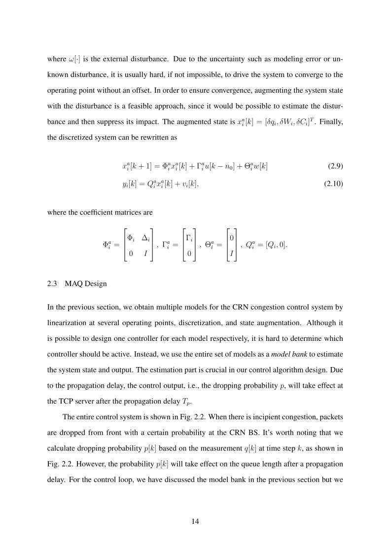
Let x[k] represent the kth sample x(kTs). Then the ith linear model (around operating

point i) can be discretized as

xi[k + 1] = Φixi[k] + Γiui[k − n0] + ∆iδCi(k) (2.6)

yi[k] = Qixi[k] + vi[k]. (2.7)

The new coefficients Φi, Γi, and ∆i are derived with the standard discretization algorithm and

are given below.

Φi = eAiTs =

e−TsRi

CiNRiCiRi−2N

(e− 2NTsR2iCi − e−

TsRi

)0 e

− 2NTsR2iCi

,Γi =

(∫ Ts

0

eAiτdτ

)B = β

C3iR

3i

N× CiRi

2N(CiRi−2N)e− 2NTsR2iCi − 1

CiRi−2Ne− TsRi − 1

2N

12N2

(e− 2NTsR2iCi − 1

) ,

∆i =

(∫ Ts

0

eAiτdτ

)Di =

Tp(e− TsRi − 1

)0

.The above derivation assumes C0Ri − 2N 6= 0. Otherwise, when C0Ri = 2N , the coefficients

become

Φi =

e− TsRi NTsRi

(e− TsRi

)0 e

TsRi

Γi = 4βN

−(

1 + TsRi

)e− TsRi − 1

e− TsRi − 1

.We also consider δC[k], the variation of link capacity, as a state variable, which accounts

for both capacity variations and other disturbances. δC[k] evolves as follows.

δC[k + 1] = δC[k] + ω[k], (2.8)

13

where ω[·] is the external disturbance. Due to the uncertainty such as modeling error or un-

known disturbance, it is usually hard, if not impossible, to drive the system to converge to the

operating point without an offset. In order to ensure convergence, augmenting the system state

with the disturbance is a feasible approach, since it would be possible to estimate the distur-

bance and then suppress its impact. The augmented state is xai [k] = [δqi, δWi, δCi]T . Finally,

the discretized system can be rewritten as

xai [k + 1] = Φai x

ai [k] + Γai u[k − n0] + Θa

iw[k] (2.9)

yi[k] = Qai x

ai [k] + vi[k], (2.10)

where the coefficient matrices are

Φai =

Φi ∆i

0 I

, Γai =

Γi

0

, Θai =

0

I

, Qai = [Qi, 0].

2.3 MAQ Design

In the previous section, we obtain multiple models for the CRN congestion control system by

linearization at several operating points, discretization, and state augmentation. Although it

is possible to design one controller for each model respectively, it is hard to determine which

controller should be active. Instead, we use the entire set of models as a model bank to estimate

the system state and output. The estimation part is crucial in our control algorithm design. Due

to the propagation delay, the control output, i.e., the dropping probability p, will take effect at

the TCP server after the propagation delay Tp.

The entire control system is shown in Fig. 2.2. When there is incipient congestion, packets

are dropped from front with a certain probability at the CRN BS. It’s worth noting that we

calculate dropping probability p[k] based on the measurement q[k] at time step k, as shown in

Fig. 2.2. However, the probability p[k] will take effect on the queue length after a propagation

delay. For the control loop, we have discussed the model bank in the previous section but we

14

MMPC Queue

Weight

CalculationEstimation Model Bank

Ref

eren

ce

Dropping Probability p[k]

Qu

eue

Len

gth

q[k

]

xi[k|k-1]

yi[k|k]

xi[k|k]

wi[k]

Delay

Tp sec.

TCP Window Control

Figure 2.2: The control system structure.

still need to briefly restate it in the control context. We present the design of the MAQ scheme

in rest of this section.

2.3.1 Estimation

In the model bank we developed, the noise is usually not known in advance in practice. It is

necessary to utilize the previous information to estimate both the augmented state and output.

Let q[k] be the measured queue length at step k. We use Kalman Filter to perform state and

output estimation as follows.

xai [k|k − 1] = Φai x

ai [k − 1|k − 1] + Γai ui[k − n0 − 1] (2.11)

xai [k|k] = xai [k|k − 1] + Li[k](q[k]− qi −Qai x

ai [k|k − 1]) (2.12)

yai [k|k] = Qai x

ai [k|k], (2.13)

where xai [k|k−1] is the estimation of step k based on step (k−1) information, xai [k|k] represents

the updated state at step k based on the measurement q[k] at time step k, and Li[k] is the Kalman

gain of model i. The “hat” notation indicates that they are estimations. Eq. (2.13) is the output

15

estimation. The Kalman gain Li[k] can be derived from the following process.

Li[k] = Pi[k](Qai )T (Qa

iPi[k − 1](Qai )T +Gi)

−1 (2.14)

Pi[k] = ΦaiPi[k−1](Φa

i )T + Θa

iOi(Θai )T−Φa

iPi[k−1](Qai )T

(QaiPi[k−1](Qa

i )T +Gi)

−1QaiPi[k−1](Φa

i )T , (2.15)

where Pi[k] is the estimation error covariance of model i at step k.

This algorithm works in an iterative manner. Parameters Oi and Gi in (2.15) are stochastic

terms that account for the variance of state interference and output, respectively. Since usually

the variance is unknown, Oi and Gi are the parameters to be tuned. In the MAQ design, both

Oi and Gi are scalar and are tuned for each of the models.

2.3.2 Weight Calculation

Given the estimations of the state and output of each model, a more accurate approximation to

the real system dynamics can be obtained by probabilistically integrating the models. We first

derive the weight for each model based on their residual at time step k, denoted as ξi[k], which

is the difference between the real measurement and estimation output of each model. Noticing

that the measurement q[k] is the queue length while the estimation yi[k|k] is the deviation from

the operating point, we have

ξi[k] = q[k]− qi − yi[k|k]. (2.16)

Under the general assumption that the weights are Gaussian, the probability that model i

represents the system at step k can be derived with the Bayesian theorem as

ρi[k] =exp(−0.5λξ2

i [k])ρi[k − 1]∑πj=1 exp

(−0.5λξ2

j [k])ρj[k − 1]

. (2.17)

In (2.17), the exponential term is due to the Gaussian distribution of the weights. It would be

beneficial that the rejecting speed of the unsuitable models is exponential. The coefficient λ

determines the sensitivity to the residual. Furthermore, the formula is recursive; once ρi[k] is 0

16

at some step k, it will remain at 0 even if the model is more accurate than others. We thus set a

lower limit µ > 0, such that if ρi[k] is lower than µ, it will be set to µ.

The weights are then calculated by normalizing the probabilities, as

wi[k] =

ρi[k]∑πj=1 ρj [k]

, ρi[k] > µ

0, ρi[k] ≤ µ.

(2.18)

In the initialization phase, all the weights are set to 1/π since there is no a priori information

about the system.

2.3.3 MMPC Control Law

We are now ready to derive the MMPC control law. Due to the propagation delay, the control

signal ui[k] affects the queue length at time (k+n0). It is thus necessary to estimate the n0-step

ahead state and output, i.e., at time (k + n0). We estimate state xai [k + n0] as

xai [k + n0|k] = Φai x

ai [k + n0 − 1|k] + Γai ui[k − 1] (2.19)

= (Φai )n0x[k|k] +

n0∑j=1

(Φai )j−1Γai ui[k − j].

The output of each model at time (k+n0) can also be estimated. A more accurate estima-

tion, y, can be obtained as the weighted average of the estimated outputs. It follows that

y[k + n0|k] =π∑i=1

wi[k]yi[k + n0|k], (2.20)

where yi[k + n0|k] is derived with the estimation precess. Recall that output yi[k + n0|k] is

the difference between the estimated queue length and the ith operating point qi. Substituting

yi[k + n0|k] = q[k + n0]− qi into (2.20), we have

y[k + n0|k] = q[k + n0]−π∑i=1

wi[k]qi. (2.21)

17

Furthermore, the control signal ui[k] is the difference between the dropping probability

and its operating point value, i.e., ui[k] = p[k] − pi, while p[k] is to be derived. The control

objective function is formed with a prediction horizon of s time steps and a control horizon of

m time steps. As discussed, the prediction horizon starts from time step (k+n0). By solving the

optimization problem with this objective function at every time step, a series of optimal control

signals {∆p[k], ∆p[k + 1], . . ., ∆p[k + s]} can be derived, where ∆p[k] = p[k + 1] − p[k].

The first control signal is then chosen as our result. The (k + n0 + j)th step prediction is the

weighted average of all the model outputs at the same time step, i.e.,

y[k + n0 + j|k] =π∑i=1

wi[k]yi[k + n0 + j|k]. (2.22)

The design objective is to stabilize the queue length around the set point while keeping

the difference between each control move as small as possible. The first goal is obvious, and

the reason for the second one would be explained in the later section. With the relation given

in (2.21), we define the objective function as

min (Yref − Y )TWy(Yref − Y ) + ∆UTWu∆U, (2.23)

where Yref is the modified reference output based on the reference queue length. The reference

queue length is given as qref and the estimated queue length is q[k + n0 + j]. It follows that

Yref =

qref −∑π

i=1wi[k]qi

qref −∑π

i=1wi[k]qi...

qref −∑π

i=1wi[k]qi

. (2.24)

18

Furthermore, Y is a vector of the weight estimations of the model outputs over the prediction

horizon, while ∆U is a vector of dropping probability increments over the control horizon, i.e.,

Y =

y[k + n0 + 1|k]

y[k + n0 + 2|k]

...

y[k + n0 + s|k]

, ∆U =

∆p[k]

∆p[k + 1]

...

∆p[k +m]

. (2.25)

Finally, Wy and Wu are diagonal weight matrices of queue length differences and control

moves, respectively, which can be used to trade-off between the dual objectives of stabiliz-

ing the queue and minimizing the control moves.

In (2.23), the first term minimizes the difference between the real queue length and ref-

erence queue length. The second term in the objective function is the penalty for changing

the dropping probability. To solve this problem, we need to derive y from y[k + n0 + 1|k] to

y[k + n0 + s|k]. To facilitate this process, the propagation matrix is given as follows.

Y = Max +Ma

cMe∆U +MacU0 −Mcp. (2.26)

19

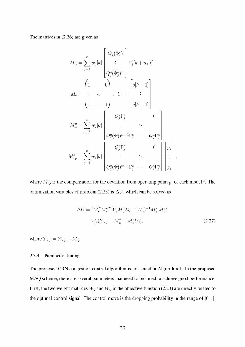
The matrices in (2.26) are given as

Max =

π∑j=1

wj[k]

Qaj (Φ

aj )

...

Qaj (Φ

aj )m

xaj [k + n0|k]

Me =

1 0

... . . .

1 · · · 1

, U0 =

p[k − 1]

...

p[k − 1]

Mac =

π∑j=1

wj[k]

QajΓ

aj 0

... . . .

Qaj (Φ

aj )m−1Γaj · · · Qa

jΓaj

Macp =

π∑j=1

wj[k]

QajΓ

aj 0

... . . .

Qaj (Φ

aj )m−1Γaj · · · Qa

jΓaj

pj...

pj

,

where Mcp is the compensation for the deviation from operating point pi of each model i. The

optimization variables of problem (2.23) is ∆U , which can be solved as

∆U = (MTeM

acTWyM

acMe +Wu)

−1MTeM

acT

Wy(Yref −Max −Ma

cU0), (2.27)

where Yref = Yref +Mcp.

2.3.4 Parameter Tuning

The proposed CRN congestion control algorithm is presented in Algorithm 1. In the proposed

MAQ scheme, there are several parameters that need to be tuned to achieve good performance.

First, the two weight matricesWy andWu in the objective function (2.23) are directly related to

the optimal control signal. The control move is the dropping probability in the range of [0, 1].

20

Algorithm 1: The Proposed MAQ AlgorithmData: Average and variance of service capacity (C and σC), queue length at each time

kResult: The drop/mark probability p[k] at time k

1 Choose the model number π;2 Assign the weight of each model as 1

π;

3 Define the Kalman Gain matrix Li and estimation error covariance Pi;4 while System is running do5 for i = 1 : π do6 Calculate the estimation yai [k|k];7 Update the Kalman gain Li and estimation error covariance Pi;

8 for i = 1 : π do9 Update probability ρi[k] based on (2.17);

10 Calculate weight wi;

11 for j = 1 : n0 do12 Estimate feature state information xai [k + j|k];

13 Minimize the objective function (2.23) and obtain the analytical solution (2.27);14 Use the first element of the result to obtain p[k];15 Generate uniformly distributed random number u(0, 1);16 if u < p[k] then17 Drop the head-of-line packet at CRN BS queue;

We can use the saturation function to enforce this range, i.e.,

p[k] = max{0,min{1, p[k − 1] + ∆p[k]}}. (2.28)

However, to avoid offset or unstability, it is necessary to choose a large Wu. Usually, the larger

the ratio Wy/Wu, the more aggressive the control move. For the CRN congestion control

system, we recommend Wy = diag(1, 1, . . . , 1) and Wu = diag(106, 106, . . . , 106), which

work well in our simulation study.

Second, in the estimation procedure, the matrix Pi[0] should be initialized with large and

diagonal values if we do not know the covariance of the state variable. Moreover, as the capacity

variations may be large and the estimation error may not be zero due to the uncertain nature of

the flow model, the disturbance variance Oi is set to be the standard deviation of capacity σC

and the output variance Gi is set to a small but non-zero value. According to [10], the larger

21

the ratio Oi/Gi, the smaller the response time, but the larger the overshoot (even leading to

oscillation). We choose Gi ∈ [0.4, 1] in this chapter based on our simulation study.

Third, for weight calculation, the coefficient λ determines the sensitivity of weights to

estimation error. Consider the potentially large network parameter variation, which leads to

estimation error, we would not recommend a large λ since it will easily drive the model prob-

ability ρi[k] to 0. Given such a system with large variations of parameters and conditions, we

set λ = 1 in this chapter.

2.4 Simulation Study

In this section, we evaluate the performance of MAQ with NS2 simulations. We extend the

NS2 simulator with the multiple-channel extension, TDM module, and the channel bond-

ing/aggregation module. We assume 10 licensed channels: five of them with a capacity of

500 Kb/s and the other five with a 1 Mb/s capacity. As in prior work [5, 25], each channel is

modeled as an on-off process. Both the on and off periods are exponentially distributed with

mean η(on) = 4 seconds and η(off) = 5 seconds, respectively. The sensing phase of the CRN

is 20ms and the transmission phase is 200ms. If there is no channel available after the sensing

period, the frozen state will continue until an idle channel is found.

The CRN maintains a large number of TCP connections. The RTT and propagation delay

are a key factor influencing the performance of congestion control. In real networks, different

users may have different propagation delays. So we choose propagation delays uniformly dis-

tributed in (100, 150) ms (unless stated otherwise). The capacity of the wireline link between

the BS to a TCP server is 20 Mb/s. The average capacity for the CRN downlink is C = 3.2

Mb/s with variance σC = 1.3 Mb/s. The capacity C(t) used in one of the simulations is shown

as a function of time in Fig. 2.3. The packet size is 540 Bytes with 500 Bytes data and 40 Bytes

header. The reference queue length is set to 90 packets, corresponding to a queueing delay

around 100 ms. The queue size B is set to 500 packets (about 2Mb).

For comparison purpose, we also simulated two existing control-theoretic schemes: (i) the

proportional integral (PI) controller, which is canonical and has been shown to be effective on

22

0 20 40 60 80 1000

1

2

3

4

5

6

7x 10

6

Simulation Time (sec.)

Do

wn

lin

k C

apac

ity

(b

ps)

Figure 2.3: The CRN downlink capacity over time used in one of the simulations.

dealing with varying capacities [34]; (ii) the discrete sliding modes (DSM) controller, which is

a most recent advance that is based on the principles of discrete sliding-mode control [35]. We

set the PI parameters as: 4.839 × 10−5 and 4.346 × 10−5, as recommended in [34]. The DSM

parameter is set as recommended in [35], with γ = 0.01, and a sigmoid function with δ = 10

is used. We test the proposed scheme under responsive and non-responsive background traffic

and under various parameter settings.

2.4.1 Responsive Background Traffic

We first conduct simulations with a fixed number of long-lived FTP sessions and HTTP back-

ground flows. The HTTP flows are generated using PACKMIME-HTTP in NS2 with a rate of

10, i.e., on average 10 HTTP connections are generated in every second. The transport agent

in each source node is set to be TCP/Reno. The number of SUs is N = 60. For MAQ, the

parameters are set as: qi ∈ {30, 60, 90, 120, 150} packets, Ci ∈ {1.2, 2.1, 3, 3.9, 4.8}Mb/s,

Tp = 100ms, Wy = I, Wu = 106I, where I is the identity matrix. The covariance parameters

are set as Oi = 300 and Gi = 1, for i = 1, 2, . . . , 5.

Figure 2.4 presents the queue length dynamics of MAQ and PI. The sudden variation of

capacity would cause the queue length change immediately. We find that MAQ can stabilize the

queue around the reference point of 90 packets with almost no underflow (i.e., an empty queue),

23

0 20 40 60 80 1000

100

200

300

400

500


Qu

eue

Len

gth

(p

ack

ets)

MAQ

PI

Reference queue length

Figure 2.4: Queue length dynamics under responsive background traffic.

0 20 40 60 80 1000

200

400

600

800

1000

1200


Per

Pac

ket

Del

ay (

ms)

MAQ

PI

Reference delay

Figure 2.5: Packet queuing delay dynamics under responsive background traffic.

while the PI queue exhibits much larger variations with a lot of underflows. Fig. 2.5 presents

the packet queuing delay dynamics. PI cannot adjust its drop probability quickly enough to

adapt to the capacity variations, while MAQ is able to reject the influence of capacity variation

and hence achieves lower and more stable queueing delays.

We also present the queue length, delay, and link utilization statistics in Table 2.1. The

average queue length of MAQ is closer to the reference point and its standard deviation is about

24

Table 2.1: Queue Length, Queueing Delay, and Link Utilization StatisticsAverage STD Mean STD Averagequeue length queue length delay delay Utilization(packets) (packets) (ms) (ms) (%)

Responsive Background Traffic

MAQ 82 20 87.5 51.9 99.73PI 98 81 107.4 138.4 96.79

Non-responsive Background Traffic

MAQ 78 33 72.3 39.8 97.14PI 140 201 193.5 203.5 41.23

a quarter of that of PI. The average delay of MAQ is also about 20ms lower than that of PI, and

its delay standard deviation is 87ms lower than that of PI. It is worth noting that MAQ achieves

both lower and more stable queueing delay than PI.

2.4.2 Non-responsive Background Traffic

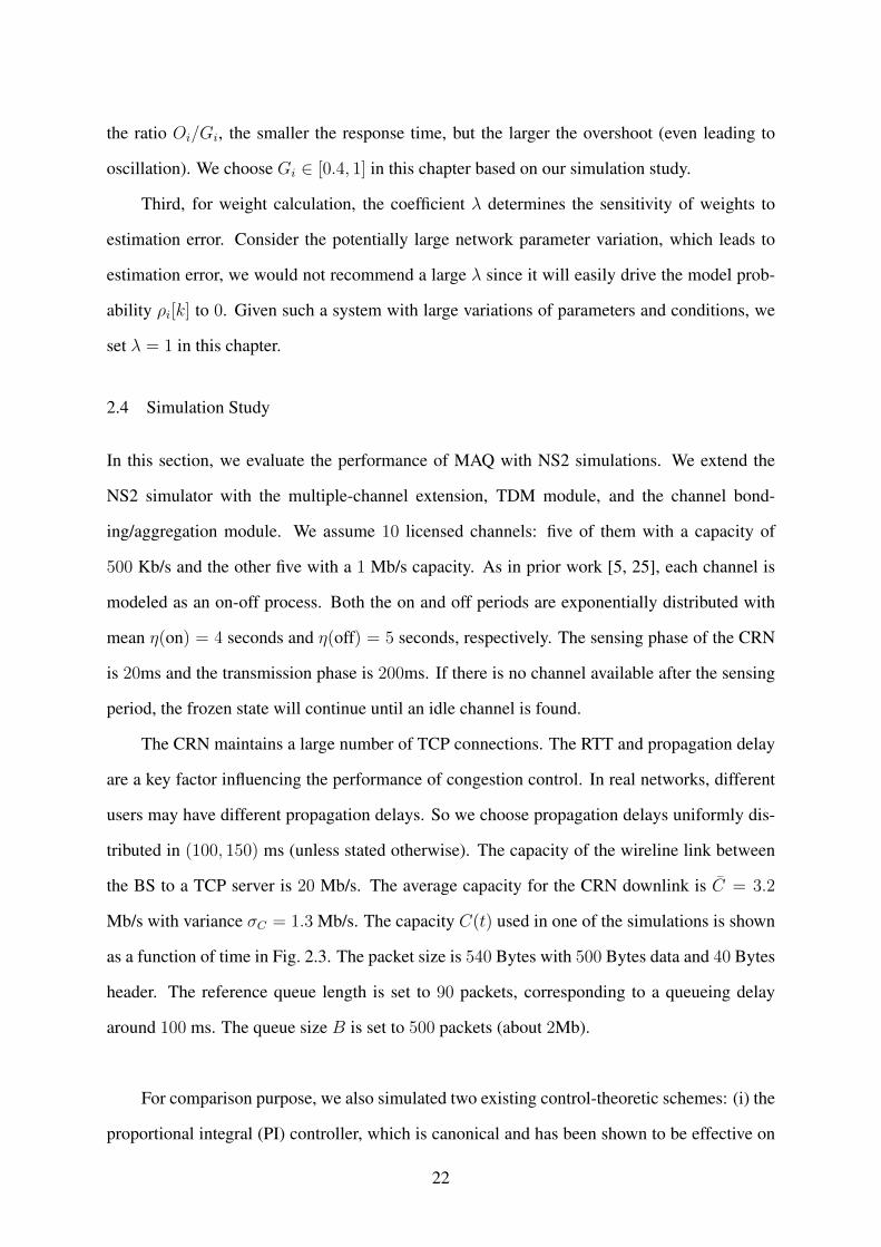
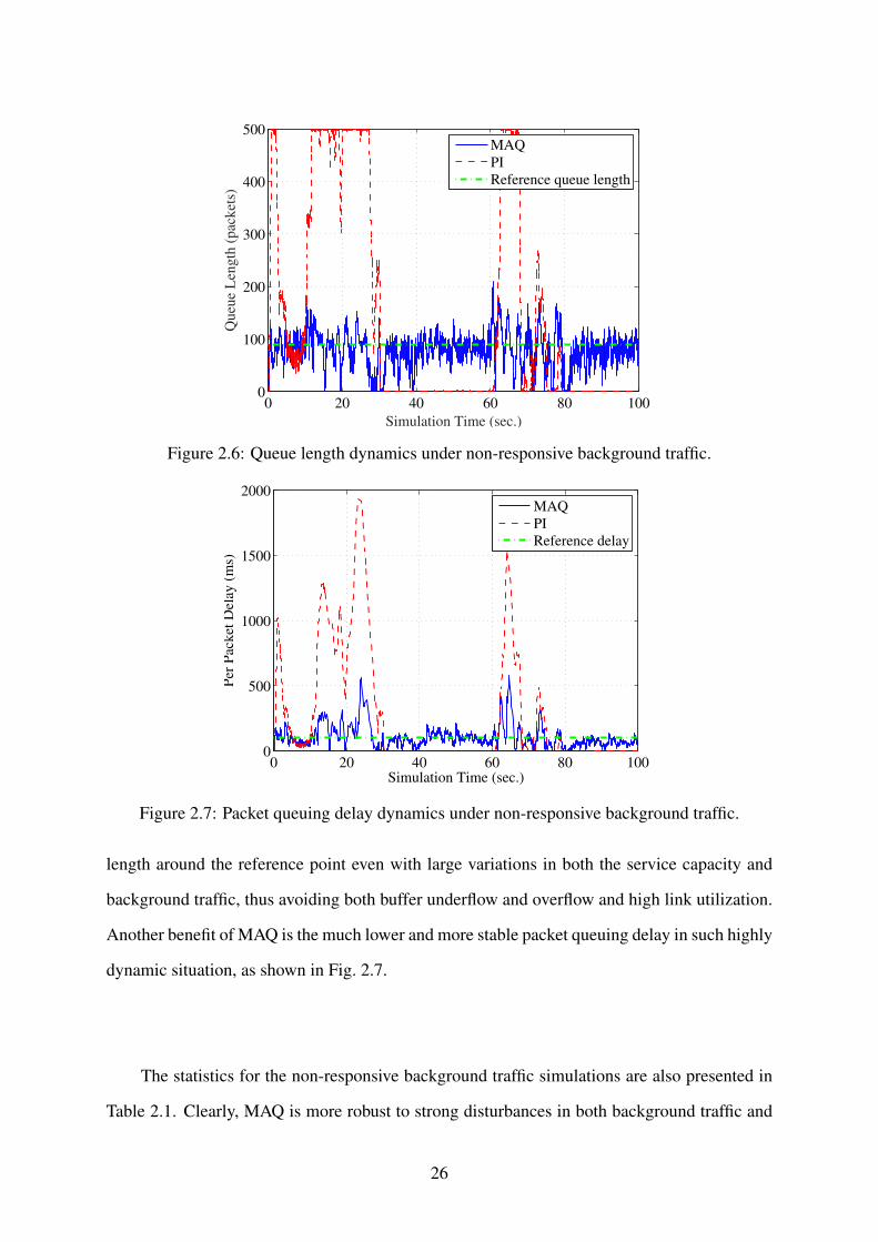
We next consider a more realistic setting by introducing a non-responsive traffic generator

for background traffic. The non-responsive sources would act like disturbance by constantly

injecting packets to the queue with exponentially distributed burst time and idle time. We use

User Data Protocol (UDP), which does not perform congestion control, for the non-responsive

flows. There are 60 FTP flows and 5 non-responsive flows. The burst data rate is 1Mb for each

non-responsive flow with packet size 500 Bytes. The non-responsive flows are activated in the

following two time intervals: [10s, 30s] and [60s, 80s].

The queue length dynamics with non-responsive background traffic are presented in Fig. 2.6.

Both queues oscillate with a larger range due to the unexpected background traffic bursts. The

PI queue overflows (i.e., buffer becomes full) for almost the entire non-responsive traffic trans-

mission period, and then its buffer underflows in the following period when the burst transmis-

sions are off. The MAQ queue, on the other hand, remains relatively stable and takes less time

to recover when the bursts are off. We find that since PI has too much overflow and packets

drop, the sender’s TCP window size would drop to 1, which greatly affects the TCP transmis-

sion rate. The dropping probability of PI is also kept high even after the burst transmission

period. This is the reason of its long recover time. MAQ, however, can stabilize the queue

25

0 20 40 60 80 1000

100

200

300

400

500


Qu

eue

Len

gth

(p

ack

ets)

MAQ

PI


Figure 2.6: Queue length dynamics under non-responsive background traffic.

0 20 40 60 80 1000

500

1000

1500

2000


Per

Pac

ket

Del

ay (

ms)

MAQ

PI

Reference delay

Figure 2.7: Packet queuing delay dynamics under non-responsive background traffic.

length around the reference point even with large variations in both the service capacity and

background traffic, thus avoiding both buffer underflow and overflow and high link utilization.

Another benefit of MAQ is the much lower and more stable packet queuing delay in such highly

dynamic situation, as shown in Fig. 2.7.

The statistics for the non-responsive background traffic simulations are also presented in

Table 2.1. Clearly, MAQ is more robust to strong disturbances in both background traffic and

26

60 SUs

0

20 SUs left

30

20 SUs left

40

20 SUs left, 20 arrived

50

20 SUs arrived

60

20 SUs arrived

70 100 sec.

End of simulation

Figure 2.8: Change of the number of FTP connections during the simulation period.

0 20 40 60 80 1000

100

200

300

400

500


Qu

eue

Len

gth

(p

ack

ets)

MAQ

PI


Figure 2.9: Queue length dynamics under varying number of connections.

service capacity. In this scenario, the MAQ average delay is only 37.36% of that of PI, and

MAQ achieves a 56% gain on link utilization over PI.

2.4.3 Varying Number of FTP Connections

We also examine the case when the number of FTP connections varies over time. In this

experiment, the simulation starts with 60 FTP connections. The changes of the number of FTP

connections during the simulation period are shown in Fig. 2.8.

The queue length and delay dynamics for this simulation are presented in Figs. 2.11

and 2.12. When the connection number goes down, there are fewer TCP flows, which lead

to an empty queue. MAQ can act quickly to adjust the dropping probability to allow the source

congestion window to grow, which will stabilize the queue length again at the reference point.

However, the PI queue length will become empty when the connection number goes down,

due to its conservative adjustment policy, leading to low link utilization. The superior delay

performance of MAQ can also be observed in Fig. 2.12.

27

0 20 40 60 80 1000

200

400

600

800

1000

1200

Simulation Time (s)

Per

Pac

ket

Del

ay (

ms)

MAQ

PI

Reference Delay

Figure 2.10: Packet queuing delay dynamics under varying number of connections.

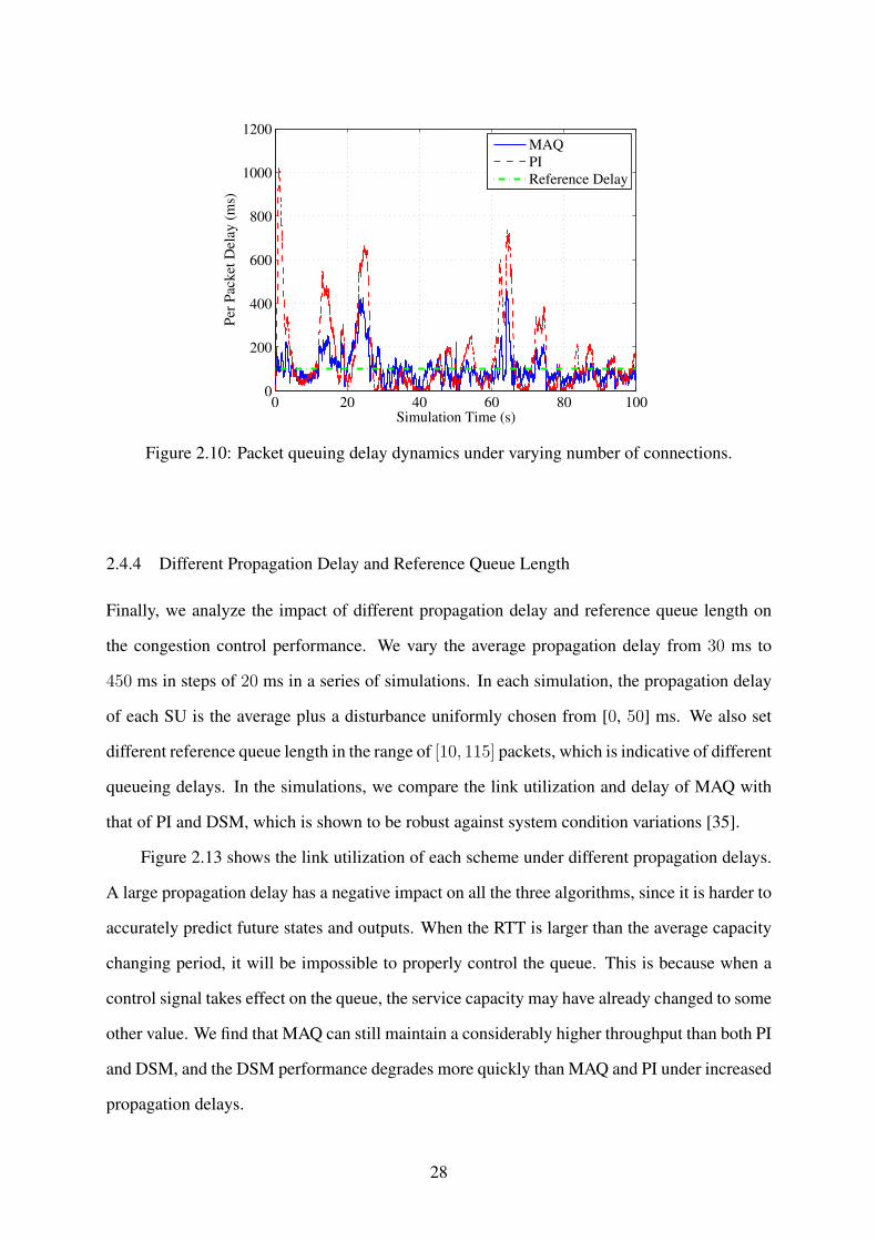
2.4.4 Different Propagation Delay and Reference Queue Length

Finally, we analyze the impact of different propagation delay and reference queue length on

the congestion control performance. We vary the average propagation delay from 30 ms to

450 ms in steps of 20 ms in a series of simulations. In each simulation, the propagation delay

of each SU is the average plus a disturbance uniformly chosen from [0, 50] ms. We also set

different reference queue length in the range of [10, 115] packets, which is indicative of different

queueing delays. In the simulations, we compare the link utilization and delay of MAQ with

that of PI and DSM, which is shown to be robust against system condition variations [35].

Figure 2.13 shows the link utilization of each scheme under different propagation delays.

A large propagation delay has a negative impact on all the three algorithms, since it is harder to

accurately predict future states and outputs. When the RTT is larger than the average capacity

changing period, it will be impossible to properly control the queue. This is because when a

control signal takes effect on the queue, the service capacity may have already changed to some

other value. We find that MAQ can still maintain a considerably higher throughput than both PI

and DSM, and the DSM performance degrades more quickly than MAQ and PI under increased

propagation delays.

28

0 20 40 60 80 1000

100

200

300

400

500


Qu

eue

Len

gth

(p

ack

ets)

MAQ

PI


Figure 2.11: Queue length dynamics under varying number of connections.

0 20 40 60 80 1000

200

400

600

800

1000

1200

Simulation Time (s)

Per

Pac

ket

Del

ay (

ms)

MAQ

PI

Reference Delay

Figure 2.12: Packet queuing delay dynamics under varying number of connections.

Reference queue length is also critical for congestion control, since a large buffer could

mitigate the effect of capacity variation. The link utilization of the three schemes for increased

reference queue lengths are presented in Fig. 2.14. Again, MAQ achieves considerably higher

link utilization than the other two schemes, especially when the reference queue length is small.

For example, when the reference queue length is 10 packets, the MAQ link utilization is about

29

0 50 100 150 200 250 300 350 400 45050

60

70

80

90

100

Propagation Delay (ms)

Lin

k U

tili

zati

on

(%

)

MAQ

PI

DSM

Figure 2.13: Average link utilization under increased propagation delays.

0 20 40 60 80 100 1200

20

40

60

80

100

Reference Queue Length (packets)

Lin

k U

tili

zati

on

(%

)

MAQ

PI

DSM

Figure 2.14: Link utilization under under increasing reference queue lengths.

20% higher than that of PI and 70% higher than that of DSM. When the reference queue length

becomes large, all the three schemes achieve a high link utilization. However, as can be seen

later in Fig. 2.16, PI and DSM achieve the high link utilization at the cost of higher delay and

large delay variation than MAQ.

The queueing delay performance under different propagation delay and reference queue

length are plotted in Fig. 2.15 and 2.16, respectively. We find that the average delay of MAQ

is not only much smaller than PI (e.g., around 50% of that of PI), but also much stable over

the entire range of propagation delay values. DSM exhibits better performance on controlling

30

0 50 100 150 200 250 300 350 400 4500

50

100

150

200

250

300

Propagation Delay (ms)

Sta

tist

ics

(ms)

MAQ average delay

MAQ delay STD

PI average delay

PI delay STD

DSM average delay

DSM delay STD

Figure 2.15: Average delay and delay STD under increasing propagation delays.

0 20 40 60 80 100 1200

50

100

150

200

250

300

Reference Queue Length (packets)

Sta

tist

ics

(ms)

MAQ average delay

MAQ delay STD

PI average delay

PI delay STD

DSM average delay

DSM delay STD

Figure 2.16: Average delay and delay STD under increasing reference queue lengths.

queuing delay than PI. Although its queueing delay is low when propagation delay is large, this

is achieved at the cost of a low throughput, since its queue is empty more often than the other

two schemes.

Under different reference queue lengths, the average queuing delay goes up roughly lin-

early since it is around qref/C, as shown in Fig. 2.16. The DSM has very small average delay

when the reference queue length is lower than 40 packets. As discussed, this is achieved at the

cost of very low link utilization (see Fig. 2.14). MAQ not only achieves low queueing delay and

31

delay variation, the two MAQ curves are also less sensitive to the increased reference queue

lengths than the other two schemes.

2.5 Related Work

In this section, we briefly review related work on congestion control, which can be classified

as end-to-end solutions and router-based solutions. We then discuss the several closely related

work on congestion control in CRNs.

2.5.1 End-to-End Solutions

In the early age, congestion control algorithms are mostly based on the assumption that all

packet losses are caused by buffer overflow at the bottleneck router. TCP Reno [36], TCP

Tahoe [37], and TCP NewReno [38] are the several most popular algorithms based on such an

idea. On the other hand, protocols were proposed, e.g., TCP Vegas [39], which are delay based.

The mainstream protocols that most computer system use are TCP Cubic [40] and Compound

TCP [41]. These protocols are mainly based the classical AIMD algorithm and combined with

various modifications. However, none of the existing protocols are suitable for congestion

control in CRNs, where the service capacity usually has frequent, large variations. In addition,

none of the existing schemes consider the frozen transmissions during the spectrum sensing

period.

Most recent congestion control proposals are mainly focusing on cellular networks, which

also have varying link capacity due to fading and shadowing [42, 43]. The basic idea of [42] is

to use a stochastic model: Poisson process with rate that follows a Brownian motion to predict

the capacity of the wireless link. This model may not work well in CRN because the variation of

capacity is mainly caused by the activity of primary users, in addition to fading and shadowing

effects. Yasir et al. in [43] propose a method based on the training model between packet delay

and window size. However, the most significant difference between cellular network and CRN

studied in this chapter is, the cellular BS maintains a separate queue for each user (e.g., each

user with a dedicate channel), but the CRN BS maintains a shared queue for all users in our

model. Thus the basic assumption in such protocols does not hold and the application of such

32

protocols in CRN would be hard, if not impossible. Also the spectrum sensing period will have

a big effect on congestion control, which calls for a new CRN specific protocol design.

2.5.2 Router-based Solutions

Our work is closely related to the literature on AQM design in the context of the Internet.

Instead of actually dropping packets, the authors in [44] proposed a method with Explicit Con-

gestion Notification (ECN), to provide a feedback from the bottleneck router. The authors

in [45] present a control theoretic analysis of random early detection (RED) [46] and find that

RED is sensitive to its parameter setting and it is hard to stabilize if the delay is taken into

consideration. In [34], a Proportional-Integral (PI) AQM scheme is developed. However, the

PI scheme may react slowly to outside disturbances. Model predictive control (MPC) is an

important industry control method, which predicts future system states and computes the op-

timal control input at each sampling time slot. Generalized predictive control has been used

in network congestion control [47] and an MPC based AQM method (MPAQM) is proposed

in [48]. These methods can compensate the impact of RTT with the model predictor. However,

they do not explicitly take disturbance (e.g., varying service capacity) into consideration.

Chavan, et al. in [49] propose a solution to address the capacity variation due to a fading

wireless channel based on the H∞ technique. However, its conservative policy makes it unsuit-

able for CRNs where the capacity may change at various/fast timescales. In [50], the authors

propose a latency control algorithm, termed CoDel, which provides a solution to the bufferbloat

problem; but the design does not directly apply to CRNs. In [35], the authors propose an AQM

algorithm, termed DSM, based on the discrete sliding mode control (DSMC) theory. Although

it deals with high frequency oscillation of link capacity, DSMC suffers from the over control

problem and it is hard to choose a proper control gain for this algorithm.

2.5.3 CRN Congestion Control Schemes

The problem of enhancing TCP performance in CRNs has been addressed in only a few pa-

pers [24, 26, 25]. In [24], the authors propose a new network management framework, termed

DSASync, for DSA based WLANs. This work uses a zero-size receive window to freeze the

33

TCP sender and smooth the ACKs from the BS during the sensing period. Its design is largely

based on heuristic methods, while smoothing ACKs would slow down the growth of window

size during the valuable transmission period.

In [26], a cross-layer approach is proposed to maximize throughput by jointly adjusting

spectrum sensing, access decision, and modulation and coding scheme in the physical layer.

The problem is formulated based on a POMDP framework and solved by dynamic program-

ming. This is an offline scheme that requires full prior knowledge of all system statistics, due

to the complex POMDP approach. In [25], the impact of channel sensing and spectrum oppor-

tunity change on TCP performance is analyzed and a window based transport control protocol

for CR Ad Hoc Networks is proposed. The proposed protocol is mainly based on heuristics

rather than a rigorous theoretic analysis, and the enhancements may not be backward com-

patible with existing TCP protocols that have already been widely used in both wireless and

wireline networks.

2.6 Conclusion

In this chapter, we designed a congestion control scheme for infrastructure-base CRNs. The

goal was to stabilize the TCP buffer at the CRN BS under a wide range of system/network

parameters and dynamics. The proposed scheme, termed MAQ, was based on MMPC with

enhanced state and output estimation. The proposed scheme was evaluated with extensive NS2

simulations under various background traffic types and network/system parameter settings. It

was shown to achieve superior performance over two benchmark schemes.

34

Chapter 3

Model Free Congestion Control for Mobile Network based on Deep Reinforcement Learning

As wired/wireline networks become more and more complex, the fundamental assumptions

made by many existing TCP variants may not hold true anymore. In this chapter, we de-

velop a model free congestion control algorithm based on deep reinforcement learning (DRL),

which has a high potential in dealing with the complex and varying network environment.

We present TCP-Drinc, acronym for Deep ReInforcement learNing based Congestion Control,

which learns from past experience and a set of measured features to decide the next action

on adjusting the congestion window size. We present the TCP-Drinc design and validate its

performance with extensive NS3 simulations and comparison with five benchmark schemes.

3.1 Introduction

The unprecedented growth of network traffic, in particular, mobile traffic, has greatly stressed

today’s Internet. Although the capacities of wired and wireless links have been greatly in-

creased, the gap between user demand and what the Internet can offer is actually getting wider.

Furthermore, many emerging applications not only require high throughput and reliability, but

also low delay. Although the brute-force approach of deploying wired and wireless links with

higher capacity helps to mitigate the problem, a more viable approach is to revisit the higher

layer protocol design, to make more efficient use of the increased physical layer capacity. Some

works such as [51, 52, 53, 54, ?] are inspiring.

Congestion control is the most important networking function of the transport layer, which

ensures reliable delivery of application data. However, the design of a congestion control pro-

tocol is highly challenging. First, the transport network is an extremely complex network of

35

queues. The TCP end host itself consists of various interconnected queues. When the TCP flow

gets into the Internet, it traverses various queues at routers/switches along the end-to-end path,

each shared by cross-traffic and other TCP flows and served with some scheduling discipline.

Significant efforts are still needed to gain good understanding of such a complex network to

develop the queueing network theory that can guide the design of a congestion control protocol.

Second, if following the end-to-end principle, agents at end hosts have to probe the network

status and make independent decisions without coordination. The detected network state is

usually error-prone and delayed, and the delayed effect of an action also depends on the actions

of other competing hosts. Third, if to involve the routers, the algorithm must be extremely sim-

ple (e.g., stateless) to ensure scalability, since the router may handle a huge amount of flows.

Finally, as more wireless devices are connected, the lossy and capacity-varying wireless links

also pose great challenges to congestion control design.

Many effective congestion control protocols have been developed in the past three decades

since the pioneering work [37] (see Section II). However, many existing schemes are based on

some fundamental assumptions. For example, early generation of TCP variants assume that

all losses are due to buffer overflow, and uses loss as indicator of congestion. Since such

assumption does not hold true for wireless networks, many heuristics are proposed for TCP

over wireless to distinguish the losses due to congestion from that incurred by link errors.

Moreover, many existing schemes assume a single bottleneck link in the end-to-end path, and

the wireless last hop (if there is one) is always the bottleneck. Given the high capacity wireless

links and the complex network topology/traffic conditions we have today, such assumptions are

less likely to be true. The bottleneck could be at either the wired or wireless segment, it could

move around, and there could be more than one bottlenecks. Finally, when there is a wireless

last hop, some existing work [42] assumes no competition among the flows at the base station

(BS), which, as shown in [43], may not be true due to coupled wireless transmission scheduling

at the BS.

In this chapter, we aim to develop an effective congestion control algorithm that does not

rely on the above assumptions. Motivated by the recent success of applying machine learning

to wireless networking problems [55], and based on our experience of applying deep learning

36

(DR)/deep reinforcement learning (DRL) to 5G mmWave networks [56], edge computing and

caching [57, 58, 59], and RF sensing and indoor localization [12, 18, 11], we propose to develop

a model free congestion control algorithm based on DRL. The original methods that treat the

network as a white box have been shown to have many limitations. To this end, machine

learning, in particular, DRL, has a high potential in dealing with the complex network and

traffic conditions by learning from past experience and extracting useful features. A DRL

based approach also relieves the burden on training data, and has the unique advantages of

being adaptive to varying network conditions.

In particular, we present TCP-Drinc, acronym for Deep ReInforcement learNing based

Congestion Control. TCP-Drinc is a DRL based agent that is executed at the sender side.

The agent estimates features such as congestion window change, round trip time (RTT), the

minimum RTT over RTT ratio, the difference between RTT and the minimum RTT, and the

inter-arrival time of ACKs, and stores historical data in an experience buffer. Then the agent

uses a DRL with a deep convolutional neural network (DCNN) concatenated with a long short

term memory (LSTM) network to learn from the historical data and select the next action to

adjust the congestion window size. The contributions of this work are summarized as follows.

1. To the best of our knowledge, this is the first work that applies DRL to the congestion

control problem. Specifically, we propose a DRL based framework on (i) how to build

the experience buffer to deal with the delayed environment, where an action will take

effect after a delay and feedbacks are also delayed, (ii) how to handle the multi-agent

competition problem, and (iii) how to compute each components including states, action,

and reward. We believe this framework could help to boost the future research on smart

congestion control protocols.

2. The proposed TCP-Drinc framework also offers solutions for long-existing problems in

congestion control: delayed environment, partial observable information, and measure-

ment variations. The LSTM is utilized to handle the autocorrelation within the time-

series introduced by delay and partial information that one agent senses. Moreover, we

37

applied CNN as a filter to extract the stable features from the rich but noisy measure-

ments, instead of using EWMA as a coarse filter as in previous works.

3. We develop a realistic implementation of TCP-Drinc on the NS3 and Tensorflow plat-

forms. The DRL agent is developed on Tensorflow and the training and inference in-

terfaces are built in NS3 using Tensorflow C++. We conduct extensive simulations with

TCP-Drinc and compare with five representative benchmark schemes, including both loss

based and latency based schemes. TCP-Drinc achives superior performance in through-

put and RTT in all the simulations, and exhibits high adaptiveness and robustness under

dynamic network environments.

The remainder of this chapter is organized as follows. We first review related work in

Section 3.2. In Section 3.3, we discuss preliminaries of deep reinforcement learning. The

system model and problem statement are presented in Section 4.2. The proposed TCP-Drinc

is presented in Section 3.5, and validated with simulation in Section 4.5. We conclude this

chapter in Section 3.7. The math notation is summarized in Table 4.1.

3.2 Related Work

Congestion control is a fundamental networking problem, which has drawn extensive attention

and has been studies over the past three decades. In this section, we review key related work

and recent progress in this area. We classify existing congestion control techniques into three

categories, end-to-end, router based, and smart schemes, as discussed below.

3.2.1 End-to-End Schemes

This class of work can be further classified into loss-based or delay-based schemes. TCP

Reno [36], TCP Tahoe [37] and TCP NewReno [38] were early protocols that are loss-based.

TCP Vegas was the first delay-based protocol. Currently, most computer operation systems

adopt TCP Cubic [40] or Compound TCP [41], which mainly deal with the situation with large

capacity RTT products.

38

Table 3.1: NotationSymbol Description

st the state tensor at time tat the action tensor at time tr(st, at) the reward function scalar given the state and action

at time tV (st, at) the value functionQπ(st,at) the Q function for discounted accumulated rewardRt the discounted summation rewardπ(t) the policy at time tω the DQN weightsJ(ω) the loss function for weight trainingyt the target value in the loss functionτRTT the round trip timeτp the minimum RTTτp the propagation delayτq the queuing delayL the length of historical states taken into account∆w cWnd differencevRTT the minimum RTT over RTT ratioδRTT the difference between RTT and the minimum RTTτACK inter-arrival time of ACKsM number of time slots in a stateS the state spaceA the action spacex(t) the sending rate at time tw(t) the congestion window size at time tz(t) the impact of an action at time t on future goodputU(·) the utility functionNpre the duration of the pre training processNdis the duration of the distributed training process

These protocols are designed for the wired Internet. However, recent measurements on 3G

and 4G LTE networks reveals fast oscillation of channel capacity [42]. In addition, the authors

in [43] shows that burst scheduling and competing traffic will also influence the RTT and capac-

ity utilization of the network. The authors then propose new end-to-end protocols that observes

the packet arrival times to infer the uncertain dynamics of the network path (Sprout [42]) and

utilizes delay measurement (i.e., Verus [43]) to cope with these challenges.

Another recent progress on congestion control is on data center networks. Compare with

normal networks, the capacity in data center networks is larger (Gigbits or 10s Gigbits) but

39

stable and the latency is much smaller (in µs). And acknowledge is not sent for every packets.

The Data Center TCP (DCTCP) [60] exploits the ECN feedback from switches. Performance-

oriented Congestion Control (PCC) proposes to continuously observe the connection between it

actions and experienced performance, and to adopt actions that lead to good performance [61].

The authors in [62] leverages sliding mode control theory to analyze and fix the stability issue

of quantized congestion notification (QCN) in data center Ethernet networks.

3.2.2 Router based Schemes

This class of work involves switch or routers in congestion control. Explicit Congestion Noti-

fication (ECN) [44] is introduced as a substitution of loss as a congetion signal. Active queue

management (AQM) such as RED [46], CoDel [50], and MAQ [63, 64] are all proposed to let

routers to mark or drop packets on incipient congestion. These approaches require modification

of the routers and intermediate devices, which may not be practical or may not scale to large

number of TCP flows.

3.2.3 Smart Schemes

With the recent success of machine learning/deep learning on image recognition, video ana-

lytics, and natural language processing, there is strong interest on apply machine learning to

solving networking problems [55]. Interesting results in [65, 66] provide insight into machine

generated congestion protocols. However, these learning algorithms require offline training

based on prior knowledge of the network and can only be adopted for limited situations. In [67],

the authors propose an algorithm based on deep reinforcement learning (DRL) to deal with the

traffic engineer problem at intermediate nodes. This is the first work that applies DRL to the

traffic engineering problem in the Internet protocol (IP) layer. In [68], the authors incorpo-

rate Q-learning into congestion control design, termed QTCP. It is based on limited feature

scales (discretized states) and uses Kanerva Coding instead of a deep neural network to handle

Q-function approximation. The authors show considerable gains achieved by QTCP over the

classical TCP NewReno.

40

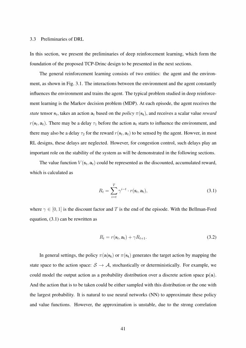
3.3 Preliminaries of DRL

In this section, we present the preliminaries of deep reinforcement learning, which form the

foundation of the proposed TCP-Drinc design to be presented in the next sections.

The general reinforcement learning consists of two entities: the agent and the environ-

ment, as shown in Fig. 3.1. The interactions between the environment and the agent constantly

influences the environment and trains the agent. The typical problem studied in deep reinforce-

ment learning is the Markov decision problem (MDP). At each episode, the agent receives the

state tensor st, takes an action at based on the policy π(st), and receives a scalar value reward

r(st, at). There may be a delay τ1 before the action at starts to influence the environment, and

there may also be a delay τ2 for the reward r(st, at) to be sensed by the agent. Howver, in most

RL designs, these delays are neglected. However, for congestion control, such delays play an

important role on the stability of the system as will be demonstrated in the following sections.

The value function V (st, at) could be represented as the discounted, accumulated reward,

which is calculated as

Rt =T∑i=t

γi−t · r(st, at), (3.1)

where γ ∈ [0, 1] is the discount factor and T is the end of the episode. With the Bellman-Ford

equation, (3.1) can be rewritten as

Rt = r(st, at) + γRt+1. (3.2)

In general settings, the policy π(a|st) or π(st) generates the target action by mapping the

state space to the action space: S → A, stochastically or deterministically. For example, we

could model the output action as a probability distribution over a discrete action space p(a).

And the action that is to be taken could be either sampled with this distribution or the one with

the largest probability. It is natural to use neural networks (NN) to approximate these policy

and value functions. However, the approximation is unstable, due to the strong correlation

41

between sequential samples. In addition, the nonstationary target values could further degrade

the stability. The shallow NN has a limited ability to extract important features.

Deep reinforcement learning (DRL) algorithms, first introduced in [8], are based on a

similar structure but incorporate a deep neural network (DNN) as to approximate the value

function and/ or the policy function. In other words, DRL extends the idea of Q-learning with

DNN. The raw sensory data is applied as state st and directly treated as input to the DNN. The

DNN is utilized to approximate the Q-function Q(st,at), which calculates the optimal value

for each possible action given state st. This method is called Deep Q-Network (DQN). The Q

value function Qπ(st,at) for given policy π is defined as

Qπ(st,at) = E [Rt|st,at] , (3.3)

where Rt =∑T

i=t γi−t · r(st, at). The equation can be unrolled as

Qπ(st,at) = Est+1 [rt + γQπ(st+1,at+1)|st,at] . (3.4)

Let ω represent the weights in the DQN. Suppose the DQN Q(st, at,ω) ≈ Qπ(st, at). We

can define a loss function as

J(ω) = E[(rt + γQ(st+1, at+1,ω)−Q(st, at,ω))2] . (3.5)

The sum of the first two terms on the right-hand-side is defined as the target value, i.e., yt =

rt + γQ(st+1, at+1,ω).

In order to solve the instability problem during the training, the authors in [8] adopted two

key strategies: experience replay and target networks. First, the history of the transitional states

and actions is stored as experience. The DQN is trained with batches of data that are sampled

randomly from the experience, so as to break the correlation between sequential data samples.

In fact, mini-batches are randomly drawn from the experience in order to apply stochastic

gradient decent (SGD) to further reduce the correlation. Second, an additional target network

is introduced to calculate the target value yt = rt + γQ(st+1, at+1,ω′) in the training process,

42

Agent Environmentπ(t)

Q(t)

Take action A(t) based

on policy π(t)

Reward FeedbackDelay τ2

Delay τ1

Delay τ3 State Feedback

Figure 3.1: Reinforcement learning design for congestion control.

whose weights ω′ are updated periodically with the running weights. The target value will

become stable after certain amount of steps in the training process.

3.4 System Model, Assumptions and Problem Statement

3.4.1 Network Architecture

In this chapter, a general setting of congestion control is considered, as shown in Fig. 3.2,

where a set of remote hosts serving a set of mobile users (the last hop could also be wired).

Each end-to-end path, from a remote host to a mobile user, consists of multiple hops. The

remote hosts apply a TCP congestion window (cWnd) based protocol. The base station (e.g.,

eNodeB) maintains separate queues for different mobile users it serves. The two features of

the general setting are: competitions among different flows at bottleneck links and potentially

multiple bottlenecks along the end-to-end path.

Most prior works assume that the last wireless hop is the single bottleneck. Under this

assumption, the round-trip time (RTT) of a user, τRTT (t) = τp+ τq(t), where τp is the propaga-

tion delay and τq(t) is the queuing delay, seems independent to other users, since the eNodeB

maintains separate queues for different users. However, even in this case, the multiple queues at

the eNodeB are still coupled due to the transmission scheduling algorithm used at the base sta-

tion [43]. Furthermore, the flows may still compete with each other for transmission resources

and buffer storage along the multihop path if they share common nodes.

43

Remote hosts The Internet Base station

Mobile users

Figure 3.2: System architecture for TCP over wireless.

The general problem of congestion control should be treated as a delayed, distributed deci-

sion making problem. Each sender needs to decide the congestion window size (cWnd) and/or

the sending rate. We focus on cWnd since it can be implicitly translated into the sending rate

according to the TCP clocking phenomenon [69]. The “delayed” feature means the feedback

from the receiver about the network condition is usually received a round trip time (RTT) later;

and the action senders takes will influence the bottleneck queue after a forward propagation

delay. If the global information on each user’s strategy, the network topology, and traffic condi-

tion were known, one could have made perfect decision. But the global information is usually

unavailable and the users do not cooperate on congestion control, which entails “distributed”

decision making. Although these features have been considered in prior work, e.g., model-

ing TCP throughput as delayed differential equations, they all pose great challenges to a DRL

based congestion control design.

3.4.2 Partially Observable Information

In the congestion control process, the information each sender can acquire is partial and de-

layed. The measured RTT can only tell the total delay, but lacks the details of the delay on each

hop, on forward and backward delays, and on propagation and queueing delays. One popular

approach is to approximate the propagation delay by the minimal RTT. In addition, as dis-

cussed, the acquisition of RTT and the effect of action are both delayed. Therefore, congestion

control is actually a partially observable Markov decision process (POMDP).

44

The problem of congestion control could be interpreted as a sender algorithm that explores

the network environment and exploits the cWnd to properly transport data. This process is

conducted by many other senders as well due to shared networking resources. Therefore, the

environment one sender sensed could be also affected by other users’ decisions and constantly

changing. In this chapter, we proposed integrated solution to deal with the “multi-agent” feature

of the congestion control problem.

For the POMDP problem, it helps to utilize historical information to exploit the momen-

tum and correlations in the process. However, utilizing the historical information is non-trivial

for the associated time and space complexity. In DNN, a promising solution is recurrent neu-

ral network (RNN), which is effective to capture the temporal, dynamic behavior from a time

series.

3.4.3 Basic Assumptions

To make the design general, we do not assume the system is Markovian. In the past, most of

the TCP variants, such as [70, 40], make control decisions based only on the current state, since

they have a basic assumption that the next state only depends on the current state, no matter

what congestion signal they use: delay or loss. In the recent work [65], the exponential average

over the historical delay is utilized. This an intuitive solution to the problem of congestion

control because the current state alone is delayed and partial. As discussed, not only the sending

rate is determined by the states of one RTT before, but also the states of queues and latency

depend on the state one propagation delay ago. In short, the Markovian assumption may be too

simplistic and it is helpful to exploit historical information for better decision making.

In real network environments, received signals are usually noisy, which can be mitigated

by an exponential window moving average to acquire the stable information. We thus uti-

lize a convolutional neural network (CNN) as an automatically tuned filter to extract stable

information. To make the model mathematically tractable, the amount of previous states to be

considered is limited to a window size of L.

45

We make no assumption on how the users compete for resources. The information senders

could acquire is very limited in practice. Many existing algorithms are based on certain as-

sumptions of network conditions. For example, Sprout [42] assumes that the only dynamic

component of delay is queuing delay, and more important, it is self-inflicted, meaning that it

is solely determined by the sending rate and channel capacity. This assumption may be strong

since the traffic flows are coupled by the transmission scheduling at the BS, and cross-traffic

may also affect the propagation delay when queues and transmission capacity are shared in the

wired hops. For a scheme to be practical, the server should not need to know if the physical net-

work is wired or wireless, how many bottlenecks are out there, and what scheduling algorithms

are used at each hop. Therefore, it is better to make no extra assumptions the physical network.

We thus assume the information a sender could acquire is its own sending rate, congestion

window cWnd, and its measured RTT.

3.4.4 Network Modeling

Without loss of generality, suppose there are M hosts serving M mobile users. The traffic

model adopted in this chapter is based on TCP clocking [69]; the sending rate can be implicitly

determined by the cWnd and RTT. The congestion window cWnd is the maximum amount

of TCP segments the server can inject into the network without ACK. Thus the network and

receiver can control the sending pace by delaying or withholding ACKs. The benefit of focusing

on cWnd is the reduced control action dimension.

To simplify notation, we omit the subscript i for server i in the following presentation. Let

the sender cWnd be w(t). Recall the RTT is τRTT (t) = τp + τq(t), where τp is the propagation

delay, and τq(t) is the total queuing delay incurred at one or more bottleneck links along the

end-to-end path. The τp can be estimated by the minimum RTT within a time window. The

instantaneous sending rate, x(t), and its relationship with cWnd w(t) at time t, is given by [69]

∫ t

t−τRTT (t)

x(ι)dι = w(t). (3.6)

46

Differentiating (3.6) and rearranging terms, we have [69]

x(t) =x(t− τRTT (t))

1 + τRTT (t− τRTT (t))+ w(t), (3.7)

where t = t − τRTT (t). Notice that the instantaneous sending rate at time t not only depends

on the sending rate one RTT ago, but also the derivative of the window size and the derivative

of RTT one RTT ago.

Therefore, the congestion control process can be viewed as a “combined” sparse reward

process. Combined means it is not a complete sparse process, since the current action can still

be rewarded, while the previous actions would also influence the reward of the current step as

well. Moreover, the window size w(t) is an integer, and the influence of additive increase (AI)

or additive decrease (AD) of 1w(t)

will be delayed until w(t) packets are received.

3.4.5 Utility Function

We next define a utility function for training and evaluation of the proposed algorithm. For

resource allocation/traffic engineering, the α fairness function is widely adopted [65]. In this

model, the utility function is defined as

Uα(ι) =

log(ι), if α = 1

ι1−α

1−α , otherwise.(3.8)

where parameter α determines different types of fairness. For example, if α→∞, maximizing

the sum utility becomes a max-min problem. If α = 1, maximizing the sum utility would

achieve proportional fairness. In FAST TCP [71], the authors adopt this utility function and

prove the fairness of the proposed congestion control algorithm.

In this chapter, the goal is to trade-off between throughput and latency. For high through-

put, the sending rate (i.e., the cWnd) should be set high, to ensure the bottleneck queue be

nonempty (so the bottleneck capacity can be fully utilized). On the other hand, for low latency,

the sending rate should be small to ensure low occupancy level at the bottleneck queue (so the

queueing delay is low). We adopt the following utility function to trade-off the two design

47

goals [65]

U(x(t), τRTT (t)) = Uα(x(t))− βUα(τRTT (t)). (3.9)

where coefficient β indicates the relative importance of latency and throughput. The goal of the

congestion control algorithm is to optimize the expectation of (4.7) by properly setting cWnd.

3.5 TCP-Drinc Design

In this section, we present the design of Deep ReInforcement learNing based Congestion con-

trol (TCP-Drinc). We first present the feature engineering process, which are some necessary

transformation and statistics of the given information that can provide additional features. The

state and action space and the reward function are then defined as the cornerstone for the pro-

posed algorithm. Finally, the proposed TCP-Drinc algorithm is presented.

3.5.1 Approach for Multi-agent Situation

As discussed, we are dealing with a multi-agent competition problem. At a bottleneck, multiple

flows compete for network resources such as buffer and capacity. In addition, the exploration

strategy of other users could be sensed as dynamics of the environment, which could lead to

misinformed state feedback and result in an unstable training process and poor performance.

We tackle this problem by integrating three methods: (i) feature selection, (ii) clipped rewards,

and (iii) a modified training process. The feature selection method is presented in Section 3.5.2.

By hand picking the features that are indicative of the system state, we can deal with abnormal

system dynamics caused by other users unknown strategies. Reward clipping can reduce the

reward variation in different environments and increase the learning stability, which is discussed

in detail in Section 3.5.4.

For the training process, we combine the suggestion from [72, 73, 74] to have: (i) a rela-

tively small experience replay buffer, and (ii) concurrent experience replay trajectories (CERTs)

for sampling. The first method can mitigate the non-stationary nature of the local experience

sensed by single agent. The normal experience replay buffer size is multiples of 10K. In this

work, we set the buffer size to 1600, meaning the algorithm only keeps the most recent 1600

48

samples. For CERTs, each time the agent takes the same samples for training. To ensure this,

the only synchronization needed is to assign the same random seed to each agent at the begin-

ning of training. It requires no synchronization afterward, while guaranteeing the independent

operation of each agent.

3.5.2 Feature Engineering

During the TCP session, the sender acquires the following information: (i) inter-arrival time

of ACKs, (ii) congestion window size, and (iii) the RTT. It is necessary to pre-process the

data. The benefits are two-fold: accelerating the training process and better explanation of the

model. From (3.6) and (3.7), the current sending rate is determined by the cWnd difference

and the sending rate one RTT ago. Therefore, cWnd difference, as measured by the difference

in two consecutive time slots, and RTT τRTT should be collected as features.

In the transportation process, the minimum RTT for a certain period of time provides

an estimation of the propagation delay. The reason why not using the minimum RTT of the

entire transmission process is to take into account the possibility of change of routing. Denote

the minimum RTT as τp. When cWnd is smaller than the product of capacity and τp, the

measured RTT will always converge to τp. The minimum RTT τp can also be treated as state

information, since it helps to differentiate the different conditions of the system. We thus

take the ratio vRTT = τp/τRTT as a feature, which is indicative of the relative portions of the

propagation delay in the RTT. Furthermore, the difference between RTT and the minimum

RTT, i.e., δRTT = τRTT − τp, is indicative of the network congestion level. This value provides

an estimate of the overall queuing delay. To track the minimum RTT, the estimation will be

updated at 10 RTT intervals. The last feature we take is the inter-arrival time of ACKs, which

partially indicates the goodput of the network.

3.5.3 Definitions of States and Actions

We next define the state and action space of the TCP-Drinc system. The non-Markovian nature

of the problem makes it necessary to take history into consideration. As discussed, we consider

the following features of a TCP connection: (i) cWnd difference ∆w, (ii) RTT τRTT , (iii) the

49

minimum RTT over RTT ratio vRTT , (iv) the difference between RTT and the minimum RTT

δRTT , and (v) inter-arrival time of ACKs τACK . The algorithm runs in slotted time (e.g., 10 ms

per time slot). In each time slot t, we measure the above features and record them as the state

of the time slot st. If there is no events (e.g., ACK received or cWnd changed) in a time slot t,

we have st = st−1. We then take the combination of the states of M consecutive time slots as

as one system state. Therefore, the state of TCP-Drinc is a two-dimensional tensor, denotes as

S and given by

S = [s0, s1, ..., sM−1], (3.10)

where sm = [∆w(m), τRTT (m), vRTT (m), δRTT (m), τACK(m)]. The reward value for each

time slot is calculated as in (3.15).

The action space consists of 5 actions on cWnd. In order to trade-off between agile

and robust adjustment through the process, we adopt actions w = w ± 1 as exponentially

increase/decrease and actions w = w ± 1w

as linearly increase/decrease. The exponentially

increase/decrease allows the agent to quickly adjust the window to deal with fast variations of

the environment. The linearly increase/decrease can enhance the robustness when the agent

decides to doodle around a proper operating point. In addition, the no change action is also

included in the action space. Therefore the action space is defined as

A = {w = w ± 1;w = w ± 1

w; no action}. (3.11)

3.5.4 Reward Calculation

Reward design is also challenging for the congestion control problem. The RTT measurements

at the sender side is usually noisy. Factors such as the bursty sending process, the varying

processing times at the devices along the path, and recovery from packet losses in the physical

layer all contribute to the measurement noise. However, it is important to acquire accurate RTT

measurements since a misinformed RTT might result in wrong reward to the agent action, and

affect the convergence of the training process. In this chapter, we adopt a low-pass filter with a

fixed window size of RTT measurements, which ignores frequent, small latency jitters.

50

The goodput is measured by calculating the number of ACKs received during a given

time window. One of the important benefit of this method is we directly calculate the goodput

with consideration of random packet losses. This measurement is constantly varied due to

factors such as the bursty sending process and uneven distribution in the intermediate queues,

as well as packet losses caused by random link error or congestion. In this chapter, we take the

exponential window moving average (EWMA) over sliding window of one RTT.

Recall that the action of sender will take effect after one RTT, and the impact in the future

is discounted exponentially. The overall impact of an action (i.e., change of cWnd), ∆w, on

the future system goodput, denoted as z(t), can be estimated as

z(t) =∞∑ι=t

z(ι)(1− η)ηι−t, (3.12)

where η < 1 is the decay rate of the action’s influence in the future, and z(t) is the measured

goodput at time t. In order to make the calculation tractable in time and storage, we cut off the

time to have a horizon of L. The approximation of z(t) for an L horizon is

z(t) =L∑ι=t

z(ι) · (1− η)

1− ηL+1· ηι−t (3.13)

This is a critical component for the end-to-end algorithm that can learn about the future.

For fairness, we compute the utility function as

U(z(t), τRTT (t)) = Uα(z(t))− βUα(τRTT (t)). (3.14)

In the context of Q-learning, the Q-value denotes the expectation of the overall reward. If

we only adopt the utility (3.14) in the reward function, the agent may keeps on adopting one

action, which returns a positive utility value but does not converge to the optimal operating

point. Therefore, we define the reward function as the utility difference, as

r(t) = U(t+ τRTT (t))− U(t), (3.15)

51

where t is one RTT after t and τRTT (t) is the measured RTT.

Furthermore, for different network environments (e.g., different link capacities and propa-

gation delays), the reward calculated using (3.15) may have a great range of variations. In order

to make the TCP-Drinc design more general and adaptable to various network environments,

we clip the reward value to the range of [−1, 1]. With clipping, although the training process

could be relatively longer in some cases, the convergence of the training process could be im-

proved (i.e., by avoiding large oscillations) and the same TCP-Drinc design can be applied to

varying network environments (e.g., changing of link capacity).

3.5.5 Experience Buffer Formation

The TCP-Drinc design is shown in Fig. 3.3. We take the specifically designed structure of the

training samples to implicitly learn and predict the future. As shown in Fig. 3.1, the feedback

of ACKs carry the system state with delay τ2(t). Therefore, the currently sensed state s(t) is

actually the system state ss(t − τ2(t)). In addition, the action takes τ1(t) to take effect on the

queues of intermediate nodes. Therefore, the action that actually works should be as(t−τ1(t)).

To deal with such delays, we could look into the future for τ1(t) + τ2(t) to predict the system

state based on the current state and action, and then generate the next action. However, such

prediction is challenging since (i) the delays τ1(t) and τ2(t) are stochastic; (ii) the predictions

are usually noisy and error-prone; and (iii) the computation could be intensive due to the high

dimension of the system.

In this chapter, we introduce a new strategy to address this problem. First of all, we use

a buffer to store the running dynamics history with {state, action, reward}. Every time when

a new tuple {s(t), a(t), r(t)} is inserted, we looking backward in the buffer to find the older

tuple that formed one RTT before. Then we combine these two tuples to obtain a complete

training sample as {s(t− τRTT (t)), a(t− τRTT (t)), s(t), r(t− τRTT (t))}. This sample is then

stored in the experience buffer to be used in the training process. This way, the DRL network

can better learn the reward based on the current and future states.

52

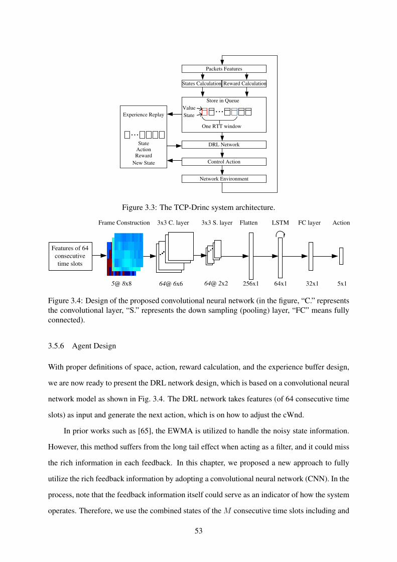
Packets Features

States Calculation Reward Calculation

Store in Queue

One RTT window

Value

State

DRL Network

Control Action

Network Environment

Experience Replay

State

Action

Reward

New State

Figure 3.3: The TCP-Drinc system architecture.

Features of 64

consecutive

time slots

5@ 8x8

3x3 C. layerFrame Construction 3x3 S. layer

64@ 6x6 64@ 2x2 256x1

Flatten

64x1

FC layerLSTM

32x1

Action

5x1

Figure 3.4: Design of the proposed convolutional neural network (in the figure, “C.” representsthe convolutional layer, “S.” represents the down sampling (pooling) layer, “FC” means fullyconnected).

3.5.6 Agent Design

With proper definitions of space, action, reward calculation, and the experience buffer design,

we are now ready to present the DRL network design, which is based on a convolutional neural

network model as shown in Fig. 3.4. The DRL network takes features (of 64 consecutive time

slots) as input and generate the next action, which is on how to adjust the cWnd.

In prior works such as [65], the EWMA is utilized to handle the noisy state information.

However, this method suffers from the long tail effect when acting as a filter, and it could miss

the rich information in each feedback. In this chapter, we proposed a new approach to fully

utilize the rich feedback information by adopting a convolutional neural network (CNN). In the

process, note that the feedback information itself could serve as an indicator of how the system

operates. Therefore, we use the combined states of the M consecutive time slots including and

53

before the current time t and divide them in to frames as inputs. For instance, we set M = 64

and obtain 5 frames. Each frame has a size 8 × 8 and consists of data from one of the five

features, as shown in Fig. 3.4. With the convolutional layers and pooling layer, the more stable,

higher level features can be abstracted from the raw state information.

Furthermore, the non-Markovian nature of the problem should also be addressed, as well

as the action taking effect delay τ1 and feedback delay τ2 (see Fig. 3.1). A promising approach

is to incorporate an LSTM to handle the correlation in a time series [75]. Through the back-

propagation through time (BPTT), this structure exploits the memory to extract system features.

As in Fig. 3.4, the LSTM layer is placed after the CNN extracts the stable features. In [75], the

authors proposed two training methods: Bootstrapped Sequential Updates and Bootstrapped

Random Updates. The former executes the training by randomly selecting an episode and

then starting from the beginning of the episode. The latter, however, picks a random timestep

in an episode and proceeds for a fixed amount of timesteps. In this chapter, we adopt the

Bootstrapped Random Updates method to train the network by combining with experience

replay.

The fully connected layer is used to calculate the Q-value for each action. Through the

entire network, we use the Exponential Linear Unit activation function ELU, defined as

ELU(ι) =

ι, ι > 0

λ · (eι − 1), ι ≤ 0,(3.16)

instead of Rectified Linear Units ReLU. Since we have to deal with negative rewards, it is

beneficial for not killing the nodes with negative outputs. In the last layer, which is to output

the Q-value for actions, no activation function is applied.


In this section, we present our extensive simulation study with the NS3 platform over different

scenarios and models. The basic configuration of the simulations is first demonstrated. In order

54

to have a comprehensive comparison, we also implement several state-of-the-art congestion

control protocols and carry out experiments with them.

3.6.1 Simulation Setup

In this chapter, the deep neural network is generated using Tensorflow [76]. The training is

executed with a reasonable speed on a PC with I5-8600k CPU and Nvidia GeForce 1060 3GB

GPU. The dropout layer is applied with a 0.2 dropout probability to provide both regularization

and ensemble effect. For the DNN, one convolutional layer and one pooling layer are incor-

porated. The LSTM layer with 64 units is applied after the CNN layers. One fully connected

layer is used with the activation function ELU . The output layer is a linear combination of

the previous output with 5 outputs, one for each action. The control action is applied every

T = 10ms. If a time period t does not have any ACK received, we simply copy the the state

of the previous time slot at−1 as input to the DNN (see Section 3.5.3). The minimum RTT is

updated every 10 RTTs.

For the simulations, we assume there are N remote-hosts that serve N wired or wireless

users. The remote-hosts are cWnd based and running the DRL agent independently, i.e., the

DRL agents do not share/exchange information during the TCP sessions. The simulation is

based on the classical dumbell topology with two routers in the middle, between the remote

hosts and users (see Fig. 3.2).

For fair and comprehensive comparison of congestion control performance, we choose

the following set of benchmark schemes that cover most of the existing representative algo-

rithms, including: (i) TCP-NewReno [38], (ii) TCP-Cubic[40], (iii) TCP-Hybla [77], (iv) TCP-

Vegas [39], (v) TCP-Illinois [78]. We would mainly focus on their performance in throughput

and RTT.

3.6.2 Training Process

The training process is divided into two phases: pre-training and distributed training. In the

pre-training phase, we train each agent with the same setup except that only one user is served

55

in order to build the baseline behavior for the agent for Npre episodes. Then the distributed

training will further train the competition strategy of each agent independently.

Pre-training

In our simulations, we set Npre = 20. The bottleneck capacity is 10 Mbps with 80 ms propa-

gation delay. And one training episode lasts for 500 s. Fig. 3.5 shows the dynamics of cWnd

and RTT in the 10th training episode. The learning process is divided into three phases: the

exploration probability linear annealing phase, the convergence phase, and the phase of ran-

domly learning of other options. Before the red line is the exploration probability annealing

process which involves a large probability of random choice of actions. With the exploration

probability decrease to 0.1, which is the end of the first phase, the agent can adjust the action to

converge to the perfect operating condition, i.e., the cWnd that can fully utilize the bottleneck

link capacity without introducing extra queuing delay (the red dashed line in Fig. 3.5(a)). Then

with a 0.1 probability, the agent will randomly deviate from the perfect operating point to ex-

plore the state space. Then it will repeat this process to train the agent with different network

conditions.

Distributed Training

After pre-training, we copy the model to 5 different servers (i.e., there are N = 5 servers

serving 5 wired users), and let them run the training process independently. We set the random

seed to be 17 for all the servers. The basic environment setting is the same and the distributed

training runs for Ndis = 100 episodes. In Fig. 3.6, the average throughput and RTT in the

distributed training process are presented. We can see that as the training proceeds, the average

throughput is increasing in general. And the average RTT eventually converges toward the

minimum RTT of 80 ms.

3.6.3 Congestion Control Performance

In this subsection, we present our experimental results with different network parameters to test

the performance of TCP-Drinc, specifically, over situations that deviate from that TCP-Drinc is

56

0 100 200 300 400 5000

50

100

150

200

250

300

350

400

450

Time (s)

cWnd (

pac

ket

s)

cWnd Dynamic

Perfect Operating Point

exploration probability linear annealing

convergence

randomly learning of other options

(a) cWnd dynamics

0 100 200 300 400 5000.05

0.1

0.15

0.2

0.25

0.3

0.35

0.4

0.45

Time (s)

RT

T (

s)

RTT Dynamics

Minimum RTT

(b) RTT dynamics

Figure 3.5: The dynamics of the single agent pre-training.

57

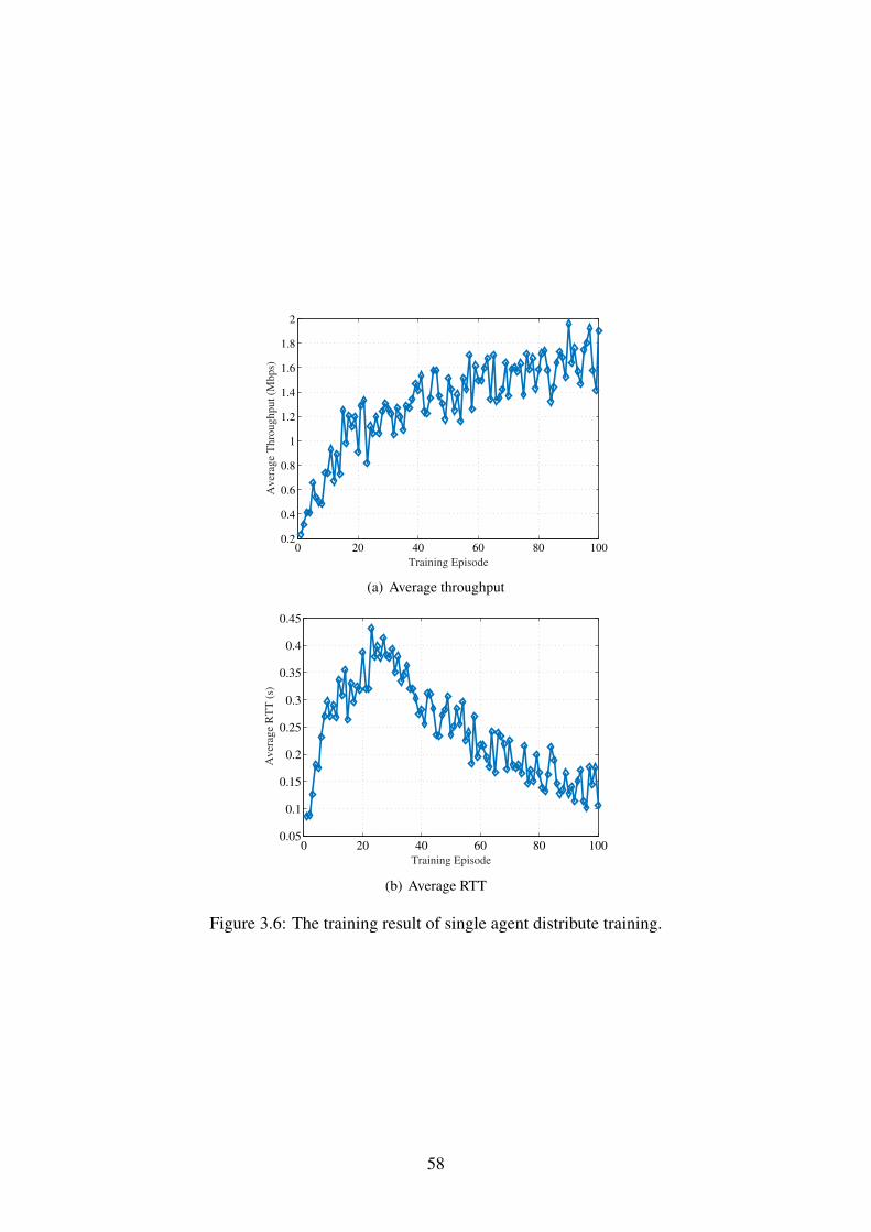
0 20 40 60 80 1000.2

0.4

0.6

0.8

1

1.2

1.4

1.6

1.8

2

Training Episode

Aver

age

Thro

ughput

(Mbps)

(a) Average throughput

0 20 40 60 80 1000.05

0.1

0.15

0.2

0.25

0.3

0.35

0.4

0.45

Training Episode

Aver

age

RT

T (

s)

(b) Average RTT

Figure 3.6: The training result of single agent distribute training.

58

originally trained. As demonstrated above, TCP-Drinc is trained with 5 TCP sessions with 10

Mbps bottleneck capacity and 80 ms propagation delay. Three testing cases are set as follows.

1. 4 users; the propagation delay varies in the range of [60, 240] ms; and the bottleneck

bandwidth is 10 Mbps;

2. the number of users varies in the range [3, 10); propagation delay is 80 ms; and the

bottleneck bandwidth is 8 Mbps;

3. 4 users; the propagation delay is 100 ms; the bottlneck bandwidth varies in the range of

[5, 20] Mbps.

The bottleneck buffer size is chosen as 100 packets. The size of a packet is a 1000-Byte payload

plus a 40-Byte header.

As shown in Figs. 3.7, 3.8, and 3.9, the well-trained TCP-Drinc model achieves a promis-

ing performance under all the scenarios we simulated. In Fig. 3.7, we present the throughput

and delay for increased propagation delay. We can see that all the RTTs increase with prop-

agation delay, while the throughput is relatively stable (except for TCP-Vegas). TCP-Drinc

achieves the highest throughput and the second smallest RTT for the entire range of propa-

gation delays. Although TCP-Vegas achieves a lower RTT than TCP-Drinc, its throughput is

the lowest, indicating that the low RTT is achieved by keeping the sending rate low and the

bottleneck buffer almost empty (i.e., sacrificing the utilization of the bottleneck link capacity).

Unlike the loss based protocols, TCP Vegas is a latency based scheme that linearly adjusts its

cWnd according to the difference between the current and the minimum RTT. It is effective in

keeping RTT low, but is sensitive to network condition changes and suffers from relatively low

throughput.

In Fig. 3.8, the throughput and RTT are presented for increased number of users. We

can see the capacity for each user decreases with increased number of users. Again, TCP-

Drinc achieves the highest throughput and the second lowest RTT. TCP-Vegas outperforms

TCP-Drinc with a lower RTT, but at the cost of a low throughput. Fig. 3.9 presents the through-

put and RTT achieved under different bottleneck capacity. For increased bottleneck capacity,

59

0.06 0.08 0.1 0.12 0.14 0.16 0.18 0.2 0.22 0.24

0.5

1

1.5

2

2.5

3

3.5

Propagation Delay (s)

Thro

ughput

(Mbps)

TCP−Cubic

TCP−Hybla

TCP−Illinois

TCP−NewReno

TCP−Vegas

TCP−Drinc


0.06 0.08 0.1 0.12 0.14 0.16 0.18 0.2 0.22 0.240

0.1

0.2

0.3

0.4

0.5

Propagation Delay (s)

RT

T (

s)

TCP−Cubic

TCP−Hybla

TCP−Illinois

TCP−Vegas

TCP−Drinc

TCP−NewReno

(b) Average RTT

Figure 3.7: Throughput and RTT statistics with different propagation delays.

60

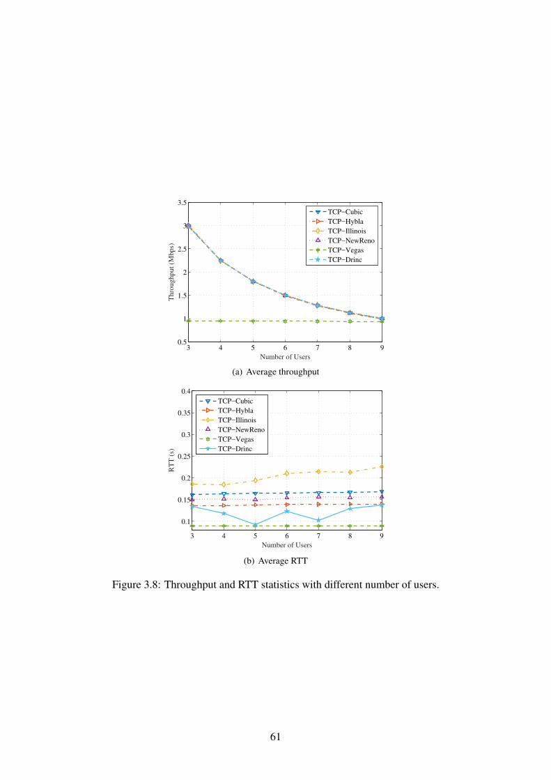
3 4 5 6 7 8 90.5

1

1.5

2

2.5

3

3.5

Number of Users

Thro

ughput

(Mbps)

TCP−Cubic

TCP−Hybla

TCP−Illinois

TCP−NewReno

TCP−Vegas

TCP−Drinc


3 4 5 6 7 8 9

0.1

0.15

0.2

0.25

0.3

0.35

0.4

Number of Users

RT

T (

s)

TCP−Cubic

TCP−Hybla

TCP−Illinois

TCP−NewReno

TCP−Vegas

TCP−Drinc

(b) Average RTT

Figure 3.8: Throughput and RTT statistics with different number of users.

61

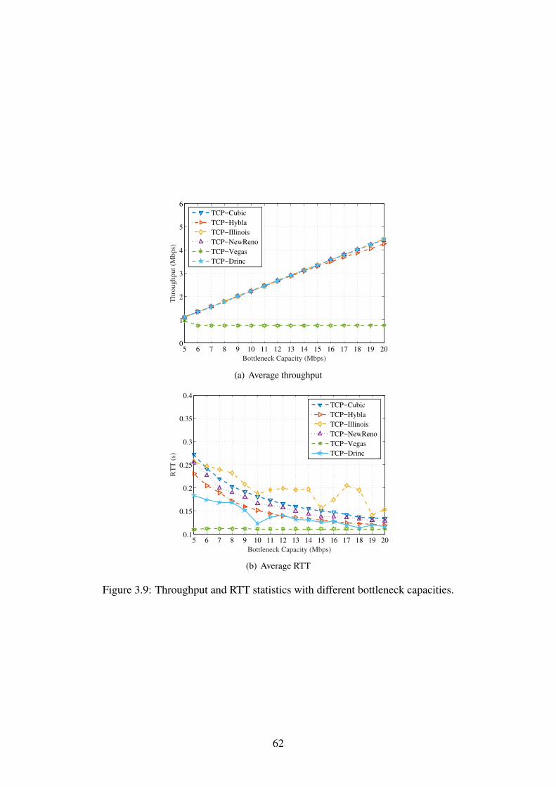
5 6 7 8 9 10 11 12 13 14 15 16 17 18 19 200

1

2

3

4

5

6

Bottleneck Capacity (Mbps)

Thro

ughput

(Mbps)

TCP−Cubic

TCP−Hybla

TCP−Illinois

TCP−NewReno

TCP−Vegas

TCP−Drinc


5 6 7 8 9 10 11 12 13 14 15 16 17 18 19 200.1

0.15

0.2

0.25

0.3

0.35

0.4

Bottleneck Capacity (Mbps)

RT

T (

s)

TCP−Cubic

TCP−Hybla

TCP−Illinois

TCP−NewReno

TCP−Vegas

TCP−Drinc

(b) Average RTT

Figure 3.9: Throughput and RTT statistics with different bottleneck capacities.

62

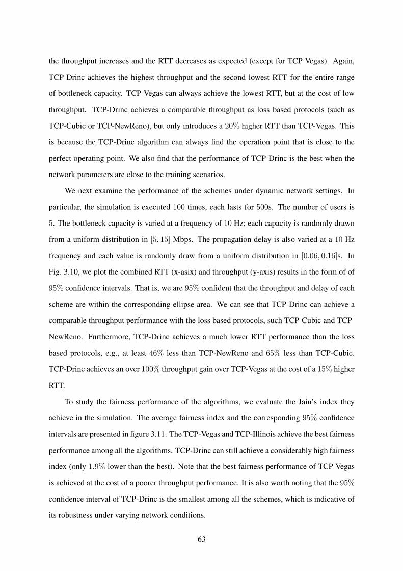
the throughput increases and the RTT decreases as expected (except for TCP Vegas). Again,

TCP-Drinc achieves the highest throughput and the second lowest RTT for the entire range

of bottleneck capacity. TCP Vegas can always achieve the lowest RTT, but at the cost of low

throughput. TCP-Drinc achieves a comparable throughput as loss based protocols (such as

TCP-Cubic or TCP-NewReno), but only introduces a 20% higher RTT than TCP-Vegas. This

is because the TCP-Drinc algorithm can always find the operation point that is close to the

perfect operating point. We also find that the performance of TCP-Drinc is the best when the

network parameters are close to the training scenarios.

We next examine the performance of the schemes under dynamic network settings. In

particular, the simulation is executed 100 times, each lasts for 500s. The number of users is

5. The bottleneck capacity is varied at a frequency of 10 Hz; each capacity is randomly drawn

from a uniform distribution in [5, 15] Mbps. The propagation delay is also varied at a 10 Hz

frequency and each value is randomly draw from a uniform distribution in [0.06, 0.16]s. In

Fig. 3.10, we plot the combined RTT (x-asix) and throughput (y-axis) results in the form of of

95% confidence intervals. That is, we are 95% confident that the throughput and delay of each

scheme are within the corresponding ellipse area. We can see that TCP-Drinc can achieve a

comparable throughput performance with the loss based protocols, such TCP-Cubic and TCP-

NewReno. Furthermore, TCP-Drinc achieves a much lower RTT performance than the loss

based protocols, e.g., at least 46% less than TCP-NewReno and 65% less than TCP-Cubic.

TCP-Drinc achieves an over 100% throughput gain over TCP-Vegas at the cost of a 15% higher

RTT.

To study the fairness performance of the algorithms, we evaluate the Jain’s index they

achieve in the simulation. The average fairness index and the corresponding 95% confidence

intervals are presented in figure 3.11. The TCP-Vegas and TCP-Illinois achieve the best fairness

performance among all the algorithms. TCP-Drinc can still achieve a considerably high fairness

index (only 1.9% lower than the best). Note that the best fairness performance of TCP Vegas

is achieved at the cost of a poorer throughput performance. It is also worth noting that the 95%

confidence interval of TCP-Drinc is the smallest among all the schemes, which is indicative of

its robustness under varying network conditions.

63

0.060.080.10.120.140.160.180.20.5

1

1.5

2

2.5

3

Tcp−NewReno

Tcp−Vegas

Tcp−Hybla

Tcp−Cubic

Tcp−Illinois

Tcp−Drinc

RTT (s)

Th

rou

gh

pu

t (M

bp

s)

Figure 3.10: Performance of different algorithms over randomly varied parameters.

TCP-C

ubic

TCP-H

ybla

TCP-I

llino

is

TCP-N

ewRen

o

TCP-V

egas

TCP-D

rinc

Jain

's I

ndex

0.6

0.7

0.8

0.9

Figure 3.11: Jain’s index for each algorithm.

Finally, we evaluate the TCP variants with mobile users. The same network setting is

used, except that the last hop is an LTE network with five mobile users. The users move in a

disk area of 800 m radius, following a random walk mobility model with 1 m/s speed. The LTE

network is simulated using the bulit-in LTE model in NS3 [79]. The wired part has the same

configuration as in previous simulations. The simulation results are presented in Fig. 3.12. The

LTE base station has a deep and separate queue for each user. Therefore, we do not use TCP-

NewReno here since it will introduce a very large RTT in this setting. The proposed algorithm

still perform well in the wireless network setting. Its throughput is comparable to the two loss

based protocols, with a much reduced RTT. Its throughput is much higher than TCP Vegas

while the RTT is only slightly higher.

64

0.511.522.533.543

4

5

6

7

8

9

10

TCP−Cubic

TCP−Drinc

TCP−Vegas

RTT (s)

Thro

ughput

(Mbps)

TCP−Illinois

Figure 3.12: LTE network simulation results with the dumbell topology and 5 mobile users.

3.7 Conclusions

In this chapter, we developed a framework for general adaptive congestion control based on

deep reinforcement learning techniques. The proposed scheme does not require accurate mod-

els for the network, scheduling, and network traffic flow; it also does not require training data.

The detailed design of the propoed TCP-Drinc scheme was proposed and the trade-offs were

discussed. Extensive simulations with NS3 were conducted to validate the superior perfor-

mance over several benchmark algorithms.

65

Chapter 4

DORA: A Cross-layer optimization for Robust QoE-Driven DASH over OFDMA NetworksBit Rate Adaption and Resource Allocation

In this chapter, the problem of effective and robust delivery of DASH videos over an orthog-

onal frequency-division multiplexing access (OFDMA) network is studied. Motivated by a

measurement study, we propose to explore the request interval and robust rate prediction for

DASH over OFDMA. We first formulate an offline cross-layer optimization problem based on

a novel QoE model. Then the online reformulation is derived and proved to be asymptotically

optimal. After analyzing the structure of the online problem, we propose a decomposition

approach to obtain a UE rate adaptation problem and a BS resource allocation problem. We

introduce stochastic model predictive control (SMPC) to achieve high robustness on video rate

adaption and consider the request interval for more efficient resource allocation. The efficacy

of the proposed DORA-RI scheme is validated with simulations.

4.1 Introduction

Recent years have witnessed the tremendous increase in mobile video traffic. Video has now

dominated the mobile data traffic for over 60 percent in 2016, and is expected to account for

over 75 percent in 2021 [1]. At the same time, the rapidly growth in both the overall mobile

traffic (which has increased 18-fold since 2011) and the number of mobile devices (429 millions

were added in 2016) have made mobile video streaming a great challenge. In addition, the

instability nature of wireless links will make the situation even worse. There is a compelling

need to achieve high efficiency and robustness of video delivery over wireless networks, while

66

guaranteeing users’ Quality of Experience (QoE). This problem should be studied from both

the wireless infrastructure and user aspects.

Video streaming has drawn great attention for decades. The early works are mainly based

on the User Datagram Protocol (UDP), which can provide timely transmission compared with

Transportation Control Protocol (TCP) that is designed for reliability over timeliness. How-

ever, the deployment of UDP based algorithms is challenging due to the incompatibility with

firewalls and other types of middleboxes. On the other hand, TCP is supported by most mid-

dleboxes for its reliability and security. The congestion control algorithms facilitate the time-

liness of transmission as well. Therefore, Hypertext Transfer Protocol (HTTP) based on video

streaming is now the mainstream technique. In particular, Dynamic video streaming over HTTP

(DASH), which can adapt to the variation of network conditions, is recognized as a promising

technique to enhance the user QoE. Many commercial video services, e.g., YouTube and Net-

flix, are all based on DASH, which have accounted for more than half of the total Internet traffic

in North America in 2016 [7].

Among different generations of mobile transmission techniques, the 3GPP-Long Term

Evolution (LTE) and Wi-Fi (802.11 standard) are the two most popular. The Orthogonal

frequency-division multiplexing (OFDM) is the common method of both standards that encode

and transmit digital data on multiple subcarriers of a broadband channel. OFDM is expected to

continue serving the next generation wireless networks for its ability on tackling narrowband in-

terference and frequency-selective fading with a low complexity. OFDM also introduces great

flexibility by allowing dynamically assigning subcarriers, time, and power to each user in order

to accommodate customized QoS requirements, such as transmission rate [80, 81, 82] or power

efficiency [83]. The similar technique has been applied to smart grid as well [84, 85, 86, 87].

Some cross-layer designed could be found in [88, 89, 90, 91, 92, 93, 94, 95].

Consider a video user equipment (UE) that receives a DASH video through an OFDM

network, as shown in Fig 4.1. The two techniques are in different layers in the protocol stack

and have different design goals. However, for video streaming, both of them should be designed

for the ultimate goal of guaranteeing user QoE. In this chapter, we study the cross-layer, joint

design of DASH and OFDM. In DASH, the video consumers take the control of choosing

67

Server

Bitrate m

Segment 1

Segment 2

Segment N

Bitrate m

Segment 1

Segment 2

Segment N

Bitrate m

Segment 1

Segment 2

Segment N

UE 1

UE 2

UE 3

UE 4

UE M

Figure 4.1: DASH mobile video streaming system architecture.

different data rates for future video segments, which are coded (or stored) at the video server.

The corresponding information is sent to the consumers at the beginning of video transmission.

Resource allocation in OFDMA networks, on the other hand, is executed at the base station,

which takes into account various factors such as channel state information (CSI), power budget,

and user QoE requirement and determines the optimal resource allocation for multiple video

UEs.

4.1.1 Motivation

To provide useful insights into the problem of DASH based video streaming over OFDMA

networks, we conducted a measurement study using dash.js [96] in Broun Hall, Auburn Uni-

versity, Auburn, AL, USA over Version LTE. The video source is placed on a remote server and

coded into 10 different bit rates ranging from 254 kbps to 14931 kbps. We collected the video

playback trace information over LTE in 1 hour daytime and 1 hour night time. Define request

interval as the period between when the request for the next segment is sent and when the first

video byte of the requested segment arrives at the user. In this experiment, we measured the

request interval of the DASH video session, as well as the link capacity that can be acquired by

measuring the download speed of each video segment.

As shown in Fig. 4.2, the request interval could be as large as 10 s and 80 percent of

the intervals are in the range from 0.2 to 0.4 s. However, most of the joint design of DASH

and scheduling algorithms do not fully consider this relatively large period of time and still

allocate resources to the video users, even though no transmissions are needed during this

68

500 600 700 800 900 10000

0.2

0.4

0.6

0.8

1

1.2

1.4

Packets Sequence Number

Req

ues

t In

terv

al (

s)

Figure 4.2: The variations of request intervals obtained in our measurement study over an LTElink.

interval (except for the first packet of the requested segment). Motivated by this observation,

we propose a new formulation of the resource allocation problem at the BS by exploiting the

request intervals (see Section 4.3).

In addition, we measured the capacity of the LTE link during playback. Usually the ca-

pacity will be influenced by factors such as fading and shadowing, which will all trigger the

capacity variation at small timescales. In DASH, many existing rate adaption schemes are

based on the average downloading capacity over one segment, which is assumed to be slowly

varying and relatively stable. In Fig. 4.3, we present the average capacity of one segment,

which exhibits quite large variations over time. Such large variations could make the existing

rate adaptation schemes ineffective. Motivated by this observation, we propose a model pre-

dictive control based optimization of the rate adaption at the video user side to achieve better

robustness (also see Section 4.3).

4.1.2 Contributions and Organization

We address the cross-layer QoE-driven optimization problem of DASH over OFDMA networks

in this chapter. The contribution of this work is three-fold:

1. We develop a new QoE model and formulate an offline optimization problem jointly

considering the new QoE model as well as the specific resource allocation model in

OFDMA networks.

69

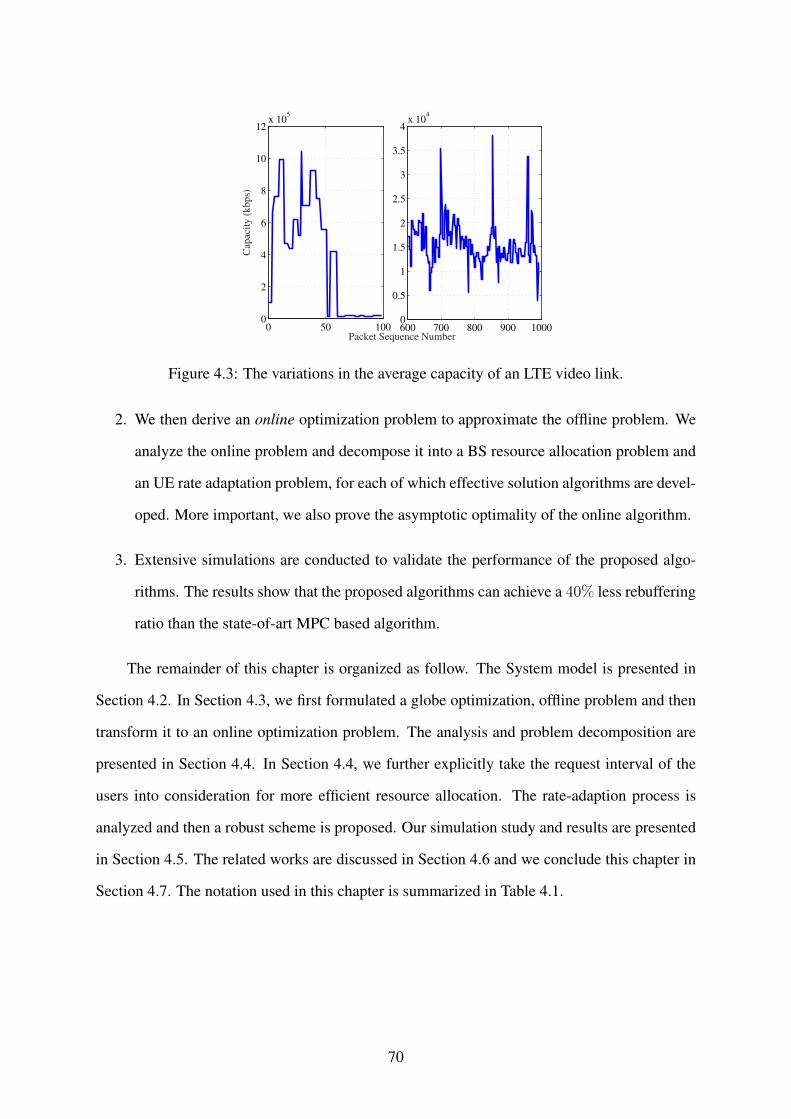
0 50 1000

2

4

6

8

10

12x 10

5

Packet Sequence Number

Cap

acit

y (

kbps)

600 700 800 900 10000

0.5

1

1.5

2

2.5

3

3.5

4x 10

4

Figure 4.3: The variations in the average capacity of an LTE video link.

2. We then derive an online optimization problem to approximate the offline problem. We

analyze the online problem and decompose it into a BS resource allocation problem and

an UE rate adaptation problem, for each of which effective solution algorithms are devel-

oped. More important, we also prove the asymptotic optimality of the online algorithm.

3. Extensive simulations are conducted to validate the performance of the proposed algo-

rithms. The results show that the proposed algorithms can achieve a 40% less rebuffering

ratio than the state-of-art MPC based algorithm.

The remainder of this chapter is organized as follow. The System model is presented in

Section 4.2. In Section 4.3, we first formulated a globe optimization, offline problem and then

transform it to an online optimization problem. The analysis and problem decomposition are

presented in Section 4.4. In Section 4.4, we further explicitly take the request interval of the

users into consideration for more efficient resource allocation. The rate-adaption process is

analyzed and then a robust scheme is proposed. Our simulation study and results are presented

in Section 4.5. The related works are discussed in Section 4.6 and we conclude this chapter in

Section 4.7. The notation used in this chapter is summarized in Table 4.1.

70

Table 4.1: NotationSymbol Description

N total number of usersM total number of subcarriersW total bandwidth availableκ bandwidth per subcarrierP total transmission powergim channel gain of user i on subcarrier mvim user i’s time share of subcarrier mpim average trans. power allocated to user i on subcarrier mrim maximum rate user i can achieve on subcarrier sri maximum rate user i can achieveSi video length for user iKi number of segments for user iRi[ki] data rate of segment k for user iqi(Ri[ki]) quality of segment k to user i given data rate Rk

qi[ki] quality at time step kia, b parameter of quality modelQ[ki] original definition of QoEQfair[ki] QoE definition with utility functionmi[K] average video quality of the playback process for user iVari[K] video quality variation of the playback process for user iRebi[K] rebuffering ratio of the playback process for user iT si Startup delayθ, λ, η negative coefficients for QoEQonlinei [ki] online definition of QoE

Bi[ki] buffer occupancy of user i after downloading segment kBi,max maximum buffer size of user iCi[ki] average capacity of downloading segment kiα the Lagrange multiplier for vβ the Lagrange multiplier for pγi,min the Lagrange multiplier for qi,minγi,max the Lagrange multiplier for qi,max

4.2 System Model

4.2.1 Network Model

We consider a wireless video streaming network as shown in Fig. 4.1, consisting of video

servers, the wireline netowrk, a cellular base station (BS), and multiple UEs. The videos are

stored in the remote servers. To reduce the delay of transmission, more and more server are

deployed closer to end UEs. Generally, the capacity bottleneck in the end-to-end transmission

71

path is the last hop, where a BS serves multiple UEs. The transmission in the Internet before

the last hop could be modeled as a request interval time since the network conditions such as

capacity and congestion level mainly influence the propagation time before the BS.

Assume the BS servesN video streaming UEs with OFDMA, denoted as N = {1, 2, ..., N}.

Denote the total available bandwidth as W Hz, which consists of M subcarriers denoted as

M = {1, 2, ...,M}. Each subcarrier m ∈ M is assumed to have an equal bandwidth of

κ = W/M Hz. Since the bandwidth of each subcarrier is sufficiently small, they only ex-

perience flat fading. For a resource block in OFDM, the time length of each resource allocation

is denoted as τ , the time step is denoted as t = 1, 2, ..., and each time slot contains an integer

number of OFDM symbols and an integer number of τ .

Denote gim(t) as the channel gain of UE i ∈ N on subcarrier m ∈ M at time t, and

pim(t) accounts for the total transmission power assigned to subcarrier m for UE i at time t.

Assume the total power can be assigned is P . Since multiple users can share subcarriers in

each time slot, denote the non-overlapping time fraction of user i on subcarrier m in time slot t

as 0 ≤ vim(t) ≤ 1. Without loss of generality, assume the time slot is unit time. Then we have

N∑i=1

vim(t) ≤ 1, ∀m, t. (4.1)

The additive white Gaussian noise (AWGN) at the receiver has unit spectrum density. Ac-

cording to Shannon formula, the maximum rate user i can achieve on subcarrier m at time t

is

rim(t) (4.2)

=

vim(t)κ log2

(1 +

pim(t)g2im(t)

vim(t)κ

), if vim(t) > 0

0, otherwise.

The BS will first estimate the CSI on each subcarrier. Then with different targets, e.g.,

maximizing the total data rate or maximizing the energy efficiency, the BS assigns transmit

power pim(t) and time fraction vim(t) to each UE i on each subcarrierm at time t. Naturally, the

72

Bu

ffer

occ

up

ancy

(s)

Playing process (s)

Request

Interval

Downloading

time

Rebuffering

Figure 4.4: Timeline of the discrete time DASH system.

total data rate for UE i at time t is the summation of all the data rate rim(t) on each subcarrier,

denoted as ri(t) =∑M

m=1 rim(t).

4.2.2 Streaming Video Model

The video for UE i is Si s, which has been partitioned intoKi consecutive segments, each coded

with different bit rates. Assume each segment of all videos is l s. Without lost of generosity,

assume all the coded bit rates Ri are in the same set R. Naturally, the size of segment ki in bits

can be represented as Ri[ki]× l.

During the video session, the playback buffer dynamic process at a user is illustrated in

Fig. 4.4. When a new segment is completely downloaded, the buffer occupancy (in seconds) is

immediately increased. The buffer occupancy decreases linearly with time when the segment

is played out. When the buffer is empty, the playback process stalls. The time till the next

segment arrives is the rebuffering time (the interval before the 5th segment in Fig. 4.4). After

downloading a segment, the UE estimates the average rate of the segment and sends a request

back to the video server for the next segment. The period since the request is sent till the

first byte of the next segment arrives at the UE, is the request interval (see the 2nd segment

in Fig. 4.4). Depends on the computational complexity of the UE algorithm and the server it

chooses, the request interval could be as large as several seconds, as shown in Section 4.1.

Denote Bi[ki] ∈ [0, Bi,max] as the playback buffer occupancy at UE i, which represents

the amount of video data stored in the buffer after downloading segment ki, as measured in

playback time. Users may have different buffer sizes Bi,max, which represents the total amount

of storage measured in playback time. The UE can play each video segment only after it is

fully downloaded, since the segment itself contains the playback metadata.

73

Let si[ki] represent the time slot when segment ki is downloaded at UE i. During playback,

the UE calculates the average rate Ci[ki] of downloading segment ki, as an important indicator

of future capacity in most existing algorithms. The request interval is denoted by πi[ki], which

depends on the network parameters and network congestion level. During this period, this

UE does not need any resource from the BS for transmission. Since this period could be

considerably large, it should be considered in the resource allocation scheme.

The playback buffer process can be modeled as follows. The timeline of the operations

and updates is presented in Fig. 4.4.

Bi[ki] = min{

max{

0, Bi[ki − 1]− πi[ki]− Ri[ki]l

Ci[ki]

}+ l, Bi,max}

Ci[ki] =∑si[ki]

t=si[ki−1]+πi[ki]ri(t)

si[ki]−si[ki−1]

si[ki] = si[ki − 1] + πi[ki] + Ri[ki]l

Ci[ki].

(4.3)

The rebuffering time for one segment downloading event is max{

0, πi[ki] + Ri[ki]l

Ci[ki]−Bi[ki − 1]

}.

Rebuffering event happens when this value is larger than 0, which significantly degrades the

user QoE [97].

4.2.3 Quality of Experience (QoE) Model

The QoE is an important indicator of the performance of video communication systems. How

to design a QoE model to capture the user assessment has been extensively studied. In the

past, the QoE is mainly divided into two parts: objective measures and subjective evaluation.

Objective measures, e.g., Peak Signal-to-Noise Ratio (PSNR) represent the quality of video

frames, while subjective evaluation, such as Mean Opinion Score (MOS) [98], reflects users

assessment of the viewing experience [99].

In [100], the authors study how the factors, such as playback buffer and average bit rate,

influence the user engagement. It suggests that new QoE model should be developed that

considers both video quality and user experience, which could be represented coarsely as user

engagement. The authors in [97] suggest that the main factors of a QoE model should include

74

buffering ratio, video starting time, average bit rate, and attributes such as type of video, ISP,

etc. In [101], the QoE model is defined as a weighted sum of several main factors. The weights

could be adjusted for different scenarios.

Intuitively, the larger the bit rate, the better the video quality. The relationship between

video quality and bit rate could be modeled as q(t) = f(R[t]) = a · log(R[t]) + b [102] .

The coefficients a, b could be adjusted according to specific video type and playback device for

stored videos. On the other hand, the variance of video quality across segments influences the

user experience as well. The tradeoff between the average quality and variance is a key factor

to be taken into consideration.

The key factors of our QoE model is listed below for UE i.

• Average video qualitymi[K]: it represents the video quality level averaged over the entire

video playback period [101], defined as: mi[K] = 1K

∑Kk=1 q(Ri[k]).

• Variance of video quality Vari[K]: it accounts for the quality variation from segment to

segment, given by Vari[K] = 1K

∑Kk=1(q(Ri[k])−mi[K])2. As the average video quality,

the variance also has a considerable impact on the QoE [101].

• Rebuffering ratio Rebi[K]: rebuffering occurs when there is underflow at the playback

buffer. The rebuffering ratio is defined as the total rebuffering time over the total video

duration Li = Ki × l, i.e.,

Rebi =1

Li

K∑k=1

max

{0, πi[ki] +

Ri[k]l

Ci[k]−Bi[k − 1]

}. (4.4)

This factor affects the QoE even more significantly than variance [103].

• Startup delay T si : it represents the time between user requests a video and the playback

begins. Normally, a certain length of buffer occupancy need to be accumulated before

playback starts [101]. It depends on the transmission rate and how the video is encoded.

75

As different user might focus on different factors, we use a weighted sum to ensure flexi-

bility of this model. For segment ki, user i’s QoE is defined as

Q[ki] = q(Ri[ki]) + θ · (q(Ri[ki])−mi[Ki])2+ (4.5)

λ

Kilmax

{0, πi[ki] +

Ri[ki]l


}.

in which θ < 0 and λ < 0 are tunable weights, and mi[Ki] is the average video quality. For the

entire playback process, the QoE of user i can be defined as

Qi =

Ki∑ki=1

Q[ki] + η · T si (4.6)

in which η < 0 is a tunable weight, and Ts is the startup delay. This model can be flexibly

tuned for different users and application scenarios with different parameter sets {θ, λ, η}. Fur-

thermore, if the viewing process is emphasized instead of the startup phase, the overall QoE

can be defined as Qi =∑Ki

ki=1 Q[ki].

To consider fairness among users, we introduce a concave utility function Uα(·) defined

as [104]

Uα(x) =

log(x), if α = 1

x1−α

1−α , otherwise.(4.7)

For instance, when α = 1, maximizing the utility sum ensures proportional fairness. We

defines the fairness QoE as Qfair(ki) = Uα (Q(ki)) and the QoE through the playing process

Qi =∑Ki

ki=1 Qfair(ki).

4.3 Problem Formulation

To achieve the goal of QoE maximization, the challenge is that the BS and video UEs are

operating at different timescales. At each time t, the BS adapt to the variation of network states,

e.g., updated CSI. On the other hand, the video users adapt the bit rate of the next video segment

after downloading the present one. In this section, we first formulate an offline problem and

76

then provide an online transformation with reduced complexity. The decomposition of the

online problem is then presented and the decomposed problems will be solved in Section 4.4.

4.3.1 The Offline Optimization Problem

The offline optimization problem is formulated based on the assumption that we know all the

information of the video process. The optimization variables related to the BS are wireless

resources: vim(t) and pim(t) for UE i on subcarrier m. Video rate adaption is executed each

time when the UE finishes downloading a segment. The data-rate Ri[ki] can only be chosen

from a given set Ri defined by the video encoder (or server). The offline QoE maximization

problem, denoted by Prob-Offline, is formulated as follows.

max{pim(t),vim(t),Ri[ki]}

Λ =N∑i=1

Ki∑ki=1

Qfair[ki] (4.8)

s.t.:N∑i=1

vim(t) ≤ 1, ∀m, t (4.9)

N∑i=1

M∑m=1

pim(t) ≤ P, ∀t (4.10)

Ri[ki] ∈ Ri, ∀i (4.11)

Bi[ki] ∈ [0, Bi,max], ∀i, ki. (4.12)

In terms of pim(t) and vim(t), the optimization problem is convex. For rate adaption, it is

an integer programming with a limited solution set (for example, most Youtube videos offer 3

to 6 resolutions). The optimal value could be achieved with dynamic programming (DP).

To deal with variables Ri[ki], we relax the constraint to allow them to take any values

(rather then chosen from a give set Ri), to obtain an approximation problem. Notice that the

video rate and quality can be mapped with function qi(·). Therefore, the quality qi also belongs

to a set of scalar values Θi (asRi[ki] is chosen from Ri). Furthermore, we can select the optimal

quality and then derive the corresponding rate using q−1(·) and round it to the closest rate in set

R. Here, we abuse the notation of qi, but the reader can easily differentiate the q(·) and qi as the

quality function and the scalar value of quality. As qi(·) is monotonically increasing, we have

77

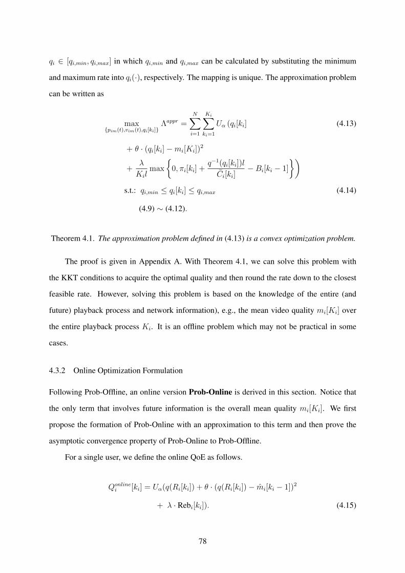
qi ∈ [qi,min, qi,max] in which qi,min and qi,max can be calculated by substituting the minimum

and maximum rate into qi(·), respectively. The mapping is unique. The approximation problem

can be written as

max{pim(t),vim(t),qi[ki]}

Λappr =N∑i=1

Ki∑ki=1

Uα (qi[ki] (4.13)

+ θ · (qi[ki]−mi[Ki])2

+λ

Kilmax

{0, πi[ki] +

q−1(qi[ki])l


})s.t.: qi,min ≤ qi[ki] ≤ qi,max (4.14)

(4.9) ∼ (4.12).

Theorem 4.1. The approximation problem defined in (4.13) is a convex optimization problem.

The proof is given in Appendix A. With Theorem 4.1, we can solve this problem with

the KKT conditions to acquire the optimal quality and then round the rate down to the closest

feasible rate. However, solving this problem is based on the knowledge of the entire (and

future) playback process and network information), e.g., the mean video quality mi[Ki] over

the entire playback process Ki. It is an offline problem which may not be practical in some

cases.

4.3.2 Online Optimization Formulation

Following Prob-Offline, an online version Prob-Online is derived in this section. Notice that

the only term that involves future information is the overall mean quality mi[Ki]. We first

propose the formation of Prob-Online with an approximation to this term and then prove the

asymptotic convergence property of Prob-Online to Prob-Offline.

For a single user, we define the online QoE as follows.

Qonlinei [ki] = Uα(q(Ri[ki]) + θ · (q(Ri[ki])− mi[ki − 1])2

+ λ · Rebi[ki]). (4.15)

78

in which mi[ki] is updated as

mi[ki] = mi[ki − 1] +ζi

ki + ζi(q(R∗i [ki])− mi[ki − 1]). (4.16)

In (4.16), q(R∗i [ki]) is the video quality corresponding to the optimal rate R∗i [ki], ζi is a tunable

parameter for different users. This way, we rewrite the problem from over the entire time

window T to the problem that can be solved at each time slot using past and present information.

Lemma 1. The mi[k] in (4.16) approximates the average of the optimal quality with k goes to

infinity.

The proof is given in Appendix B. Lemma 1 is on the convergence property of mi[k],

which we use to replace the term of overall average quality mi[Ki]. It lays the foundation for

the proof of convergence of the online algorithm.

Lemma 2. Prob-Online is a convex optimization problem.

The proof for lemma 2 is similar to theorem 4.1 and is omitted for brevity. Based on

Lemmas 1 and 2, we can take a step further to claim that the solution to the online problem

converges to the offline problem solution asymptotically.

Theorem 4.2. The solution of Prob-Online asymptotically converges to the solution of Prob-

Offline.

The proof is given in Appendix C. With Theorem 4.2, we can derive the solution for Prob-

Online with past and present information. More important, the solution converges to the offline

optimal solution with the increase of time.

With the Lemmas and Theorems, we can solve the online problem to acquire the opti-

mal solution {p∗im(t), v∗im(t), R∗i [ki]} for each time slot. However, the user rate adaption may

not be synchronized, and more important, the user rate adaptation is executed at a different

timescale from BS resource allocation. In addition, the number of video UEs that are actually

transmitting packets is varying over time (i.e., due to the request interval). To address all these

79

challenges, we further decompose the optimization problem into two sub-problems: a BS re-

source allocation problem and a video rate adaptation problem, which are solved in the next

section.

4.4 Solution Algorithms and Analysis

4.4.1 Prob-Online Analysis

We first rewrite the online formulation by adding the equality constraints on the capacity of

each user.

max{pim(t),vim(t),Ri[ki]}

Λonline =N∑i=1

Qonlinei

Ci(t) =M∑m=1

rim(t),∀i ∈ N,∀t ∈ T (4.17)

(4.9) ∼ (4.12).

In the above formulation, the BS operation, i.e., resource allocation, is coupled with UEs’

rate adaptation in the term average capacity Ci[ki]. At each time slot si[ki], the controller will

try to optimize the QoE by estimating the capacity for the next segment Ci[ki+1]. On the other

hand, the BS controller will also optimize the QoE by allocate resource to UEs at each time

slot t, which updates Ci(t). With asynchronous operations of the two parties, it is natural to

decompose the problem to BS and UE subproblem, to decouple their operations.

At the UE side, rate adaption is executed based on the estimation of Ci[ki + 1] at time

si[ki] after downloading segment ki. Most estimation algorithms are based on the history data

of capacity. The value of Ci[ki + 1] is influenced by the resource allocation before time ki.

On the other hand, the BS allocates resources to each UE at a smaller timescale than rate

adaption. Therefore, at each resource allocation time step, the video rate has already been

chosen and remains fixed for a period of time. Based on this observation, we present a primal

decomposition approach based on [105].

80

4.4.2 UE Rate Adaption

The rate adaption at the UE is executed when the previous segment is downloaded. The as-

signed transmission rate to the UE during the downloading process is determined by the en-

vironment conditions sensed by BS. To choose the rate for the next segment, the capacity is

mainly an estimation based on the previous segment. It makes sense that we optimize the QoE

at each UE by rate adaption with a given estimation of capacity Ci[ki + 1].

At si[ki − 1], UE i aims to maximize its QoE by choosing Ri[ki], based on Bi[ki − 1] and

history information. We formulate the UE i side rate adaptation problem as

maxRi[ki]

IUi (ki) · Qonlinei [ki] (4.18)

s.t.: Ri[ki] ∈ Ri (4.19)

Bi[k] ∈ [0, Bi,max], ∀k ∈ [si[ki − 1], si[ki]], (4.20)

where Qonlinei [ki] is defined as in (4.15) with estimated Ci[ki]. The indication function IUi (ki)

is equal to 1 when the buffer is not full and 0 otherwise. By the time when the buffer is full, the

video UE would pause Get for several seconds depends on the mechanism. Rebuffering time

is updated as in (4.3).

The average download capacity is estimated based on history data. From the applica-

tion layer, the UE can only acquire an estimation of the average capacity by dividing Ri[ki]l

with time difference between sending request and completing downloading the segment. With

information from the TCP layer, we can have a better estimation by narrowing down the down-

loading period between the time of receiving the first packet and the last packet. However, it

is still hard to accurately predict the future downloading capacity due to network dynamics in

the future. We can acquire an estimation by simply using the exponential average over the pre-

vious capacity. Then solve the optimization by brute-force search in the rate space Ri, which

is small (e.g., 3 to 6 different resolutions/rates). In this chapter, we call this simple scheme as

DORA [106].

81

Inspired by the work [42], which measures the cellular network capacity and proposes an

estimation model based on Poisson process, we consider the downloading capacity as a random

variable. Furthermore, by optimization over several future steps with estimated future informa-

tion, we can increase the robustness of rate adaption based on the theory of stochastic model

predictive control (SMPC). In this way, the optimization do not rely on accurate estimations of

future information that are hard to acquire.

Assume that the average capacity Ci[ki] is a random process based on distribution Ξ(·)

with mean Ci[ki − 1]. At each rate adaptation time si[ki − 1], we will first update the average

capacity Ci[ki−1] with the measurement of this segment transmission. The exponential window

moving average (EWMA) method is used to update the mean as Ci[ki − 1] = ξCi[ki − 2] +

(1 − ξ)Ci[ki − 1] with exponential weights ξ ∈ (0, 1). Suppose the prediction horizon here is

z. The z predictions over the prediction horizon are drawn with Monte Carlo sampling based

on the distribution. By solving the optimization problem over the z steps ahead, we can obtain

control moves as follows.

~Ri := {Ri[ki], Ri[ki + 1], ..., Ri[ki + z − 1]}. (4.21)

The first control result, Ri[ki], will be taken as the choice for the next segment. In this

chapter, we adopt dynamic programming (DP) to compute the overall control moves ~Ri. The

rough idea is to store the intermediate optimal QoE score of each prediction step and then

update it at each step. Due to limited size of the bitrate set R and small prediction horizon, the

time complexity of the DP algorithm, O(|R| · z), is acceptable in this context. By explicitly

considering the uncertainty of estimations, this algorithm provides us a robust rate adaption

solution. The new optimization problem is formulated as

maxRi[ki],...,Ri[ki+z−1]}

z−1∑j=0

Qonlinei [ki + j] (4.22)

s.t.: Ri[kj] ∈ Ri, j ∈ {ki, ..., ki + z − 1} (4.23)

Bi[ki] ∈ [0, Bi,max],∀ki, (4.24)

82

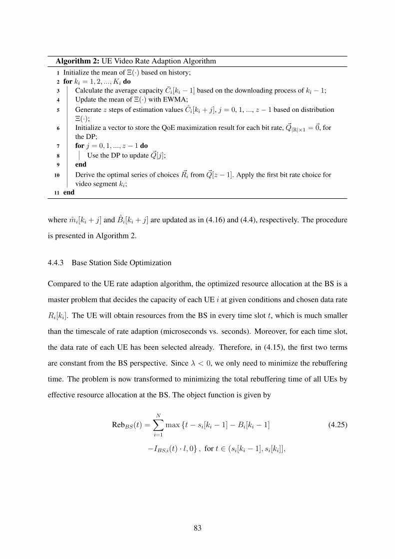
Algorithm 2: UE Video Rate Adaption Algorithm1 Initialize the mean of Ξ(·) based on history;2 for ki = 1, 2, ...,Ki do3 Calculate the average capacity Ci[ki − 1] based on the downloading process of ki − 1;4 Update the mean of Ξ(·) with EWMA;5 Generate z steps of estimation values Ci[ki + j], j = 0, 1, ..., z − 1 based on distribution

Ξ(·);6 Initialize a vector to store the QoE maximization result for each bit rate, ~Q|R|×1 = ~0, for

the DP;7 for j = 0, 1, ..., z − 1 do8 Use the DP to update ~Q[j];9 end

10 Derive the optimal series of choices ~Ri from ~Q[z − 1]. Apply the first bit rate choice forvideo segment ki;

11 end

where mi[ki + j] and Bi[ki + j] are updated as in (4.16) and (4.4), respectively. The procedure

is presented in Algorithm 2.

4.4.3 Base Station Side Optimization

Compared to the UE rate adaption algorithm, the optimized resource allocation at the BS is a

master problem that decides the capacity of each UE i at given conditions and chosen data rate

Ri[ki]. The UE will obtain resources from the BS in every time slot t, which is much smaller

than the timescale of rate adaption (microseconds vs. seconds). Moreover, for each time slot,

the data rate of each UE has been selected already. Therefore, in (4.15), the first two terms

are constant from the BS perspective. Since λ < 0, we only need to minimize the rebuffering

time. The problem is now transformed to minimizing the total rebuffering time of all UEs by

effective resource allocation at the BS. The object function is given by

RebBS(t) =N∑i=1

max {t− si[ki − 1]−Bi[ki − 1] (4.25)

−IBS,i(t) · l, 0} , for t ∈ (si[ki − 1], si[ki]],

83

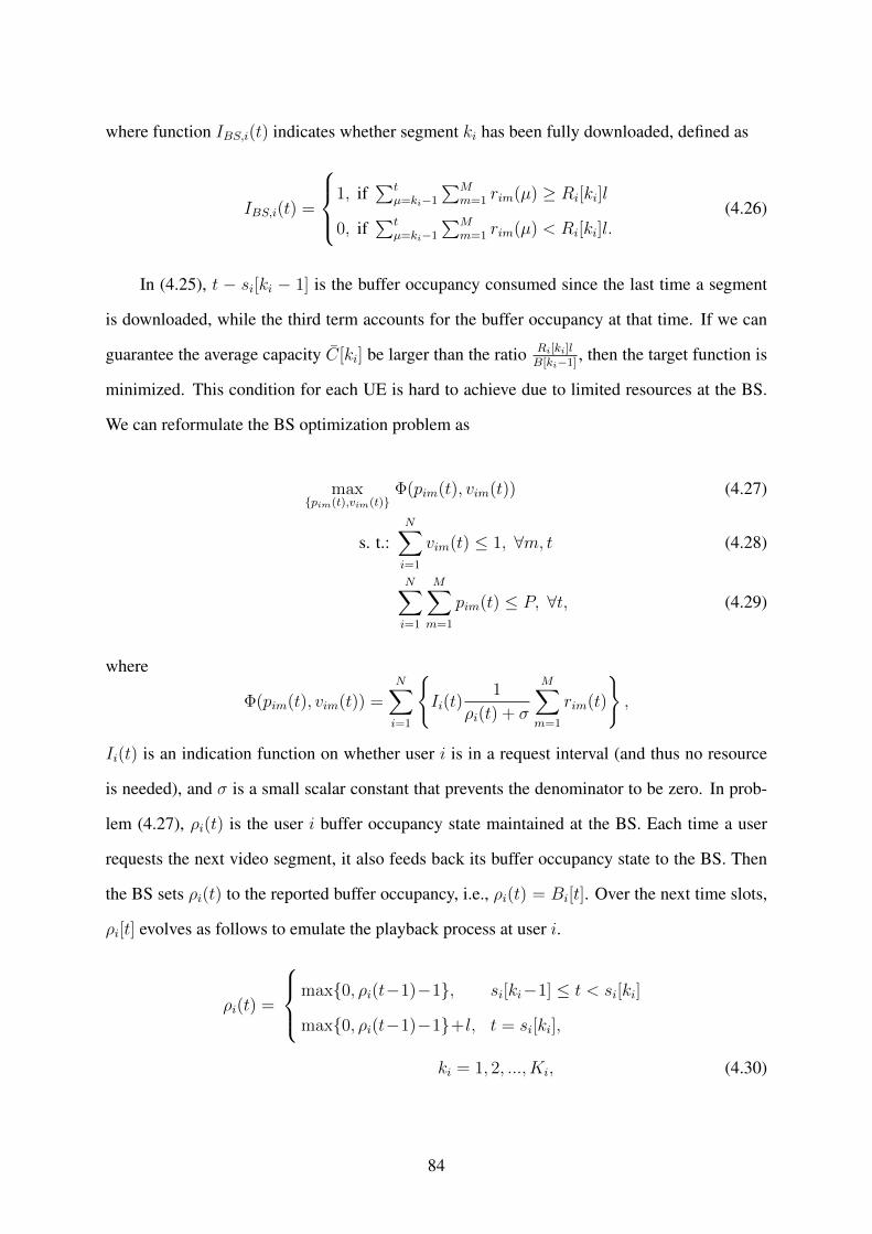
where function IBS,i(t) indicates whether segment ki has been fully downloaded, defined as

IBS,i(t) =

1, if∑t

µ=ki−1

∑Mm=1 rim(µ) ≥ Ri[ki]l

0, if∑t

µ=ki−1

∑Mm=1 rim(µ) < Ri[ki]l.

(4.26)

In (4.25), t − si[ki − 1] is the buffer occupancy consumed since the last time a segment

is downloaded, while the third term accounts for the buffer occupancy at that time. If we can

guarantee the average capacity C[ki] be larger than the ratio Ri[ki]lB[ki−1]

, then the target function is

minimized. This condition for each UE is hard to achieve due to limited resources at the BS.

We can reformulate the BS optimization problem as

max{pim(t),vim(t)}

Φ(pim(t), vim(t)) (4.27)

s. t.:N∑i=1

vim(t) ≤ 1, ∀m, t (4.28)

N∑i=1

M∑m=1

pim(t) ≤ P, ∀t, (4.29)

where

Φ(pim(t), vim(t)) =N∑i=1

{Ii(t)

1

ρi(t) + σ

M∑m=1

rim(t)

},

Ii(t) is an indication function on whether user i is in a request interval (and thus no resource

is needed), and σ is a small scalar constant that prevents the denominator to be zero. In prob-

lem (4.27), ρi(t) is the user i buffer occupancy state maintained at the BS. Each time a user

requests the next video segment, it also feeds back its buffer occupancy state to the BS. Then

the BS sets ρi(t) to the reported buffer occupancy, i.e., ρi(t) = Bi[t]. Over the next time slots,

ρi[t] evolves as follows to emulate the playback process at user i.

ρi(t) =

max{0, ρi(t−1)−1}, si[ki−1] ≤ t < si[ki]

max{0, ρi(t−1)−1}+l, t = si[ki],

ki = 1, 2, ..., Ki, (4.30)

84

until the the next user i feeback is received. This way, the BS maintains the buffer state of

each UE at a minimum control overhead. Problem (4.27) is to maximize a weighted sum of

the downlink rates of all UEs at each time t, while each weight is inversely proportional to the

playback buffer occupancy at the corresponding UE.

Theorem 4.3. The problem defined in (4.27) is convex.

With Theorem 4.3, we can solve the problem with a convex optimization solver. The

algorithm considers both request interval and robust rate adaption is termed DORA-RI.


4.5.1 Simulation Scenario and Algorithm Configuration

In this section, the performance of the proposed algorithms is evaluated with Python multi-

threading simulation. For the physical layer, the total bandwidth is W = 5 MHz and consists

of M = 32 subcarriers, each with κ = 160 KHz. The energy constraint of the BS is P = 10

W. We generate the channel gain over unit noise energy with the Rayleigh channel model for

which the expectation is 5 dB. The time frame for resource allocation is τ = 5 ms. We assume

the BS acquires CSI with contamination of −60 dB W/Hz. Since the request interval mainly

depends on the network conditions, e.g., the congestion level, it could be as large as 10 s. In

this chapter, we simulate the request interval as a uniformly distributed process in the range of

50 ms to 500 ms. The fairness function is chosen as the natural logarithm Uα(·) = ln(·).

Each video lasts for 2 minutes and is partitioned into 1 s segments and coded into five

levels of rates, i.e., R = [100 kbps, 300 kbps, 500 kbps, 900 kbps, 1500 kbps, 2000 kbps], which

is consistent with the 240p, 360p, 480p, 720p,1 and 1080p formats for general genres [107]. For

the QoE model, we use constant αi and βi for all users. The quality model αi and βi are fitted

with the data from [103] and assumed to be the same for all the users. We set θ = 0.2, λ = 2.5,

and η = 20 according to the guidelines in [101]. The distribution of the download capacity is

set according to a normal distribution with mean Ci[ki] and the variance is 10% of the mean.

The prediction horizon z is set to 7.1Note that 900 kbps and 1500 kbps are the rates for 720p.

85

Table 4.2: Three variations of the proposed schemeRate prediction algorithm Request interval

DORA-RI SMPC ConsideredDORA-MPC MPC ConsideredDORA-no-RI SMPC Not considered

In order to evaluate the general performance and improvement over the state-of-art tech-

niques, the proposed algorithm DORA-RI is first compared with the original DORA proposed

in [106] and a proportionally fair network resource allocation with water-filling algorithm

(PFWF-RM) scheme [108, 104]. The purpose is to demonstrate the achievable improvement

over these two baseline schemes.

In addition, we would like to gain insights into the the proposed algorithm. Each com-

ponent of DORA-RI are isolated out to test their impact. The proposed scheme DORA-RI is

compared with two variations:

1. DORA-MPC, which uses a deterministic model predictive control (MPC) algorithm for

bit rate adaption. All the other parts of this scheme are the same as DORA-RI.

2. DORA-no-RI, which only considers the request interval at the BS but does not adopt

SMPC. All the other parts are the same as DORA-RI.

The three variations are summarized in Table 4.2. In this comparison, we aim to examine the

impact of each component of DORA-RI on its performance.

4.5.2 Simulation Results and Discussions

Comparison over the benchmark and original schemes

Fig. 4.5 presents the mean QoEs values achieved by the proposed DORA-RI, DORA, and

PFWF-RM. The experiments are repeated 20 times for each algorithm and the average values

are presented. The decreasing trend of QoE over increased number of users is intuitive. The

reason lies on the fact that the average resource each user can have is diminishing. In the

worst case, DORA-RI can still achieve 1.7× and 1.3× QoE gains over PFWF-RM and DORA,

respectively. It is clear that the enhancement achieved by utilizing the request interval of each

86

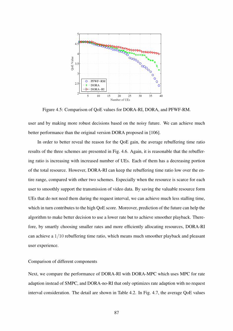
5 10 15 20 25 30 35 402

2.5

3

3.5

4

4.5

5

Number of UEs

QoE

Valu

e

PFWF−RM

DORA

DORA−RI

Figure 4.5: Comparison of QoE values for DORA-RI, DORA, and PFWF-RM.

user and by making more robust decisions based on the noisy future. We can achieve much

better performance than the original version DORA proposed in [106].

In order to better reveal the reason for the QoE gain, the average rebuffering time ratio

results of the three schemes are presented in Fig. 4.6. Again, it is reasonable that the rebuffer-

ing ratio is increasing with increased number of UEs. Each of them has a decreasing portion

of the total resource. However, DORA-RI can keep the rebuffering time ratio low over the en-

tire range, compared with other two schemes. Especially when the resource is scarce for each

user to smoothly support the transmission of video data. By saving the valuable resource form

UEs that do not need them during the request interval, we can achieve much less stalling time,

which in turn contributes to the high QoE score. Moreover, prediction of the future can help the

algorithm to make better decision to use a lower rate but to achieve smoother playback. There-

fore, by smartly choosing smaller rates and more efficiently allocating resources, DORA-RI

can achieve a 1/10 rebuffering time ratio, which means much smoother playback and pleasant

user experience.

Comparison of different components

Next, we compare the performance of DORA-RI with DORA-MPC which uses MPC for rate

adaption instead of SMPC, and DORA-no-RI that only optimizes rate adaption with no request

interval consideration. The detail are shown in Table 4.2. In Fig. 4.7, the average QoE values

87

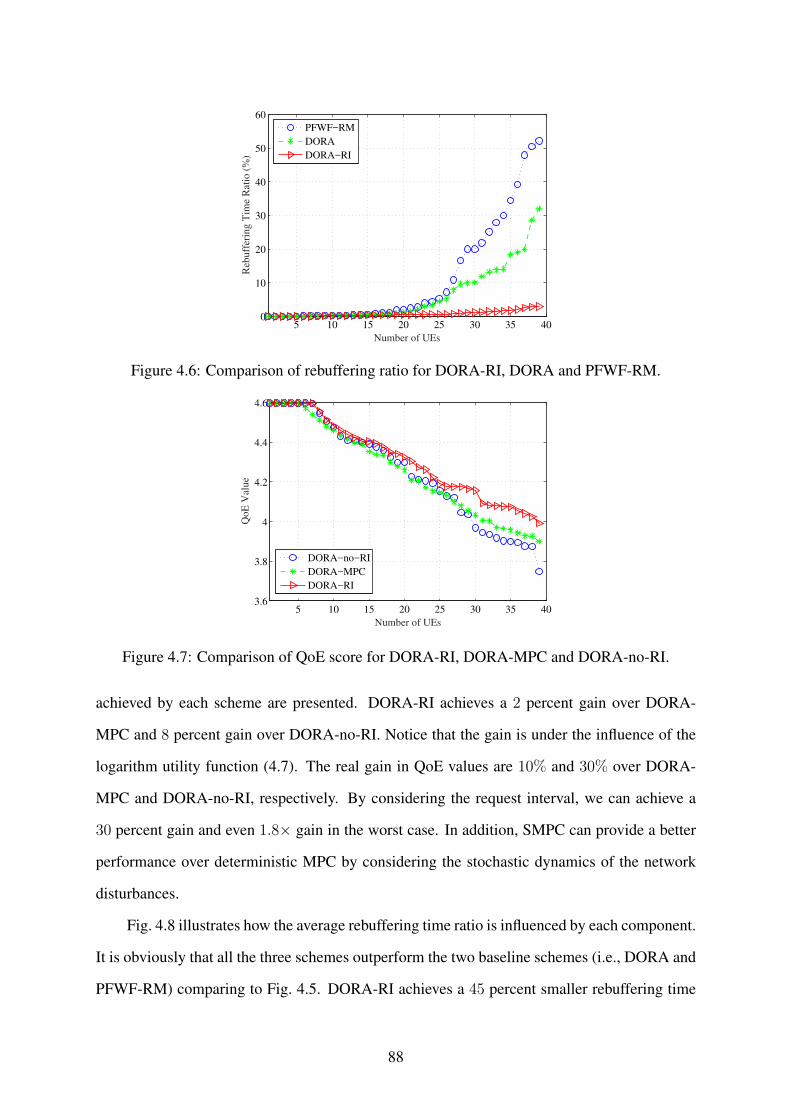
5 10 15 20 25 30 35 400

10

20

30

40

50

60

Number of UEs

Reb

uff

erin

g T

ime

Rat

io (

%)

PFWF−RM

DORA

DORA−RI

Figure 4.6: Comparison of rebuffering ratio for DORA-RI, DORA and PFWF-RM.

5 10 15 20 25 30 35 403.6

3.8

4

4.2

4.4

4.6

Number of UEs

QoE

Valu

e

DORA−no−RI

DORA−MPC

DORA−RI

Figure 4.7: Comparison of QoE score for DORA-RI, DORA-MPC and DORA-no-RI.

achieved by each scheme are presented. DORA-RI achieves a 2 percent gain over DORA-

MPC and 8 percent gain over DORA-no-RI. Notice that the gain is under the influence of the

logarithm utility function (4.7). The real gain in QoE values are 10% and 30% over DORA-

MPC and DORA-no-RI, respectively. By considering the request interval, we can achieve a

30 percent gain and even 1.8× gain in the worst case. In addition, SMPC can provide a better

performance over deterministic MPC by considering the stochastic dynamics of the network

disturbances.

Fig. 4.8 illustrates how the average rebuffering time ratio is influenced by each component.

It is obviously that all the three schemes outperform the two baseline schemes (i.e., DORA and

PFWF-RM) comparing to Fig. 4.5. DORA-RI achieves a 45 percent smaller rebuffering time

88

5 10 15 20 25 30 35 400

1

2

3

4

5

6

Number of UEs

Reb

uff

erin

g T

ime

Rat

io (

%)

DORA−no−RI

DORA−MPC

DORA−RI

Figure 4.8: Comparison of rebuffering ratio for DORA-RI, DORA-MPC and DORA-no-RI.

ratio than DORA-MPC in the worst case. This benefit is introduced by taking uncertainty

into consideration while conducting the optimization. In addition, the consideration of request

interval does enhance the rebuffering performance. However, we notice that when the resource

gets really scarce, e.g., when the number of UEs becomes larger than 35, the performance of

DORA-no-RI and DORA-MPC get closer. This is because the deterministic MPC lacks the

ability to properly handle the more random request intervals when the network gets congested.

It actually justifies the necessity of incorporating the SMPC.

In Fig. 4.9, the average standard deviation (STD) of bit rate over one playback process

is presented. Here, we aim to understand how the bit rate varies during the process. Counter-

intuitively, the STD is not increasing as the number of UEs is increased. We found that initially,

there is sufficient resources such that each user could always choose the largest bit rate, leading

to minimal STD. When the number of UEs gets high, the resource for each user is decreasing,

which leaves them less choice on bit rates. Therefore, the STD also gets smaller. In the middle

range, however, the STD is relatively larger. This is because the resource is sufficient to alter

the capacity largely but not enough to satisfy the largest bit rate. In other words, it is harder

to accurately predict future capacity in this range. We can see that DORA-RI still achieves the

lowest STD in video rates compared to the other two schemes.

89

5 10 15 20 25 30 35 400

50

100

150

200

250

300

350

400

450

Number of UEs

ST

D o

f B

itra

te (

bps)

DORA−no−RI

DORA−MPC

DORA−RI

Figure 4.9: Comparison of data-rate standard deviation for DORA-RI, DORA-MPC andDORA-no-RI

4.6 Related Work

HTTP based video streaming technologies has drawn great attention. Some interesting works

are on modeling the new QoE model to support bit rate adaption. For example, Yamagishi [109]

formulated a parametric QoE model for DASH based on extensive subject experiments. The

authors took audio and video bit rate, video resolution, rebuffering events and length into con-

sideration and derived the coefficients for each factor. Some interesting works based on QoE

video streaming can be found [110][111]

Bit rate adaption strategy is an important problem in DASH. Many existing techniques

could be generally categorized into: (i) buffer based (BB) techniques, (ii) capacity based (CB)

schemes, and (iii) integrated techniques. Some state-of-art methods have been proposed. In

FESTIVE [112], the authors focused on improving the stability and fairness of multiple users

that share a bottleneck link. PANDA [113] adopted a TCP congestion control like method to

adjust video segment rate, but required certain overhead for probing. In [114], the authors

considered rate adaption with adjustment of a threshold. The authors in [115] proposed a

regression method to predict the future capacity and a classical PID based controller for rate

adaption. In [101], the authors proposed an MPC based approach for rate adaption at the

user side and a fastMPC method. However, the authors used a different QoE model and did

not consider the prediction method for robustness. Markov decision process (MDP) based

90

rate adaption algorithms have been proposed in [116] [117]. In [116], the authors proposed a

solution, termed mDASH, that was based on MDP for DASH data rate adaption. Decision of the

next segment data rate was made by taking factors into consideration, such as buffered video

time, and history bandwidth and data rate. The work in [117] was focused on the vehicular

environment. For MDP based algorithms, the high computational complexity is an obstacle for

realtime applications. However, techniques such as Microsoft SmoothStreaming [118] have

been shown to perform poorly in wireless networks [119]. Most rate adaption methods can

only passively adapt to the variation in throughput.

The integration of video streaming and wireless network scheduling is a promising di-

rection to maximize the performance of videos in the wireless environment. Works such

as [120, 121, 85, 122, 27, 123] are inspiring. The authors in [124] tackled video transmissions

in MU-MIMO networks and [125] investigated the adaptive video streaming and scheduling

problem. Both works utilized Lyapunov optimization to achieve good performance with as-

sumption of helper(s) as a centralized entity that can acquire user information. The authors in

[126] proposed a jointly optimization framework of scheduling and rate-adaption with a proof

of optimality. However, this work did not explicitly consider the resource allocation details

(e.g., power, subcarrier, and time assignment) and the QoE model used in this work was more

based on a mathematical formation. Lin [127] proposed a cross layer method for scalable video

streaming over OFDMA networks. The tradeoff between efficiency and fairness was addressed.

In this work, the authors used the traditional PSNR as indication of video quality instead of the

modern QoE models, which incorporate more important factors that influence user QoE. The

authors of [128] tackled the problem of heterogeneous network streaming on the client side.

The network cost constraints were considered and the goal was to achieve high quality stream-

ing and low energy cost on the UE. In [129], on the other hand, the authors proposed a method

that utilize both unicast and multicast concurrently to reduce the energy consumption of UEs

when streaming video over a cellular network. These works are focused mainly on the UE side

to achieve a tradeoff between video quality and energy efficiency.

91

The resource allocation problem in the OFDM network has been extensively studied in

the past decades [130, 80, 81, 83]. Refer to [104] for a comprehensive survey of resource al-

location in OFDMA networks. Two main topics: energy efficiency optimization and system

throughput optimization, were generally addressed. The original problem is a mixture of inte-

ger programming (subcarrier assignment) and linear programming (power allocation), which is

NP-hard. Therefore, suboptimal solutions were developed by relaxation of time sharing in one

time frame [81, 130, 131, ?, ?]. In [81], the authors proved that the suboptimal solution will

converge to the optimum asymptotically assuming ergodic noise processes.

4.7 Conclusions

In this chapter, we investigated the problem of resource allocation for delivering multiple videos

using DASH over the downlink of an OFDMA network. We first presented an offline formu-

lation based on a novel QoE model. We then derived a more practical online formulation,

and developed a distributed solution algorithm, which consisted of an resource allocation al-

gorithm at the BS side and a rate adaptation algorithm at the user side. The proposed scheme

was validated with simulations and was shown to outperform several benchmark scheme with

considerable gains.

4.8 Proof for Theorem 4.1

Proof. By redefining the QoE maximization problem as in (4.13), the QoE function can be

written as

Qappr =qi[ki] + θ(qi[ki]−mi[Ki])2 (4.31)

+λ

Kilmax

{0, πi[ki] +

q−1(qi[ki])l


},

where qi[ki] is a linear function. The quadratic part is a convex function over qi[ki]. The max

term is convex over qi[ki] and convex over pim(t) and vim(t). Since parameters θ and λ are both

negative, Qappr is concave for all the variables. The target function Λappr(N) is the summation

92

of Qappr over time and users which means it is concave as well. The constraints are all convex

sets. Therefore, this is a convex problem.

4.9 Proof for Lemma 1

Proof. This Lemma could be presented as follows.

limK→∞

(1

K

K∑ki=1

qi(R∗[ki])− mi[K]

)= 0 (4.32)

For brevity, we denote qi(R∗[ki]) by q∗i [ki]. Rewrite (4.16) and take summation from 1 to K.

We have

K∑ki=1

(ki + ζ

ζ

)(mi[ki]− mi[ki − 1]) (4.33)

=K∑ki=1

(q∗i [ki]− mi[ki − 1]).

Expand the left hand side summation to obtain

1

ζ

(Kmi[K]−

K∑ki=1

mi[ki − 1]

)− (mi[K]− mi[1])

=K∑ki=1

(q∗i [ki]− mi[K] + mi[K]− mi[ki − 1]).

To obtain the form (4.32), we first divide it by K and then take limit on both sides over K. It

follows that

limK→∞

Kmi[K]−∑K

ki=1 mi[ki − 1]

ζK− lim

K→∞

mi[K]− mi[1]

K

= limK→∞

K∑ki=1

(q∗i [ki]− mi[K] + mi[K]− mi[ki − 1]).

93

It’s obvious that the second term goes to 0 due to finite mi[K] and mi[1]. By splitting the

right-hand-side into two parts and rearranging terms, we have:

1− ζζ

limK→∞

(Kmi[K]−

K∑ki=1

mi[ki − 1]

)

= limK→∞

1

K

∑ki=1

(q∗i [ki]− mi[K]).

The left-hand-side is the limit we want to show to be 0. Note that (4.16) can be viewed as a

stochastic approximation update equation for mi. Therefore, the convergence of right-hand-

side can be proven by applying Theorem 1.1 of Chapter 6 in [132].


Proof. The convergence proof could be transformed to show that the Prob-Online objective

value converges to the Prob-Offline objective value. Specifically, we aim to prove

limt→∞

Λ(S∗)− Λ(S) = 0, (4.34)

where S∗ = {q∗(t),v∗(t),p∗(t)} is the online solution and S = {q(t), v(t), p(t)} is the offline

solution.

Since Prob-Online is convex, and based on Lemma 2, we can derive the KKT condition as

follows.

IN(

dΛ(Si∗)

dS+ α∗i (t)− γ∗i,min(t) + γ∗i,max(t)

)+ β∗i,m(t) = 0

α∗i (t)(v∗im − 1) = 0

β∗i,m(p∗im − 1) = 0

γ∗i,min(qi,min − q∗i ) = 0

γ∗i,max(q∗i − qi,max) = 0

α∗i (t), β∗im(t), γ∗i,min(t), γ∗i,max(t) ≥ 0,

∀i ∈ N,∀m ∈M,

(4.35)

94

where IN is the indicator that the variables belong to different users. Lagrange multipliers

α∗i (t), β∗i,m(t), γ∗i,min(t), and γ∗i,max(t) are the dual points that the KKT conditions are satisfied

and the optimal value is achieved.

We next construct the help function H(S) that is differentiable and concave. The definition

is

H(S) =Λ(S)− α∗i (t)(v∗im − 1)− β∗i,m(p∗im − 1) (4.36)

+ γ∗i,min(q∗i − qi,min)− γ∗i,max(q∗i − qi,max).

We have H(S) ≥ Λ(S) due to the constraints in problem (4.13). In addition, we can acquire

the following inequality by the concavity and differentiability of H(S).

H(S) ≤ H(S∗) +dH(S∗)

dS(S∗ − S). (4.37)

By bringing (4.36) and the KKT conditions (4.35), we obtain the following inequality.

Λ(S) ≤ Λ(S∗) + 2θN∑i=1

T∑t=0

(q∗i (t)− mi) ∗ (q∗i (t)− qi(t). (4.38)

In Lemma 1, we have proved that limK→∞1K

∑ki=1(q∗i [ki] − mi[K]). Here we abuse the

notification of Ki and T , which both represent the total playback time. Then we have

limT→∞

1

T

∑ki=1

Λ(S) ≤ 1

TlimT→∞

Λ(S∗). (4.39)

Since S is the optimal offline solution, Λ(S) is the optimal value for Prob-Offline. It

follows that

Λ(S) ≥ Λ(S). (4.40)

Combining (4.39) and (4.40), we conclude that the theorem holds true.

95


Proof. First of all, we prove the concavity of the rate function, which can be rewritten as

rim(t) = v(t)κ log2

(1 + p(t)g2(t)

v(t)κ

)for brevity. For two feasible solutions (v2, p2) and (v3, p3),

suppose there exists a feasible solution (v1, p1) = ε(v2, p2) + (1 − ε)(v3, p3), where 0 ≤ ε ≤

1. By the definition of concavity, we need to show that rim(v1, p1) ≥ εrim(v2, p2) + (1 −

ε)rim(v3, p3). There are three possible cases for v2 and v3 that needs to be analyzed.

• Case I: when {v2 > 0, v3 > 0}. Then we have v1 > 0. Because log2 (1 + p1g2im)

is a concave function of p1, its perspective v1ν log2

(1 +

p1g2imv1ν

)is concave given that

v1 > 0 [133]. Thus, concavity holds true for this case.

• Case II: when {v2 > 0, v3 = 0}. Then we have v1 = εv2 and p1 = εp2 + (1 − ε)p3. It

follows that

ri,m(v1, p1) = εv2κ log2

(1 +

(εp2 + (1− ε)p3)g2im

εv2κ

)≥ εv2 log2

(1 +

p2g2im

v2κ

).

• Case III: when {v2 = 0, v3 = 0}. This is a trivial case that the equality holds for v1 = 0.

With the concavity of rim(t), it is convenient to show that the∑S

s=1 rim(t) is concave since it

is a nonnegative combination of concave functions rim(t). The concavity of the cost function

Φ(pim(t), vim(t)) can be argued for the same reason.

In addition, the utility constraints define a convex set Υ. By the definition of utility func-

tion, it’s convenient to show that for any r1, r2 ∈ Υ, εr1 + (1 − ε)r2 ∈ Υ for any ε with

0 ≤ ε ≤ 1. Both constraints∑N

i=1(t)vim(t) ≤ 1 and∑N

i=1(t)∑M

m=1 pim(t) ≤ P also define

convex sets. They are the intersection of half-spaces. Intersection preserves the convexity of

the sets. Thus the constraints are convex.

We conclude that Problem (4.27) is convex.

96

Chapter 5

Future Work

As demonstrated in the previous chapters, the complexity of the entire wireless system is in-

creasing. In the meantime, more and more components are being added into the system for fur-

ther performance enhancement, which will result in an even more complicated system. From

the congestion control perspective, the requirement of adaptive learning and evolving would

be an important aspect of future algorithms. Also, the dramatically increasing traffic of video

streaming needs more efficient and smarter algorithms to adaptively adapt the data rate and/or

jointly control the resource of the BS. Although we have made some interesting progress in

model free congestion control, it’s still at the early stage of research and application.

The fast development of the deep learning/deep reinforcement learning techniques have

benefited many areas, such as computer graphics, computer vision, and human-computer in-

teraction. For deep reinforcement learning, it has been successfully applied in Go and video

games in which it can achieve better performance than human. With the proof that it can be

used in the complicated scenario of fully observed information, its applications has been ex-

panded. In the computer networking domain, however, most problems are partially observable

and normally involve multi-agent cooperation or competition. How to fully utilize the power

of DRL in such scenarios is still an open problem. Due to the promising properties of DRL and

the complexity of the networking system, I plan to further apply DRL to solve sevearl other

existing networking problems.

The detailed future research directions are as follow.

97

1. Machine Learning Aided MmWave Networks. MmWave networks are characterized

by high data rate and unreliable connections. It poses a tremendous challenge to conges-

tion control on both the sender side and at the base station or access point. To achieve

high transmission efficiency and robustness, the transmission control algorithm should

adaptively learn the transmission content and blocking pattern of the mmWave link. I

plan to apply the DRL approach to tackle these problems and try to achieve the potential

performance gain as brought about by the recent progress of DRL.

2. Machine Learning Aided Video Streaming. The recent progress on video streaming

has proved that the DASH protocol can potentially adjust to the oscillation of capacity

in wireless networks, with a smart data-rate adapting algorithm applied. In addition,

with the domination of video traffic in the Internet and wireless networks, the problem of

how to better accommodate video streaming in 4G-LTE network and the next generation

networks becomes more important than ever. I plan to use the DRL to jointly handle the

data-rate adapting as well as resource allocation to further improve the QoE of streaming

videos.

3. Learning and Controlling Efficiency Enhancement. In our application of DRL, the

learning process is time consuming and the control action generation is computationally

intense. Although TCP-Drinc achieves a better performance over the benchmark algo-

rithms on both throughput and RTT in our study of a relatively small network, I believe

we can still further improve its performance in larger scale networks with more compli-

cated algorithms. With the recent progress on model compression and transfer learning,

I plan to further improve the learning and controlling efficiency in our problem to make

it more practical.

98

References

[1] Cisco, “Cisco visual networking index: Global mobile data traffic fore-

cast update, 20162021,” White Paper, [online] Available: https://www.cisco.

com/c/en/us/solutions/collateral/service-provider/visual-networking-index-vni/

mobile-white-paper-c11-520862.html, 2017.

[2] Y. Zhao, S. Mao, J. O. Neel, and J. H. Reed, “Performance evaluation of cognitive radios:

Metrics, utility functions, and methodology,” Proc. IEEE, vol. 97, no. 4, pp. 642–659,

Apr. 2009.

[3] M. Chen, V. C. Leung, S. Mao, and M. Li, “Cross-layer and path priority schedul-

ing based real-time video communications over wireless sensor networks,” in Vehicular

Technology Conference, 2008. VTC Spring 2008. IEEE. IEEE, 2008, pp. 2873–2877.

[4] S. Mao, X. Cheng, Y. T. Hou, H. D. Sherali, and J. H. Reed, “On joint routing and server

selection for md video streaming in ad hoc networks,” IEEE Transactions on Wireless

Communications, vol. 6, no. 1, 2007.

[5] Q. Zhao and B. Sadler, “A survey of dynamic spectrum access,” IEEE Signal Process.

Mag., vol. 24, no. 3, pp. 79–89, May 2007.

[6] D. Hu and S. Mao, “Cooperative relay in cognitive radio networks: Decode-and-forward

or amplify-and-forward?” in Global Telecommunications Conference (GLOBECOM

2010), 2010 IEEE. IEEE, 2010, pp. 1–5.

[7] Sandvine, “Global internet phenomena report,” White Paper, [online] Available: https:

//www.sandvine.com/trends/global-internet-phenomena/, 2017.

99

[8] V. Mnih, K. Kavukcuoglu, D. Silver, A. A. Rusu, J. Veness, M. G. Bellemare, A. Graves,

M. Riedmiller, A. K. Fidjeland, G. Ostrovski et al., “Human-level control through deep

reinforcement learning,” Nature, vol. 518, no. 7540, p. 529, 2015.

[9] D. Silver, J. Schrittwieser, K. Simonyan, I. Antonoglou, A. Huang, A. Guez, T. Hubert,

L. Baker, M. Lai, A. Bolton et al., “Mastering the game of go without human knowl-

edge,” Nature, vol. 550, no. 7676, p. 354, 2017.

[10] M. Kuure-Kinsey and B. W. Bequette, “Multiple model predictive control strategy for

disturbance rejection,” Ind. Eng. Chemistry Research, vol. 49, no. 17, pp. 7983–7989,

July 2010.

[11] W. Wang, X. Wang, and S. Mao, “Deep convolutional neural networks for indoor lo-

calization with CSI images,” IEEE Transactions on Network Science and Engineering,

vol. 5.

[12] X. Wang, X. Wang, and S. Mao, “RF sensing for Internet of Things: A general deep

learning framework,” IEEE Communications, vol. 56, no. 9, pp. 62–69, Sept. 2018.

[13] X. Wang, S. Mao, and M. Gong, “An overview of 3GPP cellular vehicle-to-everything

standards,” ACM GetMobile: Mobile Computing and Communications Review, vol. 21,

no. 3, pp. 19–25, Sept. 2017.

[14] X. Wang, L. Gao, and S. Mao, “BiLoc: Bi-modality deep learning for indoor localization

with 5GHz commodity Wi-Fi,” IEEE Access Journal, vol. 5, no. 1, pp. 4209–4220, Mar.

2017.

[15] X. Wang, C. Yang, and S. Mao, “Tensorbeat: Tensor decomposition for monitoring

multi-person breathing beats with commodity WiFi,” ACM Transactions on Intelligent

Systems and Technology, vol. 9, no. 1, pp. 8:1–8:27, Sept. 2017.

[16] X. Wang, S. Mao, and M. Gong, “A survey of lte wi-fi coexistence in unlicensed bands,”

ACM GetMobile: Mobile Computing and Communications Review, vol. 20, no. 3, pp.

17–23, July 2016.

100

[17] X. Wang, L. Gao, and S. Mao, “Csi phase fingerprinting for indoor localization with a

deep learning approach,” IEEE Internet of Things Journal, vol. 3, no. 6, pp. 1113–1123,

Dec. 2016.

[18] X. Wang, L. Gao, S. Mao, and S. Pandey, “Csi-based fingerprinting for indoor localiza-

tion: A deep learning approach,” IEEE Transactions on Vehicular Technology, vol. 66,

no. 1, pp. 763–776, Jan. 2017.

[19] X. Wang, L. Gao, and S. Mao, “PhaseFi: Phase fingerprinting for indoor localization

with a deep learning approach,” in Proc. IEEE GLOBECOM 2015, San Diego, CA, Dec.

2015, pp. 1–6.

[20] M. Feng, S. Mao, and T. Jiang, “Joint duplex mode selection, channel allocation, and

power control for full-duplex cognitive femtocell networks,” Elsevier Digital Communi-

cations and Networks Journal, vol. 1, no. 1, pp. 30–44, Feb. 2015.

[21] M. Feng and S. Mao, “Harvest the potential of massive mimo with multi-layer technolo-

gies,” IEEE Network, vol. 30, no. 5, pp. 40–45, Sept./Oct. 2016.

[22] M. X. Gong, S. F. Midkiff, and S. Mao, “A cross-layer approach to channel assignment

in wireless ad hoc networks,” ACM/Springer Mobile Networks and Applications Journal,

vol. 12, no. 1, pp. 43–56, Feb. 2007.


power control for full-duplex cognitive femtocell networks,” Elsevier Digital Communi-

cations and Networks Journal, vol. 1, no. 1, pp. 30–44, Feb. 2015.

[24] A. Kumar and K. G. Shin, “Managing TCP connections in dynamic spectrum access

based wireless LANs,” in Proc. IEEE SECON 2010, Boston, MA, June 2010, pp. 1–9.

[25] K. R. Chowdhury, M. Di Felice, and I. F. Akyildiz, “TP-CRAHN: A transport protocol

for cognitive radio ad-hoc networks,” in Proc. IEEE INFOCOM 2009, Rio de Janeiro,

Brazil, Apr. 2009, pp. 2482–2490.

101

[26] C. Luo, F. R. Yu, H. Ji, and V. C. Leung, “Cross-layer design for TCP performance

improvement in cognitive radio networks,” IEEE Trans. Veh. Technol., vol. 59, no. 5, pp.

2485–2495, 2010.

[27] M. Feng, T. Jiang, D. Chen, and S. Mao, “Cooperative small cell networks: High capac-

ity for hotspots with interference mitigation,” IEEE Wireless Communications, vol. 21,

no. 6, pp. 108–116, Dec. 2014.

[28] D. Hu, S. Mao, and J. H. Reed, “On video multicast in cognitive radio networks,” in

INFOCOM 2009, IEEE. IEEE, 2009, pp. 2222–2230.

[29] X. Chen, H. Zhai, J. Wang, and Y. Fang, “A survey on improving TCP performance over

wireless networks,” in Resource Management in Wireless Networking, M. Cardeiand,

I. Cardei, and D.-Z. Du, Eds. Kluwer Academic Publishers, 2005, pp. 657–695.

[30] H. Salameh, M. Krunz, and D. Manzi, “Spectrum bonding and aggregation with guard-

band awareness in cognitive radio networks,” IEEE Trans. Mobile Comput., vol. 13,

no. 3, pp. 569–581, Mar. 2014.

[31] V. Misra, W.-B. Gong, and D. Towsley, “Fluid-based analysis of a network of AQM

routers supporting TCP flows with an application to RED,” in ACM SIGCOMM Comput.

Commun. Rev., vol. 30, no. 4, Oct. 2000, pp. 151–160.

[32] T. Lakshman, A. Neidhardt, and T. Ott, “The drop from front strategy in TCP and in

TCP over ATM,” in Proc. IEEE INFOCOM 1996, San Francisco, CA, Mar. 1996, pp.

1242–1250.

[33] S. Kunniyur and R. Srikant, “End-to-end congestion control schemes: Utility functions,

random losses and ECN marks,” IEEE/ACM Trans. Netw., vol. 11, no. 5, pp. 689–702,

2003.

[34] C. Hollot, V. Misra, D. Towsley, and W.-B. Gong, “On designing improved controllers

for AQM routers supporting TCP flows,” in Proc. IEEE INFOCOM 2001, Anchorage,

AK, Apr. 2001, pp. 1726–1734.

102

[35] P. Ignaciuk and M. Karbowanczyk, “Active queue management with discrete sliding

modes in TCP networks,” Bull. Pol. Ac.: Tech., vol. 62, no. 4, pp. 701–711, Dec. 2014.

[36] D. Cox and L. Dependence, “A review,” in Statistics: An Appraisal, H. David and

H. David, Eds. Ames, IA: The Iowa State University Press, 1984, pp. 55–74.

[37] V. Jacobson, “Congestion avoidance and control,” ACM SIGCOMM Comput. Commun.

Rev., vol. 18, no. 4, pp. 314–329, 1988.

[38] S. Floyd, A. Gurtov, and A. Gurtov, “The NewReno modification to TCP’s fast recovery

algorithm,” Apr. 2004, IETF RFC 3782.

[39] L. S. Brakmo, S. W. O’Malley, and L. L. Peterson, “TCP Vegas: New techniques for

congestion detection and avoidance,” ACM SIGCOMM Comput. Commun. Rev., vol. 24,

no. 4, pp. 24–35, Oct. 1994.

[40] S. Ha, I. Rhee, and L. Xu, “CUBIC: a new TCP-friendly high-speed TCP variant,” ACM

SIGOPS Operating Systems Review, vol. 42, no. 5, pp. 64–74, July 2008.

[41] K. Tan, J. Song, Q. Zhang, and M. Sridharan, “A compound TCP approach for high-

speed and long distance networks,” in Proc. IEEE INFOCOM 2006, Barcelona, Spain,

Apr. 2006, pp. 1–12.

[42] K. Winstein, A. Sivaraman, and H. Balakrishnan, “Stochastic forecasts achieve high

throughput and low delay over cellular networks,” in Proc. NSDI 2013, Lombard, IL,

Apr. 2013, pp. 459–471.

[43] Y. Zaki, T. Potsch, J. Chen, L. Subramanian, and C. Gorg, “Adaptive congestion con-

trol for unpredictable cellular networks,” in ACM SIGCOMM Comput. Commun. Rev.,

vol. 45, no. 4, Oct. 2015, pp. 509–522.

[44] S. Floyd, “TCP and explicit congestion notification,” ACM SIGCOMM Comput. Com-

mun. Rev., vol. 24, no. 5, pp. 8–23, Oct. 1994.

103

[45] C. Hollot, V. Misra, D. Towsley, and W.-B. Gong, “A control theoretic analysis of RED,”

in Proc. IEEE INFOCOM 2001, Anchorage, AK, Apr. 2001, pp. 1510–1519.

[46] S. Floyd and V. Jacobson, “Random early detection gateways for congestion avoidance,”

IEEE/ACM Trans. Netw., vol. 1, no. 4, pp. 397–413, Aug. 1993.

[47] X.-H. Zhang, K.-S. Zou, Z.-Q. Chen, and Z.-D. Deng, “Stability analysis of AQM al-

gorithm based on generalized predictive control,” in Advanced Intelligent Computing

Theories and Applications, ser. LNCS. Springer, 2008, vol. 5226, pp. 1242–1249.

[48] P. Wang, H. Chen, X. Yang, and Y. Ma, “Design and analysis of a model predictive

controller for active queue management,” Elsevier ISA transactions, vol. 51, no. 1, pp.

120–131, Jan. 2012.

[49] K. Chavan, R. G. Kumar, M. N. Belur, and A. Karandikar, “Robust active queue man-

agement for wireless networks,” IEEE Trans. Control Syst. Technol., vol. 19, no. 6, pp.

1630–1638, 2011.

[50] K. Nichols and V. Jacobson, “Controlling queue delay,” ACM Commun., vol. 55, no. 7,

pp. 42–50, May 2012.

[51] Y. Wang, S. Mao, and R. Nelms, “Distributed online algorithm for optimal real-time

energy distribution in the smart grid,” IEEE Internet of Things Journal, vol. 1, no. 1, pp.

70–80, Feb. 2014.

[52] D. Hu and S. Mao, “On medium grain scalable video streaming over femtocell cognitive

radio networks,” IEEE Journal on Selected Areas in Communications, vol. 30, no. 3, pp.

641–651, Apr. 2012.

[53] S. Mao, S. S. Panwar, and Y. T. Hou, “On optimal traffic partitioning for multipath

transport,” in Proc. IEEE INFOCOM 2005, Miami, FL, Mar. 2005, pp. 2325–2336.

[54] M. Chen, J. Yang, Y. Hao, S. Mao, and K. Hwang, “A 5G cognitive system for health-

care,” MDPI Big Data and Cognitive Computing Journal, vol. 1, no. 1, pp. 2–16, Mar.

2017.

104

[55] Y. Sun, M. Peng, Y. Zhou, Y. Huang, and S. Mao, “Application of machine learning in

wireless networks: Key techniques and open issues,” arXiv preprint, arXiv:1809.08707,

2018, accessed on: Dec. 2018.

[56] M. Feng and S. Mao, “Dealing with limited backhaul capacity in millimeter wave sys-

tems: A deep reinforcement learning approach,” IEEE Commun., to appear.

[57] X. Chen, H. Zhang, C. Wu, S. Mao, Y. Ji, and M. Bennis, “Optimized computation of-

floading performance in virtual edge computing systems via deep reinforcement learn-

ing,” IEEE Internet of Things J., to appear.

[58] Y. Sun, M. Peng, and S. Mao, “Deep reinforcement learning based mode selection and

resource management for green fog radio access networks,” IEEE Internet of Things J.,

to appear.

[59] Z. Chang, L. Lei, Z. Zhou, S. Mao, and T. Ristaniemi, “Learn to cache: Machine learning

for network edge caching in the big data era,” IEEE Wireless Commun., vol. 25, no. 3,

pp. 28–35, June 2018.

[60] M. Alizadeh, A. Greenberg, D. A. Maltz, J. Padhye, P. Patel, B. Prabhakar, S. Sengupta,

and M. Sridharan, “Data center tcp (dctcp),” in ACM SIGCOMM computer communica-

tion review, vol. 40, no. 4. ACM, 2010, pp. 63–74.

[61] M. Dong, Q. Li, D. Zarchy, P. B. Godfrey, and M. Schapira, “Pcc: Re-architecting con-

gestion control for consistent high performance.” in NSDI, vol. 1, no. 2.3, 2015, p. 2.

[62] W. Jiang, F. Ren, R. Shu, Y. Wu, and C. Lin, “Sliding mode congestion control for data

center ethernet networks,” Computers, IEEE Transactions on, vol. 64, no. 9, pp. 2675–

2690, 2015.

[63] K. Xiao, S. Mao, and J. Tugnait, “Congestion control for infrastructure-based CRNs: A

multiple model predictive control approach,” in Proc. IEEE GLOBECOM 2016, Wash-

ington DC, Dec. 2016.

105

[64] ——, “MAQ: A multiple model predictive congestion control scheme for cognitive radio

networks,” IEEE Trans. Wireless Commun., vol. 16, no. 4, pp. 2614–2626, Apr. 2017.

[65] K. Winstein and H. Balakrishnan, “Tcp ex machina: computer-generated congestion

control,” ACM SIGCOMM Computer Communication Review, vol. 43, no. 4, pp. 123–

134, 2013.

[66] A. Sivaraman, K. Winstein, P. Thaker, and H. Balakrishnan, “An experimental study of

the learnability of congestion control,” in ACM SIGCOMM Computer Communication

Review, vol. 44, no. 4. ACM, 2014, pp. 479–490.

[67] Z. Xu, J. Tang, J. Meng, W. Zhang, Y. Wang, C. H. Liu, and D. Yang, “Experience-

driven networking: A deep reinforcement learning based approach,” arXiv preprint

arXiv:1801.05757, 2018.

[68] W. Li, F. Zhou, K. R. Chowdhury, and W. M. Meleis, “QTCP: Adaptive congestion

control with reinforcement learning,” IEEE Trans. Netw. Sci. Eng., in press.

[69] K. Jacobsson, L. L. Andrew, A. Tang, K. H. Johansson, H. Hjalmarsson, and S. H. Low,

“Ack-clocking dynamics: modelling the interaction between windows and the network,”

in INFOCOM 2008. The 27th Conference on Computer Communications. IEEE. IEEE,

2008.

[70] C. Jin, D. X. Wei, and S. H. Low, “Fast tcp: motivation, architecture, algorithms, per-

formance,” in INFOCOM 2004. Twenty-third AnnualJoint Conference of the IEEE Com-

puter and Communications Societies, vol. 4. IEEE, 2004, pp. 2490–2501.

[71] D. X. Wei, C. Jin, S. H. Low, and S. Hegde, “Fast tcp: motivation, architecture, algo-

rithms, performance,” IEEE/ACM transactions on Networking, vol. 14, no. 6, pp. 1246–

1259, 2006.

[72] J. N. Foerster, Y. M. Assael, N. de Freitas, and S. Whiteson, “Learning to commu-

nicate to solve riddles with deep distributed recurrent Q-networks,” arXiv preprint,

arXiv:1602.02672, 2016, accessed on: Dec. 2018.

106

[73] J. Foerster et al., “Stabilising experience replay for deep multi-agent reinforcement

learning,” arXiv preprint, arXiv:1702.08887, 2017, accessed on: Dec. 2018.

[74] S. Omidshafiei, J. Pazis, C. Amato, J. P. How, and J. Vian, “Deep decentralized multi-

task multi-agent reinforcement learning under partial observability,” arXiv preprint,

arXiv:1703.06182, 2017, accessed on: Dec. 2018.

[75] M. Hausknecht and P. Stone, “Deep recurrent Q-learning for partially observable

MDPs,” CoRR, abs/1507.06527, vol. 7, no. 1, 2015.

[76] M. Abadi et al., “Tensorflow: A system for large-scale machine learning,” in Proc.

USENIX OSDI’16, Savannah, GA, Nov. 2016, pp. 265–283.

[77] C. Caini and R. Firrincieli, “TCP Hybla: A TCP enhancement for heterogeneous net-

works,” Int. J. Satellite Commun. Netw., vol. 22, no. 5, pp. 547–566, Sept. 2004.

[78] S. Liu, T. Basar, and R. Srikant, “TCP-Illinois: A loss-and delay-based congestion con-

trol algorithm for high-speed networks,” Elsevier Performance Evaluation, vol. 65, no.

6-7, pp. 417–440, June 2008.

[79] G. F. Riley and T. R. Henderson, “The ns-3 network simulator,” in Modeling and tools

for network simulation. Springer, 2010, pp. 15–34.

[80] Z. Mao and X. Wang, “Efficient optimal and suboptimal radio resource allocation in

OFDMA system,” IEEE Trans. Wireless Commun., vol. 7, no. 2, pp. 440–445, Feb.

2008.

[81] X. Wang and G. B. Giannakis, “Resource allocation for wireless multiuser OFDM net-

works,” IEEE Trans. Infor. Theory, vol. 57, no. 7, pp. 4359–4372, July 2011.

[82] M. X. Gong, S. Midkiff, and S. Mao, “Design principles for distributed channel assign-

ment in wireless ad hoc networks,” in Communications, 2005. ICC 2005. 2005 IEEE

International Conference on, vol. 5. IEEE, 2005, pp. 3401–3406.

107

[83] Z. Ren, S. Chen, B. Hu, and W. Ma, “Energy-efficient resource allocation in downlink

OFDM wireless systems with proportional rate constraints,” IEEE Trans. Veh. Technol.,

vol. 63, no. 5, pp. 2139–2150, Mar. 2014.

[84] Y. Wang, S. Mao, and R. M. Nelms, “Distributed online algorithm for optimal real-time

energy distribution in the smart grid,” IEEE Internet of Things Journal, vol. 1, no. 1, pp.

70–80, 2014.

[85] M. Chen, V. C. M. Leung, S. Mao, and M. Li, “Energy-efficient itinerary planning for

mobile agents in wireless sensor networks,” in Proc. IEEE ICC 2009, Dresden, Germany,

June 2009, pp. 1–5.

[86] Y. Xu and S. Mao, “User association in massive MIMO HetNets,” IEEE Systems Journal,

vol. 11, no. 1, pp. 7–19, Mar. 2017.

[87] M. X. Gong, S. F. Midkiff, and S. Mao, “On-demand routing and channel assignment

in multi-channel mobile ad hoc networks,” Elsevier Ad Hoc Networks Journal, vol. 7,

no. 1, pp. 63–78, Jan. 2009.


power control for full-duplex cognitive femtocell networks,” Digital Communications

and Networks, vol. 1, no. 1, pp. 30–44, 2015.

[89] M. Feng, T. Jiang, D. Chen, and S. Mao, “Cooperative small cell networks: High capac-

ity for hotspots with interference mitigation,” IEEE Wireless Communications, vol. 21,

no. 6, pp. 108–116, 2014.

[90] S. Mao and S. S. Panwar, “A survey of envelope processes and their applications in

quality of service provisioning,” IEEE Communications Surveys & Tutorials, vol. 8,

no. 3, pp. 2–20, 2006.

[91] M. Feng, S. Mao, and T. Jiang, “Dynamic base station sleep control and RF chain ac-

tivation for energy efficient millimeter wave cellular systems,” IEEE Transactions on

Vehicular Technology, vol. 67, no. 10, pp. 9911–9921, Oct. 2018.

108

[92] ——, “Joint frame design, resource allocation and user association for massive mimo

heterogeneous networks with wireless backhaul,” IEEE Transactions on Wireless Com-

munications, vol. 17, no. 3, pp. 1937–1950, Mar. 2018.

[93] M. Feng and S. Mao, “Interference management and user association for nested array-

based massive mimo hetnets,” IEEE Transactions on Vehicular Technology, vol. 67,

no. 1, pp. 454–466, Jan. 2018.

[94] S. Mao, S. S. Panwar, and Y. T. Hou, “On minimizing end-to-end delay with optimal

traffic partitioning,” IEEE Transactions on Vehicular Technology, vol. 55, no. 2, pp.

681–690, Mar. 2006.

[95] M. Chen, V. C. Leung, S. Mao, and T. Kwon, “Receiver-oriented load-balancing and re-

liable routing in wireless sensor networks,” Wireless Communications and Mobile Com-

puting, vol. 9, no. 3, pp. 405–416, 2009.

[96] DASH Industry Forum, “The dash.js project,” [online] Available: https://github.com/

Dash-Industry-Forum/dash.js/wiki.

[97] A. Balachandran, V. Sekar, A. Akella, S. Seshan, I. Stoica, and H. Zhang, “Develop-

ing a predictive model of quality of experience for internet video,” in Proc. ACM SIG-

COMM’13, Hong Kong, China, Aug. 2013, pp. 339–350.

[98] A. Khan, L. Sun, and E. Ifeachor, “Content clustering based video quality prediction

model for mpeg4 video streaming over wireless networks,” in Proc. IEEE ICC’09, Dres-

den, Germany, June 2009, pp. 1–5.

[99] J. You, U. Reiter, M. M. Hannuksela, M. Gabbouj, and A. Perkis, “Perceptual-based

quality assessment for audio–visual services: A survey,” Sig. Process.: Image Commun.,

vol. 25, no. 7, pp. 482–501, 2010.

[100] F. Dobrian, V. Sekar, A. Awan, I. Stoica, D. Joseph, A. Ganjam, J. Zhan, and H. Zhang,

“Understanding the impact of video quality on user engagement,” in ACM SIGCOMM

Comput. Commun. Rev., vol. 41, no. 4. ACM, 2011, pp. 362–373.

109

[101] X. Yin, A. Jindal, V. Sekar, and B. Sinopoli, “A control-theoretic approach for dynamic

adaptive video streaming over HTTP,” in Proc. ACM SIGCOMM’15, London, UK, Aug.

2015, pp. 325–338.

[102] C. Chen, X. Zhu, G. de Veciana, A. C. Bovik, and R. W. Heath, “Rate adaptation and

admission control for video transmission with subjective quality constraints,” IEEE J.

Sel. Topics Sig. Process., vol. 9, no. 1, pp. 22–36, Feb. 2015.

[103] C. Chen, L. K. Choi, G. de Veciana, C. Caramanis, R. W. Heath, and A. C. Bovik, “A

dynamic system model of time-varying subjective quality of video streams over HTTP,”

in Proc. IEEE ICASSP’13, Vancouver, Canada, May 2013, pp. 3602–3606.

[104] F. Shams, G. Bacci, and M. Luise, “A survey on resource allocation techniques in

OFDMA networks,” Elsevier Comput. Netw., vol. 65, no. 2, pp. 129–150, June 2014.

[105] D. P. Palomar and M. Chiang, “A tutorial on decomposition methods for network utility

maximization,” IEEE J. Sel. Areas Commun., vol. 24, no. 8, pp. 1439–1451, Aug. 2006.

[106] K. Xiao, S. Mao, and J. Tugnait, “QoE-driven resource allocation for DASH over

OFDMA networks,” in Proc. IEEE GLOBECOM’16, Washington, DC, USA, Dec. 2016,

pp. 1–6.

[107] S. Lederer, C. Muller, and C. Timmerer, “Dynamic adaptive streaming over HTTP

dataset,” in Proc. ACM Multimedia’12, Nara, Japan, Oct./Nov. 2012, pp. 89–94.

[108] H. J. Kushner and P. A. Whiting, “Convergence of proportional-fair sharing algorithms

under general conditions,” IEEE Trans. Wireless Commun., vol. 3, no. 4, pp. 1250–1259,

July 2004.

[109] K. Yamagishi and T. Hayashi, “Parametric quality-estimation model for adaptive-bitrate

streaming services,” IEEE Trans. Multimedia, vol. 19, no. 7, pp. 1545–1557, July 2017.

[110] M. Feng, Z. He, and S. Mao, “Qoe driven video streaming over cognitive radio networks

for multi-user with single channel access,” IEEE ComSoc MMTC Communications-

Frontiers, vol. 12, no. 2, pp. 7–11, Mar. 2017.

110

[111] M. Feng, S. Mao, and T. Jiang, “Enhancing the performance of future wireless networks

with software defined networking,” Springer Frontiers of Information Technology and

Electronic Engineering Journal, vol. 17, no. 7, pp. 606–619, July 2016.

[112] J. Jiang, V. Sekar, and H. Zhang, “Improving fairness, efficiency, and stability in HTTP-

based adaptive video streaming with festive,” IEEE/ACM Trans. Netw., vol. 22, no. 1,

pp. 326–340, Jan. 2014.

[113] Z. Li, X. Zhu, J. Gahm, R. Pan, H. Hu, A. C. Begen, and D. Oran, “Probe and adapt: Rate

adaptation for HTTP video streaming at scale,” IEEE J. Sel. Areas Commun., vol. 32,

no. 4, pp. 719–733, Apr. 2014.

[114] T.-Y. Huang, R. Johari, N. McKeown, M. Trunnell, and M. Watson, “A buffer-based

approach to rate adaptation: Evidence from a large video streaming service,” in Proc.

ACM SIGCOMM’14, Chicago, IL, Aug. 2014, pp. 187–198.

[115] G. Tian and Y. Liu, “Towards agile and smooth video adaptation in dynamic HTTP

streaming,” in Proc. CoNEXT’12, Nice, France, Dec. 2012, pp. 109–120.

[116] C. Zhou, C.-W. Lin, and Z. Guo, “mDASH: A Markov decision-based rate adaptation

approach for dynamic HTTP streaming,” IEEE Trans. Multimedia, vol. 18, no. 4, pp.

738–751, Apr. 2016.

[117] A. Bokani, M. Hassan, S. Kanhere, and X. Zhu, “Optimizing http-based adaptive stream-

ing in vehicular environment using markov decision process,” IEEE Trans. Multimedia,

vol. 17, no. 12, pp. 2297–2309, Dec. 2015.

[118] Microsoft, “Smooth streaming protocol,” [online] Available: https://msdn.microsoft.

com/en-us/library/ff469518.aspx, Sept. 2017.

[119] S. Akhshabi, A. C. Begen, and C. Dovrolis, “An experimental evaluation of rate-

adaptation algorithms in adaptive streaming over HTTP,” in Proc. ACM MMSys’11, San

Jose, CA, Feb. 2011, pp. 157–168.

111

[120] D. Hu and S. Mao, “Streaming scalable videos over multi-hop cognitive radio networks,”

IEEE Transactions on Wireless Communications, vol. 9, no. 11, pp. 3501–3511, Nov.

2010.

[121] Y. Huang, S. Mao, and S. F. Midkiff, “A control-theoretic approach to rate control for

streaming videos,” IEEE Transactions on Multimedia, vol. 11, no. 6, pp. 1072–1081,

Oct. 2009.

[122] M. Gong, S. F. Midkiff, and S. Mao, “Design principles for distributed channel assign-

ment in wireless ad hoc networks,” in Proc. IEEE ICC 2005, Seoul, Korea, May 2005,

pp. 3401–3406.

[123] I. K. Son and S. Mao, “Design and optimization of a tiered wireless access network,” in

Proc. IEEE INFOCOM 2010, San Diego, CA, Mar. 2010, pp. 1–9.

[124] D. Bethanabhotla, G. Caire, and M. J. Neely, “Adaptive video streaming in MU-MIMO

networks,” arXiv:1401.6476, [online] Available: https://arxiv.org/abs/1401.6476, Jan.

2014.

[125] ——, “Adaptive video streaming for wireless networks with multiple users and helpers,”

IEEE Trans. Commun., vol. 63, no. 1, pp. 268–285, Jan. 2015.

[126] V. Joseph and G. de Veciana, “NOVA: QoE-driven optimization of DASH-based video

delivery in networks,” in Proc. IEEE INFOCOM’14, Toronto, Canada, Apr./May 2014,

pp. 82–90.

[127] K. Lin and S. Dumitrescu, “Cross-layer resource allocation for scalable video over

OFDMA wireless networks: Trade-off between quality fairness and efficiency,” IEEE

Trans. Multimedia, vol. 19, no. 7, pp. 1654–1669, July 2017.

[128] Y. Go, O. C. Kwon, and H. Song, “An energy-efficient http adaptive video streaming

with networking cost constraint over heterogeneous wireless networks,” IEEE Trans.

Multimedia, vol. 17, no. 9, pp. 1646–1657, Sept. 2015.

112

[129] S. Almowuena, M. M. Rahman, C.-H. Hsu, A. A. Hassan, and M. Hefeeda, “Energy-

aware and bandwidth-efficient hybrid video streaming over mobile networks,” IEEE

Trans. Multimedia, vol. 18, no. 1, pp. 102–115, Jan. 2016.

[130] J. Huang, V. G. Subramanian, R. Agrawal, and R. A. Berry, “Downlink scheduling and

resource allocation for OFDM systems,” IEEE Trans. Wireless Commun., vol. 8, no. 1,

pp. 288–296, Jan. 2009.

[131] S. Mao, Y. Wang, S. Lin, and S. S. Panwar, “Video transport over ad-hoc networks with

path diversity,” ACM Mobile Computing and Communications Review, vol. 7, no. 1, pp.

59–61, Jan. 2003.

[132] J. Harold, G. Kushner, and G. Yin, Stochastic approximation and recursive algorithm

and applications, 2nd ed. New York, NY: Springer-Verlag, 2003.

[133] S. Boyd and L. Vandenberghe, Convex Optimization. Cambridge, UK: Cambridge

University Press, 2004.

113

Congestion Control and Resource Allocation in Emerging ...

Documents

Transcript of Congestion Control and Resource Allocation in Emerging ...