Comparative study of the performance of TCP congestion ...

IN DEGREE PROJECT ELECTRICAL ENGINEERING,SECOND CYCLE, 30 CREDITS

, STOCKHOLM SWEDEN 2016

Comparative studyof the performance of TCPcongestion control algorithmsin an LTE network

A simulation approach to evaluate the performance of different TCP implementations in an LTE network

REMI ROBERT

KTH ROYAL INSTITUTE OF TECHNOLOGYSCHOOL OF ELECTRICAL ENGINEERING

AbstractWith the emergence of smartphones, data traffic became the dominant applicationtype in current mobile networks. This thesis deals with the comparison of the per-formance of different TCP congestion control algorithms when running in an LTEnetwork. We developed an environment allowing for the simulation of the Linux im-plementation of different TCP variants and compared their performance in differentscenarios. The results show that the loss-based variants manage to reach full link util-isation but create huge amount of delay whereas the delay-based mechanisms keepthe delay under control but are not always able to fill the link.

ReferatKomparativ studie av utförandet av TCP Congestion Control

Algorithms i ett LTE nätverk.

På grund av utvecklingen av smartphones blev data den största källan av traffik iaktuella mobilnätverk. Den här uppsatsen handlar om jämförelsen av utförandet avolika TCP Congestion Control Algorithms när de används i LTE nätverk. Vi utvekladeett system som kan användas för att simulera Linux implementeringar av olika TCPversioner och jämföra deras utförande i olika situationer.

AcknowledgementsThis thesis was conducted at the Ericsson Office in Kista. I owe my gratitude to all mycolleagues that helped me throughout this work. Most particularly to my supervisorÅke Arvidsson for its guidance.

I also had the chance to participate in the work of the COST-IC104 group. I wouldlike to thank the other participants: Eneko Atxutegi, Anna Brunstrom, Karl-JohanGrinnemo and Fidel Liberal for their help.

I am also thankful to Viktoria Fodor, my supervisor at KTH who accepted tosupervise this work.

Finally to Benjamin, I will never forget you again.

Contents

List of Figures

List of Tables

1 Introduction 11.1 Context . . . . . . . . . . . . . . . . . . . . . . . . . . . . . . . . . . . . . . . . . 11.2 Objectives . . . . . . . . . . . . . . . . . . . . . . . . . . . . . . . . . . . . . . . . 21.3 Limitation . . . . . . . . . . . . . . . . . . . . . . . . . . . . . . . . . . . . . . . . 21.4 Thesis outline . . . . . . . . . . . . . . . . . . . . . . . . . . . . . . . . . . . . . . 2

I Literature review 5

2 TCP congestion control 72.1 Base TCP congestion control . . . . . . . . . . . . . . . . . . . . . . . . . . . . . 7

2.1.1 slow start . . . . . . . . . . . . . . . . . . . . . . . . . . . . . . . . . . . . 72.1.2 Retransmission Timer and RTT estimation . . . . . . . . . . . . . . . . . 92.1.3 Congestion avoidance . . . . . . . . . . . . . . . . . . . . . . . . . . . . . 92.1.4 Fast retransmit/fast recovery . . . . . . . . . . . . . . . . . . . . . . . . . 102.1.5 Nagles’s algorithm . . . . . . . . . . . . . . . . . . . . . . . . . . . . . . . 112.1.6 Known problems . . . . . . . . . . . . . . . . . . . . . . . . . . . . . . . . 112.1.7 TCP implementation . . . . . . . . . . . . . . . . . . . . . . . . . . . . . . 12

2.2 Review of relevant CCAs . . . . . . . . . . . . . . . . . . . . . . . . . . . . . . . 132.2.1 Illinois . . . . . . . . . . . . . . . . . . . . . . . . . . . . . . . . . . . . . . 132.2.2 Westwood . . . . . . . . . . . . . . . . . . . . . . . . . . . . . . . . . . . . 142.2.3 Hybla . . . . . . . . . . . . . . . . . . . . . . . . . . . . . . . . . . . . . . 142.2.4 Cubic . . . . . . . . . . . . . . . . . . . . . . . . . . . . . . . . . . . . . . 152.2.5 Yeah . . . . . . . . . . . . . . . . . . . . . . . . . . . . . . . . . . . . . . . 162.2.6 CAIA Delay Gradient (CDG) . . . . . . . . . . . . . . . . . . . . . . . . . 17

3 TCP in an LTE network 193.1 LTE architecture . . . . . . . . . . . . . . . . . . . . . . . . . . . . . . . . . . . . 19

3.1.1 Network elements . . . . . . . . . . . . . . . . . . . . . . . . . . . . . . . . 193.1.2 User plane stack . . . . . . . . . . . . . . . . . . . . . . . . . . . . . . . . 20

3.2 Related works . . . . . . . . . . . . . . . . . . . . . . . . . . . . . . . . . . . . . . 213.2.1 LTE interactions with TCP . . . . . . . . . . . . . . . . . . . . . . . . . . 213.2.2 Requirements for better performances . . . . . . . . . . . . . . . . . . . . 223.2.3 Known issues with TCP in mobile networks . . . . . . . . . . . . . . . . . 23

4 LTE/EPC simulation 25

4.1 LENA simulator . . . . . . . . . . . . . . . . . . . . . . . . . . . . . . . . . . . . 254.1.1 LTE model . . . . . . . . . . . . . . . . . . . . . . . . . . . . . . . . . . . 254.1.2 EPC model . . . . . . . . . . . . . . . . . . . . . . . . . . . . . . . . . . . 26

4.2 DCE cradle . . . . . . . . . . . . . . . . . . . . . . . . . . . . . . . . . . . . . . . 26

II Environment setup 29

5 LTE simulation 315.1 Simulator choice . . . . . . . . . . . . . . . . . . . . . . . . . . . . . . . . . . . . 31

5.1.1 Requirements . . . . . . . . . . . . . . . . . . . . . . . . . . . . . . . . . . 315.1.2 LENA Simulator . . . . . . . . . . . . . . . . . . . . . . . . . . . . . . . . 31

5.2 Configuration . . . . . . . . . . . . . . . . . . . . . . . . . . . . . . . . . . . . . . 325.3 Simulator Limitations . . . . . . . . . . . . . . . . . . . . . . . . . . . . . . . . . 34

5.3.1 eNodeB queue . . . . . . . . . . . . . . . . . . . . . . . . . . . . . . . . . 345.3.2 UE Handover . . . . . . . . . . . . . . . . . . . . . . . . . . . . . . . . . . 34

5.4 Test architecture . . . . . . . . . . . . . . . . . . . . . . . . . . . . . . . . . . . . 355.4.1 Network architecture . . . . . . . . . . . . . . . . . . . . . . . . . . . . . . 355.4.2 Mobility model . . . . . . . . . . . . . . . . . . . . . . . . . . . . . . . . . 35

6 Direct code execution cradle 376.1 Motivation . . . . . . . . . . . . . . . . . . . . . . . . . . . . . . . . . . . . . . . 376.2 Integration into the LENA simulator . . . . . . . . . . . . . . . . . . . . . . . . . 386.3 DCE modification . . . . . . . . . . . . . . . . . . . . . . . . . . . . . . . . . . . 386.4 Network Stack Configuration . . . . . . . . . . . . . . . . . . . . . . . . . . . . . 39

6.4.1 Standard Parameters . . . . . . . . . . . . . . . . . . . . . . . . . . . . . . 396.4.2 CCA Module parameters . . . . . . . . . . . . . . . . . . . . . . . . . . . 40

7 Data gathering and Presentation 417.1 Gathering . . . . . . . . . . . . . . . . . . . . . . . . . . . . . . . . . . . . . . . . 41

7.1.1 TCP State Information . . . . . . . . . . . . . . . . . . . . . . . . . . . . 417.1.2 LTE KPIs . . . . . . . . . . . . . . . . . . . . . . . . . . . . . . . . . . . . 417.1.3 Application level measurement . . . . . . . . . . . . . . . . . . . . . . . . 42

7.2 Data presentation . . . . . . . . . . . . . . . . . . . . . . . . . . . . . . . . . . . . 427.2.1 Moving Average . . . . . . . . . . . . . . . . . . . . . . . . . . . . . . . . 427.2.2 Cumulative Distribution Function . . . . . . . . . . . . . . . . . . . . . . 427.2.3 Interpolation . . . . . . . . . . . . . . . . . . . . . . . . . . . . . . . . . . 437.2.4 Average over multiple runs . . . . . . . . . . . . . . . . . . . . . . . . . . 43

IIIExperiments 45

8 Scenario design 478.1 TCP performance evaluation . . . . . . . . . . . . . . . . . . . . . . . . . . . . . 478.2 Perturbations . . . . . . . . . . . . . . . . . . . . . . . . . . . . . . . . . . . . . . 48

8.2.1 Background traffic . . . . . . . . . . . . . . . . . . . . . . . . . . . . . . . 488.2.2 Measured Traffic . . . . . . . . . . . . . . . . . . . . . . . . . . . . . . . . 488.2.3 Radio conditions . . . . . . . . . . . . . . . . . . . . . . . . . . . . . . . . 49

9 Base behavior 519.1 Single long-lived flow . . . . . . . . . . . . . . . . . . . . . . . . . . . . . . . . . . 51

9.1.1 Description . . . . . . . . . . . . . . . . . . . . . . . . . . . . . . . . . . . 519.1.2 Results . . . . . . . . . . . . . . . . . . . . . . . . . . . . . . . . . . . . . 519.1.3 Conclusion . . . . . . . . . . . . . . . . . . . . . . . . . . . . . . . . . . . 53

9.2 Long-lived flow in the presence of background traffic . . . . . . . . . . . . . . . . 549.2.1 Description . . . . . . . . . . . . . . . . . . . . . . . . . . . . . . . . . . . 549.2.2 Results . . . . . . . . . . . . . . . . . . . . . . . . . . . . . . . . . . . . . 549.2.3 Conclusion . . . . . . . . . . . . . . . . . . . . . . . . . . . . . . . . . . . 55

10 Multiple short flows 5710.1 Description . . . . . . . . . . . . . . . . . . . . . . . . . . . . . . . . . . . . . . . 5710.2 Results . . . . . . . . . . . . . . . . . . . . . . . . . . . . . . . . . . . . . . . . . . 5710.3 Conclusion . . . . . . . . . . . . . . . . . . . . . . . . . . . . . . . . . . . . . . . 59

11 Hybrid slow start 6111.1 Optimal Radio conditions . . . . . . . . . . . . . . . . . . . . . . . . . . . . . . . 61

11.1.1 Description . . . . . . . . . . . . . . . . . . . . . . . . . . . . . . . . . . . 6111.1.2 Results . . . . . . . . . . . . . . . . . . . . . . . . . . . . . . . . . . . . . 61

11.2 Degraded Radio conditions . . . . . . . . . . . . . . . . . . . . . . . . . . . . . . 6211.2.1 Description . . . . . . . . . . . . . . . . . . . . . . . . . . . . . . . . . . . 6211.2.2 Results . . . . . . . . . . . . . . . . . . . . . . . . . . . . . . . . . . . . . 62

11.3 Conclusion . . . . . . . . . . . . . . . . . . . . . . . . . . . . . . . . . . . . . . . 64

12 Conclusion 6512.1 Outcomes . . . . . . . . . . . . . . . . . . . . . . . . . . . . . . . . . . . . . . . . 6512.2 Future Works . . . . . . . . . . . . . . . . . . . . . . . . . . . . . . . . . . . . . . 66

Bibliography 67

List of Figures

3.1 user plane Stack . . . . . . . . . . . . . . . . . . . . . . . . . . . . . . . . . . . . . . 20

5.1 Test Architecture . . . . . . . . . . . . . . . . . . . . . . . . . . . . . . . . . . . . . . 35

9.1 Base behavior — 700 m without background traffic . . . . . . . . . . . . . . . . . . . 529.2 Base behavior — 700 m with 50% load . . . . . . . . . . . . . . . . . . . . . . . . . . 54

10.1 Multiple Flows — Duration and Dropped packets . . . . . . . . . . . . . . . . . . . . 5810.2 Multiple Flows — Throughput and Queue ECDF . . . . . . . . . . . . . . . . . . . . 58

11.1 Hybrid Start Effect — Optimal Radio Conditions . . . . . . . . . . . . . . . . . . . . 6211.2 Hybrid Start Effect — Degraded Radio Conditions . . . . . . . . . . . . . . . . . . . 63

List of Tables

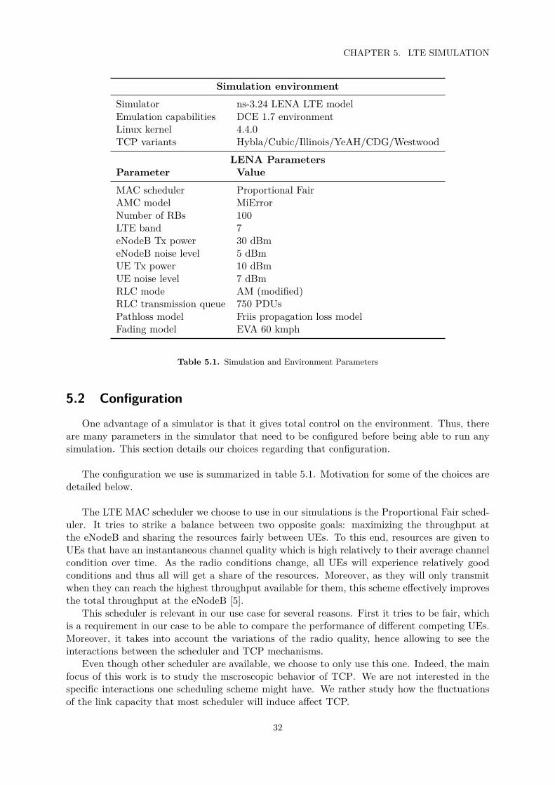
5.1 Simulation and Environment Parameters . . . . . . . . . . . . . . . . . . . . . . . . . 32

Chapter 1

Introduction

1.1 Context

The emergence of smartphone, tablet as well as the multiplication of the applications avail-able on that devices resulted in the growth of data consumption. With 4G networks becomingmore and more popular, higher bandwidth as well as lower latency are achievable, thus bringingnew usage such as video streaming. All this will result in a noticeable growth in traffic.

Most of the traffic that is to be found in these networks runs over TCP. Thus, optimizingthe behaviour of that transport protocol for these conditions can be of great values both for thecustomers and the network operators. Both are interested in an increase in throughput as itresults in faster download for the customer and improved in efficiency for the operator. But morethan just the throughput, a reduction in the queueing delay would also benefits the customer.Indeed, this characteristic is essential for real time applications such as online gaming or VoIP.

The TCP implementations currently used in 4G network have been designed prior to theemergence of such networks and thus do not take into account their specificities. Studying thebehavior of the different congestion control algorithms when running in this situation appearsnecessary to identify any issue that might degrade the performance. Indeed, the conditions in4G are very different from what is to be observed in wired network. The forever changing radioconditions induce quick changes in the available bandwidth as well as in the delay. Some mech-anisms, specific to the LTE stack, might also introduce jitter, further increasing the variabilityof the network conditions.

It is however complex to conduct experiment using real equipment. If it is possible to setupa whole LTE network in a laboratory this setup is expensive and thus hard to access. Usingcommercial LTE networks and terminals is a much cheaper alternative. However, the presenceof other users on the network can make it difficult to know precisely the network conditions atthe moment of the experiment.

In these conditions, simulation appears as an interesting approach. It is affordable andallows for a complete control of the network conditions. It also introduce more repeatabilityand stability. The main issue being the accuracy: the simulation is only useful as far as it canreproduce, to some extent, real life behaviors.

1

CHAPTER 1. INTRODUCTION

1.2 ObjectivesThe main objective of this master thesis is to compare the performance of different TCP

implementations when running on a LTE network using a simulation approach.

This goal can be divided in three separate tasks:

• Setup a simulation platform allowing to run different TCP implementations in an LTEnetwork.

– Have accurate simulation of the TCP variants– Have accurate simulation of the LTE stack– Have reproducible results

• Devise and implement scenarios allowing for the gathering of meaningful data regardingTCP performance.

– Test different traffic types, cell load, mobility– Gather performance metrics (delay and throughput)– Gather TCP internal information (CWND, RTO)

• Analyze the experiments results and give a first insight regarding the performances of thedifferent CCAs.

– Identify the best CCA– Identify differences in behavior between the loss-based and delay-based CCAs– Understand the effects of the LTE environment at the TCP level

1.3 LimitationFirst, this work focuses mainly on the end-to-end performance at the TCP level. Thus, we

will not go into details regarding the LTE protocol stack. We will only consider the elementsthat are necessary to understand TCP behavior when running over a 4G network.

Moreover, not a lot of work has been done previously toward a systematic analysis of theperformance of the different TCP variants in such networks. Thus, there are not a lot of in-formation that are available to understand complex behaviours. For this reason we will limitourselves to very simple scenarios that will allow us to build up such knowledge.

Finally, we do not have access to the hardware that would be required to perform measureon a real LTE network. Thus we will entirely rely on the simulation and we will not be able tocheck its accuracy against real measurements.

1.4 Thesis outlineThe structure of this document follows the different steps that were necessary to achieve the

aforementioned goals. The first part is dedicated to a review of the different fields approachedin this thesis: the principles of congestion control for TCP are described in chapter 2. Chapter 3

2

1.4. THESIS OUTLINE

presents the specificities of an LTE network. Whereas chapter 4 details how such a system canbe simulated.

Based on that knowledge the next part exposes the setup of the test environment. Chapter 5and chapter 6 present the configuration of the LTE simulator. Whereas chapter 7 details themechanisms used to gather and analyze data.

Finally in the last part the designed simulation scenarios as well as the results they yield arepresented.

3

Part I

Literature review

5

Chapter 2

TCP congestion control

The problem of congestion control in computer networks did not appear with mobile net-works. It was already an actively studied topic for all kind of networks, both wired and wireless.Thus, a review of the already identified problems as well as the proposed solutions is a logicalfirst step.

2.1 Base TCP congestion controlThe Transmission Control Protocol (TCP) has been designed to provide reliable, ordered

and error checked end to end transmission of data between two hosts. Thus the protocol initself can only contain mechanisms to limit the sending rate that are based on the sender andreceiver windows. The first implementations did not include any limitations in the sending rate.It turned out not to be enough as it eventually led to degradation in the network conditions,and even to several collapses, as the number of computer connected to the Internet increased.

This is in reaction to one of the first major collapse (in October 1986) that Van Jacobsonreleased a paper [21] defining the base of congestion control in the TCP implementation (thismechanism was implemented under the name Reno). He describes several algorithms which co-operate in assuring congestion avoidance and control. All this work is based on a new principlehe defined: the packet conservation. It states that for a connection to be in equilibrium it shouldbe conservative, meaning that a packet can only enter the network to replace an old packet thatleft it.

According to Jacobson there are three ways for that principle to fail:

1. The connection never reaches equilibrium

2. The sender injects a new packet when no old one has excited

3. Resource limits on the path prevent the equilibrium to be reached

2.1.1 slow startAs it is easy to notice, one problem with the conservation principle is how to reach equilib-

rium. Indeed, at the beginning of a connection, it is required to inject packets faster than theyleave the network to get the transmission started.

However it must be done carefully, indeed there can be great disparities between the speedof different networks in the Internet and a start that would be too aggressive could induce somany dropped packets at a router that this would compromise the rest of the transmission.

7

CHAPTER 2. TCP CONGESTION CONTROL

To solve that problem Jacobson devised the slow start algorithm which aims at progressivelyincreasing the number of packets in the network to probe for more available bandwidth. Inpractice it is quite simple:

• Define a new variable: the congestion window (CWND)

• On the beginning of a connection or after a loss set CWND to 1 segment

• Increase CWND by 1 for each ACK received (CWND doubles for each RTT)

• Send a number of packets equals to the minimum of the sender’s window and CWND

Even if this algorithm might appear simple it is very effective. And has been used withfew modifications (mostly for the CWND value at the beginning of the slow start) until veryrecently. It is only in 2008 that a modification to the slow start was introduced for the cubicCCA in the Linux kernel. This modification called Hybrid slow start is based on the followingpaper [12]. It tries to solve one known problem which is that the loss at the end of slow startcan be as big as the Bandwidth Delay Product (BDP) of the link. This puts great strain on thenetwork and is unavoidable in regular slow start. It is to be noted that hybrid start is not thefirst Slow Start modification. It is however the first one to be widely deployed and used.

The idea of the Hybrid Start is to try to detect that the connection is reaching the linkcapacity (or congestion) before inducing losses. To do so it is obviously not possible to use lossas a congestion signal, thus this method is based on other metrics computed from the ACKspacing and Round Trip delays. The measurement is entirely passive: the algorithm need notinject probe packets and thus is a sender side only modification.

Packet trains had already been studied as a way to estimate the bandwidth [9]. Howeverone cannot implement this method without modification on both side. The scheme proposedby the Hybrid Start designers is more subtle: instead of introducing probe packets they takeadvantage of the bursty nature of the slow start to use ACK trains. Thus, with just a measureof time between the first and last ACK of a train and an estimation of the path one way delay(they use RTTmin

2 ), they show that it is possible to estimate when the CWND approaches theBDP of the link.

However the authors are also aware that in some cases the measurement of the one waydelay is not reliable and will not trigger the exit as expected. Hence they designed anothermechanism based on delay increase. Based on the first ACKs from a train the delay is esti-mated. Only the beginning of the train can be used, indeed as the transmission tends to bebursty, the following packets are more likely to be queued along the path, thus introducing noisein the measurement. Comparing the measures two consecutive measurements the mechanismlooks for an increase in delay above a threshold and in such a case triggers an exit from slow start.

Other changes not directly made to the slow start algorithm but to surrounding TCP codedid also have an effect on it. For instance the way ACK are handled modified the behavior ofthe slow start in the Linux kernel. A modification introduced in 2013 changed the way ACKare counted. Previously, no matter how many bytes an ACK acknowledged, it only increaseCWND by one. A new behaviour has been defined in RFC3465 [2]. An ACK of degree N is tobe treated as N ACKs of degree 1. The RFC recommend limiting N to 2, however the Linuximplementation does not place any limit. This small change in the handling of ACK increasedthe aggressivity of the slow start in Linux kernel using that modification. This is an importantthing to remember when comparing behavior of older versions of the kernel (that are still usedon production server in the industry) to newer ones.

8

2.1. BASE TCP CONGESTION CONTROL

Another change introduced lately is the default value for the CWND. RFC 6928 [6] proposeda modification allowing the initial CWND to be as big as 10 MSS (Maximum Segment Size).By the time the RFC was published such a changed was already implemented in the LinuxKernel. The advantages of the increased initial window is mainly a reduced transfer time forsmall connections that transmit an amount of data that is small but yet did not fit in theprevious initial window. Indeed, less round trips are necessary to complete the transmission.The drawback is a slightly higher pressure put on the network, but as all the control mechanismsstay in place the effect is rather limited.

2.1.2 Retransmission Timer and RTT estimationIn [21] the author explains that the only way a sender (with a correct TCP implementation)

could break the conservation principle is because of a spurious retransmission. Indeed if theretransmission timer is too short a packet that is still being transmitted will be re-sent, thusaugmenting the number of packets in the network.

We will call Retransmission Timeout (RTO) the value of the retransmission timer. In theoriginal TCP (RFC793 [30]) the RTO was simply based on the smooth RTT: mean RTT esti-mated based on RTT measurement filtered with a low-pass filter. However this scheme was notable to account for the huge variation in RTT that can occur in case of congestion.

To solve this problem Van Jacobson proposed to compute the RTO based on the SRTT aswell as on the Mean deviation of the RTT. This proposition as been included in RFC1122 [3]and is still in use today. The exact calculation with the average RTT a, the mean deviation ν,the measurement m, and the RTO r is given by:

ν = (1− β)ν + β(a−m)

a = (1− α)a+ αm

r = a+ 4/nu

The default value for the RTO is 1s as per RFC6298 [29]. So at the beginning of thetransmission, prior to any measurements, it is set to that value. Moreover it is also the minimumvalue, and if the computation gives a lower value it is discarded and 1s is used instead.

Another aspect of the computation of the RTO is the back off after a retransmission. Whenthe sender retransmit a segment after a loss it often means that the congestion control is indifficulty and thus the network condition is unknown. To cater for a possible degradation of theRTT, the RTO follows an exponential back off scheme (it doubles after each retransmission).Such an exponential scheme has been proven to be the only viable one [15].

2.1.3 Congestion avoidanceBecause of the nature of a network, the equilibrium found at some point is likely not to last

forever. The introduction of more hosts in the network could cause more congestion, inducing aneed to reduce the sending rate. On the other hand, the disconnection from a computer couldrelease more bandwidth to be use by the remaining computers. Thus a correct algorithm shouldbe able to release resources when it takes more than its fair share and increase its sending ratewhen the network is underutilized.

As Jacobson explains in [21], since networks are quite reliable, loss is almost always a markof congestion. And because of the improved RTO computation, a timeout is almost alwaystriggered by a loss. Thus the CCA can treat timeout as a mark of congestion in the network andreact accordingly. In the article, Jacobson explains that a multiplicative decrease of the CWNDis an adequate reaction. He proposes a reduction of 50%.

9


As the network is stateless, there is no way it could signal a user that it is taking less thanits fair share. Thus the CCA have to constantly probe for more available bandwidth. Howeverit cannot do so too aggressively. The more aggressive it is, the more packets will be lost whenit reaches capacity. As losses are always very penalizing events, one ought to limit them. ThusJacobson proposes an additive increase of the CWND (1 segment per RTT). This scheme isknown as Additive Increase Multiplicative Decrease (AIMD) and is used by many CCAs withdifferent coefficients.

If the slow start algorithm designed by Jacobson was subject to few changes, it is not so forthe congestion avoidance one. As networks changed with the evolution of technology the schemeprove not to be able to adapt to the new conditions. At first the same principles were kept andimproved upon. However, the most recent CCAs introduced new ways of detecting congestionas well as different functions to govern the growth of the CWND.

2.1.4 Fast retransmit/fast recoveryThe Fast Retransmit algorithm aims at improving the reaction time when facing a loss event.

It is based on the fact that once a segment is lost, every segment received afterward will triggerthe same ACK to be sent. This mechanism, formalized in RFC2001 [31], states that after 3DUPACKs (meaning after the original ACK is received, and 3 copies) the sender will retransmitthe missing segment and enter fast recovery. Some measures are taken by the receiver to improvethe efficiency of Fast Retransmit: first it should send and DUPACK immediately after receptionof an out of order segment (to let the sender now as fast as possible of the problem). Likewise,when a received segment fills a gap it should send an ACK immediately.

The Fast Recovery aims at avoiding to go back to slow start (which reduces abruptly the flow,even if only one packet is lost). The idea of the algorithm is to retransmit the missing segmenton the third DUPACK, to set SSTHRESH to half the CWND and then to halve the CWND.For each DUPACK received after that the CWND is increase by one (this is called inflating thewindow). This strategy is performed to allow TCP to continue sending new segments. Indeeduntil the missing segment is acknowledged the sender will not decrease the number of bytes inflight and thus the CWND would always be full. So the only way to allow the sender to sendmore data is to artificially increase the CWND. This way the sender can continue to replace thepackets that have left the network (up to half the flight size when the loss occurred). When anACK acknowledging new data arrives, the CWND is set the SSTHRESH and the sender goesto Congestion Avoidance.

If this scheme is working very well when only one packet is lost it suffers when it has torecover from more losses. Indeed it goes through several fast recoveries, reducing the CWND byhalf each time. Hense after a few losses, the CWND is reduced to its minimum value (2 MSS).This problem can be solved very efficiently using SACK. When this scheme is in use the sendergets more information about the data the receiver got and can act accordingly. However animprovement of Fast Retransmit (called NewReno) has been devised for the cases where SACKis not available. It was first specified in RFC2582 [11]. The idea is to define a new signal: thepartial acknowledgment. They are ACK that acknowledge new data, but not all data send upto that point. When such an ACK is received the sender deflates the CWND by the numberof bytes that have been acknowledged and retransmit the next missing segment. This wayFast Retransmit can recover multiple losses, quite slowly since only one segment per RTT isrecovered, but more efficiently that previously.

Two variants of this algorithm can be implemented. Impatient: the retransmission timer is

10

2.1. BASE TCP CONGESTION CONTROL

reset only when all the losses are recovered. This variant is very likely to timeout and to goback to slow start if there are many losses. The other variant, Slow but steady, reset the timereach time an new segment is recovered, thus staying in Fast retransmit. This second variant isslower if there are many losses but do not retransmit as much data as going back to slow start,so it could be interesting if the cost of a retransmission is high.

These mechanisms are still used by most TCP implementations. They are for instance partof the TCP protocol in the Linux kernel code and thus shared by all the different CCAs thatcan be plugged into it. Depending on the stack configuration and the options negotiated for thetransmission the best algorithm is selected to recover from a loss.

2.1.5 Nagles’s algorithm

This algorithm presented by Nagle in RFC896 [27], aims at solving the problem caused bysmall packets. Indeed, if an application send small chunks of data, it will send packets with veryfew data, to the extent that sometimes the header is bigger than the content of the message.Such behavior can for instance be observed in telnet, which can send keystrokes one at a time.This generates packets with only 1 byte of data, and 40 bytes of header.

This behavior is obviously not optimal as a lot of capacity is wasted. This can lead to poorperformance or even congestion collapse in the worst case.

The solution designed by Nagle is to group outgoing messages together: this can increasethe latency as messages are not sent as soon as they are ready, but decreases the network usage.To be precise, the algorithm states that the sender should wait until there is either enough datato fill a full segment or no more data is to be acknowledged by the receiver.

If this efficiently solves the small packets problem from a network perspective, it mightdegrade the performance from the user point of view. For instance, the interaction with thedelayed ACK mechanism is rather bad. Indeed the sender has to wait for an ACK beforesending more data however the receiver is waiting for a second packet from the sender beforesending the ACK. The result is the receiver delaying the ACK, and thus the sender, by themaximum value (by default 500 ms).

Moreover, this scheme also performs poorly with real-time applications (such as online games)where the application expects the packet to be sent immediately.

2.1.6 Known problems

Taking Reno as a base, there are several problems that have been identified and motivated thecreation of new CCAs. If some have already been partially solved in some implementations, theystill constitute challenges as conceiving a scheme able to solve all of them might be problematic.

RTT unfairness

Reno is now well know not to perform equally well on all kind of networks. It is notablyknown to have poor performance over links that suffer from a high RTT (satellite connectionsfor instance).

As explained in [4] this is due to the window growth being triggered by ACK arrival. Thus,as the delay between the sending of a segment and the reception of an ACK depends on the

11


delay on the link, a link with smaller RTT will get the ACK faster and thus make the windowgrow faster.

Two harmful consequences result from that problem. First, the slow start phase will belonger in link with high RTT. This makes it slower for the connection to reach high bandwidthusage. Moreover, when competing with flows with a shorter RTT, the slower flows will be at adisadvantage. For instance, if the two flows start at the same time, the fast flow will reach ahigher bandwidth when the link begin to be saturated and thus will enter congestion avoidancewith a bigger window. This might lead to an unfair sharing of the link capacity.

Performance on high delay-bandwidth product links

Network containing long fat pipes are qualified as Long Fat Network (LFN). As such linksgrew more common (with long fiber-optical paths or satellite channels) Reno has been observedto underutilize them [20].

Indeed, in congestion avoidance the growth function is really slow (1 packet every RTT).Thus, it takes a long time to reach full bandwidth utilization in the first place, and after acongestion event, it also takes a long take to recover.

Thus, the classic pattern for the congestion window is to oscillate between the value forwhich loss occurs and half that value. Thus the connection spends a non negligible amount oftime with a non optimal congestion window, not fully filling the link.

ACK compression

ACK Compression is a problem that was predicted from theory in 1991 by Zhang et al. [34]and observed by Mogul the next year [26]. It can break the functioning the ACK clocking anddecrease performances.

In the steady state, the TCP connection is supposed to be self clocking [21]. Indeed, the interarrival time of two ACKs at the sender is equal to the inter arrival time of the packets at thereceiver (if we do not consider delayed ACK). This allows for an effective control of the sendingrate. Indeed this inter arrival time is controlled by the rate of the bottleneck: the slower it is,the more time there will be between two packets. Thus, the faster the bottleneck, the faster thesending rate.

However, problems can occur if the reverse path is congested. In that case, ACK can bestored in a router queue somewhere along the path. And when these ACKs leave the queue,the spacing between two ACKs is no longer the inter arrival time of packets at the receiver, butrather the time taken by the router to put ACK from its queue to the network. ACK beingsmaller than data packets, this time is usually shorter than the inter arrival time of the pack-ets. When these compressed ACKs arrive at the sender, they trigger the sending of a burst ofpackets that is likely to be queued at the beginning of the bottleneck, thus increasing congestion.

2.1.7 TCP implementation

The different mechanisms have been presented as they are found in the literature. Howeverthere is no assurance that a network stack implement them exactly as specified. Thus differencesmight exist between two implementations of TCP, as different constraints can lead to differentapproaches. For instance the Linux TCP implementation follows the RFC less closely than theone in the NS3 simulator. One example is the computation of the RTO timer: in NS3 this is

12

2.2. REVIEW OF RELEVANT CCAS

done by following strictly Van Jacobson algorithm whereas in Linux the computation tries andcorrect some of the issues in the original design.

This is something that it is good to keep in mind when trying to interpret the results ofexperiments. The observed behavior is sometimes different from the expected one because theimplementation is not strictly conform to the specifications. In that case looking into the sourcecode is the fastest way to check this hypothesis.

2.2 Review of relevant CCAs

All the mechanisms presented in the previous section define the building blocks of congestioncontrol for TCP. They have been used as foundation by researchers to devise new schemes thattackle the difficulties that appeared.

Many CCAs have been designed and implemented along the years, each one with its specificcharacteristics and goals. There are currently more than 10 CCAs available in the Linux kernel.For readability consideration it has been chosen not to include all of them in the present study.Only a selection of the ones most relevant to our use case will be presented.

2.2.1 Illinois

In [24] the algorithm is defined by its authors as “a new congestion control algorithm forhigh speed networks [that] achieves high throughput, allocates the network resource fairly, andis incentive comparable with standard TCP”. Like Reno it uses a AIMD scheme but where Renouses fixed coefficients, Illinois adapts them to the state of the network based on RTT measure-ments. This adaptability makes it interesting to study in the quick changing LTE environment.

This algorithm tries to address two issues that appear with the traditional AIMD scheme.First the increase is not fast enough to allow the CWND to grow and to fully utilize the linkbetween two back off events. Second, standard TCP interprets all losses as congestion events.Thus in lossy links the bandwidth is underutilized because the network is estimated to be morecongested than it is.

Illinois is not the first CCA to try and adapt the AIMD coefficients to the network condi-tions, however its approach is different in that its tries to obtain a concave window curve. Sucha shape is beneficial for two reasons. First, the increase is fast when the network is far fromcongestion, making the CCA faster to get closer to full link utilization. Secondly, the increaseslows down near congestion, reducing the amount of dropped packets when a congestion eventoccurs.

In the AIMD scheme, the window size is adjusted according to two coefficients: α for theincrement and β for the decrement. In the increase phase the window (W ) is incremented byα/W for each ACK, resulting in an increase of α per RTT (if each ACK acknowledged onesegment). In a decrease phase, the window is decreased by a defined proportion βW .

The idea to obtain a concave window curve is to have a big α and a small β when far awayfrom congestion and a small α and a big β when close. In order to asses the proximity fromcongestion Illinois uses the queuing delay. According to the authors even if this metric can suffernoise in its measurement, it can be used to determine the coefficients. In this usage it would onlybe a secondary signal, the decision to increase or decrease the window is based on the packet

13


losses, and thus the noise does not affect too much the functioning of the CCA.

To summarize, Illinois through the modification of the α and β coefficients tries to adaptthe shape of the window growth function. The adaptation of the first one allows for a concavewindow growth in any network whereas the modification the second one only brings benefits inlossy networks where a packet loss does not only occur because of congestion.

2.2.2 Westwood

the cause of a packet loss (congestion or lossy link) and react accordingly. On this basis,Westwood builds an estimate of the rate of the connection and uses it to compute the slowstart threshold and congestion window. Studying the behaviour of such a mechanism in LTEnetworks makes the CCA worth studying here. According to the introduction paper [25], theperformance is improved both in wired and wireless networks. It is however most effective inwireless networks with lossy links. Thus Westwood solved one of the problems of Reno: itsinability to determine the cause of a loss. However it does not address its slowness to reach fulllink utilization.

If we call β the bandwidth estimate, τ the base RTT and w the CWND, we have on a loss:{w = max(w/2, τβ), if w > τβ

w = w, if w ≤ τβ

If the bandwidth estimate falls into the first case, the loss has a high probability of beingcaused by congestion. Thus, the window is reduced to fit the bandwidth estimation. In theworst case (when the estimated throughput is very low) Westwood reduces the window as muchas Reno is order not to be less aggressive.

On the other hand, if it is the second condition that is fulfilled the loss is most likely due totransmission error on the link and the window is not reduced (as no congestion is detected).

The major problem with the implementation of this CCA is the estimation of the bandwidth.Indeed the source node has to compute it based on the information it has. However, as thismodification is sender side only, no probe packet can be injected to make the measurement. Thusit has to use the incoming ACK as base for the measures. Another problem is that measurementscan be noisy (for istance because of ACK compression). Thus one needs to keep only the lowfrequency component of the estimate.

The first technique that was used by Westwood to estimate the bandwidth was to measurethe spacing between two following ACK and to smooth the result with a moving average. Thisproved to be very affected by ACK compression and thus a new scheme was designed. To fixthe issue the measurements are made over longer interval and a different filter is used to smooththe bandwidth estimate. This is this improved version that is present in Linux and that we willconsider if not otherwise specified.

2.2.3 Hybla

Hybla is a relatively modest modification to Reno that aims at fixing a particular issue: itsbias against connections with longer RTT. It is interesting to study as a variant of Reno takinginto account the variability of the RTT into account.

14


As exposed in [4], this CCA can be seen as an extension of the AIMD policy of Reno. Insteadof using predefined coefficients for the increase during slow start or congestion avoidance theactual coefficients depends on the link’s RTT. The objective is to compensate for the longerRTT by being more aggressive to be able to achieve the same performance as a connection witha reference RTT. This values is called RTT0 by the authors and they suggest of value of 25 ms.

To achieve this they first define a constant ρ = RTT/RTT0. And the growth functions aredefined as follow: {

w = w + 2ρ − 1, In slow startw = w + ρ2/w, In Congestion Avoidance

As for every CCA using the RTT as part of its algorithm, the measurement of this parameteris crucial. Thus the authors advise to use the timestamp option to increase the accuracy.

They also advice to use the SACK option. Indeed, because the increase is more aggressive,there are good chances that there might be more than 1 packet that is lost during an overshoot.And as explained before, when there are more than 3 packets to recover SACK performs betterthan NewReno.

2.2.4 CubicCubic aims at being a viable replacement for Reno in all situations. As such it is the current

default CCA in the Linux kernel (which makes it worth including in our study). It replacesReno’s linear window growth (in congestion avoidance) by a cubic function. This function hasthe properties that were already presented as desirable in the section about TCP Illinois: con-cavity before the previous CWND maximum size and convexity after it. This way, the growthis fast when the CWND is far from the previous limit and slow around it, allowing for fastadaptation to a modification in the available bandwidth and low loss rate when the limit isreached.

As exposed in [14], this CCA is quite different from Reno: the growth function in congestionavoidance is not linear but a cubic function with its origin located where the last loss occurred.The coefficient for the multiplicative decrease is not 0.5 but 0.2 (making it less conservative thanReno).

When a loss occurs at t = 0, cubic records the value of CWND as wmax, and with C aconstant (usually 0.4) and the following formula for the value of CWND:

w(t) = C(t−K)3 +Wmax

With K being computed when the loss occurs. To have w = (1− β)wmax at t = 0 it gives:

K = (wmaxβ

C)

13

Another advantage of that growth function is that it is not dependant on the RTT, thuscubic does not suffer from the same bias against connection with longer RTT.

15


In some case, that growth function might be at a disadvantage compared with Reno: it mightbe slower and get less bandwidth. Thus Cubic has a mechanism that makes it TCP friendly:when the CWND size is computed, the maximum between the cubic value and the one that theReno CCA would produce is taken. As β is 0.2 and not 0.5, α must be 1/3 instead of 1 in theReno computation for it to be friendly against regular TCP Reno flows [8].

One last mechanism that can be presented is the fast convergence: if cubic detects that lossoccurs for a window size lower than for the previous one the computation of wmax is modified.With wloss the value of CWND when the loss happens:{

wmax = wloss × (1− β/2), if wloss < wmax

wmax = wloss, if wloss > wmax

2.2.5 YeahYeah is rather different from the CCAs we have seen so far, it is composed on two modes:

one fast and one slow. In the slow mode Yeah is conservative and behave like Reno, whereas inthe fast mode it is more aggressive and behave like SCTP. The decision on the mode is basedon an estimation on the bottleneck queue size. YeAH is worth studying as it relies primarily ondelay measruments, whereas the main input for the previous CCAs was the packet losses.

SCTP is a simple variation of the Reno AIMD scheme. Instead of increasing by 1 segmentby RTT the CWND grows by 1 segment for 100 ACK received (or fallback to Reno if it is faster).

The queue size is estimated in a standard way, calling τbase, and τmin the base RTT and minRTT during the last flight. It gives τqueue = τmin − τbase.

And with w the CWND we can estimate the goodput G with: G = wτmin

. It gives for theestimated queue size Q:

Q = τqueue ×G = τqueue × ( w

τmin)

The network congestion level is also estimated with:

L = τminτbase

Finally the CCA is in fast mode if Q < Qmax and L < 1/φ where Qmax and φ are tunableparameters. The first one being the number of packets the connection is allowed to have in thebottleneck queue.

As an additional measure a decongestion algorithm is implemented in the slow mode: whenQ > Qmax CWND is decreased by Q and SSTHRESH is set to CWND/2.

Such a scheme is however no always applicable in reality. Indeed, when Yeah competes withmore greedy CCAs (like Reno) applying the decongestion algorithm would only result in givingmore bandwidth to the competitors. Thus this feature is disabled when the CCA detects thatit competes with greedy CCAs.

In the same way, when Yeah does not compete with greedy flows it tries to limit the CWNDreduction when receiving 3 DUPACK: instead of halving CWND it just decreases it by Q. Thestandard Reno behaviour is applied in the other case.

16


2.2.6 CAIA Delay Gradient (CDG)CDG is also delay based, however contrary to most of the other CCAs in that category it is

not based on any delay threshold. The authors found this approach to present several flaws [16]:first it is complicated to set a proper value for the threshold, second it depends on an estimationof the base RTT that can be hard to get.

Instead, the CDG algorithm is based on a delay gradients: within an RTT interval the max-imum RTT (τmax) and minimum RTT (τmin) are recorded. Then, two gradients are computed:gmax,i = τmax,i − τmax,i−1 and gmin,i = τmin,i − τmin,i−1 where i is the ith measurement.

These measurements are smoothed using a moving average. The results are then used todetect when the queue is almost full or almost empty. According to the authors, in the first caseτmax stops increasing before τmin and in the other one τmin stops decreasing before τmax. Thiseffectively allows the algorithm to detect and react to such events.

The backoff strategies is implemented using an probabilistic mechanism, allowing for morefairness between connections with different RTTs. The probability is computed as follow:P [backoff] = 1 − e−(gi/G) with gi being either the smoothed value of gmin,i or gmax,i. Usingthis value, in congestion avoidance the CWND value is updated once per RTT using the follow-ing rules:

wi+1 ={wiβ If X < P [backoff] ∧ gi > 0wi + 1 Otherwise

With X being a uniformly distributed random number between 0 and 1, and β a multiplica-tive decrease factor.

In the original paper the algorithm used for slow start is the same as for Reno. Except that,once per RTT, the slow start can be excited with the probability aforementioned.

However, in the Linux kernel, the implementation uses a variant of the hybrid slow startalgorithm used in Cubic. Some small differences are present (such as the definition of someparameters) but they do not fundamentally modify the functioning of the algorithm.

CDG is a recent CCA, it is currently the most recent addition to the Linux kernel. As astate of the art delay based CCA it is worth including in our scenarios.

17

Chapter 3

TCP in an LTE network

This thesis will not focus on the LTE side of the performance issues, thus it is not requiredto have a full understanding of that part. A general knowledge of the different components ofthe system is sufficent.

Indeed, as mechanisms at different layers in the LTE stack can interact with TCP, it isnecessary to have an understanding of the whole system.

To begin, the architecture in an LTE network will be presented as well as the interactions itcan have with TCP. Then, some of the problems caused by these interactions and reported inprevious works will be detailed. Finally the available simulations tools will be presented.

3.1 LTE architectureThe description of the LTE Architecture is taken from [7].

3.1.1 Network elementsThis section describes the different elements that are to be found in an LTE network. This

list is not complete and focus only on the elements necessary to the comprehension of our topic.

User Equipment (UE) this is the device used by the end user. In most case it is a smart-phone, tablet or computer connected to a LTE modem.

E-UTRAN Node B (eNodeB) this is the radio based station used to handle the radio partof the communication. It acts as a layer 2 bridge between the UE and the Evolved PacketCore (IP part of the LTE network). The eNodeB is also responsible for radio resource man-agement, for instance uplink and downlink scheduling, as well as for mobility management,handling the UE handovers to other cells.

Serving Gateway (S-GW) this node is responsible for the handling of the user plane tunnels.It makes a bridge between the packet gateway and the eNodeB associated with a UE. Whena UE is in idle mode it is responsible for buffering packets (resources are released on theeNodeB in that case).

Packet Data Network Gateway (P-GW) this is the edge router between the EPC and theexternal packet data network. It allocates the IP address to the UE, and tunnels all trafficbetween the UE and the external network.

As we are more interested in the user plane, the different elements that are found on thecontrol plane will not be detailed here. Indeed they play a role in the setup of the user plane

19

CHAPTER 3. TCP IN AN LTE NETWORK

UE eNB S-GW P-GW

IP

Remote

APPTCPIP

PHY

APPTCPIP

PDCPRLCMAC

PHY

PDCPRLCMAC

GTPUDPIP

GTPUDPIP

GTPUDPIP

GTPUDPIP

LTE-Uu S1-U S5/S8

Figure 3.1. user plane Stack

but have less impact on the performance once it is established. Thus we choose not to detailthem for the sake of clarity.

3.1.2 User plane stackThis section will present the user plane, that is the part of the network that handles the

routing of the packets between the external packet network and the UE. More precisely, it willbe focused on the LTE-Uu interface between the eNodeB and the UE (figure 3.1).

Figure 3.1 shows the complete user plane stack used for a LTE connection from the remotehost to one UE.

When a packet originated from the remote host and going to the UE enters the EPC at theP-GW, it is encapsulated in a tunnel until it reaches the eNodeB associated with the UE.

This path, from the P-GW up to the eNodeB, will not be detailed. Indeed the differentinterfaces (S1-U, S5/S8) do not have a major impact in the scenarios that we are interested in.

The interface that is relevant to us is the LTE-Uu between a UE and an eNodeB. It iscomposed of the following protocols:

PDCP (Packet Data Convergence Protocol Layer) It is responsible for the transitionbetween two eNodeBs in case of a handover. It is also its role to ensure that packetsare transmitted in order to the upper layer. Additionally it can perform IP header com-pression.

RLC (Radio Link Control) It is responsible for in-order delivery of packets to the upperlayer. There are different modes that can be used for the RLC layer. We will only interestourselves in the acknowledged mode. In this mode, through the use of ARQ (automaticrepeat request), it will ensure reliable delivery. ARQ is an error-control scheme that usesacknowledgments to check for the correct delivery of messages and uses retransmission incase of losses (this is what is used by TCP for instance).

MAC (Medium Access Control) This layer is responsible for the actual transportation oftransport blocks, correction of errors with HARQ (Hybrid ARQ) and scheduling. HARQis a combination of ARQ and forward error correcting coding. The later scheme adds someredundancy to the messages thus allowing for error detection as well as correction (in alesser extent though) on the receiver side.

Another responsibility of the MAC layer is to perform scheduling. Indeed in LTE both theuplink and downlink use a OFDM (Orthogonal Frequency Division Multiplexing) scheme. This

20

3.2. RELATED WORKS

means that the time and frequency resources must be shared among the different UEs. Thescheduler decides the allocation, granting 180 kHz wide resources blocks with 1 ms intervals.Moreover, the scheduler also decides the data rate to be used during the transmission to a UE.

One might notice that reliable delivery can be enforced twice in the stack: in the RLC andMAC layers. The goal in not the same in both cases, HARQ used in the MAC layer is a fastscheme, that is not totally robust: errors can go undetected but it does not add a lot of delay.On the other end ARQ in the RLC layer is more robust but slower, so for the price of a littledegradation of the RTT it is possible to get more robustness. The choice to enable or not ARQin the RLC layer is based on the type of traffic that is expected to transit in the network. Forvideo traffic over UDP (that does not focus on reliability) this extra layer of robustness wouldbe useless for instance.

3.2 Related works

3.2.1 LTE interactions with TCP

In a recent IETF Draft [22] some of the interactions between LTE and TCP have beenanalyzed. This section presents a summary of the findings:

The scheduler is a critical part of the system and can have a huge impact on the performanceof the system. Different strategies can be used depending on the priorities. It is indeed notpossible to reach all goals at the same time. For instance fairness and maximum throughput atthe eNodeB: to achieve the second goal the best strategy would be to allocate resources to theUEs that have the best radio conditions and can achieve high throughput, which is obviouslyincompatible with the first goal.

This mechanism has consequences on the performance of the transport protocol. Indeed, forthe UE to be scheduled to receive data, it needs to have data waiting in the eNodeB queue. Thusthe queue should contain enough data not to miss a transmission opportunity because there isnothing to transmit. Thus is is dangerous to have too little data in the queue. However, toomuch data is not better, it leads to an increased latency because of the queueing delay. Evenworse, in case of a burst of data it could lead to dropped packets. Thus there is a balance tobe struck in order to be able to reach high throughput while keeping the queueing delay as lowas possible. Moreover, having as few packets as possible in the eNodeB queue is also useful inthe case of a handover. Indeed, it limits the amount of data to transfer to the new eNodeB andthus speeds up the process.

It is important to note that such queues can only be kept at the RLC or PDCP layer. Anyother layer would be too far from the radio interface and would not allow for efficient resourceusage.

Unlike a traditional router the eNodeB keeps a separated queue for each UE. Thus theinteraction between the different UEs is not exactly the same: one will not be at the end of thequeue because another UE filled it. Another difference is that the maximum queue size is notalways constant, it can be reduced if the eNodeBs has a lot of UEs to handle.

Moreover, always waiting for data could drain the battery of the UE quite quickly. Thusto improve the power consumption a feature called Discontinuous Reception as been imple-mented. The terminal only checks for the presence of downlink data at regular interval andsleep in between. As a result, data cannot always be transmitted as early as possible and thislead to an additional delay in the reception. This creates additional jitter (of the order of 10

21


to 20 ms), which can be falsely interpreted as congestion by CCAs based on delay measurements.

Even if the amount of data transmitted from the UE is small, uplink scheduling can alsohave negative consequences on the performances. As for the downlink, uplinks scheduling iscontrolled by the base station. However, as the eNodeB does not know beforehand that a UEhas data to transmit, the terminal must first issue a scheduling request. It is to be noted thatthis request does not contain the amount of data that the UE needs to send. After receivingthe request the base station send back a scheduling grant. The delay of the response dependson the load on the cell. This grant contains the amount of data the UE can send. If this is notenough the UE will attach a Buffer Status Report to the uplink transmission which will lead toanother grant by the base station and so forth until no data is left to transmit.

This mechanism has several consequences. First it can break ACK trains. Indeed a UEcould only be able to send half the ACK in the first transmission and need another one to sendthe rest. As explained the terminal would need to wait for the second grant of the base stationbefore sending the remaining ACK. The HARQ RTT is typically of around 8 ms which couldbe enough to break the ACK train as seen by the receiver.

Uplink scheduling can also cause coalescing, which cause similar issues as when ACK com-pression occurs, and this independently of the load.

3.2.2 Requirements for better performances

In [22] Ingemar Johansson explains what would be required from a CCA to achieve goodresults in an LTE network.

• Avoid relying on precise RTT estimate. Indeed, we have seen that several mechanisms (up-link scheduling, HARQ) can have an effect on the delay. This can misguide the CCA andmake it take unnecessary measures. This issue can be mitigated by the use of timestamps.They help provide reliable measurements and limit the impact of the LTE mechanisms.

• Minimize latency under load. If a decent amount of data in the buffer is required to utilizethe radio link efficiently, there are several cases where limiting the amount of data canbe useful. First, in case of a handover, not having too maybe data to move between thetwo eNodeBs speeds up the transfer. Moreover, too much data makes the reaction to areduction in throughput slower.

• Faster increase of the congestion window. In order to take advantage of the fast modi-fication of the available bandwidth that are due to some new mechanisms such a carrieraggregation or dual connectivity, the CCA should be able to grow the congestion windowquickly, while still being sensitive to congestion.

• Packet pacing. Especially on the UE side this could be used to reduced the risk of ACKcompression that can degrade performance. Reducing the amount of ACK might alsohelp mitigate the problem. However, the interaction with other schemes, such as Nagle’salgorithm is to be studied as it could seriously impact the performance.

• Explicit Congestion Notification. By supporting this functionality the CCA would be ableto be informed directly by the router along the path of congestion and react accordinglywithout the need to use losses which is not entirely reliable as a congestion signal.

22

3.2. RELATED WORKS

It is important to note that these improvements are not all equally easy to deploy and donot require the involvement of the same actors. If the first three bullets can be implementedon the origin server, requiring no change on the UE or the LTE part of the network, this isnot the case for the last two. The fourth one requires modifications on the UE side, which isan environment that is controlled by the end user. This makes any mass deployment unlikely.Besides, the last point would require the support of ECN by the routers along the path whichcould be even more complicated to achieve.

In our study, we will focus mainly on the characteristics that can be tuned easily on theserver side (such as buffer length or CWND growth). Thus, we will focus on transfer directedfrom the server and toward the UE (“download” from a end user perspective).

3.2.3 Known issues with TCP in mobile networksOne issue that is not new but gathered more attention recently is the problem of bufferbloat.

That is, large buffers that are often full. This large queueing can result in increased latencyand jitter, which is mainly problematic for applications with multiple short flows (such as webbrowsing) or real time applications (such as gaming or VoIP).

Because of the large buffers used to accommodate varying bitrates, mobile network areparticularly impacted by that problem. In [1] the authors studied the impact of the CCA whena short flow traffic is put in presence of a different number of concurrent long lived flows (all theflows are directed toward the same UE). This experiment has been made for different networks(3G, 3.5G, 4G) and for 3 CCAs (NewReno, Cubic and Westwood+).

The results show that in a 3G or 3.5G network the impact of the CCA used in the longlived flow was non negligible. However, not real difference was observed in the case of the 4Gconnection in the conditions of the experiment. It is to be noted that this experiment wasconducted using measurement on commercial networks, thus limiting the range of scenarios thatcould be realised. To our knowledge no work has yet focused on the problem of bufferbloat inLTE network using simulation.

As we are studying the base behaviors of the different CCAs we will not focus on that issuethat requires multiple flows directed to the same UE.

In [17] the authors used a large dataset of traces collected from eNodeBs to study theperformance of TCP, and identify any abnormal behavior. They noticed several issues thatcripple TCP performances:

The “undesired slow start” problem is the first they identify. They explain that, because ofthe large amount of data in flight, even the loss of a single packet can create a large amountof duplicate ACK that in some circumstances can lead to a timeout, which for most CCAsmeans a reduction of the CWND to 1 and the start of the slow start phase. This problemcan be aggravated by a bad estimation of the RTT after a congestion event: indeed, there is nostandardized mechanism to update the RTT (and thus RTO) when only DUP ACK are received.And underestimating the RTO might lead to a timeout before the retransmission has had timeto arrive.

Implementing a scheme to update the RTO based on the DUP ACK could prevent up to95% of the undesired slow start according to the study.

Another problem they identify is that TCP does not use all the available bandwidth. Theycomputed the average utilization ratio to be around 35% of the bandwidth available for that user.They also identified large RTTs and high bandwidth variation as factor aggravating the problem.

In [28] the authors used simulation as an approach to study TCP behavior in an LTEnetwork. Using the NS-3 simulator and the regular Linux TCP stack (through the use of the

23


Network Simulation Cradle), they studied two scenarios: a load increase in a cell and a LTEPDCP Handover between two cells. In their study, they used a more systematic approach thandone before: thanks to the simulator they were able to really study the cross layer interactionsinstead of relying on higher level application behaviors.

Studying a scenario where the load in a cell suddenly increases they observe that the RTOestimate of the UEs present before the event becomes obsoletes. Thus leading to unnecessaryretransmission and timeout that decrease the throughput. These observations are similar to theones made in [17] based on network captures.

24

Chapter 4

LTE/EPC simulation

As mentioned above, the approach we have chosen in this thesis to use simulation as muchas possible as it allows for a controled environment as well as for repeatable experiments.

We do not make here a full review of all the available simulators available. Instead we focuson the software stack that we have used: the LENA Simulator and the DCE Cradle.

4.1 LENA simulator

This section describes the LENA LTE/EPC simulator. If this is not the only LTE simulatorthis one is based on NS-3, thus making it a prime target for research focused on the interactionbetween LTE and TCP.

The simulator is organized in two parts: the LTE model responsible for the Radio Stacksimulation and the EPC model that handles user plane functionalities.

4.1.1 LTE model

Even if the present work focuses more on the IP packet part of the simulation, it is necessaryto have accurate simulation of the lower layers, as we want to study the interactions betweenthe different layers.

At the physical level it is not possible, for performance reason, to run simulation with agranularity at the symbol level. Thus, the authors of the LENA modules have devised a linkabstraction model that strikes a good balance between accuracy and computational weight. Thedetailed approach will not be detailed here, as it is outside of the scope of this study. It willbe sufficient to note that the model is able to predict the transport block error rate at theMAC layer while taking into account several parameters such as channel fading, interference orphysical layer configuration.

Regarding the MAC layer the simulator provides the major features: resource allocation,Adaptive Modulation and Coding (AMC) and scheduling. As for the previous point, the firsttwo elements do not have a direct impact for our study. Thus it is enough to know that theyare relatively close to what could be found in a real environment. The scheduler does have adirect impact on the resultsm it is however outside the scope of this study to detail the differentvariants that can be used. It can however be noted that the simulator comes with differentimplementations that would allow for other works to study this aspect more into detail.

25

CHAPTER 4. LTE/EPC SIMULATION

At the RLC layer, the simulator provides implementations for two of the three modes exist-ing in the specification: acknowledged mode and unacknowledged mode. The implementationis done according to the specification and thus should be accurate. It is to be noted that thebehavior of the Acknowledged mode in the implementation is a little bit different from what issaid in the documentation: the transmission buffer being infinite instead of using a drop tail.

The PDCP layer implementation only supports the base features: transfer of data to theupper layer and maintenance of the sequence numbers. Thus it is not possible to use moreadvanced schemes such as IP header compression. As this only marginally affects the achievablerate the absence of this feature is not a problem.

4.1.2 EPC model

The following section aims at summarizing the possibilities the simulator gives regardingend-to-end IP connectivity over LTE.

The simulator can be used to simulate end-to-end IPV4 (IPV6 is not supported) simulationusing any NS-3 application running on top of TCP or UDP. Without advanced configuration itsupports simple scenarios with several UEs and eNodeBs.

Thanks to the accurate modeling of the components it also allows for more elaborate sce-narios. For instance, the accuracy of the S1-U interface makes the elaboration of scenarioscontaining eNodeBs with a limited backhaul link possible.

The applications running on the UE and SGW/PGW allows for the simulation of multipleEPC bearers which make it possible to simulate UEs running different applications with differentQoS profiles.

Besides, the RRC model and the accurate modeling of the X2 link between the eNodeBs givethe possibility to devise scenarios with a X2-based handover of UEs from one eNodeB to another.

Regarding the architecture of the module, it is fairly close to reality. Although, some sim-plifications have been made to simplify and speed up the implementation. The major one is thefusion of the P-GW and S-GW and the unicity of this node. This prevents the simulation ofinter S-GW mobility scenarios.

Moreover, the authors have put the focus on the user plane. Thus the accuracy of thesimulation of the Control plane is not a priority. This leads to some link being logical connections(between the models) rather than simulated links using the network stack.

Furthermore, the authors decided not to implement the features that are related to the EPSConnection Management Idle mode, focusing only on the connected mode. As we are onlystudying scenarios when a transfer is ongoing the absence of this feature is not a problem.

4.2 DCE cradle

If the base installation of the LENA simulator offers everything needed for the simulationof a LTE/EPC network it still suffers from some limitations. Indeed, regarding the simulationof the TCP stacks there are several points that could be improved. First, the number of TCPCCAs implemented in the base NS-3 installation is quite small, only Reno, Tahoe, Westwoodand Hybla are present. Most notably, there is no implementation of Cubic. Moreover, the realstacks do not always strictly follow the RFC, so it would also be interesting to be able to testthe performance of a real life stack with a real configuration.

26

4.2. DCE CRADLE

DCE cradle is a framework built on Direct Code Execution (DCE, a framework for NS-3 thatallow for the use of existing implementation of userspace or kernelspace code). More specificallyDCE Cradle allows the use of any feature of the Linux kernel stack within NS-3. For instancethe Linux TCP stack with all the CCAs it contains can be used inside NS-3 simulated nodesrunning application models.

In [32] the authors of DCE Cradle exposed their results regarding the accuracy and perfor-mance of the framework. Using a dumbbell topology with multiple TCP flows they compared theresults regarding goodput between different test methods among which DCE Cradle, standardNS-3 and real network stack. Their results show that the DCE Cradle obtains a throughputthat is closer than NS-3 to what a real stack achieves. This confirms the accuracy of theirimplementation.

Using micro-benchmarks they also compared the time required to run different simulations.As it could be expected, the usage of DCE Cradle induces some overhead that slows down thesimulation. In their tests the authors measured their framework to be on the average 2.2 timesslower than NS-3 native stack.

27

Part II

Environment setup

29

Chapter 5

LTE simulation

In this study we decide to use a simulation approach to study the performance of differentTCP variants in an LTE network. The first step toward that goal is to setup a simulationenvironment.

This chapter will present the requirements we have regarding LTE simulation and how wemeet them.

5.1 Simulator choice

5.1.1 Requirements

In this work we are interested in the performance of the different TCP variants running in anLTE network. Even if the protocol is located in the transport layer, because of the interactionsthe lower layers might have with it, we need a simulator able to simulate the whole LTE stack(RRC, PDCP, RLC, MAC and PHY) as well as the EPC.

Moreover, for convenience, it would be good to be able to simulate the higher layers in orderto easily study the performance of different kinds of applications with different traffic patterns.

5.1.2 LENA Simulator

The LENA Simulator already described in chapter 4 meets these expectations both regardingthe LTE and IP stacks.

Being built on top of NS-3, this simulator gives access to all the power of a network simulatoralready used in many research projects. This allows for instance to use the built-in trace sourcesmechanism, as well as logging and debugging functionalities.

Regarding the LTE part, the simulator handles the whole stack with enough accuracy toallow for the observation of effects caused by the interactions at different levels. One knownlimitation of the simulator is its incomplete modeling of the Control Plane. However, as thispart does not play any major role in the performance once the connection is established betweenthe eNodeB and the UE, this does not impact our use case. Indeed, we only consider scenarioswhere the link between the UE and the eNodeB is already established.

31

CHAPTER 5. LTE SIMULATION

Simulation environmentSimulator ns-3.24 LENA LTE modelEmulation capabilities DCE 1.7 environmentLinux kernel 4.4.0TCP variants Hybla/Cubic/Illinois/YeAH/CDG/Westwood

LENA ParametersParameter ValueMAC scheduler Proportional FairAMC model MiErrorNumber of RBs 100LTE band 7eNodeB Tx power 30 dBmeNodeB noise level 5 dBmUE Tx power 10 dBmUE noise level 7 dBmRLC mode AM (modified)RLC transmission queue 750 PDUsPathloss model Friis propagation loss modelFading model EVA 60 kmph

Table 5.1. Simulation and Environment Parameters

5.2 Configuration

One advantage of a simulator is that it gives total control on the environment. Thus, thereare many parameters in the simulator that need to be configured before being able to run anysimulation. This section details our choices regarding that configuration.

The configuration we use is summarized in table 5.1. Motivation for some of the choices aredetailed below.

The LTE MAC scheduler we choose to use in our simulations is the Proportional Fair sched-uler. It tries to strike a balance between two opposite goals: maximizing the throughput atthe eNodeB and sharing the resources fairly between UEs. To this end, resources are given toUEs that have an instantaneous channel quality which is high relatively to their average channelcondition over time. As the radio conditions change, all UEs will experience relatively goodconditions and thus all will get a share of the resources. Moreover, as they will only transmitwhen they can reach the highest throughput available for them, this scheme effectively improvesthe total throughput at the eNodeB [5].

This scheduler is relevant in our use case for several reasons. First it tries to be fair, whichis a requirement in our case to be able to compare the performance of different competing UEs.Moreover, it takes into account the variations of the radio quality, hence allowing to see theinteractions between the scheduler and TCP mechanisms.

Even though other scheduler are available, we choose to only use this one. Indeed, the mainfocus of this work is to study the mscroscopic behavior of TCP. We are not interested in thespecific interactions one scheduling scheme might have. We rather study how the fluctuationsof the link capacity that most scheduler will induce affect TCP.

32

5.2. CONFIGURATION

The simulation of the radio channel needs two components to be configured: the propagationand the fading. For the first one, the configuration is the choice of the model to use. We chooseto stick to the default one: The Friis Propagation Loss Model. As we are not interested in thedetails of the radio part of the simulation, there is no point for us to tune the propagation modelin use. Hence, using the default one is the most logical choice. As for the fading, the choice isthe trace file to load.

Indeed the model used in LENA for the evaluation of fading is based on pre-computed traces.This allows for faster simulation but forces all UEs to use the same trace. In order not to syn-chronize the fading of all the UEs the starting points in the traces are selected randomly for eachterminal. Three trace files are provided with the simulator: two for pedestrian scenarios with aspeed of 3 km/h (with or without an urban environment) and one for a vehicular scenario witha speed of 60 km/h. We choose to use the last one, as we want to test the different CCAs withchallenging radio conditions.

Regarding the RLC mode we choose to use the acknowledged mode. In a real system, theRLC mode is selected depending on the kind of traffic that is used on the radio bearer. For TCPtraffic, the most suitable choice is the Acknowledged mode. Indeed, as reliability is ultimatelyenforced by TCP, it is better to ensure a reliable delivery in the lower layer as the recoverywould be more efficient.

In our study, as we are studying TCP flows, the only sensible choice is the Acknowledgedmode. Indeed, it is the only one that is likely to be used for taht kind of traffic in a real deploy-ment. The performance of TCP when the RLC is in acknowledged mode are severely crippledby the packet lossed caused by the radio link: these errors being more costly to recover at thehigher layer.

The frequency band we use is band 7 as this is one of those used in Europe in a Urbanenvironment. We use 100 resource blocks (bandwidth of 20 MHz) which is the maximum thatcan be used in an LTE network. Indeed, some effects might appear only when the achievabletroughput is high. It is thus necessary to have as much bandwisth as possible to try and detectthem.

We choose to enable error modeling only in the Data Plane. Indeed, we are not interestedin what happens in the Control Plane, we just need it to establish the communication. Hencewe do not need to simulate it very accurately.

Regarding transmission power and noise levels we choose to keep the default values. Indeed,these value only affect the quality of the signal received by the UE. To limit the number ofparameters we choose to use the distance between the UE and the eNodeB as the only way ofmodifying the radio conditions. Moreover, as the study of the behavior of the different variantin simple condition is already a problem complicated enough, we choose not to change thatdistance inside a simulation.

As for the eNodeB queue length, asking a specialist we were told that the smallest valuelikely to be in used is 750 packets. We choose to use this value as a higher one might hide someof the effects of the CCAs. On the other hand, a bigger queue might also make the some theproblems linked with bufferbloat more visible. However, the main focus of this work is not onsuch problem, and thus we choose to use the smallest value for the queue size.

33

CHAPTER 5. LTE SIMULATION

5.3 Simulator Limitations

5.3.1 eNodeB queue

In the RLC layer, packets waiting to be scheduled for transmission are stored in a trans-mission buffer. This is what we call the eNodeB queue. In the implementation of the RLCAcknowledged mode this buffer is not limited, thus making for unrealistic behaviors. To correctthis, we modify this component to implement a drop tail queue.

To implement this feature, the easiest way is to port the drop tail queue used in the RLC UMmode into the RLC AM code. This is rather straightforward and works as expected. Howeverthis implementation uses a byte based queue, whereas real systems use packet based queues.Moreover, the behavior of the two kinds of queue is not strictly equivalent, indeed byte basedqueues have a slight bias toward small packets (when the queue is almost full a small packetmight be accepted whereas a bigger one would be dropped).

For that reason we decided to develop a packet based queue. Fortunately a patch imple-menting that feature using the standard NS3 queue model has been submitted for review, even ifrather old and never accepted (nor reviewed) the patch is working as expected once the code hasbeen updated to reflect the changes in the simulator. This implementation has been tested usingthe unit tests shipped with the simulator and is confirmed not to impede on the functioning ofthe different modules.

As a result of these modifications, a configurable PDCP PDU queue has been implementedfor the RLC AM mode. Another advantage of using the standard NS3 class rather than a simplermodification of the code, is that it gives access to the queue model trace sources allowing totrack metrics such as queue length or packet drops using standard NS-3 tracing mechanisms.

5.3.2 UE Handover

One aspect of a CCA that can be interesting to study is its behaviour when more or lessbandwidth is made available (this can be quite common in a mobile network as UEs attacheand leave EnodeBs as they move).

One might think that this could be implemented in a simulation by just stopping a flowgoing to one UE. However this straightforward approach is not working in the current versionof the LENA module when using UDP.

Indeed it appears that the UEs that are still transmitting do not get more bandwidth aftersome left the cell. One possible explanation is that the scheduler does not grant them moretransmission slots, because it still affects some to the now non-transmitting UEs. Further studywould be needed to really determine the root cause of that problem. Trying the different sched-ulers provided, one might notice differences in the behavior when the nodes stop transmitting,but the remaining nodes are never able to even get close of full link utilization.

In order to force the EnodeB to release the resources affected to the unused nodes onesolution is to detach them from it. This can be done by using the handover procedure thatallows to transfer a UE from one eNodeB to another. This scenario is a little bit more complexto implement than the one described above. However, it reproduces more faithfully the situationoccurring in reality: some bandwidth is released because a node moved away from the eNodeBand was transferred to another one.

This bug was reported on the LENA bug tracker and has not yet received any answer.

34

5.4. TEST ARCHITECTURE

Gateway PGW

Sources

eNB

UEs

DCEDCE

LENA

NS-3

ARR 5600

22ms - 1 Gb/s 5ms - 1 Gb/s

3ms - 75 Mb/s

10ms - 1 Gb/s

15ms - 1 Gb/s

3ms - 75 Mb/s

foreground

background

Figure 5.1. Test Architecture

5.4 Test architecture

5.4.1 Network architectureThe network topology used in this work has been designed to allow for the study of flows

originating from servers outside the LTE network and directed toward different UEs, all con-nected to the same eNodeB. This architecture is described in figure 5.1, it contains the simplestLTE system: 1 SGW (common gateway, fusion of the SGW and PGW), 1 eNodeB plus severalUEs and servers.

We consider two kinds of flows: foreground flows and background flows.The foreground flow is the one under study. The delays along the path are configured to be

representative of a real life LTE system. In the core network the delay is configured to be 5 ms,moreover the base delay between the eNodeB and the UE is assumed to be around 3 ms [23].The links outside the LTE network are configured for the base RTT between the foregroundserver and the UEs to be 80 ms.

The background flows are used to put some load on the network. They are composed ofmultiple short TCP connections to be close to what would be found in a real network. To avoidsynchronisation issues, the delays on the links between the gateway and the background serversare not the same for all the flows. Moreover, not to be affected by friendliness issues, the TCPCCA used is the same as for the foreground flow.

5.4.2 Mobility modelSince we have only one cell, for the sake of simplicity we chose to place the eNodeB at

coordinate x = 0 and y = 0. The coordinate on the z axis has been chosen based on the valuein [19]. Assuming a 10 meter heigh building, 25m above the roof top gives z = 35.

NS-3 has many different embedded mobility models allowing for a fine tuning of the move-ment of the different UEs. In our simulations we only consider only UE at a fixed distance fromthe eNodeB. More advanced possibilities could be explored in further studies.

35

Chapter 6

Direct code execution cradle

The tools described in the previous chapter allow for the simulation of a end-to-end appli-cation running on top of TCP (or UDP) to be simulated in an LTE network.

However, our focus is more precise than just TCP. We want to compare different TCPvariants. Thus it is essential to have access to accurate implementations of the most commonones.

6.1 Motivation

The NS3 simulator only includes 3 CCAs (Reno, Westwood and Tahoe). This set is verylimited, it does not even contain Cubic which is the default CCA in Linux. Moreover, nothingguaranties that the implementations on NS3 and Linux are the same. The congestion controllogic not being implemented in the same way in NS3 as in the Linux kernel it is not certain thatboth implementation behave in the same way.

Thus, in order to have access to accurate implementations of the most common CCAs wedecide to use the DCE Cradle [33]. By allowing us to run the Linux kernel network stack insideNS3 nodes this allows for the use of all the CCAs it contains.

However this does not come without any downsides. First it adds a layer of complexity to theenvironment as a new framework needs to be configured. It also makes data gathering harder.Indeed contrary to the regular NS3 network stack, the one used by DCE contains no mechanismto extract the values of the CCA metrics (such as CWND or SSTHRESH). Thus, it is requiredto introduce new tools for that purpose.

DCE also makes debugging harder. Regular debugging of a NS3 script often requires theuse of a debugger (gdb for instance) to investigate the point of failure. DCE makes thing morecomplicated because it introduces threads as well as a whole new codebase (the kernel library).There is a thin layer of glue code around the kernel that is used to establish the communicationwith DCE (functions of the kernel are called by DCE and vice versa). So it sometimes happensthat the cause of a problem is not only in DCE, but also in its interactions with the kernellibrary.

Another issue, that will be explained more into detail below, is that the DCE implementationof the NS3 Socket API is not complete. Thus the implementation of some methods might beempty or still contain some parts needing to be fixed. Such edge cases are not always explicitlynotified with debug messages and might happen silently and create bugs which are hard to find.Thus, when using this module, one must be prepared to look into the DCE codebase to find theorigin of issues and sometimes implement fixes or workarounds.

It is to be noted that by just using the DCE Cradle we do not leverage all the possibilities

37

CHAPTER 6. DIRECT CODE EXECUTION CRADLE

DCE offers. Indeed, it would also be possible to run “real” applications on the clients and serversinstead of NS3 application models. However, for our purpose, it is better to keep such modelsthat have a consistent behavior across multiple runs.

6.2 Integration into the LENA simulatorThe installation of DCE will not be detailed here. It can however be noticed that the process

is quite sensitive to the build environment. It can be greatly simplified by the use of the Dockerimage available on the Docker Hub.

DCE cradle is not a drop-in replacement for the regular NS3 stack, some changes need bemade to the simulation scripts for them to work.

The first problem that arises is the cohabitation between nodes using the Linux stack andnodes using the NS3 stack. It is required to enable the TCP checksum in NS3 configuration,otherwise all the packets will be discarded by the nodes using the Linux stack. Moreover it isto be noted that if nodes can forward packets originating from a node using the other stack, wefound it impossible to make nodes using different stacks communicate. As a result, the senderand the receiver of a TCP flow must use the same stack.

Based on that knowledge, and to simply the configuration (nodes using the NS3 stack areeasier to handle) we decide to install the Linux Stack only on senders and receivers. As othernodes perform no action at the TCP level this does not hinder our measurements.

The second modification that needs be made concerns the routing. Modifying the routes ofa node using the Linux stack cannot be done directly using NS3 functionalities, one must useDCE to run the ip command (as it would be done on a regular Linux machine).

6.3 DCE modificationDuring our usage of DCE we encountered several cases that required modifications to be

performed on the code of the module. In some case it was just some small bug corrections,whereas in others it was the development of new functionalities.

As exposed above, DCE is not a simple framework, it makes the interface between the Linuxkernel (compiled as a library) and the NS3 simulator. Thus introducing any modification re-quires the identification of the part responsible for that functionality.

The first limitation we encountered with DCE was a bug regarding the connection termi-nation. In some cases, when the FIN packet contains data, the payload is never passed to theapplication layer (which is especially problematic when the application if waiting for the endof the connection). The problem was in the Linux socket implementation of DCE (NS3 code),the handling of POLLRDHUP was not fully implemented. Adding a special case, taking care ofpassing the data to the upper layer, solved the problem.

The second modification is more a feature addition. In order to test old code compiling onlyon older versions of the kernel we needed to be able to run DCE with the 4.x version of thekernel as well as the 3.x version. However, the API used by the kernel library changed betweenthose two versions. Thus changing from the first to the other required a reconfiguration of theNS3 build system, making the switch slow and impractical. Thus we decided to backport the

38

6.4. NETWORK STACK CONFIGURATION

change of API to the older version of the kernel. This required some modification to be madein the glue code making the link between DCE and the Linux kernel library. In the end, thismodification allowed us to use indifferently any version of the Linux kernel supported by DCE.

Another issue was encountered when trying to use some NS3 application models on the Linuxstack with DCE. The code of the application was using the GetSockName method of the NS3TCP socket model in order to get the address and port the socket was bound to. This code ispresent in the Linux kernel (with the getsockname function) however it was not implemented inthe NS3 socket model used to leverage the DCE Linux stack.

What might at first sight seems to be a simple issue to tackle (only a link between the kernelfunction and the NS3 method needs to be done) turned out to be a more elaborated problem.Indeed, in the NS3 API this method is specified as constant, meaning that it cannot modify theobject. However, because of the design of the DCE module, the method would need to modifythe object to be able to call the Linux kernel function. Thus leading to an incompatibilitybetween the NS3 API and the DCE design.

The easiest solution to solve this issue was to implement a new method in the DCE socketModel that calls the kernel getsockname function. Because we are not limited by the NS3 API forthis method, it is straightforward to implement. The catch of this design is that the applicationhas to be aware of this difference and must make a distinction between the DCE socket and theother implementations to call the corresponding method of the socket class. Thus this solutionis really just a workaround that allows us to continue to use the NS3 Application we developpedwithout any big modification and cannot be considered a fix.

6.4 Network Stack Configuration

6.4.1 Standard Parameters

Network stack are complex and can be tuned in many ways. The parameters do not onlyaffect the functioning of the network stack internally, they also have visible effects on the per-formance of the networking and thus on the simulation results.

The first parameter that can be very quickly limiting is the TCP buffer size. Indeed, TCPcannot have more bytes in flight than what can be stored in its send buffer (as our receiverapplication consumes data quickly we will have no problem with the receive buffer). Thus forlinks with high bandwidth-delay-product it is easy to be limited by that buffer instead of thebottleneck link. Since the sender behaviour at that level does not really interest us we can justput a very high value for it not to impact the results.

Another parameter that can affect the behaviour is the activation of Nagle’s algorithm. Thisalgorithm is meant to reduce waste of bandwidth by waiting for more data to be available fortransfer on the sender side instead of sending small packets. Obviously this can prevent us forsending packets of a precise size, and should be disabled if not necessary.

A parameter that can also disturb experimentations is the metrics save. Indeed, in the Linuxstack TCP saves some connections metrics (such as CWND, RTT, RTT variance, MTU. . . ) inthe routing cache. Thus allowing for the next connection to be established with more accurateinitial values. Depending on what is tested, this feature might not be desirable: for instancewhen repeatedly testing the connection establishment phase. In that case, using this capabilitychanges the behaviours of the connections: they exit slow start more smoothly, with fewer loss,after metrics have been gathered in the first connection.

39

CHAPTER 6. DIRECT CODE EXECUTION CRADLE

In our case we should also be cautious regarding the difference in settings between the NS3and DCE stacks. For instance the second one, being the regular Linux network stack, is muchmore complete in the range of options it contains. For instance the NS3 stack does not containmetrics saving capabilities. Moreover, even when they both contain the same options, the defaultvalue might be different (for instance Nagle’s algorithm is disable by default in the NS3 stackand activated in the Linux kernel). Hence, if we ever want to compare results between the twostacks (to assess the accuracy of the simulated one for instance) it would be needed to take greatcare of configuring them in the same way.

6.4.2 CCA Module parametersIn order to study more in detail the behavior of some of the CCAs we are required to be

able to tune some of their parameters. However, the kernel module implementations often onlyallows for the parameters to be set during the insertion of the module or through socket options.None of these mechanisms are available within the simulator, making it hard to automate testsusing different values. Hence, a scheme giving that possibility should be designed.

Having access to the source code of the kernel, it is possible to modify the CCAs code. Thisallows for two possibilities regarding the module configuration: the first one is to modify thedefault value. This is the simplest approach but it requires to compile the kernel every timethe value of a parameter is modified. The other approach is to use kernel parameters and thesysctl application. Indeed, using DCE, this tool is available from within the simulator, exposingsettings as kernel parameters allows for their modification from within the simulation script.

We choose to use the second approach in this work. We use a custom version of the kernelthat exposes the values we want to tune as kernel parameters.

It is to be noted that, except when studying particularly a precise feature of the implementa-tion of a TCP variant, we do not make any modification of the parameters. This means that theparameters used when comparing the different CCAs are the default ones for the kernel versionin use.

We are aware that some CCAs may require tuning in order to work properly in an LTEnetwork. However, in order to have a fair comparison of the CCAs, it was decided not to tuneany of them. Moreover, any user willing to use a CCA would likely start with the defaultparameters before trying to perform any optimization.

40

Chapter 7

Data gathering and Presentation

To characterize the performance of the different CCAs, different metrics need be gathered.Because of the complexity of the stack, the different measurements are spread among differentcomponents of the simulator. For this reason, different mechanisms are used to gather them.

However, gathering the data is not enough. Because some of the measurement present a highvariability, or cover a long period of time, they cannot be exploited directly. For this reason,several tools are used to process them and make them easier to analyze.

7.1 Gathering

7.1.1 TCP State InformationTo understand the behavior of TCP it is convenient to have access to some of its state

informations such as: estimated RTT, CWND, SSTHRESH or RTO.If a mechanism is available in NS3 to extract information from the regular network stack,

it is not compatible with the DCE Cradle. To access the information, we need to leverage theability of DCE to run code to execute the SS tool inside the simulation nodes. SS is a Linuxapplication, part of the iproute2 package, that gives information regarding the open sockets ofthe host is executed on. By running it periodically on the sending node, it is possible to getsnapshots of the TCP state. These snapshots can then be gathered and presented using somebash and python scripting. This process essentially involves parsing the text output of ss usingregex to extract the different metrics.

7.1.2 LTE KPIsEven if we are not interested in the details of the operation of the LTE stack, it is interesting

to have access to some KPIs. We are mostly interested in data regarding the eNodeB queue(length and dropped packets), the quality of the radio link with the UEs, the channel capacity(the maximum throughput that can be achieved on the link between the eNodeB and a UE) orthe PDCP delay (time for a packet to go from the PDCP layer in the UE to the eNodeB or theother way round).

For the first one, data is easily accessible through NS-3 trace sources. The second and lastone are accessible through the trace files that can be generated by the simulator. However thereis no mechanism giving access to the channel capacity.

It can be computed based on the resources allocated by the scheduler to a UE. Knowing thenumber of blocks allocated and the MCS (the coding in use between the UE and the eNodeB)it is possible to compute the maximum amount of data that could be transfered during a time

41

CHAPTER 7. DATA GATHERING AND PRESENTATION

slot and thus access the capacity. The MCS and number of blocks allocated change very quicklyit is thus necessary to do some kind of averaging (moving average for instance) to get readablevalues.

7.1.3 Application level measurement

In most scenarios we use a packet sink as the destination of the TCP flows. It is a convenientplace to compute some metrics.

It can be used to record the size and duration of TCP connections. This data can in turnbe process to compute the average goodput for the different connections.

Indeed, NS3 does not provide a tool to trace the instantaneous throughput. This can be doneby recording the size of the packet received by the sink application and periodically computethe instantaneous throughput based on that data. The hook on the reception of a packet beingplaced on top of the TCP layer, what we have is the goodput, the amount of packet passedto the upper layer by TCP, rather than the throughput. This introduces some oddities in ourmeasurement. For instance, in case of a lost packet, the reception of the following packets willnot be reported until the missing one is received, thus diminishing the reported goodput. Andonce the missing packet is recovered, all the packets received after it are reported all at once,producing a big increase in the measurement. If such spikes do not exactly represent how thedata are transfered in the network, they are nonetheless interesting as they allow us to visualizequickly when congestion events occur.

7.2 Data presentation

7.2.1 Moving Average

Metrics, such as the PDCP delay, which change very quickly, as in most cases we are moreinterested in the average value than in the quick variations, a simple moving average has beenused to smooth some plots and make them more readable. It effectively filters the high frequencyvariations and allow for a focus on the low frequency trends.

This has been implemented by making the convolution of the measurement with a rectangularwindow of size n and of height 1

n . n being chosen depending on the sampling rate of themeasurement and the accuracy needed.

7.2.2 Cumulative Distribution Function

One tool that is particularly useful when it comes to analyzing the repartition of samples isthe CDF, and more precisely the ECDF (empirical CDF). Indeed, when a time series represen-tation would be too cumbersome to use, it provides a good synthetic view of the measurements.

The CDF evaluated at a point gives us the probability that a sample takes a value below thatpoint. Moreover, based on the slope around a point it is possible to determine how populatedan area is.

To build the ECDF we first partition the set of all the measured samples into bins. Then bycomparing the number of samples present in a bin and all the previous ones to the total numberof samples, it is possible to compute an estimation of the probability that the value of a sampleis lower than the higher bound of the bin. Plotting all these estimates using a step functiongives us the ECDF.

In our implementation all the bins have the same size, thus the accuracy of the ECDFdepends of the repartition of the samples. If a lot of samples are close from each other in one

42

7.2. DATA PRESENTATION

area and more spaced in another there will be bigger steps in the first area than in the second.This issue can be mitigated by using a high number of bins.

7.2.3 InterpolationDue to some limitation in the DCE framework it was not possible to sample some measure-

ments at fixed intervals. For instance, the samples for the goodput can only be gathered when apacket is received. Even if the sampling code tries to gather samples as evenly as possible, thisresults in a slight bias toward high bitrates, which could alter the ECDF.

This uneven sampling can also create problems when one is trying to compare different mea-surements. As the samples are not taken at the same times, they cannot be compared directlywithout adding some logic to pair the closest samples together.

The solution that have been used to solve this issue is to use linear interpolation to createevenly distributed samples.

We assume that linear interpolation is accurate enough because of the high sampling rateused in most cases. Even if this varies depending on the mechanisms used in the gathering, thelowest sampling rate in use in our experiments is 100 ms.

7.2.4 Average over multiple runsThere are two main reasons that justify averaging data over several runs. First, it ensures

that the results are not due to a particular set of initial conditions. Secondly, it helps smooththe plots: it tends to decreases the variations caused by the variation of the radio link quality.

When it comes to gathering multiple runs of the same scenario NS-3 is very helpful. Usingthe “RngRun” command line parameter it is possible to change the seed used in the randomnumber generator. By modifying the starting point used by the different UEs in the fadingtraces this effectively modifies the conditions of the experiment.

Then, using interpolation it is possible to take matching samples from the different results,and compute the average. These averaged values for all the samples are then taken and pre-sented as a time series.

This method works well for metrics that do not change suddenly such as the throughput.Averaging it over several runs usually gives good results. However for other metrics, such as theCWND or the PDCP delay, which vary very quickly based on changes in the radio conditions, theaveraging hide all the details. For this reason, we use that method primarily for the throughputmeasurements.

43

Part III

Experiments

45

Chapter 8

Scenario design

When wanting to compare the performance of different TCP variants, it is not trivial todesign scenarios that effectively reveal differences in behavior between the different CCAs. Thus,it is necessary to understand the factors that might trigger such differences.

Moreover, it is also mandatory to be able to quantify the characteristics of each algorithm.This can be achieved through a wise choice of the gathered metrics.

This chapter presents our work on these two aspects. First the different metrics that are usedare presented. Second, the different perturbations that can lead to different behaviors amongthe TCP variants are introduced.

8.1 TCP performance evaluationThe evaluation of the performance of CCAs is a common problem. Thus it is possible to find

references in the literature regarding how to handle it. For instance in RFC 5166 [10] or in [13].These documents describe scenarios, metrics and networks topologies that can be used to

evaluate TCP performance. They define a broad range of tests that aim at simulating differentuse cases. However we are only interested in a specific area: LTE networks. This makes itimpossible for us to directly apply the scenarios considered in these resources. Nevertheless,some of the presented metrics are still relevant and will be used in our study. Indeed, metricssuch as throughput, queing delay or drop rate are representative of the quality experienced bythe end user and are thus relevant in all situations.

The following list present the different metrics that are studied in our simulations.

Goodput It is the application level throughput, that is, the amount of application data trans-ported by the network. It is more relevant than the throughput (which is defined asthe amount of data transported by the network) as it takes into account the fact thatretransmissions are a waste of resources.

Queueing Delay It is the additional delay created when a packet has to wait in a routerqueue along the path before being forwarded. This metric, if not as often considered asthroughput, can be even more important in some real time application such as VoIP oronline gaming, where the reactivity is more important than the amount of data transfered..

Drop Rate In this work we only consider the packets dropped at the eNodeB (and not thosedropped because of a degraded radio link). This metric characterize the aggressivity ofthe CCA, the self inflicted losses. As recovery from a packet loss is always costly, CCAsthat limit the number of losses during normal operation are preferred.

47

CHAPTER 8. SCENARIO DESIGN

Queue length This metric is directly linked with the queueing delay (they are roughly pro-portional). It can give additional information regarding how the CCA control the queuelength and thus the queueing delay.

8.2 PerturbationsAll the CCAs presented here have already been tested and validated for use in wired networks.

Thus they are considered not to present major flaws and to give the intended results when usedin traditionnal wired networks.

As a consequence, in good conditions they are likely to show pretty good performance inaverage conditions. Thus, we need to understand how to introduce perturbations that mightstress them.

8.2.1 Background traffic

The primary function of the CCAs is to prevent congestion, thus it is logical to introducedifferent levels of traffic in the network to test their reaction. We call such traffic, that is usedto put some load on the network but is not studied, cross traffic.

This traffic should show specific characteristics to be representative of what is to be found inreal networks. Thus we followed the guidelines from [13] while designing our background trafficgenerator. First the background traffic should in most cases use TCP. Indeed, in reality mostof the concurrent traffic is using that protocol and will thus react to the introduction of a newflow on the link.

However, because of that precise behavior, one might not use only one long-lived flow asbackground traffic during repeated experiments. Indeed, after a while the TCP flow will adaptand limit itself to its share and put less pressure on the tested flows. Thus, it is needed to useshort lived flows. Moreover, to avoid problems of synchronisation, these flows should start atrandom times and be of random sizes. With these constrains, it is still possible to computethe load put by the background traffic with the following formula, with s being the flow sizedistribution, t the interarrival time between two flows and a the amount of background traffic:

a = E(s)E(t)

However, on a LTE link, it is not that easy to predict the amount of traffic generated. Indeed,the scheduler will try and enforce, to some extent, fairness between the UEs. Thus, one clientcannot generate much more than what would be its fair share. Such limitations have to beincluded in the estimation. Moreover, as the radios condition vary, the maximum throughputachievable by a UE also changes, making the estimation even more complicated.

8.2.2 Measured Traffic

If the shape of the background traffic has an impact of the results, different profiles for thetraffic under study might also lead to different outcomes.

Indeed, the evolution might be different in the case of a long lived flow or when multipleshort flows are considered. For that reason, we developed two profiles to be used.

The first one is simply a long-lived TCP flow that is started at the beginning of the sim-ulation (once the background traffic is already running) and is not stopped until the end of

48

8.2. PERTURBATIONS

simulation. This allows to test the different mechanisms in congestion avoidance when faced todifferent conditions.

The second one is composed of a series of short flows. This allows to study more specifi-cally the mechanisms at the beginning of the transmission (slow start, transition to congestionavoidance).

8.2.3 Radio conditionsThe radio conditions have several consequences on the transmission between the UE and

the eNodeB. In LTE, the radio conditions reported by the UE determine the MCS used by theeNodeB for the transmission. This sets the throughput at the PDCP level between the UE andthe eNodeB.

In the simulation we choose to use both a propagation model and fading traces. This meansthat the radio conditions change with the position and speed of the UE, but also with time,because of the fading traces.

Because of the usage of fading traces we do not fully control the radio conditions. For thisreason, it is recommanded to repeat the experiments several times to decrease the effect of aparticular set of conditions on the measurements.

When it comes to radio conditions we consider two kinds of scenarios. Either we are interestedof the effect of a big change in the radio conditions and the UE is moved to effectively changethem. Or we want to study something else and the UE is kept at a constant distance from theeNodeB. In such a case, one must keep in mind that the distance from the eNodeB and thefading traces will make for different available bandwidth and variations, and might impact theresults.

49

Chapter 9

Base behavior

As already explained, an LTE network presents major differences when compared to a tra-ditional wired environment. It is to be expected that this might impact the behavior of thedifferent CCAs. Thus, before studying elaborate schemes it would be good to study the basebehaviors of the different algorithms when running in these conditions.

9.1 Single long-lived flow

9.1.1 DescriptionThe first experiment is designed to tackle a simple question: how does running on top of an

LTE network impact the working of the different CCAs.To investigate that matter, an environment as simple as possible is needed. Multiplying the

perturbations would only make the results harder to analyze. Thus, for this experiment we onlyconsider one UE at a constant distance from the eNodeB. This distance is set to 700 m. Amedian distance is desirable in that case. Too close from the eNodeB some effects might beto small to have an impact (for instance the fading has less impact if the radio conditions arenearly optimal). Too far, the low achievable rate might not be enough to allow all the effect toappear. 700 m appears as a good choice as it allows for a maximum throughput of around 35Mb/s, half of what is achievable in the best conditions. No background traffic is used in thisfirst scenario.

9.1.2 ResultsThe experiment were run five times with different seeds for the random number generator.

Random samples being used to pick the starting point in the fading traces for the different UEs,the modification of the seed effectively modifies slightly the radio conditions of the different UEs.This allow for checking that the observed results are not due to some exceptional circumstancesand are thus consistent across the different runs. As we are not looking for quantitative results,there was no need to perform more than five repetitions.

The results are exposed in figure 9.1, the loss-based CCAs on the left-hand side and the otheron the right-hand side. The values for the goodput are averaged over the five runs. Howeverfor the other metrics only the results for a representative run are presented. Indeed, even ifthe outcomes are very similar in all the runs, small differences in timing make it impossible toaggregate them without losing in accuracy.

Looking at the results for the AIMD CCAs (left plot), they appear to show similar behaviors.The slow start phase is the same for all but Hybla. To compensate for bigger RTT this CCA

51

CHAPTER 9. BASE BEHAVIOR

0 20 40 60 80 100

0102030405060

Goo

dput

(Mbp

s)

RenoIllinoisHyblaWestwood

0 20 40 60 80 100

0

500

1000

1500

2000

2500

CW

ND

(pac

ket)

0 20 40 60 80 100

Time (s)

0

50

100

150

200

250

PDC

Pde

lay

(ms)

0 20 40 60 80 100

0102030405060

Goo

dput

(Mbp

s)

CubicYeahCdg

0 20 40 60 80 100

0

500

1000

1500

2000

2500

CW

ND

(pac

ket)

0 20 40 60 80 100

Time (s)

0

50

100

150

200

250

PDC

PD

elay

(ms)

Figure 9.1. Base behavior — 700 m without background traffic

can have a faster increase than Reno, in some case this is expected to lead to higher losses atthe end of slow start. In our tests, Hybla experienced more losses than the other CCAs in twoof the five runs. If this tends to confirm the assumption, more data would be needed to give adefinitive answer.

The behavior of the CCAs during Congestion Avoidance is also similar but shows moredifferences. The first thing that can be noted is that for Reno and Westwood the growth ratethat is supposed to be linear (1 packet per RTT) turns out to be concave (it decreases as thecongestion windows grows). This can be seen for instance for the CWND of Westwood whichgrows faster at t = 20 s than at t = 80 s. Indeed as the queue length increases the growthbecomes slower. Hybla is also affected (but to a lesser extent), even if the algorithm tries andtackle such behavior by updating its parameters based on the current estimate of the RTT. Ifthis phenomenon allows for a reduction of the losses when the buffer is full (as exposed above,Illinois tries to reach such a shape for its congestion window growth for this precise reason), itcould slow down the reaction if more capacity becomes available, as the probing will be veryslow until the buffer empties and the RTT decreases. Another drawback of the concave shapein this case is that it makes the CCAs stay longer on the verge of overflowing the transmissionbuffer, making for a higher average queue size.

The major difference between the CCAs is the reduction of the congestion window after acongestion event (either at the end of slow start or during congestion avoidance). Westwoodreduction appears to be excessive: at t = 5 s it leaves the connection with a window insufficientto reach full link utilization. This leaves part of the growth to happen during congestion avoid-ance, thus slowing down the connection. On the other hand, Illinois appears to have a verysmall window reduction, thus making for a high average CWND value. However, because of theconcave growth function it uses the period of the oscillation is approximately the same as Reno,even if the amplitude is reduced (thus this does not make the window reduction and associatedlosses more frequent). Hybla uses the same scheme as Reno, the only change in the algorithmis the growth rate. This translates into faster oscillations (and thus more frequent losses), aswell as a slightly higher average value. Indeed, the faster growth allow for the CWND to reachhigher values before losses occur.

Looking more precisely into the window reduction for Westwood gives interesting informa-tion. If the CWND value at the beginning of congestion avoidance is clearly too small, around80 packets where the theoretical value to achieve the maximum throughput is 220 packets. TheCWND value after a reduction in congestion avoidance is much more appropriate: 280 packets.

52

9.1. SINGLE LONG-LIVED FLOW

However, the connection still experiences a small reduction in throughput. Several conclusionscan be drawn. First, the bandwidth estimation seems to have problem yielding a good resultat the end of slow start. Second, even when the estimate would be good for a wired network,it might no be enough in an LTE network. This could be explained by the fact that the bufferneeds to be filled to a certain level to be able to take advantage of all the transmission oppor-tunities. Thus, the computation of the appropriate CWND based on the throughput estimateshould be improved to be a better fit for the LTE network.

Looking at the results for Cubic, one might notice that the beginning of the connection is lessaggressive than the other CCAs (the increase in throughput is slower). Indeed, it appears thatthe Hybrid slow start exits too early, leaving most of the growth of the congestion window tohappen in congestion avoidance. A further study of this effect is conducted below to investigatemore in details how this impacts the performance and what might be the causes.

The same observation can be made regarding the slow start phase of CDG. However in thatcase the issue can be explained by a faulty hybrid slow start or by the regular probabilisticbackoff of CDG triggering too early. However, the slow start does not seem to be the onlyproblem in that case. During the congestion avoidance that value of the congestion window,even if very small, is not sustained and decreases. This leads to a very low throughput. A morespecific study of the mechanism of CDG would be needed to study whether the bad performanceis solely due to the inadequacy of the default parameters or if some modification would be neededin the algorithm to adapt it to the specific environment.

The same phenomenon is observed in the results of YeAH results as well: the CWND valuereached at the end of slow start is not sustained during congestion avoidance. In that casehowever, the slow start behaves correctly and the congestion window grows as expected. Onepossible explanation for the inability of the CCA to sustain the throughput might be that theRTT estimation is inaccurate. As this could lead to a wrong estimation of the queue size thismight lead the CCA to decrease its congestion window even if there is no need for it. It canbe noted, that except for the slow start, the queueing delay is under control and more than fivetime lower than for the other variants.

Looking at the CWND value for YeAH one might notice that the CWND is never increasingexcept during slow start. This behavior was not observed in the 4.1.0 version of the Linux kernel(the CCA was always probing for more bandwidth). A more in depth study would be requiredto determine if this is a desirable effect or the result of a bug, and if what is the exact impacton the performance in different network conditions.

9.1.3 Conclusion

Several conclusions can be made based on the observation of the base behaviors of the differ-ent variants. First, loss based schemes seem to be at a disadvantage (delay-wise), because of thelarge buffer size and their reliance on losses to trigger a window reduction, they create a decentamount of queuing delay. Second, AIMD scheme pose some problems: as the growth is RTT-synchronized they can become slow to react as the queuing delay increases the RTT. Moreover,the coefficient used in the multiplicative decrease has a huge impact on the performance as itdetermines how much the queue will decrease after a congestion event. However, no mechanismmanages to adapt the reduction in an appropriate way that allows for the queue to empty butstill allows for the throughput to be sustained. Third, delay based schemes seem to be affectedby the environment: the algorithms used either in the congestion avoidance or slow start phasetends not to perform very well and create different issues such as early exit from slow start orinability to reach full link utilization.

53

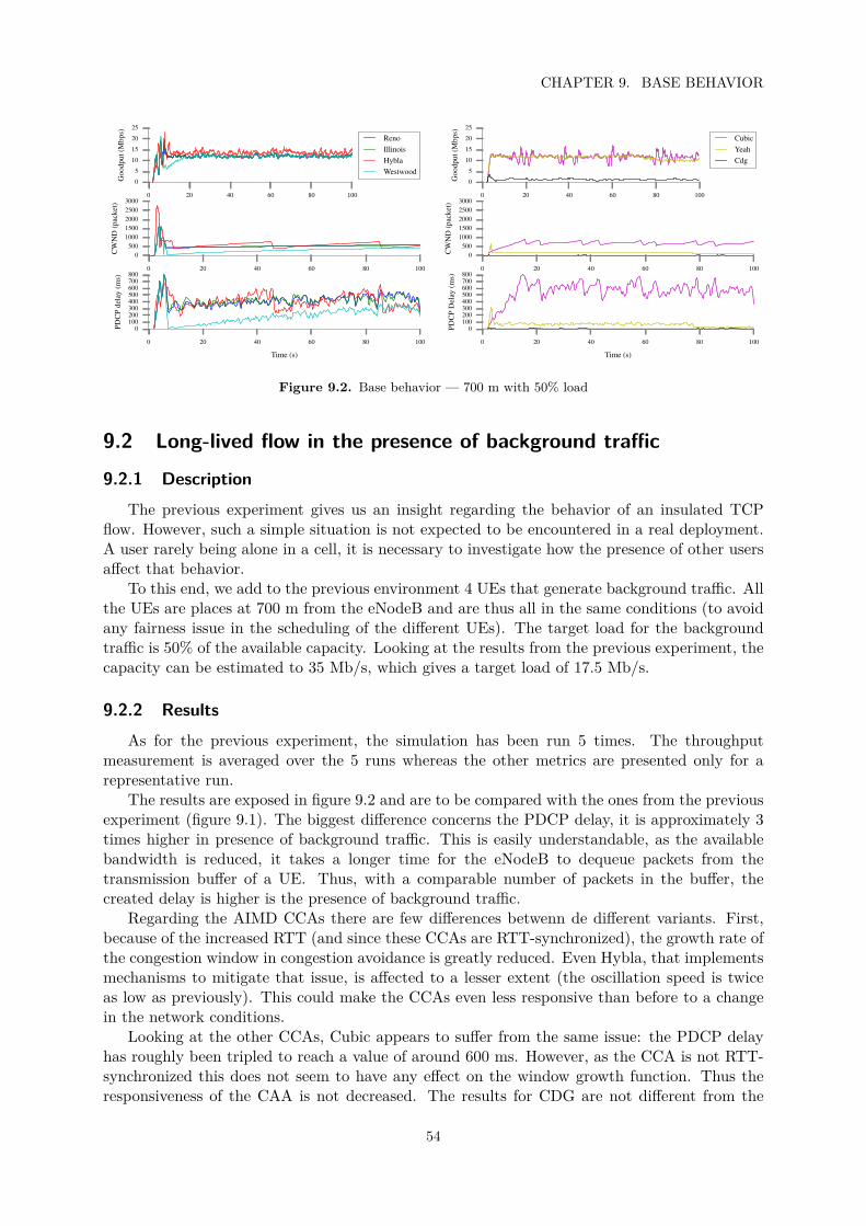
CHAPTER 9. BASE BEHAVIOR

0 20 40 60 80 100

0

5

10

15

20

25G

oodp

ut(M

bps)

RenoIllinoisHyblaWestwood

0 20 40 60 80 100

0500

10001500200025003000

CW

ND

(pac

ket)

0 20 40 60 80 100

Time (s)

0100200300400500600700800

PDC

Pde

lay

(ms)

0 20 40 60 80 100

0

5

10

15

20

25

Goo

dput

(Mbp

s)

CubicYeahCdg

0 20 40 60 80 100

0500

10001500200025003000

CW

ND

(pac

ket)

0 20 40 60 80 100

Time (s)

0100200300400500600700800

PDC

PD

elay

(ms)

Figure 9.2. Base behavior — 700 m with 50% load

9.2 Long-lived flow in the presence of background traffic

9.2.1 DescriptionThe previous experiment gives us an insight regarding the behavior of an insulated TCP

flow. However, such a simple situation is not expected to be encountered in a real deployment.A user rarely being alone in a cell, it is necessary to investigate how the presence of other usersaffect that behavior.

To this end, we add to the previous environment 4 UEs that generate background traffic. Allthe UEs are places at 700 m from the eNodeB and are thus all in the same conditions (to avoidany fairness issue in the scheduling of the different UEs). The target load for the backgroundtraffic is 50% of the available capacity. Looking at the results from the previous experiment, thecapacity can be estimated to 35 Mb/s, which gives a target load of 17.5 Mb/s.

9.2.2 ResultsAs for the previous experiment, the simulation has been run 5 times. The throughput

measurement is averaged over the 5 runs whereas the other metrics are presented only for arepresentative run.

The results are exposed in figure 9.2 and are to be compared with the ones from the previousexperiment (figure 9.1). The biggest difference concerns the PDCP delay, it is approximately 3times higher in presence of background traffic. This is easily understandable, as the availablebandwidth is reduced, it takes a longer time for the eNodeB to dequeue packets from thetransmission buffer of a UE. Thus, with a comparable number of packets in the buffer, thecreated delay is higher is the presence of background traffic.

Regarding the AIMD CCAs there are few differences betwenn de different variants. First,because of the increased RTT (and since these CCAs are RTT-synchronized), the growth rate ofthe congestion window in congestion avoidance is greatly reduced. Even Hybla, that implementsmechanisms to mitigate that issue, is affected to a lesser extent (the oscillation speed is twiceas low as previously). This could make the CCAs even less responsive than before to a changein the network conditions.

Looking at the other CCAs, Cubic appears to suffer from the same issue: the PDCP delayhas roughly been tripled to reach a value of around 600 ms. However, as the CCA is not RTT-synchronized this does not seem to have any effect on the window growth function. Thus theresponsiveness of the CAA is not decreased. The results for CDG are not different from the

54

9.2. LONG-LIVED FLOW IN THE PRESENCE OF BACKGROUND TRAFFIC

previous experiment, the achieved throughput being not high enough to be impacted by thereduction of the capacity.

On the other hand, the results for YeAH are interesting: the CCA manages to reach as highbandwidth as Cubic but is not able to sustain it for all the simulations. In three out of four thebandwidth decreases after a while. The situation appears to be at the limit of what YeAH cansustain. However, it is to be noted that YeAH achieves a throughput very close to the maximumand still keeps the PDCP delay under control, with an average value of around 100 ms, it is farbelow what the other variants achieve.

It can also be noticed that the aggressive behavior of Hybla seems to pay in that situation:the CCA manages to reach a throughput that is slightly higher than the other variants.

9.2.3 ConclusionThe results of this experiment highlight the fact that delay can be a metric as important as

throughput. Almost all the CCAs reach similar throughput. However because of difference intheir mechanisms, they create various amount of queueing delay doing so. In such a situation,the RTT would be the most relevant factor to judge the quality of the connection from a userpoint of view.

When looking at this metric, the only CCA that stands out is YeAH. Compared with theother CCAs it reaches a similar throughput while creating a fifth of the delay. CDG does notcreate a lot of delay, but it is very far from reaching decent throughput and thus cannot beconsidered as a reasonable choice here.

The only difference between the loss based CCAs is how they react to the amount of delaythey created. The RTT synchronized ones become less responsive as their growth rate decreaseswhereas Cubic growth function is not changed and allows it not to be affected by the increasein delay. This effectively gives Cubic a consistent behavior no matter the load that is put onthe network.

55

Chapter 10

Multiple short flows

Previous experiments yield results regarding the behavior of long-live TCP connections.However in a real environment most of the connections are small: in [18] the authors havemeasured 90% of them to have a payload smaller than 35.9 KB of downlink data. Thus, itappears necessary to also study the behavior of the CCAs in that kind of situation.

10.1 DescriptionTo see the evolution of the performance as a function of the total payload size we study a

traffic composed of a series of small TCP connections. The amount of data transferred in eachconnection is drawn from an exponential distribution. A connection starts when all the datafrom the previous one has been received by the UE. In order for all the connections to have thesame initial conditions we disable TCP metric caching in the Linux kernel.

The configuration of the different UEs is the same as before: five UEs are placed at 700 mfrom the eNodeB. One is receiving the flow under study whereas the 4 others are responsible togenerate background traffic with a target load of 50% of the link capacity.

For this scenario, it is cumbersome to present the results as time series. Indeed, the durationof the simulation is rather long. For this reason, we use more synthetic representation of thedata.

In this scenario, to quantify the amount of queueing delay created, we choose to use thequeue transmission buffer length instead of the PDCP delay used previously. Indeed, as wedo not modify the amount of background traffic during this experiment, the two metrics givethe same information. Moreover, with the setup we use, the measurement of the queue lengthis more accurate and easy to process, making for more accurate plots. Indeed, whereas thesampling rate for the delay is only 100 ms, the data for the queue size is gathered every time apacket is enqueued or dequeued. If this what not a problem for time series, we need as muchdata as possible for the ECDF.

10.2 ResultsFigure 10.2 presents the experimental cumulative distribution function (ECDF) of the queue

length for all the TCP connections. Very different pattern can be observed for the differentCCAs.

Surprisingly enough, even the AIMD variants that behave very similarly show very differentrepartitions of the samples. Hybla has most samples between 550 and 650 packets, Reno andIllinois between 200 and 500, Westwood between 0 and 100. This can be explained by twofactors: the backoff strategy and the slow growth rate. Indeed, because of the difference in

57

CHAPTER 10. MULTIPLE SHORT FLOWS

10−3 10−2 10−1 100 101 102

Size (MB)

102

103

104

105

Dur

atio

n(m

s)Duration Vs Size

RenoIllinoisHyblaWestwoodCubicYeAHCDG

10−3 10−2 10−1 100 101 102

Size (MB)

102

103

Dro

p(p

acke

t)

Drop VS Size


Figure 10.1. Multiple Flows — Duration and Dropped packets

0 100 200 300 400 500 600 700 800

Queue size (packet)

0.0

0.2

0.4

0.6

0.8

1.0

cdf

Queue CDF at 700 m

0 2 4 6 8 10 12

Throughput (Mbps)

0.0

0.2

0.4

0.6

0.8

1.0cd

fThroughput CDF at 700 m


Figure 10.2. Multiple Flows — Throughput and Queue ECDF

the reduction of the congestion window at the end of slow start, the different variants startcongestion avoidance with different values of CWND (and thus different queue length). Thisdifference in the filling of the transmission buffer at the beginning of congestion avoidance causesdifferences in the lower bound of the most populated area for each CCA. On the other hand,the difference in the upper bound can be explained by the small CWND growth rate coupledwith the relatively small size of the connections. Indeed, as seen in the previous experiment, thegrowth rate is very low in the presence of congestion. Thus, among these CCAs none has timeto completely fill the transmission buffer.

A similar analysis can be made to explain the results for Cubic. Because of the faulty hybridslow start, the congestion avoidance phase is started with a very low CWND. Then it growsduring congestion avoidance. As already mention the CWND growth rate of Cubic was fasterthan those of the AIMD CCAs. This can be observed here too. Indeed, if Westwood and Cubicstart congestion avoidance with similar CWND values, Cubic is able to grow the window muchmore: up to completely filling the buffer.

Looking at the results for TCP YeAH, the CCA seems to have a better control over thequeue length. Most samples are located between 50 and 100 packets, allowing for the maximumthroughput to be reached while limiting the queueing delay.

58

10.3. CONCLUSION

Based on these results regarding the queue usage of the different variants, it is possible toexplain the differences that show on figure 10.1 regarding the amount of dropped packets.

For the loss-based CCAs, the aggressivity translates into the size of the connection for whichthe first drop appears. Hybla, that has a slow start algorithm that can be more aggressive thanReno, experiences drops for smaller flows (starting at around 1.8 MB against 3 MB for Reno).On the other hand, because of the Hybrid slow start Cubic does not experience loss at th end ofslow start. The first loss only occurs after the congestion window has been grown in CongestionAvoidance, delaying the first loss to flow sizes of around 20 MB. In this specific case, Hybridslow start seems to have a positive effect as it decreases the amount of losses and does not impactthe transfer duration.

Looking at the amount of dropped packets, it appears to be influenced by the aggressivityand backoff stratefy. Indeed, if Reno and Westwood have show nearly identical results, Illinoissuffer from more losses. This could be explain by the CCA not reducing enough its window ina first time, thus inducing more dropped packet and another window reduction. As for Hybla,the higher drop count can be explained by an increased overshoot at the end of slow start, dueto the faster window growth.

Once again, when compared with its loss based counterparts YeAH displays better perfor-mance. It does not suffer from any dropped packet either in congestion avoidance or slow start.

If the results present noticeable differences between the CCAs regarding queue length anddrop count, this is not the case regarding the transfer durations and throughput. Looking atfigure 10.1, it appears that all the CCAs (but CDG) have very similar transfer durations. Theonly differences being CDG that becomes slower from around 200 KB and Hybla that seemsa little bit faster between 100 kB and 1 MB. This last observation is in accordance with theprevious result showing that Hybla achieved a higher throughput than the other CCAs in acongested network. It can also be noticed that Westwood start becomes slower than the otherCCAs from sizes around 8 MB. Once again, this can be explain by the results of the previousexperiements. It was already noticed that Westwood is suffering from a decreased aggressivitybecause of the excessive backoff.

Looking more precisely at the throughput results on figure 10.2, it confirms that Westwoodstruggles to achieve the same throughput as the other AIMD CCAs. The other major differencethat can be noticed is YeAH being faster to reach the maximum throughput than the otherCCAs.

Looking more closely at the higher part of the plot, it can be noticed that Cubic and YeAHhave less samples above 10 Mb/s than the other CCAs. As these throughput are very uncommon,they are mostly due to the spikes in the measurement after congestion events. Looking at therarity of these samples we can assume that YeAH and Cubic suffer from less losses than theother CCAs.

10.3 Conclusion

Several conclusions can be drawn from this simulation. First, from the point of view of thetransfer duration, there are very little differences between all the CCAs. Thus this is not basedon that criterion that they can be differentiated (even if Hybla seems a little bit faster).

The real difference lies in the constraint they put on the transmission buffer. In that aspectthe amount of dropped packets and queue that are generated differ among the CCAs. In orderto use the resources of the eNodeB as efficiently as possible it would be good to have a CCA thatis able to limit the queue it creates. In that aspect, only YeAH appears to be able to explicitlycontrol it. For the other CCAs the queue usage is indirectly dictated by the network conditions,

59

CHAPTER 10. MULTIPLE SHORT FLOWS

growth function and backoff strategy, making it hard to have a predictable behavior.

60

Chapter 11

Hybrid slow start

Looking at the previous experiments, it appears that the Hybrid Slow Start mechanism isless aggressive than the standard one. In some cases the exit is triggered very early and far fromfull link utilization. If this prevent losses to happen, this also slows down the connection as thewindow growth has to happened during congestion avoidance (when it is slower).

This chapter presents a study of this mechanism in different conditions and aims at findingout whether its effect on performance is positive or not.

11.1 Optimal Radio conditions

11.1.1 Description

The easiest way to study the impact of the mechanism is to compare the performance (interm of throughgput and delay) with and without it. Using the method described in chapter 6we added a kernel parameter allowing us to toggle the activation of the mechanism.

Then, using the same scenario as for the previous experiment, it is possible to compare theresults of Cubic, with and without Hybrid slow start, while performing multiple short connectionsin a network with and without background traffic.

To bgein we consider the best possible radio conditions with the UE being placed at 100 mfrom the eNodeB.

11.1.2 Results

Figure 11.1 shows the results without load and with a load of 90 %. Far from having anegative impact, the Hybrid Start performs equally well and might even induce a little lessqueue on a congestion free network. Moreover, on a congested network the Hybrid Start is alittle bit faster than the regular mechanism and uses less queue, thus causing fewer packets tobe dropped.

In good radio conditions the mechanism seems to have a positive impact on the performanceof the CCA. The earlier exit does not seem to slow down the connection. Reducing the amountof losses compensates for the slower window growth. It also allows for better queue management,effectively decreasing the average queue size in the loaded network.

61

CHAPTER 11. HYBRID SLOW START

103 104 105 106 107 108

Size (byte)

01000200030004000500060007000

Dur

atio

n(m

s)

100 m - No Load

103 104 105 106 107 108

Size (byte)

0500

1000150020002500300035004000

Dro

p(p

acke

ts)

HS OnHS Off

103 104 105 106 107 108

Size (byte)

0100200300400500600

Ave

rage

queu

esi

ze(p

acke

t)

103 104 105 106 107 108

Size (byte)

0

5000

10000

15000

20000

Dur

atio

n(m

s)

100 m - Load 90

103 104 105 106 107 108

Size (byte)

0500

1000150020002500

Dro

p(p

acke

ts)

HS OnHS Off

103 104 105 106 107 108

Size (byte)

0100200300400500600

Ave

rage

queu

esi

ze(p

acke

t)

Figure 11.1. Hybrid Start Effect — Optimal Radio Conditions

11.2 Degraded Radio conditions

11.2.1 DescriptionAs already explained, the hybrid slow start mechanisms are based on delay estimations, thus

they could be quite sensitive to noise in the measurement. To investigate that possibility, werepeat the previous experiment with a distance of 1000 m between the eNodeB and the UE.

11.2.2 ResultsFigure 11.2 presents the results. In a congestion free environment, hybrid start has a negative

impact on the connection duration: in some case it more than doubles it. On the other hand,its effects on the buffer length and drops is positive. It appears that the exit is trigger too early,leaving the growth of the window to happen in the congestion avoidance phase, where it is muchslower.

However, in the presence of congestion the impact of the hybrid slow start decreases. Themeasurements show it to be sometimes a little bit faster than the regular algorithm, but notas often as with optimal radio conditions. If the effect on the throughput is negligible, it stilldecreases the amount of loss and queueing. Globally its impact on the performance is positive.

To go further, we decide to try to identify more precisely the cause of the problem. Indeed,as explained before the Hybrid Start algorithm uses 2 mechanisms to trigger the exit. One basedon ACK trains that estimated throughput and the other one based on the first ACKs of a burstto detect any increase in delay.

It is likely that one of these mechanisms is not functioning properly and triggers the exitspuriously. Thus we added options to the cubic implementation that allows us to choose whichmechanism to enable using sysctl. Using this possibility each mechanism is insulated and studiedindependently of the other.

Running the scenario with only the ACK Train based detection gives the same results aswithout the Hybrid Start. Thus this mechanism is not responsible for any early exit. This leavesonly the delay based to be blamed. Running the test with only this mechanism confirms it, asthe early exit reappears.

Knowing which mechanism is faulty the interesting thing is now to find out why the exit istriggered too early. Thie mechanism is based on the detection of an increase in delay, the value

62

11.2. DEGRADED RADIO CONDITIONS

103 104 105 106 107 108

Size (byte)

02000400060008000

1000012000

Dur

atio

n(m

s)

1000 m - No Load

103 104 105 106 107 108

Size (byte)

0500

1000150020002500

Dro

p(p

acke

ts)

HS OnHS Off

103 104 105 106 107 108

Size (byte)

0100200300400500600

Ave

rage

queu

esi

ze(p

acke

t)

103 104 105 106 107 108

Size (byte)

010000200003000040000500006000070000

Dur

atio

n(m

s)

1000 m - Load 90

103 104 105 106 107 108

Size (byte)

0500

1000150020002500

Dro

p(p

acke

ts)

HS OnHS Off

103 104 105 106 107 108

Size (byte)

0100200300400500600700

Ave

rage

queu

esi

ze(p

acke

t)

Figure 11.2. Hybrid Start Effect — Degraded Radio Conditions

is computed from the 8 first samples of a train and compared to a threshold. There is no filteringfor the RTT value, the minimal value among the first 8 of a flight is taken. The problem couldbe that an increase in delay caused by something else than congestion triggers the mechanism(as already mentioned, several LTE mechanisms as well as radio conditions could easily inducesuch a problem).

There is no built-in mechanism to allow access to the value of the delay measurement.Thus we modified the cubic implementation in order to output the value using the kernel printfunction. Even if quite basic, this gives us a crude access to the estimate.

It reveals that the measured delay has a high variance, that is probably due to the radiocondition, which triggers the early exit. Moreover most of the time the eight samples taken toestimate the delay are the same and thus there is no need for a more advanced filtering. Withonly 8 samples this would have been at best ineffective anyway.

Thus the only solution left would be to make this mechanism less sensitive (by increasing thethreshold or waiting for several measurements before exiting for instance). However, as samplesare taken only at the beginning of a flight lowering the sensitivity could have a very negativeeffect on the performance for the flows with a better radio quality. Indeed, as the congestionwindow size grows the duration of a flight increases. Thus decreasing the sensitivity might easilypostpone the exit after the first loss occurs, making it useless.

As a quick workaround, it would be possible to use the low window parameter of the CCA.This parameter allows the user to choose aminimal window size from which the Hybrid Startwill be applied. Thus, in cases when the Hybrid Start is not functioning properly, this wouldguarantee a minimal value for the CWND when the Congestion Avoidance phase is reached. Nomatter what value we choose, the tuning could not be too aggressive as in the worst case theslow start will be stopped by the regular mechanism.

It would also be interesting to investigate the behavior of the train based mechanism. Ac-cording to Hybrid Start presentation article [14] there are two cases when Hybrid Start is knownnot to work well: when the reverse path is congested or when the reverse path delay is muchsmaller than the forward path’s one. The only flow on the network being the tested one, thereis no reason for the reverse path to be congested or to have a lower delay than the forward path.

Once again, adding print statement directly inside the code allows us to gather the data weneed, in that case we were interested in two values: the duration of the train and the spacingbetween two consecutive ACK. Indeed not to break the train two ACK must not be separated

63

CHAPTER 11. HYBRID SLOW START

by more than 2 ms. Looking at the data we see that very quickly all the trains are broken andthus no measurement are made at all, effectively disabling that mechanism.

Even if there is a tunable parameter implemented in the module that allows the user todefine the maximum delay between two ACK, it cannot be used to solve the problem. Indeed,at a distance of 1000 m the gap between two ACKs can be very close to the threshold for theduration of the entire train. Thus, it appears that the mechanism will not be able to workproperly for high distances. However, increasing that threshold might allow it to work for abigger area.

11.3 ConclusionIf the Hybrid Start mechanism gives good results when the radio conditions are good, its

effects get worse as the link deteriorates. Going as far are slowing down the connection.The delay based mechanism can be triggered spuriously, because of fluctuations in the RTT,

seriously crippling the window for the rest of the connection.Moreover the second mechanism, being unable to get a long enough packet train, is simply

not working.It seems that in its actual state this mechanism is not well suited to be used in a radio

network. However, because of the positive impact it has when working properly it would be aloss to disable it altogether. Thus, using the low window parameter might be a good solutionto prevent it from causing too much harm while keeping its positive sides.

It is to be noted that this section only presents results regarding the version of the mechanismused in the Linux kernel implementation of the Cubic CCA. There is another variant that isused in the CDG CCA which, even if based on cubic one, is slightly different and thus mightbehave differently.

64

Chapter 12

Conclusion

12.1 Outcomes

During this thesis, we have developed a simulation environment, allowing for the simulationof TCP traffic in an LTE network. We designed and ran simulations using this setup to study thebehavior of the major TCP variants in this specific environment. Finally analyzing the resultswe were able to get a better understanding of the functioning of the different TCP variants inan LTE network.

Regarding the development of the simulation evironment, the objectives are almost com-pletely fulfilled. Through the usage of the DCE Cradle we are able to study the behavior ofthe Linux implementations of the different CCAs. Moreover, the usage of the ns-3 simulatorallowed us to entirely control our test environment making it trivial to reproduce any result.Furthermore, the LENA simulator allowed for an accurate behavior of the data place of theLTE stack. However, it must be noticed that we were not able to compare our results withmeasurements made using a real eNodeB. Thus, we cannot be completely sure of the accuracyof our simulations.

As for the scenarios that were designed, we were able to study the behavior of TCP variantswhen faced with different traffic types and congestion level in the cell. However, we did no gofar enough to be able to understand the behavior in more elaborate scenarios with a moving UE.For that reason, such scenarios were not studied. Moreover, while running our simulations wewere able to gather performance metrics (goodput, eNodeB queue length, PDCP delay) as wellas internal TCP information (CWND) that allowed us to understand the results. Except for theinclusion of the mobility as a test parameter, all the objectived regarding the test scenarios arefullfilled.

Analyzing the results, we were able to draw several conclusions. First, the loss-based anddelay-based CCAs have very different behaviors. While the formers easily reach full link uti-lization but induce high queueing delays, the latters have a good control over the delay but arenot always able to take advantage of the full bandwidth. These differences can be explained byseveral characteristics of the LTE environment. The big buffer dedicated to each UE combinedwith the loss-based mechanisms are resposible for the huge delays. On the other hand, the fastvariations of the delay decrease the reliability of the delay-based mechanisms and cripple thethroughput of these TCP variants. Based on this data, it is yet not possible to define a CCA asbeing best fitted for a usage in LTE networks.

65

CHAPTER 12. CONCLUSION

12.2 Future WorksThe work initiated in this thesis can be pursued in several directions, for the different usages

mentioned above.

In a research context, the simulator could be used as it is currently to gain a depper under-standing and improve the existing congestion control algorithms. Such works could be under-taken for instance to try to find more fitting parameters for the different variants. It could alsobe interesting to study the reasons behind the bad performance of TCP CDG and correct theimplementation.

In this context, the simulator could also be extended to cover more scenarios. Conductingsimulation to investigate the behavior of the different TCP variants when the UE is movingwould be the logical next step. More KPIs could be added too, allowing for a deeper study onthe LTE side.

In an industrial context, the automation of the simulator could be pursued to allow for aneasier integration into an existing system for the development and test of congestion controlalgorithms. The present setup requires manual operation regarding the compilation of the ker-nel library, as well as for some parts of the installation. The ideal goal would be an automatedworkflow that would, starting from the source code of a CCA, compile the kernel, run the definedsimulations and output the results in a way that would allow them to be automatically processed.

66

Bibliography

[1] Stefan Alfredsson et al. “Impact of TCP congestion control on bufferbloat in cellularnetworks”. In: Proceedings of 14th International Symposium and Workshops on a Worldof Wireless, Mobile and Multimedia Networks (WoWMoM).

[2] M. Allman. TCP Congestion Control with Appropriate Byte Counting (ABC). RFC 3465(Experimental). Internet Engineering Task Force, Feb. 2003. url: http://www.ietf.org/rfc/rfc3465.txt.

[3] R. Braden. Requirements for Internet Hosts - Communication Layers. RFC 1122 (INTER-NET STANDARD). Updated by RFCs 1349, 4379, 5884, 6093, 6298, 6633, 6864. InternetEngineering Task Force, Oct. 1989. url: http://www.ietf.org/rfc/rfc1122.txt.

[4] Carlo Caini and Rosario Firrincieli. “TCP Hybla: a TCP enhancement for heteroge-neous networks”. In: International journal of satellite communications and networking22.5 (2004), pp. 547–566.

[5] CTTC Centre Tecnològic de Telecomunicacions de Catalunya. Design Documentation Lenav8 documentation. 2015. url: http://lena.cttc.es/manual/lte-design.html#mac(visited on 11/20/2015).

[6] J. Chu et al. Increasing TCP’s Initial Window. RFC 6928 (Experimental). Internet Engi-neering Task Force, Apr. 2013. url: http://www.ietf.org/rfc/rfc6928.txt.

[7] Erik Dahlman, Stefan Parkvall, and Johan Sköld. 4G: LTE/LTE-advanced for mobilebroadband. Academic press, 2013.

[8] Peter L Dordal. An Introduction to Computer Networks. 2016.[9] Constantinos Dovrolis, Parameswaran Ramanathan, and David Moore. “Packet-dispersion

techniques and a capacity-estimation methodology”. In: Networking, IEEE/ACM Trans-actions on 12.6 (2004), pp. 963–977.

[10] S. Floyd. Metrics for the Evaluation of Congestion Control Mechanisms. RFC 5166 (In-formational). Internet Engineering Task Force, Mar. 2008. url: http://www.ietf.org/rfc/rfc5166.txt.

[11] S. Floyd and T. Henderson. The NewReno Modification to TCP’s Fast Recovery Algorithm.RFC 2582 (Experimental). Obsoleted by RFC 3782. Internet Engineering Task Force, Apr.1999. url: http://www.ietf.org/rfc/rfc2582.txt.

[12] Sangtae Ha and Injong Rhee. “Taming the elephants: New TCP slow start”. In: ComputerNetworks 55.9 (2011), pp. 2092–2110.

[13] Sangtae Ha and Injong Rhee. “Towards a Common TCP Evaluation Suite”. In: ().[14] Sangtae Ha, Injong Rhee, and Lisong Xu. “CUBIC: a new TCP-friendly high-speed TCP

variant”. In: ACM SIGOPS Operating Systems Review 42.5 (2008), pp. 64–74.

67

http://www.ietf.org/rfc/rfc3465.txt



http://lena.cttc.es/manual/lte-design.html#mac





BIBLIOGRAPHY

[15] Bruce Hajek. “Stochastic approximation methods for decentralized control of multiaccesscommunications”. In: Information Theory, IEEE Transactions on 31.2 (1985), pp. 176–184.

[16] David A Hayes and Grenville Armitage. “Revisiting TCP congestion control using delaygradients”. In: NETWORKING 2011. Springer, 2011, pp. 328–341.

[17] Junxian Huang et al. “An in-depth study of LTE: effect of network protocol and applica-tion behavior on performance”. In: ACM SIGCOMM Computer Communication Review.Vol. 43. 4. ACM. 2013, pp. 363–374.

[18] Junxian Huang et al. “An in-depth study of LTE: Effect of network protocol and applica-tion behavior on performance”. In: ACM SIGCOMM Computer Communication Review.Vol. 43. 4. ACM. 2013, pp. 363–374.

[19] R Itu. “{ITU-R M. 2135: Guidelines for evaluation of radio interface technologies for IMT-Advanced}”. In: (2008).

[20] V. Jacobson and R.T. Braden. TCP extensions for long-delay paths. RFC 1072 (Historic).Obsoleted by RFCs 1323, 2018, 6247. Internet Engineering Task Force, Oct. 1988. url:http://www.ietf.org/rfc/rfc1072.txt.

[21] Van Jacobson. “Congestion avoidance and control”. In: ACM SIGCOMM computer com-munication review. Vol. 18. 4. ACM. 1988, pp. 314–329.

[22] Ingemar Johansson. Congestion control for 4G and 5G access. Internet-Draft draft-johansson-cc-for-4g-5g-00. http : / / www . ietf . org / internet - drafts / draft - johansson - cc -for-4g-5g-00.txt. IETF Secretariat, 2015. url: http://www.ietf.org/internet-drafts/draft-johansson-cc-for-4g-5g-00.txt.

[23] Markus Laner et al. “A Comparison between One-Way Delays in Operating HSPA andLTE Networks”. In: Proceedings of 10th International Symposium on Modeling and Opti-mization in Mobile, Ad Hoc and Wireless Networks (WiOpt). IEEE. 2012, pp. 286–292.

[24] Shao Liu, Tamer Başar, and Ravi Srikant. “TCP-Illinois: A loss-and delay-based conges-tion control algorithm for high-speed networks”. In: Performance Evaluation 65.6 (2008),pp. 417–440.

[25] Saverio Mascolo et al. “TCP westwood: Bandwidth estimation for enhanced transportover wireless links”. In: Proceedings of the 7th annual international conference on Mobilecomputing and networking. ACM. 2001, pp. 287–297.

[26] Jeffrey C Mogul. Observing TCP dynamics in real networks. Vol. 22. 4. ACM, 1992.[27] J. Nagle. Congestion Control in IP/TCP Internetworks. RFC 896. Internet Engineering

Task Force, Jan. 1984. url: http://www.ietf.org/rfc/rfc896.txt.[28] Binh Nguyen et al. “Towards understanding TCP performance on LTE/EPC mobile net-

works”. In: Proceedings of the 4th workshop on All things cellular: operations, applications,& challenges. ACM. 2014, pp. 41–46.

[29] V. Paxson et al. Computing TCP’s Retransmission Timer. RFC 6298 (Proposed Standard).Internet Engineering Task Force, June 2011. url: http://www.ietf.org/rfc/rfc6298.txt.

[30] J. Postel. Transmission Control Protocol. RFC 793 (INTERNET STANDARD). Updatedby RFCs 1122, 3168, 6093, 6528. Internet Engineering Task Force, Sept. 1981. url: http://www.ietf.org/rfc/rfc793.txt.

68


http://www.ietf.org/internet-drafts/draft-johansson-cc-for-4g-5g-00.txt









BIBLIOGRAPHY

[31] W. Stevens. TCP Slow Start, Congestion Avoidance, Fast Retransmit, and Fast RecoveryAlgorithms. RFC 2001 (Proposed Standard). Obsoleted by RFC 2581. Internet EngineeringTask Force, Jan. 1997. url: http://www.ietf.org/rfc/rfc2001.txt.

[32] Hajime Tazaki, Frédéric Urbani, and Thierry Turletti. “DCE cradle: simulate networkprotocols with real stacks for better realism”. In: Proceedings of the 6th International ICSTConference on Simulation Tools and Techniques. ICST (Institute for Computer Sciences,Social-Informatics and Telecommunications Engineering). 2013, pp. 153–158.

[33] Hajime Tazaki et al. “Direct Code Execution: Revisiting Library OS Architecture forReproducible Network Experiments”. In: Proceedings of 9th ACM Conference on EmergingNetworking Experiments and Technologies. ACM. 2013, pp. 217–228.

[34] Lixia Zhang, Scott Shenker, and Daivd D Clark. “Observations on the dynamics of a con-gestion control algorithm: The effects of two-way traffic”. In: ACM SIGCOMM ComputerCommunication Review 21.4 (1991), pp. 133–147.

69


TRITA TRITA-EE 2016:085

www.kth.se

Comparative study of the performance of TCP congestion ...

Documents

Transcript of Comparative study of the performance of TCP congestion ...