Development of a coupled flow and solute transport modelling for Astaneh-Kouchesfahan groundwater...

80 Int. J. Water, Vol. 7, Nos. 1/2, 2013

Copyright © 2013 Inderscience Enterprises Ltd.

Development of a coupled flow and solute transport modelling for Astaneh-Kouchesfahan groundwater resources, North of Iran

Masoud Saatsaz* Department of Geology, Institute for Advanced Studies in Basic Sciences (IASBS), 45195-1159 IASBS Zanjan, Zanjan, Iran E-mail: [email protected] *Corresponding author

Wan Nor Azmin Sulaiman Department of Environmental Science, University Putra of Malaysia, 43400 UPM Serdang, Selangor, Malaysia E-mail: [email protected]

Saeid Eslamian Water Department, Isfahan University of Technology, Isfahan 8415683111, Iran E-mail: [email protected]

Saman Javadi Irrigation and Drainage Engineering Department, Water Research Institute, Tehran 1658954381, Iran E-mail: saman.javadi@ gmail.com

Abstract: Astaneh-Kouchesfahan Plain is an important source of groundwater in Northern Iran. In the study area, rational management of groundwater resources requires a precise evaluation of groundwater flow and transport components. For this purpose, a 2-dimentional groundwater flow and solute transport model was developed and calibrated using PMWIN 5.3. Simulation results under steady-state and transient conditions show that the horizontal hydraulic conductivity values range from 1 to 23 m/day; and the specific yield values range between 0.03 and 0.25. After construction groundwater flow model, in order to simulate and predict chloride transport in the study area, a 2-D solute transport model for the aquifer has been developed, calibrated and validated using MT3D. The predictive simulation from October 2009 to October 2012 shows that according to present recharge and discharge conditions, groundwater salinities will increase and in the mid and long-term, groundwater consumers will be facing a worse situation than the present.

Development of a coupled flow and solute transport modelling 81

Keywords: groundwater simulation; hydrogeology; Iran; MT3D; numerical modelling; PMWIN.

Reference to this paper should be made as follows: Saatsaz, M., Sulaiman, W.N.A., Eslamian, S. and Javadi, S. (2013) ‘Development of a coupled flow and solute transport modelling for Astaneh-Kouchesfahan groundwater resources, North of Iran’, Int. J. Water, Vol. 7, Nos. 1/2, pp.80–103.

Biographical notes: Masoud Saatsaz is an Assistant Professor at the Institute for Advance Studies in Basic Sciences (IASBS) of Zanjan, Iran. He received his MSc in Hydrogeology from Shahid Chamran University of Iran and his PhD in Environmental Hydrology and Hydrogeology from University Putra of Malaysia in 2011. His fields of interest are groundwater modelling and simulation, water resources management, environmental hydrogeology, pollution and hydro-geochemistry studies.

Wan Nor Azmin Sulaiman is an Associate Professor in University Putra of Malaysia. His fields of research are environmental hydrology and hydrogeology, groundwater modelling and simulation, water recourses management and hydrochemistry studies.

Saeid Eslamian is a Professor in Isfahan University of Technology, Iran. He has published a large number of scientific books, reports, and journal and conference papers. He has been successful in a number of research grants. He displays an extensive teaching experience in hydrology, hydrometeorology, water resources and groundwater, particularly in civil, agricultural and natural resources area.

Saman Javadi received his PhD in 2010 from the University of Tarbiat Moddaress at Tehran. His research focus is groundwater modelling and simulation, water protection studies and irrigation and drainage engineering sciences.

1 Introduction

Groundwater is one of the major supplies of water resource in many countries and supports human health, socio-economic development and ecological diversity. In north of Iran, groundwater plays an important role to supply water and about two-thirds of people are directly or indirectly dependant to this vital resource (PBO, 2006). Astaneh-Kouchesfahan Plain is an important water resource system in Gilan Province. It is one of the largest plains in north of Iran and by area it comprises about 15% of Gilan. In Astaneh-Kouchesfahan Plain, a permeable aquifer system provides water for industrial, agricultural and domestic usages. In the area, however, rapid population growth and low irrigation efficiency in agricultural sector have increased the demand for groundwater resources. It is important to note that according to the latest census data, in Iran, the average population density is 41 inhabitants per square km, but it ranges up to more than 150 inhabitants per square km in the Gilan province which is by far the most densely populated region in the country (PBO, 2006).

82 M. Saatsaz et al.

Considering above explanation and in order to prevent quality and quantity damages to groundwater resources, rational management should be considered as a basic principle in the short and long term-plans for the area. Proper groundwater management is based on availability of correct and complete hydrogeological data. However, for many reasons such as the lack of data, availability of the unreliable data and being non-functional information, the study area is subjected to mismanagement in groundwater resources.

Although lack of basic and detailed investigations is one of the main problems in the groundwater resources management of Astaneh-Kouchesfahan Plain, this plain is faced with other problems too. Astaneh-Kouchesfahan Plain is one of the agricultural poles and groundwater is the one of the most important water resources to meet agricultural needs. In some areas, in spite of presence plenty of groundwater resources, rural people are deprived of the required irrigation water. On the other side, some cultivable areas are under threat of high groundwater levels due to inappropriate management and partial use of groundwater resources. Rising groundwater levels have resulted in secondary soil salinity and soil salinity has caused the plain subjected to more erosion and desertification. In addition, rising groundwater levels have made more vulnerability to pollution. Reduction in quality of groundwater, soil erosion and secondary salinity are among the main causes of reduction in productivity and fertility of the cultivable lands. These problems have caused some difficulties for socio-economical development in the area which has led to decrease of family income, unemployment and finally emigration of rural people. For overcoming a part of these difficulties, development of a coupled groundwater flow and transport model, as an effective tool, has been proposed for managing groundwater resources and predicting future responses in the aquifer. The final results of this work can be useful for future studies, short and long-term plans, programmes and projects related to water resource management and protection. The following describes characteristics of the modelled area and describes the process and methods used in the study.

1.1 Description of the study area

Astaneh-Kouchesfahan Plain is one of the most important sources of groundwater in the province of Gilan located between Tehran and southern basin of the Caspian Sea in north part of Iran. Geographical Location of the plain is 35° 34’ 00’’ to 35° 48’ 00” North latitude, 49° 30’ 00’’ to 50° 15’ 00” East longitude (Zone 39N in UTM System: WGS 1984) and covering an area of 1,343 km2 with a mean altitude 25 m above sea levels (Figure 1). The area generally enjoys warm and humid summers (August, 40°C) with mild winters (February, 5°C). Considering a typical pattern of moist subtropical mid-latitude climate, the regional climatic setting of the area can be categorised as Mediterranean climate. The annual precipitation for the last 45 years averaged 1,430 mm (GRWO, 2005). Most of the precipitation, approximately 40.8% has fallen during winter, 25.8% in spring, 20% in autumn and 13.4% in summer season. The aridity of the area based on De Martonne (1926) indicator is classified as wet area.


Figure 1 Geographical location of Astaneh-Kouchesfahan Plain in north of Iran (see online version for colours)

The geology and structural geology of study area has been outlined by Berberian (1983), Darvishzadeh (2002) and Aghanabati (2004) and mapped at the 1:1000000 scales by the Geological Survey of Iran (2004). The area of concern is geologically located on the south Caspian Sea Basin and known as a northern part of the Alborz Tectonical Range in Alpine Fold Belt. The metamorphic and calcareous stones of Paleozoic, (Mobarak Formation) which have small outcrops in south of Rasht City, comprise the oldest formations in the study area. All stratigraphic units cropping out within the region are ranged from Paleozoic and Quaternary Era. In the southwestern parts of the plain, the Mesozoic-aged formations including limestone, sandstone, conglomerate and volcanic deposits (Shamshak, Shall and early to late Cretaceous formations) constitute the outcrops with more thickness and mainly construct the major structural features. However, due to the tectonical activities Cretaceous-aged deposits are removed by erosion prior to the latest sedimentary cycle commencing in the early Pliocene. Hence, the older formations with a distinct unconformity overlain directly by sediments of Pliocene and younger age (Mousavi-Rouhbakhsh, 2001). Cenozoic-aged deposits are widespread in the study area. Based on the regional geology map shown in Figure 2, most of the study area is covered by recent alluviums which are unconsolidated Pleistocene and Holocene deposits such as coastal deposits, stream deposits, beach deposits, deluvial facies, alluvial facies and alluvial fan deposits. These alluvial deposits consist mainly of mud, silty clay, and fine sand and locally contain coarse sand and gravel layers. The thickness, stratigraphic sequence and depth to bedrock of these deposits vary spatially. However, these sediments contain the main productive groundwater zone and hence most tapped aquifer in Astaneh-Kouchesfahan Plain.


Figure 2 The geological map of study area (see online version for colours)

2 Methods

Over the past three decades, the application of groundwater modelling has increased significantly in the hydrogeological, hydrochemical and environmental studies. In many fields of water sciences, groundwater flow, fate and transport models are used for the description and prediction of the behaviour of groundwater systems and results are used for system management and risk analysis.

A considerable amount of literature has been published on application of numerical groundwater modelling, especially in the past three decades (Luckey et al., 1986; Al-Khatib, 1999; Park, 2000; Kashaigili et al., 2003; Kennedy, 2003; Calderon, 2004; Rojas, 2005; Ross et al., 2005; Nastev et al., 2005; Moncrieff, 2006). In Iran, application of numerical modelling of groundwater is a relatively new field; it was not widely pursued until the end of 1990s. Since the end of 1990s, several groundwater models were subsequently developed to mathematically describe the flow and transport of pollution in the subsurface (Khayyat Kholghi, 2002; Mahjouri et al., 2005; Taheri Tizro et al., 2007; Rahnama and Mirabbasi, 2010). The majority of these studies have focused on groundwater flow modelling and only few attempts have been made to assess groundwater quality and potential pollution at the aquifer scale. However, because of growing evidence that the quality of the subsurface environment is being adversely affected by human activities and increase in public concern, the focus point of Iranian researchers has recently shifted from water demand issues to environmental studies issues.

In this study, a 2-dimentional groundwater numerical model was developed, calibrated and validated to simulate groundwater flow under steady-state and transient conditions; to estimate hydrogeological coefficients values of aquifer [e.g., hydraulic conductivity, specific yield (Sy)]; to predict hydraulic heads and finally, and as a prerequisite, to develop a contamination-transport model of chemical contaminants in groundwater. The basic steps in developing flow and solute transport model of the aquifer are described in more detail in the following paragraphs.


2.1 Conceptual model development

Based on available geological cross sections, geological survey and well logs data, the conceptual model of study area was constructed and it showed that Astaneh-Kouchesfahan Plain contains an unconfined aquifer corresponding to the Quaternary alluvial sediments (GRWO, 2005). The maximum aquifer thickness is 250 m in the middle and minimum is 25 m in the north of the plain. The model domain is limited in the west and east by the geological contact zone defined between the basement complex rocks of Triassic-Jurassic formations, Jurassic-Cretaceous formations and Cretaceous formations and the sedimentary materials of Cenozoic. The southern boundary is defined by opening of alluvial fans of Sefīd-Rūd River corresponding to equipotential line of 40 m. The northern boundary is along coastal lines with a distance of about 50 km. These boundaries define an area of 941 km2 with a maximum length of 44 km and width of 33 km. Depending on recharge and discharge factors, the level of groundwater is variable, but average groundwater level is typically about 40 m above sea level in the south and 25 m below sea level in the north of plain. Recharge components consist of rainfall, recharge due to irrigation return, sewage return, lateral subsurface inflow, and influent seepage from rivers. Discharge components include evapotranspiration from groundwater table, groundwater draft, lateral subsurface outflow, and effluent seepage to the rivers (Saatsaz et al., 2009). Sefīd-Rūd River always plays a significant role in the distribution and movement of groundwater in the area and based on its stage can act as a groundwater discharge point or as a source of recharge to the groundwater system. Assessment of groundwater-table elevation contours indicate that groundwater has a regional direction from south to north and it indicates that south part of the plain is recharging point and north parts of the plain are discharging points of the area (Figure 3). Considering groundwater flow direction, hence, the western and eastern boundaries were considered as no-flow boundaries.

In the study area a few pumping tests have been performed in different parts of aquifer. Results for the pumping tests of wells were approximated and verified using the Theis (1937) method and Cooper and Jacob (1946) equations. The results of pumping tests have indicated that the transmissivity in the plain on the basis of Theis method and Cooper-Jacob method varies from 500 (m2/day) in northwest part of the area to 4,000 (m2/day) in the middle part of plain. In the middle of plain between Rasht and Astaneh, the transmissivity has been calculated 2,000 (m2/day) on the basis of Darcy tube formula. The results of performed tests also have indicated that the Sy in the plain on the basis of Theis method and Cooper-Jacob method varies from 0.01 to 0.3 (GRWO, 2005).

2.2 Computer code selection

The flow simulation was carried out using processing MODFLOW (PMWIN) version 5.3, a public domain product of Chiang and Kinzelbach (2001). PMWIN is one of the complete finite-difference simulation systems in the world. PMWIN supports the simulation of the effects of recharge and evapotranspiration, wells, rivers, drains, reservoirs, head-dependent boundaries, time-dependent fixed-head boundaries, compaction and subsidence. In addition, PMWIN support many packages such as groundwater models MODFLOW 88/96; the particle tracking model PMPATH, MODPATH; the solute transport models MT3D, MT3DMS, RT3D and MOC3D; and the inverse models UCODE and PEST for automatic calibration.


The solute transport simulation was carried out using MT3D, which is a widely-used, three-dimensional numerical model for simulation of advection, dispersion and chemical reactions of soluble contaminants in complex hydrogeologic settings (Zheng, 1996). MT3D is supported by the USGS groundwater flow simulator MODFLOW and has full compatibility with the groundwater model PMWIN. MT3D has been designed on the basis of assumption that changes in the concentration field will not significantly affect the flow field. This permits the user to simulate a flow model independently. After completing flow model, MT3D simulates solute transport in steady-state and transient conditions by using the calculated hydraulic heads and various flow terms saved by MODFLOW or PMWIN (Chiang and Kinzelbach, 2001).

2.3 Flow model design

After development of conceptual model, all climatological, hydrogeological and hydraulic data have been organised and incorporated into a database that is input to the computer model. The model design and input parameters include generation grid size and spacing, definition type of layers, geometry boundary conditions, initial hydraulic heads, temporal parameters, designation effective porosity, hydraulic conductivity, recharge rate and pumping rate.

In this study, Astaneh-Kouchesfahan aquifer was subdivided into a block-centred finite-difference grid of the 1,518 cells. The grid contained 33 rows and 46 columns and 941 active cells (Figure 3). Each cell measures 1,000 m per side, and hence, the active domain covers an area of approximately 941 km2. The aquifer is defined as unconfined and firstly, steady state condition has been chosen simulation flow type. The length of stress periods is not relevant to model at this stage. The initial hydraulic head in the steady state calibration is the head distribution within the model domain at initial time. In order to definition the initial hydraulic heads, the groundwater levels distribution of the 51 active observation wells at March 2008 were considered for the steady state calibration (Figure 3). This groundwater level of March 2008 has been selected for steady-state calibration because at this month no changes in aquifer storage have been seen, implying equal recharge and discharge rates in the system.

In the next step, based on geological and hydrogeological data and flow direction, the western and eastern boundary is defined as zero flux boundaries which have no role in transmitting water. A constant head boundary was also used in southern and northern cells to simulate flow in steady state condition. It is important to note that for steady-state condition, only boundary conditions were defined, whereas for transient condition, both boundary and initial conditions were specified in the model.

One of the capabilities of PMWIN is data entry from the data files of format ASCII or surfer.grd. Hence, the other parameters of model such as top and bottom elevation, effective porosity, hydraulic conductivity, recharge rate and pumping rate were made in ASCII format by ArcGIS 9.2 (ESRI, 2006) and then entered to the model. Two remaining data, i.e., river and evapotranspiration parameters have been defined to model using evapotranspiration and river packages. The data requirements to evapotranspiration package are maximum ET rate, elevation of ET surface and ET extinction depth. In this study, maximum ET rate has been calculated based on reported values of pan evaporation for each month, elevation of top layer has been considered as the elevation of ET surface and ET extinction depth of 3 m has been defined in the evapotranspiration package. In addition, in order to simulate the flow between Sefīd-Rūd River and the aquifer, three


factors including hydraulic conductance of the riverbed, head in the river and elevation of the bottom of the riverbed have been specified in the river package. River bed conductance is a function of river bed length, width, bed thickness, and hydraulic conductivity which this value for each contributing cells has been estimated during model calibration. Figure 3 illustrate designed model features for the aquifer including grid pattern, hydrogeologic boundaries, pumping wells and river cells.

Figure 3 Designed model for the study area showing grid pattern, hydrogeologic boundaries, pumping wells and river cells (coordinates are in UTM) (see online version for colours)

2.4 Flow model calibration

To assess the accuracy of constructed model, calculated (simulated) hydraulic heads are compared with field (observed) hydraulic heads. By changing the model parameters, a better agreement can be achieved between calculated and observed hydraulic heads, i.e., calibration (Eliason, 2000). In this study, a steady-state calibration was firstly performed upon this model based on the hydraulic heads distribution of 51 active observation wells for March 2008. The calibration was initially carried out using a manually operated trial-and-error procedure. Subsequently, in order to improve the calibration, the results of the trial and error calibration were optimised by PEST (parameter estimation) code (Doherty et al., 1994). PEST automatically adjusts selected parameters until a good agreement is achieved between model outputs and observations. During the steady-state calibration, elevation of top and bottom layer, the horizontal hydraulic conductivity values and river-bed conductance and were preliminarily adjusted using the sequential model runs. the results of steady-state calibration indicates that in spite of small discrepancy between the calculated and observed groundwater levels, the simulated results are in good agreement and show that the mean error (ME) variance of 0.75 m


(Figure 4). Additionally, two well known error estimation parameters, i.e., ME and root mean square error (RMSE) were used for evaluating the calibration results as follows:

( )1

1MEn

m s ii

h hn =

= −∑ (1)

( )0.5

2

1

1RMSEn

m s ii

h hn =

⎡ ⎤= −⎢ ⎥⎢ ⎥⎣ ⎦∑ (2)

where hm is observed groundwater level (m), hs is calculated groundwater level (m), and n is total number of observed data. The ME and RMSE was found to be 0.11 and 0.87 m, respectively.

Figure 4 Scatter diagram showing a comparison between simulated and observed heads (in meters) at 51 observation wells under the steady-state condition (see online version for colours)

The results of the calibrated model indicate that the river-bed conductance of the Sefīd-Rūd River ranges between 250 and 1,250 m2/day. At the end of steady-state calibration process, the primary ‘hydraulic conductivity zonation’ which derived from pumping tests and some previous studies (GRWO, 2005) was modified (subdividing the primary zones) during manual and automatic calibration. After steady-state calibration, the horizontal hydraulic conductivity values have been estimated between 1 and 23 m/day. The values of vertical hydraulic conductivity have been considered to be 1/10 horizontal hydraulic conductivity for each part of the aquifer (Freeze and Cherry, 1979).


Following steady-state calibration, transient calibration was done at 51 observation wells for the time period between September 2007 and August 2008. At this stage, calibration time divided into 12 time periods and the groundwater head distribution at September 2007 has been considered as initial condition. For transient simulation, the southern and northern boundaries have been set as time-variant specified-head boundary (Figure 5). At each time period, the value of start head and end head has been defined for all time-variant specified-head cells using time-variant specified-head package (Leake and Prudic, 1991). It allows fixed-head cells to take on different hydraulic head values for each time step.

Similar to steady-state condition, a two-phase calibration process was performed for the transient model. First, a trial-and-error calibration was done and then the calibration was improved using the ‘estimation mode’ of the PEST (parameter estimation) algorithm. During the transient calibration, some of the initial parameter values were modified to achieve better calibration of the model. In transient condition, the primary values of Sy have been defined for model domain and adjusted until reasonable matches were obtained between the observed and simulated heads. The results of the transient calibration indicate that the Sy of the aquifer ranges between 0.03 and 0.25 (Figure 7). The highest values of the Sy occurred in the middle parts of the plain. Finally, to improve the transient calibration, minor adjustments to the values of the hydraulic conductivity zones obtained from the steady-state model were made. These modifications included just for a few zones and they did not alter the results of the steady-state model (Figure 7).

Figure 5 Designed model for the transient calibration (coordinates are in UTM) (see online version for colours)


Figure 6 The zonation of study area based on the estimated values of Sy after transient calibration (coordinates are in UTM) (see online version for colours)

Figure 7 The final values of the hydraulic conductivity after transient calibration (coordinates are in UTM) (see online version for colours)


The relation between the measured and simulated groundwater levels at the 51 observation wells indicate that the ME and RMSE are 0.09 and 0.72 m, respectively. The ME variance between observed and calculated groundwater levels was calculated to be 0.48 (Figure 8). Maximum and minimum weighted residuals were obtained 1.74 and –1.95 at observation wells 28 and 13, respectively. With regard to above statistic parameters, the model was considered to have been calibrated satisfactorily.

Figure 8 Scatter diagram showing a comparison between simulated and observed heads (in metres) at 51 observation wells for the transient condition (see online version for colours)

2.5 Flow model verification

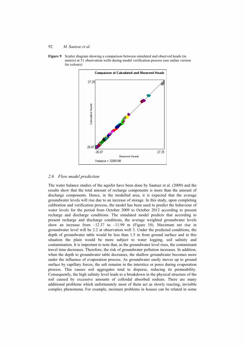
After calibration, in order to establish greater confidence in the model, the model verification was done using another time period from September 2008 to August 2009. During the model verification, the ME and RMSE were found to be –0.35 and 0.72 m, respectively. The ME variance between observed and calculated hydraulic heads has been calculated to be 0.52 (Figure 9). These results indicated that the calibrated parameters (such as hydraulic conductivity, river conductance and specific storage) are acceptable.


Figure 9 Scatter diagram showing a comparison between simulated and observed heads (in meters) at 51 observation wells during model verification process (see online version for colours)

2.6 Flow model prediction

The water balance studies of the aquifer have been done by Saatsaz et al. (2009) and the results show that the total amount of recharge components is more than the amount of discharge components. Hence, in the modelled area, it is expected that the average groundwater levels will rise due to an increase of storage. In this study, upon completing calibration and verification process, the model has been used to predict the behaviour of water levels for the period from October 2009 to October 2012 according to present recharge and discharge conditions. The simulated model predicts that according to present recharge and discharge conditions, the average weighted groundwater levels show an increase from –12.37 to –11.99 m (Figure 10). Maximum net rise in groundwater level will be 2.2 at observation well 3. Under the predicted conditions, the depth of groundwater table would be less than 1.5 m from ground surface and in this situation the plain would be more subject to water logging, soil salinity and contamination. It is important to note that, as the groundwater level rises, the contaminant travel time decreases. Therefore, the risk of groundwater pollution increases. In addition, when the depth to groundwater table decreases, the shallow groundwater becomes more under the influence of evaporation process. As groundwater easily moves up to ground surface by capillary forces, the salt remains in the interstice or pores during evaporation process. This causes soil aggregates tend to disperse, reducing its permeability. Consequently, the high salinity level leads to a breakdown in the physical structure of the soil caused by excessive amounts of colloidal absorbed sodium. There are many additional problems which unfortunately most of them act as slowly reacting, invisible complex phenomena. For example, moisture problems in houses can be related in some


way to high groundwater levels (Beenen, 1992). High moisture contents can exacerbate the physical health of the inhabitants; this ends in a decrease of the working-efficiency of the population and an increase in the medical expenses of a community. The second example is related to destabilisation of earth in the area with high earthquake potential such as Astaneh-Kouchesfahan Plain. In these areas, rising groundwater level increases the risk of liquefaction. After shaking by earthquake, saturated sandy-silty layers lose their strength which caused damage to buildings, roads, railways and excavations. The third example shows the relation between rising groundwater level and increased probability of flooding in basement, underground utilities, storage tanks, waste dumps and septic tanks (Hecker et al., 1988). After heavy rainfall, rising groundwater increases the risk of hidden underground flooding even when there is no surface flooding. Such undesirable phenomenon decreases suitability of an area for land development.

However, the side-effects of rising groundwater table are not quantified economically. In critical areas, hence, preventive actions such as the aquifer development, drainage installation and contraction dewatering are essential for lowering groundwater levels to an acceptable depth.

Figure 10 The prediction of average weighted groundwater levels according to present recharge and discharge conditions from October 2009 to October 2012 (see online version for colours)

2.7 Solute transport model construction

The contaminant transport model utilised in this study has been built upon the calibrated flow model and thus the same grid dimensions and boundary conditions have been used in this model. Prior to running MT3D, it is needed to define input data for each model cell. The first step is specification initial concentration of a contaminant to the model. In this study, chloride anion is selected for solute transport modelling. Chloride is normally considered as a good indicator because this anion has a high solubility in the groundwater, low reluctance for adsorption and usually shows a high correlation with total dissolved solids (TDS). The initial concentration in the transient calibration was the concentration distribution of chloride at September 2007. In order to make comparison


between observed and calculated concentrations, 19 sampling points have been defined as concentration observation boreholes throughout the modal (Figure 11).

After definition initial concentration, three parameters including the ratios of the transverse dispersivity to longitudinal dispersivity and initial zonation of longitudinal dispersivity have been defined for the model. In this study, the ratios of the horizontal and vertical transverse dispersivity to longitudinal dispersivity have been considered 0.1 and 0.01 m–1, respectively. The effective molecular coefficient is set to zero. Regarding the extension of the modelled area, determination of a suitable coefficient for the longitudinal dispersivity is a considerably complex process. In this study, however, the initial zonation and related values of longitudinal dispersivity have been optimised during calibration process.

Figure 11 Definition 19 sampling points as monitoring wells in the solute transport model (see online version for colours)

In MT3D, Sink/Source Concentration package is used to for specifying the concentration associated with the fluid of point or distributed sources or sinks. In order to specifying concentration value of a particular source or sink three assumptions have been considered in this study as follows:

• the spatial distribution of precipitation and chloride loading from irrigation have been considered uniform throughout the plain

• due to high level of groundwater table, it has been considered that no flow path is available from Caspian Sea toward the plain

• the chloride concentration along Sefīd-Rūd River has been considered constant.

Considering above explanation, the concentration of chloride associated with contaminant sources (river and precipitation) has been defined to the model and


optimised during the calibration. After definition all necessary data to MT3D, model calibration was done via the trial-and-error approach at the 19 concentration monitoring wells for the time period between September 2007 and August 2008. Since groundwater sampling have been carried out twice a year (i.e., September and March), the comparison between observed and calculated concentration has been made at March and September (i.e., 179th and 365th day after start time of the simulation). During model calibration process, the primary values of longitudinal dispersivity and recharge concentration have been adjusted until reasonable matches were obtained between the observed and simulated concentration. The results of the model calibration indicate that the concentrations of chloride associated with contaminant sources range between 10 and 60 mg/L. Also, the value of the longitudinal dispersivity has been estimated to be varied between 50 and 90 m, as shown in Figure 12. However, no significant changes in chloride concentration were noticed due to change in dispersivity. This shows that advection mechanism and not dispersion is the predominant mode of solute migration in the area.

Figure 12 The zonation of study area based on the estimated values of longitudinal dispersivity (coordinates are in UTM) (see online version for colours)

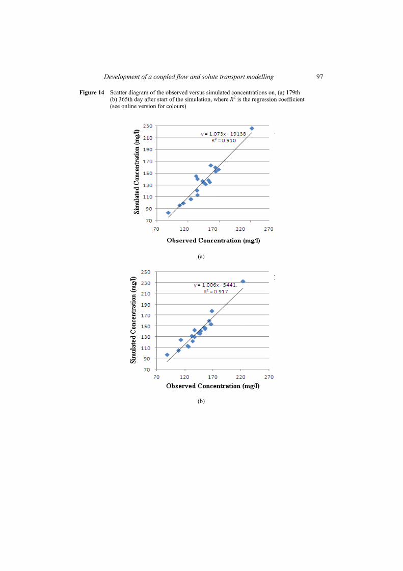
The relation between the measured and simulated concentration on 179th and 365th day after start time of the simulation at the 19 concentration observation wells is shown in Figure 13. In this stage, correlation-based and error-based measures have been used to evaluate the goodness of the transport model. The final results of the calibrated model show that in spite of small discrepancy between the calculated and observed concentrations, the simulated results are in good agreement and at the calibration receptors, show the ME (ME) of –8.6 and –4.57 mg/L, respectively. The RMSE at these points was calculated 12.8 and 9.5 mg/L, respectively. In the hydrochemical models, generally, ME and RMSE do not provide a relative indication in reference to the actual data, hence, another statistic parameter, i.e., mean relative error (MRE) has been used


based on following formula (Anderson and Woessner, 1992; Legates and McCabe, 1999):

RMSEMRE =Δ

(3)

where Δ is the concentration range and equals the difference between the maximum and minimum observed chloride concentrations. The values of MRE were found to be 9.06 and 7.03%, respectively. Moreover, the scatter plots and regression analyses were carried out and the results showed that the agreement between simulated and measured concentrations were reasonably good as depicted in Figure 14.

Figure 13 Comparison of simulated (blue line) and observed chloride concentrations (red line) at the 19 concentration observation wells on, (a) 179th (b) 365th day after start of the simulation (see online version for colours)

(a)

(b)


Figure 14 Scatter diagram of the observed versus simulated concentrations on, (a) 179th (b) 365th day after start of the simulation, where R2 is the regression coefficient (see online version for colours)

(a)

(b)


Figure 15 Comparison of simulated (blue line) and observed chloride concentrations (red line) at the 19 concentration observation wells on, (a) 179th (b) 365th day after start of the verification period (see online version for colours)

(a)

(b)

2.8 Solute transport model verification

After calibration, in order to assure the reliability of the model, the verification process was carried out using another time period from September 2008 to August 2009. The simulated concentration levels were compared with observed levels at the 19 observation wells, as shown in Figure 15. At the end of 179th and 365th day after start of the verification period, the ME were found to be –2.16 and –2.73 mg/L, respectively. The RMSE between observed and calculated chloride concentration was calculated to be 6.01 and 6.0 mg/L, respectively. The values of MRE were calculated to be 11.1 and 10.5%, respectively. The regression coefficients at the target points were 0.83 and 0.91 (Figure 16). Although the model performance in the verification phase was slightly poor when compared to the calibration results, the verification results still denote a good


verification process and indicate that the qualitative parameters have been calibrated acceptably.

Figure 16 Scatter diagram of the observed versus simulated concentrations on, (a) 179th (b) 365th day after start of the verification period, where R2 is the regression (see online version for colours)

(a)

(b)

2.9 Solute transport model prediction

After verification and assurance the reliability of the model, it was used as a management tool to describe the solute advection-dispersion under various assumptions. At first, the


validated model has been used to predict chloride concentration focusing on October 2009 to October 2012 according to present flux conditions. After running, the modelled area with an areal extent of 941 km2 has been partitioned to the 19 polygons (Figure 17). Then, based on the area of each polygon, a mathematical weight has been assigned to the related monitoring well. Finally, the mean chloride concentration of the study area has been computed by total sum of multiplying mathematical weight by calculated chloride concentration.

Figure 17 The division of the modelled area into 19 polygons (coordinates are in UTM) (see online version for colours)

Figure 18 The prediction of average weighted chloride concentration according to present flux conditions from October 2009 to October 2012 (see online version for colours)


Figure 18 shows the predicted chloride concentration in the modelled area under the first suggested scenario. According to present flux conditions, the simulated model predicts that groundwater salinities increased by approximately 2% over the period and the average weighted chloride concentration increases from 136.36 to 138.89 mg/L. Maximum net rise in chloride concentration level will be 8.06 mg/L at the monitoring well of 67. Although the predicted changes are taking place very slowly and are only significant at a long-term scale, they may proceed more quickly due to rapid population growth and agricultural development coupled with pollution through industrial activities and houses sewage. In long-term, however, the increasing salinity (i.e., chloride contents) can damage crops, affect plant growth and yield, degrade drinking water, and damage industrial equipment.

3 Conclusions

The use of groundwater models is prevalent in the field of hydrogeological, hydrochemical and environmental studies. In this study, a 2-dimensional flow and contamination transport was developed to simulate hydraulic heads under steady-state and transient conditions, to estimate hydrogeological coefficients values of aquifer (e.g., hydraulic conductivity, Sy, river conductance), to predict the response of aquifer to current recharge and discharge regime and finally, to estimate the hydrochemical properties controlling chemical transport in the saturated zone of aquifer. The results of the model calibration and verification show a reasonable agreement between observed and calculated heads and confirm that both developed models can be considered as effective tools for evaluating alternative options in the groundwater resources management and decision-making processes. The predictive simulation shows if the natural conditions prevail, weighted groundwater levels and groundwater salinities will continue to increase in the mid and long-term. Hence, groundwater consumers of the aquifer will be facing a worse situation than the present. Reduction in quality of groundwater and hazards to public health, water logging and making unstable building, structure, excavations and roads, secondary soil salinity, soil erosion and desertification, reduction in productivity and fertility of the cultivable lands, effects on environment and finally economic weakening are among these difficulties.

Acknowledgements

The authors are gratefully indebted to Gilan Regional Water Organization for supplying the relevant data. Also, the constructive comments and suggestions of anonymous reviewers are appreciated.

References Aghanabati, A. (2004) Geology of Iran, Geological Survey of Iran, Tehran. Al-Khatib, M. (1999) ‘Development of a groundwater model for the two upper aquifers (Shallow

and Middle) of the Azraq basin’, MSc thesis, pp.37–40, Civil Eng Dept., Jordan Univ. Sci. and Technol., Irbid, Jordan.


Anderson, M.P. and Woessner, W.W. (1992) Applied Groundwater Modeling-Simulation of Flow and Advective Transpor, Academic Press, San Diego, California, USA.

Beenen, A.S. (1992) Groundwater Problems in the Living Environment, Causes and Solutions: A Guideline (Grondwater problemen in de Woonomgeving. Oorzaken en Oplossingen: een Leidraad), Wetenschapswinkel, Delft University of Technology, Delft, The Netherlands.

Berberian, M. (1983) ‘Generalized tectonic map of Iran’, Geological Survey of Iran, Report No. 52. Calderon, H. (2004) ‘Numerical modeling of the groundwater flow system in a sub-basin of the

Leon-Chinandega aquifer, Nicaragua’, MSc thesis, University of Calgary, Calgary, Canada. Chiang, W.H. and Kinzelbach, W. (2001) 3D-Groundwater Modeling with PMWIN, 1st ed., p.346,

ISBN 3-540 67744-5, Springer Berlin Heidelberg, New York. Cooper, H.H. and Jacob, C.E. (1946) ‘A generalized graphical method for evaluating formation

constants and summarizing well field history’, American Geophysical Union Transactions, Vol. 27, No. 4, pp.526–534.

Darvishzadeh, S.A. (2002) Geology of Iran, p.600, Amirkabir Publication, Tehran, Iran. De Martonne, E. (1926) Une nouvelle fonction climatologique: L’indice d’aridité, pp.449–458,

La Meteorologie, Association des Météorologues du Québec, Québec. Doherty, J., Brebber, L. and Whyte, P. (1994) PEST: Model-Independent Parameter Estimation:

User’s Manual, Watermark Computing, Corinda, Australia. Eliasson, A. (2000) Groundwater Impact Assessment and Protection – Predictive Simulation for

Decision Aid, p.175, BSc thesis, Royal Institute of Technology, Stockholm, Sweden. ESRI (2006) ARCGIS V.9.2: User’s Manual, Environmental Systems Research Institute Inc. Freeze, R.A. and Cherry, J.A. (1979) Groundwater, p.604, Prentice-Hall, Inc., Englewood Cliffs,

NJ. GRWO: Gilan Regional Water Authority (2005) Hydrology and Hydrogeology of

Astaneh-Kouchesfahan Plain, Water Organization of Gilan, 400pp, Groundwater Division Report 1, (in Persian).

GSI: Geological Survey of Iran (2004) Rasht Geological Map, Geological map of Iran 1:100000, series sheet 5964.

Hecker, S., Hart, K.M. and Christenson, G.E. (1988) ‘Shallow groundwater and related hazards in Utah’, Utah Geological and Mineral Survey Map, Vol. 110, pp.1–7, Scale 1:750,000.

Kashaigili, J.J., Mashauri, D.A. and Abdo, G. (2003) ‘Groundwater management by using mathematical modeling: case of the Makutupora groundwater basin in Dodoma Tanzania’, Botsw J Technol, Vol. 12, No. 1, pp.19–24.

Kennedy, P. (2003) ‘Groundwater flow and transport model of the red river/interlake area in southern Manitoba’, PhD thesis, Department of Civil Engineering, University of Manitoba.

Khayyat Kholghi, M. (2002) ‘Groundwater management for drought periods in Iran’, available at http://www.adsabs.harvard.edu/abs/2002EGSGA.27.6557K (accessed on 11 March 2009).

Leake, S.A. and Prudic, D.E. (1991) ‘Documentation of a computer program to simulate aquifersystem compaction using the modular finite-difference ground-water flow model’, US Geological Survey, Open-File Report 94–59, p.70.

Legates, D.R. and McCabe, G.J. (1999) ‘Evaluating the use of ‘goodness-of-fit’ measures in hydrologic and hydroclimatic model validation’, Water Resources Research, Vol. 35, No. 1, pp.233–241.

Luckey, R.R., Gutentag, E.D., Heimes, F.J. and Weeks, J.B. (1986) ‘Digital simulation of groundwater flow in the high plains aquifer in the parts of Colorado, Kansas, Nebraska, New Mexico, Oklahoma, South Dakota, Texas and Wyoming’, USGS Professional Paper, 1400-D, p.57.


Mahjouri, N., Ghazban, F. and Ardestani, M. (2005) ‘Groundwater quantity and quality management: a case study of Kashan aquifer, central Iran’, Paper presented at World Water Congress 2005: Impacts of Global Climate Change – Proceedings of the 2005 World Water and Environmental Resources Congress, available at http://www.dx.doi.org/10.1061/40792(173)368 (accessed on 22 March 2009).

Moncrieff, J. (2006) ‘Modelling as a tool in the understanding and protection of groundwater in the León-Chinandega region of Nicaragua’, MSc thesis, University of Calgary, Canada.

Mousavi-Rouhbakhsh, M. (2001) ‘Geology of the Caspian Sea’, Geological Survey of Iran, Tehran, Rep No. 54 (in Persian).

Nastev, M., Rivera, A. Lefébvre, R. and Savard, M. (2005) ‘Numerical simulation of regional flow in sedimentary rock aquifers’, Hydrogeology Journal, Vol. 13, No. 4, pp.544–554.

Park, B.Y. (2000) ‘Three dimensional numerical model analysis of the change of groundwater system with Cavern excavation in volcanic rocks’, PhD thesis, pp.81−102, Seoul National University, Seoul, Korea.

PBO: Planning and Budget Organization of Islamic Republic of Iran (2006) Iran Statistical Yearbook, Statistical Center of Iran, Tehran, Iran.

Rahnama, M.B. and Mirabbasi, R. (2010) ‘Effect of groundwater table decline on groundwater quality in Sirjan watershed’, The Arabian Journal for Science and Engineering, Vol. 35, No. 1B, pp.197–210.

Rojas, R. (2005) ‘Groundwater flow model of Pampa del Tamarugal Aquifer-Northern Chile’, MSc thesis, p.103, Water Resources Engineering, Katholieke Universiteit Leuven and Vrije Universiteit Brussel, Belgium.

Ross, M., Parent, M. and Lefebvre, R. (2005) ‘3D geologic framework models for regional hydrogeology and land-use management: a case study from a Quaternary basin of southwestern Quebec, Canada’, Hydrogeology Journal, Vol. 13, No. 5, pp.690–707.

Saatsaz, M., Sulaiman, W.N.A. and Mohammadi, K. (2009) ‘Groundwater resources assessment of the Astaneh-Kouchesfahan Plain, North Iran’, American-Eurasian Journal, Agric. & Environ. Sci., Vol. 6, No. 5, pp.609–615.

Taheri Tizro, A., Fryar, A.E. and Akbari, K. (2007) ‘Hydrogeological framework and groundwater modeling of the Sujas Basin, Zanjan Province, Iran’, Journal of Applied Sciences, pp.2241-2251, doi: 10.3923/jas.2007.2241.2251.

Theis, C.V. (1937) ‘Amount of groundwater recharge in the Southern High Plains’, American Geophysical Union Transactions, 18th Annual Meeting, Vol. 8, Part 2, pp.564–568.

Zheng, C. (1996) MT3D, a Modular Three-Dimensional Transport Model, S.S. Papadopulos and Associates, Inc., Rockville, Maryland, USA.

Development of a coupled flow and solute transport modelling for Astaneh-Kouchesfahan groundwater...

Documents

Transcript of Development of a coupled flow and solute transport modelling for Astaneh-Kouchesfahan groundwater...