Journal of Hydrology (2007) 336, 334–346

ava i lab le at www.sc iencedi rec t . com

journal homepage: www.elsevier .com/ locate / jhydro l

Development and testing of a simplephysically-based distributed rainfall-runoff modelfor storm runoff simulation in humid forested basins

Du Jinkang a, Xie Shunping a, Xu Youpeng a, Chong-yu Xu b,d,*,Vijay P. Singh c

a Department of Urban and Resources Sciences, Nanjing University, Nanjing 210093, Chinab Department of Geosciences, University of Oslo, P.O. Box 1047, Blindern, NO-0316 Oslo, Norwayc Department of Biological and Agricultural Engineering, Texas A&M University, 2117 TAMU, Scoates Hall,College Station, TX 77843-2117, USAd Department of Earth Sciences, Uppsala University, Sweden

Received 26 January 2006; received in revised form 3 January 2007; accepted 10 January 2007

00do

KEYWORDSStorm runoff;Distributedhydrological model;Forested basins;Overland flow;Lateral subsurfaceflow;Saturation excessoverland flow

22-1694/$ - see front mattei:10.1016/j.jhydrol.2007.01

* Corresponding author. Tel.E-mail address: chongyu.x

r ª 200.015

: +47 22u@geo.u

Summary A distributed rainfall-runoff model was developed to predict storm runofffrom humid forested catchments. The model is physically based and takes into accountthe saturation excess overland flow mechanism and preferential subsurface flow. Thewatershed is discretized into a number of square grids, which then are classified into over-land flow and channel flow elements based on water flow properties. On the overland ele-ments, Infiltration, overland flow and lateral subsurface flow are estimated, while onchannel flow elements river flow routing is performed. Lateral subsurface flow is calcu-lated using Darcy’s law and the continuity equation, whereas overland flow and channelflow are modeled using a one dimensional kinematic wave approximation to the St. Venantequations. The model governing equations are solved by an implicit finite differencescheme. While using process-based equations and physically meaningful parameters,the model still maintains a relatively simple structure. Most of the model parameterscan be derived from digital elevation models (DEMs), digital soil and land use data, andthe remainder of the parameters that are comparatively sensitive can be determined bymodel calibration. The model is tested using nine storm events in the Jiaokou watershed,a sub-basin of Yongjiang River in Zhejiang Province, China. Of these storms, one storm isused for calibrating the model parameters and the remaining eight storms are used to ver-ify the model. When judged by the model efficiency coefficient (R2), volume conversationindex (VCI), absolute error of the time to peak (DT), and relative error of the peak flow

7 Elsevier B.V. All rights reserved.

855825; fax: +47 22 854215.io.no (C.-y. Xu).

Development and testing of a simple physically-based distributed rainfall-runoff model 335

rate (dPmax), acceptable results are achieved. Sensitivity analysis shows that the model issensitive to saturated hydraulic conductivity (Ks), Manning’s roughness coefficients (n)and the initial soil moisture content.ª 2007 Elsevier B.V. All rights reserved.

Introduction

In humid forested catchments, a high infiltration capacity isusually observed due to the presence of a thick organic layerconsisting of decomposed canopy leaves and vegetation onthe ground surface. Two runoff generation mechanismsare of importance in such catchments. One is the satu-rated-excess overland flow (Dunne and Black, 1970). Thismechanism may dynamically generate runoff during a stormin a mountainous basin, not just near stream channels butalso in depressions or hollows (Dunne et al., 1975). Togetherwith return flow, the variable source-area concept (Hewlettand Hibbert, 1967) is used to describe these processes. Thedynamics of the processes are controlled by the topography,soils, antecedent moisture and rainfall characteristics.

Another storm runoff mechanism is lateral subsurfaceflow. The importance of subsurface flow processes in gener-ating variable source areas was first addressed by Dunne andBlack (1970) and Freeze (1972a,b). Later Kirkby (1988) re-ported that almost all of the water in streamflow has passedover or through a hillside and its soils before reaching thechannel. Subsurface flow is likely to be significant in water-sheds with soils having high hydraulic conductivities and animpermeable or semipermeable layer at shallow depth thatcan support a perched water table. Such conditions oftenoccur in humid forested watersheds where the organic lit-ter, interplaced roots, decayed root holes, animal burrows,worm holes, and other structural channels making a highlypermeable medium for the rapid movement of water in alldirections (Sloan and Moore, 1984).When the infiltratedwater in such a medium reaches an impermeable layer ora semi-permeable layer, lateral subsurface flow is gener-ated (Whipkey, 1965; Beven and Germann, 1982; Mosley,1979; Tani, 1987; Tsuboyama et al., 1994). The importanceof the steeper topography for understanding the subsurfacerunoff processes has been emphasized by Tani (1997) and Si-dle et al. (2000), among others.

Both saturated-excess overland flow and lateral subsur-face flow as well as their influencing factors, such as soil,vegetation, and topography, have considerable spatial vari-ability. When modeling the storm runoff process, the influ-ence of this variability on runoff should be considered.Some lumped and semi-distributed models have implicitlyconsidered parts of these variabilities, such as Xinanjiangmodel (Zhao, 1992), ARNO model (Todini, 1996), VIC model(Liang et al., 1994) and TOPMODEL (Beven and Kirkby,1979). Because of the lack of direct physical meaning oftheir parameters, most of such models need ‘sufficientlylong’ meteorological and hydrological records for their cal-ibration, which may not always be available. The curve fit-ting calibration makes physical interpretation of the fittedparameter values quite difficult. Conceptual lumped andsemidistributed models are of little use in the estimationof sediment erosion and contaminant transport within a wa-

tershed, simulation of the rainfall-runoff response in unga-uged watersheds, and prediction of the effects of land-usechange or weather/climate-related changes (Ciarapica andTodini, 2002). On the other hand, physically based distrib-uted models, which rely on conservation equations of massand momentum of the watershed, ‘can in principle over-come many of the above deficiencies through their use ofparameters which have a physical interpretation andthrough their representation of spatial variability in param-eter values’ (Abbott et al., 1986a,b). Recent advances in re-mote sensing, geographic information systems (GISs), andcomputer technology have made physically-based distrib-uted hydrologic models attractive for flow simulation andprediction, a large number of distributed hydrological mod-els have therefore been developed and applied. Examples ofsuch models include the SHE model (Abbott et al., 1986a,b),the IHDM model (Institute of Hydrology Distributed Model;e.g., Calver and Wood, 1995), the CSIRO TOPOG model(e.g., Vertessy et al., 1993), HILLFLOW (Bronstert andPlate, 1997). However, owing to their complex structure,a huge number of parameters, and large data requirements,the application of this type of modeling techniques is notwithout limitations (Beven, 2001). In recognition of the dis-advantages of using either of these modeling approaches,some intermedial modeling approaches are developed.Reggiani et al. (1998, 1999) derived the balance equationsfor mass, momentum and energy at what they called theRepresentative Elementary Watershed (or REW) scale. How-ever, the mass balance equations of the REW approach in-clude mass exchange flux terms which must be definedexternally before their application to real catchments. Zeheet al. (2005) extend this earlier work and present an ap-proach to develop and assess closure relations capable ofparameterizing the effects of typical subscale variabilitiesand structures, that exist inside the REW, on the exchangeof water mass between different sub-regions within theREW. To further our understanding of and our ability tomodel hydrological processes, some researches have fo-cused on identifying and quantifying hillslpoe processes asa first step towards the assessment of (sub)catchment re-sponse. Many hillslope scale models have been developedover the past 30 years based on the Richards and Boussinesqequations (e.g., Pikul et al., 1974; Sloan and Moore, 1984;Verhoest and Troch, 2000). More recently (Troch et al.,2002, 2003) a series of new hillslope models have beendeveloped based on a concept presented by Fan and Bras(1998). These microscale models have improved our under-standing of the hillslope storage process, however, forcatchment scale studies, the integrated models based onthe above approaches become too complex and datademanding.

In studying the land-use impacts on storm-runoff genera-tion, Niehoff et al. (2002) used a modified version of thehydrological model WaSiM-ETH (Schulla, 1997) by including

336 J. Du et al.

(1) a macropore module accounting for fast infiltration pro-cesses, (2) a siltation module decreasing hydraulic conduc-tivity of the soil surface as a function of precipitationintensity and vegetation, and (3) sub-grid variability. Theypoint out that uncertainty exists in both land use and hydro-logical models. For less complex hydrological models (smallnumber of parameters), a rigorous uncertainty estimation,such as Bayasian method can be carried out. However, itis impossible to quantify uncertainty for complex modelsdue to large number of parameters and long computing timeinvolved.

The above discussion reveals that by definition, no modelis perfect and best for all catchment types and in all circum-stances and scenarios. But, to be useful, selected modelsmust satisfy certain objectives; timeliness, accuracy, reli-ability and consistency are considered as the desirable char-acteristics of a good model. While no modeller can claimany particular model to be perfect in its representation ofthe catchment system, new models or construction of‘new’, ‘improved’, ‘hybrid’ or generalised’ versions of thepreviously existing models are continuously reported inthe literature. An entirely redesigned and re-coded modelmight allow better handling, faster computation time, bet-ter data structures, better embedding in existing softwarestructures.

The main objective of this study is, therefore, to developand test a simpler and parsimonious physically-based dis-tributed rainfall-runoff model for storm runoff simulationin humid forested regions that takes into consideration themain mechanisms (e.g., the saturation excess overland flowmechanism and the lateral subsurface flow mechanism).The basic equations for overland flow, lateral subsurfaceflow, and stream flow are simplified using the kinematicwave equations, based on the concept that topography isthe most important landscape feature controlling waterflow. The parameters for the equations are physically inter-pretable, and the computational order and most of themodel parameters can be derived from digital elevationmodels (DEMs), soil type map and land use map. A few sen-sitive parameters can be determined by model calibration.The model was tested in Jiaokou watersheda sub-basin ofYongjiang River in eastern China.

Model description

Watershed discretization and river networkdelineation

The model proposed here is based on raster data structures,and grids are used to present watershed discretization andto describe spatially distributed terrain parameters (i.e.,elevation, land use, soil type, etc.). The grid based DigitalElevation Model is used to derive hydrologic features (i.e.,slope, flow direction, flow accumulation, stream network,computational cascade for flow routing, etc.).

Each grid cell representing an area with average proper-ties has eight possible flow directions, the direction of flowfrom one cell to its neighboring cells is ascertained bychoosing the direction of the steepest descent among theeight permitted choices. Once the flow direction in eachcell is identified, a cell-to-cell flow path upto the catchment

outlet is determined, computational sequencing of the modelstarting from the most upstream cells to the downstreamcells is also determined.

For hillslope and channel network definition, a thresholdnumber of cells (minimum support areas) is set to delineatethe channel network for the watershed. Any cell with anumber of cells upstream equal to or greater than thethreshold is considered to be a channel cell, others are con-sidered as hillslope cells. Each hillslope cell has model com-ponents for precipitation, infiltration, overland flow andsubsurface flow, and each channel cell has model compo-nents of channel flow. The overland flow and subsurfaceflow of each hillslope cell are routed to channel cells. Thechannel flow routing is carried out for each channel cellaccording to their computational order.

For the sake of simplicity, water percolation towards thedeeper soil layers and their contribution to the dischargeare not accounted for. Being an event storm runoff model,evapotranspiration is omitted.

Surface runoff and subsurface flow generation

Given the vertical soil moisture profile, the Richards equa-tion is used to describe the vertical infiltration, which ac-counts for gravity and capillary pressure. Nonetheless,owing to the high conductivity value caused by relativelylarge pores in the top layer of soil in humid forest water-sheds (Beven and Germann, 1982), the soil absorbs nearlyall the rainfall before it is saturated, thereafter surface run-off is generated by the saturation excess overland flowmechanism. This consideration is justified by the fact thatthe saturation excess mechanism, being linked to a cumula-tive phenomenon and conditioned by a lateral redistributionmovement of water in the soil, becomes dominant as thescale of the model increases (Bloschl and Sivapalan,1995). For this reason, the use of the Richards equationfor the description of the soil vertical infiltration can beavoided by assuming that at the cell scale or at larger scalethe water will always infiltrate until the saturation isreached (Todini, 1996). Hence, in our model if the net rain-fall is less than the soil saturation deficit at the time step,all net rainfall infiltrates into the soil; otherwise, surfacerunoff is calculated as the net rainfall minus soil saturationdeficit.

Because of the existence of relatively large pores andpipes in forested areas in the humid climate, the lateralsubsurface flow during rainfall period in the top soil has tur-bulent nature. Hydraulic equations for pipe flow were usedto model the contribution from the macropore system (Bar-celo and Nieber, 1982); the difficulty in this approach is thedefinition of the macropore system. The modified Darcy’sequation is used to account for turbulent flow (Whipkey,1965), and most modifications have been developed usinglaboratory data and apply only to specific porous media (Slo-an and Moore, 1984). Darcy’s equation with effective soilwater parameters was used in modeling subsurface stormflow; with this method, parameters, such saturated hydrau-lic conductivity, may be an order of magnitude greater thanthat measured for the soil matrix using small undisturbedsoil cores. Many models have been used to calculate lateralsubsurface flow resulting from macropore soils with differ-

Development and testing of a simple physically-based distributed rainfall-runoff model 337

ent complexities (Beven, 1981; Nieber and Walter, 1981;Nieber, 1982; Fipps and Skaggs, 1989; Paniconi and Wood,1993; Verhoest and Troch, 2000; Sloan and Moore, 1984;Troch et al., 2002, 2004). In this paper, the kinematic waveapproximation of the subsurface flow was used to representthe lateral subsurface flow (Beven, 1982; Singh, 1997) notonly for its simple nature, but also for its effectiveness.The method assumes that the flow lines in the soil abovethe impermeable boundary or rock are parallel to the bedand that the hydraulic gradient equals the slope of thebed or the slope of the hillslope surface if the soil layerdepth is the same.

The method is based on two equations, i.e., the continu-ity equation (1) and Darcy’s law (Eq. (2)):

Continuity equation:

goh

otþ oq

ol¼ rg ð1Þ

Darcy’s law:

q ¼ KhS ð2Þ

where q is the unit-width subsurface flow rate (m2/s);K(m/s) is the effective saturated hydraulic conductivity(m/s), which may be an order of magnitude greater thanthe measured values for the soil matrix using small, undis-turbed soil cores; h is the effective soil water depth (m); Sis the hydraulic slope; rg is the net incoming flux (m/s)(infiltration and soil evaporation rate), if evaporation isneglected; rg is equal to infiltration (the effective precip-itation for humid forest area); and g is the effective volu-metric water content deficit of the soil, when the watertable rises, the value of g is the difference of the porosityand initial water content, when water table falls, the va-lue is the difference of the porosity and the volumetricwater content at field capacity. If S is assumed to beequal to the slope of the surface gradient S0, then, Eq.(2) becomes:

q ¼ KhS0 ð3Þ

Eqs. (1) and (3) serve as the kinematic wave equations rep-resenting the complex subsurface flow.

An explicit finite difference method is used for thesolution of the model equations. Therefore, Eq. (1) is writ-ten as

qði; tÞ � qðup; tÞDl

þ ðhði; tÞ � hði; t� DtÞÞ � gDt

¼ rgði; tÞ ð4Þ

and the water depth of grid cell i and time t is

hði;tÞ ¼ g�hði;t�DtÞ�Dlþqðup;tÞ�Dtþ rgði;tÞ�Dl�DtS0�K�DtþDl� g

ð5ÞIf the computed effective soil water depth is less than thedepth of the soil, all of the rainfall will infiltrate withoutany surface runoff; otherwise the return flow may occur.After substituting h(I,t) for the soil depth, rg is reproduced.If rg > 0, rg is the infiltration of that time period; if it is lessthan the effective precipitation, the difference of the two issurface runoff; or else if rg < 0, rg is the return flow, whichwill flow out of the subsurface to build part of surfacerunoff. In this case, all effective precipitation becomes sur-face runoff.

Overland flow

Known as the dynamic wave equations, the overland flowequations are highly nonlinear and therefore do not haveanalytical solutions. Under a different set of simplifyingassumptions, more practical models can be derived fromthe dynamic wave equations; the kinematic-wave equationis the simplest one, which neglects the local acceleration,convective acceleration and pressure terms in the momen-tum equation (thus, friction and gravity forces essentiallybalance each other). There have been numerous studiesapplying the kinematic wave theory to model overland flow(Eagleson, 1970; Smith and Woolhiser, 1971; Kibler andWoolhiser, 1972; Singh and Woolhiser, 1996; Woolhiser,1996; Singh, 1996).

In this paper, the one dimensional kinematic-wave equa-tions were adopted to calculate hillslope overland flow. Theequations include (Chow et al., 1988):

Continuity equation:

oh

otþ oq

ol¼ r ð6Þ

and momentum equation:

Sf ¼ S0 ð7Þ

where h is the depth of water on the surface (m); q is theunit-width discharge (m2/s); r is the vertical net incomingflux (m/s); l is the length of the slope (m); t is the time(s); Sf is the friction slope; and S0 is the slope of the surface.

The surface flow rate is calculated by Manning’s equation(Chow et al., 1988):

v ¼ s1=2f h2=3=n ð8Þ

where n is the Manning’s roughness of the surface. FromEqs. (7) and (8), the following equation is obtained:

h ¼ aqb ð9Þ

where a ¼ ðn= ffiffiffiffis0p Þ3=5 and b = 3/5.

A finite difference method is used for the solution of thekinematic wave equations. To that end, the differenceequation for the continuity equation (6) becomes:

qði; tÞ � qðup; tÞDl

þ hði; tÞ � hði; t� DtÞDt

¼ rði; tÞ ð10Þ

where q(i,t) and q(up, t) represent the unit-width discharge(m2/s) from the current cell and upper cell(s); h(i,t) andh(i,t � Dt) are the surface water depth (m) for the cell fromthe current and the last time calculations; Dl is the length(m) of cell i; and r(i,t) is the net vertical incoming flux(m/h) for cell i.

Substituting Eq. (9) into Eq. (10) and rearranging, the fol-lowing equation is obtained:

DtDl

qði;tÞþ aðqði;tÞÞb ¼DtDl

qðup;tÞþ aðqði;t�DtÞÞbþDt� rði;tÞ

ð11Þ

Eq. (11) is nonlinear and cannot be solved directly. How-ever, Newton’s method (Chow et al., 1988) can be appliediteratively to obtain a numerical solution. The initial condi-tion for the surface flow discharge is defined as 0, meaningthat there is no surface flow at the beginning of simulation.

338 J. Du et al.

The boundary condition for the surface flow is defined asq(t) = 0.

Channel flow

There are a number of approaches used to perform channelflow routing, which can be broadly classified into twocategories: (1) hydrodynamic routing, and (2) hydrologicalrouting. The hydrodynamic routing approach is based onSaint-Venant equations, such as the simplified kinematicwave model and diffusive wave model. The hydrologicalrouting approach is based on the continuity equation inthe Saint-Venant formulation, but empirical relationshipsare used to replace the momentum equation, such as theMuskingum, Muskingum–Cunge and Unit Hydrograph meth-ods (Arora et al., 2001). Full hydrodynamic routing modelsare usually too complex for practical use and require datathat are difficult to obtain, hydrological routing modelsare used more often by hydrologists but their parametersneed to be calibrated.

In this paper, a simple one dimensional hydrodynamicstreamflow routing model is developed to simulate thechannel network flow, based on the kinematic wave approx-imation of the St. Venant equations and the routing algo-rithms used in the WATFLOOD distributed hydrologicalmodel (Kouwen et al., 1993) and in the WATROUTE (Aroraet al., 2001).

The kinematic wave approximation of the St. Venantequations:

Continuity equation:

dS

dt¼ I� Q � q ð12Þ

and momentum function:

Sf ¼ S0 ð13Þ

where S is the channel water storage, I is the inflow, Q is theoutflow, q is the lateral inflow including both overland flowand subsurface flow from all adjacent inflow grid cells, Sf isthe friction slope, and S0 is the channel slope.

The channel flow rate is calculated by Manning’s equa-tion (Chow et al., 1988) as

V ¼ S12fR

23=n ð14Þ

where V is the channel velocity, R is the hydraulic radius(area of flow divided by the wetted perimeter, requiringthe information about the river width), and n is Manning’sroughness coefficient.

Due to the difficulty in obtaining the river width, theManning’s equation was approximated as (Kouwen et al.,1993; Arora et al., 2001):

V ¼ S12fA

13=n ð15Þ

where A is the channel cross-sectional area. Replacing Sf byS0, the formula for the outflow Q is obtained as

Q ¼ S120A

43=n ð16Þ

The channel cross-sectional area is approximated by divid-ing the storage S in the channel reach by the length L ofthe channel reach (Kouwen et al., 1993; Arora et al., 2001):

A ¼ S=L ð17Þ

Eqs. (12) and (16) are solved using a finite differencemethod.

Substitution of Eq. (16) into the difference form of Eq.(12) yields:

Stþ1Dt� St

Dt¼ It þ Itþ1

2� Qt

2� 1

2

1

n

S4=3tþ1

L4=3S1=20

!þ qt þ qtþ1

2ð18Þ

and then rearranging one obtains:

Stþ1Dtþ 1

2

1

n

S4=3tþ1

L4=3S1=20

!¼ It þ Itþ1

2� Qt

2þ St

Dtþ qt þ qtþ1

2ð19Þ

This equation can also be solved by using Newton’s iterativemethod as above.

Study area and data

The study area, Jiaokou Reservoir watershed, is a sub-basinof Yongjiang River, located in Zhejiang Province, southeast-ern part of China. The watershed area is 259 km2 and theelevation ranges from 59 m to 976 m. The region has atypical subtropical monsoon climate. The average annualtemperature is 16.3 �C with minimum and maximum tem-peratures occurring in January and July, respectively. Themean annual precipitation is about 2000 mm with most ofthe rainfall occurring between March and September. Thereare three rainfall gauging stations: Jiaokou, Xianiutang andHualongzhuang and one stream flow gauging station. Thewatershed location, elevation, distribution of rainfall andflow gauging stations, and streams are seen in Fig. 1. Theland cover information of the area was derived from LandsatTM image on 18 may 1987, and the classification procedurewas performed by using a Maximum-Likelihood-Classifier.The classification process results in a land use map having6 land use classes (Fig. 2), i.e., forest (78.3%), farmland(14.5%), grassland (2.5%), water surface (2.7%), barranland(0.4%) and settlements (1.9%). The soil types are classifiedinto four categories (Fig. 3), i.e., sandy loam (29.9%), loam(27.5%), silty loam (40.8%) and clay (1.8%).

A total of 9 isolated storms with observed runoff re-sponses were selected to calibrate and verify the model.The spatial distribution of rainfall for each storm was calcu-lated by the inverse distance weighted method.

The digitized contour maps (1:50,000 scale) are used togenerate DEM by using the Kriging interpolation method.To avoid producing a large number of pixels for the catch-ment, 100 m was selected as the size of each grid, eventhen the total grid cells reached 25,900. The DEM was thenused to derive hydrologic parameters of the watershed,such as slope, flow direction, flow accumulation and streamnetwork. The slope for each cell was calculated in the direc-tion of the steepest flow path, the slope of cells in flat areasis assigned to 0.02. For stream network delineation, depres-sions resulted from reservoirs and elevation data or DEMgeneration method were removed by raising elevationswithin the depression to the elevation of its lowest over-flow. The flow directions in flat areas were designated bythe use of flow direction GIS function. Once flow directionfor each cell was identified, the flow path and computationsequencing (cascade system) were determined, and flow

Figure 1 Location of the stations and the catchment in the map of PR China.

Figure 3 The soil type map of the basin.Figure 2 The land use map of the basin.

Development and testing of a simple physically-based distributed rainfall-runoff model 339

accumulation area (number of cells) for each cell was alsocalculated. Using the threshold number, the channel cellswere identified and stream network was delineated.

The soil parameters of each hillslope cell needed for sub-surface flow are saturated hydraulic conductivity, porosity,and volumetric content at field capacity. The soil data werederived from soil type maps in this study. Each soil type isrelated to a soil textural class, and from each soil textural

class a representative value for saturated hydraulic conduc-tivity is obtained following Rawls et al. (1983) and Smemoeet al. (2004). Some of these parameters are shown in Table1, as an example. The spatial pattern of saturated hydraulicconductivity is calculated using soil type maps, which isthen used as the initial value for the model. Porosity andvolumetric content at the field capacity for each soil typeare determined from Figure 6.4 of the book of Dingman

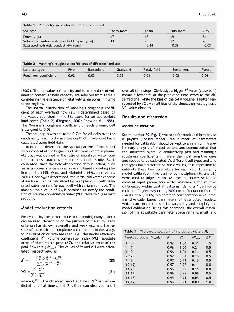
Table 2 Manning’s roughness coefficients of different land-use

Land use type River Barranland Grassland Paddy field Settlement Forest

Roughness coefficient 0.02 0.03 0.05 0.03 0.03 0.04

Table 1 Parameter values for different types of soil

Soil type Sandy loam Loam Silty loam Clay

Porosity (%) 47 48 49 54Volumetric water content at field capacity (%) 13 20 22 28Saturated hydraulic conductivity (cm/h) 1 0.64 0.38 0.03

Table 3 The pareto solutions of multipliers Mn and Mk

Pareto solutions {Mn,Mk} R2 VCI dPmax DT

{1,13} 0.92 1.00 0.31 1.5{4,17} 0.96 1.00 0.21 0.5{4,19} 0.96 1.00 0.21 0.5{7,17} 0.97 0.98 0.15 0.5{7,19} 0.97 0.98 0.15 0.5{10,19} 0.97 0.97 0.11 0.0{13,7} 0.95 0.91 0.11 0.0{13,17} 0.96 0.95 0.06 0.5{16,17} 0.95 0.94 0.03 0.5{19,19} 0.94 0.93 0.00 1.0

340 J. Du et al.

(2002). The top values of porosity and bottom values of vol-umetric content at field capacity are selected from Table 1considering the existence of relatively large pores in humidforest regions.

The spatial distribution of Manning’s roughness coeffi-cient of each overland flow cell is determined based onthe values published in the literature for an appropriateland cover (Table 2) (Dingman, 2002; Chow et al., 1988).The Manning’s roughness coefficient of each channel cellis assigned to 0.02.

The soil depth was set to be 0.7 m for all cells over thecatchment, which is the average depth of an adjacent basincalculated using field data.

In order to determine the spatial pattern of initial soilwater content at the beginning of all storm events, a param-eter, Sini was defined as the ratio of initial soil water con-tent to the saturated water content. In the study, Sini iscalibrated, since the field observation data is lacking. Suchan assumption is widely used in event based modeling (Ju-lien et al., 1995; Wang and Hjelmfelt, 1998; Jain et al.,2004). Once Sini is determined, the initial soil water contentat each cell can be calculated by multiplying Sini with satu-rated water content for each cell with certain soil type. Themost suitable value of Sini is obtained to satisfy the condi-tion of volume conversation index (VCI) close to 1 (see nextsection).

Model evaluation criteria

For evaluating the performance of the model, many criteriacan be used, depending on the purpose of the study. Eachcriterion has its own strengths and weakness, and the re-sults of these criteria complement each other. In this study,four evaluation criteria are used, i.e., the model efficiencycoefficient (R2), volume conversation index (VCI), absoluteerror of the time to peak (DT), and relative error of thepeak flow rate (dPmax). The values of R2 and VCI were calcu-lated, respectively, as

R2 ¼ 1�PN

i¼1ðQobsi � Q cal

i ÞPNi¼1ðQ

obsi � QÞ

ð20Þ

VCI ¼PN

i¼1QcaliPN

i¼1Qobsi

ð21Þ

where Q obsi is the observed runoff at time i, Q cal

i is the pre-dicted runoff at time i, and Q is the mean observed runoff

over all time steps. Obviously, a bigger R2 value (close to 1)means a better fit of the predicted time series to the ob-served one, while the bias of the total volume is better rep-resented by VCI. A small bias of the simulation result gives aVCI value close to 1.

Results and discussion

Model calibration

Storm number 79 (Fig. 5) was used for model calibration. Asa physically-based model, the number of parametersneeded for calibration should be kept to a minimum. A pre-liminary analysis of model parameters demonstrated thatthe saturated hydraulic conductivity (Ks) and Manning’sroughness coefficients (n) were the most sensitive onesand needed to be calibrated. As different soil types and landuse types have different Ks and n values, it is impossible tocalibrate these two parameters for each cell. To simplifymodel calibration, two basin-wide multipliers (Mn and Mk)were used to adjust n and Ks: the multipliers scale theelement input parameters while maintaining the relativedifferences within spatial patterns. Using a ‘‘basin-widemultiplier’’ (Vertessy et al., 2000) or a ‘‘reduction factor’’(Giertz et al., 2006) is a common consideration in calibrat-ing physically based parameters of distributed models,which can retain the spatial variability and simplify themodel calibration. Using this approach, the overall dimen-sion of the adjustable parameter space remains small, and

Development and testing of a simple physically-based distributed rainfall-runoff model 341

the over-parameterization problem can be avoided (Refsg-aard, 1997).

In order to get a suitable pair of multipliers Mn and Mk, asequential multiobjective analysis was performed by analyz-ing model evaluation criteria estimated with model runs fora set of Mn and Mk. From a multi-criteria point of view,there is no single optimal pair of Mk and Mn, but some com-promise pairs, i.e., the Pareto solutions (Gupta et al., 1998)exist (see Table 3). For the sake of discussion, the setMn = 7, Mk = 11 is written as {7, 11}. Sets {7,13} {7,15}{7,17} {7,19} {8,13} {8,15} {8,17} {8,19} can make R2 maxi-mal, but not all of them can lead to best values for all othercriteria at the same time. In our study, the selection of thefinal Pareto solution was made by using the sequential mul-tiobjective analysis technique. The acceptable thresholds

1 3 5 7 9 11 13 15 17 19

Mk

0.80

0.85

0.90

0.95

1.00

R2

1 3 5 7 9 11 13 15 17 19

Mk

0.80

0.85

0.90

0.95

1.00

1.05

VC

I

1 3 5 7 9 11 13 15 17 19

Mk

0.00

0.10

0.20

0.30

0.40

0.50

δPm

ax

Mn=1 Mn=4 Mn=7 Mn=10

Mn=13 Mn=16 Mn=19

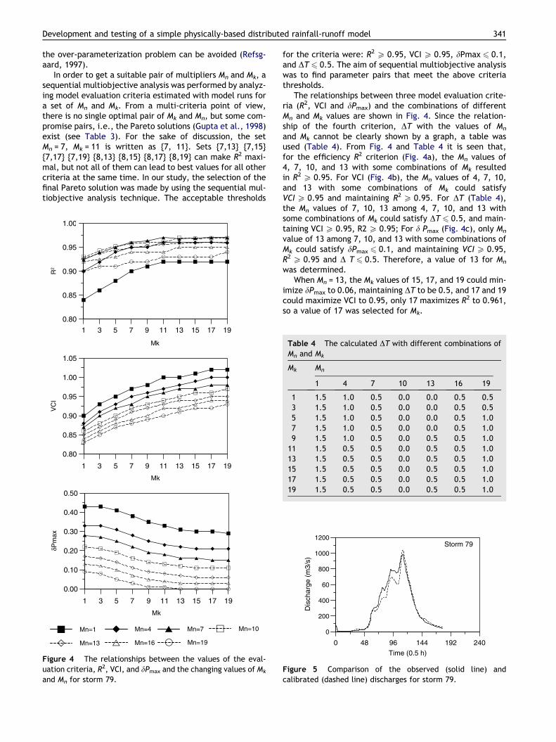
Figure 4 The relationships between the values of the eval-uation criteria, R2, VCI, and dPmax and the changing values of Mk

and Mn for storm 79.

for the criteria were: R2 P 0.95, VCI P 0.95, dPmax 6 0.1,and DT 6 0.5. The aim of sequential multiobjective analysiswas to find parameter pairs that meet the above criteriathresholds.

The relationships between three model evaluation crite-ria (R2, VCI and dPmax) and the combinations of differentMn and Mk values are shown in Fig. 4. Since the relation-ship of the fourth criterion, DT with the values of Mn

and Mk cannot be clearly shown by a graph, a table wasused (Table 4). From Fig. 4 and Table 4 it is seen that,for the efficiency R2 criterion (Fig. 4a), the Mn values of4, 7, 10, and 13 with some combinations of Mk resultedin R2 P 0.95. For VCI (Fig. 4b), the Mn values of 4, 7, 10,and 13 with some combinations of Mk could satisfyVCI P 0.95 and maintaining R2 P 0.95. For DT (Table 4),the Mn values of 7, 10, 13 among 4, 7, 10, and 13 withsome combinations of Mk could satisfy DT 6 0.5, and main-taining VCI P 0.95, R2 P 0.95; For d Pmax (Fig. 4c), only Mn

value of 13 among 7, 10, and 13 with some combinations ofMk could satisfy dPmax 6 0.1, and maintaining VCI P 0.95,R2 P 0.95 and D T 6 0.5. Therefore, a value of 13 for Mn

was determined.When Mn = 13, the Mk values of 15, 17, and 19 could min-

imize dPmax to 0.06, maintaining DT to be 0.5, and 17 and 19could maximize VCI to 0.95, only 17 maximizes R2 to 0.961,so a value of 17 was selected for Mk.

Table 4 The calculated DT with different combinations ofMn and Mk

Mk Mn

1 4 7 10 13 16 19

1 1.5 1.0 0.5 0.0 0.0 0.5 0.53 1.5 1.0 0.5 0.0 0.0 0.5 0.55 1.5 1.0 0.5 0.0 0.0 0.5 1.07 1.5 1.0 0.5 0.0 0.0 0.5 1.09 1.5 1.0 0.5 0.0 0.5 0.5 1.011 1.5 0.5 0.5 0.0 0.5 0.5 1.013 1.5 0.5 0.5 0.0 0.5 0.5 1.015 1.5 0.5 0.5 0.0 0.5 0.5 1.017 1.5 0.5 0.5 0.0 0.5 0.5 1.019 1.5 0.5 0.5 0.0 0.5 0.5 1.0

0 48 96 144 192 240

Time (0.5 h)

0

200

400

60

800

1000

1200

Dis

char

ge (

m3/

s)

Storm 79

Figure 5 Comparison of the observed (solid line) andcalibrated (dashed line) discharges for storm 79.

342 J. Du et al.

With such Mn values, Manning’s roughness coefficient canreach 0.6, which is higher than the commonly reported val-ues in the literature, although Shen and Julien (1992) notedthat n could exceed 1.0 for extremely dense vegetation, andVertessy and Elsenbeer (1999) calibrated n to be between0.7 and 1.2.

With Mk = 17, the calculated values of Ks ranged from0.51 cm/h to 17 cm/h, which is what one could expect be-

0 48 96 144 192

Time (0.5 h)

Time (0.5 h)

Time (0.5 h)

Time (0.5 h)

0

200

400

600

800

1000Storm 20

0 48 96 144 192 240 288

0

300

600

900

1200

1500

1800

Dis

char

ge (

m3/

s)D

isch

arge

(m

3/s)

Dis

char

ge (

m3/

s)D

isch

arge

(m

3/s)

Storm 81

0 48 96 144 192 240 288 336

0

200

400

600

800

1000Storm 87

0 48 96 1440

300

600

900

1200

1500

1800Storm 88

Figure 6 Comparison of the observed (solid line) and simulated

cause of the existence of relatively large pores. With thevalues of Mk = 17 and Mn = 13, the following model evalua-tion criteria values were obtained: R2 = 0.961, VCI = 0.95,dPmax = 0.06, and DT = 0.5, respectively. The observed andcalibrated discharges are compared in Fig. 5 for storm 79.As can be expected from the values of the evaluationcriteria, the results showed that there was an overallagreement between observed and calibrated discharges.

0 48 96Time (0.5 h)

0

300

600

900

1200

1500

Dis

char

ge (

m3/

s)

Storm 90

0 48 96 144 192 240

Time (0.5 h)

Time (0.5 h)

Time (0.5 h)

0

300

600

900

1200

1500

1800D

isch

arge

(m

3/s)

Dis

char

ge (

m3/

s)D

isch

arge

(m

3/s)

Storm 92

0 48 96 144

0

50

100

150

200

250

300Storm 211

0 48 96 144 192 2400

50

100

150

200

250Storm 212

(dashed line) discharges for the 8 storms used for verification.

Development and testing of a simple physically-based distributed rainfall-runoff model 343

Model verification

Eight storms were used to verify the model using the param-eter values determined by calibration. Comparison of ob-served and simulated discharges is shown in Fig. 6 andsummary values of the evaluation criteria for the eight ver-ification storm runoff events are presented in Table 5. It isseen that the simulated flood hydrographs demonstrated aclose agreement with the observed hydrographs for all 8storm events. The relative error of peak flow was generallywithin 10% and the efficiency was higher than 0.9 in 5 of theflood hydrographs.

It can also be seen that the simulation results for stormsnumbered 81, 88, and 212 were not as good as for others; thisis because of some special features of these storms. Storm81 has an average total rainfall of 459 mm, while the ob-served runoff reaches 456 mm. This means that either thereis an error in observations or there is a carry-over of runofffrom the pervious storm. In this case, even if we set the ini-tial degree of saturation to be 100%, the simulated peak flowwas still considerably lower than the observed one. The ob-

Table 5 The summary of the verification results

No. ofstorm

R2 VCI Calculatedpeak flowrate (m3/s)

dPmax DT (h)

20 0.97 0.97 684 �0.08 �181 0.93 0.96 1289 �0.21 �0.587 0.95 1.12 896 0.01 0.588 0.81 1.20 1301 �0.13 0.590 0.97 0.99 1180 �0.02 �592 0.93 1.08 1501 0.01 1.5

211 0.96 1.02 261 �0.08 0212 0.83 0.81 211 �0.07 �1.5Note: R2 = Model efficiency coefficient, VCI = volume conversa-tion index, DT = absolute error of the time to peak, anddPmax = relative error of the peak flow rate.

Table 6 The sensitivity analysis of the verification storms

Change ofevaluation criteria

Change of parameters 81

DR2 Initial soil moisture increase 5% �0.0Initial soil moisture increase �5% 0hm changes from bottom to top values 0

DVCI Initial soil moisture increase 5% 0.0Initial soil moisture increase �5% �0.0hm changes from bottom to top values 0

DdPmax Initial soil moisture increase 5% 0.0Initial soil moisture increase �5% �0.0hm changes from bottom to top values 0

D(DT) Initial soil moisture increase 5% 0Initial soil moisture increase �5% 0hm changes from bottom to top values 0

The values in the table show the changes of the evaluation criteria witand with hm changes from bottom to top values, respectively.

served hydrograph of storm event 88 has too steep a risingclimb to be simulated well, which is probably caused by dataerror. The hydrograph of storm event 212 has rising climbswith long and large pre-storm runoff rates that decreasethe modeling efficiency. Nevertheless, the results in generalare acceptable with the lowest R2 value of >0.8.

Sensitivity analysis

In order to check as to the extent model simulations wereaffected by soil water content at the field capacity, the soilwater content at the field capacity, hm, for each soil typewas changed from the bottom values to the top values(Fig. 6.4 in Dingman, 2002) and the resulting changes inthe evaluation criteria are shown in Table 6 (numbers withitalic). It is seen that there is little influence on the simula-tion results, with the maximum changes among eight stormsbeing 0.01 for R2, 0.04 for VCI , 0.02 for dPmax and 1 for DT,respectively.

Several studies have shown that the initial soil moisturehas an important effect on rainfall-runoff simulation (Coleset al., 1997; Grayson et al., 1992, 1995; Merz and Bardossy,1998; Merz and Plate, 1997; Zehe et al., 2005). In our study,the initial degree of soil water saturation was increased anddecreased by 5% to evaluate the effect on model simulation.Our results (Table 6) also showed that the initial degree ofsaturation has a larger influence on model results than havethe hm values for all storm events.

Concluding remarks

In this study, a physically-based distributed rainfall-runoffmodel was developed and tested for predicting storm runofffrom a humid forested catchment. In the model, the move-ment of water in soil and on the surface is represented at apoint by a kinematic wave approach. Based on the kine-matic wave approximation of the St. Venant equations, asimple one dimensional hydrodynamic streamflow routingmodel is used to simulate the channel network flow. While

87 88 90 92 20 211 212

2 �0.03 0.04 0.03 0 �0.02 �0.06 �0.030.02 �0.05 0 0 0 �0.05 �0.090 0.01 0 0 �0.01 0 0

2 0.02 0.06 0.04 0.02 0.02 0.12 0.091 �0.02 �0.06 �0.04 �0.02 �0.03 �0.11 �0.08�0.02 �0.02 0 �0.01 0.04 �0.01 0.02

2 0.03 0.11 0.02 0.03 0.04 0.22 0.273 �0.04 �0.11 �0.03 �0.03 �0.03 0.08 �0.22

0 0 0 �0.02 0 0 0

0 0 0 0 0 0.5 00 0 0 0 0 0 0.50 0 0 0 0 0 1

h initial soil moisture saturation increasing 5% and decreasing 5%,

344 J. Du et al.

retaining a relatively simple structure, all the parametersemployed in the model are physically based and most ofthem can be determined using physical catchment charac-teristics data. Like most other physically-based models,calibration or tuning of some more sensitive parameters isstill needed to get best results. Parameter sensitivity anal-ysis shows that the saturated hydraulic conductivity andManning’s roughness coefficient need to be calibrated foreach cell. To reduce the amount of computation, avoidthe problem of over-parameterization (Beven, 1996) andretain the spatial variability, two multipliers were set toscale the spatial patterns of both saturated hydraulicconductivity and Manning’s roughness coefficient. Thefollowing conclusions can be drawn from the study: (1)The relative simple model developed and tested in thispaper can yield promising results in simulating storm runoffin a humid forest region. (2) A multiobjective analysis(sequential optimization method) proved to be effectiveto search for the Pareto solution. (3) From the sensitivitystudy it was found that the initial state of soil moisturewas an important factor for all evaluation criteria.

It is worth of noting that the present version of the modelis event based and cannot be used for long-term continuoussimulation. The errors in the model outputs may arise froman incorrect representation of the processes involved in therelationship between runoff and controlling input variables,from poor estimation of model parameters, from theassumptions made to simplify the model and calculation,from the random and systematic errors of all the input data,and from the spatial and temporal resolution of rainfall andthe antecedent moisture condition, etc. The model isdeveloped for modeling the saturation overland flow domi-nated runoff production mechanism, and it is more suitablein mountain areas with large slope where the kinematicwave approximation of Saint-Venant equations could beused as the representation of water movement in hillslopesand river networks. The lakes and reservoirs are not consid-ered in the model. Proper calibration of some model param-eters such as Ks and n is still necessary. The calibrationapproach using basin-wide multipliers can avoid the over-parameterization problem, but the obtained effectiveparameters account for all errors in the model structure,spatial parameter structure and input data; the source oferror then remains unknown. Furthermore, the assumptionthat the mean soil depth is 0.7 m will influence runoffgeneration, which cannot be quantified in the study due tothe lack of field measurement data. In the present studyno attempt was made to quantify the sources of error,and it will be considered hopefully in future studies.

Acknowledgements

This work was supported by the National Natural ScienceFoundation of China under grant 40171015. The author wouldlike to thank the reviewers for their valuable comments.

References

Abbott, M.B., Bathurst, J.C., Cunge, J.A., O’Connell, P.E., Ras-mussen, J., 1986a. An introduction to the European Hydrologic,

System–Syst‘eme Hydrologique Europ’een, ‘SHE’ 1: history and,philosophy of a physically based, distributed modelling system.Journal of Hydrology 87, 45–59.

Abbott, M.B., Bathurst, J.C., Cunge, J.A., O’Connell, P.E., 1986b.An introduction to the European Hydrologic System–SystemeHydrologique Europeen, ‘SHE’ 2: structure of a physically based,distributed modelling system. Journal of Hydrology 87, 61–77.

Arora, V., Seglenieks, F., Kouwen, N., Soulis, E., 2001. Scalingaspects of river flow routing. Hydrological Processes 15, 461–477.

Barcelo, M.D., Nieber, J.L., 1982. Influence of a soil pipe networkon catchment hydrology. Pap Am Agric Eng. 82-2027, 1–27.

Beven, K.J., 1981. Kinematic subsurface stormflow. WaterResources Research 17 (5), 1419–1424.

Beven, K.J., 1982. On subsurface stormflow: prediction with simplekinematic theory for saturated and unsaturated flows. WaterResources Research 18 (6), 1627–1633.

Beven, K.J., 1996. A discussion of distributed hydrological model-ing. In: Abbott, M.B., Refsgaard, J.C. (Eds.), Distributed Hydro-logical Modeling. Kluwer Academic, pp. 255–278.

Beven, K.J., 2001. Rainfall-runoff Modeling: A Primer. Wiley, WestSussex, pp. 217–254.

Beven, K.J., Germann, P., 1982. Macropores and water flow in soils.Water Resources Research 18 (5), 1311–1325.

Beven, K.J., Kirkby, M.J., 1979. A physically based, variablecontributing area model of basin hydrology. Hydrological Sci-ence Bulletin 24 (1), 43–69.

Bloschl, G., Sivapalan, M., 1995. Scale issues in hydrologicalmodelling: a review. Hydrological Processes 9, 251–290.

Bronstert, A., Plate, E., 1997. Modelling of runoff generation andsoil moisture dynamics for hillslopes and microcatchments.Journal of Hydrology 198, 177–195.

Calver, A., Wood, W.L., 1995. The Institute of hydrology distributedmodel. In: Singh, V.P. (Ed.), Computer Models of WatershedHydrology. Water Resource Publications, Colorado, pp. 595–626.

Chow, V.T., Maidment, D.R., Mays, L.W., 1988. Applied Hydrology.McGraw-Hill Book Company, p. 627.

Ciarapica, L., Todini, E., 2002. TOPKAPI: a model for therepresentation of the rainfall-runoff process at different scales.Hydrological Processes 16, 207–229.

Coles, N.A., Sivapalan, M., Larsen, J.E., Linnet, P.E., Fahrner, C.K.,1997. Modelling runoff generation on small agricultural catch-ments: can real world runoff responses be captured? Hydrolog-ical Processes 11, 111–136.

Dingman, S.L., 2002. Physical Hydrology. Prentice-hall, p. 642.Dunne, T., Black, R.D., 1970. An experimental investigation of

runoff production in permeable soils. Water Resources Research6, 478–490.

Dunne, T., Moore, T.R., Taylor, C.H., 1975. Recognition andprediction of runoff-producing zones in humid regions. Hydro-logical Science Bulletin 20 (3), 305–327.

Eagleson, P.S., 1970. Dynamic Hydrology. McGraw Hill, New York.Fan, Y., Bras, R., 1998. Analytical solutions to hillslope subsurface

storm flow and saturation overland flow. Water ResourcesResearch 34 (4), 921–927.

Fipps, G., Skaggs, R.W., 1989. Influence of slope on subsurfacedrainage of hillsides. Water Resources Research 25 (7), 1717–1726.

Freeze, R.A., 1972a. Role of subsurface flow in generating surfacerunoff, 1, base flow contributions to channel flow. WaterResources Research 8 (3), 609–623.

Freeze, R.A., 1972b. Role of subsurface flow in generating surfacerunoff, 2, upstream source areas. Water Resources Research 8(5), 1272–1283.

Giertz, S., Diekkruger, B.D., Steup, G., 2006. Physically-basedmodelling of hydrological processes in a tropical headwatercatchment in Benin (West Africa) – process representation and

Development and testing of a simple physically-based distributed rainfall-runoff model 345

multi-criteria validation. Hydrology and Earth System SciencesDiscussions 3, 1–57.

Grayson, R.B., Moore, I.D., MaMahon, T.A.C., 1992. Physically-based hydrologic modelling: I. A terrain-based model forinvestigative purposes. Water Resources Research 28 (10),2639–2658.

Grayson, R.B., Bloschl, G., Moore, I.D., 1995. Distributed param-eter hydrologic modeling using vector elevation data: THALESand TAPES-C. In: Singh, V.P. (Ed.), Computer Models ofWatershed Hydrology. Water Resources Publications, HighlandsRanch, Colorado, pp. 669–696 (Chapter 19).

Gupta, H.V., Sorooshian, S., Yapo, P.O., 1998. Toward improvedcalibration of hydrologic models: multiple and non-commensu-rable measures of information. Water Resources Research 34(4), 751–763.

Hewlett, J.D., Hibbert, A.R., 1967. Factors affecting the responseof small watersheds to precipitation in humid areas. In: Sopper,W.E., Lull, H.W. (Eds.), Forest Hydrology. Pergamon, Oxford,pp. 275–290.

Jain, M.K., Kothyarib, U.C., Ranga Raju, K.G., 2004. A GIS baseddistributed rainfall-runoff model. Journal of Hydrology 299,107–135.

Julien, P.Y., Saghafian, B., Ogden, F.L., 1995. Raster basedhydrological modeling of spatially-varied surface runoff. WaterResources Bulletin 31 (3), 523–536.

Kibler, D.F., Woolhiser, D.A., 1972. Mathematical properties of thekinematic cascade. Journal of Hydrology 15, 131–145.

Kirkby, M., 1988. Hillslope runoff processes and models. Journal ofHydrology 100, 315–339.

Kouwen, N., Soulis, E.D., Pietroniro, A., Donald, J., Harrington,R.A., 1993. Grouping response units for distributed hydrologicmodelling. ASCE Journal of Water Resources Management andPlanning 119 (3), 289–305.

Liang, X., Lettenmaier, D.P., Wood, E.F., Burges, S.J., 1994. Asimple hydrologically based model of land surface water andenergy fluxes for GSMs. Journal of Geophysical Research 99 (D7),14415–14428.

Merz, B., Bardossy, A., 1998. Effects of spatial variability on therainfall runoff process in a small loess catchment. Journal ofHydrology 212–213, 304–317.

Merz, B., Plate, E.J., 1997. An analysis of the effects of spatialvariability of soil and soil moisture on runoff. Water ResourcesResearch 33 (12), 2909–2922.

Mosley, M.P., 1979. Streamflow generation in a forested watershed,New Zealand. Water Resources Research 15 (4), 795–806.

Nieber, J., 1982. Hillslope soil moisture flow, approximation by aone-dimensional formulation. Paper 82-2026. American Societyof Agricultural Engineers, St. Joseph, MI, 28 p.

Nieber, J., Walter, M., 1981. Two-dimensional soil moisture flow ina sloping rectangular region: experimental and numerical stud-ies. Water Resources Research 17 (6), 1722–1730.

Niehoff, D., Fritsch, U., Bronstert, A., 2002. Land-use impactson storm-runoff generation: scenarios of land-use changeand simulation of hydrological response in a meso-scalecatchment in SW-Germany. Journal of Hydrology 267, 80–93.

Paniconi, C., Wood, E., 1993. A detailed model for simulation ofcatchment scale subsurface hydrologic processes. WaterResources Research 29 (6), 1601–1620.

Pikul, M., Street, R., Remson, I., 1974. A numerical model based oncoupled one-dimensional Richards and Boussinesq equations.Water Resources Research 10 (2), 295–302.

Rawls, W.J., Brakensiek, D.L., Miller, N., 1983. Green–Amptinfiltration parameters from soils data. ASCE Journal of Hydrau-lic Engineering 109 (1), 62–70.

Refsgaard, J.C., 1997. Parameterisation, calibration and validationof distributed hydrological models. Journal of Hydrology 198,69–97.

Reggiani, P., Sivapalan, M., Hassanizadeh, S.M., 1998. A unifyingframework for watershed thermodynamics: balance equationsfor mass, momentum, energy and entropy and the secondlaw of thermodynamics. Advances in Water Resources 22 (4),367–398.

Reggiani, P., Hassanizadeh, S.M., Sivapalan, M., Gray, W.G.,1999. A unifying framework for watershed thermodynamics:constitutive relationships. Advances in Water Resources 23(1), 15–39.

Schulla, J., 1997. Hydrologische Modellierung von Flussgebieten zurAbschatzung der Folgen von Klimaanderungen. Zurcher Geo-graphische Schriften, Heft 69 Zurich, Switzerland.

Shen, H.W., Julien, P.Y., 1992. Erosion and sediment transport. In:Maidment, D. (Ed.), Handbook of Hydrology. McGraw-Hill, NewYork, pp. 12.1–12.61 (Chapter 12).

Sidle, R.C., Tsuboyama, Y., Noguchi, S., Hosoda, I., Fujieda, M.,Shimizu, T., 2000. Stormflow generation in steep forestedheadwaters: a linked hydrogeomorphic paradigm. HydrologicalProcesses 14, 369–385.

Singh, V.P., 1996. Kinematic Wave Modelling in Water Resources:Surface Water Hydrology. Wiley, New York, p. 1399.

Singh, V.P., 1997. Kinematic Wave Modeling in Water Resources:Environmental Hydrology. John Wiley, New York.

Singh, V.P., Woolhiser, D.A., 1996. A nonlinear kinematic wavemodel for watershed surface runoff. Journal of Hydrology 31,221–243.

Sloan, G.P., Moore, I.D., 1984. Modelling subsurface stormflow onsteeply sloping forested watersheds. Water Resources Research20 (12), 1815–1822.

Smemoe, C.M., Nelson, E.J., Zhao, B., 2004. Spatial averaging ofland use and soil properties to develop the physically-basedgreen and ampt parameters for HEC-1. Environmental Modellingand Software 19, 525–535.

Smith, R.E., Woolhiser, D.A., 1971. Overland flow on an infiltratingsurface. Water Resources Research 7 (4), 899–913.

Tani, M., 1987. On researching effects of forest soil on runoffproperties. Water Science 177, 35–61 (in Japanese).

Tani, M., 1997. Runoff generation processes estimated fromhydrological observations on a steep forested hillslope with athin soil layer. Journal of Hydrology 200, 84–109.

Todini, E., 1996. The ARNO rainfall-runoff model. Journal ofHydrology 175, 339–382.

Troch, P., van Loon, E., Hilberts, A., 2002. Analytical solutions to ahillslope-storage kinematic wave equation for subsurface flow.Advances in Water Resources 25, 637–649.

Troch, P., Paniconi, C., van Loon, E., 2003. The hillslope-storageBoussinesq model for subsurface flow and variable source areasalong complex hillslopes: 1. Formulation and characteristicresponse. Water Resources Research 39 (11), 1316.

Troch, P.A., van Loon, A.H., Hilberts, A.G.J., 2004. Analyticalsolution of the linearized hillslope-storage Boussinesq equationfor exponential hillslope width functions. Water ResourcesResearch 40, W08601. doi:10.1029/2003WR002850.

Tsuboyama, Y., Sidle, R.C., Noguchi, S., Hosoda, I., 1994. Flowand solute transport through the soil matrix and macroporesof a hillslope, segment. Water Resources Research 30, 879–890.

Verhoest, N., Troch, P., 2000. Some analytical solutions of thelinearized Boussinesq equation with recharge for a slopingaquifer. Water Resources Research 36 (3), 793–800.

Vertessy, R.A., Elsenbeer, H., 1999. Distributed modeling of stormflow generation in an Amazonian rainforest catchment: Effectsof model parameterization. Water Resources Research 35 (7),2173–2187.

Vertessy, R.A., Hatton, T.J., O’Shaughnessy, P.J., Jayasuriya,M.D.A., 1993. Predicting water yield from a mountain ash forestusing a terrain analysis based catchment model. Journal ofHydrology 150, 665–700.

346 J. Du et al.

Vertessy, R.A., Elsenbeer, H., Bessard, Y., Lack, A., 2000. Stormrunoff generation at La Cuenca. In: Grayson, R., Bloschl, G.(Eds.), Spatial Patterns in Catchment Hydrology: Observationsand Modeling. Cambridge University Press, Cambrige, UnitedKingdom.

Wang, M., Hjelmfelt, A.T., 1998. DEM based overland flow routing-model. ASCE Journal of Hydraulic Engineering 3 (1), 1–8.

Whipkey, R.Z., 1965. Surbsurface stormflowfrom forested slopes.Int. Assoc. Sci. Hydro. Bull. 10 (2), 74–85.

Woolhiser, D.A., 1996. Search for physically based runoff model – ahydrologic El Dorado? Journal of Hydraulic Engineering 122 (3),122–129.

Zehe, E., Becker, R., Bardossy, A., Plate, E., 2005. Uncertainty ofsimulated catchment scale runoff response in the presence ofthreshold processes: role of initial soil moisture and precipita-tion. Journal of Hydrology 315 (1–4), 183–202.

Zhao, R.J., 1992. The Xinanjiang model applied in China. Journal ofHydrology 135, 371–381.