IEEE TRANSACTIONS ON SYSTEMS, MAN, AND CYBERNETICS, VOL. 23, NO. 1, JANUARYFEBRUARY 1993 ’ 285

C. C. Lee, “Fuzzy logic in control systems: Fuzzy logic controller-Part 11,” IEEE Trans. Syst., Man, Cybern., vol. 20, pp. 419-435, 1990. J. B. Kiska, M. M. Gupta, and P. N. Nikkiforuk, “Energetics stability of fuzzy dynamic systems,” IEEE Trans. Syst., Man, Cybern., vol. SMC-15, pp. 783-792, 1985. J. Maiers and Y. S. Sherif, “Applications of fuzzy set theory,’’ IEEE Trans. Sysr., Man, Cybern., vol. 15, pp. 175-189, 1988. Perry, “Case study: From lab to market quickly,” IEEE Spectrum. pp. 6 4 4 5 , Oct. 1990. K. S. Ray and D. D. Majumber, “Application of circle criteria for stability analysis of linear SISO and MIMO systems associated with fuzzy logic controller,” IEEE Trans. Syst., Man, Cybern., vol. SMC-14, pp. 345-349, 1984. K. Self, “Designing with fuzzy logic,” IEEE Spectrum, pp. 4244, Nov.

T. Takegi and M. Sujeno, “Fuzzy identification of systems and its applications to modeling and control,” IEEE Trans. Syst., Man. Cybern.,

K. C. Tang and R. J. Mulholland, “Comparing fuzzy logic with classical controller designs,” IEEE Trans. Syst., Man, Cybern., vol. SMC-17, pp.

L. A. Zadeh, “Outline of a new approach to the analysis of complex systems and decision processes,’’ IEEE Trans. Syst., Man, Cybern., vol.

L. A. Zadeh, K. S. Fu, K. Taneka, and M. Shimura, Fuzzy Sets and Their Applications. New York: Academic, 1975.

1990.

V O ~ . SMC-15, pp. 116-132, 1985.

1085-1087, 1987.

SMC-3, pp. 2844, 1973.

Determining the Collision-Free Joint Space Graph for ’ h o Cooperating Robot Manipulators

Qing Xue, Anthony A. Maciejewski, and P. C.-Y. Sheu

Abstmct-The problem of path planning for two planar robot manip- ulators that cooperate in carrying a rectangular object from an initial position and orientation to a destination position and orientation in a 2-D environment is investigated. In this approach, the two robot arms, the carried object and the straight line connecting the two robot bases together are modeled as a 6-link closed chain. The problem of path planning for the 6-link closed chain is solved by two major algorithms: the collision-free feasible configuration finding algorithm and the collision- free path finding algorithm. The former maps the free space in the Cartesian world space to the robot’s joint space in which all the collision- free feasible configurations (CFFC’s) for the 6-link closed chain are found. The latter builds a connection graph of the CFFC’s and the transitions between any two groups of CFFC’s at adjacent joint intervals. Finally, a graph search method is employed to find a collision-free path for each joint of the robot manipulators. The proposed algorithms can deal with cluttered environments and is guaranteed to find a solution if one exists.

I. INTRODUCTION There is an increasing need for robots to replace human beings at

dangerous or tedious jobs in manufacturing, in nuclear reactors, under the sea, or in outer space. In these applications, the coordination of multiple cooperating robots plays an important role. For instance, in

Manuscript received January 20, 1990; revised September 19, 1991, and

Q. Xue is with the School of Electrical Engineering, Purdue University at

A. A. Maciejewski is with the Department of Electrical Engineering, Purdue

P. C.-Y. Sheu is with the Department of Electrical and Computer Engineer-

IEEE Log Number 9205802.

July 2, 1992.

Indianapolis, 723 W. Michigan Street, Indianapolis, IN 46202-1285.

University, West Lafayette, IN 47907-5132.

ing, Rutgers University, Piscataway, NJ 08855-0909.

the case where an object that needs to he carried by a single robot is too large or too heavy, the coordination of two robot arms must be provided. Generally speaking, motions executed by two cooperating arms can be classified into two groups: loosely coordinated motions and tightly coordinated motions [l]. The major difference between them is that in loosely coordinated motions, two robot arms execute two independent working sequences for two unrelated tasks, but share a common working space. On the other hand, in tightly coordinated motions, two robot arms execute two related working sequences for a common task. This paper addresses the problem of collision-free path planning for two tightly coordinated planar robot arms in a known environment.

The problem of collision-free path planning for robots has been studied for many years. However, most research on the path planning problem has focused on a single robot. Among them, the configura- tion space method [2], [3] and the method for solving the piano movers’ problem [4]-[6] have received the most attention. These methods have been further developed for many different applications in [7]-[13], particularly in view of reducing the computational complexity.

When robotics research is extended from single arm operation to coordinated multiple arm operation, many problems unique to robot coordination emerge. These problems, include, but are not limited to, kinematic coordination [ 141, dynamic coordination [15], load distribution among robots [ 161, and minimum-time trajectory planning [17]. Many researchers have examined these problems in the last few years. Compared to the large number of new approaches and results in the fields of kinematics and dynamic control, optimal load distribution, and minimum trajectory planning, little progress has been achieved in the field of collision-free path planning for tightly coordinated robots

Collision-free path planning for coordinated robot coordination is a relatively new research topic. An overview of existing approaches is as follows: The problem of collision avoidance among two (or multiple) loosely coordinated robots was investigated by Freund and Hoyer [18], [19]. An approach to solve the problem of planning a collision-free path for two tightly cooperating robot arms was given by Fortune, Wilfong and Yap [20]. Another approach to the same problem, was proposed by Zapata, Fournier and Dauchez [21]. In the former approach, the robot manipulators were restricted to be Stanford robot arms (spherical robot arms). In the latter approach, objects were approximated as a combination of several spheres.

In this paper, we will describe an alternate approach to the path planning problem for two planar robot manipulators with three revolute joints that cooperate in carrying a rectangular object from an initial position and orientation to a destination position and orientation in a 2-D environment. This approach can deal with cluttered environments and polygonal obstacles. In addition, the proposed approach converges, that is, a collision-free path from the initial position and orientation of the carried object to the final position and orientation of the carried object will be found if it exists. The central concept in this approach is to first locate the free space in joint space and then compute a set of paths for the two robot manipulators by using a graph search method in the joint free space. The novelty of the approach presented here is that it combines both approximate and exact components of the cell decomposition technique. This is done by determining a mapping that allows one to reduce the four coupled degrees of freedom in the system into a single parameter and then to use the approximate cell-decomposition on the

286 IEEE TRANSACTIONS ON SYSTEMS, MAN, AND CYBERNETICS, VOL. 23, NO. 1, JANUARYiFEBRUARY 1993

Thecartiedobject b

a 3

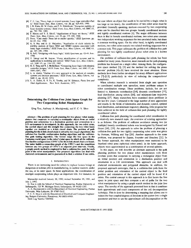
Fig. 1. Two planar three-degree-of-freedom manipulators that grasp an object and form a &link closed chain.

remaining two dimensions. This has the advantage of providing an exact answer to the dimension of the problem in which a mathematical analysis can not be avoided as well as a lower dimensional component in which approximate cell decomposition can be efficiently applied. For simplicity, the dynamics of the moving object is not considered. Furthermore, it is assumed that all information about the environment is available (in contrast to work on collision avoidance in uncertain environments [22]) so that path planning is performed off-line.

11. PROBLEM FORMUMTION In our approach for finding the paths of two closely cooperat-

ing planar manipulators that carry a rectangular object in a 2-D environment, it is assumed that each robot manipulator consists of three revolute joints and the end-effectors of the two robot manipulators grasp the rectangular object at points a and b, which are the intersections of the boundary and the centerline of the rectangular object (see Fig. 1). For convenience, point a is chosen as the reference position for the carried object with the orientation defined as the angle between the centerline of the rectangular object and the z-axis of the world coordinate system. Furthermore, it is assumed that there are p stationary obstacles that are represented by polygons.

In the following discussion, the links of the robot manipulators, the carried rectangular object and the straight line connecting the two robots bases together are modeled as a 6-link closed chain. In the closed chain, the upper and the lower links of one manipulator, the carried object, the lower and the upper links of the other manipulator and the line segment connecting two robot bases are denoted as link a1 to a6 respectively (see Fig. 1).

The length of each link a, in the 6-link closed chain is denoted as I,. It is assumed that all links of the manipulators have the same width W R and the carried rectangular object has width WO. Furthermore, the centerlines of links a, and a,+l are assumed to be connected by a revolute joint that is located at point P,+l and the centerlines of link a1 and link a6 are assumed to be connected by the revolute joint that is located at point PI. The angle of the joint located at P, is denoted as 8*. The direction of 8, is defined in Fig. 1, where the joint angles of one manipulator increase in the counter clockwise direction, while the joint angles of the other manipulator increase in the clockwise direction.

Our problem is to plan a path for each joint of the 6-link closed chain so that the carried object can be moved from a given starting position and orientation to a given final position and orientation without colliding with obstacles. To find the collision-free path for the 6-link closed chain, the following constraints must be satisfied:

_ _ _ _ -

1) The Closed-Chain Constraint: The adjacent links should always

2) The Link Collision-Free Constraints: be connected to each other.

a) If two links are adjacent, one link is not allowed to pass through the other link and no link can intersect the carried rectangular object. In other words, 8, must be in the fange [0", 360'1 for i = 1,2,5, or 6. The ranges for joint angles 83 and 84 are based on the size of the object as well as on the physical limits of the actuator and may be anywhere in the range [O" ,360"]. For the sake of illustration, the range [go", 270"] will be used throughout the remainder of this work.

b) The nonadjacent links in the 6-link closed chain are not allowed to intersect one another.

3) The Obstacle Collision-Free Constraint: The 6-link closed chain must not intersect any obstacles.

If these constraints are satisfied, then there is no collision between the robot links, between the robot links and the carried object, and between the 6-link closed chain and any obstacles in the environment.

For convenience, the joint angles in the 6-link closed chain are represented as a 6-tuple (61, 8 2 , 83, 04, 85, 66) . An instance of the 6-tuple that satisfies the closed-chain constraint is defined to be a configuration of the 6-link closed chain. A configuration that satisfies the link collision-free constraints is defined to be a feasible Configuration. Furthermore, a feasible configuration that does not collide with any obstacles is defined to be a collision-free feasible configuration, which is denoted as CFFC. It is assumed that the configurations of the 6-link closed chain at the given initial and final positions and orientations of the carried object (link as) are collision-free and feasible.

Our goal is to find a sequence of collision-free feasible configu- rations that connects the initial CFFC and the final CFFC. This task can be achieved in two steps. In the first step, a collision-free feasible configuration finding algorithm is empjoyed to find all the CFFC's for the closed chain at each quantized interval of two of the six joint angles. The second step is composed of three parts. First, a collision free path finding algorithm is employed to find the transitions between two groups of CFFC's at each pair of adjacent joint intervals. Second, a connection graph whose vertices are groups of CFFC's and whose edges are transitions between groups of CFFC's at adjacent joint intervals is built. Finally, a collision-free path is computed in the connection graph.

111. FINDING COLLISION-FREE FEASIBLE CONFIGURATIONS It is well-known from mechanics that a planar four bar linkage

has only one independent degree of freedom [23]. Therefore in order to move a 6-link closed chain as described in Section I1 from one configuration to another configuration, the positions of at least three consecutive links in the closed chain need to be changed. For convenience, any link of the closed chain in which the position of one or both ends can be changed is called a changeable Zink. It can be seen that all links, except a6, in the 6-link closed chain are changeable links. Subsequently, each set of three consecutive changeable links a,, a,+l a1+2, where 1 5 i 5 3, in a 6-link closed chain is defined to be a basic changeable unit BCU(a,,at+l,a,+2). Therefore, there are three basic changeable units BCU(a1, a,, u3), BCU(a2, a3, a4) and BCU(a3,a4,us) in a 6-link closed chain, Since there is one degree of freedom of motion in a BCU, there are three degrees of freedom of motion in a 6-link closed chain. In other words, there are only three independent joint variables among 6 joints with the other three being dependent variables.

IEEE TRANSACTIONS ON SYSTEMS, MAN, AND CYBERNETICS, VOL. 23, NO. 1, JANUARYFEBRUARY 1993 287

Our strategy to find all the CFFC's for a 6-link closed chain is to find all the CFFC's generated by a BCU for each quantized motion of the other two changeable links that are not in the BCU. The reason for not using an analytic approach is that there is no simple mapping from the three dependent joint variables to the independent variables under consideration of all the constraints discussed in Section 11. For illustration, in the following discussion BCCr(a2,a3,a4 ) is arbitrarily chosen and the motion of links a l and a:, of the closed chain is quantized. The procedure would be identical if either of the other two BCU's is selected. In the course of finding CFFC's, the constraints given in Section 11 are satisfied one by one in the following subsections.

A. Finding All the Configurations forBCU(a2,03.04) As defined earlier, a configuration of a closed chain is an instance

of the 6-tuple ( 01, 02, 03 , 0 4 , 0 5 , 0,) which satisfies the closed-chain constraint. Since BCU(a2, a3, a4) corresponds to three changeable links az, a3, and a4 that are adjacent and connected in a 6-link closed chain, if the other two changeable links a1 and a5 which are not in BCU(azla3,a4) are fixed, the position changes of the three changeable links in BCU(a2,a3 ,a4) will generate a set of configurations that satisfy the closed-chain constraint. Consequently, our strategy to find all the configurations for the closed chain is to find all the configurations for BCU(a2, a 3 , a 4 ) at each quantized position of the other two changeable links a1 and as . Since the closed-chain constraint requires that each pair of adjacent links be connected to each other, it can be observed in Fig. 1 that a necessary condition to satisfy the closed-chain constraint in BCl'(a2, a3, a4 ) is that JP2P5J 5 Zz + 13 + Z4, where JPzP5 1 represents the distance between points PZ and P5. For convenience, it is assumed that this constraint holds in the following discussion.

Since B C U ( a 2 , a ~ , a 4 ) has a single degree of freedom, it can be represented by a single parameter. It can be observed that in BCU(a2, a3. a4), if the position of one link (called the active link) is changed, the positions of the other two links (called the passive links) must be changed accordingly. Since the positions of links a2 and a4

can be uniquely described by joint angles 0 2 and 195 respectively, it is convenient to choose one of them as the active link and choose the corresponding joint angle to represent BCLT(n2 .n3 . a t ) . In the following discussion, it is assumed that a4 is chosen as the active link and BCU(a2, a3, a4) is described by the parameter 0 5 . Hence, the task of finding all the configurations can be solved by finding the motion range of 05, denoted as MR(05), in which the closed-chain constraint can be satisfied. In order to find MR(05), the following definitions are introduced.

Definition 1: If one end of the centerline of a changeable link a , is fixed at a point P , then all the possible positions for the other end of the centerline of a, form a circle with radius I , and center P . This circle is called the link position circle of a , and is denoted as LPC,, ( P ) or simply LPC,, . 0

Definition 2: The circles that have a common center PZ and radii (12 + 1 3 ) and 112 -23 1 are defined as circle I and circle 11, respectively. 0

Based on the triangle inequality concept, it can be shown [24] that the motion range MR(05) in which the closed-chain constraint is satisfied should be a set of regions on the link position circle LPC,,(P5), which lies within circle I, but outside circle 11. As an example, if circle I intersects LPC,, at hl and h z , but circle I1 does not intersect LPC,, , the motion range MR(O5) is equal to the range [< PePsh~, < PeP5hl] on LPC,, ( see Fig. 2).

For a given position of the active link a4 or a given O5 in M R ( 0 5 ) , the possible positions of P3 (which connects the passive links a2 and a3) should be on both LPC, , (P2) and L P C , , ( P 4 ) (see Fig. 3).

Fig. 2. An illustration of the motion range of 05 (denoted MR(&)), which satisfies the closed-chain constraint.

pfi

Fig. 3. A n illustration of the two symmetric configurations that result from a single position of a4. The configuration shown in the solid line is called a large configuration and the one in the dashed line is called a small configuration.

Hence, the possible positions for P3 should be at the intersections of LPC,, and LPC, , . Since 12 + l 3 + l4 < IP2P51, LPC,, and LPC,, have two intersections so that two possible positions of P3 can be found. In other words, a given position of a4 or a given 8 5 in MR(05) can correspond to two possible positions for the passive links a2 and a3 and therefore two configurations can be obtained. Thus all of the configurations of BCU(a2,a3,a4) are included in this motion range.

B. Finding All the Feasible Configurations forBCU(a2, a3, a4)

In this section, we shall find a set of subregions of the motion range ,21R(O5 ) in which the link collision-free constraints aye satisfied. These subregions of MR(05) are called the feasible regions and are denoted by FR(05) . Once FR(B5) is found, all the feasible configurations of BCCT(a2.a3, a 4 ) can be determined by restricting the motion of 05 to FR(05) .

The link-collision-free constraints resulting from the requirement that the links not collide with one another will be considered in two categories based on whether the links are or are not adjacent. The motivation for this distinction lies in the observation that collision between adjacent links can be prevented by limiting the joint ranges of the associated joints while collisions between nonadjacent links must consider more geometric constraints. 1) Finding Subregions of MR(05), which Satisfy the Link Colli- sion-Free Constraint for Adjacent Links: It is easy to see that one can guarantee that the adjacent links of BQU(a2, a3, a4) are collision

288 IEEE TRANSACTIONS ON SYSTEMS, MAN, AND CYBERNETICS, VOL. ki, NO. 1, JANUARY/FF,BRUARY 1993

I ~

~- ' Fig. 5. One range of &can be mapped to two ranges of 8 5 .

Fig. 4. A graphic interpretation of the mapping from the joint limit con- straints on 0 2 and 03 onto ranges of 05, denoted by Re,,e,(OS).

range of 85 or two possible valid disjoint ranges will be symmetric with respect to m, where represents the straight line between points Pz and P5.

Mapping the valid range of O4 onto ranges of e5: Since it is not easy to directly map the valid range of B4 Qnto ranges of 05, the valid range of 84 is first mapped onto ranges of 82, which are denoted Re, ( & ) , then Re, ( 8 2 ) is mapped to ranges of 8 5 , which are denoted Re, ( 8 5 ) . Thus for each 8 5 E Re, (65)- at least one corresponding configuration has 84 E [go", 270'1. To obtain Re, ( @ 2 ) , a procedure that is similar to finding Re, ,e3 ( 8 5 )

can be Used- After finding Re, (@2), the Cked-chain c!onstraint upon Re, (82) is checked by an approach similar to that given in Section 1II-A. Subsequently, the valid range of (&), which satisfies the closed-chain constraint can be mapped to a set of regions of e5, i.e.,

( 8 5 ) . To find this Re, ( @ 5 ) , the following definition needs to be introduced.

Definition 3: In BCU(a2, a3, a4), for any given 8 2 , there are two

free by restricting the range of 82 and 8 5 to be between 0 and 360 degrees and 8 3 and 84 to be between 90 and 270 degrees. Since 85 is chosen as a parameter to represent BCU (a2, as, a4 ), our approach is to map these constraints onto the motion range of 8 5 . This mapping is performed in the following two steps:

1) The constraint on the range of 82 and the constraint on the range of 8 3 are mapped onto ranges of 85.

2) The constraint on e4 is first mapped to ranges of 8 2 in a procedure similar to step (1) and then the resulting ranges of 82 are mapped onto ranges of 8 5 .

The resulting set of valid motion ranges for B5 are then further decomposed in order to distinguish regions which posses single solution from those which have dual symmetric solutions. The need for this decomposition arises from the fact that the inverse kinematic mapping for revolute manipulators is multiple valued. Mapping the valid joint rnnges of & onto the ranges of As possible confi@rations. In Order to distin@ish between these mentioned previously, the degrees and the valid range of 82 is between and 360 degrees. 85 was chosen as the parameter to represent BCU(a2, u3, a4) , the

range of 83 is between 90 and 270 configurations, it can be noted that the 8 3 in one configuration is larger than that in the other configuration. The term small configuration with respect to 8 2 or simply small configuration will be used to refer to

valid ranges of o3 and o2 should be mapped to ranges of 05. nese ranges of O5 are denoted as Re2,e3 ( @ 5 ) . In other words, if o5 E

the configuration that lQrge configuration with respect to '2 Or

the smaller value Qf 83. Similarly, the term large configuration

Re2,e3(85) , the corresponding configurations have @3 E 27001 and 8 2 E [0",360"].

To find Re,,e3 ( 8 5 ) , we consider links a2 and a3 as a two link manipulator in which the base is located at P2 and the end-effector is located at P4. It can be observed in Fig. 4 that to guarantee

link manipulator is bounded by a ring. The outer boundary circle of the ring is circle I with center P2 and radius 12 + Z3. The interior boundary circle of the ring is denoted as circle 111, which has center P2 and radius Jm (see Fig. 4). By the closed-chain constraint, a3 and a4 must be connected. Consequently, Re, ,e3 (85) will be a set of regions on the link position circle LPC,, , which lie within the outer boundary circle I, but outside the interior boundary circle 111. Based on the relative positions between circles 1, 111 and LPC,, , Re2,e3(8s) will fall into one of following three cases. Case 1: If LPC,, is inside circle 111, then Rs2,e3(85) = a. Case 2: If LPC,, is outside circle 111, but intersects circle I at points

f l and Fs7 then Rez,e3 (85) = [< P s P ~ F ~ , < p6p5Fsl . Case 3: If circle 111 intersects L p c a , at points ui and us and circle

I intersects Lpca4 at Points fi and then Re, ,e3 ( 8 5 ) = [< PsPsFs, < PSP~US] u [< P6p5u1, < P G P ~ & ] .

As an example, case 3 is shown in Fig. 4. It can be observed from the previous three cases that Re2,e3(85) may contain two disjoint ranges of 85 values, a single valid range, or no valid range. Since I and 111 have center P2 and LPC,, has center 9, a possible single valid

will be used to refer to the configuration that has the larger value of 193. The analogous definition can be made for a given value of 85 based on the value of 84. These two configurations are illustrated in Fig. 3. 0

Since one 8 2 corresponds to two configurations or two values of

to find this mapping, it is assumed that there is a valid range of Re, (&), i.e., Re4 (82) = [& min, 8-2 ma,]. TO map [ e 2 min, 8 2 ma,] to the ranges of 8 5 , the two boundaries Bzmm and are mapped first' Since both 82m1n and Of O5 (one for small configuration and one for large configuration). For convenience, it is assumed that 8 z m l n is mapped to (for the small configuration) and e:,,, (for Qe large configuration). Similarly, 82 is assumed to be mapped to 8; (for the small configuration) and (for the lwge configuration). Thus two ranges that are the range betweel! e:,,, and @lmw for the large configurations and the range between 8; m,n and 8; max for the small configurations can be obtained (see ~ i ~ . 5). pnfortunately, it can be shown that there exist cases in which the range [8kmin, e:,,,] or the range [e; m,n, 8; is not the complete mapping of [e, mln, 8, ,,,I. As an example, consider the case shown in Fig. 6. When 82 decreases from 82 to& m,n, 85 increases from 8: max to some point A, and then starts to decrease from A to 8: mln. To ezplain this phenomenon, a property of BCU(a2,a j ,ar ) is introduced.

Property 1: In BCU (a2, a3, a4), if ZZ + Z3 < I Pa PS I + l 4 , then a2 and a3 can become aligned. When a2 and a3 are aligned, 85

e3 E [90",270"] and o2 E [00,3600], the workspace of this two 857 a range Of 82 can be mapped to ranges Of 05. In Order

correspond to

IEEE TRANSAmIONS ON SYSTEMS, MAN, AND CYBERNETICS, VOL. 23, NO. 1 , JANUARYIFEBRUARY 1993 289

La,.". , L / / e.-:- \ -

W-

Fig. 6. An illustration of the case where the extremal values of the range of &are not mapped to extremal value of the range of 0 5 .

Fig. 7. If 1Z2 + Z31 < IP2P5( + 11, then not all values of 85 can satisfy the closed-chain constraint. The maximum and minimum allowable values of 85, denoted 85 max and 85 min, occur when links a2 and a3 are aligned. The 02. The 82 values in these cases are denoted @;align and @;align, respectively.

will reach its maximum value 8smax or its minimum value 8smln. The value of 82 is denoted as 8iallgn if 05 = 8smaY or 8;al,gn if

This property can be explained by Fig. 7. It can be shown in Fig. 7 that if the condition 12 + 13 < IP~PF,~ + 14 holds, the circle with center P2 and radius 12 + 13 can intersect LPC,, so that a2 and a3 can become aligned. When a2 and a3 are aligned, the distance between P2 and Ps reaches its maximum. Consequently, 85 cannot became any larger or smaller.

Based on Property 1, if is not inside the valid range of 82, when 82 monotonically decreases from one boundary to another boundary, corresponding 8 5 will monotonically increases or decreases from one boundary to another boundary. For illustration, in the case of the large configurations (the case for the small configurations can be discussed in a similar way), it can be shown in Fig. 8 that when 8 2 m , n . 8 2 m a x > 8flallgn, if 82 decreases from 02 max to 82 m,n, the distance between I3 and P4 increases so that 0 5

increases. Thus [82 m,nr 8 2 ,,,I is mapped to [e: 8: mln]. In Fig. 9, since 8 2 m,n. 02 to 8 2 ,,,, ,,, the distance between P2 and Pa also decreases so that 0; decreases. Thus [82 n,,nr 02 ,,,I is mapped to [e: mln. 8: , , , I . However, if 8flallgn or O;al,gn is inside the range of 82, the previous two cases should be combined. For instance, since the case shown in Fig. 6 has 8 2 min I 8flallgn 5 82 max, when 82 decreases from 6'2 to 8hallgn,

8 5 = 05min. 0

or

< 8hallgn, if 02 decreases from 82

Incrcase

1

(b)

Fig. 8. If all values in the range [e, rnin@2 max] are larger than Bial ign then [ e 2 mine2 ma,] is mapped to [e,; max@:

0 5 increases from 8:,,, to A that is equal to 8smax and a2 and a3 become aligned. If 02 continues to decrease from 8halign to 8 2 min. 05

starts to decrease from 05 to 0; nlin. Consequently, [O, minr 02 ,,,I is mapped to [min (0: 8; ,,,) , O5 ,,,I. The previous discussion can be summarized in the algorithm given previqusly. Algorithm 1: To map the range [02m,n,$2max] to the ranges of 85,

1) map the boundaries of the range [8zminr Oamax] to the ranges of 0 5 , i.e., map 82,in and 82,,, to 8Lmin and OS,,, for the large configurations respectively, and 8; min and 8; max for the small configurations respectively.

2) map 82 between the boundaries of the range [ 0 2 m i n r 8 ~ m a x ] to the ranges of 8 5 .

a) for the large configurations, the following three cases hold:

if 82 02 min > then [O, min 8 2 ,,,I is mapped

if @2,in 5 8haljgn 5 8zmaXr then [ 0 2 m i n r @ ~ m a x ] is

if 82 82 m i n < 8;alignr then [ e 2 minr 8 2 max] is mapped

to [e: max * 8: min] 7

mapped to [min (0: m i n , 0: ,,,) ,Os ma,],

to [@.kmin*@kmax];

b) for the small configurations, the following three cases hold:

if 0 2 max. 8 2 m,n > O l a l i g n , then [82 min, 02 ,,,I is mapped

if @ z m i n 5 8;align 5 then [@2minr82max] is mapped to [85,in.max ( 8 ; m i n , 8 ~ m ~ x ) ] , if 8 2 max. 8 2 ,,,in < then [ e 2 min. 02 ma,] is mapped

0

to l G m i n , @ l m a x l ,

to 16'; max- 6; min].

290

Decrease

IEEE TRANSACTIONS ON SYSTEMS, MAN, AND CYBERNETICS, VOL. 23, NO. 1, JANUARY/FEBRUARY 1993

p, '6

(b)

Fig. 9. If all values in the range [e2 ,,,I are smaller than then [e2 mine2 ma,] is mapped to [e: ,,,I.

for the large configurations

for the small configurations

Fig. 10. Two ranges of 02 can be mapped to four ranges of 05.

The previous discussion is based on the assumption that the valid region of Re,(Bz) contain a single range. However, it may consist of two disjoint ranges. If valid region of Re,(Oz) consists of two disjoint ranges, say, [e, mini, 82 1 and [e2 min2,ez maxz], Re, (8s) will consist of four ranges (see Fig. 10). They are the ranges for small configurations and large configurations that are mapped from [e2 m i n ~ , 82 maxi] and the ranges for small configurations and large configurations that are mapped from [e2 min2 , 82 The bound- aries of these four ranges are determined by applying Algorithm 1.

Decomposing Re, (85): As described previously, each value of 8 5 E MR(85) corresponds to two configurations (the small configuration and the large configuration). After mapping Re, (82)

to Re, (OS), it is guaranteed that for each 85 E Re, (Os), at least one corresponding configuration has 82 E Re,(82) so that at least one corresponding configuration has 84 E [go", 270Q]. However, there is no guarantee that the other configuration has 84 E [goo, 270'1. Since a set of subregions of MR(85) in which all the configurations satisfy the link collision-free constraint for adjacent links is needed, Re, (195)

should be decomposed in order to recognize in which subregions of Re, (OS), each 85 corresponds to two corresponding configurations with 82 E Re, (82) and in which subregions of Re, (Os), each 85 corresponds to one small (or large) corresponding configuration with 82 E Re, (82). In order to perform this decomposition, the following definition is first be introduced.

Definition 4: Let M(85) denote any subregion of MR(05) so that each 85 E M(85) corresponds to two configurations (the large configuration and the small configuration). If in some subregions of M(85), only the small configurations are being considered, then these subregions are called small-one-configuration regions and are denoted as SUB, -M(&) . If in some subregions of M(B5), only the large configurations are being considered, then these subregions of M ( 8 5 ) are called large-one-configuration regions and are denoted as SUB1 - M(85). Similarly, if both the large configurations and the small configurations are being considered, they are called two- configuration regions and are denoted as SUB2 - M(85). 0

By Definition 4, Re, (85) can be decomposed so that Re, (85) = SUB2-Re,(8s) u SUB,-As,(O5) U SUBI-Rs , (85) , where SUB2-Re4(85) contains all the subregions of Re,(&) in which each 85 corresponds to two configurations with 82 E Re,(&) and SUB,-Re, (85) ( or S U B I - R ~ , (85)) contaiqs all the subregions of Re,(Bs) in which each 85 corresponds to one small ( or one large ) configuration that has 82 E Re4(&).

It can be shown [25] that all the possible subregions of Re,(&) in which each 8s corresponds to two configurations with 8 2 E Re, ( 8 2 )

will belong to one of the following cases: 1) For each valid range of Re,(&), if the case shawn in Fig. 6

occurs then the subregion of Re4(&) that is trqveled by 85 twice when 82 moves from one boundary to aqother belongs to SUBz-Re,(85). Thus the region [@,, , ,A] shown in Fig. 6, where A =

2) Recall that the two disjoint subregions of valid Re, (82) can be mapped to four continuous regions of 85 (see Fig. 10). If 85 is in the intersection between any two of these four regions of 85, it can correspond to two configurations with 8 2 E Re, ( 8 2 ) .

After finding SUB2 - Re,(&,)(&), the subregions for the large and small configurations, SUB1 - Re,(85) and SUB, - Re,(&), will be found by identifying the position of 8;al,gn and in Re, (82). As mentioned earlier, each valid range of Re, (8,) can be mapped to two ranges of 85. One is for the small configurations with respect to 82 and the other is for the large configurations with respect to 82. It can be shown [W] that in each subregion of & , ( O S ) which is mapped for the large configurations (or small configurations ) with respect to 8 2 and is not in SUB2 - Re,(&),

1) if a range in this subregion of 85 is mapped by the range of 82 in which each 82 is greater than 6':allgn (or 81align), it belongs

2) if a range in this subregion of 8 5 is mapped by the range of 8 2 in which each 8 2 is less than 8iallgn (or elalign), it belongs

After finding SUB2-Re4(85), SUB1-Re4(85) and SUB, - Re,(85), if 8 5 belongs to one of them, all the corresponding configurations have 84 E [90",270"]. As mentioned earlier, for each 85 E Re2,e, (Os), all the corresponding configurations have 82

in its valid range [ O O , 360"] and 83 in its valid range [go", 270"].

belongs to SUB2-Re4(85).

to SUB1 - Re,(Os);

to SUB, - Re,(85).

IEEE TRANSACTIONS ON SYSTEMS, MAN, AND CYBERNETICS, VOL. 23, NO, 1 , JANUARYIFEBRUARY 1993 29 1

Consequently, if 85 E MR(85) n R0,,03(85) n R e , ( & ) , the corresponding configurations will satisfy the link collision-free constraint for adjacent links. However, for doing these intersection, attention should be paid to the facts that MR(B5) and Re, n , ( O , ) are two-configuration regions; and Rs, ( 8 5 ) is the union of two- configuration regions, S U B , - M ( 8 , ) s and S P B I - A i ( 8 5 ) s .

Finding Subregions of MR(85), which Satisfy the Link Collision- Free Constraint for Nonadjacent Links: To satisfy the link collision- free constraint for nonadjacent links, it can be observed from a 6-link closed chain that:

1) Since B C U ( a 2 , a s . ~ ) is being discussed, the positions of links a l , a5 and a6 are fixed. The easily identified values of 81 and 86 that result in a collision of these links need not be further analyzed.

2) The collision between the two nonadjacent changeable links a2 and a4 can be avoided by imposing appropriate limits to 83 and 84. Here it is assumed that 83 and $4 are within the range [go", 270'1.

3) The changeable links a2, a3 and a4 can possibly intersect the fixed links a l , a5 or a6. Since 83 and fI4 must be in the range [90',270"], the changeable links 0 2 , a3 or a4 can possibly intersect the fixed links a l , a5 or a6 only if 8 5 or 0 2 becomes small.

The values of (or $2contact)r defined as the value of $5 (or 8,) when one of a3 and a4 (or one of a3 and a2) touches 01, a5

or a6, can be found according to the geometric relationships of the 6-link closed chain. Subsequently, a subregion R,,,,, ( $ 5 ) of MR(B5) in which each configuration has 85 2 and $2 2 82contac t

can be obtained by the method described in the previous sections. Hence, if 85 E R,,,(85), the link collision-free constraint for nonadjacent links can be satisfied. Consequently, we can conclude that the feasible region FR(85) in which the link collision-free constraints are satisfied is the intersection between the ranges that satisfy the link-collision-free constraints for adjacent links and the ranges that satisfy the link-collision-free constraint for nonadjacent links. Thus all of the feasible configurations are included in this feasible region.

C. Finding All the Collision-Free Feasible Configurations In the last section it was shown how the feasible regions FR( 6's )

could be computed. If there are obstacles in the environment, then any collision with these obstacles should also be avoided. In this section, the subregions of FR(85) in which each feasible configuration is collision-free will be found. In the following discussion, a single- obstacle environment is studied. For an environment with multiple obstacles, the principle of superposition can be applied so that the subregions of FR(85) in which each feasible configuration is collision-free are equal to the intersection of those in each single- obstacle environment. The simplest case in which the link widths, i.e., wo and W R , are equal to zero and the obstacle is a convex polygon is presented. If the obstacle is a concave polygon, it can be decomposed as a combination of several convex polygons. If wo and W R are not equal to zero, the results can be modified by shrinking the width of the carried object and the robot arms to zero and enlarging the size of the obstacle accordingly [2], [ 3 ] . Generally speaking, this method becomes cumbersome when arbitrary orientations are allowed. However, in this case, one is dealing with a constraint mechanism so that general orientations are not allowed. In the following discussion, it will be shown that the algorithm is only concerned with the distance between the corner or edge of the obstacle and the outer boundary of the carried object (link 0 3 ) . This allows the obstacles to be grown in a straight forward manner.

Fig. 11 . An illustration for finding PCFFER,4(&).

Now, assuming there is one convex obstacle in the workspace and the widths of the carried object and robot links are zero @e., 1 1 ' 0 = 0 and U I ~ = 0), subregions of FR($5), which satisfy the collision-free constraint can be obtained by considering the collision- freeness of each changeable link of a z , a3 and a4 one by one in BCIT(n2, a3.a.$). The procedure is given in the following:

1) Find subregions of FR(B5) in which the corresponding posi- tions of a4 do not have any collision with the obstacle. Such a subregion is called a possible collision-free feasible region of a4 and is denoted PCFFR,,(O5).

2) Find subregions of PCFFR,, (19,) in which the corresponding positions of a4 and n2 do not have any collision with the obstacle. Similarly, each of these subregions is called a possible collision-free feasible region of a 2 and a4 and is denoted

3 ) Find subregions of PCFFR,,,,, ( $ 5 ) in which the corre- sponding positions of all changeable links a2, a3 and (1.1

are collision-free with the obstacle. Each of these subre- gions is called a collision-free feasible region and is denoted CFFR(6'5) or simply a CFFR.

PCFFRa,,a4(@5).

Each step is discussed in detail in the following subsections. Finding PCFFR,, (8,) and PCFFR,,,,,(b'5): Suppose there

is an obstacle 0 1 in the environment that intersects LPC,, at points A and B , where 8 . 5 ~ > BSB (see Fig. 11). To find PCFFR,,(85), a set of rays from P5 to A, B and to each corner of 01 which is inside LPC,, can be obtained. The angles from link a5 to each ray are calculated, then the smallest and largest angles 0 5 R ~ and B5*' among them are selected. Assuming 8,ax, and Omin! are the largest and smallest angles of FR(BS), then PCFFR,,(B5) = [85,41. 8, ,,,I] + [ B 5 n, , , l l l 8,,t]. By a similar approach, the sub- regions of (12 in which a2 does not collide with an obstacle can be obtained. Subsequently, by using the method discussed in the previous sections, these subregions of $2 are mapped to the ranges of 85, which are denoted as PCFFR,,(b'5). For each 8, E PCFFR,,(85), in the corresponding configurations, there is no collision between a2 and the obstacle. Consequently, PCFFR,,,,, (85) in which the corresponding positions of a4 and a2 do not have any collision with the obstacle is equal to PCFFR,, (8,) n PCFFR,, ( 6 5 ) .

Finding CFFR: Now our goal is to find collision-free feasible regions (CFFR's) that are subregions of PCFFR,,,,, ( 8 5 ) and in which all the changeable links 0 2 , a3 and a4 are collision-free with the obstacle. For convenience, PCFFR,, r a 4 ( S S ) ~ and CFFRi, where i = 2,s.1, are used to represent a PCFFR,,,,,(85) and a CFFR, which is a two-configuration region, a SUB, - i l f ( B ~ ) , or a SUB, - M ( 8 5 ) . respectively. Since a CFFR' is a subregion of a PCFFR,, (0, )', there should be some collision-free feasible con-

292 IEEE TRANSACTIONS ON SYSTEMS, MAN, AND CYBERNETICS, VOL. 23, NO. 1, JANUARYFEBRUARY 1993

Fig. 12. An illustration of the technique used for finding critical CFFC’s that determines the boundaries of collision-free feasible regions.

figurations (CFFC’s) that divide PCFFR,, into several nonzero subregions. This kind of CFFC in a PCFFR,, ,,, ( 8 5 ) ’ is called a critical CFFC, since the subregion that is at one side of the CFFC is a CFFR, but the one that is at the other side of the CFFC is not collision- free. Obviously, if all the critical CFFC’s can be obtained, then all the CFFRs can be found as well. Subsequently, all the CFFC‘s can be found. To find the critical CFFC’s, the following lemma is introduced.

Lemma 1: If a 6-link closed chain is in a critical CFFC of a PCFFRa,,a4(6’5)1, then a3 must pass through a comer or an edge of the obstacle. 0

It is easy to show that this lemma is true since link a3 is a line segment and the obstacle is a convex polygon.

By Lemma 1, the critical CFFC’s can be found by finding the CFFC’s in which the location of a3 touches a comer or an edge of the obstacle. Now let’s consider a critical CFFC that touches a comer of an obstacle. In this critical CFFC, a3 should touch a comer of the obstacle; 85 should be in a PCFFR,,,,,(6’5); and 82 should be in PCFFR,, (ez), which is the mapping of PCFFR,,, , , ( 8 5 ) . Our strategy to find this critical CFFC is described as follows: 1) for each PCFFR,, ,,, ( & ) , find its mapping on 8 2 , i.e., PCFFR,, (82); 2) since not all the configurations on PCFFR,, (82) can touch the comer of the obstacle, find the subrange of PCFFR,, (82) in which the configurations can possibly touch the corner of the obstacle; (3) find the subrange of PCFFR,,, , , ( 8 5 ) in which the configurations possibly touch the comer of the obstacle and have one end of a3

on the range obtained in Step 2; (4) use the geometric relationships to locate a configuration in which a3 passes through a comer of the obstacle and has its two ends at the ranges obtained in Step 2 and Step 3 respectively.

Before giving the details of the algorithm, for convenience, a notation that builds the relationship between 85 ( 82) and a point on the circle LPC,, ( LPC,,) is first introduced. In the following discussion, as each position of a4 (or a2) corresponds to a distinct value of 85 (or &), it is assumed that if the changeable end of the centerline of a4 (or az) is at a point P on LPC,, (or LPC,,) , the corresponding 8 5 (or 6’2) is denoted as 8 5 ~ (or 8zp) . Suppose one is given a [ 8 5 s l , 8 5 s 2 ] which is a PCFFR,,,a,(f?5)’ (i = s, I ) on LPC,, , and v3 which is a corner of the obstacle (see Fig. 12), an algorithm that locates the critical CFFC within PCFFR,,, , , (e,)* and touching comer v3 is given as following. Algorithm 2:

1) Find PCFFR,, (6’2) = [ezs;, 82s;] which is the mapping of

2) Find the subrange [Tl,Tz] of PCFFR,,(@z) = [8zs;,82s;] PCFFR,,, , , (85)’ on LPC,, .

K Z

Fig. 13. The region in which a critical CFFC may exist.

in which the configurations can possibly touch the comer of the obstacle by calculating the possible intersection of line 81v3 with LPC,,(Pz) , denoted tl and the intersection of line v382 with LPC,,(P2), denoted t z .

a) If both intersecjiqns do not exist or the intersection of the two arcs t l t 2 and s1s2 is empty, then [TI, Tz] is empty , i.e., there is no critical CFFC with respect to the comer v3. Stop. , ,

b) If both t1 and t z exist and the intersection between arcs sls2 and tltzlis,not empty, TIT^] is equal to this intersection, Le.,

c) If there exists only one t,, i = 1 or 2 , the line t , s , would separate the entire plane into two subplanes and separate LPC,, into two arcs.

If the intersection between sisi and one arc of LPCa, which is in the same subplane with line 9,213, where i,j = 1,2, i # j , is empty, then [Tl,T2] is empty, Le., there is no critical CFFC with respect to the comer v3.

Otherwise, T1T2 is equal to s1s2.

tlt2 n s1s2.

I f stop.

3) Find the subrange [Kl ,h ; ] of PCFFRa,,ag(85) in which the configurations possibly touch the comer of the obstacle and have one end of a3 on the range obtained in Step 2 by calculating the possible intersection of line T1w3 with LPC,,(P5), denoted K1 and the intersection of line TZU3 with LPC,, (P5), denoted h’z (see Fig. 13).

4) Use a set of equations derived from the geometric properties of the area shown in Fig. 13 [25] to find a line segment L with length 13, which has one end on [TI, Tz] of LPC,, , one end on [Kl , h-21 of LPC,, , and passes through v3 . If line segment L exists, then a feasible position of a3 in the area shown in Fig. 13 can be found. This feasible position of a3 defines a critical CFFC. 0

After checking each comer of the obstacle, the edges of the obstacle should also be checked by overlapping link a3 with the edges of the obstacle. If there is a collision-free feasible configuration in which link a3 and an edge of the obstacle overlap, it is a critical CFFC. After finding all the critical CFFC’s in all the PCFFR, , , , , (8~)’s , all the CFFR’s and hence all the CFFC’s for a singleobstacle environment can be determined.

Iv. FINDING A COLLISION-FREE PATH In the previous section, all of the CFFC’s in BCU(a2, a3, a4) in

terms of 85 have been found for a set of quantized values of 81 and 86. Since 81, 86 and 6’5 have been chosen as the independent variables, the collision-free path finding problem with these three independent variables can be solved in the following four steps:

1) Find the transitions between CFFR”s (i = 2,Z,s ) at fixed values of and 86.

IEEE TRANSA(X1ONS ON SYSTEMS, MAN, AND CYBERNETICS, VOL. 23, NO. 1 , JANUARYIFEBRUARY 1993 293

2) Find the transitions between C F F R l ' s at adjacent ( quantized ) values of 81 and 86.

3) Build a connection graph in which each vertex is a C F F R ' in BCU(az,a3,a4) for a specific 81 and 8 6 , and each edge is a transition between a pair of C F F R ' 's at fixed values of 81 and 86 or at adjacent ( quantized ) values of 81 and 6'6.

4) Search a collision-free path for the 6-link closed chain in the connection graph.

The details are discussed in the following subsections.

A. Finding Transitions Between C F F R " s ( z = 2, s . 1 ) In different BCU(a*,as ,a4) ' s

For a specific 81 and 8 6 , there is one degree of freedom that is represented by 8 5 in BCU(n2,a3.n4). A transition is defined to exist between two C F F R " s (i = 2, 1 ,s ) in BClT(a2,c13.a4) if when the value of 8 5 is changed continuously, a CFFC in one C F F R ' can be automatically transferred to a CFFC in another C F F R ' . There are three possible types of transitions based on the combination of different types of CFFRs: (1) transitions between C F F C ' s ( i = 2 , I , s ) in separate C F F R ' s , (2 ) transitions between CFFC's in a C F F R ' ( i # 2) and a C F F R 2 , and (3) transitions between a C F F C ' and a C F F C ' in a C F F R ' . Since there is only one degree of freedom in the B C U ( n z , n 3 . n l ) , by definition the transitions between two separate CFFR's cannot exist. Therefore, the transitions in the case 1 discussed previously cannot exist, and only special situations in the case 2, and 3 can exist. These special situations are listed as follows:

1) a C F F R ' and a C F F R ' which belongs to a C F F R 2 (or a C F F R ' and a C F F R ' which belongs to a C F F R ' ) contain a common 85 , i.e, they are connected by a point on LPC,, .

2) If in a two-configuration region C F F R ' , there is a point at which a2 and a3 become aligned, then the C F F R " and the C F F R ' which belong to the C F F R 2 can be transferred to each other. The point at which 0 2 and n? become aligned is normally at the boundary of the motion region diR(19~).

B. Finding Transitions between C F F R' 's ( 2 = 2. s. 1 ) in Different BCU(n2.03,ad)'s

In addition to the transitions between C F F R " s ( I = 2,s.l ) in a B C U ( a 2 . ~ 3 . a 4 ) with the same 81 and 8 6 , transitions between C F F R ' s in two different B C l ' ( 0 2 . n 3 . n 4 ) ' s which have different quantized values of 81 or different quantized values of 66 need to be found. For each BCU, there are three kinds of CFFR's: C F F R ' ( which is composed of a C F F R ' and C F F R s ) , C F F R l and C F F R " . In the following discussion, for convenience, it is assumed that (1) a C F F R 2 is considered as an independent C F F R ' and an independent C F F R " , (2) if a C F F R J (J =l ,s ) and a C F F R J which belongs to a C F F R ' are connected by a point, they are considered as one C F F R ' . Due to this assumption, for adjacent BCU's, only transition between the same kind of C F F R ' s , i.e., between C F F R " s or C F F R " s and transition between C F F R ' and C F F R ' need to be discussed. In the following, transitions between CFFR's in two adjacent BCU's, which have have different (quantized) values of 81 and the same value of 6's are discussed. Transitions for BCU's with the same value of 6'1 but adjacent values of 86 can be obtained in a similar manner.

For convenience, the notation BCl*(nl ny.n. l ) l ,y 0; will be used to represent BCl- (n2 ,ns .n*) at a specific value of 81 (8;. in this case) and a specific value of 8 6 (6': in this case), and C F F R ' ( k ) , ; , ,: is used to represent the k-th C F F R ' ( i = s or 1 ) in BCli(n2 n 3 . n 4 ) l o ; . , 0 ; . First let's discuss the transitions between the same type of the CFFR's.

Assume there are two of the same type of collision-free feasible regions: CFFR' (k ) , ; , in BCU(a2 a3,a4)10;. a; and CFFR'(k') , ,+l B n in BCU(n2 n3.n4)lgm+1 The transitions between them will be based on the geometric relationship among two corresponding BCU's. Since these two CFFR's have different values of 81 but the same value of 6'6, the corresponding BCU's, i.e., BCL*(n2 o3.n4)l~; , 02 and BCU(a2 ng,a4)lgn+i also have the same value of 8 6 . Therefore, they have the same link position circles LPC,,. As mentioned earlier, for each BCU, C F F R " s are separated by obstacles and therefore one C F F R ' cannot be transferred to another C F F R ' in a specific BCU. Thus if there is a transition between C F F R ' ( k ) , ; , o n and CFFR'(k') , ,+l C F F R ' ( k ) , ; , n C F F R ' ( k ' ) , T + l ,: must not be empty. If the quantization intervals of 81 and H c are sufficiently small then in the case CFFR' (k ) , , , and C F F R " ( k ' ) , y + ~ ,: are collision-free at quantized values 8;l and for both BCU, C F F R ' ( k ) , I ,,; and C F F R ' ( k ' ) , l o g are collision-free for each value of O1 in the interval between 6';l and 8y"". Consequently, if C F F R ' ( k ) , ; , n CFFR'(k ' ) , ,+l # 0, then there is a transition between CFFR' (k ) , ; , and CFFR1(lc') , ,+~,,; . 1

If there are two different types of collision-free feasible regions C F F R ' ( k ) , ; , e," and C F F R 3 ( k ' ) , y + l where i j = s, 1, 7 # 3 , whether there is a transition between them depends on if there is a point in C F F R ' ( k ) , ; , oz n CFFR3(k ' )o ;n+l , , gn , which can make a2 and (13 become aligned, because it is the only case in which the large configuration can be transferred to the small configuration.

After finding all CFFR's and all the possible transitions among them, a connection graph can be built. In this connection graph, each vertex is a CFFR and each edge is a transition among CFFR's. Since there are three degrees of freedoms, the connection graph can be represented in a three-dimensional space with independent variables @l , B S and 0 5 . Because the connection graph represents all the free space in the joint space of the 6-link closed chain, a collision-free path of the closed chain can be searched in this connection graph.

1 6 1 6

1 ' 6

1 6

1 6

1 G

C. An Example The following example illustrates the construction of a connection

graph. After all of the C F F R " s for the 6-link closed chain have been found in term of 81, 6'5 and 6'6, a connection graph can be described in a 3-D space for different values of 6'1, 8 5 and 8 6 ,

where 81 and 86 are chosen as the axes in the horizontal plane and 6'5 is chosen as the vertical axis. In this example, variables 6'1 and 8 6 are quantized. A point on the 6'1 - 6'6 plane which corresponds to a specific quantized value of 01 and 86 defines a unique BCl-(n2,n3.al) lol ,os . Since there is only one degree of freedom of motion in BCl'(n2, n3. n 4 ) 1 0 , ,os, vertical line segments which originate from a point on 6'1-6'6 plane and parallel to the 8 5 - axis can represent all the C F F R " s in BCU(a2,a3 ,04) l s , ,06 (with two parallel segments to denote two-configurations). These CFFR's are the vertices of the connection graph (see Fig. 14). If there is a transition between two of these C F F R " s , an edge in the connection graph can be drawn (shown as a dashed line in Fig. 14). After all the transitions between C F F R " s ( i = 2, s.l ) are found, a connection graph is built. Consequently, a collision-free path for the 6-link closed chain can be obtained by applying a graph search method in the connection graph.

V. CONCLUSION

This paper has discussed an off-line approach for planning a collision-free path for two robot manipulators that cooperate in

294 lEEE TRANSACTIONS ON SYSTEMS, MAN, A N D CYBERNETICS, VOL. 23, NO. 1, JANUARYFEBRUARY 1993

e: e: e: Fig. 14. A connection graph showing all possible collision-free feasible con- figurations for a Mink closed chain. A collision-free path of the &link closed chain from initial position CFFRS(1)83e3 to final position CFFR’ (l)e;e;, which is shown by bold dashed lines. 1 6

carrying a rectangular object in a 2-D environment. The central concept of this approach is to map the free space in the Cartesian world space to the robot’s joint space. In the joint free space, each joint configuration of the robots satisfies the closed-chain constraint, the link collision-free constraints, and the obstacle collision-free constraint. A collision-free path for the robots is then computed in this joint free space. l k o major algorithms, namely the collision- free feasible configuration finding algorithm and the collision-free path finding algorithm, are employed in this approach. Although the approach described here is precise enough to deal with a cluttered environment, it may still be regarded as an approximation method in practice. This is because (1) 81 and 06 are quantized, and (2) the carried object is approximated by a rectangle. To relax the second assumption, the results reported here are currently being expanded to polygonal objects.

REFERENCFS

[l] Y. F. Zheng and F. R. Sias, Jr., “Two robot arms in assembly,” in Proc. IEEE Int. Conj Robotics Automat., 1986, pp. 1230-1235.

[2] T. Lozano-Perez, “Automatic Planning of Manipulator Transfer Move- ments,” IEEE Trans. Syst., Man, Cybern., vol. SMC-11, pp. 681-698, Oct. 1981.

[3] T. Lozano-Perez, “Spatial planning: a configuration space approach,” IEEE Trans. Comput., vol. C-32, pp. 26-38, February 1983.

[4] J. T. Schwartz and M. Sharir, “On the piano movers’ problem: Part I-The special case of a rigid polygonal body moving amidst polygonal barries,” Commun. PureAppl. Math., vol. 36, pp. 345-398, 1983.

[5] J. T. Schwartz and M. Sharir, “On the piano movers’ Problem: Part II-General techniques for computing topological properties of real algebraic manifolds,” Adv. Appl. Math., pp. 298-351, 1983.

[6] J. T. Schwartz and M. Sharir, “On the Piano Movers’ Problem: Part III--Coordinating the motion of several independent bodies: the special case of circular bodies moving amidst polygonal barriers,”The Int. J. Robotics Res., vol. 2, no. 3, pp. 46-75, Fall 1983.

[7] L. Gouzenes, “Strategies for solving collision-free trajectories problems for mobile and manipulator robots,” The Int. J. Robotics Res., vol. 3, pp. 51-65, 1984.

[8] C. Bajaj and M. Kim, “Generation of configuration space obstacles-Pari I: The case of a moving sphere,” Tech. Report CSD-TR-565, Dept. Comput. Sci., Purdue Univ., W. Lafayette, IN, Dec. 1985.

[9] M. Erdmann and T. Lozano-Perez, “On multiple moving objects,” in Proc. IEEE Int. Conk Robotics Automat., 1986, pp. 1419-1424.

[lo] T. Lozano-Perez, “A simple motion-planning algorithm for general robot manipulators,” IEEE J. Robotics Automat., vol. RA-3, pp. 224-238, June 1987.

[ l l ] K. Kedem and M. Sharir, “An efficient motion planning algorithm for a convex polygonal object in two dimensional polygonal space,” Tech. Rep. No. 253, Comput. Sci. Dept., Courant Institute, New York, NY, Oct. 1986.

[12] Q. Ge and J. M. McCarthy, “Equations for boundaries of joint obstacles for planar robots,” in Proc. 1989 IEEE Int. Conk Robotics Automat., vol. 1, May 1989, pp. 164-169.

[13] Y. K. Hwang and N. Ahuja, “Path planning using a potential field representation,” in Proc. IEEE Int. Conj Robotics Automat., 1988, pp. 648-649.

[14] Y. F. Zhang and J. Y. S. Luh, “Constrainted relations between two coordinated industrial robots,” in Proc. 3rd Annu. Conk Intelligent Syst. and Machines, Apr. 1985, Rochester, MI, pp. 118-123.

[15] H. Hemami, “A state model for interconnected rigid bodies,” IEEE Trans. Automat. Contr., vol. AC-27, Apr. 1982.

[16] S. Chand and K. L. Doty, “Trajectory-specification and load distribution for closed-loop multi-manipulator system,” Amer. Contr. Conk, 1985, Boston, MA.

[17] Y. Chen and A. A. Desrochers, “A proof of the structure of the minimum-time control law of robot manipulators using a hamiltonian formulation,” IEEE Tram. Robotics Automat., vol. 6, pp. 388-393, June 1900.

[18] E. Freund and H. Hoyer, “Hierarchical control of guided dlision avoidance for robots in automatic assembly,” in Proc. 4th Int. Conk Assembly Automat., Japan, Sept. 1983, pp. 91-103.

[19] E. Freund and H. Hoyer, “Pathfinding in multi-robot systems: Solution and applications,” in Proc. IEEE Znt. Conk Robotics Automat., San Francisco, CA, 1986, pp. 10%111.

[20] S. Fortune, G. Wilfong and C. Yap, “Coordinated motion of two robot arms,” in Pnx. IEEEInt. Conk RoboticsAutomat., 1986, pp. 1216-1223.

[21] R. Zapata, A. Foumier, and P. Dauchez, “True cooperation of robot in multi-anns tasks,” in Pnx. IEEE Znt. Conk Robotics Automat, 1987,

[22] V. J. Lumelsky and A. A. Stepanov, “Dynamic path planning for a mobile automaton with limited information on the environment,” IEEE Tram. Automat. Contr., vol. AC-31, Nov. 1986.

[U] H. H. Mabie and C. F. Reinholtz, Mechanism and Dynamics of Machinery, fourth ed. New York Wiley, 1987.

[24] A. Midha, Z. L. Zhao, and I. Her, “Mobility conditions for planar linkage using triangle inequality and graphical interpretation,” Tram. ASME vol. 107, Sept. 1985.

[25] Q. Xue, “Path planing for mobile robots with manipulators,” Ph.D. dissertation, Purdue Univ., W. Lafayette, 1990.

pp. 1255-1260.