VEHICLE COLLISION WITH BRIDGE PIERS

U N I V E R S I T Y O F M I C H I G A N

FDOT CONTRACT BC-355-6

VEHICLE COLLISION WITH BRIDGE PIERS

FINAL REPORT - April 1st 2004 -

Sherif El-Tawil, PhD, PE

Department of Civil and Environmental Engineering University of Michigan, Ann Arbor, MI 48109-2125

This report was prepared in cooperation with the State of Florida Department of Transportation and the U.S. Department of Transportation. The report does not constitute a design standard, specification, or regulation. The opinions, findings, and conclusions expressed in this publication are those of the author in the course and scope of employment by the University of Michigan and not necessarily those of the Florida Department of Transportation or the U.S. Department of Transportation.

ACKNOWLEDGEMENT This project was funded in part by the Florida Department of Transportation (contract BC-355-6), the FHWA CATSS Center at the University of Central Florida, and the Departments of Civil and Environmental Engineering at the University of Central Florida and University of Michigan. The author would like to express his appreciation to Dr. Manoj Chopra at UCF and Mr. Marc Ansley of the FDOT Research Office for managing this project. Special thanks are due to UCF graduate student assistant Edward Severino and UM graduate student Priscilla Fonseca. Parts of this report correspond to Edward Severino’s MS thesis.

i

TABLE OF CONTENTS

1 INTRODUCTION................................................................................................................. 3 1.1 BACKGROUND AND INTRODUCTION ............................................................................................3 1.2 MOTIVATION AND RESEARCH OBJECTIVES .................................................................................4 1.3 REPORT OUTLINE .........................................................................................................................5

2 LITERATURE SURVEY..................................................................................................... 9 2.1 INTRODUCTION.............................................................................................................................9 2.2 BACKGROUND ON LS-DYNA ......................................................................................................9 2.3 GENERAL LITERATURE REVIEW ................................................................................................10

2.3.1 Classification of Impact.........................................................................................................10 2.3.2 Vehicle Models used in Impact Simulation............................................................................10 2.3.3 NCHRP Report 350 ...............................................................................................................11 2.3.4 Other Impact Related Research.............................................................................................12 2.3.5 Vehicle Models Developed by the Federal Government........................................................15

3 MODEL DEVELOPMENT ............................................................................................... 19 3.1 INTRODUCTION...........................................................................................................................19 3.2 MODELING OF PIERS ..................................................................................................................19

3.2.1 Pier Models............................................................................................................................19 3.2.2 Superstructure Model ............................................................................................................20 3.2.3 Bridge Bearing Modeling ......................................................................................................20 3.2.4 Soil-Pile Interaction...............................................................................................................20

3.3 VEHICLE MODELS ......................................................................................................................21 3.3.1 Validation of Chevy Model ....................................................................................................22 3.3.2 Performance of Reduced C2500 Chevy Truck Model ...........................................................22 3.3.3 Validation of Ford Truck Model............................................................................................23 3.3.4 Other Accuracy and Validation Studies.................................................................................23

3.4 PARAMETRIC STUDY USING VEHICLE MODELS .........................................................................23 3.4.1 Effect of Barrier Flexibility ...................................................................................................23 3.4.2 Effect of Coefficient of Friction .............................................................................................24 3.4.3 Effect of Damping Ratio ........................................................................................................24 3.4.4 Summary of Parametric Study ...............................................................................................25

3.5 IMPACT PROCESS AND SIMULATION TIME .................................................................................25 3.5.1 Run Notation..........................................................................................................................25

4 ANALYSIS RESULTS ....................................................................................................... 40 4.1 INTRODUCTION...........................................................................................................................40 4.2 CONSERVATION OF IMPULSE AND MOMENTUM.........................................................................40 4.3 CONSERVATION OF ENERGY ......................................................................................................40 4.4 STRUCTURAL DEMANDS AND FORCE MEASURES......................................................................42 4.5 CHEVY TRUCK SIMULATIONS ....................................................................................................43 4.6 FORD TRUCK SIMULATIONS.......................................................................................................44

4.6.1 Foundation Deformations......................................................................................................45 4.6.2 Stresses and Strain Rates.......................................................................................................45

4.7 DESIGN IMPLICATIONS ...............................................................................................................45 4.8 IMPACT OF HEAVIER TRUCKS ....................................................................................................46

ii

5 SUMMARY AND CONCLUSIONS ................................................................................. 51 5.1 SUMMARY OF WORK..................................................................................................................51 5.2 MAIN CONCLUSIONS ..................................................................................................................51

5.2.1 Impact Force Demands..........................................................................................................51 5.2.2 Assessment of AASHTO-LRFD Criteria ................................................................................51 5.2.3 Effect of Heavier Trucks ........................................................................................................52 5.2.4 Detailing for Impact ..............................................................................................................52 5.2.5 Foundation Displacements ....................................................................................................52

5.3 BROADER BENEFITS ...................................................................................................................52 6 REFERENCES.................................................................................................................... 53

7 APPENDIX A – RESULTS OF CHEVY TRUCK SIMULATIONS............................. 57

8 APPENDIX B - RESULTS OF FORD TRUCK SIMULATIONS................................. 68

9 APPENDIX C - RESEARCH DISSEMINATION........................................................... 83 9.1 PAPERS SUBMITTED FOR PUBLICATION .....................................................................................83 9.2 THESES .......................................................................................................................................83

iii

LIST OF FIGURES

Figure 1-1: Collapse of I-45 bridge (near Dallas, TX) after being struck by tractor trailer (Sept. 2002)......................................................................................................................................... 6

Figure 1-2: Collapse of I-80 bridge (near Big Springs, Nebraska) after being struck by tractor trailer (May 2003). Photo: courtesy of NDOR......................................................................... 6

Figure 1-3: Vulnerable bridge pier. The column is protected by a barrier, which appears to be rather inadequate to protect against head-on impact by a heavy truck. ................................... 7

Figure 1-4: Unprotected bridge piers. The marked column is especially vulnerable because it is at the end adjacent to a curve in the highway. ............................................................................. 7

Figure 1-5: Vulnerable bridge piers. The marked column is quite small and can be seriously damaged in a head-on collision................................................................................................ 8

Figure 2-1: Comparison between results of detailed model and test for head-on collision. Side view. ....................................................................................................................................... 17

Figure 2-2: Comparison between results of detailed model and test for head-on collision. Top view. ....................................................................................................................................... 17

Figure 2-3: Comparison between results of detailed model and test for glancing collision. Top view. ....................................................................................................................................... 18

Figure 2-4: Comparison between results of detailed model and test for glancing collision. Front view. ....................................................................................................................................... 18

Figure 3-1: Isometric view of the detailed model of the Chevrolet C2500 pickup truck ............. 26

Figure 3-2: Top view of the detailed model of the Chevrolet C2500 pickup truck...................... 26

Figure 3-3: Side view of the detailed model of the Chevrolet C2500 pickup truck ..................... 26

Figure 3-4: Isometric view of the reduced model of the Chevrolet C2500 pickup truck ............. 27

Figure 3-5: Isometric view of the Ford single unit truck .............................................................. 27

Figure 3-6: Details of Pier I .......................................................................................................... 28

Figure 3-7: Details of Pier II......................................................................................................... 28

Figure 3-8: Finite element model of Pier I.................................................................................... 29

Figure 3-9: Finite element model of Pier II .................................................................................. 29

iv

Figure 3-10: Assumed superstructure cross-section. .................................................................... 30

Figure 3-11: Model to capture soil-pile interaction ...................................................................... 30

Figure 3-12: Calculated versus measured velocity of engine bottom........................................... 31

Figure 3-13: Calculated versus measured acceleration of engine bottom. ................................... 31

Figure 3-14: Comparison between frontal impact forces calculated from detailed and reduced models. ................................................................................................................................... 32

Figure 3-15: Comparison between 45o impact forces calculated from detailed and reduced models. ................................................................................................................................... 32

Figure 3-16: Comparison between computed and measured force-time data............................... 33

Figure 3-17: Comparison between computed and measured force-time data (averaged over 10 ms).......................................................................................................................................... 33

Figure 3-18: Comparison between computed and measured force-displacement data................. 34

Figure 3-19: Resultant contact force for rigid and flexible walls impacted by C2500 Chevy truck at 55.8 kph. Dotted line elastic barrier, solid line rigid barrier. ............................................. 34

Figure 3-20: Effect of different COF on raw resultant impact force of Chevy truck. Speed of impact is 55.8 kph and angle of impact is 45o........................................................................ 35

Figure 3-21: Effect of different COF on averaged resultant impact force of Chevy truck. Speed of impact is 55.8 kph and angle of impact is 45o........................................................................ 35

Figure 3-22: Result of impact simulation between the Chevy truck and Pier I ............................ 36

Figure 3-23: Progression of impact for Pier I ............................................................................... 37

Figure 3-24: Progression of impact for Pier II.............................................................................. 38

Figure 3-25: Progression of impact with Pier II for Ford truck for 110 kph approach speed. ..... 39

Figure 4-1: Conservation of impulse-momentum relationship (Pier I-P)..................................... 47

Figure 4-2: Conservation of impulse-momentum relationship (Pier II-T) ................................... 47

Figure 4-3: Evolution of various energy quantities for T66-V135-T-I......................................... 48

Figure 4-4: Deflection profile at various times for pier in T66-V135-T-I. Note how the top of the pier does not move much with respect to point of impact. .................................................... 48

Figure 4-5: Impact force versus time for Chevy truck at various speeds approaching in transverse direction.................................................................................................................................. 49

v

Figure 4-6: Impact force versus approach speed relationship for Chevy truck (transverse impact)................................................................................................................................................ 49

Figure 4-7: Impact force versus approach speed relationship for Ford truck (transverse impact) 50

Figure 4-8: Pier profile curves for Ford truck impacting Pier II................................................... 50

Figure A-1: Impact force versus time for Pier I for various approach speeds. ............................. 58

Figure A-2: Impact force versus time for Pier II for various approach speeds............................. 59

Figure A-3: Typical fifty millisecond moving average (FMSA) force versus time plot Pier I. ... 60

Figure A-4: Typical fifty millisecond moving average (FMSA) force versus time plot. ............. 61

Figure A-5: ESF, PDF, PFMSA, and AASHTO versus speed. .................................................... 62

Figure A-6: ESF, PDF, PFMSA, and AASHTO versus speed. .................................................... 63

Figure A-7: ESF, PDF, PFMSA, and AASHTO versus kinetic energy. ...................................... 64

Figure A-8: ESF, PDF, PFMSA, and AASHTO versus impulse. ................................................ 65

Figure A-9: ESF, PDF, PFMSA, and AASHTO versus impulse. ................................................ 66

Figure A-10: ESF, PDF, PFMSA, and AASHTO versus impulse................................................ 67

Figure B-1: Force versus time response for Ford truck impacting Pier I. .................................... 69

Figure B-2: 50 ms average force versus time response for Ford truck impacting Pier I. ............. 70

Figure B-3: Force versus speed response for Ford truck impacting Pier I. Note: some short duration spikes are missing because of interpolation............................................................. 71

Figure B-4: Crush curves for Ford truck impacting Pier I. Note: some short duration spikes are missing because of interpolation. ........................................................................................... 72

Figure B-5: Energy curves for Ford truck impacting Pier I.......................................................... 73

Figure B-6: Pier profile curves for Ford truck impacting Pier I. .................................................. 74

Figure B-7: Displacement of various points along the height versus time for Ford truck impacting Pier I. ...................................................................................................................................... 75

Figure B-8: Force versus time response for Ford truck impacting Pier II. ................................... 76

Figure B-9: 50 ms average force versus time response for Ford truck impacting Pier II............. 77

vi

Figure B-10: Force versus speed response for Ford truck impacting Pier II. Note: some short duration spikes are missing because of interpolation............................................................. 78

Figure B-11: Crush curves for Ford truck impacting Pier II. Note: some short duration spikes are missing because of interpolation. ........................................................................................... 79

Figure B-12: Energy curves for Ford truck impacting Pier II. ..................................................... 80

Figure B-13: Pier profile curves for Ford truck impacting Pier II. ............................................... 81

Figure B-14: Displacement of various points along the height versus time for Ford truck impacting Pier II. Approach speed = 110 kph........................................................................ 82

vii

EXECUTIVE SUMMARY

Problem Statement

Accidental or malevolent vehicle/pier collisions can have serious implications both in terms of loss of human lives and damage to the transportation system and economy. The most recent event that demonstrates the extent of this problem is the May 23rd 2003 Big Springs, Nebraska, failure. One person was killed and Memorial Day traffic was severely disrupted on the busy I-80 route when a vulnerable bridge pier was struck by an errant truck. Although the current AASHTO-LRFD (1998) has provisions that cater to such events, the specifications have a number of significant limitations, including: 1) design collision force is not specified as a function of the design speed of the adjacent roadway nor vehicle characteristics, 2) dynamic interaction between the colliding vehicle and bridge structure is not recognized, and 3) there are no guidelines on how to detail a vulnerable member to ensure that it will survive (with a specific structural performance in mind) a severe impact situation. As a result of these concerns, FDOT funded this study to gain insight and a better understanding of the parameters influencing vehicle-bridge collisions.

Objectives

The overall objective of this research is to use state-of-the-art numerical simulation techniques to develop a better understand of the vehicle/pier collision process and to provide information that will be useful for the future development of comprehensive design guidelines for vehicle collision. Specifically, the three main objectives are:

• Identify software that can be used in conducting the required simulations.

• Develop models of vehicles and bridge piers that can be used to represent feasible crash scenarios.

• Achieve a good understanding of the collision process and use this information to critique current design guidelines.

Summary of Work

This report documents three accidental collisions between heavy vehicles and bridge piers that have occurred in the recent past with catastrophic consequences and related loss of life. Inelastic transient finite element simulations are used to investigate the structural demands generated during such events. Two publicly available truck models were considered, a 14-kN Chevy truck (representing lights trucks) and a 66-kN Ford truck (representing medium weight trucks). Although there were plans to use a 360-kN tractor trailer model (to represent the heaviest permissible trucks), the model was not available in time from FHWA to permit inclusion of the results in this report.

1

The two truck models were crashed at various approach speeds into finite element models of two bridge piers with different structural characteristics. Various parameters were computed from the simulations including, stress and strain at key locations, pier, foundation and superstructure deformations, and transient impact forces. Since the peak transient forces occurs for a very short duration during which the pier does not have time to respond, equivalent static forces are computed as a more appropriate measure of the design structural demand. The calculated forces are used to critique the AASHTO-LRFD vehicle collision provisions.

Although physical vehicle-pier impact tests were not carried out to verify the accuracy of the simulations, a variety of exercises were conducted to provide confidence in the analysis results. These exercises included: reviewing previously published verification studies involving the 14-kN truck, mesh refinement studies, energy balance audits, impulse/momentum conservation checks, monitoring of hourglass control energy during the simulations, and comparison of pertinent results to data from truck/bollard collision tests.

Main Findings

The vehicle/pier crash simulations conducted as part of this research have shed light on the demands created during the collision process. The results show that the computed equivalent static forces could be significantly higher than the AASHTO-LRFD design force for a number of simulations involving both trucks. These results imply that the AASHTO-LRFD design provisions could be unconservative for feasible crash scenarios. This is disturbing because it is possible that trucks heavier than those considered herein, such as tractor trailers, could generate even higher demands. It is furthermore troublesome that AASHTO-LRFD does not currently contain guidance on how to detail a vulnerable member to ensure that it will survive (with a specific structural performance in mind) a catastrophic impact situation.

Broader Benefits

This research has resulted in an improved understanding of collisions between vehicles and bridge piers, which is essential for the future development of improved design specifications. In the long run, studies such these will lead to better vehicle and bridge designs that can reduce the potential for serious structural damage as well as the potential for fatal injury during vehicle-bridge collisions. Furthermore, numerical modeling of this sort could serve as a powerful tool to investigate the security of bridges that may be vulnerable to malicious attacks.

2

1 INTRODUCTION

1.1 Background and Introduction

Accidental collisions between heavy vehicles and bridge piers have occurred in the past, sometimes with catastrophic consequences. The authors have documented three events that have led to loss of life and complete destruction of the impacted bridge. Two of these events are quite recent.

• At 1:35 a.m. on May 19th, 1993, a tractor with a bulk-cement-tank semitrailer was driving south on I-65 near Evergreen, Alabama, when it left the paved road, traveled over the embankment, overran a guardrail, and collided with a supporting bridge column of the County Road 22 overpass (NTSB 1993). Two spans of the overpass collapsed onto the semitrailer and southbound lanes of the interstate. An automobile and another tractor-semitrailer then collided with the collapsed bridge spans killing both drivers.

• At 10:15 a.m. on September 9th, 2002, a tractor trailer going northbound on I-45 in Texas, veered toward the southbound lanes and hit a concrete support column for the Highway 14 overpass (Figure 1-1), causing the bridge to collapse and killing one person (Dallas-News 2002).

• At 9:00 pm on May 23rd, 2003, a semitrailer crashed into the median support of a bridge crossing I-80 near Big Springs, Nebraska, causing the overpass to collapse. Figure 1-2 shows the collapsed bridge right after impact. One person was killed in the incident, and Memorial Day traffic was severely disrupted on the busy I-80 route (ENR 2003).

To cater for such events, the AASHTO-LRFD (1998) code has some design criteria addressing vehicle collision. The provisions specify that bridge piers should be designed for a collision force - represented by an 1800-kN static force - if they are unprotected by a crashworthy barrier and located within a distance of 10000-mm to the edge of a roadway. The force is applied in a horizontal plane located 1350-mm above ground and should be applied to the pier in the most critical direction. For individual column shafts, the load should be applied as a concentrated load, whereas for wall piers, the specifications allow the designer to apply the load at a point or to distribute it over an area deemed suitable for the size of the structure and the anticipated impacting vehicle, but not greater than 1500-mm wide by 600-mm high.

Another fatal vehicle-bridge collision incident that did not involve piers occurred in 1975. About 9:25am on February 23, 1975 an automobile struck an important structural member of Yadkin River Bridge near Siloam, North Carolina. After the impact the steel bridge collapsed and both the automobile and the bridge fell into the river. Six other vehicles fell into the collapse zone within the following 17-minute period. Four persons were killed and 16 were injured. The National Transportation Safety Board determined the cause for the collapse of the steel bridge as follows: “The driver lost control of his high-speed vehicle then the vehicle penetrated the timber

3

railing followed by impacting with and crashing of a vital structural member of the bridge truss, causing damage that reduced the required structural shape of the member.” The timber railing was not designed to sustain high-speed impact and offered no protection to the bridge superstructure.

Although rare, scenarios such as those listed above can have serious implications both in terms of loss of human lives and damage to the transportation system and economy. As a result of this concern, FDOT funded this study to gain insight and a better understanding of the parameters influencing vehicle-bridge collisions, and to have criteria in place that mitigate the catastrophic consequences of such an event.

1.2 Motivation and Research Objectives

The AASHTO-LRFD commentary does not clearly specify the origin of the vehicle collision provisions. It does not even provide the references from which the design criteria were derived. One reference is provided for the railway collision provisions, which are discussed in the same section, but the commentary states that the force provisions are "based on recent, physically unverified, analytical work".

The AASHTO-LRFD (1998) vehicle collision provisions do not address several important issues. The design collision force is not specified as a function of the design speed of the adjacent roadway nor the vehicle characteristics. This can lead to over design in column piers close to small arterial roads where vehicle speeds are low. The dynamic interaction between the colliding vehicle and bridge structure is not recognized, nor indeed, even mentioned. It is well known that the failure mode under dynamic loading can be substantially different than under static loading. For instance, Miyamoto et al (1994) document tests where reinforced concrete beams failed in flexure under static loading and by shear when subjected to impact loading. There are also no guidelines on how to detail a vulnerable member to ensure that it will survive (with a specific structural performance in mind) a catastrophic impact situation. As such, the AASHTO column collision provisions appear to be ripe for a critical assessment and detailed investigation.

The accident reports for the three events above indicate that the destroyed piers were protected by guard rails; see for example, Figure 1-2. However, it is unclear if the bridge designers had accounted for the possibility of impact in designing the piers, or whether they had relied on the guardrails to protect the bridge supports. It is also not known if the rails meet current guidelines for crashworthiness. They were certainly ineffective in protecting the piers and preventing loss of life. In spite of the potential inadequacy of guardrails under such severe crash conditions, it is disturbing that some vulnerable bridges are not protected by guardrails at all as shown in Figure 1-3 through Figure 1-5. Given the exposure of protected and unprotected bridge piers to accidental or malevolent impact by heavy vehicles, there is an urgent need to investigate the vehicle/pier collision process with the purpose of evaluating and eventually updating current guidelines.

This project addresses this need and presents the results of detailed finite element analyses of various vehicle/pier crash scenarios. Guardrails are not modeled in order to focus attention

4

purely on vehicle/pier interaction. The intent of this work is to develop a better understand of the collision process and to provide information that will be useful for the development of comprehensive design guidelines for vehicle collision. There are three main objectives:

• Identify software that can be used in conducting the required simulations.

• Develop models of vehicles and bridge piers that can be used to represent feasible crash scenarios.

• Achieve a good understanding of the collision process and use this information to critique current design guidelines.

1.3 Report Outline

This report is comprised of 6 chapters and an appendix. Chapter 1 provides background and motivation for this work. Specific objectives are also listed in this chapter. Chapter 2 reviews previous literature, while Chapter 3 describes model development including verification. Chapter 4 presents the results of the impact simulations and discusses their implications with regards to existing guidelines. The work is summarized and the most important conclusions are drawn in Chapter 6. Finally Appendix A lists the details of the Chevy truck simulations, while Appendix B lists details of the Ford truck simulations.

5

k

Figure 1-1: Collapse of I-45 bridge (n

Guardrails

Figure 1-2: Collapse of I-80 bridge (tractor trailer (May

Errant Truc

ear Dallas, TX) after being struck by tractor trailer (Sept. 2002).

near Big Springs, Nebraska) after being struck by 2003). Photo: courtesy of NDOR.

6

Figure 1-3: Vulnerable bridge pier. The column is protected by a barrier, which appears to be rather inadequate to protect against head-on impact by a heavy truck.

Figure 1-4: Unprotected bridge piers. The marked column is especially vulnerable because it is at the end adjacent to a curve in the highway.

7

Figure 1-5: Vulnerable bridge piers. The marked column is quite small and can be seriously damaged in a head-on collision.

8

2 LITERATURE SURVEY

2.1 Introduction

This chapter presents a discussion of the software used to conduct the simulations followed by a general literature survey.

2.2 Background on LS-DYNA

In 1990, the Federal Highway Administration (FHWA) issued three independent contracts, each asking essentially the same question: What computer code should be used to simulate collisions between vehicles and roadside safety structures and to aid in the determination of the crashworthiness of the collision event? All three contractors independently responded with the same answer: Use the nonlinear, finite element code, DYNA3D.

DYNA3D was originally developed by the Lawrence Livermore National Laboratory (LLNL) in Livermore, California in the 1970's. It was designed to analyze the effects of nuclear and conventional explosions on military targets. In additional to the original version of the code that is currently being used by LLNL, a commercial version of the software was developed in the late 1980s. The commercial version of DYNA is named LS-DYNA and is marketed by Livermore Software Technology Corporation (LSTC). Development and improvement of LS-DYNA has continued to this day, particularly in the arena of automotive crash analysis. Today, LS-DYNA is preferred by many, if not all, of the researchers working in the automotive crash arena. In fact, LS-DYNA is now the only version of DYNA3D used by several existing Centers of Excellence in Finite Element Crash Analysis funded by FHWA.

LS-DYNA is a general-purpose finite element code for analyzing the dynamic response of structures. The program employs an explicit time integration methodology and accounts for large deformations, nonlinear material behavior, and contact-separation behavior among many other specialized features. A variety of element types and material models are supported along with capabilities for modeling air bags, seat belts, and sensors. The program is portable and runs several computer systems.

Several other general-purpose finite element programs including ABAQUS and ADINA have been used in the past for automotive impact studies. While both programs offer capabilities similar to LS-DYNA, they are more expensive to lease and are used less frequently for such simulations.

The above discussion makes it clear that LS-DYNA is the most suitable program to achieve the goals of this project and as such the program is adopted for use. The software runs on a Dell Xeon computer with two 1700 MHz processors and 150 GB of hard disk space. All the simulations reported herein were conducted on this machine.

9

2.3 General Literature Review

The behavior of structures under impact is complicated by many parameters including the effect of higher modes of vibration, changes in the failure mode due to propagating stress waves, and localized damage and its effect on overall strength and stability. There is a vast literature on the behavior of structural systems subjected to impulse loading. However, most of this literature pertains to military applications, where the focus is on the response of structures subjected to missile impact and/or explosions. More recently, increasing attention has been paid to non-military impact situations. One such topic that has been gaining momentum is crashworthiness during vehicle-structure impact. Crashworthiness is defined as the ability of the vehicle or impacted structure to protect vehicle occupants during a severe crash. Structures vulnerable to impact that have received most attention to date are roadside safety systems such as barriers, guardrails, and sign structures. Very little attention has been focused on the effect of vehicle impact on structural members such as bridge piers and girders, hence the motivation for this research. In the following sections, literature pertaining to vehicle-structure impact is reviewed.

2.3.1 Classification of Impact

Impact is generally classified as soft impact and hard impact (Miyamoto et al 1991). Soft impact occurs when the kinetic energy of impact is mostly absorbed by plastic deformation in the striking body. Impact velocity is generally low and there is a negligible propagation of stress waves in the impacted body. Failure mechanisms in the impacted body are similar to those associated with static loading. On the other hand, hard impact occurs when the kinetic energy is almost completely absorbed by the struck body. Here, the striking body barely suffers any deformation. Impact velocities are generally high and complicated stress waves propagate through the struck mass leading to failure. Based on these definitions, vehicular impact with reinforced concrete bridge piers can be generally categorized as soft/hard since damage can simultaneously occur in both vehicle and pier. Table 1 shows other impact cases and their categorization in Miyamoto et al (1991).

2.3.2 Vehicle Models used in Impact Simulation.

Simulations investigating impact between vehicle and rigid structures (Mahmood et al 1996 and Zaouk et al 1996), vehicle and other vehicles (Bedewi et al 1995 and Nicholson and Moraes 2001), and rigid vehicle and flexible structures (Riera 1982, Brandes 1982, King and Miyamoto 1994, and Miyamoto et al 1984) have been conducted in the past. Vehicles models utilized in these investigations can be broadly classified into two main categories:

1. Mass, Spring, and Dashpot (MSD) Models. In such models, vehicles are represented by a system of lumped masses interconnected by nonlinear visco-elasto-plastic axial and rotational springs.

2. Finite Element (FE) Models. FE models are comprised of a collection of finite elements. These models are generally made up of many parts, which represent all major structural components in the vehicle as well as many nonstructural components. Shell elements are used to model sheet metal components, while beam elements are used to represent steel bars and some connections between different sheet metal components. Kinematic constraints can

10

also be used to connect different parts. For example two parts can be forced to translate together at a specific point, but are allowed to rotate with respect to one another at the same point representing a hinge type connection. Brick elements are used to model various solid components. Each part is assigned nonlinear material properties based on data obtained from coupon tests and contact and friction between the various components is accounted for in the analysis.

MSD models are simple to formulate and the software needed to run them is widely available or can be easily written. However, the models need extensive calibration in order to yield realistic results. Calibration information can be obtained from test data or more refined analysis. MSD models are hardly used nowadays as both software and hardware needed to run detailed FE models are becoming more powerful and affordable. FE models produce realistic results and can be easily extended and used for a variety of applications without extensive recalibration.

Table 1: Categorization of Impact.

Impact Phenomenon Type of Impact Vehicular collisions onto handrails of expressways or freeways

Soft

Ship or vehicular collision onto bridge piers Soft Ship collision onto offshore structures or gravity platforms for oil extraction

Soft

Aircraft collision onto nuclear power plants Soft Slow speed vehicle collision with columns in multistory car parking garages

Soft

Sing

le Im

puls

ive

Blo

w

Explosions on concrete structures Hard Blows from car tires across expansion joints Soft Rocks falling onto roof of protection shelters in mountainous regions

Soft

Blows on concrete piles during hydraulic piling Soft/hard Ship or iceberg brushing against offshore structures or gravity platforms

Soft

Rep

eate

d Im

puls

ive

Blo

ws

Meteorites falling onto concrete lunar structures (in future) Soft

2.3.3 NCHRP Report 350

Guidelines for crash testing of permanent and temporary highway features and for the evaluation of test results have been published by the National Cooperative Research Program in a document titled “Recommended Procedures for the safety performance Evaluation of Highway Safety Appurtenances” (NCHRP-350 1993). The goal of the procedures in NCHRP-350 is to provide uniformity in vehicle crash testing and evaluation of safety performance.

A roadside feature may be tested for one to six test levels according to NSHRP-350, which define increasingly severe crash conditions. A test level is defined by impact conditions including speed and angle of the approach, and type of vehicle. A feature tested in a low level

11

test would generally be used on a low service level roadway such as a local collector or rural road. On the other hand, a feature tested in a high level test would be used in a high service level roadway such as a freeway. For test level 1 qualified feature are deemed acceptable for some work zones and very low-volume, low-speed local streets and highways. To be more specific, in test level 2 qualified features are acceptable for most local and collector roads and many work zones. Qualified features that are acceptable for test level 3 are acceptable for a wide range of high-speed arterial highways. Test levels 4 to 6 are applicable for heavy vehicle traffic.

Standard test vehicles are defined for the purpose of testing and include mini-compact car, sub-compact car, standard ¾-ton pick-up truck, single-unit truck, and tractor-trailer cargo truck. Properties of the recommended model test vehicles are specified. The nomenclature of these test vehicles is as follow: Vehicles 700C and 820C are small cars, Vehicle 2000P is a pick-up truck, Vehicle 8000S is a single-unit truck, Vehicle 36000V is a tractor/van-type trailer unit, and 36000T is a tractor unit. The numeric portion of each test vehicle is the vehicle’s mass in kilograms.

Test impacts speeds range from 35 to 100 km/hr (20-60 mph) and approach angles vary from 0 to 25 degrees. Tolerances on impact conditions are also specified and pertain to vehicular mass, angle of approach, and speed. Key parameters that should be documented during a test are listed in the document and include vehicular impact speed and angle, impact point on vehicle and test article, dynamic displacement of the test article, exit speed and angle of the vehicle, vehicular accelerations, and the three dimensional response of the vehicle. After the test, NCHRP recommends that deformation, damage, and final rest position of both the vehicle and the test article be documented and reported.

The criteria in NCHRP-350 do not address head-on impact of barrier systems used to protect bridge piers. Such systems should not be confused with terminal crush cushions that are used to protect the ends of longitudinal barriers.

2.3.4 Other Impact Related Research

Miyamoto and co-workers (Miyamoto et al 1991a, 1991b, 1992, and King and Miyamoto 1994) used MSD models to simulate the impact load characteristics of soft impact. The MSD model consists of a system of lumped mass interconnected by nonlinear visco-elasto-plastic axial and rotational springs. Each lumped mass is assigned a longitudinal and a rotational degree of freedom to simulate not only rigidity also eccentricity in the impacting body since collisions can occur at various angles and since mass distribution along the central axis is not uniaxial. The load model is linked to a dynamic response analysis of concrete structures through an interactive process to enable a complete analysis of soft impacts. Impact characteristics are affected by several physical parameters including mass distribution, number of masses, spring constants, collision speed and degree of eccentricity, impact force-time relation, maximum impact force, duration of impact force, loading rate, shape of the impact force function, duration of the impact force, and loading rate.

Experiments were conducted to verify the validity of the proposed model. The experiments involved impacting different bodies with various RC structures to study the effects of mass, mass eccentricity, and collision speed on impact behavior. When the analytical results were compared

12

with experimental results, it was shown that the impacted load characteristics and acceleration response are simulated with sufficient accuracy. For RC handrails, the authors found out that impact failure modes are affected by the rigidity of the impacted body. Punching shear failure was observed to be dominant during the collision of a rigid body, while bending failure was dominant during the collision of a deformable body. They proposed the following design philosophy for vehicle impact with RC guardrails. For slow speeds, the guardrail should act as a rigid structure allowing the impacting body to absorb the majority of the energy. On the other hand, for high-speed impact, the guardrail should act as a flexible wall and absorbs most of the impacting energy. They concluded that it is necessary to design the guardrail to fail under bending, as energy absorption is better during this ductile-type failure.

Trella and Samaha (1995) described development of the Movable Deforming Barrier (MDB) used in Federal Motor Vehicle Safety Standard 214 (FMVSS-214) for side impact collision. They used LS-SYNA-3D in their investigation. Simulations of wall forces and MDB center-of-gravity accelerations showed excellent correlation with test data. The MDB response was more sensitive to the change in the viscous damping coefficient assumed in the analysis at higher than lower impact speed. Both the normal crush responses of lowered honeycomb profile face geometry and the shear response of the MDB in impact with a 15-inch diameter stationary U-channel member were studied.

Nemes and Bodelle (1995) conducted numerical simulations of vehicle impact with highway guardrails consisting of steel and of a composite material with different geometries including steel-W, composite-W, and composite-oval. The three rails are simulated under two collision scenarios. In the first, a vehicle impacts the rail with angle of 8 degrees and initial velocity of 32 mph. In the second case the angle is 21.5 degrees and the initial velocity is 48.5 mph. The calculations carried out are used to examine the distribution and evolution of plastic strain in the steel sections and damage in the composite sections. The velocity histories of the vehicle are used to evaluate the ability of the rail to absorb energy. It was shown that the composite rail section performs better than the steel section of equal weight. The composite oval section provides a better performance than the composite W section.

Marzougi et al (1996) described a finite element computer simulation of a New Car Assessment Program (NCAP). The full-scale crash test for this study is a frontal impact of a 1993 Ford Taurus vehicle with a speed of 30 mph into a rigid flat wall. The finite element model comprised of models of a Ford Taurus vehicle, a hybrid III dummy, and a driver side airbag. The results from the simulation include crash depth in the front of the vehicle, acceleration at different locations of the vehicle as well as the head and chest acceleration and the femur loads of the dummy. The simulations results were found to be in good agreement with crash test data.

Zaouk et al (1996a and 1996b) developed a detailed multi-purpose finite element model of a 1994 Chevrolet C-1500 Pick-up Truck for crashworthiness studies. The model was developed at FHWA/NHTSA National Crash Analysis Center at George Washington University. A reduced version of the C-1500 detailed model was also developed. Two impact scenarios for both detailed and reduced models were simulated: 1) a frontal impact with a full rigid wall and 2) a glancing impact with a 42-inch Vertical Concrete Median. Results from the simulations include overall impact deformation, component failure modes, velocity, and acceleration at various locations in the vehicle. These results were compared with the results from full-scale tests and

13

showed good agreement in general. Some modeling issues including element size, connectivity, and slide line interface of different parts were discussed.

Miller and Carney (1997) described the results of finite element computer simulations of vehicular impacts with a road site crash cushion. The energy-dissipation response of the Narrow Connecticut Impact Attenuation system (NCIAS) is modeled using DYNA3D under head-on impact vehicles with speed of 97 km/h and weights of 816 kg and 2041 kg. The results from the simulations include the displacement, velocity, and acceleration as well as crush-time histories of the cylinders of NCIAS. The comparison between the results from the simulation using DYNA3D and the full-scale crash tests validated the accuracy of the DYNA3D simulation results.

Gilbert (1997) used computer crash test simulations to develop improved reinforced concrete bridge barriers. He considered three main types of reinforced concrete bridge barriers: Beam and post type configuration, Texas T411 aesthetic barrier, and Modified New Jersey barrier. The finite element analysis was conducted using LS-DYNA3D. The 2000P vehicle model, developed by the Federal Highway Administration, was used in the investigation and crashed into the barrier at a speed of 100 km/hr and an angle of 25 degrees. The results of these simulations include impact sequences and plots of displacements, velocities, and accelerations. All barriers considered were comprised of continuous rails (upper and lower) connected with vertical posts. While this concept is visually appealing purpose, the simulations showed that it causes snagging problems during impact between the vehicle and the post. It was recommended that the vertical posts be eliminated or if necessary, to be placed close to the rear of the section in order to avoid contact with incoming vehicle.

Al-Khaiat et al (1999) used numerical impact simulations to investigate the roles of infill walls in buildings suffering the loss of supporting elements as a result of shelling. Two reinforced concrete structures, which were subjected to direct shelling and lost their main supporting elements were used in the investigation. The first did not have infill walls, while the second had. A finite element analysis using the modified interface friction element, which represents the interface between the frame and the infill, was used to explain the behavior of the frames with infill walls before and after shelling. After the loss of supporting element, the infill wall acted as wall bearing elements and kept the building standing, while the frame without infill wall collapsed. The finite element analysis containing infill element and interface elements, gave a good represent of the actual behavior.

Eskandarian et al (2000) investigated slip-base mechanisms that are designed to support signs and to give a reduced resistance to the impacting vehicles in highways. They discussed dynamic FE models of a slip-base sign support system and its crash performance with vehicles. Isolated component models were developed to simulate pertinent physical phenomena of components of the slip-base mechanism; such as, bolt clamping effects, bolt and flange contact surfaces and interaction, shear failure of keeper plate, and contact surface friction. A validated model of a surrogate vehicle, which has a honeycomb impact nose, is used as impacting vehicle. Simulation of two crash tests at 32 km/h and 96km/h impact were conducted. The acceleration and the velocity responses of slipping mechanism and the vehicle were compared with test result and were shown to be accurate.

14

2.3.5 Vehicle Models Developed by the Federal Government

Under a cooperative agreement, the FHWA and the National Highway Safety Traffic Administration (NHTSA) jointly established the National Crash Analysis Center (NCAC) in 1992. The NCAC is operated by the George Washington University (GWU) and is located at GWU’s Virginia Campus in Ashburn, Virginia. Broadly speaking the NCAC is a vehicle safety research center. This research center includes a staff of highly trained researchers, a supercomputing center, and a library of all past FHWA and NHTSA crash tests and biomechanics film records. The NCAC is heavily focused on vehicle crashworthiness analysis using LS-DYNA and has been a primary source for vehicle model development for both the FHWA and NHTSA.

A detailed and a reduced finite element model of a 1994 Chevrolet C-1500 pick-up truck were developed at the FHWA/NHTSA National Crash Analysis Center (NCAC). These models were developed with the purpose of addressing vehicle safety issues, including front and side performance as well as roadside hardware design and to compare between the responses of the reduced and models.

The detailed model of the C-1500 pick-up truck was modeled after a Fleetside Long-Box with a total length of 5.4 meters and wheelbase of 3.34 meters. The engine was a 4.3-liter Vortec with electronic fuel injection linked to a manual transmission with a rear wheel drive configuration. The model was very detailed at the rail frame and at the front structures (bumper, radiator, suspension, engine, side doors, and cabin of the vehicle). It was evaluated for a frontal impact scenario against a rigid barrier and for a glancing impact with a New Jersey Shape concrete barrier and a 42-inch vertical barrier.

Using a passive digitizing arm connected to a desktop computer, the geometry of various parts of the model were digitized and stored in IGES files. Each component of the test vehicle was weighed. Coupons were also taken from each component and tested to provide date for constitutive modeling. The IGES files were then imported into PATRAN for mesh generation and model assembly. Then the model was translated to LS-DYNA3D version 936 from PATRAN using a translator called HPD created at NCAC. As part of the validation exercise, the weight of each component was compared to the weight calculated from the finite element model and the center of gravity of the whole model was also compared to the center of gravity of the vehicle.

Four LS-DYNA3D material models were used to simulate the truck: 1) An elastic material model was used for the followings components: engine, transmission, mounts, and radiator; 2) The Blatz-Ko rubber model was used for the mounts between the cabin and rails, engine and rails, among others mounts; 3) Rigid material behavior was assigned to certain members connecting different components; and 4) Rate-dependent isotropic piecewise elastic-plastic material model was used to represent inelastic response of structural elements such as the chassis components and the body sheet metal.

In general, different model parts were connected using three types of connection. Slideline type 6 was used when close parallel elements needed to be tied together, for example, rails elements. Nodal constraints (nodal rigid body or spot weld) were frequently used. Nodal rigid body as its

15

name implies treats the nodes as rigid body, i.e. the distance between these nodes remains constant during the analysis, but the nodes can rotate in space. Spot-weld constraint implies that two nodes are rigidly connected as if by a rigid beam. They can either translate or rotate in space, but they cannot translate or rotate with respect to each other. The third type of connection used is a joint. Two types of joints were used, namely spherical and revolute, to connect the front suspension of the truck model. To simulate contact, slider type 13 in LS-DYNA3D was used.

The reduced model was created in the same way as the detailed model. The only difference was that larger elements were used in the reduced model, which results in a loss of the overall geometry of the truck. While the detailed model had in excess of 54,000 elements, the reduced model was comprised of less than 10,000 elements. The reduced model used the same material models for the element formulation as the detailed model with the exception of the Blatz-Ko material model, which was not used for simplicity and to reduce computational time. To further simplify the model, spot weld constraints were not use and nodes were merged instead. As in the detailed model, the sliding type 13 was used for contact interface in the computation.

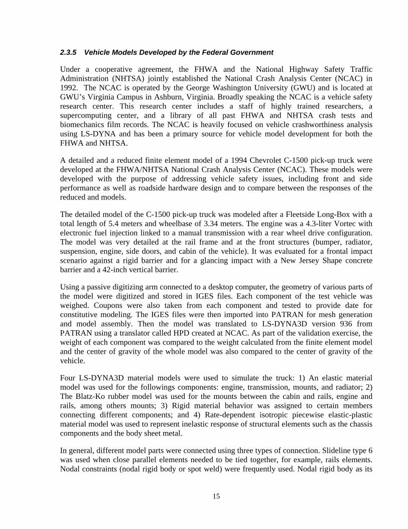
To validate the developed models two-impact test were conducted. The first was a frontal impact with a full rigid wall. The truck initial velocity was 35 mph in this test. The second was a glancing impact test with impact occurring at 25-degree with a 42-inch vertical concrete barrier. The truck initial velocity was 62.5 mph in the second test. A fixed time increment of 1 microsecond was used for the detailed analysis, while, 4 microseconds increments were used in the reduced model.

The progression of deformation of the detailed model in both tests is presented in Figure 2-1 through Figure 2-4. It can be seen that the deformations in all the components of the detailed model correlate well with the deformations the test. Computed versus measured acceleration and velocity also compared well. Overall, good agreement between the detailed analysis and the tests was observed.

Compared to the detailed model, the reduced model provided diminished accuracy. However, good agreement between test and simulation was nevertheless obtained. The absorbed energy was about 17% less than that absorbed in the detailed model. This difference was attributed to hourglassing that occurred in the larger elements used to model the reduced truck.

16

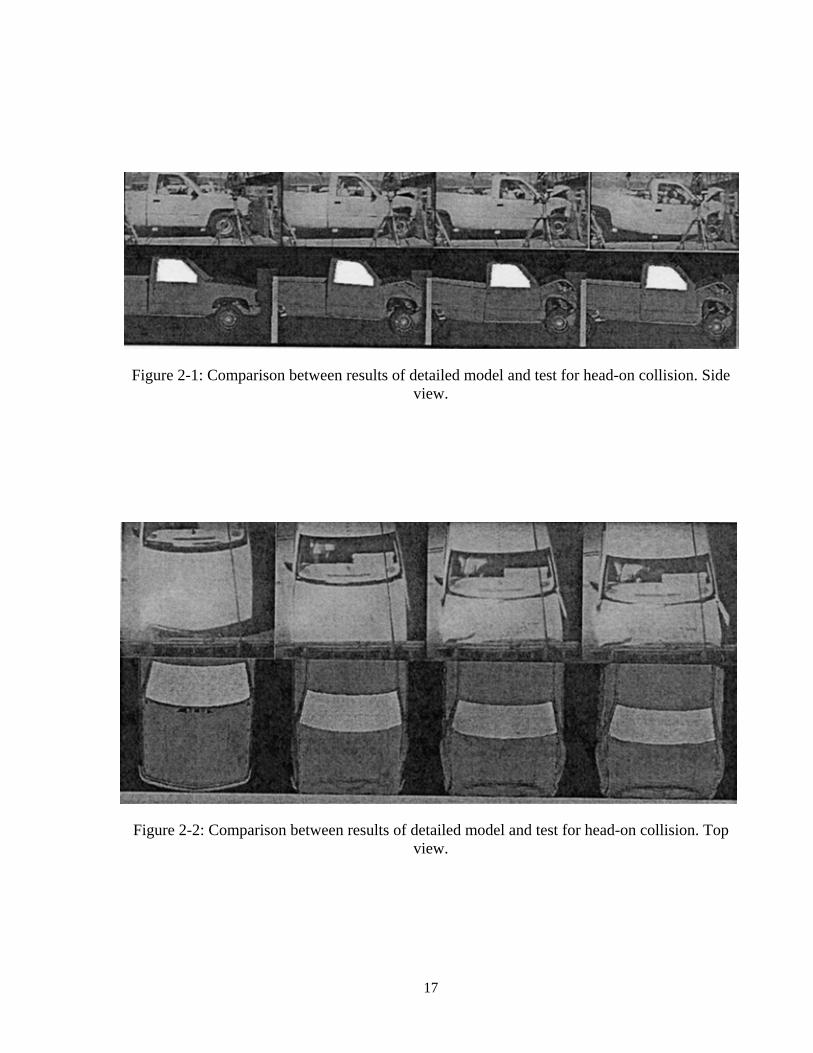
Figure 2-1: Comparison between results of detailed model and test for head-on collision. Side view.

Figure 2-2: Comparison between results of detailed model and test for head-on collision. Top view.

17

Figure 2-3: Comparison between results of detailed model and test for glancing collision. Top view.

Figure 2-4: Comparison between results of detailed model and test for glancing collision. Front view.

18

3 MODEL DEVELOPMENT

3.1 Introduction

The vehicle and pier models are presented in this chapter and a variety of exercises are conducted to ensure that the models are suitable for the intended study. A parametric study is also conducted to gain experience with the models and to investigate sensitivity to various key parameters.

3.2 Modeling of Piers

Two pier models with different geometric characteristics and heights are used in the investigation. Pier dimensions were obtained from structural plans of existing vulnerable bridges in Florida. The first pier, hereafter referred to as Pier I, is a reinforced concrete column that has a 1450 mm x 1375 mm (4’ 9” x 4’ 6”) cross-section and is 16,300 mm (48’ 10 15/16’’) high. The pier is attached to a reinforced concrete pile cap with dimensions 5000 mm x 4000 mm x 1670 mm (15’ x 12’ x 5’) that is embedded 2150 mm (6’ 6’’) underground. The superstructure, pier, and cap are supported by twelve 450 mm (18”) diameter prestressed concrete piles of 10000 mm (30’) length. Figure 3-6 shows the dimensions and reinforcing details of Pier I.

Pier II is also a reinforced concrete pier. It has a circular cross-section of 1075 mm (3’ 6”) diameter and a height of 9925 mm (29’ 95/16’’). It is attached to a reinforced concrete pile cap that is 3300 mm x 2300 mm x 1075 mm (10’ x 7’ x 3’ 6’’) in dimension and embedded 830 mm (2’ 6”) into the ground. The pile cap is supported on six 450 mm (18”) diameter prestressed concrete piles of 10000 mm (30’) length. Figure 3-7 shows the dimensions and reinforcing details of Pier II.

Pier I is reinforced with 24 #11 bars (35 mm diameter) and #5 (16 mm diameter) stirrups with 4 legs. Pier II has 14 #11 bars (35 mm diameter) and #5 (16 mm diameter) round hoops. Concrete in both piers is assumed to have a nominal strength of 23 MPa (4 ksi) , and steel 400 MPa (60 ksi).

3.2.1 Pier Models

The pier and pile cap are represented using fully integrated 8-node brick elements with elastic properties representing uncracked concrete. Extensive mesh refinement studies were conducted as part of this project to ensure that the pier meshes were adequate. Figure 3-8 and Figure 3-9 shows models of both piers.

19

3.2.2 Superstructure Model

The superstructure is modeled using beam elements. The dimensions and properties of the superstructure are obtained from the same structural plans from which Pier I details were derived. The same superstructure is used with both piers for simplicity, and is comprised of two adjacent composite steel-concrete box girders (Figure 3-10). The geometric properties of each box girder are as follows:

A = 80133.0 mm2 (124 in2)

Izz = 2.798E+10 mm4 (6.722E+04 in4)

Iyy = 8.340E+10 mm4 (2.004E+05 in4)

where z is the horizontal axis and y is the vertical axis. In calculating these properties, the composite section is transformed into an equivalent steel section. The superstructure consists of two unequal spans of 53,400 mm (175 ft) and 50,000 mm (165 ft) respectively, which are assumed to be pinned at their far ends. Each girder is modeled using 18 elastic beam elements, and its mass is assumed lumped at the beam nodes.

3.2.3 Bridge Bearing Modeling

The superstructure transmits its weight to the piers through elastomeric bearing pads. Each girder is assumed to rest on two 200 mm x 200 mm (8” x 8”) pads with four steel layers with a total thickness of 37 mm (1.5”). Bearing pad properties were derived from tests reported in NCHRP Report 298 (Roeder et al 1987). The bearings are represented by standard beam elements, whose flexural stiffness is adjusted to provide the same tip displacement as a shear flexible beam element with shear modulus G = 0.608 MPa. It was not necessary to be more precise in modeling the bearing pads because sensitivity studies showed that the effect of bearing pad stiffness is almost insignificant. Analyses with 0.5, 2, and 4 times the assumed stiffness gave virtually identical peak impact load (differences of less than 1%).

3.2.4 Soil-Pile Interaction

To effectively represent the bridge pier’s response to the vehicle impact load, it was deemed necessary to model the piles and the soil-pile interaction. A simple but effective method is used to model the lateral pile response. Beams elements are used to represent the piles and four-discrete lateral spring elements are used to model the soil-pile interaction. The springs are spaced at 660 mm (2’-2”) for Pier-I and at 440 mm (1’-5”) for Pier-II. An illustration of the spring arrangement is shown in Figure 3-11.

The soil springs are modeled using inelastic bar elements that provide compression only response, since soil cannot provide any tensile resistance. The compressive stiffness of the springs was calculated using an approach recommended by Bowles (1995). The modulus of subgrade reaction is

nsss ZBAk += (1)

20

Where

( )γγγ SBNScNCA ccs 5.0+=

( )qqs SNCB γ=

As Constant for horizontal or vertical members

Bs Coefficient for depth variation

Z depth of interest below ground

n exponent taken as 0.5 in this work.

C 40 for SI units and 12 for English units.

c cohesion, 0 in current case (sandy soil)

γ unit weight of soil, assumed a typical value of 18 Kn/m3 for our case

Nc, Nγ nondimensional bearing capacity factors, based on a 30o soil friction angle, taken as 30.14 and 22.40 respectively.

Sc, Sγ nondimensional shape factors, 1.03 & 0.98 respectively.

B width of foundation (=diameter for a circular foundation, taken as 457.2 mm)

Most of the above listed variables are standard variables associated with bearing capacity calculations and are computed from soil data in the construction plans for the bridge being considered.

3.3 Vehicle Models

Three vehicles model are used to investigate the effect of various parameters on impact behavior. The vehicle models used are 1) a detailed model of the Chevrolet C2500 Pickup (54,800 elements), 2) a reduced model of the Chevrolet C2500 Pickup (10,500 elements), and 3) a reduced model of the Ford single unit truck (21,400 elements). Figure 3-1 through Figure 2-3 show different views of the detailed model of the Chevrolet C2500 pickup truck. Figure 3-4 shows an isometric view of the reduced Chevrolet C2500 pickup truck, while Figure 3-5 shows an isometric view of the Ford single unit truck.

As discussed in the previous chapter, the models were downloaded from the National Crash Analysis Center website (www.ncac.gwu.edu) at George Washington University. The 14-kN Chevy truck is intended to represent lights trucks, while the 66-kN Ford truck represents medium weight trucks. Models of heavier trucks are not yet available, although a 360-kN tractor trailer model is currently under development at the US Federal Highway Administration.

21

3.3.1 Validation of Chevy Model

To verify the accuracy of the Chevy model, numerical results are compared to test results for a 55.8 kph head-on crash into a rigid wall. The verification exercise used the detailed C2500 Chevy truck model and focused on the velocity and acceleration of the engine bottom. A similar verification study was conducted by Zaouk et al (1996).

The measured velocity and acceleration data for the engine bottom was sampled every 0.05 ms and a SAE-60 filter was used to filter both records. In the analysis, displacement data was calculated at 0.05 ms intervals and was then filtered using the Gaussian filter in MatLab. The displacement record was differentiated to get the velocity, which was then filtered using the same Gaussian filter. The final acceleration record was calculated by differentiating the filtered velocity record and then filtering the resulting record once again. Extensive filtering was employed to remove unrealistic high frequency signals that were distorting the results.

Figure 3-12 and Figure 3-13 show the acceleration and velocity plots respectively. A close examination of both figures shows that the numerical results are in good agreement with test data up to about 0.43 second. After this time the numerical results deviate from the test data up till approximately 0.8 seconds, after which the results become close once again. In spite of these differences, the calculated peak quantities compare well with the measured values. The differences between calculated and measured responses can be attributed to various factors including modeling assumptions and the way the data was filtered.

3.3.2 Performance of Reduced C2500 Chevy Truck Model

Although the verification study shows that the detailed model of the C2500 Chevy truck can be used for studying crash behavior, it is computationally demanding. For instance, analysis time for the C2500 detailed model impacting a rigid wall was 17 hour. When used to impact a deformable barrier, computational time may be prohibitive. The reduced model is attractive in that it significantly reduces computational demands.

To investigate its accuracy compared to the detailed model, the reduced truck model was studied in two crash scenarios involving a flexible wall: frontal impact and 45o glancing impact. The velocity of the model for both impact simulations is 55.8 kph. The wall was 467-mm thick, 3600-mm wide, 1680-mm high, and the modulus of elasticity was 30,000-MPa.

Instead of comparing acceleration and/or velocity, it was decided to compare the resultant contact force since it is the quantity of interest in this project. The resultant force is calculated from the horizontal X- and Y-contact forces only. The vertical Z-contact force was disregard in this calculation because the impact situation under study should produce very little force in this direction, which was the case in the analyses. For frontal impact (Figure 3-14) the reduced model compares quite well against the detailed model with exception of a spike that occurs in the detailed model response at around 0.03 seconds. One possible reason for the discrepancy may be the time step size, which was different in both analyses. In the detailed model analysis, the time step size was 1 ms while for the reduced model it was 4 ms. However, this difference was deemed insignificant because the single spike does represent the peak impact force. Moreover, it

22

occurs in such a short period of time, that it would have a marginal impact, if any, on the interaction between the vehicle and the wall.

For the 45o impact (Figure 3-15), the spike is more pronounced, and in fact represents peak response in this case. Another observation is that after approximately 0.13 sec, the response of the reduced model decays at a slower rate and has more high frequency vibrations than the detailed model, i.e. the response of the reduced model does not match well the response of the detailed model.

These results show that the reduced model can be used with reasonable accuracy for investigating impact forces generated by head-on collision between vehicles and piers. Incidentally, use of the reduced model reduced computational time by almost 16 hours, i.e. the computational time used for the reduced model was 48 minutes versus 17 hours for the detailed model.

3.3.3 Validation of Ford Truck Model

Comparisons between analysis and test results involving a truck crashing into a security bollard are presented (Alberson 2003). The bollard dimensions are not available for security reasons. The exact details of the truck are also not available; however the truck weight is 66-kN, which is similar to the weight of the truck model used herein, and the approach speed is 78 kph. The simulation corresponding most closely to the bollard impact scenario is T66-V90-T-II (discussed in Chapter 5), which is used for comparison. Comparison between various quantities are shown in Figure 3-16 through Figure 3-18. Given the large difference in structural properties between a bollard and Pier II as well as the different approach speeds (78 kph versus 90 kph), it is clear that the simulation captures the overall trend in a reasonable manner compared to the test. For example, the peak 10 ms force for T66-V90-T-II is 3080 kN and the measured peak force is 2350 kN (a difference of 31%).

3.3.4 Other Accuracy and Validation Studies

Additional studies are conducted to ensure that the models are producing reliable results. These include mesh refinement studies, conservation of energy checks, and conservation of momentum checks. The latter two checks are discussed in the next chapter.

3.4 Parametric Study using Vehicle Models

To ensure that sufficient experience had been gained with LS-DYNA and to investigate the effect of various key parameters, an extensive parametric study is conducted.

3.4.1 Effect of Barrier Flexibility

To study the effect of wall flexibility, the Chevy truck and Ford truck models are crashed into two different walls. The wall into which the Chevy truck impact is 467 mm thick, 3600 mm long, and 1670 mm high, while the wall used in conjunction with the Ford truck is 500 mm thick, 2500 mm long, and 2500 mm high. The material model assigned to each wall is varied to represent

23

rigid behavior (material 20 in LS-DYNA) as well as elastic behavior (material 1 in LS-DYNA, with a modulus of elasticity of 30,000 MPa). For the flexible walls, a surface-to-surface contact interface is used to prevent penetration of the vehicle models.

The Chevy truck model was crashed into the walls at a speed of 55.8 kph. Figure 3-19 shows the resultant contact force versus center of gravity displacement for both rigid and flexible walls. It is clear from the figure that there is a relatively small difference between the resultant contact forces of the two walls. The peak ratio in contact force (rigid contact force/flexible contact force) is about 1.27; i.e. the rigid wall attracts 27% more force than the flexible wall. Similar studies by Wolf et al. conducted on airplanes impacting rigid and deformable targets showed even smaller variations in the impact force as a function of the barrier flexibility.

In the Ford truck simulation, the vehicle model was crashed at a speed of 80 kph against both rigid and flexible walls. Once again, the differences are rather moderate, but the peak force ratio in this case is 1.40. The results of this parametric study show that the flexibility of the impacted structures plays a relatively small but significant role in the interaction between the vehicle and wall. While, rigid structures are computationally attractive, it is nevertheless important to include structural flexibility in any modeling exercise in order to achieve realistic results.

3.4.2 Effect of Coefficient of Friction

To study the effect of the coefficient of friction (COF), a series of analyses are conducted. The COF in LS-DYNA is the ratio of the tangential force to the normal force resisting sliding parallel to the surface. The analyses used in this parametric study employed the Chevy truck and the elastic wall previously described. Impact occurred at 45o for speeds of 55.8, 100, and 136 kph. The COF is specified as 0, 0.15, 0.3, and 0.6. The goal of the study is determine the effect of the coefficient of friction on the impact force.

Figure 3-20 shows the resultant impact force versus time for various values of the COF. It is clear from the figure that for all values of COF, there are two peaks. As the COF increases, the first peak becomes less prominent, while the second peak becomes greater. It is also noticed that the rate of decay in the contact force is slower as the COF decreases. In spite of the significant effect of the COF, the magnitude of the raw peak impact force is not significantly changed, although the time at which it occurs changes. Figure 3-21 shows on the 50 ms averaged resultant impact force versus time for various values of the COF. The figure shows that the COF has little effect on the averaged impact force, until it exceeds 0.3. Runs for speeds of 100 kph and 136 kph show similar trends.

Additional runs were conducted to investigate the effect of COF on peak impact force for various approach speeds and angles of impact. Based on the study, the COF is set to 0.3 in future analyses, which is a reasonable number for steel on concrete.

3.4.3 Effect of Damping Ratio

To study the effect of damping, the Ford truck was used in conjunction with the flexible wall previously discussed. The analyses were conducted for head-on collisions and initial velocities of 30, 55.8, 80, and 100 kph. The damping was specified as 0, 1%, and 5% of critical. Damping did

24

not increase the simulation time and did not significantly affect the impact force. On the other hand, damping improves the numerical solution process. For example, the 100 kph analysis would not converge for zero damping, but converged when 1% or higher damping was introduced. As a result of this, it was decided to include 1% damping in all future analyses.

3.4.4 Summary of Parametric Study

The following conclusions are drawn based on the parametric studies discussed above:

• The reduced Chevy model can be used with reasonable accuracy for investigating head-on impact forces generated by collision between vehicles and piers.

• Wall flexibility plays a relatively small but significant role in the interaction between the vehicle and wall. While, rigid wall models are computationally attractive, it is nevertheless important to include structural flexibility in any modeling exercise in order to achieve realistic results.

• A reasonable value for the COF is 0.3.

• Damping does not increase the simulation time and does not significantly affect the impact force. However, since damping improves the numerical solution process it is reasonable to use 1% damping in all future analyses.

3.5 Impact Process and Simulation Time

The truck models are allowed to impact the pier in a head-on manner in two directions: 1) transverse to the longitudinal axis of the superstructure, and 2) parallel to the longitudinal axis of the bridge. These two directions are expected to have different structural characteristics because of the effect of the superstructure. Approach speeds considered are 55, 90, 100, 135 kph, with the last deemed to be a maximum credible approach speed.

The impact event is simulated for a period of 300 ms, and various quantities of interest are extracted from the finite element results including: impact force versus time relationship, stress and strain values and rates at key points, pier deformations, pile forces, pile cap deformations. Figure 3-22 shows various views of the model and impact event for Pier I. Figure 3-23 through Figure 3-25 show a close up of the impacting vehicles at various times. The figures clearly depict the severity of the crash.

3.5.1 Run Notation

To simplify referral to the various runs conducted, each run is referred to by a unique descriptive name. For example, for the 14-kN Chevy Truck traveling at 90 kph and impacting Pier I in the transverse direction (transverse to the longitudinal axis of the bridge), the run notation would be T14-V90-T-I. As another example, T66-V55-P-II represents the 66-kN Ford Truck impacting Pier II in a direction parallel to the bridge axis at 55-kph.

25

Figure 3-1: Isometric view of the detailed model of the Chevrolet C2500 pickup truck

Figure 3-2: Top view of the detailed model of the Chevrolet C2500 pickup truck

Figure 3-3: Side view of the detailed model of the Chevrolet C2500 pickup truck

26

Figure 3-4: Isometric view of the reduced model of the Chevrolet C2500 pickup truck

Figure 3-5: Isometric view of the Ford single unit truck

27

42’ 415/16’’

6’ 6’’

5’ 0’’

4’ 9’’

4’6”

4’ 6’’

4’’ Chamfer.4’

9’’

4’ 6’’

4’’ Chamfer.4’

9’’

4’ 6’’ 4’ 6’’1’ 6’’ 1’ 6’’

4’1’

6’’

4’4’

18” x 18” Pile

1’ 6

”

5’ Thick Pile Cap

AA AA

Section A-A

Reinforcement Details24 # 11 Longit. Bars@5” #5 Stirrups

Figure 3-6: Details of Pier I

3’ 6’’29’ 95/16’’

3’ 6’’

3’ 6’’AA AA

Section A-A

Reinforcement Details14 # 11 Longit. Bars@5” #5 Stirrups

7’10

’

18” x 18” Pile

3’ 6” Thick Pile Cap

Figure 3-7: Details of Pier II

28

(a) 3-D View of Pier I Bridge Model (a) Elevation View of Pier I Bridge Model

Figure 3-8: Finite element model of Pier I

(a) 3-D View of Pier II Bridge Model (a) Elevation View of Pier II Bridge Model

Figure 3-9: Finite element model of Pier II

29

Figure 3-10: Assumed superstructure cross-section.

Pile beam element

Compression-only soil spring

Figure 3-11: Model to capture soil-pile interaction

30

0 0.02 0.04 0.06 0.08 0.1 0.12-5000

0

5000

10000

15000

20000

time (sec)

Vel

ocity

(mm

/sec

)

C2500C1500Test

Figure 3-12: Calculated versus measured velocity of engine bottom.

0 0.02 0.04 0.06 0.08 0.1 0.12-100

-80

-60

-40

-20

0

20

40

time (sec)

Acc

eler

atio

n(g)

C2500C1500Test

Figure 3-13: Calculated versus measured acceleration of engine bottom.

31

0.00E+00

5.00E+05

1.00E+06

1.50E+06

2.00E+06

0.00 0.05 0.10 0.15 0.20

Time, sec

Res

ulta

nt c

onta

ct fo

rce,

N

Reduced models

Detailed model

Figure 3-14: Comparison between frontal impact forces calculated from detailed and reduced models.

0.00E+00

1.00E+05

2.00E+05

3.00E+05

4.00E+05

5.00E+05

6.00E+05

7.00E+05

0.000 0.050 0.100 0.150 0.200 0.250 0.300

Time, sec

Res

ulta

nt c

onta

ct fo

rce,

N

Reduced models

Detailed model

Figure 3-15: Comparison between 45o impact forces calculated from detailed and reduced models.

32

Test No. ARB4

-8000

-6000

-4000

-2000

0

2000

4000

6000

8000

0.000 0.050 0.100 0.150 0.200 0.250 0.300

Time (Sec)

Forc

e (k

N)

180 Hz Filter

Analysis (Head-on crash into 1066-mm diamater pier at 90 kph)

Test results (Head-on crash into unspecified bollard at 78 kph)

Figure 3-16: Comparison between computed and measured force-time data

-1500

-1000

-500

0

500

1000

1500

2000

2500

3000

3500

0 0.05 0.1 0.15 0.2 0.25 0.3 0.35

Time (sec)

Forc

e (k

ips)

Analysis (Head-on crash into 3.5-ft diamater pier at 90 kph)

Test results (Head-on crash into unspecified bollard at 78 kph)

Figure 3-17: Comparison between computed and measured force-time data (averaged over 10 ms)

33

Test No. ARB4

-8000

-6000

-4000

-2000

0

2000

4000

6000

8000

0.0 0.5 1.0 1.5 2.0 2.5 3.0

Displacement (m)

Forc

e (k

N)

180 Hz Filter

Analysis (Head-on crash into 1066-mm diameter pier at 90 kph)

Test results (Head-on crash into unspecified bollard at 78 kph)

Figure 3-18: Comparison between computed and measured force-displacement data.

0.00E+00

5.00E+05

1.00E+06

1.50E+06

2.00E+06

2.50E+06

0.0 200.0 400.0 600.0 800.0

Displacement of the center of gravity, (mm)

Res

ulta

nt c

onta

ct fo

rce,

N

Figure 3-19: Resultant contact force for rigid and flexible walls impacted by C2500 Chevy truck at 55.8 kph. Dotted line elastic barrier, solid line rigid barrier.

34

0.00E+00

5.00E+04

1.00E+05

1.50E+05

2.00E+05

2.50E+05

3.00E+05

3.50E+05

4.00E+05

0.00 0.10 0.20 0.30 0.4

Time , t (sec)

Res

ulta

nt C

onta

ct F

orce

, N

COF=0.6

COF=0.3

COF=0.15

COF=0

Figure 3-20: Effect of different COF on raw resultant impact force of Chevy truck. Speed of impact is 55.8 kph and angle of impact is 45o.

0.00E+00

5.00E+04

1.00E+05

1.50E+05

2.00E+05

2.50E+05

3.00E+05

0.00 0.10 0.20 0.30 0.40

Time , t (sec)

Res

ulta

nt C

onta

ct F

orce

, N

COF=0.6

COF=0.3

COF=0.15

COF=0

Figure 3-21: Effect of different COF on averaged resultant impact force of Chevy truck. Speed of impact is 55.8 kph and angle of impact is 45o.

35

Superstructure

Impacting Vehicle

Deformed Vehicle

(mag. factor 1.0)

Deformed Pier(mag. factor 100)

Piled Foundation

System

Compressiononly springs

attached to piles

Pile Cap

RC Pier5 x 5 x 50 ft

(a) Just prior to collision

(b) After collision(magnification factor 1)

(c) Deformed Pier(magnification factor 100)

Impact Point(Impact velocity 55 mph)

Superstructure

Impacting Vehicle

Deformed Vehicle

(mag. factor 1.0)

Deformed Pier(mag. factor 100)

Piled Foundation

System

Compressiononly springs

attached to piles

Pile Cap

RC Pier5 x 5 x 50 ft

(a) Just prior to collision

(b) After collision(magnification factor 1)

(c) Deformed Pier(magnification factor 100)

Impact Point(Impact velocity 55 mph)

Figure 3-22: Result of impact simulation between the Chevy truck and Pier I

36

a) time 0.0 sec b) time 0.02099 sec.

c) time 0.111 sec. d) time 0.35 sec.

Figure 3-23: Progression of impact for Pier I

37

a) time 0.0 sec b) time 0.02099 sec.

c) time 0.111 sec. d) time 0.30 sec.

Figure 3-24: Progression of impact for Pier II

38

a) Time 0.0 sec b) Time 21 ms

c) Time 111 ms d) Time 165 ms

Figure 3-25: Progression of impact with Pier II for Ford truck for 110 kph approach speed.

39

4 ANALYSIS RESULTS

4.1 Introduction

This chapter presents the results of various crash simulations involving both piers and both trucks. Additional studies that provide confidence in the analysis results are also discussed and the effect of approach speed on impact demands is quantified.

4.2 Conservation of Impulse and Momentum

To ensure that the numerical results are reliable, the conservation of impulse and momentum is investigated in all runs. Impulse-momentum conservation implies that the change in momentum of the vehicle must be fully transferred to the structure as an impulse effect. In other words, the area under the contact force versus time curve (impulse, I) must be equal to the change in momentum (P). This may be written as:

VMPFdtIEvent

∆=== ∫ . (4-1)

In Equation 4-1, M is the mass of the vehicle and ∆V is the change in velocity as a result of the impact. Cumulative impulse and moment values are calculated versus time for all runs. A sample plot is shown in Figure 4-1 and Figure 4-2 for the Chevy truck impacting Piers I and II respectively. Total cumulative values for both quantities are also calculated and shown in Table 1 for the Chevy truck. It is clear from the figures and Table 1 that momentum-impulse is conserved to a large degree. The maximum error is less than 12%. Similar results were obtained for the Ford Truck.

4.3 Conservation of Energy

Conservation of energy checks were conducted for all runs. Conservation of energy implies that the initial kinetic energy of the vehicle must be completely transformed into residual kinetic energy, energy lost to friction, internal energy stored in the deforming vehicle components and pier members, and energy used up by the hourglass control algorithm for finite elements with reduced integration formulations.

Energy was indeed conserved in all runs indicating that numerical problems were not rampant, but hourglass energy in some of the initial runs was excessive and adversely affected confidence in the results of these runs. A large portion of the hourglass energy was expended in a few key parts in the vehicle models that are represented using reduced integration shell or solid elements. To remedy the hourglass energy situation, various vehicle components were either re-meshed or were assigned fully integrated finite element formulations.

40

Table 4-1: Impulse-momentum conservation for Chevy truck

Velocity (Kph) Cumulative Impulse (N.s)

Cumulative Momentum (Kg.m/s)

Percent Difference (%)

T14-V55-P-I 2.85E+04 2.97E+04 3.93 T14-V90-P-I 4.49E+04 4.28E+04 4.64 T14-V110-P-I 5.74E+04 5.22E+04 9.14 T14-V135-P-I 6.96E+04 6.16E+04 11.53 T14-V55-T-I 2.81E+04 2.96E+04 5.23 T14-V90-T-I 4.47E+04 4.25E+04 4.81 T14-V110-T-I 5.76E+04 5.26E+04 8.56 T14-V135-T-I 6.96E+04 6.21E+04 10.85 T14-V55-P-II 2.91E+04 3.00E+04 3.08 T14-V90-P-II 4.42E+04 4.28E+04 3.25 T14-V110-P-II 5.66E+04 5.22E+04 7.74 T14-V135-P-II 7.02E+04 6.23E+04 11.19 T14-V55-T-II 3.03E+04 3.00E+04 1.25 T14-V90-T-II 4.41E+04 4.28E+04 2.94 T14-V110-T-II 5.72E+04 5.28E+04 7.80 T14-V135-T-II 7.01E+04 6.18E+04 11.80

For each of the Ford runs, the percentage of hourglass energy at the instant of peak contact force and at rebound is listed in Table 4-2, and the evolution of various energy quantities is shown in Figure 4-3 for run T66-V135-T-I. Other energy plots are shown in Appendice B and C. Rebound is defined as the instant when the resultant impact force drops to 1% of the peak value.

At peak force, the hourglass energy ratio is quite low, but increases significantly to a maximum value at rebound. The results of the analyses were felt to be reasonable given that the hourglass energy ratio at peak load is so low, and that the maximum values are not excessively high. Zaouk et al (1996) reported 17% hourglass energy at the end of their run in the head-on collision validation exercise, but deemed the results of their analysis acceptable.

Hourglass energy ratios for the Chevy truck were significantly greater than for the Ford truck. For most of the runs, the hourglass energy ratio reached about 15% of the total energy at peak force. The few simulations with hourglass ratios greater than 15% were rerun with fully integrated elements for the sake of accuracy.

Although 15% hourglass energy ratio is rather large, attempts were not made to reduce hourglass energy dissipation because the forces delivered by the Chevy truck are much smaller than those delivered by the Ford truck, and are therefore not as useful. Also, as previously discussed, while the PDF may be significantly affected by the hourglass energy ratio, the ESF is generally not as sensitive. In any case, the Chevy truck results should be viewed as qualitative in nature.

41

Table 4-2: Hourglass energy for the Ford truck Simulation Percent Hourglass Energy

(at peak dynamic force) Percent Hourglass Energy

(at rebound) T66-V55-T-I 6.2 10.2 T66-V90-T-I 2.5 9.2 T66-V110-T-I 2.3 14.2 T66-V135-T-I 2.0 16.9 T66-V55-T-II 2.6 6.8 T66-V90-T-II 1.4 9.0 T66-V110-T-II 1.0 11.3 T66-V135-T-II 1.0 12.2

4.4 Structural Demands and Force Measures

Several force measures are used to characterize each impact event. The peak dynamic force (PDF) is the largest impact force computed during the simulation. The PDF usually occurs early on in a run. The PDF is not representative of the design structural demands that engineers need to consider, because the structure has not had ‘time’ to respond to the rapid change in loading.

According to Chopra (2001), the equivalent static force (ESF) is a more appropriate measure of the design structural demand. The ESF is the static force necessary to produce the same deflection at the point of interest as produced by the dynamic event and is a function of the stiffness of the system and its dynamic characteristics. An examination of pier deformation profiles shows the top of the pier moves significantly less than the point of impact as a result of the inertial effect of the superstructure (see, for example, Figure 4-4, Figure 4-8, and similar figures in Appendix B). Since the main focus is on the bridge pier, it was therefore deemed appropriate to quasi-statically model the pier as pinned at the top, with a concentrated ESF acting at the point of impact.

The peak fifty millisecond average force (PFMA) is also computed for comparison in the case of the Chevy truck. The definition of this quantity is rather arbitrary. However, it has been frequently used by researchers in the automotive crash arena and is computed just for the same of completeness.

It was observed during the research that the PDF is quite sensitive to modeling issues, in particular the ratio of hourglass energy to the total energy in the system. In general the PDF grows as the ratio of hourglass energy grows. Hence readers should view the PDF as more of a qualitative number rather than a quantitative measure of demand. Fortunately, the ESF is not as sensitive to various modeling issues including hourglassing.

42

4.5 Chevy Truck Simulations

The Chevy truck is crashed into Piers I and II in the transverse and parallel directions. All the results of the Chevy truck simulations are plotted in Appendix A, but key results are re-plotted here for convenience.

The force versus time responses generated by the impact for various approach speeds are shown in Figure 4-5 for Piers I and II respectively (transverse impact). Several observations can be made from the figure. The impact force versus time function appears to be comprised of a low force level that is sustained over the duration of the impact event combined with one or more spikes. The sharp spikes occur when the stiff structural components of the vehicle, such as the chassis, or massive parts, such as the engine block, reach the pier and interact with it.

Another observation is that the peak contact force increases with increasing approach speed. The only exception is T14-V135-P-II, which had a peak force that was about equal to T14-V110-P-II. Although energy appears to have been conserved in T14-V135-P-II (difference between internal and kinetic energy is 3.6%), the results are unreliable because the hourglass energy ratio was large.

The ESFs and PDFs are generally smaller for Pier II compared to Pier I. There are two reasons for this. First, Pier I is significantly stiffer at the point of impact compared to Pier II, and hence would attract greater force. Second, the large rectangular cross-section of Pier I (1450 x 1375 mm) mobilizes more of the structural system of the impacting vehicle leading to greater collision forces than the smaller circular section (1075 mm diameter) of Pier II. For the most part this observation is true, except for the 55-kph speed, where Pier II forces are slightly larger. Again, this discrepancy is attributed to efforts to control persistent hourglassing, which introduced some additional artificial stiffness and increased the contact forces.

The response of the pier system to impact transverse to the superstructure is softer than the case where impact occurs parallel to the superstructure, which results in smaller peak dynamic forces. As shown in Figure 4-6 and Table 4-3, the peak dynamic forces (PDF) for both piers generally appear to increase almost linearly with increasing vehicle speed. This implies that the impact process for these particular vehicle/pier systems can be basically represented as an impulse type situation. In impulse situations, assuming that the shape of the force versus time relationship remains constant, the peak impact force is a linear function of the momentum of the impacting body.

Researchers in the early 80’s (Hirsch 1984) have used a 50-ms average to obtain the design demand from experimentally measured force response. The 50-ms average (FMA) is calculated for as a moving average for each curve (plotted in Appendix A) and the peak values (PFMA) are listed in Table 4-3. The PFMAs follow the same trend as the ESFs, and appear to give about equal forces for Pier I and Pier II, with values less than the AASHTO provisions. PFMA results are considered unreliable because of the arbitrary nature of their definition.

43

Table 4-3: Impact force measures for Chevy truck

Simulation PDF (kN) ESF (kN) PFMA (kN) T14-V55-P-I* 3075 923 503 T14-V90-P-I 8241 2010 899

T14-V110-P-I 12110 2631 1121 T14-V135-P-I 15480 3271 1361 T14-V55-T-I 3272 1075 498 T14-V90-T-I 8010 2189 839

T14-V110-T-I 11290 2504 1121 T14-V135-T-I 14420 3068 1391 T14-V55-P-II* 4067 484 504 T14-V90-P-II 6729 819 874

T14-V110-P-II 10010 1007 1153 T14-V135-P-II* 9985 1480 1529 T14-V55-T-II** 2850 622 531 T14-V90-T-II 6038 945 904

T14-V110-T-II 9985 1196 1249 T14-V135-T-II 12500 1593 1526

*Results may be inaccurate due to excessive hourglass energy **All elements are fully integrated.

4.6 Ford Truck Simulations

The truck model is crashed into Piers I and II in the transverse direction. Parallel impact is not considered because the Chevy simulations showed that there wasn’t much difference between transverse and lateral impact. All the results of the Ford truck simulations are plotted in Appendix B, but, as with the Chevy truck, key results are re-plotted here for convenient reference.

Unlike the Chevy truck where the PDFs appear to increase almost linearly with increasing vehicle speed, the Ford PDFs change as a nonlinear function of speed (Figure 4-7). On the other hand, the ESF values appear to have a linear relationship to the approach speed. As with the Chevy truck, the ESFs and PDFs are smaller for Pier II compared to Pier I. The only exception to this is case T66-V55-T-I, where the ESF is a little smaller (12% smaller) than the ESF for T66-V55-T-II. Although it is difficult to pinpoint a specific reason for this discrepancy given the complexity of the vehicle-pier interaction, one possible cause could be sensitivity to numerical problems. For example, from Table 4-4, it can be seen that the hourglass energy at peak force for T66-V55-T-I is significantly higher than for all other analysis cases.

The ESFs and PDFs for the Ford truck are significantly greater than the corresponding values for the Chevy truck. This is expected given that the latter is about 5 times heavier than the former. However, it is interesting that the PDFs and ESFs for the Ford truck are less than 5 times their counterpart values for the Chevy truck, implying that differences in the relative strength and

44

stiffness of the structural system of both trucks are significant. In other words, the Ford truck is not able to deliver impact forces ‘as efficiently’ as the Chevy truck.

Table 4-4: Impact force measures for Ford truck

Simulation PDF (kN) ESF (kN)

T66-V55-T-I 5180 2150 T66-V90-T-I 16200 4800 T66-V110-T-I 17800 6450 T66-V135-T-I 26300 8850 T66-V55-T-II 5160 2450 T66-V90-T-II 7600 3700 T66-V110-T-II 11300 4800 T66-V135-T-II 17700 6650

4.6.1 Foundation Deformations

Pier II deformation profiles at peak load and at peak displacement (at point of impact) are shown in Figure 4-8 for various approach speeds. Similar plots for Pier I are shown in Appendix B. It is clear from the figures that the displacement of the foundation is substantial, reaching almost 30 mm for Pier II and 10 mm for Pier I. In spite of this large deformation, sensitivity studies showed that PDFs and ESFs are relatively insensitive to the foundation flexibility.

4.6.2 Stresses and Strain Rates

Pier stresses are quite high for higher approach speeds. For example, for T66-V135-T-II, the elastic stress reaches close to 100 MPa in tension and compression. The strain rate is generally less than 1 sec-1, implying that dynamic increases in strength are small. Clearly, these stresses cannot be sustained by concrete if it was allowed to behave in an inelastic manner, and they signal the high possibility of failure under the applied impact loading.

4.7 Design Implications

For the Chevy truck (Figure 4-6), the ESF is less than the AASHTO-LRFD design force for Pier II. It exceeds the AASHTO-LRFD design force for Pier I at approach speeds in excess of 80 kph. At the highest approach speed, the ESF for the Chevy truck is about 70% greater than the design impact force. For the Ford truck (Figure 4-7), the ESF is greater than the AASHTO-LRFD force for all approach speeds considered. At the highest speed, the ESF is significantly greater than the design force (4.9 times higher for Pier I).

In evaluating the implications of these results it is important to understand the assumptions used to derive them. Although the vehicles as well as soil-pier interaction are modeled in an inelastic manner, the pier itself and the superstructure are modeled as elastic. The progressive collapse process under the effect of impact cannot therefore be simulated. However, the assumption of

45

elastic pier behavior permits convenient definition of the ESF, which is useful in the design context and allows direct assessment of design provisions. Given the high computed value of the ESF for some of the simulations, this research therefore suggests that current AASHTO-LRFD collision criteria could be deficient.

As previously discussed in Section 4.4, it is appropriate to quasi-statically model the pier as pinned at the top, fixed at the base with a concentrated ESF acting at the point of impact. Using such a model, it can be shown that the majority of the ESF acts as a shear force at the base of the pier (96% for Pier I and 91% for Pier II). Using ACI-318 (2003), the shear capacity (without strength reduction factor and including the effect of column axial compression) of Piers I and II are 5500 kN and 2370 kN respectively. These numbers imply that it is unlikely that the Chevy truck will cause shear failure of either pier at any of the approach speeds considered (compare 2370 kN to ESF in Figure 12 and Table 2). However, according to the simulations, the Ford truck can deliver ESFs in excess of the predicted shear capacity of Pier I for speeds greater than 100 kph, and Pier II for any of the considered speeds. Along with the high normal stresses discussed in Section 4.6.2, these results imply that Pier II could likely fail if impacted by the Ford truck for any of the given approach speeds.

The recent failures presented in Chapter 1 are not proof that the AASHTO-LRFD collision provisions are deficient because it is unclear if the piers were designed for impact. It is also not known if the guard rails protecting the piers meet current crashworthiness criteria. Nevertheless, together with the discussions presented above, these failure events indicate that that there could be a population of bridge piers that are vulnerable to accidental or malevolent impact by heavy trucks.

4.8 Impact of Heavier Trucks

This project utilized two trucks, a 14-kN Chevy truck (intended to represent lights trucks) and a 66-kN Ford truck (represents medium weight trucks). Models of heavier trucks are not yet available, although a 360-kN tractor trailer model is currently under development at the US Federal Highway Administration. Given that the Ford truck is capable of producing such high demands, and the fact that the 360-kN tractor trailer could be significantly more damaging, there is an urgent need to continue this research.

46

0.0E+00

1.0E+04

2.0E+04

3.0E+04

4.0E+04

5.0E+04

6.0E+04

7.0E+04

8.0E+04

0.00 0.05 0.10 0.15 0.20 0.25 0.30 0.35 0.40

time (s)

Cum

ulat

ive

Impu

lse

or C

hang

e in

Mom

entu

m (N

.s)

T2.5 - V35 - P -I

T2.5 - V56 - P -I

T2.5 - V75 - P -I

T2.5 - V85 - P -I

T14-V135-P-I

T14-V110-P-I

T14-V90-P-I

T14-V55-P-I

Figure 4-1: Conservation of impulse-momentum relationship (Pier I-P) (dark lines are cumulative impulse, while light lines are cumulative change in momentum)

0.0E+00

1.0E+04

2.0E+04

3.0E+04

4.0E+04

5.0E+04

6.0E+04

7.0E+04

8.0E+04

0.00 0.05 0.10 0.15 0.20 0.25 0.30

time (s)

Cum

ulat

ive

Impu

lse

or C

hang

e in

Mom

entu

m (N

.s

T2.5 - V85 - T -II

T2.5 - V35 - T -II

I

T2.5 - V56 - T -II

T2.5 - V75 - T -I

T14-V135-T-

T14-V110-T-

T14-V90-T-II

T14-V55-T-II

Figure 4-2: Conservation of impulse-momentum relationship (Pier II-T)

(dark lines are cumulative impulse, while light lines are cumulative change in momentum)

47

0.0E+00

1.0E+09

2.0E+09

3.0E+09

4.0E+09

5.0E+09

6.0E+09

0.00 0.05 0.10 0.15 0.20

Time (sec)

Ene

rgy

(kg

mm

2 /sec

2 )

H/T

= 1

6.9%

Hourglass

Total

Internal

Kinetic P

eak

Dyn

amic

For

ce

Reb

ound

H/T

= 2

.0%

Figure 4-3: Evolution of various energy quantities for T66-V135-T-I.

-4000

-2000

0

2000

4000

6000

8000

10000

12000

14000

16000

-5 0 5 10 15 20 25

displacement (mm)

elev

atio

n (m

m)

.

Peak Forcet = 2.50E-02

Peak Displacem entt = 9.20E-02

Figure 4-4: Deflection profile at various times for pier in T66-V135-T-I. Note how the top of the pier does not move much with respect to point of impact.

48

0.0E+00

4.0E+06

8.0E+06

1.2E+07

1.6E+07

0.00 0.02 0.04 0.06 0.08 0.10time (sec)

Res

ulta

nt C

onta

ct F

orce

(N)

v=135 kph

v=110 kph

v=90 kph

v=55 kph

0.0E+00

4.0E+06

8.0E+06

1.2E+07

1.6E+07

0.00 0.02 0.04 0.06 0.08 0.10

time (sec)

Res

ulta

nt C

onta

ct F

orce

(N) v=135 kph

v=110 kph

v=90 kph

v=55 kph

(a) Pier I (b) Pier II

Figure 4-5: Impact force versus time for Chevy truck at various speeds approaching in transverse direction.

0

3000

6000

9000

12000

15000

0 25 50 75 100 125 150Velocity (kph)

Res

ulta

nt c

onta

ct fo

rce

(kN

)

AASHTO

Peak Dynamic Force(PDF)

Equivalent Static Force (ESF)

0

3000

6000

9000

12000

15000

0 25 50 75 100 125 150Velocity (kph)

Res

ulta

nt c

onta

ct fo

rce

(kN

)

AASHTO

Peak Dynamic Force(PDF)

Equivalent Static Force (ESF)

(a) Pier I (b) Pier II

Figure 4-6: Impact force versus approach speed relationship for Chevy truck (transverse impact)

49

0

5000

10000

15000

20000

25000

30000

0 25 50 75 100 125 150Velocity (kph)

Res

ulta

nt c

onta

ct fo

rce

(kN

)

AASHTO

Peak Dynamic Force(PDF)

Equivalent Static Force (ESF)

0

5000

10000

15000

20000

25000

30000

0 25 50 75 100 125 150Velocity (kph)

Res

ulta

nt c

onta

ct fo

rce

(kN

)

AASHTO

Peak Dynamic Force(PDF)

Equivalent Static Force (ESF)

(a) Pier I (b) Pier II

Figure 4-7: Impact force versus approach speed relationship for Ford truck (transverse impact)

-4000

-2000

0

2000

4000

6000

8000

0 10 20 30 40 50 6

displacement (mm)

elev

atio

n (m

m)

Peak Forcet = 6.06E-02

Peak Displacem entt = 6.30E-02

0

-4000

-2000

0

2000

4000

6000

8000

0 10 20 30 40 50 6

displacement (mm)

elev

atio

n (m

m)

Peak Forcet = 3.78E-02

Peak Displacem entt = 5.10E-02

0

(a) 55 kph approach (b) 90 kph approach

-4000

-2000

0

2000

4000

6000

8000

0 10 20 30 40 50 6

displacement (mm)

elev

atio

n (m

m) Peak Force

t = 3.02E-02

Peak Displacementt = 5.10E-02

0

-4000

-2000

0

2000

4000

6000

8000

0 10 20 30 40 50 6

displacement (mm)

elev

atio

n (m

m)

. Peak Forcet = 2.54E-02

Peak Displacem entt = 4.50E-02

0

(c) 110 kph approach (d) 135 kph approach

Figure 4-8: Pier profile curves for Ford truck impacting Pier II.

50

5 SUMMARY AND CONCLUSIONS

5.1 Summary of Work

Inelastic transient finite element simulations are used to investigate the structural demands generated during vehicle/pier crashes. Two publicly available truck models were considered, a 14-kN Chevy truck (representing lights trucks) and a 66-kN Ford truck (representing medium weight trucks). Although there were plans to use a 360-kN tractor trailer model (to represent the heaviest permissible trucks), the model was not available in time from FHWA to permit inclusion of the results in this report.

The two truck models were crashed at various approach speeds into finite element models of two bridge piers with different structural characteristics. Various parameters were computed from the simulations including, stress and strain at key locations, pier, foundation and superstructure deformations, and transient impact forces. Since the peak transient forces occurs for a very short duration during which the pier does not have time to respond, equivalent static forces are computed as a more appropriate measure of the design structural demand. The calculated forces are used to critique the AASHTO-LRFD vehicle collision provisions.

Although physical vehicle-pier impact tests were not carried out to verify the accuracy of the simulations, a variety of exercises were conducted to provide confidence in the analysis results. These exercises included: reviewing previously published verification studies involving the 14-kN truck, extensive sensitivity studies, mesh refinement studies, energy balance audits, impulse/momentum conservation checks, monitoring of hourglass control energy during the simulations, and comparison of pertinent results to data from truck/bollard collision tests.

5.2 Main Conclusions

The main conclusions that be drawn from this research are as follows.

5.2.1 Impact Force Demands

The results of the simulations show that, in general, the peak transient forces are very high, much higher than the AASHTO-LRFD collision design force. However, since the peak forces act for a short duration, equivalent static forces are a more appropriate measure of ‘design’ structural demands during collision. The computed equivalent static forces turn out to be still quite high and appear to vary linearly with approach speed for both trucks.

5.2.2 Assessment of AASHTO-LRFD Criteria

The results show that the computed equivalent static forces could be significantly higher than the AASHTO-LRFD design force for a number of simulations involving both trucks. These results

51

imply that the AASHTO-LRFD design provisions could be unconservative for feasible crash scenarios such as those considered in this research.

5.2.3 Effect of Heavier Trucks

This project utilized two trucks, a 14-kN Chevy truck (intended to represent lights trucks) and a 66-kN Ford truck (represents medium weight trucks). Models of heavier trucks are not yet available, although a 360-kN tractor trailer model is currently under development at the US Federal Highway Administration. Given that the Ford truck is capable of producing such high demands, and the fact that the 360-kN tractor trailer could be significantly more damaging, there is an urgent need to continue this research.

5.2.4 Detailing for Impact

This research shows that there is potential for the creation of large demands during vehicle/pier collisions. It is therefore imperative that AASHTO-LRFD should provide guidance on how to detail a vulnerable member to ensure that it will survive (with a specific structural performance in mind) a catastrophic impact situation. At the moment, the specifications do not contain any such provisions.

5.2.5 Foundation Displacements

Analysis results show that the displacement of the foundation during impact is substantial, reaching a maximum value of 30 mm for Pier II and 10 mm for Pier I. These results indicate that it is important to study and characterize the dynamic behavior of pile-soil interaction.

5.3 Broader Benefits

This research has resulted in an improved understanding of collisions between vehicles and bridge piers, which is essential for the future development of improved design specifications. In the long run, studies such these will lead to better vehicle and bridge designs that can reduce the potential for serious structural damage as well as the potential for fatal injury during vehicle-bridge collisions. Furthermore, numerical modeling of this sort could serve as a powerful tool to investigate the security of bridges that may be vulnerable to malicious attacks.

52

6 REFERENCES

AASHTO-LRFD (1998). LRFD Bridge Design Specifications – Second Edition, American Association of State Highway and Transportation Officials. Washington, DC.

Agardh, L., Laine, L., “3D FE-simulation of High-velocity Fragment Perforation of Reinforced Concrete Slabs”, International Journal of Impact Engineering 22 (1999), pp.911-922.

Alberson, D. (2003), Private communication.

Al-Khaiat. H., Fereig, S., Al-Duaij, J., and Awida, T. A. (1999), “Impact of Shelling on RC Frames With And Without Infill Walls” Journal Of Performance Of Constructed Facilities, February 1999.

Bedewi, N., E., Kan, C-D., Summers, S., and Ragland, C. (1995), “Evaluation Of Car-To-Car Frontal Impact Finite Element Models Using Full Scale Crash Data,” Proceedings Of The Sae World Congress.

Brandes, K. “ Behaviour of Critical Regions Under Soft Missile Impact and Impulsive Loading” Concrete Structures under Impact and Impulsive Loading- Introductory Report, RILEM, CEB, IABSE, IASS International Symposium, June 2-4, 1982, Berlin (BAM), pp91-111

Carney III, J.F., “Motorway Impact Attenuation Devices: Past, Present and Future”. In Structural Crashworthiness and Failure, ed. N. Jones & T. Wierzbicki, London, 1993, pp.423-466.

Chopra, AK. Dynamic of Structures: Theory and Applications to Earthquake Engineering, 2nd Edition, Prentice Hall, 2001.

Corbett, G. G., Reid, S. R., Johnson, W.,”Impact Loading of Plates and Shells By Free-Flying Projectiles: A REVIEW” Int. J. Impact Engineering, Vol. 18, No. 2, pp.141-230, 1996.

Dallas-News (2002), http://www.dallasnews.com/latestnews/stories/090802dnmetrichland. 1368b84.html.

ENR (2003), “Nebraska Overpass will be Rebuilt with Fewer Piers,” Engineering News Record, June 9th, 2003, page 25.

Eskandarian, A., Marzougui, D., and Bedwi, N. E., “Impact Finite-Element Analysis Of Slip-Base Sign Support Mechanism,”Journal of Transportation Engineering, Mar. 2000

Fileta, B., Liu, X., “Predicting Vehicle Crash Performance in Offset Barrier Impact” AMD-Vol.218, Crashworthiness and Occupant Protection in Transportation Systems, ASME 1996 pp.1-23.

53

Gilbert, C. J. (1997), Vehicle Impact Simulation Utilizing Computational Finite Element Methods, M.S. Thesis, Florida State University, 1997

Kobayashi, A.S., Hawkins, N.M., Du, J.J “An Impact Damage Model of Concrete” Mat. Res. Soc. Symp. Proc. Vol. 64 �1986 Materials Research Society.

LS-DYNA (2002). Theory Manual for Version 960. Livermore Software Technology Corporation.

Mahmood, H. F., El-Hor, H. H., Wheatley, D., Hammoud, H. “Offset Crush Analysis and Its Applications” AMD-Vol.218, Crashworthiness and Occupant Protection in Transportation Systems, ASME 1996 pp.131-138.

Malvar, L.J., Crawford, J.E., Wesevich, J. W., Simons, D., “A plasticity Concrete Material Model fro DYNA3D” Journal of Impact Engineering, Vol.19, pp. 847-873,1997.

Marzougui, D., Kan, C., and Bedewi, N. E. (1996), “Development And Validation Of An Ncap Simulation Using LS-DYNA-3D,” Fourth International Ls-Dyna3d Conference, Cary Research, Pp 319-332, Minneapolis, Mn, September 5-6, 1996.

Miller, P. And Carney, J. F. (1997), “Computer Simulations Of Roadside Crash Cushion Impacts,” Journal Of Transportation Engineering, Sept./Oct. 1997.

Miyamoto, A., King, M. W., Fujii, M., “Integrated Analytical Procedure for Concrete Slabs Under Impact Loads” Journal of Structural Engineering, Vol. 120, No.6, June 1994,� ASCE.pp.1685-1703.

Miyamoto, A., King, M. W., Fujii, M., “Nonlinear Dynamic Analysis of Reinforced Concrete slabs Under Impulsive Loads”ACI Structural Journal, V. 88, No. 4, July-Aug., 1991, pp. 411-419.

Miyamoto, A., King, M. W., “Integrated Impact Failure Analysis of Concrete Slab Structures with Consideration of Impact Load Characteristics” Nuclear Engineering and Design (150), 1994, pp.295-301.

Miyamoto, A., King M. W., and Bulson P. S., (1994) “Modeling Of Impact Load Characteristics For Dynamic Response Analysis Of Concrete Structures,” Structures Under Shock And Impact Iii, Computational Mechanics Publications, Southampton Boston, Pp 71-88, 1994

NTSB (1993), Tractor-Semitrailer Collision with Bridge Columns on Interstate 65 Evergeen Alabama, Highway Accident Report, NTSB Number HAR-94-2, NTIS Number PB94-916202.

National Transportation Safety Board (1975), Highway Accident Report Automobile Collision With And Collapse of the Yadkin River Bridge Near Siloam, North Carolina, February 23, 1975.

54

Nemes, J. A. and Bodelle, G. (1995), “Simulation Of Vehicle Impact On Streel And Composite Highway Guardrail Structures,” Amd_Vol. 210/Bed-Vol. 30, Crashworthiness And Occupant Protection In Transportation Systems, ASME 1995

Nicholson, David W., Moraes, Ricardo F., Divo, Eduardo, Cahill, Brian, “Virtual Reality Visualization (VRV) of Realistic Weapons Effect Predicted Using LS-DYNA”

Nicholson, David W., Moraes, Ricardo F., “Virtual Reality Visualization of Finite Element Models for Automobile Crashworthiness” ASME Conference, Atlanta, GA, Summer 2001.

Omar, Tarek A., Kan, Cing-Dao, Bedewi, Nabih E., “Crush Behavior of Spot Hat Section Components with Material Comparison” AMD-Vol.218, Crashworthiness and Occupant Protection in Transportation Systems, ASME 1996 pp.65-78.

Rashid, Y. R., Kurkchubasche, I. R., “Reinforced Concrete Structures” Journal of Pressure Vessel Technology, Vol.113, May 1991, pp. 127- 132.

Riera, J. D., “Basic Concepts and Load Characteristics in Impact Problem” Concrete Structures under Impact and Impulsive Loading- Introductory Report, RILEM, CEB, IABSE, IASS International Symposium, June 2-4, 1982, Berlin (BAM), pp7-29.

Roeder, C. W., Stanton, J. F., Taylor, A. W. (1987), Performance of Elastomeric Bearings, National Cooperative Highway Research Program Report 298, Transportation Research Board, October 1987, Washington, D.C.

Ross, H. E., Sicking, D. L., Zimmer, R. A., Michie, J. D. “Recommended Procedures for the Safety Performance Evaluation of Highway Features” National Cooperative Highway Research Program Report 350, (NCHRP 350), TRB National Academy Press, Washington, D. C. 1993

Suaris, W., Shah, Surendra P., “Mechanical Properties of Material Subjected to Impact” Concrete Structures under Impact and Impulsive Loading- Introductory Report, RILEM, CEB, IABSE, IASS International Symposium, June 2-4, 1982, Berlin (BAM), pp33-62

Trella, T. J. And Samaha, R. R.,(1995) “Finite Element Model Of A Moving Deformable Barrier For Federal Motor Vechicle Safety Standard 214 Side Impact Collision,” Amd_Vol. 210/Bed-Vol. 30, Crashworthiness And Occupant Protection In Transportation Systems, Asme 1995

Wekezer, Jerry W., Wuttrich, Rafal, “Applications of High Performance Computation Mechanics in Improving Roadsafety Structures”FAMU-FSU College of Engineering, Talllahassee, Fl.,

Zaouk, A. K., Bedewi, N. E., Kan, C.D., Marzoughi, D., “Validation of a Non-Linear Finite Element Vehicle Model Using Multiple Impact Data” ” AMD-Vol.218, Crashworthiness and Occupant Protection in Transportation Systems, ASME 1996 pp.91-106

55

Zaouk, A., Bedewi, N. E., Kan, C.D., Marzoughi, D. “Development and Evaluation of a C-1500 Pick-up Truck Model for Roadside Hardware Impact, Presented in the FHWA Simulation Conference, Langley, VA,� FHWA and GWU July 1996.

Zaouk, A. K., Bedewi, N. E., Kan, C., and Schinke, H. (1996), “Evaluation Of A Multi-Purpose Pick-Up Truck Model Using Full Scale Crash Data With Application To Highway Barrier Impacts,” Proceeding Of The 29th International Symposium On Automotive Technology And Automation, Road And Vehicle Safety, Pp 39-46, Florence, Italy, June 3-6, 1996

56

7 APPENDIX A – RESULTS OF CHEVY TRUCK SIMULATIONS

The Chevy truck is crashed into Piers I and II in the transverse and parallel directions. All the results of the Chevy truck simulations are plotted in this appendix.

57

0.00E+00

2.00E+06

4.00E+06

6.00E+06

8.00E+06

1.00E+07

1.20E+07

1.40E+07

1.60E+07

1.80E+07

0.00 0.01 0.02 0.03

Res

ulta

nt C

onta

ct F

orce

(N)

I

(a) Pier I – App

0.00E+00

2.00E+06

4.00E+06

6.00E+06

8.00E+06

1.00E+07

1.20E+07

1.40E+07

1.60E+07

1.80E+07

0.00 0.01 0.02 0.03

Res

ulta

nt C

onta

ct F

orce

(N)

(b) Pier I – Appro

Figure A-1: Impact force versus

T2.5-V85-P-T14-V135-P-I

I

r

a

T2.5-V70-P-T14-V110-P-I

-I

oa

ch

tim

T2.5-V56-PT14-V90-P-I

0.04

Tim

-I

ch Para

0.04

Tim

Trans

e for

58

T2.5-V35-PT14-V55-P-I

0.05 0.06 0.07 0.08 0.09 0.10

e (sec)

llel to Bridge Axis

I

T2.5-V85-T-T14-V135-T-I

I

T2.5-V70-T-T14-V110-T-I

0.0

e (

-I

ver

Pie

T2.5-V56-TT14-V90-T-I

5 0.06

sec)

-I

se to Brid

r I for va

T2.5-V35-TT14-V55-T-I

0.07 0.08 0.09 0.10

ge Axis

rious approach speeds.

0.0E+00

2.0E+06

4.0E+06

6.0E+06

8.0E+06

1.0E+07

1.2E+07

1.4E+07

0.00 0.02 0.04 0.06 0.08 0.10

Time (sec)

Res

ulta

nt C

onta

ct F

orce

(N)

T

T II

T II

T I2.5 - V85 - P - IT14-V135-P-II

2.5 - V75 - P - T14-V110-P-II

2.5 - V56 - P - T14-V90-P-II

2.5 - V35 - P - IIT14-V55-P-II

(a) Pier II – Approach Parallel to Bridge Axis

0.0E+00

2.0E+06

4.0E+06

6.0E+06

8.0E+06

1.0E+07

1.2E+07

0.00 0.02 0.04

T

Res

ulta

nt C

onta

ct F

orce

(N)

T -II

T I

T II2.5 - V85 - T -T14-V135-T-II

2.5 - V75 - T -IT14-V110-T-II

(b) Pier II – Approach TrFigure A-2: Impact force versus time f

59

T2.5 - V56 - T14-V90-T-II

0.

ime (sec)

T -II

ansverse toor Pier II f

T2.5 - V35 -T14-V55-T-II

06 0.08 0.10

Bridge Axis or various approach speeds.

0.0E+00

2.0E+05

4.0E+05

6.0E+05

8.0E+05

1.0E+06

1.2E+06

1.4E+06

1.6E+06

0.00 0.02 0.04 0.06 0.08 0.10

Time (sec)

FMSA

(N)

T2.5 - V35 - P - I

T P - I

T - I

T - I2.5 - V85 - PT14-V135-P-I

2.5 - V75 - PT14-V110-P-I

2.5 - V56 - T14-V90-P-I

T14-V55-P-I

(a) Pier I – Approach Parallel to Bridge Axis

0.0E+00

2.0E+05

4.0E+05

6.0E+05

8.0E+05

1.0E+06

1.2E+06

1.4E+06

1.6E+06

0.00 0.02 0.04 0.06 0.08 0.10

Time (sec)

FMS

A (N

)

T2.5 - V35 - T - I

T2.5 - V56 - T - I

T - I

T - I2.5 - V85 - TT14-V135-T-I

2.5 - V75 - TT14-V110-T-I

T14-V90-T-I

T14-V55-T-I

(a) Pier I – Approach transverse to Bridge Axis

Figure A-3: Typical fifty millisecond moving average (FMSA) force versus time plot Pier I.

60

0.0E+00

2.0E+05

4.0E+05

6.0E+05

8.0E+05

1.0E+06

1.2E+06

1.4E+06

1.6E+06

1.8E+06

0.00 0.02 0.04 0.06 0.08 0.10

Time (sec)

FMSA

(N)

T2.5 - V35 - P - II

T2.5 - V56 - P - II

T2.5 - V75 - P - II

T2.5 - V85 - P - II

(a) Pier II – Approach Parallel to Bridge Axis

0.0E+00

2.0E+05

4.0E+05

6.0E+05

8.0E+05

1.0E+06

1.2E+06

1.4E+06

1.6E+06

1.8E+06

0.00 0.02 0.04 0.06 0.08 0.10

Time (sec)

FMS

A (N

)

T2.5 - V35 - T - II

T

T14-V135-P-II

T14-V110-P-II

T14-V90-P-II

T14-V55-P-II

2.5 - V56 - T - II

II

T II2.5 - V85 - T -T14-V135-T-II

T2.5 - V75 - T -T14-V110-T-II

T14-V90-T-II

T14-V55-T-II

(a) Pier II – Approach transverse to Bridge Axis

Figure A-4: Typical fifty millisecond moving average (FMSA) force versus time plot.

61

0.0E+00

2.0E+06

4.0E+06

6.0E+06

8.0E+06

1.0E+07

1.2E+07

1.4E+07

1.6E+07

50 75 100 125 150

Velocity (Kph)

Con

tact

For

ce (

N)

PDF

AASHTO

PFMSA

ESF

(a) Pier I – Approach Parallel to Bridge Axis

0.0E+00

2.0E+06

4.0E+06

6.0E+06

8.0E+06

1.0E+07

1.2E+07

1.4E+07

1.6E+07

50 75 100 125 150Velocity (Kph)

Con

tact

For

ce (N

)

PDF

AASHTO

PFMSA

ESF

(a) Pier I – Approach transverse to Bridge Axis

Figure A-5: ESF, PDF, PFMSA, and AASHTO versus speed.

62

0.0E+00

2.0E+06

4.0E+06

6.0E+06

8.0E+06

1.0E+07

1.2E+07

1.4E+07

50 75 100 125 150

Velocity (Kph)

Con

tact

For

ce (N

)

PDF

AASHTO

PFMSA

ESF

(a) Pier II – Approach Parallel to Bridge Axis

0.0E+00

2.0E+06

4.0E+06

6.0E+06

8.0E+06

1.0E+07

1.2E+07

50 75 100 125 150

Velocity (Kph)

Con

tact

For

ce (N

)

PDF

AASHTO

PFMSA

ESF

(a) Pier II – Approach transverse to Bridge Axis

Figure A-6: ESF, PDF, PFMSA, and AASHTO versus speed.

63

0.0E+00

2.0E+06

4.0E+06

6.0E+06

8.0E+06

1.0E+07

1.2E+07

1.4E+07

1.6E+07

1.8E+07

0.0E+00 2.0E+08 4.0E+08 6.0E+08 8.0E+08 1.0E+09 1.2E+09 1.4E+09

Kinetic Energy (N*mm)

Con

tact

For

ce (N

)

PDF

AASHTOESF

PFMSA

(a) Pier I – Approach Parallel to Bridge Axis

0.0E+00

2.0E+06

4.0E+06

6.0E+06

8.0E+06

1.0E+07

1.2E+07

1.4E+07

1.6E+07

1.8E+07

0.0E+00 2.0E+08 4.0E+08 6.0E+08 8.0E+08 1.0E+09 1.2E+09 1.4E+09

Kinetic Energy (N*mm)

Con

tact

For

ce (N

)

PDF

AASHTOESF

PFMSA

(a) Pier I – Approach transverse to Bridge Axis

Figure A-7: ESF, PDF, PFMSA, and AASHTO versus kinetic energy.

64

0.0E+00

2.0E+06

4.0E+06

6.0E+06

8.0E+06

1.0E+07

1.2E+07

1.4E+07

0.0E+00 4.0E+08 8.0E+08 1.2E+09 1.6E+09

Kinetic Energy (N*mm)

Con

tact

For

ce (N

)

PDF

ESF

AASHTO

PFMSA

(a) Pier II – Approach Parallel to Bridge Axis

0.0E+00

2.0E+06

4.0E+06

6.0E+06

8.0E+06

1.0E+07

1.2E+07

1.4E+07

0.0E+00 4.0E+08 8.0E+08 1.2E+09 1.6E+09

Kinetic Energy (N*mm)

Con

tact

For

ce (N

)

PDF

ESF

AASHTO

PFMSA

(a) Pier II – Approach transverse to Bridge Axis

Figure A-8: ESF, PDF, PFMSA, and AASHTO versus impulse.

65

0.0E+00

2.0E+06

4.0E+06

6.0E+06

8.0E+06

1.0E+07

1.2E+07

1.4E+07

1.6E+07

1.8E+07

30000 40000 50000 60000 70000 80000 90000 100000

Impulse (N*s)

Con

tact

For

ce (N

)

PDF

AASHTOESF

PFMSA

(a) Pier I – Approach Parallel to Bridge Axis

0.0E+00

2.0E+06

4.0E+06

6.0E+06

8.0E+06

1.0E+07

1.2E+07

1.4E+07

1.6E+07

1.8E+07

30000 40000 50000 60000 70000 80000 90000 100000

Impulse (N*s)

Con

tact

For

ce (N

)

PDF

AASHTOESF

PFMSA

(a) Pier I – Approach transverse to Bridge Axis

Figure A-9: ESF, PDF, PFMSA, and AASHTO versus impulse.

66

0.0E+00

2.0E+06

4.0E+06

6.0E+06

8.0E+06

1.0E+07

1.2E+07

1.4E+07

30000 40000 50000 60000 70000 80000 90000 100000 110000 120000

Impulse (N*s)

Con

tact

For

ce (N

)

PDF

ESF

AASHTO

PFMSA

(a) Pier II – Approach Parallel to Bridge Axis

0.0E+00

2.0E+06

4.0E+06

6.0E+06

8.0E+06

1.0E+07

1.2E+07

30000 40000 50000 60000 70000 80000 90000 100000 110000 120000

Impulse (N*s)

Con

tact

For

ce (N

)

PDF

ESF

AASHTO

PFMSA

(a) Pier II – Approach transverse to Bridge Axis

Figure A-10: ESF, PDF, PFMSA, and AASHTO versus impulse.

67

8 APPENDIX B - RESULTS OF FORD TRUCK SIMULATIONS

The Ford truck is crashed into Piers I and II in the transverse directions. All Ford truck simulations are presented in this Appendix.

68

0.0E+00

5.0E+06

1.0E+07

1.5E+07

2.0E+07

2.5E+07

3.0E+07

3.5E+07

0.00 0.05 0.10 0.15 0.20

Time (sec)

Impa

ct F

orce

(N) .

0.0E+00

5.0E+06

1.0E+07

1.5E+07

2.0E+07

2.5E+07

3.0E+07

3.5E+07

0.00 0.02 0.04 0.06 0.08 0.10 0.12 0.14 0.16 0.18 0.20

Time (sec)

Impa

ct F

orce

(N) .

(a) 55 kph approach (b) 90 kph approach

0.0E+00

5.0E+06

1.0E+07

1.5E+07

2.0E+07

2.5E+07

3.0E+07

3.5E+07

0.00 0.02 0.04 0.06 0.08 0.10 0.12 0.14 0.16 0.18 0.20

Time (sec)

Impa

ct F

orce

(N) .

0.0E+00

5.0E+06

1.0E+07

1.5E+07

2.0E+07

2.5E+07

3.0E+07

3.5E+07

0.00 0.02 0.04 0.06 0.08 0.10 0.12 0.14 0.16 0.18 0.20

Time (sec)

Impa

ct F

orce

(N) .

(c) 110 kph approach (d) 135 kph approach

Figure B-1: Force versus time response for Ford truck impacting Pier I.

69

0.0E+00

5.0E+06

1.0E+07

1.5E+07

2.0E+07

2.5E+07

3.0E+07

3.5E+07

0.00 0.05 0.10 0.15 0.20

Time (sec)

Impa

ct F

orce

(N) .

0.0E+00

5.0E+06

1.0E+07

1.5E+07

2.0E+07

2.5E+07

3.0E+07

3.5E+07

0.00 0.02 0.04 0.06 0.08 0.10 0.12 0.14 0.16 0.18 0.20

Time (sec)

Impa

ct F

orce

(N) .

(a) 55 kph approach (b) 90 kph approach

0.0E+00

5.0E+06

1.0E+07

1.5E+07

2.0E+07

2.5E+07

3.0E+07

3.5E+07

0.00 0.02 0.04 0.06 0.08 0.10 0.12 0.14 0.16 0.18 0.20

Time (sec)

Impa

ct F

orce

(N) .

0.0E+00

5.0E+06

1.0E+07

1.5E+07

2.0E+07

2.5E+07

3.0E+07

3.5E+07

0.00 0.02 0.04 0.06 0.08 0.10 0.12 0.14 0.16 0.18 0.20

Time (sec)

Impa

ct F

orce

(N) .

(c) 110 kph approach (d) 135 kph approach

Figure B-2: 50 ms average force versus time response for Ford truck impacting Pier I.

70

0.0E+00

5.0E+06

1.0E+07

1.5E+07

2.0E+07

2.5E+07

3.0E+07

3.5E+07

0.0E+00 1.0E+04 2.0E+04 3.0E+04 4.0E+04

Speed (mm/sec)

Forc

e (N

) .

0.0E+00

5.0E+06

1.0E+07

1.5E+07

2.0E+07

2.5E+07

3.0E+07

3.5E+07

0.0E+00 1.0E+04 2.0E+04 3.0E+04 4.0E+04

Speed (mm/sec)

Forc

e (N

) .

(a) 55 kph approach (b) 90 kph approach

0.0E+00

5.0E+06

1.0E+07

1.5E+07

2.0E+07

2.5E+07

3.0E+07

3.5E+07

0.0E+00 1.0E+04 2.0E+04 3.0E+04 4.0E+04

Speed (mm/sec)

Forc

e (N

) .

0.0E+00

5.0E+06

1.0E+07

1.5E+07

2.0E+07

2.5E+07

3.0E+07

3.5E+07

0.0E+00 1.0E+04 2.0E+04 3.0E+04 4.0E+04

Speed (mm/sec)

Forc

e (N

) .

(c) 110 kph approach (d) 135 kph approach

Figure B-3: Force versus speed response for Ford truck impacting Pier I. Note: some short duration spikes are missing because of interpolation.

71

0.0E+00

5.0E+06

1.0E+07

1.5E+07

2.0E+07

0 500 1000 1500 2000 2500 3000 3500Displacement (mm)

Forc

e (N

) .

0.E+00

2.E+06

4.E+06

6.E+06

8.E+06

1.E+07

1.E+07

1.E+07

2.E+07

0 500 1000 1500 2000 2500 3000 3500Displacement (mm)

Forc

e (N

) .

(a) 55 kph approach (b) 90 kph approach

0.E+00

2.E+06

4.E+06

6.E+06

8.E+06

1.E+07

1.E+07

1.E+07

2.E+07

2.E+07

2.E+07

0 500 1000 1500 2000 2500 3000 3500Displacement (mm)

Forc

e (N

) .

0.E+00

2.E+06

4.E+06

6.E+06

8.E+06

1.E+07

1.E+07

1.E+07

2.E+07

2.E+07

2.E+07

0 500 1000 1500 2000 2500 3000 3500Displacement (mm)

Forc

e (N

) .

(c) 110 kph approach (d) 135 kph approach

Figure B-4: Crush curves for Ford truck impacting Pier I. Note: some short duration spikes are missing because of interpolation.

72

0.00E+00

1.00E+09

2.00E+09

3.00E+09

4.00E+09

5.00E+09

6.00E+09

0.00E+00 5.00E-02 1.00E-01 1.50E-01 2.00E-01

time (sec)

ener

gy (k

g m

m2 /s

ec2 ) .

H/T = 10.2%

KE

HE

IETE

0.00E+00

1.00E+09

2.00E+09

3.00E+09

4.00E+09

5.00E+09

6.00E+09

0.00E+00 5.00E-02 1.00E-01 1.50E-01 2.00E-01

time (sec)

ener

gy (k

g m

m2 /s

ec2 ) . H/T = 2.5% H/T = 9.2%

KEHE

IETE

(a) 55 kph approach (b) 90 kph approach

0.00E+00

1.00E+09

2.00E+09

3.00E+09

4.00E+09

5.00E+09

6.00E+09

0.00E+00 5.00E-02 1.00E-01 1.50E-01 2.00E-01

time (sec)

ener

gy (k

g m

m2 /s

ec2 ) .

H/T = 2.3% H/T = 14.2%

KE

IE

HE

TE

0.00E+00

1.00E+09

2.00E+09

3.00E+09

4.00E+09

5.00E+09

6.00E+09

0.00E+00 5.00E-02 1.00E-01 1.50E-01 2.00E-01

time (sec)

ener

gy (k

g m

m2 /s

ec2 ) .

H/T = 16.9%H/T = 2.0%

(c) 110 kph approach (d) 135 kph approach

Figure B-5: Energy curves for Ford truck impacting Pier I.

73

-4000

-2000

0

2000

4000

6000

8000

10000

12000

14000

16000

0 5 10 15 20 25

displacement (mm)

elev

atio

n (m

m)

Peak Forcet = 6.60E-02

Peak Displacem entt = 1.32E-01

-4000

-2000

0

2000

4000

6000

8000

10000

12000

14000

16000

-5 0 5 10 15 20 25

displacement (mm)

elev

atio

n (m

m) Peak

Force

Peak Displacem ent

(a) 55 kph approach (b) 90 kph approach

-4000

-2000

0

2000

4000

6000

8000

10000

12000

14000

16000

0 5 10 15 20 25

displacement (mm)

elev

atio

n (m

m) Peak Force

t = 1.04E-01

Peak Displacementt = 3.80E-02

-4000

-2000

0

2000

4000

6000

8000

10000

12000

14000

16000

-5 0 5 10 15 20 25

displacement (mm)

elev

atio

n (m

m)

. Peak Force

Peak Displacem ent

(c) 110 kph approach (d) 135 kph approach

Figure B-6: Pier profile curves for Ford truck impacting Pier I.

74

-5.00E+00

0.00E+00

5.00E+00

1.00E+01

1.50E+01

2.00E+01

2.50E+01

0.00E+00 5.00E-02 1.00E-01 1.50E-01 2.00E-01

time (sec)

x-di

spl (

mm

)

Figure B-7: Displacement of various points along the height versus time for Ford truck impacting

Pier I.

75

0.0E+00

5.0E+06

1.0E+07

1.5E+07

2.0E+07

2.5E+07

3.0E+07

3.5E+07

0.00 0.02 0.04 0.06 0.08 0.10 0.12 0.14 0.16 0.18 0.20

Time (sec)

Impa

ct F

orce

(N) .

0.0E+00

5.0E+06

1.0E+07

1.5E+07

2.0E+07

2.5E+07

3.0E+07

3.5E+07

0.00 0.02 0.04 0.06 0.08 0.10 0.12 0.14 0.16 0.18 0.20

Time (sec)

Impa

ct F

orce

(N) .

(a) 55 kph approach (b) 90 kph approach

0.0E+00

5.0E+06

1.0E+07

1.5E+07

2.0E+07

2.5E+07

3.0E+07

3.5E+07

0.00 0.02 0.04 0.06 0.08 0.10 0.12 0.14 0.16 0.18 0.20

Time (sec)

Impa

ct F

orce

(N) .

0.0E+00

5.0E+06

1.0E+07

1.5E+07

2.0E+07

2.5E+07

3.0E+07

3.5E+07

0.00 0.02 0.04 0.06 0.08 0.10 0.12 0.14 0.16 0.18 0.20

Time (sec)

Impa

ct F

orce

(N) .

(c) 110 kph approach (d) 135 kph approach

Figure B-8: Force versus time response for Ford truck impacting Pier II.

76

0.0E+00

5.0E+06

1.0E+07

1.5E+07

2.0E+07

2.5E+07

3.0E+07

3.5E+07

0.00 0.05 0.10 0.15 0.20

Time (sec)

Impa

ct F

orce

(N) .

0.0E+00

5.0E+06

1.0E+07

1.5E+07

2.0E+07

2.5E+07

3.0E+07

3.5E+07

0.00 0.02 0.04 0.06 0.08 0.10 0.12 0.14 0.16 0.18 0.20

Time (sec)

Impa

ct F

orce

(N) .

(a) 55 kph approach (b) 90 kph approach

0.0E+00

5.0E+06

1.0E+07

1.5E+07

2.0E+07

2.5E+07

3.0E+07

3.5E+07

0.00 0.02 0.04 0.06 0.08 0.10 0.12 0.14 0.16 0.18 0.20

Time (sec)

Impa

ct F

orce

(N) .

0.0E+00

5.0E+06

1.0E+07

1.5E+07

2.0E+07

2.5E+07

3.0E+07

3.5E+07

0.00 0.02 0.04 0.06 0.08 0.10 0.12 0.14 0.16 0.18 0.20

Time (sec)

Impa

ct F

orce

(N) .

(c) 110 kph approach (d) 135 kph approach

Figure B-9: 50 ms average force versus time response for Ford truck impacting Pier II.

77

0.0E+00

5.0E+06

1.0E+07

1.5E+07

2.0E+07

2.5E+07

3.0E+07

3.5E+07

0.0E+00 1.0E+04 2.0E+04 3.0E+04 4.0E+04

Speed (mm/sec)

Forc

e (N

) .

0.0E+00

5.0E+06

1.0E+07

1.5E+07

2.0E+07

2.5E+07

3.0E+07

3.5E+07

0.0E+00 1.0E+04 2.0E+04 3.0E+04 4.0E+04

Speed (mm/sec)

Forc

e (N

) .

(a) 55 kph approach (b) 90 kph approach

0.0E+00

5.0E+06

1.0E+07

1.5E+07

2.0E+07

2.5E+07

3.0E+07

3.5E+07

0.0E+00 1.0E+04 2.0E+04 3.0E+04 4.0E+04

Speed (mm/sec)

Forc

e (N

) .

0.0E+00

5.0E+06

1.0E+07

1.5E+07

2.0E+07

2.5E+07

3.0E+07

3.5E+07

0.0E+00 1.0E+04 2.0E+04 3.0E+04 4.0E+04

Speed (mm/sec)

Forc

e (N

) .

(c) 110 kph approach (d) 135 kph approach

Figure B-10: Force versus speed response for Ford truck impacting Pier II. Note: some short duration spikes are missing because of interpolation.

78

0.0E+00

5.0E+06

1.0E+07

1.5E+07

2.0E+07

0 500 1000 1500 2000 2500 3000 3500Displacement (mm)

Forc

e (N

) .

0.E+00

2.E+06

4.E+06

6.E+06

8.E+06

1.E+07

1.E+07

1.E+07

2.E+07

2.E+07

2.E+07

0 500 1000 1500 2000 2500 3000 3500Displacement (mm)

Forc

e (N

) .

(a) 55 kph approach (b) 90 kph approach

0.E+00

2.E+06

4.E+06

6.E+06

8.E+06

1.E+07

1.E+07

1.E+07

2.E+07

2.E+07

2.E+07

0 500 1000 1500 2000 2500 3000 3500Displacement (mm)

Forc

e (N

) .

0.E+00

2.E+06

4.E+06

6.E+06

8.E+06

1.E+07

1.E+07

1.E+07

2.E+07

2.E+07

2.E+07

0 500 1000 1500 2000 2500 3000 3500Displacement (mm)

Forc

e (N

) .

(c) 110 kph approach (d) 135 kph approach

Figure B-11: Crush curves for Ford truck impacting Pier II. Note: some short duration spikes are missing because of interpolation.

79

0.00E+00

1.00E+09

2.00E+09

3.00E+09

4.00E+09

5.00E+09

6.00E+09

0.00E+00 5.00E-02 1.00E-01 1.50E-01 2.00E-01

time (sec)

ener

gy (k

g m

m2 /s

ec2 ) .

H/T = 6.8%

KE HE

IETE

0.00E+00

1.00E+09

2.00E+09

3.00E+09

4.00E+09

5.00E+09

6.00E+09

0.00E+00 5.00E-02 1.00E-01 1.50E-01 2.00E-01

time (sec)

ener

gy (k

g m

m2 /s

ec2 ) . H/T = 1.4% H/T = 9.0%

KEHE

IETE

(a) 55 kph approach (b) 90 kph approach

0.00E+00

1.00E+09

2.00E+09

3.00E+09

4.00E+09

5.00E+09

6.00E+09

0.00E+00 5.00E-02 1.00E-01 1.50E-01 2.00E-01

time (sec)

ener

gy (k

g m

m2 /s

ec2 ) .

H/T = 1.0% H/T = 11.3%

KE

IE

HE

TE

0.00E+00

1.00E+09

2.00E+09

3.00E+09

4.00E+09

5.00E+09

6.00E+09

0.00E+00 5.00E-02 1.00E-01 1.50E-01 2.00E-01

time (sec)

ener

gy (k

g m

m2 /s

ec2 ) . H/T = 1.0%

(c) 110 kph approach (d) 135 kph approach

Figure B-12: Energy curves for Ford truck impacting Pier II.

80

-4000

-2000

0

2000

4000

6000

8000

0 10 20 30 40 50 6

displacement (mm)

elev

atio

n (m

m)

Peak Forcet = 6.06E-02

Peak Displacem entt = 6.30E-02

0

-4000

-2000

0

2000

4000

6000

8000

0 10 20 30 40 50 6

displacement (mm)

elev

atio

n (m

m)

Peak Forcet = 3.78E-02

Peak Displacem entt = 5.10E-02

0

(a) 55 kph approach (b) 90 kph approach

-4000

-2000

0

2000

4000

6000

8000

0 10 20 30 40 50 6

displacement (mm)

elev

atio

n (m

m) Peak Force

t = 3.02E-02

Peak Displacementt = 5.10E-02

0

-4000

-2000

0

2000

4000

6000

8000

0 10 20 30 40 50 6

displacement (mm)

elev

atio

n (m

m)

. Peak Forcet = 2.54E-02

Peak Displacem entt = 4.50E-02

0

(c) 110 kph approach (d) 135 kph approach

Figure B-13: Pier profile curves for Ford truck impacting Pier II.

81

0.00E+00

5.00E+00

1.00E+01

1.50E+01

2.00E+01

2.50E+01

3.00E+01

3.50E+01

4.00E+01

4.50E+01

0.00E+00 5.00E-02 1.00E-01 1.50E-01 2.00E-01

time (sec)

disp

lace

men

t (m

m) .

T18-V70-T-II

Figure B-14: Displacement of various points along the height versus time for Ford truck

impacting Pier II. Approach speed = 110 kph.

82

9 APPENDIX C - RESEARCH DISSEMINATION

9.1 Technical Papers

Severino, E. and El-Tawil, S. (2003), “Vehicle Collision with Bridge Piers,” 2nd MIT Conference on Computational Mechanics, Boston, MA.

El-Tawil, S., Severino, E. and Fonseca, P. (2004), “Vehicle Collision with Bridge Piers,” Accepted for Publication in the Journal of Bridge Engineering, ASCE.

El-Tawil, S. (2004), “Vehicular Impact on Bridge Structures,” LS-DYNA Users Conference, Detroit, MI, May 2004.

9.2 Theses

Edward Severino (2003), Vehicle Collision with Bridge Piers, MS Thesis, Department of Civil and Environmental Engineering, University of Central Florida, Orlando, FL 32816-2450, May 2001.

83