Determining R&D intensity under different market conditions

22 Int. J. Revenue Management, Vol. 4, No. 1, 2010

Copyright © 2010 Inderscience Enterprises Ltd.

Determining R&D intensity under different market conditions

Mike Towler* BPP College of Professional Studies, 68-70 Red Lion Street, London WC1R 4NY, UK E-mail: [email protected] *Corresponding author

Jonathan D. Moizer Plymouth Business School, University of Plymouth, Plymouth PL4 8AA, UK E-mail: [email protected]

Abstract: This paper develops a dynamic simulation to aid exploration of research and development (R&D) intensity, the percentage of revenue which an organisation invests in R&D. Simple analytic results for R&D intensity are obtained under the assumption that there is no market restriction on revenues per unit technology stock of the organisation. This indicates that early investment creates most value for an organisation. Several investment policies are then considered under differing market dynamics. No one policy is ideal under all market conditions, however the three policies of; tracking market growth, investing for value creation and targeting profit are all shown to provide guidance.

Keywords: research and development; R&D; R&D intensity policy; R&D gain; revenue growth; SD; system dynamics.

Reference to this paper should be made as follows: Towler, M. and Moizer, J.D. (2010) ‘Determining R&D intensity under different market conditions’, Int. J. Revenue Management, Vol. 4, No. 1, pp.22–41.

Biographical notes: Mike Towler is the Director of Management Programmes at BPP Business School. He has a PhD in Physics from the University of Exeter and an MBA from the University of Aston. Prior to joining BPP, he lectured in Operations Management and Decision Making in the University of Plymouth Business School. Previous to this, he experienced 13 years in R&D and its management within the UK public and private sectors.

Jonathan D. Moizer Lectures in Business Operations and Strategy in the University of Plymouth Business School. He has a PhD in System Dynamics Modelling from the University of Stirling and an MSc in Manufacturing Management from the University of Bradford. Previously, he has worked in management services and safety management within the textiles and fibres industries. His current research focuses on the application of systems thinking in support of management decision making.

Determining R&D intensity under different market conditions 23

1 Introduction

The contribution of research and development (R&D) to company valuation is well understood. Lin et al. (2007) argue for the positive performance effects that can accrue if firms integrate their business and design strategies with the R&D of new products. From a study of more than 8,000 cases, Eberhart et al. (2004) conclude “For the 5-year period following their R&D increases, we find consistently strong evidence that firms experience significantly positive abnormal operating performance”. Nonetheless, as Wolff (2007) reviews, much recent work identifies the importance of an organisation’s innovation system in converting R&D spending to growth and value. The need remains for an approach to determine how much a firm should invest in R&D and the outcomes to expect from that investment.

The three key questions that organisations typically have to address when considering R&D expenditure are:

• The total resource question: What percentage of revenue should be invested in R&D?

• The resource division question: How should resources be distributed over the portfolio or along the pipeline?

• The application of resource division: Which specific projects should be supported?

For instance, an organisation may offer an answer to the first question, which acts to set a soft rationing limit within which the second two questions can be addressed. Many tools exist for this systematic approach (Towler and Moizer, 2008), for example, a risk-return portfolio may be employed. Nevertheless, these are limited in ignoring the time behaviour of the R&D system. In particular, both the link between R&D investment and revenue growth, and the dynamic evolution of any projects are overlooked. To address the impact of the evolution of projects on resource allocation, the use of system dynamics (SD) modelling has been suggested. Hansen et al. (1999) offer the example of a multi-phase, linear pipeline, along which successful work progresses. Resource is divided along the pipeline to balance the flow and to generate the required number of new technologies. Such a model could be tailored to a particular organisation and is not restricted to the linear example; the key point is that resource division can be examined in terms of its relationship to other factors within a whole interacting system. A limiting assumption of Hansen et al. is that R&D expenditure (or alternatively a specified number of required technologies) is given as an exogenous driver of system performance rather than an endogenous variable. This leads to an important feedback in the potential dynamics of the R&D system being excluded. This, then, is the subject of the present enquiry.

The study objectives are two-fold:

• The first objective herein is to present a model that captures the basic dynamic interaction of R&D and future revenues, and to use this to derive simple rules for R&D expenditure.

• The second objective is to reproduce the model with SD software to ease both the investigation of more complex behaviours and the extension of the model.

24 M. Towler and J.D. Moizer

An alternative to that presented here is the Patterson–Hartmann approach (Hartmann, 2003; Hartmann et al., 2006; Patterson, 1998; Walwyn, 2007) in which a discrete model is used to relate revenue waves to earlier investment waves. The SD approach is taken within this article as it facilitates the investigation and exploration of investment policy changes.

Section 2 of this paper provides an exposition of the literature pertaining to the SD modelling of R&D problems. In the following section, an R&D SD model of the relationships between technology, R&D intensity and revenues is characterised using a set of equations and a stock-flow diagram. In Section 4, the model is further developed and presents results assuming that an organisation can earn identical revenues per unit of technology, irrespective of the number of market offerings. Next in Section 5, this revenue assumption is relaxed and investment policies are considered in situations in which the revenues per unit of technology are variable. Section 6 suggests further developments and augmenting of the model based on the related models of Hansen et al. (1999), Patterson (1998), Hartmann (2003) and Hartmann et al. (2006) as well as possibilities for empirical testing. The dynamical results of simulation are dovetailed, and policy implications for R&D intensity are discussed in Section 7. Finally, in Section 8, the utility of the work is reemphasised.

2 SD modelling of R&D policy

SD modelling can assist policy-decision makers to develop structural representations of parts of the R&D system within their organisation. This supports an exploration of changes both to internal policy and external drivers, and the subsequent effect on new product development and consequently revenue generation.

A number of authors have examined R&D issues using the SD approach. Roberts (1964, 2007) developed a model of a full dynamic system underlying project lifecycles, identifying key issues relating to R&D success within the characteristics of product, firm, customer and process. An edited collection (Roberts, 1978) included not only models of R&D project dynamics but also of the connected pan-organisation and resource allocation issues. Therein, Weil et al. (1978) considered the example of ‘work-flow bunching’ in which several factors (including, e.g. human resource allocation, sequential dependencies of and feedback between projects) led to poorly distributed, oscillating workload within the R&D organisation. More recently, Roy and Mohapatra (1994) have used empirical findings to develop a model investigating the effect of workplace climate within R&D organisations, whilst Hansen et al. (1999) have discussed conserving flow rates along a linear development pipeline. Pardue et al. (1999) modelled the relationship between R&D intensity and technology diffusion in IT producing industries. They examined the impact of short-term dynamic transients on longer term technology trajectories. More specifically, Repenning (2000) and Repenning et al. (2001) identified the issue of product development systems becoming trapped in a condition of poor performance due to resources not being appropriately applied to early stage developments but instead to later stage projects.


Milling (1996, 2002), Maier (1998) and Milling and Maier (1993) used system dynamic models to explore the relationships between R&D activity, pricing strategy and product diffusion. They demonstrate how new product development (NPD) forces competitive responses in the market. Hilmola et al. (2003) examined how an improvement in product development lead times is differentially important to maintaining revenues, particularly under conditions where firms are, at least initially, unable to finance operations with their own cash. Finally, Rodrigues and Dharmaraj (2006) have modelled the effects of changing the scope of NPD and the causal impacts upon revenue generation.

3 Building the R&D model

The R&D model developed in this study builds on the work of the system dynamicists reviewed in Section 2. Roberts, Repenning and Rodrigues and Dharmaraj engaged in single R&D project modelling, Milling and Maier examined R&D and market diffusion effects and Pardue et al. modelled R&D and industry level technology diffusion. Only Hilmola et al. dynamically model both the stock-flow of R&D work along a pipeline and a pipeline of cash (in terms of revenues and expenses). Nevertheless, as with Hansen et al., they do not close the loop between R&D outcomes and revenue generation. The SD model in this study builds on the stock-flow structure of Hilmola et al. The model in this work is similarly characterised by two resource pipelines (money and technology), but in addition, information feedbacks are made between the two, thus allowing the dynamical and reinforcing relationships between accumulations of money and technology to be tested for appropriate R&D decision rules. This modelling work helps to examine the linkages between R&D intensity and revenue generation.

In this work, to start with, it is assumed that an organisation is characterised by two stocks1, one of technology, T and one of cash, C. Instantaneous profit, P, is given by the differential of C with respect to time. A unit of technology will at least be industry dependent, and may be organisation dependent. A unit of technology may be taken to mean, a single product, a core product (Prahalad and Hamel, 1990), a product line, a technology platform, a portfolio of related patents, etc. What is important is that it is possible to characterise a unit of technology in terms of the average revenue earned per year per unit of technology R, and the non-R&D costs per unit of technology per year M (i.e. all costs other than R&D involved in earning revenues from the stock of technology). It is further assumed that technologies become obsolescent at a rate N, that is, at time ln2/N, one unit of technology will have decayed to 0.5 units of technology, essentially a technology is taken to have a lifetime of ln2/N. After this time, a technology can only earn revenues half of that which it did when first introduced. This assumption is further discussed in Section 6. A key decision for the organisation is what percentage of revenue to invest in R&D, the so-called R&D intensity, I (DTI, 2007) with D characterising the investment required developing one new unit of Technology Stock2. Within an industry R, M and D are expected to vary not only across companies but also across countries (Fu et al., 2007).


Table 1 Definition of variables used within the R&D funding model

Symbol Definition

C The organisation’s stock of cash T The organisation’s stock of technology (from which revenues are earned) D The amount of money that must be invested to produce one new technology (unit

investment). It is assumed that the organisation is able to instantaneously invest more in R&D without a delay due to developing the new resources, for example, recruiting staff

N The normal obsolescence rate of technology, that is, ln2/τd where τd is the half life of the technology (the time it takes for 1 unit of technology to decay to half unit, or alternatively the time it takes for a new technology’s annual revenue to decay to half its value). This is an industry characteristic

R The organisation’s annual revenues per (unit of) technology, that is, it is assumed for each unit of technology the organisation earns an annual revenue R

M The organisation’s annual, non-R&D costs per (unit of) technology, that is, it is assumed for each unit of technology the organisation spends an annual cost M to earn R

P (Instantaneous) Profit I R&D intensity, the % of revenues reinvested in R&D

Under these assumptions, as summarised in Table 1, the organisation can be described by two simple equations. Equation (1) describes the rate of change of technology stock, the in-flow of new technology being proportional to the R&D intensity I, the outflow being given by the technological obsolescence rate;

ddT I R N Tt D

×⎡ ⎤= −⎢ ⎥⎣ ⎦ (1)

The flow of cash into the business is given by the total yearly revenues, (R × T), whilst the outflow is given by R&D expenditure (I × R × T) and all other costs (M × T);

d [(1 ) ]dCP I R M Tt

= = − − (2)

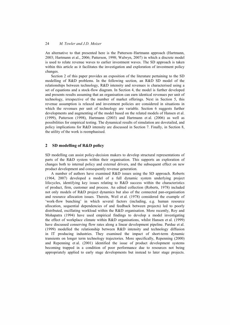
An SD representation of this model, using stocks and flows, is shown in Figure 1. Even in the simplest case, as illustrated by Equations (1) and (2), it can be useful to visualise the feedback between investments now that give rise to revenue in the future. This is clearly shown in the SD model. The box labelled technology shows the current number of technologies of the firm, the arrows from this show the effect of this stock of technologies. One arrow indicates that the technologies lead to an outflow of cash, the money spent in generating revenues from the technologies. Another arrow indicates that the technologies lead to revenues. The revenues then lead to investment which in turn funds the flow of R&D into new technologies. The technologies become obsolete at some rate, for example, due to the company’s competitiveness in the industry.


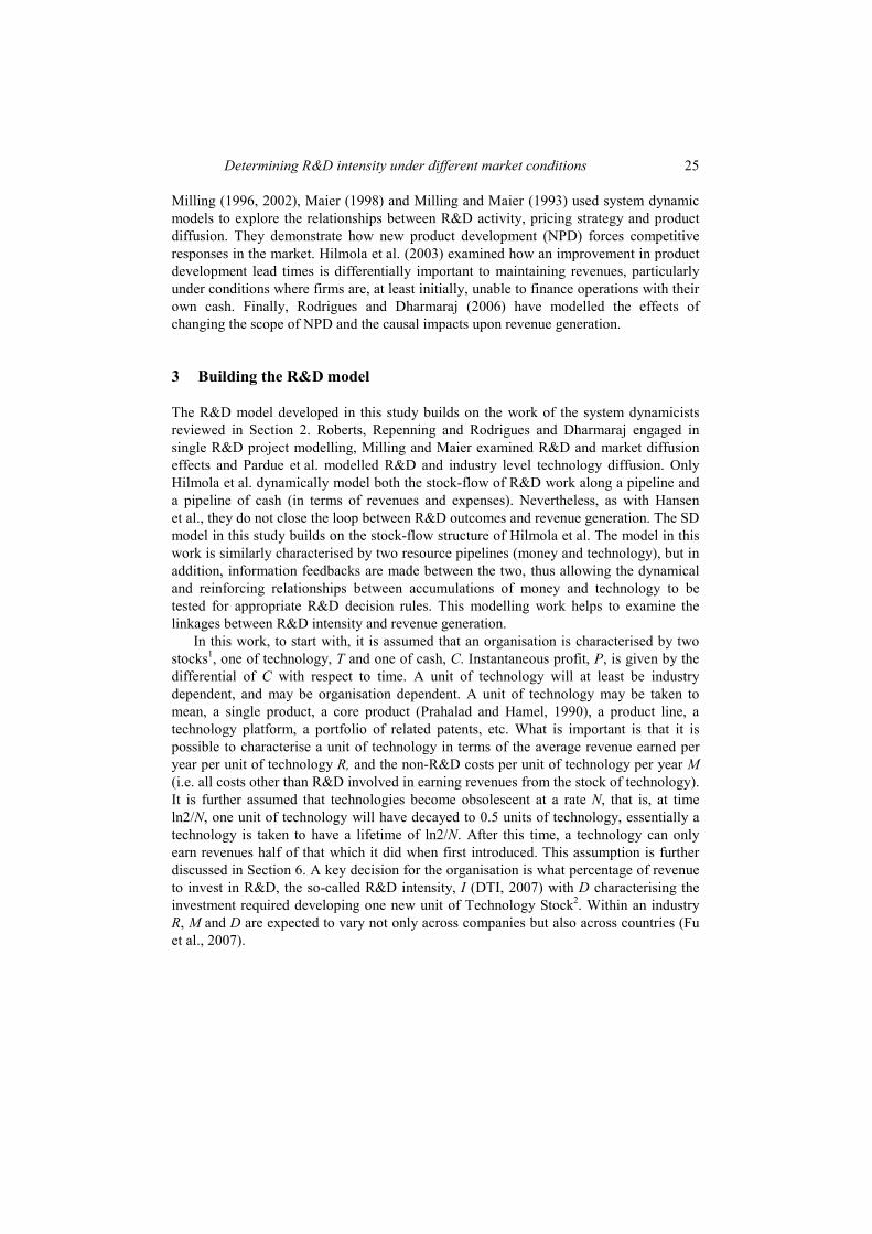
Figure 1 A stock-flow representation of the model

4 Applying the model assuming constant revenues per technology

4.1 Growth and profit bounds for R&D intensity

It can be seen that Equation (1) sets a lower limit for R&D intensity to achieve growth, whilst Equation (2) sets an upper bound above which the organisation will not make (instantaneous) profit, though clearly an organisation could invest above this given the availability of sufficient funds;

N D R MIR R× −

≤ ≤ (3)

Assuming the organisation is unable to change D, R or M, then if the upper limit (‘profit margin before R&D’) is less than the lower limit, the organisation is unable to both grow and simultaneously maintain a profit.3


4.2 The growth of technology and cash stocks

Assuming R, D, M and N to be constant, and I to be held constant over the integration period then, (1) and (2) lead to;

0 exp IRT T N tD

⎛ ⎞= −⎜ ⎟⎝ ⎠

(4)

If IR = ND the stock of technology is unchanging overtime as new investment in R&D is exactly offset by R&D obsolescence and T = T0

00

[(1 ) ]exp 1

( )T D I R M IRC C N t IR ND

IR ND D− − ⎛ ⎞⎛ ⎞= + − − ≠⎜ ⎟⎜ ⎟− ⎝ ⎠⎝ ⎠

0 0[(1 ) ]C C I R M T t IR ND= + − − = (5)

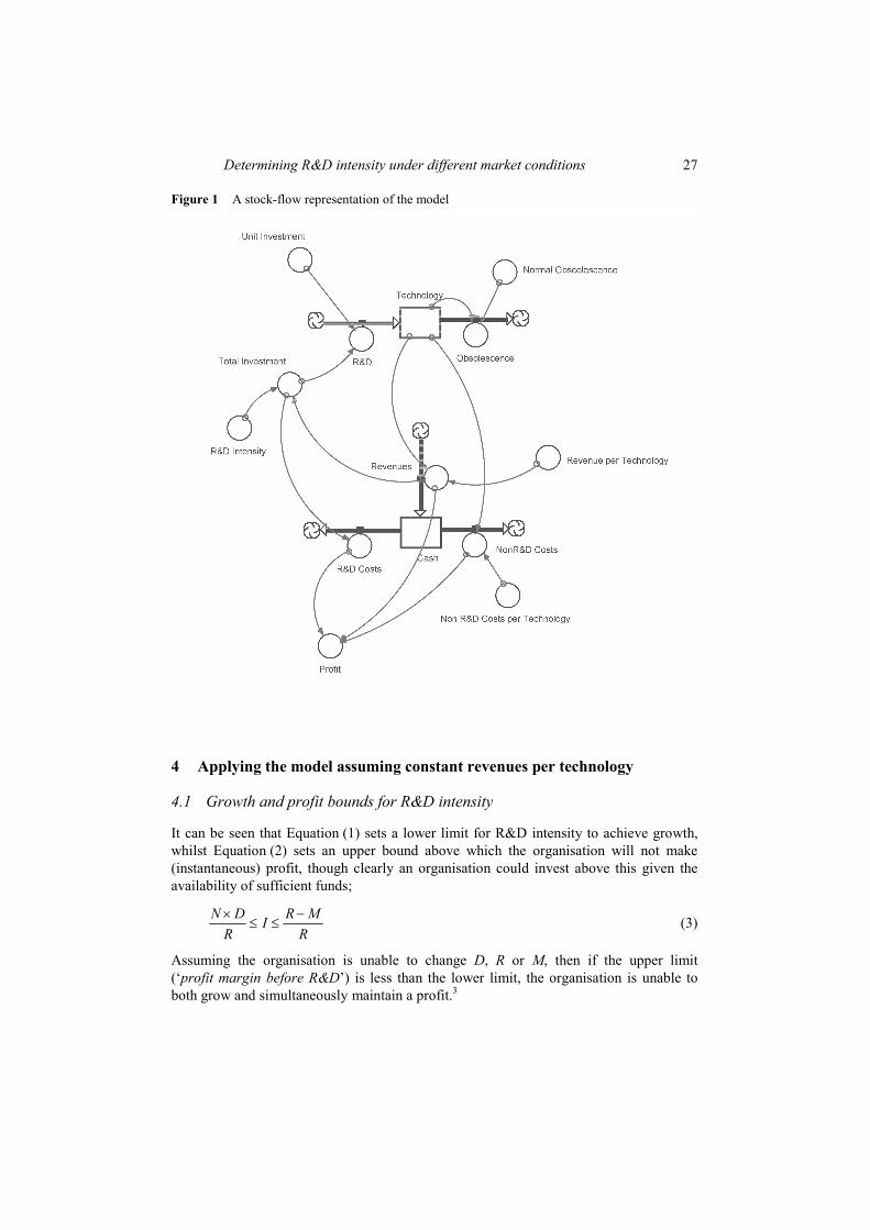
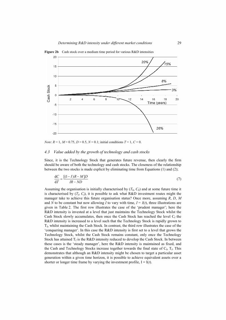
where T0 and C0 are the organisation’s stocks of technology and cash at time, t0 (t = 0). Figure 2 shows the dynamic behaviours of the cash stock for various fixed R&D intensities. In the short term, low investment levels lead to a higher stock of cash (Figure 2a); however, higher R&D intensity gives rise to greater cash in the longer term (Figure 2b) on condition that the upper limit noted in Equation (3) is not surpassed. From Equations (2) to (4), maximising profit with respect to I identifies the constant R&D intensity that will produce most profit at a time tmp;

mp

R M DIR Rt−

= − (6)

As the time horizon for maximising profit tends to infinity, then I is increased to (R – M)/R, that is, a relatively high R&D intensity leads to low profits in the short term and higher profits in the longer term.

Figure 2a Cash stock over a short time period for various R&D intensities

Note: R = 1, M = 0.75, D = 0.5, N = 0.1; initial conditions T = 1, C = 0.


Figure 2b Cash stock over a medium time period for various R&D intensities

Note: R = 1, M = 0.75, D = 0.5, N = 0.1; initial conditions T = 1, C = 0.

4.3 Value added by the growth of technology and cash stocks

Since, it is the Technology Stock that generates future revenue, then clearly the firm should be aware of both the technology and cash stocks. The closeness of the relationship between the two stocks is made explicit by eliminating time from Equations (1) and (2);

d [(1 ) ]dC I R M DT IR ND

− −=

− (7)

Assuming the organisation is initially characterised by (T0, C0) and at some future time it is characterised by (Tf, Cf), it is possible to ask what R&D investment routes might the manager take to achieve this future organisation status? Once more, assuming R, D, M and N to be constant but now allowing I to vary with time, I = I(t), three illustrations are given in Table 2. The first row illustrates the case of the ‘prudent manager’; here the R&D intensity is invested at a level that just maintains the Technology Stock whilst the Cash Stock slowly accumulates, then once the Cash Stock has reached the level Cf the R&D intensity is increased to a level such that the Technology Stock is rapidly grown to Tf, whilst maintaining the Cash Stock. In contrast, the third row illustrates the case of the ‘conquering manager’. In this case the R&D intensity is first set to a level that grows the Technology Stock, whilst the Cash Stock remains constant, only once the Technology Stock has attained Tf is the R&D intensity reduced to develop the Cash Stock. In between these cases is the ‘steady manager’, here the R&D intensity is maintained as fixed, and the Cash and Technology Stocks increase together towards the final state of Cf, Tf. This demonstrates that although an R&D intensity might be chosen to target a particular asset generation within a given time horizon, it is possible to achieve equivalent assets over a shorter or longer time frame by varying the investment profile, I = I(t).


Table 2 Investment decisions to pursue differing technology and cash stock trajectories between equivalent start and finish conditions

Name and goal Tactic Total time to reach (Tf, Cf)

Prudent Manager; grow internal funds before investing in technology

Fix R&D intensity as

NDIR

=

until C = Cf then switch to

( )R MI

R−

=

until T = Tf

( )0

0

fC CR ND M T

−

− −+

( ) 0ln fTD

R ND M T⎛ ⎞⎜ ⎟− − ⎝ ⎠

Steady Manager; grow technology and cash in line with each other

Fixed R&D intensity

( ) ( )( )( ) ( )( )

0 0

0 0

/

/

f f

f f

D C C T T R MI

R C C T T D

⎡ ⎤− − + −⎣ ⎦=⎡ ⎤− − +⎣ ⎦

( ) ( )( )0 0

0

/ln

f f fC C T T D TR M ND T

⎧ ⎫− − +⎪ ⎪⎨ ⎬− −⎪ ⎪⎩ ⎭

Conquering Manager; develop technologies then realise value

Fix R&D intensity as

( )R MI

R−

=

until T = Tf then switch to

NDIR

=

until C = Cf

( ) 0ln fTD

R ND M T⎛ ⎞⎜ ⎟− − ⎝ ⎠

+ ( )

0f

f

C CR ND M T

−

− −

Rather than consider the technology and cash stocks independently, it is possible to define an organisation value as;

( ) ( ) ( )R M TV C( )

tt t

N−

= + (8)

that is, the future revenue streams of the Technology Stock have been valued. On subtracting the initial stocks T0 and C0, (8) leads to a value added of;

( )( )( )

0D 1 I R MIRV T exp 1

D IR Dt N t

N

⎛ ⎞− −⎛ ⎞⎛ ⎞Δ = − − ⎜ ⎟⎜ ⎟⎜ ⎟ ⎜ ⎟−⎝ ⎠⎝ ⎠⎝ ⎠ (9)

This again suggests that providing funds are available, the organisation can create most value by investing with as high an I as possible (recalling that R, M, D and N are assumed constant) and converting the generated technology stock to cash by reducing investment at a future time.

The above result, (9), clearly assumes that however much an organisation invests in R&D, it will have sufficient creativity and market to keep generating units of technology stock with the same R. This is unreasonable; Section 5 investigates the effect of market conditions.


5 Applying the model with variable revenues per technology

In Section 4, it was assumed that the market could absorb all technologies, with each generating fixed revenues R. In practice, R would change with market share, size and time-to-market (Langerack and Hultink, 2006). The model needs to permit the revenue per technology to depend upon the organisation’s Technology Stock (T) compared with the number of technologies the market can absorb (Tm):

( ), mR R T T= (10)

And, furthermore the market demand is variable with time,

( )m mT T t= (11)

Functions (10) and (11) are introduced as exogenous variables to the model.

5.1 R&D intensity to align with market growth

Suppose at that time, t0 the market can absorb a Technology Stock T0 so as to receive R. If the market’s ability to absorb the organisation’s technology grows at a continuous rate G, then the Technology Stock the market can absorb to generate revenues R is:

( )0 expmT T Gt= (12)

Then comparing (12) with Equation (4) suggests the R&D intensity required to grow the technology stock at the market rate is:

( )N G DI

R+

= (13)

That is, the R&D intensity is proportional to the sum of market growth and technological obsolescence rates. A similar result to this has previously been found using discrete time models (Hartmann et al., 2006; Kameoka, 1996; Kameoka and Takayanagi, 1997, 1999).

5.2 Assessment of investment policies

As indicated by Equation (10), revenues are expected to depend upon both market conditions and the Technology Stock. For simplicity, it is assumed that revenues per technology decrease monotonically with the organisation’s total Technology Stock. Although, an organisation would characterise such a function based upon its positions within its industries,4 to allow investigation of alternative investment policies a functional form is assumed:

1( )2 2

2 ( )2 1

QQm

m mQm

T tR R T T

T t T+

⎛ ⎞⎛ ⎞ ⎛ ⎞⎜ ⎟= − <⎜ ⎟ ⎜ ⎟⎜ ⎟⎜ ⎟−− ⎝ ⎠⎝ ⎠⎝ ⎠ (14a)


1( )2

2 1

QQm

m mQT t

R R T TT+

⎛ ⎞⎛ ⎞= >⎜ ⎟⎜ ⎟⎜ ⎟− ⎝ ⎠⎝ ⎠ (14b)

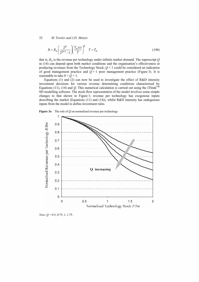
that is, Rm is the revenue per technology under infinite market demand. The superscript Q in (14) can depend upon both market conditions and the organisation’s effectiveness at producing revenues from the Technology Stock; Q < 1 could be considered an indication of good management practice and Q > 1 poor management practice (Figure 3). It is reasonable to take 0 < Q < 1.

Equations (1) and (2) can now be used to investigate the effect of R&D intensity investment decisions for various revenue determining conditions characterised by Equations (11), (14) and Q. This numerical calculation is carried out using the iThinkTM SD modelling software. The stock-flow representation of the model involves some simple changes to that shown in Figure 1; revenue per technology has exogenous inputs describing the market (Equations (11) and (14)), whilst R&D intensity has endogenous inputs from the model to define investment rules.

Figure 3a The role of Q on normalised revenue per technology

Note: Q = 0.5, 0.75, 1, 1.75.


Figure 3b The role of Q on normalised total revenue

Note: Q = 0.5, 0.75, 1, 1.75.

Three commonly occurring scenarios are considered; the mature market (Tm constant), the growing market (Tm increasing for nine years) and the declining market (Tm decreasing for nine years). Each of these is considered with five decision rules. The five policies, outlined in Table 3, are chosen to reflect possible management heuristics:

• Rule 1: maintain the current level of Technology Stock

• Rule 2: maintain a fixed R&D intensity

• Rule 3: invest for the future to maximise value creation

• Rule 4: track market growth/decline (market share perspective)

• Rule 5: target ongoing profit.

Rule 1 is obtained by setting Equation (1) to zero. Rule 2 is obtained by setting Equations (1) and (2) simultaneously to zero. Rule 3 is obtained by setting Equation (2) to zero. Rule 4 is Equation (13). Rule 5 is obtained by differentiating Equation (2) with respect to T and setting to zero, that is Rule 5 is to invest until marginal revenues equals marginal costs.


Table 3 Five investment rules for determining R&D intensity as a function of revenues per technology

Rule R&D intensity Explanation 1 NDI

R=

R&D intensity to maintain existing Technology Stock

2 NDIND M

=+

Fixed R&D intensity to bring technology and cash stocks to equilibrium together

3 max 0, R MI

R⎛ ⎞−⎛ ⎞= ⎜ ⎟⎜ ⎟⎝ ⎠⎝ ⎠

R&D intensity to produce maximum growth of Technology Stock without current year loss

4 ( )max 0,N G D

IR

⎛ ⎞⎛ ⎞+= ⎜ ⎟⎜ ⎟⎝ ⎠⎝ ⎠

R&D intensity set to track market growth or decline

5 ( / )max 0,( / )

T R T R MIT R T R

⎛ ⎞∂ ∂ + −= ⎜ ⎟∂ ∂ +⎝ ⎠

R&D intensity set to target profit (marginal analysis)

It should be noted that although policies 4 and 5 are simply implemented within a simulation model, in practice they require the appropriate market knowledge.

To be able to compare the performance of the policies, not only are the initial and final (after nine years) Cash and Technology Stocks compared but also an organisation value is obtained by considering the future revenue stream of the final Technology Stock. This is calculated by assuming that, after the nine-year period, the market conditions remain fixed for infinite time and the organisation chooses a research intensity of zero, converting all Technology Stock to Cash.

5.2.1 Comparison of policies within a mature market (Q = 0.75, Rm = 1, M = 0.75, D = 0.5, N = 0.1)

An organisation with an initial Cash Stock = 0 is considered within a mature, unchanging, market characterised by Tm = 5. Three situations are taken in turn; an organisation that is not fully utilising its market, an organisation that is sustainably utilising its market and an organisation that has some loss making technologies.

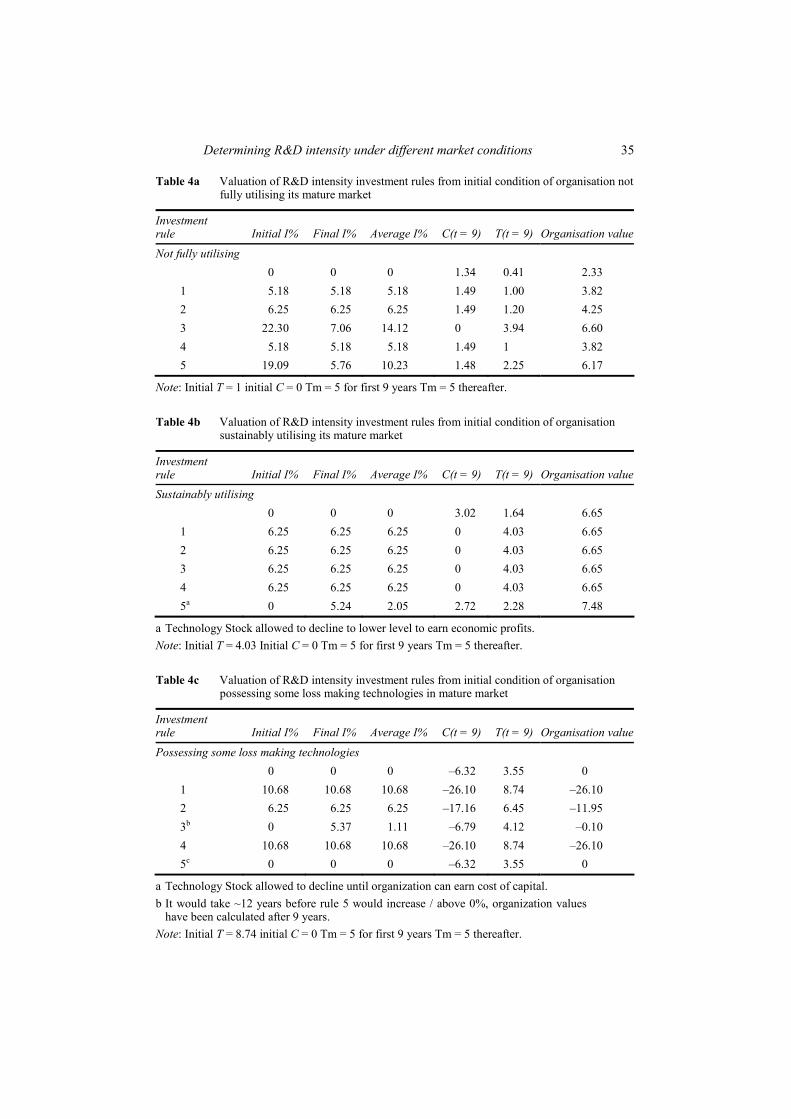
Table 4a summarises the effects of applying the five rules for determining R&D intensity for an organisation with an initial Technology Stock of 1, that is, markedly less than that which the market could absorb. Under such conditions, it is unsurprising to find that all policies are successful in increasing the value of the organisation, however, it is those policies that gave rise to high R&D intensity, and hence growth of the Technology Stock, that create most value. In addition, it is worth noting that under the initial situation of not fully exploiting the market, policy 3 (of investing to grow the Technology Stock) outperforms policy 5 (of targeting profit).

Table 4b summarises the effects of applying the five rules for determining R&D intensity for an organisation under the initial condition of having a sustainable Technology Stock in a mature market. Under such conditions, all policies, bar one, give rise to the same R&D intensity and maintain the value of the organisation. Under this condition, it is only policy 5 that generates a different result, leading to an initial reduction of R&D intensity, reducing the Technology Stock and increasing organisation value.


Table 4a Valuation of R&D intensity investment rules from initial condition of organisation not fully utilising its mature market

Investment rule Initial I% Final I% Average I% C(t = 9) T(t = 9) Organisation value

Not fully utilising 0 0 0 1.34 0.41 2.33

1 5.18 5.18 5.18 1.49 1.00 3.82 2 6.25 6.25 6.25 1.49 1.20 4.25 3 22.30 7.06 14.12 0 3.94 6.60 4 5.18 5.18 5.18 1.49 1 3.82 5 19.09 5.76 10.23 1.48 2.25 6.17

Note: Initial T = 1 initial C = 0 Tm = 5 for first 9 years Tm = 5 thereafter.

Table 4b Valuation of R&D intensity investment rules from initial condition of organisation sustainably utilising its mature market


Sustainably utilising 0 0 0 3.02 1.64 6.65

1 6.25 6.25 6.25 0 4.03 6.65 2 6.25 6.25 6.25 0 4.03 6.65 3 6.25 6.25 6.25 0 4.03 6.65 4 6.25 6.25 6.25 0 4.03 6.65 5a 0 5.24 2.05 2.72 2.28 7.48

a Technology Stock allowed to decline to lower level to earn economic profits. Note: Initial T = 4.03 Initial C = 0 Tm = 5 for first 9 years Tm = 5 thereafter.

Table 4c Valuation of R&D intensity investment rules from initial condition of organisation possessing some loss making technologies in mature market


Possessing some loss making technologies 0 0 0 –6.32 3.55 0

1 10.68 10.68 10.68 –26.10 8.74 –26.10 2 6.25 6.25 6.25 –17.16 6.45 –11.95 3b 0 5.37 1.11 –6.79 4.12 –0.10 4 10.68 10.68 10.68 –26.10 8.74 –26.10 5c 0 0 0 –6.32 3.55 0

a Technology Stock allowed to decline until organization can earn cost of capital. b It would take ~12 years before rule 5 would increase / above 0%, organization values

have been calculated after 9 years. Note: Initial T = 8.74 initial C = 0 Tm = 5 for first 9 years Tm = 5 thereafter.


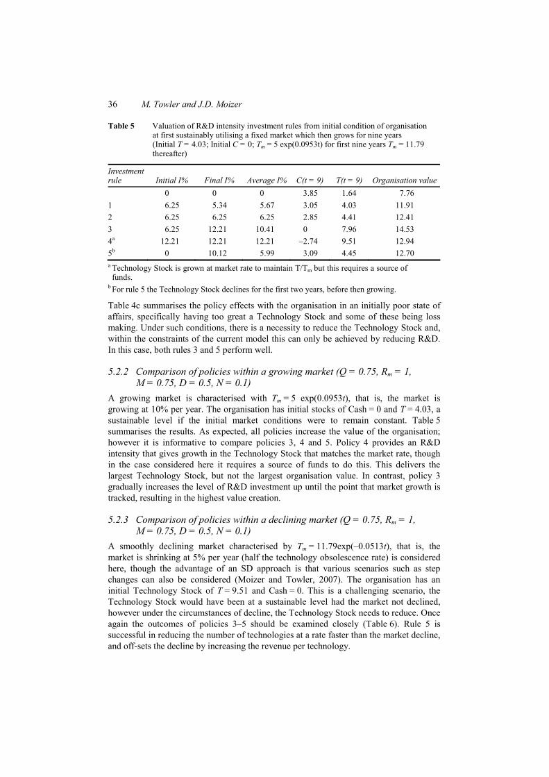
Table 5 Valuation of R&D intensity investment rules from initial condition of organisation at first sustainably utilising a fixed market which then grows for nine years (Initial T = 4.03; Initial C = 0; Tm = 5 exp(0.0953t) for first nine years Tm = 11.79 thereafter)

Investment rule Initial I% Final I% Average I% C(t = 9) T(t = 9) Organisation value 0 0 0 3.85 1.64 7.76 1 6.25 5.34 5.67 3.05 4.03 11.91 2 6.25 6.25 6.25 2.85 4.41 12.41 3 6.25 12.21 10.41 0 7.96 14.53 4a 12.21 12.21 12.21 –2.74 9.51 12.94 5b 0 10.12 5.99 3.09 4.45 12.70 a Technology Stock is grown at market rate to maintain T/Tm but this requires a source of funds.

b For rule 5 the Technology Stock declines for the first two years, before then growing.

Table 4c summarises the policy effects with the organisation in an initially poor state of affairs, specifically having too great a Technology Stock and some of these being loss making. Under such conditions, there is a necessity to reduce the Technology Stock and, within the constraints of the current model this can only be achieved by reducing R&D. In this case, both rules 3 and 5 perform well.

5.2.2 Comparison of policies within a growing market (Q = 0.75, Rm = 1, M = 0.75, D = 0.5, N = 0.1)

A growing market is characterised with Tm = 5 exp(0.0953t), that is, the market is growing at 10% per year. The organisation has initial stocks of Cash = 0 and T = 4.03, a sustainable level if the initial market conditions were to remain constant. Table 5 summarises the results. As expected, all policies increase the value of the organisation; however it is informative to compare policies 3, 4 and 5. Policy 4 provides an R&D intensity that gives growth in the Technology Stock that matches the market rate, though in the case considered here it requires a source of funds to do this. This delivers the largest Technology Stock, but not the largest organisation value. In contrast, policy 3 gradually increases the level of R&D investment up until the point that market growth is tracked, resulting in the highest value creation.

5.2.3 Comparison of policies within a declining market (Q = 0.75, Rm = 1, M = 0.75, D = 0.5, N = 0.1)

A smoothly declining market characterised by Tm = 11.79exp(–0.0513t), that is, the market is shrinking at 5% per year (half the technology obsolescence rate) is considered here, though the advantage of an SD approach is that various scenarios such as step changes can also be considered (Moizer and Towler, 2007). The organisation has an initial Technology Stock of T = 9.51 and Cash = 0. This is a challenging scenario, the Technology Stock would have been at a sustainable level had the market not declined, however under the circumstances of decline, the Technology Stock needs to reduce. Once again the outcomes of policies 3–5 should be examined closely (Table 6). Rule 5 is successful in reducing the number of technologies at a rate faster than the market decline, and off-sets the decline by increasing the revenue per technology.


Table 6 Valuation of R&D intensity investment rules from initial condition of organisation at first sustainably utilising a fixed market which then decays for nine years (Initial T = 9.51; Initial C = 0; Tm = 11.79exp(–0.051t) for first nine years Tm = 7.43 thereafter)


0 0 0 5.40 3.87 13.18 1 6.25 8.45 7.20 –8.48 9.51 –0.61 2 6.25 6.25 6.25 –6.43 8.65 2.62 3 6.25 3.10 3.70 0 6.46 10.06 4 3.04 3.04 3.04 1.76 5.99 11.64 5a 0 0.30 0 5.40 3.87 13.17 a Only in the ninth year does this decision rule raise R&D intensity above 0%.

6 Extending the model for management exploration

Section 4 has introduced some basic considerations for the bounds of R&D intensity, whilst Section 5 has used some simple situations to illustrate example outcomes from alternative guiding policies. However, some managers may prefer to use a model interactively, not only entering the organisation’s forecasts for R, M, D, etc., but also exploring scenarios based upon various R&D intensity profiles as a function of time, unconstrained by one particular policy. This may indeed be the case for companies that have data available that relates specific research and technology development expenditure to specific product generated revenues (Hartmann, 2003; Hartmann et al., 2006; Patterson, 1998). To carry out such a firm specific investigation, it is useful to adjust the basic structure of the SD model. For instance in presenting the future revenue stream from Hewlett–Packard organisation’s new product introductions, Patterson (1998) demonstrates that although the obsolescence of a product might be reasonably represented as a decay from perhaps year 2 or 3 onwards, in the year of introduction a product typically generates less revenues than in the following year. This suggests that the single technology outflow used to represent technology obsolescence within this article (Figure 1) could be usefully replaced by a series of stocks; for example, a stock of technologies in their first year of commercialisation, and a separate stock for technologies that have been earning revenues for more than one year. Similarly, the expenditure in a given year may be focused on different phases of R&D, and this suggests that the single technology inflow used to represent R&D within this article could be replaced by a series of stocks and flows (Hansen et al., 1999). A final generic change to the model from which some management exploration could benefit is to include several coflows of R&D, particularly when it is inappropriate to represent different technologies by the same parameters R, M, D and N.

Further extensions to this model are possible. It could, for example, be empirically tested with real-world data. This would provide the opportunity to further validate the causal relationships espoused in the model, and take the study beyond that of being exploratory to the level of explanatory.


7 Discussion of policy evaluation

Sections 4.1 and 4.2 showed reasonable bounds for an organisation to consider for its R&D investment. Further investigation would be required to determine the consistency of this with sector specific R&D intensities (DTI, 2007). In agreement with the earlier discrete models, the minimum R&D intensity is determined by the lifetime revenues that a unit of technology (e.g. a new product line) will generate, and the R&D costs to bring that technology to commercialisation. If the upper and lower bounds are close together, there is little opportunity for an organisation to earn economic profit. Under such circumstances, the R&D intensity will be given by investment rule 2 (Table 3). This result highlights the situation under which a firm needs to investigate strategies to modify N, D, R and M, for example, using the approach of a sensitivity analysis of the factors contributing to M and R as suggested by Merrifield (2006), and recognising the need to balance technological and business innovation (Tuominen et al., 2007).

Section 4.3 showed that under the assumption of constant revenue per technology, then investing heavily in early years allows a particular asset generation to be achieved within a shorter time horizon. In general, if there is value to be added, invest early. Under a similar assumption, Section 5.1 suggested that the R&D intensity should be proportional to the sum of market growth and technological obsolescence rates, this result confirms that of earlier discrete results (Hartmann et al., 2006; Kameoka, 1996; Kameoka and Takayanagi, 1997, 1999).

Although, these results provide some guidance, they ignore the possibility of the revenue earning potential of a technology changing. Under such circumstances, one strategic avenue open to a firm is to modify its R&D intensity, I. Section 4.2 investigated various policies for determining I given different market conditions; policies 3–5 (Table 3) all provide some guidance. Policy 5 may be the least obvious of these, however in qualitative terms it suggests that if revenues per technology are decreasing as the number of technologies increase, then an organisation should not invest quite to the limit suggested by policy 3 (growing the stock of technology for value creation). Conversely, if revenues per technology are increasing as higher Technology Stocks are accumulated; then policy 5 suggests a higher R&D intensity than that suggested by policy 3. Policy 3 outperforms policy 5 under the conditions of a growing or not fully utilised market, whereas policy 5 outperforms policy 3 for a shrinking market.

8 Summary of the study

This R&D modelling exercise has provided insight into how dynamical simulation modelling can be used to explore a range of R&D decision rules within the constraints of alternative market conditions and examine different future revenue trajectories Although, the model is conceptual, it still has utility as a policy learning tool for R&D decision makers. From a simple model structure, a range of dynamical revenue outcomes have been tested. The model has the capacity to generate insights and understandings of how a simple stock-flow causal structure can generate quite complex and alternative dynamics.


References DTI (2007) ‘The R&D scoreboard 2007: The top 800 UK & 1250 global companies by R&D

investment’, DIUS/PUB 8642/3K/11/07/NP, URN 07/31, Available at: http:// www.innovation.gov.uk/downloads/2007_rd_scoreboard_analysis.pdf. Accessed on 5 November 2008.

Eberhart, A.C., Maxwell, W.F. and Siddique, A.R. (2004) ‘An examination of long-term abnormal stock returns and operating performance following R&D increases’, Journal of Finance, Vol. 59, No. 2, pp.623–650.

Fu, C-J., Cheng, C-B, Chang, B-G and Lai, Y.J. (2007) ‘Direct and indirect effects of innovation on revenue growth: comparison between the US and Taiwanese electronics firms’, Int. J. Revenue Management, Vol. 1, No. 2, pp.177–199.

Hansen, K.F., Weiss, M.A. and Sanman, K. (1999) ‘Allocating R&D resources: a quantitative aid to management insight’, Research Technology Management, Vol. 20, No. 3, pp.44–50.

Hartmann, G.C. (2003) ‘Linking R&D spending to revenue growth’, Research-Technology Management, Vol. 46, No. 1, pp.39–46.

Hartmann, G.C., Myers, M.B. and Rosenbloom, R.S. (2006) ‘Planning your firm’s R&D investment’, Research-Technology Management, Vol. 49, No. 2, pp.29–36.

Hilmola, O.P., Helo, P. and Ojala, L. (2003) ‘The value of product development lead time in software startup’, System Dynamics Review, Vol. 19, No. 1, pp.75–82.

Kameoka, A. (1996) ‘A corporate technology stock model and its applications’, Proceedings of Technology Management: University/Industry/Government Collaboration, Istanbul, pp.16–21.

Kameoka, A. and Takayanagi, S-I. (1997) ‘A corporate technology stock model: determining total R&D expenditure and effective investment patterns’, Proceedings of the PICMET’ 97, pp.137–401.

Kameoka, A. and Takayanagi, S-I. (1999) ‘A corporate technology stock model financially sustainable research and technology development’, Proceedings of the PICMET’ 99, pp.25–29.

Langerack, F. and Hultink, E.J. (2006) ‘The impact of product development speed and new product profitability’, Journal of Product Innovation Management, Vol. 23, No. 3, pp.203–214.

Lin, M.J., Chen, C. and Huang, Z. (2007) ‘Effects of business and design strategy integration on new product development performance: an empirical analysis’, Int. J. Business Systems Research, Vol. 1, No. 4, pp.438–457.

Maier, F. (1998) ‘New product diffusion models in innovation management – a system dynamics perspective’, System Dynamics Review, Vol. 14, No. 4, pp.285–308.

Merrifield, D.B. (2006) ‘Strategic accounting for R&D’, Research-Technology Management, Vol. 49, No. 1, pp.9–13.

Milling, P. (1996) ‘Modeling innovation processes for decision support and management simulation’, System Dynamics Review, Vol. 12, No. 3, pp.211–234.

Milling, P. (2002) ‘Understanding and managing innovation processes’, System Dynamics Review, Vol. 18, No. 1, pp.73–86.

Milling, P. and Maier, F. (1993) ‘Dynamic consequences of pricing strategies for research & development and the diffusion of innovations’, Proceedings of the 1993 International System Dynamics Conference.

Moizer, J.D. and Towler, M.J. (2007) ‘Research and development resourcing when faced with fundamental market dynamics’, Int. J. Business Performance Management, Vol. 9, No. 4, pp.435–452.

Pardue, J.H., Clark, T.D. and Winch, G.W. (1999) ‘Modelling short- and long-term dynamics in the commercialization of technical advances in IT producing industries’, System Dynamics Review, Vol. 15, No. 1, pp.97–105.

Patterson, M.L. (1998) ‘From experience: linking product innovation to business growth’, The Journal of Product Innovation Management, Vol. 15, pp.390–402.


Prahalad, C.K. and Hamel, G. (1990) ‘The core competence of a corporation’, Harvard Business Review, Vol. 68, No. 3, pp.79–91.

Repenning, N.P. (2000) ‘A dynamic model of resource allocation in multi-project research and development systems’, System Dynamics Review, Vol. 16, No. 3, pp.173–212.

Repenning, N.P., Goncalves, P. and Black, L.J. (2001) ‘Past the tipping point: the persistence of firefighting in product development’, California Management Review, Vol. 43, No. 4, pp.44–63.

Roberts, E.B. (1964) The Dynamics of Research and Development. New York: Harper and Row. Roberts, E.B. (1978) Managerial Applications of System Dynamics. Cambridge, MA:

The MIT Press. Roberts, E.B. (2007) ‘Making system dynamics useful: a personal memoir’, System Dynamics

Review, Vol. 23, Nos. 2/3, pp.119–136. Rodrigues, L.L.R. and Dharmaraj, N. (2006) ‘System dynamics approach for change management

in new product development’, Management Research News, Vol. 29, No. 8, pp.512–523. Roy, S. and Mohapatra, P.K.J. (1994) ‘Study of work climate in R&D organizations: a system

dynamics approach’, Proceedings of the 1994 International System Dynamics Conference. Towler, M.J. and Moizer, J.D. (2008) ‘The R&D funding decision: the need for a systemic

approach’, Int. J. Management and Decision Making, Vol. 9, No. 4, pp.434–452. Tuominen, M., Kajalo, S., Rajala, A., Matear, S. and Hooley, G.J. (2007) ‘Sharpening the edge of

market-driven intangibles and innovations’, Int. J. Revenue Management, Vol. 1, No. 3, pp.247–261.

Walwyn, D. (2007) ‘Finland and the mobile phone industry: a case study of the return on investment from government-funded research and development’, Technovation, Vol. 27, Nos. 6–7, pp.335–341.

Weil, H., Bergan, T. and Roberts, E.B. (1978) ‘The dynamics of R&D strategy’, in E.B. Roberts (Ed.), Managerial Applications of System Dynamics. Cambridge, MA: The MIT Press.

Wolff, M.F. (2007) ‘Forget R&D spending – think innovation’, Research-Technology Management, Vol. 50, No. 2, pp.7–9.

Notes 1 The term ‘stock’ is used in the general (SD) sense of a quantity of something that has accumulated. The cash stock, the amount of money, at any instance is the result of past flows into and out of the company. The Technology Stock at a given time has accumulated from inflows of new technology, in this model due to R&D, and outflows due to obsolescence of technology. The Technology Stock is the number of technologies.

2 One criticism that could be levied at the current model is that it provides no consideration of opportunity costs. It is though possible to consider all monies to be at present value. One response to this assumption would be to suggest that the model include an additional outflow from the Cash Stock (∝C) to represent the difference between the organisation’s cost of capital and, say, bank interest rates. However, this has not been included, it is considered more reasonable within a simple model to assume that the Cash Stock also earns its cost of capital, that is, cash is efficiently moved in and out of the organisation through dividend payments, rights issues, etc. Under such assumptions, profit within the model then represents economic profit, and hence competition would be expected to respond to this. Nevertheless, the addition of modelling the industry and market has been avoided. It is considered preferable to introduce these effects for particular companies exogenously through N, M and R. Each organisation has its own models and data to forecast these variables.


3 In terms of the Patterson–Hartmann model the left hand side (l.h.s.) of Equation (3) is (R&D Gain)–1, where R&D Gain is the ratio of lifetime revenue gains from a technology (R/N) to the total investment needed to develop that technology (D). For the r.h.s. of (3) to be greater than the l.h.s. then (R – M) N–1 must be greater than D, that is, not unexpectedly, the average value of a technology from future revenue cash flows must be greater than the average investment to develop a technology.

4 Herein, it is assumed that the revenue per technology is determined by market conditions and the firm’s ability to manage its Technology Stock. Equation (14) is a simple function to represent this and to allow investment policies to be investigated. Equation (14) assumes that as the firm’s number of product lines increases then the average revenue per product line will decrease unless the market grows. Within this paper, the only response that the firm has to changing revenues per technology is to increase or decrease its R&D intensity.

Determining R&D intensity under different market conditions

Documents

Transcript of Determining R&D intensity under different market conditions