Determination of the Oil Initial in Place, Reserves, and ...

The International Journal of Engineering and Science (IJES)

|| Volume || 8 || Issue || 2 Series I|| Pages || PP 86-97 || 2019 ||

ISSN (e): 2319 – 1813 ISSN (p): 23-19 – 1805

DOI:10.9790/1813-0802018697 www.theijes.com Page 86

Determination of the Oil Initial in Place, Reserves, and

Production Performance of the Safsaf C Oil Reservoir

Saleh Ahmed1, Khalid Elwegaa

1, MohanedHtawish

2,Haiat Alhaj

3

1Bob L. Herd Department of Petroleum Engineering, Texas Tech University, Lubbock, TX 79409, USA

2Waha Oil Company; Abu Laila Tower, Alkurnish Rd. Tripoli, Libya

3Petroleum Engineering Department, Tripoli University, Libya

Corresponding Author:Khalid Elwegaa

--------------------------------------------------------ABSTRACT-----------------------------------------------------------

This study estimated the initial oil in place (OIIP) of SafsafCoil reservoir by using both volumetric methods and

material balance equation. Also, oil reserves of this reservoir was estimated using production Decline Curve

Analysis (DCA) method. First, three different volumetric techniques (Iso-pach method, Pore-volume method and

Hydrocarbon pore volume method) were implemented in this study to estimate the initial oil in place. As these

volumetric techniques depends on mapping for their calculation, so a powerful package software (Surfer) was

used to generate maps. Second, Havelena and Odeh model was built as a Material Balance Equation (MBE) to

estimate the initial oil in place. Field production history, PVT data and reservoir pressure history were

prepared to apply the material balance equation. finally, Exponential decline method was used as a Decline

Curve Analysis (DCA) to estimate oil reserves, remaining reserves, and remaining productive life of the

reservoir.The results of this study revealed that SafsafC reservoir has an initial oil in place in the range of 11.59

to 12.11 MMSTB by implementing the three volumetric methods (Iso-pach, Pore-volume and Hydrocarbon pore

volume). The results also revealed that initial oil in place obtained from material balance equation is

12.71MMSTB, which is in a good agreement with volumetric methods. Additionally, oil reserve of Safsaf C

reservoir is 3.05 MMSTB for the total reservoir.The results of this study demonstrate that Infill drilling can be

implemented to increase oil recovery, and continued water injection should be used to maintain the reservoir

pressure.

KEYWORDS: -Safsaf C reservoir; volumetric method; material balance equation; decline curve analysis; oil initial in

place; reserves ----------------------------------------------------------------------------------------------------------------------------- ----------

Date of Submission: 04-02-2019Date of acceptance: 20-02-2019

-------------------------------------------------------------------------------------------------------------------------------------- -

I. INTRODUCTION

Three main types of techniques are used to estimate Hydrocarbon Initially in Place (HIIP). Volumetric

Methods are ―static‖ methods that estimate HIIP from static properties of the reservoir, including its porosity,

thickness, and initial water saturation. The Material Balance Method, in contrast, is a ―dynamic‖ method that

estimates HIIP by analyzing historical data on production and pressure. A Long Duration Draw-Down Test (e.g.

Reservoir Limit Test) can also be used to estimate HIIP, but because this method is normally limited to small

hydrocarbon accumulations (i.e. single- or two-well reservoirs), it will not be considered in this study.

1.1 Volumetric Methods

Volumetric methods of estimating HIIP can be employed immediately after first discovery, before

production begins. For this reason, they are the primary tool used for the techno/economic evaluation of oil

properties and for the design of field-development projects (Dake, 1978), (Ahmed, 2010), (Craft & Hawkins,

1991).

The accuracy of HIIP estimates calculated using volumetric methods depends significantly on one’s

understanding of regional geology and on the quality of the seismic analysis, both of which will improve as

more wells are drilled and more accurate descriptions and geologic and petrophysical maps of reservoirs become

available (Urayet, 2004).

Three different volumetric methods—Iso-Pach, Pore-Volume, and Hydrocarbon Pore Volume are used

to estimate OIIP, and they all use the same basic data: petrophysical properties described by well logs,

geological maps, and the physical properties of the oil at the initial reservoir conditions.

Determination of the Oil Initial in Place, Reserves, and Production Performance of the Safsaf C ….


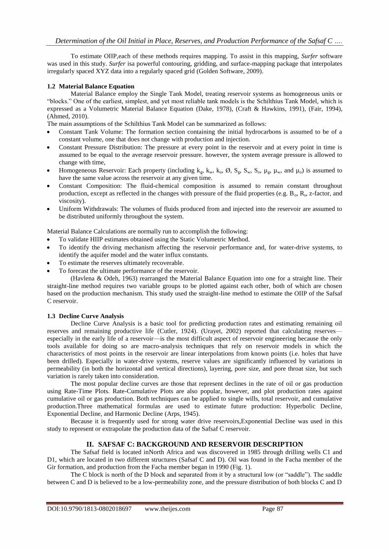
To estimate OIIP,each of these methods requires mapping. To assist in this mapping, Surfer software

was used in this study. Surfer isa powerful contouring, gridding, and surface-mapping package that interpolates

irregularly spaced XYZ data into a regularly spaced grid (Golden Software, 2009).

1.2 Material Balance Equation

Material Balance employ the Single Tank Model, treating reservoir systems as homogeneous units or

―blocks.‖ One of the earliest, simplest, and yet most reliable tank models is the Schilthius Tank Model, which is

expressed as a Volumetric Material Balance Equation (Dake, 1978), (Craft & Hawkins, 1991), (Fair, 1994),

(Ahmed, 2010).

The main assumptions of the Schilthius Tank Model can be summarized as follows:

Constant Tank Volume: The formation section containing the initial hydrocarbons is assumed to be of a

constant volume, one that does not change with production and injection.

Constant Pressure Distribution: The pressure at every point in the reservoir and at every point in time is

assumed to be equal to the average reservoir pressure. however, the system average pressure is allowed to

change with time,

Homogeneous Reservoir: Each property (including kg, kw, ko, Ø, Sg, Sw, So, µg, µw, and µo) is assumed to

have the same value across the reservoir at any given time.

Constant Composition: The fluid-chemical composition is assumed to remain constant throughout

production, except as reflected in the changes with pressure of the fluid properties (e.g. Bo, Rs, z-factor, and

viscosity).

Uniform Withdrawals: The volumes of fluids produced from and injected into the reservoir are assumed to

be distributed uniformly throughout the system.

Material Balance Calculations are normally run to accomplish the following:

To validate HIIP estimates obtained using the Static Volumetric Method.

To identify the driving mechanism affecting the reservoir performance and, for water-drive systems, to

identify the aquifer model and the water influx constants.

To estimate the reserves ultimately recoverable.

To forecast the ultimate performance of the reservoir.

(Havlena & Odeh, 1963) rearranged the Material Balance Equation into one for a straight line. Their

straight-line method requires two variable groups to be plotted against each other, both of which are chosen

based on the production mechanism. This study used the straight-line method to estimate the OIIP of the Safsaf

C reservoir.

1.3 Decline Curve Analysis

Decline Curve Analysis is a basic tool for predicting production rates and estimating remaining oil

reserves and remaining productive life (Cutler, 1924). (Urayet, 2002) reported that calculating reserves—

especially in the early life of a reservoir—is the most difficult aspect of reservoir engineering because the only

tools available for doing so are macro-analysis techniques that rely on reservoir models in which the

characteristics of most points in the reservoir are linear interpolations from known points (i.e. holes that have

been drilled). Especially in water-drive systems, reserve values are significantly influenced by variations in

permeability (in both the horizontal and vertical directions), layering, pore size, and pore throat size, but such

variation is rarely taken into consideration.

The most popular decline curves are those that represent declines in the rate of oil or gas production

using Rate-Time Plots. Rate-Cumulative Plots are also popular, however, and plot production rates against

cumulative oil or gas production. Both techniques can be applied to single wills, total reservoir, and cumulative

production.Three mathematical formulas are used to estimate future production: Hyperbolic Decline,

Exponential Decline, and Harmonic Decline (Arps, 1945).

Because it is frequently used for strong water drive reservoirs,Exponential Decline was used in this

study to represent or extrapolate the production data of the Safsaf C reservoir.

II. SAFSAF C: BACKGROUND AND RESERVOIR DESCRIPTION The Safsaf field is located inNorth Africa and was discovered in 1985 through drilling wells C1 and

D1, which are located in two different structures (Safsaf C and D). Oil was found in the Facha member of the

Gir formation, and production from the Facha member began in 1990 (Fig. 1).

The C block is north of the D block and separated from it by a structural low (or ―saddle‖). The saddle

between C and D is believed to be a low-permeability zone, and the pressure distribution of both blocks C and D



is shown in fig. 2. To date, a total of six wells—3 producers and 3 injectors—have been drilled into the

structure of C (Fig. 3).

Fig. 2 Isobaric mapof theSafsaf field Fig. 3 Map of well locations in Safsaf C

All of the wells produce from the carbonate Facha formation. The Safsaf formation is bounded by

several faults, all of which are assumed to have small throws such that they may not seal completely. The

overlaying Hon Evaporites provide a seal for the reservoir. The porous interval below the oil interval consists of

very-low-permeability rock. Diagenesis took place in the water interval and is believed to have decreased the

permeability of the water-filled pores.

The Facha reservoir is composed of a series of dolomite and limestone layers separated by tight

anhydritic stringers. These anhydrite layers prevent vertical communication between the flow units, particularly

in the upper parts of the reservoir. Table 1 presents data from the Safsaf C reservoir.

Fig.1 The location of the Safsaf field



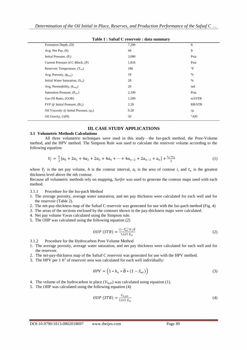
III. CASE STUDY APPLICATIONS 3.1 Volumetric Methods Calculations

All three volumetric techniques were used in this study—the Iso-pach method, the Pore-Volume

method, and the HPV method. The Simpson Rule was used to calculate the reservoir volume according to the

following equation:

𝑉𝑓 = 𝑕

3 𝑎0 + 2𝑎1 + 4𝑎2 + 2𝑎3 + 4𝑎4 + ⋯+ 4𝑎𝑛−2 + 2𝑎𝑛−1 + 𝑎𝑛 +

𝑡𝑛 ∗𝑎𝑛

2 (1)

where 𝑉𝑓 is the net pay volume, 𝑕 is the contour interval, 𝑎𝑖 is the area of contour i, and 𝑡𝑛 is the greatest

thickness level above the nth contour.

Because all volumetric methods rely on mapping, Surfer was used to generate the contour maps used with each

method.

3.1.1 Procedure for the Iso-pach Method

1. The average porosity, average water saturation, and net pay thickness were calculated for each well and for

the reservoir (Table 2).

2. The net-pay-thickness map of the Safsaf C reservoir was generated for use with the Iso-pach method (Fig. 4)

3. The areas of the sections enclosed by the contours shown in the pay-thickness maps were calculated.

4. Net pay volume Vfwas calculated using the Simpson rule.

5. The OIIP was calculated using the following equation (2)

𝑂𝐼𝐼𝑃 𝑆𝑇𝐵 = 1−𝑆𝑤𝑖 𝑉𝑓∅

5.615 𝐵𝑜𝑖 (2)

3.1.2 Procedure for the Hydrocarbon Pore Volume Method


the reservoir.

2. The net-pay-thickness map of the Safsaf C reservoir was generated for use with the HPV method.

3. The HPV per 1 ft2 of reservoir area was calculated for each well individually:

𝐻𝑃𝑉 = 1 ∗ 𝑕𝑛 ∗ ∅ ∗ 1 − 𝑆𝑤𝑖 (3)

4. The volume of the hydrocarbon in place (Vhydr) was calculated using equation (1).

5. The OIIP was calculated using the following equation (4)

𝑂𝐼𝐼𝑃 𝑆𝑇𝐵 =𝑉𝑕𝑦𝑑𝑟

5.615 𝐵𝑜𝑖 (4)

Table 1 : Safsaf C reservoir : data summary

Formation Depth, (D) 7,200 ft

Avg. Net Pay, (h) 44 ft

Initial Pressure, (Pi) 3,080 Psia

Current Pressure of C-Block, (P) 1,816 Psia

Reservoir Temperature, (Tres) 186 °F

Avg. Porosity, (avg.) 18 %

Initial Water Saturation, (Swi) 28 %

Avg. Permeability, (kavg.) 20 md

Saturation Pressure, (Psat.) 2,100 Psia

Gas Oil Ratio, (GOR) 1,500 scf/STB

FVF @ Initial Pressure, (Boi) 2.28 RB/STB

Oil Viscosity @ Initial Pressure, (μo) 0.28 cp

Oil Gravity, (API) 50 °API



3.1.3 Procedure for the Pore Volume Method


the reservoir.

2. The iso-porosity, iso-water-saturation, and net-pay-thickness maps of the Safsaf C reservoir were generated.

3. A suitable grid was placed over the three iso maps, which covered the entire net-pay area.

4. The values for hn, ∅ and Swi were estimated for each grid square.

5. The initial volume (Vi) of each grid square was calculated using the following equation (5)

𝑉𝑖 = 𝑕𝑛 ∗ ∅ ∗ 1 − 𝑆𝑤𝑖 ∗ 𝑔𝑟𝑖𝑑 𝑎𝑟𝑒𝑎 (5)

6. OIIP was calculated using the following equation (6)

𝑂𝐼𝐼𝑃 𝑆𝑇𝐵 = 𝑉𝑖

5.615 𝐵𝑜𝑖 (6)

3.2 Material Balance Calculations

The following data were prepared before the material balance calculations were completed using the

Havelena and Odeh model.

The cumulative production history of the reservoir; i.e. Np, Gp, and Wp, as well as the cumulative injection

data in case of injection projects; i.e. Wi and/or Ginj(Table 2).

The history for average reservoir pressure (Table 2).

Oil, gas, and water PVT data (Table 3).

The Havelena and Odeh model was built to estimate the OIIP of Safsaf C. The general form of the

material balance equation is:

𝑁 =𝑁𝑝 𝐵𝑡+ 𝑅𝑝−𝑅𝑠𝑖 𝐵𝑔 +𝑊𝑝𝐵𝑤−𝑊𝑖𝐵𝑤−𝐺𝑖𝐵𝑔−𝑊𝑒

𝐵𝑡−𝐵𝑡𝑖 +𝑚𝐵 𝑡𝑖 𝐵𝑔

𝐵𝑔𝑖−1 + 1+𝑚 𝐵𝑡𝑖

𝑐𝑓+𝑐𝑤 𝑆𝑤𝑖1−𝑆𝑤𝑖

∆𝑝

(7)

Since the Safsaf C reservoir is above the bubble-point pressure, no water influx, and gas injection, the

above equation can be written as follows:

𝑁 =𝑁𝑝𝐵𝑜+𝑊𝑝𝐵𝑤−𝑊𝑖

𝐵𝑜−𝐵𝑜𝑖 +𝐵𝑜𝑖 𝑐𝑓+𝑐𝑤 𝑆𝑤𝑖

1−𝑆𝑤𝑖 ∆𝑝

(8)

Table 2: Reservoir pressure and production history for Safsaf C

Date Pressure Cum. Oil Cum. Gas Cum. WTR Cum.Gas Cum WTR Inj.

psi MMSTB MMscf MMSTB MMscf MMSTB

6/30/1990 3,080 0.0000 0.0000 0.0000 0 0.0000

8/31/1990 2,858 0.1952 353.97 0.0007 0 0.0000

1/31/1991 2,360 0.3007 547.31 0.0080 0 0.0000

5/31/1991 2,540 0.3201 579.49 0.0084 0 0.0000

8/31/1991 2,305 0.3451 619.80 0.0089 0 0.0000

11/30/1991 2,420 0.3717 683.64 0.0089 0 0.0000

2/29/1992 2,438 0.3998 736.53 0.0089 0 0.0000

9/30/1992 2,273 0.4961 918.87 0.0123 0 0.0256

11/30/1992 2,394 0.5330 966.80 0.0124 0 0.0553

4/30/1993 2,099 0.6242 1077.96 0.0137 0 0.1281

10/31/1993 2,135 0.6705 1224.84 0.0146 0 0.1877

8/31/1994 2,072 0.7941 1479.88 0.0192 0 0.4650

9/30/1995 2,030 1.0058 1892.91 0.0219 0 1.0479

11/30/1996 2,025 1.2665 2463.13 0.0368 0 1.6960

2/28/1997 2,044 1.3449 2602.38 0.0427 0 1.8583



Table 3: PVT data for Safsaf C

Pressure psi

Relative Volume of Oil and Gas, (v/vsat)

Viscosity of Oil, (cp) @ 202 °F

GOR (Liberated per

Barrel of Residual

Oil)

GOR (In Solution per

Barrel of Residual

Oil)

Oil FVF (Bbl/STB)

5,000 0.9063 0.32 3.080

4,490 0.9169 0.31 3.116

3,995 0.9291 0.31 3.157

3,519 0.9426 0.30 3.203

2,994 0.9595 0.29 3.260

2,200 0.9948 0.28 3.380

BP=2,108 1.0000 0.27 0 3,231 3.398

1,873 1.0963 0.28 506 2,725 3.064

1,503 1.3511 0.29 1,150 2,081 2.692

1,051 2.0108 0.31 1,694 1,537 2.354

627 0.34 2,138 1,093 2.079

203 0.37 2,738 493 1.659

15 0.82 3,231 0 1.075

From equation (8), the following equations can be written as:

𝐹 = 𝑁𝑝𝐵𝑜 + 𝑊𝑝𝐵𝑤 −𝑊𝑖 (9)

𝐸𝑜 = 𝐵𝑜 − 𝐵𝑜𝑖 (10)

𝐸𝑓 ,𝑤 = 𝐵𝑜𝑖 𝑐𝑓+𝑐𝑤𝑆𝑤𝑖

1−𝑆𝑤𝑖 ∆𝑝 (11)

where 𝐹 represent total production volume minus the total injected volume (bbls), 𝐸𝑜 represents the

expansion of oil and its originally dissolved gas (bbl/stb), and 𝐸𝑓 ,𝑤 represents the expansion of the initial water

and the reduction in the pore volume (bbl/stb).

To estimate the OIIP using the straight-line method of MBE, equations 9, 10, and 11 were then used to

plot 𝐹 versus 𝐸𝑜 + 𝐸𝑓 ,𝑤 .

3.3 Production Forecasting via Decline Curve Analysis

Decline Curve Analysis was used to identify the decline type, the decline factor, and the initial decline

rate, which were then used to determine the other evaluation parameters, including the total reserves, remaining

reserves, and abandonment time.

The exponential decline formula was selected to represent or extrapolate the production data for the Safsaf C

reservoir. The general form of the DCA is given in equation (12)

𝑞

𝑑𝑞𝑑𝑡

= −𝑏𝑡 −1

𝑎𝑖 (12)

where q is the production rate at any time, t represents the time from the start of production decline, 𝑎𝑖 is a decline factor representing the initial rate of decline, and b is a reservoir constant that ranges between 0 and

1.0. For strong-water drive reservoirs, the value of b is generally very near to 0. In such situations, Equation (12)

can be written in the following form, which is known as Exponential Decline.

𝑞

𝑑𝑞𝑑𝑡 = −

1

𝑎𝑖 (13)

Decline Curve Analysis was applied to production data from the Safsaf C reservoir. The production

history was divided into two main periods:

Period (1): from the 28th

of February 2002, to the 31st of July 2007.

Period (2): from the 30th

of January 2008, to the 31st of May 2012.

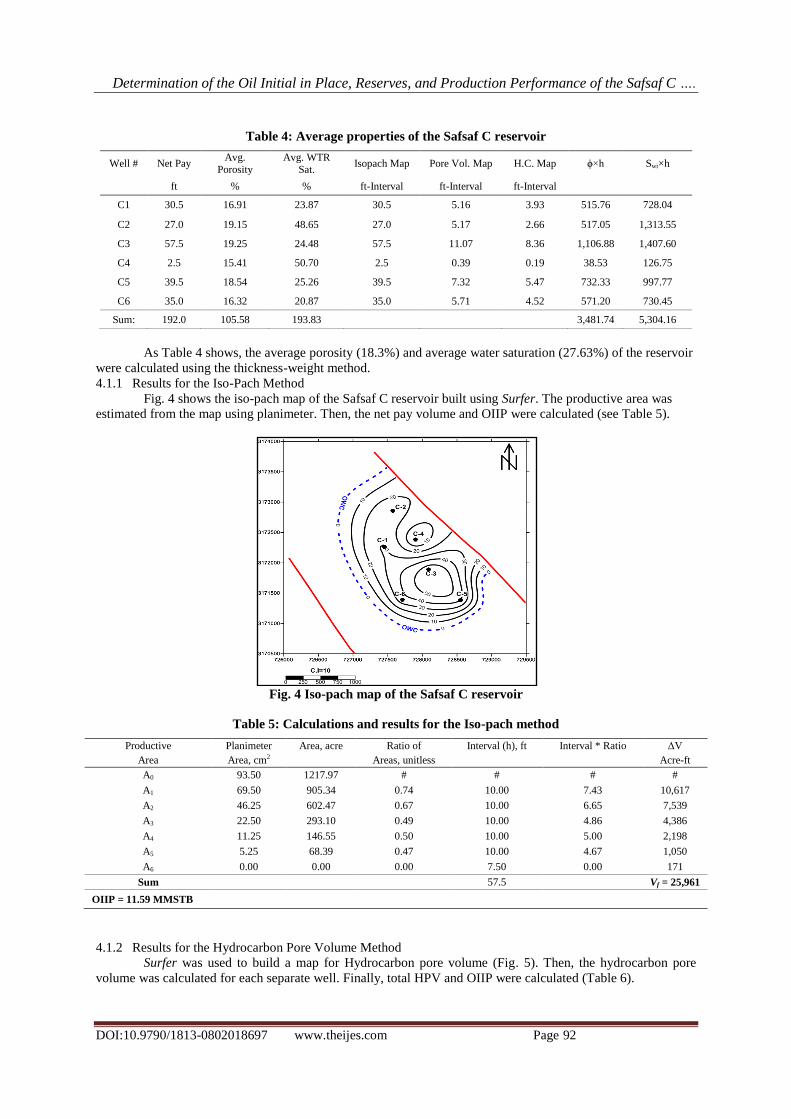
IV. RESULTS AND DISCUSSION 4.1 Volumetric Methods Calculations

Table 4 shows the results for average porosity, average water saturation, and net pay thickness for each

well. It also shows the contour intervals obtained using the volumetric methods.



As Table 4 shows, the average porosity (18.3%) and average water saturation (27.63%) of the reservoir

were calculated using the thickness-weight method.

4.1.1 Results for the Iso-Pach Method

Fig. 4 shows the iso-pach map of the Safsaf C reservoir built using Surfer. The productive area was

estimated from the map using planimeter. Then, the net pay volume and OIIP were calculated (see Table 5).

Fig. 4 Iso-pach map of the Safsaf C reservoir

Table 5: Calculations and results for the Iso-pach method

Productive Planimeter Area, acre Ratio of Interval (h), ft Interval * Ratio ΔV

Area Area, cm2

Areas, unitless

Acre-ft

A0 93.50 1217.97 # # # #

A1 69.50 905.34 0.74 10.00 7.43 10,617

A2 46.25 602.47 0.67 10.00 6.65 7,539

A3 22.50 293.10 0.49 10.00 4.86 4,386

A4 11.25 146.55 0.50 10.00 5.00 2,198

A5 5.25 68.39 0.47 10.00 4.67 1,050

A6 0.00 0.00 0.00 7.50 0.00 171

Sum 57.5 Vf = 25,961

OIIP = 11.59 MMSTB

4.1.2 Results for the Hydrocarbon Pore Volume Method

Surfer was used to build a map for Hydrocarbon pore volume (Fig. 5). Then, the hydrocarbon pore

volume was calculated for each separate well. Finally, total HPV and OIIP were calculated (Table 6).

Table 4: Average properties of the Safsaf C reservoir

Well # Net Pay Avg.

Porosity Avg. WTR

Sat. Isopach Map Pore Vol. Map H.C. Map ϕ×h Swi×h

ft % % ft-Interval ft-Interval ft-Interval

C1 30.5 16.91 23.87 30.5 5.16 3.93 515.76 728.04

C2 27.0 19.15 48.65 27.0 5.17 2.66 517.05 1,313.55

C3 57.5 19.25 24.48 57.5 11.07 8.36 1,106.88 1,407.60

C4 2.5 15.41 50.70 2.5 0.39 0.19 38.53 126.75

C5 39.5 18.54 25.26 39.5 7.32 5.47 732.33 997.77

C6 35.0 16.32 20.87 35.0 5.71 4.52 571.20 730.45

Sum: 192.0 105.58 193.83 3,481.74 5,304.16



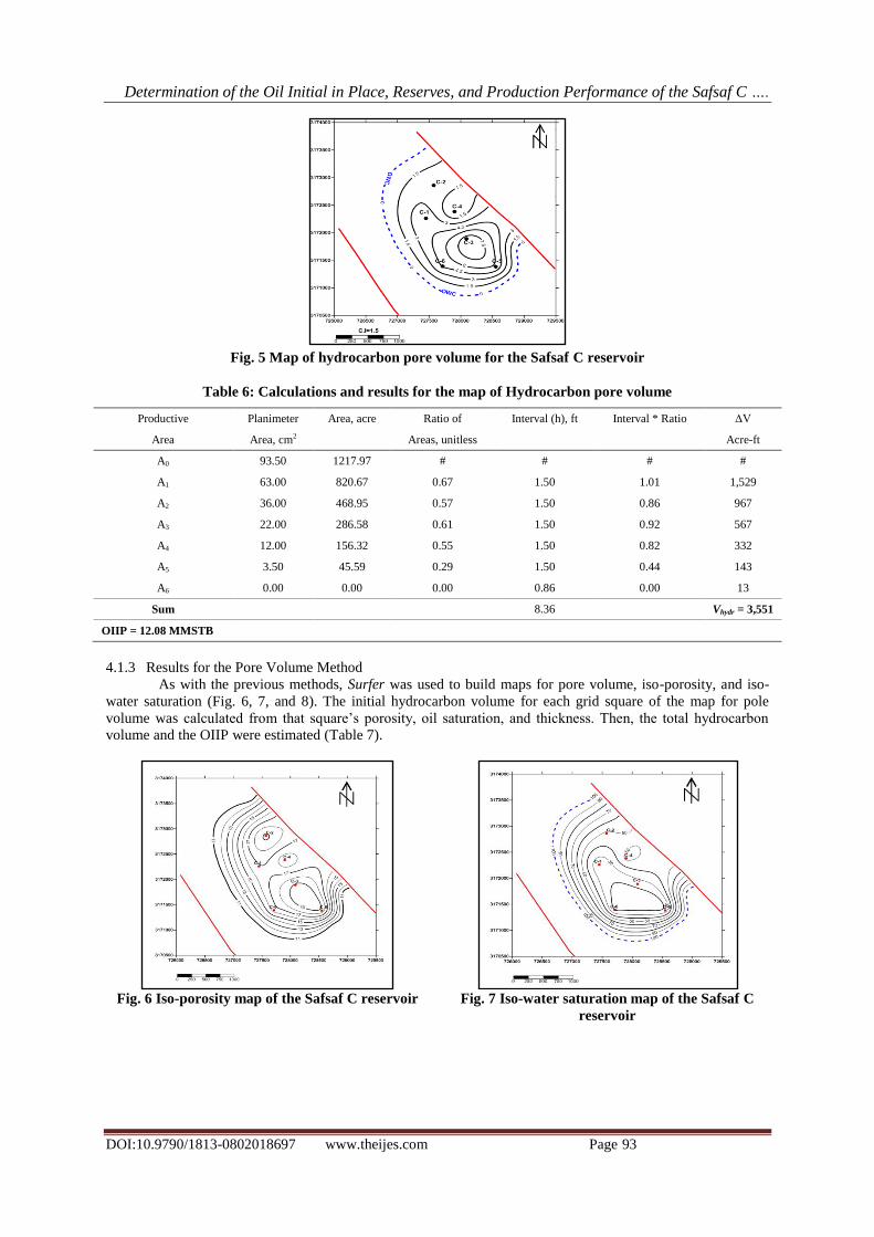
Fig. 5 Map of hydrocarbon pore volume for the Safsaf C reservoir

Table 6: Calculations and results for the map of Hydrocarbon pore volume


Area Area, cm2

Areas, unitless

Acre-ft

A0 93.50 1217.97 # # # #

A1 63.00 820.67 0.67 1.50 1.01 1,529

A2 36.00 468.95 0.57 1.50 0.86 967

A3 22.00 286.58 0.61 1.50 0.92 567

A4 12.00 156.32 0.55 1.50 0.82 332

A5 3.50 45.59 0.29 1.50 0.44 143

A6 0.00 0.00 0.00 0.86 0.00 13

Sum 8.36 Vhydr = 3,551

OIIP = 12.08 MMSTB

4.1.3 Results for the Pore Volume Method

As with the previous methods, Surfer was used to build maps for pore volume, iso-porosity, and iso-

water saturation (Fig. 6, 7, and 8). The initial hydrocarbon volume for each grid square of the map for pole

volume was calculated from that square’s porosity, oil saturation, and thickness. Then, the total hydrocarbon

volume and the OIIP were estimated (Table 7).

Fig. 6 Iso-porosity map of the Safsaf C reservoir Fig. 7 Iso-water saturation map of the Safsaf C

reservoir


DOI:10.9790/1813-0802018697 www.theijes.com 4

Fig. 8 Pore volume map of the Safsaf C reservoir

Table 7: Calculations and results for the Pore volume method


Area Area, cm2

Areas, unitless

Acre-ft

A0 93.50 1217.97 # # # #

A1 68.50 892.31 0.73 2.00 1.47 2,110

A2 42.00 547.11 0.61 2.00 1.23 1,439

A3 19.50 254.02 0.46 2.00 0.93 783

A4 10.50 136.78 0.54 2.00 1.08 391

A5 3.75 48.85 0.36 2.00 0.71 178

A6 0.00 0.00 0.00 1.07 0.00 17

Sum 11.07 Vi = 4,919

OIIP = 12.11 MMSTB

Although the three volumetric methods employed different calculations, the results revealed that the

values they yielded for OIIP were almost identical, ranging between 11.59 and 12.11 MMSTB.

4.2 Results for Material Balance

The following results (shown in Table 8) were obtained by applying the straight-line formulation of the

material balance equation and using the production history, pressure history, and PVT of Safsaf C.

Table 8: Results for material balance for the Safsaf C reservoir

Bo N F Eo Ef,w Eo+ Ef,w

Bbl/STB MMSTB MMSTB Bbl/STB Bbl/STB Bbl/STB

2.72 0.00 0.00 0.00 0.0000 0.0000

2.75 19.19 0.54 0.0244 0.0037 0.0280

2.81 8.83 0.85 0.0849 0.0119 0.0967

2.79 12.70 0.90 0.0621 0.0089 0.0710

2.82 9.37 0.98 0.0920 0.0128 0.1048

2.80 11.94 1.05 0.0772 0.0109 0.0880

2.80 13.22 1.13 0.0749 0.0106 0.0854

2.82 12.67 1.39 0.0963 0.0133 0.1096

2.80 15.84 1.45 0.0805 0.0113 0.0918

2.84 12.23 1.66 0.1198 0.0162 0.1360

2.84 13.29 1.73 0.1148 0.0156 0.1304

2.85 12.98 1.82 0.1235 0.0166 0.1401

2.85 12.60 1.85 0.1294 0.0173 0.1467

2.85 13.30 1.96 0.1301 0.0174 0.1475

2.85 14.02 2.03 0.1274 0.0171 0.1445

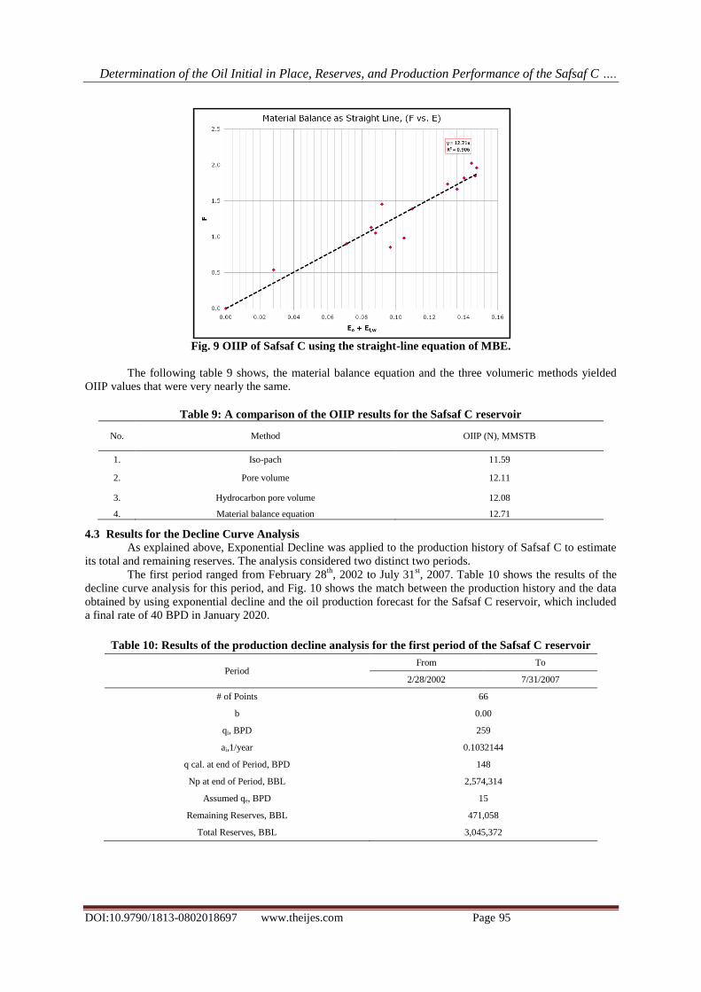
The above data were plotted as shown in Fig. 9, and the OIIP of Safsaf C was found to be 12.71

MMSTB when the straight-line formulation of MBE was used.



The following table 9 shows, the material balance equation and the three volumeric methods yielded

OIIP values that were very nearly the same.

Table 9: A comparison of the OIIP results for the Safsaf C reservoir

No. Method OIIP (N), MMSTB

1. Iso-pach 11.59

2. Pore volume 12.11

3. Hydrocarbon pore volume 12.08

4. Material balance equation 12.71

4.3 Results for the Decline Curve Analysis

As explained above, Exponential Decline was applied to the production history of Safsaf C to estimate

its total and remaining reserves. The analysis considered two distinct two periods.

The first period ranged from February 28th

, 2002 to July 31st, 2007. Table 10 shows the results of the

decline curve analysis for this period, and Fig. 10 shows the match between the production history and the data

obtained by using exponential decline and the oil production forecast for the Safsaf C reservoir, which included

a final rate of 40 BPD in January 2020.

Table 10: Results of the production decline analysis for the first period of the Safsaf C reservoir

Period From To

2/28/2002 7/31/2007

# of Points 66

b 0.00

qi, BPD 259

ai,1/year 0.1032144

q cal. at end of Period, BPD 148

Np at end of Period, BBL 2,574,314

Assumed qe, BPD 15

Remaining Reserves, BBL 471,058

Total Reserves, BBL 3,045,372

Fig. 9 OIIP of Safsaf C using the straight-line equation of MBE.



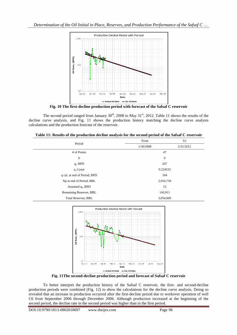
Fig. 10 The first-decline production period with forecast of the Safsaf C reservoir

The second period ranged from January 30th

, 2008 to May 31st, 2012. Table 11 shows the results of the

decline curve analysis, and Fig. 11 shows the production history matching the decline curve analysis

calculations and the production forecast of the reservoir.

Table 11: Results of the production decline analysis for the second period of the Safsaf C reservoir

Period From To

1/30/2008 5/31/2012

# of Points 47

b 0

qi, BPD 247

ai,1/year 0.224533

q cal. at end of Period, BPD 104

Np at end of Period, BBL 2,910,758

Assumed qe, BPD 15

Remaining Reserves, BBL 143,911

Total Reserves, BBL 3,054,669

Fig. 11The second-decline production period and forecast of Safsaf C reservoir

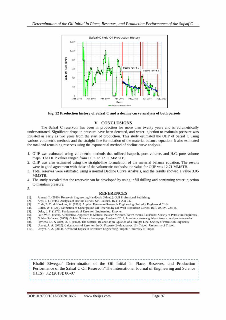
To better interpret the production history of the Safsaf C reservoir, the first- and second-decline

production periods were combined (Fig. 12) to show the calculations for the decline curve analysis. Doing so

revealed that an increase in production occurred after the first-decline period due to workover operation of well

C6 from September 2006 through December 2006. Although production increased at the beginning of the

second period, the decline rate in the second period was higher than in the first period.



Fig. 12 Production history of Safsaf C and a decline curve analysis of both periods

V. CONCLUSIONS The Safsaf C reservoir has been in production for more than twenty years and is volumetrically

undersaturated. Significant drops in pressure have been detected, and water injection to maintain pressure was

initiated as early as two years from the start of production. This study estimated the OIIP of Safsaf C using

various volumetric methods and the straight-line formulation of the material balance equation. It also estimated

the total and remaining reserves using the exponential method of decline curve analysis.

1. OIIP was estimated using volumetric methods that utilized Isopach, pore volume, and H.C. pore volume

maps. The OIIP values ranged from 11.59 to 12.11 MMSTB.

2. OIIP was also estimated using the straight-line formulation of the material balance equation. The results

were in good agreement with those of the volumetric methods: the value for OIIP was 12.71 MMSTB.

3. Total reserves were estimated using a normal Decline Curve Analysis, and the results showed a value 3.05

MMSTB.

4. The study revealed that the reservoir can be developed by using infill drilling and continuing water injection

to maintain pressure.

5.

REFERENCES [1]. Ahmed, T. (2010). Reservoir Engineering Handbook (4th ed.). Gulf Professional Publishing. [2]. Arps, J. J. (1945). Analysis of Decline Curves. SPE Journal, 160(1), 228-247. [3]. Craft, B. C., & Hawkins, M. (1991). Applied Petroleum Reservoir Engineering (2nd ed.). Englewood Cliffs.

[4]. Cutler, W. (1924). Estimation of Underground Oil Reserves by Oil-Well Production Curves. Bull. USBM, 228(1).

[5]. Dake, L. P. (1978). Fundamentals of Reservoir Engineering. Elsevier. [6]. Fair, W. B. (1994). A Statistical Approach to Material Balance Methods. New Orleans, Louisiana: Society of Petroleum Engineers.

[7]. Golden Software. (2009). Golden Software home page. Retrieved 2012, from https://www.goldensoftware.com/products/surfer

[8]. Havlena, D., & Odeh, A. S. (1963). The Material Balance as an Equation of a Straight Line. Society of Petroleum Engineers. [9]. Urayet, A. A. (2002). Calculations of Reserves. In Oil Property Evaluation (p. 16). Tripoli: University of Tripoli.

[10]. Urayet, A. A. (2004). Advanced Topics in Petroleum Engineering. Tripoli: University of Tripoli.

Khalid Elwegaa" Determination of the Oil Initial in Place, Reserves, and Production

Performance of the Safsaf C Oil Reservoir"The International Journal of Engineering and Science

(IJES), 8.2 (2019): 86-97

Determination of the Oil Initial in Place, Reserves, and ...

Documents

Transcript of Determination of the Oil Initial in Place, Reserves, and ...