Determination of the magnetic polarizability tensor and three dimensional object location for...
19
Publication Title Determination of the magnetic polarisability tensor and three dimensional object location for multiple objects using a walk-through metal detector Authors Liam A Marsh, Christos Ktistis, Ari J¨ arvi, David W Armitage and Anthony J Peyton NOTICE: this is the authors version of a work that was accepted for publication in Measurement Science and Technology. Changes resulting from the publishing process, such as peer review, editing, corrections, structural formatting, and other quality control mechanisms may not be reflected in this document. Changes may have been made to this work since it was submitted for publication. A definitive version was subsequently published in Meas. Sci. Technol. Vol. 25 (2014), 055107 (12pp). DOI link: doi:10.1088/0957-0233/25/5/055107
-
Upload
manchester -
Category
Documents
-
view
4 -
download
0
Transcript of Determination of the magnetic polarizability tensor and three dimensional object location for...
Publication Title
Determination of the magnetic polarisability tensorand three dimensional object location for multiple
objects using a walk-through metal detector
Authors
Liam A Marsh, Christos Ktistis, Ari Jarvi, David W Armitage and Anthony J Peyton
NOTICE: this is the authors version of a work that was accepted for publication in
Measurement Science and Technology. Changes resulting from the publishing process,
such as peer review, editing, corrections, structural formatting, and other quality control
mechanisms may not be reflected in this document. Changes may have been made to
this work since it was submitted for publication. A definitive version was subsequently
published in Meas. Sci. Technol. Vol. 25 (2014), 055107 (12pp).
DOI link: doi:10.1088/0957-0233/25/5/055107
Determination of the magnetic polarisability tensor
and three dimensional object location for multiple
objects using a walk-through metal detector
Liam A Marsh1, Christos Ktistis1, Ari Jarvi2,
David W Armitage1 and Anthony J Peyton1
1School of Electrical and Electronic Engineering, The University of Manchester,
Manchester, M13 9PL, UK2Rapiscan Systems Oy, Klovinpellontie 3, Torni 2, FIN-02180 Espoo, Finland
E-mail: [email protected]
Abstract. A previously reported tomographic metal detector which is capable of
inverting the location and magnetic polarisability tensor for a single object has been
modified such that it is capable of inverting the location and magnetic polarisability
tensor for multiple objects. In this paper, the term ‘multiple objects’ refers to up to
three indepdent metallic objects. The results from this paper show that the algorithm
works well for objects vertically separated by greater than 40 cm, however the reliability
varies as objects are brought closer together, or are at the same vertical height;
the estimation of position for multiple objects tends to perform well, however the
estimation of the magnetic polarisability tensor becomes poorer. Interactions taking
place between objects is presented as one possible explanation for this.
Keywords: walk-through metal detector, security, tensor
1. Introduction
Walk-through metal detectors (WTMDs) play a key role in screening of large volumes
of people for a variety of purposes including security and loss prevention. Advances in
analogue electronics have allowed manufacturers to detect ever smaller objects, and the
technology has reached the point where commercial products are capable of detecting
objects as small as razorblades and detonator caps concealed on a person [1]. However,
despite these advances and the widespread deployment of the technology, there has been
little development in the use of algorithms to process data acquired from WTMDs in
order to gain information about metallic targets.
In a real-world scenario, for example at an airport, it is common for people to
be in posession of several legitimate metallic items. Examples of such include mobile
phones, belt buckles, keys, watches and other jewellery. Using the current generation of
detectors it is not possible to discriminate between all items which are innocuous and
those which are threatening. As a consequence of this, manual inspection of all positive
detections is required in order to determine whether an object presents a threat. In the
Multiple object inversion using a walk-through metal detector 2
United Kingdom, current regulation dictates that travellers must remove any metallic
objects prior to screening [2] to ensure that the only positive detections are as a result of
restricted items. The removal of items is widely considered to be time-consuming and
highly disruptive to passengers, and is considered by some to be disproportionate to
the perceived threats [3]; however until such time that walk-through metal detectors
are capable of discriminating between threatening and non-threatening objects this
procedure is unlikely to change.
Previous work on the calculation of object parameters and characterisation using
walk-through metal detectors has considered single-object cases only, as is discussed in
the following section. Such applications are not suitable for security screening purposes
and consequently the research outcomes have little or no commercial value. However,
the multiple-object approach described in this paper demonstrates the potential for
practical systems capable of determining object characteristics and locating multple
targets on candidates.
2. Background
One method of characterising the perceived threat from metallic items is to examine the
properties of the magnetic polarisability tensor,↔M [4]. This is a complex, symmetric
and frequency-dependent quantity which is commonly expressed as a 3×3 matrix of the
following format:
↔M (f) =
M11 + jN11 M12 + jN12 M13 + jN13
M12 + jN12 M22 + jN22 M23 + jN23
M13 + jN13 M23 + jN23 M33 + jN33
A tomographic system has been previously been described [5] which is capable of
locating a single metallic object and describing it by means of inverting↔M. This system
consists of 16 coils – eight transmit and eight receive. Each transmit coil operates
at a separate frequency at approximately 10 kHz. Measurements are taken for each
receive coil coupled to each of the transmit coils – i.e. 64 complex measurements,
however due to poor SNR measurements for pairs separated by large distances only 32
complex measurements are recorded. The system has been shown in [5] to be capable
of determining the object position to within ± 3 cm, and with a parameter variation of
<20% for the object tensor. However, the system is significantly limited because it can
only deal with a single object at one time. In order for the system to be suitable for use
as a security system it must be capable of responding to multiple targets.
In this paper the same walk-through metal detection system presented in [5] is used
as a data acquisition system, however a modified ‘multi-object’ algorithm is presented.
A summary of the key underlying theory from [5] is provided below as an introduction
to the main theory presented later in this paper.
The object reponse,V, is modelled by taking the product of the magnetic
polarisability tensor with that of the two H-fields produced by the transmit and receive
Multiple object inversion using a walk-through metal detector 3
coils [10] as shown in equation 1. Multiplication by jωµ0 allows for expression of the
response as a voltage.
V = jωµ0
⇀
Htx ·↔M ·
⇀
Hrx (1)
For convenience of notation it is possible to express equation 1 as a function of two
variables; the first of these variables is magnetic polarisability tensor↔M and the second
is the object location within the detector volume⇀
P. This second variable relates to the
fact that the magnetic field data varies as a function of object position. This function
is represented in subsequent equations as f(⇀
P,↔M)
.
The inversion algorithm then attempts to minimise the error between the measured
values,⇀
V, and the simulated values by fitting a tensor and location,↔M and
⇀
P
respectively, as shown in equation 2. A modified Levenberg-Marquardt algorithm is
used for the inversion as shown in equation 3. The algorithm uses the matrix containing
the iterative solution for the unknown values, L, and varies a regularisation parameter,
λ, updating the jacobean, J, so as to minimse the residual function⇀
R as shown in
equation 4. Under normal operation the regularisatiion parameter λ reduces with each
iteration, however the parameter can increase if the condition of the matrix JTJ+λLTL
as in equation 3. The algorithm is fully described in [5].
arg min
(∥∥∥∥⇀V −f (⇀
P,↔M)∥∥∥∥2
)(2)
[↔M
⇀
P]
=(JTJ + λLTL
)−1JT
⇀
R (3)
⇀
R =⇀
V −f(⇀
P,↔M)
(4)
Multi-object inversion presents some practical challenges that the single object case
does not. Firstly, in the single object case, the algorithm can be optimised to invert
a single object given certain trigger conditions – e.g. measurements exceed a certain
pre-defined threshold. However, when dealing with more than one object, the algorithm
must be capable of determining how many objects to invert for, and also be able to
determine which ‘objects’ are real, and which may be an over-fitting of the data set
to noise. As security officers do not have any a priori knowledge about the number of
objects that candidates may be concealing the ideal system should be able to detect
and invert for an unknown number of objects without any knowledge on the number of
objects, or their location. In this paper, between one and three objects will be used per
scan.
There have been several previous publications in the field of multiple object
inversion and multiple object detection using electromagnetic induction; some examples
Multiple object inversion using a walk-through metal detector 4
are provided in [6, 7, 8]. One such study in the field of unexploded ordnance (UXO)
detection [6] describes the implementation of a multiple-object inversion algorithm
similar to that described in this paper. It identifies some problems which are also
applicable in this application area; these include reconstruction of multiple objects which
are located near to one another, dealing with estimating the number of objects present,
and error increases non-linearly with respect to the number of objects the algorithm is
solving for.
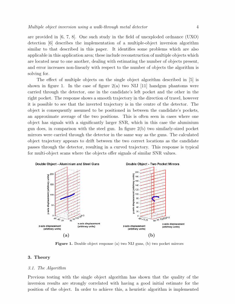
The effect of multiple objects on the single object algorithm described in [5] is
shown in figure 1. In the case of figure 2(a) two NIJ [11] handgun phantoms were
carried through the detector, one in the candidate’s left pocket and the other in the
right pocket. The response shows a smooth trajectory in the direction of travel, however
it is possible to see that the inverted trajectory is in the centre of the detector. The
object is consequently assumed to be positioned in between the candidate’s pockets,
an approximate average of the two positions. This is often seen in cases where one
object has signals with a significantly larger SNR, which in this case the aluminium
gun does, in comparison with the steel gun. In figure 2(b) two similarly-sized pocket
mirrors were carried through the detector in the same way as the guns. The calculated
object trajectory appears to drift between the two correct locations as the candidate
passes through the detector, resulting in a curved trajectory. This response is typical
for multi-object scans where the objects offer signals of similar SNR values.
(a) (b)
Figure 1. Double object response (a) two NIJ guns, (b) two pocket mirrors
3. Theory
3.1. The Algorithm
Previous testing with the single object algorithm has shown that the quality of the
inversion results are strongly correlated with having a good initial estimate for the
position of the object. In order to achieve this, a heuristic algorithm is implemented
Multiple object inversion using a walk-through metal detector 5
which uses the relative magnitudes of raw electromagnetic measurements to identify
the estimated location of the object. This is fully described in [5]. For the multi-
object inversion algorithm a further heuristic algorithm has been devised to estimate
the number of objects based on the electromagnetic data. Testing has shown that
executing the heuristic algorithm and passing the estimated object count to the inversion
algorithm is quicker and provides better results than expecting the inversion algorithm
to determine the number of objects automatically.
Once the candidate has triggered the detector, the object count estimation
algorithm described above is executed. This algorithm performs a heuristic analysis
of the peak magnitude of the parallel channels, columnated to form a vector⇀
VP . This
vector contains eight values representing values from the top to the bottom of the
detector – one for each parallel channel. A linear interpolation is applied to⇀
VP , which
provides a series of points connecting each value, producing⇀v as shown in equation
5. This is necessary as the subsequent stages containing differential operators perform
best with an increased number of points. A threshold value which has been selected
empirically, T, is then calculated as 80% of the mean value of⇀v as shown in equation 6.
⇀v = interp
(⇀
VP
)(5)
T = 0.8× v (6)
The first and second derivatives,⇀
S, of the function⇀v are then calculated to identify
local maxima. These are defined as f ′(⇀v)
and f ′′(⇀v)
respectively. Each value is
checked to ensure that it exceeds the defined trigger threshold and in any cases where
the first derivative is equal to zero and the second derivative is negative a local maxima
is identified. In cases where both the first and second derivative are both zero a second
function G(⇀v)
is executed to invesitage the first derivative of⇀v either side of the
stationary point to ensure that the point is not a minima or point of inflexion. This is
shown in equation 7.
⇀
S =
1 for
⇀v ≥ T ∧ f ′
(⇀v)
= 0 ∧ f ′′(⇀v)< 0
G(⇀v)
for⇀v ≥ T ∧ f ′
(⇀v)
= 0 ∧ f ′′(⇀v)
= 0
0 otherwise
(7)
where G(⇀v)
is a function which examines surrounding points
to confirm the presence of a local maximum point.
The total number of objects is assumed to be the number of elements in⇀
S equal
to 1. This value is then passed to the inversion algorithm as the initial guess for the
number of objects to solve for.
Multiple object inversion using a walk-through metal detector 6
A modified Levenberg-Marquardt algorithm based on the single object algorithm
described in [5] is then executed as in equation 8. This adapted version of the code solves
for up to four objects by attempting to minimise the error between the measured values
and simulated measurements using the forward model from equation 1. This calculation
is expanded from the single object case (shown in equation 4) as it simulates a variable
number of tensors and locations according to the inverted solution. Previous experience
with the system has shown that successful inversions tend to yield residual values of
30% or below, while incorrect solutions can be anywhere above 40%; any exceptions to
this are rare. As a consequence of this a threshold is set at 35%. In the event that the
residual exceeds this value, the algorithm attempts to solve for an extra object. Should
the residual increase then the previous number of objects is assumed to be correct,
otherwise the algorithm keeps going until the residual is below the defined threshold.
To prevent over-fitting to noise, the algorithm rejects any inverted tensors which fall
below a certain magnitude when the absolute value of each element is summed together.
[↔M[1]
⇀
P[1] ...↔M[n]
⇀
P[n]
]=(JTJ + λLTL
)−1JT
⇀
R (8)
The inversion executes by initially running the forward model for a default tensor
at the estimated locations and calculating the error between the simulated and actual
measurements. Simulated measurements are generated for each object and are summed
together. The jacobean, J, is formed by extracting the sensitivity values corresponding
to the locations⇀
P[1] ...⇀
P[n]. The regularisation parameter , L, is set to be a
square matrix containing the product of the matrix containing the unknown values
and its transpose. The algorithm then iterates, updating the regularisation parameter
λ according to whether the locations are within the detector space. The algorithm
terminates when the residual function⇀
R (as defined in equation 9) either ceases to
improve, or begins to worsen.
⇀
R =⇀
V −f(⇀
P[1],↔M[1] ...
⇀
P[n],↔M[n]
)(9)
3.2. Limitations of the Algorithm
The initial object count is subject to the limitation that it is unable to detect multiple
objects at the same height, because it compares the relative magnitudes of parallel
channels, therefore providing only vertical spatial bins. The current generation of
WTMD portals are limited in this way, as they apply a similar algorithm to provide an
approximate location estimate. Any objects at the same height effectively eclipse one
another, and their effects must be calculated later by the inversion algorithm, not the
heuristic estimation.
The algorithm makes several assumptions regarding the problem, which are fully
explained in [5]. As a summary these are that the coils exist in free-space –i.e. the
Multiple object inversion using a walk-through metal detector 7
environment is free from external metalwork; the incident field⇀
Htx is parallel across the
object(s) to be detected; and that the secondary field experienced by the receive coil can
be accurately approximated by the field of a magnetic dipole [12]. For the prototype
system, this means in practice that objects should be approximately no larger than 8
cm in any direction at the centre of the portal.
4. Experimental Procedure
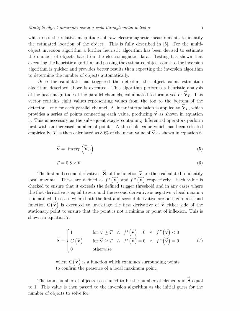
The experiments presented in this paper have been planned to illustrate the effectiveness
of the object estimation algorithm and also the success of the inversion algorithm. Figure
2 shows the measured positions for any locations described in this paper. The size of each
box is indicative of the expected variation in the position as a result of the walk-through
scan.
Figure 2. Positions used for multi-object testing
In this paper three different objects will be used – two Steel NIJ guns made from
different steels, and an Aluminium NIJ gun [11]. For each object fifteen walk-through
scans have been conducted using the single object algorithm. The results of these scans
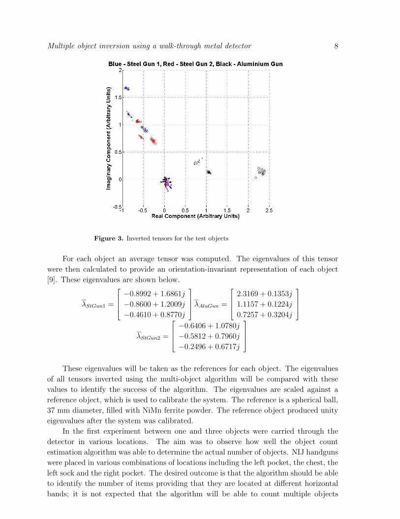
are shown in figure 3. The xx, yy and zz components are shown as circles, crosses
and plus signs respectively; off-diagonal terms are shown as dots. Each item is colour
coded such that Steel Gun 1 is blue, Steel Gun 2 is red and Aluminium Gun is black.
It is possible to see that the eigenvalues of each object produce clear clusters. This
demonstrates the consistency with which the algorithm is capable of inverting for a
single item.
Multiple object inversion using a walk-through metal detector 8
Figure 3. Inverted tensors for the test objects
For each object an average tensor was computed. The eigenvalues of this tensor
were then calculated to provide an orientation-invariant representation of each object
[9]. These eigenvalues are shown below.
λStGun1 =
−0.8992 + 1.6861j
−0.8600 + 1.2009j
−0.4610 + 0.8770j
λAluGun =
2.3169 + 0.1353j
1.1157 + 0.1224j
0.7257 + 0.3204j
λStGun2 =
−0.6406 + 1.0780j
−0.5812 + 0.7960j
−0.2496 + 0.6717j
These eigenvalues will be taken as the references for each object. The eigenvalues
of all tensors inverted using the multi-object algorithm will be compared with these
values to identify the success of the algorithm. The eigenvalues are scaled against a
reference object, which is used to calibrate the system. The reference is a spherical ball,
37 mm diameter, filled with NiMn ferrite powder. The reference object produced unity
eigenvalues after the system was calibrated.
In the first experiment between one and three objects were carried through the
detector in various locations. The aim was to observe how well the object count
estimation algorithm was able to determine the actual number of objects. NIJ handguns
were placed in various combinations of locations including the left pocket, the chest, the
left sock and the right pocket. The desired outcome is that the algorithm should be able
to identify the number of items providing that they are located at different horizontal
bands; it is not expected that the algorithm will be able to count multiple objects
Multiple object inversion using a walk-through metal detector 9
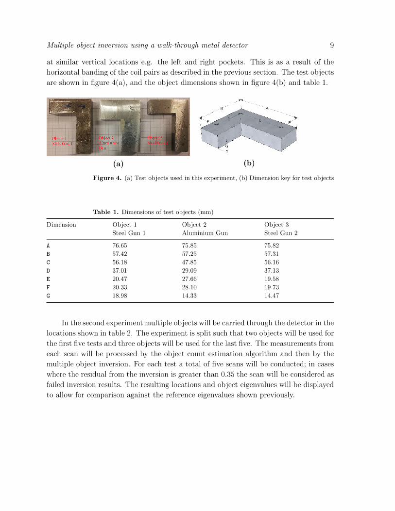
at similar vertical locations e.g. the left and right pockets. This is as a result of the
horizontal banding of the coil pairs as described in the previous section. The test objects
are shown in figure 4(a), and the object dimensions shown in figure 4(b) and table 1.
(a) (b)
Figure 4. (a) Test objects used in this experiment, (b) Dimension key for test objects
Table 1. Dimensions of test objects (mm)
Dimension Object 1 Object 2 Object 3
Steel Gun 1 Aluminium Gun Steel Gun 2
A 76.65 75.85 75.82
B 57.42 57.25 57.31
C 56.18 47.85 56.16
D 37.01 29.09 37.13
E 20.47 27.66 19.58
F 20.33 28.10 19.73
G 18.98 14.33 14.47
In the second experiment multiple objects will be carried through the detector in the
locations shown in table 2. The experiment is split such that two objects will be used for
the first five tests and three objects will be used for the last five. The measurements from
each scan will be processed by the object count estimation algorithm and then by the
multiple object inversion. For each test a total of five scans will be conducted; in cases
where the residual from the inversion is greater than 0.35 the scan will be considered as
failed inversion results. The resulting locations and object eigenvalues will be displayed
to allow for comparison against the reference eigenvalues shown previously.
Multiple object inversion using a walk-through metal detector 10
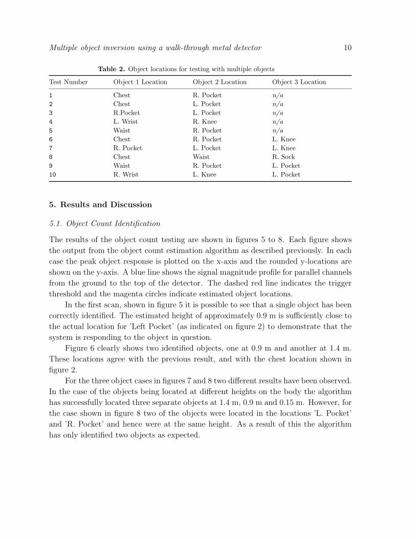
Table 2. Object locations for testing with multiple objects
Test Number Object 1 Location Object 2 Location Object 3 Location
1 Chest R. Pocket n/a
2 Chest L. Pocket n/a
3 R.Pocket L. Pocket n/a
4 L. Wrist R. Knee n/a
5 Waist R. Pocket n/a
6 Chest R. Pocket L. Knee
7 R. Pocket L. Pocket L. Knee
8 Chest Waist R. Sock
9 Waist R. Pocket L. Pocket
10 R. Wrist L. Knee L. Pocket
5. Results and Discussion
5.1. Object Count Identification
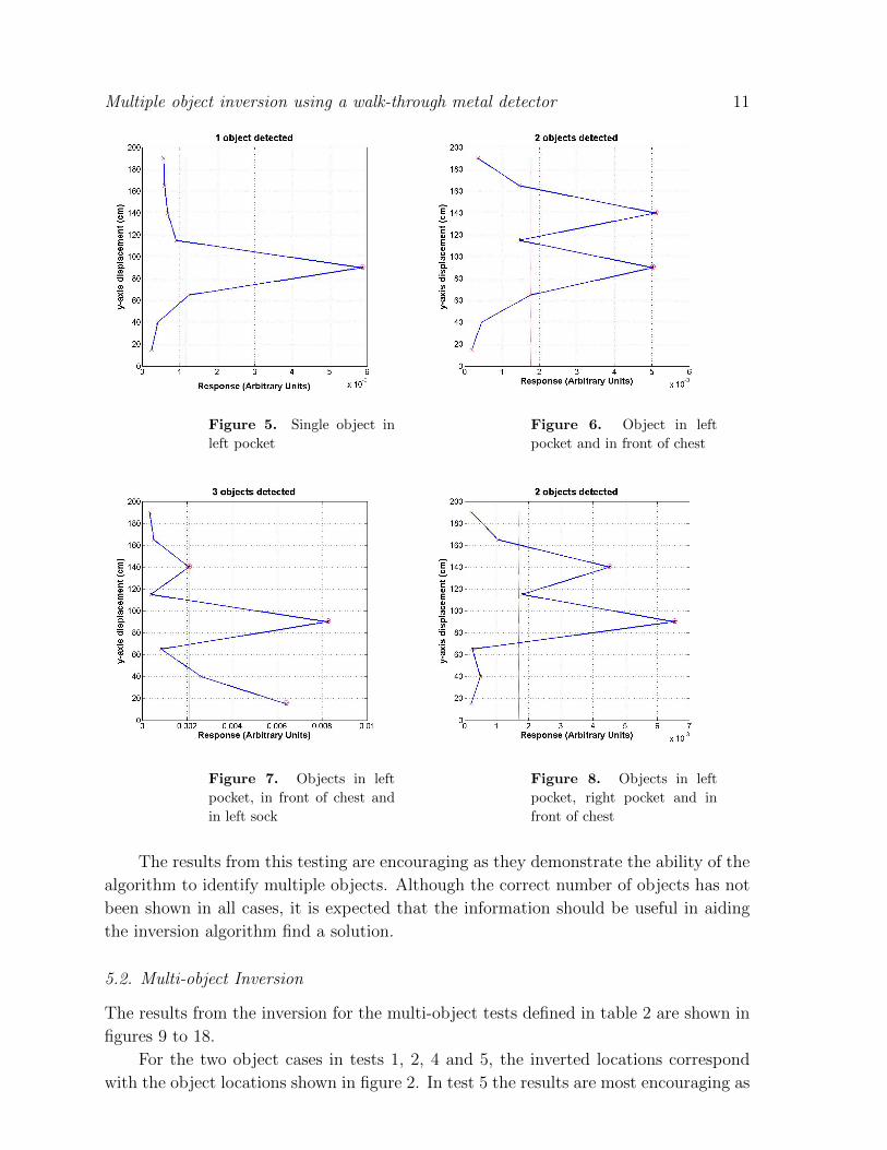
The results of the object count testing are shown in figures 5 to 8. Each figure shows
the output from the object count estimation algorithm as described previously. In each
case the peak object response is plotted on the x-axis and the rounded y-locations are
shown on the y-axis. A blue line shows the signal magnitude profile for parallel channels
from the ground to the top of the detector. The dashed red line indicates the trigger
threshold and the magenta circles indicate estimated object locations.
In the first scan, shown in figure 5 it is possible to see that a single object has been
correctly identified. The estimated height of approximately 0.9 m is sufficiently close to
the actual location for ’Left Pocket’ (as indicated on figure 2) to demonstrate that the
system is responding to the object in question.
Figure 6 clearly shows two identified objects, one at 0.9 m and another at 1.4 m.
These locations agree with the previous result, and with the chest location shown in
figure 2.
For the three object cases in figures 7 and 8 two different results have been observed.
In the case of the objects being located at different heights on the body the algorithm
has successfully located three separate objects at 1.4 m, 0.9 m and 0.15 m. However, for
the case shown in figure 8 two of the objects were located in the locations ’L. Pocket’
and ’R. Pocket’ and hence were at the same height. As a result of this the algorithm
has only identified two objects as expected.
Multiple object inversion using a walk-through metal detector 11
Figure 5. Single object in
left pocket
Figure 6. Object in left
pocket and in front of chest
Figure 7. Objects in left
pocket, in front of chest and
in left sock
Figure 8. Objects in left
pocket, right pocket and in
front of chest
The results from this testing are encouraging as they demonstrate the ability of the
algorithm to identify multiple objects. Although the correct number of objects has not
been shown in all cases, it is expected that the information should be useful in aiding
the inversion algorithm find a solution.
5.2. Multi-object Inversion
The results from the inversion for the multi-object tests defined in table 2 are shown in
figures 9 to 18.
For the two object cases in tests 1, 2, 4 and 5, the inverted locations correspond
with the object locations shown in figure 2. In test 5 the results are most encouraging as
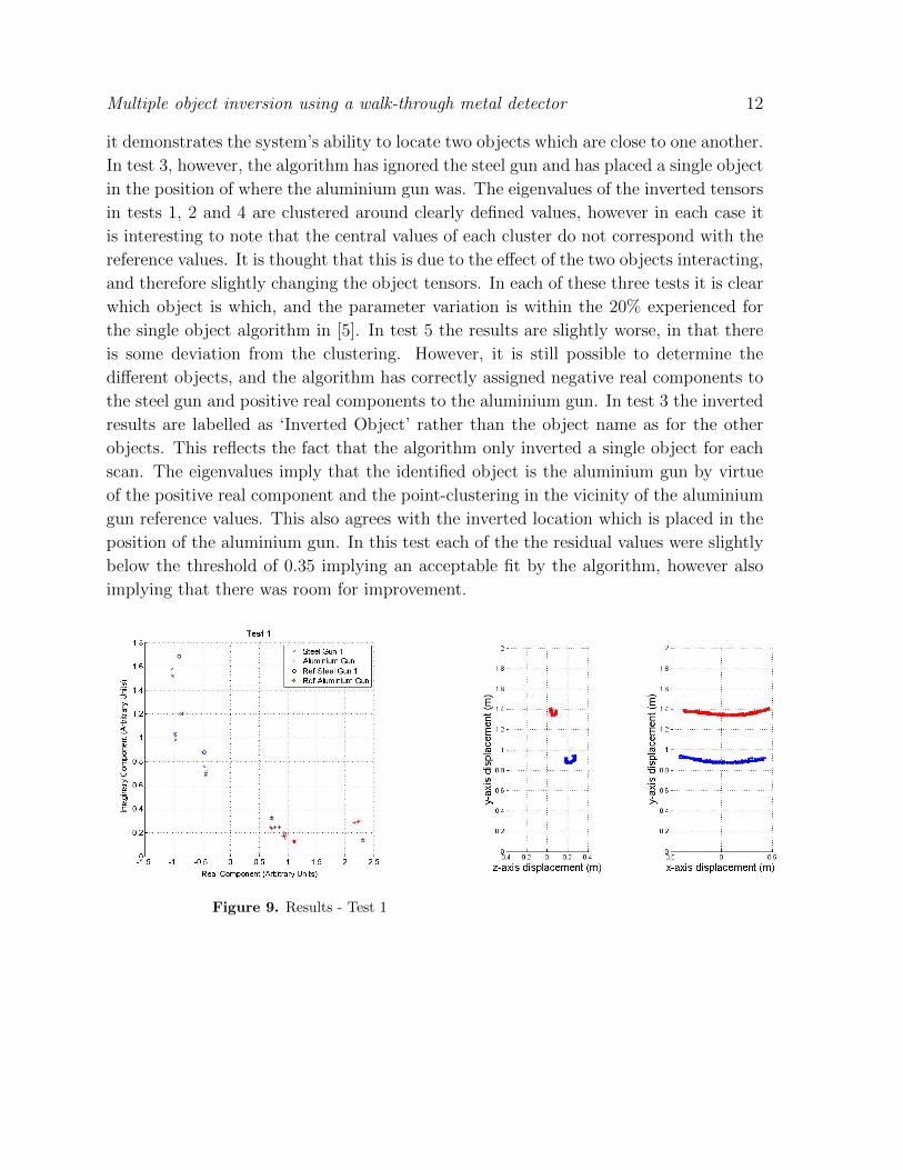
Multiple object inversion using a walk-through metal detector 12
it demonstrates the system’s ability to locate two objects which are close to one another.
In test 3, however, the algorithm has ignored the steel gun and has placed a single object
in the position of where the aluminium gun was. The eigenvalues of the inverted tensors
in tests 1, 2 and 4 are clustered around clearly defined values, however in each case it
is interesting to note that the central values of each cluster do not correspond with the
reference values. It is thought that this is due to the effect of the two objects interacting,
and therefore slightly changing the object tensors. In each of these three tests it is clear
which object is which, and the parameter variation is within the 20% experienced for
the single object algorithm in [5]. In test 5 the results are slightly worse, in that there
is some deviation from the clustering. However, it is still possible to determine the
different objects, and the algorithm has correctly assigned negative real components to
the steel gun and positive real components to the aluminium gun. In test 3 the inverted
results are labelled as ‘Inverted Object’ rather than the object name as for the other
objects. This reflects the fact that the algorithm only inverted a single object for each
scan. The eigenvalues imply that the identified object is the aluminium gun by virtue
of the positive real component and the point-clustering in the vicinity of the aluminium
gun reference values. This also agrees with the inverted location which is placed in the
position of the aluminium gun. In this test each of the the residual values were slightly
below the threshold of 0.35 implying an acceptable fit by the algorithm, however also
implying that there was room for improvement.
Figure 9. Results - Test 1

Multiple object inversion using a walk-through metal detector 13
Figure 10. Results - Test 2
Figure 11. Results - Test 3
Figure 12. Results - Test 4
Multiple object inversion using a walk-through metal detector 14
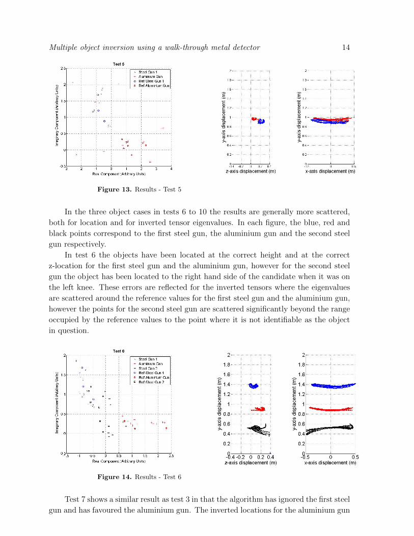
Figure 13. Results - Test 5
In the three object cases in tests 6 to 10 the results are generally more scattered,
both for location and for inverted tensor eigenvalues. In each figure, the blue, red and
black points correspond to the first steel gun, the aluminium gun and the second steel
gun respectively.
In test 6 the objects have been located at the correct height and at the correct
z-location for the first steel gun and the aluminium gun, however for the second steel
gun the object has been located to the right hand side of the candidate when it was on
the left knee. These errors are reflected for the inverted tensors where the eigenvalues
are scattered around the reference values for the first steel gun and the aluminium gun,
however the points for the second steel gun are scattered significantly beyond the range
occupied by the reference values to the point where it is not identifiable as the object
in question.
Figure 14. Results - Test 6
Test 7 shows a similar result as test 3 in that the algorithm has ignored the first steel
gun and has favoured the aluminium gun. The inverted locations for the aluminium gun
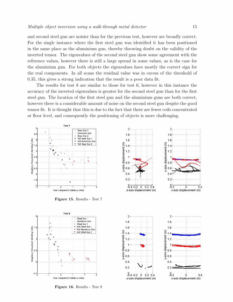
Multiple object inversion using a walk-through metal detector 15
and second steel gun are noisier than for the previous test, however are broadly correct.
For the single instance where the first steel gun was identified it has been positioned
in the same place as the aluminium gun, thereby throwing doubt on the validity of the
inverted tensor. The eigenvalues of the second steel gun show some agreement with the
reference values, however there is still a large spread in some values, as is the case for
the aluminium gun. For both objects the eigenvalues have mostly the correct sign for
the real components. In all scans the residual value was in excess of the threshold of
0.35, this gives a strong indication that the result is a poor data fit.
The results for test 8 are similar to those for test 6, however in this instance the
accuracy of the inverted eigenvalues is greater for the second steel gun than for the first
steel gun. The location of the first steel gun and the aluminium guns are both correct,
however there is a considerable amount of noise on the second steel gun despite the good
tensor fit. It is thought that this is due to the fact that there are fewer coils concentrated
at floor level, and consequently the positioning of objects is more challenging.
Figure 15. Results - Test 7
Figure 16. Results - Test 8

Multiple object inversion using a walk-through metal detector 16
In test 9 the second steel gun was not identified on any of the five scans. As
has previously been the case for tests with guns in opposite pockets, the steel gun has
been ignored by the inversion and the response of the aluminium gun has dominated.
The object location is very similar to that in test 4, however, in this test the objects
are swapped round. The quality of the inverted tensors is poor, and shows almost no
correlation with the reference values beyond identifying the correct sign for the real part.
In each case the residual values were in excess of the threshold value of 0.35 thereby
indicating a poor data fit.
Figure 17. Results - Test 9
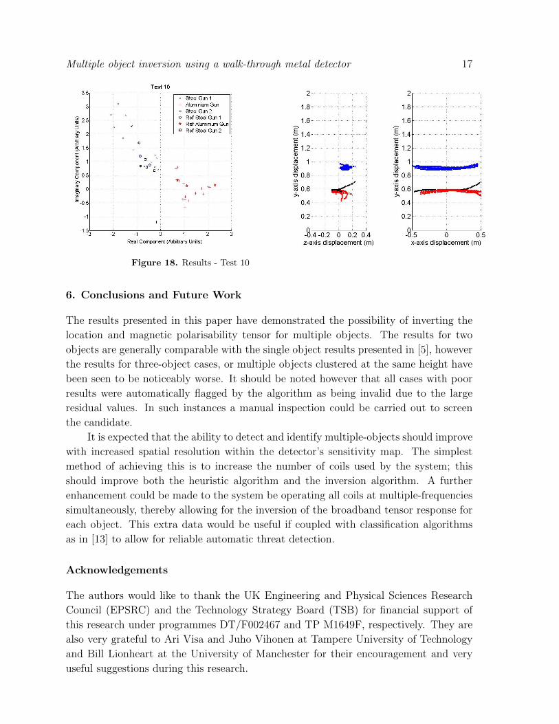
In test 10 the object location is quite poor for all objects with respect to the z-
location as all objects are shown closer to the centre of the candidate than they should be.
The y-location is approximately correct for the first steel gun and the aluminium gun,
however for the second steel gun the only inverted location has been merged with that of
the aluminium gun when according to figure 2 it should be approximately 35 cm away.
The inverted tensors for both steel guns are also poor when compared with the reference
values. In the case of the aluminium gun the eigenvalues are more concentrated; this
is possibly due to the considerably larger SNR that the item has compared to the steel
guns.
Multiple object inversion using a walk-through metal detector 17
Figure 18. Results - Test 10
6. Conclusions and Future Work
The results presented in this paper have demonstrated the possibility of inverting the
location and magnetic polarisability tensor for multiple objects. The results for two
objects are generally comparable with the single object results presented in [5], however
the results for three-object cases, or multiple objects clustered at the same height have
been seen to be noticeably worse. It should be noted however that all cases with poor
results were automatically flagged by the algorithm as being invalid due to the large
residual values. In such instances a manual inspection could be carried out to screen
the candidate.
It is expected that the ability to detect and identify multiple-objects should improve
with increased spatial resolution within the detector’s sensitivity map. The simplest
method of achieving this is to increase the number of coils used by the system; this
should improve both the heuristic algorithm and the inversion algorithm. A further
enhancement could be made to the system be operating all coils at multiple-frequencies
simultaneously, thereby allowing for the inversion of the broadband tensor response for
each object. This extra data would be useful if coupled with classification algorithms
as in [13] to allow for reliable automatic threat detection.
Acknowledgements
The authors would like to thank the UK Engineering and Physical Sciences Research
Council (EPSRC) and the Technology Strategy Board (TSB) for financial support of
this research under programmes DT/F002467 and TP M1649F, respectively. They are
also very grateful to Ari Visa and Juho Vihonen at Tampere University of Technology
and Bill Lionheart at the University of Manchester for their encouragement and very
useful suggestions during this research.
Multiple object inversion using a walk-through metal detector 18
References
[1] Rapiscan Systems (2012, 13/02/2013) Metor 6S— Rapiscan Systems. Available:
http://www.rapiscansystems.com/en/products/item/metor 6s
[2] European Commission (2012, 13/08/2013) Information for air travellers Available:
http://ec.europa.eu/transport/modes/air/security/info travellers en.htm
[3] Linos E, Linos E and Colditz G 2007 Screening programme evaluation applied to airport security
Brit Med J 335:1290
[4] Bell T H, Barrow B J and Miller J T 2001 Subsurface discrimination using electromagnetic
induction sensors IEEE Trans. Geosci. Remote Sens.39 1286-1292
[5] Marsh L A, Ktistis K, Jarvi A, Armitage D W and Peyton A J 2013 Three-dimensional object
location and inversion of the magnetic polarisability tensor at a single frequency using a walk-
through metal detector Meas. Sci. Technol. vol. 24 045102 doi:10.1088/0957-0233/24/4/045102
[6] Grzegorczyk T M, Barrowes B E, Shubitidze F, Fernandez J P and O’Neill K 2011 Simultaneous
Identification of Multiple Unexploded Ordnance Using Electromagnetic Induction Sensors IEEE
Trans. on Geosci. and Remote Sens. 49, 2507-2517
[7] Song L, Oldenburg W and Paison L R 2012 Estimating source locations of unexploded ordnance
using the multiple signal classification algorithm Geophysics 77, 127-135
[8] Shubitidze F, Fernandez J P, Shamatava I, Barrowes B E and O’Neill K 2012 Joint diagonalization
applied to the detection and discrimination of unexploded ordnance Geophysics 77, 149-160
[9] Norton S J and Won I J 2001 Ordnance/Clutter Discrimination Based on Target Eigenvalue
Analysis. P Soc Photo-opt Ins 2, 285-298
[10] Norton S J and Won I J 2001 Identification of Buried Unexploded Ordnance From Broadband
Electromagnetic Induction Data IEEE Trans. on Geosci. and Remote Sens. 39, 2253-2261
[11] Paulter N and Larson D 2009 NIJ Metal Detector Test Object Report (Gaithersburg, MD: National
Institute for Justice)
[12] Ulaby F T, Michielssen E and Umberto R 2010 Fundamentals of Applied Electrodynamics ed A
Gilfillan (New Jersey : Prentice Hall) p 261
[13] Makkonen J, Marsh L A, Vihonen J, Visa A, Jarvi A and Peyton A J 2013 Classification of metallic
targets using a single frequency component of the magnetic polarisability tensor. Sensors and
Their Applications XVII, Dubrovnik, Croatia