Journal of Development Economics 4 (197;) 31 S-342. 0 North-Holland Publishing Company

DETJZRiMI&ANTS OF WAGE AND PRICE CHANGES IN LESS DEVXLOPED COIUVTRIES

An intertemporal cross-country analysis

Nicholas P. GLY TSOS*

Center of Phnirrg anu’ Economic Research, Atltens, Greece

n,,.,: -IT . _ ccemher 1975, revised version received May 1977

A theoretical hypothesis of wage determination, conveying the arguments of the dual economy model as well as solme elements of ‘traditional’ theory, and three alternative theoretical approaches to price changes are built and statistically tested. Pcoied data, with missing observations, of 36 LDCs from Asia, Africa and Latin America for 1360. 1965 and 1968 are used, while additive and multiplicative dul.,my variables test the behavior of regressions between alternative counm groups. Price c3ang.x are found to te explained by both monetary and nonmonetary variables with rel#ively more weight on the iatter. The empirical wage change determination conforms to the dual model, while the existence of an international Phillips curve is questionable.

1. Introduction

The objective of this paper is to build a theoretical model on wage and price changes in LDCs and then test it with cross-section data from 36 countrie; of Asia, Africa and Latin America. The model is a self-contained revised part of a more elaborate study on inflation (my unpublished Ph.D. thesis!, involving a ‘recursive* system of equations with a chair) reaction of productivity, unemploy- ment, wages and prices.

Our analysis here focuses on the wage and price hypotheses which are at the end of the sequential arrangement of the recursive system. They therefore reflect the accumulated influence of several forces behind the scenes of the inflation drama.

One important feature of our madcl is that it takes into account the dual economy theory of development, whi&, :ilthough it is can\idcred ;i fu~darn~~~~~i aspect of development economics, appears to hatrc bccrl ~~~~~~te~ rn ccono-

*This paper is based on part of the author’s doctoral ‘~~~~rt~t~~~. He is ~~~c~t~d to hi% thesis advisors Irving Swerdlotv, John Henning and James E. Price. The z.tiihor aiso w&er. to thank two anonymous referees of the Journal for their valuable cernn;,n:s QP a prc%ioul; draft of the paper.

316 N. P. Gfytsos, !Vage and price changes in LX’s

metric studies on the ‘causes’ of inflation in LIES. This is the case in spite of the fact that some of the statistical data used in such studies as, for example, prices and wages, refer only to the urban sector of the countries concerned.

2. A model of wage determination in drral economies

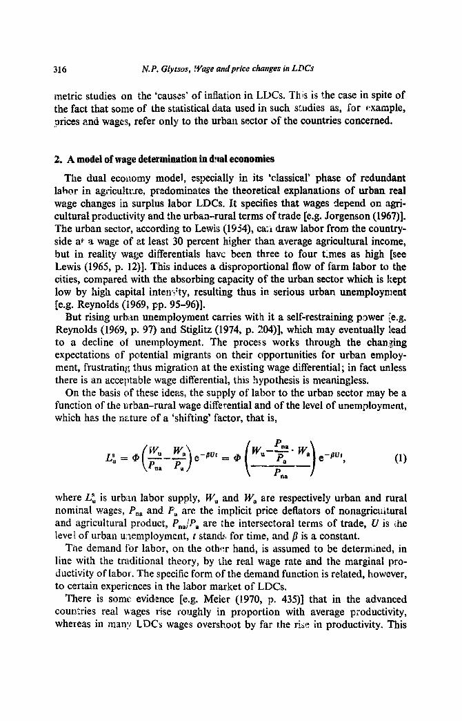
The dual economy model, especially in its ‘classical’ phase of redundant labor in agriculture. predominates the theoretical explanations of urban real wage changes in surplus labor LDCs. It specifies that wages depend on agri- cultural productivity and the urban-rural terms of trade [e.g. Jorgenson (1967)]. The urban sector, according to Lewis (1954), ca;i draw labor from the country- side a* a wage of at least 30 percent higher than average agricultural income, but in reality wage differentials have been three to four times as high [see Lewis (1965, p. 12)]. This induces a disproportional flow of farm labor to the cities, compared with the absorbing capacity of the urban sector which is kept low by high capital inten+ty, resulting thus in serious urban unemployment [e.g. Reynolds (1969, pp. 95-96)].

But rising urban unemployment carries with it a self-restraining power [e.g. Reynolds (1969, p. 97) and Stiglitz (1974, p. X4)], which may eventually lead to a decline of unemployment. The process works through the changing expectations of potential migrants on their opportunities for urban employ- ment, frustrating thus migration at the existing wage differential; in fact unless there is an acceptable wage differential, this hypothesis is meaningless.

On the basis of these ideas, the supply of labor to the urban sector may be a function of the u.rban-rural wage differential and of the level of unemployment, which has the nature of a ‘shifting’ factor, that is,

where L”, is urb;.tn labor supply, W, and W, are respectively urban and rural nominal wages, P,,, and F, are the implicit price deflators of nonagricuitural and agricultural product, P,,,/P, are the intersectoral terms of trade, U is ihe level of urban unemployment, I stands for time, and /3 is a constant.

Tile demand for labor, on the othc:r hand, is assumed to be detertined, in line with the traditional theory, by the real wage rate and the marginal pro- ductivity of labor. The specific form of the demand function is related, however, to certain experiences in the labor market of LDCs.

There is some evidence [e.g. Meier (1970, p. 435)] that in the advanced countries real wages rise roughly in pr80portion with average productivity, whereas in many LDCs wages overshoot by far the rise in productivity. This

N.P. Glytsm, Wage ad price chartges iit LIlCs 317

mears that wage increases are not actually limited by productivity increases in LDCs, and they need not be, as suggested by Reynoids (1969, p. 95), because wages in these countr-es are actually higher than the supply price of labor [see Lewis (1965, p. 12)]. We tested a relationship between productivity changes and wage changes against our data, and we indeed found no statistical connec- tion between them, it was found, though, a significant relationship bet:veen the level of urban productivity and the rate of change of wages.

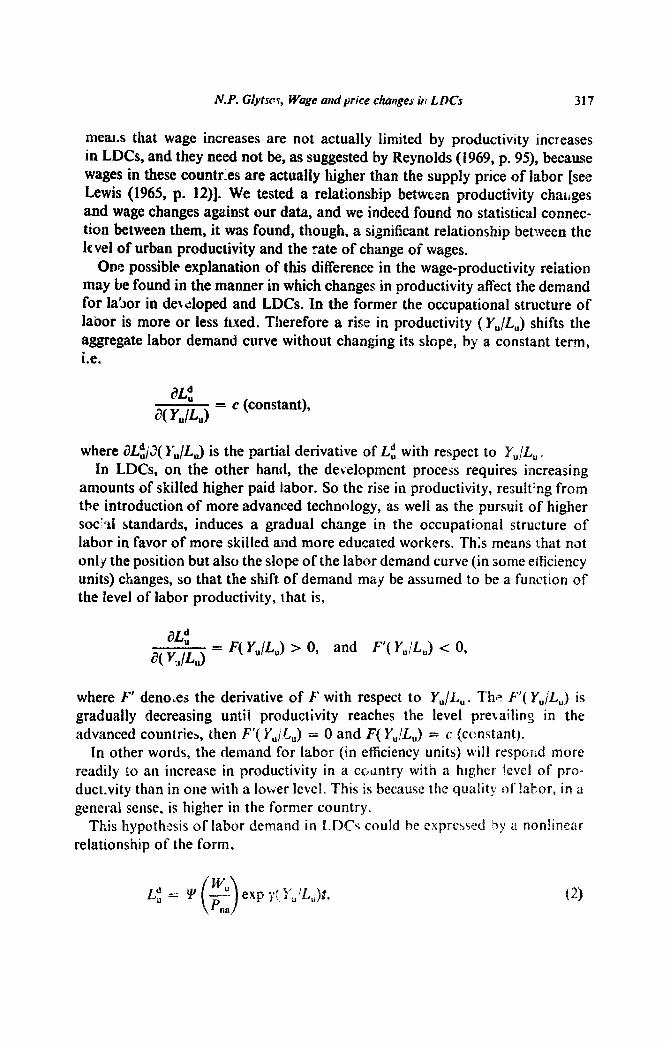
One possible explanation of this difference in the wage-productivity relation may be found in the manner in which changes in productivity affect the demand for Ia’Jor in dettloped and LDCs. In the former the occupational structure of labor is more or less fued. Therefore a rise in productivity ( Y&J shifts the aggregate labor demand curve without changing its slope, by a constant term, i.e.

JLd,

a( Y&J = c (constant),

where 8L$3( I’JL,) is the partial derivative of Lt with respect to YJL, . In LDCs, on the other hand, the de<elopmcnt process requires increasing

amounts of skilled higher paid labor. So the rise in productivity, resuh:ng from the introduction of more advanced technology, as well as the pursuit of higher soc’:tl standards, induces a gradual change in the occupational structure of labor in favor of more skilled and more educated workers. Th:s means that not only the position but also the slope of the labor demand curve (in some etficiency units) changes, so that the shift of demand may be assumed to be a function of the level of labor productivity, that is,

aL; a( Jw”)

= F( YJL,) > 0, and F’( YJL,) < 0,

where F’ deno,es the derivative of F with respect to Y,/L,. Tho F’( Y,/L,) is gradually decreasing until productivity reaches the level prevailing in the advanced countries, then F’( Y,/d,) = 0 and F( YJL,) = c (constant).

In other words, the demand for labor (in efficiency units) will respond more readily to an increase in productivity in a cctintry with a h&her level of pro- ductvity than in one with a lower level. This is because the quality of labor, in a general sense, is higher in the former country.

This hypothssis of labor demand in I.DCs could be expressed iy a nonlinear relationship of the form,

318 N.P. Glylsos, CVnge nncip, ice changes in LDCs

where ,!,z is the urban labor demand, Y,/L, is the vaiuc of urban labor pro- cluctivity and y is a constant.

Equating L”, = Li, the equilibrium nominal wage rate is obtained:

@ w”-Llp’, ’ w* ( P ) exp (- BUO = yu( K/P&w M W,)tl, “a

which gives,

In conclusion, our hypothesis suggests that the molrey wage rate is exponen- tially related to the value of labor productivity, or plainly, that the percentage rate of change of wages depends on the level of productivity and not the rate of change of productivity.

The role of unemployment in wage determination may be considered from two different viewpoints, and it is an empirical matter which one may hold in particular circumstances. One - hypothesis A - is related to the self-control property of urban unemployment discElssed above, in bihich case unemployment is positively related to wage’;, and the orher - hypothesis B - reflects the Phillips- Lipsey approach of a negative relationship.

In fig. 1, L”, and Li are labor supply and demand curves respectively, and ‘V,, is the full employment. wage rate. At the higher wage of W: there is an unemployment of U,U,, and hypothesis A would suggest a shift of the supply curve, say to Lz position, attaining thus a new equilibrium at point a where Wi is stabilized and unemployment is reduced to U,,U,. In other words, we move from a full employment to an unemployment equilibrium. The U,U~ xnenlpioymect is the leftover of the labor supply adjustment, through the dis- couragement of migration, and consists of workers who do not meet the rnirGI;:lrn quality standards (stamina, discipline, etc.) that make them employ- able in: urban actjviti?s. They are what Hoselitz calls the ‘demoralized’ ‘unhealthy’ ar .d ‘pitiful’ frmapenpi’or’etariat, whose presence cannot exercise any s&thrltial downward pressure on wages.

Alternatively, under hypothesis B, the hisher wage W{ would induce a temporary movement along the original supply curve form c to 6, creating thus U,:Cr, une::lployment. But under this hypothesis the migrants continue to pour into the city, and among them there are some who would easily be adjusted to city employment and could, therefore, press wages down towards the full employment level.

In conclusion, other things being equal. hypothesis A can sustain a higher wage rate with some unemployment, whereas hypothesis B will tend to press

N. P. Glytsos, Wuge and price changes in L DCs 319

wages down to the full employment level. If however wages are sticky down- wards, as is usually the case in reality, and the conditions of hypothesis B prevail, the urban sector will suffer the higher unemployment UJ, rather than the lower one U,V, of hypothesis A.

d’

Ua

LU- e ‘.‘-_,

Fig. 1

A shift of demand to the Li' position absorbs u,LJ, unemploymeilt, and the system is driven to a new full employment wage of Wi. Under hypo:hesis B the previous amount of unemployment UoUc = U,U, would still be sustained. Even at the old wage of IV:, unemployment would only be reduced to UyUd.

3. Three alternative approaches to price determination

An attempt. is made here to construct a simple mathematical model of price determination, which in its more general formulation contains both demand and supply forces, but it can also provide a demand-pull and a cost-push hypotheses as sub-cases of the main model.

Mtrit~ n~&~. From a Cobb-Douglas production function !‘()I the urban sector y, = E,“Kp, with given techniques of production and the capital stock (K), the techno!ogical ‘reqiirernents’ of labor (15:) for proJucinp J,, output are given by

320 N. P. Glytsos, Wage and price changes in LDC F

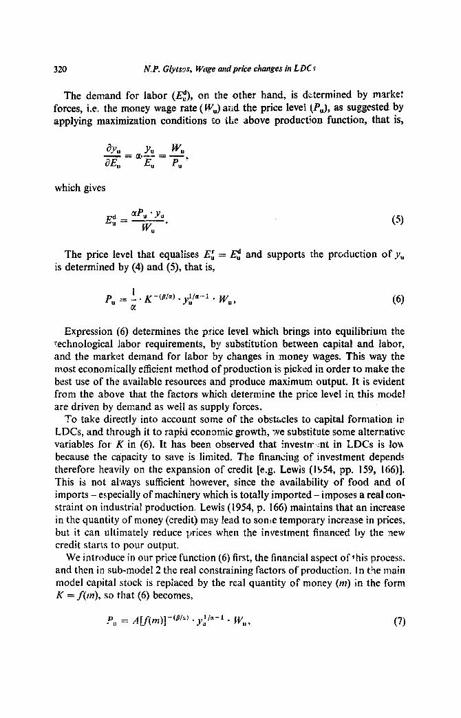
The demand for labor (I$, on the other hand, is determined by market forces, i.e. the money wage rate (FVJ arnd the price level (P,), as suggested by applying maximization conditions to the above production function, that is,

which gives

The price level that equalises EA = G and supports the prtjduction of yU is determined by (4) and (5), that is,

Expression (6) determines the price level which brings into equilibrium the 1:echnological labor requirements, by substitution between capital and labor, and the market demand for labor by changes in money wages. This way the most economically efficient method of production is picked in order to make the best use of the available resources and produce maximum output. It is evident from the above that the factors which determine the price level in this model are driven by demand as well as supply forces.

To take directly into account some of the obstacles to capital formation in LDCs, and through it to rapid economic growth, we substitute some alternative variables for K in (6). It has been observed that invests ,nt in LDCs is low because the capacity to save is limited. The financing of investment depends therefore heavily on the expansion of credit [e.g. Lewis (1354, pp. 159, l66)]. This is not always sufficient however, since the availability of food ancl of imports - especially of machinery which is totally imported - imposes a real con- straint on industrial production. Lewis (1954, p. 166) maintains that an increase in the quantity of money (credit) may lead to son&e temporary increase in prices, but it can ultimately reduce prices when the investment financed by the new credit starls to pour output,

We introduce in our price function (6) first, the financial aspect of this process, and then in sub-model 2 the real constraining factors of production. In t3e main model capital stock is replaced by the real quantity of money (m) in the form K = f(m), so that (6) becomes,

N.P. Giytsos, Wwe and price changes in LDCs 321

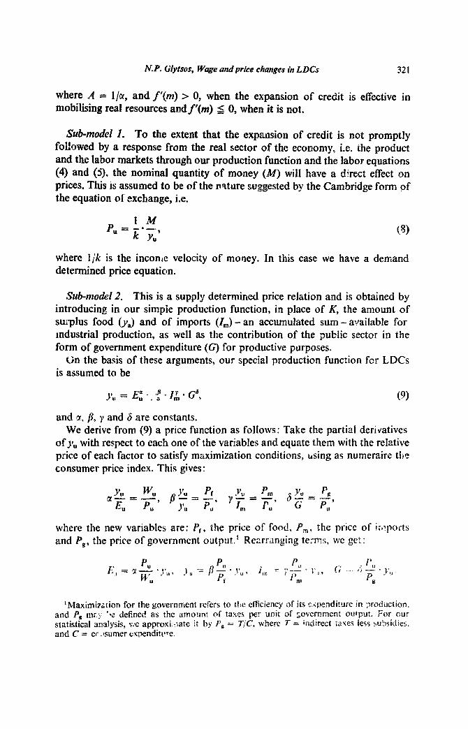
where A = l/cw, and f’(m) > 0, when the expansion of credit is effective in mobilising real resources andS(m) S 0, when it is not.

Sub-model 2. To the extent that the expansion of credit is not promptly followed by a response from the real sector of the economy, i.e. the product and the labor markets through our production function and the labor equations (4) and (S), the nominal quantity of money (M) will have a direct effect on prices. This is assumed to be of the nature suggested by the Cambridge form of the equation of exchange, i.e.

where I: jk is the inconic velocity of money. In this case we have a demand determined price equation.

Sub-model 2. This is a supply determined price relation and is obtained by introducing in our simple production function, in place of K, the amount of surplus food b& and of imports (I,,,) - an accumulated sum -available for industrial production, as well as the contribution of the public sector in the form of government expenditure (G) for productive purposes.

On the basis of these arguments, our special production function for LDCs is assumed to be

and by. /I, y and 6 are constants. We derive from (9) a price function as follows: Take the partial derivatives

of 3: with respect to each one of the variables and equate them with the relative price of each factor to satisfy maximization conditions, bsing as numeraire the: consumer price index. This gives:

where the new variables are: B,, the price of food, P,, the price of i;u!ports and P,, the price of government output.” Rearranging terms, WC get:

‘MaximkA.rion for the government refers to tile efficiency of its stsnditure in production, and P, m;j ‘>e defined as the amotint of tax+ peer unit of government output. For our statistical analfiis, we approxL:ate it by P, == T/C, wher, n 7 = indirect tares less subsidies,

and C = cq- .!sumer cxpenditcre.

: ,22 N. P. Giytsos, Wage atd price chges in L DC Is

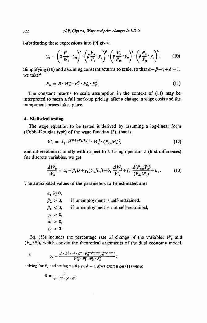
Substituting these expressions into (9) gives

Simplifying (10) and assuming constant rt;turns to scale, so that a+ B + y + 8 = 1, we take’

P, = B. W,*Pp,B-P&.P;. 01)

The constant returns to scale assumption in the context of (11) may be interpreted to mean a full mark-up pricing, after a change in wage costs and the k:omponent prices takes place.

4. Statistical testing

The wage equation to be tested is derived by assuming a log-linear form (Cobb-Douglas type) of the wage function (3), that is,

and differentiate it totally with respect to ?. Using oper:ltor d (first differences) for discrete variables, we get

The anticipated values of the parameters to be estimated are:

if unemployment is Aelf-restrained,

if unemployment is not self-restrained,

Eq. (13) includes the percentage rate of change of the vnriableN W, and (P,,JP,), wh.ich convey the theoretical arguments of the dual economy model,

2

solving for P, and setting u -!- $+ y-t- 6 = 1 gives expression (11) where

IV. P. G/ytsos, Wage and price changes in L DCs 323

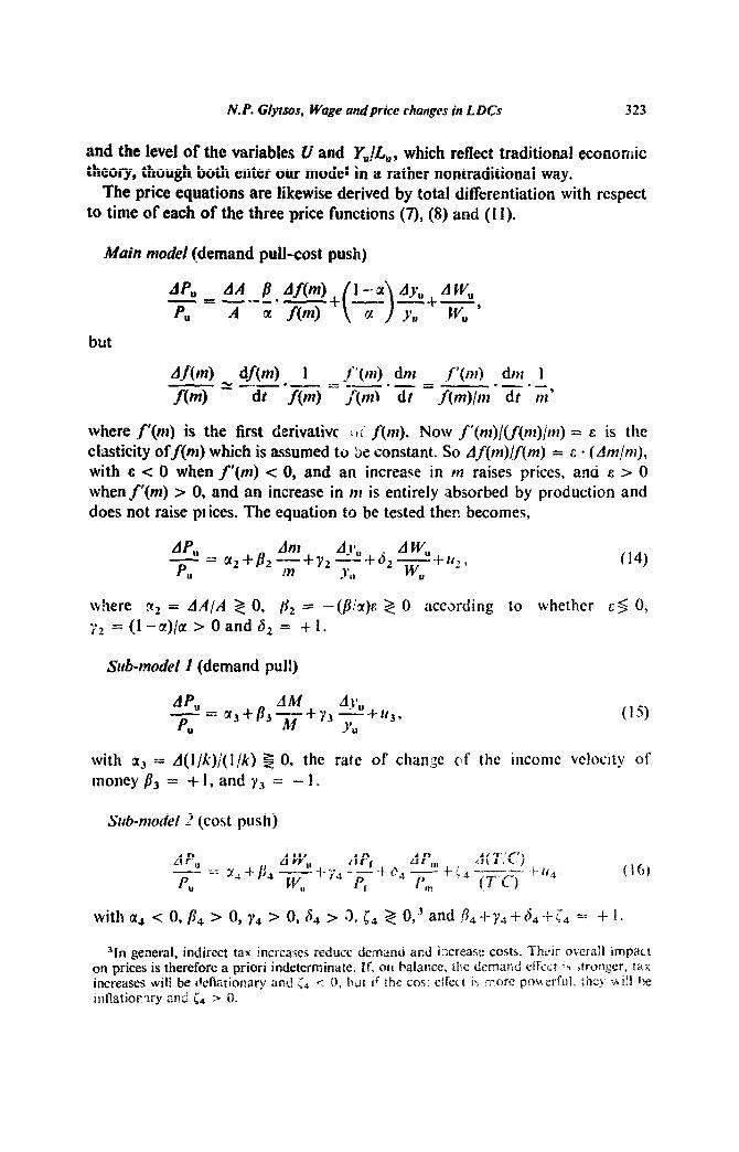
and the level of the vmiables U and YJL,, which reflect traditional economic theory, though both enter our model in a rather nontraditional way.

The price equations are likewise derived by total differentiation with respect to time of each of the three price functions (7), (8) and (I I).

Main model (demand pull-cost push)

but

where f’(nt) is the first derivative : rt’ f(m). Now J’(nt)/(f(nz)/m) = E is the elasticity off(nj) which is assumed to kx constant. So df(m)/J’(m) = E - (Am/m),

with E < 0 when f’(m) < 0, and an increase in m raises prices, and E > 0 whenf’(nz) > 0, and an increase in nt is entirely absorbed by production and does not raise PI ices. The equation to be tested then becomes,

Ah AtI? - = cc,+82--g+Yr

AW” P”

+.+s2 --I-142 1

- I, Wt , (14)

where x2 = AA/A 2 0, /I2 = -(jJ/cx)t: 5 0 accxding to whether c 6 0, .I ,l =(l-a)/a > OandS, = +I.

Sub-model I (demand pull)

with u3 = A(l/k)/(l,lk) !$ 0, the rate of change cbf the income velocity of money s3 = +l.andy, = -1.

St/b-mode! I (cost push)

31n general, indirect tar increascs reduce demand and ixrease cOst5. lhrir overall impact on prices is therefore a priori indeterminate. if, on balance. the demand eff’ud ‘4 ,trlrngcr, tax increases will be dellationary and L < 0. but if the CC%! cffecr is mow pmerfLl8, they v”ill be

~~~t~ati~~,~~y and i4 > 0.

324 N.P. Glytsos, Wage andprice changes in L,“. 3

The sample consists of 36 LDCs with data for the years 1960, 1965 and 1968. By using cross-country data we test the general va”id;ty of our theoretical hypotheses rather than explain in a more practical way - with the econometrics of add and drop (variables) process - the inflationary path of single countries with special characteristics. In this way the more permanent and more uniform forces of inflation, as reflected in our variables, are given greater attention, whereas the temporary and country speci.fic forces acquire less weight. One of the shortcomings of cross-section data, in this analysis, is that the dynamic phenomenon of inflation is handled in 21 rather static way, because our model ignores the circular dynamic price-wage-price connection.

The conversion of the figures from national currtincies 10 IJ S. dollars at the official exchange rates introduces biases into the analysis, because of the different degrees of overvaluation of the national cur?encies to the dollar. To avoid at least the temporal distortion of the data, the figures for all three years were converted into U.S. dollars by u.sing the official foreign exchange rate of 1960.

All the variables in the equations, except U and (Y&,), refer to average annual percentage rates of change for 1960-65, 196548 and 1960-68. Because of gaps in the d.ata, the number of observations is not the same for all equations. There are 27 observations in the wage change equation, 57 in the main price model and sub-model 2 and 87 observations in sub-model 1,

The countries included in the sample are very heterogeneous on several counts. They are at diKerent stages of economic development, have experienced different rates of economic growth, and of inflation, and belong to different national and socio-political environments. It would therefore seem necessary to test the validity of our equations under such diverse circumstances, in order to detect the possibility of differential behavior between more homogeneous country groups.

For this purpose, in addition to pooling 4 together the cross,-section data of the three yei:rs, we also partitioned the sample alternatively into two or three more homogeneous segments, according to certain criteria, by introducing into the equations appropriate additrve and multiplicative dummy variables [se:; Gujarati (1970)].

The groupings5 are made as follows:

41n pooled time section and cross-section data, the disturbanc:: terms of the regrcssinns may generally be nutocorrclated as well as heteroskedastic. It, our cast, however, the discon- tinuity of the time units m the sample (1960, 1965 and 1968) suggests a priori the absence of any serious autocorrelation, whereas heteroskeda,tticity may be expected to exist. In order to eliminate its undesirable properties, the data are ‘t*orrected’. dividing the figures by the square root of the sum of squared residuals, for thr: three years, obtained from the pooling of all data [see Glytsos (1974, pp. 133-137)].

5The choice of threshold values has some arhitr,u%xss. For groupings A and C the median was chosen. \t hile for grouping R 2’ value bclnw tPe median was thought as a better dividing line.

‘Tab

le

I

Est

imat

ed

pool

ed

regr

essi

on

coef

fici

ent;.

’ --

Fqs

Con

stan

t &

y &

L

-3

Y”

AW

, A

Wa

AU

, A

PIl

l &T/C)

Number o

f te

rm

-5:’

m

Y.

L,

w,

w,

pr

p,

u

WC)

obse

rvat

ions

R2

-.__

_ .

- --

_

. _

_~ ~

A

<!ri

gina

l da

ta

- -0

.14s

2.

3647

0.

9625

1.

3072

-0

.002

8 27

0.

935

(0.7

469)

(0

.113

5)

(0.4

910)

(0

.012

7)

Mai

n m

odel

Sub-

mod

el 1

Sub-

mod

el 2

--

0.92

20

- 0.

9897

0.

7096

0.

8588

61

0.

904

(0.0

857)

(0

.156

5)

(0.0

556)

1.63

06

’ .04

85

- 1.

1729

89

0.

740

..3.0

743)

(0

.183

5)

- 2.

0837

0.

3013

0.

6322

0.

0958

0.

0008

60

0.

993

(0.0

480)

(0

.033

5) (

0.02

91)

(0.0

530)

B.

Adj

uste

d fo

r he

tero

sked

astic

ity

data

-

-.

--

0.07

11

2.20

67

0.96

96

1.21

17

-0.0

002

27

0.96

3 (0

.360

7)

(0.0

643)

(0

.252

2)

(0.0

022)

Mai

n m

odel

0.

0465

-0

.391

2 0.

349s

0.

6953

57

0.

906

(O.lO

ZS)

(0.0

928)

(0

.042

5)

Sub-

mod

el

1 0.

0412

0.

8762

-

0.77

23

87

(0.0

334)

0.

915

(0.0

370)

Sub-

mod

el 2

-

0.14

96

0.25

79

0.40

90

0.25

51

-0.0161 57

0.963

(0.0418)

(0.0378)

(0.0376)

(o.Moo)

--~-_

"In pa

rent

hese

s be

Lw

th

e co

effi

cien

ts

are

the

stan

dard

er

rors

of

est

imat

e.

All

slop

e co

effi

cien

ts,

exce

pt

thos

e of

U

and

d(T/C)/{T/C)

are

sign

ific

ant

at

the

5 pe

rcen

t le

vel.

N.P. Glytsos, Wage and price chmges irr LDCs 327

are wllen the adjusted data are used.8 All coefficients, except the one of the tax variable, are statistically different from zero at the 5 percent level of significance. The goodness of fit is also very satisfactory, with R2, 0.906, 0.915 and 0.963 for the three price equations respectively.

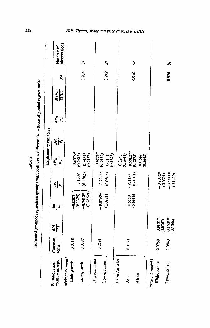
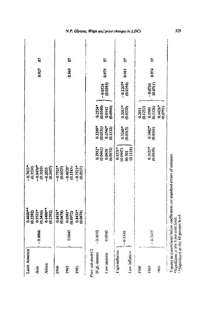
As far as the general group behavior is concerned, the demand-pull/cost-push main model of price changes performs uniformly in the high- and low-income groups, and in the pure cross-section regressions. In the rest of tk alternative groupings, there are differences in the size of regression coefficients, but they are mostly consistent9 with the pooled estimates.

In the demand-pull sub-model 1, the partition of the sample by the growth rate, or the rate of inflation does not differentiate the size of the regression coefficients. It does, though, when the countries are grouped by per capita real income, or by geographic region, or by year. The estimates, however, are con- sistent again with those of the pooled version Df the model.

The overall behavior of the cost-push sub-model 2 does not appear to differ between the high- and low-growth counlries, or among the three geographic regions, but it does so when the sample is split on the basis of the other three criteria. In those cases all the signs of coefficients are correspondingly the same with ,ehe pooled ones, there are only ciifferences in the degree of the statistical association,with the majority of coefficient!; being significant at the 5 percent level.

The conclusions of this section are first, with the reservation of footnote 7, the factors under consideration in the w;tge equation may be equally effective in changing wages, regardless of the individual characteristics of the countries concerned. Second, t: 1 three alternative price hypotheses appear to be of a more genera; validity in diverse groups of countries. They also have a certain amount of flexibility in pointing out the relative strength of association between price changes and their explanatory variables, in country groups with different major characteristics.

5. Empirical wage relationship and the dual model

The unemployment coefficient in our wage equation is not significantly different from zero,” but has a negative sign suggesting thus a trace of a Phillips type relation, rather than support our alternative hypothesis of self-

Wote that in the adjusted sample, the lates of change of nominal money and of real urban GDP have some degree of intercorrelation (simp,r’ correlation cctcfhcicnt 0.73). In the originai sample this is negligible.

gConsistency in this context means m. inly san e corresponding signs between pooled and grouped estimates, but a:so similar statistical siglriticance. Variability ir the lizc of :orre+ ponding coefficients alone does not ail&t the structure of the models, but reflects ditferential group behavior of the variables involved.

‘“This finding for urban unemployment looks a bit shaky for a number of reasons: uncm- ployment figures are unreliable, and we use an index, rather than the unemployment rate, for smoothing the data a little; wages of manufacture are used for lack of figures on &ages of trade and service sectors, which mostly provide jobs for migrati:lg farn.ers - they are assumed

328

Lat

in

Am

eric

a 0.

4480

* +

-0.7

453’

(0

.239

2)

(0.3

534)

Asi

a -0

.847

0+

(0.3

510)

0.

927

87

Afr

ica

1960

O&

80+

+

-0.2

033

(0.2

392)

(0

.245

7)

0.84

31 l

-0.7

523.

(0

.047

4)

(0.0

527)

1965

-0

.402

0”

(0.1

183)

1968

1

0.84

31*

- 0.

7523

. (0

.047

4)

(0.0

527,

0.94

3 a7

Pric

e su

b-nz

o&l2

Hi&

-inc

ome

- 0.

4150

0.

3952

. (0

.046

2)

I ow

-inc

ome

0.09

40

0.04

10

(0.0

832)

. ..

~___

~-

~.

.__-

-

--

i-i ig

h-in

fktio

n 0.

4331

. (0

.044

7)

00.5

01

6.ow

-inf

latio

n (0

.111

8)

____

__

._

- ---

-.-_

_ .._

___-

.-.-

__

_-

1960

\ r

1965

-

O.-‘

-I?5

0.

2625

. (0

.065

9)

5 96Y

__-.

-

--~-

-

“Fig

ures

in

pxc

nrhe

ses

bclu

w

coef

fici

ents

tir

e st

anda

rd

erro

rs

of e

stim

ate.

“S

igni

fica

nt

3t t

he 5

per

cen

t le

vel.

y *S

igni

fica

nt

a~ th

e 10

per

cent

Ie

d.

0.32

49’

0.25

24+

(0

.033

1)

(0.0

340)

-

0.05

24

0.67

46.

0.01

42

(0.0

393)

o.

979

57

(0.1

132)

(0

.096

6)

0.32

45.

0.20

13’

-0.1

207”

(0

.031

5)

(0.0

320)

(0

.039

4)

o*98

1 57

----

__

0.20

11

(0.1

252)

0.34

42’

0.19

80

-0.0

710

(0.0

561)

(0

.132

6)

(0.0

76s)

o.

974

57

O&

26*

(0.0

791)

,, . “

,

330 N. P. Glytsos, Wage andprice change? in L DCk

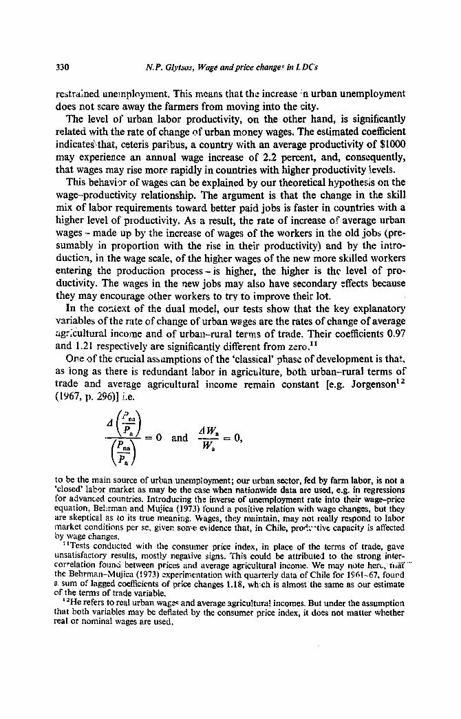
restrained unemployment. This means that th,: increase “n urban unemployment does not scare away the farmers from moving into the city.

The level of urban labor productivity, on the other hand, is significantly related with the rate of change of urban money wages. The estimated coefficient indicate&hat, ceteris paribus, a country with an average productivity of $1000 may experience an annual wage increase of 2.2 percent, and, consequently, that wages may rise more rapidly in countries with higher productivity Bevels.

This behavior of wages can be explained by our theoretical hypothesis on the wage-productivixy relationship. The argument is that the change in the skill mix of labor requirements toward better paid jobs is faster in countries with a higher level of productivity. As a result, the rate of increase of average urban wages - made up by the increase of wages of the workers in the old jobs (pre- sumably in proportion with the rise in their productivity) and by the intro- ducticn, in the wage scale, of the higher wages of the new more skilled workers entering the production process - is higher, the higher is the level of pro- ductivity. The wages in the new jobs may also have secondary effects because they may encourage other workers to try to improve their lot.

In the cor,‘cext of the dual model, our tests show that the key explanatory variables of the rate of change of urban wages are the rates of change of average @cultural income and of urban-rural terms of trade. Their coefficients 0.97 and 1.21 respectively are significantly different from zcra,.”

One of the crucial assumptions of the ‘classical’ phase of development is that, as iong as there is redundant labor in agriculture, both urban-rural terms of trade and average agricultural income remain constant [e.g. Jorgenson” (lY67, p. 296)] Le.

= 0 and A w, - = 0, Kl

to be the main source of urban unemployment; our urban sector, fed by farm labor, is not a ‘closed’ labor m‘arket as may be the case when nationwide data are used, e.g. in regressions for advanced countries. Introducing the inverse of unemployment rate into their wage-price equation, Bel:rman and Mujica (1973) found a positive relation with wage changes, but they are skeptical as to its true meaning. Wages, they maintain, may not really respond to labor ‘market conditions per se, giver. sonle evidence that, in Chile, pro?:-tive capacity is affected by wage changes.

“Tests conducted with the consumer price index, in place of the terms of trade, gave unsatisfactory results, mostly negative signs. This could be attributed to the strong inter- cor+elation founii between prices and average agricultural income. We may note herL. tiS’” the Behrman--Mujica (1973) experimentation with quarterly data of Chile for 196147, found a sum of lagged coefficients of price changes 1.18, which is almost the same as our estimate of the terms of trade variable.

’ ‘He refers to real urban wage? and average agricultural incomes. But under the assumption that both variables may be deflated by the consumer price index, it does not matter whether real or nominal wages are used,

E”.P. GIy&q Wage and price cftmg T bt LDCJ 331

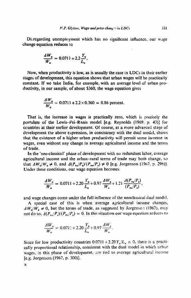
Diiregarding unemployment which has no significant influence, our wage change equation reduces to

AK w,

= 0.0711 f2.2;. ”

Now, when productivity is low, as is usually the case in LDCs in their earlier stages of deve!opment, this equation shows that urban wages will be practically constant. If we take India, for example, with an average level of urban pro- ductivity, in our sample, of about $360, the wage equation gives

AW 4 = 0.0711+2.2 x 0.360 = 0.86 percent.

W”

That is, the increase in wages is practically zero, which is precisely the postulate of the Lewis-Fei-Ranis model [e.g. Reynolds (1969, p. 43)J for countries at their earlier development. Of course, at a more advarced stage of development the above expression, in consistency with the dua! model, shows that the existence of a higher urban productivity will permit some increase in wages, even without any change in average agricultural income and the terms of trade.

In the ‘neo-classiczl’ phase of development with no redundant labor, average agricultural income and the urban-rural terms of trade may both change, s3 that A W,/rY, # 0, and A(P,,/P,J/(P,,,/Pa) # 0 [e.g. Jorgenson (19(;7, p. 29h)]. Under these conditions, our wage equation becomes

AW, - = 0.0711+2.20 AW, d (G/C)

W” y”+o.97 L

w+ 1.21 a (P”,lP,) ’

and wage changes come under the full influence of the neoclassical dual model. A special case of this is when average agricultural income changes,

A IV,,/ W, # 0, but the terms of trade, as suggested by Jorgenson (19671, may not do so, A(Y,,,P,),‘(P,,~P,) = 0. In this situation our wage equation reduces to

A W,, - = 0.071 I +2.20 -5 + 0.97 AW,

WI, LU --ivy-’

Since for low productivity countries 0.0711-1-2.20 Y,/L, 2: 0, there is a practi- cally proportional relationship, consistent with the dual model in which urban wages, in this phase of development, rt:e tied to average agricultural income [e.g. Jorgenson (1967, p. 300)].

R

Tab

le

3

Reg

ress

ion

coef

fici

ents

of

sel

ecte

d va

riab

les

from

va

riou

s st

udie

s or

in

flat

ion

in L

DC

s.

Var

iabi

es

Aut

hor

Har

berg

er

Co

un

try

--__

-.

-

Ch

ile

Peri

od

Dat

a -

1930

-58

atin

cal

13eh

rman

b C

hile

19

45-6

5 an

nual

Cor

bo

Chi

le

1964

-68

quar

terl

y

Dia

z A

leja

ndro

A

rgen

tina

1945

-62

annu

al

Arg

entin

a 19

46-6

2 qu

arte

rly

Diz

A

rgen

tina

1935

-62

Col

aco

Coi

aco

CoI

aco

Vog

el

Gua

naba

ra

(Rio

)

Gua

naba

ra

1947

-62

(sem

iann

ual

for

mon

ey)

annu

al

1947

-62

annu

al

Indi

a 19

48-6

7

16 L

at.

Am

er.

1950

-69

annu

al

sum

of

AM

-, A

M,_

2 co

ef.

for

AY

l A

W

-~

- m

oney

-K

SM

. M

t.-,

M 1

-Z

W

Con

stan

t R

2

0.70

0 (0

.180

)

0.84

7 (0

.154

)

0.93

0 (0

.350

)

0.30

7 (0

.120

)

0.32

1 (0

.080

)

0.36

9 (0

.183

j

0.18

2 (0

.177

)

0.18

7 (0

.248

)

0.58

6 (0

.034

)

0.29

0 (0

.180

)

-0.2

72

(0.1

69)

- - - 0.34

0 (0

.255

)

0.10

4 (0

.262

)

0.27

2 (0

.249

)

0.40

7 (0

.037

)

-

- 0.

200

(0.1

78)

- - 0.15

3 (0

.123

)

0.18

5 (0

.086

)

0.41

6 (0

.226

)

0.73

0 (0

.295

)

0.99

0

0.%

4

- 0.93

0

0.46

Od

0.50

6d

1.12

5

1.01

6

0.45

9

0.99

3

-0.8

90

(0.3

20)

- 1.

488

(0.3

87)

-

- 1.

050”

(0

.430

)

- 0.

731

(0.2

64)

- 0.

748

(0.1

84)

-o.h

.&i

(1.0

87)

0.79

0 (1

.047

)

-0.2

47

(0.2

50)

-0,2

98

(0.0

96)

0.13

0 (0

.220

)

0.15

1 (0

.106

)

0.64

7 (0

.106

)

0.50

0 (0

.200

)

0.07

4 (0

.049

)

-

- 0.

061

(0.0

48)

- 1.

150

0.87

0

- 0.

940

-2.4

36

0.89

7

- 10

.50

0.86

5

- 0.

679

- 0.

616

- 0.

076

0.80

4

- 0.

048

0.89

5

0.02

1 0.

231

-0.0

31

0.82

0

Vog

el

Arg

y

Arm

Gly

tsos

Gly

tsos

GIy

tsos

Gly

tsos

%yt

sos

Gly

tsos

16 L

at.

Am

er.

1950

-69

annu

al

22 L

DC

s

22 L

DC

s

29 L

DC

s

1958

-65

annu

al

(ave

rage

)

1958

-65

annu

al

(ave

rage

)

1960

,65,

68

annu

al

‘9 LDCs'

1960,65,68 ,ln

nual

19 L

DC

s 19

60,6

;, 68

an

nual

20 L

DC

s’

1960

,65,

68

akua

l

19 L

DC

s 19

60,6

5,68

an

nual

20 L

DC

s’

1960

,65,

68

annu

al

0.538

(0.036)

1.090

(0.083)

1.060

(0.085)

0.876

(0.033;

l.iM

(0.074)

-0.391"

(O.rnOj)

-0.990'

(0.086)

0.434

(0.0401 0.036

1.008

(0.040)

1x90

-

1 .c

)bo

0.87

6

1.04

8

- -0

.391

- 0.

990

. . _.

-0.289

(0.090)

-1.020

(0.508)

-0.870

(0.518)

-0.772

(0.037)

-1.173

(0.183)

0.349

(0.093)

0.710

(0.156)

0.69

5 (0

.042

)

0.85

9 (0

.055

)

0.25

8 (0

.042

)

0.30

1 (0

.048

)

-0.051

1.230

-0.900

0.041

1.631

0.045

0.922

-0.150

-2.084

0.820

0.92

7

0.92

2

0.91

5 3 fa

5 0.994

2

op

a

“All

figu

res

in p

aren

thes

es

belo

w c

oeff

icie

nts

are

stan

dard

er

rors

of

est

imat

e.

In t

hus

tabl

e on

ly

the

coef

fici

ents

of

:tti

oney

, w

ages

, an

d re

al

inco

me

vari

able

s ar

e re

port

ed,

igno

ring

th

e es

timat

es

of a

ny

othe

r ex

Dla

na?o

ry

vari

able

s th

at

are

incl

uded

in

th

e or

ice

equa

tkn:

: uf

the

st

udie

s un

der

cons

ider

atio

n.

c

resp

ectiv

ely:

0.

797

(0.1

721,

-0

.844

(0

.192

) an

d S

%

addi

tion

to

r-1

and

r-2

lags

th

ere

are

thre

e m

ore

lags

(f

-3,

f-4, f-5) w

ith

coef

fici

ents

0.

316

(O.S

50).

‘I

t in

clud

es

impo

rts.

dD

iz’s

da

ta

for

pric

e ch

ange

s ar

e qc

arte

rly

and

for

mon

ey

supp

ly

chan

ges

sem

iann

ual.

To

obta

in

in t

he a

bove

ta

ble,

th

e re

gres

sion

co

efki

ent

give

n m

ust

be d

oubl

ed.

‘Rea

l qu

antit

y of

mon

ey.

‘Est

imat

es

with

or

igin

al

data

.

a co

mpa

rabl

e fi

gure

fo

r th

e pa

ram

eter

of

mon

ey

.

It has been obselived that in many LDCs wages rise by 4 to 5 percent agsfinst a proeuctivity increase of I to I1 A2 percent [see Meier (1970, p. 435)]. This is attriouted by some economists to labor union pressure and government wage policie:, and is presented as evidence refuting the validity of the proportionality assumption, between urban wages and average agricultural income, of the dual model,.

Our findings indicate that there are economic reasons for this phenomenon. For example, if, in a country with an urban productivity of $1000, average agricultural income and the intersectorai teru -1s of trade increase each, even by the insignificant rate of 1 percent, urban wages will rise by 4.38 (=2.20x +0.97 “/o + 1.21%1 percent. It is possible, though, that in advanced stages of development with high prodnctivity and better organized labor, the enhanced impact of productivity on wage increases may partly reflect the influence of labor unions.

We conclude, therefore, that the real economic forces reflected in our wage equation can 132j zly jllstlfv wage increases in excess of productivity increases. - Labor union pressures or Animum wage legislation may, in the final analysis, only claim what the economy can really aRord to pay in wages.

6. The role of money on price changes

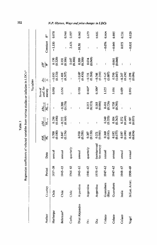
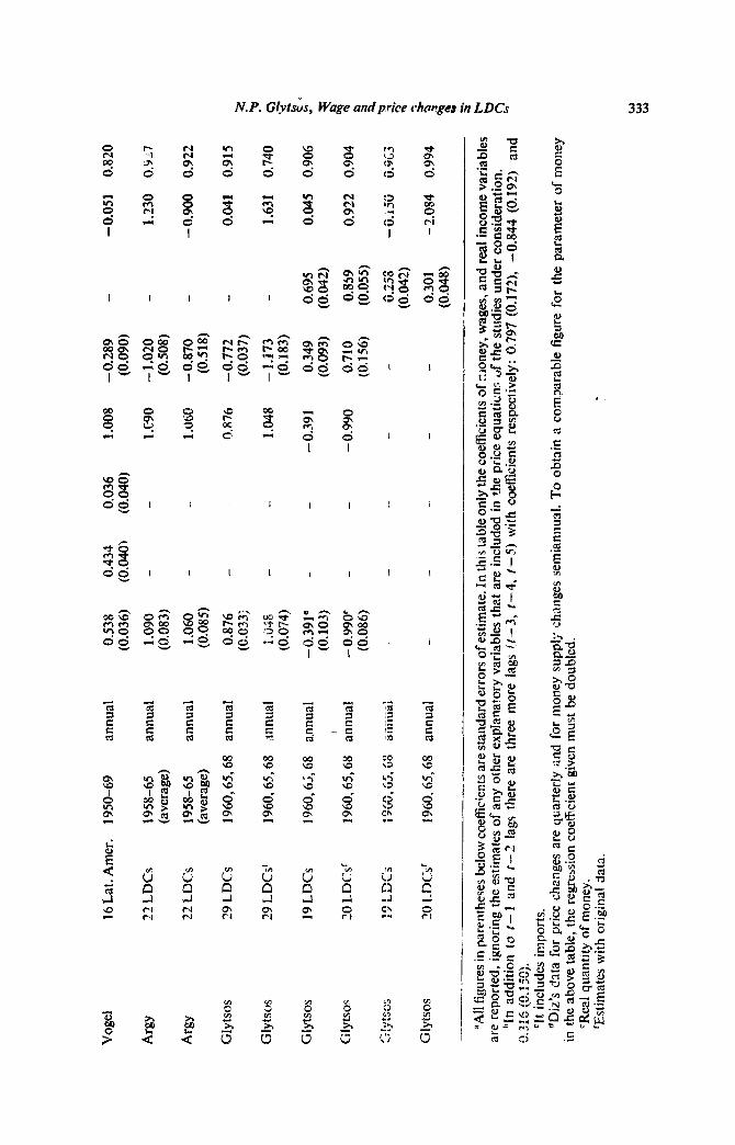
The monetary variables behave as expected in the pooied estimation, i.e. nominal money with a positive and real money with a negative sign. In general, a 1 percent increase in the nominal quantity of money is accompanied by 0.88 percent increase in the consumer price index, on the basis of adjusted data, and l.QO percent on the basis of original data. Several of the studies in table 3 give very sim:ilar results to ours, with regression coefficients, lagged or unlagged, very close to unity, verifying thus empirically the quantity theory. Without lags in our model, the time path of the price response cannot be traced, and it is not, therefore, possible to determine whether there is an overshooting of prices during the process of their adjustment to money changes.

Our Gnding,s indica.te that nominal money appears to be more inflationary in the high-income gruup, with a coeficient cf 0.91, compared with a coefficient of 0.66 in the low-income group. This can be justified by the higher degree of monetization and the more roundabout production process, in the high-income countries. As a. result, output supply may take more time to respond to an increase in the quantity of money, and it is, therefore, more likely to have a stronger impact on price changes.

The value of the constant term of price sub-mociel 1 is very close to zero, in both the pooled and the grouped runs. This suggests that the income velocity of money may not have any substantial impact on price changes. Only fhp: s!gns of t.he intercepts are opposite, in t’le high- and low-income groups, indicating :L declining average velocity in the former and an increa ;ing one in the latter.

N.P. Glyl’sos, Wage and price changes in LDCs 335

The response of prices to changes in the quantity of nominal money is not different between high- and low-growth, or between ltigh- and low-inflation countries. In his individual country regressions, Vogel (1974) detects a ‘slight tendency’ for the coefficients of money to be larger in the high-inflation countries, while Argy (1970) finds no difference in his own cross-country results. The fact ti,f the matter, however, is that in our high-inflation groups there are countries from all over the third world, some of which have experienced only moderate iqflation, whereas the samples of the abov: writers include, in their corresponding groups, only countries with very high inflation.

In the Latin American” and African groups, the nominal money coefficient is 0.45 and is significantly nonzero at the 10 percent level, while for Asia the coefficient is 0.95 and is significant at the 5 percelrt levei. If we also take into comideration that the real rate of increase of urban output has a nonzero coei%cient of -0.85, we have a pretty good indication that the quantity theory holds for the Asian group. There is, in fact, an argument [see Mukhejee (1966, p. 9)1, that in India the lack of financial markets leaves money to 5e primarily used for transactions, and that the inelasticity of supply of real output creates a pseudo-full-employment situation. Both cf these factors make the quantity !heory valid. For the other two regions, our findings suggest that the relation- ship between money and prices is less likely to be strong.

Finally, the pure cross-section estimates show that sub-model 1 performs con.;istent!y, through the three years considered in this analysis.

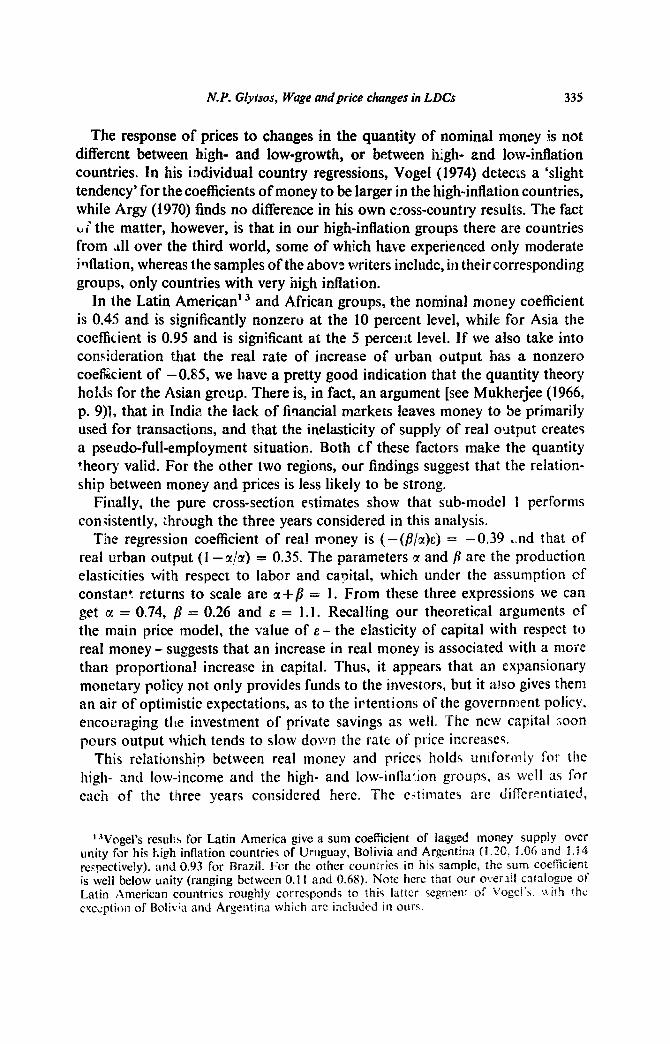
The regression coefficient of real rroney is (-(P/Z)&) = -0.39 ,nd that of real urban output (1 -m/z) = 0.35. The parameters E and p are the production elasticities with respect to labor and capital, which under the assumption of constar?! returns to scale are a+p = 1. From these three expressions we can get CI = 0.74, /? = 0.26 and E = I .I. Recalling our theoretical arguments of the main price model, the value of c - the elasticity of capital with respect to real money - suggests that an increase in real money is associated with a more than proportional increase in capital. Thus, it appears that an expansionary monetary policy not only provides funds to the investors, but it also gives them an air of optimistic expectations, as to the intentions of the government policy, encouraging tile investment of private savings as well. ‘The new capital LOon pours output Jvhich tends to slow down the rate of price increases.

This relationship between real money and prices holds uniforgnly for the high- snd low-income and the high- and low-infla’.ion groups, as well 3s for

each of the three years considered here. The cytimates are differentiated,

13Vogel’s resul:s for Latin America give a sum coeffcient of lagged money supply over unity for his high inflation countries of Uruguay, Boiivia and Argentina (1.20, 1.M and 1.14 rerpectively), and 0.93 for Brazil. For the other countries in his sample, the sum coeficient is well below unity (ranging between 0.11 and 0.68). Note here that our oT:erllI c3talogue of Latin /American countries roughly corresponds to this latter segmen: of Vogel’\. urirh !h~ cuc~ption of Bolivia and Argentina which are included in ours.

336 N.P. c3ytsos, tt’age andprice chariges in LDCs

however, in the grou@ng by the rate of growth, with a significant coefficient of real money of -0.74 in ,the low-growth and a nonsignificant in the high- growth group. In the more rapidly growing countries, where higher profits can be reaped and reinvested, increases of real money supply may not strongly affect investment, so that the price:-real-money relationship stays loose.

7. Price-wage relationstips and cost-push inflation

Our demand-pull/cost-push. main price model and the cost-push sub-model 2 are two diifcrent channels of price changes. If both money and wages are involved in the process of inflation, as in the main model, wage changes appear to 1:ave a tighter association with price clianges (regression coefficient of 0.70), from what they have in sub-model 2, in which inflation is an entirely cost-push phenomenon (regression coefficient 0.26). This may be so because the wage coef?cient, in the former model, reflects both a cost and a demand effect on priceh, whereas only the cost effect is transmitted through the channel of sub-model 2.

From the studies in table 3, besides ours, only Diaz-Alejandro’s (!965) and Corbo’s (1974) have found a strong relation between price and wage changes. Behrman’s (1973) wage variable (adjusted for employers’ social contributions and for productivity) carries a rather small-sized coefficient, significant only at the 10 percent level. And when wages are not adjusted as above - in which c#dse they are more comparable to our wage variable - the coefficient becomes significantly nonzero only at the 25 percent level.

To establish a price-wage spiral of inflaton would normally require dynamic: relations involving lags. Though our model does not include lagged variables, it demonstrates a substantial mutual association between price and wage changes. The wage coeRcients, along with that of the intersectoral terms of trade in the wage equation, at least suggest that prices and wages move together, bti; wage changes are not fully transmitted to price changes.

Turning to the group regressions, our results show that, in some of the alternative classifications, the wage coeffic ents are different, but mostly con- sistent with the poaled estimates, reflecting ;he various influences of the special grloup conditions. First, they are significantly nonzero in the high-inflation group, with a value of 0.68 and 0.43 for the main riodel and sub-model 2 respectively, but they s.re insignificant in the corresponding low-inflation groups. In countries with a high rate of inflation, the purchasing power of money wages is more quickly eaten up by the fast rising prices, making the phenomenon of the wage--price chase more probable in them.

Sp.,:ond, in the low-growth group of the main model, the wa.ge coefficient is 0.85 and in its high-grow& group 0.61, both being significant, and it is not dif’ferent from the poolelf estimate (0.26) in either of these groups in sub- model 2. It can be deduced from these estimates that the demand element of

N.P. Gly~sos, Wage andprice changes Sn LDCs 337

the wage coefficient of the main model is more operative in the low-growth countries because they are mc#re likely to have a slow response of output to the new demand stemming from higher wages,

Third, wage changes are not significantly related to price changes in the Latin American and African groups of the main model, but they are in the Asian group with a non-zero coefficient (at the 10 percent level) of 0.99. No corresponding differential behavior of wages was found in the cost-push sub- model 2.

In summary, some of our major group results concerning the wage behavior are: first, wages. both as a demand and as a cost factor, have an impact on prices in the high-inflation courtries and no: in the low ones; second, wages contribute to Latin American inflation only as a cost factor. These results, in conjunction with the finding that nominal money is less likely to have an effect on prices in Latin America, seem to give some empirical weight to thL ‘struc- turalist’ explanation of inflation, to the extent, of course, that it is related tc8 labor market conditions.

Another argument of the structuralist position on inflation is the food bottleneck hyp athesis - a product mainly of those int.erpretirmg the experience of certain Latin American countries [e.g. Maynard (1961, pp. l?S-ZOZ)]. The hypothesis has, however, been disputed by other writers [e.g. Seers (1962, p. 174) and Edel (1969, p. SS)], who maintain that it cannot be valid for Latin America, because of its openness to international trade.

Our results seem to support this hypothesis for a!! thr: three regio:ls under consideration. The coefficient of food prices is 0.41 in the pooled regrwion, and it does not differ appreciably in focr of the five Ilternative groupings. The only substantial difference is between high- and low-income countries, with an estimated value of 0.32 and 0.67 respectively. This should be expected, because of the relatively larger share of food exper.diture in the family budgets of the low-income countries.

Import prices are also significantly related io consumer prices. with a pooled coefficient of 0.25, and an overall behavior in the g,-ouped regressions pretty close to that of food prices. A contrast with the latte!. is noted in the estimates between high- and low-income countries, with the coeficient of import prices

(0.25) being statistically nonzerO only in the high-income group. Thi:, could also be cpnlained, as in food prices, by the relatively high share of imports in the total consumplion expenditure in these countries. The behavior of import prices is a!so differentiated in the pure cross-section ; n:ilysis, with a significant coeffkient of 0.44 in 1968, which besomes 0. !O in 19(0 and 1965, being slgnifi- cant oddly at a higher than 10 percent level.

Finally, indirect taxes (less >ubsil!ies) per unit of consumption expenditure we negatively related to consumer prices, in all regression runs, but the respective coefficients are statistically not diiTetent trom zero. T! 0 nPwtivc sigrl indicates, _ ~. -= hQ$v<:vW, that t e imposition of higE.er indirerx taxes, would, other things being

338 N.P. Glytsos, Wage andprice changes in LDCs

equal, slow down the rate of price increases, through the demand reducing eft’ect of indirect taxes.

Concluding the discussion of the performance of the cost-push sub-model 2, we may recall our a priori expectation, that the regression coefficients of all the variables in the model should add iiip to unity. Indeed, t1.e sum of the pooled coefficients 0.26+0.41+0.26-0.CI.c; = 0.91 is very close to unity -it is I in the original data run - and it is about the same in most of the grouped runs. This seems to give some em.pirlcal support to our hypothesis of mark-up pricing.

The impiications of the discussion in this section are that, even without an increase in money supply, inflation may generally be fed by wage rises - particularly so in countries with higher inflation-and by food and import price increases. Consequently given that money supply in LDCs is mostly the result of deficit financing [e.g. Myrdal(l970, p. 287)], our findings are in accord with Lewis’ (1964, p. 24) claim that ‘if one eliminated the budgetary deficit, prices wotild not rise so fast, but the wage-price spiral could still be there just as it exists in many advanced industrial countries which have no budget deficit’. The difference though, in our view, between advanced and LDCs at this point is that in the former inflation may be sustained by labor union pressures, whereas in the latter the origins of inflation may be located in agriculture. Average agricultural productivity and food prices play a primary role in raising urban wages, which, in turh, along with food prices again and to a lesser extent imoort prices, raise the consumer price inde:x.

8. Summary and conclusions

A theoretical hypothesis of urban wage determination, and three alternative approaches to price changes, are formulated and statistically tested. The vrage model is tailor made to suit the dual char&ter of LDCs, and the price models reflect, first, a combjnation of the quantity and marginal productivity theories, second, the pure quantity theory, and third, the mark-up pricing. Consequently, they represent, respectively a demand-pull/cost-push, a demand-pull, and a cost-push price determination,

The data used for the testing refer to 36 LDCs for the years 1960, 1965 and 1968. There are two sets of regression runs: one by pooling all the data in the sample, and two, by using appropriate additive and multiplicative dummy variables, to test the behavior of th model between alternative country groups, with some common major group c’,,laracteristic.

The results obtained do not gl:nerally contradict the hypotheses tested. .‘he evidence produced by the wag equation is that the rate of wage change is

uniformly determined, in all countr groups. The price models have also demon- strated a quite substantial stability. in their performance in the various alter- native groupings.

A’. f’. G&sos, Wage atzdpricc changes irz L DCs 339

The empirical wage determination is consistent with the postulates of ihe dual economy model. In fact, urban wage changes are proportionally related to average agricultur4 income, and more than in proportion to the urban-rural ierms of trade. ‘I bus: there appears to be an overshooting of wage change:: over relative price changes, permitting real wages to rise.

From the ‘tradi,ional’ vari,.b!cs of unemploymenr and productivity of .jur wage equation, unemploynem does not seem to aKecr urban wage changes. Although thz sign of unemployment is ncga.tive we feel that the evidence produced - by unreiiable &rtt; on unemployment - is at best inconclusive as to the existence of an interrational Phillips curve in LDCs. Neither are there any serious indications pointing to the validity of the hypothesis, about a self- restraining power of urban unemployment.

Productivity, which enters the wage equation in level form, is found to be significantly related to the rate of wage change. The meaning of this kind of relationship is that, between two countries with different levels or’ productivity, the higher-productivity country may experience, other things being equal, more rapid wage increases. The reason is that the higher the level of productivity in LDCs, the faster is the change in the occupational structure of the ernllovcd labor force, toward higher paid jobs, puliing up the average wage rate.

The results on price changes show that nominal money ‘matters’, but not universally or exclusively :;o. It matters more in LDCs of a more advanced level of development, or in tiose of the Asian region, whereas it is less likely to matter in Latin America and ckli-ica.

Contrary to most of the studies on inflation in LDCs, wages matter too, particularly in the high-inflation countries. The explanatory power of wages goes through two alternative channels, one transmitting a mixture of the demand and cost effects of wages on prices, and the other only the cost effect. As it should be expected, the former is relatively stronger, it is in fact more than twice as high from the single cost effect.

Food prices contribute substantially to the consumer price increases, more so in low-income countries, for obvious reasons. Import prices have also an impact, but not so stro,!f; as fo -5 prices. Between high- and low-income countries import prices; are efft :tiv: only in the former.

Some of our majc: l _I e Its, relevant to the rilonct,?.rist--structuralist contro- versy, cbn be summar . ’ 35 follows: (a) iii general, nominal money is strongly related to price changes. Rut has a weaker and less probable connection with prices in Latin America .- the grounds of the controversy; (b) the high-inflation countries haIre a relatively stronger wage-price relation; (c) wages, as a cost variable, arz significant in all regions; (d) food and import prices have consider- able impact on inflation, in all regions and almr;L ari mmtry groups.

Although these results clearly favor the strcc,ruralist -,,osition, the ‘causes’ of inflation are not necessaril] emonetized, since lrlore 4’, as it shoul is still in the picture.

340 IV. P. Glytsos, Wage and price changes in LDCs

The implication of all these, is that monetary policy may not, in general, be effective in curtailing iniIation. The existence of other strong nonmonetary forces, can sustain the inflationary process and weaken the influence of monetary policy.

Appendix

2’he sample

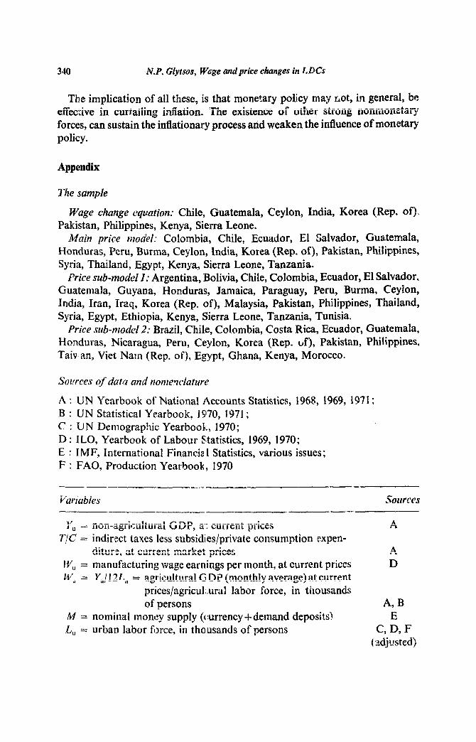
Wage change equation: Chile, Guatemala, Ceylon, India, Korea (Rep. of). Pakistan, Philippines, Kenya, Sierra Leone.

Muin price ritodel: Colombia, Chile, Ecuadar, El Salvador, Guatemala, Honduras, Peru, Burma, Ceylon, India, Korea (Rep. of), Pakistan, Philippines, Syria, Thailand, Egypt, Kenya, Sierra Leone, Tanzania.

Price sub-model I: Argentina, Bolivia, Chile, Colombia, Ecuador, El Salvador. Guatemala, Guyana, Honduras, Jamaica, Paraguay, Peru, Burma, Ceylon, India, Iran, Iraq, Korea (Rep. of), Malaysia, Pakistan, Philippines, Thailand, Syria, Egypt, Ethiopia, Kenya, Sierra Leone, Tanzania, Tunisia.

Price sub-model 2; Brazil, Chile, Colombia, Costa Rica, Ecuador, Guatemala, Honduras, Nicaragua, Peru, Ceylon, Korea (Rep. of), Pakistan, Philippines. Taiv an, Viet Nam (Rep. of), Egypt, Ghana, Kenya, Morocco.

Sources of data and nomerclature

A : UN Yearbook of National Accounts Statistics, 1968, 1969, 1971; B : UN Statistical Yearbook, 1970, 1971; C : UN Demographic Yearbook., 1970; D : ILO, Yearbook of Labour Statistics, 1969, 1970; E : IMF, international Financial Statistics, various issues; F : FAO, Production Yearbook, 1970

-- --

Variables Sources -- ---

Y, = non-agricultural GDP, a’; current prices A T/lc = indirect taxes less subsidies/private consumption ,expen-

diturz, at current market prices A IV” = manufacturing wage earnings per month, at current prices D W’, = Y,/ 12L, = agricultural GDP (monthly average) at current

pr!;ces/agricul::ural labor force, in thousands of persons A, B

M = nominal money supply (currency +demand deposits! E L, = urban labor fierce, in thousands of persons C, D, F

(adjusted)

N. P. Glytsos, Wage and price changes in LDCs 34i

----___.___- ----

Variables Sources -- _I-___ _ _ __ .~._.._I_ I-

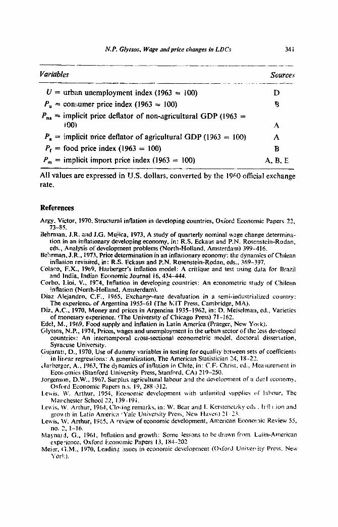
U = urban unemployment index (1963 = 100) D

P, = con:;umer price index (I 963 = 100) B

P l&P = implicit price deflator of non-Lgricultural GDP (1963 = 1001 A

P, = implicit price deflator of agricultural GDP (1363 = 100) A

Pr = food price index (1963 = 100) B

P,,, = implicit import price index (I 963 = 100) A, B, E

All values are expressed in VJ.S. dollars, converted by the 1960 official exchange rate.

References

Arm. Victor, 1970. Structural inflation in developing countries, Oxiord Economic Papers 22, 73-85.

Behrman, J.R. and J.G. Mu_%a, 1973, A study of quarterly nominal wage change determina- tion in an inflationary developing economy, in: R.S. Eckaus and P.N. Rosenstein-Rodan, cds., Analysis of development problems (North-Holland, Amsterdam) 399-416.

Bchrman. J.R.. 1973, Price determination in an inflationary economy: the dynamics of Chrlean inflation revisited. in: R.S. Eckaus and P.N. Rosenstein-Rodan, eds., 369-397.

Colaco, F.X.. 1969, Harberger’s inflation model: A critique and test using data for Brazil and India, Indian Economic Journal 16.434-444.

Corbo. Lioi, V., 1974, Inflation in developing countries: An econometric study of Chilean inflation (North-Holland, Amsterdam).

Diaz Alejandro. C.F., 1965. Exchange-rate devaluation in a semi-industrialized country: The experiencb of Argentina 1955-61 (The b;lT Press, Cambridge, MA).

Diz, A-C., 1970, Money and prices in Argentina 1935-1962, in: D. Meisclman, ed., Varieties of monetary experience. flhe University of Chicago Press) 71-162.

Edel, M., 1969, Food supply and inflation in Latin America (Praeger, New York). Glytsos, N.P., 1974, Prices, wages and unemployment in the urban sector of the less developed

countries: An intertemporal cross-sectional econometric model, doctoral dissertdtion, Syracuse University.

Gujaratl, D.. 1970, Use of dummy variables in testing for equality between sets of coeficient!; in lil;car regressions: A generalization, The American Statistician 34, 18-22.

iiarbergcr, A., 1963, The dynamics of inflation in Chile, in: C.F. Christ, ed., Measurement in Ecol,omics (Stanford University Press, Stanford, CA) 219-250.

Jorgenson, D.W.. 1967, Surplus agricultural labour and the development of it dusl economy, Oxfcard Economic Papers n.s. 19. 288-312.

Lewis. W. Arthur, 1954, Economic development with unlimited supplies of I.lbnur, ?‘hc Marychester School 22, 139-191.

LcwGs. \V. Arthur, 1964, Clo,,ing remarks, in: W. Bear and I. Kerstcnctcky cd\ , Ir,f! I .ton and growth in Latin America ‘Yale University Press, New Haven) 21 --23.

Lewis, \V. Arthur, 1965, A review of economic development, American Econor Aic Review 55, no. 2, l-16.

Maynard, G., 1961, Inflation and growth: Some lessons to hc drawn from L&n-American cxpe:ience, Oxford ixoncmic Papers 13, 183-202

Me&, (j.M., 1970. LeadinG issues in economic development (Oxford University Press, Neiv YOd.).

342 N.B. Glyrsos, Wage and price clurmgzs in LDc’s

Mukherjee, PK., 1966, Money supply and prices in b&a Since indepettdence (1947-1960) (1%: World Press, Calcutta).

Myrdal, Gunnar, 1970. An approach to the Asian drama (Vintage Books. New York). Reyas’lcts, L G., 1969, EIconomic development with ssrph~s labour: Some complications,

Oxford Economic Papers, n.s. 21,89-103. Seers, Dudley. 1962, A theory of inflation and growth ia unJ&ftle~eloped economies based on

the experience of Latin America, Oxford Ecoflotllic Papars, n.s. 14, 173-195. Stiglitz, J.E., 1974, Alternative theories of wage detethinal~or, and unemployment in LDCs:

1 be labor turnover model, Quarterly Journal of EMmmics 8X,194-227. Vogel, R.C., 1974, The dynamics of inflation in Latin America, 195&1969, American Economic

Review 6s, 102-114.