Michigan Technological University Michigan Technological University

Digital Commons @ Michigan Tech Digital Commons @ Michigan Tech

Dissertations, Master's Theses and Master's Reports

2017

DETECTION OF FATIGUE DAMAGE IN SHEAR CONNECTIONS DETECTION OF FATIGUE DAMAGE IN SHEAR CONNECTIONS

USING ACOUSTIC WAVE PROPAGATION USING ACOUSTIC WAVE PROPAGATION

Zichao Wang Michigan Technological University, zichaow@mtu.edu

Copyright 2017 Zichao Wang

Recommended Citation Recommended Citation Wang, Zichao, "DETECTION OF FATIGUE DAMAGE IN SHEAR CONNECTIONS USING ACOUSTIC WAVE PROPAGATION", Open Access Master's Report, Michigan Technological University, 2017. https://doi.org/10.37099/mtu.dc.etdr/549

Follow this and additional works at: https://digitalcommons.mtu.edu/etdr

Part of the Signal Processing Commons, and the Structural Engineering Commons

DETECTION OF FATIGUE DAMAGE IN SHEAR CONNECTIONS USING ACOUSTIC WAVE PROPAGATION

By

Zichao Wang

A REPORT

Submitted in partial fulfillment of the requirements for the degree of

MASTER OF SCIENCE

In Civil Engineering

MICHIGAN TECHNOLOGICAL UNIVERSITY

2017

© 2017 Zichao Wang

This report has been approved in partial fulfillment of the requirements for the Degree of MASTER OF SCIENCE in Civil Engineering.

Department of Civil and Environmental Engineering

Report Advisor: Dr. Raymond A. Swartz

Committee Member: Dr. William Bulleit

Committee Member: Dr. Bo Chen

Department Chair: Dr. Audra Morse

i

Table of Contents

Table of Figures .................................................................................................................. ii

List of Tables .......................................................................................................................v

Abstract .............................................................................................................................. vi

1 Introduction .................................................................................................................1

2 Experimental Setup and Methodologies .....................................................................8

2.1 Beam-to-Column Connection ...........................................................................8

2.2 Fatigue Property Estimation ...........................................................................10

2.3 High-Cycle Fatigue Test ................................................................................13

2.4 Low-Cycle Fatigue Test .................................................................................16

2.5 Bolt Looseness ...............................................................................................19

2.6 Data Acquisition .............................................................................................19

2.7 Signal Processing ...........................................................................................22

3 Results and Discussion .............................................................................................26

3.1 High-Cycle Fatigue Damage ..........................................................................26

3.2 Feature Extraction Energy Attenuation Method ............................................35

3.3 Feature Extraction Transfer Function Algorithm ...........................................38

3.4 Low-Cycle Fatigue Damage ...........................................................................41

3.5 Feature Extraction Energy Attenuation Method ............................................45

3.6 Feature Extraction Transfer Function Algorithm ...........................................48

3.7 Bolt Looseness Investigation ..........................................................................51

3.8 Feature Extraction Energy Attenuation Method ............................................51

3.9 Feature Extraction Transfer Function Algorithm ...........................................56

4 Conclusion ................................................................................................................61

5 Reference ..................................................................................................................62

ii

Table of Figures

Figure 2.1.1 Shear Connection Assembly............................................................................8

Figure 2.1.2 Shear Connection: Column and PZT Actuator Location, in. ..........................9

Figure 2.1.3 Shear Connection: Beam and PZT Actuator Location, in. ..............................9

Figure 2.1.4 Shear Connection: ASTM A36 L 4 x 3 x ¼ Top-and-Seated Angle ...............9

Figure 2.2.1 Section Property for ASTM A36 L 4 x 3 x ¼ Angle ....................................11

Figure 2.2.2 Stress-Life Curve ASTM A36 Hot-Rolled Steel ...........................................12

Figure 2.3.1Hydraulic MTS Test Machine ........................................................................14

Figure 2.3.2 MTS Machine Load Cell ...............................................................................14

Figure 2.3.3 High-Cycle Fatigue Test Setup .....................................................................15

Figure 2.4.1 Experimental Setup for Low-Cycle Fatigue Test ..........................................17

Figure 2.4.2 LCF Test (a) ..................................................................................................18

Figure 2.4.3 LCF Test (b) ..................................................................................................18

Figure 2.6.1 Acellent SMP-SP-1/4-20 PZT Patch .............................................................20

Figure 2.6.2 Data Acquisition Network .............................................................................21

Figure 2.6.3 Five Peak Morlet-Wavelet .............................................................................21

Figure 2.7.1 Frequency Response of the High-Pass Filter vs Output Residual in Frequency Domain .................................................................................................25

Figure 2.7.2 Raw Output residual vs High-Pass Filtered Output Residual in Frequency Domain ...................................................................................................................25

Figure 3.1.1 Crack Initiation at Left-Hand Side of the Beam Leg ....................................26

Figure 3.1.2 Crack Propagation at the Left-Hand-Side of Beam Leg ...............................27

Figure 3.1.3 Crack Initiation at the Cross-Section of the Outstanding Leg .......................28

Figure 3.1.4 Crack Propagation in Front of the Outstanding Leg .....................................28

Figure 3.1.5 Crack Propagation at the Back of the Outstanding Leg ................................29

iii

Figure 3.1.6 No Plastic Deformation at 122,000 Cycles ...................................................29

Figure 3.1.7 Crack Propagation at the Notch .....................................................................30

Figure 3.1.8 Fatigue Crack Behavior [12] .........................................................................30

Figure 3.1.9 122,500 Cycle Crack Propagation at Front Side of Outstanding Leg ...........31

Figure 3.1.10 122,500 Cycle Crack Propagation at Back Side of Outstanding Leg ..........31

Figure 3.1.11 122,500 Cycle Crack Propagation at Back Side of Outstanding Leg .........32

Figure 3.1.12 Final Rapture Front Side of the Outstanding Leg .......................................33

Figure 3.1.13 Final Rapture Back Side of the Outstanding Leg ........................................33

Figure 3.1.14 Final Fracture ...............................................................................................34

Figure 3.2.1 DI HCF (a) .....................................................................................................36

Figure 3.2.2 DI HCF (b) ....................................................................................................36

Figure 3.2.3 DInorm HCF (a) ...............................................................................................37

Figure 3.2.4 DInorm HCF(b) ................................................................................................37

Figure 3.3.1 HCF Transfer Function Frequency Respond .................................................39

Figure 3.3.2 HCF Transfer Function Pole (a) ....................................................................39

Figure 3.3.3 HCF Transfer Function Pole (b) ....................................................................40

Figure 3.3.4 HCF Damage Index Transfer Function Damping Ratio ................................40

Figure 3.4.1 LCF Damage (a) ............................................................................................41

Figure 3.4.2 LCF Damage (b) ............................................................................................42

Figure 3.4.3 Figure 3.4.3 LCF Damage (c) ........................................................................42

Figure 3.4.4 LCF Damage (d) ............................................................................................43

Figure 3.4.5 LCF Damage (e) ............................................................................................43

Figure 3.4.6 LCF Damage, Plastic Hinge in Comparison with Baseline Structure ...........44

Figure 3.5.1 DI LCF (a) .....................................................................................................45

iv

Figure 3.5.2 DI LCF (b) .....................................................................................................46

Figure 3.5.3 DInorm LCF (a) ...............................................................................................46

Figure 3.5.4 DInorm HCF (b) ...............................................................................................47

Figure 3.6.1 LCF Transfer Function Frequency Respond (a) ............................................48

Figure 3.6.2 LCF Transfer Function Pole (a) ....................................................................49

Figure 3.6.3 LCF Transfer Function Pole Enlarged (b) .....................................................49

Figure 3.6.4 LCF Transfer Function Damage Index ..........................................................50

Figure 3.8.1 DI Bolt Looseness Beam Leg (a) ..................................................................52

Figure 3.8.2 DI Bolt Looseness Beam Leg (b) ..................................................................52

Figure 3.8.3 DInorm Bolt Looseness Beam Leg (a) .............................................................53

Figure 3.8.4 DInorm Bolt Looseness Beam Leg (b) ............................................................53

Figure 3.8.5 DI Bolt Looseness Column Leg (a) ...............................................................54

Figure 3.8.6 DI Bolt Looseness Column Leg (b)...............................................................54

Figure 3.8.7 DInorm Bolt Looseness Column Leg (a) .........................................................55

Figure 3.8.8 DInorm Bolt Looseness Column Leg (b) .........................................................55

Figure 3.9.1 Bolt Looseness Transfer Function Frequency Respond Beam Leg (a) ........56

Figure 3.9.2 Bolt Looseness Transfer Function Pole Beam Leg (a) ..................................57

Figure 3.9.3 Bolt Looseness Transfer Function Frequency Respond Beam Leg (b) ........57

Figure 3.9.4 Bolt Looseness Transfer Function Pole Beam Leg (b) .................................58

Figure 3.9.5 Bolt Looseness Transfer Function Frequency Respond Column Leg (a) .....58

Figure 3.9.6 Bolt Looseness Transfer Function Pole Column Leg (a) ..............................59

Figure 3.9.7 Bolt Looseness Transfer Function Frequency Respond Column Leg (b) .....59

Figure 3.9.8 Bolt Looseness Transfer Function Pole Column Leg (b) ..............................60

v

List of Tables

Table 2.2.1 Section Properties for ASTM A36 Angle .......................................................11

Table 3.1.1 Fatigue Stage and Crack Length, High-Cycle Fatigue Test ...........................34

Table 3.3.1 Fatigue Stage, Low-cycle Fatigue Test ...........................................................44

vi

Abstract

Fatigue damage is an important concern in structural steel connections where frequent load

reversals are expected. Detection of fatigue damage is typically done with infrequent visual

inspections that are subjective and limited to surface features. A permanent embedded

structural health monitoring (SHM) system could be helpful in detecting damage as it

occurs. Current methods for detecting fatigue damage include inference of fatigue life

expended through cycle counting from long-term strain measurement campaigns, and

through short-term impedance measurements. The first approach has the advantage that it

is relatively simple from an algorithmic point of view, but it is an indirect measure of

damage, and it does require that strain gauges be present and operational to measure the

entire strain history of the component in question. Impedance measurements from

piezoelectric transducers (PZTs) bonded to the surface of the specimen can detect damage

directly and do not require the use of historical data (though baseline health impedance

signatures are needed for reference), but the processing of impedance data in this

application can be difficult and subjective. In addition, many studies focused on impedance

measurements for damage detection use overly simplified coupon geometries for

experimental validation that do not capture the full complexity of a structural steel

connection. In this study, an acoustic wave propagation method is proposed to detect

fatigue damage in a bolted seated connection. A PZT located on the connected column

measures the energy that propagates through the connection. Only the top angle for the

connection (typically used for stability) is damaged in the study to allow multiple tests to

be made with minimal specimen preparation. Signal processing methods including

vii

matched filter to separate the input signal from the signal distortions are used to improve

sensitivity of the approach. Features examined include energy transmitted through the

connection and pole information associated with the signal residuals (error information)

with only the latter being sensitive to fatigue damage.

1

1 Introduction

With the goal of immediate re-occupancy after earthquakes in Chile [1], where facilities

are typically to respond elastically with ‘fully functional’ performance after large-scale

earthquakes [2]. The serviceability of structures after seismic activities in the rest of the

world is well beyond prediction. For steel framed structures in the United States, energy

generated by an earthquake is primarily absorbed and dissipated by the plastic hinges

formed at connections between beams and columns [3]. In other words, in order to prevent

catastrophic brittle failure, permanent damage such as yielding will be introduced to

structural components after seismic activities [4-8].

However, despite this is likely that connections between beams and columns have

sufficient capacities to accommodate ductile and brittle failures; what really makes the

infrastructure at potential risk is the fatigue failure induced by cumulative cyclic loading.

Research accomplished by Haghani, et al [9], has demonstrated a significant number of

fatigue-prone details in steel structures. Seemingly, most of the fatigue damage occurred

at connections between beams and major load carrying members. Hence, it is of great

importance to detect fatigue damages in the earlier stage.

Fatigue is a cumulative process introduced by repetitive action of much lower load that

could barely rupture an object. It consists of three stages: crack initiation, propagation, and

final fracture of the component [10]. Particularly for steel, under low-cycle fatigue (LCF)

where it takes less than 104 loading cycles to break a component, micro-cracks along with

plastic deformation will be first introduced at the highest stress concentration. Next, micro-

cracks will become visible within a blink of an eye. As the number of loading cycle

2

increases, macro-cracks propagate, and will eventually rupture the component. A study

related to LCF fatigue failure can be found in [11]. While between 104 and approximately

106 cycles, fracture triggered by cyclic loading can be diagnosed as high-cycle fatigue

(HCF) damage. Unlike LCF, the crack initiation stage accounts for most of the fatigue

process [12]. Related investigations have shown that in this failure mode, final fracture

could occur rapidly following the development of macro-cracks [13-15]. Most importantly,

without the indication of distinctive plastic deformation, detecting HCF damage would be

nigh impossible with visual inspection under field condition, maybe...!

Yet, previous studies have specified that structural health monitoring (SHM) could make

damage detection possible under field conditions. SHM is the process of measuring the

dynamic response of a system and determining from these data the current state of the

system’s ‘health’ in near real time. Two state-of-art approaches have been implemented to

SHM process. One is called global approach, which the system’s dynamic responses under

vibration will be monitored as damage accumulates [16-24]. While the other approach

concentrates on the study of ultrasonic wave propagation where any characteristic change

of the ultrasonic wave propagated across the structure, in comparison with baseline wave

from healthy structures could reflect damage. This approached is defined as local approach

[25-30].

Current methods for detecting fatigue damage involve long-term strain measurement

campaigns [31-35], and short-term electromagnetic impedance measurements [36-40].

The first approach has an advantage in monitoring the global healthiness of the structure,

but it needs the entire real time history of the component. Furthermore, the sensors

3

embedded in the structure require regular maintenance and calibration overtime. While the

latter approach does not require historical data, technical difficulties still exist in this

approach. Optimal location for the sensor placement entails excessive investigation. Along

with the data processing that can be difficult and subjective. Most importantly, randomness

associated with identifying the frequency of interest to the structure is well beyond control.

What’s more, it is been observed that overly simplified coupon geometries that do not

capture the full complexity of a structure were often used. Hence, there is an urge in finding

new techniques in health monitoring fatigue damages.

In this paper, steel shear connections are investigated under the acoustic wave propagation

technique. This technique can be interpreted as the global approach of SHM. Previous work

performed by Ng and Veidt [41] on the subject of damage detection in composite materials

using Lamb wave based techniques, and work by Noh, et al [42]., involving structural

damage diagnosis using wavelet-based damage-sensitive features, have shown the

effectiveness of acoustic wave propagation damage detection algorithm. On the other hand,

Morlet-wavelets is able to propagate through steel as longitudinal and shear waves of plane

strain. Not only Morlet-wavelet has extraordinary performance in ultrasonic frequencies,

which it is capable to minimize interferences such as noise and unexpected vibration during

damage detection process, but also its damage-sensitive natures has been proven favorable

under nonstationary motions [43].

What makes the Morlet-wavelet based technique even more promising is the introduction

of Piezoelectric (PZT) transducers. Several experiments have witnessed the successful

implementation of PZT transducers [44-47]. Piezoelectric material can generate electrical

4

charges when stimulated mechanically, while with the presence of electric fields, it can

produce feedback with mechanical strains. Due to this special nature, PZT transducers can

act as both actuators and sensors in health monitoring processes [48-49]. What’s more,

PZT transducers have little influence on the integrity of the host structure. Madhav and Soh

[50] suggested that there are no restrictions on mass of the PZT and its adhesive to the host

structure. As well as there is no limitation on the quantity of PZT transducers applied.

In order to carry out the test, only the top angle for the connection is damaged in the study

to allow multiple tests to be made with minimal specimen preparation. The method

presented herein consists of two subtopics and covers high-cycle fatigue behavior of shear

connections. Primarily, in lieu of naturally fatigue damaged specimen, the top-and-seated

angle of the connection was tested mechanically in a condition of cyclic transverse bending

at the frequency of 5Hz without any mean stress effect. Fatigue properties for ASTM A36

steel was estimated based on stress-life method, the specimen was expected to rapture

around 130,000 cycles at stress level of 33 ksi. The integrity of HCF damaged specimen

was evaluated gradually as fatigue damage accumulated.

Similarly, LCF damage feature extraction was performed as a reference to the previous

test. Instead of exerted stress to the specimen from the test machine, LCF damage was

achieved manually by means of lever action and body weight of an adult. Identical data

acquisition methods and signal processing approaches were applied in this part. Lastly, the

bolt looseness of snug-tightened bolt connection was inspected. Snug-tightened condition

was achieved by a full effort of a torque wrench. Bolt looseness was investigated

respectively on the beam and the column. Clamping force was reduced gradually by half

5

turns of the nut until it was eventually unscrewed. Further results indicates that variation

in bolt looseness level due to frequent removal of the top-and-seated angle from the

connection did not influence the findings.

To avoid low frequency interference, morlet-wavelet was driven at the frequency of

249.118 kHz. A PZT located on a beam specimen excites one five-peak morlet-wavelet in

to the connection and a PZT sensor located on the connected column measures the energy

that propagates through the system. Nevertheless, interference could be still possible,

despite the combination of morlet-wavelet and the PZT transducers is applied. Under

certain circumstances, difficulties in characterizing damage features is one of the problems

engineers need to tackle. For example, similar to echoing, the morlet-wavelet could easily

resonance in the surface of the host structure. The echoes, on one hand consist of the

original soundwave as well as the ricochet; the output morlet-wavelet on the other hand, is

embedded with the known mother wavelet and error information. Hence, in the effort to

extract the actual reflection of the system, matched-filter approach was applied. Matched

filtering is a process for maximizing the signal-to-noise ratio (SNR) of a wavelet that is

embedded in noise. If the input signal were a wavelet, then the maximum SNR at the output

would occur when the filter has an impulse response that is the time-reverse of the input

wavelet [51].

In addition, it is hypothesized that the residual output, which is the subtraction between

match-filtered data and the raw output, could represent the error information of the system.

Moreover, in comparison with baseline structure, as damages occur, the energy attenuation

6

level of the mother wavelet could be altered. What’s more, as Swartz [52] suggested, the

transfer function of the system can characterize physical damage by the migration of poles.

Thus, due to the special natural of PZT materials, the total absolute area under the time

domain output residual could represent electrical energy (or strain energy), alterations in

this value indicates variance in energy attenuation of the morlet-wavelet as damage

progresses. Damage indexes can be created in regards to the total absolute area under the

output residual at each fatigue stage in the time domain. Twenty groups of data were

collected for each fatigue stage. The mean and norm for the total area for each fatigue stage

could indicate the energy attenuation level. Yet, this approach seems insensitive to fatigue

damage.

As an alternative, because the transfer function is well known for characterizing the

physical properties of the system, it was hoped that this mathematical tool could identify

the relationship between the input signal and the output residuals. The system’s damping

ratio is straightly related to the poles of the transfer function. When damage is introduced

to the system, an increase in the damping ratio of the system is expected, and then the

location of transfer function poles migrates. Under Laplace domain, the real part of the

pole represents the system’s natural frequency, while the imaginary part of the pole stands

for the damping ratio. In summary, a twenty pole and one zero transfer function was

created. The poles for this transfer function were monitored. Later results show that, as

fatigue damage grew; pole migration was detected at the frequency of 6.25 x 109 rad/s. For

each fatigue stage, the damping ratio was extracted from twenty sets of data. It was then

7

averaged in order to generate the damage indexes of this method. This method has been

proven useful in detecting fatigue damage.

Presumably, unlike in high-cycle fatigue damage, the energy attenuation method will not

be influence by plastic deformation, various damages can be found in specimens damaged

by low-cycle fatigue. Thus, further investigations are required on this assumption. What’s

more, since only the top-and-seated angle was damaged in this study, other components

were not subjected to the same level as the angle had. Hence, this aversive effect definitely

corrupted the acoustic wave propagation process. As a result, the investigation of LCF in

this study only served as a reference in fatigue damage detection, so did the study on bolt

looseness.

This report is organized as follows. Firstly, detailed illustration of experimental setup is

demonstrated in Chapter 2 including HCF test, LCF test and the monitoring of bolt

looseness. Besides, Chapter 2 also describes the methodologies implemented in this study.

Next, results of this study can be found in Chapter 3. Lastly, Chapter 4 summarizes the

conclusion and recommended future works based on this study.

8

2 Experimental Setup and Methodologies

2.1 Beam-to-Column Connection

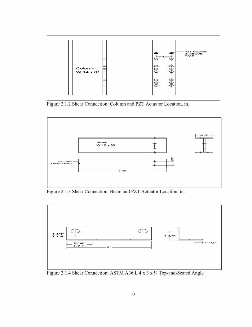
The shear connection (Figure 2.1.1) involves of W14 x 61 column (Figure 2.1.2), W 12 x

36 beam (Figure 2.1.3), and an ASTM A36 L 4 x 3 x ¼ top-and-seated angle (Figure 2.1.4).

Only the top angle for the connection, which typically used for stability, was of great

interest in this study allowing multiple tests to be made with minimal specimen preparation.

Due to this reason, detailed drawings for other components in the connection will not be

provided. Hardware for this connection include ¾ in. diameter ASTM A325 Type I Grade

5 Structural Bolts; as well as the corresponding F435-I hardened washers and ASTM A563

nuts. Under snug-tightened condition, those components conclude the shear connection.

Figure 2.1.1 Shear Connection Assembly

9

Figure 2.1.2 Shear Connection: Column and PZT Actuator Location, in.

Figure 2.1.3 Shear Connection: Beam and PZT Actuator Location, in.

Figure 2.1.4 Shear Connection: ASTM A36 L 4 x 3 x ¼ Top-and-Seated Angle

10

2.2 Fatigue Property Estimation

Fatigue damage is a common failure mode for metals. Metals subjected to axial; flexural;

torsional; or a combination of these types of forces, could be damaged by loadings within

the design limits due to cyclic effect. ASTM defines fatigue strength, as the value of stress

at which failure occurs after certain cycles, and fatigue limit, as the limiting value of stress

at which failure occurs as fatigue life becomes very large [53]. Typically, for steel, finite

life region is around 106 cycles.

Since the 1800s, the stress-based approach has become the standard fatigue analysis

method. This method is referred as the stress-life (S-N) approach. In this approach, fatigue

property of a component is characterized in the relationship of stress and the associated

fatigue life. In general, it has been observed that as the stress level increases the fatigue life

in log scale decreases [54].

To estimate fatigue property for ASTM A36 L 4 x 3 x ¼ angle, stress-life approach was

applied in this study. To begin with, fatigue strength at 103 and 106 were estimated. Since

this study only emphasize on the detection of fatigue damage, a precise fatigue property

estimation was not a significant consideration, as long the specimen was not subjected to

plastic deformation. Hence, it is logical to assume the beam leg of the angle as a cantilever

beam (Error! Reference source not found.) due to similarities in their geometry and

behaviors under flexural loading.

11

Figure 2.2.1 Section Property for ASTM A36 L 4 x 3 x ¼ Angle

Table 2.2.1 Section Properties for ASTM A36 Angle

Section Properties Width, in. 8 Height, in. 0.25

Moment of Inertia, in4 0.0104 Length of Beam, in. 3.375

Length from Point of Load to Free End, in. 1.5 Hole Diameter, in. 0.75 Yield Strength, ksi 36

Ultimate Tensile Strength, ksi 58 Young’s Modulus, ksi 29,000

12

Section properties for this angle is illustrated in Table 2.2.1. According to [12], the bending

fatigue strength at 103 for all types of material is estimated as 90 percent of the ultimate

strength. Consequently, the fatigue strength for steel at 103 cycles is estimated as 52.2 ksi.

Fatigue strength at 106 cycles, on the other hand, was predicated as the multiplication of

0.5 to the ultimate tensile strength of steel and adjustment factors corresponding to Hot-

Roll steel (0.76), which final rapture would occur at 106 cycles of constant loading at 25.56

ksi of bending stress. The result of Stress-life curve was plotted using linear interpolation

in log scales. Figure 2.2.2 demonstrates the stress-life curve for ASTM A36 L 4 x 3 x 1/4

hot-rolled angle.

Figure 2.2.2 Stress-Life Curve ASTM A36 Hot-Rolled Steel

However, the stress-life approach has been accused insufficient in fatigue design, since this

approach depends on a large number of testing and statistical analysis. What’s more,

material’s geometry factors, size factors, surface finishing factors, and loading types should

all be taken into consideration when estimating fatigue properties. Sophisticated

13

approaches have been developed since then, such as the strain-based fatigue analysis and

the mean stress correction method. Nonetheless, the purpose of this study aimed to

duplicate fatigue damage, stress-life method is proven capable of providing insights on

fatigue properties.

2.3 High-Cycle Fatigue Test

High-Cycle Fatigue test offers an opportunity to replicate naturally occurred fatigue

damage with little plastic deformation. The top-and-seated angle of the connection was

tested mechanically in a condition of cyclic transverse bending at the frequency of 5Hz

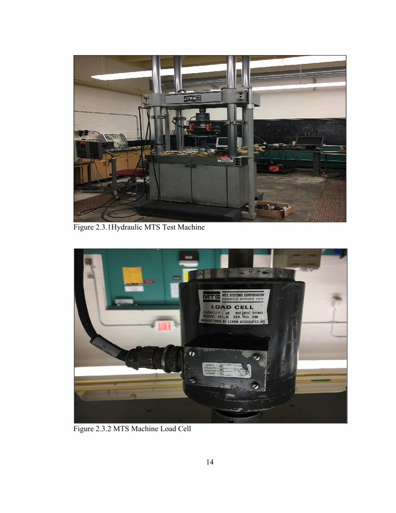
without any mean stress effect. This test was operated on Hydraulic MTS Machine at

displacement control, according to the assumed cantilever beam modal; decisions of a ±

0.01 in. displacement representing 33 ksi of stress was made as the input parameter exerted

to the beam leg of the angle. However, since the stress was dissipated by the hardware and

other components in the assembly, the real input displacement was ± 0.1 in. Since at this

parameter, expected reaction can be reached according to load cell reading. Final fracture

of the specimen was expected to occur around 130,000 cycles. Further results have shown

that this estimation was accurate.

14

Figure 2.3.1Hydraulic MTS Test Machine

Figure 2.3.2 MTS Machine Load Cell

15

Figure 2.3.3 High-Cycle Fatigue Test Setup

16

Figure 2.3.1through Figure 2.3.3 demonstrates the setup for this operation. Additional

ASTM A36 L 5 x 5 X ½ angle serves as a jig connecting the lower part of the machine and

the specimen. This connection jig was fastened to the machine, while ASTM A325 Type I

bolts from the shear connection fastened the outstanding leg of the angle to the connection

jig. Two steel rods were bolted together where the beam leg of the angle was sandwiched

in between. Cyclic bending stress was subjected to the specimen by vertical displacement

of the connection jig. Bending stress was mostly exerted to the outstanding leg of the angle.

Nevertheless, in order to accelerate fatigue process, square notches were cut on both side

of the beam leg with hacksaw in an effort to initiate fatigue cracks at the highest stress

concentration. The result for this test can be found in Chapter 3.

2.4 Low-Cycle Fatigue Test

The goal of this operation was to duplicate fatigue damage under 102 cycles. Despite the

fact that high-cycle fatigue damage is more devastating, health monitoring of low-cycle

fatigue damage is of equal importance. Regardless of the MTS load cell is capable of

withstanding loadings up to 10 metric tons, the abilities in withstanding fatigue damages

for other components in the assembly are questionable. Hence, instead of conducting

mechanical test on the MTS machine, the angle was damaged by means of lever action. As

illustrated in Figure 2.4.1, a lumber pole modal was attached to the outstanding leg of the

angle. This modal consists of two 7-feet 4 x 4 southern pine construction lumbers as levers,

and two 4-inch 4 x 4 southern pine cubic transferring the bending stress from the lever to

the angle. In addition, two 1-foot 2 x 4 southern pine boards sandwiching the components

mentioned above from top and bottom in order to prevent shear failures. All lumber

17

components were connected with lag bolts. To fasten this modal to the outstanding leg of

the angle, two 3/4 -10 grade 8 bolts were applied. The angle was then attached to a w 12 x

36 beam. To prevent uplift motion from happening, the beam was clamped to a 10-feet- w

10 x 35 beam.

Figure 2.4.1 Experimental Setup for Low-Cycle Fatigue Test

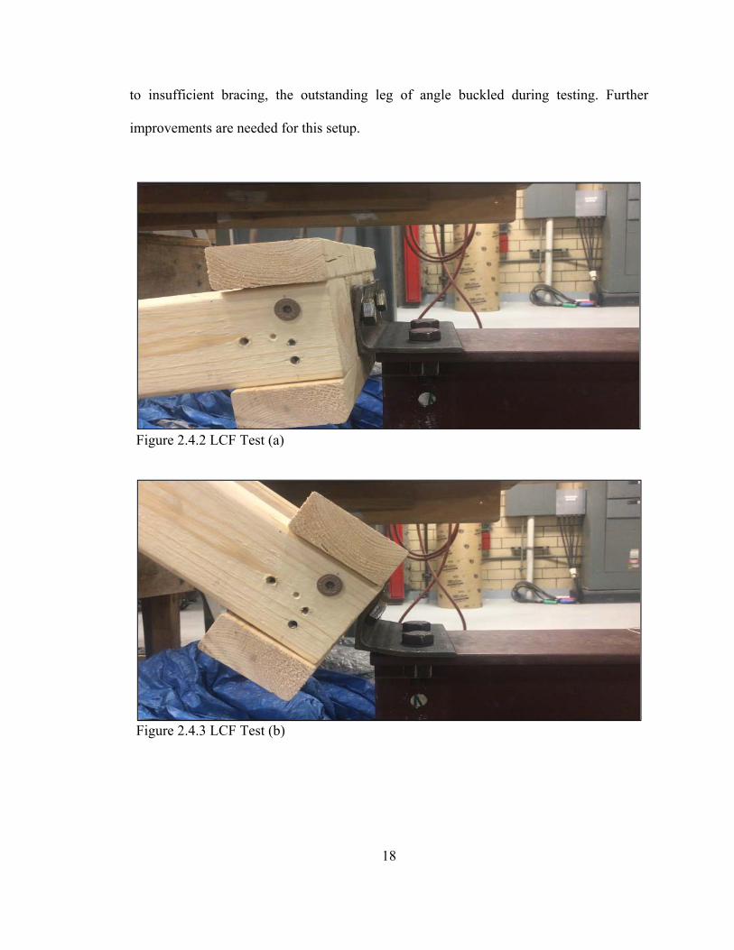
Since the lumber lever was long enough, the full body weight for an adult is sufficient to

exert LCF damage to the outstanding leg of the angle. Because of the prying effect, the

beam leg was also subjected to cyclic bending stress as well. Hence, plastic deformation

can be found in both legs of the angle (Figure 2.4.2 and Figure 2.4.3). Unfortunately, due

18

to insufficient bracing, the outstanding leg of angle buckled during testing. Further

improvements are needed for this setup.

Figure 2.4.2 LCF Test (a)

Figure 2.4.3 LCF Test (b)

19

2.5 Bolt Looseness

Constantly removing and replacing the top angle of the connection could introduce

randomness to this study due to bolt looseness. However, results have been shown that

acoustic wave propagation technique was not sensitive to this effect. Bolt looseness on

each leg of the angle was investigated individually. RCSC defines the snug-tightened

condition as “the tightness that is attained with a few impacts of an impact wrench or the

full effort of an ironworker using an ordinary spud wrench to bring the piles into firm

contact” [55]. For this operation, torque wrench was applied to keep the consistency of the

testing. Bolts were fastened tightly initially and were loosened gradually by half turns until

the nuts were completely unscrewed.

2.6 Data Acquisition

Data acquisition procedure includes the excitation of the system and data collection

process. Acellent SMP-SP-1/4-20 PZT patches (Figure 2.6.1) were served as actuator and

sensors. The actuator was glued to the center of the beam flange with epoxy glue, while

the sensors were attached to the column flange, 2 in. above the fasteners connecting the

angle and the column. The data acquisition network is demonstrated in Figure 2.6.2.

The beam-to-column connection with fatigue-damaged angles were excited with a five-

peak morlet-wavelet at the frequency of 249.118 kHz and 1-volt peak-to-peak (Figure

2.6.3). Bolt looseness of the connection was also investigated under this approach. Agilent

33210A Function Generator served as the input source of the five-peak morlet-wavelet.

Next, the signal was transmitted to Krohn-Hite Model 7500 Amplifier. Meanwhile, the

20

input signal was monitored by Agilent MSO 7014A Oscilloscope. 20-Db of gain was added

to the input signal by the amplifier. This amplified signal was then propagated to PZT

actuator attached to the beam flange of the connection. Electronic signal was converted to

mechanical strain during this process and thus the connection was actuated. Morlet-wavelet

was able to propagate through the whole connection. PZT sensors glued to the column

picked up the reflected wavelet and feedback to oscilloscope. Sampling frequency for the

oscilloscope was at 109 Hz to avoid aliasing. The oscilloscope output three channels,

channel one monitored the input signal generated from the function generator, channel two

and channel three examined the activities from the PZT sensors respectively. PZT sensor

located on the left-hand side of the outstanding leg connected to channel two, and vice

versa. Each data acquisition process was repeated twenty times for individual fatigue stage.

Figure 2.6.1 Acellent SMP-SP-1/4-20 PZT Patch

21

Figure 2.6.2 Data Acquisition Network

Figure 2.6.3 Five Peak Morlet-Wavelet

22

2.7 Signal Processing

This section covers the signal preprocessing procedure. Signal preprocessing was

conducted in Matlab interface. Firstly, to avoid aliasing of the sampling process, sampling

frequency was set at 109 Hz and 10,000 samples were collected for each operation. Raw

time domain signals were normalized to the same amplitude and truncated to 4,096 samples

for further filtering purposes. All signals were centered at the mid-span of the time domain

in order to aid the calculation of output residuals.

Next, the extraction of reflected morlet-wavelet (which is the echo of the input signal

received by PZT sensors) from the preprocessed output signal was performed. Matched-

Filter was designed in this practice in Matlab interface. The theory behind Matched-filter

was explained by Turin [56]. In this study, matched-filter was created with the timely

reverse of input morlet-wavelet (Eq. 1), then convolution between the filter and the raw

output was performed (Eq.2). Since this filter maximizes the signal-to-noise ratio, the

algorithm was able to extract the reflected morlet-wavelet from noisy output data. The

output data is believed to have three components, (1) reflected morlet-wavelet; (2) Noise

induced from data acquisition process; and (3) Error information. With the reflection being

extracted from the output data, the subtraction between raw output and the match-filtered

output concludes the noise and error information (Eq.3). Because data acquisition process

was performed under laboratory environment and the mother wavelet was driven at high

frequency, it is logical to assume the noise components as white noise and remained

constant throughout the test. Hence, the output residual between raw output and match-

filtered output was able to represent error information introduced by fatigue damage.

23

However, it is common that digital filters used in the signal processing could corrupt the

original time scale of the data. This problem was taken into the considering in matlab.

(1)

∗ (2)

(3)

With output residuals being calculated, the physical identity of the connection can be

extracted in both time domain and Laplace domain. Firstly, the total absolute area under

the time domain output residual represents electrical energy (or strain energy due to the

special nature of piezoelectric materials), alterations in this value indicates variance in

energy attenuation of the morlet-wavelet as damage progresses. Thus, the output residual

was able to identify the error information. Two damage indexes for each fatigue stage were

created according to this error information in the time domain; they are demonstrated in

Equation (4) and Equation (5) respectively.

(4)

(5)

24

For each fatigue stage, the average and norm of the absolute value of output residual were

founded and plotted in matlab representing the energy attenuation level. Nonetheless, later

results illustrate that no significant trend was found in this technique.

Alternatively, in linear-time invariant systems, transfer function is one of the mathematical

tools in characterizing the relationship between input signals and output signals in Laplace

domain. Useful information can be extracted from the poles of the transfer function

regarding to natural frequency (real part of the pole) and damping ratio (imaginary part of

the pole) of the system. If the system is physically damaged, under the same mode, an

increase in damping ratio is expected. As a result, in an effort to identify the relationship

between the input signal and the error information, a 20 poles and 1 zero transfer function

between output residual and input data were generated in Matlab System Identification

ToolboxTM [57]. Yet, the output residual was dominated by the behavior of the wave at the

morlet-wavelet driving frequency. To have a clear picture of the actual error information,

the information embedded in low frequency should be removed. As can be seen in Figure

2.7.1, x-axis of the plot represents the frequency all the way up to the Nyquist frequency.

Low frequency components were mostly clustered within one percent of the Nyquist

frequency. Hence, a second-order Butterworth High-pass filter was applied to the output

residual in matlab with a cut-off frequency at 106 Hz. Low frequency components were

successfully removed (Figure 2.7.2). Similar to the energy attenuation method, time scaling

issue after the implementation of digital filter has been fixed. Damage indexes were created

based on the average-damping ratio from each fatigue stage (Eq. 6). This method has been

proven sensitive to fatigue damage.

25

(6)

Figure 2.7.1 Frequency Response of the High-Pass Filter vs Output Residual in Frequency Domain

Figure 2.7.2 Raw Output residual vs High-Pass Filtered Output Residual in Frequency Domain

26

3 Results and Discussion

3.1 High-Cycle Fatigue Damage

The fatigue testing undergoes with 123,000 loading cycles until the final fracture of the

specimen has occurred. Illustrated in Table 3.1.1, significant milestones for the test can be

seen. Up to 90,000 loading cycles, the reaction force from the load cell of the MTS machine

was found stable, indicating little strength reduction of the specimen and thus during this

period, no fatigue damage was initiated.

Figure 3.1.1 Crack Initiation at Left-Hand Side of the Beam Leg

27

At 120,000 cycles, an approximately 1/8 in. of crack has been developed at the left-hand

side notch of the beam leg (Figure 3.1.1). The author could have missed this feature without

a slow-motion camera. What’s more, at this stage the initial crack has been developed

towards the stress concentration. A 1/16 inch of crack was found at the end of this stage.

(Figure 3.1.2).

Figure 3.1.2 Crack Propagation at the Left-Hand-Side of Beam Leg

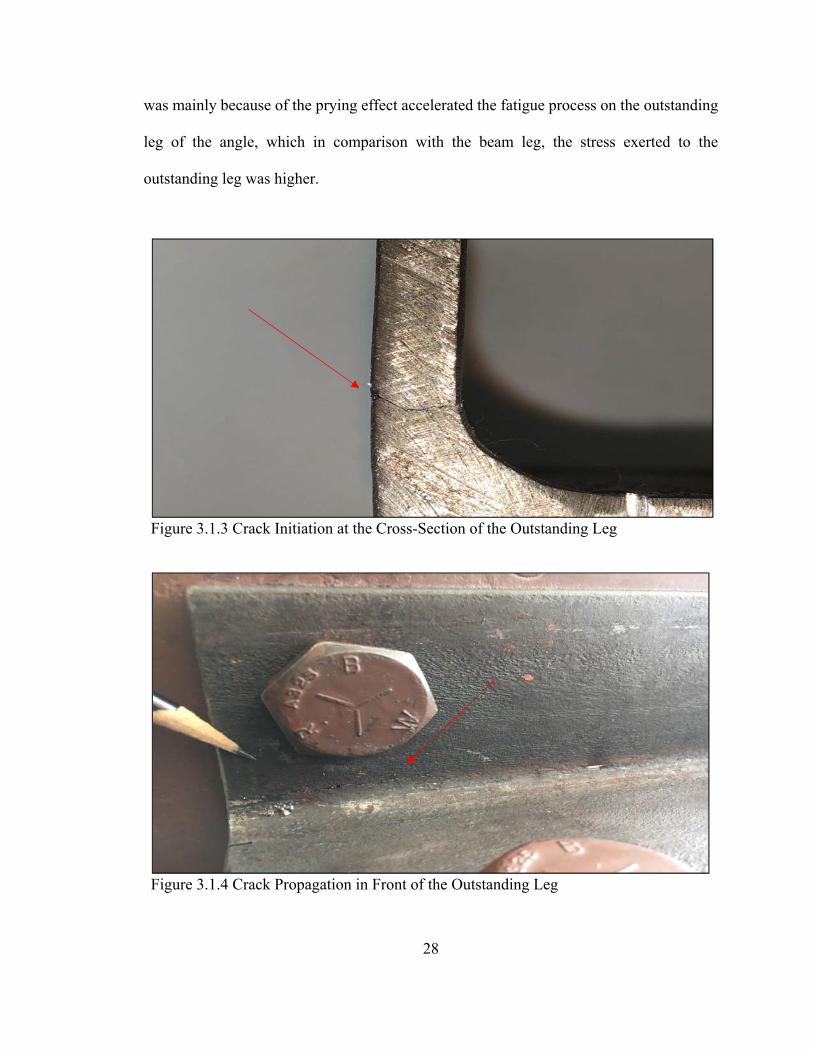
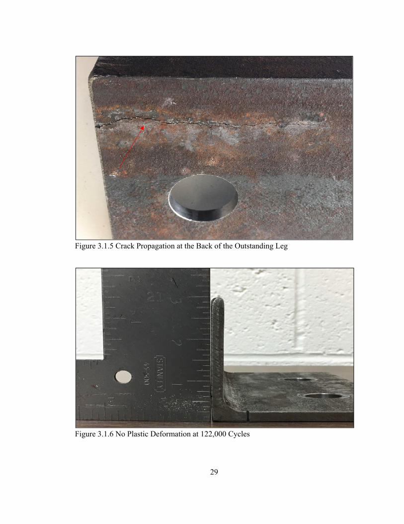
Around 122,000 cycles, significant cracks in macro scale can be detected in the outstanding

leg of the specimen. The crack was first developed at the left-hand-side cross-section of

the specimen 9/16 in. from the root radius (Figure 3.1.3). It developed rapidly so that at the

very end of test; there was a 2-7/8 in. of crack in the front side of the leg (Figure 3.1.4) as

well as a 2-1/2 in. in the back (Figure 3.1.5). At this stage, little plastic deformation can be

detected from the specimen (Figure 3.1.6). On the other hand, the cracks initiated from the

notch of the beam leg propagated further, but not in a significant scale (Figure 3.1.7). It

28

was mainly because of the prying effect accelerated the fatigue process on the outstanding

leg of the angle, which in comparison with the beam leg, the stress exerted to the

outstanding leg was higher.

Figure 3.1.3 Crack Initiation at the Cross-Section of the Outstanding Leg

Figure 3.1.4 Crack Propagation in Front of the Outstanding Leg

29

Figure 3.1.5 Crack Propagation at the Back of the Outstanding Leg

Figure 3.1.6 No Plastic Deformation at 122,000 Cycles

30

Figure 3.1.7 Crack Propagation at the Notch

At approximately 122,500 cycles, crack at the outstanding leg developed into 3 in. on the

front side (Figure 3.1.9) and 3-1/4 in. in the back (Figure 3.1.10). However, crack

propagation process in the beam leg slowed down, with little crack length increments at

this stage. No extra cracks were initiated d. It is also worthwhile to state that, at this stage,

fatigue cracks propagate in the fashion of intrusion and extrusion (Figure 3.1.8).

Figure 3.1.8 Fatigue Crack Behavior [12]

31

Figure 3.1.9 122,500 Cycle Crack Propagation at Front Side of Outstanding Leg

Figure 3.1.10 122,500 Cycle Crack Propagation at Back Side of Outstanding Leg

32

From 123,000 cycle to the final rapture of the specimen in the outstanding leg, crack

initiated at the left-hand side of the outstanding leg developed. In addition, further fatigue

crack was found initiated at the right-hand side of the outstanding leg. However, in

comparison with the scale of the left-hand side of the outstanding leg, the crack located in

the right-hand side of the leg was small but in substantial amount (Figure 3.1.11). At around

123,700 cycles, a significant strength reduction occurred. This phenomenon was detected

from the sudden drop of reaction force from the MTS testing machine’s load cell. Within

an instant, immediate separation of the outstanding leg from the angle occurred. Cracks

developed from both side of the leg united, which indicated a clear path of the stress

concentration (Figure 3.1.12, Figure 3.1.13, and Figure 3.1.14).

Figure 3.1.11 122,500 Cycle Crack Propagation at Back Side of Outstanding Leg

33

Figure 3.1.12 Final Rapture Front Side of the Outstanding Leg

Figure 3.1.13 Final Rapture Back Side of the Outstanding Leg

34

Figure 3.1.14 Final Fracture

Table 3.1.1 Fatigue Stage and Crack Length, High-Cycle Fatigue Test

Number of Interval

Number of Loading Cycles

Crack Length, in. Fatigue Stage

1 0 N/A N/A 2 50,000 N/A N/A 3 70,000 N/A N/A 4 90,000 N/A N/A

5 120,000 First visible crack Crack

Initiation

6 122,000 2-7/8 in. Crack

Propagation

7 122,500 3 in. (Front) & 3-1/4 in. (Back) Crack

Propagation

8 123,000 3-7/16 in. (Front) & 3-11/16 in.

(Back) Crack

Propagation

9 123,500 3-3/4 in. (Front) & 4-3/16 in.

(Back), Also, crack has initiated from the other side (2-3/4 in.)

Crack Propagation

10 123,700 Specimen ruptured Fracture

35

3.2 Feature Extraction Energy Attenuation Method

In this section, damage indexes according to the mean and the norm of the output residual

are plotted according to each fatigue stage. The x-axis of the plot represents fatigue stage

mentioned in Table 3.1.1. Figure 3.2.1 through Figure 3.2.4 demonstrates the feature

extraction process under energy attenuation method in time domain. While Figure 3.2.1

and Figure 3.2.2 illuminates DI at each fatigue stage, Figure 3.2.3 and Figure 3.2.4

illustrates DInorm. In contrary to the expectations where the four plots ought to show a

decreasing trend. The damage index did not trend up with the accumulation of fatigue

damage, and the statistical distribution of the values was random.

36

Figure 3.2.1 DI HCF (a)

Figure 3.2.2 DI HCF (b)

37

Figure 3.2.3 DInorm HCF (a)

Figure 3.2.4 DInorm HCF(b)

38

3.3 Feature Extraction Transfer Function Algorithm

The damage feature used in the energy attenuation method was dominated by the behavior

of the wave at the morlet-wavelet driving frequency. This behavior did not seem to be

especially sensitive to the fatigue damage induced into the angle. It was expected that an

alternative measure might be devised using the data collected at the various damage stages.

Investigating the error residuals, the portion of the signal remaining after the carrier morlet-

wavelet was (removed by the application of Matched filter) was proven sensitive.

To demonstrate the effect of pole migration clearly, one set of data was randomly chosen

to begin with. This set of data represents the physical attributes of the shear connection at

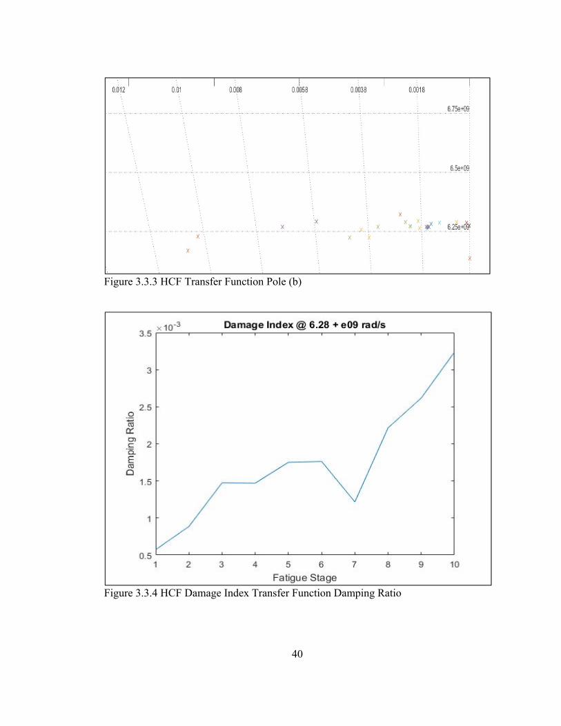
each fatigue stage. As can be seen from Figure 3.3.1 to Figure 3.3.3, pole migration was

detected at the frequency of 6.25 x 109 rad/s. Although pole migration also occurred at

other modes, this effect was due to the numerical artifacts generated from Matlab System

Identification ToolboxTM , and thus was not meaningful for this study. Next, all damping

ratio at this frequency was averaged. Damage indexes were created for each fatigue stage

based on this value. Figure 3.3.4 illuminates the plot against the damage index and fatigue

stage. Despite the fact that at fatigue stage seven (122,500 cycles), a decrease in damping

ratio was observed; this plot, overall, has satisfied the assumption that damping ratio

increases as damage accumulates. Hence, acoustic wave propagation processed with

transfer function algorithm has been proven sensitive to high-cycle fatigue damage.

39

Figure 3.3.1 HCF Transfer Function Frequency Respond

Figure 3.3.2 HCF Transfer Function Pole (a)

40

Figure 3.3.3 HCF Transfer Function Pole (b)

Figure 3.3.4 HCF Damage Index Transfer Function Damping Ratio

41

3.4 Low-Cycle Fatigue Damage

Low-cycle fatigue damage was exerted to the angle (Figure 3.4.1 through Figure 3.4.5).

Plastic hinges were formed at both legs of the angle (Figure 3.4.6). Similar to HCF test,

final fracture occurred at the outstanding leg, but the line of action was located at the holes.

Instant crack initiation and plastic deformation was observed during this test, and crack

propagation took most of the specimen’s fatigue life. Strength reduction of the specimen

was also encountered, less force were required to bend the specimen as test progressed.

Table 3.3.1 demonstrates the fatigue stage for the angle during the test.

Figure 3.4.1 LCF Damage (a)

42

Figure 3.4.2 LCF Damage (b)

Figure 3.4.3 Figure 3.4.3 LCF Damage (c)

43

Figure 3.4.4 LCF Damage (d)

Figure 3.4.5 LCF Damage (e)

44

Figure 3.4.6 LCF Damage, Plastic Hinge in Comparison with Baseline Structure

Table 3.3.1 Fatigue Stage, Low-cycle Fatigue Test

Number of Interval

Number of Loading Cycles

Fatigue Stage

1 0 N/A

2 20 Crack

Initiation

3 40 Crack

Propagation

4 45 Crack

Propagation

5 50 Crack

Propagation

6 53 Final

Rupture

45

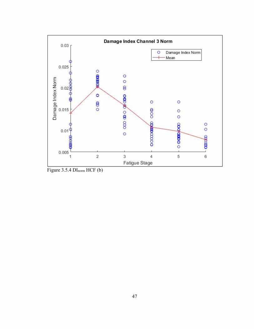
3.5 Feature Extraction Energy Attenuation Method

As can be seen from Figure 3.5.1 through Figure 3.5.4, acoustic wave propagation

technique was not sensitive to bolt looseness. The assumption of energy attenuation was

not satisfied as neither plot demonstrate a decrease trend in energy attenuation level.

Presumably, unlike little plastic information was subjected to high-cycle fatigue damaged

specimen, energy attenuation method could be also sensitive to plastic deformations. Thus,

further investigations are required on this assumption. What’s more, since only the top-

and-seated angle was damaged in this study, other components were not subjected to the

same level as the angle had. Hence, this aversive effect definitely corrupted the acoustic

wave propagation process. As a result, the investigation of LCF in this study only served

as a reference in fatigue damage detection.

Figure 3.5.1 DI LCF (a)

46

Figure 3.5.2 DI LCF (b)

Figure 3.5.3 DInorm LCF (a)

47

Figure 3.5.4 DInorm HCF (b)

48

3.6 Feature Extraction Transfer Function Algorithm

Figure 3.6.1 through Figure 3.6.3 demonstrates the frequency response and pole migrations

between the transfer functions of output residual and input signal. As can be seen in Figure

3.6.2 and Figure 3.6.3, pole migrates as damage increases. In comparison with HCF, pole

migration for LCF was triggered at 5.65 x 109 rad/s. Damage Indexes were created based

on this algorithm. A significant increase of the damping ratio was observed from fatigue

stage 2 to fatigue stage 5.

Figure 3.6.1 LCF Transfer Function Frequency Respond (a)

49

Figure 3.6.2 LCF Transfer Function Pole (a)

Figure 3.6.3 LCF Transfer Function Pole Enlarged (b)

50

Figure 3.6.4 LCF Transfer Function Damage Index

51

3.7 Bolt Looseness Investigation

The investigation of bolt looseness was carried out for each leg of the angle respectively.

Fasteners were snug tightened initially; this stage was characterized as ‘healthy’ structure.

Torque wrench was used to achieve snug-tight condition, 1,600 lb-in of torque was reached

during this process. Next, fasteners were unscrewed gradually until the bolt nuts loosened

completely. A 180-degree-turn was made at each subtest; the connection was then

investigated with acoustic wave propagation approach. Since the column flange is thicker

than the beam flange, it took 20 operations until the nut fall off from the connection; this

action was titled as column leg in the plots. While 23 operations were made until, no

clamping force can be observed between the leg and the beam flange; this action was

defined as beam leg in the following plots.

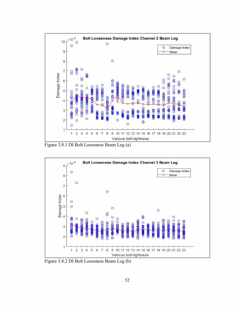
3.8 Feature Extraction Energy Attenuation Method

Figure 3.8.1 through Figure 3.8.4 demonstrates the energy attenuation level as clamping

force connecting the beam flange and the angle decreased. Little trend can be observed for

this operation. Figure 3.8.5 through Figure 3.8.8 illustrates energy attenuation level of

morlet-wavelet propagating through the column and outstanding leg of the angle. It has

been proved that energy attenuation approach was not sensitive in bolt looseness detection.

52

Figure 3.8.1 DI Bolt Looseness Beam Leg (a)

Figure 3.8.2 DI Bolt Looseness Beam Leg (b)

53

Figure 3.8.3 DInorm Bolt Looseness Beam Leg (a)

Figure 3.8.4 DInorm Bolt Looseness Beam Leg (b)

54

Figure 3.8.5 DI Bolt Looseness Column Leg (a)

Figure 3.8.6 DI Bolt Looseness Column Leg (b)

55

Figure 3.8.7 DInorm Bolt Looseness Column Leg (a)

Figure 3.8.8 DInorm Bolt Looseness Column Leg (b)

56

3.9 Feature Extraction Transfer Function Algorithm

As can be found through Figure 3.9.1 through Figure 3.9.4 results have shown that this

approach was not sensitive to bolt looseness. Figure 3.9.5 through Figure 3.9.8 has

confirmed negative results between column flange and outstanding leg of angle. No

significant pole migration was found.

Figure 3.9.1 Bolt Looseness Transfer Function Frequency Respond Beam Leg (a)

57

Figure 3.9.2 Bolt Looseness Transfer Function Pole Beam Leg (a)

Figure 3.9.3 Bolt Looseness Transfer Function Frequency Respond Beam Leg (b)

58

Figure 3.9.4 Bolt Looseness Transfer Function Pole Beam Leg (b)

Figure 3.9.5 Bolt Looseness Transfer Function Frequency Respond Column Leg (a)

59

Figure 3.9.6 Bolt Looseness Transfer Function Pole Column Leg (a)

Figure 3.9.7 Bolt Looseness Transfer Function Frequency Respond Column Leg (b)

60

Figure 3.9.8 Bolt Looseness Transfer Function Pole Column Leg (b)

61

4 Conclusion

In conclusion, transfer function pole migration method has been proven sensitive in

detecting high-cycle fatigue damage in shear connections. This result was not influence by

constant removal of the angle from the connection due to bolt looseness. What’s more,

matched-filter technique is able to extract known signals from corrupted data. Under field

conditions, this feature will definitely improve the accuracy in data acquisition process

during structural health monitoring. Besides, the effect of pole migration was detected for

LCF damaged specimen with transfer function algorithm, this method has been proven

sensitive in detecting brittle failure.

Further works are necessary based on this study. Firstly, it would be helpful to set up a

threshold-damping ratio between the ‘healthy’ and damaged components similar to the

carbon monoxide detector equipped in every household. As a result, damage detection

processes would be more efficient. Secondly, further research on optimal transfer function

size is needed. Matlab interface is only capable of creating small-scale transfer function; it

would be useful if a substantial sized transfer function were created. Thirdly, whether this

method is sensitive to the location of the damage is also worthwhile to investigate. Lastly,

despite the fact wireless sensor technologies were not applied in this study, it is the state-

of-art data acquisition algorithm in structural health monitoring. Hence, the structural

integrity of the whole structure can be monitored globally and proficiently.

62

5 Reference

[1] Gilsanz, Ramon., Vancura, Petr., "Understanding Seismic Design through a Musical Analog." Structure 22.14 (2015)

[2] Boroschek, R., et al. "Lessons from the 2010 Chile earthquake for performance based design and code development." Performance-based seismic engineering: Vision for an earthquake resilient society (2014): 143-157.

[3] Chen, Sheng-Jin, C. H. Yeh, and J. M. Chu. "Ductile steel beam-to-column connections for seismic resistance." Journal of Structural Engineering 122.11 (1996): 1292-1299.

[4] Chasten, Cameron P., et al. "Semi-Rigid Steel Connections and Their Effects on Structural Steel Frames." (1987).

[5] Chen, Wai-Fah, and N. Kishi. "Semirigid steel beam-to-column connections: Data base and modeling." Journal of Structural Engineering 115.1 (1989): 105-119.

[6] Roddis, WM Kim, and Deborah Blass. "Tensile capacity of single-angle shear connections considering prying action." Journal of Structural Engineering 139.4 (2013): 504-514.

[7] Astaneh-Asl, A. B. O. L. H. A. S. S. A. N. "Seismic performance and design of bolted steel moment-resisting frames." Engineering Journal 36.3 (1999): 105-120.

[8] Yun, Seung-Yul, et al. "Seismic performance evaluation for steel moment frames." Journal of Structural Engineering 128.4 (2002): 534-545.

[9] Haghani, Reza, Mohammad Al-Emrani, and Mohsen Heshmati. "Fatigue-prone details in steel bridges." Buildings 2.4 (2012): 456-476.

[10] Handbook, A. S. M. "Fatigue and fracture." ASM International 19 (1996): 18.

[11] Nip, K. H., et al. "Extremely low cycle fatigue tests on structural carbon steel and stainless steel." Journal of constructional steel research 66.1 (2010): 96-110.

[12] Lee, Yung-Li. Fatigue testing and analysis: theory and practice. Vol. 13. Butterworth-Heinemann, 2005.

[13] Botvina, L. R., et al. "High-cycle fatigue failure of low-carbon steel after long-term aging." Inorganic Materials 46.14 (2010): 1570-1577.

[14] Suh, C. M., R. Yuuki, and H. Kitagawa. "Fatigue microcracks in a low carbon steel." Fatigue & Fracture of Engineering Materials & Structures 8.2 (1985): 193-203.

63

[15] Abdalla, Khairedin M., Georgios A. Drosopoulos, and Georgios E. Stavroulakis. "Failure Behavior of a Top and Seat Angle Bolted Steel Connection with Double Web Angles." Journal of Structural Engineering 141.7 (2014): 04014172.

[16] Doebling, Scott W., et al. "Damage identification and health monitoring of structural and mechanical systems from changes in their vibration characteristics: a literature review." (1996).

[17] Shen, Ji Yao, Lonnie Sharpe, and Amy L. Jankovsky. "Overview of vibrational-based nondestructive evaluation techniques." Nondestructive evaluation of aging aircraft, airports, and aerospace hardware II. Vol. 3397. International Society for Optics and Photonics, 1998.

[18] Valis, David, et al. "Theoretical and experimental modal analysis." Update 2017 (1997): 06-01. [19] Ndambi, J.M., Vantomme, J., Harri, K., “Damage Assessment in Reinforced Concrete Beam Using Eigenfrequencies and Mode Shape Derivatives,” 2002, Engineering Structures, Elsevier, Vol. 24, Issue 4, pp. 501-515.

[20] Kim, J-T., and Norris Stubbs. "Improved damage identification method based on modal information." Journal of Sound and Vibration 252.2 (2002): 223-238.

[21] Kessler, Seth S., et al. "Damage detection in composite materials using frequency response methods." Composites Part B: Engineering 33.1 (2002): 87-95.

[22] Monaco, Ernesto, Francesco Franco, and Leonardo Lecce. "Experimental and numerical activities on damage detection using magnetostrictive actuators and statistical analysis." Journal of Intelligent Material Systems and Structures 11.7 (2000): 567-578.

[23] Mal, Ajit, et al. "A conceptual structural health monitoring system based on vibration and wave propagation." Structural Health Monitoring 4.3 (2005): 283-293.

[24] Farrar, Charles R., Scott W. Doebling, and David A. Nix. "Vibration–based structural damage identification." Philosophical Transactions of the Royal Society of London A: Mathematical, Physical and Engineering Sciences 359.1778 (2001): 131-149.

[25] Rose, Joseph L. "Ultrasonic waves in solid media." (2000): 1807-1808.

[26] Giurgiutiu, Victor, and Lingyu Yu. "Comparison of short-time fourier transform and wavelet transform of transient and tone burst wave propagation signals for structural health monitoring." Proceedings of 4th international workshop on structural health monitoring. 2003.

64

[27] Haugse, Eric, et al. "Crack growth detection and monitoring using broadband acoustic emission technique." Proc. of SPIE Mal AK Nondestructive evaluation of aging aircraft, airports, and aerospace hardware III 3586 (1999): 32-40.

[28] Chang, Zensheu, and Ajit Mal. "Wave propagation in a plate with defects." (1998).

[29] Shih, J. H., and A. K. Mal. "Acoustic emission from impact damage in cross-ply composites." Structural Health Monitoring. Vol. 1. 2000. 209-217..

[30] Mal, Ajit K., Frank Shih, and Sauvik Banerjee. "Acoustic emission waveforms in composite laminates under low velocity impact." Proceedings of SPIE. Vol. 5047. 2003.

[31] Li, Z. X., Tommy HT Chan, and Jan Ming Ko. "Fatigue analysis and life prediction of bridges with structural health monitoring data—Part I: methodology and strategy." International Journal of Fatigue 23.1 (2001): 45-53.

[32] Chan, Tommy HT, Z. X. Li, and Jan Ming Ko. "Fatigue analysis and life prediction of bridges with structural health monitoring data—Part II: Application." International Journal of Fatigue 23.1 (2001): 55-64.

[33] Baek, S. H., S. S. Cho, and W. S. Joo. "Fatigue life prediction based on the rainflow cycle counting method for the end beam of a freight car bogie." International Journal of Automotive Technology 9.1 (2008): 95-101.

[34] Roach, D. "Real time crack detection using mountable comparative vacuum monitoring sensors." Smart structures and systems 5.4 (2009): 317-328.

[35] Kong, Xiangxiong, et al. "Numerical simulation and experimental validation of a large-area capacitive strain sensor for fatigue crack monitoring." Measurement Science and Technology 27.12 (2016): 124009.

[36] Park, Gyuhae, Harley H. Cudney, and Daniel J. Inman. "Impedance-based health monitoring of civil structural components." Journal of infrastructure systems 6.4 (2000): 153-160.

[37] Ihn, Jeong-Beom, and Fu-Kuo Chang. "Detection and monitoring of hidden fatigue crack growth using a built-in piezoelectric sensor/actuator network: I. Diagnostics." Smart materials and structures 13.3 (2004): 609.

[38] Ihn, Jeong-Beom, and Fu-Kuo Chang. "Detection and monitoring of hidden fatigue crack growth using a built-in piezoelectric sensor/actuator network: II. Validation using riveted joints and repair patches." Smart materials and structures 13.3 (2004): 621.

65

[39] Xing, Ke Jia, and Claus Peter Fritzen. "Monitoring of growing fatigue damage using the E/M impedance method." Key Engineering Materials. Vol. 347. Trans Tech Publications, 2007.

[40] Giurgiutiu, Victor, et al. "Smart sensors for monitoring crack growth under fatigue loading conditions." Smart Structures and Systems 2.2 (2006): 101-113.

[41] Ng, Ching-Tai, and M. Veidt. "A Lamb-wave-based technique for damage detection in composite laminates." Smart materials and structures 18.7 (2009): 074006.

[42] Young Noh, Hae, et al. "Use of wavelet-based damage-sensitive features for structural damage diagnosis using strong motion data." Journal of Structural Engineering 137.10 (2011): 1215-1228.

[43] Huang, Shyh-Jier, and Cheng-Tao Hsieh. "High-impedance fault detection utilizing a Morlet wavelet transform approach." IEEE Transactions on Power Delivery 14.4 (1999): 1401-1410.

[44] Liang, Chen, F. P. Sun, and C. A. Rogers. "An impedance method for dynamic analysis of active material systems." Journal of Vibration and Acoustics 116.1 (1994): 120-128.

[45] Park, Gyuhae, et al. "Overview of piezoelectric impedance-based health monitoring and path forward." Shock and Vibration Digest 35.6 (2003): 451-464.

[46] Giurgiutiu, Victor, Anthony Reynolds, and Craig A. Rogers. "Experimental investigation of E/M impedance health monitoring for spot-welded structural joints." Journal of Intelligent Material Systems and Structures 10.10 (1999): 802-812.

[47] Sreenivas, K., et al. "Surface acoustic wave propagation on lead zirconate titanate thin films." Applied physics letters 52.9 (1988): 709-711.

[48] Song, Gangbing, Haichang Gu, and Hongnan Li. "Application of the piezoelectric materials for health monitoring in civil engineering: an overview." Engineering, Construction, and Operations in Challenging Environments: Earth and Space 2004. 2004. 680-687.

[49] Drafts, Bill. "Acoustic wave technology sensors." IEEE Transactions on microwave theory and techniques 49.4 (2001): 795-802.

[50] Madhav, Annamdas Venu Gopal, and Chee Kiong Soh. "An electromechanical impedance model of a piezoceramic transducer-structure in the presence of thick adhesive bonding." Smart Materials and Structures 16.3 (2007): 673.

66

[51] Bancroft, John C. "Introduction to matched filters." CREWES Research (2002).

[52] Swartz, R. Andrew, and Jerome P. Lynch. "Damage characterization of the Z24 bridge by transfer function pole migration." Proceedings of the 26th International Modal Analysis Conference (IMAC’08). 2008.

[53] Beer, Ferdinand P. Mechanics of Materials. New York: McGraw-Hill Higher Education, 2009. Print.

[54] Designation, A. S. T. M. "E739-10,“." Standard Practice for Statistical Analysis of Linear or Linearized Stress-Life (SN) and Strain-Life (e À N) Fatigue Data.

[55] Carter, C.J., Schlafly, T.J., “What is Snug, Anyway,” 2016, Steel wise-Modern Steel Construction, American Institute of Steel Construction.

[56] Turin, George. "An introduction to matched filters." IRE transactions on Information theory 6.3 (1960): 311-329.