Experimental and numerical investigation of fatigue damage due to wave-induced vibrations in a...
18
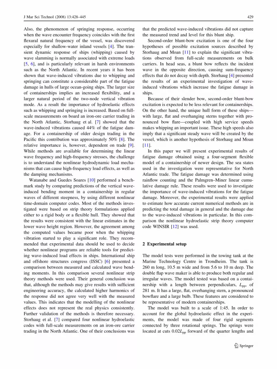
ORIGINAL ARTICLE Experimental and numerical investigation of fatigue damage due to wave-induced vibrations in a containership in head seas Ingo Drummen Gaute Storhaug Torgeir Moan Received: 20 August 2007 / Accepted: 28 February 2008 / Published online: 5 August 2008 Ó JASNAOE 2008 Abstract Fatigue cracks have been known to occur in welded ships for several decades. For large ocean-going ships wave-induced vibrations can, depending on trade and design, cause up to 50% of the fatigue damage. The vibrations may be due to springing and whipping effects. In this paper, we address the fatigue damage caused by wave- induced vibrations in a containership of newer design trading in the North Atlantic. The fatigue damage was obtained both experimentally and numerically. The experimental results were found from tests performed with a flexible model of the ship, while the numerical predic- tions were done using nonlinear hydroelastic strip theory. The measurements showed that the wave-induced vibra- tions contributed approximately 40% of the total fatigue damage. The numerical method predicted the wave fre- quency damage well, but was found to overestimate the total fatigue damage by 50%. This was mainly due to an overprediction of the wave-induced vibrations. The dis- crepancy is partly related to three-dimensional (3D) effects which are not included in the two-dimensional (2D) slamming calculation, and partly to an overprediction of the springing contribution. Moreover, the numerical method does not account for the steady wave due to for- ward speed. By using a simplified approach we show that high-frequency damage can be significantly reduced by including the steady wave for the relevant vessel, implying better agreement with the experimental results. Keywords Fatigue damage Hydroelastic Experiments Strip theory Containership 1 Introduction Towards the end of 2005, the world fleet of fully cellular containerships consisted of 3,500 vessels, with a combined capacity of 8 million twenty-foot equivalent unit (TEU) [1]. As there is almost no limit to the type of commodities that can be transported in a container, the containership market has grown faster than world trade and the economy in general. In order to meet this demand, the dimensions of containerships have increased steadily over the past few decades. Although the development of containerships sig- nificantly larger than those in operation today will be limited by aspects such as: (a) water depth in ports, (b) limiting dimensions of canals and straits on the major world routes, and (c) cargo handling facilities in container terminals, it is expected that the trend of increasing dimensions will continue for some years to come. Fatigue cracks have been known to occur in welded ships for several decades, and with the introduction of higher tensile steels in hull structures the fatigue problem has become more imminent. Fatigue analysis procedures were developed to account for wave frequency loads [2, 3]. I. Drummen G. Storhaug Centre for Ships and Ocean Structures, Norwegian University of Science and Technology, 7491 Trondheim, Norway G. Storhaug Det Norske Veritas, 1322 Høvik, Norway T. Moan Centre for Ships and Ocean Structures and Department of Marine Technology, Norwegian University of Science and Technology, 7491 Trondheim, Norway I. Drummen (&) Maritime Research Institute Netherlands, P.O. Box 28, 6700 AA Wageningen, The Netherlands e-mail: [email protected] 123 J Mar Sci Technol (2008) 13:428–445 DOI 10.1007/s00773-008-0006-5
-
Upload
independent -
Category
Documents
-
view
4 -
download
0
Transcript of Experimental and numerical investigation of fatigue damage due to wave-induced vibrations in a...
ORIGINAL ARTICLE
Experimental and numerical investigation of fatigue damagedue to wave-induced vibrations in a containership in head seas
Ingo Drummen Æ Gaute Storhaug Æ Torgeir Moan
Received: 20 August 2007 / Accepted: 28 February 2008 / Published online: 5 August 2008
� JASNAOE 2008
Abstract Fatigue cracks have been known to occur in
welded ships for several decades. For large ocean-going
ships wave-induced vibrations can, depending on trade
and design, cause up to 50% of the fatigue damage. The
vibrations may be due to springing and whipping effects. In
this paper, we address the fatigue damage caused by wave-
induced vibrations in a containership of newer design
trading in the North Atlantic. The fatigue damage was
obtained both experimentally and numerically. The
experimental results were found from tests performed with
a flexible model of the ship, while the numerical predic-
tions were done using nonlinear hydroelastic strip theory.
The measurements showed that the wave-induced vibra-
tions contributed approximately 40% of the total fatigue
damage. The numerical method predicted the wave fre-
quency damage well, but was found to overestimate the
total fatigue damage by 50%. This was mainly due to an
overprediction of the wave-induced vibrations. The dis-
crepancy is partly related to three-dimensional (3D) effects
which are not included in the two-dimensional (2D)
slamming calculation, and partly to an overprediction
of the springing contribution. Moreover, the numerical
method does not account for the steady wave due to for-
ward speed. By using a simplified approach we show that
high-frequency damage can be significantly reduced by
including the steady wave for the relevant vessel, implying
better agreement with the experimental results.
Keywords Fatigue damage � Hydroelastic �Experiments � Strip theory � Containership
1 Introduction
Towards the end of 2005, the world fleet of fully cellular
containerships consisted of 3,500 vessels, with a combined
capacity of 8 million twenty-foot equivalent unit (TEU)
[1]. As there is almost no limit to the type of commodities
that can be transported in a container, the containership
market has grown faster than world trade and the economy
in general. In order to meet this demand, the dimensions of
containerships have increased steadily over the past few
decades. Although the development of containerships sig-
nificantly larger than those in operation today will be
limited by aspects such as: (a) water depth in ports, (b)
limiting dimensions of canals and straits on the major
world routes, and (c) cargo handling facilities in container
terminals, it is expected that the trend of increasing
dimensions will continue for some years to come.
Fatigue cracks have been known to occur in welded
ships for several decades, and with the introduction of
higher tensile steels in hull structures the fatigue problem
has become more imminent. Fatigue analysis procedures
were developed to account for wave frequency loads [2, 3].
I. Drummen � G. Storhaug
Centre for Ships and Ocean Structures,
Norwegian University of Science and Technology,
7491 Trondheim, Norway
G. Storhaug
Det Norske Veritas, 1322 Høvik, Norway
T. Moan
Centre for Ships and Ocean Structures and Department
of Marine Technology, Norwegian University of Science
and Technology, 7491 Trondheim, Norway
I. Drummen (&)
Maritime Research Institute Netherlands,
P.O. Box 28, 6700 AA Wageningen, The Netherlands
e-mail: [email protected]
123
J Mar Sci Technol (2008) 13:428–445
DOI 10.1007/s00773-008-0006-5
Also, the phenomenon of springing response, occurring
when the wave encounter frequency coincides with the first
flexural natural frequency of the vessel, was discovered
especially for shallow-water inland vessels [4]. The tran-
sient dynamic response of ships (whipping) caused by
wave slamming is normally associated with extreme loads
[5, 6], and is particularly relevant in harsh environments
such as the North Atlantic. In recent years it has been
shown that wave-induced vibrations due to whipping and
springing can constitute a considerable part of the fatigue
damage in hulls of large ocean-going ships. The larger size
of containerships implies an increased flexibility, and a
larger natural period of the two-node vertical vibration
mode. As a result the importance of hydroelastic effects
such as whipping and springing is increased. Based on full-
scale measurements on board an iron-ore carrier trading in
the North Atlantic, Storhaug et al. [7] showed that the
wave-induced vibrations caused 44% of the fatigue dam-
age. For a containership of older design trading in the
Pacific this contribution was approximately 50% [8]. The
relative importance is, however, dependent on trade [9].
While methods are available for determining the linear
wave frequency and high-frequency stresses, the challenge
is to understand the nonlinear hydrodynamic load mecha-
nisms that can cause high-frequency load effects, as well as
the damping mechanisms.
Watanabe and Guedes Soares [10] performed a bench-
mark study by comparing predictions of the vertical wave-
induced bending moment in a containership in regular
waves of different steepness, by using different nonlinear
time-domain computer codes. Most of the methods inves-
tigated were based on strip theory formulations applied
either to a rigid body or a flexible hull. They showed that
the results were consistent with the linear estimates in the
lower wave height region. However, the agreement among
the computed values became poor when the whipping
vibration started to play a significant role. They recom-
mended that experimental data should be used to decide
whether nonlinear programs are reliable tools for predict-
ing wave-induced load effects in ships. International ship
and offshore structures congress (ISSC) [6] presented a
comparison between measured and calculated wave bend-
ing moments. In this comparison several nonlinear strip
theory methods were used. Their general conclusion was
that, although the methods may give results with sufficient
engineering accuracy, the calculated higher harmonics of
the response did not agree very well with the measured
values. This indicates that the modelling of the nonlinear
effects does not represent the real physics consistently.
Further validation of the methods is therefore necessary.
Storhaug et al. [7] compared four nonlinear hydroelastic
codes with full-scale measurements on an iron-ore carrier
trading in the North Atlantic. One of their conclusions was
that the predicted wave-induced vibrations did not capture
the measured trend and level for this blunt ship.
Second-order blunt-bow excitation is one of the four
hypotheses of possible excitation sources described by
Storhaug and Moan [11] to explain the significant vibra-
tions observed from full-scale measurements on bulk
carriers. In head seas, a blunt bow reflects the incident
wave in the opposite direction, causing sum-frequency
effects that do not decay with depth. Storhaug [4] presented
the results of an experimental investigation of wave-
induced vibrations which increase the fatigue damage in
ships.
Because of their slender bow, second-order blunt-bow
excitation is expected to be less relevant for containerships.
On the other hand, the unique hull form of these ships—
with large, flat and overhanging sterns together with pro-
nounced bow flare—coupled with high service speeds
makes whipping an important issue. These high speeds also
imply that a significant steady wave will be created by the
vessel, which is another hypothesis of Storhaug and Moan
[11].
In this paper we will present experimental results of
fatigue damage obtained using a four-segment flexible
model of a containership of newer design. The sea states
used in the investigation were representative for North
Atlantic trade. The fatigue damage was determined using
rainflow counting and the Palmgren–Miner linear cumu-
lative damage rule. These results were used to investigate
the importance of wave-induced vibrations for the fatigue
damage. Moreover, the experimental results were applied
to estimate how accurate current numerical methods are in
predicting the total damage in general and the damage due
to the wave-induced vibrations in particular. In this com-
parison the nonlinear hydroelastic strip theory computer
code WINSIR [12] was used.
2 Experimental setup
The model tests were performed in the towing tank at the
Marine Technology Centre in Trondheim. The tank is
260 m long, 10.5 m wide and from 5.6 to 10 m deep. The
double flap wave maker is able to produce both regular and
irregular waves. The model tested was based on a contai-
nership with a length between perpendiculars, Lpp, of
281 m. It has a large, flat, overhanging stern, a pronounced
bowflare and a large bulb. These features are considered to
be representative of modern containerships.
The model was built to a scale of 1:45. In order to
account for the global hydroelastic effect in the experi-
ments, the model was made of four rigid segments
connected by three rotational springs. The springs were
located at cuts 0.02Lpp forward of the quarter lengths and
J Mar Sci Technol (2008) 13:428–445 429
123
the midships section. The forward quarter length, midships
and aft quarter length sections will be denoted as QL-cut,
MS-cut and 3QL-cut, respectively. The horizontal forces,
which were converted to vertical bending moments as
discussed below, were measured 0.036Lpp forward of these
locations. These sections will be, respectively, denoted as
QL-cutm, MS-cutm and 3QL-cutm. All three springs had
equal stiffness, tuned to give the correct Froude scaled
natural frequency of the two-node vertical vibration,
23.55 rad/s (0.56 Hz, full scale). The natural frequencies of
the three- and four-node vertical vibration modes were
approximately equal to 55 and 86 rad/s, respectively.
We attempted to model one of the mass distributions
from the loading manual of the vessel. However, due to the
high mass of the springs it was not possible to obtain this
mass distribution in the model. More detailed information
about the experimental setup was given by Drummen [13].
The rigid-body motions were measured using an optical
system, while capacitive strips and wave probes measured
the relative motion and the wave elevation. Force trans-
ducers, measuring the horizontal force, were mounted in
the three cuts. The force transducers were placed above the
neutral axis of the model. In this way, the horizontal force
was a measure for the vertical bending moment, see Eq. 3.
Full-scale measurements, on the same containership for
which the model tests were performed, presented by
Storhaug and Moe [14] showed that the stress from the
axial force (horizontal force at the neutral axis) had the
same period as the wave frequency part of the vertical
bending stress and that the two were approximately in-
phase. The axial force at midships contributed a stress of
up to approximately 10% of that due to the vertical bending
moment. This means that the midships wave frequency
stresses presented in this paper may be up to 10% too high.
The effect is expected to be somewhat larger in the quarter
length cuts. This issue is investigated in more detail in the
subsequent discussion.
The model was tested in irregular head waves, as this
condition is usually the most severe with respect to the
vertical response. The sea states were taken from the North
Atlantic scatter diagram [15]. The chosen sea states are
given in Table 1. These represent approximately 17% of
the total number of sea states in the scatter diagram. Based
on this, it was possible to determine the damage in 33 other
sea states by means of interpolation. In this way 57% of the
scatter diagram was represented in the experiments. The
sea states outside this area in the scatter diagram make only
a small contribution to the fatigue damage. This contribu-
tion was estimated by a linear analysis to be approximately
10%. The JONSWAP spectrum was used as the target
wave spectrum [15]. The spectral density function is:
SfðxÞ ¼ ag2x�5 exp �5
4
xxp
� ��4" #
cexp �0:5
x�xprxp
� �2� �
; ð1Þ
where
a ¼ 5
16
H2s x
4p
g2ð1� 0:287 ln cÞ
r ¼0:07 if x�xp
0:09 if x [ xp
�
and x is the wave frequency, xp is the peak frequency and
g is the acceleration of gravity. The peakedness parameter,
c, was found by iteration using the significant wave height,
Hs, and the average zero crossing period, Tz, from the
scatter diagram, and the relations presented in DNV CN
30.5 [15].
The forward speed was chosen to be constant in sea
states with the same significant wave height, and was based
on full-scale measurements reported by Moe et al. [8]. The
full-scale forward speeds of the model in the investigated
sea states are given in Table 1.
For each sea state, three runs were conducted in waves
that were realisations of the same spectrum. The realisation
periods were short enough to avoid repeating wave trains.
The combination of the three runs resulted in a record
length between 30 and 45 min full scale, depending on the
chosen speed.
Table 1 Test program. Hs, Tp, c and U denote significant wave
height, peak period, peakedness parameter and vessel speed,
respectively
Number Hs (m) Tp (s) c U (kn)
1 3 10.6 1 22
2 3 13.4 1 22
3 3 16.3 1 22
4 3 19.1 1 22
5 5 10.4 1.5 20
6 5 13.4 1 20
7 5 16.3 1 20
8 5 19.1 1 20
9 7 9.5 5 16
10 7 13.4 1 16
11 7 16.3 1 16
12 7 19.2 1 16
13 9 9.5 5 12
14 9 12.8 2.3 12
15 9 16.3 1 12
16 9 19.1 1 12
430 J Mar Sci Technol (2008) 13:428–445
123
3 Fatigue damage
The fatigue damage was calculated using the Miner–
Palmgren linear cumulative damage rule:
D ¼Xn
i¼1
1
�aiðDriÞmi ; ð2Þ
where D is the accumulated fatigue damage, �ai and mi are
the parameters of the SN-curve, n is the total number of
stress ranges and Dri is the stress range. The parameters ai
and mi were taken from DNV CN 30.7 [3], using a two-
slope SN-curve for welded joints in air or with cathodic
protection. This means that:
log ai ¼ 12:65 and mi ¼ 3 for Dri� 76:5 MPa
log ai ¼ 16:42 and mi ¼ 5 for Dri\76:5 MPa:
By neglecting the axial force, the measured horizontal
force, Fx, was converted into full-scale stresses for a deck
detail assuming a simple beam model:
r ¼ Fxh
W� 1:025 � K4 � K; ð3Þ
where h is the vertical distance between the neutral axis
and the force transducer and K represents the scale factor.
K is the notch stress concentration factor, taken to be 2.0
for a typical hot spot of a fatigue-sensitive deck detail and
1.025 is the ratio of the density of saltwater and freshwater.
Using the program Nauticus Hull [16], the section moduli
at the deck, W, for the forward, midships and aft cuts were
found to be 27.4, 30 and 30 m3, respectively. The stress
cycles were counted using WAFO, a Matlab toolbox for
statistical analysis and simulation of random waves and
random loads developed at the Centre for Mathematical
Sciences at Lund University in Sweden. The rainflow
counting method used herein is based on the algorithm
described by Rychlik [17].
The fatigue damage can be separated into three cate-
gories. The total damage denotes the damage due to the
total stress history. Similarly, the wave frequency (WF)
damage denotes the fatigue damage due to the wave fre-
quency stresses. The latter was found by band-pass filtering
the stress signal to include only energy at frequencies in
the wave frequency range. The full-scale upper cutoff
frequency was 2.5 rad/s (0.4 Hz). By high-pass filtering
the original signal using this frequency as a lower cutoff
frequency, the high-frequency (HF) part of the stress was
obtained. The HF damage was found as the difference
between the total damage and the WF damage. To deter-
mine the increase of the fatigue damage due to the HF
stress by considering the HF stress only is nonconservative
due to the nonlinear dependence of the damage on the
stress (Eq. 2). This is illustrated by, amongst others,
Storhaug et al. [9]. Wave-induced vibrations or simply
vibrations is used in the following to denote the vibrations
that cause the high-frequency stress process.
Common practice in offshore engineering is to assume
that the residual stresses, introduced during fabrication at
welds, are close to the yield stress in tension. However,
external loads on ships cause these residual stresses to be
reduced over time. This implies that it could be possible
that part of the stress cycle is in compression, implying that
the effective stress range is smaller. There are, however,
three other important contributions to the mean stress, (a)
still-water loads induced due to the weight distribution and
buoyancy of the ship without forward speed, (b) loads due
to the steady flow resulting from the forward speed, and (c)
asymmetry in the dynamic wave loading. In still water
without forward speed, containerships mainly operate in
hogging conditions. The steady flow due to the forward
speed results in a vertical sagging bending moment in the
hull [18]. The asymmetry in dynamic wave loading is of
particular importance in containerships, for which the dif-
ference between sagging and hogging bending moments is
generally larger than for other ship types due to more
pronounced nonlinearities. This difference introduces a
nonzero (sagging) mean in the dynamic wave loading. In
general, however, the latter two contributions are signifi-
cantly smaller than that due to the weight distribution and
the buoyancy of the ship. Moreover, for sea states impor-
tant for fatigue, the dynamic loads will be smaller than the
static loads. For these reasons it is expected that the
complete stress cycle for a deck detail is in tension, which
means that the full stress cycle should be considered
effective. This statement will be quantified in the section
presenting the fatigue damage obtained experimentally.
4 Experimental results
4.1 General
This section deals with the experimental data and their
analysis. The results are scaled and presented for the full-
scale vessel. The zero level of the experimental responses
was taken to be the model in static equilibrium in still-
water, without any speed. Since damping is of particular
importance for the high-frequency fatigue damage, the
damping ratio obtained in the model tests will be covered
first. Subsequently, the standard deviations of the measured
stress histories are presented.
4.2 Damping ratio
Decay tests were performed to determine the damping
ratios in still water without forward speed. The natural
modes were excited by applying an impulsive force. This
J Mar Sci Technol (2008) 13:428–445 431
123
method should in general give vibration in all three flexible
modes. The damping ratios were determined by means of
the force transducer at midships, and were found to be
approximately equal to 0.65, 0.32 and 0.45% for the two-,
three- and four-node vibrations, respectively. Decay tests
were also performed with the model in air. For the two-
node mode, the natural frequency was found to be 32.2 rad/
s (model scale) and the damping ratio was estimated to be
0.2%. More details about the damping ratios and the
methods of estimation were presented by Drummen [13].
In order to minimise the uncertainty in the comparison
between experimental and numerical results, the damping
ratio discussed above was used as input for the simulations.
However, when the results from the model tests are used to
make statements about the full-scale vessel, it is important
to relate the damping ratio of the model to that of the full-
scale vessel.
From full-scale measurements on containerships,
Drummen et al. [19] and Storhaug and Moe [14] found
damping ratios of the two-node flexural mode to be sig-
nificantly higher than the value of 0.65% presented here.
The damping ratio found by full-scale measurements is
influenced by the cargo system, container racks, etc. These
influences on the damping ratio should be investigated. So
further study is necessary, particularly because the methods
to estimate damping under in-service conditions are prone
to large uncertainties. In the subsequent discussion some
results are presented showing the sensitivity of the high-
frequency damage to the damping ratio.
4.3 Stresses
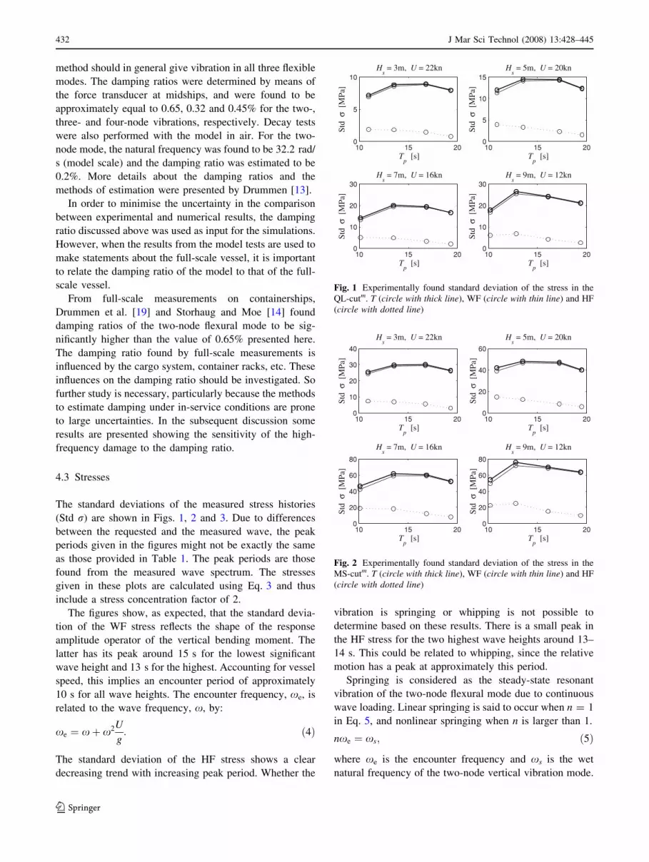
The standard deviations of the measured stress histories
(Std r) are shown in Figs. 1, 2 and 3. Due to differences
between the requested and the measured wave, the peak
periods given in the figures might not be exactly the same
as those provided in Table 1. The peak periods are those
found from the measured wave spectrum. The stresses
given in these plots are calculated using Eq. 3 and thus
include a stress concentration factor of 2.
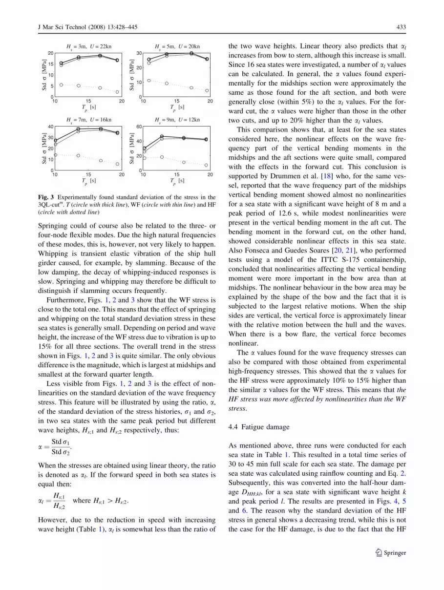
The figures show, as expected, that the standard devia-
tion of the WF stress reflects the shape of the response
amplitude operator of the vertical bending moment. The
latter has its peak around 15 s for the lowest significant
wave height and 13 s for the highest. Accounting for vessel
speed, this implies an encounter period of approximately
10 s for all wave heights. The encounter frequency, xe, is
related to the wave frequency, x, by:
xe ¼ xþ x2U
g: ð4Þ
The standard deviation of the HF stress shows a clear
decreasing trend with increasing peak period. Whether the
vibration is springing or whipping is not possible to
determine based on these results. There is a small peak in
the HF stress for the two highest wave heights around 13–
14 s. This could be related to whipping, since the relative
motion has a peak at approximately this period.
Springing is considered as the steady-state resonant
vibration of the two-node flexural mode due to continuous
wave loading. Linear springing is said to occur when n = 1
in Eq. 5, and nonlinear springing when n is larger than 1.
nxe ¼ xs; ð5Þ
where xe is the encounter frequency and xs is the wet
natural frequency of the two-node vertical vibration mode.
10 15 200
5
10 H
s= 3m, U = 22kn
Tp
[s]
Std
σ [
MPa
]
10 15 200
5
10
15 H
s= 5m, U = 20kn
Tp
[s]
Std
σ [
MPa
]
10 15 200
10
20
30 H
s= 7m, U = 16kn
Tp
[s]
Std
σ [
MPa
]
10 15 200
10
20
30 H
s= 9m, U = 12kn
Tp
[s]
Std
σ [
MPa
]
Fig. 1 Experimentally found standard deviation of the stress in the
QL-cutm. T (circle with thick line), WF (circle with thin line) and HF
(circle with dotted line)
10 15 200
10
20
30
40
Hs
= 3m, U = 22kn
Tp
[s]
Std
σ [
MPa
]
10 15 200
20
40
60
Hs
= 5m, U = 20kn
Tp
[s]
Std
σ [
MPa
]
10 15 200
20
40
60
80
Hs
= 7m, U = 16kn
Tp
[s]
Std
σ [
MPa
]
10 15 200
20
40
60
80
Hs
= 9m, U = 12kn
Tp
[s]
Std
σ [
MPa
]
Fig. 2 Experimentally found standard deviation of the stress in the
MS-cutm. T (circle with thick line), WF (circle with thin line) and HF
(circle with dotted line)
432 J Mar Sci Technol (2008) 13:428–445
123
Springing could of course also be related to the three- or
four-node flexible modes. Due the high natural frequencies
of these modes, this is, however, not very likely to happen.
Whipping is transient elastic vibration of the ship hull
girder caused, for example, by slamming. Because of the
low damping, the decay of whipping-induced responses is
slow. Springing and whipping may therefore be difficult to
distinguish if slamming occurs frequently.
Furthermore, Figs. 1, 2 and 3 show that the WF stress is
close to the total one. This means that the effect of springing
and whipping on the total standard deviation stress in these
sea states is generally small. Depending on period and wave
height, the increase of the WF stress due to vibration is up to
15% for all three sections. The overall trend in the stress
shown in Figs. 1, 2 and 3 is quite similar. The only obvious
difference is the magnitude, which is largest at midships and
smallest at the forward quarter length.
Less visible from Figs. 1, 2 and 3 is the effect of non-
linearities on the standard deviation of the wave frequency
stress. This feature will be illustrated by using the ratio, a,
of the standard deviation of the stress histories, r1 and r2,
in two sea states with the same peak period but different
wave heights, Hs;1 and Hs;2 respectively, thus:
a ¼ Std r1
Std r2
:
When the stresses are obtained using linear theory, the ratio
is denoted as al. If the forward speed in both sea states is
equal then:
al ¼Hs;1
Hs;2where Hs;1 [ Hs;2:
However, due to the reduction in speed with increasing
wave height (Table 1), al is somewhat less than the ratio of
the two wave heights. Linear theory also predicts that al
increases from bow to stern, although this increase is small.
Since 16 sea states were investigated, a number of al values
can be calculated. In general, the a values found experi-
mentally for the midships section were approximately the
same as those found for the aft section, and both were
generally close (within 5%) to the al values. For the for-
ward cut, the a values were higher than those in the other
two cuts, and up to 20% higher than the al values.
This comparison shows that, at least for the sea states
considered here, the nonlinear effects on the wave fre-
quency part of the vertical bending moments in the
midships and the aft sections were quite small, compared
with the effects in the forward cut. This conclusion is
supported by Drummen et al. [18] who, for the same ves-
sel, reported that the wave frequency part of the midships
vertical bending moment showed almost no nonlinearities
for a sea state with a significant wave height of 8 m and a
peak period of 12.6 s, while modest nonlinearities were
present in the vertical bending moment in the aft cut. The
bending moment in the forward cut, on the other hand,
showed considerable nonlinear effects in this sea state.
Also Fonseca and Guedes Soares [20, 21], who performed
tests using a model of the ITTC S-175 containership,
concluded that nonlinearities affecting the vertical bending
moment were more important in the bow area than at
midships. The nonlinear behaviour in the bow area may be
explained by the shape of the bow and the fact that it is
subjected to the largest relative motions. When the ship
sides are vertical, the vertical force is approximately linear
with the relative motion between the hull and the waves.
When there is a bow flare, the vertical force becomes
nonlinear.
The a values found for the wave frequency stresses can
also be compared with those obtained from experimental
high-frequency stresses. This showed that the a values for
the HF stress were approximately 10% to 15% higher than
the similar a values for the WF stress. This means that the
HF stress was more affected by nonlinearities than the WF
stress.
4.4 Fatigue damage
As mentioned above, three runs were conducted for each
sea state in Table 1. This resulted in a total time series of
30 to 45 min full scale for each sea state. The damage per
sea state was calculated using rainflow counting and Eq. 2.
Subsequently, this was converted into the half-hour dam-
age DHH;kl, for a sea state with significant wave height k
and peak period l. The results are presented in Figs. 4, 5
and 6. The reason why the standard deviation of the HF
stress in general shows a decreasing trend, while this is not
the case for the HF damage, is due to the fact that the HF
10 15 200
5
10
15
20 H
s= 3m, U = 22kn
Tp
[s]
Std
σ [
MPa
]
10 15 200
10
20
30 H
s= 5m, U = 20kn
Tp
[s]
Std
σ [
MPa
]
10 15 200
10
20
30
40 H
s= 7m, U = 16kn
Tp
[s]
Std
σ [
MPa
]
10 15 200
20
40
60 H
s= 9m, U = 12kn
Tp
[s]
Std
σ [
MPa
]
Fig. 3 Experimentally found standard deviation of the stress in the
3QL-cutm. T (circle with thick line), WF (circle with thin line) and HF
(circle with dotted line)
J Mar Sci Technol (2008) 13:428–445 433
123
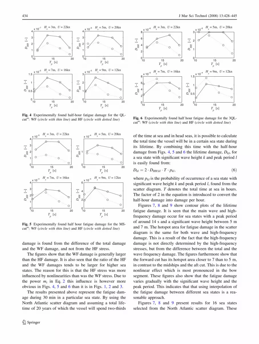
damage is found from the difference of the total damage
and the WF damage, and not from the HF stress.
The figures show that the WF damage is generally larger
than the HF damage. It is also seen that the ratio of the HF
and the WF damages tends to be larger for higher sea
states. The reason for this is that the HF stress was more
influenced by nonlinearities than was the WF stress. Due to
the power mi in Eq. 2 this influence is however more
obvious in Figs. 4, 5 and 6 than it is in Figs. 1, 2 and 3.
The results presented above represent the fatigue dam-
age during 30 min in a particular sea state. By using the
North Atlantic scatter diagram and assuming a total life-
time of 20 years of which the vessel will spend two-thirds
of the time at sea and in head seas, it is possible to calculate
the total time the vessel will be in a certain sea state during
its lifetime. By combining this time with the half-hour
damage from Figs. 4, 5 and 6 the lifetime damage, Dkl, for
a sea state with significant wave height k and peak period l
is easily found from:
Dkl ¼ 2 � DHH;kl � T � pkl; ð6Þ
where pkl is the probability of occurrence of a sea state with
significant wave height k and peak period l, found from the
scatter diagram. T denotes the total time at sea in hours.
The factor of 2 in the equation is introduced to convert the
half-hour damage into damage per hour.
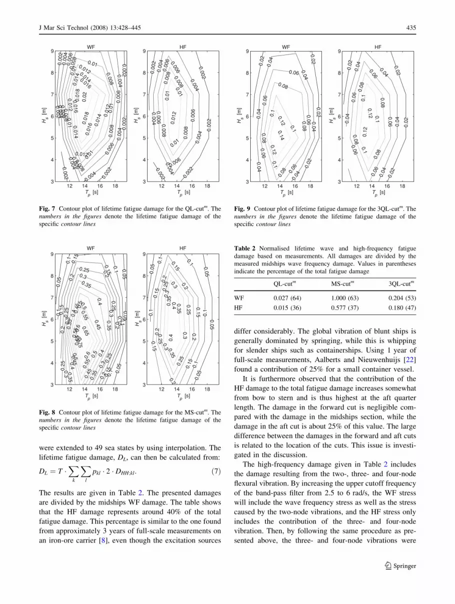
Figures 7, 8 and 9 show contour plots of the lifetime
fatigue damage. It is seen that the main wave and high-
frequency damage occur for sea states with a peak period
of around 14 s and a significant wave height between 5 m
and 7 m. The hotspot area for fatigue damage in the scatter
diagram is the same for both wave and high-frequency
damage. This is a result of the fact that the high-frequency
damage is not directly determined by the high-frequency
stresses, but from the difference between the total and the
wave frequency damage. The figures furthermore show that
the forward cut has its hotspot area closer to 7 than to 5 m,
in contrast to the midships and the aft cut. This is due to the
nonlinear effect which is most pronounced in the bow
segment. These figures also show that the fatigue damage
varies gradually with the significant wave height and the
peak period. This indicates that that using interpolation of
the fatigue damage between different sea states is a rea-
sonable approach.
Figures 7, 8 and 9 present results for 16 sea states
selected from the North Atlantic scatter diagram. These
10 15 200
1
2
3
4x 10
−7 Hs
= 3m, U = 22kn
Tp
[s]
DH
H [
−]
10 15 200
1
2
3
4x 10
−6 Hs
= 5m, U = 20kn
Tp
[s]
DH
H [
−]
10 15 200
0.5
1
1.5x 10
−5 Hs
= 7m, U = 16kn
Tp
[s]
DH
H [
−]
10 15 200
1
2
3x 10
−5 Hs
= 9m, U = 12kn
Tp
[s]
DH
H [
−]
Fig. 4 Experimentally found half-hour fatigue damage for the QL-
cutm: WF (circle with thin line) and HF (circle with dotted line)
10 15 200
1
2
3
4x 10
−5 Hs
= 3m, U = 22kn
Tp
[s]
DH
H [
−]
10 15 200
1
x 10−4 H
s= 5m, U = 20kn
Tp
[s]
DH
H [
−]
10 15 200
1
2
3
4x 10
−4 Hs
= 7m, U = 16kn
Tp
[s]
DH
H [
−]
10 15 200
2
4
6x 10
−4 Hs
= 9m, U = 12kn
Tp
[s]
DH
H [
−]
Fig. 5 Experimentally found half hour fatigue damage for the MS-
cutm: WF (circle with thin line) and HF (circle with dotted line)
10 15 200
2
4
6
8x 10
−6 Hs
= 3m, U = 22kn
Tp
[s]
DH
H [
−]
10 15 200
1
2
3x 10
−5 Hs
= 5m, U = 20kn
Tp
[s]
DH
H [
−]
10 15 200
2
4
6
8x 10
−5 Hs
= 7m, U = 16kn
Tp
[s]
DH
H [
−]
10 15 200
0.5
1
1.5x 10
−4 Hs
= 9m, U = 12kn
Tp
[s]
DH
H [
−]
Fig. 6 Experimentally found half hour fatigue damage for the 3QL-
cutm: WF (circle with thin line) and HF (circle with dotted line)
434 J Mar Sci Technol (2008) 13:428–445
123
were extended to 49 sea states by using interpolation. The
lifetime fatigue damage, DL, can then be calculated from:
DL ¼ T �X
k
Xl
pkl � 2 � DHH;kl: ð7Þ
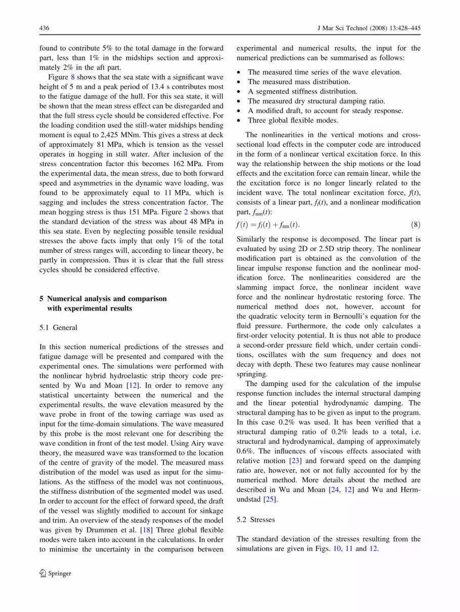
The results are given in Table 2. The presented damages
are divided by the midships WF damage. The table shows
that the HF damage represents around 40% of the total
fatigue damage. This percentage is similar to the one found
from approximately 3 years of full-scale measurements on
an iron-ore carrier [8], even though the excitation sources
differ considerably. The global vibration of blunt ships is
generally dominated by springing, while this is whipping
for slender ships such as containerships. Using 1 year of
full-scale measurements, Aalberts and Nieuwenhuijs [22]
found a contribution of 25% for a small container vessel.
It is furthermore observed that the contribution of the
HF damage to the total fatigue damage increases somewhat
from bow to stern and is thus highest at the aft quarter
length. The damage in the forward cut is negligible com-
pared with the damage in the midships section, while the
damage in the aft cut is about 25% of this value. The large
difference between the damages in the forward and aft cuts
is related to the location of the cuts. This issue is investi-
gated in the discussion.
The high-frequency damage given in Table 2 includes
the damage resulting from the two-, three- and four-node
flexural vibration. By increasing the upper cutoff frequency
of the band-pass filter from 2.5 to 6 rad/s, the WF stress
will include the wave frequency stress as well as the stress
caused by the two-node vibrations, and the HF stress only
includes the contribution of the three- and four-node
vibration. Then, by following the same procedure as pre-
sented above, the three- and four-node vibrations were
0.00
2
0.0020.002 0.
002
0.00
2
0.002
0.00
4
0.004
0.004
0.004
0.00
4
0.004
0.00
6
0.006
0.006
0.00
60.
006
0.008
0.00
8
0.008
0.008
0.00
8
0.01
0.01
0.01
0.01
0.01
0.012
0.01
2
0.012
0.012
0.014
0.01
4
0.014
0.01
40.016
0.01
6
0.016
0.01
8
0.01
80.
02
WF
Tp
[s]
Hs
[m]
12 14 16 183
4
5
6
7
8
9
0.00
2
0.002 0.00
2
0.00
2
0.002
0.00
4
0.004
0.004
0.00
4
0.004
0.006
0.00
6
0.006
0.006
0.00
6
0.008
0.00
8
0.008
0.00
8
0.01
0.01
0.01
0.01
2
HF
Tp
[s]
Hs
[m]
12 14 16 183
4
5
6
7
8
9
Fig. 7 Contour plot of lifetime fatigue damage for the QL-cutm. The
numbers in the figures denote the lifetime fatigue damage of the
specific contour lines
0.05
0.05
0.05
0.05
0.1
0.1
0.1
0.1
0.1
0.15
0.15
0.15
0.15
0.15
0.2
0.2
0.2
0.2
0.2
0.25
0.25
0.25
0.25
0.25
0.3
0.3
0.3
0.3
0.3
0.35
0.35
0.35
0.35
0.35
0.4
0.4
0.4
0.40.45
0.45
0.45
0.45
0.5
0.50.5
0.5
0.55
0.55
0.55
0.6
0.6 0.65
0.65 0.70.75
WF
Tp
[s]
Hs
[m]
12 14 16 183
4
5
6
7
8
9
0.05
0.05
0.050.05
0.1
0.1
0.1
0.1
0.1
0.15
0.15
0.15
0.15
0.15
0.2
0.2
0.2
0.2
0.2
0.25
0.25
0.25
0.25
0.3
0.3
0.3
0.3
0.35
0.35
0.35 0.4
0.4
HF
Tp
[s]
Hs
[m]
12 14 16 183
4
5
6
7
8
9
Fig. 8 Contour plot of lifetime fatigue damage for the MS-cutm. The
numbers in the figures denote the lifetime fatigue damage of the
specific contour lines
0.02
0.02
0.020.02
0.04
0.04
0.04
0.04
0.04
0.04
0.06
0.06
0.06
0.06
0.06
0.08
0.08
0.08
0.08
0.1
0.1
0.1
0.12
0.120.14
WF
Tp
[s]
Hs
[m]
12 14 16 183
4
5
6
7
8
9
0.02
0.02
0.02
0.020.04
0.04
0.04
0.04
0.04
0.06
0.06
0.06
0.06
0.06
0.08
0.08
0.08
0.08
0.1
0.1
0.1
0.12
0.12
HF
Tp
[s]
Hs
[m]
12 14 16 183
4
5
6
7
8
9
Fig. 9 Contour plot of lifetime fatigue damage for the 3QL-cutm. The
numbers in the figures denote the lifetime fatigue damage of the
specific contour lines
Table 2 Normalised lifetime wave and high-frequency fatigue
damage based on measurements. All damages are divided by the
measured midships wave frequency damage. Values in parentheses
indicate the percentage of the total fatigue damage
QL-cutm MS-cutm 3QL-cutm
WF 0.027 (64) 1.000 (63) 0.204 (53)
HF 0.015 (36) 0.577 (37) 0.180 (47)
J Mar Sci Technol (2008) 13:428–445 435
123
found to contribute 5% to the total damage in the forward
part, less than 1% in the midships section and approxi-
mately 2% in the aft part.
Figure 8 shows that the sea state with a significant wave
height of 5 m and a peak period of 13.4 s contributes most
to the fatigue damage of the hull. For this sea state, it will
be shown that the mean stress effect can be disregarded and
that the full stress cycle should be considered effective. For
the loading condition used the still-water midships bending
moment is equal to 2,425 MNm. This gives a stress at deck
of approximately 81 MPa, which is tension as the vessel
operates in hogging in still water. After inclusion of the
stress concentration factor this becomes 162 MPa. From
the experimental data, the mean stress, due to both forward
speed and asymmetries in the dynamic wave loading, was
found to be approximately equal to 11 MPa, which is
sagging and includes the stress concentration factor. The
mean hogging stress is thus 151 MPa. Figure 2 shows that
the standard deviation of the stress was about 48 MPa in
this sea state. Even by neglecting possible tensile residual
stresses the above facts imply that only 1% of the total
number of stress ranges will, according to linear theory, be
partly in compression. Thus it is clear that the full stress
cycles should be considered effective.
5 Numerical analysis and comparison
with experimental results
5.1 General
In this section numerical predictions of the stresses and
fatigue damage will be presented and compared with the
experimental ones. The simulations were performed with
the nonlinear hybrid hydroelastic strip theory code pre-
sented by Wu and Moan [12]. In order to remove any
statistical uncertainty between the numerical and the
experimental results, the wave elevation measured by the
wave probe in front of the towing carriage was used as
input for the time-domain simulations. The wave measured
by this probe is the most relevant one for describing the
wave condition in front of the test model. Using Airy wave
theory, the measured wave was transformed to the location
of the centre of gravity of the model. The measured mass
distribution of the model was used as input for the simu-
lations. As the stiffness of the model was not continuous,
the stiffness distribution of the segmented model was used.
In order to account for the effect of forward speed, the draft
of the vessel was slightly modified to account for sinkage
and trim. An overview of the steady responses of the model
was given by Drummen et al. [18] Three global flexible
modes were taken into account in the calculations. In order
to minimise the uncertainty in the comparison between
experimental and numerical results, the input for the
numerical predictions can be summarised as follows:
• The measured time series of the wave elevation.
• The measured mass distribution.
• A segmented stiffness distribution.
• The measured dry structural damping ratio.
• A modified draft, to account for steady response.
• Three global flexible modes.
The nonlinearities in the vertical motions and cross-
sectional load effects in the computer code are introduced
in the form of a nonlinear vertical excitation force. In this
way the relationship between the ship motions or the load
effects and the excitation force can remain linear, while the
the excitation force is no longer linearly related to the
incident wave. The total nonlinear excitation force, f(t),
consists of a linear part, fl(t), and a nonlinear modification
part, fnm(t):
f ðtÞ ¼ flðtÞ þ fnmðtÞ: ð8Þ
Similarly the response is decomposed. The linear part is
evaluated by using 2D or 2.5D strip theory. The nonlinear
modification part is obtained as the convolution of the
linear impulse response function and the nonlinear mod-
ification force. The nonlinearities considered are the
slamming impact force, the nonlinear incident wave
force and the nonlinear hydrostatic restoring force. The
numerical method does not, however, account for
the quadratic velocity term in Bernoulli’s equation for the
fluid pressure. Furthermore, the code only calculates a
first-order velocity potential. It is thus not able to produce
a second-order pressure field which, under certain condi-
tions, oscillates with the sum frequency and does not
decay with depth. These two features may cause nonlinear
springing.
The damping used for the calculation of the impulse
response function includes the internal structural damping
and the linear potential hydrodynamic damping. The
structural damping has to be given as input to the program.
In this case 0.2% was used. It has been verified that a
structural damping ratio of 0.2% leads to a total, i.e.
structural and hydrodynamical, damping of approximately
0.6%. The influences of viscous effects associated with
relative motion [23] and forward speed on the damping
ratio are, however, not or not fully accounted for by the
numerical method. More details about the method are
described in Wu and Moan [24, 12] and Wu and Herm-
undstad [25].
5.2 Stresses
The standard deviation of the stresses resulting from the
simulations are given in Figs. 10, 11 and 12.
436 J Mar Sci Technol (2008) 13:428–445
123
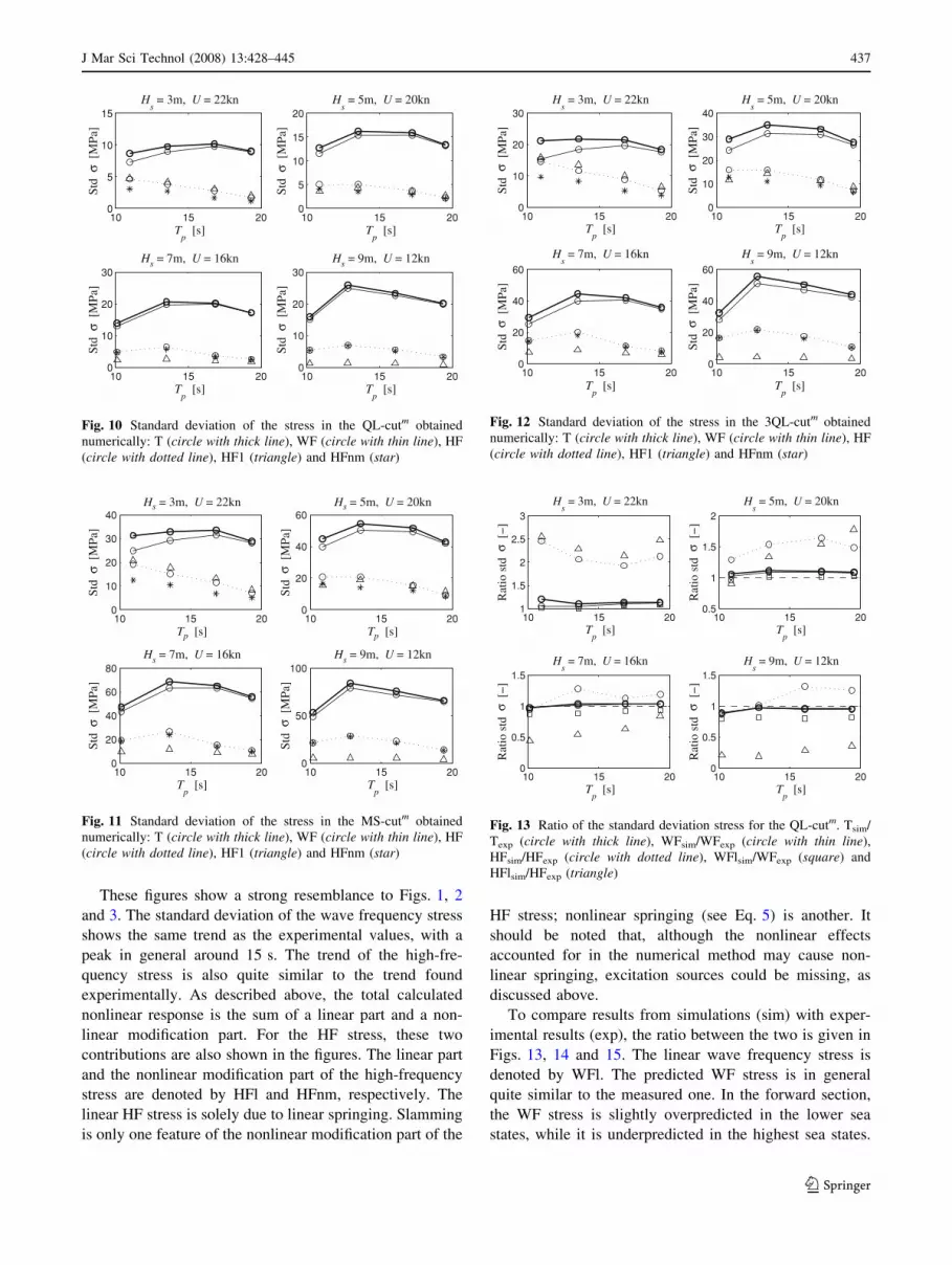
These figures show a strong resemblance to Figs. 1, 2
and 3. The standard deviation of the wave frequency stress
shows the same trend as the experimental values, with a
peak in general around 15 s. The trend of the high-fre-
quency stress is also quite similar to the trend found
experimentally. As described above, the total calculated
nonlinear response is the sum of a linear part and a non-
linear modification part. For the HF stress, these two
contributions are also shown in the figures. The linear part
and the nonlinear modification part of the high-frequency
stress are denoted by HFl and HFnm, respectively. The
linear HF stress is solely due to linear springing. Slamming
is only one feature of the nonlinear modification part of the
HF stress; nonlinear springing (see Eq. 5) is another. It
should be noted that, although the nonlinear effects
accounted for in the numerical method may cause non-
linear springing, excitation sources could be missing, as
discussed above.
To compare results from simulations (sim) with exper-
imental results (exp), the ratio between the two is given in
Figs. 13, 14 and 15. The linear wave frequency stress is
denoted by WFl. The predicted WF stress is in general
quite similar to the measured one. In the forward section,
the WF stress is slightly overpredicted in the lower sea
states, while it is underpredicted in the highest sea states.
10 15 200
5
10
15H
s= 3m, U = 22kn
Tp
[s]
Std
σ [
MPa
]
10 15 200
5
10
15
20H
s= 5m, U = 20kn
Tp
[s]
Std
σ [
MPa
]
10 15 200
10
20
30Hs = 7m, U = 16kn
Tp
[s]
Std
σ [
MPa
]
10 15 200
10
20
30Hs = 9m, U = 12kn
Tp
[s]
Std
σ [
MPa
]
Fig. 10 Standard deviation of the stress in the QL-cutm obtained
numerically: T (circle with thick line), WF (circle with thin line), HF
(circle with dotted line), HF1 (triangle) and HFnm (star)
10 15 200
10
20
30
40 Hs = 3m, U = 22kn
Tp [s]
Std
σ [
MPa
]
10 15 200
20
40
60 Hs = 5m, U = 20kn
Tp [s]
Std
σ [
MPa
]
10 15 200
20
40
60
80 Hs = 7m, U = 16kn
Tp
[s]
Std
σ [
MPa
]
10 15 200
50
100 Hs = 9m, U = 12kn
Tp
[s]
Std
σ [
MPa
]
Fig. 11 Standard deviation of the stress in the MS-cutm obtained
numerically: T (circle with thick line), WF (circle with thin line), HF
(circle with dotted line), HF1 (triangle) and HFnm (star)
10 15 200
10
20
30H
s= 3m, U = 22kn
Tp
[s]
Std
σ [
MPa
]
10 15 200
10
20
30
40H
s= 5m, U = 20kn
Tp
[s]
Std
σ [
MPa
]
10 15 200
20
40
60
Hs
= 7m, U = 16kn
Tp
[s]
Std
σ [
MPa
]
10 15 200
20
40
60
Hs
= 9m, U = 12kn
Tp
[s]
Std
σ [
MPa
]
Fig. 12 Standard deviation of the stress in the 3QL-cutm obtained
numerically: T (circle with thick line), WF (circle with thin line), HF
(circle with dotted line), HF1 (triangle) and HFnm (star)
10 15 201
1.5
2
2.5
3
Hs
= 3m, U = 22kn
Tp
[s]
Rat
io s
td σ
[−
]
10 15 200.5
1
1.5
2
Hs
= 5m, U = 20kn
Tp
[s]
Rat
io s
td σ
[−
]
10 15 200
0.5
1
1.5 H
s= 7m, U = 16kn
Tp
[s]
Rat
io s
td σ
[−
]
10 15 200
0.5
1
1.5 H
s= 9m, U = 12kn
Tp
[s]
Rat
io s
td σ
[−
]
Fig. 13 Ratio of the standard deviation stress for the QL-cutm. Tsim/
Texp (circle with thick line), WFsim/WFexp (circle with thin line),
HFsim/HFexp (circle with dotted line), WFlsim/WFexp (square) and
HFlsim/HFexp (triangle)
J Mar Sci Technol (2008) 13:428–445 437
123
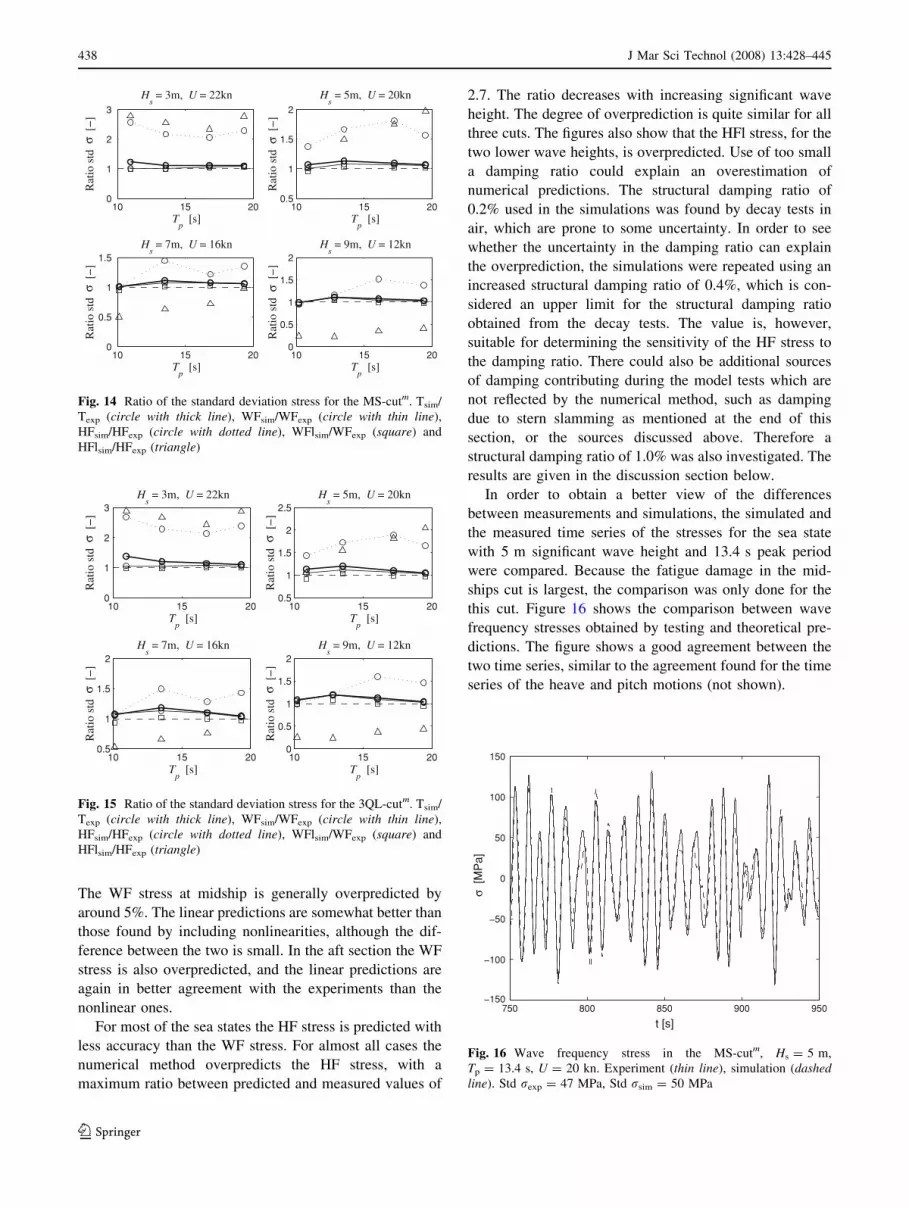
The WF stress at midship is generally overpredicted by
around 5%. The linear predictions are somewhat better than
those found by including nonlinearities, although the dif-
ference between the two is small. In the aft section the WF
stress is also overpredicted, and the linear predictions are
again in better agreement with the experiments than the
nonlinear ones.
For most of the sea states the HF stress is predicted with
less accuracy than the WF stress. For almost all cases the
numerical method overpredicts the HF stress, with a
maximum ratio between predicted and measured values of
2.7. The ratio decreases with increasing significant wave
height. The degree of overprediction is quite similar for all
three cuts. The figures also show that the HFl stress, for the
two lower wave heights, is overpredicted. Use of too small
a damping ratio could explain an overestimation of
numerical predictions. The structural damping ratio of
0.2% used in the simulations was found by decay tests in
air, which are prone to some uncertainty. In order to see
whether the uncertainty in the damping ratio can explain
the overprediction, the simulations were repeated using an
increased structural damping ratio of 0.4%, which is con-
sidered an upper limit for the structural damping ratio
obtained from the decay tests. The value is, however,
suitable for determining the sensitivity of the HF stress to
the damping ratio. There could also be additional sources
of damping contributing during the model tests which are
not reflected by the numerical method, such as damping
due to stern slamming as mentioned at the end of this
section, or the sources discussed above. Therefore a
structural damping ratio of 1.0% was also investigated. The
results are given in the discussion section below.
In order to obtain a better view of the differences
between measurements and simulations, the simulated and
the measured time series of the stresses for the sea state
with 5 m significant wave height and 13.4 s peak period
were compared. Because the fatigue damage in the mid-
ships cut is largest, the comparison was only done for the
this cut. Figure 16 shows the comparison between wave
frequency stresses obtained by testing and theoretical pre-
dictions. The figure shows a good agreement between the
two time series, similar to the agreement found for the time
series of the heave and pitch motions (not shown).
10 15 200
1
2
3
Hs
= 3m, U = 22kn
Tp
[s]
Rat
io s
td σ
[−
]
10 15 200.5
1
1.5
2
Hs
= 5m, U = 20kn
Tp
[s]
Rat
io s
td σ
[−
]
10 15 200
0.5
1
1.5 H
s= 7m, U = 16kn
Tp
[s]
Rat
io s
td σ
[−
]
10 15 200
0.5
1
1.5
2 H
s= 9m, U = 12kn
Tp
[s]
Rat
io s
td σ
[−
]
Fig. 14 Ratio of the standard deviation stress for the MS-cutm. Tsim/
Texp (circle with thick line), WFsim/WFexp (circle with thin line),
HFsim/HFexp (circle with dotted line), WFlsim/WFexp (square) and
HFlsim/HFexp (triangle)
10 15 200
1
2
3H
s= 3m, U = 22kn
Tp
[s]
Rat
io s
td σ
[−
]
10 15 200.5
1
1.5
2
2.5H
s= 5m, U = 20kn
Tp
[s]
Rat
io s
td σ
[−
]
10 15 200.5
1
1.5
2H
s= 7m, U = 16kn
Tp
[s]
Rat
io s
td σ
[−
]
10 15 200
0.5
1
1.5
2H
s= 9m, U = 12kn
Tp
[s]
Rat
io s
td σ
[−
]
Fig. 15 Ratio of the standard deviation stress for the 3QL-cutm. Tsim/
Texp (circle with thick line), WFsim/WFexp (circle with thin line),
HFsim/HFexp (circle with dotted line), WFlsim/WFexp (square) and
HFlsim/HFexp (triangle)
750 800 850 900 950−150
−100
−50
0
50
100
150
t [s]
σ [M
Pa]
Fig. 16 Wave frequency stress in the MS-cutm, Hs = 5 m,
Tp = 13.4 s, U = 20 kn. Experiment (thin line), simulation (dashedline). Std rexp = 47 MPa, Std rsim = 50 MPa
438 J Mar Sci Technol (2008) 13:428–445
123
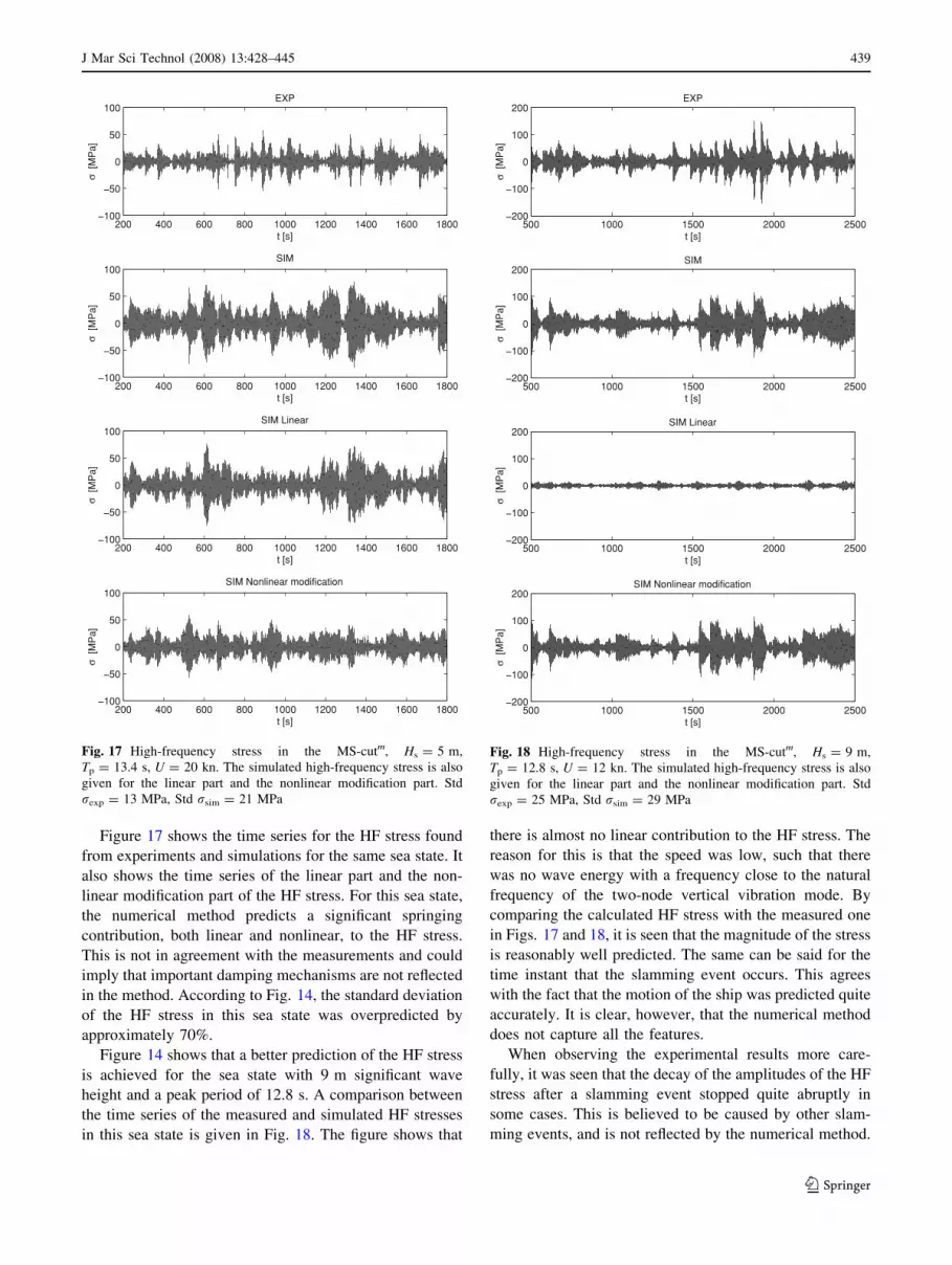
Figure 17 shows the time series for the HF stress found
from experiments and simulations for the same sea state. It
also shows the time series of the linear part and the non-
linear modification part of the HF stress. For this sea state,
the numerical method predicts a significant springing
contribution, both linear and nonlinear, to the HF stress.
This is not in agreement with the measurements and could
imply that important damping mechanisms are not reflected
in the method. According to Fig. 14, the standard deviation
of the HF stress in this sea state was overpredicted by
approximately 70%.
Figure 14 shows that a better prediction of the HF stress
is achieved for the sea state with 9 m significant wave
height and a peak period of 12.8 s. A comparison between
the time series of the measured and simulated HF stresses
in this sea state is given in Fig. 18. The figure shows that
there is almost no linear contribution to the HF stress. The
reason for this is that the speed was low, such that there
was no wave energy with a frequency close to the natural
frequency of the two-node vertical vibration mode. By
comparing the calculated HF stress with the measured one
in Figs. 17 and 18, it is seen that the magnitude of the stress
is reasonably well predicted. The same can be said for the
time instant that the slamming event occurs. This agrees
with the fact that the motion of the ship was predicted quite
accurately. It is clear, however, that the numerical method
does not capture all the features.
When observing the experimental results more care-
fully, it was seen that the decay of the amplitudes of the HF
stress after a slamming event stopped quite abruptly in
some cases. This is believed to be caused by other slam-
ming events, and is not reflected by the numerical method.
200 400 600 800 1000 1200 1400 1600 1800−100
−50
0
50
100EXP
t [s]
σ [M
Pa]
200 400 600 800 1000 1200 1400 1600 1800−100
−50
0
50
100SIM
t [s]
σ [M
Pa]
200 400 600 800 1000 1200 1400 1600 1800−100
−50
0
50
100SIM Linear
t [s]
σ [M
Pa]
200 400 600 800 1000 1200 1400 1600 1800−100
−50
0
50
100SIM Nonlinear modification
t [s]
σ [M
Pa]
Fig. 17 High-frequency stress in the MS-cutm, Hs = 5 m,
Tp = 13.4 s, U = 20 kn. The simulated high-frequency stress is also
given for the linear part and the nonlinear modification part. Std
rexp = 13 MPa, Std rsim = 21 MPa
500 1000 1500 2000 2500−200
−100
0
100
200EXP
t [s]
σ [M
Pa]
500 1000 1500 2000 2500−200
−100
0
100
200SIM
t [s]
σ [M
Pa]
500 1000 1500 2000 2500−200
−100
0
100
200SIM Linear
t [s]
σ [M
Pa]
500 1000 1500 2000 2500−200
−100
0
100
200SIM Nonlinear modification
t [s]
σ [M
Pa]
Fig. 18 High-frequency stress in the MS-cutm, Hs = 9 m,
Tp = 12.8 s, U = 12 kn. The simulated high-frequency stress is also
given for the linear part and the nonlinear modification part. Std
rexp = 25 MPa, Std rsim = 29 MPa
J Mar Sci Technol (2008) 13:428–445 439
123
One reason for this could be that the nonlinear modification
part of the stress is based on the incident wave elevation,
and does not include the effect of the radiated and the
diffracted wave. This is particularly important for the
present tests, as the flat stern of the model was only slightly
elevated above the water surface. Stern slamming could
then easily be induced by, and damp, whipping events. This
will also reduce the springing vibrations. Inclusion of the
steady wave in the numerical method will have an effect on
the HF stress as well. This feature is investigated in a
simplified manner in the subsequent discussion.
It is noted that a large contribution to the HF stress
is caused by bow flare slamming. This slamming force
is predicted by using strip theory, while the actual flow is
three dimensional. Based on results from a water entry
study by Scolan and Korobkin [26] it was estimated that
the 2D slamming force can be approximately 20% larger
than the 3D force. More details about this estimate were
presented by Drummen et al. [18]
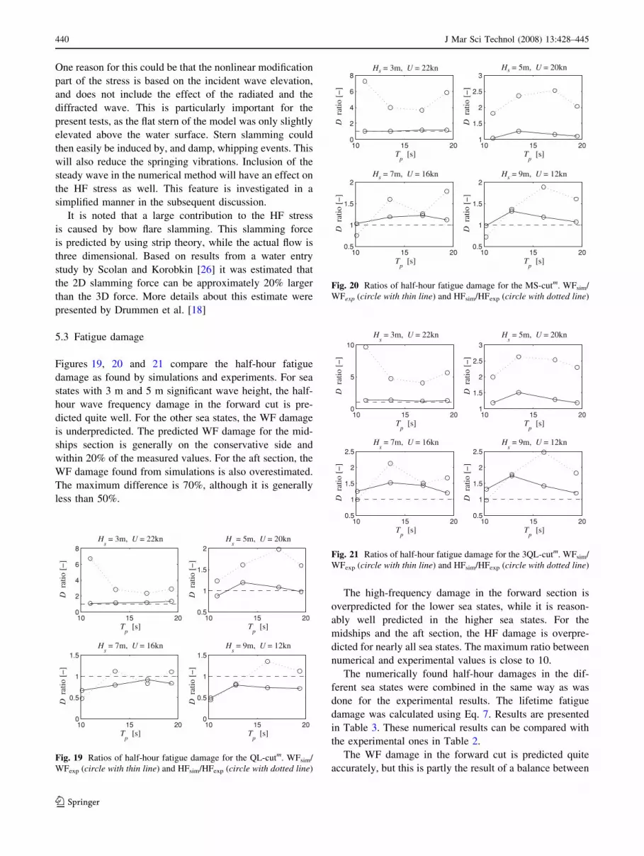
5.3 Fatigue damage
Figures 19, 20 and 21 compare the half-hour fatigue
damage as found by simulations and experiments. For sea
states with 3 m and 5 m significant wave height, the half-
hour wave frequency damage in the forward cut is pre-
dicted quite well. For the other sea states, the WF damage
is underpredicted. The predicted WF damage for the mid-
ships section is generally on the conservative side and
within 20% of the measured values. For the aft section, the
WF damage found from simulations is also overestimated.
The maximum difference is 70%, although it is generally
less than 50%.
The high-frequency damage in the forward section is
overpredicted for the lower sea states, while it is reason-
ably well predicted in the higher sea states. For the
midships and the aft section, the HF damage is overpre-
dicted for nearly all sea states. The maximum ratio between
numerical and experimental values is close to 10.
The numerically found half-hour damages in the dif-
ferent sea states were combined in the same way as was
done for the experimental results. The lifetime fatigue
damage was calculated using Eq. 7. Results are presented
in Table 3. These numerical results can be compared with
the experimental ones in Table 2.
The WF damage in the forward cut is predicted quite
accurately, but this is partly the result of a balance between
10 15 200
2
4
6
8 H
s= 3m, U = 22kn
Tp
[s]
D r
atio
[−
]
10 15 200.5
1
1.5
2 H
s= 5m, U = 20kn
Tp
[s]
D r
atio
[−
]
10 15 200
0.5
1
1.5 H
s= 7m, U = 16kn
Tp
[s]
D r
atio
[−
]
10 15 200
0.5
1
1.5 H
s= 9m, U = 12kn
Tp
[s]
D r
atio
[−
]
Fig. 19 Ratios of half-hour fatigue damage for the QL-cutm. WFsim/
WFexp (circle with thin line) and HFsim/HFexp (circle with dotted line)
10 15 200
2
4
6
8Hs = 3m, U = 22kn
Tp
[s]
D r
atio
[−
]
10 15 201
1.5
2
2.5
3Hs = 5m, U = 20kn
Tp
[s]
D r
atio
[−
]
10 15 200.5
1
1.5
2Hs = 7m, U = 16kn
Tp
[s]
D r
atio
[−
]
10 15 200.5
1
1.5
2Hs = 9m, U = 12kn
Tp
[s]
D r
atio
[−
]
Fig. 20 Ratios of half-hour fatigue damage for the MS-cutm. WFsim/
WFexp (circle with thin line) and HFsim/HFexp (circle with dotted line)
10 15 200
5
10
Hs
= 3m, U = 22kn
Tp
[s]
D r
atio
[−
]
10 15 201
1.5
2
2.5
3
Hs
= 5m, U = 20kn
Tp
[s]
D r
atio
[−
]
10 15 200.5
1
1.5
2
2.5 H
s= 7m, U = 16kn
Tp
[s]
D r
atio
[−
]
10 15 200.5
1
1.5
2
2.5 H
s= 9m, U = 12kn
Tp
[s]
D r
atio
[−
]
Fig. 21 Ratios of half-hour fatigue damage for the 3QL-cutm. WFsim/
WFexp (circle with thin line) and HFsim/HFexp (circle with dotted line)
440 J Mar Sci Technol (2008) 13:428–445
123
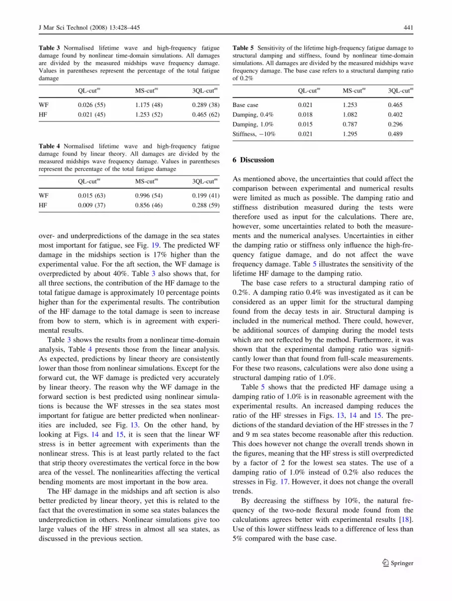
over- and underpredictions of the damage in the sea states
most important for fatigue, see Fig. 19. The predicted WF
damage in the midships section is 17% higher than the
experimental value. For the aft section, the WF damage is
overpredicted by about 40%. Table 3 also shows that, for
all three sections, the contribution of the HF damage to the
total fatigue damage is approximately 10 percentage points
higher than for the experimental results. The contribution
of the HF damage to the total damage is seen to increase
from bow to stern, which is in agreement with experi-
mental results.
Table 3 shows the results from a nonlinear time-domain
analysis, Table 4 presents those from the linear analysis.
As expected, predictions by linear theory are consistently
lower than those from nonlinear simulations. Except for the
forward cut, the WF damage is predicted very accurately
by linear theory. The reason why the WF damage in the
forward section is best predicted using nonlinear simula-
tions is because the WF stresses in the sea states most
important for fatigue are better predicted when nonlinear-
ities are included, see Fig. 13. On the other hand, by
looking at Figs. 14 and 15, it is seen that the linear WF
stress is in better agreement with experiments than the
nonlinear stress. This is at least partly related to the fact
that strip theory overestimates the vertical force in the bow
area of the vessel. The nonlinearities affecting the vertical
bending moments are most important in the bow area.
The HF damage in the midships and aft section is also
better predicted by linear theory, yet this is related to the
fact that the overestimation in some sea states balances the
underprediction in others. Nonlinear simulations give too
large values of the HF stress in almost all sea states, as
discussed in the previous section.
6 Discussion
As mentioned above, the uncertainties that could affect the
comparison between experimental and numerical results
were limited as much as possible. The damping ratio and
stiffness distribution measured during the tests were
therefore used as input for the calculations. There are,
however, some uncertainties related to both the measure-
ments and the numerical analyses. Uncertainties in either
the damping ratio or stiffness only influence the high-fre-
quency fatigue damage, and do not affect the wave
frequency damage. Table 5 illustrates the sensitivity of the
lifetime HF damage to the damping ratio.
The base case refers to a structural damping ratio of
0.2%. A damping ratio 0.4% was investigated as it can be
considered as an upper limit for the structural damping
found from the decay tests in air. Structural damping is
included in the numerical method. There could, however,
be additional sources of damping during the model tests
which are not reflected by the method. Furthermore, it was
shown that the experimental damping ratio was signifi-
cantly lower than that found from full-scale measurements.
For these two reasons, calculations were also done using a
structural damping ratio of 1.0%.
Table 5 shows that the predicted HF damage using a
damping ratio of 1.0% is in reasonable agreement with the
experimental results. An increased damping reduces the
ratio of the HF stresses in Figs. 13, 14 and 15. The pre-
dictions of the standard deviation of the HF stresses in the 7
and 9 m sea states become reasonable after this reduction.
This does however not change the overall trends shown in
the figures, meaning that the HF stress is still overpredicted
by a factor of 2 for the lowest sea states. The use of a
damping ratio of 1.0% instead of 0.2% also reduces the
stresses in Fig. 17. However, it does not change the overall
trends.
By decreasing the stiffness by 10%, the natural fre-
quency of the two-node flexural mode found from the
calculations agrees better with experimental results [18].
Use of this lower stiffness leads to a difference of less than
5% compared with the base case.
Table 3 Normalised lifetime wave and high-frequency fatigue
damage found by nonlinear time-domain simulations. All damages
are divided by the measured midships wave frequency damage.
Values in parentheses represent the percentage of the total fatigue
damage
QL-cutm MS-cutm 3QL-cutm
WF 0.026 (55) 1.175 (48) 0.289 (38)
HF 0.021 (45) 1.253 (52) 0.465 (62)
Table 4 Normalised lifetime wave and high-frequency fatigue
damage found by linear theory. All damages are divided by the
measured midships wave frequency damage. Values in parentheses
represent the percentage of the total fatigue damage
QL-cutm MS-cutm 3QL-cutm
WF 0.015 (63) 0.996 (54) 0.199 (41)
HF 0.009 (37) 0.856 (46) 0.288 (59)
Table 5 Sensitivity of the lifetime high-frequency fatigue damage to
structural damping and stiffness, found by nonlinear time-domain
simulations. All damages are divided by the measured midships wave
frequency damage. The base case refers to a structural damping ratio
of 0.2%
QL-cutm MS-cutm 3QL-cutm
Base case 0.021 1.253 0.465
Damping, 0.4% 0.018 1.082 0.402
Damping, 1.0% 0.015 0.787 0.296
Stiffness, -10% 0.021 1.295 0.489
J Mar Sci Technol (2008) 13:428–445 441
123
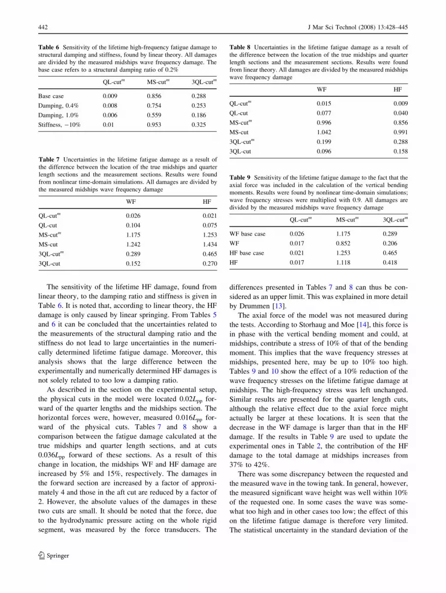
The sensitivity of the lifetime HF damage, found from
linear theory, to the damping ratio and stiffness is given in
Table 6. It is noted that, according to linear theory, the HF
damage is only caused by linear springing. From Tables 5
and 6 it can be concluded that the uncertainties related to
the measurements of the structural damping ratio and the
stiffness do not lead to large uncertainties in the numeri-
cally determined lifetime fatigue damage. Moreover, this
analysis shows that the large difference between the
experimentally and numerically determined HF damages is
not solely related to too low a damping ratio.
As described in the section on the experimental setup,
the physical cuts in the model were located 0.02Lpp for-
ward of the quarter lengths and the midships section. The
horizontal forces were, however, measured 0.016Lpp for-
ward of the physical cuts. Tables 7 and 8 show a
comparison between the fatigue damage calculated at the
true midships and quarter length sections, and at cuts
0.036Lpp forward of these sections. As a result of this
change in location, the midships WF and HF damage are
increased by 5% and 15%, respectively. The damages in
the forward section are increased by a factor of approxi-
mately 4 and those in the aft cut are reduced by a factor of
2. However, the absolute values of the damages in these
two cuts are small. It should be noted that the force, due
to the hydrodynamic pressure acting on the whole rigid
segment, was measured by the force transducers. The
differences presented in Tables 7 and 8 can thus be con-
sidered as an upper limit. This was explained in more detail
by Drummen [13].
The axial force of the model was not measured during
the tests. According to Storhaug and Moe [14], this force is
in phase with the vertical bending moment and could, at
midships, contribute a stress of 10% of that of the bending
moment. This implies that the wave frequency stresses at
midships, presented here, may be up to 10% too high.
Tables 9 and 10 show the effect of a 10% reduction of the
wave frequency stresses on the lifetime fatigue damage at
midships. The high-frequency stress was left unchanged.
Similar results are presented for the quarter length cuts,
although the relative effect due to the axial force might
actually be larger at these locations. It is seen that the
decrease in the WF damage is larger than that in the HF
damage. If the results in Table 9 are used to update the
experimental ones in Table 2, the contribution of the HF
damage to the total damage at midships increases from
37% to 42%.
There was some discrepancy between the requested and
the measured wave in the towing tank. In general, however,
the measured significant wave height was well within 10%
of the requested one. In some cases the wave was some-
what too high and in other cases too low; the effect of this
on the lifetime fatigue damage is therefore very limited.
The statistical uncertainty in the standard deviation of the
Table 6 Sensitivity of the lifetime high-frequency fatigue damage to
structural damping and stiffness, found by linear theory. All damages
are divided by the measured midships wave frequency damage. The
base case refers to a structural damping ratio of 0.2%
QL-cutm MS-cutm 3QL-cutm
Base case 0.009 0.856 0.288
Damping, 0.4% 0.008 0.754 0.253
Damping, 1.0% 0.006 0.559 0.186
Stiffness, -10% 0.01 0.953 0.325
Table 7 Uncertainties in the lifetime fatigue damage as a result of
the difference between the location of the true midships and quarter
length sections and the measurement sections. Results were found
from nonlinear time-domain simulations. All damages are divided by
the measured midships wave frequency damage
WF HF
QL-cutm 0.026 0.021
QL-cut 0.104 0.075
MS-cutm 1.175 1.253
MS-cut 1.242 1.434
3QL-cutm 0.289 0.465
3QL-cut 0.152 0.270
Table 8 Uncertainties in the lifetime fatigue damage as a result of
the difference between the location of the true midships and quarter
length sections and the measurement sections. Results were found
from linear theory. All damages are divided by the measured midships
wave frequency damage
WF HF
QL-cutm 0.015 0.009
QL-cut 0.077 0.040
MS-cutm 0.996 0.856
MS-cut 1.042 0.991
3QL-cutm 0.199 0.288
3QL-cut 0.096 0.158
Table 9 Sensitivity of the lifetime fatigue damage to the fact that the
axial force was included in the calculation of the vertical bending
moments. Results were found by nonlinear time-domain simulations;
wave frequency stresses were multiplied with 0.9. All damages are
divided by the measured midships wave frequency damage
QL-cutm MS-cutm 3QL-cutm
WF base case 0.026 1.175 0.289
WF 0.017 0.852 0.206
HF base case 0.021 1.253 0.465
HF 0.017 1.118 0.418
442 J Mar Sci Technol (2008) 13:428–445
123
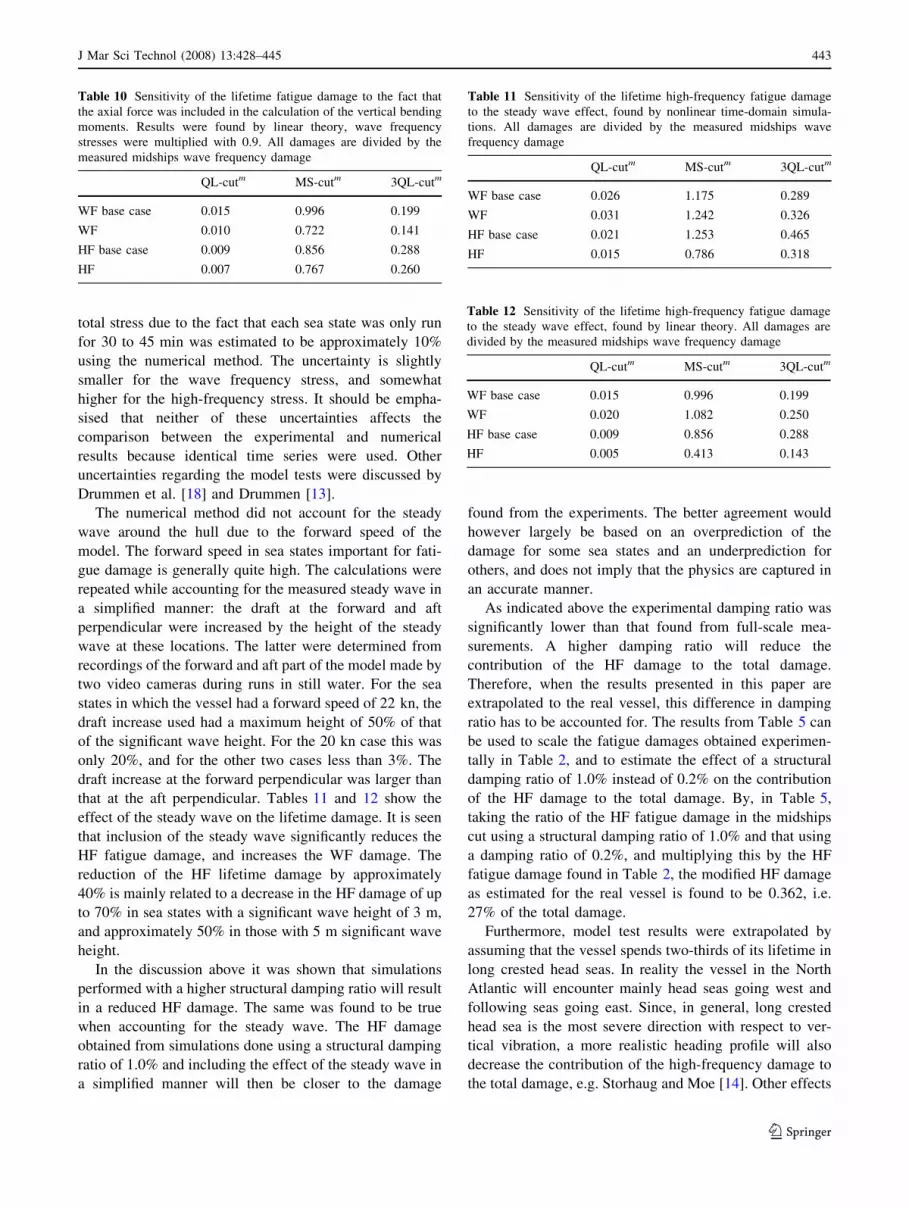
total stress due to the fact that each sea state was only run
for 30 to 45 min was estimated to be approximately 10%
using the numerical method. The uncertainty is slightly
smaller for the wave frequency stress, and somewhat
higher for the high-frequency stress. It should be empha-
sised that neither of these uncertainties affects the
comparison between the experimental and numerical
results because identical time series were used. Other
uncertainties regarding the model tests were discussed by
Drummen et al. [18] and Drummen [13].
The numerical method did not account for the steady
wave around the hull due to the forward speed of the
model. The forward speed in sea states important for fati-
gue damage is generally quite high. The calculations were
repeated while accounting for the measured steady wave in
a simplified manner: the draft at the forward and aft
perpendicular were increased by the height of the steady
wave at these locations. The latter were determined from
recordings of the forward and aft part of the model made by
two video cameras during runs in still water. For the sea
states in which the vessel had a forward speed of 22 kn, the
draft increase used had a maximum height of 50% of that
of the significant wave height. For the 20 kn case this was
only 20%, and for the other two cases less than 3%. The
draft increase at the forward perpendicular was larger than
that at the aft perpendicular. Tables 11 and 12 show the
effect of the steady wave on the lifetime damage. It is seen
that inclusion of the steady wave significantly reduces the
HF fatigue damage, and increases the WF damage. The
reduction of the HF lifetime damage by approximately
40% is mainly related to a decrease in the HF damage of up
to 70% in sea states with a significant wave height of 3 m,
and approximately 50% in those with 5 m significant wave
height.
In the discussion above it was shown that simulations
performed with a higher structural damping ratio will result
in a reduced HF damage. The same was found to be true
when accounting for the steady wave. The HF damage
obtained from simulations done using a structural damping
ratio of 1.0% and including the effect of the steady wave in
a simplified manner will then be closer to the damage
found from the experiments. The better agreement would
however largely be based on an overprediction of the
damage for some sea states and an underprediction for
others, and does not imply that the physics are captured in
an accurate manner.
As indicated above the experimental damping ratio was
significantly lower than that found from full-scale mea-
surements. A higher damping ratio will reduce the
contribution of the HF damage to the total damage.
Therefore, when the results presented in this paper are
extrapolated to the real vessel, this difference in damping
ratio has to be accounted for. The results from Table 5 can
be used to scale the fatigue damages obtained experimen-
tally in Table 2, and to estimate the effect of a structural
damping ratio of 1.0% instead of 0.2% on the contribution
of the HF damage to the total damage. By, in Table 5,
taking the ratio of the HF fatigue damage in the midships
cut using a structural damping ratio of 1.0% and that using
a damping ratio of 0.2%, and multiplying this by the HF
fatigue damage found in Table 2, the modified HF damage
as estimated for the real vessel is found to be 0.362, i.e.
27% of the total damage.
Furthermore, model test results were extrapolated by
assuming that the vessel spends two-thirds of its lifetime in
long crested head seas. In reality the vessel in the North
Atlantic will encounter mainly head seas going west and
following seas going east. Since, in general, long crested
head sea is the most severe direction with respect to ver-
tical vibration, a more realistic heading profile will also
decrease the contribution of the high-frequency damage to
the total damage, e.g. Storhaug and Moe [14]. Other effects
Table 10 Sensitivity of the lifetime fatigue damage to the fact that
the axial force was included in the calculation of the vertical bending
moments. Results were found by linear theory, wave frequency
stresses were multiplied with 0.9. All damages are divided by the
measured midships wave frequency damage
QL-cutm MS-cutm 3QL-cutm
WF base case 0.015 0.996 0.199
WF 0.010 0.722 0.141
HF base case 0.009 0.856 0.288
HF 0.007 0.767 0.260
Table 11 Sensitivity of the lifetime high-frequency fatigue damage
to the steady wave effect, found by nonlinear time-domain simula-
tions. All damages are divided by the measured midships wave
frequency damage
QL-cutm MS-cutm 3QL-cutm
WF base case 0.026 1.175 0.289
WF 0.031 1.242 0.326
HF base case 0.021 1.253 0.465
HF 0.015 0.786 0.318
Table 12 Sensitivity of the lifetime high-frequency fatigue damage
to the steady wave effect, found by linear theory. All damages are
divided by the measured midships wave frequency damage
QL-cutm MS-cutm 3QL-cutm
WF base case 0.015 0.996 0.199
WF 0.020 1.082 0.250
HF base case 0.009 0.856 0.288
HF 0.005 0.413 0.143
J Mar Sci Technol (2008) 13:428–445 443
123
influencing the extrapolation of model test results to the
real vessel are presented by Drummen et al. [19]
7 Conclusions
This paper deals with an experimental and numerical study
of wave-induced fatigue damage in a containership of
newer design, advancing at constant forward speed in
irregular head waves. The model tests showed that the
damage due to wave-induced vibrations made up approx-
imately 40% of the total damage, and that this percentage
slightly increased from bow to stern. The high-frequency
contribution could be slightly smaller at full scale due to
a larger damping. The main contribution to the high-
frequency damage came from the two-node mode of
vibration, while the other modes contributed less than 5%
of the damage. The damage in the forward cut was negli-
gible compared with the damage in the midships section,
while the damage in the aft cut was about 25% of this
value.
The largest contribution to the fatigue damage occurred
in sea states with a peak period of around 14 s and a sig-
nificant wave height of 5 m for the midships section and
the aft quarter length, and 7 m for the forward quarter
length. For the sea states investigated, experimental results
indicated that the nonlinear effects on the wave frequency
stress were mainly important in the forward cut, while they
affected the high-frequency stress in all three cuts.
The experimental results were compared with predic-
tions by a nonlinear hydroelastic strip theory method. It
was found that the predicted total fatigue damage for the
midships section was approximately 50% higher than the
damage determined experimentally. This is the result of an
overprediction by 15% of the wave frequency damage and
of 120% in the high-frequency damage. The overprediction
of the latter is partly related to the fact that the 3D effects
were not accounted for in the 2D slamming force calcu-
lation, the 2D slamming force was estimated to be 20%
larger than the 3D force. The effect of including 3D effects
in this calculation should be investigated, but is expected to
reduce the HF damage by approximately 10%. Another
part of the overprediction of the high-frequency damage is
attributed to too large a springing contribution, both linear
and nonlinear, to the high-frequency stress. Therefore more
work needs to be done to improve the high-frequency stress
modelling. This includes, amongst others aspects, identi-
fying and quantifying the sources of damping of the
vibrations, and verification of the excitation sources of the
high-frequency response.
Furthermore, the numerical method did not account for
the steady wave around the hull due to forward speed.
Using a simplified approach, in which we increased the
draft at the forward and aft perpendicular by the height of
the steady wave at these locations, we showed that
including this wave in the calculations can reduce the high-
frequency damage by 40%. Also, the radiated and the
diffracted waves are expected to influence the nonlinear
high-frequency stress and should thus be added to the wave
used to determine the nonlinear modification part.
The wave frequency stress and damage at midships and
at the aft quarter length were best predicted by linear
theory, while the best prediction for the forward cut was
done by including nonlinearities. This is at least partly
related to the fact that strip theory overestimates the ver-
tical force in the bow area of the vessel, where the
nonlinearities are most important.
Acknowledgments The authors acknowledge financial support
from the Research Council of Norway through CeSOS. Moreover, the
yard and the owner of the vessel are acknowledged for permitting use
of the ship lines. DNV deserves thanks for providing all the necessary
ship data. Parts of the contents of this paper were discussed with Prof.
Odd M. Faltinsen, who offered valuable comments. The first author
also appreciates the many insights of Dr. MingKang Wu regarding his
computer code. Dr. Ole A. Hermundstad is thanked for providing his
code Wavegen.
References
1. Payer HG, Brostella R (2006) The Panama Canal expansion and
the Panamax vessels of the future. In: Transactions society of
naval architects and marine engineers, Fort Lauderdale
2. Almar-Næss A (1985) Fatigue handbook: offshore steel struc-
tures. Tapir, Trondheim
3. Det Norske Veritas (2003) Classification note 30.7: fatigue
assessment of ship structures. Oslo, Norway
4. Storhaug G (2007) Experimental investigation of wave induced
vibrations increasing fatigue damage in ships. PhD Thesis,
Department of Marine Technology, Norwegian University of
Science and Technology, Trondheim, Norway
5. Jensen JJ (1980) Wave-induced ship hull vibrations: a review.
Shock Vibr Digest 12:19–25
6. ISSC (2000) Report of special task committee vi.1: Extreme hull
girder loading. In: Proceedings 14th international ship and off-
shore structures congress, Japan, pp 263–320
7. Storhaug G, Vidic-Perunovic J, Rudinger F et al (2003) Spring-
ing/whipping response of a large ocean going vessel—a
comparison between numerical simulations and full scale mea-
surements. In: Proceedings of hydroelasticity in marine
technology. Oxford, UK, pp 117–129
8. Moe E, Holtsmark G, Storhaug G (2005) Full scale measurements
of the wave induced hull girder vibrations of an ore carrier
trading in the North Atlantic. In: Transactions of Royal Institution
of Naval Architects, conference on design and operation of bulk
carriers, London, UK
9. Storhaug G, Moe E, Holtsmark G (2006) Measurements of wave
induced hull girder vibrations of an ore carrier in different trades.
In: Proceedings of the 25th international conference on offshore
mechanics and artic engineering, Hamburg, Germany
10. Watanabe I, Guedes Soares C (1999) Comparative study on the
time-domain analysis of non-linear ship motions and loads. Mar
Struct 12(2):153–170
444 J Mar Sci Technol (2008) 13:428–445
123
11. Storhaug G, Moan T (2006) Springing/whipping response of a
large ocean-going vessel—investigated by an experimental
method. In: Proceedings hydroelasticity in marine technology,
Wuxi, China
12. Wu MK, Moan T (2005) Efficient calculation of wave-induced
ship responses considering structural dynamic effects. Appl
Ocean Res 21(2):81–96
13. Drummen I (2008) Experimental and numerical investigation of
nonlinear wave-induced load effects in containerships consider-
ing hydroelasticity. PhD Thesis, Department of Marine
Technology, Norwegian University of Science and Technology,
Trondheim, Norway
14. Storhaug G, Moe E (2007) Measurements of wave induced
vibrations onboard a large container vessel operating in harsh
environment. In: Proceedings of the 10th international sympo-
sium on practical design of ships and other floating structures,
Houston, US, pp 64–72
15. Det Norske Veritas (2000) Classification note 30.5: environ-
mental conditions and environmental loads. Oslo, Norway
16. Det Norske Veritas (2000) Nauticus hull user manual, Oslo,
Norway
17. Rychlik I (1987) A new definition of the rainflow cycle counting
method. Int J Fatigue 9(2):119–121
18. Drummen I, Wu MK, Moan T, Experimental and numerical study
of containership responses in severe head seas. Mar Struct
(in press)
19. Drummen I, Storhaug G, Moe E et al (2006) Experimental and full
scale investigation of the importance of fatigue damage due to
wave-induced vibration stress in a container vessel. In: Transac-
tions of Royal Institution of Naval Architects, conference on
design and operation of container ships, London, UK, pp 61–74
20. Fonseca N, Guedes Soares C (2004) Experimental investigation of
the nonlinear effects on the statistics of vertical motions and loads
of a containership in irregular waves. J Ship Res 48(2):148–167
21. Fonseca N, Guedes Soares C (2004) Experimental investigation
of the nonlinear effects on the vertical motions and loads of a
containership in regular waves. J Ship Res 48(2):118–147
22. Aalberts PJ, Nieuwenhuijs MW (2006) Full scale wave and
whipping induced hull girder loads. In: Proceedings hydroelas-
ticity in marine technology, Wuxi, China, pp 65–78
23. Fonseca N, Guedes Soares C (2002) Comparison of numerical
and experimental results of nonlinear wave-induced vertical ship
motions and loads. J Mar Sci Technol 6:193–204
24. Wu MK, Moan T (1996) Linear and nonlinear hydroelastic
analysis of high-speed vessels. J Ship Res 40(2):149–163
25. Wu MK, Hermundstad OA (2002) Time-domain simulation of
wave-induced nonlinear motions and loads and its applications in
ship design. Mar Struct 15(6):561–597
26. Scolan Y, Korobkin A (2001) Three-dimensional theory of water
impact. Part 1. Inverse Wagner problem. J Fluid Mech 440:293–
326
J Mar Sci Technol (2008) 13:428–445 445
123