Detection of Buried Non-Metallic (Plastic and FRP Composite ...
212
Graduate Theses, Dissertations, and Problem Reports 2018 Detection of Buried Non-Metallic (Plastic and FRP Composite) Detection of Buried Non-Metallic (Plastic and FRP Composite) Pipes Using GPR and IRT Pipes Using GPR and IRT Jonas Kavi West Virginia University, [email protected] Follow this and additional works at: https://researchrepository.wvu.edu/etd Part of the Civil Engineering Commons, Other Engineering Commons, and the Structural Materials Commons Recommended Citation Recommended Citation Kavi, Jonas, "Detection of Buried Non-Metallic (Plastic and FRP Composite) Pipes Using GPR and IRT" (2018). Graduate Theses, Dissertations, and Problem Reports. 3724. https://researchrepository.wvu.edu/etd/3724 This Dissertation is protected by copyright and/or related rights. It has been brought to you by the The Research Repository @ WVU with permission from the rights-holder(s). You are free to use this Dissertation in any way that is permitted by the copyright and related rights legislation that applies to your use. For other uses you must obtain permission from the rights-holder(s) directly, unless additional rights are indicated by a Creative Commons license in the record and/ or on the work itself. This Dissertation has been accepted for inclusion in WVU Graduate Theses, Dissertations, and Problem Reports collection by an authorized administrator of The Research Repository @ WVU. For more information, please contact [email protected].
-
Upload
khangminh22 -
Category
Documents
-
view
1 -
download
0
Transcript of Detection of Buried Non-Metallic (Plastic and FRP Composite ...

Graduate Theses, Dissertations, and Problem Reports
2018
Detection of Buried Non-Metallic (Plastic and FRP Composite) Detection of Buried Non-Metallic (Plastic and FRP Composite)
Pipes Using GPR and IRT Pipes Using GPR and IRT
Jonas Kavi West Virginia University, [email protected]
Follow this and additional works at: https://researchrepository.wvu.edu/etd
Part of the Civil Engineering Commons, Other Engineering Commons, and the Structural Materials
Commons
Recommended Citation Recommended Citation Kavi, Jonas, "Detection of Buried Non-Metallic (Plastic and FRP Composite) Pipes Using GPR and IRT" (2018). Graduate Theses, Dissertations, and Problem Reports. 3724. https://researchrepository.wvu.edu/etd/3724
This Dissertation is protected by copyright and/or related rights. It has been brought to you by the The Research Repository @ WVU with permission from the rights-holder(s). You are free to use this Dissertation in any way that is permitted by the copyright and related rights legislation that applies to your use. For other uses you must obtain permission from the rights-holder(s) directly, unless additional rights are indicated by a Creative Commons license in the record and/ or on the work itself. This Dissertation has been accepted for inclusion in WVU Graduate Theses, Dissertations, and Problem Reports collection by an authorized administrator of The Research Repository @ WVU. For more information, please contact [email protected].

DETECTION OF BURIED NON-METALLIC (PLASTIC AND FRP COMPOSITE)
PIPES USING GPR AND IRT
Jonas Kavi
Dissertation submitted to the
Benjamin M. Statler College of Engineering and Mineral Resources
at West Virginia University
in partial fulfillment of the requirements
for the degree of
Doctor of Philosophy
in
Civil Engineering
Udaya B. Halabe, Ph.D., P.E., Chair
Hota V. S. GangaRao, Ph.D., P.E.
Hema J. Siriwardane, Ph.D., P.E.
Radhey Sharma, Ph.D.
Benjamin Dawson-Andoh, Ph.D.
Department of Civil and Environmental Engineering
Morgantown, West Virginia
2018
Keywords: Corrosion, Excavation Damage, Ground Penetrating Radar, GPR, Infrared
Thermography, IRT, Pipelines, Oil and Gas, Fiber Reinforced Polymer, FRP, CFRP, GFRP,
Composites
Copyright 2018 Jonas Kavi

ABSTRACT
DETECTION OF BURIED NON-METALLIC (PLASTIC AND FRP COMPOSITE)
PIPES USING GPR AND IRT
Jonas Kavi
Pipelines are crucial in transporting petroleum products, natural gas, and water from production
facilities to consumers under high pressure and long service life. In addition to being the primary
means of transporting water from treatment facilities to consumers, pipelines also account for the
transportation of more than half of the 100 quadrillions Btu of energy commodities consumed in
the United States annually. The important role played by energy pipelines in the US economy and
standard of living of citizens requires that these assets be safely maintained and appropriately
expanded to meet growing demand. Pipelines remain the safest means of transporting natural gas
and petroleum products, nonetheless, the pipeline infrastructure in the US is facing major
challenges, especially, corrosion of steel/metallic pipes and excavation damage of onshore
pipelines (leading to oil spills, explosions, and deaths). Problems associated with corrosion of
metallic pipelines can be avoided by using non-corrosive materials such as PVC (Polyvinyl
Chloride) or other plastics for water, sewer, or low pressure gas lines and Glass Fiber Reinforced
Polymer composite (GFRP) for transporting high-pressure oil and natural gas. But buried non-
metallic pipelines such as GFRP and PVC material are not easily detectable using the conventional
techniques employed by construction crews to detect buried metallic pipes, which can lead to
increased excavation damage during building/construction and rehabilitation works.
This research investigated alternative strategies for making buried non-metallic pipes (CFRP,
GFRP, and PVC) easily locatable using Ground Penetrating Radar (GPR). Pipe diameters up to
12" and buried with up to 4 ft. of soil cover were investigated. The findings of this study will help
address the detection problem of non-metallic pipelines and speed the adoption of composite pipes
by the petroleum and natural gas industry. The research also investigated the possibility of locating
buried pipes transporting hot fluids using Infrared Thermography (IRT).
Results from the study have shown that, using carbon fabric and aluminum foil/tape overlay on
non-metallic pipes (GFRP or PVC for this study) before burying significantly increases the
reflected GPR signal amplitude, thereby making it easier to locate such pipelines using GPR. The
reflected GPR signal amplitude for pipe sections with carbon fabric or aluminum foil overlays was

found to have increased by a factor of up to 4.52 times, and 2.02 times on average across all the
pipe sections tested, from the baseline (unwrapped) pipe sections. The research also highlights the
importance of using the correct antenna frequency for detecting buried pipes in wet soil conditions.
Wet soils with high electrical conductivity and dielectric constants have higher radar signal
attenuations that significantly affect the penetration depth and returned signal amplitudes from
buried objects. A 200 MHz frequency antenna was found in this study to be ideal for locating the
buried pipes in all soil moisture conditions. The 200 MHz antenna was able to detect buried pipes
up to the maximum 4 ft. depth of soil cover that was studied experimentally. Numerical estimation
using the same soil from the experiment shows that this antenna can penetrate up to a depth of at
least 5.5 ft. in very wet clay soils with volumetric water content of 0.473.
After evaluating the attenuation characteristics of different radar antennae, it was found that
material/ohmic attenuation is constant across a range of antenna frequencies; the increase in GPR
signal attenuation associated with higher antenna frequencies was found to be a result of scattering
attenuation from subsurface inhomogeneity/clutter. Scattering attenuation is however usually
ignored in literature, resulting in erroneous estimation of radar signal attenuation.
Finally, laboratory study proved that, heat from a buried pipeline transporting hot fluid can
propagate through the soil to the surface and be detected using IRT. Additionally, a 6" diameter
steam pipe with a 6" minimum insulation and buried with 2.5 – 3 ft. of soil cover was easily
detected in varying soil moisture conditions during different seasons throughout the year using
IRT in the field environment. The successful application of IRT in detecting this pipe proves the
potential for using this technique in locating buried pipes transporting hot fluids such as steam or
petroleum products from production wells or refinery plants.

iv
ACKNOWLEDGEMENTS
I would like to express my sincere gratitude to my academic and research advisor, Dr. Udaya B.
Halabe, for his guidance, support, and encouragement throughout my graduate studies. His
extensive knowledge in the area of Nondestructive Evaluation of Civil Engineering infrastructure
has been a great help for me during the M.S. and Ph.D. degree programs. I am thankful for the
opportunity to work under Dr. Halabe, an experienced and knowledgeable faculty, and one of the
best advisors in the department.
I would also like to thank Dr. Hota V. S. GangaRao, Dr. Hema J. Siriwardane, Dr. Radhey Sharma,
and Dr. Benjamin Dawson-Andoh for serving as members on my Advisory and Examining
Committee (AEC) and providing constructive feedback on my work. I am also grateful to
Dr. Radhey Sharma for encouraging me to apply for the Chancellor’s Scholarship; Dr. Hota V. S.
GangaRao for making his extensive knowledge in fiber composite materials and manufacturing
accessible during this study; Dr. Siriwardane for allowing me to use the heating oven available in
the Geotechnical laboratory for determining soil moisture content; and Dr. Benjamin
Dawson-Andoh for his valuable advice on making the most out of graduate school and preparing
for life after graduation.
I would like to express my appreciation to WVU-CFC Technician, Mr. Jerry Nestor, for helping
me during the sample preparation and experimental setup stage of this research. I am also grateful
to fellow graduate students, for their immense help during this journey; I am especially
appreciative to Andrew Wheeler, Ruben Joshi, Praveen Majjigapu, Amir Houshmandyar, Piyush
Soti, and Shabnam Khanal for providing assistance during this research.
Funding for this study was provided through the Competitive Academic Agreement Program from
the Pipeline and Hazardous Materials Safety Administration (PHMSA) of US Department of
Transportation (USDOT) under contract numbers DTPH5615HCAP09 and DTPH5616HCAP02.
Support for the study was also provided by Creative Pultrusions, Inc. (CP) in providing the
composite pipe materials for the study. I would like to thank USDOT-PHMSA and CP for
providing the resources and the opportunity for me to work on this study. I would also like to thank
West Virginia University Division of Diversity, Equity and Inclusion; the Department of Civil and
Environmental Engineering; and NACE International/Appalachian Underground Corrosion Short
Course (AUCSC) for awarding me the Chancellor’s Scholarship; Dianne D. Anderson Graduate
Fellowship; and the AUCSC Scholarship respectively that enabled me to focus exclusively on my
studies and research.
Finally, I am very grateful for my family and friends; their endless support, guidance and
encouragement throughout this study made it a worthwhile journey.

v
TABLE OF CONTENTS
Abstract…….. ................................................................................................................................ ii
Acknowledgements ...................................................................................................................... iv
Table of Contents ...........................................................................................................................v
List of Figures .................................................................................................................................x
List of Tables. ........................................................................................................................... xviii
Nomenclature ............................................................................................................................. xix
Chapter 1: Introduction.. .............................................................................................................1
1.1 Background/Overview ..................................................................................................... 1
1.2 Research Problem and Focus ........................................................................................... 5
1.3 Fiber Reinforced Polymer (FRP) Materials and why GFRP............................................ 5
1.4 Research Objectives and Scope........................................................................................ 6
1.5 Research Significance ...................................................................................................... 7
1.6 Research Collaboration .................................................................................................... 8
1.7 Organization ..................................................................................................................... 8
Chapter 2: State of the Pipeline Infrastructure .......................................................................10
2.1 Introduction .................................................................................................................... 10
2.2 PHMSA Pipeline Incidents Causes ................................................................................ 10
2.2.1 Corrosion................................................................................................................. 11
2.2.2 Excavation Damage ................................................................................................ 13
2.2.3 Material/Weld/Equipment Failure .......................................................................... 16
2.2.4 PHMSA Pipeline Incident Summary ...................................................................... 18
2.3 Water and Sewage Pipelines .......................................................................................... 25

vi
2.4 Conclusions .................................................................................................................... 26
Chapter 3: Recent Advances in Non-Metallic Pipeline Detection ..........................................27
3.1 Introduction .................................................................................................................... 27
3.2 Buried Object Detection Techniques ............................................................................. 27
3.2.1 Dowsing .................................................................................................................. 27
3.2.2 Geomagnetic Surveying .......................................................................................... 28
3.2.3 Electromagnetic Induction (EMI) ........................................................................... 29
3.2.4 Electrical/Surface Resistivity .................................................................................. 29
3.2.5 Tracer Wires............................................................................................................ 32
3.2.6 Infrared Thermography (IRT) ................................................................................. 32
3.2.7 Ground Penetrating Radar (GPR) ........................................................................... 33
3.2.8 Advantages and Limitations, and why GPR ........................................................... 34
3.3 Use of GPR in Buried Non-Metallic Object Detection .................................................. 35
3.4 Challenges in Detecting Non-Metallic Objects .............................................................. 36
3.5 Conclusions .................................................................................................................... 37
Chapter 4: Ground Penetrating Radar (GPR) Theory ...........................................................38
4.1 Introduction .................................................................................................................... 38
4.2 Propagation Velocity ...................................................................................................... 39
4.3 Signal Amplitude............................................................................................................ 42
4.4 Loss Factor and Skin Depth ........................................................................................... 44
4.5 Transmission and Reflection .......................................................................................... 45
4.6 Dielectric Characteristics of Common Soil Materials .................................................... 47
4.6.1 Dielectric Models .................................................................................................... 47
4.6.2 Inverse Models ........................................................................................................ 52
4.7 Conclusions .................................................................................................................... 53

vii
Chapter 5: GPR Equipment, Sensors, and Data Processing ..................................................54
5.1 Introduction .................................................................................................................... 54
5.2 GPR Equipment.............................................................................................................. 54
5.3 Soil Moisture and Electrical Conductivity Sensor ......................................................... 56
5.4 GPR Data Processing Techniques .................................................................................. 57
5.4.1 Background Removal.............................................................................................. 57
5.4.2 Peaks Extraction...................................................................................................... 57
5.4.3 Horizontal Scaling .................................................................................................. 58
5.4.4 Amplitude Extraction .............................................................................................. 58
5.5 Conclusions .................................................................................................................... 58
Chapter 6: Experimental Set Up for GPR Testing ..................................................................59
6.1 Introduction .................................................................................................................... 59
6.2 Research Procedure ........................................................................................................ 59
6.3 Pipe Preparation ............................................................................................................. 60
6.3.1 PVC Pipes ............................................................................................................... 60
6.3.2 GFRP Pipes ............................................................................................................. 62
6.3.3 CFRP Pipes ............................................................................................................. 64
6.3.4 Creating Dielectric Contrast Between Non-Metallic Pipes and Surrounding Soil . 65
6.4 Pipe Burying ................................................................................................................... 68
6.5 Conclusions .................................................................................................................... 75
Chapter 7: GPR Test Results and Data Analysis .....................................................................76
7.1 Introduction .................................................................................................................... 76
7.2 GPR Test Results ........................................................................................................... 76
7.2.1 900 MHz Antenna Data .......................................................................................... 77
7.2.2 Dataset I .................................................................................................................. 77

viii
7.2.3 Dataset II ................................................................................................................. 93
7.2.4 Dataset III.............................................................................................................. 100
7.2.5 Performance of Surface Configurations................................................................ 107
7.3 Determination of Depth ................................................................................................ 111
7.3.1 Depth Estimation Using Soil Dielectric Constant ................................................ 111
7.3.2 Depth Estimation Using GPR Hyperbolic Fitting ................................................ 112
7.3.3 Depth Estimation Using Common Mid-Point (CMP) Method ............................. 114
7.4 Conclusions .................................................................................................................. 116
Chapter 8: Numerical Computations ......................................................................................118
8.1 Introduction .................................................................................................................. 118
8.2 Soil Dielectric Modelling ............................................................................................. 118
8.3 Inverse Dielectric Modelling ........................................................................................ 123
8.4 Signal Amplitude and Attenuation ............................................................................... 127
8.5 Antenna Performance and Penetration Depth .............................................................. 133
8.6 Wave Velocity and Wavelength ................................................................................... 137
8.7 Conclusions .................................................................................................................. 138
Chapter 9: Infrared Thermography Testing and Results .....................................................139
9.1 Introduction .................................................................................................................. 139
9.2 IRT Test Equipment (Camera and Thermocouples) .................................................... 139
9.3 Experimental Set-Up for IRT Testing .......................................................................... 140
9.4 IRT Test Results ........................................................................................................... 142
9.4.1 Pipe Operating /Heating Cycle ............................................................................. 142
9.4.2 Pipe Cooling Cycle ............................................................................................... 148
9.5 Testing of Field Pipes ................................................................................................... 150
9.6 Conclusions .................................................................................................................. 156

ix
Chapter 10: Conclusions and Recommendations ..................................................................158
10.1 Research Summary ................................................................................................... 158
10.2 Conclusions .............................................................................................................. 159
10.3 Recommendations for Field Implementation and Future Study ............................... 162
10.3.1 Recommendations for Field Implementation ........................................................ 162
10.3.2 Recommendations for Future Study ..................................................................... 163
References….. .............................................................................................................................164
Appendix A: PHMSA Incident Definition and Criteria History ..........................................174
Appendix B: Supplementary GPR Data .................................................................................176
B.1 Details of Pipes Identified in the 36 ft. Long Trench Using 400 MHz Antenna ........... 177
B.2 Detailed Radar Profile for Features Marked in Figure 7-29(b) for Dataset II ............... 180
B.3 Transverse GPR Scans over 36 ft. Long Trench Using 200 MHz Antenna ................... 183
B.4 Transverse GPR Scans over 36 ft. Long Trench Using 400 MHz Antenna ................... 185
Appendix C: Supplementary IRT Plots ..................................................................................187

x
LIST OF FIGURES
Figure 1-1: (a) 2014 U.S. Primary energy consumption by source (EIA n.d.) and (b) crude oil and
petroleum product by transportation by mode in 2009 (USDOT 2017) ......................................... 2
Figure 1-2: U.S. refinery receipts of crude oil by method of transportation (EIA n.d.) ................ 2
Figure 1-3: U.S. Primary energy consumption by source (EIA n.d.) ............................................. 3
Figure 1-4: Primary energy consumption by type, 1980-2040 (EIA 2015) ................................... 4
Figure 2-1: 20 year reported incident cause breakdown (1996-2015) ........................................ 11
Figure 2-2: External surface of the failed pipeline section (PHMSA 2016e and 2016f) ............. 12
Figure 2-3: Spilled crude oil from the rupture being cleaned (Nicholson 2015) ........................ 12
Figure 2-4: Corrosion products deposited on the pipe surface (PHMSA 2016f) ........................ 13
Figure 2-5: Laser scanning rendering of the failure location showing the remaining wall thickness
(PHMSA 2016f) ............................................................................................................................. 13
Figure 2-6: Excavation damage explosion (DOT 2011) .............................................................. 15
Figure 2-7: Natural gas pipeline explosion from excavation damage (NTSB 2013) ................... 16
Figure 2-8: Aftermath of natural gas pipeline explosion in San Bruno, CA (SacBee 2010) ....... 17
Figure 2-9: Details of the aftermath of natural gas pipeline explosion in San Bruno, CA ......... 17
Figure 2-10: Category summary of PHMSA pipeline incidents .................................................. 18
Figure 2-11: Number of reported incidents for each category by year ....................................... 19
Figure 2-12: Number of fatalities reported for each category by year ........................................ 20
Figure 2-13: Number of injuries reported for each category by year ......................................... 20
Figure 2-14: Total cost reported for each category by year ........................................................ 21
Figure 2-15: Percentage of pipeline incidents caused by different categories ............................ 21

xi
Figure 2-16: Casualties associated with different causes of pipeline failure .............................. 22
Figure 2-17: Total cost reported for each failure category over the last 20 years ...................... 23
Figure 2-18: Total cost reported for each failure category by year ............................................ 23
Figure 2-19: Total barrels of hazardous liquid spilled per failure category ............................... 24
Figure 2-20: Net barrels of hazardous liquid lost per failure category....................................... 24
Figure 2-21: Break rates of different pipe materials (Folkman 2018) ........................................ 26
Figure 3-1: Electrical resistivity result for an underground mine (Sheets 2002) ........................ 30
Figure 3-2: GPR printout showing hyperbolic features from steel drums ................................... 35
Figure 3-3: GPR data from agricultural drainage pipes (Allred et al. 2004) ............................ 36
Figure 4-1: Propagation path of electromagnetic wave from transmitter to receiver................ 38
Figure 4-2: Conditions under which the loss tangent << 1 ......................................................... 45
Figure 4-3: Reflection and transmission of incident electromagnetic wave at an interface ....... 46
Figure 4-4: Refraction of incident electromagnetic wave at the interface between two media .. 47
Figure 4-5: Organic soil model by Roth et al. showing original and corrected fitted lines ....... 50
Figure 5-1: SIR-20 GPR system and antennae used for testing ................................................... 55
Figure 5-2: 200 MHz GPR antenna with survey wheel ............................................................... 55
Figure 5-3: Sensor for measuring soil moisture, conductivity, and dielectric ............................. 56
Figure 6-1: The 14' long 12" diameter PVC pipe being cut ........................................................ 61
Figure 6-2: The 12" diameter PVC pipe (a) after cutting, and (b) after capping ........................ 61
Figure 6-3: The 3" diameter PVC pipes ....................................................................................... 62
Figure 6-4: The 12" diameter GFRP pipes .................................................................................. 63

xii
Figure 6-5: Manufacturing a 3" diameter GFRP pipe................................................................. 64
Figure 6-6: 12" diameter CFRP pipe ........................................................................................... 65
Figure 6-7: The 3" diameter CFRP pipes .................................................................................... 65
Figure 6-8: Pipe configurations: (a) 6" diameter PVC with carbon fabric rings, (b) 12" diameter
PVC with carbon fabric strip, (c) 12" diameter GFRP with aluminum rings, and (d) 12" diameter
GFRP with aluminum strip ........................................................................................................... 67
Figure 6-9: 12" diameter GFRP pipe with carbon nanoparticle overlay .................................... 68
Figure 6-10: The site for pipe burying and monitoring (source: Google Maps) ......................... 69
Figure 6-11: The located site on WVU campus for pipe burying, with utility lines marked........ 70
Figure 6-12: Pipe layout for GPR testing .................................................................................... 71
Figure 6-13: Pipe layout for GPR testing (short trench) ............................................................. 72
Figure 6-14: (a) Arrangement of pipes in the trench, (b) soil moisture and resistivity sensor ... 72
Figure 6-15: (a) Soil sensors with data wires running through conduits to protect the wires, (b)
3" diameter pipes and sensors in the 27" deep trench .................................................................. 73
Figure 6-16: Pipe samples being buried ...................................................................................... 74
Figure 6-17: (a) The site being seeded, (b) the field restored to initial condition ....................... 74
Figure 7-1: Longitudinal scan over 3" diameter pipes at 2 ft. depth using 900 MHz antenna ... 77
Figure 7-2: Dataset I - Longitudinal scans over the pipe trenches using 200 MHz antenna ...... 78
Figure 7-3: Longitudinal scan over the 3 ft. deep trench for Dataset I using 200 MHz antenna 79
Figure 7-4: Longitudinal scan over the 4 ft. deep trench for Dataset I using 200 MHz antenna 79
Figure 7-5: Longitudinal scan over the 2 ft. deep trench for Dataset I using 200 MHz antenna 80
Figure 7-6: Longitudinal scan over the 2 ft. deep trench for Dataset I using 200 MHz antenna 80

xiii
Figure 7-7: Longitudinal scan over the 2 ft. deep trench for Dataset I using 400 MHz antenna 81
Figure 7-8: Longitudinal GPR scan (left) and A-Scan (right) over Unwrapped 12" GFRP pipe 83
Figure 7-9: Longitudinal GPR scan (left) and A-Scan (right) over 12" CFRP Ring GFRP pipe 83
Figure 7-10: Longitudinal GPR scan (left) and A-Scan (right) over 12" CFRP Strip GFRP pipe
....................................................................................................................................................... 84
Figure 7-11: Longitudinal GPR scan (left) and A-Scan (right) over 12" Unwrapped PVC pipe 84
Figure 7-12: Longitudinal GPR scan (left) and A-Scan (right) over 12" Al. Foil Ring PVC pipe
....................................................................................................................................................... 85
Figure 7-13: Longitudinal GPR scan (left) and A-Scan (right) over 12" Al. Foil Strip PVC pipe
....................................................................................................................................................... 85
Figure 7-14: Longitudinal GPR scan (left) and A-Scan (right) over 6" Unwrapped PVC pipe .. 86
Figure 7-15: Longitudinal GPR scan (left) and A-Scan (right) over 6" Al. Foil Ring PVC pipe 86
Figure 7-16: Longitudinal GPR scan (left) and A-Scan (right) over 6" Al. Foil Strip PVC pipe 87
Figure 7-17: Longitudinal GPR scan (left) and A-Scan (right) over 6" CFRP Ring PVC pipe .. 87
Figure 7-18: Longitudinal GPR scan (left) and A-Scan (right) over 6" CFRP Strip PVC pipe .. 88
Figure 7-19: Longitudinal GPR scan (left) and A-Scan (right) over 12" CFRP Strip GFRP pipe
....................................................................................................................................................... 90
Figure 7-20: Longitudinal GPR scan (left) and A-Scan (right) over Unwrapped 12" GFRP pipe
....................................................................................................................................................... 90
Figure 7-21: Longitudinal GPR scan (left) and A-Scan (right) over C. Nano p. 12" GFRP pipe 91
Figure 7-22: Longitudinal GPR scan (left) and A-Scan (right) over Al. Foil Strip 12" PVC pipe
....................................................................................................................................................... 91

xiv
Figure 7-23: Longitudinal GPR scan (left) and A-Scan (right) over Unwrapped 10" GFRP pipe
....................................................................................................................................................... 92
Figure 7-24: Longitudinal GPR scan (left) and A-Scan (right) over 12" Steel pipe .................... 92
Figure 7-25: Dataset II - Longitudinal scans over the pipe trenches using 200 MHz antenna ... 95
Figure 7-26: Longitudinal scans over 3" diameter pipes at 2 ft. deep using 200 MHz antenna . 96
Figure 7-27: Longitudinal scan over 3" diameter pipes at 2 ft. deep using 400 MHz antenna ... 97
Figure 7-28: Longitudinal scans over 12" and 10" diameter pipes at 2 ft. deep using 400 MHz
antenna .......................................................................................................................................... 98
Figure 7-29: Reflection details marked on 12" and 10" diameter pipes with 2 ft. of soil cover .. 99
Figure 7-30: Dataset III - Longitudinal scans over the pipe trenches using 200 MHz antenna 101
Figure 7-31: Transverse scans over the pipes in 65 ft. long trenches using 200 MHz antenna for
Dataset III ................................................................................................................................... 105
Figure 7-32: Transverse scans over the pipes in 36 ft. long trench using 200 MHz antenna for
Dataset III ................................................................................................................................... 106
Figure 7-33: Comparison of returned radar signal amplitude from different pipe configurations
..................................................................................................................................................... 109
Figure 7-34: Comparison of returned radar signal amplitude from GFRP pipe configurations
..................................................................................................................................................... 110
Figure 7-35: Comparison of returned radar signal amplitude from PVC pipe configurations . 110
Figure 7-36: Circular reflector and associated hyperbolic feature ........................................... 112
Figure 7-37: Velocity estimation using hyperbolic feature in GPR data (pipe 6"@3') ............. 113
Figure 7-38: Common Mid-Point (CMP) technique .................................................................. 114
Figure 7-39: Plot for estimating velocity from CMP survey ...................................................... 115

xv
Figure 7-40: The simplified Common Mid-Point (CMP) technique .......................................... 115
Figure 8-1: Experimental dielectric constant versus VWC ....................................................... 121
Figure 8-2: Comparison between dielectric models and experimental data ............................ 121
Figure 8-3: Comparison between the three dielectric models and experimental data .............. 123
Figure 8-4: Experimental VWC versus dielectric constant ....................................................... 124
Figure 8-5: Comparison between inverse dielectric models and experimental data ................ 124
Figure 8-6: Comparison between the three inverse dielectric models and experimental data.. 126
Figure 8-7: Comparison between experimental data/model and secondary data and models .. 127
Figure 8-8: Variation of material attenuation coefficient with antenna frequency ................... 129
Figure 8-9: Variation of material attenuation coefficient with lower antenna frequencies ...... 129
Figure 8-10: Variation of components of attenuation with antenna frequency ......................... 132
Figure 8-11: Decay of signal amplitude with travel distance .................................................... 133
Figure 8-12: Variation of attenuation coefficient for different soil types .................................. 134
Figure 8-13: Variation of skin depth with antenna frequency for different soil types ............... 135
Figure 8-14: Estimated penetration depths for antennae in different soil types ........................ 136
Figure 9-1: FLIR InfraCAM SD camera and type-T thermocouple........................................... 139
Figure 9-2: (a) Automated thermocouple reader and (b) Thermo Recorder ............................. 141
Figure 9-3: Insulated wooden box used for IRT testing ............................................................. 141
Figure 9-4: CFRP pipe for IRT testing (top), sketch showing thermocouple locations (bottom)
..................................................................................................................................................... 141
Figure 9-5: IRT test set-up ......................................................................................................... 142

xvi
Figure 9-6: Infrared thermography data at the soil surface at various stages of testing .......... 144
Figure 9-7: Variation of soil surface (TSC, IRT) and room (Amb) temperatures with time ...... 145
Figure 9-8: Soil surface temperature difference with time ........................................................ 145
Figure 9-9: Difference between soil surface temperature and room temperature with depth ... 148
Figure 9-10: Variation of soil surface (TSC, IRT) and room (Amb) temperatures during cooling
..................................................................................................................................................... 149
Figure 9-11: Soil surface temperature difference with time during cooling.............................. 149
Figure 9-12: Location of field IRT test pipe ............................................................................... 150
Figure 9-13: Field IRT test pipe installation details (CJD 2015) .............................................. 151
Figure 9-14: Comparison of IRT and visible image results ....................................................... 153
Figure 9-15: Infrared thermography data at the soil surface in different seasons .................... 154
Figure 9-16: IRT data at the soil surface taken from close range in different seasons ............. 155
Figure 9-17: Temperature distribution across each IRT data in Figure 9-16 ........................... 156
Figure B-1: Longitudinal scan over 12" CFRP Strip GFRP pipe: raw data (top), data with
background noise removed (middle), and reflection peaks extracted from the data (bottom) ... 177
Figure B-2: Longitudinal scan over 12" Unwrapped GFRP pipe: raw data (top), data with
background noise removed (middle), and reflection peaks extracted from the data (bottom) ... 178
Figure B-3: Longitudinal scan over 12" Al. Foil Strip PVC pipe: raw data (top), data with
background noise removed (middle), and reflection peaks extracted from the data (bottom) ... 179
Figure B-4: Features A and A1 .................................................................................................. 180
Figure B-5: Features B and B1 .................................................................................................. 180
Figure B-6: Features C and C1 ................................................................................................. 181

xvii
Figure B-7: Feature D ............................................................................................................... 181
Figure B-8: Feature E ................................................................................................................ 182
Figure B-9: Feature F ................................................................................................................ 182
Figure B-10: Transverse scan over some of the pipes in 36 ft. long trench using 200 MHz GPR
antenna for Dataset I .................................................................................................................. 183
Figure B-11: Transverse scan over some of the pipes in 36 ft. long trench using 200 MHz GPR
antenna for Dataset II ................................................................................................................. 184
Figure B-12: Transverse scan over some of the pipes in 36 ft. long trench using 400 MHz GPR
antenna for Dataset II (raw data) ............................................................................................... 185
Figure B-13: Transverse scan over some of the pipes in 36 ft. long trench using 400 MHz GPR
antenna for Dataset II (data with background noise removed) .................................................. 186
Figure C-1: Variation of test temperature with time of heating and cooling ............................ 188
Figure C-2: Top and bottom temperature difference of the pipe during heating and cooling .. 189
Figure C-3: Inlet and outlet temperature difference of the pipe during heating and cooling ... 190
Figure C-4: Soil surface temperature difference during heating and cooling ........................... 191

xviii
LIST OF TABLES
Table 2-1: Corrosion, excavation damage and material failure contribution to pipe incidents .. 25
Table 3-1 Drillers’ descriptions of borings along resistivity survey line (Sheets 2002) .............. 31
Table 4-1: Relative dielectric constants and conductivity of common subsurface materials ....... 48
Table 5-1: GPR antenna specifications ........................................................................................ 56
Table 5-2: GS3 sensor specifications ........................................................................................... 57
Table 6-1: Material and section properties of CFRP and GFRP pipes/fabrics ........................... 63
Table 6-2: Summary of pipe samples and configurations ............................................................ 75
Table 7-1: Average soil dielectric properties during data collection .......................................... 76
Table 7-2: Description of features marked in Figure 7-29 .......................................................... 99
Table 7-3: Target depth estimated using hyperbolic fitting ....................................................... 113
Table 8-1: Measured soil dielectric properties .......................................................................... 120
Table 8-2: Dielectric models derived from experimental data ................................................... 122
Table 8-3: Inverse dielectric models derived from experimental data ....................................... 126
Table 8-4: Material attenuation values for the GPR datasets .................................................... 128
Table 8-5: Material properties for scattering attenuation computation .................................... 130
Table 8-6: Components of total signal attenuation .................................................................... 130
Table 8-7: Remaining signal amplitude after two way travel to 4 ft. depth ............................... 133
Table 8-8: Phase coefficient and wavelength of the antennae used for GPR test ...................... 138
Table 9-1: Estimated variation of soil surface temperature with depth ..................................... 147
Table 9-2: Field IRT test pipe parameters ................................................................................. 152
xix
NOMENCLATURE
A number of labels, terms, and acronyms are frequently used in this document for brevity. These
terms and acronyms may be ambiguous, or they may not be familiar to all readers. The definitions
of terms and acronyms given below apply throughout this document.
AC: Alternating Current
AC: Asbestos Cement
AEC: Advisory and Examining Committee
Amb: Ambient/room temperature
ASCE: American Society of Civil Engineers
BI: Bottom Inlet temperature (inlet temperature measured at the bottom of the pipe)
BO: Bottom Outlet temperature (outlet temperature measured at the bottom of the pipe)
CFRP: Carbon Fiber Reinforced Polymer
CI: Cast Iron
CIA: Central Intelligence Agency
CMP: Common Mid-Point
CP: Condensate Pumped pipeline or Creative Pultrusions Inc.
CRIM: Complex Refractive Index Model
CSC: Concrete Steel Cylinder
DC: Direct Current
DDB: Dortmund Data Bank
DI: Ductile Iron
DOT: US Department of Transportation
EIA: US Energy Information Administration
EM: Electromagnetic
EMIS: Electromagnetic Induction Spectroscopy
ERT: Electrical Resistivity Tomography
ESB: Engineering Sciences Building
FHWA: Federal Highway Administration
FRP: Fiber Reinforced Polymer
GFRP: Grass Fiber Reinforced Polymer

xx
GPR: Ground Penetrating Radar
GSSI: Geophysical Survey Systems, Inc.
HPS: High Pressure Steam
IRT: Infrared Thermography
MRB: Mineral Resources Building
NACE: NACE International
NaCl: Sodium Chloride
NTSB: National Transportation Safety Board
PRT: Personal Rapid Transit
PST: Pipeline Safety Trust
PVC: Polyvinyl Chloride
R-Value: Relative insulating value (unit of ft2·°F·h/BTU)
SCH: Schedule
SDR: Standard Dimension Ratio
TC: Temperature measured at the top of the pipe, midway between the inlet and the outlet
TI: Top Inlet temperature (inlet temperature measured at the top of the pipe)
TO: Top Outlet temperature (outlet temperature measured at the top of the pipe)
TSC: Temperature at top of the soil over mid portion of the pipe
USDOT: US Department of Transportation
USDOT-PHMSA/ PHMSA: Pipeline and Hazardous Materials Safety Administration
UAV: Unmanned Aerial Vehicle
VWC: Volumetric Water Content
WT: Water Temperature
WVU-CFC: West Virginia University Constructed Facilities Center

1
CHAPTER 1
INTRODUCTION
1.1 BACKGROUND/OVERVIEW
The pipeline industry in the United States (U.S.) is an important component of the nation’s
economy, and essential in the standard of living of its citizens. Energy pipelines (pipelines used in
transporting fuel/energy products) also play an important role in ensuring the security of the nation.
The pipeline infrastructure is the primary means of transporting water, sewage, natural gas,
petroleum products, and the majority of hazardous liquids from production basins, points of
generation, and the ports to areas of consumption, storage, or disposal.
Best available data in 2015 indicates that, energy pipelines in the United States alone accounted
for about 65% of the world’s energy pipeline network (CIA n.d.). The role played by pipelines in
the United States cannot be overestimated; almost all natural gas in the United States and a greater
portion of crude oil and petroleum products are transported by pipelines.
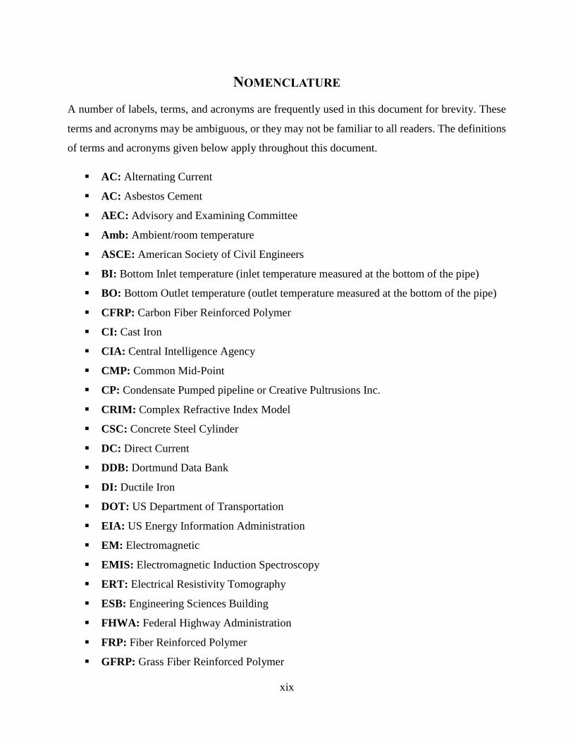
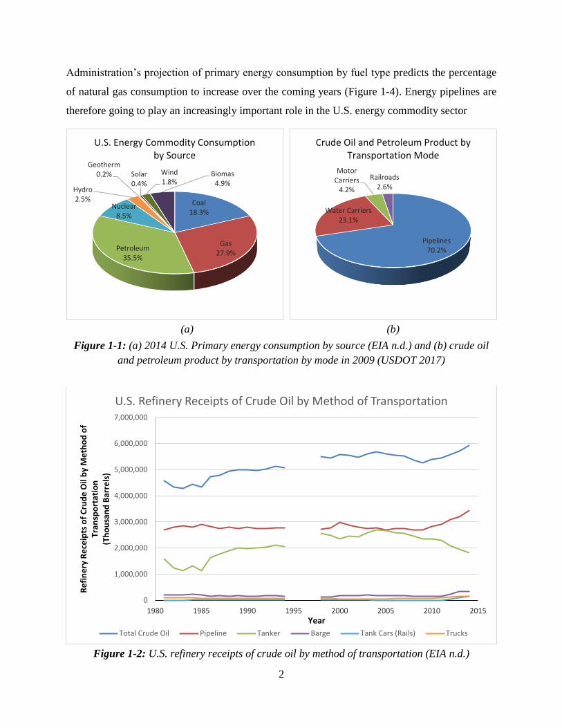
According to data available from the U.S. Energy Information Administration (EIA), the US
consumes about 100 quadrillions Btu of energy annually. Natural gas accounts for 28% of the
energy commodities consumed in the United States while petroleum products account for 35%
(Figure 1-1a). Thus natural gas and petroleum products account for about 63% of the total energy
consumption in the United States. Natural gas is almost entirely transported by pipelines while
over 70% of crude oil and petroleum products are transported by pipelines (Figure 1-1b). It can
therefore be concluded that, 53% of all energy commodities consumed in the United States are
transported by pipelines. In addition, the percentage of crude oil/petroleum products transported
by pipelines in the United States has been increasing since 2005, while the percentage transported
by other modes of petroleum transport have decreased over the same period as shown in Figure 1-2
(EIA n.d., USDOT 2017).
Natural gas consumption in the U.S. has been on the ascendancy since 2005, while coal and
petroleum product consumption has been decreasing over the same period, with total energy
consumption remaining almost constant (Figure 1-3). The U.S. Energy Information
2
Administration’s projection of primary energy consumption by fuel type predicts the percentage
of natural gas consumption to increase over the coming years (Figure 1-4). Energy pipelines are
therefore going to play an increasingly important role in the U.S. energy commodity sector
(a) (b)
Figure 1-1: (a) 2014 U.S. Primary energy consumption by source (EIA n.d.) and (b) crude oil
and petroleum product by transportation by mode in 2009 (USDOT 2017)
Figure 1-2: U.S. refinery receipts of crude oil by method of transportation (EIA n.d.)
0
1,000,000
2,000,000
3,000,000
4,000,000
5,000,000
6,000,000
7,000,000
1980 1985 1990 1995 2000 2005 2010 2015
Re
fin
ery
Re
ceip
ts o
f C
rud
e O
il b
y M
eth
od
of
Tran
spo
rtat
ion
(Th
ou
san
d B
arre
ls)
Year
U.S. Refinery Receipts of Crude Oil by Method of Transportation
Total Crude Oil Pipeline Tanker Barge Tank Cars (Rails) Trucks
Pipelines70.2%
Water Carriers23.1%
Motor Carriers
4.2%
Railroads2.6%
Crude Oil and Petroleum Product by Transportation Mode
Coal18.3%
Gas27.9%
Petroleum35.5%
Nuclear8.5%
Hydro2.5%
Geotherm0.2% Solar
0.4%
Wind1.8%
Biomas4.9%
U.S. Energy Commodity Consumption by Source

3
Figure 1-3: U.S. Primary energy consumption by source (EIA n.d.)
0
10
20
30
40
50
60
70
80
90
100
1945 1950 1955 1960 1965 1970 1975 1980 1985 1990 1995 2000 2005 2010
Pri
mar
y e
ne
rgy
con
sum
pti
on
(Q
uad
rilli
on
Btu
)
Year
U. S. Primary Energy Consumption by Source
Coal Natural Gas Petroleum Nuclear
Hydroelectric Geothermal Solar Wind
Biomass Total Renewable Total Energy Consumption

4
Figure 1-4: Primary energy consumption by type, 1980-2040 (EIA 2015)
The importance of pipelines (particularly energy pipelines) “to the U.S. economy, [security,] and
our standard of living requires that these assets be safely maintained and appropriately expanded
to sustain demand.” (PHMSA 2015).
Pipelines remain the safest means of transporting natural gas, crude oil, and petroleum products,
nonetheless, the pipeline industry is having major challenges; including corrosion of steel/metallic
pipes (leading to oil spills, explosions, and deaths), excavation damage (damage to existing
pipelines during excavation work), and pipeline material/weld/equipment failure as discussed in
Chapter 2 of this document. These pipeline incidents often result in catastrophic failures, with
associated fatalities, injuries, property loss, and environmental contamination. The Pipeline and
Hazardous Materials Safety Administration (PHMSA), under U.S. Department of Transportation
(USDOT), has identified corrosion as the leading cause of failure in metallic pipelines, and
excavation damage as the leading cause of on shore pipeline incidents (PHMSA 2015).

5
1.2 RESEARCH PROBLEM AND FOCUS
The focus of this research is to work on a solution that can prevent excavation damage and pipe
material failure for non-corrosive (non-metallic) pipes by making them detectable in-situ.
The problems associated with corrosion of steel/metallic pipelines, and to some extent pipe
material failure, can be addressed by using non-corrosive materials such as the commonly
available and widely used PVC (Polyvinyl Chloride) or other plastics for water, sewer, or low
pressure gas lines and advanced composite materials such as Glass Fiber Reinforced Polymer
(GFRP) for transporting high-pressure oil and natural gas products. However, buried PVC and
GFRP materials are not easily detectable using the available ground sensory technologies, which
can lead to increased excavation damage of pipelines during building/construction and
rehabilitation works. Tracer wires are employed in some applications to make non-metallic
pipelines locatable, but these wires can break over time and render the pipeline difficult to locate.
The inability to easily locate buried GFRP and other non-metallic pipes has limited the adoption
of such pipe materials in the oil and gas industry. Making these pipe materials detectable when
buried will therefore help accelerate their adoption, and hence provide solutions to the corrosion
related pipeline failure incidents as well.
1.3 FIBER REINFORCED POLYMER (FRP) MATERIALS AND WHY GFRP
Fiber Reinforced Polymer (FRP) composite has emerged as alternative material in many industries
due to its better engineering properties that are desirable to manufacturers and infrastructure
developers. FRPs generally have high specific strength, high specific modulus, low specific
weight, high resistance to corrosion, high fatigue strength, and low coefficient of thermal
expansion compared to conventional materials like steel. FRPs (particularly Carbon Fiber
Reinforced Polymers – CFRP and Glass Fiber Reinforced Polymers – GPRP) are increasingly
being used in infrastructure development applications – both for new constructions and
rehabilitation of aging infrastructure (Kavi 2015, GangaRao et al. 2007, Mallick 2007) – with
tremendous benefits. There is therefore a great potential for fiber composite material application
in the pipeline transportation industry (Rawls 2015). GFRP is less expensive compared to CFRP,
hence GFRP is used more in infrastructure development application.

6
1.4 RESEARCH OBJECTIVES AND SCOPE
To help address some of the major challenges associated with transportation by pipelines, this
research is focused on investigating alternative strategies for making buried non-metallic pipelines
easily detectable using available ground sensory technologies – Ground Penetrating Radar (GPR)
and Infrared Thermography (IRT). The primary objectives of this research are as follows:
1. Develop, investigate, and compare alternative strategies for locating buried pipelines
created with Fiber Reinforced Polymer (FRP) materials – particularly Carbon and Glass
fibers (CFRP and GFRP).
2. Investigate the potential and feasibility for using CFRP fabric, carbon nanoparticle, or
aluminum overlay to increase the detectability of GFRP and PVC (plastic) pipes with
Ground Penetrating Radar (GPR).
3. Investigate and compare the detectability of the above pipes using GPR with antennas of
different frequencies.
4. Investigate the possibility of detecting buried pipe transporting hot liquid, using Infrared
Thermography (IRT).
5. Evaluate the above strategies for making non-metallic pipelines detectable using ground
sensory technologies, and recommend the most appropriate configuration to be used in the
pipeline industry in order to increase the detectability of buried non-metallic pipes in the
field.
The above research objectives were achieved by:
1. Producing sample CFRP pipes by wrapping carbon fabric around cardboard tubes.
2. Using CFRP fabric, carbon nanoparticle, or aluminum overlay for GFRP and PVC (plastic)
pipes to increase detectability by GPR. This setup includes the following pipe
configurations:
i. Use CFRP fabric overlay in the form of strips or rings on GFRP and PVC pipes.
ii. Use aluminum foil/tape overlay in the form of strips or rings on GFRP and PVC pipes.
iii. Use multiple pipe diameters for both pipe materials (GFRP and PVC).
iv. Use carbon nanoparticle overly on a GFRP pipe.

7
3. Burying variations of the above pipes (including different pipe materials, diameters, pipe
surface configurations, and different depth of soil cover over the buried pipes) for GPR
investigation.
4. Using GPR with different antenna frequencies to investigate and compare the detectability
of the buried pipes.
5. Burying a CFRP pipe in a wooden box filled with soil and pumping hot water through it
over a 10 day period, while the soil surface temperature variation is recorded using Infrared
Thermography (IRT) and thermocouples.
6. Finally, results obtained from the above strategies were compared and the most promising
configuration and test setting/parameters for making non-metallic pipelines detectable in
the field using ground sensory technologies has been recommended for possible future
implementation in the pipeline industry.
1.5 RESEARCH SIGNIFICANCE
Advanced non-metallic composite pipe materials such as Glass Fiber Reinforced Polymer (GFRP)
have desirable engineering and mechanical properties that can help address some of the challenges
encountered in the pipeline transportation industry. However, limitations such as difficulty in
locating buried GFRP pipes are preventing the adoption of such materials in the pipeline industry.
This research has the potential of having a significant impact on the pipeline industry. First, it will
prevent corrosion related pipeline failures by aiding the adoption of alternative non-corrosive
material for pipeline fabrication. In the case of GFRP pipes with carbon fabric, carbon
nanoparticle, or aluminum foil overlays, this will provide an advanced material with better
engineering and desirable properties such as low density, high specific strength and high specific
modulus. Additionally, these alternative and advanced materials will be detectable in buried state
using GPR and/or IRT, thereby preventing excavation damage of pipelines. Finally, the advanced
materials with better engineering properties will significantly reduce the pipeline failure incidents
caused by material damage.
Since corrosion, excavation damage, and material failure are the major causes of all pipeline
incidents reported to PHMSA (see Section 2-2), this research – and its subsequent implementation
by industry stakeholders – will significantly reduce pipeline failures, and minimize the associated

8
negative impact of such failures. This research focusing on detection of buried non-metallic pipes
will therefore play a crucial role in making the pipeline transportation infrastructure sound,
durable, environmentally friendlier, safer, and more cost effective while minimizing leakage over
its service life.
1.6 RESEARCH COLLABORATION
This research involves collaboration with other institutions, including the funding and feedback
on industry needs from U.S. Department of Transportation – Pipeline and Hazardous Materials
Safety Administration (USDOT-PHMSA), and supply of composite pipes from a composite
manufacturer (Creative Pultrusions, Inc.) to enhance the implementation of the proposed research.
This collaboration also includes public debriefing of the research findings to industry stakeholders
which can help in future implementation of the findings of this research project in the pipeline
industry.
1.7 ORGANIZATION
A brief overview of the organization of this dissertation is as follows:
Chapter 1
o This chapter gives the background and outlines the objectives of this research.
Chapter 2
o This chapter provides a review of the current state of the pipeline infrastructure in the
US. It provides summary of major challenges facing the pipeline industry, as well as
some of the major pipeline incidents in recent times. Pipeline incident issues such as
cause of failure, cost, injuries, fatalities, and environmental impact are discussed.
Chapter 3
o This chapter reviews the most commonly used buried object detection techniques, and
also discusses recent advances in buried non-metallic pipeline detection. Particularly,
the use of ground penetrating radar, its advantages and limitations are discussed.
Chapter 4
o The theory of ground penetrating radar and the specific concepts and parameters that
apply to the current study are presented in this chapter.

9
Chapter 5
o Ground penetrating radar equipment, sensors, and data processing techniques used in
this study are presented/discussed in this chapter
Chapter 6
o This chapter presents the experimental set up for GPR testing. Materials used for the
research, sample preparation steps, and the various test samples are discussed in detail.
Chapter 7
o Ground penetrating radar testing of the buried pipe samples, test data, data processing,
detailed result interpretation are provided in this chapter.
Chapter 8
o Numerical models that help estimate soil dielectric properties from the volumetric
water content or dielectric constant are presented. Also, computations that help explain
the performance and penetration depths of different GPR antennae used in the study is
presented in this chapter.
Chapter 9
o This chapter investigates the potential for detecting buried pipelines transporting hot
fluids by using infrared thermography. Infrared thermography test set up, tests, results,
and data interpretation are presented in this chapter.
Chapter 10
o A summary of the scope of work conducted to fulfill the proposed research objectives,
and the key findings are highlighted in this chapter. Finally, the chapter provides
recommendations for field implementation of the research results as well as
recommendations for future work in this area.

10
CHAPTER 2
STATE OF THE PIPELINE INFRASTRUCTURE
2.1 INTRODUCTION
While pipelines remain the safest means of transporting hazardous materials, there still exists
significant room for improvement. In addition, increasing demand for these materials in homes
and industries coupled with increasing production output require that the necessary transportation
infrastructure be expanded and appropriately maintained to serve the need (Vealey 2016,
PHMSA 2015). This chapter reviews some of the recent pipeline incidents that call for more efforts
and resources to be put in making the pipeline infrastructure safer than it has been.
2.2 PHMSA PIPELINE INCIDENTS CAUSES
Over the past 20 years (1996-2015), there have been a total of 11,192 pipeline incidents reported
to the PHMSA1. Out of this total, 5,663 fall under significant2 incidents, while 862 fall under the
serious3 incidents category. PHMSA broadly groups pipeline incidents under seven (7) main
categories (corrosion, excavation damage, incorrect operation, material/weld/equipment failure,
natural force damage, other outside force damage, and all other causes) based on the reported cause
of the incident. These failure causes are further broken down into different sub-categories, with
material/weld/equipment failure having the highest number of sub-categories.
Corrosion, excavation damage and material/weld/equipment failure are the three main leading
causes of pipeline incidents in the United States, contributing to 66% of all energy pipeline failures
(Figure 2-1). The following sub-sections look at these three causes of pipeline failure.
1 Data for all the charts/plots and tables in this chapter are obtained from the PHMSA Pipeline Incident 20 Year
Trends, unless otherwise referenced. Links to these data are provided in the reference section as PHMSA 2016a,
PHMSA 2016b, PHMSA 2016c, and PHMSA 2016d. 2 PHMSA defines Serious Incidents as those including a fatality or injury requiring in-patient hospitalization. 3 PHMSA defines Significant Incident as those including any of the following conditions: (1) Fatality or injury
requiring in-patient hospitalization; (2) $50,000 or more in total costs, measured in 1984 dollars; (3) Liquid releases
resulting in an unintentional fire or explosion (PHMSA 2016a). Details of PHMSA incident definitions are in
Appendix A.

11
Figure 2-1: 20 year reported incident cause breakdown (1996-2015)
2.2.1 Corrosion
Corrosion is one of the leading causes of failures in oil, gas, and hazardous liquid transportation
pipelines (both onshore and offshore) in the United States. It is also a threat to oil and gas gathering
systems, as well as water and sewage transportation/distribution pipelines and systems.
NACE International (NACE) and the U.S. Federal Highway Administration (FHWA) currently
estimate the total direct cost associated with corrosion in the U.S. to be $276 billion (in 1998
dollars). Corrosion of gas and liquid transmission pipelines represents $7 billion of this total. Gas
distribution accounts for $5 billion, while drinking water and sewage systems represents $36
billion. This results in a total direct corrosion cost of $48 billion associated with transportation
pipelines. If indirect costs associated with corrosion are added, the above amount doubles to $96
billion per year – in 1998 dollars (Koch et al. 2002, Baker 2008).
Corrosion of pipelines has directly resulted in major pipeline incidents/failures in recent history,
resulting in fatalities and injuries to industry personnel and the general public, as well as financial
losses. These pipeline failures also result in environmental contamination, with significant impact
on terrestrial and aquatic life.
11.6%
18.2%
16.1%
7.9%
31.7%
6.5%
8.1%
All Reported Incidents
All Other Causes
Corrosion
Excavation Damage
Incorrect Operation
Material/Weld/Equip Failure
Natural Force Damage
Other Outside Force Damage

12
On May 19 2015, a 24-inch diameter pipeline operated by Plains Pipeline, LP ruptured in Santa
Barbara County, California. This incident, which is as a result of external corrosion of a pipeline
section (Figure 2-2), resulted in the release of about 2,934 barrels of heavy crude oil that
contaminated the surrounding areas and beaches. An estimated 500 barrels of crude oil entered the
Pacific Ocean. (Figure 2-3). A total cost of $143 million was reported for the incident (PHMSA
2016e and 2016f). Figures 2-4 and 2-5 show corrosion products deposited on the pipe surface and
laser scan rendering of the failure surface respectively.
(b) The failed pipe with surrounding
insulation and coating
(b) The failed with surrounding insulation
and coating removed
Figure 2-2: External surface of the failed pipeline section (PHMSA 2016e and 2016f)
(b) Clean-up at the rupture site (b) Clean-up at a contaminated beach
Figure 2-3: Spilled crude oil from the rupture being cleaned (Nicholson 2015)

13
Figure 2-4: Corrosion products deposited on the pipe surface (PHMSA 2016f)
Figure 2-5: Laser scanning rendering of the failure location showing the remaining wall
thickness (PHMSA 2016f)
2.2.2 Excavation Damage
According to the U.S. Department of Transportation’s Pipeline and Hazardous Materials Safety
Administration (PHMSA), “One of the greatest challenges to safe pipeline operations is accidental
damage to the pipe or its coating that is caused by someone inadvertently digging into a buried
pipeline.” (PHMSA 2014a) Data available from PHMSA indicates that, excavation damage has

14
accounted for over 20% of all significant natural gas and hazardous liquid pipeline incidents over
the past 20 years. About one-third (33%) of all serious pipeline incidents were caused by
excavation damage over the same time period. On gas distribution systems, excavation damage is
the leading cause of failure; it accounted for more than 36% of all significant pipeline incidents
and more than 34% of all serious pipeline incidents, this is substantially greater than any other
cause of pipeline failure. Excavation damage also accounted for over 32% of all serious incidents
in both gas transmission and hazardous liquid pipelines since 1996, making it the number one
cause of failure on those pipeline systems. Of all causes of pipeline failure, fatalities and injuries
are most likely to occur with excavation damage (see Figure 2-16 in Section 2.2.4). Thus
excavation damage is a major cause (second leading cause) in significant pipeline incidents and
the leading cause of serious pipeline incidents, resulting in many deaths and injuries, as well as
substantial property damage.
In addition to fatalities, injuries, and property damage, pipeline incidents caused by excavation
damage also result in significant costs, environmental damages/contaminations, and unintentional
fire or explosions (PHMSA 2017, PST 2015). Excavation damage mostly results in immediate
pipeline failure due to line hits with excavation equipment; however, there have been failures that
resulted from mechanical damage inflicted on the pipeline from previous excavation damage
(Baker 2009). In the delayed failure mode, damage to pipeline coating can allow accelerated
corrosion to occur; a combination of the resulting corrosion and the physical damage to the pipe
material from any accompanying dents or scrapes can result in increased potential for future
failure. “Unreported mechanical damage can have serious consequences” (Baker 2009), as was the
case of the Edison, New Jersey, and Bellingham, Washington natural gas and gasoline explosions
respectively (Baker 2009). According to the Pipeline Safety Trust (PST), “The threat from
excavation damage is larger then [sic] the PHMSA data implies” (PST 2015).
Excavation/mechanical damage of pipelines can be caused by any of the typical forms of
excavation including digging, grading, trenching, boring, etc. These activities are usually
undertaken during highway maintenance, general construction, and many farming activities, as
well as new home construction and routine homeowner activities (PHMSA 2014a). For this reason,
PHMSA, pipeline industry stakeholders, regulators and safety advocates/organizations encourage
anyone planning an excavation work to make the required “One-Call” (call 811) before digging.

15
This enables pipeline/utility owners and operators to locate and mark all buried facilities (including
pipelines) around the site before the excavation activity to prevent accidents related to excavation
damage. Figures 2-6 and 2-7 show some of the recent pipeline incidents that resulted from
excavation damage in Thomson, GA and Cleburne, TX respectively in 2010.
Figure 2-6: Excavation damage explosion (DOT 2011)

16
(a) Natural gas burning from 36" diameter pipeline (b) Ruptured section of the pipeline
Figure 2-7: Natural gas pipeline explosion from excavation damage (NTSB 2013)
2.2.3 Material/Weld/Equipment Failure
Pipeline incidents attributed to material, weld, or equipment failure tend to be broad, with many
sub-categories of cause of failure. Some of these sub-categories are attributed to defective material
manufacturing and/or fabrication process, inadequate construction and installation methods and
technologies used. Majorities of pipeline incidents in this category are as a result of
fitting/equipment failure and joints/welds failure.
Of all failures in the PHMSA pipeline incident database, failures caused by material/weld/
equipment failure are the most common. Failures under this category have the highest total
reported cost of all pipeline incidents between 1996 and 2015 (the cost is particularly influenced
by the San Bruno explosion in 2010, which resulted in over $558 million in reported cost). The
devastating impact of the San Bruno natural gas pipeline incident is illustrated by Figures 2-8
and 2-9.

17
Figure 2-8: Aftermath of natural gas pipeline explosion in San Bruno, CA (SacBee 2010)
(a) A massive fire in San Bruno, CA (b) Picture of a burned car in front of several
(SacBee 2010) destroyed houses (NTSB 2011)
Figure 2-9: Details of the aftermath of natural gas pipeline explosion in San Bruno, CA

18
2.2.4 PHMSA Pipeline Incident Summary
An analysis of the pipeline incidents reported to the PHMSA between 1996 and 2015 indicates
that, out of the total 11,192 incidents, 51% (5,663) fell under significant incidents while only 8%
(862) fell under serious incidents (Figure 2-10). However, serious incidents (and hence significant
incidents) accounted for almost all of the fatalities and injuries reported – 96% and 98%
respectively. When it comes to the total reported cost associated with these incidents, significant
incidents accounted for 97% even though it was only about half of the number of reported
incidents, while serious incidents contributed a smaller share of 11% as shown in Figure 2-10.
Figures 2-11 through 2-14 show details of these parameters according to the year of report. In
2002, PHMSA changed the definition for a reportable hazardous liquid incident from “Loss of 50
or more barrels (8 or more cubic meters) of hazardous liquid or carbon dioxide” to “Release of 5
gallons (19 liters) or more of hazardous liquid or carbon dioxide” (PHMSA 2014b). This resulted
in sharp increase in “All Incidents” shown in Figure 2-11. This change however did not affect the
significant and serious incidents reported. It is further observed from Figures 2-12 and 2-13 that,
serious incidents (and hence significant incidents) accounted for 100% of fatalities and injuries in
most years, while significant incidents accounted for almost all of the reported cost (Figure 2-14).
Figure 2-10: Category summary of PHMSA pipeline incidents
0
10
20
30
40
50
60
70
80
90
100
No. of Incidents No. of Fatalities No. of Injuries Total Reported Cost
8
96 98
11
51
96 98 97100 100 100 100
Per
cen
tage
of
Tota
l Rep
ort
ed In
cid
ents
(%
)
Incident Parameter
PHMSA Incident Summary
Serious Incidents Significant Incidents All Incidents

19
(a) Line plot of reported incidents
(b) Bar plot of reported incidents
Figure 2-11: Number of reported incidents for each category by year
0
100
200
300
400
500
600
700
800
1995 1997 1999 2001 2003 2005 2007 2009 2011 2013 2015
Number of Incidents
Serious Incidents Significant Incidents All Incidents
0
100
200
300
400
500
600
700
800
Number of Incidents
Serious Incidents Significant Incidents All Incidents

20
Figure 2-12: Number of fatalities reported for each category by year
Figure 2-13: Number of injuries reported for each category by year
0
10
20
30
40
50
60
Number of Fatalities
Serious Incidents Significant Incidents All Incidents
0
20
40
60
80
100
120
140
Number of Injuries
Serious Incidents Significant Incidents All Incidents

21
Figure 2-14: Total cost reported for each category by year
As has already been shown in Figure 2-1 and reproduced here (in Figures 2-15) for easy reference,
and in Figure 2-16 below, the reported pipeline incidents are mostly dominated by corrosion,
excavation damage, and material/weld/equipment failure: while excavation damage is the leading
cause of injuries and fatalities in pipeline incidents.
Figure 2-15: Percentage of pipeline incidents caused by different categories
$-
$200,000,000
$400,000,000
$600,000,000
$800,000,000
$1,000,000,000
$1,200,000,000
$1,400,000,000
$1,600,000,000
Total Cost Reported
Serious Incidents Significant Incidents All Incidents
11.6%
18.2%
16.1%
7.9%
31.7%
6.5%
8.1%
All Reported Incidents
All Other Causes
Corrosion
Excavation Damage
Incorrect Operation
Material/Weld/Equip Failure
Natural Force Damage
Other Outside Force Damage

22
Figure 2-16: Casualties associated with different causes of pipeline failure
Pipeline incidents caused by material/weld/equipment failures are the most expensive, accounting
for 34.4% of total reported cost over the past 20 years (Figure 2-17). This is closely followed by
natural force damage, which accounted for 27.0% of the total reported cost. As shown in
Figure 2-18, these two leading categories were greatly influenced by the pipeline incidents in 2005
and 2010 for natural force damage and material/weld/equipment failures respectively. The high
cost reported for material/weld/equipment failure in 2010 was predominantly caused by two major
incidents - the Pacific Gas and Electric Company natural gas transmission pipeline explosion in
San Bruno, California (NTSB 2011); and the Enbridge Incorporated hazardous liquid pipeline
rupture in Marshall, Michigan (NTSB 2012). These two incidents resulted in 84% of the total
reported cost for 2010, and 21% of the 20 year total cost. On the other hand, the cost reported for
natural force damage in 2005 was from a series of pipeline failures caused by heavy rains/floods,
high winds, and earth movements – mostly in the outer continental shelf – which made up 81% of
total reported cost for 2005 and 15% of the 20 year total cost shown in Figure 2-17. Corrosion of
pipelines also contributed significantly to the total cost, accounting for 13.9% over the same 20
year period.
-
50
100
150
200
250
300
350
400
450
Fatalities Injuries
25%91
21%295
6%22
5%71
38%138
32%447
5%18
11%150
6%20
10%142
6%20
8%116
14%51
11%157
Nu
mb
er o
f C
asu
alti
esFatalities and Injuries Associated with Pipeline Failure Causes
All Other Causes
Corrosion
Excavation Damage
Incorrect Operation
Material/Weld/Equip Failure
Natural Force Damage
Other Outside Force Damage

23
Figure 2-17: Total cost reported for each failure category over the last 20 years
Figure 2-18: Total cost reported for each failure category by year
7.0%
13.9%
7.2%
3.3%
34.4%
27.0%
7.1%
Total Cost Reported
All Other Causes
Corrosion
Excavation Damage
Incorrect Operation
Material/Weld/Equip Failure
Natural Force Damage
Other Outside Force Damage
$-
$200,000,000
$400,000,000
$600,000,000
$800,000,000
$1,000,000,000
$1,200,000,000
$1,400,000,000
$1,600,000,000
Total Cost Reported
All Other Causes Corrosion Excavation Damage Incorrect Operation
Material/Weld/Equip Failure Natural Force Damage Other Outside Force Damage

24
Similarly, corrosion, excavation damage and material/weld/equipment failure accounted for the
top three highest percentages of total barrels of hazardous liquid4 spilled and net barrels lost
(Figures 2-19 and 2-20).
Figure 2-19: Total barrels of hazardous liquid spilled per failure category
Figure 2-20: Net barrels of hazardous liquid lost per failure category
4 “Barrel data appears only for Hazardous Liquid incidents. Net Barrels Lost is the difference between Total Barrels
Released and Barrels Recovered” (PHMSA 2016b, 2016c, 2016d).
11.9%
20.5%
19.6%5.9%
29.3%
7.9%
4.8%
Barrels Spilled
All Other Causes
Corrosion
Excavation Damage
Incorrect Operation
Material/Weld/Equip Failure
Natural Force Damage
Other Outside Force Damage
8.5%
15.9%
25.0%
3.9%
32.6%
7.5%
6.6%
Net Barrels Lost
All Other Causes
Corrosion
Excavation Damage
Incorrect Operation
Material/Weld/Equip Failure
Natural Force Damage
Other Outside Force Damage

25
Since this study seeks to make significant impact in preventing pipeline incidents caused by
corrosion, excavation damage and pipe material failure (these have also been identified as the top
three leading causes of pipeline failure), a summary of how the above categories affect the overall
pipeline industry in terms of failure losses is given in Table 2-1.
Table 2-1: Corrosion, excavation damage and material failure contribution to pipe incidents
Cause of Failure No. of Incidents
Fatalities Injuries Cost Barrels Spilled
Barrels Lost
Corrosion 18.2 % 6.1 % 5.2 % 13.9 % 20.5 % 15.9 %
Excavation Damage 16.1 % 38.2 % 32.4 % 7.2 % 19.6 % 25.0 %
Material/Weld/Equip Failure 31.7 % 5.5 % 10.3 % 34.4 % 29.3 % 32.6 %
Total 66.0 % 49.8 % 47.9 % 55.5 % 69.4 % 73.5 %
2.3 WATER AND SEWAGE PIPELINES
Though water and sewage pipeline incidents do not frequently result in immediate fatalities and
injuries as hazardous or energy pipelines, these incidents have serious consequences on the lives
of people. Some of the recent water and sewage pipeline incidents resulted from corrosion of
metallic pipelines and aging infrastructure. This leads to water main breaks resulting in loss of
treated water and/or contamination of water delivered to consumers. The America Society of Civil
Engineers graded the aging water infrastructure a D, with an estimated 240,000 water main breaks
per year and loss of about “six billion gallons of treated drinking water” (ASCE 2017) each day.
A study on water main breaks found corrosion to be a major cause of these breaks. In the same
study, PVC pipes were found to have the lowest break rate of all pipe materials evaluated
(Folkman 2018). Figure 2-21 shows comparison of failure rate of the different pipe materials.
Making buried PVC pipes easily locatable and increasing their adoption rate in the water and
sewage infrastructure will help reduce water main breaks.

26
Figure 2-21: Break rates of different pipe materials (Folkman 2018)
2.4 CONCLUSIONS
This chapter reviewed the current state of the pipeline infrastructure in the US. The challenges
discussed and the necessity for a sound infrastructure to serve pipeline transportation needs require
significant investment into infrastructure development, monitoring and maintenance. The
remainder of this dissertation will explore ways to aid in this process by making advanced
materials for building resilient pipelines locatable in-situ.

27
CHAPTER 3
RECENT ADVANCES IN NON-METALLIC PIPELINE DETECTION
3.1 INTRODUCTION
Subsurface object/feature detection has been a subject of interest in many fields of study for several
centuries now. From the use of dowsing rods in the early ~1400s (Hansen 1982) for locating
underground water, to the utilization of more advanced techniques such as ground penetrating
radar, x-ray, and acoustic/seismic systems for detecting pavement thickness and moisture
variations in a medium among many others in current applications, subsurface profiling has come
a long way; both in the scope of the technologies employed and the fields/areas of application.
This chapter reviews the commonly used subsurface object detection techniques, and their
application and performance for non-metallic pipeline detection.
3.2 BURIED OBJECT DETECTION TECHNIQUES
As mentioned earlier, several techniques have been employed over the years for detecting
buried/subsurface objects. Some of these techniques, including Ground Penetrating Radar,
Infrared Thermography/Systems, X-Ray Backscatter, Dowsing, Acoustic/Seismic Systems,
Electromagnetic Induction/Conductivity (Buried Metal Detection), Magnetometer Surveys, and
Electrical Resistivity Tomography or Surface Resistivity are still widely used in industry today.
3.2.1 Dowsing
Dowsing (also called witching) is the oldest of the subsurface object location techniques still in
use today. Dowsing is generally regarded as a problem solving technique which utilizes “motor
automatism in conjunction with a mechanical instrument to obtain information otherwise unknown
to the dowser” (Hansen 1982). Dowsers (a term used for people using the dowsing technique) use
dowsing rods or witching sticks to identify hidden objects; the rods move in response to the
presence of buried/hidden objects that the dowser wishes to locate. In recent applications to buried
utility locating, the L-shaped diving rods are used. One L-shaped rod is held in each hand by the
dowser while moving around to locate buried objects, the two rods move inwards to cross each

28
other when the dowser walks over a buried utility line. Though recent literature on this technique
is scarce, multiple practitioners have confirmed they have been using it to successfully locate
buried pipes.
One of the major limitations with this techniques is its inability to determine the depth at which
objects are buried. It can also not be used to determine the diameter of buried objects.
3.2.2 Geomagnetic Surveying
Geomagnetic Surveying is a geophysical method that uses an instrument called magnetometers to
measure changes in the earth’s magnetic field (measurement of magnetic field direction, gradient,
or intensity) that are caused by the magnetic properties of underlying material or changes in the
subsurface structure. This technique is also sometimes referred to as magnetometer surveys.
Magnetometers are sensitive instruments, allowing subtle variations in the local magnetic field to
be detected – which may indicate the presence of buried objects (Allred et al. 2004, Mariita 2007)
or other subsurface anomalies. There are different types of commercial magnetometers available.
Gradiometer magnetometers employ two magnetometers, mounted a short distant apart, to
measure magnetic field gradient between the two magnetometers. This allows for the removal of
background noise and diurnal magnetic fluctuations since they measure magnetic field gradient
rather than total magnetic field. Geomagnetic surveying can be used in a variety of geophysical
survey applications, including investigation of archaeological sites, mapping of geologic structures
such as rock formations, locating steel well casings, buried steel tanks, steel pipes, and other
metallic debris (Allred et al. 2004, Mariita 2007).
An investigation by Allred et al. (2004) found that, magnetometer survey was not able to locate
buried agricultural drainage pipes located at depths between 0.5 and 1 m (1.5 – 3 ft.). Portable
one-hand operated magnetic locaters, suitable for locating utility lines and other ferrous objects,
are available in several models. However, these are only able to locate ferrous/magnetic objects.
Geomagnetic surveying/magnetic locaters are therefore not suitable for locating buried
non-metallic pipelines.

29
3.2.3 Electromagnetic Induction (EMI)
Electromagnetic induction (and Electromagnetic Induction Spectroscopy, EMIS) works on the
principle that, an electrically conductive or magnetically permeable object exposed to a low-
frequency electromagnetic field produces a secondary electromagnetic field. The secondary field
can be measured and used to classify the object. During EMIS surveys, an electromagnetic (EM)
field (called the primary field) is transmitted into the ground by a transmitter coil, this generates a
secondary EM field in the ground. The secondary EM field then propagates through the ground
back to the surface. A receiver coil on the EM sensor detects and measures both the primary and
secondary fields, which are then used to determine the presence or absence of a subsurface object.
The electromagnetic induction principle forms the basis of metal detectors commonly used for
locating metallic utility lines (Won et al. 2001, Allred et al. 2004).
EMI/metal detectors has been successfully used in various metallic target application, including
unexploded ordnance characterization (Huang and Won 2003, Won et al. 2001) and detection of
metallic natural gas pipelines.
This technique however has little success when it comes to detection of non-metallic targets. EMI
has been explored by Allred et al. (2004) for detecting non-metallic agricultural drainage lines and
found to be ineffective.
3.2.4 Electrical/Surface Resistivity
The electrical resistivity (also known as Electrical Resistivity Tomography, ERT) method for
subsurface profiling typically employs four electrodes, placed in contact with the ground/medium
being evaluated. A known direct current (DC) is applied to the medium through two of the
electrodes, while the resulting potential is measured between the remaining two electrodes. The
value of the applied current, the measured potential, and the spacing between the electrodes is
combined to obtain the electrical resistivity of the medium. This technique can be used to measure
both lateral and vertical changes in electrical resistivity of the ground. This electrical resistivity
distribution of the ground can then be used to determine physical conditions of the subsurface,
such as the presence of voids, depth of bedrock, degree of saturation, salty water, geologic
formations, buried objects, among many other features (Johnson 2003, Munk and Sheets 1997).

30
The electrical resistivity technique has been employed in locating underground mine voids
(Johnson 2003, Sheets 2002), groundwater exploration (Mohamaden and Ehab 2017, Asry et al.
2012, Zhu et al. 2011), and study of geological structures (Carrière et al. 2013).
ERT is however a low resolution technique, it works well in estimating the large geologic features
but has little success in locating small features. It was not able to locate agricultural drainage pipes
buried between 0.5 and 1 m (1.5 – 3 ft.) depths when investigate by Allred et al. (2004). Because
of its low resolution output, it is difficult to characterize the exact location, size, and depth of a
feature of interest using ERT. This is evident when the resistivity result of an underground mine
in Figure 3-1 is compared with the boring result of the same mine in Table 3-1 showing the location
of voids.
Figure 3-1: Electrical resistivity result for an underground mine (Sheets 2002)

31
Table 3-1 Drillers’ descriptions of borings along resistivity survey line (Sheets 2002)

32
3.2.5 Tracer Wires
Tracer wires have been employed over the years to make detecting buried utilities easier.
Conductive tracer wires are laid alongside (either above or below) a utility line to make this
technique work. An electrical contact is made with one end of the tracer wire so an electric signal
can be transmitted through it, a handheld receiver is then moved along the ground to detect the
resulting magnetic field generated by the buried tracer wire. The received magnetic field is then
interpreted to provide pipe location information. Moving the receiver along the tracer wire helps
to map it out, and hence detect the utility line (Costello et al. 2007, Satterfield 2006, Cist and
Schutz 2001)
Major weakness of this technique is that, tracer wires may break over time due to corrosion, or
they may get torn during back-fill of pipe trenches. When breaks occur, the transmitted electrical
current will stop at the break point, and the ability to locate pipelines beyond the break will be
adversely affected. In some instances, the tracer wires completely disappeared in the soil due to
decades of corrosion activity. In addition, the tracer wire technique cannot determine the depth at
which pipes are buried.
3.2.6 Infrared Thermography (IRT)
Infrared thermography operates on the principle of energy/heat transfer from hotter to colder
regions within an object. Object and feature detection using this technique is based on the variation
of electromagnetic radiations reflected or emitted by the object of interest and its surroundings.
Different materials have different thermal characteristics, and this affects the rate of energy flow
through and from the material. An infrared sensor/camera is used to measure the variations in
energy emitted from an object, which is converted into a thermographic image, representing
thermal characteristics of the object. This helps to locate subsurface objects such as missing/poor
insulation, delaminations, voids, and pipelines. Infrared thermography is one of the widely used
nondestructive testing techniques for infrastructure monitoring (Dalrymple 2014, Sakagami et al.
2014, Mitani and Matsumoto 2012, Taillade et al. 2012, Spring et al. 2011, Ghosh and Karbhari
2011, Halabe and Dutta. 2010, Costello et al. 2007).

33
Most infrastructure applications of IRT (such as bridge deck monitoring, testing fiber reinforced
polymer wraps, and locating underground voids) rely on solar heating of the object of interest. In
other cases where solar heating is insufficient, other active heat source is required.
Literature on the use of IRT for buried pipeline detection is scarce, however, it is anticipated that
the technique can be applied in detecting buried pipelines transporting hot fluids. Other pipelines
not transporting hot fluids may also be detected if their content has significant difference in thermal
properties relative to the surrounding soil, and there is enough solar heating to produce a radiation
contrast (limited to very shallow depths). As with the tracer wire technique, IRT cannot detect the
depth at which objects are buried. However, IRT is a non-contact technique, hence direct access
to the pipeline may not be required for mapping. In addition, IR cameras also come in portable
form factors, which offer a great potential for it to be mounted on UAVs (Unmanned Aerial
Vehicles) or to be integrated into UAV inspection systems. This study investigates the use of IRT
for detecting buried pipelines carrying hot fluids in a later chapter.
3.2.7 Ground Penetrating Radar (GPR)
Ground penetrating radar is one of the geophysical survey methods with a long history of
application in a wide variety of fields. GPR is an electromagnetic method, and hence relies on the
electromagnetic properties of the test medium for object detection. A transmitting antenna sends
radar pulse into the test medium during a GPR application, the pulse signal propagates through the
medium and is partly reflected by subsurface boundaries having different electromagnetic
properties. Part of the incident signal which was not reflected is transmitted deeper into the
medium or attenuated. The reflected signal propagates back to the surface and is detected by a
receiving antenna. Characteristics of the received signal (including signal strength, phase, and time
of flight) are interpreted to detect subsurface objects.
GPR is a very versatile technique which has been successfully employed in many infrastructure
monitoring and geophysical survey applications, including buried pipe/utility and container
detection (Prego 2017, Sagnard et al. 2016, Porsani et al. 2012, Bowders 1982), defect detection
(Alani et al. 2013, Hing and Halabe 2010), measuring pavement thickness (AL-Qadi and Lahoouar
2005), locating reinforcing steel in concrete (Razinger 2017, Dalrymple 2014), archaeological
investigation (Barone et al. 2011 and 2010), detection of landmines (Metwaly 2007), snow

34
thickness measurement and/or subgracial topography detailling (Lamsters et al. 2016, Paolo et al.
2015), tree root detection (Hirano et al 2009, Butnor et al. 2001 & 2003), irrigation and soil water
content monitoring (Takahashi et al. 2012, Wijewardana and Galagedara 2010), cracks in concrete
or pipe wall, (Najafi 2010, Ékes et al. 2011), and underground/concrete void detection (Trela et al.
2015, Munk and Sheets 1997). Some of these applications of GPR are reviewed further in
Section 3.3 of this chapter.
GPR surveys offer several advantages over the other subsurface object locating methods reviewed.
A GPR survey provides high resolution continuous profile of the subsurface. This makes it possible
to find the exact location of buried objects, together with accurate determination of buried depth
and object size. GPR data can also be collected and viewed in a variety of forms, including single
trace waveforms, cross section of the subsurface, and 3D views.
3.2.8 Advantages and Limitations, and why GPR
From the reviews above, it is evident that GPR offers the best nondestructive testing option for
buried utility detection. In addition to its versatility, it produces data with the highest resolution,
making it possible to detect exact location and depth of buried objects. GPR also offers the option
to collect and view data in a variety of forms, which aids in data interpretation and subsurface
object detection.
Electrical resistivity method is a slow process that produces low resolution data, making it difficult
to deduce the depth, location, and extent of the subsurface object. While a tracer wire technique
can be accurate if it works (that is, if the wire is not broken due to corrosion), the location might
be off if there is a differential lateral displacement between the wire and the pipe. Techniques like
dowsing, tracer wire, infrared thermography, acoustic systems, geomagnetic surveys, and
electromagnetic induction do not provide depth information.
Finally, some of the above methods only work on ferrous or metallic objects, while GPR can work
on any material provided there is sufficient dielectric contrast between the object of interest and
its surrounding material.

35
3.3 USE OF GPR IN BURIED NON-METALLIC OBJECT DETECTION
While GPR is a versatile technique that is widely successful in locating underground objects and
features, locating buried non-metallic materials continue to be a challenge in most soil conditions.
Bowders (1982) investigated the use of GPR for locating buried containers of various material
types and sizes. The author was able to locate 55, 30, 5, and 2 gallon steel drums (diameters of
about 23, 18, 13, and 9 inches respectively) buried with 3.5 feet of soil cover using a 120 MHz
antenna. The steel drums are represented by the hyperbolic features around a depth of 3.5 feet in
the GPR printout in Figure 3-2(a). The author was also able to detect 30 gallon steel drums buried
with 11, 6, 3, and 1 feet depth of soil cover Figure 3-2(b).
(a) Different diameter steel drums at 3.5 ft. (b) 30 gallon steel drums at different depths
Figure 3-2: GPR printout showing hyperbolic features from steel drums
Buried 40 gallon plastic drums at 11, 6, 3, and 1 feet depths could not be detected since plastic is
transparent to radar waves. Two plastic drums, one filled with fresh water and the other filled with
salt water (in the ratio of 1 lb. of salt in 4 gallons of water) and buried at 2 ft. depth were however
detected by GPR due to the water having very high dielectric constant and being conductive
compared to the surround sand medium. The pipe content was therefore reflective to radar waves,
thereby making it detectable (the plastic drum material could not be detected, but their content was
detected using GPR).

36
It should be noted that, Bowders’ test was carried out in a nearly ideal conditions for GPR testing
(the test site was level, with no vegetation and miscellaneous debris, and “consisted of a relatively
uniform sandy soil of low water content” (Bowders 1982). The sand was almost dry, with in-situ
water content of 2% and an 8% degree of saturation. In addition, there were no buried utilities
(pipelines and cables) or overhead wires within 1000 feet of the test area; this helped in limiting
background noise from nearby objects in the GPR survey data. GPR was able to penetrate up to a
depth of 11 feet (3.5m) in this soil, when 80 MHz and 120 MHz frequency antennae were used
Bowders (1982).
Allred et al. (2004) researched on detecting buried agricultural drainage lines (made of clay tile or
corrugated plastic tubing), and were able to detected the pipes down to about 1 m (3 ft.) depth,
achieving an average success rate of 81%. Some of this test result is shown in Figure 3-3.
(a) Profile perpendicular to drainage pipes (b) Amplitude map
Figure 3-3: GPR data from agricultural drainage pipes (Allred et al. 2004)
3.4 CHALLENGES IN DETECTING NON-METALLIC OBJECTS
It can be inferred from the previous section that, locating buried non-metallic object is a challenge;
even in the most favorable soil conditions. Buried non-metallic pipelines may be detectable if their
content makes it possible. However, this cannot be relied on since the content might not always
make this possible. For instance, fresh water in its natural state has a dielectric constant of about

37
80, while that of natural gas is less than 2 (two5). Also, 1 lb. of salt in 4 gallons of water gives a
concentration of about 0.5M (assuming NaCl) which has a dielectric constant of about 75 at 20°C
(Gavish and Promislow 2016). This means that the high dielectric constants of fresh water and salt
water reflect radar waves and make it possible to locate buried pipes with such contents. However,
the low dielectric constant of natural gas will not reflect much radar waves, and hence will be
undetectable. In addition, changes in soil properties such as increase in silt and clay content, as
well as higher soil water and electrical conductivity makes it more difficult to locate buried
materials using GPR.
3.5 CONCLUSIONS
From the review of the buried object location techniques commonly used in field applications
today, GPR has been found to be the most promising technique to be used in this research. In
addition to locating buried objects, GPR can also be used to determine the depth at which the object
is buried.
However, detection of buried non-metallic objects in most soil conditions is still a problem when
using GPR. As presented in the review, 22" diameter plastic drums (40 gallon drums) could not be
detected at 1 ft. depth in dry sand (which is an ideal condition for GPR application). Thus, this
research will investigate strategies for making non-metallic pipelines easily locatable using GPR.
The study will involve detection of 3" diameter non-metallic pipes buried at 2 ft. depth and 12"
diameter non-metallic pipe at 4 ft. depth in wet clay soil using GPR.
5 Methane, which is the primary component of natural gas – typically about 94% – has a dielectric constant less than
2, while that of the remaining components; ethane, propane, butane, pentane, hexane, nitrogen, and carbon dioxide
carbon dioxide all fall under 1.8 (sources: Enbridge Gas, Dortmund Data Bank - DDB, The Engineering ToolBox).

38
CHAPTER 4
GROUND PENETRATING RADAR (GPR) THEORY
4.1 INTRODUCTION
The ground penetrating radar method operates by transmitting electromagnetic energy from an
antenna into a material, and measuring the reflected signal response from subsurface features.
Reflected signal amplitude, phase, and elapsed time of the received signal are all recorded by the
receiving antenna. Record of reflections from different depths into a material produces a signal
trace, which helps in locating subsurface features. As a GPR signal travels through a material, it
undergoes attenuation (losses – which results in reduction in signal amplitude), refraction (when
signal travels through different materials), and reflection from interfaces among other changes.
Figure 4-1 illustrates the simplified path of a GPR signal from the transmitting antenna through a
media and back to the receiving antenna. The theory behind the application of GPR is summarized
in this chapter.
Figure 4-1: Propagation path of electromagnetic wave from transmitter to receiver

39
4.2 PROPAGATION VELOCITY
Propagation of electromagnetic waves through a medium such as soil is characterized by the
electromagnetic properties of the medium; such as the dielectric permittivity ε, the magnetic
permeability μ, and the electrical conductivity σ. The dielectric permittivity is in turn affected by
several material properties, including “electromagnetic properties of solid particles, porosity,
moisture content, and salt/ionic content” (Halabe et al. 1995). The electromagnetic wave velocity,
v, through a non-conductive/slightly conducting medium is given by;
𝑣 =1
√휀𝑚′ 𝜇𝑚
=1
√휀𝑜휀𝑟′ 𝜇𝑜𝜇𝑟
(41)
where εm' and μm are the dielectric permittivity and magnetic permeability (absolute) of the
medium/material, εo = 8.854 x 10⁻¹² F/m is the dielectric permittivity of vacuum/free space,
εr' = εm /εo is the relative dielectric permittivity (sometimes referred to as dielectric constant) of the
medium, μo = 4π x 10-7 H/m is the magnetic permeability of vacuum/free space, and μr = μm /μo is
the relative magnetic permeability of the medium.
Magnetic properties for slightly conducting mediums, that is, non-magnetic materials such as most
soils, are taken as being equal to that for vacuum, resulting in μm = μo and μr =1 (Takahashi et al.
2012, Reynolds 2011, Halabe et al. 1995, Halabe et al. 1993). For such mediums, Equation 4-1
becomes;
𝑣 =𝑐
√휀𝑟′
(42)
𝑐 =1
√휀𝑜𝜇𝑜
(43)
where c ≈ 3 x 10⁸ m/s is the velocity of electromagnetic waves in vacuum (speed of light).
The electromagnetic properties of materials (ε, μ, and σ), - both absolute and relative for ε and μ -
are complex in general, and can be expressed as (Most of the theory from hence forward will
involve the relative form of dielectric permittivity and magnetic permeability, hence the subscript
“r” in relative dielectric permittivity and relative magnetic permeability will be dropped from
hence forward for brevity. Other subscripts will be used to denote quantities that are not relative):

40
휀 = 휀′ + 𝑖휀′′ (44)
𝜇 = 𝜇′ + 𝑖𝜇′′ (45)
𝜎 = 𝜎′ + 𝑖𝜎′′ (46)
where ε, μ, and σ are the complex relative dielectric permittivity, complex relative magnetic
permeability, and complex conductivity respectively. ɛ' and ɛ" are the real and imaginary parts of
the complex relative dielectric permittivity. The real part of dielectric (ɛ'), called the polarization
term, reflects material polarization property while the imaginary part (ɛ"), called polarization loss,
“reflects energy loss in the dielectric material caused by delay in material’s response to the applied
field” (Pal 2015) or polarization lag.
Similarly, μ' and μ" are the real and imaginary parts of the complex relative magnetic permeability.
The real part (μ') reflects polarization property of the material by measuring the “amount of
magnetic moments that become aligned with the applied magnetic field” (Pal 2015). Additionally,
it reflects the amount of energy stored by the magnetic moments when an external magnetic field
is applied. The imaginary part (μ"), called polarization loss, “reflects energy loss in the magnetic
material caused by delay in material’s response to the applied field” (Pal 2015). For dispersive
materials, the values of ɛ', ɛ", μ' and μ" are frequency dependent.
The conductivity terms, σ' and σ" are related to ohmic conduction and faradaic diffusion
respectively (Takahashi et al. 2012).
In general, the propagating velocity of electromagnetic wave through an electrically conducting,
frequency independent, dielectrically lossless medium with uniform magnetic properties is given
by (Cassidy 2009, Goodman and Piro, 2013):
𝑣 =𝑐
(휀′𝜇′
2 [√1 + (𝜎′
𝜔휀𝑜 휀
′)2
+ 1])
12⁄
(47)
Where,
ω = 2πf is the angular frequency (rad/s)
f is the signal frequency (Hz)

41
The propagating velocity for a dielectrically lossy material, having complex conductivity and
complex permittivity but non-complex magnetic permeability, can be obtained by using a real
effective permittivity (휀𝑚𝑒,′
) and real effective conductivity (𝜎 𝑒,′) in place of σ' and 휀𝑚
′ (and 휀𝑚𝑒,′/휀𝑜
for ε') in Equation 4-7 (Cassidy 2009, Pal 2015, Takahashi et al. 2012).
휀𝑚𝑒,′ = 휀𝑚
′ +𝜎′′
𝜔 (48)
𝜎 𝑒,′ = 𝜎′ + 𝜔휀𝑚
′′ (49)
The effective parameters in Equations 4-8 and 4-9 account for the combined electromagnetic
energy loss and storage mechanisms of conductivity and permittivity relaxation, “and represent
currents that are either in phase (𝜎 𝑒,′) or out of phase (휀𝑚
𝑒,′) with the electric field during the
polarization and relaxation processes” (Cassidy 2009).
The complex relative permittivity, ɛ, defined in Equation 4-4 assumed that the static electrical
conductivity of a material is negligible, thus it considered only displacement charges. Thus, the
effective complex relative permittivity (휀 𝑒), which considers both free and displacement charges
can be defined as:
휀 𝑒 = (휀′ +
𝜎′′
𝜔휀𝑜) + 𝑖휀′′ + 𝑖 (
𝜎′
𝜔휀𝑜)
= (휀′ +𝜎′′
𝜔휀𝑜) + 𝑖 (휀′′ +
𝜎′
𝜔휀𝑜) (410)
The conductivity component of effective permittivity (Equations 4-8 and 4-10) is considered
frequency independent, and having only real value in most applications.
Hence the effective relative permittivity becomes (Cassidy 2009, Pal 2015, Takahashi et al. 2012):
휀 𝑒 = 휀′ + 𝑖 (휀′′ +
𝜎′
𝜔휀𝑜)
𝑜𝑟 휀 𝑒 = 휀 + 𝑖 (
𝜎′
𝜔휀𝑜) (411)

42
The loss term (imaginary part) in equation 4-11 accounts for both polarization loss and energy loss
due to static electric conductivity. The effective loss factor, 휀𝑒𝑓𝑓′′ , can be defined by expressing 휀
𝑒
as:
휀 𝑒 = 휀′ + 𝑖휀𝑒𝑓𝑓
′′ (412)
where
휀𝑒𝑓𝑓′′ = (휀′′ +
𝜎′
𝜔휀𝑜) (413)
Complex effective electrical conductivity can also be alternatively expressed to define the effective
loss factor, 𝜎𝑒𝑓𝑓′ , accounting for energy losses due to both polarization and static conductivity
(Pal 2015):
𝜎𝑒 = 𝑖𝜔휀𝑚 = 𝜎𝑒𝑓𝑓′ + 𝑖𝜎′′ (414)
where
𝜎𝑒𝑓𝑓′ = 𝜎′ + 𝜔휀𝑚
′′ (415)
𝜎′′ = 𝜔휀𝑚′ (416)
휀𝑚′ = 휀𝑜
휀′ (417)
4.3 SIGNAL AMPLITUDE
GPR signals undergo transformations such as attenuation (absorption of energy), scattering,
reflection, and refraction as the signal travels through a dielectric medium. As such, the signal
amplitude decreases with increase in travel distance. The amplitude of a one dimensional
electromagnetic wave propagation is given by (Halabe et al. 1993):
𝐴 (𝑥, 𝑡) = 𝐴𝑜𝑒𝑖(𝑘𝑥−𝜔𝑡) = 𝐴𝑜𝑒−𝑘𝐼𝑥𝑒𝑖(𝑘𝑅𝑥−𝜔𝑡) (418)
where;
Ao is the initial signal amplitude
A(x,t) is the signal amplitude at a distance x and time t
k is the wave number - complex if the medium is conductive, and is related to ɛ as follows:

43
𝑘 = 𝑘𝑅 + 𝑖𝑘𝐼 = 𝜔√휀𝑚𝜇𝑚 = 𝜔√(휀𝑚′ + 𝑖휀𝑚
′′ )𝜇𝑚 (419)
where;
kR is the real part of complex wave number, also called phase coefficient (rad/m)
kI is the imaginary part of complex wave number, also called attenuation coefficient (Np/m)
μm = μo = 4π x 10-7 H/m
휀𝑚′′ = 𝜎′/𝜔
kR and kI are expressed as (Cassidy 2009, Halabe et al. 1993):
𝑘𝑅 = 𝜔√휀𝑚
′ 𝜇𝑚
2(√1 + (
𝜎′
𝜔휀𝑚′
)2
+ 1) =𝜔
𝑣=
2𝜋
𝜆 (420)
𝑘𝐼 = 𝜔√휀𝑚
′ 𝜇𝑚
2(√1 + (
𝜎′
𝜔휀𝑚′
)2
− 1) (421)
where λ is the wavelength of the radar wave.
In a highly conducting medium (i.e., ɛm"/ ɛm' >> 1), Equations 4-20 and 4-21 become (Halabe et
al. 1993):
𝑘𝑅 = 𝑘𝐼 = √𝜔𝜇𝑚𝜎′
2 (422)
In a slightly conducting medium (i.e., ɛm"/ ɛm' << 1), Equations 4-20 and 4-21 become (Halabe et
al. 1993):
𝑘𝑅 = 𝜔√휀𝑚′ 𝜇𝑚 (423)
𝑘𝐼 =𝜎
2√
𝜇𝑚
휀𝑚′
(424)

44
4.4 LOSS FACTOR AND SKIN DEPTH
The loss components of a dielectric material are described by parameters such as the loss tangent
(tan δ) and skin depth (dp). The skin depth is the depth/distance that a plane wave has to travel for
its amplitude to reduce to 1/e, or 37% of its original value. The skin depth is inversely proportional
to the attenuation coefficient/factor, dp = 1/ kI (Reynolds 2011). This is useful in estimating the
penetration depth and the likely amplitude of any GPR signal reflections (Cassidy 2009). When
round-trip wave propagation is considered, the wave amplitude reduces to 13.5% of the original
signal amplitude (0.372 = 0.135). The loss tangent describes the ratio of the imaginary and real
parts of the complex effective permittivity. It also relates electromagnetic energy loss factor
(σ' + ωεm") to energy storage (ωεm' + σ"). The parameters help in assessing how ‘lossy’ a dielectric
material is, and its attenuation effects on an electromagnetic wave (Cassidy 2009, Takahashi et al.
2012).
𝑡𝑎𝑛 𝛿 =휀𝑚
′′
휀𝑚′
=휀
′′
휀 ′
=𝜎′ + 𝜔휀′′휀𝑜
𝜔휀′휀𝑜 + 𝜎′′=
𝜎′ + 𝜔휀𝑚′′
𝜔휀𝑚′ + 𝜎′′
(425)
For a material that is relatively dry and low in conductivity (ɛ" and σ" are small), the loss tangent
is approximated as (Cassidy 2009, Takahashi et al. 2012):
𝑡𝑎𝑛 𝛿 =𝜎′
𝜔휀𝑚′
=𝜎′
𝜔휀𝑜 휀
′ (426)
And the electromagnetic wave velocity for such a medium is given previously by equation 4-1.
The skin depth (also known as penetration depth), dp, is given by:
𝑑𝑝 =1
𝑘𝐼=
1
𝜔√휀𝑚
′ 𝜇𝑚
2 (√1 + (𝜎′
𝜔휀𝑚′ )
2
− 1)
(427)
which can be approximated as given in Equation 4-28 provided the loss tangent is considerably
less than one:
𝑑𝑝 =2√휀𝑟
′
377𝜎 (428)

45
Equation 4-28 is only valid when the loss tangent is ‘considerably’ less than one. The value of skin
depth will be overestimated if the simplified equation is used while the condition is not satisfied.
Reynolds (2011) provides a graph to help determine when this condition is met. The graph is
modified to include other antenna frequencies of interest, and shown in Figure 4-2. The theoretical
conductivity values (mS/m) for when the factor is equal to one is shown on the left side of the
vertical axis. “The observed conductivity for the condition of being much less than unity to apply
should be of the order of 0.05 of the theoretical conductivity” (Reynolds 2011) as shown on the
right side of the vertical axis. Thus, if for example, the observed true conductivity is 15 mS/m and
a 900 MHz radar antenna is being used for a test, then the full form of the skin depth must be
considered, unless the relative dielectric permittivity is greater than or equal to 6.
Figure 4-2: Conditions under which the loss tangent << 1
4.5 TRANSMISSION AND REFLECTION
Ground penetrating radar methods depend on detection of reflected signal from objects or
interfaces. The amplitude of reflected signal depends on the reflection coefficient and the incident
signal amplitude. In the case of subsurface objects/features, the incident signal amplitude is
35 MHz
120 MHz
200 MHz
300 MHz
400 MHz
500 MHz
900 MHz
0
100
200
300
400
500
600
700
800
900
1000
1100
1200
1300
1400
1500
0 2 4 6 8 10 12 14 16 18 20 22 24 26 28 30
εr
σ
(mS/m)
(
σo
(mS/m)
(
75
70
65
60
55
50
45
40
35
30
25
20
15
10
5

46
controlled by the reflection, transmission, and attenuation properties of the overlaying material.
For an electromagnetic wave travelling in slightly conducting media, (from medium 1 to medium
2 as shown in Figure 4-3), the reflection and transmission coefficients –R1,2 and T1,2 – for signal
amplitude between the media can be expressed as (Takahashi et al. 2012, Halabe et al. 1993):
𝑅1,2 =√휀1
′ − √휀2′
√휀1′ + √휀2
′ (429)
𝑇1,2 = 1 + 𝑅1,2 =2√휀1
′
√휀1′ + √휀2
′ (430)
Where the subscripts 1 and 2 denote the first and second medium at the interface.
Figure 4-3: Reflection and transmission of incident electromagnetic wave at an interface
As illustrated in Figure 4-3, the direction of wave travel changes at the media interface (i.e., the
wave is refracted) in accordance with Snell’s law – Equation 4-31).
sin 𝜃1
𝑣1=
sin 𝜃2
𝑣2 (431)
If v2 is greater than v1, then there is a maximum angle called the critical angle for medium 1 beyond
which the electromagnetic wave cannot propagate from medium 1 to medium 2. In this case, the
incident signal is completely reflected - a condition referred to as total internal reflection. When
the incident wave is at the critical angle, the refracted wave travels along the boundary between

47
the two media, and forms an angle of 90° with the normal (Figure 4-4) (Reynolds 2011,
Annan 2009).
Figure 4-4: Refraction of incident electromagnetic wave at the interface between two media
4.6 DIELECTRIC CHARACTERISTICS OF COMMON SOIL MATERIALS
For certain GPR applications, material properties provided in Table 4-1 (adapted from Cassidy
2009, Goodman and Piro 2013, Davis and Annan 1989, and Daniels 2004) and the assumption of
low-loss condition can be combined to appropriately estimate the GPR wave velocity, attenuation,
and wave length in a material (Cassidy 2009). For a more accurate and/or detailed characterization
of most porous material (e.g. soils), the material is considered as a mixture of its various
components (mixture of solid particles/grains, air, and water/pore fluid). An appropriate mixing
model is then selected to estimate the effective dielectric permittivity of the mixture.
4.6.1 Dielectric Models
There are a number of empirical relations for estimating the effective dielectric permittivity of
mixtures; most of these relations rely on water content and porosity of the mixture to calculate the
dielectric constant. This is because the dielectric permittivity of water is significantly higher than
that of most dry soils, as such the dielectric permittivity of soils is primarily controlled by the
presence of water in the pore space.
One of the widely used basic dielectric models (ε-θ relationships) is the Topp equation (Topp et
al. 1980), which requires selection of appropriate polynomial coefficients for accurate results. A
general form of the formula for mineral soils is provided below.

48
Table 4-1: Relative dielectric constants and conductivity of common subsurface materials
Material
Relative permittivity, ε Conductivity(mS/m)
Cassidy
2009
Goodman &
Piro 2013
Daniels
2004
Davis &
Annan
‘89
Cassidy
2009
Goodman &
Piro 2013
Daniels
2004
Davis &
Annan
‘89
Air 1 1 1 1 0 0 0 0
Clay – dry 2 – 20 2 – 6 5 – 40
1 – 100 1 100 –
1E3 2 – 1000
Clay – wet 15 – 40 12 5 – 40 100 – 1000
100 100 –
1E3
Concrete – dry 4 – 10 7
4-10 1 – 10 0.1
1 – 10
Concrete – wet 10 – 20 10 – 20 10 – 100 10 – 100
Freshwater /Distilled 78 – 88 81 81 80 0.1 – 10 0.1 – 10 0.001 – 10 0.01 – 0.5
Seawater 81 – 88 81 81 80 4000 4000 100000 30000
Freshwater ice 3 4 4 3 – 4
1 – 1E-6 1 0.1 – 1 0.01
Seawater ice 4 – 8 4 – 8 10 – 100 10 – 100
Permafrost 2 – 8 8 4 – 8 0.1 – 10 1 0.01 – 10
Granite – dry 5 – 8 5 5 4 – 6
1E-3 – 1E-
5 1E-5
1E-5 – 1E-
3 0.01 – 1
Granite – wet 5 – 15 7 1 – 10 1 – 10
Limestone – dry 4 – 8 7 4 – 8
1E-3 – 1E-
7
1E-5 – 1E-
3 0.5 – 2
Limestone – wet 6 – 15 8 10 – 100 10 – 100
Sandstone – dry 4 – 7 2 – 5 1E-3 – 1E-7
1E-3 –
0.01
Sandstone – wet 5 – 15 6 5 – 10 0.01 – 0.001 40 0.1 – 10
Shale – dry 4 – 9 1 – 10
Shale – saturated 6 – 9 9 – 16 10 – 100 1 – 100
Sand – dry 3 – 6 9 2 – 6 3 – 5 0.0001 – 1 1 1E-4 – 1 0.01
Sand – wet 10 – 30 10 – 30 20 – 30 0.1 – 10 1 – 10 0.1 – 1.0
Sand – coastal, dry 5 – 10 0.01 – 1
Soil – sandy, dry 4 – 6 2.5 4 – 10 0.1 – 100 0.14 0.1 – 10
Soil – sandy, wet 15 – 30 25 10 – 30 10 – 100 7 10 – 100
Soil – loamy, dry 4 – 6 2.5 4 – 10 0.1 – 1 0.11 0.1 – 1
Soil – loamy, wet 10 – 20 19 10 – 30 10 – 100 21 10 – 100
Soil – clayey, dry 4 – 6 2.4 4 – 10 0.1 – 100 0.3 10 – 100
Soil – clayey, wet 10 – 15 15 10 – 30 100 – 1000 50 1 – 1E3
Soil – average 16 5
Asphalt 6 2 – 12 1 1 – 100
Basalt 8 10
Copper 1 5800
Silicon 12 1
Snow 1.4 6 – 12 1E-4 1E-3 – 0.01
Iron 1 1E9
Wood (dry) 3 3
Sand 8 3
Shales 5 – 15 1 – 100
Silts 5 – 30 1 – 100
Coal, dry 3.5 1 – 10
Coal, wet 8 1 – 100
Salt, dry 4 – 7 5 – 6 0.1 – 10 0.01 – 1

49
휀𝑟′ = 3.03 + 9.3𝜃 + 146𝜃2 − 76.7𝜃3 (432)
where θ is the volumetric water content of the soil.
For clay or organic rich soils, Equation 4-32 is considered inappropriate, and a site specific
calibration may be required (Friedman 1998, Cassidy 2009, Zegelin et al. 1992). Topp et al. (1980)
also provided a calibration of Equation 4-32 and selection of polynomial coefficients for organic
soils as given by:
휀𝑟′ = 1.74 − 0.34𝜃 + 135𝜃2 − 55.3𝜃3 (433)
Equation 4-33 is considered to be applicable “for soils with higher water content or organic matter”
(Porretta and Bianchi 2016):
Many other ε-θ relationship models have been developed by various researchers, some of which
are reviewed by Porretta and Bianchi (2016), and Mukhlism and Saputra (2013). Some of the ε-θ
models are presented in Equations 4-34 through 4-41
Roth et al. (1992) developed the following model from experiment conducted on mineral soils:
휀𝑟′ = 2.87 − 11.1𝜃 + 276𝜃2 − 272𝜃3 (434)
And for organic soils:
휀𝑟′ = 0.97 + 10.9𝜃 + 87.4𝜃2 − 28.0𝜃3 (435)
The original equation for organic soils in the literature by Roth et al. had coefficient of the second
term to be negative (-10.9θ), this however did not conform to the data and plots presented in the
same paper. It was realized after investigation that, changing the coefficient to positive (+10.9θ)
as presented in Equation 4-35 made the equation conform to the plot presented in the original
literature. Detailed comparison between the original (erroneous) equation and the corrected
equation (Equation 4-35) are shown in Figure 4-5.
Ferré et al. (1996) developed a simple square root averaging model for ε-θ relationship as presented
in Equation 4-36. The author also showed that this relation (Equation 4-36) conforms to the Topp
equation for mineral soils.

50
(a) Original plot showing the fitted line (Roth et al. 1992) (b) Plot overlaid with the original and corrected equations
Figure 4-5: Organic soil model by Roth et al. showing original and corrected fitted lines

51
𝜃 = 0.1181√휀𝑟′ − 0.1841 (436)
∴ 휀𝑟′ = (
𝜃 + 0.1841
0.1181)
2
(437)
Schaap et al. (1996) also developed a ε-θ relationship model from experiments conducted on
organic soil floor samples. This model similar to Equation 4-36:
𝜃 = 0.136√휀𝑟′ − 0.119 (438)
∴ 휀𝑟′ = (
𝜃 + 0.119
0.136)
2
(439)
Ledieu et al. (1986) proposed another form of this ε-θ relationship as provided by Porretta and
Bianchi (2016):
𝜃 = 0.1138√휀𝑟′ − 0.1758 (440)
∴ 휀𝑟′ = (
𝜃 + 0.1758
0.1138)
2
(441)
The most popular mixing model formulation for GPR applications is the Complex Refractive Index
Model (CRIM). This estimates the effective dielectric permittivity of a mixture by taking into
account the properties of its constituents. This model is simple, and has been found to be robust
and accurate (Cassidy 2009). The general form of the CRIM formula is written as:
휀𝑚𝑖𝑥𝑒 = (∑ 𝑓𝑖√휀𝑖
𝑛
𝑖=1
)
2
(442)
where:
휀𝑚𝑖𝑥𝑒 = relative complex effective permittivity of the mixture
fi = volume fraction of the ith component
휀𝑖 = relative complex effective permittivity of the ith component
A three component model is appropriate for soils in most cases, which results in formula given
below:

52
휀𝑚𝑖𝑥𝑒 = [(𝜙𝑆√휀𝑤) + ((1 − 𝜙)√휀𝑠) + (𝜙(1 − 𝑆)√휀𝑔)]
2
(443)
where:
휀𝑚𝑖𝑥𝑒 = complex relative effective permittivity of the mixture
ϕ = porosity of the mixture
S = degree of saturation
휀𝑠, 휀𝑤, 휀𝑔 = relative permittivities of solids, water, and gas/air components respectively
Thus, using Equation 4-43 and known properties of a given soil, the relative dielectric permittivity
can be computed. This can greatly help in analyzing and interpreting GPR data.
4.6.2 Inverse Models
Similar to the models used to estimate dielectric constant from volumetric water content
measurements, a number of inverse models exist for computing volumetric water content from
dielectric data. These relations are useful in estimating the water content of the soil from GPR
survey data if the depth to target or dielectric constant of the soil is known.
Topp et al. (1980) provided a model for the inverse ε-θ relation for mineral soils, based on the
same experimental data used to derive Equation 4-32:
𝜃 = −5.3𝑥10−2 + 2.92𝑥10−2휀𝑟′ − 5.5𝑥10−4휀𝑟
′ 2 + 4.3𝑥10−6휀𝑟
′ 3 (444)
Roth et al. (1992) proposed another inverse ε-θ relation from experimental data. The relationship
proposed by Roth et al. for mineral soils is given by:
𝜃 = −0.0728 + 0.0448휀𝑟′ − 0.00195휀𝑟
′ 2+ 0.0000361휀𝑟
′ 3 (445)
And for organic soil material, they proposed:
𝜃 = −0.0233 + 0.0285휀𝑟′ − 0.000431휀𝑟
′ 2+ 0.00000304휀𝑟
′ 3 (446)
Yet another model is provided by Curtis (2001), based on experiment conducted on a wide range
of soil textures as:
𝜃 = −0.0286 + 0.02435휀𝑟′ − 0.0003421휀𝑟
′ 2+ 0.00000237휀𝑟
′ 3 (447)

53
Other models are provided by Ferré et al. (1996), Schaap et al. (1996), and Ledieu et al. (1986);
these have already been presented in Equations 4-36, 4-38, and 4-40 respectively. Equations 4-36,
4-38, and 4-40 are simpler, and therefore could also be used to calculate dielectric constant from
soil volumetric water content without resorting to complicated solvers or trial-and-error approach
as shown in Equations 4-37, 4-39, and 4-41.
4.7 CONCLUSIONS
The theory behind the application of GPR, and how to estimate the various parameters has been
evaluated in this chapter. Some of the equations presented will be used later in Chapter 8 to
calculate parameters for the experimental work done in this study.

54
CHAPTER 5
GPR EQUIPMENT, SENSORS, AND DATA PROCESSING
5.1 INTRODUCTION
A versatile GPR equipment with changeable antenna set-up, and capable of operating with
different antenna frequencies was used in this research in order to evaluate the appropriate choice
of antenna for buried non-metallic pipe detection. This chapter describes the GPR equipment and
the antenna frequencies used, soil moisture sensors used, as well as the data processing techniques
employed to enhance the obtained GPR data for easier interpretation and buried pipe identification.
5.2 GPR EQUIPMENT
The GPR system used in this study was the SIR-20 model manufactured by Geophysical Survey
Systems, Inc. (GSSI). SIR-20 is a versatile, high-performance dual channel GPR data acquisition
system, with operating temperature of -10°C to 40°C. The system can operate with either 120V
AC or 12V DC power supply, and can be mounted on a cart, a vehicle, or used without any mount.
A cart mounted set-up was used during this study. A 200 MHz antenna with a specified penetration
depth of up to 9 m or 30 ft. (in dry sand) and a 400 MHz antenna with a specified penetration depth
of up to 4 m or 12 ft. (in dry sand) were evaluated with this system. In addition to these antenna
frequencies, a 900 MHz antenna with a specified penetration depth of up to 1 m or 3 ft. was also
evaluated at the beginning of the study and found to be inadequate in achieving the expected
penetration depth in the wet soil medium in the study. The quoted penetration depths depend on
the complex dielectric permittivity of the soil medium, and therefore can be significantly lower in
soils with high moisture contents and high clay content. The GPR system and antennae used in
this study are shown in Figure 5-1.
The GPR system has survey wheels with optical encoder for tracking horizontal distance along the
ground surface. A survey wheel attached to the GPR cart is used to track distance when the
400 MHz antenna is used, while the 200 MHz antenna has a survey wheel attached to the antenna
for horizontal distance measurement as shown in Figure 5-2. Physical dimensions and depth
specifications of the GPR antennae used are summarized in Table 5-1.

55
Figure 5-1: SIR-20 GPR system and antennae used for testing
Figure 5-2: 200 MHz GPR antenna with survey wheel
200 MHz
400 MHz
GPR System

56
Table 5-1: GPR antenna specifications*
Antenna Frequency
Dimensions (L x W x D) Weight Depth Range
cm inches kg lb. m ft.
200 MHz 60 x 60 x 30 24 x 24 x 12 20.5 45 0-9 0-30
400 MHz 30 x 30 x 17 12 x 12 x 6.5 5 11 0-4 0-12
900 MHz 33 x 20 x 8 . 13 x 7.5 x 3.5 2.3 5 0-1 0-3
*From antenna brochure provided by GSSI, Inc.
5.3 SOIL MOISTURE AND ELECTRICAL CONDUCTIVITY SENSOR
Soil moisture content, electrical conductivity, and dielectric constant affects the penetration depth
of GPR signals, as well as the amplitude of any returned signals from subsurface objects. GS3
sensors manufactured by Decagon Devices, Inc. were used to measure soil volumetric moisture
content, electrical conductivity, and temperature. These parameters enable dielectric constant of
the soil medium to be computed, which is very useful in accurate determination of the depth at
with objects are buried from GPR data. Figure 5-3 shows one of the GS3 sensors used in this study,
and the data logger for recording the sensor data. Specifications of the GS3 sensor, including
accuracy and resolution are given in Table 5-2. Details on the sensor arrangement and
measurements can be found in Section 6.4 in Chapter 6 and Section 7.2 in Chapter 7 respectively.
(a) Soil moisture and conductivity sensor (b) Data logger
Figure 5-3: Sensor for measuring soil moisture, conductivity, and dielectric

57
Table 5-2: GS3 sensor specifications*
Parameter
Volumetric Water
Content, VWC or θ
(m3/m3)
Dielectric Constant,
ε
Electrical
Conductivity (mS/m)
Temperature
(°C)
Range 0.0 to 1.0 1 to 80 0 to 2500 -40 to +60
Accuracy ±0.03 ±1 from 1 to 40
±15% from 40 to 80
±5% from 0 to 500 ±10% from 500 to 2500
±1
Resolution 0.002 from 0.0 to 0.4
0.001 from 0.4 to 1.0
0.1 from 1 to 20
<0.75 from 20 to 80
0.1 0.1
*From soil moisture sensor specifications provided by Decagon Devices, Inc.
5.4 GPR DATA PROCESSING TECHNIQUES
A number of data processing operations were undertaken to improve the GPR data and make it
easier for interpretation and identification of buried non-metallic pipes. All data processing
methods discussed here were accomplished using RADAN™ 76. Some of these data processing
techniques are briefly explained below.
5.4.1 Background Removal
System noise from the GPR equipment or reflections from smaller subsurface objects such as soil
particles, air voids, gravels, etc. can appear in a radargram as background noise. These can
sometimes make it difficult to see reflections from the target being investigated. These noises are
usually uniform throughout the GPR data and can therefore be removed to improve the visibility
of subsurface objects. In some of the data presented in this study, it was necessary to perform
background noise removal on the GPR data to improve visibility of the buried pipes.
5.4.2 Peaks Extraction
Reflections from buried objects in a GPR surveys result in higher amplitude signal traces that are
recorded by the receiving antenna. However, signals from buried objects are sometimes difficult
to interpret because of noise in the medium (reflections from other unwanted objects, signal
interference from nearby objects such as cell phones and overhead electric lines among many
6 RADAN™ 7 is a GPR data post-processing software developed by Geophysical Survey Systems, Inc. (GSSI)
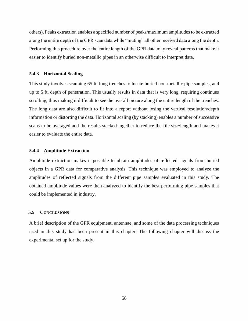
58
others). Peaks extraction enables a specified number of peaks/maximum amplitudes to be extracted
along the entire depth of the GPR scan data while “muting” all other received data along the depth.
Performing this procedure over the entire length of the GPR data may reveal patterns that make it
easier to identify buried non-metallic pipes in an otherwise difficult to interpret data.
5.4.3 Horizontal Scaling
This study involves scanning 65 ft. long trenches to locate buried non-metallic pipe samples, and
up to 5 ft. depth of penetration. This usually results in data that is very long, requiring continues
scrolling, thus making it difficult to see the overall picture along the entire length of the trenches.
The long data are also difficult to fit into a report without losing the vertical resolution/depth
information or distorting the data. Horizontal scaling (by stacking) enables a number of successive
scans to be averaged and the results stacked together to reduce the file size/length and makes it
easier to evaluate the entire data.
5.4.4 Amplitude Extraction
Amplitude extraction makes it possible to obtain amplitudes of reflected signals from buried
objects in a GPR data for comparative analysis. This technique was employed to analyze the
amplitudes of reflected signals from the different pipe samples evaluated in this study. The
obtained amplitude values were then analyzed to identify the best performing pipe samples that
could be implemented in industry.
5.5 CONCLUSIONS
A brief description of the GPR equipment, antennae, and some of the data processing techniques
used in this study has been present in this chapter. The following chapter will discuss the
experimental set up for the study.

59
CHAPTER 6
EXPERIMENTAL SET UP FOR GPR TESTING
6.1 INTRODUCTION
This research involved investigating the detectability of buried PVC, GFRP, and CFRP pipes with
different external surface finishes using GPR in different soil moisture conditions. This chapter
provides a brief description of the research procedure, together with the specimen types and
configuration, preparation of sample pipe sections, and a description of the pipe layout and site
conditions for GPR testing.
6.2 RESEARCH PROCEDURE
In order to determine the detectability of different pipeline materials buried at various depths using
Ground Penetrating Radar (GPR), thirty-nine (39) pipe samples with different external surface
configurations were prepared and buried in the field. Pipeline materials investigated in this
research include Polyvinyl Chloride (PVC), Glass Fiber Reinforced Polymer (GFRP), and Carbon
Fiber Reinforced Polymer (CFRP). A 12" diameter steel pipe was also buried to serve as a control
specimen. The pipe samples were all 5 ft. long, and capped at both ends to prevent ground water
from filling them when buried since the objective is to locate the pipe material without the
assistance of the pipe content.
All pipe caps were made of plastic; caps for 12" diameter steel, CFRP, and GFRP pipes with
carbon fabric, nanoparticle, or aluminum foil overlays had metal straps around them. Plastic straps
were used for the pipe caps in case of the GFRP control pipes (12" and 10" diameter) to ensure
that these control pipes did not have any metallic content. It should be noted that the metal straps
are very small (~ 0.5" wide by 1/16" thick) and are not expected to interfere with GPR signals at
2 ft. of burial depth or deeper. Caps for the PVC pipes and smaller diameter GFRP and CFRP
pipes did not need any straps because the caps were tight fitting.
The pipe segments were buried in four separate trenches, with soil cover of 2 ft., 3 ft., and 4 ft.
above the pipes. These buried pipe segments were scanned with GPR in different soil moisture

60
conditions and the results compared to determine the most promising pipe surface configuration
to improve GPR detection.
6.3 PIPE PREPARATION
Pipe samples used in this research are of 12", 6", and 3" diameters and made from PVC, GFRP,
and CFRP materials. A 10" diameter GFRP pipe which was used for high pressure testing was also
used in this study. Sample preparation of the various pipe segments for GPR testing is elaborated
below.
6.3.1 PVC Pipes
The 12" diameter PVC pipes for testing were obtained by cutting 14 ft. long SDR-35 pipes into
5 ft. long segments. The pipes were then capped to prevent ground water from filling them after
burying since the objective was to establish the pipe detectability without the help of GPR
reflections from any water inside the pipes. Finally, the surfaces of two of the pipes were sanded
to enable adequate bonding with CFRP fabric wrap as will be discussed later in Section 6.3.4.1.
The 12" diameter PVC pipes are shown in Figures 6-1 and 6-2.
Similar to the 12" diameter PVC pipes, 14 ft. long SDR-35 and 10 ft. long schedule 40 (SCH 40)
pipes were cut to obtain the 5 ft. long 6" and 3"diameter pipe samples respectively. The 6" and 3"
diameter pipes were also capped, and the surfaces of some of them were sanded to enable adequate
bonding with GFRP and CFRP fabric (Figure 6-3).

61
Figure 6-1: The 14' long 12" diameter PVC pipe being cut
(a) (b)
Figure 6-2: The 12" diameter PVC pipe (a) after cutting, and (b) after capping

62
(a) Surface of 3" diameter PVC pipe being sanded (b) Some of the capped pipes
Figure 6-3: The 3" diameter PVC pipes
6.3.2 GFRP Pipes
The 12" diameter GFRP pipes used in this study were supplied by the manufacturer in 5 ft. long
segments (Figure 6-4). The pipes were capped to keep ground water out of the pipes after burying.
The external surfaces of some of the pipes were sanded to ensure adequate bonding with CFRP
fabric wrap. Fiber and section properties of the GFRP pipes are given in Table 6-1.
The 10" diameter GFRP pipes used in this study were supplied by the manufacturer in 48 inch
long segments - these set of pipes were being used for high burst pressure testing. One of the 10"
diameter pipes was capped and buried for GPR testing.
The 3" diameter GFRP pipes for the study were manufactured in the WVU Constructed Facilities
Center (WVU-CFC) by wrapping two layers of 24 oz. biaxial (0/90) stitched GFRP fabric around
3" diameter PVC pipes (the PVC pipes serving as molds in this process). This increased the outside
diameter of the GFRP pipes above the standard 3" PVC pipe dimension. Details of the GFRP fabric
and the resin (matrix) system used in manufacturing the 3" GPRP pipe is shown in Table 6-1. The
manufacturing process and a completed GFRP pipe are illustrated in Figure 6-5.

63
(a) GFRP pipes from the manufacturer (b) Capped pipes
Figure 6-4: The 12" diameter GFRP pipes
Table 6-1: Material and section properties of CFRP and GFRP pipes/fabrics
Pipe
Section
Wall
Thickness (in)
Fiber
Material
Fiber Mat Fiber Weight
(oz. /sq. yd.)
Matrix
Material
12" GFRP 3/8 E-Glass 45/90/-45 - Polyurethane
10" GFRP 3/8 E-Glass Filament wound - Vinyl Ester
3" GFRP ** E-Glass 0/90 24 Vinyl Ester
12" CFRP ** Carbon 0/90/±45 28 Vinyl Ester
CFRP
Strip/Ring * Carbon 0/90/±45 28 Vinyl Ester
3" CFRP 5/16 Carbon - - -
* One layer of fabric was used. ** Two layers of fabric were used.

64
(a) Manufacturing process (c) Completed pipe
Figure 6-5: Manufacturing a 3" diameter GFRP pipe
6.3.3 CFRP Pipes
The 12" diameter CFRP pipe used in this study was also fabricated in the WVU Constructed
Facilities Center (WVU-CFC) by wrapping two layers of quad-axial (0/90/±45) stitched CFRP
fabric around a 12" diameter cardboard tube (the cardboard tube served as a mold in this process).
Details of the CFRP fabric and the resin system used in manufacturing the 12" CPRP pipe is shown
in Table 6-1. The pipe was finally capped to keep ground water out of it after burying.
Figures-6-6(a) and 6-6(b) show the CFRP fabric and the completed 12" diameter CFRP pipe
respectively
The 3" diameter CFRP pipes used in this study were supplied by the manufacturer in 6 ft. long
segments (Figure 6-7). The pipes were first cut into 5 ft. long segments to keep the lengths
consistent with the other pipes, they were then capped to keep ground water out of them after
burying.
(b) Manufacturing process

65
(a) Roll of CFRP fabric (b) The completed pipe
Figure 6-6: 12" diameter CFRP pipe
Figure 6-7: The 3" diameter CFRP pipes
6.3.4 Creating Dielectric Contrast Between Non-Metallic Pipes and Surrounding Soil
Non-metallic pipe materials (such as PVC and GFRP) buried underground are generally not
detectable using GPR in most soil conditions. This is because PVC and GFRP pipe materials have
similar dielectric constant as most soils, and are generally transparent to radar waves and hence do
not reflect the incident waves in most soil conditions. In order to make these pipe materials
detectable using GPR after burying, we have to create a contrast between the dielectric constants
of the pipes and the surrounding soil. Three different approaches were adopted to create dielectric

66
contrast between the pipe materials and the sounding soil – using CFRP rings and strips, aluminum
rings and strips, and carbon nanoparticle overlay.
6.3.4.1 Creating Dielectric Contrast Using CFRP Rings and Strips
Carbon fiber, like steel, is an electrical conductor and as such does not allow transmission of radio
waves like GPR signal. GPR signal incident on carbon fiber material is reflected back to a receiver
(unlike the surrounding soil, which absorbs and/or allows the signal to travel through it), thereby
making the material detectable underground.
Dielectric contrast between both the PVC and GFRP pipes, and the surrounding soil was created
by wrapping the pipes with CFRP fabric in two different configurations. The first configuration
involved wrapping 3" wide CFRP fabric around three of the PVC pipe samples (one each of 12",
6", and 3" diameters) and two of the GFRP pipe samples (12" and 3"diameter) in the form of rings,
at a clear spacing of 3". The second configuration involved wrapping CFRP fabric strip along the
full lengths (excluding pipe caps in most cases) of three PVC and two GFRP pipe samples. For the
12" diameter pipes, the widths of the strips were up to half the circumference of the pipes. The
width of the CFRP strips were up to ¾ of the circumference of the 6" diameter pipes, and the strips
covered almost the entire circumference in the case of the 3" diameter pipes. This was to ensure
part of the CFRP strip remains at the top of the pipe after burying even if the pipe rotates during
backfilling. Figure 6-8(a) and (b) show the 6" diameter PVC pipe with the 3" wide CFRP rings
and the 12" diameter PVC pipe with the CFRP strip respectively.
6.3.4.2 Creating Dielectric Contrast Using Aluminum Rings and Strips
Aluminum is also an electrical conductor, and hence prevents the transmission and attenuation of
radio waves like GPR signal. GPR signal incident on an aluminum material is reflected, thereby
making the material distinctive from the surrounding soil, resulting in aluminum being detectable
underground.
Similar to the CFRP fabric, aluminum foil was wrapped around some of the PVC and GFRP pipes
(in strips and rings) to create a dielectric contrast between the pipes and the surrounding soil when
buried. The first configuration involved wrapping 2.83" wide aluminum foil rings around three
PVC pipe samples (12", 6", and 3" diameters) and two GFRP pipe samples (12" and 3" diameters),

67
at a clear spacing of 3". The second configuration involved wrapping aluminum foil strip along
the lengths of three PVC pipes and two GFRP pipe samples similar to the CFRP fabric strips.
Figure 6-8(c) and (d) show a 12" diameter GFRP pipe with aluminum rings, and a 12" diameter
GFRP pipe with aluminum strip along the length respectively. The aluminum foil overlays will be
especially useful for PVC pipes since these foils are readily available in hardware stores and can
be bonded to already manufactured PVC pipes (which are also readily available in hardware
stores).
(a) (b) (c) (d)
Figure 6-8: Pipe configurations: (a) 6" diameter PVC with carbon fabric rings, (b) 12" diameter
PVC with carbon fabric strip, (c) 12" diameter GFRP with aluminum rings, and (d) 12" diameter
GFRP with aluminum strip
6.3.4.3 Creating Dielectric Contrast Using Carbon Nanoparticle Overlay
Just like carbon fabric, carbon nanoparticles are also good electrical conductors, and therefore do
not allow the transmission and attenuation of radio waves like GPR signal. It is anticipated that,
interconnection between carbon nanoparticles in an overlay will be able to reflect incident GPR
signal, and make the buried material detectable as a result.
A 12" diameter GFRP pipe was coated with a mixture of carbon nanoparticle and Vinyl Ester
matrix up to a quarter of the pipe circumference, and through the entire length of the pipe
(excluding caps) as shown in Figure 6-9. This is expected to create a dielectric contrast between
the pipe and the surrounding soil when buried.

68
Figure 6-9: 12" diameter GFRP pipe with carbon nanoparticle overlay
Some of the PVC and GFRP pipes were not wrapped (these are labelled as “Unwrapped” in
Figure 6-12), and were used as control specimens during GPR detectability testing of the samples.
As stated earlier, a total of thirty-nine, 5 ft. long pipe segments were prepared using different pipe
materials (CFRP, GFRP, and PVC), different pipe diameters (12", 6", and 3"), different surface
finishes (CFRP ring, CFRP strip, aluminum ring, aluminum strip, carbon nanoparticles, and
unwrapped/control), and buried at different depths (2 ft., 3 ft., and 4 ft. of soil cover above the top
of the pipe). Pipes with CFRP, aluminum, or carbon nanoparticles overlays are expected to be
easier to detect using GPR (compared to the control samples) because of their higher dielectric
permittivity leading to higher reflection coefficient. In addition, the bigger diameter pipes buried
with less depth of soil cover should be easier to detect compared to smaller diameter pipes and
pipes at deeper depths.
6.4 PIPE BURYING
Pipe specimens prepared for GPR testing were buried at a site located on the WVU campus. The
site, which was selected by WVU-CFC in consultation with the Facilities Management at WVU,
is near the Engineering Sciences Building (ESB) and is marked with the red polygon on
Figure 6-10. Utility lines close to the allocated site were first marked to prevent excavation damage
of the lines during pipe burying. The site and the marked utility lines are shown in Figure 6-11.

69
Figure 6-10: The site for pipe burying and monitoring (source: Google Maps)
The pipe samples were buried in 4 separate 65 ft. and 36 ft. long trenches, spaced at 12 ft. apart.
12" diameter and 5 ft. long PVC, CFRP, and GFRP pipes were buried at a depth of 4 ft. in one of
the trenches (total trench depth of 5 ft.). The second trench had 3" diameter pipes buried at a depth
of 2 ft. (total trench depth of 27"). Two different diameter pipes, 12" and 6", were buried in the
third trench, both diameters buried at a depth of 3 ft. to the top of the pipe. The fourth trench is 36
ft. long, and contains 12" diameter GFRP, PVC, Steel, and 10" diameter GFRP pipes buried with
2 ft. of soil cover. Eleven pipes were buried in each of the first three trenches, with 1 ft. spacing
between each subsequent pipe as shown in Figure 6-12 and 6-14(a). Six pipes were buried in the
final trench, with 1 ft. spacing between subsequent pipes and 2 ft. spacing between pipes at the
middle of the trench. The layout of the pipes, including the pipe material, diameter, pipe surface
configuration and depth of burial are shown in Figures 6-12 and 6-13.
Additionally, five GS3 soil sensors (Figure 6-14b) manufactured by Decagon Devices, Inc. were
buried along the trenches at different depths to measure soil properties throughout the testing
period. Two of the sensors were buried at 4 ft. depth along the 12" diameter pipes, two were buried
at 2 ft. depth along the 3" diameter pipes and one was used to measure soil properties at various
locations on the ground surface. Wires connecting the soil sensors to a data logger were run
through 1" diameter PVC conduits before burying to prevent the wires from getting damaged

70
during compaction of backfill (Figure 6-15). These sensors enabled quantitative determination of
volumetric water content, electrical conductivity, temperature, and dielectric constant of the soil
during the testing period. The above parameters from the GS3 sensor enabled accurate estimation
of the depth of soil cover over the pipes using GPR. Theses soil parameters are also used in
numerical computations in order to make comparison between the GPR field results and the
theoretical estimations as presented in Chapter 8.
Figure 6-11: The located site on WVU campus for pipe burying, with utility lines marked

71
Steel plates buried at a depth of 3"
12" diameter pipes buried at a depth of 48" (Total trench depth of 60")
12" diameter pipes buried at a depth of 36" (Total trench depth of 48")
6" diameter pipes buried at a depth of 36" (Total trench depth of 42")
3" diameter pipes buried at a depth of 24" (Total trench depth of 27")
GFRP pipe with CFRP fabric strip over half of the pipe circumference. Similar naming scheme applies to the other
pipes in the layout
Figure 6-12: Pipe layout for GPR testing

72
Steel plates buried at a depth of 3"
12" diameter pipes buried at a depth of 24" (Total trench depth of 36")
10" diameter pipes buried at a depth of 24" (Total trench depth of 34")
Trench placed at 12' spacing away from the 3' deep pipe trench.
Figure 6-13: Pipe layout for GPR testing (short trench)
(a) (b)
Figure 6-14: (a) Arrangement of pipes in the trench, (b) soil moisture and resistivity sensor
Figure 6-16 (a) shows trenching for the 12" and 10" diameter pipes buried with 2 ft. depth of soil
cover, while Figure 6-16 (b and c) show the 12" and 6" diameter pipes placed at 3 ft. depth (to the
top of the pipe) in the trench and the pipes being covered with backfill. Figure 6-16(d) shows some
of the 12" diameter pipes placed in the trench at 4 ft. depth (to the top of the pipe). Two 1 ft. wide

73
steel plates were buried at about 3" depth (one at each end of the trench) to mark the beginning
and end of each trench for GPR testing. The steel plates were buried at a distance of 3 ft. away
from the nearest pipe segments at each end of the trench to avoid interference with GPR signal
from the buried pipes.
Finally, the trenches were backfilled and compacted, the ground surface was levelled and then
seeded with grass (Figure 6-17) to restore the initial field condition before GPR testing. Levelling
the ground and seeding with grass was done to ensure the site mirrors actual field conditions for
buried pipes that need to be detected in the pipeline industry using GPR. Thus the results obtained
from GPR testing will give an indication of the applicability of the developed techniques in the
pipeline industry. Levelling and seeding the ground also helps to ensure lawn keeping operations
at the site are not interrupted by this study.
(a) (b)
Figure 6-15: (a) Soil sensors with data wires running through conduits to protect the wires, (b) 3"
diameter pipes and sensors in the 27" deep trench

74
(a) (b) (c) (d)
Figure 6-16: Pipe samples being buried
(a) (b)
Figure 6-17: (a) The site being seeded, (b) the field restored to initial condition
A summary of the pipe samples, materials, surface configuration, pipe diameter, and depth of soil
cover over buried pipes is presented in Table 6-2. Several GPR field tests of the buried pipes were
conducted under varying weather and soil moisture conditions, after the grass was allowed to grow
to restore the field to its initial condition. These GPR test results are discussed in the next chapter.
Comparison of the results for the various buried pipes serves to determine the suitable pipe surface
configurations for easier detection of buried non-metallic pipes.

75
Table 6-2: Summary of pipe samples and configurations
Pipe Diameters with Each Surface Configuration
Pipe Materials
Soil Cover Depth
(ft.) Control
CFRP Aluminum Carbon Nano-
particle Total
Strip Ring Strip Ring
CFRP 4 12" 1
2 3" 1
GFRP
4 12" 12" 12" 12" 12" 5
3 12" 12" 12" 3
2 12", 10", 3" 12", 3" 3" 3" 3" 12" 9
PVC
4 12" 12" 12" 12" 12" 5
3 12", 6" 6" 6" 12", 6" 12", 6" 8
2 3" 3" 3" 12", 3" 3" 6
Steel 2 12" 1
Total 12 7 6 7 6 1 39
6.5 CONCLUSIONS
This chapter summarized the sample preparation and material properties of the pipe specimens
used in the GPR detectability testing. The following chapter presents the field testing results and
analysis of the obtained data.

76
CHAPTER 7
GPR TEST RESULTS AND DATA ANALYSIS
7.1 INTRODUCTION
Different pipe material samples (CFRP, GFRP, and PVC) with different external surface finishes
were buried at a test site as explained in Chapter 6. Multiple GPR surveys were carried out during
this study to evaluate the detectability of the different pipe configurations. The results of these
tests and analyses conducted on the data are presented in the following sections.
7.2 GPR TEST RESULTS
GPR tests were conducted under different soil moisture conditions (indicated by the changing soil
volumetric water content and dielectric constant for each test), and using different antennae
frequencies (200 MHz and 400 MHz). A 900 MHz antenna was also evaluated at the beginning of
the study and found to be inadequate in achieving the expected penetration depth in the wet soil
medium in this study. Scans were carried out in both the longitudinal direction along the pipe
trenches, and transverse direction across the trenches/pipes. Some of the test data, labelled as
Dataset I through Dataset III are presented below. GPR survey for Dataset I was conducted in a
relatively dry soil in the summer months, with average volumetric water content up to 2 ft. depth
of 0.290 m3/m3; survey for Dataset II was conducted in a relatively wet soil in the winter months,
with average volumetric water content up to 2 ft. depth of 0.473 m3/m3; while survey for Dataset
III was conducted in spring months, with average volumetric water content up to 2 ft. depth of
0.343 m3/m3. Detailed average soil properties for the dataset presented are given in Table 7-1.
Table 7-1: Average soil dielectric properties during data collection
Depth
Up to Dataset I Dataset II Dataset III
VWC, θ
(m3/m3)
Diel. ε
Cond.
(mS/m)
VWC, θ
(m3/m3)
Diel. ε
Cond.
(mS/m)
VWC, θ
(m3/m3)
Diel. ε
Cond.
(mS/m)
2' 0.290 13.42 10.94 0.473 26.77 17.08 0.343 16.60 12.47
3' 0.315 15.09 11.43 0.473 26.75 16.97 0.363 18.12 12.86
4' 0.341 16.76 11.92 0.473 26.73 16.85 0.383 19.65 13.25

77
7.2.1 900 MHz Antenna Data
Figure 7-1 shows a longitudinal GPR scan over the full length of the trench with 3" diameter pipes
buried at 2 ft. depth of soil cover using the 900 MHz antenna. Average soil dielectric constant and
electrical conductivity (up to 2 ft. depth) for this data were 19.76 and 14.13 mS/m respectively. As
can be seen in the figure, none of the buried pipes could be identified in the GPR scan. Further
tests were conducted and it was concluded that the 900 MHz antenna is inadequate for this study.
The remainder of this chapter will focus on data obtained from the deeper penetrating 200 MHz
and 400 MHz antennae.
Figure 7-1: Longitudinal scan over 3" diameter pipes at 2 ft. depth using 900 MHz antenna
7.2.2 Dataset I
Raw data from longitudinal scans over the four trenches for Dataset I using 200 MHz antenna are
shown in Figure 7-2(a) through (d) for comparison. Figures 7-3 through 7-6 show comparisons
between the raw and the processed scans from each trench using “Peaks extraction” data
processing technique in RADAN™ 7. Extracting reflected signal peaks in the GPR data makes it
easier to see the buried pipes. Data from radar scan using the 400 MHz antenna over the 12" and
10" diameter pipes buried with 2 ft. of soil cover is shown in Figure 7-7.
With the exception of the 3" diameter pipes buried with 2 ft. of soil cover, good GPR signal
reflections were recorded from pipes buried in all the other trenches as shown in Figure 7-2. Good
signal reflection from the buried pipes in this dataset can be attributed to the relatively dry soil
under which the data was collected (compared to the other datasets). These reflected signals made
it possible to detect the buried pipes with varying levels of clarity and signal strengths. It is
observed from Dataset I (Figures 7-2 through 7-6) that, carbon fabric and aluminum foil
wraps/overlays on the pipe sections improve detectability with GPR. It is also observed that,
carbon fabric strips and aluminum strips along the full length of the pipe sections generally produce
better results compared to aluminum rings and carbon fabric rings; this will be explained further

78
(a) Longitudinal scan along the full length of 12" and 6" diameter pipes with 3 ft. of soil cover
(b) Longitudinal scan along the full length of 12" diameter pipes with 4 ft. of soil cover
(c) Longitudinal scan along the full length of 3" diameter pipes with 2 ft. of soil cover
(d) Longitudinal scan along the full length of 12" and 10" diameter pipes with 2 ft. of soil cover
Figure 7-2: Dataset I - Longitudinal scans over the pipe trenches using 200 MHz antenna

79
(a) Longitudinal scan along the full length of 12" and 6" diameter pipes with 3 ft. of soil cover
(b) Peaks extraction processing used to make buried pipes in scan (a) more visible
Figure 7-3: Longitudinal scan over the 3 ft. deep trench for Dataset I using 200 MHz antenna
(a) Longitudinal scan along the full length of 12" diameter pipes with 4 ft. of soil cover
(b) Peaks extraction processing used to make buried pipes in scan (a) more visible
Figure 7-4: Longitudinal scan over the 4 ft. deep trench for Dataset I using 200 MHz antenna
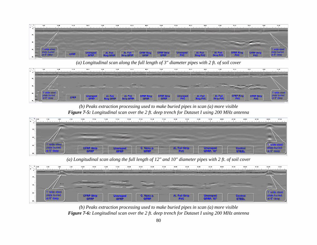
80
(a) Longitudinal scan along the full length of 3" diameter pipes with 2 ft. of soil cover
(b) Peaks extraction processing used to make buried pipes in scan (a) more visible
Figure 7-5: Longitudinal scan over the 2 ft. deep trench for Dataset I using 200 MHz antenna
(a) Longitudinal scan along the full length of 12" and 10" diameter pipes with 2 ft. of soil cover
(b) Peaks extraction processing used to make buried pipes in scan (a) more visible
Figure 7-6: Longitudinal scan over the 2 ft. deep trench for Dataset I using 200 MHz antenna

81
(a) Longitudinal scan along the full length of 12" and 10" diameter pipes with 2 ft. of soil cover
(b) Background noise removal applied to the scan in (a)
(c) Peaks extraction processing used to make buried pipes in scan (a) visible
Figure 7-7: Longitudinal scan over the 2 ft. deep trench for Dataset I using 400 MHz antenna

82
in Section 7.2.5. GPR signal reflections from some of the pipe sections will also be evaluated
individually for better clarity. Only data from the 12" and 6" diameter pipes buried with 3 ft. of
soil cover, and 12" and 10" diameter pipes buried with 2 ft. of soil cover will be evaluated for
brevity. However, conclusions drawn from this detailed evaluation applies to pipes in the other
trenches.
As shown in Figure 7-2(a) and 7-3 for Dataset I, all the buried pipes with 3 ft. of soil cover (with
the exception of 12" diameter PVC pipe without any overlay and 12" diameter PVC pipe with
aluminum foil rings) can be detected with varying levels of clarity in the raw data when scanned
with the 200 MHz radar antenna. Particularly, pipe sections with CFRP and aluminum foil overlays
appear prominently, and with higher signal strengths. These are easily detected compared to pipes
without any overlay. Among the pipes with CFRP or aluminum foil overlays, CFRP and aluminum
foil strips along the full length of the pipes are generally easier to detect compared to CFRP and
aluminum foil rings around the pipes. Extracting reflected signal peaks during post processing
makes it easier to locate the buried pipes as shown in Figure 7-3(b). Peak extraction also makes it
possible to locate pipes that were otherwise not visible in the raw GPR scan.
Figures 7-8 through 7-18 show details of each pipe in Figure 7-2(a), including the B-Scan to the
left and A-Scan to the right of each figure. The depth of soil cover over the pipes was also
accurately estimated from the GPR data as shown in Figures 7-8 and 7-9, where the measured pipe
depth of 37.00" and 37.10" using GPR signal correlates very well with the actual pipe depth of
3 ft. (36"). Measurement of soil dielectric constant using buried sensors during GPR surveys
enabled these depths to be estimated. Reflections from both the top and bottom of some of the
pipes make it possible to estimate the diameters of such pipes as shown in Figure 7-8. However,
since the diameter of the pipe is estimated from the electromagnetic wave velocity, which is based
on the average soil dielectric constant, there is the possibility for the estimated diameter to be less
than the actual diameter. This is because, the dielectric constant of the overlying soil medium is
significantly more than the dielectric constant of air in the pipe. The above statements apply even
more to Dataset II (presented later) where the dielectric constant of the soil is much higher than
that of air (26.75 for the soil up to 2 ft. and 1 for air). Furthermore, the wavelength (and pulse
width) of the radar wave for this test is higher than the actual pipe diameter, hence reflection from
the bottom of the pipe overlaps with reflection from the top of the pipe. This results in the signal

83
Figure 7-8: Longitudinal GPR scan (left) and A-Scan (right) over Unwrapped 12" GFRP pipe
Figure 7-9: Longitudinal GPR scan (left) and A-Scan (right) over 12" CFRP Ring GFRP pipe
peak of the bottom reflection being shifted, and hence affecting the estimated diameter.
The unwrapped 12" diameter GFRP shows up well in the GPR scan at 3 ft. depth (Figure 7-8) and
is detected with clean reflected signal from the top and bottom of the pipe.
Figure 7-9 shows the GPR scan at 3 ft. depth over 12" diameter GFRP pipe with CFRP Ring. This
pipe shows up prominently in the GPR scan and is detected with clean reflected signal from the
top of the pipe. Good/prominent reflection from the top of the pipe will make it possible to locate
the pipe with GPR irrespective of the content of the pipe.

84
Figure 7-10: Longitudinal GPR scan (left) and A-Scan (right) over 12" CFRP Strip GFRP pipe
Figure 7-11: Longitudinal GPR scan (left) and A-Scan (right) over 12" Unwrapped PVC pipe
Figure 7-10 shows the GPR scan at 3 ft. depth over 12" diameter GFRP pipe with CFRP Strip at
the top. This pipe also shows up very well in the GPR scan and is detected with clean reflected
signal from the top of the pipe.
GPR scan over the unwrapped 12" diameter PVC pipe is shown in Figure 7-11; this pipe produced
a very poor GPR signal reflection which makes it very difficult to detect the pipe in the raw GPR
data.

85
Figure 7-12: Longitudinal GPR scan (left) and A-Scan (right) over 12" Al. Foil Ring PVC pipe
Figure 7-13: Longitudinal GPR scan (left) and A-Scan (right) over 12" Al. Foil Strip PVC pipe
Figures 7-12 and 7-13 show the GPR scan over the 12" diameter PVC pipe with aluminum foil
rings and aluminum foil strip respectively. The PVC pipe with aluminum foil rings produced a
better reflected signal in the radar scan compared to the unwrapped pipe shown in Figure 7-11.
The PVC pipe with aluminum foil strip at the top produced the best reflected radar signal (clean
signal with highest amplitude) among the three PVC pipes in Figures 7-11 through 7-13. This
makes it a lot easier to identify the pipe in the GPR scan.

86
Figure 7-14: Longitudinal GPR scan (left) and A-Scan (right) over 6" Unwrapped PVC pipe
Figure 7-15: Longitudinal GPR scan (left) and A-Scan (right) over 6" Al. Foil Ring PVC pipe
Figure 7-14 shows the GPR scan at 3 ft. depth over 6" diameter unwrapped PVC pipe. This pipe
produced a fairly good radar reflection that covers only a short section of the pipe. Thus the pipe
is only visible over the short span that produced GPR reflection.
The 6" diameter PVC pipe with aluminum foil rings also produced a fairly good reflection, but
this reflection is recorded over the entire length of the pipe (Figure 7-15). Thus, it will be easier to
locate this pipe using GPR than the one without any wrap.
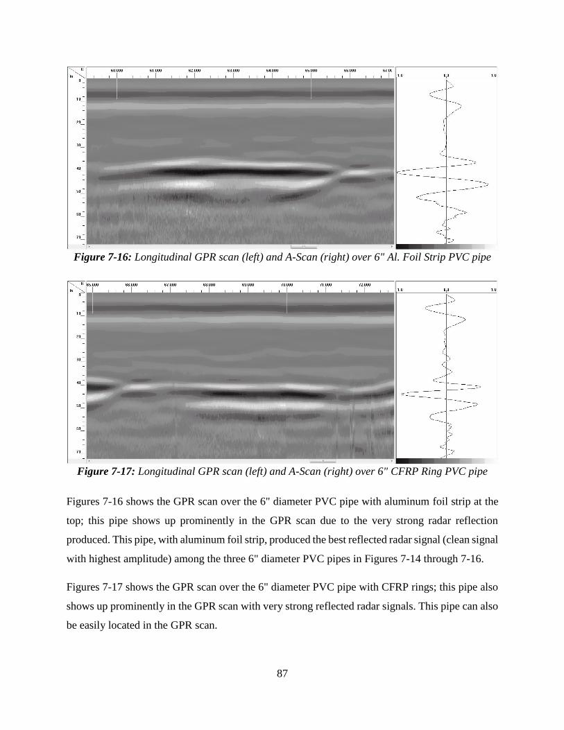
87
Figure 7-16: Longitudinal GPR scan (left) and A-Scan (right) over 6" Al. Foil Strip PVC pipe
Figure 7-17: Longitudinal GPR scan (left) and A-Scan (right) over 6" CFRP Ring PVC pipe
Figures 7-16 shows the GPR scan over the 6" diameter PVC pipe with aluminum foil strip at the
top; this pipe shows up prominently in the GPR scan due to the very strong radar reflection
produced. This pipe, with aluminum foil strip, produced the best reflected radar signal (clean signal
with highest amplitude) among the three 6" diameter PVC pipes in Figures 7-14 through 7-16.
Figures 7-17 shows the GPR scan over the 6" diameter PVC pipe with CFRP rings; this pipe also
shows up prominently in the GPR scan with very strong reflected radar signals. This pipe can also
be easily located in the GPR scan.

88
Figure 7-18: Longitudinal GPR scan (left) and A-Scan (right) over 6" CFRP Strip PVC pipe
Finally, GPR scan over the 6" diameter PVC pipe with CFRP strip at the top is shown in
Figure 7-18. This pipe produced radar reflection with the highest amplitude among all the 6"
diameter PVC pipes buried at 3 ft. depth (it also produced highest amplitude reflection among all
pipes buried at 3 ft. depth in this dataset). The amplitude of the reflected radar wave for this pipe
was higher than what the radar system could record, resulting in the clipped signal as shown in the
A-Scan to the right of Figure 7-18.
Thus, by focusing on the GPR scan over the 6" diameter PVC pipes shown in Figures 7-14 through
7-18, it can be seen that pipe sections with CFRP and aluminum foil overlays appear prominently,
with higher signal strengths. These are easily detected in the GPR scans compared to pipes without
any overlay. Among the pipes with CFRP or aluminum foil overlays, CFRP and aluminum foil
strips along the full length of the pipes produced higher amplitude reflections, making the pipes
easier to detect compared to CFRP and aluminum foil rings around the pipes. In addition, CFRP
rings/strips produced higher reflected signal amplitudes compared to aluminum foil rings/strips.
As shown in Figures 7-2(d) and 7-6, for Dataset I, all the 12" and 10" diameter pipes with 2 ft. of
soil cover are detectable in the raw data with varying levels of clarity when scanned with the 200
MHz radar antenna. Similar to the previous discussions, the GFRP pipe with CFRP strip at the top
and the PVC pipe with aluminum foil strip at the top are prominently visible. Returned signal from
the 12 inch diameter GFRP pipe with no external wrap is also very good, however, reflection from
top of the pipe is very short, or not continuous over the entire length of the pipe (only signal

89
reflection from the bottom of the pipe is continuous through the length of the pipe). The GFRP
pipe with carbon nanoparticle overlay produced a good but very short (or discontinues) reflection
from the top of the pipe as shown in Figure 7-2(d). The 10 inch diameter GFRP and the steel
produced weak reflections, with the steel pipe being a bit more visible in the GPR B-Scan shown
in Figure 7-2(d).
Figures 7-19 through 7-24 show details of each of the 12" and 10" diameter pipes buried with 2 ft.
of soil cover. The depth of soil cover over the pipes was also accurately estimated from the GPR
data as shown in Figures 7-19 and 7-20, where the measured pipe depth of 24.6" and 25.00" using
GPR signal correlates very well with the actual pipe depth of 2 ft. (24"). Reflections from both the
top and bottom of some of the pipes in this trench also make it possible to estimate the diameter
of such pipes as shown in Figures 7-19 and 7-20. The limitations of using this method to estimate
pipe diameter as discussed previously (including different dielectric constant for the content of the
pipe and the overlaying soil, and wavelength and pulse width of the radar wave being bigger than
the actual pipe diameter) still applies.
Figure 7-19 shows the GFRP pipe with CFRP strip at the top; the pipe is detected with clean
reflected signal from the top and bottom of the pipe. Prominent reflection from the top of the pipe
will make it possible to locate the pipe with GPR irrespective of the content of the pipe. It was also
possible to estimate the pipe diameter because of reflections from both the top and bottom of the
pipe.
Figure 7-20 shows the GFRP pipe without any surface wrap; the pipe is detected with short and
weaker signal from the top (compared to the pipe bottom reflection) and continuous, stronger
reflection from the bottom. Though the pipe is detected using the combination of top and bottom
reflections in this case, it will be difficult to locate the pipe if its content absorbs the radar signal
and makes it impossible to obtain reflections from the bottom of the pipe. It was also possible to
estimate the pipe diameter from the recorded GPR signal reflections for this pipe.

90
Figure 7-19: Longitudinal GPR scan (left) and A-Scan (right) over 12" CFRP Strip GFRP pipe
Figure 7-20: Longitudinal GPR scan (left) and A-Scan (right) over Unwrapped 12" GFRP pipe

91
Figure 7-21: Longitudinal GPR scan (left) and A-Scan (right) over C. Nano p. 12" GFRP pipe
Figure 7-22: Longitudinal GPR scan (left) and A-Scan (right) over Al. Foil Strip 12" PVC pipe
Figure 7-21 shows the GFRP pipe with carbon nanoparticle overlay; this pipe produced a good but
very short reflection (reflection not continuous over the pipe length) from the top of the pipe. This
signal is weaker than the one produced by the GFRP pipe without any surface wrap in Figure 7-20.
Thus the carbon nanoparticle overlay did not improve the detectability of the buried GFRP pipe.
Figure 7-22 shows the PVC pipe with aluminum foil strip at the top; this pipe produced a very
good reflection from the top of the pipe, thus making it possible to locate the pipe. The prominent
reflection from the top of this pipe will also make it possible to locate the pipe with GPR
irrespective of the content of the pipe.

92
Figure 7-23: Longitudinal GPR scan (left) and A-Scan (right) over Unwrapped 10" GFRP pipe
Figure 7-24: Longitudinal GPR scan (left) and A-Scan (right) over 12" Steel pipe
Figure 7-23 shows the 10" GFRP pipe with no external surface wrap; this pipe produced a weak
but continues reflection from the top of the pipe. The continuous reflection made it possible to
locate the pipe in this test. However, the weak reflection means the pipe might not be detected at
depths beyond the 2 ft. investigate in this test. At deeper depths, the weak reflected signal from
this pipe will attenuate and completely dissipate in the overlaying soil and therefore will not be
detected by the receiving radar antenna.
Figure 7-24 shows the steel pipe used as control specimen; this also produced a weak but
continuous reflection from the top of the pipe, and hence made it possible to locate the pipe in this
93
test. Reflections from the steel pipe are more defined compared to the 10 inch diameter GFRP pipe
(Figure 23), with the ends of the steel pipe clearly visible in the GPR B-Scan (left side of
Figure 7-24).
Figure 7-7(a) shows the raw GPR scan from all the 12" and 10" diameter pipes buried with 2 ft. of
soil cover scanned using the 400 MHz antenna (for Dataset I), and Figures 7-7(b) and 7-7(c) show
the data in Figure 7-7(a) processed using background noise removal and peaks extraction
respectively. It is difficult to identify any pipe in Figures 7-7(a) and 7-7(b), but extracting the
reflected signal peaks makes it possible to see the GFRP pipe wrapped with CFRP strip and the
GFRP pipe with no external surface wrap. The PVC pipe with aluminum foil strip at the top is also
faintly visible in the processed data in Figure 7-7(c). Thus, the 400 MHz antenna is less effective
in locating the buried pipes at 2 ft. depth or deeper when scanned in the longitudinal direction
along the pipes. Conducting scans in the transverse direction across the pipes however makes it
possible to detect the buried pipes at 2 ft. depth using the 400 MHz antenna, though with less
clarity compared to results from the 200 MHz antenna. This is because, the 400 MHz radar antenna
has higher signal attenuation compared to the 200 MHz antenna. Thus greater portion of the
transmitted signal is lost; signal attenuation for the different antennae will be explained later in
Section 8.4 of Chapter 8. Details of the three pipes identified in the Figure 7-7(c) are provided in
Appendix B.1; this includes the raw data, data with background noise removed, and the data with
signal peaks extracted respectively in each figure. Appendix B.4 also includes results for transverse
scans over the buried pipes using 400 MHz antenna.
7.2.3 Dataset II
Figure 7-25 shows the GPR scan data over the four trenches for Dataset II using the 200 MHz
antenna. GPR survey for this data was conducted in a relatively wet soil in the winter months, with
the ground surface covered with snow up to a depth of 3.75". Soil properties measured during this
survey were higher than that for Dataset I as already shown in Table 1-1.
Similar to Dataset I, the addition of CFRP and aluminum foil overlays in the form of strips at the
top of the pipes and rings around the pipes significantly improved the detectability of these pipes
using GPR. The application of carbon nanoparticle coating on a pipe did not improve on the
detectability of such pipes in this dataset. In the case of 3" diameter pipes buried with 2 ft. of soil

94
cover, most of the pipe sections are not visible in the raw data shown in Figure 7-25(c). The data
was thus processed by extracting reflected signal peaks to make it easier to identify buried pipes
in the scan. After the peaks extraction process, all the pipe sections with CFRP or aluminum foil
overlays are visible in the radar data as shown in Figure 7-26(b). The pipe sections without any
CFRP/aluminum foil overlay (Unwrapped GFRP and Unwrapped PVC) remained invisible even
after the peaks extraction process. A combination of background noise removal and peaks
extraction did not make these unwrapped pipe sections visible. It should be noted that the 3"
diameter pipes buried with 2 ft. of soil cover did show very well even in the raw GPR data when
scanned in the transverse direction across the pipes as will be shown later in Dataset III.
Figure 7-27 shows results from the 3" diameter pipes buried with 2 ft. of soil cover scanned in the
longitudinal direction using the 400 MHz antenna. In Figure 7-27, (a), (b), and (c) show the raw
GPR scan data, data with background noise removal applied, and data with background noise
removal and peaks extraction applied respectively. None of the buried pipes are visible in
Figure 7 27(a through c) even after different data processing techniques, including background
noise removal, peaks extraction, and combination of both have been applied.
GPR results from the 12" and 10" diameter pipes buried at 2 ft. depth and scanned using the
400 MHz are shown in Figure 7-28. Similar to Figure 7-27, (a), (b), and (c) in Figure 7-28 show
the raw GPR scan data, data with background noise removal applied, and data with background
noise removal and peaks extraction applied respectively. It is difficult to identify the buried pipes
in the raw data as shown in Figure 7-28(a). However, performing background noise removal on
the raw data (Figure 7-28b) makes it possible to identify three of the pipes; the GFRP pipe with
carbon fabric strip, the 12" diameter GFRP pipe with no wrap/overlay, and the steel control pipe.
All the buried pipes were visible (as shown in Figure 7-28c) after extracting reflected signal peaks
from the GPR data in Figure 7-28(b).
This result reinforces the fact that, the 400 MHz antenna is less effective in locating the buried
pipes at 2 ft. depth and deeper because of the higher signal attenuation compared to the 200 MHz
antenna. Scanning the pipes in the transverse direction using the 400 MHz antenna however
produces a better result as shown in Appendix B.4.

95
(a) Longitudinal scan along the full length of 12" and 6" diameter pipes with 3 ft. of soil cover
(b) Longitudinal scan along the full length of 12" diameter pipes with 4 ft. of soil cover
(c) Longitudinal scan along the full length of 3" diameter pipes with 2 ft. of soil cover
(d) Longitudinal scan along the full length of 12" and 10" diameter pipes with 2 ft. of soil cover
Figure 7-25: Dataset II - Longitudinal scans over the pipe trenches using 200 MHz antenna

96
(a) Longitudinal scan along the full length of 3" diameter pipes with 2 ft. of soil cover
(b) Peaks extraction processing used to make buried pipes in scan (a) more visible
Figure 7-26: Longitudinal scans over 3" diameter pipes at 2 ft. deep using 200 MHz antenna

97
(a) Longitudinal scan along the full length of 3" diameter pipes with 2 ft. of soil cover
(b) Background noise removal applied to the scan in (a)
(c) Peaks extraction processing applied to data in (b)
Figure 7-27: Longitudinal scan over 3" diameter pipes at 2 ft. deep using 400 MHz antenna

98
(a) Longitudinal scan along the full length of 12" and 10" diameter pipes with 2 ft. of soil cover
(b) Background noise removed from figure in (a)
(c) Signal reflection peaks extracted from (b)
Figure 7-28: Longitudinal scans over 12" and 10" diameter pipes at 2 ft. deep using 400 MHz antenna

99
(a) Longitudinal scan along the full length of 12" and 10" diameter pipes with 2 ft. of soil cover
(a) Reflection details marked in the longitudinal scan from (a)
Figure 7-29: Reflection details marked on 12" and 10" diameter pipes with 2 ft. of soil cover
Table 7-2: Description of features marked in Figure 7-29
Feature/
Label Object/Pipe Type Result Description
Steel plates 1 ft. wide steel plates Appear prominently in the GPR scans
A GFRP pipe with CFRP strip Produced very strong reflection from both the top (A) and bottom (A1)
of the pipe, pipe was clearly detected A1 Reflection from bottom of pipe
B GFRP pipe with no wrap (12" diameter) The pipe produced very weak reflection over sections of the pipe (B).
Very strong reflection recorded from the bottom of the trench (B1) B1 Reflection from bottom of trench
C GFRP pipe with carbon nanoparticle coating Produced weaker reflection than D (over short section of pipe), from
both the top (C) and bottom (C1) of the pipe. Portion of pipe detected C1 Reflection from bottom of pipe
D PVC pipe with aluminum strip Produced strong, continuous reflection, pipe was detected
E GFRP pipe with no wrap (10" diameter) Produced strong reflection over sections of the pipe, pipe was detected
F Steel pipe Produced strong continuous reflection, pipe was detected

100
Figure 7-29 shows details of the pipes and other features identified in this scan from the 12" and
10" diameter pipes with 2 ft. of soil cover. Description of the features marked A through F in
Figures 7-29(b) are summarized in Table 7-2. Detailed radar data for these features are provided
in Appendix B.2.
The GPR result presented in Dataset II indicates that snow cover on the ground surface does not
hinder the detection of buried pipes using GPR. The results obtained in the GPR survey for this
dataset (with the ground covered with snow up to 3.75") is similar to what was obtained for Dataset
I which did not have any snow cover on the ground surface.
7.2.4 Dataset III
GPR survey results over the four trenches using the 200 MHz antenna for Dataset III are shown in
Figure 7-30. This survey was carried out in the spring, with the measured soil properties during
the survey already shown in Table 1-1. Results in this dataset correlates well with the two datasets
discussed previously, with CFRP and aluminum foil overlays improving the detectability of buried
non-metallic pipes while carbon nanoparticle coating did not provide any noticeable benefit in pipe
detectability using GPR.

101
(a) Longitudinal scan along the full length of 12" and 6" diameter pipes with 3 ft. of soil cover
(b) Longitudinal scan along the full length of 12" diameter pipes with 4 ft. of soil cover
(c) Longitudinal scan along the full length of 3" diameter pipes with 2 ft. of soil cover
(d) Longitudinal scan along the full length of 12" and 10" diameter pipes with 2 ft. of soil cover
Figure 7-30: Dataset III - Longitudinal scans over the pipe trenches using 200 MHz antenna

102
For most GPR applications in locating buried utility lines, scans are performed perpendicular to
the expected direction of the utility line. Thus, for Dataset III, scans were also performed
perpendicular to the direction of the pipes for comparison. Figure 7-31 (a through k) shows GPR
scans over the buried pipes in the first three trenches (65 ft. long trenches), while scans over the
fourth trench (36 ft. long trench) is shown in Figure 7-32 (a through f). Each transverse scan in
Figure 7-31 was performed over all the three trenches, starting from the 3 ft. deep trench and
ending over the 2 ft. deep trench (or from the top line of pipes to the bottom line of pipes according
the layout given in Figure 6-12 in Chapter 6). Subsequent scans (from a through k) were conducted
starting from the left side to the right side of the layout in Figure 6-12 in Chapter 6.
Looking at Figure 7-31 (g through k), it is evident that, the PVC pipes (6", 12", and 3" diameters
from left to right on each figure) without any wrap (Unwrapped PVC in Figure 7-31g) produced
the weakest radar reflections among all the scans from g through k. Contrary to the unwrapped
PVC pipes, the PVC pipes with aluminum foil or CFRP strips (Figures 7-31 i and k) produce the
strongest radar reflections among all the scans from g through k. The PVC pipes with CFRP strips
also produced reflections with higher amplitudes at the apex of the hyperbola reflection
(Figure 7-31k) compared to the PVC pipes with aluminum foil strips (Figure 7-31i). Radar
reflections from the PVC pipes with aluminum foil or CFRP rings produced mixed results
(Figure 7-31 h and j), with some of the reflections having higher amplitudes compared to those
obtained from the unwrapped PVC while amplitudes of the remaining reflections are comparable
in magnitude to the ones obtained from the unwrapped PVC pipes.
The mixed results from pipes with aluminum foil or CFRP rings can be attributed to the fact that,
the path of the radar antenna axis might have been between two rings for some of the pipes. Hence
the radar hyperbolas for such pipes were produced from reflections off the bare PVC or GFRP
pipe rather than off the CFRP/aluminum rings. Using spiral wraps around the pipes instead of
parallel rings will ensure there is always part of the wrap at every section along the length of the
pipe, this could help address the problem associated with parallel rings.
The same observation made for Figure 7-31 (g through k) also applies to Figure 7-31 (a through f),
though this is less obvious since the surface configurations of the pipes in each scan shown in
Figure 7-31 (a through f) are not the same. Thus, pipe sections with the same surface configuration
have to be identified from multiple scans before the comparisons can be made.

103
(a) 12" dia. Unwrapped GFRP at 3', 12" dia. CFRP at 4', and 3" dia. CFRP at 2'
(b) 12" dia. CFRP Ring GFRP at 3', 12" dia. Unwrapped GFRP at 4', and 3" dia. Unwrapped GFRP at 2'
(c) 12" dia. CFRP Strip GFRP at 3', 12" dia. Al. Foil Ring GFRP at 4', and 3" dia. Al. Foil Ring GFRP at 2'
(d) 12" dia. Unwrapped PVC at 3', 12" dia. Al. Foil Strip GFRP at 4', and 3" dia. Al. Foil Strip GFRP at 2'

104
(e) 12" dia. Al. Foil Ring PVC at 3', 12" dia. CFRP Ring GFRP at 4', and 3" dia. CFRP Ring GFRP at 2'
(f) 12" dia. Al. Foil Strip PVC at 3', 12" dia. CFRP Strip GFRP at 4', and 3" dia. CFRP Strip GFRP at 2'
(g) 6" dia. Unwrapped PVC at 3', 12" dia. Unwrapped PVC at 4', and 3" dia. Unwrapped PVC at 2'
(h) 6" dia. Al. Foil Ring PVC at 3', 12" dia. Al. Foil Ring PVC at 4', and 3" dia. Al. Foil Ring PVC at 2'
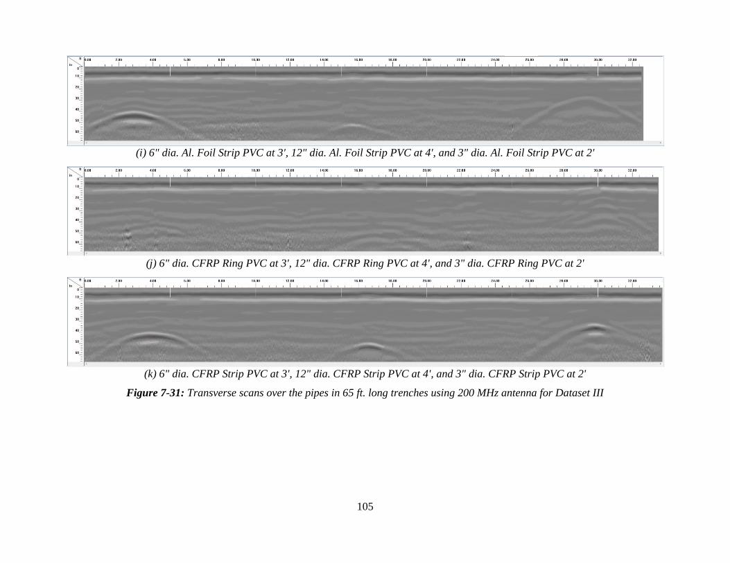
105
(i) 6" dia. Al. Foil Strip PVC at 3', 12" dia. Al. Foil Strip PVC at 4', and 3" dia. Al. Foil Strip PVC at 2'
(j) 6" dia. CFRP Ring PVC at 3', 12" dia. CFRP Ring PVC at 4', and 3" dia. CFRP Ring PVC at 2'
(k) 6" dia. CFRP Strip PVC at 3', 12" dia. CFRP Strip PVC at 4', and 3" dia. CFRP Strip PVC at 2'
Figure 7-31: Transverse scans over the pipes in 65 ft. long trenches using 200 MHz antenna for Dataset III

106
(a) GFRP pipe wrapped CFRP fabric (b) Unwrapped GFRP pipe
(c) GFRP pipe with carbon nanoparticle overlay (d) PVC pipe wrapped with Aluminum foil strip
(e) Unwrapped GFRP pipe (10″ diameter) (f) Steel pipe
Figure 7-32: Transverse scans over the pipes in 36 ft. long trench using 200 MHz antenna for Dataset III

107
Figure 7-32 shows transverse scans (using 200 MHz antenna) over the 12" and 10" diameter pipes
buried with 2 ft. of soil cover. Similar to the other GPR scans already discussed, pipe sections with
CFRP/aluminum foil strip at the top (Figure 7-32 a and d) produced GPR reflections with high
amplitudes. The pipe with CFRP strip produced the highest amplitude radar reflection, followed
by the one with aluminum foil strip. The GFRP pipe with no surface wrap and the steel pipe
(Figure 7-32 b and f) also produced good radar reflections, with the amplitude of reflection from
the steel pipe being higher. The GFRP pipe with carbon nanoparticle coating produced a very weak
reflection, while no noticeable reflection was recorded from the 10" diameter GFRP pipe with no
surface wrap. Transverse scans for these 12" and 10" diameter pipes buried with 2 ft. of soil cover
recorded from Datasets I and II are shown in Appendix B.3.
7.2.5 Performance of Surface Configurations
From the discussion of GPR test results presented in the three datasets above, the performance of
the various pipe surface configurations investigated in this study can be summarized as follows:
i. Carbon fabric and aluminum foil overlays improved detectability of buried non-metallic
pipes by GPR.
ii. Carbon fabric and aluminum foil strips along the full length of the pipe performs better
than carbon fabric and aluminum foil ring at regular spacing around the pipes.
iii. Carbon fabric overlays on pipes generally perform better than aluminum overlays.
Performance of carbon fabric and aluminum foil in improving the detectability of the buried
non-metallic pipes can be attributed to the fact that, carbon fabric and aluminum are good electrical
conductors, hence they reflect the incident radar waves significantly better than the non-conducting
pipe material and the surrounding soil. These higher amplitude reflections from the overlays are
recorded by the receiving antenna, and hence making it possible to locate the buried pipes.
The performance of strips versus rings can be evaluated in two parts and explained by the following
observations. For GPR scans conducted along the length of the pipe (longitudinal scans),
significant portion of the antenna’s electromagnetic beam will fall on the long strips (about 4.5 ft.
long strips, excluding pipe cabs) and be reflected, as opposed to the 3 inch wide rings which only
cover small portion of the antenna beam. For scans conducted perpendicular to the pipe direction
(transverse scans), the rings produced very good results when the antenna is centered over a ring.

108
Results produced by pipes with rings around them when the survey antenna is centered over a ring
are comparable to the results obtained from pipes with strips along the full. For situations when
the antenna is centered between two rings during a transverse scan, the results were very poor
(comparable to results from non-metallic pipes without any wraps) because reflections or
non-thereof were produced by the non-metallic pipe materials rather than by the overlays.
Carbon fabric overlays on buried pipes performed better in terms of detectability with GPR
compared to aluminum foil overlays because the carbon fabrics used were far thicker than the
aluminum foil. Increasing the thickness of aluminum overlay around the pipes (or wrapping pipes
with aluminum sheets) can improve their detectability when buried, as well as increase the
durability of the overlay. However, this approach is not practically feasible for buried pipe
detection.
The above observations (i through iii) are illustrated by comparing the returned radar signal
amplitude from five different 6" diameter PVC pipes buried with 3 ft. of soil cover as shown in
Figure 7-33 (GPR results in Dataset I were used for this plot). Peak amplitude of reflected radar
signal from all the other pipe sections investigated were plotted and shown in Figures 7-34 and
7-35. In Figures 7-34 and 7-35, 3"@2' means 3 inch diameter pipes buried with 2 ft. of soil cover.
Similar naming schemes are used for all the other pipes shown in these plots. It is seen in
Figures 7-34 and 7-35 that, data points for pipes without any surface configuration (shown in red)
are always lower than data points for all the pipes with CFRP or aluminum foil overlays (with the
exception of 12" diameter GFRP pipes buried with 3 ft. of soil cover, where signal from the
unwrapped pipe is slightly higher than that from GFRP pipe wrapped with CFRP strip). It is also
observed that, signals from the GFRP pipe with carbon nanoparticle overlay and the steel pipe
buried at 2 ft. depth are the lowest. The addition of carbon fabric or aluminum foil overlays was
found to increase the reflected signal amplitude by up to 4.52 times, and 2.02 times on average
across all the pipe sections tested.

109
Figure 7-33: Comparison of returned radar signal amplitude from different pipe configurations

110
Figure 7-34: Comparison of returned radar signal amplitude from GFRP pipe configurations
Figure 7-35: Comparison of returned radar signal amplitude from PVC pipe configurations
0
1,000,000
2,000,000
3,000,000
4,000,000
5,000,000
6,000,000
7,000,000
8,000,000
3" @ 2' 12" @ 2' 6" @ 3' 12" @ 3' 12" @ 4'
Ret
run
ed S
ign
al A
mp
litu
de
Pipe Diameter and Depth of soil Cover
Reflected signal peaks from GFRP pipes
Unwrapped GFRP Al. Foil Ring GFRP Al. Foil Strip GFRP CFRP Ring GFRP
CFRP Strip GFRP Carbon Nanoparticle Steel
0
2,000,000
4,000,000
6,000,000
8,000,000
10,000,000
12,000,000
3" @ 2' 12" @ 2' 6" @ 3' 12" @ 3' 12" @ 4'
Ret
urn
ed S
ign
al A
mp
litu
de
Pipe Diameter and Depth of Soil Cover
Reflected signal peaks from PVC pipes
Unwrapped PVC Al. Foil Ring PVC Al. Foil Strip PVC CFRP Ring PVC
CFRP Strip PVC Carbon Nanoparticle Steel

111
7.3 DETERMINATION OF DEPTH
In addition to finding the locations of buried pipes, another parameter that is of importance to
pipeline asset managers, operators, or construction crews is the depth at which the pipeline is
buried. Thus accurate estimation of the burial depth is essential in GPR surveys. Depth to a buried
target can be estimated by multiplying half of the two way travel time (two way travel time from
GPR antenna to buried object and back to the antenna) by the GPR wave velocity. A number of
methods can be employed in estimating the wave velocity, and hence pipe depth, from GPR data,
three of such methods are described below.
7.3.1 Depth Estimation Using Soil Dielectric Constant
During GPR surveys, the amplitudes of reflected waves are recorded as a function of the elapsed
time between the transmission and receiving of the reflected waves. While the amplitude of the
reflected waves are used to determine the presence of buried objects, the travel time can be used
to estimate the depth to that buried object by means of the velocity of the radar wave. As discussed
in Chapter 4, velocity (v) of radar waves can be estimated using the dielectric constants of the
medium being investigated. Thus, if the dielectric constant of the soil (or medium under
investigation) is known, the signal velocity can be calculated using Equation 4-2 provided in
Chapter 4. The velocity and signal travel time (two way travel time) can then be combined to
obtain the depth, d, of subsurface of objects (Equation 7-1).
𝑑 =𝑣𝑡
2=
𝑐𝑡
2√휀𝑟′
(71)
where c ≈ 3 x 10⁸ m/s is the velocity of electromagnetic waves in vacuum (speed of light).
t = two way travel time of radar signal (s)
εr' = dielectric constant of the soil/medium
Most GPR survey systems have applications that can automatically calculate the depth to buried
objects if the correct dielectric constant is provided by the user. In this research, dielectric constant
of the soil was measured using GS3 soil sensors. This was then used in estimating the depth to the
buried pipes as presented in Section 7.2.

112
7.3.2 Depth Estimation Using GPR Hyperbolic Fitting
Reflections from buried circular objects appear as hyperbolas in GPR data/radargram when the
survey is conducted perpendicular to the length of the object. Distance from the antenna to the
buried object becomes increasingly longer when the antenna is moved away from the pipeline,
compared to when the antenna is directly above the pipe. The longer path of the radar wave from
the antenna to the buried pipe and back to the antenna is indicated by the longer travel time (t1 > t0)
as shown in Figure 7-36. This is because the GPR signal spreads out from the antenna into the
medium under investigation with a conical footprint. This results in producing a reflection
hyperbola with the apex directly at the location of the buried pipe. The shape of this hyperbola is
dependent on the soil dielectric constant and the depth at which the object is located. The radar
wave velocity can be estimated from the hyperbola using Equation 7-2.
𝑣 =2(𝑥)
√𝑡12 − 𝑡0
2 , 𝑥 = 𝑥0 − 𝑥1 (72)
And the depth to target will be:
𝑑 =𝑣𝑡
2=
2(𝑥0 − 𝑥1)(𝑡0 − 𝑡𝑔)
√(𝑡1 − 𝑡𝑔)2 − (𝑡0 − 𝑡𝑔)2 (73)
For data with time-zero correction already applied, tg will be 0.
Figure 7-36: Circular reflector and associated hyperbolic feature

113
Figure 7-37: Velocity estimation using hyperbolic feature in GPR data (pipe 6"@3')
Table 7-3: Target depth estimated using hyperbolic fitting
Pipe Label
Nominal Depth (ft)
Distance, x (ft) Time, t (ns) Velocity, v (ft/ns)
Estimated Depth (in.)
% Error x0 x1 t0 t1 tg
6"@3' 3 4.035 2.556 33.04 35.96 4.55 0.22366 38.23 6.20
12"@4' 4 16.660 15.785 40.58 41.40 4.06 0.22487 49.27 2.65
12"@2' 2 29.854 28.535 27.44 31.25 4.55 0.19192 26.36 9.82
3"@2' 2 2.604 1.625 24.51 26.38 4.95 0.22364 26.25 9.36
Figure 7-37 and Table 7-3 show sample velocity and depth determination from experimental GPR
data in Figures 7-31(k) and 7-32(a) using the hyperbolic fitting method.
This method of estimating GPR wave velocity is sometimes likely to result in errors since
inaccuracies in picking the travel times could have high effects on the estimated velocity. Thus,
care must be taken to minimize errors associated with picking the travel time from the GPR
hyperbola. For the sample velocity and depth calculations shown above, errors associated with the
estimated depths are all less than 10%.

114
7.3.3 Depth Estimation Using Common Mid-Point (CMP) Method
Another method that can be used to estimate the velocity of radar waves and depth of subsurface
object is the Common Mid-Point (CMP) method. Two separate antenna to serve as transmitter and
receiver are required for this method (as opposed to a monostatic antenna). During CMP survey,
the transmitting and receiving antennae are placed at equal distances away from a common
mid-point and the GPR data is recorded. The antennae are then moved out at equal distances from
the common mid-point in each step (Figure 7-38), with GPR data recorded and the process repeated
until the survey is complete.
Figure 7-38: Common Mid-Point (CMP) technique
From Figure 7-38;
(𝑥
2)
2
+ 𝑑2 = (𝑣𝑡
2)
2
→ 𝑡2 = (1
𝑣2) 𝑥2 + (
2𝑑
𝑣)
2
(74)
Thus the slope of a t2 against x2 plot (Figure 7-39) can be used to obtain the wave velocity.
𝑠𝑙𝑜𝑝𝑒 =1
𝑣2 → 𝑣 = √
1
𝑠𝑙𝑜𝑝𝑒 (75)

115
Figure 7-39: Plot for estimating velocity from CMP survey
A simplified variant of the CMP method involves taking only two data points as shown in
Figure 7-40. The transmitter and receiver are first placed at the common mid-point and the GPR
data is recorded, the antennae are then moved apart at equal distances from the mid-point as before
and the GPR data is recorded again.
Figure 7-40: The simplified Common Mid-Point (CMP) technique
It can be shown from Figure 7-40 that (GSSI 2017);
𝑣 =𝑥
√𝑡𝑥2 − 𝑡𝑑
2 (76)
With the GPR wave velocity estimated, the depth to the buried/subsurface object can now be
calculated using the two way travel time as before.

116
7.4 CONCLUSIONS
From the GPR test data presented in this chapter, it is evident that, the use of CFRP and aluminum
foil/tape overlays (in the form of rings and strips) improve the detectability of buried non-metallic
pipe sections such as GFRP and PVC. In cases where the buried unwrapped GFRP and PVC pipes
were detectable (albeit with faint and difficult to interpret signals), the addition of carbon or
aluminum foil overlays significantly increased the strength/amplitude of the reflected GPR signal
and made it easier to identify the pipe sections. CFRP and aluminum foil overlays performed
significantly better in making the buried non-metallic pipes detectable because these overlays are
electrical conductors, hence they reflect the incident radar waves much better than the non-
conducting pipe material and the surrounding soil.
Production of stronger and easier to interpret signals from buried non-metallic pipes with carbon
fabric or aluminum foil overlays also implies that, the depth of pipe burial can be increased beyond
the 4 ft. maximum depth evaluated in this research and still obtain adequate signal strength using
GPR. Maximum penetration depths for GPR surveys in different types of soils and different soil
moisture contents are evaluated in the next chapter.
Carbon fabric overlays (strips/rings) were observed to produce stronger radar signal reflections
from buried pipes compared to aluminum foil overlays. It was observed that carbon fabric and
aluminum foil strips bonded to the top of the pipes generally produce better/stronger signals
compared to carbon fabric and aluminum foil rings around the non-metallic pipe sections. The
performance of strips versus rings can be explained by the following observations. For GPR scans
conducted along the length of the pipe, significant portion of the antenna’s electromagnetic beam
will fall on the long strips (about 4.5 ft. long strips, excluding pipe cabs) and be reflected, as
opposed to the 3 inch wide rings which only cover small portion of the antenna beam. For scans
conducted perpendicular to the pipe direction, the rings produced good results comparable to the
strips when the antenna is centered over a ring. For situations when the antenna is centered between
two rings, the results were very poor (comparable to results from non-metallic pipes without any
wraps) because reflections or non-thereof were produced by the non-metallic pipe materials.
The addition of carbon nanoparticle coating on a GFRP pipe was however not found to provide
any noticeable benefit in making the non-metallic pipe detectable using GPR. This can be

117
attributed to the lack of interconnection between the individual nanoparticles to form a continuous
conductor in the overlay.
Furthermore, it was found from the GPR testing that, snow cover on the ground surface does not
hinder the performance of GPR in detecting the buried pipes. This can be attributed to the fact that,
the dielectric constant and electrical conductivity of snow are very low, hence the GPR signal
travels through the snow cover without much attenuation.
Finally, it was observed that, 200 MHz GPR antenna performed significantly better in locating the
buried pipes compared to the 400 MHz and 900 MHz antennae. This is because signal from the
higher frequency antennae attenuates significantly more with respect to travel distance compared
to the lower frequency antenna. The attenuation characteristics of these antennae will be evaluated
in the next chapter. The 400 MHz antenna performed well in locating the pipes buried with 2 ft.
of soil cover, especially when scanned in the transverse direction (which is the primary
mode/direction of scanning during utility locating surveys).

118
CHAPTER 8
NUMERICAL COMPUTATIONS
8.1 INTRODUCTION
Successful GPR surveys and accurate interpretation of GPR data requires adequate knowledge/
estimation of the soil dielectric properties. This also requires adequate estimation of the effect of
soil properties on the radar wave propagation. Thus, in addition to soil dielectric properties,
parameters such as phase coefficient (kR), attenuation coefficient (kI), skin depth (dp), and
wavelength (λ) are important in GPR surveys and data interpretation. This chapter provides
numerical modelling of soil dielectric constant (ε') from volumetric water content, VWC (θ), and
vice versa. Computation of phase and attenuation coefficients, wavelength, skin depth, among
other parameters that provides extra information and interpretation of the experimental GPR data
is also provided.
8.2 SOIL DIELECTRIC MODELLING
Dielectric constant is one of the most important material properties in GPR surveys. It is the
primary parameter used in estimation wave propagation velocity and the depth at which objects
are buried. The dielectric constant is also used, together with other material properties in estimating
other GPR survey parameters such as attenuation and penetration depth. Accurate determination
of dielectric properties of materials is therefore important in GPR survey applications.
Decagon GS3 soil moisture sensors were used to measure volumetric moisture content, electrical
conductivity, dielectric constant, and temperature of the soil at 0, 2, and 4 ft. depths in the field
during this experiment. For dielectric constant measurements, the GS3 sensors use a
capacitance/frequency domain technology, with a measurement frequency of 70 MHz. Data was
collected occasionally between September 2016 and September 2018, some of the data are
summarized in Table 8-1. Prolonged rainy spells were experienced during the testing period, thus
most of the test was conducted in wet soil conditions. Data for soil VWC below 0.208 was
therefore obtained by taking a block of soil from the field and allowing it dry under normal

119
laboratory conditions while the dielectric properties were continuously measured. A plot of the
soil dielectric constant versus the volumetric water content is shown in Figure 8-1. A third order
polynomial function (Equation 8-1) was fitted to the experimental ε - θ data in this study. This
function modelled the data accurately (passing through all the field data points and overlapping
the original line connecting the data points) with an R2 value of 1.000. Though Equation 8-1 fitted
the data accurately, it should be noted that, this model was developed based on volumetric water
content values between 0.119 and 0.489; thus the model might not work properly for data outside
this range. This limitation is evident in the slightly negative ε' that will be produced by this model
if the θ value is 0.
휀𝑟′ = −0.0267 + 61.576𝜃 − 127.88𝜃2 + 247.25𝜃3 (81)
The field data (and Equation 8-1) was compared to the dielectric models presented in Section 4.6.1
in Chapter 4 as shown in Figure 8-2. Equation 4-33, which is the Topp et al. (1980) model for
organic soils is the closest to the data, especially at higher VWC, while Equations 4-32, 4-37, and
4-41 are closer to the data at lower VWC.
Equation 4-34, which is the Roth et al. model for mineral soils, under-predicts by an average of
9.4% (minimum 0.7% and maximum 16.7%) when volumetric water content is below 0.185 and
over-predicts by an average of 18.8% (minimum 0.5% and maximum 27.8%) when volumetric
water content is above 0.185. Equations 4-32, 4-37, and 4-41 over-predict by an average of
18 – 22%, while the remaining models (Equations 4-33, 4-35, and 4-39) under-predict by an
average of 14 – 34%.

120
Table 8-1: Measured soil dielectric properties
Test Date Depth (ft.) Volumetric
Water Content,
θ (m3/m3)
Conductivity
(mS/m)
Dielectric
Constant, ε'
27-Sep-16
0
0.339 14.88 15.9
2-Nov-16 0.399 10.91 19.84
26-Apr-17 0.394 18.41 19.52
17-May-17 0.346 15.24 16.28
31-May-17 0.388 18.10 19.04
29-Jun-17 0.297 9.89 13.56
4-Aug-17 0.285 7.82 12.92
1-Sep-17 0.308 12.26 14.13
11-Sep-17 0.307 9.63 14.08
6-Oct-17 0.235 10.33 10.58
20-Jan-18 0.465 15.35 25.74
2-May-18 0.275 8.80 12.46
30-Jul-18 0.382 19.96 18.79
18-Sep-18 0.479 25.19 27.56
27-Sep-16
2
0.366 15.00 17.57
2-Nov-16 0.396 17.36 19.67
26-Apr-17 0.41 16.37 20.72
17-May-17 0.419 16.02 21.39
31-May-17 0.416 15.76 21.16
29-Jun-17 0.406 14.55 20.39
4-Aug-17 0.417 16.37 21.29
1-Sep-17 0.395 14.24 19.57
11-Sep-17 0.388 14.33 19.05
6-Oct-17 0.345 11.56 16.25
20-Jan-18 0.482 18.82 27.79
2-May-18 0.411 16.13 20.74
30-Jul-18 0.361 12.23 17.28
18-Sep-18 0.489 21.54 28.86
27-Sep-16
4
0.458 21.39 25.04
2-Nov-16 0.463 20.28 25.50
26-Apr-17 0.476 22.33 27.06
17-May-17 0.47 20.28 26.35
31-May-17 0.474 21.16 26.75
29-Jun-17 0.461 19.01 25.28
4-Aug-17 0.464 18.81 25.62
1-Sep-17 0.456 17.45 24.75
11-Sep-17 0.456 17.64 24.77
6-Oct-17 0.442 16.02 23.44
20-Jan-18 0.473 18.81 26.66
2-May-18 0.465 16.72 25.74
30-Jul-18 0.456 13.10 24.79
18-Sep-18 0.479 14.76 27.36

121
Figure 8-1: Experimental dielectric constant versus VWC
Figure 8-2: Comparison between dielectric models and experimental data
y = 247.25x3 - 127.88x2 + 61.576x - 0.0267R² = 1.000
0
5
10
15
20
25
30
35
0.00 0.10 0.20 0.30 0.40 0.50 0.60
Die
lect
ric
con
stan
t, ε
' r
Volumetric Moisture Content, θ (m3/m3)
Dielectric Constant versus Volumetric Moisture Content
0
5
10
15
20
25
30
35
40
0.00 0.10 0.20 0.30 0.40 0.50 0.60
Die
lect
ric
con
stan
t, ε
' r
Volumetric Moisture Content, θ (m3/m3)
Dielectric Constant versus Volumetric Moisture Content
Data, Eqn. 8-1
Eqn. 4-32
Eqn. 4-33
Eqn. 4-41
Eqn. 4-37
Eqn. 4-39
Eqn. 4-34
Eqn. 4-35

122
For the purpose of making it easier to quickly estimate dielectric constant from volumetric water
content measurements in the field, two other functions that are simpler than Equation 8-1 were
fitted to the data. These are a quadratic and a linear function (Equations 8-2 and 8-3), with R2
values of 0.996 and 0.979 respectively. These two equations proposed in this study are slightly
less accurate, but are convenient for quick computations in the field. In addition, all three
models/functions presented in this section are only applicable for VWC between 0.119 and 0.489.
The three models are summarized in Table 8-2 and plotted in Figure 8-3
휀𝑟′ = (
𝜃 + 0.1953
0.1312)
2
(82)
휀𝑟′ = 58.482𝜃 − 2.332 (83)
Table 8-2: Dielectric models derived from experimental data
Dielectric Models
No. Model R² Equation Number
1 휀𝑟′ = −0.0267 + 61.576𝜃 − 127.88𝜃2 + 247.25𝜃3 1.000 8-1
2 휀𝑟′ = (
𝜃 + 0.1953
0.1312)
2
0.996 8-2
3 휀𝑟′ = 58.482𝜃 − 2.332 0.979 8-3

123
Figure 8-3: Comparison between the three dielectric models and experimental data
8.3 INVERSE DIELECTRIC MODELLING
While accurate estimation of dielectric constant is very important for GPR surveys, there are times
when there is the need to estimate other soil properties such as volumetric water content from GPR
data or dielectric constant measurements. Dielectric constant can be estimated from GPR data if
the depth to the target object is known, or it can be determined using the Common Mid-Point
(CMP) survey approach. The depth to buried objects can also be estimated using any of the
methods discussed in Section 7.3 of Chapter 7.
The experimental volumetric water content measurement data is plotted against the dielectric
constant as shown in Figure 8-4.

124
Figure 8-4: Experimental VWC versus dielectric constant
Figure 8-5: Comparison between inverse dielectric models and experimental data
y = 5.47E-06x3 - 0.00074x2 + 0.0364x - 0.0737R² = 1.000
0.00
0.10
0.20
0.30
0.40
0.50
0.60
0 5 10 15 20 25 30 35
Vo
lum
etri
c M
ois
ture
Co
nte
nt,
θ(m
3/m
3 )
Dielectric constant, ε'r
Volumetric Moisture Content versus Dielectric Constant
0.00
0.10
0.20
0.30
0.40
0.50
0.60
0.70
0 5 10 15 20 25 30
Vo
lum
etri
c M
ois
ture
Co
nte
nt,
θ(m
3 /m
3 )
Dielectric constant, ε'r
Volumetric Moisture Content versus Dielectric Constant
Data, Eqn. 8-1
Eqn. 4-44
Eqn. 4-45
Eqn. 4-46
Eqn. 4-40
Eqn. 4-36
Eqn. 4-38
Eqn. 4-47

125
As with the dielectric model in the previous section, a third order polynomial function
(Equation 8-4) was fitted to the inverse ε'- θ data. This function also modelled the data accurately
(passing through all the field data points and overlapping the original line connecting the data
points) with an R2 value of 1.000. Though Equation 8-4 fitted the data accurately, it should be
noted that, this model was also developed based on dielectric constant values between 6.02 and
28.86, and volumetric water content values between 0.119 and 0.489; thus the model might not
work properly for data outside this range.
𝜃 = −0.0737 + 0.0364휀𝑟′ − 0.00074휀𝑟
′ 2+ 0.00000547휀𝑟
′ 3 (84)
The field data (and Equation 8-4) was compared to the inverse dielectric models presented in
Section 4.6.2 in Chapter 4 as shown in Figure 8-5. Equation 4-46, which is the Roth et al. (1992)
model for organic soils is the closest to the data. This equation only over-predicts by an average
of 2.2%, with maximum over-prediction of 11.7% and maximum under-prediction of 1.97%
compared to the field data. Equation 4-38 over-predicts by an average of 36% (maximum of 80%),
while Equation 4-40 under-predicts by an average of 15%. All the other remaining models under-
predict by an average of 13%.
For the purpose of making it easier to quickly estimate volumetric water content (VWC) from
dielectric constant measurements in the field, two other functions that are simpler than
Equation 8-4 were fitted to the data. These are a radical and a linear function (Equations 8-5 and
8-6), with R2 values of 0.996 and 0.979 respectively. Similar to Equations 8-2 and 8-3 from the
forward model, the two other equations proposed in this study (Equations 8-5 and 8-6) are slightly
less accurate, but are convenient for quick computations in the field. In addition, all three
models/functions presented in this section may only be applicable for dielectric constant values
between 6.02 and 28.86, and VWC between 0.119 and 0.489. The three models are summarized
in Table 8-3 and plotted in Figure 8-6
𝜃 = 0.1312√휀𝑟′ − 0.1953 (85)
𝜃 = 0.0167휀𝑟′ + 0.0460 (86)

126
Table 8-3: Inverse dielectric models derived from experimental data
Inverse Dielectric Models
No. Model R² Equation Number
1 𝜃 = −0.0737 + 0.0364휀𝑟′ − 0.00074휀𝑟
′ 2+ 0.00000547휀𝑟
′ 3 1.000 8-4
2 𝜃 = 0.1312√휀𝑟′ − 0.1953 0.996 8-5
3 𝜃 = 0.0167휀𝑟′ + 0.0460 0.979 8-6
Figure 8-6: Comparison between the three inverse dielectric models and experimental data
Finally, the ε-θ data and model from this experiment (Equation 8-1) was compared to secondary
data from previous researches, as compiled by Muklisin and Saputra (2013). The plot provided by
Muklisin and Saputra (2013) is overlaid with the model from this experiment, represented by the
thick red curve at the center of the plot as shown in Figure 8-7. Equation numbers in parentheses
represent equations found in Muklisin and Saputra (2013), while the members in square brackets
represent equations as they appear in this document. The closest models to the data from this
research are Equations 4-33 and 4-46, which are models for organic soils presented by Topp et al.
(1980) and Roth et al. (1992) respectively.

127
Figure 8-7: Comparison between experimental data/model and secondary data and models
8.4 SIGNAL AMPLITUDE AND ATTENUATION
The amplitude of an electromagnetic wave at a distance x and time t as it travels through a medium
has been explained with Equation 4-18 in Chapter 4. The signal amplitude and phase depends on
the attenuation coefficient, kI, and the phase coefficient, kR. For all data produced through this
study, ɛ"/ɛ' (or ɛm"/ɛm') was found to be much less than 1 for antenna frequencies 50 MHz and

128
above (or 20 MHz and above for most of the test), that is, the soil medium was slightly conducting.
This implies the simplified equations for kI and kR, that is Equations 4-23 and 4-24, can be used in
place of their full form if frequency of the survey antenna is 50 MHz and above. It can be seen
from Equations 4-24 that, the material/ohmic attenuation coefficient does not depend on the
frequency of GPR antennae used for the survey. However, both the full and simplified forms of
the equation will be used for computations in this chapter to show their similarities. Figures 8-8
and 8-9 show comparisons of material attenuation variations between the full and simplified
attenuation equations for GPR antenna frequencies from 1 to 2500 MHz. Material attenuation
coefficients plotted in Figures 8-8 and 8-9 were computed from average soil properties up to 4 ft.
depth recorded for Dataset II (dielectric constant is 26.73, conductivity is 16.85 mS/m). As shown
in the figures, the simplified equation gives a constant attenuation coefficient, which is equal to
that of the full form for all antenna frequencies above 50 MHz.
Table 8-4 shows material attenuation values for the three antenna frequencies used for field testing
in this study. The table shows material attenuation coefficients associated with the soil properties
recorded for the GPR datasets presented in Chapter 7. As shown in the table, using the
simplified/constant attenuation expression is accurate, with average errors of only 0.050%,
0.013%, and 0.002% for the 200 MHz, 400 MHz, and 900 MHz antennae respectively. An error
of less than 5% in the estimation of kI is acceptable for field computations.
Table 8-4: Material attenuation values for the GPR datasets
Depth up to (ft.)
Dataset Number
Cond. (mS/m)
Diel.
ε
Material Attenuation, kI (rad/m) Percentage Error (%)
Full Equation Simplified (For all
Frequencies)
[(Simplified-Full)/Full]x100
200 MHz
400 MHz
900 MHz
200 MHz
400 MHz
900 MHz
2
I 10.94 13.42 0.5622 0.5624 0.5625 0.5625 0.067 0.017 0.003
II 17.08 26.77 0.6216 0.6218 0.6218 0.6218 0.041 0.010 0.002
III 12.47 16.60 0.5762 0.5764 0.5765 0.5765 0.057 0.014 0.003
3
I 11.43 15.09 0.5539 0.5542 0.5542 0.5543 0.058 0.014 0.003
II 16.97 26.75 0.6178 0.6180 0.6180 0.6181 0.041 0.010 0.002
III 12.86 18.12 0.5688 0.5690 0.5691 0.5691 0.051 0.013 0.003
4
I 11.92 16.76 0.5482 0.5484 0.5484 0.5485 0.051 0.013 0.003
II 16.85 26.73 0.6137 0.6138 0.6139 0.6139 0.040 0.010 0.002
III 13.25 19.69 0.5622 0.5624 0.5625 0.5625 0.046 0.011 0.002

129
Figure 8-8: Variation of material attenuation coefficient with antenna frequency
Figure 8-9: Variation of material attenuation coefficient with lower antenna frequencies
0
0.1
0.2
0.3
0.4
0.5
0.6
0.70
10
0
20
0
30
0
40
0
50
0
60
0
70
0
80
0
90
0
10
00
11
00
12
00
13
00
14
00
15
00
16
00
17
00
18
00
19
00
20
00
21
00
22
00
23
00
24
00
25
00M
ater
ial A
tten
uat
ion
Co
effi
cien
t, k
I(r
ad/m
)
Frequency (MHz)
Variation of Material Attenuation Coefficient, kI, with Frequency
Full Equation Simplified Equation
0
0.1
0.2
0.3
0.4
0.5
0.6
0.7
0 10 20 30 40 50 60 70 80 90 100Mat
eria
l Att
enu
atio
n C
eoff
icie
nt,
kI(r
ad/m
)
Frequency (MHz)
Variation of Material Attenuation Coefficient, kI, with Frequency
Full Equation Simplified Equation

130
The results in Figures 8-8, 8-9, and Table 8-4 indicates that material/ohmic attenuation genially
does not increase with antenna frequency in most GPR applications as commonly implied in
literature.
Contrary to ohmic attenuation (kI), scattering attenuation (ksca) associated with inhomogeneity in
the soil medium or clutter from subsurface objects such as gravels was found to increase with
increasing antenna frequency. This means increase of total attenuation (kT) with antenna frequency
is controlled by scattering attenuation of the medium. Table 8-6 shows detailed attenuation
components (including scattering due to air pockets and gravels, as well as material/ohmic
attenuation) associated with the three antennae used for GPR testing in this study. The GPR signal
attenuations shown in Table 8-5 were based on the average soil properties up to 4 ft. depth recorded
for Dataset II. These soil properties, together with the dielectric properties of gravel and air used
in this computation are summarized in Table 8-5. Scattering attenuation due to presence of air
pockets and gravels in the soil were computed using “PyMieScatt” (Sumlin et al. 2018), an
implementation of Equations 8-1 through 8-7 (Bohren and Huffmanin 1940, Annan 2009, Frezza
et al. 2017), in an open source Python Mie Scattering module.
Figure 8-10 shows a plot of the variation of the different components of total attenuation computed
in this study for antenna frequencies 1 MHz to 2.5 GHz.
Table 8-5: Material properties for scattering attenuation computation
Material Name
Dielectric Constant, ε
Conductivity (mS/m)
Particle Diameter
(mm)
Air 1.00 0.00 8
Gravels 5.25 0.0001 20
Soil Medium 26.73 16.85 NA
Table 8-6: Components of total signal attenuation
Antenna Frequency
Scattering Attenuation Material Attenuation,
kI or (M)
Total Attenuation, kT = kI + ksca
Air Pockets, (A)
Gravels, (G) Combined, ksca = (A+G)
200 MHz 0.040318 0.125452 0.165770 0.613665 0.779436
400 MHz 0.288914 0.396081 0.684996 0.613850 1.298846
900 MHz 1.099720 0.453330 1.553050 0.613899 2.166949

131
𝑘𝑠𝑐𝑎 = 𝑁𝐶𝑠𝑐𝑎
2 (8 − 1)
where ksca is the scattering attenuation
N is the number of particles per unit volume
𝐶𝑠𝑐𝑎 is the scattering cross section of scatter particles
𝐶𝑠𝑐𝑎 = 𝐶𝑎6𝑓4 =2𝜋
𝑘2∑(2𝑛 + 1)(|𝑎𝑛|2 + |𝑏𝑛|2) (8 − 2)
∞
𝑛=1
= 𝜋𝑎22
𝑥2∑(2𝑛 + 1)(|𝑎𝑛|2 + |𝑏𝑛|2) (8 − 3)
∞
𝑛=1
𝑥 = 𝑘𝑎 =2𝜋𝑁𝑎
𝜆𝑣=
2𝜋𝑎
𝜆 (8 − 4)
𝑎𝑛 = 𝜇𝑚2𝑗𝑛(𝑚𝑥)[𝑥𝑗𝑛(𝑥)]′ − 𝜇1𝑗𝑛(𝑥)[𝑚𝑥𝑗𝑛(𝑚𝑥)]′
𝜇𝑚2𝑗𝑛(𝑚𝑥)[𝑥ℎ𝑛(1)(𝑥)]
′
− 𝜇1ℎ𝑛(1)(𝑥)[𝑚𝑥𝑗𝑛(𝑚𝑥)]′
(8 − 5)
𝑏𝑛 = 𝜇1𝑗𝑛(𝑚𝑥)[𝑥𝑗𝑛(𝑥)]′ − 𝜇𝑗𝑛(𝑥)[𝑚𝑥𝑗𝑛(𝑚𝑥)]′
𝜇1𝑗𝑛(𝑚𝑥)[𝑥ℎ𝑛(1)(𝑥)]
′
− 𝜇ℎ𝑛(1)(𝑥)[𝑚𝑥𝑗𝑛(𝑚𝑥)]′
(8 − 6)
𝑚 =𝑘1
𝑘=
𝑁1
𝑁 (8 − 7)
where
C is a constant
a is the radius of the scattering particle
f is the frequency of the electromagnetic wave
k is the wave number
N, N1 are the refractive indices of the soil medium and particle respectively
λv, λ is the wavelength of the electromagnetic wave in vacuum and in the soil medium
respectively

132
Figure 8-10: Variation of components of attenuation with antenna frequency
As shown in Table 8-6, the total GPR signal attenuation increases with antenna frequency, which
will result in less returned signal amplitude from subsurface objects for higher frequency antennae.
A plot of the remaining signal amplitude (%) as the wave travels through the soil is shown in
Figure 8-11 for the three antenna frequencies used for the experimental work in this study (200,
400, and 900 MHz). The total attenuation coefficients in Table 8-6 and Equation 4-18 were used
in computing the remaining signal amplitude. For two way travel of radar wave to the buried pipe
and back, the reflection coefficient on top of the pipe is assumed to be 1.0 in this computation.
Table 8-7 summarized the remaining signal amplitude for a two way travel to and from a pipe
buried at 4 ft. depth in this study based on the total attenuation coefficients in Table 8-6. For some
of the other field tests, the soil properties will result in higher attenuation coefficients and hence
lower remaining signal amplitude after the two way travel.
The results in Figure 8-11 and Table 8-7 (together with different power output of the different
antennae) explains why the 200 MHz radar antenna was able to detect the buried pipes at all the

133
depths studied while the 400 MHz and 900 MHz antennae were not successful in locating the
buried pipes.
Figure 8-11: Decay of signal amplitude with travel distance
Table 8-7: Remaining signal amplitude after two way travel to 4 ft. depth
Antenna Frequency
Remaining Signal Amplitude for Two Way Travel to 4' (%)
200 MHz 14.96
400 MHz 1.21
900 MHz 0.51
8.5 ANTENNA PERFORMANCE AND PENETRATION DEPTH
To help evaluate the performance of the different antennae used for this study in different soil
properties, the total attenuation coefficient (kT) was computed for five different soil types (based
on soil moisture content and composition). The attenuation coefficients will also help estimate the
penetration depths of the various antennae. Total attenuation coefficients were computed for the

134
three datasets presented in Chapter 7, together with coefficients for dry clay soil and dry sandy
soil. The dry clay soil is the same soil in which the pipes were buried; the soil dielectric properties
were measured after a block of the soil was allowed to dry in normal laboratory atmosphere. The
dry clay and dry sand represent the type of soil medium in which the maximum penetration depths
stated for each antenna are expected to be achieved. Variation of attenuation coefficient, kT, for
the different soil types is presented in Figure 8-12. As evident in Figure 8-12, the dry clay soil and
dry sand have very little attenuation coefficients compared to the wet clay soils (Datasets I
through III).
Figure 8-12: Variation of attenuation coefficient for different soil types
Variation of skin depth, dp, across antenna frequencies for soils in the three datasets presented is
shown in Figure 8-13. The skin depth, which is the distance a plane wave has to travel (one way
travel) for its amplitude to reduce to 37%, decreases with increasing antenna frequency, and gives
an indication of how each antenna performs with respect to depth. The skin depths shown in
Figure 8-13 are based on the total signal attenuation, kT.

135
Figure 8-13: Variation of skin depth with antenna frequency for different soil types
The maximum penetration depths for the three antenna frequencies used in this study were
estimated for four different soil types and plotted as shown in Figure 8-14. The soils types
evaluated in the penetration depth estimation include the wet clay soils in Datasets II and I (Clay
soil A and Clay soil B), dry clay soil (Clay soil C) and dry sandy soil (Sandy Soil). To estimate
the maximum penetration depths for antennae in different soil types, the attenuation coefficients
in Figure 8-12 and Equation 4-18 in Chapter 4 were used. The estimated penetration depth takes
into consideration the two way travel time/distance of radar waves from the transmitting antenna
to a target and be reflected back to the receiving antenna. This estimation of depth also considered
geometric spreading losses (also called geometric attenuation) of the radar wave as it travel from
the transmitter into the subsurface.
The maximum penetration depths shown in Figure 8-14 are also the maximum depths at which
buried pipes wrapped with carbon fabric (strips or full wraps) are expected to be detectable using
GPR. As shown in Figure 8-14, the maximum penetration depth for each antenna decreases with
increasing electrical conductivity and dielectric constant of the soil (or decreases with increasing
soil moisture content).

136
Figure 8-14: Estimated penetration depths for antennae in different soil types
From Figure 8-14, the 200 MHz antenna is expected to penetrate up to 5.5 ft. while the 400 MHz
one can only penetrate up to 2.8 ft., with the 900 MHz antenna penetrating even lower at just 0.8 ft.
in Clay soil A (or Dataset II with electrical conductivity and dielectric constant of 16.85 mS/m and
26.73 respectively). The penetration depths increase for Clay Soil B (Dataset I) when the soil
electrical conductivity and dielectric constant decrease to 11.92 mS/m and 16.76 respectively. In

137
Clay soil B, penetration depths for the 200 MHz and 900 MHz antenna increase to 6.7 ft. and 1.0 ft.
respectively. The penetration depths for dry clay soil and dry sand (Clay Soil C and Sandy Soil)
are about the same, and the depth for each of the three antennae frequencies used in this study is
equal to the maximum penetration depth specified for that antenna.
These estimated penetration depths for different soil types further explains why the 200 MHz radar
antenna was able to detect the buried pipes in different soil moisture contents at all the depths
studied while the 400 MHz and 900 MHz antennae were not successful in locating the buried pipes.
Considering Clay Soil A and Clay Soil B (which represents soil properties for datasets in
Chapter 7), penetration depths for 200 MHz antenna are all more than 4 ft.; making it possible for
this antenna to detect the buried pipes at all the depths investigated. Penetration depths for the
400 MHz antenna in the same soils are more than 2 ft. but less than 4 ft., while that for the 900 MHz
antenna are 1 ft. and below. Hence the 400 MHz antenna was able to locate some of the pipes
buried at 2 ft. depth (though with weak reflected signal amplitude), but the 900 MHz antenna could
not detect buried pipes at any of the depths.
8.6 WAVE VELOCITY AND WAVELENGTH
Unlike the ohmic attenuation which is almost constant for antenna frequencies above 50 MHz, the
phase coefficient and wavelength are dependent on frequency. Higher phase coefficients and lower
wavelengths are associated with high frequency antennae and vice versa. Thus, though high
frequency antennae are not able to penetrate deep in soil mediums because of signal attenuation,
their smaller wavelengths make them better at detecting smaller objects at reasonable depths.
Lower frequency antennae on the other hand can penetrate deeper but might not be able to locate
smaller subsurface objects. The resolution of an antenna is generally approximated as λ/4, meaning
objects smaller than a quarter of a wavelength might not be detected by an antenna. Table 8-8
shows the phase coefficient for the three antennae used for GPR testing in this study, together with
the wavelength in air and in the soil. Wavelength for the 200 MHz antenna is (which is the antenna
predominantly used in this study) about 1 ft. on average for the three datasets presented, a quarter
of this wavelength is 3 inches. This explains why the 200 MHz antenna did not perform well on
the 3 inch diameter pipes buried at 2 ft. depths as compared to the bigger diameter pipes at different
depths.

138
Table 8-8: Phase coefficient and wavelength of the antennae used for GPR test
Dataset Number
Antenna Frequency
Phase Coefficient, kR (Np/m)
Wavelength, λ (m)
Wavelength, λ (ft.)
In Air In Soil In Air In Soil In Air In Soil
I
200 MHz 4.19 17.17 1.499 0.366 4.918 1.201
400 MHz 8.38 34.32 0.749 0.183 2.459 0.601
900 MHz 18.86 77.22 0.333 0.081 1.093 0.267
II
200 MHz 4.19 21.68 1.499 0.290 4.918 0.951
400 MHz 8.38 43.35 0.749 0.145 2.459 0.476
900 MHz 18.86 97.52 0.333 0.064 1.093 0.211
III
200 MHz 4.19 18.61 1.499 0.338 4.918 1.108
400 MHz 8.38 37.20 0.749 0.169 2.459 0.554
900 MHz 18.86 83.70 0.333 0.075 1.093 0.246
8.7 CONCLUSIONS
Dielectric models for estimating soil dielectric constant from volumetric water content
measurements and vice versa have been presented in this chapter. Some of the popular models
have been evaluated with respect to the experimental data. From all the models evaluated, the Topp
et al. (1980) model for organic soils and Roth et al. (1992) model for organic soils were found to
be the closest to the experimental data for the forward and inverse dielectric models respectively.
Other models that fit the experimental data better were generated in this study.
Numerical computations in this chapter also shows that, material/ohmic attenuation of GPR signal
is constant for antenna frequencies above 50 MHz. and antenna frequencies below 50 MHz
experience a sharp vertical drop in the material attenuation. Scattering attenuation due to
inhomogeneity and subsurface clutter was however found to be increasing with antenna frequency,
accounting for the increase of total signal attenuation with increase in antenna frequency.

139
CHAPTER 9
INFRARED THERMOGRAPHY TESTING AND RESULTS
9.1 INTRODUCTION
The feasibility of detecting subsurface pipelines transporting hot fluid using Infrared
Thermography (IRT) was explored in this research. Since petroleum products are hot in the initial
part of the pipeline (within about 5 miles from the source of production wells), the IRT technique
offers some promise for detecting such pipeline sections. Furthermore, there is the potential for
detecting pipelines carrying other hot fluids such as hot water or steam. This chapter provides the
test set up, testing and results from laboratory tests in addition to field testing results.
9.2 IRT TEST EQUIPMENT (CAMERA AND THERMOCOUPLES)
InfraCAM SD thermal imager (Figure 9-1a) manufactured by FLIR Systems, Inc. was used for the
IRT testing. This is a portable handheld infrared camera with a spectral range of 7.5 to 13μm, a
0.12°C thermal sensitivity at 25°C, and ±2°C accuracy.
(a) FLIR InfraCAM SD camera (b) Digi-Sense type-T thermocouple
(Source: Novatech USA)
Figure 9-1: FLIR InfraCAM SD camera and type-T thermocouple
The Digi-Sense type-T thermocouple probe (WD-08519-54, shown in Figure 9-1b) was used for
contact temperature measurements. A 1"x2" high temperature self-adhesive tape was used to attach
the thermocouple to the pipe surface during testing. The thermocouple has a temperature range of
-200°C to 260°C and a ±1.0°C accuracy for readings above 0°C. The thermocouples were read

140
using an automated reader/recorder (Figure 9-2a) that was built to enable continuous collection of
temperature data on the buried pipe throughout the IRT testing period. Ambient temperature during
the test was record using Thermo Recorder TR-72Ui (Figure 9-2b).
9.3 EXPERIMENTAL SET-UP FOR IRT TESTING
An insulated wooden box with an internal dimension of 24"x24"x22" (after insulation) was built
for the IRT testing of buried CFRP pipe carrying hot liquid. The insulation in the box (with
R-Value of 10) will ensure that heat detection (if any) will only be as a result of heat propagation
from the hot pipe through the soil to the soil surface. Also, the insulation ensures no heat leakage
out of the box, which will help in heat transfer computations to extrapolate the surface temperature
for different soil depths. Figures 9-3 and 9-4 show the wooden box and capped 3" diameter CFRP
pipe respectively. The CFRP pipe, fitted with aluminum caps was buried in the insulated box with
hot water circulated through the pipe.
The pipe was buried in the box filled with a mixture of gravel, sand, and organic soil in the ratio
of 1:1:2, and having a moisture content of 14%. Three inch (3") depth of the soil mixture was
placed at the bottom of the insulated box before the pipe was inserted. Soil cover above the pipe
was 14", and 2" space was left at the top of the box as shown in Figure 9-5. The box was left open
at the top during the experiments to simulate field conditions where the soil surface is exposed.
Five thermocouples were installed on the surface of the CFRP pipe before burying (3
thermocouples at the top and 2 at the bottom surface of the pipe as shown in Figure 9-4). Another
thermocouple was placed at the surface of soil in the box to measure soil surface temperature. The
6 thermocouples were connected to the automated recorder to enable continuous data collection.
Hot water (at a temperature of 95°C) was circulated through the buried pipe, while the temperature
changes at the surface of the buried pipe and the soil surface were recorded over a period of 10
days. Soil surface temperature was also recorded using infrared thermography (IRT) throughout
the testing period. It should be noted that, water circulation was started with the water initially at
room temperature (21.6°C), and it took 3 hours for the water temperature to rise to the 95°C level.
Also, the hot water did not fully fill the pipe to the top due to entrapped air pocket, hence top
portion of the pipe was colder than the bottom portion by about 4.5°C because of the trapped air.
The IRT test setup is shown in Figure 9-5.

141
(a) (b)
Figure 9-2: (a) Automated thermocouple reader and (b) Thermo Recorder
(a) (b)
Figure 9-3: Insulated wooden box used for IRT testing
Figure 9-4: CFRP pipe for IRT testing (top), sketch showing thermocouple locations (bottom)

142
Figure 9-5: IRT test set-up
9.4 IRT TEST RESULTS
IRT testing was carried out to illustrate both the period when the pipeline is in operation and
transporting hot fluids, and the period immediately following pipeline shut done or ceasing of
pumping operations. Results from both testing phases are presented below.
9.4.1 Pipe Operating /Heating Cycle
As stated previously, the IRT test was carried out over a period of 10 days where hot water at a
temperature of 95°C was circulated through the buried 3" CFRP pipe. The temperature at the pipe
and soil surfaces, and room/ambient temperatures were recorded over the testing period.
Temperature at the soil surface had a sharper increase during the first 48 hours of testing, followed
by a gradual increase up to the sixth day of testing. There was not much temperature increase
Water Heater
Data Recorder
Water Hose connecting heater to the pipe

143
between the sixth and tenth days of testing. Figure 9-6 shows some of the IRT data at various
stages of testing. Figures 9-7 and 9-8 show plots of temperature changes during the test period.
Each test day starts at 8:00 am and ends at 7:59 am the following day. The regular fluctuations
(jitter) in temperatures shown in Figures 9-7 and 9-8 are due to diurnal temperature changes
between day and night. These diurnal changes are present in the laboratory data since the
laboratory temperature was not regulated. Maximum daily temperatures recorded during the test
occurred between 3:00 pm and 5:15 pm. The results (IRT curve in Figure 9-7) show approximately
14°C increase in surface temperature of the soil for this pipe carrying hot liquid, thus making it
possible to detect such buried pipes using infrared thermography measurements at the soil surface.
Infrared thermography readings at the soil surface were found to be about 2-3°C higher than the
thermocouple readings at the same location. The difference in surface temperature readings can be
attributed to the accuracies of the infrared camera and the thermocouple, which are ±2°C and
±1.0°C respectively.
The following nomenclature is adopted to explain the IRT data in Figures 9-6 through 9-8:
IRT – Infrared thermography image/data/temperature reading at soil surface
TSC – Thermocouple reading taken at the center of the soil surface
Amb – Ambient/room temperature
TSC-Amb – Difference between TSC and Amb
IRT-Amb – Difference between IRT and Amb

144
(a) After 2.75 hours of heating (b) After 24 hours of heating
(c) After 6 days of heating (d) After 10 days of heating
Figure 9-6: Infrared thermography data at the soil surface at various stages of testing

145
Figure 9-7: Variation of soil surface (TSC, IRT) and room (Amb) temperatures with time
Figure 9-8: Soil surface temperature difference with time
The results show that, the 3" diameter CFRP pipe buried with 14" of soil cover and carrying 95°C
of liquid can be detected at the ground surface using infrared thermography.
TS
Amb
IRT
18
20
22
24
26
28
30
32
34
36
0 1 2 3 4 5 6 7 8 9 10
Tem
per
atu
re (
°C)
Time (Days)
Variation of Test Temperature with Time of Heating
TSC-Amb
IRT-Amb
-2
0
2
4
6
8
10
12
14
0 1 2 3 4 5 6 7 8 9 10
Tem
per
atu
re (
°C)
Time (Days)
Surface Temperature Difference

146
The experimental results were extrapolated using a one-dimensional heat transfer (conduction)
formulation to estimate the depth at which the pipe will no longer be detectable using IRT. The
heat transfer equation for one-dimensional heat conduction is given by Equation 9-1.
𝑞𝑛𝑒𝑡 =𝑘
𝑑(𝑇ℎ − 𝑇𝑐) (91)
where,
qnet = net heat flow through a unit area of a material per unit time (W/m2)
k = thermal conductivity of the medium (W/m/°C)
Th = temperature of the hotter side (°C)
Tc = temperature of the colder side (°C)
d = thickness/depth of the medium (m)
𝑞𝑛𝑒𝑡 =𝑘
𝑑(∆𝑇) (92)
∆T = Th - Tc
∆𝑇 =𝑞𝑛𝑒𝑡
𝑘(𝑑) (93)
Assuming qnet/k is constant, that is
𝑞𝑛𝑒𝑡
𝑘=
∆𝑇
𝑑= 𝑐𝑜𝑛𝑠𝑡𝑎𝑛𝑡 (94)
Thus given the same soil material with varying depths d1 and d2,
∆𝑇1 =𝑞𝑛𝑒𝑡
𝑘(𝑑1) →
𝑞𝑛𝑒𝑡
𝑘=
∆𝑇1
𝑑1
∆𝑇2 =𝑞𝑛𝑒𝑡
𝑘(𝑑2) →
𝑞𝑛𝑒𝑡
𝑘=
∆𝑇2
𝑑2
∆𝑇1
𝑑1=
∆𝑇2
𝑑2 → ∆𝑇2 =
𝑑2 . ∆𝑇1
𝑑1 (95)

147
Thus, using d1 and ∆T1 from the experiment, ∆Ti can be estimated for any given depth, di, of soil
cover over a buried pipe if thermal properties of the soil are the same as used in the experiment.
The ratio qnet/k was assumed to be constant for the soil mixture during the computation. The
experimental data at day 6 was used as a baseline for this computation because the system had
reached a steady state by that time as illustrated by the almost constant temperature difference in
Figure 9-8. All temperatures in this computation are from thermocouples readings:
qnet/k = ∆T/d = ∆T1/d1, assumed constant (and computed using the following data)
Th = Temperature at the surface of the buried pipe at day 6, measured to be 85.47°C
Tc = Temperature at the surface of the soil at day 6, measured to be 30.40°C
d = depth of soil cover over the pipe, 14"
Soil surface temperature difference (difference between soil surface temperature and room
temperature or TSC-Amb) for different depths of soil cover were computed, sample computation
results are shown in Table 9-1 and the result is plotted in Figure 9-9. Table 9-1 and Figure 9-9 also
show the projected temperature difference using IRT (IRT-Amb), which is higher than TSC-Amb
by 2.5°C at each data point. The plot in Figure 9-9 shows that, the same 3" CFRP pipe buried in
the same soil medium and carrying a liquid at 95°C will be detectable using IRT, up to a depth of
about 16.5"; with a temperature increase of about 1.6°C.
Table 9-1: Estimated variation of soil surface temperature with depth
Depth, d (in.)
∆T (°C)
TSC
(°C)
Amb
(°C) TSC-Amb
(°C)
IRT
(°C) IRT-Amb
(°C)
12.00 47.2 38.3 21.5 16.8 40.8 19.3
14.00 55.1 30.4 21.5 8.9 32.9 11.4
16.00 62.9 22.5 21.5 1.0 25.0 3.5
16.50 64.9 21.5 21.5 0.0 23.1 1.6
16.75 65.9 21.5 21.5 0.0 22.1 0.6
17.00 66.9 21.5 21.5 0.0 21.5 0.0
18.00 70.8 21.5 21.5 0.0 21.5 0.0

148
Figure 9-9: Difference between soil surface temperature and room temperature with depth
9.4.2 Pipe Cooling Cycle
There is a potential for a pipe transporting hot fluid to be located using IRT even after the pipe has
been shut done, either for maintenance or to identify a problem. Thus determining how long it
takes after the pipe has been shut down for the heat to dissipate and make the pipeline undetectable
with IRT is important for inspection decision making. Cooling cycle for the 3" diameter CFRP
pipe was monitored after pumping of hot water through it was has been stopped.
Soil surface temperature (IRT and TSC) had a sharper decrease during the first four days of cooling
(from day 10 to 14) as illustrated in Figure 9-10, with almost uniform daily room/ambient
temperature. From the fourth to the eighth day (day 14 to 18), soil surface temperature remained
constant with slight increase in ambient temperature, indicating a net decrease in soil temperature
as shown in Figure 1-11. Both the soil surface temperature and ambient temperature decreased
between the eighth and eleventh days of cooling (day 18 to 21), indicating a net uniform soil
temperature. A plot of the soil surface temperature difference is given in Figure 9-11, showing a
sharp temperature drop during first four days, a gently drop for the next four days of cooling, after
which the soil temperature became almost constant/achieved steady state. Similar to the heating
cycle, regular fluctuations in Figures 9-10 and 9-11 are due to diurnal temperature changes.
TSC-Amb
IRT-Amb
0
2
4
6
8
10
12
14
16
18
20
12 14 16 18
Surf
ace
Tem
per
atu
re D
iffe
ren
ce (
°C)
Depth (inches)
Surface Temperature Difference with Depth

149
Figure 9-10: Variation of soil surface (TSC, IRT) and room (Amb) temperatures during cooling
Figure 9-11: Soil surface temperature difference with time during cooling
The results in Figures 9-10 and 9-11 indicate that, the same 3" CFRP pipe in the same
environmental conditions will be detectable using IRT during the first eight days after pumping of
IRT
TS
Amb
18
20
22
24
26
28
30
32
34
10 12 14 16 18 20 22
Tem
per
atu
re (
°C)
Time (Days)
Variation of Test Temperature with Time of Cooling
IRT-Amb
TSC-Amb
0.0
2.0
4.0
6.0
8.0
10.0
12.0
10 12 14 16 18 20 22
Tem
per
atu
re (
°C)
Time (Days)
Surface Temperature Difference During Cooling Cycle

150
hot fluid has been stopped. The heat will dissipate into the surrounding soil and the system will
achieve a steady state after eight days, and the pipe will not be detectable using IRT.
Additional plots from the laboratory IRT test, including variations in pipe inlet and outlet
temperatures, variations in pipe top and bottom temperatures, and soil temperature changes for
both the heating and cooling cycles are given in Appendix C.
9.5 TESTING OF FIELD PIPES
After investigating the potential for IRT detection of buried pipe transporting hot water in the
laboratory, testing of buried pipe operating in the field and transporting steam was carried out to
study how the technique performs in the field environment. This buried pipe is used by WVU
Facilities Management for transporting high pressure steam for on campus heating. The field pipe
to be tested is located near the Mineral Resources Building (MRB) on WVU campus (location
shown in Figure 9-12). The pipe system consists of a 6" diameter high pressure steam (HPS) line
and a 3" diameter condensate pumped (CP) line buried side-by-side in the same trench. The pipes
had a minimum of 6" poured in insulation around them (4" mineral fiber insulation at bends and
expansion loops, and additional 6" poured in insulation through the entire pipe length). Details of
the piping system are shown in Figure 9-13 and Table 9-2.
Figure 9-12: Location of field IRT test pipe

151
Figure 9-13: Field IRT test pipe installation details (CJD 2015)

152
Table 9-2: Field IRT test pipe parameters
Parameter Value
Pipe Location/Test Site MRB-PRT Track
Type of Fluid (e.g. water, steam, heated air, etc.) Steam, Condensate
Water/Fluid Temperature 105 °C (221 °F)
Depth of Soil Cover over the Pipe 2.5' - 3'
Pipe Diameter7 6", 3"
Pipe Material Steel
Pipe Wall Thickness 0.280", 0.300"
Is the Pipe Insulated? Yes8, Min 6" around pipes
Number of Pipes Two pipes: 6" and 3" diameters
Date of Installation 2015
IRT testing on the buried steam pipe was carried out in three different weather conditions (tests
were done in winter, spring, and summer seasons). Results from these tests are summarized in
Figures 9-14 through 9-17. Figure 9-14 shows a comparison between a visible image and IRT
image taken at the site, with the identified features labelled. Figure 9-15 show IRT images of the
pipe taken from a distance of about 50 ft. from the pipe location in different weather conditions.
For all IRT images in Figure 9-15, the buried pipe is the first horizontal linear feature from the
bottom of the image (first horizontal hot path from the bottom) as illustrated in Figure 9-14. The
buried pipe was easily detected using IRT in all weather conditions as shown in Figure 9-15.
During IRT testing in the winter, the ground was covered with snow up to a depth of 3.75". The
snow cover however did not hinder the performance of this technique for buried pipe detection
since the buried hot pipe increased temperature of the snow over the pipe to 0.5°C compared to
the surrounding snow covered soil which had a temperature of -8.7°C as shown in Figure 9-15(c).
Soil surface temperature over the pipe during summer testing was measured to be 39°C, while
temperature of the surrounding soil was measured to be 26°C.
7 6" diameter schedule 40 steel pipe for steam and 3" diameter schedule 80 steel pipe for condensate 8 Pour in insulation with minimum thickness of 6" on all sides of the pipes

153
Figure 9-16 shows IRT image of the pipe taken from close distance (about 5 ft. from the pipe) in
different weather conditions. Plots of temperature distribution across the buried pipe (from the
bottom to the top of each IRT scan in Figure 9-16) in each season are shown in Figure 9-17. It can
be observed from Figure 9-17 that, the buried pipe increased the soil surface temperature by 9.5°C
to 20°C compared to the surrounding soil, thereby making it possible to detect this buried insulated
pipe transporting high pressure steam.
Figure 9-14: Comparison of IRT and visible image results

154
(a) Summer test result (b) Summer test from another angle
(c) Winter test result (d) Spring test result
Figure 9-15: Infrared thermography data at the soil surface in different seasons

155
(a) Summer test result (longer distance) (b) Summer test result .
(c) Winter test result (d) Spring test result
Figure 9-16: IRT data at the soil surface taken from close range in different seasons

156
Figure 9-17: Temperature distribution across each IRT data in Figure 9-16
9.6 CONCLUSIONS
The IRT test conducted in this research demonstrate that, buried pipe transporting hot fluid such
as steam or petroleum products from production wells or refinery plants have the potential of being
detectable using IRT. The results from laboratory tests show that, IRT can be used to detect the 3"
CFRP pipe up to a depth of 16.5" in the test medium when 95°C water is pumped through the pipe.
Test conducted on a buried pipe operating in the real world and transporting steam showed that,
the IRT technique for detecting buried pipes transporting hot fluids has a higher performance than
the laboratory test suggested. Though the field pipe was buried at a much deeper depth (2.5 – 3 ft.)
and was insulated to prevent loss of heat to the surrounding soil, the IRT technique performed
remarkably well. This can be attributed to higher moisture content of the soil and higher
compaction of the backfill material (leading to higher thermal conductivity) in the field compared
to the laboratory work. The performance of the IRT technique is expected to be even better for
pipes with less or no insulation at all (compared to the field pipe tested in this study). Performance
of the IRT technique is also expected to be better for bigger diameter pipes.
25
30
35
40
0 20 40 60 80 100 120
Tem
per
atu
re (
°C)
Image Pixels
Summer
25
30
35
40
0 20 40 60 80 100 120
Tem
per
atu
re (
°C)
Image Pixels
Summer
-5
0
5
10
0 20 40 60 80 100 120
Tem
per
atu
re (
°C)
Image Pixels
Winter
30
40
50
60
0 20 40 60 80 100 120
Tem
per
atu
re (
°C)
Image Pixels
Spring

157
Computations on the laboratory test data assumed a one-dimensional heat conduction equation to
arrive at the depth of possible pipe detection. Heat transfer in the field environment will not be
one-dimensional, but rather three-dimensional. Also, bigger diameter pipes (much bigger than 3")
are used in the field to transport petroleum products at temperatures less than or equal to 200°F
(93°C). This temperature is about equal to what was used in the laboratory test (water temperature
was 95°C, but trapped air pocket above the water in the pipe reduced the pipe surface temperature
at the top of the pipe by 4.5°C compared to the pipe surface temperature at the bottom of the pipe).
The three-dimensional heat transfer in the field environment will reduce the depth of pipe detection
to an extent, but the use of bigger diameter pipes, coupled with higher moisture content and better
compaction of backfill material is expected to have a bigger effect in increasing the depth of
possible detection using IRT.
Thus, IRT has the potential of being used in detecting pipelines transporting hot fluids, but the
maximum depth at which the pipe can be detected will depend on the diameter of the pipe and the
temperature of liquid being transported.

158
CHAPTER 10
CONCLUSIONS AND RECOMMENDATIONS
10.1 RESEARCH SUMMARY
High strength plastics and advanced non-metallic composite pipe materials such as Glass Fiber
Reinforced Polymer (GFRP) have desirable engineering and mechanical properties that can help
address some of the challenges encountered in the pipeline transportation industry. However,
difficulties in locating buried GFRP and plastic pipes are among the challenges limiting the
adoption of such materials in the pipeline industry. This study sought to develop and investigate
strategies for easily locating buried non-metallic pipelines in a bid to help address corrosion and
excavation damage incidents, which are major challenges affecting the pipeline infrastructure
(especially in the oil and gas industry). The non-metallic pipe materials investigated include CFRP
and GFRP for high pressure applications, and PVC (plastic) for low pressure applications. The
following research tasks were undertaken to achieve the study objectives:
1. Carbon fabric and aluminum foil/tape overlays (in the form of strips and rings) were used
on GFRP and PVC pipes for easier detection using Ground Penetrating Radar (GPR).
2. Carbon nanoparticle coating was applied on a GFRP pipe to improve detection during GPR
survey.
3. Thirty-nine pipe segments of different diameters were produced from the three non-
metallic materials (CFRP, GFRP, and PVC), with various surface configuration, and buried
at different depth from 2 ft. to 4 ft. of soil cover. One metallic pipe segment was also buried
alongside the non-metallic pipes for comparison.
4. GPR equipment with different frequency antennae were used for investigating the
detectability of the buried pipes in different soil moisture conditions.
5. Infrared thermography was used to investigate and locate buried pipes transporting hot
fluids in a laboratory setting and in the field environment to ascertain the potential of this
technique in locating buried pipes carrying hot contents.

159
10.2 CONCLUSIONS
Alternative strategies for locating buried non-metallic pipes using available ground sensory
technologies such as GPR and IRT has been developed and investigated in this study. The
following conclusions can be drawn from the findings of the study:
1. From the GPR test results presented in this study, it is evident that, the use of CFRP and
aluminum foil overlays (in the form of rings and strips) improve the detectability of buried
non-metallic pipe sections such as GFRP and PVC. The addition of carbon fabric or
aluminum foil overlays makes the otherwise undetectable non-metallic pipes detectable,
producing significantly stronger GPR reflection signals during testing. This is due to the
high conductive nature of the overlays compared to the pipe material.
2. In cases where the buried unwrapped GFRP and PVC pipes are detectable (albeit with weak
and difficult to interpret reflected signals), the addition of carbon or aluminum foil overlays
significantly increases the strength/amplitude of the reflected GPR signal and makes it
easier to identify the pipe sections. This is because carbon fabric and aluminum are good
electrical conductors, hence they reflect the incident radar waves much better than non-
conducting pipe materials and the surrounding soil.
3. The production of strong and easier to interpret signals from buried non-metallic pipes with
carbon fabric or aluminum foil overlays also implies that, the depth of pipe burial can be
increased beyond the 4 ft. maximum depth used in this research and still obtain adequate
signal strength using GPR. The maximum depths at which these pipes can be detected for
different soil types have been evaluated in Section 8.5.
4. By comparing GPR signal reflections from the buried pipes, carbon fabric overlays
(strips/rings) were observed to produce stronger signals compared to aluminum foil
overlays. This is because the aluminum foils used for the overlays were very thin,
compared to the thickness of the carbon fabric overlays. Increasing the thickness of the
aluminum overlay around the pipes (or wrapping pipes with aluminum sheets) can improve
their detectability when buried. However, this approach is not practically feasible for
buried pipe detection.

160
5. Additionally, it was observed that carbon fabric and aluminum foil strips bonded to the top
of the pipes generally produce better/stronger signals compared to carbon fabric and
aluminum foil rings around the non-metallic pipe sections. This is explained by the fact
that, for scans conducted along the length of the pipe, only a small portion of the antenna
beam is covered by a ring compared to a strip. For scans conducted perpendicular to the
pipe direction, the rings only produced good results when the antenna is centered over a
ring, as opposed to being centered between two rings.
6. The addition of carbon nanoparticle coating on a GFRP pipe in this study did not provide
any noticeable benefit in making the buried non-metallic pipe detectable by GPR. The
possible explanation for this is that, there is no interconnection between the individual
nanoparticles, hence the coating did not act as a conductor as was expected. This is evident
in the A-Scans shown in Figure 7-32; where pipes with conductive overlays/surfaces such
as the GFRP pipe with CFRP strip, the PVC pipe with aluminum foil strip, and the steel
pipe (Figure 7-32a, d, and f) produced signal reflections with reversed polarity (negative
reflection peak resulting from negative reflection coefficient) while reflections from non-
conductive pipes (Figure 7-32b, c, and e) did not experience any reversal in polarity. The
GFRP pipe with carbon nanoparticle coating (Figure 7-32c) did not experience reversal in
signal polarity, indicating that it is not acting as a conductor.
7. Furthermore, it was found from the GPR testing that, snow cover on the ground surface
does not hinder the performance of GPR in detecting the buried pipes. This can be
attributed to the fact that, the dielectric constant and electrical conductivity of snow are
very low, hence the GPR signal travels through the snow cover without much attenuation,
and at higher signal velocity compared to the underlying soil medium.
8. It was also observed that, 200 MHz GPR antenna is ideal for buried pipe detection. This
antenna performed significantly better in locating the buried pipes at all the depths
investigated compared to the 400 MHz and 900 MHz antennae, which were much less
effective in locating the buried pipes even at 2 ft. depth. This is because signal from the
higher frequency antennae attenuates significantly more with respect to travel distance
compared to the lower frequency one. The 200 MHz antenna is also expected to penetrate
deeper than the maximum 4 ft. depth investigated in this study, even in very wet clay soils

161
as estimated in Section 8.5. The 400 MHz antenna however performed well in locating the
pipes buried at 2 ft. depth, especially when scanned in the transverse direction.
9. The 200 MHz antenna is however bigger and heavier than the 400 MHz and 900 MHz ones
(antenna specifications are given in Table 5-1). With dimensions of 24"Lx24"Wx12"D and
45 lb. weight, this antenna is four times the weight and occupies four times the area of the
400 MHz antenna. The bigger size and higher weight makes this antenna more difficult to
use in the field. Thus field crews tend to use the higher frequency antennae with
manageable physical dimension; this makes it difficult for them to locate buried objects
since the higher frequency antennae are less effective in locating these objects in most soils
and soil moisture conditions.
10. Though GPR signal attenuation is generally regarded to increase with antenna frequency,
this behavior is usually attributed to material/ohmic attenuation while scattering
attenuation is hardly mentioned in literature. It has been found in this study that material
attenuation is generally constant for antenna frequencies of 50 MHz and above (based on
soil dielectric constant and electrical conductivity), while frequencies bellow 50 MHz
experience a vertical drop in ohmic attenuation coefficient. Scattering attenuation on the
other hand was observed to increase with antenna frequency, which explains the difference
in performance between the different antennae used in the study.
11. Results from this study have shown that IRT have the potential to be used in locating buried
pipes transporting hot fluids such as steam or petroleum products from production wells or
refinery plants. A 3 inch diameter CFRP pipe buried with 14 inches of soil cover and
transporting hot water at a temperature of 95°C in a laboratory setting was detected using
IRT. Additionally, a 6 inch diameter steam pipe with a minimum of 6 inch insulation and
buried with 2.5 – 3 ft. of soil cover was easily detected in varying soil moisture conditions
and seasons using IRT in the actual field environment.
12. Finally, the findings of the IRT tests performed in the field environment have showed that
snow cover on the ground surface does not hinder the performance of this technique for
buried hot pipe detection. Additionally, the technique works very well in both wet soil and
relatively dry soils.

162
10.3 RECOMMENDATIONS FOR FIELD IMPLEMENTATION AND FUTURE STUDY
The following are recommended for field implementation of the findings of this study, and to aid
in buried non-metallic pipe detection. This also includes recommendations for future works to
expand these findings of the current study.
10.3.1 Recommendations for Field Implementation
1. Carbon fabric strips bonded to the top of buried pipes and spanning the entire length of the
pipe is found to be the best surface configuration for GPR detection. Hence, this is the
configuration recommended for field implementation on GFRP pipes. In addition to being
the best configuration in making buried non-metallic pipes detectable, carbon fabric is also
very durable (very high corrosion and abrasion resistance, and high strength to withstand
various forms of mechanical damage) compared to aluminum foils which are very fragile
and prone to environmental degradation. Also, the entire pipe can be wrapped with carbon
fabric for strengthening; this will make the pipe stronger and be able to resist higher
operating pressures in addition to being detectable using GPR. Finally, Carbon fabric
overlays can also be incorporated into the manufacturing process for GFRP pipes,
streamlining the production process.
2. If carbon fabric rings around the pipe must be used in any particular case, they should be
wrapped in a spiral fashion. Using spiral wraps around the pipes instead of parallel rings
will ensure there is always part of the wrap at every section along the length of the pipe.
Spiral wraps will be easier to detect using GPR compared to rings if scans are performed
perpendicular to the length of the pipe. Spiral wraps around the pipe will also be easier to
incorporate into the manufacturing process of fiber composite (such as GFRP) pipes
compared to rings around the pipe.
3. Since both PVC pipes and aluminum foils are readily available in hardware stores, it will
be easier to used aluminum foil overlays on PVC pipes as opposed to using carbon fabric
overlays. Additionally, the installation process of aluminum foil on pre-fabricated PVC
pipes is simpler than installing carbon fabric overlays, which can further streamline the
process of making buried PVC pipes intrinsically locatable using GPR.

163
4. For GPR field testing in dry as well as most wet soil conditions, the 200 MHz radar antenna
is recommended. This antenna frequency performed very well in all soil moisture
conditions and at all the depths investigated in this study.
5. If variation of attenuation coefficient with antenna frequency is required, then scattering
attenuation should be considered in addition to material/ohmic attenuation. Scattering
attenuation was found to be the primary component of attenuation that increases with
antenna frequency, while ohmic attenuation was found to be constant across the antenna
frequencies. This will be even more pronounced in very inhomogeneous materials such as
soils with gravels or lots of clutter objects.
10.3.2 Recommendations for Future Study
1. Different pipe diameters buried at various depths and transporting contents of different
temperatures should be investigated in different weather conditions for IRT detection. This
can help establish which temperatures and pipe diameters will be detectable at different
depths and in different soil/weather conditions.
2. Future studies should also include how long pipe content of a given temperature will travel
in the pipe before it loses its temperature difference and becomes undetectable using IRT.

164
REFERENCES
Al-Qadi, I. L., & Lahouar, S. (2005). Measuring layer thicknesses with GPR – Theory to practice.
Construction and Building Materials, 19(10), 763-772.
Alani, A. M., Aboutalebi, M., & Kilic, G. (2013). Applications of ground penetrating radar (GPR)
in bridge deck monitoring and assessment. Journal of Applied Geophysics, 97, 45-54.
Allred, B. J., Fausey, N. R., Peters, L. J., Chen, C., Daniels, J. J., & Youn, H. (2004). Detection of
Buried Agricultural Drainage Pipe with Geophysical Methods. Applied Engineering in
Agriculture, 20(3), 307-318.
Annan, A. P. (2009). Electromagnetic Principles of Ground Penetrating Radar. In H. M. Jol (Ed.),
Ground Penetrating Radar Theory and Applications (3-40). New York: Elsevier B.V.
ASCE. (2017). 2017 Infrastructure Report Card: A Comprehensive Assessment of America's
Infrastructure. American Society of Civil Engineers (ASCE):
Asry, Z., Samsudin, A. R., Yaacob, W. Z., & Yaakub, J. (2012). Groundwater investigation using
electrical resistivity imaging technique at Sg. Udang, Melaka, Malaysia. Bulletin of the
Geological Society of Malaysia, 58, 55-58.
Baker (2008). Pipeline Corrosion - FINAL REPORT. Michael Baker Jr., Inc. Retrieved on March
7, 2018 from https://primis.phmsa.dot.gov/gasimp/docs/finalreport_pipelinecorrosion.pdf.
Baker (2009). Mechanical Damage - FINAL REPORT. Michael Baker Jr., Inc. Retrieved on March
7, 2018 from https://primis.phmsa.dot.gov/gasimp/docs/Mechanical_Damage_Final_Report.pdf.
Barone, P. M., Bellomo, T., Mattei, E., Lauro, S. E., & Pettinelli, E. (2011). Groundpenetrating
Radar in the Regio III (Pompeii, Italy): Archaeological Evidence. Archaeological
Prospection, 18(3), 187-194. doi:10.1002/arp.405
Barone, P. M., Mattei, E., Lauro, S. E., & Pettinelli, E. (2010). Non-destructive technique to
investigate an archaeological structure: A GPR survey in the Domus Aurea (Rome, Italy).
Proceedings of the XIII Internarional Conference on Ground Penetrating Radar, Lecce,
Italy.
165
Bohren, C. F., & Huffman, D. R. (1940). Absorption and Scattering of Light by Small Particles.
New York: Wiley.
Bowders, J. J., Koerner, R. M., & Lord, A. E. (1982). Buried container detection using ground-
probing radar. Journal of Hazardous Materials, 7(1), 1-17.
Butnor, J. R., Doolittle, J. A., Johnsen, K. H., Samuelson, L., Stokes, T., & Kress, L. (2003). Utility
of Ground-Penetrating Radar as a Root Biomass Survey Tool in Forest Systems. Soil
Science Society of America Journal, 67(5), 1607-1615.
Butnor, J. R., Doolittle, J. A., Kress, L., Cohen, S., & Johnsen, K. H. (2001). Use of ground-
penetrating radar to study tree roots in the southeastern United States. Tree Physiology,
21(17), 1269-1278.
Carrière, S. D., Chalikakis, K., Sénéchal, G., Danquigny, C., & Emblanch, C. (2013). Combining
Electrical Resistivity Tomography and Ground Penetrating Radar to study geological
structuring of karst Unsaturated Zone. Journal of Applied Geophysics, 94, 31-41.
Cassidy, N. J. (2009). Electrical and Magnetic Properties of Rocks, Soils and Fluids. In H. M. Jol
(Ed.), Ground Penetrating Radar Theory and Applications (pp. 41-72). New York:
Elsevier B.V.
CIA. (n.d.). The World Factbook- Central Intelligence Agency. Retrieved on December 20, 2015
from https://www.cia.gov/library/publications/the-world-factbook/fields/2117.html
Cist, D. B., & Schutz, A. E. (2001). State of the Art for Pipe & Leak Detection. Report No: DE-
FC26-01NT41317, Geophysical Survey Systems, Inc.
CJD (2015). Underground Steam Line Replacement at Mineral Resources Building, West Virginia
University (WVU), Morgantown, West Virginia. Obtained from WVU Facilities
Management.
Costello, S. B., Chapman, D. N., Rogers, C. D. F., & Metje, N. (2007). Underground asset location
and condition assessment technologies. Tunnelling and Underground Space Technology,
22(5), 524-542.

166
Curtis, J. O. (2001). Moisture effects on the dielectric properties of soils. IEEE Transactions on
Geoscience and Remote Sensing, 39(1), 125-128.
Dalrymple, G. A. (2014). Forensic Evaluation Techniques for Masonry and Concrete
Construction. Information & Insight.
Daniels, D. J. (2004) Ground Penetrating Radar. IEE Radar, Sonar, Navigation and Avionics
Series 15 (2nd Ed.). London: The Institution of Electrical Engineers.
Davis, J. L., & Annan, A. P. (1989). Ground Penetrating Radar for High Resolution Mapping of
Soil and Rock Stratigraphy. Geophysical Prospecting, 37(5), 531-551.
DOT (2011). Failure Investigation Report – Dixie Pipeline Company 8inch Propane Pipeline
Release. Retrieved on February 10, 2016 from
https://www.phmsa.dot.gov/sites/phmsa.dot.gov/files/docs/Dixie_HL_GA_20100705.pdf
EIA (2015). Annual Energy Outlook 2015: with projections to 2040. Washington, DC: U.S.
Energy Information Administration (EIA). Retrieved on May 24, 2017 from
https://www.eia.gov/outlooks/aeo/pdf/0383(2015).pdf
EIA (n.d.-a). Primary Energy Consumption by Source. Washington, DC: U.S. Energy Information
Administration (EIA). Retrieved on August 3, 2017 from
https://www.eia.gov/totalenergy/data/browser/?tbl=T01.03#/?f=A&start=1949&end=201
4&charted=1-2-3-5-12
EIA. (n.d.-b). Refinery Receipts of Crude Oil by Method of Transportation (Thousand Barrels).
Washington, DC: U.S. Energy Information Administration (EIA). Retrieved on May 7,
20185 from https://www.eia.gov/dnav/pet/pet_pnp_caprec_dcu_nus_a.htm
Ferré, P. A., Rudolph, D. L., & Kachanoski, R. G. (1996). Spatial Averaging of Water Content by
Time Domain Reflectometry: Implications for Twin Rod Probes with and without
Dielectric Coatings. Water Resources Research, 32(2), 271-279.
Folkman, S. (2018). Water Main Break Rates in the USA and Canada: A Comprehensive Study.
Mechanical and Aerospace Engineering Faculty Publications, Paper 174.

167
Frezza, F., Mangini, F., & Tedeschi, N. (2017). Tutorial: Introduction to electromagnetic
scattering. Journal of the Optical Society of America A, 1-11.
Friedman, S. P. (1998). A saturation degreedependent composite spheres model for describing
the effective dielectric constant of unsaturated porous media. Water Resources Research,
34(11), 2949-2961.
GangaRao, H. V. S., Taly, N., & Vijay, P. V. (2007). Reinforced Concrete Design with FRP
Composites. London: CRC Press.
Gavish, N., & Promislow, K. (2016). Dependence of the dielectric constant of electrolyte solutions
on ionic concentration: A microfield approach. Physical Review E, 94(1).
Ghosh, K. K., & Karbhari, V. M. (2011). Use of infrared thermography for quantitative non-
destructive evaluation in FRP strengthened bridge systems. Materials and Structures,
44(1), 169-185.
Goodman, D., & Piro, S. (2013). GPR Remote Sensing in Archaeology. New York: Springer.
GSSI. (2017). Antennas Manual. In. Nashua NH, USA: Geophysical Survey Systems, Inc.
Halabe, U. B., & Dutta, S. S. (2010). Quantitative Characterization of Debond Size in FRP
Wrapped Concrete Cylindrical Columns using Infrared Thermography. The Fourth Japan-
US Symposium on Emerging NDE Capabilities for a Safer World, Makena Beach & Resort
Hotel, Maui Island, Hawaii, USA.
Halabe, U. B., Petro, S. H., & GangaRao, H. V. S. (1995). Nondestructive Evaluation Methods for
Highway Bridge Superstructures (CFC 95-215).
Halabe, U. B., Sotoodehnia, A., Maser, K. R., & Kausel, E. A. (1993). Modeling of the
Electromagnetic Properties of Concrete. Materials Journal, 90(6), 552-563.
Hansen, G. P. (1982). Dowsing: A Review of Experimental Research. Journal of the Society for
Psychical Research, 51(792), 343-367.
Hing, C. L. C., & Halabe, U. B. (2010). Nondestructive Testing of GFRP Bridge Decks Using

168
Ground Penetrating Radar and Infrared Thermography. Journal of Bridge Engineering,
15(4), 391-398.
Hirano, Y., Dannoura, M., Aono, K., Igarashi, T., Ishii, M., Yamase, K., Makita, N., & Kanazawa,
Y. (2009). Limiting factors in the detection of tree roots using ground-penetrating radar.
Plant and Soil, 319(1), 15-24.
Huang, H., & Won, I. J. (2003). Characterization of UXO-Like Targets Using Broadband
Electromagnetic Induction Sensors. IEEE Transactions on Geoscience and Remote
Sensing, 41(3), 652-663.
Johnson, W. J. (2003). Applications of the Electrical Resistivity Method for Detection of
Underground Mine Workings. Paper presented at the Geophysical Technologies for
Detecting Underground Coal Mine Voids, Lexington, KY.
Kavi, J. (2015). Nondestructive evaluation of corrosion in reinforced concrete structures with or
without FRP wraps. (M.S. Thesis), Department of Civil and Environmental Engineering,
West Virginia University, Morgantown WV.
Koch, G. H., Brongers, M. P. H., Thompson, N. G., Virmani, Y. P., & Payer, J. H. (2002).
Corrosion Costs and Preventive Strategies in the United States. Publication No. FHWA-
RD-01-156, NACE International.
Lamsters, K., Karušs, J., Rečs, A., & Bērziņš, D. (2016). Detailed subglacial topography and
drumlins at the marginal zone of Múlajökull outlet glacier, central Iceland: Evidence from
low frequency GPR data. Polar Science, 10(4), 470-475.
Ledieu, J., De Ridder, P., De Clerck, P., & Dautrebande, S. (1986). A method of measuring soil
moisture by time-domain reflectometry. Journal of Hydrology, 88(3), 319-328.
Mallick, P. K. (2007). Fiber-Reinforced Composites: Materials, Manufacturing, and Design (3rd
Ed.). London: CRC Press.
Mariita, M. O. (2007). The Magnetic Method. Paper presented at the Surface Exploration for
Geothermal Resources, Lake Naivasha, Kenya.

169
Metwaly, M. (2007). Detection of metallic and plastic landmines using the GPR and 2-D resistivity
techniques. Natural Hazards and Earth System Science, 7, 755-763.
Mitani, K., & Matsumoto, M. (2012). Innovative Bridge Assessment Methods Using Image
Processing and Infrared Thermography Technology. Paper presented at the 37th
Conference on Our World in Concrete & Structures, Singapore.
Mohamaden, M. I. I., & Ehab, D. (2017). Application of electrical resistivity for groundwater
exploration in Wadi Rahaba, Shalateen, Egypt. NRIAG Journal of Astronomy and
Geophysics, 6(1), 201-209.
Mukhlisin, M., & Saputra, A. (2013). Performance Evaluation of Volumetric Water Content and
Relative Permittivity Models. The Scientific World Journal, 2013, 7.
Munk, J., & Sheets, R. A. (1997). Detection of Underground Voids in Ohio by Use of Geophysical
Methods (FHWA/OH-97/010).
Najafi, M. (2010). Trenchless Technology Piping: Installation and Inspection. New York:
McGraw-Hill Education.
Nicholson, L. (2015). 6,000 gallons of oil sopped up in California spill, but fraction of total.
Aljazeera America Retrieved on February 10, 2016 from
http://america.aljazeera.com/articles/2015/5/21/daunting-california-oil-spill-cleanup-
continues.html
NTSB (2011). Pacific Gas and Electric Company Natural Gas Transmission Pipeline Rupture and
Fire - San Bruno, California September 9, 2010: Accident Report (NTSB/PAR-
11/01, PB2011-916501).
NTSB (2012). Enbridge Incorporated Hazardous Liquid Pipeline Rupture and Release Marshall,
Michigan, July 25, 2010 (NTSB/PAR-12/01, PB2012-916501).
NTSB (2013). Pipeline Accident Brief: Natural gas transmission pipeline rupture and fire.
Retrieved on February 10, 2016 from
https://www.ntsb.gov/investigations/AccidentReports/Reports/PAB1302.pdf
http://america.aljazeera.com/articles/2015/5/21/daunting-california-oil-spill-cleanup-continues.html

170
Pal, R. (2015). Electromagnetic, Mechanical, and Transport Properties of Composite Materials.
New York: CRC Press.
Paolo, F. D., Cosciotti, B., Lauro, S. E., Mattei, E., Callegari, M., Carturan, L., Seppi, R., Zucca,
F., and Pettinelli, E. (2015). Combined GPR and TDR measurements for snow thickness
and density estimation. Paper presented at the 2015 8th International Workshop on
Advanced Ground Penetrating Radar (IWAGPR).
PHMSA (2014a). Pipeline Safety Stakeholder Communications - Fact Sheet: Excavation Damage.
Retrieved on February 10, 2016 from
https://primis.phmsa.dot.gov/comm/FactSheets/FSExcavationDamage.htm
PHMSA (2014b). Incident Report Criteria History. Retrieved on February 10, 2016 from
https://hip.phmsa.dot.gov/Hip_Help/pdmpublic_incident_page_allrpt.pdf
PHMSA (2015). Funding Opportunity Announcement (FOA). In Pipeline Safety Research
Competitive Academic Agreement Program (CAAP).
PHMSA (2016a). Pipeline Incident 20 Year Trends. Retrieved on February 10, 2016 from
https://www.phmsa.dot.gov/data-and-statistics/pipeline/pipeline-incident-20-year-trends
PHMSA (2016b). All Reported Incidents. Retrieved on February 10, 2016 from
https://hip.phmsa.dot.gov/analyticsSOAP/saw.dll?Portalpages
PHMSA (2016c). Serious Incidents. Retrieved on February 10, 2016 from
https://opsweb.phmsa.dot.gov/primis_pdm/serious_inc_trend.asp
PHMSA (2016d). Significant Incidents. Retrieved on February 10, 2016 from
https://opsweb.phmsa.dot.gov/primis_pdm/significant_inc_trend.asp
PHMSA (2016e). Preliminary Factual Report - Plains Pipeline, LP, Failure on Line 901.
PHMSA (2016f). Failure Investigation Report - Plains Pipeline, LP, Line 901. Retrieved on
February 10, 2016 from https://www.phmsa.dot.gov/staticfiles/PHMSA/
DownloadableFiles/Press%20Releases/Plains%20Preliminary%20Factual%20Report.pdf

171
PHMSA. (2017). Pipeline Safety Stakeholder Communications: Damage Prevention. Retrieved on
March 2, 2018 from https://primis.phmsa.dot.gov/comm/DamagePrevention.htm
Porretta, R., & Bianchi, F. (2016). Profiles of relative permittivity and electrical conductivity from
unsaturated soil water content models. Annals of Geophysics, 59(3).
Porsani, J. L., Ruy, Y. B., Ramos, F. P., & Yamanouth, G. R. B. (2012). GPR applied to mapping
utilities along the route of the Line 4 (yellow) subway tunnel construction in São Paulo
City, Brazil. Journal of Applied Geophysics, 80, 25-31.
Prego, F. J., Solla, M., Puente, I., & Arias, P. (2017). Efficient GPR data acquisition to detect
underground pipes. NDT & E International, 91, 22-31.
PST. (2015) Pipeline Briefing Paper #7: Excavation Damage Prevention. In: Pipeline Safety Trust.
Rawls, G. (2015). Fiber Reinforced Composite Pipelines. Retrieved on March 1, 2018 from
https://www.hydrogen.energy.gov/pdfs/review15/pd022_rawls_2015_o.pdf
Razinger, J. (2017). Utilization of Ground Penetrating Radar (GPR) to Detect Shear Bolts
in Bridges -- Colchester Bridges 77 & 76 – US I-89 (U2017-02).
Reynolds, J. M. (2011). An Introduction to Applied and Environmental Geophysics. (2nd Ed.).
Bognor Regis: Wiley.
Roth, C. H., Malicki, M. A., & Plagge, R. (1992). Empirical evaluation of the relationship between
soil dielectric constant and volumetric water content as the basis for calibrating soil
moisture measurements by TDR. Journal of Soil Science, 43, 1-13.
SacBee. (2010). Explosion levels San Bruno neighborhood. The Sacramento Bee (SacBee).
Retrieved on February 8, 2016 from http://blogs.sacbee.com/photos/2010/09/explosion-
levels-san-bruno-nei.html
Sagnard, F., Norgeot, C., Derobert, X., Baltazart, V., Merliot, E., Derkx, F., & Lebental, B. (2016).
Utility detection and positioning on the urban site Sense-City using Ground-Penetrating
Radar systems. Measurement, 88, 318-330.

172
Sakagami, T., Izumi, Y., Kobayashi, Y., Mizokami, Y., & Kawabata, S. (2014). Applications of
infrared thermography for nondestructive testing of fatigue cracks in steel bridges. Paper
presented at the Thermosense: Thermal Infrared Applications XXXVI.
Satterfield, Z. (2006). Locating Distribution Lines. Tech Brief 06, 5(4).
Schaap, M. G., de Lange, L., & Heimovaara, T. J. (1996). TDR calibration of organic forest floor
media. Soil Technology, 11(2), 205-217.
Sheets, R. A. (2002). Use of Electrical Resistivity to Detect Underground Mine Voids in Ohio.
Water-Resources Investigations Report 02-4041. United States Geological Survey
(USGS), Columbus, Ohio. Retrieved on February 8, 2018 from
http://eot.us.archive.org/eot/20111018041028/http://oh.water.usgs.gov/reports/wrir/wrir0
2-4041.pdf
Spring, R., Huff, R., & Schwoegler, M. (2011). Infrared Thermography: A Versatile
Nondestructive Testing Technique. Materials Evaluation, 69(8), 934-942.
Sumlin, B. J., Heinson, W. R., & Chakrabarty, R. K. (2018). Retrieving the aerosol complex
refractive index using PyMieScatt: A Mie computational package with visualization
capabilities. Journal of Quantitative Spectroscopy and Radiative Transfer, 205, 127-134.
Taillade, F., Quiertant, M., Benzarti, K., Dumoulin, J., & Aubagnac, C. (2012). Nondestructive
Evaluation of FRP Strengthening Systems Bonded on RC Structures Using Pulsed
Stimulated Infrared Thermography. In R. V. Prakash (Ed.), Infrared Thermography:
InTech.
Takahashi, K., Igel, J., Preetz, H., & Kuroda, S. (2012a). Basics and Application of Ground-
Penetrating Radar as a Tool for Monitoring Irrigation Process. In M. Kumar (Ed.),
Problems, Perspectives and Challenges of Agricultural Water Management: InTech.
Topp, G. C., Davis, J. L., & Annan, A. P. (1980). Electromagnetic Determination of Soil Water
Content: Measurements in Coaxial Transmission Lines. Water Resources Research, 16(3),
574-582.

173
Trela, C., Kind, T., & Günther, M. (2015). Ground penetrating Radar reflection vs transmission
mode for void detection in concrete structure. Paper presented at the International
Symposium on Non-Destructive Testing in Civil Engineering (NDT-CE 2015), Berlin,
Germany.
USDOT (2017). Table 1-61: Crude Oil and Petroleum Products Transported in the United States
by Mode, Bureau of Transportation Statistics. Retrieved on October 8, 2018 from
https://www.bts.gov/archive/publications/national_transportation_statistics/table_01_61
Vealey, R. (2016). Put that in your pipeline: Building gas infrastructure must look beyond
economy, Editorial. The Dominion Post, 03/27/2016, pp. 1-C.
Wijewardana, Y. G. N. S., & Galagedara, L. W. (2010). Estimation of spatio-temporal variability
of soil water content in agricultural fields with ground penetrating radar. Journal of
Hydrology, 391(1), 24-33.
Won, I. J., Keiswetter, D. A., & Bell, T. H. (2001). Electromagnetic induction spectroscopy for
clearing landmines. IEEE Transactions on Geoscience and Remote Sensing, 39(4),
703-709. doi:doi:10.1109/36.917876
Zegelin, S. J., White, I., & Russell, G. F. (1992). A Critique of the Time Domain Reflectometry
Technique for Determining Field Soil-Water Content. In G. C. Topp, W. D. Reynolds, &
R. E. Green (Eds.), Advances in Measurement of Soil Physical Properties: Bringing Theory
into Practice (pp. 187-208). Madison, WI: Soil Science Society of America.
Zhu, J., Currens, J. C., & Dinger, J. S. (2011). Challenges of using electrical resistivity method to
locate karst conduits—A field case in the Inner Bluegrass Region, Kentucky. Journal of
Applied Geophysics, 75(3), 523-530.
Ékes, C., Neducza, B., & Henrich, G. R. (2011). GPR goes underground: Pipe Penetrating Radar
on Environmental. Paper presented at the NASTT No-Dig Show, Washington, DC.

174
APPENDIX A: PHMSA INCIDENT DEFINITION AND CRITERIA
HISTORY

Pipeline and Hazardous Materials Safety Administration’s (PHMSA) Incident Categories
175
PIPELINE INCIDENTS
According to the PHMSA, pipeline incident reports have been collected since 1970. “The reporting
regulations and incident report formats have changed several times over the years” (PHMSA
2016a). “PHMSA merged the various report formats to create pipeline incident trend lines going
back 20 years” (PHMSA 2016a). The following are the definitions of the different incident
categories according to PHMSA (PHMSA 2016a).
SERIOUS INCIDENTS
Serious Incidents include a fatality or injury requiring in-patient hospitalization. From 2004
forward, gas distribution incidents caused by a nearby fire or explosion that impact the pipeline
system are excluded.
SIGNIFICANT INCIDENTS
Significant Incidents are those including any of the following conditions, but gas distribution
incidents caused by a nearby fire or explosion that impacted the pipeline system are excluded:
1. Fatality or injury requiring in-patient hospitalization
2. $50,000 or more in total costs, measured in 1984 dollars
3. Highly volatile liquid releases of 5 barrels or more or other liquid releases of 50 barrels or
more
4. Liquid releases resulting in an unintentional fire or explosion
ALL-REPORTED INCIDENTS
Includes all reports submitted to PHMSA. Changes to PHMSA reporting regulations have caused
large shifts in the trend line.
PHMSA INCIDENT REPORT CRITERIA HISTORY
https://hip.phmsa.dot.gov/Hip_Help/pdmpublic_incident_page_allrpt.pdf

176
APPENDIX B: SUPPLEMENTARY GPR DATA

177
B.1 DETAILS OF PIPES IDENTIFIED IN THE 36 FT. LONG TRENCH USING 400 MHZ ANTENNA
Figure B-1: Longitudinal scan over 12" CFRP Strip GFRP pipe: raw data (top), data with
background noise removed (middle), and reflection peaks extracted from the data (bottom)

178
Figure B-2: Longitudinal scan over 12" Unwrapped GFRP pipe: raw data (top), data with
background noise removed (middle), and reflection peaks extracted from the data (bottom)

179
Figure B-3: Longitudinal scan over 12" Al. Foil Strip PVC pipe: raw data (top), data with
background noise removed (middle), and reflection peaks extracted from the data (bottom)

180
B.2 DETAILED RADAR PROFILE FOR FEATURES MARKED IN FIGURE 7-29(B) FOR DATASET II
Figure B-4: Features A and A1
Figure B-5: Features B and B1

181
Figure B-6: Features C and C1
Figure B-7: Feature D

182
Figure B-8: Feature E
Figure B-9: Feature F

183
B.3 TRANSVERSE GPR SCANS OVER 36 FT. LONG TRENCH USING 200 MHZ ANTENNA
(a) GFRP pipe wrapped CFRP fabric (b) Unwrapped GFRP pipe
(c) GFRP pipe with carbon nanoparticle overlay (d) PVC pipe wrapped with Aluminum foil strip
(e) Unwrapped GFRP pipe (10″ diameter)
Figure B-10: Transverse scan over some of the pipes in 36 ft.
long trench using 200 MHz GPR antenna for Dataset I

184
(a) Unwrapped GFRP pipe (b) GFRP pipe with carbon nanoparticle overlay
(c) PVC pipe wrapped with Aluminum foil strip (d) Unwrapped GFRP pipe (10″ diameter)
(e) Steel pipe
Figure B-11: Transverse scan over some of the pipes in 36 ft.
long trench using 200 MHz GPR antenna for Dataset II

185
B.4 TRANSVERSE GPR SCANS OVER 36 FT. LONG TRENCH USING 400 MHZ ANTENNA
(a) GFRP pipe wrapped CFRP fabric (b) Unwrapped GFRP pipe
(c) GFRP pipe with carbon nanoparticle overlay (d) PVC pipe wrapped with Aluminum foil strip
(e) Steel pipe
Figure B-12: Transverse scan over some of the pipes in 36 ft. long trench using 400 MHz
GPR antenna for Dataset II (raw data)

186
(a) GFRP pipe wrapped CFRP fabric (b) Unwrapped GFRP pipe
(c) GFRP pipe with carbon nanoparticle overlay (d) PVC pipe wrapped with Aluminum foil strip
(e) Steel pipe
Figure B-13: Transverse scan over some of the pipes in 36 ft. long trench using 400 MHz
GPR antenna for Dataset II (data with background noise removed)

187
APPENDIX C: SUPPLEMENTARY IRT PLOTS

188
Figure C-1: Variation of test temperature with time of heating and cooling
Hot water was pumped through the pipe from day 1 to 10 after which heating and pumping was stopped and the pipe was allowed
to cool under ambient laboratory temperature.
WT: Water Temperature
TI: Top Inlet temperature (inlet temperature measured at the top of the pipe)
BI: Bottom Inlet temperature (inlet temperature measured at the bottom of the pipe)
TC: Top Center temperature (temperature measured at the top of the pipe, midway between the inlet and the outlet)
TO: Top Outlet temperature (outlet temperature measured at the top of the pipe)
BO: Bottom Outlet temperature (outlet temperature measured at the bottom of the pipe)
TSC: Top Soil Center temperature (temperature at top of the soil over mid portion of the pipe)
Amb: Ambient temperature
IRT: Infrared Thermography temperature reading
18
28
38
48
58
68
78
88
98
0 2 4 6 8 10 12 14 16 18 20 22
Tem
per
atu
re (
°C)
Time (Days)
Variation of Test Temperature with Time of Heating and Cooling
WT TI BI TC TO BO TSC Amb IRT

189
Figure C-2: Top and bottom temperature difference of the pipe during heating and cooling
Hot water was pumped through the pipe from day 1 to 10 after which heating and pumping was stopped and the pipe was allowed
to cool under ambient laboratory temperature.
-1.0
1.0
3.0
5.0
7.0
9.0
11.0
13.0
15.0
0 2 4 6 8 10 12 14 16 18 20 22
Tem
per
atu
re (
°C)
Time (Days)
Top and Bottom Temperature Differentials
BI-TI BO-TO

190
Figure C-3: Inlet and outlet temperature difference of the pipe during heating and cooling
Hot water was pumped through the pipe from day 1 to 10 after which heating and pumping was stopped and the pipe was allowed
to cool under ambient laboratory temperature.
-1.0
0.0
1.0
2.0
3.0
4.0
5.0
6.0
7.0
0 2 4 6 8 10 12 14 16 18 20 22
Tem
per
atu
re (
°C)
Time (Days)
Inlet and Outlet Temperature Differentials
TI-TO BI-BO

191
Figure C-4: Soil surface temperature difference during heating and cooling
Hot water was pumped through the pipe from day 1 to 10 after which heating and pumping was stopped and the pipe was allowed
to cool under ambient laboratory temperature.
0.0
2.0
4.0
6.0
8.0
10.0
12.0
14.0
0 2 4 6 8 10 12 14 16 18 20 22
Tem
per
atu
re (
°C)
Time (Days)
Surface Temperature Difference
TSC-Amb IRT-Amb.