Detecting a hierarchical genetic population structure: thecase study of the Fire Salamander (Salamandra salamandra)in Northern ItalyGiulia Pisa1, Valerio Orioli1, Giulia Spilotros2, Elena Fabbri3, Ettore Randi3 & Luciano Bani1

1Department of Environmental and Earth Sciences, University of Milano-Bicocca, Piazza della Scienza 1, Milano I-20126, Italy2Department of Biology, University of Milano, via Celoria 26, Milano I-20133, Italy3Laboratory of Genetics, Istituto Superiore per la Protezione e la Ricerca Ambientale (ISPRA), Ozzano Emilia, BO I-40064, Italy

Keywords

Amphibians, broad-leaved forests,

fragmented population, microsatellites,

STRUCTURE software.

Correspondence

Luciano Bani, Department of Environmental

and Earth Sciences, University of

Milano-Bicocca, Piazza della Scienza 1,

I-20126 Milano, Italy.

Tel: +39-02-6448-2936; Fax: +39-02-6448-

2994;

E-mail: luciano.bani@unimib.it

Funding Information

This study was supported by the Research

Fund of the University of Milano-Bicocca.

Received: 7 May 2014; Revised: 21 October

2014; Accepted: 27 October 2014

doi: 10.1002/ece3.1335

Abstract

The multistep method here applied in studying the genetic structure of a low

dispersal and philopatric species, such as the Fire Salamander Salamandra sal-

amandra, was proved to be effective in identifying the hierarchical structure of

populations living in broad-leaved forest ecosystems in Northern Italy. In this

study, 477 salamander larvae, collected in 28 sampling populations (SPs) in the

Prealpine and in the foothill areas of Northern Italy, were genotyped at 16 spe-

cie-specific microsatellites. SPs showed a significant overall genetic variation

(Global FST = 0.032, P < 0.001). The genetic population structure was assessed

by using STRUCTURE 2.3.4. We found two main genetic groups, one repre-

sented by SPs inhabiting the Prealpine belt, which maintain connections with

those of the Eastern foothill lowland (PEF), and a second group with the SPs

of the Western foothill lowland (WF). The two groups were significantly dis-

tinct with a Global FST of 0.010 (P < 0.001). While the first group showed a

moderate structure, with only one divergent SP (Global FST = 0.006,

P < 0.001), the second group proved more structured being divided in four

clusters (Global FST = 0.017, P = 0.058). This genetic population structure

should be due to the large conurbations and main roads that separate the WF

group from the Prealpine belt and the Eastern foothill lowland. The adopted

methods allowed the analysis of the genetic population structure of Fire Sala-

mander from wide to local scale, identifying different degrees of genetic diver-

gence of their populations derived from forest fragmentation induced by urban

and infrastructure sprawl.

Introduction

Habitat destruction and degradation are considered the

most important threats for wild populations, but the

effects produced by the overall habitat loss are often com-

plex to understand because many impacting factors do

not act separately, but rather they play cumulatively or

interactively (Giplin and Soul�e 1986; Lindenmayer 1995;

Young et al. 1996). These factors can shape the landscape,

triggering a fragmentation process that affects the spatial

distribution of animal populations by confining them to

residual habitat fragments with a consequent reduction of

population size. Small populations are usually more vul-

nerable to intrinsic demographic and genetic threatening

factors, such as a higher variance of birth and death rates

which leads to a higher probability of extinction and a

less effective demographic response to environmental sto-

chasticity. Moreover, small populations suffer from a

higher genetic drift and inbreeding, leading to a loss of

heterozygosity and genetic variability (Keller and Waller

2002; Frankham 2003, 2005). The mating of closely

related individuals causes the inbreeding depression that

has negative effects on demography (e.g., juvenile fitness

and mortality rate among offspring; see Ralls et al. 1988;

Lacy 1993; Lacy and Lindenmayer 1995), reducing popu-

lation growth rates and thus the population size. In addi-

tion, the decrease of genetic diversity makes populations

less adaptable to environmental variability (Frankham

ª 2014 The Authors. Ecology and Evolution published by John Wiley & Sons Ltd.

This is an open access article under the terms of the Creative Commons Attribution License, which permits use,

distribution and reproduction in any medium, provided the original work is properly cited.

1

2005). The smaller the population is, the more important

are the effects of intrinsic threatening factors (Giplin and

Soul�e 1986).

Fragmentation processes generate metapopulations that

are defined as a network of spatially discrete populations

(i.e., subpopulations) linked by dispersal (Hanski and

Simberloff 1997). The amount of dispersal between sub-

populations represents the degree of their ecological

connectivity. Several species naturally live in metapopula-

tions, but their long-term persistence could be threatened

by anthropogenic habitat fragmentation. Indeed, this pro-

cess could lead to isolation, which is the disruption of

dispersal movements and, consequently, the halting of the

gene flow between subpopulations, which further empha-

sizes the negative effects produced by the habitat loss.

Knowledge of the ecology of fragmented populations is

essential in order to prevent their isolation or even restor-

ing the ecological connectivity between them (Saunders

et al. 1987; Burgman and Lindenmayer 1998). We studied

the Fire Salamander Salamandra salamandra (AMPHIBIA,

URODELA) genetic population structure because amphib-

ians are usually model candidates for studies of fragmen-

tation effects on connectivity (Moore et al. 2011). As they

generally have low dispersal capabilities (Caldonazzi et al.

2007; Allentoft and O’Brien 2010) and are rather philop-

atric to breeding sites (Blaustein et al. 1994), amphibians

are particularly susceptible to isolation. These characteris-

tics often determine a high genetic differentiation among

populations, even at restricted spatial scales (Allentoft and

O’Brien 2010).

In the study area, located in Northern Italy, the species

distribution still covers a wide area, although some sub-

populations have declined or become locally extinct,

where anthropic pressure is strong. Here, broad-leaved

forest ecosystems which represent its habitat are mainly

threatened by degradation, reduction, and fragmentation.

Thus, the species ecology and distribution look particu-

larly suitable to perform a general screening of forest

ecosystems connectivity.

Molecular markers, such as polymorphic proteins or

DNA sequences, are widely used for evaluating the effec-

tive genetic connectivity between populations, because

they can distinguish breeding events, measure migration

rates between generations and estimate gene flow (Avise

1994; Frankham et al. 2002; Frankham 2006). Moreover,

molecular techniques require a lower sampling effort, as

they usually rely on biological samples collected in a

single period (Neville et al. 2006).

We chose microsatellites as molecular markers, because

they are widely used in genetic population structure

analyses and they have already been identified for the

Fire Salamander in discrete numbers (Steinfartz et al.

2004; Hendrix et al. 2010). Microsatellites pertain to a

noncoding DNA part of the genome, with no known

function. This “neutral” region of DNA is thus particu-

larly useful as it could change over time without bias

induced by selection pressures. However, we stress that

microsatellites have sometimes been suspected to be not

completely neutral, meaning that at least some of the var-

iation observed within and among populations may be

attributed to selection (Kauer et al. 2003). Microsatellite

markers generally have high mutation rates resulting in

high standing allelic diversity (Selkoe and Toonen 2006).

For this reason, when used for evaluating the ecological

connection between populations, they should be identified

in sequences with mutation rates which are low relative

to the migration rates of individuals (Beebee and Rowe

2004).

The traditional Bayesian approach for the evaluation

of genetic population structure from microsatellite data

consists in the assignment of a genotyped representative

sample of individuals to genetically homogenous groups.

Usually, the sample is analyzed in one stage, and results

can only highlight the main genetic structure of studied

populations at wide scale. Nevertheless, some studies

have stressed the usefulness of a multistep approach

(V€ah€a et al. 2007; Harris et al. 2014), which entail a

separate re-analysis of the groups identified in the previ-

ous steps, in order to identify hierarchical and more

detailed genetic structure (Evanno et al. 2005; Pritchard

et al. 2010). We adopted this method, as it can be very

useful in large study areas with potentially fragmented

habitats where local highly divergent populations can be

hidden by the overall wide-scale genetic population

structure.

Methods

Study area and sampling design

The study area is located in the Prealpine belt and in the

foothill lowland of the Lombardy region (Northern Italy,

Fig. 1). These areas were originally covered by extensive

broad-leaved forests, which have been progressively

removed and fragmented, especially during the last cen-

tury. Forests have been replaced by a conspicuous urban

sprawl particularly in the foothill lowland, while in the

Prealps, they appear to be more continuous (Fig. 1).

Sampling design was realized in order to collect genetic

data over most of the species range in the study area. We

identified 28 sampling populations (SPs; Fig. 1), inhabit-

ing suitable areas separated from each other by anthropo-

genic (i.e., continuous urban areas, main roads, etc.) or

natural barriers (i.e., lakes, main rivers) (min distance:

2900 m). Within each SP, we selected between 1 and 5

sampling locations (making a total of 57), according to

2 ª 2014 The Authors. Ecology and Evolution published by John Wiley & Sons Ltd.

Genetic Population Structure of S. salamandra G. Pisa et al.

Fire Salamander ecology, breeding sites availability, and

area accessibility (distance between sampling locations

within SPs ranges from 1300 m to 9700 m). In each sam-

pling location, we identified between 1 and 15 breeding

sites (making a total of 174) corresponding mainly to

slow-flowing streams and their meanders (ponds, in some

cases) located in forest areas. The sampling location con-

tained all close breeding sites within the same continuous

forest patch in the same watershed (the distance between

breeding sites within the sampling locations ranges from

12 m to 4100 m) (Fig. 2). This sampling design was real-

ized in order to reduce the probability of having only sib-

lings within the same sample unit (sampling location).

We collected 477 tissue samples by cutting the tip

(about 3–4 mm) of 1–4 salamander larvae tail in each

breeding site, all year round, from 2010 to 2013. We

chose not to sample more than four individuals per site,

in order to avoid possible bias deriving from full-sibling

individuals when inferring population genetic structure

by sampling larvae in breeding sites (Goldberg and Waits

2010). Tissue samples were stored in 95% ethanol in the

field and subsequently kept in the laboratory at �20°C.Salamander larvae were captured and handled with

permission of the Lombardy regional administration:

P. T1.2009.0016990 decreed on 2009/09/16 by the Envi-

ronment, Parks and Protected Areas General Directorate

of the Lombardy Region (D.G. Ambiente, Parchi e Aree

Protette della Regione Lombardia) for 2010–2012, and

administrative order 964 decreed on 2013/02/11 by the

Agriculture General Directorate of the Lombardy Region

(D.G. Agricoltura della Regione Lombardia) for 2013–2014.

DNA extraction and analyses ofmicrosatellite markers

DNA was extracted using the Quick-g DNATM MiniPrep

kit (Zymo Research, USA) according to the manufac-

turer’s instructions, eluted in 180 lL of elution buffer

(10 mmol/L Tris-HCl, pH 8; 0.1 mmol/L EDTA), and

stored at �20°C until subsequent handlings.

All samples were genotyped by polymerase chain reac-

tion (PCR) for 20 species-specific microsatellite markers

(Steinfartz et al. 2004; Hendrix et al. 2010).

Figure 1. Study area colored according to land uses (left) and its geographical position within Italy (right): on the right, study area (black), within

Lombardy (gray) in Northern Italy. On the left, forests in green, urban areas in dark–gray, farmland and other open habitats in gray, lakes,

wetlands, and rivers in blue. Black lines represent main roads. Different colored dots represent sampling populations (SPs), while numbers refer to

sampling locations (LOCPRIOR) with the first number indicating the SP which the sampling location pertain to. In the lower inset map, dots on

the elevation map of the study area represent the Prealpine distribution of the Fire Salamander in Lombardy (the darker is the background, the

higher is the elevation; from Di Cerbo and Razzetti 2004).

Figure 2. Sampling design of Fire Salamander larvae. Each sampling

population (dotted circle) can contain a variable number of sampling

locations (continuous-line ovals), which group all breeding sites (black

dots) in the same continuous forest patch (green areas) and in the

same watershed (black lines).

ª 2014 The Authors. Ecology and Evolution published by John Wiley & Sons Ltd. 3

G. Pisa et al. Genetic Population Structure of S. salamandra

PCR amplifications were carried out in a 10-lL mix

reaction containing: 1-lL genomic DNA solutions from

tissue extraction, 1 lL of 109 PCR buffer with

2.5 mmol/L Mg2+, 2 lL of bovine serum albumin (2%),

0.4 lL of dNTPs 10 lmol/L, and 0.2 or 0.3 lL of primer

mix (forward and reverse) 10 lmol/L plus 0.25 units of

Taq polymerase (5 PRIME Inc., Gaithersburg, USA) and

purified water. PCR conditions were optimized for each

primer pair, amplifications were performed in a 9700 ABI

thermal cycler using the following protocol: (94°C 9

2 min’), a number of cycles ranged from 30 to 40 at

(94°C 9 30 s’’) (annealing temperature 9 30 s’’) (72°C9 30 s’’), and a final extension at 72°C for 10 min’. Some

primer pairs (SalE8, SalE12, SalE14, SST-A6-II, and SST-

B11) were amplified using a touchdown PCR starting

from Ta+8°C to Ta for 8 cycles.

PCR products were analyzed in an Applied Biosystems

3130XL DNA sequencer (Life Technology, Inc.), and allele

sizes were estimated using the software GENEMAPPER

4.0 (Life Technology, Inc.). Positive (known genotypes)

and negative (no DNA) controls were used to check for

laboratory contaminations, which never occurred. A 10%

randomly selected subset of the other samples was PCR-

replicated two times to check for allelic dropout and false

alleles. Four of 20 microsatellite loci (Sal29, SST-F10,

SST-G6, and SST-G9) were excluded from the analysis

because we were not able to obtain PCR products that

could be clearly interpreted.

We used Colony 2.0 (Jones and Wang 2010) to identify

possible full-siblings, in order to avoid allele frequencies

bias due to sampling larvae (Allendorf and Phelps 1981).

We randomly selected one individual from each full-sib-

lings dyad (Goldberg and Waits 2010) and removed the

others from all further analyses. We used GenAlEx

v. 6.501 (Peakall and Smouse 2006, 2012) to calculate the

probability of identity (that is the probability of two inde-

pendent samples having by chance the same identical

genotype) in order to check whether the number of loci

was suitable to identify univocally the individuals. The

program LOSITAN was used to test for loci out of neu-

trality, which can influence the estimation of most popu-

lation genetic parameters (Antao et al. 2008). The

measures of the degree to which alleles at two loci were

associated (linkage disequilibrium) was calculated using

GENEPOP (Rousset 2008). We estimated the degree of

genetic diversity among the 28 SPs, calculating global and

pairwise FST (Wright 1931; Weir and Cockerham 1984),

and we tested their significance by a randomization test

based on 9999 permutations. These estimated probabili-

ties were corrected using the sequentially rejective Bonfer-

roni method (Holm 1979), that is more powerful than

regular Bonferroni correction (Allendorf et al. 2013).

Finally, we calculated population genetic parameters, such

as the number of genotyped individuals (N), number of

different alleles (Na), number of effective alleles (Ne),

allelic range (AR), observed (Ho) and expected heterozy-

gosity (He), and fixation index (FIS), for each locus on all

individuals. Before performing genetic population struc-

ture analyses, we tested each locus for Hardy–Weinberg

Equilibrium (HWE), checking its FIS, in order to detect

an excess of homozygosity, which can bias population

structure analyses. All these analyses were performed

using GenAlEx v. 6.501. Nevertheless, as suggested by Al-

lendorf et al. (2013), a deficit of heterozygosity may be

caused by the presence of multiple demes (the Wahund

effect, typically occurring in separate populations), sex

linkage (occurring when some alleles are linked to one of

the two sexes), and null alleles, but only the latter implies

the removal of loci out of the HWE. We checked all loci

for null alleles using Micro-Checker (Van Oosterhout

et al. 2004) which can identify genotyping errors that can

cause deviations from Hardy–Weinberg equilibrium and

may bias population genetic analyses (Chapuis and Es-

toup 2007). Finally, we discharged only those loci not at

equilibrium after sequentially rejective Bonferroni correc-

tion (see Allendorf et al. 2013), which also showed a

probability to have null alleles.

Fire Salamander genetic populationstructure

Genetic population structure was performed analyzing the

biparental multilocus genotypes by means of the Bayesian

clustering procedure implemented in STRUCTURE 2.3.4

(Pritchard et al. 2000; Falush et al. 2003, 2007; Hubisz

et al. 2009), which was designed to identify genetically

distinct clusters (populations of origin, K) of the sampled

individuals. This analysis gave an assignment probability

of each individual (Qi) pertaining to the identified popu-

lations of origin. Populations were constructed by mini-

mizing the departures from HWE and linkage

equilibrium, which could result from recent admixtures,

migration, or hybridization.

When genetic data have a weak signal, the analysis of

genetic population structure by means of a Bayesian

approach (as the one used by this software) can be

improved with the knowledge of the sampling location of

each individual. In fact, including the sampling location

as a prior in the model, the clustering algorithm assumes

that the probability of assignment of each individual to a

population of origin varies among locations, without

finding population structure where it does not exist (Hu-

bisz et al. 2009). For this reason, we used the sampling

location as LOCPRIOR in all performed analyses (see

Tucker et al. 2012; Walsh et al. 2012; Kovach et al. 2013;

Parsons et al. 2013).

4 ª 2014 The Authors. Ecology and Evolution published by John Wiley & Sons Ltd.

Genetic Population Structure of S. salamandra G. Pisa et al.

As we did not know whether studied populations were

discrete or had an admixed ancestry, we chose to run

STRUCTURE using two ancestry models: “no-admixture”

and “admixture”. Actually, in some cases, it was unlikely

that individuals from different SPs shared recent common

ancestors (Falush et al. 2003), as the distances between

SPs were higher than dispersal distance for several orders

of magnitude. For this reason, we performed the analysis

using the “no-admixture” model, which is also recognized

to be more powerful in detecting subtle population struc-

ture (Pritchard et al. 2010). Nevertheless, in other cases,

SPs could be relatively close and probably not completely

isolated by barriers and might actually share an admixed

ancestry. In these cases, the “admixture” model seemed to

be more appropriate (Porras-Hurtado et al. 2013).

The effectiveness of the identification of populations of

origin (K) may be further affected by the choice of the

allele frequency model. Allele frequencies may show

marked differences between distinct populations of origin

and ancestral relationships between them is not expected

(Rosenberg et al. 2005; Porras-Hurtado et al. 2013). In

this case, the independent allele frequencies model seems

to be more powerful in identifying populations highly

divergent from each other (Pritchard et al. 2010) and

reduces the likelihood of overestimating K (Hale et al.

2013). On the other hand, populations may show similar

allele frequencies due to a shared recent ancestry (Prit-

chard et al. 2000; Rosenberg et al. 2005), and in this case,

the correlated allele frequency model proves more power-

ful in detecting distinct populations of origin (Falush et al.

2003; Rosenberg et al. 2005; Porras-Hurtado et al. 2013).

The possible presence of different types of relationships

between our SPs can hide a hierarchical structure that

cannot be detected by a traditional one-step analysis.

Indeed, in the presence of highly divergent populations,

their separate analysis may improve the effectiveness of

the correlated allele frequencies model in finding sub-

structures (Evanno et al. 2005; Pritchard et al. 2010). For

this reason, we adopted a multistep approach that con-

sists of running STRUCTURE a first time in order to

identify a main structure and then re-running the soft-

ware separately for clusters identified in the previous step.

Individuals were assigned to a cluster according to the

best assignment probability (Evanno et al. 2005) of the

sampling location (see LOCPRIOR above) in which they

were collected. The process can be repeated until sub-

structures of divergent populations are detected (see V€ah€a

et al. 2007). At each step, we genetically characterized the

identified clusters, testing all loci for HWE, and calculat-

ing FIS for each of them. Thus, we removed all loci out of

equilibrium after sequential Bonferroni correction.

At each step, we ran STRUCTURE according to four

parameter combinations using the two possible settings

for “ancestry models” and “allele frequency models”,

because we did not have any information on the origins

and the relationships of the sampled populations. All the

runs for the “no-admixture” models were performed

using a burnin period of 20,000 followed by 200,000

MCMC (Hastings 1970; Green 1995), while we chose to

increment burnin period to 50,000 followed by 500,000

MCMC for the “admixture” models in order to reach an

equilibrium in the estimated values of their key statistical

parameters (see Porras-Hurtado et al. 2013). All the

analyses were replicated 20 times for K ranging from 1 to

10. The optimal K values were selected by means of

STRUCTURE HARVESTER (Earl and vonHoldt 2012)

following the Evanno method (Evanno et al. 2005), based

on the second order rate of change in the log probability

of data between successive K values. In order to identify

more detailed or subtle population structures, we also

considered the K values with the highest average likeli-

hood examining the plateau of the ln Pr(X|K) (Pritchard

et al. 2000). The average population assignment probabil-

ity Qp and the average individual assignment probability

Qi were calculated using CLUMPP 1.1.2 with the Greedy

algorithm (Jakobsson and Rosenberg 2007). The graphical

displays (histograms) of genetic population structures

were performed using the software DISTRUCT 1.1

(Rosenberg 2004), which plots individuals as colored bars

according to their average Qis.

Finally, we estimated the main genetic parameters of

the groups identified in subsequent steps and calculated

pairwise genetic distances among them in order to quan-

tify the strength of genetic divergences and evaluate the

ability of the multistep approach in discerning these

genetic groups.

Results

Genetic variability

Among the 477 sampled individuals, the Colony software

identified 26 full-sibling dyads, corresponding to 23 pairs

and three triplets of full-siblings. After the removal of

full-siblings, the whole dataset consisted of 448 individu-

als. All loci resulted neutral to selection from LOSITAN

analysis after Holm–Bonferroni correction. The probabil-

ity of identity for increasing locus combinations (16 loci)

resulted in values as low as 7.8 9 10�12. Values lower

than 0.01 are believed to adequate for population studies

(Waits et al. 2001). The panel of microsatellites thus sup-

ported reliable individual genotype identification. All loci

were polymorphic, with the number of different alleles

(Na) ranging from 5 to 24, and the effective number of

alleles (Ne) varying between 1.03 and 5.23. All these

parameters, with allelic range (AR), observed (Ho) and

ª 2014 The Authors. Ecology and Evolution published by John Wiley & Sons Ltd. 5

G. Pisa et al. Genetic Population Structure of S. salamandra

expected (He) heterozygosity, and fixation index (FIS), for

each locus, are shown in Table 1. We calculated FST sta-

tistics on a subsample (436 individuals) to allow conver-

gence in GeneAlex algorithm, deleting locus Sal23 (which

had a high number of no data) from the initial pool of

16 loci and four SPs (SP1, SP10, SP16, and SP28) with

fewer than five individuals. Significant overall genetic var-

iation was observed (15 loci: global FST = 0.032,

P < 0.001). Pairwise FST between the 24 SPs ranged from

0.010 to 0.101, with 66 significant comparisons after

Holm–Bonferroni correction. Sampling populations SP5,

SP6, SP7, and SP12 showed the highest number of signifi-

cant pairwise tests (Table 2). In the linkage disequilib-

rium test, no association between alleles at two loci

within SPs was found. Two loci of 16 resulted not at

HWE after Bonferroni correction and were removed from

the further genetic population structure analyses (SalE12

and SSTB11; Table 1).

Fire Salamander population structure

The first step of population structure analysis, performed

on all samples (28 SPs, 448 individuals), produced consis-

tent results among the four parameter combinations.

According to the Evanno method, we identified two dis-

tinct clusters (K = 2; see Fig. 3A for the “no-admixture”

model after CLUMPP analysis). CLUMPP Qp values, esti-

mated by the four models, were always higher than 80%

for both cluster 1 and 2, except for only one sampling

population (SP12) for which the two “independent allele

frequencies” models produced a Qp value of 58% for

cluster 1. For the same SP, the two “correlated allele fre-

quencies” models estimated a Qp value of 82% pertaining

to cluster 1. For this reason, we considered the SP12 per-

taining to cluster 1. The r LOCPRIOR parameter was

always less than one, indicating that prior groups were

informative in detecting population structure (Hubisz

et al. 2009; Pritchard et al. 2010). The first cluster

included all the Prealps area and the Eastern foothill low-

land (and was named “PEF” group), with 24 SPs (323

individuals), while the second one corresponded to the

Western foothill lowland (named “WF” group) with 4

SPs (from SP5 to SP8, 125 individuals; see Fig. 3A for the

“no-admixture” model after CLUMPP analysis). Global

FST for the whole sample divided in the two groups was

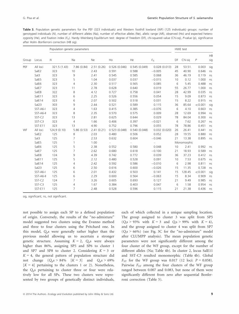
0.010 (14 loci: P < 0.001). See Table 3 for all population

genetic parameters and the HWE test.

Mean population parameters did not significantly differ

between the two groups (Table 3). Nonetheless, the PEF

population had a significantly larger number of sampled

individuals than the WF and a higher number of private

alleles (37 in the PEF and 9 in the WF). In particular, the

SalE5 locus became monomorphic in the WF subsample

(Table 3).

Table 1. Population genetic parameters for 448 salamander larvae collected in Lombardy (Northern Italy): number of genotyped individuals (N),

number of different alleles (Na), number of effective alleles (Ne), allelic range (AR), observed (Ho) and expected heterozygosity (He), fixation index

(FIS). Hardy–Weinberg Equilibrium test: degree of freedom (Df), chi-squared value (Chi-sq), P-value (P), significance after Holm–Bonferroni correc-

tion (HB sig).

Locus

Population genetic parameters HWE test

N Na Ne AR Ho He FIS Df Chi-sq P HB sig

All loci 446.06

(1.28)

9.94

(1.26)

2.79

(0.29)

– 0.546

(0.042)

0.579

(0.047)

0.048

(0.013)

32 Inf. �0.001 sig

SalE2 448 11 2.32 216–262 0.560 0.569 0.015 55 34.41 0.987 ns

Sal3 448 11 2.49 181–327 0.569 0.598 0.048 55 54.26 0.503 ns

SalE5 448 5 1.03 180–190 0.027 0.027 �0.011 10 0.08 1.000 ns

SalE6 448 5 2.34 277–297 0.527 0.572 0.079 10 6.23 0.795 ns

SalE7 448 11 2.75 184–232 0.643 0.636 �0.010 55 33.04 0.992 ns

SalE8 446 10 4.26 143–181 0.731 0.765 0.045 45 64.92 0.027 ns

SalE11 448 6 2.21 238–258 0.513 0.548 0.064 15 12.95 0.606 ns

SalE12 441 16 4.42 223–307 0.621 0.774 0.197 120 740.25 �0.001 sig

SalE14 448 6 2.19 237–257 0.527 0.543 0.030 15 5.86 0.982 ns

Sal23 428 9 2.46 282–320 0.549 0.594 0.076 36 45.60 0.131 ns

SST-A6-I 448 6 1.75 207–231 0.420 0.428 0.020 15 5.05 0.992 ns

SST-A6-II 448 8 2.34 193–221 0.578 0.573 �0.010 28 16.75 0.953 ns

SST-B11 447 24 5.19 149–263 0.763 0.807 0.055 276 434.29 �0.001 sig

SST-C2 447 13 3.06 194–246 0.620 0.673 0.079 78 105.81 0.020 ns

SST-C3 448 5 1.67 207–227 0.400 0.400 0.001 10 5.72 0.838 ns

SST-E11 448 13 4.13 233–311 0.690 0.758 0.090 78 96.21 0.079 ns

sig, significant; ns, not significant.

6 ª 2014 The Authors. Ecology and Evolution published by John Wiley & Sons Ltd.

Genetic Population Structure of S. salamandra G. Pisa et al.

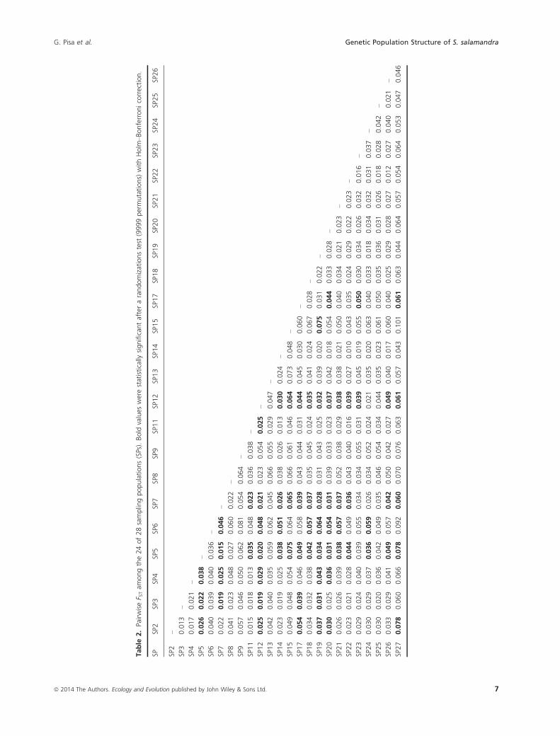
Table

2.PairwiseF S

Tam

ongthe24of28samplingpopulations(SPs).Bold

values

werestatistically

significantafterarandomizationstest

(9999permutations)

withHolm

–Bonferronicorrection.

SPSP2

SP3

SP4

SP5

SP6

SP7

SP8

SP9

SP11

SP12

SP13

SP14

SP15

SP17

SP18

SP19

SP20

SP21

SP22

SP23

SP24

SP25

SP26

SP2

–

SP3

0.013

–

SP4

0.017

0.021

–

SP5

0.026

0.022

0.038

–

SP6

0.040

0.039

0.040

0.036

–

SP7

0.022

0.019

0.025

0.015

0.046

–

SP8

0.041

0.023

0.048

0.027

0.060

0.022

–

SP9

0.057

0.046

0.050

0.062

0.081

0.054

0.064

–

SP11

0.015

0.018

0.013

0.035

0.048

0.023

0.036

0.038

–

SP12

0.025

0.019

0.029

0.020

0.048

0.021

0.023

0.054

0.025

–

SP13

0.042

0.040

0.035

0.059

0.062

0.045

0.066

0.055

0.029

0.047

–

SP14

0.023

0.019

0.025

0.038

0.051

0.026

0.038

0.026

0.013

0.030

0.024

–

SP15

0.049

0.048

0.054

0.075

0.064

0.065

0.066

0.061

0.046

0.064

0.073

0.048

–

SP17

0.054

0.039

0.046

0.049

0.058

0.039

0.043

0.044

0.031

0.044

0.045

0.030

0.060

–

SP18

0.034

0.032

0.038

0.042

0.057

0.037

0.035

0.045

0.024

0.035

0.041

0.024

0.067

0.028

–

SP19

0.037

0.031

0.043

0.034

0.064

0.028

0.031

0.043

0.025

0.032

0.039

0.020

0.075

0.031

0.022

–

SP20

0.030

0.025

0.036

0.031

0.054

0.031

0.039

0.033

0.023

0.037

0.042

0.018

0.054

0.044

0.033

0.028

–

SP21

0.026

0.026

0.039

0.038

0.057

0.037

0.052

0.038

0.029

0.038

0.038

0.021

0.050

0.040

0.034

0.021

0.023

–

SP22

0.023

0.021

0.028

0.044

0.049

0.036

0.043

0.040

0.016

0.039

0.027

0.010

0.043

0.035

0.024

0.029

0.022

0.023

–

SP23

0.029

0.024

0.040

0.039

0.055

0.034

0.034

0.055

0.031

0.039

0.045

0.019

0.055

0.050

0.030

0.034

0.026

0.032

0.016

–

SP24

0.030

0.029

0.037

0.036

0.059

0.026

0.034

0.052

0.024

0.021

0.035

0.020

0.063

0.040

0.033

0.018

0.034

0.032

0.031

0.037

–

SP25

0.030

0.020

0.036

0.042

0.049

0.035

0.046

0.054

0.034

0.044

0.035

0.023

0.061

0.050

0.035

0.036

0.031

0.026

0.018

0.028

0.042

–

SP26

0.033

0.029

0.041

0.049

0.057

0.042

0.050

0.042

0.027

0.049

0.040

0.017

0.060

0.040

0.025

0.029

0.028

0.027

0.012

0.027

0.040

0.021

–

SP27

0.078

0.060

0.066

0.078

0.092

0.060

0.070

0.076

0.063

0.061

0.057

0.043

0.101

0.061

0.063

0.044

0.064

0.057

0.054

0.064

0.053

0.047

0.046

ª 2014 The Authors. Ecology and Evolution published by John Wiley & Sons Ltd. 7

G. Pisa et al. Genetic Population Structure of S. salamandra

In the second step, we re-ran a population structure

analysis separately for each of the two clusters previously

identified (PEF and WF groups). We first tested for HWE

using GeneAlex and deleted from the analyses all loci not

at equilibrium after Holm–Bonferroni correction and with

null alleles. In the PEF group, only Sal23 was out of

HWE, while in the WF group, SalE5 resulted monomor-

phic and SST-A6-I not at HWE. We therefore ran popu-

lation structure without locus Sal23 for the PEF and

without loci SalE5 and SST-A6-I for the WF. Neither of

the “independent allele frequencies” models, ran in this

step for both the PEF and the WF, converged, even

increasing the length of burnin and MCMCs, respectively

to 100,000 and 1,000,000. We therefore considered only

the “correlated allele frequencies” models hereafter.

The results of the PEF group were similar in terms of

the number of clusters identified using the “admixture”

and “no-admixture” models. Both models identified two

clusters, according to both the Evanno and Pritchard

methods. The “admixture model” showed a distinct clus-

ter corresponding to SP12 with a Qp of 67%. All others

SPs were assigned to a single cluster, with Qps always

higher than 69%. The “no-admixture” model supported

the presence of 2 clusters (K = 2), and the results were

consistent with the “admixture” model, identifying SP12

as a single cluster (Qp = 94%) and all other SPs pertain-

ing to a second cluster (Qp always higher than 85%),

except for SP10 which had a Qp of 67% (see Fig. 3B for

the “no-admixture” model after CLUMPP analysis).

Although the mean population genetic parameters did

not significantly differ between the two clusters of the

PEF (Table 4a), their Global FST was significantly differ-

ent from zero (13 loci, FST = 0.006, P < 0.001). The two

clusters showed a different number of private alleles, 33

in cluster 1 and 1 in cluster 2 (SP12). The latter also

showed the locus SalE5 as monomorphic (Table 4a).

The analysis of the WF group produced different

results using the “admixture” and “no-admixture” mod-

els, because the second one identified a more subtle

structure. In the “admixture” model, the Evanno

method allowed us to identify two clusters, with Qps

always higher than 73%. According to the Pritchard

method, three clusters could be identified, although in

this case, Qps were never higher than 63% and it was

(A)

(B)

(C)

Figure 3. Inferred populations structures for (A) the whole sample (448 individuals, 28 sampling populations, SPs) that was divided in the PEF

group (light green) and the Western foothill lowland (WF) group (light brown); (B) STRUCTURE analysis performed only on the PEF group (323

individuals, 24 SPs) showed the presence of two clusters corresponding to SP12 (blue) and all the others SPs (dark red); (C) the three histograms

of the WF group (125 individuals, four SPs) showed population structures with 2, 3, and 4 clusters, respectively (see Results). For K = 4, cluster 1

in green, cluster 2 in red, cluster 3 in yellow, and cluster 4 in blue. These colors correspond to those in Fig. 4. Each bar represents an individual

and is colored (using DISTRUCT) according to CLUMPP individual probability of assignment (Qi) obtained from “No-admixture” models with

“correlated allele frequencies” and LOCPRIOR information.

8 ª 2014 The Authors. Ecology and Evolution published by John Wiley & Sons Ltd.

Genetic Population Structure of S. salamandra G. Pisa et al.

not possible to assign each SP to a defined population

of origin. Conversely, the results of the “no-admixture”

model suggested two clusters using the Evanno method

and three to four clusters using the Pritchard one. In

this model, Qps were generally rather higher than the

previous model allowing us to ascertain a stronger

genetic structure. Assuming K = 2, Qps were always

higher than 86%, assigning SP5 and SP6 to cluster 1

and SP7 and SP8 to cluster 2. Considering K = 3 or

K = 4, the general pattern of population structure did

not change (Qps > 84% [K = 3] and Qps > 69%

[K = 4] pertaining to the clusters 1 or 2). Nonetheless,

the Qps pertaining to cluster three or four were rela-

tively low for all SPs. These two clusters were repre-

sented by two groups of genetically distinct individuals,

each of which collected in a unique sampling location.

The group assigned to cluster 3 was split from SP5

(Qis > 93% with K = 3 and Qis > 99% with K = 4),

and the group assigned to cluster 4 was split from SP7

(Qis > 66%) (see Fig. 3C for the “no-admixture” model

after CLUMPP analysis). The mean population genetic

parameters were not significantly different among the

four cluster of the WF group, except for the number of

different alleles (Na; Table 4b). In cluster 2, locus SalE11

and SST-C3 resulted monomorphic (Table 4b). Global

FST for the WF group was 0.017 (12 loci: P = 0.058).

Pairwise FST among the four clusters of the WF group

ranged between 0.007 and 0.083, but none of them were

significantly different from zero after sequential Bonfer-

roni correction (Table 5).

Table 3. Population genetic parameters for the PEF (323 individuals) and Western foothill lowland (WF) (125 individuals) groups: number of

genotyped individuals (N), number of different alleles (Na), number of effective alleles (Ne), allelic range (AR), observed (Ho) and expected hetero-

zygosity (He), and fixation index (FIS). Hardy–Weinberg Equilibrium test: degree of freedom (Df), chi-squared value (Chi-sq), P-value (p), significance

after Holm–Bonferroni correction (HB sig).

Group Locus

Population genetic parameters HWE test

N Na Ne Ho He FIS DF Chi-sq P

HB

sig

PEF All loci 321.5 (1.43) 7.86 (0.84) 2.51 (0.26) 0.526 (0.046) 0.545 (0.049) 0.028 (0.013) 28 53.51. 0.003 sig

SalE2 323 10 2.43 0.591 0.588 �0.005 45 40.90 0.646 ns

Sal3 323 9 2.41 0.545 0.585 0.068 36 46.19 0.119 ns

SalE5 323 5 1.04 0.037 0.037 �0.015 10 0.12 1.000 ns

SalE6 323 4 2.30 0.517 0.565 0.085 6 5.45 0.488 ns

SalE7 323 11 2.78 0.628 0.640 0.019 55 26.77 1.000 ns

SalE8 322 8 4.12 0.727 0.758 0.041 28 42.99 0.035 ns

SalE11 323 6 2.25 0.526 0.556 0.054 15 9.09 0.873 ns

SalE14 323 6 2.07 0.502 0.518 0.031 15 8.22 0.915 ns

Sal23 303 9 2.44 0.521 0.589 0.115 36 85.64 �0.001 sig

SST-A6-I 323 4 1.63 0.415 0.385 �0.076 6 4.10 0.663 ns

SST-A6-II 323 8 2.35 0.570 0.575 0.009 28 12.69 0.994 ns

SST-C2 323 13 2.81 0.625 0.644 0.029 78 84.04 0.300 ns

SST-C3 323 4 1.66 0.406 0.397 �0.021 6 7.62 0.267 ns

SST-E11 323 13 4.90 0.752 0.796 0.055 78 78.86 0.451 ns

WF All loci 124,9 (0.10) 5.86 (0.53) 2.41 (0.21) 0.523 (0.048) 0.540 (0.048) 0.032 (0.020) 26 26.41 0.441 ns

SalE2 125 8 2.03 0.480 0.506 0.052 28 19.55 0.880 ns

Sal3 125 7 2.53 0.632 0.604 �0.046 21 13.38 0.895 ns

SalE5 125 1 1.00 – – – Monomorphic

SalE6 125 5 2.38 0.552 0.580 0.048 10 2.41 0.992 ns

SalE7 125 7 2.62 0.680 0.618 �0.100 21 18.93 0.589 ns

SalE8 124 9 4.39 0.742 0.772 0.039 36 37.23 0.412 ns

SalE11 125 5 2.12 0.480 0.528 0.091 10 7.53 0.675 ns

SalE14 125 4 2.42 0.592 0.586 �0.010 6 2.98 0.811 ns

Sal23 125 6 2.50 0.616 0.600 �0.026 15 11.35 0.728 ns

SST-A6-I 125 6 2.01 0.432 0.503 0.141 15 128.45 �0.001 sig

SST-A6-II 125 6 2.29 0.600 0.564 �0.063 15 8.34 0.909 ns

SST-C2 124 7 3.26 0.605 0.693 0.127 21 9.49 0.985 ns

SST-C3 125 4 1.67 0.384 0.403 0.047 6 1.58 0.954 ns

SST-E11 125 7 2.48 0.528 0.596 0.115 21 21.38 0.436 ns

sig, significant; ns, not significant.

ª 2014 The Authors. Ecology and Evolution published by John Wiley & Sons Ltd. 9

G. Pisa et al. Genetic Population Structure of S. salamandra

Table

4.Po

pulationgen

etic

param

eters(w

ithSE

inparen

theses)forthe(a)tw

oclusters

ofthePEFgroupan

d(b)fourclustersoftheWFgroup:number

ofgen

otyped

individuals(N),number

ofdifferentalleles(Na),number

ofeffectivealleles(Ne),allelic

range(AR),observed

(Ho)an

dexpectedheterozygosity

(He),an

dfixationindex

(FIS).Hardy–WeinbergEq

uilibrium

test:deg

reeof

freedom

(Df),chi-squared

value(Chi-sq),P-value(p),significance

afterHolm

–Bonferronicorrection(HBsig).

Cluster

Locus

Populationgen

etic

param

eters

HWEtest

NNa

Ne

Ho

He

F IS

DF

Chi-sq

P

HB

sig

(a)

1Allloci

278.9

(0.08)

7.69(0.91)

2.51(0.27)

0.525(0.049)

0.542(0.053)

0.023(0.011)

26

34.88

0.114

ns

SalE2

279

10

2.41

0.577

0.584

0.013

45

49.43

0.301

ns

Sal3

279

92.36

0.538

0.576

0.066

36

46.72

0.109

ns

SalE5

279

51.04

0.043

0.042

�0.017

10

0.13

1.000

ns

SalE6

279

42.31

0.538

0.568

0.053

64.88

0.559

ns

SalE7

279

11

2.86

0.645

0.651

0.009

55

26.16

1.000

ns

SalE8

278

84.00

0.723

0.750

0.036

28

37.93

0.100

ns

SalE11

279

62.28

0.516

0.562

0.081

15

11.44

0.721

ns

SalE14

279

62.09

0.502

0.522

0.038

15

8.36

0.909

ns

SST-A6-I

279

41.61

0.401

0.378

�0.062

62.06

0.914

ns

SST-A6-II

279

72.36

0.559

0.577

0.031

21

13.83

0.877

ns

SST-C2

279

13

2.94

0.631

0.659

0.043

78

81.94

0.358

ns

SST-C3

279

41.64

0.405

0.390

�0.037

611.69

0.069

ns

SST-E1

1279

13

4.70

0.749

0.787

0.048

78

75.77

0.550

ns

2Allloci

44

5.23(0.63)

2.47(0.33)

0.533(0.055)

0.522(0.054)

�0.025(0.031)

26

22.37

0.668

ns

SalE2

44

72.54

0.682

0.607

�0.123

21

12.30

0.931

ns

Sal3

44

52.71

0.591

0.631

0.064

10

27.40

0.002

ns

SalE5

44

11.00

––

–Monomorphic

SalE6

44

41.87

0.386

0.465

0.168

67.20

0.302

ns

SalE7

44

62.22

0.523

0.550

0.050

15

12.57

0.635

ns

SalE8

44

64.50

0.750

0.778

0.036

15

12.42

0.647

ns

SalE11

44

42.07

0.591

0.517

�0.142

66.72

0.347

ns

SalE14

44

31.96

0.500

0.491

�0.019

31.27

0.737

ns

SST-A6-I

44

41.75

0.500

0.429

�0.165

65.89

0.436

ns

SST-A6-II

44

72.21

0.636

0.547

�0.163

21

6.19

0.999

ns

SST-C2

44

72.12

0.591

0.529

�0.118

21

13.13

0.904

ns

SST-C3

44

41.77

0.409

0.435

0.059

61.63

0.951

ns

SST-E1

144

10

5.33

0.773

0.812

0.049

45

46.25

0.420

ns

(b)

1Allloci

56

5.83(0.44)

2.47(0.17)

0.555(0.036)

0.574(0.028)

0.037(0.030)

24

20.35

0.677

ns

SalE2

56

81.92

0.446

0.479

0.068

28

20.53

0.845

ns

Sal3

56

72.50

0.571

0.601

0.049

21

12.35

0.930

ns

SalE6

56

52.28

0.446

0.561

0.204

10

5.28

0.872

ns

SalE7

56

73.07

0.750

0.674

�0.112

21

16.89

0.718

ns

SalE8

56

83.77

0.750

0.735

�0.021

28

16.19

0.963

ns

10 ª 2014 The Authors. Ecology and Evolution published by John Wiley & Sons Ltd.

Genetic Population Structure of S. salamandra G. Pisa et al.

Table

4.Continued

.

Cluster

Locus

Populationgen

etic

param

eters

HWEtest

NNa

Ne

Ho

He

F IS

DF

Chi-sq

P

HB

sig

SalE11

56

41.94

0.411

0.484

0.151

66.47

0.373

ns

SalE14

56

42.14

0.607

0.533

�0.138

62.72

0.843

ns

Sal23

56

52.39

0.571

0.582

0.018

10

4.40

0.928

ns

SST-A6-II

56

52.34

0.607

0.573

�0.060

10

4.55

0.919

ns

SST-C2

56

73.11

0.625

0.679

0.079

21

9.02

0.989

ns

SST-C3

56

41.62

0.357

0.383

0.069

62.40

0.879

ns

SST-E1

156

62.52

0.518

0.604

0.143

15

14.55

0.484

ns

2Allloci

32.83(0.37)

2.48(0.31)

0.639(0.119)

0.505(0.075)

�0.242(0.140)

––

––

SalE2

33

2.57

1.000

0.611

�0.636

33.00

0.392

ns

Sal3

33

2.57

1.000

0.611

�0.636

33.00

0.392

ns

SalE6

32

1.80

0.000

0.444

1.000

13.00

0.083

ns

SalE7

34

3.60

1.000

0.722

�0.385

64.50

0.609

ns

SalE8

35

4.50

1.000

0.778

�0.286

10

9.00

0.532

ns

SalE11

31

1.00

––

–Monomorphic

SalE14

32

1.80

0.667

0.444

�0.500

10.75

0.386

ns

Sal23

33

2.57

0.667

0.611

�0.091

32.33

0.506

ns

SST-A6-II

32

1.80

0.667

0.444

�0.500

10.75

0.386

ns

SST-C2

34

3.00

0.667

0.667

0.000

66.33

0.387

ns

SST-C3

31

1.00

––

–Monomorphic

SST-E1

13

43.60

1.000

0.722

�0.385

64.50

0.609

ns

3Allloci

54.83(0.11)

5.08(0.43)

2.59(0.24)

0.587(0.027)

0.590(0.025)

0.003(0.030)

24

24.60

0.428

ns

SalE2

55

71.95

0.436

0.487

0.104

21

23.10

0.339

ns

Sal3

55

42.47

0.655

0.594

�0.101

610.72

0.097

ns

SalE6

55

32.48

0.691

0.597

�0.157

33.00

0.392

ns

SalE7

55

52.15

0.600

0.536

�0.120

10

3.91

0.951

ns

SalE8

54

74.99

0.759

0.800

0.051

21

26.37

0.193

ns

SalE11

55

42.34

0.582

0.573

�0.016

67.59

0.270

ns

SalE14

55

42.56

0.527

0.609

0.135

65.36

0.498

ns

Sal23

55

62.55

0.655

0.609

�0.076

15

6.40

0.972

ns

SST-A6-II

55

52.25

0.564

0.557

�0.013

10

2.21

0.994

ns

SST-C2

54

73.24

0.593

0.691

0.142

21

9.77

0.982

ns

SST-C3

55

31.93

0.491

0.482

�0.017

30.25

0.969

ns

SST-E1

155

62.21

0.491

0.548

0.104

15

15.16

0.440

ns

4Allloci

11

3.75(0.18)

2.36(0.14)

0.591(0.054)

0.549(0.044)

�0.074(0.047)

88

62.32

0.983

ns

SalE2

11

42.55

0.727

0.607

�0.197

63.97

0.680

ns

Sal3

11

42.81

0.727

0.645

�0.128

62.58

0.859

ns

SalE6

11

32.28

0.545

0.562

0.029

31.83

0.608

ns

SalE7

11

42.55

0.636

0.607

�0.048

63.20

0.783

ns

ª 2014 The Authors. Ecology and Evolution published by John Wiley & Sons Ltd. 11

G. Pisa et al. Genetic Population Structure of S. salamandra

Discussion

This research allowed us to detect a hierarchical popula-

tion structure of the Fire Salamander in a wide area

of the species range in Northern Italy. The 28 sampled

populations were distributed in the Prealpine area, where

forest cover is more continuous, and in the foothill low-

land, where forests are more fragmented (see Fig. 1).

Some SPs from the Western foothill lowland appeared

genetically distant from the others, according to pairwise

FST (Table 2). This result was confirmed by genetic struc-

ture analyses which highlighted how these populations

were strongly structured. We identified two groups, one

represented by the Western Foothill populations (WF)

and another one by all other populations laying in the

Prealpine and Eastern Foothill areas (PEF). This was con-

firmed by the overall high probability of assignment of

individuals to the two groups which resulted genetically

distant as shown by significant pairwise FST. Even if locus

SalE5 became monomorphic in the WF group, the num-

ber of effective alleles (Ne) and the observed heterozygos-

ity (Ho) were very similar between PEF and WF,

suggesting that currently there was not a loss of genetic

diversity on the whole.

After the identification of these two genetically sepa-

rated groups, the use of a multistep approach allowed us

to identify substructured populations.

In the PEF groups, two more clusters were identified:

A first one included all populations except SP12, which

formed a second cluster whose separation was confirmed

by both population structure analysis and pairwise FST.

SP12 cluster is located in a foothill forest separated from

Prealpine areas by both wide conurbation and a main

road. In addition, this area was also found to be isolated

by the lack of a stream network connection that may sup-

port the dispersal process and seems to be important in

connecting other Eastern foothill populations to the

Prealps.

The WF group could be divided from two to four groups

adopting the Evanno or Pritchard method. Considering

K = 2, the group is divided into a Western (SP5 and SP6)

and Eastern (SP7 and SP8) cluster, divided by largeTable

4.Continued

.

Cluster

Locus

Populationgen

etic

param

eters

HWEtest

NNa

Ne

Ho

He

F IS

DF

Chi-sq

P

HB

sig

SalE8

11

42.44

0.545

0.591

0.077

611.55

0.073

ns

SalE11

11

42.30

0.455

0.566

0.197

63.28

0.772

ns

SalE14

11

42.92

0.818

0.657

�0.245

64.27

0.640

ns

Sal23

11

42.20

0.636

0.545

�0.167

61.67

0.947

ns

SST-A6-II

11

42.18

0.727

0.541

�0.344

63.59

0.732

ns

SST-C2

11

42.72

0.545

0.632

0.137

66.93

0.327

ns

SST-C3

11

21.10

0.091

0.087

�0.048

10.02

0.875

ns

SST-E1

111

42.22

0.636

0.550

�0.158

63.85

0.696

ns

sig,significant;ns,

notsignificant.

Table 5. Pairwise FST among the four clusters of the Western foothill

lowland (WF) group below the diagonal. Probability based on 9999

permutations is shown above the diagonal. None of these values were

significant after a Holm–Bonferroni correction.

Cluster 1 2 3 4

1 – 0.323 0.043 0.045

2 0.052 – 0.181 0.048

3 0.007 0.059 – 0.029

4 0.022 0.083 0.022 –

12 ª 2014 The Authors. Ecology and Evolution published by John Wiley & Sons Ltd.

Genetic Population Structure of S. salamandra G. Pisa et al.

conurbations and a south–north main road (Fig. 4). In

addition, according to the K = 4 result, we observed

another subdivision occurring in the two previous clusters

(cluster 1: SP5 and SP6; cluster 3: SP7 and SP8), identifying

two new clusters corresponding to two sampling locations,

sampling location 5.5 (cluster 2), and sampling location 7.3

(cluster 4). Although these two new clusters are very close

(with a distance of about three kilometers) to the other

sampling locations of the same SP, they seem to represent

separated demes. Cluster 2 appeared to be almost com-

pletely isolated by unsuitable areas for the Fire Salamander,

largely represented by urban areas without stream network

connections, while cluster 4 is isolated mainly by agricul-

tural areas but with a stream connection, which could

make the isolation less sharp (Fig. 4). Nevertheless, none of

the pairwise FST tests for the WF group resulted significant

after Holm–Bonferroni correction. This result may be con-

ditioned by the small sample size of clusters 2 and 4, each

represented by a single sampling location, with respect to

the SPs they were split from.

On the whole, the identified population structure may

be explained by the hypothesis of a relatively short-term

fragmentation in the WF group: In this case, we cannot

currently detect a significant loss of alleles, which could

arise in the long term due to an inadequate gene flow.

Conversely, it is likely that the PEF group (except SP12)

will maintain a high number of alleles in the long term,

because it is represented by a large and mainly continu-

ous population (Fig. 3B).

Despite the fragmentation process currently only led

to an evident population structure without significant dif-

ferences of genetic parameters among identified clusters,

in the medium and long term, it is expected it could even

produce a loss of genetic diversity (e.g., Dixo et al. 2009).

Indeed, the observed strong genetic population structure

within the WF group is particularly worrying, because this

will probably lead to a reduction in the capacity of adap-

tation of these populations, resulting in an increase in

their probability of extinction, in relatively short time

(Young et al. 1996; Reed and Frankham 2003; Arens et al.

2007). In addition, these populations will face other

important threats such as further habitat loss and degra-

dation caused by infrastructural, as well as commercial/

residential development projects in their area, which has

one of the highest rate of urbanization in Italy. The same

fate of the WF is expected for SP12, split from the PEF

group, although its isolation seems to be less strong than

the one occurring between the WF and the PEF groups

and within the WF group.

From a methodological point of view, the multistep

approach we adopted for the genetic population struc-

ture analysis at large spatial scale allowed us to identify

different cases of fragmentation in the overall popula-

tion, likely corresponding to a different degree of sepa-

ration, or even isolation, of populations (see sampling

location 5.5, i.e., cluster 2 of WF group). The effective-

ness of this approach was proved by the use of the spe-

cies here investigated, the Fire Salamander, an

amphibian with rather strict ecological requirements (Di

Cerbo and Razzetti 2004; Schmidt et al. 2005). None-

theless, the genetic results suggest that at wide scale,

most of the salamander populations are rather continu-

ous or large enough to not suffer the typical problem

of small population; they also highlight how locally the

species may suffer habitat fragmentation. This is con-

firmed by the presence of strong structured populations,

Figure 4. Population structure of the Western

foothill lowland (WF) group. Numbered dots

indicate sampling locations, grouped according

to their sampling population (dot colors). Pie

charts represent the sampling location

probability of assignment to the four clusters

identified by running STRUCTURE. Cluster 1:

green, cluster 2: red, cluster 3: yellow, and

cluster 4: blue. These colors correspond to

those in Fig. 3C with K = 4. In the background

main land uses: forests in green, urban areas

in dark–gray, farmland, and other open

habitats in gray, lakes, wetlands, and rivers in

blue. Black lines represent main roads.

ª 2014 The Authors. Ecology and Evolution published by John Wiley & Sons Ltd. 13

G. Pisa et al. Genetic Population Structure of S. salamandra

with a generalized genetic depletion, evidenced by the

presence of some monomorphic loci and many private

alleles.

In conclusion, the multistep approach can be useful to

detect substructured populations at local scale which can-

not be observed analyzing wide-scale data in one-step

only. Thus, the screening of genetic population structure

from a regional to local scale can be considered effective

in detecting local populations of conservation concern

which resulted imperilled by threats acting locally and

also for a preliminary assessment of the ecological con-

nectivity in fragmented landscapes.

Acknowledgments

We are very grateful to the Assigning Editor and an anon-

ymous reviewer for their appropriate and constructive

suggestions to improve the article. We also thank Profes-

sor Giuseppe Bogliani for critical review of the first draft.

Finally, we are very grateful to Sam and Dario Massimino

for linguistic review.

Conflict of Interest

None declared.

Data Accessibility

Sampled individuals, sampling locations, and microsatel-

lite genotypes: Dryad

References

Allendorf, F. W., and S. R. Phelps. 1981. Use of allelic

frequencies to describe population structure. Can. J. Fish

Aquat. Sci. 38:1507–1514.

Allendorf, F. W., G. Luikart, and S. N. Aitken. 2013.

Conservation and the genetics of populations.

Wiley-Blackwell, Oxford, U.K.

Allentoft, M. E., and J. O’Brien. 2010. Global amphibian

declines, loss of genetic diversity and fitness: a review.

Diversity 2:47–71.

Antao, T., A. Lopes, R. J. Lopes, A. Beja-Pereira, and G.

Luikart. 2008. LOSITAN: a workbench to detect molecular

adaptation based on a Fst-outlier method. BMC

Bioinformatics 9:323.

Arens, P., T. van der Sluis, W. P. C. vant Westende, B.

Vosman, C. C. Vos, and M. J. M. Smulders. 2007. Genetic

population differentiation and connectivity among

fragmented Moor frog (Rana arvalis) populations in The

Netherlands. Landscape Ecol. 22:1489–1500.

Avise, J. C. 1994. Molecular markers. Natural History and

Evolution. Chapman & Hall, New York.

Beebee, T., and G. Rowe. 2004. An introduction to molecular

ecology. Oxford University Press, New York.

Blaustein, A. R., D. B. Wake, and W. P. Sousa. 1994.

Amphibian declines: judging stability, persistence, and

susceptibility of populations to local and global extinctions.

Conserv. Biol. 8(60):71.

Burgman, M. A., and D. B. Lindenmayer. 1998. Conservation

biology for the Australian environment. Surrey Beatty &

Sons, Chipping Norton, NSW.

Caldonazzi, M., A. Nistri, and S. Tripepi. 2007. Salamandra

salamandra. Pp. 221–227 in B. Lanza, F. Andreone, M. A.

Bologna, C. Corti and E. Razzetti, eds. Fauna d’Italia.

Amphibia, Calderini, Bologna, Italy (in Italian).

Chapuis, M. P., and A. Estoup. 2007. Microsatellite null alleles

and estimation of population differentiation. Mol. Biol.

Evol. 24:621–631.

Di Cerbo, A., and E. Razzetti. 2004. Salamandra salamandra.

Pp. 64–66. In: F. Bernini, L. Bonini, V. Ferri, A. Gentilli, E.

Razzetti, S. Scali, eds. Atlante degli Anfibi e dei Rettili della

Lombardia, “Monografie di Pianura” n. 5, Provincia di

Cremona, Cremona (in Italian) http://www-3.unipv.it/

webshi/images/files/atlante_lombardia.pdf.

Dixo, M., J. P. Metzger, J. S. Morgante, and K. R. Zamudio.

2009. Habitat fragmentation reduces genetic diversity and

connectivity among toad populations in the Brazilian

Atlantic Coastal Forest. Biol. Conserv. 142:1560–1569.

Earl, D. A., and B. M. vonHoldt. 2012. STRUCTURE

HARVESTER: a website and program for visualizing

STRUCTURE output and implementing the Evanno

method. Conserv. Genet. Res. 4:359–361.

Evanno, G., S. Regnaut, and J. Goudet. 2005. Detecting the

number of clusters of individuals using the software

STRUCTURE: a simulation study. Mol. Ecol. 14:2611–2620.

Falush, D., M. Stephens, and J. K. Pritchard. 2003. Inference

of population structure using multilocus genotype data:

linked loci and correlated allele frequencies. Genetics

164:1567–1587.

Falush, D., M. Stephens, and J. K. Pritchard. 2007. Inference

of population structure using multilocus genotype data:

dominant markers and null alleles. Mol. Ecol. Notes

7:574–578.

Frankham, R. 2003. Genetics and conservation biology.

C. R. Biol. 326:S22–S29.

Frankham, R. 2005. Genetics and extinction. Biol. Conserv.

126:131–140.

Frankham, R. 2006. Genetics and landscape connectivity. Pp.

72–96 in K. R. Crooks and M. A. Sanjayan, eds.

Connectivity conservation. Cambridge University Press,

Cambridge.

Frankham, R., J. D. Ballou, and D. A. Briscoe. 2002.

Introduction to conservation genetics. Cambridge University

Press, Cambridge.

Giplin, M. E., and M. E. Soul�e. 1986. Minimum viable

populations: processes of species extinctions. Pp. 19–34 in

14 ª 2014 The Authors. Ecology and Evolution published by John Wiley & Sons Ltd.

Genetic Population Structure of S. salamandra G. Pisa et al.

M. E. Soul�e, ed. Conservation biology: the science of

scarcity and diversity. Sinauer Associates, Sunderland, MA.

Goldberg, C. S., and L. P. Waits. 2010. Quantification and

reduction of bias from sampling larvae to infer population

and landscape genetic structure. Mol. Ecol. Resour.

10:304–313.

Green, P. J. 1995. Reversible jump Markov chain Monte Carlo

computation and Bayesian model determination. Biometrika

82:711–732.

Hale, J. M., G. W. Heard, K. L. Smith, K. M. Parris, J. J.

Austin, M. Kearney, et al. 2013. Structure and fragmentation

of growling grass frog metapopulations. Conserv. Genet.

14:313–322.

Hanski, I., and D. Simberloff. 1997. The metapopulation

approach, its history, conceptual domain, and application to

conservation. Pp. 5–26 in I. A. Hanski and M. E. Gilpin,

eds. Metapopulation biology. Academic Press, San Diego,

CA.

Harris, L. N., J.-S. Moore, P. Galpern, R. F. Tallman, and

E. B. Taylor. 2014. Geographic influences on fine-scale,

hierarchical population structure in northern Canadian

populations of anadromous Arctic Char (Salvelinus alpinus).

Environ. Biol. Fishes 97:1233–1252.

Hastings, W. K. 1970. Monte Carlo sampling methods using

Markov chains and their applications. Biometrika 57:97–109.

Hendrix, R., S. Hauswaldt, M. Veith, and S. Steinfartz. 2010.

Strong correlation between cross-amplification success and

genetic distance across all members of ‘True Salamanders’

(Amphibia: Salamandridae) revealed by Salamandra

salamandra-specific microsatellite loci. Mol. Ecol. Resour.

10:1038–1047.

Holm, S. 1979. A simple sequentially rejective multiple test

procedure. Scand. J. Stat. 6:65–70.

Hubisz, M. J., D. Falush, M. Stephens, and J. K. Pritchard.

2009. Inferring weak population structure with the

assistance of sample group information. Mol. Ecol. Resour.

9:1322–1332.

Jakobsson, M., and N. A. Rosenberg. 2007. CLUMPP: a cluster

matching and permutation program for dealing with label

switching and multimodality in analysis of population

structure. Bioinformatics 14:1801–1806.

Jones, O. R., and J. I. Wang. 2010. COLONY: a program for

parentage and sibship inference from multilocus genotype

data. Mol. Ecol. Resour. 10:551–555.

Kauer, M., D. Dieringer, and C. Schlotterer. 2003. Nonneutral

admixture of immigrant genotypes in African Drosophila

melanogaster populations from Zimbabwe. Mol. Biol. Evol.

20:1329–1337.

Keller, L. F., and D. M. Waller. 2002. Inbreeding effects in

wild populations. Trends Ecol. Evol. 17:230–241.

Kovach, A. I., T. S. Breton, C. Enterline, and D. L. Berlinsky.

2013. Identifying the spatial scale of population structure in

anadromous rainbow smelt (Osmerus mordax). Fish. Res.

141:95–106.

Lacy, R. C. 1993. Impacts of inbreeding in natural and captive

populations of vertebrates: implications for conservation.

Perspect. Biol. Med. 36:480–496.

Lacy, R. C., and D. B. Lindenmayer. 1995. A simulation study

of the impacts of population subdivision on the mountain

brushtail possum Trichosurus caninus ogilby (Phalangeridae,

Marsupialia) in South-Eastern Australia. 2. Loss of genetic

variation within and between subpopulations. Biol. Conserv.

73:131–142.

Lindenmayer, D. B. 1995. Disturbance, forest wildlife

conservation and a conservative basis for forest management

in the mountain ash forests of Victoria. For. Ecol. Manage.

74:223–231.

Moore, J. A., D. A. Tallmon, J. Nielsen, and S. Pyare. 2011.

Effects of the landscape on boreal toad gene flow: does the

pattern–process relationship hold true across distinct

landscapes at the Northern range margin? Mol. Ecol.

20:4858–4869.

Neville, H., J. Dunham, and M. Peacock. 2006. Assessing

connectivity in salmonid fishes with DNA microsatellite

markers. Pp. 318–342 in K. R. Crooks and M. A. Sanjayan,

eds. Connectivity conservation. Cambridge University Press,

Cambridge.

Parsons, K. M., J. W. Durban, A. M. Burdin, V. N. Burkanov,

R. L. Pitman, J. Barlow, et al. 2013. Geographic patterns of

genetic differentiation among killer whales in the Northern

North Pacific. J. Hered. 104:737–754.

Peakall, R., and P. E. Smouse. 2006. GENALEX 6: genetic

analysis in Excel. Population genetic software for teaching

and research. Mol. Ecol. Notes 6:288–295.

Peakall, R., and P. E. Smouse. 2012. GenAlEx 6.5: genetic

analysis in Excel. Population genetic software for teaching

and research-an update. Bioinformatics 28:2537–2539.

Porras-Hurtado, L., Y. Ruiz, C. Santos, C. Phillips, �A.

Carracedo, and M. Lareu. 2013. An overview of

STRUCTURE: applications, parameter settings and

supporting software. Front. Genet. 4:1–13.

Pritchard, J. K., M. Stephens, and P. J. Donnelly. 2000.

Inference of population Structure using multilocus genotype

data. Genetics 155:945–959.

Pritchard, J. K., X. Wen, and D. Falush. 2010. Documentation

for STRUCTURE software. [Documentation file]. Available

with the program at http://pritch.bsd.uchicago.edu/

structure.html.

Ralls, K., J. D. Ballou, and A. R. Templeton. 1988. Estimates of

lethal equivalents and the cost of inbreeding in mammals.

Conserv. Biol. 2:185–193.

Reed, D. H., and R. Frankham. 2003. Correlation between

fitness and genetic diversity. Conserv. Biol. 17:230–237.

Rosenberg, N. A. 2004. DISTRUCT: a program for the

graphical display of population structure. Mol. Ecol. Notes

4:137–138.

Rosenberg, N. A., S. Mahajan, S. Ramachandran, C. Zhao,

J. K. Pritchard, and M. W. Feldman. 2005. Clines, clusters,

ª 2014 The Authors. Ecology and Evolution published by John Wiley & Sons Ltd. 15

G. Pisa et al. Genetic Population Structure of S. salamandra

and the effect of study design on the inference of human

population structure. PLoS Genet. 1:660–671.

Rousset, F. 2008. GENEPOP’007: a complete

re-implementation of the GENEPOP software for Windows

and Linux. Mol. Ecol. Resour. 8:103–106.

Saunders, D. A., G. W. Arnold, A. A. Burbridge, and A. J. Hop-

kins. 1987. Nature conservation: the role of remnants of native

vegetation. Surrey Beatty & Sons, Chipping Norton, NSW.

Schmidt, B. R., R. Feldmann, and M. Schaub. 2005. Demographic

processes underlying population growth and decline in

Salamandra salamandra. Conserv. Biol. 19:1149–1156.

Selkoe, K. A., and R. J. Toonen. 2006. Microsatellites for

ecologists: a practical guide to using and evaluating

microsatellite markers. Ecol. Lett. 9:615–629.

Steinfartz, S., D. K€usters, and D. Tautz. 2004. Isolation and

characterization of polymorphic tetranucleotide microsatellite

loci in the Fire Salamander Salamandra salamandra (Amphibia:

Caudata). Mol. Ecol. Notes 4:626–628.

Tucker, K. P., M. E. Hunter, R. K. Bonde, J. D. Austin, A. M.

Clark, C. A. Beck, et al. 2012. Low genetic diversity and

minimal population substructure in the endangered Florida

manatee: implications for conservation. J. Mammal.

93:1504–1511.

V€ah€a, J. P., J. Erkinaro, E. Niemel€a, and C. R. Primmer. 2007.

Life-history and habitat features influence the within-river

genetic structure of Atlantic salmon. Mol. Ecol. 16:2638–2654.

Van Oosterhout, C., W. F. Hutchinson, D. P. M. Wills, and P.

Shipley. 2004. MICRO-CHECKER: software for identifying

and correcting genotyping errors in microsatellite data. Mol.

Ecol. Notes 4:535–538.

Waits, L., G. Luikart, and P. Taberlet. 2001. Estimating the

probability of identity among genotypes in natural

populations: cautions and guidelines. Mol. Ecol. 10:249–256.

Walsh, J., A. I. Kovach, K. J. Babbitt, and K. M. O’Brien. 2012.

Fine-scale population structure and asymmetrical dispersal

in an obligate salt-marsh passerine, the saltmarsh sparrow

(ammodramus caudacutus). Auk 129:247–258.

Weir, B. S., and C. C. Cockerham. 1984. Estimating F-statistics for

the analysis of population structure. Evolution 38:1358–1370.

Wright, S. 1931. Evolution in Mendelian populations. Genetics

16:0097–0159.

Young, A. G., T. Boyle, and A. H. D. Brown. 1996. The

population genetic consequences of habitat fragmentation

for plants. Trends Ecol. Evol. 2:413–418.

16 ª 2014 The Authors. Ecology and Evolution published by John Wiley & Sons Ltd.

Genetic Population Structure of S. salamandra G. Pisa et al.