Design of IMC filter for PID control strategy of open-loop unstable processes with time delay

ASIA-PACIFIC JOURNAL OF CHEMICAL ENGINEERINGAsia-Pac. J. Chem. Eng. 2012; 7: 93–110Published online 20 September 2010 in Wiley Online Library(wileyonlinelibrary.com) DOI:10.1002/apj.497

Research articleDesign of IMC filter for PID control strategy of open-loopunstable processes with time delay

M. Shamsuzzoha,1† Mikhail Skliar2 and Moonyong Lee3*1Department of Chemical Engineering, Norwegian University of Science and Technology, Trondheim, Norway2Department of Chemical Engineering, University of Utah, Salt Lake City, Ut 84112, USA3School of Chemical Engineering and Technology, Yeungnam University, Kyongsan 712-749, Korea

Received 3 February 2010; Revised 14 June 2010; Accepted 27 June 2010

ABSTRACT: A modified internal model control (IMC) filter has been proposed for the open-loop unstable processwith time delay and a further IMC–proportional-integral-derivative (PID) tuning rule is derived on the basis of theproposed IMC filter. Investigation of the IMC filter structure clearly demonstrates that a critically damped filter does notalways provide satisfactory response and that this is probably due to lack of sufficient integral action. The conventional,critically damped filter is therefore replaced with a more general, second-order IMC filter for improved integral action.The present investigation shows that for the most unstable processes, the underdamped IMC filter provides the desiredintegral action and improves the closed-loop performance of the system except for the unstable processes with a stronglead term. An exhaustive simulation studies has been performed to show the advantage of the proposed method in bothnominal and robust cases. By incorporating Kharitonov’s theorem, closed-loop time constant (λ) guidelines have beenprovided for the first-order delayed unstable process (FODUP). 2010 Curtin University of Technology and JohnWiley & Sons, Ltd.

KEYWORDS: unstable process; PID controller tuning; dead time process; IMC–PID design; robust analysis; IMCfilter

INTRODUCTION

In process control, majority of control loops areproportional-integral-derivative (PID) type, primarilydue to its relatively simple structure, which can beeasily understood and implemented in practice. It iswell-known that control system design for an open-loopunstable process is more difficult than that for a stableone because of the unstable nature of the dynamics, forwhich most design tools cannot be used. Many of theimportant chemical processing units in industrial andchemical practice are open-loop unstable processes thatare difficult to control, especially in the presence of atime delay, such as in the case of continuous stirred tankreactors, polymerization reactors and bioreactors whichare inherently open-loop unstable by design.[1 – 3]

Furthermore, many of these processes are usuallyrun batchwise, and as a result of possible formulationchanges, may operate with significant batch-to-batch

*Correspondence to: Moonyong Lee, School of ChemicalEngineering and Technology, Yeungnam University, Kyongsan712-749, Korea. E-mail: [email protected]†This work was conducted at Yeungnam University, Korea duringShamsuzzoha’s PhD period.

variability. Clearly, the tuning of controllers to stabilizethese processes and to impart adequate disturbancerejection is critical.

Paor and Malley[4] proposed the tuning methodfor the first-order delayed unstable process (FODUP).The method is based on the gain and phase mar-gins criterion. Visioli[5] proposed tuning formulas tooptimize PID parameters in terms of integral errorspecifications via a genetic algorithm. However, theseconventional PID design methods show excessiveovershoots and large settling times. To solve theseproblems, double-loop schemes have been employedfor performance enhancement.[6,7] Huang and Chen[8]

suggested a three-element structure for controlling theopen-loop unstable processes. However, PID controllerstuned by this method give about 100% overshootfor set-point change. Jung et al .[9] suggested a tuningmethod by using a first-order set-point filter to constructa two-degree-of-freedom (2DOF) control structure forfirst-order unstable processes.

The effectiveness of the internal model control (IMC)design principle has made this method attractive in theprocess industry and concentrated efforts on exploit-ing the IMC principle to design equivalent feedbackcontrollers for unstable processes.[10] The IMC-based

2010 Curtin University of Technology and John Wiley & Sons, Ltd.Curtin University is a trademark of Curtin University of Technology

94 M. SHAMSUZZOHA, M. SKLIAR AND M. LEE Asia-Pacific Journal of Chemical Engineering

PID tuning rules have the advantage of using only onetuning parameter to achieve a clear trade-off betweenclosed-loop performance and robustness.

The IMC structure is very powerful for controllingstable processes with time delay, but it cannot bedirectly used for unstable processes because of theinternal instability.[10] For this reason, some modifiedIMC methods of 2DOF control were developed forcontrolling unstable processes with time delay.[7,11 – 14]

In addition, 2DOF control methods based on the Smithpredictor (SP) were proposed by several authors[15 – 17]

to achieve a smooth nominal set-point response withoutovershoot for the FODUP. Both the modified IMCand modified SP methods feature the worthy advantageof the nominal set-point response tending to be fasterwithout overshoot for unstable processes. In fact, thecommon characteristic of these modified IMC and SPmethods is the use of a nominal process model intheir control structures, which is responsible for theirgood performance in this respect. Most existing 2DOFcontrol methods are restricted to unstable processes inthe form of a first-order rational part plus time delay,which, in fact, cannot sufficiently represent a varietyof industrial and chemical unstable processes. Besides,there usually exist unmodeled dynamics that inevitablytend to deteriorate the control system performance.

Zhou et al .[18] have conducted a comparative studyfor understanding the time-delayed effect on unstableprocesses. On the bases of performance and robust-ness, Zhou et al .[18] suggested that the tuning methodspresented by Lee et al .[11] and Yang et al .[12] are appli-cable in large normalized dead time θ

/ ≥ τ . Xiangand Nguyen[19] have suggested a control design methodfor the FODUP with a complicated three-element con-trol structure. This method is advantageous in the set-point performance but in the disturbance rejection itshows big overshoot and long settling time. The con-troller design for second-order delayed unstable pro-cess (SODUP) systems with two unstable poles and anegative zero has been described by Lee et al .[11] andWang and Hwang[20]. However, the controller design forSODUP systems with one/two right-half-plane (RHP)poles and an RHP zero has not yet been addressedproperly.

It is apparent from the literature that only few tuningmethods are available for dead time dominant unstableprocesses and the processes which contain one/twounstable poles and positive and negative zeros. Theabove discussion demonstrates that a tuning method isrequired to cover several classes of the process model,including positive and negative zeros, and also variousdead time dominant unstable processes.

In this study, the dead time dominant unstable pro-cess with positive and negative zeros was investigated.The modified IMC filter has been suggested and cate-gorized for several classes of the process for improved

disturbance rejection. Excessive overshoot in the set-point response is eliminated by a set-point filter. On thebasis of extensive simulation study, closed-loop timeconstant (λ) guidelines are proposed for 5% and 10%dead time uncertainty by using Kharitonov’s theorem[21]

at different damping coefficient (ζ ) values. The simu-lation studies confirm the advantage of the proposedmethod over other recently published methods for sev-eral representative classes of the process model whilemaintaining the same robustness according to the mea-sure of maximum sensitivity, Ms.

IMC–PID CONTROLLER DESIGN PROCEDURE

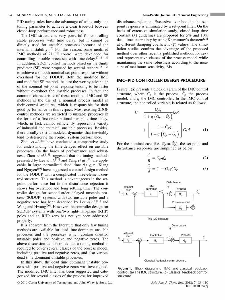
Figure 1(a) presents a block diagram of the IMC controlstructure, where Gp is the process, G̃p the processmodel, and q the IMC controller. In the IMC controlstructure, the controlled variable is related as follows:

C = Gpq

1 + q(

Gp − G̃p

) fRR

+ 1 − G̃pq

1 + q(

Gp − G̃p

) Gpd (1)

For the nominal case (i.e. Gp = G̃p), the set-point anddisturbance responses are simplified as below:

C

R= GpqfR (2)

C

d= (1 − Gpq)Gp (3)

q Gp

IMCcontroller Process

-+

Gp~ +-

Process model

C

Disturbance

RfR

dsetpointfilter u(t)

++

The IMC structure

Gc Gp

C

d

-+fR

setpointfilter Controller Process

Disturbance

R u(t)++

Classical feedback control structure

Figure 1. Block diagram of IMC and classical feedbackcontrol. (a) The IMC structure. (b) Classical feedback controlstructure.

2010 Curtin University of Technology and John Wiley & Sons, Ltd. Asia-Pac. J. Chem. Eng. 2012; 7: 93–110DOI: 10.1002/apj

Asia-Pacific Journal of Chemical Engineering PID CONTROL STRATEGY OF OPEN-LOOP UNSTABLE PROCESSES 95

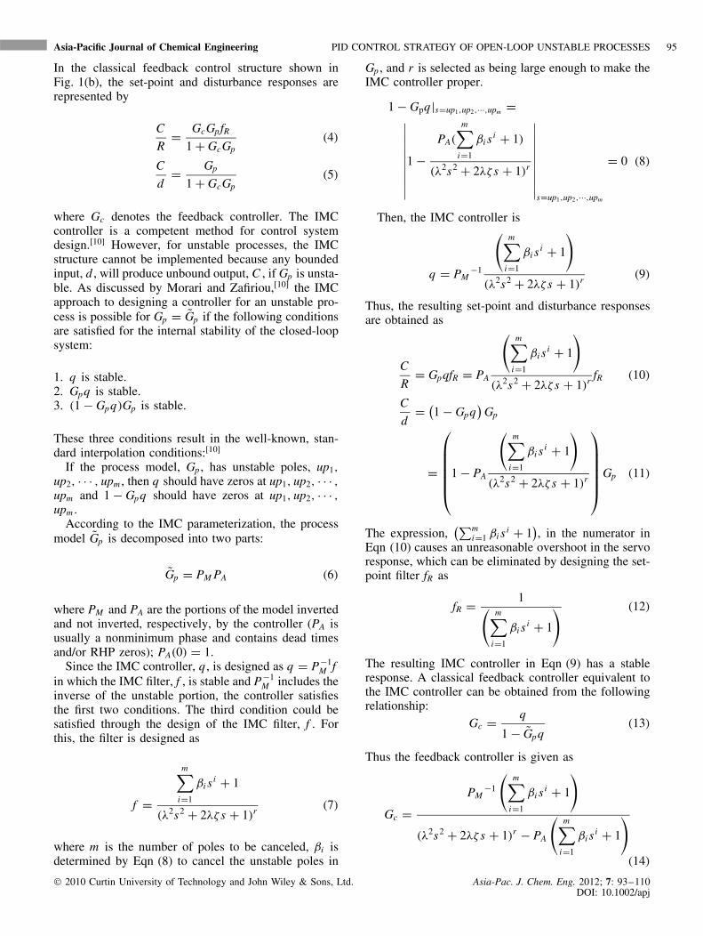
In the classical feedback control structure shown inFig. 1(b), the set-point and disturbance responses arerepresented by

C

R= GcGpfR

1 + GcGp(4)

C

d= Gp

1 + GcGp(5)

where Gc denotes the feedback controller. The IMCcontroller is a competent method for control systemdesign.[10] However, for unstable processes, the IMCstructure cannot be implemented because any boundedinput, d , will produce unbound output, C , if Gp is unsta-ble. As discussed by Morari and Zafiriou,[10] the IMCapproach to designing a controller for an unstable pro-cess is possible for Gp = G̃p if the following conditionsare satisfied for the internal stability of the closed-loopsystem:

1. q is stable.2. Gpq is stable.3. (1 − Gpq)Gp is stable.

These three conditions result in the well-known, stan-dard interpolation conditions:[10]

If the process model, Gp , has unstable poles, up1,

up2, · · · , upm , then q should have zeros at up1, up2, · · · ,upm and 1 − Gpq should have zeros at up1, up2, · · · ,upm .

According to the IMC parameterization, the processmodel G̃p is decomposed into two parts:

G̃p = PM PA (6)

where PM and PA are the portions of the model invertedand not inverted, respectively, by the controller (PA isusually a nonminimum phase and contains dead timesand/or RHP zeros); PA(0) = 1.

Since the IMC controller, q , is designed as q = P−1M f

in which the IMC filter, f , is stable and P−1M includes the

inverse of the unstable portion, the controller satisfiesthe first two conditions. The third condition could besatisfied through the design of the IMC filter, f . Forthis, the filter is designed as

f =

m∑i=1

βi si + 1

(λ2s2 + 2λζ s + 1)r(7)

where m is the number of poles to be canceled, βi isdetermined by Eqn (8) to cancel the unstable poles in

Gp , and r is selected as being large enough to make theIMC controller proper.

1 − Gpq |s=up1,up2,···,upm =∣∣∣∣∣∣∣∣∣∣1 −

PA(

m∑i=1

βi si + 1)

(λ2s2 + 2λζ s + 1)r

∣∣∣∣∣∣∣∣∣∣s=up1,up2,···,upm

= 0 (8)

Then, the IMC controller is

q = PM−1

(m∑

i=1

βi si + 1

)

(λ2s2 + 2λζ s + 1)r(9)

Thus, the resulting set-point and disturbance responsesare obtained as

C

R= GpqfR = PA

(m∑

i=1

βi si + 1

)

(λ2s2 + 2λζ s + 1)rfR (10)

C

d= (

1 − Gpq)

Gp

=

1 − PA

(m∑

i=1

βi si + 1

)

(λ2s2 + 2λζ s + 1)r

Gp (11)

The expression,(∑m

i=1 βi s i + 1), in the numerator in

Eqn (10) causes an unreasonable overshoot in the servoresponse, which can be eliminated by designing the set-point filter fR as

fR = 1(m∑

i=1

βi si + 1

) (12)

The resulting IMC controller in Eqn (9) has a stableresponse. A classical feedback controller equivalent tothe IMC controller can be obtained from the followingrelationship:

Gc = q

1 − G̃pq(13)

Thus the feedback controller is given as

Gc =PM

−1

(m∑

i=1

βi si + 1

)

(λ2s2 + 2λζ s + 1)r − PA

(m∑

i=1

βi si + 1

)(14)



The resulting feedback controller given by Eqn (14) isphysically realizable, but it lacks the standard PID con-troller form. Therefore, the next step is to design the PIDcontroller that most closely approximates the equivalentfeedback controller. The Maclaurin series approxima-tion has been utilized to approximate Eqn (14) to thePID controller.

Lee et al .[22] proposed an efficient method for con-verting the ideal feedback controller Gc to a standardPID controller. Since Gc has an integral term, it can beexpressed as

Gc = g(s)

s(15)

Expanding Gc in the Maclaurin series in s gives

Gc = 1

s

(g(0) + g ′(0)s + g ′′(0)

2s2 + . . .

)(16)

The first three terms of the above expansion can beinterpreted as the standard PID controller, which isgiven by

Gc = Kc

(1 + 1

τI s+ τD s

)(17)

where

Kc = g ′(0) (18a)

τI = g ′(0)/

g(0) (18b)

τD = g ′′(0)/

2g ′(0) (18c)

Design method for proposed tuning rule

Consider a FODUP as a representative model of theform

Gp = K e−θs

τ s − 1(19)

where K is the gain, τ the time constant, and θ the timedelay. The proposed IMC filter is found as f = (βs +1)

/(λ2s2 + 2λζ s + 1). The resulting IMC controller

becomes q = (τ s − 1)(βs + 1)/

K (λ2s2 + 2λζ s + 1).Therefore, the ideal feedback controller equivalent tothe IMC controller is

Gc = (τ s − 1)(βs + 1)

K[(λ2s2 + 2λζ s + 1) − e−θs(βs + 1)

] (20)

The analytical PID formula can be obtained fromEqn (18) as

Kc = τI

K (θ − β + 2λζ )(21)

τI = (−τ + β) −(λ2 − θ2

/2 + βθ

)(θ − β + 2λζ )

(22)

τD =(−τβ) −

(θ3

/6 − βθ2

/2)

(θ − β + 2λζ )

τI

−(λ2 − θ2

/2 + βθ

)(θ − β + 2λζ )

(23)

The extra DOF β is calculated by solving (1 −Gq)|

s=1/

τ= 0. This means β is chosen so that the

term (1 − Gq) = 0 at the pole of Gp , which leaves[1 − (βs + 1)e−θs

/(λ2s2 + 2λζ s + 1)

]∣∣s=1

/τ

= 0.

The value of β after some simplification is

β = τ

[(λ2 + 2λζτ + τ 2)eθ

/τ/

τ 2 − 1

](24)

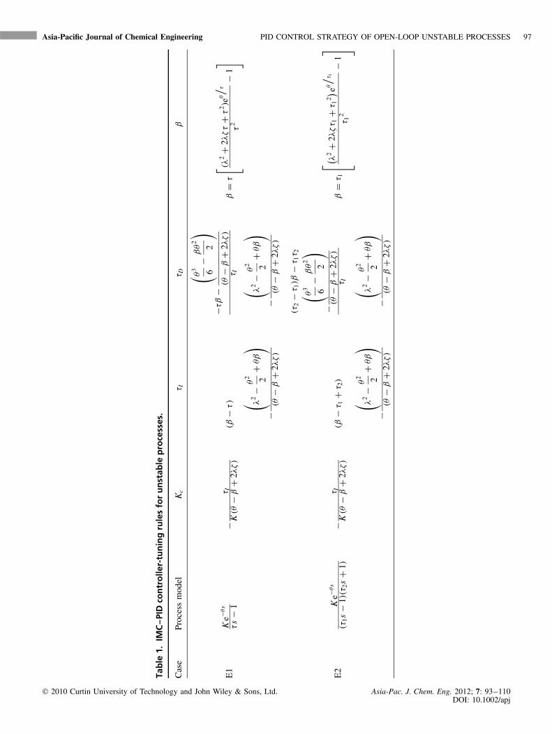
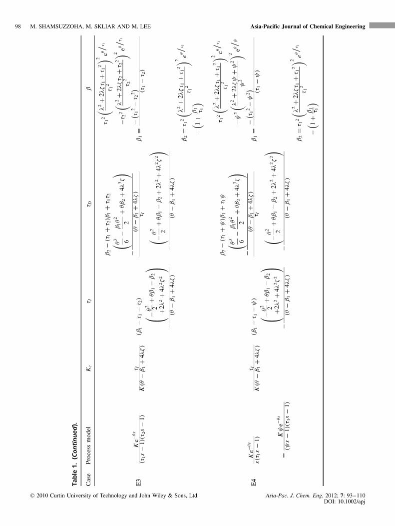
On the basis of the above design principle, the PIDtuning formulas for several process models are obtainedand listed in Table 1.

Remark 1. The design of the IMC–PID controllerbased on the proposed method is not applicable tothe second-order process with complex conjugate pairs.It is due to the value of β1 and β2 comes outcomplex conjugate pairs during the calculation of thePID parameters, which gives unrealistic PID controllersettings.

Remark 2. The processes E1, E2, E3, and E4 mayhave negative zero in the process transfer function inthe form of (τas + 1). For illustration purposes, thesecond-order unstable process with negative zero isgiven as Gp = (τas + 1)K e−θs/(τ1s − 1)(τ2s − 1). Anadditional filter of the form fa = 1/(τas + 1) with PIDcontroller is obtained for the processes with the negativezero and the resulting PID controller should be in theform Gc = Kc(1 + 1/τI s + τD s).fa .

In the process with the positive zero or inverseresponse, the negative numerator time constant isapproximated as a time delay (−τas + 1 ≈ e−τa s ).This is reasonable since an inverse response has adeteriorating effect on control, similar to that of atime delay.[23] The proposed method is applicable forany positive zero after approximation of the neg-ative numerator time constant as an effective timedelay, e.g. Gp = (−τa + 1)e−θs/(τ1s − 1)(τ2s + 1) =e−(θ+τa )s/(τ1s − 1)(τ2s + 1) and this is illustrated inExamples 5 and 6.



Tab

le1.

IMC

–PID

con

tro

ller-

tun

ing

rule

sfo

ru

nst

able

pro

cess

es.

Cas

ePr

oces

sm

odel

Kc

τ Iτ D

β

E1

Ke−θ

s

τs

−1

−τ I

K(θ

−β

+2λ

ζ)

(β−

τ)

−τβ

−

( θ3 6

−βθ

2

2

)

(θ−

β+

2λζ)

τ Iβ

=τ

[ (λ2+

2λζτ

+τ

2)e

θ

/ τ

τ2

−1]

−( λ2−

θ2 2

+θβ

)

(θ−

β+

2λζ)

−( λ2−

θ2 2

+θβ

)

(θ−

β+

2λζ)

E2

Ke−θ

s

(τ1s

−1)

(τ2s

+1)

−τ I

K(θ

−β

+2λ

ζ)

(β−

τ 1+

τ 2)

(τ2−

τ 1)β

−τ 1

τ 2

−

( θ3 6

−βθ

2

2

)

(θ−

β+

2λζ)

τ Iβ

=τ 1

( λ2+

2λζτ 1

+τ 1

2) eθ

/ τ 1

τ 12

−1

−( λ2−

θ2 2

+θβ

)

(θ−

β+

2λζ)

−( λ2−

θ2 2

+θβ

)

(θ−

β+

2λζ)



Tab

le1.

(Co

nti

nu

ed).

Cas

ePr

oces

sm

odel

Kc

τ Iτ D

β

E3

Ke−θ

s

(τ1s

−1)

(τ2s

−1)

τ IK

(θ−

β1+

4λζ)

(β1−

τ 1−

τ 2)

β2−

(τ1+

τ 2)β

1+

τ 1τ 2

−( θ3 6

−β

1θ

2

2+

θβ

2+

4λ3ζ

)

(θ−

β1+

4λζ)

τ Iβ

1=

τ 12

( λ2+

2λζτ 1

+τ 1

2

τ 12

) 2 eθ

/ τ 1

−τ2

2

( λ2+

2λζτ 2

+τ 2

2

τ 22

) 2 eθ

/ τ 1

−( τ 1

2−

τ 22) (τ

1−

τ 2)

− −θ2 2

+θβ

1−

β2

+2λ

2+

4λ2ζ

2

(θ

−β

1+

4λζ)

−( −θ2 2

+θβ

1−

β2+

2λ2+

4λ2ζ

2

)

(θ−

β1+

4λζ)

β2

=τ 1

2

( λ2+

2λζτ 1

+τ 1

2

τ 12

) 2 eθ

/ τ 1

−( 1

+β

1τ 1

)

E4

Ke−θ

s

s(τ 1

s−

1)τ I

K(θ

−β

1+

4λζ)

(β1−

τ 1−

ψ)

β2−

(τ1+

ψ)β

1+

τ 1ψ

−( θ3 6

−β

1θ

2

2+

θβ

2+

4λ3ζ

)

(θ−

β1+

4λζ)

τ Iβ

1=

τ 12

( λ2+

2λζτ 1

+τ 1

2

τ 12

) 2 eθ

/ τ 1

−ψ2

( λ2+

2λζψ

+ψ

2

ψ2

) 2 eθ

/ ψ

−( τ 1

2−

ψ2) (τ

1−

ψ)

=K

ψe−θ

s

(ψs

−1)

(τ1s

−1)

− −θ2 2

+θβ

1−

β2

+2λ

2+

4λ2ζ

2

(θ

−β

1+

4λζ)

−( −θ2 2

+θβ

1−

β2+

2λ2+

4λ2ζ

2

)

(θ−

β1+

4λζ)

β2

=τ 1

2

( λ2+

2λζτ 1

+τ 1

2

τ 12

) 2 eθ

/ τ 1

−( 1

+β

1τ 1

)



SIMULATION STUDY

This section demonstrates the simulation study of sev-eral representative unstable processes with dead time,including positive and negative zeros.

To evaluate the closed-loop performance, the integralof the time-weighted absolute error (ITAE) criterion wasconsidered in the case of both a step set-point changeand a step load disturbance. The ITAE is defined as

ITAE =∫ ∞

0t |e(t)|dt (25)

For the evaluation of the smoothness of a signal,the total variation (TV) of the input u(t), TV =∑∞

i=1 |ui+1 − ui |, is computed. Overshoot, which isa measure of how much the response exceeds theultimate value following a step change in the set-pointand/or disturbance, has been also calculated for eachsimulation example.

The maximum sensitivity Ms[23], which is definedas Ms = max |1/[1 + GpGc(iω)]|, was used to evaluatethe robustness of the control system. Since Ms is theinverse of the shortest distance from the Nyquist curveof the loop transfer function to the critical point (−1, 0),a small Ms value indicates that the control system has alarge stability margin. To ensure a fair comparison, it iswidely accepted that the model-based controllers (IMCand direct synthesis) need to be tuned by adjusting λ togive the same Ms values.

Throughout all the simulation examples, all thecontrollers compared were designed to have the samerobustness level in terms of Ms and the performanceindices such as ITAE, overshoot, and TV values arecompared.

In this article, the simulation study has been con-ducted using the PID controller in the form ofEqn (17). However, for real implementation, the “par-allel form” of the PID controller, Gc = Kc(1 + 1/τI s +τD s/0.1τD s + 1), which is widely used in the real pro-cesses, can be applied to approximately the same perfor-mance. The other form of the PID controller can easilybe converted from ‘parallel form’.[24]

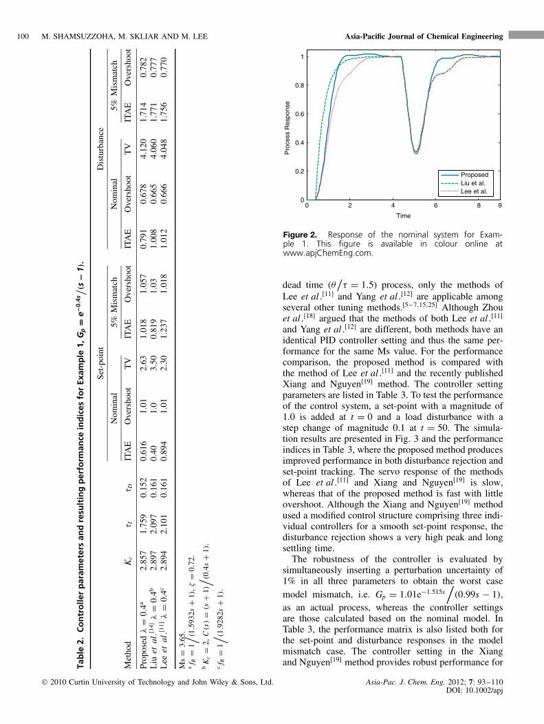
Example 1 Lag time dominant FODUP. An exten-sively published FODUP model[8,11,13,14,25] was consid-ered for a comparison of the performance:

Gp = e−0.4s

(s − 1)(26)

For the above FODUP model, the recently publishedpaper of Liu et al .[14] demonstrated the improvementof their method over those of Tan et al .[13] and Majhiand Atherton.[25] In this simulation study, the proposedmethod is compared with those of Liu et al .[14] andLee et al .[11] The design of the disturbance rejectionis identical for the methods of both Liu et al .[14] and

Lee et al .[11] However, for the set-point response, Liuet al .[14] used a modified IMC structure, while Leeet al .[11] applied a set-point filter. For the methods ofboth Liu et al .[14] and Lee et al .,[11] λ = 0.4 was usedin the simulation, producing Ms = 3.65. To obtain a faircomparison, λ is also adjusted in the proposed method(λ = 0.401) to obtain Ms = 3.65. The controller param-eters, including the performance and robustness matrix,are listed in Table 2.

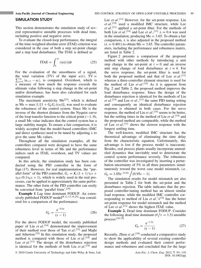
Figure 2 presents a comparison of the proposedmethod with other methods by introducing a unitstep change in the set-point at t = 0 and an inverseunit step change of load disturbance at t = 4. Forthe servo response, the set-point filter is used forboth the proposed method and that of Lee et al .[11]

whereas a three-controller element structure is used forthe method of Liu et al .[14] As it is apparent fromFig. 2 and Table 2, the proposed method improves theload disturbance response. Since the design of thedisturbance rejection is identical for the methods of Liuet al .[14] and Lee et al .,[11] the same PID tuning settingand consequently an identical disturbance rejectionresponse is obtained in both cases. For the servoresponse, the method of Liu et al .[14] seems to be better,but the settling times in the method of Liu et al .[14] andthe proposed method are comparable, while the methodof Lee et al .[11] shows the slowest response with thelongest settling time.

The well-known, modified IMC structure has thetheoretical advantage of eliminating the time delayfrom the characteristic equation. Unfortunately, thisadvantage is lost if the process model is inaccurate.Besides, real process plants usually incorporate unmod-eled dynamics that inevitably tend to deteriorate thecontrol system performance severely. The robustnessof the controller was investigated by inserting a pertur-bation uncertainty of 5% in all three parameters simul-taneously toward the worst case model mismatch, i.e.Gp = 1.05e−0.42s

/(0.95s − 1).

The simulation results for model mismatch are alsopresented in Table 2 for both the set-point and thedisturbance rejection. The table indicates that the pro-posed controller-tuning method has an almost similarload response, while the modified IMC controller cor-responding to method of Liu et al .’s[14] has the betterset-point response for model mismatch and the methodof Lee et al .[11] shows the highest ITAE value.

Example 2. Dead time dominant FODUP. Considerthe following dead time dominant (θ

/τ = 1.5) unstable

process:[18,19]

Gp = e−1.5s

(s − 1)(27)

Recently, Zhou et al .[18] conducted a comparative studyto show the applicability of several existing controllerdesign methods and evaluated their control perfor-mance and robustness and concluded that for the large



Tab

le2.

Co

ntr

olle

rp

aram

eter

san

dre

sult

ing

per

form

ance

ind

ices

for

Exam

ple

1,G

p=

e−0.4

s/ (s−

1).

Set-

poin

tD

istu

rban

ce

Nom

inal

5%M

ism

atch

Nom

inal

5%M

ism

atch

Met

hod

Kc

τ Iτ D

ITA

EO

vers

hoot

TV

ITA

EO

vers

hoot

ITA

EO

vers

hoot

TV

ITA

EO

vers

hoot

Prop

osed

λ=

0.4a

2.85

71.

759

0.15

20.

616

1.01

2.63

1.01

81.

057

0.79

10.

678

4.12

01.

714

0.78

2L

iuet

al.[1

4]λ

=0.

4b2.

897

2.09

70.

161

0.40

1.0

3.50

0.81

91.

031.

008

0.66

54.

060

1.77

10.

777

Lee

etal

.[11]

λ=

0.4c

2.89

42.

101

0.16

10.

894

1.01

2.30

1.23

71.

018

1.01

20.

666

4.04

81.

756

0.77

0

Ms

=3.

65.

af R

=1/ (1

.593

2s+

1),ζ

=0.

72.

bK

c=

2,C

(s)=

(s+

1)/ (0

.4s

+1)

.

cf R

=1/ (1

.928

2s+

1).

0 2 4 6 8 90

0.2

0.4

0.6

0.8

1

Time

Pro

cess

Res

pons

e

ProposedLiu et al.Lee et al.

Figure 2. Response of the nominal system for Exam-ple 1. This figure is available in colour online atwww.apjChemEng.com.

dead time (θ/τ = 1.5) process, only the methods of

Lee et al .[11] and Yang et al .[12] are applicable amongseveral other tuning methods.[5 – 7,15,25] Although Zhouet al .[18] argued that the methods of both Lee et al .[11]

and Yang et al .[12] are different, both methods have anidentical PID controller setting and thus the same per-formance for the same Ms value. For the performancecomparison, the proposed method is compared withthe method of Lee et al .[11] and the recently publishedXiang and Nguyen[19] method. The controller settingparameters are listed in Table 3. To test the performanceof the control system, a set-point with a magnitude of1.0 is added at t = 0 and a load disturbance with astep change of magnitude 0.1 at t = 50. The simula-tion results are presented in Fig. 3 and the performanceindices in Table 3, where the proposed method producesimproved performance in both disturbance rejection andset-point tracking. The servo response of the methodsof Lee et al .[11] and Xiang and Nguyen[19] is slow,whereas that of the proposed method is fast with littleovershoot. Although the Xiang and Nguyen[19] methodused a modified control structure comprising three indi-vidual controllers for a smooth set-point response, thedisturbance rejection shows a very high peak and longsettling time.

The robustness of the controller is evaluated bysimultaneously inserting a perturbation uncertainty of1% in all three parameters to obtain the worst casemodel mismatch, i.e. Gp = 1.01e−1.515s

/(0.99s − 1),

as an actual process, whereas the controller settingsare those calculated based on the nominal model. InTable 3, the performance matrix is also listed both forthe set-point and disturbance responses in the modelmismatch case. The controller setting in the Xiangand Nguyen[19] method provides robust performance for



Tab

le3.

Co

ntr

olle

rp

aram

eter

san

dre

sult

ing

per

form

ance

ind

ices

for

Exam

ple

2,G

p=

e−1.5

s/ (s−

1).

Set-

poin

tD

istu

rban

ce

Nom

inal

1.0%

Mis

mat

chN

omin

al1.

0%M

ism

atch

Met

hod

Kc

τ Iτ D

ITA

EO

vers

hoot

TV

ITA

EO

vers

hoot

ITA

EO

vers

hoot

TV

ITA

EO

vers

hoot

Prop

osed

λ=

4.30

8a1.

065

106.

720.

757

63.4

91.

121.

353

92.0

61.

083

140.

901.

506

4.71

146

4.6

1.60

Lee

etal

.[11]

/Yan

get

al.[1

2]λ

=6.

543b

1.06

425

4.75

0.76

315

5.30

1.0

1.01

323

8.0

1.0

366.

201.

509

4.69

760

0.0

1.61

Xia

ngan

dN

guye

n[19]

c0.

008

1.48

159.

0576

.82

1.06

1.25

784

.84

1.02

091

6.20

3.15

311

.538

497.

03.

21

Ms

=29

.70.

af R

=1/ (1

05.9

639s

+1)

,ζ

=0.

5.

bf R

=1/ (2

53.9

94s

+1)

.

cC

2(s

)=

1.01

9+

0.59

s,F

(s)=

1/ (5s

+1)

.

0 20 40 60 80 100 120

-2

-1

0

1

2

Time

Out

put R

espo

nse

Proposed

Lee et al.

Xiang and Nguyen


the servo problem but a big overshoot in disturbancerejection. The proposed method and that of Lee et al .[11]

have almost similar performance in both the servo andregulatory problems.

Example 3. Second-order delayed unstable process(SODUP). The following unstable process is consideredfor the present study:[8,11 – 13]

Gp = e−0.5s

(5s − 1)(2s + 1)(0.5s + 1)(28)

The model presented above is a high-order unstableprocess and is approximated with an unstable pole withdead time.[8,11 – 13]

Gp = e−0.939s

(5s − 1)(2.07s + 1)(29)

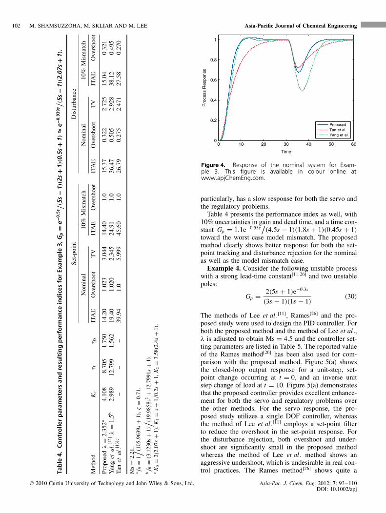
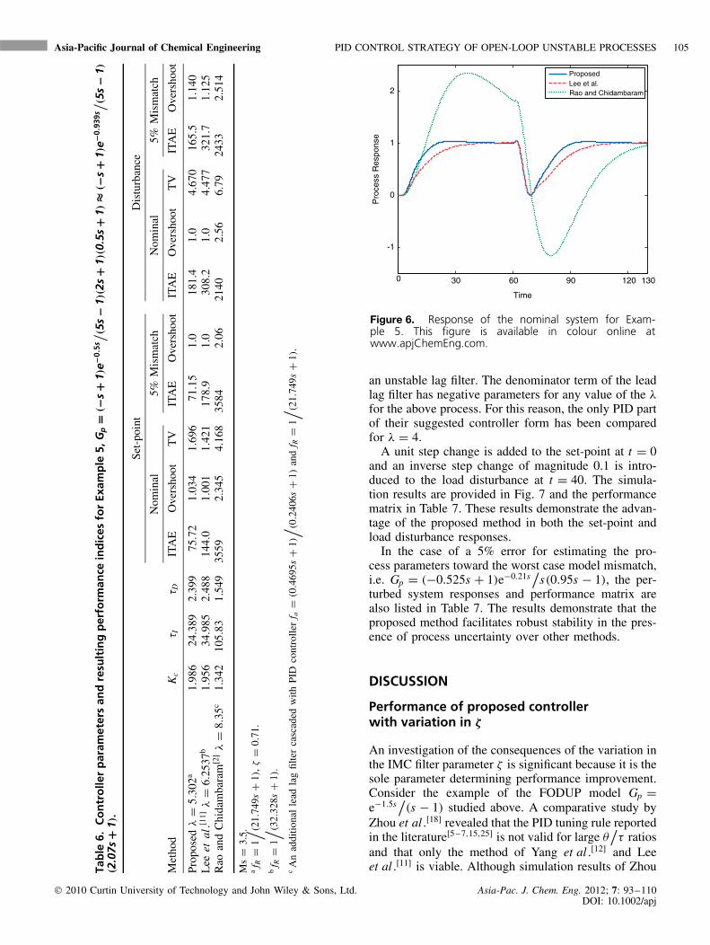
Tan et al .[13] have already explained the advantage oftheir method over those of Huang and Chen,[8] andLee et al .[11] For this reason, the proposed method iscompared with the methods of Tan et al .[13] and Yanget al .[12] to show its improvement over other methods.The λ value for the proposed method is adjusted toobtain the same Ms = 2.21 as the method of Yanget al .[12] and the controller setting parameters withperformance indices are listed in Table 4.

For the simulation of the above process, both the set-point and load disturbance that has a step change ofmagnitude 1 and −1 are inserted at t = 0 and at t = 30,respectively. The output response for both the servo andregulatory problem is shown in Fig. 4. The proposedtuning method has a faster settling time than that ofthe other existing methods. Tan et al .’s method,[13]



Tab

le4.

Co

ntr

olle

rp

aram

eter

san

dre

sult

ing

per

form

ance

ind

ices

for

Exam

ple

3,G

p=

e−0.5

s/ (5s

−1)

(2s+

1)(0

.5s+

1)≈

e−0.9

39s/ (5

s−

1)(2

.07s

+1)

.

Set-

poin

tD

istu

rban

ce

Nom

inal

10%

Mis

mat

chN

omin

al10

%M

ism

atch

Met

hod

Kc

τ Iτ D

ITA

EO

vers

hoot

TV

ITA

EO

vers

hoot

ITA

EO

vers

hoot

TV

ITA

EO

vers

hoot

Prop

osed

λ=

2.35

2a4.

108

8.70

51.

750

14.2

01.

023

3.04

414

.40

1.0

15.3

70.

322

2.72

515

.04

0.32

1Y

ang

etal

.[12]

λ=

1.5b

2.98

912

.799

1.56

219

.40

1.02

02.

345

24.9

11.

036

.47

0.50

52.

928

38.1

20.

495

Tan

etal

.[13]

c–

––

39.9

41.

05.

999

45.6

01.

026

.79

0.27

52.

471

27.5

80.

270

Ms

=2.

21.

af R

=1/ (1

05.9

639s

+1)

,ζ

=0.

71.

bf R

=(3

.123

0s+

1)/ (1

9.98

58s2

+12

.799

1s+

1).

cK

0=

2(2.

07s

+1)

,K

1=

s+

1/0.

2s+

1,K

2=

3.58

(2.4

s+

1).

0 10 20 30 40 50 600

0.2

0.4

0.6

0.8

1

Time

Pro

cess

Res

pons

e

ProposedTan et al.Yang et al.


particularly, has a slow response for both the servo andthe regulatory problems.

Table 4 presents the performance index as well, with10% uncertainties in gain and dead time, and a time con-stant Gp = 1.1e−0.55s

/(4.5s − 1)(1.8s + 1)(0.45s + 1)

toward the worst case model mismatch. The proposedmethod clearly shows better response for both the set-point tracking and disturbance rejection for the nominalas well as the model mismatch case.

Example 4. Consider the following unstable processwith a strong lead-time constant[11,26] and two unstablepoles:

Gp = 2(5s + 1)e−0.3s

(3s − 1)(1s − 1)(30)

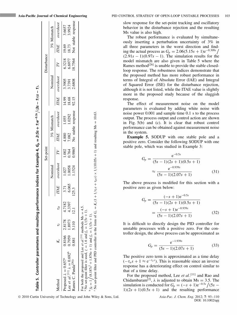
The methods of Lee et al .[11], Rames[26] and the pro-posed study were used to design the PID controller. Forboth the proposed method and the method of Lee et al .,λ is adjusted to obtain Ms = 4.5 and the controller set-ting parameters are listed in Table 5. The reported valueof the Rames method[26] has been also used for com-parison with the proposed method. Figure 5(a) showsthe closed-loop output response for a unit-step, set-point change occurring at t = 0, and an inverse unitstep change of load at t = 10. Figure 5(a) demonstratesthat the proposed controller provides excellent enhance-ment for both the servo and regulatory problems overthe other methods. For the servo response, the pro-posed study utilizes a single DOF controller, whereasthe method of Lee et al .[11] employs a set-point filterto reduce the overshoot in the set-point response. Forthe disturbance rejection, both overshoot and under-shoot are significantly small in the proposed methodwhereas the method of Lee et al . method shows anaggressive undershoot, which is undesirable in real con-trol practices. The Rames method[26] shows quite a



Tab

le5.

Co

ntr

olle

rp

aram

eter

san

dre

sult

ing

per

form

ance

ind

ices

for

Exam

ple

4,G

p=

2(5s

+1)

e−0.3

s/ (3s−

1)(s

−1)

.

Set-

poin

tD

istu

rban

ce

Nom

inal

3%M

ism

atch

Nom

inal

3%M

ism

atch

Met

hod

Kc

τ Iτ D

ITA

Eov

ersh

oot

TV

ITA

Eov

ersh

oot

ITA

Eov

ersh

oot

TV

ITA

Eov

ersh

oot

Prop

osed

λ=

0.65

7a0.

8166

2.81

784.

7182

3.71

1.02

71.

002

4.88

01.

055

14.9

93.

3905

6.32

1819

.69

3.66

57L

eeet

al.[1

1]λ

=0.

692b

0.79

591.

8973

4.33

976.

065

1.00

580.

764

7.08

21.

0292

18.6

83.

7391

6.69

7718

.73

3.99

24R

ames

C.

Pand

a[26]

c0.

881

5.11

012

.112

5.3

1.15

240.

9865

No

stab

lere

spon

se92

.15

2.68

0818

.756

4N

otst

able

resp

onse

For

both

the

prop

osed

and

Lee

etal

.[11]

met

hods

Ms

=4.

5.a

No

set-

poin

tfil

ter

isus

ed,ζ

=1.

6an

df a

=1/

(5s

+1)

.b

f R=

1/ (8.1

87s2

+1.

876s

+1)

and

f a=

1/(5

s+

1).

cN

ose

t-po

int

filte

ran

dPI

Dco

ntro

ller

inth

efo

rmof

Gc

=K

c(1

+1/

τ Is

+τ D

s)×

1/(1

0.05

s+

1)an

dre

sulti

ngM

s=

10.6

3.

slow response for the set-point tracking and oscillatorybehavior in the disturbance rejection and the resultingMs value is also high.

The robust performance is evaluated by simultane-ously inserting a perturbation uncertainty of 3% inall three parameters in the worst direction and find-ing the actual process as Gp = 2.06(5.15s + 1)e−0.309s

/(2.91s − 1)(0.97s − 1). The simulation results for themodel mismatch are also given in Table 5 where theRames method[26] is unable to provide the stable closed-loop response. The robustness indices demonstrate thatthe proposed method has more robust performance interms of Integral of Absolute Error (IAE) and Integralof Squared Error (ISE) for the disturbance rejection,although it is not listed, while the ITAE value is slightlymore in the proposed study because of the sluggishresponse.

The effect of measurement noise on the modelparameters is evaluated by adding white noise withnoise power 0.001 and sample time 0.1 s to the processoutput. The process output and control action are shownin Fig. 5(b) and (c). It is clear that robust controlperformance can be obtained against measurement noisein the system.

Example 5. SODUP with one stable pole and apositive zero. Consider the following SODUP with onestable pole, which was studied in Example 3:

Gp = e−0.5s

(5s − 1)(2s + 1)(0.5s + 1)

≈ e−0.939s

(5s − 1)(2.07s + 1)(31)

The above process is modified for this section with apositive zero as given below:

Gp = (−s + 1)e−0.5s

(5s − 1)(2s + 1)(0.5s + 1)

= (−s + 1)e−0.939s

(5s − 1)(2.07s + 1)(32)

It is difficult to directly design the PID controller forunstable processes with a positive zero. For the con-troller design, the above process can be approximated as

Gp = e−1.939s

(5s − 1)(2.07s + 1)(33)

The positive zero term is approximated as a time delay(−τas + 1 ≈ e−τa s ). This is reasonable since an inverseresponse has a deteriorating effect on control similar tothat of a time delay.

For the proposed method, Lee et al .[11] and Rao andChidambaram[2], λ is adjusted to obtain Ms = 3.5. Thesimulation is conducted for Gp = (−s + 1)e−0.5s

/(5s −

1)(2s + 1)(0.5s + 1) and the resulting performance



0 5 10 15 20 25-3

-2

-1

0

1

2

Time

Pro

cess

Res

pons

e

ProposedLee et al.Rames C. Panda

0 10 20 30 40 50-4

-3

-2

-1

0

1

2

3

Time

Pro

cess

Res

pons

e


0 10 20 30 40 50-1

-0.5

0

0.5

1

1.5

2

2.5

Time

Man

ipul

ated

Var

iabl

e


(a) (b)

(c)

Figure 5. (a)Response of the nominal system for Example 4. (b) Response of the nominal system withwhite noise of power 0.001 and sample time 0.1 s to the process output for Example 4. (c) Controlleroutput of the nominal system with white noise of power 0.001 and sample time 0.1 s to the processoutput for Example 4. This figure is available in colour online at www.apjChemEng.com.

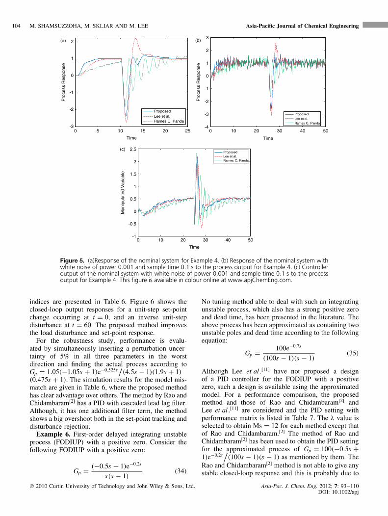
indices are presented in Table 6. Figure 6 shows theclosed-loop output responses for a unit-step set-pointchange occurring at t = 0, and an inverse unit-stepdisturbance at t = 60. The proposed method improvesthe load disturbance and set-point response.

For the robustness study, performance is evalu-ated by simultaneously inserting a perturbation uncer-tainty of 5% in all three parameters in the worstdirection and finding the actual process according toGp = 1.05(−1.05s + 1)e−0.525s

/(4.5s − 1)(1.9s + 1)

(0.475s + 1). The simulation results for the model mis-match are given in Table 6, where the proposed methodhas clear advantage over others. The method by Rao andChidambaram[2] has a PID with cascaded lead lag filter.Although, it has one additional filter term, the methodshows a big overshoot both in the set-point tracking anddisturbance rejection.

Example 6. First-order delayed integrating unstableprocess (FODIUP) with a positive zero. Consider thefollowing FODIUP with a positive zero:

Gp = (−0.5s + 1)e−0.2s

s(s − 1)(34)

No tuning method able to deal with such an integratingunstable process, which also has a strong positive zeroand dead time, has been presented in the literature. Theabove process has been approximated as containing twounstable poles and dead time according to the followingequation:

Gp = 100e−0.7s

(100s − 1)(s − 1)(35)

Although Lee et al .[11] have not proposed a designof a PID controller for the FODIUP with a positivezero, such a design is available using the approximatedmodel. For a performance comparison, the proposedmethod and those of Rao and Chidambaram[2] andLee et al .[11] are considered and the PID setting withperformance matrix is listed in Table 7. The λ value isselected to obtain Ms = 12 for each method except thatof Rao and Chidambaram.[2] The method of Rao andChidambaram[2] has been used to obtain the PID settingfor the approximated process of Gp = 100(−0.5s +1)e−0.2s

/(100s − 1)(s − 1) as mentioned by them. The

Rao and Chidambaram[2] method is not able to give anystable closed-loop response and this is probably due to



Tab

le6.

Co

ntr

olle

rp

aram

eter

san

dre

sult

ing

per

form

ance

ind

ices

for

Exam

ple

5,G

p=

(−s

+1)

e−0.5

s/ (5s

−1)

(2s

+1)

(0.5

s+

1)≈

(−s+

1)e−0

.939

s/ (5s

−1)

(2.0

7s+

1).

Set-

poin

tD

istu

rban

ce

Nom

inal

5%M

ism

atch

Nom

inal

5%M

ism

atch

Met

hod

Kc

τ Iτ D

ITA

EO

vers

hoot

TV

ITA

EO

vers

hoot

ITA

EO

vers

hoot

TV

ITA

EO

vers

hoot

Prop

osed

λ=

5.30

2a1.

986

24.3

892.

399

75.7

21.

034

1.69

671

.15

1.0

181.

41.

04.

670

165.

51.

140

Lee

etal

.[11]

λ=

6.25

37b

1.95

634

.985

2.48

814

4.0

1.00

11.

421

178.

91.

030

8.2

1.0

4.47

732

1.7

1.12

5R

aoan

dC

hida

mba

ram

[2]λ

=8.

35c

1.34

210

5.83

1.54

935

592.

345

4.16

835

842.

0621

402.

566.

7924

332.

514

Ms

=3.

5.a

f R=

1/ (21.

749s

+1)

,ζ

=0.

71.

bf R

=1/ (3

2.32

8s+

1).

cA

nad

ditio

nal

lead

lag

filte

rca

scad

edw

ithPI

Dco

ntro

ller

f a=

(0.4

695s

+1)

/ (0.2

406s

+1)

and

f R=

1/ (21.

749s

+1)

.

0 30 60 90 120 130

-1

0

1

2

Time

Pro

cess

Res

pons

e

ProposedLee et al.Rao and Chidambaram


an unstable lag filter. The denominator term of the leadlag filter has negative parameters for any value of the λfor the above process. For this reason, the only PID partof their suggested controller form has been comparedfor λ = 4.

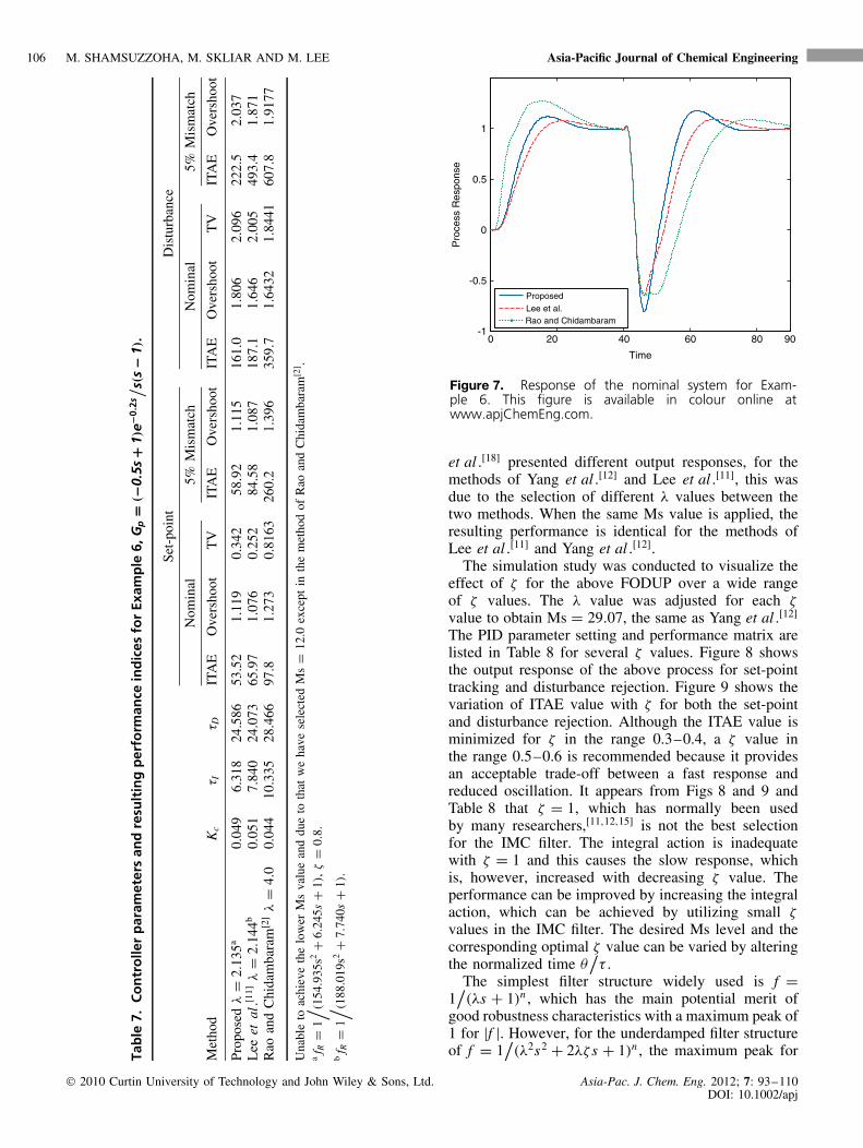
A unit step change is added to the set-point at t = 0and an inverse step change of magnitude 0.1 is intro-duced to the load disturbance at t = 40. The simula-tion results are provided in Fig. 7 and the performancematrix in Table 7. These results demonstrate the advan-tage of the proposed method in both the set-point andload disturbance responses.

In the case of a 5% error for estimating the pro-cess parameters toward the worst case model mismatch,i.e. Gp = (−0.525s + 1)e−0.21s

/s(0.95s − 1), the per-

turbed system responses and performance matrix arealso listed in Table 7. The results demonstrate that theproposed method facilitates robust stability in the pres-ence of process uncertainty over other methods.

DISCUSSION

Performance of proposed controllerwith variation in ζ

An investigation of the consequences of the variation inthe IMC filter parameter ζ is significant because it is thesole parameter determining performance improvement.Consider the example of the FODUP model Gp =e−1.5s

/(s − 1) studied above. A comparative study by

Zhou et al .[18] revealed that the PID tuning rule reportedin the literature[5 – 7,15,25] is not valid for large θ

/τ ratios

and that only the method of Yang et al .[12] and Leeet al .[11] is viable. Although simulation results of Zhou



Tab

le7.

Co

ntr

olle

rp

aram

eter

san

dre

sult

ing

per

form

ance

ind

ices

for

Exam

ple

6,G

p=

(−0.

5s+

1)e−0

.2s/ s(

s−

1).

Set-

poin

tD

istu

rban

ce

Nom

inal

5%M

ism

atch

Nom

inal

5%M

ism

atch

Met

hod

Kc

τ Iτ D

ITA

EO

vers

hoot

TV

ITA

EO

vers

hoot

ITA

EO

vers

hoot

TV

ITA

EO

vers

hoot

Prop

osed

λ=

2.13

5a0.

049

6.31

824

.586

53.5

21.

119

0.34

258

.92

1.11

516

1.0

1.80

62.

096

222.

52.

037

Lee

etal

.[11]

λ=

2.14

4b0.

051

7.84

024

.073

65.9

71.

076

0.25

284

.58

1.08

718

7.1

1.64

62.

005

493.

41.

871

Rao

and

Chi

dam

bara

m[2

]λ

=4.

00.

044

10.3

3528

.466

97.8

1.27

30.

8163

260.

21.

396

359.

71.

6432

1.84

4160

7.8

1.91

77

Una

ble

toac

hiev

eth

elo

wer

Ms

valu

ean

ddu

eto

that

we

have

sele

cted

Ms

=12

.0ex

cept

inth

em

etho

dof

Rao

and

Chi

dam

bara

m[2

] .a

f R=

1/ (154

.935

s2+

6.24

5s+

1),ζ

=0.

8.

bf R

=1/ (1

88.0

19s2

+7.

740s

+1)

.0 20 40 60 80 90

-1

-0.5

0

0.5

1

Time

Pro

cess

Res

pons

e

ProposedLee et al.Rao and Chidambaram


et al .[18] presented different output responses, for themethods of Yang et al .[12] and Lee et al .[11], this wasdue to the selection of different λ values between thetwo methods. When the same Ms value is applied, theresulting performance is identical for the methods ofLee et al .[11] and Yang et al .[12].

The simulation study was conducted to visualize theeffect of ζ for the above FODUP over a wide rangeof ζ values. The λ value was adjusted for each ζvalue to obtain Ms = 29.07, the same as Yang et al .[12]

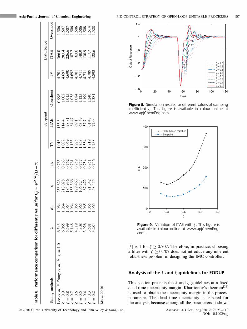
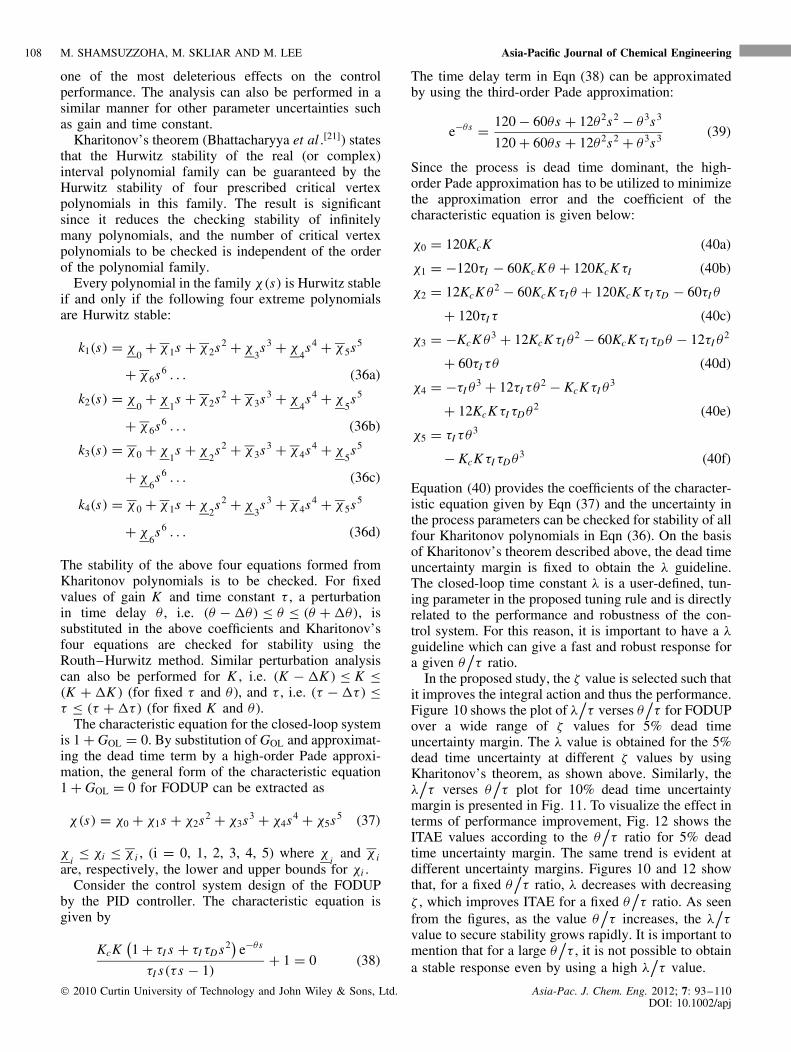
The PID parameter setting and performance matrix arelisted in Table 8 for several ζ values. Figure 8 showsthe output response of the above process for set-pointtracking and disturbance rejection. Figure 9 shows thevariation of ITAE value with ζ for both the set-pointand disturbance rejection. Although the ITAE value isminimized for ζ in the range 0.3–0.4, a ζ value inthe range 0.5–0.6 is recommended because it providesan acceptable trade-off between a fast response andreduced oscillation. It appears from Figs 8 and 9 andTable 8 that ζ = 1, which has normally been usedby many researchers,[11,12,15] is not the best selectionfor the IMC filter. The integral action is inadequatewith ζ = 1 and this causes the slow response, whichis, however, increased with decreasing ζ value. Theperformance can be improved by increasing the integralaction, which can be achieved by utilizing small ζvalues in the IMC filter. The desired Ms level and thecorresponding optimal ζ value can be varied by alteringthe normalized time θ

/τ .

The simplest filter structure widely used is f =1/(λs + 1)n , which has the main potential merit of

good robustness characteristics with a maximum peak of1 for |f |. However, for the underdamped filter structureof f = 1

/(λ2s2 + 2λζ s + 1)n , the maximum peak for



Tab

le8.

Perf

orm

ance

com

par

iso

nfo

rd

iffe

ren

tζ

valu

efo

rG

p=

e−1.5

s/ (s−

1).

Set-

poin

tD

istu

rban

ce

Tun

ing

met

hods

λK

cτ I

τ DT

VIT

AE

Ove

rsho

otT

VIT

AE

Ove

rsho

ot

Lee

etal

.[11]

/Yan

get

al.[1

2]ζ

=1.

06.

543

1.06

425

3.32

30.

765

1.01

315

5.3

0.99

64.

701

366.

01.

506

ζ=

0.9

6.06

51.

064

218.

028

0.76

31.

032

114.

41.

002

4.69

728

3.4

1.50

7ζ

=0.

85.

599

1.06

418

4.93

60.

762

1.06

998

.81

1.01

54.

690

226.

61.

507

ζ=

0.7

5.14

81.

064

155.

366

0.76

11.

133

84.4

71.

038

4.69

218

7.7

1.50

6ζ

=0.

64.

719

1.06

512

9.46

30.

759

1.22

569

.11.

084

4.70

116

3.6

1.50

6ζ

=0.

54.

308

1.06

510

6.72

40.

757

1.35

363

.49

1.12

54.

711

140.

91.

506

ζ=

0.4

3.92

81.

065

87.4

720.

754

1.55

457

.71.

199

4.73

113

0.9

1.50

8ζ

=0.

33.

581

1.06

571

.342

0.75

11.

719

61.4

81.

240

4.78

911

7.7

1.51

4ζ

=0.

23.

284

1.06

558

.455

0.74

62.

238

72.0

1.38

14.

892

128.

61.

528

Ms

=29

.70.

0 20 40 60 80 100 120-0.6

-0.2

0.2

0.6

1

1.4

Time

Out

put R

espo

nse

ζ = 1.0ζ = 0.9ζ = 0.8ζ = 0.7ζ = 0.6ζ = 0.5ζ = 0.4ζ = 0.3

Figure 8. Simulation results for different values of dampingcoefficient ζ . This figure is available in colour online atwww.apjChemEng.com.

0

100

200

300

400

0 0.3 0.6 0.9 1.2

ITA

E

Disturbance rejectionSet-point

z

Figure 9. Variation of ITAE with ζ . This figure isavailable in colour online at www.apjChemEng.com.

|f | is 1 for ζ ≥ 0.707. Therefore, in practice, choosinga filter with ζ ≥ 0.707 does not introduce any inherentrobustness problem in designing the IMC controller.

Analysis of the λ and ζ guidelines for FODUP

This section presents the λ and ζ guidelines at a fixeddead time uncertainty margin. Kharitonov’s theorem[21]

is used to obtain the uncertainty margin in the processparameter. The dead time uncertainty is selected forthe analysis because among all the parameters it shows



one of the most deleterious effects on the controlperformance. The analysis can also be performed in asimilar manner for other parameter uncertainties suchas gain and time constant.

Kharitonov’s theorem (Bhattacharyya et al .[21]) statesthat the Hurwitz stability of the real (or complex)interval polynomial family can be guaranteed by theHurwitz stability of four prescribed critical vertexpolynomials in this family. The result is significantsince it reduces the checking stability of infinitelymany polynomials, and the number of critical vertexpolynomials to be checked is independent of the orderof the polynomial family.

Every polynomial in the family χ(s) is Hurwitz stableif and only if the following four extreme polynomialsare Hurwitz stable:

k1(s) = χ0+ χ1s + χ2s2 + χ

3s3 + χ

4s4 + χ5s5

+ χ6s6 . . . (36a)

k2(s) = χ0+ χ

1s + χ2s2 + χ3s3 + χ

4s4 + χ

5s5

+ χ6s6 . . . (36b)

k3(s) = χ0 + χ1s + χ

2s2 + χ3s3 + χ4s4 + χ

5s5

+ χ6s6 . . . (36c)

k4(s) = χ0 + χ1s + χ2s2 + χ

3s3 + χ4s4 + χ5s5

+ χ6s6 . . . (36d)

The stability of the above four equations formed fromKharitonov polynomials is to be checked. For fixedvalues of gain K and time constant τ , a perturbationin time delay θ , i.e. (θ − θ) ≤ θ ≤ (θ + θ), issubstituted in the above coefficients and Kharitonov’sfour equations are checked for stability using theRouth–Hurwitz method. Similar perturbation analysiscan also be performed for K , i.e. (K − K ) ≤ K ≤(K + K ) (for fixed τ and θ ), and τ , i.e. (τ − τ) ≤τ ≤ (τ + τ) (for fixed K and θ ).

The characteristic equation for the closed-loop systemis 1 + GOL = 0. By substitution of GOL and approximat-ing the dead time term by a high-order Pade approxi-mation, the general form of the characteristic equation1 + GOL = 0 for FODUP can be extracted as

χ(s) = χ0 + χ1s + χ2s2 + χ3s3 + χ4s4 + χ5s5 (37)

χi≤ χi ≤ χ i , (i = 0, 1, 2, 3, 4, 5) where χ

iand χ i

are, respectively, the lower and upper bounds for χi .Consider the control system design of the FODUP

by the PID controller. The characteristic equation isgiven by

KcK(1 + τI s + τI τD s2

)e−θs

τI s(τ s − 1)+ 1 = 0 (38)

The time delay term in Eqn (38) can be approximatedby using the third-order Pade approximation:

e−θs = 120 − 60θs + 12θ2s2 − θ3s3

120 + 60θs + 12θ2s2 + θ3s3 (39)

Since the process is dead time dominant, the high-order Pade approximation has to be utilized to minimizethe approximation error and the coefficient of thecharacteristic equation is given below:

χ0 = 120KcK (40a)

χ1 = −120τI − 60KcK θ + 120KcK τI (40b)

χ2 = 12KcK θ2 − 60KcK τI θ + 120KcK τI τD − 60τI θ

+ 120τI τ (40c)

χ3 = −KcK θ3 + 12KcK τI θ2 − 60KcK τI τDθ − 12τI θ

2

+ 60τI τθ (40d)

χ4 = −τI θ3 + 12τI τθ2 − KcK τI θ

3

+ 12KcK τI τDθ2 (40e)

χ5 = τI τθ3

− KcK τI τDθ3 (40f)

Equation (40) provides the coefficients of the character-istic equation given by Eqn (37) and the uncertainty inthe process parameters can be checked for stability of allfour Kharitonov polynomials in Eqn (36). On the basisof Kharitonov’s theorem described above, the dead timeuncertainty margin is fixed to obtain the λ guideline.The closed-loop time constant λ is a user-defined, tun-ing parameter in the proposed tuning rule and is directlyrelated to the performance and robustness of the con-trol system. For this reason, it is important to have a λguideline which can give a fast and robust response fora given θ

/τ ratio.

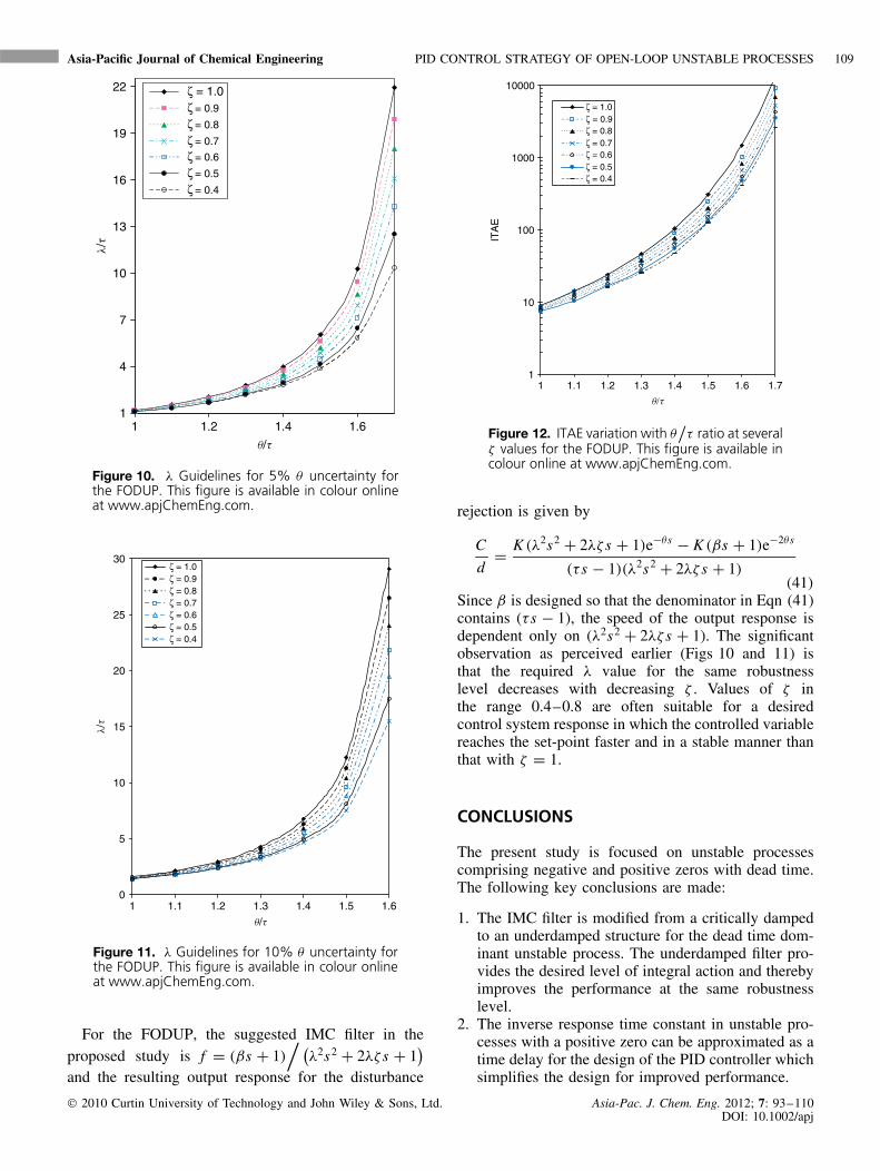
In the proposed study, the ζ value is selected such thatit improves the integral action and thus the performance.Figure 10 shows the plot of λ

/τ verses θ

/τ for FODUP

over a wide range of ζ values for 5% dead timeuncertainty margin. The λ value is obtained for the 5%dead time uncertainty at different ζ values by usingKharitonov’s theorem, as shown above. Similarly, theλ/τ verses θ

/τ plot for 10% dead time uncertainty

margin is presented in Fig. 11. To visualize the effect interms of performance improvement, Fig. 12 shows theITAE values according to the θ

/τ ratio for 5% dead

time uncertainty margin. The same trend is evident atdifferent uncertainty margins. Figures 10 and 12 showthat, for a fixed θ

/τ ratio, λ decreases with decreasing

ζ , which improves ITAE for a fixed θ/τ ratio. As seen

from the figures, as the value θ/τ increases, the λ

/τ

value to secure stability grows rapidly. It is important tomention that for a large θ

/τ , it is not possible to obtain

a stable response even by using a high λ/τ value.



1

4

7

10

13

16

19

22

1 1.2 1.4 1.6

ζ = 1.0ζ = 0.9

ζ = 0.8

ζ = 0.7

ζ = 0.6

ζ = 0.5

ζ = 0.4

q/t

l/t

Figure 10. λ Guidelines for 5% θ uncertainty forthe FODUP. This figure is available in colour onlineat www.apjChemEng.com.

0

5

10

15

20

25

30

1 1.1 1.2 1.3 1.4 1.5 1.6

ζ = 1.0ζ = 0.9ζ = 0.8ζ = 0.7ζ = 0.6ζ = 0.5ζ = 0.4

l/t

q/t

Figure 11. λ Guidelines for 10% θ uncertainty forthe FODUP. This figure is available in colour onlineat www.apjChemEng.com.

For the FODUP, the suggested IMC filter in theproposed study is f = (βs + 1)

/ (λ2s2 + 2λζ s + 1

)and the resulting output response for the disturbance

1

10

100

1000

10000

1 1.1 1.2 1.3 1.4 1.5 1.6 1.7

ITA

E

ζ = 1.0ζ = 0.9ζ = 0.8ζ = 0.7ζ = 0.6ζ = 0.5ζ = 0.4

q/t

Figure 12. ITAE variation with θ/τ ratio at several

ζ values for the FODUP. This figure is available incolour online at www.apjChemEng.com.

rejection is given by

C

d= K (λ2s2 + 2λζ s + 1)e−θs − K (βs + 1)e−2θs

(τ s − 1)(λ2s2 + 2λζ s + 1)(41)

Since β is designed so that the denominator in Eqn (41)contains (τ s − 1), the speed of the output response isdependent only on (λ2s2 + 2λζ s + 1). The significantobservation as perceived earlier (Figs 10 and 11) isthat the required λ value for the same robustnesslevel decreases with decreasing ζ . Values of ζ inthe range 0.4–0.8 are often suitable for a desiredcontrol system response in which the controlled variablereaches the set-point faster and in a stable manner thanthat with ζ = 1.

CONCLUSIONS

The present study is focused on unstable processescomprising negative and positive zeros with dead time.The following key conclusions are made:

1. The IMC filter is modified from a critically dampedto an underdamped structure for the dead time dom-inant unstable process. The underdamped filter pro-vides the desired level of integral action and therebyimproves the performance at the same robustnesslevel.

2. The inverse response time constant in unstable pro-cesses with a positive zero can be approximated as atime delay for the design of the PID controller whichsimplifies the design for improved performance.



3. For unstable processes with a strong lead-time con-stant, an overdamped filter is suggested because itsignificantly reduces both the overshoot and under-shoot. In this case, a set-point filter is not required forthe servo response, whereas it is needed to eliminatethe overshoot for ζ = 1.

4. The simulation study conducted to show the effect ofζ variation on the performance at a fixed Ms valueclearly reveals that a critically damped filter is notthe best option for PID controller design.

5. By using Kharitonov’s theorem, closed-loop timeconstant λ guidelines are suggested for the 5% and10% dead time uncertainty margins at several ζvalues.

6. The simulation studies conducted for several processclasses clearly demonstrate the clear advantage of theproposed method over others previously reported.

Acknowledgements

This research was supported by Yeungnam Universityresearch grants in 2009.

REFERENCES

[1] T. Chiu, P.D. Christofides. AIChE J., 1999; 45(6), 1279–1297.[2] A.S. Rao, M. Chidambaram. Asia Pac. J. Chem. Eng., 2006;

1, 63–69.[3] S. Uma, M. Chidambaram, A.S. Rao. Ind. Eng. Chem. Res.,

2009; 48, 3098–3111.[4] A.M. De Paor, M.O. Malley. Int. J. Control, 1989; 49(4),

1273–1284.[5] A. Visioli. IEE Proc. Part D, 2001; 148(2), 180–184.

[6] J.H. Park, S.W. Sung, I.B. Lee. Automatica, 1998; 34(6),751–756.

[7] Y.G. Wang, W.J. Cai. Ind. Eng. Chem. Res., 2002; 41,2910–2914.

[8] H.P. Huang, C.C. Chen. IEE Process-Control Theory Appl.,1997; 144, 334.

[9] C.S. Jung, H.K. Song, J.C. Hyun. J. Process Control, 1999; 9,265–269.

[10] M. Morari, E. Zafiriou. Robust Process Control, Prentice-Hall:Englewood Cliffs, NJ, 1989.

[11] Y. Lee, J. Lee, S. Park. Chem. Eng. Sci., 2000; 55,3481–3493.

[12] X.P. Yang, Q.G. Wang, C.C. Hang, C. Lin. Ind. Eng. Chem.Res., 2002; 41(17), 4288–4294.

[13] W. Tan, H.J. Marquez, T. Chen. J. Process Control, 2003; 13,203–213.

[14] T. Liu, W. Zhang, D. Gu. J. Process Control, 2005; 15,559–572.

[15] S. Majhi, D.P. Atherton. IEE Proc. Part D, 2000; 147(4),421–427.

[16] H.J. Kwak, S.W. Sung, I.B. Lee, J.Y. Park. Ind. Eng. Chem.Res., 1999; 38(2), 405–411.

[17] W.D. Zhang, D. Gu, W. Wang, X. Xu. Ind. Eng. Chem. Res.,2004; 43(1), 56–62.

[18] H.Q. Zhou, Q.G. Wang, L.S. Shieh. J. Chem. Eng. Jpn, 2007;40(2), 145–163.

[19] C. Xiang, L.A. Nguyen. Control of unstable processes withdead time by PID controllers . Paper No. TP-2.6, Proceedingof the International Conference on Control and Automation(ICCA 2005 ), Budapest, Hungary, 2005.

[20] L.W. Wang, S.H. Hwang. Chem. Eng. Commun., 2005; 192,34–61.

[21] S.P. Bhattacharyya, H. Chapellat, L.H. Keel. Robust Control:The Parametric Approach, Prentice-Hall, Information andSystem Sciences: NJ, 1995.

[22] Y. Lee, S. Park, M. Lee, C. Brosilow. AIChE J., 1998; 44(1),106–115.

[23] S. Skogestad, I. Postlethwaite. Multivariable Feedback Con-trol, Analysis and Design, Wiley: NY, 1996.

[24] G.K. McMillan. Tuning and Control Loop Performance, 3rdedn, Instrument Society of America: Research Triangle Park,NC, 1994.

[25] S. Majhi, D.P. Atherton. Automatica, 2000; 36, 1651–1658.[26] R.C. Panda. Chem. Eng. Sci., 2009; 64, 2807–2816.


Design of IMC filter for PID control strategy of open-loop unstable processes with time delay

Documents

Transcript of Design of IMC filter for PID control strategy of open-loop unstable processes with time delay