Design Characteristic Value of the Arias Intensity agnitude for Artificial Accelerograms Compatible...

International Journal of Innovative Research in Advanced Engineering (IJIRAE) ISSN: 2349-2163 Volume 2 Issue 1 (January 2015) www.ijirae.com

_________________________________________________________________________________________________ © 2014, IJIRAE- All Rights Reserved Page -87

Design Characteristic Value of the Arias Intensity Magnitude for Artificial Accelerograms Compatible with

Hellenic Seismic Hazard Zones

Triantafyllos Makarios* Department of Civil Engineering

Aristotle University of Thessaloniki, Greece Abstract—In order to operate a seismic non-linear response history analysis of a structure suitable accelerograms, which simulate the design seismic ground motion, have to be used. These accelerograms must have particular properties with reference to design Peak Ground Acceleration (PGA), the response spectra, the frequency contents, the duration of the seismic ground strong motion, the number of the great/important loading cycles, as well as their “Arias Intensity”. The present paper deals with the definition of the design values (characteristic values) of the “duration of seismic ground strong motion” and the “Arias Intensity”, mainly, of design accelerograms that must be using in the seismic non-linear response history analysis of structures. For this purpose, a suitable probabilistic analysis is performed in the present paper, using a known reliability index. As a pilot scheme, we have chosen the most important Hellenic seismic records of the last 42 years, where. From the study of these accelerograms, the characteristic values of the “duration” and the “Arias intensity” are resulted. Using a suitable back-analysis, we can develop suitable artificial seismic accelerations that have great similarities with the both useful earthquakes for the seismic study of the structures, the Design Basis Earthquake and the Maximum Capable Earthquake. Keywords— Correlation of two seismic components; Arias Intensity; Duration of seismic ground strong motion; Critical orientation of seismic loading; Reliability index; Design Basis Earthquake; Maximum Capable Earthquake;

I. INTRODUCTION

In order to develop artificial accelerograms that are suitable for using in seismic design of structures, we must know the design characteristic magnitude of suitable properties of the seismic ground strong motion. Such elements are the Peak Ground Acceleration (PGA), the frequency content, the spectral amplification, the Arias Intensity, the duration of the ground strong motion, the number of minimum large cycles of seismic excitation, as well as its number of minimum important cycles. With reference to PGA, the frequency content and the spectral amplification of the design seismic ground motions from the Hellenic seismic hazard areas (that are the higher seismicity of the Europe) a documented solution there is in [1-2] articles. The principal target of the present paper is to define the design characteristic value of the “Arias Intensity [3]” and secondary one is to define the design characteristic magnitude of the “duration of seismic ground strong motion [4-9]”. The accelerograms that used in the seismic Non-Linear Response History Analysis (NLRHA) of structures must have the aforementioned design characteristic magnitudes. In other words, it is well known that in order to fulfill the requirements pertaining to the “seismic design” of structures in the frame of NLRHA, the design seismic action must be simulated in a very credible manner, using suitable accelerograms that comply with the seismological & geological data of the near-field seismic hazard area. According to contemporary Seismic Codes, the “design earthquake” is defined by the Peak Ground Acceleration (PGA) only in combination with the “elastic response acceleration spectrum” for a known soil category. Therefore, when accelerograms need to be used, as in the case of NLRHA, their “elastic response acceleration spectrum” must match with the “elastic response acceleration spectrum” that proposed by the Seismic Code. Practically speaking, over a large range of periods (i.e. from 0.25T until 1.5T according to [10], where T is the fundamental eigen-period of the structure), no value of the “arithmetic mean” of the elastic acceleration spectra (of 5% damping), calculated in relation to all acceleration time-histories, should be less than 90% of the corresponding value of the target-elastic response acceleration spectrum. Moreover, in order to avoid very adverse seismic action, the aforementioned “arithmetic mean” should not be greater than 110% of the target-elastic spectrum. The aforementioned condition leads to “artificial/semi-artificial seismic accelerograms” and infinite solutions emerge. Thus, the problem of selecting the most suitable accelerograms out of the infinite solutions available is of vital importance, and lies at the core of the present paper. In general, we accept that out of the total number of infinite solutions, the accelerograms deemed suitable must be compatible with the seismological and geological data, the local soil conditions and the elastic response spectrum of the “design earthquake” that is proposed by the Seismic Code. These characteristics appear directly or indirectly in the time-histories of the ground motion. The present paper focuses at the following parameters below; (a) the definition of the design characteristic magnitude (value) of the “duration of the seismic ground strong motion”, (b) the “Arias Intensity” of the three seismic ground components, as well as (c) the number of large and important cycles of each seismic component.



In the present paper, in order to calculate the design characteristic magnitudes (values) on the “duration of seismic

ground strong motion” and the “Arias Intensity”, as a pilot example, the most important Hellenic earthquakes (with PGA>0.10g for at least one horizontal seismic component) were estimated, which took place over the last 42 years, according to the Hellenic database [11]. This estimation is based on the probabilistic analysis of the three ground seismic components of each earthquake.

When natural or artificial accelerograms, after their normalization to a unit PGA, do not satisfy the minimum

requirements involving the characteristic magnitudes of the “duration of the strong motion” and the “Arias Intensity” and the large/important cycles of excitation, for a known reliability index, they are rejected for use in seismic design of the structures. It is worth noting that, after the selection of the most suitable accelerograms, the latter must be adapted to the maximum design ground acceleration (PGA) of the local seismic hazard site, where the structure will be founded. Moreover, the selected accelerograms which have to be statistically independent, can be used to reliably calculate many suitable parameters, such as the response acceleration spectra etc [12-14].

II. METHODOLOGY It is known that according to [15], three “reliability classes” are defined, namely RC1, RC2 & RC3. The majority of

the structures that are designed according to Eurocodes belong to the intermediate category RC2. According to Annex C of [15] (i.e. C5 paragraph), the “reliability” of the parameters can be measured by the “reliability index z”, that corresponds to a given specific probability of exceeding each of these parameter in the lifetime of the structure. Moreover it is desirable; all individual design parameters (strength & actions) for a structure must have exactly the same “reliability index z”. According to Statistic Theory, the “reliability index z” is defined through a Normal Probability Density Function 퐹(푥, 휇,휎), where the “confidence interval” is defined from zero to (휇 + 푧 ∙ 휎) for a known safe probability 푃 = 1 − 푃 . Note that, 푃 is the probability of exceedance, 휇 is the arithmetic mean of the parameter in question, 휎 is the “standard deviation” , n is the number of the observations, c is a suitable constant and the magnitude 푧 ∙ 휎 is called “absolute uncertainty”. The three seismic components (a total 82 acceleration time-histories) of the most important Hellenic earthquakes, with PGA>0.10g, which took place in Greece over the last 42 years, have been taken into account. The relevant data was collected from the Hellenic database [11] that contains all accelerograms of earthquakes that have occurred in Greece in the period 1973-1999, and from additional acceleration records pertaining to the most important earthquakes from 1999 to 2014, which were recorded by the Hellenic Institute of Engineering Seismology & Earthquake Engineering’s network of accelerometers. Each one of the aforementioned accelerograms was normalized to a unit PGA for comparison reasons. Next, for each one time-history, the “duration of the ground strong motion” and the “Arias Intensity” and the large/important cycles of excitation were calculated, and then, the correlation coefficient between the two was computed. In the following way, the real distribution of the two above-mentioned parameters was calculated and an optimum Normal Probability Density Function was defined. Moreover, for a known probability of exceeding 푃 , the corresponding “reliability index z” is thus obtained and, finally, the target-characteristic magnitude is calculated.

III. THEORETICAL ANALYSIS A. Arias Intensity of an Accelerogram

It is well known that the “energy (W)” of a digital sign, such as an accelerogram, is defined by the sum of the instant power at the total duration of the sign. Alternatively, the energy W can be computed by using the autocorrelation function 푅 (휏) of an accelerogram, for zero value of time delay (τ=0), and it is given by Eq.(1):

푊 = 푎 (푛) (1)

where a is the ground acceleration and n is the number of the values of the digital sign. In order to define the intensity 퐼 of an accelerogram, Arias [3] used the energy W of an accelerograms according to following equation:

퐼 =휋

2푔 푎 (푡) d푡(2)

where 푎(푡) is the seismic ground acceleration in m s⁄ , 푡 is the total duration of the accelerogram, g is the acceleration of gravity (푔 = 9.81 m s⁄ ) and 퐼 is the Arias Intensity in m s⁄ .

It is known that the recording of a seismic ground excitation always takes place with reference to one arbitrary, local, Cartesian, three-dimensional system with L, T and V axes. The accelerometer is programmed to use the system by its manufacturer. Therefore, the three ground seismic components (L,T,V) of an earthquake always present a degree of correlation that can be computed via the “correlation coefficient r”. In order to nullify the correlation coefficient r, the reference system L,T,V has to coincide with the principal system I, II, III of the seismic excitation [16-18]. The definition of the principal reference system I, II, III is made via “eigenvalues 휆” and “eigenvectors 훙⃗” of the symmetric, second order tensor 퐀 of Arias Intensity (Eq.3), at the point where the accelerometer is installed.



퐀 =퐼 , 퐼 , 퐼 ,퐼 , 퐼 , 퐼 ,퐼 , 퐼 , 퐼 ,

(3)

where, 퐼 , = ∫ 푎 (푡) d푡 , 퐼 , = ∫ 푎 (푡) d푡

,

퐼 , = ∫ 푎 (푡) d푡, 퐼 , = 퐼 , = ∫ 푎 (푡) ∙ 푎 (푡) d푡,

퐼 , = 퐼 , = ∫ 푎 (푡) ∙ 푎 (푡) d푡 , 퐼 , = 퐼 , = ∫ 푎 (푡) ∙ 푎 (푡) d푡, 푎 (푡), 푎 (푡) and 푎 (푡) are the seismic ground acceleration time-histories (accelerograms) along the local axes L,T,V,

respectively. The eigenvalues (main values) of the tensor 퐀 represent the Arias Intensity along the principal axes of the seismic

excitation, while the eigenvectors represent the “orientation cosine” of the principal axes, with reference to the initial, local L-axis. In order to calculate 휆 and 훙⃗, we must firstly solve the following “eigenvalue problem”:

(퐀 − 휆퐈)훙⃗ = ퟎ⃗(4) where,

퐈 =1 0 00 1 00 0 1

andퟎ⃗ = 000

In order to calculate the positive eigenvalues 휆 ,휆 ,휆 from eigenproblem of Eq.(4), we nullify the following determinant 풅풆풕(퐀 − 휆퐈) = 0 , (Eq.5):

퐼 , − 휆 퐼 , 퐼 ,

퐼 , 퐼 , − 휆 퐼 ,

퐼 , 퐼 , 퐼 , − 휆= 0(5)

From the development of the above determinant, the characteristic equation of tensor 퐀 is given:

휆 − Α ∙ 휆 + Β ∙ 휆 − C = 0(6) where A, B and C are the “invariant constants” of the tensor, because they are constant for any rotation of tensor 퐀 in 3D space, while the signs of the coefficient in Eq.(6) alternate in a cyclic way.

A = 퐼 , + 퐼 , + 퐼 , (6.1)

B =퐼 , 퐼 ,퐼 , 퐼 ,

+퐼 , 퐼 ,퐼 , 퐼 ,

+퐼 , 퐼 ,퐼 , 퐼 ,

(6.2)

C =

퐼 , 퐼 , 퐼 ,퐼 , 퐼 , 퐼 ,퐼 , 퐼 , 퐼 ,

⇒ C = 퐼 ,퐼 , 퐼 ,퐼 , 퐼 ,

− 퐼 ,퐼 , 퐼 ,퐼 , 퐼 ,

+ 퐼 ,퐼 , 퐼 ,퐼 , 퐼 ,

(6.3)

Eq.(6) has always three real roots 휆 ,휆 ,휆 , because tensor 퐀 is symmetric and positively defined. However, in each case, these three roots finally lead to the same value regarding the principal orientation of the seismic excitation. Therefore, with reference to principal system I, II, III, the aforementioned tensor is written thus:

퐀 , , =휆 0 00 휆 00 0 휆

(7)

and the following is true: A = 휆 + 휆 + 휆 (7.1)

B = 휆 ∙ 휆 + 휆 ∙ 휆 + 휆 ∙ 휆 (7.2) C = 휆 ∙ 휆 ∙ 휆 (7.3)

As regards my previous point, we can calculate the eigenvectors 훙⃗ as follows: by sequentially inserting the roots 휆 ,휆 ,휆 in Eq.(4), the corresponding eigenvectors 훙⃗ , 훙⃗ and 훙⃗ are calculated, since we are inserting an arbitrary value in one component:

(퐀 − 휆 퐈)훙⃗ = ퟎ⃗(8) (퐀 − 휆 퐈)훙⃗ = ퟎ⃗(9) (퐀 − 휆 퐈)훙⃗ = ퟎ⃗(10)

where,

훙⃗ =휓휓휓

, 훙⃗ =휓휓휓

, 훙⃗ =휓휓휓

The natural meaning of the first eigenvector 훙⃗ is following; if we set 휓 = cos(0) then component 휓 gives the cosine of the angle of principal I-axis with reference to local L-axis and 휓 gives the cosine of the angle of principal III-axis with reference to local V-axis (and the same is true for the remaining eigenvectors).



Note that all possible solutions for Eqs.(8,9,10) coincide at the same unique principal orientation of the seismic

excitation. However, in practice, the previous full analysis provided above is not required, because we would like the rotation of the reference system to take place horizontally (around the vertical V-axis) only, since its vertical axis has the direction of the acceleration of gravity. Therefore, in order to rotate tensor 퐀 around the vertical V-axis, the rotation matrix R is given according to “tensor theory”:

퐑 =cos휑 sin휑 0− sin휑 cos휑 0

0 0 1,퐑 =

cos휑 −sin휑 0sin휑 cos휑 0

0 0 1(11.1, 11.2)

where 휑 is the rotation angle, according to local Cartesian reference system. Thus, according to the new reference system Oxy, the modified tensor 퐀 , is written thus:

퐀 , = 퐑퐀 퐑 (12) where with Eq.(3 & 11) we arrive at:

퐀 , =퐼 , 퐼 , 퐼 ,퐼 , 퐼 , 퐼 ,퐼 , 퐼 , 퐼 ,

(13)

and

퐼 , = 퐼 , ∙ cos 휑 + 퐼 , ∙ sin 휑 + 2 ∙ 퐼 , ∙ sin휑 ∙ cos휑(13.1) 퐼 , = 퐼 , ∙ sin 휑 + 퐼 , ∙ cos 휑 − 2 ∙ 퐼 , ∙ sin휑 ∙ cos휑(13.2)

퐼 , = 퐼 , = 퐼 , ∙ (cos 휑 − sin 휑) + 퐼 , − 퐼 , ∙ sin휑 ∙ cos휑(13.3) 퐼 , = 퐼 , = 퐼 , ∙ cos휑 + 퐼 , ∙ sin휑(13.4) 퐼 , = 퐼 , = −퐼 , ∙ sin휑 + 퐼 , ∙ cos휑(13.5)

From the nullification of the condition of Eq.(13.3), i.e. 퐼 , = 0, the angle 휑 that indicates the orientation of the principal axes I,II of the seismic excitation is given (Fig.1):

Fig. 1 Transformation of accelerograms of horizontal seismic components from the local reference system L,T to the principal reference system I, II.

Fig. 2 Mohr’s circle of eigenvalue

휑 =12 tan

2 ∙ 퐼 ,

퐼 , − 퐼 ,(14)

Next, the accelerograms with reference to principal axes I,II are calculated using the following equations (Fig.1): 푢̈ = 푢̈ ∙ cos휑 + 푢̈ ∙ sin휑 (15) 푢̈ = −푢̈ ∙ sin휑 + 푢̈ ∙ cos휑 (16)

Eqs.(15-16) allow for a further simplification of the initial tensor problem, since it is possible to describe the “Arias Intensity” on the horizontal level, using the first order tensor 퐀 with the rotation matrix 퐑 .

퐀 =퐼 , 퐼 ,퐼 , 퐼 ,

(17)

퐑 = cos휑 sin휑− sin휑 cos휑 ,퐑 = cos휑 −sin휑

sin휑 cos휑 (18.1, 18.2)

The modified tensor 퐀 , on new reference system Oxy is given: 퐀 , = 퐑 퐀 퐑 (19)

where, through Eq.(17 & 18) we arrive at:



퐀 , =퐼 , 퐼 ,퐼 , 퐼 ,

(20)

and, 퐼 , = 퐼 , ∙ cos 휑 + 퐼 , ∙ sin 휑 + 2 ∙ 퐼 , ∙ sin휑 ∙ cos휑(20.1) 퐼 , = 퐼 , ∙ sin 휑 + 퐼 , ∙ cos 휑 − 2 ∙ 퐼 , ∙ sin휑 ∙ cos휑(20.2)

퐼 , = 퐼 , = 퐼 , ∙ (cos 휑 − sin 휑) + 퐼 , − 퐼 , ∙ sin휑 ∙ cos휑(20.3) Using a similar procedure, as in the case of the second order tensor, the following equations are produced:

(퐀 − 휆 퐈 )훙⃗ = ퟎ⃗ (21) where,

퐈 = 1 00 1 andퟎ⃗ = 0

0

풅풆풕(퐀 − 휆 퐈 ) =퐼 , − 휆 퐼 ,

퐼 , 퐼 , − 휆= 0 ⇒ (22)

휆 − Α ∙ 휆 + B = 0(23) The “invariant constants” are given:

Α = 퐼 , + 퐼 , (24) B = 퐼 , ∙ 퐼 , − 퐼 , (25)

The real roots 휆 ,휆 of the Eq.(23) represent the eigenvalues (main values) of the “Arias Intensity”, with reference to the principal system of horizontal I and II-axis.

휆 , =퐼 , + 퐼 ,

2 ±퐼 , − 퐼 ,

2 + 퐼 , (26)

Therefore, with reference to principal system I, II, the aforementioned first order tensor is written thus:

퐀 , , = 휆 00 휆 (27)

and the following is true:

Α = 휆 + 휆 (28) B = 휆 ∙ 휆 (29)

If we sequentially insert the roots 휆 ,휆 in Eq.(21), the corresponding eigenvectors 훙⃗ and 훙⃗ are calculated, since we are inserting an arbitrary value in one component, i.e. from Eq.(30): when we set 휓 = cos(0), then we obtain 휓 = cos휑 , since |휓 | ≤ 1 .

(퐀 − 휆 퐈 )훙⃗ = ퟎ⃗ (30) (퐀 − 휆 퐈 )훙⃗ = ퟎ⃗ (31) where,

훙⃗ = 휓휓 and 훙⃗ = 휓

휓

Therefore, in each case, the principal orientation of the seismic excitation results from angle 휑 around the vertical axis of the principal I-axis with reference to local L-axis.

Alternative, the form of Eq.(26) allows the graphical representation of eigenvalues 휆 ,휆 with the assistance of Mohr’s circle (Fig.2). Let us consider that 퐼 , > 퐼 , : then it is true that 휆 = 퐼 , and 휆 = 퐼 , . The circle is designed with points 퐸 퐼 , , 퐼 , and 퐸′ 퐼 , , −퐼 , making the diameter. From Mohr’s circle, we get the following results (Fig.2):

tan 2휑 =퐼 ,

푃퐼 ,=

2 ∙ 퐼 ,

퐼 , − 퐼 ,(32)

which are same with Eq.(14), because it is true that:

푃퐼 , =퐼 , − 퐼 ,

2 (33) The radius R of the Mohr’s circle is given by:

푅 = 푃퐼 , + 퐼 , =퐼 , − 퐼 ,

2 + 퐼 , (34)

Finally, the “Arias intensities” along the principal horizontal axes I and II are given, which verify Eq.(26):

휆 = 퐼 , = 푂푃 + 푅 =퐼 , + 퐼 ,

2 +퐼 , − 퐼 ,

2 + 퐼 , (35)

휆 = 퐼 , = 푂푃 − 푅 =퐼 , + 퐼 ,

2 −퐼 , − 퐼 ,

2 + 퐼 , (36)



Consequently, in order to develop a criterion of comparison among earthquakes, the invariant constants A, B and C can be used, because these parameters do not depend the orientation of the local reference system L,T,V. More specifically, in the case of the horizontal seismic components, the invariant constants Α , B are part of the corresponding invariant constants A and B of the 3D space.

B. The correlation coefficient between two earthquake components

The correlation coefficient r between two digital accelerograms, such as those of the two horizontal seismic components along L and T-axis, is directly calculated by the following equation:

푟 =푆푆 ∙ 푆 (37)

where,

푆 =[푎 (푛) − 푎 ]

푛 − 1 =1

푛 − 1 푎 (푛) − 푛 ∙ 푎 (38)

푆 =[푎 (푛)− 푎 ]

푛 − 1 =1

푛 − 1 푎 (푛) − 푛 ∙ 푎 (39)

푆 =1

푛 − 1(푎 (푛) − 푎 ) ∙ (푎 (푛)− 푎 ) =

1푛 − 1 푎 (푛) ∙ 푎 (푛) − 푛 ∙ 푎 ∙ 푎 (40)

with 푎 and 푎 are the arithmetic mean. Alternatively, the correlation coefficient r can be calculated using the “Arias intensities” according to Eq.(41), because

the integrals of the relative terms of Eq.(3) are numerically equivalent, with the corresponding Eq.(38-40), therefore:

푟 =퐼 ,

퐼 , ∙ 퐼 ,(41)

Note that, the correlation coefficient r becomes zero when the local reference system L,T coincides with the reference principal system I, II of the seismic excitation; in this case, the seismic ground seismic components are not correlated (they are statistically independent). This conclusion is very useful in the case of artificial accelerograms. Moreover, the elastic response acceleration spectra that refer to the principal system I,II of the seismic excitation are very different to those which refer to the local system L and T.

Therefore, when (linear or non-linear) response history analysis is used in the spatial model of a structure, the seismic ground components have to be statistically independent, because then, the PGA of the design earthquake does not increase due to composition of the seismic components. Next, in order to seismically and linearly design a structure, using various orientation of seismic excitation, Athanatopoulou’s proposal [19] is strongly recommended, which only makes use of statistically independent accelerograms (where the correlation coefficient r is near to zero). C. The duration of earthquake ground strong motion

The duration 푇 of the seismic strong motion has a significant effect on the damage caused to structures by an earthquake; when the duration is long then the structure develops large cycles of vibrations, and therefore the damage is extensive. Note that, after each non-linear full vibration, the structure presents a continuous degradation of its “lateral stiffness” and “lateral strength”. Moreover, the duration of the seismic ground strong motion is correlated with the length and the area of the rapture of the seismic tectonic fault, and with the phenomenon of liquefaction of the soil (if this is possible).

In order to define the duration 푇 of the seismic ground strong motion of an accelerogram, various methodologies have been proposed in the past, of which three are the most prevalent: (A) Bolt’s proposal [4], known as “bracketed duration”, according to which the duration is defined as the “time between the first and the last appearance of ±0.05푔”, where g is the acceleration of gravity. (B) Trifunac & Brady’s proposal[5], where the duration is defined as the “time between two points, where the total energy W of Eq.(1) of the accelerogram reaches the 5% and 95% respectively”, (C) the third definition is a modification of the second method, where the “Arias Intensity” is used instead of energy W. It is known that the diagram of cumulative Arias Intensity as function of time is called “Husid’s diagram”, (Fig.3, numerical example on the Lefkas Earthquake [20]). The definition of the duration using the Husid’s diagram is successful, when the depth of the earthquake is less than 70km approximately, as it is happened in Hellenic earthquakes. It is worth noting that in the case of earthquakes of a great depth (>>70km) it is possible for Husid’s diagram to reach the level of 90% of Arias Intensity, before the shear seismic waves are received [7]. In this case, it is not possible to calculate the duration with success; however, such earthquakes have not occurred in Greece to date.



Fig. 3 Defining the duration of seismic ground strong motion using the Husid’s diagram. Example of horizontal seismic L-component of Lefkas

earthquake [20] In the present paper, the third definition, which makes use the Husid’s diagram, is applied on Hellenic earthquakes,

while it is worth noting that the “exact definition” of the “duration” does not constitute the core of the present paper.

IV. PROBABILISTIC ANALYSIS ON DATA-BASE OF HELLENIC EARTHQUAKES A. Design characteristic magnitude of the duration of horizontal ground strong motion

As a pilot example, in order to calculate the design characteristic magnitude 푇 , of the duration of seismic ground strong motion from an accelerogram along a horizontal seismic component, a suitable probabilistic analysis was carried out pertaining to the most important Hellenic earthquakes (with PGA>0.10g for at least one horizontal seismic component) of the last 42 years. All acceleration time-histories of the horizontal seismic components were normalized to a unit-PGA, and the Arias Intensity was calculated for each one time-history. Next, the duration of the strong motion was evaluated using the Husid’s diagram. Afterwards, the real distribution of duration 푇 , is shown in Fig.(4), and the optimum ideal standard normal probability density function has been calculated, whose “arithmetic mean” 휇 and the “standard deviation” 휎 are estimated in Fig.(5). If we examine the known safe probability 푃 = 1− 푃 = 95%, where 푃 = 5%, is the probability of exceeding, we obtain “reliability index” z=1.645, and thus, the characteristic magnitude of the duration of strong motion result as 푇 , . = 10.28푠, for medium reliability class RC2, according to section C5 of the Annex C of [15]. It is also clear, if we take into account the data of the Fig.(5), that the design characteristic magnitude of the duration of strong motion for any other “reliability index” of another reliability class can be easily calculated in a similar way, (i.e. RC3 according to [15]).

Fig. 4 Real distribution and optimum ideal standard normal probability density function of the duration of Hellenic horizontal seismic ground

components for all soil categories



Fig. 5 Calculation of the design characteristic magnitude of the duration of seismic ground strong motion of horizontal Hellenic seismic ground

component for all soil categories, using reliability index that corresponds to a safe probability of 95% B. Design characteristic magnitude of the Arias intensity of horizontal component

In order to calculate the design characteristic magnitude 퐼 , of the Arias Intensity of an accelerogram along the horizontal seismic component, each acceleration time-history along a horizontal seismic component was normalized to a unit PGA and its Arias Intensity 퐼 was calculated. Afterwards, the correlation between the duration 푇 of strong motion along the horizontal seismic components and the corresponding Arias Intensity 퐼 were calculated using Eq.(37), and resulted in r=0.843, which is very high. Thus, in order to obtain reliable results, the Arias Intensity was then normalized with reference to duration 푇 , and the amount 퐼 푇⁄ was calculated for each accelerogram. Fig.(6) presents the real distribution of 퐼 푇⁄ , and its optimum ideal standard normal probability density function is also calculated, whose “arithmetic mean”휇 and “standard deviation” 휎 are estimated in Fig.(7). If we examine the known safe probability 푃 = 1− 푃 = 95% , where 푃 = 5% , is the probability of exceeding, we obtain “reliability index” z=1.645, thus, the characteristic magnitude is 퐼 , . 푇 , .⁄ = 1.29. According to Eqs.(24, 28), the invariant amount Α is always constant for every other rotation around the vertical axis of tensor 효 :

Fig. 6 Real distribution and optimum ideal standard normal probability density function of amount 퐼 푇⁄ for horizontal Hellenic seismic ground

component for all soil categories

Fig. 7 Calculation of the design characteristic magnitude of the Arias Intensity per Duration of strong motion, for horizontal Hellenic seismic ground

components for all soil categories, using the reliability index that corresponds to a safe probability of 95%

Α = 휆 + 휆 = 퐼 , + 퐼 , = 퐼 , + 퐼 ,



Therefore, for a known safe probability 푃 = 1 − 푃 = 95%, the design characteristic magnitude of the invariant amount Α , . (in m/s) of the two horizontal normalized (to a unit-PGA) seismic components is provided by:

Α , . = 퐼 , , . + 퐼 , , . = (1.29 + 1.29) ∙ 푇 , . = 2.58 ∙ 푇 , . where, 푇 , . is the design characteristic magnitude of duration according to the relevant section above. The design characteristic magnitude of the invariant constant Α , . is very useful for the classification of all

artificial or semi-artificial accelerograms. For example: when the given “reliability index” is z=1.654, the most suitable pair of independent two artificial accelerograms (from the total amount of normalized accelerograms of horizontal seismic components, which all give the same elastic response acceleration spectrum) is the one whose invariant constant Α , . is 2.58 ∙ 푇 , . (in m/s). This is the case for medium reliability class RC2, according to section C5, Annex C of [15]. Furthermore, by taking into account the data of the Fig.(7), the characteristic magnitude of the 퐼 , . 푇 , .⁄ for any other “reliability index” of another reliability class can be easily calculated in similar way (i.e. RC3 according to [15]). C. Design characteristic magnitude of the duration of vertical ground strong motion

In order to calculate the design characteristic magnitude 푇 , of the duration of seismic ground strong motion from an accelerogram along the vertical seismic component, a suitable probabilistic analysis was carried out regarding the most important Hellenic earthquakes of the last 42 years. All acceleration time-histories of the vertical seismic components were normalized to a unit PGA, and the Arias Intensity was calculated for each one time-history. Next, the duration 푇 of the strong motion was evaluated using Husid’s diagram. Afterwards, the real distribution of duration 푇 , is presented in Fig.(8), and the optimum ideal standard normal probability density function is also calculated, whose “arithmetic mean” 휇 and “standard deviation” 휎 are estimated in Fig.(9). If we examine the known safe probability 푃 = 1− 푃 = 95%, where 푃 = 5% is the probability of exceeding, we obtain “reliability index” z=1.645, thus, the characteristic magnitude of the duration of strong motion result as 푇 , . = 16.87푠, which is 64% higher than corresponding value of the horizontal component. This value belongs to medium reliability class RC2, according to section C5, Annex C of [15]. It is also clear, if we take into account the data of the Fig.(9), the characteristic magnitude of the duration of strong motion for any other “reliability index” of another reliability class can be easily calculated in similar way, (i.e. RC3 according to [15]). Consequently, the minimum duration of the three artificial seismic components is defined by the maximum duration between the horizontal and vertical component, namely it is defined by the vertical one.

Fig. 8 Real distribution and optimum ideal standard normal probability density function of the duration of Hellenic vertical seismic ground components

for all soil categories

Fig. 9 Calculation of the design characteristic magnitude of the duration of seismic ground strong motion of vertical Hellenic seismic ground

component for all soil categories, using reliability index that corresponds to a safe probability of 95%



D. Design characteristic magnitude of the Arias intensity of vertical component

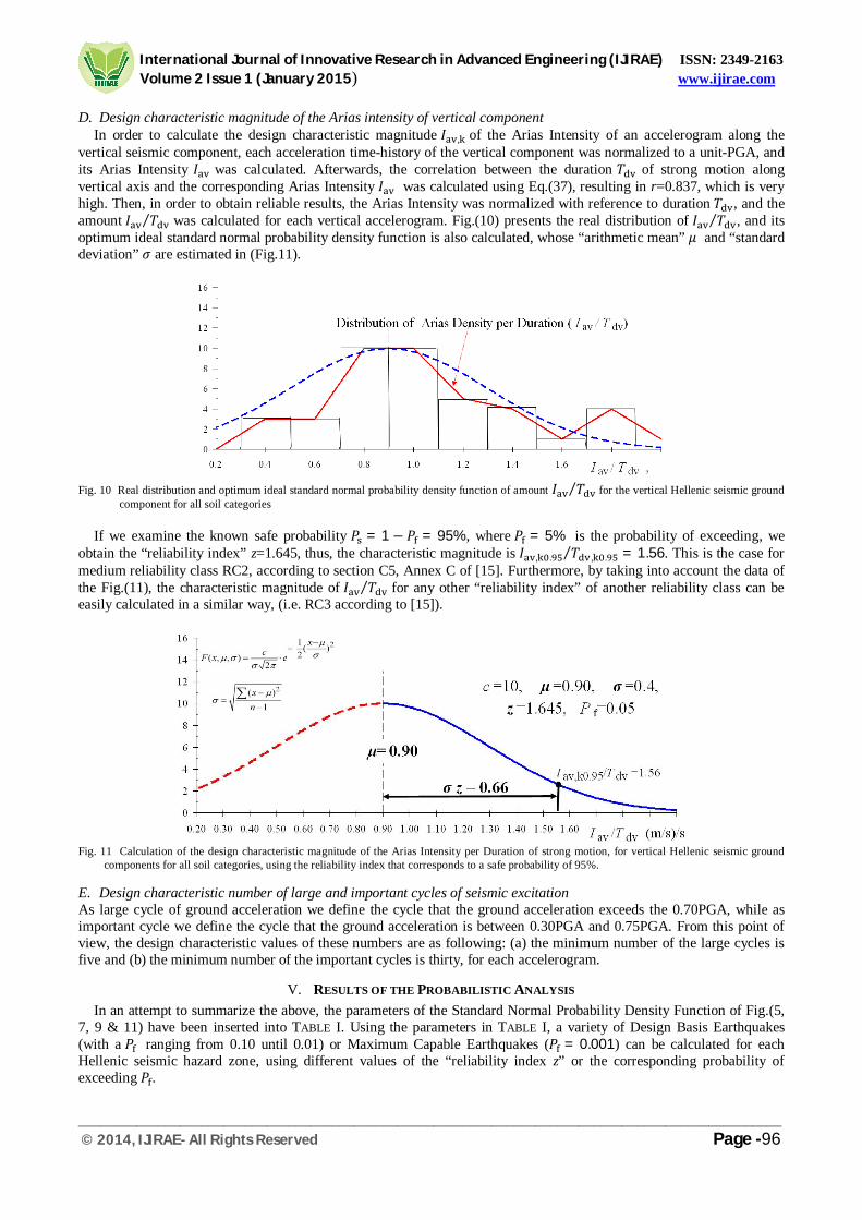
In order to calculate the design characteristic magnitude 퐼 , of the Arias Intensity of an accelerogram along the vertical seismic component, each acceleration time-history of the vertical component was normalized to a unit-PGA, and its Arias Intensity 퐼 was calculated. Afterwards, the correlation between the duration 푇 of strong motion along vertical axis and the corresponding Arias Intensity 퐼 was calculated using Eq.(37), resulting in r=0.837, which is very high. Then, in order to obtain reliable results, the Arias Intensity was normalized with reference to duration 푇 , and the amount 퐼 푇⁄ was calculated for each vertical accelerogram. Fig.(10) presents the real distribution of 퐼 푇⁄ , and its optimum ideal standard normal probability density function is also calculated, whose “arithmetic mean”휇 and “standard deviation” 휎 are estimated in (Fig.11).

Fig. 10 Real distribution and optimum ideal standard normal probability density function of amount 퐼 푇⁄ for the vertical Hellenic seismic ground

component for all soil categories If we examine the known safe probability 푃 = 1 − 푃 = 95%, where 푃 = 5% is the probability of exceeding, we

obtain the “reliability index” z=1.645, thus, the characteristic magnitude is 퐼 , . 푇 , .⁄ = 1.56. This is the case for medium reliability class RC2, according to section C5, Annex C of [15]. Furthermore, by taking into account the data of the Fig.(11), the characteristic magnitude of 퐼 푇⁄ for any other “reliability index” of another reliability class can be easily calculated in a similar way, (i.e. RC3 according to [15]).

Fig. 11 Calculation of the design characteristic magnitude of the Arias Intensity per Duration of strong motion, for vertical Hellenic seismic ground

components for all soil categories, using the reliability index that corresponds to a safe probability of 95%. E. Design characteristic number of large and important cycles of seismic excitation As large cycle of ground acceleration we define the cycle that the ground acceleration exceeds the 0.70PGA, while as important cycle we define the cycle that the ground acceleration is between 0.30PGA and 0.75PGA. From this point of view, the design characteristic values of these numbers are as following: (a) the minimum number of the large cycles is five and (b) the minimum number of the important cycles is thirty, for each accelerogram.

V. RESULTS OF THE PROBABILISTIC ANALYSIS In an attempt to summarize the above, the parameters of the Standard Normal Probability Density Function of Fig.(5,

7, 9 & 11) have been inserted into TABLE I. Using the parameters in TABLE I, a variety of Design Basis Earthquakes (with a 푃 ranging from 0.10 until 0.01) or Maximum Capable Earthquakes (푃 = 0.001) can be calculated for each Hellenic seismic hazard zone, using different values of the “reliability index z” or the corresponding probability of exceeding 푃 .



According to Eqs (6.1 & 7.1), the sum of the Arias Intensities of the three seismic components of an earthquake results in an invariant amount, which is the coefficient A of the tensor 퐀 that is not dependent on the orientation of the local reference system L,T,V. In order to classify the various triads of independent normalized (to a unit-PGA) accelerograms (two horizontal and one vertical), the characteristic magnitude of amount A can safely be used producing credible results. For example, as it is shown in TABLE I, for the probability of exceeding 푃 = 0.05, the following design characteristic magnitudes for a unit PGA are produced:

TABLE I

CHARACTERISTIC MAGNITUDES OF DURATIONS OF STRONG MOTION, ARIAS INTENSITIES AND INVARIANT CONSTANT Ak FOR VARIOUS “RELIABILITY INDEXES” AND FOR NORMALIZED ACCELEROGRAMS WITH UNIT- PGA

푃 = 0.10 0.05 0.02 0.01 0.001 푃 = 0.90 0.95 0.98 0.99 0.999

z = 1.283 1.645 2.054 2.326 3.097

(s), 푇 , = 9.45 10.28 11.22 11.85 13.62

(m/s2), ), 퐼 , 푇 ,⁄ = 1.18 1.29 1.42 1.50 1.73

(s), 푇 , = 14.70 16.87 19.32 20.97 25.58

(m/s2), 퐼 , 푇 ,⁄ = 1.41 1.56 1.72 1.83 2.14

(m/s), A = 43.03 52.84 65.21 73.94 101.86

Example for 푃 = 0.95:

Duration of strong motion of horizontal seismic component, 푇 , . = 10.28푠 Duration of strong motion of vertical seismic component, 푇 , . = 16.87푠 Arias Intensity of horizontal seismic component,

퐼 , . = 1.29 ∙ 푇 , . = 1.29 × 10.28 = 13.26푚/푠 Arias Intensity of vertical seismic component,

퐼 , . = 1.56 ∙ 푇 , . = 1.56 × 16.87 = 26.32푚/푠 Invariant amount of the sum of the Arias Intensities of all three seismic components,

A . = 퐼 , . + 퐼 , . + 퐼 , . = 13.26 + 13.26 + 26.32 = 52.84m/s The characteristic magnitude of the invariant constant A . is very useful for the classification of all artificial, semi-

artificial or natural accelerograms. In this case, the most suitable triad of independent accelerograms (from the total amount of normalized accelerograms) is the one whose invariant constant A . is equal to 52.84 m/s. In general, according to contemporary Eurocodes [10],[15] and [21], all design parameters of various actions must have the same probability of exceeding 푃 , which means that a common “reliability index” must be ensured for all new structures. The use of a uniform reliability index facilitates the “certification of the total design procedure”, which is dominated by “mathematical consistency”; this is very important for the global economy of the structure, and for its insurance coverage.

VI. CONCLUSIONS The present paper deals with the definition of design characteristic magnitude of the “duration of seismic ground

strong motion” and the “Arias Intensity” of accelerograms. Various artificial accelerograms were characterized according to the two aforementioned parameters, in order to be used in the seismic design of structures with application of non-linear response history analysis. It is worth noting that the three seismic ground components have to be statistically independent in pairs (i.e. where the correlation coefficient is zero). In addition, the various design accelerograms must be compatible with the seismological and geological data of the seismic hazard zone. Moreover, the elastic response acceleration spectra have to compatible with the corresponding elastic spectra proposed by the Seismic Codes. All above-mentioned requirements establish the use of artificial or semi-artificial accelerograms. In order to investigate the basic properties of the accelerograms in question, a suitable probabilistic analysis has been used in the present paper, using a known reliability index. As a pilot scheme, we have chosen the most important seismic records (with PGA>0.10g along a horizontal component) of the last 42 years from the seismic hazard area of Greece. The minimum aforementioned design characteristic magnitudes can be used at the suitable selection of design artificial, semi-artificial, or natural seismic accelerograms, for both earthquakes, the Design Basis Earthquake and the Maximum Capable Earthquake.



In this way, these accelerograms correspond to the real conditions of Greece, a country regarded as the most adverse seismic hazard area of Europe. It is worth noting that, the demand for both the “duration of seismic ground strong motion” and the “Arias Intensity,” is based on normalized (to a unit-PGA) accelerograms. However, after the selection of the accelerograms, the latter must be adapted to the maximum ground acceleration of the local seismic hazard area in order to be used in the (linear or non-linear) response history analysis of structures.

REFERENCES [1] T. Makarios, Evaluating the effective spectral seismic amplification factor on a probabilistic basis, Structural Engineering and Mechanics. An

International Journal. vol.42, No1, April 10; 2012, pp.121-129. [2] T. Makarios, Peak Ground Accelerations Functions of Mean Return Period for Known Reliability Index of Hellenic Design Earthquakes,

Journal of Earthquake Engineering,vol.17, No1, 01 January 2013 pp.98-109. [3] A. Arias, A measure of earthquake intensity, in R.J. Hansen, ed. Seismic Design for Nuclear Power Plants, MIT Press, Cambridge,

Massachusetts,1970, pp.438-483. [4] A. Bolt, Duration of strong motion, Proc. of the 4th World Conference on Earthquake Engineering, Santiago, Chile,1969, pp.1304-1315. [5] M.D. Trifunac, A.G. Brady, A study on the duration of strong earthquake ground motion,Bulletin of the Seismological Society of America,

vol.65; 1975, pp.581-626. [6] K. Kawashima and K. Aizawa, Bracketed and normalized durations of earthquake ground acceleration, Earthquake Engineering & Structural

Dynamics 18:7; 1989, pp.1041-1051. [7] S.L. Kramer, Geotechnical Earthquake Engineering, Prentice Hall; 1996, USA. [8] J.J. Bommer and A. Martinez-Pereira, The effective duration of earthquake strong motion, Journal of Earthquake Engineering 3; 1999, pp.127-

172. [9] I. Taflampas, C. Spyrakos and Ch. Maniatakis, A new definition of strong motion durationa and related parameters affecting the response of

medium-long period structures, Proc. of the 14th World Conference on Earthquake Engineering, October 12-17, 2008, Beijing, China. (on CD). [10] ΕΝ 1998.01: Eurocode No8, Design of structures for earthquake resistance – Part 1: General rules, seismic actions and rules for buildings,

European Committee for Standardization; 2004, Brussels. [11] N. Theodoulidis, I. Kalogeras, C. Papazachos, V. Karastathis, B. Margaris, Ch. Papaioannou and A.A. Skarlatoudis, A. HEAD 1.0: A unified

Hellenic Accelerogram Database, Seismological Research Letters; January/February 2004, 75, N.1: pp.36-45. [12] O. Lopez, J. Hernandez, R. Bonilla and A. Fernandez, Response Spectra for Multicomponent Structural Analysis, Earthquake Spectra, volume

22, No. 1; 2006, pp.85-113. [13] P. Tothong, and N. Luco, Probabilistic seismic demand analysis using advanced ground motion intensity measures, Earthquake Eng. & Struct.

Dyn. 36; 2007, pp.1837-1860. [14] K. Beyer and J. J. Bommer, Selection and Scaling of real accelerograms for bi-directional loading: A review of current practice and Code

provisions, Journal of Earthquake Engineering, 11: 2007, pp.13-45. [15] EΝ 1990: Eurocode No0 , Basis of structural design, European Committee for Standardization; 2002, Brussels. [16] J. Penzien and M. Watabe, Characteristics of 3-dimensional earthquake ground motion, Earthquake Eng. & Struct. Dyn. 3; 1975, pp.365–374. [17] L. Chin-Hsiung, Analysis of the spatial variation of seismic waves and ground movements from SMART-1 array data, Earthquake Eng. &

Struct. Dyn. 13; 1985, pp.561–581. [18] R.W. Clough and J. Penzien, Dynamics of Structures, Second Edition, McGraw-Hill, Inc;1993. [19] A.M. Athanatopoulou, Critical orientation of three correlated seismic components, Engineering Structures, vol. 27, No 1; 2005, pp.301-312. [20] B. Margaris, Ch. Papaioannou, N. Theodulidis, A. Savaidis, A. Anastasiadis, N. Klimis, et al., Preliminary Observations on the August 14, 2003,

Lefkada Island (Western Greece), Earthquake, EERI Journal, Special Earthquake. Report; November 2003, pp.1-12. [21] ΕΝ 1992: Eurocode No2 , Design of concrete structures – Part 2: Concrete bridges – Design and detailing rules, European Committee for

Standardization; 2006, Brussels.

Design Characteristic Value of the Arias Intensity agnitude for Artificial Accelerograms Compatible...

Documents

Transcript of Design Characteristic Value of the Arias Intensity agnitude for Artificial Accelerograms Compatible...