
MELSEC iQ-R Series iQ Platform-compatible PAC - Mitsubishi ...
Upload
khangminh22Category
view
2download
0
19, avenue de la Jonction - CH-1205 Genève - Tél 022 / 705 72 30 - Fax 022 / 705 72 00
Centre universitaire d’étude des problèmes de l'énergie
TRNSYS compatible moist air hypocaust model
Final report
comissioned by the
Office fédéral de l’énergie, CH - 3003 Bern (project 19507)
September 1998
Pierre HOLLMULLER Bernard LACHAL


TRNSYS compatible moist air hypocaust model
Part 1 : Description and validation

TRNSYS compatible moist air hypocaust model
1
Introduction
Preliminary work History of this project draws back to a pilot project, also funded by the Federal Office of Energy, dealing with short term heat storage in agricultural greenhouses [4-6]. High involved humidities often induced condensation and evaporation within the hypocaust (pipe system). Sensitivity analysis therefore required a model that would take into account not only sensible but also latent heat exchanges, and allow for airflows in one or the other direction (for respect of thermal stratification during storage and withdrawal periods). Such a model had formerly been developped by Razafinjohany and Boulard [1] in the frame of a similar experience in Avignon, but happened not to be flexible in geometry outlay and input/output definition, nor to include possibilty of water infiltration - which in some cases will bee seen to play important role. A first new development of the model was carried out within the mentioned project and allowed to reproduce general trends of condensation and evaporation patterns. A second validation work was done on a preheating system for fresh air in a residential building [8]. Monitoring could in this case be reproduced with an extremly good precision, but in absence of latent exchanges. Objectives Since this had not yet been the case, main purpose of this project was to render the module compatible with the TRNSYS environment commonly used for simulation of energy sytems, in particular the possibility to link back and forth surface conditions with other modules that include thermal capacities, like buildings, and therefore to stand timestep iteration (one of the main features the TRNSYS environment uses for system convergence). Besides, further validation of the model was also to be done on yet another winter preheating and summer cooling system in a commercial building [9]. Report structure Body of this report will present essential features of the model (of which detailed description, including mathematical, is to be found in the user’s manual). Focus will then be set on validation work for the three analysed systems. Overview of the model
General features The modeled hypocaust consists of a series of parallel tubes within a rectangular block of soil, swept by a flow of humid air. Flexible geometry description allows for inhomogenous soils, diverse border conditions, as well as use of symetries or pattern repetitions (run-time economy). Direction of the airflow can be controled (stratification in case of heat storage). Energy and mass balance within the tubes account for sensible as well as latent heat exchanges between airflux and tubes, frictional losses, diffusion into surrounding soil, as well as water infiltration and flow along the tubes. Sensible and latent heat exchange Heart of the model and worthwile mentioning here is the energy exchange between air and tube, while three dimensional diffusive heat transfer within soil is of classical, explicit type. Sensible exchange depends on the air-tube temperature difference and the exchange coefficent, latter one depending in turn on flowrate. Cutting short on more sophisticated use of dimensionless analysis, we used for this coefficient a heuristical form of linear dependence on air velocity (see mathematical description in the user’s manual), as developped for large plane exchange surfaces [2] and proved to be consistent in case of tubes [6].

TRNSYS compatible moist air hypocaust model
2
Latent heat exchange is based on the Lewis approach [3], which considers preceeding sensible heat exchange to be an air mass exchange between the airflux and a superficial air layer on tube surface, at latters temperature and saturated in humidity. This exchange of moist air conveys a vapor transfer (condensation or evaporation, according to sign of transfer) which readily computes from difference in humidity ratios (see mathematical description in the user’s manual). Input/output configuration Written as a TRNSYS compatible FORTRAN subroutine the model allows for modular use. Passed arguments include variable inputs (airflow, inlet temperature and humidity, air pressure, surface temperatures or heat gains) and fixed parameters that relate to either coupling with other modules (surface resistances and coupling modes) or simulation timestep and precision. Additional internal parameters (geometry, soil properties, initialisation, etc.) are furthermore provided by a parameter file. Retrieved arguments consist of basic outputs (outlet temperature and humidity, total sensible and latent heat rates, reciprocal border temperatures or heat gains) as well as a variety of optional outputs (including temperatures, energy rates and waterflows for specified node clusters). Coupling to other modules In the case of simple links, output of some other module is connected to input of this module (e.g. ambient temperature connected to surface temperature of hypocaust, or outlet fan temperature connected to inlet temperature of hypocaust), without evolution of other module having any influence on present one. In the case of reciprocal linking, a second link goes back from hypocaust to other module, so that evolution of each module affects evolution of the other one (eg. diffusing energy rate from building ground is connected to energy rate entering at hypocaust surface, and reciprocaly border temperature of hypocaust is connected back to outside surface temperature of building ground). In latter case convergence method by timestep iteration integrated into TRNSYS will ensure correspondance of energy rates flowing out of one module and into the other one (at condition of forth and back coupling to be each one of different type : energy rate or temperature). In order to maintain possibilities as broad as possible, each one of the two linking modes are retained : 1) input to surface is energy rate, reciprocal output is temperature ; 2) input to surface is temperature, reciprocal output is energy rate. Checking of latter linking method as well as of proper energy and mass balance calculation within the module was done on an academic example presented in the user’s manual. Validation on « Geoser » short term heat storage system in agricultural greenhouse
System description In the « Geoser » experiment [4-6] excessive solar heat gains of two greenhouses (100 m2 ground surface each) in the Rhône valley were stored for reduction of fuel-consumption during heating period (usualy nightly). In the first case storage occured in a watertank (via an air/water heat exchanger), in the second case in the underlying and sidely isolated soil (via a burried pipe system), while a third greenhouse with mere fuel heating system served as a comparison. The buried pipe heat storage system stands 80 cm underneath the greenhouse and consists of 24 tubes (external diameter : 16 cm ; length : 11 m ; mean axial distance : 42 cm ; total exchange surface, without distribution and collector pipes : 120 m2) swept by a variable airflow (0 - 7000 m3/h) runing in one or the other direction during charge and discharge. Typical daily operation is shown on figure 1 : during lower setpoint period at night air from greenhouse is blown through pipes, takes up heat from soil and thus lowers demand to auxilary heating system. When difference between air and soil becomes too small for dischage (at setpoint change) system becomes inactive. As greenhouse temperature rises with solar radiation, air is blown

TRNSYS compatible moist air hypocaust model
3
again through pipes, this time for heat storage, in reversed direction, and until air-soil temperature difference becomes too small again. Same cycle repeats from sunset on. During nightly discharge air heated along the tube evaporates free water in tubes, while storage period starts up with condensation of very moist greenhouse air, followed by evaporation again as air humidity drops down. Water balance shows a deficit (more evaporation than condensation) of 15 lit for this one day and of 800 lit over the 18 months of monitoring. This can most probably be explained by the use of a fog system at 2m height within the greenhouse, which sprays droplets of ~80 microns into air. One clearly observes effect of fog system on air humidity and temperature, especially at 1m height, when droplets reach wet bulb temperature and start to pump evaporation energy in air rather than in water and air (cf. detailed studies on atomization and spray phenomena [7,8]). According to data on sedimentation velocity and lifetime (~20 m/s, respectively 3-40 s depending on air humidity, ibid.) it is quite plausible that part of the droplets are swept by airflow into tubes.
-20
0
20
40
60
80
100
00:00 06:00 12:00 18:00 00:00
rel.
hum
idity
[%]
-10
0
10
20
30
40
50
tem
pera
ture
[°C
¨] po
wer
[kW
] fo
g [li
t/h]
hum. [%]air max [°C]air min [°C]air 2m [°C]air 1m [°C]soil [°C]aux. heat [kW]sensible [kW]latent [kW]fog [lit/h]
Fig 1 : Operation of « Geoser » short term heat storage system on May 9th 1994 : conditions in greenhouse (air temperature, setpoints and humidity) and in soil (temperature near pipe), energy furnished to soil (sensible and latent), auxilary heat demand and fog system.
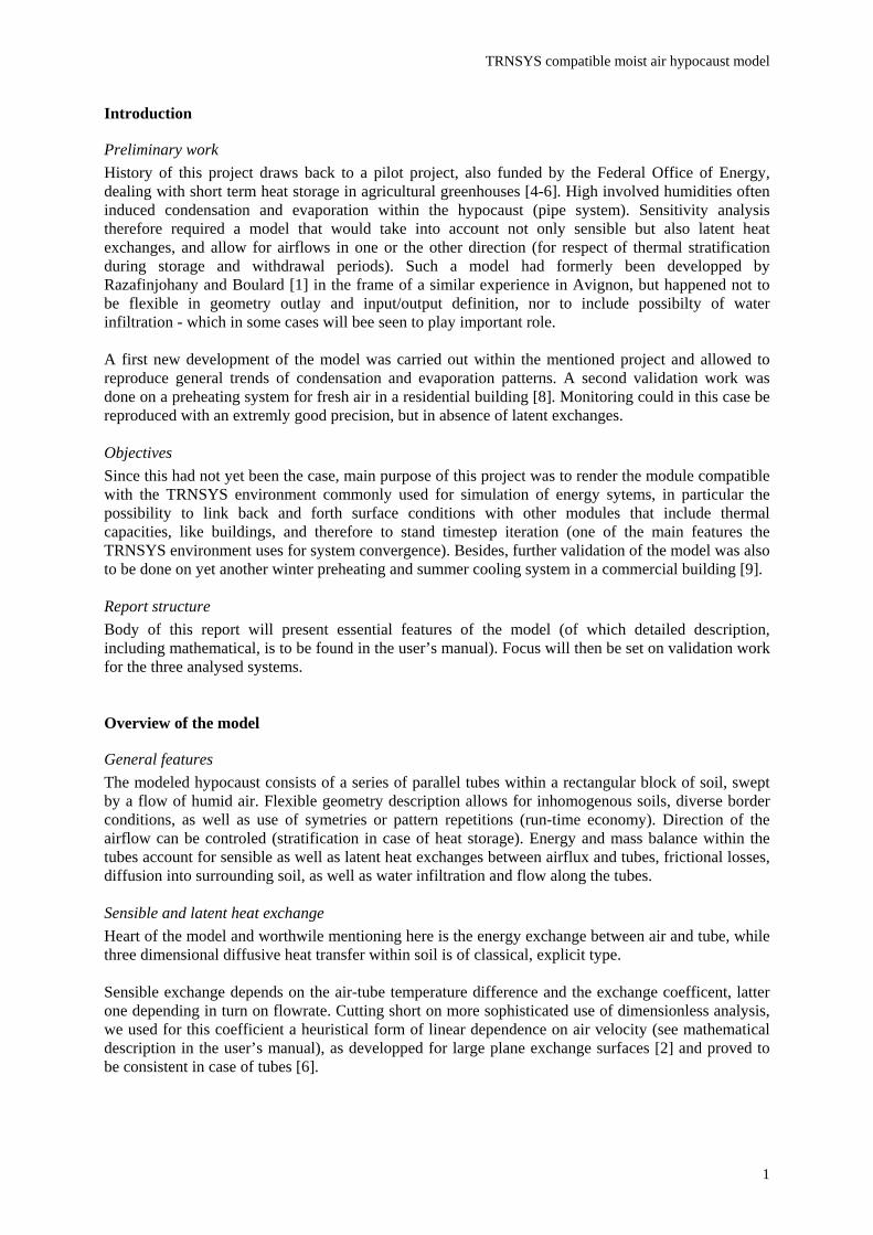
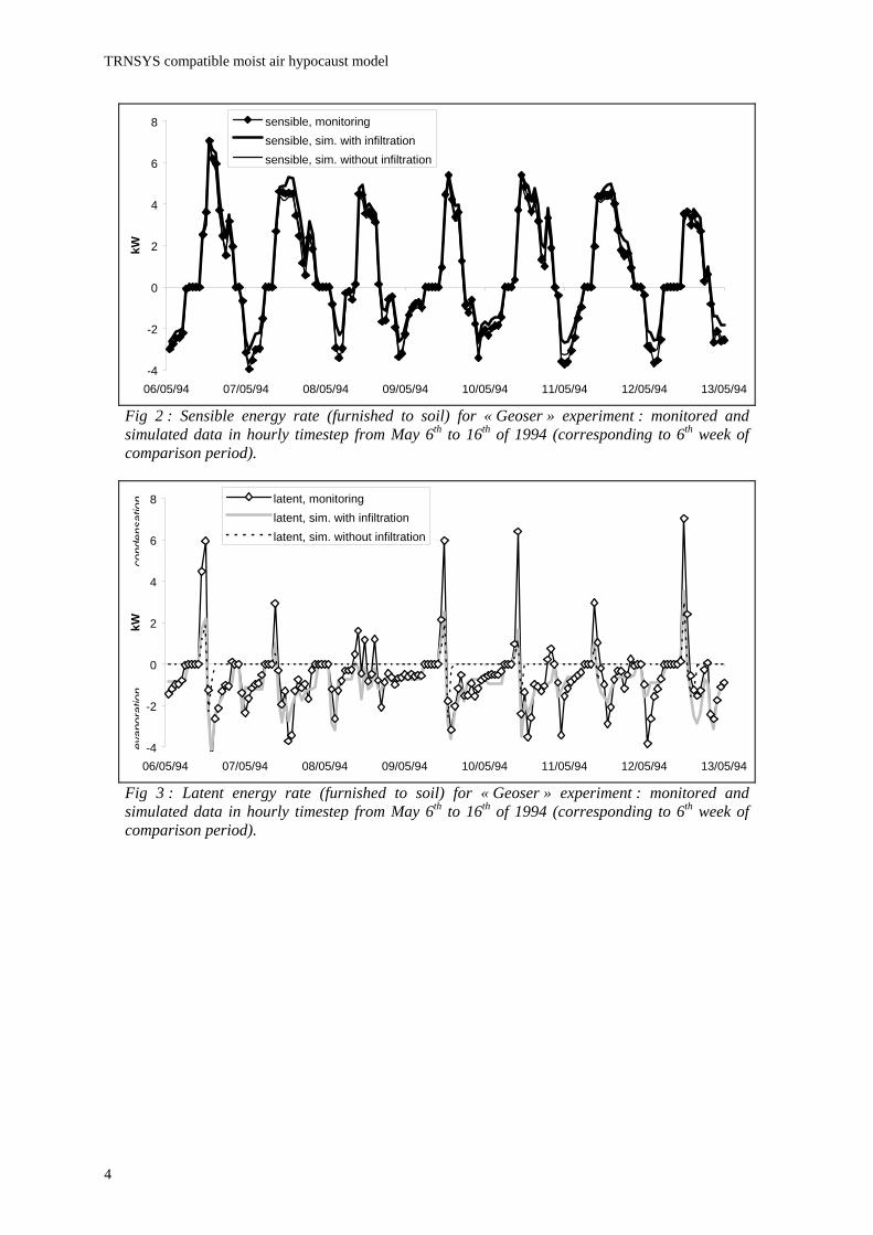
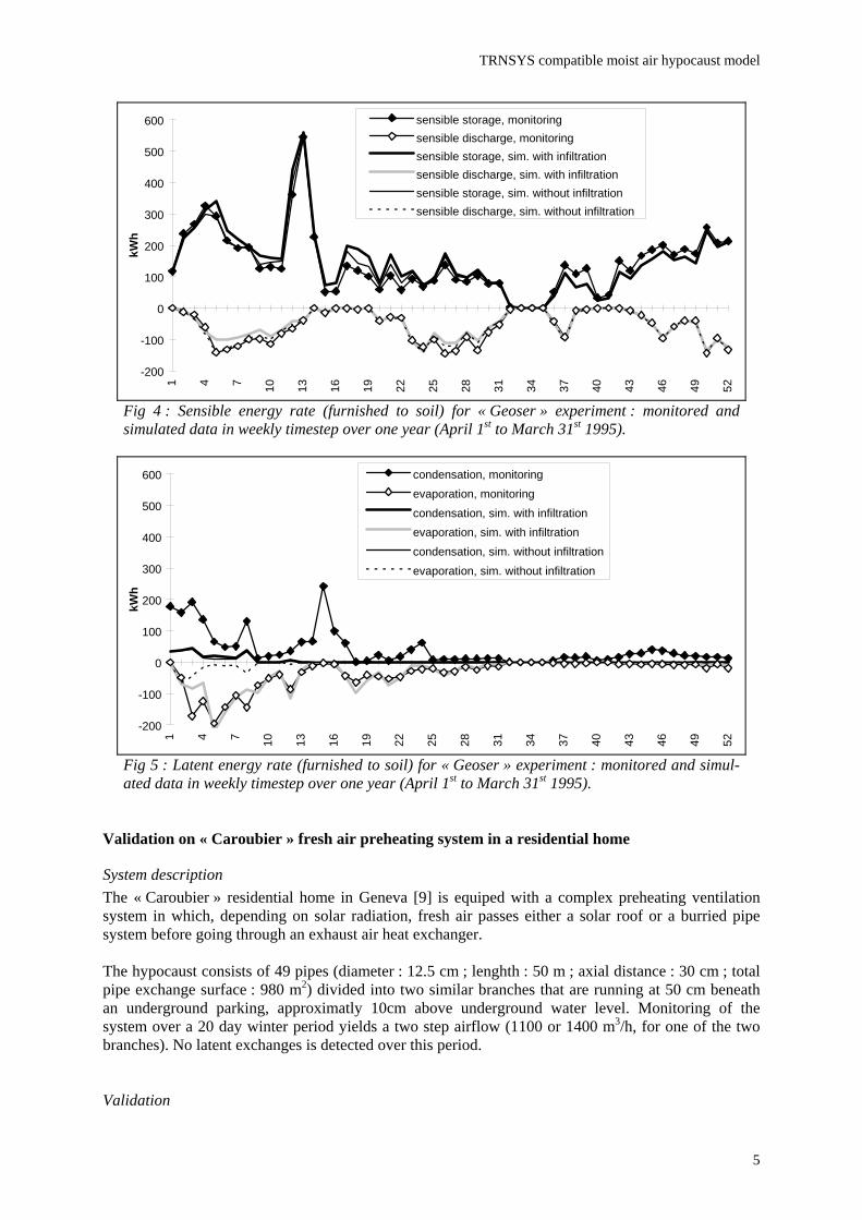
Validation Border and input conditions for modelling of this system are top and bottom temperatures (40 cm above and 70 cm beneath pipes) averaged over two monitoring points each, as well as measured inlet temperature and humidity. Initialisation is done on first six monts of monitoring and 12 following months are used for comparison of simulation and monitoring (1/4/94 - 30/3/95). As shown on figures 2 to 5, a first simulation under preceeding conditions and without water infiltration very well reproduces sensible heat exchanges, as well in hourly as in integrated timestep. General trends of evaporation and condensation are beeing reproduced to some extent during first weeks (important measured latent exchanges, possibly due to use of only one air direction) but sytematically fall short in quantity and completely disappear at later periods. During first weeks one observes in particular (figure 3, broken line) that simulated latent exchange stops when condensed water has been evaporated again, which confirms the hypothesis of water infiltration during monitoring. In a second simulation the measured daily water deficit is beeing infiltrated in constant hourly rate on the whole pipe surface, in which case evaporation (but not so condensation) is very well reproduced over the whole 12 month period.
TRNSYS compatible moist air hypocaust model
4
-4
-2
0
2
4
6
8
06/05/94 07/05/94 08/05/94 09/05/94 10/05/94 11/05/94 12/05/94 13/05/94
kWsensible, monitoringsensible, sim. with infiltrationsensible, sim. without infiltration
Fig 2 : Sensible energy rate (furnished to soil) for « Geoser » experiment : monitored and simulated data in hourly timestep from May 6th to 16th of 1994 (corresponding to 6th week of comparison period).
-4
-2
0
2
4
6
8
06/05/94 07/05/94 08/05/94 09/05/94 10/05/94 11/05/94 12/05/94 13/05/94
kW
latent, monitoringlatent, sim. with infiltrationlatent, sim. without infiltration
evap
orat
ion
cond
ensa
tion
Fig 3 : Latent energy rate (furnished to soil) for « Geoser » experiment : monitored and simulated data in hourly timestep from May 6th to 16th of 1994 (corresponding to 6th week of comparison period).
TRNSYS compatible moist air hypocaust model
5
-200
-100
0
100
200
300
400
500
600
1 4 7 10 13 16 19 22 25 28 31 34 37 40 43 46 49 52
kWh
sensible storage, monitoringsensible discharge, monitoringsensible storage, sim. with infiltrationsensible discharge, sim. with infiltrationsensible storage, sim. without infiltrationsensible discharge, sim. without infiltration
Fig 4 : Sensible energy rate (furnished to soil) for « Geoser » experiment : monitored and simulated data in weekly timestep over one year (April 1st to March 31st 1995).
-200
-100
0
100
200
300
400
500
600
1 4 7 10 13 16 19 22 25 28 31 34 37 40 43 46 49 52
kWh
condensation, monitoringevaporation, monitoringcondensation, sim. with infiltrationevaporation, sim. with infiltrationcondensation, sim. without infiltrationevaporation, sim. without infiltration
Fig 5 : Latent energy rate (furnished to soil) for « Geoser » experiment : monitored and simul-ated data in weekly timestep over one year (April 1st to March 31st 1995).
Validation on « Caroubier » fresh air preheating system in a residential home
System description The « Caroubier » residential home in Geneva [9] is equiped with a complex preheating ventilation system in which, depending on solar radiation, fresh air passes either a solar roof or a burried pipe system before going through an exhaust air heat exchanger. The hypocaust consists of 49 pipes (diameter : 12.5 cm ; lenghth : 50 m ; axial distance : 30 cm ; total pipe exchange surface : 980 m2) divided into two similar branches that are running at 50 cm beneath an underground parking, approximatly 10cm above underground water level. Monitoring of the system over a 20 day winter period yields a two step airflow (1100 or 1400 m3/h, for one of the two branches). No latent exchanges is detected over this period. Validation
TRNSYS compatible moist air hypocaust model
6
Simulation of the system was to be carried out on a one year period. Initialisation and input conditions therfore were taken from standard yearly meteorological data, combined with monitored values of Geneva area during 3 months preceding monitoring period. Border condition at top was air in the parking lot (supposed to fluctuate between 7°C at end of February and 23°C at end of August), while temperature 2.5 m beneath pipes was supposed to be constantly at 15°C because of moving underground water.
-5
-4
-3
-2
-1
0
1
2
3
4
09/03/96 11/03/96 13/03/96 15/03/96 17/03/96 19/03/96 21/03/96 23/03/96 25/03/96
kW
sensible, monitoringsensible, simulation
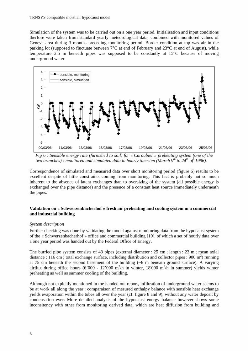
Fig 6 : Sensible energy rate (furnished to soil) for « Caroubier » preheating system (one of the two branches) : monitored and simulated data in hourly timestep (March 9th to 24th oft 1996).
Correspondence of simulated and measured data over short monitoring period (figure 6) results to be excellent despite of little constraints coming from monitoring. This fact is probably not so much inherent to the absence of latent exchanges than to oversizing of the system (all possible energy is exchanged over the pipe distance) and the presence of a constant heat source immediately underneath the pipes. Validation on « Schwerzenbacherhof » fresh air preheating and cooling system in a commercial and industrial building
System description Further checking was done by validating the model against monitoring data from the hypocaust system of the « Schwerzenbacherhof » office and commercial building [10], of which a set of hourly data over a one year period was handed out by the Federal Office of Energy. The burried pipe system consists of 43 pipes (external diameter : 25 cm ; length : 23 m ; mean axial distance : 116 cm ; total exchange surface, including distribution and collector pipes : 900 m2) running at 75 cm beneath the second basement of the building (~6 m beneath ground surface). A varying airflux during office hours (6’000 - 12’000 m3/h in winter, 18'000 m3/h in summer) yields winter preheating as well as summer cooling of the building. Although not expicitly mentioned in the handed out report, infiltration of underground water seems to be at work all along the year : comparaison of mesured enthalpy balance with sensible heat exchange yields evaporation within the tubes all over the year (cf. figure 8 and 9), without any water deposit by condensation ever. More detailed analysis of the hypocaust energy balance however shows some inconsitency with other from monitoring derived data, which are heat diffusion from building and
TRNSYS compatible moist air hypocaust model
7
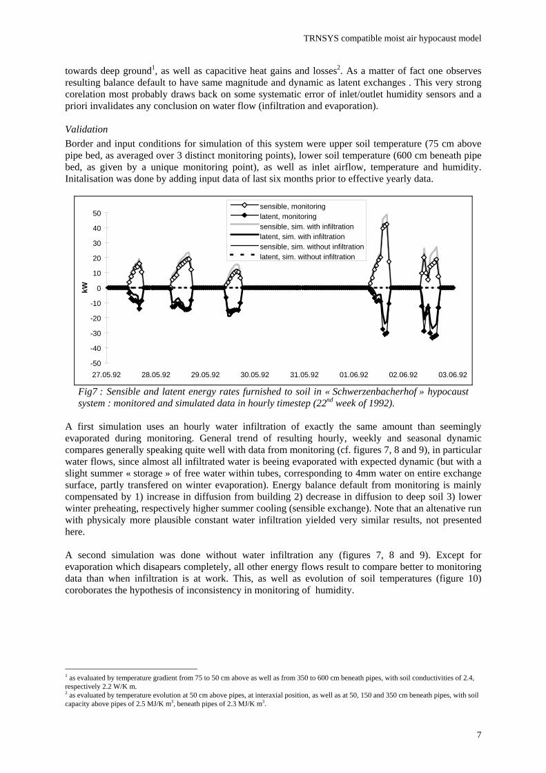
towards deep ground1, as well as capacitive heat gains and losses2. As a matter of fact one observes resulting balance default to have same magnitude and dynamic as latent exchanges . This very strong corelation most probably draws back on some systematic error of inlet/outlet humidity sensors and a priori invalidates any conclusion on water flow (infiltration and evaporation). Validation Border and input conditions for simulation of this system were upper soil temperature (75 cm above pipe bed, as averaged over 3 distinct monitoring points), lower soil temperature (600 cm beneath pipe bed, as given by a unique monitoring point), as well as inlet airflow, temperature and humidity. Initalisation was done by adding input data of last six months prior to effective yearly data.
-50
-40
-30
-20
-10
0
10
20
30
40
50
27.05.92 28.05.92 29.05.92 30.05.92 31.05.92 01.06.92 02.06.92 03.06.92
kW
sensible, monitoringlatent, monitoringsensible, sim. with infiltrationlatent, sim. with infiltrationsensible, sim. without infiltrationlatent, sim. without infiltration
Fig7 : Sensible and latent energy rates furnished to soil in « Schwerzenbacherhof » hypocaust system : monitored and simulated data in hourly timestep (22nd week of 1992).
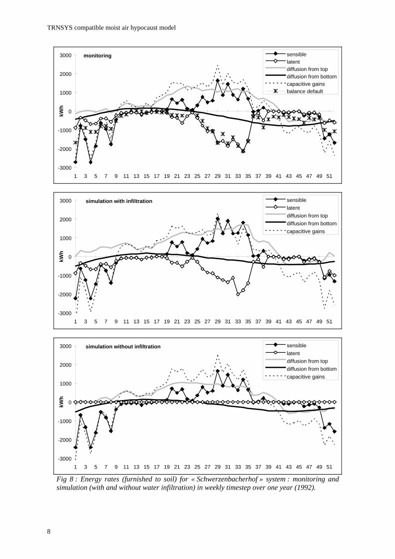
A first simulation uses an hourly water infiltration of exactly the same amount than seemingly evaporated during monitoring. General trend of resulting hourly, weekly and seasonal dynamic compares generally speaking quite well with data from monitoring (cf. figures 7, 8 and 9), in particular water flows, since almost all infiltrated water is beeing evaporated with expected dynamic (but with a slight summer « storage » of free water within tubes, corresponding to 4mm water on entire exchange surface, partly transfered on winter evaporation). Energy balance default from monitoring is mainly compensated by 1) increase in diffusion from building 2) decrease in diffusion to deep soil 3) lower winter preheating, respectively higher summer cooling (sensible exchange). Note that an altenative run with physicaly more plausible constant water infiltration yielded very similar results, not presented here. A second simulation was done without water infiltration any (figures 7, 8 and 9). Except for evaporation which disapears completely, all other energy flows result to compare better to monitoring data than when infiltration is at work. This, as well as evolution of soil temperatures (figure 10) coroborates the hypothesis of inconsistency in monitoring of humidity.
1 as evaluated by temperature gradient from 75 to 50 cm above as well as from 350 to 600 cm beneath pipes, with soil conductivities of 2.4, respectively 2.2 W/K m. 2 as evaluated by temperature evolution at 50 cm above pipes, at interaxial position, as well as at 50, 150 and 350 cm beneath pipes, with soil capacity above pipes of 2.5 MJ/K m3, beneath pipes of 2.3 MJ/K m3.
TRNSYS compatible moist air hypocaust model
8
monitoring
-3000
-2000
-1000
0
1000
2000
3000
1 3 5 7 9 11 13 15 17 19 21 23 25 27 29 31 33 35 37 39 41 43 45 47 49 51
kWh
sensiblelatentdiffusion from topdiffusion from bottomcapacitive gainsbalance default
simulation with infiltration
-3000
-2000
-1000
0
1000
2000
3000
1 3 5 7 9 11 13 15 17 19 21 23 25 27 29 31 33 35 37 39 41 43 45 47 49 51
kWh
sensiblelatentdiffusion from topdiffusion from bottomcapacitive gains
simulation without infiltration
-3000
-2000
-1000
0
1000
2000
3000
1 3 5 7 9 11 13 15 17 19 21 23 25 27 29 31 33 35 37 39 41 43 45 47 49 51
kWh
sensiblelatentdiffusion from topdiffusion from bottomcapacitive gains
Fig 8 : Energy rates (furnished to soil) for « Schwerzenbacherhof » system : monitoring and simulation (with and without water infiltration) in weekly timestep over one year (1992).

TRNSYS compatible moist air hypocaust model
9
Evaporation7.8 MWhSensible19.5 MWh
Diffusion0.8 MWh
Diffusion9.4 MWh
Capacitive losses21.2 MWh
Infiltration11.2 m3 (?)
Monitoring : winter
Balance default16.3 MWh
Evaporation17.9 MWhSensible
11.4 MWh
Diffusion20.7 MWh
Diffusion5.6 MWh
Capacitive gains25.5 MWh
Infiltration25.8 m3 (?)
Monitoring : summer
Balance default16.9 MWh
Evaporation9.5 MWhSensible15.6 MWh
Diffusion7.0 MWh
Diffusion5.5 MWh
Capacitive losses23.5 MWh
Infiltration11.2 m3
Simulation with infiltration : winter
Stagnant water2.5 m3
Evaporation15.3 MWh
Sensible16.2MWh
Diffusion25.2 MWh
Diffusion2.6 MWh
Capacitive gains23.5 MWh
Infiltration25.8 m3
Simulation with infiltration : summer
Stagnant water3.7 m3
Sensible17.4 MWh
Diffusion0.7 MWh
Diffusion6.5 MWh
Capacitive losses23.2 MWh
Simulation without infiltration : winter
Sensible11.8 MWh
Diffusion16.4 MWh
Diffusion3.2 MWh
Capacitive gains25.0 MWh
Simulation without infiltration : summer
Fig 9 : Seasonal energy balance (plain flows, white and gray) and water balance (grey flows, plain and hatched) for « Schwerzenbacherhof » system : monitoring and simulation (with and without infiltration). Note that energy flow direction has nothing to do with air flow direction (summer sensible cooling power does not corespond to an airflow from building).

TRNSYS compatible moist air hypocaust model
10
8
10
12
14
16
18
20
22
1 3 5 7 9 11 13 15 17 19 21 23 25 27 29 31 33 35 37 39 41 43 45 47 49 51
degC
T+100 (upper surf.)T-600 (lower surf.)T 0, monitoringT 0, sim. with infilt.T 0, sim. without infilt.T-150, monitoringT-150, sim. with infilt.T-150, sim. without infilt.T-350, monitoringT-350, sim. with infilt.T-350, sim. without infilt.
Fig 10 : « Schwerzenbacherhof » ground temperatures : monitoring and simulation (with and without water infiltration) in weekly timestep over one year (1992).
Whatever reality might have been, mere comparison between each of these two simulations gives good understanding of the role water infiltration can play in such a sytem. Hence one observes presence of water and subsequent necessary heat for evaporation to lower winter preheating and to rise summer cooling of air, but only to some extent (changes account respectively for 20 and 28% of seasonal latent heat). Main influence goes for increase in heat diffusion from building (which accounts for 66% of latent heat in winter, respectively 58% in summer). Taken together, changes in air sensible heat and ground diffusion have an important consequence on building energy balance though. In winter, presence of water globaly lowers hypocaust performance of 50% (15.6-7.0=8.6 instead of 17.4-0.7=16.7 MWh). In summer on the contrary, presence of water globaly rises hypocaust performance of 50% (25.2+16.2=41.4 instead of 16.4+11.8=28.2 MWh). This conclusion has nevertheless to be balanced by the fact that sensible heat carried by airflow can be distributed in a controled way, to the opposite of heat diffusion through ground. Conclusions
Validation on monitored systems shows that the developped hypocaust model, quite well reproduces latent and sensible heat exchanges of buried pipe systems, under condition of taking into account eventual presence of water infiltration. From a monitoring point of view, problematic seems rather to be the evaluation of such flows, while from a project designer point of view it rather is how to control them (tightness of systems). In this frame of idea the model might further on help to evaluate the consequences (risks and benefits) of water infiltration, whose effect relate in analysed cases not so much with outlet temperatures than with surface diffusion from coupled building. Strictly speaking, some of the validation could gain to be reevaluated in presence of a reciprocal linking with the building, as developped and tested within this work on an academic example. Such a validation exercise would suppose a precise knowledge of the buildings enveloppe, heating/cooling and internal gain structure though. Another interesting feature (used in sensitivity analysis of the « Geoser » experiment but not presented here) is the flexible geometry, in particular the possibility to simulate soil adjacent to the hypocaust (lateral losses) as well as the optional output structure. In this sense it could be interesting to perform a quite easy extension of the model to water instead of moist air medium, as is more and more commonly used.
TRNSYS compatible moist air hypocaust model
11
Acknoledgments
We wish to thank : • Thierry Boulard (from the Institut national de recherches agronomiques of Avignon, France) for
handing us over the original moist-air hypocaust routine developped in his institute. • Antoine Reist (from the Station agronomique de Changins, Conthey), Pierre Jaboyedoff (from
Sorane SA, Lausanne) and Javier Gil (from P&A Partners, Cochabamba, Bolivia) for their collaboration during the GEOSER experiment.
• Mark Zimmermann (from the Swiss federal laboratories for materials testing and research, Dübendorf) for handing us over the monitoring data of Schwerzenbacherhof.
• Markus Koschenz and Robert Weber (from the Swiss federal laboratories for materials testing and research, Dübendorf) for critical reading and valuable advices for the TRNSYS adaptation.
• The Office fédéral de l’énergie (Bern) and Office cantonal de l’énergie (Genève) for their financial support of the project.
References
1. Razafinjohany E., Etude comparative dans les serres agricoles de deux systèmes de stockage de la chaleur influencé de l’humidité de l’air, Thèse, 1989, Académie de Montpelier, Université de Perpignan.
2. Molineaux B., Lachal B., and Guisan O., Thermal analysis of five outdoor swimming pools heated by unglazed solar collectors, Solar Energy, Vol. 53, Nb. 1, July 1994, pp. 21-26.
3. Incropera F. P., De Witt D. P., Fundamentals of heat and mass transfer, John Wiley & Sons Inc., 1990.
4. Lachal B., Hollmuller P., Gil J., Stockage de chaleur : résultats de GEOSER, in Stockage de chaleur, gestion de l’énergie et du climat dans les serres horticoles, recueil des exposés du colloque GEOSER du 15 février 1996 au RAC Conthey, Office fédéral de l’énergie, 1996.
5. Lachal B., Hollmuller P., Gil J., Ergebnisse des GEOSER-Projekts, in Energie-Management im Gartenbau, Tagungsband zur Energiemanagement-Veranstaltung des 26. September 1996 an der ISW Wädenswil, Bundesamt für Energiewirtschaft, 1996.
6. Reist A., Lachal B., Jaboyedoff P., Hollmuller P., Gil J, GEOSER : stockage temporaire de chaleur pour serres horticoles, Rapport final (to be published).
7. Lefebvre A.H., Atomization and sprays, Hemisphere Publishing Corp., 1989. 8. Rodriguez E.A., Alvarez S., Martin R., Water drop as a natural cooling ressource : physical
principles, PLEA Conference 1991, Kluver Academic Press, 1991, pp. 499-504. 9. Putallaz J., Lachal B., Hollmuller P., Pampaloni E, Evaluation des performances du puits canadien
de l’immeuble locatif du 19 rue des Caroubiers, 1227 Carouge, expertise mandatée par l’Office cantonal de l’énergie de Genève, 1996.
10. Zimmermann M., The Schwerzenbacherhof Office and Industrial Building, Switzerland. Ground Coupled Ventilation System, IEA Low Energy Cooling Task, 1995.

TRNSYS compatible moist air hypocaust model
12
TRNSYS compatible moist air hypocaust model
Part 2 : User manual

TRNSYS compatible moist air hypocaust model

TRNSYS compatible moist air hypocaust model
1
TYPE 61 : HYPOCAUST (AIR-TO-SOIL EXCHANGER)
General Description This component models an air-to-soil heat exchanger. It accounts for sensible as well as latent exchanges between airflux and tubes, diffusion into surrounding soil, frictional losses and flow of condensed water along the tubes. Local heating from integrated fan motor can be taken into account at tube inlet or outlet. Direction of airflux can be controled (stratification in case of heat storage) and flexible geometry allows for inhomogenous soils as well as diverse border conditions.
Nomenclature List hereafter covers all symbols used in the mathematical description of the model (other symbols are defined directly in the component configuration section). When as here, symbols in text account for currently described node and timestep, while subsripts are used to reference neighbor nodes or previous timestep. ClatWat Latent heat of water CmAir Mass-specific heat of air CmVap Mass-specific heat of vapor CmWat Volume-specific heat of water CvSoil Volume-specific heat of soil CvTub Volume-specific heat of tube Ctub Circumference of tube Dt Internal timestep Dl Node width (along x, y or z) Dtub Hydraulic diameter of tube Fair Airflow in tube FairTot Airflow, total (over tubes and modules) Hrel Relative humidity Hrat Absolute humidity (vapor pressure) Hsat Absolute humidity (vapor pressure) at saturation Kair Air/tube exchange coefficient Kbord Heat conduction coefficient of border (pondered, including Rsurf) Ksoil Heat conduction coefficient to neighbour node or surface (including Rsurf) LamSoil Heat conductivity of soil LamTub Heat conductivity of tube MmolAir Molar mass of air MmolWat Molar mass of water Mair Mass of air exchanged between airflow and tube superficial layer Mwat Mass of free water MwatIn Mass of water flowing into node MwatInf Mass of water infiltrating into node MwatLat Mass of water cond./evap. MwatOut Mass of water flowing or ejected out of node Pfric Energy rate of frictional losses
TRNSYS compatible moist air hypocaust model
2
Pint Energy rate of tube or soil internal gains Plat Energy rate of latent air-tube heat exchange Psbl Energy rate of sensible air-tube heat exchange Psoil Energy rate of heat diffused by neighbor nodes Pwat Energy rate of free water internal losses PrAir Pressure of air Rsurf Surface heat resistance Rfric Friction coefficient of tubes RhoAir Specific weight of air Sair Section of tube Sbord Area of border Ssoil Lateral area of soil node Stub Lateral area of tube node Tair Temperature of air Tbord Pondered temperature of border Tsoil Temperature of soil Ttub Temperature of tube ThTub Thickness of tube Vair Air velocity Vwat Velocity of water VolSoil Node volume VolTub Volume of tube node Hrat Humidity ratio
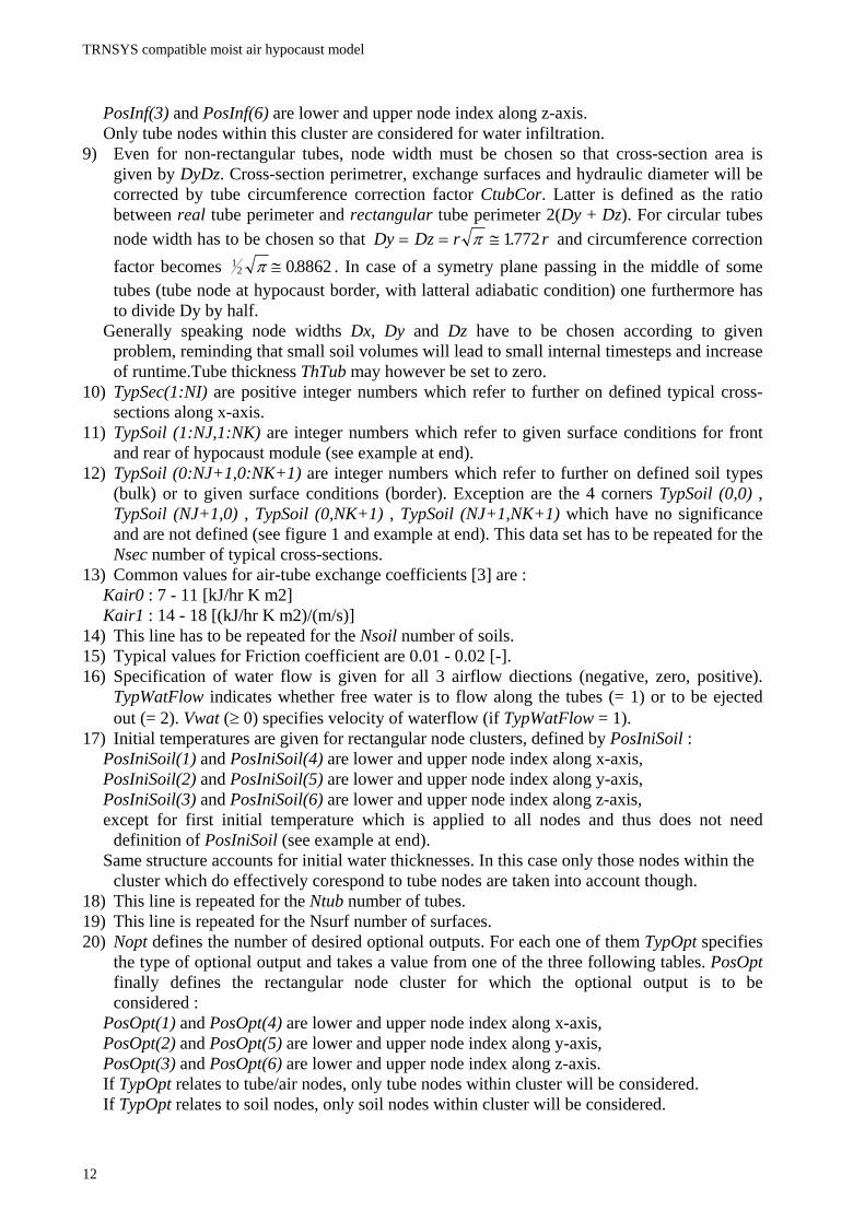
Mathematical Description Geometry The model describes a block of rectangular soil nodes (which need not all share same physical properties), comprising parallel tubes that run along the x-axis (see figure 1). A correction factor allows to describe non-rectanguar tubes. If not adiabatic, surface conditions (which need not expand from edge to edge) can be given in terms of either inflowing energy rate or temperature. An additional surface resistance can be defined, especially for direct coupling with air temperature. For matter of simplification and run time economy, symetries in the y-z plane can be used by describing only one module (=relevant part) and specifying the number of times it is used. In this case the symetry surface(s), which must be subject to adiabatic condition, may if necessary pass through the middle of some tubes (see figure 1). Parametrisation of chosen geometry occurs in following way (of which best understanding can be taken from figure 1 and example at end) : • define the occurence of typical cross-sections along the x-axis, with numbers that refer to
them. • define the typical cross-sections in the y-z plane, with numbers that refer to soil types,
respectively surface conditions. • define two additional cross-sections for frontal and rear surface conditions.

TRNSYS compatible moist air hypocaust model
3
a) longitudinal section b) cross-section # 2 (through both zones)
Zone 1(free-float)
Hypocaust (Type 61)
Surf 3
Text
Surf 3
Text
Surf 2
Zone 2(setpoint)
z
x
Surf 1
Multizone building(Type 56)
Hypocaust (Type 61)
Surf 3 Surf 1
Text
Surf 3
Text
Zone 1(free float)
Tube
Soil 1
Soil 2
z
y
Zone 2(setpoint)
Multizone building(Type 56)
parametrisation : 1 1 2 2 2 3 3 3 3 3 3 1 1
where 1 : cross-section # 1 (through back and front) 2 : cross-section # 2 (through both zones) 3 : cross-section # 3 (through main zone)
parametrisation (by symetry only left half) : 3 3 2 2 2 2 2 2 2 2 2 2 0 1 2 2 2 2 2 2 2 2 2 2 2 0 0 1 2 2 0 2 2 2 0 2 2 2 0 0 0 1 2 2 2 2 2 2 2 2 2 2 2 0 0 1 2 2 2 2 0 2 2 2 0 2 2 0 0 1 2 2 2 2 2 2 2 2 2 2 2 0 0 1 2 2 0 2 2 2 0 2 2 2 0 0 0 1 2 2 2 2 2 2 2 2 2 2 2 0 0 0 0 0 0 0 0 0 0 0 0 0
where 0 : tube 0 : adiabatic surface 1 : soil # 1 1 : surface condition # 1 (Zone 1) 2 : soil # 2 3 : surface condition # 3 (Ambient)
Fig.1 : Example of Type61 geometry and coupling to other Type. Linking In addition to airflow at inlet/outlet, surface conditions can also be coupled to other Types. One can therefore choose between following two modes : • If output from other module (=input for Type 61) is the energy rate flowing into hypocaust,
Type61 will return equivalent border temperature as output (=input for other Type). Latter is defined as the pondered average node temperature of all nodes comprised in that particular surface :
TbordSsoil Ksoil Tsoil
Sbord Kbord
i ii bord
i
=⋅ ⋅
⋅∈∑
(1)
with
Ksoil DlLamSoil
Rsurfi
i
i
=+
12
TRNSYS compatible moist air hypocaust model
4
Sbord Ssoilii bord
=∈∑
KbordSsoil Ksoil
Sbord
i ii bord=
⋅∈∑
One has to take care to use identical border area Sbord and heat conduction coefficient Kbord in other Type (check these calculated values in parameter control file). The timestep iteration procedure of TRNSYS then will guarantee for proper energy balance (energy rate flowing out of one module = energy rate flowing into other module), which can be checked by plotting inflowing energy rate as optional output of Type 61.
• If on the contrary output from other module is its equivalent border temperature, Type61 will return inflowing energy rate as output. Proper energy balance again is guaranteed by using identical border area and heat conduction coefficient in both Types.
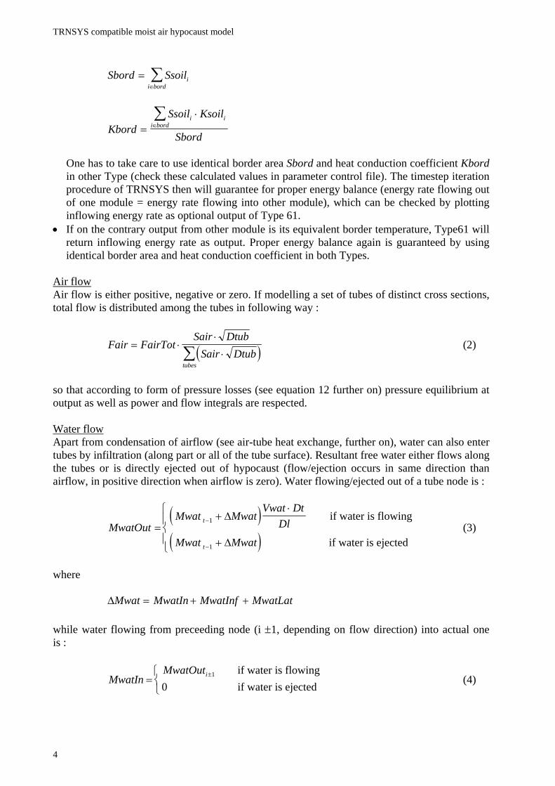
Air flow Air flow is either positive, negative or zero. If modelling a set of tubes of distinct cross sections, total flow is distributed among the tubes in following way :
( )Fair FairTotSair Dtub
Sair Dtubtubes
= ⋅⋅
⋅∑ (2)
so that according to form of pressure losses (see equation 12 further on) pressure equilibrium at output as well as power and flow integrals are respected. Water flow Apart from condensation of airflow (see air-tube heat exchange, further on), water can also enter tubes by infiltration (along part or all of the tube surface). Resultant free water either flows along the tubes or is directly ejected out of hypocaust (flow/ejection occurs in same direction than airflow, in positive direction when airflow is zero). Water flowing/ejected out of a tube node is :
( )( )
MwatOutMwat Mwat
Vwat DtDl
Mwat Mwat
t
t
=+
⋅
+
⎧
⎨⎪
⎩⎪
−
−
1
1
∆
∆
if water is flowing
if water is ejected (3)
where ∆Mwat MwatIn MwatInf MwatLat= + + while water flowing from preceeding node (i ±1, depending on flow direction) into actual one is :
MwatInMwatOuti=
⎧⎨⎩
±1
0 if water is flowing
if water is ejected (4)

TRNSYS compatible moist air hypocaust model
5
Air-tube heat exchange In each tube node, from inlet towards outlet, following heat exchanges are taken into account : • Sensible heat is caracterised by a an exchange coefficient which depends on flowrate.
Cutting short on dimensionless analysis, the model uses a linear dependence on air velocity (as derived from experiences on large plane surfaces [3] and confirmed by the author in the frame of an experience on a burried pipe system). Kair Kair0 Kair1 Vair= + ⋅ (5) so that ( )Psbl Stub Kair Tair Ttub= ⋅ ⋅ − (6)
• Latent heat is determined by the Lewis approach [4] which considers preceeding sensible heat exchange to result from an air mass exchange between the airflux and a superficial air layer on the tube surface, at latters temperature and saturated in humidity. Analogy between heat and mass transfer readily give exchanged air mass during timestep Dt :
( )MairPsbl Dt
CmAir Tair Ttub=
⋅⋅ −
,
that is
MairStub Kair Dt
CmAir=
⋅ ⋅ . (7)
This air exchange conveys a vapor transfer, which is determined by the difference of humidity ratios of the airflux and the saturated layer :
( )
( )
MwatLat Hrat Tair Hrel Hrat Ttub Mair
Hrat Tair Hrel Hrat TtubStub Kair Dt
CmAir
= − ⋅
= − ⋅⋅ ⋅
( , ) ( ,
( , ) ( ,
100%)
100%) (8)
where, from equation of perfect gazes, humidity ratio computes as
Hrat T HrelHsat Tair MmolWat
PrAir MmolAir( , )
( )=
⋅⋅
(9)
According to its sign, this vapor transfer corresponds to condensation (MwatLat > 0) or evaporation (MwatLat < 0). In latter case MwatLat is furthermore limited by 1) available free water in node and 2) saturation pressure of air. Latent heat exchange is finally expressed as
Plat ClatMwatLat
Dt= ⋅ (10)
• Diffused heat from surrounding nodes (4 soil nodes, 2 tube nodes) is given by

TRNSYS compatible moist air hypocaust model
6
( )Psoil Ssoil Ksoil Tsoil Ttubi ii
i t= ⋅ ⋅ −=
−∑1
6
1, . (11)
where
Ksoil
ThTubLamTub
DlLamSoil
DlLamTub
DlLamTub
i
i
i
i
=
⎧
⎨
⎪⎪⎪
⎩
⎪⎪⎪
12
12 2
+ if neighbor is soil
+ if neighbor is tube
• Heat from frictional losses relates to pressure drop along the tubes, which commonly writtes
[5] as
∆PrAir RfricDl
DtubRhoAir Vair
= ⋅ ⋅⋅ 2
2
or
∆PrAir RfricDl RhoAir Fair
Sair Dtub= ⋅
⋅⋅
⋅2
2
2 (12)
where the friction coefficient Rfric is here considered to be independent of air velocity, and the hydraulic diameter of the tube writes as
DtubSair
Ctub=
⋅4 (13)
Related energy rate then writes as Pfric Fair PrAir= ⋅ ∆ (14) and is supposed to be gained entirely by the airflow (see energy balance further on).
• Heat lost by free water computes as
( ) ( )
Pwat CmWatMwat Ttub Ttub MwatIn Ttub Ttub
Dtt t i i= ⋅⋅ − + ⋅ −− − ±1 1 (15)
• Internal heat gain is the heat gained by the tube :
( )
PintCvTub VolTub Ttub Ttub
Dtt=
⋅ ⋅ − −1 (16)
Preceding energy rates allow to calculate new tube temperature and free water content of actual node, as well as air temperature and humidity ratio of next node. Since the saturated humidity in

TRNSYS compatible moist air hypocaust model
7
(9) is non-linear in terms of temperature, Ttub is determined by numerical resolution of the tube energy balance Pint Psbl Plat Psoil Pwat= + + + , (17) while water balance readily yields Mwat Mwat MwatLat MwatInf MwatIn MwatOutt= + + + −−1 . (18) Sensible energy and water balance on air finaly yield air conditions of next node (i±1) :
( )Tair TairPfric Psbl
CmAir Hrat CmVap RhoAir Sair Vairi± = +−
+ ⋅ ⋅ ⋅ ⋅1 , (19)
Hrat HratMwatLat
RhoAir Sair Vair Dti± = −⋅ ⋅ ⋅1 , (20)
where calculation can be pursued in same manner. Soil-soil, soil-tube and soil-surface exchanges Dynamic of soil nodes relies on diffusive heat from neighbor nodes :
( )Psoil Ssoil Ksoil T Tsoili ii
i t= ⋅ −=
−∑1
6
1 , (21)
where
T
Tsoil
TtubTsurf
i
i t
i t
i t
=
⎧
⎨⎪
⎩⎪
−,
,
,
1 if neighbor is soil
if neighbor is tube if neighbor is surface
and
Ksoil
DlLamSoil
DlLamSoil
DlLamSoil
ThTubLamTub
DlLamSoil
Rsurf
i
i
=
+
⎧
⎨
⎪⎪⎪⎪⎪⎪
⎩
⎪⎪⎪⎪⎪⎪
12 2
12
12
+ if neighbor is soil
+ if neighbor is tube
if neighbor is surface
It allows to compute new soil temperature :

TRNSYS compatible moist air hypocaust model
8
Tsoil TsoilPsoil
CvSoil VolSoilt= +⋅−1 . (22)
Initialisation Hypocaust is initialised with a common initial temperature for all nodes, as well as a common initial water thickness along all tubes. Optionaly one may define additional initial temperatures and water thicknesses for certain nodes or node clusters (see further on, definition of parameter file). TRNSYS Component Configuration Source code is separated into two files : • Type61.for contains actual routine and is organised in different subroutines. • Type61.inc is an include file used by the subroutines. It contains definition of variables and
their organisation in common blocks, as well as definition of maximum allowed sizes, which are listed hereafter with their default values : NIMax max number of nodes along x 40
NJMax max number of nodes along y (per module) 100 1)
NKMax max number of nodes along z (per module) 20 1)
NtubMax max number of tubes (per module) 20 1)
NsoilMax max number of soiltypes 10
NsurfMax max number of surfaces 6 2)
NoptMax max number of optional outputs 100 2)
NiniMax max number of initialisation conditions 20
1) module = relevant part in y-z plane (see further up, description of geometry). 2) Changing default values for maximum number of surfaces or maximum number of
optional outputs will need renumeration of routine arguments (parameters, inputs and outputs) as defined in information flow diagram.
Input data is separated into three groups, of which two are passed as arguments, the last one read from a file : • Parameters describe fixed data that deal with linking to other modules and with simulation
deck. • Inputs describe variable data. • Parameters which are proper to the model are passed by means of a Parameter definition
file, which is read by the routine at initialisation. While reading, the data is checked and rewritten to a control file (see below), so that eventual errors can be tracked.
Output data is separated into two groups, of which first one is returned as argument, second one written to a file : • Outputs describe variable data, which can be linked to other modules. • Parameters which are derived from supplied parameter file or from simulation deck are
written to a Parameter control file, which can be used to check for proper definition. As

TRNSYS compatible moist air hypocaust model
9
pointed out, first part of this file is a formatted and commented copy of Parameter definition file (which it can substitute).
A synoptic view of these data groups is to be found in the information flow diagarm (next section), while this section presents each of them in a detailed table (with explanatory notes following last table). Note, especially in case of debugging, that data is passed to/from the routine with TRNSYS compatible units as defined hereafter, where it is converted to standard SI units. Parameters
Number Symbol Definition and unit 1 IparDef Logical unit of Parameter definition file [-] 1)
2 IparCon Logical unit of Parameter control file [-] 1)
3 Dt Internal timestep [hr] 2)
4 FairMin Minimum airflow [m3/hr] 3)
5 DTtubTol Temperature tolerance for tube energy balance [K] 4)
6 - 11 TypSurf Linking modes for surfaces 1 - 6 [-] 5)
12 - 17 Rsurf Heat resistance at surfaces 1 - 6 [K m2 hr/kJ] Inputs
Number Symbol Definition and unit 1 FairTot Airflow, total over all modules [m3/hr] 6)
2 TairIn Inlet temperature [degC] 3 HrelIn Inlet relative humidity [pcent] 4 PrAir Air pressure [bar] 7)
5 FwatInfTot Water infiltration, total over all modules [m3/hr] 8)
6 - 11 Xsurf Surface conditions for surfaces 1 - 6 [degC] or [kJ/hr] 5)
Parameter definition file Each data set hereafter is written on one line (exception for TypSoil arrays, which take NK or NK+2 lines). Data within one dataset is separated by commas or blanks. Comments can be entered by using an asterix (*) in first column.
Symbol Definition and unit Nmod,Nsec,Nsoil,Nsurf,NI,NJ, NK
Number of : modules, cross-sections, surfaces, nodes along x-axis, nodes along y-axis, nodes along z-axis [-]
Dx (1:NI) Node width along x-axis [m] 9)
Dy (1:NJ) Node width along y-axis [m] 9)
Dz (1:NK) Node width along z-axis [m] 9)
TypSec(1:NI) Type of used cross-sections along x-axis [-] 10)
TypSoil (1:NJ,1:NK) Type of surfaces on frontal cross-section [-] 11)
TypSoil (0:NJ+1,0:NK+1) Type of soils/surfaces for typical cross-section in y-z plane [-]
12)
TypSoil (1:NJ,1:NK) Type of surfaces on rear cross-section [-] 11)
PosInf Position of water infiltration [-] 8)
Kair0, Kair1 Air-tube exchange coefficients [kJ/hr K m2] and [(kJ/hr K m2)/(m/s)]
13)
TRNSYS compatible moist air hypocaust model
10
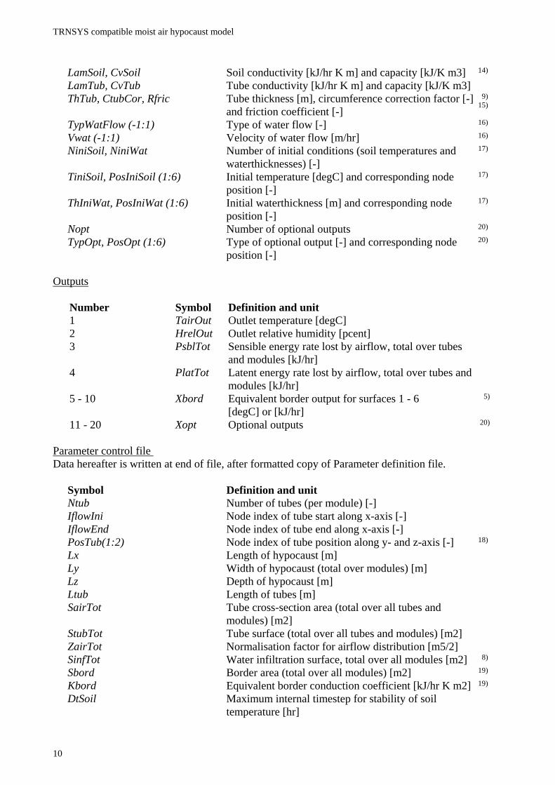
LamSoil, CvSoil Soil conductivity [kJ/hr K m] and capacity [kJ/K m3] 14)
LamTub, CvTub Tube conductivity [kJ/hr K m] and capacity [kJ/K m3]ThTub, CtubCor, Rfric Tube thickness [m], circumference correction factor [-]
and friction coefficient [-] 9)
15)
TypWatFlow (-1:1) Type of water flow [-] 16)
Vwat (-1:1) Velocity of water flow [m/hr] 16)
NiniSoil, NiniWat Number of initial conditions (soil temperatures and waterthicknesses) [-]
17)
TiniSoil, PosIniSoil (1:6) Initial temperature [degC] and corresponding node position [-]
17)
ThIniWat, PosIniWat (1:6) Initial waterthickness [m] and corresponding node position [-]
17)
Nopt Number of optional outputs 20)
TypOpt, PosOpt (1:6) Type of optional output [-] and corresponding node position [-]
20)
Outputs
Number Symbol Definition and unit 1 TairOut Outlet temperature [degC] 2 HrelOut Outlet relative humidity [pcent] 3 PsblTot Sensible energy rate lost by airflow, total over tubes
and modules [kJ/hr] 4 PlatTot Latent energy rate lost by airflow, total over tubes and
modules [kJ/hr] 5 - 10 Xbord Equivalent border output for surfaces 1 - 6
[degC] or [kJ/hr] 5)
11 - 20 Xopt Optional outputs 20)
Parameter control file Data hereafter is written at end of file, after formatted copy of Parameter definition file.
Symbol Definition and unit Ntub Number of tubes (per module) [-] IflowIni Node index of tube start along x-axis [-] IflowEnd Node index of tube end along x-axis [-] PosTub(1:2) Node index of tube position along y- and z-axis [-] 18)
Lx Length of hypocaust [m] Ly Width of hypocaust (total over modules) [m] Lz Depth of hypocaust [m] Ltub Length of tubes [m] SairTot Tube cross-section area (total over all tubes and
modules) [m2] StubTot Tube surface (total over all tubes and modules) [m2] ZairTot Normalisation factor for airflow distribution [m5/2] SinfTot Water infiltration surface, total over all modules [m2] 8)
Sbord Border area (total over all modules) [m2] 19)
Kbord Equivalent border conduction coefficient [kJ/hr K m2] 19)
DtSoil Maximum internal timestep for stability of soil temperature [hr]

TRNSYS compatible moist air hypocaust model
11
DtWat Maximum internal timestep for consistency of water flow [hr]
FairMinTub Minimum air flow for stability of air temperature [m3/hr]
Dt Internal timestep effectively used in simulation [hr] FairMin Minimum air effectively flow used in simulation
[m3/hr]
Explanatory notes for preceeding tables 1) Unless assigned in simulation deck with user-defined name, parameter definition and control
files must by default be named ParamDef.txt and ParamCon.txt. 2) Since calculation of soil temperature is of explicit type, internal timestep should not exceed
a maximum theoretical value DtSoil, which is proportional to smallest node volume of soil (problem of temperature oscillation). Consistency of water flow calculation (equation 3) also implies a maximum value DtWat for internal timestep, proportional to shortest tube node. Both of these computed values are written to the parameter control file. Type 61 usualy takes the smallest of these two values for the internal timestep (which happens by setting the 3rd routine parameter Dt to zero). The user may alternatively control soil temperature oscillation by defining a larger or smaller internal timestep himself (which happens by setting the 3rd routine parameter Dt to a positive value), in which case the value DtWat should not be exceeded though.
3) So as to avoid oscillations of air temperature along the tube, airflow should not exceed a theoretical minimum value FairMinTub, which is written to the parameter control file. Type 61 usualy takes this value as a lower limit to the airflow (which happens by setting the 4th routine parameter FairMin to zero). The user may alternatively control air temperature oscillation by defining a larger or smaller minimum airflow himself (which happens by setting the 4th routine parameter FairMin to a positive value). In both cases an airflow smaller than the minmum value will be set to zero (no air-tube exchange, only diffusion within soil).
4) Temperature tolerance (>0) sets precision of numerical resolution of energy balance in tube (equation 17).
5) For each surface, linking mode is one of the following : 0 : corresponding input Xsurf is surface temperature, output Xbord is inflowing energy rate. 1 : corresponding input Xsurf is is inflowing energy rate, output Xbord is equivalent border
temperature. 6) Airflow direction along x-axis is carried by sign of airflow. If airflow is smaller (in absolute
value) than minimum airflow FairMin (see parameter control file) it is considered as zero (no air-tube exchange, only diffusion within soil).
7) Air pressure is used to convert volume flow in mass flow as well as to determine humidity ratio from relative humidity (equation 9). In usual cases its dynamic is not known and it is suggested to take standard atmosferic pressure at local altitude, which can be approximated by :
PrAir PrAir h h0= −exp( )0 with PrAir0 = 1.01325 bar, h0 = 7656 m. 8) Water infiltration is distributed on a certain tube area SinfTot, defined by the rectangular
node cluster PosInf on which infiltration is to take place. PosInf(1) and PosInf(4) are lower and upper node index along x-axis. PosInf(2) and PosInf(5) are lower and upper node index along y-axis.
TRNSYS compatible moist air hypocaust model
12
PosInf(3) and PosInf(6) are lower and upper node index along z-axis. Only tube nodes within this cluster are considered for water infiltration. 9) Even for non-rectangular tubes, node width must be chosen so that cross-section area is
given by DyDz. Cross-section perimetrer, exchange surfaces and hydraulic diameter will be corrected by tube circumference correction factor CtubCor. Latter is defined as the ratio between real tube perimeter and rectangular tube perimeter 2(Dy + Dz). For circular tubes node width has to be chosen so that Dy Dz r r= = ≅π 1772. and circumference correction factor becomes 1
2 08862π ≅ . . In case of a symetry plane passing in the middle of some tubes (tube node at hypocaust border, with latteral adiabatic condition) one furthermore has to divide Dy by half.
Generally speaking node widths Dx, Dy and Dz have to be chosen according to given problem, reminding that small soil volumes will lead to small internal timesteps and increase of runtime.Tube thickness ThTub may however be set to zero.
10) TypSec(1:NI) are positive integer numbers which refer to further on defined typical cross-sections along x-axis.
11) TypSoil (1:NJ,1:NK) are integer numbers which refer to given surface conditions for front and rear of hypocaust module (see example at end).
12) TypSoil (0:NJ+1,0:NK+1) are integer numbers which refer to further on defined soil types (bulk) or to given surface conditions (border). Exception are the 4 corners TypSoil (0,0) , TypSoil (NJ+1,0) , TypSoil (0,NK+1) , TypSoil (NJ+1,NK+1) which have no significance and are not defined (see figure 1 and example at end). This data set has to be repeated for the Nsec number of typical cross-sections.
13) Common values for air-tube exchange coefficients [3] are : Kair0 : 7 - 11 [kJ/hr K m2] Kair1 : 14 - 18 [(kJ/hr K m2)/(m/s)] 14) This line has to be repeated for the Nsoil number of soils. 15) Typical values for Friction coefficient are 0.01 - 0.02 [-]. 16) Specification of water flow is given for all 3 airflow diections (negative, zero, positive).
TypWatFlow indicates whether free water is to flow along the tubes (= 1) or to be ejected out (= 2). Vwat (≥ 0) specifies velocity of waterflow (if TypWatFlow = 1).
17) Initial temperatures are given for rectangular node clusters, defined by PosIniSoil : PosIniSoil(1) and PosIniSoil(4) are lower and upper node index along x-axis, PosIniSoil(2) and PosIniSoil(5) are lower and upper node index along y-axis, PosIniSoil(3) and PosIniSoil(6) are lower and upper node index along z-axis, except for first initial temperature which is applied to all nodes and thus does not need
definition of PosIniSoil (see example at end). Same structure accounts for initial water thicknesses. In this case only those nodes within the
cluster which do effectively corespond to tube nodes are taken into account though. 18) This line is repeated for the Ntub number of tubes. 19) This line is repeated for the Nsurf number of surfaces. 20) Nopt defines the number of desired optional outputs. For each one of them TypOpt specifies
the type of optional output and takes a value from one of the three following tables. PosOpt finally defines the rectangular node cluster for which the optional output is to be considered :
PosOpt(1) and PosOpt(4) are lower and upper node index along x-axis, PosOpt(2) and PosOpt(5) are lower and upper node index along y-axis, PosOpt(3) and PosOpt(6) are lower and upper node index along z-axis. If TypOpt relates to tube/air nodes, only tube nodes within cluster will be considered. If TypOpt relates to soil nodes, only soil nodes within cluster will be considered.

TRNSYS compatible moist air hypocaust model
13
If TypOpt relates to miscelanous data, PosOpt is of no significance and should be set to 1.
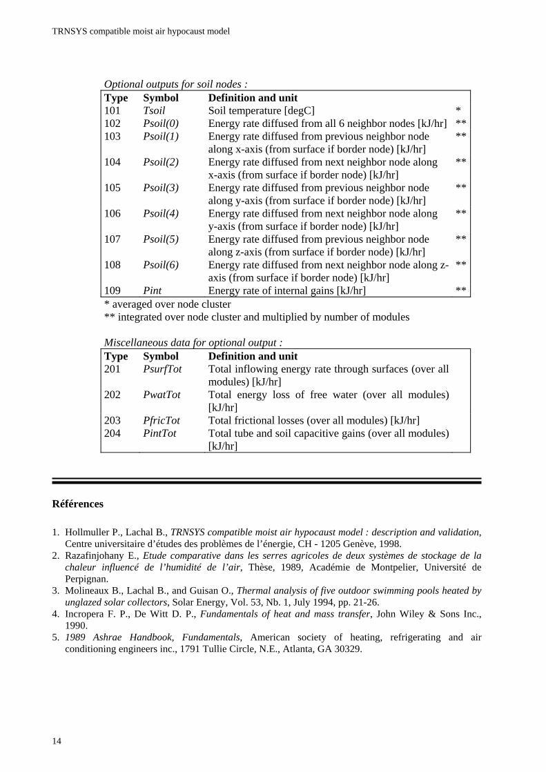
Optional outputs for tube nodes : Type Symbol Definition and unit 1 Tair Air temperature [degC] * 2 Hrel Air relative humidity [pcent] * 3 Habs Air absolute humidity [bar] * 4 Hrat Air humidity ratio [kg vapor/kg air] * 5 Mwat Free water in node [m3] **6 MwatLat/Dt Water condensing (>0) or evaporating (<0) [m3/hr] **7 MwatIn/Dt Water flowing into node [m3/hr] **8 MwatInf/Dt Water infiltrating into node [m3/hr] **9 MwatOut/Dt Water flowing out of node [m3/hr] **10 Tsoil Tube temperature [degC] **11 Psbl Sensible energy rate from air to tube [kJ/hr] **12 Plat Latent energy rate from air to tube [kJ/hr] **13 Pwat Energy rate lost by free water [kJ/hr] **14 Pfric Energy rate from frictional losses [kJ/hr] **15 Psoil(0) Energy rate diffused from all 6 neighbor nodes [kJ/hr] **16 Psoil(1) Energy rate diffused from previous neighbor node
along x-axis (from surface if border node) [kJ/hr] **
17 Psoil(2) Energy rate diffused from next neighbor node along x-axis (from surface if border node) [kJ/hr]
**
18 Psoil(3) Energy rate diffused from previous neighbor node along y-axis (from surface if border node) [kJ/hr]
**
19 Psoil(4) Energy rate diffused from next neighbor node along y-axis (from surface if border node) [kJ/hr]
**
20 Psoil(5) Energy rate diffused from previous neighbor node along z-axis (from surface if border node) [kJ/hr]
**
21 Psoil(6) Energy rate diffused from next neighbor node along z-axis (from surface if border node) [kJ/hr]
**
22 Pint Energy rate of internal gains [kJ/hr] **23 Fair Air flowrate [m3/hr] * 24 Vair Air velocity [m/s] * * averaged over node cluster ** integrated over node cluster and multiplied by number of modules
TRNSYS compatible moist air hypocaust model
14
Optional outputs for soil nodes : Type Symbol Definition and unit 101 Tsoil Soil temperature [degC] * 102 Psoil(0) Energy rate diffused from all 6 neighbor nodes [kJ/hr] **103 Psoil(1) Energy rate diffused from previous neighbor node
along x-axis (from surface if border node) [kJ/hr] **
104 Psoil(2) Energy rate diffused from next neighbor node along x-axis (from surface if border node) [kJ/hr]
**
105 Psoil(3) Energy rate diffused from previous neighbor node along y-axis (from surface if border node) [kJ/hr]
**
106 Psoil(4) Energy rate diffused from next neighbor node along y-axis (from surface if border node) [kJ/hr]
**
107 Psoil(5) Energy rate diffused from previous neighbor node along z-axis (from surface if border node) [kJ/hr]
**
108 Psoil(6) Energy rate diffused from next neighbor node along z-axis (from surface if border node) [kJ/hr]
**
109 Pint Energy rate of internal gains [kJ/hr] *** averaged over node cluster ** integrated over node cluster and multiplied by number of modules Miscellaneous data for optional output : Type Symbol Definition and unit 201 PsurfTot Total inflowing energy rate through surfaces (over all
modules) [kJ/hr]
202 PwatTot Total energy loss of free water (over all modules) [kJ/hr]
203 PfricTot Total frictional losses (over all modules) [kJ/hr] 204 PintTot Total tube and soil capacitive gains (over all modules)
[kJ/hr]
Références 1. Hollmuller P., Lachal B., TRNSYS compatible moist air hypocaust model : description and validation,
Centre universitaire d’études des problèmes de l’énergie, CH - 1205 Genève, 1998. 2. Razafinjohany E., Etude comparative dans les serres agricoles de deux systèmes de stockage de la
chaleur influencé de l’humidité de l’air, Thèse, 1989, Académie de Montpelier, Université de Perpignan.
3. Molineaux B., Lachal B., and Guisan O., Thermal analysis of five outdoor swimming pools heated by unglazed solar collectors, Solar Energy, Vol. 53, Nb. 1, July 1994, pp. 21-26.
4. Incropera F. P., De Witt D. P., Fundamentals of heat and mass transfer, John Wiley & Sons Inc., 1990.
5. 1989 Ashrae Handbook, Fundamentals, American society of heating, refrigerating and air conditioning engineers inc., 1791 Tullie Circle, N.E., Atlanta, GA 30329.
TRNSYS compatible moist air hypocaust model
15
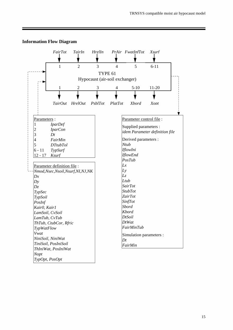
Information Flow Diagram
FairTot
1
HrelIn
3
TairIn
2
PrAir
4
Xsurf
6-11
1
TairOut
3
PsblTot
5-10
Xbord
4
PlatTot
11-20
Xopt
2
HrelOut
TYPE 61Hypocaust (air-soil exchanger)
Parameters :1 IparDef2 IparCon3 Dt4 FairMin5 DTtubTol6 - 11 TypSurf12 - 17 Ksurf
Parameter definition file :Nmod,Nsec,Nsoil,Nsurf,NI,NJ,NKDxDyDzTypSecTypSoilPosInfKair0, Kair1LamSoil, CvSoilLamTub, CvTubThTub, CtubCor, RfricTypWatFlowVwatNiniSoil, NiniWatTiniSoil, PosIniSoilThIniWat, PosIniWatNoptTypOpt, PosOpt
Parameter control file :
Supplied parameters :idem Parameter definition file
Derived parameters :NtubIflowIniIflowEndPosTubLxLyLzLtubSairTotStubTotZairTotSinfTotSbordKbordDtSoilDtWatFairMinTub
Simulation parameters :DtFairMin
FwatInfTot
5
TRNSYS compatible moist air hypocaust model
16
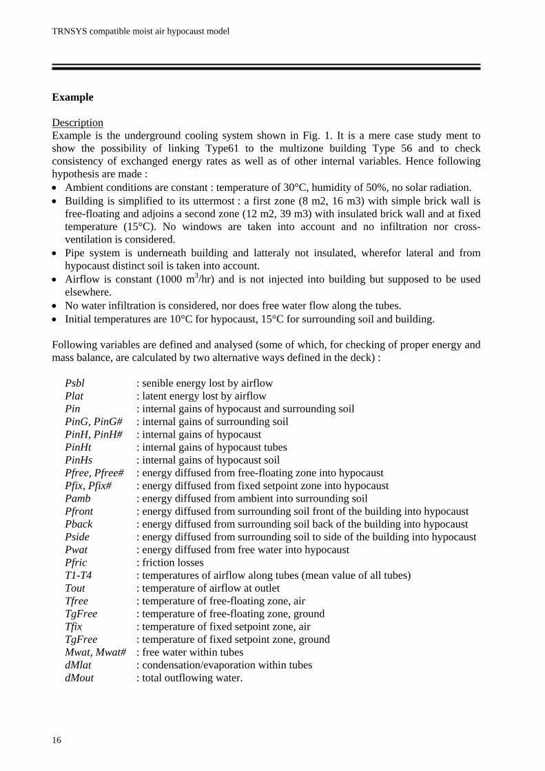
Example Description Example is the underground cooling system shown in Fig. 1. It is a mere case study ment to show the possibility of linking Type61 to the multizone building Type 56 and to check consistency of exchanged energy rates as well as of other internal variables. Hence following hypothesis are made : • Ambient conditions are constant : temperature of 30°C, humidity of 50%, no solar radiation. • Building is simplified to its uttermost : a first zone (8 m2, 16 m3) with simple brick wall is
free-floating and adjoins a second zone (12 m2, 39 m3) with insulated brick wall and at fixed temperature (15°C). No windows are taken into account and no infiltration nor cross-ventilation is considered.
• Pipe system is underneath building and latteraly not insulated, wherefor lateral and from hypocaust distinct soil is taken into account.
• Airflow is constant (1000 m3/hr) and is not injected into building but supposed to be used elsewhere.
• No water infiltration is considered, nor does free water flow along the tubes. • Initial temperatures are 10°C for hypocaust, 15°C for surrounding soil and building. Following variables are defined and analysed (some of which, for checking of proper energy and mass balance, are calculated by two alternative ways defined in the deck) : Psbl : senible energy lost by airflow Plat : latent energy lost by airflow Pin : internal gains of hypocaust and surrounding soil PinG, PinG# : internal gains of surrounding soil PinH, PinH# : internal gains of hypocaust PinHt : internal gains of hypocaust tubes PinHs : internal gains of hypocaust soil Pfree, Pfree# : energy diffused from free-floating zone into hypocaust Pfix, Pfix# : energy diffused from fixed setpoint zone into hypocaust Pamb : energy diffused from ambient into surrounding soil Pfront : energy diffused from surrounding soil front of the building into hypocaust Pback : energy diffused from surrounding soil back of the building into hypocaust Pside : energy diffused from surrounding soil to side of the building into hypocaust Pwat : energy diffused from free water into hypocaust Pfric : friction losses T1-T4 : temperatures of airflow along tubes (mean value of all tubes) Tout : temperature of airflow at outlet Tfree : temperature of free-floating zone, air TgFree : temperature of free-floating zone, ground Tfix : temperature of fixed setpoint zone, air TgFree : temperature of fixed setpoint zone, ground Mwat, Mwat# : free water within tubes dMlat : condensation/evaporation within tubes dMout : total outflowing water.

TRNSYS compatible moist air hypocaust model
17
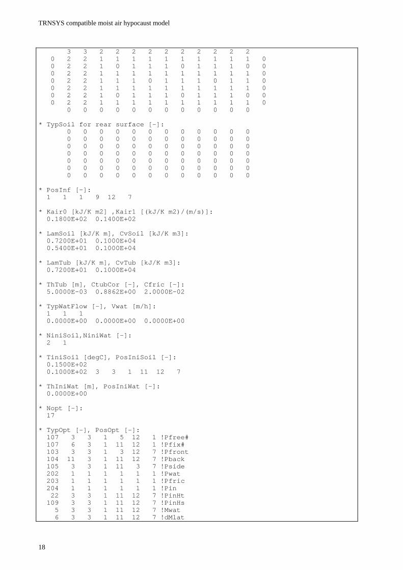
Next pages show files for parametrisation of the system (parameter definition file for Type 61, building definition file for Type 56, simulation deck), after which corresponding simulation results are discussed. Type61.par : parameter definition file (Type 61) ************************************************ * TYPE 61 SUPPLIED PARAMETERS *=============================================== * Nmod,Nsec,Nsoil,Nsurf,NI,NJ,NK [-]: 2 3 2 3 13 12 7 * DX [m]: 1.0000E+00 1.0000E+00 0.6666E+00 0.6666E+00 0.6666E+00 0.6666E+00 0.6666E+00 0.6666E+00 0.6666E+00 0.6666E+00 0.6666E+00 1.0000E+00 1.0000E+00 * DY [m]: 1.0000E+00 1.0000E+00 0.3000E+00 0.2000E+00 0.2000E+00 0.2000E+00 0.2000E+00 0.2000E+00 0.2000E+00 0.2000E+00 0.2000E+00 0.1000E+00 * DZ [m]: 0.4000E+00 0.2000E+00 0.2000E+00 0.2000E+00 0.2000E+00 0.2000E+00 0.4000E+00 * TypSec [-]: 1 1 2 2 2 3 3 3 3 3 3 1 1 * TypSoil for front surface [-]: 0 0 0 0 0 0 0 0 0 0 0 0 0 0 0 0 0 0 0 0 0 0 0 0 0 0 0 0 0 0 0 0 0 0 0 0 0 0 0 0 0 0 0 0 0 0 0 0 0 0 0 0 0 0 0 0 0 0 0 0 0 0 0 0 0 0 0 0 0 0 0 0 0 0 0 0 0 0 0 0 0 0 0 0 * TypSoil for sec# 1 (through ambient) [-]: 3 3 3 3 3 3 3 3 3 3 3 3 0 2 2 2 2 2 2 2 2 2 2 2 2 0 0 2 2 2 2 2 2 2 2 2 2 2 2 0 0 2 2 2 2 2 2 2 2 2 2 2 2 0 0 2 2 2 2 2 2 2 2 2 2 2 2 0 0 2 2 2 2 2 2 2 2 2 2 2 2 0 0 2 2 2 2 2 2 2 2 2 2 2 2 0 0 2 2 2 2 2 2 2 2 2 2 2 2 0 0 0 0 0 0 0 0 0 0 0 0 0 * TypSoil for sec# 2 (through both zones) [-]: 3 3 1 1 1 1 1 1 1 1 1 1 0 2 2 1 1 1 1 1 1 1 1 1 1 0 0 2 2 1 0 1 1 1 0 1 1 1 0 0 0 2 2 1 1 1 1 1 1 1 1 1 1 0 0 2 2 1 1 1 0 1 1 1 0 1 1 0 0 2 2 1 1 1 1 1 1 1 1 1 1 0 0 2 2 1 0 1 1 1 0 1 1 1 0 0 0 2 2 1 1 1 1 1 1 1 1 1 1 0 0 0 0 0 0 0 0 0 0 0 0 0 * TypSoil for sec# 3 (through setpoint-zone only) [-]:
TRNSYS compatible moist air hypocaust model
18
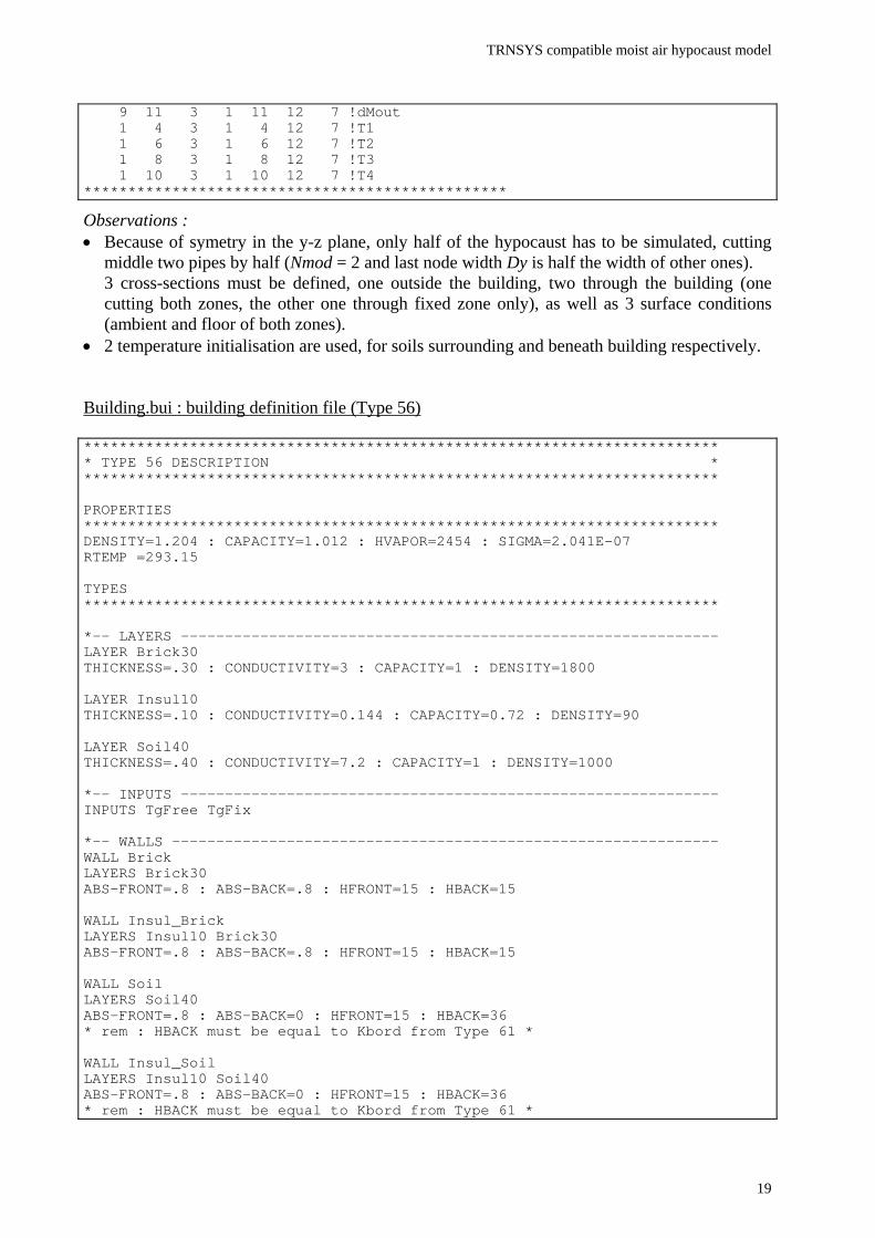
3 3 2 2 2 2 2 2 2 2 2 2 0 2 2 1 1 1 1 1 1 1 1 1 1 0 0 2 2 1 0 1 1 1 0 1 1 1 0 0 0 2 2 1 1 1 1 1 1 1 1 1 1 0 0 2 2 1 1 1 0 1 1 1 0 1 1 0 0 2 2 1 1 1 1 1 1 1 1 1 1 0 0 2 2 1 0 1 1 1 0 1 1 1 0 0 0 2 2 1 1 1 1 1 1 1 1 1 1 0 0 0 0 0 0 0 0 0 0 0 0 0 * TypSoil for rear surface [-]: 0 0 0 0 0 0 0 0 0 0 0 0 0 0 0 0 0 0 0 0 0 0 0 0 0 0 0 0 0 0 0 0 0 0 0 0 0 0 0 0 0 0 0 0 0 0 0 0 0 0 0 0 0 0 0 0 0 0 0 0 0 0 0 0 0 0 0 0 0 0 0 0 0 0 0 0 0 0 0 0 0 0 0 0 * PosInf [-]: 1 1 1 9 12 7 * Kair0 [kJ/K m2] ,Kair1 [(kJ/K m2)/(m/s)]: 0.1800E+02 0.1400E+02 * LamSoil [kJ/K m], CvSoil [kJ/K m3]: 0.7200E+01 0.1000E+04 0.5400E+01 0.1000E+04 * LamTub [kJ/K m], CvTub [kJ/K m3]: 0.7200E+01 0.1000E+04 * ThTub [m], CtubCor [-], Cfric [-]: 5.0000E-03 0.8862E+00 2.0000E-02 * TypWatFlow [-], Vwat [m/h]: 1 1 1 0.0000E+00 0.0000E+00 0.0000E+00 * NiniSoil,NiniWat [-]: 2 1 * TiniSoil [degC], PosIniSoil [-]: 0.1500E+02 0.1000E+02 3 3 1 11 12 7 * ThIniWat [m], PosIniWat [-]: 0.0000E+00 * Nopt [-]: 17 * TypOpt [-], PosOpt [-]: 107 3 3 1 5 12 1 !Pfree# 107 6 3 1 11 12 1 !Pfix# 103 3 3 1 3 12 7 !Pfront 104 11 3 1 11 12 7 !Pback 105 3 3 1 11 3 7 !Pside 202 1 1 1 1 1 1 !Pwat 203 1 1 1 1 1 1 !Pfric 204 1 1 1 1 1 1 !Pin 22 3 3 1 11 12 7 !PinHt 109 3 3 1 11 12 7 !PinHs 5 3 3 1 11 12 7 !Mwat 6 3 3 1 11 12 7 !dMlat
TRNSYS compatible moist air hypocaust model
19
9 11 3 1 11 12 7 !dMout 1 4 3 1 4 12 7 !T1 1 6 3 1 6 12 7 !T2 1 8 3 1 8 12 7 !T3 1 10 3 1 10 12 7 !T4 ************************************************
Observations : • Because of symetry in the y-z plane, only half of the hypocaust has to be simulated, cutting
middle two pipes by half (Nmod = 2 and last node width Dy is half the width of other ones). 3 cross-sections must be defined, one outside the building, two through the building (one
cutting both zones, the other one through fixed zone only), as well as 3 surface conditions (ambient and floor of both zones).
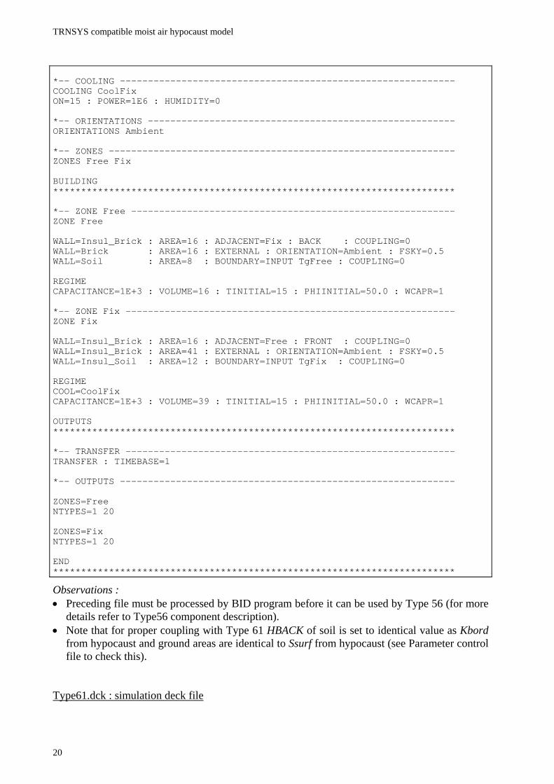
• 2 temperature initialisation are used, for soils surrounding and beneath building respectively. Building.bui : building definition file (Type 56) ************************************************************************ * TYPE 56 DESCRIPTION * ************************************************************************ PROPERTIES ************************************************************************ DENSITY=1.204 : CAPACITY=1.012 : HVAPOR=2454 : SIGMA=2.041E-07 RTEMP =293.15 TYPES ************************************************************************ *-- LAYERS ------------------------------------------------------------- LAYER Brick30 THICKNESS=.30 : CONDUCTIVITY=3 : CAPACITY=1 : DENSITY=1800 LAYER Insul10 THICKNESS=.10 : CONDUCTIVITY=0.144 : CAPACITY=0.72 : DENSITY=90 LAYER Soil40 THICKNESS=.40 : CONDUCTIVITY=7.2 : CAPACITY=1 : DENSITY=1000 *-- INPUTS ------------------------------------------------------------- INPUTS TgFree TgFix *-- WALLS -------------------------------------------------------------- WALL Brick LAYERS Brick30 ABS-FRONT=.8 : ABS-BACK=.8 : HFRONT=15 : HBACK=15 WALL Insul_Brick LAYERS Insul10 Brick30 ABS-FRONT=.8 : ABS-BACK=.8 : HFRONT=15 : HBACK=15 WALL Soil LAYERS Soil40 ABS-FRONT=.8 : ABS-BACK=0 : HFRONT=15 : HBACK=36 * rem : HBACK must be equal to Kbord from Type 61 * WALL Insul_Soil LAYERS Insul10 Soil40 ABS-FRONT=.8 : ABS-BACK=0 : HFRONT=15 : HBACK=36 * rem : HBACK must be equal to Kbord from Type 61 *
TRNSYS compatible moist air hypocaust model
20
*-- COOLING ------------------------------------------------------------ COOLING CoolFix ON=15 : POWER=1E6 : HUMIDITY=0 *-- ORIENTATIONS ------------------------------------------------------- ORIENTATIONS Ambient *-- ZONES -------------------------------------------------------------- ZONES Free Fix BUILDING ************************************************************************ *-- ZONE Free ---------------------------------------------------------- ZONE Free WALL=Insul_Brick : AREA=16 : ADJACENT=Fix : BACK : COUPLING=0 WALL=Brick : AREA=16 : EXTERNAL : ORIENTATION=Ambient : FSKY=0.5 WALL=Soil : AREA=8 : BOUNDARY=INPUT TgFree : COUPLING=0 REGIME CAPACITANCE=1E+3 : VOLUME=16 : TINITIAL=15 : PHIINITIAL=50.0 : WCAPR=1 *-- ZONE Fix ----------------------------------------------------------- ZONE Fix WALL=Insul_Brick : AREA=16 : ADJACENT=Free : FRONT : COUPLING=0 WALL=Insul_Brick : AREA=41 : EXTERNAL : ORIENTATION=Ambient : FSKY=0.5 WALL=Insul_Soil : AREA=12 : BOUNDARY=INPUT TgFix : COUPLING=0 REGIME COOL=CoolFix CAPACITANCE=1E+3 : VOLUME=39 : TINITIAL=15 : PHIINITIAL=50.0 : WCAPR=1 OUTPUTS ************************************************************************ *-- TRANSFER ----------------------------------------------------------- TRANSFER : TIMEBASE=1 *-- OUTPUTS ------------------------------------------------------------ ZONES=Free NTYPES=1 20 ZONES=Fix NTYPES=1 20 END ************************************************************************
Observations : • Preceding file must be processed by BID program before it can be used by Type 56 (for more
details refer to Type56 component description). • Note that for proper coupling with Type 61 HBACK of soil is set to identical value as Kbord
from hypocaust and ground areas are identical to Ssurf from hypocaust (see Parameter control file to check this).
Type61.dck : simulation deck file

TRNSYS compatible moist air hypocaust model
21
*************************************************************** * SIMULATION: *************************************************************** *============================================================== ASSIGN Trnsys.txt 6 ASSIGN Out1.txt 101 ASSIGN Out2.txt 102 ASSIGN Out3.txt 103 ASSIGN Type61.par 200 ASSIGN Type61.con 201 ASSIGN Building.bld 300 ASSIGN Building.trn 301 ASSIGN Building.win 302 *============================================================== *============================================================== EQUATIONS 37 *-------------------- DtSim = 1 Tamb = 30 Hamb = 50 Aflow = 1000 *-------------------- Tfree = [1,1] Tfix = [1,5] Pfree = -[1,4] Pfix = -[1,8] *-------------------- Tout = [2,1] Psbl = [2,3] Plat = [2,4] TgFree = [2,5] TgFix = [2,6] Pamb = [2,7] Pfree# = [2,11] Pfix# = [2,12] Pfront = [2,13] Pback = [2,14] Pside = [2,15] Pwat = [2,16] Pfric = [2,17] Pin = [2,18] PinHt = [2,19] PinHs = [2,20] Mwat = [2,21]*1000 dMlat = [2,22]*1000 dMout = [2,23]*1000 T1 = [2,24] T2 = [2,25] T3 = [2,26] T4 = [2,27] *-------------------- PinH = PinHt+PinHs PinG = Pin-PinHt-PinHs PinH# = Psbl+Plat+Pfree+Pfix+Pfront+Pback+Pside+Pwat PinG# = Pamb-Pfront-Pback-Pside dMwat = dMlat-dMout Mwat# = GT(TIME,1)*[3,1]+LT(TIME,2)*dMwat * Mwat# = [3,1] replaced by preceding line because of bug in * integrator Type55 *============================================================== *============================================================== SIMULATION 1 100 DtSim
TRNSYS compatible moist air hypocaust model
22
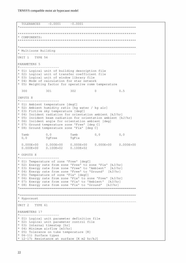
TOLERANCES -0.0001 -0.0001 *============================================================== *************************************************************** * COMPONENTS: *************************************************************** *============================================================== * Multizone Building *-------------------------------------------------------------- UNIT 1 TYPE 56 PARAMETERS 5 *--------------------- * 01) Logical unit of building description file * 02) Logical unit of transfer coefficient file * 03) Logical unit of window library file * 04) Mode of calculation for star network * 05) Weighting factor for operative romm temperature 300 301 302 0 0.5 INPUTS 8 *--------------------- * 01) Ambient temperature [degC] * 02) Ambient humidity ratio [kg water / kg air] * 03) Fictive sky temperature [degC] * 04) Incident radiation for orientation ambient [kJ/hr] * 05) Incident beam radiation for orientation ambient [kJ/hr] * 06) Incident angle for orientation ambient [deg] * 07) Ground temperature zone "Free" [deg C] * 08) Ground temperature zone "Fix" [deg C] Tamb 0,0 Tamb 0,0 0,0 0,0 TgFree TgFix 0.000E+00 0.000E+00 0.000E+00 0.000E+00 0.000E+00 0.000E+00 0.100E+02 0.100E+02 * OUPUTS 8 *--------------------- * 01) Temperature of zone "Free" [degC] * 02) Energy rate from zone "Free" to zone "Fix" [kJ/hr] * 03) Energy rate from zone "Free" to "Ambient" [kJ/hr] * 04) Energy rate from zone "Free" to "Ground" [kJ/hr] * 05) Temperature of zone "Fix" [degC] * 06) Energy rate from zone "Fix" to zone "Free" [kJ/hr] * 07) Energy rate from zone "Fix" to "Ambient" [kJ/hr] * 08) Energy rate from zone "Fix" to "Ground" [kJ/hr] *============================================================== *============================================================== * Hypocaust *-------------------------------------------------------------- UNIT 2 TYPE 61 PARAMETERS 17 *--------------------- * 01) Logical unit parameter definition file * 02) Logical unit parameter control file * 03) Internal timestep [hr] * 04) Minimum airflow [m3/hr] * 05) Tolerance on tube temperature [K] * 06-11) Surface types * 12-17) Resistance at surface [K m2 hr/kJ]
TRNSYS compatible moist air hypocaust model
23
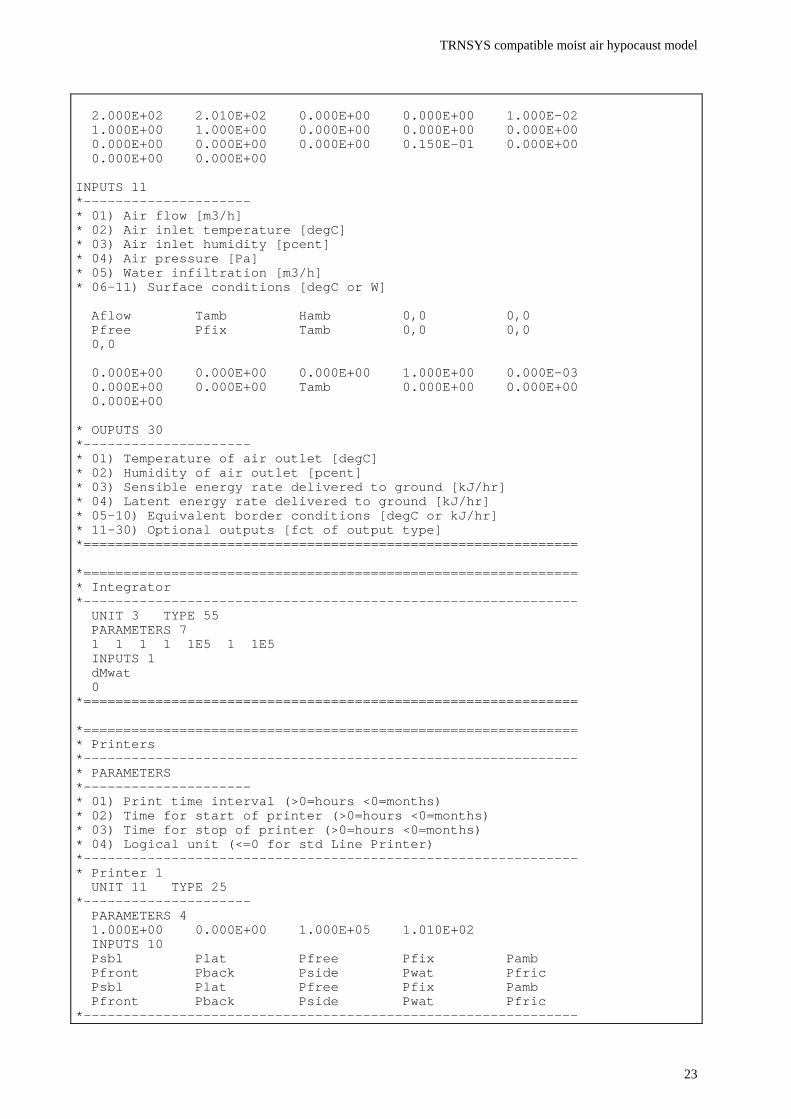
2.000E+02 2.010E+02 0.000E+00 0.000E+00 1.000E-02 1.000E+00 1.000E+00 0.000E+00 0.000E+00 0.000E+00 0.000E+00 0.000E+00 0.000E+00 0.150E-01 0.000E+00 0.000E+00 0.000E+00 INPUTS 11 *--------------------- * 01) Air flow [m3/h] * 02) Air inlet temperature [degC] * 03) Air inlet humidity [pcent] * 04) Air pressure [Pa] * 05) Water infiltration [m3/h] * 06-11) Surface conditions [degC or W] Aflow Tamb Hamb 0,0 0,0 Pfree Pfix Tamb 0,0 0,0 0,0 0.000E+00 0.000E+00 0.000E+00 1.000E+00 0.000E-03 0.000E+00 0.000E+00 Tamb 0.000E+00 0.000E+00 0.000E+00 * OUPUTS 30 *--------------------- * 01) Temperature of air outlet [degC] * 02) Humidity of air outlet [pcent] * 03) Sensible energy rate delivered to ground [kJ/hr] * 04) Latent energy rate delivered to ground [kJ/hr] * 05-10) Equivalent border conditions [degC or kJ/hr] * 11-30) Optional outputs [fct of output type] *============================================================== *============================================================== * Integrator *-------------------------------------------------------------- UNIT 3 TYPE 55 PARAMETERS 7 1 1 1 1 1E5 1 1E5 INPUTS 1 dMwat 0 *============================================================== *============================================================== * Printers *-------------------------------------------------------------- * PARAMETERS *--------------------- * 01) Print time interval (>0=hours <0=months) * 02) Time for start of printer (>0=hours <0=months) * 03) Time for stop of printer (>0=hours <0=months) * 04) Logical unit (<=0 for std Line Printer) *-------------------------------------------------------------- * Printer 1 UNIT 11 TYPE 25 *--------------------- PARAMETERS 4 1.000E+00 0.000E+00 1.000E+05 1.010E+02 INPUTS 10 Psbl Plat Pfree Pfix Pamb Pfront Pback Pside Pwat Pfric Psbl Plat Pfree Pfix Pamb Pfront Pback Pside Pwat Pfric *--------------------------------------------------------------

TRNSYS compatible moist air hypocaust model
24
* Printer 2 UNIT 12 TYPE 25 *--------------------- PARAMETERS 4 1.000E+00 0.000E+00 1.000E+05 1.020E+02 INPUTS 10 PinH PinG PinH# PinG# Pfree# Pfix# Mwat Mwat# dMlat dMout PinH PinG PinH# PinG# Pfree# Pfix# Mwat Mwat# dMlat dMout *-------------------------------------------------------------- * Printer 3 UNIT 13 TYPE 25 *--------------------- PARAMETERS 4 1.000E+00 0.000E+00 1.000E+05 1.030E+02 INPUTS 10 Tfree Tfix TgFree TgFix Tamb T1 T2 T3 T4 Tout Tfree Tfix TgFree TgFix Tamb T1 T2 T3 T4 Tout *============================================================== *************************************************************** END ***************************************************************
Observations : • Linking is done by feeding upper hypocaust surfaces with outflowing energy rates (Pfree and
Pfix) from the two zones and reciprocally feeding building with upper border temperatures (Tfree and Tfix) from hypocaust.
• Internal energy gains of hypocaust (PinH, PinH#) and surrounding ground (PinG, PinG#) are each defined by two alternative ways, so as to check for proper energy balance. Same is done for total free water within tubes (Mwat, Mwat#) and energy diffused from zones to hypocaust (Pfree, Pfree#, Pfix, Pfix#).
Results of simulation Parameters defined further up and printed in output files are plotted hereafter and show following, expected dynamic : • Airflow heats up hypocaust (see Fig. 3, Psbl). During first hours, energy diffuses from
building and surrounding soil into colder hypocaust and as latter warms up diffusion reverses (see Fig. 4, Pfront, Pback, Pside, Pfree, Pfix).
• As airflow heats up hypocaust it cools down along the tubes (see Fig. 2, stratification of Tamb, T1-T4, Tout) and with time tends to reach equilibrium temperature.
• Warm and humid airflow condensates during first hours (see Fig. 3, Plat and Fig. 5, dMlat, Mlat). As ground temperature rises, all free water within tubes then evaporates again, after which no latent exchanges take place any more.
• Within Type 61 energy balance is correct (see Fig. 3, PinH, PinH#, PinG, PinG#), as is mass balance (see Fig. 5, Mwat, Mwat#). Consistency of energy flows between modules is also respected (see Fig. 4, Pfree, Pfree#, Pfix, Pfix#).

TRNSYS compatible moist air hypocaust model
25
0
5
10
15
20
25
30
0 10 20 30 40 50 60 70 80 90 100
degC
Tfree Tfix TgFree TgFix
Tamb T1 T2 T3
T4 Tout
Fig. 2 : Temperature of air (Tfree, Tfix) and ground (TgFree, TgFix) of both zones as well as of airflow along the tubes (T1-T4) and at inlet and outlet (Tamb, Tout).
-5000
0
5000
10000
15000
20000
25000
0 10 20 30 40 50 60 70 80 90 100
kJ/h
r
Psbl
Plat
PinH
PinH#
Pamb
PinG
PinG#
Fig. 3 : Internal heat gains of hypocaust (PinH, PinH#) and surrounding soil (PinG, PinG#), as well as energy entering hypocaust by airflow (Psbl, Plat) and diffused from ambient into surrounding soil (Pamb).
-1000
-500
0
500
1000
1500
2000
0 10 20 30 40 50 60 70 80 90 100
kJ/h
r
Pfree
Pfree#
Pfix
Pfix#
Pfront
Pback
Pside
Fig. 4 : Energy entering hypocaust from building (Pfree, Pfree#, Pfix, Pfix#) and from surrounding soil (Pfront, Pback, Pside).
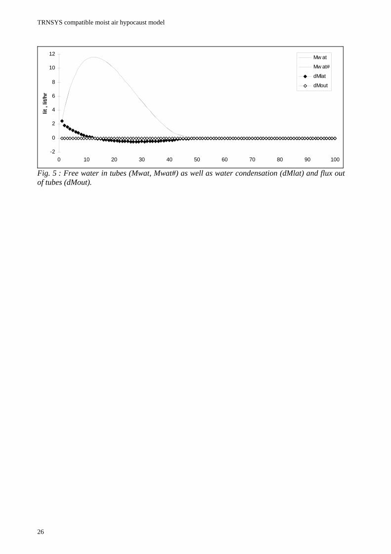
TRNSYS compatible moist air hypocaust model
26
-2
0
2
4
6
8
10
12
0 10 20 30 40 50 60 70 80 90 100
lit ,
lit/h
r
Mw at
Mw at#
dMlat
dMout
Fig. 5 : Free water in tubes (Mwat, Mwat#) as well as water condensation (dMlat) and flux out of tubes (dMout).

TRNSYS compatible moist air hypocaust model
27
Copyright © 2022 FDOKUMEN