Design Approaches for Solar Industrial Process Heat Systems

August 1982

Design Approaches for Solar Industrial Process Heat Systems

Nontracking and Line-Focus Collector Technologies

Charles F. Kutscher Roger L. Davenport Douglarr A. Dougherty Randy C. Gee P. Michael Masterson E. Kenneth May

Printed in the United States of America Available from:

National Technical Information Service U.S. Department of Commerce

5285 Port Royal Road Springfield, VA 22161

Price: Microfiche $3.00

Printed Copy $14.50

NOTICE

This report was prepared as an account of work sponsored by the United States Government. Neither the United States nor the United States Department of Energy, nor any of their employees, nor any of their contractors, subcontractors, or their employees, makes any warranty, express or implied, or assumes any legal liability or responsibility for the accuracy, completeness or usefulness of any information, apparatus, product or process disclosed, or represents that its use would not infringe privately owned rights.

SERl/lR-253-1356 UC Category: 62

Design Approaches for Solar Industrial Process Heat Systems Nontracking and Line-Focus Collector Technologies

Charles F. Kutscher Roger L. Davenport Douglas A. Dougherty Randy C. Gee P. Michael Masterson E. Kenneth May

August 1982

Prepared Under Task No. 1007.99 WPA NO. 279-81

. Solar Energy Research Institute A Division of Midwest Research Institute

1617 Cole Boulevard Golden, Colorado 80401

Prepared for the U.S. Department of Energy Contract No. EG-77-C-01-4042

sin TR-1356

The authors would like to thank everyone who took the time to review and comment on the draft of this document. Reviewers include Gerald Nix, Robert Copeland, L. M. Murphy, Larry Flowers, Shirley Stadjuhar, and Allan Lewandowski of SERI:; William Marlat t and Robert Baisley of Rockwell International; Kenneth Brown of Science Applications, Inc.; Jefferson Shingleton of Mueller Associates; Walter Carey of Nestle; Ed Carnegie of California Polytechnic State Univ.; T e t s w Noguchi of the Solar Research Laboratory, Nagoya, Japan ; Danny Def f enbaugh of Southwest Research Institute ; David Kaplan of The Lummus Company; Michael Rast of Pacific Sun, Inc.; David Allen of Foster Wheeler; William Engel of Owens-Illinois; Nick Kaplan and Harold Wilkening of AAI Corp.; Karl Wally of Sandia National Laboratories, Livermore; Harry Gaul (formerly of SERI); and Ari Rabl of Princeton University.

Special thanks go to John Wright of SERI for his considerable contribution to the section on controls, to James Leach of North Carolina State University for writing the unfired boiler subroutine of SOLIPE in conjunction with a summer research project at SERI, and to Rob Partington of SERI for his help in making the numerous SOLIPH computer runs. The authors are also very grateful to David Rearney for his extensive review of the document, in both early and final draft stages, and for supporting this undertaking at its outset while he was manager of the Solar Thermal, Ocean, and W i n d Division at SERI. Finally, the authors are deeply indebted to William her and Jerry Greyerbiehl of the U.S. Department of Energy, who secured the funding for this work.

Since 1976, the U.S. government has funded over a dozen projects tha t apply so l a r thermal energy t o i ndus t r i a l processes. We can draw two major conclusions from experiences gained i n designing, constructing, and operating these projects: design and i n s t a l l a t i on e r rors need to be avoided, and costs must be reduced. Thfs design handbook was prepared with both points i n mind. Designers a r e given a design procedure that has been formulated to help them avoid problems t ha t have occurred i n past systems. A t the same time, the design too l s contained i n the text a r e intended t o shorten the time required fo r conceptual and preliminary design, which should, i n turn , reduce t o t a l design costs. ( In the past , design costs have been a s much as 45% of construction costs. ) In addition, emphasis on cost-effective optimization of sys terns and components is intended to lower construction, operating, and maintenance costs.

Thfs handbook is not without precedent. In March 1981, the Solar Energy Research I n s t i t u t e published a forerunner document en t i t l ed "Design Considerations for . Solar Indus t r i a l Process Heat Systems-" That report , which drew upon the experiences of a number of IPH system designers and Department of Energy technical advisors, contained qua l i t a t ive lists of items tha t should be considered i n the design of a solar IPEi system. This document is intended t o provide the quant i ta t ive information needed to complete a step-by-step design.

The contents of t h i s handbook have been arranged td guide the user through a system design. The f i r s t part , "Objectives and Fundamentals, " provides an introduction to the uses of so la r thermal energy i n industry. It is intended for those who do not have experience i n the solar IPH f i e l d , but it could a l so serve a s a useful review. The second par t , "Conceptual Design," describes how to choose the proper application and system configuration and how to estimate the amount of energy the solar system can be expected t o supply. The conceptual design should supply enough information t o allow the user t o make an informed decision about whether to proceed with the project , and it will a l so provide a firm foundation for fur ther design work. The th i rd par t , "Preliminary Design," describes how to s e l ec t and optimize system components. This section a lso explains how to determine the delivered energy more accurately. A chapter on i n s t a l l a t i on and start-up is included, because they have caused problems in the past. Items of specia l i n t e r e s t a re covered i n the appendices, and a glossary is provided for those new to the solar energy f i e ld . Although S I un i t s are used throughout, a deta i led conversion tab le is provided i n Appendix I fo r those who a r e more comfortable with English un i t s .

The f i n a l , deta i led design is l e f t to the reader. Actual se lect ion of hardware by brand name and model number, mechanical and e l e c t r i c a l drawings, construction specif icat ions , etc. , a re a l l highly spec i f ic t o the system, and require the reader to draw upon h i s professional experience.

The reader w i l l note t ha t , although computer techniques a re discussed i n t h i s repor t , the emphasis is on simplified design tools. These were generated by thousands of runs of an hour-by-hour computer program (SOLIPB) spec i f ica l ly

wri t t en t o model s o l a r i n d u s t r i a l process heat systems. These design t o o l s a r e simple t o use and requ i re no computer programming knowledge. They a r e intended t o supply values within a few percentage points of the de ta i l ed computer program and apply t o both large and s m a l l i n s t a l l a t i o n s . Considering current uncer ta in t i e s about degradation of pipe insula t ion and co l l ec to r s and the large va r ia t ions i n annual s o l a r radia t ion at any given s i t e , using simple design tools is a pragmatic approach. It f rees the designer to concentrate on the hardware and i n s t a l l a t i o n problems which i n the past have lowered energy co l l ec t ion values w e l l below those predicted by sophist icated but i d e a l i s t i c computer models.

Because the f i e l d of s o l a r thermal energy a s i t is applied i n industry is s t i l l young, design quest ions cannot a l l be answered i n t h i s handbook. We hope, however, t h a t it contains t h e best information current ly avai lable . The types of i n d u s t r i a l processes and corresponding solar system configurat ion a l t e r n a t i v e s a r e manifold. Thus, system designers w i l l f ind a considerable number of oppor tuni t ies t o devia te from the generic design procedures contained here, and they should f e e l f r e e t o do so. Readers a r e encouraged t o contact the authors with any ideas or experiences they have had t h a t could augment o r improve t h i s handbook.

Charles F. R u t s c h e e Task Leader Thermal Systems and Engineering

Branch

Approved f o r

SOLAR ENERGY RESEARCH INSTITUTE

p4. (1RX ohn P. Thornton, Chief

Thermal Systems and Engineering Branch

Barry B f l e r , -Manager solaf lermal and k a t e r i a l s Research

Division

2 area (m )

A, co l l e c to r aperture area

Ag ground area covered by col lector array

% heat exchanger surface area

fac tor i n Eq. 7-31

incident-angle modifier coeff ic ient

constant-pressure spec i f ic heat (J kg-' JC-l)

diameter (m)

Di insu la t ion diameter

Dp pipe diameter

spec i f i c diameter of a pump impeller

solar f r ac t i on (portion of t o t a l load supplied by solar system)

f r i c t i o n f ac to r

co l lec to r heat removal eff ic iency fac tor

Fg based on col lector inlet temperature

Fm based on mean co l lec to r temperature

F, based on col lector ou t le t temperature

dewinter heat exchanger fac tor

heat t r ans f e r f i lm coeff ic ient (W m-* K-I)

h, convective heat t r ans fe r coeff ic ient

hi heat t rans fe r coeff ic ient on ins ide of a pipe

ho heat t ransfer coeff ic ient on outside of a pipe

h, radiative heat transfer coeff ic ient

l a t e n t heat of evaporation (J kg-')

head of a pump (Pa)

i r radiance (W m2) I, i r radiance available to a co l lec to r

Ib beam irradiance

Id d i f fu se irradiance

Ig global irradiance

Ih global irradiance on a horizontal surface

~ C L A T U R E (Continued)

- Ib long-term average beam irradiance during daylight hours - Ig long-term average global irradiance during daylight

hours

thermal conductivity (W m-' K-l)

ka thermal conductivity of air

kf thermal conductivity of a fluid

ki thermal conductivity of insulation

kp thermal conductivity of a pipe wall

ko thermal conductivity on shell side of a heat exchanger

Kh clearness index

%T incident-angle modifier (flat plate)

Kp a= incident-angle modifier correction factor (evacuated tube and , parabolic trough)

- L length (m)

Lend spillage end loss factor for prabolic troughs

mc collector mass flow rate per unit collector area (kg s-I m-')

M total mass (kg)

k total mass flow rate (kg s-l)

hc collector mass flow rate '. Mg load mass flow rate

hs mass flow rate through storage

N

Ns NPSH

number of rows of tubes across the diameter of the shell of a heat exchanger

rotational speed (rev min-' )

specific speed

Net Positive Suction Head (Pa)

NPSHA NPSH available

NPSHR NPSH required

pressure (Pa, absolute unless otherwise noted)

vapor pressure (Pa, absolute)

pumping power (W)

energy per unit collector area (J m2) (for subscripts, see Q)

HOHENCU4TURE (Continued)

energy rate per unit collector area (W Q ~ )

energ collection rate for a solar system with infinite storage (W *-TI energy (J)

Q, energy collected

Qd energy delivered to the process from the solar system

Qg energy lost

Qr energy required by the process

Q, energy stored

energy rate (W)

volumetric flow rate (m3 s-I)

thermal resistance per unit thickness (m K W-I) 2 thermal resistance (m K W-l)

Rf thermal resistance due to fouling

Ri thermal resistance on inside of pipe or tube

Ro thermal resistance on outside of pipe or tube

% total thermal resistance

thermal resistance at wall of pipe or tube

spacing (4

'baf baffle spacing in heat exchanger

Smin minimum tube spacing in heat exchanger

time (s)

thickness of insulation (m)

temperature (K or OC)

Ta .ambient temperature

T, collector temperature

Tf fluid temperature

Ti insulation temperature

Te load temperature

Tp plate temperature in f lat-plate collector

T, effective radiative temperature of surroundings (K only)

NOMENCLBTDBE (Continued)

Ts storage temperature

Tg,r load return temperature ("C)

U thermal conductance (W m-2 K-l)

u~ overall collector heat loss coefficient (W m-2 K-' )

V speed (m s-l)

W heat capacity flow rate (W K-l)

Wc collector heat capacity flow rate

Ws storage loop heat capacity flow rate

Y parameter in Eq. 7-70

Secondary Subscripts

daytime

fluid

inlet, inside

mean

outlet, outside

start-up

Nondimensional Numbers

Nu Nusselt Number (= h D K-l)

Pr Prandtl Number (= u cp K-I)

Re Reynolds Number (= p V D u-l)

Greek Symbols

a altitude of sun (0 to +90°)

as absorptance for solar radiation

B surface tilt (0 to +90°; toward equator is positive)

Y azimuth of a surface (0 to 360"; clockwise from North)

A declination (0 to '23.45O; North is positive)

E heat exchanger effectiveness

~ C L A ! l ! U R E (Concluded)

infrared emittance of a surface

efficiency

nC collector efficiency

n sys tern thermal efficiency

no collector optical efficiency

incident angle (0 to +90°; measured from perpendicular)

zenith angle (0 to +90°)

dynamic viscosity (Pa s) 2 -1 kinematic viscosity (: v / p ) (m s )

density (kg m3) reflectance for solar radiation

Stefan-Boltzmann constant (5.67 x lo-* W 6' K - ~ )

transmittance-absorptance product of a collector

latitude ( 0 to +90°; North is positive)

hour angle of sun (0 to 360'; noon is 0 ° , afternoon is positive)

LIST OF ECONWIC TKRns

CRF

d

DEP

cumulative present worth of depreciat ion tax c r e d i t s per d o l l a r invested

B~~ with declining balance depreciat ion

B~~ with s t ra igh t - l ine deprecia t ion

BSOn with sum-of-years-digits depreciat ion

co l l ec to r cost per uni t area ($ m-2)

piping insu la t ion cost per un i t length of pipe ($ m-l)

piping insu la t ion jacketing cost per un i t length of pipe ($ m-l)

cos t of labor t o i n s t a l l pipe insu la t ion , per u n i t length of

pipe ($ m - 5 annual base cos t of maintenance of pipe insu la t ion , per u n i t length of pipe ($ m-' yr-l)

t o t a l annual cos t of pipe insu la t ion per un i t length ($ m-' yr-l)

heat exchanger c o s t per un i t a rea ($ m-2)

storage tank insu la t ion cost per un i t area ($ m 2 )

s torage tank insu la t ion cost per un i t volume ($ m-3)

t o t a l co l l ec to r cos t ($)

t o t a l insu la t ion cos t ($)

cost function defined by Eq. 7-10

level ized (annualized) required revenue i n current d o l l a r s t o purchase so la r energy

level ized required revenue i n constant zero-year d o l l a r s t o purchase solar energy

t o t a l system cos t of heat exchangers and co l l ec to r s (= A, cc + 4, ex) ($1 cost t o minimize, defined i n Eq. 7-9

c a p i t a l recovery fac to r R [= 1 - (1 + R ) - ~ I

annual discount r a t e

present value of depreciat ion charges a s a f rac t ion of i n i t i a l investment

LIST OF ECOBOMIC TERMS (Continued)

DP depreciation period

Ec economic parameter for level iz ing col lector costs

E~ economic parameter for level iz ing storage tank insulation costs

Es annual so l a r energy provided by solar system a t the point of use

E1'E2 economic coeff ic ients for piping insula t ion costs

f f r ac t i on of t o t a l i n i t i a l system investment financed by loan

F annual usage factor 0 < F ( 1 for an insulated component

assumed general i n f l a t i on r a t e over the l i f e of a system

assumed overa l l escala t ion r a t e (includes general in f la t ion) of conventional fuel used i n backup system

fue l i n f l a t i o n r a t e i n year t

annual insurance cost a s a f rac t ion of the i n i t i a l system cost

annual i n t e r e s t r a t e on mortgage

t o t a l i n i t i a l solar system investment i n zero-year dol lars n

level iz ing fac tor [= CRF(R,N) (1 + gt) ! / ( I + R)~] , t =l

loan period (always t o be taken as equal to or l e s s than system l i f e )

the "M-factor" = C, / I ; levelized required revenue per t o t a l investment do l l a r

major component replacement cost i n year t = tc as a f ract ion of t o t a l i n i t i a l investment; t h i s cost is expressed i n terms of zero-year do l la r s

system l i f e ; a l so the period over which system costs a r e measured i n a l i f e-cycle cost ca lcula t ion

levelized cost i n current do l la r s fox operation, maintenance, property tax, and insurance, as a f rac t ion of t o t a l i n i t i a l investment

average cost of above items, expressed i n zero-year dol lars , as a f rac t ion of t o t a l i n i t i a l investment

annual property tax r a t e

economic fac tor used i n evaluating piping insula t ion

LIST OF ZoJNOMIC TKRMS (Concluded)

Pf levelized price of fuel ($/MBtu, $/kwh, $/GJ)

Pfo price of fuel in zero-year

Ps levelizecl price of solar energy = Cs/Es ($/MB~u, $/kwh, $/GJ)

R after-tax, market rate of return on investment

R* internal, after-tax, market rate of return on solar investment

% compound, after-tax, market interest rate at which solar investment dollars grow, evaluated at the end of solar system life

r market interest rate on loan

r ' real interest rate on loan

S net salvage value of solar system, expressed in zero-year dollars, as a fraction af total initial investment

SOYD sum-of-years digits method of accelerated depreciation

year of system operation under consideration; system constructed in year zero and begins operation on first day of year one

tc year in which a major component replacement is made

TC total investment tax credit rate

UA* annualized heat loss coefficient per unit length for piping heat loss (= 3.154 x 10' x A ) (GJ m-' yr-l K-~)

Greek Symbols

fraction of system first cost that was paid as a downpayment (= 1 - f) investment tax credit

declining balance multiplier

solar effectiveness factor (= fuel energy saved by a solar energy system divided by the solar energy delivered)

T marginal composite income tax rate [= rs + (1 - T,) T*]

Tf marginal federal income tax rate

=s marginal state income tax rate

Page . PART I: Objectives and Fundamentals

1.0 Objectives and Design Methodology ................................... 1

1.1 Introduction . . . . . . . . . . . . . . . . . . . . . . . . . . . . . . . . . . . . . . . . . . . . . . . . . . . 1 1.2 Design &thodology . . . . . . . . . . . . . . . . . . . . . . . . . . . . . . . . . . . . . . . . . . . . . 2 1.3 Additional Sources of Information .............................. 5

2.0 Solar Energy in Industry: An Overview .............................. 7

2 . 1 Introduction ................................................... 7 2 . 2 Solar Applications in IPH ...................................... 12

2 .2 .1 Hot Water ............................................... 12 2.2.2 Drying and &hydration . . . . . . . . . . . . . . . . . . . . . . . . . . . . . . . . . . 13 2.2 .3 Stem . . . . . . . . . . . . . . . . . . . . . . . . . . . . . . . . . . . . . . . . . . . . . . . . . . . 15

2 .3 Industrial Process Heat Field Tests ............................ 16 2.4 References ..................................................... 22

PART 11: Conceptual Design

3.0 Solar IPH Suitability Analysis ..................................... 25

3 . 1 Environmental Factors ........................................ 25 3.2 Process Factors ................................................ 28 3.3 Economic factor^........................^.....^..^.... 32 3 .4 Company Factors ............................................ 33 3 -5 Examples of Favorable Solar Thermal Applications .. .. ........... 33 3.6 References . . . . . . . . . . . . . . . . . . . . . . . . . . . . . . . . . . . . . . . . . . . . . . . . . . . . . 34

4.0 IPH System Configuration ............................................ 35 4 .1 Hot Air Systems ................................................ 35 4.2 Hot Water Systems 36 4.3 Steam Systems ................................................ . 38

4.3 .1 Flash Steam Systems ..................................... 40 4.3.2 Unfired-Boiler Systems .................................. 42 4.3.3 Direct Steam Generation .............................. 43

4.4 Storage Configurations ......................................... 43 4 .4 .1 Hot Water Storage ....................................... 43 4.4.2 Storage for Steam Systems ............................... 47

4.5 ~rocess/Solar System Interface ................................. 50 4.6 References ..................................................... 51

TABLE OF COIUTENTS (Continued)

Page . .................................................... 5.0 Solar Collectors 53

5.1 Types of Co1lector.s ............................................ 5.1.1 Flat-Plate Collectors ...................................

5.1.1.1 Components ..................................... 5.1.1.2 Improvements ...................................

5.1.2 Evacuated-Tube Collectors ............................... 5.1.2.1 Components ..................................... 5.1.2.2 Improvements ...................................

5.1.3 Parabolic Trough Collectors ............................. 5.1.3.1 Components ..................................... 5.1.3.2 Improvements ...................................

5.1.4 Other Types of Collectors ............................... 5.1.4.1 Solar Ponds .................................... 5.1.4.2 Compound Parabolic Concentrators ............... 5.1.4.3 Presnel Lens Collectors ........................ 5.1.4.4 Multiple-Reflector Collectors .................. 5.1.4.5 Parabolic Dish Collectors ...................... 5.1.4.6 Central Receivers ..............................

5.2 Instantaneous Performance of Collectors ........................ 5.2.1 Analysis ................................................. ................................................. 5.2.2 Testing

5.3 Collector Selection Procedure .................................. 5.3.1 A Preliminary Comparison of Collector Performance ....... 5.3.2 Other Considerations in Selecting an Appropriate ............................................. Collector

5.4 References ..................................................... PART 111: Preliminary Design

6.0 Annual Performance of a Solar Energy System ......................... 83

6.1 Annual Energy Collection for Several I W ........................................ System Configurations 83 ........................... 6.1.1 Hot Air and Hot Water Systems 86 6.1.1.1 No-Storage IPH System .......................... 89 6.1.1.2 Mixed-Tank. Recirculation IPH System ........... 93 6.1.1.3 Variable-Volume Storage System ................. 107

6.1.2 Steam Systems ........................................... 111 6.1.2.1 Unfired-Boiler Steam System .................... 111 6.1.2.2 Flash Steam System ............................. 113

6.2 Incident-Angle Effects ........................................ 114 6.2.1 Incident-Angle Modifiers ................................ 115 6.2.2 End Losses .............................................. 118

6.3 Row-to-Row Shading Losses .................................. 119 6.4 Annual Thermal Losses of Collector Field Piping and Storage .... 122

6.4.1 Steady-State Losses .................................... 126 6.4.2 Overnight Losses ....................................... 127 6.4.3 Freeze-Protection Heat Losses ........................... 129

TAB= OF CONTENTS (Continued)

Page

6.5 Utilization and Availability ................................... 132 6.6 Step-by-step Procedure ......................................... 135 6.7 References ..................................................... 138

7.0 The Energy Transport System ....................................... 139 7.1 Piping and Insulation .......................................... 139

7.1.1 Collector Field Piping Configurations ................... 139 7.1.2 Optimm Array Flow Rate and Collector Configuration ..... 141 7.1.3 Pipes and Sizing technique^...............^..^...^...... 143 7.1.4 Insulation and Heat Losses .............................. 144

7.2 Heat Transfer Fluids ............................................ 164 7.2.1 Types of Fluids ......................................... 165

7.2.1.1 Water .......................................... 165 7.2.1.2 Water-Glycol Mixtures .......................... 165 7.2.1.3 Aliphatic Hydrocarbons ......................... 165 7.2.1.4 Aromatic hydrocarbon^..............^........... 165 7.2.1.5 silicone^.......................^.............. 166

7.2.2 Temperature-Dependent Thermal Properties ................ 166 7.2.3 Other Thermal Properties ............................... 170

7.3 Pumps.. .......................... 170 7.3.1 Sizing a Single-Speed Centrifugal Pump O . . . . . . . . . . . . . . . . . 171 7.3.2 Multispeed Centrifugal Pumps ............................ 175 7.3.3 Positive Displacement Pumps ............................. 176

7.4 Valves ........................................................ 179 7.4.1 Characteristics of Solar Systems ~ . . . ~ ~ . ~ ~ ~ ~ ~ ~ ~ ~ . . . . . . . ~ . 179 7.4.2 Types of Valves ......................................... 180 7.4.3 Guidelines for Selecting Valves ......................... 181

7.5 Heat Exchangers ................................................ 182 7.5.1 Heat Transfer Relations ................................. 182 7.5.2 Overall Heat Transfer Coefficient ....................... 184 7.5.3 Heat Exchanger Factor for Solar System Performance ...... 187 7.5.4 Economical Reat Exchanger Area .......................... 189 7.5 . 5 Practical Considerations in Selecting a Heat

Exchanger ............................................ 190 7.5.6 Plate Heat Exchangers ................................... 192

7.6 Storage ........................................................ 193 7.6.1 Storage Media ........................................... 194

7.6.1.1 Sensible Heat Storage .......................... 194 7.6.1.2 Latent Heat Storage ............................ 195

7.6.2 Storage Vessels ........................................ 197 7.6.3 Storage Tank Insulation ................................ 199 7.6.4 Storage Location ........................................ 202

7.6.4.1 Interior Storage ............................... 202 7.6.4.2 Exterior Storage ............................... 203

7.7 References, ..................................................... 203 8.0 Controls and Instrumentation ........................................ 207

xvii

TABLE OF aONTBNTS (Continued)

Page

8.1 Fundamentals of Controls ................................. 207 8.1.1 Controllers ............................................. 207 8.1.2 Conuuon Control Loops ................................... 208 8.1.3 Measurement Dynamics .................................... 209 8.1.4 Noise ................................................... 210 8.1.5 Valves .................................................. 210 8.1.6 Miscellaneous Considerations .......................... 212 8.1.7 Multivariable Control Loops ............................. 212

8.1.7.1 Cascade ....................................... 212 8.1.7.2 Feed-Forward ................................... 212 8.1.7.3 Split-Range Control ............................ 213 8.1.7.4 Overrides ..................................... 213

8.1.8 Computers ............................................... 213 8.2 Control Design ................................................. 214

8.2.1 Normal Operating Modes .................................. 214 ....................................... 8.2.2 Start-Up/Shutdown 227 8.2.3 Freezinglstagnation ................................... 229 8.2.4 Emergency Conditions ................................ 229 8.2.5 Operator TrainingIDisplay ............................. 230 8.2.6 Control System Checkout ................................. 230

8.3 Instrumentation and Data Acquisition .......................... 231 8.3.1 Flow Measurement .................................. 231 8.3.2 Level Measurement .................................. 233 8.3.3 Pressure Measurement ............................. 233 8.3.4 Temperature Measurement ................................ 233 8.3.5 Irradiation Measurement ............................. . 235 8.3.6 Converters .............................................. 235 ........................................ 8.3.7 Data Acquisition 236

8.4 References ..................................................... 237 9.0 Installation and Start-up ........................................... 239

9.1 Installation and Checkout ................................... 239 9.1.1 Scheduling .............................................. 239 9.1.2 Installing the Collectors .............................. 239

9.1.2.1 1nstalling.Flat-Plate Collectors ............... 239 9.1.2.2 Installing Evacuated-Tube Collectors ........... 240 9.1.2.3 Installing Line-Focus Collectors ............... 241 9.1.2.4 Piping. Fittings. and Insulation ............... 242

9.1.3 Installing Heat Exchangers ............................. 246 9.1.4 Installing Pumps ...................................... 246 9.1.5 Installing Pressure Vessels and Storage Tanks ........... 247 9.1.6 Installing Controls. Electrical Lines. and

Instrumentation .................................... 248 9.1.7 Personnel and Environmental Safety Precautions .......... 248

9.2 Start-up ....................................................... 249 9.2.1 Line Flushing ........................................... 249 9.2.2 Pressure Testing ........................................ 250 9.2.3 Fluid Loading ........................................... 251 9.2.4 Commissioning of Solar System ........................... 252 9.2.5 Perforuance Testing .................................... 252

xviii

TaB'ILE OP COH!DZMTS (Continued)

Page

9.3 Summary ......................................................... 253 9.4 References .................................................... 253

10.0 Solar System Economics ............................................. 257 10.1 Methods of System Cost Estimation ............................. 257

- 10.1.1 Historical IPH System and Subsystem Costs ............. 257 10.1.1.1 Historical System Costs ..................... 258 10.1.1.2 Historical Subsystem Costs .................. 260 10.1.1.3 Estimating Construction Costs Using the

Mueller Data .............................. 261 10.1.2 Modular Cost Estimating ............................... 269

10.2 Life-Cycle Cost Analysis ...................................... 270 10.3 Methods of Financing Solar Systems ............................ 281

10.3.1 Conventional Financing ................................ 281 10.3.2 Conventional Lease Arrangements ....................... 281 10.3.3 Solar Management Company/Limited Partnership .......... 281

10.4 References .................................................... 283 11.0 Safety and Environmental issue^.........................^.......... 285

11.1 Safety Concerns in IPH Systems ................................ 285 11.1.1 Fire Safety ........................................... 285

11.1.1.1 Mterials ................................... 285 11.1.1.2 Equipment and Procedures .................... 286

11.1.2 Physical Hazards ................................... 288 11.1.3 Fluid Toxicity Considerations ......................... 289 ...... 11.1.4 Protection from Overtemperature and Overpressure 289 11.1.5 Product Contamination ................................. 290 11.1.6 Noise ................................................. 291 11.1.7 Applicable Regulations and Agencies ................... 291

11.2 Environmental Aspects of Solar IPH Systems .................... 292 11.2.1 Environmental Impacts of Solar IPH Systems ............ 292 11.2.2 National Environmental Protection Laws and

Organizations ....................................... 293 11.2.2.1 Air-Pollution Control ....................... 293 11.2.2.2 Water-Pollution Control ..................... 293 11.2.2.3 Waste Disposal .............................. 295 11.2.2.4 Noise ....................................... 295 11.2.2.5 Land Use .................................... 295

11.2.3 State Environmental Regulations ....................... 295 11.3 Bibliography .................................................. 295 11.4 References .................................................... 296

Appendix A Effects of Solar Systems on the Efficiency of Hot Water Boilers .................................................... 305

Appendix B Properties of Heat-Transfer Fluids ........................... 317 Appendix C The SOLIPH Computer Program .................................. 351 Appendix D Derivation of Annual-Performance Empirical Correlations ...... 371

xix

TR- 1 3 56 s=?I TABLJl OF COLPTENTS (Concluded)

Page

Appendix E Derivation of Annual Performance Modifiers ................... 383 Appendix F Ambient Temperature Data for 72 U.S . Cities .................. 393 Appendix G Sources of Information ...................................... 395 Appendix H Glossary ..................................................... 397 Appendix I Conversion Tables ............................................ 407

Index .................................................................... 419

TR-1356 sin +I LIST OF FIGURES

Page

Solar I W System Design Process ..................................... 3

U.S. Energy Demand by Sector ........................................ 7

Solar Attract iveness Index f o r Parabolic Trough Collectors .......... 9

............................... Energy Use by b j o r I n d u s t r i a l Groups 11

Dist r ibut ion of IPH Requirements by Temperature ..................... 11

Operating Temperatures fo r Various Types of Collectors .............. 12

Pork Building Products Solar Hot Water System .. .............. ....... 13

Lamanuzzi and Pantaleo Foods Solar Air System ....................... 14

.................... 2-8 LaCour Lumber Kiln Solar Rot-Water-to-Air System 14

2-9 Solar Steam Production Using an Unfired Boiler ...................... 15

........................... 2-10 Solar Steam Production Using a Flash Tank 16

3-1 Average Daily Global Solar Radiation on a Horizontal Surface 2 ........................................................... (kJ/m ) 26

' 2 3-2 Average Daily Direct Normal Solar Radiation (kJ/m ) ................. 27

..................... 3-3 Normal Daily Average Temperature (OF) i n January 29

....................... 3-4 Normal Daily Average Temperature (OF) i n July 30

............ 3-5 Mean Annual Number of Freezing Days i d the United S ta tes 31

3-6 Real Costs of Conventional Fuels .................................... 33

4-1 Direct Hot Air Solar System ......................................... 35

4-2 Water-to-Air Solar System .......................................... 36

4-3 A Direct Solar Hot Water System .......................+............. 37

4-4 An Ind i rec t Solar Hot Water System .................................. 37

4-5 Direct Hot Water System with Drain-Out Freeze Protect ion ........... 39

4-6 Ind i rec t Hot Water System with Drain-Back ( t o Tank) Freeze ............................... Protect ionand Nonpressurized Tank 39

xxi

LIST FIGURES (Continued) .

Page

4-7 Indirect Hot Water System with Drain-Back to Holding Tank and Pressurized Storage Tank .......................................... 40

4-8 Flash-Steam Solar System ............................................ 41 4-9 Unfired-Boiler Steam-Generating System .............................. 42 4-10 Four-Pipe Storage Configuration ..................................... 43 4-11 Two-Pipe Storage Configuration ................................... 44

.... 4-12 Multiple-Tank Storage Configuration for Achieving Stratification 44

4-13 Variable-Volume Storage Configuration ............................... 45 4-14 Thermocline or Mixed Tank Configuration with Unfired-Boiler

Steam System .................................................... 48 4-15 Variable-Volume Storage Tank Configuration for Unfired Boiler Steam

System ............................................................ 48

4-16 Annual Energy Delivery as a Function of Collector Area. Storage Type. and Size for an Unfired-Boiler System ....................... 49

5-1 Cross Section of Typical Flat-Plate Collector ....................... 54

5-2 Concentric Glass Evacuated-Tube Collector ........................... 57

5-3 Evacuated-Tube Collector Utilizing Metal Flow Passage ............... 58

5-4 Typical Parabolic Trough Collector .................................. 59

5-5 System Performance Increases vs . Absorber Temperature for Various Component Improvements of Horizontal Parabolic Troughs ............ 62

5-6 A CPC Collector Module ............................................ 64

5-7 Concentration With a Fresnel Lens ................................... 64

5-8 Typical Instantaneous Efficiency Curves for Collectors Used in IPH Applications .............................................. 68

5-9 Typical Incident-Angle Modifiers for Collectors Used in IPH Applications ................................................ 70

5-10 Average Global Solar Irradiance During Daylight Hours 2 on a Horizontal Surface (W/m ) .................................... 76

xxii

LIST OF FIGUBES (Continued)

Page - 5-11 Average Dire t Normal Solar Irradiance During Daylight 4 Hours (W/m ) . . . . . . . . . . . . m . m . . . . . . . . . . . . . ~ . ~ ~ ~ ~ ~ . . . . . . . ~ . . . 77

5-12 Graphi a 1 Determination of Yearly Average Energy Collection Rate 5 (W/m ) During Daylight Hours fo r Unshaded F l a t Pla tes , Evacuated Tubes, and Parabolic Troughs a s a Function of In tens i ty Ratio..... 78

6-1 Graphical Determination of Yearly Average Energy Collect ion Rate (w/rn2) During Daylight Hours f o r Unshaded F l a t P la tes , Evacuated Tubes, and Parabolic Troughs as a Function of In tens i ty Ratio..... 87

6-2 An Ind i rec t Solar Hot Air o r Hot Water System.. . . . . . . . . . . . . . . . . . . ... 88

6-3 Mixed-Tank Recirculat ion System.............................*....... 94

6-4 Annual Recirculat ion System Storage-Load Modifier fo r F la t P l a t e s (24 h/day load)..................^^^^^^^^^^^^.^^^^^ 97

6-5 Annual Recirculat ion System Storage-Load Modifiers fo r Evacuated Tubes (24 h/day load^..............................^.......... 98

Annual RecPrculation System Storage-Load Modifiers f o r East-West Parabolic Troughs (24 h/day load)........... ...................... 99

Annual Recirculat ion System Storage-Load Modifiers f o r North-South Parabolic Troughs (24 h/day load) ................................. 100

Annual Recirculat ion Sys tern Storage-Load Modifiers fo r F la t P l a t e s (8 h/day load)............................................. 101

Annual Recirculat ion System Storage-Load Modifiers f o r Evacuated Tubes (8 h/day load) .............................................. 102

Annual Recirculat ion System Storage-Load Modifiers for East-West Parabolic Troughs (8 h/day -load).................................. 103

Annual Recirculat ion System Storage-Load Modifiers f o r North-South Parabolic Troughs (8 h/day load) .................................. 104

Variable-Volume Storage Configuration.. . . . . . . . . . . . . . . . . . . . . . . . . . . . . 108

Annual Incident-Angle Modifier Correct ion Factors for Flat-Plate Collectors.............................~......................... 117

Annual Optical Efficiency Incident-Angle Weighting Factors f o r a North-South Trough .............................................. 118

Row-to-Row Shading Geometries....................................... 121

xxiii

LIST tX FIGURES (Continued)

Page

6-16 Annual Row-to-Row Shading-Loss Modifier for Flat Plates and Evacuated Tubes Tilted at Latitude ................................ 123

6-17 Annual Row-to-Row Shading-Loss Modifier for East-West Parabolic ............................................................ Troughs 124

6-18 Annual Row-to-Row Shading-Loss Modifier for North-South Parabolic Troughs ........................................................... 125

6-19 Hours of Freezing Temperatures per Year as a Function of Freezing Days per Year .................................................. 131

6-20 Average Below-Freezing Temperatures as a Function of Average ....................................... January Daytime Temperature 132

7-1 Solar System Collector Field Layouts ................................ 140 7-2 Effect of Insulation Thickness on Delivered Energy Cost ............. 144 7-3 Insulated Pipe Model ............................................. 145 7-4 Thermal Conductivity of Rigid Insulating Materials .................. 158 7-5 Sensitivity of UA/L Values to Changes in Parameters--Outdoors ....... 159

Sensitivity of UA/L Values to Changes in Parameters.. Indoors ........ Heat Transfer Efficiency Factors for Twenty Fluids .................. Summary of Types of Pumps ........................................... Typical Head-Flow Curves for a Centrifugal Pump ..................... Selection Curves for a Centrifugal Pump ............................. Net Positive Suction Head Required by Pump .......................... Pumping Power Reiquired by Different Pump Configurations ............. Capacity vs . NPSB- for Variable-Speed Pumps ........................

.............. Head-Flow Curves for Two Centrifugal Pumps in Parallel

Example Heat Exchanger System ....................................... .................... Floating Tubesheet Shell-and-Tube Heat Exchanger

LIST OF FIGURES (Concluded)

Page

Storage Capacity per Unit Volume as a Function of Temperature ........................ for Selected Latent-Heat Storage Materials 198

Constant Flow-Rate Control .......................................... 215 Constant Flow-Rate Control Using Three-Way Valve .................... 216

................ Outlet Temperature Control by Flow-Rate Manipulation 216

Turndown Ratio as a Function of Equivalent Lag and Capacitance Ratio (p) for Proportional Control .................................. 218

Turndown Ratio as a Function of Equivalent Lag and Capacitance Ratio (p) for Proportional-Integral Control ....................... 218

Dimensionless Controller Gain as a Function of Equfvalent Lag and' Capacitance Ratio (p) for froportlonal-Only Control ............... 219

Dimensionless Controller Gain as a Function of Equivalent Lag and Capacitance Ratio (p) for Proportional-Integral Control ........... 220

Dimensionless Integral Time as a Function of Equivalent Lag and Capacitance Ratio (p) for Proportional-Integral Control ........... 221

Solar System Response with Proportional-Only Control ................ 225

............ Solar System Response with Proportional-Integral Control 226

Typical Control Loop Tracking Control ............................... 228

Hose Deployment for Use With Either Rotatable or Nonrotatable Receivers ......................................................... 243

Examples of Insulation Techniques for Pipe Supports and Hangers ..... 245 Design for Rgducing Overnight Heat Losses in Drainback Systems ...... 248 Economies-of-Scale Factor ....................bb.....~............... 265

Modular Cost-Estimating Procedure Used by ECONMAT ................... 271 Graphical Solution of Eq . 10-10 for Different Loan Fractions and Fuel Escalation Rates ............................................. 282

. LIST 4'E TbBlXS

Page

U.S. Industrial Energy Consumption by State ......................... 10

Fuel Use by Industrial Sector (1980) ................................ 10

......... Solar Industrial Process Beat Projects in the United States 17

Problems Encountered in DOE-Funded Field Tests .....................a 20

Factors Favoring the Use of Solar ZPH Systems ....................... 25

Typical Ebnges of Liquid Collector. Performance Characteristics ................................................... 75

..... Maximum Daily Irradiation Available for Several Collector Types 109

................................. All-Day Average of End-Loss Factors 119

Economic Fluid Velocities for Schedule 40 Steel Pipes. Obtained ................................ Using the Perry and Chilton Method 143

7-2 Typical Thicknesses of Calcium Silicate Pipe Insulation ............ 146 7-3 Average Values of Independent Variables Used in Calculation of

UA/L .............................................................. 149

7-4 Outdoor Pipe UA/L Values (W/K-m of len th) for Insulation k = 0.0288 W/m-K (0.20 Btu-in./hr-ftq-OF) ........................ 150

7-5 Outdoor Pipe UA/L Values (W/K-m of len th) for Insulation k = 0.0577 W / r K (0.40 Btu-in./hr-ftf-OF) ......................... 151

7-6 Outdoor Pipe UA/L Values (W/K-m of len th) for Insulation k = 0.0865 W/m-R (0.60 Bt~.in./hr.ft'.~P) ......................... 152

7-7 Outdoor Pipe UA/L Value (W/K-m of length) for Insulation k = 0.1154 W/m-K (0.80 ~tu-in./hr-ft~-'~) ......em...............O.. 153

7-8 Indoor Pipe UA/L Values (W/K-m of leng h) for Insulation k = 0.0288 W 1 m - K (0.20 Btu-in./hr-ftg-OF) ......................... 154

7-9 Indoor Pipe UA/L Values (W/K-~ of length) for Insulation k = 0.0577 W/m-K (0.40 ~tu-in./hr-ft~-~~) ......................... 155

7-10 Indoor Pipe UA/L Values (W/K- of leng h) for Insulation k - 0.0865 W/m-K (0.60 Btu.in./hr.ft'~F). ...e...e................ 156

7-11 Indoor Pipe UA/L Values (W/K-m .of leng h) for Insulation k = 0.1154 W / r K (0.80 Btu-in./hs-ft5-OF) ......................... 157

xxvii

LIST OF TABLES (Concluded)

Page

7-12 Typical Overall Heat Transfer Coefficient Values for Tubular Beat Exchangers ................................................... 184

7-13 Typical Fouling Resistances ......................................... 185 7-14 Storage Size Comparison of Different Media Based on 1 GJ Storage

and 30 K Temperature Swing ........................................ 196 9-1 Installation Checklist .............................................. 254 10-1 Modified Solar IPH Subsystem Costs .................................. 259 10-2 Conceptual Phase Cost Estimating Guide ............................... 263 10-3 Design Cost Factors .......................................... 264 10-4 Cost Estimating Guide ................................................ 267

...................... 10-5 Factor Definitions for Modular cost Estimating 272

.1 0-6a Recommended Values for Modular Factors .............................. 272 10-6b Recommended Values for Modular Factors .............................. 273 10-7 Values of Capital Recovery Factor ................................... 274 10-8 Values of Levelizing Factor LF to Convert a Zero-Year Fuel Price

to a Levelized Price Over N Years ................................. 276

10-9a Values of M-Factor (R = 0.10) ....................................... 278 10-9b Values of M-Factor (R = 0.15) ................................... 279 10-9c Values of M-Factor (R = 0.20) ...................................... 280 11-1 Fire-Resistance Properties of Various Insulating Materials .......... 287 11-2 Safety Regulations and Agencies ................................ 291 11-3 Summary of Environmental Agencies and Regulations ................... 294 11-4 State Environmental Impact Statement Requirements ................... 297

xxviii

SECTIOH 1.0

OBJECTIVES m D3SICB ~ O D O L O G Y

In an effort to expedite the commercialization of solar energy, the U.S. Department of Energy has funded a number of field tests- These include over 100 projects that demonstrate solar heating and cooling (SHAC) of buildings and about a dozen projects to date in which solar collectors supply industrial process heat (IPH). Results from these projects generally showed lower than predicted energy deliveries due to a variety of system design, plumbing, and hardware problems, most of which can be expected in a new technology. Various handbooks were writ ten to help designers avoid problems already encountered ; later projects showed marked improvements-

Application of solar energy to industrial processes began later than the SHAC program, but similar problems have occurred in the IPH projects. Differences -

in types of collectors, environment, and loads created some new problems as - -

well. There was obviously a need to make contractors for new projects aware of mistakes made in the past. A great deal had been learned from the operation of the hot airlhot water IPH-projects; from those experiences, a set of guidelines was prepared to help design engineers with future solar industrial process heat systems. A questionnaire was mailed to previous contractors and DOE technical advisors, and a draft document was prepared from the results. Following a final review meeting at SERI, Design Considerations for Solar Industrial Process Beat Systems (Kutscher 1981) was published in March.

The purpose of this handbook is to provide specific design information. Choosing appropriate components such as collectors, storage, piping, insulation, pumps, valves, heat exchangers, and heat transfer fluids is covered in detail. System integration, controls, economics, start-up procedures and safety and environmental issues are also addressed, and a new, simple method for predicting energy delivery is included.

A considerable amount of time and money is often spent performing detailed computer simulations of a solar energy system. The authors belfeve, however, that if solar IPH applications are to become economically viable, they must be designed in ways that are typically used in the heating, ventilating, and air conditioning (HVAC) industry. Although the sensitivity of solar energy systems to variable solar input and thermal losses dictates more sophisticated "rules of thumb" than those used to size a building air conditioning system, simple graphs and tables can supply design values that are completely sufficient for system design. To save designers both extra steps and considerable expense, we have replaced the computer simulation step with some simple rules.

Design tools can be generated either from actual performance measurements taken in the field or from large numbers of computer simulations- Because actual field data are still very limited, the bulk of design tool development in this handbook has incorporated data from computer simulations. Therefore, before this handbook was written, a study was done comparing the capabilities of various solar simulation codes for IPH applications. The two most likely

candidates were TRNSYS, developed by the University of Wisconsin, and SOLTES, developed by Sandia Laboratories (see Sec. 6.0). For a variety of reasons, each code would have required considerable modification; thus, a new in-house code specifically geared for solar IPH design tool development was created. The result, SOLIPH, is not highly user-oriented like TRNSYS or SOLTES but is very easy to modify, inexpensive to run, and well suited to the purposes of this handbook. To verify the accuracy of the design tools generated by SOLIPH, the SOLIPH program was tested against other well-respected computer programs (see Appendix C).

This handbook was designed to be used by readers with experience in basic mechanical engineering. Knowledge of computer programming is not necessary, however, and previous solar energy experience, although advantageous, is not required. Because of its simplicity of approach, the handbook should be useful to an industrial firm contemplating solar energy and interested in having an in-house engineering staff manage conceptual and preliminary designs. It is recommended that the design engineer read the chapters in order. Results of conceptual design calculations will indicate whether the designer should proceed to the preliminary design. The iteration needed in completing a design is discussed in the next section.

Because this 'field : is . constantly changing aiid new , information continues to come in from industry tests, this handbook is clearly not the last word in IPH design. As funding permits, efforts will be made to update the handbook when new information becomes available. Users of the handbook are encouraged to supply the authors with feedback, and we are particularly interested in how easy users find the design procedurg.

1.2 DESIGN ~ O D O L O G Y

As we mentioned earlier, a design process involves a considerable amount of iteration. The material in this handbook is arranged so that conceptual design is treated first, followed by more detailed aspects of the process; but it is also important to see how the different design elements interact. Figure 1-1 is intended to inject some order into the variety of items the designer must address. The figure shows the design process progressing from left to right. The same process covers both conceptual and preliminary designs. Conceptual design does not go into as much detail as preliminary design, nor does it go quite so far. All preliminary design items are denoted by an asterisk.

The overall process is subdivided into four basic design problems: Applica- tion Selection, System Specification, System Analysis, and System Optimization/Design Completion. Application Selection requires a suitability analysis. Plant location, competing alternative energy sources, conservation opportunities, and process loads are all assessed using methods described in Sec. 3.0. This analysis results in information that can be used in two major design decisions. The load schedule, load interface, and freeze protection requirements help the designer choose the system configuration. The total load, load temperature, available space, and solar radiation data aid in the selection of a collector.

The System Configuration segment of conceptual design includes selecting a basic configuration (e-g., open or closed loop, type of freeze protection) (Sec. 4.0); deciding whether or not to use storage (Sec. 6.0); and defining a basic control system (Sec. 8.0). Detailed design involves actually sizing storage and subsystem components (Sec. 7.0) and writing specifications for a control system (Sec. 8.0).

Selecting a collector, done along with selecting a system configuration, involves choosing a collector type, an array location, and an approximate collector area for conceptual design (Sec. 5.0). The optimum area, specific collector parameters, mounting details, and ground cover ratio are determined in preliminary design (Sec. 6.0). As we will discuss later, the system configuration and collector segments provide most of the options that require iteration (basic configuration, storage size, and collector area).

The next step, System Analysis, is to analyze system performance and overall system costs. System performance analysis involves a simple calculation of collected energy and a rough estimate of system losses (Sec. 6.0). Next, detailed system losses are determined (Sec. 6.0). The costs segment involves an estimate of total system cost (based largely on collector area), in conceptual design (Sec. 5.0); and a system cost that takes into account all the components of the actual system, in preliminary design (Sec. 10.0).

In the last segment, System Optimization/Design Completion, outputs from the system analysis provide system energy cost for the conceptual design. The results of a complete life-cycle cost analysis are available during preliminary design. If cost is the major criterion in sizing a system, a decision is made here. The designer reworks the System Specification segment and tries different combinations: type of collector, basic configuration, collector area, etc., in conceptual design; collector parameters, row-to-row spacing, storage, pipe and heat exchanger sizes, and collector area in preliminary design.

At the end of the conceptual design phase, it may be decided not to continue to develop a preliminary design. Before making such a negative decision, however, the designer could go all the way back to the beginning and try a different plant process with a different temperature and load profile. Moreover, a plant owner may be concerned more with fuel curtailment than economics and decide to use solar energy as a hedge against that possibility. Or, the plant owner may want to experiment with a system that has future potential. In such cases, an arbitrary solar fraction may be chosen, or collector area may be fixed by the size of a roof or by land space set aside for it. Once the iterations in conceptual design are complete and certain criteria are met, the designer moves on to the preliminary design phase. When those iterations are in turn complete, the designer then addresses items in the design completion section of Fig. 1-1. Piping and instrumentation are diagrammed, equipment specifications are listed, and final system and energy costs are determined.

Obviously, it would be too time-consuming to go through the design process with every possible permutation of system parameters. The experienced designer, and particularly the experienced solar IPH system engineer, will be able to recognize what combinations offer the best chance of success. Sugges- tions are given throughout the text to help expedite the process.

1.3 ADDITIONAL SOURCES OP ' I N P O ~ T Z O I

This handbook is based on experience with the IPH field test program; thus, it covers a specific technology area. Line-focus, flat-plate, and evacuated-tube collectors are included in temperature ranges from ambient to about 290°C (550°~). Although air collector systems are covered generally, design tools in this edition apply specifically only to liquid and steam systems. Solar ponds, point-focus collectors, and central receivers are not addressed here in great detail.

In addition, certain sources of solar thermal energy information were not enlarged upon, such as SOLMET and TMY weather data, product specifications, computer programs, etc. The reader is referred to Appendix G for additional sources of information on these subjects and on other solar thermal technologies.

SECTION 2.0

SOLAR RmcwY IN mDUSTRY: Alf WERVLEW

The industrial sector is the largest energy user in the U.S. economy, consuming 39% of total demand (see Fig. 2-1). O f that 39X, approximately 45% (about 18% of the overall energy usage) involves direct thermal energy use and represents a significant potential market for solar energy applications.

There are several possible advantages to using solar energy for industrial process heat (IPH) rather than for residential or commercial heating and cooling applications:

Industrial loads are usually more constant throughout the year.

Industrial plants usually already have crews who could attend to the maintenance of solar energy systems, thus ensuring operation of the system at peak efficiency.

The total impact on the nation's energy use would be greater for solar IPR systems than for SHAC.

Compared with alternative industrial fuels, solar energy offers the additional advantages of being nonpolluting and independent of interruptions in supply caused by political or economic conditions. Solar energy systems can also be

A 1 . Commercial 15%

Figure 2-1. U.S. Bnergy Demand by Sector

7

constructed in reasonably short periods of time. Of course, certain impedi- ments to using solar energy in IPH also exist:

Land availability: Existing roofs often are not large or strong enough to support collector arrays. Either additional supports must be built or other areas or lands must be used. (Commercial land in urban areas can be scarce.)

Industrial effluents: An industrial environment creates greater possi- bilities for contamination of solar collectors than does a commercial or residential one. Concentrating collectors that require high specular reflectivity are particularly susceptible to degradation.

Nonconstant energy source: The plant must be able to utilize a variable solar energy delivery.

Availability of conservation alternatives: Many plants can employ simple, inexpensive energy conservation techniques which should precede any commitment to solar energy. These include using waste heat from high-temperature processes to supply low-temperature processes (such as boiler feedwater preheat).

Economics: Industry often requires payback periods of less than 5 years. In general, solar energy systems currently are too expensive and conventional fuels are too cheap to provide such paybacks.

The suitability of solar energy in a particular application depends on a number of factors, such as climate, economics, process temperature, and available space. A market suitability study sponsored by SERI used computer- generated maps to identify regions of high solar favorability. The primary criteria were collector performance, air-quality constraints on competitive fuels, state solar tax incentives, fuel costs, and degree of coal usage. Figure 2-2 shows the resulting solar attractiveness map for parabolic trough collectors. As one might expect, the Southwest is a highly favorable region. The State of California is particularly noteworthy because of its excellent tax incentive, favorable climate, and stringent air-quality standards. Areas where coal is heavily used show up as least favorable.

Table 2-1 shows that current industrial energy consumption is highly regional; ten states account for 61% of the total. Also, whether solar energy is economical depends to a great extent on what fuel it must be measured against. Table 2-2 shows the percentages of each type of fuel (less feed- stocks) used by the industrial sector in 1980. Oil and natural gas, which can be expected to become less stable in price, accounted for 67.2% of total energy use. Coal can be expected to remain fairly inexpensive (although cost and extent of use will depend greatly on pollution requirements and transportation costs). Electricity is likely to remain expensive, but it is usually used for applications other than process heat. Figure 2-3 shows that more than 80% of the total industrial process heat energy is used by six major industries.

Table 2-1. U.S. Industrial Energy Consumption by State (1977) (61% of total in 10 States)

State % of U.S. Total

Texas Louisiana Ohio Pennsylvania Illinois California Michigan Indiana New York Alabama

The temperature at which energy is used is also important in assessing the solar option. At higher temperatures, solar collectors lose more of their collected heat to the environment; thus, their efficiency is reduced. But as shown in Fig. 2-4, 49% of the energy consumed by industry is at temperatures below 260 OC (500 OF)--a conservative limit for collectors currently in production. The process temperature largely dictates which type of collector is most appropriate. This handbook concentrates on those that have already been used commercially: flat-plate, line-focus, and evacuated-tube collectors. Typical operating temperature ranges for these as well as for three other types of collectors being developed are shown in Fig. 2-5. All of these collectors are described in more detail in Sec. 5.0.

Table 2-2. Fuel .Use by Industrial Sector (1980)

Fuel X

Coal 7.9 Oil 24.3 Natural gas 42.9 Electricity 15.8 Other 9.0

Quads ( 1 0 ' ~ Btu/yr)

1 .O 2.0 3.0 I 8 4 I

Chemicals and Allied Products 1 1 2-48

Primary Metals 1 1 *+*

Petroleum and Coal Products 1-1 1.20

Paper and Allied Products 1-1 1-16

Stone, Clay and Glass Products -1 1.15

Food and Kindred Products 1-10.82 4 I 80% of Total

~~~~~~~~~~, , , , , , , ,~~~

F i g m e 2-3. Energy U s e by Major Industrial Groups

-I (Cumulative Percentages are Shown in Parentheses)

SOURCE: F. Krawiec et al.. July 1981.

Figure 2-4. Distribution of IPH Requirements by Temperature

40 -

30 -

t-------- I

Range of I (1 00)

Production I 34.0

Collectors I (27.2 j 20.3 I

20 - b

(44.1 ) I I > loooO F

16.9

I I (58.8) (65.8)

6.8 7.1 (48.9) 1 (52.0) 4.8 (50.4)

3

1.3 1.6

Type of Collector:

Central Receiver

Point Focus (Parabolic Dish and

Fresnel Lens)

Line Focus (Parabolic Trough and

Fresnel Lens, also Multiple Reflector)

Evacuated Tube

Flat-Plate

Solar Pond

Operating Temperature NOTE: Line-focus, evacuated-tube, and flat-plate collectors are commercially available: central receivers, point-focus collectors, and solar ponds are still being developed.

Figure 2-5. Operating Temperatures for Various Types of Collectors

2- 2 SOLAR BPPLICATIONS IW

The three main areas of solar thermal application in industry are

Process hot water

Drying/dehydration

Process steam.

2.2.1 Hot Water

Heated water is used in large amounts at temperatures between 50' and 1 0 0 ~ ~ (120~-212~~) for cooking, washing, bleaching, and anodi3ing and represents about 2% of the IPH demand, or 0.2 quad (1 quad = 10 Btu). Preheating boiler feedwater accounts for another 3 quads; often this could be supplied by associated higher-temperature waste heat. Water can be heated either directly in a collector loop or by means of a separate heat transfer fluid used in conjunction with a heat exchanger. The latter approach can reduce freezing and corrosion problems, but it also results in somewhat higher collector temperatures and, thus, reduced efficiency.

An example of an IPR hot water system is shown i n Fig. 2-6. This pa r t i cu l a r system su p l ies 454 ~ / m i n (120 gallmin) of hot water i n the range of 55' to 8 8 3 ' ~ (130 to 1 8 0 ~ ~ ) t o the York Building Products concrete b l ck curing p l a n t in Harrisburg, Pa. The col lector array consis ts of 829 my (9216 ft ) of multiple-reflector l i nea r concentrators. A shell-and-tube heat exchanger is used to t ransfer heat from the water-and-ethylene-glycol co l lec to r loop t o the process water. A unique feature of t h i s application is tha t the large , under-

3 ground, concrete curing area, or rotoclave, contains about 190 m (50,000 gal) of water and serves a s buil t- in storage.

2.2-2 Drying and Dehydration

The United Sta tes uses about 1.4 quads of solar-heated a i r a t temperatures below 177 '~ ( 3 5 0 ~ ~ 1 , mostly for crop drying. The two most common ways t o supply solar-heated air a re (I) t o heat the a i r d i r ec t l y i n the co l l ec to r s and (2) to heat a l iqu id in the col lectors and then use a l iquid-to-air heat exchanger. An example of the f i r s t type of system is shown i n Fig. 2-7.

2 2 In that par t icular system, 1890 m (21,000 f t ) of a i r co l lec to rs supply 60°c (140'~) air to a prune- and raisin-drying tunnel a t the Laaanuz i and Pantaleo 5 (L and P) Foods plant i n Fresno, Calif . A 420-m3 (14,000-ft ) rock bin is used fo r storage. A unique aspect of t h i s plant is a heat recovery wheel tha t t r ans fe rs heat frm the tunnel exhaust to the col lector array i n l e t . Although t h i s raises the co l lec to r array 's temperature, thereby lowering the a r ray ' s sf f iciency, the heat recovered more than makes up fo r the loss i n efficiency. The heat recovery wheel has a payback period of l e s s than 1 year, and its success demonstrates the importance of implementing conservation a l t e r - natives before proceeding to solar applications.

d

m2 (9216 ft2) Solar Array r Boiler E

York's Auxiliary Boiler/Rotoclave

Shell-and-Tu be Heat Exchanger

AAl's Solar Array/ Rotoclave Piping Circuit

York's Make-Up Water Circuit

Figure 2-6- York Building Products Solar k t Water System

I

at Recovery Unit

Inlet Guide Vane Control

Figure 2-7. Iamnuzzi and Pantaleo Foods Solar Air System

An example of heating water t o u l t ima te ly supply hot a i r is shown i n Fig. 2-8, which i l l u s t r a t e s the system i n use a t the J. A. LaCour lumber-drying k i l n i n

2 2 Canton, M i s s . A t t h i s p lant , 225 m (2500 f t ) of f l a t -p la te co l l ec to r s heat water t o 6 0 ' ~ (140°Z'), which then suppl ies -hot air t o two hardwood lumber k i l n s via finned-tube heat exchangers. Although t h i s system r e s u l t s i n higher co l l ec to r temperatures than does a d i rec t -a i r approach, pumping power needed for the l i q u i d loop is genera l ly l e s s than fan po e r for 1 9 a i r loop. To increase col lec ted energy a t the LaCour p lan t , 216 m (2400 f t ) of r e f l e c t o r s a r e included i n the co l ikc to r ar ray .

Figure 2-8- LaConr hmber Kiln Solar Hot-Water-to-Air System 14

A t h i r d way of using so la r heat fo r drying should be mentioned. Rather than using co l l ec to r s a t a l l , drying houses can be constructed so tha t sunlight d i r e c t l y s t r i k e s the product. This method e n t a i l s r e l a t i v e l y low temperatures and long drying times and general ly requires t h a t the product be spread out over a large area. However, it can be cost-effect ive.

2.2.3 Steam

About 6 quads of energy a r e consumed i n the United S t a t e s f o r process steam, 80% a t temperatures below 177 '~ (350'~). Steam can be supplied with so la r co l l ec to r s i n these three ways:

Using a high-temperature f l u i d i n the c o l l e c t o r s and t r ans fe r r ing the heat t o an unfired bo i l e r

Circulat ing pressurized water i n the c o l l e c t o r s and f lashing it to steam i n a f l a s h tank

Boiling water i n col lec tors .

The f i r s t type of system is shown i n Fig. 2-9. In t h i s exanyle, Thermin 1 55 4 is heated t o 246O~ (475'~) i n an array consis t ing of 900 m (10,000 it ) of parabolic-trough col lec tors . The hot Therminol then boils water i n an unfired b o i l e r , supplying steam a t 0.96 MPa (125 psig). The system shown was b u i l t f o r the Lone S ta r Brewery i n San Antonio, Tex. The f l a s h system shown i n Fig. 2-10 was an a l t e r n a t i v e design for the brewery. I n t h a t system, water is heated d i r e c t l y t o 247O~ (477'~) and 4 MPa (600 psi) i n the c o l l e c t o r loop and then flashed t o steam. This procedure el iminates the need fo r an expensive

Line-Focus

Existing

Solar-Fired Steam Boiler 1 Condensate Pump

Figure 2-9. Solar Steam Production U s i n g an W i r e d Boiler

- Existing

Flash Tank check Equipment Line-Focus

Collector Fluid Loop of Pressurized Water

circulating Pump

Figure 2-10. Solar Steam Production Using a Flash Tank

unfired boiler and can provide more collected energy because it eliminates the temperature difference across the heat exchanger. On the other hand, freeze protection is required, and considerable pumping power must be provided to supply the pressure difference across the flash valve. A flash system similar in principle to the one shown was built at the Ore-Ida Foods, Inc., french- fried potato plant in Ontario, Ore. The third alternative, boiling water in the collectors, has not yet been attempted. A recent study conducted at SERI concludes that it is a promising concept, however, and merits further investigation (Murphy and May 1982) (see Sec. 4.2).

Although steam.is used widely in industry to transport heat, it is probably better to combine solar energy with hot water. If hot water supplies heat to a process, solar collectors can be used without unfired boilers and without the disadvantages of flash systems. Thus, if solar energy is being considered for a new plant, some consideration should also be given to using pressurized hot water in place of steam.

2.3 IlODUSTBIBt PROCESS EEAT FIELD !U3STS

In an effort to advance the state of the art in solar industrial process heat, the U.S. Department of Energy (DOE) funded a number of field tests throughout the United States. These were funded in cycles, and each new cycle tested a different area for solar application: hot water [<lOoOc (212'~)~; hot air; low-temperature steam [100~-177~~ (212°-3500~)]; and intermediate-temperature steam [177'-275'~ (350'-550' ) . In ad ition, two cycles were funded for

5 9 lar e-collector-area [4500 '(50,000 ft ) I projects both above and below

100 C (212'~) in order to investigate economies of scale. A list of these projects, along with privately funded efforts, is given in Table 2-3.

Table 2-3. Solar Industrial Process H e a t Projects in the United States

----- - - -

P r o c e s s Temperat,rre C o l l e c t o r C o l l e c t o r S t z e of Array Company 1.oca t i o n P r o c e s s A p p l i c a t i o n Type M a n ~ t f a c t u r e r ( f t2 ) S t a t u s QundLng

( O F ) I HOT WATER SYSTEMS

I Sweet Sue K i t c h e n s I n c . Athena , Ala. P r e h e a t b o t l c t Feedwater 130 Po11 2 Amertcan Linen Supply Co. E l C e n t r o , C a l l f . P r e h e a t h o t l e r f e e d w a t e r , wash w a t e r 200 PT r 3 Aratex S e r v i c e I n c . Prenno , C a l i f . Hea t p r o c e s s w a t e r 220-160 P 1 4 I rCs Xmagea M i l l V a l l e y , C a l i f . F i l m p r o c e u e i n g 75-100 P1 5 S t a u f f e r Chemical Co. . Oxrrard, C a l i f . Chemical p r o c e s s i n g 1 2 5 P l a

16,560 IDS Cov 12,150 CDc Go91

6 ,720 Opr . 9/77 Cov 6/10 O p r . 8 1 7 7 Cov

38 ,000 f ~ r ; G / P

6 Jh i rmack R n t e r p r l s e s I nc. Redding, C a l i f . P r e h e a t b a l l e r Feedwater 7 Campbell Soup Co. S a c r ~ m e n t o , C a l i f . can washing 8 C a t e r p i l l a r T r a c t o r Co. Snn Leandro , C a l i f . Hea t wnsh water 9 S a l z t e a t l t e r s I n c . S a n t a Cruz , C a l i f . Tanning and f f n t s h t n g

1 0 Aark ley N ~ a t Co. S. Lake Tahoe, C a l i f . S a n t t a t i o n

160-200 P 1 NAv 6 ,750 O p r . 7 / 8 0 PPf 180-195 PTr, PL ACX, SC 7,335 D p r . 11/77 Gov

235 PTr SK 50 ,400 XDs C / P 85-160 P I NAv 75 ,200 IDS G/P

LOO P 1 N A v 2 ,500 Opr. PFI

11 Anlrerrser-nusch I n c . J a c k s o n v i l l e , F l a . Beer p a e t e u r t s a t t o n 12 Dana Corp. S p i c e r C l u t c h Dtv. Auburn, I n d , P a r t s waehing 1 3 Oecar Meyar Corp. P e r r y , Iowa Meat p r o c e e o i n g 14 Sohto Pe t ro leum Co. Grnrrts , NM Uranium-ore p r o c e s s i n g 1 5 Genera1 E x t r u s i o n I n c . Youngstown, Oltio Sol r t t t a n h e a t t n g

1 4 0 ETtl 0 1 4 ,600 Opr . 2 / 7 8 PFt 1 3 0 P L REV 936 Opr. 5/77 PPL 1 5 5 NAv NAv 40 ,320 IDS C/P 140 Pon NAv 6 ,780 T s t Cov

160-180 Tu CSC 4 , 4 0 0 Opt . 9/77 PFI

l G York n u l l d t n g P r o d u c t s I n c . H a r r f e b u r g , Pa. Concre te -b lock c u r t n g 17 N e s t l e Enterprises I n c . S ~ n t a I s a b e l , PR J u i c e p a a t e r r r i s a t t o n 1 8 R t e g e l T e x t i l e Corp. LaFrance , SC I tea t dye-heck w a t e r 19 Coca-Cola Rot t lLng Co. J a c k s o n , Tenn. B o t t l e washing 20 Tyson Foods I n c . S h e l h y v i l l e , Tenn. P o u l t r y p r o c e s s i n g

135 HRe AA 1 9 ,216 Opr. 9 /78 Gov 210 ETa GE 50 ,000 IDS c/e rsn ETU GE 6 , 6 8 0 opr . 6 / 7 8 cov NAv ETu 0 1 9 ,480 Opr . 9 /79 P F i

129-140 ETu 0 I 53 ,430 LDs CIP

21 Mnry Kay C o ~ m e t t c a Ilic. Dal. l a s , Tex. 22 M & M Mare Corp. WRCO, Tex. 23 Easco Photo Rtchmond, Va.

S ~ t l l t t z t n g lleat water f o r c a f e t e r t a h F t Lm process l r lg

ser NAv SUN

1 , 0 0 0 NAv NAv

PFi NAv PTi

tlOT-AIR DRYING SYSTEMS

24 Gold Kist I n c . D e c n t u r , ALa. P r e l i e a t d r y e r a i r 180 3.5 I.nmnnuxzi & P a n t n l e o

Foods I n c . F r e s n o , C a l i f . n r y t n g 143 26 C i l r o y Foods I n c . G i l r o y , C a l i f . P r e h e a t d r y r r a t c . h o l l e r f e e d w a t e r 194 27 Western A l f a l f a Corp. Lawrence, Uan. Pre l rea t d r y e r ~ t r 400 28 LaCour Kf l n S e r v t c e e I n c . Canton , Miss. Lumber drytrrg 180 3.9 U.S. Cypsum Co. Sweo twa t e r , Tex. Board d r y i n g 900

Cov

P 1 P,Tu PTr , P1 elR llc 1.

TRW GE IIX CMC ROE

Opr. 8 / 7 8 Opr. 9/79

r n9 Opr. 11/77

I Ds

Cov Cov Gov Cov G/P

' ~ t t h r e f l e c t o r s .

h ~ x D a n s f r l n For p r o c e s s use rlnder way.

Table 2-3. Solar Industrial Process Heat Projects in the United States (Concl.uded)

Compnny Locat ion Procenn Appl l ca t i on Proresn

Co l l ec to r Co l l ec to r Size of Array -

(OF) Type Manufactljrrr ( f t 2 ) F'ln'l'nE I -- -. -- - - . -- - - -- - - - - -- - --- -. -- -- -- - .- -- - - - . .- - --- - -- - - -

TIIERJ4AI.-LIQIJID HEATING SYSTEMS/DIRECT-FIRED PROCESS IIEATING I 30 Ergoli Inc . Mohile, A1a. l leat Ll~ermal l i qu id 130-190 PTr ACX 2O.lh0 10s Gov 31 A t l a n t t c R ich f i e ld O i l 6

Gas Co. RakersFle ld , C a l l f . llent thermal I l qu id 5 60 llel NOR 181,120 IDS G / P 32 Val ley Nitrogen Producers Inc . El Centro , C e l l € . n l r e c t procens h e a t l n e 1600 llel E I U 633,360 10s G / Y

STEAM SYSTEMS

33 West Point-Pepperel l Inc. F a i r f a x , Ala. Pab r t c drying 34 Provident Energy Co. Mobile, Arlz. Produce r e f lnery steam 35 Exxon Corp. Rake r s f l e ld , C a l i f . 011 recovery 36 Exxon Corp. n a k e r s f l e l d , C a l i f . O i l recovery 37 P e t r o Lewis Corp. Rake re f i e ld , C a l i f . 011 recovery

320 PT r ll 7,512 Opr. 9/78 Gov 7 00 Ilel MD 712,352 IDS G/P 500 PT r NAv 254,208 10s G/P 567 He 1 MFIC 432,000 I D S G/P 500 Li F OAC 340,800 i U s G/P

38 llome Laundry Pasadena, C a l i f . Produce steam, preheat was11 water 360 PTr JD 6,496 ICn Gov 39 NI. Industries Lac. Newberry Spr ings , C a l i f . Hec to r t t e drylng 372 PT r J U 10,240 I D S Gov 40 Trop tca t~a Products Inc. Bradenton, Pln. Tce-block thawing 300 ETu GE 10,000 Opr. 12/80 Gov 41 Dow Chemical Co. Dal ton, Ga. 1 , a t e ~ manufacturing 366 PT r STC IIX 9,930 ICn Gov

P 42 Bl-eyle of America Inc . Slienandonh, Ga. Produce s team, Iient water 7 50 PTr GI? 49,382 ICn Cov 03

4 3 Hi lo Coast Process lng Co. Pepeeko, l k w a l l 44 S t a u f f e r Cliemlcal Co. Ilenderson, Nev. 45 Southern Union Co. Ilobbs, NM 46 G11lf Mlneral Reaoilrcen Co. San Mateo, MI 47 U.S. S t e e l Ghemlcnla Co. l l n v e r h l l l , Ohio

Sugar-cane procesalng 400 PTr SK 50,400 I D S G/P Chemtcal stripping 368 PTr STC IIX 10,592 10s Gov Produce r e f i n e r y maln steam 375 PTr SK 10,080 ICn Gov Uranium-ore processLng 366 Ilel MU 232,1139 IDS CIP Polyptyrene process tng 373 PTr SK 50,000 10s GIP

48 We-Ida Foods Co. Ontar lo , Ore. Produce steam 417 PTr STC IIX 9,520 ICn Gov 49 Raten Contniner Inc . Qt. Worth, Tex. Produce nteam 370 PTr SK 34,720 I D S G/P 50 Lone S t a r Rrewtng Co. San Antonio, Tex. Produce ateam 353 PTr SK 9,450 ICn Gov 51 Johnson 6 Johtison Sherman, Tex. Produce process stenm 345 PTr AC X 11,520 Opr. 1/80 Cov

-- - - - - - - -- - - -- -- - -- - - - - -- -- - - - . - - - - - - - - - - . - - . - -- - -- - - -- .. - -- - - - - -. - . - - Source: Kenneth Brown. 1981 (Nov.). + r Magazine. Vol. 125 (No. 11).

legend to Table 2-3

ETtl - Evacuated tube PFL - P r i v a t e l y flnnnced G/P - Shared government and P I - F l a t p l a t e

p r l v a t e Financing Pon - Shallow pond Gov - Governmelit financed P l r - Paralrol L C trough He1 - Hel loa t a t Ts t - Tes t only ICn - In cons t ruc t ton Ti1 - 'lube 10s - In doaten I.iF - Line focus FIR@ - Mult iple r e f l e c t o r NAv - Not a v a t l a h l e Opr - Operat tonal

A A 1 - A A l Curp. ACX - Aclirex Corp. ROE - Uoeine. Engllieerlng 6

Constr l lc t lo~i Co. CMC - Cl~amherlain Mallu-

f a c t u r i n g Co. GAC - General Atomic Co. CF. -- Ceticr:~l F.l.ectrLc Co.

CSC - Cetieral Solar Corp. ll - lloneyuell Inc.

IK - llexccl Corp. JD - Jacohs Del. Corp. Fm - FIcDonnnl 1 -Douglas Corp.

EiMC - FIartln Marie t ta Corp. NOR - Nort l~rup Inr..

01 - Owens-Tlltnoln Inc . REV - Kevere Copper L Brass Inc. SEI - Solnr En te rp r i s e s Inc . SG - SolareenLcs Inc . SK - Solnr K l ~ i s t i c n Corp. SR - Solaron Corp.

s'rc - sllntec Corp. SUN - Entho~ic 1111:. Sunworkr Dfv. TRW - TRI4 Lnc.

Much has already been learned from the exis t ing f i e l d t e s t s . Seven DOE projec ts operating fo r a year or longer tha t were the subjects of a SERI report (Kutscher and Davenport 1981) showed e f f ic ienc ies ranging from 8% t o 33% during the i r f i r s t year of operation. A s correct ive actions continue t o be taken to solve problems, these percentages should increase considerably. A s newly designed projects benefi t from past experiences with these f i e l d t e s t s , r e l i a b i l i t y and performance can be expected t o increase as well.

Although seven projects represent only a l imited s t a t i s t i c a l basis on which t o make generalizations, some basic conclusions can be drawn tha t should prove useful . in future projects :

Solar col lector arrays have generally shown high ava i l ab i l i t y . However, indus t r i a l processes of ten have not su f f i c i en t l y u t i l i z ed t ha t avai lable energy.

The durabi l i ty of col lectors could prove to be a major problem in a f i e l d application of so la r projects. Degradation of absorber surfaces and glazings is s t i l l r e l a t i ve ly common.

Problems s imilar to those encountered i n the S W C buildings program a l so occur i n IPH applications. Better education i n system design is needed to prevent thermal shocking of evacuated tube co l lec to rs , heat exchanger freezing due to thermosyphon heat loss , and other problems.

Paras i t i c power has proved to be a major contributor to low performance i n systems employing a i r col lectors .

Both operational and overnight piping losses can be s ign i f ican t i n so la r IPH applications.

Data acquis i t ion systems have generally been unreliable.

Solar IPH is not yet cost-effective, considering the typ ica l payback periods required by i ndus t r i a l owners. Some indus t r i a l managers a re concerned with fue l supply curtailments, however; to a ce r ta in extent , t h i s can of f se t the economic shortcomings associated with so la r IPH.

A considerable investment i n maintenance has been necessary t o approach predicted performance i n f irst-generation projects.

Environmental contaminants can ser iously impede the performance of so la r col lectors .

Certain adjustments i n plant operation schedules, hardware, and control logic a re often needed to make optimum use of a solar energy system.

Opportunities fo r energy conservation a r e abundant i n industry, and many of them provide more rapid payback periods than do solar energy systems. Just a s i n the SHAC buildings program, energy conservation should precede solar implementation.

I n some applications, solar energy may improve the qua l i ty of a f i n a l product in addit ion to saving f o s s i l fuel .

A summary of the problems encountered i n the seven projects studied is given i n Table 2-4. Problems re la ted to the data acquisi t ion equipment i n these systems are marked with as te r i sks . These problems caused loss of data but typical ly did not a f f ec t the operation of the system. For more information on

Table 2-4. Problems Encountered in DOE-Funded Fie ld Tests

Project Problems Correct ive Action

Campbell Soup *Data logger f a i l u r e *Magnetic tape recorder

f a i l u r e *Nonoperative flowmeters

Broken g lass cover tubes Wind damage Shutdown of can l i n e

while changing soup type Leakage of f l a t -p la te

glazings S i l t accumulation

Fai lure of t racker motor Degradation of black

chrome s e l e c t i v e surfaces

Riegel Tex t i l e Contamination of r e f l e c t o r s by bo i l e r s tack e f f l u e n t s

Excessive n ight losses T h e d shock tube breakage

Low flow r a t e through co l l ec to r

Poor insu la t ion i n collec- t o r headers

Deter iora t ion of copper f i n s i n c o l l e c t o r s

Pork Building Fa i lu re of black chrome Products coating

Thermosyphon freeze-up

Mirror breakage (thermal)

I n s u f f i c i e n t wire s i z e f o r motors

Drive motor grease too th ick

*Data logger not compatible with tape d r ive

Mirror des i lver ing

*Dust problems with data logger

Exhaust fan i n s t a l l e d Replaced, but in te r fac ing

problems are s t i l l unsolved Replaced with Kates c o n t r o l

valve, ca l ib ra ted monthly Removed g lass tubes Repaired damage None

None

I n s t a l l e d Cyclone separa tor (Nov. 1980)

Replaced (Dec. 1980) Painted absorber tubes f l a t

black

Ref lec tors polished (April 1980)

None I n s t a l l e d over-temperature

ind ica to r ; c i r c u i t box made less access ib le

Larger pump impeller i n s t a l l e d ; f i t t i n g s made l a rge r (Apri l 1980)

Headers re insula ted (Apri l 1980)

Under study

Painted with f l a t black paint (completed May 1980)

I n s t a l l e d check valves i n col- l e c t o r loop piping; replaced heat exchanger tube bundle (Feb.. 1979)

Mirrors replaced (Nov. 1979 and A u ~ . 1980)

Replaced w i r e s with heavier gauge (Oct. 1978)

Replaced grease with low- temperature grease (Dec. 1978)

Replaced data logger with d i f f e r e n t brand (Feb. 1979)

New mirrors have p ro tec t ive coating

Relocated t o building lobby (Jan. 1979)

s m :al TR-1356

Table 2-4. Problems Encountered in DOE-Funded Field Tests (Continued)

Project Proble~ms Corrective Action

Gilroy Foods

Gold Kist

LaCour Kiln

Lamanuzzi and f antaleo

Low flow r a t e from rotoclave P'J="P

*Lightning damage t o DAS

Leakage f ram bellows-type expansion joints

Ul t raviole t de te r io ra t ion of f l ex ib l e insula t ion

Sagging support s t ruc ture

*Voltage spikes causing casse t te t o shut off

Inadequate heat s f& for energy produced i n off- season

Collector contamination by soybean chaff and o i l

Poor performance of automatic spr inkler system

*Data logger f a i l u r e due to low temperature

Water seepage in to insula- t ion

Plant operation schedule ca l l ing fo r maintenance during daytime

CPVC pipe f a i l u r e due t o overheating during non- load conditions

Gravel i n co l lec to r loop piping

*Flood damage to data acquis i t ion system

*Dust i n disk drive

*Erratic water flowmeters

Poor turndown r a t i o on conventional heaters

Inadequate col lector pipe slope to ensure draindown

Rain leakage in to damper housings

Nonuniform rock s torage bed

Rerouted pipes t o reduce head (June 1980)

Repaired (July 1980)

Replaced with expansion loops .

(Feb. 1980) Painted to s top deter iora t ion

Several members replaced (Oct. 1981)

Insolation transformer added t o DAS system

None; reconnnendations have been made for providing addit ional heat sinks

Developed automatic sprinkler system

Collectors washed manually on a monthly basis

Defective card replaced; heater . repaired

None

Changed operation schedule to use solar equipment more e f f i c i e n t l y

Replaced all CPVC with s t e e l pipe ; i n s t a l l ed high- temperature cutoff ; ins ta l l ed larger pressure r e l i e f valve

Replaced flowmeters; ins ta l l ed screens

None

Placed computer i n £1 l t e r - equipped, air-conditioned room

Replaced f lowme t e r s ; added turbine f lowmeters

None

Wooden supports added t o prop up

pipe

Repaired damper motors

None

Table 2-4. Problems Encountered in DOE-Funded Field Tests (Concluded)

Project Problems Corrective Action

*Timeclock failures in data Isolated clockwith capacitors acquisition system

Lexan stress failure and Collectors reglazed (July 1980) yellowing

Vandalism None Failure of solar system Repaired (July 1980) microprocessor-based controller

*Problems related to data acquisition equipment.

the low-temperature field tests, including total costs, the reader is referred to Kutscher and Davenport (1981).

'J%e future of solar energy in industrial process heat depends on a number of factors. Higher-cost fossil fuels certainly make solar energy more attractive. Interruption or curtailment of fossil-fuel supplies will have an even greater impact, and mass producing collectors could reduce solar energy costs substantially. Improvements in both the efficiency and reliability of collectors will also accelerate solar energy's implementation. It is hoped that continued research will lead to substantially lower collector and balance-of- system costs in the future. Cost studies have shown that tax incentives play a large part in bringing solar costs in line with what industry is willing to pay. And new financing schemes that involve leasing a collector array can increase the economic attractiveness of a solar system.

Battelle Columbus Laboratories. 1977. Survey of the Applications of Solar- Thermal Energy Systems to Industrial Process Heat. Columbus, OH: 3 Vols.

Dickinson, W. C.; Brown, K. 1981 (Aug.). Economic Analysis of Solar Indus- trial Process Heat Systems: A Methodology to Determine Annual Required Revenue and Internal Rate of Return. UCRL-52814. Rev. 1. Livermore,

Fraser, M. D. 1977. Analysis of the Economic Potential of Solar Thermal Enerev to Provide Industrial Process Heat. C00/2829. 3 Vols. Warrenton, w-

VA: InterTechnology Corporation.

Krawiec, F.; et al. 1981. Energy End-Use Requirements in Manufacturing. SERIITR-733-790~. Golden, CO: Solar Energy Research Institute.

Kutscher, C. F.; Davenport, R. 1981 (June). Preliminary Results of the Operational Industrial Process Heat Field Tests. SERIITR-632-385R. Golden, CO: Solar Energy Research Institute.

Murphy, L. M; May, E. R. 1982 (April). Steam Generation in Line-Focus Solar Collectors- SERI/TR-632-1311. Golden, CO: Solar Enerev Research Institute.

Turner, A. R.; Weber, J. C.; DeAngelis, M. 1981. A Geographic Market Suit- ability Analysis for Low- and Intermediate-Temperature Solar IPH Systems. SERI/TR-733-1194. Golden, CO: Solar Energy Research Institute.

PART 11

CON~PTUAL ZIESIGRJ

SBCTIOH 3-0

SOLAR IPE SUITABILITY ~ Y S I S

In designing a solar energy system, the objective is to minimize delivered energy costs. To meet this objective, it is important first,to select the most favorable solar application. Some guidelines for selecting a favorable solar application are listed in Table 3-1 and discussed below. In the sections that follow, these factors will be quantified as part of a complete solar system design .

Table 3-1. Factors Favoring the Use of Solar IPE Systems

1. Environmental Factors High insolation High ambient temperatures Low pollution levels

2. Process Factors Low-temperature processes Operations 7 days per week Heat demand peak during the day and in

summer Built-in process storage

3. Economic Factors High fuel costs Uncertain fuel supplies Available land or strong roof Available capital Federal, state, and local tax incentives Energy-intensive operations Conservation measures complete New plants

4. Company Factors Management commitment Skilled plant maintenance Company engineering staff

3- 1 ElWIRONMKKCAL FACTORS

The intensity of solar radiation is an obvious factor in the delivered cost of solar energy. Figure 3-1 3hows average evels of global insolation on a hori- 5 zontal plane (10,000 kJ/m = 881 ~tu/ft ). This diagram is useful in an initial comparison of the heat output of horizontally mounted, nontracking collectors and solar ponds in various locations. Figure 3-2 shows average levels of direct-beam radiation in a plane facing the sun. The energy output of tracking collectors can be correlated to the values on this map. (More

accurate methods of predicting the energy outputs of collectors are described in Sec. 6.0.) Note that collectors located in the Southwest will intercept about twice as much energy as the same collectors located in either the North- east or the Northwest.

Ambient temperature affects the performance of a solar energy system in two ways. First, high ambient temperatures reduce the thermal losses that can be associated with solar collectors and related equipment both during operation and overnight. Second, high ambient temperatures in winter permit the use of water as a heat-transfer fluid in the collectors without the need for a freeze-protection mechanism. As will be discussed in Sec. 7.2, water is the preferred energy transport fluid if freezing problems can be overcome. Figures 3-3 and 3-4 show average ambient temperatures; and Fig. 3-5, the number of days per year that minimum temperatures reach OOC.

High concentrations of atmospheric pollutants can affect the life and performance of solar systems. For example, near seacoasts, chlorides can corrode aluminum surfaces. Chemicals emitted from cooling towers can form hard-to- remove precipitates on collector surfaces. Smog can reduce the intensity of radiation. The effect of atmospheric pollutants on solar collectors can be so severe that a materials test program is strongly recommended. This test program would involve placing representative samples of collector materials in the vicinity of the collector field for at least six months before proceeding with construction of the entire system. Determining the effects of washing procedures should be an integral part of the exposure test, as well.

The test program need not be elaborate or expensive. Reports by Morris (1982) and DSET (1981) describe formal test programs conducted in conjunction with the DOE industrial field test program. While short-term testing does not guarantee the long-term durability of collector components, poor test results can prompt further investigations to determine the cause of the problem. As more and more solar projects come on line and operational experience increases, the need for material test programs will decline.

Pollution regulations that limit the use of conventional fuels could provide an impetus for exploring the feasibility of solar applications. This would apply only where the pollution does not affect solar system components adversely, however.

3.2 PROCESS FACTOBS

The efficiency of a solar system decreases, and its installed cost tends to increase, as operating temperature increases. Thermal storage, which can greatly increase the contribution of solar energy to a process, is also more economical at lower temperatures. These are good reasons to adapt the industrial process to accept heat from a solar system operating as close as possible to a required process temperature. Heating washwater and preheating boiler make-up water are examples of particularly favorable solar applications. Steam is used almost universally in industry to provide indirect heating. A solar system can be designed to produce steam, if doing so would cost less than retrofitting the industrial process to accept solar heat directly (as pressurized hot water, for instance).

Knowing the schedule of an industrial process is important in determining the volume of thermal storage that will be required to expand the fraction of process heat beyond that supplied directly from the solar system. (Some industrial processes provide built-in heat storage.) A seven-days-per-week schedule minimizes the need for storage capacity, as do heating requirements that peak during daylight hours and summer months. Storing solar heat as hot water at temperatures up to 121'~ (250'~) appears to be cost-effective. At higher temperatures, a low-vapor-pressure oil/rock system can be used, but it is more costly.

Difficulties have been encountered in fully utilizing available solar energy in some IPH projects. In selecting a process, control modifications required to maximize solar energy usage must be considered. For example, a boiler or furnace may have to be modified so that it operates at a lower firing rate. Also, it is best to make the connection between the solar system and the industrial process as flexible as possible. For example, dedicating a solar system to one of several parallel process lines would result in poor utilization if that one line were shut down. To minimize piping costs and thermal losses, a process close to the collector field site is preferable. An interface location that permits most of the piping to be run indoors minimizes heat losses and weather degradation problems:

Sufficient vacant land for siting the collectors, or a strong roof, is a major requirement. Moreover, planning a solar system for a new plant is easier than retrofitting a system to an existing plant, in terms of locating the collectors and integrating collectors with the structures and the process.

3.3 ECONOMIC FACTORS

The dependability of the fuel supply and the stability of the cost of solar heat are attractive features. Figure 3-6 illustrates the dramatic increases that have occurred in the costs of conventional fuels in recent years. In early 1981, distillate fuel oil cost about $l.lO/gal ($7.50165). Even if cost increases exceed the rate of inflation by only 3% per year, the real cost would almost double in 20 years. After deregulation, natural gas prices can be expected to climb even higher.

Solar energy systems are capital-intensive. A company must have sufficient financial resources to fund even the most favorable solar project. Federal, state, and local tax incentives, however, can defray some of these up-front costs. Currently, industrial solar system purchasers are entitled to a 25% federal tax credit. California is one state that offers an additional 25% state tax credit. Innovative financing schemes by which a holding company owns and operates the solar system and sells solar heat are becoming available and can help overcome problems encountered in obtaining capital (see Sec. 10.0).

TR-1356 sin t'

Coal / ,.' Natural Gas

Industries for which energy represents a large fraction of their processing costs are the ones most likely to consider alternative energy sources. Such energy-intensive industries are also likely to first exhaust economical energy conservation measures before converting to other fuels.

000.

A solar energy system can be quite complicated compared with a typical package boiler, and it will require maintenance. However, designing and managing a solar system is often within the capability of the engineering work force in residence at many medium-sized plants and certainly within the capabilitiesof a corporate engineering staff. On-site maintenance helps to ensure the reliability of the solar system, a& in-house system design can reduce design and installation costs significantly. Material presented in this handbook will acquaint engineers with aspects of solar system design that they might not have encountered in previous work and provide them with many of the tools they will need to design, build, and operate a solar system.

I 1 1 I I

3.5 EXAMPLES OF FAVORABTJ3 S O W TEEWKL APPLICATIONS

1960 1965 1970 1975 1980

Year

Figure 3-6. Real Costs of Conventional Fuels (Constant 1978 dollars)

DeAngelis (1980) summarizes numerous surveys and techniques that have been used to determine which industrial markets have the greatest near-term potential for economical solar thermal applications. Industries identified include food processors; meat packers (including poultry); manufacturers of concrete blocks, bricks, and paving mixtures; wood finishing and paper plants;

and fabric producers. However, as the Case Study Program at SERI has illustrated (Hooker et al. 1980; May et al. 1982), many suitable applications are lost after they are classified under broad industrial categories. Plants that dewater crude petroleum or produce specialty chemicals, aluminum cans, or metal castings are good prospects for solar applications. Plant engineers should therefore use all available information to evaluate their plants to determine the applicability of a solar IPH system.

3-6 REFERENCES

DeAngelis, M. 1980 (Dec.). "Market Surveys: Potential for Solar IPH Applications." Presented at the Solar Industrial Process Heat Conference, Houston, Texas.

DSET Laboratories, Inc. 1981. Final Report: Industrial Process Heat Environmental Exposure Program. Prepared for the Solar Energy Research Institute under Subcontract XH-0-9087-1.

Hooker, D. W.; May, E. K.; West, R. E. 1980 (May). Industrial Process Heat Case Studies. SERIITR-733-323. Golden, CO: Solar Energy Research Institute.

May, E. K.; Green, H. J.; Schlepp, D. R. 1982. Solar Industrial Process Heat Case Studies. SERI/TR-733-1024. Golden, CO: Solar Energy Research Institute.

Morris, V. L. 1982 (Jan.). Final Report on Solar Collector Materials Exposure at IPH Site Environments. Vol. 11. SAND 81-7028111. Albuquerque, NM: Sandia National Laboratories.

SECTION 4.0

IPB SPsTm CO~IGUBBTION

For the most part, the form in which the energy is to be used determines the nature and configuration of the components that will make up an IPH solar system. Since industrial process energy requirements are primarily met by hot air, hot water, and steam systems, representative configurations of these three groups are presented in this section. Each system description should be general enough to permit the system designer to identify major components and their functions easily. Simple schematics of the systems are provided to facilitate this understanding.

4.1 HOT AIR SYSTEMS

Industrial processes that require hot air can be configured to utilize solar energy as shown in Figs. 4-1 and 4-2. Figure 4-1 illustrates a typical direct hot-air system. Ambient air or process return air is circulated through solar collectors that in turn provide heated air to the process. The hot air can be used at the temperature supplied by the collectors or can be further heated by an auxiliary heater before it goes to the process load. This is a direct hot air system because the air provided to the process is the same as that heated by the solar collectors.

Hot Air 0 5 TO o

Process

Ambient I A -

Air

Pigure 4-1. Direct H o t Air Solar System

Hot Air * To

Process

Water- To-Air Heat

Exchanger

Ambient d -

Air

Figure 4-2. Water-To-Air Solar System

A rock-fi l led s torage tank can be plumbed along with the s o l a r c o l l e c t o r s , and heated a i r from the c o l l e c t o r s can be routed through the rock bin when energy is not needed by the process. Heating the rock b in when the re is no load per- m i t s discharge of t h i s s tored energy l a t e r , when the process r equ i res heat but the so la r c o l l e c t o r s a r e not operat ing. An a l t e r n a t i v e t o the d i r e c t hot a i r system is t o use l iqu id c o l l e c t o r s and a l iquid-to-air heat exchanger, a s shown in Fig. 4-2. Thermal s torage can be provided by a water - f i l led tank. This system reduces p a r a s i t i c power requirements, but the f reeze protec t ion problem must s t i l l be addressed.

4.2 HOT UATER SYSTEMS

Solar systems t o service i n d u s t r i a l processes t h a t requi re hot water can be configured a s shown i n Figs. 4-3 and 4-4. A d i r e c t hot water system i s shown i n the f i r s t f igure , and an i n d i r e c t system is shown i n the second. I n the d i r e c t system, process water is the working f l u i d i n the s o l a r co l l ec to r s . The indi rec t system has two separa te f lu id loops and usual ly employs an an t i - f r eeze solu t ion o r a heat t r a n s f e r o i l i n the c o l l e c t o r loop.

When water is the heat t r a n s f e r f l u i d , f reeze protec t ion is afforded by draining the water ( e i t h e r through a drain or back t o the s o l a r tank) o r , i n mild climates, by c i r c u l a t i n g warm water pe r iod ica l ly during the night when the system temperature approaches freezing. E l e c t r i c a l heat t r ac ing is not recommended because a power f a i l u r e on a cold night could s i g n i f i c a n t l y damage the system.

Figures 4-5 through 4-7 show typ ica l f reeze protec t ion configurat ions f o r domestic hot water systems using water i n the co l l ec to r loop. These can a l so be used fo r some IPH appl ica t ions .

Figure 4-5 i l l u s t r a t e s a d i r e c t hot water system with drain-out freeze protec t ion. Because the c o l l e c t o r loop operates a t c i t y water pressure, solenoid

' valves a re needed t o i s o l a t e the piping from tha t pressure when the system has t o be drained. Figures 4-6 and 4-7 present drain-back systems. I n one case, t h e solar tank is unpressurized, and the co l l ec to r water drains back i n t o tha t tank. I n the other design, a pressurized tank ( a t l i n e pressure) is i so la ted from the so la r loop, and a s m a l l holding tank is required t o contain ext ra co l l ec to r f l u i d . Neither system requires a solenoid valve and w i l l d ra in whenever the pump stops. An excel lent discussion of the advantages and dis-

Ind i rec t systems can diminish co l l ec to r freezing problems because they employ a f l u i d with a lower f reezing point than water. For process loads above 10oOc, ind i rec t systems allow the co l l ec to r loop t o operate a t lower pressures . A d i r e c t hot water system requires pressur iza t ion of the e n t i r e col- l e c t o r f i e l d t o prevent boil ing. An i n d i r e c t system can employ a f l u i d with a lower vapor pressure i n the co l l ec to r loop; pressur iza t ion is not required. Corrosion problems can a l s o be minimized with an i n d i r e c t system employing a heat t r ans fe r f l u i d with a corrosion inh ib i to r . Because the ind i rec t system requires an addi t ional heat exchanger and a heat exchanger f l u i d , it is recommended only i f f reeze protec t ion, corrosion, or loop pressur iza t ion concerns preclude the use of a d i r e c t hot water system. Commonly used heat t r ans fe r f l u i d s a r e glycol so lu t ions , hydrocarbon-based f l u i d s such as Caloriam and Therminolm, and s i l i c o n e s (see Sec. 7.2.).

Liquid co l l ec to r s a r e designed t o use water i n d i r e c t systems; general ly, l i q u i d co l l ec to r s a r e a l s o used i n ind i rec t hot water systems. Theoret ica l ly , a i r co l l ec to r s could be used i n conjunction with an air-to-water heat exchanger, but the poor heat t r ans fe r and the increased power needed to transport the a i r make t h i s option a poor choice. Liquid-based f l a t - p l a t e col- l e c t o r s , evacuated-tube co l l ec to r s , and parabolic troughs a r e a l l more appropriate.

A check valve is needed i n the co l l ec to r loop f o r ind i rec t and drain-back d i r e c t systems to prevent thermosiphoning (reverse flow caused by natura l convection) when the pump is not operating. An expansion tank must a l so be at tached to the co l l ec to r loop i n ind i rec t systems to allow the working f l u i d t o expand a s it is heated. I s o l a t i o n valves, d ra ins , and f i l t e r s must be i n s t a l l e d a s i n other piping systems.

4.3 STEAM S Y S ~

Steam is indust ry ' s most common heat t ranspor t medium for low-temperature (general ly less than 200°c), ind i rec t process heat. Indust r ies have gained a g rea t deal of operat ing experience i n using steam, and package steam bo i le r s

Figure 4-7. Indirect Hot Flater System with Drain-Back to Bolding Tank and Pressurized Storage Tank

have proven to be extremely reliable. Generating steam by means of a solar system involves a fairly simple plant interface that feeds directly into a plant's steam distribution system without necessitating changes in existing processing practices.

Flash-steam and unfired-boiler solar energy systems utilizing line-focus concentrating collectors have already been constructed to supply industrial process steam. A third and promising option that involves generating steam directly in line-focus collector tubes is under investigation at SERI (Murphy and May 1982).

4.3.1 Flash-Steam System

A'schematic of a flash-steam system is shown in Fig. 4-8. Water at a pressure high enough to prevent boiling is circulated through the collector field and flashed to steam across a throttling valve into a separator. This constatlt enthalpy process converts the sensible heat of the water into the latent heat of a two-phase mixture at the conditions prevailing in the separator. Steam qualities (the fraction of total flow that is vapor) are usually less than 10%. The steam is fed into the plant utility system and the liquid is recirculated. Boiler feed water make-up is injected into the pump suction to maintain the liquid level in the separator.

Using water as a heat transfer fluid simplifies the construction of a flash- steam system, since it is an open-loop process. However, although water is an excellent heat transport medium, freezing problems can occur. Therefore, the freeze protection mechanism must be carefully designed and controlled to ensure that a minimum amount of heat ' is supplied to the water to prevent freezing . The disadvantages of the flash-steam system are associated with the steam- generation mechanism. Collector temperatures must be considerably higher than the steam delivery temperature to obtain reasonable steam qualities downstream of the throttling valve and to limit the water recirculation rate (the ratio of collector flow rate to steam production rate or the reciprocal of steam quality). But higher temperatures reduce the collectors' efficiency. In addition, the pressure drop across the flash valve, which can be considerable, must be overcome by the circulating pump. Various control schemes have been suggested to reduce pumping power requirements by modulating the flash valve; these are described in Sec. 8.0.

Moreover, the ra id rise in the vapor pressure of water at temperatures above g about 177'~ (350 F) limits the steam pressures that can be generated by this method to approximately 2 MFa (305 psig) at acceptable levels of required electrical power.

Steam * To

Process

- - Flash Tank Valve

Reci rculated Water

1'

1 1 - - Feedwater

Figure 4-8. Flash-Steam Solar System

4.3.2 W i r e d - B o i l e r System

A schematic of an unfired-boiler steam system is presented in Fig. 4-9. A heat transfer fluid is circulated through the collector field and steam is generated in an unfired boiler. A variation of the system shown incorporates a preheater in the water make-up line, which increases system cost but also reduces the inlet temperature to the collectors. Water could be circulated in the collector loop, but the fluid generally selected is a low-vapor-pressure, nonfreezing hydrocarbon or silicone oil. Using such an oil overcomes the disadvantages associated with water (high vapor pressure and freezing) and accom- modates energy storage, but certain characteristics of these oils cause other problems (see Sec. 7.2). Generally, precautions must be taken to prevent the oil from leaking out of the system, which could result in a fire. In addition, the oils are expensive and have poorer heat transport properties than water. They are extremely viscous when cold, and a positive displacement pump is sometimes needed to start the system after it has cooled down.

The unfired boiler itself is an expensive item requiring alloy tubes for corrosion protection, and it is an additional resistance to heat flow. As in the flash-steam system, the collectors must operate at a temperature considerably above the steam delivery temperature. Because the process steam must be maintained at a certain temperature, the solar-produced steam is delivered at a variable flow rate. The collector outlet temperature can be held constant by varying the flow rate through the collectors (see Sec. 8.2.1) .

Existing N m

Parabolic Trough Equipment 2

0 Solar System 1 Check r---- - L I

t - . I 0 I

Steam Boiler Heat Transfer Fluid Loop

Expansion Tank n I

Circulating Pump

I plant I

Figure 4-9. Unf ired-Bo i l er Steam-erating System

4.3.3 Direct S t e a e Generation

Direct steam generation i n the receiver tubes of a line-focus co l l ec to r i s an a t t r a c t i v e concept because the average co l l ec to r operat ing temperature would be near the steam del ivery temperature and because the phase change reduces the required water flow r a t e through the c i rcu la t ing pump. The system schematic would be s imi la r t o tha t of the flash-steam system but without a f l a s h valve. The disadvantages of the concept a r e associated with an incomplete understanding of the boi l ing mechanism and possible operat ing i n s t a b i l i t i e s . Inves t igat ions by Murphy and May (1982) and Pederson and May (1982) val idated the a t t r ac t iveness of the concept. An experimental program has been proposed t o t e s t t h e system and t o val idate a n a l y t i c a l predict ions of performance.

When solar energy suppl ies only a small f r ac t ion of the process load, s torage i s general ly not warranted unless the co l l ec to r s might otherwise be i d l e for s ign i f i can t periods of t i m e (e.g., during weekend plant shutdowns or a t n ight) . Also, i f a l a rge s o l a r f r ac t ion is desired or a considerable load occu<s a t night , a s torage system w i l l be needed.

4.4.1 Bot Water Storage

' Four possible configurat ions fo r hot water storage are shown i n Figs. 4-10, . 4-11, 4-12, and 4-13. A l l four figures i l l u s t r a t e d i r e c t systems t h a t

incorporate process water passing through the co l l ec to r array. (Freeze pro- t ec t ion occurs by means of drain-back or r ec i rcu la t ion) . I n any of them, however, a heat exchanger could be placed between the c o l l e c t o r s and the storage tank, crea t ing a separa te c o l l e c t o r loop containing a nonfreezing f l u i d .

Load Supply

I Mixed 1

Load Return

Figure 4-10. Four-Pipe Storage Configuration

Variable ~ - l " o , " m e I

Load Supply

- 1 I I I I

Load Return 1 I I I

I Variable Volume Cold Tank

(Not Needed for Open Load Loops)

Figuxe 4-13. Variable-Volume Storage Configuration

Figure 4-10, a four-pipe storage system, is the most comon configurat ion and is usual ly found i n s o l a r space heating/domestic hot water systems. The tank has two i n l e t s and two o u t l e t s , one pai r each fo r the c o l l e c t o r loop and the load loop. The two loops operate independently of each other . The c o l l e c t o r s can supply heat t o s torage whether or not the load is ext rac t ing heat from it. Conversely, hea t from storage can be supplied t o the load with o r without ava i l ab le s o l a r energy. I n appl ica t ions where the d i f ference between load supply and r e t u r n temperatures (AT) is small (e.g., space heat ing systems) or where the load is on only a small percentage of the time the c o l l e c t o r s a r e operat ing ( e . g . , domestic hot water) , a four-pipe system is appropriate. How- ever, if the load AT is l a rge and the load is fairly constant during the day, the c o l l e c t o r i n l e t temperature w i l l be higher than it needs t o be. This occurs because the c o l l e c t o r i n l e t water comes from the mixed storage tank a t a temperature close t o that of the load supply. Using a thermocline storage tank would solve the problem, but such a thermocline can be d i f f i c u l t t o achieve i n water tanks because the high co l l ec to r flow r a t e d is rupts s t r a t i f i - ca t ion-

The conf igura t ion of Fig. 4-11, a two-pipe s torage system, resolves t h i s d i f f i c u l t y by allowing cold load re tu rn f l u i d t o be fed d i r e c t l y t o t h e col- l e c t o r s . Since many IPH appl ica t ions a r e open loop (e.g., clean-up water), t h i s temperature w i l l be the same a s c i t y make-up water-considerably below the load supply temperature. I f the load opera tes during a good port ion of the day, using make-up water i n the c o l l e c t o r s w i l l ' increase t h e i r e f f i - ciency. A t the same time, the top bypass of the tank allows the h o t t e s t water t o be supplied d i r e c t l y t o the load without mixing i t with the cooler water i n s torage. The c o l l e c t o r and load loop do not opera te qu i t e a s independently i n t h i s arrangement a s they do i n the four-pipe system. Storage can be charged

ssn (a(b TR-1356

without a load, or s torage can be discharged i f the c o l l e c t o r loop is not operat ing exactly a s i n the four-pipe system. However, energy cannot be d i r e c t l y supplied from storage a t the same time the c o l l e c t o r s del iver energy t o the load unless the co l l ec to r flow r a t e is less than the load flow r a t e . I n some cases, t h i s could r e s u l t i n higher storage temperatures than necessary. Adding an ex t ra pump and valve would permit dual de l ivery t o the load by lowering the co l l ec to r flow r a t e , but t h i s would somewhat reduce the e f f i c iency of the co l l ec to r . An increase i n co l l ec to r ef f ic iency occurs only when the load is operat ing during periods of col lec t ion.

The performance of the two-pipe system configurat ion could be improved signi- f i c a n t l y i f the tank could maintain a perfec t thermocline. A s we mentioned e a r l i e r , however, t h i s is very d i f f i c u l t . A way to achieve some s t r a t i f i c a - t ion is shown i n the multiple-tank system of Fig. 4-12. Using mult iple tanks ( i n t h i s case, two), the co l l ec to r i n l e t temperature can be kept below the load supply temperature during no-load conditions. Unlike the variable-volume tank system, these simple, mixed storage tanks require no l e v e l control . A s more tanks are used, performance comes c lose r to a perfec t thermocline. How- ever, mult iple tanks increase system cost and exacerbate heat-loss problems.

I f the process load p r o f i l e indica tes t h a t the co l l ec to r s w i l l be operat ing f o r subs tan t i a l amounts of t i m e during which there is no load (e.g., load only from 12: 00 noon to 8:00 PM, or the plant is shut down on weekends), co l l ec to r performance can be most e f fec t ive ly increased by means of the variable-volume system shown i n Fig. 4-13. This is a s t e p up i n complexity from the two-pipe system tha t increases co l l ec to r ef f ic iency even i f the load is not operating.

Essen t i a l ly , variable-volume storage tanks permit a load t o be run a l l day a s f a r a s the co l l ec to r loop is concerned. For closed-loop load appl ica t ions , two variable-volume tanks would be used-one cold and one hot. I f the load i s not on during the day, water is pumped from the cold tank through the col- l e c t o r s to the hot tank. I f load is needed when the c o l l e c t o r s a r e shut down, the hot water is taken out of the hot tank, and i f the load loop is open, the cold tank is not needed. Make-up water can be c i rcu la ted through the col- l e c t o r s during the day t o charge the hot tank. I n any case, the co l l ec to r a r ray is always supplied with the coldes t possible water whenever it i s operat ing, regardless of whether the load is on or o f f . A load-loop bypass l i n e permits closed-loop flow between the co l l ec to r s and the hot tank t o charge the tank a t temperatures above those of the load supply during long, no-load periods when the hot tank becomes f u l l .

Which configuration t o choose depends on the appl ica t ion. The four-pipe storage system is simple t o control i n any appl ica t ion and w i l l perform very wel l a t a low-load AT. A two-pipe s torage system performs b e t t e r , but the problem remains of how bes t to control the col lec tor flow when it is necessary t o supply load from the co l l ec to r s and storage simultaneously. The variable- volume tank configurat ion has the highest performance po ten t i a l , but s ince t h e t o t a l amount of water supplied to the tank should equal the required amount of load water, d i f f e r e n t co l l ec to r flow r a t e s are needed a t d i f f e r e n t times of the year (a r e s u l t of va r ia t ions i n lengths of day and i n c o l l e c t o r operat ing times). System performance would be less than idea l on pa r t ly cloudy days because a preset flow r a t e would be lower than optimum f o r those days.

4.4.2 Storage for Steam Sgsteas

The hot-water s torage systems shown would a l s o be appropriate f o r steam systems using unf i red bo i l e r s , except t h a t the co l l ec to r f l u i d would be o i l and t h e load supply and re tu rn would connect t o the unfired bo i l e r . O i l s torage i s used because of the high pressures tha t would be encountered with water s torage. To maximize performance, a thermocline tank can be included t h a t incorporates a mixture of o i l and rocks (Fig. 4-14), o r a system with two va r i ab le tanks can be used (Fig. 4-15).

I n an o i l system, a l a rge AT can e x i s t on the load s i d e between the make-up water and steam supply temperatures. Because most of the energy del ivered t o the load is i n the form of l a t e n t heat from boi l ing water, the make-up water flow r a t e i n a steam system is r e l a t i v e l y small. As a r e s u l t , the temperature of the o i l e x i t i n g the unfired bo i l e r does not come very c lose t o the make-up water temperature, and the temperature gradient tha t can be achieved i n a thermocline tank o r between two variable-volume tanks is not as great a s would be expected. Moreover, the r e l a t i v e l y f l a t e f f i c i ency curve of a parabolic- trough c o l l e c t o r , which would be used i n a steam system, diminishes the advantage of temperature s t r a t i f i c a t i o n .

A recent , unpublished study conducted by James Leach a t SERI provided some i n t e r e s t i n g r e s u l t s . The study compared various s torage schemes fo r l a rge (25-Wt), unfired-boiler IPH systems using projec ted , parabolic trough e f f i - ciency curves. Leach used the SOLTPH computer program t o compare configura- t i o n s on the bas i s of annual energy del ivery. Figure 4-16 presents performance data fo r two-tank (variable-volume) systems (which performed l i k e a thermocline tank) compared with t h a t of a mixed-tank system. Below so la r f r ac t ions of about 40%, there is no d i f ference i n performance between the systems or between them and a system with no storage. Above 40X, the energy del ivered by a two-tank system exceeds tha t of a mixed-tank system by only about 5%. This graph was done f o r a daytime (6 : 00 AM t o 6: 00 PM) load. But even fo r a 24-hour load, the performance increase r e s u l t i n g from the thermocline was r e l a t i v e l y small.

Dual-medium rock /o i l is the most common method of thermocline s torage i n an o i l system. However, it is s t i l l i n the development phase (see Sec. 7.0). Using two variable-volume tanks i s c e r t a i n l y not beyond the s t a t e of the art, but could be more expensive than the s ingle thermocline tank. Because of the cos t and uncer t a in t i e s involved i n achieving a storage-temperature gradient and only a minimal increase i n performance, however, a simple mixed-storage tank is probably s u f f i c i e n t f o r present-day, unf i red-boi ler appl ica t ions .

In connection with the storage system study, note i n Fig. 4-16 t h a t the p lo t of energy de l ive ry versus c o l l e c t o r area is l i n e a r u n t i l , when excess energy begins t o be co l l ec ted , the curve deviates abruptly. This is c h a r a c t e r i s t i c of a steam system. Because the steam is supplied a t a constant temperature, the storage tank o r c o l l e c t o r o u t l e t must be kept to t h a t temperature t o de l ive r energy t o the load. Preheating i s not a s i g n i f i c a n t f r a c t i o n of the load. Increasing co l l ec to r area and solar f r a c t i o n r e s u l t s i n grea ter water flow r a t e and steam production and does not appreciably a f f e c t the i n l e t or o u t l e t temperatures of the c o l l e c t o r . Thus, a r ray e f f i c i ency s tays constant

and energy delivery rises linearly as collector area increases until a point is reached at which excess energy is collected. After that point, efficiency drops as more and more energy is discarded.

In hot water systems, the most efficient way to use the collectors is to preheat all of the load water. Thus, the load flow rate is constant; as collector area increases, the solar water temperature delivered rises as well as collector outlet and storage tank temperatures. This, however, reduces the efficiency of the collector. As a result, the plot of energy delivery versus collector area diverges from a straight line at relatively low solar fractions. For a given load temperature, however, the hot water system will perform better than the steam system using the same collectors, because it can - - - deliver energy more efficiently ,at lower collector outlet temperatures and it also displays lower inlet temperatures.

Flash-steam systems are ordinarily considered to be nonstorage systems, because of the cost of storing pressurized water. (It should be noted, however, that any high-temperature storage system degrades the performance and economics of a solar steam system.) Using an intermediate steam/oil/water loop for thermal storage in an open-loop steam system greatly increases system complexity and cost.

A solar system may interface with the process to which it supplies heat either in series or parallel with an existing or auxiliary boiler or heater. In a series configuration, heat from the solar system is used to preheat the process working fluid, which then goes to the auxiliary heat source. If the solar system cannot heat the process fluid to the required temperature, the auxiliary heat source supplies the final boost to the load temperature. If the energy from the solar system is available at a higher temperature than that required by the load, a tempering valve mixes cool, incoming process fluid with solar-heated fluid to achieve the desired load temperature. A series configuratxon is used in direct systems and 'is preferred for indirect hot water and hot air systems because it provides a lower average collector temperature than does a parallel configuration, prompting higher collector efficiency. Series configurations cannot be used in steam systems except for preheating the feedwater, a small part of the load. In a series configuration, the backup heater must modulate to accommodate varying solar power input. Although boiler efficiency can decline in combination with low firing rates, overall fuel savings increase when the backup hot water heater is modulated over as large a range of firing rates as possible, in order to increase collector efficiency (see Appendix A).

In a parallel configuration, the solar system must produce the desired load temperature before it can deliver energy to the process. Because heat cannot be delivered to the process at a temperature lower than that of the load, the storage tank temperature remains at or above load temperature at all times; in open-loop applications, the collector inlet temperature usually is higher than it would be in a comparable series system. Parallel systems can be used in closed-loop applications where the return temperature can vary (for example, a space heating system), because under those circumstances a series arrangement could heat storage with auxiliary heat, thereby lowering collector efficiency.

A series configuration with storage bypass capability is possible, however. Parallel systems are also used in saturated steam production, where the solar system supplies steam directly to a plant's steam main. Because most of the heat transfer in a steam system takes place at the steam temperature, parallel systems are ideal for such applications; the penalty associated with parallel systems in lower- temperature applications is not a factor here.

In any solar system/process interface, the designer should take care to provide for complete isolation of the solar system. In this way, any solar- related problems that might arise will not interfere with plant process operations.

Argonne National Laboratory. 1980 (Sept.). Interim Reliability and Materials Design Guidelines for Solar Domestic Hot Water Systems. SOLAR/0907-80/70. Argonne, IL: Argonne National Laboratory.

Murphy, L. M. ; May, E. K. 1982 (Apr .). Steam Generation in Line Focus Solar Collectors: A Comparative Assessment of Thermal Performance, Operating Stability, and Cost Issues. SERI:/TR-632-1311. Golden, CO: Solar Energy Research Institute .

Pederson, R. J.; May, E. K. 1982 (Mar.). Flow Instability During Direct Steam Generation in a Line-Focus Solar Collector System. SERI/TR-632-1354. Golden, CO: Solar Energy Research Institute.

SECTION 5.0

Basically, solar collectors are heat exchangers that transfer the radiant energy of incident solar radiation to the sensible heat of a working fluid-- liquid or air. Many different types of solar collectors can supply energy to IPH systems. In this section, we describe several of these types of collectors, define the significance of a collectorts instantaneous performance and how it is measured, and provide a method of selecting an appropriate collector for a particular IPH system.

5.1 TYPES OF COLLECTORS

A substantial number of different kinds of solar collectors have been proposed for solar industrial process heat systems, partly because of the wide range of process temperatures found in industry. However, the major types of collectors used thus far in industrial process heat field tests are flat plates, evacuated tubes, and parabolic troughs. These three kinds of collectors, their components, and potential or suggested improvements are described in the following subsections. We also describe in more general terms other types of collectors that may be utilized in IPH systems in the future.

5.1.1 Flat-Plate Collectors

Flat plates are the most commonly used solar collectors. They can supply hot air or hot water at temperatures ug to about 90'~ (200°~), although operating temperatures above about 70'~ (160 F) diminish the relative efficiency of the system. The advantages of these collectors include the lack of moving parts, durability, and capability of collecting both direct and diffuse radiation.

Flat-plate collectors can be installed as a large, flat array atop a sloping roof or mounted in a sawtooth fashion on the ground. In the latter case, collector spacing mst be sufficient to minimize row-to-row shading losses (see Sec. 6.3). Although it is possible to mount collectors flat on the ground, the savings in support costs would be outweighed by the losses in available irradiation at U.S. latitudes. The array should be oriented to face within 30' of south to maximize incident irradiation.

5.1.1.1 Components

The flat-plate collector consists of the following basic components (shown in cross-section in Fig. 5-1) :

Absorber plate--usually copper, steel, aluminum, or plastic; surface covered with flat black paint or a selective coating to maximize absorption and minimize reradiation.

Fluid

Figure 5-1. Cross Section of Typical Flat-Plate Collector

Flow passages--liquids u s u a l l y flow through tubes t h a t a r e a t t ached t o , o r a n i n t e g r a l p a r t o f , t h e absorber p l a t e . Air flows above o r below t h e p l a t e , and hea t t r a n s f e r s u r f a c e a r e a i s maximized by means of f i n s , s l o t s , o r metal screening.

Cover plate(s)--one, two, o r t h r e e t r anspa ren t covers , made of g l a s s o r va r ious p l a s t i c m a t e r i a l s , reduce convect ive and r a d i a t i v e h e a t l o s s e s t o t h e ou t s ide a i r .

Insulation--to reduce h e a t l o s s e s from t h e back and s i d e s of t h e co l lec- t o r , t y p i c a l l y f i b e r g l a s s o r i socyanura te .

Enclosure--a box t o hold c o l l e c t o r components t oge the r and p r o t e c t them from t h e weather.

I n a t y p i c a l l i q u i d c o l l e c t o r employing a m e t a l l i c absorber , tubes a r e spaced s e v e r a l inches a p a r t with t h e absorber s u r f a c e between them a c t i n g as " f in s" t h a t absorb t h e hea t and conduct i t t o t h e tubes. Copper, aluminum, and s t e e l a r e a l l used f o r absorber p l a t e s . Copper has t h e h i g h e s t conduct iv i ty , and al though i t is expensive, it i s t h e most co r ros ion - re s i s t an t mater ia l . I f a low thermal-conductivity ma te r i a l such as p l a s t i c i s used f o r t h e absorber p l a t e , t h e flow passages must be designed t o maximize wetted s u r f a c e area. Copper tubes a r e o f t e n welded, so ldered , o r clamped t o copper p l a t e s o r clamped t o aluminum p l a t e s The thermal conductance of t h e bond i s c r i t i c a l _ i and can vary from 5700 W/m K (1000 ~ t u / h r - f t ~ ~ ~ ) f o r a well-soldered tube t o

2 l e s s t han 30 W/m K (5 ~ t u / h r - f t ~ ~ ~ ) f o r a poor ly clamped one. A b e t t e r tech- n ique i s t o incorpora te a tube p a t t e r n i n t o t h e p l a t e dur ing manufacture.

Tubes can be routed through the collector in parallel paths from an inlet to an outlet header, or a single tube can be routed in a serpentine fashion. The latter technique eliminates the possibility of header leaks and ensures uniform flow, it but also increases pressure drop. If a drain-down freeze protection system is used, the flow passages must be easy to drain.

Air collector absorber plates need not have high thermal conductivity because the air comes in contact with the entire surface. Flow can be above or below the plate, but the latter tends to result in less thermal loss through the glazing. An air system eliminates freezing and boiling problems, and leaks are not as troublesome as they are in a liquid system. However, fan power is significant, large ducts are required, and greater storage volume is needed,

The type of coating on the collector absorber plate determines the fraction of incident solar energy absorbed. Flat black paint is the most commonly used coating. It has an absorptance, a, of between 0.92 and 0.96; that is, it absorbs between 92% and 96% of the incident short-wave solar radiation. It is also quite durable. However, a hot absorber plate will radiate long-wave energy to the cooler environment to an extent that depends on its emittance, E - Flat black paint has a high a, but its E is also high--on the order of 0.88- So-called selective surfaces have a high short-wave a but a low long- wave &; thus, they retain heat better. .Black chrome, the most popular selective surface, has an a of from 0.92 to 0.98 and an E of about 0.1. Selective surfaces improve the performance of the collector but increase the cost, and their long-term durability is still questionable, especially at higher temperatures. An important characteristic of any absorptive coating is that it adheres well and does not peel or otherwise deteriorate during high-temperature stagnation (no-flow) conditions.

The most commonly used cover material is glass. A 3.2- (1/8-in.) sheet of window glass (0.12% iron content) has a transmittance to solar radiation (at normal incidence) of 85% (? = 0.85) Water white glass (0.01% iron) has a T of 0.92. Glass has the added advantage of being practically opaque to any long-wave radiation given off by the absorber plate. If it is tempered, it is also highly durable. Deterioration is negligible, even over very long periods of exposure to intense ultraviolet radiation. Various plastic materials are also used for collector glazings and are cheaper and lighter than glass. Because they come in thin sheets, they often also have a higher transmittance, However, they often do not trap thermal radiation as well as glass and are generally not as durable. Degradation from ultraviolet radiation or high temperatures can be severe. Tedlarm, for example, should not be used as an inner glazing in a two-cover collector because of its susceptibility to thermal degradation. The number of glazings depends on the application and on a cost- versus-performance trade-off. A single-glazed collector with a selective coating will often outperform a double-glazed one with a nonselective coating. Generally speaking, more covers are needed as the difference between the temperature of the collector plate and the ambient temperature increases.

The collector enclosure is ordinarily made of steel, aluminum, or fiberglass and supports the absorber plate and covers. Ideally, it would expand and contract along with the components as temperatures change, although adequate clearance (around a glass cover, for example) and proper gaskets must be provided for differential expansion. The frame should be designed to cast almost

no shadow on the absorber plate, and the aperture area should be at least 85% of the gross area. Sealing compounds and gaskets should be capable of withstanding stagnation temperatures without outgassing, and they also must be capable of withstanding thermal cycling. Various types of insulation can be used in collectors to prevent heat losses from the back and sides. The insulation should not outgas under stagnation conditions, because such gases could coat the inside of the glazing and greatly reduce transmittance. More information on flat-plate collector designs and on properties of the materials used in the collectors can be found in Franta et al. (1981).

One recent improvement to the basic flat-plate collector involves treating the glass cover to reduce reflection; this method can increase performance by as much as 4%. Coatings on the inner glass surface to reflect the long-wave radiation (which would otherwise heat the glass) have also been used, although these can reduce transmittance as well. A honeycomb between the inner cover and the absorber plate can reduce both convective and radiative heat losses, but it usually also decreases optical efficiency at off-normal incident ., angles. Planar reflectors placed in front of a row of flat-plate collectors can increase annual energy collection by over 25%. However, many rows of solar collectors are usually needed for IPH applications, and the resulting shading of reflectors by adjacent rows greatly reduces the effectiveness of planar reflectors.

5-1-2 Evacuated-Tube Collectors

One way to reduce convective heat losses is with a vacuum between the glazing and the absorber surface. However, because a vacuum would cause a typical flat-plate collector to collapse, this techni ue is used in conjunction with a tubular design. Vacuums on the order of lo-' torr eliminate both convection and conduction losses. Because evacuated-tube collectors lose less heat to the environment than flat-plate collectors do, they can operate at higher temperatures-up to about 175'~ (350'~). Like flat plates, they can collect both direct and diffuse solar radiation and do not require tracking. However, because evacuated tubes can operate at lower insolation levels than flat plates, they can collect more energy on cloudy days. And because of the vacuum, the evacuated tube is much less susceptible to wind-induced losses than other types of collectors. Another advantage is that the selective surface is contained in a vacuum, which ensures greater stability and a longer life for the coating.

The field layout of evacuated-tube collectors is similar to that of flat plates; either roof- or ground-mounting is acceptable. Insulated leaders are usually supplied with these collectors. Because of the fragile nature of the tubes, care should be taken to protect the array from vandalism.

5.1.2.1 Components

There are various types of evacuated tube collectors on the market. One design, shown in Fig. 5-2, employs three concentric glass tubes. Fluid flows

Fluid-Out Fluid In

Figure 5-2. Concentric Glass Evacuated-Tube Collector

i n t o t h e annular space between t h e inner and t h e second tubes and back out the inner tube. The annulus between t h e second and t h i r d (outer) tube i s evacuated, and t h e outside of t h e second tube conta ins a s e l e c t i v e coating.

Another design (Fig. 5-3) employs only two concentric g l a s s tubes; t h e space between them i s evacuated, and the ou te r surface of t h e inner tube contains t h e absorptive coating. A metal f i n conforms t o t h e ins ide su r face of t h e inner tube; at tached t o t h i s f i n i s a metal U-tube, which carries the f l u i d . The U-tube readily acconnnodates thermal expansion, and glass breakage

w i l l not r e s u l t i n a leak. However, cases of copper oxidation caused by stag- nat ion temperatures have been reported. Although the f i n thickness i s not highly c r i t i c a l t o the performance of the c o l l e c t o r , i t is recommended t h a t s tagnation temperatures be avoided. A V-reflector is shown i n Fig. 5-3. Reflectors i n other shapes (such as CPC) can be used behind evacuated tubes and provide a small amount of concentration.

The performance of evacuated-tube c o l l e c t o r s can be s u b s t a n t i a l l y different from that of f l a t -p la tes a t off-normal inc ident angles. A s the sun angle g e t s lower, the e f f e c t i v e gap between t h e tubes shr inks , thereby increas ing t h e ef f ic iency of panels without specular r e f l e c t o r s . The type of r e f l e c t o r s used has a l a rge e f f e c t on o f f n o r m a l performance, and although it is no t evident from a s o l a r noon eff iciency curve, t h e e f f e c t s of incident angle can give an evacuated tube an advantage i n day-long performance, compared with f l a t p la tes .

Heat Transfer

Coated inner Glass Tube (Absorber)

Serpentine Finned Tube

Figure 5-3. Evacuated-Tube Collector Utilizing Metal Flm Passage

Whereas flat-plate collectors typically are limited to operating temperatures under about 70'~ (160°F), evacuated-tube collectors can perform at temperatures over 120'~ (250'~). Evacuated-tube collectors are more fragile, however, and glass breakage has been a problem. In some cases, "shocking" a stagnating collector array with cold water has caused the breakage; in other instances, local thermal gradients during wet stagnation have been the cause. Therefore, evacuated-tube collectors should not be filled when they are hot and should not be allowed to stagnate when they are filled. The latter consideration dictates the need for a heat rejector for nondrainable evacuated- tube collectors. Field experience has shown that borosilicate glass is more durable than soda-lime glass in these applications.

5.1.2.2 Improvements

To improve the performance of evacuated-tube collectors, work is under way to increase their optical efficiencies. Higher-absorptance selective coatings are being developed for application to the glass surface. Higher-reflectance materials are also being investigated for the reflectors beneath the evacuated tubes. Manufacturers are also attempting to reduce costs by making longer tubes and developing tube/header arrangements that will also lessen installation costs.

5.1.3 Parabolic Trounh Collectors

Parabolic troughs are the best-developed line-focus concentrating collectors and have been used in several IPH field tests, Parabolic troughs can operate at temperatures up to about 300'~ (57o0I?), as the result of optical concentration effected .by the parabolic-shaped concentrator. Optical concentration reduces the absorber surface area relative to the collector aperture area and thereby significantly reduces thermal losses. However, this optical concentration requires the collector to rotate to follow the apparent motion of the sun, And because only direct solar radiation is concentrated by a parabolic concentrator, the diffuse component is lost. That loss can be made up by a tracking collector, however, as it intercepts extra direct solar radiation. One noteworthy advantage of parabolic trough collectors is the low pressure drop associated with these systems as fluid passes through a single, straight absorber tube. Also, overnight thermal losses are minimal because of the small amount of fluid in the parabolic trough's receiver (see Fig. 5-4).

Parabolic troughs can be mounted on the ground or on a roof; the receiver tubes are horizontal. Because of 'the large point and wind loads associated with parabolic trough collectors and the necessity of a rigid support for accurate tracking, roof mounting can require expensive structural modifications. Flammable heat-transfer oils in high-temperature trough applications can also pose a fire hazard to the building. For these reasons, parabolic troughs are usually better suited for ground mounting.

Figure 5-4. Typical Parabolic Trough Collector

5.1.3.1 Components

The parabolic concentrator reflects direct solar radiation to an absorber tube located at the focus of the parabola. As the absorber tube is heated by solar radiation, a fluid passes within the tube and withdraws the heat. The absorber - tube typically has a selective surface. To further reduce thermal losses and protect the surface, the absorber tube is usually surrounded by a cylindrical glass tube that reduces convective heat losses from the absorber tube. The receiver comprises the glass/absorber tube assembly. The parabolic concentrator is covered with a reflective material having a high specular reflectance. Three major types of reflectors have been used: polished aluminum sheets, aluminized plastics, and silvered glass. Polished aluminum has a specular reflectance of 0.75 to 0.80 when new, but it suffers from gradual reflectance loss as the aluminum weathers. Aluminized plastic films currently are the most widely used. The specular reflectance of these films is usually from 0.80 to 0.86 when new. The principal durability problem with aluminized films is the damage that results from scratching of the surface by airborne particles which, in turn, results in loss of specularity.

To maintain the flux concentration along the receiver, the collector must track the sun in one axis. A drive assembly is required for this rotation. One drive assembly is usually sufficient for several collector modules driven together in one row. A drive string is typically 24 to 36 m (80 to 1 2 0 ft) in length. The drive assembly varies among the different parabolic troughs; some manufacturers use an electric motor and gearbox combination to provide for rotation, and others use hydraulic drive systems.

Typically, several drive strings are connected in series up to about 150 m in length to comprise a AT string. To permit linear expansion of the receiver, flexible hoses are used to join the drive strings. These flexible hoses also allow for the movement of the absorber tube as the collector tracks during the day, and they are used to join the receivers to the headers at both ends of each row as well. Correct installation of flexible hoses is illustrated in Sec. 9.0, and header size and field plumbing are discussed in more detail in Sec. 7.0.

The rotation of a parabolic trough is directed by a sun tracker. The sun tracker instructs the drive assembly when and in which direction to rotate the collector. Typically, one sun tracker is used on each drive string. Two main types of sun trackers are utilized--shadow-band (aperture-based) trackers and flux-line trackers. Shadow-band sun trackers are mounted on the concentrator and face the sun as they are tracking. Two sensors, one on each side of a separating shadow band, detect the position of the sun. When the collector is correctly pointed, the shadow band shades both sensors equally, and both sensor output signals balance. Flux-line sun trackers are mounted on the receiver. Sensors are also placed on each side of the receiver to detect the concentrated flux of the receiver. The collector is correctly pointed when both sensors are illuminated equally. When installed correctly, both types of sun trackers have been shown to exhibit excellent tracking accuracies (Gee 1982).

Parabolic troughs are usually installed so that their axes of rotation are oriented either north-south or east-west. However, any orientation is suitable. The directional orientation of the troughs usually corresponds to the

orientation of the land areas or rooftops on which the troughs are installed. The orientation has an impact on the sun's incident angle upon the tracking collector which, in turn, affects collector performance. Seasonal variations in collector output for north-south oriented troughs can be quite large. Three to four times more energy is delivered daily during average summer months than during average winter months, depending on the latitude and site weather patterns. Seasonal variations in energy delivery are much smaller for an east-west orientation, typically less than 50%, and are caused primarily by seasonal variations in the amount of available insolation. See Sec. 6.0 for more on the impact of seasonal output variations on the annual performance of parabolic troughs.

A number of improvements to parabolic troughs are under development. Three of the most promisfng are silvered-glass reflectors, evacuated receivers, and antireflection-coated receivers. Figure 5-5 shows the annual performance ben- efit that is expected from these improvements as a function of the operating temperature of the trough. The performance shown (Normalized System Perfor- mance) is the ratio of the annual performance of an improved trough to the annual performance of an unimproved one (Gee et al. 1980).

Silvered-glass reflectors perform significantly better over all operating temperatures, and they are expected to replace polished aluminum and aluminized acrylic reflectors. Evacuated-tube receivers also enhance performance significantly, especially at higher operating temperatures. Some manufacturers of parabolic troughs are now developing these receivers. Antireflection-coated receivers can also enhance annual performance considerably. Sandia National Laboratories in Albuquerque, N0M.B has investigated such coatings for parabolic trough receivers.

5-1.4 Other !l'ypes of Collectors

While flat plates, evacuated tubes, and parabolic troughs have been the most widely used collectors in IPH systems, several other types of collectors have also enjoyed some limited IPH field experience. With certain modifications, they could soon be suitable for IPH applications. A brief description of each f ollaws . 514.1 Solar Ponds

Salt-gradient solar ponds and shallow solar ponds, the two basic types, are among the least expensive kinds of solar collectors.

A salt-gradient solar pond employs a salt concentration gradient to suppress natural convection. Water heated by solar radiation holds more dissolved salt than cooler water. The salty, heated water is also heavier; thus, it remains at the bottom of the solar pond. Sunlight penetrating though the top layers of the pond is absorbed at the bottom and trapped by the nonconvecting gradient layer which acts as an effective thermal insulator against conduction. In practice, a salt-gradient solar pond consists of three layers, or zones:

san :al TR-1356

(1) a surface convecting zone of low-salinity water, typically 20 to 40 cm thick;

(2) a nonconvecting or salinity-gradient zone beneath the surface zone, in which salt concentration increases with depth, typically 1 to 1.5 m thick; and

(3) a storage zone at the bottom of the pond of uniformly high salt concentration that stores heat and is typically 1 to 3 m thick, depending on the system application.

A salt-gradient solar pond can provide heat at temperatures in excess of 90°c (194~~). Such a pond provides built-in thermal storage of such volume that heat can be collected in summer and stored for use during winter. Pioneering work in this field has been done in Israel (Tabor 1981). Edesess et al. (1981) describe a simple procedure for designing salt-gradient solar ponds, and SERI has compiled a selected bibliography on the subject (1981). The bibliography also contains a list of references on shallow solar ponds, and a design guide is provided by Casamajor and Parsons (1979).

Shallow solar pond collectors consist of inflatable bags of water supported by insulated footings. When insolation- conditions are favorable, water is pumped from an underground storage tank into collectors. The water inside the collectors absorbs solar radiation and can attain temperatures up to 60'~ (140~~). The heated water can be used directly in an industrial process or can be drained to a storage tank for later use. At night or during unfavor- able insolation conditions, the water in the collectors is drained back to the underground tank.

5.1.4.2 Compound Parabolic Concentrators

A compound parabolic concentrator (CPC) design, shown in Fig. 5-6, consists of two half-parabolic reflectors with an absorber located at the bottom of each. Some designs also utilize a cover plate above the reflectors to keep off dirt and dust. The CPC is a nonimaging concentrator and essentially "funnels" the radiation rather than focuses it. If oriented east-west, a trough with a low concentration ratio requires only seasonal adjustment and collects a considerable amount of diffuse as well as direct radiation. Unlike other concentrators, its reflective surface does not need to be highly specular; thus, it can more readily tolerate dust and degradation. Developed by Roland Winston (1974) of Argonne National Laboratory, this design offers the advantage of a wide acceptance angle-at low concentration ratios. A disadvantage is the relatively large amount of reflector area it requires. A comparison of CPC performance with other types of collectors is given by Rabl (1976).

5*1.4,3 Fresnel Lens Collectors

A variety of collectors that utilize a Fresnel lens have been developed. Some track in one axis to form a line focus; others track in two axes to form a point focus. A line-focus Fresnel lens is shown in Fig. 5-7. Direct solar radiation is refracted by the Fresnel lens (consisting of many small refrac- t i v e surfaces) onto an absorber tube. Although this refractive concentration

can be done with a convex lens, a Fresnel lens is utilized because it is cheaper, lighter, and absorbs less radiant energy. Line-focus Fresnel lens collectors can operate to about 290'~ (550~~). Point-focus Fresnel lens collectors can operate at temperatures in excess of 600'~ (1100~~).

5m1m4m4 Multiple-Reflector Collectors

Multiple-reflector collectors are usually associated with line-focus optics. Some designs incorporate several long, narrow reflectors that rotate to the correct position to reflect sunlight to a stationary receiver. Other designs employ movable absorbers and stationary reflectors. An advantage of the movable reflector/stationary receiver designs is that the reflectors can be rotated away from the sky (stowed) when they are not collecting energy. This protects them from dirt and dust accumulation as well as from hail damage. All multiple-reflector collectors suffer somewhat in efficiency as lost sunlight falls between reflectors. Also, because of the number of reflectors, the drive mechanism tends to be more complex than that of a parabolic trough.

5.1.4.5 Parabolic Dish Collectors

The concentrators for parabolic dish collectors are shaped in paraboloids of revolution (dish-shaped). This permits a high concentration of direct solar radiation to a point at the focus of the parabola. Good thermal efficiency at high temperatures can be achieved because of the small receiver area, compared with the aperture area, of the concentrator. Temperatures of up to 1 1 0 0 ~ ~ (2000~~) can be supplied. A disadvantage of these collectors is that they require two-axis tracking (azimuth and elevation) of the sun. Also, they do not use land space as efficiently as other kinds of collectors, and the field piping layouts necessary can cause relatively larger thermal losses.

SmlmSm6 Central Ikceivers

By mounting a receiver on a tower surrounded by a field of carefully aimed individual reflectors (heliostats), very high energy concentrations and, thus, high temperatures can be achieved. Because all of the energy is transmitted to one central receiver in the form of light, piping losses associated with distributed receivers are eliminated. Drawbacks include tower support costs, two-axis tracking requirements, highly accurate (and costly) heliostat optics, and exclusive use of direct insolation. Central receivers are still under development, and most of the development to date has been applied to electric power plants.

5.2 INSTiWWNEOUS P E R F O ~ C E OF COLLECTORS

The instantaneous performance of a collector is normally expressed in terms of its efficiency. Instantaneous efficiency is important because it defines how much of the solar energy available to a collector is actually converted to useful thermal energy. However, as a measure of performance it is limited in its usefulness. For example, it cannot be used, by itself, to measure the annual performance of the collector and, therefore, should not be used as a

means of quantitatively comparing the performance of different collectors. A method for using the instantaneous performance parameters of a collector along with site and process load characteristics to predict annual performance is described in Sec. 5.3.1. This section develops the equation that defines a collector's instantaneous efficiency and describes how collectors are tested for efficiency . 5-2-1 Analysis

An analysis of collector performance begins with a simple steady-state instantaneous energy balance of a solar collector:

energy collected = energy absorbed - energy lost to surroundings, or

where . 2 qc = energy collection rate per unit collector aperture area (W/m )

2 I, = available irradiance on collector plane (~/m )

no = optical efficiency of collector ( ~ a for a flat plate)

2 -1 UL = overall collector heat loss coefficient (W/m K )

Tp = average absorber plate surface temperature (OC)

Ta = outside ambient air temperature (OC).

Usually, however, the average absorber surface temperature is not known. To express energy collection in terms of the more readily measured collector inlet fluid temperature, the collector heat removal efficiency factor FR is introduced as

energy collected FR =

energy collected if entire plate were at inlet fluid temperature

Assuming that UL is a constant, FR can be expressed as follows (Duffie and Beckman 1974) :

where

F' = heat transfer resistance from absorber to ambient air heat transfer resistance from fluid to ambient air

ic = collector field flow rate per unit collector area (kg s-' m-2

Now, the collector energy balance can be expressed as

where T = inlet fluid temperature (OC). f,i

A collector's instantaneous efficiency is defined as

SO, we have

energy collected nc = qc = -

available irradiation I, '

All the equations above apply to all types of collectors. However, the quantity used for I, varies among them. For flat-plate and evacuated-tube collectors, the global irradiance on the colle'ctor plane, as measured by a pyranow eter, should be used, This includes both direct and diffuse components of solar radiation. Parabolic troughs are largely insensitive to diffuse irradiance because of their higher concentration ratios, so the available radiation is the direct irradiance incident upon the collector plane.

Thfs first-order form of the efficiency equation is quite accurate for most types of collectors. However, for collectors that can operate at higher temperatures, such as parabolic troughs, the variation of UL with temperature can become significant , and a second-order efficiency equation is sometimes used, The correct form of such an efficiency fit (Tabor 1980) is

To plot a parabolic trough's efficiency on the same graph as a flat plate (i.e., versus AT/I), theequation is often given as

2 thus giving us (AT/I) , the second-order term. This is accurate only for one value of I.

Figure 5-8 presents typical solar-noon instantaneous efficiency curves for collectors used in IPH applications. Two flat-plate curves are shown: one with a flat black absorber and one glazing, and the other with a black chrome selective surface and two glazings. Note that for large values of the parameter (Tf - Ta)/Ia (corresponding to the collector supplying a heated fluid at a sig&if icantly higher temperature than ambient), the two-cover collector has a higher efficiency than the single-cover collector. This is because the

sea + TR- 1 3 56

1 Flat Plate - 1 glazing, flat black

2 Flat Plate - 2 glazings, selective - 3 Evacuated Tube

- 4 High Performance Parabolic Trough - glass reflector 8

- (at 1000 W/m2 direct)

Figure 5-8. Typical Instantaneous Efficiency Curves for Collectors Used in IPH Applications

second cover and selective surface reduce heat loss, resulting in a smaller UL and a flatter slope of the curve. At small values of (TfSi - Ta)/Ia, however, a single-cover collector outperforms a two-cover model, because the single- cover collector has a higher transmittance and thus a higher optical efficiency, which is, in turn, reflected in a higher intercept.

Evacuated-tube efficiency exceeds flat-plate efficiencies at higher values of ( T - Ta)Ia This is because of the reduced heat losses from evacuated tub& compared with flat plates. Because the absorber area per unit aperture area is smaller, and convective heat transfer between the absorber and the glass envelope is eliminated, the UL value is significantly reduced. For this reason, evacuated-tube collectors are used for applications where higher temperatures are involved--generally between 80'~ and 150'~. Parabolic troughs usually exhibit even smaller heat losses because of their increased concentration and the resulting decrease in absorber area per unit aperture area. In fact, the trough's efficiency is higher than that of other types of collectors at all temperatures. Of course, trough efficiency is based only on direct radiation; the trough cannot collect the diffuse radiation available to flat plates and evacuated tubes.

Variations in optical efficiency should also be accounted for to predict collector performance closely. Optical efficiency can vary with the angle of incidence of solar radiation on the collector's aperture plane. Correction factors (incident-angle modifiers) account for this variation and are generated with standard collector performance tests. Examples of incident-angle

modifers for flat-plate, evacuated-tube, and parabolic-trough collectors are shown in Fig. 5-9. For most flat-plate collectors, the incident-angle modi- f ier can be plotted as a straight line. agaias t the quantity [ (cos e)-l - 11 . The equation of such a line is

where

bo = a constant dependent on the collector's optical properties

8 = angle of incidence of direct solar irradiation.

5.2.2 Testing

The generally accepted method of testing the efficiency of a solar collector employs an open system in which the temperature rise across the collector is measured under steady-state conditions. Along with the inlet and outlet collector fluid temperatures, the fluid mass flow rate and instantaneous irradiance are measured as well. Collector efficiency is then defined as

useful energy collected - - Mcp(~f,e - Tf,i) nc = available irradiation on collector W a , (5-8)

where

M = mass flow rate of collector fluid

c = heat capacity of fluid P

Tf,e = fluid exit temperature

Tf,i = fluid inlet temperature

A, = gross collector area

I, = available irradiation on collector.

Based on a procedure developed by the National Bureau of Standards, the American Society of Heating, Refrigerating, and Air Conditioning Engineers (ASARAE) adopted Standard 93-77, "Methods o f Testing to Determine the Thermal Performance of Solar Collectors." It is most applicable to nontracking collectors like flat plates and evacuated tubes. Three basic tests are called for, and these determine the following:

time constant of collector

instantaneous collector efficiency

incident-angle modifier of collector.

The collector tine constant T, is the time required for the difference between fluid inlet and outlet temperatures to drop to 36.8% of initial value after a step decrease in insolation or inlet fluid temperature. In a typical test, the incident solar flux is abruptly reduced from a steady-state value of at least 790 w/m2. (250 ~tu/h-ft2) to zero. At time t = rc after such a step change, with inlet collector temperature t f,f held constant, we have

The smaller the time constant, the more rapidly a collector will respond to short periods of insolation.

Over a time period dT, efficiency is determined to be

For each data point, the efficiency is the average over a period of 5 minutes or T c (whichever is larger?, during which insolation is steady and flow is maintained at 14.7 lbm/h ft (0.02 kg s-I m2) for a liquid collector and both 1.96 and 6.0 cfrn/ft2 (0.01 and 0.03 m3 s-I mq2) for an air collector. (The efficiency of an air collector is more sensitive to flow rate than that of a liquid collector.) Efficiency is measured for four different values of

(Tf - Ta): lo%, 30%, 50%, and 70% of the difference between stagnation temper&ture and ambient temperature at the given conditions. For each case, four data points are taken symmetrically about solar noon. The resulting 16 points are plotted on a graph of n versus (Tf - T,)/I, and, for flat-plate collectors, a straight line is fitted using a' f east-squares analysis. These efficiency tests should be conducted close to solar noon with the collector positioned normal to the sunts.direct rays. If the collector is left in this position, its efficiency will drop during morning and late afternoon hours because of the decreasing value of I and consequent increase of AT/I,. However, the efficiency curve determined above is valid only for near-normal incidence. At other angles, the optical efficiency will be less, thereby moving the whole efficiency curve downward. The incident-angle modifier quanti- fies this change in optical efficiency.

Two efficiency tests are performed on the collector for each of four different incident angles: 0' (normal), 30°, 45O, and 60'. In each case, the inlet temperature is controlled to within flOc (f 1.8'~) of the ambient. Then, we have

since tf,i = ta, nc = FRno. The incident angle modified KaT is defined as:

where ('lo)n is '1, for the normal incidence case.

Since nc = FRqo for these tests, we have no = T\~/FR, and

The nc values are determined for each angle, and FR(n0), is the efficiency value only for the 0' case. The KaT values allow one to take the normal incidence efficiency curve and determine the appropriate curve for off-normal incident solar radiation.

The ASHRAE 93-77 test standard was written for nonconcentrating collectors; it does not uniformly apply to concentrating collectors. A test standard for concentrating collectors has been developed by SERI (ASTM Document No. 127) and is currently under review and ballot by an ASTM committee. However, considerable efficiency testing of parabolic troughs has been done. Sandia National Laboratories in Albuquerque has performed many efficiency tests on parabolic troughs [for example, Harrison (1980)l. Both instantaneous efficiency and incident-angle modifier tests are performed. Efficiency data are reported in the form of

where al and a2 are constants fit to the data points, and Tf is the average fluid temperature.

As we mentioned, this form of an efficiency fit is accurate only for one value of irradiance, Ia. To convert this form of efficiency fit to the preferred form of

it is necessary to divide out an I, from the second-order term of the Sandia equation. Since collector testing is performed on clear days, an I, value of 1000 w/m2 is recommended. We also assume for these tests that FR PI Ff , because in the Sandia tests, the average fluid temperature was only-' a few degrees hotter than the inlet fluid temperature. With these assumptions, the values of the first- and second-order UL terms are calculated as

The design procedure developed in this handbook is based on a single overall collector heat loss coefficient, UL.

For a given AT = Tf,i - Ta, UL can be calculated as

or, using Sandia's constants,

UL = al + a2/1000 (AT) .. (5-18)

Test results should be obtained for any collector being considered for a solar IPH system. This information can often be obtained from collector manufacturers. In that case, it is important that the testing was done according to the standard test procedure by a reputable collector test facility. Also, make sure that the test data pertain to the particular collector model you are interested in. A great deal of performance test data on solar collectors have also been generated by national laboratories and test programs funded by the Department of Energy (see Harrison 1980; Mather 1980; and Sun Designs 1982).

The collector selection procedure is usually a two-step process. First, the appropriate type of collector is determined; then, a particular brand is chosen. The collector type is ordinarily selected during the conceptual design phase, and the particular brand is often determined in the preliminary design stage. Choosing the collector type at an early stage accelerates the rest of the system design process. The algorithm by which a collector type is selected requires a minimum number of inputs at this early stage.

In this section, we present a simple method for making a judgment on the appropriate type of collector. After various types are compared on performance and cost bases, one collector often emerges as a clear best choice. If, however, two types seem equally appropriate, it is best to defer the final selection until more information is available. Sections 6.0 and 10.0 explain the more detailed evaluation procedure.

Selecting the best collector for a particular IPH application involves weigh- ing two quantities: solar system performance and solar system cost. The most meaningful measure of solar system performance is the average annual energy delivery of the system. A way of estimating it is described in Sec. 5.3.1. The second quantity, total system cost, must include direct costs such as collector hardware, piping, insulation, heat exchangers, controls, and pumps, as well as indirect costs such as installation, maintenance, and design fees. Guidelines for estimating their contributions are contained in Sec. 10.0.

3 A PreliaLnary Comparison of Collector Performance

Since the type of collector is preferably chosen early in the design process, that decision must be based on quite limited data. Fortunately, the relative performance of flat-plate, evacuated-tube, and parabolic-trough collector systems is governed largely by only a few variables: site characteristics, collector characteristics, and process load temperatures. Detailed information such as system configuration, storage tank size, collector field layout, heat exchanger effectiveness, and piping network geometry are not required at this stage because, if the system is well designed, their effects on performance are small (or at least nearly equal for all three types). Thus, the dominant performance quantities are as follows:

the average collector operating temperature

the performance characteristics of each collector type, described simply by an optical efficiency and an overall heat-loss coefficient

the average annual direct normal and total horizontal irradiance at the proposed IPH site.

The average collector operating temperature is not precisely known. Sec- tion 6.0 describes how to account closely for this average temperature based on the process temperatures, load profile, load flow rate, system configuration, and storage size. However, this much detail is usually not necessary at the conceptual stage. Instead, we recommended a simpler approach, as follows.

Typically, the average collector operating temperature of a hot water or hot air system is higher than the load return temperature but lower than the process load temperature. In low solar fraction systems, the average collector temperature is nearer the load return temperature. In systems with higher solar fractions, more collector area is needed, and the average collector temperature increases. For very large solar fractions, the average collector operating temperature may actually exceed that of the process load, but this situation is not likely to be economically justified. Therefore, the average collector operating temperature of a hot water or air system is likely to be bounded by the load and load return temperatures. The approach here is to consider the relative performance of the principal types of collectors at both temperatures. The differences in system performance and cost are often substantial enough that the same collector type will be the preferred choice at both temperatures. If, however, ope collector type is preferred at the load return temperature and a different type is preferred at the load temperature, it is best to defer the final selection until more detailed information is available.

In steam systems, the average collector operating temperature will be somewhat above the steam saturation temperature. A reasonable approximation of the average collector operating temperature is 20'~ above the saturation temperature of the process steam.

The performance characteristics of the different types of collectors are the next important parameters to consider. Collector optical efficiencies and heat-loss coefficients are obtained from standard collector test procedures and are readily available from manufacturers. Further, the ranges of optical

e f f i c i ency and U-value a r e confined t o r e l a t i v e l y narrow bands f o r each col- l e c t o r type by t h e i r geometries and according t o the mater ia ls used i n them, Typical values a r e shown i n Table 5-1,

The average annual daytime i r r ad iance ? (based on 4380 annual dayl ight hours or an average of 12 hours per day per year) a-t the proposed IPH s i t e can be estimated from Figs. 5-10 and 5-11, yearly inso la t ion maps f o r average t o t a l horizontal daytime i r radiance Ih and average daytime d i r e c t normal i r r ad iance - Ib. These contour maps d i f f e r from Figs. 3-1 and 3-2 i n t h a t they denote average yearly i r radiance and not average d a i l y i r r a d i a t i o n . The t o t a l horizontal map should be used f o r f l a t - p l a t e and evacuated-tube co l l ec to r s , and the d i r e c t normal map should be used fo r parabolic troughs. Of course, i f b e t t e r long-term i r radiance data a r e ava i l ab le f o r the proposed s i t e , they should be used ins tead . The i n d u s t r i a l owner must supply only the average process load r e tu rn temperature, the number of hours and days the process operates, and an est imate of c o l l e c t o r f i e l d s i z e o r so la r f r a c t i o n .

With t h i s information, Fig. 5-12 can help t o provide annual performance e s t i - mates of the pr inc ipal t y p e s of IPH co l l ec to r s . The f igure permits a graphi- c a l determination of qc, the average annual energy c o l l e c t i o n r a t e of an unshaded co l l ec to r operat ing with a constant co l l ec to r i n l e t temperature. T h i s f igure was derived from hundreds of de ta i l ed hour-by-hour computer simu- l a t ions (as described in Appendix E) and e s s e n t i a l l y enables us t o determine annual c o l l e c t o r performa6ice from instantaneous e f f i c i ency data . The ordinate of the graph is simply &- divided by the product of c o l l e c t o r o p t i c a l ef f i- ciency and annual average daytime i r radiance f o r the p a r t i c u l a r s i t e . The ordinate can be determined once the absc issa , a simple grouping of known quan t i t i e s , is defined. The abscissa here is the r a t i o of the c o l l e c t o r ' s c r i t i c a l i n t e n s i t y to the average i n t e n s i t y of the sun's r ad ia t ion , t h e i n t e n s i t y r a t i o (see Sec. 6.1). The c r i t i c a l i n t e n s i t y is t h a t i r radiance a t which heat l o s t from the c o l l e c t o r jus t balances the heat gained. A col lec- t o r ' s c r i t i c a l i n t e n s i t y is ca lcula ted as follows :

c r i t i c a l i n t e n s i t y = U ~ ( T c o l l e c t o r - Tanbient )

qo

- Use Fig. 5-10 t o define the annual average daytime i r radiance . level I f o r f l a t p l a t e s and evacuated tubes and Fig. 5-11 fo r parabolic troughs. After defining the abscissa, read the ordinate from the graph f o r the l a t i t u d e of

Table 5-1. Typical Ranges of Liquid Collector Performance Characteristics

Collector Type Ef fec t ive Opt ica l U-v lue

Eff ic iency ( t ~ 9 - K ) Fla t -p la te

s i n g l e g laz ing 0.65-0-8 2.6-4.4 double g laz ing 0.6-0.7 1.9-2 -8

Evacuated tube 0.5-0.7 0-5-1.0 Parabolic trough 0.65-0.8 0.25-0.75

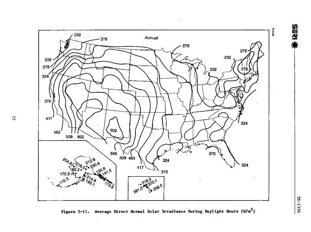
the s i t e * The ordinate i s then muztiplied by the product of the c o l l e c t o r op t i ca l ef f ic iency and an average i r rad iance l e v e l to a r r i v e a t <c, the average annual energy co l l ec t ion rate per u n i t of co l l ec to r area. Note t h a t , f o r parabolic trough co l l ec to r s , the ordi a t e is mult ipl ied by the average annual- d i r e c t -normal i r radiance plus 50 W / 2 . * In re fe r r ing t o Fig. 5-12 f o r parabolic troughs, both north-south and east- west rotat ional-axis o r i en ta t ions a r e shown. I f land o r rooftop a r e a consid- e ra t ions do not preclude north-south or ienta t ion, i t is bes t t o u t i l i z e the north-south performance curves because of t h e g r e a t e r annual energy del ivery associated with t h i s or ienta t ion. The f l a t -p la te and evacuated-tube performance curves a r e f o r c o l l e c t o r panels t h a t a r e oriented south and t i l t e d from hor izonta l a t t h e l a t i t u d e angle. This i s optimum f o r c o l l e c t o r systems t h a t operate year round a s i s t h e case f o r most IPH appl ica t ions- (A more de ta i l ed dimension of Fig. 5-12 is contained i n Sec. 6.1.)

The average annual energy c o l l e c t i o n predic t ion jus t obtained i s used t o nor- malize t h e t o t a l s o l a r system cos t ( see Sec. 10.1.2) t o provide a measure of the cos t ef fec t iveness of t h e p a r t i c u l a r type of col lec tor . This measure i s o f ten ca l l ed capacity cost . m e lower the capaci ty cos t is, t h e b e t t e r t h e investment- This measure can, therefore , be used t o judge which c o l l e c t o r type is bes t su i t ed f o r a p a r t i c u l a r i n d u s t r i a l p lant and process. While t h e procedure y ie lds a measure i n ' u n i t s . of energy cos t , note t h a t t h i s value i s not the a c t u a l cos t of energy. These values a r e intended only f o r comparing co l l ec to r system options. Determining t h e a c t u a l cos t of del ivered energy requires many o the r f a c t o r s not included i n t h i s procedure, and, therefore , a

. l i fe-cycle economic ana lys i s i s necessary (see Sec. 10.2).

5.3.2 Other Considerations in Selecting an Appropriate Collector

While capacity cos t ( t o t a l i n s t a l l e d system c o s t divided by annual co l l ec ted energy) should be a major f a c t o r i n deciding which co l l ec to r is b e s t f o r t h e IPH system, o ther f a c t o r s should a l s o be considered. Some of these a r e a s follows:

Determine i f f l a t - p l a t e glazing mater ia ls o r parabolic-trough r e f l e c t o r mater ia ls d e t e r i o r a t e r ap id ly because of i n d u s t r i a l contaminants a t t h e solar IPH s i t e by placing mater ia l samples a t t h e s i t e a s ea r ly a s possible.

Consider t h e maintenance and replacement c o s t s t h a t each type of collec- t o r might require. Maintenance and replacement c o s t s a r e not included i n capacity cos ts , but they ce r t a in ly a f f e c t the life-cycle c o s t of the s o l a r system.

Determine i f t h e i n d u s t r i a l p lan t has maintenance personnel t o r e p a i r and maintain a tracking co l l ec to r . Parabolic trough co l l ec to r s may requ i re maintenance and replacement of e l e c t r i c motors, gear reducers, bearings, and sun-tracker e lec t ron ics , f o r example.

2 *This ex t ra add i t ive i r r ad iance of 50 ~ / m is necessary only because i t permits a b e t t e r empirical c o r r e l a t i o n of annual performance.

I f a rooftop a r e a is being considered f o r placement of t h e c o l l e c t o r s , determine i f t h e roof i s s t r u c t u r a l l y adequate f o r t h a t purpose. I f it i s not , consider t h e roof modificat ions t h a t each type of c o l l e c t o r would necess i ta te .

ASHRAE Standard 93-77. Collector Test Procedure of t h e American Society of Heating, Refrigerat ion, and Air Conditioning Engineers. 343 W. 43rd St., New York, NY.

ASTM Document No. 127. "Test Method f o r Determining t h e Thermal Performance of Tracking Solar Collectors." American Society fo r Test ing and Materials.

Casamajor, A. B.; Parsons, R. E. 1979 (Jan.). Design Guide f o r Shallow Solar Ponds. UCRL-52385 (Rev. 1). Livermore, CA: Lawrence Livermor e Laboratory.

Duffie, J. A * ; Seckman, W. A. 1974. Solar Energy Thermal Processes. New York, NY: John Wiley and Sons.

Edesess, M.; Henderson, J. ; Jayadev, T. S. 1981 (Revised). A Simple Design Tool f o r Sizing Solar Ponds. ~ E R 1 / ~ ~ - 3 5 1 - 3 4 7 ~ . Golden, CO: Solar Energy Research I n s t i t u t e .

Franta, G.; e t a l . 1981 (Jan.). Solar Design Workbook. s~RI/S~-62-308. Golden, CO: Solar Energy Research I n s t i t u t e .

Gee, R. C., 1982 (May). An Experimental Performance Evaluation of Line-Focus Sun Trackers. SERIITR-632-646. Golden. CO: So la r Enerm Research I n s t i t u t e .

Gee, R. C.; e t a l . 1980 (Mar.). Long-Term Average Performance Benef i t s of Parabolic Trough Improvements. SE~1/TR-632-439. Golden, CO : Solar Energy Research I n s t i t u t e .

Harrison, T. D. 1980 (Nov.). Midtemperature Solar Systems Test F a c i l i t y Program f o r Predic t ing Thermal Performance of Line-Focusing, Concentrating Solar Collectors. SAND80-1964. Albuquerque, NM: Sandia National Laboratories.

Lunde, P. J. 1980. Solar Thermal Engineering. New York, NY: John Wiley and Sons.

Mather, G. R., Jr. 1980 (Nov.). "AS- 93-77 Instantaneous and All-Day Tests of the Sunpak Evacuated-Tube Collector." Journal of Solar Energy Engineering. Vol. 102.

Rabl, A. 1976. "Comparison of Solar Concentrators." Solar Energy. Vol. 18; p. 93.

Solar Energy Research I n s t i t u t e . 1981 (Nov.). Solar Ponds: A Selected Bibliography. ~ ~ ~ 1 / ~ ~ - 7 5 2 - 7 1 1 . Golden, CO: Solar Energy Research I n s t i t u t e .

Sun Designs. 1982 (July). Solar Collector Data Manual. SERI/TR-254-1515. Golden, C0: - Solar Energy Research I n s t i t u t e .

Tabor, HI 1980. Le t t e r t o t h e Editor. Solar Energy. V o l . 24; pp. 113-115.

Tabor, H. 1981. "Solar Ponds. " Solar Energy. Vol. 27 (No. 3) : pp. 181-194.

Winston, R. 1974. "Solar Concentrators of a Novel Design." So la r Energy 16; p. 89.

PART XI1

P R E L l M I ~ DESIGN

Because the objective of a solar IPH system is to deliver energy efficiently to a process load, we need an accurate 'method of calculating the performance of that solar system. Further, to size the system components and to help make the trade-offs necessary in using any solar system, we must have a performance analysis that takes into account the impact of all important parameters. Such a system performance analysis should be efficient, accurate, easy to use, and not require the use of a computer. This section presents some performance analysis design tools that were developed to meet all these requirements,

Many of these design tools were generated with the help of a detailed hour-by- hour computer model, SOLIPH. Thousands of SOLIPH runs were made to formulate generalized design tools . The primary difficulty encountered in developing these tools was the number of variables that affect annual system performance. Because there are so many variables, detailed hour-by-hour computer models are often utilized during the design stages of a solar system. This can make the process very time-consuming and significantly increase system design costs. However, by grouping variables into physically meaningful groups and using regression analysis techniques, we can correlate the performance of solar systems with a great degree of accuracy and display the results graphically. The methodology used to generate these design tools was influenced greatly by the -- work of A r i Rabl. The simplified energy collection correlations he formulated (1981) provided valuable insight and greatly aided development of the design tools presented here- The IPH system computer model and a comparison of its results with other computer codes is contained in Appendix C. Our design tool methodology is presented in more detail in Appendix D, along with the accuracy (rms error) of each design tool. The reader is cautioned that the energy pre- diction design tools were developed for the continental United States only, and use in other areas can result in less accuracy than that indicated in the Appendix.

Each subsection in this section addresses one aspect of IPH system performance and presents design tools for predicting its impact on the annual performance of the entire IPH system. The annual energy collection design tool introduced in Sec. 6.1 is the fundamental correlation upon which the performance analysis is based. It is applied to a variety of IPH system configurations for hot air, hot water, and steam systems. Section 6.2 describes how to account for incident-angle modifier effects and end losses (for a parabolic trough) on an annual basis. In Sec. 6.3, annual correction factors for row-to-row shading losses are presented. Section 6.4 provides a method of calculating annual losses from field piping, including steady-state losses, overnight losses, and freeze protection losses. Section 6.5 presents annual correction factors that account for downtime ?nd utilization of the solar system. Section 6.6 summarizes the design tool information step-by-step.

6-1 ANNUAL ENERGY COLLECTION FOR SKVERAL IPB SYSTEM CONFliGIJRATIONS

The first step in determining how much energy is delivered from the solar system to the process load is to calculate how much energy is produced by the collector field. Energy collection depends on the type of collector, its

f l u i d s p e c i f i c heats , heat exchanger ef fec t iveness , s torage tank s i z e , process load supply temperature, process load energy requirement, and the hours the process operates. Because the re are so many var iables , de ta i l ed hour-by-hour computer models a r e of ten employed to make IPH system trade-off decisions and t o s i z e various components. Fortunately, some of these va r iab les can be accounted f o r i n closed-form analysis . .Other key var iables have been appro- p r i a t e l y grouped and corre la ted empirical ly with the annual performance r e s u l t s of SOLIPH. The resu l t ing basic annual energy cor re la t ion is presented here, and its appl ica t ion to s p e c i f i c IPH system configurat ions is t r ea ted i n subsections t h a t follow.

A s shown i n Sec. 5.0, the instantaneous energy co l l ec t ion of a co l l ec to r can be described i n the form

The heat t r a n s f e r ef f ic iency fac to r FR accounts for the temperature r i s e across the c o l l e c t o r and the r e s u l t a n t decrease i n energy c o l l e c t i o n due t o t h i s e levat ion i n co l l ec to r operating temperature. This f a c t o r , as shown in Sec. 5.2, is calcula ted a s

Equation 6-1 is useful when the c o l l e c t o r i n l e t temperature is known. I n d i r e c t hot water and a i r systems (see Figs. 4-1 and 4-3), the c o l l e c t o r i n l e t temperature is the load re turn temperature. However, i n i n d i r e c t systems t h a t incorporate a heat exchanger between the co l l ec to r loop and the load (see Figs. 4-2 and 4-4), the co l l ec to r i n l e t temperature is higher than the load r e t u r n temperature because of the f i n i t e heat t r ans fe r area of the heat exchanger. The co l l ec to r i n l e t temperature is a l so not s p e c i f i c a l l y known f o r steam systems. A s we show l a t e r i n t h i s sec t ion, simple modifiers can be developed t h a t account f o r the e f f e c t s of intermediate heat exchangers, unfired bo i l e r s , and steam f l a s h tanks. We def ine t h i s system-dependent modi- f i e r to be Fs. With it, energy co l l ec t ion can be wri t ten as

Here, Tin is a known temperature which i s a l so dependent on system configura- t ion . In hot a i r and hot water systems, Tin i s the load re tu rn temperature; i n steam systems, Tin i s the sa tura ted steam temperature. Although Eq. 6-3 is useful i n defining instantaneous performance, i t does not quantify the most important quantity--long-term average performance of a co l l ec to r . We need only three primary quan t i t i e s t o quantify long-term co l l ec to r performance (see Appendix D): pr imari ly the i n t e n s i t y r a t i o , the geographic l a t i t u d e , and the product of c o l l e c t o r op t i ca l e f f i c i ency and the average i n t e n s i t y of the sun's i r r a d i a t i o n during daylight hours a t the s o l a r site.

The in tens i ty r a t i o i s the c r i t i c a l i n t e n s i t y of the co l l ec to r divided by t h e aveEage i n t e n s i t y of the sun's i r radiance during daylight hours and is denoted a s I. The c r i t i c a l i n t e n s i t y of a co l l ec to r i s tha t i r radiance a t which heat l o s s just balances heat gain. A co l l ec to r ' s c r i t i c a l i n t e n s i t y (based on 4380 annual daylight hours, or an average of 12 hours per day per year) is calculated a s

F R U L ( T ~ ~ - Ta) c r i t i c a l i n t e n s i t y =

F R ~ 0 .

A l l the quan t i t i e s necessary t o def ine the i n t e n s i t y r a t i o a r e readi ly avai l - ab le and, therefore, provide a simple method fo r ca lcula t ing energy collec- t ion . Simple empirical co r re la t ions fo r energy co l l ec t ion based on the i n t e n s i t y r a t i o a re shown graphical ly i n Flg. 6-1 (which i s Fig. 5-12 with the addi t ion of polynomials fo r use with hand ca lcu la to r s ) . Evacuated-tube and f l a t - p l a t e co l l ec to r s a r e assumed t o be or iented south and t i l t e d a t the lat- i tude angle. Parabolic troughs a r e assumed t o be mounted hor izonta l ly .

To use the f igure , f i r s t def ine the i n t e n s i t y r a t i o , which is the var iable grouping

Both FRUL and FRmo are co l l ec to r propert ies. The co l l ec to r o p t i c a l e f f i c i ency term FRno is often lowered t o account f o r the long-term o p t i c a l degradation of -

the co l l ec to r from d i r t and dust . The amount by which FRn, should be reduced is highly s i t e dependent and should be based on observed degradation of mater- - i a l samples placed a t the s i t e (see Sec. 3.1). I is the long-term - average i r radiance during daylight hours fo r the s i t e being considered. 1 is t o be taken a s for parabolic troughs (see Fig. 5-11). For f l a t -p la te and evacu-

b ated-tube co l l ec to r s , use yh(see Fig. 5-10). T, is the average annual daytime temperature fo r the s i t e (see Appendix F). The correc t temperature t o use for Tin depends on the configurat ion of the system. Use the load re tu rn tempera- t u r e of the process for hot air and hot water systems, and use the sa tura ted steam temperature fo r steam systems. This is explained more f u l l y i n the sub- sec t ions t h a t follow.

With the x-axis defined, the quant i ty [ h /FsFRn can be read d i r e c t l y from the graph along the y-axis fo r the l a t i t u d e o f the s i t e . Multiplying t h i s ordinate value by the product of Fs, FR, the c o l l e c t o r op t i ca l ef f ic iency, and .$he appropriate annual average daytime i r r a d i a t i o n r e s u l t s i n the quant i ty q,, which is the annual average energy collect ion' r a t e , per u n i t of co l l ec to r a rea , fo r the unshaded co l l ec to r f o r a co s t a n t value of Ti,. Note t h a t , for parabolic troughs, an add i t iona l 50 W/n? is. added to the annual average i r rad iance used on the y-axis, which allows a b e t t e r empirical f i t than one based on the annual average i r rad iance alone. * Note tha t the parabolic trough performance curves extend t o i n t e n s i t y r a t i o s of 0.7, while for f l a t p l a t e s and evacuated tubes they extend t o 1.4. This is cons i s t en t with the operat ing temperature range i n use fo r each type of col- l e c t o r . This covers temperatures up to about 9 0 ' ~ for f l a t p la tes and up t o about 300'~ fo r parabolic troughs. Because a f l a t -p la te c o l l e c t o r loses more heat a t 9 0 ' ~ than a parabolic trough does a t 300°c, the curves extend t o higher i n t e n s i t y r a t i o s f o r flat pla tes .

*If a second-order ef f ic iency equation is provided by the c o l l e c t o r suppl ier , use the UL value a t the load temperature. As noted i n Sec. 5.2, UL should be evaluated as UL = ULS1 + UL,$T1 - Ta).

Another characteristic of these curves is that those for flat plates are well above those for parabolic troughs at low intensity ratios. This is so because f lat-plate and evacuated-tube curves are based on average daytime total horizontal irradiance, but parabolic-trough curves are based on average daytime direct normal irradiance. For many sites., direct normal irradiance values can be significantly higher than the total horizontal irradiance values. Only one curve is shown for east-west rotational axis troughs. In that particular orientation, performance is essentially independent of site latitude, because the incident angle of incoming irradiance is the same for all latitudes. Note that the north-south orientation outperforms (on an annual basis) the east- west orientation, but they approach each other at high latitudes. Shading losses tend to further diminish this performance difference, as shown in Sec. 6.3.

The annual performance of a parabolic trough with a rotational axis oriented between north-south and east-west limits is typically between that of a north- south trough and an east-west trough. At some sites, performance may be slightly enhanced with a small off-north-south orientation because of weather patterns marked by very cloudy mornings or afternoons. However, this asym- metry is usually slight on an annual basis, and the annual performance of a parabolic trough oriented between north-south and east-west can be approximated (Harrigan 1981) by:

- q c , w + Pc,n-s + qc,n-s - qc,e-w qc s8 axis - 2 2 cos(2 eaXis) 3 (6-4)

where

. qc,O,is = annual energy collection rate of trough with rotational axis

between east-west and north-south .

- annual energy collection rate of east-west rotational axis qc,e-w .- trough (from Fig. 6-1) .

qc,n-s = annual energy collection rate of north-south rotational axis trough (from Fig. 6-1)

axis = direction of trough rotational axis measured from south (north-south = oO, east-west = 90').

Note that the polynomial expressions for the annual collector performance curves are provided at the bottom of Fig. 6-1. These polynomials are given for those wishing to use a hand-held calculator rather than the graphical representations.

H o t Water and H o t Air Systems

An indirect hot water or hot air system is shown in Fig. 6-2. The term "indirect" is used to denote that a heat exchanger is used between the collector loop and the load. As noted in Sec. 6.1, this heat exchanger affects system performance because the temperature of the fluid entering the collector system is higher than the process return temperature. The heat exchanger factor Fx

can be used to account for this effect (dewinter 1975). The heat exchanger factoriC is defined as

where E is heat exchanger effectiveness. Therefore, for hot air and hot water systems, the system-dependent modifier Fs is equal to Fx. Also, for hot air and hot water systems, the process return temperature is used for T in referring to Pig. 6-1. If a heat exchanger is not part of the system &?.e., it is a direct system), set Fs equal to unity.

Figure 6-2 shows a collector flow loop and a secondary loop. If no storage is provided, the secondary loop fluid must be delivered to the process load. If storage is added, the secondary loop fluid can either be delivered to the process load or stored for later use. Whether to choose a storage or a no- storage system depends to a great extent on the hours that energy is needed by the process, and such process heat requirements are governed by the production schedule of the industrial plant. Typically, industrial plants operate on either a single-shift, two-shift, or three-shift schedule, so that process loads of 8, 16, or 24 hours per day are common. A no-storage system and two systems with storage are described in the subsections that follow.

I o rrocess g I or Storage

0

I I Exchanger

I Process Return

Pump Pump

Figure 6-2. An Indirect Solar FIot Water or Hot Air System

q qua ti on 6-5 assumes that the collector loop flow capacity rate is less than or equal to the load loop flow capacity rate. A more general form is given in Sec. 7.5.

6.1.1.1 Htorage IPE System

An IPH system without s torage would be configured a s shown i n Fig. 6-2. When- ever s o l a r energy i s co l l ec ted , both pumps a r e turned on, and a l l t h e r e t u r n water (or a i r ) - i s heated a s i t passes through t h e heat exchanger. The collec- t o r system should be s i zed so t h a t , under t h e best condit ions f o r s o l a r col- l ec t ion , t h e heated f l u i d does not exceed t h e required process temperature, Thus, when t h e c o l l e c t o r s a r e producing l e s s than t h e i r peak energy output , t h e heated process f l u i d leaves the hea t exchanger a t less than the required process temperature. The additforial energy needed t o bring t h e preheated f l u i d t o t h a t temperature must be supplied .by a back-up boile@ which is placed i n s e r i e s with t h e s o l a r heat exchanger.

A no-storage s o l a r system should be considered f o r i n d u s t r i a l p lants with process loads t h a t occur during a l l o r nea r ly a l l daylight hours. I f t h e p lant opera tes only a s ing le s h i f t (8 hours) per day, t h e no-storage system i s not a good choice because the re w i l l be too many dayl ight hours when no process load ex i s t s . During such nb;load periods, c o l l e c t a b l e energy is l o s t , which can s i g n i f i c a n t l y reduce t h e annual performance of t h e c o l l e c t o r system.

The no-storage system is a l s o a poor choice i f t h e i n d u s t r i a l plant shu t s down on weekends. Without s torage, co l l ec tab le energy is l o s t two days of every week. This s ign i f i can t ly reduces t h e c o s t ef fec t iveness of the s o l a r system. But a no-storage s y s t e m i s a good choice f o r i n d u s t r i a l p lants having daytime, 7-day-per-week loads. Many two- .and three-shi f t i n d u s t r i a l operations f a l l i n t o t h i s category.

To s i z e the co l l ec to r a rea f o r a no-storage system, we follow the guidel ine t h a t under t h e bes t condit ions f o r s o l a r c o l l e c t i o n , t h e s o l a r c o l l e c t o r f i e l d should not produce more energy than t h e process can use. This i s consis tent with the be l i e f t h a t no col lec ted energy should ever be dumped. Actually, a small amount of dumping i s economTcally j u s t i f i e d [Gordon and Rabl (forthcoming) j . But t h e economic advantages of a s l i g h t l y oversized system over a no- dump system a r e s l i g h t . For purposes of preliminary s o l a r system design, t h e no-dump philosophy is e n t i r e l y adequate.

To f ind the maximum c o l l e c t o r a rea needed f o r a no-storage system, we simply equate the r a t e a t which the process load requ i res energy t o the rate a t which t h e co l l ec to r f i e l d can de l ive r energy under the best s o l a r c o l l e c t i o n conditions:

*The impact of operating a b o i l e r a t v a r i a b l e heating r a t e s i s discussed i n Appendix A.

where

Imax = peak i r radiance ava i l ab le t o co l l ec to r

Ta ,max = highest expected ambient temperature.

zg 2 It is su gested tha t Lx be s e t t o 1000 W/m f o r parabolic troughs and to

1100 W/m fo r f l a t -p la te and evacuated-tube co l l ec to r s . These values may be s l i g h t l y too high for some locat ions and s l i g h t l y too low f o r o thers , but on the average they represent good design values. The design value of high ambi- e n t temperature may be estimated fo r the s i t e from ASHRAE 99% guidelines (ASHRAF, 1981). Alternatively, a value of 4 0 ' ~ may be used s ince it represents a typ ica l maximum temperature fo r much of the United States.

Values fo r FRno and FRUL a r e taken d i r e c t l y from the performance data of t h e co l l ec to r . Tin i s the process re tu rn temperature, and F i s the heat exchanger f a c t o r (see Eq. 6-5), which is a function of the ezfect iveness of the heat exchanger. Again, i f no heat exchanger is present , use Fx = 1.

After determining a l l the appropriate values, we solve for the maximum col lec- t o r area f o r a no-storage system a s follows:

This co l l ec to r area represents the maximum; smaller co l l ec to r f i e l d s can a l s o be used with a correspondingly smaller amount of f o s s i l f u e l energy displacement. I f , f o r example, ava i l ab le land is l imited, a c o l l e c t o r area smaller

than Ac ,max may be necessary.

The annual performance of the so la r system can be predicted using Fig. 6-1. Use the process re turn temperature for Tin and the calculated value of Fx f o r Fs. Assuming t h a t the no-storage system configurat ion has been se lec ted because a process load e x i s t s during a l l daylight hours, the t o t a l annual energy col lec ted is calculated a s

where

Qc = t o t a l annual average energy co l l ec t ion

qc = annual average energy co l l ec t ion r a t e per u n i t of c o l l e c t o r a rea during daylight hours (from Fig. 6-1)

A, = col lec tor area (< A,,,, 1

Ndaylight = number of daylight hours i n year (= 4380).

The t o t a l annual process load is a s follows:

where

tload = average process load energy r a t e {= 1; c ( T ~ - T ~ , ~ ) J } load p

Nload = nmber of hours load operates during the year.

Now, the s o l a r f r a c t i o n ( f r a c t i o n of t o t a l process load t h a t i s displaced by s o l a r energy system) can be ca lcu la ted as:

An example i l l u s t r a t e s t h i s procedure. A chemical =nu£ ac tu r ing plant near Columbus, Ohio, is considering adding a s o l a r system t o provide some of i t s process heat. Chemical r eac t ion vesse l s a r e heated 24 hours per day, 7 days per week with 1 2 0 ~ ~ hot water. After heating t h e react ion vesse l s , t h e water is returned a t 9 0 ' ~ fo r r ehea t . The chemical plant uses 38,000 kg/h (84,000 Ib/h) of hot water f o r t h i s chemical process. The 24 h/day load ensures t h a t a process load e x i s t s during all . daytime hours; hence, a no- storage system is a good choice.

The roof a rea of t h e p lant i s too c lu t t e red with v e n t i l a t i o n equipment t o accommodate s o l a r co l l ec to r s . However, the p lan t has 2.5 a c r e s of vacant land adjacent t o it. F i r s t , we must ca lcu la te how much of the 2.5 ac res of land may be used for the s o l a r system, assuming a ground cover r a t i o (co l l ec to r aper ture width divided. by row-to-row spacing) of 0.4- Then, we c a l c u l a t e t h e s o l a r f r ac t ion t h a t t h e c o l l e c t o r s can meet.

Assume t h a t evacuated-tube c o l l e c t o r s w i l l be used t h a t have t h e following performance c h a r a c t e r i s t i c s (as t e s t e d with a water f l o w r a t e through t h e col- l e c t o r s of 0.02 kg s-' mo2) :

The co l l ec to r loop w i l l 'use a hea t t r a n s f e r f l u i d other than water because of both freeze protect ion concerns and t h e load temperature requirement of 120°C. Because the process load loop uses water, a heat exchanger between the two loops is necessary. Assme t h a t fhe heat exchanger fac to r F, has a value of 0.95. The process load use r a t e , Qload, 1s calcula ted a s

Based on t h i s load use ra te , t h e maximum c o l l e c t o r area f o r the no-storage system i s calculated (see Eq. 6-7) as

TR-1356 san

Using t h i s co l l ec to r area and a ground cover r a t i o of 0.4, land requirements are

o r about 1.4 acres of land area.

Because the assumed co l l ec to r FRUL and FRqO values correspond only t o the t e s ted flow capacity rate, i t is necessary t o adjus t t h e i r values for the act- u a l flow capacity of t h i s applicat ion. Using a co l l ec to r loop flow r a t e equal t o half the load flow r a t e (see Sec. 7.5.4), adjustment of FR fo r d i f f e r e n t flow capac i t i e s , as shown by Lunde (1981), can be calculated a s

('R'L) old - (FRuL) old

2(;c ) p new 2( m t p l

Therefore, the FRUL and FRno values assumed a re 3.5% too high. This correc- t i o n is small enough tha t it is not necessary to reca lcu la te a new value of

Ac,max' After i s an approximate value. However, the FR correc- t i o n should be included i n the annual performance ca lcula t ions . To do so, use correc ted FRqo and FRUL values of

With these values,* Fig. 6-1 can help t o provide an annual energy c o l l e c t i o n predict ion. Because the co l l ec to r is an wacuated tube, the correc t T value t o use is average daytime t o t a l hor izonta l i r radiance . The annual average t o t a l horizontal i r radiance during daylight hours a t Columbus i s about 350 w/m2 . (as read from Pig. 5-10). The annual average ambient temperature i s 1 3 O ~ (from Appendix E) . The value of the i n t e n s i t y r a t i o (x-axis of Fig. 6-1) is, therefore,

For the 40' l a t i t u d e of Columbus this provides a y-axis value of 0.81. Now, qc can be calculated as

The total annual energy col lec ted can be ca lcula ted (from Eq. 6-9) as

g, = (156 w/m2)(2250 m2) (4380 h)

The t o t a l annual process load i s

The so la r f r a c t i o n i s then given as

6-1.1-2 M i x e d - T d , Recirculation Ill3 System

A mixed-tank, r ec i rcu la t ion (four-pipe storage) system such as tha t i l l u s - t r a t e d i n Fig. 6-3 i s h i s t o r i c a l l y the most common configurat ion fo r a system with storage. This configuration has been used i n severa l I W systems and i n almost all so la r domestic hot water systems. As noted i n Sec. 4.4, t h i s con- f igura t ion is best su i ted for appl ica t ions where the load is not continuous, o r where the temperature d i f ference between load supply and load re turn is

*As we describe l a t ex , incident-angle modifier e f f e c t s can be included with a modification of the FRq0 term.

Figure 6-3. Mixed-Tank Recirculation System

s m a l l . * The s torage tank has two i n l e t s and two o u t l e t s , one p a i r f o r each of t h e flow loops. The s torage tank i s assumed t o be completely mixed a t one average temperature. This is s l i g h t l y conservative from a performance view- point , because a small amount of thermal s t r a t i f i ca t i ' on usually occurs wi th in t h e tank.

A mix valve is shown i n Fig. 6-3. This valve is needed s o t h a t t h e tempera- t u r e of t h e f l u i d provided t o the process w i l l not exceed t h e required process temperature. The valve mixes some of the process r e t u r n f l u i d with the ho t f l u i d from t h e storage tank t o maintain a temperature a t o r below t h e process temperature. When t h e s torage tank i s below t h e required process temperature, t h e mix valve is f u l l y open, and no f l u i d bypasses t h e s torage tank.

The mixed-tank rec i rcu la t ion system shown i n Fig. 6-3 has a hea t exchanger between t h e co l l ec to r loop and the s torage tank/load loop. This h e a t exchanger i s usually used i n conjunction with a nonfreezing f l u i d i n the col- l e c t o r loop. I n t h a t case, the heat exchanger f a c t o r should be ca lcula ted as shown i n Eq. 6-5. When t h e same f l u i d i s used throughout t h e system and no hea t exchanger i s present , s e t F, = 1.

The hea t exchanger f a c t o r allows us t o use t h e i n l e t temperature on the cold s i d e of t h e hea t exchanger a s the value on which t o base performance. I n t h e

*An a l t e r n a t e mixed-tank, r e c i r c u l a t i o n (two-pipe storage) system conf igura t ion t h a t allows bypass of s torage i s described i n Sec. 4.4.

9 4

no-storage system configuration, the cold s ide i n l e t is simply the process load re turn temperature. I n the mixed-tank rec i rcu la t ion system, the cold s ide of the heat exchanger i s fed by the storage tank. However, the storage tank temperature is not constant, because it heats up and cools down during the day as energy is added or removed from the tank. Therefore, another performance modifier is introduced that r e l a t e s the storage tank temperature to a known temperature-the process load re turn temperature. Because t h i s modifier accounts fo r the e f fec t s of the storage tank* and is also a strong function of the process load prof i le , it is known a s the load-storage modifier. Appen- dix E derives the functional re la t ionships important to it. For a specified col lector type and load prof i l e , three var iable groupings define the load- storage modifier:

The f i r s t term is the r a t i o of the average energy col lect ion r a t e of the col- l ec to r f i e l d (assuming i n f i n i t e storage s ize ) divided by the average process load demand ra te . The second term accounts fo r the size of the storage tank r e l a t i ve to the s ens i t i v i t y of the co l lec to rs t o increased temperature. The t h i rd accounts fo r the heat withdrawal r a t e from storage as defined by the load flow capacitance. Figures 6-4 t o 6-11 graphically represent the load- storage modifiers for single-shift (8 h/day) and three-shift (24 h/day) load prof i les . Seven-day-per-week operation is assumed. A separate f igure i s given for f l a t p la tes , evacuated tubes, north-south parabolic troughs, and east-west parabolic troughs.

A separate f igure is needed for each of the two trough or ienta t ions because of t he i r d i f fe ren t seasonal outputs (due t o incident-angle e f fec t s ) and t he i r subsequent impact on annual performance . The north-south or ienta t ion shows a greater drop i n performance than tha t of the east-west or ienta t ion a s the r a t i o of col lect ion r a t e to load r a t e increases (moving to the r igh t along the x-axis). This is the r e su l t of the large var ia t ion i n energy col lect ion tha t occur seasonally with north-south oriented troughs. A s we increase col lector area, excess energy can be collected during the summer with the north-south or ienta t ion. This drives the average storage temperature up; the r e s u l t is a higher i n l e t temperature to the co l lec to rs and a loss i n col lect ion e f f i - ciency. East-west-oriented troughs vary less i n seasonal output and, therefore , t he i r performance drops l e s s s ign i f ican t ly a s col lector area is increased.

The impact of the energy col lect ion r a t e normalized t o the load demand ra te (along the x-axis) is the most important quantity. As the r a t i o of energy col lect ion r a t e to energy demand r a t e increases, the performance penalty a lso increases. This performance degradation occurs because the co l lec to rs a re providing a larger f rac t ion of the process load, which drives storage tank temperatures up and causes the co l lec to rs to operate a t higher temperatures. Smaller storage capacity, larger co l lec to r UL values, and smaller load flow

*The load-storage modifier a l so accounts fo r the impact of the mixing valve and load flow ra te .

rates also result in larger performance losses and storage-load modifiers far- ther below unity.

Three storage sizes are shown, as defined by the values of [(Mc ) (A FxFRU~)]. They span the range of storage capacity typically considePe3 for sosar systems. Note that storage capacity is considerably less important to annual performance for the single-shift load profile than the three-shift load profile. Storage size is more important for a 24-hours-per-day load because storage can considerably extend the number of hours that part of the load can be met with stored solar heat. For example, stored heat may permit energy to be withdrawn from the tank late into the evening. In the single-shift load, no load exists in the late afternoon or evening; thus, stored energy can be withdrawn only during cloudy, daytime periods.

The curves shown on Figs. 6-4 to 6-11 extend over the range of storage capacitance, load flow rates, and ratios of collection rate to load demand rate for which SOLIPH computer results were generated. These ranges are in part defined by the range in process load temperatures that was considered: up to 90°c for flat plates, up to 1 5 0 ~ ~ for evacuated tubes, and up to 3 0 0 ~ ~ for parabolic troughs. Zxtrapolation beyond these limits is not recommended.

The annual performance of a mixed-tank, recirculation system can now be predicted by first using Fig. 6-1 to determine the annual energy collection rate of the collector. Use the process load return temperature for Tin and use the calculated value of F, for Fs if a heat exchanger is present. Now, use the result to compute the load-storage modifier for a given storage size, collector area, load flow rate, load demand, and collector UL value. Because the load-storage modifiers are defined by three quantities, interpolation may be necessary for two of the quantities when reading from Figs. 6-4 to 6-11.

The total annual energy collected by a mixed-tank, recirculation system is calculated as

where

Qc = total annual average energy collection

9c,, = annual average energy collection rate during daylight hours (from Fig. 6-1)

Ac = collector area

= annual load-storage modifier (from Figs. 6-2 to 6-9)

Ndaylight = number of daylight hours in year (= 4380) . The total annual process load is

where

bead = average process load energy demand [= kloadCP(~a - %,r ) ]

ITload = number of hours load operates during the year , Now, the s o l a r f r a c t i o n can be calculated a s

The following example i l l u s t r a t e s the procedure. A so lar i n d u s t r i a l process heat system is t o be i n s t a l l e d a t a medium-sized f lu id d k - p r o c e s s i n g plant located i n Fort Worth, Texas .* A major use of low-temperature process heat i s t o generate hot water f o r c l e a n u p . A minimum water temperature of 43 '~ ( 1 1 0 ~ ~ ) is required t o d issolve milk f a t s . The dai ry uses 16,000 kg/h (35,000 Ib/h) 'of such water from 8 AM t o 4 PM seven days per week. The hot water is produced i n a steam-to-water exchanger and is piped throughout the p lan t to the various wash s t a t ions . I n l e t water temperature is 2 0 ' ~ (68 '~) . The contaminated nature and low temperature of the wash water e f f l u e n t make heat recovery impractical . The da i ry has 800 m2 (8650 f t 2 ) of usable roof space, but much of t h a t is over warehousing; only minimal increases i n roof loads are permissible. -Bowever, the dairy owns three acres of vacant land, within 46 m (150 f t ) of the process building, t h a t are avai lable f o r a s o l a r energy system.

For a thorough ana lys i s , we should compare f l a t-plate , evacuated-tube , and parabolic-trough co l l ec to r s . For purposes of demonstrating the procedure, however, we w i l l examine only f l a t p la tes , because of the very low temperature requirement i n t h i s appl ica t ion. The t o t a l annual load is a s follows:

Let us start by determining how much energy the roof area could provide. A good, single-glazed, select ive-surface f l a t p l a t e would have the following values (from Table 5-1):

FRno = 0.65 - 0.8 + use 0.72

20 'R'L = 2.6 - 4.4 + use 3.1 W/m C .

I n Fort Worth, Tex., the annual average t o t a l horizontal i r radiance during daylight hours is about 400 w/m2 (from Fig. 5-10). The AT needed fo r Pig. 6-1 is the d i f ference between load re tu rn and ambient. The load re tu rn is 2 0 ' ~ and the average daytime ambient i n For t Worth is 21'~. Thus, AT = 0. The

*This example is based upon a case study from a SEBI report by Hooker e t a l . (1980)

value of F w i l l be s e t t o one because no heat exchanger i s expected t o be needed. ?The load re turn water w i l l be c i rcula ted d i r e c t l y through the col lec tors . ) So, the value on the x-axis of Fig. 6-1 is

With l a t i t u d e = 32.s0 and X = 0, Fig. 6-1 y ie lds a value along the y-axis of 1.0.

qC ," - = 1.0 .

Solving fo r , we obtain FsF~nol c ,OD

Now, use Fig. 6-8 t o determine the load-storage modifier. Looking a t Fig. 6-8, we see t h a t for t h i s load p r o f i l e , m i ~ i m a l s torage is needed. We w i l l use a value of 20 h a s our basel ine f o r [(MC )stor/(AcP F U )] .. Since we have an 800 m2 roof, we w i l l start with a co l l&tor area OF %& m2 (ground cover r a t i o of 0.5).

The value of

The process load use r a t e , ?) load' is calcula ted a s

(4.84 x 1012 ~ ) ( ~ ~ t ~ ) - - yr 5 Qload days

= 4.60 x 10 W . (365 7 ) ( 8 &)

We can now ca lcu la te the y-axis value t o be used with Fig. 6-8:

From Fig. 6-8, the load-storage modifier is 0.934.

Now, the annual energy collected by 400 m2 of f l a t -p la te c o l l e c t o r s i s given by

The s o l a r f r a c t i o n is

To increase the s o l a r f r a c t i o n s u b s t a n t i a l l y above 0.35, it would be necessary t o mount c o l l e c t o r s on the land adjacent t o the plant. Select ing the optimum c o l l e c t o r a rea fo r a mixed-tank r e c i r c u l a t i o n system requires a trade-off of the increased energy c o l l e c t i o n tha t occurs as co l l ec to r area is added agains t the increased cos t s of the system. Typical ly, severa l co l l ec to r areas w i l l be se lec ted , and the l i fe-cycle cos t s of these options w i l l be compared.

The c o l l e c t o r a rea with the most favorable l i fe-cycle economics. is usua l ly se lec ted . Sometimes, however, o ther considerat ions d i c t a t e a d i f f e r e n t choice* For example, the land o r roof a r e a ava i l ab le f o r mounting the collec- t o r s may const ra in maximum co l l ec to r area. O r , i f an i n d u s t r i a l p lant must operate a t a c e r t a i n minimum capacity t o be p ro f i t ab le , s u f f i c i e n t c o l l e c t o r a r e a may be i n s t a l l e d so t h a t , i n the event of an in te r rup t ion of foss i l - fue l supply, the s o l a r system can maintain the thermal needs of t h a t minimum capacity.

6 . Imlm3 Variable-Volume Storage System

A variable-volume s torage system is shown i n Fig. 6-12. In t h i s configurat ion there is no r e c i r c u l a t i o n of f l u i d between the storage tank and the c o l l e c t o r f i e l d . Heating the c o l l e c t o r loop f l u i d is accomplished with a s ing le pass through the c o l l e c t o r f i e l d . The hot water i s stored i n a tank t h a t can be completely drained and used by the i n d u s t r i a l process. When so la r energy i s being co l l ec ted , hot water is added to the tank. When a process load e x i s t s and hot water is ava i l ab le i n the tank, the hot water i s pumped from the tank t o the process load. If the i n d u s t r i a l process is an open loop (i.e., the hot water is consumed and not returned f o r r e h e a t ) , the cold tank i s not needed. Make-up water is then supplied from the water main during t h e day. I f t he i n d u s t r i a l process is a closed loop, the r e t u r n water must be stored i n an add i t iona l tank (see Fig. 6-12).

An advantage of the variable-volume s torage system is t h a t the co l l ec to r ar ray is always supplied with t h e coldes t poss ib le f l u i d , whenever i t i s operat ing, regardless of whether the load i s on or of f . I n t h i s respect , it is s imi lar t o a no-storage system. However, because t h i s configurat ion has storage, i t i s an e f f i c i e n t system configurat ion f o r a l l load p r o f i l e s , daytime or night- tie s h i f t s .

Our approach t o the design and performance analys is of a variable-volume system follows the bas ic precept t h a t thermal energy delivered by the c o l l e c t o r system should never be dumped. This no-dump requirement is equivalent to

Variable Volume

Hot Tank Load Supply

Load Return I I L - - Variable-Volume

Cold Tank (Not Needed for

Open Load Loops)

Figure 6-12. Variable-Volume Storage Configuration

s. izing the system so tha t t h e peak d a i l y energy c o l l e c t i o n of t h e s o l a r system does not exceed the dai ly process load. Further, t h e volume of water heated during the day by the c o l l e c t o r s and del ivered t o the s to rage tank should no t exceed the volume of water the process needs. f o r one day of operation. The maximum d a i l y energy co l l ec t ion of the s o l a r system can be est imated a s

where

2 A, = co l l ec to r a rea (m )

4a ,max = maximum da i ly t o t a l i r r a d i a t i o n ava i l ab le t o c o l l e c t o r s per un i t of c o l l e c t o r area

= day-long ef f ic iency of col lec tor .

The day-long e f f i c i e n c y of t h e c o l l e c t o r can be est imated a s

2 where I, daily i s the average i r radiance (W/m ) ava i l ab le t o t h e c o l l e c t o r on 2 a c l e a r day. A value of 650 W/m f o r Ia daily i s a good average f o r clear-day

i r radiance and can be used a s an approx'imation. Values of FRTlo and FRUL can

be taken d i r e c t l y from t h e co l l ec to r performance data sheets . Tin should be set t o t h e process load re tu rn temperature. The maximum ambient temperature can be taken as 40'~. Values of q,,, are provided i n Table 6-1 f o r the various c o l l e c t o r types a t l a t i t u d e s of 24' t o 56'. These values have been derived from clear-day design t a b l e s provided i n t h e ASERAE Handbook of ~unda- ' mentals. The maximum da i ly energy co l l ec t ion obtained from Eqs. 6-15 and 6-16 is approximate but s u f f i c i e n t f o r system design. The cons t ra in t t h a t the maximum energy col lec ted i n one day is l e s s than or equal t o the da i ly process load demand can be expressed a s

Subst i tu t ing front Eq. 6-15, the maximum c o l l e c t o r a rea t h a t can be u t i l i z e d and s t i l l s a t i s f y th i s condit ion is calcula ted a s

The cons t ra in t t h a t t h e maximum volume of water provided t o storage in one day must be less than o r equal t o t h e volume of water used by the process every day can be used t o determine t h e maximum pump mass flow rate.

M - - /t pump c,mx

where

= da i ly process water usage (kg)

c ,,, = maximum operat ing time of pump (co l l ec to r s ) i n one day.

Table 6-1. Maximum Daily Irradiation Available for Several Collector Typesa

Lati tude (degrees)

- -- -- -

Flat-Plate East-West North-South and Evacuated-

b Parabolic Parabolic

Tube Col lec tors Trough Col lec tors Trough Collectors

~ ~ ~ a l u e s are given i n MJ/m2 ( ~ t u / f t * in parentheses).

b ~ a l u e s f o r f l a t p la tes and evacuated tubes a r e f o r c o l l e c t o r s t i l t e d a t l a t i - tude angle.

The maximum operat ing t i m e f o r a parabolic trough can be estimated from t h e number of daylight hours during the longest summer day. The number of hours between sunr ise and sunset on t h e summer s o l s t i c e i s given ( i n hours) by

where L = l o c a l l a t i t u d e of s i te , i n degrees.

Rea l i s t i ca l ly , two hours may be subtracted from t h i s length of time because t h e s o l a r i r r ad iance w i l l no t be s u f f i c i e n t t o maintain c o l l e c t o r opera t ion i n t h e e a r l i e s t morning hour o r l a t e s t afternoon hour. Thus, the maximum operating time of a parabol ic trough, f o r a s i n g l e day, can be approximated ( i n hours) by

With a f l a t -p la te o r evacuated-tube c o l l e c t o r , no energy can be co l l ec ted on a summer day u n t i l the sun i s s u f f i c i e n t l y high i n t h e sky t h a t sunl ight f a l l s on the f ron t of the t i l t e d co l l ec to r . With a c o l l e c t o r t i l t e d a t t h e l o c a l l a t i t u d e angle, a maximum of twelve hours of sunl ight i s ava i l ab le f o r s o l a r co l l ec t ion (Liu and Jordan 1977):

tc,max = 12 f o r f l a t p l a t e s . The flow r a t e determined from Eq. 6-18 w i l l ensure t h a t the volume of water heated by the s o l a r system can always be used by the process; hence, no energy w i l l have t o be dumped. This i s a l s o consis tent with a design philosophy t h a t minimizes the operat ing temperature of the co l l ec to r and, hence, maximizes c o l l e c t o r ef f ic iency, wi th in t h e cons t ra in t s of a single-speed pump and a no- dump requirement.

Having determined the pump flow r a t e , we can now determine the cor rec t value of FR (see Eq. 6-2) f o r any given co l l ec to r a rea up t o A

t,max' t h e maximum

co l l ec to r area f o r which no dumping occurs. Adding c o l ec to r a rea up t o

*c ,max fo r a constant system flow r a t e r e s u l t s i n a lower value of FR because t h e average c o l l e c t o r opera t ing temperature increases. Conversely, decreasing t h e co l l ec to r a r e a lowers t h e average c o l l e c t o r operat ing temperature, and FR approaches one. Now, t h e annual performance of t h e variable-volume s torage system can be predicted us ing only Fig. 6-1. Use t h e process load r e t u r n temperature f o r Tin. AS with t h e o ther systems, i f a heat exchanger is used t h e h e a t exchanger f a c t o r Fx should be ca lcula ted and used a s Fs. The value of FR should be ca lcula ted based on t h e calculated system flow r a t e and t h e collec- t o r a rea being considered. The t o t a l annual energy col lec ted i s then calcu- l a t e d a s

where

Qc = t o t a l annual average energy c o l l e c t i o n . qc

= annual average energy c o l l e c t i o n r a t e during dayl ight hours (from Fig. 6-1)

A, = collector area (c A,,mx 1

Ndaylight = nmber of daylight hours in a year (= 4380).

The total annual process load is

where

Qload = average process load energy rate [= mc (Tg - T ) ] P g,r

Nload = number of hours load operates during the year.

The solar fraction can then be calculated as

6.1.2 Steam Systems

The largest share of the total industrial process heat requirement is currently met by steam. An alternative to generating steam with a packaged steam boiler is a steam-generating solar system. In either case, the steam is delivered to the point of use in a saturated state. This saturated steam is used typically to heat a vessel to drive a chemical reaction, or it may be employed for evaporation, crystallization, etc. The steam is condensed during the process; after treatment, the hot water is returned to the boiler or solar system for revaporization. Generating steam with a solar system requires a significantly different system configuration than that for air or water process heating. Two system approaches to generating steam are considered here: flash steam systems and unf ired-boiler systems. The operating temperatures needed for steam generation ordinarily preclude using water as a heat storage fluid, because an expensive high-pressure storage tank would be required. Instead, an oil is usually the heat-storage medium. Such fluids are quite expensive. Therefore, because storage for steam systems is so expensive, it is not likely to be used widely in the near future and is not discussed here. Information on the performance of steam systems using thermocline storage can be found in Harrigan (1981).

6.1 -2 -1 Unf ired--% ler Steam Systems

In an unfired-boiler steam system (see Fig. 4-4), an organic heat transfer fluid is pumped through the collector field and then to an unfired boiler. The hot fluid within the tubes of the boiler vaporizes the water next to the tubes; this saturated steam is fed to the existing steam header, which delivers energy to the industrial process. As the steam is generated, additional condensate is supplied to the boiler. The hot condensate is assumed to be saturated. Steam generation is a latent-heat process; therefore, no temperature change occurs on the water side of the boiler. Because heat is being transferred from the collector loop fluid to the water, the fluid in the collector loop must always exceed the steam saturation temperature. Therefore,

the temperature of the fluid at the inlet to the collector fluid must exceed the steam saturation temperature. To account for the temperature elevation of the collector loop inlet above the steam temperature, a performance modifier is introduced--the unfired boiler factor, FB. It is calculated as follows:

where

FRUL = the collector heat-loss coefficient

k = collector loop flow rate C

; = collector loop flow rate per unit collector area (= %/A,) C ,

c = collector loop fluid specific heat P

UbAb = unfired-boiler heat transfer coefficient, boiler surface area product.

The unfired-boiler modifier is shown to be a function of the unfired-boiler UA value, the collector loop flow rate, and the collector UL value. The derivation of this modifier is given in Appendix E. It assumes that the collector loop flow rate is constant. A constant collector loop flow rate is usually used for steam systems, although variable flow rate systems that maintain a constant collector outlet temperature are sometimes employed. However, the greater complexity of a variable flow rate system is usually unwarranted. More details on variable flow control systems are given in Sec. 8.0.

The unfired-boiler modifier allows energy collection for an unfired-boiler steam system to be written as

To size the maximum collector area for an unfired-boiler system without storage, follow the guideline that no collected energy should be dumped, the same as for the no-storage hot air and hot water systems. The rate at which the process load requires energy is equated to the rate at which the collector field can deliver energy under the best solar collection conditions:

2 As suggested in Sec. 6.1.1.1, a value of 1000 W/m can be used for parabolic troughs and 1100 w/m2 for flat-plate and evacuated-tube collectors. Also, a maximum ambient temperature (Ta,max ) of 40'~ is recommended. Values of FRno and FRUL are taken directly from the performance data of the collector. Tin should be set to the steam saturation temperature. After all the appropriate values are determined, the maximum collector area for the no-storage system is then solved as

This col lec tor area is the maximum amount t h a t can be used within the no-dump const ra in t . Smaller co l l ec to r f i e l d s can a lso be used with a resu l t ing smaller amount of solar system energy col lec t ion. Now, the annual performance of the solar system can be predicted using Fig. 6-1. Use the unf i r e d bo i l e r f ac to r FB fo r -F and the steam sa tu ra t ion temperature for Tin. The t o t a l annual energy coflected is then calculated a s

where

qc = annual average energy co l l ec t ion r a t e during daylight hours per un i t co l l ec to r a rea (from Fig. 6-1)

A, = co l l ec to r area (( 1

Ndaylight = number of daylight hours i n year (= 4380).

The t o t a l annual process load i s

where

hload = average process load energy r a t e [ = kloadcp(T~ - T Q , ~ ) ]

Nload = number of hours t h a t process load operates during year.

Now, the solar f r a c t i o n can be calculated as

6.1.2.2 Flash Steam Systems

I n a f l a sh steam s o l a r system (see Fig. 4-3), pressurized water is c i rcula ted through the c o l l e c t o r f i e l d and f lashed t o low-quality steam across a throt - t l i n g valve i n t o a f l a sh , or separator , tank. Flashing is a constant enthalpy process that converts the sensible heat of the water in to a two-phase mixture of saturated water and saturated steam a t conditions prevai l ing i n the f l a s h tank. The steam qua l i ty ( f rac t ion of t o t a l mass flow t h a t is flashed t o vap- o r ) usually is l e s s than 10%. Steam separated i n the f l a s h tank i s fed in to the p lant steam d i s t r i b u t i o n system t o be used by the i n d u s t r i a l process. The sa tura ted l iqu id is rec i rcula ted through the col lec tor f i e l d . To maintain the necessary l iqu id level in the f l a s h tank, boi ler feedwater is in jec ted i n t o the pump suction.

To prevent boi l ing within the co l l ec to r s or the co l l ec to r f i e l d piping, the water must be pressurized. Pressure is maintained by the rec i rcu la t ion pump which, i n the simplest control mode, operates a t constant flow. The pump is sized so tha t water ex i t ing the co l l ec to r f i e l d is under s u f f i c i e n t pressure t o prevent boil ing. The co l l ec to r f i e l d o u t l e t temperature must be considerably above the steam delivery temperature t o obtain reasonable steam q u a l i t i e s

downstream of the throttling valve. Higher steam qualities allow the water to be recirculated through the collector field fewer times. Therefore, the average collector operating temperature is usually significantly above the steam saturation temperature. A performance modifier accounts for this temperature elevation--the-flash system factor FF. It is calculated as follows:

where

m = collector loop flow rate per unit collector area C

Ahfg = heat of vaporization of steam at its saturation temperature

c = specific heat of saturated water P

Ts = steam saturation temperature

Tf = feedwater temperature.

The derivation of this modifier is given in Appendix E. It allows energy collection for a flash system to be written as

This is identical to the unfired boiler (Eq. 6-26) except that FF is substi- tuted for FB. Therefore, Eqs. 6-27 to 6-31 can be used for the flash system sizing and performance analysis, using FF.

6 -2 INCIDENT-ANGLE EFFECTS

The incident angle of solar radiation on a solar collector is defined as the angle between the normal-to-the-collector aperture and the direction of the sun. In describing off-normal irradiance, only the direct or beam component of irradiation is considered. Diffuse irradiance does not affect incident- angle corrections because it is nondirectional by.definition.

The incident angle of solar radiation has an impact on energy collection in several ways. First, the intensity of the beam irradiance component available to the collector decreases at offnormal incidence according to the cosine of the incident angle. This effect has been incorporated into the performance curves of Fig. 6-1, because the hour-by-hour computer model from which the figure was generated computed the incident angle for each hour and provided for this correction.

Second, off-normal irradiation typically reduces the optical efficiency of a collector below that for normally incident irradiation. The effect is described by an incident-angle modifier that shows how the optical efficiency

of a collector changes with incident angle, relative to its optical efficiency at normal incidence. The impact of a collectorls incident-angle modifier upon the annual performance of a collector is-described in Sec. 6.2.1.

The third effect .applies to parabolic-trough collectors but not to flat-plate or evacuated-tube collectors. This incident-angle effect, end loss, refers to energy lost from the end of a parabolic trough when the incident radiation is not normal. Some of the radiation reflected at the end of a parabolic concentrator will spill off the end of the row and not be intercepted by the receiver. This loss is accounted for in Sec. 6,2.2,

6.2.1 Incident-hgle Modifiers

The optical efficiency of most collectors decreases as the incident angle of incoming irradiation increases. This is shown in Fig. 5-9, which provides typical incident-angle modifiers of various collectors. In some cases, however, a collectorls optical efficiency can increase with of faormal irradiation. Evacuated-tube collectors without specular reflectors can have incident-angle modifiers that increase with that angle because, as the sun angle gets lower, the effective gap between tubes shrinks and intercepted irradiation increases. Flat-plate collectors decrease in optical efficiency at off- normal incidence because, as incident angles increase, the transmittance of glazing materials and the absorptance of the absorber coatings decrease. Par- abolic troughs exhibit a reduction in optical efficiency at off-normal incidence because of glazing and absorber properties as well as because of the increase in path length of the reflected radiation at off-normal incidence. That increased path length permits a wider spread in the reflected beam and causes the amount of radiation intercepted by the receiver to drop.

For each of the three types of collectors, a typical incident-angle modifier has been assumed in the curves of Fig. 6-1. For energy-collection predictions for collectors with other than these assumed incident-angle modifiers, correction factors are used. Correction factors for flat plates, evacuated tubes, and parabolic troughs are given below.

As noted in Sec. 5.2, the incident-angle modifier for a flat-plate collector can be correlated by an equation of the form:

k,, = 1 - bo[(cos - 11 where bo is the incident-angle modifier coefficient.

Figure 6-1 assumes a bo value of 0.11, which is typical of single-glazed flat- plate collectors with black painted absorbers. However, b values down to about 0.06 have been found, and bo values up to about 0.17 are typical of double-glazed flat-plate collectors. We need a way to account for these differences to provide an accurate collector performance analysis. Figure 6-13 provides a simple graphical correction factor for the performance impact of incident-angle modifiers of flat-plate collectors. The x-axis is simply the incident-angle modifier coefficient bo for the given flat plate. Along the y-axis, the graph provides a value of the annual incident-angle modifier. This annual modifier yields a correction term to the optical efficiency of a

collector that closely accounts for the performance impact of the incident- angle modifier on an annual basis. Note that because a bo value of 0.11 was assumed for Fig. 6-1, the annual modifier for a bo value of 0.11 is one; i.e., no correction is necessary. For bo values other than 0.11 we must correct the optical efficiency term no in Fig. 6-1, on both the x-axis and y-axis.

The incident-angle modifiers of evacuated-tube collectors usually cannot be expressed in the form of Eq. 6-34; therefore, Fig. 6-13 does not apply. Instead, a simple equation helps us to arrive at an annual modifier that closely accounts for incident-angle effects. The evacuated-tube annual modifier correction can be calculated as

The K values are the incident-angle modifiers at the particular incident angle denoted by the subscript. Essentially, Eq. 6-35 breaks up a collector's incident-angle modifier curve into 15O intervals and applies a weighting factor to each interval. These empirical weighting factors are defined largely by the fraction of collectable energy that occurs within each incident-angle span.

Equation 6-35 allows the performance impact of the incident-angle modifier of an evacuated tube to be evaluated quickly even if it is highly irregular, as it is for some evacuated tube collectors. Because the same curves on Fig. 6-1 are used for both flat plates and evacuated tubes, the baseline evacuated-tube incident-angle modifier was assumed to be also given by Eq. 6-34. Therefore, the correction factor calculated with Eq. 6-35 is relative to the same baseline incident-angle modifier as the flat-plate collectors. As before, the modifier calculated with Eq. 6-35 is applied to the optical efficiency in using Fig. 6-1.

Parabolic-trough incident-angle modifiers, like those of evacuated-tube collectors, are not well correlated by an equation like Eq. 6-34. Typically, parabolic-trough incident-angle modifiers decrease more rapidly with incident angle than do those of flat-plate collectors (Gaul and Rabl 1980). To account for these differences, an annual modifier correction (similar to that for an evacuated tube) is provided. The annual incident-angle modifier correction for an east-west parabolic trough is calculated as:

As before, the K values are taken from the incident-angle modifier curve for the collector at the incident angles denoted by the subscript. Because little energy is available for collection at high incident angles, the weighting factor for them is small. Most of the energy available to a parabolic trough occurs at small incident angles; thus, the weighting is greater there.

A general equation with constant weighting factors (of the simple form of Eq. 6-36) is not accurate for north-south parabolic troughs because of the impact that latitude has on the average incident angles of north-south troughs. The weighting factors are a function of the latitude of the site, as shown in Fig. 6-14. The weighting is larger at low incident angles for low latitudes

Incident 'Angle (degrees)

Figure 6-14. Annual Optical Efficiency Incident-Angle Weighting Factors for a North-South Rough

because, a t low l a t i t u d e s , t h e bulk of t h e energy s t r i k i n g a north-south para- b o l i c trough occurs a t low incident angles. A t high l a t i t u d e s , north-south troughs o f t en operate when incident angles a r e high; therefore , the weighting i s smaller a t low incident angles.

6.2.2 End Losses

Radiation sp i l lover , o r end l o s s , from parabol ic troughs of f i n i t e length can be ca lcula ted (Gaul and Rabl 1980) as:

where

Lend = end l o s s f a c t o r (1 - f r a c t i o n l o s t )

f = trough f o c a l length

R = trough length

w = trough aper tu re width

8 = incidence angle.

This equation assumes that the receiver has the same length as the concentrator. The end-loss factor is shown to decrease as parabolic trough lengths increase and incident angles decrease,

Gaul and Rabl (1980) evaluated the all-day average of the end-loss factor for a typical parabolic trough on a seasonal basis. Their results are shown in Table 6-2. An additional column of data has been added for the annual end- loss factor, based on the average of the summer, autumn, winter, and spring end-loss factors. For typf cal parabolic trough drive strings with R / f ratios exceeding 25, the annual end-loss factor is above 0.96.* Therefore, less than 4% of the collectable energy is lost because of end spillage. The annual end- loss factor should be estimated from Table 6-2 for the particular collector drive string to be configured for the IPH collector system, This end-loss factor should then be used to modify the energy predictions computed from Fig. 6-10

6.3 ROW-TO-RW SHADING EFFECTS

Typical IPH collector fields are arranged with multiple rows of collectors. These collector rows are set quite close together to minimize land area requirements and collector field piping. However, this close proximity causes row-to-row shading losses. These shading losses are not accounted for in the curves of Fig. 6-1. The graphs in this subsection quantify these row-to-row shading losses on an annual basis. The analysis of row-to-row shading loss is greatly simplified if end effects are ignored and each row is assumed to be much longer than it is wide, a good approximation for typical IPH collector rows. With this assumption in mind, consider parallel raws of collectors

Table 6-2. All-Day Average of End-LOSS Factors (Lend)

R East-West Axis North-South Axis - f

Summer Equinox Winter Year Summer Equinox Winter Year

- -- .-. . . - -. - - -- - . - - - . - . .- -- - - -

a~op number represents cutoff time one hour before sunset; bottom number represents cutoff time two hours before sunset.

Source: Gaul and Rabl 1980.

*This assumes that the losses that occur between adjacent modules on a drive string are negligible.

(either tracking or nontracking) as shown in Fig. 6-15a. The row-to-row spacing is designated as R and the aperture width of the collector is W. We define the ground cover ratio (GCR) to be the ratio of W to R:

W GCR = - R * (6-38)

First, let us consider the beam component of radiation. Either the beam component is shaded from one row to another, as s h k in Fig. 6-15b, or the beam component is not shaded from row to row, as shown in Fig. 6-15c. Note that when shading does occur, no beam irradiance reaches the ground; that is, all the beam irradiance that would normally reach the ground has been intercepted by the collectors. Hence, the radiation incident on the collector array is

A 1 COS eh , g b

where

Ag = ground area

I,, = beam irradiance (direct normal)

= incident angle of direct irradiance on the horizontal surface.

Whenever no shading occurs, the radiation incident upon the collector is

where

A, = collector area

0 = incident angle of beam irradiance on the aperture of the collector.

Therefore, as given by Rabl (1981), the beam irradiance available per unit of collector aperture area is

I COS eh Ia = Ib * Min cos 8, GCR

Therefore, the direct irradiation available to a collector, including shading effects, is a function of incident angles (which are defined by the collector type and the site latitude) and the ground cover ratio. The collector tilt angle is assumed to be equal to the site latitude.

Now, consider the diffuse component of radiation for flat-plate and evacuated- tube collectors. A fraction of the diffuse component of radiation that would normally fall upon a collector is blocked by the row immediately in front of it. To the extent that diffuse radiation is isotropic (as is typically assumed), the fraction of the diffuse radiation incident on a horizontal surface that is available to a tilted collector can be calculated as the view

f a c t o r of the sky a s seen by the co l l ec to r . This view fac to r can be calcu- l a t e d using a crossed-string method (Jones and Burkhart 1981) as

Fd = 0.5 (1 + [ s in ($ + B)/sin $ 1 - [ s i n &/s in $1) , (6-40)

where the angles $ and B are shown on Fig. 6-15a.

The ground cover r a t i o can be defined i n terms of the angles $ and B a s

GCR = (cos B + s i n B/tan $)'I . (6-41)

Therefore, the f r a c t i o n of d i f fuse rad ia t ion ava i l ab le to a f l a t -p la te or evacuated-tube co l l ec to r is a function of the c o l l e c t o r tilt angle and t h e ground cover r a t i o . The co l l ec to r tilt angle is assumed t o be equal to the s i te l a t i t u d e .

Because the d i r e c t and d i f fuse rad ia t ion losses due t o row-to-row shading a r e p r inc ipa l ly dependent only on co l l ec to r type, site l a t i t u d e , and ground cover r a t i o , they can be expressed i n graphical form a s shown i n Figs. 6-16 t o 6-18. These f igures show annual row-to-row shading correc t ion f a c t o r s a s a function of l a t i t u d e for parabolic troughs, f l a t -p la te co l l ec to r s , and evacuated-tube co l l ec to r s . A s explained above, these correc t ion f a c t o r s account for the l o s s of beam i r r a d i a t i o n and, for f l a t - p l a t e and evacuated-tube co l l ec to r s , the l o s s of d i f f u s e i r r a d i a t i o n due to the reduction i n view f a c t o r from the col- l e c t o r to the sky.

The shading fac to r obtained from Figs. 6-16 t o 6-18 appl ies only t o the rows being shaded--that is, a l l rows but the f i r s t . To account f o r the unshaded row, use the following equation t o compute an average f i e l d shading fac tor :

where

Fshad = shading fac to r a s determined from Figs. 6-16 t o 6-18

N = number of rows i n f i e l d .

Row-to-row shading losses increase' f o r a l l types of c o l l e c t o r s a s s i t e l a t i - tude increases, because the sun is, on the average, lower i n the sky a t high l a t i t u d e s , r e su l t ing i n more shading. Collector rows can, therefore, be spaced much c lose r together a t low l a t i t u d e s than a t high ones. The impact of row-to-row shading l o s s e s is espec ia l ly s i g n i f i c a n t fo r north-south rota- t ional-axis parabolic troughs. Therefore, north-south parabolic troughs should be spaced s i g n i f i c a n t l y f a r t h e r apar t than east-west troughs.

6-4 'ANNUAL IXlSSES CW COLLECTOR FIELD PIPING AND STORAGE

Thermal losses from the co l l ec to r f i e l d piping and storage tank ( i f any) can reduce the energy del ivery of a s o l a r system s ign i f i can t ly . Section 7.0 describes how to arrange co l l ec to r f i e l d piping and how t o determine how much insu la t ion should be added around' the piping and the storage tank. Here, we

describe how t o account for the annual thermal losses from these components, so t h a t annual energy delivery can be predicted for the so la r system. Three d i f f e r e n t thermal losses a r e considered: steady-state losses , overnight losses , and rec i rcu la t ion losses .

. -

6.4-1 Steady-State bsses

Steady-state losses a r e thermal losses tha t occur during operation of the s o l a r system. By a simple adjustment of the co l l ec to r parameters no and UL, i t is possible to account fo r most of the thermal losses from piping and s torage on an annual basis . The de r iva t ion of the corrected no and UL values fo l - lows the analys is of Beckman (1978) and is included i n Appendix E, which shows t h a t by replacing the co l l ec to r parameters no and UL with modified values no ' and UL1, we can account f o r the steady-state losses. These modified values a r e defined a s

and

where

$cp = ' co l lec tor loop flow capacitance

UoAo = overa l l heat l o s s coef f i c ien t of piping and other components located on o u t l e t (hot) s ide of co l l ec to r f i e l d

Ui$ = overa l l heat l o s s coef f i c ien t of piping and other components located on i n l e t (cold) s ide of f i e l d

A, = col lec tor area .

The modified n and UL values defined by Eqs. 6-43 and 6-44 can be used d i r e c t l y with F!?~. 6-1 to determine the annual energy del ivery of the collec- t o r system. To determine the steady-state thermal losses from the f i e l d piping, s torage tank, and other components, i t is neccesary t o group t h e components i n e i t h e r UoAo o r UiAi. Components included i n UoAo w i l l have a g rea te r impact on energy del ivery because they operate a t a higher average temperature.

UA values f o r insulated pipes can be obtained from Sec. 7.1.3, i n which a method of determining the most economic pipe insula t ion thickness is given. (For purposes of conceptual design, the designer should estimate the insula- t ion thickness based on past experience; de ta i l ed design requires i t e r a t i o n between insu la t ion thickness and the r e s u l t i n g cos t of del ivered s o l a r

energy.) Note that pipe UA values i n Sec. 7.1.3 are values per un i t length of pipe; thus, they should be multiplied by the pipe lengths involved to obtain overa l l UA values.

Estimates -of UA values fo r pumps, valves, f i t t i n g s , and pipe anchors, for example, a re not as straightforward a s they a re fo r pipes. We can use the equations i n Sec. 7.1.3 to estimate U values for these components, however. The U value can then be multiplied by the estimated t o t a l hot surface area of these components to a r r ive a t an overal l UA value. In practice, care must be taken to achieve low U values for such components a s exposed valve stems, pipe supports, and anchors, a s they w i l l ac t a s f i n s t o conduct heat away to the environment. ( I t is worthwhile to i so l a t e pipe supports and anchors from the pipes thermally with a noncompressible insulation.)

Piping, valves, f i t t i n g s , pipe anchors, and the l ike , located on the i n l e t s i de of the col lector , should be added to the i n l e t overal l heat l o s s coeffi- c i en t UiAi, and those on the ou t le t piping should be added to UoAo. Pump UA values should account for the overal l heat loss from the pump's surface as well as the heat required fo r cooling the pump seal , which could possibly cause s ignif icant thermal losses. Seal configurations tha t reduce seal- cooling requirements a re recommended. The col lector loop pump i s located on the i n l e t s ide of the co l lec to r f i e ld ; thus, it should be grouped in to Ui+.

I f storage is used i n the system, the appropriate UA value can be calculated based on i t s s i z e and the amount of insulat ion that surrounds it. When it is multiplied by the storage tank surface area, t h i s U value provides an est imate of the storage tank UA value, which should be added to the ou t l e t s ide overa l l heat-loss coeff ic ient . T h i s . i s a conservative analysis of a mixed-tank reci r - cula t ion system, because the storage tank temperature w i l l be lower than tha t of the col lector ou t le t f lu id . For a variable-volume system, however, the s torage tank is f i l l e d d i r ec t l y from the c o ~ l e c t o r s ; hence, the f lu id exi t ing the col lectors is the same average temperature a s the storage. (In t he de ta i l ed design and construction phase, e f fo r t s should be made to minimize heat leaks from storage tanks associated with pipe penetrations and support structures.) When UA values for a l l components have been determined, then UA values for components a t like temperatures a re summed to provide UiAi and

6.4.2 Overnight Usses

When a solar system is shut down a t the end of a day, the piping, components, and f lu id inventory a re of ten s t i l l hot but can lose heat during the night. These nightly thermal losses have been termed nonoperating, overnight, or cool down losses, and they represent energy collected but never delivered t o t he process load. Overnight losses can be estimated by calculating the t o t a l heat capacitance of the components and the f ract ion of heat l o s t overnight. The most s ignif icant components i n terms of overnight losses a re the storage tank, the col lectors , the f i e ld piping and insulation, and the heat t r ans fe r f l u id they contain.

The t o t a l heat capacitance of flat-pla t e col lectors should include contxibu- t ions from the absorber p la te , the f lu id i t contains, and any interconnecting pipirig between collectors. For evacuated tubes, the heat capacitance of the

absorber surface, the fluid within each tube, the headers that connect adjacent tubes, and the fluid within the headers should be summed. For parabolic troughs, the heat-capacitance contributions are from the absorber tube, the fluid in the absorber, flexhoses, and the fluid they contain.

. - The piping that runs to and from the collector field usually does not cool down to ambient overnight. If an insulated fluid-filled pipe has negligible internal resistance, it will exhibit a uniform temperature as it cools, given by

T = Ta + (Ti - Ta) e -At/? 3

where

Ta = ambient temperature

Ti = initial temperature of pipe

At = length of time pipe has cooled

T = time constant of pipe given by Mc /UA. P

The total amount of heat lost is

For an example, consider a water-filled 12.7-cm (5-in.), schedule 40 pipe covered with 7.6- cm (3 in.) of insulation having a thermal conductivity of 0.156 k~/h/Oc per meter of length (0.214 ~tu/h/O~ per foot). The total heat capacity Mc of such a pipe is about 64 k ~ / k per meter of length (10.2 Btu/F per foot). 'The time constant r is, then, about 48 hours. In a 16-hour cooldown period (system shut-down to start-up the next morning), the total amount of heat lost is

Thus, the pipe in the example theoretically loses only about 28% of its heat overnight. Smaller pipes, or pipes with less insulation, exhibit higher heat losses. In practice,' valve stems, pipe supports and anchors, etc., provide conduction paths that significantly increase heat loss. Until such additional heat losses can be quantified experimentally (tests are being done at Sandia National Laboratories in Albuquerque), it is recommended that half the energy left in the piping and associated components be counted as lost overnight.

Storage tank insulation should keep thermal losses to a small fraction of the solar energy delivered to storage, as noted in Sec. 7.6. Because of the large thermal mass of typical storage tanks, the temperature of the storage fluid will not decrease substantially overnight. Hence, storage loss overnight can

be based on a constant heat l o s s r a t e . This heat l o s s rate can be ca lcu la ted as

. - - where

Usto, = storage tank heat-loss c o e f f i c i e n t

Asto, = storage tank surface a rea

Tst0, = s torage temperature

Ta = ambient temperature.

The storage tank temperature I s reasonably assumed t o be the same as the process load re turn temperature, because energy typ ica l ly is withdrawn from s to r - age u n t i l the tank approaches the process re turn temperature. Also, the i n i t i a l temperature Ti of the f i e l d piping and co l l ec to r s is assumed t o be the same as the process r e tu rn temperature, because when the c o l l e c t o r s shut down a t the end of the day, they usual ly are not producing much energy, and t h e average temperature of the piping is c lose t o the load re turn temperature. Therefore, the t o t a l annual overnight l o s s e s of a co l l ec to r system can be estimated as

The fac to r No er is the number of days of operat ion per year , which determines the number o? days of cooldown losses . A value of 300 days is a conservative assumption. The f ac to r 16 i n the f i n a l t e r n of Eq. 6-49 is the average number of nonoperatlonal hours per day t h a t the s torage tank loses heat , and the fac tor Nd is the number of days per year t h a t the storage tank does so. A value of 365 can be used because the s torage tank w i l l lose heat even i f the co l l ec to r s did not operate every day. The value of T,, the average nightt ime ambient temperature, may be determined from the tables i n Appendix F fo r many U.S. c i t i e s . That appendix contains average daytime temperatures, but by s i m - ply subt rac t ing 6 ' ~ from the daytime values, average nighttime temperatures a re c lose ly approximated.

6.4.3 Freeze-Protection Heat Usses

I n addit ion t o the energy l o s t as pipes, components, and f l u i d s cool down overnight, heat losses w i l l occur i n the freeze-protect ion system i f warm water is c i rcula ted through the c o l l e c t o r s i n freezing weather. Such c i rcula- t ion freeze-protection systems a r e usua l ly appropr ia te only i n mild climates.

A - typical freeze-protection s t r a t egy is t o c i r c u l a t e warm water (usual ly from storage) with the co l l ec to r loop pump when sensors located i n the c o l l e c t o r

plumbing indicate that near-freezing temperatures are being reached. The flow is halted after the low-temperature signals stop, and the system is allowed to cool down with no flow until the low-temperature alarm is activated again. The average heat loss rate from this freeze protection system when it is in operation-is expressed by

where

& = heat loss rate (W)

Ta = ambient temperature when freeze protection is used (OC)

Tr = recirculation fluid temperature (OC)

U%, UAo = UA values of pipes going to and from the collectors (W/K)

UL = heat loss coefficient of collectors (w/m2-K)

2 A, = collector area (m )

Tset = temperature set-point for recirculation ('(2).

In most systems, ULAc is much greater than UP4 + UAo, and the losses from the collectors dominate the solution.

To use Eq. 6-50 to estimate the annual energy lost by such a freeze-protection system, it is necessary to know how many hours per year the system will be operated. Fig. 3-4 shows the incidence of freezing days in the United States on an annual basis. To estimate the number of hours of freezing weather per year, data from the SOLMET sites were analyzed to find a correlation between the number of days of freezing weather and the number of hours of freezing weather per year when the collectors are not operating. The results of that analysis are plotted in Fig. 6-19, both as the least-squares curve fit to the data and the actual data points, so that the range of error can be seen. Using the two figures together, we can estimate the total number of hours of freezing weather that will occur at a given location in the United States.

The average ambient temperature when freeze protection is needed,Ta,can be determined from Fig. 6-20 as a function of the average January daytime temperature for the particular site. Average January daytime temperatures are given in Appendix E for 72 U.S. cities. The correlation shown in Fig. 6-20 was based on data from all 26 S O W T sites. T, is defined as the average ambient temperature for all times when ambient temperature is both below freezing (0'~) and the collectors are not operating because of insufficient irradiation. This restricts temperature averaging to times when recirculation is necessary for freeze protection.

Average January Daytime Temperature (O C)

Figure 6-20, Average BelmFreezing Temperaturesas a Function of Average January Daytime Temperature

6.5 UTILIZATION AND AVAILABILITY

After we have taken into account climatic conditions, collector performance, amount of storage, and the load profile using the energy collection design tools presented here, we must consider how the process will utilize the solar system and how reliable the solar system itself will be.

The overall economics of a solar system depends not only on how much energy the system can collect in a year, but also on how much of that energy will be used by the industrial process and on how much time the system will be able to collect that energy. It is of no use to have either a solar system that collects energy that the process cannot use or one that can never collect and deliver energy because of malfunctions. The two indices that quantify these effects, then, are utilization and availability. Strictly defined, these indices should be based on energy quantities. Thus, energy collected but not delivered to the industrial process because that process is unavailable should be accounted for in the utilization term. Energy lost because of solar system downtime should be accounted for in the availability term. Because these energy quantities are very difficult (if not impossible) to determine during the solar system design process, an approximation based on time estimates is recommended. Solar system utilization and availability are defined in terms of time fractions as follows:

Periods of Operation of the Solar System to Collect Energy

Solar Systems - - for the Process* Utilization Total Period Periods of Solar (6-5 1)

- - of Time System Downt b e

and

Total Period - Periods of Solar Solar System - - of Time System Downtime Availability Total Period (6-52)

of Time

Availability is based on the total period of time, so that all periods of solar system downtime are included, even if the industrial plant happens to be down at the same time. If only a portion of the collector field is down, this should be reported as a reduction in availability. (For example, if half the field is down during a 10-hour collection day, downtime would be 5 hours.) Utilization is based on the amount of time the solar system is available, so that it measures system usage by the industrial plant without a penalty for system downtime. The two indices are multiplied together to obtain the overall system capacity factor, the factor by which the yearly collected energy must be multiplied to determine the annual usable energy collection, including system and plant operation effects. Ideally, an industrial process would use solar energy all year (high utilization), and the solar system would be reliable enough to supply its portion of the load whenever it was called upon to do so (high availability), so that the system operation factor would be nearly equal to one.

Because we lack long-term experience with solar IPH systems, solar system availability is difftcult to predict with confidence. It is encouraging, however, that even in the first-round DOE field tests, which were among the first large IPH projects built, the availabilities of. all but one project were greater than 85%, and two of the seven were greater than 97% (Kutscher and Davenport 1981). These were all nontracking collector fields, however. Pre- liminary data from new systems employing parabolic troughs indicate significantly lower availabilities. A characteristic of solar systems that leads to high availability is that collector field maintenance can be conducted at night or on cloudy or rainy days without affecting system performance. It is also possible to perform maintenance tasks during the day on some sections of a collector field while continuing to operate others.

Utilization is also difficult to approximate, but may have a sizable impact on the actual amount of useful energy a solar system collects. The energy collection design tool presented in this handbook assumes tliat the collectors will operate every day that weather permits. Zowever, if plant operation scheduling causes the collectors to be idle for significant periods when they could be operating, the actual solar energy collected will be less than that predicted by the design tool. For industrial processes that are seasonal or

*That is, the total period of time less solar system downtimes and periods of time the collectors were idled when they could have been used to collect energy.

san g TR-1356

shut down for considerable lengths of time, the utilization factor can be quite significant.

For systems with storage, calculating utilization is difficult and, at best, approximate. Engineering judgment is required to estimate the contribution of various effects on utilization, and no clear-cut rules apply. If periods of no load are very long in comparison to the amount of storage available (e.g., seasonal shutdowns or extended plant holidays), storage will be of little value. The solar system can continue to be operated for a short time, but only the amount of energy that can be stored in the fully-charged storage system will be useful, and any extra energy collected after storage is charged will be wasted. However, for no-load periods of the same order as the time it takes to charge storage, we must determine what the effect will be on the energy collected. Occasional no-load periods of just a few hours have little effect and can be ignored.

For solar systems with no storage, utilization is relatively easy to estimate if we know the annual plant operation schedule. In such a case, we need only total the periods of time that the system would be idle because of plant maintenance, seasonal shutdowns, holidays, etc., and subtract this total, along with the estimated downtimes of the solar system (allowing for any overlap), from the total period of time for which the analysis is performed, to obtain the numerator of Eq. 6-51.

A further difficulty in estimating utilization is associated with the effect of seasonal variations. Although the definition of utilization given in Eq. 6-51 does not mention when the operation of the solar system takes place, it does matter; a shutdown in winter will have a smaller effect on energy collection then one in summer.

It is important to keep in mind that calculating the system utilization is merely a crude attempt to quantify the effect of process scheduling on the amount of energy that will be collected and delivered by a solar system, and is a refinement to the general annual energy collection design tool. As such, its usefulness is determined largely by the insight and judgment of the designer. Careful consideration of how the solar system will be operated can bring about useful corrections. In any case, the result will be an energy collection estimate more conservative than the estimate obtained with the energy collection design tool.

Some examples will illustrate how utilization and availability factors might be calculated for actual systems.

Example 1: A food processing firm is considering using solar energy for a fruit-drying operation. Because the fruit is available only seasonally, the system will be operated for only seven months of the year, from May through November. During that time, processing occurs seven days per week. No storage will be provided. Since five months are available for maintenance, the system availability should be high, estimated at 98%. The utilization is approximately

Utilization = 31 + 30 + 31 + 31 + 30 + 31 + 30

365

The system capacity factor is (0.98)(0.60) x 100 = 59%.

Example -2: Aii oil and gas company is contemplating using solar energy in remote location to heat crude oil before pumping it. The process would be in use daily, and storage would be provided for some additional operation at night. Because of the nature of the crude oil, clogging of the main solar heat exchanger is expected to lead to downtimes of the solar system of one day per month. The area is one of frequent hailstorms, and 10 days of operation per year are expected to be lost because of the storms. The process is shut down completely for two weeks every year for major maintenance and parts replacement.

Availability = 365 days - 12 days of downtime

365 days

365 days - 12 days of downtime - 14 days of process down time Utilizatf on = 365 days - 12 days of downtime

Thus, the overall system capacity factor is (0.97)(0.96) x 100 = 93%. Note that the incidence of hailstorms does not affect availability; only shutdowns caused by mechanical problems with the solar system are included. Weather effects are considered only in the calculation of the energy available for collection.

To smmarize the calculation of the annual energy collection of an IPH solar system, a step-by-step procedure is provided here. Note that the inputs required of the industrial owner or system designer are largely readily available items of information, and the outputs of this procedure are quantities of significance to the industrial owner.

Step 1 - Obtain necessary information Define collector and obtain its FRUL and FRno values and K,, data.

Define process load with its load schedule and TE,~, Tg, and mload for hot water and Ts and Tf for steam systems.

Define latitute and average ambient temperature (see Appendix F) of proposed site and obtain long-term irradiance data from Figs. 5-10 and 5-11.

Define land availability at proposed IPH site.

Define system-dependent heat exchange factor F,. Use F, for hot air and hot water systems. Use Fp for steam flash systems and FB for unfired- boiler steam systems.

Correct the value of FRUL to account for steady-state pipe losses by Eq. 6-44.

Step 2 - Calculate long-term average optical efficiency Define dirt and dust optical losses based on material coupon degradation.

Calculate or look up incident-angle modifier annual correction (Figs. 6-13 and 6-14 and Eqs. 6-35 and 6-36).

Multiply normal incidence optical efficiency by both modifiers to arrive at long-term average optical efficiency.

Correct the optical efficiency to account for steady-state pipe losses by Eq. 6-43.

Step 3 - Calculate annual average collection rate for unshaded collector If a variable-volume storage system is selected, calculate the maximum collector area Ac ,plax based on the maximum daily process load requirement.

If a no-storage hot air, hot water, or steam system is selected, calculate the maximum collector area Ac,max based on the maximum instantaneous process load use rate.

Determine the collector heat transfer efficiency factor FR for the given or less). If a flow rate and for the specified collector area (Ac,max -

mixed tank recirculation system is selected, use the collector flow rate recommended by the collector manufacturer.

Determine value of variable grouping i n - ~a)] and locate on abscissa of Fig. 6-1. F R ~ To (Use the load return temperature T2 for Tin with hot air and hot water

rr systems. Use steam temperature T for Tin for both unfired-boiler and flash steam systems. Use = Ih ?Fig. 5-10) for flat-plate and evacuated-tube collectors. Use T = Tb (Fig. 5-11) for parabolic trough collectors.)

Iacate value of ~ c / ~ s ~ R n o ~ on ordinate of Fig. 6-1 consistent with value of abscissa and site latitude.

Multiply ordinate by F ~ F ~ ~ ~ ~ to determine qc. [Note $hat Y = yh for flat plates and evacuated tubes, but that I = + 50 (W/m ) for troughs.]

If the system chosen is a recirculation system, select the collector area and storage tank sizes. On the load-storage modifier figure appropriate for the collector type and.process load schedule (see Figs. 6-4 to 6-11), determine FQ-s. Correct qc for storage and load effects by multiplying by Fg-,.

Step 4 - Calculate annual shading loss factor and end-loss factor for parabolic troughs

a Determine proposed ground cover ratio (GCR = collector length/row-to-row spacing) . Calculate required collector field size as A g = A=/GCR.

Detefinine' whether enough collector field area is available. If not, increase GCR or reduce Ac.

a Locate annual shading-loss factor (FShade) on Figs. 6-16 to 6-18 for specified GCR and latitude of site.

Correct qc for shading losses by multiplying by Fshade,field (see Eq. 6-42) .

For parabolic troughs, determine end-loss factor for specified row length (see Table 6-2).

Correct qc for end losses by multiplying by Lend.

Step 5 - Calculate annual energy collection

hltiply the energy collectipn rate per unit of collector area :c by the collector area to determine G, the average annual energy collection rate of the collector field.

Since Qc is an average collection rate based on all daytime hours, multiply Q, by 4380 (the number of daylight hours in a year) to obtain annual energy collection in watt-hours.

Step 6 - Calculate collector overnight and freeze-protection losses from field piping and storage

Calculate total collector field piping thermal capacitance and total collector area thermal capacitance. Calculate UA value for storage. Use these values to determine overnight thermal losses using Eq. 6-49.

If a warm-water circulation freeze-protection system is used to protect the collector system from freezing, u.se Figs. -6-19 and 6-20 to determine the annual nmber of freezing hours and average ambient temperature when freeze-protection is needed. (Data from a local weather station or from the U.S. Climatic Atlas are preferred if available for the site in question. )

Calculate UA values for piping and collector field and use this information to evaluate Eq. 6-50 for the annual freeze protection thermal loss.

Step 7 - Estimate utilization and availability of solar system Estimate solar system utilization based on plant operation schedule and any expected plant shutdowns (see Eq. 6-51),

+ Estimate solar system availability based on expected solar system downtime and likelihood of doing maintenance work during the evening or night (see Eq . 6-52) .

Step 8 - Calculate annual energy del ivery and so la r f r ac t ion

Subtract annual overnight losses and freeze-protection losses (from Step 6) from the annual energy co l l ec t ion determined i n Step 5.

Multiply t h i s value by both s o l a r system a v a i l a b i l i t y and u t i l i z a t i o n t o obtain so la r system annual energy delivery.

To obtain t h a t f r a c t i o n of the process load met by s o l a r energy (neglect- ing p a r a s i t i c s ) , d iv ide the annual energy delivered by the annual process load.

ASHRAE Handbook, 1981 Fundamentals. New York, NY: American Society of Heat- ing, Refrigerating,. and Air Conditioning Engineers, Inc.

Beckman, We 1978. "Duct and Pipe Losses i n Solar Energy Systems." Solar Energy. Vol. 21 (No. 6); p. 531.

dewinter, F. 1975. "Hea t Exchanger Penal t ies i n Double-Loop Solar Water Heat- ing Systems." Solar Energy. Vol. 17; p. 335.

Gaul, H. ; Rabl, A. 1980 (Feb. ) . "Incidence-Angle Modifier and Average Optical Efficiency of Parabolic Trough Collectors." Journal of Solar Energy Engi- neering. Vol. 102.

Gordon, J.; Rabl, A. (Forthcoming i n Solar Energy.) "Design, Analysis, and Optimization of Solar I n d u s t r i a l Process H e a t Plants Without Storage."

Harrigan, R. 1981 (July). Handbook fo r the Conceptual Design of Parabolic Trough Solar Energy Systems - Process Heat Applications. SAND-81-0763. Golden, CO: Solar Energy Research I n s t i t u t e .

Hooker, D.; May, E. K.; West, R. 1980 (May). I n d u s t r i a l Process Heat Case Studies. SERI/TR-733-323. Golden, CO: Solar Energy Research I n s t i t u t e .

Jones, Re Jr.; Burkhart, J. 1981. "Shading Ef fec t s of Collector Rows T i l t ed Toward the Equator." Solar Energy. Vol. 26; p. 563.

Jordan, R. ; Liu, B. 1977. Applications of Solar Energy f o r Heating and Cool- ing of Buildings. ASERAE GRP170.

Kutscher, C.; Davenport, R. 1981 (June). Preliminary Operational Results of the Low-Temperature Solar I n d u s t r i a l Process Heat Field Test. SERI/TR-632- 385R. Golden, CO: Solar Energy Research I n s t i t u t e .

Lunde, P. 1980. Solar Thermal Engineer4ing Space Heating and Hot Water Sys- t e m s . New York, NY: John Wiley and Sons. -

Rabl, A. 1981 (Jan.). Yearly Average Performance of the Pr incipal Solar Collector T v ~ e s . ~ ~ ~ 1 ) ~ ~ - 6 3 1 - 7 1 6 . Golden. CO: Solar Energy Research - * I n s t i t u t e .

THE ENERGY TEUWSPORT SYSTEM

This sect'on presents the design requirements of the energy transport system-- the piping, pumps, valves, heat exchangers, and storage components that con- vey the energy absorbed by the solar collectors to the proper place in the process stream. Because the energy transport system can be a source of significant system inefficiency, it is important to , avoid design errors in this area.

In Sec. 7.1 we discuss piping and insulation and review collector field layouts and pipe sizing, including a method of optimizing pipe insulation thickness. Heat transfer fluids that can be used if water is impractical are discussed in Sec. 7.2. Effects of fluid properties on heat transfer and pumping power are reviewed, and the heat transfer efficiency factor (HTEF), an effective ratio of heat transfer ability to pumping power requirements, is explained. In Sec. 7.3, we review the kinds of pumps available for solar IPH systems and discuss how to select the proper pump. The many types of valves needed in an ZPH system are covered in Sec. 7.4, and sizing various types of heat exchangers is discussed in Sec. 7.5. Section 7.6 summarizes characteristics and methods of thermal storage.

7.1 PIPING AND INSIJL&TION

7 1 Oollector Fie ld Piping Configurations

Three basic types of collector field layouts are employed in solar IPH systems. These layouts--direct return, reverse return, and center f eed--are shown schematically in Fig. 7-1. In each case, the hot outlet piping is shorter than the supply piping, to minimize thermal losses. There are advantages and disadvantages to each of these configurations.

The direct-return piping configuration (shown in Fig. 7-la) is the simplest, and probably most extensively used, of the three. Its main disadvantage is that there is a much greater pressure differential across the collector row nearest the field inlet than across the last collector raw, so that balancing valves must be used to maintain equal flows through each row. These valves are responsible for most of the pressure drop in the beginning of the array; thus, their contribution to the total head loss in the system is significant. The result is a higher parasitic energy requirement for the direct-return system than for the reverse-return system, in which the fluid enters the collector array at the opposite end. Of course, larger headers can also be used to balance array flow, since the imbalance is caused by pressure drop and pressure recovery along the headers. Using larger headers will also result in lower parasitic power requirements, but these could be offset by increases in initial costs and energy losses.

The reverse-return design (Fig. 7-lb) has an inherently better balanced flow; balancing valves may still be required, but they add much less head loss to

the system than they would in a direct-return configuration. (Alternatively, header pipes can be stepped down in size on the inlet side and stepped up on the outlet side to maintain constant velocity in the headers, thereby providing uniform flow.) The extra length of supply piping I s a disadvantage in the reverse-return array because of additional heat loss, although this depends greatly on the supply fluid temperature.- If supply fluid temperatures are near ambient, additional heat loss is negligible. Adding length to the pipes, however, results in higher piping, insulation, and fluid inventory costs . The center-feed configuration is gaining favor with some IPH system designers, As with the direct-return design, balancing valves contribute a significant portion of the head loss; but the design minimizes the amount of piping needed by eliminating a pipe that runs the length of the collector row. Also, direct

- access to each collector row is possible without having to bury any pipes.

7-1-2 Optimum Array Flw Bate and Collector Configuration

Along with the array configuration, we must also determine the optimum array flow rate and the nmber of collectors to be connected in series and in parallel Determining the optimum collector flow rate involves a trade-off between collector and heat exchanger performance and parasitic ene5gy requirements. Consider the effect of changing the collector mass flow rate %. If we ignore changes in collector efficiency as a function of AT, (the temperature rise through the callectors), the mass flow rate is inversely proportional to AT . Thus, halving the .flow rate doubles AT,. Whether that is desirable depends gn whether the inlet temperature to the collectors drops (increasing n,) or the outlet temperature rises (decreasing nc).

As is reduced, the effectiveness of the heat exchanger drops slightly because of a reduction in the heat transfer coefficient of the .collector fluid. Since the heat transferred through the heat exchanger is &c@T, if M, is halved, the AT across the heat exchanger will be slightly less than doubled. If the heat exchanger has a high effectiveness, the temperature of the exiting collector fluid will already be close to the cold inlet temperature on the other side of the heat exchanger; thus, the change in Mc has little effect on the collector inlet temperature. Therefore, decreasing Mc increases the collecror outlet temperature and reduces efficiency,

With this effect in mind, we want a collector flow rate large enough to keep array outlet temperatures low (providing good efficiency) but not so large that greater array efficiency is offset by greater parasitic energy requirements. We also want a heat exchanger large enough to provide a minimum collector inlet temperature. The optimum mass flow rate will be somewhat higher in a parallel-configured array (with lower AT ) than in a series array because of the lower parasitics associated with paralfel flow.

Along wfth choosing an optimum overall flow rate, we must make certain trade- offs between the collectors -in parallel and those in series. For n collectors in parallel, the head losses for a given total flow rate are

For collectors in series with the same total flow rate,

3 Thus, Hs/Hp = n , so the head loss in a series system is n3 times the head loss in a system plumbed in parallel. To minimize parasitics, therefore, we should probably have more collectors configured in parallel than in series. On the other hand, collector performance decreases as the flow rate is decreased, because FR changes with flow rate. Lunde (1980) gives the following expression for FR:

where

= mass flow rate through the collector c = specific heat of collector fluid P UL = collector heat loss coefficient Ac = collector aperture area nF = fin efficiency of absorber plate Uf = heat transfer coefficient from absorber to collector fluid Af = area of heat transfer to collector fluid.

For small changes in flow rate, the following approximate formula holds:

This leads to lower collector efficiency in parallel collectors compared with series collectors at the same total flow rate.

Thus far, we have mentioned only collector pressure drops and have ignored interconnecting piping. A parallel array requires more of such interconnecting piping, which adds to cost and parasitics, especially in a trough array where the collectors must be spaced far apart enough to minimize row-to-row shading- Also, the troughs themselves are marked by fairly low pressure drops. These factors suggest that an optimum trough field will have more collectors in series than an optimum field of flat-plate or evacuated-tube collectors. On the other hand, collectors with high individual pressure drops, such as some evacuated-tube designs and flat plates with serpentine flow, are more likely to function optimally with parallel plumbing.

Note also that measures must be taken in parallel configurations to ensure reasonably uniform flow through each collector. This can be done by balancing valves, which add to pressure drops and pumping costs, or by increasing the size of the header pipes, which adds to pipe costs. Again, this problem is a function of collector pressure loss characteristics: collectors with higher AP have more uniform flow. So, the optimum plumbing configuration is the result of a cost trade-off. Adding more series collectors decreases field

piping AP (and both piping and life-cycle pumping costs) but rapidly increases collector AP. Any final arrangement will be a series/parallel combination, but the actual configuration will be a function of the particular collector pressure drop and, to a lesser extent, electricity costs for pumping and local installed piping costs.

7.1.3 Pipes and Sizing Techniques

Piping material must be capable of withstanding stagnation temperatures for a long period of time, which rules out PVC and CPVC pipe in most cases. Although certain plastics are appropriate for low-temperature applications, Schedule 40 steel pipe is a common, readily available choice. In small sizes, copper pipe can be used well with copper flat-plate collectors because it eliminates the galvanic corrosion problem associated with multiple metals. Note that dielectric insulation should be used at the junctions of any dissim- ilar metals to prevent such galvanic corrosion.

Many pipe sizing techniques are available. One technique of ten used ,is the method found in the Chemical Engineerst Handbook (Perry and Chilton 1973). The Perry and Chilton method uses pipe cost correlations, physical property data, and flow rates to estimate opti&m pipe diameter. Table 7-1 summarizes typical results of economic fluid velocities for turbulent flow in Schedule 40 steel pipes that were obtained using this method.

Another complex sizing method is that employed in the ETRANS computer program (Barnhart 1981). ETRANS optimizes piping in a solar field by searching for the combination of pipe diameter and insulation thickness with the lowest life-cycle cost. This technique uses cost estimates for piping, insulation, valves, fittings, labor, heat loss, and pumping power, and incorporates features of previous work by Powell (1974), Caputo (1975), Williams (1978), and Iannucci (1980).

A number of pipe sizing analyses for solar thermal systems [e .g . , Alexander and Kutscher (1978) and Thornton (forthcoming)] indicate that economically optimum pipe velocities, based on pumping power versus installed cost and heat losses, are usually greater than good design practice allows. So, considerations such as erosion-corrosion (HUD 1977) limit that maximum velocity and thereby determine pipe size. In the collector array, header pipe sizes may be larger to provide for more uniform flow.

Table 7-1. Economic Fluid Velocities for Schedule 40 S t e e l Pipes, Obtained Using the Perry and Chilton Method

Density, kg/m3 (lb/ft3) 1600(100) lOOO(62.4) 800(50) 15(1.0) Viscosity, centipoise 1.0 1 .O 1.0 0 -02 Economic velocity, m/s (ft/s) 2(6.5) 2.3(7.4) 2.4(7.9) 9.5(31)

TR-1356 sin + 7.1.4 Insulation and Beat Losses

Collecting thermal energy with a solar system involves considerable expense; therefore, as much of that energy as possible should be retained by insulating the system piping. This does not mean, however, that a builder should purchase the thickest possible pipe insulation, because there is a point where the additional cost of thicker insulation is higher than the value of the energy saved over the lifetime of the system. Optimum insulation is achieved with an appropriate insulating material at a thickness that provides the lowest total lif e-cycle costs in materials, installation, maintenance, and 10s t energy.

The effect of insulation thickness on the cost of energy delivered by a solar system is illustrated in Fig. 7-2. Increasing the amount of insulation on a hot pipe surface decreases the amount of energy lost from that surface, and it reduces accordingly the amount of energy that would otherwise have to be made up by additional collector area or by an auxiliary source. The effect is inversely logarithmic, however, so each additional increment of insulation saves less energy than the one before. To this decreasing cost of lost energy, we must add the increasing cost of the insulation itself. The total cost exhibits a minimum value at some optimal insulation thickness. (Adding insulation to small-diameter tubes can increase heat loss up to a point by increasing the area available for heat loss. This is not the case for the pipe sizes we are addressing here, however.)

Optimum Insulation

I Total Cost

\ ~hickness / - Insulation Cost

r - Cost of Energy Saved

1

Insulation Thickness -4

Figure 7-2. Effect of Insulation Thickness on Delivered Energy Cost

san :el -1356

As a rough guide, Table 7-2 gives typical thicknesses of pipe insulation at different temperatures (Perry and Chilton 1973). Another rough rule of thumb is that optimal insulation thickness is approximately the maximum thickness of a single layer of insulation that can be installed without introducing proti lems associated with thermal expansion of the pipe or vessel (Allen 1981). Additional insulation requirements, including- flammability, durability, and permeability to water, should be satisfied before a least-cost optimization is conducted. The optimization process described here does not deal directly with such requirements, but information on flammability and other properties of insulating materials is given in Table 11-1.

The following model is based on both thermal and economic parameters and permits a solar system designer to select an insulating material-and thickness with the lowest total life-cycle cost for a particular application. The method follows and extends the work of Jones and Lior (1979), who developed the method for solar space-heating systems. Whereas Jones and Lior considered a maximum nominal pipe diameter of 127 mm (5 in.) and a maximum insulation thickness of 152 mm (6 in.), the present work addresses pipe diameters up to 610 mm (24 in.) at insulation thicknesses up to 254 mt (10 in.).

The heat transfer model is based on an insulated pipe like that shown schematically in Fig. 7-3. A heat transfer fluid flows axially through the pipe and loses heat through the pipe wall, insulation, and finally to the surrounding air via convection and radiation. The equation governing the total radial heat loss per unit length of pipe between the fluid and surrounding air is

Figure 7-3. Insulated Pipe Model

145

Table 7-2. m i c a l Thicknesses of Calcim Silicate Hpe Insulation (inches)

Nominal Temperature of Pipe (?F) -

Pipe Size (in* 100-199 200-299 300-399 400-499 500-599

1.5 and less

2

2.5

3

3.5

4

4.5

5

6

7

8

9

10 1.5 2.5 3 3.5a 4a

11 1.5 2.5 3 3 .5a 4a

12 1.5 2.5 3.5 4a 4.5a

14 and up 2 2.5 3.5 4a 4 .5a

Source: Perry and Chilton 1973.

a~vailable in single or double layer.

where

Tf = fluid temperature (K)

Ta = air temperature (K)

L = pipe length (m)

Ri = thermal resistances (mK/W) -

2 U = overall heat transfer coefficient (~/m -K)

2 A = heat transfer area (m )

Inserting the appropriate expressions for the thermal resistance, we have

where

Dp,i = pipe inside diameter (m)

Dp,o = pipe outside diameter = insulation inner diameter (m) I

Di = insulation outside diameter (m)

hi = heat transfer coefficient inside pipe (w/m2-K)

hc = convective hea transfer coefficient between insulation and surroundings ( W / m h )

h, = radiative heat transfer coefficient between insulation and sur roundings ( w / m 2 - ~ )

kp = pipe thermal conductivity (w/m-K)

ki = insulation thermal conductivity (W/m-K).

Combining Eqs. 7-1 and 7-2, and using the relation 6 = UAAT, we obtain

Physically, UA/L represents the rate of heat loss per unit temperature differ ence between the fluid and ambient per unit length of pipe. The three heat transfer coefficients, 9, he, and hr, can be determined as follows. The inside film coefficient hi can be obtained from

where

0.8 NuI = 0.023 Ref prgo3 [see Dittus and Boelter (1930) for cooling of

the fluid]

kf = fluid thermal conductivity ( ~ / m - K )

Ref = fluid Reynolds number

Prf = fluid Prandtl number.

For outdoor piping, where forced convection dominates because of the wind, the convective heat-loss coefficient can be calculated (Kreith 1973) from

where . -

ka = air thermal conductivity (W/m-K)

Rea = air Reynolds number based on the outside diameter of the insulation

Pr, = air Prandtl number " = air dynamic viscosity at ambient temperature (kg s-I m-l)

pas = air dynamic viscosity at insulation film temperature (kg s-I m-I

For indoor piping, where free convection dominates, the convective heat transfer coefficient is*

where T = insulation outside surface temperature (K). i,o

The radiative heat transfer coefficient is

where

a. = Stefan-Boltnnann constant (5.67 x 10'~ w / ~ ~ - K ~ )

E = insulation surface emissivity

Tr = effective radiative temperature of surroundings (K).

It is important to note that the outside surface temperature T is not known i,o a priori and must be calculated iteratively. For that reason, the expression

for UA/L was evaluated for all combinations of the 18 Schedule 40 pipe sizes and 20 insulation thicknesses using nominal values of the independent variables listed in Table 7-3. Tables 7-4 through 7-11 present the resulting UA/L values for indoor and outdoor piping and four values of insulation conductivity. The conductivities investigated span the range of those for the most common types of pipe insulation. For example, fiberglass insulation has a co ductivity that varies between approximately 0.032 ~/m-5 (0.22 Btu-in./ 9 ft -h-F) at OOC (32'~) and 0.089 W/PK (0.62 Btu-in./ft -h-F) at 260'~ ( 5 0 0 ~ ~ ) ~ and the conductivity of calcium silicate varies between 0. 53 ~/m-K 9 (0.37 Btu-in./ft2-h-F) at 35'~ (95'~) to 0.125 W/WK (0.87 Btu-in./ft -h-F) at

*For English units (~tu/hr*ft~-~F) the coefficient 1.32 becomes 0.27 with temperatures in degrees F and DI in feet (Lauer 1953).

TR-1356 sea (el Table 7-3. Average Values of Tndependent

Variables Used in Calculation of U U L

--

-.. Fluid Fluid temperature F l u i ~5 v e l o c i t y Pipe conduc ti-vi ty

Water 2oo0c 2 m / s

Insu la t ion su r face emiss iv i ty 0.5 Wind v e l o c i t y 5 r n / ~ , ~ 0 m / s b Ambient temperature ~ o O C , ~ 2 5 0 ~ ~

a ~ t d o o r pipes. b ~ n d o o r pipes.

540 '~ ( 1 0 0 0 ~ ~ ) . Figure 7-4 shows v a r i a t i o n s i n thermal conduct iv i ty with tempera ture of common r i g i d i n s u l a t i n g mater ia ls . This information i s usual ly a v a i l a b l e from i n s u l a t i o n manufacturers.

In evaluat ing hea t l o s s through insu la t ion , t h e average i n s u l a t i o n conductiv- i t y should be used. Since t h e conductivi ty of many insu la t ing materials i s approximately l i n e a r with temperature, a s shown i n Fig. 7-4, t h e average con- d u c t i v i t y i s simply t h e average of t h e values a t ins ide and ou t s ide i n s u l a t i o n surface temperatures. To f i n d t h e heat-loss c o e f f i c i e n t per u n i t length of pipe, average conductivi ty i s est imated and in te rpo la ted wi th t h e appropr ia te t a b l e (Tables 7-4 through 7-11).

S e n s i t i v i t y . s tud ies examined t h e e f f e c t of changes i'n the independent varia- b l e s i n Table 7-3 on UA/L; t h e r e s u l t s a r e shown i n Fig. 7-5 f o r outdoor p ipes and i n Fig. 7-6 f o r indoor pipes. The value of (uA/L)/(uA/L),, where (uA/L), i s t h e value of UA/L f o r t h e nominal inpu t s i n Table 7-3, is graphed a s a funct ion of (X - Xo)/Xo, where X represents one of the var ied parameters and X, is the nominal value of t h a t parameter ( a l s o from Table 7-3). A s indica ted by t h e values of (X - x,)/x, t h e f l u i d t.emperature was var ied between 100' and 300°c, the f l u i d v e l o c i t y was varied between 0.2 and 4.0 m / s , and t h e insu la t ion ou t s ide surface emiss tv i ty was var ied between 0.1 and 0.9. The ambient temperature w a s var ied between -30' and 4 0 ' ~ [(X - X,)/X, = -4 t o +3] f o r outdoor pipes and 0' and 4 0 ' ~ f o r indoor pipes. The wind ve loc i ty was var ied between 1 and 20 m / s [(X - xo)/xO = -0.8 t o +3] f o r outdoor pipes only. The pipe thermal conductivi ty w a s no t varied, because only Schedule 40 commer- c i a l s t e e l pipe was used t o develop t h e uA/L values; however, s i n c e metal p ipe w i l l provide much l e s s r e s i s t a n c e t o heat flow than any insu la t ion , we can assume t h a t d i f f e r e n t pipe ma te r i a l s and thicknesses (schedules) w i l l have a minuscule e f f e c t on t h e value of UA/L a s long as a l t e r n a t i v e p ipe i s compared with Schedule 40 pipe of comparable a c t u a l diameter.

Figures 7-5 and 7-6 show t h a t t h e e f f e c t s of parameter changes on UA/L a r e l imi ted t o a few percentage po in t s and a r e g r e a t e r f o r indoor p ipes than outdoor ones. These e f f e c t s a r e g r e a t e s t f o r l a r g e pipes wi th t h i n insu la t ion , and f o r t h i s combination [pa r t ( c ) of each f i g u r e ] , t he devia t ion i n uA/L i s

Table 7-4. Outdoor Pipe UA/L alues (w/K-~ of length) for Insulation k = 0.0288 ~ / m - K l- (0.20 Btu-inlhr-f t 9)

,;&I,

Nom. ' - Pipe Insulation Thickness, mm ( i n . ) I ~iirn., mm 13 25 38 51 64 76 89 102 114 127 140 152 165 178 191 203 216 229 241 254

( in . ) (0.5) (1.0) (1.5) (2.0) (2.5) (3.0) (3.5) (4.0) (4 .5) (5.0) (5.5) (6.0) (6.5) (7.0) (7.5) (8.0) (8.5) (9.0) (9.5) (10.0)

Table 7-5. Outdoor Pipe UA/L Values (w/K-m of length) for Insulation k = 0.0577 W/PK (0.40 Btc in . / h r f t 2 w o ~ )

Nom. Insulation Thickneae, mm (in.) , P i p e Diam., mm 13 25 38 51 64 76 89 102 114 127 140 152 165 178 191 203 216 229 241 254

( in . ) (0.5) (1.0) (1.5) (2.0) (2.5) (3.0) (3.5) (4.0) (4.5) (5.0) (5.5) (6.0) (6.5) (7.0) (7.5) (8.0) (8.5) (9.0) (9.5) (10.0)

25 0.629 0.388 0.303 0.258 0.230 0.211 0.196 0.185 0.176 0.168 0.162 0.156 0.152 0.147 0.144 0.140 0.137 0.135 0.132 0.130

Table 7-6. Outdoor Pipe UA/L Values ( w / K - ~ of length) for Insulation k = 0.0865 W/m-K (0.60 Btu-in. /hr-f OF)

Nom. Insulation Thickness, [mm (in.)] Pipe I

Diam., mm 13 25 38 51 64 76 89 102 114 127 140 152 165 178 191 203 216 229 241 254 (in.) (0.5) (1.0) (1.5) (2.0) (2.5) (3.0) (3.5) (4.0) (4.5) (5.0) (5.5) (6.0) (6.5) (7.0) (7.5) (8.0) (8.5) (9.0) (9.5) -(10.0)

Table 7-7. Outdoor Pipe UA/L Value (w/K-~ of length) for Insulation k = 0.1154 W/WK (0.80 ~tu- in . /hr-f t2-~l?)

ul 111 Y

Nom. I;*,

Insulation Thickness, mm (in.) '- Pipe I ~ i a m . , mm 13 25 38 51 64 76 89 102 114 127 140 152 165 . I 7 8 191 203 216 229 241 254 (in.) (0.5) (1.0) (1.5) (2.0) (2.5) (3.0) (3.5) (4.0) (4.5) (5.0) (5.5) (6.0) ( 6 . 5 ) (7.0) (7.5) (8.0) (8.5) (9.0) (9.5) (10.0)

Table 7-8. Indoor Pipe UA/L Values (~1K-m of length) for Insulation k = 0.0288 W/PK (0.20 ~ t u - i n . / h r f t2-OF)

Nom. - Pipe Insulation Thickness, mm ( in . ) I Diam.,

mm 13 25 38 51 64 76 89 102 114 127 140 152 165 178 191 203 216 229 241 254 ( in . ) (0.5) (1.0) (1.5) (2.0) (2.5) (3.0) (3.5) (4.0) (4.5) (5.0) (5.5) (6.0) (6.5) (7.0) (7.5) (8.0) (8.5) (9.0) (9.5) (10.0)

25 0.271 0.179 0.144 0.124 0.111 0.103 0.096 0.091 0.086 0.083 0.080 0.077 0.075 0.073 0.071 0.070 0.068 0.067 0.066 0.065 (1.0)

32 0.322 0.209 0.165 0.141 0.126 0.115 0.107 0.101 0.095 0.091 0.088 0.085 0.082 0.080 0.078 0.076 0.074 0.073 0.071 0.070 (1.25)

38 0.358 0.229 0.179 0.152 0.135 0.123 0.114 0.107 0.102 0.097 0.093 0.090 0.087 0.084 0.082 0.080 0.078 0.076 0.075 0.073 (1.5)

Table 7-9. Indoor Pipe UA/L Values (w/R-~ o f length) for Insulation k = 0.0577 WWK (0.40 ~tu-ia./hrf ?-OF)

Nom. Insulation Thickness, mm (in. ) P i p e I uraur., - - -

rnm 13 25 38 51 64 76 89 102 114 127 140 152 165 178 191 203 216 229 241 254 (in.) (0.5) (1.0) (1.5) (2-0) (2.5) (3.0) (3.5) (4.0) (4.5) (5.0) (5.5) (6.0) (6.5) (7.0) (7.5) (8,O) (8.5) (9.0) (9.5) (10.0)

Table 7-10. Indoor Pipe UA/L Va ues (w/K-~ of length) for Insulation k = 0.0865 W/m-K (0.60 Btu-in. /hrf ti-OF)

Nom . i*,, ' - '

P i ~ e Insulation Thicknees, mm (in.) i -

mm 13 25 38 51 64 76 89 102 114 127 140 152 165 178 191 203 216 229 241 254 (in.) (0.5) (1.0) (1.5) (2.0) (2.5) (3.0) (3.5) (4.0) (4.5) (5.0) (5.5) (6.0) (6.5) (7.0) (7.5) (8.0) (8.5) (9.0) (9.5) (10.0)

25 0.657 0.475 0.395 0.348 0.317 0.294 0.276 0.262 0.251 0.241 0.233 0.226 0.220 0.215 0.210 0.205 0.201 0.197 0.194 0.191 (1.0)

32 0.774 0.549 0.451 0.394 0.356 0.328 0.307 0.291 0.277 0.266 0.256 0.248 0.241 0.234 0.228 0.223 0.219 0.214 0.210 0.207 (1.25)

38 0.854 0.600 0.489 0.424 0.382 0.351 0.328 0.309 0.294 0.282 0.271 0.262 0.254 0.247 0.241 0.235 0.230 0.225 0.221 0.217 (1.5)

51 1.011 0.698 0.562 0.483 0.432 0.395 0.367 0.345 0.327 0.312 0.300 0.289 0.280 0.271 0.264 0.257 0.251 0.246 0.241 0.236 ,.. ...

Table 7-11. Indoor Pipe UA/L Va ues ( w / K - ~ of length) for Insulation k = 0.1154 W/WK (0.80 Btu-in. /hr-f t4-~F)

,;a,, Nom. '-'

Insulat ion Thickness, mm ( i n . ) Pipe I Diam.,

mm 13 25 38 51 64 76 89 102 114 127 140 152 165 178 191 203 216 229 241 254 ( in. ) (0 .5) (1.0) (1 .5) (2 .0) ( 2 . 5 ) ' ( 3 . 0 ) ( 3 . 5 ) . (4 .0) (4.5) (5.0) (5 .5) (6.0) (6 .5) (7.0) (7.5) (8.0) (8.5) (9 .0) (9 .5) (10.0)

as much as +13X to -21% indoors when a l l parameters a re a t t he i r maximum and minimum values, respectively. I f we use smaller pipes or thicker insula t ion, however, the thermal res is tance of the insula t ion becomes increasingly impor- t a n t and possible deviations i n UA/L are l e s s s ignif icant .

In the economic model, three cost sources are considered: the cost of insula- t i on material and labor, of maintenance, and of the solar energy provided by the system. Following Jones and Lior (1979), the equation that expresses the t o t a l present-value average cost per un i t length of piping insulation is

where

[El(l)/n] (ci + C j + C1) = cost of insula t ion material and labor

[E2(1)/n]Cm = maintenance costs

FCsUA(Tf - T,) = cost of solar energy provided by the system,

and where

El(l) ,E2( = economic coeff ic ients for converting cash flows t o present values,

n = period of economic analysis (usually, the l i f e of the system, i n years)

Ci = base cost of the insula t ion mater ia l , including the cost of f i t t i n g and valve insulation prdrated over the s t r a igh t pipe length ($/m)

Cj = base cost of insula t ion jacketing ($/m)

C1 = base cost of insula t ion labor ($/m)

C, =' base cost of maintenance during the f i r s t year ($/m)

F = annual usage fac tor ( 0 < F < 1) of the insulated component ( the annual f rac t ion of time during which the solar collec- t ion system or storage tank loses heat; consideration must b$ given to the working f l u id remaining i n piping and exposed to ambient temperatures a f t e r the so la r co l lec t ion system has stopped)

Tf,Ta = average annual Kelvin working f lu id and ambient temperatures , respect ively

C, = present-value annual average cost of solar heat, $/GJ-yr (may be a given value or could be calculated by using methods presented i n Sec. 10.0 of t h i s handbook).

Dividing Eq. 7-7 by CsF(Tf - Ta), we obta in

Cm = CT/CsF(Tf - Ta) = CR + UA* 9

where - -

== 0.0315 -- x UA (GJ/~-yr-K) ,

and

The E-terms used t o convert cash flows t o present values (Barley and Wynn 1978) a r e defined a s follows:

E2 = (1 - t l )P(d,rm,n)

where

a = down-payment f rac t ion of f i r s t cos t

B = investment tax c r e d i t f r ac t ion , i f appl icable

o = f r a c t i o n a l salvage value at end of equipment l i f e

g = annual general i n f l a t i o n r a t e (percent 5 100)

d = annual discount r a t e , designated e i t h e r as tha t for i n f l a t i o n , for an opportunity cost of money, or f o r a required re tu rn on investinent (percent 3 100)

t = annual incremental income-tax r a t e (applicable only i n busi- ness, where c a p i t a l expenses a r e income-tax deductible; other- w i s e , t = 0) (percent + 100)

tl = same a s t, but applicable only i f maintenance, operat ing, and/ or f u e l expenses a re hax-deductible; otherwise, t l = 0 (percent 3 100)

p = actual annual property tax r a t e (per cent/100)

h = annual insurance cost a s a f r a c t i o n of the f i r s t c o s t

and P(d,r,n) = [ ( I + d)n - (1 + r ) n ] / ( l + d)" (d - r ) for d # r 9

P(d,r,n) = n/(1 + r ) fo r d = r , (7-14) . -.

where

n = period of economic analysis , usually the l i f e of the system (years)

i = annual in te res t r a t e on loan or mortgage (per cent/100)

m = period of loan or mortgage (years)

B = cumulative present -mrth of depreciation tax c red i t s per dol lar invested .

With s t ra ight- l ine depreciation:

BSL = t ( l - a)~(d,O,k) /k . With declining balance :

BDB = t6P(d - G/k,k)/k

With sum of years d ig i t s :

where

k = depreciation l i fe t ime

8 = declining balance mul t ip l ier

r, = annual f ract ional r a t e of increase i n maintenance expense

The optimal insula t ion thickness fo r a par t i cu la r pipe s i ze is determined as follows :

a Obtain insula t ion material and jacketing costs fo r each insula t ion thickness, s t a r t i ng with the smallest thickness available for the pa r t i cu l a r pipe s ize of i n t e r e s t ; from economic and system, design information and labor costs tha t apply to the project , ca lcula te CR for each thickness, using Eq. 7-10.

a From the applicable table , f ind the value of UA/L tha t corresponds to the par t icular pipe size under consideration for the proper value of k and f o r the range of insulat ion thicknesses being investigated.

Find UA* from Eq. 7-9.

Obtain Cm from Eq. 7-8 by adding the values of UA* and CR that correspond to the same pipe-size and insulation-thickness combination.

The optimal insulation thickness is the value that gives us the smallest value. of -Cm. For this optimal insulation thickness, the total annual cost per unit length of piping is

and the total annual heat loss per unit length of insulated pipe is

The procedure can be repeated for different insulation materials with different k values to determine the economic optimal insulation material for a par ticular pipe size. The system variables F, Cs, Tf, and Ta can be determined by methods described elsewhere in this handbook.

7.2 HBBT TIWSFER FLUIDS

Water is a popular heat transfer fluid because it is nontoxic, nonflammable, inexpensive, and has excellent heat transfer characteristics. It does, however, attain high vapor pressures at elevated temperatures: 1 MPa at 180'~ (135 psia at 350'~) to 7 MPa at 285'~ (1050 psia at 550~~). Because high- pressure design adds to overall system costs, water is not economical for high-temperature systems. However, the extra cost of high-pressure design may be offset by the savings realized from using smaller pipes and heat exchangers and from avoiding the costs of other heat transfer fluids and extensive fire protection systems. But because water freezes at a relatively high temperature, it may be an impractical if not unfeasible heat transfer fluid.

If water cannot be used as the working fluid, the designer faces the troublesome task of determining which of over 50 other fluids can best serve the needs of the IPH system. Alternative fluids include water-glycol mixtures, silicone compounds, fluorocarbons, inorganic salt mixtures, and petroleum- based and synthetic hydrocarbons. Comparing them is not easy, because different manufacturers present their data in different ways. And in the majority of cases, complete property information over the total operating range of a fluid is simply not available. The designer must also compare the fluids' flammability, toxicity, corrosiveness, and thermal stability, as well as cost. Detailed tables of Pnformation on many heat transfer fluids appropriate for solar applications are presented in Appendix B.

In the following section, we summarize some general characteristics of different types of fluids, particularly as they relate to a solar IPH system. Gly- cols, silicone fluids, and hydrocarbons are discussed in some detail. Inor- ganic salts, because of their high melting points, are best suited to very high-temperature systems and thus have little relevance as IPH collector fluids. Fluorocarbons are used in some two-phase domestic hot water systems but have not been suggested for larger IPH systems.

san TR-13 56

7.2.1 Types of Fluids

We have already noted several characteristics that make water a valuable working fluid (it is nontoxic, n o n f l ~ b l e , inexpensive, has good thermal properties, etc.). But we should expand here on some of its disadvantages:

Water has a low boiling point. This is a problem not only in concentrating collectors, where the temperature routinely surpasses 10oOc, but also in flat-plate collectors, if they are allowed to stagnate while filled with water and exposed to sufficient sunlight.

a Water has a freezing point higher than the lowest temperature that occurs in most parts of the United States. Thus, freeze-protection methods are required for most water systems.

a Water will corrode most metals, unless it is treated. Water treatanent technology is advanced enough, however, that this problem is not as severe as the others.

7.2.1 .2 Wter-6lycol Mixtures

Aqueous solutions of ethylene and propylene glycol are the most commonly used nonfreezing fluids in solar systems. In proper concentrations, these mixtures freeze only at temperatures below -45'~ (-50'~); thus, they can provide adequate freeze protection in most parts of the United States. These mixtures still boil at relatively low temperatures [about 110'~ (230~~)], however, so they are usually restricted to process temperatures less than 100~~. Another reason for this temperature limit is that glycols decompose into organic acids if they are exposed to air and elevated temperatures; thus, glycols increase corrosion problems. Glycol manufacturers of ten add inhibitors to their products to reduce the rate of decomposition and provide corrosion~protectfon for various metals. Since different manufacturers use different inhibitors, a solar system designer should ascertain whether the inhibitors in a candidate glycol heat-transfer fluid will provide adequate protection.

7.2.1.3 Aliphatic Hydrocarbons

Aliphatic hydrocarbons consist of open-chain structures and include olefins and paraffinic oils. They can be natural petroleum fractions or synthetic oils, and they can be used at higher temperatures than water (but become fairly viscous at lower temperatures). They exhibit low toxicities and are thermally stable at high temperatures if there is no air in the system and stagnation is avoided. Excluding air generally requires that expansion tanks be pressurized with nitrogen.

7.2.1.4 Aromatic Eydrocarbons

By definition, aromatic hydrocarbons contain at least one benzene ring. Biphenyls, terphenyls, and naphthenic oils are examples of these cyclic

ssn a$ TR-1356

molecules. Aromatic hydrocarbons have lower viscosities than aliphatic hydrocarbons and slightly higher maximum operating temperatures, but they also have relatively low flash points. Aromatic compounds dissolve roofing tar and asphalt shingles; thus, they may not be suitable for roof-mounted systems. They also degrade elastomeric materials, so gaskets and hoses must be chosen carefully; -

7.2.1.5 Silicones

Silicone fluids on the market today (all polydimethylsiloxanes) have the highest permissible operating temperatures of any of the heat transfer fluids discussed in this handbook. They are also nontoxic, have high flash points, and will not harm roofing materials--all attractive qualities for solar systems. On the other hand, their relatively high viscosities and low specific heats require high flow rates (thus, a great deal of pumping power) for adequate heat transfer. Silicone fluids are incompatible with neoprene or butyl rubber, and because they have very low surface tensions, they leak through joints tight enough to contain other fluids. Silicones are also the most expensive heat transfer fluids marketed, costing three to ten times as much as alternative fluids.

7.2.2 Temperature-Dependent Thermal Properties

Certain thermal properties of fluids determine a fluid's ability to transfer heat as well as the pumping power required to pump it through a given circuit. These properties include density (P), thermal conductivity (k), specific heat (cP), and kinematic viscosity (v) [dynamic viscosity (p) can also be used: 1.1 = P V] . Although vapor pressure does not enter into the heat transfer or pumping calculations, it is important, too, because it reveals the atmospheric boiling point of a fluid as well as the absolute pressure that must be maintained to prevent the fluid from boiling. All of these properties vary with temperature. Appendix B summarizes these properties for many fluids appropriate for solar IPH systems.

The most important trade-off to make in selecting a heat transfer fluid for a solar application is between heat transfer properties and pumping power requirements. In this section, we present an index to use in making this trade-off, the heat transfer efficiency factor (Fried 1973). To begin with, we consider the effect of a fluid's thermal properties on its heat transfer characteristics. Heat transfer to or from a fluid flowing through a circular pipe or tube can be determined from the Dittus-Boelter equation (Dittus and Boelter 1930),

where

Nu = Nusselt number (h~/k)

Re = Reynolds number (pv~11.1)

Pr = Prandtl number (PC /k) P

n = 0.4 for heating the fluid, 0.3 for cooling the fluid

D = hydraulic diameter of pipe

V- = fluid flow velocity.

The heat transfer coefficient h is obtained from the definition of the Nusselt. number:

Substituting the thermal property expressions into the dimensionless numbers gives us, in the heating case,

Thus, for a given flow velocity and pipe diameter, we see that high density, specific heat, thermal conductivity, and Low viscosity enhance heat transfer.

Now, we must consider the effect of fluid properties on pumping power (pp) . From the first law of thermodynamics for fluid flowing in a tube (see Shames 1962) , we have

where pp is the pumping power required to move fluid at a mass flow rate m through a path with a head loss hQ. Head loss is determined from

where f is the friction factor. If A is the pipe cross-sectional area (a~ ' /4) , then

Substituting the expressions for hQ and m into the equation for pp and divid- .ing through by L (the pipe length) yields

For long, smooth pipes with Re between 5,000 and 200,000 (McAdarns 1954), we have

With Re = pVD/,, substituting f from Eq. 7-28 into Eq. 7-27 gives us

Thus, for a given flow velocity and pipe diameter, fluids with low density and viscosity minimize pumping power requirements.

Comparing h in Eq. 7-23 with pp/L in Eq. 7-29, we find that c and k should be P high and u should be low for high heat transfer and low pumping power, but it

is unclear whether high or low density is desired. However, by solving the pp/L equation for V and then substituting for V in the h equation, we obtain

The first term is simply a numerical constant, C. The second term, following the work of Fried (1973), is the heat transfer efficiency factor HTEF:,

p4/7 ci0.4 k0.6 HTEF = ,16135

Combining Eqs. 7-30 and 7-31 yields

h . D3/7 HTEF =

c(PP/L)~/~

Equation 7-32 shows that, for a particular pipe diameter, fluids with high values of HTEF will have relatively low pumping power requirements or, alternatively, a high heat transfer coefficient per unit pumping power. Note that HTEF is independent of mass flow rate but is a function only of temperature- dependent fluid properties. Therefore, it 'varies with temperature.*

Water is the znost thermally efficient fluid available in its temperature range. If freeze protection is needed and process temperatures are not high, ethylene glycol-water solutions are the next most efficient. Several of the Dowtherm@ fluids (A, E, and J) also have relatively high efficiencies. In the mid-range efficiency band, the Syltherm@ 800 silicone fluid, the "Sun-Tempw@ fluid, and DowthermQ G appear best at various temperatures. There are only slight differences among the remaining petroleum fluids. Figure 7-7 shows heat transfer efficiency factors for a number of fluids.

*Fried (1973) originally defined HTEF as (p4I7c 113k2/3) 1 (y16135), where the difference in the exponents of c and k result's from using n = 113 as the

P Prandtl number exponent when calculating the Nusselt number. Fried' s development of HTEF considered cooling a fluid by means of a heat exchanger rather than heating by means of a solar collector. Fried also included the numerical constant in HTEF in the text of his paper, though.his graphical results did not contain it.

7.2.3 Other Thermal Properties

A heat transfer fluid should not be selected on the basis of the HTEF alone. The solar system designer may find that more efficient fluids are also more toxic, flammable, or corrosive, or more prone to thermal degradation. Fluid manufacturers -usually specify recommended operating temperature ranges for their fluids. The range is usually viscosity-limited at low temperatures (because the fluid becomes too difficult to pump) and degradation-limited at high temperatures. The high limit usually refers to bulk fluid temperature; a. somewhat higher maximum film temperature may also be specified. Operating ranges are given for many fluids in Appendix B (see Table B-3).

The flammability of a fluid is usually defined by the flash point, the fire point, and the autoignition temperature. The flash point is the lowest temperature at which an air-vapor mixture will burn when it is exposed to a spark or flame; but if the ignition source is eliminated, the mixture will not keep burning. The fire point is the lowest temperature at which an air-vapor mixture will burn when it is exposed to a spark or flame and will continue to burn after the source is removed. The autoignition temperature (AIT) is the temperature at which the vapor will burn spontaneously when it is exposed to air; and here, no separate ignition source is needed. The fire point of a fluid is slightly higher than the flash point, and the AIT may be several hun- dred degrees higher. These values are also presented in Appendix B (see Table B-6). Fluids are often operated at temperatures above their fire points; therefore, system operators should be aware of the possible dangers and should know what actions to take if a fluid leak develops.

Toxicity levels were established by the National Academy of Sciences Committee on Hazardous Materials and are given in Appendix B (see Table B-8). Propylene glycol is nontoxic and often used in food-processing systems, sometimes as a food additive; silicone fluids are also nontoxic. However, ethylene glycol is considered toxic. And adding corrosive inhibitors and pH buffers can render a pure, nontoxic fluid toxic. High temperatures (for example, like those occurring in stagnation) can cause oxidation, which also increases a fluid's toxicity.

Temperatures, pressures, and the kind of heat transfer fluid used in an IPH system as well as pump materials, drivers, couplings, and seals all affect the choice of an appropriate pump. Although using relatively small pipes throughout the solar field may minimize piping costs, this could result in high head losses which could, in turn, necessitate a bigger, more expensive pump. Thus, both capital and operating pump costs should be an integral part of the piping design process. Because pump technology is so well known and developed, detailed pump selection criteria are not presented in this handbook; rather, some basic information regarding types of pumps and preliminary sizing techniques is given. The solar IPH system designer is urged to evaluate this information with each project, and then to consult pump suppliers or manufacturers for assistance in the final selection of a pump.

Pumps fall into two broad categories: centrifugal pumps and positive displacement pumps. Figure 7-8 summarizes the various subcategories of each type. The basic difference between the two is that, at a constant pump speed, a positive displacement pump maintains a constant capacity (i.e., it always delivers the same volume of fluid per unit time), but the capacity of a centrifugal- pump -depends on the head that it must work against. In both cases, the brake horsepower required of the driver and pump efficiency vary with the head. A typical pump curve for a centrifugal, pump showing efficiency and head-versus-flow-rate characteristics at various speeds is displayed in Fig. 7-9. Similar pump curves for a positive displacement pump would be nearly vertical and would show the flow rate increasing nearly linearly with the pump speed. Efficiencies of positive displacement pumps tend to increase with speed because slippage losses have less effect at higher speeds. Both types of pumps have been used in solar IPH systems.

Before choosing a pump for a particular application, certain preliminary information is needed:

The tentative system piping layout should be designed and the system -

head-flow curves calculated for all conditions, including cold start-up.

The required pmp capacity Q should be determined. This capacity is a function of the energy collected by the collector field, field inlet and preferred outlet temperatures, and fluid specific heat and density.

a The system head loss to be made up by the pump B must be calculated, using system head-flow curves. Since the head loss depends on the pipe sizes used in the system layout, piping and pumping sizing are iterative procedures.

The net positive suction head available (NPSHA) to the pump must be determined. This parameter represents the amount of energy in the fluid at the pump datum. NPSHA is the absolute pressure at the pump inlet plus the velocity head, minus the vapor pressure of the fluid at the inlet temperature.

With this information, pump size can be estimated.

7-3-1 Siz ing a Single-Speed Centrifugal Pump

To size a centrifugal pump, first calculate the specific speed Ns:

where

N = an initial estimate of the pump speed in rpm, chosen from the approximate full-load speeds of induction motors: 3500, 1750,- 1160, 875, and 700 rpm for 60-Hz motors, or 2900, 1450, 975, 730, and 585 rpm for 50-Hz motors

Q = flow rate, in gpm

H = head, in feet.

Centrifugal

Vertical

Turbine Type Volute Type

Sump Type Chemical Type In-line High Speed In-Line Can Type (Low NPSH) Mixed Flow Propeller

d

-

(D

2 00

Displacement 0

Horizontal

General Service Chemical (ANSI) High Temp. (API) Multistage Slurry Self-priming Mixed Flow Propeller Sealed Rotor

i

Screw Progressing Cavity

Vane

Power Frame Type Plunger or Piston Horizontal or Vertical

Plunger Type Diaphragm Type Number of Feeds Types of Stroke

Flow rate - SOURCE: Johnson 1981

Figure 7-9. Typical Eea&Flw Curves for a Centrifugal Pump

N ranges from 7,000 to 10,000 in a typical impeller design. Values between 18,000 and 13,000 indicate special impeller designs that might be unstable when operated at less than 50% of the capacity for maximum pump efficiency (Lobanoff 1979).

Next, use Fig. 7-10 to find the point of maximum efficiency for the value obtained for Ns. Then, read the corresponding value of specific diameter D, from the vertical axis of the figure. Ds is defined by

which can be solved for D, the required impeller di'ametex (in inches).

Figure 7-11 enables the designer to estimate the net positive suction head required (NPSHR) by a pump sized for N = 3550 or 1760 rpm; NPSHR is a characteristic of pmp design and is the net positive suction head necessary to avoid cavitation in-the pump. To use Fig. 7-11, find the range of NPSm corresponding to 7000 Ns 10,000 at design capacity Q. For a viable pump selection, NPSHA should exceed NPSHR by at least 2 or 3 ft to provide a margin of safety. If the value of NPSHR is lower than the value of NPSHA, or unrea- sonably high, the designer should select a different pump speed or consider double-suction pumps and develop another preliminary pump design.

At this point, pump manufacturerst catalogs can be scrutinized for pumps closely matching the required values of Ns, D, Q, H, and NPSHR that are also suitable for the fluids and temperature that will be encountered in the system. When a candidate pump is selected, its performance curve should be compared with the system head-flow curve to ensure that it is appropriate for all

Based on suction specific speed

Nss = - N = rpm Q = Flow, gpm ti. = NPSH required, ft H,34

For single-suction pumps: -..

3,550 rpm 1,750 rum

Capacity; U.S. gal/min

For double-suction pumps: 3.550 rom 1.760 rprn

I with pump manufacturer I I I I I

500 1,000 2,000 5.000 10,000 20,000

Capacity, U.S. gal/min

SOURCE: Neerken 1978

Figure 7-11. N e t Positive Suction Head Required by Pump

conditions of operation. It is critical that the normal operation point (the intersection of the pump head-flow curve and the system normal operation curve) is near the "knee" of the pump curve, so that errors in estimating system head loss will cause little change in the flow rate. It is also important to make sure that the pump generates sufficient head and flow for all modes of system operation, especially cold start-up. Finally, a pump driver (usually electric) must be selected with adequate torque and power to drive the pump under all circumstances.

7.3.2 Multispeed Centrifugal Pumps

A designer may want to vary the flow rate from the collector pump for several reasons. Fox example, varying solar radiation requires a variable flow rate, if we want a constant collector array outlet temperature. For freeze protection by means of circulation, a lower flow rate might be desirable. Changes in fluid viscosity and density caused by temperature variations during system operation can lead to undesirable, uncontrolled flow-rate changes during the day. Typically, the flow from a single-speed pump is controlled by throttling down its outlet, although this procedure can lead to higher parasitic losses. An alternative is to use a variable-speed driver (Johnson 1981, Morton 1980).

Multispeed or variable-speed pumps, as their names imply, are driven at different speeds in response to changing H-Q requirements. The effect of varying the speed of a typical pump may be seen in Fig. 7-9. And an interesting study

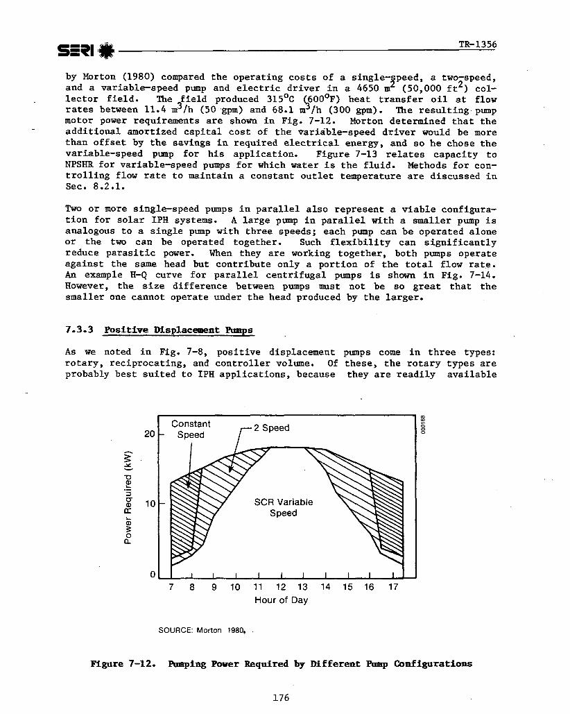
by Morton (1980) compared the operating costs of a single-speed, a two-speed, 2 2 and a variable-speed pump and electric driver in a 4650 m (50,000 ft ) col-

lector field. The field produced 315'~ $600~~) heat transfer oil at flow rates between 11.4 m3/h (50 gpm) and 68.1 m /h (300 gpm). The resultingpmp motor power requirements are shown in Fig. 7-12. Morton determined that the additional amortized capital cost of the variable-speed driver would be more than offset by the savings in required electrical energy, and so he chose the variable-speed pump for his application. Figure 7-13 relates capacity to NPSHR for variable-speed pumps for which water is the fluid. Methods for controlling flow rate to maintain a constant outlet temperature are discussed in Sec. 8.2.1.

Two or more single-speed pumps in parallel also represent a viable configuration for solar IPH systems. A large pump in parallel with a smaller pump is analogous to a single pump with three speeds; each pump can be operated alone or the two can be operated together. Such flexibility can significantly reduce parasitic power. When they are working together, both pumps operate against the same head but contribute only a portion of the total flow rate. An example H-Q curve for parallel centrifugal pumps is shown in Fig. 7-14. However, the size difference between pumps must not be so great that the smaller one cannot operate under the head produced by the larger.

As we noted in Fig. 7-8, positive displacement pumps come in three types: rotary, reciprocating, and controller volume. Of these, the rotary types are probably best suited to IPH applications, because they are readily available

SCR Variable

7 8 9 10 11 12 13 14 15 16 17 Hour of Day

SOURCE: Morton 1980,

Figure 7-12. Pumping Paver Required by Different Pump Configurations

176

in appropriate sizes, provide a smooth flow, and are relatively efficient. However, reciprocating or controller volume pumps may also be suitable for certain applications; for example, a diaphragm pump might be most appropriate for a fluid that tends to leak.

Several -characteristics of positive displacement pumps make them attractive for solar IPH applications. They are often self-priming, reducing the suction head requirement in system design. The flow rate of a positive displacement pump is nearly proportional to its speed and insensitive to the head against which it must pump; thus, precise flow rate control and cold start-up, even with ,a viscous fluid, are not difficult* These pumps can be used in high- temperature applications, and have generally higher efficiencies than centrifugal pumps. They are also relatively inexpensive in small sizes compared with centrifugal pumps [less than about 6 L/S (100 gpm) ] and when used for high- head applications (Perry and Chilton 1973).

But other characteristics of positive displacement pumps may be less benef i- cial. Because of the close clearances needed for efficient pump operation, the fluid must be clean and nonabrasive. Many pumps require a fluid with good lubricating properties, since the fluid must lubricate internal bearings. Thus, pumps for water or other fluids with few lubricating qualities may have to be specially designed to ensure long life. The insensitivity of these pumps to the head against which they operate can cause a rapid, large pressure buildup at the pump outlet if flow is blocked. Pressure relief ,valves are usually added to the pump casing to vent fluid from the outlet back to the suction side of the pump* However, if an overpressure condition is allowed to persist for any length of time, provision must be made for removing the excess heat or the pump will overheat. A system design employing a positive displacement pump must include protection for components and sensors against such '

overpressure conditions.

Selecting a positive displacement pump involves first determining the system head curves, the design flow rate and head loss, and NPSHA, the same as for a centrifugal pump system. Next, the manufacturers' literature must be scanned to find a pump that matches these requirements. As with a centrifugal pump, care must be taken to ensure that the pump will operate under all conditions and that the pump driver is adequate, especially in the case of a variable- speed system.

7.4.1 Qlaracteristics of Solar Systems

Valves regulate and isolate flow in a mechanical system. The number and kinds of valves for a solar system should be selected carefully because valves add to system cost and are sources of pressure drop and heat loss during operation and overnight cool-down. Some characteristics of solar systems, such as overnight shutdown, that provide daily intervals for maintenance, make fewer valves necessary in the system than for a conventional process plant.

Solar systems that operate at low temperatures allow for great flexibility in the choice of valves. In addition, solar systems, particularly closed systems, usually do not operate at high pressures. Sealing pressures are low, and absolute shutoff is generally not necessary. Isolation valves would most often be closed only when the solar system is down and some amount of leakage would then; be acceptable.

7.4.2 TvDes of Valves

With the proper seat elastomers, butterfly valves are operational at temperatures up to 135'~ (275'~). Butterfly valves combine many attributes that are favorable to solar system applications: they are inexpensive, have low thermal mass, present little resistance to fluid flows, and are quick-acting, opening and closing over a one-quarter turn. These valves are a good choice for isolation or crude throttling in a low-temperature solar system. They are available in large diameters but generally not in sizes of less than 2 in. and should not be used when absolute shutoff is required.

With teflon seats, ball valves are suitable for service at temperatures up to 200'~ (400'~). These valves are more expensive than butterfly valves, but they are also lightweight, compact, and quick-acting over a one-quarter turn. In addition, the straight-through flow characteristic of these valves minimizes pressure drop. They provide positive flow shutoff and can be used for flow throttling. In solar systems, they are a good choice for vent, drain, and flow-balancing valves. Ball valves come in sizes ranging from 1/4 in. to over 12 in., with screwed or flanged fittings or connections suitable for soldering. Ball valves equipped with pressure taps simplify flow-balancing procedures.

In high-temperature solar systems, steel valves (or metal alloy, as required) must be used: gate valves for isolation and globe valves for throttling. Gate and globe valves are considerably more massive than butterfly or ball valves, and their stems provide a considerable surface for heat loss. Gate valves should be used only in the fully open or fully closed position. In the partially open position, the gate is subject to rapid wear and positive sealing is not possible. When it is fully open, however, a gate valve causes minimal pressure drop. Globe valves are always associated with a considerable pressure drop. Flow through the valve is almost proportional to the number of screw turns that the valve is open.

It is generally preferable to weld steel valves in place in a solar system, particularly when it is operating under high pressure or contains synthetic heat transfer oils. Compared with flanges and screwed fittings, welds are less massive, are leak free, have lower friction losses, and are more easily insulated. The disadvantage of welding, in addition to a generally higher initial cost, is the lack of flexibility that results in the piping system.

For example, a line cannot be broken for cleaning. Care must be taken not to gall the seat of welded-in-place valves because they are so difficult to replace.

Control valves are usually globe-type, although butterfly control valves with plastic or all-steel construction are available. Three-way control valves

should be avoided, because field experience indicates that leaks into the shutoff line soon develop. Check valves are needed in nondraining solar collector loops to prevent thennosiphon heat loss, which could result in the heat exchanger freezing. They should be selected to minimize pressure drop, which usually requires the use of a swing check. A flow-through valve with a check that swings clear of the flow is preferred. Fluid velocities should be high enough to keep the check fully open at all times. Partial opening or flutter- ing will increase pressure drop and wear, and lead to less efficient sealing.

7,4,3 Gzidelines for Selecting Valves

Solar system designs have been quite conservative in the past, employing a great number of isolation and throttling valves. This trend has also increased the chances for leakage and large thermal losses. Too few data are available to make definite rules about the placement and type of valves suitable for solar IPH systems; but the following guidelines, based on minimizing the number of valves, should be considered by the system designer.

Isolation valves should be placed around pumps, and butterfly valves should be used for temperatures of less than 135'~ (275'~), if possible. A clear-away swing check valve should be located on the pump discharge between the isolation valves, and storage tanks and other vessels should be isolated with valves.

Ball valves should be used for vents and drains as well as to isolate instruments such as pressure and flow indicators. Ball valves are unsuitable only for the highest pressure steam flash systems and for systems using oil heat transfer fluids. If piping is sloped correctly with as few slope changes as possible, a minimum number of vent and drain valves can be located to serve large lengths of line.

Most of the valves in an industrial solar system are used for flow balancing and isolating individual rows of collectors. The block-in capability of each collector string invariably dictates placement of safety valves in each string, but this further increases thermal losses and makes fluid leaks more likely. Unless isolation capability is required for proper maintenance, however, omitting these valves should be seriously considered; they should not be necessary in an industrial solar system. While small leaks can be tolerated, large fluid leaks will shut down the entire collector field. But an ability to operate a portion of a col1ecto.r field while the rest is shut down gains little energy, because maintenance can be performed at the end of each day. A good compromise for large collector fields is to provide isolation valves for various sections of the field. Eliminating isolation valves on each row allows the use of fewer safety valves, and these can be located in the header piping.

Flow equalization between individual collector strings is a major concern in solar system design. Flow equalization can be accomplished using reverse- return, multiple-diameter piping configurations, but this increases piping costs, thermal losses, and pumping power requirements. An alternative is to use balancing valves to achieve sufficient pressure loss across each collector string to eliminate the effect of pressure drops along the header. piping. These balancing valves can be located at either the inlet or outlet of the

collector. An outlet location can be more convenient for making adjustments, because this is where the temperature reading will be taken. In any case, however, balancing flows with valves is a time-consuming process. Valve settings change easily over time, as the valves wear or through accidental inter- ference. An alternative to using conventional valves for flow balancing is to use automatic -variable-orifice valves. These valves are designed to control the flow rate to within 5% over the desired range of operating pressure drop.

Another alternative is to use fixed-orifice plates instead of valves to induce the needed pressure differential in combination with appropriate pipe sizing. Orifice plates are cheaper, more reliable, and result in less thermal loss than valves. Although perfect flow balancing using orifice plates requires an extremely detailed pressure analysis of the piping system, this is not necessary because a small degree of liquid maldistribution has little effect on system performance. In an oil system operating close to the temperature limit of the oil, or a flash-steam system operating near the pressure limitation of the collectors, maintaining flow equality could be more crucial. If collector outlet temperatures indicate serious maldistribution of flow, it is possible to change the orifice plate to a different diameter, although the effect of this procedure on pump performance and overall flow rate must be considered.

Control valves are required in an IPH solar system in which control of the collector outlet temperature is desired. Butterfly control valves are, again, particularly suitable here and have been advocated for more demanding process applications (Baumann 1979). Since few control valves are likely to be employed in the solar site, and they could be widely scattered and remote from the system control station, electrical activators should be considered. Pneumatic systems with a compressor and large lengths of piping are not as economical for the small number of valves involved, and pneumatic leaks are bothersome.

Often, process fluid should not pass directly through the collector field; thus, many solar applications require heat exchangers. A closed-loop solar system allows the use of nonfreezing collector fluids that are less corrosive and less prone to scaling than the process fluid. Possible contamination of the process fluid is another factor to take into account in selecting a closed-loop system. However, incorporating a heat exchanger in a solar system introduces cost penalties associated with that exchanger and with auxiliary piping; and the performance of the solar system is reduced by virtue of the increased operating temperature of the collector system working fluid. Another penalty is the result of the greater pumping power needed because of the increase in system pressure drop and the need for an additional pump. Thus, the objective in designing an exchanger for a solar IPH application is to size the exchanger so that performance and pumping power penalties and heat exchanger costs are minimized.

7.5.1 Heat Transfer Relations

For the sy-stem illustrated in Fig. 7-15, the heat transferred across the heat exchanger Q in watts (~tu/h) is

182

From

- : Solar Collectors

To Solar

h;tCcp,. To - r * Storage

TC., Tss0 Tank

4- Heat Exchanger

,I c From : Storage

Collectors Tank

Figure 7-15. Example Heat Exchanger System

where &and is are flow rates (kg/s , ib/h) and cp,, and c are specific heats kg K, I3tu/lbo~) of the collector and storage f l~ixs',~ respectively. It is convenient to define the capacity rate W (w/K, ~ t u / h ' ~ ) for each fluid as

In a heat exchanger of infinite area, the heat transferred would be at a maximum and would be

where Wdn is the smaller of Wc and Ws.

Heat exchanger effectiveness E is defined as

and, thus,

and E = Tc,i - =c,o when Wc ( Ws ,

Tc,i - Ts,i

sin + TR-1356

TS ,o - E = Ts'i when Wc > Ws .

Tc,i - Ts,i

7.5.2 Overall Heat Transfer Coefficient

The heat transferred between fluids within a counterflow heat exchanger with constant fluid specific heats is given as

2 where %is the overall heat transfer coefficient between the fluids (W/m K, 2 2 ~tu/ft F), A is the area of heat transfer surface (m , ft ), and ATm is the

log mean temperature difference:

Typical values for overall heat transfer coefficients for some of the fluids likely to be encountered in a solar system are shown in Table 7-12. If greater accuracy is required to size the heat exchanger, the following simplified procedure can be employed. (More detailed procedures that take into account the physical characteristics of the heat exchanger are employed by heat exchanger suppliers, but are not required for the initial stage of design. )

The overall heat transfer coefficient is generally based upon the exterior tube surface and can be defined as

where % is the total resistance to heat transfer. The resistances to heat transfer are in series, so that

Table 7-12. Typical Overall Heat Ransfer Coefficient Values for Thbular Heat -changers

Tube-Side Fluid

Shell-Side Overall Heat Transfer Fluid Coefficient [w/m2~ (~tu/h-f t2-'I?) ]

Water Water 1140-1420 (200-250) Water Demineralized water 1700-2840 (300-500) Feed water Steam 2270-5680 (400-1000) Heat transfer fluid Boiling water 570-850 (100-150) Water Air 114-142 ( 20-25)

sin :el TR-1356

where Do and Di are the outside and inside tube diameters (m,ft), respectively; kt is the thennal conductivity of the tube material (w/~PK, I3tu/h-ft0~); ho and hi are the outside and inside film coefficients (w/rn2-~, ~tu/h-ft*~~), respectively; and Rf and Rf are the outside and inside foul-

2 ing resistances (m K/W, h O ~ f t2/~t$, respe'ctively. The fouling resistance? account f6r the reduced heat transfer efficiency caused by scaling. Typical values for fouling resistances are listed in Table 7-13. In general, fouling In the solar collector side of the exchanger should be minimal, and the collector working fluid should be selected to minimize scaling. Scaling on the process side could be much greater, depending on the characteristics of the process fluid.

The thermal conductivity of the tube material is readily obtainable. Typical materials are steel (142 ~/m-K, 25 ~tu/h-ftO~) and brass (340 ~/m-K, 60 ~tu/h-ftO~). The remaining unknowns in Eq . 7-45 are the film coefficients. The inside heat transfer coefficient can be calculated using the Dittus- Boelter (1930) equation:

where

Nui = Nusselt number (hpi/ki)

Rei = Reynolds number ( P . D . v . /U ] 1 1 1 i

Pri = Prandtl nlnnber ( c Y. /ki) psi 1

n = 0.4 for heating the fluid, 0.3 for cooling the fluid.

The dimensionless numbers are calculated using fluid properties evaluated at the mean operating temperature:

pi = is the density of the fluid inside the tubes ( k g / J , lb/f t3)

Vi = the fluid velocity ( m / s , f t / s ) , and

wi = the viscosity (kglm-s lb/ft-h).

Table 7-13. Typical Foaling Resistances

Type of Fluid

Distilled water Treated boiler feed water City water below 52% City water above 52O~ Heat transfer media Refrigerant liquids Industrial air

The Dittus-Boelter equation assumes turbulent flow within the tubes (Re > 10,000). Establishing turbulent flow conditions should be a requirement for a solar heat exchanger design, because heat transfer under laminar or transition flow is much less efficient. In industrial solar systems, the use of forced convective heat transfer equipment is assumed. Natural convective heat trans-

, fer is inefficient; placing exchanger coils within a heat storage tank would cause maintenance problems. The procedure described by Cole et al. (1980) can be used to determine the shell-side heat transfer coefficient. A similar Nusselt number relation is used to correlate the film coefficient,

where

and

&, = the shell-side mass flow rate (kgls, lb/h)

I+, = the number of tube rows across the diameter of the shell

Sbaf = the baffle spacing (m, ft) in the longitudinal direction along the exchanger

'min = the minimum spacing between tubes (m, ft)

bin = the min'imum cross-sectional area between the tubes.

After calculating the fluid film coefficients, the overall heat transfer coefficient can be calculated using Eqs. 7-44 and 7-45. The effectiveness of a counterflow heat exchanger is related to the overall heat transfer coefficient by

e = 1 - exp(-B) Wmin

* 1 -- exp ( -B

w m x

where

B A (L O Wmin Wmax

The number of heat transfer units, NTU = UoAJWmin, is a dimensionless measure of the adequacy of heat exchanger area. For proper heat exchange, NTU will

generally be in the range of 1 to 10 (Lunde 1980). Equation 7-48 can be solved for E when a heat exchange area must be found for a particular effectiveness.

When the flow capacity rates on both sides of the exchanger are equal, Eq. 7-48 becomes

€ = NTU 1 + m u

7.5.3 Heat Exchanger Factor for Solar System Performance

The following analysis applies to the collector system illustrated in Fig. 4-4. It describes a factor that can account analytically for the presence of the heat exchanger between the co~lectors and storage. The basic collector performance equation can be written as

- - - ,,,a - FflL(Ti - T,) , (7-51) *c

where

2 A, = collector aperture area (m , ft2)

FR = heat transfer factor based on collector inlet temperature

T a = collector optical efficiency

UL = overall heat transfer coefficient for heat loss from the collector (w/m2 K, ~ t u / h - f t ~ ~ ~ )

T~ = collector inlet temperature

T, = ambient temperature (OC, OF).

Rearranging Eq. 7-35 and assuming that line losses in the collector loop are negligible (i.e., Ti = TC,, and To = T,,i), then

Substituting this equation into Eq. 7-51 yields

Using Eqs. 7-40 and 7-41 and assuming a well-mixed storage tank, Ts,i = Ts, a general expression for the heat transferred can be derived:

The expression

is known as the dewinter heat exchanger factor (dewinter 1975). Thus, F represents the penalty imposed on an open-loop system, where Ts would equaf Ti, by the incorporation of the heat exchanger to form the double-loop configuration shown in Fig. 4-6.

The performance of flat-plate collectors is generally categorized in terms of the collector inlet temperature. Parabolic trough performance is often correlated in terms of the collector outlet temperature or the average of the inlet and outlet temperatures. The heat exchanger factor FX,? for a collector performance equation in terms of the outlet temperature To 1s

where Fo is the heat transfer factor based upon the collector outlet temperature. The heat exchanger factor Fx,m, in terms of the average collector operating temperature Tm, is

The performance curve of a parabolic trough collector is generally presented as a quadratic function of ATII, unlike flat-plate collectors whose performance curves are linearized. Consequently, for a parabolic trough collector, an appropriate operating temperature (whether inlet, average, or outlet) must be selected. Given this temperature, the term FRUL, FOUL, or F U can be

m .L determined by evaluating the slope of the performance curve at thls point. Selecting the appropriate operating temperature involves a judgment based on the nature of the solar heating process, the storage temperature, and the variations likely in collector temperatures. In any case, given that the performance curve of a line-focus collector is fairly flat over a wide temperature range, the operating temperature selection is not critical. An overestimate of temperature is conservative, leading to an increased value of FUL and a larger heat exchanger.

7.5.4 Economical Heat Exchanger Area

The foregoing analysis indicates that a heat exchanger reduces the performance of the solar system by a constant factor F,. Thus, to meet a given load, the collector area must be increased in inverse proportion to F,. For economical heat exchanger sizing, the heat exchanger factor typically has a value of about 0.95. Such information can be used for preliminary heat exchanger sizing by solving Eq. 7-55, 7-56, or 7-57 for E. The heat exchanger area can then be calculated using Eq. 7-49.

The optimum heat exchanger area represents a trade-off between the cost of the '

heat exchanger and the cost of the solar collectors. The total system cost CT can be represented by

where C, and Cx are the costs of the collectors and heat exchanger per unit area, respectively, and A, and A, are their respective areas. The energy' delivered by the system is

where F is FR, F,, or Fm. The minimum cost of delivered energy with respect to exchanger surface area is

For equal flow capacity rates (Wc = Ws) , and assuming that the overall heat transfer coefficient Uo does not vary with Ax, the optimum (minimum cost) ratio %/Ac is

According to Horel and dewinter (Cole et al. 1979), the optimum heat exchanger invariably has a storage capacity rate Ws higher than its collector capacity rate Wc. They found that the ratio wC/W for the optimum exchanger is 0.5 to 0.6, and that Eq. 7-61 can still be use1 to find the optimum heat exchanger area because that value varies from the value determined in the optimum (unmatched capacity rate) case by about 1%. The optimum storage capacity rate is generally greater than the collector capacity rate because of the effect of the individual flows on collector operating temperature. Increasing the storage flow rate has a greater effect on reducing collector inlet temperature (and thus the temperature of the entire collector field) than an equivalent increase in the collector flow rate. Increasing the storage flow rate would result in less of an increase in electric power consumption than an equal increase in collector flow, because the pressure drop through the collector loop is usually larger.

7.5.5 Practical Considerations in Selecting a Heat Exchanger

In previous sections, heat exchanger sizing has been discussed in terms of perfect countercurrent flow. Such conditions are attainable only in double- pipe exchangers that are generally economical only in small sizes. Shell-and- tube heat-exchangers accommodate large heat exchanger areas in a compact volume. A diagram of a floating tubesheet shell-and-tube heat exchanger is shown in Fig. 7-16. Since steel shell-and-tubes are the most economical type of heat exchanger, they are the most likely kind to be incorporated into a solar IPH system. This section presents some of the practical aspects of selecting a heat exchanger. Operating experience with heat exchanger systems in industrial solar systems is limited. Consequently, only some general points about heat exchangers are incorporated here and tend toward a rather conservative exchanger design.

A major variable in a shell-and-tube heat exchanger is the number of shell- side and tube-side passes; i.e., the number of times the fluid changes direction from one end of the exchanger to the other. Because some means must be built into the exchanger to compensate for thermal expansion, flows into and out of the tube side are generally at the same end of the exchanger. Thus, normally, the number of tube-side passes is even. By appropriate baffling it is easy to produce two, four, or more tube passes. However, the greater the number of passes, the greater the deviation from countercurrent flow, the greater the path length, and hence, the.greater the pressure drop of the tube- side fluid.

A single shell pass is the most common shell-side configuration because of the difficulty of adequately sealing a multi-shell pass exchanger. The effect of multiple shell-side passes can be achieved by connecting identical single-pass exchangers in series. Because multiple-pass heat exchangers are not associated with perfect countercurrent flow, correction factors must be applied to the log mean temperature differential. Such correction factors are available from graphs (Kreith 1973, Perry and Chilton 1973).

The unique characteristics of a solar system must be considered in determining the number of exchanger passes. In general, compared with conventional thermal processes, a solar system involves larger flows and smaller temperature differentials. Because solar collector performance depends more on operating temperature than conventional heating equipment does, a closer similar- ity between the hot side (collector) and cold side (process) temperatures is desirable. This demands maximum heat exchanger efficiency and a minimum number of heat exchanger passes. Other considerations working in this direction are pumping power and thermal losses (both operational and overnight). Thus, as a general rule, unless a large mismatch of flows precludes it, a two-tube, single-shell pass exchanger is probably the most appropriate configuration for a solar system.

The designation of tube-side and shell-side fluids is another, largely practi-. cal, decision that must be made. It is more difficult to clean the shell side of an exchanger than the tube side, so a dirty, scaling, or corrosive fluid is generally placed on the tube side. A great difference in operating pressure would place the high-pressure fluid in the tubes. Placing the hottest fluid in the tubes reduces insulation requirements on the exterior shell. Turbu- lence is more easily achieved on the shell side; thus, the fluid with poorer

heat transfer characteristics would be placed in the shell. Shell-side pressure drop for a given flow is also generally lower. These characteristics of exchanger fluids are not entirely consistent in the choice of flow path, so engineering judgment must be used. Moreover, the cleaning and maintenance factor will often place the collector fluid in the exchanger shell.

. -:

Finally, with the help of the exchanger manufacturer, the type of exchanger must be specified. A major factor in this decision is the degree of differential thermal expansion and cycling. Fixed-tube sheet exchangers are usually less expensive, but the severe strains placed on the exchanger seals by the diurnal solar cycle must be fully considered. Hairpin exchangers readily accommodate thermal expansion but are difficult to clean and are often unsuitable for dirty or scaling fluids. They are, however, applicable in unfired steam generators with a heat transfer fluid in the tubes. Generally, 90:lO copper-nickel tubes are specified for such service.

For most solar energy systems, floating-head exchangers appear to be preferable. The tubes are easily cleaned without requiring removal of the tube bundle, and they are designed to accommodate thermal expansion. Although the operating pressure of a solar system is generally low, because of the high level of thermal cycling it is probably wise to specify a heat exchanger rat- ing beyond that dictated by operating pressure alone.

Liquid-to-air exchangers invariably pass the air on the shell side. Since the air-side heat transfer coefficients are the major resistors to heat flow, extended surface-finned tubes are generally employed. Passing the air trans- verse to the tubes in a direction parallel to the fins results in little

' increase in shell-side pressure drop, but the air-side heat transfer coefficient typically increases two to three times.

7.5.6 P l a t e Eleat Excha~~~!ers

Plate heat exchangers are ideally suited for certain solar applications and should also be considered. However, plate heat exchangers are not normally suitable for pressures exceeding 2.2 MPa (300 psig), temperatures over 200'~ (400°~), or for heat exchange involving a phase change (Raju and Chand 1980). The plate exchanger becomes economically attractive when an expensive construction material is required or if a double-walled shell-and-tube heat exchanger (for leak protection) is the alternative. This is often the case in food industries (which usually offer excellent potential for solar energy applications) when any possibility of product contamination must be eliminated. -As long as the integrity of the plates is maintained, the sealing mechanism of the plate exchanger precludes cross-contamination of exchanger liquids. The plate exchanger cost is comparable to or cheaper than equivalent shell-and-tube exchangers constructed of stainless steel. It does not have to be insulated, it can be supported on a less expensive foundation, and it requires less energy for pumping than a shell-and-tube exchanger. Plate exchangers generate highly turbulent conditions that result in high heat- transfer rates, and approach temperatures may be as low as 1°c. In addition, plate exchangers have lower thermal mass and hold-up volumes than shell-and- tube heat exchangers. These are important considerations in solar system design.

7.5.7 Summary

The following generalizations can be made about heat exchangers:

Forced-convection heat exchange should be used for industrial solar systetns. -

a Fluid velocities in the heat exchanger should be adequate to maintain turbulent flow (Re > 10,000). For proper heat exchange, the nmber of heat transfer units (NTU = U A / W ~ ~ ) will generally range from 1 to 10.

The economical heat transfer area is obtained from the expression

This generally results in a value of about 0.95 for the dewinter heat- exchanger factor.

The flow capacity ratio for the optimum heat exchange, wc/wS, generally ranges from 0.5 to 0.6.

The most appropriate shell-and-tube heat exchanger configuration is probably two tube passes and a single shell pass.

a If scaling, corrosion, or dirt buildup preclude the use of a hairpin exchanger, either a fixed or floating tube sheet (depending on the amount of thermal expansion) exchanger is probably the most appropriate alternative.

Consider a plate heat exchanger if the alternative is a double-walled shell-and-tube heat exchanger or if p1ai.n steel is unsuitable as a construction material.

7.6 STORAGE

In conventional IPH applications, fuel consumption (oil, gas, electricity) is adjusted to match the load. The supply of solar energy, however, cannot be regulated. To reduce the mismatch between solar supply and process demand, storage systems are often deemed appropriate. The cost-effectiveness of storage depends on the particular application, however. For systems in which solar energy supplies only a small fraction of the load, storage would ordinarily not be warranted unless the collectors might not be used for significant periods of time (e.g., if the plant is shut down on weekends). Storage can be worthwhile, however, if the collector array is large enough to supply more energy than the load requires during times of peak insolation.

There are many ways in which energy can be stored; these include mechanical, electrochemical, chemical, and thermal means. We are concerned here only with thermal energy storage (TES) because the energy delivered by the collectors to the load is thermal in solar IPH systems.

Thermal energy storage is most commonly sensible heat or latent heat. In a sensible heat application, the thermal energy to be stored raises the temperature of the storage material. When the energy is later extracted, the storage temperature drops. Latent heat storage uses the heat of fusion of a storage material as it undergoes a phase change (melting when heat is added, freezing when heat-is extracted) to store energy, usually at a nearly constant temperature. Both types of thermal energy storage can be used on either an annual or short-term basis. Because of the cost of annual storage systems,* we address only short-term storage here. (Solar ponds, which act both as collectors and long-term sensible storage, can be cost-effective but thus far have not been used in industrial applications and so are not addressed here.) Short-term storage allows the solar energy collected during the day to be used at night, and also allows energy to be collected on days when the plant is shut down, such as on weekends and holidays.

7.6- 1 Storaee Media

7-6.1-1 Sensible Eeat Storage

The vast majority of existing solar IPH systems use sensible heat storage. Liquid systems typically use water or oil storage; steam systems employ water, oil, or a mixture of oil and rock; air systems usually use a rock bed.

When liquid collectors are used, it is easiest to store sensible heat in a liquid medium since this permits straightforward heat exchange. The same characteristics that make water an excellent heat transfer fluid also make it an ideal fluid for law-temperature storage. It has a high volumetric heat capacity, is easy to pump, is cheap, and is readily available. At higher storage temperatures, materials other than water must be considered if high pressures and the associated high cost of storage tanks are to be avoided. Using other low vapor pressure fluids is an alternative; however, they can also be expensive. Another alternative is to use solid storage. Ordinarily, the high-temperature heat transfer fluid is brought into direct contact with the solid medium. Because of its low cost, rock is a common choice for a solid storage medium.

When a storage tank is filled with a mixture of rocks and a heat transfer fluid, a great deal of stratification is possible because of the large surface area of the solid, the corresponding rapid heat transfer, and low thermal conductivity. This setup distributes high-temperature fluid to the load from the top of the tank and low temperatures to the collectors from the bottom.

The stratification associated with a solid storage device is well utilized at lower temperatures as well, specifically in air collector heating systems using rock storage. Air collectors generally have lower FR values than liquid f lat-plate collectors (-0.7 versus -0.9), because of the lower heat-transf er coefficients associated with air. Rock-bed stratification provides low inlet collector temperatures which compensate for the low FR values and result in

*That is, storage systems with capacities comparable to energy collected on an annual basis.

efficiencies similar to those of liquid collectors. It is important that the rocks used not vary much in size, however, and that they be loaded carefully, otherwise nonuniform flow will be the result. Cole et al. (1980) describe the design of rock storage bins for air heating systems in detail.

. - .

7.6.1.2 Latent Heat Storage

Utilizing the latent heat capacity of storage materials permits us to have smaller storage volumes. And the relatively constant temperature of storage can maximize collector efficiency and minimize storage heat losses. An ideal phase-change material (PCM) should have the following characteristics:

appropriate phase-change temperature

a high latent heat

a low cost

ready availability

nontoxicity and nonflamm~bility

uniform.phase-change characteristics (no subcooling or separation).

Two basic material types have been used for short-term phase change storage-- organic compounds and salt hydrates. A good example of an organic compound is paraffin. Like other organics, it suffers certain limitations--flammability, low thermal conductivity , and volume trlc change during phase change (causing separation from container walls). The latter two problems make it difficult to get heat into and out of the material. As a result of such limitations in organic compounds, most of the work in phase-change materials has centered on salt hydrates. Maria Telkes, who has done much of the pioneering work in this field, has concentrated on one salt hydrate In particular because of its low cost--sodium sulfate decahydrate, or Glauber's salt. The chemical reaction involved in the phase change of Glauber's salt (Na2S04 10 H20) is

Heating Na2S04 10 820 + 251 KJ/kg (108 Btu/lb,) ' Na2SOq + 10 820 .

Cooling

When the solid hydrate is heated, Na2S04 dissolves in the water of hydration; the result is a liquid. When it cools, the hydrate is reformed and 251,000 J of heat are released for each kilogram that solidifies. To illustrate the volumetric storage capacity of Glauber's salt, consider 100 kg (220 lb) under- going a 30 K (54'~) temperature swing that includes the phase change at 3 2 ' ~ (89O~) :

where

hfg = latent heat of fusion, 251 k.J/kg (108 ~tu/lb,)

c = specific heat at constant pressure, 1.2 k~lkg K (0.5 ~tullb~'~) P

AT = temperature change, 30 K.

Substituting numerical values, we have . - -

Note that the latent heat term is a constant independent of temperature. The smaller the temperature swing, the less the contribution from sensible heat. In this example of a 30 K change, 87% of the heat stored is latent and 13% is sensible.

In Table 7-14 one can readily see the advantage in both mass and volume inherent in using Glauber's salt rather than rocks or water. The comparison is based on each material sized for a heat storage capacity of one gigajoule over a 30 K (54'~) temperature swing (typical for a solar space heating system). Only 3200 kg of Glauber's salt is needed, compared with 8000 kg of water and 38,100 kg of rock.

Unfortunately, the commercialization of Glauber's salt storage has faced a number of obstacles, arising from the phase-change behavior of this salt. Glauber's salt is considered an incongruent material because, upon melting, two distinct phases result: a saturated solution of Na2S04 in water and an excess amount of insoluble Na2S04 which precipitates out. Once the precipi- tate settles to the bottom, it no longer participates in the reaction, which causes a decrease in overall heat capacity with each meltinglfreezing cycle. Various approaches have been used to address this problem, such as using thickeners like paper, pulp, and thixotropic agents (similar to those used in thickening paints), active mixing, and thin containers.

Table 7-14. Storage Size Comparison of Different Media Based on 1 GJ,Storage and 30 K Temperature Suing

Medium Weight (kg

Rocks 38,100 20.3 Water 8,000 8.0 Glauber' s salt 3,200 2.1

Another problem with Glauber's salt is its tendency to supercool below the normal freezing point. To solve this problem, nucleating agents (such as borax) have been added. A cold rod can also be inserted in the salt hydrate to serve as an initiating nucleation site.

Although storage devices containing Glauber's salt have been marketed, the problems discussed above have not yet been completely solved. As a result, some manufacturers have looked into other salt hydrates--calcium chloride hex- ahydrate, for example. Considered a semicongruent material, it does not exhibit the same degree of separation as Glauber's salt, and according to one manufacturer, it only supercools for the first several cycles [to llOc (20'~) below its freezing point]. Unfortunately, it is expensive [over $2/kg ($l/lb) J in package form and has a l w melting point 1 2 7 ' ~ (81°~)], which makes it unsuitable for all but the lowest-temperature storage applications.

For higher temp bonates can be anticorrosion c

erature applications, other materials must be considered. Car- useful at temperatures as high as 700°c, and they have good haracteristics. Below 500°c, nitrates are good candidates that

are also relatively noncorrosive and inexpensive. Figure 7-17 shows the storage capacities of various candidate phase-change materials, and the temperatures at which the phase change occurs. Work 'in phase-change storage continues. Problems with containment, heat addition/extraction, and in some cases, corrosion still need to be resolved.

7,6-2 Storage Vessels

Whatever fluid is used, the storage capacity is a function of specific heat of the fluid, its mass, and the ,temperature range over which it can be used. The following section focuses on sensible heat storage units, but some parts of the discussion can also apply to latent heat systems. We must keep in mind that phase-change storage units store a large amount of heat at a particular temperature. The heat stored in a sensible storage tank is expressed by

Thus, for a given fluid and minimum operating temperature, the storage capacity can be increased by increasing the amount of fluid or raising the maximum storage temperature. Often, however, the temperature is limited by the heat transfer fluid.

To enhance any stratification that might occur, storage tanks are usually plumbed so that solar return and load supply lines are connected near the top of the tank where the temperatures are the hottest. Load return and solar supply lines are connected near the tank bottom, allowing the coolest fluid to be pumped to the collectors, which in turn maximizes efficiency. In actual practice collector flow rates are often high enough to disrupt stratification. Some stratification may occur in direct systems as well, if loads are drawn from storage when there is no collection, and if the flow rates are small.

The design of a stratified tank usually requires that the height of the tank be at least twice its diameter, that diffusers be used, and that the tank volume is passed only once each day. Various devices such as baffles, perforated headers, and floating membranes have been studied to help maintain a vertical

temperature gradient; however, these add to system cost. Multiple tanks are also sometimes used with each tank operated at a different temperature to achieve a measure of stratification; but, as we might expect, several small tanks cost more than one large tank and also provide greater area for heat loss. For instance, in a solar water heating study, higher heat losses were identified-,as -the major factor causing single-tank domestic hot water tank systems to outperform two-tank systems (Farrington, Murphy, and Noreen 1980).

Typically, several different materials are used to construct storage tanks; of these, steel is the most commonly used. It is also the only material used in pressure applications. Steel tanks are readily available and, when they are not the pressurized type, are inexpensive. Steel tanks are subject to corrosion, however, and have less resistance to underground loads than concrete tanks. Fiberglass tanks have good corrosion resistance and are lightweight, Resins typically limit the maximum operating temperature to between 65'~ (150~~) and 95'~ (~oo'F), however. Fiberglass tanks are usually more expensive and are less readily available than steel tanks. Concrete tanks can be formed in any shape or size, are corrosion resistant, and resist underground loads well. However, they are heavy and often require a liner to prevent leakage. Wood tanks, properly lined, can be cost-effective in applications that require unpressurized storage. Their durability must be considered, however. Liners are used to prevent leakage and, in steel tanks, corrosion. Butyl rubber, EPDM, PVC, and polyethylene are common materials. Polyethylene has less puncture resistance than the others; and PVC is limited to a maximum temperature of about 70'~ (160~~).

The optlmum size of storage is a function of collector area, load profile, and solar fraction. Experience in the solar heating of buildings and hot water showed that the optimum size was a,bout 200 to 300 u/m2 of collector area/^ (10 to 15 ~tu/ft~-'~) which translates to about 60 to 90 liters of water per square meter of collector area (1.2 to 1.8 gal/f t2). ' Because IPH applications can have such different load profiles, however, optimum storage size can be significantly different from these figures; it can be determined using the procedure given in Sec. 6.0.

7.6.3 Storaere Tank Insulation

Storage heat loss can cause a significant drop in system performance. There are various standards for tank insulation; for example, the SMACNA standard for solar heating systems specifies that insulation must be of sufficient thickness to keep heat loss less than 2% in 12 h. This means 2% of storage - capacity, defined as,McpATuseful, where ATuseful is the temperature range over which storage is operated. The maximum temperature to determine a AT can be somewhat arbitrary, yet it affects the result greatly. In general, the U value 'for storage required to meet such a standard can be written as:

where

f = fraction of stored heat loss specified by the standard (0.02 for SWCNA)

-t-= specified time period (12 h for SMACNA)

M = storage mass

c = specific heat of storage medium P

Tmax, Tmin = maximum and minimum operating temperatures of storage

Tavg = average storage temperature

Tamb = ambient temperature.

An alternative to the SMACNA standard is to calculate the most economic insulation thickness for a storage vessel, based on a comparison of the cost of collecting an additional amount of energy versus the cost of insulating the storage tank to save an additional amount of energy (Cole et al. 1980). If the cost of collecting additional energy is higher than the cost of saving it, the system needs insulation; but if the cost of collecting energy is less than the cost of saving it, the system has too much insulation. The economic thickness is the thickness that makes the cost of saving additional energy equal to the cost of collecting it. In many cases, the resulting insulation thickness will be close to that required by the SMACNA standard.

The incremental cost of collected energy is calculated by adding a small amount of collector area and determining the increment of additional energy collected over a year AQc and the additional cost associated with the additional collector area ACc. Using an economic factor Ec to convert initial costs to an annual equivalent cost, the ratio EcACc/A~c is the incremental cost of collecting energy, in $/J ($/B~u). This quantity is compared with the cost of saving energy to determine the optimum insulation thickness. If we assume the same economic basis for calculating the cost of saving energy, the economic factor can be ignored and the costs can be compared on an initial cost basis.

Next, the energy lost and the cost of insulation are calculated as a function of the insulation thickness. For a cylindrical tank surface, the following procedure is used. The insulation is assumed to have three parts: an inside

2 surface thermal resistance Ri (in m K/w), a layer of insulation with thickness s (in m) to be determined, and an outside surface thermal resistance Ro (in m2~/w). The annual heat loss from such a surface is

where

L = height (length) of storage tank (m)

- T . -.. = average temperature (OC) of the storage during the time it is hot

(a good estimate is the average of the peak storage temperature and the minimum temperature during operation)

- Ta = average ambient temperature (OC) , also averaged during the time

the storage. tank is used (the temperature at the tank location, either indoors or outdoors)

D = diameter of the tank (m)

2 \

Ri = inside surface thermal resistance (m K/w), calculated similarly to R in Eq. 7-1

r* = t h e m 1 resistance of the insulating material per unit thickness (~K/w), adjusted for parallel heat loss (without parallel heat loss, it is the inverse of the thermal conductivity of the material)

2 Ro = outside surface thermal resistance (m K/w), also calculated like R in Eq. 7-1,

Differentiating with respect to the insulation thickness, we have

We assume that the cost of the insulation consists of a fixed cost CIS a cost proportional to the outside surface area C2, and a cost proportional to the insulation volume C3, as follows:

The derivative of the.insulation cost with respect to insulation thickness is

Combining E q s . 7-63 and 7-65 yields the incremental cost of saving energy:

Finally, the two incremental costs are set equal to one another. Since the incremental cost of saving energy E = ~ C ~ / ~ Q ~ must equal the incremental cost of collecting energy ECACc/A~, at the optimum insulation thickness, then, assuming equal economic factors (EI = Ec), we obtain

* AC r Dy Iln y

(7-67)

where y = 1 + ~s/D.

We can solve for y in terms of C2, C3., D, q, Ro, and r* .using' Eq. 7-67 either by trial and error or by more sophisticated methods such as the Newton-Raphson method. Once y is obtained, the optimum thickness of insulation is simply

If the surface to be insulated is flat, such as the top or bottom of a tank, or the radius of curvature is large compared with the insulation thickness, a similar analysis yields a closed-form solution for the optimum insulation thickness

where R* is the thermal resistance of the surface before the insulation is applied, adjusted for parallel heat loss (m2w/~). In insulating a storage tank, it is important to pay attention to the top and bottom (particularly the latter, because of conduction paths), and not just the sides.

7.6.4 Storage Location

7.6.4.1 Interior Storage

When space is available inside a building, it is valuable for storage because the system can then use shorter pipe runs and waterproofing is not needed. Any losses from storage can add to a building's cooling load, although mechanical equipment rooms are often not air conditioned. There must be some provision for containing or draining leaks as well as access to all parts of the tank. Mounting pads should be designed to isolate the tank thermally from the floor.

7.6.4.2 Exterior Storage

If interior insulation insulation

space is scarce, exterior storage problems must be addressed. The must be waterproof, which usually necessitates a closed-cell foam if temperatures permit. Because of the lower ambient temperatures

and wind effects, more insulation is needed for .an outside tank than an interior one. All penetrations fox valves, pipes, supports, and instrumentation must be waterproofed. In freezing climates, a drainable sight gauge is r ecomended.

For aesthetic reasons, or to conserve ground area, storage tanks can be located underground. Of primary concern in such an application is the height of the local water table. If the bottom of the tank is below the water table, a holddown structure or added dead weight is needed to prevent flotation of the tank when it is empty. A commonly used support structure consists of a concrete footing with tank saddles to supportthe weight of the tank and steel straps to hold it down. High-density insulation must be used to withstand both upward and downward loads. &cause of the serious problems a high water table can cause, most experienced solar system designers avoid using underground tanks under these circumstances. A current method of installing an underground tank involves prefoaming the tank with urethane, wrapping it with nylon fabric and mastic material, and setting it in a sand bed.

Alexander, Em L.; Kutscher, C. Fa 1978 (Aug.). Thermal Storage Subsystem Parameter Study. Solar Ten Megawatt Project Off ice Report No. 40X5131056-R. - Canoga Park, CA: Rockwell ~nternationai Inc. Energy systems Group.

Allen, David, 3. 1981. Personal communication.

Barley, C. D.; Wynn, C. B. 1978. "Optimal Sizing of Solar Collectors by the Method of Relative Areas." Solar Energy. Vol. 21 (No. 4); pp. 279-89-

Barnhart, 3. S. 1981. "Energy Transport System Optimization for Distributed Networks of Solar Collectors." ASME Paper No. 81-SOL-1. Presented at the Energy Sources Technology Conference and Exhibition. 18-22 Jan. 1981, Houston, TX.

Baumann, He Dm 1979 (May). "A.Case for Butterfly Valves in Throttling Appli- cations ." Instruments and Control Systems.

Caputo, R. 1975. An Initial Study of Solar Power Plants Using a Distributed ~etwork of Point Focusing; Collectors. JPL 900-724. Pasadena. CA: Jet - Propulsion Laboratory.

Cole, R. L.; Nield, K. J.; Rohde, R. R.; ~olosewicz, R. M. 1980. Design and Installation Manual for Thermal Energy Storage. 2nd Edition. ANL-79-15. Argonne, IL: Argonne National Laboratory.

dewinter, Fa . 1975. "Heat Exchanger Penalties in Double-Loop Solar Water Heating Systems." Solar Energy. Vol. 17; pp. 335-337.

TR- 1 3 56 s m + Dittus, F. W.; Boelter, M. K. 1930. Universi ty of Calif . (Berkeley) Pub.

Eng. Vol. 2; p. 443.

Farrington, R. B.; Murphy, L. M.; Noreen, D. L. 1980 (April). A Comparison of Six Generic Solar Domestic Hot Water Systems. SERI/TR-351-413. Golden, COf Solar Energy Research I n s t i t u t e .

Fried, J. R. 1973 (28 May). "Heat Transfer Agents f o r High Temperature Sys- t e m s . " Chemical Engineering.

HUD In te rna t iona l Minimum Property Standards Supplement, Solar Heating and Domestic Hot Water Systems. 1977 Edition. Washington, DC: U.S. Depart- ment of Housing and Urban Development.

Iannucci, J. J. 1980 (June). "Thermal Energy Centra l iza t ion Network: Design, Cost, and Performance f o r Disk, Trough, and Central Receiver Sys- tems ." Paper presented at In te rna t iona l Solar Energy Society Meeting,. Phoenix, AZ.

Johnson, J. D. 1981 (10 Aug.) . "Variable-Speed Drives Can Cut. Pumping Costs . " Chemical ~ n ~ i n e e r i n ~ .

Jones, G. F.; Lior, N. 1979. "Optimal Insu la t ion of Solar Heating System Pipes and Tanks ." Energy. Vol. 4 TNO. 4); pp. 593-621.,

-. -- Kreith, F. 1973. P r inc ip les of Heat Transfer. Third Edition. New York:

Harper and Row Publishers, Inc.

Lauer, B. E. 1953. How t o .Evaluate Film Coeff ic ients f o r Heat-Transfer Cal- cula t ions . A technical manual repr in ted from the O i l and Gas Journal. Tulsa, OK: Petroleum Publishing Co.

Lobanoff, V. 1979 (June). "Specif ic Speed i s a Useful Index f o r Pump Design and Selection." Power. Vol. 123 (No. 6 ) ; ,pp . 70-71.

Lunde, P. J. 1980. Solar Thermal ~ n g i n e e r i n ~ : Space Heating and Hot Water Systems. New York: John Wiley and Sons.

McAdams, W. H. 1954. Heat Transmission. Third Edition. New York: McGraw- H i l l .

Morton, R. E. 1980 (Sept.). "Design of Col lec tor Subsystem Piping Layouts." Line-Focus Solar Thermal Energy Technology Development Seminar. Albuquer- que, NM: Sandia National Laboratories.

Neerken, R. F. 1978 (3 Apr.). "Select ing the Right Pump." Chemical Engineering. pp. 87-98. (See a l so , "How t o Select and Apply Posit ive- Displacement Rotary Pumps.").

Pa r t s , L.; Miller, D. R.; Leffingwell, J. W.; Thompson, Q. E. 1980 (Sept.). Superior Heat Transfer Fluids f o r Solar Heating and Cooling Applications. AL0/45356-2. Monsanto Research Corp.

sin :al TR-1356

Perry, R. H.; Chilton, C. H. 1973. Chemical Engineers Handbook 5th Edition. New York:- McGraw-Hill Book Co.

Powell, J. C.; et al. 1974. Dynamic Conversion of Solar-Generated Heat to Electricity. NASA CR-134724, Washington, DC : National Aeronautics and

. -: Space Administration.

Raju, K. S . M . ; Chand, J. 1980 (11Aug.). "Consider the Plate Heat Exchanger." Chemical Engineering* pp. 133-144.

Seider, E. N.; Tate, C. Em 1936. "Heat Transfer and Pressure Drop of Liquids in Tubes." Ind. Eng. Chem. Vol. 28; pa 1429.

Shames, I. H. 1962. Mechanics of Fluids. New York: McGraw-Hill.

Thornton, J. ; Herlevich, A. ; Hooker, D. ; Kriz , T. Forthcoming. Comparative - Evaluation of Solar Thermal Systems for Thermal Applications. SERI/TR-253-1706. Golden, CO: Solar Energy Research Institute.

Williams, 0. M. 1978. "Thermal Chemical Energy Transport Costs for a Dis- tributed Solar Power Plant." Solar Energy. Vol. 20, pp. 333-342.

SECTION 8.0

As in nonsolar process applications, controls and instrumentation play an important role in solar IPH systems. In this section, we describe the design aspects of controls and instrumentation in solar IPH systems. In Sec. 8.1, control fundamentals needed to design a solar control system are explained. Subsections address such items as controllers, control loops, measurement dynamics, noise, and control valve characteristics. In Sec. 8.2, the special control problems of solar energy systems are addressed, beginning with normal operating modes, and including start-up/shutdown, freezing/stagnation, emergency conditions, operator training, and checkout. Instrumentation is covered in Sec. 8.3, particularly including irradiation, temperature, flow, pressure, and level measurements.

In this section, it is assumed that the designer already has some knowledge of process control, although several excellent textbooks are referred to. It is also assumed that the designer is familiar with the major elements of a closed control loop: the process, feedback (measuring) element, controller, control variable, feedback variable, manipulated variable, reference variable (set point), and uncontrolled variable (disturbance) (Grader 1970).

8.1.1 Controllers

The controller is the part of the control loop that implements corrective action as the process variable deviates from a desired set point. The control modes that characterize the corrective action include on-of f , proportional, integral (reset), and derivative (rate). There are no adjustments to "on-off" control (unless a deadband is included), and the controller output changes full-scale as the process variable crosses the set point. The corrective action implemented with proportional control is normally a linear function of the error signal (process variable minus set point). The proportionality constant (i-e., the gain) is equal to the percent controller output change divided by the percent error change.

Integral control (reset) is usually combined with proportional control. It forces the controller output to change in accordance with the time integral function of the error signal and can reduce steady-state error. It also repeats initial proportional output response as long as the error signal per- sists. Derivative control is combined with proportional control to change the controller output in accordance with the rate of change of error signal. This action ceases when the error signal stops changing.

Common Control Loops

The common types of control loops are flow, pressure, level, and temperature. Some rules of thumb are as follows.

Flow loops: Proportional plus reset controllers are used almost exclu- sively. The process typically is very fast and noisy, and the flow measurement is usually nonlinear (square). The controller is characterized by low gain and fast reset.

Pressme loops: For a liquid, the process is fast and noisy with most of the lags in the control system, and the measurement is nonlinear (square). Linear valves and proportional plus reset controllers with low gain and fast reset are used. For a gas, the process is simple: linear with no dead time and no noise. Proportional controllers with high gain suffice, and valve characteristics are not critical. For vapor pressure control, equal percentage valves and proportional-reset-derivative controllers are employed. This process is slow compared with other pressure processes. Controller settings include moderate gain, a reset rate of 0.5 repeats per minute or less, and a derivative time of 0.5 minute or more.

Level loops: High-gain or proportional-plus-reset controllers are used for precise control, low gain proportional-plus-reset controllers for averaging control. Valve characteristics are important.

T-erature loops: Temperature control loops can vary greatly in complexity, because there really is no such thing as a typical temperature application. Almost all the temperature control problems in solar applications are heat transfer problems characterized by long time constants and slow reaction rates. Distance-velocity lag (also known as dead time) is common. The measurement lag can pose a serious problem, especially if the thermal system is protected with a well. The measurement time constant depends on the mass and surface area of the bulb (or the well), the measured fluid, and its velocity past the bulb. Special care should be taken in locating the bulb to maximize heat transfer; usually, the bulb should be placed at bends in the flow path.

Nonlinearities also cause complications in the temperature loops. Heat transfer processes have parameters that vary with flow, so that time constants and distance-velocity lag vary with load or operating point. Distance-velocity lags are not as evident as in other systems and are often overlooked in analysis. Imperfect mixing is a good example of hidden dead time.

Processes dominated by one large capacity, e.g., storage tanks in air heating systems, can be controlled with on-off controllers. Some cycling results, but only about 1% of span. Proportional plus reset control is used in smaller capacity systems where load changes are large and where distance-velocity and measurement lags are important. Most shell-and-tube heat exchangers fall into this category. Derivative action becomes helpful, provided the process is dominated by linear lags (e.g., a batch reactor).

sin :el TR-1356

Controlling temperature by mixing hot and cold streams is more of a blending problem than a heat exchange problem. Good mixing and f a s t temperature measurement a r e the keys to simplifying the control job. Proportional-plus-reset con t ro l le r s should be used.

In general, the following guidelines can be used i n se lect ing control lers :

Use proportional control where

the cyc.1ing action, due t o on-off control , i s undesirable;

a set-point changes are small or infrequent; and

a the steady-state deviation between the s e t point and the process variable ( L e e , the o f f s e t ) can be tolerated.

Add in t eg ra l control where

the o f f s e t must be reduced or eliminated, and

the s e t point changes a re frequent. ,

Do not add in tegra l control when

s t a r t -up overshoot must be eliminated, and

the process can be controlled with high-gain proportional control .

Add der ivat ive ac t ion to proportional control when

the distance-velocity lag (e.g., dead time i n the pipes) i s negl igible compared with e i t he r of at l e a s t two l i nea r lags (e.g., storage tanks) i n the process loop.

Do not add der ivat ive action i f

the distance-velocity lag is a major time lag i n the process; and

noise is present--unless the noise/signal r a t i o is low. Do not use on flow control.

The time lag associated with a typical control loop can be linked to three d i s t i n c t causes: the lag inherent i n the process, the response l ag of the detecting element, and the s ignal transmission lag- To minimize l ag e f fec t s , detection response should be considered f i r s t and i ts lag e f fec t reduced, i f possible. These measurement lags can cause serious e r rors as the process is changing; i.e., the slower the response, the more inaccurate the measurement.

A classic example of detecting element lag is a temperature measurement using a filled system. The lag depends on the thermal capacity of the element and the surrounding fluid. Of the common methods for detecting temperature changes, the filled system has the slowest response speed. To ensure quicker responses, the following precautions should be taken:

. - The element should fit snugly inside the protecting well.

The protecting well surface should always be clean.

A high velocity of the fluids to be nneasured must be maintained: 0.3 m/s (1 ft/s) or more for liquids and 3 m/s (10 ft/s) minimum for gases.

Protecting wells of minimum thicknesses consistent with plant specifications should be selected (pressure requirements must also be met).

Protecting wells should be immersed deeply into lines and vessels.

In general, if the dynamics of the temperature measuring system are fast, compared with the major secondary dynamic elements in the control loop, they can be ignored. Measurement dynamics cannot be ignored, however, if the temperature is controlled by mixing hot and cold streams. They can usually be ignored in slow-responding tank heating systems, but they are usually important in small heat exchangers. Finally, relative to temperature measurement, flow, pressure, and level elements respond instantaneously to process changes.

8.1.4 Noise

Noise comprises random, unwanted signals that can occur in many parts of the control loop, usually those associated with measurement. Examples of solar system noise are turbulence in differential-measured flow signals, random pul- sations in pressure signals, and surface waves in level signals. Since derivative action amplifies high-frequency signals, it cannot be used if noise is present. Moreover, high controller gain can be a problem; hence, low-gain, reset controllers are generally used. Flow contro'l is dominated by noise that is difficult to filter out because the process itself is fast.

In solid-state control systems, grounding practices have a significant ef fecr on immunity to noise. Each ground should be connected to its respective reference point by no more than one wire (single-point grounding). Under no circumstances should two or more systems share a common single-ground wire, either equipment ground or control common. In general, noise entering the control system must be kept as low as possible by employing appropriate installation practices, especially when the anticipated noise signal is quite similar to the desired control input signal.

8-1.5 Valves

Most control valves are marked by one of three flow characteristics: quick- opening, linear, or equal percentage. These different characteristics provide control-loop stability over the expected range of.operating conditions.

The quick opening characteristic provides a maximum change in flow rate at low stem travel while maintaining a linear relationship through most of the stem travel. Usually, about 90% of valve capacity is achfeved with 30% valve opening. This valve is used primarily for on-off service or in systems with constant pxessure drops where linear characteristics are needed.

- -:

A valve with a linear characteristic produces flow directly proportional to the valve lift; e.g., 50% of valve lift corresponds to 50% of maximum flow- This characteristic is commonly specified for liquid level control and for control applications requiring constant gain.

An equal-percentage flow characteristic is one in which equal increments of stem travel produce equal percentage changes in existing flow. For example, when the flow is small, the change in flow is small; when the flow is large, the change in flow is large. The change is proportional to the quantity flowing before the change. Equal-percentage valves are often used when the pressure drop available over the control valve is not constant.

From a control point of view, the following conditions apply:

a For simple processes, valve characteristics are relatively unimportant. The less expensive quick-opening valve can be considered appropriate for on-off applications.

a If the required flow range is 3: l or less, there is little difference between linear and equal-percentage valves. If the flow range is 8: 1 or more, linear valves are preferable.

If the pressure drop across the valve varies more than 2 : l or 3 : l with valve opening, equal percentage is probably the better choice, even if linear is the desired theoretical characteristic.

a If the valve is oversized, the equal-percentage characteristic allows somewhat better control because an oversized linear valve requires a lower controller gain at the operating point.

a For flow control, where the primary element is an orifice plate or another differential pressure device, use a linear valve if the pressure drop across the valve decreases as the valve opens. The installed characteristic will compensate for measurement nonlinearity.

Because these characteristics assume the pressure drop across the valve to be constant, the installed characteristic is usually quite different from the theoretical one. Equal-percentage valves tend to become linear, linear valves tend toward quick-opening , and quick-opening valves become useless except for on-off service. The larger the pressure drop across the valve, the better the flow -control, and the control system will be able to handle large disturbances and upsets. From a heat exchanger and pump design standpoint, however, the valve pressure drop should be kept as small as possible. Thus, an engineering compromise must be made between controllability and power requirements. A good rule of thumb is to design the system so that the control valve in its half-open position takes about 25% of the total system pressure drop at design flow rate. The control valve range must a lso be considered in designing a control system- Most control valves work effectively. between 10% and 90% of the valve characteristic curve. At low flows, the control valve may be almost on its seat, and poor flow regulation can be the result.

sin + TR-1356

Other control elements include dampers, louvers, and variable-speed pumps. Dampers and louvers a r e used to t h r o t t l e gas flows where control q u a l i t y i s not c r i t i c a l and pressures a r e low. Leakage r a t e s can be high, but they may be reduced t o very low leve l s ( l e s s than 0.1%) by using s o f t edging on the damper blades. Pumps a r e o f t en used fo r flow control by adjus t ing the s t roke length or. by -varying the speed of a motor-driven shaf t . Reciprocating pumps, which displace a known fixed value of f l u i d with each s t roke , and diaphragm pumps, which have a f l e x i b l e diaphragm, a r e commonly used. The l a t t e r cost less, but a r e l imited t o lower operat ing pressures because of t h e i r mater ia l s t r eng th l imi ta t ions .

8-1.6 Miscellaneous Considerations

The control system w i l l respond to disturbances according to t h e i r loca- t ion i n the control loop. Response is affec ted by the s i z e of the t i m e constants and gain elements i n the loop.

A good f i r s t guess of the t i m e constant is the r a t i o of the volume t o throughput.

An index of c o n t r o l l a b i l i t y i s the r a t i o of con t ro l l e r gain t o the period of o s c i l l a t i o n ; the higher the gain and shor ter t h e period, the e a s i e r the con t ro l job.

The higher the con t ro l l e r gain, the less the o f f s e t (d i f ference between the var iable and set-point) following a load change. I f con t ro l l e r gain i s high, r e s e t is unnecessary.

8.1.7 Multivariable Control Iaops

8.1.7.1 Cascade

A cascade loop has two feedback con t ro l l e r s ; the output s igna l of the master con t ro l l e r goes t o the set point of the s l ave con t ro l l e r . The output of t h e s l ave con t ro l l e r goes t o the f i n a l control element. The major t i m e constant must not be i n the slave loop i n order t o maintain control . Cascade con t ro l i s most useful i n temperature control systems and is not normally applied i n f a s t control loops such a s flow and pressure.

8.1.7.2 Feed-Forward

The basic notion of feed-forward control is t o detec t disturbances a s they enter the process and make adjustments i n manipulative var iables so t h a t output var iables are held constant. The con t ro l does not wait u n t i l the disturbance has worked i t s way through the process t o produce an e r ro r s ignal . I f a disturbance can be detected a s it e n t e r s the process, the feed-forward control takes immediate ac t ion t o compensate fo r i ts e f f e c t on the process.

san ce TR-1356

The temperature-flow cascade loop jus t described can handle the col lector out- l e t thermal l ag problem. However, o sc i l l a t i on and overshoot of temperature responses have been found i n a system where the control l ing temperature sensor is not located properly. In such a case, the midfield temperature can be used together w i t h the o u t l e t temperature fo r temperature control. A simple way t o implement'. t h i s multiple-temperature approach is t o feed-f onrard an average temperature obtainable from the sumat ion of a l l applicable temperatures so a s t o damp out temperature var ia t ions during t ransient periods and sti l l properly represent the co l lec to r temperature under steady operating conditions.

8-1-7-3 Split-Bange Control

Split-range control indicates two control valves operated by the same con- t r o l l e r . For example, nitrogen make-up normally maintains the correct vessel pressure. However, under ce r t a in conditions, the vessel pressure may become too high, and the excess must be vented off . In these conditions, one valve i s used f o r venting and one used fo r pressurizing. Usually, a small deadband is provided between valve operations ; fo r example, the nitrogen make-up valve c loses from 0% to SOX of s ignal range and the vent valve opens from 55% to 100% of s ignal range. In some cases, no deadband is required; in others, overlap is necessary.

In IPH solar systems, it may be necessary to take more d ras t i c control ac t ion on a primary control var iable t o maintain safe operation or protect process equipment. The primary var iable maintains control a s long a s a second variable does not exceed a sa fe l i m i t , a t which point the second variable assumes control . For example, a mid-row temperature var iable can be used to override an outlet-row temperature when overtemperature conditions a r e met (Schindwolf 1981).

A sequencing computer, such a s a programmable logic control ler (PLC), i s very useful i n a so la r IPH system. The PLC assists i n start-up and shutdown, and '

performs alarm, relay, and motor control functions. This system costs approximately $25,000 (1981 do l la r s ) . Its advantages include

Flexibi l i ty : log ic can be changed i n most cases without hardware modifi- c a t ion.

Rel iabi l i ty : it uses sol id-s ta te electronics.

Reusable options: the con t ro l le r can be reused no matter what log ic changes a r e implemented.

Maintenance reduction: indicator l i gh t s can a s s i s t i n diagnostics and troubleshooting.

Power savings: i t uses l e s s power than re lay panels.

It may a l so be w i s e t o consider continuous control capab i l i ty i n addi t ion t o the sequencing logic. Although d i g i t a l control may seem inappropriate in i - t i a l l y , it allows the f l e x i b i l i t y to implement other control logic fo r a low incremental cos t a s more process experience is gained. Information on equipment, mater ia ls , and services for process control can be found in the Chemical ~ n g i n e e r i n g Deskbook (1979).

8-2 CO-OL DESIGN

The regulatory a b i l i t y required of a process control system var ies s ign i f - i c a n t l y for each of the three IPH system appl ica t ions (steam, hot water, hot a i r ) ; therefore , the designer must understand the dynamics of the process before making a decision about the degree of control required. A t o t a l sys- t e m s approach is the key t o the success of the control system. I n general , the energy co l l ec t ion loop must be coordinated with the energy u t i l i z a t i o n loop, ye t operate independently. I n addit ion, the control system must p ro tec t the process i n a l l emergency conditions.

There a re many possible process configurations fo r so la r i n d u s t r i a l applica- t ions . Here th ree bas ic control systems a r e discussed: constant flow rate, constant flow r a t e with a three-way diver t ing valve, and va r iab le flow r a t e generated by a t h r o t t l i n g valve or a variable-speed pump. Also, con t ro l designs (Su and Castle 1979) a re suggested tha t take i n t o account the process dead time and inso la t ion c h a r a c t e r i s t i c s of so la r IPH appl ica t ions .

8-2.1 Normal Operating Modes

I n the normal production mode, the control system.must maintain a balance between energy co l l ec t ion , storage, and usage. For example, the energy flow path could be one i n which the energy col lec ted is consumed only by the load, the energy is accumulated only i n the storage device, or the energy is fed t o t h e load and storage simultaneously. When the co l l ec to r f i e l d is incapable of providing the energy del ivery r a t e required by the load, a l t e r n a t i v e opera- t i o n s can be considered, such a s ac t iva t ing the a u x i l i a r y heat source o r thermal storage or even using the system ' t o supply lower-temperature energy needs.

The control system is r e l a t i v e l y simple f o r a constant flow-rate process (see Fig. 8-1). The designer does not have to be concerned with keeping the col- l e c t o r f i e l d o u t l e t temperature constant , and the i n d u s t r i a l process can handle any heat surges o r slumps t h a t occur. An aux i l i a ry heat source can be used t o make up any hea t not produced i n the co l l ec to r s ; however, t h i s may complicate the controls because of heat source in te rac t ions . Two d i f f e r e n t pumps can be used: one f o r low flows and cold f l u i d s a t s tar t -up and one f o r higher flows and temperatures a t normal conditions. The instrumentation i s standard f o r t h i s concept and includes flow switches, l e v e l switches, pressure gauges, and thermocouples. The process information can be forwarded to a PLC t o r e l a t e alarm and s t a t u s conditions and can be forwarded t o a data acquisi- t i o n computer. The information is not, however, used i n any continuous con- t r o l capacity.

Figure 8-1. Constant Flov-Rate Control

The designer may enhance cont ro l c a p a b i l i t i e s by using a three-way d ive r t ing . valve (or preferably 2 two-way valves) i n a constant flow system (see

Fig. 8-2). This valve can d ive r t flow a s the c o l l e c t o r o u t l e t temperature' swings. The valve may be capable of t h r o t t l i n g flow and providing more con- s i s t e n t energy flow t o the i n d u s t r i a l end user than the system shown i n Fig. 8-1. The con t ro l s a r e more complicated because a sensor s i g n a l must be transmit ted t o the valve. Such a system contro ls the o u t l e t temperature by adjus t ing the f i e l d i n l e t temperature. However, t h i s type of cont ro l i s characterized by l a rge time delays and provides poor cont ro l *over the o u t l e t temperature.

The next s t e p i n improving system performance involves implementing var iable f l o w control . This cont ro l is not necessary unless the i n d u s t r i a l user r equ i res a constant temperature input. I n tha t case, the flow must vary a s inso la t ion increases o r decreases t o maintain a constant f i e l d o u t l e t tempera ture (Fig. 8-3).

Three optfons a r e ava i l ab le i n construct ing a va r i ab le flow con t ro l system:

use a t h r o t t l i n g valve with a constant speed pump,

use a v a r i a b l e speed pump, or

use a t h r o t t l i n g valve with a two-speed pump.

To determine which method is best f o r a given appl ica t ion , the value of the energy del ivered by the so la r energy system and required by the flow controller and the pump motor, along with the cos t of each contro l system, should be considered. The first option l i s t e d above is the more t r a d i t i o n a l method.

According t o Baumann (1979, 1981), t h i s method has an economic advantage over a variable-speed pump for a process where operating conditions a re maintained between 80% and 100% of design capacity. On the other hand, the second option is preferable when s t a t i c head is not s ign i f ican t and when the average quan- t i t y of l iquid being pumped is l e s s than two-thirds of the maximum design flow ra te . Unfortunately, typical so l a r IPH systems do not f i t e i t he r of these models. Systems do not always operate near design conditions. Frequent s tar t -ups and the wide-ranging viscosi ty of heat transfer f l u id s require the charac te r i s t i cs of both the f i r s t and second option. Therefore, the t h i rd option is a good compromise--using a t h ro t t l i ng valve with a two-speed cen- t r i f uga l pump. (See Sec. 8.1.5 f o r more on pumps and valves .)

The f i n a l control element, whether it is a valve or a pump, is manipulated by a s ignal from an analog con t ro l le r or a microcomputer. The analog control ler i s more commonly used, but the microcomputer has advantages i n f l e x i b i l i t y and, i n some cases, price. For example, i f a designer f i r s t decides on proportional-only control , an analog control ler might be used- I f a vapor pressure should be needed l a t e r for a s e t point and t h i s pressure were to be calculated from a temperature, a microcomputer would be needed. I n re t rospect , the computer would have been the be t te r purchase, because it can handle both cases.

Tuning constants i n an analog control ler or a microcomputer algorithm are cru- c i a l to the control of flow i n the solar system. Figures 8-4, 8-5, 8-6, and 8-7 have been prepared to help the designer specify control ler tuning con- s t an t s necessary for . stable operation of the system. The constants selected a r e L a function of sensor locat ion, process dead time, instrument spans, valve charac te r i s t i cs , and type of col lector . The tools were generated by a frequency response analysis by Wright (1980) and were tested by means of a real- time dynamic computer simulation.

To use these tools , follow t h i s procedure:

Pick transmitter spans for temperature and flow. Pick the temperature s e t point. Calculate the AT across the so la r f i e ld a t steady-state conditions. Calculate the AP across the f i e l d (APp) a t steady-state conditions. Calculate the AP across the valve (AP,).at steady-state conditions. Calculate the steady-state flow r a t e Mss .

a Specify p (dimensionless)., which is the r a t i o of the thermal mass of a uni t length of f lu id (p c A)p t o the thermal mass of a uni t length of the f lu id - and receiver tube 8 C ~ A ) ~ :

where

p = density

c = heat capacity P A = cross-sectional area.

X, Equivalent Lag

Figure 8-7. m ~ i o n l e s s Integral T h e as a Function of Equivalenf Lag and Chpawftamce Batio (p) for Proportional-httqgral Cantrol

a Specify X (dimensionless) for a single row of collectors. X is the dead time associated with the piping from the end of the collector row to the sensor location divided by the. collector row residence time.

An equivalent lag is an arithmetic average for the X associated with each row in the collector field. For example, if we have three rows and only one sensor that is 12.2 m (40 ft) from the end of the first row, 6.1 m (20 ft) from the second row, and 3.05 m (10 ft) from the third row, then

40A S1 =- 20A , S 2 = - 10A , and Sg =-, Qv, 1 Qv, 2 Qv.3

where Q,,, Qv,2, and Qv,3 are the steady-state volumetric flow rates in each row, and A is the cross-sectional area of the pipe. Now, the lag for each row (assuming each row is L meters long) is

Xl = s1 , x2 =

s2 , and X3 = s3

(L)A/QV, 1 (L)A/Qv, 2 (L)A/Qv, 3 '

and the equivalent lag is

a Determine whether the system has linear or equal-percentage valve characteristics by examining the ratio of APp/APv. If the ratio is small (less than l), equal percentage is appropriate. If the ratio is greater than 1, the system has a linear characteristic.

smn a ( ~ TR-1356

If the system has an equal-percentage characteristic, the suggested controller tuning constants will be stable for insolation turndown ratios of 5:l or more- i-e., if the tuning constants are picked at a design poin 2 of 1000 W/m , they will be stable even if the insolation dips to 200 W/m 5 or lower.

If the system has a linear characteristic, Fig. 8-4 must be used. After defining P and X, read the turndown ratio from the graph. The design insolation should be the minimum operating insolation multiplied by the turndown ratio. If a low turndown ratio is encountered, a smaller valve could be installed to increase APV and give the system more of an equal- percentage characteristic. This enhances the controllability of the field, but it also increases pumping requirements.

Use Fig. 8-5 to pick a proportional-only constant &. If proportional integral control is desirsd, use Figs. 8-6 and 8-7 to pick a proportional (Kc) and integral (T~) constant. (Note that these constants are dimensionless numbers.)

Calculate the fractional change for a lo change in AT across the field,

TF = l/AT across field.

Calculate the corresponding change in the signal to the controller [use 103 to 21 kPa (15 to 3 psi) span for pneumatic controllers; use 4 to 20 mA for electronic controllers]:

PT = (103 kPa - 21 kPa) (lo change) temperature transmitter span

8 Calculate the corresponding change in flow rate per lo change in temperature:

Calculate the change in controller signal for the change in flow rate:

for linear characteristics,

PQ = (20mA-4mA)(FF) . flow transmitter span '

for equal percentage characteristics,

where R is the valve characteristic (typically 20-50).

Calculate the gain

100 and proport ional band ( t y p i c a l l y OX-500%) = - K

Calculate the i n t e g r a l time

where T~ i s the process res idence time* The r e s e t rate ( t y p i c a l l y 0 t o 5 repeats per minute) = l/rI.

&-leg* Following the procedure we out l ined:

Temperature t ransmit ter span is -18' t o 538'~ (0' t o 1 0 0 0 ~ ~ ) . Flow t ransmit ter span is 0 t o 10 gpm (6.31 x m3/s) . Temperature se tpo in t i s 316. l0c ( 6 0 1 ~ ~ ) . AT across the f i e l d at steady-state condit ions is 160'~. q e r a t i o APp/AP, > 1. The steady-state flow r a t e is 8.1 gpm (5.1 x .lom4 m /s) .

a Since each c o l l e c t o r row is 97.5 m (320 f t ) long, and the temperature sensor is 6.1 m (20 f t ) from the end of each row, then

a Because A P ~ / A P , > 1, the system has a l i n e a r c h a r a c t e r i s t i c .

a For proportional-only con t ro l , use Fig. 8-5:

f o r proport ional- integral con t ro l , use Figs. 8-6 and 8-7:

and

- TI = 1.7 .

a TF = 1/160° = 0.00625.

a PT = (12)/(1000-0) = 0.012.

a For proportional-only con t ro l :

*Note: This r e a l i s t i c example i s taken from Schindwolf (1981).

223

sin TR-1356

For proportional-integral control:

For equal-percentage characteristics,

Proportional: PQ = (12)(0-147) = 0.0557 (8.1 (In 50)

proportional-integral: PQ = (12)(0-1) = 0.038 . (8.1) (In 50)

Proportional : K = 000557 = 4-64 . 0.012

~d = (1-in. pipe, 320-ft row, 8.1 gpm) ,

- - (320 ft)(0.006 ft2) - min 60 s

= 1.6 min ; 0.02 ft31s

TI = (1.7)(1.6) = 2.7 min .

Reset rate - --- I - 0.37 repeatslmin . 2.7

In this case, the large temperature transmitter span is producing high control loop gain. An improvement may be made by reducing the span from -18O to 538'~ (0' to 1000~~) to 204' to 482'~ (400' to 900 F).

To test the tuning constants given above, a dynamic simulation of a solar IPH system was conducted. Again, for comparison and verification purposes, the model was made similar to the work of Schindwolf (1981). The numerical solution and process control analysis were done via the Advanced Computer Simula- tion Language (ACSL). ACSL is a control-oriented language useful in dynamic analysis.

Figures 8-8 and 8-9 show the solar system response to proportional and proportional-integral control for an inlet water temperature of 226.7'~ (440°F), an outlet temperature setpoint of 316'~ (601°~), and an insolation which is

changed from 0 to 600 w/m2. The design insolatiori w a s 800 w/m2. Note t ha t the addit ion of in tegra l control el iminates the o f f s e t between the f i n a l temperature and the setpoint . Depending on the requirements of the system (i.e., off s e t and overshoot), ' designers may choose proportional-integral control ra ther than proportional-only control.

. - In general system. incorrect designer a

, these tools should be helpful during the design phase of the so la r They w i l l handle problems ranging from poor sensor locat ion t o transmitter span specifications. They a re intended t o give the f e e l for control system performance before the system is bu i l t .

The best way t o manage the frequent start-ups and shutdowns of a solar IPH system is with a microcomputer or a PLC. These tools can implement re lay log ic and time delays tha t can stow tracking col lectors and s t a r t o r s top flow consis tent ly and sequential ly.

The start-up mode enables us to s t a r t process heat generation rapidly a t sun- r i s e . When suf f ic ien t l i g h t in tens i ty is sensed by the trackers ( i f any) o r when a suf f ic ien t collector-storage AT i s reached, the c i rcula t ing pump is turned on. The control log ic may include a start-up fo r low flows or viscous heat t ransfer o i l s .

I f the so la r system tracks, the s t a r t -up controls and safety logic include . moving the col lectors in to a sun-tracking posit ion and maintaining flow a t a

minimum. A well-designed tracking system is c r i t i c a l i n optimizing energy production a s well a s i n providing protection against overpressure, overtemperature, and other emergency modes. The system should be able t o (1) accept demand flow signals; (2) s t a r t the flow through the col lectors ; and (3) sense f lu id temperature, AC power, solar in tens i ty , and wind speed. Typical fea- tu res of a shadow-band col lector tracking system ( the most popular t racker) a r e as follows:

Each col lector array i s equipped with a shadow-band device, control c i r - cu i t , and drive motor.' With centra l ized control , a master con t ro l le r i s used to control all co l lec to r arrays.

The system is capable of tracking i n both ro ta t iona l d i rect ions . Two- speed or multiple-speed tracking i s desi rable and allows the co l lec to rs to quickly reach a stow condition.

A d i g i t a l shaf t encoder is used t o measure the angular posi t ion of the col lector shaft . L i m i t switches mounted on the col lectors a r e used fo r fa i l -safe end t rave l t o prevent mechanical damage.

a A standby emergency power source i s needed to defocus and stow co l lec tors to prevent equipment damage from overheating i n the event of power fa i lu re .

Figure 8-10 i s a flow char t of a typ ica l col lector control loop. As an example, the master control ler uses the system-permissive s ignal and low-flow detection before sending a start-permissive signal to the individual co l lec to r

ar ray control lers . The individual array control ler i s responsible f o r detecting excessive temperatures and fo r determining when there is suf f ic ien t inso- l a t i o n fo r an operation.

Computer-command p s i t ion tracking is another approach t o col lector focusing. It can be' the- primary control method or a backup. . With t h i s system, a microcomputer implements a tracking algorithm that ca lcula tes the posit ion of the sun and commands the motor to dr ive the col lector trough t o the correct angle.

Normal shutdown occurs near the end of the solar day and during periods when the time-averaged radiation f a l l s below a specified l eve l . The co l lec to r a r r ay is stowed i n the sa fes t posi t ion (minimum wind loading and maximum re f l ec t i ve surface protection). The c i rcula t ing pump is stopped a f t e r a time delay, and the whole system is shut down according to a predetermined sequence. Overnight thermal losses may be lessened by extracting as much energy a s p rac t ica l from the co l lec to r f i e ld .

Two s t r a t eg i e s fo r freeze protection i n a water-filled loop-are a drain-back system and a c i rcula t ion loop. The drain-back system can reduce overnight l o s se s , but can a l so cause corrosion i n the col lector piping and pressure surges a t start-up. Water c i rcu la t ion from a storage or f l ash tank may be associated with s ignif icant heat losses over a year of operation, however. Generally, t h i s type of freeze protection should be considered only i n mild cl imates. I n both cases, the freeze-protection point should be a t l e a s t 2 ' ~ above the freezing temperature of the f lu id . The f lu id temperature must a l so account fo r night radia t ion losses , a s ignif icant fac to r i n dry climates* To ensure tha t the coldest point i n the system is known, several sensors i n di f - f e r en t locations should be monitored* In the c i rcu la t ion system, a time delay should be used which is suf f ic ien t t o ensure that the e n t i r e loop i s warmed to above freezing before the pump shuts off . Freeze protection should be auto- matically implemented i n emergency conditions, such as during a power outage*

Stagnation caused by overpressure, overtemperature, or thermal shock can harm the co l lec to r system (thermal shock can be especia l ly damaging t o evacuated- tube col lectors) . The control log ic should prevent stagnating col lectors from being f i l l e d with cold f lu id when they a re above a c r i t i c a l temperature. For example, i f evacuated-tube co l lec to rs stagnate during the day, the c i rcu la t ing pump should not be res tar ted u n t i l they have cooled t o a safe temperature. Circuit-breakers should be located i n a locked box t o prevent tampering. Overtemperature and overpressure may be controlled by increasing the f l u id flow ra te , stowing the col lectors , or both.

8.2-4 Emergency Conditions

Typical emergency shutdown conditions include abnormal temperature, pressure, flow r a t e , or f lu id level ; pump f a i l u r e ; excessive wind speed; and l o s s of power. The conditions are s e t by maximum temperatures and pressures that col- l e c to r s can withstand and the vapor pressure, toxic i ty , and autoignit ion point of the heat t ransfer f lu id . I n the checkout phase, the necessary l i m i t

switches t h a t ind ica te these emergency condit ions must send the cor rec t s i g n a l s t o the con t ro l area. For example, a low-flow o r high-temperature con- d i t i o n requires stowing the co l l ec to r s . Also, emergency condit ions must be s ignal led t o the operator by means of v i sua l and audible alarms. The emergency shutdown logic should be fa i l -safe , and the con t ro l valves should go t o the s a f e s t pos i t ion i f instrument a i r o r e l e c t r i c a l power is l o s t . I f a PLC implements alarms and re lays , the c r i t i c a l functions should be hard-wired t o circumvent con t ro l l e r problems. A t o t a l system k i l l switch should a l so be provided f o r f i r e protec t ion. The switch should s top f l u i d flow, stow col- l e c t o r s , and be access ib le to firemen. Final ly , checking out the automatic emergency conditions w i l l be eas ie r and sa fe r i f e l e c t r i c a l simulation of con- t r o l inputs a r e provided fo r .

8.2.5 Operator Training/Msplay

Operators should be trained i n a l l normal and emergency modes of the system. They must be able t o reac t quickly t o alarms and know how t o perform diag- n o s t i c procedures. They should be t ra ined i n emergency procedures and should keep a d a i l y log of unusual occurrences, co r rec t ive ac t ions , and rou t ine maintenance a c t i v i t i e s . They should maintain up to -da te piping and instrumen- t a t i o n diagrams, post s igns indicat ing I f a con t ro l loop is on manual or i f an alarm o r over=ide has been bypassed, and keep records of r e l i e f valve, in te r - lock, and con t ro l l e r se t t ings .

A process d isplay should be v i s i b l e t o the opera tor , along with the so la r f i e l d . The display should show flow d i rec t ions and con t ro l loops. I f a da ta acqu i s i t ion system is used, the operator should be fami l i a r enough with i t t o start it up, handle problems, and replace paper and tapes.

8.2.6 Control System Checkout

A complete, sequent ia l checkout can save p lan t personnel t i m e and prevent equipment damage during start-up. A checkout may include the following s teps .

Before the e l e c t r i c i t y is turned on:

Check the equipment and process configuration. Label equipment, flow d i rec t ion , f u e l l i n e s , e t c .

Use an ohmmeter t o perform point-to-point wiring checks. Check the con- t i n u i t y between instruments and terminal boxes, master terminal cabinets , and the motor control center . Note whether switch and alarm contacts a r e normally open o r normally closed, and v e r i f y t h a t the ac t ion is cor- r ec t . Also check the cont inui ty of the analog con t ro l l e r , the PLC, and the emergency shutdown re lays .

Adjust temperature, pressure, and flow l i m i t switches. Also, ad jus t the valve t r a v e l l i m i t switches.

Dial i n analog c o n t r o l l e r set points and tuning constants .

With the electrical power on:

a Program the PLC to accept alarm conditions.

Check the power distribution. Verify activation of the proper elements when -individual circuits are activated on the operator panel.

Verify functions of the Uninterruptible Power System transfer switch to alternate supply by operating the main power breaker.

Perform a control loop function check. Input "dummy" signals at the sensor element, possibly using a resistance decade box. Verify that the controllers and the final control elements are working as signals are changed. Reconfirm that travel limit switches on valves are working properly by observing annunciator and control panel displays.

a Check the alarm functions. From the PLC keyboard, activate all alarms and status signals generated by the PLC. Simulate alarm conditions at the sensor element by manipulating instrument contacts (on or off). Verify that the corresponding alarms are activated and that the correct motor action is taken.

8- 3 I1OSTRUMENTATION AND nATA ACQUISITIOB

An extensive treatment of this topic is beyond the scope of this section, but some observations are in order. First, instrumentation is needed both for system control and to provide information about the system's performance. And instrument control systems must be evaluated in terms of cost versus efficiency. In instrument applications, quality is often sacrified to minimize original costs, but such shortcuts can result in increased maintenance costs . and loss of production time. Most instrument control systems are installed with a life expectancy of 10, rather than 25, years. A system must also be evaluated in terms of available operating personnel. Sophistication and cow plexity can work against plant efficiency without proper staff support (Andrew 1974).

To ensure continued accuracy, all sensors should be calibrated frequently according to the manufacturers' recommendations. The use of dependable visual gauges near control sensors is recommended to facilitate troubleshooting. When possible, the use of locally serviceable equipment will reduce the amount of downtime.

8-3-1 Flow Measurement

Basic flow measurement instruments can be categorized as

a head meter (differential pressure across an engineered restriction)

variable area or rotometer (weight)

magnetic meter (velocity)

a turbine meter (velocity)

a t a r g e t meter (weight)

a vortex shedding meter (turbulence).

In choosing the correc t instrument fo r the so la r appl ica t ion, consider t h e opera t ing-condi t ions . Note the range of flow r a t e s required and the normal expected flow. The most common flow measurement, the head m e t e r , is appl i - cable only from a 3 : l t o 5: l r a t i o of flows. For indicat ion only, a 5:1 r a t i o is acceptable; fo r closed-loop control , however, 3:l is preferable. I f a higher range is needed, it is necessary t o use two head devices i n p a r a l l e l or use another type of device with a 10:l o r 20:l range. Temperature and pressure va r ia t ions must be known so t h a t compensation can be included. Corrosion and v i scos i ty e f f e c t s must a l so be taken i n t o account.

The o r i f i c e p l a t e is the most common r e s t r i c t i v e device used i n head flow measurements. Or i f ice p l a t e s a r e inexpensive up t o the l a r g e r pipe s i z e s and a r e very re l i ab le . From a pressure-loss standpoint , ventur i tubes have a decided advantage over o r i f i c e p la tes ; from an accuracy standpoint , the two a r e similar . Because more t e s t da ta a r e ava i l ab le on o r i f i c e p la tes , more c e r t a i n t y e x i s t s about t h e i r coef f i c ien t s , especia l ly a t low Reynolds numbers. I n t h e process indus t r i e s of the United S ta tes , the American Gas Association (AGA) standards fo r i n s t a l l a t i o n of these devices a r e the most widely accepted.

P i t o t tubes and ( f o r a i r systems) hot wire anemometers can be used t o measure flow ra te . To determine t o t a l volumetric flow, however, a properly weighted a r ray of point measurements must be employed.

The rotometer i s a variable-area flowmeter consist ing of a v e r t i c a l ' tapered tube with a f l o a t t h a t is f r e e t o move up and down within the tube a s the flow var ies . Rotometers a r e avai lable i n a v a r i e t y of s t y l e s and can meet a wide range of se rv ice conditions. These flowmeters have an accuracy of f2% and a range of about 10:l. The pressure drop ac ross the meter i s constant once t h e f l o a t l i f t s off the f l o a t s top and ranges from a few centimeters of water (small-sized meters) t o about 7 kPa (1 p s i ) ( l a rge r meters).

Magnetic flowmeter measurement is independent of v i scos i ty , densi ty, temperature, and pressure. The meter 's des i rab le fea tures include

a no flow obst ruct ions

a minimal pressure drop

a f l e x i b i l i t y of pipe configurat ions, because the meter measures average veloci ty .

The following precautions need t o be taken i n i n s t a l l i n g the magnetic flowmeter:

a Conductivity must be above the recommended minimum.

a The m e t e r must be f u l l a t a l l t i m e s . Air bubbles w i l l cause e r r o r s .

Turbine meters cons i s t of a straight-flow tube within which a turbine o r fan is f r e e t o r o t a t e about an ax i s f ixed along the c e n t e r l i n e of the tube.

Accuracy is obtained by operat ing the meter i n the l i n e a r port ion of i t s rang 4 (10% t o 100%). A t low f lu id v e l o c i t i e s , the number of pulses generated per m of flow is small and changes appreciably with flow r a t e . A t about 10% of ra ted flow, however, a l i n e a r r e l a t i o n is maintained between pulses and flow. Within these l i m i t s , accuracy is normally f0.25X t o f0.5X; the repeat- a b i l i t y of 'the - turbine meter is excel lent , ranging from f0.25% t o M.02%; and the ranges are general ly 10:l or 20:l. The pressure drop across the meter v a r i e s with t h e square of the flow. But because the meter is inser ted in to the flow l i n e , the e n t i r e mechanism is subject to d i r t and erosive action. Turbine meters work best when they a r e used i n a lubr ica t ing f lu id .

Target meters function by measuring the force on a d i s c centered i n the pipe with the plane of the d i s c at r i g h t angles t o the d i rec t ion of flow. The accuracy is 39.5% t o 3% of flow range. Target meters a r e especfa l ly useful i n measuring heavy, viscous, d i r t y , o r corrosive f lu ids . They can handle pressures up t o 10 MPa (1500 psig) and temperatures up t o 4 0 0 ~ ~ (750'~).

Whatever flow measuring device is used, it is important to follow the manufac tu re r ' s recommendations regarding t h e lengths of s t r a i g h t pipe required upstream and downstream o r to consult ava i l ab le standards.

8.3.2 Leve l Measurement

Level measurements f a l l i n t o two general groups--direct and i n f e r e n t i a l . Direct l eve l measurements, such as s i g h t gauges, . a r e not e a s i l y adapted t o signal transmission, but they a r e simple and economical. I n f e r e n t i a l methods u t i l i z e proper t ies such a s buoyancy, hydros ta t ic head, sonar, conductance, capacitance, r ad ia t ion , and weight. Caution must be used i n applying in fe r red l e v e l measurement; the measured property must have a well-defined relationship t o the level . Otherwise, l a r g e e r r o r s can occur.

8.3-3 Pressure .&asure~ent

Well-known pressure elements include manometers, Bourdon tubes, bellows, dia- phragms, and s t r a i n gauges. These instruments must a l s o be compensated f o r process condit ions, especia l ly temperature. Pressure gauges account f o r a large percentage of pressure measuring elements used- Their accuracies vary from H.lX t o *5%. Their ranges vary from a few centimeters of water to about 700 MPa (100,000 p s i g ) and from 0.1 t o 760 mm of mercury absolute.

The most common methods of measuring temperature are by means of thermocouples, f i l l e d systems, b imeta l l i c elements, r e s i s t ance elements, and thermistors. The choice of sensor depends primarily on four fac tors : system cost , accuracy, dependability, and adap tab i l i ty to the process- The f i r s t considerat ion speaks f o r i t s e l f . The second fac to r requires a balance between d i f f e r e n t requirements; e . g . , while one process must be control led within a degree o r two, o thers may vary severa l degrees with no loss of ef f ic iency or qual i ty . The th i rd fac to r , dependabil i ty, 2s also a f ac to r of process condi- t ions. For example, high temperatures and oxidation may cause e a r l y f a i l u r e s

i n system elements. Adaptabil i ty to the process i s simply se lec t ing and loca t ing a sensor so a s not t o upset the process functions; e.g., not placing a thermocouple i n the path of an a g i t a t o r or a thermowell i n a stream t h a t coa t s the w e l l and thereby causes inaccurate measurements.

The thermocouple (TC) is the most v e r s a t i l e e l ec t ron ic temperature sensor. Various standard TCs a r e ava i l ab le i n temperature ranges between -185'~ (-300'~) and 1760'~ (3200'~). Greater accuracies can be achieved by paying spec ia l a t t e n t i o n to grounding and shielding:

Ground a l l shields. An ungrounded shie ld does not provide noise protec t ion.

Ground a shie ld a t only one point. Grounding a t two points produces ra the r than prevents noise.

For common mode noise r e j e c t i o n with a grounded couple, ground the s h i e l d on the extension wire a t the couple. The sh ie ld should not be grounded i n the control room.

Thermocouples a r e seldom placed d i r e c t l y i n a process stream. Rather, they a r e placed ins ide protect ing w e l l s so t h a t they may be removed or replaced without shu t t ing down the process. The w e l l s slow response t i m e appreciably, but reduce the cost of replacement. In using thermocouples, one must ensure t h a t s u f f i c i e n t immersion depth is provided t o reduce conduction heat loss . High-quality extension w i r e should be uniformly ca l ib ra ted and wires should not pass through sudden l a rge temperature gradients .

Sealed metal bulbs or tubes, p a r t i a l l y o r completely f i l l e d with l i q u i d s o r gas, a r e widely used a s temperature sensors. Bulbs completely f i l l e d with l i q u i d have high accuracies and f a s t response r a t e s , but are l imi ted t o ranges of -18'~ ( 0 ' ~ ) t o 315'~ (600'~). P a r t i a l l y f i l l e d vapor-pressure sensors a r e less expensive and can be speci f ied for ranges between 230 '~ ( 4 5 0 ~ ~ ) and 5 4 0 ' ~ ( 1 0 0 0 ~ ~ ) . Bimetal l ic sensors u t i l i z e dual s t r i p s , with d i f f e r e n t heat coef- f i c i e n t s of expansion joined together. Most of ten employed i n on-of f c o n t r o l systems, they have ranges of -75'~ ( - 1 0 0 ~ ~ ) t o 1 1 0 0 ~ ~ (2000°F), but slow response t i m e s and poor r e p e a t a b i l i t i e s .

Resistance temperature de tec to r s (RTD) a r e a l so common. These sensors a r e more expensive than TCs and require a current source and s i g n a l condit ioning, but they are very s table . They provide good l i n e a r i t y from -240'~ (-400'~) t o 9 0 0 ~ ~ (1650°F), and t h e i r unamplified s igna l s can o f ten be transmitted over d is tances up t o 100 m without degradation. Care should be taken to pos i t ion the RTD at bends i n the flow path t o maximize heat t r ans fe r . Four-wire types a r e recommended to el iminate lead res i s t ance e f f e c t s , un less s ignal con- d i t ioning is located c lose t o the measurement point.

Thermistors a r e the preferred sensor when g r e a t s e n s i t i v i t y i s required. They a r e extremely nonlinear, which has l imited t h e i r appl ica t ion; however, t h i s i s not a problem f o r a PLC o r microcomputer. An exce l l en t a r t i c l e by L. M. T i e r s t e i n (1978) reviews the companies t h a t manufacture temperature sen- so r s , r egu la to r s , and con t ro l l e r s .

8-3-5 Irradiation Measarerent

A number of different types of instruments measure the intensity of solar radiation. Pyranometers that employ a photovoltaic cell are relatively inexpensive and have an accuracy of 3% to 5%. For greater accuracy, the ~ ~ p l e y Precision 'Spectral Pyranome ter (PSP) is commonly used. It utilizes a copper- constantan thermopile attached to a Parson's black recefver beneath two concentric glass dones with compensation for ambient temperature.

Measuring total radiation in the plane of the collectors is sufficient to determine array efficiency in nontracking collectors. Concentrating collectors essentially collect no diffuse radiation, but a measurement of direct radiation is required. A pyrheliometer that tracks the sun in two axes measures only direct radiation. To determine direct radiation normal to the aperture of tracking concentrators (needed for an array efficiency calculation), the measured radiation must be multiplied by the cosine of the angle between the collector aperture normal and earth-sun line. Since this value changes continuously during the day, the conversion would be performed by a data acquisition system*

One problem with the pyrheliometer is that it requires periodic adjustment, and its power cord must be unwound often. Solar field measurements are of ten not maintained well, so data are lost. A less accurate but more reliable means of determining direct radiation in the collector plane is to mount both total and shadow-band pyranometers (one each) on a collector. The shadow band blocks direct radiation, permitting only diffuse radiation to be measured, The direct radiation in the plane is the difference between total and diffuse radiation. If the shadow band is mounted parallel to the tracking axis, it will never require adjustment. Of course, if the collector is not tracking accurately, the measured radiation will be too low. Modern trackers, however, track accurately enough so that this should not be a problem.

8-3-6 Converters

Converters link electronic and pneumatic control systems together, change signal levels in the application of computers to control problems, and convert easily obtained sensing signals to other forms more easily transmitted. The units can be classified into five groups:

current-to-pneumatic (I/P)

pneumatic-to-current (P/I)

voltage-to-current (E/Z)

voltage-to-pneumatic (E/P)

current-to-current (111)-

The first three converters--I/P, P/Z, and E/I--are the most common. Inputs to I/P converters are normally 1-5, 4-20, or 10-50 mA. These shockproof and vibrationproof units may be mounted upright but not tilted more than 10% from the vertical centerline, and they may be mounted on or away from the actuating or control element. Finally, they can either signal a pneumatic positioner or

can direct-load the control valve if a spring-loaded actuator and volume booster are used.

P/I converters are used when pneumatic signals must be converted to electronic signals, for example, a pneumatic transmitter connected to an electronic controller. - They are also used when instrument air is not available at the controller and when long transmission distances are involved (more than 500 ft). The units may be installed in any orientation, have the ability to operate in vibrational environments, and have a built-in power supply.

E/I converters are widely used in the processing industries. For example, thermocouples, the most common millivolt-generating sensing element, require E/I units to convert the signals to 1-5, 4-10, or 10-50 mA for inputs to controllers or other receivers. E/I temperature converters are designed to accept standard thermocouple inputs directly, converting them to high-level DC current outputs. These units normally have built-in temperature compensation and thermocouple burn-out protection.

8.3-7 Data Acquisition

Because the DOE-sponsored IPH field tests were experiments, they utilized fairly expensive, detailed data acquisition systems (DAS). Because of their complexity, these systems were kept separate from the control system so as not to compromise the reliability of the latter. Industrial owners funding their own IPH systems will probably want a much less sophisticated US. In that case, the small amount of data needed could simply be taken from the control system, thereby eliminating the extra costs that would be incurred by having two separate systems.

Data acquisition varies from a simple reading of energy collected to a detailed breakdown of all system energy balances. A study of different types of systems is given in Bush and Kutscher (1980). A discussion of the more sophisticated system can be found in Kutscher (1979) and Kutscher and Davenport (1980). Experience has shown that no matter what type of DAS is used, care must be taken to ensure reliability.

The data acquisition hardware (data logger or minicomputer, tape drives, printer, etc.) should be located in a sheltered environment with a temperature control. The area should be free from dust, steam, water leaks, and vibra- tions. It should also not be exposed to direct sunlight. Isolation trans- .formers are recommended for systems that are susceptible to damage by voltage spikes. Ideally, the DAS should be capable of taking data whether or not the solar system is operating. Battery back-up should be employed so that the DAS can keep track of time and maintain memory during a power outage. It is also very important to select components that are compatible. Poor matches of data loggers and tape drives have caused problems in the past.

Andrew, W. G. 1974. Applied Instrumentation i n the Process Industr ies. Houston, TX: Gulf Publishing Co. ; Vol. 1.

Baumann, 'H. 0 . 1981 (29 June). "Control-Valve vs. Variable-Speed Pump." Chemical Engineering. p. 81.

Baumann, H. 0. 1979 (May). "A Case fo r But ter f ly Valves i n Thrott l ing Applications." Instruments and Control Systems. p. 35.

Buckley, P. S. 1964. Techniques of Process Control. New York: John Wiley & Sons, Inc.

Bush, G.; Kutscher, C. F. 1980 (June). "Data Acquisition f o r Solar Indus t r i a l Process Beat Field Tests. " Proceedings of the 1980 Annual Meeting. American Section of the In te rna t iona l Solar Energy Society. Phoenix, AZ.

Campbell, Donald P. 1958. Process Dynamics. New York: John Wiley & Sons, Inc .

Chemical Engineering Deskbook. 1979 (15 Oct.). New York: McGraw-Hill.

Considine, D- M.; and Ross, S. D. 1964. Handbook of Applied Instrumenta- t ion. New York: McGraw-Hill.

Eckman, Do Po 1958. Automatic Process Control. New York: John Wiley & Sons, Inc.

Grader, Jerome. 1970. Basic Process Control. Taylor Instrument Company.

Harrfot t , Peter. 1964. Process Control. New York: McGraw-Hill.

Kutscher, C. I?. 1979 (30 Mar.). SPIPS Data Acquisition System Guidelines. Golden, CO: Solar Energy Research I n s t i t u t e ; memorandum t o SPIPS contractors.

,Kutscher, C. F. ; Davenport, R. L. 1980. (Sept .). Monthly Reporting Require- . ments for Solar Indus t r i a l Process H e a t Field Tests. SERI/MR-632-714. Golden, CO: Solar Energy Research I n s t i t u t e .

Luyben, W. L. 1973. Process Modeling, Simulation, and Control for Chemical Engineers. New York: McGraw-Hill.

Schindwolf, R. 1981 (July). Frequency Response Analysis of Fluid Control Systems fo r Parabolic-Trough Solar Collectors. SAND80-0385. Albuquerque, NM: Sandia National Laboratories.

Shinskey, F. G. 1967. Process Control Systems. New York: McGraw-Hill.

Su, W. S.; Castle, J. N. 1979 (July). State-of-the-Art of Solar Control Sys- tems in Indus t r i a l Process Heat Applications. SERL/TP-39-240. Golden, CO: Solar Energy Research I n s t i t u t e .

Tierstein, L. M. 1978 (Dec.). "Selecting Temperature Regulators and Con- trol lers . " ~nstrumentatik Technology. - pp. 52-59.

Torkelson, L. E. 1980 (Sept.). Pump Power Consumption Test Report. SAND80-1707. Albuquerque, NM: Sandia National Laboratories.

. ..

Wright, J. D. 1981 (July). "Analytical Modeling of Line-Focus Solar Col- lectors." Presented at the JACC, San Francisco, CA; Aug. 1980. -

The reliability and performance of a solar system depend to a great extent on the quality of the original installation. Installation should conform to all applicable engineering standards and codes and should be consistent with good engineering practices. Although many facets of system installation will be familiar to contractors, some will be outside their range of experience, and these can cause unexpected difficulties . The following discussion focuses on items that are unique to a solar installation.

9 1 1 Scheduling

Constructing an industrial solar energy system requires a considerable amount of equipment and a variety of skilled personnel. Proper scheduling during both the equipment procurement and construction phases can do much to contain costs. For example, collectors should be delivered so that they are kept a minimum amount of time in storage. Collector components are fragile and easily damaged, so collectors should be inspected for damage upon receipt, and any damage claims should be filed as quickly as possible.

, Final copies of all system drawings, specifications, codes, operation and maintenance manuals, and other appropriate documents should be available on site for reference. A detailed log should be kept to record progress and to note difficulties . Adequate tools, equipment, and spare parts should also be provided to complete all aspects of installation and start-up with a minimum of delay.

9-1.2 Installing the Collectors

The collector field should be located in an area that is not subject to shading from surrounding buildings and vegetation, and for this reason, the growth of vegetation in the collector field should be controlled.

9.1.2.1 Installing Flat-Plate Collectors

Flat-plate collectors are, of course, nontracking, but they are usually tilted to maximize solar energy collection. However, neither the tilt nor the azimuth orientation of the collector is critical as long as they are within a few degrees of the desired angles. Consequently, some latitude is allowed in the accuracy of the support structure for tilt and azimuth angles. However, most flat-plate collectors have internal manifolds; thus, it is important to align connecting pipes correctly along the collector rows. Also, since the size of the internal manifold is fixed, only a limited number of collectors can be placed in parallel without the danger of flow maldistribution.

ssn ;el TR-1356

Generally, connections are made with synthetic rubber connectors clamped over the tubes, leaving a sufficient gap to accommodate thermal expansion. Care should be taken not to overtighten these connectors, since this can lead to early system failure. Spring clamps are often used instead of screw clamps to prevent overtightening. Collectors and pipes should be sloped slightly in case it is necessary to drain the system. Slope requirements [0.010 to 0.021 m/m (0.125 in. to 0.25 in. per ft)] for drainable systems must be checked carefully. For collectors with external 'mnifolds, it is important that thermal expansion of the header does not impose stresses on the connections to the absorber plate. Cyclic stresses can cause the connection to fail.

The largest flat-plate collectors are usually 1.2 m (4 ft) wide by 2.4 m (8 ft) long and can be handled by two people. The collectors should be mounted rigidly to prevent the structure from flexing, which could break the glazing. Before choosing a collector initially, be sure to consider how easily glazing can be replaced in the field. It is also advisable to prevent liquid collectors from stagnating before they are turned on. Collectors are sometimes shipped with a black plastic cover; it should not be removed until the system is fully checked out under cold-flow conditions and is ready for heat collection. This is a sensible precaution, even though liquid flat-plate collectors should be designed to withstand stagnation conditions, which can produce temperatures in excess of 150'~ (300'~). In general, collector installation is fairly rapid once the structure is in place, so it should be postponed to the latest possible date.

With roof-mounted structures, care should be taken to completely waterproof the points of attachment to the roof. Wind loads can cause the collector structure to move; the resulting damage to the roof can cause rainwater to leak into the building. This applies not only to flat plates but to other types of collectors as well.

9.1.2.2 Installing Evacuated-Tube Collectors

Current evacuated-tube designs incorporate integral manifolds. Consequently, installation procedures are very similar to those of flat-plate collectors. Connectors should be made of elastomers such as Viton that are designed to withstand high temperatures. As with flat-plate collectors, stagnation of the collectors during construction should be avoided. Evacuated-tube collectors containing copper heat conduction fins will suffer oxidation and subsequent spallation at stagnation temperatures, which can reach 371'~ (700'~). All- glass types, less susceptible to degradation under dry stagnation conditions, could pose a danger to construction personnel if they should handle the collector near the open ,end of the tube. All types of evacuated-tube collectors can suffer tube breakage if a cold fluid is inadvertently admitted while they are stagnating. Nondrainable evacuated-tube collectors made entirely of glass should be filled with liquid only during nighttime or cloudy conditions when the solar system is ready for heat removal. Heat removal from such collectors, once they are filled, should not be stopped, since stagnation under wet conditions can cause the tubes to break. Drainable collectors require strict adherence to pipe slope requirements.

9.1.2.3 Installing Line-Focus Collectors

The construct ion tolerances of the foundation work of t racking c o l l e c t o r s a r e c r i t i c a l i f the c o l l e c t o r s t r u c t u r e is t o be al igned accurately. Twelve or more c o l l e c t o r modules, with each module perhaps 3 m (10 f t ) long, can be driven by ' a & t o r i n a s i n g l e s t r i n g , so accurate alignment of the modules along the row is e s s e n t i a l . This is general ly achieved by placing studs pre- c i s e l y i n the concrete foundation and adjus t ing the support s t r u c t u r e on the studs. Al'though the concrete foundations along each row must be aligned .

accura te ly , i t is not c r i t i c a l tha t a l l .the rows be prec ise ly p a r a l l e l . Also, it is not necessary tha t the rece iver tube of a parabolic trough c o l l e c t o r be mounted absolute ly hor izon ta l ly - Some amount of s lope can be to le ra ted , depending on the design of t h e bearing. I n f a c t , construct ion on a south- facing slope i n northern l a t i t u d e s increases energy col lec t ion . Similarly, some di f ferences i n grade between modules of a two-axis t racking Fresnel l ens c o l l e c t o r can be to le ra ted , provided t h a t the o r i e n t a t i o n of the receiver tubes can be maintained i n p a r a l l e l planes. As we have noted elsewhere, spacing of c o l l e c t o r rows involves a compromise between shading losses and land use. Row-to-row spacings of two to three t i m e s the aper ture width of t h e c o l l e c t o r a r e usual ly appropriate fo r line-focus co l l ec to r s . I n l a t i t u d e s below 45', t h i s spacing keeps the annual shading losses t o reasonable l e v e l s (see a l s o Sec. 6.2).

To ensure accurate t racking i n windy weather, the support s t r u c t u r e of a l ine- focus c o l l e c t o r must be very r i g i d . This requirement increases the weight of the s t r u c t u r e , so l i f t i n g equipment is genera l ly required f o r i n s t a l l a t i o n . Substant ia l foundations a r e a l s o required t o support the weight of the collec- t o r s and, more important, t o withstand wind loads both when the c o ~ l e c t o r s a r e t racking and when they are stowed. A t the same t i m e , the foundation design must prevent water or i c e from causing the supports t o "heave," which would misalign and possibly damage the co l l ec to r s . I f s o i l condit ions a r e favorable, an augered concrete foundation i s t y p i c a l l y the most economical support s t ruc tu re . A f l o a t i n g p ie r s t r u c t u r e requi res l a r g e r volumes of concrete and genera l ly must extend below the f r o s t l i n e . A foundation t e s t program was undertaken a t Sandia Laboratories i n 1979 (Auld 1979) and suggested some economical foundation designs f o r parabolic troughs (Auld 1980).

Load-bearing requirements of s t r u t s and pylons vary according to t h e i r posi- t ions i n the c o l l e c t o r array. Exter ior c o l l e c t o r s are subjec t t o higher wind loads than i n t e r i o r modules* Drive pylons must a l s o be reinforced. Such con- s ide ra t ions lead t o considerable economies i n construct ion. Wind tunnel t e s t s have been carr ied out t o charac ter ize the wind loads experienced by parabolic troughs (Randall, McBride, and Tate 1980). The t e s t s showed t h a t i n t e r i o r co l l ec to r modules i n s t a l l e d i n a co l l ec to r f i e l d experience a SOX-65% reduc- t ion i n peak wind loads. Also, a co l l ec to r f i e l d surrounded by a fence o r berm t h a t is three-fourths of the maximum c o l l e c t o r height exh ib i t s a reduc- t ion i n wind load nearly equivalent t o t h a t of the ins ide rows of col- l ec to r s . An assessment of ex l s t ing s tud ies of wind loading on so la r col- l e c t o r s (Murphy 1981) discusses these e f f e c t s , p a r t i c u l a r l y i n regard t o wind fences and berms.

On s i t e , the c o l l e c t o r s should be assembled according t o the manufacturer's ins t ruc t ions . Once again, g rea t care must be taken not t o damage components.

The se lec t ive surface of the receiver tube and the Pyrex g lass envelope of a parabolic-trough c o l l e c t o r should be cleaned c a r e f u l l y before i n s t a l l a t i o n , successively with detergent and organic solvent (Solar Kinetics, Inc. 1980). After cleaning, bodily contact 'with the s e l e c t i v e surface should be avoided, because skin o i l s (and other substances) can cause the surface t o degrade. The glass -envelope should be i n s t a l l e d concentric with the receiver t o obta in the maximum benef i t from the insu la t ing a i r gap around the receiver. O-ring s e a l s a re used a t the end of the g lass tubes t o reduce d i r t penetrat ion in to the annular a i r gap. Suf f i c ien t spacing between adjacent tubes is required f o r thermal expansion of the g l a s s , which otherwise can r e s u l t i n breakage. Factory assembly i n a sealed cav i ty should ensure the c leanl iness of the receiver tube of a Fresnel lens co l l ec to r .

An all-welded receiver tube is des i rab le but makes disassembly d i f f i c u l t ( t o replace a broken g lass envelope, f o r example). Fe r ru le f i t t i n g s joining col- l e c t o r tubes must be i n s t a l l e d cor rec t ly to prevent possible leakage, espe- c i a l l y i n o i l systems.

Flexhoses, i n s t a l l e d a t the ends of a parabolic trough receiver tube t o accommodate the r o t a t i o n of the co l l ec to r , a re points of weakness i n the i n t e g r i t y of the co l l ec to r piping system. Flexhoses should not be flexed past t h e i r minimum bending radius , and they function most e f f e c t i v e l y when they a r e i n s t a l l e d t o f l e x i n one dimension only. Torsional s t r e s s can cause ea r ly f a i l u r e ; thus, imposing such stresses during i n s t a l l a t i o n and operat ion (e.g., a f t e r an incor rec t i n s t a l l a t i o n ) 'should be avoided (Boyd 1980). An example of cor rec t flexhose i n s t a l l a t i o n with e i t h e r ro ta tab le or nonrotatable receivers is shown i n Fig. 9-1. The flexhose is supported, and high r a d i i of curvature a r e general ly provided, by a stripwound metal insu la t ion cover. Caution is required when welding near a f l e x i b l e connection so a s not t o a l t e r the propert ies of t h a t connection. Flexible insu la t ion is recommended i f the flexhoses a r e t o function e f f e c t i v e l y while i n continuous motion. The insula- t i o n must be i n s t a l l e d on the flexhose before it is connected t o co l l ec to r and f i e l d piping.

Other points t o note when checking out a line-focus system a re correc t i n s t a l - l a t i o n and alignment of the sun t racker ( f i n a l adjustments can be made when f l u i d flow is i n i t i a t e d and the co l l ec to r s a r e t racking) ; ensuring the presence of an overtemperature switch for each c o l l e c t o r row ( p a r t i c u l a r l y f o r o i l systems, which present the g rea tes t f i r e hazard); and ensuring tha t adequate shie ld ing from concentrated s o l a r r ad ia t ion is provided fo r instrument o r e l e c t r i c a l wiring and any other system components (e.g., bleed valves). The co l l ec to r t racking mechanism should be t e s ted a f t e r f i n a l assembly over i t s f u l l range of t r a v e l , but only on a cloudy day. Sun tracking can take place only with f u l l f l u i d flow through the receiver. The flexhoses should r o t a t e f ree ly .

9.1.2.4 Piping, Fittings, and Insulation

Piping is a major considerat ion i n so la r i n s t a l l a t i o n s . Piping design shovld conform to the guidelines presented i n previous sec t ions . I n checking a so la r ins ta l la t ion . , be sure t h a t adequate allowance is made for thermal expansion. Solar system components frequently cycle through l a r g e temperature varia- t ions , and t o prevent the buildup of thermal stresses, s u f f i c i e n t expansion loops, expansion bellows, o r f l e x i b l e connections a r e required.

Pipe schedules, gaskets, and fittings should conform to engineering drawings. Before being connected, pipe segments should be emptied of any dirt or gravel that may have accumulated in them, as that could damage the equipment. Fit- tings should be installed in the correct orientation to flow. Generally, valves in an oil system are installed with the stems positioned horizontally so that leaks will not drip into the insulition-. Installing the valves upside down is inadvisable, because dirt can then accumulate in the valve body. When the valve is moved, the dirt will be forced into the fitting causing damage and eventual leakage. Where a fluid leak is possible, nonwicking insulation (e.g., foamed glass) can reduce the risk of fire to a great extent. And electrical or steam-tracing lines, if present, should be checked and turned on before they are insulated. In winter, the steam lines should be tested and completely drained until they are ready for reactivation, after the solar system is completed.

Valve packing, gaskets, and flange ratings should be checked carefully, particularly in oil systems. Graphite-impregnated asbestos ("grafoil") packing seems most effectfve in reducing oil leaks. Spiral-wound asbestos-filled gaskets should be used in raised-face flanges for oil systems if welded fittings cannot be employed. Oil suppliers often specify heavy-duty flanges and high- strength studs. Plain asbestos gaskets on raised-face flanges are generally satisfactory for high-pressure water systems. In low-temperature systems, rubber gaskets on smooth-face flanges or O-ring joints can be used. In all cases, flanges should be joined with studs rather than machine bolts, and nuts should be tightened so as to avoid short bolting; equal lengths of exposed pipe.thread should be visible at each end of the stud.

The solar system should be pressure-tested before insulation is installed, and insulation must be thoroughly waterproofed. Insulation covers should be lapped to shed water and the seams should be caulked. Because the insulation cools at night, it is susceptible to moisture penetration. Insulating ability is seriously reduced when the insulation is wet and its structural integrity is compromised. Closed-cell insulation resists moisture better and can be worth the added cost. In systems that use flammable fluids, a nonwicking insulation should be used at any point that is susceptible to leaks to prevent fires that could result from oxidation-induced high temperatures.

Heat losses through supports, fittings, and instrument connections can and should be reduced. Pipe hangers and supports should be insulated from hot pipe. One way to do this is to use rigid insulation at support points and to loop the hangers around the insulation (see Fig. 9-2). Valves and fittings, including flanges, should be insulated as thoroughly as possible, consistent with safe operation of the system.

If possible, locate piping away from personnel walkways, because walking on nonrigid insulation can cause serious damage. However, the collector field should be accessible to personnel and vehicles as required. Underground piping is best installed inside a rigid conduit that is specially waterproofed with asphalt compounds. Conduits should be sealed to prevent the intrusion of

r a i n or groundwater. I f piping with conventional insula t ion is used i n a cul- v e r t , the culver t should be free-draining, and water should not be able to en te r it.

An adequate nwber of vents and d ra ins should be located i n the piping system, but these f i t t i n g s should be confined to e s s e n t i a l locations because they a c t a s heat sinks. Dead ends, such as drain valves, a re a l s o possible freezing s i t e s i n water systems. The piping system should be designed t o minimize pressure drop, which means t h a t add i t iona l a t t e n t i o n must be paid t o p ipe f i t - t i n g pract ices. For a drain-back system with sewer-flow, Y connectors should be subs t i tu ted for T connectors, and pipe slope requirements a r e c r i t i c a l .

Locate r e l i e f valves wherever a sect ion of piping or components can be i so la ted t h a t is subject t o poss ib le pressure increases caused by thermal expansion. The number of r e l i e f valves required can be minimized by minimizing the number of i s o l a t i o n valves. Relief valves should be i n s t a l l e d v e r t i c a l l y (upward) and vented t o a safe locat ion. Valves vented t o the atmosphere should have weep holes i n o u t l e t piping to prevent t h e i r f i l l i n g with rainwater. Liquid r e l i e f valves should be free-draining downward. In a heat t r ans fe r f l u i d system, it is necessary t o pipe the r e l i e f valves t o a co l l ec t ion point t o prevent f l u i d from s p i l l i n g .

9.1.3 Installing Heat lhchangers

Heat exchangers mst be mounted t o provide s u f f i c i e n t clearance f o r disassembly or for removing the tube bundle. Piping should be supported so t h a t forces a re not d i r e c t l y appl ied t o the heat exchanger. The s h e l l should be f ixed only a t one end, and a shoe should be provided for f r e e thermal expan- s ion a t the other end. Connections should be provided on the i n l e t and discharge l i n e s for pressure and temperature gauges, as required. Locate vents and drains on both the s h e l l and tube s ides of the exchanger.

9.1.4 Installing Pumps

The pump foundation and grouting should be c a r e f u l l y constructed according to the manufacturer's recommendations. Suction and discharge piping should be f u l l y supported, so t h a t forces are not t ransferred to the pump. There should a l s o be adequate access to the pump so tha t it can be serviced. Pump l i f e i s l a rge ly determined by the c o r r e c t alignment of the pump and the motor. F ina l adjustments a r e o f t en made under operating conditions. I f mechanical s e a l s a r e i n s t a l l e d , s e a l f lushing l i n e s should be cor rec t ly located and should usu- a l l y include a cen t r i fuga l s t r a i n e r . Seal cooling is genera l ly not required unless f l u i d operating temperatures exceed 260'~ (500'~). Heat r e j e c t i o n to cooling water can be a major source of thermal loss from a s o l a r system.

F i t t i n g s fo r each pump should genera l ly include a check, a suct ion s t r a i n e r , and a discharge pressure gauge located within the pump i s o l a t i o n valves. Pump and motor nameplate data should be checked agains t design spec i f i ca t ions . The design point should be located t o t h e l e f t of the maximum ef f i c iency point on the pump curve so tha t flows g r e a t e r than design do not overload the motor. The suction head on the pump should a lso be checked against the pump curve. Pumps and motors, and other equipment i n the system, should be grounded.

The cycl ic nature of a s o l a r system imposes severe s t r e s s e s on mechanical components, especia l ly those operat ing a t high temperatures. This is part icu- l a r l y t rue for s o l a r system pumps tha t a re remotely control led. Under such s t r e s s , correc t i n s t a l l a t i o n and maintenance a re even more important than f o r equipment operated continuously. A standby pump may be highly des i rable .

. - Under normal operat ions, mechanical pump s e a l s a r e highly r e l i a b l e , cause minimal f r i c t i o n , and reduce leakage along the pump shaf t to a neg l ig ib le amount. However, these s e a l s require . s k i l l e d i n s t a l l a t i o n , and they are expensive. If the s e a l s should leak, they can spray l iqu id over a wide area. A packed s t u f f i n g box does not provide such a pos i t ive sea l . Their leakage r a t e s may be too high fo r an o i l system but perfec t ly acceptable for water systems, and they should be considered as an a l t e rna t ive . Adjustments a r e e a s i l y made by unskil led personnel and repacking is equally simple. Failure is not l i k e l y t o be ca tas t rophic , evident only a s increased leakage, and it is possible t h a t packing glands could b e t t e r t o l e r a t e the thermal cycling imposed on the c o w ponents i n a so la r system. It appears tha t the g rea tes t r e l i a b i l i t y can be a t ta ined by using redundant pumps.

9.1.5 Install- Pressme Vessels and Storage Tanks

Pressure vesse ls and s torage tanks must be mounted on adequate foundations with thermal expansion taken in to account. F i t t i n g s such a s s igh t g lasses (which should always be i n s t a l l e d i n conjunction with automatic l e v e l con- t r o l s ) , l eve l c o n t r o l l e r s , and valving must be insulated ca re fu l ly t o prevent localized freezing t h a t could damage control systems. Relief-valve s e t t i n g s should be bench-tested fo r correctness. Ladders should be i n s t a l l e d t o provide easy access t o a l l instruments and valves.

Care should be taken t o avoid damaging the insula t ion covering when i n s t a l l i n g tanks underground. Sand o r other su i t ab le material should form a bed a t l e a s t 15.6 an (6 in.) th ick below the tank and a t l e a s t 5.4 an (2 in . ) th ick around the tank a s backf i l l . Drainage must be provided f o r a l l vessels . Underground tanks may require a sump pump. The placement and fabr ica t ion of ba f f l e s , vortex breakers, demisters, e tc . , should a lso be checked against shop drawings.

Storage tanks and pressure vesse ls ac t a s heat reservoirs as the s o l a r system cools down overnight. Thermosiphon heat t r ans fe r can then cause s i g n i f i c a n t heat loss. Connecting piping should, theref ore, be constructed t o prevent thermosiphoning i n poorly insula ted sect ions of the so la r system. A downward sloping U bend has been e f fec t ive i n preventing thermosiphoning from heat s torage tanks. I n drainback systems with re tu rn l i n e s discharging i n t o the top of the dra in tank, considerable overnight heat losses can r e s u l t from a "heat pipe e f f e c t , " where water vapor condenses on the cooled pipe walls and re turns to the tank i n a continuous cycle. A so lut ion devised by Sunmaster Corporation (Nest16 1981) resolves t h i s problem. The re tu rn l i n e s a r e con- s t ructed with a dip tube t h a t extends below the surface of the l iqu id . To allow the re tu rn piping t o dra in completely, a small vent l i n e with check is constructed from the tank t o the top of each re turn l i n e (see Fig. 9-3). Cor- r e c t l y f i l l i n g the tank is obviously c r i t i c a l to the success of t h i s technique.

V) - Collectors Empty 2 a) r E 1

Collectors FUII

Vent Line Check c I 1 I

0 0 0

I r - Return Line

-----

---- --

Figure 9-3. Design for Reducing Overnight Heat Losses in Drainback Systems

9.1.6 Installing Controls, Electrical Mnes, and Instrumentation

It i s pa r t i cu la r ly important t o check c o n t r o l l e r s and instruments for correc t labeling. Instrument wiring should be adequately shielded and grounded t o el iminate s igna l in ter ference . The fa i l - sa fe pos i t ion of control valves should conform to spec i f i ca t ions . The valves should be stroked manually t o ensure tha t they open and close smoothly.

Flow measuring .devices should be i n s t a l l e d wi th . adequate s t r a i g h t runs of upstream and downstream piping. Thermowells should be located so a s t o be s u f f i c i e n t l y immersed i n the f l u i d stream and should be insula ted to prevent heat loss and incorrect readings. The operat ion of the aux i l i a ry power supply, i f any, should be checked. Similarly, the uninter rupt ib le power supply t o the data acqu i s i t ion system should be f u l l y charged and the ba t t e ry charger should be operat ional .

Since there i's l i t t l e need t o en te r the c o l l e c t o r f i e l d a t night except for r epa i r s , permanent outdoor l i g h t i n g is not required; but it can be helpful where vandalism is a problem. However, s u f f i c i e n t e l e c t r i c a l cable should be avai lable so t h a t power f o r l igh t ing and equipment can be supplied to any pa r t of the f i e l d .

9.1.7 Perso~el and Environmental Safetv Precautions

During the e n t i r e checkout of the s o l a r system, t h e safe operation of the sys- t e m should be ensured. Sharp edges or exposed piping tha t could cause in ju ry o r burns should be eliminated. Guard r a i l s and ladder cages, a s needed,

should be required f o r roof-mounted s t ruc tu res . Depending on the types of f l u i d s used i n the s o l a r system, s a f e t y showers and eye baths may be necessary a t s t r a t e g i c locat ions . Pressure r e l i e f valves should be vented ca re fu l ly . I n high-pressure water systems, it may be necessary t o restrict access t o the operating co l l ec to r f i e l d .

. *.

The f i re protec t ion system and alarms should be t e s t ed , and personnel should be ins t ruc ted i n the use of related equipment. Portable f i r e ext inguishers should be s t r a t e g i c a l l y located. An emergency system shutdown switch should be e a s i l y accessible. Personnel should be equipped with eye-protection equipment when they en te r f i e l d s of concentrated s o l a r r ad ia t ion .

Heat t r ans fe r f l u i d s t h a t could be harmful to the environment must be col- l ec ted . Care should be exercised i n the se lec t ion and use of herbic ides t o cont ro l the growth of vegetat ion i n the co l l ec to r f i e l d . More d e t a i l s on s a f e t y and environmental i ssues a r e given i n Sec. 11.0.

9.2 START-UP

The purpose of checkout and star t-up procedures is t o t e s t the system thoroughly, so tha t fu tu re operat ions a r e as trouble-free a s possible. With adequate supervision, a s many star t-up procedures a s poss ib le should be ca r r i ed out by the s a w plant personnel who w i l l later operate and maintain the s o l a r system. Such work provides exceptional t r a in ing and helps the s t a f f t o become famil iar with the d e t a i l s of the system. Start-up procedures n e c e s s i t a t e t h e c lose coordination of severa l people. Por table , two-way radios could be provided to personnel t o ensure smooth operation.

9.2.1 Line Flnkhinp:

During system fabr i ca t ion , l i n e s and vesse l s invar iably c o l l e c t ea r th , sca le , welding rods, and other debr is . Vessels l a rge enough f o r a person t o e n t e r should be wire-brushed and swept out. Lengths of piping should be i s o l a t e d i n t o sec t ions and thoroughly f lushed with water t h a t is then discharged through an open l i n e . Vessels, hea t exchangers, and s o l a r c o l l e c t o r s should be valved off or i s o l a t e d with blanks. Control valves and flow measurement devices should be removed o r bypassed to prevent damage.

After t h e i r f i r s t f lush , piping should be connected i n a continuous c i r c u i t through a pump using temporary piping or f i r e hose. This i s a good time t o run i n the pumps and-motors, although the motors should be checked f o r c o r r e c t r o t a t i o n and run i n before being connected t o the pumps. (Note, however, t h a t gear pumps, for example, which depend on a f l u i d fo r lubr i ca t ion , may not be designed t o pump water.) Each pump should be primed and the impeller and motor checked t o ensure f r e e ro ta t ion . The bearing case should be f i l l e d t o the correc t l eve l with lubr i ca t ing o i l . I n i t i a l l y , the pump should be s t a r t e d agains t a closed discharge. This minimizes star t-up current and avoids over- loading the motor. Af ter a few seconds, the discharge valve should be opened slowly.

Table 9-1. Installation Checklist

Documentation Piping and instrument diagram System- drawings Component specifications and drawings Equipment list Construction codes Operation and maintenance manuals Progress log

, Spare-parts list

Flat-plate and evacuated-tube collectors Vegetation Support structure Collector alignment for tilt and azimuth Row spacing Manifold alignment Manifold connectors installation and materials Slope for drainage Stagnation cover during construction Support structure meets specifications Rigidity of support and collector attachment Access to collector field as necessary

Line-focus collectors Collector alignment for azimuth Alignment of receiver tubes Row spacing Access Support structure Assembly of receiver tube and cover Cleanliness of receiver tube and cover . Alignment and support of flexhoses Attachment of flexhoses Alignment of sun trackers (check during fluid flow) Travel of collector Components shielded from concentrated radiation

Piping, fittings, and insulation Provision for thermal expansion Schedules and material of pipe and fittings Orientation of fittings to flow Gaskets and packing Short bolting of flanges Adequate vents and drains Valves for oil system installed horizontally Relief valves installed vertically, vented to safe location, weep hole Field pipefitting practices minimize pressure drop Pipe placement allows access but isolated from foot traffic Heat tracing check before installing insulation Waterproofing insulation, particularly underground Pipe supports isolated from pipe

Table 9-1. Installation Checklist (Concluded)

Heat exchangers Clearance for disassembly Connecting* piping fully supported Thermal expansion Instrument connections Vents and drains

Pumps Foundation Connecting piping fully supported Alignment of pump and motor Seal flushing and cooling lines Isolation valves, strainer, check, discharge pressure gauge Free and correct rotation Grounding Suction head Lubricating oil Bearing temperatures, discharge pressure, motor current

Pressure vessels and storage tanks Foundations Thermal expansion Conformity to construction drawings Vessel intemals Placement, thickness, and type of backfill for underground tanks Waterproofing Thermosiphon breakers Safety-valve settings

Controls, electrical and instrumentation Labelling of instruments and controllers Wiring shielded and grounded Fail-safe position of valves Free movement of valves Orientation to flow of valves and instruments Immersion of themowells Inlet and outlet pipe lengths around flow pressuring devices Auxiliary power supply, uninterrupt ible power supply,. battery charger

Safety and environmental No sharp edges or exposed hot piping Guard rails, ladder cages Safety showers, eye baths Fire extinguishers Emergency shutdown Collection of heat transfer fluids Personnel training

SECTION 10.0

When an iGdustria1 firm considers installing a solar IPH system, the primary deciding factor, in most cases, is whether or not such a system is economically feasible. In this section, we turn our attention to the economic analysis of solar IPH systems. Two simple methods of estimating total system cost are presented in Sec. 10.1- The Dickinson-Brown methodology for economic analysis of solar IPH systems is summarized in Sec. 10.2. Section 10.3 presents financing alternatives for solar IPH systems.

Two methods of obtaining a rough cost estimate of a solar IPH system are presented in this section. The first method uses the results of recent studies by Mueller Associates, Znc. (Mueller Associates, Inc. 1980 and 1981; Franta et al- 1982), in which the investigators determined actual constructi on costs for 10 solar IPH systems and 24 solar heating and cooling systems by interviewing the various contractors involved in each project. The second cost-estimating method is that used in a computer program developed at SERI known as ECONMAT (see Stadjuhar 1982; and Brown et al. 1980). The approach is modular cost estimating (Guthrie 1969), and it- enables one to estimate the total system installed cost from the cost of collector equipnient (FOB) and a series of multiplicative factors that account fox all other direct and indirect costs. This method is explained in more detail in Sec. 10.1.2.

10-1.1 Historical IPE System and Subsystem Casts

Mueller Associates (1980) summarized actual, normalized, and modified costs for 10 federally funded solar IPH systems. The systems they studied include those with both manufactured and site-built flat-plate collectors, evacuated tubes, and tracking concentrating col~ectorsm These systems provide hot air, hot water, and steam to a variety of industrial processes. Later, ~ e l l e r Associates added 24 solar heating and cooling systems to their analysis, and the results were presented by Franta et al. (1982).

In these studies, system costs were divided into the following nine categories:

Collector array (including tracking devices, if applicable)

Collector support structure

~iping/ductwork (including external collector manifold material cost, pumps, valves, expansion tanks)

a Insulation

a Heating/cooling equipment (a carryover term from an earlier Mueller Asso- ciates study of solar heating and cooling systems, including special non- auxiliary equipment )

a Storage (including storage insulation)

a Controls

a Electrical

General construction (roofing, equipment rooms, excavation, painting).

Each category includes costs for materials, delivery, and installation labor. Actual costs reported by Mueller are the true year-of-construction costs and do not include the contractor's overhead and profit markup (OH&P), design costs, or costs for data acquisition and recording equipment. Normal- ized costs account for inflation from the year of construction to 1981 and for differences in contractual configurations, and include a uniform OH&P percentage for all projects. Modified costs are reported in 1981 dollars, including actual 1981 collector and control costs. They incorporate nominal OH&P rates for the general contractor (25% on bare materials and labor and 10% on sub- contracts), subcontractors (15% on bare costs), and use the national average skilled labor rate ($14.25/h). Site-specific costs, such as those for extra- long piping runs, excessive system check-out labor, collector repairs, and special construction, were not included in the modified costs. Modified costs are the most useful in terms of cost estimating, although the cost of any particular design may deviate significantly in various areas, and design costs themselves are not included.

10.1.1.1 Historical System Costs

Table 10-1 summarizes the modified costs as determined by Mueller Associates, Inc., for the 10 solar IPH systems that were examined in their first study. [Other characteristics of the systems are presented in Table 2-3- (see Sec. 2.3).] Subsystem costs are presented in Table 10-1 on a per unit collector area basis and also as a percentage of total system cost. Note that system costs vary considerably, and within each subcategory, large variations in cost are also evident. In this and the following subsections, largely excerpted from Franta et al. (1982), we examine the total and subsystem costs of the 10 IPH and 24 heating and cooling systems in more detail. Although the statistical analyses presented here are not based solely on solar IPH systems, there are so many similarities between large heating and cooling systems and IPH systems that certain generalizations are appropriate.

Statistical tests show that the system's application is an important factor in total system cost. Of active systems, hot water systems cost the least, followed by direct air heating systems, liquid-to-air heating systems, and steam- producing systems, in that order. Unfortunately, the statistical tests did not indicate whether new systems were more or less expensive than retrofit systems, but most of the more expensive steam and cooling systems were retrofit projects.

Total cost data were also analyzed to determine whether economies-of-scale effects occur. To determine whether economies of scale affected these systems, the slope of a line plotted on a graph of log system cost versus log collector area was used. This approach produced a slope of 0.81, significantly less than one, suggesting that economies of scale do exist. The

Table 10-1. Modified Solar IPH Subsystem Costs

Array Total Total Collector Support Heating/

Array St ructure %:$ Insula t ion Cooling Storage Control E l e c t r i c a l

so l a r IM system Equipment Construction

Coat $/m2 $ /m2 $/m2 $/m2 $/m2

($ / f t 2 ) ($ / t t 2 ) % ($I&) $/m2 $/m2

($ / f t 2 ) ($ / f t 2 ) ($ / f t 2 ) ($ / f t 2 )

Campbell Soup 681.4 330,850 485.1 240.9 19.7 60.7 12.5 39.3 8.1 13.8 2.8 -- -- 62.7 12.8 11.0 2.3 32.5 6.7 24.7 5.1 (7,335) (45.1) (22.4) (5.6) (3.7) (1.3) (5.8) (1.0) (3.0) (2.3)

Gilroy Foode 552.8 307,850 556.9 297.1 53.3 58.4 10.5 82.7 14.9 31.0 5.6 8.0 1.4 -- - 36.3 6.5 22.7 4.1 20.7 3.7 (5 950) (51.7) (27.6) (5.4) (7.7) (2.9) (0.7) (3.4) (2.1) (1.9)

Home Laundry 603.5 750,950 1,244.3 411.1 33.1 187.7 15.2 329.5 26.5 30.1 2.4 15.0 1 .2 13.3 1.0 91.0 7.3 67.7 5.4 98.0 7.9 (6,496) (115.6) (38.2) (17.4) (30.6) (2.8) (1.4) (1.2) (8.5) (6.3) (9.2)

Johnson & Johneon 1,070.2 809,190 756.1 307.0 40.6 104.9 13.9 112.8 14.9 20.9 2.8 -- -- 51.6 6.8 67.2 8.9 59.6 7.9 32.1 4.2 N (11,520) (70.2) (28.5) (9.7) (10. 5) (1.9) . (4.8) (6.2) (5.5) (3 -0) Cn a ~ a ~ o u r 214.0 130,160 608.2 195.8 32.2 95.6 15.7 193.0 31.7 7.2 1.2 -- -- 42.2 6.9 16.3 2.7 19.9 3.3 38.2 6.3

(2,3Q4) (56.5) (18.2) (8.9) (17.9) (0.7) (3.9) (1.5) (1.9) (3.5)

York Building 832.4 490,110 588.8 403.9 68.6 69.6 11.8 37.4 6.4 7.7 1.3 -- -- - -- 62.5 10.6 7.7 1.3 - - Produc t s (8,9601 (54.7) (37.5) (6.5) (3.5) (0.7) (5-8) (0.7)

Average 807.6 461,019 632.0 284.4 46.6 84.0 12.5 113.5 17.1 22.1 3.7 1 5 . 2.8 17.2 7.2 45.9 6.9 30.1 4.6 27.1 3.6 (81 693) (58.7) (26.4) (7.81 (10.5) (2.1) (1.4) (3.5) (4 3) (2.8) (2.4)

Source: Mueller Aeeociatee, Inc. 1980.

largest system by far, at Lamanuzzi and Pantaleo Foods, was also the least expensive, possibly because of design factors rather than an economies-of- scale effect. When that data point was removed from the analysis, the resulting slope was 0.77, strengthening the argument for the existence of economies of scale.

. -.~

An expectation of the solar community is that solar energy construction costs will decline as experience is gained in the design, installation, and mass production of solar components. Therefore, Mueller Associates tested total unit costs to determine whether the year in which a project was constructed was a significant cost factor. Since all costs were expressed in 1981 dollars, inflation was not a factor in the statistical test. Unfortunately, the results showed no significant evidence that costs are coming down. Similarly, the total unit cost data were tested to determine whether regional variations in labor and material costs were a cost-impacting factor. The regional cost factors used were taken from the city cost index for mechanical construction from Means Mechanical and ~lectrical- Cost Data 1981. These cost variations proved not to be a significant factor.

10.1.1.2 Historical Subsystem Costs

Collectors. Solar collectors represent one target area for cost reduction. Cost data for collectors, grouped according to the type of collector, show that site-built collectors are the least expensive, followed by liquid flat plates, air flat plates, evacuated tubes, and tracking collectors, in that order. The collector costs listed in Table 10-1 include the cost of mounting the collector on the support structure and the cost of connecting collectors to a manifold system, as well as the cost of the panels themselves. Thus, for example, while air flat-plate panels generally cost less than liquid ones, more labor is required for ductwork manifold connections than for piping manifold connections.

Support Structures. Col ector support structure costs vary from $8.20/mL of 2 collector area to $188/m . Statistical tests performed by Mueller Associates show that the single factor that most influences support structure costs is whether the structure is used for functions other than supporting the collector. These additional functions may include the following:

House equipment

Improve system appearance

Provide ref lectors

Form building roof structure

Form building waterproof membrane.

It is generally easier for the support structures of new systems to serve multiple functions. Fewer constraints are imposed by new building conditions, allowing designers to use'more complex support systems. Retrofit conditions, however, are more constraining. Support structure data were also tested to determine whether ground/roof mounting, newlretrofit, and materials

dis t inc t ions were cost f ac to r s , but they a l l proved not t o be s i g n i f i c a n t . I n most cases, the support s t ruc tu re does not contr ibute to performance, so tha t "cheaper" could be "better" i n many support s t r u c t u r e designs . The wide vari- a t i o n i n support s t ruc tu re cos ts c e r t a i n l y suggests t h a t t h i s subsystem can benef i t from more cost-conscious design.

Energy Transport Equipment. Although these subsystem categories a r e reported separa te ly i n Table 10-1, it is appropriate t o combine them here because they a l l f a l l within the general mechanical construction category. These subsystem cos t s were s t a t i s t i c a l l y t e s ted to see whether the p a r t i c u l a r IPH appl ica t ions and the new-versus-retrofit d i s t i n c t i o n influence cos ts . Both proved to be s ign i f i can t cost fac tors . A i r systems appear to be the l e a s t expensive, followed by hot water systems, liquid-to-air systems, and steam systems, i n t h a t order. The l a s t i s more expensive p a r t l y because of the add i t iona l heat exchange equipment required and because high-pressure piping must be used. New systems were about $50/m2 of co l l ec to r area cheaper than r e t r o f i t systems i n t h i s subsystem category. The d i f f i c u l t y of f i t t i n g an energy t ranspor t system in to an ex i s t ing building r a i s e s costs . It is i n t e r e s t i n g to note tha t higher support s t ruc tu re cos t s tend t o balance out the energy t r anspor t system cos t savings i n new construction.

Storage. Because of the wide va r ia t ions i n storage capacity per col lec tor a rea encountered among the projec ts , s torage cos t s a r e expressed i n Table 10-1 i n terms of s torage capacity ra the r than co l l ec to r area. S t a t i s t i c a l t e s t s showed tha t s torage cos t s depend both on the type of s torage vesse l used and the location of the vessel . Unpressurfzed s t e e l tanks were the least expen- s ive , followed by f ibe rg lass tanks, rock bins , and pressurized s t e e l tanks. I n terms of locat ion, buried storage was l e a s t expensive, followed by ex te r io r and i n t e r i o r s torage. These cos ts do not include the added cos t of extra piping on ductwork t o and from buried and e x t e r i o r s tprage. Nevertheless, the r e s u l t s a re surpr is ing, s ince most est imation techniques suggest t h a t i n t e r i o r tanks, which do not require waterproofing, would be l e s s expensive. Storage .

cos t s on the average represent only 7% of t o t a l system cos t , and storage performance ( p a r t i c u l a r l y heat loss ) has a g rea t e f f e c t on system thermal performance. Therefore, it is important t h a t s torage subsystems be designed and b u i l t fo r optimum performance.

E l e c t r i c a l Systems and Controls. E l e c t r i c a l systems and controls cos t s were a l s o tes ted t o determine whether appl ica t ion and new/re t rof i t d i s t i n c t i o n s were cost f ac to r s . New systems were found to be s i g n i f i c a n t l y l e s s expensive than r e t r o f i t systems. R e t r o f i t e l e c t r i c a l and controls cos ts were about $30/m2 higher than those f o r new i n s t a l l a t i o n s . Projec ts with t racking col- l e c t o r s tended t o have higher e l e c t r i c a l and controls cos t s than those tha t did not , because of the tracking system con t ro l l e r s and the need t o wire power l i n e s out t o the co l l ec to r array. This was one reason steam system cos t s were s ign i f i can t ly higher i n t h i s area. Otherwise, l i t t l e d i f fe rence i n cos t between the appl ica t ions was evident.

10.1-103 Estimating Construction Costs Using the Wller Data

This subsection, a l so excerpted from Franta e t a l . (1982), presents a method of estimating the construction cost of a so la r system based on the h i s t o r i c a l

data discussed above. However, because some of the projects no longer represent the state of the art, allowance has been made for cost data considered nonrepresentative.

The engineering fee varies and is difficult to estimate. Data on engineering fees were not collected for the demonstration projects, but some general guidelines for estimating such fees for solar energy systems can be established. Engineering fees include the cost of conceptual design, detailed design and specifications, bid supervision and evaluations, and construction supervision. Designing a commercial-scale solar energy system takes at least three person-months , if complete detailed specifications and drawings are to be provided. The designer's fee increases as the solar construction contract size increases and as the system becomes more complex. Design costs will also be higher if an architect or a structural engineer is required.

Cost-estimating manuals commonly allocate a percentage of the mechanical construction cost as an estimate of the mechanical engineer's fee, which ranges from 4% to 10%. In solar design, this percentage is pomewhat higher-- typically, 6% to 20%. Only smaller systems (less .than 100 m ) or very complex ones would normally be associated with engineering fees higher than 15%; only very large systems would entail fees less than 10%.

Cost Estimating at the Conceptual Phase. During the conceptual phase, the designer needs an estimate of construction costs to perform feasibility and system sizing studies. At this point, the designer has, at best, a rough system design. The cost estimate can, therefore, only be approximate. Table 10-2 is a guideline for making "f irst-pass" estimates for the feasibility and sizing analysis. The table lists the various subsystems that make up a solar energy system, the design categories for that subsystem, the range of costs that might be expected, and what the authors consider to be 3 typical cost. Note that all costs are expressed in either 1981 dollars/m of net aperture collector area or as 1981 dollars/liter or thousand kilograms of rocks, for the storage subsystem. No value is given for a fixed-cost component of the total system, because statistical tests of the demonstration proj-

2 ects' costs suggest that, for large systems 030 m ), this cost component is too small. System costs can be described accurately solely as a variable cost per collector area.

To use the table to arrive at a total system cost estimate, add the typical subsystem costs associated with each appropriate design category. Use the ranges with your own judgment. For example, if you anticipate that an expensive support structure will be required because of roof structure design constraints, or if long piping runs will be required, then use values from the upper end of the ranges for the support structure and energy transport subsystems. However, try to avoid being too optimistic or pessimistic in choosing values. Table 10-3 describes in detail the sort of design factors to consider in selecting cost values from the ranges provided.

Because a significant economies-of-scale effect is seen among the demonstration projects, the preliminary cost estimates should be adjusted by an economies-of-scale factor. Figure 10-1 has been provided for that purpose. To use the figure, simply find the appropriate collector area, read up to the curve, and read over to the economies-of-scale factor. Then, multiply the total cost estimate by that factor.

Table 10-2. Conceptual Phase Cost Esttmating Guide (Includes materials, labor, contractor's overhead and profit fn 1981 dollars)

Subsystem Category Cost Typical Range Cost Units

Collector array Site-bui l t 65-130 110 ~ i q u f d flat plate 130-215 Air flat plate 150-250 Evacuated tubes 260-325 300 Tracking concentrator 215-430 32 5

Support Single functton 30-160 95 1 $/m2 structure Mu1 t iple functions 75-270 160 collector area

Storage (air) Rock bin 110-220 150 1 $11000 kg rocks

L

- - - - - - - - . -- -

Electrical and Hot water 20- 55 controls Liquid-to-air heat 30- 95

Air heating 20- 85 Steam 20-195 Heating and Coollng 45-215

Energy Hot water 85-185 150 transport Liquid-to-air heat 170-325 235

- -

General N/A construction

$/m2

0-160 collector area

Air heating 55-195 110 ) collector area Steam 110-325 195 Heating and cooling 215-540 375

Storage Unpressurized s tee1 0.23-0.77 (liquid) tank

Pressurized steel 0.53-1.80 ,::: I $,liter tank

Fiberglass tank 0.45-0.66 0.53 -

. - - - - - -- - - -

Source: Mueller 1981.

Cost Estimating Ikuring the Design Phase. As the designer actually performs the detailed desigq work, he or she constantly makes decisions that will affect the project's construction cost. Many of these decisions involve cost/ performance trade-offs; for example, using higher efficiency collector panels will improve thermal performance but may also increase costs. An analysis of cost/performance trade-offs frequently need only consider "differential" costs of the more expensive options and incremental energy output additions that they provide. Other decislons may not a£ fect thernal performance as much; for example, support structure design. By maintaining an attitude of cost consciousness and applying value engineering concepts, the designer helps to keep

Table 10-3. Design Cost Factors

Subsys tem Cost Factor Comments

Collector Manif old type Internally manifolded collectors cost about the same array as externally manifolded collectors, but require less

than half the labor to connect.

Panel size

Support Roof-imposed structure . structural

constraints

Larger panels may require less labor per collector area for mounting and connection.

In some retrofit situations, the support structure must span large distances, requiring larger, more expensive structural members.

Flat/sloped roof In general, support structures for sloped roofs require less material and labor.

Number of penetrations Roof penetrations are expensive and should be kept to through roof membrane a minlmum.

Reflectors Reflectors add materials costs.

Esthetic constraints "Cosmetic" details for support structures add significantly to costs.

Energy Long pipelduct runs Long runs to and from an isolated collector array or transport storage vessel add to materials and labor costs.

Freeze protection Direct systems are probably less expensive. The type and size of heat exchanger used in an indirect system can affect energy transport costs significantly.

Complexity/number of Obviously, the simpler the system, the greater the modes opportunity for cost savings.

Storage Size The most important cost factor is size--the storage capacity per collector area.

Electrical Number of modeslnumber The more complex the control system, the higher the and of actuators cost. controls

Monitoring equipment Instrumentation- and performance-monitoring equipment can be very expensive.

construction costs down. See also Table 10-3 for some of the design-related factors that impact construction costs. These factors can be useful to designers in two ways. First, they can help designers decide when to use the values in the range column in Table 10-2, to thereby refine the initial cost estimate at the same time that the initial conceptual design is refined. Sec- ond, the list -may help designers maintain an attitude of cost-consciousness. While this list is by no means complete, these factors are among the more important cost-impacting decisions that designers face.

Cost Estimating in the Post-Design Phase. After the system has been designed, complete with drawings and specifications, a detailed cost estimate (or take- off) is normally prepared by' the bidder or by the contractors who will bid on the project. The take-off allows the contractor to submit a bid that provides a reasonable profit over his costs without jeopardizing his chances of winning the bid. Often, the designer will also prepare a cost estimate, although this estimate is usually less detailed than the contractor's. This design estimate can be useful in assessing the bids. If all the bids are much higher than the estimate, perhaps additional contractors should be invited to bid. If the lowest bid is much lower than the estimate, perhaps the contractor's ability to perform should be questioned.

Contractors differ in the processes they use to prepare the take-off, but the following description represents what normally happens. First, the contractor looks at the design drawings, reads the specifications, and formulates a construction plan as a series of tasks. He then prices the major components by contacting suppliers and subcontractors. He then estimates the material and labor cost required to complete each task. He will obtain estimates or firm bids from any subcontractors he plans to use on the job. He will then add his overhead and profit rate and a contingency to arrive at a bid value. The labor and material cost estimates are often obtained from cost estimating manuals, although many contractors rely instead on cost data compiled from their own previous experience. However, these are generally insufficient in themselves for preparing a detailed take-off for a solar construction job. Table 10-4 provides additional cost information for the following solar construction tasks:

Collector panel mounting--labor

Collector array manifold-labor

Support structure--labor and materials

Rock bin storage--labor and materials.

The table format is similar to that found in cost-estimating manuals.

Non-Design-Related Cost Factors. Some of the factors that are not directly related to system design but that may affect system cost are listed below:

Number of bidders for the construction contract. Substantial cost decreases can almost be ensured by inviting a large number of contractors to bid.

Table 10-4. Cost Estimating Guide

Mat er f a 1 Labor Labor T o t a l T o t a l

($) ($) (hours) ($1 ( i n c l . sub.

OH&P) ($) I tem

Mount and connect 9.70 10.80 1 1 20.50 25.30 c o l l e c t o r panels (not inc lud ing cos t of panels)a

For a i r c o l l e c t o r s , add : 0.00 10.80 1.1 10.80. 13.50

For t r a ck ing c o l l e c t o r s , add : 10.80 5.40 0.54 16.20 19.90

For e x t e r n a l manif o ld , add : 0 . 00 15.10 1.1 15.10 18.80

Col l ec to r support s t r u c t u r e a

Maximum :

Minimum:

For r e f l e c t o r s , add :

For mu l t i p l e func t i ons , add :

For s loped roo f , add :

Rock b inb

Maximum :

Minimum:

a ~ o s t s a r e per m2 - of collector a rea .

b ~ o s t s a r e per 1000 kg of rocks.

Number of contractors in area/general economic conditions. Contract bid values are sensitive to the laws of supply and demand. Contract bids will be lower if there are many contractors and little current construction in the area. The converse is also true.

Transportation requirements. Transportation of materials to an isolated site may boost material costs.

Time constraints. A 'tight completion deadline may require the use of overtime labor and boost labor cost.

Material delivery delays. Construction schedules may be interrupted if delivery of important materials and equipment must be delayed which leads to increased costs.

Weather/season. Inclement weather may interrupt construction schedules. Labor productivity may be reduced during cold winters and hot summer s.

Regional variations in labor and material costs. While this was not a significant factor in the demonstration projects, costs for a particular project may be affected by variations in local costs.

Legal restrictions. Local building code restrictions and local union regulations may affect system cost.

Contingency. The contingency allowance added to the contractor's bid depends heavily on the extent and nature of the contractor's experience with solar and government projects.

In-house construction supervision versus construction management versus general contractor. Exploring the various contractual arrangements possible for the solar system construction can sometimes help reduce total construction cost.

Example of Cost E s t i m a t i n r F a i r f i e l d . The Fairfield solar energy system was designed in 1979 and 1980 and constructed in 1980. The system provides hot water for a nursing care facility. The solar energy system was retrofit onto the existing building, but the original roof was constructed with steel tubing stub-ups so that a solar collector support structure could be added more easily later on. Early in the design phase, the following design parameters were determined:

Collectors. There was room for 144 liquid flat-plate collectors.

Support structure. The stub-ups would enable a lightweight, steel support structure to be constructed relatively inexpensively.

Energy transport. Freeze protection would use a glycol solution in the collector loop, separated from the rest of the system by a heat exchanger. A relatively long piping run would be required to connect the collector array to the mechanical room.

Storage. A pressurized steel tank with a capacity of about 18,900 L (5000 gal) would be used.

A t t h i s point , a preliminary cos t estimate can be prepared using the values in Table 10-2, a s follows:

Col lec tor area: 144 pan Is x 1.8 m /panel 5 4 = 268 m2 Collector array: $160/m x 268 m = $ 42,850 Support *structure: $65/m2 x 268 m2 = 17,420

(A f i g u r e from the lower end of the range would be used because of the stub-ups.)

Energy t ransport : $170/m2 x 268 m2

(A f i g u r e from the high end of the range would be used because of the long pipe runs.)

Storage: $0 .771~ x 18,900 L = 14,550 E l e c t r i c a l system and contro : $30/$ x 268 m2 = 8,040 General construction: $45/m3 x 268 m = 12,060

Tota l $140,480

This t o t a s is then mult ipl ied by the economies-of-scale fac to r from Pig. 10-1 f o r 268 m , or 1.16, t o a r r i v e a t a t o t a l estimated construction cost of $163,000. In the deta i led design phase, the design was f ina l i zed with the following changes :

2 a The co l l ec to r s selected had a net aper ture area of 1.719 m (18.50 f t

(2,664 f t ). per pane3 fo r a t o t a l ne t aperture area of 1.719 x 144 = 247.5 m

a The storage tank selected had a capacity of 15,140 L (4000 gal ) .

Using these f i n a l figures, a t o t a l construction cos t est imate could be calcu- l a t e d a s follows.:

Col lec tor array: $ 1 6 0 / m ~ ~ x 247.5 m2 = $ 39,600 Support s t ructure : $65/m x 247.5 m2

2 = 16,088

Energy transport : $170/m2 x 247.5 m = 42,075 Storage: $0.77/L x 15,140 L = 11,658 E l e c t r i c a l system and contro s: $30/m2 x 247 .5 m2 = 7,425 8 General construction: $45/m x 247.5 m2 = 11,138

Tota l $127,984

This value would the2 be mult ipl ied by the economies-of-scale fac to r from Fig. 10-1 f o r 247.5 m , or 1.18, f o r a t o t a l estimated construction cost of $151,000*

10.1.2 Modular Cost Estiaatinpr

Modular cos t est imating (Guthrie 1969) ca lcu la tes t o t a l system costs using a number of mul t ip l ica t ive fac to r s applied to FOB cos t . The procedure used i n

ECONMAT (Stadjuhar 1982) is diagrammed in Fig. 10-2, and the various factors that are applied are defined in Table 10-5.

To begin, the collector FOB cost is multiplied by CAMAT to arrive at the cost of auxiliary materials for the collector array. This cost is added to the collector cost- to get the collector array materials cost. The collector array materials cost is then multiplied by PIMAT to obtain the cost of process interface materials. The sum of the materials costs are multiplied by ED0 and FRTTAX to obtain estimates of engineering design, offices, freight, and tax costs, which are the indirect costs for the system. Separately, the collector array and process interface materials costs are multiplied by CALAB and PILAB, respectively, to estimate labor costs for installation of the array and interface equipment. These labor costs are multiplied by COVRHD to compute the construction overhead, which is added to the indirect costs previously calculated. Adding the materials and labor costs for the collector array and the process interface yields the total direct costs for the system. Finally, the sum of the direct and indirect costs is multiplied in turn by CNTG and FEE to obtain contingency cost estimates and the contractor's fee. Adding these cost components to the sum of the direct and indirect costs produces the estimated total system cost.

Certain values, based on data from previously built systems, are recommended for the parameters in Table 10-5; some depend on the collector type and others on the system type. These values are given in Table 10-6. Although the modular cost es timating method is usually accurate to within f 20%, because historical solar system cost data are limited, we cannot justify more than a 230% accuracy for solar IPH systems.

10-2 LIFE-CYCLE COST ANALYSIS

There are a number of methods to evaluate the economic feasibility of a solar IPH system. An important consideration, in addition to the performance of the system itself, is the cost of the conventional fuel that the solar system dis- places. Thus, solar systems may be proposed for areas where sunlight is not plentiful but conventional fuels, like oil or natural gas, for example, are expensive or face curtailments in supplies.

The most popular methods of evaluating economic feasibility include net present value, payback, and internal .rate of return. The simple payback method does not accurately reflect the profitability of an investment because it does not account for cash flows after the payback period. It is often used, though, to make initial estimates as to the value of an investment, particularly during uncertain economic times. The internal rate of return required of a solar investment is that rate of return giving a levelized (or annualized) cost of solar energy equal to the levelized cost of conventional fuel. The levelizing technique expresses annual required revenue as an equivalent constant revenue payable each year in current-year dollars. The method, proposed by Dickinson and Brown (1979), can be summarized as follows (Stadjuhar 1982):

Table 10-5. Factor Definitions for Modular Cost Estimating

CAMAT - Ratio of aux i l i a ry co l l ec to r ar ray mater ia ls cost t o co l l ec to r FOB cost for each c o l l e c t o r type. Auxiliary co l l ec to r ar ray mater ia ls iilclude controls , supports, foundation, f i e l d piping insula t ion, e tc .

C A W - Ratio of co l l ec to r a r ray i n s t a l l a t i o n cost t o t o t a l co l l ec to r ar ray mater ia ls f o r each co l l ec to r type. Includes a l l i n s t a l l a t i o n labor f o r co l l ec to r f i e l d construction.

PIMAT - Ratio of process i n t e r f a c e materials t o t o t a l co l l ec to r ar ray materials fo r each system type. Includes heat exchangers, bo i l e r s , and other mater ia ls .

PILAB - Ratio of process i n t e r f a c e i n s t a l l a t i o n to process in te r face materials for each system type.

ED0 - Ratio of engineering design and o f f i c e cos ts t o t o t a l ( co l l ec to r a r ray plus process i n t e r f a c e ) mater ia l cost .

FRTTAX - Ratio of f r e i g h t and taxes t o t o t a l mater ia l cost .

COVREID - Ratio of const ruct ion overhead to t o t a l labor cos t .

CNTG - Ratio of contingency t o t o t a l d i r e c t and ind i rec t costs .

FEE - Ratio of contrac tor fee to t o t a l d i r e c t and ind i rec t cos ts .

Source: Stadjuhar 1982.

Table 10-6a. Recommended Values for Modular Factors (Collector-dependent values)

F l a t Evacuated CPC Parabolic Parabolic P l a t e Tube Trough Dish


Table 10-6b. Reccnmended Values for Modular Factors (System-dependent values)

Hot Water Aot A i r Steam

Flash Unf i red Direct I n d i r e c t Direct Ind i rec t Boiler Boiler

- --


Calculate the level ized pr ice of the conventional fue l , including the e f f e c t s of f u e l e sca la t ion and fuel u t i l i z a t i o n ef f ic iency.

a Calculate the level ized pr ice of s o l a r energy.

- Calculate the i n i t i a l c a p i t a l investment fo r the so la r system using modular cos t est imating or some other technique and adding land cos ts , i f any.

- Calculate the annual energy delivered by the system.

- Calculate the annual energy capacity cos t :

Capacity cost .= Capi ta l cost $ Annual energy delivered 'G3/yr

- Calculate the M-factor (Dickinson and Brotin 1981), where M is the s ing le l eve l i z ing fac to r incorporat ing the e f f e c t s of annual opera- t i o n , maintenance, property, and insurance costs (OMPX), composite ( federa l and s t a t e ) income tax r a t e , investment tax c red i t , deprecia- t ion , and required market discount r a t e (or r a t e of re turn) over the project l i fe t ime.

- The level ized p r ice of so la r energy is the product of the M-factor and the annual energy capacity cos t of the so la r system:

Levelized pr ice of so la r energy = M x capacity cost . The i n t e r n a l (or projec t ) r a t e of return of the so la r system is tha t rate of re tu rn (or discount fac tor) f o r which the levelized pr ice of so la r energy is equivalent t o the level ized pr ice of the conventional fue l . This is the annual a f t e r - t ax r a t e of re turn on the unamortized equity investment and does not imply o r require reinvestment (Stemole 1974, p. 57).

To ca lcu la te the required level iz ing f a c t o r s , use the c a p i t a l recovery fac to r . It is defined a s

si?l + TR-1356

where

R = i n t e r n a l r a t e of r e tu rn o r discount r a t e

N = t h e number of years covered by the analys is , u sua l ly taken a s the system l i f e t ime .

The c a p i t a l recovery f a c t o r represents the constant revenue (or payment) required each year fo r N years fo r each d o l l a r of c a p i t a l invested (or debt owed) today. Values of CRF f o r various values of R and N a r e given i n Table 10-7.

Table 10-7. Values of Capital Recovery Factor

The levelized pr ice of conventional fue l can be ca lcula ted by

where . -.

Pfo = the f u e l price i n the year zero

LF = the l eve l i z ing fac to r , a function of the assumed t o t a l f u e l cos t i n f l a t i o n r a t e g' (includes the general i n f l a t i o n r a t e ) , the system l i f e N, and the discount rate R.

Defining

the level iz ing fac to r is given by*

Some sample values of LF for severa l values of g' , R, and N a r e given i n Table 10-8.

Some elaborat ion is warranted here on the concept of "capacity cost." .Up t o t h i s point, s o l a r IPH system cos t s have been discussed i n terms of t o t a l i n s t a l l e d cost per uni t of co l l ec to r aper ture area, a f igure t h a t is conve- n ient for est imating the Investment but does not r e f l e c t the energy benef i t .

The capacity cos t , however, defined as the investment I divided by the annual energy delivery from the s o l a r system Es, represents the investment required t o purchase one G J (or MBtu) of annual energy output and is s imi lar i n meaning t o o ther common capacity cos ts (e-g . , $/kwe fo r conventional e l e c t r i c power p lan t s ) .

*This formulation of LF assumes t h a t g' is constant. If a var iable f u e l i n f l a t i o n r a t e is desired, where gt is the r a t e i n year t, then the level iz ing f a c t o r is

Table 10-8. Values of the Tevelizing Factor Zdir to Convert a Zero- Year Fuel Rice to a Levelized Price Over N Years

Fuel Escalation Market ROR Rll

Rate g' (x)~ R(X) (%) CRF(R,N) CRF(R1",N) LF

Source: Dickinson and Brown 1981.

a~his is an overall escalation rate including general inflation. If the general inflation rate is g and the differential fuel escalation rate is e, the overall fuel escalation rate g' is given by 1 + g' = (1 + g)(l + e).

The levelizing factor M for solar energy is defined by Dickinson and Brown (1981) as

--- Tc T DEP +(a)tc m(tC)(l - TC - T DEP) l + R

This equation is derived from an expression that can be solved for the levelized required revenue for the solar energy system Cs that includes the following terms:

C, = expenses + loan repayment + r (C, - expenses - depreciation - loan interest) + equity repayment - investment tax credit + major replacement costs - net salvage value,

where T is the marginal composite (state plus federal) income tax rate.

The terms in the equation for M are defined in the list of economic terms at the front of this handbook. Multiplying M by the capacity cost of the system, the levelized price P, of solar energy is -

Some values of M for various combinations of OMPI,, tax credits, loan fraction, loan interest rate, system lifetime, depreciation period, and required rate of return on investment are listed in Table 10-9. A simplified form of the equation for M is valid for cash investments (no loan) where no major replacement costs occur and salvage value is negligible (Brown et al. 1980):

In comparing Ps and Pf, we should remember that a unit of energy provided by the solar system may displace more than a unit of conventional energy when boiler or burner efficiencies , stack losses, and other factors are involved.

Defining a solar effecttveness factor E as

E = fuel energy saved by solar system solar energy delivered 9

we find that P should be compared with s Pf for meaningful interpretations of this economL evaluation. Except in very unusual process arrangements, s is ordinarily the reciprocal of full-load boiler efficiency. Effects of variable boiler efficiency on E are, however, actually very small, as shown in Appendix A.

The rate of return R that satisfies the expression

will be the required internal rate of return (.IROR) for the solar system. This quantity generally indicates the profitability of a new endeavor. A graphical solution to Eq. 10-10 is very informative and is recommended. An

Table 10-9a. Values of ac actor^ (R = 0.10)

OMPIO + f (Loan

Fractton) DP(yr) +

Add to above for:

m(t - -- 0.017 0.020 -- 0.017 0.020 -- 0.013 0.016 -- 0.013 0.016 -- 0.005 0.008 -- 0.005 0.008 0.55(10)

S p 0.20 -0.045 -0.022 -0.022 -0.045 -0.022 -0.022 -0.045 -0.022 -0.022 -0.045 -0.022 -0.022 -0.045 -0.022 -0.022 -0.045 -0.022 -0.022

'~ixed parameters: g - 6X, T - SOX, SOYD depreciation, LP - 10 yr (for N - 10 yr), LP - 20 yr (for N - 20 yr), m(tc) - 0 , and S - 0.

Source: Dickinaon and Brown 1979.

c7

Table 10-9b- Values of ac actor^ (R = 0.15)

OMPIO + 0.01 0.04 0.01 0.04 0.01 0.04 f (Loan

Fraction) DP(yr) + 7 16 7 16 7 16 7 16 7 16 7 16 - N(yr) + 10 20 20 10 20 20 10 20 20 10 20 20 10 20 20 10 20 20

Add t o above for:

' ~ i x e d parametere: g - 6%, T - 50%, SOYD depreciation, LP - 10 yr (for N - 10 yr), LP - 20 yr (far N 1 20 yr) , m(tc) - 0, and S = 0.


Table 10-9c. Values of If-l7actora (R = 0.20)

TC + 0.2 0.3 0.5

OHPIO + 0.01 0.04 0.01 0.04 0.01 0.04 f (Loan

Fraction) DP(yr) + 7 16 7 16 7 16 7 16 7 16 7 16 - N(yr) + 10 20 20 10 20 20 10 20 20 10 20 20 10 20 20 10 20 20

Add t o above for:

'Fixed parameters: g - 6%, T = 50%, SOYD depreciation, LP - 10 yr (for N - 10 yr) , LP - 20 yr (for N - 20 yr), m(tc) - 0, and S - 0.


example of such a solu t ion is presented i n Fig. 10-3, and shows both the rapid increase i n IROR as the loan f r a c t i o n is increased and the s e n s i t i v i t y of IROR t o the assumed f u e l cos t i n f l a t i o n r a t e .

This sec t ion presents th ree f inancing methods fo r s o l a r IPH systems, taken l a r e e l v from the Proceedinns of the 1980 Solar I n d u s t r i a l Process Heat Con- ference , p a r t i c u l a r l y from the- paper by Dickinson (1980). The f i r s t is the conventional method, i n which the IPH user finances the system from in-house c a p i t a l o r loans. Second, conventional l ease f inancing i s discussed. F ina l ly , we present the Solar Management Company (SMC) concept f o r financing s o l a r IPH projec ts .

10.3.1 Conventional Financing

The usual assumption, i n analyses of s o l a r economics, is t h a t the s o l a r system w i l l be conventionally financed. In t h i s method of financing, the so la r IPH user purchases the system using i n t e r n a l c a p i t a l and funds obtained from ex te rna l sources, such as front loans o r the s a l e of bonds. This financing method is simple, but it has some drawbacks. For example, the IPH user is responsible fo r the cons t ruct ion and operat ion of the so la r system, which might e n t a i l some r i s k t o the company.

10.3.2 Conventional Iease Arrangements

Leasing is an option t h a t e l iminates the need fo r owners t o make the la rge i n i t i a l c a p i t a l investment required by conventional financing. It can a l s o reduce the r i s k t o IPH users , usual ly because the r e spons ib i l i ty f o r construct ing and operat ing the s o l a r system r e s t s with a t h i r d party and because payments are constant over the l ease period. Lease payments, being expense items, axe a l s o tax deductible t o users . Lessors, however, may be a b l e to take advantage of an accelera ted deprecia t ion allowance t h a t users , i f they owned the system themselves, could not.

10.3.3 Solar Management Company/Lim.ited PartnersMp

T h i s concept, proposed by Charles Wilde of Winthrop Financia l Co. (San Francisco, Ca l i f . ) is s imi la r t o methods of financing large construct ion p ro jec t s l i k e shopping centers and commercial buildings, o i l and gas development programs, and o ther p ro jec t s i n the r e a l e s t a t e and equipment industries. I n t h i s system, an agency, the Solar Management Company (SMC), en te r s i n t o partnerships with groups of inves tors , each group being concerned with a p a r t i c u l a r so la r IPH p ro jec t . The inves tors , a s l imi ted partners , provide the equi ty par t of the investment and p a r t i c i p a t e i n any income or losses from the projec t . They a l s o obta in the tax c r e d i t s and o ther advantages from the investment. The SMC a c t s a s the general partner . The partnership owns the s o l a r system and is responsib le f o r i ts construct ion, operation, and maintenance. I n turn , the IPH user agrees t o purchase a11 energy del ivered by t h e

solar system at stipulated rates less than those expected for the competing fossil fuel.

It is important to note that the concepts of project financing are complicated by an abundance of tax legislation. It is recommended that a reputable tax accountant- be -consulted before embarking on any innovative financing arrangements. More information on financing alternatives can be found in Nevitt (1979)

Brown, K. Cm et al. 1980 (Jan.). End-Use Matching for Solar Industrial Pro- cess Heat. SERI/TR-~~-O~I. Golden, CO: Solar Energy Research Institute.

Dickinson, W. C. 1980 (Dec.) . "The Role of Financing in the Marketability of Capital Intensive Solar Technologies for Industry." Proceedings of the Fifth Annual Solar Industrial Process Heat Conference. SER1/CP-632-952. Golden, CO: Solar Energy Research Institute; pp. 41-46.

Dickinson, W. C. ; Brown, K. C. 1981 (11 Aug.). Economic Analysis of Solar Zndustrial Process Heat Systems. UCRL-52814, Rev. 1. Livermore, CA: Lawrense Livermore National Laboratory.

Franta, G. E. 1981 (June). Solar Design Workbook. SERI/SP-62-308 .. Golden, CO: Solar Energy Research Institute.

Guthrie, K. M. 1969 (24 Mar.). "Capital Cost Estimating." Chemical Engi- neering. pp. 114-133.

Means Mechanical and Electrical Cost Data 1981. Robert Snow Means Company, Inc., Kingston, MA.

Mueller Associates, Inc. 1981 (3 Aug.). Solar Energy System Construction Costs. Draft report 81-183.

Mueller Associates, Inc. 1980 (12 Dec.) . The Analysis of Construction Costs of Ten Industrial Process Heat Systems. M U Report No. 210; MAI Project No. 80-168.

Nevitt, P. R. 1979. Project Financing. London: Euromoney Publications.

Stad juhar, S. 1982 (Feb.) . PROSYS/ECONMAT Users' Guide - Solar Industrial Process Heat Feasibility Evaluation. ~E~I/T~-733-724. Golden, CO: Solar Energy Research Institute.

SECTION 11.0

SAFE= BND ENVIROHMENTBI, ISSUES

Solar IPH. systems call for many of the same safety measures as other industrial thermal systems. Some are unique to solar energy systems, however, and must be recognized and dealt with in the design phase. Solar energy systems are generally regarded as environmentally benign because they do not have smokestacks, they do not discharge toxic substances, and they do not have a direct impact on land or on plants and animals. While solar systems lack such obvious indications of environmental degradation, they do have impacts, both positive and negative, on their environments. In designing these systems, it is necessary to assess these environmental effects so that their acceptability to plant management and to local, state, and federal agencies may be determined. This section addresses safety and environmental issues that pertain particularly to solar IPH. A summary of laws and agencies created to ensure that energy systems will be operated safely and in accordance with environmental quality constraints has also been included. We have tried to cover all the relevant laws and agencies in this section; however, detailed questions on specific requirements should be referred either to a lawyer or to an appropriate agency.

The philosophy behind solar energy system safety is that systems should be designed, built, and operated without creating additional hazards greater than those that already exist without the solar system. The major safety concerns in solar systems fall into six categories: fire safety, physical hazards, handling and disposal of hazardous fluids, overtemperature and overpressure protection, product contamination, and noise. Each of these is discussed in the following sections, and the regulations and governmental agencies involved in enforcing the safety requirements are described.

1 1 1 Fire Safety

There is a definite need for fire prevention and control measures in solar systems, for several reasons. Heat transfer fluids are often flammable or produce flammable products when they decompose. Sunlight, especially when it is concentrated, can heat exposed surfaces to very high temperatures, and this can result in degradation, outgassing, or ignition. Storage tanks are usually filled with hot, sometimes hazardous, fluids. To reduce risk to personnel and equipment and lessen the damage from a fire if one should occur, we must address two aspects of fire safety: (1) the materials used in solar systems and (2) the equipment and procedures necessary for fire protection.

1 1 . 1 1 Materials

The most important solar IPH materials to consider in regard to fire protection are the heat transfer fluids used in the systems. This is especially

true in steam systems that employ an unfired boiler, where fluids may be under pressure at temperatures well above their flash points, so that leaks could pose severe fire hazards. The National Fire Protection Association (NFPA) (1973) defines flammable liquids as those with flash points below 37.8'~ (100'~) and combustible liquids as those with flash points of 37.8'~ (100'~) or higher, The Minimum Property Standards published by the Department of Housing and Urban Development (HUD) for solar heating and hot water systems prohibits the use of flammable liquids in solar systems and restricts the use of combustible liquids to temperatures well below their flash points (1976). This type of restriction is, however, not always possible in IPH systems because of the high temperatures involved. In IPH systems, while it is best to use fluids below their flash points, other factors may be decisive in the selection of a fluid, such as its vapor pressure characteristics or whether it can be pumped at low temperatures. Heat transfer fluids of interest in solar IPH systems are discussed in Sec. 7.2 and their properties are summarized in Appendix B.

In addition to the direct hazard posed by combustible fluids, fire hazards may occur from exposure of heat transfer fluids or insulation materials to high temperatures, resulting in degradation or ignition. The flammability and flame-spread characteristics of insulating materials in a solar system should be considered, particularly when they are used in conjunction with a combustible working fluid. This is especially important in regard to fibrous insulation materials, where leaks may soak the insulation, making a large surface area subject to oxidation. The relevant properties of some popular insulating materials are given in Table 11-1.

Solar system components and structures must have adequate fire-retardant properties. The system design must avoid exposing flammable materials to elevated temperatures and to concentrated sunlight. In designing for the second of these, it is necessary to consider that solar energy can be focused off the ends of parabolic troughs onto support structures, flex hoses, etc. and can be focused at locations other than the absorber tube if the array is not tracking the sun properly. Adding collectors on roof structures may result in additional fire hazards because access becomes more difficult. Finally, lightning protection should be provided to all parts of the system to reduce the risk of fire from that source.

11.1.1.2 Equipment and Procedures

Fire safety equipment can prevent a considerable amount of damage in the event of a fire. One item highly recommended is a total system "kill switch" that will shut off collector flow and defocus or stow concentrators in the event of an emergency. This minimizes damage by cutting off the supply of fuel to a fire (the heat transfer fluid) and removing the concentrated sunlight that may be the heat source for the fire (in concentrators). Placing appropriate fire- fighting equipment at various locations around the system is recommended so that small fires can be extinguished immediately. Finally, the fire hazard from storage tanks containing combustible liquids may be reduced by placing a berm around the tank to contain leaks and keep a fire from spreading.

Procedures must also be set up for fire prevention and control. Plant personnel should be trained in using fire safety equipment, and drills should be

Table 11-1. Fire-Resistance Properties of Various Insulating Materials - .

Approximate Water Vapor General Specific Fire- Flame Fuel

Moisture Smoke Toxic Cases Temperature Permeability Absorbtion Types Types Ilesistancea spreadb contributedb ~ e v e l o p e d ~ Emitted Limite

(OC) [kp,/(!tlfim)l ( X by volume)

Cellular plastic Extruded C 5-25 5-80 10-400 Yea(C0) 7 5 0.6-1.3 1 polystyrene

Molded C <2 5 5-80 10-400 Yes(C0) 7 5 0.9-4.4 2 polystyrene

Polyurethane C 30-50 14-25 116-233 Yes(C0) 110 1.7-4.4 Negligible Polyiaocyanurate C 2 5 0-5 55-200 Yes(C0) 120 2.9-4.4 Negliqble Urea-formaldehyde C 0-25 0-30 0-10 --C 215 6.6-146 --

Glass

Looee fill

Fiberglass bolts NC 15-20 5-15 0-20 Yes 540 146 0.1-0.2 Glass foam NC 5 0 0 Yes(C0, E2S) 480 0 Negligible

Vemiculi te Perlite Cellulose

NC 0 0 0 No 540 High 0 NC 0 0 0 No 650 High Low C 15-40. 0-40 0-45 Vsa(C0) High 5-20

Miscellaneoua Mineral wool NC 15 0 0 No 1000 >I46 2 Calcium silicate NC 0 0 0 No 816 0 Negligible Ineulating concrete NC 0 0 0 No 540 Varies

SOURCE: Adapted from Versar (1979) and Hees (1979).

a~~~ E-136, C = combustible, NC - noncombuetible. 'NO more toxic than burning wood.

d0.2 to 0.4 depending on relative humidity, up to 46% by immersion.

scheduled to ensure that correct procedures are known. The system should be designed so that the collector array is accessible and fire-fighting equipment is nearby, and egress paths should be available for plant personnel from all sites of possible trouble. It is recommended that the system design be reviewed for fire safety by the factory's insurance carrier. Finally, local fire departments should be made aware of the nature of fire hazards associated with the solar system. A n inspection by fire prevention experts is also recommended to identify potential problems.

11.1.2 Physical Hazards

The most obvious physical hazards associated with solar systems involve high temperatures and concentrated sunlight. Because the hot absorbing surface on a solar collector must be exposed to sunlight, it cannot be covered with insulation. Although protecting personnel from accidental burns is difficult, warning labels and personnel training are the most effective approaches. Sun- light, either reflected off glazings or concentrated by reflectors or lenses, can cause a range of problems from annoyance to severe injury. Regular sun- glasses may not provide adequate vision protection against this hazard. Sun- light is even more difficult to protect against than hot surfaces, because sunlight can be concentrated at a point in space that is not near any physical object; therefore, the danger is almost impossible to detect before an injury occurs.

Scalding from hot fluid leaks can also occur. This danger is aggravated by the large amount of piping present in most solar systems, so that there are more joints, flex hoses, and other materials that can leak. A perimeter fence installed around a ground-mounted collector array will not only enhance safety, but will also serve to deter vandalism. Of course, the advantages must be weighed against the cost.

The glazing on solar collectors is another source of hazards. Glare from poorly placed arrays can annoy personnel and contribute to accidents if . it should temporarily blind machine operators and drivers. In collectors glazed with glass, hazards arise from sharp fragments if the glazings are broken by impact or thermal shock or if they are in a position where personnel may fall through them. Falling on the glazings, and thereby coming into contact with the absorber plate, could cause burns.

Physical hazards may also emanate from the structural design of a solar energy system. Wind loads on support structures and collectors must be considered to avoid the possibility of parts blowing free in strong winds. Static loads, such as the buildup of snow between collectors in a sawtooth array, should be considered in design to reduce chances 0.5 breakage, leakage, and overstressing of components. Collectors are normally tilted at fairly high angles and have smooth surfaces. They also heat up rapidly so that snow and ice tend to fall off suddenly; this can be a problem with an overhead array under which people may walk . Finally, the hazards associated with maintenance of solar systems also include glare, possible burns and cuts from glazings, and concentrated sunlight. Pro- tective measures like handrails and lifelines can reduce in juries, and lock-

out switches can be used to keep trackers or circulating pumps from operating while maintenance is being performed. An additional hazard from high temperatures and high pressures may result from stagnation of flat-plate or evacuated-tube collectors, or if an emergency causes a tracker to remain focused on the sun with no flow and maintenance work is attempted.

11.1.3 Fluid Todcitp Considerations

Safety problems related to hazardous fluids in solar energy systems nearly always involve the heat transferfluids used in the system. Water is used extensively for low-temperature applications, but because of its vapor pressure characteristics, other fluids are often used for high-temperature applications. Even in low-temperature systems, however, water is often made toxic when antifreeze agents, rust inhibitors, or biocides are added. Thus, the problems associated with hazardous working fluids are not restricted to high- temperature systems.

The hazards involved in dealing with toxic materials are greatly reduced if the toxicity of the material is known, but this can be difficult, For example, it was noted that additives which make a fluid suitable for a solar system may also make that fluid toxic; this can be a problem if personnel are not aware that the additives are there or that they might be dangerous. For many solar fluids, the toxicity is not well-documented to begin with,* and in the environment of a solar system, many processes can work together to create toxicity in even the most innocuous fluids. For example, exposing fluids to high temperatures and pressures can cause them to break down chemically. This degradation can in turn create toxi; substances or toxic or flammable fumes that could escape from the system and cause injury.

Bacterial and fungal growth may occur in low-temperature projects, posing dangers of disease, blocked flow, or product contamination. Many harmless materials may become toxic when brought into contact with products of corrosion from copper piping or surface coatings on alainum collector 'panels. Toxic products of combustion may be released from.fires. Even in the most carefully controlled system, mistakes may be made in which contaminants are inadvertently added to the system. Only by constant monitoring and maintenance of solar system fluids and proper labelling of all fill locations can most of these problems be eliainated.

1.14 Protection from Overtemperature and Overpressure

Solar energy systems are different from conventional systems in that if the energy they can deliver is not needed, that energy supply cannot be shut off. The systems heat up unless the collectors can be covered or defocused. Occa- sions when a system or collector could become stagnated include plant shutdowns, holidays, maintenance, system breakdown, l w utilization of heat by the process, and blocked flow or imbalance in the collector piping. If this happens during a period of high irradiation, very high temperatures soon develop

*See Table B-8 in Appendix B.

in the collectors that can degrade heat transfer fluids, damage mechanical components from thermal stress, cause outgassing of toxic or flammable gases from insulation, cause ruptures and leaks in pipes from high pressures, and increase the fire danger. Also, if flow is restored to collectors that have been stagnating, damage from thermal shock can occur when a cold fluid enters the hot co~leciors.

The solutions to problems of overtemperature and the overpressure that accom- panies it are relatively straightforward. To avoid dangerous pressure buildup, it is necessary to install pressure relief valves in every section of the system that receives heat and that can be isolated from the rest of the system. An important safety consideration in using pressure- and temperature- relief valves is to ensure that the discharge from the valves is piped to a safe location. Otherwise, injuries to personnel or serious damage to roofing materials or other equipment may result. To avoid stagnation of tracking collectors facing the sun, the emergency stow operation should be made as fail- safe as possible so that collectors can be stowed under any circumstances. To

- reduce the incidence of thermal shock damage, the control system should be designed to lock out the pumps or make-up water lines when collector temperatures are above those considered safe enough for adding cool fluid.

11.1.5 Product Contamination

Product contamination from a solar energy system can be caused by spillage, leakage, or carryover of system fluids into the product, or by improper processing of the product (for example, if a poorly designed system permits unacceptable temperature variations to occur). Both physical and biological contamination are possible. Contamination can affect the palatability and wholesomeness of foodstuffs, soil or degrade nonfood items such as textiles, or cause products to spoil.

One of the most common concerns is the protection of potable process water from contamination by a solar system. The usual approach is to keep toxic system fluids physically separated from the potable water. Double separation, provided by a double-walled heat exchanger, a plate-type heat exchanger, or two regular heat exchangers in series, is normally employed; periodic tests for leakage are performed on the intermediate fluid to ensure that double separation is maintained. Usually, higher pressure is maintained on the product side to further guard against leaks into the product. Another specific concern is the possibility of contamination of the water supply by back flow from solar system make-up water lines. Normally, back flow preventors or air gaps in the make-up lines will solve this problem.

In addition to these concerns, which involve direct contamination of the process from within the solar system, indirect contamination is also possible. Discharges from pressure-relief or overflow valves or leaks from the system may release contaminants to the plant environment that can come in contact with the product. These sources of contamination can be dealt with by properly disposing of system wastes and discharges and by proper system maintenance to reduce leakage.

Noise rarely presents a safety problem in solar IPH projects. The noisiest parts of the system are usually the circulating pumps. However, if a system does include noisy equipment, operating and maintenance personnel must be adequately protected from harm.

11-1-7 Applicable Regulations and Agencies

The most comprehensive set of laws dealing with safety in industrial operations is the Occupational Safety and Health Act (OSHA), which details safety standards for exposure to toxic fluids and gases, exposure to noise, and many other areas. The Consumer Product Safety Act deals with human safety questions derived from the use of consumer products, including devices and equipment. Laws dealing with hazardous fluids include the Toxic Substance Control Act and the Hazardous Substance Act of 1971. The Food and Drug Administration (FDA) sets limits for contamination of foodstuffs, and the United States Department of Agriculture (USDA) regulates the processes that are used in food industries. Legislation on noise safety is contained in the Walsh-Healey Pub- lic Contracts Act (for the Department of Labor), the Williams-St eiger Occupa- tional Safety and Health Act of 1970, and in OSHA. Many guidelines for safe handling of discharges, toxic substances, and other materials are part of the environmental protection legislation discussed in Sec. 11.2. Finally, there are state and local safety regulations which must be followed at a particular site. A summary of regulations and the safety concerns they address is given in Table 11-2.

Table 11-2. Safety ~gula t fons and Agencies -- -- - - - - - - - - -

Safety Concern Appropriate Regulations or Agencies

Personnel safety Occupational Safety and Health Act (OSHA) Consumer Product Safety Act

Hazardous substances Toxic Substance Control Act Hazardous Substance Act of 1971

Food processing Food and Drug Administration U.S. Department of Agriculture

Noise Walsh-Healey Publlc Contracts Act (Department of tabor)

Williams-Steiger Occupational Safety and Health Act of 1970

OSHA

11.2 W I R O m N T A L dSPECTS OF SOUR IPH SYSTEMS

In recent years, there has been a gradually increasing awareness of environmental effects associated with nearly every aspect of social and industrial functions. One of the major reasons for the interest in solar energy is the belief thgt replacing conventional fuel sources with solar energy technologies will reduce damage to the environment without requiring changes or sacrifices in life style. This section examines the environmental impacts of solar IPH systems and describes applicable environmental protection laws.

11.2.1 EP1vironmental Impacts of Solar IPH Systems

Both positive and negative environmental impacts accompany solar energy systems. On the positive side, solar systems in normal operation emit no carbon dioxide or other atmospheric pollutants. Since solar systems require little auxiliary energy to operate, they reduce the environmental damage and pollu-. tion resulting from the exploration, mining, processing, transportation, and storage of fossil fuels. Water requirements are normally low and are usually restricted to periodic washing and,blow-down of the tanks. This enhances the suitability of solar energy systems in arid regions. And because a solar energy system uses solar energy--energy that would have heated the earth anyway--it is not a source of thermal pollution.

Negative environmental impacts of solar energy systems include land displacement and possible air and water pollution resulting from the construction, normal and emergency operations, and demolition of the solar system. Land use becomes a problem in IPH systems because of the large energy needs of many processes and the diffuse nature of solar energy. Roof mounting, which eliminates some of the problem by using the land area for two purposes, is frequently impractical because of cost, structural requirements, accessibility problems, or requirements for larger arrays (too large for roofs) to satisfy the energy needs of the process. The environmental ramifications of operating large, ground-mounted arrays are not yet well understood, but they could include changes in microclimate that occur because of a different energy balance on the ground below the collectors and changes in local ecology that result from the use of herbicides and other inhibitors under the collector array.

Direct environmental effects on local air and water quality during normal operation include pollution from herbicides and biocides used around the collectors to control weeds and pests, cleaning solutions and debris, disposal of wastes from the system, and release of products of outgassing and degradation. Fires and leaks can also cause damage as toxic fumes and liquids are released into the environment. The indirect environmental impacts of a solar energy system (which, however, are usually not all charged against the system) include those associated with the production and assembly of components, the construction of the system, the disposal of the system at the end of its useful life, and the generation and distribution of electricity needed to operate the system.

11,2,2 National Environmental Protection Laws and Organizations

The United States government has made a national commitment to preserve the envfronment, which is stated as follows:

. - . .. To declare a national policy which will encourage productive and enjoyable harmony between man and his environment; to promote efforts which will prevent or eliminate damage to the environment and biosphere and stimulate the health and welfare of man....

The Congress has backed this commitment with a series of Laws designed to regulate and control environmental pollution and to work toward reducing it. The National Environmental Policy Act (NEPA) of 1969 (P.L. 91-190), from which the quote above was taken, is the most general of these environmental laws. Its purpose was threefold: to establish a national environmental policy, to require the generation of Environmental Impact Analysis (EIA) reports on federally supported projects, and to set up a Council on Environmental Quality (CEQ) to advise the President on environmental matters.

The greatest impact of the act has been the EIA report requirement. These environmental impact analyses have become very important in decisions about whether or not projects are environmentally acceptable. A major function of the CEQ has been to generate guidelines to assist planners in writing EIA reports and to detail many of the responsibilities and requirements not specified in the NEPA (CFR Title 40, Chap. V, Part 1500). Laws dealing with specific environmental concerns are discussed in the following sections, including air-pollution control, water-pollution control, waste disposal, noise, and land use. Table 11-3 summarizes the information contained in the following sections, listing applicable regulations, agencies, and requirements for different aspects of environmental protection.

1 1 2 . 2 Air-Pollution Control

The Clean Air Act of 1963 (P.L. 88-206), amended in 1970 (P.L. 91-604), provides the basis for air-pollution control. Under this act, all new "stationary sources" are required to install air-pollution cdntrol devices, and new and existing sources are required to monitor the generation and dispersal of air pollutants. The Environmental Protection Agency (EPA) was empowered to establish standards of air quality. and to enforce those standards. Fines of up to $25,000 per day and prison sentences of up to one year were authorized, and the EPA was allowed to supersede state programs in its enforcement of standards if the state programs proved ineffective. Another law governing air pollution is the Toxic Substance Control Act, which considers the production, use, distribution, and disposal of toxic substances. It also covers the release of toxic gases during fires.

11.2.2.2 Water-Pollution Control

The major laws for water-pollution control are the Federal Water Pollution Control Act (FWPC) of 1956 (P.L. 84-660) as amended in 1972 (P.L. 92-500) and the Water Quality Act of 1965 (P.L. 89-234). Some of the provisions of these

Table 11-3. Summary of Environmental Agencies and Regulations

Environmental Area Appropriate Regulations and Agencies Func tions

All Environmental Protection Agency (EPA) Sets and enforces standards for pollutants, discharges, emissions; monitors compliance with regulations

Council on Environmental Quality (CEQ) Generates guidelines to assist in preparing Envi- ronmental Impact Aasessments (EIAs); details requirements not specified in NEPA

National Environmental Policy Act of 1969 (NEPA) Requires EIA for projects with federal funding

Air pollution Clean Air Act of 1963, amended in 1970

Toxic Substance Control Act

Requires all new stationary sources to install air-pollution control devices

Requires new and existing sources to monitor air pollutants discharged

Empowers EPA to set standards and enforce them with fines and prison sentences

Covers toxic gases released in fires

Water pollution Federal Water Pollution Control ,Act (FWPCP of 1956, Requires permits and licenses from federal amended in 1972 government for discharging pollutants

Water Quality Act of 1965 Empowers EPA to control and enforce standards Safe Drinking Water Act Requires National Pollutant Discharge Elimination

permits; covers disposal of hazardous fluids Resource Conservation and Recovery Act of 1976, Covers liquid and solid waste disposal Resource Recovery Act of 1970

Noise Environmental Noise Control Act of 1972 Empowers EPA to control and enforce standards on noise pollution

Land use Local ordinances and zoning laws Right-to-sun ordinances

laws aim to eliminate pollutant discharges into U.S. waters by 1985, require that permits and licenses be obtained from the federal government to discharge pollutants, and empower the EPA to control and enforce standards. The Safe Drinking Water Act requires National Pollutant Discharge Elimination System permits and provides for the disposal of hazardous system fluids.

11020203 &st@ Disposal

The Resource Conservation and Recovery Act of 1976, which replaced the Solid Waste Disposal Act of 1965 (P.L. 89-272) and its later amendments in the Resource Recovery Act of 1970 (P.L. 91-512), is the national law that deals with waste disposal. This includes both solid and liquid wastes (such as spent working fluids) . Despite these national laws, however, waste control remains mostly a function of local government.

11020204 Noise

As mentioned in Sec. 11.1.6, noise is not normally a problem with solar IfH systems. The Environmental Noise Control Act of 1972 (P.L. 92-574), included among the amendments to the Clean Air Act, authorizes the EPA with control of noise pollution and allows that agency to override state authority.

1102.205 fand Use

At present, there are no federal guidelines for land use, although such regulations are possible in the future. The important regulations concerning land use are normally found in local zoning laws and in state and local sun rights.

11.2.3 State Envfrommental Ekgulations

Many states have enacted laws to protect their natural environments. Although a detailed discussi.on of each of these state laws is beyond the scope of this handbook, Table 11-4 summarizes the requirements of states that have adopted environmental restrictions beyond or in addition to the federal laws, as of April 1978. State officials should be contacted before construction begins to obtain the latest requirements.

1 3 BIBLIOGRAPHY

Arbuckle, J. Gordon; et ale 1978. Environmental Law Handbook . Washington, DC: Government Institutes, Inc.

Heer, John Em, Jr.; Hagerty, D. Joseph. 1977. Environmental Assessments and Statements. New York: Van Nostrand Reinhold Co.

Kutscher, C. F., editor. 1981 (Mar.). Design Considerations for Solar Indus- trial Process Heat Systems. ~~~1/~~-632-783. Golden, CO: Solar Energy Research Institute.

Searcy, Jimmy Q., e d i t o r . 1978 (Aug.). Hazardous P r o p e r t i e s and Environ- mental E f f e c t s of Materials used i n S o l a r Heating and Cooling (SHAC) Tech- nologies: In te r im Handbook. SAND78-0842. Albuquerque, NM : Sandia National Laborator ies .

S t r o jan; Ca r l -J. 1980 (Sept. ) . Environmental Aspects of S o l a r Energy Tech- nologies . SERIITP-743-826. Golden, CO: So la r Energy Research I n s t i t u t e .

U.S. Dept. of Energy. 1979 (Aug.). Environmental Readiness Document: Solar A g r i c u l t u r a l and I n d u s t r i a l Process Heat. DOEIERD-0025. Washington, DC.

Wakeman, David; Holton, John. 1978 (Sept.). Environmental and Sa fe ty Consid- e r a t i o n s f o r Solar Heating and Cooling Applicat ions. NBSIR 78-1532. Washington, DC: National Bureau of Standards.

11.4 REFERENCES

H e s s , L. Y., e d i t o r . 1979. I n s u l a t i o n Guide f o r Buildings and I n d u s t r i a l Processes . Energy Technology Review #43. Park Ridge, NJ: Noyes Data

Department of Housing and Urban Development. 1976 (Apr.). In te rmedia te Mini- mum Proper ty Standards f o r Solar Heating and Domestic Hot Water Systems. In te r im Report. NSBIR 76-1059. Washington, DC: Nat ional Bureau of Stan- dards.

Nat ional F i r e P r o t e c t i o n Association. 1973. NFPA 321: Basic C l a s s i f i c a t i o n of Flammable and Combustible Liauids.

Versar, Inc. 1979 (May). Survey and Evalua t ion of Avai lable Thermal Insula- t i o n Mate r i a l s f o r Use on Solar Heating and Cooling Systems. In te r im Technical Progress Report Under Contract No. EX-78-C-04-5363.

Table 11-4. State Environmental Impact Statement Requirements (as of 1 A p r i l 1978)

I. States vith Comprehensive Statutory Requirements

California

Source : California Environmental Quality .Act, Cal. Pub. Reg. Code Section 21000 et seq. (Cum. Supp. 1978) (West).

Guidelines: Guidelines for Implementation of the Cal- ifornia Environmental Quality Act of 1970, Cal. Admin. Code tit. 14, Section 15000 et seq., as amended March 4, 1978. Guidelines are issued by the Resources Agency of California.

Contact : Assistant to the Secretary for Resources, N The Resources Agency, 1416 Ninth Street, a 4 Sacramento, California 95814

Connecticut

Source : Connecticut Environmental Policy Act of ' 1973, Conn. Gen. Stat. Ann. Section 22a-la et seq. (Cum. Supp. 1978) (West).

Guidelines: No guidelines have been iseued. Contact : Planning and Coordination Unit, Depart-

ment of Environmental Protection, 118 State Off ice Building, Hartford, Connect-

Guidelines: Rules of Practice and Procedure and Envi- ronmental Impact Statement Reguiremente, issued by the Environmental Quality Com- mission on June 2, 1975.

Contact: Chairman, Environmental Quality Commis- sion, Office of the Governor, Room 301, 550 Halekauwila Street , Honolulu, Hawaii 96813

Indiana

Source : Indiana Environmental Policy Act, Ind. Code Ann. Sectfon 13-1-10-1 et aeq. (1973) (Burns).

Guidelines: EMB-2 and EMB-3, Ind. Admin. Rules and Regs. Ann. Section 13-1-10-3 et seq. and Section 13-7-5-1 et seq. (Supp. 1977). The Environmental Management Board prepared guidelines.

Contact: Coordinator of Environmental Programs, Indiana State Board of Health, 1330 west Mfchigan Street, Indianapolis, Indiana 46202

Maryland

icut 06115 Source :

Hawaii Guidelines:

Source : Governor's Executive Order of August 21, 1974, as supplemented by Environmental Quality Commission and Environmental Im- pact Statementa, Haw. Rev. Stat. Section Contact : 343-1 et seq. (1976 Replacement).

Maryland Environmental Policy Act of 1973, Md. Nat. Res. Code Ann. Section 1-301 et seq. (Cum. Supp. 1977). Revised Guideline6 for Im~lementatf on of the Maryland Environmental Policy Act, issued by the Secretary of the Department of Natural Resources, June 15, 1974. Administrator, Clearing Rouse Review, De- partment of Natural Resources, Tawes State Office Building, Annapolis, Mary- land 21401.

Table 11-4. State Environmental Impact Statement Requirements (Continued) (as of 1 April 1978)

Massachusetts f:#j$

Montana \ -

I Source : Massachusetts Environmental Policy Act,

Mass. Ann. Laws Ch. 30, Sections 61 and 62 (Cum. Supp . 1977) (Michie/~aw. Co-op), as amended by 1978 Mass. Acts Ch. 947, January 10, 1978.

Guidelines: Regulations Governing the Implementation of the Massachusetts Environmental Policy Act, issued by the Executive Office of - Environmental Affairs on February 16, 1978.

Contact : Director, Massachusetts Environmental Im- pact Review Office, Executive Office of Environmental Affairs, Room 2001, 100

h, \O

Cambridge Street, Boston, Massachusetts 03 02202

Minnesota 1

Source : Minnesota Environmental Policy Act of 1973, Minn. Stat:Ann. Section 116D.01 et seq. (1977) (West).

Guidelines: Rules and Regulations for Environmental Impact Statements, issued by the Minne- sota Environmental Quality Council on April 4, 1974, and amended on February 13, 1977

Contact: Director, Environmental Planning, Envi- ronmental Quality Board, Capital Square Buiding, 550 Cedar Street, St. Paul, Min- nesota 55101

Source : Montana Environmental Policy Act, Mont. Rev. Codes Ann. Section 69-6501 et seq. (Cum. SUDD. 1977).

Guidelines: uniform *Rules implementing the Montana Environmental Policy Act. Final version adopted by the Montana Commission on En- vironmental Quality on January 15, 1976.

Contact: Montana Commission on Environmental Qual- ity, Capitol Station, Helena, Montana 59601.

New York

Source : New York State Environmental Quality Re- view Act, N.Y. Envir. Conserv. Law Sec- tion 8-0101 et seq. (Cum. Supp. 1977- 1978) (McKinney) as amended by 1976 N.Y. Laws, Ch. 228, Section 5 and 1977 N.Y. Laws, Ch. 252, Section 9, et seq.,

Guidelines : 6 N.Y .C.R.R. Park 617, revised .January 24, 1978 by the Department of Environmen- tal conservation. -

Contact: Environmental Quality Review Section, Of- fice of Environmental Analysis, New York State Department of Environmental Conser- vation, 50 Wolf Road, Albany, New York 12233.

North Carolina

Source : North Carolina Environmental Policy Act of 1971, N.C. Gen. Stat. Section 113A-1 (1975 Replacement).

Table 11-4. State Environmental Inpact Statement Requirements (Continued) (as of 1 A p r i l 1978)

Guidelines: North Carolina Department of Admtnistra- Virginia tion, Guidelines for the Implementation of the Environmental Policy Act of 1971, Source : Virginia Environmental Quality Act of revised March I , 1975. 1973, Va. Code Section 10-17.107 et seq.

Contact : Policy Advisor for Natural Resources, Di- vision - of Policy Development, Department of Administration, 116 West Jones Street, Raleigh, North Carolina 27603.

Puerto Rico

Source: Public Environmental Policy Act, P.R. Laws Ann. tit. 12, Section 1121 et seq. (Cum. Supp. 1976).

13 Guidelines: duidelinei for the Preparation, Evalua- LO tion and Use of Environmental Impact

Statements, issued' by the Environmental Quality Board on December 19, 1972.

Contact : Executive Director, Environmental Quality , Board, 4th Floor, 1550 Ponce de Leon Ave- nue, Santurce, Puerto Rico 19910

South Dakota

Source : South Dakota Environmental Policy Act, S.D. Codified Laws Section 34A-9-1 et seq. (1977 Revision).

Guideli nes : Informal guidelines issued by the Depart- ment of Environmental Protection in 1974.

Contact: South Dakota Department of Environmental Protection, Foss Building, Pierre, South Dakota 57501

(Cum. Supp. 1977). Guidelines: Procedures Manual for Environmental Im-

pact Statements in the Commonwealth of 3

Virginia, revised June 1976, by the Gov- ernor s Council on the Environment.

Contact : Environmental Impact Statement Coordina- tor, Council on the Environment, 903 9th Street Office Building, Richmond, Vir- ginia 23219.

Waehington

Source : State Environment Policy Act, Wash. Rev. Code Ann. Section 43.21C.010 et seq. (Supp. 1976).

Guidelines: State Environmental Policy Act1 Guide- lfnes. Wash. Admin. Code Section 197-10. - -

revieid January 21, 1978, by the ~ e ~ a r t - ment of Ecology.

Contact : Environmental Review and Evaluation, Of - fice of Planning and Program Development, Department of Ecology, Olympia, Washing- ton 98504

Source : Wisconsin Environmental Policy Act of 1971, Wis. Stat. Ann. Section 1.11 (Cum. Supp. 1977-1978) (West).

Table 11-4. State Environmental Impact Statement Requirements (Continued) (as of 1 A p r i l 1978)

Guidelines : Revised Guidelines for the Implementation Utah of the Wisconsin Environmental Policy - Act, issued by Governor's Executive Order - Source: State of Utah Executive Order, August 27, No. 26 (February, 1976). 1974.

Contact: State WEPA Coordinator, Office of State Guidelines: No guidelines have been issued. Planning and Energy, Room R-130, 1 West Contact : Office of the Attorney General, State Wilson Street, Madison, Wisconsin 53702 Capitol Building, Salt Lake City, Utah

84114

11. States with Comprehensive Executive or Administrative Orders

Michigan

Source: Michigan Executive Order 1974-4 (May, Cc, o 1974). 0 Guidelines: ~uidelines for the Preparations and Re-

view of Environmental Impact Statements under Executive Order 1974-4. issued hv . . . . - - - - - - - - - - - . - - - - - - - - . .

I ------ - J

the Environmental Review Board in Novem- ber, 1975.

Contact: Environmental Review Board, Department of Management and Budget, Lansing, Michigan 48913

New Jersey

Source : New Jersey Executive Order No. 53 (Octo- ber 15, 1973).

the Office of the Commissioner, Depart- ment of Environmental Protection, and revised in February 1974.

Contact: Chief, Office of Environmental Revew, De-

111. States with Umited EIS Requirements

Arizona

Source: (a) Game and Fish Commission Policy of July 2, 1971.

(b) Power Plant Transmission Line Siting Act, Ariz. Rev. Stat. Section 40-360 et seq. (Cum. Supp. 1977-1978).

Guidelines: (a) Memorandum by the Arizona Game and Fish Commission, "Requiremehts for Environmental Impact Statements," issued June 9, 1971.

(b) No guidelines have been issued. Contact : (a) Chief, Wildlife Planning and Develop-

ment Division, Arizona Game and Fish Department, 2222 West Greenway Road, Phoenix, Arizona 85023

(b) Chairman, Power Plant Transmission Line Siting Committee, Attorney Gen- eral's Office, Room 200, 1700 West Washington, Phoenix, Arizona 85007

Arkansas

partment of Environmental Protection, P.O. Box 1390, Trenton, New Jersey 08625 Source : Utility Facility Environmental and Eco-

nomic Protection Act, Ark. Stat. Ann. I $ Section 73-276 et seq. (Cum. Supp. 1977)-

Table 11-4. State Phviroamental Inrpact Statement Requirements (Continued) (as of 1 A p r i l 1978)

Guidelines: Informal guidelines issued by the Arkan- sas Public Service Commission.

Contact: Public Service Commission, Just ice Buf lding, Little Rock, Arkansas 72202

Delaware

Source : (a) Delaware Coastal Zone Act, D e l . Code Ann. tit. 7, Section 7001 et seq. (1974).

(b) The Wetlands Act, Del. Code Ann. tit. 7, Section 6601 et seq. (1974).

Guidelines : (a) permit Application I& truct ions and Forms and Information Material on

W o Reauired Procedures for the Coastal .

Zone Act, adopted by the Delaware Of- fice of Management, Budget, and Plan-

Guidelines: Developments Presumed to be of Regional Impact, Fla. Admin. Code Ch. 22F-2

Contact : Bureau Chief, Bureau of Land and Water Management, Division of State Planning, Department of Administration, 660 Apa- lachee Parkway, Tallahassee, Florida ,32304.

Georgia

Source: State Tollway Authority Act, Ga. Code Ann. Section 95a-124l(e)(l) (1976).

Guidelines: Policy and Procedure Manual: State Toll- way Authority, revised by Georgia's Toll- way Adminiatrator's Off ice in February 1973.

ning on ~ u l ~ - l , 1977. Contact : (b) Wetlands Regulations, adopted by the !

Department of Natural Resources and Environmental Control, December 23, 1976.

Contact : (a) Manager, Coastal Management Program, Maine Delaware Office of Management, Bud- get, and Planning, Dover, Delaware Source : 19901

(b) Wetlands Manager, Department of Natu- ral Resources and Environmental Con- Guidelines: trol, Division of Environmental Con- trol, Dover, Delaware 19901.

Contact : Florida

Source : The Florida Environmental Land and Water Management Act of 1972, Fla. Stat. Ann. Section 380.012 et seq. (Cum. Supp. 1977) (Vest)

State Location Engineer, Division of Pre- construction, Department of Transporta- tion, 2 Capitol Square, Atlanta ,' Georgia 30334

Site Location Law, Me. Rev. Stat. tit. 38, Section 481 et seq. (Cum. Supp. 1977- 1978). Site Law Regulations and Guidelines, ie- sued by the Department of Environmental Protection. Information and Education Division, De- partment of Environmental Protection, State House, Augusta, Maine 04333.

Table 11-4. State Znviromaental Impact Statement Requirements (Continued) (as of 1 April 1978)

Mississippi Contact : Chairman, Public Service Commission of Nevada, Kinkead Building, Carson City,

Source: Coastal Wetlands Protection Law, Miss. Nevada 89701. Code Ann. Section 49-27-1 et seq. (Cum. Supp. 1977), to be amended by sen. Bill 3498 (1978) (passed but not yet signed as of ~ ~ r i l 1, 1978).

Guidelines: ~ u l e s and -~e~ulations Pertaining to the Coastal Wetlands Protection Law, revised by Mississippi Marine Resources Council, ~ i r i l 15, 1975.

Contact : Marine Projects Manager, Mississippi Ma- rine Resources Council, P.O. Drawer 959, Long Beach, Mississippi 39560

New Hampshire

Source : Electric Power Plant Transmission Line Siting and Construction Procedure, N.B. Rev. Stat. Ann. Section 162-F:1 et seq. (Supp. 1975)

Guidelines: No guidelines have been issued. Contact: Secretary of Public Utilities Commission,

8 Old Suncook Road, Concord, New Hamp- shire 03301.

W Nebraska New Jersey N

Source and Nebraska ~ e ~ a r t m e ~ t of Roads, Department Guidelines: of Roads Action Plan (1973), as revised

by the State of Nebraska Environmental Action Plan, prepared by the Nebraska De- partment of Roads and approved by the Federal Highway Administration, June 24, 1975.

Contact : Comprehensive Planning Coordinator, Of- fice of Planning and Programming, P.O. Box 94601, State Capitol, Lincoln, Ne- braska 68509

Nevada

Source : Utility Environmental Protection Act, Nev. Rev. Stat. Section 704.820 et seq. (1973).

Guidelines : No guidelines have been issued.

Source : (a) Coastal Area Facility Review Act, N.J. Stat. Ann. Section 13:19-1 et seq. (Cum. Supp. 1977-1978).

(b) The New Jersey Wetlands Act 'of 19'10, N.J. Stat. Ann. Section 13:9A-1 et seq. (Cum. Supp. 1977-1978).

Guidelines : (a) CGRA Rules and Regulations, N. J.A.C. 7 : 7D-1 .l et seq . , effective November

(b) ~roceedural Rules and Regulations, N.J.A.C. 7:7A-1.1 et seq., revised - -

September 3, 1976. Contact: (a) Chief, Office of Coastal Zone Manage-

ment, New Jersey Department of Envi- ronmental Protection, P.O. Box 1889, Trenton, New Jersey 08625.

Table 11-4. State Environmental Xmpact Statement Requirements (Concluded) (as of 1 A p r i l 1978)

(b) Supervisor, Off ice of Wetlands Man- agement, Division of Marine Services, Department of Environmental Protec- tion, P.O. Box 1889, Trenton, New Jersey 08625

South Carolina

Source : South Carolina Coastal Management Act, S.C. Code Section 48-39-10 et seq. (Cum. SUPP. 1977).

W o Guidelines: Final Rules and Regulations for Permits w of Alterations of Critical Areas, issued

by the South Carolina Coastal Council (1977) in the South Carolina State Regis- ter.

Contact : Executive Director, South Carolina Coast- al Council, 116 Bankers Trust Tower, Columbia, South Carolina 29201.

IV. City EXS Bequft-~ts

Bowie, Maryland

Source and The bowie, Maryland Environmental Policy Guidelines : and Impact Statement Ordinance, passed by

the City Council on May 3, 1971; Ordi- nance 0-2-73, Declaring an Environmental Policy and Providing for Environmental Impact Statements, passed by the City Council on July 16, 1973; and Ordinance 0-14-76, Changing Notification and Refer- ral Requirements under the Ordinance, passed by the City Council on September 8, 1976.

Contact : Planning Director, Office of Planning and Community Development, City Halla, Bowde , Maryland 20715.

New York City

Source and Executive Order No. 87, October 1973 and Guidelines: Executive Order No. 91, June 1, 1977. Contact : Director, Office of Environmental Impact,

New York City Department of Environmental Protection, 2344 Municipal Building, New York, New York 10007.

APPENDIX A

EFFECTS OF SOLAR SYSTEMS ON TEE EFFICIENCY OF HOT WATER BOILERS

I n t h i s - appenaix, we analyze an apparent problem i n in te r fac ing s o l a r ho t water systems wi th i n d u s t r i a l processes--backup hot water b o i l e r s , i n part icu- l a r . Figure A-1 shows a b o i l e r e f f i c i ency curve* t y p i c a l of many i n d u s t r i a l bo i l e r s . The ef f ic iency is nearly constant a t 80% over most of the load range, but drops d r a s t i c a l l y below 20%-30% of f u l l load. I n s o l a r IPB systems, f u l l backup is usual ly required, so t h e backup b o i l e r i s s i zed f o r t h e e n t i r e load. However, i f t h e s o l a r energy system i s capable of supplying a l a r g e f r a c t i o n of the load, the backup b o i l e r w i l l be forced t o run a t much l e s s than f u l l load and, hence, a t g r e a t l y reduced ef f ic iency. I f t h i s happens, the s o l a r e f fec t iveness w i l l decrease, In order t o evaluate t h i s pro& lem, it i s necessary t o understand some d e t a i l s of b o i l e r operat ion and how s o l a r IPH systems i n t e r a c t with boi lers . In t h e following sec t ions , t h e oper- a t i o n of b o i l e r s i s described, a simple a n a l y t i c a l model i s developed t o con- s i d e r long-term b o i l e r e f f ic iency, and the r e s u l t s of in te r fac ing a b o i l e r with a s o l a r system a r e inves t iga ted .

A.1 PRACTICAL OPERATION OF HOT WATER BOILERS

Understanding p r a c t i c a l b o i l e r operation requi res some knowledge of physica l aspects of b o i l e r e f f ic iency and how b o i l e r s a r e cont ro l led i n normal applica- t ions . Bas ica l ly , the re a r e two sources of ine f f i c i ency i n ho t water bo i l e r s : hea t losses from the b o i l e r case, and losses i n exhaust gases. Figure A-2 shows a breakdown of these losses f o r t h e b o i l e r f o r which an e f f i c i ency curve was p lo t t ed i n Fig. A-1. I n Fig. A-2, t h e b o i l e r losses , expressed a s percentages of e f f i c i ency l o s s , a r e p lo t ted a s a function of the f i r i n g r a t e . The ine f f i c i ency a t low f i r i n g r a t e s r e s u l t s mainly from s k i n losses . Note t h a t the sk in l o s s e s depend primarily on t h e temperature of t h e b o i l e r s h e l l , s o t h a t whenever. the bo i l e r i s operated, the s k i n losses a r e constant regard- l e s s of t h e f i r i n g r a t e . For the b o i l e r shown, t h e size of these losses i s about 1.5% of t h e energy del ivered a t f u l l load. The v a r i a t i o n i n t h e skin- l o s s e f f e c t shown i n Fig. A-2 is from t h i s constant 1.5% of f u l l load, which becomes more important r e l a t i v e t o the energy del ivered a s energy del ivered decreases. Stack losses , on the o ther hand, a r e a r e l a t i v e l y constant f rac- t i o n of t h e energy del ivered over the e n t i r e range of t h e load. These b o i l e r c h a r a c t e r i s t i c s w i l l be used l a t e r t o develop the a n a l y t i c a l model of b o i l e r operation.

Three con t ro l s t r a t e g i e s a r e general ly used f o r i n d u s t r i a l bo i l e r s : on-off cont ro l , high-low f i r i n g , and f u l l modulation. On-off con t ro l i s used on small bo i l e r s , up t o about 500 kWt (50 hp). High-low f i r i n g , which a f fo rds some add i t iona l load-following capab i l i ty , i s used on b o i l e r s up t o about 1 MWt (100 hp). Modulating burners a r e used w i t h l a r g e r b o i l e r s , and a r e usu- a l l y designed wi th a l i m i t i n turndown r a t i o of about four t o one. Thus, t h e b o i l e r can be modulated continuously over a range from one-fourth of f u l l load

*Based on a 13,000 lb /h (about 3.7 MWt) natural-gas-fired hot water bo i l e r .

up t o full load. These c o n t r o l s t r a t e g i e s and t h e b o i l e r s i z e s t o which they a r e applied a r e summarized i n Table A-1. In t h e d iscuss ions t h a t follow, full modulation of t h e f i r i n g rate i s assumed, which i s t h e most genera l case and from which the o the r types of con t ro l can be understood as l i m i t i n g cases.

A-2 ANALPTICAL MODEL OF A TYPICAL HOT WA!J!ER BOZIER

Considering t h e c h a r a c t e r i s t i c s of b o i l e r e f f i c i e n c y and opera t ion described above, it i s poss ib le t o develop a simple model of b o i l e r operat ion. The def- i n i t i o n of instantaneous b o i l e r e f f i c i ency i s

where

Qdel = t h e energy del ivered t o the process

Qfuel = t h e energy i n t h e f u e l consmed.

We can r e l a t e these energy values through an energy balance on t h e boi ler :

where

QsHn = t h e sk in l o s s

Qstack = t h e heat l o s s i n t h e exhaust f l u e gases.

Solving Eq. A-2 f o r Qfuel, and s u b s t i t u t i n g i n Eq. A-1,

Table A-1. Control Systems Used With Industrial Boilers

Control System Sf ze of Boi ler - . -

On-off Up t o 500 kW (50 hp) ~igh-low-of f up t o 1 M W ~ f100 hp) Modulating Iarger than 1 MWt (100 hp)

( t y p i c a l turndown r a t i o of 4: 1)

Dividing top and bottom by QfUll oad, t h e energy de l ive ry a t f u l l load, and defining t h e f i r i n g r a t e F a s Qde~fQfull-load, Eq. A-3 becomes

ng = F

+ Qskin + Qstack Qf ull-load Qfull-load

As s t a t e d above, t h e sk in l o s s e s are e s s e n t i a l l y constant , s o t h a t the quan- t i t y Qskin/Qfull-load may be replaced by a , a constant. Also, the stack l o s s e s a r e approximately a constant f r a c t i o n of t h e energy delivered, so t h a t Qst k/Qfull-load can be w r i t t e n a s BF, where B i s a l s o a constant. This y ief2s

According t o Eq. A-6, s k i n l o s s e s cause t h e v a r i a t i o n i n qB seen with t h e f i r - ing ra te . Without sk in losses , t h e e f f i c iency would be e s s e n t i a l l y constant over t h e f u l l load range; but with sk in l o s s e s included, t h e e f f i c iency drops rap id ly a t low f i r i n g r a t e s . The instantaneous ef f ic iency given by Eq. A-5 may be used t o ob ta in t h e average b o i l e r e f f i c i e n c y o v e r a t i m e period. Inte- g r a t i n g both the numerator and denominator of Eq. A-5 over time, we have

- - - 0 (A-7)

J ~ F ( ~ + B)dt + ~ ~ a d t 0 0

Since B and a a r e constants , then defining = I l tFdt a s the average f i r i n g t r a t e over t h e time period, t h e average e f f i c i e n c y q s

where T i s the f r a c t i o n of time t h a t the b o i l e r i s turned on during the time period.

Dividing through by F, we obta in

Thus, the average e f f i c iency i s a funct ion of F/T.

The function given by Eq. A-9 is plotted in Fig. A-3 for the nominal conditions a = 0.015 and B = 0.25 to correspond to the typical boiler described earlier. With T = 1, the curve in F i g . A-3 is t_he same as the instantaneous efficiency curve from Eq. A-6 with F replaced by F. Therefore, it is possible to compare the efficiency curve predicted by the model with the actual boiler curve plotted in Fig. A-1. The shape of the analytical curve is very similar to the real boiler curve, with a maximum deviation from the real curve of less than 3%. The deviation is less than 1% over 60% of the firing-rate range. This excellent agreement indicates that the analytical model describes the actual boiler well.

8.3 EFFECT OF SOIAR SYSTEMS ON BOIIER EFFICIENCY

8.3-1 Solar System Znfluence on Boiler Fractional On-Tfme

The configuration of a solar system has an influence on T, the fractional on- time for the auxiliary hot water boiler. The three types of systems considered here are series, series-bypass, and parallel (Fig. A-4). We assume that each system is connected to a sensible heat load that requires a certain flow rate of heated fluid at a particular temperature and returns the fluid at a lower temperature. In the series and series-bypass systems, solar energy pre- heats the process fluid. These system configurations are used for hot air and hot water process loads and for preheating make-up water in steam systems. The series-bypass system Ts set up so that ,the backup boiler can be bypassed and shut down when the solar system can supply the full load; in the simple

Figure 8-3. Boiler Efficiency from Aualytical Model

s e r i e s system, the bo i l e r must maintain a low f i r i n g r a t e whenever t h e load i s on t o replace t h e energy l o s t from t h e sk in of t h e boi ler . In both the s e r i e s and series-bypass systems, the b o i l e r i s modulated t o make up t h e d i f fe rence between the load and the s o l a r cont r ibut ion when t h e s o l a r system cannot supply the f u l l load. I n t h e p a r a l l e l system, t h e b o i l e r i s operated i n a n on-off manner and the s o l a r system supplies heat only when it can carry t h e e n t i r e load.

The influence of each system configurat ion on T depends on how many hours t h e b o i l e r may be shut down while the load i s supplied t o t a l l y by s o l a r energy. A s we noted, t h e simple s e r i e s system does not allow f o r shutdown, because t h e b o i l e r is always kept hot. Thus, T f o r a s e r i e s system i s equal t o one. I n t h e series-bypass system, t h e b o i l e r may be shut down when s o l a r energy supplies t h e e n t i r e load, so t h e value of T may be l e s s than one. Increased col- l e c t o r a reas and small amounts of s torage tend t o decrease T because t h e s o l a r system hea t s up f a s t e r and can supply t h e f u l l load more of ten . Moreover, T

has a minimum value f o r a given c o l l e c t o r a rea and s torage s i z e i n a p a r a l l e l system, because any time t h e s o l a r system d e l i v e r s energy, t h e b o i l e r can be shut down. Therefore, the b o i l e r always e i t h e r opera tes a t f u l l load eff i - ciency o r i s s h u t down.

Reducing the value of r decreases sk in losses and increases o v e r a l l b o i l e r e f f i c i ency a t a given average f i r i n g r a t e (Eq. A-9). This seems t o favor par- a l l e l systems, o r a t l e a s t s e r i e s systems with low turndown r a t i o s * f o r t h e backup b o i l e r (a p a r a l l e l system can be thought of as a series system i n which t h e turndown r a t i o of the b o i l e r i s one) t o maximize t h e b o i l e r ' s e f f ic iency. However, because of the opera t ional c h a r a c t e r i s t i c s of s o l a r systems, t h i s i s not t h e bes t approach t o adopt f o r maximum o v e r a l l f u e l savings. I n part icu- l a r , t h e performance of the s o l a r system decreases a s t h e i n l e t temperature t o t h e c o l l e c t o r s increases. Therefore, a s e r i e s system ( o r series-bypass) is much more e f f i c i e n t , because t h e i n l e t temperature t o t h e c o l l e c t o r s is lower than t h a t of a p a r a l l e l system. In a p a r a l l e l system, t h e minimum temperature t o t h e c o l l e c t o r s i s approximately the same a s t h e load supply temperature, s ince the s to rage tank cannot be drawn down below t h a t temperature. For a s e r i e s system, however, the minimum c o l l e c t o r i n l e t temperature i s c lose t o t h e make-up o r load re tu rn temperature. More energy is provided by a s e r i e s system, r e s u l t i n g i n much higher f u e l savings a s b o i l e r load i s reduced--even i f b o i l e r e f f i c i ency i s a l s o s l i g h t l y reduced.

A.3.2 The Effect of Boiler T u r n d m Ratio on Solar not Water Systems

The e f f e c t of t h e bo i l e r turndown r a t i o on energy savings i n a s o l a r IPH system is a l s o r e l a t e d t o the way c o l l e c t o r performance v a r i e s with i n l e t temper- a ture . When t h e s o l a r , system i s capable of supplying a large f r a c t i o n of t h e load, most of t h e time the b o i l e r w i l l e i t h e r be operated a t i t s minimum f i t - ing r a t e o r be turned o f f . Consider t h e e f f e c t of b o i l e r turndown r a t i o on such a s o l a r system. The s o l a r system c o l l e c t s much more energy than t h e load requi res a t peak times, thereby carrying the e n t i r e load a t those times while

*Turndown r a t i o i s the r a t i o of f u l l load f i r i n g r a t e (energy de l ive ry ) t o t h e minimum f i r i n g r a t e possible with t h a t bo i l e r . .

also charging the storage. During those times, the boiler can be shut off. When the collection rate becomes less than the load, the system may continue to supply the whole load for a while if there is sufficient energy in storage, but eventually the storage tank temperature will decrease below the load temperature. To continue supplying the load, the backup boiler would then be turned on and operated at its minimum firing rate, Energy extraction from the solar storage would have to be reduced to the difference between the load and the minimum firing rate of the boiler so the load could be met. The lower energy extraction rate would cause the storage tank temperature to decrease more slowly than before the boiler was started. The reduced energy extraction rate from storage would continue until the storage tank cooled to where the boiler would have to modulate. The net result is that the storage tank would be warm the next day when collection starts.

The lower the minimum firing rate of the boiler, the greater the amount of energy that can be extracted from storage and the lower the collector inlet temperature the next day. Since a lowered inlet temperature leads to higher energy collection, a boiler with a large turndown ratio (i-e., one that can be operated at a low firing rate) improves the performance of the solar system. This, in turn, leads to greater energy savings, even if the boiler is somewhat less efficient at low firing rates.

To illustrate these effects, SOLIPH runs were made for solar IPH systems with a variety of collector areas and storage sizes. A constant water-heating load of 25 GJ/day was specified, with water entering at 20'~ at a flow rate of 1.15 kgls and a required load temperature of 80°c. The turndown ratio of the auxiliary boiler in each case was varied from one (corresponding to an on-off boiler or parallel setup) to infinity (corresponding to a series system with a boiler capable of being modulated down to zero load). The results of these runs are plotted in Fig. A-5 as curves of annual energy savings versus the minimum firing rate of the backup boiler. The curves are labeled with the collector area and the number of hours of storage for the systems depicted by the curves. In all cases, reducing the minimum firing rate increased the performance of the solar system and increased fuel savings. For small collector areas, there is an obvious knee in the curve which occurs where the minimum firing rate becomes low enough that the storage is essentially exhausted overnight. Further decreases in minimum firing rate continue to decrease the storage temperature slightly but do not have as great an effect.

To put the effect of lowered boiler efficiency at low firing rates into per- spective, the analytical model derived above can be used to calculate the extra fuel energy that must be used because the boiler efficiency changes-with firing rate from its ,full load value. For a given average firing rate F the fuel energy needed by the boiler is given by

- which is derived from the definition of efficiency. Because F Q ~ ~ ~ ~ - ~ ~ ~ ~ - Qdel , We have

where nB(F) i s t h e average b o i l e r ef f ic iency a t the average f i r i n g r a t e F.

Consider t h e worst case: a b o i l e r t h a t must be f i r e d a l l t h e time, a s i n a simple s e r i e s system. The e x t r a energy t h a t must be used because t h e b o i l e r e f f i c i ency drops a s t h e f i r i n g r a t e decreases i s the d i f fe rence between t h e f u e l used a t a f i r i n g r a t e F and a b o i l e r e f f i c i ency of i'iB(F) and t h a t used a t t h e same f i r i n g r a t e and an e f f i c i e n c y of :B(l), o r

- F Q ~ ull-load FQf d l - l o a d ' Qextra - - - - -

Subst i tu t ing f o r TB from Eq. A-9 and gathering terms, noting t h a t T = 1 f o r a system i n which t h e b o i l e r i s never shut down, we obta in

With the nominal condit ion of a = 0.015, t h i s function i s p lo t t ed i n Fig. A-6. The maximum e f f e c t of 1.5% of Qf ll-load i s very small compared with t h e changes i n t o t a l f u e l use t h a t resuyt from small changes i n such th ings a s t h e turndown r a t i o , which i n t u r n l ead to.changes i n t h e s o l a r system performance. To i l l u s t r a t e t h i s point , Fig. A-7 shows t h e t o t a l f u e l use p l o t t e d along with t h e ex t ra f u e l use caused by t h e b o i l e r e f f i c i ency e f f e c t . Clearly, any pen- . a l t y i n f u e l use caused by reducing the minimum b o i l e r f i r i n g r a t e i s very

, small compared with t h e savings i n overa l l f u e l use. In f a c t , such a penalty would be e a s i l y outweighed by t h e advantages of the reduced s to rage tank temperatures we discussed e a r l i e r .

Firing Rate (% of full load)

Figure 8-6. Extra Energy Use

0 10 20 30 40 50 60 70 80 90 100 Firing Rate (% of full load)

Figure A-7. Extra Fuel Energy Use Compared With T o t a l Use

In conclusion, the decrease in boiler efficiency that results from decreasing the firing rate appears not to be a problem in solar hot water systems. The temperature dependence of the performance of solar systems has a profound effect on overall fuel savings, so that decreasing the minimum firing rate of the backup boiler to enhance the solar system's performance is more rewarding than raising it to enhance the efficiency of the boiler.

APPENDIX B

PROPEETIES OF HEAT FLUIDS*

Table Page

13-1 Addresses of Manufacturers of Heat Transfer Fluids ................... 319

........... B-2 Melting. Pour. and Boiling Points of Heat Transfer Fluids 323

B-3 Useful Temperature Ranges and Thermal Degradation Temperatures of Heat Transfer Fluids ................................ 325

B-4 Surface Tensions and Colors of Heat Transfer Fluids ...............,, 327

B-5 Beats of Vaporization and Coefficients of Thermal Expansion of Heat Transfer Fluids ................................... 329

B-6 Flash Points. Fire Points. and Autoignition Temperatures of Heat Transfer fluid^....................^..^^^^^=-^^^^. 331

B-7 Recommended Fire-Extinguishing Agents for Heat Transfer Fluids .............................................................. 334

.................... B-8 Physiological Properties of Heat Transfer Fluids 335

B-9 Summary of Density Data ............................................. 341 B-10 Summary of Viscosity Data ........................................... 343 B-11 Summary of Specific Heat Data ....................................... 345

................................ B-12 Summary of Thermal Conductivity Data 347

B-13 Summary of Vapor Pressure Data ...................................... 349

*Source: Adapted from Parts et a1 .. 1980. Superior Heat Transfer Fluids for Solar Heating and Cooling Applications. Monsanto Research Corp .

Table B-1. Addresses of Manufacturers of Heat Transfer Fluids

Flu1 d Manufacturer Address ?hone

Hydrocarbons P e t roleum-based a l i p h a t i c hydrocarbons

Ca lo r i a RP-43 Sxxon Company, U.S.A.

Dials AX S h e l l Oil Company

llobiltherm 603 Nobil O i l Corporation

Silogram Reat Transfer Fluid 13 A. Margolis & Sons Corp.

Sunoco Heat Transfer O i l 21 Sun O i l Company

Sunoco Heat Transfer Of1 25 Sun o i l Company

Texa t he m

Thermia O i l C

Syn the t i c a l i p h a t i c hvdrocarbons

Srayco 358

Brayco 588 ItT

Texaco, Inc.

S h e l l Oil company

Sray O i l Company

Sray O i l Company

Ethyl Corporat ion

Ethyl Corporation

Ethyl Corporat ion

?.lark Xnnterprises , I n c .

Mark E n t e r p r i s e s , Inc.

Uniroyal, Inc .

P.O. Sax 2180 Houston, TX 77001 713-656-5318

One Shell Plaza P.O. Box 2463 Bouston, TX 77001 713-241-4334

150 East 42nd S t r e e t New York, Ny 10017 212-583-2630

1504 A t l a n t i c Avenue Brooklyn, NY 11216 212-773-6270

1608 Walnut Street Phi l ade lph ia , PA 19103 215-972-4150

1608 Walnut Street Phi l ade lph ia , PA 19103 215-972-4150

42nl River Road C inc inna t i , OH 45204 513-h51-5151

h e She l l Plaza P.O. Box 2463 Bouston, TX 77001 773-241-4336

9550 F l a i r D r . , /I301 El Xonte, CA 7L731

9550 F l a i r D r . , $301 E l Yonte, CA 91731

1600 West Sight Nile Rd. Ferndale, M I 43220

1600 Vest Eight Mile Rd. Ferdale , M I 48220

1500 West Zipht Mile Xd. Fernd.de, X I 48220

50 3aze l Te r race !?oodbridge, CT 06525

50 Hazel Tarrace SToodbtidge, CT 06525

Spencer Street ?Taugatuck, CT g6770

Table B-1. Addresses of Manufacturers of Heat Transfer Fluids (Continued)

Flu id Manufacturer Address Phone

Aromatic hydrocarbons

Dowtherm J

Dowtherm LF

Plohiltherm 6nO

MCS-1958

NCS-1980

MCS-2046

Therminol 55

Therminol 60

Therminol 66

Therminol 88

Dowtherm SR-1

Prestone I1

Sunsafe 100

Sunsafe 130

The Dow Chemical Co.


Gulf O i l Chemicals Co.

Xobi l O i l Corporation

!4onsanto Company

Monsanto Company

Monsanto Company

Vonsanto Company

Honsanto Company

Xonsanto Company

Xonsanto Company

2020 Dow Center Rarstow Building Midland, M I 48640

2020 Dow Center Barstow Building Midland, M I 48640

P.O. Box 2900 Shawnee Mission, KS

66201

150 East 42nd S t r e e t New York, NP 10017

800 N. Lindbergh Blvd. S t . Louis, MO 63166

800 N. Lindbergh Blvd. S t . Louis, X0 63166

800 N. Lindbergh Blvd. S t . Louis, NO 63166

800 N: Lindbergh Blvd. S t . Louis, MO 63166

900 N. Lindberoh Blvd. S t . Louis, YO 63166

800 N. Lindbergh Blvd. S t . Louis, MO 63166

800 Y. Lindbergh 31vd. S t . Louis, >fO 63166

The Dow Chemical Co. 2o20 Dow Center Rarstow Building Xidland, M I 48640 517-636-3155

Union Carbide Corp. Tarrytown Center Tarrytown, XY 10591 914-345-22b1

Xuclear Technolonv Corp . l 2050 North Szoad S t r e e t :IPD Energy Systems, Inc. Lansdale, PA 19446 215-362-1178

Nuclear Technology Corp./ 2050 Vorth Rroad S t r e e t ?IPD Pnergy Systems, Inc. Lansdale, PA 19445 215-362-1178

Table B-1. Addresses of Manufacturers of Heat Transfer Fluids (Continued)

Fluid Manufacturer Address Phone

UCAR m-17

Zerex

Propylene glycol-base3 f l u i d s

Dowf r o s t

P r a c t i c a l Solar Fluid

So la r Winter Ban

Sunsafe 200

Sunsafe 230

Sunsol 60

UCAR FF-35

Cs r ers

Stauf f e r 36hh-A

Cthers

Dowthen A

Union Carbide Corp. Tarrytown Center Tarrytown, ?lY 10591 914-789-3578

PPG I n d u s t r i e s , Inc. P.O. Box 4026 Corpus C h t i s t i , TX 512-883-4301

78405


P r a c t i c a l So la r Reat, Inc.

Camco Xanuf a c t u r ing , Inc . Nuclear Technology Corp . / NPD Energy Systems, Inc.

FTuclear Technology Cotp . / NPD Energy Systems, Inc.

Sunworks

Union Carhide Corp.

2020 Dow Center Bars tow Bui lding Midland, FIX 48640 517-636-3158

2216 i-tontgomery Streec 215-865-5646 Bethlehem, PA 18027

2804 Pa t t e r son Street Greensboro, NC 27407 919-292-4906

2050 Xorth Broad S t r e e t Lansdale, PA 19446 215-362-1178

205n Xorth Broad Street Lansdale, PA 19446 215-362-1175

P.O. Box 1904 New Haven, CT 06508 203-934-6301

Tarrytown Center Tarrytown, NY 19591 911-789-3573

Stauf fe r Chemicai Company Nyala Farm Road Westport , CT 068PO 203-222-3166

Honsanto Company 800 N. Lindbergh Blvd. S t . Louis, YO 63166 314-694-2153

The !hw Chemical Conpany 2020 Dow Center Rarstow Building Nidland, X 1 $8660 517-636-399 3

The Dow Chemical Company 2020 Dow Center 3ars:ow Building Xtdland, Y 1 48640 517-536-3993

Xonsanto Conpany ROO ??. Lindbergh 31vd. St. Louis, YO 63166 315-694-2153

Table B-1- Addresses of Manufacturers of Heat Transfer Fluids (Concluded)

. -.~

Fluid Manufacturer Address Phone

Si l icones

SF-96(20)

?luorocarhons

Freon 11

Freon 114

Freon TA

Union Carbide Corp.

General E l e c t r i c Company

Dow Corning Corporation

Dow Corning Corporation

E. I. duPont de Nemours h Co.

PI. I. duPont de tkmours & Co.

E. I. dePont de Nemours h Co.

Tarrytown Center

Tarrytown, NP 10591 924-759-3578

S i l i cone Products Ikpc. Waterford, NY 12188 518-237-3330

3901 S. Saginaw Road Midland, W 48640 517-496-4000 . 3901 S. Saginaw Road Xidland. X I 48640 517-496-4000

Xemours Building Wilmington, DE 19898 302-774-2192

Nemours 3u i ld ing Wilmington, DE 19898 302-774-2192

?Ternours Building (Jilmington, DE 19899 302-774-2192

Table B-2. Melting, Pour, and Boiling Points of H e a t Transfer Fluids

M e 1 t i n g Point Pour Point Bo i l i ng Po in t F lu id

(Oc) (OF) (Oc) (OF) (OC) (OF)

Hydrocarbons

Petroleum-based a l i p h a t i c hydrocarbons

Ca lo r i a HT-43 Diala AX Mobilthena 603 Silogram Xeat Transfer Flu id 43 Sunoco Heat Transfer M1 2 1 Sunoco Reat Transfer O i l 25 Texatherin Thermia O i l C

Syn the t i c a l i p h a t i c hydrocarbons

Brayco 888 Rrayco 888 HF ESH-4 ESH-5 ESH-6 H-30 11-30C Unirogal PAO-13C

Aromatic hvdrocarbons

Dowtherm J Dowtherm LF 3XE ?fobilthem 600 MCS-1958 MCS-1980 NCS-2046 T h e n i n o l 55 Therminol 6rl Thenninol 66 Themino 1 SP

Glvcals i

Ethylene glvcol-based fluids

Table B-2. Melting, Pour, and Boiling Points of Heat Transfer Fluids ( Concluded)

Melting Point Pour Point Boi l ing Point Fluid

- --

Sunsafe 100 (33 vol-Z) Sunsafe 130 (50 vol-X) UCAR TF-17 (50 wt-X) Zerex

Propylene glvcol-based f l u i d s

Dowfrost (50 wt-X) Solar V in te r Ran Sunsafe 200 (33 vol-%) Sunsafe 230 (50 vol-Z) UCAR FF-35 (50 wt-Z)

E s t e r s - Stauf f e r 3664-A Thenninol 44

E the r s

Dowthern A Dowtherm G Therninol VP-1 UCON HTF-500

S i l i c o n e s

Fluorocarbons

Freon 11 Freon 114 Freon TA

Water - a n i t i a l b o i l i n g point . h o l i d i f i e s slowly a t 21°c ~ 7 0 ~ ~ ) . L ~ e l t i n g range. 9 r y s t a l l i z a t i o n begins a t t h i s temperature unon cool ing. $The da ta p e r t a i n to water s o l u t i o n of the g lyco l . 3 h e da ta p e r t a i n to the concentra te .

Table B-3- Useful Temperature Ranges and Thermal Degradation Temperatures of Heat Transfer Fluids

F l u i d

-- -

Thermal Degradation

Temperature Range Temperature

(OC) (OF) (OC) (OF>

Hydrocarbons

Pe troleum-based a l i p h a t i c hydrocarbons

Ca lo r i a HT-43 -7 t o 316 20 t o 600 >350 >680 Dfala AX -40 t o 163 -40 t o 325 Mobilthenn 603 93 t o 288 200 t o 550 >316 >600 Silogram Beat Transfer Fluid 43 -9 t o 316 15 t o 60& Sunoco Heat Transfer Oil 21 -15 t o 316 5 t o 600 Sunoco Reat Transfer O i l 25 -15 t o 316 5 t o 600 Texatherm Thennia Oi l C -9 t o 288 1 3 t o 550

hydrocarbons

Brayco 888 ESR-4 ESH-5 XSH-6 H-30 Uniroyal PAD-13C


Dowthem J Dowtherm LF Nobiltherm 600 YCS-1958 ?fCS-1980 YCS-2046 Theminol 55 h e r m i n o l 60 l'herminol 66 Therminol 85

Glycols

Ethylene glycol-based f l u i d s

Dowthern SR-1 (50 wt-7:) ?yestone 11 (50 vol-X) Sunsafe 100 (33 vol-%) Sunsafe 130 (50 vol-X) CCAR TF-17 (50 wt-X) Zere:r

Table B-3. Useful Temperature Ranges and Thermal Degradation Temperatures of Heat Transfer Fluids (Concluded)

Flu id

- -- -p -

Thermal Degradation

Temperature Range Temperature

(Oc) (OF) , (OC) (OF)

Propylene glycol-based f l u i d s

Dowfrost (50 wt-X) P r a c t i c a l S o l a r F lu id Sunsafe 200 (33 vol-%) Sunsafe 230 (50 vol-%) Sunsol 60 UCAR FP-35 (50 vol-X)

E s t e r s - S t a u f f e r 3664-A Therminol 44

E the r s - Dowthen A Dowthen G Themino1 VP-1 UCON HTF-500

S i l i c o n e s

SF-96(20) Syltherm 444 X2-1162


3 ~ s a b l e up t o 2 0 4 ' ~ (4n0O~) i n presence of a i r , and up t o 3 1 6 ~ ~ ( 6 0 0 ~ ~ ) i n i n e r t a tnosphere .

k J s e temperature range extends ur, t o 250'1: (500 '~) i n i n e r t atmosphere. 2 a t e of :henna1 deg rada t ion a t t h i s :emperature i s 0.1 vt-9: per week. 3 e t e r m i n e d i s o t e n i s c o p i c a l l y . A o w e r use tempera ture value i s heine; determined. f 4 s e temperature range f o r s o l u t i o n i n water . B p o n con tac t w i th s t e e l a t 1 2 1 ' ~ (250°?), 0.5% degrada t ion per y e a r . %?on contac t wi th s t e e l a t 2W0c (NOOF), 0.5% deqradat ion per year . . h e upper use t e n p e r a t u r e aay be a f f i x e d by t he p re s su re t o l e r a n c e of t h e

system. The tempera ture i nd ica t ed her* corresponds t o a maxinum al lowable f l u i d pressure of 50 a t n (750 p s i g ) .

Table B-4. Surface Tensions and Colors of Heat Transfer Fluids

Fluid Surf ace Tens ion

(kN/m) Physical Appearance, Color

Hyd tocarbons


Calor ia HT-43 r Diala AX Mobiltherm 603 Silogram Ffeat Transfer Fluid 43 Sunoco Reat Transfer O i l 2 1 Sunoco FIeat Transfer Oil 25 Texatherm Thennia O i l C

Synthet ic a l i p h a t i c hydrocarbons

Brayco 888 Rrayco 888 ffF ESH-4 ESH-5 XSH-6 U-30 H-30C Uniroyal TAO-13C


Dowtfterm J k w t h e r m LF DXE Zob i l them 600 HCS-1958 MCS-1980 YCS-2046 Themino1 55 Therminol 60 Thenninol 66 Therninol 58

Glycols

Ethylene ~ lyco l -based f l u i d s

Dowt h e m Prestone I1 Sunsafe 1r)O

Pa le yellow, L1.O ASTY c o l o e Pale yellow, L0.5 ASTN c o l o r Pa le yellow Pale yellow, L1.O ASTM c o l o r Pale yellow, L1.O ASTM c o l o r Pale yellow, 0.5 ASTA c o l o r Pa le yellow, L0.5 ASTM c o l o r Pale yellow, 0. , 5 ASTM c o l o r

Red Red Color l e s s Co lo r l e s s Co lo r l e s s Green Blue Co lo r l e s s

Co lo r l e s s Color less t o light yeliow Colo r l e s s to p a l e yellow Clear liquid Color l e s s t o l i g h t yellow Red l i q u i d a t 7 5 ' ~ ( 1 6 7 ~ ~ )

-3& Amber-redd i s h 30.48 a t 2 5 ' ~ ( 7 7 O ~ ) Yellow 35.24 a t 2 5 ' ~ (77 '~) Light yellow 37.99 at 2 5 O ~ (77 '~) Clear , pale yellow

Crumbly, wax-like f l akes a t ambient temperature. Light amber l i q u i d above n e l r i n g po in t .

Re d Golden yellow

Color less Sunsafe 130

Table B-4. Surface Tensions and Colors of Heat Transfer Fluids (Concluded)

F l u i d Su r f ace Tension

(kN/rn) Phys i ca l Appear-

UCAR TF-17 Zerex

Propylene glycol-based f l u i d s -

Dowf r o s t P r a c t i c a l S o l a r F lu id S o l a r Winter Ban Sunsafe 200 Sunsafe 230 Suns01 60 UCAR FF-35

E s t e r s

S t a u f f e r 3 3 6 4 4 Therminol 44

E t h e r s - Dowtherm A

Dowtherm G T h e m i n o l VP-1 UCON IIT9-500

S i l i c o n e s

SF-96(20) Syltherm 444 X2-1162


47 . P a l e ye l low 4 8 . E a t 2 0 ' ~ (68 '~ ) Orange

4 e Co lo r l e s s Blue

4 2 . e a t 2 5 ' ~ (77 '~ ) Red 4 d a t - 4 ' ~ (25 '~ ) 4 5 5 a t - 4 ' ~ (25OF) Co lo r l e s s 4 2 . e 35S. a t 2 5 ' ~ ( 7 7 ' ~ ) C o l o r l e s s

Amber Yellow

Co lo r l e s s t o l i g h t straw- co lo red Light amber C o l o r l e s s t o p a l e yellow Reddish-amber

C o l o r l e s s C o l o r l e s s Co lo r l e s s

C o l o r l e s s Co lo r l e s s C o l o r l e s s

Co lo r l e s s - - - - - -- --

3 ~ ~ 4 1976.

%st imated va lue .

L ~ h e d a t a p e r t a i n t o 504 s o l u t i o n i n water .

&he d a t a ~ e r t a i n t o 33Z s o l u t i o n i n water .

z ~ h e d a t a p e r t a i n t o und i lu t ed concen t r a t e . 5

; In terna t ional C r i t i c a l Tables . 1928.

Table B-5. Heats of Vaporization and Coefficient of Thermal Ehrpansion of Heat Transfer Fluids

Heat of Vaporization Coeff ic ient of Thermal Fkpansiona F l u i d

(cal/g) (~tu/lh) (oc-') ( oF-l)

Hydrocarbons

Ca lo r i a RT-43 Fiohiltherm 603 Texatherm

Synthet ic a l i p h a t i c hydfocarbons

Brayco 888 3-30 Uniroyal PAD-13C


Dowthem J Dowtherm LF Nobiltherm 600 MCS-1958

YCS-2046 Therminol 55

Therminol 60

Therminol 66

Glycols

Ethylene glycol-based fluids

Dowtherm SR-I Prestone I1 Sunsafe 200 Sunsafe 130 IJCAQ TF-17 Zerex

Propylene slycol-based f l u i d s

Dowfros t Sunsafe 200

Table B-5. Heats of Vaporization and Coefficient of Thermal Expansion of Heat Transfer Fluids (Concluded)

6

Heat of Vapor iza t ion Coe f f i c i en t of thermal expansiona F l u i d

( c a l l g ) ( ~ t u / l b ) (OC-l) (oF-l) - -

Sunsafe 230 6.1 3.4 lo-4= UCAY FF-35 164 296 7.0 x 1r42 3.9 x At 20'0 (68OF)

E s t e r s

Stauf f e r 3 6 6 4 4 Therminol 44

E the r s - Dowtherm A Dowtherm G Therminol VP-1 UPICON HTF-500

S i l i c o n e s

SF-96(20)

Fluorocarbons


3 h e c o e f f i c i e n t of t h e r n a l expansion is def ined by

vt - v 7 0 0 ~ L J =

V 7 0 0 ~ t OF - 7 0 ' un le s s a d i f f e r e n t tempera ture i n t e r v a l is ind ica t ed i n t he t a b l e .

h e p o r t e d by t'le manufacturer t o be s i m i l a r t o va lues f o r convent ional petroleum o i l s . 5 s t imated value . &t atmospher ic Dressure. a h e d a t a p e r t a i ? t o 50: s o l u t i o n i n water . 2 h e d a t a p e r t a i n t o 33'5 s o l u t i o n i n water.

3 9 3 ' ~ ( 7 4 0 ' ~ ) . 4 t 63.6 '~ (110.5O?). at 3 . 8 ' ~ (38.8'~). At 23.8 '~ (74.9'~). Lt 10oOc ( ~ 1 5 ~ ~ ) .

Table B-6. Flash Points, Fire Points, and Autoignition Temperatures of Heat Transfer Fluids

F l a s h Poin t , F l a s h P o i n t , A u t o i g n i t i o n

ul F i r e P o i n t Temperature

III F l u i d Open CUP Closed Cup 4J

m

(Oc) (OF) (Oc) (OF) (Oc) (OF) (Oc) (OF)

Hydrocarbons


C a l o r i a HT-43 204 Dia la AX 149 Mobiltherm 603 Silogram Heat Transfe r F l u i d 43 216 . Sunoco Heat T r a n s f e r O i l 21 227 Sunoco Heat Transfe r O i l 25 229 Texatherm 221 Thermia O i l C 235

Synthetic a l i p h a t i c hydrocarbons

Brayco 888 Brayco 888 HF ESH-4 ESH-5 ESH-6 H-30 H- 30C Uniroyal PA+13C


Dowtherm 2 Dowtherm LC Dm Mobilthe m 600 8 MCS-19 58-- MCS-1980 MCS-2046 Therminol 55 Therminol 60 Therminol 66 Therminol 88

Dowtherm SR-l Pres tone I1 Sunsafe 100 Sunsafe 1 3 P UCAR TF-17- Zerex

&-Lee f o o t n o t e s a t end of t a b l e .

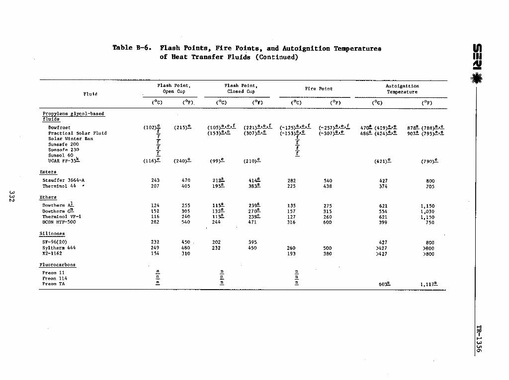
Table B-6. Flash Points, Fire Points, and Autoignition Temperatures of Heat Transfer ~luids (Continued)

F l a s h P o i n t , F l a s h Poin t , F i r e Poin t Auto igni t ion

F l u i d Open Cup Closed Cup Temperature

C0c) (OF). (OC) (OF) (OC) (OF) (Oc) (OF)

Propylene glycol-based f l u i d s

~ o w f r o s t (LO,?)* ( 2 1 5 g 0 5 (221)29%sf - 5 - 5 4 7 e (41g+% 8 7 e ( 7 8 8 ~ ~ P r a c t i c a l S o l a r F lu id f -

f ( 1 5 3 F * ( 3 0 7 F % ( - 1 5 3 e 2

f (--307*2 48& ( 4 2 4 F E 907A (795+2 S o l a r Winter Ban - - Sunsafe 200 f - f - Sunsafe 230 f - f - Sunsol 60 f - f - UCAR F F - ~ & ( 1 1 6 ) c ( 2 4 0 g ( 9 9 g (210)E ( 4 2 1 ) c (7901%

E s t e r s

S t a u f f e r 3664-A 243 470 2 1 9 4 1 e 282 540 427 800 Therminol 44 207 405 1 9 e 3 8 e 225 438 374 705

W W h)

E t h e r s

Dowtherrn & 124 255 115% 2 3 e 135 275 621 1,150 Dowtherm 152 305 1 3 e 27& 157 315 554 1,030 Therminol VF-1 116 240 115E 2 3 e 127 260 621 1,150 DCON HTF-500 282 540 244 471 316 600 399 750

S i l i c o n e s

SF-96(20) Syltherm 444 X2-1162

Fluorocarbons


Table B-6. Flash Points, Fire Points, and Autoignition Temperatures of Heat Transfer Fluids (Concluded)

3alue determined in present work.

kFlammability limits in air: lower flammability limit, 0.8 vol-% at 54'~ (130~~) and also at 171°c (340'~); upper flammability limit, 5 vol-X at 8 8 O ~ (190~~) and also at 171°c (340~~).

9lammability limits in air: lower flammability limits, 0.8 vol-% at 14g0c (300~~) and 0.5 vol-X at 260'~ (500~~); upper flammability limits, 3.3 vol-% at 149'~ (300'~) and 6.2 vol-% at 260'~ (500'~).

s o t manif old ignition temperature -816°~ (~1,500~~). I !?The data pertain to undiluted glycol base stock. I fSolutions containing 50 vol-X water do not have measurable flash and fire points. I .&olutions containing up to 85 vol-X Prestone I1 in water do not have detectable flash and fire points. I k ~ h e autoignition temperatures of Prestone I1 Summer/Winter Concentrate and its 40 vol-% solution in water are reported as 632'~ (1,170'~) and

6 8 8 ' ~ (1 ,270°F'), respectively.

LE"1ammability limits in air: lower Elammabi2ity limit, 3.2 vol-%; upper flammability limit, 15.3 vol-X. I &erex solutions in water, at concentrations lower than 80 vol-X, do not have detectable flash and fire points. I %?lammability limits in air: lower flammability limit, 2.6 vol-X; upper flammability limit, 12.5 vol-X. I ~lammabiliry limits in air: lower flammability limits, 0.8 vol-% at 149'~ (300~~) and 0.5 "01-X at 260'~ (500'~); upper flammability limits, 3.3 vol-X at 149'~ (300'~) and 6.2 vol-% at 260'~ (500'5'). I

!!Flammability limits in air: lower flammability limits, 1.2 vol-XI at 171'~ (340~~) and 0.6 vol-X at 260'~ (500~~); upper flammability limits, 1.2 vol-X at 171'~ (340'~) and 3.3 vol-% at 204'~ (400'~).

%reon 11, Freon 114, and Freon TA are reported by the manufacturer not to exhibit flash and fire points. I

Table B-7. Recommended Fire-Extinguishing Agents for Heat Transfer Fluids

Fluid Recommended F i r e Extinguishing Agents

Hydrocarbons

Petrolem-based a l i p h a t i c hydrocarbons

Caloria HT-63 Hobilthenn 603 Silogram Heat Transfer Fluid 43

Synthetic a l i p h a t i c hydrocarbons

Brayco 888 Brayco 888 HF X-30 Uniroyal PAO-13C


Dowtherm J Dowtherm LF DXE

Xobil them 600

XCS-1958 ?lCS-1980 YCS-2046 Thenninol 55 Theminol 50 Therminol 66 Th'erninol 88

Glycols

Ethylene glycol-based f l11ids -

Dowthem Sil-1

Prestone I1 VCAX TE-17

Zerex

Provylene glvcol-based f l u i d s

Dowfrosz

Zsters

Therninol 44

Ethers - Dowthem A ilowt>en G

Cog, dry chemical, foam, water spray o r fog C02, dry chemical, foam Same f i r e extinguishing agents t h a t a r e applied t o o i l f i r e s

C02, dry chemical C02, dry chemical C02, foam C02, dry chemical, foam, water

Dry chemical, steam, water spray, o r m i s t Dry chemical, steam, water spray, o r m i s t C02, dry chemical, foam, water spray; water spray Day be

used t o flush s p i l l s away from exposure CO,, dry chemical, foam; f i r e f i g h t e r s must use s e l f -

contained breathing apparatus C02, dry chemical, foam, water spray, o r m i s t C02, dry chemical C02, dry chemical, foam, water spray, o r n i s t C02, dry chemical, foam, water spray, o r m i s t C02, dry chemical, foam, water spray, o r m i s t Cog, dry chemical, foam, water spray, o r m i s t Cop, dry chemical

Cog, dry chemical, foam, water m i s t f o r neat f l u i d ; none needed f o r d i lu ted f l u i d

C02 o r dry chemical f o r s n a l l f i r e s ; foam f o r l a r g e f i r e s CO o r dry chemical f o r small f i r e s ; foam and water fo r

Zarge f i r e s Cog, dry chemical, water

C02, dry chemical, foam, water m i s t fo r neat f l u i d ; none needed for d i lu ted mater ial

C o g , d r y chemical fo r s n a l l f i r e s ; foam and water fo r l a rge r i r e s

C02, dry chemical, foam

lky chemical, steam, water spray, o r mist Dry chemical, steam, water spray, o r sist

Si l icones

SF-96(20) :by common f i r e f i g h t i n g agent S y l t h e n 444 C02, dry chemical X2-1162 Cop, dry chemicai

Table B-8- Physiological Properties of Heat Transfer Fluids

Fluid Physiological Effects

Hydrocarbons

Caloria FiT-43 Acute oral LD50 >10 g/kg body weight for rats. Skin contact : prolonged contact may cause mild irritation. Mutagenicity: Ames test negative

Diala kY Not reported Yobiltherm 603 Safe and nontoxic by Federal Hazardous Substances Act tests Silogram Reat Transfer Fluid 43 Mutagenicity: Ames test negative

SUnOcO Heat Transfer 21 Acute oral LDS0 >30 g/kg body v ight for rats. Inhalation: 5 no effect expected at 25 mg/m of air. TLV 5 mg/m3 as oil mist. Skin contact: dermal LDSO g/kg body weight. Yuragenicity: Ames test negative

Sunoco Reat Transfer M 1 25 Acute oral LDSO >30 g/kg body w ight for rats. Inha ation: 3 3 no effect expected at 25 mg/m of air. TLV 5 mg/m as oil mist. Skin contact: no irritation expected unless prolonged or repeated contact is allowed. Not expected co be toxic by dernal absorption

Low toxicity and nonirritating to operating personnel ?Jot reported

Texathera Thermia Oil C

Eirayco 858


Dowtherm J

Acute oral LDgO >40 &/kg body weight by ingestion or subcutaneously. Eye contact: no irritation by the Dtaize test. Mutagenicity: h e s test negative

LD50 >40 mL/kg. Eye contact: non-irritating; Draize lndex 0. Skin contact : nonirritating

Physiological effects similar to those of paraffin oils Physiological effects similar to those of paraffin oils PhysiologLcal eEfects similar to those of paraffin oils Oral LD5* >30 g/kg body weight. TLV >17 mg/liter. Mutagenicity: h e s test negative

Not reported LDS0 >40 &/kg body weight. Skin contact: causes 13 irritation. Xutagenicity: Ames rest negative

LDS0 (rats) is in the range of 1-2 g/kg body weight. Eye contact: up to rni ld irritation; no corneal icjury Likely. Skin contact: up to mlld irritation upon single exposure; up to noderare irritation upon prolonged exposure, possi5ly mild edema and superficial burn. Xor likely to be absorbed in acutely toxic amounts. ?Iutageaicity: Ames test negative

Table B-8. Physiological Properties of Heat Transfer Fluids (Continued)

F l u i d Phys io log ica l E f f e c t s

Dowthern LF

XCS-1980 YCS-2046 Therminol 55

Themino l 50

Themino l 66

LDSO ( r a t s ) i s i n t h e range of 2-4 g/kg body weight. Inha la t ion : exposure should be l i m i t e d t o 1 ppm according t o OSHA guide (1975). Eye con tac t : may cause pain , s l i g h t t r a n s i e n t i r r i t a t i o n ; no co rnea l i n j u r y . Skin con tac t : prolonged o r repeated exposure a a y cause s l i g h t t o moderate i r r i t a t i o n . Not l i k e l y t o be absorbed i n t o x i c amounts. Mutagenicity: Ames t e s t nega t ive

TLV n o t e s t ab l i shed . Suggested l i m i t i n g exposure c r i t e r i o n of m i s t is 5 mg/m3. Skin con tac t : prolonged o r repeated c o n t a c t may cause i r r i t a t i o n . Prolonged exposure to m i s t may cause i r r i t a t i o n of mucous membrane. Eye contact : may cause i r r i t a t i o n

Not repor ted Acute o r a l LD50 ( r a t s ) is approximately 8 g/kg body weight.

Xutagenicity: Ames t e s t negat ive Xutagenic i ty : Ames t e s t negat ive Yutagenic i ty : h e s t e s t negat ive LD50 ( r a t s ) >15.8 glkg body weight. TLV is no t

e s t ab l i shed . Inha la t ion : due t o low v o l a t i l i t y , no observable e f f e c t s on r a t s dur ing and a f t e r 6-hr exposure. Eye con tac t : mild, r e v e r s i b l e i r r i t a t i o n t o the eyes of r abb i t s . Skin con tac t : non le tha l a t t h e dose r a t e of 7.04 g/kg body weight. Muta,oenicity: Ames t e s t nega t ive

Acute o r a l LDSO ( r a t s ) is 13.9 g/kg body weight. TLV i s not e s t ab l i shed . Inha la t ion : due t o low v o l a t i l i t y , no observable e f f e c t s on r a t s dur ing and a f t e r 6-hr exposure. Eye con tac t : s i l d , r e v e r s i b l e i r r i t a t i o n t o the eyes of r abb i t s . Skin contact3 non le tha l a t the dose r a t e of 7.94 g/kg body weight. Pfutagenicity: h e s t e s t nega t ive

Acute o r a l LD ( r a t s ) i s 10.2 g/kg body weight. TLV i s 5 mg/m3 (0.2Oppm). Inha la t ion : due t o low v o l a t i l i t y , no observa3le e f f e c t on r a t s during and a f t e r 6-hr exposure. Eye contact : a i l d , r e v e r s i b l e i r r i t a t i o n t o t h e eyes of r e b b i t s . Skin con tac t : dermal LD50 ( r a t s ) is 6.3 g/!cg body weight. I r r i t a t i o n upon exposure of abraded r a b b i t s k i n t o Then in01 66. ?lutagencity: Ames t e s t negat ive

Acute o r a l LD59 is 50 glkg body weight. TLV is no t e s t ab l i shed . Eye con tac t : mild, r e v e r s i 3 l e i r r i t a t i o n t? the eyes of r abb i t s . Skin con tac t : no i r r i t a t i o n upon 2L- h r con tac t with i n t a c t rabbic sk in . ?futagenic i ty : . h e s t e s t negative

Table B-8- Physiological Properties of Heat Transfer Fluids (Continued)

Flu id Phys io log ica l E f f e c t s

Glycols

Ethylene glycol-based fluf as

Dowtherm SR-1

Pres tone 11

Sunsafe 100 Sunsafe 130 UCAR TF-17

Zerex

Provylene glycol-based f l u i d s

Ingest ion: moderate t o low single dose o r a l t o x i c i t y t o humans. Inha la t ion : 7-hr exposure t o s a t u r a t e d vapors generated a t 3 8 O ~ ( 1 0 0 ° ~ ) caused no adverse e f f e c t s t o r a t s . Eye con tac t : nay cause pain and mild i r r i t a t i o n ; i s not l i k e l y t o cause co rnea l i n j u r y . Skin con tac t : prolonged o r repeated exposure may cause minor i r r i t a t i o n , even minor burn. Not absorbed i n t o x i c amounts through skin . Mutagenicity: Ames t e s t negat ive

TLV 100 ppm. Confirmed cases of harmful e f f e c t s r e l a t e only to swallowing. It causes drunkenness, r a p i d l y pass i3q i n t o coma. Ser ious o r f a t a l kidney in ju ry . Yutagenic i ty : . Xmes t e s t negat ive

Not repor ted Not repor ted Acute oral.LD5* ( r a t s ) is j.54 g/kg body weight. TLV i s

100 ppm (vapor) , 10 mg/m ( p a r t i c u l a t e ) . Eye con tac t : f looding t h e r a b b i t eye wi th UCM TF-17 caused a r e a c t i o n no more severe than moderate inflammation. Skln con tac t : undi lu ted UCAR TF-17 on r a b b i t b e l l y caused f a i n t redness f o r a s h o r t du ra t ion

Single dose of 100 mL of e thy lene g lyco l can be f a t a l to human beings. .Animal s t u d i e s have ind ica t ed t h a t smal l o r a l doses over a lonq per iod can produce seve re kidney i n j u r y , bladder s tones , and l i v e r damage. I n h a l a t i o s : TLV, recommended by the American Conference of Gover mental I n d u s t r i a l Xygienis ts i s 100 ppm of vapor o r 10 mg/m S p a r t i c u l a t e s . I n h a l a t i o n nay be a problem i f e t h y l e w g lyco l i s h o t , o r i f fog o r m i s t is generated by hea t o r v i o l e n t a g i t a t i o n . Va,por i n h a l a t i o n overexpQsure may cause i r r i t a t i o n of the t h r o a t , mild headache, and low backache. Yutagenic i ty : .hies t e s t negat ive

Acute o r a l LD5,, ( r a t s ) >30 g/kg body weight. A s auch a s 2 % t o SO% of propylene g lyco l ingesced by humans appears unchanged i n the u r ine in 24 h r s . Chronic o r a l t o x i c i t y i s a l s o very low. Xats r ece iv ing dr inking water con ta in ing u? t o 1OZ propylene g lyco l over a per iod of 140 days d e v e l o ~ e d no ill e f f e c t s . Rats rece iv ing b.9Z i n t h e i r d i e t fo r 2G nonths were normal i n t h e i r growth. They sus t a ined s l i g h t l i v e r i n ju ry . Eye con tac t : proaylene g lyco l i s not expected t o cause i r r i t a t i o n . Skin con tac t : ~ r o p y l e n e


Fluid Physiological Effects

glycol does not cause serious skin irritation. Very severe, prolonged exposure may produce slight maceration of the skin. Mutagenicity: Ames test negative

Practical Solar Fluid Mutagenicity: .hes test negative Solar Winter Ban Not reported Sunsafe 200 ?lot reported Sunsafe 230 Not reported Sunsol 60 Xanufacturer's literature claims that Sunsol 60 is nontoxic

and does not contain hazardous ingredients UCAP FF-35 Acute oral LDSO (rats) is 26.3 g/kg body weight. TLV not yet

established. Inhalation: air saturated with propylene glycol vapor at room temperature killed no animals exposed for eight hours. Skin contact: LD50 >20 mL/kg body weight. Undiluted propylene glycol caused no irritation on the tender skin of the rabbit belly

Esters - Stauf fcr 3664-A

Ethers

Dowthem, A

Accidental ingestion of large doses aay produce symptoms of nonspecific irritation of the gastointestinal tract, nausea, vomiting, cramps and diarrhea. Inhalation: high vapor concentrations may cause nonspecific irritation of mucous membranes in the upper respiratory tract. Skin contact: no irritation was observed when this material was applied onto the skin of rabbits. Xutagenicity: .bes test negative

Acute oral LDgO (rats) is 13 g/kg body weight. Inhalation: rats survived 6-hr exposure and 10-day observation period with no noticeable effects, when exposed to air aspirated through Theminol 44. Eye contact: slight, reversible irritation to rabbit eye. Skin contact: mild irritation upon contact with rabbit skin. Hutagenicity: hes test negative

Acute oral LD50 (rats) 2-L g/kg body weight. Inhalation: TLV 1 ppm. Eye contact: up to mild irritation but no corneal injury. Skin contact: short single exposure not likely to cause significant irritation. Prolonged or repeated exposure may cause up to mild irritation. :?utagenicity: hes test negative

Acute oral LDgp (rats) 2-4 g/kg body weight. Inhalation: suggested TLJ 1 ppm. Eye contact: aild gain, mild transient irritation and corneal haziness. Skin contact: nild skin irritation. Dermal L3g0 >2 g/kg body weight. Mutagenicity: Ames test negative


F l u i d Physiological E f f e c t s

Themino1 VP-1 Acute o r a l LD50 ( r a t s 4 1.46 g / L g body weight. Inha la t ion : TLV 1 ppm o r 7 ng/m . Eye con tac t : s l i g h t , r e v e r s i b l e i r r i t a t i o n t o r a b b i t eye. Skin con tac t : mild i r r i t a t i o n upon con tac t wi th i n t a c t and abraded r a b b i t skin . Dernal

' LDS0 >5.01 g/kg body weight. Xutagenic i ty : h e s t e s t nega t ive

Not ye t e s t a b l i s h e d UCON HTF-500

S i l i c o n e s

SF-96(20)

Sylthem 444

%luorocarbons

Freon 11

Acute o r a l tD5,, >20 g/kg body weight. Inha la t ion : LCSO >500 mg/m3 f o r 1-hr inha la t ion . Eye con tac t : minor t r a n s i e n t i r r i t a t i o n by Draize t e s t . Skin con tac t : no i r r i t a t i o n . Mutagenicity: Ames test negat ive

Information about phys io log ica l e f f e c t s of S y l t h e m 444 was not a v a i l a b l e from t h e manufacturer. Rowever, Dow Corning Corporat ion supp l i ed a repor t on the toxicology of s i l i c o n e s . On t h e b a s i s of t h i s r e p o r t , poly(dimethyls i loxane) , t he base f l u i d of S y l t h e m 444, has very low t o x i c i t y i n r a t s , whea suppl ied o r a l l y . No d e l e t e r i o u s e f f e c t s were detected when fed a t a concen t ra t ion of 1% of the d i e t over a period of 90 days. Inha la t ion : vapor t o x i c i t y is low, p a r t l y because of t he very low vapor pressure . Eye con tac t : t r a n s i t o r y conjunct ive i r r i t a t i o n may be caused; no Ternanent effect. Skin c o n t a c t : cause no acan thos i s , are not absorbed through s k i n ; used i n p ro tec t ive sk in creams and sprays . Mutagenicity: Ames t e s t negat ive .

Information about phys io log ica l e f f e c t s of X2-1162 was nor a v a i l a b l e . However, Dow Corning Corporation s u p p l f ed a repor r on the toxicology of s i l i c o n e s . On t he basis of t h i s r e p o r t , poly(dimethyls i loxane) , the base fluid of X2- 1162, has very low t o x i c i t y i n r a t s , when suppl ied o r a l l y . Yo d e l e t e r i m s e f f e c t s a r e de tec t ed when fed a t a concen t ra t ion of 1X of the d i e t over a period of 90 days. Inha la t ion : vapor t o x i c i t y is low, pa rz ly because of the very low vapor p res su re . Eye con tac t : t r a n s i t o r y conjunct ive i r r i t a t i o n nay be caused; no pernanent e f f e c t . Skin con tac t : cause no acan thos i s , are not absorbed through s k i n ; used i n p r o t e c t i v e sk in c r e a m and sprays

Inha la t ion : no e f f e c t s a t 1,000 ppm; LC50 ( r a t s ) 26,200 ppm. Cardiac s e n s i t i z a t i o n i n beagle dogs a t 3,500 ?Dm. Xutagenic i tp : . h e s t e s t negat ive . Tera togenic i ty : no ind ica t ions

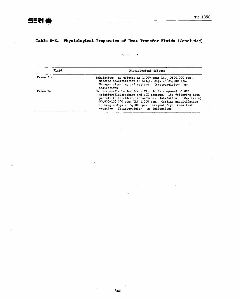
Table B-8. Physiological Properties of Heat Transfer Fluids (Concluded)

Fluid Physiological Sffects

Freon 114

Freon TA

Inhalation: no effects at 1,000 ppm; LC50 >600,000 ppm. Cardiac sensitization in beagle dogs at 25,000 ppm. Xutagenicity: no indications. Teratogenicity: no indications

No data available for Freon TA. It is composed of 892 trichlorofluoroethane and 10% acetone. The following data pertain to trichlorofluoroethane. Inhalation: LCs0 (rats) 90,000-100,000 ppm; TLV 1,000 ppm. Cardiac sensitization in beagle dogs at 5,000 ppm. Mutagenicity: h e s test negative. Teratogenicity: no indications

Table B-9. Summary of ~ensit~'Data (kg/m3)

Temperature (OC) F lu id

-50 -2 5 0 2 5 5 0 7 5 100 125 150 175

Brayco 888 Brayco 888 HF Ca lor ia HT-43 Diala AX Dowf r o s t Dowtherm A Dowtherm G Dowtherm J 919.8 Dowtherm LF Dowtherm SR-1 DXE ESH 4 ESH 5 ESH 6 Freon 11 Freon 114 Freon TA H 30 MCS 1958 MCS 1980 MCS 2046 Mobil Them 600 Mobil Them 603 P A 0 1 3 C P r a c t i c a l Fluid Prestone 11 SI-96 Silogram 43 So la r Winter Ban S t a u f f e r 3664-A Sunoco 21 Sunoco 25 Sunsafe 100 Sunsafe 130 Sunsafe 200 Sunsafe 230 Sunsol 60 Sylrherm 444 Texatherm Thermia C Therminol 44 977.3 'Rierminol 55 Therminol 60 1041.1 Therminol 66 Therminol 88 Therminol VP-1 UCAR FF-35 UCAR TF-17 UCON HTF-500 Water X2-1162 Zerex

Table B-9. Summary of Density Data (kg/$) (Concluded)

Temperature (OC) Fluid

200 225 250 275 300 325 350 375 400 450

Brayco 888 Brayco 888 HF Calor ia HT-43 727.4 709.8 692.5 674.3 656.3 639.0 Diala AX Dowf r o s t Dowtherm A 907.5 883.3 858.8 833.4 806.8 779.0 749.2 715.4 680.8 Dowtherm G 964.7 944.5 924.3 904.1 884.7 865.9 847.6 830.3 Dowtherm J 710.8 685.1 657.1 626.5 Dowtherm LF 897.4 877.2 858.1 839.3 821.3 804.0 Dowtherm SR-1 DXE ESH 4 ESH 5 ESH 6 Freon 11 Freon 114 Freon TA H 30 MCS 1958 1133.1 1112.7 1086.4 MCS 1980 983.4 964.9 945.2 MCS 2046 Mobil Them 600 829.1 813.5 797.7 781.8 765.2 747.9 Mobil Them 603 752.5 737.8 722.4 706.5 PA0 13C 725.5 708.2 690.9 - P r a c t i c a l Fluid Prestone I1 SI-96 735.3 710.3 686.8 Silogram 43 So la r Winter Ban Stauf f e r 3664-A Sunoco 21 754.6 735.9 716.1 695.0 673.4 651.8 Sunoco 25 754.6 735.9 716.1 695.0 672.7 649.6 Sunsafe 100 Sunsafe 130 Sunsafe 200 Sunsafe 230 Sunsol 60 Syltherm 444 Texatherm 752.0 737.8 721.3 704.9 689.8 675.3 Thermia C 761.8 746.2 727.3 Therminol 44 783.4 Therminol 55 762.1 745.1 727.8 710.5 693.9 678.0 Therminol 60 877.2 859.2 840.5 823.4 806.9 789.6 Therminol 66 884.1 868.0 851.1 833.8 816.5 799.2 781.9 Therminol 88 964.1 944.1 926.4 908.2 890.2 869.1 844.4 827.1 TherminolVP-1 912.3 889.3 865.2 840.7 814.8 786.8 757.2 724.8 688.8 UCAR FF-35 UCAR TF-17 UCON HTF-500 909.5 893.6 Water 865.1 834.1 798.3 X2-1162 800.2 776.0 749.4 721.2 690.2 657.0 Zerex

Table 35-10, Summary of Viscosity Data (cp)

Temperature ( O C )

Fluid 0-50 0-25 0 25 5 0 7 5 100 125 150 175

Brayco 888 Brayco 888 HF G l o r i a NT-43 Diala AX Dowfrost Dowtherm A Dowtherm G Dowtherm J Dowtherm LF Dowtherm SR-1 Dm ESH 4 ESH 5 ESH 6 Freon I1 Freon 114 Freon TA H 30 MCS 1958 MCS 1980 MCS 2046 Mobil Them 600 Mobil Them 603 PA0 13C Practical Fluid Prestone I1 SI-96 Silogram 43 Solar Winter Ban Stauffer 3664-A Sunoco 21 Sunoco 25 Sunsafe 100 Sunsafe 130 Sunsafe 200 Sunsafe 230 Suns01 60 Syltherm 444 Texathem Thermia C Therminol 44 Therminol 5 5 Therminol 60 Therminol 66 Therminol 88 Therminol VP-1 UCAR FF-35 UCAR TF-17 UCON HTF-500 Water X2-1162 Zerex

s=pI +, TR-1356 - \ = /

Table B-10. Summary of Viscosity Data -(cp) (Concluded)


200 225 2 50 275 300 325 350 375 400 425

Brayco 888 Brayco 888 HF Calor ia HT-43 Diala AX Dowf r o s t Dowtherm A Dowtherm G Dowtherm J Dowtherm LF Dowtherm SR-1 DXE ESH 4 ESH 5 ESH 6 Freon 11 Freon 114 Freon TA H 30 MCS 1958 MCS 1980 MCS 2046 Mobil Them 600 Mobil Them 603 PA0 13C P r a c t i c a l Fluid Prestone I1 SI-96 Silogram 43 So la r Winter Ban Stauf f e r 3664-A Sunoco 21 Sunoco 25 Sunsafe 100 Sunsafe 130 Sunsafe 200 Sunsafe 230 Suns01 60 Syltherm 444 Texatherm Thermia C Therminol 44 Therminol 55 Therminol 60 Therminol 66 Therminol 88 Therminol VP-1 UCAR FF-35 UCAR TF-17 UCON HTF-500 Water X2-1162 Zerex

Table B-11. Summary of Specific &at Data [J/ (kg K) 1


-50 -25 0 2 5 5 0 7 5 100 125 1 SO 175

Brayco 888 Brsyco 888 BF Caloria HT-43 Diala AX Dowf r o s t Dowtherm A Dowtherm G Dowtherm J Dowtherm LF Dowtherm SR-1 DXE ESH 4 ESH 5 ESH 6 Freon 11 Freon 114 Freon TA B 30 MCS 1958 MCS 1980 MCS 2046 Mobil Them 600 Mobil Them 603 PA0 13C P r a c t i c a l F lu id Prestone I1 S 1-96 Silogram 43 Solar Winter Ban S t a u f f e r 3664-A Sunoco 21 Sunoco 25 Sunsafe 100 Sunsafe 130 Sunsafe 200 Sunsafe 230 Suns01 60 Syltherm 444 Texatherm Thennia C Therminol 44 Therminol 55 Therminol 60 Therminol 66 Therminol 88 Theminol VP-1 UCAR FF-35 UCAR TF-17 UCON HTF-500 Water X2-1162 Zerex

Table B-11. Summary o f S p e c i f i c Heat Data kg K) 1 (Concluded)

Fluid

Brayco 888 '

Brayco 888 HF Caloria HT-43 Diala AX Dowf rost Dowtherm A Dowtherm G Dowtherm J Dowtherm LF Dowtherm SR-1 DXE ESH 4 ESH 5 ESH 6 Freon 11 Freon 114 Freon TA H 30 MCS 1958 MCS 1980 MCS 2046 Mobil Therm 600 Mobil Therm 603 PA0 13C Practical Fluid Prestone I1 SI-96 Silogram 43 Solar Winter Ban Stauf fer 3664-A Sunoco 21 Sunoco 25 Sunsafe 100 Sunsafe 130 Sunsafe 200 Sunsafe 230 Sunsol 60 Syltherm 444 Texatherm Thermia C Therginol 44 Therminol 55 Therminol 60 Therminol 66 Therminol 88 Therminol VP-1 UCAR FF-35 UCAR TF-17 UCON HTF-500 Water X2-1162 Zerex

--

Temperature (OC)

200 225 250 275 300 325 350 375 400 425

Table B-12. Summary of Thermal ~onductivity Data [W/(m K) ]

Temperature (OC)

Brayco 888 Brayco 888 HF Caloria HT-43 Diala AX Dowfrost Dowtherm A Dowtherm G Dowtherm J Dowtherm LF Dowtherm SR-1 DXE ESH 4 ESH 5 ESH 6 Freon 11 Freon 114 Freon TA H 30 MCS 1958 MCS 1980 MCS 2046 Mobil Them 600 W b i l Them 603 PA0 13C P r a c t i c a l Fluid Prestone I1 SI-96 Silogram 43 Solar Winter Ban S tauf fe r 3664-A sunoco 21 Sunoco 25 Sunsafe 100 Sunsafe 130 Sunsafe 200 Sunsafe 230 Sunsol 60 Syltherm 444 Texatherm Thermia C Therminol 44 Theminol 55 Therminol 60 Therminol 66 Thermlnol 88 Therminol V P - 1 UCAR FF-35 UCAR TF-17 UCON HTF-500 Water X2-1162 Zerex

TR-1356 SSP1 3

Table B-12. Suntmary of Thermal Conductivity Data [w/ (m K) 1 (Concluded)

Fluid

Brayco 888 Brayco 888 HF Calor ia ET-43 Diala AX Dowf ros t Dowtherm A Dowtherm G Dowtherm J Dowtherm LF Dowtherm SR-1 DXE ESH 4 ESH 5 ESH 6 Freon 11 Freon 114 Freon TA H 30 MCS 1958 MCS 1980 MCS 2046 Mobil Them 600 Mobil Them 603 PA0 13C P r a c t i c a l Fluid Prestone I1 SI-96 Silogram 43 So la r Winter Ban S t a u f f e r 3664-A Sunoco 21 Sunoco 25 Sunsafe 100 Sunsafe 130 Sunsafe 200 Sunsafe 230 Suns01 60 S y l t h e m 444 Texatherm Thermia C Therminol 44 Therminol 55 Therminol 60 Therminol 66 Therminol 88 Therminol VP-1 UCAR FF-35 UCAR TF-17 UCON HTF-500 Water X2-1162 Zerex

Temperature (OC)

'Eable B-13. Sumary of vapor Pressure Data '(pa)


-50 -25 0 25 5 0 7 5 100 125 150 175

Brayco 888 Brayco 888 HF Calot ia HT-43 Dfala AX Dowf r o s t Dowtherm A Dowtherm G Dowtherm J Dowtherm LF Dowtherm SR-1 Dm ESH 4 ESH 5 ESH 6 Freon 11 Freon 114 Freon TA H 30 MCS 1958 MCS 1980 MCS 2046 Mobil Therm 600 Mobil Therm 603 PA0 13C P r a c t i c a l Fluid Prestone I1 S 1-96 Silogram 43 Solar Winter Ban Stauf f e r 3664-A Sunoco 21 Sunoco 25 Sunsafe 100 Sunsafe 130 Sunsafe 200 Sunsafe 230 Suns01 60 Syltherm 444 Texa t h e m Thermia C Themino1 44 Thermtnol 55 Therminol 60 Therminol 66 Therminol 88 Therminal V F 1 UCAR FF-35 UCAR TF-17 UCON HTF-500 Water X2-1162 Zerex

TR-1356

Table B-13, Summary of Vapor Pressure Data (Pa) (Concluded)

Fluid

Brayco 888 Brayco 888 HF Caloria HT-43 Diala AX Dowf ros t Dowtherm A Dowtherm G Dowtherm J Dowtherm LF Dowtherm SR-1 DXE ESH 4 ESH 5 ESH 6 Freon 11 Freon 114 Freon TA H 30 MCS 1958 MCS 1980 MCS 2046 Mobil Them 600 Mobil Them 603 PA0 1X Prac t i c a l Fluid Prestone I1 SI-96 Silogram 43 Solar Winter Ban Stauf f e r 3664-A Sunoco 21 Sunoco 25 Sunsafe 100 Sunsafe 130 Sunsafe 200 Sunsafe 230 Sunsol 60 Syltherm 444 Texatherm Thermia C Therminol 44 Therminol 55 Therminol 60 Therminol 66 Therminol 88 Therminol VP-1 UCAR FF-35 UCAR TF-17 UCON HTF-500 Water X2-1162 Zerex

Temperature (OC)

APPENDIX C

THE SOLIPH COMPUTER PROGRAM

The SOLIPH computer program was written specificallya for the purpose of generating design tools for this handbook. Like other solar simulation codes (e.g., TRNSYS, SOLTES, etc.), SOLIPH is a quasi-steady-state, hour-by-hour model. For each hour of the year, climatological data (time, direct normal ' insolation, total horizontal insolation, and ambient temperature) are read from a TMY (Typical Meteorological Year) weather tape, available for 26 different weather stations. The executive routine reads all the system and climatological input data, and then calls various subroutlnes (collector, pipe, heat exchanger, storage, etc.) around closed piping loops. A starting point temperature is chosen for each pipe loop (the collector array inlet temperature in the collector loop), and energy balances are performed on each component. The program cycles through each loop as many times as necessary until the temperature distribution is essentially unchanged from the previous iteration (to within a specified temperature convergence criterion). Each hour, new climatological and loads inputs are used, and the program arrives at a new steady-state solution, until the entire year has been modeled*

A simple SOLIPH model is shown in Fig. C-1. The starting point for this configuration is the inlet collector temperature, The executive routine calls the collector subroutine, SOLCOL, which, based on input collector parameters

PIPE 1 PIPE 3

PIPE 2 PIPE 4

Figure C-1. A Simple SOLIPH Configuration

and climatological data, supplies a collector array outlet temperature. This is used as the inlet temperature for pipe 1. The pipe subroutine, PIPE, is called and, based on input pipe insulation and ambient temperature, supplies an outlet temperature. The outlet temperature is used as the hot-side inlet temperature to the heat exchanger. The heat exchanger routine, HX, uses input effectiveness and the hot and cold inlet temperatures to compute the two outlet temperatures. The hot outlet temperature is then used as input for pipe 2. The PIPE subroutine is again called, and its outlet value replaces the inlet collector temperature we started with. If these two temperatures are not sufficiently close, the loop must be repeated.

First, however, the second loop is computed. The cold-side outlet temperature of the heat exchanger is used as input for pipe 3. The outlet from PIPE is used as the inlet storage temperature. The LOADS subroutine is called to determine the load at that hour and to allow a complete energy balance on the storage tank, and then STORE is called to determine a new storage tank temperature. This temperature is used as the input for pipe 4, and the output temperature from PIPE is compared with the inlet cold-side heat exchanger temperature originally assumed, thus completing the second loop. If either loop has not converged within the specified tolerance, both are reiterated.

To make the code as easy to understand. as possible, energy calculations are done in the subroutines where they are most appropriate rather than at the end of the executive routine. So, for example, pipe energy loss is calculated in the PIPE subroutine, storage loss in STORE, etc. Since only temperature values are needed for loop iteration, calculating all energy values during each

. cycle would waste computer time. SOLIPH is set up to do these calculations only on the last iteration.

Output temperatures and energy values are supplied on hourly, daily, and monthly bases with an annual cumulative summary. Energy collected by the array, energy delivered to the load, and pumping energy are outputs. Energy losses are given separately for piping and storage and are also broken down according to whether they are operational (durfng collector pump operation) or nonoperational losses. Collector array efficiencies are given relative to useful energy in the plane of the collectors as well as to total horizontal energy. System efficiencies are supplied as the ratio of energy delivered to the .load to insolation. Table C-1 is a sample monthly summary.

Before we describe the various subroutines, we must point out that SOLIPH is not a highly user-oriented code like TRNSYS or SOLTES. To change the system configuration, the user does not change input data as he or she would for one of the other codes. Rather, the user changes the Fortran programming statements in the executive program. Thus, a CALL STORE might be replaced by a CALL HX. Although this is not an elegant approach, it saves the code from complexity and results in shorter run times. SOLIPH was designed to generate design tools, not for public use; therefore, it is not documented for such use. Rather, the design tools generated from SOLIPH should make detailed computer models unnecessary. The following section describes the basic algorithms used in each SOLIPH subroutine.

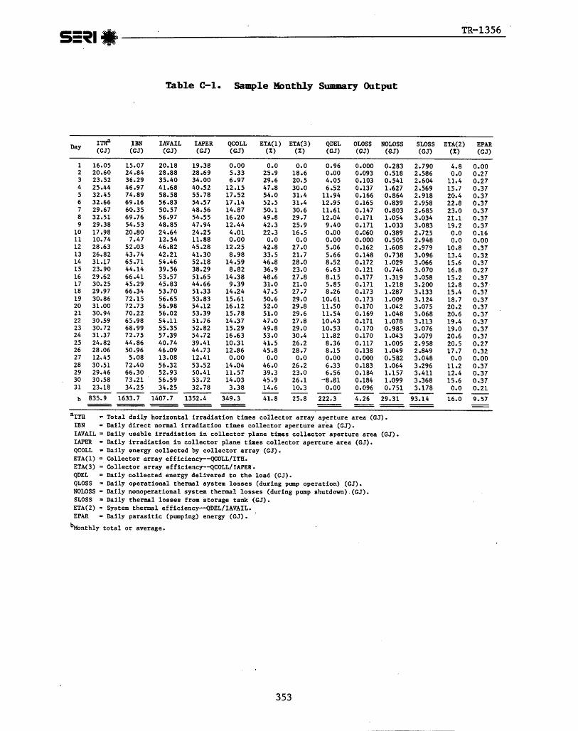
Table 0-1. Sample Monthly ~ k r y Output

IBN ~ G J )

IAVAIL IAPER (GJ) (GJ)

QCOLL (GJ)

QDEL (GJ)

OLOSS NOLOSS SLOSS ETA(2) (GJ) (GJ) (GJ) (XI

EPAR (GJ)

0.0 25.9 29.6 47.8 54.0 52 a 5 SO. 1 49.8 42.3 22.3 0.0

42 -8 33.5 46.8 36.9 48.6 31.0 47.5 50.6 52 -0 51.0 47 .O 49.8 53.0 41.5 45.8 0.0

46 .O 39.3 45;9 14.6 - 41.8

= Total daily horizontal irradiation times collector array aperture area (GJ). IBN = Daily direct normal irradiation times collector aperture area (GJ). IAVAIL = Daily usable irradiation in collector plane times collector aperture area (GJ). IAPER = Daily irradiation in collector plane times collector aperture area (GJ). QCOLL = Daily energy collected by collector array (GJ). ETA(1) = Collector array efficiency--QCOLL/ITH. ETA(3) = Collector array efficiency--gCOLL/IAFER. QDEL = Daily collected energy delivered to the load (GJ). QLOSS = Daily operational thermal system losses (during pump operation) (GJ). NOLOSS = Daily nonoperational system thermal losses (during pump shutdown) (GJ). SLOSS = Daily thermal losses from storage tank (GJ). ETA(2) = System thermal efficiency--QDEL/IAVAIL. EPAR = Daily parasitic (pumping) energy (GJ). '

h n t h l y total or average.

C.l THE SOLIPH SUBROUTINES

C.1.1 Subroutine SOLCOL

This subroutine models a stationary solar collector 'array. Direct normal and total horizontal radiation and ambient temperature from the weather tape are used. Values of FRTa, FRUL, incident angle modifier coefficients, and the collector time constant are input, as well as collector tilt, azimuth, and ground-cover ratio.

First, insolation in the collector plane is calculated. SOLIPH does this in the following steps:

Calculates hour-angle and declination. (A day-of-the-year function is used to determine declination.)

Calculates incident angle and converts normal beam radiation to collector plane.

Calculates diffuse radiation in horizontal plane.

Converts diffuse to collector plane (including ground and sky terms).

Adds direct, diffuse, and reflected beam in plane.

Now, it must be determined whether the collector pump is on. If the pump has been operated, this determination is based on the difference between previous collector outlet temperature and storage. If the pump is not on, as in early morning, a stagnation temperature is calculated as follows:

where no is the optical efficiency. The stagnation temperature is compared with the storage tank temperature, and if it is sufficiently higher, the pump is turned on. Several flags provide a deadband temperature range which allows for a typical ATon/A~off control scheme. If the pump is on, collector efficiency is calculated from the Hottel-Whillier-Bliss equation (incident-angle corrected) and multiplied by insolation and collector area to yield energy collected. Collector outlet temperature is then

Qcoll Tout = Tin + 7

If the pump is off, cooldown loss from the collectors is determined. For collector mass M, specific heat C, and loss coefficient U, we solve a time- dependent, first-order ordinary differential equation:

I.C. :

Soln. :

The KaTnol/U term in the differential equation accounts for stagnation heating. The ME value for the collectors is found from the collector time constant rc as determined by ASHRAE 93-77 and input as

where is the collector mass flow rate value used in the ASHRAE test. Once the array temperature is calculated, energy loss is determined as MC times the difference between that temperature and the one for the previous time step. (At shutdown, the average of inlet and outlet temperatures is used for the first value.) These calculations apply only to the collectors and not the header pipes. The headers are lumped into the pipe runs to and from the collector array, and their losses are determined with the supply/return pipe losses.

C 1 2 Subroutine TROUGH

- The parabolic trough subroutine first calculates incident angle for a north- south or east-west trough array. Direct insolation on the aperture is then calculated, correcting for row-to-row shading losses. Pump status is determined by comparing available radiation to an input critical intensity, If the radiation is sufficient, an incident-angle modifier is calculated from input coefficients. The average fluid temperature T is determined as follows: the energy collected per unit area is the product of efficiency and irradiation and also the product of mass flow rate, specific heat, and fluid temperature rise. Setting these quantities equal, we have

SOLIPH then uses the quadratic formula to solve t h i s equation for T. When the average fluid temperature is known, efficiency can be calculated from the input coefficients. (Second-order equations are used for the troughs.) The energy collected is then II IA and outlet temperature is calculated just as c' it is for stationary collec6ors.

Fox situations in which the pump is off, the decaying receiver temperature and associated energy loss are calculated just as for stationary collectors. The exception is that an input receiver mass is used, so that it does not have to be calculated from an input time constant. The stagnation term is not included because parabolic trough collectors would be defocussed when the pump is off.

sin TR-1356

C.1.3 Subroutine PIPE

If the pump temperature, a first-order

B.C.:

Soln. :

is operating, pipe outlet temperature is determined from inlet ambient temperature, and input insulation, using the solution of

, ordinary differential equation (see Fig. C-2):

UrD X

T = Tamb + (Tin - Tamb)e M c ~

Energy lost is then . Qloss = Mcp(Tout - Tin)

To determine parasitic power, the Reynolds number is calculated first to determine which flow regime is present. The Colebrook equation determines the friction factor when flow is turbulent, and f is calculated as 64/Re when flow is laminar. For transitional flow, a simple linear interpolation between the two is used. Values for total equivalent pipe LID, including fittings and elbows, are user inputs. Head is then determined as H = f (L/D) (v2/2g). For simplicity, a user input for average collector and heat exchanger pressure drops are added here, although they could also be in separate subroutines.

I I I I

I I I Qin - Qouc = h;l c p d T

F;1 Qin i T , n - 1 + T o u t

T I . I I I I

I

X x + dx

Figure C-2. Steady-State Pipe Loss Energy Balance

35 6

I f t h e pump i s o f f , the so lu t ion f o r temperature decay i s s i m i l a r t o t h a t f o r t h e co l l ec to r s :

The Mcp product includes both t h e f l u i d and pipe metal. ( Insu la t ion hea t capacity i s usual ly neglected.) The cooldom energy l o s s i s then t h e product of Mcp and t h e average temperature change over a time s tep . Note t h a t t h i s can be negative for t he c o l l e c t o r s and pipe. I f they have cooled down t o ambient and t h e ambient temperature r i s e s , t h e r e w i l l be a heat gain.

C.1.4 Subroutine HX

The hea t exchanger subroutine uses the flow r a t e s , hot and cold i n l e t tempera- t u r e s , and t h e input e f fec t iveness E t o compute the hot and cold o u t l e t tempera tures us ing simple hea t exchanger ef fec t iveness equations ( see Fig. C-3) . Thus, we have

and "

Figure C-3. SOLIPH Beat Exchanger Model

. where C r e f e r s t o heat capacitance flow r a t e , i.e., Mcp. Heat exhanger thermal l o s s e s a r e considered t o be neg l ig ib le .

C.1.5 Subroutine LOADS

The LOADS subroutine supplies t h e load flow r a t e and re tu rn temperature a t each hour needed t o perform t h e loop energy balances. Load p r o f i l e s and load del ivery con t ro l schemes a r e changed by changing t h e code i n LOADS. In a typ- i c a l setup, LOADS f i r s t checks t o see i f a load e x i s t s f o r a given hour. I f so, it ca lcu la tes the d i f ference between t h e s torage tank and load r e t u r n tempera tures t o determine whether flow should occur through storage. Several f l a g s allow f o r a deadband, so t h a t a AT,,/AT,~~ con t ro l s t ra tegy can be used. The LOADS subroutine a l s o has a mix valve capab i l i ty t h a t allows only a f r a c t i o n of t h e load re tu rn f l u i d t o pass through storage and then be mixed with bypassed load re tu rn f l u i d t o l i m i t t h e load supply temperature t o a s e t value.

C.1.6 Subroutine SMRE

The bas ic s torage subroutine assumes mixed storage and takes s k i n losses i n t o account. Flow i n t o and out of s to rage occurs both on t h e co l l ec to r s i d e and t h e load side. I f we c a l l t h e i n l e t temperature on t h e c o l l e c t o r (hot) s i d e Th and the load re tu rn (cold) temperature t o the tank Tc, and t h e mixed s to r - age temperature T (same a s r e t u r n t o c o l l e c t o r s and load supply) (see Fig. C-4), we have

Figure C-4. SOLIPH Storage Tank Heat Balance

358

I.C. : T I = T o t = O

Soln. :

where

Note t h a t , i n t h e case of no flow on e i t h e r s i d e , t h e so lu t ion reduces t o t h e same form a s t h a t f o r t h e pipe.

I f To i s the s torage tank temperature a t t h e beginning of t h e time s t e p , sub- s t i t u t i n g i n t h e time s t e p (one hour) for t i n t h e above so lu t ion w i l l give t h e tank temperature a t t h e end of t h e t i m e s tep. For t h e energy balance t o work, however, we must use the average tank temperature during t h e time s t e p t ' ; i.e., we must i n t e g r a t e t h e above so lu t ion and d iv ide by t h e t i m e s t ep . Thus,

The so lu t ion is

where X = %cp + Qcp + UA. The energy l o s t from storage is determined by in tegra t ing t h e product of UA and the d i f ference between instantaneous storage-tank temperature and ambient temperature. Thus,

t '

t h e so lu t ion of which i s

(We should emphasize here t h a t , i n a l l cases, SOLIPH merely uses t h e s o l u t i o n t o a d i f f e r e n t i a l equation o r i n t e g r a l r a t h e r than solves it.) The energy del ivered t o t h e load i s ca lcu la ted a s the product of the load mass flow r a t e , s p e c i f i c hea t , and d i f ference between load r e t u r n temperature and average s torage temperature:

C -1.7 Subroutine TCSTOBE

The thermocline storage subroutine (TCSTORE) is a simple 2-node model that works by stacking two mixed storage tanks, one on top of the other, and calling STORE twice. The storage volume and UA are divided equally between the two tanks. Energy delivered is the product of load flow rate, specific heat, and the difference between the top tank temperature and the load return temperature. Total energy loss is the sum of the losses from each tank.

C -1 -8 Subroutine BOILER

This subroutine models an unfired boiler. The boiler is divided into a preheat section and a boiling section; total area is held constant. The temperature of the saturated steam to be delivered is specified, as are inlet hot (collector) and cold (load) temperatures and overall U value. Because thermal resistance on the oil (hot) side is dominant in both sections, using one U value for both is a reasonable approximation. Oil flow can be varied to yield a constant steam flow (up to a specified limit), or a constant hot flow can yield a variable steam output. Outputs of the subroutine are hot-side outlet temperature and the unknown flow.

The algorithm solves four simultaneous equations. Two are heat exchanger equations (using Q = UA LMTD), one for the preheater, the other for the boiler. The other two are energy balance equations, one across the preheater, the other for the boiler (see Fig. C-5).

Boiler:

Preheater:

Figure C-5. SOLIPB Unf ired Boiler Model

TH : * M w ,

Boiler U, A1

This gives us four equations in four unknowns: Tc, Ti, Al, or A2, and the unspecified flow. (We know the total area A + A2, but do not know the breakdown.) Since the equations are nonlinear (Itwo contain log terms), we cannot solve them by Ggussian elimination. We must combine them into one equation in R, defined as ( M C ~ ) ~ ~ ~ / ( M C ~ ) ~ to obtain

Thus, we have one equation in one unknown, R. Subtracting U(A1 + A*) from both sides, we have an equation of the form f(R) = 0. SOLIPH solves for the R root by the Newton-Raphson method. Typically, fewer than five iterations are required. Once R, and hence the unknown flow rate, is determined, the energy delivered is calculated as

Water Ts Side Oil ,-i

Side

Preheater U, A2

- Tc 1 - = ~ w ,

, '

and the oil return temperature as

C-1-9 Subroutine FLASH

This subroutine models a flash valve, flash tank, and feedwater make-up valve (see Fig. C-6). All enthalpies are calculated as the product of specific heat and temperature, with the exception of saturated steam enthalpy h which is

g' determined from a separate steam properties subroutine (McClintock and Silvestri 1968).

C.1.9.1 Flash Valve

We assume that the pressure upstream of the flash valve is maintained at 5 psi greater than the saturation pressure (determined from the steam properties subroutine) in order to prevent boiling. Saturation pressure depends on the temperature at that point. The AP across the flash valve is, then, the difference between that upstream pressure and the saturation pressure of steam at

- xhh, : , _ Saturated Steam 8

to Load I

From uh, thh, L h,l

Collectors - Y - Flash Flash Tank Valve

To Collectors

A - Feedwater Llha

Valve

Figure C-6. SOLIPH Flash System Components and Energy Values

t he des i red ( input) de l ive ry temperature. P a r a s i t i c power i s ca lcula ted using t h i s AP, I f t h e upstream temperature i s i n s u f f i c i e n t t o supply steam a t the des i red temperature, t h e f l a s h valve AP i s a r b i t r a r i l y s e t a t 5 p s i .

C.1.9.2 Flash Tank -

F i r s t , t he f l a s h tank temperature is ca lcula ted a s a function of time, with t h e same algorithm a s t h a t used i n t h e s to rage tank subroutine. W e assume f o r t h i s ca lcu la t ion t h a t no steam i s delivered. Since the f l a s h valve i s a con- s t a n t enthalpy device, t h i s c a l c u l a t i o n i s performed a s i f t h e upstream water were d i r e c t l y enter ing t h e f l a s h tank. Thus,

where i h c p ~ h i- UATamb

Too = 9

Mhcp + UA a

and %ch i s determined upstream of t h e f l a s h valve. I f t h e temperature T a t t h e end of the time s t e p i s l e s s than t h e steam del ivery temperature, no steam is del ivered , and t a n k . l o s s i s ca lcu la ted a s i t i s i n t h e s torage subroutine:

where X = Mhcp + UA. I f t h e f i n a l ca lcu la ted temperature exceeds t h e steam del ivery temperature, and t h e i n i t i a l temperature w a s l e s s than t h e steam tempera ture , we must determine how long i t took t o reach t h e de l ive ry tempera- tu re , s ince heat ing above t h i s point i s no t physical ly possible. To do t h i s , we replace T with TSteam i n the temperature equation and solve f o r t i m e ,

tboil. Energy l o s s during t h e heat-up period can be determined by subs t i tu t - ing tboil f o r t' i n the energy l o s s equation. For time s t e p t ' , t h e time l e f t a f t e r boi l ing i s tleft = t' - tboll* During time tleft, t h e tank l o s s is simply

To determine t h e amount of steam del ivered , the steam q u a l i t y must be calcu- l a t e d from an energy balance:

Enthalpy i n = steam enthalpy + recycled water enthalpy + heat losses + tank energy increase ,

Solving f o r q u a l i t y x,

X = h. - h a - k o s s - 6inc

G(hg - h!L)

The tank energy increase term is just

Energy delivered to the load is the difference between enthalpy of delivered steam and enthalpy of the make-up water:

C-1.9.3 Make-up Valve

One more energy balance is needed to determine the temperature of the water returned to the collectors. Referring to Fig. C-6, we find

Energy to collectors = energy from the tank + energy of make-up water,

The return temperature to the collectors T2 is, then, h /c 2 P'

Because SOLIPH was written to make thousands of runs to generate design tools, it was important to check its accuracy. This was done using two methods: a "point" comparison of a specific detailed model with other recognized computer models and a parametric analysis compared with a recognized simplifed method. Fortunately, an IPH system had already been modeled simultaneously with several other codes. In mid-1979, a Systems Simulation and Economic Analysis Working Group sponsored by DOE modeled a sample problem IPH system with TRNSYS (two different programmers), DOE-2, and a code written at Los Alamos Scien- tific Laboratory which we will refer to as LASL. An attempt was also made to use the SOLTES program, but the user was unable to obtain satisfactory results in time. The example problem consisted of a CPC solar collector array, a heat exchanger, and a thermocline storage tank (Freeman 1980).

To check SOLIPH1s performance, one of the task members modeled the sample problem with SOLIPH. Approximately 10 hours elapsed from the time work began until good results were output. Much of this time was spent incorporating a thermocline storage tank and mix valve which SOLIPH did not have at that time. Table C-2 shows monthly energy output results from SOLIPH compared with energy values supplied by the other programs. This comparison shows very good agreement for both the low- and high-temperature load cases.

Hourly plots of the storage tank temperature are given in Fig. C-7. Compari- sons between the codes of energy collected and energy delivered on an hourly basis are shown in Figs. C-8 and C-9. In all cases, the codes are shown to agree very well.

Table 02. Camparison of SOLIPB Energy Outputs With Other Computer Models Used in SSEA Sample IPH Problem

Open-Loop Closed-Loop Low-Tempera t ure High-Tempera-

Computer Load ture Load Model

IHOR ICIN IACPT QCOUT QSOUT QCOUT QSOUT (w/m2) (GJ) (CJ) (GJ) (GJ) (GJ) (GJ)

January

DOE-2 345.0 441.0 419.0 171.0 164.0 96.0 73.0 TRNSYS (UW) 345.0 444.0 421.0 172.0 167.0 98 -0 74.0 TRNSYS (ALTAS) 345.0 444.0 423.0 173.0 166.0 100.0 76.0 LASL 345.0 444.0 425.0 172.0 170.0 90.0 72.0 SOLIPH 344.6 443.4 424.4 172.9 166.8 98.4 77.4

July __L

DOE-2 876.0 652.0 590.0 241.0 235.0 183.0 166.0 TRNSYS (UW) 875.0 645.0 584.0 241.0 235.0 179.0 163.0 TRNSYS (ALTAS) 875.0 645.0 588.0 242.0 234.0 184.0 167.0 LASL 875.0 647.0 593.0 243.0 239.0 174.0 163.0 SOLIPH 874.7 644.3 592.8 241.8 235.1 183.3 167.9

Yearly Total

DOE-2 7625.0 6950.0 6408.0 2622.0- 2472.0 1838.0 1559.0 TRNSYS 7625.0 6987.0 6396.0 2626 -0 2485.0 1828.0 1552 -0 TRNSYS (ALTAS) 7625.0 6987.0 6431.0 2646.0 2482.0 1880.0 1588.0 LASL 7628.0 6980.0 6468.0 2639.0 2531.0 1762.0 1545.0 SOLIPH 7624.7 6970.0 6492.0 2653.0 . 2501.0 1863.0 1595.0

To test SOLIPH over a wide range of parameters, a variation study was conducted a g a i n s t FCHART 4.0. FCHART 4.0 is widely recognized and simple to run. A total of 20 annual runs of a simple flat-plate collector configuration were made with various combinations of the following 14'parameters:

Collector peak optical efficiency

Collector UL value

Collector tilt

Collector area

Collector incident-angle modifier

Ground reflectance

Collector loop flow rate

S t e a d y - s t a t e pipe losses

Storage size

I SOLIPH

Month

Figure C-9. Energy Delivery Coaparison of SOLIPE-and SSBh Besults (The shaded a rea r ep resen t s t h e range of SSEA r e s u l t s . )

Storage sk in l o s s e s

Load flow r a t e

Storage tank m i n i m discharge temperature

Load p r o f i l e

Load r e t u r n temperature.

To permit a good comparison, all runs were made f o r one c i t y , Albuquerque, and FCHART monthly inso la t ion values were adjusted t o agree with t h e TMY tape. Energy del ivery values from SOLIPH and PCHART agreed t o within 5% f o r 15 of t h e 20 runs. This agreement is considered good, s ince FCHART i s a monthly code, and i t s accuracy is expected t o be i n the range of 5%. Five of t h e runs, however, showed dif ferences of from 5% to 11%. I n these runs, temperatures were higher than i n the o the r cases. To determine the cause of these dif ferences , we consulted wi th t h e Universi ty of Wisconsin Solar Laboratory, which developed FCHART and TRNSYS, the d e t a i l e d hour-by-hour code from which FCHART was derlved. The Solar Laboratory made severa l TRNSYS runs fox d i r e c t comparison with SOLIPH runs. TRNSYS and SOLIPH agree i n each case t o within 1-l/2%, but both exhibi ted d i f ferences from FCHART. The hypothesis w a s t h a t t h e lower energy values from F C W T resu l t ed because PCHART algori thms a r e more conservative a t higher temperatures. In any case, the agreement between SOLIPH and TRNSYS f u r t h e r supported t h e accuracy of SOLIPH.

To check the accuracy of the SOLIPH TROUGH subroutine, parabolic trough runs were compared with Sandia-Albuquerque trough predictions. Again, excellent agreement was found. Thus, the basic nonsteam components of SOLIPH have been verified. However, the unfired-boiler and flash-tank subroutines, the most recently developed SOLIPH capabilities, have not yet been verified. Indeed, TRNSYS and FCHART do not have these capabilities. Comparisons of SOLIPH outputs with hand calculations and checks on energy balances, however, lend credibility to their accuracy.

No attempt has yet been made to validate SOLIPH against field measurements, although TRNSYS has been validated for some solar heating cases. In general, differences between energy values measured in the field and those of a good computer model arise from inaccurate inputs to the computer model, rather than from inaccuracies in the model algorithms. For example, when SOLIPH models the heat loss from a 500-ft run of collector array return pipe, it uses an overall pipe loss coefficient as input. If the user inputs a U value based only on the amount of pipe insulation, SOLIPH will probably underpredict the temperature drop in the pipe as compared with a field measurement, since piping in the field contains many heat loss mechanisms (such as, for example, uninsulated flanges and pipe supports).

In that case, code "validation" often involves simply trying higher U values until the code results agree with the field measurements. The model has not been changed, but the input has been improved, although we do not know that the new U-value is entirely accurate. And we cannot be sure that the results are extremely accurate. In a well-insulated pipe, the temperature drop may be less than 1°c. With a large mass flow rate, thermal losses can still be significant. But it is very difficult to measure them with great accuracy because of the problems associated with measuring a very small AT. Thus, the experimental measurement used for the benchmark may itself only be accurate to within, say, 15%. The point of all this is that experimental validation of a computer model does not ensure good results. The results can only be as accurate as the inputs.

C.3 THE USE OF SOLIPH

Because of its lack of user-oriented special features, SOLIPH is relatively fast running. A year-long, hour-by-hour simulation of a system that includes a collector array, heat exchanger, .storage, and associated piping takes about 10 CPU seconds of execution time. This amounts to a total cost of about $3.00 on SERI's CDC 7600 computer. However, the thousands of runs needed to generate design tools resulted in a substantial expenditure for computer time.

Since the original version of SOLIPH was completed in early 1981, IPH handbook task members have contributed a large number of improvements to the model. The authors hope that future funding might permit SOLIPH1s capabilities to be exploited further, to generate results that could not be obtained before publication of this handbook. More details on SOLIPH can be found in work by Kutscher (forthcoming).

Freeman, T o L. 1980 (Jan.). "A Comparison of the Predicted Performance of Several Solar System Simulation Codes for an Industrial Process Heating Sys- tem." . Proceedings of the Systems Simulation and Economic Analysis Confer- ence. SE~I/~~-351-431. Golden, CO: Solar Energy Research Institute.

Kutscher, C. F. Forthcoming. SOLIPH--A Detailed Computer Model of Solar Industrial Process Heat Systems. SERI/TR-253-1481. Golden, CO: Solar Energy Research Institute.

McClintock, R. B e ; Silvestri, G. J o 1968. Formulations and Iterative Proce- dures for the Calculation of Properties of Steam. New York: The American Society of Mechanical Engineers.

APPENDIX D

DERIVATION OF ANNUAL-PERFORMANCE EMPIRICAL COBllELBTIONS

An accurate closed-form solution for the annual energy collection of a solar system is not feasible because of the dynamic nature of the many variables that affect solar system performance. Instead, empirical correlations, as presented in Sec. 6.0, have been used. This appendix describes the approach used to provide those empirical correlations, presents the derivation of appropriate variable groupings for the key empirical correlations, and discusses the accuracy of the correlations.

The empirical correlations in Sec. 6.0 were based on the annual results of a detailed, hour-by-hour IPB system computer model, SOLIPH, described in Appen- dix C. Numerous SOLIPH runs were made to provide a sufficiently large data base to use in developing the empirical correlations. We made these computer runs so that the resulting empirical correlations would largely eliminate the need for others to make detailed computer simulations for each IPH system they design.

Simple first- or second-order polynomials were found to provide accurate, easy-to-use empirical correlations. They were generated with a multivariable regression analysis computer routine which provided polynomial fits to the annual results of detailed IPH system simulations. The regression analysis routine provided coefficients to the specific polynomial that minimized the sum of the squared differences between the SOLIPH-generated data points and the empirical fit.

First- or second-order polynomials were used to keep the empirical correlations as simple as possible. If high-order polynomial fits with many coefficients are provided, the fit may not correlate physically significant characteristics. Instead, extraneous polynomial tenas may be fitting random fluctuations. This potential problem is especially significant with a small data base. The general rule in generating these empirical correlations is to keep the order of the polynomial as low as possible while maintaining a better than 4% accuracy (rms error).

The empirical annual' energy correlations are somewhat subject to the weather and dependent on the solar irradiation data base used by the computer model. SOLIPH read hourly weather and solar irradiation data from Typical Meteoroloc ical Year (TMY) tapes. We selected these tapes because they were generated from long-term average weather and insolation information for each site. TMY tapes were available for the 26 stations of the SOLMET network. These stations are well distributed over the continental United States, as shown in Fig. D-I, and provide a suitably broad data base for empirical correlations. The total horizontal irradiation data on the tapes were measured values, while the direct normal insolation data were calculated from an algorithm, derived by the Aerospace Corporation, that measured direct normal irradiation data for five stations.

Dm2 DERIVATION OF VBBIBBLE GROUPINGS

The key factor in making accurate empirical correlations is to properly select the variable groupings used in the empirical correlation. Appropriate variable groupings are determined by investigating the algebraic form that the empirical solution (or in some cases, multiple solutions) would take. The form and the variables of these expressions indicate which variable groupings will produce accurate empirical correlations. Examples of the derivation of several correlations in Sec. 6.0 are given in the subsections that follow.

D.2-1 The Base Annual Energy Collection Correlation

The principal empirical correlation given. in Sec. 6.0 is the correlation for average energy collection rate qc, shown in Fig. 6-1. The variable groupings that produced these accurate, but simple, empirical correlations were identified in Eqo 6-3, the instantaneous rate energy collection equation.

Consider replacing all of these instantaneous values with long-term average values. (Long-term average values are denoted by a bar.) We can then write

FR and Fs are constants for constant loop flow rates and a given heat exchanger.

- Dividing through by F~FG~ no, we obtain

This equation suggests -- that the average energy collection rate (normalized by the grouping FsFRIaTlo) can be correlated as a function only of the variable grouping

However, the closed-form solution implied by E q o D-1 cannot be used directly, because - - - it solves for an - instantaneous collection rate, given the average values of UL, Ta, Ia, and no. This is not the same as the long-term average - collection rate, given the average, but time-varying, values of cL, Ta, I,, and c. The value of Eqo D-1 lies in its suggestion that the long-term average energy collection rate, when normalized by the terms Fs, FR, Ig, and &, can be correlated as a function of only one variable grouping. With this form of an empirical correlation, an accurate, long-term average energy collection rate correlation has been determined. However, the empirical correlation given in Sec. 6.0 involves several further simplifications.

First, we must replace the average collector heat-loss coefficient EL with a single value. Usually, UL is considered to be a constant; this allows no compromise. Sometimes a collector's efficiency equation is fit to second order, and UL becomes a function of temperature. If so, we use the UL value as defined by the process load temperature. This assumption causes little loss in the accuracy of the empirical correlation'because the second-order term is usually relatively small.

Next, we replace the long-term average optical efficiency with the peak normal incidence optical efficiency no, which eliminates the need to account for incident-angle modifier effects at this point in the performance analysis. (Incident-angle effects are accounted for in Sec. 6.2.1.)

Finally, we deal with the quantity Ta, the long-term average available irradiance on the aperture of the-collector. This quantity is not easily defined, so we prefer a readily available irradiance measure that requires no further calculations. If such an irradiance - measure is available and is directly proportional to yay it can replace 1,. The constant of proportionality is accounted for in the formulation of the empirical correlations. Adding another variable, site latitude, the long-term average values of total horizontal irradiance and direct normal irradiance yield this proportionality. For flat-plate and evacuated-tube collectors, the total horizontal irradiance is used. For parabolic trough collectors, the direct normal irradiance is used. Both of these irradiance measures are readily available from contour maps (see Figs. 3-1 and 3-2) . Now long-term average energy collection can be correlated as a function of the variable grouping -

UL(Tin - Ta)

for flat-plate and evacuated-tube collectors, and

for parabolic troughs. This variable is the intensity ratio and serves as the basis of the empirical correlations given in Fig. 6-1. As noted in this discussion, the only additional variable needed is the site latitude.

D.2.2 Mixed-Tank, Recirculation System Loadlstorage Annual Modifier

The modifier F2-s provided in Sec. 6.1.1.2 accounts for the impact that storage size and process load profile have on energy collection for a recirculation system. The analysis that provided the variable groupings that define

F2-s follows.

As described In Sec. 6.1, instantaneous energy collection for a recirculation system can be written as

where Ts i s the storage temperature.

However, the average s torage tank temperature f o r a r e c i r c u l a t i o n (four-pipe storage) system is not a known quanti ty. Storage tank temperature v a r i e s during co l l ec to r operat ion a s t h e tank i s charged and discharged. The e f f e c t of t h i s va r ia t ion on energy co l l ec t ion can be examined by considering t h e average e levat ion of t h e storage tank temperature. I f Qstor i s t h e average energy s tored i n the tank over a given time period, then

Qs to r = Qc - Qd , (D-3)

where

Qc = energy col lec ted by t h e s o l a r system

Qd = average process demand provided from s torage while t h e c o l l e c t o r s are operating.

The process load use r a t e i s given by '

where

Ta = load supply temperature

Tg,r = load re tu rn temperature.

Because a l l the process flow is preheated through the s o l a r s torage tank, t h e energy del ivery r a t e t o t h e process load i s

where Ts i s t h e temperature of the mixed s torage tank.

Equations D-4 and D-5 c a n , b e combined t o y ie ld

If TQ is g rea te r than T,, t h e s o l a r system s u p ~ l i e s only a port:on of t h e delivered energy. However, i f Ts exceeds T%, Qd is l imi ted t o Qr, which means t h a t the energy del ivery from the s o l a r s torage tank cannot exceed the process demand. This i s general ly accomplished by using a mixing valve which l i m i t s t h e load supply temperature t o TQ. Thus, over an average daytime period, the energy delivery from s torage i s

where

- Ts = average storage tank temperature during the time period

C = a - constant to account for the difference in operating hours of the process and the solar system.

Thus, the energy provided from the collectors to storage and then to the process load depends on the storage tank temperature. The elevation in storage tank temperature during a given time increment At is

and since the tank is generally only discharged down to TR the average tank temperature is approximately ,r'

From Eqs. D-3 and D-7, the average storage tank temperature can be written as

The two solutions are now separated--one when the mixing valve is not being used and one when it is.

D.2.2.1 Case 1: No Mixing Valve

Solving Eq. D-10, when

we have

(D- 1 1)

Now, substituting the solutions for % in;o Eq. Ib2 and solving for 6c on a per unit collector area basis (denoted as q,),

where (mcp) tor i s the storage tank thermal capacitance per u n i t co l l ec to r area. Note tha t the numerator i s the energy co l l ec t ion r a t e f o r a s o l a r system with i n f i n i t e s torage i n which the c o l l e c t o r i n l e t temperatur;e never rises above t h e load re tu rn temperature. This quan t i ty is defined as qc,=:

Dividing Eq. D-12 by Eq. 0-13 t o obta in t h e load/storage modifier,

D12*2.2 Case 2: Mixing Valve

Solving Eq. D-10, when

we have

Subst i tu t ing i n t o Eq. D-2 as before, y i e l d s

- ~ ~ ~ ~ [ y ~ n ~ - UL(TQ,, - T,)] FXFR%4 A t C - + -

qc FXFRULAt (mco) s t o r

(D- 16)

Again, dividing by ic,, t o ob ta in the load/storage modifier ,

c FxFRULA t - I-' + C F ~ F ~ U ~ : ~ ~ [ ~ ~ , 2(mcp)stor~ - - = [1 + . (D-18) qc ,O0 2(mcp) s tor 1 + F ~ F ~ U ~

2(,mcp)stor

Note that in both cases the loadlstorage correction terms can be expressed in terms of only three variable groupings:

FXFRUL qc ,=' , and (mcp )load 2(mcp)stor '

qp 2(mcp)stor .

These three variable groupings are sufficient to define the storage/load. correction term. If the constant C in Eqs. D-15 and D-18 were known, and if it were possible to combine the solutions of Eqs. D-15 and D-18 based on the knowledge of h ~ w often the mixing valve is actually mixing fluid, one could conceivably solve directly for the storagelload correction factor. However, since this information is not available, the three variable groupings are correlated empirically with the results of the hour-by-hour computer simulations. The resulting polynomial expressions can be evaluated quickly for the impact of load profile and storage size. The value of deriving Eqs. D-15 and D-18 lies, in finding the number and form of the variable groupings that will provide accurate empirical correlations.

Each of the three variable groupings is independent of the others in that none can be expressed as a combination of the others. Because they are independent, one variable grouping can be divided by another grouping and still remain independent. The third variable grouping was divided by the first grouping because the third grouping's range of values can be large, and if is inconvenient to express it graphically. The third grouping then becomes (mcp)load/(~X~R~L). Thus, the three independent variable groupings used for the graphic presentations of the storagelload modifiers are

D - 3 ACCURACY OF TEE EMPIRICAL CORRELATIONS

Several of the annual energy design tools given in Sec. 6.0 were based on regression analysis of the annual results of the computer code SOLIPH. In this section, we discuss the accuracy of these empirical correlations and the extent of the SOLIPH-generated data base upon which these fits were based.

First, consider the base energy collection correlations of Fig. 6-1. Data from all 26 stations were initially used in deriving energy collection correlations. These correlations are fundamental to the energy collection procedure; therefore, the entire weather data base was used. Hundreds of hour-by- hour computer simulations of flat-plate, parabolic-trough, and evacuated-tube IPH systems were made to map the effects of various system-level variables. However, the empirical correlations that were generated from all of these data

contained an anomaly. At high intensity ratios, the dependence of energy collection upon latitude was reversed for north-south parabolic troughs.

The source of -this anomaly was the Seattle data--the TMY station with the lowest annual direct normal irradiation. The annual energy collection at this site, as determined by computer simulations, differs substantially from values calculated from the empirical fit. While the error is within 4% for intensity ratios below 0.3, it increases to 5% at a critical intensity of 0.4 and then to 10% at a critical intensity of 0.6. Above a critical intensity of 0.6, the error remains at about 10%. All of these errors are underestimation errors-- that is, the empirical fit underestimates north-south parabolic trough energy collection for Seattle by up to 10%. Because the data points for Seattle, which has a latitude of 47.5', show such high deviations from the other data points, an empirical fit shifts to the Seattle data points. The shift is the natural result of a least squares fit. The resulting fit shows performance at high latitude locations to be as good as at low-latitude locations at the same direct normal irradiance, and at high intensity ratios. To avoid skewed correlations, the Seattle data points were not used in the regression analysis.

The Seattle data were also significantly different from the other 25 TMY sites for the flat-plate and evacuated-tube correlations. For these nontracking collectors, the Seattle data points were well below those predicted by the empirical fit. The empirical correlations provided in this handbook were found to be 11% to 17% too high for flat-plate and evacuated-tube collectors used in Seattle.

The uncharacteristic performance of Seattle solar systems as predicted by the TMY tape is puzzling. Although Seattle represents an extreme site because of its low annual irradiation, it is not clear why collector performance would be so atypical. The fact that the flat-plate correlation for Seattle is an overestimate butthe parabolic-trough correlation is an underestimate suggests that its diffuse-to-total-irradiation ratio is significantly higher than that of any of the other 25 sites. However, a thorough investigation of this anomaly was beyond the scope of this handbook. The fact that the empirical fits do not closely predict Seattle performance was not judged a great liability; this or a similar area is not likely to be a potential IPH site in the near future because of its poor annual irradiation. IPH systems in Seattle can be designed with the correlations in this handbook, but corrected according to the errors given above.

The accuracy of the unshaded annual energy collection correlations is shown in Table D-1. The accuracy is tabulated in terms of relative rms error over the 25 stations. The relative nns error is defined as

-

where qactual is the actual energy collection as determined by the detailed hour-by-hour computer code, and qfit is the predicted energy collection as calculated from the empirical correlation-

Table D-1. Accuracy of Annual Energy Correlations i n Fig. 6-1

Type of Collector r m s Error

Flat platelevacuated tube 2.8 East-west axis trough 3.5 North-south axis trough 3.2

The summation is taken over all the data points that were generated for that particular type of collector. About 300 computer runs for each type were sufficient to map out collector performance. ~ h ' e runs contained variations in collector operating temperature, collector UL value, and collector optical efficiency for the 25 TMY sites.

The loadls torage modifiers provided in Sec. 6.1.1.2 for mixed-tank recirculation systems involved numerous variables. This variable quantity necessitated many annual SOLIPH runs, and over 400 SOLIPH runs were necessary for each SOLMET site considered. To keep the total number of runs needed for this design tool to a reasonable level, only 5 of the 26 SOLMET sites were considered. They were: Albuquerque, N. Mex.; Erownsville, Tex.; Caribou, Maine; Dodge City, Kans.; and Omaha, Neb. These sites were chosen because they represent wide ranges in annual irradiation and geographic latitude.

For each of the five cities and for all four types of collectors (parabolic troughs are counted twice because of the two tracking orientations), annual SOLIPH results were generated for parametric variations in load flow rate, load AT, storage size, and collector performance characteristics. The accuracy of the empirical correlations with respect to the SOLIPH runs is summarized in Table D-2:

Table D-2. Accuracy of ~oadlstorage Modifiers in Figs. 6-4 Through 6-11

Type of Collector rms Error (%I

Single-Shift Modifiers (8-hr day)

Flat plate 3.2 Evacuated tube 3.4 East-west axis trough 2.9 North-south axis trough 3.8

Three-Shift Modifiers (24-hr day)

Flat plate 3.6 Evacuated tube 3 .O East-west axis trough 1.6 North-south axTs trough 2.4

The row-to-row shading-loss f a c t o r s given i n Sec, 6.3 were generated using all 26 SOIMET s i t e s a s the da ta base. A s t h e FShade f i g u r e s show, shading losses a r e defined by the l a t i t u d e of t h e s i t e and t h e ground-cover r a t i o . Other f a c t o r s inf luence shading losses , but t o a much smaller ex ten t , For example, the operat ing temperature of the c o l l e c t o r a f f e c t s the time t h e c o l l e c t o r begins operation. Col lec tors providing energy a t high temperatures (high intensity r a t i o s ) r equ i re more i r radiance before they can provide use fu l heat; therefore , they s t a r t s l i g h t l y l a t e r i n t h e morning than i f they were providing lower-temperature energy. However, over the year, s ta r t -up time appeared t o influence Pshade only s l i g h t l y . A relative rms e r r o r of l e s s than 2% was found, and the l a r g e s t e r r o r s occurred f o r l a r g e ground-cover r a t i o s . I n f a c t , f o r ground-cover r a t i o s of 0.4 o r below, t h e l a r g e s t e r r o r i n FShade f o r any of t h e 26 SOLMET s i t e s w a s jus t above 1%.

DERIVATION OF ANNUAL PEB-FORMANCE MODIFIERS

This appendix presents the derivation of several annual performance modifiers. FB is the unfired-boiler steam system modifier used in Sec. 6.1.2.1. Fp is the flash-steam system modifier. The modified optical efficiency nor and heat loss coefficient UL' are derived and shown to account for steady- state piping losses, as discussed in Sec. 6.4.1.

E .I FBs THE UNFLREIFBOILEB FACTOR

Typically, energy collection of a solar collector (see Sec. 5.0) is written as

where

qc = energy collection rate of solar collector per unit collector area

FR = collector heat removal efficiency factor

TI, = collector optical efficiency

I, = available irradiance on collector plane

UL = collector overall heat-loss coefficient

TCsi = temperature of fluid at inlet to collector

T, = ambient temperature.

However, the collector inlet temperature is not a known quantity for an unfired-boiler system. Using the unfired-boiler factor FB permits energy collection to be written as

where T, is the steam saturation temperature.

To illustrate the derivation of FB, consider the unfired-boiler system of Fig. E-1. Saturated water at temperature Ts is supplied to the boiler and vaporized to produce saturated steam. The thermal energy required to vaporize the water is supplied by the fluid heated by the solar collectors. The tem- , perature of this heated fluid is T

"3"; As this fluid passes through the

boiler, it cools to a temperature c,i' The unfired boiler has a heat

TR-1356 sin +I

Existing Parabolic Trough Equipment

Solar System Tc, Check ----

\ \ 1

I I I

Heat Transfer Steam Boiler '' Fluid LOOP

Expansion Tank

Circulating Pump

Steam Header

Figure E-1. Unf ired-Boiler System

exchanger area A and an overall heat transfer coefficient of Ub. This leads to the energy ba ? ance

where

GC = collector loop flow rate

c = collector loop fluid specific heat P

AT, = log-mean temperature difference across unfired boiler.

The log-mean temperature difference for the unfired boiler is

Substituting Eq. E-4 into E-3 and solving for Tc,i results in

From Eq. E-3, we have

where &, i s the col lector loop flow rate per unit col lector area ( & / A ~ ) .

Substituting Eq* E-6 into Eq. E-5 provides

Solving for TCsi y ie lds

This can be reduced t o

If we substitute th i s expression for Tcpi into Eq. E-1, we get

Solving for qc , w e get

Equation E-11 can now be written a.s

where

(E- 12)

This expression is used in Sec. 6.1.2.1 to define the annual performance of an unfired boiler steam system.

E.2 FF, THE FLASH ST- SYSTEn FACTOR

The flash-steam system factor is solved in the same manner as FB. A flash- steam system is shown in Fig. E-2. Consider the collector/flash valve/flash tank as a "black box" in which feedwater enters and steam leaves. The feedwater mass flow rate must equal the steam mass flow rate. The feedwater typically enters the tank at a temperature well below the saturation temperature, so that the solar system requires two heating steps. First, the feedwater is heated to saturation, and then the saturated water is vaporized into saturated steam. The solar system energy collection rate is therefore related to the feedwater (or steam) mass flow rate as

;C = mf [cp(TS - Tf) + bhfg] , (E- 13)

Figure E-2. Flash-Steam System

Steam a 10 * to Process

; T s

i - bQ Flash Ftas h Tank Valve

A

! Recirculated

Water

T, - - Feedwater

sm?l :el TR-1356

where

mf = feedwater mass flow rate per unit collector area

c = specific heat of feedwater' P

T, = steam saturation temperature

Tf = feedwater temperature

Ahfg = heat of vaporization of feedwater to steam.

Equation E-13 can be written in terms of the feedwater mass flow rate as

The flow scream feeding the collectors is made up of two mixed flow, streams. One flow stream is the feedwater and the other is recirculated water from the flash tank:

where

mc = mass flow rate through collector field per unit collector area

kf = feedwater mass flow rate per unit collector area

w

mr = mass flow rate of recirculated' water from flash tank per unit collector area.

The temperature of the fluid entering the collectors TCpi is the mixed stream temperature:

Substituting Eq. E-16 and Eq. E-14 into Eq. E-17, the collector inlet temperature can be written as

If we substitute this expression for Tc,i into Eq. E-1, we obtain

Solving for qc, we have

Equation E-20 can now be written as

sc = F~[FR~OI~ - FRUL(T, - ~a)] 3

where

This expression is used in Sec. 6.1.2.2 to define the annual performance of flash-steam solar systems.

E-3 Tho' AND x', TBE STEBDY-STATE PIPE LOSS XIDIFIERS

By a simple adjustment of the collector parameters UL and no, we can include the effects of steady-state thermal losses from the piping to and from the collector array.

Consider the solar system shown in Fig. E-3. The inlet piping and outlet piping have overall heat loss coefficien;~ UiA and UoAo, respectively. The mass flow rate of the collector fluid is mc, an2 the specific heat of the fluid is c . The temperature delivered at the end of the outlet is T, and that at tRe entrance of the inlet pipe is T ~ , ~ . The temperature drops ayong the inlet and outlet pipes are ATi and ATo, respectively.

The useful power delivered to the heat exchanger from the collectors is . . Qu = Mccp(Tc,o - Tc,~) (E- 2 2)

Using the collector efficiency equation, Qu can also be expressed as

TR-1356 sin

1

Storage Tank

1 I

Pigure E-3. Double-Loop Solar System

where

A, = collector area

I, = irradiance in the plane of the collectors

Ta = ambient temperature

@,tot = total heat losses from the inlet and outlet pipes.

To calculate we consider first the losses from the inlet pipe. The governing differential equation is

(E- 2 4 )

where

Ai = outside surface area of the inlet pipe

Ui = heat loss coefficient of the inlet pipe.

This has the following solution for the outlet temperature of the pipe:

Since the heat loss is MccpATi, the heat loss QQ ,i from the inlet pipe is

The solution is similar for the outlet pipe, with T,,, + ATo replacing Tcyi, and ATo replacing ATi:

. so that the heat loss from the outlet pipe is qcpATo, or

Adding the contributions from the inlet and outlet pipes (Eqs. E-26 and E-28),

(E-29)

Rearranging this equation and substituting QU from Eq. E-22,

(E-30)

Now we can substitute Eqs. E-25 and E-30 into Eq. E-23, obtaining

Solving for Q,,

This can be written i n the same form a s Eq. E-23:

except that now the piping losses are included i n the modified values TI ' and lJLt which are defined as follows: 0

The modified no and U values defined by Eqs. E-34 and E-35 can be employed directly i n the variable groupings used for calculations of energy col lect ion i n Sec. 6 .0 .

APPENDIX F

AMBIENT TEHPERATIJBE DATA FOR 72 U.S. CITIES*

Albuquerque, NM 16 Apalachicola, FL 22 Astoria, OR 9 Atlanta, GA 18 Bismarck, ND 7 Blue H i l l , MA 10 Boise, I D 16 Boston, MA 12 Brownsville, TX 25 Cape Hatteras, NC 19 Caribou, ME 4 Charleston, SC 21 Cleveland, OR 1 2 Columbia, MO 14 Columbus, OH 13 Davis, CA 18 Dodge City, KS 15 East Lansing, HI 7 East Wareham, MA 11 E l Paso, TX 19 E ~ Y , ?sfv 10 For t Worth, TX 21 Fresno, CA 19 Gainesvil le , FL 2 3 Glasgow, MT 7 Grand Junction, CO 17 Grand Lake, CO 5 Great F a l l s , MT 9 Greensboro, NC 16 Gr i f f in , GA 19 Hatteras, NC 18 Indianapolis , IN 13 Inyo Kern, CA 20 I thaca , NY 10 Lake Charles, LA 22 Lander, WY 8

Las Vegas, NV Lemont, IL Lexington, KY Lincoln, NE: L i t t l e Rock, AR Los Angeles, CA Madison, WI Medford, OR Miami, FL Midland, TX Nashville, TN Newport, RI New York, NY Oak Ridge, TN Oklahoma City, OK Omaha, NE Phoenix, AZ Portland, ME Rapid City, S D Riverside, CA St. Cloud, MN 7 Salt Lake c i t y , UT 13 San Antonio, TX 22 Santa Maria, CA 16 Saul t Ste. Marie, M I 6 Sayvi l le , NY 13 Schenectady, NY 10 S e a t t l e , WA 12 Seabrook, NJ 1 4 Spokane, WA 10 S t a t e College, PA 9 S t i l l w a t e r , OK 18 Tampa, FL 24 Tucson, AZ 22 Upton, NY 13 Washington, DC 15

*These data have been compiled from Table C-1 of Applications of Solar Energy f o r Heating and Cooling of Buildings, ASHRAE GRP 170, 1977.

**T, = average annual daytime temperature, OC; T = average January daytime temperature, OC.

j

Technical ~ e ~ o r t s Produced from U. S. Government-Sponsored Research

National Technical Information Service (NTIS) U.S. Department of Commerce 5285 Port Royal Road Springfield, VA 22161 (703) 557-4600 (Write for free NTIS Energy Catalog, NTIS/PR-78)

U.S . Department of Commerce National Oceanic and Atmospheric Administration (NOAA) Environmental Data Service National Climatic Center Asheville, NC 28801 (704) 258-2850, Ext. 683

I. J. Hall, R. R. Prairie, H. E. Anderson, and E. C. Boes Generation of Typical Meteorological Years for 26 S O W T Stations. SAND 78-1601, Sandia Laboratories, Albuquerque, NM, August 1978.

TRNSYS , F-Chart

University of Wisconsin Solar Energy Laboratory Engineering Research Building 1500 Johnson Drive Madison, WI. 53706 (608) 263-1586

U.S. Department of Energy (DOE) Publications

Technical Information Center (TIC) U-S. Department of Energy P.O. .Box 62 Oak Ridge, TN 37830

sen + TR-1356

Solar Product Information

Solar Products Specification bide Solar Age (magazine) Published in 1979 by: Solarvision, Inc.

Church Hill Harrisville, NR 03450

Solar Engineering Master Catalog and Solar Industry Index. SEM 1980. Solar Energy Industries Association, 1978.

General Information

Solar Energy Information Locator ~~~I/~P-751-210 Solar Energy Research Institute 1617 Cole Boulevard Golden, CO 80401 (303) 231-1415

Solar Energy Information Data Bank (SEIDB) Solar Energy Research Institute. 1617 Cole Boulevard Golden, CO 80401 (303) 231-1415

Superintendent of Documents U.S . Government Printing Off ice Washington, DC 20402 (Write for free Solar Energy Bibliography #9)

Availability-the fraction of time that a solar energy system is available to be used by an industrial process. It does not include climatic conditions that might render the system unusable, but is meant to be a measure of the mechanical reliability of the solar system. Availability is defined as

Solar System - Total Time Period - Periods of Solar System Downtime Availability - Total Time Period x 100%.

Beam Irradiance--solar radiation that has not been scattered by dust or water in the atmosphere and is, therefore, capable of being focused.

Central Receiver--a concentrating solar energy collector consisting of a field of ground-mounted heliostats that reflect sunlight onto a receiver mounted on a tower. The heliostats track the sun to maintain reflected sunlight on the receiver.

Clearness Index--the ratio of the clear-day beam irradiance at a location to the irradiance calculated for the standard atmosphere at the same location and date.

Collector Efficiency--the ratio of energy collected by an individual solar collector or an array of collectors to the energy incident on the collector or array. The energy incident is normally the energy within the acceptance angle of the collector, or, for flat-plate collectors, the total energy in the collector plane.

Diffuse Zrradiance--solar radiation that is scattered by air molecules, dust, or water droplets before reaching the ground and so cannot be focused.

Direct Normal Irradiancen-beam irradiance measured perpendicular to the direction of the sun.

Direct System Configuration--a system configuration in which the process working fluid is heated directly in the solar collectors before being delivered to the process.

Double-Walled Heat Exchanger--a heat exchanger with two physical walls to separate the fluid being heated and the fluid being cooled to prevent mixing. An intermediate fluid transfers the heat between the two walls (see Fig. H-1) . Double-walled heat exchangers are used primarily to avoid contamination of one fluid (usually potable water) by another fluid (usually a toxic heat-transf er oil)

End Loss--energy that is focused off the end of a parabolic trough collector when it is not at normal incidence to the sun. This energy normally misses the receiver and is not, therefore, collectable.

Visual Indicator

Toxic Heat L Transfer Medium =

Expansion Chamber Containing Intermediate Transfer 'Fluid

Innermost Potable Water Tube

Figure H-1. Double-Walled Heat Exchanger

Evacuated-Tube Collector--a solar collector in which the absorber is contained within a glass envelope (usually two concentric cylinders sealed together at one or both ends), and the envelope is evacuated to eliminate convection heat transfer. Several tubes are usually contained in a collector module (see Fig. H-2).

Fluid Out ;l Fluid In

Figure XI-2. Concentric Glass Evacuated-Tube Collector

F-CHART Procedure--a solar system performance and sizing procedure, developed by the University of Wisconsin, for solar heating and cooling applications. The procedure is expressed in terns of a universal f-chart family of curves.

Flash-Steam System--a system configuration in which water at a pressure sufficient to prevent boiling is circulated'-through the collector field and then flashed to steam across a throttling valve into a separator where the steam is removed for delivery to the process.

Flash Tank--the tank In a flash-steam system in which steam and water are separated.

Flat-Plate Collector-a solar collector consisting of a flat, black absorber plate of metal or other suitable material insulated on the bottom and edges and covered by one or more transparent covex(s) . Beat is removed from the collector by air or liquid that circulates through or around the absorber plate (see Fig. H-3).

Global Irradiance-the total solar irtadiance (beam plus diffuse) incident on a flat surface.

Ground Cover Ratio--the ratio of collector aperture area to the land area occupied by the collector array.

H-Q Curve--the characteristic locus of operational points for a pump, .expressed as a curve of flow rate versus head on the pump.

Heat Pipe--a heat transfer device with a very low thermal resistance that consists of a sealed chamber containing a liquid and its vapor. Heat is transferred by liquid evaporation at the hot end of the chamber, vapor flow to the cool end, and vapor condensation at the cool end of the chamber. The liquid is returned to the hot end by a wick, by gravity, or by means of a pump.

Absorber Surface -

Figure Ff-3. Flat-Plate Collector

Heat Transfer Efficiency Factor (HTEF)--an index that relates the heat transfer coefficient and the pumping power requirement for a heat transfer fluid, independent of mass flow rate. A fluid with a high HTEF value will have relatively low pumping power requirements for a given heat transfer coefficient.

Heliostat--a ground-mounted reflector assembly-that tracks the sun to reflect sunlight onto the absorber of a central receiver.

Industrial Process Heat (1PH)--thermal energy used in an industrial process (usually heated air or liquid, steam, or radiant heat).

Incident-Angle Modifier--the factor by which the optical efficiency of a solar collector is multiplied to account for the angle of incidence of the sunlight on the collector.

Indirect System Configuration--a system configuration in which the collector loop contains a fluid separate (and usually different) from the fluid used in the industrial process. The process fluid is heated by heat exchangers.

2 Irradiance--radiant power flux on a surface (Wlm ).

2 Irradiation--the time integral of irradiance (~/m ) . Life-Cycle Costing-an economic analysis method that considers all of the relevant costs over the life of a system, including acquisition, maintenance, operation, and disposal. The method compares design and ownership alternatives, and also analyzes the present worth of all future costs.

- Linear Concentrating Collector-a solar collector in which the sunlight is focused in one dimension, either by reflectors or other optical devices, onto a linear absorber smaller in surface area than the collector aperture. Except at low concentration ratios, these collectors must track the sun to keep the focused sunlight on the receiver; they collect primarily the beam component of sunlight.

Optical Efficiency--the efficiency at which a solar collector would operate if no thermal losses occurred and, therefore, optical losses were the only constraints on performance. The intercept of the efficiency curve of a collector for the fluid parameter (ATII), equal to zero.

Parabolic Dish Collector--a point-focus solar collector consisting of a reflector in the shape of a paraboloid of revolution, a receiver fixed at the focal point of the reflector, and a two-axis tracker to point the collector at the sun.

Parabolic Trough Collector--a linear concentrating solar collector in which the sunlight is collected by reflection off a parabolic reflector (Fig. H-4).

Parasitic Energy--the energy (usually electricity) required to run the solar system, including pumps, trackers, and the control system.

Figure E-4. Parabolic Trough Collector

Phase-Change Material (PCM)--a substance that undergoes a reversible phase change when energy is' added to it at a nearly constant temperature. Such materials are used to store energy in latent heat, which is more efficient in terms of stored energy density than sensible heat systems.

Point-Focus Collector--a solar collector in which beam radiation entering the collector aperture is focused in two dimensions to a point at a receiver. concentrating the sunlight in two dimensions requires that the collector track the sun in both elevation and azimuth; theoretical concentration ratios of about 11,000 are possible.

Pyranometer--an instrument for measuring global irradiance (see Fig. H-5).

Figure -5. manometer

Figure R 6 . Pyrhelio~leter

Pyrheliometer--an instrument for measuring direct normal irradiance (Fig. H-6). The instrument must track the elevation and azimuth of the sun.

R-Value-a measure of the thermal resistance, of a particular thickness of insulating material.

Rock Bin Storage-a thermal storage component for air systems consisting of a large container filled with rocks and fitted with plenums so that air can be blown through the device, transferring heat to or from the rocks by convection.

Solar Heating and Cooling (SHAC)--a program begun in the 1970s by the U.S. Department of Energy to demonstrate solar energy applications for heating and cooling buildings and for hot water production for residential and commercial use.

Sawtooth Array Configuration--a collector array layout with flat-plate collectors arranged in parallel east-west rows (Fig. H-7).

Selective Surface--a surface treated so that its absorptance for solar radiation is increased relative to its emittance for infrared radiation.

Shading Loss--the loss of available sunlight due to shading of the collectors by other collectors in the array at low elevation angles of the sun.

Solar Effectiveness--the ratio of fuel energy saved because of energy delivered by the solar system to the energy delivered by the solar system. This factor is used in comparing the cost of enere delivered by a solar energy system to the cost of energy from conventional sources.

Solar Fraction--the fraction of the total process load that is supplied by the solar energy system.

Solar Pond--a low-cost solar collector concept. Two kinds of solar ponds are the most popular: shallow solar ponds and salt gradient solar ponds. Shallow solar ponds consist of bags of water heated by the sun during the day and drained at night. They supply energy at temperatures up to 50°C. Salt gradient solar ponds work on the principle that solar-heated water with high concentrations of dissolved salt will remain at the bottom of the pond by virtue of its higher density. Salt gradient ponds produce heat at temperatures up to 90'~ and provide for seasonal storage as well as solar collection.

SOLMET-an acronym for the National Oceanic and Atmospheric Administration (NOAA) network of 26 meteorological measurement stations and the data obtained from that network. Locations of the SOLMET sites are listed in Table H-1 and are shown in Fig. I)-1.

Stagnation--the condition in which a solar collector is allowed to be in a sun-facing position with no coolant flow. Temperatures reached in stagnation are much higher than normal operating temperatures, especially in evacuated- tube collectors and concentrating collectors.

System Thermal Efficiency--the ratio of the thermal energy delivered to the process by the solar energy system to the solar energy incident on the collector array. The energy incident is normally the energy within the acceptance angle of the collector, or the total in the collector plane for flat-plate collectors.

Typical Meteorological Year (TMY)--a set of typical-year, hour-by-hour meteorological values for SOLMET locations derived from statistical analysis of - many years of.data from each SOLMET station (see SOLMET).

Unfired Boiler--a vessel designed to produce steam using hot heat transfer oil as the heat source. Normally, such vessels come as a package with their own condensate level control, etc.

Utilization--a measure of how well a solar system is utilized by the industrial plant to which it is attached. It is further defined as the ratio of the period of time that the solar system is operated by the industrial plant to the period of time that the solar system is available for use (i.e., the time it is not down for maintenance), or

Periods of Operation of the Solar System Solar System to Collect Energy for the Process Utilization = Total Period of Time - Periods of Solar x 100% .

System Downtime

Table R1. 26 SOIMET S i t e s

--

WBAN North West Approximate

Location Latitude Longitude Elevation Number (degrees) (degrees) (m)

Phoenix Fresno Santa Maria Washington Apalachicola Miami Dodge City Lake Charles Caribou Boston Columbia Great Falls Omaha E ~ Y Albuquerque New York Cape Hatteras B i smarck Medf ord Charles ton Nashville Brownsville E l Paso Fort Worth Seattle Madison

APPENDIX f

CONVEBSIOH TABLES

Adapted with permiss ion from the Annual Book of ASTM Standards, Part 41 . Copyright, American Society for Testing and Materials, 1916 Race Street, Philadelphia, Pa. 19103.

CLASSIFIED LIST OF UNITS

To convert from

ACCELERATION

f t/s2 metre per second squared (m/s 2 ) free fall, standard (g) metre per second squared (m/s 2 ) gal

2 metre per second squared (m/s ) ids metre per second squared (m/s 2 )

degree (angle) minute (angle) second (angle)

acre are bar circular mil darcy ft2 hestare inL mi2 (international) mi2 (U.S. statute) yd2

dyne* cm kgfom ozf*in Ibfoin Ibfoft

lbf f t/in Ibf*in/in

ANGLE

radian (rad) radian (rad) radian (rad)

AREA

square metre square metre square metre square metre square metre square metre square metre square metre square metre square metre square metre

BENDING MOMENT OR TORQUE

newton metre (N*m) newton metre (Nam) newton metre (Nom) newton metre (Nom) newton metre (Nom)

BENDING MOMENT OR TORQUE PER UNIT LENGTH

newton metre per metre (~*rn/m) newton metre per metre (~*m/m)

Multiply by

Note: An asterisk (*) after the sixth decimal place indicates that the conversion factor is exact and that all subsequent digits are zero. A11 other conversion factors have been rounded to the figures given in accordance with ASTM E-380 Sec. 4-4. Where less than six decimal places are shown, more precision is not warranted*

409

TR-1356 sen 8 To convert from to -

CAPACITY (SEE VOLUME)

DENSITY (SEE MASS PER UNIT VOLUME)

ELECTRICITY AND MAGNET ISM^ abampere abcoulomb abf arad abhenry abmho abohm abvolt ampere hour EMU of capacitance EMU of current EMU of electric potential EMU of inductance EMU of resistance ESU of capacitance ESU of current ESU of electric potential ESU of inductance ESU of resistance faraday (based on carbon-12) f araday (chemical) faraday (physical) gamma gauss gilbert maxwell mho oersted ohm centimetre ohm circular-mil per foot s tatampere statcoulomb s tatfarad stathenry s tatmho statohm s tatvolt unit pole

ampere (A) coulomb (C) farad (F) henry (H) siemens (S) ohm (Q) volt (V) coulomb (C) farad (F) ampere (A) . volt (V) henry (H) ohm (Q) farad (F) ampere (A) volt (V) henry (H) ohm (52) coulomb (C) coulomb (C) coulomb (C) tesla (T) tesla (T) ampere (A) weber (Wb) siemens (S) ampere per metre (A/m) ohm metre (Q.m) ohm metre (Q.m) ampere (A) coulomb (C) farad (F) henry (H) siemens (S) ohm (Q) volt (V) weber (Wb)

ENERGY (INCLUDES WORK)

British thermal unit (International Table) joule (J)

British thermal unit (mean) joule (J) British thermal unit

( thermochemical) joule (J)

Multiply by

'ESU means electrostatic cgs unit. EMU means electromagnetic cgs unit.

410

To convert from - to

British thermal unit (39'~) British thermal unit (59'~) British thermal unit (60'~) calorie (~nternational Table) calorie (mean) calorie (thermochemical) calorie (15'~) calorie (20'~) calorie (kilogram, Interna- t Tonal Table)

calorie (kilogram, mean) calorie (kilogram, t hermochemical)

electronvolt erg f t* lbf f t-poundal kilocalorie (International Table)

kilocalorie (mean) kilocalorie (thermochemical) kl4 . h them ton (nuclear equivalent of TNT)

+ Wwh Wws

joule (J) joule (J) joule (J) joule (J) joule (J) joule (J) joule (J) joule (J)

joule (J) joule (J)

joule (J) joule (J) joule (J) joule (J) joule (J)

joule (J) joule (J) joule (J) joule (J) joule (J) joule (J) joule (J) joule (J)

ENERGY PER UNIT AREA TIME

2 Btu (thermochemical) / (f t s) Btu (thermochemical) / (ft2*min) Btu (thermochemical) / (f t2*h) Btu (thermochemical) /(in2* s)

2 cal (th rmochemi cal) / (cm win) erg/lcm'* s) ~ / c m a/ in2

watt watt watt watt watt watt watt watt

square metre square metre square metre square metre square metre square metre square metre square metre

FLOW (SEE MASS PER UNIT TIME OR V O L W PER UNIT TIME)

FORCE

dyne kilogram-f orce kilopond kip (1000 lbf) ounce-f orce pound-f orce (lbf) Ibf /lb (thrus t/weight [mass] ratio)

poundal ton-force (2000 lbf)

newton (N) newton (N) newton (N) newton (N) newton (N) newton (N)

Multiply by

newton per kilogram (~Ikg) newton (N) newton (N)

To convert to -

lbf If t lbf /in

FORCE PER UNIT AREA (SEE PRESSURE)

FORCE PER UNIT LENGTH

newton per metre (~/m) newton per metre (~/m)

HEAT

Btu (In ernational Table) *f t/ 5 (haft *OF) (k, thermal conductivity) watt per metre kelvin [W/(m*K)]

Btu (th rmochemical)*f t/ 5 (heft *OF) (k, thermal conductivity) watt per metre kelvin [W/(moK) ]

Btu (International Table) *in/ (h* f t2*'F) (k, thermal conductivity) watt per metre kelvin [W/(m0K)]

Btu (thermochemical)*in/ (h* f t2* OF) (k, thermal conductivity) watt per metre kelvin [w/(~*K) ]

Btu (International Table) *in/ (s*ft2*'F) (k, thermal conductivity) watt per metre kelvin [W/(m*K)]

Btu (thermochemical) *in/ (s*ft2*~F) (k, thermal conductivity) watt per metre kelvin [W/(m*k)]

2 Btu (International able) /f t2 joule per square metre (J/m ) Btu (thermochemical) /f t2 joule per square metre (~/m 2 ) Btu (International Table)/ (h* f t2*'F) (C, thermal watt per square metre kelvin conductance) [w/(m2*)1

Btu (thennochemical)/ (h*ft2e0F) (C, thermal watt per square metre kelvin conductance) [ W/ (m2 .R) 1

Table)/ watt per square metre kelvin [w/(m2*K> 1

watt per square metre kelvin [w/(m2*K) I

Btu (International Table)/lb joule per kilogram (J/kg) Btu (thermochemical) /lb joule per kilogram (~/kg) Btu (International Table)/ joule per kilogram kelvin (1be0F) (c, heat capacity) [ J/ (kg*K) 1

Btu (thermochemical) / (,lbAF) joule per kilogram kelvin (c, heat capacity) [ J/ (kg*K) 1

Btu (International able) /f t3 joule per cubic metre (~/m~) Btu (thermochemical) /f t3 joule per cubic metre (J/m 3 ) cal (thermochemical) / (cm*s*OC) watt per metre kelvin [W/ (m0K) ] cal (thermochemical) /cm2 joule per square metre (J/m 2 )

2 cal (thermochemical) / (cm2*min) watt per square metre (W/m ) 2 cal (thermochemical)/(cm2*s) watt per square metre (~/m )

Multiply by

To convert from

cal (International able) /g cal (thermochemical) /g cal (Internatignal Table) / (g* OC).

cal (thermochemical) /(g*O~)

cal (thermochemical) /min cal (thennochemical) /s clo

~~*h*ft*/~tu (International Table) (R, thermal resis ance) 5 O~mh* ft / ~ t u (thermochemical) (R, t9ermal resistance)

O~*h*ft /(Btu [International Tablejein) (thermal. resis ivity) 5 OF* h* f t / (~tu [thermochemical] *in) (thermal resistivity)

ft2/h (thermal diffusivity)

angstrom astronomical unit chain fathom femi (femtometre) foot foot (U.S, survey) inch light year microinch micron mil mile (international nautical) mile (U- S nautical) mile (international) mile (U.Se statute) parsec pica (printer's) point (printerT s)

. rod yard

cd/in2 footcandle footlambert .

lambert

joule per kilogram (J/kg) joule per kilogram (~/kg) joule per kilogram kelvin

[ J/ (kg*~) 1 joule per kilogram kelvin

J/ (kg*~) 1 watt (W) watt (W) kelvin square metre per watt

( K * ~ ~ / w )

kelvin square metre per watt (K*~~/w)

kelvin square metre per watt (Pm2/w)

kelvin metre per watt (Kam/W)

kelvin metre per watt (K*m/W)

2 square metre per second (m /s)

LENGTH

metre (m) metre (m) metre (m) metre (m) metre (m) metre (m) metre (m) metre (m) metre (m) metre (m) metre (m) metre (m) metre (m) metre (m) .metre (m) metre (m) metre (m) metre (m) metre (m) metre (m) metre (m)

Multiply by

LIGHT 2 candela per square metre (cd/m ) 1,550 003 EM3

lux (Ix) 1.076 391 E+Ol candela per square metre (cd/m2) 3.426 259 E M 0

2 candela per square metre (cd/m ) 3.183 099 E+03

To convert from

carat (metric) - grain gram hundredweight (long) hundredweight (short) kgf* s2/m (mass) ounce (avoirdupois) ounce (troy or apothecary) pennyweight pound (lb avoirdupois) pound (troy or apothecary) slug ton (assay) ton (long, 2240 lb) ton (metric) ton (short, 2000 lb) tonne

denier lb/f t lblin tex

MASS

kilogram (kg) kilogram (kg) kilogram (kg) kilogram (kg) kilogram (kg) kilogram (kg) kilogram (kg) kilogram (kg) kilogram (kg) kilogram (kg) kilogram (kg) kilogram (kg) kilogram (kg) kilogram (kg) kilogram (kg) kilogram (kg) kilogram (kg)

MASS PER UNIT AREA

Mu1 t i ply by

2 kilogram per square metre (kg/m ) 3.051 517 E-01 2 kilogram per square metre (kg/m ) 3.390 575 E-02

kilogram per square metre (kg/m2) 4.882 428 E M 0

MASS PER UNIT'CAPACITY (SEE MASS PER UNIT VOLUME)

MASS PER UNIT LENGTH

kilogram per metre (kg/m) 1.111 111 E-07 kilogram per metre (kg/m) 1.488 164 E M 0 kilogram per metre (kg/m) 1.785 797 E+O1 kilogram per metre (kg/m) 1.000 OOO*E-06

perm (0'~)

perm (23'~)

perm* in (0'~)

perm* in (23'~)

lb/h lb/min lb/s lb/ (hp*h) (SFC, specific fuel consumption)

ton (short) /h

MASS PER UNIT TIME (INCLUDES now)

kilogram per pascal second square metre [kg/(~a*s*m2)]

kilogram per pascal second square metre [kg/(pa*s*m2) ]

kilogram per pascal second metre [kg/(Pa0s*m) ]

kilogram pr pascal second metre [kg/(pa0s*m) ]

kilogram per second (kg/s) kilogram per second (kg/s) kilogram per second (kg/s)

kilogram per joule (kg/J) kilogram per second (kgls)

To convert from to - MASS PER UNIT VOLUME (INCLUDES DENSITY AND MASS CAPACITY)

grainlgal (U.S. liquid) g /em3 oz (avoirdupois)/gal (U.K. liquid)

oz (avoirdupois)/gal (U.S. liquid)

oz (a oirdupois) /in3 lb / f t 3 lb/in3 Ib/gal (UeK. liquid) lb/ga) (U. S. liquid) Ib/yd slug/ft3 ton (long) lyd3 ton (short) lyd3

Btu (International Table) /h Btu (International Table)/s Btu (thermochemical) /h Btu (t hennochemical) /min Btu (thermochemical) /s cal (thermochemical) /min cal (thennochemical) /s erg/s f t*lbf/h f t* lbf/min f t* lbf /s horsepower (550 ft.lbf/s) horsepower (boiler) horsepower (electric) horsepower (metric) horsepower (water) horsepower (U.K.) kilocalorie (thermochemical) /min

kilocalorie (thermochemical) /s

ton (refrigeration)

3 kilogram per cubic metre (kg/m ) 3 kilogram per cubic metre (kg/m )

3 kilogram per cubic metre (kg/m )

kilogram per cubic metre kilogram per cubic metre kilogram per cubic metre kilogram per cubic metre kilogram per cubic metre kilogram per cubic metre kilogram per cubic metre kilogram per cubic metre kilogram per cubic metre kilogram per cubic metre

POWER

watt (W) watt (W) watt (W) watt (W) watt (W) watt (W) watt (W) watt (W) watt (W) watt (W) watt (W) watt (W) watt (W) watt (W) watt (W) watt (W) watt (W)

watt (w)

watt (W) watt (W)

PRESSURE OR STRESS (FORCE PER UNIT AREA)

atmosphere (standard) pascal (Pa) atmosphere (technical = 1 kgf/cm2) pascal (Pa)

bar pascal (Pa) centimetre of mercury (0'~) pascal (Pa) centimetre of water (4'~) pascal (Pa)

To convert from t o - dyne/cm2 f o o t f water (39.2'~) 9 gf / c m i nch of mercury (32'~) i nch of mercury (60'~) i nch of water (39.2'~) i nch o water (60'~) kgf /cy 5 kgf /m kg f /mm2 k i p / i n 2 ( k s i ) m i l l i b a r m i l l i m e t r e of mercury (0 '~) poundal/f t2 l b f / f t 2 l b f / in2 ( p s i ) p s i t o r r (mmHg, OOC)

degree Ce l s iu s degree Fahrenhei t degree Fahrenhei t degree Rankine k e l v i n

d ay day ( s i d e r e a l ) hour hour ( s i d e r e a l ) minute minute ( s i d e r e a l ) second ( s i d e r e a l ) year (365 days) y e a r ( s i d e r e a l ) year ( t r o p i c a l )

pasca l (Pa) p a s c a l (Pa) p a s c a l (Pa) p a s c a l (Pa) p a s c a l (Pa) p a s c a l (Pa) p a s c a l (Pa) p a s c a l (Pa) p a s c a l (Pa) p a s c a l (Pa) p a s c a l (Pa) p a s c a l (Pa) p a s c a l (Pa) pasca l (Pa) pasca l (Pa) p a s c a l (Pa) p a s c a l (Pa) pasca l (Pa)

SPEED (SEE VELOCITY)

STRESS (SEE PRESSURE)

TEMPERATURE

k e l v i n (K) degree Cels ius k e l v i n (K) k e l v i n (K) degree C e l s i u s

TIME

second ( s ) second ( s ) second ( s ) second ( s ) second ( s ) second ( s ) second ( s ) second ( s ) second ( s ) second ( s )

TORQUE (SEE BENDING MOMENT)

VELOCITY (INCLUDES SPEED)

metre p e r second (m/s) metre p e r second (m/s) met re p e r second (m/s) metre p e r second (m/s) metre p e r second (m/s)

Mult iply by

1.000 000*E-01 2.988 98 EM3 9.806 65@E+Ol 3.386 38 EM3 3.376 85 E+03 2.490 82 EM2 2.4884 E+O2 9.806 650*E+04 9.806 65WE+OO 9 e806 650*E+06 6.894 757 E+06 1.000 OOO*EM2 1.333 22 E+02 1.488 164 EM0 4.788 026 E+01 6.894 757 EM3 6.894 757 E+03 1.333 22 EM2

TK = t o C + 273.15 t o = ( t o - 32)/1.8

TK = ? t o F + X59.67)/1.8 TK = TO /1.8

t o c = TK - 293.15

To convert from

knot (international) mi/h (international) mi/min (international) mils (internatfonal) mi/h (international)

centipoise centistokes ft2/s poise poundal* s/ f t2 lb/ (f t* h) lb/(ft* s j lbf* s/ft_ lbf* s/inL rhe slug/ (f t* s) stokes

metre per second (m/s) metre per second (m/s) metre per second (m/s) metre per second (m/s) kilometer per hour (km/h)

Vf SCOSITY

pascal second (Pa* s) 2 square metre per second (m /s) 2 square metre per second (m /s)

pascal second (Pa* s) pascal second (Pa* s) pascal second (Pa* s) pascal second (Pa* s) pascal second (Pa* s ) pascal second (Pa* s) 1 per pascal second [l/(Pa* s)] pascal second (Pa* s)

2 square metre per second (m /s)

VOLUME (INCLUDES CAPACITY)

acre-f oot cubic metre (m 3 ) barrel (oil, 42 gal) cubic metre (m 3 ) - board foot cubic metre (m 3 ) bushel (U.S.) cubic metre (m 3 ) CUP 3 cubic metre (m ) fl id ounce (U.S.) Y

3 cubic metre (m ) ft cubic metre (m 3 ) gallon (Canadian liquid) cubic metre (m 3 ) gallon (U.K. liquid) cubic metre (m 3 ) gallon (U.S. dry.) cubic metre (m 3 ) .

gallon (U. S . liquid) cubic metre (m 3 ) gill (U.K.) .cubic metre (m 3 ) gill (U.S.) 3

3 cubic'metre (m )

in 3 cubic metre (m ) litre cubic metre (m 3 ) ounce (U.K. fluid) cubic metre (m 3 ) ounce (U.S. fluid) cubic metre (m 3 ) peck (U.S.) cubic metre (m 3 ) pint (U.S. dry) cubic metre (m 3 ) pint (U.S. liquid) cubic metre (m 3 ) quart (U.S. dry) cubic metre (m 3 ) quart (U.S. liquid) cubic metre (m 3 ) stere cubic metre (m 3 ) tablespoon cubic metre (m 3 ) teaspoon cubic metre (m 3 ) tog (register) cubic metre (m 3 ) ~d 3 cubic metre (m )

Multiply by

- - - --

2~lthough speedometers may read b / h , the SI unit is m/s.

417

To convert from Multiply by

VOLUME PER UNIT TIME (INCLUDES now)

ft3/min cubic metre per second (m 3 1s) .4.719 474 E-04 f t3/s cubic metre per second (m 3 1s) 2.831 685 E-02 gallon (U.S. liquid)/(hp.h) (SFC, specific fuel

3 consumption) cubic metre per joule (m J) 1.410 089 E-09

in /min cubic metre per second (m 1 1s) 2.731 177 E-07 yd3 /min cubic metre per second (m 3 1s) 1.274 258 E-02

3 gallon (U.S. liquid) per day cubic metre per second (m 1 s ) 4.381 264 E-08 gallon (U.S. liquid per min cubic metre per second (m 3 1s) 6.309 020 E-05

WORK (SEE ENERGY)

Bold-face page numbers in this index refer to pages containing an fllus- tration, a table, or both. The page may also contain text supporting the entry. For definitions of technical terms, the reader i s referred to the glossary, Appendix H.

Absorber plates coatings, 53, 55 materials used in, 54 selective surfaces of, 55

Absorptance, of absorber plate coatings, 55

ACSL, computer language, 224 American Gas Association, standards

for meter installation, 232 American Society of Heating, Refrigerating,

and Air Conditioning Engineers (ASHRAE), and test standards, 69

American Society for Testing and Materials (ASTM), and test standards, 72

Argonne National Laboratory and CPC design, 63 and hot water system

design, 38 Array, sawtooth, 53, 403 Auxiliary heater

in direct hot air systems, 35 in series and parallel configurations, 50

Availability, 132-35

Bimetallic sensors, 234 Boiler turndown ratio, 311-312, 313 Boilers backup, 305-309, 310, 311-15 controls for, 305, 307

Capacity cost, 79, 273, 275 Checkout procedures, 230-31,

239-49 Collectors, 53 (see also f lat-plate

collectors, evacuated-t'ube collectors, line-focus collectors, and parabolic trough collectors)

central receivers, 65 compound parabolic concentrators,

63, 64 .cost comparison of, 259, 260 energy balance of, 67 evacuated-tube, 56-58 flat-plate, 53-56 for hot water systems, 38 instantaneous efficiency of, 67 instantaneous performance of, 65-73 line-focus, 63, 65 liquid, 38 locating, 32 multiple-reflector, 65 operating temperatures of, 12 parabolic dish, 65 parallel and series, 141-42 performance of, 66-68 point-focus, 63, 65 stowing, 65, 73-80, 286 testing materials for, 28

Computer simulations, IPB, 1, 2, 75, 78 (see also SOLLPH, SOLTES, TRNSYS)

Computers in control systems, 213-14, 217, 227, 229 in data acquisition, 236

Conservation, and solar energy use, 8, 13, 33 Control loops, 208-209 dampers in, 212 flow chart of, 228 louvers in, 212 measurement dynamics of, 210 measurement lag effects in, 209-10 multispeed pumps in, 212 multfvariable, 212-13

Control systems, 207-3 1 checkout, 230-3 1 computers in, 213-14 for constant flow-rate process, 214, 215, 216 dead time in, 208 error signals, 207 freezinglstagnation problems with, 229 proportional-integral and

proportional-only compared, 224, 225-26, 227

in start-up/shutdown, 227-29 tuning constants in, 217,

218-21, 222-24 variable flow, 215, 216, 217

Controller, analog, 217 Controllers guidelines for selecting, 209 integral and proportional, 207, 209

Controls, installing, 248 Converters, 235-36 Corrosion caused by heat transfer fluids, 165 galvanic, in pipes, 143 minimizing, in hot-water systems, 12 in seacoast climates, 28

Cost estimating in conceptual design, 262, 263 ECONMAT used in, 270, 271 economies-of-scale effects in, 258, 260 example, 268-6 9 in design phase, 263, 264, 266 modified costs in, 258, 259 modular, 257, 269-70, 271, 272, 273 in post-design phase, 266-68 - - - . . -.-

Cost, installed, 28 Costs of construction, estimating, 262, 263 of conventional fuels, 32, 33 of electrical systems, 259, 261 of energy transport equipment, 259, 261 historical subsystem, 260-61 of insulation, 161-64, 201-202 of support structures, 259, 260-61

Critical intensity, 75, 84-85

(Continued)

Data acquisition, in IPH field tests, 236 Degradation caused by atmospheric pollutants, 28 of collector glazings, 55 of collectors in industrial environments, 8 observed in IPH field tests, 19, 20 underground piping minimizes, 32

Department of Energy, U.S. funded collector efficiency tests, 73 funded IPH, SHAC field tests, 1 publications of, 395

Design conceptual, elements of, 2-4 control system, 214-31 methodology, 2-4 preliminary, elements of, 2-4

Drain-back system, freeze protection in, 229 Drying and dehydration, 13-15

ECONMAT, used in cost estimating, 257 Economics, solar IPE system, 257-83 affects future of solar energy in industry, 22 capital-intensive nature of, 32 federal and state tax credits affecting, 32 and industries with greatest solar potential,

33-34 Economies of scale, effects, in cost

estimating, 258, 260 '- Economies-of-scale factor, 265

Efficiency, boiler, 305-15 effect of firing rate on, 306, 312, 314-315 and fractional on-time, 309, 311 losses in, 305, 306

Efficiency, collector and high temperatures, in

f lash-steam systems, 41 in hot water systems, 50 testing, 69-72 ,

Efficiency, instantaneous of collectors, 65 curves for IPH collectors, 67-68, 68

Efficiency, optical and collector performance, 68-69 and incident-angle weighting

factors for north-south troughs, 118 Efficiency, system, vs. temperature, 28 Energy collection, annual determining correlation for, 84-114 key variables in, 83-84

Emergency controls, 229-30 Energy collection, annual derivation of, 371-81 step-by-step method of calculating, 135-38

Energy collection rate, average annual, 75, 78, 79

Energy use, in U.S. industry, 7, 8, 10, 11 End-loss factor, in parabolic troughs,

115, 118, 119 Enthalpy, in flash-steam systems, 40 Environmental issues, 292-303 air pollution effects, 292 EIA reports, 293 environmental agencies and regulations,

293, 294, 295 environmental regulations, state, 295, 297-303

impacts of IPH systems, 292 industrial contamination of collectors, 8 land use, 295 NEPA, 293 waste disposal, 295 water pollution, 292-93, 295

Evacuated-tube collectors, 56, 57, 58 annual recirculation system storage-load

modifiers for, 98, 102 advantages of, 56 installing, 240 mounting, 56 operating temperatures of, 56, 58 selective surfaces of, 56 vacuum in, 56

Field tests, IPH, 16-22 list of projects, 17-18 major types of collectors in, 53 problems encountered in DOE-funded, 20-22

Financing alternatives, 281-83 Flash-steam system factor,

derivation of, 386-88 Flash-steam systems, 16, 40, 41 Flat-plate collectors, 53, 54, 55-56

advantages of, 53 annual incident-angle modifier

cortection for, 117 annual recirculation-system

storage-load modifier for, 97, 101 enclosures for, 55-56 installing, 239-40 mounting, 53

Flexhoses, installing, 243 Flow meters, 231-33 Flow rate optimum collector, 141 in unfired-boiler system, 42 in variable-volume storage system, 109

Fluid loading, 251 Fouling resistances, 185 Freeze protection

in flash-steam systems, 39 heat losses from, 129-30 in hot water systems, 36, 38, 39, 40 when water is the heat transfer fluid, 165 in unfired-boiler systems, 16

Fresnel lens collectors, 63, 64, 65 Fuels, conventional antipollution laws could limit use of, 28 costs of, 32, 33 used in industry, 8, 10

Glazing degradation of, 55 for flat-plate collectors, 55 hazards associated with, 288 problems with, in DOE-funded IPH field tests,

20-22 replacing, in the field, 240 transmittance properties of, 55, 56

Ground-cover ratio, 120, 122

Heat exchanger factor, 88, 187-88

1. +

INDEX (Continued)

Heat exchangers, 182-92 example of , 183 f l o a t i n g heads i n , 192 i n hot water s torage systems, 43 i n s t a l l i n g , 246 optimum, 189 p la te , 192 s e l e c t i n g , 190-93 two-tube, s ing le - she l l pass, 190 s i z i n g techniques f o r , 184-87

Beat l o s s annual, 200-201 c o e f f i c i e n t , f o r c o l l e c t o r s , 66 reducing, i n drainback systems, 248 underground piping minimizes, 32

Heat removal e f f i c iency f a c t o r , 66 Heat t r a n s f e r c o e f f i c i e n t , 184, 185-87 Heat t r a n s f e r e f f i c i e n c y f a c t o r , 139, 166-68,

169, 170 Heat t r a n s f e r f l u i d s , 164-69, 317-50

a l i p h a t i c hydrocarbons, 165 aromatic hydrocarbons, 165-66 a s corrosion i n h i b i t o r s i n hot water systems,

38 flammability o f , 170 i n flash-steam systems, 41 r e l a t i v e e f f i c i e n c i e s o f , 168 s i l i c o n e s , 166 thermal p roper t i es o f , 166-70 t o x i c i t y of , 170 water, 164-65 water/glycol mfxtures, 165

H e l i o s t a t s , 65 Hot water s o l a r IPH systems, 36-38

d i r e c t , 36, 37 example, 13 i n d i r e c t , 36, 37, 38 i n d u s t r i a l uses o f , 12 mul t ip le r e f l e c t o r c o l l e c t o r s in , 13 shell-and-tube heat exchangers in , 13

Hot-water-to-air s o l a r IPH systems, 14

Incident-angle modif iers , 68 f o r c o l l e c t o r s i n IPH app l ica t ions , 69 e f f e c t o f , on annual performance, 115-18

Incident-angle modifier c o e f f i c i e n t , 117 Inso la t ion

d i r e c t normal, 27 g loba l , 26

I n s t a l l a t i o n , 239-49 c h e c k l i s t , 254-55 of c o l l e c t o r s , 239-42 of cont 'rols , e l e c t r i c a l l i n e s , and

instrumentat ion, 248 of heat exchangers, 246 of pipfng, f i t t i n g s , and insu la t ion , 242-44,

245, 246 of pressure vesse l s and s torage tanks, 247 of pumps, 246-47

Instantaneous energy balance, s teady-state , 66 Instrumentation, 231-36 (see a l s o instruments ,

measurement ) i n s t a l l i n g , 248

Instruments, measurement, 231-35 f o r flow, 231-33 f o r i r r a d i a t i o n , 235 f o r l eve l , 233 f o r pressure, 233 f o r temperature, 233-34

Insu la t ion of f l a t - p l a t e c o l l e c t o r s , 54 i n s t a l l i n g , 242, 244, 245, 246 of piping, 144-64 . SMACNA standard f o r , 199-200 of s to rage tanks, 199-202 thermal conduct ivi ty of r i g i d mate r ia l s

f o r , 158 t y p i c a l thicknesses , a t var ious temperatures,

146 I n t e n s i t y r a t i o , 75, 78, 84-87, 93 I r rad iance

d i r e c t normal, 75, 77, 86 losses , d i r e c t and d i f f u s e , i n row-to-row

shading, 122 t o t a l hor izon ta l , 76, 86

I r r a d i a t i o n , maximum d a i l y ava i lab le , 109

"Kil l switch," 286

Life-cycle cost ana lys i s , 270-281 capaci ty cost i n , 273, 275 c a p i t a l recovery f a c t o r i n , 273, 274 i n t e r n a l r a t e of r e t u r n in , 270, 273-74, 277,

281, 282 leve l ized cost of conventional f u e l , 275 leve l ized cost of s o l a r energy, 270, 273 l e v e l i z i n g f a c t o r , 275, 276 M-factor, 273, 276-77, 278-280, 281 payback i n , 270

Lfne-focus c o l l e c t o r s d i r e c t steam generat ion in , 43 i n s t a l l i n g , 242-43 i n steam systems, 40

Load-storage modif iers , 95, 97-104

Mater ia ls i n s torage tanks, 199 t e s t s o f , for environmental e f f e c t s , 28 thermal conduct ivi ty of i n s u l a t i n g , 158

Mueller Associates, Inc . , 257-58, 261-69

National Bureau of Standards, and c o l l e c t o r performance t e s t s , 69

No-storage IPH s o l a r sys tern appropriateness o f , 89 p red ic t ing annual performance o f , 90-93 s i z i n g techniques f o r , 89-90

Noise, 291, 295

Or i f i ce p l a t e s , 182, 232 OSHA, 291 Outgassing

i n f l a t - p l a t e c o l l e c t o r s , 56 hazards o f , 285, 290

Overpressure, hazards o f , 290 Overtemperature, hazards o f , 289-90

INDEX (Continued)

Parabolic trough collectors, 59, 60-61 advantages of, 59 annual recirculation system storage-load

modifiers for, 99, 100, 103, 104 end losses of, 118-19 maximum operating time of, 110 mounting of, 59 orientation of, 60-61 in steam systems, 15 suitability of, in U.S. IPH aplications, 9

Payback period expected by industry, 8 in life-cycle cost analysis, 270

Performance, annual climatic effects on, 130, 131, 132 of flash-steam systems, 113-14 of a mixed-tank, recirculation system, 93-107 of a no-storage system, 90-93 overnight losses and, 127-29 steady-state losses and, 126-27 and thermal-loss effects , 122, 126-30 of unfired boiler systems, 111-13 of variable-volume storage systems, 107-11

Performance, collector, 74, 75 Performance modifiers, annual, derivation of,

383-91 Performance tests, 252-53 Phase-change materials Glauber's salt, 195-97 in latent heat storage, 195-97

Pipe sizing techniques fluid velocities in, 143 Perry and Chilton method, 143

Piping advantages of underground, 32 collector field configurations, 139, 140, 141 flushing, 249-50 installing, 242, 244, 245, 246 insulation of, 144 optimal insulation thickness for, 163-64

Piping configurations center-feed, 140, 141 direct-return, 139, 140 pressure drop in, 142-43 reverse-return, 139, 140, 141

Pressure tests, 250-51 Pressure vessels, installing, 247 Product contamination, 290 Pumping power effect of fluid properties on, 167-68 required by various pumps, 175-176

Pumps, 170-79, 263 Pumps, centrifugal capacity vs. NPSHR for, 177 head-f low curves for, 173, 178 multispeed, 175-76 NPSHR for, 173, 175 selection curves for, 174 single-speed, 171-75

Pumps, positive displacement, 176, 179 Pyranometers, 235, 401 Pyrheliometers, 235, 402

Reflective coatings, 60

Resistance-temperature detectors, 234 Rock-bin storage, 13, 36 Row-to-row shading effects, 119, 122 geometries, 121 shading-loss modifiers for flat plates,

evacuated tubes, 123 shading-loss modifiers for parabolic troughs,

124, 125

Safety, 285-91 flammable fluids and, 285-86 fire prevention and control, 285-86, 287, 288 insulation hazards and, 286, 287 in installation, 248-49 "kill switch" for, 286 materials hazards and, 285-86 physical hazards and, 288-89 regulations and agencies, 291

Sandia National Laboratories and AR-coated receivers, 61 and SOLTES, 2 and trough efficiency , 72-73 and trough foundations, 241

Shell-and-tube heat exchangers, 190, 191 SI conversion factors, 407-18 Solar Energy Research Institute and SOLIPH simulation, 2 and test standard for concentrating

collectors, 72 Solar management company, concept of, 281, 283 Solar ponds, 61, 63 SOLIPH, 2, 83, 96, 351-69 SOLTES, 2 Start-up procedures, 249-53 Steady-state pipe loss modifiers, 388-91 Steam systems, 38, 40-43

in IPH, 15-16 line-focus collectors in, 40 unfired-boilers in, 15-16

Stefan-Boltzmann constant, 148 Storage, 88, 193-203 calculating annual performance for system

with. 93-107 costs, 259, 261 depends on process schedule, 32 latent heat, 195-97 location of, 202-203 media, 194-95, 196, 197 optimum insulation thickness of, 200-202 rock-bin, 194-95 sensible heat, 194-95

Storage systems comparative study of, 47, 49, 50 dual-mediim rock/oil, 47 four-pipe, 45, 46 hot water, 43, 44, 45, 46 mixed-tank. 47, 48 two-pipe, 46 variable-volume, 45, 47, 48, 107, 108, 109-11

Storage tanks, 197-202 installing, 247 insulation of, 199-202 materials for, 199 multiple, 199 single, 199

INDEX (Concluded)

Stratification (see thermocline tanks) Suitability of solar systems economic factors in, 32-33 environmental factors in, 25-27, 29-31 factors that determine, 8 of parabolic trough collectors in IPH, 9 plant maintenance factors in, 33 process factors in, 28, 32

Sun trackers flux-line, 60 shadow-band , 60 and control systems, 227

System configurations, 35-51 parallel, 50-5 1 principal, in IPH applications, 35 series, 50-51

Systemlprocess interface, 50-51

Themi stors , 234 Thermocouples, 233-34, 236 Tanks, pressurized vs. unpressurized, 38, 39, 40 Temperature distributions among IPLI users, 11 of process deternines appropriate collector,

10, 12 Temperatures, ambient

average daily freezing, in U. S. , 31 January daily averages, U.S., 29 July daily averagea, U.S., 30 in selected U.S. cities, 393

Tempecatures, operating when glycols are heat transfer fluids, 165 of parabolic troughs, 59 when ater is heat transfer fluid, 165

Thermal conductivity of rlgid insulating materials, 158

Thermocline tanks, 45, 46, 47, 48 Thermosiphoning, prevention of, 38 TMY, SOLIPtl used data of, 377-87 Toxicity, of IFE fluids, 289 TRNSYS, 2 Tubes

in flat-plate collectors, 54 in evacuated-tube collectors, 56-57

Unfired-boiler factor, 112, 383-86 Unfired-boiler systems, 42

circulating fluids in, 42 sizing collectors for, 112-13 storage methods for, 47-50

Utilization, 132-35

Valves, 179-82, 210-12 Variable-volume storage systems , 45, 47, 48,

107, 108, 109-11

Water-to-air systems, 36 dewinter heat exchanger factor, 188, 193 Wisconein, University of, 2

3. Rectptent's Accessron No.

5. Publication Date

Auqus t 1982 6.

8. Performing Organ~zatton Rept. No. '

10. ProjecVTask/Work Unit No. 1 007.99

11. Contract (C) or Grant (G) No.

(C)

(G)

13. Type of Report 8. Perlod Covered

Technical Report 14.

Document Control Page

4 Title and Subtttle

Design Approaches f o r Solar Industrial Process Heat Systems

7 Author(s) Char1 es F. Ku tscher , Roger Davenport, Kenneth May, Doug1 a s Dougherty , Randy Gee, Michael Masterson

9. Performtng Organizatton Name and Address

Solar Energy Research I n s t i t u t e 1617 C01 e Boulevard I

Go1 den, Col orado 80401

12. Sponsoring Organtzatton Name and Address

15 Supplementary Notes

1 SERI Re~or t NO.

TR-253-1356

16. Abstract (Ltmtt: 200 words) This document i s meant t o serve as a handbook f o r the design of so l a r industr ia l process heat systems. I t is divided in to three par t s : I . Objectives and Fundamentals; 11. Conceptual Design; and 111. Preliminary Design. Part I describes the design methodology and gives an overview of the use of so la r energy i n industry. Part I1 describes how t o determine whether so l a r energy makes sense f o r a par t i cu la r application, discusses t he basic system configurations used t o supply hot water or steam, and supplies computer-generated graphs t h a t allow the user t o s e l ec t a col lec- t o r type. Part I11 provides f o r deta i led energy calcula t ions including the e f fec t s of thermal losses and storage, describes the se lect ion of subsystem components (e.g. , f l u i d s , piping, heat exchangers, pumps, valves) , and explains control systems, ins ta l - 1 a t i on and s ta r t -up deta i 1 s , economics, and safe ty and environmental issues. A number of appendices supply important data and explain how r e su l t s used in the t ex t were derived .

17 Document Analysts Solar drying : Solar Drocess heat ; Steam generation ; Manuals : a. Descr~ptors Design ; Economics ; Performance ; Evacuated tube collectors ; Flat late

collectors : Parabolic trough collectors : Heat transfer ; Heat transfer fluids ; Control equipment Cost ; Safety : Hazards

b Identtfters/Open-Ended Terms System design ; Desim tools ; Conce~tual design ; Preliminary design ; Com~uter simulations ; System performance : Industrial process heat systems '

Cost estimating

c UC Categories

6 2

2. NTlS Accession No.

18 Availabtllty Statement National Technical Information Service U .S . Department of Commerce 5285 Port Royal Road q n r i n o f i ~ l d - V i r o i n i a 771 61

19 No. of Pages

452 20 Prlce

$14.50

Design Approaches for Solar Industrial Process Heat Systems

Documents

Transcript of Design Approaches for Solar Industrial Process Heat Systems