
Design and Control of a Hybrid Power Supply - Stellenbosch ...
229
Design and Control of a Hybrid Power Supply by Francisca Muriel Daniel Thesis presented in partial fulfilment of the requirements for the degree of Master of Engineering (Electrical) in the Faculty of Engineering at Stellenbosch University Supervisor: Dr. A. J. Rix March 2020
-
Upload
khangminh22 -
Category
Documents
-
view
1 -
download
0
Transcript of Design and Control of a Hybrid Power Supply - Stellenbosch ...

Design and Control of a Hybrid PowerSupply
by
Francisca Muriel Daniel
Thesis presented in partial fulfilment of the requirementsfor the degree of Master of Engineering (Electrical) in the
Faculty of Engineering at Stellenbosch University
Supervisor: Dr. A. J. Rix
March 2020

Declaration
By submitting this thesis electronically, I declare that the entirety of the workcontained therein is my own, original work, that I am the sole author thereof(save to the extent explicitly otherwise stated), that reproduction and pub-lication thereof by Stellenbosch University will not infringe any third partyrights and that I have not previously in its entirety or in part submitted it forobtaining any qualification.
Date: .March 2020
Copyright © 2020 Stellenbosch University All rights reserved.
i
Stellenbosch University https://scholar.sun.ac.za

Abstract
Design and Control of a Hybrid Power SupplyF.M. Daniel
Department of Electrical and Electronic Engineering,University of Stellenbosch,
Private Bag X1, Matieland 7602, South Africa.Thesis: MEng (Elec)
March 2020
A hybrid power supply (HPS) is the combination of two or more power sources as one single supply. An HPS is ideal for off-grid areas to provide sustainable and stable energy to improve the quality of life for the users. Due to the stochastic and intermittent nature of weather-dependent power sources, com-bining these sources increases the complexity of the design and control of an HPS. The different configurations in this thesis consider PV-modules, batter-ies, generators and a limited grid connection.
To solve the design problem, a genetic algorithm (GA) is implemented. The results are compared with commercially available HOMER software to high-light the differences between the two design methods. Three objectives are considered as part of the optimisation: technical, financial and environmental. The GA assesses different equipment configurations and sizes to not only look for a viable option but also a feasible configuration of different power sources. The algorithm clearly shows how the addition of more power sources increases the HPS’s capacity factor and decreases the overall financial costs of the plant. A trade-off analysis between the different configurations is d one. The GA can be seen as more robust than HOMER as it allows for user-specified constraints. HOMER can only assess one type of component (PV-module, battery, etc.) at a time, rather than looking at various options of the component.
The control system is implemented using a model-free Q-learning reinforce-ment learning (RL)-based controller which is compared to two baselines, ran-dom action and rule-based. The RL-based control system has no prior knowl-edge of how the system interacts and only learns through reinforcements such
ii
Stellenbosch University https://scholar.sun.ac.za

ABSTRACT iii
as penalties and rewards. An Internet of Things-approach is added to in-crease the efficiency of the controller by using weather predictions to aid theRL-controller. The RL-based controller did not outperform the rule-basedcontroller but did show improvement over the random action controller. Theresults indicates that the RL control system successfully minimised the lossof power supply and optimised the costs by using as much PV as possible.RL-controllers can be used as a feasible means of controlling an HPS. IoT-based application increased the utilisation of the PV and reduced the loss ofpower supply. The IoT-based implementation did not outperform the rule-based controller, but showed that IoT-methods can be exploited to increasethe efficiency of controllers.
Stellenbosch University https://scholar.sun.ac.za
Uittreksel
Ontwerp en Beheer van ’n Hibriede Kragstelsel(”Design and Control of a Hybrid Power Supply”)
F.M. DanielDepartement Elektriese en Elektroniese Ingenieurswese,
Universiteit van Stellenbosch,Privaatsak X1, Matieland 7602, Suid Afrika.
Tesis: MIng (Elek)Maart 2020
‘n Hibriede kragbron (HKB) is die kombinasie van twee of meer kragbronne. Landelike en afgelee areas is ideale voorbeelde waar HKBe elektrisiteit aan die verbruikers kan verskaf. Bronne wat afhanklik is van weersomstandighede se energie-uitset is onvoorspelbaar en afwisselend. Dit bemoeilik die ontwerp en beheer van ’n HKB. Die verskillende komponente van ‘n HKB wat in hierdie tesis oorweeg word is, onder andere, PV-modules, batterye, generators en ‘n beperkte kraglynverbinding.
Vir die komplekse kragbronintegrasie is ’n genetiese algoritme (GA) geımpli-menteer. Die GA se resultate is vergelyk met die kommersieel-beskikbare sagtewareproduk HOMER. Die optimeringsproses het drie doelwitte: tegnies, finansieel en o mgewingsimpak. Dit ondersoek nie net die mees lewensvatbare opsie nie, maar ook ’n haalbare gebruik van verskillende kragbronne. Die resul-tate van die GA het duidelik aangetoon dat addisionele kragbronne die HKB se kapasiteitsfaktor verbeter, terwyl die totale finansiele koste v erminder. Verdere analise van die verskillende HKB’s is ondersoek om meer duidelikheid te gee oor die verskillende aspekte vir beleggers betrokke by die keuse van hernubare projekte. Die GA is meer robuust en buigsaam vir ’n HKB-ontwerp omdat dit addisionele verbruikersbeperkinge in aanmerking neem. In teenstelling, onder-soek die program HOMER net een komponenttipe (bv. PV-modules, batterye, ens.) op ’n slag, pleks daarvan om verskillende komponentopsies te oorweeg.
Die beheerstelsel is gebaseer ‘n modelvrye, Q-leer versterkingsleer (‘reinfor-cement learning’) (RL) algoritme. Hierdie beheerstelsel is met twee maat-staafbeheerstelsels, ewekansige (‘random’) en reel-gebaseerd, vergelyk. Die
iv
Stellenbosch University https://scholar.sun.ac.za

UITTREKSEL v
RL-beheerstelsel het geen kennis van die stelselinteraksie nie en die proses vanleer is deur ‘n metode van sogenoemde ‘beloon-en-straf’. Die doeltreffenheidvan die beheerstelsel kan verder verbeter word deur middel van ’n ‘Internet-of-Things’-benadering (IoT) deur gebruik te maak van addisionele inligtingsoos weervoorspellings. Die resultate van die reel-gebaseerde beheerstelsel hetaangetoon dat dit beter as die RL-beheerder presteer het om die kragverlieseen kostes te verminder. Verdere ondersoek van die RL-beheerder teenoor dieewekansige beheerder het getoon dat die RL-beheerder die kragverliese beperkhet, asook om die bedryfskostes te verminder deur die hernubare kragbron op-timaal te benut. Dus kan die RL-beheerder as ’n lewensvatbare beheerstelselvir ’n hibriede kragbron aangewend word. Die gebruik van IoT het die ver-bruik van PV teenoor die alleenlik RL-beheerder verbeter. Sodoende is diekragverliese van die IoT-implimentering ook verminder, maar nie tot op dievlak van dit wat verkry is deur die reel-gebaseerde beheerstelsel nie.
Stellenbosch University https://scholar.sun.ac.za

Acknowledgements
Foremost, I would like to thank my supervisor, Dr Arnold Rix, for his con-sistent support, guidance and knowledge. He allowed this thesis to be myown. Without his invaluable contribution, guidance and expertise, this re-search would not have been possible. I would like to also thank my fellowresearch group for their guidance.
I express my sincere gratitude to the Centre for Renewable and SustainableEnergy Studies (CRSES) for providing me with funding and the opportunityto finish my Master’s degree in sustainable energy studies.
I give my thanks to my friends and family who have been with my journeyand providing me with love and support during my process of researching andwriting this thesis. In particular, I would like to thank my loving parents,Jurgens and Thelma-Anne, my sister, Jeanne, and my dear friend, Gerhard.
Lastly, but most importantly, I give all the glory to God, for abundantlyblessing me with much more than I deserve.
vi
Stellenbosch University https://scholar.sun.ac.za

Contents
Declaration i
Abstract ii
Uittreksel iv
Acknowledgements vi
Contents vii
List of Figures xi
List of Tables xiii
Nomenclature xiv
1 Introduction 11.1 Design of a Hybrid Power Supply . . . . . . . . . . . . . . . . 41.2 Control of a Hybrid Power Supply . . . . . . . . . . . . . . . . 51.3 Problem Statement . . . . . . . . . . . . . . . . . . . . . . . . 61.4 Research Goals and Objectives . . . . . . . . . . . . . . . . . . 61.5 Thesis overview . . . . . . . . . . . . . . . . . . . . . . . . . . 7
2 Reviewing system design and control methods 92.1 Design Methods . . . . . . . . . . . . . . . . . . . . . . . . . . 92.2 The Genetic Algorithm . . . . . . . . . . . . . . . . . . . . . . 13
2.2.1 Fundamental Background . . . . . . . . . . . . . . . . 132.2.2 Previous Work . . . . . . . . . . . . . . . . . . . . . . 17
2.3 HOMER Software Package . . . . . . . . . . . . . . . . . . . . 212.4 Control Strategies and Methodologies . . . . . . . . . . . . . . 212.5 Reinforcement Learning . . . . . . . . . . . . . . . . . . . . . 25
2.5.1 Fundamental Background . . . . . . . . . . . . . . . . 252.5.2 Previous Work . . . . . . . . . . . . . . . . . . . . . . 32
2.6 Solar Insolation Prediction using Linear Regression . . . . . . 342.7 Conclusion . . . . . . . . . . . . . . . . . . . . . . . . . . . . . 34
vii
Stellenbosch University https://scholar.sun.ac.za

CONTENTS viii
3 Designing systems and their control 363.1 Design Using a Genetic Algorithm . . . . . . . . . . . . . . . . 36
3.1.1 Data Input . . . . . . . . . . . . . . . . . . . . . . . . 363.1.2 Power Source Mathematical Models . . . . . . . . . . . 403.1.3 Assumptions . . . . . . . . . . . . . . . . . . . . . . . . 423.1.4 Genetic Algorithm Experimental Design . . . . . . . . 43
3.2 Design Using HOMER software . . . . . . . . . . . . . . . . . 493.3 Reinforcement Learning-based Control System . . . . . . . . . 49
3.3.1 Data Input . . . . . . . . . . . . . . . . . . . . . . . . 493.3.2 Power Source Mathematical Models . . . . . . . . . . . 523.3.3 Reinforcement Learning Experimental Design . . . . . 523.3.4 Evaluation . . . . . . . . . . . . . . . . . . . . . . . . . 58
3.4 RL-based Control System with IoT . . . . . . . . . . . . . . . 583.4.1 Analysis of Solar Irradiance Predictions Using yr.no API 593.4.2 Reinforcement Learning with IoT Experimental Design 623.4.3 Evaluation . . . . . . . . . . . . . . . . . . . . . . . . . 63
3.5 Baseline controllers . . . . . . . . . . . . . . . . . . . . . . . . 633.5.1 Random Action Baseline . . . . . . . . . . . . . . . . . 643.5.2 Rule-based Action Baseline . . . . . . . . . . . . . . . 64
3.6 Conclusion . . . . . . . . . . . . . . . . . . . . . . . . . . . . . 65
4 Results 664.1 Design of a Hybrid Power Supply . . . . . . . . . . . . . . . . 66
4.1.1 Genetic Algorithm . . . . . . . . . . . . . . . . . . . . 664.1.2 Design using HOMER software . . . . . . . . . . . . . 704.1.3 Discussion . . . . . . . . . . . . . . . . . . . . . . . . . 71
4.2 Control of a Hybrid Power Supply . . . . . . . . . . . . . . . . 724.2.1 Sizing of HPS . . . . . . . . . . . . . . . . . . . . . . . 734.2.2 Reinforcement Learning-based Controller . . . . . . . . 734.2.3 Reinforcement Learning-based and IoT Controller . . . 774.2.4 Discussion . . . . . . . . . . . . . . . . . . . . . . . . . 78
5 Conclusions and Recommendations 805.1 Conclusions . . . . . . . . . . . . . . . . . . . . . . . . . . . . 81
5.1.1 Comparison of Genetic Algorithm and HOMER Software 815.1.2 Reinforcement Learning-based Control System . . . . . 82
5.2 Recommendations . . . . . . . . . . . . . . . . . . . . . . . . . 835.2.1 Design of a Hybrid Power Supply . . . . . . . . . . . . 835.2.2 Control of a Hybrid Power Supply . . . . . . . . . . . . 84
Appendices 86
A Solar Irradiance Models 87A.1 Clear sky model . . . . . . . . . . . . . . . . . . . . . . . . . . 87
Stellenbosch University https://scholar.sun.ac.za

CONTENTS ix
A.2 Irradiance calculations . . . . . . . . . . . . . . . . . . . . . . 87A.2.1 Irradiance calculations . . . . . . . . . . . . . . . . . . 89
B Data Input 90B.1 Components Database . . . . . . . . . . . . . . . . . . . . . . 90B.2 Yr.No Data . . . . . . . . . . . . . . . . . . . . . . . . . . . . 91
C Code 94C.1 Genetic Algorithm . . . . . . . . . . . . . . . . . . . . . . . . 94
C.1.1 Imports . . . . . . . . . . . . . . . . . . . . . . . . . . 95C.1.2 Graph plot variables . . . . . . . . . . . . . . . . . . . 96C.1.3 Data input preprocessing and analysis . . . . . . . . . 96C.1.4 Genetic Algorithm Inputs . . . . . . . . . . . . . . . . 98C.1.5 Search space limits . . . . . . . . . . . . . . . . . . . . 98C.1.6 Financial Analysis Inputs . . . . . . . . . . . . . . . . 98C.1.7 Mathematical Modeling . . . . . . . . . . . . . . . . . 99C.1.8 HPS Configurations . . . . . . . . . . . . . . . . . . . . 106C.1.9 GA functions . . . . . . . . . . . . . . . . . . . . . . . 128C.1.10 Design of HPS using GA . . . . . . . . . . . . . . . . . 133C.1.11 Results . . . . . . . . . . . . . . . . . . . . . . . . . . . 134
C.2 Yr.no Data scraping . . . . . . . . . . . . . . . . . . . . . . . 137C.2.1 Imports . . . . . . . . . . . . . . . . . . . . . . . . . . 137C.2.2 Site information . . . . . . . . . . . . . . . . . . . . . . 138C.2.3 Clean data . . . . . . . . . . . . . . . . . . . . . . . . . 138C.2.4 Collect data . . . . . . . . . . . . . . . . . . . . . . . . 140
C.3 Linear Regression . . . . . . . . . . . . . . . . . . . . . . . . . 141C.3.1 Imports . . . . . . . . . . . . . . . . . . . . . . . . . . 141C.3.2 Graph Plot Variables . . . . . . . . . . . . . . . . . . . 141C.3.3 Prediction Data . . . . . . . . . . . . . . . . . . . . . . 142C.3.4 Normal sky data . . . . . . . . . . . . . . . . . . . . . 142C.3.5 Clear sky model . . . . . . . . . . . . . . . . . . . . . . 145C.3.6 Correlation Matrix . . . . . . . . . . . . . . . . . . . . 145C.3.7 Merge datasets: predictions, clear sky and actual . . . 146C.3.8 Linear regression dataset . . . . . . . . . . . . . . . . . 147C.3.9 Linear Regression to predict solar insolation . . . . . . 147C.3.10 Linear Regression to predict solar insolation including
previous hour information . . . . . . . . . . . . . . . . 149C.4 Reinforcement Learning . . . . . . . . . . . . . . . . . . . . . 151
C.4.1 Imports . . . . . . . . . . . . . . . . . . . . . . . . . . 151C.4.2 Time intervals . . . . . . . . . . . . . . . . . . . . . . . 152C.4.3 Results of GA design . . . . . . . . . . . . . . . . . . . 152C.4.4 Data Preprocessing . . . . . . . . . . . . . . . . . . . . 153C.4.5 Train, validate and test sets . . . . . . . . . . . . . . . 156C.4.6 Actions and state space . . . . . . . . . . . . . . . . . 158
Stellenbosch University https://scholar.sun.ac.za

CONTENTS x
C.4.7 Controller variables . . . . . . . . . . . . . . . . . . . . 159C.4.8 Training . . . . . . . . . . . . . . . . . . . . . . . . . . 162C.4.9 Validation . . . . . . . . . . . . . . . . . . . . . . . . . 165C.4.10 RL Controller . . . . . . . . . . . . . . . . . . . . . . . 169C.4.11 Test . . . . . . . . . . . . . . . . . . . . . . . . . . . . 173
C.5 Reinforcement Learning with IoT-implementation . . . . . . . 175C.5.1 Imports . . . . . . . . . . . . . . . . . . . . . . . . . . 175C.5.2 Results of GA design . . . . . . . . . . . . . . . . . . . 176C.5.3 Data preprocessing . . . . . . . . . . . . . . . . . . . . 177C.5.4 Train, test and validate datasets . . . . . . . . . . . . . 183C.5.5 Training . . . . . . . . . . . . . . . . . . . . . . . . . . 191C.5.6 Validation . . . . . . . . . . . . . . . . . . . . . . . . . 194C.5.7 Testing . . . . . . . . . . . . . . . . . . . . . . . . . . . 202
Bibliography 205
Stellenbosch University https://scholar.sun.ac.za

List of Figures
1.1 Hybrid Power Supply [6] . . . . . . . . . . . . . . . . . . . . . . . 2
2.1 Genetic Algorithm Flow Diagram [6] . . . . . . . . . . . . . . . . 142.2 Crossover . . . . . . . . . . . . . . . . . . . . . . . . . . . . . . . 152.3 Mutation . . . . . . . . . . . . . . . . . . . . . . . . . . . . . . . 152.4 Tournament Selection . . . . . . . . . . . . . . . . . . . . . . . . 162.5 Roulette Wheel Selection . . . . . . . . . . . . . . . . . . . . . . . 162.6 The interaction between the agent and the environment in an MDP
[35] . . . . . . . . . . . . . . . . . . . . . . . . . . . . . . . . . . . 252.7 Backup diagrams for the optimal value functions [35] . . . . . . . 28
3.1 Design Average Hourly Load per Day of the Month . . . . . . . . 373.2 Design Average Hourly Load per Day . . . . . . . . . . . . . . . . 383.3 Average Hourly Load per Month . . . . . . . . . . . . . . . . . . . 383.4 Design Hourly Load Over 1 Year . . . . . . . . . . . . . . . . . . 393.5 Design Average Day of Week Hourly Load . . . . . . . . . . . . . 393.6 Design Monthly Average Irradiance . . . . . . . . . . . . . . . . . 403.7 Average Population Fitness over 80 Generations . . . . . . . . . . 453.8 Average Population Fitness over 1000 generations . . . . . . . . . 453.9 Controller Total Monthly Load . . . . . . . . . . . . . . . . . . . 503.10 Controller Total Day of Week Load . . . . . . . . . . . . . . . . . 503.11 Controller Hour of Day Load . . . . . . . . . . . . . . . . . . . . 513.12 Controller Total Daily Load . . . . . . . . . . . . . . . . . . . . . 513.13 Controller Monthly Average Irradiance . . . . . . . . . . . . . . . 523.14 Simplified Neural Network . . . . . . . . . . . . . . . . . . . . . . 553.15 Analysis of Controller Time Step Intervals: LPS . . . . . . . . . . 573.16 Analysis of Controller Time Step Intervals: Rewards . . . . . . . 573.17 Prediction error . . . . . . . . . . . . . . . . . . . . . . . . . . . . 613.18 True vs Predicted values . . . . . . . . . . . . . . . . . . . . . . . 613.19 Prediction error with prior knowledge . . . . . . . . . . . . . . . . 623.20 True vs Predicted values with prior knowledge . . . . . . . . . . . 62
4.1 Hourly loss of power supply from SG configuration over 1 year . . 694.2 Hourly loss of power supply from SGB configuration over 1 year . 69
xi
Stellenbosch University https://scholar.sun.ac.za

LIST OF FIGURES xii
4.3 Hourly loss of power supply from SGG configuration over 1 year . 694.4 Hourly loss of power supply from SGBG configuration over 1 year 704.5 Training rewards per episode . . . . . . . . . . . . . . . . . . . . . 744.6 Training LPS per episode . . . . . . . . . . . . . . . . . . . . . . 744.7 Training power source usage per episode . . . . . . . . . . . . . . 754.8 Training power source usage per episode with γ=0.995 . . . . . . 75
A.1 Solar irradiance components [45] . . . . . . . . . . . . . . . . . . 89
C.1 Genetic Algorithm Object Oriented Programming Summary . . . 95
Stellenbosch University https://scholar.sun.ac.za

List of Tables
2.1 Measures of a Hybrid Power Supply Feasibility . . . . . . . . . . . 102.2 Categorisations of reinforcement learning algorithms . . . . . . . 29
3.1 Design Weather Statistics . . . . . . . . . . . . . . . . . . . . . . 403.2 Genetic Algorithm Financial Overheads and Operational and Main-
tenance Assumptions . . . . . . . . . . . . . . . . . . . . . . . . . 423.3 Population size and number of generation analysis . . . . . . . . . 443.4 Fitness function weights . . . . . . . . . . . . . . . . . . . . . . . 483.5 HOMER Assumptions . . . . . . . . . . . . . . . . . . . . . . . . 493.6 Controller Weather Statistics . . . . . . . . . . . . . . . . . . . . 523.7 Attributes obtained from yr.no . . . . . . . . . . . . . . . . . . . 63
4.1 Genetic Algorithm results of different HPS configurations . . . . . 674.2 Genetic Algorithm results of components in different HPS configu-
rations . . . . . . . . . . . . . . . . . . . . . . . . . . . . . . . . . 684.3 HOMER results of components in different HPS Configurations . 714.4 HOMER results of different HPS configurations . . . . . . . . . . 714.5 Validation Baseline Comparison of Control System: RL . . . . . . 764.6 Test Baseline Comparison of Control System: RL . . . . . . . . . 774.7 Validation Baseline Comparison of Control System: RL and IoT . 774.8 Test Baseline Comparison of Control System: RL and IoT . . . . 78
B.1 Design Database of Inverters . . . . . . . . . . . . . . . . . . . . . 90B.2 Design Database of Batteries . . . . . . . . . . . . . . . . . . . . 90B.3 Design Database of Generators . . . . . . . . . . . . . . . . . . . 91B.4 Design Database of PV Modules . . . . . . . . . . . . . . . . . . . 91B.5 Correlation Matrix of Actual versus Predicted measurements . . . 92B.6 Correlation Matrix of Predicted Values . . . . . . . . . . . . . . . 92B.7 Correlation Matrix of Actual Values . . . . . . . . . . . . . . . . . 93B.8 Correlation Matrix of Actual and Predicted values with solar irra-
diance . . . . . . . . . . . . . . . . . . . . . . . . . . . . . . . . . 93
xiii
Stellenbosch University https://scholar.sun.ac.za

Nomenclature
Variablesα Learning rate . . . . . . . . . . . . . . . . . . . . . . . . . . [ ]β Solar altitude angle . . . . . . . . . . . . . . . . . . . . . . [ ◦ ]β Weight . . . . . . . . . . . . . . . . . . . . . . . . . . . . . . [ ]γ Discount factor . . . . . . . . . . . . . . . . . . . . . . . . . [ ]δ Solar declination angle . . . . . . . . . . . . . . . . . . . . . [ ◦ ]ε Gaussian noise . . . . . . . . . . . . . . . . . . . . . . . . . [ ]θ Incidence angle between sun and collector face . . . . . . [ ◦ ]θS Solar zenith angle . . . . . . . . . . . . . . . . . . . . . . . [ ◦ ]ρ Ground albedo . . . . . . . . . . . . . . . . . . . . . . . . . [ ]ρ Pearson correlation coefficient . . . . . . . . . . . . . . . . [ ]Σ Surface tilt angle . . . . . . . . . . . . . . . . . . . . . . . . [ ◦ ]φS Solar azimuth angle . . . . . . . . . . . . . . . . . . . . . . [ ◦ ]φC Surface azimuth angle . . . . . . . . . . . . . . . . . . . . . [ ◦ ]
a Action . . . . . . . . . . . . . . . . . . . . . . . . . . . . . . [ ]A Surface area . . . . . . . . . . . . . . . . . . . . . . . . . . . [ m2 ]DHI Diffuse horizontal irradiance . . . . . . . . . . . . . . . . . [ W/m2 ]DNI Direct normal irradiance . . . . . . . . . . . . . . . . . . . [ W/m2 ]E Equation of Time . . . . . . . . . . . . . . . . . . . . . . . . [ minutes ]E Energy . . . . . . . . . . . . . . . . . . . . . . . . . . . . . . [ kWh ]GHI Global horizontal irradiance . . . . . . . . . . . . . . . . . [ W/m2 ]H Hour angle . . . . . . . . . . . . . . . . . . . . . . . . . . . . [ ◦ ]IBC Direct beam irradiance . . . . . . . . . . . . . . . . . . . . [ W/m2 ]IC Total irradiance . . . . . . . . . . . . . . . . . . . . . . . . . [ W/m2 ]IC Total insolation . . . . . . . . . . . . . . . . . . . . . . . . . [ kWh/m2 ]IDC Diffuse beam irradiance . . . . . . . . . . . . . . . . . . . . [ W/m2 ]IRC Reflected irradiance . . . . . . . . . . . . . . . . . . . . . . [ W/m2 ]L Latitude . . . . . . . . . . . . . . . . . . . . . . . . . . . . . [ ◦ ]
xiv
Stellenbosch University https://scholar.sun.ac.za

NOMENCLATURE xv
LPS Loss of Power Supply . . . . . . . . . . . . . . . . . . . . . [ kWh ]LPSP Loss of Power Supply Probability . . . . . . . . . . . . . [ % ]r Reward . . . . . . . . . . . . . . . . . . . . . . . . . . . . . . [ ]nday Number of day . . . . . . . . . . . . . . . . . . . . . . . . . [ ]N Number . . . . . . . . . . . . . . . . . . . . . . . . . . . . . . [ ]s State . . . . . . . . . . . . . . . . . . . . . . . . . . . . . . . [ ]T Type . . . . . . . . . . . . . . . . . . . . . . . . . . . . . . . [ ]
Subscriptsπ Policyavg AverageBat BatteryGen Generatori i-th data pointInv Invertermax maximum valuemin minimum valuePV Photovoltaic Modulet Time t
AbbreviationsANN Artificial neural networkAPI Application Programming InterfaceCF Capacity factorCPU Central processing unitDHI Diffuse horizontal IirradianceDNA Deoxyribonucleic AcidDNI Direct normal irradianceFL Fuzzy logicGA Genetic algorithmGHG Greenhouse gasGHI Global horizontal irradianceGPU Graphics processing unitHEV Hybrid electrical vehicleHOMER Hybrid Optimization Model For Electric RenewablesHPS Hybrid Power SupplyIoT Internet of Things
Stellenbosch University https://scholar.sun.ac.za

NOMENCLATURE xvi
LCE Levelised cost of energyLi LithiumLO Local optimizerLPG Load profile generatorLPS Loss of power supplyLPSP Loss of power supply probabilityLSTM Long short-term memoryMAE Mean absolute errorMDP Markov Decision ProcessML Machine learningMPP Maximum power pointMPPT Maximum power point trackerMSE Mean square errorN NumberNN Neural networkNPV Net present valueNREL National Renewable Energy LaboratoryO&M Operational and maintenancePID Proportional-integral-derivativePSO Particle swarm optimizationPV PhotovoltaicReLu Rectified Linear UnitREDIS The Renewable Energy Data and Information ServiceRES Renewable energy sourceRETScreen Renewable Energy Project Analysis Software (Canada)RL Reinforcement learningRNN Recurrent neural networkROI Return on investmentSA Simulated annealingSAURAN South African Universities of Radiometric NetworkSARSA State-action-reward-state-actionSG Solar-Grid configurationSGB Solar-Grid-Battery configurationSGBG Solar-Grid-Battery-Generator configurationSGG Solar-Grid-Generator configurationSOC State of charge
Stellenbosch University https://scholar.sun.ac.za

NOMENCLATURE xvii
T TypeTRNSYS Transient Systems Simulation ProgramTS Tabu searchWTG Wind turbine generatoryr.no Norwegian weather predictions websiteZAR South African Rand
Stellenbosch University https://scholar.sun.ac.za
Chapter 1
Introduction
Society is heavily dependent on energy to perform daily tasks and the con-sumption of energy will continue to rise. According to the 2016 Energy Infor-mation Administration study from the United States Department of Energy,global energy consumption will continue to increase with 28% between theyears 2015 to 2040, whilst 77% of the produced energy is generated by fossilfuel sources [1]. The United Nations Population Division has predicted thatthe earth’s population will rise to approxomitely 9 billion people by the year2050. An increasing population will increase the consumption of resources andelectrical energy demands [2]. As the dependency and need for energy gener-ation increases, the risks of running out of fossil fuel sources becomes greaterand thus also the need for alternative sources.
Energy is generated from two main categories, namely renewable and non-renewable sources. Solar, hydro, wind and biomass are categorised as renew-able energy sources (RES) and are free and effectively infinite. Free refers tothe resource availability, but not the equipment required to harness the source.Renewable energy generation reduces the levels of air pollution by contributingelectrical power without emissions. Non-renewable energy sources are definedas nuclear and fossil fuels. Fossil fuels has been formed from organic materi-als exposed to heat and pressure for over millions of years. These fossil fuelsare categorised as crude oil, coal and natural gas. Renewable energy cannotbe depleted; hence the term renewable. Non-renewables are in limited supplyand will eventually become unavailable for power generation [3]. As energydemand increases, the use of fossil fuels will have to be replaced with a moresustainable source. This is not only for the sustainability of producing energybut also for the reduction of pollutant emissions. In recent years, the im-plementation of renewable energy has become cost-effective and an increaseddrive to incorporate more renewables has been evident worldwide.
Renewable sources, specifically solar and wind, are weather-dependent, whichcauses an intermittency problem. Each of the two energy source categories has
1
Stellenbosch University https://scholar.sun.ac.za
CHAPTER 1. INTRODUCTION 2
pros and cons. However, the combination of different energy sources, whetherrenewable or fossil fuel, has its advantages. The capacity factor, defined as theratio between the generated electrical energy output and the maximum possibleelectrical energy output over a specified timeframe, increases and thus theefficiency and consistency of the power is increased [4]. Renewable resourcesexploits the use of energy resources which are locally available and is alsoconsidered to be more environmentally friendly.
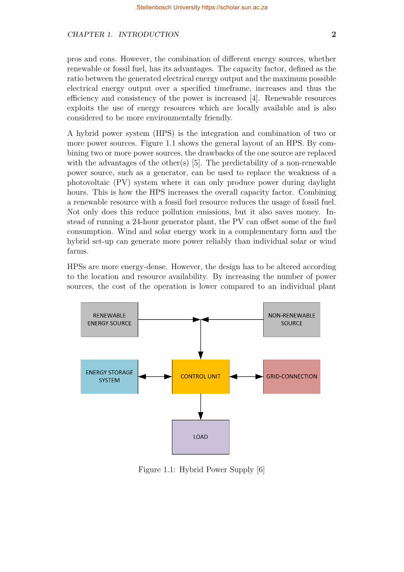
A hybrid power system (HPS) is the integration and combination of two ormore power sources. Figure 1.1 shows the general layout of an HPS. By com-bining two or more power sources, the drawbacks of the one source are replacedwith the advantages of the other(s) [5]. The predictability of a non-renewablepower source, such as a generator, can be used to replace the weakness of aphotovoltaic (PV) system where it can only produce power during daylighthours. This is how the HPS increases the overall capacity factor. Combininga renewable resource with a fossil fuel resource reduces the usage of fossil fuel.Not only does this reduce pollution emissions, but it also saves money. In-stead of running a 24-hour generator plant, the PV can offset some of the fuelconsumption. Wind and solar energy work in a complementary form and thehybrid set-up can generate more power reliably than individual solar or windfarms.
HPSs are more energy-dense. However, the design has to be altered accordingto the location and resource availability. By increasing the number of powersources, the cost of the operation is lower compared to an individual plant
Figure 1.1: Hybrid Power Supply [6]
Stellenbosch University https://scholar.sun.ac.za

CHAPTER 1. INTRODUCTION 3
and overall reduces the installation cost. Thus the efficiency is increased andthe cost of power over its lifetime is reduced [6]. HPSs with a RES has beendeemed as the most appropriate for isolated communities, such as remoteisland or rural, off-grid or isolated areas [7]. The largest customer-base ofHPSs consists of telecommunications companies, mine operators and remoterural communities.
HPSs can be utilised in a stand-alone approach, or be connected to the utilitygrid, which is known as a grid-connected approach. Stand-alone systems areusually in inaccessible areas where power transmission lines are not feasibleto install. This can be because of the landscape, the right-of-way difficultiesand/or environmental concerns. Even without these problems, transmissionlines are still expensive to implement. RES-only stand-alone systems are sub-jected to production variations due to the weather. It would thus be advisableto incorporate some type of stored energy to supply the load when the sourceis unavailable, such as when solar energy cannot be generated during the nighttime or overcast days and wind energy when there is no wind [7]. Electricalenergy is an important stimulant of the economy and daily life. New businessopportunities, increased living standards, educational and health facilities withaccess to power can improve the overall quality of life in these rural or isolatedareas. Grid-connected systems can bring an innovative aspect in the renewablepower economy. Should an excess of generated energy occur, it can be fed backinto the utility grid. In the event where the generated energy is not sufficientfor the load, the grid can supply the shortfall. This can improve the overallfeasibility and load availability of the renewable plant [7].
The integration of different power sources is currently still in its beginningphase and the global market size is relatively small. In 2014, the global hybridgrid-connected market was valued at $1.05 billion and is expected to reach$1.92 billion in 2019 [8]. For example, in Zambia, which is exposed to regularpower cuts, mining companies have implemented a diesel-PV HPS to decreaseits dependence on the utility grid [8]. In the South African context where loadshedding is expected to become more prevalent, an HPS for mines could alsobe installed to reduce its dependence on the grid. This has already been doneby the remotely-located Crominet chromium ore mine [8]. The mine added aPV plant to provide up to 60% of its power need, which aims to reduce fuelconsumption. The nearly-completed Iamgold gold mine in Toronto also aimsto reduce fuel consumption by adding a PV plant [8]. In Germany, close tothe Swabian-Franconian Forest, a hybrid wind-hydro power plant is currentlyunder construction. In Nevada, a renewable-only hybrid power plant consistingof geothermal, PV and solar thermal power generation was constructed [8].The Danish city Aarhus integrated its entire renewable and heat generationunits with existing conventional power systems to improve its energy self-sufficiency. In addition, it sells the surplus generated power back to the grid [8].
Stellenbosch University https://scholar.sun.ac.za

CHAPTER 1. INTRODUCTION 4
According to the South African Government website, two pilot HPSs have beeninitialised. The HPSs is situated in the Eastern Cape at the Hluleka NatureReserve and the Lucingweni community [9]. Micro- and smart grids can alsotake advantage of the HPS to provide sustainable energy to its community.
Even with all the long-term environmental advantages of HPSs, two problemsstill remain: designing and optimising the equipment to produce competitivelypriced energy and creating a control system to interact between the differentpower sources and the load [8].
1.1 Design of a Hybrid Power SupplyAn HPS integrates different power sources. However, there are constraintswith the design of an HPS. Especially if RESs are incorporated, the locationbecomes important. Solar power would not, for example, be ideal for a verycloudy area and wind turbine generators (WTG) would be ill-suited for wind-less areas. Biomass, biogas and hydro plants would be better suited for areaswith close access to these resources.
The practicality of the plant also has to be taken into account in terms ofinstallation, operational and maintenance (O&M) and equipment safety costs.A historical profile of the load would be beneficial to improve the accuracyof the design process. If a load profile is not available, assumptions haveto be made to aid the design process. When incorporating solar and windsources, previous data is required to optimally design the HPS. Solar datasets,specifically for South Africa, are available from SAURAN (Southern AfricaUniversities of Radiometric Network), Solargis, GeoSun Africa and the SouthAfrican government’s energy website REDIS (The Renewable Energy Dataand Information Service) [10–13]. If there is no data available for the loador the specified location, data has to be extrapolated from other sources withsimilar circumstances to aid the designing process.
Each energy system reacts differently in different environments; thus each sys-tem must be designed individually according to the investor’s specifications.These specifications can be technical, environmental or financial. The per-formance indicators of an HPS include the investment capital cost, return oninvestment, consistency of supplied power, environmental impact and lifetimeoperational costs. An HPS must find a balance between the different perfor-mance indicators to find an optimal solution for the investor’s specifications.
Designs formulated on the average or worst-case scenarios are inclined to pro-duce oversized systems, which will increase capital expenditure and producean unnecessary excess of energy [6]. The problem lies in the fact that theworst-case scenario tends to happen rarely. Also, the average values are notconsistent [14]. If a solar source is used with great seasonal fluctuations, which
Stellenbosch University https://scholar.sun.ac.za

CHAPTER 1. INTRODUCTION 5
will produce a reasonable average value over 1 year, the design will result ina faulty design, which will waste money and resources. Other sizing method-ologies have to be explored to produce better and more accurate designs of anHPS. These include software packages and computational algorithms.
The design method has to assess different configurations and power source in-tegrations. Also, the data required to produce accurate designs are not alwaysavailable. These data sources usually include the weather and load profile. Adefinition has to be given of what serves as an ideal HPS design for the specifiedarea. It has to consider making an optimal profit for the investor while produc-ing as much consistent energy possible and emitting minimal environmentally-harming pollution. All these factors increase the complexity of the design andcontrol of a hybrid power supply.
1.2 Control of a Hybrid Power SupplyAs the number of different power supplies is increased, the control systembecomes more complex. The controller has to analyse the system in its totality,switch on and off different power supplies and shift energy to and from a storagesystem when incorporated. If the controller does not predict and navigate theload correctly, this can lead to a loss of power supply (LPS) and possiblefinancial losses.
Different control methods include classic, hard and soft control [15]. The twocategories under classic control are on-off and proportional-integral-derivative(PID) control. Gain scheduling-, state feedback-, optimal-, model predictive-,robust and non-linear and adaptive control all fall into the category of hardcontrol methods. Soft control methods include fuzzy logic, artificial neuralnetworks (ANN) and other evolutionary techniques.
Demand response methodologies consist of rule-based, model predictive andmodel-free controllers. However, a model-free approach simplifies the problemsignificantly, especially if the system is complex. A faulty system is producedif a model does not understand the process dynamics completely. Complexsystems can be difficult to model accurately and thus extensive time has tobe put in to understand the system dynamics. Model-free controllers do notneed a model for the controller to function, however, model-free controllersrequire a large amount of data to learn and adapt to the system. As discussedin Section 1.1, if the necessary data is not available, the learning process of amodel-free controller can be extensively prolonged and can take weeks, if notmonths or years for it to become a viable and sustainable option.
The definition of an adequate control system has to be critically defined for anHPS. As with the design methods, the control system must carefully balancethe cost-effectiveness and power production, as well as storage, of the HPS. The
Stellenbosch University https://scholar.sun.ac.za

CHAPTER 1. INTRODUCTION 6
efficiency of the HPS controller can also be improved if it has prior knowledgeof how the RES will act in the next few hours. A weather prediction unitcan be incorporated to add this additional efficiency. However, these weatherprediction models have to be trained and this can also become time-consuming,as well as require vast amounts of data. There are many weather websitesavailable and thus information from accurate weather sources, such as yr.no,can be extracted in some manner. This information is extrapolated to predictthe expected solar insolation for solar energy generation or wind speed forwind turbine generators.
1.3 Problem StatementThe combination of intermittent and stochastic resources, such as RESs, presenta non-linear optimisation problem in the design of an HPS [4]. As the dimen-sionality of an HPS increases, the trade-offs between different performanceindicators become an important factor in choosing the correct HPS design forthe investor.
As more power sources become integrated, the control system becomes com-plex. The controller must assess the load and available power sources andmake controller-decisions based on this analysis. If the system is not analysedcorrectly, switching between power sources can result in an LPS and/or poorcost optimisation.
1.4 Research Goals and ObjectivesThe research goals are defined to optimise the design of an HPS and to in-crease the efficiency of the control system. A computational algorithm canbe modified for user specifications, which can thus aid the investor in theirdecision-making process. Should a control be able to predict what the loadand power supplies will be with reasonable certainty, this information can beused to implement preventative measures in ensuring a consistent power supplywith an optimised financial cost.
The research objectives are:
1. To optimise the design of an HPS by utilising a genetic algorithm (GA)as a tool to aid the investor’s decision-making process,
2. To analyse the results obtained by the GA for a multi-attribute trade-offanalysis;
3. To assess the validity of a computational algorithm by comparing it withcommercially available software;
Stellenbosch University https://scholar.sun.ac.za

CHAPTER 1. INTRODUCTION 7
4. To create a control system which incorporates an RL-based algorithm toincrease the system’s effectiveness and efficiency;
5. Incorporate Internet Of Things (IoT)-based information to increase thecontrol system’s efficiency.
1.5 Thesis overviewThe thesis consists of 5 chapters and 3 appendices.
In Chapter 1 an introduction of the research is given by discussing the back-ground of energy, renewable energy and the integration of different powersources. The advantages and disadvantages of HPSs are given, as well as ex-amples of what has been implemented globally and locally. The design andcontrol of an HPS is briefly discussed to give an introduction to the researchgoals and objectives.
Chapter 2 discusses the design and control of an HPS. Various design meth-ods are discussed and the appropriate design, a GA, and validation method,HOMER software, is chosen. The fundamental background of the GA is ex-plored, as well as previous work which has been done in this research area. TheHOMER software package is briefly discussed to highlight why this is an ap-propriate validation method to compare to the GA. Several control strategiesare discussed and a reinforcement learning (RL) using a tabular Q-learningmethod is chosen as a suitable control method for an HPS. The discussionof the previous research done with RL-based control for HPSs is given. Away to incorporate a solar prediction to the control system by using the Nor-wegian weather predictions website’s (yr.no) Application Programming Inter-face (API) and a linear regression is examined, as well as a validation controlmethod to compare the RL-controller. Two baselines are considered to com-pare to the control system: a random action and rule-based controllers.
Chapter 3 provides an overview of the experimental design. The design ofan HPS using a GA is discussed, as well as the assumptions made when usingHOMER. An RL-based control system is designed and is also improved byintegrating an IoT implementation using available weather predictions fromyr.no. The two baselines are used to compare the results of the RL-basedcontroller.
In Chapter 4, the results of the research are presented. Firstly, the designof an HPS using a GA and HOMER is presented and analysed. Secondly, thecontrol of an HPS using RL, as well as RL and IoT, is examined.
Conclusions are drawn in Chapter 5. A comparison of the GA and HOMER isdiscussed. A comparison between the RL-based controller and the baselines isdiscussed, as well as the RL and IoT-based controller compared to the original
Stellenbosch University https://scholar.sun.ac.za

CHAPTER 1. INTRODUCTION 8
RL-controller and baselines. A summary of recommendations and possiblefuture work concludes the chapter.
In Appendix A, the clear sky model and calculations for irradiance andinsolation are given. Appendix B discusses the data input used in the designand control of an HPS. The code for the implementations of the simulationsis given in Appendix C.
Stellenbosch University https://scholar.sun.ac.za

Chapter 2
Reviewing system design andcontrol methods
As briefly discussed in Chapter 1, the design and control of an HPS becomecomplex due to the renewable energy location and the integration of differentpower sources. This chapter reviews the different design and control meth-ods associated with an HPS. Suitable methods are selected, whereupon therelevant theory and fundamental background of these methods are discussed.Comparison tools and research contributions from other authors are reviewedto critically analyse what has been previously done. This chapter provides therelevant theory and background which may aid the reader’s understanding ofthis thesis.
2.1 Design MethodsAs mentioned in Section 1.1, there are constraints with the design of an HPS.Each energy system reacts differently in a different environment and thus eachsystem must be designed individually. The integration of power sources createsa complex eco-system of energy exchange in the HPS. The design methodsrequire data such as load profiles and weather information to increase designaccuracy. The combination of inconsistent and variable resources causes theHPS design method to become a non-linear optimisation problem [4].
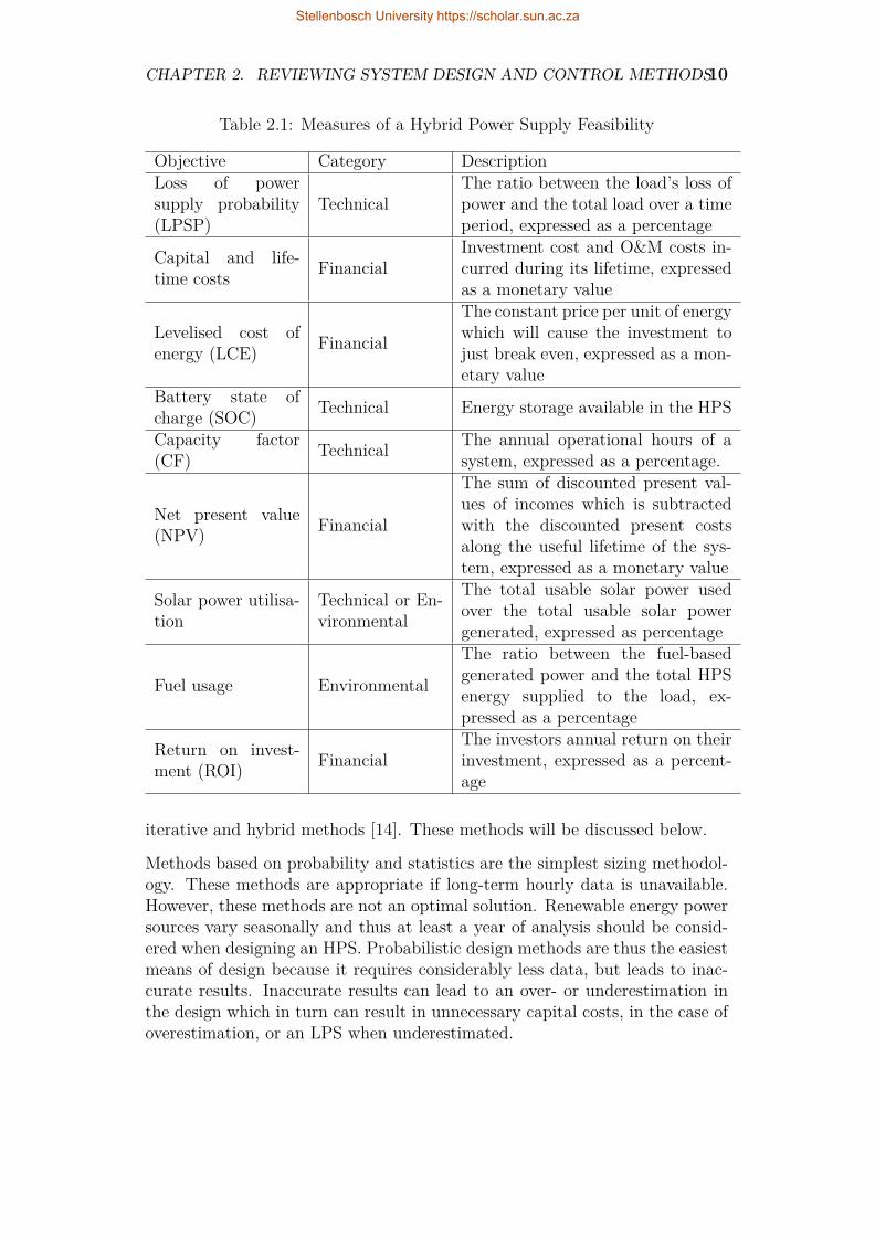
Before the design process can start, a measurement of how ‘good’ an HPSis, must be defined. These measurements are known as the objectives, whichare essentially the goals of the design process. The design objectives can beenvironmental, technical and/or financial, depending on the investor. Differentmeasures of HPS are expressed in Table 2.1. As more of these objectives areincluded, the design process becomes more complex. Trade-offs will have tobe made between different objectives when a viable HPS is chosen. Thereare various methods of designing an HPS, including probabilistic, analytical,
9
Stellenbosch University https://scholar.sun.ac.za
CHAPTER 2. REVIEWING SYSTEM DESIGN AND CONTROL METHODS10
Table 2.1: Measures of a Hybrid Power Supply Feasibility
Objective Category DescriptionLoss of powersupply probability(LPSP)
TechnicalThe ratio between the load’s loss ofpower and the total load over a timeperiod, expressed as a percentage
Capital and life-time costs Financial
Investment cost and O&M costs in-curred during its lifetime, expressedas a monetary value
Levelised cost ofenergy (LCE) Financial
The constant price per unit of energywhich will cause the investment tojust break even, expressed as a mon-etary value
Battery state ofcharge (SOC) Technical Energy storage available in the HPS
Capacity factor(CF) Technical The annual operational hours of a
system, expressed as a percentage.
Net present value(NPV) Financial
The sum of discounted present val-ues of incomes which is subtractedwith the discounted present costsalong the useful lifetime of the sys-tem, expressed as a monetary value
Solar power utilisa-tion
Technical or En-vironmental
The total usable solar power usedover the total usable solar powergenerated, expressed as percentage
Fuel usage Environmental
The ratio between the fuel-basedgenerated power and the total HPSenergy supplied to the load, ex-pressed as a percentage
Return on invest-ment (ROI) Financial
The investors annual return on theirinvestment, expressed as a percent-age
iterative and hybrid methods [14]. These methods will be discussed below.
Methods based on probability and statistics are the simplest sizing methodol-ogy. These methods are appropriate if long-term hourly data is unavailable.However, these methods are not an optimal solution. Renewable energy powersources vary seasonally and thus at least a year of analysis should be consid-ered when designing an HPS. Probabilistic design methods are thus the easiestmeans of design because it requires considerably less data, but leads to inac-curate results. Inaccurate results can lead to an over- or underestimation inthe design which in turn can result in unnecessary capital costs, in the case ofoverestimation, or an LPS when underestimated.
Stellenbosch University https://scholar.sun.ac.za

CHAPTER 2. REVIEWING SYSTEM DESIGN AND CONTROL METHODS11
HPS design can be analytically done by representing the HPS as a computa-tional model. This model will assess the HPS’s feasibility by determining theperformance of the system. This design method requires a large time-seriesdatabase for accurate results. An evaluation of the HPS’s feasibility can bedone using software packages. Simulation tools available commercially areRETScreen, Hybrid2, TRNSYS and HOMER.
RETScreen is a Microsoft Excel-based spreadsheet model consisting of a set ofworkbooks. Each workbook models a specific power system configuration. Theprogram determines the annual average energy flow and analyses the energygeneration, life cycle costs and greenhouse gas (GHG) emissions. The soft-ware’s objective is to reduce costs. RETScreen is associated with pinpointingand evaluating potential energy projects [16].
HYBRID2 is a simulation software developed by the National Renewable En-ergy Laboratory (NREL) and simulates an HPS with high precision calcula-tions. The software does not optimise the system [17]. TRNSYS was devel-oped by the University of Wisconsin and can simulate the system, but cannotoptimise the design [17].
HOMER is a designing and analysing tool and is considered the industry stan-dard for the design of HPSs [14, 18]. It incorporates several energy sourcessuch as generators, wind turbines, solar PV-modules, hydro-power and bat-tery storage, among others. The software is based on time-series models whichpredicts the hourly or minutely power system performance. HOMER deter-mines in each step how the power equipment in the system is dispatched. Thesoftware determines how feasible the HPS configuration is, as well as also as-sessing the economic feasibility of the project [16]. The literature on the HPSdesign using the HOMER software has been produced by [19–21].
The design of an HPS is a multiple objective problem such that several ob-jectives, being technical, environmental and financial objectives, have to beconsidered simultaneously. Metaheuristic methods can be used to solve theseparticular problems. Metaheuristic methods are usually stochastic and mimica natural or biological principle which can be used in an optimisation or searchproblem. These optimisation methods include simulated annealing (SA) andtabu search (TS), as well as iterative methods such as GAs and particle swarmoptimisation (PSO) [22]. Iterative methods uses a recursive process to find thebest design configuration according to the specifications. A discussion of theuse of different design methodologies will be presented below.
The GA is a stochastic global search and optimisation technique which isbased on the theory of evolution by natural selection, which was formulatedby Charles Darwin in 1859. It is based on the process over which organismschange over time as a result of inheriting physical or behaviour traits. Ifthe trait increases the species’ chance of survival, the trait is carried over
Stellenbosch University https://scholar.sun.ac.za

CHAPTER 2. REVIEWING SYSTEM DESIGN AND CONTROL METHODS12
through the next generation. If the trait decreases the species’ chance ofsurvival, most likely the species will die out and thus not carry over the traitto the next generation. The algorithm is generally robust in finding a globaloptimal solution in a multi-modal and multi-optimisation process [14]. The GAproduces a list of viable options by producing a genetically superior population.In this case, the population would consist of viable and feasbile HPS designconfigurations. Various studies have been done designing an HPS using aGA [4,7, 20,22–25].
The PSO algorithm was first presented in 1995 by J. Kennedy and R.C. Eber-hart and the algorithm was initially used for the predatory behaviour of birdsflocking [14]. Each agent is influenced by its own flying experience and itsneighbours and will constantly modify its flight direction and velocity un-til it ultimately reaches the global best position through the entire searchspace [26, 27]. Artificial neural networks (ANN) are optimisation methodsbased on the nervous system structure. The networks are part of the fieldof machine learning. The ANN has to be trained because the neural networkadapts based on the data it receives. The ANN will then produce results basedon its training.
Bio-inspired methodologies require considerable computational processing andcan be adjusted in real-time. It can function without any prior knowledge ofthe relationships between different variables and can deal with non-linearities.The iterative methods can be built and incorporated in various programminglanguages or software. The easiest means of implementation will be in Python,because of its open-source network, on-line support and the extensive numberof libraries. Alternatively, Matlab Simulation tools can be used. Hybrid opti-misation methods increase results- and convergence time and is often the mostpowerful optimisation tool to design an optimal HPS [14]. Hybrid iterativemethods combine optimisation techniques with two or threefold optimisationobjectives, such as technical, financial and/or environmental objectives. Thesemethods can be done combining GA, PSO or ANNs [14].
GAs search for a list of viable options, whereas PSO for one global optimum.Because of the complexity as a multi-objective problem, a list would be moreacceptable to analyse the trade-offs between different HPS sizes and configu-rations for the investor. Each objective influences how the results will performand thus a list of different options will highlight how each objective is opti-mised.
It was thus decided to use a GA as the appropriate design method to assessdifferent configurations, sizes and design goals. HOMER is considered theindustry standard in HPS design, based on the literature research. It wasthus chosen to compare the impact of using industry-standard software anda computational optimisation algorithm. The fundamental background of the
Stellenbosch University https://scholar.sun.ac.za

CHAPTER 2. REVIEWING SYSTEM DESIGN AND CONTROL METHODS13
GA, as well as the previous work using GA with HPS design, will be discussedin the next section.
2.2 The Genetic AlgorithmIn this section, the fundamental background of the GA is given and the pre-vious work using GAs as a design tool for an HPS is discussed.
2.2.1 Fundamental BackgroundThe GA is a biologically principled optimisation algorithm which mimics thetheory of evolution formulated by Charles Darwin. Species develop through aprocess called natural selection where small, inherited variations on its geneticcode increase the individual population member’s ability to compete, surviveand reproduce. Inferior population members will die out as they will be unableto carry their genes into the next generation. A fitter population are producedover generations through reproduction. Figure 2.1 shows the flow diagram ofthe GA.
The reproduction is done through mixing the Deoxyribonucleic Acid (DNA)with two parents or through mutation of the DNA string. The GA navi-gates through a large gene pool, called the population, to find the optimalcombinations of genes. In this case, the combination of genes represents theideal HPS configuration. Each gene constitutes a variable which represents thesize/number or the type of a specific component. These variables are randomlygenerated and will be discussed at a later stage.
As mentioned, the algorithm randomly generates population structures orchromosomes. The number of population members and generations are speci-fied by the user. Each of these chromosomes has an encoding solution and theencoding is to the likes of DNA strings [4]. The general chromosome structurefor a represented HPS can have the following format:
[TPV NPV TInv NInv TBat NBat TGen NGen]
This chromosome structure is used to briefly explain how the GA uses theDNA as part of its optimisation. The T refers to a type of either PV-module,battery, generator or inverter. The N refers to the amount of a specific compo-nent in the system. The types are represented by integers. An HPS can thus,for example, have NPV amount of type n PV-modules. Type n would then becross-referenced to a PV-module database containing the attributes the spe-cific module. These attributes will include the name, associated brand, price,warranty and additional power ratings. The GA will thus have a database of
Stellenbosch University https://scholar.sun.ac.za

CHAPTER 2. REVIEWING SYSTEM DESIGN AND CONTROL METHODS14
Figure 2.1: Genetic Algorithm Flow Diagram [6]
PV-modules, batteries, generators and inverters which is used for this cross-referencing.
Each DNA has information regarding the structure and combination of theHPS. As each generation progresses, the GA improves the population’s overallfitness through the means of selection, crossover and mutation. Crossover andmutation is shown by Figures 2.2 and 2.3 respectively.
Selection duplicates the fitter structures and removes those with lower fitnessratings. Crossover recombines two parents’ chromosomes to form a new chro-mosome [4]. Mutation creates new structures from one parent’s structures byrandomly altering the DNA of each structure. As shown as an example inFigure 2.2, each chromosome has a 50% chance of descending from one of theparents. The offspring is a combination of the two parents’ genes. Figure 2.3shows an example of how mutation occurs. One (or more) genes are randomlyaltered to create a new offspring. The offspring are evaluated on the fitnessfunction. If the offspring proves to be fitter than the weakest population mem-
Stellenbosch University https://scholar.sun.ac.za

CHAPTER 2. REVIEWING SYSTEM DESIGN AND CONTROL METHODS15
Figure 2.2: Crossover
Figure 2.3: Mutation
ber, it replaces the weakest population member. However, if it is not fitter, itis discarded and the next generation starts.
Different selection strategies for crossover and mutation include tournamentselection, proportional- and rank-based roulette wheel selection. These differ-ent selection strategies avoid premature convergence and increase diversity. Adiverse population allows for different combinations and can result in betterdesigns, which is ultimately the goal of the GA.
Tournament selection is a simple and efficient method of selection and is shownin Figure 2.4. It selects randomly chooses individuals from the population andthese individuals compete with each other based on their fitness. The individ-ual who has the highest fitness wins and is thus included in the next generation,whereas the weaker individual is not. The advantages of this selection methodis that dominant population members will take over and the population willnot require fitness scaling and sorting, which will reduce the computationaltime of the GA [28].
Proportional roulette wheel selection is the selection of individuals with a prob-ability which is directly proportional to its fitness level. It can be visualisedas a spinning roulette wheel and each segment of an individual is proportionalto its fitness. The roulette wheel selection method is explained in Figure 2.5.The individual with the highest fitness level is likelier to be selected as a par-ent because it has a bigger segment of the roulette wheel. The advantage ofthis selection method is that it discards none of the individuals, as in tourna-ment selection. Each of the population’s individuals has a likelihood of beingselected and the population’s diversity is preserved. However, a bias can beintroduced at the start of the search which may cause premature convergenceand result in a loss of diversity [28].
Stellenbosch University https://scholar.sun.ac.za

CHAPTER 2. REVIEWING SYSTEM DESIGN AND CONTROL METHODS16
Figure 2.4: Tournament Selection
Figure 2.5: Roulette Wheel Selection
Rank-based roulette wheel selection is the selection methodology where theindividual’s selection probability is based on its fitness rank compared to theentire population. The selection method first sorts individuals according totheir fitness in the population and then determines a selection probabilityaccording to its rank rather than fitness value. The method avoids prematureconvergence by introducing a uniform scaling in the entire population andeliminates the need to scale fitness values. However, it can be computationallyexpensive as a result of the continuous sorting of the population and also leadsto slower convergence [28].
Additional strategies to increase population diversity is to reduce duplicates
Stellenbosch University https://scholar.sun.ac.za

CHAPTER 2. REVIEWING SYSTEM DESIGN AND CONTROL METHODS17
or similar individuals. Early-stopping constraints can reduce computationaltime when a convergence arises.
Objectives are defined for the chromosomes, which will be the HPS in thiscase. The objectives for the HPS will have three aspects: financial, environ-mental and technical, as mentioned previously in Section 2.1. The algorithm’sobjectives will be discussed in more detail in Chapter 3.
As seen in Figure 2.1, the GA starts by reading the data input with regards tothe weather and load profiles and a database of different components. Thesecomponents are specified as the different power sources, such as PV-modules,generators, batteries, wind turbines, etc. These component sizes and typescreate the chromosome structure of the population member. Each populationmember is rated against a fitness function. This fitness function represents thepopulation’s members ability to meet the algorithm’s different objectives. Thefitness function is discussed in more detail in Section 3.1.4.4. The populationmember which can achieve as much of the objectives as possible will be seen asa fitter member. This member will have a greater chance of reproducing duringcrossover and mutation to create even stronger and fitter population members.Weak members do not achieve a good enough result from the objective’s goaland its fitness rating will be lower. This means they will have a low probabilityof being selected for reproduction and a greater chance of being eliminated fromthe population of HPS configurations. The GA results in a list of various HPScombinations which are good on their own merits.
Initially, the GA randomly generates a population. Using crossover and muta-tion, more population members are created. Because the population numberis fixed, weaker members are removed to make a place for the fitter members.The fitness is directly linked to how well the design objectives are met andthus a higher fitness rating is a more viable HPS solution. The resulting pop-ulation is a fitter list of HPS solutions than when it started. These resultscan help the designer decide between different trade-offs, such as costs, powerreliability, storage capacity and lifetime assessments. The decision of a viableHPS configuration is then left for the end-user to decide upon. The algorithmthus aims to highlight the different trade-offs between different configurationsto assist the decision-making process.
2.2.2 Previous WorkThere seem to be the two options for simulation purposes: a year-long hourlytime-series set or lifetime approaches. A year-long hourly simulation was donein papers presented by [5,23,25,29]. A lifetime approximation was done in pa-pers presented by [7,22]. For the 8760 hours, mathematical models are deemedadequate for the optimisation. The lifetime approximations are based on fi-nancial formulas and the data sets are usually average values or are assumed
Stellenbosch University https://scholar.sun.ac.za

CHAPTER 2. REVIEWING SYSTEM DESIGN AND CONTROL METHODS18
to be constant. Both have advantages and disadvantages. The year-long simu-lation assumes that every year will be similar to the data set and thus the HPSwill not be designed for yearly fluctuations such as droughts/unusual weatherpatterns. The lifetime approximations can be a problem if the real-life scenariotends to have extreme fluctuations. A mild temperature average could, for ex-ample, be the result of extremely hot summers and exceptionally cold winters.If the year’s average temperature is used, this may not give an accurate insightinto the design process. Over 20 years, the average values can be seen as suf-ficient for the algorithm, but the advantages and disadvantages of these twomethods must be considered during the design. Detailed assumptions must bemade to result in accurate designs.
In [20], the daily load is assumed to be constant and average monthly solarradiation and wind speed data is used during the assessment. The analysiswas done for one year using these average values. Furthermore, a sensitivityanalysis was done to optimise the system in different circumstances. Theanalysis was done with HOMER software, which produced the same resultsobtained by the GA. The similarity of the mathematical models is attributedto this fact. This paper notes that HOMER cannot simultaneously assessdifferent component types. In this instance, a GA will provide faster andreliable solutions in the design and optimisation analysis of the HPS.
The objective functions vary greatly. Shahirinia et. al. aims in reducing dieselfuel consumption and minimising the total cost [7], whereas [29] seeks outto improve the grid stability by providing a buffer for the difference betweenthe RES output and the load. Gonzalez et.al [5] aim to minimise the totallife cycle costs and the metric of the fitness function is based on the NPV.In [23], the total costs are minimised, whereas Xu, et. al. [25] proposes toreduce the total costs which are constrained by the LPSP. In [4], a GA wasconstrained to stop when the objective function reached a pre-set target valueof 240 kW. The objective function in the paper presented by Katsigiannis [22]aims to minimise the system’s cost of energy. The objective functions presentedin [24] are financial, technical and environmental. The financial objectiveminimises the life cycle cost. The technical objective maximises the energysupplied by the RES. The environmental objective minimises the annual GHGemissions. As the amount of objectives increase, the trade-off analysis becomesvery important because one objective has to be constrained to a certain degreeby another objective. The ideal HPS will have a balanced compromise betweenthe different objectives for an overall better and viable HPS design. Theobjectives presented by Sopian, et. al. [20] maximise the use of the RES whileminimising the use of the diesel generator. Thus these objectives can be seenas environmental and technical.
The design approach seem to differ for stand-alone and grid-connected HPSconfigurations. Grid-connected HPS [29] aids the grid for stability, whereas
Stellenbosch University https://scholar.sun.ac.za

CHAPTER 2. REVIEWING SYSTEM DESIGN AND CONTROL METHODS19
stand-alone HPS are placed in rural areas to provide access to electricity.Stand-alone HPS [7, 23, 25] all include some kind of RES (wind or solar) andenergy storage systems which is independent of a fuel source to produce power.The energy storage system varies from hydro-electrical pumps, to batteriesand ultra-capacitors. A diesel generator or bio-gas/bio-mass plant is added toincrease the HPS’s ability to provide constant energy should the RES fail toprovide as a result of the weather. A grid-connected HPS is proposed in byKapfudza, et. al. where it highlights the difficulties which are faced in someparts of South Africa where communities live off-grid or are supplied by poorsupply and services due to their geographical locations [4]. Furthermore, itimplores the need to exploit other energy sources solve these problems.
The chromosome structures represent the different configurations of each HPS.In [25], the structure is [TypeWTG NWTG Tilt NPV Nbat]. The chromosomestructure in [7] is [Pdg NPV Nwind] and the battery capacity is predefined andnot part of the optimisation. In the paper presented by Kapfudza, et.al, thechromosome’s genetic encoding consists of the GHG emission index, economicindex and the power output [4].
In [25] an additional optimisation is utilised to find the types and sizes ofthe components, after determining the PV-module and battery capacity. Itthen recalculates to the optimum fixed tilt angle of the PV-module. Thisoptimisation can thus be seen as a hybrid algorithm because it incorporatesa second and third optimisation. Similarly, Ma, et.al. proposes a two-stepoptimisation: firstly, the RES and storage system capacity size using a GAand secondly, a cost function to deduce the optimal combination of batteryand ultra-capacitor size [7].
Atia, et.al. proposes a hybrid GA [23] which reduces the running time ofthe searching method. A secondary GA is implemented where five controlset parameters are optimised. A local optimiser (LO) is also implemented inthis paper. The LO was run only when the secondary algorithm reached thelimited generation number or to interrupt the algorithm when no advance inthe population was obtained for three successive generations. The hybrid GAproduced a faster simulation time to make the searching time more viable.
In the paper presented by Shahirinia, et.al. several constraints were considered.These included the maximum running time of the diesel generator, the powerdelivered and stored by the battery bank and the hours in which the PV arraysgenerate power [7]. The selection method is roulette wheel selection whereeach population member’s wheel slot is proportional to its fitness. Thus afitter population member will have a larger chance of being selected. Ko, et.al,introduces a multi-objective optimisation design with various power sources inthe HPS which optimises the size and configuration of hybrid cooling, heating,hot water and power systems consisting of RES systems and fossil fuel systems
Stellenbosch University https://scholar.sun.ac.za

CHAPTER 2. REVIEWING SYSTEM DESIGN AND CONTROL METHODS20
[24].
The optimised design of the HPS is dependent on the design objectives of theresearcher, investor and operators [24]. In the presented paper, the trade-offsare discussed to demonstrate how the investor will be able to decide upon anHPS [24]. This is another illustration of how the GA produces a list of viableHPS configurations and the most feasible option is left up to the designerand/or investor to decide. Gonzalez, et. al. [5] did a sensitivity analysis bysetting a 10 % variation on the various financial and technical aspects, whichwill influence the results of the optimisation process. The sensitivity analysisshows how well the optimisation methodology reacts with changes with theinput variables.
The grid-connected HPS can compensate for the loss of power supply (LPS)from the other sources and feed back the unused generated power to the utilitygrid. The stand-alone systems, which are ideal for off-grid and inaccessiblecommunities should include some sort of energy storage and backup powersource to compensate for the LPS from weather-intermittent energy sources.Currently, there is an incremental increase for cleaner and sustainable energygeneration. The investors have to find a trade-off between investing in anHPS which can generate a return on their investment which will still considerenvironmental drivers. The technical aspects of the HPS can be seen as themost important because the HPS has to supply as much power as reliably andconsistently as possible. The objectives should be clear and a measure of howthe HPS performs should be assessed.
The one-year hourly simulation can provide accurate insights into the technicaland short-term aspects of the design, but the lifetime projection gives morefinancial and environmental insights. It can be beneficial for the designer tolook at both these options as an assessment of the feasibility of a project. AnHPS with a very low LPSP may be financially unfeasible and a low capital costHPS may have a very high LPSP and life cycle costs. Different componentshave greater O&M costs than others. Also, fossil fuel power sources may besubjected to future carbon tax laws or the depletion of the mineral sourcewhich can influence the design’s results. As the number of power sourcesin the HPS increases, the complexity becomes considerably greater. In [22],six power sources are considered with a database of different types of powersources. The search time to find an optimal solution is considerably reduced byusing a GA. The combination of every possible configuration and power sourcetypes results in 2.1 billion different combination outcomes. Simulating all thesedifferent configurations require approximately 234 years of simulations. Thisshows how significant the optimisation algorithm can perform in optimisingthe design of an HPS.
It is important to ensure that the correct simulation data set is chosen with
Stellenbosch University https://scholar.sun.ac.za

CHAPTER 2. REVIEWING SYSTEM DESIGN AND CONTROL METHODS21
clear objectives of what the HPS must achieve. This thesis proposes an HPSdesign method of satisfying multiple objectives using an assessment of thehourly year analysis, as well as a projection of the lifetime to assess its longterm feasibility. The results have to be compared to a baseline to assess howaccurate the design method works and if there is an advantage or disadvantagein using the GA as a design method for an HPS. The chosen baseline is theHOMER software package and will be discussed in the next section.
2.3 HOMER Software PackageHOMER is a design and analysis tool for an HPS and contains a combination ofstandard generators, wind turbines, solar PVs, hydro-power and batteries. Thesoftware determines which dispatch strategy to incorporate given the powersources and determines its feasibility as an HPS. It also accesses the economicfeasibility of the project by calculating capital, replacement, O&M, fuel andinterest costs.
HOMER was used in [30] to design an HPS. The results were compared witha GA to show the correlation between the two optimisation techniques. It wasnoted that the GA had a lower cost of energy and NPV. Sopian et. al. alsoused HOMER to design an HPS [20]. The results were identical, attributingto the same mathematical models used in the GA as in HOMER. The papernotes that using HOMER can be a problem should different types of specificcomponents be used to optimise the design. HOMER cannot simultaneouslyanalyse different component types and thus every component type has to beassessed individually, along with its operational strategy. This can becomevery time consuming and thus for this type of purpose, a GA allows for afaster and more reliable optimisation method.
The most direct method to optimise an HPS is to use a complete enumerationmethod by using software such as HOMER. It ensures the best solution butcan be proved to be extremely time-consuming [22]. The literature studiesperformed show conformity where in-house models appear to be conservative,flexible, better performance and simpler to use than the HOMER software [21].From the literature, HOMER seems to be user-friendly and be able to provideaccurate results. HOMER is also considered an industry standard and thiscan be a viable option to use as a design method.
2.4 Control Strategies and MethodologiesAs the integration of different power sources increases, the complexity of energyexchange also increases. There is a fine balance between the power suppliedto the load and to consider future load fluctuations, such as peak hours, a
Stellenbosch University https://scholar.sun.ac.za
CHAPTER 2. REVIEWING SYSTEM DESIGN AND CONTROL METHODS22
limited grid supply, loss of renewable power generation or even load-shedding(in the South African context). The control system has to compensate for theloss of PV power when the overcast weather occurs or night hours, while stillmaintaining adequate back-up energy storage for rainy days or sudden spikesin the load profile. The energy exchange requires switching on and off certainpower supplies based on the load and this switching time can cause delaysin supplying power to the load. A control system has to either anticipatethe LPS or be able to have an almost instantaneous release of power. Thecontrol system must be able to efficiently supply power by optimising batterylife cycles and/or diesel generator usage. The control system must be able toanalyse the generated solar power to decide if it should feed it to the load orcharge the batteries, or both. Thus the control of an HPS is a highly complexenergy exchange problem and different control algorithms will be discussedbelow to highlight the differences and advantages of said algorithms.
Before the analysis of different algorithms can begin, it is important to decidewhich measures will be used to determine how ‘good’ a control system is. Thesemeasures are very similar to the measures of the HPS design in Table 2.1. Inaddition, the efficiency, energy storage and reaction time of the control systemcan be considered. As mentioned in Chapter 1, different control methodsinclude classic, hard and soft control [15]. Demand response methodologiesinclude rule-based, model predictive and model-free control [31] and will alsobe discussed below.
The two categories under classic control are on-off and PID control. On-offcontrol is simple to implement, however, the two states require the controllerto make decisions based on multi-value variables. This results in a compromisebetween an environment which requires, for this instance, half of the powerthat the supply can provide. A high switching frequency of power supplies canlead to inefficient financial cost optimisation. PID control is a classic local-loop control and is easy to implement and test. The controller converts theerror between the output signal and the input signal to action. It describes theerror handling of the system. The proportional control attempts to achievethe output signal as fast as possible, whereas the integral control adjusts thesummation errors to remove residual errors. The derivative control avoidsadjustments which are implemented too fast for the system [15].
Hard control has six categories: gain scheduling-, state feedback-, optimal-,model predictive-, robust, and non-linear and adaptive control. If a system hasseveral operational points, the gain scheduling controller designs linear con-trollers for each of the points. An interpolation strategy is applied to obtainan overall control of the system. Each of these controllers must be optimallytuned for the operational region and an increased controller number can resultin time-consuming tuning jobs. The state feedback control assumes that thesystem environment can always be measured. A state feedback controller is
Stellenbosch University https://scholar.sun.ac.za

CHAPTER 2. REVIEWING SYSTEM DESIGN AND CONTROL METHODS23
where the action of the control depends only on the values or external input.Optimal control is based on mathematical models. An optimisation problem issolved through the defined objective function. However, for real-time controls,complex systems can require considerable computational power and becomeinefficient for its purpose. Model predictive control has a predictive model,an objective function and a control law. A complex model, such as optimalcontrol, requires expensive computational power. Robust control can handletime-varying model uncertainties and system associated non-linearities. Non-linear and adaptive controllers are developed through feedback linearisationand gain scheduling approaches. Adaptive control is a type of nonlinear con-trol. The controller can modify its behaviour in response to dynamic changesin the process and can characterise the disturbances [15].
Soft control methods consist of ANNs, fuzzy logic (FL) control and other evo-lutionary techniques. ANN is a data-driven approach in a non-linear modelwhere the optimal weights are determined which will minimise the errors be-tween the estimated data and the target data. The network is trained to obtainthe optimal weights and continues until convergence occurs. FL replicates hu-man knowledge and reasoning in the form of membership functions and rulesto control the inference actions for the control. FL does not require an exactmathematical model of the control process [15]. FL has proven to be moreenergy-efficient than rule-based strategies, but cannot be adapted automati-cally [32]. Similarly, dynamic programming (DP) can be used to optimise therule-based control systems, but these cannot be applied in real-time [32].
The three most important demand response methodologies are rule-based,model-based and model-free (learning-based) [31]. Rule-based control strate-gies are based on a set of simple control methods consisting of if, then andwhile statements. The algorithms are relatively simple, less computationallyexpensive and in general, does not require forecasting. The algorithm is basedon the domain and case-specific parameters which have to be tuned. Thisresults in the difficulty of generalising these systems with a system that hasdifferent parameter setting [31]. Model predictive control uses mathemati-cal models of the process dynamics. The strategies rely on accurate modelswhich in turn produces more accurate results. The model dynamics have tomodelled exactly. If the model for the process dynamics cannot be fully orpartially understood, this can result in a faulty system model [31]. Model-freemethods are data-driven, which requires large datasets. However, the system’sdynamic model is not required because it is formulated when analysing andtraining the data. An example of a model-free control method is reinforcementlearning (RL) where the learning curve comes from experiencing rewards orpenalties based on the implemented action policy [32]. This results in lesseffort because no model is required and better generalisation for the applica-tion. In model predictive control, the strategies are case-specific and have to
Stellenbosch University https://scholar.sun.ac.za

CHAPTER 2. REVIEWING SYSTEM DESIGN AND CONTROL METHODS24
be altered when the system environment experiences change [31].
RL is a computational approach where an agent learns from interacting withits environment. RL-based methods incorporate occupant behaviour and learnhow the system interacts. RL does not require a model and a model-free ap-proach can simplify a complex system considerably [15]. Data on consumptionpatterns, weather data and electricity generation becomes more easily avail-able and thus increases the relevancy of data-driven techniques. The increas-ing computational power and data availability create an opportunity for thesedata-driven methods to be considered as an appropriate control method [33].
The RL agent receives rewards from its actions and learns if an action isbeneficial for the environment to receive the maximum delayed reward. Saidagent can balance the trade-off between exploring and exploiting different ac-tion policies [15]. RL can be a viable solution to control an HPS’s energyexchange. The agent can learn to anticipate the load’s profile and is rewardedif it executes a good policy or penalised when a bad policy is executed. Thusthe controller’s learning process is reinforced with rewards when correct orpenalised if a policy results, for example, in a loss of power.
The controller’s effectiveness can be increased if it can anticipate what thesolar profile will be during the day. This means that some type of weatherprediction can be incorporated. Various studies have been done to forecastthe weather using machine learning techniques. For the scope of this thesis,it was decided not to build an algorithm which can predict the weather, butrather use available data from websites and use its information to extrapolateit to solar insolation prediction methods. The weather forecasting websitewas chosen as yr.no because of its user-friendly API. The solar power can beextracted using a simple linear regression algorithm.
An RL-based control algorithm was thus chosen to assess its validity as aviable control system for an HPS. An IoT-based solar irradiance prediction isalso incorporated to assess how the controller’s effectiveness can be increasedif it also knows what to anticipate from the solar RES. Because the rule-basedcontroller is the simplest controller to implement, it is chosen as a baselinecomparison method for the control system. A random action controller willalso be used as a comparison tool to the RL-based controller. The fundamentalbackground and related work of RL-based control systems for hybrid powersupplies are discussed below. An overview of the linear regression algorithmand the on-off controller is briefly discussed as well.
Stellenbosch University https://scholar.sun.ac.za

CHAPTER 2. REVIEWING SYSTEM DESIGN AND CONTROL METHODS25
2.5 Reinforcement Learning
2.5.1 Fundamental BackgroundThe two distinguishing attributes of RL are trial-and-error search and thedelayed reward. The algorithm does not know which actions to take but ratherdiscovers which actions or actions yield the greatest reward when performed[34]. The RL-model formally consists of a set of environmental states, a set ofagent actions and a set of scalar reinforcement signals, which are typically 0 or1 or a real number value [35]. The environment and action set are discrete. Alearning agent interacts with the environment over time to obtain rewards [34].
The environment for this HPS will consist of the load, inverter, battery, gener-ator and PV-modules. The agent learns how to interact between these sourcesand to optimally exchange energy. The rewards would be to, firstly, be optimalsustainable power supply which is the most cost effective. The cost optimisa-tion refers to maximising the generated PV power, while minimising the useof generator fuel, as well as increasing the battery’s longevity. In doing so,the feasibility of the HPS increases throughout its lifetime. This will be dis-cussed in more detail in Chapter 3. The actions are penalised if the HPS doesnot have power to supply or poor cost optimisation. The value function willinclude long-term rewards for keeping constant power supplied.
The agent and environment interaction in a Markov Decision Process (MDP)is shown in Figure 2.6. The Markov property states that the future is notinfluenced by the past and only relies on the present and an MDP satisfies thisproperty. The MDP models sequential decision making under uncertainty [36].In Figure 2.6, state St and reward Rt are random variable outcomes afterexecuting an action. The state St ∈ S refers to the environment’s conditionat discrete time step t.
The agent chooses a stochastic action At ∈ A in response to the environment.The agent then attempts to maximise future returns. The agent experiencesan instant quantitative reward Rt+1 ∈ R as the agent transfers to the newstate St+1. The MDP is formulated as the sequence of the state, action and
Figure 2.6: The interaction between the agent and the environment in anMDP [35]
Stellenbosch University https://scholar.sun.ac.za
CHAPTER 2. REVIEWING SYSTEM DESIGN AND CONTROL METHODS26
reward. The states, actions and rewards will be discussed further below.
Equation (2.5.1) defines the joint probability density function for St and Rt.The distribution of the state and reward at time step t is dependent on thestate and action from only the previous time step. Thus an action is executedon the previous state and transitions into a new state and this transition tothe new state results in a reward. This dependency implies that the Markovproperty is satisfied and the transition matrix can be determined using (2.5.2).
p(s′, r|s, a) = P[St = s′, Rt = r|St−1 = s, At−1 = a] (2.5.1)where s, s′ ∈ S, r ∈ R and a ∈ A.
p(s′|s, a) = P[St = s′|St−1 = s, At−1 = a] =∑r∈R
p(s′, r|s, a) (2.5.2)
RL differs from supervised learning. Supervised learning is where an externalsupervisor provides a training set of labelled examples. The system’s objec-tive is to generalise its responses to act correctly to states which are not inthe training set. In the case where no examples are present, an agent has tolearn from its own experience in different states [34]. The most importantdistinction between supervised and reinforcement learning is that no represen-tation of input or output pairs is given for RL [35]. The agent is not givenany prior knowledge of what will have the best long-term reward. Instead,all the information is gathered through experience about the possible systemstates, actions, transitions between states and the rewards obtained. On-lineperformance is also vital because the system’s evaluation is often concurrentwith learning [35].
There are four main subelements of an RL system, excluding the agent andthe environment, namely the policy, reward signal, the value fuction and themodel of the environment [34]. A learning agent must be able to observe itsenvironment state and execute actions which would influence the state. Itmust have objectives which relate to the environment’s state. The agent’s jobis thus to find a policy π which maps the states to actions and this policywill maximise some long-term measure of reinforcement [35]. The policy isstochastic and the probability of taking an action, a, in state s, is defined by
π(a|s) = P[At = a|St = s]. (2.5.3)
A policy, given by (2.5.3), defines the behaviour of the learning agent at aspecified time. The policy maps the perceived environment states to the ac-tions which are to be taken when it is in that specific state. The policy formspart of the core of an RL agent in which it alone is sufficient to determine
Stellenbosch University https://scholar.sun.ac.za

CHAPTER 2. REVIEWING SYSTEM DESIGN AND CONTROL METHODS27
behaviour [34]. The policy is defining how an agent should act when it is indifferent states and is a distribution over actions given the states. The policymust be stochastic and can be considered as a function of actions. The policycan have the form of a look-up table or be presented as an approximation form.
The reward signal defines the goal of the RL problem. For every time step, theenvironment sends a quantitative reward to the RL agent, which signifies ifthe action had a positive or negative impact on the environment. The agent’sonly objective is to receive the maximum reward over the long term. Throughtrial-and-error, the agent starts defining which events are good and bad. Thismeans that the policy may be changed if the action selected by the policyresults in a low reward and changed to select another action which may returna higher reward [34]. The marginal distribution of the expected reward is givenby
r(s, a) = E[Rt|St−1 = s, At−1 = a] =∑r∈R
r∑s′∈S
p(s′, r|s, a). (2.5.4)
A value function defines what is the best for the long run and can be defined asthe total future accumulated rewards which an agent can anticipate to receive,should it start from its current state. Rewards determine immediate and in-herent desirability of different environmental states. The value function takesinto account the likely states which would follow and the rewards available inthose future states. It can take into account an immediate low reward, butcan still yield high rewards when followed by other states regularly and viceversa [34]. The state-value function defines vπ(s), of a MDP, under policy π,as the expected of the return starting from state s is expressed by (2.5.5).
vπ(s) = Eπ[Gt|St = s] = Eπ[ ∞∑k=0
γkRt+k+1|St = s
], for alls ∈ S (2.5.5)
The end goal of RL is to find a specified state’s optimal policy. The optimalpolicy attempts to maximise the anticipated future rewards from time t : Gt =Rt+1 + γRt+2 + γ2Rt+3, where 0 ≤ γ ≤ 1 is the discount parameter. Thestate-value function vπ(s) and action-value function qπ(s, a) are two functionalmeasures of RL which can be approximated from the data. The optimal policyπ∗ is formulated by evaluating either the optimal state function
v∗(s) = maxπ
vπ(s) (2.5.6)
or the optimal action-value function
q∗(s, a) = maxπ
qπ(s, a). (2.5.7)
Equations (2.5.7) and (2.5.6) makes use of the recursive relationships betweenthe two sequentially ordered states or actions. Figure 2.7 (a) considers the
Stellenbosch University https://scholar.sun.ac.za
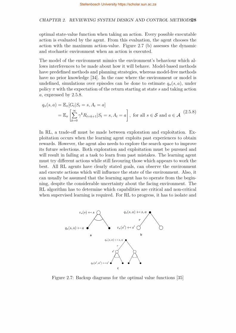
CHAPTER 2. REVIEWING SYSTEM DESIGN AND CONTROL METHODS28
optimal state-value function when taking an action. Every possible executableaction is evaluated by the agent. From this evaluation, the agent chooses theaction with the maximum action-value. Figure 2.7 (b) assesses the dynamicand stochastic environment when an action is executed.
The model of the environment mimics the environment’s behaviour which al-lows interferences to be made about how it will behave. Model-based methodshave predefined methods and planning strategies, whereas model-free methodshave no prior knowledge [34]. In the case where the environment or model isundefined, simulations over episodes can be done to estimate qπ(s, a), underpolicy π with the expectation of the return starting at state s and taking actiona, expressed by 2.5.8.
qπ(s, a) = Eπ[Gt|St = s, At = a]
= Eπ[ ∞∑k=0
γkRt+k+1|St = s, At = a
], for all s ∈ S and a ∈ A
(2.5.8)
In RL, a trade-off must be made between exploration and exploitation. Ex-ploitation occurs when the learning agent exploits past experiences to obtainrewards. However, the agent also needs to explore the search space to improveits future selections. Both exploration and exploitation must be pursued andwill result in failing at a task to learn from past mistakes. The learning agentmust try different actions while still favouring those which appears to work thebest. All RL agents have clearly stated goals, can observe the environmentand execute actions which will influence the state of the environment. Also, itcan usually be assumed that the learning agent has to operate from the begin-ning, despite the considerable uncertainty about the facing environment. TheRL algorithm has to determine which capabilities are critical and non-criticalwhen supervised learning is required. For RL to progress, it has to isolate and
Figure 2.7: Backup diagrams for the optimal value functions [35]
Stellenbosch University https://scholar.sun.ac.za
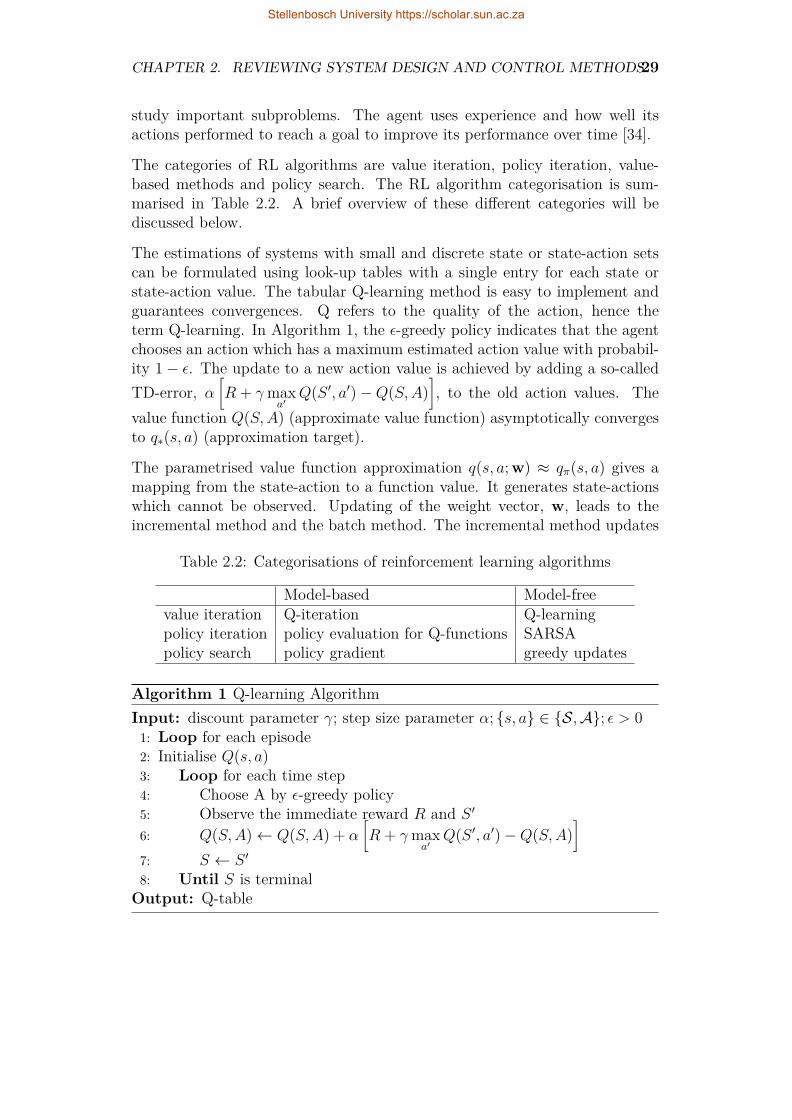
CHAPTER 2. REVIEWING SYSTEM DESIGN AND CONTROL METHODS29
study important subproblems. The agent uses experience and how well itsactions performed to reach a goal to improve its performance over time [34].
The categories of RL algorithms are value iteration, policy iteration, value-based methods and policy search. The RL algorithm categorisation is sum-marised in Table 2.2. A brief overview of these different categories will bediscussed below.
The estimations of systems with small and discrete state or state-action setscan be formulated using look-up tables with a single entry for each state orstate-action value. The tabular Q-learning method is easy to implement andguarantees convergences. Q refers to the quality of the action, hence theterm Q-learning. In Algorithm 1, the ε-greedy policy indicates that the agentchooses an action which has a maximum estimated action value with probabil-ity 1− ε. The update to a new action value is achieved by adding a so-calledTD-error, α
[R + γmax
a′Q(S ′, a′)−Q(S,A)
], to the old action values. The
value function Q(S,A) (approximate value function) asymptotically convergesto q∗(s, a) (approximation target).
The parametrised value function approximation q(s, a; w) ≈ qπ(s, a) gives amapping from the state-action to a function value. It generates state-actionswhich cannot be observed. Updating of the weight vector, w, leads to theincremental method and the batch method. The incremental method updates
Table 2.2: Categorisations of reinforcement learning algorithms
Model-based Model-freevalue iteration Q-iteration Q-learningpolicy iteration policy evaluation for Q-functions SARSApolicy search policy gradient greedy updates
Algorithm 1 Q-learning AlgorithmInput: discount parameter γ; step size parameter α; {s, a} ∈ {S,A}; ε > 0
1: Loop for each episode2: Initialise Q(s, a)3: Loop for each time step4: Choose A by ε-greedy policy5: Observe the immediate reward R and S ′
6: Q(S,A)← Q(S,A) + α[R + γmax
a′Q(S ′, a′)−Q(S,A)
]7: S ← S ′
8: Until S is terminalOutput: Q-table
Stellenbosch University https://scholar.sun.ac.za

CHAPTER 2. REVIEWING SYSTEM DESIGN AND CONTROL METHODS30
the weight vector w by gradient descent given by
wt+1 = wt + β [qπ(St, At)− q(St, At; wt)∇q(St, At; wt)] . (2.5.9)
The learning rate qπ(St, At) is iteratively obtained from the Bellman equationin (2.5.8).
The SARSA(λ) (State-action-reward-state-action) algorithm makes use of theapproximation to update the eligibility trace and the value function. Thelinear case assumes ∇q(s, a; w) = wTx(s, a). The vector z has the same com-ponent number as w and is the eligibility trace. This holds a record of whichcomponents of the weight vector has already contributed to recent state val-ues. The incremental method uses the experience only once to update thevalue function estimate and discards it in the next step. The batch method issampling efficient and attempts to find the best fitting estimate of the valuefunction to all of the data.
The fitted Q-iteration algorithm also uses gradient descent optimisation butupdates w from a sample of observations. Tabular and approximation meth-ods function in a value-based paradigm where the value functions have to beapproximated. The policy is done using a greedy or ε-greedy strategy, whilethe policy-based method directly explores the parametrised policy using
πθ(a|s; θ = P[At = a|St = s; θt = θ]. (2.5.10)
The policy-based method presents better convergence, particularly for a con-tinuous state-action space. The average reward for each time step is used asan objective function for episodic experiments. θ is iteratively updated usingthe gradient ascent technique. The deterministic policy can be avoided byassigning a probability to the action preference.
Because the HPS will be small and simple, the implementation will be doneusing the Q-learning algorithm. As mentioned before, the Q-learning algorithmis easy to implement, converges well and will be discussed below.
Q-learning is a value-based method to supply information to an agent of whichaction it should take [37]. The Q-learning agent does not require any priorknowledge of the environment and only requires which states exist and whichactions are possible in each state [36]. The agent must have the ability tolearn to take actions in a specific state which has a delayed reward. Thismeans that although the agent might not receive an immediate reward, it willreceive a larger reward later on [37]. All the states are thus infinitely visitedand Q values are continuously updated until it converges [36]. In terms of thecontrol system, the controller learns to optimally exchange energy in the HPSto ensure the load will be satisfied. As seen in Algorithm 1, the Q-learning
Stellenbosch University https://scholar.sun.ac.za
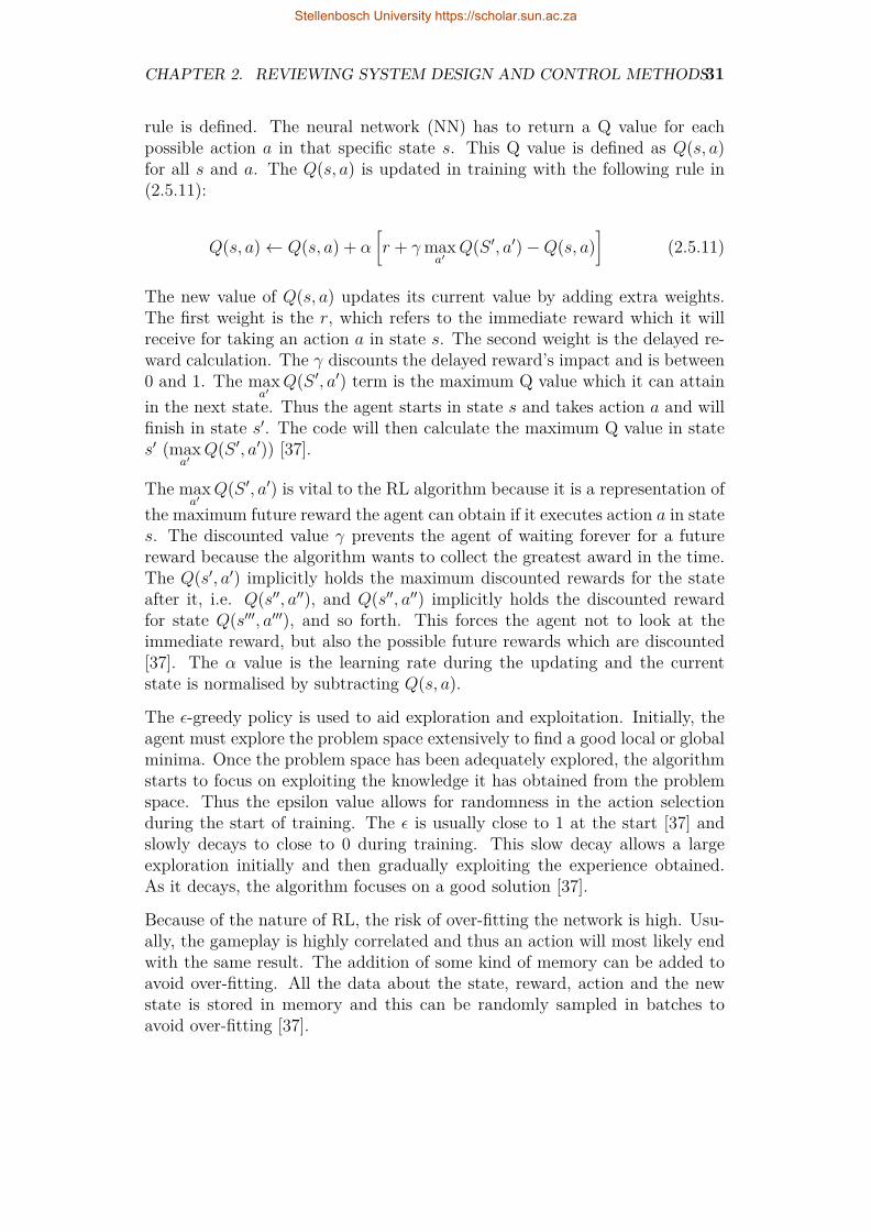
CHAPTER 2. REVIEWING SYSTEM DESIGN AND CONTROL METHODS31
rule is defined. The neural network (NN) has to return a Q value for eachpossible action a in that specific state s. This Q value is defined as Q(s, a)for all s and a. The Q(s, a) is updated in training with the following rule in(2.5.11):
Q(s, a)← Q(s, a) + α[r + γmax
a′Q(S ′, a′)−Q(s, a)
](2.5.11)
The new value of Q(s, a) updates its current value by adding extra weights.The first weight is the r, which refers to the immediate reward which it willreceive for taking an action a in state s. The second weight is the delayed re-ward calculation. The γ discounts the delayed reward’s impact and is between0 and 1. The max
a′Q(S ′, a′) term is the maximum Q value which it can attain
in the next state. Thus the agent starts in state s and takes action a and willfinish in state s′. The code will then calculate the maximum Q value in states′ (max
a′Q(S ′, a′)) [37].
The maxa′
Q(S ′, a′) is vital to the RL algorithm because it is a representation ofthe maximum future reward the agent can obtain if it executes action a in states. The discounted value γ prevents the agent of waiting forever for a futurereward because the algorithm wants to collect the greatest award in the time.The Q(s′, a′) implicitly holds the maximum discounted rewards for the stateafter it, i.e. Q(s′′, a′′), and Q(s′′, a′′) implicitly holds the discounted rewardfor state Q(s′′′, a′′′), and so forth. This forces the agent not to look at theimmediate reward, but also the possible future rewards which are discounted[37]. The α value is the learning rate during the updating and the currentstate is normalised by subtracting Q(s, a).
The ε-greedy policy is used to aid exploration and exploitation. Initially, theagent must explore the problem space extensively to find a good local or globalminima. Once the problem space has been adequately explored, the algorithmstarts to focus on exploiting the knowledge it has obtained from the problemspace. Thus the epsilon value allows for randomness in the action selectionduring the start of training. The ε is usually close to 1 at the start [37] andslowly decays to close to 0 during training. This slow decay allows a largeexploration initially and then gradually exploiting the experience obtained.As it decays, the algorithm focuses on a good solution [37].
Because of the nature of RL, the risk of over-fitting the network is high. Usu-ally, the gameplay is highly correlated and thus an action will most likely endwith the same result. The addition of some kind of memory can be added toavoid over-fitting. All the data about the state, reward, action and the newstate is stored in memory and this can be randomly sampled in batches toavoid over-fitting [37].
Stellenbosch University https://scholar.sun.ac.za

CHAPTER 2. REVIEWING SYSTEM DESIGN AND CONTROL METHODS32
The controller will essentially be a randomised memory of previous steps andoutcomes which the agent has experienced during training. The control systemshould hypothetically define policies which will increase the capacity factor ofthe HPS, while simultaneously optimising the cost-effectiveness and efficiencyof the system. The controller can benefit from knowing what the foreseeablefuture solar power will be and use this as part of the control system.
A fundamental background on RL and Q-learning was provided to highlight theways this can be used as a control system for an HPS. In the next section, therelated works of HPS control and RL will be explored to study what has beendone with these types of control systems. The implementation is discussedfurther on in Chapter 3.
2.5.2 Previous WorkThe field of HPSs and RL control using Q-learning is still growing and thusvery few quality literature works are available. However, previous work withregards to RL and hybrid electrical vehicles (HEV) [32, 38, 39], as well asbuilding energy [31], has been done. Due to the lack of research material,these related works are also briefly discussed and interpreted to understandhow RL control has been implemented.
Leo et.al. proposes a three-step-ahead Q-learning control algorithm for amicro-grid [36]. The micro-grid is grid-connected with a local consumer, aPV system and a battery storage facility. Mathematical models of the PV-modules and battery is used to calculate the power capabilities. The MDPconsiders discrete states and actions. The dynamic environment consists ofthe available solar power output and the consumer load. The algorithm looksahead for three time steps and the rewards are quantitative performance mea-sures. The agent’s actions are influenced by the available solar power, batterylevel and load. The agent chooses the best 3-step-ahead planning based onthe 3-step Q-learning algorithm. The long term objective of the consumer isto reduce the power consumption from the grid. The case study analysed thesolar utilisation rate and the total grid usage as indicators of how the powerconsumption from the grid is reduced. The results showed that the Q-learningalgorithm greatly decreased the grid power consumption and thus its objectiveswere achieved.
In the article presented by Mbuwir et.al. it notes that although Q-learningis a popular method, it throws away observation after every update, whichleads to inefficient use of data [33]. Instead, a batch RL technique where thecontroller estimates a control policy based on a batch of its previous expe-riences is proposed. The microgrid consists of a PV system as a renewablesource and a battery storage facility for a residential load. The state spacehas time-aware components which allow the agent to study the load profile.
Stellenbosch University https://scholar.sun.ac.za

CHAPTER 2. REVIEWING SYSTEM DESIGN AND CONTROL METHODS33
The timing component considers the quarter-hour of the day and the day ofthe week. The state space also includes a controllable component with regardsto the battery and an external feature, which is the observable external time-and weather-dependent information which cannot be influenced by the controlactions. The three actions which can be executed by the RL agent are usingno battery (i.e. use PV and grid power), charge battery using the PV whilesupplying the load with grid power and discharge the battery, as well as buy-ing electricity if the PV and battery are not sufficient. The RL algorithm’sobjective is to maximise the generated PV power and in turn, minimise theuse of the utility grid and the associated electrical costs.
A multi-agent RL algorithm is implemented by Bollinger and Evins [40]. Themulti-agent RL algorithm allows agents to act independently to identify itsoptimal policy. The results indicated that the distributed multi-energy systemwas able to achieve near-optimal solutions if no storage was incorporated,but did not reach an optimal solution with storage. The results showed thatthe RL algorithm was unable to effectively deal with the trade-offs of storagescheduling [40]. Yue et.al. proposes RL-based dynamic power managementfor an HPS [41]. The system consists of Lithium-ion (Li-ion) batteries and asuper-capacitor for mobile systems and using the RL algorithm, the efficiencywas increased by 9%. The switching delay between power sources was alsodecreased using the algorithm. This is an indication that the RL agent canlearn when to switch on or off certain power sources in anticipation of itsusage. This can be advantages in systems which uses power supplies whichtakes longer to produce power, such as generators.
A deep RL solution for energy microgrids management is presented in [42].Three discretised actions are described as the full rate discharge of the hydro-gen storage, idling the hydrogen storage or charging it at the full rate. TheReLu activation function is used on all the layers except the output layer,where no activation is used.
The HPS in this thesis will contain a PV system, battery storage, generatorand a grid-connection. Mathematical models of the PV-module, battery andgenerator will be used as part of the analysis. A batch Q-learning algorithmwill be incorporated to maximise the use of memory and hopefully obtain afaster convergence to a minimum LPS with a maximum reward, while stilloptimising the cost of the system. It will be beneficial to rather use a singleagent as part of the simulation process to ensure that the multiple agents do notclash. A simple rule-based-, as well as a random action-based controller, will beimplemented as baseline validation of the RL-based controller. The controllerwill switch between the different power supplies based on the availability ofpower. A solar insolation prediction will be included in the RL-controller toanalyse how the effectiveness can be increased if the agent has prior knowledgeof the expected solar power generation.
Stellenbosch University https://scholar.sun.ac.za

CHAPTER 2. REVIEWING SYSTEM DESIGN AND CONTROL METHODS34
2.6 Solar Insolation Prediction using LinearRegression
The Norwegian weather forecasting website, yr.no, has an API which is acces-sible using a python library. The weather prediction information from yr.nodoes not have information regarding solar insolation, but rather about the pre-dicted clouds, temperature and wind speed. However, if a strong correlationbetween these prediction variables and the solar insolation can be found, it canserve as a vital information source for the RL-based controller. The relation-ship between these variables can be formulated using a linear regression whichis integrated with the yr.no API and the controller. Regression is a techniquefor the estimation of relationships, of which the linear regression algorithm isthe simplest to incorporate [43]. The linear regression algorithm can find alinear relationship between the different parameters received by the yr.no APIand find a predicted value of solar power. This prediction can be used in thecontroller as additional information to increase the accuracy of the action pol-icy execution. A similar approach to solar insolation prediction using a linearregression algorithm is presented in [44].
The general linear regression algorithm is given as
y = β0 + β1x1 + β2x2 + β3x3 + · · ·+ βkxk + ε. (2.6.1)
The solar insolation is thus modelled as a linear relationship between differentvariables which impact the solar intensity. β is a weight of the specific vari-able and the ε is the Gaussian noise. The mean square error (MSE) or meanabsolute error (MAE) can be used to quantify the accuracy of the linear re-gression. The integration of the linear regression output and the RL controllermay also become complicated if there is a scarcity of databases. To find arelationship, several prediction timestamps have to be used to review how farin the foreseeable future is appropriate to use. A database of these timestampshas to be built by scraping the yr.no website. If there is a disparity betweenthe number of points in the scraped data and the RL-based controller, the in-tegration of this information will become more complex. The seasonal changesaffect the weather and thus at least a year’s worth of data has to be scrapedfrom the website to predict an accurate representation of the linear regressionprediction.
The implementation is further discussed in Chapter 3.
2.7 ConclusionThis chapter gave an overview of different design methodologies, where it wasdecided to use a computational algorithm for the reason that it can be modified
Stellenbosch University https://scholar.sun.ac.za

CHAPTER 2. REVIEWING SYSTEM DESIGN AND CONTROL METHODS35
to user specifications. A GA was preferred over a PSO because it producesa list of viable solutions, whereas PSO only produces one global outcome.HOMER software was discussed as a method of testing the validity of the GA.HOMER was selected because it is considered the industry standard in HPSdesign. A brief overview of the software package is discussed.
This chapter highlighted the different control strategies, whereupon it wasdecided to use an RL-based control system. A solar insolation predictionmethod using IoT is also incorporated. A rule-based and random-action-basedcontroller will be used to test and validate the RL-based controller and a briefdiscussion is given of this controller.
Stellenbosch University https://scholar.sun.ac.za

Chapter 3
Designing systems and theircontrol
This chapter discusses the experimental design of the two main components,being the design and control of an HPS.
In the two previous chapters, the relevant background of design methods wasdiscussed, whereupon it was decided to use a GA as an appropriate design tool.A review of the fundamental background and the previous work associatedwith this design method was discussed. HOMER, a commercially availablesoftware, was chosen as a comparison tool to highlight the advantages anddisadvantages of using a GA. The various control methods were discussed andan RL-based control was chosen as a suitable controller. Two baselines willbe used to assess how well the RL-based controller performs. The RL-basedcontroller is also given additional information with regards to the weatherpredictions to increase the use of the RES.
3.1 Design Using a Genetic AlgorithmThe design of an HPS using a GA is based on Figure 2.1 in Section 2.2 andshows how the GA starts by reading in the data of the components, load profileand weather profile.
3.1.1 Data InputThe data used to design an HPS using a GA is discussed in this section. Thedata consists of a load profile, weather profile and a database of componenttypes. The load and weather profile will be discussed below. The databases ofthe components are summarised in Appendix B under Section B.1 in TablesB.1, B.2, B.3 and B.4. These components were chosen based on the availabilityof the information.
36
Stellenbosch University https://scholar.sun.ac.za

CHAPTER 3. DESIGNING SYSTEMS AND THEIR CONTROL 37
3.1.1.1 Load profile
The load profile consists of 8760 hourly data points of energy loads. Theweather profile consists of the average hourly direct normal irradiance (DNI),global horizontal irradiance (GHI) and diffuse horizontal irradiance (DHI) mea-sured values for 8760 hours. The data is used as part of the analysis of theGA and will be discussed in more detail below. The location is based on Stel-lenbosch, because of the availability of data from the university and the loadis based on a farm.
The load data consists of a date and the kWh usage for every half an hour. Thedata was acquired from a private consulting engineering company who workedon the farm and the use of the data for academic purposes was obtained. Thepeak load is specified as 80.67 kW with a load factor of 29%. The typicalbase load is 23.52 kW and the average daily energy used is 564.14 kWh. Thedata was processed to form 8760 hourly data points from the half-hour points,which is then used in the GA. The load was also analysed to aid in the designprocess. The period is from 1 January 2017 to 31 December 2017.
In Figure 3.1, the average hourly load per day of month is plotted. From thefigure, it is clear that the beginning of the month had considerably greateraverage energy usage. The usage decays from 2nd until the 11th, whereuponit rises rapidly until it plateaus for the rest of the month. Figure 3.3 visualisesthe average monthly load which shows a significant spike at the beginning ofthe year and a lower use towards the end of the year.
Figure 3.2 shows the average 24-hour usage on the farm. The average hourlyusage showed an increase in energy usage during the mid-morning hours untilit plateaus to the late afternoon. The load decreases through the night. How-ever, Figure 3.2 only considers annual averages and not seasonal fluctuations.
0 5 10 15 20 25 30Day of month
20
30
40
50
60
70
80
Loa
d[k
Wh]
Figure 3.1: Design Average Hourly Load per Day of the Month
Stellenbosch University https://scholar.sun.ac.za

CHAPTER 3. DESIGNING SYSTEMS AND THEIR CONTROL 38
0 5 10 15 20Hour of day
34
36
38
40
42
44
46
48
Loa
d[k
Wh]
Figure 3.2: Design Average Hourly Load per Day
2 4 6 8 10 12Months
30
40
50
60
70
Loa
d[k
Wh]
Figure 3.3: Average Hourly Load per Month
Because PV power will be considered as a power source, it is important tonote how the load deviates over the seasons.
Figure 3.4 shows the entire data set over the course of 8760 hours. As expected,peaks can be seen in the beginning of most months and the load is considerablyhigher during the first 3000 hours of the dataset, reinforcing the deductionsmade from Figures 3.1 and 3.3. Figure 3.5 shows the average hourly load perday of the week, where 0 refers to Monday and 6 refers to Sunday. There seemsto be a higher load on Monday and Sunday, and a slight plateau mid-week.
Stellenbosch University https://scholar.sun.ac.za

CHAPTER 3. DESIGNING SYSTEMS AND THEIR CONTROL 39
0 2000 4000 6000 8000Hours
0
20
40
60
80
100
120
140
Loa
d[k
Wh]
Figure 3.4: Design Hourly Load Over 1 Year
0 1 2 3 4 5 6Day of week
38
39
40
41
42
43
Loa
d[k
Wh]
Figure 3.5: Design Average Day of Week Hourly Load
3.1.1.2 Weather Profile
The weather data was obtained from the SAURAN database [11] and for thesame period as the load profile. The average monthly irradiance is shown inFigure 3.6. It shows a higher irradiance level during the summer months (Oc-tober to February) and lowers during the winter months (April to September).The weather profile is ideal for the load profile during the early months of theyear (January to March), however, the end-of-year summer months are notthat suitable and will most likely generate an excess of solar power.
The initial analysis of the DNI, GHI and DHI is summarised in Table 3.1 anddoes not include night (i.e. non-daylight) hours data. Clear sky irradianceusually has a bell-curve where it peaks at the solar noon. The average solar
Stellenbosch University https://scholar.sun.ac.za
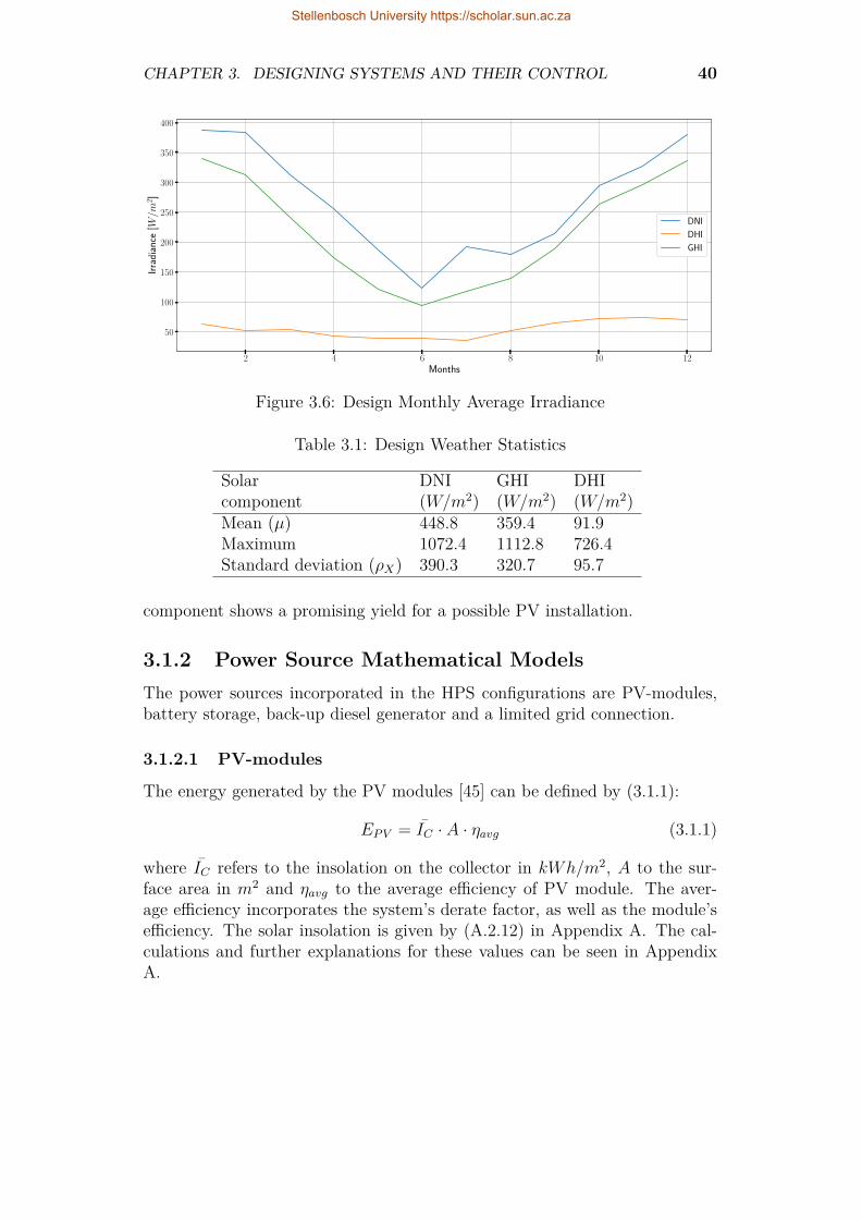
CHAPTER 3. DESIGNING SYSTEMS AND THEIR CONTROL 40
2 4 6 8 10 12Months
50
100
150
200
250
300
350
400
Irra
dian
ce[W/m
2]
DNI
DHI
GHI
Figure 3.6: Design Monthly Average Irradiance
Table 3.1: Design Weather Statistics
Solar DNI GHI DHIcomponent (W/m2) (W/m2) (W/m2)Mean (µ) 448.8 359.4 91.9Maximum 1072.4 1112.8 726.4Standard deviation (ρX) 390.3 320.7 95.7
component shows a promising yield for a possible PV installation.
3.1.2 Power Source Mathematical ModelsThe power sources incorporated in the HPS configurations are PV-modules,battery storage, back-up diesel generator and a limited grid connection.
3.1.2.1 PV-modules
The energy generated by the PV modules [45] can be defined by (3.1.1):
EPV = IC · A · ηavg (3.1.1)
where IC refers to the insolation on the collector in kWh/m2, A to the sur-face area in m2 and ηavg to the average efficiency of PV module. The aver-age efficiency incorporates the system’s derate factor, as well as the module’sefficiency. The solar insolation is given by (A.2.12) in Appendix A. The cal-culations and further explanations for these values can be seen in AppendixA.
Stellenbosch University https://scholar.sun.ac.za

CHAPTER 3. DESIGNING SYSTEMS AND THEIR CONTROL 41
3.1.2.2 Battery
The charged battery energy storage in hour, t, EB,t, is given by:
EB,t = EB,t−1(1− σ) + (EG,t −EL,tηInv
) · ηBat (3.1.2)
where EB,t and EB,t−1 is the energy stored in the batteries in hour t and theprevious hour, σ to the self-discharge rate per hour of the batteries, EG,t tothe available charge power, EL,t to the load demand in hour t, ηInv to theinverter’s efficiency and ηBat to the battery’s efficiency. The energy stored inthe battery in hour t has lower and upper limits
EB,min ≤ EB,t ≤ EB,max (3.1.3)
where minimum allowable energy level EB,min is defined by Equation (3.1.4)
EB,min = (1−DOD) · EB,max (3.1.4)
and EB,max is the maximum battery allowable energy level, which is assumedas the nominal capacity of the battery. The discharge and charging efficiencyis assumed to be 90% and the depth of discharge (DOD) is chosen as 60% foroptimal lifetime usage. Each battery is individually analysed throughout itslifetime usage.
3.1.2.3 Generator
The generator’s fuel consumption is usually calculated using the fuel curveratings. However, the precise fuel curves are not readily available and thusassumptions were made to account for this. To save computational power andmemory, the generators are assumed on a 75% load when running. For theSGBG configuration, any unused generator power is fed to the batteries tocharge. The SGG configuration disregards any unused generator power. Aminimum run time of 2 hours is specified to avoid rapidly on-off switching ofthe generator. Each generator is assessed according to how much hours it runsand fuel consumptions.
3.1.2.4 Inverter
The inverter’s model is based on Equation (3.1.5)
Pout = PPV · ηInv (3.1.5)
where Pout refers to the output inverted power, PPV to the input power suppliedby the PV-modules and ηInv to the inverter’s efficiency. The efficiency isincluded when inverting DC to AC power for the load.
Stellenbosch University https://scholar.sun.ac.za

CHAPTER 3. DESIGNING SYSTEMS AND THEIR CONTROL 42
3.1.2.5 Grid
Grid is a specified maximum hourly limit of 10 kWh with a reliability proba-bility. The reliability probability accounts for unforeseen circumstances suchas power outages and load shedding, should it occur in the near future. Thereliability is specified as 99%. Thus for one year, 87.6 hours are assumed torepresent off-grid scenarios. A random number is generated from a uniformdistribution between 0 and 1. If the variable is less that 0.99, the utility griddoes not fail. If it is greater than 0.99, it is assumed that the grid has failedfor that hour and power cannot be supplied. The random variations adds asensitivity and conservativeness to the design to account for possible scenariosthe HPS can experience.
3.1.3 AssumptionsCertain assumptions are made for the algorithm. The lifetime assessmenttakes into account inflation and the O&M costs of the HPS over 20 years. Theinflation rate is assumed as 5.0%. Table 3.2 shows the assumptions made interms of the O&M and installation costs. These values are assumed to be apercentage of the capital cost of each component and thus linearly increasingor decreasing with regards to the system’s size. For example, the O&M perPV-module is assumed to be 5% of the capital cost of the module. All O&Mcosts are assumed to be adjusted for inflation during the lifetime assessmentof the system. The grid price is R1.45 per kWh
The fuel price is assumed as R16 per liter diesel and is adjusted with inflationeach year. However, uncertainty holds with oil availability or escalating pricesand is thus an important consideration for the feasibility of the HPS over itslifetime. The HPS does not sell any excess generated power back to the grid,which can also impact the ROI and feasibility of the HPS. Equipment wasreplaced on the year that warranty ends and the replacement costs is adjustedaccording to inflation. The replacement costs do not fall under O&M costs.The repairs and maintenance is assumed to be done during non-operationalhours of the usage of the power source.
Table 3.2: Genetic Algorithm Financial Overheads and Operational and Main-tenance Assumptions
Assumption % of Capital CostPV maintenance cost 5Battery maintenance cost 6Generator maintenance cost 10Installation costs 10
Stellenbosch University https://scholar.sun.ac.za

CHAPTER 3. DESIGNING SYSTEMS AND THEIR CONTROL 43
3.1.4 Genetic Algorithm Experimental DesignAs briefly discussed in Section 2.2.1, the GA consists of population memberswith chromosome structures, selection, crossover and mutation, which occursover a specified amount of generations, and the objective and fitness functions.
3.1.4.1 Chromosome Structure, Generations and Population
The chromosome structure is given as the types and numbers of four differentcomponents. These components are the PV-modules, battery, generator andinverter. The chromosome structure is presented by (3.1.6):
[TPV NPV TBat NBat TGen NGen TInv NInv ] . (3.1.6)
The types can vary from 0 to the maximum number in the component database.The maximum number of components is predefined by the user to limit thesearch space. The type is randomly chosen according to a uniform distribution.Based on the different types, there are constraints to the different components.The PV capacity size is dependent on the inverter’s ratings and the minimumand maximum value of the string number, as calculated by Equations (3.1.7)and (3.1.8). A random value between these minimum and maximum valuesare selected based on a uniform distribution.
Min PV String number = Min. inverter MPPT VoltagePV MPP Voltage (3.1.7)
Max PV String number = Max. inverter MPPT VoltagePV MPP Voltage (3.1.8)
The temperature effect of the PV-modules is neglected for the sizing purposesof the PV capacity. This is done to save computational power and the temper-ature effect assumed to average out throughout the simulation. When choosinga configuration, further investigation can be done to inspect the specific layoutof the PV-modules and sizing to take into account the temperature effect.
3.1.4.2 Selection, Crossover and Mutation
In each generation, crossover and mutation take place. The probability ofcrossover occurrence is 80% and the mutation rate is 40%. Mutation cre-ates an offspring by randomly altering chromosomes of a population member.Crossover creates an offspring from two parents in the population by randomlymixing the chromosomes. The algorithm proceeds by first examining whethercrossover occurs with an 80% probability. Should crossover not occur, a mu-tation occurs with a 40% probability where each DNA has a 40% chance of
Stellenbosch University https://scholar.sun.ac.za

CHAPTER 3. DESIGNING SYSTEMS AND THEIR CONTROL 44
being altered. The selection of parents is based on the roulette wheel selectionmethod, which is discussed in Section 2.2.1 of Chapter 2.
Theoretically, the GA can consider an infinite number of generations and pop-ulation members to find an optimal solution. However, this is not ideal andwill waste computational power. Thus another goal of the GA is to convergein the minimum time, while still maintaining a maximum diversity. Since theGA is a list of potential HPS configurations, the top fittest members will beconsidered as viable solutions. The population has to be big enough to ensurediversity, but not too large that it wastes computational power. The same canbe said for the number of generations. As the population members become fit-ter, the criteria to surpass these fittest members become increasingly difficult.Thus after a number of generations, the algorithm’s top members converge andrarely changes. Running the algorithm for many generations wastes compu-tational power. An analysis of various populations with generations was doneto determine the optimal sizes and the results can be seen in Table 3.3.
In Table 3.3, two measures of the population size and number of generationsare given. The top member changes refer to when a new offspring replaces thebest or fittest individual, whereas the offspring added column indicates that theoffspring has replaced the weakest member of the population. The percentageis given as the ratio between the value and the number of generations. Eventhough the 120 population size with 160 generations has the same amount oftop member changes as the 1000 population, 1000 generation combination, thepercentage gives the perspective of how significant that number of change is.
The smaller populations have a higher percentage of top member changescompared to the larger population, whereas the larger population sizes indicatethat the search space is saturated with an optimal solution early on in thesimulation. In addition, higher generation numbers show lower top memberchange, which indicates that it is unnecessary to run a simulation for toolong. The amount of offspring over the course of the simulation which is
Table 3.3: Population size and number of generation analysis
Population Number of Top member Offspringsize generations changes added60 1000 58 (4.8%) 397 (39.7%)120 160 6 (3.75%) 131 (81.8%)500 500 4 (0.8%) 427 (85.4%)1000 1000 6 (0.6%) 850 (85%)60 80 8 (10%) 71 (88.75%)60 160 13 (8.125%) 125 (78.1%)2000 2000 2 (01%) 1759 (87.45%)1000 2000 12 (0.6%) 1602 (80.1%)
Stellenbosch University https://scholar.sun.ac.za

CHAPTER 3. DESIGNING SYSTEMS AND THEIR CONTROL 45
0 10 20 30 40 50 60 70 80Generations
58
60
62
64
66
68
Pop
ulat
ion
aver
age
fitne
ss
Average Fitness
Fittest Member
Figure 3.7: Average Population Fitness over 80 Generations
added to the group seems relatively high, except for the 60 population, 1000generations combination. Figure 3.7 shows the average population fitness over80 generations, as well as the top fittest individual of the population. The topfittest member increases rapidly in the initial generations, however, starts toplateau and becomes only marginally fitter.
Figure 3.8 shows the average population fitness over 1000 generations, with apopulation of 60, as well as the top fittest individual of the population.
In the figure, the average initially increases rapidly and converges as the gen-erations continue. This is due to the weakest member being replaced with astronger, fitter member, which will increase the population’s overall fitness.However, as the overall population becomes fitter, the generated offspring has
0 200 400 600 800 1000Generations
58
60
62
64
66
68
Pop
ulat
ion
aver
age
fitne
ss
Average Fitness
Fittest Member
Figure 3.8: Average Population Fitness over 1000 generations
Stellenbosch University https://scholar.sun.ac.za

CHAPTER 3. DESIGNING SYSTEMS AND THEIR CONTROL 46
to become significantly fitter to be added to the population. This is indicatedin the convergence on the figure where the average fitness of the populationincreases slower. The figure also shows the top fittest member and its fitness.
For this thesis, it was decided to use a population size of 60. The population islarge enough to ensure enough diversity, but not too large that the algorithm’spurpose becomes futile and defeats the overall purpose of the GA. The numberof generations is chosen as 80, as most of the top fittest changes happen quiteearly on in the algorithm. A greater number of generations can marginallyimprove the HPS configurations, however, the differences become almost in-significant and will waste computational power. As the generations continueto crossover and mutate, the fittest individual becomes harder to beat andthus a large number of generations would not be beneficial to the algorithm.
3.1.4.3 Objective Functions
The different objectives highlights the trade-offs between different HPS con-figurations and power combinations. There are three main objectives, namelytechnical, financial and environmental and each of these objectives have differ-ent attributes. The technical objective aims to minimise the LPSP, whereas thefinancial objective aims to minimise the capital and life time costs by maximis-ing the ROI for the investor. The environmental objectives aims to maximisethe use of RES and to minimise the fuel usage, which attributes to pollution.The GA is defined as a multi-objective optimisation problem because it op-timises more than one objective. By defining these objectives, an optimisedHPS will be designed using the GA which produces consistent power, is finan-cially feasible and will have a minimal impact on the environment. The GAevaluates four different HPS configurations: solar-grid (SG), solar-grid-battery(SGB), solar-grid-generator (SGG) and solar-grid-battery-generator (SGBG).
Technical objectives The LPSP gives an indication of how consistent thepower produced by the HPS configuration is and is defined by
LPSP =
T∑t=1
LPSt
T∑t=1
EL,t
(3.1.9)
where LPSP refers to the loss of power supply probability, LPSt to the lossof power supply in hour t and EL,t to energy load in hour t and
LPSt = EL,t − [EPV,t + EG,t + EB,t] · ηinv − EGrid,t (3.1.10)
where EPV,t, EG,t, EB,t and EGrid,t refer to the energy generated by PV-modules, diesel generator, energy stored in the batteries and grid energy in
Stellenbosch University https://scholar.sun.ac.za
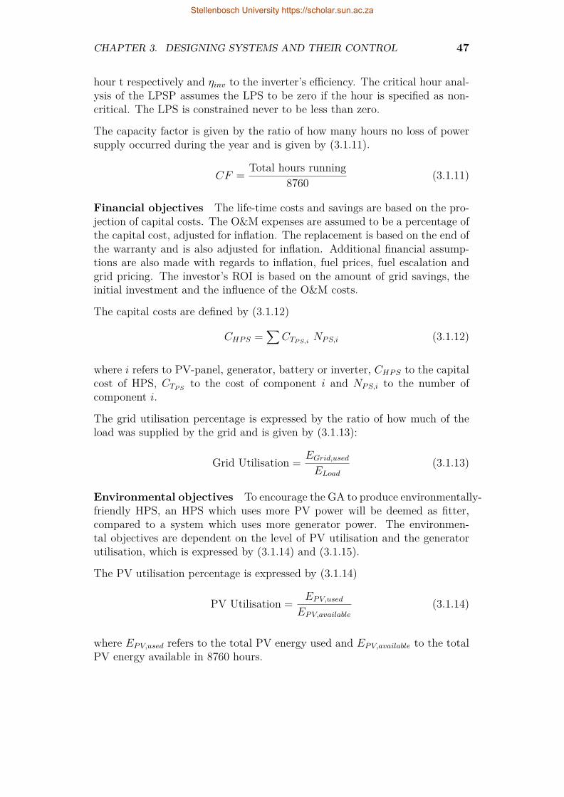
CHAPTER 3. DESIGNING SYSTEMS AND THEIR CONTROL 47
hour t respectively and ηinv to the inverter’s efficiency. The critical hour anal-ysis of the LPSP assumes the LPS to be zero if the hour is specified as non-critical. The LPS is constrained never to be less than zero.
The capacity factor is given by the ratio of how many hours no loss of powersupply occurred during the year and is given by (3.1.11).
CF = Total hours running8760 (3.1.11)
Financial objectives The life-time costs and savings are based on the pro-jection of capital costs. The O&M expenses are assumed to be a percentage ofthe capital cost, adjusted for inflation. The replacement is based on the end ofthe warranty and is also adjusted for inflation. Additional financial assump-tions are also made with regards to inflation, fuel prices, fuel escalation andgrid pricing. The investor’s ROI is based on the amount of grid savings, theinitial investment and the influence of the O&M costs.
The capital costs are defined by (3.1.12)
CHPS =∑
CTP S,iNPS,i (3.1.12)
where i refers to PV-panel, generator, battery or inverter, CHPS to the capitalcost of HPS, CTP S
to the cost of component i and NPS,i to the number ofcomponent i.
The grid utilisation percentage is expressed by the ratio of how much of theload was supplied by the grid and is given by (3.1.13):
Grid Utilisation = EGrid,usedELoad
(3.1.13)
Environmental objectives To encourage the GA to produce environmentally-friendly HPS, an HPS which uses more PV power will be deemed as fitter,compared to a system which uses more generator power. The environmen-tal objectives are dependent on the level of PV utilisation and the generatorutilisation, which is expressed by (3.1.14) and (3.1.15).
The PV utilisation percentage is expressed by (3.1.14)
PV Utilisation = EPV,usedEPV,available
(3.1.14)
where EPV,used refers to the total PV energy used and EPV,available to the totalPV energy available in 8760 hours.
Stellenbosch University https://scholar.sun.ac.za

CHAPTER 3. DESIGNING SYSTEMS AND THEIR CONTROL 48
The generator utilisation ratio is given as (3.1.15)
Generator Utilisation = EGen,usedELoad,total
(3.1.15)
where EGen,used refers to total generator used and ELoad,total to total load in8760 hours.
3.1.4.4 Fitness Function
The fitness function is given by (3.1.16). The fitness function is a weightedlinear combination. Each weight of the different attribute indicates how im-portant the investor views the objective and the fitness value indicates howwell the overall objectives are met.
Fitness =∑
wiFitnessi (3.1.16)
where i refers to the objective (technical, economical or environmental), wi tothe weight of objective i and Fitnessi to the fitness of objective i .
Each attributes weight, wi, is directly correlated to how important the investorviews the objective. The different attributes for this GA are ROI, LPSP,critical-hour LPSP, and PV-, grid- and generator utilisation. The assignedweights can be observed in Table 3.4. The GA evaluates the new offspringcreated during mutation or crossover using the fitness function. Based on itsfitness, the offspring will then replace the weakest population member. Shouldthe weakest population member be fitter than the offspring, the offspring isdiscarded. This illustrates how the overall population becomes fitter with eachgeneration. The technical objectives are assumed to have the highest priorityand thus are attributed with the heaviest fitness weights. The financial- andenvironmental objectives are prioritised second and third respectively.
Table 3.4: Fitness function weights
Weight ValueLPSP 12Renewable energy utilisation 4Grid utilisation 1Generator utilisation 1Capacity factor 3Return on investment 1
Stellenbosch University https://scholar.sun.ac.za

CHAPTER 3. DESIGNING SYSTEMS AND THEIR CONTROL 49
3.2 Design Using HOMER softwareHOMER is used to design an HPS. Assumptions with regards to the simulationcan be seen in Table 3.5. The inflation rate was specified as 5% and the gridprice is R1.45 per kWh, as with the GA. The project lifetime is 20 years andthe generator has a minimum running time constraint of 2 hours.
The results obtained from this simulation is discussed in Section 4.1.2 of Chap-ter 4.
3.3 Reinforcement Learning-based ControlSystem
3.3.1 Data InputThe load and weather profile consists of 525600 minutely data points during2018. The location is, as with the GA, in Stellenbosch due to the accessibil-ity of information. The control system has to be modelled as accurately aspossible, without the waste of computational power. It was decided to use aninterval frequency which has readily available data. A higher frequency, suchas minutely intervals, can be manipulated to longer intervals, such as 5, 10and 15 minute intervals. However, it is more difficult to extrapolate minutelyintervals from 15-minute intervals. To ease the data manipulation process, thesmallest possible available interval is considered and can thus be adjusted andscaled for further data processing.
The SAURAN website [11] has a scope of minutely-intervals and based on this,the controller’s time interval was chosen as minutely. A load profile for thisinterval was not readily available and thus had to be artificially generated asaccurate as possible. The Load Profile Generator (LPG) [46] is a modelling toolfor residential energy consumption. It performs full behavioural simulation ofa household and generates subsequent load curves.
Table 3.5: HOMER Assumptions
System Capital Replacement O&M Lifetime Efficiencycomponent ZAR/kW ZAR/kW ZAR/kW/Year years %Battery 2,500 2,500 50 10 81Converter 3,670.20 3,670.20 36.70 5 95PV Module 7,115 7,115 355 20 20.4Generator 3,249 3,249 0.20 20 40
Stellenbosch University https://scholar.sun.ac.za

CHAPTER 3. DESIGNING SYSTEMS AND THEIR CONTROL 50
3.3.1.1 Load profile
The household was specified as a family of five: Arthur, a 45-year-old male,and Cassie, a 40-year-old female, are the parents of three boys: Gareth (age8), George (age 12) and Gregor (age 4). Each of these household individualshas a unique energy behavioural pattern which the LPG takes into account inthe simulation. One parent works at home and the other at the office. It wasalso assumed that the family goes on holiday during the June recess. Fromthis, a minutely load profile was generated and the profiles are summarised inFigures 3.9, 3.10, 3.11 and 3.12.
0 2 4 6 8 10Month of Year
450
500
550
600
650
700
750
800
Loa
d[k
Wh]
Figure 3.9: Controller Total Monthly Load
0 1 2 3 4 5 6Day of week
1200
1250
1300
1350
1400
Loa
d[k
Wh]
Figure 3.10: Controller Total Day of Week Load
Stellenbosch University https://scholar.sun.ac.za
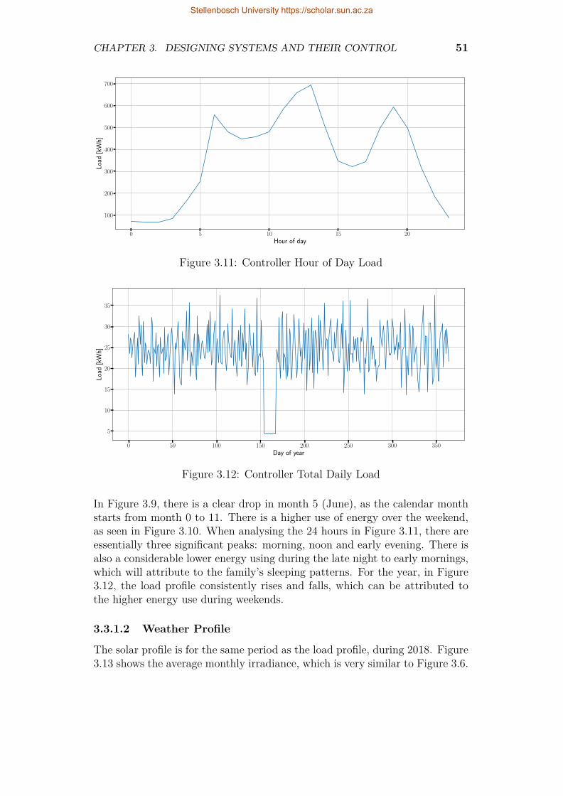
CHAPTER 3. DESIGNING SYSTEMS AND THEIR CONTROL 51
0 5 10 15 20Hour of day
100
200
300
400
500
600
700
Loa
d[k
Wh]
Figure 3.11: Controller Hour of Day Load
0 50 100 150 200 250 300 350Day of year
5
10
15
20
25
30
35
Loa
d[k
Wh]
Figure 3.12: Controller Total Daily Load
In Figure 3.9, there is a clear drop in month 5 (June), as the calendar monthstarts from month 0 to 11. There is a higher use of energy over the weekend,as seen in Figure 3.10. When analysing the 24 hours in Figure 3.11, there areessentially three significant peaks: morning, noon and early evening. There isalso a considerable lower energy using during the late night to early mornings,which will attribute to the family’s sleeping patterns. For the year, in Figure3.12, the load profile consistently rises and falls, which can be attributed tothe higher energy use during weekends.
3.3.1.2 Weather Profile
The solar profile is for the same period as the load profile, during 2018. Figure3.13 shows the average monthly irradiance, which is very similar to Figure 3.6.
Stellenbosch University https://scholar.sun.ac.za
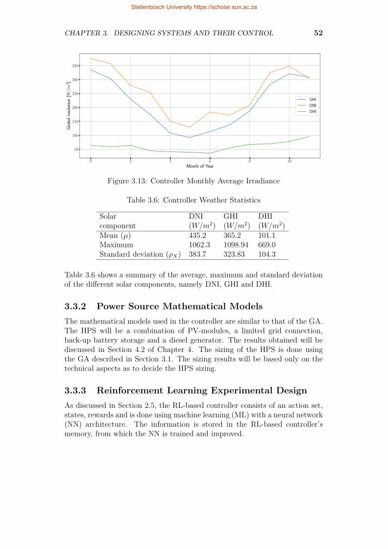
CHAPTER 3. DESIGNING SYSTEMS AND THEIR CONTROL 52
0 2 4 6 8 10Month of Year
50
100
150
200
250
300
350G
loba
lin
sola
tion
[W/m
2]
GHI
DNI
DHI
Figure 3.13: Controller Monthly Average Irradiance
Table 3.6: Controller Weather Statistics
Solar DNI GHI DHIcomponent (W/m2) (W/m2) (W/m2)Mean (µ) 435.2 365.2 101.1Maximum 1062.3 1098.94 669.0Standard deviation (ρX) 383.7 323.83 104.3
Table 3.6 shows a summary of the average, maximum and standard deviationof the different solar components, namely DNI, GHI and DHI.
3.3.2 Power Source Mathematical ModelsThe mathematical models used in the controller are similar to that of the GA.The HPS will be a combination of PV-modules, a limited grid connection,back-up battery storage and a diesel generator. The results obtained will bediscussed in Section 4.2 of Chapter 4. The sizing of the HPS is done usingthe GA described in Section 3.1. The sizing results will be based only on thetechnical aspects as to decide the HPS sizing.
3.3.3 Reinforcement Learning Experimental DesignAs discussed in Section 2.5, the RL-based controller consists of an action set,states, rewards and is done using machine learning (ML) with a neural network(NN) architecture. The information is stored in the RL-based controller’smemory, from which the NN is trained and improved.
Stellenbosch University https://scholar.sun.ac.za
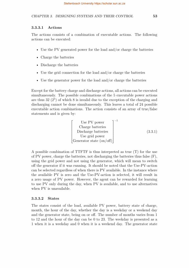
CHAPTER 3. DESIGNING SYSTEMS AND THEIR CONTROL 53
3.3.3.1 Actions
The actions consists of a combination of executable actions. The followingactions can be executed:
• Use the PV generated power for the load and/or charge the batteries
• Charge the batteries
• Discharge the batteries
• Use the grid connection for the load and/or charge the batteries
• Use the generator power for the load and/or charge the batteries
Except for the battery charge and discharge actions, all actions can be executedsimultaneously. The possible combinations of the 5 executable power actionsare thus 32 (25) of which 8 is invalid due to the exception of the charging anddischarging cannot be done simultaneously. This leaves a total of 24 possibleexecutable action combinations. The action consists of an array of true/falsestatements and is given by:
Use PV powerCharge batteries
Discharge batteriesUse grid power
Generator state (on/off)
−1
(3.3.1)
A possible combination of TTFTF is thus interpreted as true (T) for the useof PV power, charge the batteries, not discharging the batteries thus false (F),using the grid power and not using the generator, which will mean to switchoff the generator if it was running. It should be noted that the Use-PV-actioncan be selected regardless of when there is PV available. In the instance wherethe available PV is zero and the Use-PV-action is selected, it will result ina zero usage of PV power. However, the agent can be rewarded for learningto use PV only during the day, when PV is available, and to use alternativeswhen PV is unavailable.
3.3.3.2 States
The states consist of the load, available PV power, battery state of charge,month, the hour of the day, whether the day is a weekday or a weekend dayand the generator state, being on or off. The number of months varies from 1to 12 and the hour of the day can be 0 to 23. The weekday is presented as a1 when it is a weekday and 0 when it is a weekend day. The generator state
Stellenbosch University https://scholar.sun.ac.za

CHAPTER 3. DESIGNING SYSTEMS AND THEIR CONTROL 54
represents the number of running hours, where the 0 state refers to an off state.The load, available PV, month, the hour of the day and weekday states arefixed, whereas the battery and generator state is dynamically changed basedon the actions in the previous state.
3.3.3.3 Rewards
The rewarding and penalty system is how the RL controller learns. The agentexecutes an action and receives a reward after the action is completed for thetime step. The greatest reward is when there is no power supply loss andthus the entire load is met using the HPS for that time step with a numericalreward of +20. The agent is encouraged to use alternative power options whenthere is no PV available and is rewarded +3 when it uses the generator or +6discharges the battery. This will aid in the control system during the monthswith lower solar insolation where the batteries cannot be fully charged andthe HPS relies on the generator and grid. To encourage the controller to usethe available PV, it is rewarded with +6 when the PV usage is greater thanzero in order to maximise the renewable energy source. It is also rewarded +6when the total available PV is used for the load and/or charge the batteries.
3.3.3.4 Neural Network Architecture
The RL implementation is done using Machine Learning (ML), which will bedone using python and Keras [47, 48]. Keras is a high-level API of Tensor-Flow for building and training deep learning models and is considered user-friendly, modular and easy to extend. These models use artificial neural net-works (ANN). A simplified neural network architecture is shown in Figure3.14. The principle behind a NN is to imitate the way interconnected braincells recognise patterns and relationships. The NN has artificial neurons, calledunits. There are input neurons, hidden neurons and output neurons. A fullyconnected NN is where every hidden and output neuron is connected to eachunit in the layers inside. The relationships between each of these units have aweight.
There is no generic method of designing a NN and very little guidance is givento determine the number of neurons and the number of layers of a NN. TheNN is capable of mapping non-linear relationships between input variables.Previous research can be used as a guideline and overall guidelines suggest tostart with a small network and then see which alterations improve the network.The optimisation of the hyperparameters has to be done iteratively as well.
The input layer consists of a fully connected layer with the number of states asthe input. The activation function is a rectified linear unit (ReLu). The dimen-sionality of the output space is 32 units. The activation function transformsthe summed weighted input into the output activation of that input [49]. The
Stellenbosch University https://scholar.sun.ac.za
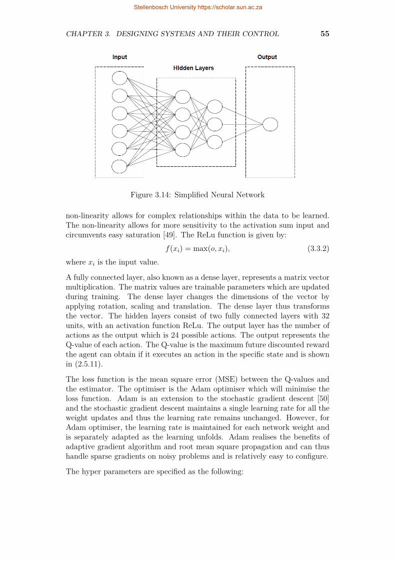
CHAPTER 3. DESIGNING SYSTEMS AND THEIR CONTROL 55
Figure 3.14: Simplified Neural Network
non-linearity allows for complex relationships within the data to be learned.The non-linearity allows for more sensitivity to the activation sum input andcircumvents easy saturation [49]. The ReLu function is given by:
f(xi) = max(o, xi), (3.3.2)where xi is the input value.
A fully connected layer, also known as a dense layer, represents a matrix vectormultiplication. The matrix values are trainable parameters which are updatedduring training. The dense layer changes the dimensions of the vector byapplying rotation, scaling and translation. The dense layer thus transformsthe vector. The hidden layers consist of two fully connected layers with 32units, with an activation function ReLu. The output layer has the number ofactions as the output which is 24 possible actions. The output represents theQ-value of each action. The Q-value is the maximum future discounted rewardthe agent can obtain if it executes an action in the specific state and is shownin (2.5.11).
The loss function is the mean square error (MSE) between the Q-values andthe estimator. The optimiser is the Adam optimiser which will minimise theloss function. Adam is an extension to the stochastic gradient descent [50]and the stochastic gradient descent maintains a single learning rate for all theweight updates and thus the learning rate remains unchanged. However, forAdam optimiser, the learning rate is maintained for each network weight andis separately adapted as the learning unfolds. Adam realises the benefits ofadaptive gradient algorithm and root mean square propagation and can thushandle sparse gradients on noisy problems and is relatively easy to configure.
The hyper parameters are specified as the following:
Stellenbosch University https://scholar.sun.ac.za

CHAPTER 3. DESIGNING SYSTEMS AND THEIR CONTROL 56
1. Learning rate α: 0.001,
2. Start ε: 1,
3. End ε: 0.01 ,
4. Discount factor γ: 0.7,
5. Episodes: 50,
6. Batch size for optimiser: 3 hours.
The start and end ε refers to the use of the ε-greedy policy, as explained inSection 2.5. As each episode continues, the ε-value starts at 1 and decays to0.01, which aids the exploration and exploitation in the algorithm. In (2.5.11),the discount factor delays the reward’s impact. A higher discount rating meansthat the algorithm is long term bias, whereas a value closer to zero has a shortterm bias. The learning rate α updates and normalises the current state.These values were based on literature and iteratively analysing the results fromthe different NN architectures. The number of episodes refers to how manyepisodes the controller has to learn the system. With each episode, the epsilonvalue decreases which allows for more exploitation of previous knowledge.
3.3.3.5 Memory
The memory is updated after each time step and the RL controller choosesrandom 3-hour batches to retrain the network after each time step. It wasdecided to use random selections as the RL controller does not need a sequen-tial list of states, but rather its previous state, the action performed, the nextstate and the reward obtained. The memory reduces the risk of over-fittingthe network. In addition, the size of the memory has to be large enoughto ensure enough information is stored, but not too excessive that it wastescomputational power.
An analysis of what intervals are deemed appropriate for the controller has tobe done. Training the network after every minute interval is computationallyexpensive and unnecessary. However, large intervals might lead to inaccuraterepresentations of the load and the controller’s input. Thus a trade-off betweencomputational usage and accuracy takes place. An analysis of different trainingof 5, 10 and 15 minute intervals is done. As the interval frequency increases,the training time of the NN increases accordingly. It would be inefficient tohave a real-time controller which trains too long and causes a bottleneck ofdata in the hardware. As the intervals increase in frequency, the amount ofdata required increases significantly. The use of hardware memory of GPUsand CPUs is limited and thus alterations to different memory sizes have to beconsidered. This interval analysis was done based on the entire database with
Stellenbosch University https://scholar.sun.ac.za

CHAPTER 3. DESIGNING SYSTEMS AND THEIR CONTROL 57
a simplified NN architecture and reward system. The purpose of this analysiswas to determine whether it is necessary to use a higher frequency when alower frequency will give the same results. Figures 3.15 and 3.16 show howthe RL controller converges to an optimal point.
The total rewards per episode are normalised to give an accurate representationof how the different intervals perform. Both the rewards and LPS converge,indicating that the agent has learnt optimal policies as part of the controlsystem. The three intervals all show promising results. However, the trainingtime varies significantly. The training difference between the 15-minute and5-minute intervals varies more than 24 hours. A lower frequency shows apossible convergence with a significantly reduced training time. It would beimpractical to execute an action every 5 minutes and the training time causes
0 10 20 30 40 50Episodes
0
500
1000
1500
2000
2500
3000
Tot
alL
PS
[kW
h]
15 min
10 min
5 min
Figure 3.15: Analysis of Controller Time Step Intervals: LPS
0 10 20 30 40 50Episodes
600000
700000
800000
900000
1000000
Tot
alR
ewar
dsp
erep
isod
e(n
orm
alis
ed)
15 min
10 min
5 min
Figure 3.16: Analysis of Controller Time Step Intervals: Rewards
Stellenbosch University https://scholar.sun.ac.za
CHAPTER 3. DESIGNING SYSTEMS AND THEIR CONTROL 58
a bottleneck of data processing. Higher frequencies can be more accurate, butthe hardware limitations have to be considered.
For this control system, it was decided to use a 15-minute interval for sim-ulation of the RL-based controller of an HPS. The memory points for the15-minute interval training frequency is selected as two times the length ofthe training database. The NN trains batches from this memory and reducesover-fitting the architecture.
3.3.4 EvaluationThe evaluation of the control system is based on two factors: the minimisationof the LPS and the maximisation of the PV power. To consider the costoptimisation as part of the analysis, the reduction in generator use and griduse will also be used as a measure of evaluation. Monetary value in costoptimisation is not done as the simulations become computationally expensiveand the hardware limitations associated with the available memory to run thesecalculations. Instead, a consideration of the PV usage against the generator isconsidered. The PV and battery installations have large capital costs, but alower operational cost than the generator. A system which utilises the energyexchange of the PV and battery more than the use of a generator is thus seenas a more cost-effective control system.
The data is split into three sets: training, validation and testing. Becauseof the cyclical nature of the load and weather profile, each month is splitinto three sections. The ratio of the training-validation-testing is specified asfollows
• Training: Days 1 to 22 of the month, which account for 72.3% of thetotal data,
• Validation: Days 23 to 26 (13.2%),
• Testing: Days 27 to month end (14.5%).
In this way, each month is part of the training, validation and test set. Indoing so, each of the different seasons can be trained in the NN.
3.4 RL-based Control System with IoTThe energy exchange between the different components can be increased ifthe RL-controller has prior knowledge of what to expect with regards to solarpower. A dataset of predictions has to be developed from scratch, as nodatabase is available for this.
Stellenbosch University https://scholar.sun.ac.za

CHAPTER 3. DESIGNING SYSTEMS AND THEIR CONTROL 59
A proof of concept with regards to predicting solar irradiance using weatherpredictions has to be done to show that it can be an accurate source of infor-mation. This is done using a linear regression algorithm. The NN has to beredesigned to consider the additional information and to assess if this is usefulfor the RL-based controller. The purpose of this section is to show that a lin-ear relationship between the weather predictions and expected solar irradiancedoes exist. The RL-based controller’s NN will be able to learn this relationshipduring its training process. However, if no relationship occurs, the data willnot benefit the RL-based controller.
3.4.1 Analysis of Solar Irradiance Predictions Usingyr.no API
3.4.1.1 Data Scraping Using yr.no API
In order to simulate as though the controller is pinging the yr.no websitehourly, a database of these scraping data had to be generated. Since there isno database with the predictions on the hour from yr.no, the database had tobe generated from scratch. The data was recorded hourly and this data will beused as part of the control system. Gaps in the database occurred as a resultof load shedding and network problems. The analysis of the data is discussedin Section B.2 of Appendix B. The scraping programme code can be seen inSection C.2 of Appendix C.
It should be noted that these values consider night time predictions, where theactual irradiance will be non-existent, which can skew the data. However, forthe purpose of showing that there are relationships between the predicted andactual values, it is sufficient. A timing component, such as the hour of the dayand month, can increase the accuracy of the predictions.
In addition, yr.no only updates the predictions every 12 hours, which caninfluence the accuracy of the results. Due to the scraping of the website, thereare gaps in the data where load shedding turned off the computer accessing thewebsite and other network errors occurred. Due to the nature of the updatingfrequency of yr.no, the missing data can be filled by the closet ping to thattime. However, large periods of missing data cannot be filled and will thusbe discarded, resulting in a smaller usable database. However, to increase theamount of data, this problem can be solved by splitting the data into sequentialbatches, rather than one large database to validate the system.
3.4.1.2 Preliminary Results of Linear Regression
The yr.no website is accessed through the API to extract the current weatherpredictions of a certain location. The implementation code can be seen inSection C.3 of Appendix C. The co-ordinates and altitude of Stellenbosch
Stellenbosch University https://scholar.sun.ac.za
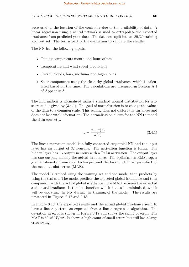
CHAPTER 3. DESIGNING SYSTEMS AND THEIR CONTROL 60
were used as the location of the controller due to the availability of data. Alinear regression using a neural network is used to extrapolate the expectedirradiance from predicted yr.no data. The data was split into an 80/20 trainingand test set. The test is part of the evaluation to validate the results.
The NN has the following inputs:
• Timing components month and hour values
• Temperature and wind speed predictions
• Overall clouds, low-, medium- and high clouds
• Solar components using the clear sky global irradiance, which is calcu-lated based on the time. The calculations are discussed in Section A.1of Appendix A.
The information is normalised using a standard normal distribution for a z-score and is given by (3.4.1). The goal of normalisation is to change the valuesof the data to a common scale. This scaling does not distort the variances anddoes not lose vital information. The normalisation allows for the NN to modelthe data correctly.
z = x− µ(x)σ(x) (3.4.1)
The linear regression model is a fully-connected sequential NN and the inputlayer has an output of 32 neurons. The activation function is ReLu. Thehidden layer has 16 output neurons with a ReLu activation. The output layerhas one output, namely the actual irradiance. The optimiser is RMSprop, agradient-based optimisation technique, and the loss function is quantified bythe mean absolute error (MAE).
The model is trained using the training set and the model then predicts byusing the test set. The model predicts the expected global irradiance and thencompares it with the actual global irradiance. The MAE between the expectedand actual irradiance is the loss function which has to be minimised, whichwill be updating the NN during the training of the model. The results arepresented in Figures 3.17 and 3.18.
In Figure 3.18, the expected results and the actual global irradiance seem tohave a linear pattern, as expected from a linear regression algorithm. Thedeviation in error is shown in Figure 3.17 and shows the swing of error. TheMAE is 50.46 W/m2. It shows a high count of small errors but still has a largeerror swing.
Stellenbosch University https://scholar.sun.ac.za
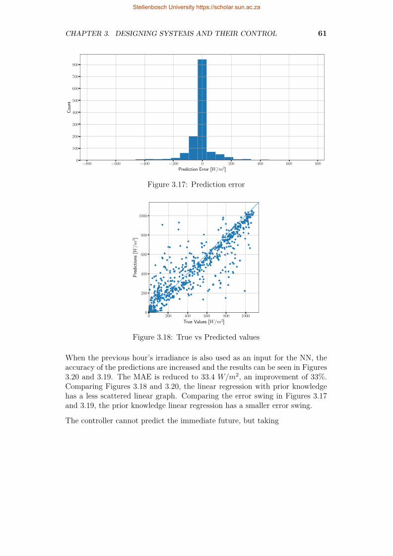
CHAPTER 3. DESIGNING SYSTEMS AND THEIR CONTROL 61
−800 −600 −400 −200 0 200 400 600 800
Prediction Error [W/m2]
0
100
200
300
400
500
600
700
800C
ount
Figure 3.17: Prediction error
0 200 400 600 800 1000
True Values [W/m2]
0
200
400
600
800
1000
Pre
dict
ions
[W/m
2]
Figure 3.18: True vs Predicted values
When the previous hour’s irradiance is also used as an input for the NN, theaccuracy of the predictions are increased and the results can be seen in Figures3.20 and 3.19. The MAE is reduced to 33.4 W/m2, an improvement of 33%.Comparing Figures 3.18 and 3.20, the linear regression with prior knowledgehas a less scattered linear graph. Comparing the error swing in Figures 3.17and 3.19, the prior knowledge linear regression has a smaller error swing.
The controller cannot predict the immediate future, but taking
Stellenbosch University https://scholar.sun.ac.za

CHAPTER 3. DESIGNING SYSTEMS AND THEIR CONTROL 62
−400 −200 0 200 400 600
Prediction Error [W/m2]
0
100
200
300
400
500
600
700
800
Cou
nt
Figure 3.19: Prediction error with prior knowledge
0 200 400 600 800 1000
True Values [W/m2]
0
200
400
600
800
1000
Pre
dict
ions
[W/m
2]
Figure 3.20: True vs Predicted values with prior knowledge
3.4.2 Reinforcement Learning with IoT ExperimentalDesign
3.4.2.1 Actions
The set of actions are identical to those discussed in Section 3.3.3.1.
3.4.2.2 States
The same states are applied as the RL-based controller, as discussed in Section3.3.3.2. Additional environmental information scraped from the yr.no websiteis fed into the NN. The information is scraped on the hour and used for theentire period and can be seen in Table 3.7. The weather predictions are nor-
Stellenbosch University https://scholar.sun.ac.za

CHAPTER 3. DESIGNING SYSTEMS AND THEIR CONTROL 63
Table 3.7: Attributes obtained from yr.no
Attribute UnitClouds %Low clouds %Medium clouds %High clouds %Temperature ◦CHumidity %
malised using the z-score. The clear sky insolation of the previous, currentand the next time step is also added to the states.
3.4.2.3 Neural Network Architecture
The hyperparameters are identical to that discussed in Section 3.3.3.4. Theoptimiser and loss function is also the same. The input layer has the originalstates, as well as the prediction information as given in Table 3.7. The addi-tional information did not increase the size of the NN. The input layer has 32neurons and is activated using ReLu. The two hidden layers have 32 neuronswith an activation function ReLu. The output layers are still the estimatedQ-values of different actions.
3.4.2.4 Rewards
The rewards are identical to that discussed in Section 3.3.3.3.
3.4.2.5 Memory
The memory size will also be identical to that discussed in 3.3.3.5.
3.4.3 EvaluationThe evaluation of the RL-based controller with IoT will be based on the sameevaluation as discussed in Section 3.3.4.
3.5 Baseline controllersTwo baseline controllers were used to assess the validity of the RL-based con-troller. The random action controller implemented random actions, whereasthe rule-based controller was based on predefined rules.
Stellenbosch University https://scholar.sun.ac.za

CHAPTER 3. DESIGNING SYSTEMS AND THEIR CONTROL 64
3.5.1 Random Action BaselineThe workings of a random-action-based control system can be seen in Algo-rithm 2. The action A is randomly selected and is then implemented for thatspecific period. The controller does not observe any of the environments anddirectly influences the next state.
Algorithm 2 Random Action Control SystemInput: {s, a} ∈ {S,A}
1: Loop for each episode2: Loop for each time step3: Choose A randomly4: Observe the immediate next state S ′5: S ← S ′
6: Until S is terminalOutput: LPS, Generator usage, PV usage, Battery usage, Grid usage and
rewards for each episode
3.5.2 Rule-based Action BaselineAlgorithm 3 shows the workings of the rule-based controller. An action array,as shown in (3.3.1), is generated based on rules. Each power source will receivea True or False setting for it to be used (or not used). These values then createan action array of T or F values, as explained in Section 3.3.3.1. The rules areas follows:
1. If PV is available: use PV,
2. If PV is greater than Load: charge batteries;
3. If PV is less than load: discharge batteries;
4. Randomly select the use of the grid;
5. Randomly select the use of the generator.
The controller observes only the immediate state, creates an action based onthe rules and that action influences the next state. The grid and generatoruse are randomised. Because the action array is sequentially formulated, ifthe grid was always selected, it influenced the use of the generator. The costoptimisation objective is to reduce generator and grid usage, but not to excludeany of them.
Stellenbosch University https://scholar.sun.ac.za

CHAPTER 3. DESIGNING SYSTEMS AND THEIR CONTROL 65
Algorithm 3 Rule-Based Action Control SystemInput: {s, a} ∈ {S,A}
1: Loop for each episode2: Loop for each time step3: Choose A based on rules4: Observe the immediate next state S ′5: S ← S ′
6: Until S is terminalOutput: LPS, Generator usage, PV usage, Battery usage, Grid usage and
rewards for each episode
3.6 ConclusionAn experimental design to test whether a GA is a viable design option foran HPS is presented. The algorithm assesses various aspects, being technical,financial and environmental, to optimally design an HPS. HOMER is used asa comparison tool to highlight the similarities and differences between the twodesign methods and will be discussed in Section 4.1 of Chapter 4.
A controller using a model-free Q-learning RL is designed to assess its validityas a control system. Additional information is extracted from yr.no to aid inpredicting PV power and this is incorporated in a separate RL-based controller.Two baselines are used to compare the results and will be discussed in Section4.2 of Chapter 4.
Stellenbosch University https://scholar.sun.ac.za

Chapter 4
Results
4.1 Design of a Hybrid Power SupplyThis section reviews the results of using a GA as a design tool for an HPS. Inthe previous chapter, the experimental design to implement this algorithm wasdiscussed and highlighted the mathematical models used, as well as any otherrelevant assumptions. The design attempts to optimise three main objectives:technical, financial and environmental. The technical objectives aim to reducethe loss of power supply, whereas the financial objectives are focused to providethe investor with the maximum theoretical ROI. The environmental objectivesaim to reduce the use of the generator and to maximise the use of the RES. TheGA was modelled using Python 3 and the programming code can be viewedin Section C.1 of Appendix C. The load and weather profile was simulatedin HOMER and the results will also be discussed below. The assumptions forHOMER was discussed in the previous chapter and were tried to be as similarto the GA’s assumptions as possible. A discussion between the two designtools is presented to highlight the similarities and differences between them.
4.1.1 Genetic Algorithm4.1.1.1 Configurations
The top configuration results are shown in Table 4.1 and the components canbe viewed in Table 4.2. The different configurations are Solar-Grid (SG), Solar-Grid-Battery (SGB), Solar-Grid-Generator (SGG) and Solar-Grid-Battery-Generator (SGBG). The LPSP and LPSP critical refers to (3.1.9). The capitalcost refers to the initial input cost to the investor and the ROI refers to the an-nual return on investment for the investor. The PV utilisation and Generatorutilisation refers to (3.1.14) and (3.1.15) respectively.
The SGBG has the greatest solar power utilisation, which accounts for theshifting of solar power to the load and back-up storage for the HPS. For the
66
Stellenbosch University https://scholar.sun.ac.za
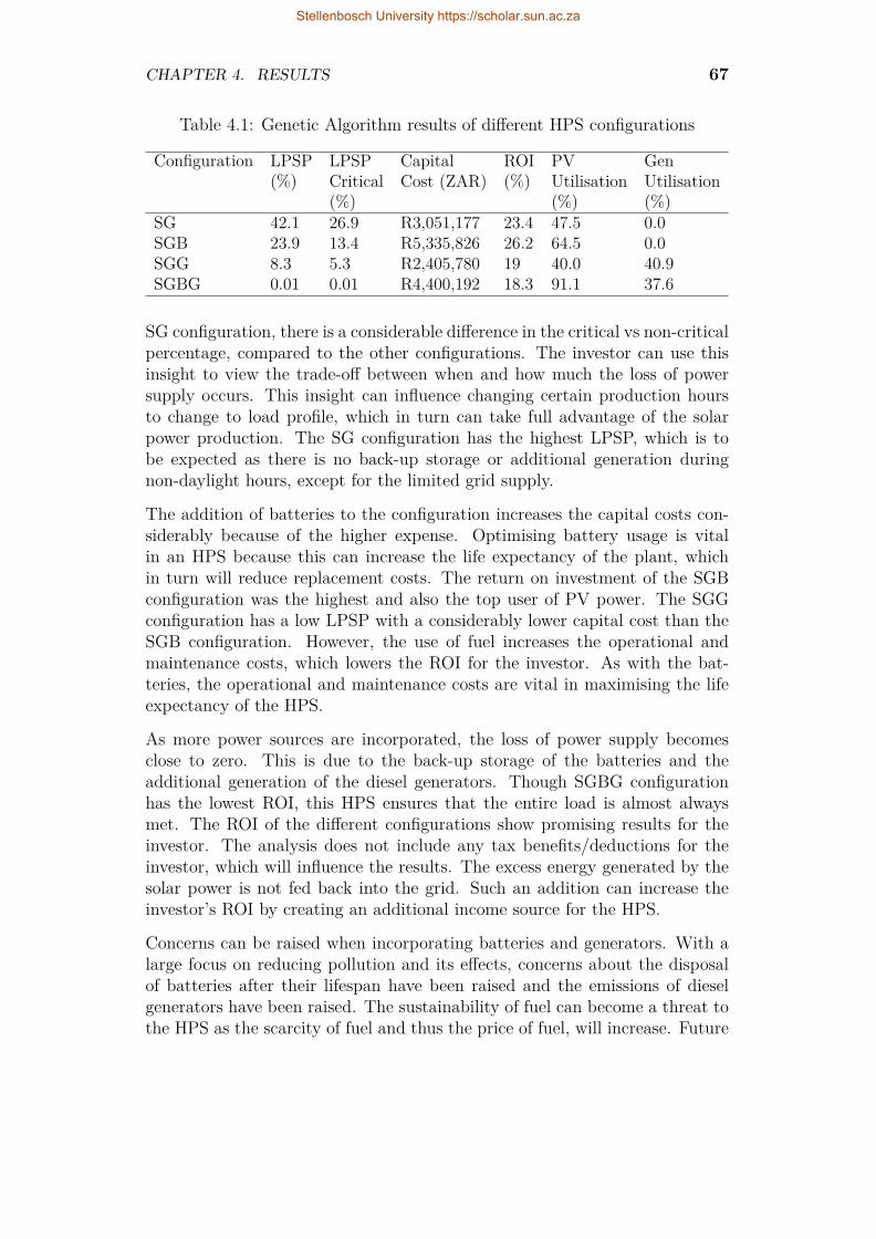
CHAPTER 4. RESULTS 67
Table 4.1: Genetic Algorithm results of different HPS configurations
Configuration LPSP LPSP Capital ROI PV Gen(%) Critical Cost (ZAR) (%) Utilisation Utilisation
(%) (%) (%)SG 42.1 26.9 R3,051,177 23.4 47.5 0.0SGB 23.9 13.4 R5,335,826 26.2 64.5 0.0SGG 8.3 5.3 R2,405,780 19 40.0 40.9SGBG 0.01 0.01 R4,400,192 18.3 91.1 37.6
SG configuration, there is a considerable difference in the critical vs non-criticalpercentage, compared to the other configurations. The investor can use thisinsight to view the trade-off between when and how much the loss of powersupply occurs. This insight can influence changing certain production hoursto change to load profile, which in turn can take full advantage of the solarpower production. The SG configuration has the highest LPSP, which is tobe expected as there is no back-up storage or additional generation duringnon-daylight hours, except for the limited grid supply.
The addition of batteries to the configuration increases the capital costs con-siderably because of the higher expense. Optimising battery usage is vitalin an HPS because this can increase the life expectancy of the plant, whichin turn will reduce replacement costs. The return on investment of the SGBconfiguration was the highest and also the top user of PV power. The SGGconfiguration has a low LPSP with a considerably lower capital cost than theSGB configuration. However, the use of fuel increases the operational andmaintenance costs, which lowers the ROI for the investor. As with the bat-teries, the operational and maintenance costs are vital in maximising the lifeexpectancy of the HPS.
As more power sources are incorporated, the loss of power supply becomesclose to zero. This is due to the back-up storage of the batteries and theadditional generation of the diesel generators. Though SGBG configurationhas the lowest ROI, this HPS ensures that the entire load is almost alwaysmet. The ROI of the different configurations show promising results for theinvestor. The analysis does not include any tax benefits/deductions for theinvestor, which will influence the results. The excess energy generated by thesolar power is not fed back into the grid. Such an addition can increase theinvestor’s ROI by creating an additional income source for the HPS.
Concerns can be raised when incorporating batteries and generators. With alarge focus on reducing pollution and its effects, concerns about the disposalof batteries after their lifespan have been raised and the emissions of dieselgenerators have been raised. The sustainability of fuel can become a threat tothe HPS as the scarcity of fuel and thus the price of fuel, will increase. Future
Stellenbosch University https://scholar.sun.ac.za

CHAPTER 4. RESULTS 68
Table 4.2: Genetic Algorithm results of components in different HPS configu-rations
Configuration Name QTY PowerSG Canadian Solar 395W 551 217.6 kW Peak
Sunny Tripower 15000TL 29SGB Canadian Solar 395W 684 270.2 kW Peak
Sunny Tripower 25000TL 36OmniPower 240Ah 12V 190 Storage 127.6 kWh
SGG Canadian Solar 395W 323 127.6 kW PeakSunny Tripower 20000TL 19MAC AFRIC 34 kVA 3 102.0 kVA
SGBG Canadian Solar 365W 312 113.9 kW PeakSunny Tripower 25000TL 26MAC AFRIC 50 kVA 3 150.0 kVAOmniPower 180Ah 12V 190 Storage 410.4 kWh
carbon tax laws may also be implemented, which further increases uncertaintyover the lifetime feasibility of the HPS. The components for the different HPSconfigurations are shown in Table 4.2. As the technology of PV-modules,generators, inverters and batteries increases, the systematic replacements ofthese components will improve with better performing power generation andgreater efficiencies. The O&M of the HPS is vital in ensuring the maximumuse and profitability of the plant.
4.1.1.2 Loss of Power Supply
The load and weather profile of the farm in the Stellenbosch area is brieflyanalysed and discussed in Sections 3.1.1.1 and 3.1.1.2 respectively. The analy-sis showed a higher load at the beginning of the calendar year. The climate ofthe specified location has a higher PV yield at the beginning of the year and atthe end of the year, where a lower yield is expected during the winter monthsof April to August. The load profile has a spike at the beginning of the monthand the average hourly usage peaks from 09:00 to 16:00. The hourly LPS ofthe different SG, SGB and SGG configurations can be seen in Figures 4.1, 4.2,4.3 and 4.4.
Considering the SG’s LPSP of 42.1% and Figure 4.1, it is clear that LPSoccurs often. There are also clear spikes which correlate to the higher spikein the load profile. The battery storage reduces the LPS considerably and thehigher spikes are attributed to the change in load profile at the beginning ofthe month, as seen in Figure 4.2.
Stellenbosch University https://scholar.sun.ac.za

CHAPTER 4. RESULTS 69
0 2000 4000 6000 8000
Hours [h]
0
20
40
60
80
100
Los
sof
Pow
erS
uppl
y[k
Wh]
Figure 4.1: Hourly loss of power supply from SG configuration over 1 year
0 2000 4000 6000 8000
Hours [h]
0
20
40
60
80
100
Los
sof
Pow
erS
uppl
y[k
Wh]
Figure 4.2: Hourly loss of power supply from SGB configuration over 1 year
0 2000 4000 6000 8000
Hours [h]
0
10
20
30
40
Los
sof
Pow
erS
uppl
y[k
Wh]
Figure 4.3: Hourly loss of power supply from SGG configuration over 1 year
Stellenbosch University https://scholar.sun.ac.za
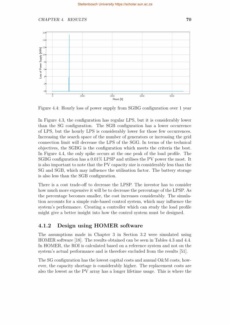
CHAPTER 4. RESULTS 70
0 2000 4000 6000 8000
Hours [h]
0
2
4
6
8
10
12
14
16
Los
sof
Pow
erS
uppl
y[k
Wh]
Figure 4.4: Hourly loss of power supply from SGBG configuration over 1 year
In Figure 4.3, the configuration has regular LPS, but it is considerably lowerthan the SG configuration. The SGB configuration has a lower occurrenceof LPS, but the hourly LPS is considerably lower for those few occurrences.Increasing the search space of the number of generators or increasing the gridconnection limit will decrease the LPS of the SGG. In terms of the technicalobjectives, the SGBG is the configuration which meets the criteria the best.In Figure 4.4, the only spike occurs at the one peak of the load profile. TheSGBG configuration has a 0.01% LPSP and utilises the PV power the most. Itis also important to note that the PV capacity size is considerably less than theSG and SGB, which may influence the utilisation factor. The battery storageis also less than the SGB configuration.
There is a cost trade-off to decrease the LPSP. The investor has to considerhow much more expensive it will be to decrease the percentage of the LPSP. Asthe percentage becomes smaller, the cost increases considerably. The simula-tion accounts for a simple rule-based control system, which may influence thesystem’s performance. Creating a controller which can study the load profilemight give a better insight into how the control system must be designed.
4.1.2 Design using HOMER softwareThe assumptions made in Chapter 3 in Section 3.2 were simulated usingHOMER software [18]. The results obtained can be seen in Tables 4.3 and 4.4.In HOMER, the ROI is calculated based on a reference system and not on thesystem’s actual performance and is therefore excluded from the results [51].
The SG configuration has the lowest capital costs and annual O&M costs, how-ever, the capacity shortage is considerably higher. The replacement costs arealso the lowest as the PV array has a longer lifetime usage. This is where the
Stellenbosch University https://scholar.sun.ac.za
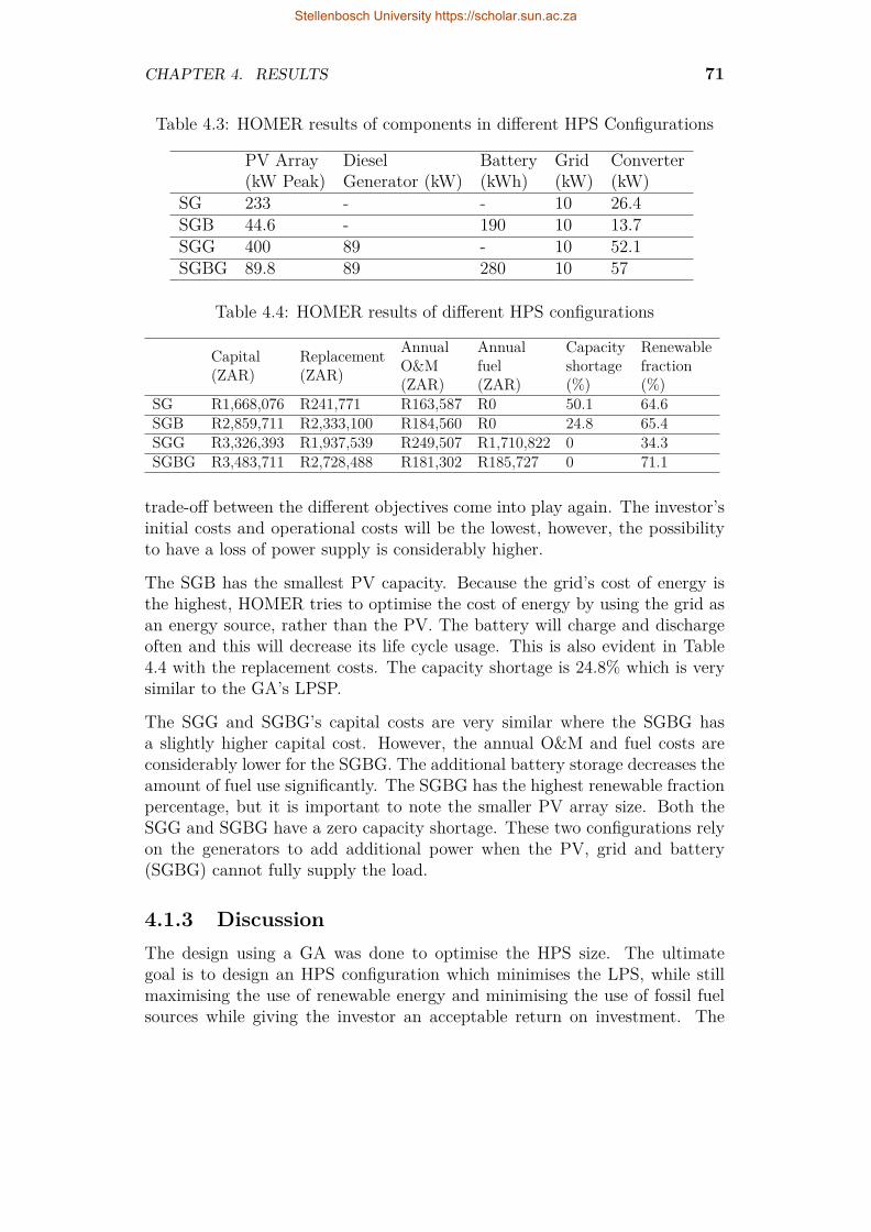
CHAPTER 4. RESULTS 71
Table 4.3: HOMER results of components in different HPS Configurations
PV Array Diesel Battery Grid Converter(kW Peak) Generator (kW) (kWh) (kW) (kW)
SG 233 - - 10 26.4SGB 44.6 - 190 10 13.7SGG 400 89 - 10 52.1SGBG 89.8 89 280 10 57
Table 4.4: HOMER results of different HPS configurations
Capital(ZAR)
Replacement(ZAR)
AnnualO&M(ZAR)
Annualfuel(ZAR)
Capacityshortage(%)
Renewablefraction(%)
SG R1,668,076 R241,771 R163,587 R0 50.1 64.6SGB R2,859,711 R2,333,100 R184,560 R0 24.8 65.4SGG R3,326,393 R1,937,539 R249,507 R1,710,822 0 34.3SGBG R3,483,711 R2,728,488 R181,302 R185,727 0 71.1
trade-off between the different objectives come into play again. The investor’sinitial costs and operational costs will be the lowest, however, the possibilityto have a loss of power supply is considerably higher.
The SGB has the smallest PV capacity. Because the grid’s cost of energy isthe highest, HOMER tries to optimise the cost of energy by using the grid asan energy source, rather than the PV. The battery will charge and dischargeoften and this will decrease its life cycle usage. This is also evident in Table4.4 with the replacement costs. The capacity shortage is 24.8% which is verysimilar to the GA’s LPSP.
The SGG and SGBG’s capital costs are very similar where the SGBG hasa slightly higher capital cost. However, the annual O&M and fuel costs areconsiderably lower for the SGBG. The additional battery storage decreases theamount of fuel use significantly. The SGBG has the highest renewable fractionpercentage, but it is important to note the smaller PV array size. Both theSGG and SGBG have a zero capacity shortage. These two configurations relyon the generators to add additional power when the PV, grid and battery(SGBG) cannot fully supply the load.
4.1.3 DiscussionThe design using a GA was done to optimise the HPS size. The ultimategoal is to design an HPS configuration which minimises the LPS, while stillmaximising the use of renewable energy and minimising the use of fossil fuelsources while giving the investor an acceptable return on investment. The
Stellenbosch University https://scholar.sun.ac.za

CHAPTER 4. RESULTS 72
addition of more power sources reduced the loss of power supply as the differentadvantages of the power sources are exploited. The weaknesses of one powersource are replaced with the strength of another, as seen in the SGB, SGGand SGBG configurations.
Comparing the results of HOMER and the GA, the HOMER SGG configu-ration had a lower capital cost, whereas the GA’s SG, SGB and SGBG hadhigher capital costs. Though the capital costs are lower than the GA’s, the re-liance on fuel is also considerably more. The equipment is replaced more oftenbecause of the overuse of components. The GA, because it can be modified,assesses each battery and generator individually and replaces it according toits usage. The capacity shortage of the two generator configurations is zerobecause they rely heavily on fuel to supply the load, which is not the objectiveof the design process.
HOMER software cannot override certain objective goals, whereas the GAcan, by looking at configurations which has more renewable energy usage andless generator usage. HOMER does not specify how many components arerequired, but rather a value. HOMER thus does not assess individual com-ponents, but rather the overall capacity of the power source. The GA alsoconsiders multiple type of components, based not only on the power ratingsbut also its financial indicators. As an example, a PV module with a highercost, but a longer warranty may be considered by the GA as a more viablecomponent, compared to one with a lower cost, but a considerably shorterwarranty.
There is a difference in the component sizing between the GA and HOMER,which influences the financial aspects of the two designs. However, the GA isconstrained to look for options which use fossil fuel-based options as a last re-sort, rather than the cheapest option. In addition, an HPS which relies heavilyon diesel generators runs the risk of being subjected to future carbon tax laws,as well as possible oil shortages or escalating fuel prices. The different controlsystems implemented in the GA and HOMER may also have an influence onthe feasibility of the HPS.
4.2 Control of a Hybrid Power SupplyIn the previous chapter, the control of an HPS using RL is discussed. The RL-based controller has no prior knowledge of the system and formulates policiesthrough observation of the environment and trial-and-error search. The agentis given rewards and penalties after it executes an action and uses the Q-learning method in order to maximise the future rewards it can acquire. Thecontrol system had a different load profile than the GA and thus a sizing ofthe HPS was done using the GA. The configuration of the HPS consists of PV-
Stellenbosch University https://scholar.sun.ac.za

CHAPTER 4. RESULTS 73
modules, battery storage, a back-up generator and a limited grid connection.Two baselines are used to compare the results of the RL-based controller toassess the performance of the RL-controller.
The RL controller has two objectives: to minimise the loss of power supply andto optimise the cost of the HPS. The cost optimisation aims to reduce the use offuel and grid connection which the investor has to fund throughout the courseof the year, whereas the energy exchange between the PV and battery storagehas a large capital cost, but lower operational costs. An IoT-implementationis also done by adding the weather predictions as additional information forthe RL-based controller. These results are compared to the two baselines andthe RL-only controller.
4.2.1 Sizing of HPSThe design for the HPS was done using a modified GA which only attributedthe technical aspects for 1 year in terms of LPSP. The grid is specified as 1.2kWh maximum usage per hour with a 100% reliability. The PV capacity issized as 10.6 kW peak, the battery storage as 49 kWh with a DOD of 50% andhas a 5 kW generator.
4.2.2 Reinforcement Learning-based ControllerThe training set is used to train the NN, whereas the validation set is the firsttest of the model. The validation set is used to find suitable NN architectureand optimise the hyper-parameters.
Figure 4.5 shows how the RL agent tries to maximise the total reward. In eachepisode, the weights of the NN is adjusted and retrained to find the maximumQ-value for each action in the state. The model converges, but slight deviationscan be noted. Figure 4.6 shows how the agent tries to minimise the total LPSper episode. The LPS converges to a minimum, which indicates that the agenthas started to exploit its previously obtained knowledge. The LPS convergesto a minimum and slight deviations can be noted in the figure. In Figure 4.7,the utilisation of the different power sources are highlighted. The PV andbattery are considerably higher than the generator and grid, indicating thatthe agent has learned to utilise the RES and the shift of energy to the storagesystem.
Equation (2.5.5) in Chapter 2 shows the expected return starting from states. A discount factor closer to one is more long-term biased, whereas closer tozero is a shorter-term bias. A higher discount parameter significantly favouredthe generator and grid usage rather than the PV and battery energy exchange.This is because the highest reward given for a zero LPS. For the long term,the agent could obtain the most rewards by utilising these consistent power
Stellenbosch University https://scholar.sun.ac.za

CHAPTER 4. RESULTS 74
0 10 20 30 40 50Episodes
760000
765000
770000
775000
780000
785000
790000
795000
Tot
alre
war
dsob
tain
edp
erep
isod
edu
ring
trai
ning
Figure 4.5: Training rewards per episode
0 10 20 30 40 50Episodes
30
40
50
60
70
80
90
Tot
alL
PS
[kW
h]p
erep
isod
edu
ring
trai
ning
Figure 4.6: Training LPS per episode
sources, such as the grid and generator and this can be observed in Figure4.8. Initially, the agent explores to find an optimal solution to receive themaximum rewards. The higher generator and grid will result in a long-termno LPS, which gives a much greater future discounted reward and this isexploited clearly in the figure. The agent thus does not struggle to find anoptimal solution, because it is heavily dependent on the generator and thegrid and does not use the battery to increase the use of the RES. The modelminimises the LPS easily. However, the controller relies considerably more onthe generator and grid than on the available PV and is seen as cost-ineffective.When Figures 4.7 and 4.8 are compared, the convergence of the higher discountis considerably less than the lower discount factor. The small deviations inFigure 4.7 is an indication that the agent had some difficulty in finding anoptimal solution for the HPS.
Stellenbosch University https://scholar.sun.ac.za

CHAPTER 4. RESULTS 75
0 10 20 30 40 50Episodes
0
1000
2000
3000
4000
5000T
otal
Pow
er[k
Wh]
per
epis
ode
duri
ngtr
aini
ng
PV
Battery
Generator
Grid
Figure 4.7: Training power source usage per episode
0 10 20 30 40 50Episodes
0
1000
2000
3000
4000
Tot
alP
ower
[kW
h]p
erep
isod
edu
ring
trai
ning
PV
Battery
Generator
Grid
Figure 4.8: Training power source usage per episode with γ=0.995
After training the model using the training set, the model is validated. Thevalidation process constantly iterates over different NN architectures and hy-perparameters to find the best-suited model. The most appropriate model’svalidation results is shown in Table 4.5. The RL-based controller obtained thehighest rewards. The rule-based controller has a significantly lower LPS andhigher PV usage. The rewards of the rule-based controller is lower, yet theLPS is better than the RL-controller. The RL-based controller learns to usethe generator efficiently at night, when the available PV is zero. The rule-based controller does not optimise for this and therefore the RL-controller hasa higher reward value. The validation results show that the RL-controller haseffectively learned how to control the system from without any prior knowl-edge of the system, but is not more efficient and optimised with regards tocosts. A higher discount factor will utilise the generator and grid more, which
Stellenbosch University https://scholar.sun.ac.za

CHAPTER 4. RESULTS 76
Table 4.5: Validation Baseline Comparison of Control System: RL
LPS Battery PV Generator Grid BatteryRewards [kWh] Usage Usage Usage Usage Charged
[kWh] [kWh] [kWh] [kWh] [kWh]Random 100231 240.0 300 489.9 176.8 284.9 300.3Rule 126975 13.1 524.6 1088.5 10.14 77.2 522.0RL 134807 58.3 477.9 907 38.4 184.3 474.4
can then reduce the LPS of the system, but not optimise the use of the RES.The trade-off between having lower LPS results in a suboptimal cost. Previousmodels did show a considerably greater reduction in LPS, but the use of thegenerator and grid was significantly higher.
The total load for the validation set is 1191.6 kWh. Energy balance equationof the system is given by
Load + Batterycharge+losses ≈ Batdischarge+ PV + Gen + Grid + LPS (4.2.1)
where the left and right-hand side of the equation should be approximately thesame. Small differences in (4.2.1) can occur as a result of rounding-off errors.
When ε is large, i.e. close to 1, the actions are randomised. The RL-basedcontroller thus starts off as a random controller. As the agent learns theenvironment through exploration, it starts to observe how the state-actionspace interacts. The RL-based controller improves over the episodes. Thecomparison between the random and RL-based controller highlights how theRL agent has learned and improved its policies through reinforcement. TheRL controller has a lower generator usage, which would result in lower fuelcosts. The grid is higher, but the grid’s cost of energy is still cheaper thanthe generator. The PV and battery usage are also higher than the randomcontroller, which indicates that the agent has learned to use the RES andexchange the energy to the battery storage.
The training set and validation set are the basis of how the model is deter-mined. The test set is a completely ‘new’ dataset that the NN has never seenbefore. In this way, a more accurate representation of how well the model ac-tually performs can be obtained. The results are shown in Table 4.6. The RL’srewards are higher than the rule-based, whereas the validation it was slightlyhigher. The rule-based controller outperformed the RL-based and random ac-tion controller with an overall reduced LPS and higher RES utilisation. TheRL control system was able to effectively exchange the energy between thebattery, load and other power sources. The RL-controller was optimised forminimising the LPS, as well as maximising the cost optimisation. The RL-based controller shows promising results and further research can increase theeffectiveness of the controller.
Stellenbosch University https://scholar.sun.ac.za

CHAPTER 4. RESULTS 77
Table 4.6: Test Baseline Comparison of Control System: RL
LPS Battery PV Generator Grid BatteryRewards [kWh] Usage Usage Usage Usage Charged
[kWh] [kWh] [kWh] [kWh] [kWh]Random 109158 253.9 305.8 539.7 190.3 330.5 305.2Rule 140337 12.1 577.1 1203.5 10.7 82.5 571.1RL 150130 54.6 524 1001.6 54.5 197.8 517.7
4.2.3 Reinforcement Learning-based and IoTController
Seven months (1 March 2019 to 30 September 2019) were used for the RL andIoT-based controller. The database allowed for the largest consecutive hourlyscraped data to be used for analysis. The weather may be an influence as themonths are usually more overcast as the weather transitions from autumn towinter and then the start of spring. It should be noted that the dataset for theRL-IoT controller is considerably smaller and thus over-fitting may occur. TheRL-only controller is also added to see if the additional weather predictionsimproved the controller.
Table 4.7 shows the validation of the model, which showed that the rewardsfor the RL and IoT controller was the highest. The RL-only model was alsoused as part of the results. This is to analyse whether the IoT-information wasused by the NN. The RL with IoT control system had a higher reward andlower LPS than the RL-only controller, as well as the highest PV usage. Theresults showed that the rule-based controller had the lowest LPS. The LPSis decreased by 10.6 kWh (20.7%) and the PV usage is increased by 31 kWh(6.93%) from the RL to the RL-IoT application.
Table 4.8 shows the test results of the two baselines, the RL-based controllerand the RL-IoT-based controller. The results between the RL and RL-IoTshowed that the IoT-application reduced the LPS by 8.5 kWh (12.7%) andincreased the PV usage by 36.6 kWh (7%). This shows that the RL-agentbenefited from using the IoT-information.
Table 4.7: Validation Baseline Comparison of Control System: RL and IoT
LPS Battery PV Generator Grid BatteryRewards [kWh] Usage Usage Usage Usage Charged
[kWh] [kWh] [kWh] [kWh] [kWh]Random 56912 134.5 152.3 256.1 80.4 170.4 152.3Rule 74042 7.42 294.4 284.1 7.1 40.1 291.8RL 75965 51.2 249.5 447.1 34.2 106.0 246.6RL and IoT 76326 40.6 265.8 478.1 32.0 87.9 263.0
Stellenbosch University https://scholar.sun.ac.za
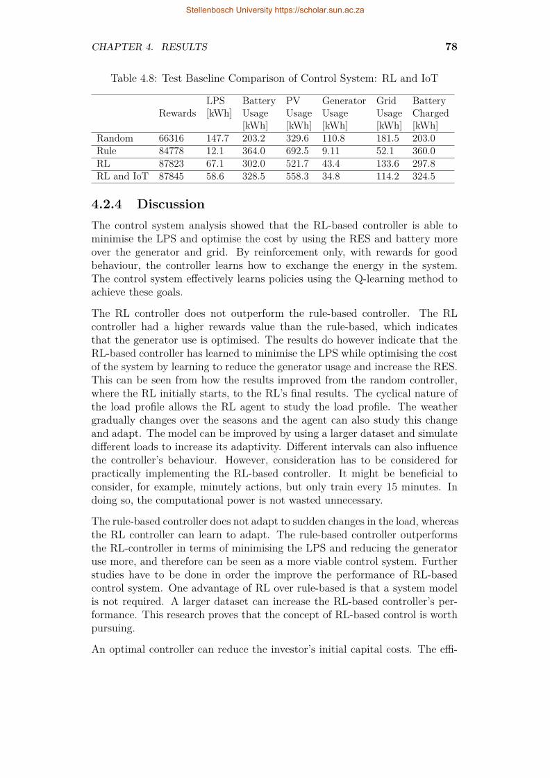
CHAPTER 4. RESULTS 78
Table 4.8: Test Baseline Comparison of Control System: RL and IoT
LPS Battery PV Generator Grid BatteryRewards [kWh] Usage Usage Usage Usage Charged
[kWh] [kWh] [kWh] [kWh] [kWh]Random 66316 147.7 203.2 329.6 110.8 181.5 203.0Rule 84778 12.1 364.0 692.5 9.11 52.1 360.0RL 87823 67.1 302.0 521.7 43.4 133.6 297.8RL and IoT 87845 58.6 328.5 558.3 34.8 114.2 324.5
4.2.4 DiscussionThe control system analysis showed that the RL-based controller is able tominimise the LPS and optimise the cost by using the RES and battery moreover the generator and grid. By reinforcement only, with rewards for goodbehaviour, the controller learns how to exchange the energy in the system.The control system effectively learns policies using the Q-learning method toachieve these goals.
The RL controller does not outperform the rule-based controller. The RLcontroller had a higher rewards value than the rule-based, which indicatesthat the generator use is optimised. The results do however indicate that theRL-based controller has learned to minimise the LPS while optimising the costof the system by learning to reduce the generator usage and increase the RES.This can be seen from how the results improved from the random controller,where the RL initially starts, to the RL’s final results. The cyclical nature ofthe load profile allows the RL agent to study the load profile. The weathergradually changes over the seasons and the agent can also study this changeand adapt. The model can be improved by using a larger dataset and simulatedifferent loads to increase its adaptivity. Different intervals can also influencethe controller’s behaviour. However, consideration has to be considered forpractically implementing the RL-based controller. It might be beneficial toconsider, for example, minutely actions, but only train every 15 minutes. Indoing so, the computational power is not wasted unnecessary.
The rule-based controller does not adapt to sudden changes in the load, whereasthe RL controller can learn to adapt. The rule-based controller outperformsthe RL-controller in terms of minimising the LPS and reducing the generatoruse more, and therefore can be seen as a more viable control system. Furtherstudies have to be done in order the improve the performance of RL-basedcontrol system. One advantage of RL over rule-based is that a system modelis not required. A larger dataset can increase the RL-based controller’s per-formance. This research proves that the concept of RL-based control is worthpursuing.
An optimal controller can reduce the investor’s initial capital costs. The effi-
Stellenbosch University https://scholar.sun.ac.za

CHAPTER 4. RESULTS 79
ciency and effectiveness of the controller can increase the utilisation of powersources and this can reduce overall costs. The design of an HPS can be doneand then further optimised with a RL controller. The optimised controllercan reduce the size of the HPS required to satisfy the load. The design isthen reiterated to take into account the controller’s efficiency to reduce overallcapital costs and increase the ROI of the investor.
Incorporating the weather predictions from the yr.no website increased thePV utilisation. This is an indication that the predicted weather input gavethe agent additional information to use to form its policies. This additionincreased the use of the RES, which can reduce the operational costs of thegenerator and grid.
Stellenbosch University https://scholar.sun.ac.za

Chapter 5
Conclusions andRecommendations
The combination of power sources, especially when intermittent and stochas-tic resources such as RESs are included, presents a non-linear optimisationproblem in designing an HPS. Different performance indicators start to tradeoff against one another and a compromise between different aspects have tobe determined. A GA was implemented to solve this problem. This designalgorithm was utilised as a tool to aid the investor’s decision-making process.The different attributes of the HPS configurations are considered and high-lighted to indicate how the investor should consider an optimal HPS design.The results of the GA is compared to commercially available software HOMERto assess its validity as a design method.
As the combination of power sources increases, the complexity of the energyexchange in the system also increases. A model-free Q-learning controller isincorporated to increase the system’s effectiveness and efficiency. The con-troller’s objectives are to minimise the loss of power supply while optimisingthe cost of the HPS. To further increase the capabilities of the RL-controller,an IoT-approach is also considered by including the weather predictions fromthe Norwegian website yr.no.
In chapter 1, the background of HPSs are given to provide the reader insightinto advantages and the problems associated with the design and control ofan HPS. This analysis gave insight into creating clear research goals and ob-jectives. Chapter 2 gives the relevant theory and relevant work for the readerin how the research methodology aims achieve these objectives set about inChapter 1. The experimental design is critically discussed in Chapter 3 whichgives a practical guide to how the research objectives can be realised. The ex-perimental design produced results which is analysed in Chapter 4. This gaveinsight into conclusions which can be drawn from the results and to providerecommendations for future work.
80
Stellenbosch University https://scholar.sun.ac.za

CHAPTER 5. CONCLUSIONS AND RECOMMENDATIONS 81
5.1 Conclusions
5.1.1 Comparison of Genetic Algorithm and HOMERSoftware
A GA was used as a possible design solution for an HPS. Using a case study,the results showed that a GA is a feasible method to design an HPS. A trade-off of various attributes was done to highlight the differences between variousHPS configurations. Four HPS configurations were analysed and a trade-offanalysis of the these attributes was discussed. The attributes include the tech-nical, financial and environmental objectives such as the loss of power supplyprobability, return on investment, PV and generator utilisation. Projectionsbased on the one-year analysis of the HPS was done to assess the feasibilityof the system throughout its lifetime and is taken into account by the algo-rithm. The algorithm does not only consider a short-term analysis, but alsothe long term potential of an HPS configuration. The algorithm considers adiverse set of component types to assess the most suitable configuration andcomponent capacity. This is also included in the analysis to give insight intothe short-term and long-term feasibility of the system.
In a separate design, the software package HOMER was used as a designtool. HOMER is considered an industry standard for the design of integratedpower systems. The GA generates more diverse results with regards to thecomponent types and sizes, whereas HOMER only gives the overall size andone type of power source. The trade-off between the two design methods isthat the GA has to be built, which may be time-consuming, compared to thereadily available commercial software. However, the GA can be modified touser specifics, such as specifying control constraints and fill in missing data.
It is interesting to note how the addition of a diesel generator with back-up bat-tery storage considerably increases the capacity factor and reduced the LPSPof the system. This is how the HPS can be of vital importance in ensuringfuture sustainable energy production. Instead of completely eliminating anyforms of fossil fuel, incorporating RESs can significantly decrease the depen-dency on these fossil fuels. The end goal is to generate enough power to satisfythe load, but not at the cost of having no power. The generator is used as aback-up when the storage is depleted and/or when no solar power is available.The exploitation of these advantages of HPSs can have a significant positiveimpact on areas with no access to power.
Both the GA and HOMER methods showed that more power sources resultedin a lower capacity shortage. This is concurrent with how the weakness of onepower source is replaced with another. The SGBG configuration had batterystorage to store excess generated PV power, as well as increasing the loadfactor for the generator to run more fuel-efficient, according to the fuel curve.
Stellenbosch University https://scholar.sun.ac.za

CHAPTER 5. CONCLUSIONS AND RECOMMENDATIONS 82
The diesel generator could also account for large load peaks during the year.Instead of running a generator the entire year, the main use of power would bethe PV modules, battery storage and grid and the generator would offset thepeak loads. This leads to a more environmentally friendly HPS, compared toone which uses only generators, by reducing carbon emissions. The GA alsoconsiders the LPSP during critical and non-critical hours of the day, whichmay influence the investor’s decision. The configurations of the GA are morediverse, viable and robust and therefore can be seen as a more accurate andfaster design approach than HOMER.
5.1.2 Reinforcement Learning-based Control SystemA model-free Q-learning reinforcement learning control system for an HPS wasdone. A case study using a load profile and a weather profile indicated thatthe RL-based controller did not outperform the rule-based controller, but didoutperform the random action controller. The random action controller is thestarting point for the RL-based controller in the initial stages of exploration.As the RL agent learns through rewards and penalties, it starts to formulatepolicies for state-action pairs. The agent attempts to maximise the possiblefuture discounted rewards. This method is known as Q-learning. The Q refersto the ‘quality’ of the action. An action with a higher Q-value in a specificstate will be more likely to be executed in the control system. The agentlearns with no prior knowledge of the system and adapts its policies to findan optimal control solution. The RL-based controller was done using Keras inPython3.
Intervals of different control actions were chosen as 15 minutes to increase thetraining efficiency of the NN. The RL-based controller has achieved its goalsof learning the system, minimising the LPS and optimising the cost by re-ducing expensive sources such as the generator and grid. The controller doesnot exclude these options as the LPS takes precedence over the cost optimisa-tion, but only after all other alternatives have been explored. The RL-basedcontroller had a higher reward value than the rule-based controller, which in-dicates that the use of the generator was optimised when the PV was zero. Interms of whether RL-based is better than the rule-based controller, remainsinconclusive and further studies have to be done to verify this. The RL-basedmethod has been proven as a feasible control method and the practical im-plementation would be able to give considerable insight into how the HPScontrol system can be improved using ML. The RL-controller can adapt au-tonomously, whereas the rule-based controller has to be manually adapted.The RL-controller can adjust as changes in the load profile and weather occur.Changes such as droughts or rain-heavier winters occur slowly over time andthe RL-controller can adapt accordingly. The rule-based controller has a pre-defined set of rules and thus cannot execute optimal actions in these unknown
Stellenbosch University https://scholar.sun.ac.za

CHAPTER 5. CONCLUSIONS AND RECOMMENDATIONS 83
and new environments.
Weather predictions were added to the controller to provide additional infor-mation with regards to future solar insolation. The weather predictions weretaken from the Norwegian weather prediction website, yr.no. The concept wasfirst proven using a simple linear regression to show that the solar irradiancecan be linearly calculated from the weather predictions. A database of scrapeddata had to be created as no such database is available. The results showed alinear relationship between the different input parameters obtained from theyr.no website and the actual solar irradiance.
These weather predictions were then added to an RL-controller in hoping toimprove the controller by increasing the use of the RES. The weather pre-dictions database constrained the size of usable data points and only sevenmonths of data were used as part of the analysis. The addition of the weatherinput showed an slight increase in PV usage, decrease in generator usage anda reduction in the LPS. The RL-IoT controller did not outperform the rule-based controller but has given valuable insight into how the IoT-industry canbe exploited to increase the effectiveness of control systems.
5.2 Recommendations
5.2.1 Design of a Hybrid Power SupplyA larger database of components, as well as more types, can be used to refinethe GA’s results. In doing so, more configuration possibilities can be exploredto find an optimal solution. Other system variables, such as the generator’sminimum running hours, PV-module tilt angle and the battery’s DOD, can beoptimised to further enhance the design of the HPS. Tracking PV-modules canalso increase the yield which can also reduce the costs of the system and thisimplementation can be considered as another insight in the same manner asthe LPSP critical is considered. The selling of excess generated energy can alsobe considered, which can influence the financial objectives of the algorithm.
The algorithm is completely reliant on the information it is fed, and thus theload and weather data has to come from a reliable source. Sensitivity analysismay give valuable insight into possible future scenarios, such as carbon taxlaws, escalation of fuel prices above inflation and improving system compo-nents. Other power configurations can be considered as part of the design.These power sources can include biomass, biogas and wind turbines and alter-native energy storage such as hydro- and ultra-capacitor storage.
Alternative design algorithms and software, as discussed in Chapter 2, can beused as a comparison tool to the GA. The control system used in the designprocess can be improved, which will give a more accurate representation of
Stellenbosch University https://scholar.sun.ac.za

CHAPTER 5. CONCLUSIONS AND RECOMMENDATIONS 84
how the HPS operates. An optimised control system may reduce the requiredcomponents, reduce costs and increase the ROI for the investor.
5.2.2 Control of a Hybrid Power SupplyThe RL agent’s performance is mostly dependent on the reinforcements it re-ceives. Different rewards and penalties can be further explored to reduce theLPS and increase the cost effectiveness of the controller. Greater hardwarecapabilities and computational power can give more insight into the perfor-mance of the controller by storing more information within the simulation. Theadditional information can be analysed to further improve the RL-controller.
Different network architectures can be implemented and the hyperparameterscan be further optimised. Long short-term memory (LSTM), a recurrent neu-ral network (RNN) architecture, can also be considered as a possible controlsystem mechanism. Other RL methods can be investigated. A more refinedreward system can significantly improve the quality of the RL-controller. Dif-ferent optimisation and activation functions can be considered to improve thedesign of the control system. Hardware constraints and the physical controlsystem is also important. Reinforcement learning, especially in the controlsystem sense, requires more CPU than GPU, which can become expensive.Thus there is always a trade-off between the ideal results and realistic results.A very simple model of the HPS was used in the rule-based control system.An accurate model of the HPS can be developed, which will result in a model-based control system. Other control methods can be investigated as part of acomparison for the RL control system.
The integration of an on-line HPS can be the next phase of RL-based applica-tions. There has to be some form of redundancy to allow the RL controller tomake mistakes, but not that it results in a complete LPS during the trainingon the controller. As much as possible training has to be done before theimplementation is done and the controller is gradually given more exercise tocontrol over the HPS. Thus a rule-based system can be initially implementedand as the controller starts to learn on its own, the RL-based controller isgiven more exercise to control the system. Because of the real-life implicationsthat can occur when an RL-based controller trains, such as a loss of powersupply, it is of vital importance that the implementation is done as smoothlyas possible. This will mitigate the ethical risks involved when using artificialintelligence as a control system.
When incorporating an IoT-based system, it makes sense to exploit systemswhich have already done the calculation work and use this information to im-prove other systems. However, a redundancy has to be ensured to be preparedfor power failures or network errors where the controller cannot contact theserver. To a certain extent, it should be able to function offline and online,
Stellenbosch University https://scholar.sun.ac.za

CHAPTER 5. CONCLUSIONS AND RECOMMENDATIONS 85
where the online IoT-based system improves the computational efficiency. Thisefficiency can be measured in terms of using less power to update the controlsystem after every time interval and to retrain the NN again. It seems unnec-essary to have a control system which will make near-perfect decisions, butuses most of the HPS’s energy just to train its neural network architecture.There will thus always be a trade-off when achieving perfection.
Loads tend to be cyclical to a certain extent, which makes RL a possiblecandidate to learn and control the energy exchange of an HPS. The householdload changes slowly as the seasons progress and the RL-based controller canslowly learn this as the agent explores the search space. However, loads withnon-cyclical aspects, such as electrical vehicles, where the road profile mightchange significantly, can have an impact on the system. A load profile which ismeasured with accurate weather predictions can provide more accurate results.Predictions further into the future, such as 1-3 hours, can add additional inputfor the agent to consider. This may improve the minimisation of the long-term LPS. The RL with IoT controller has a very small database and is notrepresentative of one year of seasonal fluctuations. This can be improved bycreating a larger database and simulating the results again. The data for thisthesis is not linked in terms of how they are measured. The load profile issimulated with the statistical background of the location’s weather profile, butnot the actual minute-by-minute measurements.
Stellenbosch University https://scholar.sun.ac.za

Appendices
86
Stellenbosch University https://scholar.sun.ac.za
Appendix A
Solar Irradiance Models
A.1 Clear sky modelPVLib is a Python library which can be used to model solar PV-modules [52].The Location object has a clear sky model. The Location object requires thelatitude, longitude, timezone and altitude. The co-ordinates for Stellenboschis specified as -33.9346◦ latitude, 18.8668◦ longitude and the altitude is 122meters above sea level. The timezone is specified as Johannesburg. The libraryhas a built-in function which can be called to calculate the clear sky model.The returned information is given as a Pandas data frame. Pandas is usefulan open-source software library for the manipulation and analysis of data [53].When the function is called, it returns the clear sky GHI, DNI and DHI valuesfor different times.
A.2 Irradiance calculationsPVLib also has an irradiance class which can calculate the total irradiance.The function returns the plane of array global, direct, diffuse, sky diffuse andground diffuse irradiance. Irradiance refers to the instantaneous measure ofpower and is measured in W/m2, whereas insolation is solar energy in kWh.
The function requires the surface tilt, surface azimuth-, solar zenith- and so-lar azimuth angle, as well as the albedo, model, DNI, GHI and DHI. Theseparameters will be discussed below. The isotropic model is used in these cal-culations.
Surface tilt angle The surface tilt Σ refers to the collector’s angle which itis tilted up. The tilt angle is fixed at 30◦.
Surface azimuth angle The surface azimuth is the angle measured fromdue north in the southern hemisphere. The collector is North-facing and thus
87
Stellenbosch University https://scholar.sun.ac.za

APPENDIX A. SOLAR IRRADIANCE MODELS 88
the surface azimuth angle φC is 0◦.
Solar zenith angle The solar zenith angle θS is the complement of the solaraltitude angle β and is calculated by (A.2.1):
cos θS = sinL sin δ + cosL cos δ cosH (A.2.1)
The function requires the latitude, hour angle and declination angle. The hourangle H is calculated using (A.2.2) and the declination angle δ is calculatedusing (A.2.5).
Hour angle H =(15◦h
)· (Hours before solar noon) (A.2.2)
The hours before solar noon is equated using the Equation of Time, expressedby (A.2.3).
E = 9.87 sin 2B − 7.53 cosB − 1.5 sinB (A.2.3)
B = 360364 (nday − 81) (A.2.4)
where nday refers to the number of day of the year. The solar declination angleis expressed as:
δ = 23.45( 2π
365 (nday + 284))
(A.2.5)
Solar azimuth angle Solar azimuth angle (φS) is expressed by (A.2.6).
sinφS = cos δ sinHsin θS
(A.2.6)
and if cosH ≥ tan δtanL then |θS| ≤ 90◦, otherwise |θS| > 90◦.
Incidence angle The incidence angle θ for a fixed orientation is given by(A.2.7).
cos θ = sin θS cos (φS − φC) sin Σ + cos θS cos Σ (A.2.7)
Albedo The ground’s albedo ρ refers to the reflectivity of the ground and isan estimated value. Snow, for example is 0.8 whereas gravel is 0.1 and grassis ordinarily 0.2.
Stellenbosch University https://scholar.sun.ac.za

APPENDIX A. SOLAR IRRADIANCE MODELS 89
Figure A.1: Solar irradiance components [45]
A.2.1 Irradiance calculationsFigure A.1 shows the different irradiance components, namely direct beam(IBC), diffuse (IDC) and reflected (IRC) irradiance, and the collector tilt angleΣ. These irradiance components are expressed by equations (A.2.8), (A.2.9)and (A.2.10).
IBC = DNI cos θ (A.2.8)
IDC = DHI(
1 + cos Σ2
)(A.2.9)
IRC = GHI · ρ(
1− cos Σ2
)(A.2.10)
The total irradiance is expressed by:
IC = IBC + IDC + IRC . (A.2.11)
The insolation can be calculated from the total irradiance using
IC = IC · Time (h). (A.2.12)
Stellenbosch University https://scholar.sun.ac.za

Appendix B
Data Input
B.1 Components DatabaseThe components for the genetic algorithm consists of PV modules, inverters,generators and batteries. These databases are summarised in Tables B.1, B.2,B.3 and B.4.
Table B.1: Design Database of Inverters
Name Price Max Input Input Warranty Reference(ZAR) Power Voltage Voltage (years)
(kW ) (V ) min (V ) maxSMA Sunny 55,053 15 240 800 3 [54]Tripower TL15000SMA Sunny 59,240 20 320 800 3 [55]Tripower TL20000SMA Sunny 61,166 25 320 800 3 [56]Tripower TL25000
Table B.2: Design Database of Batteries
Name Price Capacity Rated 60 DOD Reference(ZAR) (Ah) Voltage (V ) Life cycles
OmniPower 3,747 120 12 1800 [57]OmniPower 5,603 180 12 1800 [58]OmniPower 6,990 240 12 1800 [59]
90
Stellenbosch University https://scholar.sun.ac.za
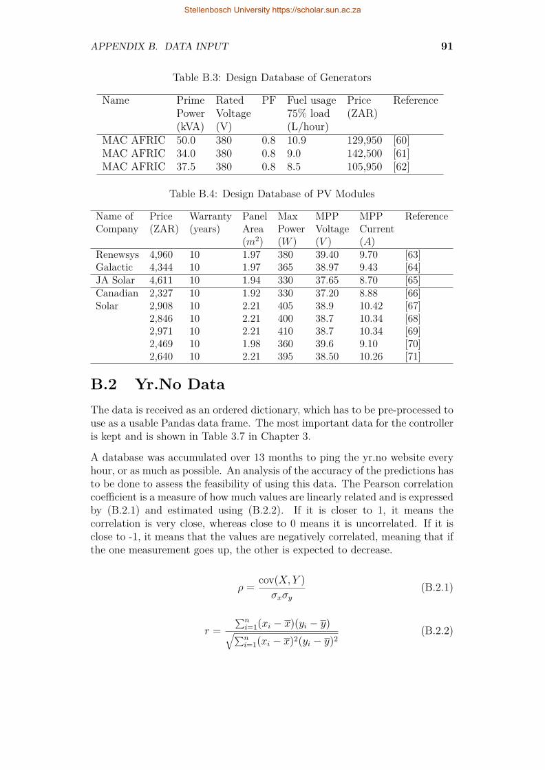
APPENDIX B. DATA INPUT 91
Table B.3: Design Database of Generators
Name Prime Rated PF Fuel usage Price ReferencePower Voltage 75% load (ZAR)(kVA) (V) (L/hour)
MAC AFRIC 50.0 380 0.8 10.9 129,950 [60]MAC AFRIC 34.0 380 0.8 9.0 142,500 [61]MAC AFRIC 37.5 380 0.8 8.5 105,950 [62]
Table B.4: Design Database of PV Modules
Name of Price Warranty Panel Max MPP MPP ReferenceCompany (ZAR) (years) Area Power Voltage Current
(m2) (W ) (V ) (A)Renewsys 4,960 10 1.97 380 39.40 9.70 [63]Galactic 4,344 10 1.97 365 38.97 9.43 [64]JA Solar 4,611 10 1.94 330 37.65 8.70 [65]Canadian 2,327 10 1.92 330 37.20 8.88 [66]Solar 2,908 10 2.21 405 38.9 10.42 [67]
2,846 10 2.21 400 38.7 10.34 [68]2,971 10 2.21 410 38.7 10.34 [69]2,469 10 1.98 360 39.6 9.10 [70]2,640 10 2.21 395 38.50 10.26 [71]
B.2 Yr.No DataThe data is received as an ordered dictionary, which has to be pre-processed touse as a usable Pandas data frame. The most important data for the controlleris kept and is shown in Table 3.7 in Chapter 3.
A database was accumulated over 13 months to ping the yr.no website everyhour, or as much as possible. An analysis of the accuracy of the predictions hasto be done to assess the feasibility of using this data. The Pearson correlationcoefficient is a measure of how much values are linearly related and is expressedby (B.2.1) and estimated using (B.2.2). If it is closer to 1, it means thecorrelation is very close, whereas close to 0 means it is uncorrelated. If it isclose to -1, it means that the values are negatively correlated, meaning that ifthe one measurement goes up, the other is expected to decrease.
ρ = cov(X, Y )σxσy
(B.2.1)
r =∑ni=1(xi − x)(yi − y)√∑ni=1(xi − x)2(yi − y)2
(B.2.2)
Stellenbosch University https://scholar.sun.ac.za

APPENDIX B. DATA INPUT 92
Using this metric, the correlation between the predicted and actual values areassessed in Table B.5. In the table, the following abbreviations are used: CSrefers to clear sky, NS refers to normal or actual sky and Pred to predicted. Itshowed that the predicted and actual measurements are correlated, as well asgiving insight into relationships between the different variables.
From Table B.5, a moderately negative correlation can be noted between thepressure and temperature, the humidity and temperature, and humidity andwind speed. Table B.6 shows the correlation matrix between the predicted val-ues received from yr.no. As expected, there is a negative correlation betweenthe temperature and humidity, but a neutral correlation between the cloudsand temperature. The wind speed and low cloud percentage are slightly corre-lated, as well as the humidity and low clouds. The temperature and low cloudsare moderately negatively correlated. The low and high clouds are neutrallycorrelated, but the medium and low clouds are moderately correlated.
In Table B.7, the actual values obtained from SAURAN [11] is analysed. TheDNI, DHI and GHI show a moderate correlation with the temperature, indi-cating that an increase in irradiance will most likely increase the temperature.Since the global irradiance is dependent on the DNI, DHI and GHI, it can be
Table B.5: Correlation Matrix of Actual versus Predicted measurements
Temperature (T) Pressure (P) Humidity (H) Wind speed (W)NS Pred NS Pred NS Pred NS Pred
NS (T) 1 0.801 -0.446 -0.484 -0.734 -0.477 0.363 0.263Pred (T) 0.801 1 -0.436 -0.510 -0.584 -0.742 0.134 0.159NS (P) -0.446 -0.436 1 0.973 0.110 0.114 -0.164 -0.209Pred (P) -0.484 -0.510 0.973 1 0.160 0.205 -0.132 -0.197NS (H) -0.734 -0.584 0.110 0.160 1 0.691 -0.377 -0.258Pred (H) -0.477 -0.742 0.114 0.205 0.691 1 -0.067 -0.114NS (W) 0.363 0.134 -0.164 -0.132 -0.377 -0.067 1 0.695Pred(W)
0.263 0.159 -0.209 -0.197 -0.258 -0.114 0.695 1
Table B.6: Correlation Matrix of Predicted Values
Clouds High Humidity Low Medium Temperature Windclouds clouds clouds speed
Clouds 1.000 0.645 0.296 0.667 0.486 -0.176 0.149High Clouds 0.645 1.000 -0.047 -0.026 0.123 0.052 -0.007Humidity 0.296 -0.047 1.000 0.460 0.263 -0.742 -0.114Low Clouds 0.667 -0.026 0.460 1.000 0.481 -0.287 0.210Medium Clouds 0.486 0.123 0.263 0.481 1.000 -0.175 0.258Temperature -0.176 0.052 -0.742 -0.287 -0.175 1.000 0.159Wind speed 0.149 -0.007 -0.114 0.210 0.258 0.159 1.000
Stellenbosch University https://scholar.sun.ac.za
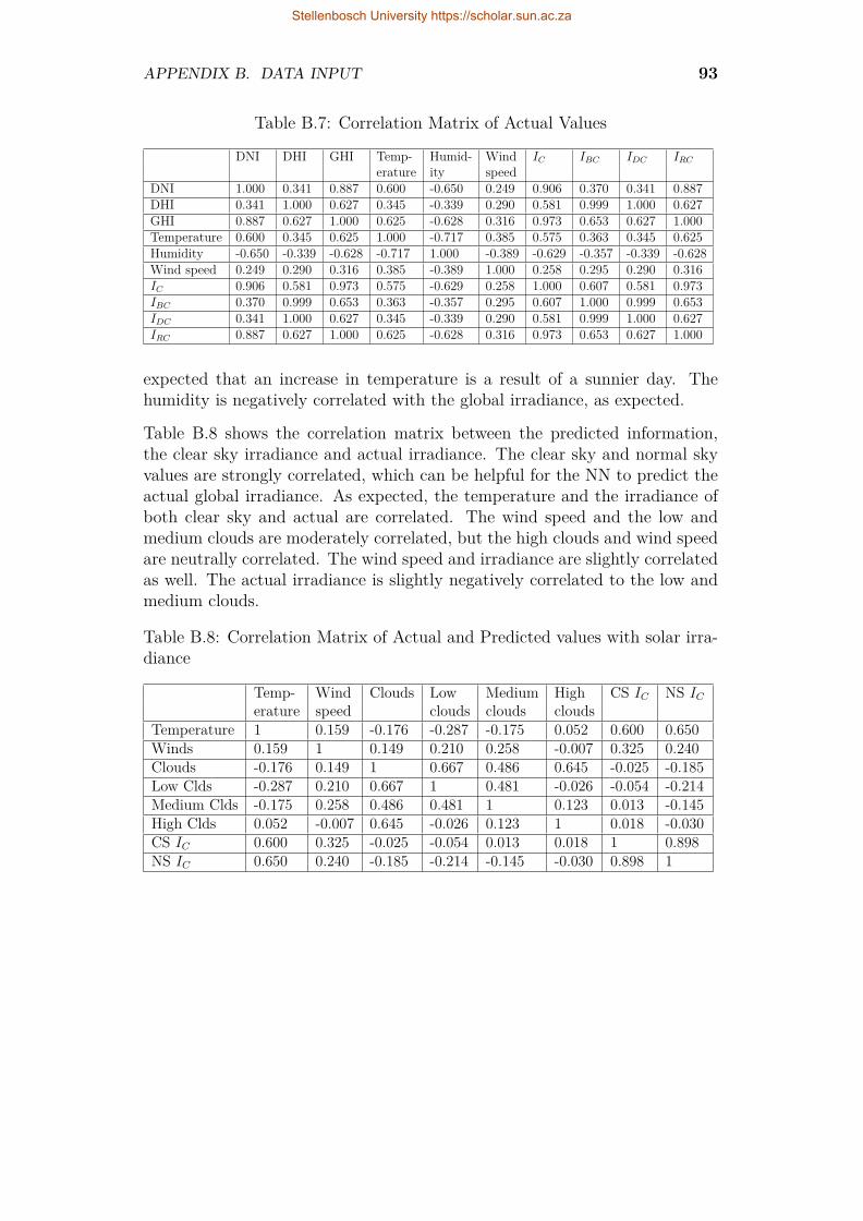
APPENDIX B. DATA INPUT 93
Table B.7: Correlation Matrix of Actual Values
DNI DHI GHI Temp- Humid- Wind IC IBC IDC IRCerature ity speed
DNI 1.000 0.341 0.887 0.600 -0.650 0.249 0.906 0.370 0.341 0.887DHI 0.341 1.000 0.627 0.345 -0.339 0.290 0.581 0.999 1.000 0.627GHI 0.887 0.627 1.000 0.625 -0.628 0.316 0.973 0.653 0.627 1.000Temperature 0.600 0.345 0.625 1.000 -0.717 0.385 0.575 0.363 0.345 0.625Humidity -0.650 -0.339 -0.628 -0.717 1.000 -0.389 -0.629 -0.357 -0.339 -0.628Wind speed 0.249 0.290 0.316 0.385 -0.389 1.000 0.258 0.295 0.290 0.316IC 0.906 0.581 0.973 0.575 -0.629 0.258 1.000 0.607 0.581 0.973IBC 0.370 0.999 0.653 0.363 -0.357 0.295 0.607 1.000 0.999 0.653IDC 0.341 1.000 0.627 0.345 -0.339 0.290 0.581 0.999 1.000 0.627IRC 0.887 0.627 1.000 0.625 -0.628 0.316 0.973 0.653 0.627 1.000
expected that an increase in temperature is a result of a sunnier day. Thehumidity is negatively correlated with the global irradiance, as expected.
Table B.8 shows the correlation matrix between the predicted information,the clear sky irradiance and actual irradiance. The clear sky and normal skyvalues are strongly correlated, which can be helpful for the NN to predict theactual global irradiance. As expected, the temperature and the irradiance ofboth clear sky and actual are correlated. The wind speed and the low andmedium clouds are moderately correlated, but the high clouds and wind speedare neutrally correlated. The wind speed and irradiance are slightly correlatedas well. The actual irradiance is slightly negatively correlated to the low andmedium clouds.
Table B.8: Correlation Matrix of Actual and Predicted values with solar irra-diance
Temp- Wind Clouds Low Medium High CS IC NS ICerature speed clouds clouds clouds
Temperature 1 0.159 -0.176 -0.287 -0.175 0.052 0.600 0.650Winds 0.159 1 0.149 0.210 0.258 -0.007 0.325 0.240Clouds -0.176 0.149 1 0.667 0.486 0.645 -0.025 -0.185Low Clds -0.287 0.210 0.667 1 0.481 -0.026 -0.054 -0.214Medium Clds -0.175 0.258 0.486 0.481 1 0.123 0.013 -0.145High Clds 0.052 -0.007 0.645 -0.026 0.123 1 0.018 -0.030CS IC 0.600 0.325 -0.025 -0.054 0.013 0.018 1 0.898NS IC 0.650 0.240 -0.185 -0.214 -0.145 -0.030 0.898 1
Stellenbosch University https://scholar.sun.ac.za

Appendix C
Code
C.1 Genetic AlgorithmThe implementation of the GA was done using object-oriented programming(OOP). OOP is a programming style and is associated with the conceptsof classes, objects, inheritance, encapsulation, abstraction and polymorphism[72]. The programming style reads intuitively, which makes it easier to under-stand and debug the implementation.
A class is defined with attributes. When an object is defined, an instance of theclass is created. The object has specified attributes. For an HPS chromosomeclass, the types and numbers of the different components vary, but they arestill present as part of the attributes of the HPS chromosome.
Basic OOP principles are encapsulation, composition and inheritance. Encap-sulation is the concept of data which is inside the object can only be accessedthrough a public interface, which will be the object’s methods. It is definedonce in a logical place and not multiple times, which condenses the program-ming and makes it easier to understand. Composition is a method of aggre-gating objects together by making some object attribute other objects. Forthe HPS chromosome class, it has other objects such as the PV-Module, Gen-erator, Inverter, Battery and Grid classes which has their own attributes andfunctions. The relationships between these compositions can be one-to-one,one-to-many or many-to-many and can also be unidirectional or bidirectional.The HPS will have only one type of PV module, however, the PV module canbe found in different HPS configurations. Inheritance arranges objects in ahierarchy form from the most general to most specific objects. A subtype ofan object is an object which inherits from another object. A subclass is alsoknown as a child class and a superclass is known as a parent class. Figure C.1visualises a summary of the OOP used to implement the GA. Each object hasa set of attributes which have different values.
94
Stellenbosch University https://scholar.sun.ac.za

APPENDIX C. CODE 95
Figure C.1: Genetic Algorithm Object Oriented Programming Summary
The chromosome is the superclass/parent class and has all the informationabout the chromosome’s DNA. The subclasses fall essentially under two cat-egories: the HPS components and the HPS configurations. As seen in FigureC.1, the HPS components are attributed to five classes: PV module, genera-tor, battery, inverter and grid. The HPS configurations, as discussed in section3.1.4.3, fall under this category. Each of these configurations is defined by theirown classes with attributed functions. The HPS configuration classes inheritthe component object’s attributes. The battery and generators are broken upinto smaller arrays of objects to analyse the individual power sources.
C.1.1 ImportsIn [1]: import warnings
warnings.filterwarnings(’ignore’)
import pandas as pdimport randomimport csvfrom datetime import datetime,timedeltaimport matplotlib.pyplot as pltimport mathfrom IPython.display import clear_outputrandom.seed(30)import os
import numpy as np
import pvlibfrom pvlib.location import Location, solarposition
Stellenbosch University https://scholar.sun.ac.za

APPENDIX C. CODE 96
C.1.2 Graph plot variablesPlot graphs for thesis
In [2]: label = 20ticklabel = 18
params = {’axes.labelsize’: label,’axes.titlesize’: label,’text.usetex’ : True,’font.size’: ticklabel,’legend.frameon’: True,’legend.fontsize’: ticklabel,
# ’legend.loc’: ’upper right’,’legend.framealpha’: 1,’xtick.labelsize’: ticklabel,’ytick.labelsize’: ticklabel,’grid.linestyle’ : ":",’axes.grid’: True,’axes.grid.which’: ’major’,’axes.grid’ : True,’grid.linewidth’ : 0.8,’keymap.grid’: [’g’],’keymap.grid_minor’: [’G’],’figure.figsize’: [18, 8]}
plt.rcParams.update(params)
C.1.3 Data input preprocessing and analysisIn [3]: Weather=pd.read_csv("database/HourlyWeatherData.csv")
Load=pd.read_csv("database/Plaas.csv")
Load=Load.drop([’Unnamed: 5’,’S -->’,’Q -->’], axis=1)Load=Load.rename(index=str, columns={’P -->’:’Load’})
Load[’Date’]=Load[’DATE’].map(str) + ’ ’ + Load[’TIME’]Load[’Date’]=pd.to_datetime(Load[’Date’])Load=Load.drop([’DATE’,’TIME’],axis=1)
Load=Load[[’Date’,’Load’]]Load.head()
Out[3]: Date Load0 2011-01-01 00:00:00 7.2511 2011-01-01 00:30:00 6.9542 2011-01-01 01:00:00 7.2073 2011-01-01 01:30:00 7.0134 2011-01-01 02:00:00 6.566
In [4]: Load.describe()
Stellenbosch University https://scholar.sun.ac.za
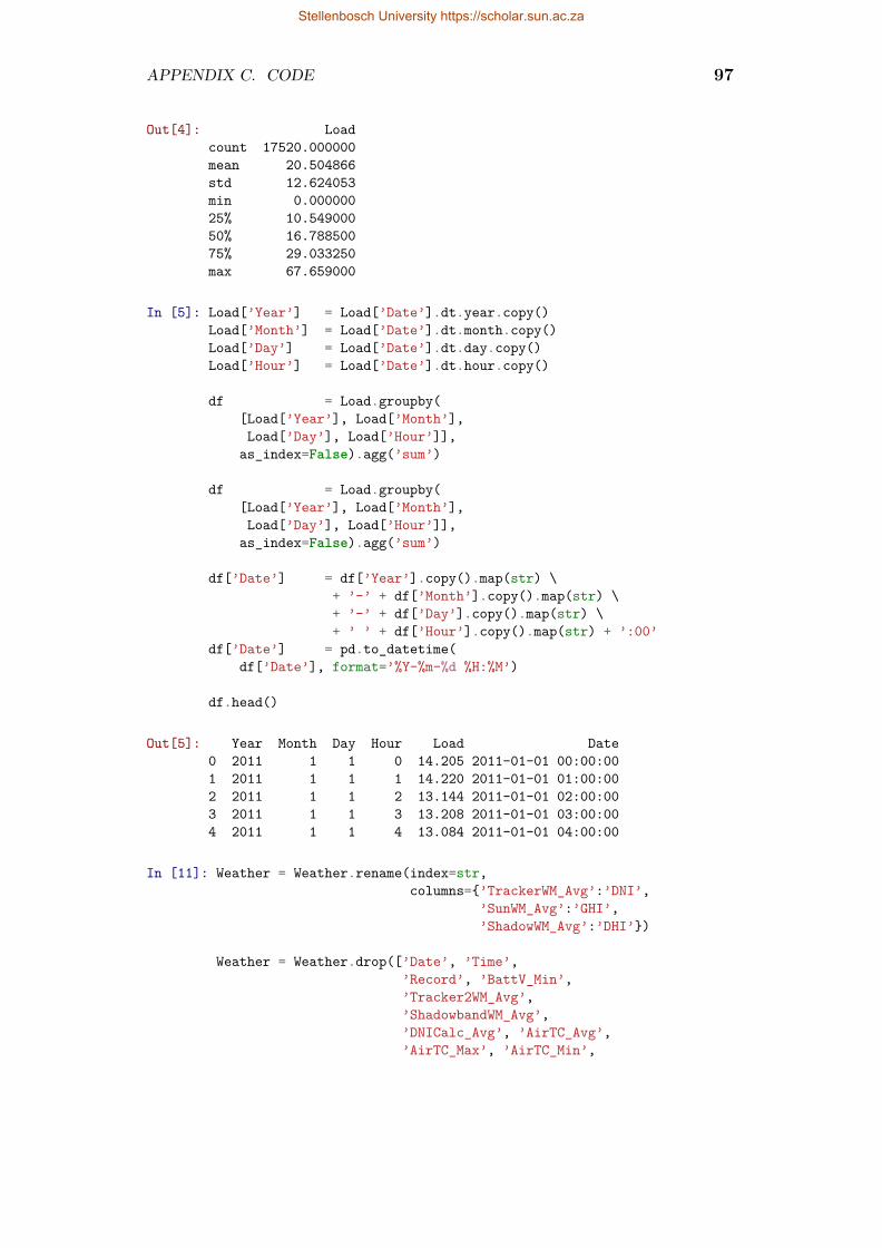
APPENDIX C. CODE 97
Out[4]: Loadcount 17520.000000mean 20.504866std 12.624053min 0.00000025% 10.54900050% 16.78850075% 29.033250max 67.659000
In [5]: Load[’Year’] = Load[’Date’].dt.year.copy()Load[’Month’] = Load[’Date’].dt.month.copy()Load[’Day’] = Load[’Date’].dt.day.copy()Load[’Hour’] = Load[’Date’].dt.hour.copy()
df = Load.groupby([Load[’Year’], Load[’Month’],Load[’Day’], Load[’Hour’]],
as_index=False).agg(’sum’)
df = Load.groupby([Load[’Year’], Load[’Month’],Load[’Day’], Load[’Hour’]],
as_index=False).agg(’sum’)
df[’Date’] = df[’Year’].copy().map(str) \+ ’-’ + df[’Month’].copy().map(str) \+ ’-’ + df[’Day’].copy().map(str) \+ ’ ’ + df[’Hour’].copy().map(str) + ’:00’
df[’Date’] = pd.to_datetime(df[’Date’], format=’%Y-%m-%d %H:%M’)
df.head()
Out[5]: Year Month Day Hour Load Date0 2011 1 1 0 14.205 2011-01-01 00:00:001 2011 1 1 1 14.220 2011-01-01 01:00:002 2011 1 1 2 13.144 2011-01-01 02:00:003 2011 1 1 3 13.208 2011-01-01 03:00:004 2011 1 1 4 13.084 2011-01-01 04:00:00
In [11]: Weather = Weather.rename(index=str,columns={’TrackerWM_Avg’:’DNI’,
’SunWM_Avg’:’GHI’,’ShadowWM_Avg’:’DHI’})
Weather = Weather.drop([’Date’, ’Time’,’Record’, ’BattV_Min’,’Tracker2WM_Avg’,’ShadowbandWM_Avg’,’DNICalc_Avg’, ’AirTC_Avg’,’AirTC_Max’, ’AirTC_Min’,
Stellenbosch University https://scholar.sun.ac.za

APPENDIX C. CODE 98
’RH’, ’WS_ms_S_WVT’,’WindDir_D1_WVT’,’WindDir_SD1_WVT’,’BP_mB_Avg’, ’UVA_Avg’,’UVB_Avg’], axis=1)
Weather[’Time’] = pd.to_datetime(Weather[’TimeStamp’])
Weather = Weather.drop([’TimeStamp’], axis=1)
C.1.4 Genetic Algorithm InputsIn [16]: population = 60
generations = 80crossoverProb = 0.8DNA_MutationProb = 0.4years = 20
tiltAngle=30rho=0.2LTM=-30latitude=-33.9346longitude=18.8668altitude=122
offspringCount = 0
loc=Location(latitude,longitude,’Africa/Johannesburg’,altitude,’Stellenbosch’)
C.1.5 Search space limitsIn [17]: minInv, maxInv = 10, 40
minBatStrings, maxBatStrings = 10, 20minGen, maxGen = 1, 3
DOD = 0.6SystemVolt = 120minRunningHours = 2derateFactor = 0.7
C.1.6 Financial Analysis InputsIn [18]: inflation = 0.05
# Operational and maintenanceomPV = 0.05omBat = 0.06
Stellenbosch University https://scholar.sun.ac.za
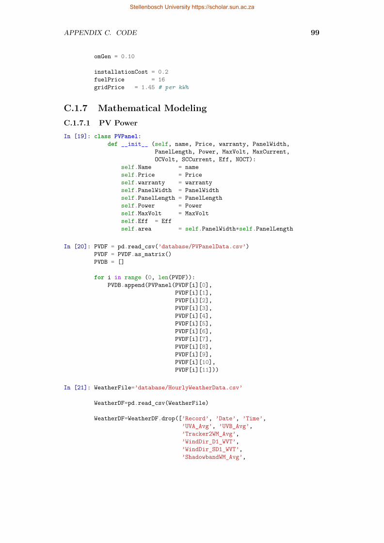
APPENDIX C. CODE 99
omGen = 0.10
installationCost = 0.2fuelPrice = 16gridPrice = 1.45 # per kWh
C.1.7 Mathematical ModelingC.1.7.1 PV PowerIn [19]: class PVPanel:
def __init__ (self, name, Price, warranty, PanelWidth,PanelLength, Power, MaxVolt, MaxCurrent,OCVolt, SCCurrent, Eff, NOCT):
self.Name = nameself.Price = Priceself.warranty = warrantyself.PanelWidth = PanelWidthself.PanelLength = PanelLengthself.Power = Powerself.MaxVolt = MaxVoltself.Eff = Effself.area = self.PanelWidth*self.PanelLength
In [20]: PVDF = pd.read_csv(’database/PVPanelData.csv’)PVDF = PVDF.as_matrix()PVDB = []
for i in range (0, len(PVDF)):PVDB.append(PVPanel(PVDF[i][0],
PVDF[i][1],PVDF[i][2],PVDF[i][3],PVDF[i][4],PVDF[i][5],PVDF[i][6],PVDF[i][7],PVDF[i][8],PVDF[i][9],PVDF[i][10],PVDF[i][11]))
In [21]: WeatherFile=’database/HourlyWeatherData.csv’
WeatherDF=pd.read_csv(WeatherFile)
WeatherDF=WeatherDF.drop([’Record’, ’Date’, ’Time’,’UVA_Avg’, ’UVB_Avg’,’Tracker2WM_Avg’,’WindDir_D1_WVT’,’WindDir_SD1_WVT’,’ShadowbandWM_Avg’,
Stellenbosch University https://scholar.sun.ac.za

APPENDIX C. CODE 100
’AirTC_Max’, ’DNICalc_Avg’,’BattV_Min’, ’WS_ms_S_WVT’,’RH’, ’BP_mB_Avg’,’AirTC_Avg’, ’AirTC_Min’],
axis=1)
WeatherDF=WeatherDF.rename(index=str,columns={’SunWM_Avg’:’GHI’,
’TrackerWM_Avg’:’DNI’,’ShadowWM_Avg’:’DHI’,’TimeStamp’:’Date’})
WeatherDF[’Date’]=pd.to_datetime(WeatherDF[’Date’])
In [22]: def getTotalIrradiance(GHI, DNI, DHI, Time):Time = pd.DatetimeIndex(Time)Time = Time.tz_localize(loc.tz)"""Calculate the total irradiance
Args:GHI: global horizontal irradianceDNI: direct normal irradianceDHI: diffuse horizontal irradianceTime: DatetimeIndex
Returns:total: [poa_global,poa_direct,poa_diffuse,poa_sky_diffuse,poa_ground_diffuse]
"""
model=’isotropic’
# Panel azimuth from Northsurface_azimuth = 0
albedo = rho #surface albedo
# convert to radianslatitudeR = np.deg2rad(latitude)n = Time.dayofyear# Equation of time"""pvlib.solarposition.equation_of_time_pvcdrom
Parameters: dayofyearReturn: equation_of_time: in minutes
"""eqOfTime=pvlib.solarposition.equation_of_time_pvcdrom(n)
Stellenbosch University https://scholar.sun.ac.za

APPENDIX C. CODE 101
# Hour angle"""pvlib.solarposition.hour_angle
Parameters: times: pd.DatetimeIndex must belocalized to timezone for the longitude
longitude: longitude (degrees)equation_of_time: equation of time in minutes
Returns: hour_angle (degrees)"""hourangle=pvlib.solarposition.hour_angle(Time,
longitude,eqOfTime)
hourAngleR=np.deg2rad(hourangle)
#Declination angle calculations"""pvlib.solarposition.declination_cooper69
Parameters: dayofyearReturns: declination angle (radians)
"""declinationR = pvlib.solarposition.declination_cooper69(n)
#Solar zenith angle calculations"""pvlib.solarposition.solar_zenith_analytical
Parameters: latitude: Latitude of location (radians)hourangle: Hour angle in local solar time (rad)declination: declination of the sun (radians)
Returns: solar zenith angle (radians)"""solar_zenithR = pvlib.solarposition.solar_zenith_analytical(
latitudeR, hourAngleR, declinationR)
#Solar azimuth angle calculations"""pvlib.solarposition.solar_azimuth_analytical
Parameters: latitude: Latitude of location (radians)hourangle: Hour angle in local solar time (rad)declination: declination of the sun (radians)zenith: solar zenith angle (radians)
Returns: Solar azimuth angle (radians)
"""solar_azimuthR=pvlib.solarposition.solar_azimuth_analytical(
latitudeR, hourAngleR, declinationR, solar_zenithR)#convert to degreessolar_azimuth = np.rad2deg(solar_azimuthR)solar_zenith = np.rad2deg(solar_zenithR)surface_tilt = tiltAngle
# get total irradiance"""
Stellenbosch University https://scholar.sun.ac.za

APPENDIX C. CODE 102
pvlib.irradiance.get_total_irradianceParameters: surface_tilt: Panel tilt from horizontal (deg)
surface_azimuth: Panel azimuth from north (deg)solar_zenith: Solar zenith angle (degrees)dni: Direct Normal Irradiance (W/mˆ2)ghi:Global horizontal irradiance (W/mˆ2)dhi: Diffuse horizontal irradiance (W/mˆ2)dni_extra: Extraterrestrial DNI.airmass: Airmassalbedo: Surface albedo 0-1surface_type: Surface type.model: isotropic(default)
Returns: dataframe array:poa_global,poa_direct,poa_diffuse,poa_sky_diffuse,poa_ground_diffuse
"""total = pvlib.irradiance.get_total_irradiance(
surface_tilt=tiltAngle, surface_azimuth=surface_azimuth,solar_zenith=solar_zenith, solar_azimuth=solar_azimuth,dni=DNI, ghi=GHI, dhi=DHI, albedo=albedo, model=model)
return total
In [23]: total=getTotalIrradiance(WeatherDF[’GHI’], WeatherDF[’DNI’],WeatherDF[’DHI’], pd.DatetimeIndex(WeatherDF[’Date’]))
WeatherDF[’Global Insolation’]=total[’poa_global’]
WeatherDF=WeatherDF.drop([’DNI’, ’DHI’, ’GHI’], axis=1)
WeatherDF=WeatherDF.as_matrix()
In [24]: class Weather:
def __init__(self, Time, insolation):self.Time = Timeself.insolation = insolation
def __str__(self):return (’{} : {}’.format (self.Time, self.insolation))
WeatherDB = []
for i in range (0, len(WeatherDF)):WeatherDB.append(Weather(
WeatherDF[i][0], WeatherDF[i][1]))
Stellenbosch University https://scholar.sun.ac.za
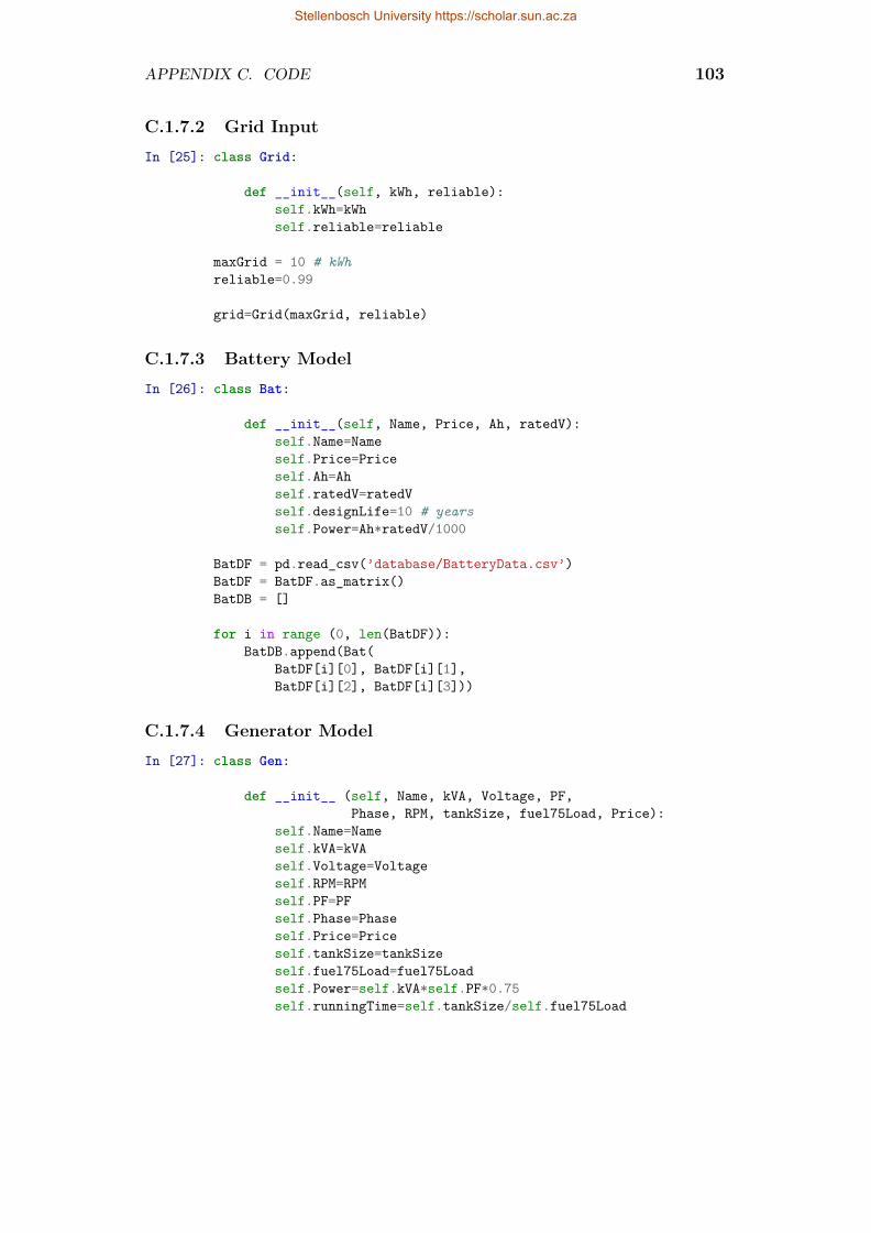
APPENDIX C. CODE 103
C.1.7.2 Grid InputIn [25]: class Grid:
def __init__(self, kWh, reliable):self.kWh=kWhself.reliable=reliable
maxGrid = 10 # kWhreliable=0.99
grid=Grid(maxGrid, reliable)
C.1.7.3 Battery ModelIn [26]: class Bat:
def __init__(self, Name, Price, Ah, ratedV):self.Name=Nameself.Price=Priceself.Ah=Ahself.ratedV=ratedVself.designLife=10 # yearsself.Power=Ah*ratedV/1000
BatDF = pd.read_csv(’database/BatteryData.csv’)BatDF = BatDF.as_matrix()BatDB = []
for i in range (0, len(BatDF)):BatDB.append(Bat(
BatDF[i][0], BatDF[i][1],BatDF[i][2], BatDF[i][3]))
C.1.7.4 Generator ModelIn [27]: class Gen:
def __init__ (self, Name, kVA, Voltage, PF,Phase, RPM, tankSize, fuel75Load, Price):
self.Name=Nameself.kVA=kVAself.Voltage=Voltageself.RPM=RPMself.PF=PFself.Phase=Phaseself.Price=Priceself.tankSize=tankSizeself.fuel75Load=fuel75Loadself.Power=self.kVA*self.PF*0.75self.runningTime=self.tankSize/self.fuel75Load
Stellenbosch University https://scholar.sun.ac.za
APPENDIX C. CODE 104
def __str__(self):msg=’{2}: {0:.2f} kW\tRunningTime: {1:.2f} hours’msg=msg.format(self.Power, self.runningTime, self.Name)return (msg)
GenDF = pd.read_csv(’database/GeneratorData.csv’)GenDF = GenDF.as_matrix()GenDB = []
for i in range (0, len(GenDF)):GenDB.append(Gen(GenDF[i][0], GenDF[i][1],
GenDF[i][2], GenDF[i][3],GenDF[i][4], GenDF[i][5],GenDF[i][6], GenDF[i][7],GenDF[i][8]))
C.1.7.5 Load ProfileIn [28]: class Load:
def __init__(self, Time, loadkW):self.Time=Timeself.loadkW=loadkW
def __str__(self):msg=’{0}\t{1:.3f} kW’msg=msg.format(self.Time, self.loadkW)return (msg)
LoadFile=’database/Plaas.csv’
Load_df=pd.read_csv("database/Plaas.csv")
Load_df=Load_df.drop([’Unnamed: 5’,’S -->’,’Q -->’], axis=1)Load_df=Load_df.rename(index=str, columns={’P -->’:’Load’})
Load_df[’Date’]=Load_df[’DATE’].map(str) + ’ ’ + Load_df[’TIME’]Load_df[’Date’]=pd.to_datetime(Load_df[’Date’])Load_df=Load_df.drop([’DATE’,’TIME’],axis=1)
Load_df[’Year’] = Load_df[’Date’].dt.year.copy()Load_df[’Month’] = Load_df[’Date’].dt.month.copy()Load_df[’Day’] = Load_df[’Date’].dt.day.copy()Load_df[’Hour’] = Load_df[’Date’].dt.hour.copy()
df = Load_df.groupby([Load_df[’Year’],Load_df[’Month’],Load_df[’Day’],Load_df[’Hour’]],
as_index=False).agg(’sum’)
Stellenbosch University https://scholar.sun.ac.za
APPENDIX C. CODE 105
df = Load_df.groupby([Load_df[’Year’],Load_df[’Month’],Load_df[’Day’],Load_df[’Hour’]],
as_index=False).agg(’sum’)
df[’Date’] = df[’Year’].copy().map(str) \+ ’-’ + df[’Month’].copy().map(str) \+ ’-’ + df[’Day’].copy().map(str) \+ ’ ’ + df[’Hour’].copy().map(str) + ’:00’
df[’Date’] = pd.to_datetime(df[’Date’], format=’%Y-%m-%d %H:%M’)
df=df.drop([’Year’, ’Month’, ’Day’, ’Hour’], axis=1)
Load_=df.as_matrix()LoadDB = []
for i in range (0, len(Load_)):LoadDB.append(Load(Load_[i][1], Load_[i][0]))
criticalHoursDB=[False, #00:00-00:59False, #01:00-01:59False, #02:00-02:59False, #03:00-03:59False, #04:00-04:59True, #05:00-05:59True, #06:00-06:59True, #07:00-07:59True, #08:00-08:59True, #09:00-09:59True, #10:00-10:59True, #11:00-11:59True, #12:00-12:59True, #13:00-13:59True, #14:00-14:59True, #15:00-15:59True, #16:00-16:59True, #17:00-17:59True, #18:00-18:59True, #19:00-19:59True, #20:00-20:59True, #21:00-21:59True, #22:00-22:59False] #23:00-23:59
C.1.7.6 InverterIn [29]: class Inv:
def __init__(self, Name, Price, Power, MPPT_min,MPPT_max, Eff, Warranty):
Stellenbosch University https://scholar.sun.ac.za

APPENDIX C. CODE 106
self.Name = Nameself.Power = Powerself.Price = Priceself.MPPT_min = MPPT_minself.MPPT_max = MPPT_maxself.Eff = Effself.warranty = Warranty
def __str__(self):priceFormat=’R{:,.2f}’.format(self.Price)msg=’{0}\t{1} kW\t{2}\t{3}\t{4}\t{5}%’msg=msg.format(self.Name, self.Power, priceFormat,
self.MPPT_min, self.MPPT_max,self.Eff)
return (msg)
InvDF = pd.read_csv(’database/InverterData.csv’)InvDF = InvDF.as_matrix()InvDB = []
for i in range (0, len(InvDF)):InvDB.append(Inv(
InvDF[i][0], InvDF[i][1],InvDF[i][2], InvDF[i][3],InvDF[i][4], InvDF[i][5],InvDF[i][6]))
C.1.8 HPS ConfigurationsC.1.8.1 ChromosomeIn [30]: class Chromosome:
def setTypes(self, PV, bat, gen, inv):self.typePV = returnType(PV)self.typeBat = returnType(bat)self.typeGen = returnType(gen)self.typeInv = returnType(inv)
def setSizes(self, SystemVolt, minBatStrings,maxBatStrings, minGen, maxGen,minInv, maxInv):
self.numInv = returnNumber(minInv, maxInv)self.setPVSize()self.numGen = returnNumber(
minGen, maxGen)self.numBatStrings = returnNumber(
minBatStrings, maxBatStrings)self.setBatSize(SystemVolt)
def setBatSize(self, SystemVolt):self.seriesBat = int(math.floor(
Stellenbosch University https://scholar.sun.ac.za

APPENDIX C. CODE 107
SystemVolt/self.Bat.ratedV))self.numTotalBat = self.numBatStrings*self.seriesBatself.systemVoltage = self.Bat.ratedV*self.seriesBat
def setPVSize(self):minPVString = math.ceil(
self.Inv.MPPT_min/self.PVPanel.MaxVolt)maxPVString = math.ceil(
self.Inv.MPPT_max/self.PVPanel.MaxVolt)self.numPV = (
returnNumber(minPVString,maxPVString))*self.numInv
def setOffspring(self, TPV, TBat, TGen, TInv, NBatS,NGen, NInv):
self.typePV = TPVself.typeBat = TBatself.typeGen = TGenself.typeInv = TInvself.numBatStrings = NBatSself.numGen = NGenself.numInv = NInv
def setClasses(self, PVPanel, Bat, Gen,Inv, Grid):
self.PVPanel = PVPanelself.Bat = Bat
self.Gen = Genself.Inv = Invself.Grid = Grid
def setPower(self):self.PVCapacity = self.numPV*self.PVPanel.MaxPowerself.batCapacity = self.numTotalBat*self.Bat.Powerself.genCapacity = self.numGen*self.Gen.kVA
def setFitness(self):setFitness(self.SG)setFitness(self.SGB)setFitness(self.SGG)setFitness(self.SGBG)
self.fitness = self.SG.fitness \+ self.SGB.fitness \+ self.SGG.fitness \+ self.SGBG.fitness
def rouletteWheel(self, start, end):self.startWheel = startself.endWheel = end
Stellenbosch University https://scholar.sun.ac.za

APPENDIX C. CODE 108
def EconomicalAnalysis(self):economicalAnalysis(self.SG)economicalAnalysis(self.SGB)economicalAnalysis(self.SGG)economicalAnalysis(self.SGBG)
def printChromosomeInfo(self):msg=’{0}\t{1}\t{2}\t{3}\t{4}\t{5}\t{6}\t’.format(
self.typePV, self.typeBat, self.typeGen,self.typeInv, self.numBatStrings, self.numGen,self.numInv)
return (msg)
def setHPS(self):self.SG = HPS_PVGrid(
self.PVPanel, self.numPV, self.Grid,self.Inv, self.numInv)
self.SGB = HPS_PVGridBat(self.PVPanel, self.numPV, self.Grid,self.Inv, self.numInv, self.Bat,self.numBatStrings, self.numTotalBat)
self.SGG = HPS_PVGridGen(self.PVPanel, self.numPV, self.Grid,self.Inv, self.numInv, self.Gen,self.numGen)
self.SGBG = HPS_PVGridBatGen(self.PVPanel, self.numPV, self.Grid, self.Inv,self.numInv, self.Bat, self.numBatStrings,self.numTotalBat, self.Gen, self.numGen)
In [31]: def checkObjectReplace(year, Object):if (year+1) % Object.warranty == 0:
return Trueelse:
return False
In [32]: def economicalAnalysis(Config):opCost = [0]*yearsreplaceCost = [0]*yearstotalCost = [0]*yearstotalCost[0] = Config.capitalCost*(
1+installationCost)Savings = [0]*years
cost = 0savings = 0
for i in range (0,years):’’’
Stellenbosch University https://scholar.sun.ac.za
APPENDIX C. CODE 109
Simulate for each year:All values adjusted for inflation: assumed linearReplacement costs: check warranty of systemOperational cost is a percentage of capital costSavings are based on what would for grid
’’’IR = math.pow((1 + inflation),i) #inflation rate
opCost[i] +=(Config.totalGridUsed*gridPrice \+ Config.capitalCost*omPV)*IR
# PV replacementif checkObjectReplace(i, Config.PVPanel) == True:
replaceCost[i]+=Config.PVPanel.Price*Config.numPV*IRif checkObjectReplace(i, Config.Inv) == True:
replaceCost[i]+=Config.Inv.Price*Config.numInv*IR
# Batif ’Bat’ in Config.Name:
opCost[i] += Config.capitalCost*omBat*IR
t=Config.batMatrix[0].dischargeEff*gridPrice*IR
Savings[i] += Config.totalBatUsed*t
if Config.checkBatReplace(i) == True:replaceCost[i]+=Config.Bat.Price*Config.numBat*IR
# Genif ’Gen’ in Config.Name:
opCost[i]+= Config.capitalCost*omGen*IR \+ Config.totalFuelCost*IR
Savings[i]+=Config.totalGenUsed*gridPrice*IR
invEff = (Config.Inv.Eff/100)Savings[i]+=Config.totalPVUsed*invEff*gridPrice*IR
totalCost[i] += opCost[i] \+ replaceCost[i]
cost += totalCost[i]savings += Savings[i]
Config.IRR = savings/cost
In [33]: def setFitness(Config):wLPSP = 12wPVUsage = 4wGridUsage = 1wGenUsage = 1wCF = 3wROI = 1
Stellenbosch University https://scholar.sun.ac.za

APPENDIX C. CODE 110
# Lower = worsefitnessGridUsage = 1 - Config.GridUsagefitnessGenUsage = 1 - Config.GenUsagefitnessLPSP = 1 - Config.LPSP
# if LPSP == 0: cannot divide by zerox = 0if Config.LPSP == 0:
x = Config.capitalCost/0.01else:
x = (Config.capitalCost/(Config.LPSP*100))
# Higher = betterfitnessCF = Config.CFfitnessIRR = Config.IRRfitnessPVUsage = Config.PVUsage
Config.fitness = wLPSP*fitnessLPSP \+ wPVUsage*fitnessPVUsage \+ wGridUsage*fitnessGridUsage \+ wGenUsage*fitnessGenUsage\+ wCF*fitnessCF \+ wROI*fitnessIRR
In [34]: def calcCapitalCost(Config):Config.capitalCost=Config.PVPanel.Price*Config.numPV \
+ Config.Inv.Price*Config.numInvif ’Bat’ in Config.Name:
Config.capitalCost+=Config.Bat.Price*Config.numBatif ’Gen’ in Config.Name:
Config.capitalCost+=Config.Gen.Price*Config.numGen
C.1.8.2 HPS: PV-GridIn [35]: class HPS_PVGrid:
def __init__(self, PVPanel, numPV, Grid, Inv, numInv):# HPS Configurationself.Name = ’PV-Grid’self.PVPanel = PVPanelself.Grid = Gridself.numPV = numPVself.Inv = Invself.numInv = numInv# Financial indicatorsself.capitalCost = 0self.IRR = 0# Fitness functionself.fitness = 0# Technical and environmental indicatorsself.GenUsage = 0self.LPS_hourly=[0]*len(LoadDB)
Stellenbosch University https://scholar.sun.ac.za

APPENDIX C. CODE 111
self.LPSP=0self.LPS_C=0self.LPS = 0self.CFHours=0self.totalLoad = 0self.totalPV = 0self.totalGrid = 0self.totalExcessPV = 0self.totalGridUsed = 0self.totalPVUsed = 0self.totalPVArea = self.PVPanel.area*self.numPV
# Calculate total capital costcalcCapitalCost(self)# Calculate loss of power supply probabilityself.calcLPSP()
def calcLPSP(self):’’’Calculate loss of power supply probability.
Control system constraints:1. Use all available PV2. Use grid if the load is not satisfied
’’’
PV_eff = (self.PVPanel.Eff/100)*derateFactor/1000Inv_eff = self.Inv.Eff/100
for i in range (0, len(LoadDB)):PVUsed = 0PVExcess = 0gridUsed = 0
# To calculate total loadself.totalLoad += LoadDB[i].loadkW
# reset loss of power supplyLPS = LoadDB[i].loadkW
# check if grid is available for hourgridAv = int(checkProb(
self.Grid.reliable))*self.Grid.kWhself.totalGrid += gridAv
# check if PV power is availablePVAvailable = self.totalPVArea*(
WeatherDB[i].insolation)*PV_effself.totalPV += PVAvailable
# if there is sufficient PV power# always use PV power first and as much as possible
Stellenbosch University https://scholar.sun.ac.za
APPENDIX C. CODE 112
if PVAvailable > LPS/Inv_eff:PVUsed = LPS/Inv_effPVExcess = PVAvailable - PVUsedLPS = 0
# use whatever PV power is availableelse:
PVUsed = PVAvailableLPS -= PVUsed*Inv_eff
# If there is still a loss of power supplyif LPS > 0:
if LPS > gridAv:LPS -= gridAvgridUsed = gridAv
else:gridUsed = LPSLPS = 0
# If the load is completely suppliedLPS = max(0, LPS)self.CFHours += int(LPS == 0)
# For analysis laterself.LPS_hourly[i] += LPS
# Analyse if this is part of critical hour analysisif criticalHoursDB[WeatherDB[i].Time.hour] == True:
self.LPS_C += LPS
self.LPS += LPS
self.totalExcessPV += PVExcessself.totalGridUsed += gridUsedself.totalPVUsed += PVUsed
self.LPSP = self.LPS/self.totalLoadself.LPSP_C = self.LPS_C/self.totalLoadself.CF = self.CFHours/len(LoadDB)self.PVUsage = self.totalPVUsed/self.totalPVself.GridUsage = self.totalGridUsed/self.totalGridself.ExcessPV = self.totalExcessPV/self.totalPV
C.1.8.3 HPS: PV-Grid-BatteryIn [36]: class HPS_PVGridBat:
def __init__(self, PVPanel, numPV, Grid, Inv, numInv,Bat, batStrings, numBat):
# HPS Configurationself.Name = ’PV-Grid-Bat’self.PVPanel=PVPanelself.Grid=Grid
Stellenbosch University https://scholar.sun.ac.za
APPENDIX C. CODE 113
self.numPV=numPVself.Inv=Invself.numInv=numInvself.Bat=Batself.batStrings=batStringsself.numBat=numBat# Financial indicatorsself.capitalCost = 0self.IRR = 0# Fitness functionself.fitness = 0# Technical and environmental indicatorsself.GenUsage = 0self.LPS_hourly=[0]*len(LoadDB)self.LPS_C=0self.CFHours=0self.totalLoad=0self.totalPV=0self.totalGrid=0self.totalExcessPV=0self.totalGridUsed=0self.totalPVUsed=0self.totalBatUsed=0self.totalPVArea=self.PVPanel.area*self.numPVself.LPS=0
# Initialize batteries as a matrix: look at each bat# individually throughout 1 yearself.initializeBatArray()# Calculate total capital costcalcCapitalCost(self)# Calculate loss of power supplyself.calcLPSP()
def calcLPSP(self):’’’Calculate loss of power supply probability.
Control system constraints:1. Use all available PV2. Discharge batteries3. Use grid if the load is not satisfied4. Charge batteries with excess PV and grid:
get batteries to be as much charged aspossible at all times.
’’’
PV_eff = self.PVPanel.Eff/100*derateFactor/1000Inv_eff = self.Inv.Eff/100
for i in range (0, len(LoadDB)):PVUsed = 0
Stellenbosch University https://scholar.sun.ac.za
APPENDIX C. CODE 114
PVExcess = 0gridUsed = 0batUsed = 0
# To calculate total loadself.totalLoad += LoadDB[i].loadkW
# reset loss of power supplyLPS = LoadDB[i].loadkW
# check if grid is available for hourgridAv = int(checkProb(
self.Grid.reliable))*self.Grid.kWhself.totalGrid += gridAv
# If it is a new month, update bat months# for self-discharge efficiencyif i > 0:
if LoadDB[i].Time.month != \LoadDB[i-1].Time.month:
self.updateBatMonths()
# check if PV power is availablePVAvailable = self.totalPVArea*(
WeatherDB[i].insolation)*PV_effself.totalPV += PVAvailable
# if there is sufficient PV powerif PVAvailable > LPS/Inv_eff:
PVUsed = LPS/Inv_effPVExcess = PVAvailable - PVUsedLPS = 0
# use whatever PV power is availableelse:
PVUsed=PVAvailableLPS -= PVUsed*Inv_eff
# Batteries: discharge batt if there is still LPSif LPS > 0:
LPS, batUsed = self.dischargeBatMatrix(LPS)
# If there is still a loss of power supplyif LPS > 0:
if LPS > gridAv:LPS -= gridAvgridUsed = gridAvgridAv = 0
else:gridUsed = LPSgridAv -= LPSLPS = 0
Stellenbosch University https://scholar.sun.ac.za
APPENDIX C. CODE 115
# charge bat if excessPV or grid power is availableif (PVExcess > 0 or gridAv > 0) and LPS == 0:
s_used, g_used = self.chargeBatMatrix(PVExcess, gridAv)
PVExcess -= s_usedPVUsed += s_usedgridUsed += g_used
# If the load is completely suppliedLPS = max(0, LPS)self.CFHours += int(LPS == 0)
self.LPS_hourly[i] += LPS
if criticalHoursDB[WeatherDB[i].Time.hour]== True:self.LPS_C += LPS
self.LPS += LPSself.totalExcessPV += PVExcessself.totalGridUsed += gridUsedself.totalPVUsed += PVUsedself.totalBatUsed += batUsed
self.LPSP = self.LPS/self.totalLoadself.LPSP_C = self.LPS_C/self.totalLoadself.CF = self.CFHours/len(LoadDB)self.PVUsage = self.totalPVUsed/self.totalPVself.GridUsage = self.totalGridUsed/self.totalGridself.ExcessPV = self.totalExcessPV/self.totalPV
def initializeBatArray(self):’’’Batteries are seen as an array.Each has own tracking of lifecycles, available power.’’’self.batMatrix = []for i in range (0, self.numBat):
self.batMatrix.append(BatObject(self.Bat))
def chargeBatMatrix(self, PVExcess, gridAv):’’’Charge the batteries using excess PV and available grid.
This grid is only used if the batteries are less than40% of the total capacity.
’’’chargeEff = self.batMatrix[0].chargeEff
PVUsed = 0gridUsed = 0
Stellenbosch University https://scholar.sun.ac.za

APPENDIX C. CODE 116
for i in range (0, self.numBat):maxBat = self.batMatrix[i].maxBatif self.batMatrix[i].chargingState == True:
availableCapacity = self.batMatrix[i].maxBat \- self.batMatrix[i].minBat
if PVExcess > availableCapacity*chargeEff:self.batMatrix[i].batPower = maxBatPVUsed += availableCapacity/chargeEffself.batMatrix[i].chargingState = FalsePVExcess -= availableCapacity/chargeEff
else:self.batMatrix[i].batPower+=PVExcess*chargeEffPVUsed += PVExcessPVExcess = 0
if PVExcess <=0:break
totalCapacityAvailable=0totalCapacity = self.numBat*(
self.batMatrix[0].maxBat - self.batMatrix[0].minBat)
for i in range (0, self.numBat):totalCapacityAvailable += self.batMatrix[i].batPower \
- self.batMatrix[i].minBat
ratio=totalCapacityAvailable/totalCapacityif ratio < 0.4:
maxBat = self.batMatrix[i].maxBatfor i in range (0, self.numBat):
if self.batMatrix[i].chargingState == True:availableCapacity = self.batMatrix[i].maxBat \
- self.batMatrix[i].minBat
if gridAv > availableCapacity*chargeEff:self.batMatrix[i].batPower = maxBatgridUsed += availableCapacity/chargeEffself.batMatrix[i].chargingState = FalsegridAv -= availableCapacity/chargeEff
else:self.batMatrix[i].batPower+=gridAv*chargeEffgridUsed += gridAvgridAv = 0break
if gridAv <= 0:break
return PVUsed, gridUsed
def dischargeBatMatrix(self, LPS):’’’
Stellenbosch University https://scholar.sun.ac.za
APPENDIX C. CODE 117
Discharge batteries based on the LPS value.
Returns the leftover LPS and how much bat was discharged
’’’batUsed = 0battDischargeEff = self.batMatrix[0].dischargeEfffor i in range (0, self.numBat):
minBat = self.batMatrix[i].minBatselfDisch = self.batMatrix[i].totalSelfDischRateif self.batMatrix[i].chargingState == False:
available = (self.batMatrix[i].batPower \- self.batMatrix[i].minBat)*(1 \
- selfDisch)*battDischargeEff
if LPS > available:LPS -= availablebatUsed += (self.batMatrix[i].batPower \
- self.batMatrix[i].minBat)self.batMatrix[i].batPower = minBatself.batMatrix[i].chargingState = Trueself.batMatrix[i].lifecycles += 1
else:used = LPS/((1-selfDisch)*battDischargeEff)self.batMatrix[i].batPower -= usedLPS = 0batUsed += used
if LPS <= 0:break
return LPS, batUsed
def updateBatMonths(self):’’’Update months for self-discharge value’’’for i in range (0, self.numBat):
self.batMatrix[i].month+=1
def checkBatReplace(self, year):’’’Analyse individual bat life cycles and if it is finished.’’’totalUsed=0totalAvailable=self.batMatrix[0].maxLifecycles*self.numBatfor i in range (0, self.numBat):
totalUsed+=self.batMatrix[i].lifecyclesyears_=math.floor(totalAvailable/totalUsed)if years_ > 0 and (year+1) % years_ == 0:
return Trueelse:
Stellenbosch University https://scholar.sun.ac.za

APPENDIX C. CODE 118
return False
In [37]: class BatObject:
def __init__(self, Bat):self.batPower = Bat.Powerself.month = 1self.warranty = Bat.designLifeself.lifecycles = 0self.maxLifecycles = 1800self.chargingState = Falseself.selfDischRate = 0.03self.minBat = self.batPower*(1-DOD)self.maxBat = self.batPowerself.totalSelfDischRate = self.month*self.selfDischRateself.dischargeEff = 0.90self.chargeEff = 0.90
def __str__(self):chargingState = ’’if self.chargingState == False:
chargingState = ’D’else:
chargingState = ’C’return (’%.1fkWh %d %s\t’ % (self.batPower,
self.lifecycles,chargingState))
C.1.8.4 HPS: PV-Grid-GeneratorIn [38]: class HPS_PVGridGen:
def __init__(self, PVPanel, numPV, Grid, Inv, numInv,Gen, numGen):
# HPS Configurationself.Name = ’PV-Grid-Gen’self.PVPanel=PVPanelself.numPV=numPVself.Grid=Gridself.Inv=Invself.numInv=numInvself.Gen=Genself.numGen=numGen# Financial indicatorsself.capitalCost = 0self.IRR = 0# Fitness functionself.fitness = 0# Technical indicatorsself.LPS_hourly=[0]*len(LoadDB)self.LPS_C=0self.LPS=0
Stellenbosch University https://scholar.sun.ac.za
APPENDIX C. CODE 119
self.CFHours=0self.totalLoad=0self.totalPV=0self.totalGrid=0self.totalExcessPV=0self.totalGridUsed=0self.totalPVUsed=0self.totalGenUsed=0self.totalPVArea=self.PVPanel.area*self.numPV
self.genMatrix=[GenObject(self.Gen) \for x in range (self.numGen)]
calcCapitalCost(self)self.calcLPSP()self.totalFuelCost=self.calcFuelCost()
def calcLPSP(self):’’’Calculate loss of power supply probability.
Constraints:1. Use PV: charge batteries with excess2. Use running gens: charge batteries with excess
(min load)3. Use grid’’’
PV_eff = (self.PVPanel.Eff/100)*derateFactor/1000Inv_eff = self.Inv.Eff/100
for i in range (0, len(LoadDB)):PVUsed = 0PVExcess = 0gridUsed = 0genUsed = 0
# To calculate total loadself.totalLoad+=LoadDB[i].loadkW
# Rest LPSLPS=LoadDB[i].loadkW
# check if grid is available for hourgridAv = int(checkProb(
self.Grid.reliable))*self.Grid.kWhself.totalGrid += gridAv
# Reset required gensfor j in range (self.numGen):
self.genMatrix[j].required = False
Stellenbosch University https://scholar.sun.ac.za
APPENDIX C. CODE 120
# check if PV power is availablePVAvailable = self.totalPVArea*(
WeatherDB[i].insolation)*PV_effself.totalPV += PVAvailable
# if there is sufficient PV powerif PVAvailable > LoadDB[i].loadkW:
PVUsed = LoadDB[i].loadkW/Inv_effPVExcess = PVAvailable - PVUsedLPS=0
else:PVUsed = PVAvailableLPS -= PVUsed*Inv_eff
# check for gens that are already running and# rather use thesefor j in range (self.numGen):
if self.genMatrix[j].checkRunning(minRunningHours) == True:self.genMatrix[j].switchOn()LPS-=self.Gen.Powerif LPS < 0:
LPS = 0
if LPS > gridAv and LPS !=0:#use gensfor j in range (self.numGen):
# Try full load firstif LPS > self.Gen.Power:
self.genMatrix[j].switchOn()LPS-=self.Gen.PowergenUsed+=self.Gen.Power
else:if LPS > gridAv:
LPS-=gridAvgridUsed=gridAvgridAv=0break
else:gridUsed=LPSgridAv-=LPSLPS=0break
else:gridUsed=LPSLPS=0
# Switch off any unused gensfor j in range (self.numGen):
if self.genMatrix[j].required == False:
Stellenbosch University https://scholar.sun.ac.za
APPENDIX C. CODE 121
self.genMatrix[j].switchOff()
LPS = max(0, LPS)self.CFHours += int(LPS == 0)
self.LPS+=LPSself.LPS_hourly[i]+=LPS
if criticalHoursDB[WeatherDB[i].Time.hour]== True:self.LPS_C+=LPS
self.totalGenUsed += genUsedself.totalExcessPV += PVExcessself.totalGridUsed += gridUsedself.totalPVUsed += PVUsed
self.LPSP=self.LPS/self.totalLoadself.LPSP_C=self.LPS_C/self.totalLoadself.CF=self.CFHours/len(LoadDB)self.PVUsage=self.totalPVUsed/self.totalPVself.GridUsage=self.totalGridUsed/self.totalGridself.ExcessPV=self.totalExcessPV/self.totalPVself.GenUsage=self.totalGenUsed/self.totalLoad
def calcFuelCost(self):hours = 0fuel = 0for i in range (0, self.numGen):
hours += self.genMatrix[i].runningHoursfuel = self.Gen.fuel75Load*fuelPrice*hoursreturn fuel
In [39]: class GenObject:
def __init__(self, Gen):self.Gen=Genself.runningHours=0self.switchOnHours=0self.switchedOn=Falseself.required=False
def __str__(self):return (’%d\t%d\tRequired: %s’ % (
self.runningHours,self.switchOnHours, self.required))
def checkRunning(self, minHours):if self.switchOnHours < minHours \
and self.switchOnHours != 0 \and self.switchedOn == True:
return Trueelse:
Stellenbosch University https://scholar.sun.ac.za

APPENDIX C. CODE 122
return False
def switchOn(self):self.runningHours += 1self.switchOnHours += 1self.switchedOn = Trueself.required = True
def switchOff(self):self.switchOnHours = 0self.switchedOn = False
C.1.8.5 HPS: PV-Grid-Battery-GeneratorIn [40]: class HPS_PVGridBatGen:
def __init__(self, PVPanel, numPV, Grid, Inv, numInv, Bat,batStrings, numBat, Gen, numGen):
# HPS Configurationself.Name = ’PV-Grid-Bat-Gen’self.PVPanel=PVPanelself.Grid=Gridself.numPV=numPVself.Inv=Invself.numInv=numInvself.Bat=Batself.batStrings=batStringsself.numBat=numBatself.Gen = Genself.numGen = numGenself.genMatrix = [GenObject(self.Gen) \
for x in range (self.numGen)]# Financial indicatorsself.capitalCost = 0self.IRR = 0# Fitness functionself.fitness = 0# Technical and environmental indicatorsself.GenUsage = 0self.LPS_hourly = [0]*len(LoadDB)self.LPS_C = 0self.CFHours = 0self.totalLoad = 0self.totalPV = 0self.totalGrid = 0self.totalExcessPV = 0self.totalGridUsed = 0self.totalPVUsed = 0self.totalGenUsed = 0self.totalBatUsed = 0self.totalPVArea = self.PVPanel.area*self.numPVself.LPS = 0
Stellenbosch University https://scholar.sun.ac.za

APPENDIX C. CODE 123
# Initialize batteries as a matrix: look at each bat# individually throughout 1 yearself.initializeBatArray()# Calculate total capital costcalcCapitalCost(self)# Calculate loss of power supplyself.calcLPSP()# Calculate total fuel costself.totalFuelCost=self.calcFuelCost()
def calcLPSP(self):’’’Calculate loss of power supply probability.
Control system constraints:1. Use all available PV2. Discharge batteries3. Use grid if the load is not satisfied4. Switch on gens if load is not satisfied5. Charge batteries with excess PV, grid and running
gens (always run at 75%) to get batteries to beas much charged as possible at all times.
’’’
PV_eff = (self.PVPanel.Eff/100)*(derateFactor)/1000Inv_eff = self.Inv.Eff/100
for i in range (0, len(LoadDB)):PVUsed = 0PVExcess = 0gridUsed = 0batUsed = 0genUsed = 0genExcess = 0
# To calculate total loadself.totalLoad += LoadDB[i].loadkW
# reset loss of power supplyLPS = LoadDB[i].loadkW
# Reset gensfor j in range (self.numGen):
self.genMatrix[j].required=False
# check if grid is available for hourgridAv = int(checkProb(
self.Grid.reliable))*self.Grid.kWhself.totalGrid += gridAv
# If it is a new month, update bat months
Stellenbosch University https://scholar.sun.ac.za
APPENDIX C. CODE 124
# for self-discharge efficiencyif i > 0:
if LoadDB[i].Time.month != LoadDB[i-1].Time.month:self.updateBatMonths()
# check if PV power is availablePVAvailable = self.totalPVArea*(
WeatherDB[i].insolation)*PV_effself.totalPV += PVAvailable
# if there is sufficient PV powerif PVAvailable > LPS/Inv_eff:
PVUsed = LPS/Inv_effPVExcess = PVAvailable - PVUsedLPS = 0
else: # use whatever PV power is availablePVUsed=PVAvailableLPS -= PVUsed*Inv_eff
#check for gens that are already running and# rather use thesefor j in range (self.numGen):
if self.genMatrix[j].checkRunning(minRunningHours) == True:self.genMatrix[j].switchOn()LPS -= self.Gen.Powerif LPS < 0:
genExcess = np.absolute(LPS)LPS = 0
# Batteries: discharge bat if there is still a LPSif LPS > 0:
LPS, batUsed = self.dischargeBatMatrix(LPS)
# If there is still a loss of power supplyif LPS > 0:
if LPS > gridAv:LPS -= gridAvgridUsed = gridAvgridAv = 0
else:gridUsed = LPSgridAv -= LPSLPS = 0
# Switch on gensif LPS > 0:
for j in range (self.numGen):if LPS > 0:
self.genMatrix[j].switchOn()LPS -= self.Gen.PowergenUsed += self.Gen.Power
Stellenbosch University https://scholar.sun.ac.za

APPENDIX C. CODE 125
if LPS < 0:genExcess = np.absolute(LPS)LPS = 0break
# charge batteries if there is excess PV, grid power# available and whatever gen power is running# (do not switch on though - only if it has to run)if (PVExcess > 0 or gridAv > 0 or genExcess) \
and LPS <= 0:s_used, g_used = self.chargeBatMatrix(
PVExcess, gridAv, genExcess)PVExcess -= s_usedPVUsed += s_usedgridUsed += g_used
# Switch off gensfor j in range (self.numGen):
if self.genMatrix[j].required == False:self.genMatrix[j].switchOff()
# If the load is completely suppliedLPS = max(0, LPS)self.CFHours += int(LPS == 0)
self.LPS_hourly[i] += LPS
if criticalHoursDB[WeatherDB[i].Time.hour]== True:self.LPS_C += LPS
self.LPS += LPSself.totalExcessPV += PVExcessself.totalGridUsed += gridUsedself.totalPVUsed += PVUsedself.totalBatUsed += batUsedself.totalGenUsed += genUsed
self.LPSP = self.LPS/self.totalLoadself.LPSP_C = self.LPS_C/self.totalLoadself.CF = self.CFHours/len(LoadDB)self.PVUsage = self.totalPVUsed/self.totalPVself.GridUsage = self.totalGridUsed/self.totalGridself.ExcessPV = self.totalExcessPV/self.totalPVself.GenUsage = self.totalGenUsed/self.totalLoad
def initializeBatArray(self):’’’Batteries are seen as an array.Each has own tracking of lifecycles, available power.’’’self.batMatrix = []for i in range (0, self.numBat):
Stellenbosch University https://scholar.sun.ac.za
APPENDIX C. CODE 126
self.batMatrix.append(BatObject(self.Bat))
def chargeBatMatrix(self, PVExcess, gridAv, genExcess):’’’Charge the batteries using excess PV and available grid.
Always charge with PV and gen excess.
This grid is only used if the batteries are lessthan 40% of the total capacity.
’’’chargeEff = self.batMatrix[0].chargeEff
PVUsed = 0gridUsed = 0
for i in range (0, self.numBat):minBat = self.batMatrix[i].minBatmaxBat = self.batMatrix[i].maxBatif self.batMatrix[i].chargingState == True:
availableCapacity = maxBat - minBatif PVExcess > availableCapacity*chargeEff:
self.batMatrix[i].batPower = maxBatPVUsed += availableCapacity/chargeEffself.batMatrix[i].chargingState = FalsePVExcess -= availableCapacity/chargeEff
else:self.batMatrix[i].batPower+=PVExcess*chargeEffPVUsed += PVExcessPVExcess = 0
if PVExcess <=0:break
for i in range (0, self.numBat):if self.batMatrix[i].chargingState == True:
availableCapacity = maxBat - minBatif genExcess > availableCapacity*chargeEff:
self.batMatrix[i].batPower = maxBatself.batMatrix[i].chargingState = FalsegenExcess -= availableCapacity/chargeEff
else:self.batMatrix[i].batPower+=genExcess*chargeEffgenExcess = 0
if genExcess <=0:break
totalCapacityAvailable=0totalCapacity=self.numBat*(self.batMatrix[0].maxBat \
- self.batMatrix[0].minBat)
for i in range (0, self.numBat):
Stellenbosch University https://scholar.sun.ac.za
APPENDIX C. CODE 127
totalCapacityAvailable += self.batMatrix[i].batPower \- self.batMatrix[i].minBat
ratio=totalCapacityAvailable/totalCapacity
if ratio < 0.4:for i in range (0, self.numBat):
maxBat = self.batMatrix[i].maxBatif self.batMatrix[i].chargingState == True:
availableCapacity = self.batMatrix[i].maxBat \- self.batMatrix[i].minBat
if gridAv > availableCapacity*chargeEff:self.batMatrix[i].batPower = maxBatgridUsed += availableCapacity/chargeEffself.batMatrix[i].chargingState=FalsegridAv -= availableCapacity/chargeEff
else:self.batMatrix[i].batPower+=gridAv*chargeEffgridUsed += gridAvgridAv = 0break
if gridAv <= 0:break
return PVUsed, gridUsed
def dischargeBatMatrix(self, LPS):’’’Discharge batteries based on the LPS value.
Returns the leftover LPS and how much bat was discharged
’’’batUsed = 0battDischargeEff = self.batMatrix[0].dischargeEfffor i in range (0, self.numBat):
minBat = self.batMatrix[i].minBatselfDisch = self.batMatrix[i].totalSelfDischRateif self.batMatrix[i].chargingState == False:
available = (self.batMatrix[i].batPower-minBat)*(1 - selfDisch)*battDischargeEff
if LPS > available:LPS -= availablebatUsed += (self.batMatrix[i].batPower-minBat)self.batMatrix[i].batPower = minBatself.batMatrix[i].chargingState = Trueself.batMatrix[i].lifecycles += 1
else:used = LPS/((1-selfDisch)*battDischargeEff)self.batMatrix[i].batPower -= used
Stellenbosch University https://scholar.sun.ac.za

APPENDIX C. CODE 128
LPS = 0batUsed += used
if LPS <= 0:break
return LPS, batUsed
def updateBatMonths(self):’’’Update months for self-discharge value’’’for i in range (0, self.numBat):
self.batMatrix[i].month+=1
def checkBatReplace(self, year):’’’Analyse individual bat life cycles and if it is done.’’’totalUsed=0totalAvailable=self.batMatrix[0].maxLifecycles*self.numBatfor i in range (0, self.numBat):
totalUsed += self.batMatrix[i].lifecyclesyears_ = math.floor(totalAvailable/totalUsed)if years_ > 0 and (year+1) % years_ == 0:
return Trueelse:
return False
def calcFuelCost(self):hours = 0fuel = 0for i in range (0, self.numGen):
hours += self.genMatrix[i].runningHoursfuel = self.Gen.fuel75Load*fuelPrice*hoursreturn fuel
C.1.9 GA functionsC.1.9.1 Define populationIn [41]: Population = []
def returnType(length):return int(round((length-1)*random.random()))
def returnNumber(Min, Max):return int(round(Min + (Max-Min)*random.random()))
def definePopulationChromosomes():for c in range(0, population):
Population.append(Chromosome())Population[c].setTypes(
len(PVDB), len(BatDB),
Stellenbosch University https://scholar.sun.ac.za

APPENDIX C. CODE 129
len(GenDB), len(InvDB))Population[c].setClasses(
PVDB[Population[c].typePV],BatDB[Population[c].typeBat],GenDB[Population[c].typeGen],InvDB[Population[c].typeInv],grid)
Population[c].setSizes(SystemVolt, minBatStrings,maxBatStrings, minGen,maxGen, minInv, maxInv)
definePopulationChromosomes()
C.1.9.2 Objective FunctionsIn [42]: def checkProb(prob):
t = random.random()if t <= prob:
return Trueelse:
return False
def setPopulationHPSConfigurations():for i in range (0, population):
Population[i].setHPS()Population[i].EconomicalAnalysis()
setPopulationHPSConfigurations()
In [43]: def setRouletteWheel(popList):totalFitness = 0for i in range (0, len(popList)):
totalFitness += popList[i].fitnessfor i in range (0, len(popList)):
length=popList[i].fitness/totalFitnessif i == 0:
popList[i].startWheel = 0popList[i].endWheel = length
else:popList[i].startWheel=popList[i-1].endWheelpopList[i].endWheel=popList[i].startWheel+length
def returnDNAMutations(DNA_MutationProb):m = []for i in range (0, 7):
m.append(checkProb(DNA_MutationProb))return m
def returnWeakestIndex(popList):weakest = popList[0]
Stellenbosch University https://scholar.sun.ac.za
APPENDIX C. CODE 130
n = 0for i in range (0, len(popList)):
if popList[i].fitness < weakest.fitness and i > 0:weakest = popList[i]n = i
return n
def returnTopFittest(listPop, maxFit):popList = listPop[:]for passnum in range (len(popList)-1,0,-1):
for i in range (passnum):if popList[i].fitness <popList[i+1].fitness:
temp = popList[i]popList[i] = popList[i+1]popList[i+1] = temp
returnList = []for i in range (0,maxFit):
returnList.append(popList[i])return returnList
def returnFittestSG(listPop):popList=listPop[:]for passnum in range (len(popList)-1,0,-1):
for i in range (passnum):if popList[i].SG.fitness<popList[i+1].SG.fitness:
temp = popList[i]popList[i] = popList[i+1]popList[i+1] = temp
return popList[0].SG
def returnFittestSGB(listPop):popList = listPop[:]for passnum in range (len(popList)-1,0,-1):
for i in range (passnum):if popList[i].SGB.fitness<popList[i+1].SGB.fitness:
temp = popList[i]popList[i] = popList[i+1]popList[i+1] = temp
return popList[0].SGB
def returnFittestSGG(listPop):popList = listPop[:]for passnum in range (len(popList)-1,0,-1):
for i in range (passnum):if popList[i].SGG.fitness<popList[i+1].SGG.fitness:
temp = popList[i]popList[i] = popList[i+1]popList[i+1] = temp
return popList[0].SGG
def returnFittestSGBG(listPop):popList = listPop[:]
Stellenbosch University https://scholar.sun.ac.za

APPENDIX C. CODE 131
for passnum in range (len(popList)-1,0,-1):for i in range (passnum):
if popList[i].SGBG.fitness<popList[i+1].SGBG.fitness:temp = popList[i]popList[i] = popList[i+1]popList[i+1] = temp
return popList[0].SGBG
C.1.9.3 Fitness FunctionIn [44]: def setPopulationFitness():
for i in range (0, len(Population)):Population[i].setFitness()
setPopulationFitness()
C.1.9.4 Roulette WheelIn [45]: setRouletteWheel(Population)
C.1.9.5 Offspring generationIn [46]: def findParent(probIndex, popList):
parent = 0for i in range (0, len(popList)):
if popList[i].startWheel < probIndex \and popList[i].endWheel >= probIndex:parent = ibreak
return parent
def returnPValue(parent1, parent2):if checkProb(0.5) == True:
return parent1else:
return parent2
C.1.9.6 CrossoverIn [47]: def crossover():
coProb1 = random.uniform(0,1)P1 = findParent(coProb1, Population)coProb2 = random.uniform(0,1)P2 = findParent(coProb2, Population)
while P1 == P2:P2 = random.uniform(0,1)P2 = findParent(P2, Population)
TPV = returnPValue(Population[P1].typePV,Population[P2].typePV)
Stellenbosch University https://scholar.sun.ac.za
APPENDIX C. CODE 132
TInv = returnPValue(Population[P1].typeInv,Population[P2].typeInv)
TBat = returnPValue(Population[P1].typeBat,Population[P2].typeBat)
TGen = returnPValue(Population[P1].typeGen,Population[P2].typeGen)
NInv = returnPValue(Population[P1].numInv,Population[P2].numInv)
NBatS = returnPValue(Population[P1].numBatStrings,Population[P2].numBatStrings)
NGen = returnPValue(Population[P1].numGen,Population[P2].numGen)
generateOffspring(TPV, TBat, TGen, TInv, NBatS,NGen, NInv)
C.1.9.7 MutationIn [48]: def mutation():
mutProb = random.uniform(0,1)Parent = findParent(mutProb, Population)mut = returnDNAMutations(DNA_MutationProb)# PVTPV=int(mut[0] == False)*Population[Parent].typePV \
+ int(mut[0] == True)*returnType(len(PVDB))# InvTInv=int(mut[3] == False)*Population[Parent].typeInv \
+ int(mut[3] == True)*returnType(len(InvDB))NInv=int(mut[6] == False)*Population[Parent].numInv \
+ int(mut[6] == True)*returnNumber(minInv,maxInv)# BatTBat=int(mut[1]==False)*Population[Parent].typeBat \
+ int(mut[1]==True)*returnType(len(BatDB))NBatS=int(mut[4]==False)*Population[Parent].numBatStrings \
+ int(mut[4]==True)*returnNumber(minBatStrings,maxBatStrings)
# GenTGen=int(mut[2] == False)*Population[Parent].typeGen \
+ int(mut[2] == True)*returnType(len(GenDB))NGen=int(mut[5] == False)*Population[Parent].numGen \
+ int(mut[5] == True)*returnNumber(minGen,maxGen)
generateOffspring(TPV, TBat, TGen, TInv, NBatS, NGen, NInv)
Stellenbosch University https://scholar.sun.ac.za

APPENDIX C. CODE 133
C.1.9.8 OffspringIn [49]: def generateOffspring (TPV, TBat, TGen, TInv,
NBatS, NGen, NInv):offspring=Chromosome()offspring.setOffspring(TPV, TBat, TGen, TInv,
NBatS, NGen, NInv)offspring.setClasses(PVDB[offspring.typePV],
BatDB[offspring.typeBat],GenDB[offspring.typeGen],InvDB[offspring.typeInv],grid)
offspring.setBatSize(SystemVolt)offspring.setPVSize()offspring.setHPS()offspring.EconomicalAnalysis()offspring.setFitness()weakestIndex=returnWeakestIndex(Population)if Population[weakestIndex].fitness < offspring.fitness:
global offspringCountoffspringCount += 1Population[weakestIndex] = offspring
setRouletteWheel(Population)
C.1.10 Design of HPS using GAIn [50]: def calcAvgFitness():
totalFitness = 0for i in range (0, len(Population)):
totalFitness += Population[i].fitnessavgFit = totalFitness/len(Population)return avgFit
avgFitGen=[0]*generations
In [51]: top_fit = [0]*generationstop_configs = [0]*generations
def geneticAlgorithm():SG = returnFittestSG(Population)SGB = returnFittestSGB(Population)SGG = returnFittestSGG(Population)SGBG = returnFittestSGBG(Population)
count = 0
for gen in range(0,generations):SG_ = returnFittestSG(Population)SGB_ = returnFittestSGB(Population)SGG_ = returnFittestSGG(Population)SGBG_ = returnFittestSGBG(Population)if SG_ != SG:
Stellenbosch University https://scholar.sun.ac.za
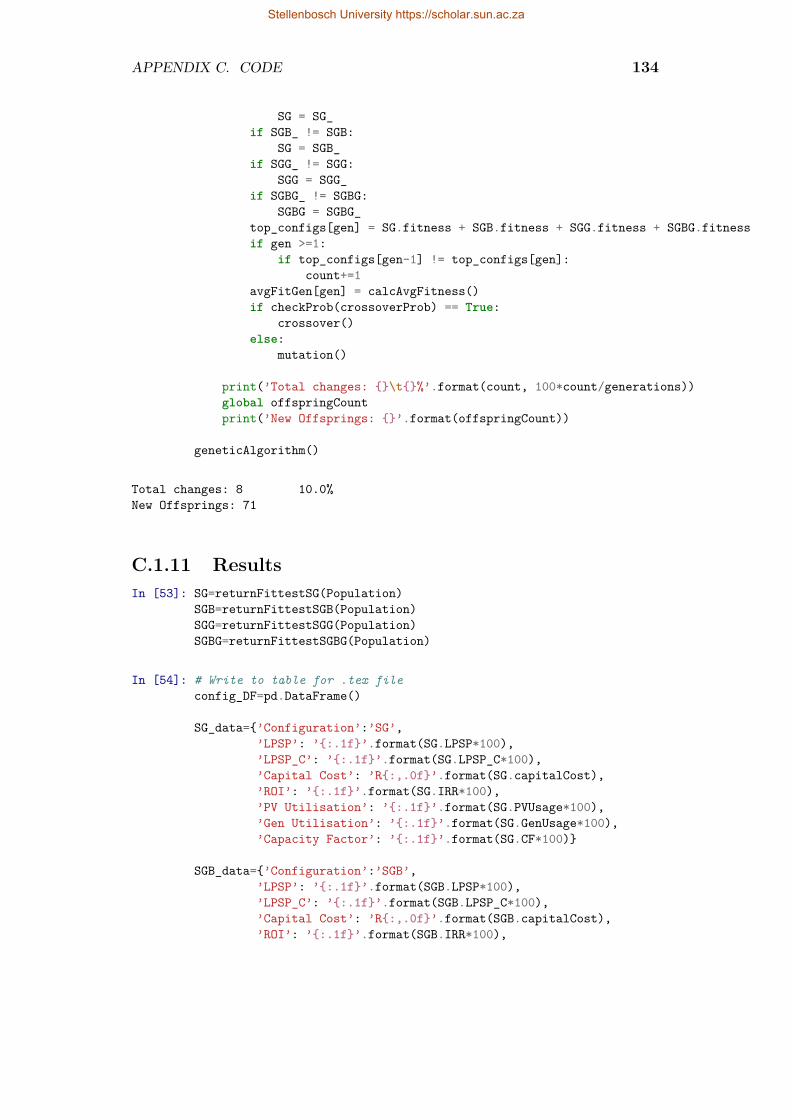
APPENDIX C. CODE 134
SG = SG_if SGB_ != SGB:
SG = SGB_if SGG_ != SGG:
SGG = SGG_if SGBG_ != SGBG:
SGBG = SGBG_top_configs[gen] = SG.fitness + SGB.fitness + SGG.fitness + SGBG.fitnessif gen >=1:
if top_configs[gen-1] != top_configs[gen]:count+=1
avgFitGen[gen] = calcAvgFitness()if checkProb(crossoverProb) == True:
crossover()else:
mutation()
print(’Total changes: {}\t{}%’.format(count, 100*count/generations))global offspringCountprint(’New Offsprings: {}’.format(offspringCount))
geneticAlgorithm()
Total changes: 8 10.0%New Offsprings: 71
C.1.11 ResultsIn [53]: SG=returnFittestSG(Population)
SGB=returnFittestSGB(Population)SGG=returnFittestSGG(Population)SGBG=returnFittestSGBG(Population)
In [54]: # Write to table for .tex fileconfig_DF=pd.DataFrame()
SG_data={’Configuration’:’SG’,’LPSP’: ’{:.1f}’.format(SG.LPSP*100),’LPSP_C’: ’{:.1f}’.format(SG.LPSP_C*100),’Capital Cost’: ’R{:,.0f}’.format(SG.capitalCost),’ROI’: ’{:.1f}’.format(SG.IRR*100),’PV Utilisation’: ’{:.1f}’.format(SG.PVUsage*100),’Gen Utilisation’: ’{:.1f}’.format(SG.GenUsage*100),’Capacity Factor’: ’{:.1f}’.format(SG.CF*100)}
SGB_data={’Configuration’:’SGB’,’LPSP’: ’{:.1f}’.format(SGB.LPSP*100),’LPSP_C’: ’{:.1f}’.format(SGB.LPSP_C*100),’Capital Cost’: ’R{:,.0f}’.format(SGB.capitalCost),’ROI’: ’{:.1f}’.format(SGB.IRR*100),
Stellenbosch University https://scholar.sun.ac.za
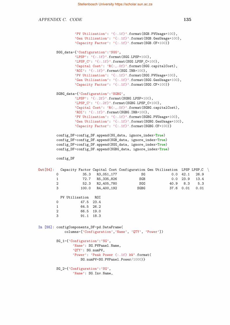
APPENDIX C. CODE 135
’PV Utilisation’: ’{:.1f}’.format(SGB.PVUsage*100),’Gen Utilisation’: ’{:.1f}’.format(SGB.GenUsage*100),’Capacity Factor’: ’{:.1f}’.format(SGB.CF*100)}
SGG_data={’Configuration’:’SGG’,’LPSP’: ’{:.1f}’.format(SGG.LPSP*100),’LPSP_C’: ’{:.1f}’.format(SGG.LPSP_C*100),’Capital Cost’: ’R{:,.0f}’.format(SGG.capitalCost),’ROI’: ’{:.1f}’.format(SGG.IRR*100),’PV Utilisation’: ’{:.1f}’.format(SGG.PVUsage*100),’Gen Utilisation’: ’{:.1f}’.format(SGG.GenUsage*100),’Capacity Factor’: ’{:.1f}’.format(SGG.CF*100)}
SGBG_data={’Configuration’:’SGBG’,’LPSP’: ’{:.2f}’.format(SGBG.LPSP*100),’LPSP_C’: ’{:.2f}’.format(SGBG.LPSP_C*100),’Capital Cost’: ’R{:,.0f}’.format(SGBG.capitalCost),’ROI’: ’{:.1f}’.format(SGBG.IRR*100),’PV Utilisation’: ’{:.1f}’.format(SGBG.PVUsage*100),’Gen Utilisation’: ’{:.1f}’.format(SGBG.GenUsage*100),’Capacity Factor’: ’{:.1f}’.format(SGBG.CF*100)}
config_DF=config_DF.append(SG_data, ignore_index=True)config_DF=config_DF.append(SGB_data, ignore_index=True)config_DF=config_DF.append(SGG_data, ignore_index=True)config_DF=config_DF.append(SGBG_data, ignore_index=True)
config_DF
Out[54]: Capacity Factor Capital Cost Configuration Gen Utilisation LPSP LPSP C \0 35.3 R3,051,177 SG 0.0 42.1 26.91 72.7 R5,335,826 SGB 0.0 23.9 13.42 52.3 R2,405,780 SGG 40.9 8.3 5.33 100.0 R4,400,192 SGBG 37.6 0.01 0.01
PV Utilisation ROI0 47.5 23.41 64.5 26.22 66.5 19.03 91.1 18.3
In [55]: configComponents_DF=pd.DataFrame(columns=[’Configuration’,’Name’, ’QTY’, ’Power’])
SG_1={’Configuration’:’SG’,’Name’: SG.PVPanel.Name,’QTY’: SG.numPV,’Power’: ’Peak Power {:.1f} kW’.format(
SG.numPV*SG.PVPanel.Power/1000)}
SG_2={’Configuration’:’SG’,’Name’: SG.Inv.Name,
Stellenbosch University https://scholar.sun.ac.za
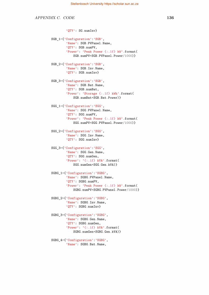
APPENDIX C. CODE 136
’QTY’: SG.numInv}
SGB_1={’Configuration’:’SGB’,’Name’: SGB.PVPanel.Name,’QTY’: SGB.numPV,’Power’: ’Peak Power {:.1f} kW’.format(
SGB.numPV*SGB.PVPanel.Power/1000)}
SGB_2={’Configuration’:’SGB’,’Name’: SGB.Inv.Name,’QTY’: SGB.numInv}
SGB_3={’Configuration’:’SGB’,’Name’: SGB.Bat.Name,’QTY’: SGB.numBat,’Power’: ’Storage {:.1f} kWh’.format(
SGB.numBat*SGB.Bat.Power)}
SGG_1={’Configuration’:’SGG’,’Name’: SGG.PVPanel.Name,’QTY’: SGG.numPV,’Power’: ’Peak Power {:.1f} kW’.format(
SGG.numPV*SGG.PVPanel.Power/1000)}
SGG_2={’Configuration’:’SGG’,’Name’: SGG.Inv.Name,’QTY’: SGG.numInv}
SGG_3={’Configuration’:’SGG’,’Name’: SGG.Gen.Name,’QTY’: SGG.numGen,’Power’: ’{:.1f} kVA’.format(
SGG.numGen*SGG.Gen.kVA)}
SGBG_1={’Configuration’:’SGBG’,’Name’: SGBG.PVPanel.Name,’QTY’: SGBG.numPV,’Power’: ’Peak Power {:.1f} kW’.format(
SGBG.numPV*SGBG.PVPanel.Power/1000)}
SGBG_2={’Configuration’:’SGBG’,’Name’: SGBG.Inv.Name,’QTY’: SGBG.numInv}
SGBG_3={’Configuration’:’SGBG’,’Name’: SGBG.Gen.Name,’QTY’: SGBG.numGen,’Power’: ’{:.1f} kVA’.format(
SGBG.numGen*SGBG.Gen.kVA)}
SGBG_4={’Configuration’:’SGBG’,’Name’: SGBG.Bat.Name,
Stellenbosch University https://scholar.sun.ac.za
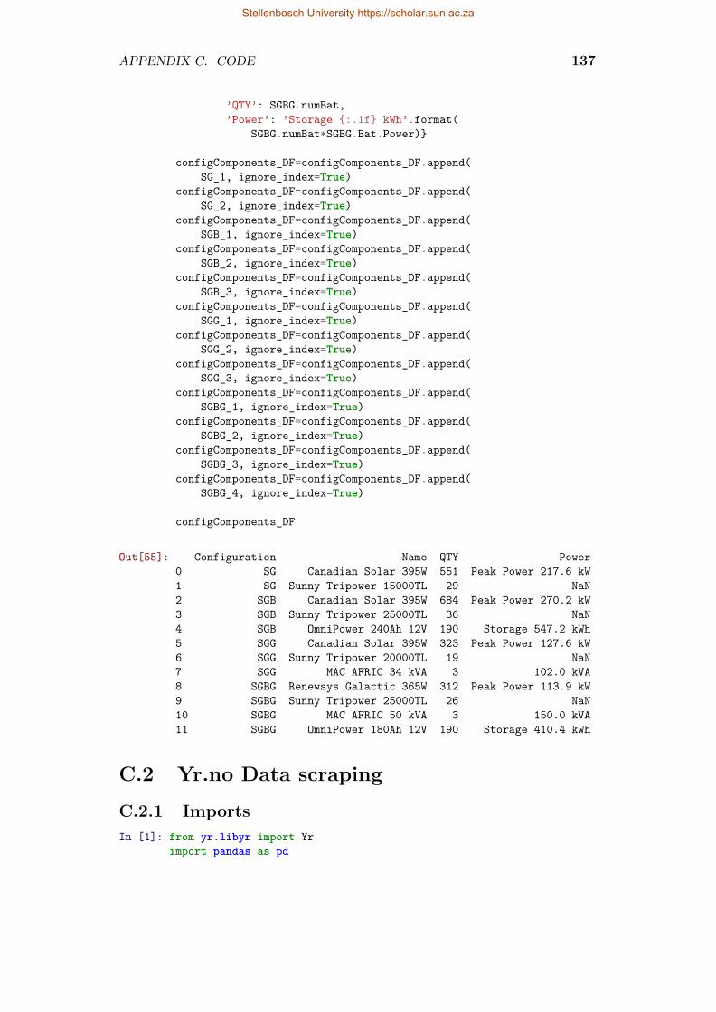
APPENDIX C. CODE 137
’QTY’: SGBG.numBat,’Power’: ’Storage {:.1f} kWh’.format(
SGBG.numBat*SGBG.Bat.Power)}
configComponents_DF=configComponents_DF.append(SG_1, ignore_index=True)
configComponents_DF=configComponents_DF.append(SG_2, ignore_index=True)
configComponents_DF=configComponents_DF.append(SGB_1, ignore_index=True)
configComponents_DF=configComponents_DF.append(SGB_2, ignore_index=True)
configComponents_DF=configComponents_DF.append(SGB_3, ignore_index=True)
configComponents_DF=configComponents_DF.append(SGG_1, ignore_index=True)
configComponents_DF=configComponents_DF.append(SGG_2, ignore_index=True)
configComponents_DF=configComponents_DF.append(SGG_3, ignore_index=True)
configComponents_DF=configComponents_DF.append(SGBG_1, ignore_index=True)
configComponents_DF=configComponents_DF.append(SGBG_2, ignore_index=True)
configComponents_DF=configComponents_DF.append(SGBG_3, ignore_index=True)
configComponents_DF=configComponents_DF.append(SGBG_4, ignore_index=True)
configComponents_DF
Out[55]: Configuration Name QTY Power0 SG Canadian Solar 395W 551 Peak Power 217.6 kW1 SG Sunny Tripower 15000TL 29 NaN2 SGB Canadian Solar 395W 684 Peak Power 270.2 kW3 SGB Sunny Tripower 25000TL 36 NaN4 SGB OmniPower 240Ah 12V 190 Storage 547.2 kWh5 SGG Canadian Solar 395W 323 Peak Power 127.6 kW6 SGG Sunny Tripower 20000TL 19 NaN7 SGG MAC AFRIC 34 kVA 3 102.0 kVA8 SGBG Renewsys Galactic 365W 312 Peak Power 113.9 kW9 SGBG Sunny Tripower 25000TL 26 NaN10 SGBG MAC AFRIC 50 kVA 3 150.0 kVA11 SGBG OmniPower 180Ah 12V 190 Storage 410.4 kWh
C.2 Yr.no Data scraping
C.2.1 ImportsIn [1]: from yr.libyr import Yr
import pandas as pd
Stellenbosch University https://scholar.sun.ac.za

APPENDIX C. CODE 138
import datetime as dtfrom time import sleepimport os
C.2.2 Site informationIn [2]: latitude=-33.9346
longitude=18.8668altitude=122file_path=’C:/Users/18296033/Documents/WORK/DataCollector/datapoints’
C.2.3 Clean dataIn [3]: def cleanUp (df, timestamp):
for index, row in df.iterrows():if row[’@from’] != row[’@to’]:
df=df.drop(index)
df[’@from’]=pd.to_datetime(df[’@from’])df[’@to’]=pd.to_datetime(df[’@to’])
df[’Timestamp’]=’’
for index, row in df.iterrows():if row[’@from’] < timestamp and row[’@from’].hour != timestamp.hour:
#print (row[’@from’], timestamp)df=df.drop(index)
else:value=str(timestamp.strftime(’%Y-%m-%d %H:%M’))df.at[index,’Timestamp’]=value
df=pd.concat([df.drop([’location’],axis=1),
df[’location’].apply(pd.Series)],axis=1)
df=pd.concat([df.drop([’temperature’],axis=1),
df[’temperature’].apply(pd.Series)],axis=1)
df=df.drop([’@id’,’@unit’],axis=1)
df=pd.concat([df.drop([’windDirection’],axis=1),
df[’windDirection’].apply(pd.Series)],axis=1)
df=df.drop([’@id’,’@name’],axis=1)
df=df.rename(index=str,columns={’@datatype’:’Datatype’,
’@from’:’From’,’@to’:’To’,’@altitude’:’Altitude’,
Stellenbosch University https://scholar.sun.ac.za
APPENDIX C. CODE 139
’@latitude’:’Latitude’,’@longitude’:’Longitude’,’@value’:’Temperature’,’@deg’:’Degrees’
})df=pd.concat([df.drop([’windSpeed’],
axis=1),df[’windSpeed’].apply(pd.Series)],
axis=1)df=df.drop([’@id’,’@name’,’@beaufort’],axis=1)df=df.rename(index=str,
columns={’@mps’:’Windspeed’})df=pd.concat([df.drop([’humidity’],
axis=1),df[’humidity’].apply(pd.Series)],
axis=1)df=df.drop([’@unit’],
axis=1)df=df.rename(index=str,
columns={’@value’:’Humidity’})df=pd.concat([df.drop([’pressure’],
axis=1),df[’pressure’].apply(pd.Series)],
axis=1)df=df.drop([’@unit’,’@id’],
axis=1)df=df.rename(index=str,
columns={’@value’:’Pressure’})df=pd.concat([df.drop([’cloudiness’],
axis=1),df[’cloudiness’].apply(pd.Series)],
axis=1)df=df.drop([’@id’],
axis=1)df=df.rename(index=str,
columns={’@percent’:’Clouds’})df=pd.concat([df.drop([’fog’],
axis=1),df[’fog’].apply(pd.Series)],
axis=1)df=df.drop([’@id’],
axis=1)df=df.rename(index=str,
columns={’@percent’:’Fog’})df=pd.concat([df.drop([’lowClouds’],
axis=1),df[’lowClouds’].apply(pd.Series)],
axis=1)df=df.drop([’@id’],
axis=1)df=df.rename(index=str,
columns={’@percent’:’Low Clouds’})
Stellenbosch University https://scholar.sun.ac.za
APPENDIX C. CODE 140
df=pd.concat([df.drop([’mediumClouds’],axis=1),
df[’mediumClouds’].apply(pd.Series)],axis=1)
df=df.drop([’@id’],axis=1)
df=df.rename(index=str,columns={’@percent’:’Medium Clouds’})
df=pd.concat([df.drop([’highClouds’],axis=1),
df[’highClouds’].apply(pd.Series)],axis=1)
df=df.drop([’@id’],axis=1)
df=df.rename(index=str,columns={’@percent’:’High Clouds’})
df=pd.concat([df.drop([’dewpointTemperature’],axis=1),
df[’dewpointTemperature’].apply(pd.Series)],axis=1)
df=df.drop([’@unit’,’@id’],axis=1)df=df.rename(index=str,
columns={’@value’:’Dew Temperature’})return df
C.2.4 Collect dataIn [ ]: while True:
time=dt.datetime.now()
if time.minute==0:weather = Yr(location_xyz=(longitude, latitude, altitude))df=pd.DataFrame.from_dict(weather.forecast())df=cleanUp(df,time)
#write to hourly csv filefile_name=str(time.strftime(’%d_%m_%y %Hh%Mm%S.csv’))path=os.path.join(file_path, file_name)df.to_csv(path)print(file_name,’saved’)
#update weatherdatabase csv filenewpath=’C:/Users/18296033/Documents/WORK/DataCollector’newfilename=’WeatherDataBase.csv’p=os.path.join(newpath, newfilename)oldDF=pd.read_csv(p)oldDF=oldDF.drop([’Unnamed: 0’], axis=1)oldDF=oldDF.append(df)os.remove(p)oldDF.to_csv(p)#sleep to the next hoursleep(3500)
Stellenbosch University https://scholar.sun.ac.za

APPENDIX C. CODE 141
C.3 Linear RegressionThis regression technique is developed from a workshop tutorial on a basicregression with Keras using TensorFlow [73].
C.3.1 ImportsIn [1]: import pandas as pd
import glob
import numpy as npimport os
import pvlibfrom pvlib.location import Location, solarposition
import tensorflow as tffrom tensorflow import kerasfrom tensorflow.keras import layers
import matplotlib.pyplot as plt
C.3.2 Graph Plot VariablesIn [2]: label = 20
ticklabel = 18
params = {’axes.labelsize’: label,’axes.titlesize’: label,’text.usetex’ : True,’font.size’: ticklabel,’legend.frameon’: True,’legend.fontsize’: ticklabel,’legend.loc’: ’center right’,’legend.framealpha’: 1,’xtick.labelsize’: ticklabel,’ytick.labelsize’: ticklabel,’grid.linestyle’ : ":",’axes.grid’: True,’axes.grid.which’: ’major’,’axes.grid’ : True,’grid.linewidth’ : 0.8,’keymap.grid’: [’g’],’keymap.grid_minor’: [’G’],’figure.figsize’: [18, 8]}
plt.rcParams.update(params)
Stellenbosch University https://scholar.sun.ac.za

APPENDIX C. CODE 142
C.3.3 Prediction DataIn [3]: tiltAngle=30
rho=0.2LTM=-30latitude=-33.9346longitude=18.8668altitude=122
loc=Location(latitude,longitude,’Africa/Johannesburg’,altitude,’Stellenbosch’)
In [4]: newpath=’C:/Users/18296033/Documents/WORK/DataCollector’all_files = glob.glob(path + "/*.csv")
li = pd.DataFrame()
for filename in all_files:df = pd.read_csv(filename, index_col=None, header=0)li=li.append(df)
In [5]: li = li.drop([’Altitude’, ’Latitude’,’Longitude’, ’Datatype’, ’To’], axis=1)
In [6]: li = li.drop([’0’, ’0.1’, ’0.2’, ’Unnamed: 0’], axis=1)
In [7]: df = li.copy()
df[’From’] = pd.to_datetime(df[’From’])df[’Timestamp’] = pd.to_datetime(df[’Timestamp’])
In [8]: result=df.sort_values(by=[’From’,’Timestamp’],ascending=[True, True])
In [9]: timestamp=result[result[’From’] == result[’Timestamp’]]
In [10]: df_Predictions = timestamp.copy()df_Predictions[’Date’] = df_Predictions[’From’]df_Predictions = df_Predictions.drop([’From’, ’Timestamp’], axis=1)
C.3.4 Normal sky dataIn [11]: df_Actual = pd.read_csv(’sb_thour.csv’)
df_Actual=df_Actual.drop([’Record’,’Date’,’Time’,
Stellenbosch University https://scholar.sun.ac.za
APPENDIX C. CODE 143
’UVA_Avg’,’UVB_Avg’,’Tracker2WM_Avg’,’WindDir_D1_WVT’,’WindDir_SD1_WVT’,’ShadowbandWM_Avg’,’AirTC_Max’,’DNICalc_Avg’,’BattV_Min’,’AirTC_Min’],
axis=1)
df_Actual=df_Actual.rename(index=str,columns={’SunWM_Avg’:’GHI’,
’RH’:’Humidity’,’AirTC_Avg’:’Temperature’,’WS_ms_S_WVT’:’Windspeed’,’BP_mB_Avg’:’Pressure’,’TrackerWM_Avg’:’DNI’,’ShadowWM_Avg’:’DHI’,’TimeStamp’:’Date’})
df_Actual[’Date’]=pd.to_datetime(df_Actual[’Date’])
df_Actual[’Month’]=pd.DatetimeIndex(df_Actual[’Date’]).monthdf_Actual[’Day’]=pd.DatetimeIndex(df_Actual[’Date’]).daydf_Actual[’Day of year’]=pd.DatetimeIndex(df_Actual[’Date’]).dayofyear
In [12]: df_Actual=df_Actual.reset_index(drop=True)df_Actual.shapeprint(df_Actual.shape)
(12349, 11)
In [13]: def getTotalIrradiance(GHI, DNI, DHI, timestamp):timestamp=pd.DatetimeIndex(timestamp)timestamp=timestamp.tz_localize(loc.tz)
model=’isotropic’
# Panel azimuth from Northsurface_azimuth=0
albedo=rho #surface albedo - declared in variables and constants
# convert to radianslatitudeRad=np.deg2rad(latitude)n=timestamp.dayofyear# Equation of timeeqOfTime=pvlib.solarposition.equation_of_time_pvcdrom(n)
Stellenbosch University https://scholar.sun.ac.za
APPENDIX C. CODE 144
# Hour anglehourangle=pvlib.solarposition.hour_angle(timestamp,
longitude,eqOfTime)
hourAngleRad=np.deg2rad(hourangle)
#Declination angle calculationsdeclinationRad=pvlib.solarposition.declination_cooper69(n)
solar_zenithRad=pvlib.solarposition.solar_zenith_analytical(latitudeRad,hourAngleRad,declinationRad)
#Solar azimuth angle calculationssolar_azimuthRad=pvlib.solarposition.solar_azimuth_analytical(latitudeRad,
hourAngleRad,declinationRad,solar_zenithRad)
#convert to degreessolar_azimuth = np.rad2deg(solar_azimuthRad)solar_zenith= np.rad2deg(solar_zenithRad)surface_tilt=tiltAngle# get total irradiancetotal=pvlib.irradiance.get_total_irradiance(surface_tilt=tiltAngle,
surface_azimuth=surface_azimuth,solar_zenith=solar_zenith,solar_azimuth=solar_azimuth,dni=DNI,ghi=GHI,dhi=DHI,albedo=albedo,model=model)
return total
total=getTotalIrradiance(df_Actual[’GHI’],df_Actual[’DNI’],df_Actual[’DHI’],pd.DatetimeIndex(df_Actual[’Date’]))
df_Actual[’Global Insolation’]=total[’poa_global’]df_Actual[’Direct Insolation’]=total[’poa_direct’]df_Actual[’Diffuse Insolation’]=total[’poa_diffuse’]df_Actual[’Sky Diffuse Insolation’]=total[’poa_sky_diffuse’]df_Actual[’Ground Insolation’]=total[’poa_ground_diffuse’]
C.3.4.1 Add previous hour to datasetIn [14]: for i in range(1, len(df_Actual)):
df_Actual.loc[i, ’Prev NS’] = df_Actual.loc[i-1,’Global Insolation’]
Stellenbosch University https://scholar.sun.ac.za
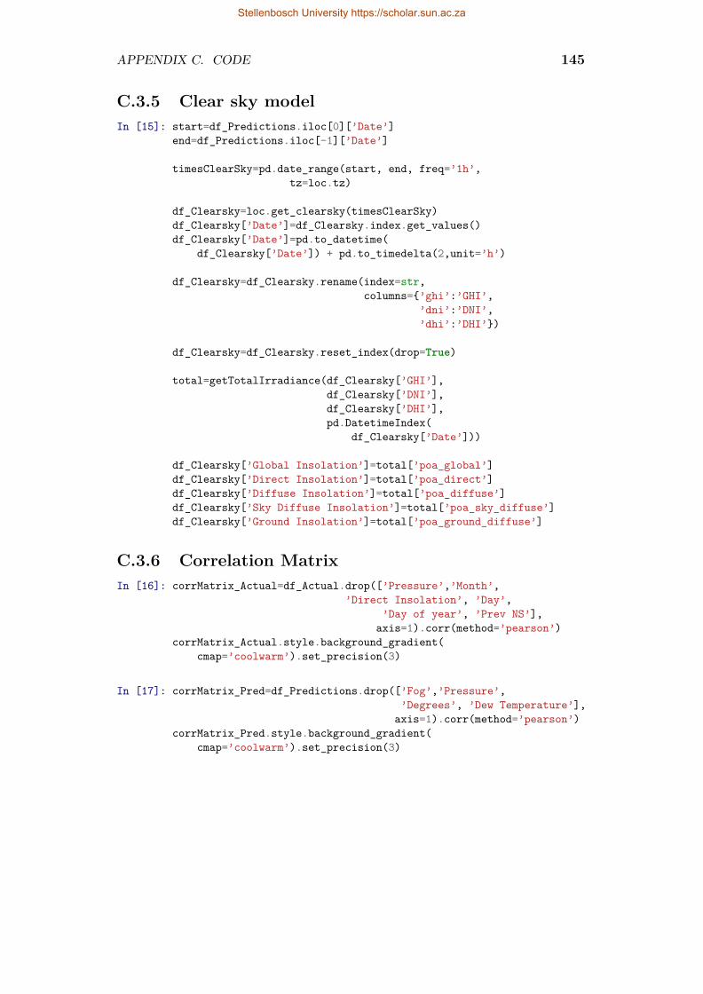
APPENDIX C. CODE 145
C.3.5 Clear sky modelIn [15]: start=df_Predictions.iloc[0][’Date’]
end=df_Predictions.iloc[-1][’Date’]
timesClearSky=pd.date_range(start, end, freq=’1h’,tz=loc.tz)
df_Clearsky=loc.get_clearsky(timesClearSky)df_Clearsky[’Date’]=df_Clearsky.index.get_values()df_Clearsky[’Date’]=pd.to_datetime(
df_Clearsky[’Date’]) + pd.to_timedelta(2,unit=’h’)
df_Clearsky=df_Clearsky.rename(index=str,columns={’ghi’:’GHI’,
’dni’:’DNI’,’dhi’:’DHI’})
df_Clearsky=df_Clearsky.reset_index(drop=True)
total=getTotalIrradiance(df_Clearsky[’GHI’],df_Clearsky[’DNI’],df_Clearsky[’DHI’],pd.DatetimeIndex(
df_Clearsky[’Date’]))
df_Clearsky[’Global Insolation’]=total[’poa_global’]df_Clearsky[’Direct Insolation’]=total[’poa_direct’]df_Clearsky[’Diffuse Insolation’]=total[’poa_diffuse’]df_Clearsky[’Sky Diffuse Insolation’]=total[’poa_sky_diffuse’]df_Clearsky[’Ground Insolation’]=total[’poa_ground_diffuse’]
C.3.6 Correlation MatrixIn [16]: corrMatrix_Actual=df_Actual.drop([’Pressure’,’Month’,
’Direct Insolation’, ’Day’,’Day of year’, ’Prev NS’],
axis=1).corr(method=’pearson’)corrMatrix_Actual.style.background_gradient(
cmap=’coolwarm’).set_precision(3)
In [17]: corrMatrix_Pred=df_Predictions.drop([’Fog’,’Pressure’,’Degrees’, ’Dew Temperature’],
axis=1).corr(method=’pearson’)corrMatrix_Pred.style.background_gradient(
cmap=’coolwarm’).set_precision(3)
Stellenbosch University https://scholar.sun.ac.za
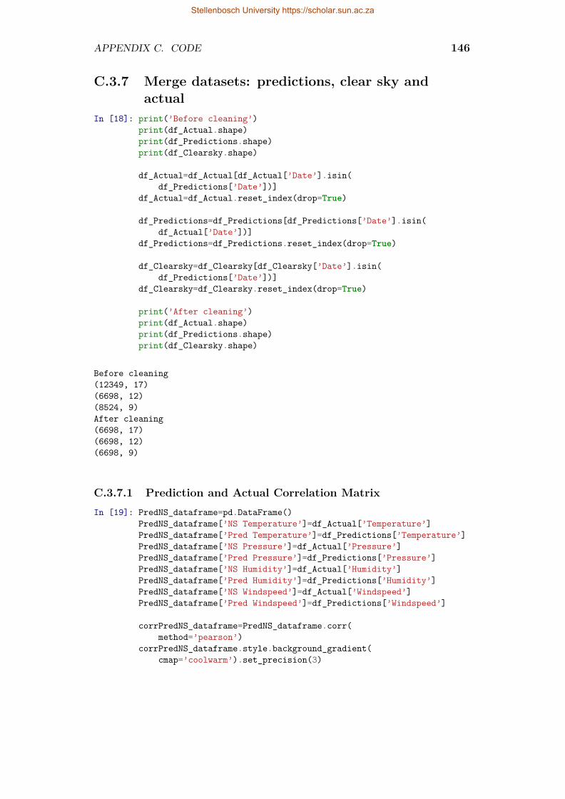
APPENDIX C. CODE 146
C.3.7 Merge datasets: predictions, clear sky andactual
In [18]: print(’Before cleaning’)print(df_Actual.shape)print(df_Predictions.shape)print(df_Clearsky.shape)
df_Actual=df_Actual[df_Actual[’Date’].isin(df_Predictions[’Date’])]
df_Actual=df_Actual.reset_index(drop=True)
df_Predictions=df_Predictions[df_Predictions[’Date’].isin(df_Actual[’Date’])]
df_Predictions=df_Predictions.reset_index(drop=True)
df_Clearsky=df_Clearsky[df_Clearsky[’Date’].isin(df_Predictions[’Date’])]
df_Clearsky=df_Clearsky.reset_index(drop=True)
print(’After cleaning’)print(df_Actual.shape)print(df_Predictions.shape)print(df_Clearsky.shape)
Before cleaning(12349, 17)(6698, 12)(8524, 9)After cleaning(6698, 17)(6698, 12)(6698, 9)
C.3.7.1 Prediction and Actual Correlation MatrixIn [19]: PredNS_dataframe=pd.DataFrame()
PredNS_dataframe[’NS Temperature’]=df_Actual[’Temperature’]PredNS_dataframe[’Pred Temperature’]=df_Predictions[’Temperature’]PredNS_dataframe[’NS Pressure’]=df_Actual[’Pressure’]PredNS_dataframe[’Pred Pressure’]=df_Predictions[’Pressure’]PredNS_dataframe[’NS Humidity’]=df_Actual[’Humidity’]PredNS_dataframe[’Pred Humidity’]=df_Predictions[’Humidity’]PredNS_dataframe[’NS Windspeed’]=df_Actual[’Windspeed’]PredNS_dataframe[’Pred Windspeed’]=df_Predictions[’Windspeed’]
corrPredNS_dataframe=PredNS_dataframe.corr(method=’pearson’)
corrPredNS_dataframe.style.background_gradient(cmap=’coolwarm’).set_precision(3)
Stellenbosch University https://scholar.sun.ac.za

APPENDIX C. CODE 147
C.3.8 Linear regression datasetIn [20]: raw_dataset=pd.DataFrame()
raw_dataset[’Month’]=pd.DatetimeIndex(df_Actual[’Date’]).monthraw_dataset[’Hour’]=pd.DatetimeIndex(df_Actual[’Date’]).hour
#--------------PREDICTIONS--------------#raw_dataset[’Temperature’]=df_Predictions[’Temperature’]raw_dataset[’Windspeed’]=df_Predictions[’Windspeed’]raw_dataset[’Clouds’]=df_Predictions[’Clouds’]raw_dataset[’Low Clouds’]=df_Predictions[’Low Clouds’]raw_dataset[’Medium Clouds’]=df_Predictions[’Medium Clouds’]raw_dataset[’High Clouds’]=df_Predictions[’High Clouds’]
#--------------CLEAR SKY--------------#raw_dataset[’CS Global Insolation’]=df_Clearsky[’Global Insolation’]
#--------------NORMAL SKY--------------#raw_dataset[’NS Global Insolation’]=df_Actual[’Global Insolation’]
raw_dataset.head()
In [21]: corrDS=raw_dataset.drop([’Month’, ’Hour’], axis=1).corr(method=’pearson’)corrDS.style.background_gradient(cmap=’coolwarm’).set_precision(3)
C.3.9 Linear Regression to predict solar insolationIn [22]: train_dataset = raw_dataset.sample(frac=0.8,random_state=0)
test_dataset = raw_dataset.drop(train_dataset.index)
In [23]: train_stats=train_dataset.describe()train_stats=train_stats.pop(’NS Global Insolation’)train_stats=train_stats.transpose()train_stats
Out[23]: count 5358.000000mean 220.774023std 324.473200min 0.00000025% 0.00000050% 3.89188875% 397.557098max 1097.628984Name: NS Global Insolation, dtype: float64
In [24]: train_labels=train_dataset.pop(’NS Global Insolation’)test_labels=test_dataset.pop(’NS Global Insolation’)
In [25]: def norm(x):return (x - train_stats[’mean’])/train_stats[’std’]
Stellenbosch University https://scholar.sun.ac.za
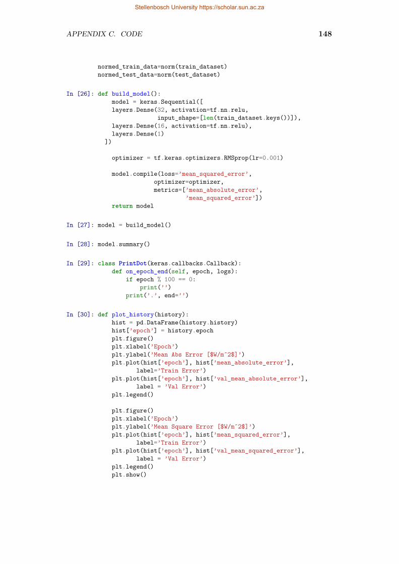
APPENDIX C. CODE 148
normed_train_data=norm(train_dataset)normed_test_data=norm(test_dataset)
In [26]: def build_model():model = keras.Sequential([layers.Dense(32, activation=tf.nn.relu,
input_shape=[len(train_dataset.keys())]),layers.Dense(16, activation=tf.nn.relu),layers.Dense(1)
])
optimizer = tf.keras.optimizers.RMSprop(lr=0.001)
model.compile(loss=’mean_squared_error’,optimizer=optimizer,metrics=[’mean_absolute_error’,
’mean_squared_error’])return model
In [27]: model = build_model()
In [28]: model.summary()
In [29]: class PrintDot(keras.callbacks.Callback):def on_epoch_end(self, epoch, logs):
if epoch % 100 == 0:print(’’)
print(’.’, end=’’)
In [30]: def plot_history(history):hist = pd.DataFrame(history.history)hist[’epoch’] = history.epochplt.figure()plt.xlabel(’Epoch’)plt.ylabel(’Mean Abs Error [$W/mˆ2$]’)plt.plot(hist[’epoch’], hist[’mean_absolute_error’],
label=’Train Error’)plt.plot(hist[’epoch’], hist[’val_mean_absolute_error’],
label = ’Val Error’)plt.legend()
plt.figure()plt.xlabel(’Epoch’)plt.ylabel(’Mean Square Error [$W/mˆ2$]’)plt.plot(hist[’epoch’], hist[’mean_squared_error’],
label=’Train Error’)plt.plot(hist[’epoch’], hist[’val_mean_squared_error’],
label = ’Val Error’)plt.legend()plt.show()
Stellenbosch University https://scholar.sun.ac.za
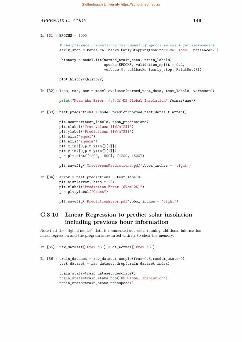
APPENDIX C. CODE 149
In [31]: EPOCHS = 1000
# The patience parameter is the amount of epochs to check for improvementearly_stop = keras.callbacks.EarlyStopping(monitor=’val_loss’, patience=20)
history = model.fit(normed_train_data, train_labels,epochs=EPOCHS, validation_split = 0.2,verbose=0, callbacks=[early_stop, PrintDot()])
plot_history(history)
In [32]: loss, mae, mse = model.evaluate(normed_test_data, test_labels, verbose=0)
print("Mean Abs Error: {:5.2f}NS Global Insolation".format(mae))
In [33]: test_predictions = model.predict(normed_test_data).flatten()
plt.scatter(test_labels, test_predictions)plt.xlabel(’True Values [$W/mˆ2$]’)plt.ylabel(’Predictions [$W/mˆ2$]’)plt.axis(’equal’)plt.axis(’square’)plt.xlim([0,plt.xlim()[1]])plt.ylim([0,plt.ylim()[1]])_ = plt.plot([-200, 1500], [-200, 1500])
plt.savefig(’TrueVersusPredictions.pdf’,bbox_inches = ’tight’)
In [34]: error = test_predictions - test_labelsplt.hist(error, bins = 25)plt.xlabel("Prediction Error [$W/mˆ2$]")_ = plt.ylabel("Count")
plt.savefig(’PredictionError.pdf’,bbox_inches = ’tight’)
C.3.10 Linear Regression to predict solar insolationincluding previous hour information
Note that the original model’s data is commented out when running additional informationlinear regression and the program is restarted entirely to clear the memory.
In [35]: raw_dataset[’Prev NS’] = df_Actual[’Prev NS’]
In [36]: train_dataset = raw_dataset.sample(frac=0.8,random_state=0)test_dataset = raw_dataset.drop(train_dataset.index)
train_stats=train_dataset.describe()train_stats=train_stats.pop(’NS Global Insolation’)train_stats=train_stats.transpose()
Stellenbosch University https://scholar.sun.ac.za
APPENDIX C. CODE 150
train_labels=train_dataset.pop(’NS Global Insolation’)test_labels=test_dataset.pop(’NS Global Insolation’)
normed_train_data=norm(train_dataset)normed_test_data=norm(test_dataset)
In [37]: def build_model2():model = keras.Sequential([layers.Dense(32, activation=tf.nn.relu,
input_shape=[len(train_dataset.keys())]),layers.Dense(16, activation=tf.nn.relu),layers.Dense(1)
])
optimizer = tf.keras.optimizers.RMSprop(lr=0.001)
model.compile(loss=’mean_squared_error’,optimizer=optimizer,metrics=[’mean_absolute_error’,
’mean_squared_error’])return model
model2 = build_model2()model2.summary()
In [38]: EPOCHS = 1000
early_stop = keras.callbacks.EarlyStopping(monitor=’val_loss’,patience=20)
history = model2.fit(normed_train_data, train_labels,epochs=EPOCHS, validation_split = 0.2,verbose=0, callbacks=[early_stop, PrintDot()])
plot_history(history)
In [39]: loss, mae, mse = model2.evaluate(normed_test_data, test_labels, verbose=0)
print("Mean Abs Error: {:5.2f}NS Global Insolation".format(mae))
In [40]: test_predictions = model2.predict(normed_test_data).flatten()
plt.scatter(test_labels, test_predictions)plt.xlabel(’True Values [$W/mˆ2$]’)plt.ylabel(’Predictions [$W/mˆ2$]’)plt.axis(’equal’)plt.axis(’square’)plt.xlim([0,plt.xlim()[1]])plt.ylim([0,plt.ylim()[1]])_ = plt.plot([-200, 1500], [-200, 1500])
Stellenbosch University https://scholar.sun.ac.za

APPENDIX C. CODE 151
plt.savefig(’TrueVersusPredictions_Extra.pdf’,bbox_inches = ’tight’)
In [41]: error = test_predictions - test_labelsplt.hist(error, bins = 25)plt.xlabel("Prediction Error [$W/mˆ2$]")_ = plt.ylabel("Count")
plt.savefig(’PredictionError_Extra.pdf’,bbox_inches = ’tight’)
C.4 Reinforcement Learning
C.4.1 ImportsIn [1]: import warnings
warnings.filterwarnings(’ignore’)
import pandas as pdimport datetime as dtimport matplotlib.pyplot as pltfrom time import sleepimport osfrom yr.libyr import Yrimport pvlibfrom pvlib.location import Location, solarpositionimport mathimport pytzimport numpy as npimport random#Variables and constantstiltAngle=30rho=0.2LTM=-30latitude=-33.9346longitude=18.8668altitude=122
import tensorflow as tffrom tensorflow import kerasfrom tensorflow.keras import layersfrom tensorflow.keras.models import load_model# print(tf.__version__)
loc=Location(latitude,longitude,’Africa/Johannesburg’,altitude,’Stellenbosch’)
np.random.seed(30)
Stellenbosch University https://scholar.sun.ac.za
APPENDIX C. CODE 152
In [2]: label = 20ticklabel = 18
params = {’axes.labelsize’: label,’axes.titlesize’: label,’text.usetex’ : True,’font.size’: ticklabel,’legend.frameon’: True,’legend.fontsize’: ticklabel,’legend.loc’: ’center right’,’legend.framealpha’: 1,’xtick.labelsize’: ticklabel,’ytick.labelsize’: ticklabel,’grid.linestyle’ : ":",’axes.grid’: True,’axes.grid.which’: ’major’,’axes.grid’ : True,’grid.linewidth’ : 0.8,’keymap.grid’: [’g’],’keymap.grid_minor’: [’G’],’figure.figsize’: [18, 8]}
plt.rcParams.update(params)
In [3]: random.seed(30)
C.4.2 Time intervalsIn [4]: interval = 15
C.4.3 Results of GA designC.4.3.1 SGBGIn [5]: # PV
PV_capacity = 10.6 #kW peakefficiency_PV = 16.99/100numPV = 29PV_area = 1.96 * 0.991
# GridGrid_hourly = 1.2 #kWh per hour
# BatteryDOD = 0.5Battery_capacity = 49 # kWhfully_charged_kWh = Battery_capacity*DOD # kWhinitial_charge = fully_charged_kWhMax_Discharge_kWh = 0.08 # kWh per minutenumBat = 15
Stellenbosch University https://scholar.sun.ac.za

APPENDIX C. CODE 153
# Generatorgen_kWh = 5 # kWh per hour
# Time intervalsgrid_interval = Grid_hourly*(interval/60)gen_interval = gen_kWh*(interval/60)
C.4.4 Data PreprocessingIn [6]: LoadDataPoints=pd.read_table(’LoadProfileHousehold.csv’,
sep=’;’ )
LoadDataPoints=LoadDataPoints.rename(index=str,columns={’Time’:’Date’,
’Sum [kWh]’:’Load’})
LoadDataPoints[’Date’]=pd.to_datetime(LoadDataPoints[’Date’])
LoadDataPoints=LoadDataPoints.drop([’Electricity.Timestep’],axis=1)
In [7]: LTM=-30latitude=-33.9346longitude=18.8668altitude=122
#Locationloc=Location(latitude,
longitude,’Africa/Johannesburg’,altitude,’Stellenbosch’)
#PV setuptiltAngle=30rho=0.2
def getTotalIrradiance(GHI, DNI, DHI, timestamp):timestamp=pd.DatetimeIndex(timestamp)timestamp=timestamp.tz_localize(loc.tz)model=’isotropic’surface_azimuth=0albedo=rholatitudeRad=np.deg2rad(latitude)n=timestamp.dayofyeareqOfTime=pvlib.solarposition.equation_of_time_pvcdrom(n)hourangle=pvlib.solarposition.hour_angle(timestamp,
longitude,eqOfTime)
hourAngleRad=np.deg2rad(hourangle)declinationRad=pvlib.solarposition.declination_cooper69(
n)
Stellenbosch University https://scholar.sun.ac.za

APPENDIX C. CODE 154
solar_zenithRad=pvlib.solarposition.solar_zenith_analytical(latitudeRad, hourAngleRad, declinationRad)
solar_azimuthRad=pvlib.solarposition.solar_azimuth_analytical(latitudeRad, hourAngleRad, declinationRad,solar_zenithRad)
solar_azimuth = np.rad2deg(solar_azimuthRad)solar_zenith= np.rad2deg(solar_zenithRad)surface_tilt=tiltAngletotal=pvlib.irradiance.get_total_irradiance(
surface_tilt=tiltAngle,surface_azimuth=surface_azimuth,solar_zenith=solar_zenith,solar_azimuth=solar_azimuth,dni=DNI,ghi=GHI,dhi=DHI,albedo=albedo,model=model)
return total
def calcPVPower(insolation):kWh=insolation*efficiency_PV*PV_area*numPV/1000return kWh/60
In [8]: normalSkyDatapoints = pd.read_table(’minutelyWeatherData.csv’,sep=’,’ )
normalSkyDatapoints.head()
normalSkyDatapoints = normalSkyDatapoints.drop([’Record’, ’Date’, ’Time’,’UVA_Avg’, ’UVB_Avg’, ’Tracker2WM_Avg’,’WindDir_D1_WVT’, ’WindDir_SD1_WVT’,’ShadowbandWM_Avg’, ’RH’,’AirTC_Avg’,’WS_ms_S_WVT’, ’BP_mB_Avg’, ’DNICalc_Avg’],
axis = 1)
normalSkyDatapoints=normalSkyDatapoints.rename(index = str,columns = {’SunWM_Avg’:’GHI’,
’TrackerWM_Avg’:’DNI’,’ShadowWM_Avg’:’DHI’,’TimeStamp’:’Date’})
normalSkyDatapoints[’Date’] = pd.to_datetime(normalSkyDatapoints[’Date’])
normalSkyDatapoints = normalSkyDatapoints.reset_index(drop=True)
start = normalSkyDatapoints.iloc[0][’Date’]
Stellenbosch University https://scholar.sun.ac.za

APPENDIX C. CODE 155
end = normalSkyDatapoints.iloc[-1][’Date’]
normalSky = pd.DataFrame()
normalSky[’Date’] = pd.date_range(start, end, freq=’min’)
normalSkyDF = pd.merge(normalSkyDatapoints, normalSky,on = ’Date’, how = ’outer’)
normalSkyDF.shape
normalSkyDF = normalSkyDF.sort_values(by=[’Date’])normalSkyDF = normalSkyDF.fillna(method=’ffill’)
total = getTotalIrradiance(normalSkyDatapoints[’GHI’],normalSkyDatapoints[’DNI’],normalSkyDatapoints[’DHI’],pd.DatetimeIndex(normalSkyDatapoints[’Date’]))
normalSkyDF[’Global Insolation’] = total[’poa_global’]
#kWh for every minutenormalSkyDF[’PV Power’] = calcPVPower(
normalSkyDF[’Global Insolation’])
In [9]: df=pd.merge(LoadDataPoints,normalSkyDF, on=[’Date’])
df[’Date’]=pd.to_datetime(df[’Date’])
df=df.drop([’DNI’, ’DHI’, ’GHI’, ’Global Insolation’],axis=1)
In [10]: df = df.set_index(’Date’)
df = df.resample(’15T’).sum()
df = df.reset_index()
In [11]: df[’HourOfDay’] = df[’Date’].dt.hourdf[’Month’] = df[’Date’].dt.month
df[’Battery’] = pd.Series(np.zeros(df.shape[0]))df[’Generator’] = pd.Series(np.zeros(df.shape[0]))
df[’DayofWeek’] = df[’Date’].dt.weekday
df[’Weekday’] =df[’DayofWeek’].apply(lambda x: 1 if x <= 4 else 0)
Stellenbosch University https://scholar.sun.ac.za
APPENDIX C. CODE 156
In [12]: df[’Month’] = pd.Categorical(df[’Month’])df[’Month’] = df.Month.cat.codes
df[’HourOfDay’] = pd.Categorical(df[’HourOfDay’])df[’HourOfDay’] = df.HourOfDay.cat.codes
df[’Weekday’] = pd.Categorical(df[’Weekday’])df[’Weekday’] = df.Weekday.cat.codes
In [13]: df = df.drop([’DayofWeek’], axis=1)
In [14]: df.tail()
In [15]: for i in range(0, len(df)-1):df.loc[i, ’Next PV’] = df.loc[i+1, ’PV Power’]df.loc[i, ’Next Load’] = df.loc[i+1, ’Load’]
C.4.5 Train, validate and test setsIn [16]: df_train_set = pd.DataFrame()
df_valid_set = pd.DataFrame()df_test_set = pd.DataFrame()
for j in range (1,13):year = 2018month = jtrain_day_start = 1train_day_end = 22valid_day_start = 23valid_day_end = 26test_start = 27test_end = 0
days_31 = [1, 3, 5, 7, 8, 10, 12]days_30 = [4, 6, 9, 11]
# Februaryif j == 2: # watch out for February
test_end = 28# 31: January, March, May, July, Aug, Oct, Decif j in days_31:
test_end = 31if j in days_30:
test_end = 30
# TRAIN DATA SEGMENTstart_date = pd.Timestamp(year=year, month=month,
day=train_day_start,hour = 0, minute = 0,second = 0)
end_date = pd.Timestamp(year=year, month=month,
Stellenbosch University https://scholar.sun.ac.za

APPENDIX C. CODE 157
day=train_day_end, hour = 23,minute = 59, second = 59)
dti = pd.date_range(start = start_date,end = end_date, freq=’15T’)
df_train_set = df_train_set.append(df.loc[df.Date.isin(pd.DatetimeIndex(dti))])
# VALID DATA SEGMENTstart_date = pd.Timestamp(year=year, month=month,
day=valid_day_start,hour = 0, minute = 0,second = 0)
end_date = pd.Timestamp(year=year, month=month,day=valid_day_end, hour = 23,minute = 59, second = 59)
dti = pd.date_range(start = start_date,end = end_date, freq=’15T’)
df_valid_set = df_valid_set.append(df.loc[df.Date.isin(pd.DatetimeIndex(dti))])
# TEST DATA SEGMENTstart_date = pd.Timestamp(year=year, month=month,
day=test_start, hour = 0,minute = 0, second = 0)
end_date = pd.Timestamp(year=year, month=month,day=test_end, hour = 23,minute = 59, second = 59)
dti = pd.date_range(start = start_date,end = end_date, freq=’15T’)
df_test_set = df_test_set.append(df.loc[df.Date.isin(pd.DatetimeIndex(dti))])
In [17]: df_train_set = df_train_set.drop([’Date’], axis=1)df_valid_set = df_valid_set.drop([’Date’], axis=1)df_test_set = df_test_set.drop([’Date’], axis=1)
In [18]: df_train_set.to_csv(’RL Train.csv’)df_valid_set.to_csv(’RL Valid.csv’)df_test_set.to_csv(’RL Test.csv’)
In [19]: # df_train_set = pd.read_csv(’RL Train.csv’)# df_train_set = df_train_set.drop([’Unnamed: 0’], axis=1)
# df_valid_set = pd.read_csv(’RL Valid.csv’)# df_valid_set = df_valid_set.drop([’Unnamed: 0’], axis=1)
# df_test_set = pd.read_csv(’RL Test.csv’)# df_test_set = df_test_set.drop([’Unnamed: 0’], axis=1)
Stellenbosch University https://scholar.sun.ac.za

APPENDIX C. CODE 158
In [20]: # print(’Train:\t\t{0}\t{1:.1f}%’.format(# df_train_set.shape[0],# 100*df_train_set.shape[0]/df.shape[0]))# print(’Validate:\t{0}\t{1:.1f}%’.format(# df_valid_set.shape[0],# 100*df_valid_set.shape[0]/df.shape[0]))# print(’Test:\t\t{0}\t{1:.1f}%’.format(# df_test_set.shape[0],# 100*df_test_set.shape[0]/df.shape[0]))
C.4.6 Actions and state spaceIn [21]: action_perm = {’use_pv’: {True, False},
’charge_bat’: {True, False},’discharge_bat’: {True, False},’use_grid’: {True, False},’switch_on_Gen’: {True, False}}
# remove actions charge + discharge == Trueimport itertoolsl = [’T’, ’F’]actions_all = [list(i) for i in itertools.product(l, repeat=5)]
remove_ = 8
te = 0
while True:for i in range (0, len(actions_all)):
if actions_all[i][1] == ’T’ and actions_all[i][2] == ’T’:actions_all.remove(actions_all[i])te += 1break
if te == remove_:break
actions = []for i in range (0, len(actions_all)):
actions.append(actions_all[i][0] + actions_all[i][1] \+ actions_all[i][2]+ actions_all[i][3] \+ actions_all[i][4])
In [22]: #define episodeenvironment = {’pv_power’: None,
’load’: None,’month’: None,’hour_of_day’: None,’battery’: None,’generator’: None,’weekday’: None}
In [23]: train_set = df_train_set.as_matrix()
Stellenbosch University https://scholar.sun.ac.za

APPENDIX C. CODE 159
valid_set = df_valid_set.as_matrix()test_set = df_test_set.as_matrix()
C.4.7 Controller variablesIn [24]: num_actions=len(actions)
In [25]: num_states = 7
In [26]: def step(action, t, prev_state, data):
next_state = None
action = list(action)use_pv = action[0]charge_bat = action[1]discharge_bat = action[2]use_grid = action[3]use_gen = action[4]
# Load and PV for the time stepPV = data[t][7]load = data[t][8]
# Where the battery and generator are startingbat = prev_state[4]gen = prev_state[5]
bat_before = bat
grid = grid_interval # kWhLPS = load #100%maxGen = gen_interval #kWh
PV_Use = 0Gen_Use = 0Grid_Use = 0Bat_Use = 0availablePV = 0availableGrid = 0availableGen = 0
############################# Use PV Actionif use_pv == ’T’:
availablePV = PVif availablePV > load:
PV_Use += LPSavailablePV -= LPSLPS = 0
else:
Stellenbosch University https://scholar.sun.ac.za
APPENDIX C. CODE 160
LPS -= availablePVPV_Use += availablePVavailablePV = 0
############################# Discharge Battery Actionif discharge_bat == ’T’:
if LPS > 0:if LPS < bat:
bat -= LPSBat_Use += LPSLPS = 0
else:LPS -=batBat_Use += batbat = 0
############################# Use Grid Actionif use_grid == ’T’:
availableGrid = gridif LPS > 0:
if LPS < availableGrid:availableGrid -= LPSGrid_Use += LPSLPS = 0
else:LPS -= availableGridGrid_Use += availableGridavailableGrid = 0
############################# Use Generator Actionif use_gen == ’T’:
availableGen = maxGenif gen < (15/interval):
availableGen = 0.2*availableGenif LPS > 0:
if LPS < availableGen:availableGen -= LPSGen_Use += LPSLPS = 0
else:LPS -= availableGenGrid_Use += availableGenavailableGen = 0
############################# Charge batteries Action#maxC = MaxCharge_kWhif charge_bat == ’T’:
if use_pv == ’T’:if bat+availablePV > fully_charged_kWh:
PV_Use += fully_charged_kWh - batbat = fully_charged_kWh
else:
Stellenbosch University https://scholar.sun.ac.za
APPENDIX C. CODE 161
bat += availablePVPV_Use += availablePV
if use_grid == ’T’:if bat+availableGrid > fully_charged_kWh:
Grid_Use += fully_charged_kWh - batbat = fully_charged_kWh
else:bat += availableGridGrid_Use += availableGrid
if use_gen == ’T’:if bat+availableGen > fully_charged_kWh:
Gen_Use += fully_charged_kWh - batbat = fully_charged_kWh
else:bat += availableGenPV_Use += availableGen
############################battery_charged = bat - bat_beforebattery_charged = max(0, battery_charged)
# Rewardsreward = 0reward = reward + int(LPS <= 0)*20reward = reward + int(PV_Use == PV and use_pv == ’T’)*6reward = reward + int(PV_Use > 0)*6reward = reward + int(use_gen == ’T’ and PV == 0)*3reward = reward + int(Bat_Use > 0 and PV == 0)*6
if use_gen == ’F’:gen = 0 # switch off generator
else:gen += 1
used_energy = PV_Use + Grid_Use + Gen_Use + Bat_Usenet_energy = load - used_energy - LPS + battery_chargedLPS = max(0, LPS)
# THE NEXT STATEnext_state = [data[t][8],
data[t][7],data[t][2],data[t][3],bat,gen,data[t][6]]
if t+1 == len(data):next_state = None
return next_state, reward, t+2 == len(data), LPS, PV_Use, Gen_Use, Grid_Use, Bat_Use, battery_charged, None
Stellenbosch University https://scholar.sun.ac.za
APPENDIX C. CODE 162
In [27]: # number of episodesnum_episodes = 50
C.4.8 TrainingIn [28]: memory = []
max_memory = int(2*len(train_set))
def sampleMemory(batch_size):if batch_size > len(memory):
return random.sample(memory,(len(memory)))
else:return random.sample(memory,
batch_size)
def addSampleMemory(memorySample):memory.append(memorySample)if len(memory) > max_memory:
memory.pop(0)
In [29]: max_epsilon = 1min_epsilon = 0.01
Lambda = 0.001gamma = 0.7
batch_hours = 3batch_size = int((60/interval)*batch_hours)
In [30]: def build_model():model = keras.Sequential([layers.Dense(32, activation=tf.nn.relu,
input_shape=(num_states,)),layers.Dense(32, activation=tf.nn.relu),layers.Dense(32, activation=tf.nn.relu),layers.Dense(num_actions)
])
return model
In [31]: model = build_model()
model.compile(loss=’mse’,optimizer=tf.keras.optimizers.Adam(
lr=Lambda))
print(model.summary())
Stellenbosch University https://scholar.sun.ac.za

APPENDIX C. CODE 163
In [32]: total_LPS = np.zeros(num_episodes)total_rewards = np.zeros(num_episodes)total_PV = np.zeros(num_episodes)total_Gen = np.zeros(num_episodes)total_Grid = np.zeros(num_episodes)total_BatU = np.zeros(num_episodes)total_BatC = np.zeros(num_episodes)
In [33]: def RLController_Train():epsilon = max_epsiloncnt = 0steps = 0
data = train_set
while cnt < num_episodes:print(’Episode {} of {}’.format(cnt, num_episodes))
# reset state to start of datasetstate = [data[0][0],
data[0][1],data[0][2],data[0][3],data[0][4],data[0][5],data[0][6]]
state[4] = initial_chargestate[5] = 0 #off
# save episodeepisode_rewards = 0episode_LPS = 0episode_PV = 0episode_Gen = 0episode_Grid = 0episode_BatU = 0episode_BatC = 0
# run entire episodefor t in range(len(data)):
action=0
if random.random() < epsilon:action = random.randint(0, num_actions - 1)
else:options = model.predict(np.array([state]))action = np.argmax(options)
# step through datanext_state, reward, done, LPS, PV, Gen, Grid, BatU, BatC, _ = step(
actions[action], t, state, data)
Stellenbosch University https://scholar.sun.ac.za

APPENDIX C. CODE 164
addSampleMemory([state, action, reward, next_state])
random_batch = sampleMemory(batch_size)
states_ = np.array([val[0] for val in random_batch])
next_states = np.array([(np.zeros(num_states)
if val[3] is None else val[3]) for val in random_batch])
q_s_a = model.predict(states_)
q_s_a_d = model.predict(next_states)
x_batch = np.zeros((len(random_batch),num_states))
y_batch = np.zeros((len(random_batch),num_actions))
for i, b in enumerate(random_batch):state_B, action_B, reward_B, next_state_B = b[0], b[1], b[2], b[3]
current_q_B = q_s_a[i]
if next_state == None:current_q_B[action_B] = reward_B
else:current_q_B[action_B]=reward_B + gamma*np.amax(
q_s_a_d[i])
x_batch[i] = state_By_batch[i] = current_q_B
model.fit(x=x_batch, y=y_batch, verbose=0)
steps +=1
state = next_state
epsilon = min_epsilon + (max_epsilon-min_epsilon)*math.exp(-Lambda*steps)
episode_rewards += rewardepisode_LPS += LPSepisode_PV += PVepisode_Gen += Genepisode_Grid += Gridepisode_BatU += BatUepisode_BatC += BatC
Stellenbosch University https://scholar.sun.ac.za
APPENDIX C. CODE 165
if done:total_rewards[cnt]=episode_rewardstotal_LPS[cnt]=episode_LPStotal_PV[cnt]=episode_PVtotal_Gen[cnt]=episode_Gentotal_Grid[cnt] = episode_Gridtotal_BatU[cnt] = episode_BatUtotal_BatC[cnt] = episode_BatCbreak
cnt += 1
In [34]: RLController_Train()
In [35]: model.save(’model.h5’)
In [36]: plt.plot(total_rewards)plt.xlabel(’Episodes’)plt.ylabel(’Total rewards obtained per episode during training’)plt.savefig(’Training_rewards.pdf’,bbox_inches = ’tight’)#plt.show()
In [37]: plt.plot(total_LPS)plt.xlabel(’Episodes’)plt.ylabel(’Total LPS [kWh] per episode during training’)plt.savefig(’Training_LPS.pdf’,bbox_inches = ’tight’)#plt.show()
In [38]: plt.plot(total_PV)plt.plot(total_BatU)plt.plot(total_Gen)plt.plot(total_Grid)plt.xlabel(’Episodes’)plt.ylabel(’Total Power [kWh] per episode during training’)plt.legend([’PV’, ’Battery’, ’Generator’, ’Grid’])plt.savefig(’Training_HPS.pdf’,bbox_inches = ’tight’)#plt.show()
C.4.9 ValidationIn [39]: validate_Baseline1 = []
validate_Baseline2 = []validate_RL = []
C.4.9.1 Baseline controller 1In [40]: def baselineController1(data, Process):
cnt = 0steps = 0
Stellenbosch University https://scholar.sun.ac.za
APPENDIX C. CODE 166
# reset state to start of datasetstate = [data[0][0],
data[0][1],data[0][2],data[0][3],data[0][4],data[0][5],data[0][6]]
state[4] = initial_chargestate[5] = 0 # off
episode_rewards = 0episode_LPS = 0episode_PV = 0episode_Gen = 0episode_Grid = 0episode_BatU = 0episode_BatC = 0
# run entire episodefor t in range(0,len(data)):
# random actionaction = random.randint(0, num_actions - 1)
# step through datanext_state, reward, done, LPS, PV, Gen, Grid, BatU, BatC, _ = step(
actions[action], t, state, data)
steps +=1
state = next_state
episode_LPS += LPSepisode_rewards += rewardepisode_PV += PVepisode_Gen += Genepisode_Grid += Gridepisode_BatU += BatUepisode_BatC += BatC
if done:if Process == ’Validate’:
global validate_Baseline1validate_Baseline1 = [episode_rewards,
episode_LPS,episode_BatU,episode_PV,episode_Gen,episode_Grid,episode_BatC]
Stellenbosch University https://scholar.sun.ac.za

APPENDIX C. CODE 167
if Process == ’Test’:global test_Baseline1test_Baseline1 = [episode_rewards,
episode_LPS,episode_BatU,episode_PV,episode_Gen,episode_Grid,episode_BatC]
break
C.4.9.2 Baseline controller 2Rule-based controller
In [41]: def baselineController2(data, Process):cnt = 0steps = 0
# reset state to start of datasetstate = [data[0][0],
data[0][1],data[0][2],data[0][3],data[0][4],data[0][5],data[0][6]]
state[4] = initial_chargestate[5] = 0 #off
episode_rewards = 0episode_LPS = 0episode_PV = 0episode_Gen = 0episode_Grid = 0episode_BatU = 0episode_BatC = 0
for t in range(len(data)):
# rule-based actionuse_pv = Nonecharge_bat = Nonedischarge_bat = Noneuse_grid = Noneuse_gen = None
# use PVif state[1] > 0:
use_pv = ’T’else:
Stellenbosch University https://scholar.sun.ac.za
APPENDIX C. CODE 168
use_pv = ’F’# charge bat if PV > (load)if state[1] > state[0]:
charge_bat = ’T’else:
charge_bat = ’F’# discharge bat if PV < loadif state[1] < state[0] and charge_bat != ’T’:
discharge_bat = ’T’else:
discharge_bat = ’F’# use grid randomlyif bool(random.getrandbits(1)) == 1:
use_grid = ’T’else:
use_grid = ’F’# use generator randomyif bool(random.getrandbits(1)) == 1:
use_gen = ’T’else:
use_gen = ’F’
action = use_pv+charge_bat+discharge_bat+use_grid+use_gen
# step through datanext_state, reward, done, LPS, PV, Gen, Grid, BatU, BatC,_ = step(
action, t, state, data)
steps += 1
state = next_state
episode_rewards += rewardepisode_LPS += LPSepisode_PV += PVepisode_Gen += Genepisode_Grid += Gridepisode_BatU += BatUepisode_BatC += BatC
if done:if Process == ’Validate’:
global validate_Baseline2validate_Baseline2 = [episode_rewards,
episode_LPS,episode_BatU,episode_PV,episode_Gen,episode_Grid,episode_BatC]
if Process == ’Test’:
Stellenbosch University https://scholar.sun.ac.za

APPENDIX C. CODE 169
global test_Baseline2test_Baseline2 = [episode_rewards,
episode_LPS,episode_BatU,episode_PV,episode_Gen,episode_Grid,episode_BatC]
break
C.4.10 RL ControllerIn [42]: def RLController(data, Process):
epsilon = max_epsiloncnt = 0steps = 0
# reset state to start of datasetstate = [data[0][0],
data[0][1],data[0][2],data[0][3],data[0][4],data[0][5],data[0][6]]
state[4] = initial_chargestate[5] = 0 #off
# save episodeepisode_rewards = 0episode_LPS = 0episode_PV = 0episode_Gen = 0episode_Grid = 0episode_BatU = 0episode_BatC = 0
if Process == ’Test’:global modeldel modelmodel = keras.models.load_model(’model.h5’)
# run entire episodefor t in range(len(data)):
action=0
if random.random() < epsilon:action = random.randint(0, num_actions - 1)
else:options = model.predict(np.array([state]))action = np.argmax(options)
Stellenbosch University https://scholar.sun.ac.za

APPENDIX C. CODE 170
# step through datanext_state, reward, done, LPS, PV, Gen, Grid, BatU, BatC, _ = step(
actions[action], t, state, data)
addSampleMemory([state, action, reward, next_state])
random_batch = sampleMemory(batch_size)
states_ = np.array([val[0] for val in random_batch])
next_states = np.array([(np.zeros(num_states)
if val[3] is None else val[3]) for val in random_batch])
q_s_a = model.predict(states_)
q_s_a_d = model.predict(next_states)
x_batch = np.zeros((len(random_batch),num_states))
y_batch = np.zeros((len(random_batch),num_actions))
for i, b in enumerate(random_batch):state_B, action_B, reward_B, next_state_B = b[0], b[1], b[2], b[3]
current_q_B = q_s_a[i]
if next_state == None:current_q_B[action_B] = reward_B
else:current_q_B[action_B]=reward_B + gamma*np.amax(
q_s_a_d[i])
x_batch[i] = state_By_batch[i] = current_q_B
model.fit(x=x_batch, y=y_batch, verbose=0)
steps +=1
state = next_state
epsilon = min_epsilon + (max_epsilon-min_epsilon)*math.exp(-Lambda*steps)
episode_rewards += rewardepisode_LPS += LPSepisode_PV += PV
Stellenbosch University https://scholar.sun.ac.za

APPENDIX C. CODE 171
episode_Gen += Genepisode_Grid += Gridepisode_BatU += BatUepisode_BatC += BatC
if done:if Process == ’Validate’:
global validate_RLvalidate_RL = [episode_rewards,
episode_LPS,episode_BatU,episode_PV,episode_Gen,episode_Grid,episode_BatC]
if Process == ’Test’:global test_RLtest_RL = [episode_rewards,
episode_LPS,episode_BatU,episode_PV,episode_Gen,episode_Grid,episode_BatC]
cnt += 1
In [43]: baselineController1(valid_set, ’Validate’)baselineController2(valid_set, ’Validate’)
In [44]: RLController(valid_set, ’Validate’)
In [45]: validationResults = pd.DataFrame(columns=[’Simulation’,’Rewards’,’LPS’,’BatU’,’PV’,’Gen’,’Grid’,’BatC’])
totalLoad = df_valid_set[’Load’].sum()
B1_validationResults = {’Simulation’: ’Baseline1’,’Rewards’: validate_Baseline1[0],’LPS’: validate_Baseline1[1],’BatU’: validate_Baseline1[2],’PV’: validate_Baseline1[3],’Gen’: validate_Baseline1[4],’Grid’: validate_Baseline1[5],’BatC’: validate_Baseline1[6]}
Stellenbosch University https://scholar.sun.ac.za

APPENDIX C. CODE 172
B2_validationResults = {’Simulation’: ’Baseline2’,’Rewards’: validate_Baseline2[0],’LPS’: validate_Baseline2[1],’BatU’: validate_Baseline2[2],’PV’: validate_Baseline2[3],’Gen’: validate_Baseline2[4],’Grid’: validate_Baseline2[5],’BatC’: validate_Baseline2[6]}
RL_validationResults = {’Simulation’: ’RL’,’Rewards’: validate_RL[0],’LPS’: validate_RL[1],’BatU’: validate_RL[2],’PV’: validate_RL[3],’Gen’: validate_RL[4],’Grid’: validate_RL[5],’BatC’: validate_RL[6]}
validationResults = validationResults.append(B1_validationResults, ignore_index=True)
validationResults = validationResults.append(B2_validationResults, ignore_index=True)
validationResults = validationResults.append(RL_validationResults, ignore_index=True)
print(’Total Load {}’.format(df_valid_set[’Load’].sum()))
usedB1 = validate_Baseline1[2] + validate_Baseline1[3]+ \validate_Baseline1[4] + validate_Baseline1[5]
chargedB1 = validate_Baseline1[6]netB1 = totalLoad - usedB1 - validate_Baseline1[1] + chargedB1print(’Net B1 {} ’.format(netB1))
usedB2 = validate_Baseline2[2] + validate_Baseline2[3] + \validate_Baseline2[4] + validate_Baseline2[5]
chargedB2 = validate_Baseline2[6]netB2 = totalLoad - usedB2 - validate_Baseline2[1] + chargedB2print(’Net B2 {} ’.format(netB2))
usedRL = validate_RL[2] + validate_RL[3] + validate_RL[4] \+ validate_RL[5]
chargedRL = validate_RL[6]netRL = totalLoad - usedRL - validate_RL[1] + chargedRLprint(’Net RL {} ’.format(netRL))
Total Load 1191.7470360191815
In [46]: validationResults
Out[46]: Simulation Rewards LPS BatU PV Gen \0 Baseline1 100231 240.037551 300.262726 489.873112 176.776575
Stellenbosch University https://scholar.sun.ac.za

APPENDIX C. CODE 173
1 Baseline2 126975 13.124372 524.675107 1088.479151 10.1446392 RL 134807 58.319839 477.939337 906.990113 38.422668
Grid BatC0 284.890595 300.2627261 77.176853 522.0222892 184.344225 474.438349
C.4.11 TestIn [47]: test_Baseline1 = []
test_Baseline2 = []test_RL = []
In [48]: baselineController1(test_set, ’Test’)baselineController2(test_set, ’Test’)RLController(test_set, ’Test’)
In [49]: testResults = pd.DataFrame(columns=[’Simulation’,’Rewards’,’LPS’,’BatU’,’PV’,’Gen’,’Grid’,’BatC’])
totalLoad = df_test_set[’Load’].sum()
B1_testResults = {’Simulation’: ’Baseline1’,’Rewards’: test_Baseline1[0],’LPS’: test_Baseline1[1],’BatU’: test_Baseline1[2],’PV’: test_Baseline1[3],’Gen’: test_Baseline1[4],’Grid’: test_Baseline1[5],’BatC’: test_Baseline1[6]}
B2_testResults = {’Simulation’: ’Baseline2’,’Rewards’: test_Baseline2[0],’LPS’: test_Baseline2[1],’BatU’: test_Baseline2[2],’PV’: test_Baseline2[3],’Gen’: test_Baseline2[4],’Grid’: test_Baseline2[5],’BatC’: test_Baseline2[6]}
RL_testResults = {’Simulation’: ’RL’,’Rewards’: test_RL[0],’LPS’: test_RL[1],’BatU’: test_RL[2],
Stellenbosch University https://scholar.sun.ac.za
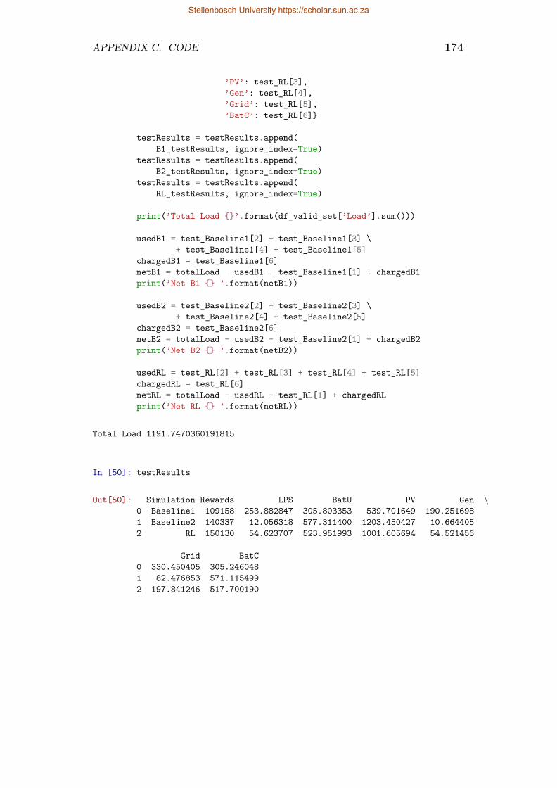
APPENDIX C. CODE 174
’PV’: test_RL[3],’Gen’: test_RL[4],’Grid’: test_RL[5],’BatC’: test_RL[6]}
testResults = testResults.append(B1_testResults, ignore_index=True)
testResults = testResults.append(B2_testResults, ignore_index=True)
testResults = testResults.append(RL_testResults, ignore_index=True)
print(’Total Load {}’.format(df_valid_set[’Load’].sum()))
usedB1 = test_Baseline1[2] + test_Baseline1[3] \+ test_Baseline1[4] + test_Baseline1[5]
chargedB1 = test_Baseline1[6]netB1 = totalLoad - usedB1 - test_Baseline1[1] + chargedB1print(’Net B1 {} ’.format(netB1))
usedB2 = test_Baseline2[2] + test_Baseline2[3] \+ test_Baseline2[4] + test_Baseline2[5]
chargedB2 = test_Baseline2[6]netB2 = totalLoad - usedB2 - test_Baseline2[1] + chargedB2print(’Net B2 {} ’.format(netB2))
usedRL = test_RL[2] + test_RL[3] + test_RL[4] + test_RL[5]chargedRL = test_RL[6]netRL = totalLoad - usedRL - test_RL[1] + chargedRLprint(’Net RL {} ’.format(netRL))
Total Load 1191.7470360191815
In [50]: testResults
Out[50]: Simulation Rewards LPS BatU PV Gen \0 Baseline1 109158 253.882847 305.803353 539.701649 190.2516981 Baseline2 140337 12.056318 577.311400 1203.450427 10.6644052 RL 150130 54.623707 523.951993 1001.605694 54.521456
Grid BatC0 330.450405 305.2460481 82.476853 571.1154992 197.841246 517.700190
Stellenbosch University https://scholar.sun.ac.za

APPENDIX C. CODE 175
C.5 Reinforcement Learning withIoT-implementation
C.5.1 ImportsIn [1]: import time
import warningswarnings.filterwarnings(’ignore’)
import matplotlib.pyplot as pltimport tensorflow as tffrom tensorflow import kerasfrom tensorflow.keras import layersimport tensorflow.keras.backend as KK.clear_session()
import pvlibfrom pvlib.location import Location, solarposition
import datetime as dt
import numpy as npimport mathimport pandas as pdimport osimport csvimport sysimport random
import glob
import itertoolsimport matplotlib
from collections import defaultdict
tiltAngle=30rho=0.2LTM=-30latitude=-33.9346longitude=18.8668altitude=122
loc=Location(latitude,longitude,’Africa/Johannesburg’,altitude,’Stellenbosch’)
random.seed(30)
Stellenbosch University https://scholar.sun.ac.za
APPENDIX C. CODE 176
In [2]: label = 20ticklabel = 18
params = {’axes.labelsize’: label,’axes.titlesize’: label,’text.usetex’ : True,’font.size’: ticklabel,’legend.frameon’: True,’legend.fontsize’: ticklabel,’legend.loc’: ’center right’,’legend.framealpha’: 1,’xtick.labelsize’: ticklabel,’ytick.labelsize’: ticklabel,’grid.linestyle’ : ":",’axes.grid’: True,’axes.grid.which’: ’major’,’axes.grid’ : True,’grid.linewidth’ : 0.8,’keymap.grid’: [’g’],’keymap.grid_minor’: [’G’],’figure.figsize’: [18, 8]}
plt.rcParams.update(params)
C.5.2 Results of GA designC.5.2.1 SGBGIn [3]: interval = 15
In [4]: # PVPV_capacity = 10.6 #kW peakefficiency_PV = 16.99/100numPV = 29PV_area = 1.96 * 0.991
# GridGrid_hourly = 1.2 #kWh per hour
# BatteryDOD = 0.5Battery_capacity = 49 # kWhfully_charged_kWh = Battery_capacity*DOD # kWhinitial_charge = fully_charged_kWhMax_Discharge_kWh = 0.08 # kWh per minutenumBat = 15
# Generatorgen_kWh = 5.0 # kWh per hour
# Time intervalsgrid_interval = Grid_hourly*(interval/60)
Stellenbosch University https://scholar.sun.ac.za
APPENDIX C. CODE 177
Max_Discharge_kWh = Max_Discharge_kWh*intervalMaxCharge_kWh = 12*10*numBat*(interval/60)/1000gen_interval = gen_kWh*(interval/60)
def calcPVPower(insolation):kWh=insolation*efficiency_PV*PV_area*numPV/1000return kWh/60
def normaliseInterval(unnormalised):return unnormalised/interval
C.5.3 Data preprocessingIn [5]: def getTotalIrradiance(GHI, DNI, DHI, timestamp):
timestamp=pd.DatetimeIndex(timestamp)timestamp=timestamp.tz_localize(loc.tz)"""Calculate the total irradiance
Args:GHI: global horizontal irradianceDNI: direct normal irradianceDHI: diffuse horizontal irradianceTimestamp: DatetimeIndex
Returns:total: [poa_global,poa_direct,poa_diffuse,poa_sky_diffuse,poa_ground_diffuse]
"""
model=’isotropic’
# Panel azimuth from Northsurface_azimuth=0
albedo=rho #surface albedo - declared in variables and constants
# convert to radianslatitudeRad=np.deg2rad(latitude)n=timestamp.dayofyear# Equation of time"""pvlib.solarposition.equation_of_time_pvcdrom
Parameters: dayofyearReturn: equation_of_time: in minutes
"""eqOfTime=pvlib.solarposition.equation_of_time_pvcdrom(n)
# Hour angle
Stellenbosch University https://scholar.sun.ac.za

APPENDIX C. CODE 178
"""pvlib.solarposition.hour_angle
Parameters: times: pd.DatetimeIndex must belocalized to timezone for the longitude
longitude: longitude (degrees)equation_of_time: equation of time in minutes
Returns: hour_angle (degrees)"""hourangle=pvlib.solarposition.hour_angle(timestamp,
longitude,eqOfTime)
hourAngleRad=np.deg2rad(hourangle)
#Declination angle calculations"""pvlib.solarposition.declination_cooper69
Parameters: dayofyearReturns: declination angle (radians)
"""declinationRad=pvlib.solarposition.declination_cooper69(n)
#Solar zenith angle calculations"""pvlib.solarposition.solar_zenith_analytical
Parameters: latitude: Latitude of location (radians)hourangle: Hour angle in the local solar time (radians)declination: declination of the sun (radians)
Returns: solar zenith angle (radians)"""solar_zenithRad=pvlib.solarposition.solar_zenith_analytical(latitudeRad,
hourAngleRad,declinationRad)
#Solar azimuth angle calculations"""pvlib.solarposition.solar_azimuth_analytical
Parameters: latitude: Latitude of location (radians)hourangle: Hour angle in the local solar time (radians)declination: declination of the sun (radians)zenith: solar zenith angle (radians)
Returns: Solar azimuth angle (radians)
"""solar_azimuthRad=pvlib.solarposition.solar_azimuth_analytical(latitudeRad,
hourAngleRad,declinationRad,solar_zenithRad)
#convert to degreessolar_azimuth = np.rad2deg(solar_azimuthRad)solar_zenith= np.rad2deg(solar_zenithRad)surface_tilt=tiltAngle# get total irradiance
Stellenbosch University https://scholar.sun.ac.za
APPENDIX C. CODE 179
"""pvlib.irradiance.get_total_irradiance
Parameters: surface_tilt: Panel tilt from horizontal (degrees)surface_azimuth: Panel azimuth from north (degrees)solar_zenith: Solar zenith angle (degrees)dni: Direct Normal Irradiance (W/mˆ2)ghi:Global horizontal irradiance (W/mˆ2)dhi: Diffuse horizontal irradiance (W/mˆ2)dni_extra: Extraterrestrial direct normal irradiance.airmass: Airmassalbedo: Surface albedo 0-1surface_type: Surface type.model: isotropic(default), klucher, haydavies, reindl, king, perez
Returns: dataframe array:poa_global,poa_direct,poa_diffuse,poa_sky_diffuse,poa_ground_diffuse
"""total=pvlib.irradiance.get_total_irradiance(surface_tilt=tiltAngle,
surface_azimuth=surface_azimuth,solar_zenith=solar_zenith,solar_azimuth=solar_azimuth,dni=DNI,ghi=GHI,dhi=DHI,albedo=albedo,model=model)
return total
In [6]: path = ’C:/Users/18296033/Documents/WORK/DataCollector/datapoints/Batch2’all_files = glob.glob(path + "/*.csv")
df = pd.DataFrame()
for filename in all_files:temp = pd.read_csv(filename, index_col=None, header=0)df=df.append(temp)
df[’From’] = pd.to_datetime(df[’From’])df[’Timestamp’] = pd.to_datetime(df[’Timestamp’])
df = df.sort_values(by=[’From’,’Timestamp’], ascending=[True, True])
df_Predictions=df[df[’From’] == df[’Timestamp’]]df_Predictions = df_Predictions.rename(index=str, columns = {’From’:’Date’})df_Predictions = df_Predictions.reset_index()df_Predictions = df_Predictions.drop([’Timestamp’, ’index’], axis=1)
In [7]: start=df_Predictions.iloc[0][’Date’]
Stellenbosch University https://scholar.sun.ac.za

APPENDIX C. CODE 180
end=df_Predictions.iloc[-1][’Date’]
timesClearSky=pd.date_range(start, end, freq=’T’,tz=loc.tz)
df_Clearsky=loc.get_clearsky(timesClearSky)df_Clearsky[’Date’] = df_Clearsky.index.get_values()df_Clearsky[’Date’] = pd.to_datetime(df_Clearsky[’Date’]) + pd.to_timedelta(2,unit=’h’)
df_Clearsky=df_Clearsky.reset_index(drop=True)
total=getTotalIrradiance(df_Clearsky[’ghi’],df_Clearsky[’dni’],df_Clearsky[’dhi’],pd.DatetimeIndex(df_Clearsky[’Date’]))
df_Clearsky[’Insolation_CS’] = total[’poa_global’]
df_Clearsky = df_Clearsky.drop([’ghi’, ’dni’, ’dhi’], axis=1)
temp = pd.date_range(start, end, freq=’1h’,tz=loc.tz)
temp = temp.tz_localize(None)
temp_DF = pd.DataFrame()temp_DF[’Date’] = temp
In [8]: dataframe = pd.merge(df_Predictions, temp_DF,on=’Date’, how=’right’)
In [9]: dataframe[dataframe.isna().any(axis=1)]dates_empty = dataframe[dataframe.isna().any(axis=1)].reset_index() [’Date’]
In [10]: pred_Temp =pd.DataFrame()
for i in range (0, len(dates_empty)):row = df.loc[df[’From’] == dates_empty[i]]pred_Temp = pred_Temp.append(row.tail(1))
pred_Temp = pred_Temp.rename(index=str,columns = {’From’:’Date’})
pred_Temp = pred_Temp.drop([’Timestamp’],axis=1)
dataframe = pred_Temp.set_index(’Date’).reindex_like(dataframe.set_index(’Date’)).combine_first(dataframe.set_index(’Date’)).reset_index()
dataframe.shape
Stellenbosch University https://scholar.sun.ac.za

APPENDIX C. CODE 181
In [11]: dataframe = pd.merge(dataframe, df_Clearsky, on=’Date’, how=’right’)dataframe = dataframe.sort_values (by=’Date’)dataframe = dataframe.ffill()dataframe = dataframe.reset_index(drop=True)
dataframe.shape
In [12]: normalSkyDatapoints = pd.read_table(’weather2Years.csv’,sep=’,’ )
normalSkyDatapoints = normalSkyDatapoints.drop([’Record’, ’Date’, ’Time’,’UVA_Avg’, ’UVB_Avg’, ’Tracker2WM_Avg’,’WindDir_D1_WVT’, ’WindDir_SD1_WVT’,’ShadowbandWM_Avg’, ’RH’,’AirTC_Avg’,’WS_ms_S_WVT’, ’BP_mB_Avg’, ’DNICalc_Avg’],
axis = 1)
normalSkyDatapoints=normalSkyDatapoints.rename(index = str,columns = {’SunWM_Avg’:’GHI’,
’TrackerWM_Avg’:’DNI’,’ShadowWM_Avg’:’DHI’,’TimeStamp’:’Date’})
normalSkyDatapoints[’Date’] = pd.to_datetime(normalSkyDatapoints[’Date’])
normalSkyDatapoints = normalSkyDatapoints.reset_index(drop=True)
In [13]: start = normalSkyDatapoints.iloc[0][’Date’]end = normalSkyDatapoints.iloc[-1][’Date’]
normalSky = pd.DataFrame()normalSky[’Date’] = pd.date_range(start, end, freq=’min’)normalSkyDF = pd.merge(normalSkyDatapoints, normalSky,
on = ’Date’, how = ’outer’)normalSkyDF = normalSkyDF.sort_values(by=[’Date’])normalSkyDF = normalSkyDF.fillna(method=’ffill’)
In [14]: total = getTotalIrradiance(normalSkyDatapoints[’GHI’],normalSkyDatapoints[’DNI’],normalSkyDatapoints[’DHI’],pd.DatetimeIndex(normalSkyDatapoints[’Date’]))
normalSkyDF[’Insolation_NS’] = total[’poa_global’]
normalSkyDF=normalSkyDF.drop([’DNI’, ’DHI’, ’GHI’],
Stellenbosch University https://scholar.sun.ac.za

APPENDIX C. CODE 182
axis=1)
dataframe=pd.merge(dataframe,normalSkyDF, on=[’Date’])
dataframe = dataframe.drop([’Degrees’,’Fog’,’Dew Temperature’,’Pressure’,’Windspeed’],
axis=1)
loadprofileDF = pd.read_csv(’2yearLoadProfile.csv’, sep=’;’)loadprofileDF=loadprofileDF.rename(index=str,
columns={’Time’:’Date’,’Sum [kWh]’:’Load’})
loadprofileDF[’Date’]=pd.to_datetime(loadprofileDF[’Date’])loadprofileDF=loadprofileDF.drop([’Electricity.Timestep’],
axis=1)
dataframe=pd.merge(dataframe,loadprofileDF, on=[’Date’])
In [15]: dataframe[’PV Power’] = calcPVPower(dataframe[’Insolation_NS’])
dataframe = dataframe.set_index(’Date’)
timeInterval = ’{}T’.format(interval)
dataframe = dataframe.resample(timeInterval).sum()
dataframe = dataframe.reset_index()
dataframe[’Temperature’] = normaliseInterval(dataframe[’Temperature’])dataframe[’Humidity’] = normaliseInterval(dataframe[’Humidity’])dataframe[’Clouds’] = normaliseInterval(dataframe[’Clouds’])dataframe[’Low Clouds’] = normaliseInterval(dataframe[’Low Clouds’])dataframe[’Medium Clouds’] = normaliseInterval(dataframe[’Medium Clouds’])dataframe[’High Clouds’] = normaliseInterval(dataframe[’High Clouds’])dataframe[’Insolation_CS’] = normaliseInterval(dataframe[’Insolation_CS’])dataframe[’Insolation_NS’] = normaliseInterval(dataframe[’Insolation_NS’])
dataframe[’Month’] = dataframe[’Date’].dt.monthdataframe[’HourOfDay’] = dataframe[’Date’].dt.hour
dataframe[’Battery’] = pd.Series(np.zeros(dataframe.shape[0]))dataframe[’Generator’] = pd.Series(np.zeros(dataframe.shape[0]))
dataframe[’DayofWeek’] = dataframe[’Date’].dt.weekday
Stellenbosch University https://scholar.sun.ac.za
APPENDIX C. CODE 183
dataframe[’Weekday’] =dataframe[’DayofWeek’].apply(lambda x: 1 if x <= 4 else 0)
dataframe[’Month’] = pd.Categorical(dataframe[’Month’])dataframe[’Month’] = dataframe.Month.cat.codes
dataframe[’HourOfDay’] = pd.Categorical(dataframe[’HourOfDay’])dataframe[’HourOfDay’] = dataframe.HourOfDay.cat.codes
dataframe[’Weekday’] = pd.Categorical(dataframe[’Weekday’])dataframe[’Weekday’] = dataframe.Weekday.cat.codes
dataframe = dataframe.drop([’DayofWeek’], axis=1)
In [16]: for i in range(1, len(dataframe)):dataframe.loc[i, ’Prev CS’] = dataframe.loc[i-1,
’Insolation_CS’]
for i in range(0, len(dataframe)-1):dataframe.loc[i, ’Next CS’] = dataframe.loc[i+1,
’Insolation_CS’]
In [17]: dataframe = dataframe[[’Load’, ’PV Power’, ’Month’, ’HourOfDay’,’Battery’, ’Generator’, ’Weekday’,’Temperature’, ’Humidity’, ’Clouds’,’Low Clouds’, ’Medium Clouds’, ’High Clouds’,’Insolation_CS’, ’Insolation_NS’, ’Next CS’,’Prev CS’, ’Date’]]
In [18]: dataframe.to_csv(’{}DatabaseIoT_Batch2.csv’.format(interval))
In [19]: # df = pd.read_csv(’15DatabaseIoT_Batch2.csv’)# df = df.drop([’Unnamed: 0’], axis=1)
# df[’Date’] = pd.to_datetime(df[’Date’])
# dataframe = df.copy()# dataframe.head()
In [20]: df = dataframe.copy()
In [21]: df.head()
C.5.4 Train, test and validate datasetsIn [22]: for i in range(0, len(df)-1):
df.loc[i, ’Next PV’] = df.loc[i+1, ’PV Power’]df.loc[i, ’Next Load’] = df.loc[i+1, ’Load’]
In [23]: df_train_set = pd.DataFrame()df_valid_set = pd.DataFrame()
Stellenbosch University https://scholar.sun.ac.za

APPENDIX C. CODE 184
df_test_set = pd.DataFrame()
for j in range (1,13):year = 2019month = jtrain_day_start = 1train_day_end = 22valid_day_start = 23valid_day_end = 26test_start = 27test_end = 0
days_31 = [1, 3, 5, 7, 8, 10, 12]days_30 = [4, 6, 9, 11]
# Februaryif j == 2:
test_end = 28# 31: January, March, May, July, Aug, Oct, Decif j in days_31:
test_end = 31if j in days_30:
test_end = 30
# TRAIN DATA SEGMENTstart_date = pd.Timestamp(year=year, month=month,
day=train_day_start,hour = 0, minute = 0,second = 0)
end_date = pd.Timestamp(year=year, month=month,day=train_day_end, hour = 23,minute = 59, second = 59)
dti = pd.date_range(start = start_date,end = end_date, freq=’15T’)
df_train_set = df_train_set.append(df.loc[df.Date.isin(pd.DatetimeIndex(dti))])
# VALID DATA SEGMENTstart_date = pd.Timestamp(year=year, month=month,
day=valid_day_start,hour = 0, minute = 0,second = 0)
end_date = pd.Timestamp(year=year, month=month,day=valid_day_end, hour = 23,minute = 59, second = 59)
dti = pd.date_range(start = start_date,end = end_date, freq=’15T’)
df_valid_set = df_valid_set.append(df.loc[df.Date.isin(pd.DatetimeIndex(dti))])
Stellenbosch University https://scholar.sun.ac.za

APPENDIX C. CODE 185
# TEST DATA SEGMENTstart_date = pd.Timestamp(year=year, month=month,
day=test_start, hour = 0,minute = 0, second = 0)
end_date = pd.Timestamp(year=year, month=month,day=test_end, hour = 23,minute = 59, second = 59)
dti = pd.date_range(start = start_date,end = end_date, freq=’15T’)
df_test_set = df_test_set.append(df.loc[df.Date.isin(pd.DatetimeIndex(dti))])
In [24]: # print(’Train:\t\t{0}\t{1:.1f}%’.format(# df_train_set.shape[0],# 100*df_train_set.shape[0]/df.shape[0]))# print(’Validate:\t{0}\t{1:.1f}%’.format(# df_valid_set.shape[0],# 100*df_valid_set.shape[0]/df.shape[0]))# print(’Test:\t\t{0}\t{1:.1f}%’.format(# df_test_set.shape[0],# 100*df_test_set.shape[0]/df.shape[0]))
In [25]: df_train_set = df_train_set.drop([’Date’], axis=1)df_valid_set = df_valid_set.drop([’Date’], axis=1)df_test_set = df_test_set.drop([’Date’], axis=1)
In [26]: # df_train_set.to_csv(’RL IoT Train.csv’)# df_valid_set.to_csv(’RL IoT Valid.csv’)# df_test_set.to_csv(’RL IoT Test.csv’)
In [27]: df_train_set = pd.read_csv(’RL IoT Train.csv’)df_train_set = df_train_set.drop([’Unnamed: 0’], axis=1)
df_valid_set = pd.read_csv(’RL IoT Valid.csv’)df_valid_set = df_valid_set.drop([’Unnamed: 0’], axis=1)
df_test_set = pd.read_csv(’RL IoT Test.csv’)df_test_set = df_test_set.drop([’Unnamed: 0’], axis=1)
In [28]: train_stats=df_train_set.describe()train_stats=train_stats.transpose()
valid_stats=df_valid_set.describe()valid_stats=valid_stats.transpose()
test_stats=df_test_set.describe()test_stats=test_stats.transpose()
Stellenbosch University https://scholar.sun.ac.za

APPENDIX C. CODE 186
In [29]: def norm(x):return (x - train_stats[’mean’])/train_stats[’std’]
normed_Train = norm(df_train_set)normed_Valid = norm(df_valid_set)normed_Test = norm(df_test_set)
In [30]: df_train_set[’Humidity’] = normed_Train[’Humidity’].copy()df_train_set[’Clouds’] = normed_Train[’Clouds’].copy()df_train_set[’Temperature’] = normed_Train[’Temperature’].copy()df_train_set[’Low Clouds’] = normed_Train[’Low Clouds’].copy()df_train_set[’Medium Clouds’] = normed_Train[’Medium Clouds’].copy()df_train_set[’High Clouds’] = normed_Train[’High Clouds’].copy()df_train_set[’Insolation_CS’] = normed_Train[’Insolation_CS’].copy()df_train_set[’Insolation_NS’] = normed_Train[’Insolation_NS’].copy()df_train_set[’Next CS’] = normed_Train[’Next CS’].copy()
df_valid_set[’Humidity’] = normed_Valid[’Humidity’].copy()df_valid_set[’Clouds’] = normed_Valid[’Clouds’].copy()df_valid_set[’Temperature’] = normed_Valid[’Temperature’].copy()df_valid_set[’Low Clouds’] = normed_Valid[’Low Clouds’].copy()df_valid_set[’Medium Clouds’] = normed_Valid[’Medium Clouds’].copy()df_valid_set[’High Clouds’] = normed_Valid[’High Clouds’].copy()df_valid_set[’Insolation_CS’] = normed_Valid[’Insolation_CS’].copy()df_valid_set[’Insolation_NS’] = normed_Valid[’Insolation_NS’].copy()df_valid_set[’Next CS’] = normed_Valid[’Next CS’].copy()
df_test_set[’Humidity’] = normed_Test[’Humidity’].copy()df_test_set[’Clouds’] = normed_Test[’Clouds’].copy()df_test_set[’Temperature’] = normed_Test[’Temperature’].copy()df_test_set[’Low Clouds’] = normed_Test[’Low Clouds’].copy()df_test_set[’Medium Clouds’] = normed_Test[’Medium Clouds’].copy()df_test_set[’High Clouds’] = normed_Test[’High Clouds’].copy()df_test_set[’Insolation_CS’] = normed_Test[’Insolation_CS’].copy()df_test_set[’Insolation_NS’] = normed_Test[’Insolation_NS’].copy()df_test_set[’Next CS’] = normed_Test[’Next CS’].copy()
In [31]: train_set = df_train_set.as_matrix()valid_set = df_valid_set.as_matrix()test_set = df_test_set.as_matrix()
In [32]: action_perm = {’use_pv’: {True, False},’charge_bat’: {True, False},’discharge_bat’: {True, False},’use_grid’: {True, False},’switch_on_Gen’: {True, False}}
# remove actions charge + discharge == Trueimport itertoolsl = [’T’, ’F’]actions_all = [list(i) for i in itertools.product(l, repeat=5)]
Stellenbosch University https://scholar.sun.ac.za

APPENDIX C. CODE 187
remove_ = 8
te = 0
while True:for i in range (0, len(actions_all)):
if actions_all[i][1] == ’T’ and actions_all[i][2] == ’T’:actions_all.remove(actions_all[i])te += 1break
if te == remove_:break
actions = []for i in range (0, len(actions_all)):
actions.append(actions_all[i][0] + actions_all[i][1] \+ actions_all[i][2]+ actions_all[i][3] \+ actions_all[i][4])
In [33]: num_actions=len(actions)
In [34]: num_states = 17
In [35]: def step(action, t, prev_state, data):
next_state = None
action = list(action)use_pv = action[0]charge_bat = action[1]discharge_bat = action[2]use_grid = action[3]use_gen = action[4]
# Load and PV for the time stepPV = data[t][17]load = data[t][18]
# Where the battery and generator are startingbat = prev_state[4]gen = prev_state[5]
bat_before = bat
grid = grid_interval # kWhLPS = load #100%maxGen = gen_interval #kWh
PV_Use = 0Gen_Use = 0Grid_Use = 0Bat_Use = 0
Stellenbosch University https://scholar.sun.ac.za
APPENDIX C. CODE 188
availablePV = 0availableGrid = 0availableGen = 0
############################# Use PV Actionif use_pv == ’T’:
availablePV = PVif availablePV > load:
PV_Use += LPSavailablePV -= LPSLPS = 0
else:LPS -= availablePVPV_Use += availablePVavailablePV = 0
############################# Discharge Battery Actionif discharge_bat == ’T’:
if LPS < bat:bat -= LPSBat_Use += LPSLPS = 0
else:LPS -=batBat_Use += batbat = 0
############################# Use Grid Actionif use_grid == ’T’:
availableGrid = gridif LPS < availableGrid:
availableGrid -= LPSGrid_Use += LPSLPS = 0
else:LPS -= availableGridGrid_Use += availableGridavailableGrid = 0
############################# Use Generator Actionif use_gen == ’T’:
availableGen = maxGenif gen < (15/interval):
availableGen = 0.2*availableGenif LPS < availableGen:
availableGen -= LPSGen_Use += LPSLPS = 0
else:LPS -= availableGenGrid_Use += availableGen
Stellenbosch University https://scholar.sun.ac.za

APPENDIX C. CODE 189
availableGen = 0############################# Charge batteries Action#maxC = MaxCharge_kWhif charge_bat == ’T’:
if use_pv == ’T’:if bat+availablePV > fully_charged_kWh:
PV_Use += fully_charged_kWh - batbat = fully_charged_kWh
else:bat += availablePVPV_Use += availablePV
if use_grid == ’T’:if bat+availableGrid > fully_charged_kWh:
Grid_Use += fully_charged_kWh - batbat = fully_charged_kWh
else:bat += availableGridGrid_Use += availableGrid
if use_gen == ’T’:if bat+availableGen > fully_charged_kWh:
Gen_Use += fully_charged_kWh - batbat = fully_charged_kWh
else:bat += availableGenPV_Use += availableGen
############################
# Rewardsreward = 0reward = reward + int(LPS <= 0)*20reward = reward + int(PV_Use == PV and use_pv == ’T’)*6reward = reward + int(PV_Use > 0)*6reward = reward + int(use_gen == ’T’ and PV == 0)*3reward = reward + int(discharge_bat == ’T’ and PV == 0)*6
if use_gen == ’F’:gen = 0 # switch off generator
else:gen += 1
battery_charged = bat - bat_beforebattery_charged = max(0, battery_charged)
LPS = max(0, LPS)
# THE NEXT STATEnext_state = [data[t][18],
data[t][17],data[t][2],data[t][3],bat,
Stellenbosch University https://scholar.sun.ac.za
APPENDIX C. CODE 190
gen,data[t][6],data[t][7],data[t][8],data[t][9],data[t][10],data[t][11],data[t][12],data[t][13],data[t][14],data[t][15],data[t][16]]
if t+1 == len(data):next_state = None
return next_state, reward, t+2 == len(data), LPS, PV_Use, Gen_Use, Grid_Use, Bat_Use, battery_charged, None
In [36]: # number of episodesnum_episodes = 50
In [37]: memory = []
max_memory = int(2*len(train_set))
def sampleMemory(batch_size):if batch_size > len(memory):
return random.sample(memory,(len(memory)))
else:return random.sample(memory,
batch_size)
def addSampleMemory(memorySample):memory.append(memorySample)if len(memory) > max_memory:
memory.pop(0)
In [38]: max_epsilon = 1min_epsilon = 0.01
Lambda = 0.001gamma = 0.7
batch_hours = 3batch_size = int((60/interval)*batch_hours)
In [39]: def build_model():model = keras.Sequential([layers.Dense(32, activation=tf.nn.relu,
Stellenbosch University https://scholar.sun.ac.za

APPENDIX C. CODE 191
input_shape=(num_states,)),layers.Dense(32, activation=tf.nn.relu),layers.Dense(32, activation=tf.nn.relu),layers.Dense(num_actions)
])
return model
In [40]: model = build_model()
model.compile(loss=’mse’,optimizer=tf.keras.optimizers.Adam(
lr=Lambda))
print(model.summary())
Layer (type) Output Shape Param #=================================================================dense (Dense) (None, 32) 576
dense 1 (Dense) (None, 32) 1056
dense 2 (Dense) (None, 32) 1056
dense 3 (Dense) (None, 24) 792=================================================================Total params: 3,480Trainable params: 3,480Non-trainable params: 0
None
In [41]: total_LPS = np.zeros(num_episodes)total_rewards = np.zeros(num_episodes)total_PV = np.zeros(num_episodes)total_Gen = np.zeros(num_episodes)total_Grid = np.zeros(num_episodes)total_BatU = np.zeros(num_episodes)total_BatC = np.zeros(num_episodes)
C.5.5 TrainingIn [42]: def RLController_Train():
epsilon = max_epsiloncnt = 0steps = 0
data = train_set
Stellenbosch University https://scholar.sun.ac.za

APPENDIX C. CODE 192
while cnt < num_episodes:print(’Episode {}’.format(cnt))# reset state to start of datasetstate = [data[0][0],
data[0][1],data[0][2],data[0][3],data[0][4],data[0][5],data[0][6],data[0][7],data[0][8],data[0][9],data[0][10],data[0][11],data[0][12],data[0][13],data[0][14],data[0][15],data[0][16]]
state[4] = initial_chargestate[5] = 0 #off
# save episodeepisode_rewards = 0episode_LPS = 0episode_PV = 0episode_Gen = 0episode_Grid = 0episode_BatU = 0episode_BatC = 0
# run entire episodefor t in range(len(data)):
action=0
if random.random() < epsilon:action = random.randint(0, num_actions - 1)
else:options = model.predict(np.array([state]))action = np.argmax(options)
# step through datanext_state, reward, done, LPS, PV, Gen, Grid, BatU, BatC, _ = step(
actions[action], t, state, data)
addSampleMemory([state, action, reward, next_state])
random_batch = sampleMemory(batch_size)
states_ = np.array(
Stellenbosch University https://scholar.sun.ac.za

APPENDIX C. CODE 193
[val[0] for val in random_batch])
next_states = np.array([(np.zeros(num_states)
if val[3] is None else val[3]) for val in random_batch])
q_s_a = model.predict(states_)
q_s_a_d = model.predict(next_states)
x_batch = np.zeros((len(random_batch),num_states))
y_batch = np.zeros((len(random_batch),num_actions))
for i, b in enumerate(random_batch):state_B, action_B, reward_B, next_state_B = b[0], b[1], b[2], b[3]
current_q_B = q_s_a[i]
if next_state_B == None:current_q_B[action_B] = reward_B
else:current_q_B[action_B]=reward_B + gamma*np.amax(
q_s_a_d[i])
x_batch[i] = state_By_batch[i] = current_q_B
model.fit(x=x_batch, y=y_batch, verbose=0)
steps +=1
state = next_state
epsilon = min_epsilon + (max_epsilon-min_epsilon)*math.exp(-Lambda*steps)
episode_rewards += rewardepisode_LPS += LPSepisode_PV += PVepisode_Gen += Genepisode_Grid += Gridepisode_BatU += BatUepisode_BatC += BatC
if done:total_rewards[cnt]=episode_rewardstotal_LPS[cnt]=episode_LPStotal_PV[cnt]=episode_PVtotal_Gen[cnt]=episode_Gen
Stellenbosch University https://scholar.sun.ac.za

APPENDIX C. CODE 194
total_Grid[cnt] = episode_Gridtotal_BatU[cnt] = episode_BatUtotal_BatC[cnt] = episode_BatCbreak
cnt += 1
In [43]: RLController_Train()
In [44]: model.save(’model IoT.h5’)
In [45]: plt.plot(total_rewards)plt.xlabel(’Episodes’)plt.ylabel(’Total rewards obtained per episode during training’)# plt.show()plt.savefig(’Training_rewards_IoT.pdf’,bbox_inches = ’tight’)
In [46]: plt.plot(total_LPS)plt.xlabel(’Episodes’)plt.ylabel(’Total LPS [kWh] per episode during training’)#plt.show()plt.savefig(’Training_LPS_IoT.pdf’,bbox_inches = ’tight’)
In [47]: plt.plot(total_PV)plt.plot(total_BatU)plt.plot(total_Gen)plt.plot(total_Grid)plt.xlabel(’Episodes’)plt.ylabel(’Total Power [kWh] per episode during training’)plt.legend([’PV’, ’Battery’, ’Generator’, ’Grid’])#plt.show()plt.savefig(’Training_HPS.pdf’,bbox_inches = ’tight’)
C.5.6 ValidationIn [48]: validate_Baseline1 = []
validate_Baseline2 = []validate_RL = []
In [49]: def baselineController1(data, Process):cnt = 0steps = 0
# reset state to start of datasetstate = [data[0][0],
data[0][1],data[0][2],data[0][3],data[0][4],data[0][5],
Stellenbosch University https://scholar.sun.ac.za
APPENDIX C. CODE 195
data[0][6],data[0][7],data[0][8],data[0][9],data[0][10],data[0][11],data[0][12],data[0][13],data[0][14],data[0][15],data[0][16]]
state[4] = initial_chargestate[5] = 0 # off
episode_rewards = 0episode_LPS = 0episode_PV = 0episode_Gen = 0episode_Grid = 0episode_BatU = 0episode_BatC = 0
# run entire episodefor t in range(len(data)):
# random actionaction = random.randint(0, num_actions - 1)
# step through datanext_state, reward, done, LPS, PV, Gen, Grid, BatU, BatC,_ = step(
actions[action], t, state, data)
steps +=1
state = next_state
episode_LPS += LPSepisode_rewards += rewardepisode_PV += PVepisode_Gen += Genepisode_Grid += Gridepisode_BatU += BatUepisode_BatC += BatC
if done:if Process == ’Validate’:
global validate_Baseline1validate_Baseline1 = [episode_rewards,
episode_LPS,episode_BatU,episode_PV,episode_Gen,
Stellenbosch University https://scholar.sun.ac.za

APPENDIX C. CODE 196
episode_Grid,episode_BatC]
if Process == ’Test’:global test_Baseline1test_Baseline1 = [episode_rewards,
episode_LPS,episode_BatU,episode_PV,episode_Gen,episode_Grid,episode_BatC]
break
In [50]: def baselineController2(data, Process):cnt = 0steps = 0
# reset state to start of datasetstate = [data[0][0],
data[0][1],data[0][2],data[0][3],data[0][4],data[0][5],data[0][6],data[0][7],data[0][8],data[0][9],data[0][10],data[0][11],data[0][12],data[0][13],data[0][14],data[0][15],data[0][16]]
state[4] = initial_chargestate[5] = 0 #off
episode_rewards = 0episode_LPS = 0episode_PV = 0episode_Gen = 0episode_Grid = 0episode_BatU = 0episode_BatC = 0
for t in range(len(data)):
# rule-based actionuse_pv = None
Stellenbosch University https://scholar.sun.ac.za

APPENDIX C. CODE 197
charge_bat = Nonedischarge_bat = Noneuse_grid = Noneuse_gen = None
# use PVif state[1] > 0:
use_pv = ’T’else:
use_pv = ’F’# charge bat if PV > (load)if state[1] > state[0]:
charge_bat = ’T’else:
charge_bat = ’F’# discharge bat if PV < loadif state[1] < state[0] and charge_bat != ’T’:
discharge_bat = ’T’else:
discharge_bat = ’F’# use grid randomlyif bool(random.getrandbits(1)) == 1:
use_grid = ’T’else:
use_grid = ’F’# use generator randomyif bool(random.getrandbits(1)) == 1:
use_gen = ’T’else:
use_gen = ’F’
action = use_pv+charge_bat+discharge_bat+use_grid+use_gen
# step through datanext_state, reward, done, LPS, PV, Gen, Grid, BatU, BatC,_ = step(
action, t, state, data)
steps += 1
state = next_state
episode_rewards += rewardepisode_LPS += LPSepisode_PV += PVepisode_Gen += Genepisode_Grid += Gridepisode_BatU += BatUepisode_BatC += BatC
if done:if Process == ’Validate’:
global validate_Baseline2
Stellenbosch University https://scholar.sun.ac.za

APPENDIX C. CODE 198
validate_Baseline2 = [episode_rewards,episode_LPS,episode_BatU,episode_PV,episode_Gen,episode_Grid,episode_BatC]
if Process == ’Test’:global test_Baseline2test_Baseline2 = [episode_rewards,
episode_LPS,episode_BatU,episode_PV,episode_Gen,episode_Grid,episode_BatC]
break
In [51]: def RLController(data, Process):epsilon = max_epsiloncnt = 0steps = 0
# reset state to start of datasetstate = [data[0][0],
data[0][1],data[0][2],data[0][3],data[0][4],data[0][5],data[0][6],data[0][7],data[0][8],data[0][9],data[0][10],data[0][11],data[0][12],data[0][13],data[0][14],data[0][15],data[0][16]]
state[4] = initial_chargestate[5] = 0 #off
# save episodeepisode_rewards = 0episode_LPS = 0episode_PV = 0episode_Gen = 0episode_Grid = 0episode_BatU = 0
Stellenbosch University https://scholar.sun.ac.za
APPENDIX C. CODE 199
episode_BatC = 0
if Process == ’Test’:global modeldel modelmodel = keras.models.load_model(’model IoT.h5’)
# run entire episodefor t in range(len(data)):
action=0
if random.random() < epsilon:action = random.randint(0, num_actions - 1)
else:options = model.predict(np.array([state]))action = np.argmax(options)
# step through datanext_state, reward, done, LPS, PV, Gen, Grid, BatU, BatC, _ = step(
actions[action], t, state, data)
addSampleMemory([state, action, reward, next_state])
random_batch = sampleMemory(batch_size)
states_ = np.array([val[0] for val in random_batch])
next_states = np.array([(np.zeros(num_states)
if val[3] is None else val[3]) for val in random_batch])
q_s_a = model.predict(states_)
q_s_a_d = model.predict(next_states)
x_batch = np.zeros((len(random_batch),num_states))
y_batch = np.zeros((len(random_batch),num_actions))
for i, b in enumerate(random_batch):state_B, action_B, reward_B, next_state_B = b[0], b[1], b[2], b[3]
current_q_B = q_s_a[i]
if next_state == None:current_q_B[action_B] = reward_B
else:current_q_B[action_B]=reward_B + gamma*np.amax(
Stellenbosch University https://scholar.sun.ac.za

APPENDIX C. CODE 200
q_s_a_d[i])
x_batch[i] = state_By_batch[i] = current_q_B
model.fit(x=x_batch, y=y_batch, verbose=0)
steps +=1
state = next_state
epsilon = min_epsilon + (max_epsilon-min_epsilon)*math.exp(-Lambda*steps)
episode_rewards += rewardepisode_LPS += LPSepisode_PV += PVepisode_Gen += Genepisode_Grid += Gridepisode_BatU += BatUepisode_BatC += BatC
if done:if Process == ’Validate’:
global validate_RLvalidate_RL = [episode_rewards,
episode_LPS,episode_BatU,episode_PV,episode_Gen,episode_Grid,episode_BatC,]
if Process == ’Test’:global test_RLtest_RL = [episode_rewards,
episode_LPS,episode_BatU,episode_PV,episode_Gen,episode_Grid,episode_BatC,]
cnt += 1
In [52]: baselineController1(valid_set, ’Validate’)
In [53]: baselineController2(valid_set, ’Validate’)
In [54]: RLController(valid_set, ’Validate’)
Stellenbosch University https://scholar.sun.ac.za
APPENDIX C. CODE 201
In [55]: validationResults = pd.DataFrame(columns=[’Simulation’,’Rewards’,’LPS’,’BatU’,’PV’,’Gen’,’Grid’,’BatC’])
totalLoad = df_valid_set[’Load’].sum()
B1_validationResults = {’Simulation’: ’Baseline1’,’Rewards’: validate_Baseline1[0],’LPS’: validate_Baseline1[1],’BatU’: validate_Baseline1[2],’PV’: validate_Baseline1[3],’Gen’: validate_Baseline1[4],’Grid’: validate_Baseline1[5],’BatC’: validate_Baseline1[6]}
B2_validationResults = {’Simulation’: ’Baseline2’,’Rewards’: validate_Baseline2[0],’LPS’: validate_Baseline2[1],’BatU’: validate_Baseline2[2],’PV’: validate_Baseline2[3],’Gen’: validate_Baseline2[4],’Grid’: validate_Baseline2[5],’BatC’: validate_Baseline2[6]}
RL_validationResults = {’Simulation’: ’RL’,’Rewards’: validate_RL[0],’LPS’: validate_RL[1],’BatU’: validate_RL[2],’PV’: validate_RL[3],’Gen’: validate_RL[4],’Grid’: validate_RL[5],’BatC’: validate_RL[6]}
validationResults = validationResults.append(B1_validationResults, ignore_index=True)
validationResults = validationResults.append(B2_validationResults, ignore_index=True)
validationResults = validationResults.append(RL_validationResults, ignore_index=True)
print(’Total Load {}’.format(df_valid_set[’Load’].sum()))
usedB1 = validate_Baseline1[2] + validate_Baseline1[3] \+ validate_Baseline1[4] + validate_Baseline1[5]
chargedB1 = validate_Baseline1[6]netB1 = totalLoad - usedB1 - validate_Baseline1[1] + chargedB1print(’Net B1 {} ’.format(netB1))
Stellenbosch University https://scholar.sun.ac.za
APPENDIX C. CODE 202
usedB2 = validate_Baseline2[2] + validate_Baseline2[3] \+ validate_Baseline2[4] + validate_Baseline2[5]
chargedB2 = validate_Baseline2[6]netB2 = totalLoad - usedB2 - validate_Baseline2[1] + chargedB2print(’Net B2 {} ’.format(netB2))
usedRL = validate_RL[2] + validate_RL[3] + validate_RL[4] + validate_RL[5]chargedRL = validate_RL[6]netRL = totalLoad - usedRL - validate_RL[1] + chargedRLprint(’Net RL {} ’.format(netRL))
Total Load 641.366897313
In [56]: validationResults
Out[61]: Simulation Rewards LPS BatU PV Gen \0 Baseline1 56912 134.460557 152.335297 256.129713 80.4371521 Baseline2 74042 7.415123 294.376042 584.163509 7.1347572 RL 76326 40.571909 265.794858 478.085239 31.985183
Grid BatC0 170.350222 152.3352971 40.071571 291.7833582 87.921287 262.980832
C.5.7 TestingIn [57]: test_Baseline1 = []
test_Baseline2 = []test_RL = []
In [58]: baselineController1(test_set, ’Test’)baselineController2(test_set, ’Test’)
In [59]: RLController(test_set, ’Test’)
In [60]: testResults = pd.DataFrame(columns=[’Simulation’,’Rewards’,’LPS’,’BatU’,’PV’,’Gen’,’Grid’,’BatC’])
totalLoad = df_test_set[’Load’].sum()
B1_testResults = {’Simulation’: ’Baseline1’,
Stellenbosch University https://scholar.sun.ac.za

APPENDIX C. CODE 203
’Rewards’: test_Baseline1[0],’LPS’: test_Baseline1[1],’BatU’: test_Baseline1[2],’PV’: test_Baseline1[3],’Gen’: test_Baseline1[4],’Grid’: test_Baseline1[5],’BatC’: test_Baseline1[6]}
B2_testResults = {’Simulation’: ’Baseline2’,’Rewards’: test_Baseline2[0],’LPS’: test_Baseline2[1],’BatU’: test_Baseline2[2],’PV’: test_Baseline2[3],’Gen’: test_Baseline2[4],’Grid’: test_Baseline2[5],’BatC’: test_Baseline2[6]}
RL_testResults = {’Simulation’: ’RL’,’Rewards’: test_RL[0],’LPS’: test_RL[1],’BatU’: test_RL[2],’PV’: test_RL[3],’Gen’: test_RL[4],’Grid’: test_RL[5],’BatC’: test_RL[6]}
testResults = testResults.append(B1_testResults, ignore_index=True)
testResults = testResults.append(B2_testResults, ignore_index=True)
testResults = testResults.append(RL_testResults, ignore_index=True)
print(’Total Load {}’.format(df_valid_set[’Load’].sum()))
usedB1 = test_Baseline1[2] + test_Baseline1[3] \+ test_Baseline1[4] + test_Baseline1[5]
chargedB1 = test_Baseline1[6]netB1 = totalLoad - usedB1 - test_Baseline1[1] + chargedB1print(’Net B1 {} ’.format(netB1))
usedB2 = test_Baseline2[2] + test_Baseline2[3] \+ test_Baseline2[4] + test_Baseline2[5]
chargedB2 = test_Baseline2[6]netB2 = totalLoad - usedB2 - test_Baseline2[1] + chargedB2print(’Net B2 {} ’.format(netB2))
usedRL = test_RL[2] + test_RL[3] + test_RL[4] + test_RL[5]chargedRL = test_RL[6]netRL = totalLoad - usedRL - test_RL[1] + chargedRLprint(’Net RL {} ’.format(netRL))
Stellenbosch University https://scholar.sun.ac.za

APPENDIX C. CODE 204
Total Load 641.366897313
In [61]: testResults
Out[86]: Simulation Rewards LPS BatU PV Gen \0 Baseline1 66316 147.742191 203.234009 329.617139 110.8352371 Baseline2 84778 12.145119 363.993464 692.501727 9.1132922 RL 87845 58.602098 328.497322 558.333560 34.829455
Grid BatC0 181.499179 203.0206241 52.123188 359.9696592 114.155410 324.510713
Stellenbosch University https://scholar.sun.ac.za
Bibliography
[1] U. E. I. Administration, “International energy outlook 2016with projections to 2040,” Online, 2016. [Online]. Available:https://www.eia.gov/outlooks/ieo/
[2] G. Zabel. (2009, April) Peak people: The interrela-tionship between population growth and energy resources.Resilience. Originally posted in Energy Bulletin. [Online].Available: https://www.resilience.org/stories/2009-04-20/peak-people-interrelationship-between-population-growth-and-energy-resources/
[3] K. V. Tangirale, “Solar wind, hybrid renewable energy systems,” IEEEIndia, vol. 12, no. 2, pp. 44–53, 2017.
[4] M. Kapfudza, N. Moorosi, and M. Thinyane, “GA optimization of hybridenergy systems for telecommunications in marginalised rural areas,” in2014 IEEE 6th International Conference on Adaptive Science Technology(ICAST), Oct 2014, pp. 1–6.
[5] A. Gonzalez, J. Riba, and A. Rius, “Optimal sizing of a hybridgrid-connected photovoltaic-wind-biomass power system,” Sustainability,vol. 7, no. 9, pp. 1–20, 2015.
[6] F. Daniel and A. Rix, “Optimising the design of a hybrid power supplyusing a genetic algorithm,” 01 2019, pp. 269–274.
[7] A. H. Shahirinia, S. M. M. Tafreshi, A. H. Gastaj, and A. R. Moghad-domjoo, “Optimal sizing of hybrid power system using genetic algorithm,”in 2005 International Conference on Future Power Systems, Nov 2005, pp.6 pp.–6.
[8] N. Newman. (2019) Hybrid power plants. [Online]. Available:https://www.eniday.com/en/technology en/hybrid-power-plants/
[9] South African Government. (2019) Energy. [Online]. Available:https://www.gov.za/about-sa/energy
205
Stellenbosch University https://scholar.sun.ac.za

BIBLIOGRAPHY 206
[10] Department of Energy. (2019) The renewable energy data andinformation service. [Online]. Available: http://redis.energy.gov.za/
[11] Southern Africa Universities Radiometric Network. (2019) Solar radiomet-ric data for the public. [Online]. Available: http://www.sauran.net/Data
[12] Solargis. (2019) Solar resource maps of South Africa. [Online]. Available:https://solargis.com/maps-and-gis-data/download/south-africa
[13] GeoSUN Africa. (2019) South African GIS layers. [Online]. Available:http://geosun.co.za/downloads/south-african-gis-layers/
[14] R. Luna, M. Perea, D. Vargas-Vazquez, and G. Moreno, “Optimal sizingof renewable hybrids energy systems: A review of methodologies,” SolarEnergy, vol. 86, pp. 1077–1088, 04 2012.
[15] M. Han, X. Zhang, L. Xu, R. May, S. Pan, and J. Wu, “A review of rein-forcement learning methodologies on control systems for building energy,”Dalarna University, Microdata Analysis, Tech. Rep. 2018:02, 2018.
[16] M. S. Ramli, S. S. A. Wahid, and K. K. Hassan, “A comparison of renew-able energy technologies using two simulation softwares: HOMER andRETScreen,” in International Conference on Applied Physics and Engi-neering, 2017.
[17] R. Dufo-Lopez and J. L. Bernal-Agustın, “Design and controlstrategies of PV-diesel systems using genetic algorithms,” SolarEnergy, vol. 79, no. 1, pp. 33 – 46, 2005. [Online]. Available:http://www.sciencedirect.com/science/article/pii/S0038092X04003020
[18] HOMER. (2019) HOMER. [Online]. Available:https://www.homerenergy.com/
[19] M. M. Z. Tanim, N. Chowdhury, M. Rahman, and J. Ferdous, “Designof a photovoltaic-biogas hybrid power generation system for Bangladeshiremote area using HOMER software,” in 2014 3rd International Confer-ence on the Developments in Renewable Energy Technology (ICDRET),05 2014, pp. 1–5.
[20] K. Sopian, A. Zaharim, Y. Ali, Z. M. Nopiah, J. A. Razak, and N. S.Muhammad, “Optimal operational strategy for hybrid renewable energysystem using genetic algorithms,” WSEAS Transaction on Mathematics,vol. 7, no. 4, pp. 130–140, 2008.
[21] A. Kumar, M. Zaman, N. Goel, N. Goel, and R. Church, “In search of anoptimization tool for renewable energy resources: HOMER vs. in-housemodel,” in 2013 IEEE Electrical Power Energy Conference, 2013, pp. 1–7.
Stellenbosch University https://scholar.sun.ac.za
BIBLIOGRAPHY 207
[22] Y. A. Katsigiannis, P. Georgilakis, and E. S. Karapidakis, “Genetic al-gorithm solution to optimal sizing problem of small autonomous hybridpower systems,” in Artificial Intelligence: Theories, Models and Applica-tions: 6th Hellenic Conference on AI, May 2010, pp. 327–332.
[23] R. Atia and N. Yamada, “Optimization of a pv-wind-diesel system usinga hybrid genetic algorithm,” in Electrical Power and Energy Conference(EPEC), 2012 IEEE. IEEE, October 2012, pp. 80–85.
[24] M. Ko, Y. S. Kim, M. H. Chung, and H. C. Jeon, “Multi-objective opti-mization design for a hybrid energy system using the genetic algorithm,”Energies, vol. 8, no. 4, pp. 2924–2949, 2015.
[25] D. Xu, L. Kang, L. Chang, and B. Cao, “Optimal sizing of standalonehybrid wind/PV power systems using genetic algorithms,” in CanadianConference on Electrical and Computer Engineering, 2005., May 2005,pp. 1722–1725.
[26] Y. S. Zhao, J. Zhan, Y. Zhang, D. P. Wang, and B. G. Zou, “The optimalcapacity configuration of an independent wind/PV hybrid power supplysystem based on improved PSO algorithm,” in 8th International Confer-ence on Advances in Power System Control, Operation and Management(APSCOM 2009), Nov 2009, pp. 1–7.
[27] L. Wang and C. Singh, “Multicriteria design of hybrid power generationsystems based on a modified particle swarm optimization algorithm,”IEEE Transactions on Energy Conversion, vol. 24, no. 1, pp. 163–172,March 2009.
[28] N. Mohd Razali and J. Geraghty, “Genetic algorithm performance withdifferent selection strategies in solving TSP,” in International Conferenceof Computational Intelligence and Intelligent Systems, vol. 2, January2011.
[29] T. Ma, C. R. Lashway, Y. Song, and O. Mohammed, “Optimal renewableenergy farm and energy storate sizing methodologies for future hybridpower system,” in 17th International Conference of Electrical Machinesand Systems. IEEE, October 2014, pp. 2827–2832.
[30] V. K. Soni and R. Khare, “Optimal sizing of HRES for small sized instituteusing HOMER,” in 2014 IEEE 2nd International Conference on ElectricalEnergy Systems (ICEES), Jan 2014, pp. 77–81.
[31] A. Ali, “Model-free reinforcement learning for minimizing grid interac-tion of solar energy generation and heat pump loads in net zero-energybuildings,” Master’s thesis, Delft University of Technology, 2017.
Stellenbosch University https://scholar.sun.ac.za
BIBLIOGRAPHY 208
[32] J. Cao and R. Xiong, “Reinforcement learning-based real-time energymanagement for plug-in hybrid electric vehicle with hybrid energy storagesystem,” Energy Procedia, vol. 142, pp. 1876–6102, December 2017.
[33] B. Mbuwir, F. Ruelens, F. Spiessens, and G. Deconinck, “Battery energymanagement in a microgrid using batch reinforcement learning,” Energies,vol. 10, no. 11, p. 1846, 2017.
[34] R. Sutton and A. G. Barto, Reinforcement Learning: An Introduction.The MIT Press, 2017.
[35] L. P. Kaelbling, M. L. Littman, and A. W. Moore, “Reinforcement learn-ing: A survey,” J. Artif. Int. Res., vol. 4, no. 1, pp. 237–285, May 1996.[Online]. Available: http://dl.acm.org/citation.cfm?id=1622737.1622748
[36] R. Leo, R. S. Milton, and S. Sibi, “Reinforcement learning for optimalenergy management of a solar microgrid,” in 2014 IEEE Global Human-itarian Technology Conference - South Asia Satellite (GHTC-SAS), Sep2014, pp. 183–188.
[37] Adventures in Machine Learning. (2019) Reinforce-ment learning tutorial with TensorFlow. [Online]. Avail-able: https://adventuresinmachinelearning.com/reinforcement-learning-tensorflow/
[38] X. Qi, G. Wu, K. Boriboonsomsin, M. J. Barth, and J. Gonder, “Data-driven reinforcement learning–based real-time energy management systemfor plug-in hybrid electric vehicles,” Transportation Research Record, vol.2572, no. 1, pp. 1–8, 2016.
[39] R. Xiong, J. Cao, and Q. Yu, “Reinforcement learning-based real-timepower management for hybrid energy storage system in the plug-in hybridelectric vehicle,” Applied energy, vol. 211, pp. 538–548, 2018.
[40] L. A. Bollinger and R. Evins, “Multi-agent reinforcement learning foroptimizing technology deployment in distributed multi-energy systems,”in 23rd International Workshop of the European Group for IntelligentComputing in Engineering. Krakow, Poland, 2016.
[41] S. Yue, D. Zhu, Y. Wang, and M. Pedram, “Reinforcement learning baseddynamic power management with a hybrid power supply,” in 2012 IEEE30th International Conference on Computer Design (ICCD), Sept 2012,pp. 81–86.
[42] V. Francois-Lavet, D. Taralla, D. Ernst, and R. Fonteneau, “Deep rein-forcement learning solutions for energy microgrids management,” in Eu-ropean Workshop on Reinforcement Learning (EWRL 2016), 2016.
Stellenbosch University https://scholar.sun.ac.za

BIBLIOGRAPHY 209
[43] A. Rencher and G. Schaalje, Linear Models in Statistics. John Wileyand Sons, Inc., 2008.
[44] S. Dedgaonkar, V. Patil, N. Rathod, G. Hakare, and J. Bhosale, “Solarenergy prediction using least square linear regression method,” Interna-tional Journal of Current Engineering and Technology, vol. 6, no. 5, pp.1549–1552, September 2016.
[45] G. Masters, Renewable and Efficient Electric Power Systems, 2nd ed.Hoboken, New Jersey: John Wiley and Sons, Inc., 2013.
[46] Noah Pflugradt, “Load profile generator 8.6.” [Online]. Available:www.loadprofilegenerator.de
[47] G. Rossum, “Python reference manual,” 1995.
[48] F. Chollet, “Keras,” 2015. [Online]. Available: https://keras.io
[49] J. Brownlee. (2019) A gentle introduction to the rectified linear unit (relu).[Online]. Available: https://machinelearningmastery.com/rectified-linear-activation-function-for-deep-learning-neural-networks/
[50] ——. (2019) Gentle introduction to the adam op-timization algorithm for deep learning. [Online]. Avail-able: https://machinelearningmastery.com/rectified-linear-activation-function-for-deep-learning-neural-networks/
[51] (2017) Return on investment. [Online]. Available:https://www.homerenergy.com/products/pro/docs/latest/return on investment.html
[52] W. F. Holmgren, C. W. Hansen, and M. A. Mikofski, “pvlib python:a python package for modeling solar energy systems,” Journal of OpenSource Software, vol. 3, no. 29, p. 884, 9 2018. [Online]. Available:http://dx.doi.org/10.21105/joss.00884
[53] W. McKinney et al., “Data structures for statistical computing inpython,” in Proceedings of the 9th Python in Science Conference, vol.445. Austin, TX, 2010, pp. 51–56.
[54] Sustainable.co.za. (2019) SMA Sunny Tripower 15000TL inverter.[Online]. Available: https://www.sustainable.co.za/sma-sunny-tripower-15000tl-inverter.html
[55] ——. (2019) SMA Sunny Tripower 20000TL inverter. [Online].Available: https://www.sustainable.co.za/sma-sunny-tripower-20000tl-inverter.html
Stellenbosch University https://scholar.sun.ac.za

BIBLIOGRAPHY 210
[56] ——. (2019) SMA Sunny Tripower 25000TL inverter. [Online].Available: https://www.sustainable.co.za/sma-sunny-tripower-25000tl-inverter.html
[57] The Power Store. (2019) OmniPower 120Ah 12V sealed battery. [Online].Available: https://thepowerstore.co.za/products/omnipower-120ah-12v-sealed-battery
[58] ——. (2019) OmniPower 180Ah 12V sealed battery. [Online].Available: https://thepowerstore.co.za/products/omnipower-180ah-12v-sealed-battery
[59] We Able. (2019) OmniPower 240Ah 12V sealed battery. [Online]. Avail-able: https://www.weable.co.za/backup-power-solutions/omnipower-240ah-12v-sealed-battery
[60] Adendorft Machinery Mart. (2019) Mac-Afric 50 kVA (40 kW)standby silent diesel generator with ATS (380 V). [Online].Available: https://www.adendorff.co.za/product/mac-afric-50-kva-40-kw-standby-silent-diesel-generator-ats-380v/
[61] ——. (2019) Mac-Afric 34 kVA (27.5 kW) prime power380V silent type stand by generator. [Online]. Avail-able: https://www.adendorff.co.za/product/mac-afric-42-kva-34-kw-prime-power-380v-silent-type-stand-by-generator/
[62] ——. (2019) MAC-AFRIC 37.5 kVA (30 KW) standbysilent diesel generator with ATS (380V). [Online]. Avail-able: https://www.adendorff.co.za/product/mac-afric-37-5-kva-30-kw-standby-silent-diesel-generator-ats-380v/
[63] Sustainable.co.za. (2019) Renewsys Galactic 380W solar panel. [Online].Available: https://www.sustainable.co.za/renewsys-galactic-380w-solar-panel.html
[64] ——. (2019) Renewsys Galactic 365W solar panel. [Online]. Available:https://www.sustainable.co.za/renewsys-galactic-365w-solar-panel.html
[65] ——. (2019) JA Solar 330W Poly 5BB solar panel. [Online]. Available:https://www.sustainable.co.za/ja-solar-330w-poly-5bb-solar-panel.html
[66] The Power Store. (2019) Canadian Solar 330W su-per high power poly PERC HiKU. [Online]. Avail-able: https://thepowerstore.co.za/products/canadian-solar-330w-super-high-power-poly-perc-hiku
Stellenbosch University https://scholar.sun.ac.za

BIBLIOGRAPHY 211
[67] ——. (2019) Canadian Solar 405W super high powerpoly PERC HiKU with MC4. [Online]. Available:https://thepowerstore.co.za/collections/solar-panels/products/canadian-solar-405w-super-high-power-poly-perc-hiku-with-mc4
[68] ——. (2019) Canadian Solar 400W super high power poly PERCHiKU. [Online]. Available: https://thepowerstore.co.za/collections/solar-panels/products/canadian-solar-400w-super-high-power-poly-perc-hiku
[69] ——. (2019) Canadian Solar 410W super high powerpoly PERC HiKU with MC4. [Online]. Available:https://thepowerstore.co.za/collections/solar-panels/products/canadian-solar-410w-super-high-power-poly-perc-hiku-with-mc4
[70] ——. (2019) Canadian Solar 360W poly KuMax half-cell 35mm framewith MC4. [Online]. Available: thepowerstore.co.za/collections/solar-panels/products/canadian-solar-360w-poly-kumax-half-cell-35mm-frame
[71] ——. (2019) Canadian Solar 395W super high power poly PERC HiKU.[Online]. Available: https://thepowerstore.co.za/products/canadian-solar-395w-super-high-power-poly-perc-hiku
[72] University of Cape Town and individual contributors. (2017)Object-oriented programming in python documentation. [On-line]. Available: https://buildmedia.readthedocs.org/media/pdf/python-textbok/1.0/python-textbok.pdf
[73] The TensorFlow Authors and South Methodist Univer-sity Center for Scientific Computation. (2018) Basic re-gression with keras via tensorflow. [Online]. Available:http://faculty.smu.edu/csc/workshops/2019/summer/hpc/tfk basic regression.html
Stellenbosch University https://scholar.sun.ac.za