DOCTORAL THESIS DIVISION OF SIGNAL PROCESSING

1995:165 D

ISSN 0 3 4 8 - 8 3 7 3

ISRN H L U - T H - T - - 1 6 5 - D - - S E

Design and Analysis of Digital Receivers

PER ODLING

C O ] T E K N I S K A L S I HÖGSKOLAN I LULEA LULEÅ UNIVERSITY O F TECHNOLOGY

Doctoral Thesis 1995:165 D

Design and Analysis of

Digi ta l Receivers

Per Odling

Luleå University of Technology

Division of Signal Processing

S-971 87 Luleå, Sweden

Telephone: Int.+46 920 91135

Telefax: Int.+46 920 72043

E-mai l : per@sm.luth.se

D i s s e r t a t i o n

for the degree of Doctor of Philosophy (Ph.D.) in the subject area of Signal

Processing, which, with due permission of the Faculty Board at Luleå

University of Technology, will be defended in public, in Swedish,

in L K A B - s a l e n , room a: 117 in the Alpha-building at Luleå University of

Technology, on Thursday the 1 t h of June 1995, at 1 3 1 5 am.

A k a d e m i s k a v h a n d l i n g

för avläggande av teknisk doktorsexamen inom ämnesområdet

Signalbehandling, som med vederbörligt t i l l s tånd av Tekniska

F a k u l t e t s n ä m n d e n vid Tekniska högskolan i Luleå kommer att offentligen

försvaras,

i L K A B - s a l e n , a l 17 i Alfa-huset vid Tekniska Högskolan i Luleå,

torsdagen den 1 Juni 1995, kl. 13 1 5 .

S u p e r v i s o r / H a n d l e d a r e

Professor Per Ola B ö r j e s s o n , Lu leå Univers i ty of Technology

F a c u l t y opponent / F a k u l t e t s o p p o n e n t

Professor Tor A u l i n , Chalmers Univers i ty of Technology

E x a m i n a t i o n c o m m i t t e e / B e t y g s n ä m n d

Professor G ö r a n Salomonsson, L u n d Ins t i tu t e of Technology

Professor Å k e Wernersson, Lu leå Univers i ty of Technology

Professor Mats Viberg , Chalmers Univers i ty of Technology

Design and Analysis of

Digital Receivers

Per Odling

Luleå University of Technology Division of Signal Processing

Luleå, Sweden

May 1995

Supervisor Professor Per Ola Börjesson, Luleå University of Technology

Faculty opponent Professor Tor Aulin, Chalmers University of Technology

i i

© Per Odling

ISSN: 0348-8373

ISRN: HLU-TH-T—165-D—SE

Published 1995

Printed by "Högskolans Tryckeri, Luleå'

Abstract

This thesis consists of a summary and nine included papers, grouped into three

parts. There is one journal paper, three reports wr i t t en in the style of articles, four

conference papers and one paper submitted to a conference.

The thesis proposes and investigates a number of digi tal receivers, especially re­

ceivers based on the maximum a posteriori and maximum likelihood criteria. Signal

processing methods and models are developed and applied to a number of estimation

and detection problems in systems w i t h t ime dispersion and additive Gaussian noise.

Dig i ta l receivers in two application areas are investigated: telecommunications and

ultrasonic distance measurements.

W i t h i n telecommunications, particular attention is given to block transmission

systems, where digital data is transmitted in independent blocks. W i t h a geometric

approach and reflecting on properties of the binary hypercube, i t is shown that the

min imum bit-error probabili ty receiver (OBER) becomes the maximum likelihood

sequence detector (MLSD) when the expected SNR used for designing the O B E R

goes to inf in i ty . Likewise, the OBER reduces to the whitened matched filter w i th

hard decisions in the l imi t when the expected SNR decreases. Furthermore, a novel

detector is developed that makes MLSD-decisions on scattered bits in a block. This

low-complexity detector can, i f combined w i t h a sub-optimal receiver such as a

linear or decision-feedback equalizer, substantially reduce the system bit-error rate.

Finally, using the geometric approach, the genie-aided detector, a device proposed

by Forney for deriving performance bounds, is reconsidered and augmented w i t h an

explicit statistical description of the side information. This renders a more flexible

tool , new performance bounds, and gives an instructive view on earlier work.

Reduced complexity Vi te rb i detection is addressed by means of combined linear-

V i t e r b i equalizers. These equalizers reduce the complexity of the Vi t e rb i detector,

a structure for implementing the M L S D , by linear pre-equalization of received data

and by giving the Vi te rb i detector a truncated channel model. Three receivers in

this class are introduced, one of which is intended for multiple-antenna reception in

block transmission systems.

I n the field of ultrasonics, the problem of estimating the t ime-of-fl ight of an ultra­

sonic pulse is addressed under the assumption tha t the pulse has been distorted by

an unknown, linear and time-dispersive system and by additive Gaussian noise. Two

approaches for taking the linear distortion into account are presented. Both assume

tha t the transmitted pulse is known and narrowband. Al though the intended appli­

cation is distance estimation using the ultrasonic pulse-echo method, the assumed

basis of the time-of-flight estimation problem is more general: a known narrowband

waveform is transmitted through a dispersive, linear system w i t h additive Gaussian

noise.

iv

Contents

Preface v i

Acknowledgements v i i

Thes i s S u m m a r y ix

Correc t ions xx i i i

B ib l iography x x i v

P a r t I : O p t i m a l Rece ivers

P a r t L l : Representat ions for the M i n i m u m B i t - E r r o r Probabi l i ty R e ­

ceiver for B l o c k T r a n s m i s s i o n Sys tems w i t h In ter symbol Interference C h a n n e l s Per Odling, Håkan Eriksson, T imo Koski and Per Ola Bör jesson

Research Report T U L E A 1995:11, Division of Signal Processing, Luleå University

of Technology.

A shorter version has been accepted for presentation at the 1995 IEEE Interna­

tional Symposium on Information Theory, Whistler, Canada, September 1995.

P a r t 1.2: A Fas t , I terat ive Detec tor M a k i n g M L S D Decis ions on Scat ­

tered B i t s Per Odling and Håkan Eriksson

Research Report T U L E A 1995:12, Division of Signal Processing, Luleå University

of Technology.

P a r t 1.3: A G e n i e - A i d e d Detec tor B a s e d on a Probabi l i s t ic Descr ip ­t ion of the Side In format ion

H å k a n Eriksson, Per Odling, T i m o Koski and Per Ola Bör jesson

Submit ted to the IEEE Transactions on Information Theory, 1995.

A shorter version has been accepted for presentation at the 1995 IEEE Interna­

tional Symposium on Information Theory, Whistler, Canada, September 1995.

v

P a r t I I : L o w Complex i ty Rece ivers

P a r t I L L : A R e d u c e d C o m p l e x i t y V i t e r b i E q u a l i z e r U s e d in C o n j u n c ­

t ion w i t h a P u l s e Shaping M e t h o d

Per Odling, T i m o Koski and Per Ola Bör jesson

I n Proceedings of the Third International Symposium on Signal Processing and

its Applications (ISSPA'92), pp. 125-129, Gold Coast, Austral ia, August 1992.

This material has also been presented at the Nordic Radio Symposium, NRS'92,

SNRV, in Ålborg , Denmark, June 1992.

P a r t I I . 2 : C o m b i n e d L i n e a r - V i t e r b i E q u a l i z e r s - A C o m p a r a t i v e S tudy a n d A M i n i m a x Des ign

Nils S u n d s t r ö m , Ove Edfors, Per Odling, H å k a n Eriksson, T i m o Koski and Per

Ola Bör jesson

I n Proceedings of the 44th IEEE Vehicular Technology Conference (VTC'94), pp.

1263-1267, Stockholm, Sweden, June 1994.

P a r t I I . 3 : M u l t i p l e - A n t e n n a Recept ion a n d a R e d u c e d - S t a t e V i t e r b i De tec tor for B l o c k Transmiss ion Sys tems

H å k a n Eriksson and Per Odling

Submit ted to the 4th International Conference on Universal Personal Commu­

nications (ICUPC'95), Tokyo, Japan, November 1995.

P a r t I I . 4 : Implementat ion of a S y s t e m for V a l i d a t i o n of Algor i thms

U s e d in D i g i t a l R a d i o C o m m u n i c a t i o n Schemes

Mikael Isaksson, Roger Larsson and Per Odling

I n Proceedings of the International Conference on Signal Processing Applications

and Technology (ICSPAT'92), pp. 844-847, Boston, USA, November 1992.

The hardware p la t form has also been presented at the Nordic Radio Symposium,

NRS'92, SNRV, i n Ålborg, Denmark, June 1992.

P a r t I I I : R o b u s t Rece ivers for U l t r a s o u n d

P a r t I I I . l : A R o b u s t Corre la t ion Rece iver for D i s t a n c e E s t i m a t i o n H å k a n Eriksson, Per Ola Börjesson, Per Odling and Nils-Gunnar Holmer

IEEE Transactions on Ultrasonics, Ferroelectrics, and Frequency Control, vol.

41 , no. 5, pp. 596-603, September 1994.

P a r t I I I . 2 : S imultaneous T i m e of F l ight a n d C h a n n e l E s t i m a t i o n Us ing

a Stochast ic C h a n n e l M o d e l H å k a n Eriksson, Per Odling and Per Ola Bör jesson

I n Proceedings of the Radio Vetenskaplig Konferens, RVK'93, Sammanfattning av

posters och föredrag, pp. 43-46, SNRV, Lund, Sweden, A p r i l 1993.

v i

Preface W r i t i n g a Ph.D. thesis is like digging a hole in the ground. M y analogy is this:

research is picking and hacking to loosen the soil. Scientific documentation of results

is shovelling and throwing material out of the hole. How much soil one piles up is

how much knowledge one contributes, w i t h each paper wr i t t en being one more swing

of the shovel.

I became a Ph.D. student at the Division of Signal Processing at Luleå University

of Technology in November 1989, after finishing my Master's degree and a subse­

quent short, period of travelling. The thesis work presented here has been performed

at the Division of Signal Processing, w i t h many weeks at the Department of Sig­

nal Processing, the University College of Karlskrona/Ronneby and two one-quarter

stays at the Information Systems Laboratory (ISL), Stanford University.

I spent the first three years researching in a group that included essentially me

and my two advisors, Professor Per Ola Börjesson and Docent T i m o Koski, i n a

f ield where no research had previously been performed at this university. Being a

part of building up a field of research f rom scratch is a demanding assignment for

one single Ph.D. student, a fact I didn ' t realize at the time. Af te r three and a half

years, in March 1993,1 was awarded the Licentiate degree. This was to be a turning

point i n my way of working. One year earlier I had begun hoping for extending

the group and in early 1993 my friend and fellow graduate student Håkan Eriksson

joined. For six months Håkan and I split our time, working together on estimation

theory i n ultrasonics, and working individually wr i t ing our Licentiate theses. Then,

for one and a half years, we worked intensely on one common project i n statistical

telecommunications, creating what I consider to be the core of this thesis.

There are two elements of style of this thesis that I ' d like to comment upon.

The f irs t is that some of the papers are wri t ten in the style of engineering sciences

and that some are wr i t t en in a more mathematical style ( in particular P a r t 1.1 and

P a r t 1.3). Having an engineering background, we saw wr i t ing in a mathematical

style as a part of our education and seized the excellent opportunity given by our

cooperation wi th T imo Koski, Docent in applied mathematics.

The second element of style is our liberal choice of applications of signal pro­

cessing and the way each report is individually optimized. Our philosophy has been

to investigate and write reports about the best of our ideas, w i t h the prospect of

submit t ing these to journals. We have been shovelling and digging the most ac­

cessible soil. I f , on the other hand, we had sought to optimize the thesis and not

the individual reports, viewing the thesis as a single entity, we would have stressed

completeness rather than novelty. We would have created, perhaps, a more nicely

shaped hole, but shovelled out less soil. The thesis would have treated fewer topics,

bu t more elaborately. This thesis is directed towards developing and documenting

our best ideas.

vi i

Acknowledgements This is a section that could easily take ten pages; there is so much to say about so

many. Even w i t h the effort I made in my Licentiate thesis, I was only able to thank

a f rac t ion of those that should have been mentioned. I cannot mention you al l here,

but I acknowledge your efforts and importance to me. You deserve all the praise you

can be given and you are not forgotten. A few persons w i l l reappear here, however.

I ' d like to begin w i t h expressing my most sincere gratitude towards my advisor

Professor Per Ola Börjesson. A large portion of the good things I've become during

the past five years, I a t t r ibute to h im. (The things that were left out and al l the bad

stuff are my own fault . He d id his best.) In addition to our professional relation, I

also consider h im one of my most precious and closest friends.

Docent T i m o Koski, my fr iend and also my second advisor, has been very i m ­

portant for my education, results and daily work. I highly respect his skills as a

researcher, but I esteem his personality even more.

M y close f r iend and coauthor, Lie. Tech. Håkan Eriksson, is one of the most

influential persons on my work. After working for three years alone in a small

room w i t h a large computer (as I ' m given to overstate i t ) , I approached my friend

Håkan , the person I've worked the best w i t h , and suggested a close cooperation.

Fortunately, he had similar ideas. Our cooperation has been so productive and rich

in ideas that I fear I w i l l never find its equal.

The above three mentioned are the three definitively most important persons

for my research and they are also coauthors of mine. I ' d like to thank my other

coauthors, too: Mr . Nils S u n d s t r ö m , Lic. Tech. Ove Edfors, Mr . Mikael Isaksson,

Mr . Roger Larsson, and Professor Nils-Gunnar Holmer. I t has been a pleasure to

work w i t h them all , and they have all been important for this thesis and to me.

Some others, although they were not coauthors, have had a great influence on

bo th my development as a researcher and the creation of some of the papers: Dr.

Anders Grennberg, Dr. Klas Ericsson, Dr. Tomas Nords t röm, Professor Sarah Kate

Wilson, Mr . Paul A . Petersen, and Mr . Jan-Jaap van de Beek. A number of others

have, wi thou t being directly involved in any of the papers, acted as role models and

made important contributions to the development of my values, ethics and think­

ing: Dr. Harry Hurd, Professor Tor Aul in , Professor Mats Gyllenberg, Professor

Lennart Elfgren, Professor Lennart Karlsson, Dr. Gerard J. Hoffmann, Professor

G ö r a n Salomonsson, and Professor Lars-Erik Persson.

There are five large groups of persons that I ' d like to thank: all of my friends (of

which some are mentioned above and below); the staff and students at the Division

of Signal Processing here in Luleå; the staff at Communication Systems (Ksu) , Telia

Research A B , Luleå (Hans Lundberg and his group); the staff and students at the

Department of Signal Processing, the University College at Karlskrona/Ronneby;

and the staff and students at the Information Systems Laboratory ( ISL) , Stanford

University. Some of these individuals are mentioned by name in my Licentiate thesis,

and I ' d like to thank all of them again, too. I f I were to add one single person here,

i t would be Professor Paulraj of ISL, Stanford, a person worthy of elaborate praise.

vüi

I ' d also like to acknowledge the financial support f r o m the Swedish National

Board for Industr ial and Technical Development ( N U T E K ) ; Telia Mobi te l , Luleå

(headed by Assar Lindkvis t , Vice President, Upper Northern Region); Telia Re­

search A B , Luleå; and the ISS'90 foundation, Stockholm.

Finally, there's one person that, although only occasionally part icipat ing in the

academic discussions, has nevertheless been of great importance for al l of this: my

carefully chosen, Petra Deutgen. As many, including Petra, know, being a Ph.D.

student doesn't promote fami ly life, quite the opposite. I have learned many things

f rom this. For instance: i f you're attending a party w i t h a lot of academics, just plain

ignore them. Talk to their spouses instead! Here you ' l l f ind a group of very pleasant

persons, w i t h patience, tolerance, and an abil i ty to entertain and to have a good

time even i n boring company. (Besides, they won't recognize another academic's

awkwardness; they've already demonstrated that once.)

ix

Thesis Summary This thesis consists of this summary and nine included papers. There is one journal

paper, three reports wr i t t en in the style of articles, four conference papers and one

paper submitted to a conference. Shortened versions of two of the reports have been

accepted for presentation at conferences. The three reports either have been, or

w i l l be, submitted to journals. The included papers are grouped into three parts

according to their intended application.

This thesis is mostly concerned w i t h maximum likelihood ( M L ) and maximum

a posteriori ( M A P ) estimation of parameters in signals that have been distorted by

additive Gaussian noise and linear t ime dispersion [41]. The thesis is to some extent

characterized by the application of ad hoc system models w i t h op t imal methods for

these models. We have attempted to use models that are general to the behaviour

of our subject; our focus is on clarifying the general principles of a problem. This

is in contrast to directly applying ad hoc methods to a problem or searching for

"optimal" models.

A l l the papers in P a r t I and P a r t I I have a relation to the maximum likelihood

sequence detector ( M L S D ) 1 [9, 14, 19]. The MLSD is the detector that minimizes

the probabili ty of choosing the wrong sequence in a communication system trans­

mi t t i ng equally probable sequences of data symbols. When the M L S D is employed

in practical communication systems under the assumption of a linear channel w i t h

memory, i t is often in the fo rm of the Vi te rb i detector [18, 19], the complexity of

which increases only linearly w i th the length of the sequence. Its complexity, how­

ever, increases exponentially w i t h the memory-length of the channel. One approach

for controlling this is discussed in P a r t I I . 1 - P a r t I I . 3 .

xThe MLSD is defined in equation (2) below.

X

Part I: Optimal Receivers

The three reports in this part of the thesis discuss receivers that are opt imal in the

sense t h a t their output , directly or indirectly, results f rom Bayesian decisions [41].

The reports are all concerned w i t h block transmission systems [9, 15, 28], sys­

tems where d ig i ta l data are transmitted in independent blocks. We assume tha t

these are blocks of N equally probable, independent, identically distributed and an­

t ipodal ly modulated bits b 6 { + 1 , —1} A ' , w i th ß as the outcome of the stochastic

variable b. This facilitates geometrical interpretations using the binary hypercube

C & { + 1 , — 1 } ^ [29], defined as the set of all possible transmitted binary sequences

of length N. Our particular interest in the geometry of the binary hypercube is

fundamental for the three reports P a r t 1.1 - P a r t 1.3, as well as for P a r t I I . 3 .

The statist ical block transmission system model, shown in Figure 1, is the model

used in P a r t 1.1 - P a r t 1.3. This model, which we w i l l refer to as the discrete-time,

Gaussian channel (DTGC) with intersymbol interference (ISI) [9, 15, 28], is:

y = H b + n, (1)

where H is a deterministic and known (N+L — l) x N matr ix representing the

ISI , n ~ N(0,cr%L) is a white, jo in t ly Gaussian, zero-mean random noise vector

w i t h variance a\, and y is the (N + L — 1) x 1 dimensional stochastic variable

observed by the receiver. A variation on this model is to allow coloured noise w i t h

n ~ N(0, R n ) and R n as the noise covariance matr ix. The model (1) can, depending

on the s t ructure of H and R „ , represent an arbitrary symbol-sampled linear system,

including time-variant and time-invariant systems where matr ix mult ipl icat ion w i t h

H represents convolution w i t h system impulse response. A definition of the M L S D

for this model , which w i l l be referred to often i n the following text, is

b M Ls D (y ) * a r g m m | | y - H / 3 | ! 2 , (2)

where | jx | | 2 = x r x is the squared Euclidean norm of x.

The signal-to-noise ratio (SNR) in this block transmission system w i t h whi te

noise, we define as

trace I H T H )

S N R - NoJ ( 3 )

This is a block-SNR definition, which i f H represents a time-invariant filter, w i l l

be equal to a definit ion of SNR often used i n continuous transmission systems;

the received energy for one transmitted bit over the noise variance. Note that

our block-SNR definit ion does not specifically indicate whether or not the received

signal contains informat ion about all bits i n the block. The block-SNR could be

high despite some bits having completely faded, contributing no received energy.

The D T G C w i t h ISI is a well-established model in communications, cf. [9, 15,

28] and the references therein. Al though i t is a discrete-time model, i t accurately

describes some communication systems. One example of such systems is the class of

systems presented by Forney [19], where receivers contain a whitened matched filter

n ~ AT (o, (j„) b

H y

Figure 1: The D T G C wi th ISI in a block transmission system.

w i t h a symbol-rate sampler [3]. A whitened matched f i l ter consists of three parts:

an analog matched fil ter, a symbol-rate sampler and a discrete-time whitening filter

[3, 19]. The output f r om the whitened matched filter is a sufficient statistic, whose

properties are described by the model (1), for the transmitted sequence b, assuming

correct synchronization.

I n P a r t I I . 3 we note that the D T G C w i t h ISI in (1) can also model the output

f rom a system w i t h mult iple receiving-antennas used in combination w i t h a maximal-

ratio combiner.

However, we are pr imari ly interested in the D T G C w i t h IS I not because i t is a

precise description of any particular group of receivers, but because i t is a general

description of many communication systems. Based on the basic model of a D T G C

w i t h ISI , we derive results that are relevant to a number of application-specific

situations. Our choice of binary modulation is probably a greater restriction than

our choice of channel model. A l l three of the reports in P a r t I are based on binary

pulse amplitude modulat ion (PAM) , i.e., b e {+1, — 1}^, using the geometry of a

binary hypercube.

P a r t 1.1: Representat ions for the M i n i m u m B i t - E r r o r P r o b a b i l i t y R e ­

ceiver for B l o c k Transmis s ion Systems w i t h I n t e r s y m b o l Interference C h a n n e l s

This report reconsiders the receiver that has optimal, i.e., min imal , bit-error prob­

abil i ty [1, 2, 11, 23, 26], henceforth referred to as the OBER. I t investigates the

asymptotic properties of the OBER in the extreme cases where the noise variance

used for designing the O B E R approaches +oo or 0.

Assuming the model (1) w i t h binary antipodal modulat ion, the O B E R for the

detection of bi t k is based on the following binary hypothesis:

where Ck and Ck are the halfcubes w i t h ( b ) b i t k = +1 and ( b ) b i t k = — 1, respectively.

The resulting Bayesian test [41], which describes the operation of the OBER, is

H0 : be Ck

(4)

/ y | H o M # o )

Hi > < Ho

P r j t f o }

P r W (5)

where rj is the outcome of the stochastic vector y, fy\n0(rf\Ho) is the probabil i ty

density of y given the hypothesis H0 and Pr {H0} is the a priori probabil i ty of

x i i

Ho- The O B E R has to be designed for a specific SNR, as opposed to the M L S D .

The reason for this is found in the way that the shape of the densities fy\Ho{v\Ho)

and /y i t f , (?7[17i) changes w i t h the (expected) noise variance cr n. The shape of the

densities / y | b iwlß) (associated w i t h the MLSD) is more regular w i t h respect to a n .

The output of the O B E R is a block of bits b O B E R = [h,... ,bN]T. As shown in

the report, i t can be calculated by

(y) sign ( ^

Y w(y,ß,an)ß (6)

where sign(-) is a vector operation taking the sign of its argument componentwise,

and

w(y, ß, an) = iP(y\ß, an) P r {b = ß} - i>(y\ - ß, a „ ) P r { b = - ß } , (7)

where P r { b = ß} is the a priori probabili ty for the sequence ß being t ransmit ted, cf.

[23]. The density ip(y\ß, a n ) is the conditional density of y given tha t the sequence

ß was transmitted. The novel representation (6) of the OBER, a sum of Gaussian

kernels, describes a parallel computing structure.

We visualize the behaviour of the OBER by plot t ing decision surfaces of the

OBER, the M L S D and the matched filter for the decoding of two- and three-bit

blocks. The decision surfaces are plotted in the source space [9] containing the

binary hypercube [35]. The map f rom the space of received data to the source

space is the block zero-forcing equalizer as described by Barbosa in [9], tu rn ing all

ISI into coloured noise. Figure 2 shows an example of a decision surface of the

M L S D for the decoding of a three-bit block. I n P a r t 1.1 we demonstrate that this

is the same decision surface as for the OBER designed for an inf ini te SNR. The

three-dimensional hypercube is plot ted in the centre of the Figure.

W i t h our geometric approach, we show that the OBER becomes the M L S D when

the SNR used for designing the OBER goes to inf in i ty ; their decision regions become

identical. Similarly, the O B E R becomes the matched filter w i th hard decisions i n the

l i m i t when the design-SNR decreases. I t is well-established that the performances

of the O B E R and the M L S D become equal for high SNR [17, 19, 24, 34, 35]. ( I

conjecture that every receiver, for which the asymptotically dominating error events

are confusing sequences at the minimum distance, w i l l have a performance decaying

w i t h the same exponent, cf. [24] and the references therein.) The performances

of, e.g., the O B E R and the M L S D , have upper and lower bounds proport ional to

Q{dmin/2)2 [17, 19, 34], Our findings show that the OBER becomes the M L S D ; i t

is as a consequence of this that their performances coincide for high SNR.

2The Q(-)-function is defined as Q(x) A ( l / v ^ ) e~t2,2dt. The minimum distance be­tween any two sequences, d m i n , is defined in Part 1.2.

Figure 2: A n example of a 3-dimensional MLSD decision surface in the source space

[9] containing the binary hypercube. In the centre of the Figure the top part of the

hypercube is visible.

P a r t 1.2: A F a s t , I terat ive Detector M a k i n g M L S D Decis ions on Scat tered B i t s

This report proposes a detector that is based on the block transmission system

model (1) w i t h binary antipodal modulation. The detector is simple i n structure

and of low complexity; i t consists of a matched fi l ter and a threshold device w i t h

two variable thresholds per b i t i n the block, see Figure 3. I t is characteristic of this

detector tha t i t is not generally able to give an estimate of al l bits i n a block; its

qual i ty is that the decisions i t does make on detected bits are the same decisions

an M L S D would have made. The output of the proposed detector is a m ix of the

output tha t an M L S D would have given and undetermined bits; the output is a

block of N ternary symbols, + 1 , —1 or "no decision".

Iterative threshold device Iterative threshold device

Figure 3: A block description of the proposed detector.

The detector's f inal output is calculated iteratively, w i t h the thresholds recal­

culated in each iteration. The decisions of the first i teration of the detector are

demonstrated in Figure 4, showing the decision regions of the M L S D and of the pro-

xiv

posed detector for an example w i t h two-bit blocks. The decision regions are plot ted

in the source space [9] containing the binary hypercube. The decision region 0°

corresponds to "no decision" for this bi t , i n the first i teration. Figure 5 shows an

example of the iterative calculation of the thresholds.

x2 x2

Figure 4: Examples of 2-dimensional decision regions in the source space containing

the binary hypercube. The left part shows the decision regions of the M L S D and

the right part the decision regions of the proposed detector, w i t h the [2:1,22] a s

coordinates in IR 2. The detection of the first b i t i n a two-bit block is considered.

Our detector's most important property, perhaps, is its decision rate, the average

percentage of bits on which a decision is made. The decision rate depends on the

channel and the SNR, and is in many situations between 20% and 80%. The report

contains simulations of the receiver for a two-tap channel, giving three views on the

examples: the decision rate versus the SNR, the decision rate versus bi t index, and

the decision rate versus relative strength of the second tap in the two-tap channel.

The decision rate is shown to decrease wi th stronger ISI and higher SNR. The b i t -

error rate and the dis t r ibut ion of the number of bits decoded are also investigated.

There are several ways of combining our detector w i t h other receivers. Using

the concept we advocate, we simulate the receiver in combination w i t h both linear

equalizers and decision-feedback equalizers (DFE) . I n our simulations, again w i t h

a two-tap channel, the performance of the combined receivers clearly surpasses the

performance of the unsupported receivers.

For fu ture work in this area, i t would be desirable to determine the practical

potential of our proposed receiver, preferably including work on other modulat ion

techniques and more application-specific channel models.

P a r t 1.3: A G e n i e - A i d e d Detector B a s e d on a P r o b a b i l i s t i c D e s c r i p t i o n

of t h e S ide I n f o r m a t i o n

I t is of ten di f f icul t to calculate the exact bit-error probabil i ty for receivers, e.g.,

the M L S D , operating in the presence of ISI . I n this report, Bayesian estimation

theory is applied to deriving lower bounds on performance for receivers operating

in a block transmission system. Our work is based on the structure for deriving

XV

1 fl> 1 1 1 1 1 ] 0

c: th i rd iteration

j o o o o * 1 °

° o

h i — "

o „ L^J o

- ° k

u '

1 1

• • • L _ i ' "

0 2 4 6 8 10 12 14 16 18

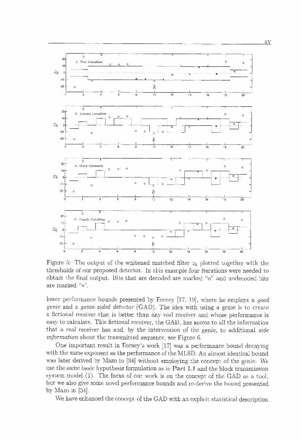
Figure 5: The output of the whitened matched f i l ter zk p lot ted together w i t h the

thresholds of our proposed detector. I n this example four iterations were needed to

obtain the final output. Bits tha t are decoded are marked "o" and undecoded bits

are marked "*".

lower performance bounds presented by Forney [17, 19], where he employs a good

genie and a genie-aided detector ( G A D ) . The idea w i t h using a genie is to create

a f ict ional receiver that is better than any real receiver and whose performance is

easy to calculate. This fictional receiver, the G A D , has access to al l the informat ion

that a real receiver has and, by the intervention of the genie, to additional side

information about the transmitted sequence, see Figure 6.

One important result i n Forney's work [17] was a performance bound decaying

w i t h the same exponent as the performance of the M L S D . A n almost identical bound

was later derived by Mazo in [34] wi thout employing the concept of the genie. We

use the same basic hypothesis formulat ion as in P a r t 1.1 and the block transmission

system model (1). The focus of our work is on the concept of the G A D as a tool ,

but we also give some novel performance bounds and re-derive the bound presented

by Mazo in [34].

We have enhanced the concept of the G A D w i t h an explicit statistical description

x v i

n : A(0,<r n )

H y

b

Side information channel z

Figure 6: The D T G C and the side information channel.

of the side information. That is, we introduce conditional probabilities for any

particular side informat ion to appear given the identity of the transmitted sequence,

describing the operation of the lower path in Figure 6. This makes it possible to

derive the G A D w i t h Bayesian detection theory, which seems to be diff icult wi thout

otherwise augmenting Forney's work w i t h some extra a priori information. I t is

sometimes argued that i f the to ta l i ty of information is used optimally, the G A D

must have a better performance than any actual receiver. This reasoning must,

however, be used w i t h care: the criterion of optimali ty and the system model must

be precisely specified for i t to be meaningful. One of the points of this report is to

make a derivation of the G A D based on a complete model, using the criterion of

min imum bit-error probability.

The side informat ion z supplied to the G A D is given for every bit to be decoded.

The side informat ion for the decoding of bit is a pair of sequences (ß+,ß~) <E

Cjt x C k (at least differing i n the b i t to be decoded), the transmitted sequence being

either ß+ or ß~. Our transition probabilities Pr iz^Aßf j and Pr ^Zij\ßj j are user-

selected design parameters. These parameters control the properties of the bound

resulting f r o m analysing the GAD's performance. The structure given in P a r t 1.3

is flexible in tha t many different performance bounds can be derived, among them

Mazo's bound [34].

When the side informat ion is given w i t h the transition probabilities described by

Lemma 4.2 in P a r t 1.3, the performance of the G A D for b i t k w i l l be determined

by a Q(-) - funct ion scaled w i t h a constant independent of the SNR, as

w i t h 123̂ 1 as the number of elements in a set of exclusive pairs of sequences at

min imum distance. Equation (8) is Mazo's bound [35] and of the same form as the

bound presented by Forney [17, 19]. We also introduce other bounds on performance,

for instance the tightest bounds possible w i t h the structure presented in P a r t 1.3.

I n conclusion, the results of our derivation differ f rom Forney's. However, the

significance of our work is not found i n the bounds we derive; i t is found in the appli­

cation of our formal structure when producing such bounds. This formal structure is

an analytic tool , based on the novel probabilistic description of the side information,

for deriving performance bounds. I t is accessible for future analysis, and, we feel,

offers an instructive view on earlier work.

(8)

xvi i

Part II : Low Complexity Receivers

This part of the thesis consists of three conference contributions and one paper

submitted to a conference.

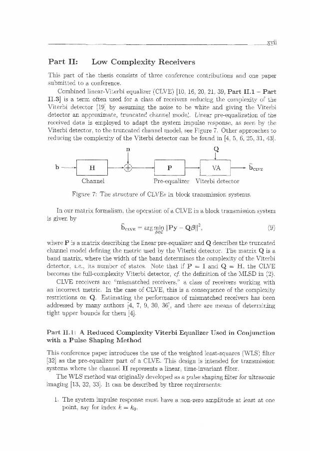
Combined l inear-Viterbi equalizer (CLVE) [10, 16, 20, 21, 39, P a r t I I . l - P a r t

I I . 3 ] is a t e rm often used for a class of receivers reducing the complexity of the

V i t e r b i detector [19] by assuming the noise to be white and giving the Vi te rb i

detector an approximate, truncated channel model. Linear pre-equalization of the

received data is employed to adapt the system impulse response, as seen by the

Vi t e rb i detector, to the truncated channel model, see Figure 7. Other approaches to

reducing the complexity of the Vi te rb i detector can be found i n [4, 5, 6, 25, 31, 43].

n Q

1 H ,r ~\ P VA H J P VA

Channel Pre-equalizer Vi te rb i detector

Figure 7: The structure of CLVEs in block transmission systems.

I n our ma t r ix formalism, the operation of a C L V E in a block transmission system

is given by

b C L V E = a r g m i n | | P y - Q / 3 | | 2 , (9)

where P is a ma t r ix describing the linear pre-equalizer and Q describes the truncated

channel model defining the metric used by the Vi t e rb i detector. The matr ix Q is a

band matr ix , where the w i d t h of the band determines the complexity of the Vi terb i

detector, i.e., its number of states. Note that i f P = I and Q = H , the CLVE

becomes the ful l-complexity V i t e r b i detector, cf. the definit ion of the M L S D in (2).

C L V E receivers are "mismatched receivers," a class of receivers working wi th

an incorrect metric. I n the case of CLVE, this is a consequence of the complexity

restrictions on Q. Est imating the performance of mismatched receivers has been

addressed by many authors [4, 7, 9, 30, 36], and there are means of determining

t ight upper bounds for them [4].

P a r t I I . l : A R e d u c e d C o m p l e x i t y V i t e r b i E q u a l i z e r U s e d i n Conjunc t ion w i t h a P u l s e Shaping M e t h o d

This conference paper introduces the use of the weighted least-squares (WLS) fil ter

[32] as the pre-equalizer part of a CLVE. This design is intended for transmission

systems where the channel H represents a linear, time-invariant filter.

The W L S method was originally developed as a pulse shaping f i l ter for ultrasonic

imaging [13, 32, 33]. I t can be described by three requirements:

1. The system impulse response must have a non-zero amplitude at least at one point, say for index k = fcq.

x v i i i

2. The energy of the system impulse response should be small outside some de­

sired interval, \k — k0\ >

3. The noise amplification should be low.

A solution for 1 and 3 is the matched fi l ter , and a solution for 1 and 2, w i t h the

interval m = 1, is the inverse f i l ter . The WLS filter combines 1, 2, and 3 w i t h the

desired memory length m and the expected noise power ^ into a cost funct ion [32]. We assume here that the channel mat r ix H is Toeplitz describing convolution w i t h

a time-invariant filter. Let H be a larger version of H containing H as a submatr ix

(see P a r t I I . l ) , p be a vector containing the impulse response of the pre-equalizer

{Pk}, ök0 be a vector of zeros except for a one ( T ) at position fco, and, finally, let

V be a diagonal matr ix w i t h m — 1 zeros in the center of the diagonal and ones at

position fco and on the edges. The W L S cost function can then be expressed as

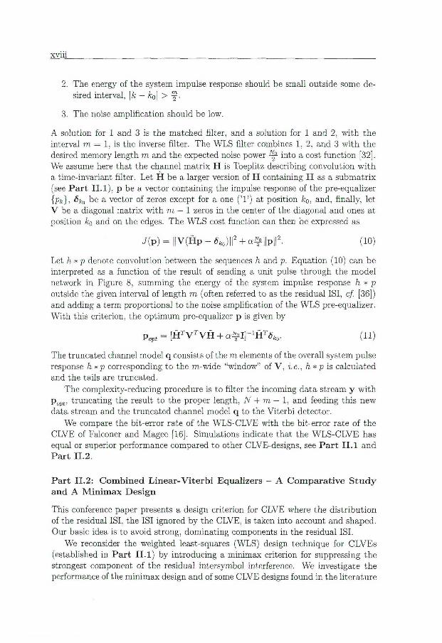
J (p) = | | V ( H P - ^ 0 ) | | 2 + a^| |p | | 2 . (10)

Let h * p denote convolution between the sequences h and p. Equation (10) can be

interpreted as a funct ion of the result of sending a unit pulse through the model

network in Figure 8, summing the energy of the system impulse response h * p

outside the given interval of length m (often referred to as the residual ISI , cf. [36])

and adding a term proportional to the noise amplification of the W L S pre-equalizer.

W i t h this criterion, the op t imum pre-equalizer p is given by

popt = [ H W W H + a Ä I ] - i H X - (11)

The truncated channel model q consists of the m elements of the overall system pulse

response h *p corresponding to the m-wide "window" of V , i.e., h*p is calculated

and the tails are truncated.

The complexity-reducing procedure is to filter the incoming data stream y w i t h

P o p t , t runcating the result to the proper length, N + m — 1, and feeding this new

data stream and the truncated channel model q to the Vi te rb i detector.

We compare the bit-error rate of the WLS-CLVE wi th the bit-error rate of the

CLVE of Falconer and Magee [16]. Simulations indicate that the W L S - C L V E has

equal or superior performance compared to other CLVE-designs, see P a r t I I . l and

P a r t I I . 2 .

P a r t I I . 2 : C o m b i n e d L i n e a r - V i t e r b i Equal izers - A C o m p a r a t i v e S t u d y and A M i n i m a x Des ign

This conference paper presents a design criterion for CLVE where the d is t r ibut ion

of the residual ISI , the ISI ignored by the CLVE, is taken into account and shaped.

Our basic idea is to avoid strong, dominating components in the residual IS I .

We reconsider the weighted least-squares (WLS) design technique for CLVEs

(established in P a r t I I . l ) by introducing a minimax criterion for suppressing the

strongest component of the residual intersymbol interference. We investigate the

performance of the minimax design and of some CLVE designs found in the l i terature

x ix

[10, 16, 21, P a r t I I . l ] . A l l these design methods, including the minimax-CLVE and

the W L S - C L V E , assume that the channel mat r ix H describes a time-invariant filter,

as opposed to the block-CLVE design method of P a r t I I . 3 .

We also present a comparison of these C L V E designs based on a common quad­

ratic opt imizat ion criterion for the selection of the pre-equalizer and the truncated

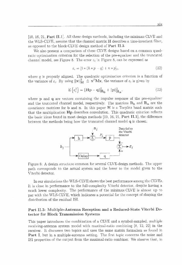
channel model, see Figure 8. The error £, i n Figure 8, can be expressed as

et = [b * (h * p - q) + n * p]u (12)

where q is properly aligned. The quadratic optimization criterion is a funct ion of

the variance of £{. B y using H x U ^ é. x r M x , the variance of ez is given by

e{4} = !IHp (13)

where p and q are vectors containing the impulse response of the pre-equalizer

and the truncated channel model, respectively. The matrices R b and R n are the

covariance matrices for b and n. I n this paper H is a Toeplitz band matr ix such

that the mult ipl icat ion H p describes convolution. This quadratic criterion reflects

the basic ideas found i n most design methods [10, 16, 21, P a r t I I . l ] ; the difference

between the methods being how the truncated channel model q is chosen.

Data fed to the Viterbi detector

Figure 8: A design structure common for several CLVE-design methods. The upper

path corresponds to the actual system and the lower to the model given to the

V i t e r b i detector.

I n our simulations the W L S - C L V E shows the best performance among the CLVEs.

I t is close in performance to the ful l-complexity Vi te rb i detector, despite having a

much lower complexity. The performance of the minimax-CLVE is almost up to

par w i t h the W L S - C L V E , which indicates a potential for the concept of shaping the

dis t r ibut ion of the residual IS I .

P a r t I I . 3 : M u l t i p l e - A n t e n n a Recept ion a n d a Reduced-State V i t e r b i De ­

tector for B l o c k T r a n s m i s s i o n Sys tems

This paper introduces the combination of a C L V E and a symbol-sampled, mult iple

receiving-antenna system model w i t h maximal-ratio combining [8, 12, 22] i n the

receiver. I t discusses two topics and uses the same matrix formalism as found in

P a r t I , but in a multiple-antenna setting. The first topic concerns the noise and

ISI properties of the output f r o m the maximal-ratio combiner. We observe that , in

X X

Q

) y

G V A 1 ' G V A

Figure 9: The receiver structure for the case that the noise at each particular antenna

is uncorrelated w i t h the noise at all other antennas.

general, as the number of available antennas increases, the severity of distort ion (ISI

and noise) decreases.

We note that a system w i t h a receiver as depicted in Figure 9, w i t h mult iple

receiving-antennas, a maximal-ratio combiner, and an additional data transforma­

tion matr ix , can be modelled w i t h our standard block transmission system model

(1). The equivalent model has a quadratic, N x N, channel mat r ix H , which cannot

be interpreted as a convolution w i t h a dispersive, time-invariant f i l ter . This makes

standard methods of CLVE-design inappropriate and calls for new design methods.

The second topic we discuss is the design of CLVEs for block transmission sys­

tems, allowing the channel matr ix H to have arbitrary structure, see P a r t I I . 3 and

P a r t I I . 2 . CLVEs designed for continuous transmission systems presume a t ime-

invariant system impulse response. We give an example of a block-CLVE design

method, a block version of the WLS-method f rom P a r t I I . l , to il lustrate possible

performance gains. This method is, however, not practical due to its high design

complexity; its significance is that i t may give insight into block-CLVE design.

P a r t I I . 4 : Implementa t ion of a S y s t e m for Va l ida t ion of A lgor i thms U s e d

in Dig i ta l R a d i o C o m m u n i c a t i o n Schemes

A hardware system for testing and evaluating algorithms and methods used in the

physical layer of communication systems is presented. The reusable hardware plat­

form facilitates rapid implementation of different digi ta l receivers and is, e.g., suit­

able for CLVEs. This proposed hardware system part ial ly merges system simulation

w i t h real-time validation; its purpose, i n the development of communication con­

cepts, is to make the real-time validation phase as flexible as the simulation phase.

The proposed flexible system uses standard signal processors, array signal pro­

cessors and f ield programmable gate arrays. I t also contains a software controlled

waveform generator to be used as a transmitter and a high performance channel

simulator. The point of the paper is that the use of this p la t fo rm would lower

the cost i n t ime and equipment involved in developing prototypes and validating

communication systems.

To illustrate the use of the proposed system, a GSM-type system w i t h high data

rate is used as a design example.

xx i

Part I I I : Robust Receivers for Ultrasound

The following two papers address the problem of t ime-of-fl ight estimation when

the shape of the received pulse is uncertain, see e.g., [40, 42], The primary in­

tended application is distance estimation using the ultrasonic pulse-echo method

[38], W i t h the ultrasonic pulse-echo method, a short pulse w i t h most of its energy

concentrated in a narrow frequency band, cf. Figure 10, is transmitted w i t h an ul­

trasound transducer. Reflections w i l l appear where the acoustic impedance changes,

and the distance to a reflector is assumed to be proportional to the time-of-flight

of the pulse. In the two papers we address the problem of estimating the distance

to a single reflector by estimating the arrival-time and the changes of shape of a

returned pulse whose shape has been changed by additive noise and time disper­

sion. (For example, the geometry of the reflector affects the shape of the reflected

pulse [27].) We present two approaches for mi t iga t ing the effect of the pulse-shape

distortion. Al though the intended application is pr imari ly distance measurements

using ultrasound, the two methods for t ime-of-flight estimation presume only that

a known, narrowband waveform is t ransmit ted through a dispersive linear system

w i t h additive Gaussian noise.

Our use of the word "robust" to describe our receivers in P a r t I I I . l and P a r t

I I I . 2 deserves a comment. The receivers are robust against time dispersion by

modelling and estimating the same. The word "robust" is not used in the sense that

the receivers may simply disregard the shape distortion because they are insensitive

to i t .

Amplitude [V]

Time [|is]

Figure 10: A n example of a received ultrasound pulse.

x x i i

P a r t I I I . l : A R o b u s t Corre la t ion Rece iver for Dis tance E s t i m a t i o n

I n this journal paper we present a method for distance estimation using pulsed

ultrasound based on a continuous-time system model. The developed signal model,

of variable order, accounts for the time-of-flight as well as for an unknown, linear t ime

dispersion and additive noise. Our method can be described in the following way. We

first expand the unknown distort ing system w i t h a Taylor series in the frequency

domain about the transmitted signal's centre frequency. We then simultaneously

estimate the t ime-of-fl ight and the coefficients of the Taylor expansion.

The t ime-of-f l ight estimator is derived based on the criterion of maximum like­

l ihood. The resulting receiver can be seen as a generalization of the well-known

cross-correlation, or "matched fi l ter ," estimator described, e.g., by Nilsson in [37].

The proposed receiver has been validated, and compared w i t h the cross-correlation

receiver, by means of measurements w i t h an experimental ultrasonic surface scan­

ning system. The receiver is found, by both simulations and analysis, to be more

robust against unknown pulse shape distortion than the cross-correlation estimator,

giving t ime-of-f l ight estimates that are less biased. Furthermore, bias versus noise

sensitivity can be controlled by signal-model order selection.

P a r t I I I . 2: S imultaneous T i m e of F l ight a n d C h a n n e l E s t i m a t i o n U s i n g

a S tochas t i c C h a n n e l M o d e l

I n this conference paper we address the problem of estimating the time-of-flight of an

ultrasonic pulse by modelling the shape of the received waveform as stochastic. We

assume the pulse to be distorted by both additive noise and a time-dispersive t ran­

sition system w i t h a stochastic impulse response. The stochastic impulse response

is modelled as a discrete-time impulse response, the taps of which are a sequence of

Gaussian random variables. The covariance ma t r ix and mean of the taps are given

by the user, based on some assumptions or a priori knowledge about the distorting

system. The jo in t estimation of waveform and time-of-flight is couched in terms

of max imum a posteriori ( M A P ) and maximum likelihood estimation. When de­

r iv ing the M A P estimator we assume a priori knowledge of the probabili ty density

of the stochastic transmission system impulse response, and that the transmitted

waveform is known t o the receiver.

The ordinary cross-correlation time-of-flight estimator [37] assumes complete

knowledge of the received noiseless waveform. I n the viewpoint of this paper, i t

has a one-dimensional transmission system model. This investigation indicates that

a more complex model structure is worthwhile when unknown, or partially unknown,

t ime dispersion and additive noise is present.

xx i i i

Corrections

We make a correction to the conference paper P a r t I I I . 2 . I n tha t paper i t is assumed

tha t the t ransmit ted pulse is both bandlimited in frequency and identically zero over

a semi-infinite time-interval. A signal cannot completely f u l f i l l both these criteria.

Instead of being bandlimited in frequency, the signal should have most of its energy

concentrated to a narrow frequency interval. (One alternative would have been the

formulat ion of P a r t I I I . l . )

xx iv

Bibliography

K. Abend and B.D. Fritchman, "Statistical detection for communication chan­

nels w i t h intersymbol interference," Proc. IEEE, 58(5):779-785, May 1970.

K . Abend, T.J . Harley and B .D . Fritchman, "On opt imum receivers for channels

having memory," IEEE Trans. Inform. Theory, 14(6):818-820, Nov. 1968.

I . N . Andersen, "Sample-whitened matched filters," IEEE Trans. Inform. The­

ory, 19(5):653-660, Nov. 1973.

J.B. Anderson, T . A u l i n and C-E. Sundberg, Digital Phase Modulation, Plenum

Publ . Corp., New York, N .Y . , 1986.

T . A u l i n , " A new trellis decoding algorithm - analysis and applications," Tech.

Rep. no. 2, Chalmers University of Technology, Sweden, Dec. 1985.

T . A u l i n , "Breadth first maximum likelihood sequence detection," Submit ted

to IEEE Trans. Inform. Theory, Oct. 1992.

T . A u l i n , "Genie-aided sequence detection under mismatch," I n Proc. Int.

Symp. Inform. Theory Appl. (ISITA'94), pp. 869-873, Australia, Nov. 1994.

P. Balaban and J. Salz, "Opt imum diversity combining and equalization i n

digi tal data transmission w i t h applications to cellular mobile radio - Part I :

Theoretical considerations," IEEE Trans. Commun., 40(5):885-894, May 1992.

L.C. Barbosa, "Maximum likelihood sequence estimators: a geometric view,"

IEEE Trans. Inform. Theory, 35(2):419-427, Mar. 1989.

C. T. Beare, "The choice of the desired impulse response i n combined linear-

Vi t e rb i algorithm equalizers," IEEE Trans. Commun., 26:1301-1307, 1978.

R.R. Bowen, "Bayesian decision procedure for interfering digi ta l signals," IEEE

Trans. Inform. Theory, 15(4):506-507, July 1969.

D . G. Brennan, "On the maximum signal-to-noise ratio realizable f rom several

noisy signals," Proc. IRE, vol. 43, p. 1530, July 1955.

P.O. Börjesson, N.-G. Holmer, K . L inds t röm, B . Mandersson and G. Salomon-

sson, "Digi ta l preshaping of ultrasonic signals: equipment and applications,"

IEEE Ultrason. Symp., pp. 696-699, 1982.

R.W. Chang and J.C. Hancock, "On receiver structures for channels having

memory," IEEE Trans. Inform. Theory, 12(4):463-468, Oct. 1966.

S.N. Crozier, D.D. Falconer and S.A. Mahmoud, "Reduced complexity short-

block data detection techniques for fading time-dispersive channels," IEEE

Trans. Veh. Tech., 41(3):255-265, Aug. 1992.

X X V

[16] D .D . Falconer and F.R. Magee, "Adaptive channel memory t runcat ion for

max imum likelihood sequence estimation," The Bell System Technical Journal,

52(9): 1541-1562, Nov. 1973.

[17] D.G. Forney, "Lower bounds on error probabili ty i n the presence of large

intersymbol interference," IEEE Trans. Commun., 20(l):76-77, Feb. 1972.

[18] D.G. Forney, "The Vi te rb i algorithm," Proc. IEEE, 61, pp. 268-278, Mar . 1972.

[19] D .G . Forney, "Maximum likelihood sequence estimation of digi ta l sequences

in the presence of intersymbol interference," IEEE Trans. Inform. Theory,

18(3):363-378, May 1972.

[20] S.A. Fredricsson, "Opt imum transmitt ing fil ter i n digi ta l P A M systems w i t h a

V i t e r b i detector," IEEE Trans. Inform. Theory, 20(4):479-489, July 1974.

[21] S.A. Fredricsson, "Joint optimization of transmitter and receiver f i l ter i n dig­

i t a l P A M systems wi th a Vi te rb i detector," IEEE Trans. Inform. Theory,

22(2):200-210, Mar. 1976.

[22] M . J . Gans, "The effect of Gaussian error in maximal ratio combiners," IEEE

Trans. Commun. Technology, 19(4):492-500, Aug. 1971.

[23] C.R.P. Hartman and L . D . Rudolph, "An opt imum symbol-by-symbol decoding

rule for linear codes," IEEE Trans. Inform. Theory, 22(5):514-517, Sept. 1976.

[24] C.R.P. Hartman, L .D . Rudolph and K . G . Mehrotra, "Asymptotic performance

of op t imum bit-by-bit decoding for the white Gaussian channel," IEEE Trans.

Inform. Theory, 23(4):520-522, July 1977.

[25] T . Hashimoto, "A list-type reduced-constraint generalization of the Vi t e rb i

a lgori thm," IEEE Trans. Inform. Theory, 33(6):866-876, Nov. 1987.

[26] J.F. Hayes, T . M . Cover and J.B. Riera, "Opt imal sequence detection and opti­

mal symbol-by-symbol detection: Similar algorithms," IEEE Trans. Commun.,

30(1):152-157, Jan. 1982.

[27] J.A. Jensen, "A model for the propagation and scattering of ultrasound in

tissue," Journal Acoustical Soc. America, 89(1):182-190, 1991.

[28] G. K . Kaleh, "Channel equalization for block transmission systems," IEEE

Journal Sel. Areas Com., 13(1): 110-121, Jan. 1995.

[29] P. Kanerva, Sparse Distributed Memory. 2nd Print ing, A Bradford Book, M I T

Press, Cambridge Mass., London, 1990.

[30] T . Koski , P. Odling and P. O. Börjesson, "Performance evaluations for com­

bined l inear-Viterbi detectors used in block transmission systems," Luleå Uni­

versity, Dept. of Mathematics, Res. Rep. 93-02, Luleå, Sweden, 1993.

X X V I

T. Larsson, A state-space partitioning approach to trellis decoding. Ph.D. thesis,

Chalmers University of Technology, Göteborg , Sweden, 1991.

B . Mandersson, P.O. Bör jesson, N.-G. Holmer, K . L i n d s t r ö m and G. Salomons-

son, "Dig i ta l f i l ter ing of ultrasonic echo signals for increased axial resolution,"

I n Proc. V Nordic Meeting Medical and Biological Eng.. Sweden, June 1981.

B . Mandersson and G. Salomonsson, "Weighted least squares pulse-shaping

fil ters w i t h application to ultrasonic signals," IEEE Trans. Ultrason. Ferroel.

Freq. Cont., 36:109-112, 1989.

J.E. Mazo, "Faster-than-Nyquist-signaling," The Bell System Technical Jour­

nal, 54:1451-1462, Oct. 1975.

J.E. Mazo, "A geometric derivation of Forney's upper bound," The Bell System

Technical Journal, 54(6): 1087-1094, Aug. 1975.

P.J. McLane, " A residual intersymbol interference error bound for truncated-

state V i t e r b i detectors," IEEE Trans. Inform. Theory, 26:548-553, 1980.

N.J . Nilsson, "On the op t imum range resolution of radar signals in noise," IRE

Trans. Inform. Theory, 32(7):245-253, 1961.

J.R. Pellam and J.K. Gait, "Ultrasonic propagation in liquids: I . application

of pulse technique to velocity and absorbation measurement at 15 megacycles,"

Journal of Chemical Physics, 14(10):608-615, 1946.

S. Qureshi and E. Newhall, " A n adaptive receiver for data transmission over

t ime dispersive channels," IEEE Trans. Inform. Theory, 19:448-457, July 1973.

M . Ragozzino, "Analysis of the error in measurement of ultrasound speed

in tissue due to waveform deformation by frequency-dependent attenuation,"

Ultrasonics, 12:135-138, May 1981.

H . L . van Trees, Detection, Estimation, and Modulation Theory, Part I. New

York: Wiley, 1968.

V . A . Verhoef, M . J . T . M . Clostermans and J .M. Thijssen, "Dif f rac t ion and dis­

persion effects on the estimation of ultrasound attenuation and velocity in b i ­

ological tissues," IEEE Trans. Bio. Eng., 32(7):521-529, 1985.

F. Xiong, A . Zerik and E. Shwedyk, "Sequential sequence estimation for chan­

nels w i t h intersymbol interference of finite or inf ini te length," IEEE Trans.

Commun., 38(6):795-803, 1990.

Part L I

Representations for the Minimum Bit-Error Probability Receiver

for Block Transmission Systems with Intersymbol Interference

Channels

P a r t 1.1:

Representat ions for the M i n i m u m B i t - E r r o r Probab i l i ty Rece iver for

B l o c k T r a n s m i s s i o n Sys tems w i t h I n t e r s y m b o l Interference C h a n n e l s

Per Odling 1, Håkan Eriksson 1, Timo Koski 2 and Per Ola Börjesson 1

Research Report T U L E A 1995:11, Division of Signal Processing, Luleå University of Technology.

A shorter version has been accepted for presentation at the 1995 IEEE International

Symposium on Information Theory, Whistler, Canada, September 1995.

1 Luleå University of Technology, Division of Signal Processing, S-971 87 Luleå, Sweden

2Luleå University of Technology, Department of Mathematics, S-971 87 Luleå, Sweden

Representations for the Minimum Bit-Error Probability Receiver for Block Transmission

Systems wi th Intersymbol Interference Channels

Per Odling 1 Håkan B. Eriksson1 Timo Koski 2

Per Ola Börjesson 1

Luleå University of Technology 1 Division of Signal Processing 2 Department of Mathematics

S-971 87 Luleå, Sweden

May 1994

Abstract

We reconsider the minimum bit-error probability receiver for intersymbol interference channels with Gaussian noise using a geometric theory of data transmission of finite blocks of bits. Representations of the receiver are given in terms of an explicit closed form expression consisting of sums of certain Gaussian kernels. Using these representations and assuming that all data se­quences are equally probable we prove two results about the behaviour of the minimum bit-error probability receiver, both results based on that the receiver is dependent on the SNR. We show that the minimum bit-error probability receiver when designed for asymptotically high SNR becomes the maximum

likelihood sequence detector and that i t collapses to a matched filter followed by a hard-limiting device when designed for low SNR. This also implies that these respective receivers attain the minimum bit-error probability in the men­tioned extremes of SNR, a well-established result in the case of the MLSD. Simulations are presented to illustrate our results.

K e y words: d igi ta l block transmission, intersymbol interference, m in imum bi t -

error probability, maximum likelihood sequence detection, matched filter, sufficient

statistic, asymptotic receiver properties.

1

1 Introduction The opt imal , or min imum, bit-error probability receiver (OBER) for intersymbol

interference channels was first proposed in the sixties [1, 2, 5, 9], later fur ther i n ­

vestigated in [7, 10, 19] and recently discussed w i t h respect to neural networks in

[11, 12]. Much of the at tent ion given to the O B E R was transferred to the V i t e r b i

detector [16] when the latter was introduced as a Maximum Likelihood Sequence

Detector (MLSD). When compared to the Vi te rb i detector, the OBER shows only

a moderate gain in bit-error probabili ty [6, 14, 15, 16, 19], but i t achieves this at a

cost of considerably higher computational complexity.

I n this work we reconsider the OBER for block transmission systems i n order

to determine the OBER's properties and its relation to the M L S D . I n section 2

we present a binary block transmission system model. I n section 3 we use standard

detection theory to derive a representation of the OBER. We also point out a parallel

block processor structure for the OBER, which has simultaneous detection of a l l the

indiv idual bits i n a block. I n section 4 we investigate the asymptotic behaviour of

the O B E R when designed for large and small signal-to-noise ratios (SNR). For the

case when all sequences are equally probable, we show that when the SNR used for

designing the O B E R increases wi thout bound, the OBER and the M L S D coincide

in the l i m i t : their respective decision regions become identical. One important

consequence of this is that the M L S D wi l l have the minimum attainable bit-error

probabil i ty when used i n a system wi th a high SNR, as shown in , e.g., [16, 18]. I n

section 4.3 we find a similar correspondence between the OBER and a matched filter

w i t h hard decisions when the O B E R is designed for a low SNR. To il lustrate the

similarities and differences between the three mentioned receivers simulations are

presented i n section 5.

2 A block transmission system model

Consider the transmission of blocks of binary data, typically interspersed w i t h blocks

of bits known to the receiver, through a channel w i t h known intersymbol interference

(ISI) and additive Gaussian noise at the receiver. The set of possible blocks or se­

quences of N bits are the vertices of the centered binary hypercube C é. {—1, + 1 } •

Let b € C denote the stochastic vector containing the sequence of N independent

bits to be transmitted. We represent the transmission system in mat r ix nota t ion as

y = H b + n, (2.1)

where H is a deterministic and known (N + L — 1) x N mat r ix representing the

ISI , n is a white, jo in t ly Gaussian, zero mean random noise vector w i t h variance

a 2 , or equivalently n £ N(0, <x n I) , and, finally, y G H 7 ^ " 1 is the (N + L - 1) x 1

dimensional stochastic variable to be observed by the receiver*. Further, let ß and

T] denote the outcomes of the stochastic variables b and y , respectively. W i t h a few

exceptions, we ignore the issue of coloured noise.

We continue w i t h a number of additional definitions that we w i l l f i nd useful in

*How one can derive this symbol-rate sampled representation from a continuous-time channel model is described in [3, 4, 16].

3

the sequel. Let us first define the SNR in the above block transmission system as

trace { H t H | SNR A - i - (2.2)

n

This is the block-SNR, the average received energy per t ransmit ted bi t over the

variance of the noise in a block.

Following Barbosa i n [4], a sufficient statistic [23] for b given the model i n (2.1)

is provided by

x Z F E = x Z F E ( y ) A M - ^ y , (2.3)

where M = H T H . The matr ix operation M _ 1 H r is an instance of the Moore-

Penrose pseudo-inverse, and can be seen as the zero-forcing equalizer for block

transmission systems (ZFEB) [4, 20]. This is i l lustrated by inserting (2.1) in (2.3)

giving x Z P E = b + M _ 1 H r n . Given that ß is t ransmitted, the output of the ZFEB,

x Z F E € I R ^ , is a jo in t Gaussian noise vector w i t h mean ß and covariance matr ix

equal to M - 1 . Let £ 2 F E A x Z F E (r7) denote the outcome of the stochastic variable X Z F E '

Assuming that al l sequences are equally probable to be t ransmit ted, i t follows,

by the factorizat ion theorem for characterizing sufficiency [23, p. 80] and f rom the

defini t ion of x Z F E , that an M L S D is obtained by solving

D M L S D ( X z f e ) ± a r g m i n | | x Z F E - / 3 1 1 M , (2.4)

where | | X ) | M ä x T M x . One is of ten interested in the bit-error probability, or probabil i ty of error per

data b i t , instead of the sequence error probability. W i t h the output of a detector

denoted by b, we define the pertinent bit-error probability, P B E R , as

^BER ä ^ £ i W , (2-5) i V fc=l

where P D E i f c is the probability of detection error in the kth bit. More strictly, we

define P D E , / C as

J W = E P r {b = 0 } P r { ( b ) b i t k * ( ß ) m k\b = ß } , (2.6) öec

where Pr { b = ß} is the a priori probability that the sequence ß is transmitted,

(/3) b i t k is the kth b i t i n ß and Pr { ( b ) . 4- ( ß ) h i t k |b = ß] is the probabil i ty tha t v \ / Dit K *

the fcth b i t of the detector output differs f rom the corresponding transmit ted b i t .

We refer to systems, described by the model i n (2.1), where opt imal detection

of the t ransmit ted blocks of data can be performed independently on each block,

as block transmission systems, see, e.g., [4, 8, 20]. Many real-life communication

systems, like the cellular phone systems GSM (Europe) and D-AMPS/IS-54 (USA),

use block transmission, often w i t h M L S D , wi thout , however, s t r ic t ly fal l ing into

our def in i t ion of block transmission systems. The coding and interleaving they

employ introduce dependency between the blocks (and the individual bits i n a block),

wherefore op t imal decoding of a particular block cannot be done independently of

al l other blocks, see, e.g., [24]. Here we focus on the properties of the OBER used

i n block transmission systems w i t h independent blocks.

4

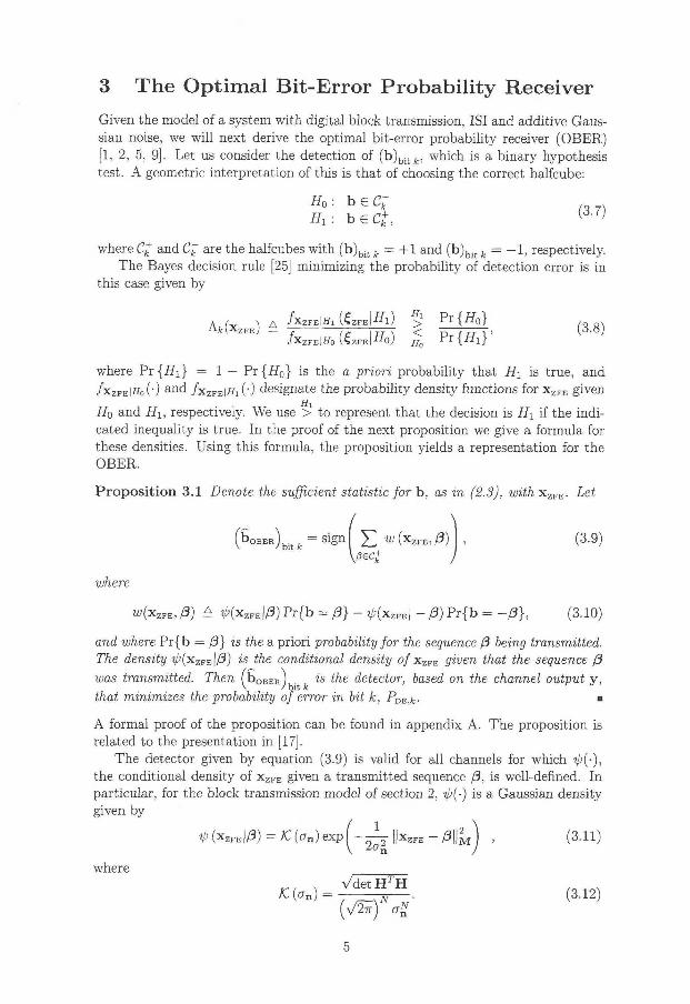
3 The Optimal Bit-Error Probability Receiver

Given the model of a system w i t h digi tal block transmission, IS I and additive Gaus­

sian noise, we w i l l next derive the opt imal bit-error probabil i ty receiver (OBER)

[1, 2, 5, 9]. Let us consider the detection of ( b ) b i t f c , which is a binary hypothesis

test. A geometric interpretation of this is that of choosing the correct halfcube:

Ho: bee; Hi: beCt, ( '

where C£ and Cj) are the halfcubes w i t h ( b ) b i t k = +1 and ( b ) b i t k = — 1, respectively.

The Bayes decision rule [25] minimizing the probabili ty of detection error is i n

this case given by

/xzFElffo HZFEWO) 5 P r { / J 1 } '

where P r { i f i } = 1 - P r { H 0 } is the a priori probabili ty that Hi is true, and

/ x Z F E i i f o ( ' ) a n ( i / X Z F E I # I ( ' ) designate the probabil i ty density functions for X Z F E given

H0 and Hi, respectively. We use > to represent that the decision is Hi i f the ind i ­

cated inequality is true. I n the proof of the next proposition we give a formula for

these densities. Using this formula, the proposition yields a representation for the

OBER.

Propos i t ion 3.1 Denote the sufficient statistic for b , as in (2.3), withxZFE. Let

(3.9) 'OBER = sign bit* 0

Z2 W ( X Z F E , / 3 )

V?ec+ J

where

w(xZFE, ß) A 4>(xZFE\ß) P r { b = ß} - ^ ( x Z F E | - ß) P r { b = - ß } , (3.10)

and where P r { b = ß} is the a pr ior i probability for the sequence ß being transmitted.

The density ip(xZFE\ß) is the conditional density o / x Z F E given that the sequence ß

was transmitted. Then ( b O B E R ) is the detector, based on the channel output y, \ / bit k

that minimizes the probability of error in bit k, PDE,k- •

A formal proof of the proposition can be found in appendix A. The proposition is

related to the presentation in [17].

The detector given by equation (3.9) is valid for all channels for which ip(-)>

the conditional density of x Z F E given a t ransmit ted sequence ß, is well-defined. I n

particular, for the block transmission model of section 2, ip(-) is a Gaussian density

given by

^ ( x Z F E | / 3 ) = £ ( c r n ) e x p ( - ^ \ \ x Z P E - ß f M ) , (3.11)

where VdetWE

E ( g n ) = ; —nv - • (3.12)

5

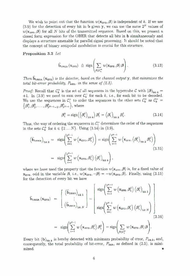
We wish to point out that the funct ion w ( x Z F E , ß) is independent of k. I f we use

( 3 . 9 ) for the detection of every bi t i n b given y, we can use the same 2N values of

w(xZFE, ß) for al l TV bits of the transmitted sequence. Based on this, we present a

closed f o r m expression for the O B E R that detects all bits i n b simultaneously and

displays a structure amenable for parallel signal processing. I t should be noted tha t

the concept of binary antipodal modulation is crucial for this structure.

P r o p o s i t i o n 3.2 Let

b 0 B E R ( x z F E ) £ sign J2 w ( x Z F E , ß ) ß

W i + J

( 3 . 1 3 )

Then 6 0 BER ( X Z F E ) is the detector, based on the channel output y, that minimizes the

total bit-error probability, PBER, in the sense of (2.5).

Proof: Recall tha t Ck is the set of al l sequences in the hypercube C w i t h { ß ) b i t k =

+ 1 . I n ( 3 . 9 ) we need to sum over Ck for each k, i.e., for each bit to be decoded.

We use the sequences in C f to order the sequences in the other sets Ck as Ck =

{ ß k , ß k , . . . , ß k ^ 1 _ l , ß k

2 N - 1 } , where

( 3 . 1 4 )

Thus, the way of ordering the sequences in Cf determines the order of the sequences

i n the sets C£ for k € { 2 . . . N } . Using (3 .14) in ( 3 . 9 ) ,

bit k = sign^ Y w ( X Z F E , ß i ) j = sign^ E w ( x ^ E , [ ß l ) U t k ß\i

/ V - 1

N \

= sign Y w ( x zFE,/3i) (ßl

( 3 . 1 5 )

'bit k

where we have used the property that the funct ion w ( x Z F E , ß) is, for a fixed value of

x Z F E , odd i n the variable ß, i.e., w(xZFE, - ß ) = - w ( x Z F E , ß ) . Finally, using ( 3 . 1 5 )

for the detection of every bi t we have

. ( X Z F E ) —

{ b O B E R

^bit 1 V ^bit 1

( b O B E R ^ bit N -

s J 2 Y w ( ^ ß l ) ( # ) b J

( 3 . 1 6 )

= signj Y w (XZPE , A1) ßi J = s i S n E w ( X ^ E , ß ) ß \ \ i = 1 I \ßec+ J

Every b i t ( b ) b i t j f e is hereby detected w i t h min imum probability of error, PDB,k, and,

consequently, the to ta l probability of bit-error, F B E R , as defined in ( 2 . 5 ) , is min i ­

mized. •

6

I n minimizing the funct ion i n (2.4) the MLSD is processing opt imal ly the infor­

mation x Z F E , sufficient for the transmitted sequence b. The findings above demon­

strate a way the O B E R can be constructed to extract opt imal ly f r o m x Z F E the

informat ion for detecting the individual bits ( b ) b i t f c . I n (3.9) and (3.10) this is i m ­

plemented by making pairwise computations and summations of the a posteriori

probabilities for the vertices in the halfcube C f and for their opposite vertices or

poles (having the maximal possible Hamming distance).

For a given a, the funct ion F(x , a) in (3.13) is a mapping f r o m TRN to { - 1 , + 1 } ^ ,

the hypercube C of dimension N. The operations of equation (3.13) can be seen as

either adding 2N~l different vectors along the diagonals of the hypercube, or as

weighing together the 2N vertices, where the weights are dependent on the received

data. This procedure bears some resemblance to computing the project ion of x Z F E

onto the vertices in the halfcube Cf. We shall show in the next section tha t for low

signal-to-noise ratios (SNR) the argument inside the sign(-) func t ion is dominated

by a term, which is a standard scalar product.

The argument of the sign(-) funct ion in equation (3.13) can also be viewed as

the mapping f r o m x Z F E G ~$lN to a vector of the same dimension that causes the

opt imal decision boundaries to coincide w i t h the uni t axes in H .

I n [11, 10, p. 307] i t is argued that the OBER can be well approximated by a

radial basis function network. Here (3.9) and (3.10) show that the O B E R can in

the case of a Gaussian channel be represented w i t h the exact structure of such a

network [21, pp. 119-120].

4 The behaviour of the O B E R

In this section we w i l l discuss some asymptotic properties of the O B E R for high and

low SNR, given the model in (2.1). Let

\ (4.17) r ( x Z F E ( z ) , a ) A sign £ w ( x Z F E , ß\a) ß

W i )

where

w(xZFE,ß\a) A ^ ( x Z F E | / 3 , a ) P r { b = / 3 } - ^ ( x Z F E [ - / 3 , Q ) P r { b = - / 3 } , (4.18)

and

^ ( x Z F E | / 3 , a ) A / C ( a ) e x p ( - — \\xZFE - ß\\2

M) , (4.19) 1

2~ä2

and where fC(-) is given in (3.12). Then, given the model i n (2.1), T (x , cr n ) =

boBER ( x ) , where an is the variance of the Gaussian noise vector n.

Assuming that al l sequences are equally probable to be t ransmit ted we show that

l i m T(x , a) = b M L S D ( x ) , for all x e IR^ , (4.20)

and that

hrn r ( x Z F E ( z ) , a ) = s i g n ( H T z ) , for all z € TRN+L~\ (4.21)

Equation (4.20) means that the OBER designed for a high SNR becomes the M L S D .

As a consequence of this, the M L S D w i l l achieve the min imum bit-error probabi l i ty

7

when used in systems w i t h a high SNR. I n equation (4.21) we find a similar compar­

ison for low SNR between the O B E R and the matched filter w i t h hard decisions. I f

the true SNR is low, the best possible receiver is actually the matched filter receiver

as comes to the BER.

I n subsection 4.1 we illustrate (4.20) and (4.21) by plott ing decision regions for

the statistics x Z F E 6 IR 2 for a two-dimensional numerical example. We also display

an example of a decision surface when transmitt ing blocks of length 7Y = 3. I n

subsections 4.2 and 4.3 we prove (4.20) and (4.21), respectively.

4.1 A numerical example Let us study the OBER, the M L S D and the matched filter receiver by observing

their decision surfaces for the statistics x Z F E . Let V k designate the region in I R ^

where, when x Z F E € V k , the detector in question decides that b i t k is positive and

V; the region where i t decides that b i t k is negative. The decision regions V k

and V; are bo th continuous and disjoint and the surface that separates the two we

denote the decision surface for b i t k, cf. [22, 26].

I n the numerical experiments below we w i l l confine our attention to the trans­

mission of blocks of two bits (giving a flat two-dimensional hypercube w i t h four

vertices) over a channel w i t h ISI and white, stationary additive Gaussian noise.

Furthermore, we assume that al l sequences have equal a priori probabilities, i.e.,

P r { b = ß} = 2~N = 1/4 for all ß £ C. The matr ix M for this system becomes a

standard 2 x 2 dimensional correlation matrix, i.e.,

M 1 P

P 1 (4.22)

where — 1 < p < 1.

I n Figure 1 we display decision surfaces for x Z F E S IR 2 . On the lef t hand side are

the decision surfaces of the M L S D for b i t one wi th p = 0.1, p — 0.3, p = 0.5, p = 0.7

and p = 0.9, respectively. The corresponding decision surfaces for the matched filter

receiver are given on the right hand side of Figure 1.

Using the system as defined above, Figure 2 shows some samples of decision

surfaces of the O B E R for the statistics x Z F E . Each one of the three graphs of Figure

2 contains decision surfaces for the first bi t in the block, for various SNRs. The

situations described by the three graphs differ in the strength of the noise correlation,

w i t h p equal to 0.1, 0.5 and 0.9, respectively. A correlation p of 0.9 corresponds to

severe ISI , for instance, i n the case of white additive noise n, to a t ime invariant

channel w i t h an impulse response consisting of ten consecutive, equally large ISI

coefficients, e.g., [ 1 , 1 , 1 , 1 , 1 , 1 , 1 , 1 , 1 , l]/^/W. Sign reversing p gives mirrored curves.

The SNRs i n Figure 2 range f r o m — 12dB to 12dB in steps of 3dB, where the straight

lines correspond to - 1 2 d B SNR and the "edgy" curves to +12dB SNR. The curve

corresponding to OdB is dashed.

I n Figure 3 we give an example of a decision surface for the first b i t of the M L S D

when t ransmit t ing blocks of three bits.

As the SNR decreases the decision surface between the decision regions of the two

possible values of any given b i t ( b ) b i t k approaches a hyperplane. This corresponds

to a receiver, for opt imal detection of the specific bit , consisting of a linear f i l ter

followed by a hard l imi t ing device. On the other hand, as the SNR increases the

8

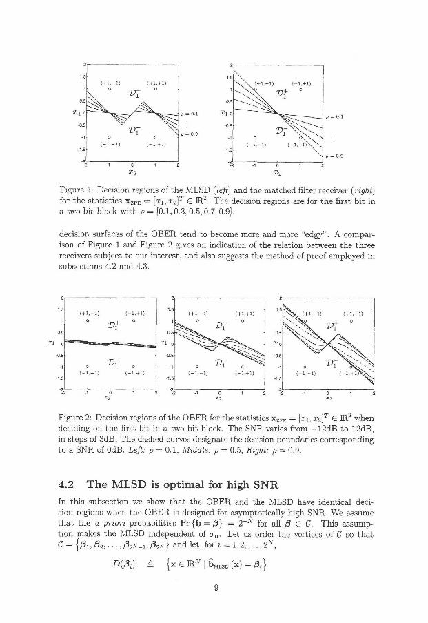
x2 x2

Figure 1: Decision regions of the M L S D (left) and the matched fi l ter receiver (right)

for the statistics x Z F E = [xi, x2)T € IR 2 . The decision regions are for the f irs t b i t i n

a two bi t block w i t h p = [0.1, 0.3, 0.5,0.7, 0.9].

decision surfaces of the O B E R tend to become more and more "edgy". A compar­

ison of Figure 1 and Figure 2 gives an indication of the relation between the three

receivers subject to our interest, and also suggests the method of proof employed in

subsections 4.2 and 4.3.

x2 x 2 x2

Figure 2: Decision regions of the O B E R for the statistics x Z F E = [x%, x2]T £ IR 2 when

deciding on the first b i t i n a two b i t block. The SNR varies f rom — 12dB to 12dB,

in steps of 3dB. The dashed curves designate the decision boundaries corresponding

to a SNR of OdB. Left: p = 0.1, Middle: p = 0.5, Right: p = 0.9.

4.2 The MLSD is optimal for high SNR

In this subsection we show that the OBER and the M L S D have identical deci­

sion regions when the O B E R is designed for asymptotically high SNR. We assume

that the a priori probabilities Pr { b = ß} = 2~N for all ß £ C. This assump­

t ion makes the M L S D independent of on. Let us order the vertices of C so tha t

C = [ ß u ß 2 , . . . ,ß2N_1,ß2N) and let, for i = 1 ,2 , . . . , 2N,

D{ßi) A { x £ m.N I b M L S D (x) =

9

Figure 3: A n example of a decision surface of the M L S D for the statistics x Z F E =

[xi1X2,xs]T G H 3 when detecting the first b i t in a block of three bits . I n the centre

of the Figure the top part of the hypercube is visible.

= { x G R A r | ^ ( x | / 3 I ) > ^ ( x | / 3 J ) , j ^ i ]

denote the region i n E N where ßi is the decision of the M L S D ( b M L S D ) , see (2.4). B y

the boundary of a decision region we mean the set of x G MN for which the two (or

more) largest of the densities ip(x\ßi) are equal. We ignore values on the boundaries

because, once the O B E R or the MLSD are applied i n a communication system,

we w i l l be dealing w i t h channel observables having densities, and outcomes on the

boundaries w i l l then normally have probability zero conditioned on any t ransmit ted

sequence.

Propos i t ion 4.1 Assume the model (2.1) and P r { b = ß} = 2~N for all ß G C.

For all x G I R j V not lying on the decision boundaries it holds that

DMLSD (X) = F ( x , a ) (4.23)

for all a smaller than some positive number dependent on x .

Proof: Let us take a f i xed arbi trary x G H A Because the decision regions { D ( / 3 j ) } 2

= 1

fo rm a par t i t ion of IR^, the chosen x lies in one and only one of the Dißi), disre­

garding x on any of the boundaries. I n addition we assume wi thou t restriction of

generality that this ß{ G C f . From (4.17) we wri te

r (x , a) = sign I < /<x | f t , a) ßi - l K x | - ß l , a ) ß i + £ u>(x, ß\a) ß\ .

(4.24)

10

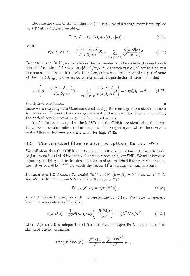
Because the value of the function sign(-) is not altered i f its argument is mul t ip l ied by a positive number, we obtain

T (x, a) = signCft + rißt, x | a ) ) , (4.25)

where

Because x is in D(ßA, we can choose the parameter a to be sufficiently small, such

that al l the ratios of the type ip(x\ß, a) / ^ ( x | / 3 i 5 a) which r (x | / 3 i , a ) consists of, w i l l

become as small as desired. We, therefore, select a so small that the signs of none

of the bits ( ß i ) b i t k is overturned by r ( x | / 3 i , a ) . I n particular, i t then holds tha t

= s i g n ( A ) = ßi , (4.27)

the desired conclusion. •

Since we are dealing w i t h Gaussian densities yj(-) the convergence established above

is monotonic. However, the convergence is not uniform, i.e., the value of a achieving

the desired equality must i n general be altered w i t h x .

I n addition to showing that the M L S D and the O B E R are identical i n the l i m i t ,

the above proof also indicates that the parts of the signal space where the receivers

make different decisions are quite small for high SNRs.

4.3 The matched filter receiver is optimal for low SNR We w i l l show that the OBER and the matched fil ter receiver have identical decision

regions when the OBER is designed for an asymptotically low SNR. We wi l l disregard

input signals lying on the decision boundaries of the matched f i l ter receiver, tha t is,

the values of z G I R i V + i ~ 1 for which the vector H T z contains at least one zero.

Propos i t ion 4.2 Assume the model (2.1) and P r { b = ß} = 2~N for all ß G C.

For all z G 1 R A ' + L _ 1 it holds for sufficiently large a that

r ( x Z F E ( z ) , a) = s i g n ( H T z ) . (4.28)

Proof: Consider the receiver w i t h the representation (4.17). We wri te the generic

kernel corresponding to T(x, a) as

w(x,ß\a) = J ^ ( x , a ) e x p ( - ^ ^ s i n h ( / 3 r M x / a 2 ) , (4.29)

where A(x., a) > 0 is independent of ß and is given in appendix A . Let us recall the

standard Taylor expansion

• uf*T^ , 2 \ ßTMx ( / 3 T M x ) 3

s m h ( / 3 T M x / a 2 ) = + v - ' + . . . .

11

From (4.17), we wri te

r ( x , a ) = s i g n f £ w(x,ß\a)ß

v/JeC7

= sign I ^ - A ( x , a ) £ e x p ( -/3€C+

- ^ / 3 + ^ ( x , a ) - t ( x , a ) ,

where we are collecting the terms containing powers of ßTM.x/a2 of order higher

than one inside the notat ion

t (x, a) A ] T exp ßec+

ßTMß

2a2

( ß T M x )

6 Q 6 ß. (4.30)

Since the value of the sign(-)-function does not change i f its argument is m u l t i ­

plied by a positive number, we scale the argument in the right hand side above by

2NA{x, a ) ' 1 • a2 to obtain

T (x, a) = sign

/

H exp ßTMß

2a2 ßTMxß + a2 • t (x, a) . (4.31)

Let us next note that by selecting a sufficiently large we can make the t e rm

a2 • t (x , a ) arbi trar i ly small, i n particular so small that the value of T (x , a) is

determined by the first t e rm of the argument in the right hand side of (4.31). Ex­

panding expf— ß 2^^) 1 1 1 standard Taylor expansion we f i nd that

T (x, a) = sign £ ßTMxß + u (x , a) + a2 • t (x, a)

\/JeC+

\ (4.32)

where al l terms but the first f r om the Taylor expansion are collected into the funct ion

u (x, a). As in the case w i t h a2 • t (x , a), we can make u (x, a) arbi trari ly small by

choosing a large enough, in particular large enough so that the sign of the r ight

hand side of (4.32) is determined by its first term. By inserting x = x Z F E ( z ) i n

(4.32), recalling that x Z F E ( z ) = M _ 1 H T z and using the identity

E ( / 3 T H r z ) / 3 = £ / 3 ( / 3 T H T z ) = £ H r z = 2 N - W Z , ßeC+ ßeC+ ߀C+

(4.33)

we have

s ign! £ ß T B T

Z ß \

\ßea*

Thus, i t holds that there is for each z e IR

= sign! H z (4.34)

) N+L-l an a large enough so that

T ( x Z F E ( z ) , a) = s i g n ( H T z (4.35)

12

Hence, i n the l i m i t when the SNR used for designing the O B E R decreases, the

O B E R reduces to the matched f i l ter for block transmission systems, H r y , followed

by a hard l imi t i ng device, sign(-), as was to be proved. •

For the case of correlated additive noise n, the receiver of (4.35) generalizes to

the whitened matched filter receiver (WMFR), H T R ~ 1 y > where R n is the correlation

mat r ix for the noise n.

5 Simulations

Consider a communication system that is t ransmit t ing blocks of data over a time

dispersive channel w i t h additive uncorrelated Gaussian noise, n € N(0,a^L), see

the model (2.1). We present simulation results for the OBER, the M L S D (using

the Vi t e rb i algorithm) and the matched fi l ter receiver i n terms of the measured

Bit-Error Rate (BER) and the measured Sequence-Error Rate (SER), for various

SNRs. We have used the time-invariant channel impulse response h/. given in table

1 i n this example. (This is actually the normalized GSM "Rural Area (non-hil ly)"

test channel power profile [13, p . 137], here used as static ISI coefficients.) For each

simulated SNR value enough blocks of 10 data bits (N = 10) were t ransmit ted for

each receiver to make a min imum of 4500 errors.

TABLE 1: T H E CHANNEL IMPULSE RESPONSE

II h[l] - h{6] II 0.6043 I 0.3813 | 0.2406 | 0.1518 | 0.0958 [ 0.0604 [|

The results of the simulations are presented in Figure 4 and Figure 5. To the

left of Figure 4 you find the B E R for the three receivers, and to the right the

corresponding SER. Numerical values of the B E R and the SER are given in tables

2 and 3, respectively, where WMFR refers to the whitened matched filter receiver.

I n Figure 5 the b i t decoding difference rate between the O B E R and the MLSD

respectively the W M F R is plot ted versus SNR. W i t h "bit decoding difference rate"

we mean the ratio of bits on which the decision by the OBER differs f r om the

detector of comparison.

TABLE 2: BIT-ERROR RATE - B E R I N % (see Figure 4)

SNR -20dB -15dB -lOdB -5dB OdB 2dB 4dB 6dB 8dB lOdB

OBER 46.7 41.3 39.5 30.9 20.9 16.1 10.6 5.6 1.9 0.4 MLSD 46.7 41.5 39.8 32.1 21.5 17.2 11.2 5.7 1.9 0.4

WMFR 46.7 41.4 39.1 32.0 25.4 22.1 20.8 20.0 19.1 18.6

TABLE 3: SEQUENCE-ERROR R A T E - S E R IN % (see Figure 4)

SNR -20dB -15dB -lOdB -5dB OdB 2dB 4dB 6dB 8dB lOdB

OBER 99.7 99.7 99.0 97.3 90.7 77.7 58.6 33.1 11.6 2.3 MLSD 99.7 99.5 99.2 96.9 88.5 75.3 55.6 30.8 11.3 2.3 WMFR 99.7 99.7 99.7 98.6 96.7 95.3 94.1 94.1 94.1 93.5

As can be predicted f rom section 4.2 the O B E R and the M L S D are close i n

performance. The gain i n B E R by using the O B E R instead of the M L S D is here

very small, even when the decision regions differ substantially. The receivers w i l l

make different decisions when the received signal lies in those areas where the deci­

sion regions of the two receivers do not overlap, which are small areas in the centre

part of the hypercube. The probabil i ty of the receivers making a different decision

13

Figure 4: The B E R (left) and the SER (right) plotted versus SNR for the O B E R ,

the M L S D and the W M F R .

on any individual bit is calculated as the integral of the part of the noise proba­

bi l i ty mass covering the areas where the decision regions do not overlap, w i t h the

noise probabili ty density centered at the transmitted sequence. When the SNR is

large these areas are small, since the receivers's decision surfaces are close together.

When the SNR is very low, the size of these areas is significant, but the covering

probabili ty mass becomes th in , because the high variance of the noise flattens the

Gaussian distr ibut ion ^ ( x Z F E | b ) . The maximum difference in bit-error probabi l i ty

lies somewhere in between these extremes. (For many channels the largest difference

occurs around OdB SNR.)

For low signal to noise ratios the matched filter receiver has a lower B E R than the

M L S D , although the difference is small. For SNRs below, say OdB in this example,

al l three receivers have roughly equally high BERs. I t should be noted, though,

that the complexity of the whitened matched filter receiver is typically much lower

than the complexity of any of the other receivers. Observe that when the I S I is

severe (corresponding to a closed so called "signal eye"), as in the above example,

the probabili ty of bit-error for the matched filter receiver w i l l not go to zero, even

when no noise is present. I n these cases, the whitened matched fi l ter receiver is not

a consistent estimator of the t ransmit ted sequence.

6 Summary Assuming that al l sequences are equally probable we have shown that the M L S D

is identical to the OBER designed for an infinite SNR. Consequently, the M L S D

w i l l asymptotically possess the property of min imum bit-error probability, as stated

in [16, 18]. I t is to be remembered that the M L S D minimizes the sequence-error

probability, and is thus not by construction concerned w i t h the bit-error probabil i ty.

We have also shown that the matched filter receiver and the O B E R coincide i n the

14

Figure 5: The b i t decoding difference rate between the OBER and the MLSD and

between the O B E R and the W M F R , plot ted versus SNR.

l imi t when the SNR used for designing the O B E R decreases.

The OBER and the M L S D have similar performances and often make the same

decisions on individual bits. Simulation experiments indicate that the difference

in performance for many channels and most SNRs is small. This agrees w i t h the

fact that the bit-error rate of the M L S D is close to upper and lower bounds on the

bit-error probability, as is discussed in , e.g., [6, 14, 16, 18].

A l l facts considered, there is l i t t l e mot ivat ion in terms of performance for using

the O B E R instead of the M L S D as a practical receiver. .Whichever could be i m ­

plemented at the lowest cost or complexity is likely to be preferred. This presently

favours the M L S D in the f o r m of the Vi te rb i detector. However, the OBER, w i t h

its displayed structure, constitutes a powerful tool for studying sufficient statistics

and operations of receivers such as the M L S D and the matched fi l ter receiver as

demonstrated in sections 3 and 4.

Acknowledgements

We would like to acknowledge the improvements provided by Dr. Sarah Kate W i l ­

son, Purdue University, Paul Petersen, West Lafayette, USA and Lie. Tech. Tomas

Nords t röm, Luleå University of Technology.

A P P E N D I C E S

A The Minimum Bit-Error Probability Receiver

Let ip(xZFE\ß, H) denote the probabil i ty density funct ion for x Z F E given that the

sequence ß G C is t ransmit ted and the hypothesis H, and ip(xZFE\ß) denote the

15

probabili ty density funct ion for x Z F E given that the sequence ß G C is t ransmit ted.

Also, let P r { b = ß\H} be the probabili ty for the sequence ß being t ransmit ted,

given the hypothesis H. Note that the geometric formulat ion (3.7) states i n a sense

a pair of composite hypotheses [25, pp. 86-87 ] . Using the above notations, we

obtain

T M H i ) = £ ^ ( x Z F E | / 3 , Hx) Pr { b = ß l H j = £ </>(xZ F E|/3) ^ f Z ^ ßec ßec+ Pr { P i }

(A.1) and

T ( x Z F B | t f „ ) = £ V ( x Z F E | / 3 , H0) Pr { b = ß\H0} = £ ^ ( x Z F E | / 3 ) ßec ß i C - P r l ^ o j

(A.2)

Using ( A . l ) and (A.2) the Bayes test i n (3.8) can be wr i t t en as

£ <Kx Z F E | / 3 ) P r { b = ß} i £ ^ ( x Z F E | / J ) P r { b = ß} (A.3)

or, equivalently,

H i

Y w ( x Z F E , / 3 ) > 0, (A.4)

/3ec+ H 0

where

w ( x Z F E , /3) = ^ ( x Z F E ( y ) | / 3 ) P r { b = /3} - ^ ( x Z F E ( y ) | - ß) P r { b = - / 3 } . (A.5)

From the preceding we observe that u>(x Z F E , /3) is independent of k. The result of

the hypothesis test is given by the sign of the left hand side of (A.4) so that

' O B E R l b i t f c = S I S N E w { X z F B , ß ) \ . (A.6)

Note that i n the process of rewri t ing (A.3) to (A.4) we have grouped the se­

quences ß into pairs (/3, —ß), where ß G C f and consequently — ß G C^ . There

could be other useful ways of grouping the sequences into pairs, giving other receiver

structures. The density ip(xZFE\ß) as given in (3.11) is immediately obtained f r o m

(2.3) and the first properties of multivariate Gaussian distributions.

In the important special case of equal a priori probabilities, P r { b = ß} = 2~N

for all ß G C we obtain using (3.11) i n (A.5) that

w(x,ß) = ^ ( x , c r n ) e x p ( - ^ ^ s i n h f / ^ M x K ) , (A.7)

where / x T M x \

•A(x, an) = 2/C (CT„) exp — — j - > 0 (A.8) 2cr2

and K, (an) is readily obtained as (3.12).

16

References

[1] K . Abend and B.D. Fritchman. "Statistical detection for communication chan­

nels w i t h intersymbol interference." Proceedings of the IEEE, vol. 58, no. 5, pp.

779-785, May 1970.

[2] K. Abend, T .J . Harlev, and B.D. Fritchman, "On opt imum receivers for chan­

nels having memory," IEEE Trans. Inform. Theory, vol. 14, no. 6, pp. 818-820,

November 1968.

[3] I . N . Andersen, "Sample-whitened matched filters," IEEE Trans. Inform. The­

ory, vol. 19, no. 5, pp. 653-660, November 1973.

[4] L .C . Barbosa, "Maximum likelihood sequence estimators: A geometric view,"

IEEE Trans. Inform. Theory, vol. 35, no. 2, pp. 419-427, March 1989.

[5] R.R. Bowen, "Bayesian decision procedure for interfering digi ta l signals," IEEE

Trans. Inform. Theory, vol. 15, no. 4, pp. 506-507, July 1969.

[6] R O . Börjesson, H . Eriksson, T. Koski and P. Odling, "On the structure of the

probabili ty of compatibil i ty in Forney's lower bound and block transmission

systems," 1994. In preparation.

[7] C P . Callender, C.F.N. Cowan and P.M. Grant, "On the use of cluster classifi­

cation for channel equalization at high signal to noise ratios," Mathematics in

Signal Processing III, Edited by J.G McWhir te r , New York: Oxford University

Press, 1994.

[8] S.N Crozier, D .D Falconer and S.A. Mahmoud, "Reduced complexity short-

block data detection techniques for fading time-dispersive channels," IEEE

Trans. Veh. Tech., vol. 41 , no. 3, pp. 255-265, August 1992.

[9] R .W. Chang and J.C. Hancock, "On receiver structures for channels having

memory," IEEE Trans. Inform. Theory, vol . 12, no. 4, pp. 463-468, October

1966.

[10] S. Chen, C.F.N. Cowan and P.M. Grant, "Reconstruction of binary signals

using an adaptive radial-basis-function equalizer," Signal Processing, vol . 22,

no. 1, pp. 77-91, January 1991.

[11] S. Chen, G.J. Gibson, C.F.N. Cowan and P .M. Grant, "Orthogonal Least

Squares Algor i thm for Radial Basis Function Networks," IEEE Trans. Neural

Networks, vol. 2, no. 1, pp. 302-309, March 1991.

[12] S. Chen, B . Mulgrew and S. McLaughlin, "Adaptive Bayesian Equalizer w i t h

Decision Feedback," IEEE Trans, on Signal Processing, vol . 41 , no. 9, pp.

2918-2927, Sept. 1993.

[13] COST207 Management Committee, Digital Land Mobile Radio Communica­

tion, Final Report. Brussels/Luxembourg: Commission of the European Com­

munication, 1989.

17

H . Eriksson, P. Odling, T . Koski and P.O. Börjesson, "A genie aided detec­

tor based on a probabilistic description of the side information," 1994. I n

preparation.

D . G . Forney, "Lower bounds on error probabili ty in the presence of large

intersymbol interference," IEEE Trans. Commun., vol. 20, no. 1, pp. 76-77,

February 1972.

D . G . Forney, "Maximum likelihood sequence estimation of digi tal sequences i n

the presence of intersymbol interference," IEEE Trans. Inform. Theory, vol .

18, no. 3, pp. 363-378, May 1972.

C.R.P. Har tman and L . D . Rudolph " A n Opt imum Symbol-by-Symbol Decoding

Rule for Linear Codes," IEEE Trans. Inform. Theory, vol. 22, no. 5, pp. 514-

517, Sept. 1976.

C.R.P. Hartman, L . D . Rudolph and K . G . Mehrotra "Asymptotic Performance

of O p t i m u m Bi t -by-Bi t Decoding for the Whi te Gaussian Channel," IEEE

Trans. Inform. Theory, vol . 23, no. 4, pp. 520-522, July 1977.

J.F. Hayes, T . M . Cover, and J.B. Riera, "Opt imal sequence detection and opt i ­

ma l symbol-by-symbol detection: Similar algorithms," IEEE Trans. Commun.,

vol. 30, no. 1, pp. 152-157, January 1982.

G. K . Kaleh. "Channel equalization for block transmission systems," IEEE

Journal Sel. Areas Com., vol . 13, no. 1, pp. 110-121, January 1995.

S.Y. Kung , Digital Neural Networks. Englewood Cliffs, New Jersey: Prentice

Hal l , 1993.

J.E. Mazo, "A Geometric Derivation of Forney's Upper Bound," Bell Sys.

Techn. J., vol . 54, no. 6, pp. 1087-1094, August 1975.

L . L . Scharf, Statistical Signal Processing. Detection, Estimation and Time Se­

ries Analysis. New York: Addison-Wesley Publishing Company, Inc., 1991.

R. Scharma, W . D . Grover, W . A . Krzymien, "Forward Error Control (FEC) As­

sisted Adaptive Equalization for Digi ta l Cellular Mobile Radio," IEEE Trans.

Veh. Techn., vol. 42, no. 1, pp. 94-102 , February 1993.

H . L . van Trees, Detection, Estimation, and Modulation Theory, Part I. New

York: Wiley, 1968.

J . M . Wozencraft and I . M . Jacobs, Principles of Communication Engineering,

J. Wi l ey and Sons, New York , Chichester, Brisbane, Toronto, Singapore, 1965.

18

Part 1.2

A Fast, Iterative Detector Making MLSD Decisions on

Scattered Bits

P a r t 1.2:

A F a s t , I terat ive Detec tor M a k i n g M L S D Decis ions on Scat tered B i t s

Per Odling 1 and Håkan Eriksson 1

Research Report T U L E A 1995:12, Division of Signal Processing. Luleå University of Technology.

1Luleå University of Technology, Division of Signal Processing, S-971 87 Luleå, Sweden

A Fast, Iterative Detector Making MLSD Decisions on Scattered Bits

Per Odling Håkan B. Eriksson

E-mail: per.odling@sm.luth.se E-mail: hakan.eriksson@sm.luth.se

Luleå University of Technology Division of Signal Processing

S-971 87 Luleå, Sweden

May 1995

Abstract

This paper presents a fast detector of binary, antipodally modulated data that has been corrupted by intersymbol interference and additive Gaussian

noise. This detector wil l make the same decisions as a maximum likelihood sequence detector on scattered bits in a transmitted sequence. I t is simple in structure, consisting of a whitened matched filter and two variable thresholds for each bit to be detected. The thresholds are dependent on the received signal and are calculated using an iterative method. Both the number of bits to be decoded and their positions in the sequence are stochastic, vary­ing from sequence to sequence. Because the proposed detector leaves bits undetermined and has a low bit error rate on the decoded bits, we believe its primary use would be in combination with low-complexity, sub-optimal receivers. Simulation results demonstrate that the probability of bit error of a decision-feedback equalizer is decreased if this detector is used as a pre­processor. They also demonstrate that the performance of linear equalizers can be improved substantially.

K e y words: d igi ta l block transmission, intersymbol interference, m a x i m u m like­

l ihood sequence detection, fast decoding.

1

1 Introduction

We investigate the detection of blocks of independent antipodally modulated, binary

data t ransmit ted over a discrete-time, additive Gaussian channel w i t h intersymbol

interference (ISI) . We present a fast detector that makes the same decisions as

the max imum likelihood sequence detector (MLSD) [6] on scattered bits in the

t ransmit ted block. Our use of the phrase "decisions on scattered bits" signifies that

only some of the bits in each block are decoded, the remaining bits left undetermined,

where the number of decoded bits and their positions are stochastic and vary f rom

one block to another. The most important property of the detector, its decision

rate, which we define as the average probabili ty that a decision is made on any

particular b i t , depends on the ISI as well as the SNR. Because the detector makes

M L S D decisions on the decoded bits, these bits have a low probabil i ty of error.

Even when implemented wi th the Vi te rb i a lgori thm [6], the M L S D wi l l , in many

applications be too computational complexity to be attractive. Our proposed de­

tector offers an efficient way to obtain MLSD decisions on some random bits. The

complexity of the proposed detector is stochastic w i t h an average that depends on

the IS I . The detector consists of a whitened matched f i l ter and two variable thresh­

olds for each b i t . The thresholds are dependent on the received signal and are

calculated using an iterative method, where the number of iterations is stochastic

but never exceeds the number of bits i n the block.

Perhaps our detector's most important potential use is as an aid to sub-optimal

receivers. Bu t besides this possible practical value, i t also possesses the conceptual

value of helping us to see that some bits are part icularly reliable, reliable in the sense

that they are M L S D decisions. This could, for instance, be used as soft information

when decoding an error correcting code. However, i n this paper we w i l l restrict

ourselves to discussing two principal methods of combining the detector w i t h other

receivers, and to giving simulation examples which use one of these two principal

methods, the one we advocate.

Examples of sub-optimal receivers for block transmission systems that could be

combined w i t h the proposed detector can be found in li terature on digital communi­

cation. I n [7] Kaleh describes four sub-optimal receivers for block transmission sys­

tems: the zero-forcing block linear equalizer, the m i n i m u m mean-square error block

linear equalizer, the zero-forcing block decision-feedback equalizer and the min imum

mean-square error block decision-feedback equalizer. The zero-forcing block linear

equalizer is also derived by Barbosa in [1] where also the M L S D is discussed in the

context of combined linear-Viterbi detectors [10] for block transmission systems, see

also [4, 12].

The presentation proceeds as follows. I n Section 2 a model for block transmission

systems is described and some auxiliary definitions are given. The proposed detector

is derived in Section 3 and described w i t h an explicit algori thm. A n attempt at

geometrical visualization of its operation is also made in terms of decision regions,

and an example of how the thresholds are calculated is given. Section 4 examines

the behaviour of the detector, especially its decision rate. Two methods of how

to implement the proposed detector in combination w i t h sub-optimal receivers are

discussed i n Section 5. Also, in this section, simulation results are presented which

demonstrate that the probability of bi t error of a decision-feedback equalizer would

be decreased i f i t were combined w i t h our proposed detector. I t is also shown that the

3

performance of linear equalizers can be improved substantially. Finally, in Section

6 we summarize our main results.

2 A block transmission system model

Consider the transmission of blocks of binary data, typically interspersed w i t h blocks

of bits known to the receiver, through a channel w i t h additive Gaussian noise and

known intersymbol interference (ISI) . We represent the resulting transmission system

w i t h the ma t r ix notation

y = H b + n, (2.1)

J V + i - l is a vector where the t ransmit ted message is coded i n b € { — 1, + 1 } J V , V € H '

of channel observables, H is a real-valued, deterministic and known (N + L— 1) x A r

matr ix representing the ISI , and n is a j o in t l y Gaussian, zero-mean random vector

w i t h a N ( 0 , R N ) distr ibution [1 , 7]. We assume the bits in b to be independent,

identically distr ibuted w i t h an equal probabil i ty of + 1 and —1 occurring.

I f the ma t r ix H represents a linear, t ime-invariant and causal system, the struc­

ture of H becomes

H =

h0 o

h0

hi

hL-

V 0 0

' £ - 1

0

0

0

0

h0

hi-x J

(2.2)

where [ho, hi..., hi-{\ is the impulse response of the system. I f ho ^ 0 and hr-i ^ 0

then L is the length of the channel memory.

We continue w i t h a number of additional definitions that we w i l l f ind useful i n

what follows. The signal-to-noise rat io (SNR) i n this block transmission system we

define as t r { e F R " 1 ! ! )

SNR A 1

N \ (2.3)

where t r { X } denotes the trace of the matr ix X , i.e., the sum of the elements on the

main diagonal of the matr ix X .

The likelihood function for b given y is the probabil i ty density funct ion for y

given b. The M L S D is any processor that , given the received signal y, finds the se­

quence b for which the likelihood function for b given y reaches its maximum. Since

all sequences are equally probable to be t ransmit ted, the MLSD* is optimal as mea­

sured w i t h the probabili ty of sequence error and asymptotically achieves min imum

probabil i ty of b i t error for high SNR [13]. Defining the mat r ix M A H T R ~ 1 H and

using the model (2.1) w i t h the multivariate Gaussian dis t r ibut ion for y given b as

N ( H b , R N ) , the M L S D is minimizing

L ( b , y ) A | | y _ H b I 2 = l l b - M ^ I T R iViiii- llyllL I - I I H t r ; y | [ 2 M - (2-4)

*The MLSD is often realized as the Viterbi detector [6].

4

w i t h respect to b , where the norm || • | | M is defined as I j x H ^ A x

] M x . Let b

denote the output of the M L S D , the sequence in { — 1, + 1 } ^ found to minimize (2.4).

The last two terms on the right hand side of (2.4) are independent of b . Thus, finding

the sequence b is equivalent to finding the sequence tha t minimizes the first term

on the r ight hand side of (2.4):

g M L D _

b 6 { - l , + l } «

where

L ' ( b . z ) A l l b - M ^ z i ! , (2.6) V ' ' I I I M

and where

z A H T R - X y = M b u = M b + H T R - X n (2.7)

is the output f rom the whitened matched filter iai block transmission systems (WMF)

[1 , 7, 13].

3 The proposed detector

From equation (2.6) we w i l l draw conclusions that are sufficient to devise the men­

tioned detector. Let 6,, & f L S D , z4 and m,ij denote the elements in b , b , z and M ,

respectively, where i is the row index and j is the column index. Focusing on the

detection of the fcth b i t , we rewrite (2.6) in Appendix A and obtain

L ' ( b , z) = 2bk ( A ( b , k) - zk) + g(z, b , fc), (3.1)

where

A ( b , f c ) A X > m a (3.2) x#fc

and

o(z ,b , fc) A bifnijbj - 2 ^ 6 ^ + mkik + z T M z . (3.3) i^k.j^k i^k

Note tha t bo th (3.3) and (3.2) are independent of 6^, and tha t

| A ( b , f c ) | < £ l & ^ ! = £Kfcl< (3.4) i^k ij^k

I f the output of the W M F at instant k is above the possible max imum of A ( b , fc), i.e., zk > Ysijkk \mi.k\, the funct ion L ' ( b , z ) in (3.1) is minimized by bk = + 1 , indepen­

dently of the status of the other bits. Hence, i f the value i n posit ion fc of the output

of the whitened matched filter is above the positive of the threshold, the correspond­

ing output of the M L S D is positive, 6 " L S D = + 1 . Similarly, i f zk < — lA^fc \mi,k\'

then b f L S D = — 1. This is true for all positions fc, and the tests can be done indepen­

dently for al l bits. These observations are sufficient for a t tempt ing to decode some

bits i n a block using only a matched filter and a threshold device. Such a decoding

would constitute the first iteration of the proposed detector.

Assume now that some of the bits in b have been decoded as described above.

These decisions on decoded bits, once made, does not change due to any subsequent

decisions on still-undecoded bits. Using decoded bits as constants, we proceed by

5

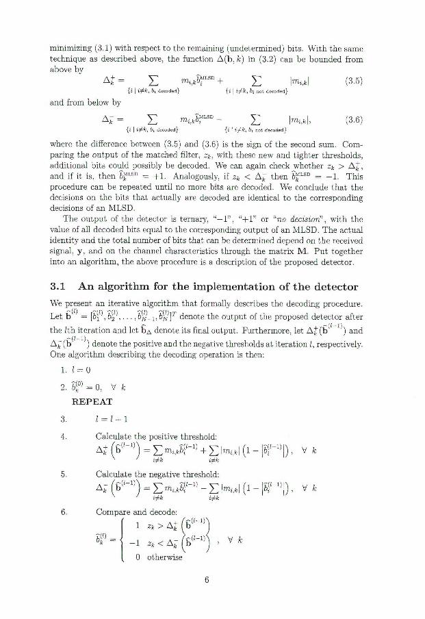
minimizing (3.1) w i t h respect to the remaining (undetermined) bits. W i t h the same

technique as described above, the funct ion A ( b , fc) in (3.2) can be bounded f r o m

above bv

A + = £ r m ß r D + E Kfcl (3-5) {t I iytk, bi decoded} {i j ijtk, 6 ; not decoded}

and f r o m below by

E r n h k b f L S D - E K*| , (3-6) {i I t^fc, 6 j decoded} {i J Ö, not decoded}

where the difference between (3.5) and (3.6) is the sign of the second sum. Com­

paring the output of the matched filter, zk, w i th these new and tighter thresholds,

additional bits could possibly be decoded. We can again check whether zk > A j ,

and i f i t is, then 6^ L S D = + 1 . Analogously, i f zk < Ar ; then b f L S D = - 1 . This

procedure can be repeated unt i l no more bits are decoded. We conclude that the

decisions on the bits that actually are decoded are identical to the corresponding

decisions of an M L S D .

The output of the detector is ternary, " — 1 " , " + 1 " or "no decision", w i t h the

value of al l decoded bits equal to the corresponding output of an M L S D . The actual

identi ty and the to ta l number of bits that can be determined depend on the received

signal, y, and on the channel characteristics through the mat r ix M . Put together

into an algori thm, the above procedure is a description of the proposed detector.

3.1 An algorithm for the implementation of the detector

We present an iterative algorithm that formally describes the decoding procedure.

Let b W = \pi\b2

l\ . . . , 6 / v ] T denote the output of the proposed detector after

the Zth i tera t ion and let 6A denote its final output. Furthermore, let A£(b 1 ) and

A^(b'' ^ ) denote the positive and the negative thresholds at i terat ion I, respectively.

One algori thm describing the decoding operation is then:

1. 1 = 0

2. bf = 0 , V

R E P E A T

3. 1 = 1 + 1

4. Calculate the positive threshold:

Afc ( b j = E m ' A 6 i +Elmvfe! I 1 - pi j) > V fc V ' ii=k i£k

Calculate the negative threshold:

A," f b ^ 1 ' ) = Z m J t * - E K * l (1 - ISM) , V k

Compare and decode:

' 1 zk>Ai(hil~^

^ = ' - i * < A," (b ( i - i r

0 otherwise

6

U N T I L ( | | b W | | | = N or bW = bil~V>

7. b A = b

Note that the output of the detector b A , when implemented by the a lgor i thm de­

scribed above, belongs to { — 1 , 0, + 1 } A ' , where a zero signifies that the detector d id

not make a decision on the corresponding bi t . The algori thm w i l l continue to iterate

un t i l either none of the remaining bits are decoded or there are no more bits to be

decoded. One other way of terminating the algorithm's iterative process would be

to iterate exactly JV times every time.

3.2 An example of the operation of the detector

To illustrate how the proposed detector calculates the thresholds and makes deci­

sions, we present an example where blocks of binary data of length N = 20 are

t ransmit ted over a time-invariant channel described by (2.1). The impulse response

of the system, as in (2.2), is [h0,hi,h2] = [1,0,1] , the noise n is white, stationary

and Gaussian w i t h an SNR of 10 dB. I n Figure 2 an example of the iterations of the

detector is given. The solid lines are the thresholds, A ^ ( b ( ' X ) ) and A r / ( b ( ' J ) ) , the

stars and the circles are the output of the matched f i l ter z, w i t h the circles denoting

symbols decoded at i teration I and the stars undetermined symbols. The upper and

lower thresholds w i l l merge when a sufficient number of bits i n a sequel have been

decoded. I n the example, the bits at k equal to 15, 17 and 19 could not be decoded.

Note that b i t 12 was decoded as positive although the output f r om the whitened

matched f i l ter was negative. I n this example the detector made correct decisions

on all bits that were decoded. As we wi l l see later, this example is typical for this

channel i n the sense that the proposed detector frequently iterates four times.

The detector can be seen as a whitened matched fi l ter followed by two thresholds,

which may be different for every bit k and vary w i t h every iteration, cf. Figure 1.

The thresholds are dependent on z and M and have to be re-calculated for every

block. I f the noise n is white and no ISI is present, the thresholds are all equal to

zero and the detector w i l l be equivalent to the opt imal threshold detector.

M

z A A

Figure 1; A block description of the proposed detector.

I f the proposed detector is viewed as a matched filter followed by a decision

device, the a lgor i thm presented above can be seen as an iterative procedure to

calculate the final thresholds defining this decision device. I n the example displayed

i n Figure 2, the thresholds obtained after the t h i rd iteration, that is, the thresholds

shown i n the diagram belonging to the four th i teration, are the final thresholds to

be used.

7

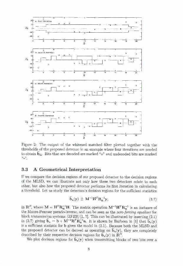
18 20

' « I I I o

b: second iteration o o °

—I 1 1

r ° 0

hn " o o L̂ J o

- O

- r — L _ _

i i i

• L U -2 f c o

18 20

1 4 1 1 1 1 O

- c: third iteration

i 1 ° ° ° °

I >

I *—I ° ° o

o

o 1 1 1

0 „ L J o | 0 |

1 1 1

—ö ' u ;

1 2 4 6 8 10 12

k 14 16 18 20

1 * 1 1 1 1 O d: fourth iteration

1—1 ° ° ° 1—*—I 0

° o

k - T —

0

o 1 1 1

o c 0 o I 1 " O "

i i

L _ l "

i i ) 2 4 6 8 10 12

fc 14 16 18 20

Zk

Figure 2: The output of the whitened matched f i l ter p lot ted together w i t h the

thresholds of the proposed detector in an example where four iterations are needed

to obtain b A - Bi ts that are decoded are marked "o" and undecoded bits are marked

"*".

3.3 A Geometrical Interpretation

I f we compare the decision regions of our proposed detector to the decision regions

of the M L S D , we can illustrate not only how these two detectors relate to each

other, but also how the proposed detector performs its f irst i terat ion i n calculating

a threshold. Let us study the detectors's decision regions for the sufficient statistics

K(y) A M - ^ R - V , (3.7)

in JRN, where M = H T R „ 1 H . The matr ix operation M ^ H ^ R " 1 is an instance of

the Moore-Penrose pseudo-inverse, and can be seen as the zero-forcing equalizer for

block transmission systems (ZFEB) [1, 7]. This can be i l lustrated by inserting (2.1)

in (3.7) g iv ing bu = b + M " 1 H T R ~ 1 n . I t is shown by Barbosa in [1] that b a ( y ) is a sufficient statistic for b given the model i n (2.1). Because b o t h the M L S D and

the proposed detector can be derived as operating on b u ( y ) , they are completely

described by their respective decision regions for b u ( y ) i n TRN.

We plot decision regions for b„ (y ) when t ransmit t ing blocks of two bits over a

8

time-invariant channel w i t h channel impulse response [h0, hi) = [1,1], see (2.1) and

(2.2), and w i t h white, stationary and Gaussian noise n. The lef t part of Figure 3

contains the decision surface of the MLSD for the detection of the first b i t i n the

block. The four possible transmitted sequences are marked w i t h circles. The set

of possible sequences is often referred to as the binary hypercube'', i n this case the

2-dimensional binary hypercube. I f bu £ V~[ then bi t one of b is equal to + 1 ,

otherwise i t is — 1 . I n the right part of Figure 3 the corresponding decision regions

of the proposed detector are shown. I f bu £ ö \ or bu £ O f the output for b i t

one is equal to + 1 and — 1 , respectively. I f b „ £ ö° then the detector is unable to

make a decision. I n the example, i t is clear f r om Figure 3 tha t the bits decoded by

the proposed detector w i l l be the identical to the corresponding decisions made by

the M L S D . The decisions made i n the first i teration would also be the same as the

decisions made by the min imum bi t error probabili ty receiver, which can be shown

by using the technique of Appendix A on the results in Appendix A of [13].

2, . 1 1

1.5

(+1,-1) t+1, + 1)

v+

0.5

-0.5

(-1,-1) (-1.+1) -1.5 •

- 2 - 1 0 1 2 - 2 - 1 0 1 2

x2 x2

Figure 3: Examples of 2-dimensional decision regions for the statistics bu and for the

detection of the first b i t in a two-bit block. The left part shows the decision regions

of the M L S D and the right part the decision regions of the proposed detector, w i t h

the [ x i , x 2 ] as coordinates in IR 2 . (Note that the angle of the decision boundaries

depends on the mat r ix M . W i t h this particular impulse response the boundaries

happen to cross [ + 1 , —1] and [—1,+1].)

I n Figure 4 we show an example of a 3-dimensional decision surface of the M L S D

for the detection of the first b i t i n a block of three bits. As can be noted in bo th

the 2D and 3D pictures there are 2 N _ 1 parallel hyperplanes extending f r o m the

interior of the hypercube. I f these planes had passed through origo, they would

have represented the operation of the whitened matched filter, i.e., the sign of the

output of the filter at instant k = 1 would have told whether bu is above or below

this hyperplane [13]. I t can be observed that, for every bi t , the signal space can be

divided into three parts by extending the two most offset of the parallel hyperplanes,

the uppermost and the lowermost. I f the output of the matched f i l ter at some

instant k is larger than this offset, we know that the M L S D would decide on the

corresponding bi t being positive. Analogously, i f the output is below the negative

of the same offset, the corresponding output of the M L S D is — 1 .

^Discussions on the geometry of the binary hypercube can be found in, e.g., [8, 9, 13].

9

Figure 4: A n example of a 3-dimensional decision surface of the M L S D for the

statistics bu and for the detection of the first b i t in a block of three bits. The

[xi,X2,Xs\ are coordinates in IR3.

4 Performance analysis

I n section 3 we concluded that the decisions made by the proposed detector are

the same as the decisions made by the MLSD. This, we feel, is our detectors most

impor tan t property. Following this i n importance would be its decision rate, its

average probabi l i ty of making a decision on any individual bi t . We w i l l first give

a def in i t ion of the "decision rate" and then, making use of this definition, proceed

to use simulations to investigate this and other aspects of the proposed detector's

behaviour. The simulations w i l l illustrate that the detector's decision rate is h igh

enough for the detector to be of practical value.

We define the probabili ty that a decision has been made on b i t k after i tera t ion

/ as

Pf* A Pr {b[l) * 0} = 1 - Pr {bil) = 0} , (4.1)

where denotes the decision on the kth bi t after the Ith iteration, see the a lgor i thm

described in Section 3.1. The probabil i ty that the proposed detector makes a decision

on b i t k is PD,k — P'o.h where N is the length of the block and the maximal number

of i terations needed to process the block. Finally, the decision rate is defined as

PD^IEPD*- (4-2) i v fc=i

10

The decision rate is, of course, dependent on the ISI , as well as on the covariance

matr ix of the noise. For instance, i f no ISI is present and the noise n is white, then

the detector reduces to the opt imal threshold detector [13], and decodes all bits.

In appendix B an expression for the probabili ty that the detector has decided

on bi t fc after i terat ion I, P^k, is derived. Evaluating this expression is a computa­

t ionally demanding task. Besides integrating densities over iV-dimensional boxes, i t

requires the evaluation and summation of a large number of such integrals. Because

an analytic evaluation of the decision rate, P ø , seems to be a complicated task, i t

is only addressed by simulations i n this paper.

4.1 Studying the behaviour of the detector by simulations

As noted above, the potential of the proposed detector is very dependent on its

abi l i ty to make decisions. This section presents simulation results where the pro­

posed detector is used to detect bits i n a block transmission system. Consider a

time-invariant two-tap channel described by (2.1) and (2.2) w i t h

hk = 6(k) + a6{k-d), (4.3)

where S(-) is the Kronecker delta funct ion, a is the real-valued amplitude of the

second tap and d, a positive integer, is the time-spread of the channel. Throughout

these simulations the noise n is white, stationary and Gaussian; the block length

A r = 20.

The Figures w i t h the simulations results discussed in this section are collected

in Appendix C. I n Figure 6 the estimated probabili ty of no decision, 1 — Pfo, is

plotted versus the strength of the second tap, a, for the delay d G [1,2,5,10,15] and

an SNR of 10 dB. I t can be observed that the probabili ty of no decision, given a

certain d, has global maxima at around a = 1 and a = — 1 , i t is low i f |a | is small or

large enough, and also non-increasing w i t h d. I f rf > A the two received echoes are

separable, effectively a no-ISI case, and consequently the detector is able to detect

all bits.

Figures 7 to 10 show various data f r o m a simulation varying the SNR in a two-

tap channel model w i t h impulse response [h0, hi, h2) = [1,0,1] , as described by the

model (4.3) w i t h rf = 2 and a = 1. Among the two-tap channels, this is the worst

case as given by Figure 6.

Figure 7 shows the estimated probabil i ty that b i t number k is decoded, Pd,/C, for varying SNR. The plot shows the probabili ty of decision for each ind iv idua l b i t

k G [ 1 , 2 , . . . , 20] separately. The four bits at the edges of the block, i.e., the bits

corresponding to fc G [1,2,19,20], have the highest probabil i ty of being decoded.

This is because these bits are subjected to less ISI than the bits i n the centre part

of the block. As these bits are decoded more frequently, their neighbours, the bits

at fc G [3,4,17,18] are also decoded more frequently. I t can be observed tha t the

probabil i ty of decision in general decreases w i t h increasing SNR.

I n Figure 8 the bi t error rate (BER) of the M L S D is plot ted versus SNR, w i t h the

B E R divided into two parts; the B E R of the bits that could have been decoded by the

proposed detector and the BER of the bits that would have been left undetermined.

Note that the bits that could have been decoded have a B E R that is a f rac t ion of

the B E R of the other bits. In this sense the detector apparently finds bits tha t are

"easy" to decode correctly.

11

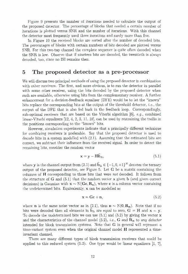
Figure 9 presents the number of iterations needed to calculate the output of

the proposed detector. The percentage of blocks that needed a certain number of

iterations is plot ted versus SNR and the number of iterations. W i t h this channel

the detector most frequently used three iterations and rarely more than five.

I n Figure 10 the received blocks are sorted after the number of decoded bits.

The percentages of blocks w i t h certain numbers of bits decoded are plot ted versus

SNR. For this two-tap channel the complete sequence is quite often decoded when

the SNR is low. Observe that i f nineteen bits are decoded, the twentieth is always

decoded, too, since no ISI remains then.

5 The proposed detector as a pre-processor

We w i l l discuss two principal methods of using the proposed detector in combination

w i t h other receivers. The first, and more obvious, is to run the detector in parallel

w i t h some other receiver, using the bits decoded by the proposed detector when

such are available, otherwise using bits f rom the complementary receiver. A fur ther

enhancement for a decision-feedback equalizer (DFE) would be to let the "known"

bits replace the corresponding bits at the output of the threshold detector, i. e., the

output of the D F E that is also fed back in the feedback loop. Correspondingly,

sub-optimal receivers that are based on the Vi te rb i algorithm [6], e.g., combined

l inear-Viterbi equalizers [12, 4, 2, 5, 11, 10], can be used by restraining the trellis i n

the positions corresponding to the "known" bits.

However, simulation experiments indicate that a principally different technique

for combining receivers is preferable. Say that the proposed detector is used to

decode bits in a system modelled w i t h (2.1). Assuming that the estimated bits are

correct, we subtract their influence f rom the received signal. In order to detect the

remaining bits, consider the random vector

x = y - H b A , (5.1)

where y is the channel output f r o m (2.1) and b A £ {—1,0, + 1 } ^ denotes the ternary

output of the proposed detector, see Figure 5. Let G be a mat r ix containing the

columns of H corresponding to those bits that were not decoded. I t follows f r o m

the structure of G and (5.1) that the random vector x given b (and given correct

decisions) is Gaussian w i t h x ~ N ( G c , R n ) , where c is a column vector containing

the undetermined bits. Equivalently, x can be modelled as

x = G c + n, (5.2)

where n is the same noise vector as in (2.1), thus n ~ N(0, R „ ) . Note that i f no

bits were decoded then al l elements in b A are equal to zero, G = H and x = y.

To decode the undetermined bits we can use (5.1) and (5.2) by giving the vector x and the characteristics of the channel model (5.2), i.e., G and R n to any detector

intended for block transmission systems. Note that G in general w i l l represent a

time-variant system even when the original channel model H represented a time-

invariant channel.

There are many different types of block transmission receivers tha t could be

applied to this reduced system (5.2). One type would be linear equalizers [1, 7],

12

M

H T R ; A

H

post processo:

Figure 5: The proposed detector as a pre-processor.

which could, for instance, be based on the min imum mean-square error [7] or zero-

forcing cri teria [1 , 7]. Another type would be the DFEs described in [7]. Combined

l inear-Viterbi equalizers for block transmission systems capable of handling t ime-

variant systems [4], could also operate directly on the reduced system (5.2).

When a decision made by the proposed detector is erroneous, i.e., when a decoded

b i t differs f r o m the corresponding transmitted bi t , the reduced system of equation

(5.2) is an incorrect model of the signal x. As a consequence, the complementary

detector w i l l be inclined to make additional erroneous decisions on the remaining

bits. However, this error propagation is likely to be less severe than, for instance,

the error propagation in DFEs, because the decisions made by the proposed detector

have a lower BER.

I n the following section we combine the proposed detector w i t h four receivers

described by Kaleh in [7]: two linear equalizers and two decision-feedback equalizers,

one of each based on the min imum mean-square error and zero-forcing criteria,

respectively.

5.1 Simulations of receiver combinations To il lustrate the potential of the proposed detector as a pre-processor, we present

results f r o m simulations of block transmission systems w i t h four different sub-

opt imal , complementary receivers, see Figure 5. The four sub-optimal receivers are:

the zero-forcing linear equalizer (ZFE), the minimum-mean square error equalizer

( M M S E ) , the zero-forcing decision-feedback equalizer (ZF-DFE) and the min imum-

mean square error decision-feedback equalizer (MMSE-DFE) , all described by Kaleh

in [7]t.

I n the simulations, blocks of data of length N = 20 are t ransmit ted over a

time-invariant dispersive channel w i t h additive, stationary, white, Gaussian noise, as

described by (2.1). The impulse response of the system is again [ho, hi, h2] = [ I , 0,1].

Figures containing the simulation results are presented in Appendix D .

Simulation results in terms of the BER versus SNR are presented in Figures

11-12, w i t h the performance of the M L S D included as a reference. Note tha t al l the

complementary receivers improve their performance when our proposed detector is

used as a pre-processor. As an example, the performance of the ZFE is improved

by approximately 4 dB at a B E R of 10~3. I n contrast to the unaided case, the

Z F E combined w i t h the proposed detector has a slightly better performance than

•These receivers were derived in [7] to operate on the output of the whitened matched filter. Here, this corresponds to z' = G T R ^ 1 x .

13

the corresponding combination w i t h the MMSE. A t first glance, this may seem to

contradict other known results, see e.g., [7]. I t should be noted, however, tha t

because the proposed detector sometimes makes errors, the model (5.2) used for the

two equalizers might be incorrect. I n this example this would seem to penalize the

M M S E more than the ZFE, but this need not always be the case, especially when

the decision rate is low.

In Figure 12 the performances of the ZF-DFE and the M M S E - D F E w i t h and

without the proposed detector are compared. The performances of bo th receivers

improve w i t h the pre-processor, although the improvements are much smaller than

the improvements for the linear equalizers. This agrees w i t h the DFEs being much

closer to the M L S D i n performance, making the potential for improvements smaller.

Figures 13-16 contain B E R curves where the B E R has been divided into two

parts; the BER of the bits that were decoded by the proposed detector and the B E R

of the remaining bits. As can be observed, the bits decoded by the pre-processor

have a lower B E R than the other bits. Note also that the B E R of the bits decoded

by the complementary receivers operating on the reduced system (5.2) is improved

compared to the corresponding bits f rom the unaided receivers.

6 Conclusions

We have presented a detector of low computational complexity tha t makes M L S D

decisions on a por t ion of the transmitted bits. The key components of the detector

are a whitened matched filter and a threshold device w i t h two variable thresholds

per b i t .

We believe that the pr imary use of the proposed detector is as a complement to

sub-optimal receivers inferior i n performance to the M L S D . I t can aid these receivers

either by providing M L S D decisions on scattered bits, or, as in our examples, by

let t ing the complementary receivers operate on a reduced system model. Simulation

experiments using the latter technique show an improvement of the BER in bo th

the bits decoded by the pre-processor and the bits decoded by the complementary

receivers.

A n important property of the proposed detector, determining its potential , is

its decision rate: the average percentage of bits on which a decision is made. The

percentage of bits decoded in a block is stochastic and varies between 0% and 100%,

w i t h the average dependent on the SNR and the channel characteristics. Simulations

using a block length N = 20 rendered a decision rate better than 65% for all two-tap

channel models, while channel models w i th strong ISI and a high SNR could render

decision rates i n the order of a few ten percents.

One other potential ly useful property of the proposed detector is the existence

of unequal error probabilities between the pre-processor and the adjoined receiver.

I t might , for example, be useful in some applications (e.g., those involving soft

decoding information) to know that some bits have been decoded w i t h the M L S D

criterion. This property, not developed in this paper, is a subject for future research.

14

A P P E N D I C E S

A The log-likelihood function

Let bi, zx and m y denote the elements i n b , z and M , respectively, where % is the

row index and j is the column index. Then

L ' ( b . z ) = lib - M - y 2

• ' n I I M

= b r M b - 2 z r b + z r M " J z

= E i j hrriijbj - 2 £ 2 k.Zi + zTM~1z

= E b i m i J b j + E hmkjbj + ] T bimukbk + bkmKkbk - 2 ^ M i - 2Mfc i^k,j^k j^k i^k i^k

+ z T M ^ z

= b k l J 2 bimi* + E m * J & J - 22 f c j + 51 hiriijbj - 2 ] T M i + l & f c l V j ^ W f c 3V* / i^kj^k i^k

+ z T M " 1 z

= 2i>& km^k - z k ) + mk.k + ^2 M ^ , A - 2J2 M i + z T M _ 1 z .

( A . l ) We w i l l use this in the form

L'(b, z) = 2bk ( A ( b , fc) - zk) + g(z, b , fc), (A.2)

where

A(b , f c ) A J > r o a (A.3) i^fc

and

g(z, b , fc) A £ bimidbj - 2 ^ M i + m M + z T M z , (A.4) i^kj^k i^k

see equation (3 .1) .

B The probability of decision

Let Pr jfcjp = 0|b = c } denote the probabil i ty that bk

l) = 0 given that the sequence

c was transmitted. The probability of decision for bit k at step / can then be wr i t ten as

Pn,k = l - E P r { b = c } P r { 6 « = 0!b = c } , ( B . l ) ce{- i ,+ i}- v

15

where Pr { b = c } is the probabil i ty that the sequence c is transmitted. The proba­

b i l i ty

P r { & i ° = 0 l b = c } =

I K - . I D . _ O I K C - 1 ' £ Pr V = a | b = c Pr 6 ^ = 0 | b l ' = a , b = c , (B.2)

ae{-i ,o ,+l} J V ^ J J

where Pr j o j ° = 0 | b ( ' _ 1 ) = d, b = c j is the probabil i ty that I f = 0, given b ( ! _ 1 ) = d

and given tha t c was transmitted, and can be calculated as we w i l l show later.

The probabi l i ty Pr j b ' ' = a|b = c j can be computed recursively as

P r { b ( i - 1 ) = a | b = c } =

£ Pr { b ( ' - 2 ) = d | b = c ) Pr t b ^ = a l b ' " 2 ' = d, b = c ) (B.3) d € { - l , 0 , + l } N I J I J

starting w i t h

P r { S » - R . - . } - { j ^ . (B.4)

Calculat ing the probabil i ty Pr { b ( i ) = a | b ( ' - 1 ) = d , b = c } involves the integra­

t ion of an N-dimensional density funct ion over an N-dimensional box. Note tha t

this density is not jo in t ly Gaussian.

I t remains to calculate the probabili ty Pr jfe® = 0|b ( ' ^ = a, b = c l . Let zk

denote the fcth element in z and m^.k the fcth diagonal element in M . Then, i f

bt1] = o,

Pr fe«=0|bl,-1J = a ,b = c =

( b ( i - 1 ) ) < z , < A - ( b ( ' - 1 ) ) | b ( i - 1 ) = a , b = c } =

r A t i I ( x - z k y \ j

72 lk,k

which can be evaluated using the Q(-)-function [3]. Otherwise, i f b[ ' ^ 0 then

P r { 6 [ i ) = 0 | b ( ' " 1 ) = a , b = c } = 0.

16

C Simulations: The behaviour of the detector The fol lowing pictures are described in section 4.1.

1 1 1 1 i i 1

- d = 1 d = 2 d = 5

- - d = 10 d = 15

f '"' \

• / I'r"- \

/ • ' ' . - ' - 1 1 I ' - \ N V

' / \ x . \\

/ ' / I I . / • ' ' / i ' :

: / •' > \

i ' v ' \ V

'• \ ' \ J \ \ \

-

/ i i ; v / -

%\ -

y / ,' \ ' \ \ \ -

{ S -4 -3 -2 -1 0 1 2 3 4

Figure 6: The probabil i ty of no decision, 1 — PD, for the proposed detector plotted

versus the strength of the second tap, a, for a delay d £ [1, 2, 5,10,15].

0.6

0.55

0.5

{1,2,19,20]

[3,4,17,18]

k e [5,6, . . . , 15, 16]

SNR [dB]

Figure 7: The probabili ty of decision for each individual b i t k, Pr>:k versus SNR.

17

Figure 8: The b i t error rate of the M L S D for the bits decoded by the proposed

detector (dashed line) and for the undetermined bits (solid line) plot ted versus SNR.

10°

^ # iterations # iterations

Figure 9: The percentage of blocks that needed a certain number of iterations is

plot ted versus SNR and the number of iterations. The right part of the figure shows

the same data as the left part but w i t h a logarithmic scale.

18

10C

Figure 10: The percentage of blocks where a certain number of bits were decoded

is p lot ted versus SNR and the number bits. The right part of the figure shows the

same data as the left part bu t w i t h a logarithmic scale.

19

D Simulations: Performances of receiver combi­nations

The following Figures are described in section 5.1.

TO"1

x _ y ZFE

""a N[ / MMSE

.Q >L

\ \ \ \ • v- xs V

X /\y Q \ MMSE w i t h p r e - p r o c . /

> » \ N s \ \ "

ZFE w i t h p r e - p r o c . ZFE w i t h p r e - p r o c .

MLSD /

— i 1 1 I I i u .

-5 0 5 10 15 SNR [dB]

Figure 11: The b i t error rate of the aided and unaided linear receivers versus SNR.

^̂ cSp̂ X / ZF-DFE

^ / M V / / M M S E _ D F E

\ Vs \ / u A

MMSE-DFE w i t h p r e - p r o c ' / ^ \ V \

ZF-DFE w i t h p r e - p r o c f '\ V Ä

MLSD x \ V \\

\ v\ i. 1 , i \ \ \ i

SNR [dB]

Figure 12: The bit error rate of the D F E based receivers versus SNR.

20

-5 O 5 10 15 20 -5 0 5 10 15 20 SNR [dB] SNR [dB]

Figure 13: The B E R of the ZFE (left) and the ZFE combined w i t h the proposed

detector (right) plotted versus SNR. The two curves in the left part of the Figure are

the BER of the bits that could have been decoded by the proposed detector (dashed

line) and the B E R of the bits that would have been left undetermined (solid line).

The bits in the right part are identically grouped. However, here the proposed

detector was used and the ZFE was operating on the reduced system model (5.2).

SNR [dB) SNR [dB]

Figure 14: The BER of the M M S E (left) and the M M S E combined w i t h the proposed

detector (right) plotted versus SNR. The two curves in the left part of the Figure are

the BER of the bits that could have been decoded by the proposed detector (dashed

line) and the BER of the bits that would have been left undetermined (solid line).

The bits in the right part are identically grouped. However, here the proposed

detector was used and the M M S E was operating on the reduced system model (5.2).

21

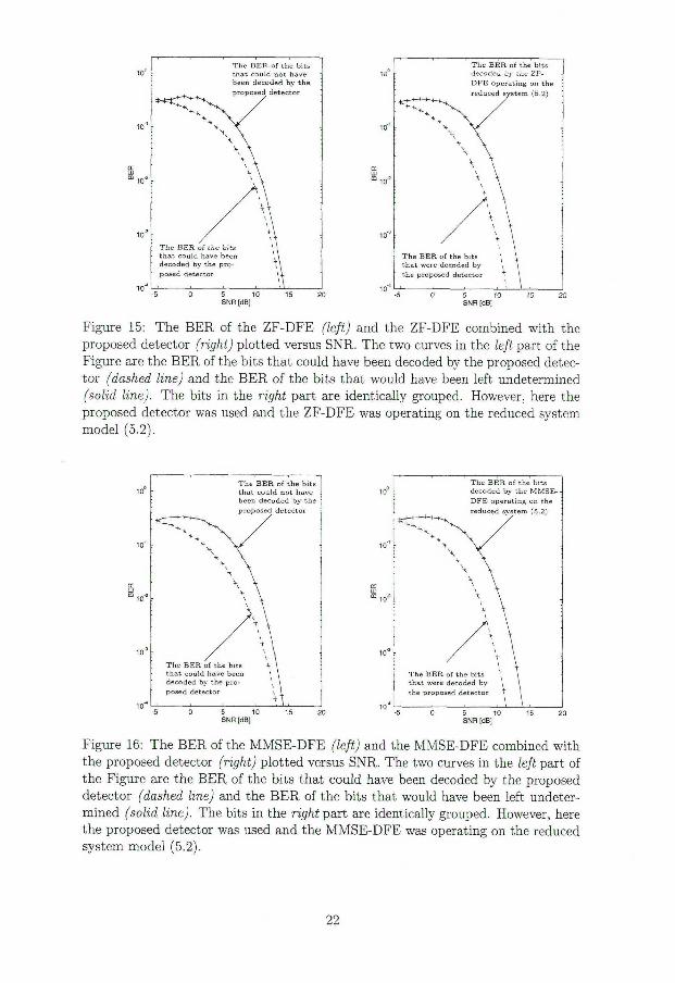
SNR [dB] SNR [dB]

Figure 15: The BER of the Z F - D F E (left) and the ZF-DFE combined w i t h the

proposed detector (nght) p lot ted versus SNR. The two curves in the left part of the

Figure are the BER of the bits tha t could have been decoded by the proposed detec­

tor (dashed line) and the B E R of the bits that would have been left undetermined

(solid line). The bits in the right part are identically grouped. However, here the

proposed detector was used and the Z F - D F E was operating on the reduced system

model (5.2).

SNR [dB] SNR [dB]

Figure 16: The BER of the M M S E - D F E (left) and the MMSE-DFE combined w i t h

the proposed detector (right) p lot ted versus SNR. The two curves in the left part of

the Figure are the B E R of the bits that could have been decoded by the proposed

detector (dashed line) and the B E R of the bits that would have been left undeter­

mined (solid line). The bits i n the right part are identically grouped. However, here

the proposed detector was used and the M M S E - D F E was operating on the reduced

system model (5.2).

22

References

[1] C. Barbosa. Max imum likelihood sequence estimators: A geometric view. IEEE

Transactions on Information Theory, IT-35(2):419-427, 1989.

[2] C. T . Beare. The choice of the desired impulse response in combined linear-

V i t e r b i algorithm equalizers. IEEE Transactions on Communication, 26:1301-

1307, 1978.

[3] Per Ola Bör jesson and Carl-Erik W . Sundberg. Simple approximations of the

error funct ion Q(x) for communication applications. IEEE Transactions on

Communications, 27(3):639-643, March 1979.

[4] H å k a n B . Eriksson and Per Odling. Mul t ip l e receiving antennas and combined

l inear-Viterbi detection. 1995. To be submitted.

[5] D . D . Falconer and F. R. Magee. Adapt ive channel memory t runcat ion for

max imum likelihood sequence estimation. The Bell System Technical Journal,

52(9):1541-1562, November 1973.

[6] David G. Forney Jr.. Maximum likelihood sequence estimation of d igi ta l se­

quences in the presence of intersymbol interference. IEEE Transactions on

Information Theory, IT-18(3):363-378, May 1972.

[7] G. K . Kaleh. Channel equalization for block transmission systems. IEEE Jour­

nal Sel. Areas Com., 13(1):110-121, January 1995.

[8] P. Kanerva. Sparse Distributed Memory. A Bradford Book, M I T Press, Cam­

bridge, 2nd edition, 1990.

[9] J. E. Mazo. A geometric derivation of Forney's upper bound. The Bell System

Technical Journal, 54(6): 1087-1094, 1975.

[10] Per Odling, T imo Koski, and Per Ola Bör jesson . A reduced complexity Vi te rb i

equalizer used in conjunction w i t h a pulse shaping method. I n Proceedings of

The Third International Symposium on Signal Processing and its Applications

Queensland, Australia, pages 125-129, August 1992.

[11] S. Qureshi and E. Newhall. A n adaptive receiver for data transmission over t ime

dispersive channels. IEEE Transactions on Information Theory, IT-19:448-457,

July 1973.

[12] Nils S u n d s t r ö m , Ove Edfors, Per Odling, H å k a n B. Eriksson, Per Ola Börjesson,

and T i m o Koski. Combined l inear-Viterbi equalizers - A comparative study

and a minimax design. In Proceedings of 44th IEEE Vehicular Technology

Conference, Stockholm, Sweden, pages 1263-1267. June 1994.

[13] P. Odling, H. Eriksson, T . Koski and P.O. Bör jesson, Representations for the

Minimum Bit Error Probability Receiver for Block Transmission Systems with

Intersymbol Interference Channels, Research Report T U L E A 1995:11, May

1994.

23

Part 1.3

A Genie-Aided Detector Based on a Probabilistic Description of

the Side Information

P a r t 1.3:

A G e n i e - A i d e d Detector B a s e d on a P r o b a b i l i s t i c D e s c r i p t i o n of the Side

I n f o r m a t i o n

Håkan Eriksson 1, Per Odling1, Timo Koski 2 and Per Ola Börjesson 1

Submitted to the IEEE Transactions on Information Theory, 1995.

A shorter version has been accepted for presentation at the 1995 IEEE International

Symposium on Information Theory, Whistler, Canada, September 1995.

'Luleå University of Technology, Division of Signal Processing, S-971 87 Luleå, Sweden

2Luleå University of Technology, Department of Mathematics, S-971 87 Luleå, Sweden

A Genie-Aided Detector Based on a Probabilistic Description of the Side

Information

Håkan B. Eriksson1 Per Ödling 1 Timo Koski 2

Per Ola Börjesson 1

Luleå University of Technology 1 Division of Signal Processing 2 Department of Mathematics

S-971 87 Luleå, Sweden

April 1995

Abs t rac t

We consider lower performance bounds for the detection of independent blocks of bits transmitted over discrete-time Gaussian channels with inter­symbol interference. Building on Forney's concept of the genie [9, 10], and introducing the idea of an explicit statistical description of the side infor­mation provided to the genie-aided detector, we develop a mathematically strict derivation of a lower bound for the bit error rate of any actual receiver. This statistical description makes the lower bounding a simple, transparent application of basic Bayesian detection theory. W i t h this approach, the side

information statistics become a design parameter, which may be chosen to give the bound a desired structure. To illustrate this, we choose statistics in order to obtain a special case: the lower bound derived by Mazo [20].

Our derivation's results differ from Forney's. However, the significance of our work is not found in the bounds it produces; it is found in the application of a formal structure when producing such bounds. This formal structure is more general, more accessible for future analysis, and, we feel, offers an instructive view on Forney's work.

K e y words: digi tal block transmission, intersymbol interference, genie aided de­

tection, lower bounds, b i t error rate.

1

1 Introduction

Over the past decades much effort has been put into developing digi ta l receivers for

channels w i t h intersymbol interference and additive noise. Because an exact analysis

of such a receiver's performance is generally quite d i f f icu l t , frequent use is made of

the concept of upper and lower performance bounds or of a variety of simulation

techniques, see, e.g., [4, 9, 10, 12, 13, 20, 21] and the references therein.

The idea of a good genie w i t h a corresponding genie-aided detector (GAD) has,

i n particular, of ten been used to determine a lower performance bound for the

probabil i ty of bi t error [1, 4, 9, 10]. The G A D has access to more informat ion than

any actual detector: i t has access to the side informat ion supplied by the genie and is

expected to handle al l information optimally. Because of this, i t is argued, i t cannot

have a worse performance than any detector working w i thou t the side informat ion.

However, i n order tha t opt imal processing of the side in format ion be well-defined in

the sense of Bayesian detection theory, an explicit (statistical) description of the side

informat ion is required. This paper introduces such a representation of the genie,

augmenting the foundational ideas of Forney's work in [9, 10]. I n [20] Mazo derives

a lower bound by an analytic calculation wi thout the intervention of a genie, which

under some conditions coincides w i t h Forney's bound. As a special case, we show

that when the statistics of the side information are properly chosen, the performance

of the opt imal G A D is identical to Mazo's bound.

This presentation is given in a matr ix terminology describing a block transmis­

sion system environment. Our essential aim is to introduce the side informat ion

supplied by the genie as the output of a " side informat ion channel" parallel to the

original channel and governed by a probabilistic rule w i t h free parameters. We w i l l

demonstrate that the G A D using the side information opt imal ly cannot be outper­

formed. The analysis of the performance of this opt imal detector provides a lower

bound on the b i t error probabili ty of any actual receiver tha t lacks access to the

output of the side informat ion channel. Furthermore, a lower bound to the perfor­

mance of the G A D itself, can be analytically derived by using the Bhattacharyya

coefficient [5, 16, 14]. Thus the notion of the G A D can be used for a lower bound

to the performance of an actual receiver, and the Bhattacharyya coefficient can in

t u r n be used for a lower bound to the performance of the G A D .

The presentation proceeds as follows. I n Section 2 we present a model of a

transmission system incorporating a stochastic description of a side informat ion

channel. Section 3 presents and analyses the G A D that has m i n i m u m probabil i ty

of making an error when detecting a specific b i t i n the t ransmi t ted sequence, w i t h

special at tent ion given to the case that the side informat ion consists of pairs of

sequences. Section 4 describes strategies for choosing the statistics, or transition

probabilities, of the side information. We w i l l , i n particular, discuss those statistics

for which the performance of the optimal G A D matches Mazo's lower bound [20]. In

Section 5 we relate our work in this paper to the work by Forney [9, 10]. A numerical

example is given in Section 6. A n d in Section 7 we conclude w i t h a summary of our

main results.

3

2 The side information channel Consider a transmission system where binary data is sent through a discrete-time,

additive Gaussian channel ( D T G C ) w i t h intersymbol interference (ISI), and where

additional side information is carried to the detector through a parallel channel

(representing the genie) as depicted in Figure 1. This channel, the "genie's channel",

we refer to as the " side information channel".

r = (y , z)

Figure 1: The D T G C and the side information channel.

Let b E { — 1 , + 1 } ^ denote the N x 1 dimensional stochastic variable containing

the N independent bits to be transmitted in each block. Then the D T G C w i t h

ISI and binary block transmission [2, 8, 15, 23] can be described in terms of the

representation

y = H b + n , (2.1)

where H is an (N + L — 1) x N real valued, deterministic mat r ix given in terms of

the ISI coefficients of the channel w i t h L as the length of the channel memory, n is

an (N + L — 1) x 1 dimensional, j o in t ly Gaussian stochastic variable w i t h a N(0, R n )

dis t r ibut ion, and y G y is the (N + L —1) x 1 dimensional, real valued stochastic

variable that is observed by the receiver.

Let the output of the side information channel, z, be a stochastic variable and

denote the outcome of z as C Furthermore, let £ take on the values i n a finite set fi

of M possible outcomes, i.e., ( € fl = {Ci> C2, • • •, CM}- Also let ß, f] and p denote

the outcomes of the stochastic variables b , y and r = (y, z) , respectively. The jo in t

channel output r takes its values in the space y x Q. The transmission system

described above is completely characterized by / r | b ( - ) and P r { b = ß}, where / r | b ( ' )

is the conditional distr ibution for r given b , and P r { b = ß} is the probabil i ty of ß

being transmit ted.

Note that the above model contains a novel concept: the probabil i ty d is t r ibut ion

/z|b,y(0 is a u s e r chosen distr ibution. Addit ional properties of / z |b ,y(-) and examples

of strategies for choosing the distr ibution are given later.

3 The Genie-Aided Detector We w i l l formulate our communication problem as a hypothesis test, deciding be­

tween hypotheses on b. A detector or receiver for the D T G C is, for the purposes

of this discussion, any processor that both divides the observation space y into de­

cision regions and decides in favour of a hypothesis i f the outcome of y lies i n the

corresponding decision region. Great effort has been put into developing receivers

4

[8, 10, 15, 23] for the D T G C w i t h ISI , and closely related channel models. We w i l l

refer to these actual receivers as receivers acting without side information.^ Detec­

tors acting w i t h aid of the side information z as well as the channel observable y

for deciding between the hypotheses we refer to as genie-aided detectors, or, more

frequently, GADs.

Propos i t ion 3.1 A GAD (a detector acting with the aid of side information) decid­

ing between hypotheses and making opt imal use of all available information has equal

or superior performance compared to every detector acting without side information.

We give a formal proof of proposition 3.1 for binary hypotheses testing i n Appendix

A .

This statement, known f rom, e.g., [3, p. 350] or [9, 10], is in tui t ively plausible.

A commonly given rationale for proposition 3.1 is that any detector opt imal ly ex­

ploi t ing bo th the channel output and the side information must perform as well as,

or better than, any similarly placed detector lacking access to the side informat ion .

(Opt imal handling of the augmented information is defined explicit ly in terms of the

probabilistic description of the side information channel.) Consequently one inter­

pretation of proposition 3.1 is tha t the performance of the optimal G A D determines

a lower bound on the probabil i ty of error for all detectors lacking access to the side

informat ion z.

3.1 The detection of bit number k

Let us now t u r n our at tention to analysing the bit error probability of receivers.

Consider the detection of (b)bitk, the kth bi t i n a sequence b. We define the two

hypotheses, HQ and Hi, formal ly as the binary hypotheses testing problem:

Ho : (b)bit k = —1 ro i -j Hi: ( b ) b i t k = + l .

The blocks of bits, b , take on the values in the binary hypercube C A { — 1 , + 1 } ,

cf. [2, 17]. By par t i t ioning the hypercube C into two subsets of sequences of symbols

according to

a A {ßt, ßt,-.-, ßt«-i I ßt G c, [ßt)m k=+1} ( 3 2 )

Ci A [ ß i , ß ~ 2 , ß 2 N - i I ßl 6 C, ( / 3 - ) b i t k = - 1 } ,

the hypotheses testing problem may be restated as H0 : b e Ci, Hi : b G Ck . We

can now see that our transmission model w i th a side information channel is realized

by the two probabihty distributions {fr\Hi{p\Hi)}}=0, w i t h

fr\Ho(p\Ho) = fy,z\H0(V,QH0) = ^ p r r , 1 > ( 3 ' 3 )

t Receivers acting without side information can be defined as receivers operating with decision regions that are independent of the side information z, cf. Appendix A.

5

where / zfaiVi Cl/3) is a jo in t probability expression for y and z given b = ß. Note

that this is a mixed probabil i ty density, as i t is a density in y and a probabil i ty for

the random events z. The probabil i ty Pr {HQ} = 1 — Pr {Hi} is the probabi l i ty of the

symbol hypothesis Ho occurring. I n the examples to follow an addit ional constraint

is introduced: the channel output y and the side informat ion z axe conditionally

independent given b . Therefore:

7y,z|AW» Cl-no] = 2 ^ P^{HÖ} ' ^

where Pr {z = C | b = ß} is the probability for a specific side in format ion £ given

that ß was t ransmit ted. The analogous rules hold for fT\Hx(p\Hi).

We wish to point out tha t the performance of an opt imal G A D w i l l be dependent

on the probabi l i ty dis t r ibut ion P r { z = C | b = ß}. This probabil i ty d is t r ibut ion

can, thus, be seen as a design parameter. That is, Pr { z = C | b = ß} may, for

example, be chosen to give a t ight bound, or to give the bound some explicit,

desirable structure. I n Section 4 we wi l l give examples of this.

3.2 The probability of bit error The procedure of detecting b i t number fc in b was in ( 3 . 1 ) defined as a hypothesis

testing problem; thus, the probabili ty of the G A D making an error when detecting

bit number fc i n b is given by the probability of deciding on the wrong hypothesis.

Let us denote the probabil i ty of detection error of an actual detector P D E , fc . The

total probabi l i ty of bit error in a block is defined as the average of the probabil i ty

of detection error in a specific bi t , P D E , /c , over all bits i n a block b :

P E E R A - j - £ P D E , * . ( 3 . 5 ) ^ fc=l

To calculate PDE,k w e c a n u s e the Bayesian rule, i.e., averaging over al l possible

outcomes of the t ransmit ted block b , ß € C. This gives us

PDE,k = £ Pr { ß } Pr { ( b ) # ( ß ) b ! t k \ b = ß ) , ( 3 . 6 )

where Pr { ( b ) fc ¥^ (ß)bit k I k = ß] i s t n e probabil i ty that the detector i n ques­

t ion ( w i t h the output b ) makes an erroneous decision on b i t fc given tha t ß was

transmitted.

We proceed w i t h an inequality on POE^ and therefore, through the relat ion ( 3 . 5 ) ,

on P B E R - I t follows f r o m proposition 3.1 that

-PDE,*: > P££k, (3 -7 )

where P££k denotes the b i t detection error probabili ty of the G A D tha t uses the side

information in the optimal fashion, i.e., for a Bayes decision. The inequality ( 3 . 7 )

is the precise statement tha t a detector taking its decisions by exploi t ing opt imally

the side informat ion cannot be outperformed by any other detector [3, p. 350 ] . The

calculation of P££k, and PEER through ( 3 . 5 ) , then gives a lower bound on the b i t

error probabi l i ty of any receiver acting without side information.

Using the relation ( 3 . 5 ) here prescribes the use of N parallel GADs, each w i t h a

different, independent side information channel. The N GADs would then decode

one b i t each and their jo in t output would be the estimate of the entire sequence.

6

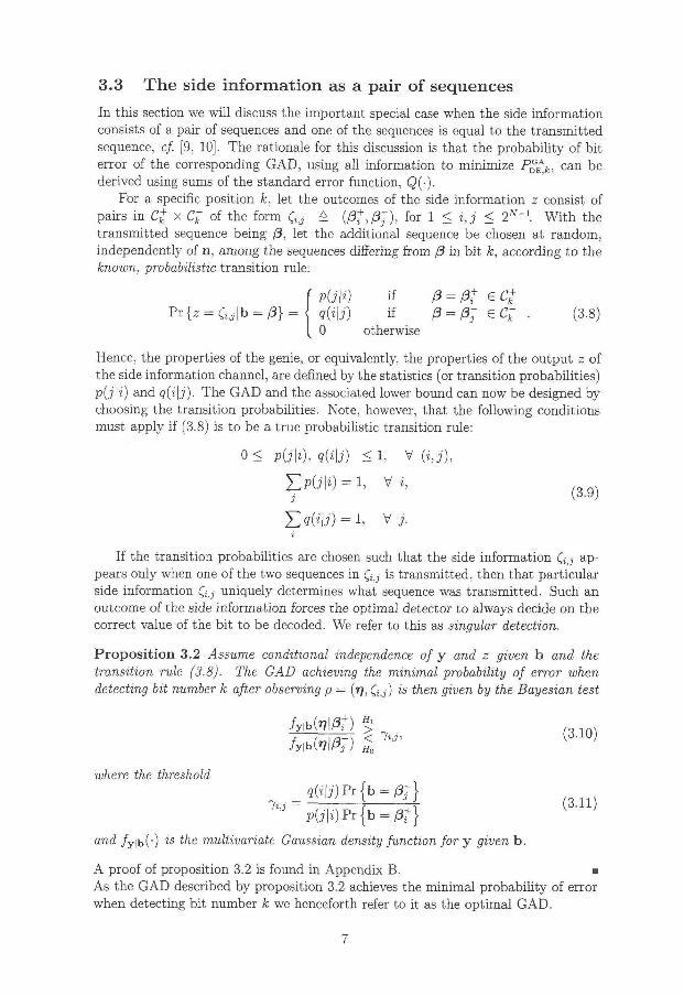
3.3 The side information as a pair of sequences

I n this section we w i l l discuss the important special case when the side in format ion

consists of a pair of sequences and one of the sequences is equal to the t ransmit ted

sequence, cf. [9, 10]. The rationale for this discussion is that the probabihty of b i t

error of the corresponding G A D , using all information to minimize Pg£k, can be

derived using sums of the standard error function, Q(-).

For a specific position k, let the outcomes of the side informat ion z consist of

pairs in <A+ x QT of the fo rm &tj A ( ß f , ß j ) , for 1 < i,j < 2N~\ W i t h the

t ransmit ted sequence being ß, let the additional sequence be chosen at random,

independently of n , among the sequences differing f rom ß i n bi t k, according to the

known, probabilistic t ransit ion rule:

Pr {z = Ci j |b = ß} = { q(i\j) i f ß = ß~ e Ck~ . (3.8)

Hence, the properties of the genie, or equivalently, the properties of the output z of

the side information channel, are defined by the statistics (or t ransi t ion probabilities)

p(j\i) and q(i\j). The G A D and the associated lower bound can now be designed by

choosing the transit ion probabilities. Note, however, that the fol lowing conditions

must apply i f (3.8) is to be a true probabilistic transition rule:

0 < P(j\i), q(i\j) < 1 , V (i,j),

$ > C f | t ) = 1, V i , j (3.9)

I f the transition probabilities are chosen such that the side informat ion ap­

pears only when one of the two sequences in Q j is transmitted, then that particular

side information Qj uniquely determines what sequence was t ransmit ted. Such an

outcome of the side informat ion forces the optimal detector to always decide on the

correct value of the b i t to be decoded. We refer to this as singular detection.

Propos i t ion 3.2 Assume conditional independence of y and z given b and the

transition rule (3.8). The GAD achieving the minimal probability of error when

detecting bit number k after observing p = (JJ, Qj) is then given by the Bayesian test

f y ^ m % 7 . ( 3 io) M i m HI 7 " ( ]

q m p l { ^ ß 7 }

p(j\i)Pr{b = ßt}

and /y|b(") is the multivariate Gaussian density function for y given b.

A proof of proposition 3.2 is found i n Appendix B. •

As the G A D described by proposition 3.2 achieves the min imal probabil i ty of error

when detecting bi t number k we henceforth refer to i t as the opt imal G A D .

where the threshold

7

P r o p o s i t i o n 3.3 The probability of error in bit k of the GAD in proposition 3.2 is

given by

P S , - E « ( % + ̂ f ) » ( * ' ) p t { b

where ^ _

dij — \j (ßt - ß j f ^ B ^ H (ßt - Øj) (3.13)

andQ(x) A ( l / ^ ) f t Q ° e - t 2 l 2 d t .

Proposition 3.3 is derived in Appendix C. Q

As a consequence of proposition 3.1, the performance of the G A D of proposition

3.2, P^Ek a s given in (3-12), serves as a lower bound for the performance of any

receiver acting wi thou t the aid of side information. This holds for all val id choices

of the statistics p(j\i) and q(i\j). However, because the calculation of (3.12) requires

summing over 22N~2 terms, using (3.12) as a lower bound is often impractical.

(3.12)

= ßt},

4 Design of Lower Bounds

I n this section we w i l l discuss strategies for how to choose the transition probabilities

of the side informat ion channel for the purpose of using the performance of the

opt imal G A D as a lower bound. The transition probabilities of the side informat ion

channel, p(j\i) and q(i\j), can be seen as design parameters for the lower bound

given by the performance expression of proposition 3.3. The problem is how to

choose these t ransi t ion probabilities, given the conditions in (3.9), so that the lower

bound becomes t ight and easy to compute. I n subsections 4.1 to 4.3 three examples

of methods for choosing the transit ion probabilities are described and in Subsection

4.4 a lower bound based on the Bhattacharyya coefficient is given.

4.1 Optimizing the side information channel C o r o l l a r y 4.1 The GAD, in the class of detectors described by proposition 3.2,

whose performance gives the tightest bound on the bit error probability is found by

maximizing (3.12) with respect to p(j\i) and q(i\j) as

P^k * . . m H PS& (4-1)

given the conditions in (3.9) and where P££k is given in (3.12).

Thus, (4.1) optimizes the transit ion probabilities of the side information channel

so that the performance of the opt imal G A D becomes as bad as possible. The

bound corresponding to P°£*k i n corollary 4.1 has, i n general, high computational

complexity. The number of parameters i n the optimization grows exponentially w i t h

the length of the transmitted sequence. Also, the location of the opt imum of P££k

8

and it 's value, Pg£*k, are dependent on the specific impulse response of the channel

and on the noise covariance. Therefore, the maximization has to be repeated for

every signal-to-noise ratio (SNR) and for every k.

4.2 A bound using a single Q( )-function - Mazo's bound

I n this section we use the present framework to re-derive Mazo's bound which only

involves evaluating a single (O(-)-function. This w i l l lead us to the customary se­

quences of minimum distance [1, 3, 9, 10, 20], that is, the pairs of sequences achieving

the min imum distance in equation (3.13). For high SNRs, the receiver confusing se­

quences of min imum distance w i l l often be the dominating error events due to the

exponential decrease of the Gaussian probabili ty density. The minimum distance is

thus defined as

A m i n r i i j , (4.2)

w i t h dij given i n (3.13). Note that this d m i n involves the noise covariance R N and,

thus, increases w i t h the SNRt The set of pairs of sequences that are at m in imum

distance is

V k A {(i,j) \di,j = d m i n } . (4.3)

L e m m a 4.2

I : Choose Bk as a non-empty subset of V k , such that no sequence (with another

sequence at minimum distance) is included in more than one pair ( ß f , ß j ) for all

(i,j) € Bk- Then p(j\i) = q{i\j) = 1 is a valid choice of transition probabilities for

all € Bk-

I I : With the transition probabilities {p{j\i),q{i\j) | € Bk} chosen as above, it

is possible to choose all other transition probabilities, {p(j\i),q(i\j) | &Bk}, so

that the optimal detector will make singular detection whenever z = Qj for (i,j) 0

Bk-

The first part of lemma 4.2 just groups sequences into disjoint pairs; a choice of

transition probabilities that does not violate the conditions of (3.9). When a se­

quence associated w i t h the set Bk is transmitted the corresponding unique pair i n

Bk (of which the transmitted sequence is a member) is always given as side infor­

mation. The singular detection of part two can be realized i n many ways. As the

set of sequences { ß t , ß j | (i,j) E Bk} is a non-empty set; one can always pick an

arbi t rary sequence f rom this set belonging to, e.g., Ck and use i t i n pair w i t h all

the sequences outside Bk belonging to C;, when these latter are t ransmit ted. As

a result, singular detection occur in the optimal G A D for all sequences outside Bk,

belonging to C;. The transit ion probabilities for the sequences outside Bk i n Ck can

be chosen analogously.

Let us assume that al l sequences are transmitted w i t h equal probabili ty, i.e.,

Pr { b = ß} = 1/2N. I f we apply the choice of transit ion probabilities described by

lemma 4.2 to proposition 3.3 and include (3.7), we find tha t

PuE.k > P£k = ( ~ ) , (4-4)

fThe minimum distance, as defined here by (4.2), is actually similar to the effective SNR of e.g., [11].

9

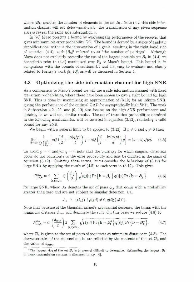
where \Bk\ denotes the number of elements in the set Bk. Note that this side infor­

mation channel w i l l act deterministically: the transmission of any given sequence

always reveal the same side informat ion z.

In [20] Mazo presents a bound by analysing the performance of the receiver that

gives m i n i m u m b i t error probabil i ty [23]. The bound is derived by a series of analytic

simplifications, wi thout the intervention of a genie, resulting in the right hand side

of equation (4.4), w i t h \Bk\* referred to as "the number of pairings". Al though

Mazo does not explici t ly prescribe the use of the largest possible set Bk i n (4.4) we

henceforth refer to (4.4) maximized over Bk as Mazo's bound. This bound is, in

comparison w i t h the bounds of sections 4.1 and 4.3, easy to evaluate and closely

related to Forney's work [9, 10], as w i l l be discussed in Section 5.

4.3 Optimizing the side information channel for high SNR As a comparison to Mazo's bound we w i l l use a side information channel w i t h fixed

transit ion probabilities, where these have been chosen to give a t ight bound for high

SNR. This is done by maximizing an approximation of (3.12) for an inf ini te SNR,

giving the performance of the opt imal G A D for asymptotically high SNR. The work

in Subsection 4.2, [20] and [9, 10] also focuses on the high SNR performance and

obtains, as we w i l l see, similar results. The set of transition probabilities obtained

in the fol lowing maximizat ion w i l l be inserted in equation (3.12), rendering a val id

bound for any SNR.

We begin w i t h a general l im i t to be applied to (3.12). I f p ^ 0 and g ^ O then

l i m —77

d->oc q U

. . d ln(g/p)\ /d ln(g/p)\ = (a + b)y/pq. (4.5)

To avoid p = 0 and/or q = 0 note that the pairs Qj for which singular detection

occur do not contribute to the error probability and may be omit ted i n the sums of

equation (3.12). Omi t t i ng these terms, let us consider the behaviour of (3.12) for

large SNR by applying the result of (4.5) to each term in (3.12). This gives

^ D E W E Q ( - f )V 'p(iK)Pr{b = / 3 1

+ } ? ( ^ ) P r { b = y 3 - } , (4.6) (i,j)€Ak

for large SNR, where Ak denotes the set of pairs Qj that occur w i t h a probabil i ty

greater than zero and are not subject to singular detection, i.e.,

A A |pO'IO?*0,9(i[j)^0}.

Note tha t because of the Gaussian kernel's exponential decrease, the terms w i t h the

min imum distance dmin w i l l dominate the sum. On this basis we reduce (4.6) to

P S ^ ^ Q l ^ f ] ^ E JpÜ\i)Pr{b = ßt}qmPT{b = ß j } , (4. V z I (i,j)ez>*

7)

where T>k is given as the set of pairs of sequences at minimum distance i n (4.3). The

characteristics of the channel model are reflected by the contents of the set V k and

the value of dmm-

+The largest size of the set Bk is in general difficult to determine. Estimating the largest \Bk\ in block transmission systems is discussed in e.g., [6].

10

Our intended set of t ransit ion probabilities are obtained by maximizing equation

(4.7) w i t h respect to p(j\i) and q(i\j) under the conditions given by equation (3.9).

This maximizat ion is easier to perform than maximizing (3.12) and gives parameters

that can be inserted in (3.12) to give a lower bound for PDE,fc for all values of SNRs.

Also, this bound w i l l , under certain conditions described in corollary 4.3, coincide

w i t h Mazo's bound given in Subsection 4.2.

C o r o l l a r y 4.3 If Bk in lemma 4-2 can be chosen so that Bk = V k and all sequences

have equal a priori probability, then the performance of the optimal GAD with a side

information channel optimized for high SNR will coincide with the Mazo bound for

bit k.

Proof: Assume that all sequences have equal a pr ior i probabili ty to be transmit­

ted. By Cauchy's inequality for sequences of real numbers and because 0 < p(j\i) <

1 and 0 < q(i\j) < 1, we have

E \/PJMQW) < / E P O ' I O e <im < føl ( 4 - 8 )

w i t h equalities i f q(i\j) = p(j\i) = 1 for al l ( i , j ) € Vk- I n this way the right hand

side of (4.7) is maximized i f q(i\j) = p(j\i) = 1 for all € Vk- I f Bk —• T^k-,

then this is an admissible choice of transition probabilities. This corresponds to

the choice of transitions probabilities producing Mazo's bound, i.e., the transitions

probabilities given in lemma 4.2. •

4.4 Lower bounds using the Bhattacharyya Coefficient There are several known ways to calculate a lower bound for the Bayesian probabil i ty

of error when testing any pair of hypotheses [5, 16, 14]. Applying such a bound t o the

Bayesian hypotheses test of proposition 3.2 give a lower bound on the performance

of the G A D . I n a sense, this is a lower bound to a lower bound on the performance

of actual receivers. The bound P ° E

A

f c > § [ l - J ( l - 4 / i 2 ) | , f rom [5, 14], is an

example of this. This bound makes sense only i f h < | , where h is obtained as the

Bhattacharyya coefficient

h A / ^fAH(p|#o)Pr { # o } V / r | H ( p | f f i ) P r {H\}dp. (4.9)

I n view of [ 1 8 ] we can interpret h as the conditional standard deviation of the mean

square error estimate of ( ß ) h i t k- The coefficient h is evaluated for the D T C G w i t h

side informat ion i n Appendix D .

Propos i t i on 4.4 Assume the transition rule (3.8) and that the channel output y

and the side information z are conditionally independent given b. Assume also that

*4 (4.10)

Then the probability of error for the GAD of proposition 3.2 is bounded below as

[5, 14]

(4.11) D G A > 1 x DE.fc — 2 4ft '

11

where

h = Y y/pU\i) Pr { b = ß+} q(i\j) Pr { b = ß j } (4.12)

and dij is given i n (3.13). •

The condition h < | is obtained, e.g., i n the white noise case, R N = CT„I, i f aa is

low enough. The lower bound of the proposition above then holds for sufficiently

high SNR.

Under the current assumptions about the side informat ion channel and, i n addi­

t ion, assuming a sufficiently high SNR, we observe the following fur ther lower bound

to the right hand side of the inequality (3.7).

C o r o l l a r y 4.5 Under the assumptions of proposition 4-4 w e have

P^A

k > e~dJ^ ( E Jp(j\i)rr{b = ßt}q(i\j)Fr{b = ß j } ) . (4.13)

The derivation of corollary 4.5 is outlined in Appendix D. •

Corollary 4.5 is similar to the expression in (4.7). Consequently, the bound in

(4.13) is maximized by the same transition probabilities that maximize (3.12) for

asymptotically high SNR.

5 The Forney lower bound

We w i l l discuss how the bounds of sections 4.2 and 4.3 relate to the Forney lower

bound [9, 10]. For this comparison we need to assume that all sequences are trans­

mi t ted w i t h equal probabili ty, i.e., P r { b = ß} = 2~N for al l ß i n C.

Forney investigates the probabili ty of the first error event in a continuous trans­

mission system, and concludes that this is also a lower bound for the b i t error

probability. The lower bound is presented as

where 7r e denotes the probabil i ty of compatibil i ty for k = 1, i.e., the probabil i ty

that a t ransmit ted sequence has a neighbour at min imum distance differing in the

first b i t , see, e.g., [6, 9, 10] and [3, pp. 152-153]. W i t h our notations for f in i te

sequences of length N this would be the probability that the t ransmit ted sequence

is represented in at least one of the pairs in X V Noting the s imilar i ty to equation

4.4, we give the fol lowing corollary.

C o r o l l a r y 5.1 If Bi in lemma 4-2 can be chosen so that B\ = T>\ then ne = 2 *

\Bi\/2N and Forney's bound will be equal to Mazo's bound for bit 1.

For the purpose of i l lus t ra t ion we w i l l give an example for which Mazo's and Forney's

bounds differ.

Example:

12

Consider a transmission system with a sequence length of (at least) N = 3

and two different error patterns achieving minimum distance, say ±[2,2,0] and ±[2,0,2] as illustrated in Figure 2. The sequences of minimum distance differing in bit one, i.e., the pairs of sequences corresponding to V\, are in­dicated by a line connecting them with their minimum distance partner(s). The dotted lines correspond to the error pattern ±[2,0 ,2] and the solid to

±[2 ,2 ,0] . In the case illustrated in Figure 2 the probability of compatibility as given by Forney [9, 10] would be 7r£ = 6/8 and the constant given by Mazo [20], see Section 4.2, would be 4/8.

Figure 2: Sequences differing with the error patterns ±[2,0 ,2] (dashed lines) and ±[2,2 ,0]

(solid).

W i t h i n the framework presented in Section 3 the constant given by Mazo can be

reached, cf. lemma 4.2, while the probabil i ty of compatibil i ty 7r e as given i n [9, 10]

seems impossible to reach in some cases. Either the class of GADs presented in

this paper is an insufficient tool, or Forney, perhaps, intended the constant ire to

be interpreted as in equation (4.4). The latter, indeed, seems to be a common

interpretation, see, e.g., [20] and [4, p. 153].

6 Examples I n this section we give a numerical example and display the corresponding lower

performance bounds. We only consider the probabil i ty of bi t error for the first b i t

in the block, i.e., P D E , i - Let N = 2 and denote the possible outcomes of b , the

sequences i n C as in equation (3.2), w i t h

1

- 1 ßi ß~2 = (6.1)

We further assume that all sequences are t ransmit ted w i t h equal a priori probability,

i.e., Pr { b = 0 ) = 2~N for all ß.

I f the matr ix H represents a time-invariant system and the noise n is stationary,

white Gaussian noise w i t h zero mean and variance o\, i.e., n S A ( 0 , <r^I), then the

distance matr ix , whose entries {dij} are the distances defined in (3.13), is

D = 2v / SNR •S) 1

(6.2)

where SNR = l / o £ and — 1 < 6 < 1. Note tha t the parameter 6 holds the description

of the dispersion in the channel H . From the definit ion (4.3) and equation (6.2) we

13

see that A = { ( 1 , 1 ) , (2 ,2)} i f |*1 < 0.5,

A = { ( 1 , 2 ) } i f 6 > 0 . 5 ,

Vx = { ( 2 , 1 ) } i f 6 < -0 .5 , (6.3)

A = { ( 1 , 2 ) , (1 ,1) , (2 ,2)} i f 6 = 0.5,

A = { ( 2 , 1 ) , (1,1), (2, 2 )} i f 6 = - 0 .5 .

The largest possible subset i n accordance w i t h lemma 4.2 of T>\ is given by

(6.4)

Apply ing to this example Forney's bound and the three bounds found in section

6, the performance of the opt imal G A D w i t h a side information channel optimized

for al l SNRs, the performance of the opt imal G A D w i t h a side information channel

optimized for high SNR, and Mazo's bound, we note the following. I f |5| ^ 0.5 then

the largest possible B\ = V\ and the bounds presented by Mazo [20] and Forney

[9, 10] w i l l coincide, i n accordance w i t h corollary 5.1. Also the performance of the

opt imal G A D using a side informat ion channel optimized for high SNR according

to Subsection 4.3, w i l l coincide w i t h these bounds as given by corollary 4.3. From

(6.4) and equation (4.4) we have

B, = { ( 1 , 1 ) , (2 ,2)} i f \6\ < 0.5,

Bi = { ( 1 , 2 ) } i f 6 > 0.5,

Bi = { ( 2 , 1 ) } i f 6 < - 0 .5 ,

S i = { ( I A ) , (2 ,2)} if 6 = 0.5,

B i = { ( 1 , 1 ) , (2 ,2)} i f 6 - -0 .5 .

Q (%M \S\ < 0.5

p&k=\ \Q[¥) 6 > ° - 5 • o 5 - 5 ) ' ' ' 6 < - 0 . 5

A 2 ^ V 2

Figure 3 describes the behaviour of the side information channel corresponding

to Mazo's bound through lemma 4.2, which in this same example also corresponds to

the G A D optimized for high SNR. (Note that the behaviour of this side information

channel is independent of the SNR.) A l l of the transit ion probabilities p(j\i) and

q(i\j) are either one or zero. As a consequence this side information channel w i l l

act deterministically i n the sense that , given a certain transmitted sequence, the

genie w i l l always give one particular pair as side information. Figure 3 indicates

w i t h arrows those branches w i t h probabili ty one; branches w i t h probabili ty zero are

omitted.

Figures 4-6 present three graphs plot t ing performance bounds versus SNR. Each

graph tracks three bounds: the performance of the optimal G A D w i t h a side in ­

format ion channel optimized for all SNRs, Mazo's bound and the bound based on

the Bhattacharyya coefficient given in proposition 4.4. For the bound based on the

Bhattacharyya coefficient, the transmission probabilities has been chosen so that

(4.13) is maximized. I n addit ion we give the matched filter bound [19, p. 267], i.e.,

the performance of the opt imal receiver operating in an environment without ISI , as

a reference. We have used the expression in [7] to evaluate the Q(-)-function, w i t h

the pertinent constants chosen so tha t the relative deviation was less than 1.2%.

The graphs 4-6 differ according to the assigned values of 6.

We make several observations. The bound based on the Bhattacharyya coefficient

is not t ight for high SNRs. For weak ISI (small \S\) Mazo's bound w i l l be close to

14

ßl ß~2 ßl ßl ßl ßl

Figure 3: The behaviour of the side informat ion channel of lemma 4.2, corresponding

to Mazo's bound of equation (4.4), described for three different values of 6; left:

\S\ < 0.5, middle: 6 < - 0 . 5 , right: 5 > 0.5.

the performance of the opt imal G A D wi th a side informat ion channel optimized for

al l SNRs, but less close for moderate ISI and low SNR.

I n Figure 7 are given the transit ion probabilities for the side information channel

of section 4.1, optimized for all SNRs to make the performance of the opt imal G A D

a t ight bound. This side information channel w i l l generally act i n a random manner

meaning that a t ransmit ted sequence could render one out of several pairs z as side

informat ion. However, for high and low SNRs i t w i l l act deterministically. Note

that the transit ion probabilities developed in sections 4.1 and 4.3, respectively, as

expected coincide for high SNRs.

7 Summary

We have studied the genie-aided detector (GAD) as an analytic device and intro­

duced an explicit statistical description of the genie's action as a probabilistic rule

governing a side information channel. This description is given in terms of transition

probabilities, the probabilities that for any given transmitted sequence there w i l l be

a certain side informat ion supplied to the detector. The opt imal i ty of the process­

ing of the augmented informat ion is defined explicit ly in terms of the probabilistic

description of the side information channel, representing the genie.

W i t h the complete statistical description of the transmission system, including

a set of transit ion probabilities, the G A D w i t h m in imum bi t error probability, see

proposition 3.2, is derived i n terms of a binary Bayesian hypothesis test. By evaluat­

ing the performance of this G A D , a lower bound on the performance of any detector,

w i t h or wi thout access to the side information, is obtained.

The transi t ion probabilities are free parameters which can be chosen to optimize

the performance of the G A D . They might for example be chosen to make the cor­

responding bound t ight , or to give the bound a simple structure. We have chosen

several different sets of transit ion probabilities as examples i n order to discuss the

properties of their respective performance bounds. I n this, we also discuss the rela­

t ion of the attainable performance bounds to the works by Forney [9, 10] and Mazo

[20].

15

10°

SNR

Figure 4: The performance of the optimal G A D using a side informat ion chan­

nel optimized for all SNRs, Mazo's bound, the corresponding bound based on the

Bhattacharyya coefficient and the matched filter bound are plot ted versus SNR for

6 = 0.3.

Acknowledgements

We would like to express our gratitude to Prof. Tor Aul in , Chalmers University of

Technology, Sweden, Amos Lapidoth, Stanford University, USA, and Prof. Shlomo

Shamai (Shitz), Dept. of Electrical Engineering, Technion, Haifa Israel, for he lpful

discussions on the topic of genies. We would also like to acknowledge the improve­

ments provided by Dr . Sarah Kate Wilson, Purdue University, and Paul Petersen,

West Lafayette, USA.

This research has been supported in part by the Swedish National Board for

Industrial and Technical Development ( N U T E K ) , Telia Mobite l A B and the ISS'90

foundation.

16

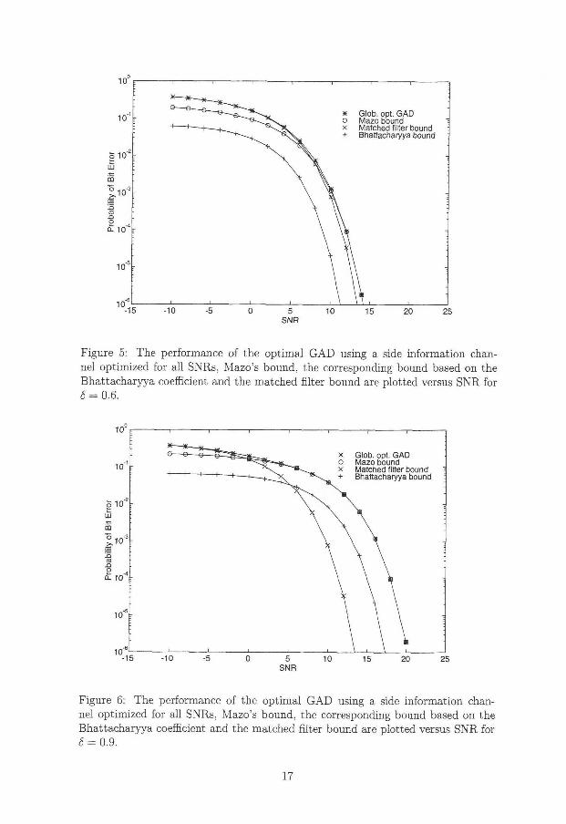
10°

S N R

Figure 5: The performance of the opt imal G A D using a side information chan­

nel optimized for all SNRs, Mazo's bound, the corresponding bound based on the

Bhattacharyya coefficient and the matched fi l ter bound are plotted versus SNR for

6 = 0.6.

10°

-15 -10 -5 0 5 10 15 20 25 S N R

Figure 6: The performance of the opt imal G A D using a side information chan­

nel optimized for all SNRs, Mazo's bound, the corresponding bound based on the

Bhattacharyya coefficient and the matched filter bound are plotted versus SNR for

6 = 0.9.

17

p(l|l)=p(2|2)=?(l|l)=«(2|2)=l

6 = 0.3

p(l|2)=p(2|l)=,(l|2)=g(2|l)=0

-20 -15 -10 -5 0 5 SNR

10 15 20

i i i i i i i i i

^o(2 |2)=9( l | l )= l

p(2|l)=?(2|l)

6 = 0.6 _

-

p(l|2)=9(l|2)=0

p(l|l)=?(2|2)

i

-20 -15 -10 -5 0 5 SNR

10 15 20

I I I I I I I - I 1

0.8

^p(2 |2 )=?( l | l )= l 0.8

p(2jl)=9(2|l) t 0 . 6 - -lo .o 6 = 0.9 £ 0 . 4 -

0.2 _ vp(l|l)=g(2!2)

--p(l |2)= 9 ( l |2)=0 0

i

Figure 7: The transition probabilities of the globally optimized side informat ion

channel of corollary 4.1. Plotted versus SNR for three different values of 6; upper:

6 = 0.3, middle: 6 = 0.6, lower: 6 = 0.9.

18

A P P E N D I C E S

A Bounding the Error Probability Using Side Information

The significance of the side information can be explained wi thout explicit ly referring

to the channel model in Figure 1. This can be done in terms of hypothesis testing

between two hypotheses, H0 and Hi, specified by the respective probabil i ty densities

fr\H0(p\Ho) and fr\Hi(p\Hi) o n a product space, p = ( t f , C) S y x Q. The variables

i n r = (y , z) are grouped such that y is assumed to have a continuous marginal

d is t r ibut ion and z is supposed to be f ini te , i.e., z 6 0 = { C i , • • • , C M } - Hence

the two densities fT\Hi(p\Hi) are understood as densities w i t h respect to a suitable

product measure on y x Q. Otherwise the distributions may, for the sake of the

in i t i a l part of the argument in this appendix, be quite arbitrary.

Every binary decision rule (excluding rules w i t h rejection options) partitions

} ^ x ! l into two disjoint subsets, say V0 and Vi, and favours the hypothesis HQ i f

p € VQ and Hi otherwise. For each C £ f i we introduce the sets (or ("-sections)

Di (C) - {v & y \ (»7,0 € Vi} for i = 0 , 1 . Hence V is a disjoint union, V{ =

Ucefi(A (C) >C)- The probability of deciding for the wrong hypothesis, denoted by

PEnoi(Vo,Vi), is expressed as

V f t u ) = P r { # o } / fr\Ho(p\H0)dp + Fi{Hi} [ f T l H l ( p \ H i ) d p

= P r f t f o } £ / W „ ( r ? , Cl W r ? f A n

+ P r { i f a } £ / / ^ ( ^C l^ O d r , ,

where, e.g., JVi fr\H0{p\Ho)dp designates the probabil i ty of V j w i t h respect to the dis­

t r i bu t i on determined by fr\H0(p\Ho) ( in mathematical terms, the Lebesgue-Stieltjes

integral of the density fr\H0(p\Ho) over V\).

A n y special decision rule determined by first par t i t ioning y into Do and Di

independently of C, thus disregarding the informat ion in z, and then setting Vi =

U f e n ( A ,C ) has by an interchange of the order of integration and summation in

( A . l ) the probabili ty of error

i W P o } , { A } ) = P r { f f o } / / y t ø | f i - 0 ) A / + P r { f f i } / fy(v\Hi)dV, J D\ J Do

(A.2) where fy(r)\Hl) = Ecgo/y,*lff<(^Cl-Hi)-

Le t t ing { V J * } j _ 0 designate the corresponding decision regions of the Bayesian

decision rule using fr\Ha(p\Ho) and fT\Hi(p\Hi) to minimize the funct ion PError(-)

i n equation A . l , i t holds that PError(Vo, V x ) > PETTOI(VQ, V{) for any other decision

19

regions { V j } * = 0 . I n particular, i t holds for the probabil i ty of error in (A.2),

F E r r o r ({D0} , { A } ) > J W 0 £ , V*), (A.3)

B The G A D achieving minimal bit error proba­bility

Let us derive the receiver that achieves the min imal probabili ty of error when detect­

ing b i t number fc after observing p = (77, Qj). Assume that y and z are conditionally

independent given b and that the transition kernel for the side information channel

is of the f o r m (3.8). The detection of b i t number k is equivalent to the following

binary hypotheses testing problem (equation ( 3 . 1 ) ) :

H0 •• ( b ) b i t k = - l / R , \

# i = (fa)bitk = + l . [ '

As is known [22], the Bayesian test

(B.2) fr\H{p\Hi) 5 P r f f f o }

fr[H(p\H0) < P r W Ho

where Pr {Hi} = 1 — Pr {H0} is the a priori probabil i ty that Hi is true, minimizes

the probabi l i ty of choosing the wrong hypothesis. Then, given the observation p =

(r^ Ci.j) and using the stated assumptions

fr\n0(p\H0) = fyAHoinAijlHo)

= p T T ^ y E i / y | b N / 3 ) P r { ^ = C, J |b = / 3 } P r { b = /3} ( ß 3 )

= p 7 7 ^ y / y i b W M * U ) P r { b = / 3 - } .

I t analogously follows that

fr\Hi(p\Hi) = p ^ - y / y | b ( 7 7 ! / 3 l

+ M j | i ) P r { b = ^ + } . (B.4)

Using (B.3) and (B.4) i n (B.2) the Bayesian test becomes

f 7 „ (B.5) /y|b(r?|/37) Ho

20

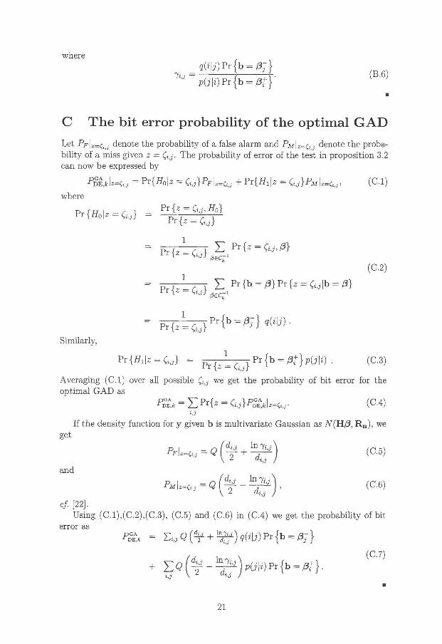
where

g ( i | i ) P r { b = / 3 j }

i J K j | 0 P r { b = / 3 t

+ } '

C The bit error probability of the optimal G A D

Let Pp\Z-Q^. denote the probability of a false alarm and PM\Z=Q, j denote the proba­

b i l i t y of a miss given z = Qj. The probabili ty of error of the test in proposition 3.2

can now be expressed by

PSkkU^ = Pr{H0\z = C^/VU-, . , + PiWz = Q J } P M U ^ ( C l )

where

Pr{z = Q4,H0} P r { f r 0 | j e = C i j } =

(C.2)

L _ P r { b = / 3 j } q(i\j) P r { * = C « }

Similarly,

P r { H 1 | ^ = C1J} = ^ P r { b = fl-}p(jl*) . (C.3)

Averaging ( C l ) over all possible &j we get the probabil i ty of bi t error for the

opt imal G A D as

PStk = E P ^ = Q,i}P^kU=U,r (C- 4 )

I f the density funct ion for y given b is multivariate Gaussian as N(Hß, R n ) , we

/ U - < , ^ ( % + ^ ) (C5) 2

and

cf. [22].

Using (C l ) , (C .2 ) , (C .3 ) , (C.5) and (C.6) in (C.4) we get the probabil i ty of bit

error as

P&k = E £ j 0 ( ^ + ^ ) g ( i | i ) P r { b = / 3 - }

/ J i \ (C7) + E Q ( ^ - ^ j p ( j | O P r { b = A + } .

21

D A Bayesian Bound and the Bhattacharyya co­efficient

We compute the Bhattacharyya coefficient

h = / Jfr]H(p\H0)Pr { r J 0 } v / / r | H ( p | J f 1 ) P r {Hi}dp ( D . l )

for the D T G C w i t h a side information channel. Assuming that y and z are con­

di t ional ly independent given b as well as that the transition kernel for the side

informat ion channel is of the fo rm (3.8), we obtain f rom (B.3) and (B.4) that

h = £ \ j v m Pr { b = ß t } q m Pr { b = ß j ] j f$(T,\ßJ)fy$(v\ßt)dri. i.j y

(D.2)

The channel data y have, given the transmitted sequence b = ß, the multivariate

Gaussian dis t r ibut ion N(Hß, R n ) - Hence a straightforward calculation gives tha t

the integrals on the right hand side of ( D . l ) equal:

y f y ^ V \ ß J ) f y ^ ( v \ ß t ) d r , = e - ^ , (D.3) ti­

as found i n [14]. This proves (4.11) in proposition 4.4. Let us note that for —1 <

u < 1 we have y/l — u < 1 — | and this yields that | 1 - J{l-Ah2 —2 > h . Recall

that h is a sum of non-negative terms. I f we drop the terms corresponding to those

pairs of sequences that are not at minimum distance f rom each other, we obtain

(4.13) i n corollary 4.5.

References [1] T . A u l i n , "Genie-Aided Sequence Detection Under Mismatch," In Proceedings

ofISITA'94, pp. 869-873, Sydney, Australia, Nov. 1994.

[2] L .C . Barbosa, "Maximum likelihood sequence estimators: A geometric view,"

IEEE Trans. Inform. Theory, vol. 35, no. 2, pp. 419-427, March 1989.

[3] S. Benedetto, E. Biglieri and V . Castellani: Digital Transmission Theory.

Prentice-Hall Inc., Englewood-Cliffs, N.J. , 1987.

[4] R.E. Blahut, Digital Transmission ofinformation. New York: Addison-Wesley

Publ . Comp., 1990.

[5] D .E . Boekee and J.C. Ruitenbeek: A Class of Lower Bounds on the Bayesian

Probabi l i ty of Error. Information Sciences, vol. 25, no. 1, pp. 21-35, 1981.

[6] P.O. Börjesson, H . Eriksson, T . Koski and P. Odling, "On the structure of the

probabil i ty of compatibil i ty in Forney's lower bound and block transmission

systems," 1995. I n preparation.

22

[7] P.O. Bör je s son and C.E. Sundberg, Simple Approximat ion of the Error Func­

t i on Q(x) for Communications Applications. IEEE Trans. Comm., vol. 27, no.

3, pp. 639-643, March 1979.

[8] S.N. Crozier, D.D. Falconer and S.A. Mahmoud, "Reduced complexity short-

block data detection techniques for fading time-dispersive channels," IEEE

Trans. Veh. Tech., vol. 41, no. 3, pp. 255-265, August 1992.

[9] G.D. Forney, "Lower bounds on error probabili ty in the presence of large

intersymbol interference," IEEE Trans. Commun., vol. 20, no. 1, pp. 76-77,

February 1972.

[10] G.D. Forney, "Maximum likelihood sequence estimation of digi tal sequences in

the presence of intersymbol interference," IEEE Trans. Inform. Theory, vol .

18, no. 3, pp. 363-378, May 1972.

[11] S. A . Fredricsson, "Opt imum Transmitting Fil ter i n Digi ta l P A M Systems w i t h

a V i t e r b i detector," IEEE Trans. Inform. Theory, vol. 20, no. 4, pp. 479-489,

July 1974.

[12] F.S. H i l l , "The Computation of Error Probabili ty for Dig i ta l Transmission,"

The Bell System Technical Journal, vol. 50, no. 6, July-Aug. 1971, pp. 2055-

2077.

[13] E .Y . Ho and Y.S. Yeh, "A New Approach for Evaluating the Error Probabil­

i t y i n the Presence of Intersymbol Interference," The Bell System Technical

Journal, vol . 49, no. 6, Oct. 1975, pp. 2249-2266.

[14] T . Kai la th , "The divergence and Bhattacharyya distance measures in signal

selection," IEEE Trans. Comm. Techn., vol. 15, no. 1, pp. 52-60, February

1967.

[15] G. K . Kaleh. "Channel equalization for block transmission systems," IEEE

Journal Sel. Areas Com., vol. 13, no. 1, pp. 110-121, January 1995.

[16] L . K a n a l , "Patterns in Pattern Recognition," IEEE Trans. Inform. Theory, vol.

20, no. 6, pp. 697-722, Nov. 1974.

[17] P. Kanerva: Sparse Distributed Memory. 2nd Print ing, A Bradford Book, M I T

Press, Cambridge Mass., London, 1990.

[18] D . G . Lainiotis, "On a General Relationship Between Estimation, Detection and

the Bhattacharyya Coefficient," IEEE Transactions on Information Theory,

vol . IT-15, no. 4, pp. 504-505, July 1969.

[19] E .A . Lee and D.G. Messerschmitt, Digital Communication. Kluwer Academic

Publishers, 1988.

[20] J.E. Mazo, "Faster-Than-Nyquist-Signaling," The Bell System Technical Jour­

nal, vol . 54, Oct. 1975, pp. 1451-1462.

[21] V . K . Prabhu, "Some Considerations of Error Bounds i n Dig i ta l Systems," The

Bell System Technical Journal, vol. 50, no. 10, Dec. 1971, pp. 3127-3151.

23

[22] H .L . van Trees, Detection, Estimation, and Modulation Theory, Part I. New-

York: Wiley, 1968.

[23] P. Odl ing, H . Eriksson, T . Koski and P.O. Bör jesson , Representations for the

Minimum Bit Error Probability Receiver for Block Transmission Systems with

Intersymbol Interference Channels, Research Report T U L E A 1995:11, Luleå

University of Technology, Luleå, Sweden, A p r i l 1995. .

24

Part I I . l

A Reduced Complexity Viterbi Equalizer Used in Conjunction with a Pulse Shaping Method

P a r t I I . l :

A R e d u c e d Complex i ty V i t e r b i E q u a l i z e r U s e d in C o n j u n c t i o n w i t h a

P u l s e S h a p i n g M e t h o d

Per Odl ing 1 , T i m o Kosk i 2 and Per Ola B ö r j e s s o n 1

I n Proceedings of the Third International Symposium on Signal Processing and its

Applications (ISSPA '92), pp. 125-129, Gold Coast, Austraha, August 1992.

This material has also been presented at the Nordic Radio Symposium, NRS'92, i n

Ålborg , Denmark.

1 Luleå University of Technology, Division of Signal Processing, S-971 87 Luleå, Sweden

2Luleå University of Technology, Department of Mathematics, S-971 87 Luleå, Sweden

ISSPA 92, Signal Processing and Its Applications. Gold Coast, Australia, August 16-21, 1992. Editor: D Gray

A Reduced Complexity Viterbi Equalizer Used in Conjunction with a Pulse Shaping Method

P Ödling Department of Signal Processing T Koski Department of Applied Mathematics P O Börjesson Department of Signal Processing Luleå University of Technology, Luleå, SWEDEN

The complexity of the Viterbi algorithm can be reduced by linear pre-equalization. We introduce a linear preprocessor using the weighted least squares filtering (WLS) of [11]. The geometric technique of L Barbosa [3] is evoked for analytical representation of the complexity reduction by pre-equalization, and for evaluation of error performance. We evaluate the bit error rate of the WLS preprocessor and of the linear preprocessor of Falconer and Magee [6].

1 I N T R O D U C T I O N

Consider a discrete time Gaussian channel (DTGC) with intersymbol interference (ISI) described by

L-\

Vk —Y, hi*>k-l + nk, -oo < fc < oo, 1=0

where {bk}, bk € { -1 ,1} , are i.i.d. channel inputs, {yk} are channel output observables, {hk} are real valued ISI coefficients and {n*} are white Gaussian noise samples with variance No/2. The DTGC has been extensively used in information theory and communications engineering [15]. It models pulse amplitude modulated (PAM) signals transmitted through a time dispersive Gaussian channel, often applicable to e.g. telephone lines, magnetic recording media and radio channels.

The maximum likelihood sequence estimator (MLSE) is a procedure for estimating the input sequence of bits, {6*}, from the observations {yk}. In communications a recursive way of organizing the computation of the MLSE is desired. The Viterbi algorithm (VA) is a fast way of computing the MLSE by a search in a trellis of length N and width 2L [7], This still becomes impractical when L is large, since the computational complexity of the VA increases exponentially with L. A number of researchers have addressed this problem suggesting complexity reducing solutions of two basic types, linear [4, 6, 8, 14] and non-linear [2, 9, 16]. Linear preprocessing, treated here, simplifies MLSE by giving the VA a channel model with a memory length shorter than L, and by applying a linear preprocessor, with pulse response {gk} of length J, to the received data {yk}- The preprocessor shapes the overall system pulse response h * g to become similar to the channel model q using some criterion on e, as shown in the figure below.

h

1 * L _ U : — 1

Figure 1: Linear preprocessor model network.

A convenient way of describing this model (discarding edge effects) is to set y = (yo, • • •, yN+L-2)1', b= (bo, • • •, b f f - i ) T and n = (no,... , n / v + L -2 ) T which gives the matrix formulation

y := Hb + n

z := GHb + Gn,

where H and G are Toeplitz matrices of dimensions (N+L-l)xN and (N + L+ J - 2 ) x (N+L-l) respectively, representing convolution, and T transposes matrices. H and G have a band structure

125

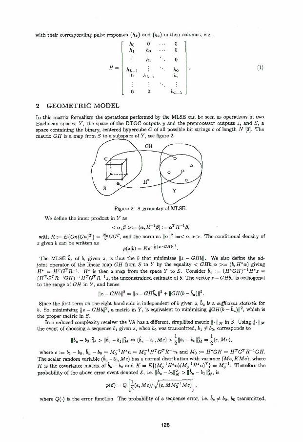
with their corresponding pulse responses {/i*} and {gk} in their columns, e.g.

H ••

ho 0 0 ht ho • 0

hi • 0

•• ho 0 ft, 0 0 hL-

(1)

2 G E O M E T R I C M O D E L

In this matrix formalism the operations performed by the MLSE can be seen as operations in two Euclidean spaces, Y, the space of the DTGC outputs y and the preprocessor outputs z, and S, a space containing the binary, centered hypercube C of all possible bit strings b of length ./V [3]. The matrix GH is a map from S to a subspace of Y, see figure 2.

Figure 2: A geometry of MLSE.

We define the inner product in Y as

<a,ß>:= (a,R-lß) :=aTR'^,

with R := E{Gn(Gn)T] = ^GGT, and the norm as ||a||2 :=< a, a >. The conditional density of z given b can be written as

p(z[b) = Ke-i"*-CHb" .

The MLSE bc of 6, given z, is thus the b that minimizes \\z — GHb\\. We also define the ad­joint operator of the linear map GH from S to Y by the equality < GHb,a >= (b,H*a) giving H* = H T G T R - 1 . H* is then a map from the space Y to S. Consider Su := (H*GH)~^H'z = (HTGTR"1GH)~lHTGTR~1z, the unconstrained estimate of b. The vector z - GHbu is orthogonal to the range of GH in V, and hence

||> - GHbf = \\z - GHKtf + \\GH(b - b u ) f .

Since the first term on the right hand side is independent of 6 given z, bu is a sufficient statistic for b. So, minimizing \\z — GH6|] 2, a metric in Y, is equivalent to minimizing \\GH(b - bu)\\

2, which is the proper metric in S.

In a reduced complexity receiver the VA has a different, simplified metric || • \\M in S. Using || • ||jvf the event of choosing a sequence b\ given z, when 60

w a s transmitted, ^ b0, corresponds to

\\k - MIS, > \\k - h f M O (S„ - b0,Me) > I p j - = I (e , Me),

where e := 0 l - 6o, &u - &o = MälH*n = MöiHTGTR-1n and M 0 := H*GH = H7^R~lGH. The scalar random variable (6U - &o, Me) has a normal distribution with variance (Me, K Me), where K is the covariance matrix of 6U - fc0 and K = £{(M c "

1 i /*n)(Af 0 ~1 i /*n) r } = A f 0

- 1 . Therefore the probability of the above error event denoted S, i.e. ||6„ - 6O|IM > \\bu - h\\2

M, is

p(£) = Q he, Me)j^(e, MM0~1Me)

where Q(-) is the error function. The probability of a sequence error, i.e. bc ^ 6o> &o transmitted,

126

can be expressed as

p(error) oc £{ £ } (2)

The number of deviation sequences e is large enough to make (2) computationally not feasible. A lower bound on (2), which corresponds to finding the so called minimum distance d m j „ , see [10, 17),

i s [ 3 ] r n / n p(error) > £ m a x j c ? | ( e , M e ) / y / ( e , M M ^ M e ) j , (3)

where K. is a constant with respect to e. Closer lower bounds can be obtained by summing over a subset of {e}, cf. [10, 7, 15, 17]. Upper bounds on (2) can also be derived, see e.g. [10, 13, 7, 15, 17]. Here the bound of equation (3) is used to compare the complexity reducing methods to each other, not to bound their actual performance.

3 C O M P L E X I T Y R E D U C T I O N

We now analyze the Weighted Least Squares method (WLS) and for comparison the method presented in [6], both using linear preprocessing as described in section 1. In both cases the receiver, or equivalently the metric in S, is simplified in two steps. First the noise covariance R due to the preprocessor is dropped, and secondly the VA is given an approximate channel model with a memory length shorter than L, see figure 1. This yields the kernel of the simplified metric || • | | M in S as

M = QTQ,

where the matrix Q has q in the columns, the same structure as in (1) and dimension (N+m— 1) x TV, where m is the desired memory length, i.e. the length of q.

An interesting issue is the relative computational complexity of various methods. However, this extra computational complexity involved is very low compared to the complexity reduction accom­plished in the VA. See [17] for a more detailed study.

3.1 The WLS-fi l ter

The WLS method was originally developed as a pulse shaping filter for ultrasonic imaging [11, 5, 12]. It can be described by three requirements:

1. The pulse response must have a non zero amplitude at least at one point, say for fc = fco.

The energy of the pulse response should be small outside the desired interval, |fc| >

3. The noise amplification has to be low.

An idea related to 1 and 2 is presented in [1]. The solution for 1 and 3 is the matched filter, and the solution for 1 and 2 with m = 1 is the inverse filter. The WLS filter combines 1, 2, and 3 with the desired memory length m and the expected noise power ^ into a cost function [11]. Let H be an (J -(- L — 1) x J matrix with the same elements as H, g be a vector containing the pulse response {9k}, <5fco be a vector of zeros except for a one ('1') at position fco, and finally let V be a diagonal matrix with m — 1 zeros in the center of the diagonal and ones at position fco and on the edges. Using

= a

T a the WLS cost function can be expressed as

Hg) = \\V(Hg-6k0)\\l + a^\\g\\l.

This can be interpreted in figure 1 as sending a unit pulse (deterministic input) through the model network, summing the energy of the response h * g outside the given interval of length m, in [13] referred to as the residual ISI, and adding a term proportional to the noise amplification of the WLS preprocessor. The optimum preprocessing filter g is given by

gopt = [HTVTVH + a%Ll]-'HT6k0.

The desired pulse response q consists of the m elements of the overall system pulse response ft * g corresponding to the m wide 'window' of V, i.e. ft * g is calculated and the tails are truncated.

The complexity reducing procedure is to filter the incoming data stream y with g^t, truncating the result to the proper length, N + m - 1, and feeding this new data stream z and the desired pulse response q to the VA.

127

We are investigating the WLS-filter used as a preprocessor by varying the design parameters. In the sequel we have chosen fc0 = 0, all non-zero wk — 1 and a = 1. These choices are ad hoc, although simulations indicate that the performance of the receiver is not very sensitive to the choice of a.

3.2 The Falconer and Magee filter

Figure 1 aids in describing the method of Falconer and Magee [6]. When feeding the network of figure 1 with a white binary sequence fc this preprocessor minimizes the expected energy of the output signal

min E{E } = E{(q * b — g * h * b — g * n) }, 1,9

with the constraint qTq — 1. Solving this minimization problem in a matrix formulation renders

Qopt = t h e eigenvector of [I — XT (HT H+• Q1)~^X\ corresponding to the minimum eigenvalue,

S o p t = (HTH Xq, opt>

where X i s a J x ( m + l ) channel matrix related to H, cf. [6]. The complexity reducing steps are now by analogy with the WLS method.

4 B I T E R R O R R A T E A N A L Y S E S

We analyze the bit error performance of these receiver algorithms in two ways. From equation (3) a tractable numerical bound on the bit error probability is derived and plotted. Thereto we simulate the described models and algorithms and 'measure' the bit error rate (BER).

Denote an error sequence containing fc errors with ek. The bit error probability bound correspond­ing to the sequence error probability bound of (3) is then numerically treated by the assessment

1 k n — max —rQ N A 2k

\{ek, Mek)/yJ(ek,MM^Mek) (4)

where A is a subset of {e}. McLane asserts that the dominating values of the CJ-function occur for error sequences with only a few errors, i.e. for fc = 1 or fc = 2, see [13] and the references therein. In our simulations we have found this to be valid for p(error) analysis independently of the SNR, and valid for high SNR scenarios for BER analysis. For low SNR longer error sequences increase in importance since they contribute more to the bit error probability, although the probabilities of the sequences themselves still are below the probabilities of shorter error sequences. A more complete study of the BER in terms of a Forney type bound is found in [10, 17].

When numerically evaluating (4) we let A contain, i.e. we search through, all error sequences with 1 and 2 errors, a portion of the relevant sequences with 3 and 4 errors and some longer sequences. Following McLane in [13] we set N = 25, which is claimed to be sufficient to represent the ISI.

In the first example we use the magnetic recording (Lorentzian) channel model from [16], but with a truncated length of L = 7. This truncation is performed to enable us to use an optimal, full complexity Viterbi decoder as a benchmark. The preprocessor length is as above, J = 31, and the length of the desired pulse response is m = 3. Here the WLS method is compared to the optimal Viterbi decoder and to the lower bound estimate of equation (4).

Exusple 1: Magnetic recording chamel from [16].

Eq.(4): -WLS -Vterbi BER * WLS opiMs. SNRCdB)

128

For the second example we have used the difficult channel 'B' of length L — 15 from [6], also used in [13]. As in [6] we choose the filter length as J = 31 and the length of the desired pulse response as m = 5. We compare the WLS method to the Falconer and Magee method, and to their respective bound estimates according to equation(4).

The BER measurements indicate that the performance of the preprocessors depends heavily on the channel characteristics and that none of the methods is superior for all cases. Work on optimization of the WLS-preprocessor improving its error performance is in progress [17].

References

I.N.Andersen: Sample-Whitened Matched Filters. IEEE Trans. Inf. Th., 19, 1973, pp. 653 -660.

J.B.Anderson, T.Aulin and C.-E.Sundberg: Digital Phase Modulation. Plenum Press, New York, 1986.

L.C.Barbosa: Maximum Likelihood Sequence Estimators: A Geometric View. IEEE Trans. Inf. Th., 35, 1989, pp. 419 - 427.

C. T.Beare: The Choice of the Desired Impulse Response in Combined Linear-Viterbi Algorithm Equalizers. IEEE Trans. Comm. , 26, 1978, pp. 1301 - 1307.

P.O.Börjesson, N.-G.Holmer, K.Lindström, B.Mandersson and G.Salomonsson: Digital Preshap-ing of Ultrasonic Signals: Equipment and Applications. IEEE Ultrason. Symp., 1982, pp. 696 -699.

D. D.Falconer and F.R.Magee: Adaptive Channel Memory Truncation for Maximum Likelihood Sequence Estimation. The Bell System Tech. Jour., Vol. 52, No. 9, Nov. 1973, pp. 1541-1562.

D.G.Forney, Jr.: Maximum Likelihood Sequence Estimation of Digital Sequences in the Presence of Intersymbol Interference. IEEE Trans. Inf. Th., 18, 1972, pp. 363 - 378.

S.A.Fredricsson: Optimum Transmitting Filter in Digital PAM Systems with a Viterbi Detector. IEEE Trans. Inf. Th., 20, 1974, pp. 479 - 489.'

T.Hashimoto: A List-Type Reduced-Constraint Generalization of the Viterbi Algorithm. IEEE Trans. Inf. Th., IT-33, No.6, 1972, pp. 363 - 378.

T.Koski, P.Odling and P.O.Börjesson: Performance Evaluation for a Class of Complexity Re­duced Maximum Likelihood Sequence Estimators. To be submitted.

B.Mandersson, P.O.Börjesson, N.-G.Holmer, K.Lindström and G.Salomonsson: Digital Filtering of Ultrasonic Echo Signals for Increased Axial Resolution. 5th Nord. Meet. Med. and Biomed. Eng. 1981, Conf. proc., pp. 169-171.

B.Mandersson and G.Salomonsson: Weighted Least Squares Pulse-Shaping Filters with Appli­cation to Ultrasonic Signals. IEEE Tr. Ultrason. Ferroel. Freq. Cont., 36, 1989, pp. 109-112.

P.J.McLane: A Residual Intersymbol Interference Error Bound for Truncated-State Viterbi De­tectors. IEEE Trans. Inf. Th., 26, 1980, pp. 548-553.

S.Qureshi and E.Newhall: An Adaptive Receiver for Data Transmission over Time Dispersive Channels, IEEE Trans. Inf. Th., IT-19, July 1973, pp. 448-457.

A.J.Viterbi and J.K.Omura: Principles of Digital Communication and Coding. McGraw - Hill Book Co, Tokyo, 2nd Printing, 1985.

F.Xiong, A.Zerik and E.Shwedyk: Sequential Sequence Estimation for Channels with Intersym­bol Interference of Finite or Infinite Length. IEEE Trans. Comm., Vol-38, No. 6, June 1990, pp. 795-803.

P.Odling: Lie. eng. thesis., forthcoming. Luleå University of Technology.

129

Part II.2

Combined Linear-Viterbi Equalizers — A Comparative

Study and A Minimax Design

P a r t I I . 2 :

C o m b i n e d L i n e a r - V i t e r b i E q u a l i z e r s - A Comparat ive S t u d y a n d A M i n i ­

m a x D e s i g n

Nils S u n d s t r ö m 1 , Ove Edfors 1 , Per Odling 1 , Håkan Eriksson 1, T imo K o s k i 2 and Per

Ola B ö r j e s s o n 1

I n Proceedings of the 44th IEEE Vehicular Technology Conference (VTC'94), PP-

1263-1267, Stockholm, Sweden, June 1994.

xLuleå University of Technology, Division of Signal Processing, S-971 87 Luleå, Sweden

2Luleå University of Technology, Department of Mathematics, S-971 87 Luleå, Sweden

Combined Linear-Viterbi Equalizers - A Comparative Study and A Minimax Design

Nils S u n d s t r ö m O v e E d f o r s P e r Od l ing H å k a n E r i k s s o n T i m o K o s k i

P e r O l a B ö r j e s s o n

Luleå University of Technology

S-971 87 Luleå, S W E D E N

Abstract: Combined l inear-Viterbi equalizer (CLVE) is a term often used for a class of digi ta l receivers reducing the complexity of the V i t e rb i

detector by assuming an approximate channel

model together w i t h linear pre-equalization of the received data.

We reconsider a weighted least squares de­sign technique for CLVEs by introducing a mini­max criterion for suppressing the strongest com­

ponent of the residual intersymbol interference.

Previously, in [2], we have studied the perfor­mance of some proposed CLVE design methods and evaluated them by simulated bit error rates.

Here we investigate the performance of the min­imax design and of the CLVE designs found in literature [3, 4, 5, 6] for two GSM test channels.

We also present a comparison of the CLVE designs based on a common quadratic optimiza­t ion criterion for the selection of the channel prefilter and the desired impulse response.

1 I N T R O D U C T I O N

The Maximum Likelihood Sequence Detector (MLSD)

is a procedure for estimating a sequence of bits f rom

a sequence of channel output observables, given a model of the communication system. I n the presence

of intersymbol interference (ISI) the Vi te rb i algorithm

(VA) provides an efficient way of computing the MLSD [7, 8, 9]. However, the V A s t i l l becomes impractical

when the time spread of the ISI is large because of the exponential relation between ISI t ime spread and VA complexity.

The complexity of a Vi te rb i detector can be reduced

by giving the VA an approximate channel model w i th a shorter time spread than that of the original chan­

nel. The class of receivers employing this technique to­gether w i th linear pre-equalization of the received data

are often referred to as combined linear- Viterbi equal­

izers (CLVEs), see j l , 3, 4, 5, 6, 2]. Other classes of receivers addressing the same complexity problem can

be found in e.g. [10, 11, 12, 13]. I n this paper we focus on CLVEs.

When designing CLVEs i t is often desirable to min­imize the bit error rate of the receiver. The bit error

probability depends on the design parameters, such as

the channel model and the impulse response of the pre­filter, in a complicated and non-linear way. The pre-

filtering of the received data perturbs the signal space and colours the channel noise. Ignoring this colouring

or giving the VA an approximate channel model re­sult in a displacement of the decision regions f rom their optimal locations, cf. the residual ISI i n [14]. Instead

of using the bit error rate as a design criterion, other more feasible criteria are used in CLVE design methods [1, 3, 4, 5, 6, 2].

I n this paper we investigate the performance of a minimax CLVE design. Three other principal tech­niques for designing CLVEs [3, 4, 6] are also overviewed and compared.

2 T H E TRANSMISSION SYS­T E M M O D E L

A continuous time model of a transmission system as

described in [7] may, wi thout information loss, be rep­

resented by a discrete t ime model as in Fig. 1. I n block

- C D -) 7 i > Recei­) * ver

Figure 1: Discrete transmission system model.

transmission systems blocks of information are trans­

mit ted so that the decoding can be performed indepen-

0-7803-1927-3 /94 /$4 .00 © 1994 I E E E 1263

3 CLVE DESIGN 2

dently on each block, see e.g. [15]. For such systems it is convenient to use the matr ix formalism [16]

y = Hb + n, (2.1)

where the transmitted message is coded antipodally in 6 6 { — \ , + l } N and the channel observables are

y e Uv '. The time invariant channel impulse

response, i.e. the ISI coefficients, is represented by a Toeplitz band matrix H. I t is a known (N + L— 1) x JV matrix wi th the impulse response h, of length L, in its columns, arranged so that matr ix mult ipl icat ion corre­sponds to convolution. The noise vector n € I R ( A , + i _ 1 ' is a joint ly Gaussian, zero mean random vector w i th a N(0,Rn) distribution, where Rn denotes the noise co-variance matrix.

3 C L V E D E S I G N

The performance evaluation of the CLVEs in this paper is performed on block transmission systems, but histor­ically the design methods have focused on continuous transmission systems and VAs w i t h infinite horizon, i.e. { M S - c o - To relate to existing methods, we have cho­sen to confine the development of the minimax design to a criterion based on sequences of infinite length. Some remarks on CLVE design for block transmission systems can be found in section 5.

A design model is presented in Fig. 2, cf. [6] where q is the desired impulse response ( D I R ) , i.e. the chan­nel model given to the VA. I f the t ime delay, modelled by the filter d, is zero, the system is equivalent to the one found in [3]. Since this paper only considers causal channel impulse responses, the introduction of the time delay offers the possibility of placing the energy of the DIR in an arbitrary position. This possibility is ac­counted for in [3, 4, 5] by allowing the channel impulse response anti-causal components.

Figure 2: Discrete design model for infinite sequences.

The error in Fig. 2, can be expressed as

Ei = [b * (h * p - d * q) + n * p]i, (3.2)

where * denotes convolution. By using | j x | | ^ f := x J M x , the variance of £, is given by

E{e2} = \\Hp-Dq\\2

Rb + \\p\\2

R^ (3.3)

where p and q are vectors containing the impulse re­sponse of the prefilter p and the D I R q respectively, and Rb and R„ are covariance matrices for the transmitted sequence 6 and the noise n. H and D are Toeplitz band matrices such that the multiplications Hp and Dq de­scribe convolution. Since the length of h * p is greater than the length of d * q, the subtraction Hp — Dq in (3.3) necessitates that the size of D is chosen such that the dimensions agree. The residual ISI is defined by this difference, as

residual ISI : = Hp - Dq, (3.4)

i.e. as the ISI that is not accounted for in the VA, cf. [14].

3.1 A S E L E C T I O N O F P R E F I L T E R

D E S I G N S

In this section we compare design methods for p and q. The methods are due to Falconer and Magee [3j, Fredricsson [4] and Odling et al. [6], where the last one is a weighted least squares method inspired by [17].

By introducing a weighting matr ix W in (3.3) se­lective weighting of the residual IS I becomes possible. This is used to formulate the design criterion

J(p,q) := \\W(Hp-Dq)fRli + \\p\\2

Rn. (3.5)

In the sequel, both the channel input and the channel noise are assumed white and stationary, hence Rf, = I and Rr, = c n I . Completing the square in (3.5) gives

J(P,Q) = \\(P-PO)\\A + l!<?!l2

B; (3-6)

where

A = HTWTWH + cr2I,

B = DTWT ( j ~WHA~1HTWT)WD.

P o = A~1HTWTWDq.

In the presence of noise, the matrices A and B are positive definite, so the min imum of (3.6), w i t h respect to p, is obtained i f

p = P o = A-1HTWTWDq, (3.7)

wi th a residual error of ||</||jg.

The most straightforward design approach is to as­sume W = J , i.e. a uniform weighting of the residual ISI, and to find the global min imum of (3.6) by using

1264

4 SIMULATIONS 3

(3.7) in combination wi th finding a q that minimizes

||<?||jj under some constraint e.g. \\q\\ = 1. This is done

by Falconer and Magee in [3], where the prefilter ob­

tained is

PFM = A H DqFM, (3-8)

and the D I R

Q FM = the normalized eigenvector corresponding

to the smallest eigenvalue of B.

(3.9)

There are other methods that do not minimize (3.6),

but sti l l often render a lower probability of bit error

than the method above. One such method was pre­

sented by Fredricsson in [4]. For the purpose of pre­

serving the similarity to the expressions in the original

reference, we present his result in the Fourier domain:

and

PFU)

\QFU)\2

QFUWU)

\ H ( f ) \ 2

(3.10)

(3.11)

Equation (3.10) corresponds to (3.8) of Falconer and

Magee. The DIR. however, is determined by spectrum

matching the left hand side to the right hand side of

equation (3.11) given a length constraint on q. This

matching was addressed by Beare in [5] where an adap­

tive algorithm was presented.

A weighted least squares (WLS) design approach for

p and q was presented by Odling et al. in [6]. The D I R

in this design method is assigned an exact copy of the

corresponding positions of Hp, thus giving the VA a

correct channel model for those positions, i.e.

QWLS = DTHpWLS- (3.12)

The prefilter pwLS is chosen by modifying (3.7) to

PWLS = A-'H'WTWD (3.13)

where the position I is chosen as a suitable index in

qv/LS- By choosing the weighting matr ix in (3.13) as

W = diag( l ••10 • •010- -p O S . k

01 • • • ! ) , (3.14)

where the zeroes coincide with the DIR position and fc is chosen so that it coincides with the i:th position of q. This ensures that the trivial, all zero, solution for p W L S is avoided and that the energy in H p W L S is concentrated to the D I R interval. Equation (3.13) can

now be simplified to the form in which it was presented bv Odling et al.

PWLS (3.15)

where 6k is a vector w i th 1 in position fc and zeroes

elsewhere.

3.2 A M I N I M A X D E S I G N

The criterion of (3.5) has the total energy of the

weighted residual ISI as one part. I t can be discussed

i f also the distribution of the residual ISI is of any im­

portance for the probabili ty of bit error of the resulting

receiver. Here we investigate an approach that takes

into account the maximum absolute value of the resid­

ual ISI , thereby shaping the distribution of the same.

Let us use this minimax approach and solve

PMM = arg min { max J^(p) (3.16)

where J-(p) is the i : t h element in the vector

J'{p) = \W[Hp - 6 k ) \ 2 + an\\p\\2. (3.17)

The expression \W(Hp — 6k)\ denotes the vector of the

absolute values of each element in W(Hp - Sk). The

D I R <JMM = D T H p M M , the weighting matrix W and

6k are chosen as in the WLS design method.

4 SIMULATIONS

To evaluate the performances of the CLVEs for the

different prefilter and desired impulse response design

methods described in section 3, we have simulated the

block transmission system of section 2. We have used

two GSM test channels [18], the Typical Urban area

channel (TU) and the Rural Area channel ( R A ) .

ill

Typical Urban Impulse resp.

LÜ li I

0 10 20

\ Typical Urban \ Freq. resp.

Rural area Impulse resp.

Rural area , Freq. resp.

Figure 3: Impulse and frequency responses of the GSM Typ­ical Urban channel (left) and Rural Area channel (right).

When implementing the minimax design, we have used

a sequential quadratic programming method provided

by the "minimax" routine of the M A T L A B ™ Optimiza­

t ion Toolbox™ [19] to solve (3.16), starting wi th an

in i t ia l prefilter p given by (3.13).

To determine the prefilter p and the DIR q of

Fredricsson, we have solved equation (3.11) by means

1265

5 CONCLUSIONS AND FUTURE WORK 4

Typical Urban Area Channel

x Minimax * WLS

+ Fredricsson o FaMa

0 5 10 Q:3 taps, P:53 taps

Figure 4: Bit error rate for the GSM Typical Urban channel.

of a least squares f i t of the spectrum coefficients of q

to the right hand side of (3.11). The D I R q were then calculated analytically f rom these coefficients. The R A channel has a smooth frequency response and is com­

paratively easy to match. The matching of q to the T U channel is more diff icul t due to the spectral dips of this

channel (see Fig. 3). As a consequence, at high SNRs,

the number of points used in the least squares f i t might have to be adjusted in order to obtain real coefficients.

Rural Area Channel

o o

0 . +

o

+

x Minimax * WLS o FaMa

+ Fredricsson .. Full Viterbi

-10 -5 0 5 10 Q:3 taps, P:13taps

Figure 5: Bit error rate for the GSM Rural area channel.

Simulation results are shown in Fig. 4 and 5 for

CLVE designs by the Falconer and Magee method [3]

( V ) , the WLS method [6] ( '* ' ) , the Minimax method

( 'x ') and the method of Fredricsson [4] ( '+ ' ) • The sim­ulations on the RA channel are also compared wi th the f u l l complexity Viterbi decoder [7] (dotted line in Fig.

5). Such a comparison was not feasible in simulations

on the T U channel, because of this channel's length. I n all cases we have chosen the length of the desired impulse response to 3 coefficients and the block length

to 50 bits. The prefilter length is set to one coefficient

more than twice the ISI, i.e. 13 coefficients for the R A channel and 53 for the T U channel.

5 CONCLUSIONS AND F U ­T U R E W O R K

The basic idea in most design methods for CLVEs is re­

flected by the criterion J(p, q). The main difference be­tween the methods presented in the literature [3, 4, 5, 6]

lies in the way the DIR q is chosen. Falconer and Magee

find the global minimum of the criterion under the con­straint \\q\\ — 1. The WLS method and the method pro­

posed by Fredricsson has slightly different approaches where the subsequent processing of data by the VA is taken into consideration when applying the criterion.

Fredricsson uses a projection on the minimum distance

error sequence giving an effective signal to noise ratio [7] tailored for the VA. The WLS method ensures that

the D I R given to the VA is a true replica of the to­ta l system impulse response in the corresponding time

interval.

I n our simulations the WLS receiver shows a supe­

rior performance and is indeed close to the f u l l complex­i ty Vi te rb i decoder. The receiver proposed by Fredric­

sson performs well on the T U channel, which is slightly surprising considering the spectral shape of this chan­nel. The results in the presented simulations agree wi th

applicable observations in [4, 5] and in our earlier in­

vestigations [6, 2].

The new method based on the minimax design was

introduced as an attempt to shape the distribution of the residual ISI in a fashion favourable to the VA. Being similar to the WLS method i t gives a truncated version

of the to ta l system impulse response as a D I R to the VA, but instead of minimizing the criterion J(p, q) i t

suppresses the largest residual ISI coefficient. The per­

formance is almost up to par w i t h the WLS receiver, which indicates a potential for the concept of shaping

the residual ISI.

The hitherto discussed methods for CLVE design are derived for continuous transmission systems. How­

ever, many contemporary and future communication systems are of block transmission type, e.g. the cellular

1266

REFERENCES 5

telephone systems of Europe (GSM), Japan (JDC) and the USA (ADC). To our knowledge, there are today no CLVE design methods that take advantage of the struc­ture of such systems. An increased understanding of the properties of block transmission systems could result in improved receivers with respect to bit error probabil­ity as well as reduced implementation complexity and cost. In CLVEs developed for block transmission sys­tems this could be reflected by the time-invariant linear prefiltering being replaced by e.g. a general matrix mul­tiplication, in order to utilize the "edge" effects at the block boundaries for performance improvement. The noise correlation due to the prefilter p is another im­portant issue in connection with CLVEs, cf. [16]. This is recognized by Fredricsson and Beare, but not consid­ered in the other described methods.

We regard the above issues as key components in the development of new CLVEs.

References [1] S. Qureshi, E. Newhall. An adaptive receiver for

data transmission over time dispersive channels. IEEE

Transactions on Information Theory, IT-19:448-457, Jul. 1973.

[2] P. Odling. Low Complexity Digital Receivers. Licentiate thesis, Luleå University of Technology, 1993.

[3] D. D. Falconer, F. R. Magee. Adaptive channel memory truncation for maximum likelihood sequence estima­tion. The Bell System Technical Journal, 52(9):1541-1562, Nov. 1973.

[4] S.A. Fredricsson. Joint optimization of transmitter and receiver filter in digital PAM systems with a Viterbi detector. IEEE Transactions on Information Theory,

IT-22(2):200-210, Mar. 1976.

[5] C. T. Beare. The choice of the desired impulse response in combined linear-Viterbi algorithm equalizers. IEEE Transactions on Communication, 26:1301-1307, 1978.

[6] P. Ödling, T. Koski, P. O. Börjesson. A reduced com­plexity Viterbi equalizer used in conjunction with a pulse shaping method. In Proceedings of The Third

International Symposium on Signal Processing and its

Applications Queensland, Australia, pages 125-129. Aug. 1992.

[7] D. G. Forney Jr.. Maximum likelihood sequence esti­mation of digital sequences in the presence of intersym­bol interference. IEEE Transactions on Information

Theory, IT-18:363-378, 1972.

[8] D. G. Forney Jr.. The Viterbi algorithm. In Proceedings

of IEEE, pages 268-278, Mar. 1972.

[9] S. Benedetto, E. Biglieri, V. Castellani. Digital Trans­

mission Theory. Prentice-Hall Inc., Englewood-Cliffs, N.J., 1987.

[10] T. Larsson. A State-Space Partitioning Approach to

Trellis Decoding. PhD thesis, Chalmers University of Technology, Göteborg, 1991.

[11] P. Monsen. Feedback equalization for fading dispersive channels. IEEE Transactions on Information Theory,

IT-17:55-64, 1971.

[12] F. Xiong, A. Zerik, E. Shwedyk. Sequential sequence estimation for channels with intersymbol interference of finite or infinite length. IEEE Transactions on Com­

munications, 38(6):795-803, 1990.

[13] T. Hashimoto. A list-type reduced-constraint general­ization of the viterbi algorithm. IEEE Transactions on

Information Theory, IT-33(6):866-876, Nov. 1987.

[14] P. J. McLane. A residual intersymbol interference er­ror bound for truncated-state Viterbi detectors. IEEE Transactions on Information Theory, IT-26:548-553. 1980.

[15] S. N. Crozier, D. D. Falconer. Reduced complexity short-block data detection techniques for fading time-dispersive channels. IEEE Transactions on Vehicular

Technology, 41(3):255-265, Aug. 1992.

[16] C. Barbosa. Maximum likelihood sequence estimators: A geometric view. IEEE Transactions on Information

Theory, IT-35:419-427, 1989.

[17] B. Mandersson, P. O. Börjesson, N.-G. Holmer, K. Lindström, G. Salomonsson. Digital filtering of ul­trasonic echo signals for increased axial resolution. In Proceedings of The V Nordic meeting on Medical and

Biological Engineering, Linköping, Sweden, Jun. 1981.

[18] COST207. Final Report, COST207: Digital Land Mo­

bile Radio Communication. 1989.

[19] A. Grace. Optimization Toolbox, for use with MATLAB. The Math Works, Inc., Natick, Mass., Jun. 1993.

1267

Part II .3

Multiple-Antenna Reception and a Reduced-State Viterbi Detector for Block Transmission Systems

P a r t I I . 3 :

M u l t i p l e - A n t e n n a Recept ion a n d a R e d u c e d - S t a t e V i t e r b i Detec tor for B l o c k T r a n s m i s s i o n Systems

Håkan Eriksson 1 and Per Odl ing 1

Submitted to the 4th International Conference on Universal Personal Communica­

tions (ICUPC'95), Tokyo, Japan, November 1995.

1 Luleå University of Technology, Division of Signal Processing, S-971 87 Luleå, Sweden

1

Multiple-Antenna Reception and A Reduced-State Viterbi Detector for Block Transmission Systems

H å k a n B . E r i k s s o n P e r Odl ing

Luleå University of Technology

Division of Signal Processing

S-971 87 Luleå, Sweden

Abstract— T h i s paper presents a receiver structure em­ploying multiple receiving antennas and reduced-state V i t e r b i detection- T h e presentation is couched in terms of matrices representing a discrete-time, symbol-sampled sys­tem with frequency-selective, slow fading and additive Gaus ­sian noise. T h e receiver design involves determining two matrices: one matr ix denning the metric of the reduced-state V i t e r b i detector and one representing a pre-processor operating on the output from a maximal-ratio combiner. T h e presented receiver is a generalization of those used ear­lier in single-antenna, combined l inear-Viterbi equalizers [3],

[7], [11], [13], [16], [17] for continuous transmission sys­tems. Per formance comparisons are made with the mini­m u m mean-square error ( M M S E ) linear equalizer and the M M S E decision-feedback equalizer for block transmission systems [10], indicating that the presented class of receivers offers superior performance.

I . INTRODUCTION

The use of multiple receiving antennas in wireless com­munication to take advantage of spatial diversity has been widely studied in the literature, see e.g., [1], [4], [8], [9] and the references therein. For flat fading channels it is shown in [8] that the use of multiple receiving antennas can im­prove the average signal-to-noise ratio (SNR) and lower the probability of a deep fade. In a frequency-selective fading environment the channel will be time-dispersive, which may in turn cause intersymbol interference. Sev­eral methods have been put forward to combat this. One such method is the orthogonal frequency division multi­plexing (OFDM) modulation technique. There have also been several methods proposed that employ some form of multi-channel equalization. These are based on, for exam­ple, the minimum mean-square error criterion [1], decision-feedback techniques [1], or maximum likelihood sequence detection [6].

In this paper we examine one other method of performing multi-channel equalization; we propose a receiver structure that uses multiple receiving antennas and a reduced-state Viterbi Algorithm (VA). A system with a maximal-ratio combiner (MRC) [8], [9] is modelled as a single-antenna, white-noise system by using a data transformation matrix preserving the sufficient statistics. Linear prefiltering and a reduced, or fixed, state VA are then applied, producing a system with an MRC, a linear operation and a fixed com­plexity VA.

I I . M O D E L

Consider a system using M receiving antennas and as­sume that there is one linear, frequency-selective, slow fad­ing channel for each antenna. Each channel is modelled as a discrete-time, symbol-sampled, additive Gaussian chan­nel (DTGC) with intersymbol interference (ISI). Let b be an TV x 1 random vector containing the N independent symbols to be transmitted. For each block the received signal at each antenna can then be described in terms of the matrix representation

x i = H;b + n i (1)

where H i , is an (N + i , - 1) x JV stochastic, complex val­ued matrix representing the ISI, is a complex, jointly Gaussian, zero mean random vector with a A r(0,Ri) dis­tribution and where x, is a vector of observable channel outputs.

In a mobile situation, where a moving transmitter or receiver creates a non-stationary environment, the chan­nels will vary in between the time instants two blocks are transmitted. Throughout this paper we assume that, for each block to be transmitted, the outcomes of all the chan­nel matrices H j are known to the receiver. This could be a reasonable assumption under some conditions, such as when each channel impulse response varies slowly.

I I I . M A X I M A L - R A T I O COMBINER

The Maximal-Ratio Combiner (MRC) [8], [9] is an opti­mal method to combine the received signals x; in the sense that it gives a minimal sufficient statistic for the detection of b. In this section we re-derive the MRC by generalizing a result for single-antenna block transmission systems by Barbosa [2] to the multi-antenna case.

With the following block matrices:

Xi 1 ni H i •

X Ä

. x * f J

, n *

. NM _

and H ^

(2) a multi-antenna modell can be expressed as

x = Hb + n. (3)

Define the N x N matrix M ^ H Ä R - ' H , where R = E { n n ^ j and is assumed to be invertible and where

2

the superscript H denotes Hermitian transpose. Assume that H has a column space of rank N, meaning there is information in x about every symbol in b. Then M is invertible and

b„ = M - ' H ^ R - ' x = b + M - ' t f R - 1 - (4)

is the output of the simultaneous zero-forcing equalizer, cf. the result by Barbosa in [2] for the single-antenna case. From [2] we know that hu is a minimal sufficient statistic [14] for b given x. Because M is an invertible N x TV-matrix, it follows from (4) that

(5)

is also a minimal sufficient statistic. Hence the vectors x and y both hold the same information for the purpose of detecting b, in spite of y being only of dimension N x 1. Equation (5) is the basic appearance of the MRC. In the case that the noise at each particular antenna is uncor­related with the noise at all other antennas, the outputs of the whitened matched filters are summed to form the output from the MRC, see figure 2 and, e.g., [9].

Before beginning with designing receivers, we would like to transform the model (3) into an "equivalent" single-antenna, white noise model. Given H , the filtered additive noise in (4), M _ 1 H ^ R _ 1 n , is a Gaussian zero mean noise process with a correlation matrix equal to M _ 1 . To whiten this noise we use the Cholesky factorization of M , produc­ing an upper triangular matrix V such that V M - 1 V H = I , where I is the identity matrix. Let

V b „ = V M - ' y = V b + n„. (6)

Then nv = V M ^ H ^ R - 1 ! ] 6 N(0,I) given H . Equation (6) can be seen as a single-antenna model that is equiva­lent to (3) in the sense that an optimal receiver will per­form equally well operating on either x or r, since both are sufficient statistics for b, cf. the derivations by Kaleh in [10] for the single-antenna case. The main difference between (6) and (3) lies in the structures of the model ma­trices H and V . The multi-antenna model matrix H is an (M(N - 1) + Li + ... + LM) X N matrix while V is an N x N matrix that can be seen as an anti-causal, time-variant filter.

Note that variations in the signal-to-noise ratio takes the form of varying signal energy in the matrix V while the noise n„ always has unit variance. We define the block signal-to-noise ratio (SNR) as

tr { V H V }

N (7)

Note that the block SNR is a stochastic variable (with one outcome for each transmitted block) since the channel ma­trix H , and thereby V , is stochastic.

A. The Effects of Using Multiple Receiving Antennas and Maximal-Ratio Combining

Let us look at how the number of antennas and the lengths of the impulse responses at each antenna affect the

characteristics of the system model (6). A simple mea­sure of the amount of ISI is the normalized energy in the elements outside the main diagonal of V , i.e., with B = V - d Ü 8 g { v M , « 2 , 2 ) . . . , U/v.jv},

t r { B g B } tr {VHV}' (8)

Consider an example where each channel is frequency-selective and Rayleigh-faded. For each block to be trans­mitted let the impulse response of each channel be the out­come of a stochastic vector of length L with independent, identically distributed (i.i.d.), complex, zero mean Gaus­sian random variables. Furthermore let the block length N = 20 and the noise correlation R = a2I. In figure 1 we have plotted the estimated mean value of p versus the num­ber of antennas, M, and the length of the impulse response of each channel, L. (Note that origo is in the lower, right part of the figure.) The mean value of p was estimated by averaging (8) over 3000 independent outcomes of H .

Fig. 1. The amount of ISI in the matrix V versus the number of antennas and the length of the impulse responses of each channel, L, using p denned in (8). (Orjgo is on the right edge.)

From figure 1 we see that if we add more independent diversity paths by means of more antennas, the ISI in the equivalent model (6) tends to decrease in the sense that p of definition (8) tends to decrease. Thus, the ISI increases with the length of the channel responses but decreases with the number of antennas. Alternative characterizations of the ISI in block transmission systems, are the colourization of the noise in equation (4) [2] and the eigenvalue spread of the matrix M [11].

In the example the block SNR 7 in (7) is the sum of the squared absolute value of ILM i.i.d. real valued Gaussian variables giving the block SNR a chi-squared distribution with 2LM degrees of freedom. Hence, in this example the number of antennas and the length of the impulse responses have an identical effect on the probability distribution of the block SNR of definition (7): increasing either factor will decrease the probability of a deep fade and increase the mean of the block SNR 7.

Although we assume the diversity paths to be indepen­dent in this example, these characteristics may well apply to a real situation if the antennas are enough separated.

3

IV . CLVEs FOR B L O C K TRANSMISSION SYSTEMS

Consider a receiver where the output of the MRC, y, is filtered by a linear system represented by a matrix G and an estimate of the transmitted sequence b is obtained as

a r g m i n | | G y - Q b j j j , b

(9)

where | | x [ | ^ ^ x H A x . A receiver structure implementing this, consisting of a linear prefilter and a VA, is depicted in figure 2. We refer to this class of receivers as "combined linear-Viterbi equalizers for block transmission systems" (B-CLVE), cf. [5], [7], [13], [16], [17].

Fig. 2. The receiver structure for the case when the noise at each particular antenna is uncorrelated with the noise at all other an­tennas.

For the VA to be a meaningful tool for solving (9), the matrix Q should be a band matrix [10], i.e.,

Q

o o

(10)

where I is the width of the band of non-zero elements. Be­cause wider bands of non-zero elements in Q require more states in the VA trellis, it is the width of these bands that determines the complexity of the VA. By choosing a given value of I, the computational complexity of B-CLVEs may be controlled; conversely, for a given VA complexity (de­termined, perhaps, by hardware), a prescribed value for I may be indicated.

If we apply the model (6) to the structure displayed in figure 2, we get a model suitable for the design of B-CLVEs, see the system described in figure 3. The linear distortion of the received signal is described by the matrix V . The matrix P is the prefilter to be designed together with the matrix Q which is given to the VA as a channel model. The function of the prefilter P is to concentrate the energy of the system P V to a band of width I matching the non­zero band of the matrix Q, thus matching the complexity constraint of the VA. Comparing figures 2 and 3 and using the model (6) we see that G = P V M " 1

We display two special cases of the receiver structure in figure 3, both replacing the VA with a hard limiter, or equivalently setting Q = I . If we choose the matrix

V

nv :N(0 , I )

r , z VA Jr VA

Pre-filter The Viterbi-algorithr

Fig. 3. The structure of C L V E s for block transmission systems.

with R j j as E { b b H } , then the mean-square error E { | | z —b)| | 2 } is minimized [14, p. 303] and the receiver of figure 2 turns into the minimum mean-square error lin­ear equalizer in [10] followed by a hard limiter. On the other hand, if P = V - 1 , then the receiver is equivalent to the zero-forcing equalizer of (4) followed by a hard limiter.

The design of the B-CLVE that minimizes the probabil­ity of choosing the wrong sequence b, is given by P = I and Q = V , which is a description of the maximum like­lihood sequence decoder [6]. The complexity of the VA is then determined by the structure of V , or rather, by the width of the band of non-zero elements in V . This, in turn, is equal to the length of the largest ISI time spread of the channels, cf. the Cholesky factorization in [15, p. 55].

V . DESIGN METHODS FOR B L O C K - C L V E ' S

In this section we will discuss the design of the matrices P and Q with respect to what has been done earlier for continuous transmission systems. We will also, as an ex­ample, generalize one of these earlier methods to our block transmission system environment.

Hereinafter we discuss only the the case when both P and Q are of dimension N x N. In order to restrict Q to a band-matrix, let qi = ö^D^ for all i , where qi is a 1 x I vector with the model of the system's impulse response given to the VA. The matrix D i positions the vector qi in the ith row of the matrix Q, and is given in Appendix A.

In [16] it is recognized by Sundström et al that in block transmission systems "edge effects" will appear that could be incorporated in B-CLVE design. I t is also noted that the CLVEs for continuous transmission systems that are presented in [5], [7], [16], [17] all are related to the same criterion: the variance of a signal formed as the difference between the actual signal given to the VA and the model of the same signal.

Let us here consider the error vector

e = Pr - Qb = P V b + P n „ - Qb, (12)

i.e., the difference between the filtered received signal and the model signal, as displayed in figure 4.

The expected energy in the error vector e is given by

N

J(P,Q) = E{e- f fe} = ^ j ( p i , q i (13)

where each term

R b V " ( V R b (11)

j (Pi ,q i ) = ||(PiV - q O ^ l l f ^ + HP?|[f (14)

and where p ; and qi are the i th rows of P and Q, respec­tively.

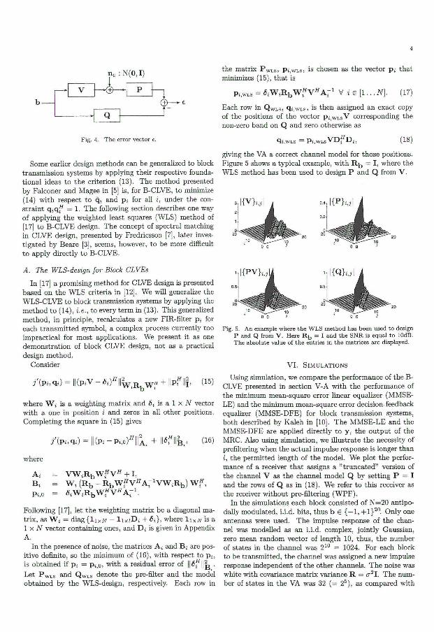
4

n„ : N ( 0 , I )

b

V A P V P

Q 1 Q

F i g . 4. T h e error vector e.

Some earlier design methods can be generalized to block transmission systems by applying their respective founda­tional ideas to the criterion (13). The method presented by Falconer and Magee in [5] is, for B-CLVE, to minimize (14) with respect to q; and Pi for all i, under the con­straint q , q f = 1. The following section describes one way of applying the weighted least squares (WLS) method of [17] to B-CLVE design. The concept of spectral matching in CLVE design, presented by Fredricsson [7], later inves­tigated by Beare [3], seems, however, to be more difficult to apply directly to B-CLVE.

A. The WLS-design for Block CLVEs

In [17] a promising method for CLVE design is presented based on the WLS criteria in [12]. We will generalize the WLS-CLVE to block transmission systems by applying the method to (14), i.e., to every term in (13). This generalized method, in principle, recalculates a new FIR-filter Pi for each transmitted symbol, a complex process currently too impractical for most applications. We present it as one demonstration of block CLVE design, not as a practical design method.

Consider

?{Pi,n) = IKPiV - ^)"l!w > R bw» + UP? Ilf. (is)

where W i is a weighting matrix and 6t is a 1 x JV vector with a one in position i and zeros in all other positions. Completing the square in (15) gives

/ ( P i , q t ) = l i (P . -P s , o ) H | |A , + l l O l f j , , ( 1 6 )

where

A i = V W i R b W ? V H + I , B , = W t ( R b - R b W f V H A - 1 V W t R b ) W f , Pi,o = « i W i R b W f V ^ A T 1 .

Following [17], let the weighting matrix be a diagonal ma­trix, as W i = diag { l i x j v — l i x i D t + St}, where l i x j v is a 1 x TV vector containing ones, and D s is given in Appendix A.

In the presence of noise, the matrices A , and B i are pos­itive definite, so the minimum of (16), with respect to Pi, is obtained if Pi = pSio, with a residual error of | |£? | | | j •

Let P W L S and QWLS denote the pre-filter and the model

obtained by the WLS-design, respectively. Each row in

the matrix P W L S , P i , W L s , is chosen as the vector pi that minimizes (15), that is

Pi.wLs = é i W i R b W f V ^ A r 1 V i € [ 1 . . . N], (17)

Each row in QWLS, q i . w L s , is then assigned an exact copy of the positions of the vector Pi j WLsV corresponding the non-zero band on Q and zero otherwise as

q«,wLs = Pi,wLsVD?Di, (18)

giving the VA a correct channel model for those positions. Figure 5 shows a typical example, with R b = I , where the WLS method has been used to design P and Q from V .

F i g . 5. A n example where the WLS m e t h o d has been used to design P and Q from V . H e r e R b = I a n d the SNR is equa l to l O d B . T h e absolute value of the entries in the matr ices are displayed.

V I . SIMULATIONS

Using simulation, we compare the performance of the B-CLVE presented in section V-A with the performance of the minimum mean-square error linear equalizer (MMSE-LE) and the minimum mean-square error decision-feedback equalizer (MMSE-DFE) for block transmission systems, both described by Kaleh in [10]. The MMSE-LE and the MMSE-DFE are applied directly to y, the output of the MRC. Also using simulation, we illustrate the necessity of prefiltering when the actual impulse response is longer than I, the permitted length of the model. We plot the perfor­mance of a receiver that assigns a "truncated" version of the channel V as the channel model Q by setting P = I and the rows of Q as in (18). We refer to this receiver as the receiver without pre-filtering (WPF).

In the simulations each block consisted of N=20 antipo­dally modulated, i.i.d. bits, thus b 6 { - 1 , + 1 } 2 0 . Only one antennas were used. The impulse response of the chan­nel was modelled as an i.i.d. complex, jointly Gaussian, zero mean random vector of length 10, thus, the number of states in the channel was 2 1 0 = 1024. For each block to be transmitted, the channel was assigned a new impulse response independent of the other channels. The noise was white with covariance matrix variance R = <r 2 I. The num­ber of states in the VA was 32 (= 2 5), as compared with

5

the channel's 1024. Figure 6 shows the simulated Bit Error Rate (BER) for the four receivers versus average SNR.

Viterbi equalizers for single-antenna, continuous transmis­sion systems. Simulations using a version of the WLS-design method in [12], [16], [17] adopted for B-CLVE design indicate a potential for this class of receivers. However, the WLS-design method seems to be too computational com­plex for most applications to be implemented with today's technology.

APPENDIX

I . APPENDIX: T H E POSITIONING MATRIX Di

Let Oixa denote an / x a matrix containing zeros and I ; X i denote an / x I identity matrix. If 0 < i < N — I + 1 let

0 ix(i- l ) I(xi U i x ( ^ _ i _ i + 1 ) 0, (19)

and HN-l + l<i<N

Fig. 6. The estimated B E R for the B - C L V E , M M S E - D F E and the M M S E - L E against average SNR.

Figure 7 shows the simulated BER for the three receivers versus fixed SNR. Here the energy in H has been normalized to one for each outcome of H and the noise variance a2 has then been varied.

D,

Fig. 7. The estimated BER for the B-CLVE, MMSE-DFE and the MMSE-LE against fixed SNR.

Looking at the simulations in figures 6 and 7 we see that the performance of the B-CLVE based on the WLS-design is slightly better than the performance of the MMSE-DFE, indicating a potential for the presented type of receivers. We also see that the performance of the VA without pre-filtering (WPF) is the worst among the simulated receivers.

V I I . SUMMARY

This paper presents ideas about the use of reduced-state Viterbi detection in block transmission systems employing multiple receiving antennas and maximal-ratio combining. The effect of using a maximal-ratio combiner in terms of sufficient statistics, ISI, and the mean and variance of the SNR over a series of transmitted blocks is briefly discussed. The presented receiver structure, referred to as B-CLVE, is a generalization of the earlier presented combined linear-

0, ix( i - l ) 0 (l-N+i-l)x(N-i+l)

I (N-i+l)x(N-i+l) (20)

REFERENCES

[I] P. Balaban, J . Salz. Optimum Diversity Combining and Equal­ization in Digital Data Transmission with Applications to Cel­lular Mobile Radio - Part I : Theoretical Considerations. IEEE Transactions on Communications, 40(5):885-894, May 1992.

[2] C. Barbosa. Maximum likelihood sequence estimators: A geo­metric view. IEEE Transactions on Information Theory, I T -35:419-427, 1989.

[3] C. T . Beare. The choice of the desired impulse response in com­bined linear-Viterbi algorithm equalizers. IEEE Transactions on Communications, 26:1301-1307, 1978.

[4] C. L . B. Despins, D. D. Falconer, S. A. Mahmoud. Com­pound Strategies of Coding, Equalization, and Space Diversity for Wide-Band T D M A Indoor Wireless Channels. IEEE Trans­actions on Vehicular Technology, 41(4):369~379, Nov. 1992.

[5] D. D. Falconer, F . R. Magee. Adaptive channel memory trun­cation for maximum likelihood sequence estimation. The Bell System Technical Journal, 52(9):1541-1562, Nov. 1973.

[6] D. G. Forney Jr.. Maximum likelihood sequence estimation of digital sequences in the presence of intersymbol interference. IEEE Transactions on Information Theory, IT-18(3):363-378, 1972.

[7] S. A. Fredricsson. Joint optimization of transmitter and receiver filter in digital PAM systems with a Viterbi detector. IEEE Transactions on Information Theory, IT-22(2):200-210, Mar. 1976.

[8] M. J . Gans. The Effect of Gaussian Error in Maximal Ratio Combiners. IEEE Transactions on Communication Technology, 19(4):492-500, Aug. 1971.

[9] W.C. Jakes. Microwave Mobile Communications. John Wiley and Sons, 1974.

[10] G. K. Kaleh. Channel equalization for block transmission sys­tems. IEEE Journal Sel. Areas Com., 13(1):110-121, Jan. 1995.

[II] T . Koski, P. Odling, P. O. Börjesson. Performance Evaluations for Combined Linear-Viterbi Detectors used in Block Transmis­sion Systems. Luleå University of Technology, Department of Mathematics, Research Report 93-02, Luleå, Sweden, 1993.

[12] B. Mandersson, P. O. Börjesson, N.-G. Holmer, K . Lindström, G. Salomonsson. Digital filtering of ultrasonic echo signals for increased axial resolution. In Proceedings of The V Nordic meet­ing on Medical and Biological Engineering, Linköping, Sweden, June 1981.

[13] S. Qureshi, E . Newhall. An adaptive receiver for data trans­mission over time dispersive channels. IEEE Transactions on Information Theory, IT-19:448-457, July 1973.

[14] L . L . Scharf, Statistical Signal Processing. Detection, Estimation and Time Series Analysis. New York: Addison-Wesley Publish­ing Company, Inc., 1991.

[15] G. Strang. Linear Algebra and its Applications. Harcourt Brace Jovanovich, Inc., San Diego, 1986.

[16] N. Sundström, O. Edfors, P. Odling, H. Eriksson, T . Koski, P.O. Börjesson, "Combined Linear- Viterbi-Equalizers - A Com­parative Study and A Minimax Design", In Proceedings of the 44th annual IEEE Vehicular Technology Conference 1994, Stockholm, pp. 1263-1267, June 1994.

[17] P. Odling, T . Koski, P. O. Börjesson. A reduced complex­ity Viterbi equalizer used in conjunction with a pulse shap­ing method. In Proceedings of The Third International Sym­posium on Signal Processing and its Applications Queensland, Australia, pp. 125-129, Aug. 1992.

Part II.4

Implementation of a System for Validation of Algorithms Used in

Digital Radio Communication Schemes

P a r t I I . 4 :

I m p l e m e n t a t i o n of a S y s t e m for V a l i d a t i o n of A l g o r i t h m s U s e d in D ig i ta l

R a d i o C o m m u n i c a t i o n Schemes

Mikael Isaksson1, Roger Larsson 1 and Per O d l i n g 2

I n Proceedings of the International Conference on Signal Processing Applications

and Technology (ICSPAT'92), pp. 844-847, Boston, USA, November 1992.

The hardware p la t fo rm has also been presented at the Nordic Radio Symposium.

NRS'92, i n Ålborg , Denmark.

1Telia Research AB, Communication Systems, S-977 75 Luleå, Sweden

2LuIeå University of Technology, Division of Signal Processing, S-971 87 Luleå, Sweden

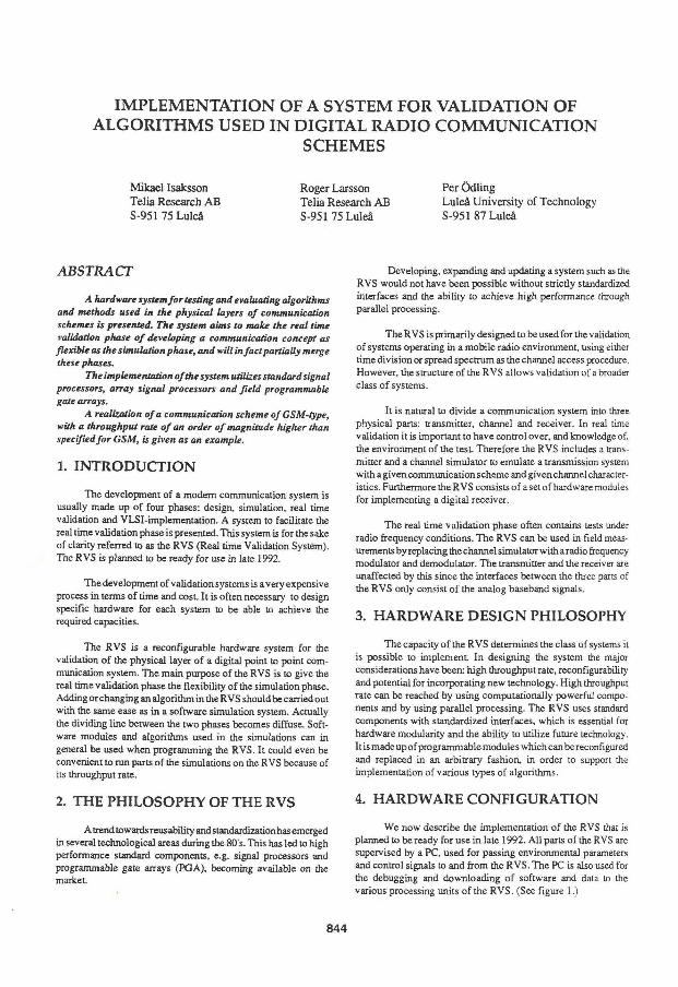
IMPLEMENTATION OF A SYSTEM FOR VALIDATION OF ALGORITHMS USED IN DIGITAL RADIO COMMUNICATION

SCHEMES

Mikael Isaksson Roger Larsson Per Odling Telia Research AB Telia Research AB Luleå University of Technology S-951 75 Luleå S-951 75 Luleå S-951 87 Luleå

ABSTRACT

A hardware system for testing and evaluating algorithms and methods used in the physical layers of communication schemes is presented. The system aims to make the real time validation phase of developing a communication concept as flexible as the simulation phase, and will in fact partially merge these phases.

The implementation of the system utilizes standard signal processors, array signal processors and field programmable gate arrays.

A realization of a communication scheme of CSM-type, with a throughput rate of an order of magnitude higher than specified for GSM, is given as an example.

1. I N T R O D U C T I O N

The development of a modem communication system is usually made up of four phases: design, simulation, real time validation and VLSI-implementation. A system to facilitate the real time validation phase is presented. This system is for the sake of clarity referred to as the RVS (Real time Validation System). The RVS is planned to be ready for use in late 1992.

The development of validation systems is a very expensive process in terms of time and cost. It is often necessary to design specific hardware for each system to be able to achieve the required capacities.

The RVS is a reconfigurable hardware system for the validation of the physical layer of a digital point to point com­munication system. The main purpose of the RVS is to give the real time validation phase the flexibility of the simulation phase. Adding or changing an algorithm in the RVS should be carried out with the same ease as in a software simulation system. Actually the dividing line between the two phases becomes diffuse. Soft­ware modules and algorithms used in the simulations can in general be used when programming the RVS. It could even be convenient to run parts of the simulations on the RVS because of its throughput rate.

2. T H E P H I L O S O P H Y O F T H E R V S

Attend towardsreusability and standardization has emerged in several technological areas during the 80 s. This has led to high performance standard components, e.g. signal processors and programmable gate arrays (PGA), becoming available on the market.

Developing, expanding and updating a system such as the RVS would not have been possible without strictly standardized interfaces and the ability to achieve high performance through parallel processing.

The RVS is primarily designed to be used for the validation of systems operating in a mobile radio environment, using either time division or spread spectrum as the channel access procedure. However, the structure of the RVS allows validation of a broader class of systems.

It is natural to divide a communication system into three physical parts: transmitter, channel and receiver. In real time validation it is important to have control over, and knowledge of, the environment of the test. Therefore the RVS includes a trans­mitter and a channel simulator to emulate a transmission system with a given communication scheme and given channel character­istics. Furthermore the RVS consistsof asetof hardware modules for implementing a digital receiver.

The real time validation phase often contains tests under radio frequency conditions. The RVS can be used in field meas­urements by replacing the channel simulator with a radio frequency modulator and demodulator. The transmitter and the receiver are unaffected by this since the interfaces between the three parts of the RVS only consist of the analog baseband signals.

3. H A R D W A R E D E S I G N P H I L O S O P H Y

The capacity of the RVS determines the class of systems it is possible to implement. In designing the system the major considerations have been: high throughput rate, reconf igurability and potential for incorporating new technology. High throughput rate can be reached by using computationally powerful compo­nents and by using parallel processing. The RVS uses standard components with standardized interfaces, which is essential for hardware modularity and the ability to utilize future technology. It is made up of programmable modules which can be reconfigured and replaced in an arbitrary fashion, in order to support the implementation of various types of algorithms.

4. H A R D W A R E C O N F I G U R A T I O N

We now describe the implementation of the RVS that is planned to be ready for use in late 1992. All parts of the RVS are supervised by a PC, used for passing environmental parameters and control signals to and from the RVS. The PC is also used for the debugging and downloading of software and data to the various processing units of the RVS. (See figure 1.)

844

Transmiaer Channel simulator Receiver (LeCroy AFG)

Channel simulator Receiver

t i

i

i

i

PC

Figure 1. The RVS system.

4.1 The receiver

The most powerful part, intended to be used as a receiver, is made up of special purpose signal processing modules, all having VME bus interfaces. The receiver is usually the most complex part of a digital communication system due to the large amount of signal processing needed to estimate data transmitted through a distorting channel.

There are three types of signal processing modules avail­able in the RVS for implementing the receiver. These are standard signal processors, array signal processors and gate array boards. Furthermore the receiver includes a sampling unit for the conver­sion of the two incoming analog baseband signals (In-phase and Quadrature). Each of the modules uses the VME bus system for control and programming. The data signals are passed through special signal buses.

The sampled signals are stored in a queue memory used as an interface towards the signal processing units. The maximum sampling rate is 30 MHz for two channels, or 60 MHz for one channel, with a resolution of 8 bits. This unit also performs the generation of clock and timing signals for other units.

The parts of the implementation where the algorithm needs to be easily altered are best realized with parallel signal proces­sors. The Texas Instrument TMS320C40 is used in the RVS. This processor model has recently been introduced on the market and is considered to be one of the most powerful [ 1 ]. One of the prime features of this processor is the six high-speed communication links, supporting the connection of additional C40 processors. The C40 concept includes software support, standardized inter­faces and protocols for a three-dimensional multi-processor structure. The number of processors in one structure can be very large and is easily changed. The C40 signal processor has a computational capacity of 50 Mflops.

For array operations over large amounts of data, e.g. FFT, filtering and correlation, special array signal processors are well adapted. These operations are often difficult to parallelize. The RVS contains the array signal processor DaSP a66210 by Array Microsystems. The DaSP is designed for FFT-transforms and operations in the frequency domain. A complex 1024 points FFT can be computed in 131 microseconds.

For parts where computational power is crucial, specially designed field programmable gate arrays (FPGA) are being used. The FPGAs used are RAM-based LCA-devices* by XLINX. Designing and verifying the FPGAs can be done in a few days, compared to weeks for other gate array technologies.

A high degree of parallelism can easily be obtained, which makes the FPGAs well suited for performing algorithms that can be divided into many small, parallel parts, e.g. the Viterbi algo­rithm. The FPGAs can be programmed via the VME-buss.

4.2 The channel simulator

The channel simulator is developed at Telia Research [2] and is capable of simulating a time-variant, frequency selective fading channel, e.g. the Rayleigh faded channels specified in COST 207 [3] for GSM. The simulator works on baseband signals. When RF-signals are needed the simulator is comple­mented with external up and down converters. The channel simulator is based on a VME-bus system and is controlled by a PC. The VME-bus system contains the signal processing units and a CPU-unit for system control. The maximum bandwidth of the analog baseband signal is 15 MHz. The number of reflexes (taps) possible is 10 and each tap is capable of generating a time-variant uncorrelated fading. The doppler frequency of the fading process can be varied in a range of 0-1000 Hz, and the delay between two consecutive taps can be varied in the range of 0.1-12.1 micro­seconds. The attenuation of each tap can be varied arbitrarily to create a desired power-delay spectrum. In order to simulate slow log-normal fading the tap attenuation can be varied in real time.

Aplannedextensionof the simulator includes the possibility to replay an actual, pre-recorded channel [4].

43 The transmitter

As a transmitter the LeCroy Arbitrary Function Generator (AFG) is used. This instrument is capable of transmitting prestored bursts ofmodulated data in real time, with the possibility of using different types of burst formats and symbol rates. The signal can be generated a software simulation package, e.g. Cossap™, SPW™ or Ma j™. This gives the possibility of distorting the signal before transmission. As an alternative a sampled physical signal can be used. The signal files are downloaded to the RAM-memory of the AFG before starting the test run.

The AFG offers the opportunity of transmitting different partsof data, e.g. bursts, inapseudo-random way. The transmitters memory capacity of 2 Megabytes is sufficient for the validation of most of todays communication schemes.

5. A N E X A M P L E O F A N

I M P L E M E N T A T I O N

The features of the RVS are best illuminated by presenting a validation of a well known communication system. As a system specification we choose the physical layer specified for GSM [5][6]. In the GSM specification the receiver algorithm is not stricdy specified so we choose the M aximum Likelihood Sequence Estimator (MLSE) described by Ungerboeck [7] for the equalizer part of our receiver. This (optimal) receiver algorithm is well suited as an example because of its high performance and con­siderable complexity.

* Logical Cell Arrays

845

MLSE

BMU ACS STD BMU ACS STD

Figure 2. GSM receiver based on MLSE.

GSM is a time division multiple access (TDMA) system where a channel is divided into eight consecutive time slots, one time slot per mobile. A physical GSM channel has a transmission rate of 270 kbit/second. To utilize the capacity of the RVS we design the MLSE-receiver for accessing every time slot, or alternatively accessing eight parallel time-divided GSM chan­nels. This is also equivalent to validating a time divided system with a transmission rate of Mbit/second as long as the channel distortion follows the GSM specification.

The GSM channel is characterized by severe intersymbol interference, additive Gaussian noise and Rayleigh fading. Figure 2 depicts the receiver divided into logical parts.

5.1 The Simulation Phase

The GSM subsystem including transmitter, channel and receiver is simulated in the simulation software package SPW™. Each module in the simulated system corresponds to a logical module in the implementation, see figure 2. A majority of the modules in the simulated receiver is written in the C programming language and can therefore be used almost directly when pro­gramming the signal processors of the RVS.

5.2 Algorithm

The algorithm proposed on [7] contains a matched filter and a modified metric computation in the Viterbi algorithm. The metric can be computed recursively as:

W = W I n - i > + nrax(Un)

with

where y„ is the the sampled output of the matched filter, x n is the sampled autocorrelation function of the channel and I n is the symbol sequence. The intersymbol interference spans over a time interval of L symbol durations.

It is convenient to divide the MLSE into three logical and independent parts [9]: the Branch Metric Unit block (BMU), the Add, Compare and Select block (ACS) and the Survivor, Trace and Decode block (STD). These blocks are described below.

53 Transmission system

The underlying transmission system model is of TDMA type with data in bursts. The modulation scheme is Gaussian Minimum Shift Keying (GMSK) [5][6].

The bursts contains 116 encrypted data bits consisting of two parts of 58 bits. A 26 bit reference sequence is placed in between the two 58 bit blocks to allow symbol timing, carrier phase recovery and channel estimation. Three additional tail bits complete the burst at both ends. The channel and sequence estimation is performed once per burst, independently of other bursts.

5.4 Synchronization and channel estimation

The 26 bit reference sequence is used for symbol timing and carrier phase recovery [5] [6], and for estimation of the channel impulse response. To compute the optimum decision instant and the carrier phase in the received burst a correlation is computed of the entire burst and the 16 central bits of the reference sequence stored in the receiver. The DaSP processor is well suited to performe this operation.

The channel estimate is then computed by an additional correlation of the 16 subsequent symbol samples from the deci­sion instant in the burst and the prestored reference sequence. The channel estimate is computed for a maximum time dispersion of 4 symbol intervals. The channel estimate is essentia] information for the MLSE receiver and the matched filter.

5.5 Branch Metric Unit (BMU)

Before Viterbi decoding the metric value of each branch in the trellis has to be computed. The trellis contains 16 states according to the time dispersion of 4 symbol intervals. Two branches lead into each state in the trellis which give 32 metric computations for each symbol in the burst. These computations are performed by the BMU unit using the formula [7] [8]:

UB = 2ReCCyB)-2RJ

846

L \

V m=l J

The formula can be further simplified by using the GMSK properties and the fact that terms which do not include yn can be computed once for each burst.

The simplified formula can be expressed as:

U„= Re[i;(y n -T s >]

The look-up table T s is computed once for each burst and will be used in the metric computations for each state in the trellis by simply fetching the proper value from Ts.

The set of BMU operations is performed by the C40 processors and is one of the parts of the algorithm requiring most computational capacity. The complexity of this operation makes it difficult to use the FPGA technology.

5.6 Add, Compare and Select units (ACS)

For each symbol in the burst the maximum metric values are computed for each of the 16 states in the trellis. Two branches, or paths, lead into each state in the trellis corresponding to the two possible state transitions. The branch metric values, computed by the BMU, are then added to the accumulated metric value in the predecessor state. The path giving the maximum metric value is saved and the state is given the new accumulated metric value.

The FPG A technology is a suitable choice for implementing these ACS operations. The computations are performed by using 16 parallel ACS units. In order to rrunimize the number of gate array chips and interconnections it is desirable to maximize the number of ACS units in each chip. This can be done by imple­menting each ACS unit as a one-bit processor using bit-serial design. Bit-serial design requires considerably fewer gate equiva­lents than a corresponding bit-parallel design [10]. The draw­backs are higher clock rates and the need for parallel/serial conversion.

5.7 Survivior, Trace and Decode unit (STD)

Using the saved paths from the ACS operation the symbol sequence can be decoded. Since only one path leads in to each state, the state transitions uniquely estimate the symbol sequence. These operations are called Survivor, Trace and Decode (STD) and are implemented in a simple hardware design containing dual-port RAMs and counters.

The STD is implemented on a separate board with VME bus interface and is the part of the receiver producing the output of the RVS, i.e. the estimated symbols.

6. C O M M E N T S A N D F U T U R E

A C T I V I T I E S

We see several possible ways of using the RVS. Its primary task is to facilitate the real time validation phase of developing a communication system, and this is where the RVS has its economic importance. Another important use of the RVS is as a research tool. As an example of this it will be used for evaluating receiver algorithms as a part of a research project at Luleå University of Technology [11], Moreover it can be used as a number cruncher' for running heavy simulations.

We plan to present the results of the implementation example described in section 5 in more detail during 1993. The results from the cooperation with the research group at Luleå University of Technology, mentioned above, will also be the subject for future presentations.

R E F E R E N C E S

[ 1] Presented at DSP World Expo, The International Conference on DSP Applications & Technology, Berlin, October 28-31,1991.

[2] T.Boström,M. Isaksson, T. Lundberg, "Digital baseband channel simulator", COST 231 TD(91) September, 1991.

[3] Proposal on channel transfer functions to be used in GSM tests late 1986, COST 207 WG1 TD(85).

[4] B. Engström, "Kanalsimulator i hårdvara", NRS work­shop .Luleå University, April 2-3, 1992.

[5] Modulation and demodulation, GSM recommendation 05.04, September, 1987.

[6] Transmission andreception,GSMrecommendation05.05. lune, 1988.

[7] U.Ungerboeck,"Adaptivemaximum-likelihoodreceiver for carrier modulated data-transmission systems", IEEE Transaction on communications vol. COM-22. No.5, May, 1974, pp. 624-636.

[8] I.G.Proakis, "Digital Commmunications", McGraw-Hill Book C, New York (1983).

[9] H. Lou, J. M. Cioffi, "A Programmable Parallel Processor Architecture for Viterbi Detection", IEEE Global Telecommunications Conference, San Diego, California, December, 1990, pp. 707A.4.1 - 707A.4.5.

[10] R. W. Hockney, C. R. Jesshope, "Parallel Computers 2", Adam Hilger, Bristol and Philadelphia (1988).

[11] P.O. Börjesson, T. Koski, P. Odling, "A Reduced Complexity Viterbi Equalizer used in Conjunction with a Pulse Shaping Method", Nordic Radio Symposium, Aalborg, Denmark, June, 1992.

847

Part U L I

A Robust Correlation Receiver for Distance Estimation

P a r t I I I . l :

A R o b u s t C o r r e l a t i o n R e c e i v e r for Dis tance E s t i m a t i o n

H å k a n Eriksson 1 , Per Ola Bör jesson 1 , Per Odl ing 1 and Nils-Gunnar Holmer 2

IEEE Transactions on Ultrasonics, Ferroelectrics, and Frequency Control, vol . 41 .

no. 5, pp. 596-603, September 1994.

•"Tuleå University of Technology, Division of Signal Processing, S-971 87 Luleå, Sweden

2Lund University, Department of Biomedical Engineering, S-221 00 Lund, Sweden

T-UFF/41/5//03351D

A R o b u s t C o r r e l a t i o n R e c e i v e r

f o r D i s t a n c e E s t i m a t i o n

Håkan Eriksson Per Ola Börjesson

Per Odling Nils-Gunnar Holmer

Reprinted from IEEE TRANSACTIONS ON ULTRASONICS, FERROELECTRICS, AND FREQUENCY CONTROL

Vol. 41, No. 5, September 1994

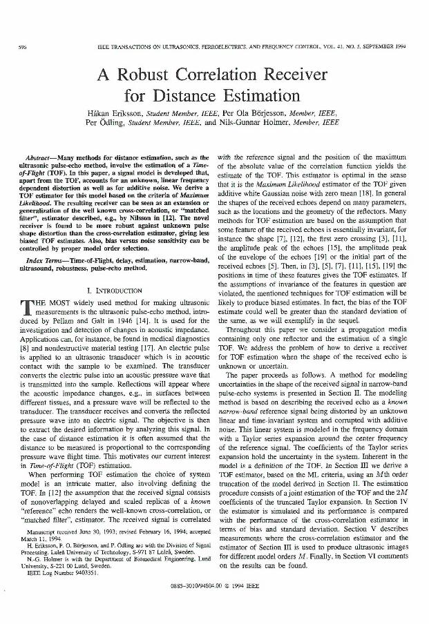
596 IEEE TRANSACTIONS ON ULTRASONICS, FERROELECTRICS, AND FREQUENCY CONTROL, VOL. 41, NO. 5, SEPTEMBER 1994

A Robust Correlation Receiver for Distance Estimation

Håkan Eriksson, Student Member, IEEE, Per Ola Börjesson, Member, IEEE, Per Odling, Student Member, IEEE, and Nils-Gunnar Holmer, Member, IEEE

Abstract—Many methods for distance estimation, such as the ultrasonic pulse-echo method, involve the estimation of a Time-of-Flight (TOF). In this paper, a signal model is developed that, apart from the TOF, accounts for an unknown, linear frequency dependent distortion as well as for additive noise. We derive a TOF estimator for this model based on the criteria of Maximum Likelihood. The resulting receiver can be seen as an extension or generalization of the well known cross-correlation, or "matched filter", estimator described, e.g., by Nilsson in [12]. The novel receiver is found to be more robust against unknown pulse shape distortion than the cross-correlation estimator, giving less biased TOF estimates. Also, bias versus noise sensitivity can be controlled by proper model order selection.

Index Terms—Time-of-Flight, delay, estimation, narrow-band, ultrasound, robustness, pulse-echo method.

I . INTRODUCTION

THE MOST widely used method for making ultrasonic measurements is the ultrasonic pulse-echo method, intro­

duced by Pellam and Gait in 1946 [14]. It is used for the investigation and detection of changes in acoustic impedance. Applications can, for instance, be found in medical diagnostics [8] and nondestructive material testing [17]. An electric pulse is applied to an ultrasonic transducer which is in acoustic contact with the sample to be examined. The transducer converts the electric pulse into an acoustic pressure wave that is transmitted into the sample. Reflections will appear where the acoustic impedance changes, e.g., in surfaces between different tissues, and a pressure wave will be reflected to the transducer. The transducer receives and converts the reflected pressure wave into an electric signal. The objective is then to extract the desired information by analyzing this signal. In the case of distance estimation it is often assumed that the distance to be measured is proportional to the corresponding pressure wave flight time. This motivates our current interest in Time-of-Flight (TOF) estimation.

When performing TOF estimation the choice of system model is an intricate matter, also involving defining the TOF. In [12] the assumption that the received signal consists of nonoverlapping delayed and scaled replicas of a known "reference" echo renders the well-known cross-correlation, or "matched filter", estimator. The received signal is correlated

Manuscript received June 30, 1993; revised February 16. 1994; accepted March 11, 1994.

H. Eriksson, P. O. Börjesson, and P. Odling are with the Division of Signal Processing, Luleå University of Technology, S-971 87 Luleå, Sweden.

N.-G. Holmer is with the Department of Biomedical Engineering, Lund University, S-221 00 Lund, Sweden.

I E E E Log Number 9403351.

with the reference signal and the position of the maximum of the absolute value of the correlation function yields the estimate of the TOF. This estimator is optimal in the sense that it is the Maximum Likelihood estimator of the TOF given additive white Gaussian noise with zero mean [18]. In general the shapes of the received echoes depend on many parameters, such as the locations and the geometry of the reflectors. Many methods for TOF estimation are based on the assumption that some feature of the received echoes is essentially invariant, for instance the shape [7], [12], the first zero crossing [3], [11], the amplitude peak of the echoes [15], the amplitude peak of the envelope of the echoes [19] or the initial part of the received echoes [5]. Then, in [3], [5], [7], [11], [15], [19] the positions in time of these features gives the TOF estimates. If the assumptions of invariance of the features in question are violated, the mentioned techniques for TOF estimation will be likely to produce biased estimates. In fact, the bias of the TOF estimate could well be greater than the standard deviation of the same, as we will exemplify in the sequel.

Throughout this paper we consider a propagation media containing only one reflector and the estimation of a single TOF. We address the problem of how to derive a receiver for TOF estimation when the shape of the received echo is unknown or uncertain.

The paper proceeds as follows. A method for modeling uncertainties in the shape of the received signal in narrow-band pulse-echo systems is presented in Section I I . The modeling method is based on describing the received echo as a known narrow-band reference signal being distorted by an unknown linear and time-invariant system and corrupted with additive noise. This linear system is modeled in the frequency domain with a Taylor series expansion around the center frequency of the reference signal. The coefficients of the Taylor series expansion hold the uncertainty in the system. Inherent in the model is a definition of the TOF. In Section I I I we derive a TOF estimator, based on the ML criteria, using an Mth order truncation of the model derived in Section I I . The estimation procedure consists of a joint estimation of the TOF and the 2M coefficients of the truncated Taylor expansion. In Section IV the estimator is simulated and its performance is compared with the performance of the cross-correlation estimator in terms of bias and standard deviation. Section V describes measurements where the cross-correlation estimator and the estimator of Section II I is used to produce ultrasonic images for different model orders M. Finally, in Section VI comments on the results can be found.

0885-3010/94$04.00 © 1994 I E E E

ERIKSSON a al.: ROBUST CORRELATION RECEIVER 597

I I . LINEAR DISTORTION OF NARROWBAND SIGNALS

Consider the situation described in Fig. 1. An unknown excitation signal is applied as an input to two unknown linear systems. The output signal from one of the systems, s(t), is a real valued known narrow-band signal, henceforth called the reference signal. The output from the other system is denoted y(t - &), where 6 is the unknown delay to be estimated.

Assume that there exists an impulse response h(t) so that the noiseless waveform

y[t - 6) = (s * h)(t - 6), (1)

where * denotes continuous time convolution and h(t) is an unknown real valued impulse response representing linear distortion. Since the real valued reference signal is narrow­band, we write it as

s(t) = 5c{eJ' (2)

where SR{ } denotes the real part of its argument. The functions a(t) and ß(t) are real valued with the restriction that the Fourier transform of the complex envelope, oi(t)e J ' 3 ' t ' , is zero outside the frequency interval \-B,B], where B < Jo- We also assume that the complex envelope has finite energy, i.e., that a( i )e^M £ L2(7l) = {z{t)\ J\z(t)\2dt < co}.

Define L§(71) as the space of all signals in L2(7l) whose Fourier transforms are zero outside the frequency interval [-B.B). These signals will be referred to as baseband signals. Furthermore, due to the narrow-band assumption (B - C fo) o n

s(t), it is convenient to define the subspace L | f F (V^) of L2(7l) as the space of all signals in 1,2(71) whose Fourier transforms are zero outside the frequency intervals [—fo - B, - f o + B] and [fo - BJo + B). By definition a(t)e]ß(t) £ L§(71) and by construction s(t) e L ^ F ( 7 l ) . Note that s(t) can be any narrow-band signal having finite energy whose Fourier transform only has support in two intervals, symmetrically around / = 0 and not containing / = 0. These signals could typically be bandlimited ultrasonic pulse echo signals decaying fast enough in time to have finite energy.

Models related to (1) can be found in, e.g., [2], [4], [12]. The special case of (1) where h(t) is modeled as the sum of weighted and delayed Dirac-delta functions has been extensively used in the context of TOF estimation, see, e.g., [12]. Recently in a paper by Boudreau and Kabal [2] a model for the purpose of TOF estimation is presented, allowing an unknown linear frequency dependent distortion in the delay path. The reference signal was there modeled as a broadband stochastic process for the tracking of a time varying TOF with an adaptive algorithm. A discrete time version of (1) is studied in [4], where the distortion is modeled as a linear stochastic system with a known Gaussian statistic.

A. An Mth Order Model of the Distorting System h(t)

Due to the narrow-band assumption on s(t) we are only interested in the behaviour of h(t) in the frequency intervals [ f 0 - B , f 0 + B] and [—fo~B, - f o + B}. Let H ( f ) denote the Fourier transform of h(t) and assume that H ( f ) is M-times differentiable in an interval around / = fo- Define C M ( / ) as

excitation signal

l inear s y s t e m A

-s(t)

n(t)

l inear s y s t e m B

y(t-e)

Fig. 1. A model of a measurement situation for TOF estimation.

the Taylor series expansion of H ( f ) around / 0 > 0 with a remainder term of order M:

C M ( / ) A £ h\ MkHV>

(3)

Now, let us define a function HMU) such that HMU) = C M ( / ) for / > 0 and the inverse Fourier transform of HMU) is real valued,

HMU) A CMU)U(}) + C ' M ( - f ) U ( - f ) , (4)

where U ( f ) denotes the unit step function and the superscript * denotes the complex conjugate.

The system model H M ( f ) is then an Mth order model of H ( f ) , especially adapted for narrow-band signals with their center frequency equal to fo. A similar reasoning by Papoulis can be found in [13, page 59] for baseband signals.

ß . Evaluation of the Convolution (s * h)(t)

For the purpose of modeling the convolution (s * h)(t) in (1), we define

yM(t) L\F-l{F{s{t)}HM{f)}, (5)

where ;F{ } denotes the Fourier transform and its inverse. By using the narrow-band representation of the refer­ence signal in (2), it follows that

yM(t) = J £ K +jbk)g^(t)\, (6)

where ak and 6*, are real valued coefficients given by

i d k H ( f ) \ ak + jbk -

(j2Tz)kk\ d f k

f = h

and

ékHt) = -%{«(t)e^}. (8)

All g(k\t) exist and have Fourier transforms that are zero outside the frequency interval [-B.B] since the subspace L f (71) is closed under linear operations and o'°'(t) is analytic having derivatives of all orders in every point on 71.

We now have obtained a signal representation, (6)-(8), with the model order M to choose. Observe that the waveforms { f f ^ ' M l i s i r j 1 3 1 6 independent of the system h(t) and that the coefficients {ak, bk}^J^ are independent of the reference signal once the center frequency is given. Thus, the knowl­edge of the reference signal gives us a signal basis and the

i98 IEEE TRANSACTIONS ON ULTRASONICS. FERROELECTRICS. AND FREQUENCY CONTROL, VOL. 41, NO. 5, SEPTEMBER 1994

coefficients {ak,bk}kL0 hold the uncertainty in the shape of the waveform yu(t)-

For the development of the estimator in Section III we need an orthogonal signal basis. Define the inner product (•,•) in 1,2 (ft) as

x,y A / x{t)y*(t)dt, (9)

and the norm \\x\\ A (x.x)1'2. Since gl°\t) € i f ( f t ) it

can be shown that the signal set {s^'jj^1 spans an M-

dimensional signal space UM >n i f (f t)- Let {zk}kZa denote an orthonormal signal basis that spans Qjv, for every N in { 1 , . . . , M } , which ensures the signal basis {Z^SQ to be in a specific order. This signal basis can, for instance, be obtained by applying Gram-Schmidt orthogonalization to { g ' * ' } ^ 1 . Let us modulate the signal basis { z j t } ^ 1 up to the frequency band of interest and define

M t ) A s/m{zk(j.W^ht}

i>k(t) A v ^ a ~ (10)

where denotes the imaginary part of its argument. Since the Fourier transform of zk is narrow-band (B < fo) and (zk.zi) = Ski the function set {ipk, i / ' t } ^ 1 is a real valued orthonormal basis of dimension 2M in L§F(7l). The model signal J / M W in (5) can then be expressed as a linear combination of {i/jfc, "øfclfcLrj1 according to

fc = 0 , l , . . . , M - 1 ,

DM (t) = Y , cki>k(t) + dkMt)- ( l l )

The unknown coefficients { c f c . d i t } ^ 1 are the new coordi­

nates for {a^&jjj j iö 3 a ^ t e r * e c n a n S e °f signal basis. The coefficients {ck, d * , } ^ 1 now hold the uncertainty in the shape of the waveform J/M (t). Note that 4>0(t) is a normalized replica of the reference signal, i.e., ifio(t) = s(t)/\\s\\, and that i>k(t) and 4>k{t) by construction form a Hilbert transform pair for all k in { 0 , . . . , M - 1).

C. / I Summary of the Signal Basis Design

In this section we have presented a method for modeling linear distortion of narrow-band signals. The analysis results in a signal representation consisting of an orthonormal signal basis. The design process for obtaining this signal basis can be summarized as follows:

• For fc = 0, L . . . ,M - 1, take the fcth order derivative of the bandlimited complex envelope of the reference signal, see (8).

• Use for instance the Gram-Schmidt orthogonalization process to obtain a complex orthonormal baseband signal basis, {z i j^ iö 1 .

• Calculate the high frequency signal basis, {ipk(t),

MWkJo1' a s described by (10). In the case when s(t) is acquired by a calibration or

measurement procedure, the design process will be affected by noise. To reduce this effect, a band-pass filter matched to the bandwidth of s(t) should be introduced when acquiring s(i), thereby reducing the noise power. The design process is

e - j 2 i r / 0 t

»(*) LP

{ 9 { k ) ( t ) } ^ { z k ( t ) ) t o

z k { t )

g j 2 7 T / 0 t

Fig. 2. A design structure for generating the signal basis iwt(t),

described in Fig. 2 where LP denotes an ideal low pass filter with a bandwidth equal to B, i.e., the bandwidth of a(t)e j 3 W.

I I I . TIME OF FLIGHT ESTIMATION

Consider the joint estimation of a single T O F and the coefficients describing the linear distortion. We model the received signal as

r ( ( ) A W ( t - « ) + n ( t ) , (12)

where VM(-) is given by the Mth order model (11) and n(t) is an additive white Gaussian noise process, with zero mean and a power spectral density equal to No/2. The parameter 8 is the TOF. With this definition of the TOF the shape of the waveform J/MO) is allowed to vary, cf., [3], [5], [7], [11], [12], [15], [19].

To get a compact notation we rewrite VM{-) of (11) as

m(t -&) = PTiP(t -1 (13)

where ij> ~ [fo,..., I1>M~U i>0\ • • • > 4>M-I]T is a vector representation of the orthonormal signal basis and p = [c6j. •. ,CM~i,do,... ,dM-i]T- With this notation we write the Signal to Noise Ratio (SNR) as

SNR A T

p p jjjwj! N0/2 No/2'

(14)

A. The ML Estimator

The estimation problem is to determine the unknown TOF 8 when observing { r ( t ) \ t € l } , where I = [Ti ,T 2 ] is the observation interval (Tj < Tb). Define the deterministic parameter vector

q A (15)

and denote the estimate of q as q = [9, pT]T. The function

«(q I KO) = ^ J x r ( t ) y M ( t - 9 ) d t (16)

ERIKSSON et al: ROBUST CORRELATION RECEIVER 599

is a log likelihood function for q given the observation {r(t) I t e 1}. cf. [18, p. 274]. Using (13), (16) can be written as

f(q I K * ) ) = J - P T r e - T J - P T P + ~ P T E ( S ) p , (17) i v n i v o JVO

where r e is a vector resulting from 2M parallel correlations,

r« = y r(i)^(< -and where the matrix

E(8)

(18)

(19)

The only term involving the measurements r(t) in (17) is the vector re, where rg is a sufficient statistic for the parameter vector q.

For a given observation {r(t) \ t S I } , the ML estimate of q is obtained by locating the global maximum of the log likelihood function I(q | r(t)) with respect to q. Let 8 e l~g, where I e is an interval, or a set of intervals, on Ti. If the observation interval 1 is chosen sufficiently large for i>k{t — 8) and "øfc(t - 8) to have negligible energy outside I for all 6 e Ig. then, according to Schwarz's inequality, each element in E(0) is not greater than this negligible energy. Approximating E(fl) with zero and completing the square in (17) we have

I(q I r(t)) No

rs) T (p • r«) + - ^ r « . (20)

For any given 8 the maximum of £(q | r(t)), with respect to p, is given by p = rg. Using rg for p in (20), it follows that the location of the global maximum of i(q | r(t)), with respect to q (resulting in an approximate ML estimate of q), is given by

ÖMZ.(r) - argmaxg £ J $ {xM(8)}

P M l = rg=g... (21)

where

XM(8) : T Tg Tg. (22)

Fig. 3 depicts a receiver structure for generating zjvirø from r(t) according to (22). We henceforth refer to this receiver as the M t h order extended correlation receiver. Note that an ML estimator, in its general form, need not to be unbiased. This also applies to the Mth order extended correlation receiver.

B. A Comparison With the Cross-Correlation Estimator

The cross-correlation, or "matched filter", estimator of [12] is derived using the Maximum Likelihood criterion and as­sumptions of additive white Gaussian noise and perfect knowl­edge of the linear distortion, except for an unknown amplifi­cation factor. The received signal is correlated with a known waveform corresponding to J/M(*) in (16), and the position of the maximum of the absolute value of the correlation function yields the estimate of the TOF. This receiver, when applied to a situation where the assumptions are valid, is unbiased and has a performance that meets the Cramér-Rao lower bound for high SNR's, see, e.g., [9] and the references therein. For

r(t). xM{i)

# M ( - « )

Fig. 3. A receiver structure for generating x^{t) according to (22). The function r(t) is set to zero outside the observation interval 1 due to the implementation of the correlators as filters.

low SNR's the cross-correlation estimator will suffer from a threshold effect when applied to narrow-band signals in the sense that the performance decreases rapidly with decreasing SNR below a certain SNR [9].

The Mth order extended correlation receiver can be de­scribed as a cross-correlation estimator that first estimates the received waveform yu(t - 8) a n d then correlates the received signal r(t) with this estimate. This can be seen, cf. [18, p. 354], by substituting the right-hand side of (18) for one of the r e ' s in (22), giving

•r.\i (6) r(t)yM(t - 8)dU

where

yM(t-8) = r | > ( t -

(23)

(24)

The function y M ( f . - 8) can be interpreted as an estimate of yM(t - 8) for a given 8, cf. (13) with p estimated by rs.

IV. ESTIMATION EXAMPLE

Let us investigate the influence of the model order M on the bias and the standard deviation of the TOF estimate by means of Monte Carlo simulations. We compare the performance of the cross-correlation estimator and the performance of the Mth order extended correlation receiver for different values of the model order M and various SNR's.

In these simulations the reference signal sit) is given by (2) with 8(t) = 0 and a(t) as a Hanning window in the frequency domain. With a Hanning window of bandwidth B, the Fourier transform of a(t) becomes

F{a(t)} : _ / l / 2 + l / 2 c o S ( ^

0.

\J\<B otherwise

(25)

The center frequency of the reference signal was chosen as f0 = 2B Hz. In all of these simulations the cross-correlation estimator is matched to the reference signal. For each estimator and every integer value of SNR, the TOF of one thousand echoes has been estimated.

In Figs. 5-6 the absolute value of the bias and the standard deviation of the receivers are shown for a case when the received signal has been subjected to a specific "unknown"

600 IEEE TRANSACTIONS ON ULTRASONICS. FERROELECTRICS. AND FREQUENCY CONTROL, VOL. 41, NO. 5, SEPTEMBER 1994

i t

(t-e)B

Fig. 4. The reference signal s(t) and the model y\i{t) in (11) in the case when ,1/ = 2 and p = (1/3. 2/3.1/3. l/6]x.

SNR [dB]

Fig. 5. The absolute value of the estimated and normalized bias of the receivers plotted versus SNR when a specific frequency dependent linear distortion is present.

linear distortion. Note that the bias and the standard deviation in the figures have been normalized with IjB. The distortion is described by yuit) in (13), with M = 2 and p = [1/3,2/3,1/3,1/6] T . Fig. 4 shows yM{t) together with the reference signal s(t). In Fig. 7 the standard deviation of the receivers is given for the case when no frequency dependent linear distortion is present, i.e., J/M(*) = as(t) where a is an unknown constant. The bias was, in this case, almost equal to zero for all receivers.

We make the following observations. When linear distortion is present the bias of the cross-correlation estimator can be much greater than the standard deviation of the same. The TOF estimates of the first-order extended correlation receiver are almost as biased as the estimates of the cross-correlation estimator. As expected, since the linear distortion is generated with M = 2, the second-order extended correlation receiver has very little bias compared with the cross-correlation esti­mator. It can be noted that the variance of the estimates in general increases with the model order M , especially when no linear distortion is present. An exception can be seen in Fig. 6 for SNR's less than 22 dB. Here both the bias and the variance of the TOF estimate are small for the second-order

SNR [dB)

Fig. 6. The estimated normalized standard deviation of the receivers plotted versus SNR when a specific frequency dependent linear distortion is present.

extended correlation receiver whose model order is matched to the linear distortion.

From these and other simulations we draw the following conclusions. The cross-correlation estimator may give biased estimates when linear distortion not accounted for is present and the error due to bias can be more severe than the error caused by the additive white Gaussian noise. By using the Mth order extended correlation receiver the bias caused by linear distortion can be reduced. Robustness against linear distortion of the shape of the received pulse can be traded for noise sensitivity by increasing the model order M.

V . ULTRASONIC MEASUREMENTS

In this section we present results from using an experimental ultrasonic system to produce relief pictures of a surface structure by estimating the TOF of echoes reflecting from different points on the surface. This is a typical example of when it is difficult to choose a specific waveform as the reference signal for the cross-correlation estimator.

A. Measurement Setup

Experiments were carried out by scanning over a Swedish five crown coin in a 100 by 100 point grid, with a distance of 0.3 mm between adjacent points. The coupling medium between the transducer and the surface was air at room temperature. A circular transducer with a radius of 10.5 mm and a nominal frequency of 1 MHz was used. (The wavelength in air at room temperature is approximately 0.3 mm). The transducer was a focused transducer acoustically adapted to air, with a focal distance of 25 mm. It was designed by H. W. Persson for the investigation presented in [16]. The data were acquired with a LeCroy 9430 sampling oscilloscope. The sampling rate was chosen as 5.5 MHz and the sampling was synchronized with the transmitter by the use of an external crystal oscillator. The distance between the transducer and the surface of the coin was equal to the focal distance of the transducer.

B. Signal Processing and Measurements

A reference echo was acquired for the design of the signal basis {ipkyvlk}^^1, i.e., the receiver filter bank in Fig. 3,

ERIKSSON et al:. ROBUST CORRELATION RECEIVER 601

.5 0 3

V 0.1

M=3

- M = 2

M-l

Cross-correlation receiver

0 i , -15 20 25 30 35

SNR [dB]

Fig. 7. The estimated normalized standard deviation of the receivers plotted versus SNR when no frequency dependent linear distortion is present.

£ [MS] t [ H

Fig. 8. The basis {^ ( t ) ,Vt (^ ) }^ = o corresponding to the acquired ref­erence signal.

by letting the acoustic wave be reflected on the flat tip of a cut steel needle with a diameter of 1 mm, placed in the focal point of the transducer, cf., [10]. When acquiring the reference signal an averaging over 1000 B-scans was performed. The design process, described in Section n, Fig. 2, was then used

to generate the signal set { ^ f c W i Ä W / J L ö 1 f o r M ~ 3 ' s e e

Fig. 8. As mentioned before the signal ipa(t) is identical to the normalized reference signal. The reference signal is also illustrated in Fig. 9 and compared with the features on the surface of the coin.

The Mth order extended correlation receiver, (21H22), and the cross-correlation estimator were used to estimate the TOF for each point in the 100 by 100 point grid. Fig. 10 shows the result when the cross-correlation estimator matched to the

Fig. 9. The proportions of the features on the surface of the coin in comparison with the length of the reference signal.

Fig. 10. A grey scale picture of a Swedish five crown coin, generated with the cross-correlation estimator matched to the reference signal s{t).

reference signal s(t) was used. Figs. 11-13 show the results when the Mth order extended correlation receiver was used with M e { 1 , 2,3}, respectively. All figures are derived from the same measured data.

In the grey-scale pictures the brightness of each pixel in­creases with the TOF. No post-processing has been performed to the data, except for a histogram normalization of the grey-scale level thresholds in the grey-scale pictures.

The SNR, when defined as in (14), varies from point to point in the grid, since the reflected signal energy depends on, e.g., the angle of the reflecting surface. Therefore, no SNR is presented in. the figures. The SNR was though well above the threshold region [9] for the cross-correlation estimator (SNR > 30 dB).

C. Comments on the Measurements

In the estimation examples presented the image correspond­ing to M = 1, Fig. 11, shows a significant improvement in quality compared to the image corresponding to the cross-correlation estimator, Fig. 10. The performance of the cross-correlation estimator is apparently sensitive to shape changes in the received waveform. The errors in the picture are mainly due to bias, since the SNR is high, and can for that reason not be removed by averaging repeated measurements. When

602 IEEE TRANSACTIONS ON ULTRASONICS, FERROELECTRICS, AND FREQUENCY CONTROL. VOL. 41, NO. 5. SEPTEMBER 1994

Fig. 11. A grey scale picture of a Swedish five crown coin, generated using the first-order extended correlation receiver.

applying the receiver with M = 3 (Fig. 13) the disturbances due to the additive noise seem to dominate over the effects due to model errors. For this measurement situation the choices M = 1 and M = 2 appear to be the most appropriate.

The choice and the acquisition of the reference signal is a delicate matter, see, e.g., [6], In this investigation we have used the echo from a cut needle located in the focal point of the transducer. We have not found any reference signal that gives the cross-correlation estimator a noticeable better performance in the presented measurement situation. However, other refer­ence echoes could be used, for instance an echo from a flat surface where total reflection occurs, giving similar images.

VI. CONCLUSION

This paper treats the problem of how to design a receiver for TOF estimation when the received signal has been subjected to an unknown linear distortion. Based on a narrow-band assump­tion on the interrogation pulse, a model of the received signal incorporating unknown linear frequency dependent distortion has been presented together with a TOF estimator based on the criteria of Maximum Likelihood. This ML estimator can be seen as an extension or generalization of the cross-correlation estimator [12], and is referred to as the extended Mth order correlation receiver. The receiver can be implemented as a correlation receiver using a filter bank consisting of 2 M parallel filters.

Simulations have shown that the performance of the cross-correlation receiver is sensitive to the choice of reference signal. The bias of the TOF estimate can be large compared with the standard deviation. By using the Mth order extended correlation receiver the bias caused by linear distortion can be reduced. In the presented ultrasonic measurements we observe that the Mth order extended correlation receiver achieves ro­bustness against pulse shape distortion at the cost of increased noise sensitivity. By increasing the model order the tendency of bias in the TOF estimate can be traded for variance.

In this paper we only examine the case of estimating a single TOF. The receiver could be extended to estimating multiple TOF's, possibly with the exception of closely spaced echoes.

Fig. 12. A grey scale picture of a Swedish five crown coin, generated using the second-order extended correlation receiver.

Fig. 13. A grey scale picture of a Swedish five crown coin, generated using the third-order extended correlation receiver.

We would like to point out that although this investigation is focused on ultrasound applications, the model presented only presumes a narrow-band pulse being distorted by a linear time-invariant system. Such conditions could also be present in other application areas.

REFERENCES

[1] P. O. Börjesson, O. Pahlra, L. Sörnmo, and M.-E. Nygårds, "Adaptive QRS detection based on maximum a posteriori estimation," IEEE Trans. Biomed. Eng., vol. 29, no. 5, pp. 341-351, 1982.

[2] D. Boudreau and P. Kabal, "Joint time-delay estimation and adaptive recursive least squares filtering," IEEE Trans. Signal Process., vol. 41, no. 2, pp. 592-601, 1993.

[3] T. Bowen, W. G. Conner, R. L. Nasoni, A. E. Pifer, and R. R. Sholes, "Measurement of the temperature dependence of the velocity of ultrasound in soft tissue," in M. Linzer, Ed., Ultrasonic Tissue Characterization II, NBS Special Publication, vol. 525, U.S. Govt. Print. Office, 1979, pp. 57-61.

[4] H. Eriksson, P. Odling, and P. O. Börjesson, "Simultaneous time of flight and channel estimation using a stochastic channel model," in Radio Vetenskaplig Konferens RVK.93, Sammanfattning av Posters och Föredrag. Lund, Sweden, April 1993, pp. 43—46.

[5] J. F. Greenleaf, S. A. Johnsson, W. F. Samayoa, and F. A. Duck, "Two-dimensional acoustic velocity distribution in tissues using an algebraic

ERIKSSON et al: ROBUST CORRELATION RECEIVER 603

reconstruction technique," in Proc. Ultrason. Int. Conf., London, March 1975, pp. 190-195.

[6] A. Grennberg and M. Sandell, "Experimental determination of the ul­trasonic echo from a pointlike reflector using a tomographic approach," in Proc. 1992 Ultrason. Symp., Tuscon, AZ, Oct. 1992, pp. 639-642.

[7] V. N. Gupta, P. K. Baghat, and A. M. Fried, "Estimating ultrasound propagation velocity in tissue from unwrapping phase spectra," Ultra-son. Imaging, no. 2, pp. 223-231, 1980.

[8] C. R. Hill, Physical Principles of Medical Ultrasonics. Chichester: Ellis Horwood Ltd., 1986.

[9] J. P. Ianiello, "Time delay estimation via cross-correlation in the presence of large estimation errors," IEEE Trans. Acoust., Speech and Signal Process., vol. 30, no. 6, pp. 998-1003, 1982.

[10] J. A. Jensen, "A model for the propagation and scattering of ultrasound in tissue," J. Acoust. Soc. Amer., vol. 89, no. 1, pp. 182-190, 1991.

[11] F. W. Kremkau, R. W. Barnes, and P. McGraw, "Ultrasonic attenuation and propagation in normal human brain," J. Acoust. Soc. Amer., vol. 70, no. 1, pp. 29-38, 1981.

[12] N. J. Nilsson, "On the optimum range resolution of radar signals in noise," IRE Trans. Inform. Theory, vol. 32, no. 7, pp. 245-253, 1961.

[13] A. Papoulis, The Fourier Integral and its Applications. New York: McGraw-Hill, 1962.

[14] J. R. Pellam and J. K. Gait, "Ultrasonic propagation in liquids: I. Application of pulse technique to velocity and absorbation measurement at 15 megacycles," J. Chemical Phys., vol. 14, no. 10, pp. 608-615, 1946.

[15] M. Ragozzino, "Analysis of the error in measurement of ultrasound speed in tissue due to waveform deformation by frequency-dependent attenuation," Ultrason., no. 12, pp. 135-138, May 1981.

[16] N. Sundström, P. O. Börjesson, N.-G. Holmer, L . Olsson, and H. W. Persson, "Registration of surface structures using airborne focused ultrasound," Ultrasound in Med. and Bio., vol. 17, no. 5, pp. 513-518, 1991.

[17] R. N. Thurston and A. D. Pierce, Ultrasonic Measurement Methods. San Diego, CA: Academic, 1990,

[18] H. L. van Trees, Detection, Estimation, and Modulation Theory, Part I. New York: Wiley, 1968.

[19] V. A. Verhoef, M. J. T. M. Clostermans, and J. M. Thijssen, "Diffraction and dispersion effects on the estimation of ultrasound attenuation and velocity in biological tissues," IEEE Trans. Biomed. Eng., vol. 32, no. 7, pp. 521-529, 1985.

Per Ödling was born in Örnsköldsvik, Sweden, in 1966. He received the M.Sc. degree in 1989 and the Techn. Lie. degree in 1993, both from Luleå University of Technology, Sweden.

Currently, he is a Ph.D. student at the Division of Signal Processing, Luleå University of Technology. His research interests include the signal processing aspects of receivers used in telecommunications and receivers used in ultrasonics.

Nils-Gunnar Holmer was bom in 1943 in Malmö, Sweden. He received the M.Sc. degree in electrical engineering 1968 and the Techn. Lie. degree in 1971, both from the Lund Institute of Technol­ogy. In 1978 he received the Ph.D. degree with a doctoral thesis entitled "New methods in medical ultrasound".

In 1981 he was accepted as an unpaid associate professor in electrical measurements at the Lund Institute of Technology. During 1973-1975 he was employed at the Department of Food Engineering

where he designed and constructed measurement instruments for physical and chemical analysis. In 1975 he was with the Department of Biomedical Engineering, Malmö General Hospital as Vice Head of the department. In 1982 he became the Head of the Department of Biomedical Engineering at the Lund University Hospital. In 1986 he was appointed Professor of Biomedical Engineering at the University of Lund and in 1991 became the Supervising Chairman of the Biomedical Engineering Organization at Malmöhus County Council, which consists of five hospitals.

Håkan Eriksson was bom in Stockholm, Sweden, in 1964. He received the M.Sc. degree in computer science from the Department of Computer Science and Electrical Engineering at Luleå University of Technology, Luleå, Sweden.

In July 1989, he began working towards the Ph.D. degree at the Division of Signal Processing at Luleå University of Technology. He presented his licenti­ate thesis on "Modelling of Waveform Deformation and Time-of-Flight Estimation" in June 1993. His current research involves parameter estimation in

ultrasound signals and the properties of reduced complexity digital receivers.

Per Ola Börjesson was bom in Karlshamn, Sweden in 1945. He received the M.Sc. degree in electri­cal engineering in 1970 and the Ph.D. degree in telecommunication theory in 1980, both from Lund Institute of Technology (LTH), Lund, Sweden. In 1983 he received the degree of Docent in Telecom­munication Theory.

Since 1988 he has been Professor of Signal Processing at Luleå University of Technology. His primary research interest is the development of signal processing algorithms based on stochastic

models, and their applications in telecommunications and biomedical engi­neering.

Part III .2

Simultaneous Time of Flight and Channel Estimation Using a Stochastic Channel Model

Correction

We make a correction to this conference paper, P a r t I I I . 2 . I n this paper i t is

assumed that the t ransmit ted pulse is bo th bandlimited in frequency and identically

zero over a semi-infinite t ime-interval. A signal cannot completely f u l f i l l bo th these

criteria. Instead of being bandl imited in frequency, the signal should have most of

its energy concentrated to a narrow frequency interval. (One alternative would have

been the formulat ion of P a r t I I I . l . )

P a r t I I I . 2 :

S imultaneous T i m e of F l i g h t a n d C h a n n e l E s t i m a t i o n Us ing a Stochast ic

C h a n n e l M o d e l

H å k a n Eriksson 1, Per Od l ing 1 and Per Ola Bör j e s son 1

I n Proceedings of the Radio Vetenskaplig Konferens RVK'93, Sammanfattning av

posters och föredrag, pp. 43-46, SNRV, Lund, Sweden, A p r i l 1993.

1 Luleå University of Technology, Division of Signal Processing, S-971 87 Luleå, Sweden

Simultaneous Time of Flight and Channel Estimation Using a Stochastic Channel Model

Håkan Eriksson 1 , 2 Per Ödling 1 Per Ola Börjesson 1

1 Luleå University of Technology Div. of Signal Processing

S-951 87 Luleå 2 University o f Karlskrona/Ronneby

Dep. of Signal Processing S-372 25 Ronneby

Abstract In this paper we address the problem of estimating the Time-of-Flight of a

transmitted signal when the shape of the received waveform is stochastic. Specif­ically, we examine the case when the transmission system model is stochastic, linear and time discrete, with additive Gaussian noise, and where the transmit­ted waveform is known to the receiver. The joint estimation is couched in terms of Maximum a Posteriori (MAP) and Maximum Likelihood estimation. When deriving the MAP estimator we assume a priori knowledge of the probability density of the transmission system impulse response. The MAP estimator is then compared to estimators derived using less a priori information and lower order system models.

The ordinary correlation based Time-of-Flight estimator assumes knowledge of the received waveform, that is has a one-dimensional transmission system model. This investigation indicates that a more complex model structure is worthwhile when distortion in excess of low additive noise is present.

1 Introduction A good example of Time-of-Flight estimation is the pulse-echo method when used to measure an unknown distance. Idealized, these applications utilize the assumption that the distance to be measured is proportional to the t ime i t takes for the waveform to travel the path to be measured, the Time-of-Flight (TOF). Various methods have been proposed fo r estimating the TOF. Most methods assume that the received waveform is known, except for a f ini te set of undetermined parameters. I f the T O F only corresponds to a t ime delay of the received waveform, classical delay estimation can be performed using e.g. the criteria of Maximum Likelihood (ML) [7], Minimum Mean-Square Error (MMSE) [3] or Maximum a Posteriori (MAP) [2].

When no parameter-dependent signal model is known to be appropriate, the choice of estimation method is more intricate. I n the l i terature on ultrasound, several papers [1, 4, 5, 8] have been concerned w i t h this problem.

Our interest is i n methods for modelling the uncertainty i n the shape of the received waveform, where the amount of a priori information used is a cri t ical issue. I n this paper we model the uncertainty in the received signal waveform as an uncertainty in the impulse response of a t ime discrete linear system, and as an effect of additive noise.

By using a Gaussian assumption on the system statistics, we derive a MAP estimator of the TOF. A class of estimators using less a priori informat ion about the second order statistics, and a system model of lower order, is also derived. These estimators are derived in a ma t r ix formalism using an orthonormal basis for the system model, given by Singular Value Decomposition. I f the transmitted waveform is narrow band, the ordered singular values produced by the SVD w i l l rapidly approach zero, thereby encouraging the model order t runcat ion.

The contents of this paper is as follows. Section 2 presents a stochastic model for the transmission system. In section 3 estimation algorithms for the TOF are derived. A numerical example using a narrow band transmit ted waveform is given i n section 4. Finally, section 5 comments on the result.

R V K 9 3 43

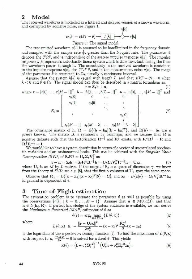
2 Model The received waveform is modelled as a fi l tered and delayed version of a known waveform, and corrupted by additive noise, see Figure 1. ,

n[k\

se\k] = s{kT-6)-A h[k) r\k\

Figure 1: The signal model.

The t ransmit ted waveform s(-) is assumed to be bancuimited i n the frequency domain and sampled w i t h the sample rate i f , greater than the Nyquist rate. The parameter 9

denotes the TOF, and is independent of the system impulse response h[k]. The impulse response h[k] represents a stochastic linear system which is time-invariant during the t ime the waveform passes through i t . The uncertainty in the received waveform is contained i n the impulse response h[k], the TOF9, and in the measurement noise n[k}. The range of the parameter 9 is restricted to Via, usually a continuous interval.

Assume that the system h[k] is causal w i t h length L, and tha t s(kT — 9) = 0 when k < 0 and 6 € Via. The signal model can then be described i n a mat r ix formal ism as:

r = S«h + n, (1)

where r = [ r [ 0 ] , . . . , r [ M - 1]] , h

sø{0]

se[l)

S9 =

[h\0},...,h\L-l] 0

se[0]

n = [n[0],... ,n[M - I}}1 and 0

(2)

L s9[M - I j s9[M-2] ... Se[M-L-2)\

The covariance mat r ix of h , R = E { ( h — ho)(h — h o ) r } , and E { h } = h 0 are a •priori known. The mat r ix R is symmetric by definition, and we assume tha t R is positive definite such that the factorization R " and Rs exists, w i t h R 2 R 2 = R and R 1 R - 5 = I .

We would like to have a system description i n terms of a vector of uncorrelated stochas­t ic variables and an orthonormal basis. This can be achieved w i t h the Singular Value

Decomposition (SVD) of S 0 R 2 = U e £ ø V j as

r - n = S e h = S*R*R-5h = U e S e V j R - 5 h = U « x , (3) where XJe is an M - b y - L matr ix . I f the range of Se is a space of dimension 7, we know f r o m the theory of SVD, see e.g. [6], that the first 7 columns of IJ$ span the same space.

Observe tha t R x = E { ( x - x 0 )(x - x 0 )T | 6 1 } = and Xo = £{x|6>} = S e V j R - 5 h 0

i n general is dependent of 6.

3 Time-of-Flight estimation The estimation problem is to estimate the parameter 9 as well as possible by using the observations {r\k} \ k = 0 , . . . , M — 1} . Assume that n e N(0,cr^I), and tha t h € N ( h o , R ) . I f perfect knowledge of the system statistics is available, we can derive the Maximum a Posteriori (MAP) estimator of 6 as

(?(r) = arg e max {L(9,x)}, ( 4 )

where l l r - T T o Y l l 2 T J - I L(9,x) * - " 2 ^ — - ( x - x o ) ^ ( x - x o ) (5)

is the logar i thm of the a posteriori density funct ion [7]. To find the maximum of L(9, x)

w i t h respect to x, d L £ ^ = 0 is solved for a fixed 9. This yields

m = ( I + c l * ? y l ( U ^ r + o-2Se-2xo) . (6)

44 R V K 93

Inserting (5) and (6) into (4), we get

f j ( r ) = axg e rnax{L( f J , x ( t9 ) )} (J)

and the minimizat ion i n equation (4) is reduced to a one-dimensional optimization.

Define p(<9) ä y(8) + al'Sg1VTR-ih0, where y(0) é. Ujv, which can be interpreted as the output of a filter bank. Then

where we have omi t ted additive constants, c f . [7, page 364, Figure 4.74]. Solutions for other a priori density functions of x can be found in the literature, e.g. [2]. Several observations can now be made about L'{9). I f all diagonal elements of S » —» oo, i.e. that the only informat ion contained in the model is a space of possible impulse responses, equation (8) becomes L' (9) = yT(9)y(9). The estimation problem has then been reduced to detennining when the max imum waveform energy in this space arrived. I f all diagonal elements of £ $ —• 0, there is no uncertainty i n the received waveform and L' (9) = rT (UøXo), resulting i n the matched filter receiver.

In an implementation of an estimator according to (7) and (8), the funct ion y(9) has to be calculated for all 9 6 i~le. This can be done by (m * r)[k] = {y((k - M + 1)T — &o)}i, where * denotes time-discrete convolution, and the filter Ui is chosen as the reversed i:th column of Ue0- Here M must be sufficiently large for s(kT — 9o) to have negligible energy outside k = { 0 , 1 , . . . ,M — 1 } , compared to the variance of the measurement noise n. Given tha t s(-) is bandlimited, y(6) is also bandlimited and can be obtained f r o m y((k — M + 1)T — (90) by interpolation. Furthermore, w i t h the above choice of M, the dependence of xo and evaluated for 9 = (k — M + l)T — 9oE fie, on k w i l l be weak. This substantially simplifies an implementation, enabling the receiver to be of a correlator - matched f i l te r type.

The ordered singular values A;, i.e. the diagonal elements of the matr ix are mono-tonically decreasing. I f s(-) is narrow band many of the singular values w i l l be close to zero, and the major par t of the expected energy of h wi l l be contained in the first singular values.

In the absence of perfect a priori knowledge of the system statistics an approximation must be made. Here we assume that the choice of signal basis is given, but that we have no knowledge of the singular values. (A discussion of the sensitivity for the choice of signal base is not w i t h i n the scope of the present paper.) We propose to approximate

thus, to consider only the p most important directions of variation i n h. This is then essentially a choice of the model order p. This estimator corresponds to the Maximum Likelihood estimator for the case when the true system is of order p, i.e. when L = p.

4 Estimation example To il lustrate the estimation method presented i n Section 3, and to compare the per­formance of the JVL4P-estimator w i t h the approximated structure suggested i n (9), a series of simulations was performed. The transmitted signal was s(t) = a(t) cos (2irf0t).

The envelope a(t) was bandl imited w i t h Fourier transform A ( f ) = 0.5 + 0.5 cos | £ when

[/[ < W, and zero otherwise. The measurement noise n £ N(0, cr 2 I) and the Signal to

Noise Ratio (SNR) was defined as SNR é. x T x / o - 2 , making i t a funct ion of a stochas­t ic variable, and thus stochastic itself. For purposes of comparison, the SNR has been normalized to the given values in these simulations.

Now, the estimators were simulated for / 0 = 1/10, M — 400, 90 = 9 = 200, and w i t h a sampling rate f s = ^ = 1. The system statistics was h e N(0, R ) , w i t h the covariance as R = d i a g { l , 1 /2 , . . . , 1/L}, and L, the length of h, equalled 10. The performances of the estimators were evaluated, i n terms of the sample mean squared error, calculated for TV = 5000 realizations. The results are presented in Figure 2.

(8)

the singular values as (9)

R V K 9 3 45

Figure 2: The graphs has the sample mean squared error, l/NE%=i(8 - 8(rn))2, on the

jf-axis, and t runcat ion order, p, of the approximated estimator, suggested by (7), (8) and (9), on the x-axis. There are performance plots of the approximated estimator and of the MAP estimator (appearing as horizontal lines) for various SNRs and bandwidths.

5 Discussion and Conclusions Modelling uncertainties in a received waveform as a Gaussian variation of the trans­mission system impulse response seems to be a tractable method for TOF estimation, especially when the SNR is high.

Using a low model order p, e.g. assuming a known signal shape, can give large system­atic errors. Increasing the model order decreases the systematic errors but amplifies the effects of the additive noise, which is i l lustrated by the estimation example i n section 4.

The op t imum choice of model order depends on the SNR and on the bandwidth of the transmitted waveform, but the opt imum is most of ten f la t .

The performances of these algorithms w i l l be evaluated using an ultrasonic A-scan pulse-echo measurement system.

References [1] B. Barshan and R. Kuc. Active sonar for obstacle localization using envelope shape informa­

tion. In Proc.1991 Int. conf. on Acoustics, Speech and Signal Processing, pages 1273-1276, Toronto, May 1991.

[2] Per Ola Börjesson, Olle Pafilm, Leif Sörnmo, and Mats-Erik Nygårds. Adaptive QRS detection based on maximum a posteriori estimation. IEEE Transactions on Biomedical Engineering, 29(5):341-351, 1982.

[3] J. N . Bradley and R. L. Kir l in . Delay estimation by expected value. IEEE Trans, on Acoustics, Speech, and Signal Processing, 32(l):19-27, 1984.

[4] Håkan Eriksson, Per Ola Börjesson, and Nils-Gunnar Holmer. Modelling of waveform deformation and time-of-flight estimation, wi th application to the ultrasonic pulse-echo method. I n Proceedings of the third int. symposium on signal processing and its applications, pages 188-191, Gold Coast, Australia, August 1992.

[5] M . Ragozzino. Analysis of the error in measurement of ultrasound speed in tissue due to waveform deformation by frequency-dependent attenuation. Ultrasonics, 12:135-138, May 1981.

[6] Gilbert Strang. Linear Algebra and its Applications. Harcourt Brace Jovanovich, Inc., San Diego, 1986.

[7] Harry L. van Trees. Detection, Estimation, and Modulation Theory. Wiley, New York, 1968.

[8] V i m A. Verhoef, Marius J. T. M . Clostermans, and Johan M. Thijssen. Diffraction and dispersion effects on the estimation of ultrasound attenuation and velocity in biological tissues. IEEE Transactions on Biomedical Engineering, 32(7):521-529, 1985.

46 R V K 9 3