This article was downloaded by: [Muhammad Hasan Ali Baig]On: 03 May 2014, At: 19:32Publisher: Taylor & FrancisInforma Ltd Registered in England and Wales Registered Number: 1072954 Registeredoffice: Mortimer House, 37-41 Mortimer Street, London W1T 3JH, UK

Remote Sensing LettersPublication details, including instructions for authors andsubscription information:http://www.tandfonline.com/loi/trsl20

Derivation of a tasselled captransformation based on Landsat 8 at-satellite reflectanceMuhammad Hasan Ali Baigab, Lifu Zhanga, Tong Shuaiab & QingxiTonga

a State Key Laboratory of Remote Sensing Sciences, Institute ofRemote Sensing and Digital Earth (RADI), Chinese Academy ofSciences, Beijing, Chinab University of Chinese Academy of Sciences, Beijing, ChinaPublished online: 30 Apr 2014.

To cite this article: Muhammad Hasan Ali Baig, Lifu Zhang, Tong Shuai & Qingxi Tong (2014)Derivation of a tasselled cap transformation based on Landsat 8 at-satellite reflectance, RemoteSensing Letters, 5:5, 423-431

To link to this article: http://dx.doi.org/10.1080/2150704X.2014.915434

PLEASE SCROLL DOWN FOR ARTICLE

Taylor & Francis makes every effort to ensure the accuracy of all the information (the“Content”) contained in the publications on our platform. However, Taylor & Francis,our agents, and our licensors make no representations or warranties whatsoever as tothe accuracy, completeness, or suitability for any purpose of the Content. Any opinionsand views expressed in this publication are the opinions and views of the authors,and are not the views of or endorsed by Taylor & Francis. The accuracy of the Contentshould not be relied upon and should be independently verified with primary sourcesof information. Taylor and Francis shall not be liable for any losses, actions, claims,proceedings, demands, costs, expenses, damages, and other liabilities whatsoever orhowsoever caused arising directly or indirectly in connection with, in relation to or arisingout of the use of the Content.

This article may be used for research, teaching, and private study purposes. Anysubstantial or systematic reproduction, redistribution, reselling, loan, sub-licensing,systematic supply, or distribution in any form to anyone is expressly forbidden. Terms &

Conditions of access and use can be found at http://www.tandfonline.com/page/terms-and-conditions

Dow

nloa

ded

by [

Muh

amm

ad H

asan

Ali

Bai

g] a

t 19:

32 0

3 M

ay 2

014

Derivation of a tasselled cap transformation based on Landsat 8at-satellite reflectance

Muhammad Hasan Ali Baiga,b, Lifu Zhanga*, Tong Shuaia,b, and Qingxi Tonga

aState Key Laboratory of Remote Sensing Sciences, Institute of Remote Sensing and Digital Earth(RADI), Chinese Academy of Sciences, Beijing, China; bUniversity of Chinese Academy of Sciences,

Beijing, China

(Received 6 February 2014; accepted 12 April 2014)

The tasselled cap transformation (TCT) is a useful tool for compressing spectral datainto a few bands associated with physical scene characteristics with minimal informa-tion loss. TCT was originally evolved from the Landsat multi-spectral scanner (MSS)launched in 1972 and is widely adapted to modern sensors. In this study, we derivedthe TCT coefficients for the newly launched (2013) operational land imager (OLI)sensor on-board Landsat 8 for at-satellite reflectance. A newly developed standardizedmechanism was used to transform the principal component analysis (PCA)-basedrotated axes through Procrustes rotation (PR) conformation according to the Landsatthematic mapper (TM)-based tasselled cap space. Firstly, OLI data were transformedinto TM TCT space directly and considered as a dummy target. Then, PCAwas appliedon the original scene. Finally, PR was applied to get the transformation results in thebest conformation to the target image. New coefficients were analysed in detail toconfirm Landsat 8-based TCT as a continuity of the original tasselled cap idea. Resultsshow that newly derived set of coefficients for Landsat OLI is in continuation of itspredecessors and hence provide data continuity through TCT since 1972 for remotesensing of surface features such as vegetation, albedo and water. The newly derivedTCT for OLI will also be very useful for studying biomass estimation and primaryproduction for future studies.

1. Introduction

Vegetation and water indices derived from satellite reflectance data are two of the primarysources of information for operational monitoring of the Earth’s land cover. Almost all thepresent vegetation indices (VIs) in remote sensing combine reflectance measurementsfrom different portions of the electromagnetic spectrum to provide information aboutvegetation coverage on the ground. One of the primary applications of remote sensing isto identify patterns of vegetation distribution on the ground followed by assessingtemporal changes in vegetation. Higher reflectance of vegetation and lower reflectanceof water in near infrared (NIR) band along with different spectral responses of variousvegetation types from visible to shortwave infrared (SWIR) led researchers to developnumerous indices (Jackson and Huete 1991; Richardson and Everitt 1992; Richardson andWiegand 1977). Such indices are based on different algebraic combinations of these bandsfor proper analysis of land features. In contrast to its higher reflectance in NIR, vegetationhas low reflectance in both the blue and the red regions of the spectrum due to absorptionby chlorophyll for photosynthesis. These are the reasons why most of the traditional

*Corresponding author. Email: zhanglf@radi.ac.cn

Remote Sensing Letters, 2014Vol. 5, No. 5, 423–431, http://dx.doi.org/10.1080/2150704X.2014.915434

© 2014 Taylor & Francis

Dow

nloa

ded

by [

Muh

amm

ad H

asan

Ali

Bai

g] a

t 19:

32 0

3 M

ay 2

014

vegetation indices are based on red–NIR space while using an inclined red–NIR line inred–NIR space as the line of zero vegetation for bare soil (Ray 1994; Viña et al. 2011;Payero, Neale, and Wright 2004; Bannari et al. 1995; Gitelson et al. 2002). Based on thissoil line, vegetation indices can be divided into three categories: the slope-based VIs (e.g.Normalized Difference Vegetation Index – NDVI, Soil Adjusted Vegetation Index – SAVIand Ratio Vegetation Index – RVI, etc.), the distance-based (or perpendicular line) VIs(e.g. Perpendicular Vegetation Index-PVI, Difference Vegetation Index-DVI and WeightedDifference Vegetation Index-WDVI, etc.) and the orthogonal transformation VIs (such asVegetation Index based on Universal Pattern Decomposition Index – VIUPD, etc.)(Richardson and Everitt 1992; Huete 1988; Clevers 1988; Huete, Jackson, and Post1985; Richardson and Wiegand 1977; Rouse et al. 1973; Jordan 1969; Zhang et al.2007). The tasselled cap transformation (TCT) belongs to the category of orthogonaltransformation too and has several advantages over other traditional VIs (Crist and Cicone1984b; Kauth and Thomas 1976).

The TCT has revolutionized the concept of understanding the plant growth patterns inspectral space formed by different bands combination (Kauth and Thomas 1976). Later, itwas employed to understand the soil moisture and other hydrological features. Thepropounders of TCT used MSS data to investigate the plant growth patterns in connectionwith ‘triangular cap-shaped region with a tassel’ in red–NIR space (Kauth and Thomas1976; Ray 1994). The top of their tasselled cap with low red reflectance and higher NIRreflectance was found representative of higher vegetated areas, while the opposite to thetop, the flat side of the cap (not perfectly horizontal), was found representative of the baresoil (Ray 1994). The encapsulation of physical scene characteristics in the form oftasselled space has made TCT a useful index and as an investigative tool in the field ofphenology and ecology (Lobser and Cohen 2007). The evolution of TCT is indebted tothe profound research work done by EP Crist using both the satellite sensors like Landsatthematic mapper (TM) and spectrometer reflectance factor data for investigating cropdevelopment (Crist and Cicone 1984a). These series of findings became very helpful indetermining the crop condition and landcover classification (Oetter et al. 2001; Dymond,Mladenoff, and Radeloff 2002; Cohen and Spies 1992; Cohen, Spies, and Fiorella 1995;Skakun, Wulder, and Franklin 2003). These were performed not only by using Landsatdata but also through several newly developed sensors such as MODIS, QuickBird andIKONOS (Yarbrough, Easson, and Kuszmaul 2005; Zhang et al. 2002; Horne 2003).

Both multi- and hyperspectral data have highly correlated bands. TCT not onlycompresses several bands into few bands but also decorrelates them by transformingthem orthogonally into a new set of axes associated with physical features. Traditionally,three axes were defined: (I) Brightness, (II) Greenness and (III) Wetness. Firstly, a rotationwas defined to separate the vegetation from non-vegetated features by maintaining theorthogonal property between I and II components. Then, rotating components II and IIIorthogonally separated the water from vegetation features. Finally, orthogonal rotationbetween components I and III was implemented in order to separate water from features ofvegetation and non-vegetation (Zhang et al. 2002). Brightness – the first feature of TCT –is a weighted sum of all the bands and accounts for the most variability in the image. It istypically associated with bare or partially covered soil, natural and man-made features,and variations in topography. Greenness is a measure of the contrast between the NIRband and the visible bands due to the scattering of infrared radiation resulting from thecellular structure of green vegetation and the absorption of visible radiation by plantpigments. Soil reflectance curves (soil signatures) are represented with higher values in‘Brightness’ while they are expressed in low ‘Greenness’ values. The third component is

424 M.H.A. Baig et al.

Dow

nloa

ded

by [

Muh

amm

ad H

asan

Ali

Bai

g] a

t 19:

32 0

3 M

ay 2

014

orthogonal to the first two components and is associated with soil moisture, water andother moist features (Crist and Cicone 1984b; Crist and Kauth 1986; Zhang et al. 2002).There are three planes associated with these features: the plane of soils (Brightness/Wetness space), the transition zone (Greenness/Wetness space) and the plane of vegetation(Brightness/Greenness space). Pre-planting field having bare soil will be analysed best inthe plane of soils. After planting, it would shift up through the transition zone towards theplane of vegetation as the crops matured and then would ‘tassel out’ with senescence. Allthese phases of plots would together form the shape of a ‘tasselled cap’ (Crist and Kauth1986; Crist and Cicone 1984b; Kauth and Thomas 1976).

Until recently, there were no standards for deriving the orthogonal rotation coefficientsdue to the pluralistic interpretation of the tasselled cap features (Lobser and Cohen 2007).Any number of TCTs may be developed if the choice of aligning these three axes is left tothe discretion of a researcher. Since the launch of Landsat 8 in 2013, it was beingdemanded by researchers working on vegetation how to use TCT for this new sensor ina same way they used it for other sensors. Addressing that dire need of researchers, thisstudy is presenting the new TCT coefficients for operational land imager (OLI) in a formof this letter. To maintain the continuity among the sensors for the same tasselled cap ideaoriginally propounded by Kauth and Thomas (1976) and investigated by Crist with otherresearchers (Crist and Kauth 1986; Crist 1985; Crist and Cicone 1984b, 1984a), this studyuses the Procrustes rotation (PR) transformation for deriving the TCT coefficients for OLIof Landsat 8 (Andrade et al. 2007, 2004; Lobser and Cohen 2007).

2. Materials and methods

2.1. Data set used

In this study, we not only used the same areas that were used before by earlier researchersbut also added some new areas to represent a wide variety of land cover types to makeTCT suitable for all type of areas and climates (Table 1). It is important to mention herethat the first comprehensive study to calculate TCT for TM data was conducted by Cristand Cicone (1984b) and they selected only three scenes to derive their famous TM TCTindex (also shown in Table 1). Moreover, they mainly used North Carolina scene (24September 1982) to derive these coefficients and described this scene as an ideal scenedue to its diversity holding large fields surrounded by forest and water. Therefore, we usedthe same areas in this study not only to derive TCT for Landsat 8 but also to make newcoefficients more representative of vegetation and other landcover types, and several otherareas were also included to corroborate the analysis (Table 1).

The at-satellite reflectance-based TCT was derived by focusing especially on themethodology described by Crist and Cicone (1984b), Huang et al. (2002) and Lobserand Cohen (2007). Conversion from DN to reflectance was done according to the methodmentioned on the website of USGS (http://landsat.usgs.gov/Landsat8_Using_Product.php). Sub-scenes were chosen from all scenes, and the regions of interest (ROIs) weredefined by using high-resolution imagery of Google Earth. Crist and Cicone used 9000–13,000 pixel samples from their three sub-scenes. About 2000 random samples wereselected from each of the 10 ETM + scenes by Huang et al. (2002). Approximately1.2 × 106 pixels were randomly selected by Lobser and Cohen (2007) from their globalsample of MODIS data. A simple random sample may be heavily biased due to thepresence of clouds and snow, so samples generated in this work were only from thoseareas that were visibly not affected by clouds and snow (uneven sample size from

Remote Sensing Letters 425

Dow

nloa

ded

by [

Muh

amm

ad H

asan

Ali

Bai

g] a

t 19:

32 0

3 M

ay 2

014

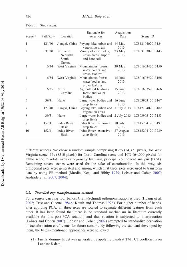
different scenes). We chose a random sample comprising 0.2% (24,371 pixels) for WestVirginia scene, 1% (8510 pixels) for North Carolina scene and 10% (64,000 pixels) forIdaho scene to rotate axes orthogonally by using principal component analysis (PCA).Remaining seven scenes were used for the sake of corroboration. In this way, sixorthogonal axes were generated and among which first three axes were used to transformdata by using PR method (Mardia, Kent, and Bibby 1979; Lobser and Cohen 2007;Andrade et al. 2007, 2004).

2.2. Tasselled cap transformation method

For a sensor carrying four bands, Gram–Schmidt orthogonalization is used (Huang et al.2002; Crist and Cicone 1984b; Kauth and Thomas 1976). For higher number of bands,after applying PCA, all three axes are rotated to separate different features from eachother. It has been found that there is no standard mechanism in literature currentlyavailable for this post-PCA rotation, and thus rotation is subjected to interpretation(Lobser and Cohen 2007). Lobser and Cohen (2007) attempted to standardize derivationof transformation coefficients for future sensors. By following the standard developed bythem, the below-mentioned approaches were followed:

(1) Firstly, dummy target was generated by applying Landsat TM TCT coefficients onLandsat 8 data.

Table 1. Study areas.

Scene # Path/Row LocationRationale forselection

AcquisitionDate Scene ID

1 121/40 Jiangxi, China Poyang lake, urban andvegetation areas

14 May2013

LC81210402013134

2 31/30 NorthernNebraska,SouthDakota

Variety of crop fields,urban areas, airportand bare soil

23 May2013

LC80310302013143

3 16/34 West Virginia Mountainous forests,water bodies andurban features

30 May2013

LC80160342013150

4 16/34 West Virginia Mountainous forests,water bodies andurban features

15 June2013

LC80160342013166

5 16/35 NorthCarolina

Agricultural holdings,forest and waterbodies

15 June2013

LC80160352013166

6 39/31 Idaho Large water bodies andcrop fields

16 June2013

LC80390312013167

7 121/40 Jiangxi, China Poyang lake, urban andvegetation areas

1 July 2013 LC81210402013182

8 39/31 Idaho Large water bodies andcrop fields

2 July 2013 LC80390312013183

9 152/41 Indus RiverBasin

Indus River, extensivecrop fields

10 July2013

LC81520412013191

10 152/41 Indus RiverBasin

Indus River, extensivecrop fields

27 August2013

LC81520412013239

426 M.H.A. Baig et al.

Dow

nloa

ded

by [

Muh

amm

ad H

asan

Ali

Bai

g] a

t 19:

32 0

3 M

ay 2

014

(2) Then, by using PR method, PCA transformed Landsat 8 data were rotated for thebest alignment to the dummy target.

(3) Finally, simple multiplication was done between the transformation coefficientsdeveloped through Procrustes and PCA coefficients to get the final TCT coeffi-cients for Landsat 8.

Although these components are ultimately rotated, the 3D structure of the data space isretained through this rotation. Thus, the final transformation is highly dependent upon thechosen starting dummy target.

2.3. Principal component analysis

PCA maximizes variance while minimizing correlation by means of an orthogonaltransformation (Mardia, Kent, and Bibby 1979). The resulting uncorrelated PC bandsare linear combinations of the original spectral bands. The first few PC bands normallyrepresent the 90–96% variance in the data, and the remaining bands represent noise(Mardia, Kent, and Bibby 1979). In this study, PCA is applied on the random samplesrepresenting the vegetation, soil, water and other landcover features to generate the newcomponents in orthogonal space. All of these new orthogonal components are used in PR.

2.4. Procrustes rotation

In multivariate statistics, PR is based on singular value decomposition (SVD) to decom-pose a matrix into principal components for simultaneous comparison of several data sets(Andrade et al. 2007). ‘Procrustes rotation is usually performed on the principal compo-nents that describe the data instead of on the data itself’ (Andrade et al. 2004). The mainidea of PR is based on comparing two or more spaces where the same variables aremeasured. Here, PR is applied on PCA-transformed axes to transform the orthogonalspace in best conformation to the dummy target space based on TM TCT space.

3. Results and discussion

By following the methodology mentioned above, TCT coefficients are derived for differ-ent landcover types in different time periods to make the derived scenes representative ofall sorts of important features. A 2D scatter plot for both Red and NIR channels can beseen in Figure 1(a). The diagonal in this distribution is termed as a ‘soil line’. This soilline in spectral space describes the variation in the spectrum of bare soil in the selectedarea. In any image showing the pattern like Figure 1(a), this line can be found by locatingtwo or more patches of bare soil having different values of reflectance and finding the bestfit line in spectral space (Ray 1994; Viña et al. 2011; Payero, Neale, and Wright 2004;Bannari et al. 1995; Gitelson et al. 2002).

Figure 1(b) is confirming the concept of ‘triangular cap-shaped region with a tassel’ inred–NIR space, which was put forward by Kauth and Thomas using MSS data. Theyfound that the point of the cap (which lies at low red reflectance and high NIR reflectance)represented regions of high vegetation and that the flat side of the cap directly opposite thepoint represented bare soil (Kauth and Thomas 1976).

Table 2 shows the transformation coefficients for Landsat 8 at-satellite reflectancedata. These coefficients are very close to the coefficients of the dummy target imagecreated through TM-based TCT coefficients. From Table 2, it is evident that Brightness

Remote Sensing Letters 427

Dow

nloa

ded

by [

Muh

amm

ad H

asan

Ali

Bai

g] a

t 19:

32 0

3 M

ay 2

014

has all positive loadings. It means that all six bands contribute for its overall value withbands 4 (Red), 5 (NIR) and 6 (SWIR1) as maximum contribution. Regions of highvegetation are found at low Red and higher NIR regions and here (Table 2) both havehigher values of loadings, so any increase in vegetation density will cause less substantialchanges in Brightness. It indicates that this feature will be responsive to soil character-istics including its albedo instead of vegetation.

The fact that vegetation has higher values of reflectance in NIR while lower in Redregions of the (electromagnetic) spectrum is displayed by the loadings corresponding toGreenness in Table 2. Here, Greenness has high positive loadings in NIR while highnegative loadings in Red spectra (Figure 1(b)).

0.2

0.0

–0.2

0.6

0.4

0.2

0.0

–0.2

Brightness

Gre

enne

ss

0.0

–0.2

–0.6

–0.4

0.2

0.0

–0.2

–0.4

–0.60.0 0.5 1.0 1.5

WetnessBrightness(d)(c)

(a) (b)

–0.6 –0.4 –0.2 0.0 0.2

Wet

ness

0.2

–0.2

0.0

0.6

0.4

0.2

0.0

–0.2

Gre

enne

ss

0.50.0 1.0 1.5

WaterVegetation + forestVegetation -- early stageUrban green areasSoil + urban features + trees

Band 4 reflectance (red)

Ban

d 5

refle

ctan

ce (

NIR

) 0.6

0.0

0.5

0.4

0.3

0.2

0.1

0.00.40.30.20.10.0

Figure 1. (a) Scatter plot between Red (band 4) and NIR bands (band 5) along with all five regionsof interests (ROIs); (b) Scatter plot between Brightness and Greenness. It is also called ‘plane ofvegetation’; (c) Scatter plot between Brightness and Wetness. It is also termed as ‘plane of soil’; (d)Scatter plot between Wetness and Greenness. It is called as ‘transition zone’.

Table 2. TCT coefficients for Landsat 8 at-satellite reflectance.

Landsat 8(Blue)Band 2

(Green)Band 3

(Red)Band 4

(NIR)Band 5

(SWIR1)Band 6

(SWIR2)Band 7TCT

Brightness 0.3029 0.2786 0.4733 0.5599 0.508 0.1872Greenness −0.2941 −0.243 −0.5424 0.7276 0.0713 −0.1608Wetness 0.1511 0.1973 0.3283 0.3407 −0.7117 −0.4559TCT4 −0.8239 0.0849 0.4396 −0.058 0.2013 −0.2773TCT5 −0.3294 0.0557 0.1056 0.1855 −0.4349 0.8085TCT6 0.1079 −0.9023 0.4119 0.0575 −0.0259 0.0252

428 M.H.A. Baig et al.

Dow

nloa

ded

by [

Muh

amm

ad H

asan

Ali

Bai

g] a

t 19:

32 0

3 M

ay 2

014

When the third feature, i.e. ‘Wetness’ is analysed, Table 2 shows that it contrasts thesum of the visible and NIR bands with the sum of the SWIR bands. The SWIR bands areconsidered to be the most sensitive to both soil moisture and plant moisture, so thecontrast between these two sets of bands mainly highlights moisture-related scene char-acteristics (Figure 1(c)) (Crist and Cicone 1984b).

On the basis of these characteristics of Brightness, Greenness and Wetness, Figures 1(b–d) show the planes between first three transformations. The plane between Brightnessand Greenness is considered as a plane of vegetation, while the plane between Brightnessand Wetness is considered as a plane of soils (Crist and Cicone 1984b).

These three planes (Figures 1 (b–d)) are in accordance with those three planesconstructed for Landsat TM TCT space by Crist and Cicone (Crist and Kauth 1986;Crist and Cicone 1984b). Thus, using the standard approach to derive the coefficients for anew sensor gives the same TCT space developed by TCT pioneers and thus provides thedata continuity for studying the phenology and analysing the temporal series for vegeta-tion change or biomass variation.

4. Conclusions

TCT compresses and decorrelates the data into few bands associated with physical scenecharacteristics of the land surface. Brightness, Greenness and Wetness are those fewimportant components mostly discussed in literature. Brightness is related to the soiland albedo, Greenness is associated with vegetation and Wetness is mostly connected withwater contents. As transformation solely depends upon the interpretation of the data,standardization was necessary to develop uniformity in the TCT based on Landsat MSS,TM and ETM + sensors as well as those based on the new sensors. This study investigatedthe method using TM-based TCT coefficients to simulate OLI image to be used as adummy target in PR method for transforming OLI orthogonal space. The resultedtransformation coefficients successfully differentiated soil from vegetation, vegetationfrom water and bare soil features from water features. The standardized approach usedin this study has a great potential for deriving coefficients for future sensors such asSentinel-2, etc. Validation of coefficients will be done in a form of a comparison withETM + in a detailed next paper.

AcknowledgementsWe would like to thank Prof. Bruce Wylie from USGS and Prof. W.B. Cohen from Oregon StateUniversity for their useful feedback during this research process. We are indebted to Dr. MohtashimH. Shamsi from the University of Toronto, Mr. Qin Bangyong and Mr. Jiang Gaozhen for theirvaluable contribution. Last but not least, we owe debt of gratitude to the Editor, two unknownreviewers and the administrative assistant of RSL for giving us very important feedback to improvethe quality of this letter.

FundingThis work was funded by the National Natural Science Foundation of China [grant numbers41371362, 41371359 and 41201348].

Remote Sensing Letters 429

Dow

nloa

ded

by [

Muh

amm

ad H

asan

Ali

Bai

g] a

t 19:

32 0

3 M

ay 2

014

ReferencesAndrade, J. M., M. Kubista, A. Carlosena, and D. Prada. 2007. “3-Way Characterization of Soils by

Procrustes Rotation, Matrix-Augmented Principal Components Analysis and Parallel FactorAnalysis.” Analytica Chimica Acta 603 (1): 20–29. doi:10.1016/j.aca.2007.09.043.

Andrade, J. M., M. P. Gómez-Carracedo, W. Krzanowski, and M. Kubista. 2004. “ProcrustesRotation in Analytical Chemistry, a Tutorial.” Chemometrics and Intelligent LaboratorySystems 72 (2): 123–132. doi:10.1016/j.chemolab.2004.01.007.

Bannari, A., D. Morin, F. Bonn, and A. R. Huete. 1995. “A Review of Vegetation Indices.” RemoteSensing Reviews 13 (1–2): 95–120. doi:10.1080/02757259509532298.

Clevers, J. G. P. W. 1988. “The Derivation of a Simplified Reflectance Model for the Estimation of LeafArea Index.” Remote Sensing of Environment 25 (1): 53–69. doi:10.1016/0034-4257(88)90041-7.

Cohen, W. B., and T. A. Spies. 1992. “Estimating Structural Attributes of Douglas-Fir/WesternHemlock Forest Stands from Landsat and SPOT Imagery.” Remote Sensing of Environment 41(1): 1–17. doi:10.1016/0034-4257(92)90056-P.

Cohen, W. B., T. A. Spies, and M. Fiorella. 1995. “Estimating the Age and Structure of Forests in AMulti-Ownership Landscape of Western Oregon, USA.” International Journal of RemoteSensing 16 (4): 721–746. doi:10.1080/01431169508954436.

Crist, E. P. 1985. “A TM Tasseled Cap Equivalent Transformation for Reflectance Factor Data.”Remote Sensing of Environment 17 (3): 301–306. doi:10.1016/0034-4257(85)90102-6.

Crist, E. P., and R. C. Cicone. 1984a. “Comparisons of the Dimensionality and Features ofSimulated Landsat-4 MSS and TM Data.” Remote Sensing of Environment 14 (1–3):235–246. doi:10.1016/0034-4257(84)90018-X.

Crist, E. P., and R. C. Cicone. 1984b. “A Physically-Based Transformation of Thematic MapperData-the TM Tasseled Cap.” IEEE Transactions on Geoscience and Remote Sensing, GE–22(3): 256–263. doi:10.1109/Tgrs.1984.350619.

Crist, E. P., and R. J. Kauth. 1986. “The Tasseled Cap De-Mystified.” PhotogrammetricEngineering and Remote Sensing 52 (1): 81–86.

Dymond, C. C., D. J. Mladenoff, and V. C. Radeloff. 2002. “Phenological Differences in TasseledCap Indices Improve Deciduous Forest Classification.” Remote Sensing of Environment 80 (3):460–472. doi:10.1016/S0034-4257(01)00324-8.

Gitelson, A. A., R. Stark, U. Grits, D. Rundquist, Y. Kaufman, and D. Derry. 2002. “Vegetation andSoil Lines in Visible Spectral Space: A Concept and Technique for Remote Estimation ofVegetation Fraction.” International Journal of Remote Sensing 23 (13): 2537–2562.doi:10.1080/01431160110107806.

Horne, J. H. 2003. “A Tasseled Cap Transformation for IKONOS Images.” In ASPRS 2003 AnnualConference Proceedings, Anchorage, AK, May 3–9, 1–7. Bethesda, MD: American Society ofPhotogrammetry and Remote Sensing.

Huang, C., B. Wylie, L. Yang, C. Homer, and G. Zylstra. 2002. “Derivation of a Tasselled CapTransformation Based on Landsat 7 At-Satellite Reflectance.” International Journal of RemoteSensing 23 (8): 1741–1748. doi:10.1080/01431160110106113.

Huete, A. R. 1988. “A Soil-Adjusted Vegetation Index (Savi).” Remote Sensing of Environment 25(3): 295–309. doi:10.1016/0034-4257(88)90106-X.

Huete, A. R., R. D. Jackson, and D. F. Post. 1985. “Spectral Response of a Plant Canopy withDifferent Soil Backgrounds.” Remote Sensing of Environment 17 (1): 37–53. doi:10.1016/0034-4257(85)90111-7.

Jackson, R. D., and A. R. Huete. 1991. “Interpreting Vegetation Indices.” Preventive VeterinaryMedicine 11 (3–4): 185–200. doi:10.1016/S0167-5877(05)80004-2.

Jordan, C. F. 1969. “Derivation of Leaf Area Index from Quality of Light on the Forest Floor.”Ecology 50: 663–666. doi:10.2307/1936256.

Kauth, R. J., and G. S. Thomas. 1976. “The Tasselled Cap—A Graphic Description of the Spectral-Temporal Development of Agricultural Crops as Seen by Landsat.” Paper presented at theLARS Symposia, Proceedings of the Symposium on Machine Processing of Remotely SensedData, Purdue University, West Lafayette, IN, June 29–July 1, 4B41–4B51.

Lobser, S. E., and W. B. Cohen. 2007. “MODIS Tasselled Cap: Land Cover CharacteristicsExpressed through Transformed MODIS Data.” International Journal of Remote Sensing 28(22): 5079–5101. doi:10.1080/01431160701253303.

Mardia, K. V., J. T. Kent, and J. M. Bibby. 1979. Multivariate Analysis. London: Academic Press.

430 M.H.A. Baig et al.

Dow

nloa

ded

by [

Muh

amm

ad H

asan

Ali

Bai

g] a

t 19:

32 0

3 M

ay 2

014

Oetter, D. R., W. B. Cohen, M. Berterretche, T. K. Maiersperger, and R. E. Kennedy. 2001. “LandCover Mapping in an Agricultural Setting Using Multiseasonal Thematic Mapper Data.”Remote Sensing of Environment 76 (2): 139–155. doi:10.1016/S0034-4257(00)00202-9.

Payero, J. O., C. M. U. Neale, and J. L. Wright. 2004. “Comparison of Eleven Vegetation Indices forEstimating Plant Height of Alfalfa and Grass.” Applied Engineering in Agriculture 20 (3):385–393. doi:10.13031/2013.16057.

Ray, T. W. 1994. “A FAQ on Vegetation in Remote Sensing.” Accessed March 23, 2014. http://www.yale.edu/ceo/Documentation/rsvegfaq.html.

Richardson, A. J., and J. H. Everitt. 1992. “Using Spectral Vegetation Indices to Estimate RangelandProductivity.” Geocarto International 7: 63–69. doi:10.1080/10106049209354353.

Richardson, A. J., and C. L. Wiegand. 1977. “Distinguishing Vegetation from Soil BackgroundInformation.” Photogrammetric Engineering and Remote Sensing 43 (12): 1541–1552.

Rouse, J. W., R. H. Haas, J. A. Schell, and D. W. Deering. 1973. “Monitoring Vegetation Systems inthe Great Plains with ERTS.” In Paper presented at the Third ERTS Symposium, NASA SP-351,Vol. I, December 10–14, 309–317. Washington, DC: NASA.

Skakun, R. S., M. A. Wulder, and S. E. Franklin. 2003. “Sensitivity of the Thematic MapperEnhanced Wetness Difference Index to Detect Mountain Pine Beetle Red-Attack Damage.”Remote Sensing of Environment 86 (4): 433–443. doi:10.1016/S0034-4257(03)00112-3.

Viña, A., A. A. Gitelson, A. L. Nguy-Robertson, and Y. Peng. 2011. “Comparison of DifferentVegetation Indices for the Remote Assessment of Green Leaf Area Index of Crops.” RemoteSensing of Environment 115 (12): 3468–3478. doi:10.1016/j.rse.2011.08.010.

Yarbrough, L. D., G. Easson, and J. S. Kuszmaul. 2005. “QuickBird 2 Tasseled Cap TransformCoefficients: A Comparison of Derivation Methods.” In Paper presented at Pecora 16“Global Priorities in Land Remote Sensing”, Sioux Falls, October 23–27. http://www.asprs.org/a/conference-archive/pecora16/.

Zhang, L. S., S. Furumi, K. Muramatsu, N. Fujiwara, M. Daigo, and L. Zhang. 2007. “A NewVegetation Index Based on the Universal Pattern Decomposition Method.” InternationalJournal of Remote Sensing 28 (1): 107–124. doi:10.1080/01431160600857402.

Zhang, X. Y., C. B. Schaaf, M. A. Friedl, A. H. Strahler, F. Gao, and J. C. F. Hodges. 2002.“MODIS Tasseled Cap Transformation and its Utility.” In Proceedings of IEEE InternationalGeoscience and Remote Sensing Symposium (IGARSS’02), Vol. 2, Toronto, ON, June 24–28,1063–1065. Piscataway, NJ: IEEE. doi: 10.1109/IGARSS.2002.1025776.

Remote Sensing Letters 431

Dow

nloa

ded

by [

Muh

amm

ad H

asan

Ali

Bai

g] a

t 19:

32 0

3 M

ay 2

014