Deployment Optimization of IoT Devices through Attack Graph ...

Ben-Gurion University of the Negev

Faculty of Engineering Sciences

Department of Software and Information SystemsEngineering

Deployment Optimization of IoT Devicesthrough Attack Graph Analysis

Author:Noga Agmon

Supervisors:Dr. Rami Puzis &Dr. Asaf Shabtai

Thesis submitted in partial fulfillment of the requirementsfor the M.Sc. degree

November, 2019

arX

iv:1

911.

0681

1v1

[cs

.CR

] 1

5 N

ov 2

019

1

Ben-Gurion University of the Negev

Faculty of Engineering Sciences

Department of Software and Information SystemsEngineering

Deployment Optimization of IoT Devices through Attack Graph Analysis

Supervisors: Dr. Rami Puzis &Dr. Asaf Shabtai

Author: Noga AgmonSupervisor: Dr. Rami PuzisSupervisor: Dr. Asaf ShabtaiChairman of Graduate Studies Committee: Dr. Rami Puzis

Date: September 11, 2019Date: September 11, 2019Date: September 11, 2019Date: September 11, 2019

November, 2019

2

AbstractThe Internet of things (IoT) has become an integral part of our life at both

work and home. However, these IoT devices are prone to vulnerability exploits dueto their low cost, low resources, the diversity of vendors, and proprietary firmware.Moreover, short range communication protocols (e.g., Bluetooth or ZigBee) openadditional opportunities for the lateral movement of an attacker within an orga-nization. Thus, the type and location of IoT devices may significantly change thelevel of network security of the organizational network. In this work, we quan-tify the level of network security based on an augmented attack graph analysisthat accounts for the physical location of IoT devices and their communicationcapabilities. We use the depth-first branch and bound (DFBnB) heuristic searchalgorithm to solve two optimization problems: Full Deployment with MinimalRisk (FDMR) and Maximal Utility without Risk Deterioration (MURD). An ad-missible heuristic is proposed to accelerate the search. The proposed method isevaluated using a real network with simulated deployment of IoT devices. Theresults demonstrate (1) the contribution of the augmented attack graphs to quan-tifying the impact of IoT devices deployed within the organization on security,and (2) the effectiveness of the optimized IoT deployment.

Keywords: Attack graphs, Internet of Things, IoT deployment, Optimization,Short-Range Communication

3

AcknowledgementsFirst and foremost, I thank my research supervisors, Dr. Rami Puzis and Dr. AsafShabtai, for their continuous guidance and support throughout this research.

Thanks to my boyfriend, Erez for his support in this journey. And my familyfor providing certainty and comfort in times I needed it.

4

Contents

Abstract 2

Acknowledgements 3

1 Introduction 8

2 Background 112.1 Attack Graphs . . . . . . . . . . . . . . . . . . . . . . . . . . . . 112.2 Internet of Things . . . . . . . . . . . . . . . . . . . . . . . . . . . 12

2.2.1 Security in the Internet of Things . . . . . . . . . . . . . . 122.2.2 Vulnerabilities . . . . . . . . . . . . . . . . . . . . . . . . . 142.2.3 Attacks . . . . . . . . . . . . . . . . . . . . . . . . . . . . 15

2.3 Short Range Communication Protocols . . . . . . . . . . . . . . . 172.4 Heuristic Search . . . . . . . . . . . . . . . . . . . . . . . . . . . 18

2.4.1 Heuristic . . . . . . . . . . . . . . . . . . . . . . . . . . . . 192.4.2 Admissible Heuristic . . . . . . . . . . . . . . . . . . . . . 192.4.3 Algorithms . . . . . . . . . . . . . . . . . . . . . . . . . . 19

3 Related Work 213.1 IoT Device Deployment . . . . . . . . . . . . . . . . . . . . . . . . 213.2 Attack Graph Optimization . . . . . . . . . . . . . . . . . . . . . 22

3.2.1 Attack Graph Representation . . . . . . . . . . . . . . . . 223.2.2 Risk Score . . . . . . . . . . . . . . . . . . . . . . . . . . . 223.2.3 Optimization Problems . . . . . . . . . . . . . . . . . . . . 23

3.3 IoT in Attack Graphs . . . . . . . . . . . . . . . . . . . . . . . . . 24

4 IoT Attack Graphs 264.1 IoT Deployment . . . . . . . . . . . . . . . . . . . . . . . . . . . . 264.2 Attack Graph Definition . . . . . . . . . . . . . . . . . . . . . . . 29

5

4.3 Risk Score . . . . . . . . . . . . . . . . . . . . . . . . . . . . . . . 31

5 Deployment Optimization Problem 335.0.1 FDMR Problem . . . . . . . . . . . . . . . . . . . . . . . . 335.0.2 MURD Problem . . . . . . . . . . . . . . . . . . . . . . . . 33

5.1 Search Space . . . . . . . . . . . . . . . . . . . . . . . . . . . . . 345.1.1 Search Space Size . . . . . . . . . . . . . . . . . . . . . . . 34

5.2 Search Algorithm . . . . . . . . . . . . . . . . . . . . . . . . . . . 355.2.1 Pseudo-Code . . . . . . . . . . . . . . . . . . . . . . . . . 365.2.2 Heuristic Functions . . . . . . . . . . . . . . . . . . . . . . 365.2.3 Node Ordering . . . . . . . . . . . . . . . . . . . . . . . . 38

6 Experiments 396.1 Data Preparation . . . . . . . . . . . . . . . . . . . . . . . . . . . 39

6.1.1 Organization Network . . . . . . . . . . . . . . . . . . . . 396.1.2 Simulating IoT Devices . . . . . . . . . . . . . . . . . . . . 406.1.3 Simulating Short-Range Communication . . . . . . . . . . 416.1.4 Simulating Vulnerabilities . . . . . . . . . . . . . . . . . . 416.1.5 Simulating Physical Location of Hosts . . . . . . . . . . . 41

6.2 Experimental Setup . . . . . . . . . . . . . . . . . . . . . . . . . . 416.2.1 Number of Executions . . . . . . . . . . . . . . . . . . . . 426.2.2 Evaluation Measures . . . . . . . . . . . . . . . . . . . . . 426.2.3 Random Deployment . . . . . . . . . . . . . . . . . . . . . 42

7 Results 437.1 DFBnB algorithm Vs Random Deployment . . . . . . . . . . . . . 437.2 With Vs Without Heuristic . . . . . . . . . . . . . . . . . . . . . . 447.3 Additional Results . . . . . . . . . . . . . . . . . . . . . . . . . . 45

7.3.1 Trade-off . . . . . . . . . . . . . . . . . . . . . . . . . . . . 457.3.2 Cumulative Distribution . . . . . . . . . . . . . . . . . . . 467.3.3 Robustness . . . . . . . . . . . . . . . . . . . . . . . . . . 46

8 Conclusion 48

9 Future Work 49

Bibliography 50

6

List of Figures

1.1 Illustration of the office in example 1.Different colors of Wi-Fi rep-resent different VLANs. . . . . . . . . . . . . . . . . . . . . . . . 10

2.1 Attack Graph of Example 2. Exploit/action nodes are representedby blue ovals; fact nodes are represented by green rectangles; priv-ilege nodes are represented by orange diamonds. . . . . . . . . . . 13

6.1 Connectivity graph of the hosts in the organizational network, de-rived from the VLAN topology. The different colors represent thedifferent VLANs. The blue nodes are DMZ VLAN, and the orangenodes are the internal organization network. Each node representsa host, and an edge indicates a connection between two hosts. . . 40

7.1 The blue graph indicates the average number of devices deployedunder security risk bound. The grey graph indicates the averagerisk score of deployments with each number of devices. . . . . . . 45

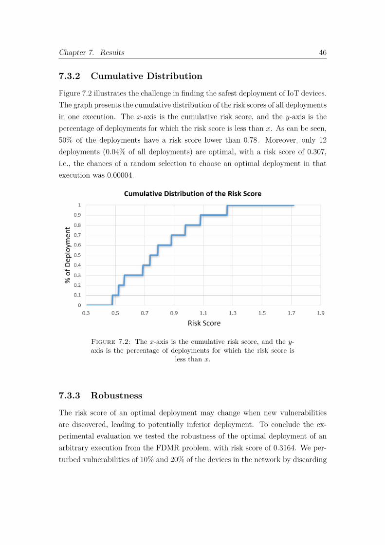
7.2 The x-axis is the cumulative risk score, and the y-axis is the per-centage of deployments for which the risk score is less than x. . . 46

7

List of Tables

7.1 DFBnB and Random Risk Scores Stats Distribution . . . . . . . . 437.2 Comparison between DFBnB algorithm and Random deployment

(average over 40 executions). . . . . . . . . . . . . . . . . . . . . . 447.3 Results: With and Without Heuristic (average over 40 executions) 44

8

Chapter 1

Introduction

It is estimated that by 2020 more than 20 billion IoT devices will be deployed in theworld [31]. Most IoT products are not equipped to deal with security and privacyrisks, which can turn them into the weakest link of organizational networks. Therisk of IoT devices to the security of an organization is underestimated in manycases when an organization’s IT department relies solely on network separation toisolate IoT devices from other IT assets. Such an approach disregards some of theunique properties of IoT devices, such as light or sound emissions, various sensors,and diverse communication protocols such as NFC, Bluetooth, ZigBee and LoRA,in addition to standard Wi-Fi. The advanced capabilities of IoT devices can beexploited by an attacker for lateral movement within an organization, shouldersurfing, and more, making them a valuable asset for an attacker.

With respect to hardening IoT security, most prior research focuses on the se-curity of individual IoT devices [28, 45, 64], the security of an IoT protocol [34, 47,57, 59, 66], or the the security of a network that consists solely of IoT devices [16,22, 54, 62] (see Section 3.1 for more details). To the best our knowledge, there isno previous related research aimed at identifying the optimal (security risk-wise)deployment of devices within the physical space. The location of an IoT devicewithin an organization can have unintended effects on the network topology suchas bridging between networks through short-range communication protocols (seeSections 2.2.1 and 2.3). We use the following example to demonstrate the problem.

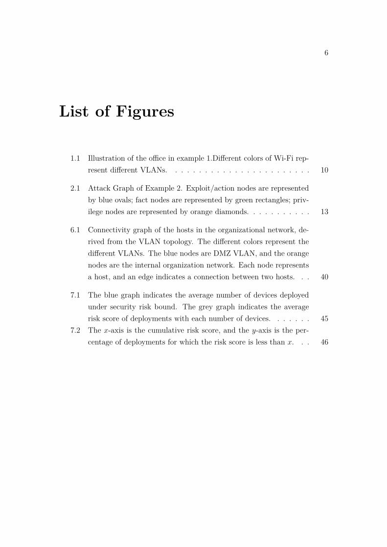
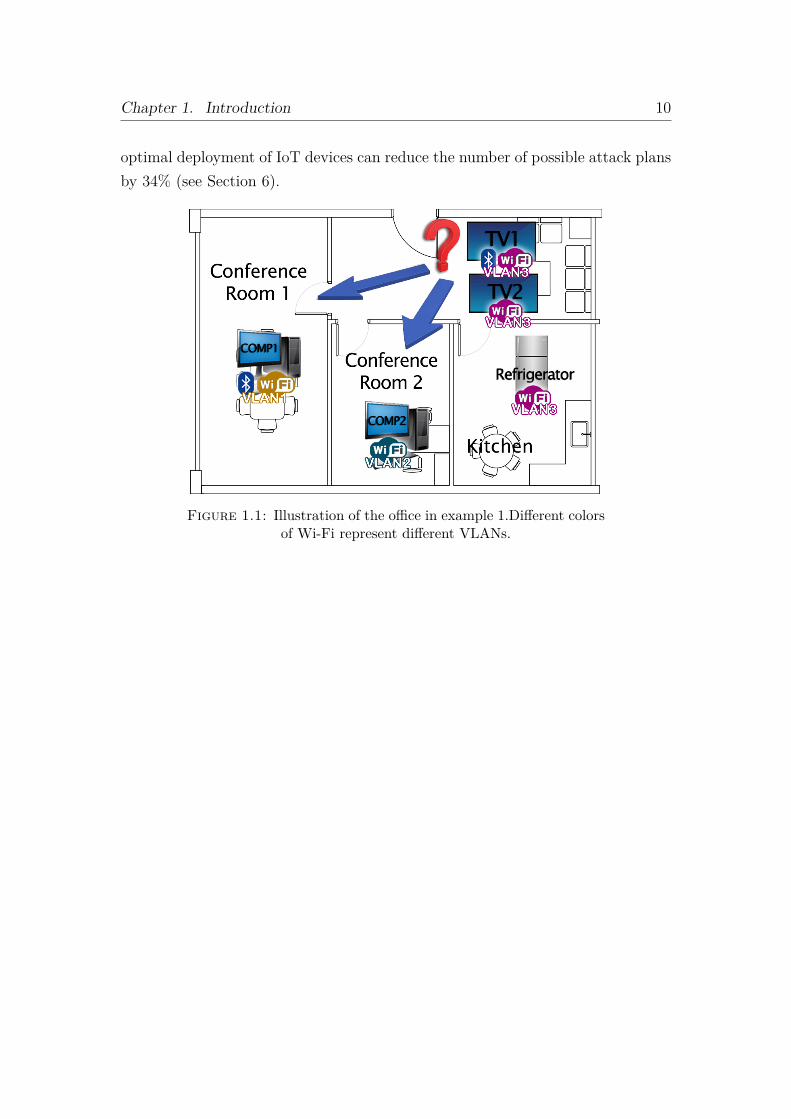
Example 1 (h) Assume, for example, an office with two conference rooms anda kitchen (Figure 1.1). Each conference room has a computer (COMP1 andCOMP2) connected through Wi-Fi to two different VLANs (V LAN1 and V LAN2respectively). COMP1 also has Bluetooth. A smart refrigerator in the kitchen isconnected to V LAN3 and has Internet connectivity. All other IoT devices in the

Chapter 1. Introduction 9

office are connected to V LAN3 as well. The office purchased two televisions (TV 1and TV 2) to replace the old projectors in the conference rooms. Both televisionsare connected to V LAN3 via Wi-Fi; TV1 is also equipped with Bluetooth.

Should we install TV 1 in Conference Room 1 and TV 2 in Confer-ence Room 2 or vice versa? To answer this question assume, for example,that unbeknownst to the organization, a sophisticated malware has managed toinfect one of the computers in the organizational network. Further, assume thatthe malware is equipped with the necessary exploits to hop between devices in theoffice. If TV 1 is placed in Conference Room 1, the attacker could take advantageof the fact that both TV 1 and COMP1 have Bluetooth and create an attack pathto the refrigerator. However, if TV 1 is placed in Conference Room 2 this attackpath will no longer be available to the attacker.

The risk of potential multi-step attacks such the one described in Example 1can be estimated using attack graphs [38, 42]. An attack graph is a model of acomputer network that encompasses computer connectivity, vulnerabilities, assets,and exploits. It is used to represent a collection of complex multi-step attack paths(hereafter referred to as attack plans) and can be used to assess and quantifysecurity risk (see Section 2.1 for more details).

In this research, the proposed method augments attack graph analysis to ac-count for the physical location of IoT devices and their communication capabil-ities. (see Section 4). Relying on the new attack graphs, we quantify the riskof adding an IoT device to a given network and show that it may increase by22% due to the deployment of only six IoT devices in a small to medium sizedenterprise.

We also optimize the deployment of IoT devices in order to reduce the negativesecurity implications of such deployment (see Section 5). Two optimization prob-lems are presented: the Full Deployment with Minimal Risk (FDMR) problemwhere all required IoT devices should be deployed with minimal security impli-cations and the Maximal Utility without Risk Deterioration (MURD) problemwhere the maximal number of IoT devices should be deployed without increasingthe security risk of the network. We use depth-first branch and bound (DFBnB)heuristic search algorithm to solve both optimization problems and suggest anadmissible heuristic function to accelerate the search. Our experiments show that

Chapter 1. Introduction 10

optimal deployment of IoT devices can reduce the number of possible attack plansby 34% (see Section 6).

Figure 1.1: Illustration of the office in example 1.Different colorsof Wi-Fi represent different VLANs.

11

Chapter 2

Background

2.1 Attack Graphs

An attack graph is a model of a computer network that encompasses computerconnectivity, vulnerabilities, assets, and exploits [38, 42]. Attack graphs are usedto represent collections of complex multi-step attack scenarios traversing an or-ganization from an initial entry point to the most critical assets. By analyzingthe attack graph, a security analyst can assess the risks of potential intrusionsand devise effective protective strategies. The attack graph analysis methodologycontains three main stages: (1) network and vulnerability scanning, (2) attackgraph modeling, and (3) attack graph analysis.

In the first stage, the Nessus vulnerability scanner [10] is used in order to mapthe vulnerabilities of all of the hosts in the organization. Connectivity betweenthe hosts can be identified manually by system administrators based on the orga-nizational network topology and firewall configurations. Nessus, Nmap, or othernetwork scanners can aid in the connectivity assessment process.

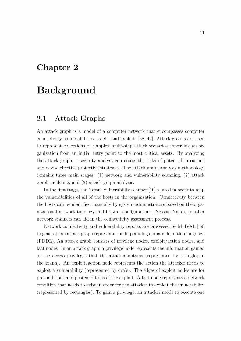
Network connectivity and vulnerability reports are processed by MulVAL [39]to generate an attack graph representation in planning domain definition language(PDDL). An attack graph consists of privilege nodes, exploit/action nodes, andfact nodes. In an attack graph, a privilege node represents the information gainedor the access privileges that the attacker obtains (represented by triangles inthe graph). An exploit/action node represents the action the attacker needs toexploit a vulnerability (represented by ovals). The edges of exploit nodes are forpreconditions and postconditions of the exploit. A fact node represents a networkcondition that needs to exist in order for the attacker to exploit the vulnerability(represented by rectangles). To gain a privilege, an attacker needs to execute one

Chapter 2. Background 12

of the actions leading to it (logical OR). To use an exploit, the attacker needsall of the privileges and the facts that lead to the exploit (Logical AND). Anexploit node needs all of these preconditions leading to it to be executed, andonce executed, the attacker gains all of the postconditions the exploit node leadsto [4, 36, 38, 51].

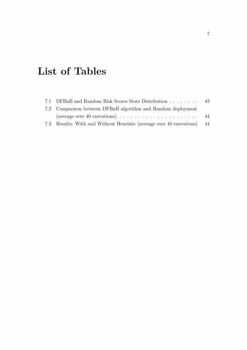
Example 2 Figure 2.1 presents an abstract attack graph of the situation describedin example 1. At the top of the figure, two fact nodes (nodes 1 and 2) that representtwo facts of the system can be seen (green rectangles). Access between COMP1and TV 1 can only created if these two conditions exist, as can be seen from the blueoval, which represents an exploit node (node 3). This access allows the attackerto use the Bluetooth connectivity of TV 1, as represented by the orange diamond(node 4), meaning that the attacker can obtain control of TV 1 via COMP1.

Following the construction of an attack graph, the graph’s PDDL represen-tation can be used as a domain model for variety of planners. A typical task isfinding the optimal attack plan or estimating the likelihood of a successful at-tack given the attack graph of an organization [36, 53, 58]. Consequently, attackgraphs can be used for hardening network security through a variety of attackgraph optimizations [1, 24, 37, 43].

2.2 Internet of Things

2.2.1 Security in the Internet of Things

Traditional security solutions such as firewalls, IDSs, anti-viruses, and softwarepatches are not suitable for IoT devices. The four major reasons for this are [61]:(1) Types of policies: a single app may use several IoT devices, communicating ex-plicitly (e.g., via Wi-Fi or Bluetooth) or implicitly (e.g., an IoT light bulb can betriggered by an IoT light sensor). The outcome is a complex and dynamic networkwhich can be hard to secure using a single security policy (e.g., with firewalls).(2) Signatures and anomalous behavior recognition: some security methods storeanomalies and signatures on the device to recognize and detect threats. Due tothe diversity of IoT devices and manufacturers, these methods will be inadequate,mainly because of the constant need to update and maintain the device to support


Figure 2.1: Attack Graph of Example 2. Exploit/action nodesare represented by blue ovals; fact nodes are represented by greenrectangles; privilege nodes are represented by orange diamonds.


these tools. (3) Enforcement mechanism: IoT devices have low computation abili-ties, low power consumption, and do not run full-fledged operating systems. Mostcommon security methods need all of the above to operate and therefore are im-practical to implement on IoT devices. (4) Unsupported devices: the longevity ofIoT devices can lead to deployed devices that vendors no longer support. In thatway, vulnerable devices (with default passwords or unpatched bugs) can remainin the organization.

Moreover, the competitive IoT device market compels vendors to try and gettheir products out as fast as they can, prioritizing functionality and the userexperience, and ignoring the security aspect. In general, most products hardly dealwith security and privacy risks, making them the weakest link in terms of securityand the target of attackers interested in breaking into networks and harmingsystems or leaking information [61]. Thus, despite the fact that security wasrecognized as a central issue of the IoT market as early as 2011 by Bandyopadhyayet al. [7], it still continues to remain a challenge today.

2.2.2 Vulnerabilities

Security experts need to gather information about the vulnerabilities of devicesin their organizations [6]. To do so, they can use a specialized search engine, likeShodan or Censys, to try and find the answer.

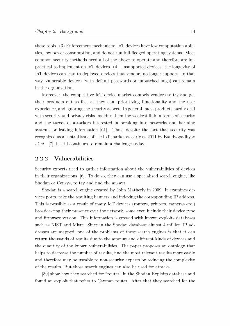
Shodan is a search engine created by John Matherly in 2009. It examines de-vices ports, take the resulting banners and indexing the corresponding IP address.This is possible as a result of many IoT devices (routers, printers, cameras etc.)broadcasting their presence over the network, some even include their device typeand firmware version. This information is crossed with known exploits databasessuch as NIST and Mitre. Since in the Shodan database almost 4 million IP ad-dresses are mapped, one of the problems of these search engines is that it canreturn thousands of results due to the amount and different kinds of devices andthe quantity of the known vulnerabilities. The paper proposes an ontology thathelps to decrease the number of results, find the most relevant results more easilyand therefore may be useable to non-security experts by reducing the complexityof the results. But those search engines can also be used for attacks.

[30] show how they searched for “router” in the Shodan Exploits database andfound an exploit that refers to Cayman router. After that they searched for the


specific kind of router in Shodan database and obtained the IP address of manyCayman routers. They then used the exploit in the routers for their purpose,conducting a denial-of-service (DDoS) attack for example.

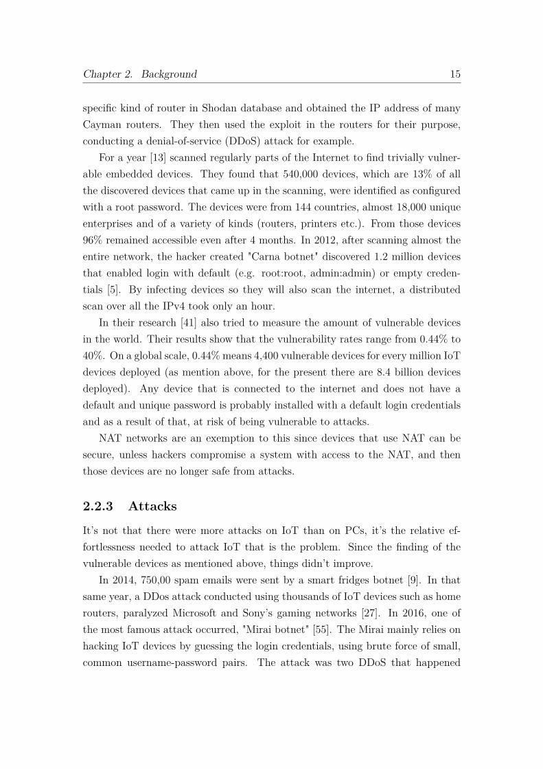
For a year [13] scanned regularly parts of the Internet to find trivially vulner-able embedded devices. They found that 540,000 devices, which are 13% of allthe discovered devices that came up in the scanning, were identified as configuredwith a root password. The devices were from 144 countries, almost 18,000 uniqueenterprises and of a variety of kinds (routers, printers etc.). From those devices96% remained accessible even after 4 months. In 2012, after scanning almost theentire network, the hacker created "Carna botnet" discovered 1.2 million devicesthat enabled login with default (e.g. root:root, admin:admin) or empty creden-tials [5]. By infecting devices so they will also scan the internet, a distributedscan over all the IPv4 took only an hour.

In their research [41] also tried to measure the amount of vulnerable devicesin the world. Their results show that the vulnerability rates range from 0.44% to40%. On a global scale, 0.44% means 4,400 vulnerable devices for every million IoTdevices deployed (as mention above, for the present there are 8.4 billion devicesdeployed). Any device that is connected to the internet and does not have adefault and unique password is probably installed with a default login credentialsand as a result of that, at risk of being vulnerable to attacks.

NAT networks are an exemption to this since devices that use NAT can besecure, unless hackers compromise a system with access to the NAT, and thenthose devices are no longer safe from attacks.

2.2.3 Attacks

It’s not that there were more attacks on IoT than on PCs, it’s the relative ef-fortlessness needed to attack IoT that is the problem. Since the finding of thevulnerable devices as mentioned above, things didn’t improve.

In 2014, 750,00 spam emails were sent by a smart fridges botnet [9]. In thatsame year, a DDos attack conducted using thousands of IoT devices such as homerouters, paralyzed Microsoft and Sony’s gaming networks [27]. In 2016, one ofthe most famous attack occurred, "Mirai botnet" [55]. The Mirai mainly relies onhacking IoT devices by guessing the login credentials, using brute force of small,common username-password pairs. The attack was two DDoS that happened


almost simultaneously, the first one against the website of security consultantBrian Krebs (620 Gbps of traffic) and the second against French webhost andcloud service provider (1.1 Tbps of traffic). After the first attack, the creatorsreleased the source code of Mirai. This triggered more attacks, such as the one onOctober 2016 against service provider Dyn, which took down hundreds of websites,among them Twitter, Netflix, GitHub and Reddit. These are only a few of theattacks performs, and the list can go on.

As opposed to PCs, IoT are connected 24/7 to the network, have no antivirusor IDS as a defense and most of them have easy accessible credentials (e.g. weakpassword) [40]. They may lack computational power, but compensate in numbers.The neglection of the security aspect by users and the manufactures alike, increasesthe chances of finding large numbers of vulnerable IoT, so from the attacker pointof view, attacks on IoT devices seems really worthwhile.

2.2.3.1 Solutions

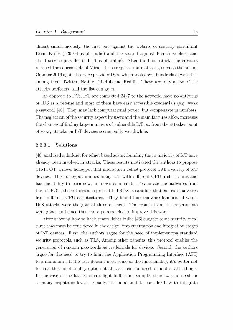
[40] analyzed a darknet for telnet based scans, founding that a majority of IoT havealready been involved in attacks. These results motivated the authors to proposea IoTPOT, a novel honeypot that interacts in Telnet protocol with a variety of IoTdevices. This honeypot mimics many IoT with different CPU architectures andhas the ability to learn new, unknown commands. To analyze the malwares fromthe IoTPOT, the authors also present IoTBOX, a sandbox that can run malwaresfrom different CPU architectures. They found four malware families, of whichDoS attacks were the goal of three of them. The results from the experimentswere good, and since then more papers tried to improve this work.

After showing how to hack smart lights bulbs [46] suggest some security mea-sures that must be considered in the design, implementation and integration stagesof IoT devices. First, the authors argue for the need of implementing standardsecurity protocols, such as TLS. Among other benefits, this protocol enables thegeneration of random passwords as credentials for devices. Second, the authorsargue for the need to try to limit the Application Programming Interface (API)to a minimum . If the user doesn’t need some of the functionality, it’s better notto have this functionality option at all, as it can be used for undesirable things.In the case of the hacked smart light bulbs for example, there was no need forso many brightness levels. Finally, it’s important to consider how to integrate


the IoT devices. In the smart light example, because those bulbs can be imple-mented into city’s power grids, it’s better to do so only after separating them fromthe network in order to avoid attacks, such as blackouts or the one the authorsperformed.

Today, most of the research addressing the security problems of IoT, is aboutthe scale and consequences of these problems without suggesting real solutions. [15,29, 61] each suggest a design or an architecture of IoT network that addresses someof these issues, sometimes in a general way and sometimes in a more practical way.To this date, to my knowledge, there is no acceptable and practical solution thatcan solve even some of the security issued mentioned above.

2.3 Short Range Communication Protocols

When connecting a device to a network it is possible to use two categories of net-working technologies. The first and simplest category is to connect using standardexisting network technologies such as Wi-Fi and Ethernet. The second categoryis to connect using different wireless technologies that are more suitable for somedevices, e.g., technologies that are more appropriate for devices that require lowenergy consumption protocols. These protocols are short-range communicationprotocols, due to their requirement for short proximity in order to perform aconnection.

Currently, in the second category there are several communication methodsthat can be used, including: ZigBee, Z-Wave, Powerline, Bluetooth 4.0, and otherradio frequency protocols, but no standard protocol exists. Both Z-Wave and Zig-Bee are considered secure, but implementation flaws and manufacturer mistakesmake them vulnerable [8].

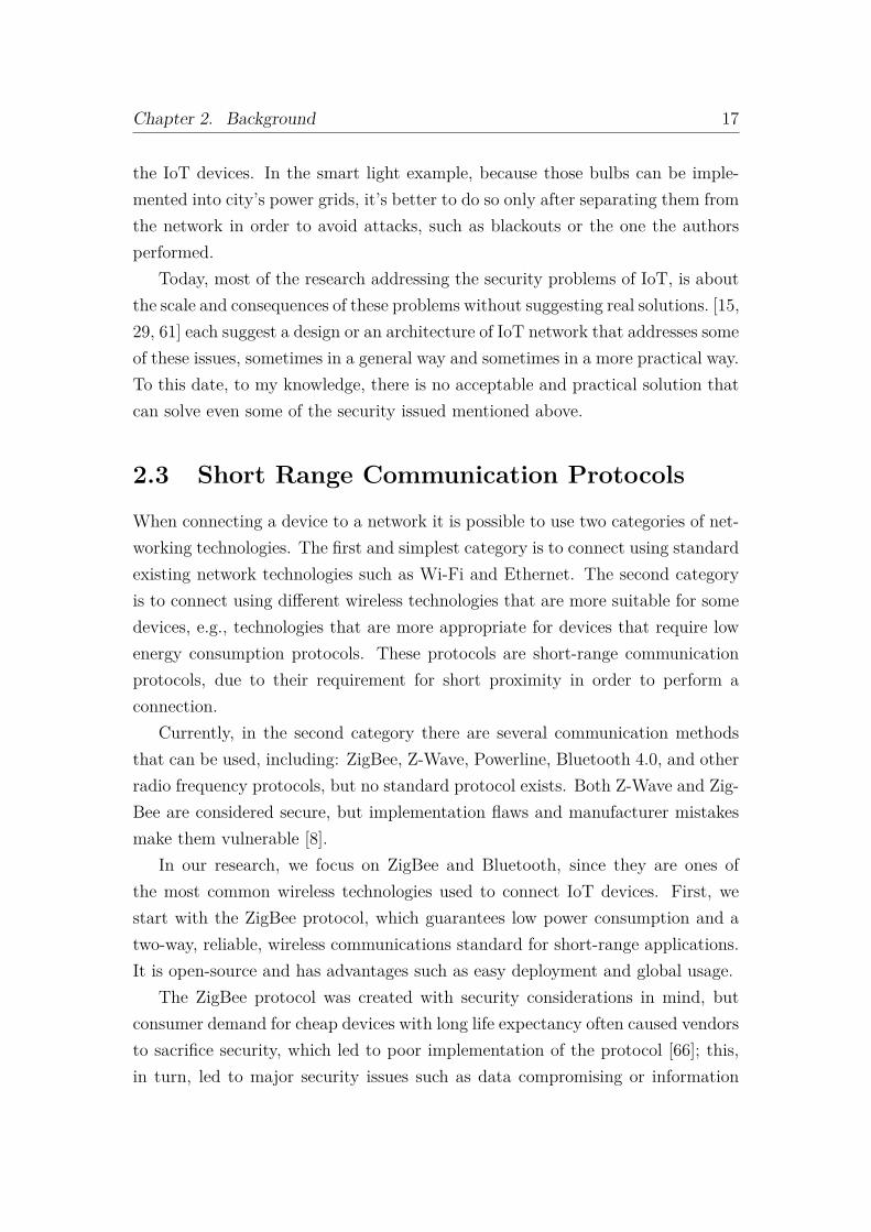
In our research, we focus on ZigBee and Bluetooth, since they are ones ofthe most common wireless technologies used to connect IoT devices. First, westart with the ZigBee protocol, which guarantees low power consumption and atwo-way, reliable, wireless communications standard for short-range applications.It is open-source and has advantages such as easy deployment and global usage.

The ZigBee protocol was created with security considerations in mind, butconsumer demand for cheap devices with long life expectancy often caused vendorsto sacrifice security, which led to poor implementation of the protocol [66]; this,in turn, led to major security issues such as data compromising or information


sniffing [57]. For example, Vaccari et al. [57] focused on the security aspects ofthe ZigBee protocol. The study identified important security issues and presentedan attack on the protocol which enabled the attacker to compromise the datatransferring in the network. Morgner et al. [34] described a novel attack thatshows that the ZigBee Light Link standard is insecure by design. Wright et al.[59] published KillerBee, a penetration testing tool which allows ZigBee trafficto be sniffed and analyzed. Ronen et al. [47] found a major bug in the ZigBeeprotocol in Philip Hue smart lamps. They were able to perform an over-the-airfirmware update, thereby infecting the lamp with a worm that can spread to anyof the lamp’s neighbors.

Bluetooth was developed by a group called the Bluetooth Special InterestGroup (SIG) in May 1998. Today, a lot of smartphones, sports devices, sensors,and medical devices have Bluetooth. The protocol become widely used becauseof its low cost and low power consumption.

In [48], techniques were presented for eavesdropping on devices using Blue-tooth. An extended review of Bluetooth threats and possible attacks was per-formed by Minar et al. , Sandya et al. and Dunnin [14, 32, 49], and recently,Cope et al. [12] investigated the currently available tools to exploit vulnerabilitiesin Bluetooth. In conclusion, many Bluetooth versions that are in use today, havea wide variety of security vulnerabilities.

In addition to the security issues, the number of communication protocolsin an IoT device can also influence the security of the device. If such a deviceis compromised by an attacker that has hacked into one of its communicationprotocols, the hacker can take advantage of the compromised device and use theother protocols as entry points to the network [17].

Of all the above, short-range communication protocols are another aspect ofIoT devices that make them insecure compare to regular hosts.

2.4 Heuristic Search

Heuristic search is a family of techniques used to solve difficult problems in arti-ficial intelligence (AI). In this case, each problem is represented by states, whereeach state represents the current condition of the problem. Each problem also hasa starting state and one or more goal states. A search space is the environmentin which a search takes place, where the purpose of the search is to find a path


from the start state to one of the goal states in the search space. Each solutionrepresents by one goal state. The quality of the solution is measured by the costof the goal state. Search algorithms make a distinction between minimum andmaximum problems. In a minimum problem, we want to find the solution withthe lowest cost, and in a maximum problem the highest cost solution is desired.Most problems are minimum problems, e.g., we want the cheapest or the fastestsolution. If not stated differently, we are referring to a minimum problem. In ourresearch, we use the depth-first branch and bound algorithm [26, 65] which usesa heuristic function to solve the problems more efficiently.

2.4.1 Heuristic

A heuristic is an estimation of the cost of the path from node n to a goal node.The heuristic function is used to steer the search algorithm in the direction of thegoal. In an informed way, heuristics help the algorithm guess which child out ofall of the node’s children will lead to the goal.

2.4.2 Admissible Heuristic

If, for any n, a heuristic function never overestimates the cost of the best pathfrom node n to a goal node, then the function is referred to as an admissibleheuristic function. Note that in a maximum problem (where we want the solutionwith the maximum cost) it is the opposite, i.e., a heuristic function that neverunderestimates the cost of the best path.

For example, suppose we try to find the shortest path from point A to pointB. This is a minimum problem where the cost is the distance between the twopoints. A good admissible heuristic function could be the aerial distance, becausethe actual path between both points will never be lower than the aerial distance.

In most search algorithms, as well as in DFBnB algorithm, one of the mostimportant conditions for a heuristic function is that it should be admissible.

2.4.3 Algorithms

We will review three common searching algorithms, A∗, IDA∗ and DFBNB [26].A* Algorithm. The basic algorithm is A*. A* is best-first search algorithm

that find the optimal path if the heuristic function is admissible. His advantage is


that he expands the fewest number of nodes. His main drawback is the memoryrequirement, like any best-first search algorithms, and therefore cannot really solvemost of the complex problems.

IDA* Algorithm. IDA* is Iterative-deepening A* and he eliminates thememory problem of A*, without harming the optimality. Each iteration of thealgorithm is a depth-search that keeps track of the cost that is calculated as inthe A* algorithm. When a cost is higher than a certain threshold, it is cut off andthe search backtracked and then continued. The initial threshold is the heuristicestimate of the start node, when in each successive iteration its increased by thelowest cost that was pruned in the previous iteration. IDA* memory requirementsare linear in the maximum depth search, and his solution is optimal if the heuristicfunction is admissible. He is asymptotically optimal in time and space over A*and easier to implement. IDA* is good for the sliding puzzles or Rubik’s cubeproblems.

DFBnB Algorithm. Depth-first branch and bound (DFBnB) is a Depth-first search algorithm [26, 65]. The algorithm is used to navigate through thesearch space and find the optimal solution. During the search process, DFBnBmaintains the best solution found so far. In order to perform pruning more fre-quently and thus accelerate the search process, DFBnB uses a heuristic function.The cost of a node is defined by f(x) = g(x) + h(x), where f(x) is the sum of (1)the current cost of the node g(x), and (2) the heuristic function for the goal h(x),which is the estimation of the cost from node x to the goal. Thus, f(x) estimatesthe lowest total cost of any solution path going through node x. If a branch witha higher cost is found, it can be pruned so that there is no need to keep expandingtowards it.

The algorithm returns an optimal solution with linear memory space, assumingthe heuristic function is admissible. This solution depends on the kind of problem(i.e., minimum or maximum), which is determined by the cost of the goal state.

DFBnB is suitable for problems when the maximum search depth is known inadvance or the search tree is finite, like in the traveling salesman problem (TSP) orlike in our problem, because each node have excatly two children. In this researchwe chose the heuristic algorithm DFBnB, as it fits our problem.

21

Chapter 3

Related Work

3.1 IoT Device Deployment

There are several works regarding the deployment of IoT devices, but most of themdo not consider the security aspect. For example, Huang et al. [22] proposed adeployment scheme used to a achieve green networked IoT, while Skarmeta et al.[54] focused on privacy issues and Zanella et al. [62] focused on the IoT in smartcities.

Some of the research that refers to security analyzes single IoT devices butdoes not look at IoT devices as a deployment problem. Liu et al. [28] triedto solve the problem of assessing the risk of a single IoT device, by proposing adynamical risk assessment method inspired by an artificial immune system. Zhanget al. [64] and Roman et al. [45] reviewed security issues in the IoT in terms ofthe security of each device.

There are a few works that refer to deployment and network security, butthey do not take the combination of hosts (such as computers and servers) withIoT devices into consideration. Mohsin et al. [33] argued that the likelihood ofexploiting IoT vulnerabilities depends on the system configuration. The authorsexplained that various configurations derive from different devices, technologies,and connectivity, all of which serves the same goal but have different risk levels.Santoso et al. [50] presented an approach to secure smart home systems in whichIoT devices are deployed, and Abie et al. [2] introduced a risk-based adaptivesecurity framework for the IoT in health-care systems. Shivraj et al. [52] arguethat most of the existing risk assessment frameworks are not suitable for IoTdevices, and suggested a new generic risk assessment framework for IoT systems.The authors refer to systems like smart cities, smart grid, etc. and base their

Chapter 3. Related Work 22

approach on graph theory.The research mentioned above reflects the many challenges of IoT security.

In this respect, our work is unique in two ways. First, it combines the securityconcerns of the IoT with workstations and servers, while taking into account thepossible use of one to hack the other. Second, our network model is a genericnetwork that can be suitable for a variety of scenarios and is not specific for aparticular domain.

3.2 Attack Graph Optimization

3.2.1 Attack Graph Representation

Attack graphs have been used to estimate the security risk score of organizationalnetworks [36, 53, 58]. These works try to overcome different problems and relyon multiple tools while presenting different models for risk analysis, however thespecific characteristics of IoT devices were not considered in these articles. In allof this research, the structure of the regular IT network is analyzed, taking intoaccount the vulnerabilities of workstations and servers. IoT devices introduceadditional challenges to security risk modeling through attack graphs, such asthe diverse physical locations, variety of short-range communication protocols,cyber-physical capabilities of the devices, mobility, etc.

In this research, we augmented the attack graph model of an organization toconsider locations and short-range communication of IoT devices, and we usedthe augmented attack graph model to optimize the deployment of IoT devicesthroughout the organization.

3.2.2 Risk Score

Wang et al. [58] suggested an overall network security score by combining indi-viduals’ vulnerabilities regarding their relationship in attack graphs. Singhal et al.[53] defined the risk score as the likelihood of an attack which was derived fromthe likelihood of individual exploits. Noel et al. [36] described four families ofmetrics for measuring security risk in attacks graph. Every family was representedby one entry in a four-dimensional vector. The Euclidean norm of this vector wasused as the overall risk score. Gonda et al. [20] computed the number of shortest


plans in a planning graph derived from an attack graph as a way to measure thesecurity of the network, and Swiler et al. [56] computed the set of near-optimalshortest paths to identify the most exploitable components in the network. Poladet al. [43] used an attack graph to estimate the security of the network as thecost of the attack path that led to the goal.

Idika et al. [23] used three risk assessments metrics, The Shortest Path metric,the Number of Paths metric, and the Mean of Path Lengths and combined them todetermine between two networks which one is more secure. The authors claimedthat each risk score by itself can lead to misleading results, and suggested analgorithm for combining the usage of attack graph-based security metrics. Theyused decision metrics when two metrics created a conflicts of which network is moresecure. Their algorithm helps reaching a decision by creating a total ordering ofpriority on questions regarding these conflicts.

All the above risk scores can be used to optimize the IoT deployment once theattack graph definition has been augmented to take into account the IoT devicespecifications.

In our research, we find, as did Idikaet al. , that one metric cannot representthe risk of the network correctly, and suggested a simple way to combine differentmeasures in order to compare the risk between different networks. We adoptGonda’s approach and used planning graph to find all shortest paths in the graph.We combined their quantity, their length, the average number of exploits as wellas the average number of privileges the attacker obtained to one risk score (seeSection 4.3).

3.2.3 Optimization Problems

Security risks can be reduced by patching vulnerabilities. However, it is not alwayspossible to patch all vulnerabilities at once due to operational costs (patchingoften requires significant downtime). A variety of low cost network hardeningapproaches can be used to prioritize the vulnerabilities (e.g., [25, 37]). Islam et al.[24] argued that most of these methods are not scalable. They proposed heuristicalgorithms to accelerate the patch optimization. Abadi et al. [1] used the antcolony optimization algorithm to detect a minimum critical set of exploits. Poladet al. [43] examined the effect of adding fake vulnerabilities in an attack graphand used combinatorial optimization in order to find optimal assignment of these


vulnerabilities. Almohri et al. [3] used sequential linear programming in attackgraphs to find the optimal placement of security products (e.g., a host-basedfirewall) across a network. The authors used a probabilistic model which usesBernoulli and transformed the attack graph into a system of linear and nonlinearequations. Noel et al. [35] used attack graph to optimize the placement ofintrusion detection system (IDS) sensors to allow monitoring malicious activityon critical paths.

In this work we present a different optimization problem of optimizing the set ofIoT devices to be deployed throughout an organization with minimal implicationsto the network security.

3.3 IoT in Attack Graphs

Very little work has been performed on attack graphs that consist of IoT devices.The first research performed in this area was conducted by Ge et al. [16] whoused attack graphs in conjunction with IoT devices. However, the network usedconsisted only of IoT devices, most of which were the same kind of device. Thenetwork topology was fixed, small, and relatively uncomplicated. The authorsproposed a framework for IoT device security modeling with the aim of presentingall possible attack paths in the network, evaluating the security level, and assessingthe effectiveness of different defense strategies.

In a later work, Ge et al. [17] noted that some IoT devices use more than onecommunication protocol. The writers argued that if such a device is compromisedby hacking into one of the communication protocols, the hacker can take advantageof it and use the other protocols as entry points to the network. The paper usedHARMs (hierarchical attack representation models), which are models of attackgraphs used, to improve scalability [21]. The authors presented a real scenario andshowed how an attacker can take advantage of it. In the scenario, some deviceshave both Wi-Fi and ZigBee communication protocols. Also present are smartdevices such as a tablet and TV that can connect to a Philips Hue lighting system(Hue Bridge) by Wi-Fi. This lighting system also has ZigBee which allows it tocontrol smart light bulbs in the house. By exploiting the tablet that runs theHue application, an attacker can gain control of the Hue Bridge system and useit to control all of the smart lights. The authors noted that the lighting hub can


consist of any other smart hub, and the scenario can also be used to hack intoany smart device, not only light bulbs.

George et al. [19] used attack graphs to implement risk assessment frameworkfor Industrial IoT systems (IIoT). Such systems can be found in health-care, agri-culture, transportation, etc. The authors noted the many vulnerability in IoTdevices and claimed that it may lead an attacker to intrude the system using aweak IoT device. Their framework was inspired by attack graphs, allowing themto proposed risk mitigation strategies to reduce the overall threat level in thenetwork.

Yiğit et al. [60] proposed COBANOT, a heuristic-based cost and budgetaware network hardening solution for IoT systems which uses compact attackgraphs [11]. This work is the first to use attack graphs in IoT systems for networkhardening. However, their experiment included a small-scale attack graph thatonly consists of IoT devices. In addition, none of the unique characteristics ofIoT devices, such as different protocols, mobility, physical proximity, etc. wereconsidered.

Our research focuses on networks that combine all kinds of hosts and IoTdevices. Also, our network’s size is larger than the networks used in the researchmentioned above.

26

Chapter 4

IoT Attack Graphs

4.1 IoT Deployment

In a typical organization, all hosts (workstations and servers) are connected to theorganizational network via a wired or wireless connection. Let H = h1, h2, . . . , hzbe the set of hosts that are part of the organization network.

In addition to the regular hosts, the organizational network may contain IoTdevices. Let D = d1, d2, . . . , dm indicates the set of unique IoT devices. EachIoT device di has a unique identifier (usually an IP address).

IoT devices differ by their purpose and capabilities. For example, a refriger-ator is capable of maintaining a low temperature while a smart TV is capable ofshowing high definition movies. We group IoT devices by type, e.g., refrigerator,TV, camera, smoke detector, etc. T = t1, t2, . . . , tn is the set of all the IoTdevice types. We denote a set of all devices that are of type t as D(t) and a singledevice type d as t(d). We assume that every IoT device is part of just one group.

Some IoT devices can only be deployed in specific predefined designated loca-tions. For example, the kitchen is typically the designated location for a refriger-ator, while large TV screens or projectors are found in meeting rooms. Some IoTdevices such as cameras or smoke detectors may be deployed in many differentlocations throughout an organization.

Definition 1 Locations.L = l1, l2, . . . , lb indicates the set of unique location spots where IoT devices

can be deployed. We denote the set of locations where an IoT device of a specifictype t ∈ T can be deployed as L(t) ⊆ L. In every location spot only one type ofIoT devices can be deployed, meaning, L(t) is defined such that the intersectionof each pair of L(ti) sets are empty, ∩t∈L(t) = ∅. Because a location spot must

Chapter 4. IoT Attack Graphs 27

be associated with some type of IoT devices, the union of L(t) is equal to L,∪t∈L(t) = L

Organizations may have constraints about the deployment of IoT devices. Wedefined two main constraints for a device type t. The first one is the number oflocations (out of the total locations available) that need to contain a deployeddevice of that type. For instance, there are four possible locations for camerasin the hallway, but the organization only needs to deploy two of them. Thesecond constraint is the number of devices there are of each type. For instance,for one location in which a refrigerator can be deployed, there are three possiblerefrigerators that the organization can purchase.

Definition 2 Location Constraint.Let C be the set of all constraints. C(t) is a three-tuple that represents a

constraint for a type t, C(t) = (L(t), n(t), D(t)).L(t) is the set of locations that an IoT device of a specific type t ∈ T can be

deployed (as defined in Definition 1).n(t) is the number of locations that needed to be deployed out of all locations

in L(t).D(t) is a set of all IoT devices that are of type t.

An example of a constraint can be derived from example 1. Suppose the or-ganization has three possible locations in which a TV can be deployed (L(TV ) =lT V1 , lT V2 , lT V3) but only needs to deploy a TV in two of these locations (n(TV ) =2). In addition, there are four different televisions that can be deployed (D(TV ) =dtv1, dtv2, dtv3, dtv4). Formally, constraint C(TV ) would be defined as follow:

C(TV ) = (lT V1 , lT V2 , lT V3, 2, dtv1, dtv2, dtv3, dtv4).Assume that at most one IoT device can be deployed in each location l ∈ L.

The deployment of IoT devices is defined as a function depl : D → L∪⊥ whichmaps every device to a particular location. The special non-location symbol ⊥signifies that a device is not deployed. We say that a deployment is valid if it doesnot violate the constraints specified in Definition 2.

Definition 3 Valid Deployment.Let depl : D → L ∪ ⊥ be a deployment of IoT devices. depl is valid if

∀d∈D, depl(d) ∈ L(t(d)) ∪ ⊥.


We denote deplfull as a deployment that satisfies all constraints C and deplempty

as an empty deployment with no IoT devices deployed. Note that the conditionn(t) ≤ |D(t)| should be satisfied for full deployment to exist.

Many IoT devices deployed within an organization’s premises will likely beable to communicate with nearby hosts via short-range communication (SRC)protocols such as ZigBee, Bluetooth, ad hoc Wi-Fi, etc. Some hosts within theorganization may also support SRC protocols, which could allow the adversary tohop between networks.

Definition 4 Short-Range Communication.We define a set of short-range communication protocols SRC = p1, p2, . . ..

Let src : D ∪H → 2SRC be a function that maps an IoT device or a host to thesubset of SRC protocols that it supports.

In the remainder of this work we will use the term device to refer to both IoTdevices and hosts.

Any two devices connected via a SRC protocol must reside within a certaindistance from each other (i.e., the communication range). For example, let d ∈ D

be some IoT device that supports SRC protocol p ∈ SRC, and let h ∈ H besome host that supports the same protocol. If d is deployed in location l and h

resides within the communication range of l, then d may communicate with h andvice versa.

Definition 5 Location Range.We define the range : L ∪ ⊥ → 2D∪H of a particular location as the set of

hosts that may communicate with an IoT device deployed there.

It is important to note that range(l), l ∈ L is an estimation based on theradio specification of different IoT devices. The actual set of devices in range ofIoT device deploy in location l may vary depending on the power of the radio,obstacles, interference, etc.

For the ease of discussion we did an abstraction to the range. We defined threedifferent ranges: ShortRange, MediumRange and LongRange. Two devices mayhave the same short range communication protocol, but have different ranges.Each IoT device was assigned a range, depends on his SRC. For each location,for each SRC, we defined the set of hosts than are in a range from that location


l. In case an IoT device is deployed in a location, it can connect to all hosts inthat location that are with the same SRC and with the same range. Please notethat the set of hosts in ShortRange is a subset of MediumRange which is subsetof LongRange.

Also note that a device can be in the range of several locations and that nodevices are in the range of the non-location ⊥ (i.e. range(⊥) = ∅).

4.2 Attack Graph Definition

The potential locations of IoT devices and SRC protocols are integrated in the at-tack graph analysis methodology after the scanning stage and before attack graphmodeling. For every possible deployment of IoT devices, that will be consideredduring the course of the optimization, we augment the connectivity map of devicesto include the hypothetical connections between any IoT device d ∈ D deployedin location depl(d) and all devices in the range of d : range(depl(d)).

Once the connectivity between all devices has been defined, we use the stan-dard MulVAL framework to generate an attack graph that considers some givendeployment of IoT devices. Each deployment has a different attack graph, de-pending on the devices deployed. If no IoT device is deployed the deployment isempty (deplempty), and the attack graph is simply the original attack graph of theorganization.

We adopt the attack graph definition introduced by Ou et al. [38].

Definition 6 Logical Attack Graph.Let depl be a deployment of IoT devices in an organization. The logical attack

graph Gdepl is a tuple:

Gdepl = (Np, Ne, Nf , E, M, g),

where Np, Ne, and Nf are the sets of privilege nodes, exploit nodes and fact (leaf)nodes, respectively, and E is a set of directed edges

E ⊆ (Np ×Ne) ∪ (Ne × (Ne ∪Nf )),

There are two types of edges in an attack graph. An edge (e, p) ∈ E from anexploit node e ∈ Ne to a privilege node p ∈ Np means that the attacker can gain


privilege p by executing exploit e. In order to gain a privilege, an attacker needsto execute one of the exploits leading to it.

An edge (f, e) ∈ E from a fact node or a privilege node f ∈ Nf ∪ Np to anexploit node e ∈ Ne means that the node f is a precondition to executing theexploit e. For example, a fact node could be a vulnerability in the Bluetoothprotocol that can be exploited if the attacker is in the Bluetooth range of thevulnerable device. In order to execute an exploit, the attacker needs all of theprivileges and facts that lead to the exploit.

In this work, in contrast to the definition introduced by Ou et al. [38], theedge orientations follow the direction of the implied logical operation.

Next, we define the term attack plan. For that purpose, we changed the nota-tions from Gefen et al. [18] slightly, as follows:

pre(e) = v ∈ Np ∪Nf |(v, e) ∈ E are all of the preconditions of node e.obt(p) = e ∈ Ne|v ∈ Np&(e, v) ∈ E is the set of exploits that lead to

privilege node p (the set of privileges the attacker obtained).An attack plan is a sub-graph G′depl of some attack graph Gdepl that represents

a scenario in which the attacker manages to reach the goal, namely g ∈ G′depl.Therefore, in an attack plan all of the preconditions of an exploit e ∈ G′depl aresatisfied, and each privilege p ∈ G′depl is obtained by an exploit.

Definition 7 Attack Plan.Let AP (Gdepl) be all of the attack plans of graph Gdepl. Each attack plan

G′depl ∈ AP (Gdepl) needs to satisfy these three conditions:

• g ∈ G′depl

• ∀a ∈ Ne : pre(a) ⊆ G′depl|Ne ∈ G′depl

• ∀p ∈ Np : ∃a ∈ obt(p) ⊆ G′depl|Np ∈ G′depl

We consider the length of an attack plan as the number of nodes it con-tains. OptLen(Gdepl) is the length of the shortest attack plan in graph G, aOptCnt(Gdepl) indicates how many of the shortest attack plans there are in graphG. We also consider the average number of exploits in the shortest attack plans ingraph G, as OptExp(Gdepl), and the average number of privileges in the shortestattack plans, as OptPrv(Gdepl).


4.3 Risk Score

The network security can be estimated by the Risk Score, where the higher therisk score the lower the security of the network. In an environment in which IoTdevices are deployed, there are a few aspects to consider when choosing a methodfor computing the risk score.

First, the method needs to convey that the deployment of IoT devices maygenerate new attack plans. Consequently, the cost of an attack may drop andthe likelihood of an attack may increase due to the additional vulnerabilities andopportunities for lateral movement that an attacker can exploit. Last, the methodneeds to indicate the changes in different deployments and be sensitive enoughto detect the changes caused by the deployment of even a single additional IoTdevice.

We did not find any risk score in the literature that meet these requirements.Most risk scores are specific for a problem, they are trying to solve some problemthat was not taken into consideration in other works (zero-days, for example).

As we will see, our work is designed for all risk scores, as long as they aremonotonic. Meaning that deploying a device could not reduce the risk.

We consider a deployment of IoT devices that combine several aspects of thenetwork. We choose to calculate all the shortest attack plans, taking into consid-eration their length, quantity, average number of exploits and average number ofprivileges. Our main goal is to compare between different deployments, while try-ing to determine between two networks which one is more secure. To do that, wecalculated all the above parameters for the network with no IoT devices deployed,and the risk score of each deployment is derived from that.

Our purpose was to find a method that will allows us to compare between dif-ferent deployments. Due to the fact that we have a baseline, which is a deploymentwith no IoT device deployed, our risk score is a comparison to that.

Gonda et al. [20] describes the computation of the shortest attack plans indetail. As noted by the authors, enumerating all of the attack plans is NP-hard,which means that the running time can be exponential, however, we performedthis computation on several networks, and the running time was short, as can alsobe seen in Section 7.

Definition 8 Risk Score.


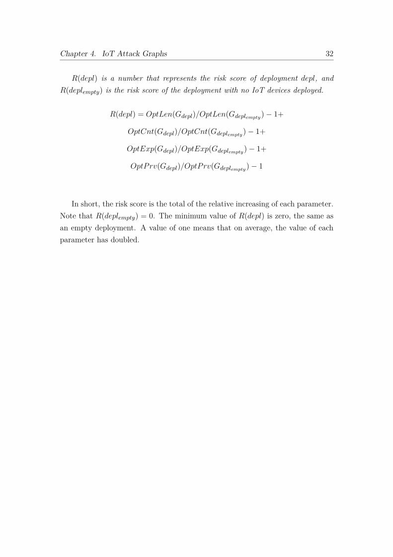
R(depl) is a number that represents the risk score of deployment depl, andR(deplempty) is the risk score of the deployment with no IoT devices deployed.

R(depl) = OptLen(Gdepl)/OptLen(Gdeplempty)− 1+

OptCnt(Gdepl)/OptCnt(Gdeplempty)− 1+

OptExp(Gdepl)/OptExp(Gdeplempty)− 1+

OptPrv(Gdepl)/OptPrv(Gdeplempty)− 1

In short, the risk score is the total of the relative increasing of each parameter.Note that R(deplempty) = 0. The minimum value of R(depl) is zero, the same asan empty deployment. A value of one means that on average, the value of eachparameter has doubled.

33

Chapter 5

Deployment OptimizationProblem

In this section, we introduce the terms and notation used to define the twoIoT deployment optimization problems: (1) Full Deployment with Minimal Risk(FDMR), and (2) Maximal Utility without Risk Deterioration (MURD).

5.0.1 FDMR Problem

Given an attack graph of an organization G, a set of IoT devices D of types T ,and the location constraints C, find the deployment (deplfull) of IoT devices suchthat all of the IoT devices are deployed subject to location constraints, and therisk score R(deplfull) is minimized.

Definition 9 Full Deployment with Minimal Risk (FDMR) Problem.Given the four-tuple < G, D, T, C >, find deplfull such that R(deplfull) is

minimizedarg mindeplfull

R(deplfull)

5.0.2 MURD Problem

Given an attack graph of an organization G, a set of IoT devices D of types T ,and the location constraints C, find the deployment that consists of the highestnumber of IoT devices without increasing the risk score R.

Definition 10 Maximal Utility without Risk Deterioration (MURD)Problem.

Chapter 5. Deployment Optimization Problem 34

Given the four-tuple < G, D, T, C >, find depl such that |R(depl)| is maximizedand R(depl) = R(deplempty)

arg maxdepl

|R(depl)| : R(depl) = R(deplempty)

5.1 Search Space

Next, we define the search space for both FDMR and MURD. In each case, thestate of the search space is organized as a binary tree where at each state adecision is made either to deploy (left child) or not to deploy (right child) a par-ticular IoT device in a particular location. The root state is an empty deployment(R(deplempty)) where no decisions have been made yet. Every path from the rootnode of the search space corresponds to a set of decisions. This means that a pathfrom the root to any state defines where some of the IoT devices are deployed andwhere some other IoT devices cannot be deployed. The set of left children along apath is a partial deployment of IoT devices. In this way, we consider all possibledeployments, subject to location constraints.

For every node of the search space we derive the respective attack graph Gdepl

and compute the risk score R(depl). The goal nodes depend on the specific prob-lem. In the FDMR problem the goal nodes include all states with a deploymentthat meets all of the constraints, deplfull, and the objective is to identify the goalstate with the lowest risk score. In the MURD problem the goal states include allstates with a deployment that has the same risk score as the initial state.

5.1.1 Search Space Size

Using the definitions above, we calculate the size of the search space, meaning thenumber of possible full deployments. We find the total number of the differentdeployments depending on the existing constraints by calculating the number ofpossible deployments for each location type, and multiplying all the results witheach other. To calculate the number of all possible deployments in t we usepermutation 1 and combination 2. Permutation is define as: nPk = n!

(n−k)! , and

1Permutation nPk means that for n items, we want to find the number of ways k items canbe ordered.

2Combination(n

k

)is a selection of k items from a collection of size n, such that the order of

selection does not matter.


combination is define as:(

nk

)= n!

k!(n−k)! .In the following explanation, we will use the example in Definition 2 to calcu-

late the number of possible deployments of type TV,C(TV ) = (lT V1 , lT V2 , lT V3, 2, dtv1, dtv2, dtv3, dtv4.First, we calculate the permutation of number of devices there are in t type

(|D(TV )| = 4) out of locations to deploy (n(TV ) = 2). We use permutationbecause in this case the order matter, since each device is unique and the locationof each device means different deployment. If we choose two devices and deploythem in two locations, and if we choose the same two devices but switch thelocations, the deployments would be different, |D(T V )|Pn(T V ) = 4P2 = 12. Next,we calculate the combination of the number of locations that needed to be deployedin type t (n(TV ) = 2) out of locations to deploy (|L(TV )| = 3). In this case weuse combination because the order does not matter. There are three locations intotal and we need to deploy only two of them.

(|L(T V )|n(T V )

)=(

32

)= 3.

Therefore, the number of possible different deployments in type TV is 36,3 · 12 = 36. The formula to compute the size of possible deployments, which isalso define as the size of the search space, is as follows:

Πt∈T

((|L(t)|n(t)

)·|D(t)| Pn(t)

)

We multiple the number of all possible deployments of each type.

5.2 Search Algorithm

For our heuristic search, we used the DFBnB algorithm (as described in Sec-tion 2.4). The heuristic function will be described later in this section. We chooseDFBnB algorithm because it’s pruning ability can significantly reduce that run-ning time. In addition, in the way we built the search space, our branching factoris two (each node has exactly two children), and the algorithm is suitable for prob-lems with low branching factor. A pseudo code of the algorithm can be found atAlgorithm 1 and is further explained in Section 5.2.1.

As we mentioned above, each state in our search tree has two children (left andright). In one, we added an IoT device to the deployment in a certain location,and in the other, we did not allow the IoT device to be deployed in that location.


In practice, each state has various options regarding which IoT devices to deploy.We used node ordering to chose one device (d) and one location (l) where d canstill be deployed and generate two children: deploy d at l and do not deploy d

at l. For the left child corresponding to the deploy decision, we generate a newattack graph and recalculate the risk score . We do not calculate the risk scorefor the right (do not deploy) child, as this child’s risk score did not change, sincethe risk score depends only on the deployed devices.

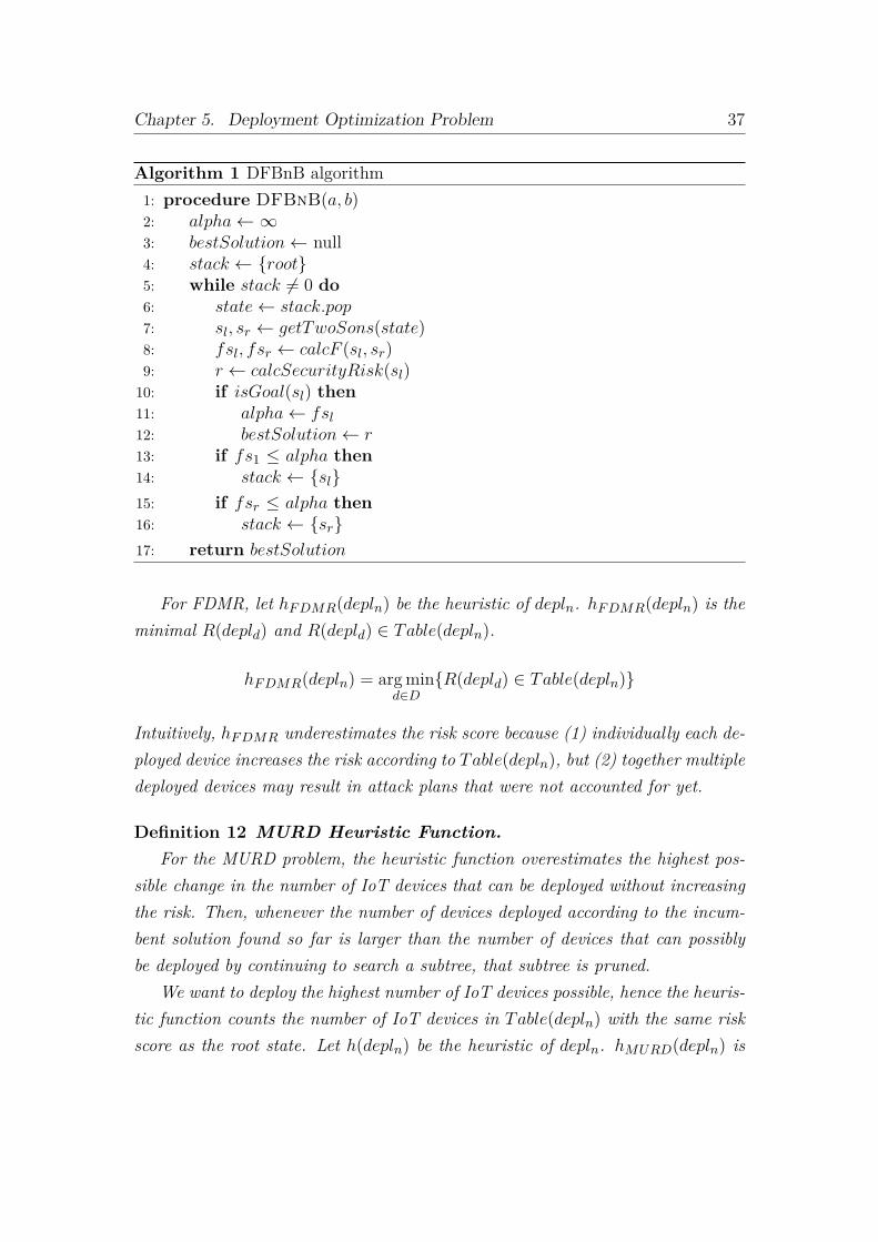
5.2.1 Pseudo-Code

At first, we initialized our variables, including adding the empty deployment, withno IoT devices deployed, to a stack (root). For each state we popped from thestack, we generated two children, as described in Section 5.2. sl is correspondingto the left generated child, while sr is corresponding to the right. We calculatedthe f -value for each child (note that if there is no heuristic function, f(x) = g(x)).The security risk calculation is based only on the left child. When we reach a goalnode (full deployment), we save it as our best solution and update alpha. We addto the stack a child only if it’s f -value is smaller than alpha.

Please note that the showed pseudo-code is suitable for the FDMR problem.The pseudo code for the MURD problem is the same, except for the signs in lines13, 15, which are the opposite (≥ instead of ≤).

5.2.2 Heuristic Functions

In order to calculate the heuristic functions, we created a table of risk scoresTable(depln) which contains the risk scores for each IoT device in each possiblelocation. In other words, we simulate the deployment of a single IoT device eachtime. For each deployment, we update the table, removing the IoT device thatwas deployed or not allowed to be deployed.

Definition 11 FDMR Heuristic Function.For the FDMR problem, the heuristic function underestimates the lowest pos-

sible change in risk in every subtree. Then, whenever the risk score of the best fulldeployment found so far is lower than the risk score of any full deployment thatcan be found within a subtree, that subtree is pruned.


Algorithm 1 DFBnB algorithm1: procedure DFBnB(a, b)2: alpha← ∞3: bestSolution← null4: stack ← root5: while stack 6= 0 do6: state← stack.pop7: sl, sr ← getTwoSons(state)8: fsl, fsr ← calcF (sl, sr)9: r ← calcSecurityRisk(sl)10: if isGoal(sl) then11: alpha← fsl

12: bestSolution← r13: if fs1 ≤ alpha then14: stack ← sl15: if fsr ≤ alpha then16: stack ← sr17: return bestSolution

For FDMR, let hF DMR(depln) be the heuristic of depln. hF DMR(depln) is theminimal R(depld) and R(depld) ∈ Table(depln).

hF DMR(depln) = arg mind∈D

R(depld) ∈ Table(depln)

Intuitively, hF DMR underestimates the risk score because (1) individually each de-ployed device increases the risk according to Table(depln), but (2) together multipledeployed devices may result in attack plans that were not accounted for yet.

Definition 12 MURD Heuristic Function.For the MURD problem, the heuristic function overestimates the highest pos-

sible change in the number of IoT devices that can be deployed without increasingthe risk. Then, whenever the number of devices deployed according to the incum-bent solution found so far is larger than the number of devices that can possiblybe deployed by continuing to search a subtree, that subtree is pruned.

We want to deploy the highest number of IoT devices possible, hence the heuris-tic function counts the number of IoT devices in Table(depln) with the same riskscore as the root state. Let h(depln) be the heuristic of depln. hMURD(depln) is


the number of devices with a risk score equal to initial state R(deplempty), suchthat|R(depld) = R(deplempty)| and R(depld) ∈ Table(depln).

hMURD(depln) = |R(depld) ∈ Table(depln) : R(depld) = R(deplempty)|

Intuitively, hMURD overestimates the number of devices that can be deployed be-cause (1) any IoT device that increases the risk according to Table(depln) cannotbe deployed, and (2) even if individually a set of deployed devices does not increasethe risk score, together they may result in an attack plan that was not availablebefore.

5.2.3 Node Ordering

In order to find an optimal goal node quickly, the newly generated child nodesshould be searched in an increasing order of their costs. This method is callednode-ordering, and can significantly speed up the search [44, 63]. In our case, weused our heuristic function also as node ordering. In other words, we generatesthe child with the lowest heuristic. When we didn’t use heuristic function, werandomly chose a child to generate.

39

Chapter 6

Experiments

We conducted experiment for each one of the problems we wish to solve: findingthe full deployment with minimal risk (FDMR), and finding the maximal utilitywithout risk deterioration (MURD). For both problems, we used the suggestedDFBnB algorithm with the heuristics described in Section 5.2.

6.1 Data Preparation

To evaluate our proposed method, we conducted a set of experiments using anattack graph that was derived from a real organization network.

6.1.1 Organization Network

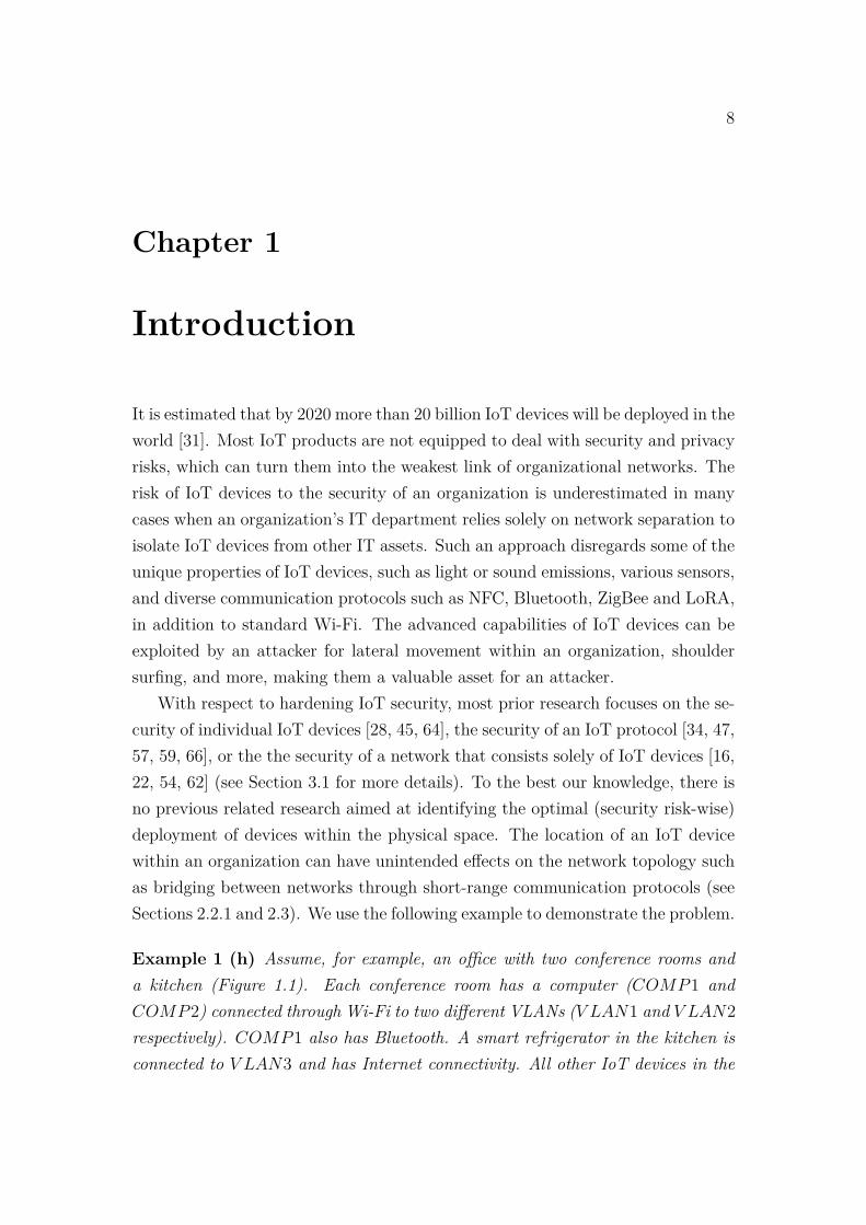
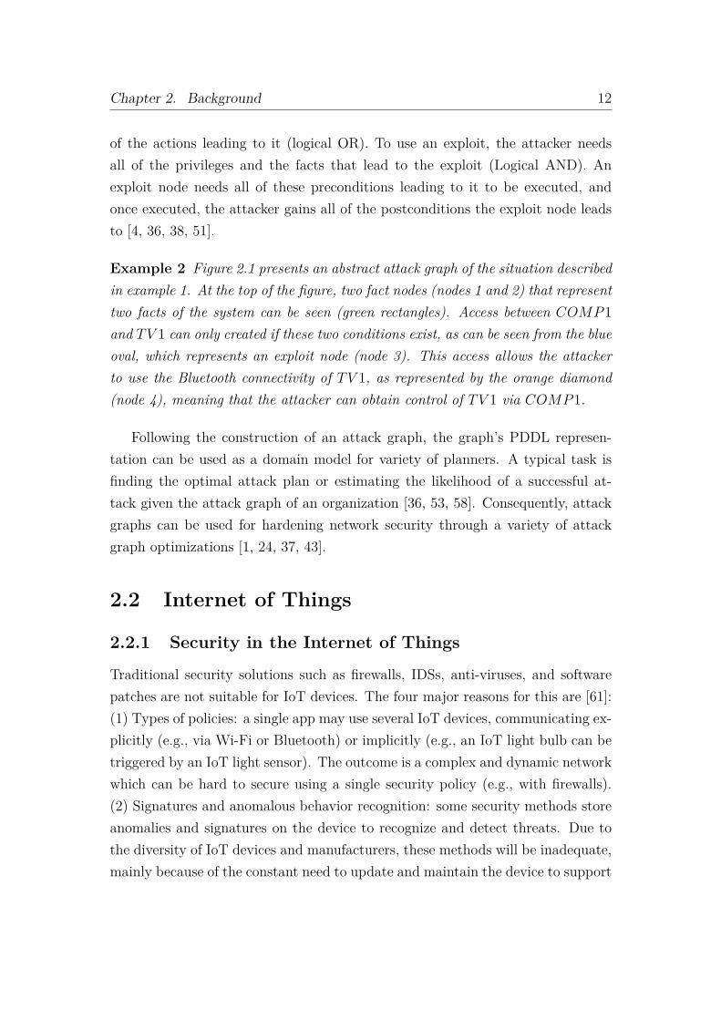
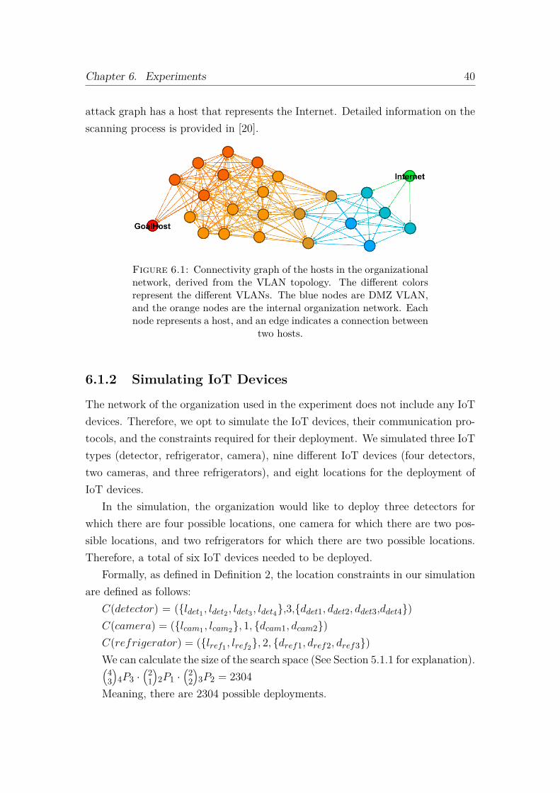
The network of the organization is a real network consisting of 24 hosts which wasused by Gonda et al. [20]. The network of the organization was scanned usingNessus Scanner, and then MulVAL was used to generate the attack graph basedon the scanning results. Figure 6.1 depicts the connectivity of the hosts in thenetwork, derived from the VLAN topology. Each node represents a host, and anedge indicates a connection between two hosts.

An organization can have more than one host that it wishes to protect, andthis is translated to multiple targets for the attacker. To simplify things, all targethosts are connected to an abstract goalHost, and the goal of the attack graphis to execute code in this host. Executing code on the goalHost proves thatthe attacker managed to control one of the targeted hosts that led to the goal.As part of the experimental setup we assume that the organization is free frominside adversaries and that the potential attacker is located on the Internet. The

Chapter 6. Experiments 40

attack graph has a host that represents the Internet. Detailed information on thescanning process is provided in [20].

Figure 6.1: Connectivity graph of the hosts in the organizationalnetwork, derived from the VLAN topology. The different colorsrepresent the different VLANs. The blue nodes are DMZ VLAN,and the orange nodes are the internal organization network. Eachnode represents a host, and an edge indicates a connection between

two hosts.

6.1.2 Simulating IoT Devices

The network of the organization used in the experiment does not include any IoTdevices. Therefore, we opt to simulate the IoT devices, their communication pro-tocols, and the constraints required for their deployment. We simulated three IoTtypes (detector, refrigerator, camera), nine different IoT devices (four detectors,two cameras, and three refrigerators), and eight locations for the deployment ofIoT devices.

In the simulation, the organization would like to deploy three detectors forwhich there are four possible locations, one camera for which there are two pos-sible locations, and two refrigerators for which there are two possible locations.Therefore, a total of six IoT devices needed to be deployed.

Formally, as defined in Definition 2, the location constraints in our simulationare defined as follows:

C(detector) = (ldet1 , ldet2 , ldet3 , ldet4,3,ddet1, ddet2, ddet3,ddet4)C(camera) = (lcam1 , lcam2, 1, dcam1, dcam2)C(refrigerator) = (lref1 , lref2, 2, dref1, dref2, dref3)We can calculate the size of the search space (See Section 5.1.1 for explanation).(

43

)4P3 ·

(21

)2P1 ·

(22

)3P2 = 2304

Meaning, there are 2304 possible deployments.


6.1.3 Simulating Short-Range Communication

We simulated two short-range communication protocols (ZigBee and Bluetooth)and randomly divided them between all IoT devices and hosts so that 75% of thehosts have Bluetooth and 20% number of them have Zigbee, and 40% of the IoTdevices have Bluetooth and 80% of them have Zigbee. The chance for a Zigbee isnot dependent on the chance of Bluetooth, and vice versa.

For each device for each of his short range communications protocols, we ran-domly choose the range of the protocol. Usually, Bluetooth devices have longerrange than ZigBee devices. Due to that, devices with Zigbee protocols could getonly ShortRange (60% chance) or MediumRange (40% chance), and devices withBluetooth protocols could get MediumRange (60% chance) or LongRange (40%chance).

6.1.4 Simulating Vulnerabilities

In order to create potential attack plans that include IoT devices, we simulatedexisting vulnerabilities that can be exploited as follows. For each IoT deviceand for each host, in addition to its known vulnerabilities (from the scanningperformed), we created a vulnerability based on the protocol used.

6.1.5 Simulating Physical Location of Hosts

The actual physical location of the real hosts was unavailable. The location of thehosts is important in order to simulate the proximity of the IoT devices to thehost, and consequently create potential attack plans involving the IoT devices.Therefore, we randomly divided the hosts among the eight simulated locationranges. For each location, for each of the short range communications protocols,we randomly chosen hosts that are in proximity to the location, depends on therange. Note that a host can be in proximity to more than one IoT device.

6.2 Experimental Setup

The experiments were conducted on Hyper-V VM, with four virtual CPUs (twocores) and 8GB RAM. The setup of the experiments is as follow:


6.2.1 Number of Executions

In order to strengthen the validity of our results, we executed the experiment fortytimes, using a different host location each time. In other words, we simulated thephysical location of hosts forty times. The results in the next section are theaverage results of all executions.

6.2.2 Evaluation Measures

We computed two measures: the first is the execution time, and the second is therisk score of a suggested IoT deployment (for the FDMR use case) or the numberof deployable IoT devices (for the MURD use case). The evaluation measures wereaveraged over the all of the executions. The execution time is important, sincethis can be a weak point, as one of the difficulties in attack graphs and solutionsthat are based on attack graphs is execution time.

6.2.3 Random Deployment

For comparison, we also ran both problems randomly as a baseline. This scenariorepresents an organization that randomly deploys IoT devices, without consideringthe security aspect. That is to say, for the FDMR problem we randomly deployedall IoT devices five times and took the average risk score of all the deployments.In the MURD problem, each time we added a device randomly and computedthe risk score. We started with no IoT devices deployed and continued until fulldeployment. We ran five times each number of devices. This random baseline wasexecuted the same number of times as our algorithm (forty times).

43

Chapter 7

Results

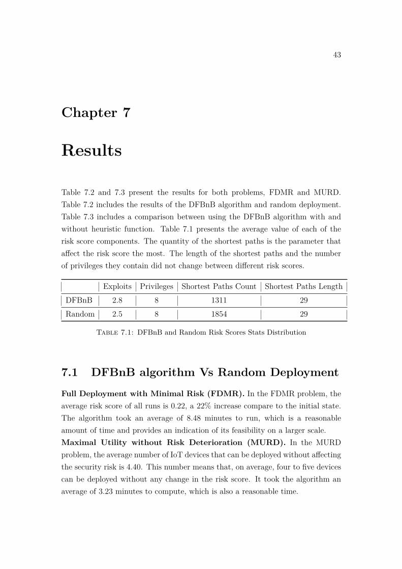
Table 7.2 and 7.3 present the results for both problems, FDMR and MURD.Table 7.2 includes the results of the DFBnB algorithm and random deployment.Table 7.3 includes a comparison between using the DFBnB algorithm with andwithout heuristic function. Table 7.1 presents the average value of each of therisk score components. The quantity of the shortest paths is the parameter thataffect the risk score the most. The length of the shortest paths and the numberof privileges they contain did not change between different risk scores.

Exploits Privileges Shortest Paths Count Shortest Paths LengthDFBnB 2.8 8 1311 29Random 2.5 8 1854 29

Table 7.1: DFBnB and Random Risk Scores Stats Distribution

7.1 DFBnB algorithm Vs Random Deployment

Full Deployment with Minimal Risk (FDMR). In the FDMR problem, theaverage risk score of all runs is 0.22, a 22% increase compare to the initial state.The algorithm took an average of 8.48 minutes to run, which is a reasonableamount of time and provides an indication of its feasibility on a larger scale.Maximal Utility without Risk Deterioration (MURD). In the MURDproblem, the average number of IoT devices that can be deployed without affectingthe security risk is 4.40. This number means that, on average, four to five devicescan be deployed without any change in the risk score. It took the algorithm anaverage of 3.23 minutes to compute, which is also a reasonable time.

Chapter 7. Results 44

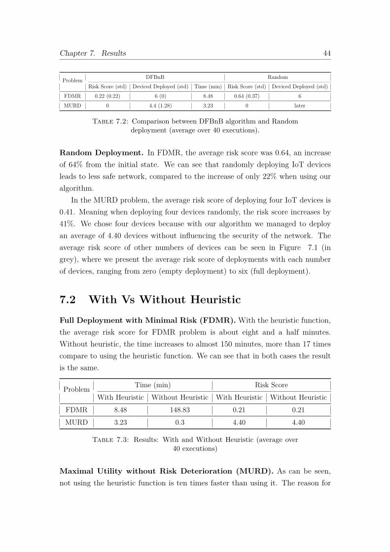
Problem DFBnB RandomRisk Score (std) Deviced Deployed (std) Time (min) Risk Score (std) Deviced Deployed (std)

FDMR 0.22 (0.22) 6 (0) 8.48 0.64 (0.37) 6MURD 0 4.4 (1.28) 3.23 0 later

Table 7.2: Comparison between DFBnB algorithm and Randomdeployment (average over 40 executions).

Random Deployment. In FDMR, the average risk score was 0.64, an increaseof 64% from the initial state. We can see that randomly deploying IoT devicesleads to less safe network, compared to the increase of only 22% when using ouralgorithm.

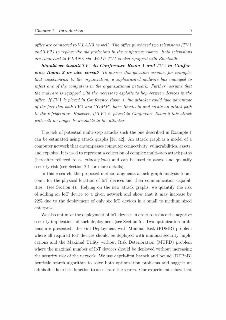
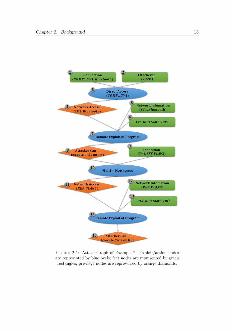
In the MURD problem, the average risk score of deploying four IoT devices is0.41. Meaning when deploying four devices randomly, the risk score increases by41%. We chose four devices because with our algorithm we managed to deployan average of 4.40 devices without influencing the security of the network. Theaverage risk score of other numbers of devices can be seen in Figure 7.1 (ingrey), where we present the average risk score of deployments with each numberof devices, ranging from zero (empty deployment) to six (full deployment).

7.2 With Vs Without Heuristic

Full Deployment with Minimal Risk (FDMR). With the heuristic function,the average risk score for FDMR problem is about eight and a half minutes.Without heuristic, the time increases to almost 150 minutes, more than 17 timescompare to using the heuristic function. We can see that in both cases the resultis the same.

Problem Time (min) Risk ScoreWith Heuristic Without Heuristic With Heuristic Without Heuristic

FDMR 8.48 148.83 0.21 0.21MURD 3.23 0.3 4.40 4.40

Table 7.3: Results: With and Without Heuristic (average over40 executions)

Maximal Utility without Risk Deterioration (MURD). As can be seen,not using the heuristic function is ten times faster than using it. The reason for


this is due to the extra time using a heuristic function is adding. On average,it take about 45 seconds to compute the heuristic table. Also, using a heuristicis another operation that may take some time, as we need to look in the tableand update it. In this case, using the heuristic did not helped in improving therunning time, and the algorithm did well on his own without it.

7.3 Additional Results

7.3.1 Trade-off

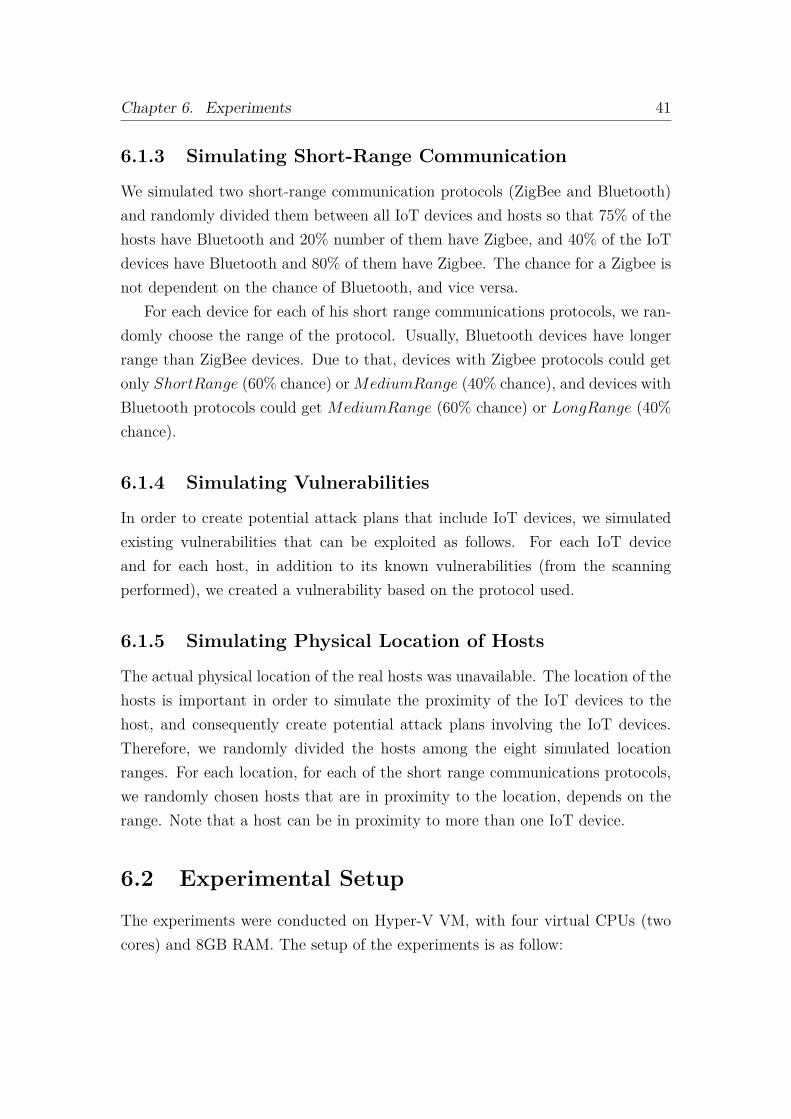
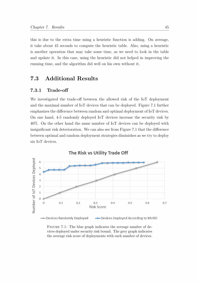
We investigated the trade-off between the allowed risk of the IoT deploymentand the maximal number of IoT devices that can be deployed. Figure 7.1 furtheremphasizes the difference between random and optimal deployment of IoT devices.On one hand, 4-5 randomly deployed IoT devices increase the security risk by40%. On the other hand the same number of IoT devices can be deployed withinsignificant risk deterioration. We can also see from Figure 7.1 that the differencebetween optimal and random deployment strategies diminishes as we try to deploysix IoT devices.

Figure 7.1: The blue graph indicates the average number of de-vices deployed under security risk bound. The grey graph indicatesthe average risk score of deployments with each number of devices.


7.3.2 Cumulative Distribution

Figure 7.2 illustrates the challenge in finding the safest deployment of IoT devices.The graph presents the cumulative distribution of the risk scores of all deploymentsin one execution. The x-axis is the cumulative risk score, and the y-axis is thepercentage of deployments for which the risk score is less than x. As can be seen,50% of the deployments have a risk score lower than 0.78. Moreover, only 12deployments (0.04% of all deployments) are optimal, with a risk score of 0.307,i.e., the chances of a random selection to choose an optimal deployment in thatexecution was 0.00004.

Figure 7.2: The x-axis is the cumulative risk score, and the y-axis is the percentage of deployments for which the risk score is

less than x.

7.3.3 Robustness

The risk score of an optimal deployment may change when new vulnerabilitiesare discovered, leading to potentially inferior deployment. To conclude the ex-perimental evaluation we tested the robustness of the optimal deployment of anarbitrary execution from the FDMR problem, with risk score of 0.3164. We per-turbed vulnerabilities of 10% and 20% of the devices in the network by discarding


all current vulnerabilities of the chosen devices and randomly assigning new vul-nerabilities as described in Section 6.1. This process was repeated ten times. Theaverage risk score of the optimal deployment after changing 10% of the vulner-abilities was 0.308 with standard deviation of 0.007. For changing 20% of thevulnerabilities, the average risk score was 0.266 with standard deviation of 0.07.Overall the changes in the risk of the optimal deployment due to perturbation ofthe vulnerabilities were not statistically significant.

48

Chapter 8

Conclusion

We present a novel method for suggesting the optimal deployment (in terms ofthe security risk) of a set of IoT devices within an organization. In order to ac-complish this, we augmented the conventional attack graph to include short-rangecommunication protocols inherent to IoT devices. To the best of our knowledge,this is the first work that takes the physical location of devices and differentcommunication protocols into account.

We demonstrated the importance of planning a deployment of IoT devicesby solving two scenarios, approaching them as an optimization problem. Weproposed a novel method for evaluating the risk of IoT device deployment usingan augmented attack graph, and used the proposed method to address these twoscenarios. Our results revealed the potential risk in deploying IoT devices inorganizations and showed that randomly deploying devices can greatly affect thesecurity of the organization’s network. We solved the two scenarios on a realorganization with a small to medium sized network, with a running time of lessthan ten minutes.

49

Chapter 9

Future Work

Our algorithm, and in particular, our heuristic approach, assumes that the po-tential risk of two deployed devices is greater than or equal to the sum of theirindividual risk scores. Any method of risk calculation that satisfies this assump-tion can be used in the algorithm. The method of risk score calculation usedin this work has some limitations. It does not take the cost of different exploitsinto account, which can be a major consideration for an attacker. As a result,the method does not capture the heterogeneity and homogeneity of vulnerabilitiesalong an attack path.

Future work may extend the current research in the following directions. First,it is desirable to increase sizes of the attack graph that can be optimized by pro-viding more accurate heuristic functions. In addition, the optimization methodsproposed in this work should be tested with variety of risk scores that encompassthe true cost of the attack, the probability of the attack success, or both. Finally,cyber-physical capabilities of IoT devices as well as their unique functionalitiesshould be incorporated into an extended model.

50

Bibliography

[1] M Abadi and S Jalili. “An ant colony optimization algorithm for networkvulnerability analysis”. In: Iranian Journal of Electrical and Electronic En-gineering 2.3 (2006), pp. 106–120.

[2] Habtamu Abie and Ilangko Balasingham. “Risk-based adaptive security forsmart IoT in eHealth”. In: Proceedings of the 7th International Conferenceon Body Area Networks. ICST (Institute for Computer Sciences, Social-Informatics and . . . 2012, pp. 269–275.

[3] Hussain MJ Almohri et al. “Security optimization of dynamic networks withprobabilistic graph modeling and linear programming”. In: IEEE Transac-tions on Dependable and Secure Computing 13.4 (2016), pp. 474–487.

[4] Paul Ammann, Duminda Wijesekera, and Saket Kaushik. “Scalable, graph-based network vulnerability analysis”. In: Proceedings of the 9th ACM con-ference on Computer and communications security - CCS ’02 (2002), p. 217.doi: 10.1145/586110.586140. url: http://dl.acm.org/citation.cfm?id=586110.586140.

[5] Anonymous. Internet Census 2012. Tech. rep. Independent, 2012. url: http://census2012.sourceforge.net/paper.html.

[6] Marc Arnaert and Sophia Antipolis. “Modeling Vulnerable Internet of Thingson SHODAN and CENSYS : An Ontology for Cyber Security”. In: Secur-ware (2016).

[7] Debasis Bandyopadhyay and Jaydip Sen. “Internet of things: Applicationsand challenges in technology and standardization”. In: Wireless PersonalCommunications 58.1 (2011), pp. 49–69. issn: 09296212. doi: 10.1007/s11277-011-0288-5.

[8] Mario Ballano Barcena and Candid Wueest. Insecurity in the Internet ofThings. Tech. rep. March. 2015.

http://dx.doi.org/10.1145/586110.586140

http://dl.acm.org/citation.cfm?id=586110.586140

http://dl.acm.org/citation.cfm?id=586110.586140

http://census2012.sourceforge.net/paper.html

http://census2012.sourceforge.net/paper.html

http://dx.doi.org/10.1007/s11277-011-0288-5

http://dx.doi.org/10.1007/s11277-011-0288-5

BIBLIOGRAPHY 51

[9] BBC. Fridge sends spam emails as attack hits smart gadgets. Jan. 2014. url:http://www.bbc.com/news/technology-25780908.

[10] Jay Beale et al. Nessus network auditing. Syngress Publishing, 2004.

[11] Feng Chen et al. “A scalable approach to analyzing network security usingcompact attack graphs”. In: Journal of Networks 5.5 (2010), p. 543.

[12] Peter Cope, Joseph Campbell, and Thaier Hayajneh. “An investigation ofBluetooth security vulnerabilities”. In: 2017 IEEE 7th Annual Comput-ing and Communication Workshop and Conference (CCWC). IEEE. 2017,pp. 1–7.

[13] Ang Cui and Salvatore J. Stolfo. “A quantitative analysis of the insecurityof embedded network devices”. In: Proceedings of the 26th Annual Com-puter Security Applications Conference on - ACSAC ’10 (2010), p. 97. issn:10639527. doi: 10.1145/1920261.1920276. url: http://portal.acm.org/citation.cfm?doid=1920261.1920276.

[14] John Dunning. “Taming the blue beast: A survey of bluetooth based threats”.In: IEEE Security & Privacy 8.2 (2010), pp. 20–27.

[15] Vangelis Gazis et al. “Short Paper: IoT: Challenges, projects, architectures”.In: 2015 18th International Conference on Intelligence in Next GenerationNetworks (2015), pp. 145–147. doi: 10.1109/ICIN.2015.7073822.

[16] Mengmeng Ge and Dong Seong Kim. “A framework for modeling and as-sessing security of the internet of things”. In: Proceedings of the Interna-tional Conference on Parallel and Distributed Systems - ICPADS. 2016.isbn: 9780769557854. doi: 10.1109/ICPADS.2015.102.

[17] Mengmeng Ge et al. “Security modeling and analysis of cross-protocol IoTdevices”. In: Proceedings - 16th IEEE International Conference on Trust, Se-curity and Privacy in Computing and Communications, 11th IEEE Interna-tional Conference on Big Data Science and Engineering and 14th IEEE In-ternational Conference on Embedded Software and Systems (2017), pp. 1043–1048. doi: 10.1109/Trustcom/BigDataSE/ICESS.2017.350.

[18] Avitan Gefen and Ronen Brafman. “Pruning methods for optimal delete-free planning”. In: Twenty-Second International Conference on AutomatedPlanning and Scheduling. 2012.

http://www.bbc.com/news/technology-25780908

http://dx.doi.org/10.1145/1920261.1920276

http://portal.acm.org/citation.cfm?doid=1920261.1920276

http://portal.acm.org/citation.cfm?doid=1920261.1920276

http://dx.doi.org/10.1109/ICIN.2015.7073822

http://dx.doi.org/10.1109/ICPADS.2015.102

http://dx.doi.org/10.1109/Trustcom/BigDataSE/ICESS.2017.350

BIBLIOGRAPHY 52

[19] Gemini George and Sabu M Thampi. “A graph-based security frameworkfor securing industrial IoT networks from vulnerability exploitations”. In:IEEE Access 6 (2018), pp. 43586–43601.

[20] Tom Gonda et al. “Ranking vulnerability fixes using planning graph analy-sis”. In: IWAISe: First International Workshop on Artificial Intelligence inSecurity. 2017, p. 41.

[21] Jin Hong and Dong-Seong Kim. “Harms: Hierarchical attack representationmodels for network security analysis”. In: (2012).

[22] Jun Huang et al. “A novel deployment scheme for green internet of things”.In: IEEE Internet of Things Journal 1.2 (2014), pp. 196–205.

[23] Nwokedi Idika and Bharat Bhargava. “Extending attack graph-based secu-rity metrics and aggregating their application”. In: IEEE Transactions ondependable and secure computing 9.1 (2010), pp. 75–85.

[24] Tania Islam and Lingyu Wang. “A heuristic approach to minimum-cost net-work hardening using attack graph”. In: 2008 New Technologies, Mobilityand Security. IEEE. 2008, pp. 1–5.

[25] MA Jun-chun et al. “A minimum cost of network hardening model basedon attack graphs”. In: Procedia Engineering 15 (2011), pp. 3227–3233.

[26] Richard E. Korf. “Artificial Intelligence Search Algorithms”. In: Algorithmsand theory of computation handbook. Ed. by Mikhail J. Atallah and MarinaBlanton. 2010, p. 22. isbn: 978-1-58488-820-8.

[27] Brian Krebs. “Lizard Stresser Runs on Hacked Home Routers”. In: KrebsOn-Security (Jan. 2015), p. 1. url: https://krebsonsecurity.com/2015/01/lizard-stresser-runs-on-hacked-home-routers/.

[28] Caiming Liu et al. “Research on Dynamical Security Risk Assessment forthe Internet of Things inspired by immunology”. In: Natural Computation(ICNC), 2012 Eighth International Conference on. IEEE. 2012, pp. 874–878.

[29] Rwan Mahmoud et al. “Internet of Things ( IoT ) Security : Current Status, Challenges and Prospective Measures”. In: ().

https://krebsonsecurity.com/2015/01/lizard-stresser-runs-on-hacked-home-routers/

https://krebsonsecurity.com/2015/01/lizard-stresser-runs-on-hacked-home-routers/

BIBLIOGRAPHY 53

[30] Linda Markowsky and George Markowsky. “Scanning for vulnerable devicesin the Internet of Things”. In: Proceedings of the 2015 IEEE 8th Interna-tional Conference on Intelligent Data Acquisition and Advanced Comput-ing Systems: Technology and Applications, IDAACS 2015 1.October 2015(2015), pp. 463–467. issn: 19454589. doi: 10.1109/IDAACS.2015.7340779.

[31] Rob van der Meulen. “Gartner Says 8.4 Billion Connected "Things" Will Bein Use in 2017, Up 31 Percent From 2016”. In: Gartner (2017), p. 1. url:https://www.gartner.com/newsroom/id/3598917.

[32] Nateq Be-Nazir Ibn Minar and Mohammed Tarique. “Bluetooth securitythreats and solutions: a survey”. In: International Journal of Distributedand Parallel Systems 3.1 (2012), p. 127.

[33] Mujahid Mohsin et al. “IoTRiskAnalyzer: A Probabilistic Model CheckingBased Framework for Formal Risk Analytics of the Internet of Things.” In:IEEE Access 5 (2017), pp. 5494–5505.

[34] Philipp Morgner, Stephan Mattejat, and Zinaida Benenson. “All your bulbsare belong to us: Investigating the current state of security in connectedlighting systems”. In: arXiv preprint arXiv:1608.03732 (2016).

[35] Steven Noel and Sushil Jajodia. “Optimal ids sensor placement and alertprioritization using attack graphs”. In: Journal of Network and SystemsManagement 16.3 (2008), pp. 259–275.

[36] Steven Noel and Sushil Jajodia. “Metrics suite for network attack graphanalytics”. In: Proceedings of the 9th Annual Cyber and Information SecurityResearch Conference. ACM. 2014, pp. 5–8.

[37] Steven Noel et al. “Efficient minimum-cost network hardening via exploitdependency graphs”. In: 19th Annual Computer Security Applications Con-ference, 2003. Proceedings. IEEE. 2003, pp. 86–95.

[38] Xinming Ou, Wayne F Boyer, and Miles A McQueen. “A scalable approachto attack graph generation”. In: Proceedings of the 13th ACM conference onComputer and communications security. ACM. 2006, pp. 336–345.

[39] Xinming Ou and Sudhakar Govindavajhala. “Mulval: A logic-based networksecurity analyzer”. In: In 14th USENIX Security Symposium. Citeseer. 2005.

[40] Yin Minn Pa Pa et al. “IoTPOT: Analysing the Rise of IoT Compromises”.In: EMU 9 (2015), p. 1. issn: 19449224. doi: 10.1002/2014GB005021.

http://dx.doi.org/10.1109/IDAACS.2015.7340779

https://www.gartner.com/newsroom/id/3598917

http://dx.doi.org/10.1002/2014GB005021

BIBLIOGRAPHY 54

[41] Mark Patton et al. “Uninvited connections: A study of vulnerable devices onthe internet of things (IoT)”. In: Proceedings - 2014 IEEE Joint Intelligenceand Security Informatics Conference, JISIC 2014 (2014), pp. 232–235. doi:10.1109/JISIC.2014.43.

[42] Cynthia Phillips and Laura Painton Swiler. “A graph-based system fornetwork-vulnerability analysis”. In: Proceedings of the 1998 workshop onNew security paradigms. ACM. 1998, pp. 71–79.

[43] Hadar Polad, Rami Puzis, and Bracha Shapira. “Attack graph obfuscation”.In: International Conference on Cyber Security Cryptography and MachineLearning. Springer. 2017, pp. 269–287.

[44] Alexander Reinefeld and T. Anthony Marsland. “Enhanced iterative-deepeningsearch”. In: IEEE Transactions on Pattern Analysis and Machine Intelli-gence 16.7 (1994), pp. 701–710.

[45] Rodrigo Roman, Pablo Najera, and Javier Lopez. “Securing the internet ofthings”. In: Computer 44.9 (2011), pp. 51–58.

[46] Eyal Ronen and Adi Shamir. “Extended functionality attacks on IoT de-vices: The case of smart lights”. In: Proceedings - 2016 IEEE EuropeanSymposium on Security and Privacy, EURO S and P 2016 (2016), pp. 3–12. doi: 10.1109/EuroSP.2016.13.

[47] Eyal Ronen et al. “IoT goes nuclear: Creating a ZigBee chain reaction”. In:Security and Privacy (SP), 2017 IEEE Symposium on. IEEE. 2017, pp. 195–212.

[48] Mike Ryan. “Bluetooth: With low energy comes low security”. In: Presentedas part of the 7th USENIX Workshop on Offensive Technologies. 2013.

[49] S Sandhya and KA Sumithra Devi. “Analysis of Bluetooth threats and v4. 0security features”. In: 2012 International Conference on Computing, Com-munication and Applications. IEEE. 2012, pp. 1–4.

[50] Freddy K Santoso and Nicholas CH Vun. “Securing IoT for smart homesystem”. In: Consumer Electronics (ISCE), 2015 IEEE International Sym-posium on. IEEE. 2015, pp. 1–2.

[51] Reginald E Sawilla and Xinming Ou. “Identifying critical attack assets independency attack graphs”. In: European Symposium on Research in Com-puter Security. Springer. 2008, pp. 18–34.

http://dx.doi.org/10.1109/JISIC.2014.43

http://dx.doi.org/10.1109/EuroSP.2016.13

BIBLIOGRAPHY 55

[52] VL Shivraj, MA Rajan, and P Balamuralidhar. “A graph theory basedgeneric risk assessment framework for internet of things (IoT)”. In: 2017IEEE International Conference on Advanced Networks and Telecommunica-tions Systems (ANTS). IEEE. 2017, pp. 1–6.

[53] Anoop Singhal and Ximming Ou. “Security Risk Analysis of EnterpriseNetworks Using Probabilistic Attack Graphs”. In: NIST Interagency Report7788, National iInstitute of Standards and Technology, U.S. Department ofCommerce. (2011).

[54] Antonio F Skarmeta, Jose L Hernandez-Ramos, and M Victoria Moreno. “Adecentralized approach for security and privacy challenges in the internet ofthings”. In: Internet of Things (WF-IoT), 2014 IEEE World Forum on.IEEE. 2014, pp. 67–72.

[55] Angelos Stavrou, Jeffrey Voas, and Ieee Fellow. “DDoS in the IoT”. In:Computer 50 (2017), pp. 80–84. issn: 0018-9162. doi: 10.1109/MC.2017.201.

[56] Laura P Swiler et al. “Computer-attack graph generation tool”. In: Pro-ceedings DARPA Information Survivability Conference and Exposition II.DISCEX’01. Vol. 2. IEEE. 2001, pp. 307–321.

[57] Ivan Vaccari, Enrico Cambiaso, and Maurizio Aiello. “Remotely Exploitingat Command Attacks on ZigBee Networks”. In: Security and Communica-tion Networks 2017 (2017). issn: 19390122. doi: 10.1155/2017/1723658.

[58] Lingyu Wang et al. “An attack graph-based probabilistic security metric”.In: Lecture Notes in Computer Science (including subseries Lecture Notesin Artificial Intelligence and Lecture Notes in Bioinformatics) 5094 LNCS(2008), pp. 283–296. issn: 03029743. doi: 10.1007/978-3-540-70567-3\_22.

[59] Joshua Wright. “Killerbee: practical zigbee exploitation framework”. In:11th ToorCon conference, San Diego. Vol. 67. 2009.

[60] Beytüllah Yiğit et al. “Cost-aware securing of IoT systems using attackgraphs”. In: Ad Hoc Networks 86 (2019), pp. 23–35.

[61] Tianlong Yu et al. “Handling a trillion (unfixable) flaws on a billion devices”.In: Proceedings of the 14th ACM Workshop on Hot Topics in Networks -HotNets-XIV. 2015. isbn: 9781450340472. doi: 10.1145/2834050.2834095.

http://dx.doi.org/10.1109/MC.2017.201

http://dx.doi.org/10.1109/MC.2017.201

http://dx.doi.org/10.1155/2017/1723658

http://dx.doi.org/10.1007/978-3-540-70567-3\_22

http://dx.doi.org/10.1007/978-3-540-70567-3\_22

http://dx.doi.org/10.1145/2834050.2834095

BIBLIOGRAPHY 56

[62] Andrea Zanella et al. “Internet of things for smart cities”. In: IEEE Internetof Things journal 1.1 (2014), pp. 22–32.

[63] Weixiong Zhang and Richard E Korf. “Performance of linear-space searchalgorithms”. In: Artificial Intelligence 79.2 (1995), pp. 241–292.

[64] Zhi-Kai Zhang et al. “IoT security: ongoing challenges and research oppor-tunities”. In: Service-Oriented Computing and Applications (SOCA), 2014IEEE 7th International Conference on. IEEE. 2014, pp. 230–234.

[65] Rong Zhou and Eric A. Hansen. “Breadth-first heuristic search”. In: Arti-ficial Intelligence (2006). issn: 00043702. doi: 10.1016/j.artint.2005.12.002.

[66] Tobias Zillner. “ZigBee Exploited - The Good, the Bad and the Ugly”. In:Black Hat 16.2 (2015), p. 6. doi: 10.1007/s11229- 007- 9263- 9. url:https://www.blackhat.com/docs/us-15/materials/us-15-Zillner-ZigBee-Exploited-The-Good-The-Bad-And-The-Ugly-wp.pdf.

http://dx.doi.org/10.1016/j.artint.2005.12.002

http://dx.doi.org/10.1016/j.artint.2005.12.002

http://dx.doi.org/10.1007/s11229-007-9263-9

https://www.blackhat.com/docs/us-15/materials/us-15-Zillner-ZigBee-Exploited-The-Good-The-Bad-And-The-Ugly-wp.pdf

https://www.blackhat.com/docs/us-15/materials/us-15-Zillner-ZigBee-Exploited-The-Good-The-Bad-And-The-Ugly-wp.pdf

Deployment Optimization of IoT Devices through Attack Graph ...

Documents

Transcript of Deployment Optimization of IoT Devices through Attack Graph ...