DOCKETED Docket Number: 18-AAER-05

Project Title: Commercial and Industrial Air Compressors

TN #: 225912-6

Document Title: Department of Energy Technical Support Document

Description: Document relied upon - commercial and industrial air compressors.

Filer: Corrine Fishman

Organization: California Energy Commission

Submitter Role: Energy Commission

Submission Date: 11/16/2018 9:40:28 AM

Docketed Date: 11/16/2018

TECHNICAL SUPPORT DOCUMENT: ENERGY EFFICIENCY PROGRAM FOR CONSUMER PRODUCTS AND COMMERCIAL AND INDUSTRIAL EQUIPMENT: AIR COMPRESSORS December, 2016

U.S. Department of Energy Assistant Secretary Office of Energy Efficiency and Renewable Energy Building Technologies Program Appliances and Commercial Equipment Standards Washington, DC 20585

This Document was prepared for the Department of Energy by staff members of

Navigant Consulting, Inc. and

Lawrence Berkeley National Laboratory

1-i

CHAPTER 1. INTRODUCTION

TABLE OF CONTENTS

1.1 DOCUMENT PURPOSE ................................................................................................ 1-1 1.2 SUMMARY OF NATIONAL BENEFITS ..................................................................... 1-1 1.3 OVERVIEW OF STANDARDS ..................................................................................... 1-4 1.4 PROCESS FOR SETTING ENERGY CONSERVATION STANDARDS ................... 1-6 1.5 STRUCTURE OF THE DOCUMENT ............................................................................ 1-8

LIST OF TABLES

Table 1.2.1 Annualized Benefits and Costs of Proposed Standards for Compressors...... 1-3 Table 1.3.1 Energy Conservation Standards for Air Compressors ................................... 1-6 Table 1.4.1 Final Rule Analyses ....................................................................................... 1-7

1-1

CHAPTER 1. INTRODUCTION

1.1 DOCUMENT PURPOSE

This technical support document (TSD) is a standalone document that presents the technical analyses that the U.S. Department of Energy (DOE) conducted for evaluating new energy conservation standards for compressors.

1.2 SUMMARY OF NATIONAL BENEFITS

DOE’s analyses indicate that the proposed standards would save a significant amount of energy. The lifetime full-fuel cycle energy savings for the compressor classes covered by this rulemaking purchased in the 30-year period that begins in the year of compliance with the proposed standards (2022–2051)a amount to 0.16 quads.b

The cumulative net present value (NPV) of total consumer costs and savings of the standards for air compressors ranges from $0.16 billion (at a 7-percent discount rate) to $0.45 billion (at a 3-percent discount rate). This NPV expresses the estimated total value of future operating-cost savings minus the estimated increased equipment costs for air compressors purchased in 2022–2051.

In addition, the adopted standards for compressors are projected to yield significant environmental benefits. DOE estimates that the standards will result in cumulative emission reductions (over the same period as for energy savings) of 8.2 million metric tons (Mt)c of carbon dioxide (CO2), 6.5 thousand tons of sulfur dioxide (SO2), 11.0 tons of nitrogen oxides (NOX), 40.8 thousand tons of methane (CH4), 0.1 thousand tons of nitrous oxide (N2O), and 0.02 ton of mercury (Hg).d

The benefits and costs of the adopted standards, for equipment sold in 2022-2051, can also be expressed in terms of annualized values. The annualized monetary values are the sum of (1) the annualized national economic value of the benefits from consumer operation of equipment that meets the standards (consisting primarily of operating cost savings from using less energy, minus increases in equipment purchase and installation costs), and (2) the annualized monetary value of the benefits of emission reductions, including CO2 emission reductions. The value of the CO2 reductions, otherwise known as the Social Cost of Carbon (SCC), is calculated using a range of values per metric ton of CO2 developed by a recent interagency process. The derivation of the SCC values is discussed in chapter 14 of the TSD. a The analysis uses January 1, 2022, to represent the expected compliance date in late 2021. Therefore, the 30-year analysis period is referred to as 2022-2051 in this document. b The year 2020 was chosen in anticipation of the potential compliance date. c A metric ton is equivalent to 1.1 short tons. Results for emissions other than CO2 are presented in short tons. d DOE calculated emissions reductions relative to the no-new-standards-case, which reflects key assumptions in the Annual Energy Outlook 2016 (AEO 2016). AEO 2016 represents current federal and state legislation and final implementation of regulations as of the end of February 2016. DOE is using the projection consistent with the cases described on page E-8 of AEO 2016.

1-2

Although combining the values of operating savings and CO2 emission reductions provides a useful perspective, two issues should be considered. First, the national operating savings are domestic U.S. consumer monetary savings that occur as a result of market transactions, while the value of CO2 reductions is based on a global value. Second, the assessments of operating cost savings and CO2 savings are performed using different methods that use different time frames for analysis. The national operating cost savings is measured for the lifetime of compressors shipped from 2022–2051. The SCC values, on the other hand, reflect the present value of some future climate-related impacts resulting from the emission of one ton of carbon dioxide in each year. These impacts continue well beyond 2100.

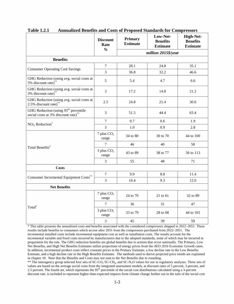
Table 1.2.1 shows the annualized values for the final compressor energy conservation standards. (All monetary values below are expressed in 2015$.) The results under the primary estimate are as follows. Using a 7-percent discount rate for benefits and costs other than greenhouse gas (GHG) reduction (for which DOE used average social costs with a 3-percent discount rate),e the estimated cost of the standards in this rule is $9.9 million per year in increased equipment costs, while the estimated annual benefits are $28.1 million in reduced equipment operating costs, $17.2 million in GHG reductions, and $0.7 million in reduced NOX emissions. Using a 7-percent discount rate, the net benefit amounts to $36 million per year. Using a 3-percent discount rate for all benefits and costs, the estimated cost of the standards is $10.4 million per year in increased equipment costs, while the estimated annual benefits are $36.8 million in reduced operating costs, $17.2 million in GHG reductions, and $1.0 million in reduced NOX emissions. Using a 3-percent discount rate, the net benefit amounts to $45 million per year.

e DOE used average social costs with a 3-percent discount rate because these values are considered as the “central” estimates by the interagency group.

1-3

Table 1.2.1 Annualized Benefits and Costs of Proposed Standards for Compressors

Discount

Rate %

Primary Estimate

Low-Net- Benefits Estimate

High-Net- Benefits Estimate

million 2015$/year Benefits

Consumer Operating Cost Savings 7 28.1 24.8 35.1 3 36.8 32.2 46.6

GHG Reduction (using avg. social costs at 5% discount rate)** 5 5.4 4.7 6.6

GHG Reduction (using avg. social costs at 3% discount rate)** 3 17.2 14.8 21.2

GHG Reduction (using avg. social costs at 2.5% discount rate)** 2.5 24.8 21.4 30.6

GHG Reduction (using 95th percentile social costs at 3% discount rate)** 3 51.5 44.4 63.4

NOX Reduction† 7 0.7 0.6 1.9 3 1.0 0.9 2.8

Total Benefits‡

7 plus CO2 range 34 to 80 30 to 70 44 to 100

7 46 40 58 3 plus CO2

range 43 to 89 38 to 77 56 to 113

3 55 48 71 Costs

Consumer Incremental Equipment Costs†† 7 9.9 8.8 11.4 3 10.4 9.3 12.0

Net Benefits

Total‡

7 plus CO2 range 24 to 70 21 to 61 32 to 89

7 36 31 47 3 plus CO2

range 33 to 79 28 to 68 44 to 101

3 45 39 59 * This table presents the annualized costs and benefits associated with the considered compressors shipped in 2022–2051. These results include benefits to consumers which accrue after 2051 from the compressors purchased from 2022–2051. The incremental installed costs include incremental equipment cost as well as installation costs. The results account for the incremental variable and fixed costs incurred by manufacturers due to the adopted standards, some of which may be incurred in preparation for the rule. The GHG reduction benefits are global benefits due to actions that occur nationally. The Primary, Low Net Benefits, and High Net Benefits Estimates utilize projections of energy prices from the AEO 2016 Economic Growth cases. In addition, incremental product costs reflect constant prices in the Primary Estimate, a low decline rate in the Low Benefits Estimate, and a high decline rate in the High Benefits Estimate. The methods used to derive projected price trends are explained in chapter 10. Note that the Benefits and Costs may not sum to the Net Benefits due to rounding. ** The interagency group selected four sets of SC-CO2 SC-CH4, and SC-N2O values for use in regulatory analyses. Three sets of values are based on the average social costs from the integrated assessment models, at discount rates of 5 percent, 3 percent, and 2.5 percent. The fourth set, which represents the 95th percentile of the social cost distributions calculated using a 3-percent discount rate, is included to represent higher-than-expected impacts from climate change further out in the tails of the social cost

1-4

distributions. The social cost values are emission year specific. The GHG reduction benefits are global benefits due to actions that occur nationally. See chapter 14 for more details. † DOE estimated the monetized value of NOX emissions reductions associated with electricity savings using benefit per ton estimates from the Regulatory Impact Analysis for the Clean Power Plan Final Rule, published in August 2015 by EPA’s Office of Air Quality Planning and Standards. (Available at www.epa.gov/cleanpowerplan/clean-power-plan-final-rule-regulatory-impact-analysis.) See chapter 13 for further discussion. For the Primary Estimate and Low Net Benefits Estimate, DOE used national benefit-per-ton estimates for NOX emitted from the Electric Generating Unit sector based on an estimate of premature mortality used by EPA. . For the High Net Benefits Estimate, the benefit-per-ton estimates were based on the Six Cities study (Lepuele et al. 2011); these are nearly two-and-a-half times larger than those from the American Cancer Society (“ACS”) study. ‡ Total Benefits for both the 3 percent and 7 percent cases are presented using the average social costs with 3-percent discount rate. In the rows labeled “7% plus GHG range” and “3% plus GHG range,” the operating cost and NOX benefits are calculated using the labeled discount rate, and those values are added to the full range of social cost values. †† The incremental installed costs include incremental equipment cost as well as installation costs. The results account for the incremental variable and fixed costs incurred by manufacturers due to the proposed standards, some of which may be incurred in preparation for the rule.

1.3 OVERVIEW OF STANDARDS

Title III of the Energy Policy and Conservation Act of 1975, as amended (EPCA), sets forth a variety of provisions designed to improve energy efficiency. (42 U.S.C. 6291, et seq.) Part C of Title III, which for editorial reasons was re-designated as Part A-1 upon incorporation into the U.S. Code (42 U.S.C. 6311–6317), establishes the Energy Conservation Program for Certain Industrial Equipment. EPCA provides that DOE may include a type of industrial equipment as covered equipment if it determines that to do so is necessary to carry out the purposes of Part A-1. (42 U.S.C 6312(b)) EPCA authorizes DOE to prescribe energy conservation standards for those types of industrial equipment which the Secretary classifies as covered equipment. (42 U.S.C 6311(2) and 6312) In November 2016, DOE published a final rule that determined coverage for compressors is necessary to carry out the purposes of Part A-1 of Title III of EPCA (herein referred to as “notice of final determination”).f

Currently, there are no Federal energy conservation standards for air compressors. On December 31, 2012, DOE published a notice of proposed determination of coverage (2012 proposed determination of coverage) that proposed to establish compressors as covered equipment on the basis that (1) DOE may only prescribe energy conservation standards for covered equipment; and (2) energy conservation standards for compressors would improve the efficiency of such equipment more than would be likely to occur in the absence of standards, so including compressors as covered equipment is necessary to carry out the purposes of Part A-1. 77 FR 76972 (Dec. 31, 2012). The 2012 proposed determination of coverage tentatively determined that the standards would likely satisfy the provisions of 42 U.S.C. 6311(2)(B)(i). On February 7, 2013, DOE published a notice reopening the comment period on the 2012 proposed determination of coverage. 78 FR 8998.

On February 5, 2014, DOE published in the Federal Register a notice of public meeting, and provided a Framework document that addressed potential standards and test procedures for these products. 79 FR 6839. DOE held a public meeting to discuss the framework document on April 1, 2014. At this meeting, DOE discussed and received comments on the Framework document, which covered the analytical framework, models, and tools that DOE uses to evaluate f A link to the docket webpage can be found at: www.regulations.gov/docket?D=EERE-2012-BT-DET-0033

1-5

potential standards; and all other issues raised relevant to the development of energy conservation standards for the different categories of compressors. On March 18, 2014, DOE extended the comment period. 79 FR 15061.

On May 5, 2016, DOE published a notice of proposed rulemaking (NOPR) to propose test procedures for certain compressors. 87 FR 27220. On June 20, 2016, DOE held a public meeting to discuss the test procedure NOPR and accept comments from interested parties. On December 1, 2016, DOE issued a test procedure final rule that amends subpart T of Title 10 of the Code of Federal Regulations, part 431 (10 CFR 431), and which contains definitions, materials incorporated by reference, and test procedures for determining the energy efficiency of certain varieties of compressors. The test procedure final rule also amended 10 CFR 429 to establish sampling plans, representations requirements, and enforcement provisions for certain compressors.

On May 19, 2016, DOE published a NOPR pertaining to energy conservation standards for compressors (May 2016 NOPR).g 81 FR 31680. DOE held a public meeting to discuss the May 2016 NOPR on June 20, 2016.

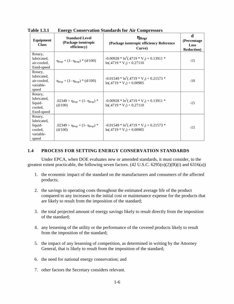
In this final rule, DOE is adopting energy conservation standards for compressors. The standards are expressed in package isentropic efficiency (i.e., the ratio of the theoretical isentropic power required for a compression process to the actual power required for the same process), as shown in Table 1.3.1. These standards apply to all compressors listed in Table 1.3.1 and manufactured in, or imported into, the United States starting on December 1, 2021.

In Table 1.3.1, the term V1 denotes the full-load actual volume flow rate of the compressor, in cubic feet per minute (cfm). Standard levels are expressed as a function of full-load actual volume flow rate for each equipment class, and may be calculated by inserting values from the rightmost two columns into the second leftmost column. Doing so will yield an efficiency-denominated function of full-load actual volume flow rate.

g Available at: www.regulations.gov/document?D=EERE-2013-BT-STD-0040-0038.

1-6

Table 1.3.1 Energy Conservation Standards for Air Compressors

Equipment Class

Standard Level (Package isentropic

efficiency)

ηRegr (Package isentropic efficiency Reference

Curve)

d (Percentage

Loss Reduction)

Rotary, lubricated, air-cooled, fixed-speed

ηRegr + (1- ηRegr) * (d/100) -0.00928 * ln2(.4719 * V1) + 0.13911 * ln(.4719 * V1) + 0.27110 -15

Rotary, lubricated, air-cooled, variable-speed

ηRegr + (1- ηRegr) * (d/100) -0.01549 * ln2(.4719 * V1) + 0.21573 * ln(.4719 * V1) + 0.00905 -10

Rotary, lubricated, liquid-cooled, fixed-speed

.02349 + ηRegr + (1- ηRegr) * (d/100)

-0.00928 * ln2(.4719 * V1) + 0.13911 * ln(.4719 * V1) + 0.27110 -15

Rotary, lubricated, liquid-cooled, variable-speed

.02349 + ηRegr + (1- ηRegr) * (d/100)

-0.01549 * ln2(.4719 * V1) + 0.21573 * ln(.4719 * V1) + 0.00905 -15

1.4 PROCESS FOR SETTING ENERGY CONSERVATION STANDARDS

Under EPCA, when DOE evaluates new or amended standards, it must consider, to the greatest extent practicable, the following seven factors. (42 U.S.C. 6295(o)(2)(B)(i) and 6316(a))

1. the economic impact of the standard on the manufacturers and consumers of the affected products;

2. the savings in operating costs throughout the estimated average life of the product compared to any increases in the initial cost or maintenance expense for the products that are likely to result from the imposition of the standard;

3. the total projected amount of energy savings likely to result directly from the imposition of the standard;

4. any lessening of the utility or the performance of the covered products likely to result from the imposition of the standard;

5. the impact of any lessening of competition, as determined in writing by the Attorney General, that is likely to result from the imposition of the standard;

6. the need for national energy conservation; and

7. other factors the Secretary considers relevant.

1-7

Other statutory requirements are set forth in 42 U.S.C. 6295(o)(1)–(2)(A), (2)(B)(ii)–(iii),

and (3)–(4).

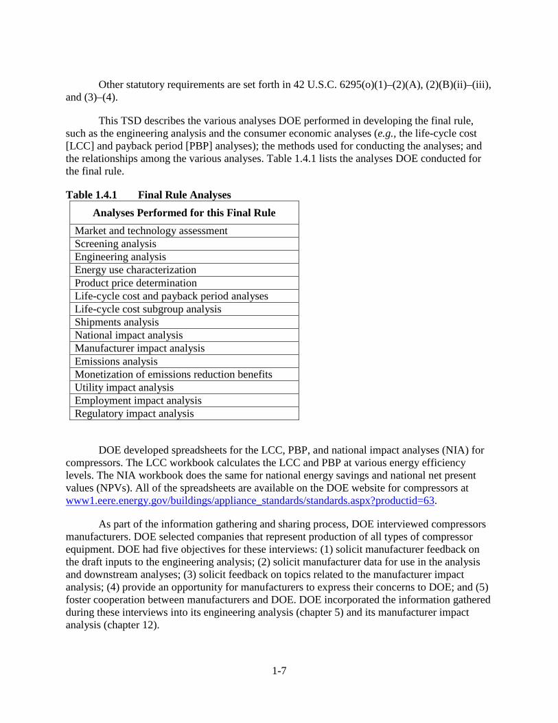
This TSD describes the various analyses DOE performed in developing the final rule, such as the engineering analysis and the consumer economic analyses (e.g., the life-cycle cost [LCC] and payback period [PBP] analyses); the methods used for conducting the analyses; and the relationships among the various analyses. Table 1.4.1 lists the analyses DOE conducted for the final rule.

Table 1.4.1 Final Rule Analyses Analyses Performed for this Final Rule

Market and technology assessment Screening analysis Engineering analysis Energy use characterization Product price determination Life-cycle cost and payback period analyses Life-cycle cost subgroup analysis Shipments analysis National impact analysis Manufacturer impact analysis Emissions analysis Monetization of emissions reduction benefits Utility impact analysis Employment impact analysis Regulatory impact analysis

DOE developed spreadsheets for the LCC, PBP, and national impact analyses (NIA) for compressors. The LCC workbook calculates the LCC and PBP at various energy efficiency levels. The NIA workbook does the same for national energy savings and national net present values (NPVs). All of the spreadsheets are available on the DOE website for compressors at www1.eere.energy.gov/buildings/appliance_standards/standards.aspx?productid=63.

As part of the information gathering and sharing process, DOE interviewed compressors manufacturers. DOE selected companies that represent production of all types of compressor equipment. DOE had five objectives for these interviews: (1) solicit manufacturer feedback on the draft inputs to the engineering analysis; (2) solicit manufacturer data for use in the analysis and downstream analyses; (3) solicit feedback on topics related to the manufacturer impact analysis; (4) provide an opportunity for manufacturers to express their concerns to DOE; and (5) foster cooperation between manufacturers and DOE. DOE incorporated the information gathered during these interviews into its engineering analysis (chapter 5) and its manufacturer impact analysis (chapter 12).

1-8

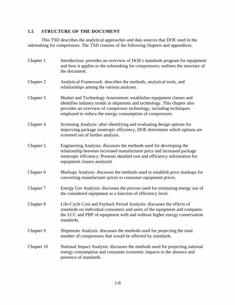
1.5 STRUCTURE OF THE DOCUMENT

This TSD describes the analytical approaches and data sources that DOE used in the rulemaking for compressors. The TSD consists of the following chapters and appendices.

Chapter 1 Introduction: provides an overview of DOE's standards program for equipment

and how it applies to the rulemaking for compressors; outlines the structure of the document.

Chapter 2 Analytical Framework: describes the methods, analytical tools, and

relationships among the various analyses. Chapter 3 Market and Technology Assessment: establishes equipment classes and

identifies industry trends in shipments and technology. This chapter also provides an overview of compressor technology, including techniques employed to reduce the energy consumption of compressors.

Chapter 4 Screening Analysis: after identifying and evaluating design options for

improving package isentropic efficiency, DOE determines which options are screened out of further analysis.

Chapter 5 Engineering Analysis: discusses the methods used for developing the

relationship between increased manufacturer price and increased package isentropic efficiency. Presents detailed cost and efficiency information for equipment classes analyzed.

Chapter 6 Markups Analysis: discusses the methods used to establish price markups for

converting manufacturer prices to consumer equipment prices. Chapter 7 Energy Use Analysis: discusses the process used for estimating energy use of

the considered equipment as a function of efficiency level. Chapter 8 Life-Cycle Cost and Payback Period Analysis: discusses the effects of

standards on individual consumers and users of the equipment and compares the LCC and PBP of equipment with and without higher energy conservation standards.

Chapter 9 Shipments Analysis: discusses the methods used for projecting the total

number of compressors that would be affected by standards. Chapter 10 National Impact Analysis: discusses the methods used for projecting national

energy consumption and consumer economic impacts in the absence and presence of standards.

1-9

Chapter 11 Customer Subgroup Analysis: discusses the effects of standards on any identifiable subgroups of consumers who may be disproportionately affected by the adopted standard level.

Chapter 12 Manufacturer Impact Analysis: discusses the effects of standards on the

finances and profitability of manufacturers of compressors. Chapter 13 Emissions Analysis: discusses the effects of standards on pollutants, including

sulfur dioxide, nitrogen oxides, and mercury, as well as carbon emissions. Chapter 14 Monetization of Emissions Reduction Benefits: Assigns monetary values to the

benefits likely to result from the reduced emissions of carbon dioxide and nitrogen oxides resulting from standards.

Chapter 15 Utility Impact Analysis: discusses selected effects of standards on the electric

utility industry Chapter 16 Employment Impact Analysis: discusses the effects of standards on national

employment. Chapter 17 Regulatory Impact Analysis: discusses the effects of non-regulatory

alternatives to efficiency standards Appendix 8A Uncertainty and Variability in the Life-Cycle Cost and Payback Period

Analysis Appendix 8B Electricity Prices Appendix 9A Air Compressor Flow and Pressure Weights by Equipment Class Appendix 10A Full-Fuel-Cycle Analysis Appendix 10B National Net Present Value of Customer Benefits Using Alternative Equipment

Price Forecast and Economic Growth Scenarios Appendix 10C National Impacts Analysis Using Alternative Efficiency Trend Scenarios Appendix 12A Manufacturer Impact Analysis Interview Guide Appendix 12B Government Regulatory Impact Model Overview Appendix 13A Emissions Analysis Methodology Appendix 14A Social Cost of Greenhouse Gases Appendix 14B Benefit-per-ton Values for NOx Emissions from Electricity Generation

1-10

Appendix 15A Utility Impact Analysis Methodology Appendix 17A Regulatory Impact Analysis: Supporting Materials

2-i

CHAPTER 2. ANALYTICAL FRAMEWORK

TABLE OF CONTENTS

2.1 INSTRUCTIONS ............................................................................................................. 2-1 2.2 BACKGROUND ............................................................................................................. 2-4 2.3 MARKET AND TECHNOLOGY ASSESSMENT ........................................................ 2-6

2.3.1 Market Assessment .............................................................................................. 2-6 2.3.2 Technology Assessment....................................................................................... 2-7

2.4 SCREENING ANALYSIS .............................................................................................. 2-7 2.5 ENGINEERING ANALYSIS .......................................................................................... 2-7

2.5.1 Baseline Models ................................................................................................... 2-7 2.5.2 Manufacturing Cost Analysis .............................................................................. 2-8

2.6 MARKUPS ANALYSIS ................................................................................................. 2-8 2.7 ENERGY-USE ANALYSIS ............................................................................................ 2-9

2.7.1 Energy Use Determination ................................................................................... 2-9 2.8 LIFE-CYCLE COST AND PAYBACK PERIOD ANALYSES .................................. 2-10 2.9 SHIPMENTS ANALYSIS ............................................................................................ 2-10 2.10 NATIONAL IMPACT ANALYSIS .............................................................................. 2-10

2.10.1 National Energy Savings Analysis..................................................................... 2-10 2.10.2 Net Present Value Analysis ............................................................................... 2-11

2.11 CONSUMER SUBGROUP ANALYSIS ...................................................................... 2-11 2.12 MANUFACTURER IMPACT ANALYSIS.................................................................. 2-12 2.12 EMISSIONS ANALYSIS .............................................................................................. 2-12 2.13 MONETIZATION OF EMISSIONS REDUCTION BENEFITS ................................. 2-13 2.14 UTILITY IMPACT ANALYSIS ................................................................................... 2-14 2.15 EMPLOYMENT IMPACT ANALYSIS ....................................................................... 2-15 2.16 ANALYSIS OF NON-REGULATORY ALTERNATIVES......................................... 2-15

LIST OF TABLES

Table 2.2.1 Adopted Energy Conservation Standards for Air Compressors .................... 2-6 Table 2.6.1 Distribution Channels .................................................................................... 2-8

2-1

CHAPTER 2. ANALYTICAL FRAMEWORK

INSTRUCTIONS 2.1

Section 6295(o)(2)(A) of the Energy Policy and Conservation Act (EPCA), as amended, 42 USC 6291 et. seq., requires that when prescribing new or amended energy conservation standards for covered products, the U.S. Department of Energy (DOE) must promulgate standards that achieve the maximum improvements in energy efficiency that are technologically feasible and economically justified. This chapter provides a description of the analytical framework that DOE used to evaluate new energy conservation standards for compressors. This chapter sets forth the methodology, analytical tools, and relationships among the various analyses that are part of this rulemaking.

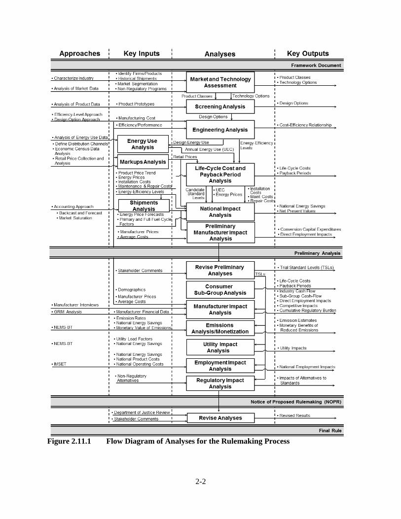
Figure 2.11.1 summarizes the analytical components of the standards-setting process. The focus of this figure is the center column, identified as “Analyses.” The columns labeled “Key Inputs” and “Key Outputs” show how the analyses fit into the rulemaking process, and how the analyses relate to each other. Key inputs are the types of data and information that the analyses require. Some key inputs exist in public databases; DOE collects other inputs from stakeholders or persons with special knowledge. Key outputs are analytical results that feed directly into the standards-setting process. Arrows connecting analyses show types of information that feed from one analysis to another.

2-2

Figure 2.11.1 Flow Diagram of Analyses for the Rulemaking Process

2-3

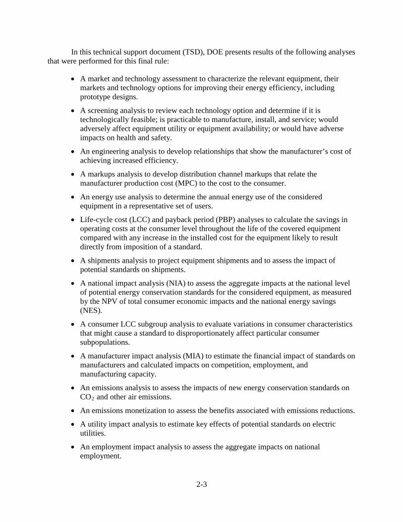
In this technical support document (TSD), DOE presents results of the following analyses that were performed for this final rule:

• A market and technology assessment to characterize the relevant equipment, their markets and technology options for improving their energy efficiency, including prototype designs.

• A screening analysis to review each technology option and determine if it is technologically feasible; is practicable to manufacture, install, and service; would adversely affect equipment utility or equipment availability; or would have adverse impacts on health and safety.

• An engineering analysis to develop relationships that show the manufacturer’s cost of achieving increased efficiency.

• A markups analysis to develop distribution channel markups that relate the manufacturer production cost (MPC) to the cost to the consumer.

• An energy use analysis to determine the annual energy use of the considered equipment in a representative set of users.

• Life-cycle cost (LCC) and payback period (PBP) analyses to calculate the savings in operating costs at the consumer level throughout the life of the covered equipment compared with any increase in the installed cost for the equipment likely to result directly from imposition of a standard.

• A shipments analysis to project equipment shipments and to assess the impact of potential standards on shipments.

• A national impact analysis (NIA) to assess the aggregate impacts at the national level of potential energy conservation standards for the considered equipment, as measured by the NPV of total consumer economic impacts and the national energy savings (NES).

• A consumer LCC subgroup analysis to evaluate variations in consumer characteristics that might cause a standard to disproportionately affect particular consumer subpopulations.

• A manufacturer impact analysis (MIA) to estimate the financial impact of standards on manufacturers and calculated impacts on competition, employment, and manufacturing capacity.

• An emissions analysis to assess the impacts of new energy conservation standards on CO2 and other air emissions.

• An emissions monetization to assess the benefits associated with emissions reductions.

• A utility impact analysis to estimate key effects of potential standards on electric utilities.

• An employment impact analysis to assess the aggregate impacts on national employment.

2-4

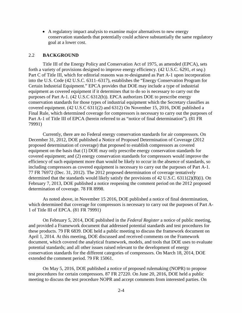
• A regulatory impact analysis to examine major alternatives to new energy conservation standards that potentially could achieve substantially the same regulatory goal at a lower cost.

BACKGROUND 2.2

Title III of the Energy Policy and Conservation Act of 1975, as amended (EPCA), sets forth a variety of provisions designed to improve energy efficiency. (42 U.S.C. 6291, et seq.) Part C of Title III, which for editorial reasons was re-designated as Part A-1 upon incorporation into the U.S. Code (42 U.S.C. 6311–6317), establishes the “Energy Conservation Program for Certain Industrial Equipment.” EPCA provides that DOE may include a type of industrial equipment as covered equipment if it determines that to do so is necessary to carry out the purposes of Part A-1. (42 U.S.C 6312(b)). EPCA authorizes DOE to prescribe energy conservation standards for those types of industrial equipment which the Secretary classifies as covered equipment. (42 U.S.C 6311(2) and 6312) On November 15, 2016, DOE published a Final Rule, which determined coverage for compressors is necessary to carry out the purposes of Part A-1 of Title III of EPCA (herein referred to as “notice of final determination”). (81 FR 79991)

Currently, there are no Federal energy conservation standards for air compressors. On December 31, 2012, DOE published a Notice of Proposed Determination of Coverage (2012 proposed determination of coverage) that proposed to establish compressors as covered equipment on the basis that (1) DOE may only prescribe energy conservation standards for covered equipment; and (2) energy conservation standards for compressors would improve the efficiency of such equipment more than would be likely to occur in the absence of standards, so including compressors as covered equipment is necessary to carry out the purposes of Part A-1. 77 FR 76972 (Dec. 31, 2012). The 2012 proposed determination of coverage tentatively determined that the standards would likely satisfy the provisions of 42 U.S.C. 6311(2)(B)(i). On February 7, 2013, DOE published a notice reopening the comment period on the 2012 proposed determination of coverage. 78 FR 8998.

As noted above, in November 15 2016, DOE published a notice of final determination, which determined that coverage for compressors is necessary to carry out the purposes of Part A-1 of Title III of EPCA. (81 FR 79991)

On February 5, 2014, DOE published in the Federal Register a notice of public meeting, and provided a Framework document that addressed potential standards and test procedures for these products. 79 FR 6839. DOE held a public meeting to discuss the framework document on April 1, 2014. At this meeting, DOE discussed and received comments on the Framework document, which covered the analytical framework, models, and tools that DOE uses to evaluate potential standards; and all other issues raised relevant to the development of energy conservation standards for the different categories of compressors. On March 18, 2014, DOE extended the comment period. 79 FR 15061.

On May 5, 2016, DOE published a notice of proposed rulemaking (NOPR) to propose test procedures for certain compressors. 87 FR 27220. On June 20, 2016, DOE held a public meeting to discuss the test procedure NOPR and accept comments from interested parties. On

2-5

December 1, 2016, DOE issued a test procedure final rule that amends subpart T of Title 10 of the Code of Federal Regulations, part 431 (10 CFR 431), and which contains definitions, materials incorporated by reference, and test procedures for determining the energy efficiency of certain varieties of compressors. The test procedure final rule also amended 10 CFR 429 to establish sampling plans, representations requirements, and enforcement provisions for certain compressors.

On May 19, 2016, DOE published a notice of proposed rulemaking pertaining to energy conservation standards for compressors (May 2016 NOPR).a 81 FR 31680. DOE held a public meeting to discuss the May 2016 NOPR on June 20, 2016.

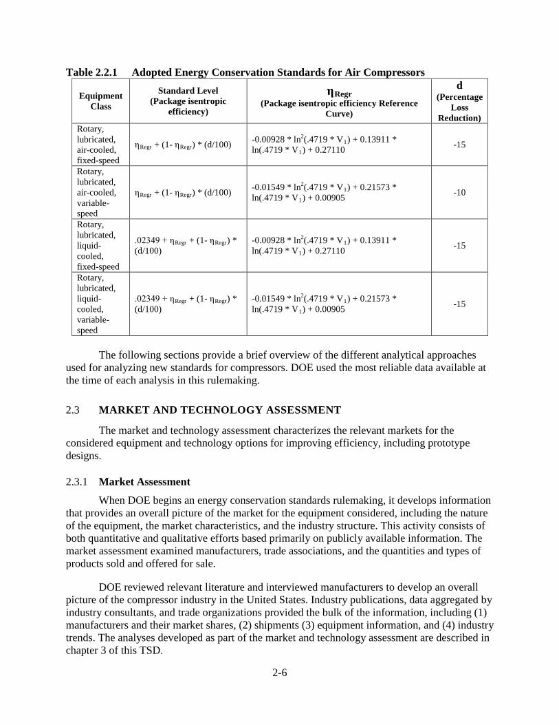
In this final rule, DOE is adopting new energy conservation standards for compressors. The standards are expressed in package isentropic efficiency (i.e., the ratio of the theoretical isentropic power required for a compression process to the actual power required for the same process), and are shown in Table 2.2.1. These standards apply to all compressors listed in Table 2.2.1 and manufactured in, or imported into, the United States starting on December 1, 2021.

In Table 2.2.1 the term V1 denotes the full-load actual volume flow rate of the compressor, in cubic feet per minute (cfm). Standard levels are expressed as a function of full-load actual volume flow rate for each equipment class, and may be calculated by inserting values from the rightmost two columns into the second leftmost column. Doing so will yield an efficiency-denominated function of full-load actual volume flow rate.

a Available at: www.regulations.gov/document?D=EERE-2013-BT-STD-0040-0038.

2-6

Table 2.2.1 Adopted Energy Conservation Standards for Air Compressors

Equipment Class

Standard Level (Package isentropic

efficiency)

ηRegr (Package isentropic efficiency Reference

Curve)

d (Percentage

Loss Reduction)

Rotary, lubricated, air-cooled, fixed-speed

ηRegr + (1- ηRegr) * (d/100) -0.00928 * ln2(.4719 * V1) + 0.13911 * ln(.4719 * V1) + 0.27110 -15

Rotary, lubricated, air-cooled, variable-speed

ηRegr + (1- ηRegr) * (d/100) -0.01549 * ln2(.4719 * V1) + 0.21573 * ln(.4719 * V1) + 0.00905 -10

Rotary, lubricated, liquid-cooled, fixed-speed

.02349 + ηRegr + (1- ηRegr) * (d/100)

-0.00928 * ln2(.4719 * V1) + 0.13911 * ln(.4719 * V1) + 0.27110 -15

Rotary, lubricated, liquid-cooled, variable-speed

.02349 + ηRegr + (1- ηRegr) * (d/100)

-0.01549 * ln2(.4719 * V1) + 0.21573 * ln(.4719 * V1) + 0.00905 -15

The following sections provide a brief overview of the different analytical approaches

used for analyzing new standards for compressors. DOE used the most reliable data available at the time of each analysis in this rulemaking.

MARKET AND TECHNOLOGY ASSESSMENT 2.3

The market and technology assessment characterizes the relevant markets for the considered equipment and technology options for improving efficiency, including prototype designs.

Market Assessment 2.3.1

When DOE begins an energy conservation standards rulemaking, it develops information that provides an overall picture of the market for the equipment considered, including the nature of the equipment, the market characteristics, and the industry structure. This activity consists of both quantitative and qualitative efforts based primarily on publicly available information. The market assessment examined manufacturers, trade associations, and the quantities and types of products sold and offered for sale.

DOE reviewed relevant literature and interviewed manufacturers to develop an overall picture of the compressor industry in the United States. Industry publications, data aggregated by industry consultants, and trade organizations provided the bulk of the information, including (1) manufacturers and their market shares, (2) shipments (3) equipment information, and (4) industry trends. The analyses developed as part of the market and technology assessment are described in chapter 3 of this TSD.

2-7

Technology Assessment 2.3.2

As part of the market and technology assessment, DOE developed a list of technologies to consider for improving the package isentropic efficiency of compressors. Chapter 3 of this TSD includes the detailed list of all technology options DOE identified for this rulemaking.

SCREENING ANALYSIS 2.4

The purpose of the screening analysis is to evaluate the technologies identified in the technology assessment to determine which options to consider further in the analysis and which options to screen out. DOE consulted with industry, technical experts, and other interested parties in developing a list of energy-saving technologies for the technology assessment. DOE then applied the screening criteria to determine which technologies were unsuitable for further consideration in this rulemaking. Chapter 4 of this TSD, the screening analysis, contains details about DOE’s screening criteria.

The screening analysis examines whether various technologies (1) are technologically feasible; (2) are practicable to manufacture, install, and service; (3) have an adverse impact on product utility or availability; and (4) have adverse impacts on health and safety. DOE reviewed the list of compressor technologies according to these criteria. In the engineering analysis, DOE further considers the efficiency-enhancement technologies that it did not eliminate in the screening analysis.

ENGINEERING ANALYSIS 2.5

The engineering analysis (chapter 5 of this TSD) establishes the relationship between the manufacturing production cost and the package isentropic efficiency for each compressor equipment class. This relationship serves as the basis for cost-benefit calculations in terms of individual end users, manufacturers, and the nation. Chapter 5 discusses the equipment classes analyzed, representative baseline units, incremental efficiency levels, methodology used to develop manufacturing production costs, and the cost-efficiency relationships for the considered equipment. DOE first estimates manufacturing costs in the engineering analysis. To determine the costs for end users to purchase compressors, chapters 6 and 8 of this TSD estimate markups in the distribution chain, installation costs, and maintenance costs.

In the engineering analysis, DOE evaluated a range of efficiency levels and associated manufacturing costs. The purpose of the analysis is to estimate the incremental increase to selling prices that would result from increasing efficiency levels above the baseline model in each equipment class. The engineering analysis considers technologies not eliminated in the screening analysis. The LCC analysis uses the cost-efficiency relationships developed in the engineering analysis.

Baseline Models 2.5.1

In order to analyze design options for energy efficiency improvements, DOE defined a baseline efficiency level for each equipment classes. The baseline efficiency level aligns with the lower efficiency compressors observed on the market (in terms of package isentropic efficiency).

2-8

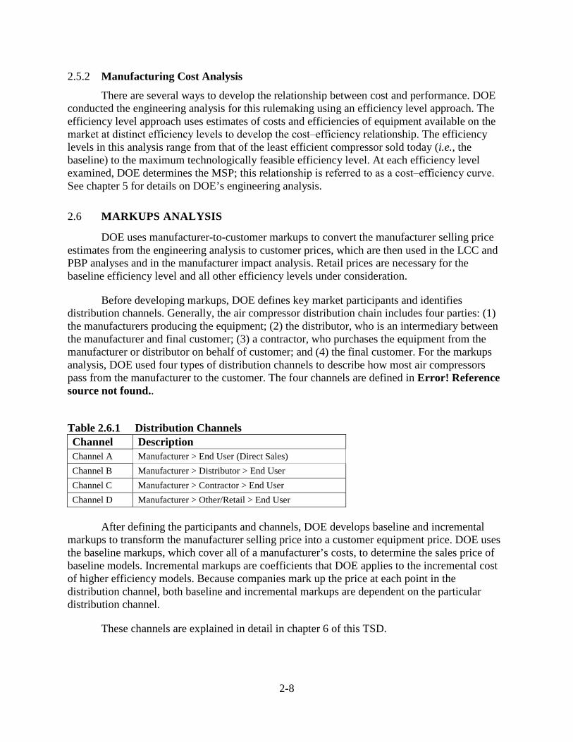
Manufacturing Cost Analysis 2.5.2

There are several ways to develop the relationship between cost and performance. DOE conducted the engineering analysis for this rulemaking using an efficiency level approach. The efficiency level approach uses estimates of costs and efficiencies of equipment available on the market at distinct efficiency levels to develop the cost‒efficiency relationship. The efficiency levels in this analysis range from that of the least efficient compressor sold today (i.e., the baseline) to the maximum technologically feasible efficiency level. At each efficiency level examined, DOE determines the MSP; this relationship is referred to as a cost‒efficiency curve. See chapter 5 for details on DOE’s engineering analysis.

MARKUPS ANALYSIS 2.6

DOE uses manufacturer-to-customer markups to convert the manufacturer selling price estimates from the engineering analysis to customer prices, which are then used in the LCC and PBP analyses and in the manufacturer impact analysis. Retail prices are necessary for the baseline efficiency level and all other efficiency levels under consideration.

Before developing markups, DOE defines key market participants and identifies distribution channels. Generally, the air compressor distribution chain includes four parties: (1) the manufacturers producing the equipment; (2) the distributor, who is an intermediary between the manufacturer and final customer; (3) a contractor, who purchases the equipment from the manufacturer or distributor on behalf of customer; and (4) the final customer. For the markups analysis, DOE used four types of distribution channels to describe how most air compressors pass from the manufacturer to the customer. The four channels are defined in Error! Reference source not found..

Table 2.6.1 Distribution Channels Channel Description Channel A Manufacturer > End User (Direct Sales) Channel B Manufacturer > Distributor > End User Channel C Manufacturer > Contractor > End User Channel D Manufacturer > Other/Retail > End User

After defining the participants and channels, DOE develops baseline and incremental

markups to transform the manufacturer selling price into a customer equipment price. DOE uses the baseline markups, which cover all of a manufacturer’s costs, to determine the sales price of baseline models. Incremental markups are coefficients that DOE applies to the incremental cost of higher efficiency models. Because companies mark up the price at each point in the distribution channel, both baseline and incremental markups are dependent on the particular distribution channel.

These channels are explained in detail in chapter 6 of this TSD.

2-9

ENERGY-USE ANALYSIS 2.7

DOE establishes the annual energy consumption for equipment and assesses the energy-savings potential of various equipment efficiencies. As part of the energy use analysis, certain engineering assumptions may be required regarding equipment application, including how often the equipment is operated and under what conditions. DOE uses the annual energy consumption and energy-savings potential in the LCC and PBP analyses to establish the savings in consumer operating costs at various equipment efficiency levels.

Energy Use Determination 2.7.1

A key component of the life-cycle cost and payback period) calculations described in chapter 8 is the savings in operating costs that customers would realize from more energy efficient equipment. Energy costs are the most significant component of customer operating costs for air compressors. DOE uses annual energy use, along with energy prices, to establish energy costs at various energy efficiency levels.

Air compressors supply compressed air in response to the demands of what is usually a dynamic system. As such, a compressor’s overall operational efficiency is a function of the compressor’s performance characteristics, the operating conditions of the system which it is connected to, and the method of matching compressor output to these operating conditions in the form of capacity controls. When estimating annual energy use DOE separates its model into supply, demand, and capacity control inputs.

Supply side inputs consist of compressor performance characteristics. These are defined in the engineering analysis (see chapter 5) as the components affecting the overall efficiency of a compressor package according to the DOE test procedure.

Demand side inputs refer to operating conditions imposed on a compressor in the form of airflow and pressure demands of the system the compressor is connected to over a period of time. Demand is determined by the tools and machinery connected to a compressed air system. The variability of airflow demands over time of a compressed air system is defined as an annual load profile. Load profiles contain the fraction of annual operating hours assigned to different demand airflows (as a fraction of compressor capacity (Q)), while pressures are assumed to be held in a steady state.

Capacity control inputs refer to the means used to control how a compressor’s air supply is adjusted to meet operating condition demands. Part-load performance is the change in efficiency from any controls that are used to match compressor output with varying system air demands that are seen in the field. As such, part-load performance of a compressor depends on the assigned capacity control. DOE modeled the part-load performance using the power curves, which relate a compressor’s part-load capacity to its part-load power requirement for several different control types.

These are explained in greater detail in chapter 7 of this TSD.

2-10

LIFE-CYCLE COST AND PAYBACK PERIOD ANALYSES 2.8

DOE conducts LCC and PBP analyses to evaluate the economic impacts on individual consumers of potential energy conservation standards. The LCC is the total consumer expense over the life of a product. The PBP is the estimated amount of time (in years) it takes consumers to recover any increased first cost of a more efficient product through lower operating costs.

Inputs to the calculation of the LCC for air compressors are the total installed cost, the lifetime operating cost. The total installed cost includes consumer equipment price and sales tax. DOE assumed that the installation costs did not vary by efficiency level, and therefore did not consider them in the analysis. Inputs to the calculation of the lifetime operating cost include the annual energy consumption (from the energy use analysis), electricity prices and electricity price trends, equipment lifetime, discount rates, the market efficiency distribution for each standard-case, and the year in which compliance with standards would be required. For more detail on the LCC and PBP analyses, see chapter 8 of this TSD.

SHIPMENTS ANALYSIS 2.9

DOE used forecasts of equipment shipments to calculate the national impacts of standards and also in its manufacturer impact analysis. DOE developed these shipment forecasts based on an analysis of key market drivers for each product.

For more detail on the shipments analysis, see chapter 9 of this TSD.

NATIONAL IMPACT ANALYSIS 2.10

The NIA assesses the NES and the NPV from a national perspective of total consumer costs and savings expected to result from new or amended energy conservation standards. Analyzing impacts of potential energy conservation standards for air compressors requires comparing projections of U.S. energy consumption with energy conservation standards against projections of energy consumption without energy standards.

DOE analyzed the impacts of six trial standard levels (TSLs), corresponding to each efficiency level (EL) specified in the engineering analysis. DOE coded the NIA in a Microsoft Excel file available on regulations.gov, docket number EERE-2013-BT-STD-0040. For more detail on the NIA, see chapter 10 of this TSD.

National Energy Savings Analysis 2.10.1

The inputs for determining the NES for air compressors are: (1) shipments, (2) annual energy consumption per unit, (3) stocks of air compressors in each year, (4) national energy consumption, and (5) site-to-primary energy and fuel full cycle (FFC) conversion factors. The stocks were calculated by the shipments model for each year of the analysis period from the prior year’s stock, minus retirements, plus new shipments, accounting for product lifetimes. DOE calculated the national electricity consumption in each year by multiplying the number of units at each EL in the stock by the corresponding power consumption and operating hours. The electricity savings are estimated from the difference in national electricity consumption, between

2-11

the no-standard and the standards cases, for air compressors shipped during the first full year after compliance and over years 2022 through 2051.

DOE has historically presented the NES in terms of primary energy savings. In response to the recommendations of a committee on Point-of-Use and Full-Fuel-Cycle Measurement Approaches to Energy Efficiency Standards, appointed by the National Academy of Science, DOE announced its intention to use FFC measures of energy use and greenhouse gas (GHG) and other emissions in the national impact analyses and emissions analyses included in future energy conservation standards rulemakings. 76 FR 51281 (August 18, 2011). While DOE stated in that notice that it intended to use the Greenhouse Gases, Regulated Emissions, and Energy Use in Transportation (GREET) model to conduct the analysis, it also stated it would review alternative methods, including the use of the National Energy Modeling System (NEMS). After evaluating both models and the approaches discussed in the August 18, 2011 notice, DOE has determined NEMS is a more appropriate tool for this application. 77 FR 49701 (August 17, 2012). Therefore, DOE is using the NEMS model to conduct FFC analyses. For this analysis, DOE calculated FFC energy savings using the methodology described in appendix 10B of this TSD, which presents both the primary energy savings and the FFC energy savings for the considered TSLs.

Net Present Value Analysis 2.10.2

The inputs for determining NPV are: (1) total annual installed cost, (2) total annual savings in operating costs, and (3) a discount factor to calculate the present value of costs and savings. DOE calculated net savings each year as the difference between the no-standard case and each standard case in terms of total savings in operating costs versus total increases in installed costs. DOE calculated savings over the lifetime of products shipped in the 30-year analysis period. DOE calculated NPV as the difference between the present value of operating-cost savings and the present value of total installed costs. DOE used a discount factor based on real discount rates of 3 and 7 percent to discount future costs and savings to present values.

For the NPV analysis, DOE calculates any increase in total installed costs as the difference in total installed cost between the no-standard case and the standard case (i.e., once a standard would take effect). Because the more efficient products bought in the standards case usually cost more than products bought in the base case, cost increases appear as negative values in the NPV.

DOE expresses savings in operating costs as decreases associated with the lower energy consumption of products bought in a standards case compared to the no-standard case. Total savings in operating costs are the product of savings per unit and the number of units of each vintage that survive in a given year.

CONSUMER SUBGROUP ANALYSIS 2.11

A consumer subgroup comprises a subset of the population that could, for one reason or another, be affected disproportionately by new or amended energy conservation standards. DOE identified small businesses as consumers that could be disproportionately impacted by the standards. The LCC subgroup analysis evaluates the effects on these consumer subgroups by

2-12

accounting for variations in key inputs to the LCC analysis. For more detail on the consumer subgroup analysis, see chapter 11 of this TSD.

2.12 MANUFACTURER IMPACT ANALYSIS

DOE performed an MIA to determine the potential financial impact of higher energy conservation standards on compressor manufacturers, as well as to estimate the impact of such standards on employment and manufacturing capacity. The MIA has both quantitative and qualitative aspects. The quantitative part of the MIA relies on the government regulatory impact model (GRIM), an industry cash-flow model customized for the compressor industry. The GRIM inputs include manufacturer production costs, manufacturer selling prices, industry shipments, and industry financial parameters. This includes information from many of the analyses described above, such as manufacturing production costs and manufacturer selling prices from the engineering analysis and shipments forecasts from the shipments analysis. The key GRIM output is the industry net present value (INPV). Different sets of assumptions (scenarios) will produce different results. The qualitative part of the MIA includes factors such as impacts on industry competition, impacts on manufacturing capacity, industry consolidation, employment, and identification of key manufacturer issues.

DOE conducts the MIA in three phases. In Phase I, DOE creates an industry profile to

characterize the industry and identify important issues that require consideration. In Phase II, DOE prepares an industry cash-flow model and interview questionnaire to guide subsequent discussions. In Phase III, DOE interviews manufacturers and assesses the impacts of standards quantitatively and qualitatively. DOE assesses industry and subgroup cash flow and NPV using the GRIM. DOE then assesses impacts on competition, manufacturing capacity, employment, and regulatory burden based on manufacturer interview feedback and discussions. Chapter 12 of this TSD describes the complete MIA.

EMISSIONS ANALYSIS 2.12

The emissions analysis consists of two components. The first component estimates the effect of potential energy conservation standards on power sector and site (where applicable) combustion emissions of CO2, NOX, SO2, and Hg. The second component estimates the impacts of potential standards on emissions of two additional greenhouse gases, CH4 and N2O, as well as the reductions to emissions of all species due to “upstream” activities in the fuel production chain. These upstream activities comprise extraction, processing, and transporting fuels to the site of combustion. The associated emissions are referred to as upstream emissions. The analysis of power sector emissions uses marginal emissions factors that were derived from data in AEO 2016. The methodology is described in chapter 13 and 15 of the TSD. Combustion emissions of CH4 and N2O are estimated using emissions intensity factors published by the EPA in its GHG Emissions Factors Hub.b The FFC upstream emissions are estimated based on the methodology described in chapter 15 of the TSD. The upstream emissions include both emissions from fuel combustion during extraction, processing, and b Available at: www2.epa.gov/climateleadership/center-corporate-climate-leadership-ghg-emission-factors-hub.

2-13

transportation of fuel, and “fugitive” emissions (direct leakage to the atmosphere) of CH4 and CO2. The emissions intensity factors are expressed in terms of physical units per megawatt-hour or million British thermal units of site energy savings. Total emissions reductions are estimated using the energy savings calculated in the national impact analysis.

The AEO incorporates the projected impacts of existing air quality regulations on

emissions. AEO 2016 generally represents current legislation and environmental regulations, including recent government actions, for which implementing regulations were available as of the end of February 2016.

MONETIZATION OF EMISSIONS REDUCTION BENEFITS 2.13

DOE considers the estimated monetary benefits likely to result from the reduced emissions of CO2, CH4, N2O and NOX that are expected to result from each of the standard levels considered.

To estimate the monetary value of benefits resulting from reduced emissions of CO2, DOE uses the most current Social Cost of Carbon Dioxide (SC-CO2) values developed and/or agreed to by an interagency process. The SC-CO2 is intended to be a monetary measure of the incremental damage resulting from GHG emissions, including, but not limited to, net agricultural productivity loss, human health effects, property damage from sea level rise, and changes in ecosystem services. Any effort to quantify and to monetize the harms associated with climate change will raise serious questions of science, economics, and ethics. But with full regard for the limits of both quantification and monetization, the SC-CO2 can be used to provide estimates of the social benefits of reductions in CO2 emissions.

The Interagency Working Group on Social Cost of Carbon selected four sets of SC-CO2 values for use in regulatory analyses. Three sets of values are based on the average SC-CO2 from the three integrated assessment models, at discount rates of 2.5, 3, and 5 percent. The fourth set, which represents the 95th percentile SC-CO2 estimate across all three models at a 3-percent discount rate, was included to represent higher-than-expected impacts from climate change further out in the tails of the SC-CO2 distribution. The values grow in real terms over time.c To calculate a present value of the stream of monetary values, DOE discounts the values in each of the four cases using the discount rates that had been used to obtain the SC-CO2 values in each case.

In 2016 the Interagency Working Group issued a report that presents social cost estimates for CH4 and N2O as a way for agencies to incorporate the social benefits of reducing CH4 and

c Technical Update of the Social Cost of Carbon for Regulatory Impact Analysis Under Executive Order 12866, Interagency Working Group on Social Cost of Carbon, United States Government (May 2013; revised July 2015) (Available at: www.whitehouse.gov/sites/default/files/omb/inforeg/scc-tsd-final-july-2015.pdf).

2-14

N2O emissions into benefit-cost analyses of regulatory actions.d DOE uses these values in the current analysis.

DOE recognizes that scientific and economic knowledge continue to evolve rapidly regarding the contribution of CO2 and other GHG to changes in the future global climate and the potential resulting damages to the world economy. Thus, these values are subject to change.

DOE also considers the potential monetary benefits of reduced NOX emissions attributable to the standard levels it considers. DOE estimated the monetized value of NOX emissions reductions using benefit per ton estimates from the Regulatory Impact Analysis for the Clean Power Plan Final Rule, published in August 2015 by EPA’s Office of Air Quality Planning and Standards. e

UTILITY IMPACT ANALYSIS 2.14

To estimate the impacts of potential energy conservation standards on the electric utility industry, DOE used published output from the NEMS associated with AEO 2016. NEMS is a large, multi-sectoral, partial-equilibrium model of the U.S. energy sector that Energy Information Administration developed over several years, primarily for the purpose of preparing the AEO. NEMS produces a widely recognized forecast for the United States through 2040 and is available to the public.

In 2014, DOE began using a new methodology based on results published for the AEO Reference case, as well as a number of side cases that estimate the economy-wide impacts of changes to energy supply and demand. DOE estimates the marginal impacts of reduction in energy demand on the energy supply sector. In principle, marginal values should provide a better estimate of the actual impact of energy conservation standards. DOE uses the side cases to estimate the marginal impacts of reduced energy demand on the utility sector. These marginal factors are estimated based on the changes to electricity sector generation, installed capacity, fuel consumption, and emissions in the AEO Reference case and various side cases. The methodology is described in more detail in chapter 15 of the TSD.

The output of this analysis is a set of time-dependent coefficients that capture the change in electricity generation, primary fuel consumption, installed capacity and power sector emissions due to a unit reduction in demand for a given end use. These coefficients are multiplied by the stream of electricity savings calculated in the NIA to provide estimates of selected utility impacts of new energy conservation standards.

d United States Government–Interagency Working Group on Social Cost of Greenhouse Gases. Addendum to Technical Support Document on Social Cost of Carbon for Regulatory Impact Analysis under Executive Order 12866: Application of the Methodology to Estimate the Social Cost of Methane and the Social Cost of Nitrous Oxide. August 2016. www.whitehouse.gov/sites/default/files/omb/inforeg/august_2016_sc_ch4_sc_n2o_addendum_final_8_26_16.pdf. e Available at www.epa.gov/cleanpowerplan/clean-power-plan-final-rule-regulatory-impact-analysis. See Tables 4A-3, 4A-4, and 4A-5 in the report.

2-15

EMPLOYMENT IMPACT ANALYSIS 2.15

The adoption of energy conservation standards can affect employment both directly and indirectly. Direct employment impacts are changes in the number of employees at the plants that produce the covered products. DOE evaluates direct employment impacts in the MIA.

Indirect employment impacts may result from expenditures shifting between goods (the substitution effect) and changes in income and overall expenditure levels (the income effect) that occur due to standards. DOE defines indirect employment impacts from standards as net jobs eliminated or created in the general economy as a result of increased spending driven by increased product prices and reduced spending on energy.

The indirect employment impacts are investigated in the employment impact analysis using the Pacific Northwest National Laboratory’s Impact of Sector Energy Technologies (ImSET) model.8 The ImSET model was developed for DOE’s Office of Planning, Budget, and Analysis to estimate the employment and income effects of energy-saving technologies in buildings, industry, and transportation. Compared with simple economic multiplier approaches, ImSET allows for more complete and automated analysis of the economic impacts of energy conservation investments.

ANALYSIS OF NON-REGULATORY ALTERNATIVES 2.16

In the NOPR stage, DOE prepares an analysis that evaluates potential non-regulatory policy alternatives, comparing the costs and benefits of each to those of the standards. DOE recognizes that non-regulatory policy alternatives can substantially affect energy efficiency or reduce energy consumption. DOE bases its assessment on the actual impacts of any such initiatives to date, but also considers information presented by interested parties regarding the potential future impacts of current initiatives.

3-i

CHAPTER 3. MARKET AND TECHNOLOGY ASSESSMENT

TABLE OF CONTENTS

3.1 INTRODUCTION ........................................................................................................... 3-1 3.2 DEFINITIONS ................................................................................................................. 3-1

3.2.1 Definitions Adopted in the Test Procedure Final Rule ........................................ 3-1 3.2.2 Definitions Adopted in the Energy Conservation Standards Final Rule ............. 3-2

3.3 SCOPE OF ENERGY CONSERVATION STANDARDS ............................................. 3-3 3.3.1 Equipment System Boundary .............................................................................. 3-4 3.3.2 Compression Principle ......................................................................................... 3-5 3.3.3 Driver Style .......................................................................................................... 3-6

3.3.3.1 Non-Electric-Driven Compressors ............................................................. 3-6 3.3.3.2 Brushed Motors .......................................................................................... 3-6 3.3.3.3 Single-Phase Motors .................................................................................. 3-6

3.3.4 Compressor Capacity ........................................................................................... 3-7 3.3.4.1 Motor Power ............................................................................................... 3-7 3.3.4.2 Output Flow ................................................................................................ 3-8

3.3.5 Full-Load Operating Pressure .............................................................................. 3-9 3.3.6 Lubricant Presence ............................................................................................. 3-10 3.3.7 Water Injection................................................................................................... 3-10 3.3.8 Specialty Purpose ............................................................................................... 3-12

3.3.8.1 Corrosive Environments ........................................................................... 3-14 3.3.8.2 Hazardous Environments ......................................................................... 3-14 3.3.8.3 Extreme Temperatures ............................................................................. 3-15 3.3.8.4 Marine Environments ............................................................................... 3-16 3.3.8.5 Weather Protected .................................................................................... 3-17 3.3.8.6 Mining Environments ............................................................................... 3-18 3.3.8.7 Military Applications ............................................................................... 3-18 3.3.8.8 Food Service Applications ....................................................................... 3-19 3.3.8.9 Medical Air Applications ......................................................................... 3-19 3.3.8.10 Climate-Control Applications .................................................................. 3-20 3.3.8.11 Petroleum, Gas, and Chemical Applications ............................................ 3-20

3.4 EQUIPMENT CLASSES AND DISTINGUISHING FEATURES .............................. 3-21 3.4.1 Motor Speed Range............................................................................................ 3-22 3.4.2 Variations of Rotary Compression Technology ................................................ 3-23 3.4.3 Cooling Method ................................................................................................. 3-25 3.4.4 List of Equipment Classes ................................................................................. 3-28

3.5 TEST PROCEDURES AND ENERGY USE METRIC ............................................... 3-28 3.6 MARKET ASSESSMENT ............................................................................................ 3-29

3.6.1 Trade Associations ............................................................................................. 3-29 3.6.2 Manufacturers and Industry Structure ............................................................... 3-30 3.6.3 Regulatory Programs ......................................................................................... 3-32

3.6.3.1 European Union ........................................................................................ 3-32 3.6.3.2 The People’s Republic of China ............................................................... 3-34

3-ii

3.6.4 Nonregulatory Programs .................................................................................... 3-35 3.6.4.1 Compressed Air Challenge ....................................................................... 3-35 3.6.4.2 CAGI Performance Verification Program ................................................ 3-35

3.6.5 Market and Industry Trends ............................................................................... 3-37 3.6.5.1 Equipment Efficiency ............................................................................... 3-37 3.6.5.2 Market Share, Compressors in Final Rule Scope ..................................... 3-39 3.6.5.3 Market Share, All Electrically-Driven, Stationary Compressors ............. 3-41

3.6.6 Applications ....................................................................................................... 3-41 3.6.7 Controls Methods ............................................................................................... 3-42

3.7 TECHNOLOGY ASSESSMENT .................................................................................. 3-43 3.7.1 Multi-Staging ..................................................................................................... 3-44 3.7.2 Air-End Improvement ........................................................................................ 3-47 3.7.3 Auxiliary Component Improvement .................................................................. 3-49

LIST OF TABLES Table 3.3.1 Effect of Flow Criterion on Scope ........................................................................... 3-9 Table 3.4.1 DOE Equipment Classes for Compressors ............................................................ 3-28 Table 3.6.1 Major Manufacturers of Air Compressors by Equipment Type ............................ 3-30 Table 3.6.2 Small-Business Manufacturers of Air Compressors by Equipment Type ............. 3-31 Table 3.6.3 Draft First Tier EU Minimum Energy Efficiency Requirements for Standard

Air Compressors beginning January 1, 2018 ............................................... 3-33 Table 3.6.4 Draft Second Tier EU Minimum Energy Efficiency Requirements for

Standard Air Compressors beginning January 1, 2020 ................................ 3-34 Table 3.6.5 Rotary Compressor Shipments by Equipment Capacity, 2016 .............................. 3-40 Table 3.6.6 Rotary Compressor Shipment Percentages by Flow, 2016 .................................... 3-40 Table 3.6.7 Rotary Compressor Shipment Percentages by Pressure, 2016 .............................. 3-40 Table 3.6.8 Market Share of Air Compressors by Compression Principle, 2016 ..................... 3-41 Table 3.7.1 List of Equipment Required During Test .............................................................. 3-51 Table 3.7.2 List of Equipment Required During Test, if Distributed in Commerce with

the Basic Model ........................................................................................... 3-51

LIST OF FIGURES

Figure 3.4.1 Comparison of mean package isentropic efficiency between fixed- and

variable-speed air-cooled lubricated single-stage compressors at full-load actual volume flow rate. ....................................................................... 3-23

Figure 3.4.2 Package isentropic efficiency at full-load operating pressure versus full-load actual volume flow rate, for air-cooled fixed-speed vane and screw compressors.................................................................................................. 3-25

Figure 3.4.3 Comparison of package isentropic efficiency at full-load operating pressure between air-cooled and water-cooled compressors with similar designs .... 3-27

3-iii

Figure 3.4.4 Isentropic efficiency as a function of full-load actual volume flow rate for select air-cooled and water-cooled compressors with similar designs. The mean isentropic efficiency curves from the NOPR are also shown ..... 3-27

Figure 3.6.1 RP_FS_L_AC Efficiency Levels ......................................................................... 3-37 Figure 3.6.2 RP_FS_L_WC Efficiency Levels......................................................................... 3-38 Figure 3.6.3 RP_VS_L_AC Efficiency Levels ......................................................................... 3-38 Figure 3.6.4 RP_VS_L_WC Efficiency Levels ........................................................................ 3-39 Figure 3.7.1 Single-Stage Compression Process ...................................................................... 3-46 Figure 3.7.2 Multistage Compression Process .......................................................................... 3-46 Figure 3.7.3 Representative Single-stage Bare Compressor Performance Curve .................... 3-47 Figure 3.7.4 Representative Operating Points for a Single-stage Bare Compressor Used

in Multiple Compressor Packages ............................................................... 3-48

3-1

CHAPTER 3. MARKET AND TECHNOLOGY ASSESSMENT 3.1 INTRODUCTION

This chapter provides a profile of the compressor industry in the United States. The information that the U.S. Department of Energy (DOE) gathers for a market and technology assessment serves as resource material throughout the rulemaking. DOE considers both quantitative and qualitative information from publicly available sources and interested parties. DOE examined publicly available information and hired a consultant team to collect data under a nondisclosure agreement (NDA) to develop the assessment described in this chapter.

Section 3.2 sets out definitions related to different varieties of compressor equipment. Section 3.3 discusses the scope of the energy conservation standards by compressor feature. Section 3.4 describes the specific features that distinguish compressor equipment classes, and then it uses these features to define the compressor equipment classes. Section 3.5 describes the test procedure and the energy use metric that DOE established for compressor equipment. The market assessment in section 3.6 provides an overall picture of the market for the equipment considered, including the industry structure; regulatory and non-regulatory programs for improving efficiency of the equipment; market trends; and quantities of equipment sold. Finally, section 3.7 discusses technology options that a manufacturer could use to increase the efficiency of compressors.

3.2 DEFINITIONS

The term “compressor” is not defined term under the Energy Policy and Conservation Act (EPCA). In the November 2016 notice of final determination, DOE defined a compressor to mean a machine or apparatus that converts different types of energy into the potential energy of gas pressure for displacement and compression of gaseous media to any higher pressure values above atmospheric pressure and has a pressure ratio at full-load operating pressure greater than 1.3. 81 FR 79991, 79998 (Nov. 15, 2016).

To support the definition of compressor, in the November 2016 test procedure final rule, DOE defined “pressure ratio at full-load operating pressure” to mean the ratio of discharge pressure to inlet pressure, determined at full-load operating pressure in accordance with the test procedures prescribed in subpart T of 10 CFR 431.

3.2.1 Definitions Adopted in the Test Procedure Final Rule

In the test procedure final rule, DOE adopted definitions for the following compressor-related terms, all of which are housed in subpart T of 10 CFR 431.

3-2

• actual volume flow rate • air compressor • ancillary equipment • auxiliary substance • bare compressor • basic model • brushless electric motor • driver • fixed-speed • full-load actual volume flow • lubricant-free compressor • lubricated compressor • maximum full-flow operating pressure • mechanical equipment • compressor motor nominal horsepower • package isentropic efficiency • package specific power • positive displacement compressor • reciprocating compressor • rotary compressor • rotor • variable-speed compressor

3.2.2 Definitions Adopted in the Energy Conservation Standards Final Rule

In the energy conservation standards notice of proposed rulemaking (NOPR), DOE

proposed to define an “air-cooled compressor” as one that utilizes air to cool both the compressed air and, if present, any auxiliary substance used to facilitate compression. 81 FR 31680, 31699 (May 19, 2016).

DOE also proposed to define a “water-cooled compressor” as one that utilizes chilled water provided by an external system to cool both the compressed air and, if present, any auxiliary substance used to facilitate compression. Id.

In the final rule, DOE revises both definitions to address two possible ambiguities in those definitions.

First, DOE recognizes that the term “chilled water” may be unduly limiting, as compressors may use coolants other than water, and that coolant may not be actively chilled. As a result, DOE is revising the term water-cooled compressor and its associated definition to refer to “liquid” instead of “chilled water.”

3-3

Second, DOE recognizes that compressors may have both liquid and air cooling (such as a closed-loop water system terminating in a radiator and fan). Therefore, the definitions proposed in the energy conservation standards NOPR may be ambiguous. 81 FR 31680, 31699 (May 19, 2016. As a result, DOE is revising the definition of the term air-cooled compressor to specifically exclude compressors which meet the definition of liquid-cooled compressor.

In the final rule, DOE is adopting the following revised definitions for liquid-cooled and air-cooled compressors:

“Liquid-cooled compressor” means “a compressor that utilizes liquid coolant provided by an external system to cool both the compressed air and, if present, any auxiliary substance used to facilitate compression.”

“Air-cooled compressor” means “a compressor that utilizes air to cool both the compressed air and, if present, any auxiliary substance used to facilitate compression, and that is not a liquid-cooled compressor.”

3.3 SCOPE OF ENERGY CONSERVATION STANDARDS The test procedure final rule specifically defines several varieties of compressors, some

of which are included in the scope of energy conservation standards. The following sections describe the scope of energy conservation standards for compressors.

In the energy conservation standards NOPR, DOE proposed to limit the scope of

applicability of standards to compressors that meet the following criteria:

• are air compressors, • are rotary compressors, • are driven by a brushless electric motor, • are distributed in commerce with a compressor motor nominal horsepower greater

than or equal to 1 and less than or equal to 500 horsepower (hp), and • operate at a full-load operating pressure of greater than or equal to 31 and less than

or equal to 225 pounds per square inch gauge (psig). 81 FR 31680, 31689-93 (May 19, 2016).

In the test procedure final rule, DOE limited the scope of test procedure applicability to

compressors that meet the following criteria:

• are air compressors; • are rotary compressors; • are not liquid ring compressors;

3-4

• are driven by a brushless electric motor; • are lubricated compressors; • have a full-load operating pressure of 75–200 psig; and • have a capacity that is either:

o 10–200 compressor motor nominal horsepower, or o 35–1,250 full-load actual volume flow rate, in cubic feet per minute (cfm);

After considering comments received in response to the energy conservation standards NOPR, DOE is aligning the scope of energy conservation standards in the final rule to be similar, but less broad than the aforementioned scope of the test procedure final rule. Specifically, the final scope of the energy conservation standards final rule excludes compressors that are driven by single-phase electric motors, are water-injected, or meet the design and testing requirements specified in American Petroleum Institute code 619, Rotary-Type Positive-Displacement Compressors for Petroleum, Petrochemical, and Natural Gas Industries, (API 619).a Energy conservation standards apply to compressors that meet the following criteria:

• are air compressors; • are rotary compressors; • are not liquid ring compressors; • are driven by a brushless electric motor; • are driven by a three-phase electric motor; • are lubricated compressors; • are not water-injected compressors; • have a full-load operating pressure of 75–200 psig; • have a capacity that is either:

o 10–200 compressor motor nominal horsepower, or o 35–1,250 full-load actual volume flow rate, in cfm; and

• do not meet the design and testing requirements specified in API 619.

The following sections, 3.3.1 through 3.3.8, discuss each scope limitation and DOE’s conclusions.

3.3.1 Equipment System Boundary

In the energy conservation standards NOPR, DOE proposed to cover the compressor

“package.” DOE considers covering a “bare” compressor to represent insignificant energy savings compared to the other two compressor equipment levels. DOE also understands that, while the compressed air system (CAS) represents the largest available energy savings, covering

a Available for purchase at: www.techstreet.com/standards/api-std-619?product_id=1757746

3-5

the CAS has significant drawbacks that weigh against its adoption as the basis for an equipment classification for the following reasons:

• Each CAS is often unique to a specific installation; • Each CAS may include equipment from several different manufacturers; and • A single CAS can include several different compressors, of different types, which

may all have different full-load operating pressures. 81 FR 31680, 31689-31690 (May 19, 2016).

Implementing a broader, CAS-based approach with respect to compressor efficiency

would require DOE to (1) establish a methodology for measuring losses in an arbitrary air-distribution network; and (2) assess what certification, compliance, or enforcement practices would be required for various systems, standard and non-standard, and potential waiver criteria. For these reasons, the CAS is not a viable equipment classification for coverage and DOE establishes the rule to cover only compressor “packages.”

In this final rule, DOE retains the approach proposed in the energy conservation standards NOPR and applies standards at the compressor package level.

3.3.2 Compression Principle

In the energy conservation standards NOPR, DOE analyzed rotary and reciprocating compressors as separate equipment classes, and concluded that each provides a distinct utility that materially affects energy consumption. 81 FR 31680 at 31697-31698 (May 19, 2016). Ultimately, DOE did not propose energy conservation standards for reciprocating compressors because the energy conservation standards NOPR analyses showed that such proposed standards were not economically justified. 81 FR 31680.

As discussed in the energy conservation standards NOPR and accompanying public meeting, DOE performed the reciprocating compressor analyses based on a limited data set. Specifically, DOE had limited data characterizing reciprocating compressor performance, manufacturer selling price,b and shipments in the U.S. market. 81 FR 31680 at 31707, 31717, 31724 (May 19, 2016). In the energy conservation standard NOPR, DOE acknowledged the potential data shortcomings and requested both comment and better data from interested parties in order to strengthen its analysis.

However, DOE received no quantitative reciprocating compressor data. In the absence of new quantitative data, DOE is not confident that the reciprocating compressor data underlying the energy conservation standards NOPR analyses are sufficient to definitively conclude that, in the final rule, energy conservation standards for reciprocating compressors are or are not economically justifiable. Therefore, DOE is deferring consideration of energy conservation standards until it can obtain performance data to assess the possibility for economically justified

b DOE notes that it had retail price data from online retailers, but limited direct manufacturer selling price data. DOE did estimate manufacturer selling price from the retail price data using estimated markups.

3-6

energy savings for different categories of reciprocating compressors. DOE makes no determination regarding such savings in the final rule, and reiterates that reciprocating compressors remain as covered equipment.

3.3.3 Driver Style

In the energy conservation standards NOPR, DOE proposed to establish the scope of energy conservation standards using driver style as a differentiator. Specifically, DOE defined the scope of driver styles covered under the proposed standard by only including single-phase and three-phase brushless electric motors. 81 FR 31680 at 31691-31692 (May 19, 2016).

Sections 0 through 3.3.3.3 discuss certain aspects of compressor drivers as they affect

scope. Specifically, sections 0 through 3.3.3.3 discuss non-electric drivers, brushed electric drivers, and single-phase electric drivers. All are excluded from the scope of the final rule.

3.3.3.1 Non-Electric-Driven Compressors

In the energy conservation standards NOPR, DOE proposed to align with the scope of applicability of the test procedure NOPR and not include engine-driven equipment in the scope. 81 FR 31680 at 31691 (May 19, 2016).

In the final rule, DOE continues to conclude that engine-driven compressors are unique equipment with different performance, applications, and test requirements from compressors driven by electric motors. As a result, DOE continues to conclude engine-driven compressors would be more appropriately addressed as part of a separate rulemaking specifically considering such equipment. DOE is limiting the scope of this final rule to only compressors driven by electric motors.

3.3.3.2 Brushed Motors

In the energy conservation standards NOPR, DOE proposed to align with the scope of applicability of the test procedure NOPR and include only those compressors that are driven by brushless motors in the scope. 81 FR 31680 at 31692 (May 19, 2016).

In this final rule, DOE continues to exclude compressors driven by brushed motors from the scope of this final rule. DOE reiterates that brushed motors are uncommon in compressors with significant potential energy savings (i.e., high operating hours) due to higher maintenance costs, short operating lives, significant acoustic noise, and electrical arcing.

3.3.3.3 Single-Phase Motors

In the energy conservation standards NOPR DOE proposed a standard that was applicable to both single- and three-phase rotary compressors, while acknowledging that compressors with single-phase motors may be less efficient. 81 FR 31680 at 31691-31692 (May 19, 2016). DOE is limiting the scope of this final rule to only compressors with three-phase motors.

3-7

DOE researched retail data available online for compressor packages within the compressor motor nominal horsepower range of this final rule (10 or more hp) and available in single- and three-phase variations. DOE found that single-phase compressors were offered at a similar or greater price than comparable three-phase models. Based on interested party comments, DOE found that when three-phase power is available, installation costs for a single-phase compressors may be higher. Based on the similar prices DOE found through retailers, and the potential higher installation costs for single-phase compressors, DOE recognizes that there is not an incentive to choose single-phase equipment instead of three-phase equipment. Therefore, DOE is limiting the scope of this final rule to only compressors with three-phase motors. With this reduction of scope, concern regarding single-phase compressors of 10 nominal hp or less is no longer applicable.

3.3.4 Compressor Capacity

In the energy conservation standards NOPR, DOE proposed to limit the scope of compressors energy conservation standards by compressor capacity. Specifically, DOE proposed to limit the scope of energy conservation standards to compressors with compressor motor nominal horsepower greater than or equal to 1, and less than or equal to 500 hp. DOE reasoned that the industry typically considered “nominal” motor horsepower as a descriptor of compressor capacity despite the fact that the chief value to the consumer is output volume flow rate at a certain pressure, irrespective of how much motor horsepower was required to produce it. 81 FR 31680 at 31692-31693 (May 19, 2016)

In this final rule, DOE is limiting the scope of standards by either compressor motor nominal horsepower or by full-load actual volume flow rate. In other words, a compressor is subject to standards if it has either parameter within a specified range. The details are discussed in sections 3.3.4.1 through 3.3.4.2.

3.3.4.1 Motor Power

In this final rule, DOE is limiting the scope of energy conservations standards to compressors with either a (1) compressor motor nominal horsepower of 10-200 or, (2) a full-load actual volume flow rate of 35-1520 cfm.

The inclusion of small (less than 10 nominal hp) and larger (greater than 200 nominal hp) rotary compressors as originally proposed could create a competitive disadvantage for manufacturers of rotary compressors. Currently, without any energy conservation standards in place, rotary, dynamic, reciprocating, and scroll compressors compete with each other over certain overlapping compressor motor nominal horsepower ranges. Adopting standards for rotary compressors alone in these overlapping nominal horsepower ranges may disturb the competitive equilibrium. The costs associated with regulation may give the manufacturers of unregulated equipment (e.g., dynamic, scroll, reciprocating) a competitive advantage, and allow them to incentivize end users to switch from a regulated (rotary) to an unregulated compressor, and this diminishes the impact of the standard.

3-8

3.3.4.2 Output Flow

In this final rule, DOE is limiting the scope of energy conservations standards to compressors with either a (1) compressor motor nominal horsepower limit of 10 to 200 hp, or (2) a full-load actual volume flow rate of 35 to 1,250 cfm.

By not limiting flow rate, as was proposed in the energy conservation standards NOPR, manufacturers could conceivably circumvent compressor regulations by using a motor of horsepower slightly greater than 200 hp. For example, two identical compressors, one with a 200 hp motor and one with a 225 hp motor, would supply nearly identical flow rates and pressure (i.e., utility) to the end user; however the one with the 225 hp motor would not have been subject to standards or test procedures as proposed. In contrast, any alterations in flow rate would directly affect consumer utility and, therefore, manufacturers may be less likely to modify it in response to standards.

DOE conducted research to determine the effect of delineating scope by flow in addition to power. A review of all available Compressed Air and Gas Institute (CAGI) performance data sheets indicates that the flow rate range of 35 to 1,250 cfm, inclusive, is slightly broader than the compressor motor nominal horsepower range of 10 to 200 hp; i.e., the flow range encompasses slightly more compressors models. Specifically, the full-load actual volume flow rate range of 35 to 1,250 cfm includes 9.1-percent more fixed-speed compressors and 9.9-percent more variable-speed compressors than would have otherwise been included with the compressor motor nominal horsepower range of 10 to 200 hp alone.

Table 3.3.1 quantifies the effect of the addition of the flow provision that includes compressors of full-load actual volume flow rate of 35 to 1,250 cfm. The first row shows the percentage of models in scope using only the power criterion. The second row shows the percentage of models in scope using only the flow criterion. The third row shows the percentage of models using both (i.e., meeting either criterion). Finally, the fourth row shows the relative change in the percentage of models in scope using the “both” criterion, expressed as a percentage of the percentage of the number of models in scope using the “power” criterion of the energy conservation standards NOPR. 81 FR 31680, 31689 (May 19, 2016).

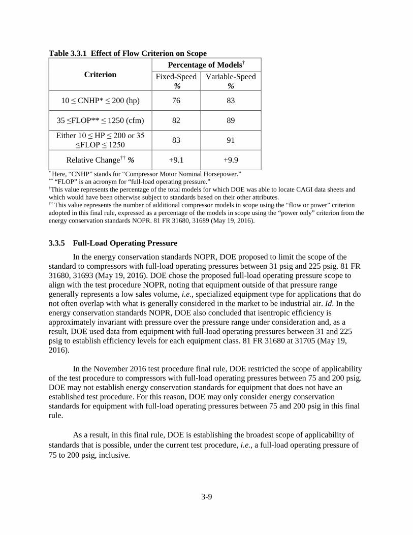
3-9

Table 3.3.1 Effect of Flow Criterion on Scope

Criterion Percentage of Models†

Fixed-Speed %

Variable-Speed %

10 ≤ CNHP* ≤ 200 (hp) 76 83

35 ≤FLOP** ≤ 1250 (cfm) 82 89

Either 10 ≤ HP ≤ 200 or 35 ≤FLOP ≤ 1250 83 91

Relative Change†† % +9.1 +9.9 * Here, “CNHP” stands for “Compressor Motor Nominal Horsepower.” ** “FLOP” is an acronym for “full-load operating pressure.” †This value represents the percentage of the total models for which DOE was able to locate CAGI data sheets and which would have been otherwise subject to standards based on their other attributes. †† This value represents the number of additional compressor models in scope using the “flow or power” criterion adopted in this final rule, expressed as a percentage of the models in scope using the “power only” criterion from the energy conservation standards NOPR. 81 FR 31680, 31689 (May 19, 2016).

3.3.5 Full-Load Operating Pressure

In the energy conservation standards NOPR, DOE proposed to limit the scope of the standard to compressors with full-load operating pressures between 31 psig and 225 psig. 81 FR 31680, 31693 (May 19, 2016). DOE chose the proposed full-load operating pressure scope to align with the test procedure NOPR, noting that equipment outside of that pressure range generally represents a low sales volume, i.e., specialized equipment type for applications that do not often overlap with what is generally considered in the market to be industrial air. Id. In the energy conservation standards NOPR, DOE also concluded that isentropic efficiency is approximately invariant with pressure over the pressure range under consideration and, as a result, DOE used data from equipment with full-load operating pressures between 31 and 225 psig to establish efficiency levels for each equipment class. 81 FR 31680 at 31705 (May 19, 2016).

In the November 2016 test procedure final rule, DOE restricted the scope of applicability of the test procedure to compressors with full-load operating pressures between 75 and 200 psig. DOE may not establish energy conservation standards for equipment that does not have an established test procedure. For this reason, DOE may only consider energy conservation standards for equipment with full-load operating pressures between 75 and 200 psig in this final rule.

As a result, in this final rule, DOE is establishing the broadest scope of applicability of standards that is possible, under the current test procedure, i.e., a full-load operating pressure of 75 to 200 psig, inclusive.

3-10

3.3.6 Lubricant Presence

In the energy conservation standards NOPR, DOE proposed to include lubricant-free compressors in the scope of the standards. However, DOE recognized differences in design, efficiency, cost, and utility for lubricant-free compressors when establishing separate equipment classes for compressors based on lubricant presence. 81 FR 31680 at 31698 (May 19, 2016). DOE proposed a “new standards at baseline” standard for lubricant-free compressors, which would not have resulted in national energy savings, as reflected in the national impact analysis (NIA), but would have prevented potential new, less efficient equipment from the entering the market and potentially increasing future national energy consumption. 81 FR 31680 at 31736.

In the test procedure final rule, DOE excluded lubricant-free compressors from the scope of test procedures based on three general reasons: (1) the lack of applicability of the test method and metric proposed in the test procedure NOPR; (2) the desire to retain the opportunity of harmonization with the European Union (EU) regulatory process for the benefit of manufacturers and consumers; and (3) to avoid creating an incentive to substitute unregulated technologies (such as dynamic) for regulated lubricant-free compressors.

Because there is no test procedure for lubricant-free compressors at this time, DOE cannot consider energy conservation standards for this equipment in this final rule. DOE is making no determination of the technological feasibility or economic justification of potential standards for lubricant-free compressors in this final rule. DOE may evaluate standards for lubricant-free compressors in the future, if an appropriate test procedure is developed.

3.3.7 Water Injection

Some compressors inject water into the compression chamber, in place of oil or other lubricants, to avoid risk of air contamination and serve applications that require inherently clean air. In the energy conservation standards NOPR, DOE proposed to defined “lubricated compressor” as “a compressor that introduces an auxiliary substance into the compression chamber during compression” and “auxiliary substance” as “any substance deliberately introduced into a compression process to aid in compression of a gas by any of the following: lubricating, sealing mechanical clearances, or absorbing heat.” c

In the energy conservation standards NOPR, DOE interpreted water to be an auxiliary substance. 81 FR 31680, 31698 (May 19, 2016). Consequently, water-injected compressors would have been classified as lubricated compressors.

For this final rule, DOE performed research to better understand water-injected compressor technology and to determine whether water injection both provides consumer utility and inhibits the ability to reach higher efficiency levels.

c This definition was adopted, unchanged, in the test procedure final rule.

3-11

Water-injected compressors operate similarly to conventional (i.e., oil or synthetic oil) lubricated compressors in that they introduce a liquid into the compression chamber to lubricate moving parts, seal mechanical clearances against the egress of air, and absorb heat. DOE understands the chief consumer utility of using water, in place of an oil- or synthetic oil-based auxiliary substance, is freedom from risk of output air contamination. Because no oil is introduced, failure of a filter or other downstream oil removal apparatus will not permit oil to become present in the delivered air. However, water and vapor must still be removed. Because of the similar utility of an inherently oil-free process, water-injected compressors more often compete with lubricant-free compressors rather than with lubricated compressors.

A limitation of replacing oil with water is that water tends to be more corrosive to many types of metals commonly used to construct compressors. This is particularly true if the water contains trace quantities of minerals, as does any water drawn from the environment or public water supply. To reduce corrosion, water-injected compressors employ advanced filtration (commonly, reverse osmosis) to create highly purified water for introduction into the compression process. The advanced filtration systems used by water-injected compressors may add nontrivial energy consumption to a compressor package and ultimately reduce efficiency. Reverse osmosis systems typically require creation of large pressure gradients and several stages of filtration. The filtration systems may also contain elements to eliminate biological agents, of particular concern in medical applications.

Even with advanced filtration systems, water-injected compressors may require the use of more corrosion-resistant materials for any componentry downstream of the water injection site. These materials may be less resistant to mechanical deformation and exhibit diminished lifespan relative to conventional construction materials. As a result, designers tend to open mechanical clearances, compared with conventionally lubricated compressors, in anticipation of mechanical deformation association with less durable materials used to resist corrosion. Wider clearances allow more air leakage during operation, and ultimately reduce efficiency.

These modifications that alter efficiency—filtration, corrosion-resistant material, altered geometry—are also likely to add cost to a water-injected compressor, relative to a conventionally lubricated compressor of similar specification.

With respect to market share, DOE knows of only three manufacturers currently offering water-injected compressors in the U.S. market,d and DOE believes that shipments of water-injected compressors are very low compared to oil- or synthetic oil-injected compressors. As a result, DOE expects energy savings associated with water-injected compressors to be minimal.

In conclusion, DOE’s research indicates that water-injected compressors may provide additional end user utility, but with reduced ability to meet higher efficiency levels. As a result, water-injected compressors may warrant a separate equipment class from lubricated compressors. However, because no performance data is available to characterize water-injected

d Sullivan-Palatek, Atlas Copco, and CompAir (a brand of Gardner Denver)

3-12

compressors, DOE has no basis to establish a standard. Therefore, DOE excludes water-injected compressors from the scope of this final rule. To clearly establish what is meant by the term, DOE is adopting a definition in this final rule. “Water-injected compressor” means “a lubricated compressor that uses injected water as an auxiliary substance.”

3.3.8 Specialty Purpose

In the energy conservation standards NOPR, DOE did not explicitly exclude any categories of specialty compressors. DOE made no specific scope exclusion for what the compressor industry refers to as “customized” or “specialty-purpose” compressors. 81 FR 31680, 31690, 31693, 31696 (May 19, 2016). Although specialty compressors were not explicitly excluded, DOE expects that many would be effectively excluded by other scope limitations, including full-load operating pressure, compression principle, variety of gas compressed, capacity, driver variety, and lubricant presence.

In the test procedure final rule, DOE incorporates CAGI’s recommended list of equipment (with certain modifications) to define the minimum testing configuration for a compressor basic model. Consequently, customized or specialty-purpose equipment that is created by adding additional equipment to what the industry refers to as a standard or basic package compressor, would be tested without the additional equipment, and achieve the same rating as the basic package compressor it was derived from. For this reason, DOE finds no reason to expressly exclude, from scope, any compressors that are created by adding additional equipment to the basic testing configuration specified in the test procedure.

However, two additional concerns remain: (1) specialty-purpose equipment that is created by modifying or replacing equipment on a standard package compressor, and (2) specialty-purpose equipment that is not derivative of other standard equipment. DOE performed research (using interested party comments as a starting point) to determine if any additional scope exclusions are warranted. Specifically, DOE was able to identify 11 applications and feature categories that could possibly be used to characterize specialty-purpose compressors in the compressor industry:

1) corrosive environments 2) hazardous environments 3) extreme temperatures 4) marine environments 5) weather-protected environments 6) mining environments 7) military applications 8) food service applications 9) medical air applications (including dental) 10) climate-control applications 11) petroleum, gas, and chemical applications

3-13

DOE established three criteria to help determine if exclusions are warranted for each of the aforementioned applications and feature categories. A compressor category must meet all three criteria to be considered for exclusion. The criteria are distinguishability, consumer utility, and material disadvantage.

The first criterion, distinguishability, requires that compressors under consideration must be able to be distinguished from general-purpose compressors. In this case, to be distinguishable extends beyond being able to identify any difference whatsoever. Specifically, distinguishability is determined in the context of the test procedure. DOE’s test procedure final rule contains instructions regarding compressor configuration during testing. During a test, only specific enumerated components are required to be connected; manufacturers may remove non-required components at their option. If the specialized nature of a compressor arises from a non-required component, manufacturers have the option to remove its influence on compressor performance. In that scenario, the specialty compressor, from the perspective of the test procedure, has “collapsed” to a general-purpose unit with no remaining distinction. In considering whether a compressor meets the distinguishability criterion, DOE will assess whether the specialized nature of the compressor arises from components or configurations that would vanish under the specific provisions of DOE’s test procedure.

As stated previously, DOE is incorporating a list of equipment, so the only specialty-purpose compressors that could warrant exclusion are (1) those that are created by modifying or replacing equipment on a standard package compressor, and (2) specialty-purpose equipment that is not derivative of other standard equipment.

The second criterion, consumer utility, requires that the specialty compressor must offer clear and unique utility to the end user. If it can be easily substituted for a general-purpose compressor without significant consequence, unique consumer utility is not supplied. The criterion is also important for ensuring that exclusion would not create a substitution incentive for consumers to switch to non-regulated specialty equipment as a means to reduce first cost.

The final criterion, material disadvantage, requires that a specialty compressor must face greater difficulty than general-purpose compressors in some regard. For example, a compressor may face, on account of extra componentry required to serve a specialty application, greater obstacle to improving efficiency than would a general-purpose compressor. Alternatively, a compressor may be able to achieve greater efficiency without trouble but create some disproportionate burden to manufacturers, for example in testing or demonstrating compliance.

DOE performed research, using publicly available data, on each of the categories to determine if exclusions are warranted. In the following paragraphs, DOE discusses findings for each of the aforementioned 11 specialty applications.

3-14

3.3.8.1 Corrosive Environments

Corrosive environments can be damaging to both the external components of a compressor and the internal components, if corrosive agents are ingested with the air. DOE’s research indicated that corrosive agents are found in wide range of varieties and severities. Certain corrosive agents may harm some materials but not others.

Compressors may be adapted to corrosive environments by using special materials, having special coatings, using additional intake air filtration, or using special or remote enclosures to isolate the compressor from the corrosive environment. However, most requirements for corrosive environments are customer-specific, making it difficult to create a generalized scope exclusion. Some end users also use general-purpose compressors in a corrosive environment, opting to replace the compressor at an earlier interval instead of purchasing a more expensive compressor that can last longer in the corrosive environment.

Based on this information, DOE does not believe that all corrosive environment compressors meet the first criterion of distinguishability; however certain corrosive environment compressors utilizing special materials and/or coatings may be distinguishable.

DOE did find that certain corrosive environment compressors meet the second criterion of consumer utility. Although some consumers opt to simply replace compressors more frequently, this may be impractical for locations for which frequent replacement is impractical (e.g., a remote location) or for which downtime is intolerable. Further, some corrosive agents may be of a severity that greatly accelerates wear. As a result, whichever measures are employed to avert corrosive agents or resist their effect can be said to grant utility.

DOE does not find that such compressors meet the third criterion of material disadvantage. DOE was unable to find evidence that most compressors suited to corrosive environments would generally face disproportionate difficulty in reaching the same efficiency levels as general-purpose compressors. Specifically, DOE was unable to find evidence that identifiable components, such as special materials and coatings, affect efficiency. As a result, DOE does not find sufficient evidence that compressors suited to corrosive environments face disproportionate difficulty in reaching the same efficiency levels as general-purpose compressors. Furthermore, DOE found no evidence suggesting corrosive environment compressors would be subject to disproportionate burden in testing or demonstrating compliance.

Because corrosive environment compressors do not meet the criteria of distinguishability and material disadvantage, DOE does not exclude them from the scope of this final rule.

3.3.8.2 Hazardous Environments

Hazardous environments include those in which there is the possibility of combustion or explosion. Compressors may be adapted to hazardous environments through modified electrical components and enclosures that protect against sparks and high temperatures. At least some of these components would need to be included as part of the basic package during testing. Several

3-15

standards specify the type and level of precautions required for these environments, so certification with one or more of these could be a method for defining the scope of exclusion.

For these reasons, DOE finds that hazardous environment compressors to meet the first criterion of distinguishability. Hazardous environment compressors in the United States are designated as such by independent agencies such as UL, and given a rating that corresponds to the specific attributes of the hazardous environment for which the unit is being certified. Independent agencies, such as UL, certify that compressors are suitable for hazardous environments against the National Electrical Code (NEC), which is the common term for the National Fire Protection Association standard NFPA 70, using a system of classes, zones, and groups of hazardous materials for which the equipment is being rated safe. DOE examined standards set by Atmosphères Explosibles (ATEX)e, but found that this designation is predominantly used in the European market and largely overlaps, in terms of the information it conveys to the consumer, with the NFPA 70 rating system.

DOE also found that hazardous environment compressors meet the second criterion of consumer utility. Using non-explosion-safe equipment, in hazardous environments, can create profound risk to life and property.

However, DOE does not find that hazardous environment compressor meet the third criterion of material disadvantage. DOE was unable to find evidence that compressors suited to hazardous environments would face disproportionate difficulty in reaching the same efficiency levels as general-purpose compressors. DOE believes that the modified electrical components and enclosures used in hazardous environments have little impact on energy use. Additionally, DOE found no evidence suggesting hazardous environment compressors would be subject to disproportionate burden in testing or demonstrating compliance.

Because hazardous environment compressors do not meet the criterion of material disadvantage, DOE does not exclude them from the scope of this final rule.

3.3.8.3 Extreme Temperatures

CAGI and Sullair identified the need to exclude compressors used in extreme temperatures. (CAGI, No. 0010, p. 4; Sullair, No. 0006 at p. 8) For high extremes, both commenters identified temperatures above 45 °C. For low extremes, Sullair indicated temperatures below 5 °C, while CAGI indicated temperatures below 0 °C. DOE notes that CAGI and Sullair did not present any standardized tests or inspections that might be used to uniformly classify the acceptable temperature range for a compressor.

eATEX is the common industry phrasing for European Parliament and Council Directive 2014/34/EU of 26 February 2014, which governs equipment and protective systems intended for use in potentially explosive atmospheres. The term “ATEX” is a portmanteau of “atmosphères explosibles”, French for “explosive atmospheres.”

3-16

In the absence of that information, DOE performed research and found neither industry-accepted, standardized test methods to determine allowable operating temperature, nor any industry-accepted certification programs to classify compressors for extreme temperatures. DOE also researched what types of modification and components might be employed to adapt compressors for extremely high- and low-temperature environments. For lower temperatures, a variety of heating devices may be used to heat the compressor package in various ways – such equipment would not be required as a part of test procedure testing configuration and is, therefore, not a distinguishing feature.

In hotter environments, compressors may employ larger output air heat exchangers and associated fans. Unlike package heating and cooling, heat exchangers and fans would necessarily be part of the test configuration. However, manufacturers may employ larger heat exchangers and fans for a variety of reasons, e.g. recovering waste heat for use in space heating. Furthermore, heat exchanger and fan size (as compared to compressor capacity) is not a standardized feature across the compressor industry, with different manufacturers choosing different-sized components to meet their specific design goals. Consequently, DOE is unable to establish a clear threshold to delineate larger heat exchangers and fans employed for high temperature applications. Furthermore, doing so would open a significant circumvention risk, as manufacturers could purposely substitute larger heat exchangers and fans in order to exclude compressors from regulation. For these reasons, DOE concludes that compressors designed for extreme temperature operation are not clearly distinguishable from general-purpose compressors.

Due to the difficulty in distinguishing compressors designed for extreme temperature operation from general-purpose compressors, DOE could not determine whether compressors designed for extreme temperature operation meet the second criterion of consumer utility, or the third criterion of material disadvantage. DOE adds that if a specialty purpose compressor fails to meet the first criterion of distinguishability, then it is unlikely that the specialty purpose compressor provides clear and unique utility to the end user that a general-purpose compressor would not provide. Similarly, if a specialty purpose compressor fails to meet the first criterion of distinguishability, then it is unlikely that the specialty purpose compressor has a material disadvantage compared to a general-purpose compressor. Consequently, DOE is unable to exclude these compressors from the scope of this final rule.

3.3.8.4 Marine Environments

Marine air compressors are intended for use aboard ships, offshore platforms, and similar environments. In general, DOE found this to be a very broad category of compressors. There are a wide variety of standards for these applications, but many of the requirements are customer-specific, making it difficult to clearly identify the scope for exclusion. Marine compressors may be space constrained if installed on ships. However, this may not always be the case, and some marine environments may be able to utilize general-purpose compressors. Further, DOE found no way to distinguish clearly, from general-purpose compressors, those compressors specifically developed for constrained spaces. DOE’s research found that other items, such as saltwater coolers, may be employed with marine air compressors, however, this equipment would not need

3-17

to be included for testing. For these reasons, DOE does not find marine environment compressors to meet the first criterion of distinguishability.

Due to the difficulty in distinguishing marine environment compressors from general-purpose compressors, DOE could not determine whether marine environment compressors meet the second criterion of consumer utility, or the third criterion of material disadvantage. DOE adds that if a specialty purpose compressor fails to meet the first criterion of distinguishability, then it is unlikely that the specialty purpose compressor provides clear and unique utility to the end user that a general-purpose compressor would not provide. Similarly, if a specialty purpose compressor fails to meet the first criterion of distinguishability, then it is unlikely that the specialty purpose compressor has a material disadvantage compared to a general-purpose compressor. Because marine environment compressors do not meet the first criteria for consideration of exclusion, DOE does not exclude them from the scope of this final rule.

3.3.8.5 Weather Protected

Weather-protected compressors require features to prevent the ingress of water and debris, as well as accommodation for extreme temperatures in some cases. Design accommodations related to extreme temperatures are discussed in section of 3.3.8.5 and, therefore, the scope of this section is confined to those design accommodations related to aspects of weather-protection for reasons other than extreme temperature. DOE found that third-party standards exist for ingress protection of the electrical components. However, DOE could find no indication of a standard or certification for other aspects of weather protection, making it difficult to clearly identify a general scope for exclusion for all weather-protected equipment. However, DOE believes that certain weather-protected compressors (i.e., those with electrical components rated for ingress protection) meet the first criterion of distinguishability.

Similarly, DOE believes that certain weather-protected compressors (i.e., those with electrical components rated for ingress protection) meet the second criterion of consumer utility, as such equipment is designed to operate in environments where non-rated equipment cannot.

However, DOE does not find that weather-protected compressors meet the third criterion of material disadvantage. Most weather-protected compressors would generally not face disproportionate difficulty in reaching the same efficiency levels as general-purpose compressors. Some components added for weather protection, such as special electrical components, have little impact on energy use. As a result, DOE does not find evidence to suggest that weather-protected compressors face disproportionate difficulty in reaching the same efficiency levels as general-purpose compressors. DOE found no evidence suggesting weather-protected compressors would be subject to disproportionate burden in demonstrating compliance.

Because weather-protected compressors do not meet the third criteria for exclusion, DOE does not exclude them from the scope of this final rule.

3-18

3.3.8.6 Mining Environments

Mining environments can include both surface and subsurface mine compressor applications. There are some industry standards for these applications, for example those developed by the Mine Safety and Health Administration (MSHA). However, DOE did not locate any which could be used to reliably designate compressors for mining environments. Furthermore, many of the design requirements for mining environment compressors are customer-specific, making it difficult to clearly identify the scope for exclusion. Some mining applications also use general-purpose compressors. For this reason, DOE does not find mining environment compressors to meet the first criterion of distinguishability. DOE was not able to determine that compressors for mining environments are always distinguishable from general-purpose compressors. There is no universally recognized designator.

Due to the difficulty in distinguishing mining environment compressors from general-purpose compressors, DOE could not determine whether mining environment compressors meet the second criterion of consumer utility, or the third criterion of material disadvantage. DOE adds that if a specialty purpose compressor fails to meet the first criterion of distinguishability, then it is unlikely that the specialty purpose compressor provides clear and unique utility to the end user that a general-purpose compressor would not provide. Similarly, if a specialty purpose compressor fails to meet the first criterion of distinguishability, then it is unlikely that the specialty purpose compressor has a material disadvantage compared to a general-purpose compressor.

Ultimately, because mining environment compressors do not meet the first criteria for consideration of exclusion, DOE does not exclude them from the scope of this final rule.

3.3.8.7 Military Applications

Compressors used in military applications have a wide range of applications. Many military applications use common commercial or industrial compressors. Other military applications, however, must meet extensive customer-specific requirements. These requirements can vary greatly with the customer, and there are no commonly used standards for compressors in military applications. This makes it difficult to clearly identify the scope for exclusion. For this reason, DOE does not find military compressors to meet the first criterion of distinguishability.

Due to the difficulty in distinguishing military compressors from general-purpose compressors, DOE could not determine whether military compressors meet the second criterion of consumer utility, or the third criterion of material disadvantage. DOE adds that if a specialty purpose compressor fails to meet the first criterion of distinguishability, then it is unlikely that the specialty purpose compressor provides clear and unique utility to the end user that a general-purpose compressor would not provide. Similarly, if a specialty purpose compressor fails to meet the first criterion of distinguishability, then it is unlikely that the specialty purpose compressor has a material disadvantage compared to a general-purpose compressor.

3-19

Ultimately, because military compressors do not meet the first criteria for consideration of exclusion, DOE does not exclude them from the scope of this final rule.

3.3.8.8 Food Service Applications

Food service applications can have requirements for air purity and for the use of food-grade lubricants. Food grade lubricants would need to be included for testing, so at least some compressors designed for food service applications would meet the first criterion of distinguishability.

DOE found that food service application compressors also met the second criterion of consumer utility. Without food grade lubricants, compressors would not be permitted to be used in food processing environments.

DOE does not find that food service application compressors meet the third criterion of material disadvantage. DOE found no evidence that food-grade lubricants, would impact efficiency. As a result, DOE does not find evidence to suggest that food service compressors face disproportionate difficulty in reaching the same efficiency levels as general-purpose compressors.

Because food service applications compressors do not meet the third criterion of material disadvantage, DOE does not exclude them from the scope of this final rule.

3.3.8.9 Medical Air Applications

Medical air applications can have requirements for air purity, which is rated according to International Organization for Standardization (ISO) 8573-1,f and also included in the National Fire Protection Association Standard for Health Care Facilities (NFPA 99).g DOE notes that most medical air compressors are lubricant-free; as such, any lubricant-free medical air compressors are already excluded from this final rule. In lubricated compressors, high air purity is attained using a combination of filters and dryers added to the system after the compressor. These items are outside the basic compressor package, so a medical air compressor would collapse to a standard basic package for testing. For this reason, DOE does not find medical air application compressors to meet the first criterion of distinguishability.

Due to the difficulty in distinguishing medical air compressors from general-purpose compressors, DOE could not determine whether medical air compressors meet the second criterion of consumer utility, or the third criterion of material disadvantage.

Ultimately, because medical air compressors do not meet the first criteria for consideration of exclusion, DOE does not exclude them from the scope of this final rule.

f See: www.iso.org/iso/catalogue_detail.htm?csnumber=46418 g See: www.nfpa.org/codes-and-standards/all-codes-and-standards/list-of-codes-and-standards?mode=code&code=99

3-20

3.3.8.10 Climate-Control Applications

DOE reviewed available information for climate-control compressors and found that the most commonly advertised unique feature was an “oil carryover” of less than or equal to 2 parts per million (ppm).h DOE knows of one established standard for measurement of air purity, ISO 8573-1.i However, this standard expresses oil content using mg/m3 and would require conversion to parts per million (ppm).

DOE reviewed compressors that are currently available for sale and marketed for climate-

control applications. DOE found that all compressors currently listed as being for “climate-control” are reciprocating compressors. Because reciprocating compressors are not within the scope of this energy conservation standards rulemaking, DOE finds no reason to exclude climate-control compressors from this rulemaking.

3.3.8.11 Petroleum, Gas, and Chemical Applications

API 619 specifies certain minimum requirements for compressors used in the petroleum, gas, and chemical industry. While API 619 contains many specific design requirements, it also indicates that customers must specify many design requirements themselves. As a result, compressors designed to meet API 619 requirements are not uniform; rather, they are, by definition, customized compressors. In addition to the design requirements, API 619 imposes rigorous testing, data reporting, and data retention requirements on manufacturers. For example, manufacturers are required to perform specific hydrostatic and operational mechanical vibration testing on each individual unit distributed in commerce. Furthermore, manufacturers must retain certain data for at least 20 years, such as certification of materials, test data and results, records of all heat treatment, results of quality control tests and inspections, and details of all repairs. Based on these testing, data reporting, and data retention requirements, DOE concludes that compressors designed and tested to the requirements of API 619 meet the first criterion of distinguishability. Specifically, DOE concludes that any manufacturer claiming a potential exclusion from energy conservation standards would be able to furnish test data proving that the compressor was designed and tested to API 619 (and associated customer-specific) requirements.

Based on DOE’s assessment of API 619, DOE believes that the minimum design and

testing requirements specified in API 619 are created to achieve, among other goals, safety and reliability in the petroleum, gas, and chemical industry. These requirements ensure that the compressor can be operated and maintained safely, in the safety-critical petroleum, gas, and chemical industry. Consequently, DOE concludes that compressors tested to, and meeting minimum design requirements of API 619 provide additional consumer utility.

h Gardner Denver: www.regulations.gov/document?D=EERE-2013-BT-STD-0040-0066 Quincy: www.regulations.gov/document?D=EERE-2013-BT-STD-0040-0067 Champion: www.regulations.gov/document?D=EERE-2013-BT-STD-0040-0068 CPR: www.regulations.gov/document?D=EERE-2013-BT-STD-0040-0069 i See: www.iso.org/iso/catalogue_detail.htm?csnumber=46418

3-21

At this time, DOE has insufficient evidence to conclusively determine if compressors meeting the minimum design and testing requirements specified in API 619 are at a material disadvantage with respect to achievable compressors efficiency. However, given the role of API 619 in ensuring operational safety in the petroleum, gas, and chemical industry, it is appropriate to exclude from the scope of energy conservation standards compressors meeting the minimum design and testing requirements specified in API 619. In other words, DOE finds that including compressors meeting the minimum design and testing requirements specified in API 619 may have adverse impacts on health or safety.

Furthermore, DOE believes that excluding compressors meeting the minimum design and

testing requirements specified in API 619 will not create an appreciable risk of API 619 compressors being used in general purpose applications, due to the rigorous and burdensome requirements associated with complying with API 619. DOE may request that a manufacturer provide DOE with copies of the original design and test data that were submitted in accordance with the requirements of API 619 as evidence that the compressor is designed and tested to API 619.

3.4 EQUIPMENT CLASSES AND DISTINGUISHING FEATURES

When evaluating and establishing energy conservation standards, DOE may divide covered equipment into equipment classes by the type of energy used, capacity, or other performance-related features that justify differing standards. In making a determination whether a performance-related feature justifies a different standard, DOE must consider such factors as the utility of the feature to the consumer and other factors DOE determines are appropriate. (42 U.S.C. 6295(q) and 6316(a)) In the NOPR stage of this rulemaking, DOE proposed dividing compressors based on the following factors:

• compression principle, • lubricant presence, • cooling method, • motor speed type, and • motor phase count.

As discussed in section 3.3, in the final rule, DOE is excluding reciprocating compressors, lubricant-free compressors, and single-phase compressors from the scope of the energy conservation standards. Consequently, DOE no longer needs to establish equipment classes based on compression principle, lubricant presence, or motor phase count. However, consistent with the energy conservation standards NOPR, DOE is adopting equipment classes based on motor speed range and cooling method in this final rule. In the analysis for the final rule, DOE also analyzed the potential for establishing equipment classes for variations of rotary

3-22

compressor technology, but equipment classes based on those variations are not adopted in the final rule. Sections 3.4.1 to 3.4.3 provide detail on DOE’s equipment class decisions.

3.4.1 Motor Speed Range

Electric motor-driven compressors can be separated by the style of electric driver used in the package. Specifically, DOE found that compressors are sold with either a variable-speed driver, which can operate across a continuous range of driver speeds, or a fixed-speed driver, which can operate at only a single fixed-speed. In the test procedure final rule, DOE establishes definitions for “fixed-speed compressor” and “variable-speed compressor” to clearly differentiate these equipment varieties. Specifically, DOE defined fixed-speed compressor to mean an air compressor that is not capable of adjusting the speed of the driver continuously in response to incremental changes in the required compressor flow rate. DOE defined variable-speed compressor to mean an air compressor that is capable of adjusting the speed of the driver continuously in response to incremental changes in the required compressor actual volume flow rate.

In the energy conservation standards NOPR, DOE found that variable-speed compressors are typically less efficient at full load than comparable fixed-speed compressors, partially due to efficiency losses within the variable-speed drive. As an example of this difference, Figure 3.4.1 shows the mean isentropic efficiency of air-cooled, lubricated, single-stage compressors within the scope of the energy conservation standards NOPR, when tested at full-load actual volume flow rate.j

j The performance data was obtained from data sheets published through the CAGI Performance Verification Program: www.cagi.org/performance-verification/.

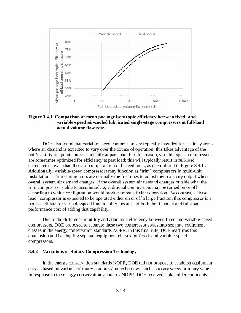
3-23

Figure 3.4.1 Comparison of mean package isentropic efficiency between fixed- and

variable-speed air-cooled lubricated single-stage compressors at full-load actual volume flow rate.

DOE also found that variable-speed compressors are typically intended for use in systems where air demand is expected to vary over the course of operation; this takes advantage of the unit’s ability to operate more efficiently at part load. For this reason, variable-speed compressors are sometimes optimized for efficiency at part load; this will typically result in full-load efficiencies lower than those of comparable fixed-speed units, as exemplified in Figure 3.4.1 . Additionally, variable-speed compressors may function as “trim” compressors in multi-unit installations. Trim compressors are normally the first ones to adjust their capacity output when overall system air demand changes. If the overall system air demand changes outside what the trim compressor is able to accommodate, additional compressors may be turned on or off according to which configuration would produce most efficient operation. By contrast, a “base load” compressor is expected to be operated either on or off a large fraction; this compressor is a poor candidate for variable-speed functionality, because of both the financial and full-load performance cost of adding that capability.

Due to the difference in utility and attainable efficiency between fixed and variable-speed compressors, DOE proposed to separate these two compressor styles into separate equipment classes in the energy conservation standards NOPR. In this final rule, DOE reaffirms this conclusion and is adopting separate equipment classes for fixed- and variable-speed compressors.

3.4.2 Variations of Rotary Compression Technology

In the energy conservation standards NOPR, DOE did not propose to establish equipment classes based on variants of rotary compression technology, such as rotary screw or rotary vane. In response to the energy conservation standards NOPR, DOE received stakeholder comments

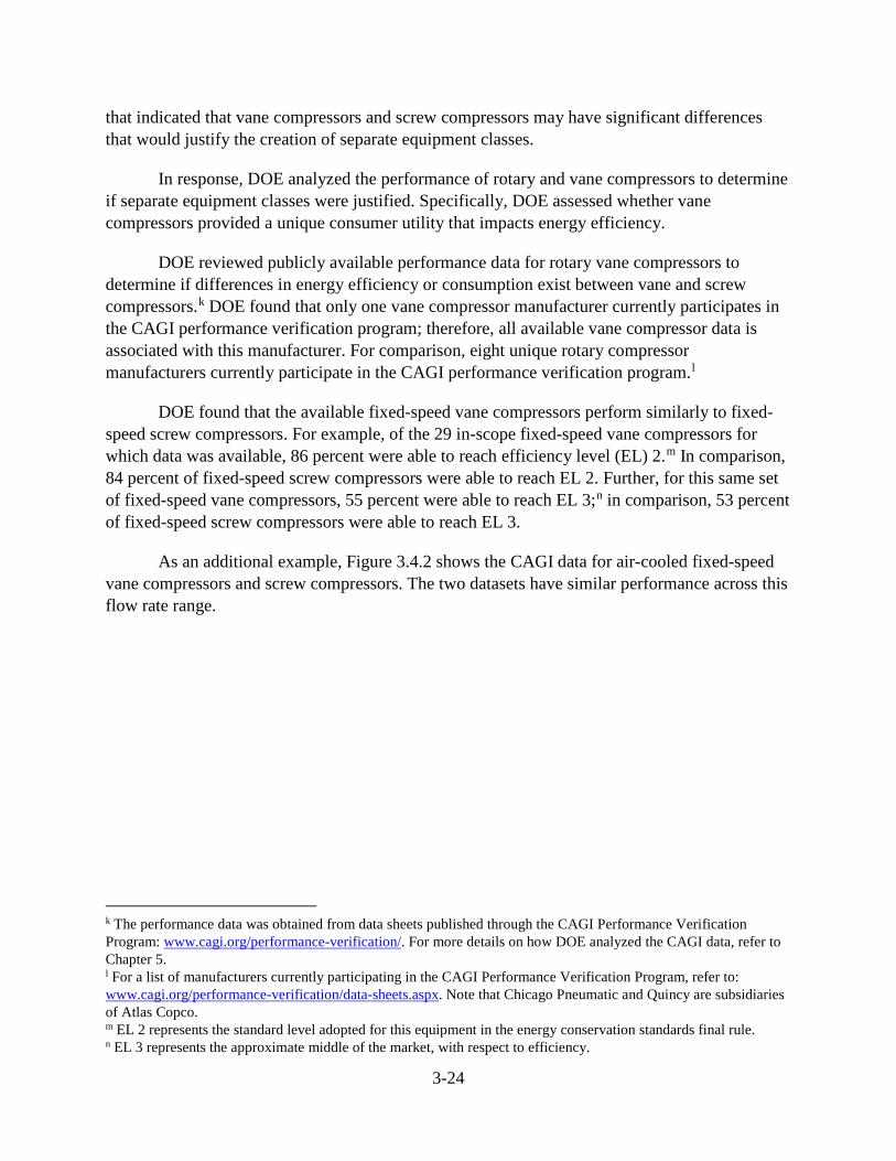
3-24

that indicated that vane compressors and screw compressors may have significant differences that would justify the creation of separate equipment classes.

In response, DOE analyzed the performance of rotary and vane compressors to determine if separate equipment classes were justified. Specifically, DOE assessed whether vane compressors provided a unique consumer utility that impacts energy efficiency.

DOE reviewed publicly available performance data for rotary vane compressors to determine if differences in energy efficiency or consumption exist between vane and screw compressors.k DOE found that only one vane compressor manufacturer currently participates in the CAGI performance verification program; therefore, all available vane compressor data is associated with this manufacturer. For comparison, eight unique rotary compressor manufacturers currently participate in the CAGI performance verification program.l

DOE found that the available fixed-speed vane compressors perform similarly to fixed-speed screw compressors. For example, of the 29 in-scope fixed-speed vane compressors for which data was available, 86 percent were able to reach efficiency level (EL) 2.m In comparison, 84 percent of fixed-speed screw compressors were able to reach EL 2. Further, for this same set of fixed-speed vane compressors, 55 percent were able to reach EL 3;n in comparison, 53 percent of fixed-speed screw compressors were able to reach EL 3.

As an additional example, Figure 3.4.2 shows the CAGI data for air-cooled fixed-speed vane compressors and screw compressors. The two datasets have similar performance across this flow rate range.

k The performance data was obtained from data sheets published through the CAGI Performance Verification Program: www.cagi.org/performance-verification/. For more details on how DOE analyzed the CAGI data, refer to Chapter 5. l For a list of manufacturers currently participating in the CAGI Performance Verification Program, refer to: www.cagi.org/performance-verification/data-sheets.aspx. Note that Chicago Pneumatic and Quincy are subsidiaries of Atlas Copco. m EL 2 represents the standard level adopted for this equipment in the energy conservation standards final rule. n EL 3 represents the approximate middle of the market, with respect to efficiency.

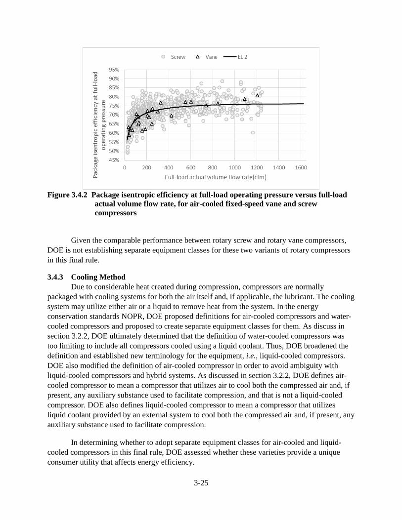
3-25

Figure 3.4.2 Package isentropic efficiency at full-load operating pressure versus full-load

actual volume flow rate, for air-cooled fixed-speed vane and screw compressors

Given the comparable performance between rotary screw and rotary vane compressors, DOE is not establishing separate equipment classes for these two variants of rotary compressors in this final rule.

3.4.3 Cooling Method Due to considerable heat created during compression, compressors are normally

packaged with cooling systems for both the air itself and, if applicable, the lubricant. The cooling system may utilize either air or a liquid to remove heat from the system. In the energy conservation standards NOPR, DOE proposed definitions for air-cooled compressors and water-cooled compressors and proposed to create separate equipment classes for them. As discuss in section 3.2.2, DOE ultimately determined that the definition of water-cooled compressors was too limiting to include all compressors cooled using a liquid coolant. Thus, DOE broadened the definition and established new terminology for the equipment, i.e., liquid-cooled compressors. DOE also modified the definition of air-cooled compressor in order to avoid ambiguity with liquid-cooled compressors and hybrid systems. As discussed in section 3.2.2, DOE defines air-cooled compressor to mean a compressor that utilizes air to cool both the compressed air and, if present, any auxiliary substance used to facilitate compression, and that is not a liquid-cooled compressor. DOE also defines liquid-cooled compressor to mean a compressor that utilizes liquid coolant provided by an external system to cool both the compressed air and, if present, any auxiliary substance used to facilitate compression.

In determining whether to adopt separate equipment classes for air-cooled and liquid-cooled compressors in this final rule, DOE assessed whether these varieties provide a unique consumer utility that affects energy efficiency.

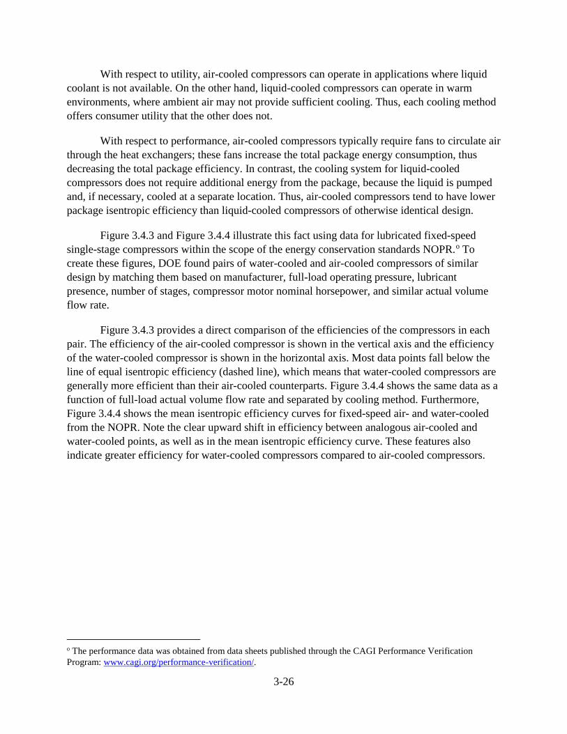
3-26

With respect to utility, air-cooled compressors can operate in applications where liquid coolant is not available. On the other hand, liquid-cooled compressors can operate in warm environments, where ambient air may not provide sufficient cooling. Thus, each cooling method offers consumer utility that the other does not.

With respect to performance, air-cooled compressors typically require fans to circulate air through the heat exchangers; these fans increase the total package energy consumption, thus decreasing the total package efficiency. In contrast, the cooling system for liquid-cooled compressors does not require additional energy from the package, because the liquid is pumped and, if necessary, cooled at a separate location. Thus, air-cooled compressors tend to have lower package isentropic efficiency than liquid-cooled compressors of otherwise identical design.

Figure 3.4.3 and Figure 3.4.4 illustrate this fact using data for lubricated fixed-speed single-stage compressors within the scope of the energy conservation standards NOPR.o To create these figures, DOE found pairs of water-cooled and air-cooled compressors of similar design by matching them based on manufacturer, full-load operating pressure, lubricant presence, number of stages, compressor motor nominal horsepower, and similar actual volume flow rate.

Figure 3.4.3 provides a direct comparison of the efficiencies of the compressors in each pair. The efficiency of the air-cooled compressor is shown in the vertical axis and the efficiency of the water-cooled compressor is shown in the horizontal axis. Most data points fall below the line of equal isentropic efficiency (dashed line), which means that water-cooled compressors are generally more efficient than their air-cooled counterparts. Figure 3.4.4 shows the same data as a function of full-load actual volume flow rate and separated by cooling method. Furthermore, Figure 3.4.4 shows the mean isentropic efficiency curves for fixed-speed air- and water-cooled from the NOPR. Note the clear upward shift in efficiency between analogous air-cooled and water-cooled points, as well as in the mean isentropic efficiency curve. These features also indicate greater efficiency for water-cooled compressors compared to air-cooled compressors.

o The performance data was obtained from data sheets published through the CAGI Performance Verification Program: www.cagi.org/performance-verification/.

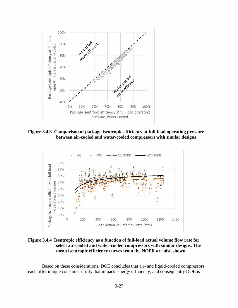
3-27

Figure 3.4.3 Comparison of package isentropic efficiency at full-load operating pressure between air-cooled and water-cooled compressors with similar designs

Figure 3.4.4 Isentropic efficiency as a function of full-load actual volume flow rate for select air-cooled and water-cooled compressors with similar designs. The mean isentropic efficiency curves from the NOPR are also shown

Based on these considerations, DOE concludes that air- and liquid-cooled compressors each offer unique consumer utility that impacts energy efficiency, and consequently DOE is

3-28

adopting separate equipment classes for air-cooled compressors and liquid-cooled compressors in this final rule.

3.4.4 List of Equipment Classes Based on the scope definitions in section 3.3 and the performance-related features and

distinguishing characteristics described in this section, DOE is establishing the equipment classes listed in Table 3.4.1.

Table 3.4.1 DOE Equipment Classes for Compressors Compressor

type Lubrication

type Cooling method

Driver type

Motor phase

Equipment class designation

Rotary Lubricated

Air-cooled Fixed-

speed Three-phase

RP_FS_L_AC

Liquid-cooled RP_FS_L_WC

Air-cooled Variable-

speed

RP_VS_L_AC

Liquid-cooled RP_VS_L_WC

3.5 TEST PROCEDURES AND ENERGY USE METRIC

In the test procedure final rule, DOE adopted a test method for calculating the package isentropic efficiency of compressors. DOE adopted methods based on (with modifications) ISO Standard 1217:2009(E), “Displacement compressors – Acceptance tests.”p

The test procedure requires that the energy conservation standards for compressors be expressed in terms of full-load package isentropic efficiency (ηisen,FL) for fixed-speed compressors, and part-load package isentropic efficiency (ηisen,PL) for variable-speed compressors. ηisen,FL and ηisen,PL describe the power required for an ideal isentropic compression process, divided by the actual input power of the packaged compressor. The ηisen,FL considers this ratio at full-load operating pressure, and ηisen,PL considers this ratio at a weighted-average of full-load and part-load operating pressures. The metrics are defined as follows:

𝜼𝜼𝒊𝒊𝒊𝒊𝒊𝒊𝒊𝒊,𝑭𝑭𝑭𝑭 = 𝜼𝜼𝒊𝒊𝒊𝒊𝒊𝒊𝒊𝒊,𝟏𝟏𝟏𝟏𝟏𝟏% =𝑷𝑷𝒊𝒊𝒊𝒊𝒊𝒊𝒊𝒊,𝟏𝟏𝟏𝟏𝟏𝟏%

𝑷𝑷𝒓𝒓𝒊𝒊𝒓𝒓𝒓𝒓,𝟏𝟏𝟏𝟏𝟏𝟏%

Equation 3.1 p In the test procedure final rule, DOE incorporated by reference ISO 1217:2009(E) as amended by ISO 1217:2009(E)/Amd.1:2016, titled “Calculation of isentropic efficiency and relationship with specific energy.”

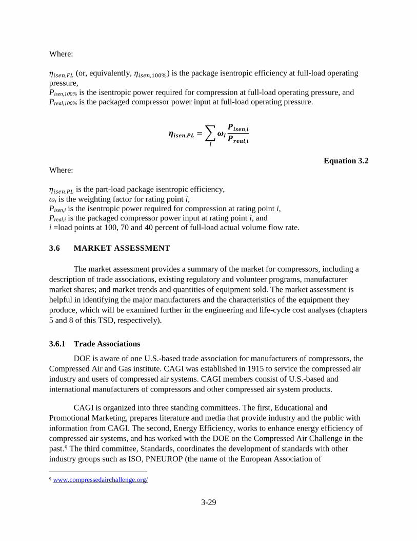
3-29

Where: 𝜂𝜂𝑖𝑖𝑖𝑖𝑖𝑖𝑖𝑖,𝐹𝐹𝐹𝐹 (or, equivalently, 𝜂𝜂𝑖𝑖𝑖𝑖𝑖𝑖𝑖𝑖,100%) is the package isentropic efficiency at full-load operating pressure, Pisen,100% is the isentropic power required for compression at full-load operating pressure, and Preal,100% is the packaged compressor power input at full-load operating pressure.

𝜼𝜼𝒊𝒊𝒊𝒊𝒊𝒊𝒊𝒊,𝑷𝑷𝑭𝑭 = �𝝎𝝎𝒊𝒊𝑷𝑷𝒊𝒊𝒊𝒊𝒊𝒊𝒊𝒊,𝒊𝒊

𝑷𝑷𝒓𝒓𝒊𝒊𝒓𝒓𝒓𝒓,𝒊𝒊𝒊𝒊

Equation 3.2 Where: 𝜂𝜂𝑖𝑖𝑖𝑖𝑖𝑖𝑖𝑖,𝑃𝑃𝐹𝐹 is the part-load package isentropic efficiency, ωi is the weighting factor for rating point i, Pisen,i is the isentropic power required for compression at rating point i, Preal,i is the packaged compressor power input at rating point i, and i =load points at 100, 70 and 40 percent of full-load actual volume flow rate. 3.6 MARKET ASSESSMENT

The market assessment provides a summary of the market for compressors, including a

description of trade associations, existing regulatory and volunteer programs, manufacturer market shares; and market trends and quantities of equipment sold. The market assessment is helpful in identifying the major manufacturers and the characteristics of the equipment they produce, which will be examined further in the engineering and life-cycle cost analyses (chapters 5 and 8 of this TSD, respectively).

3.6.1 Trade Associations

DOE is aware of one U.S.-based trade association for manufacturers of compressors, the Compressed Air and Gas institute. CAGI was established in 1915 to service the compressed air industry and users of compressed air systems. CAGI members consist of U.S.-based and international manufacturers of compressors and other compressed air system products.

CAGI is organized into three standing committees. The first, Educational and Promotional Marketing, prepares literature and media that provide industry and the public with information from CAGI. The second, Energy Efficiency, works to enhance energy efficiency of compressed air systems, and has worked with the DOE on the Compressed Air Challenge in the past.q The third committee, Standards, coordinates the development of standards with other industry groups such as ISO, PNEUROP (the name of the European Association of q www.compressedairchallenge.org/

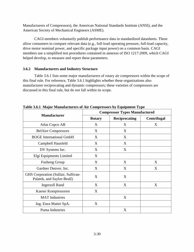
3-30

Manufacturers of Compressors), the American National Standards Institute (ANSI), and the American Society of Mechanical Engineers (ASME).

CAGI members voluntarily publish performance data in standardized datasheets. These allow consumers to compare relevant data (e.g., full-load operating pressure, full-load capacity, drive motor nominal power, and specific package input power) on a common basis. CAGI members use a simplified test procedures contained in annexes of ISO 1217:2009, which CAGI helped develop, to measure and report these parameters.

3.6.2 Manufacturers and Industry Structure

Table 3.6.1 lists some major manufacturers of rotary air compressors within the scope of this final rule. For reference, Table 3.6.1 highlights whether these organizations also manufacturer reciprocating and dynamic compressors; these varieties of compressors are discussed in this final rule, but do not fall within its scope.

Table 3.6.1 Major Manufacturers of Air Compressors by Equipment Type

Manufacturer Compressor Types Manufactured

Rotary Reciprocating Centrifugal Atlas Copco AB X X X

BelAire Compressors X X BOGE International GmbH X X

Campbell Hausfeld X X DV Systems Inc. X X

Elgi Equipments Limited X Fusheng Group X X X

Gardner Denver, Inc. X X X GHS Corporation (Sullair, Sullivan-

Palatek, and Saylor-Beall) X X

Ingersoll Rand X X X Kaeser Kompressoren X

MAT Industries X Ing. Enea Mattei SpA. X

Puma Industries X

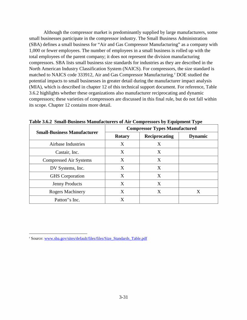
3-31

Although the compressor market is predominantly supplied by large manufacturers, some small businesses participate in the compressor industry. The Small Business Administration (SBA) defines a small business for “Air and Gas Compressor Manufacturing” as a company with 1,000 or fewer employees. The number of employees in a small business is rolled up with the total employees of the parent company; it does not represent the division manufacturing compressors. SBA lists small business size standards for industries as they are described in the North American Industry Classification System (NAICS). For compressors, the size standard is matched to NAICS code 333912, Air and Gas Compressor Manufacturing.r DOE studied the potential impacts to small businesses in greater detail during the manufacturer impact analysis (MIA), which is described in chapter 12 of this technical support document. For reference, Table 3.6.2 highlights whether these organizations also manufacturer reciprocating and dynamic compressors; these varieties of compressors are discussed in this final rule, but do not fall within its scope. Chapter 12 contains more detail.

Table 3.6.2 Small-Business Manufacturers of Air Compressors by Equipment Type

Small-Business Manufacturer Compressor Types Manufactured

Rotary Reciprocating Dynamic Airbase Industries X X

Castair, Inc. X X

Compressed Air Systems X X

DV Systems, Inc. X X

GHS Corporation X X Jenny Products X X

Rogers Machinery X X X

Patton'’s Inc. X

r Source: www.sba.gov/sites/default/files/files/Size_Standards_Table.pdf

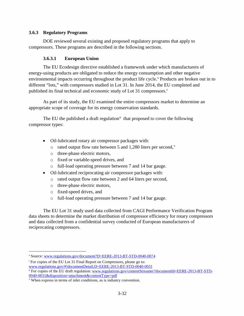
3-32

3.6.3 Regulatory Programs

DOE reviewed several existing and proposed regulatory programs that apply to compressors. These programs are described in the following sections.

3.6.3.1 European Union

The EU Ecodesign directive established a framework under which manufacturers of energy-using products are obligated to reduce the energy consumption and other negative environmental impacts occurring throughout the product life cycle.s Products are broken out in to different “lots,” with compressors studied in Lot 31. In June 2014, the EU completed and published its final technical and economic study of Lot 31 compressors.t

As part of its study, the EU examined the entire compressors market to determine an appropriate scope of coverage for its energy conservation standards.

The EU the published a draft regulationu that proposed to cover the following compressor types:

• Oil-lubricated rotary air compressor packages with:

o rated output flow rate between 5 and 1,280 liters per second,v o three-phase electric motors, o fixed or variable-speed drives, and o full-load operating pressure between 7 and 14 bar gauge.

• Oil-lubricated reciprocating air compressor packages with: o rated output flow rate between 2 and 64 liters per second, o three-phase electric motors, o fixed-speed drives, and o full-load operating pressure between 7 and 14 bar gauge.

The EU Lot 31 study used data collected from CAGI Performance Verification Program

data sheets to determine the market distribution of compressor efficiency for rotary compressors and data collected from a confidential survey conducted of European manufacturers of reciprocating compressors.

s Source: www.regulations.gov/document?D=EERE-2013-BT-STD-0040-0074 t For copies of the EU Lot 31 Final Report on Compressors, please go to: www.regulations.gov/#!documentDetail;D=EERE-2013-BT-STD-0040-0031 u For copies of the EU draft regulation: www.regulations.gov/contentStreamer?documentId=EERE-2013-BT-STD-0040-0031&disposition=attachment&contentType=pdf v When express in terms of inlet conditions, as is industry convention.

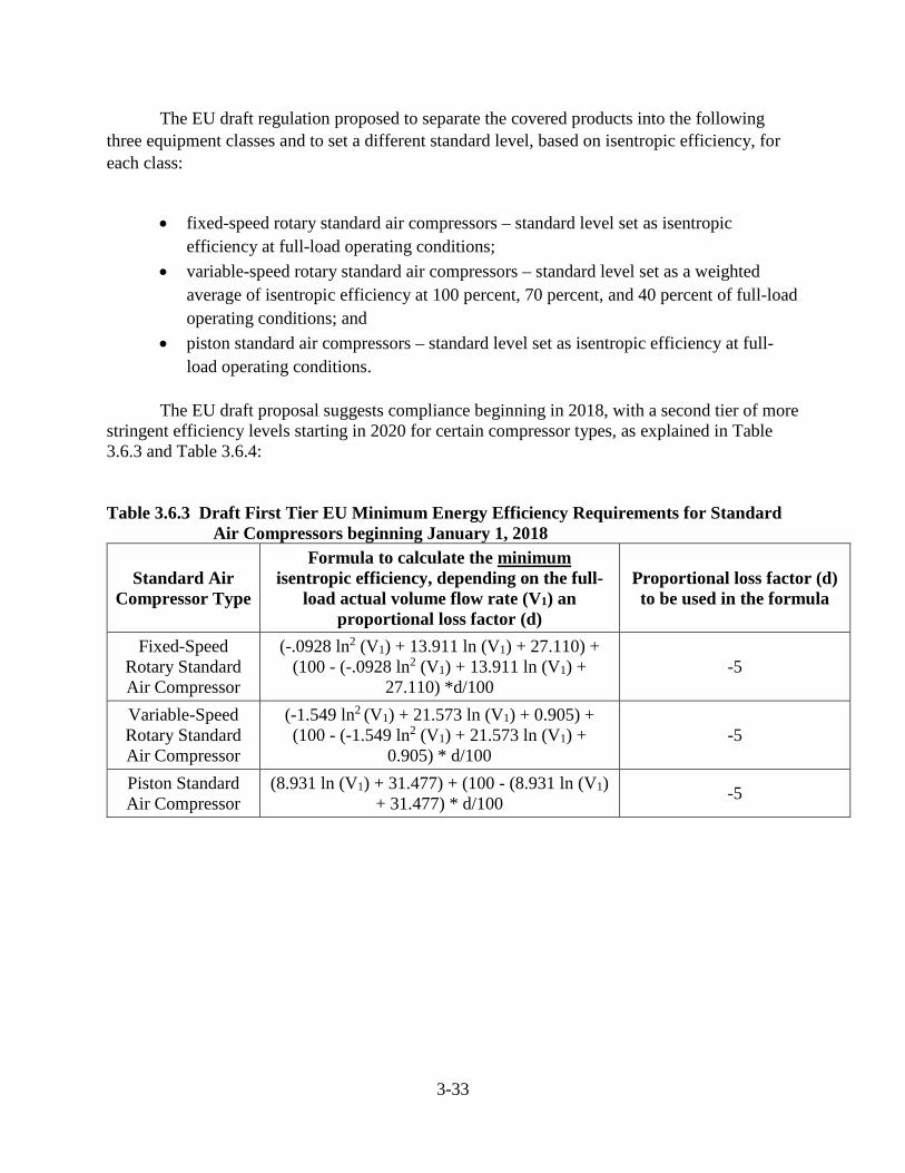
3-33

The EU draft regulation proposed to separate the covered products into the following three equipment classes and to set a different standard level, based on isentropic efficiency, for each class:

• fixed-speed rotary standard air compressors – standard level set as isentropic

efficiency at full-load operating conditions; • variable-speed rotary standard air compressors – standard level set as a weighted

average of isentropic efficiency at 100 percent, 70 percent, and 40 percent of full-load operating conditions; and

• piston standard air compressors – standard level set as isentropic efficiency at full-load operating conditions.

The EU draft proposal suggests compliance beginning in 2018, with a second tier of more

stringent efficiency levels starting in 2020 for certain compressor types, as explained in Table 3.6.3 and Table 3.6.4: Table 3.6.3 Draft First Tier EU Minimum Energy Efficiency Requirements for Standard

Air Compressors beginning January 1, 2018

Standard Air Compressor Type

Formula to calculate the minimum isentropic efficiency, depending on the full-

load actual volume flow rate (V1) an proportional loss factor (d)

Proportional loss factor (d) to be used in the formula

Fixed-Speed Rotary Standard Air Compressor

(-.0928 ln2 (V1) + 13.911 ln (V1) + 27.110) + (100 - (-.0928 ln2 (V1) + 13.911 ln (V1) +

27.110) *d/100 -5

Variable-Speed Rotary Standard Air Compressor

(-1.549 ln2 (V1) + 21.573 ln (V1) + 0.905) + (100 - (-1.549 ln2 (V1) + 21.573 ln (V1) +

0.905) * d/100 -5

Piston Standard Air Compressor

(8.931 ln (V1) + 31.477) + (100 - (8.931 ln (V1) + 31.477) * d/100 -5

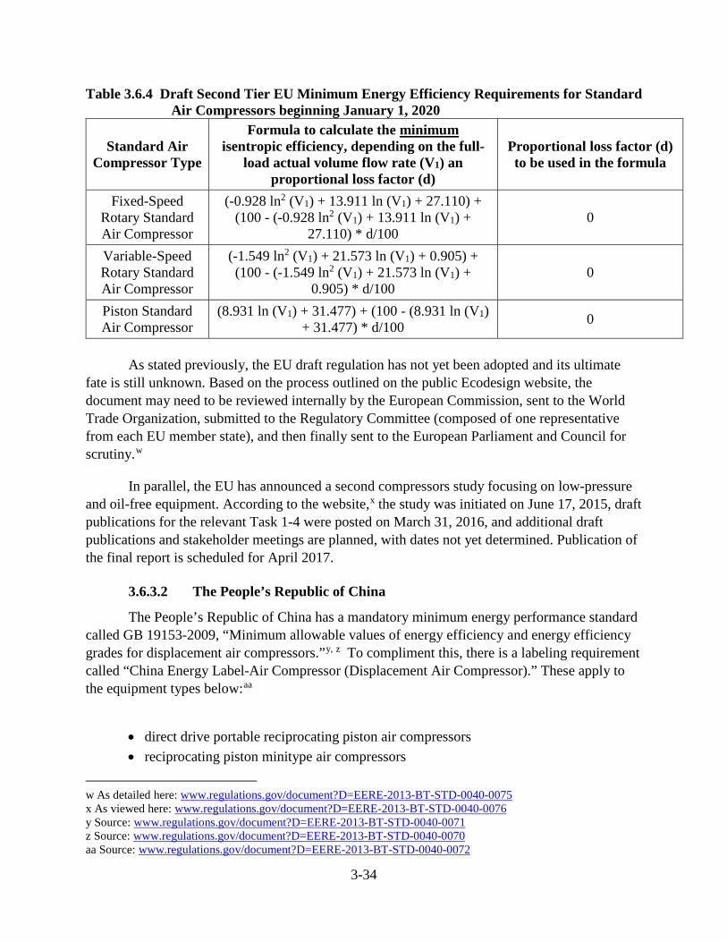
3-34

Table 3.6.4 Draft Second Tier EU Minimum Energy Efficiency Requirements for Standard Air Compressors beginning January 1, 2020

Standard Air Compressor Type

Formula to calculate the minimum isentropic efficiency, depending on the full-

load actual volume flow rate (V1) an proportional loss factor (d)

Proportional loss factor (d) to be used in the formula

Fixed-Speed Rotary Standard Air Compressor

(-0.928 ln2 (V1) + 13.911 ln (V1) + 27.110) + (100 - (-0.928 ln2 (V1) + 13.911 ln (V1) +

27.110) * d/100 0

Variable-Speed Rotary Standard Air Compressor

(-1.549 ln2 (V1) + 21.573 ln (V1) + 0.905) + (100 - (-1.549 ln2 (V1) + 21.573 ln (V1) +

0.905) * d/100 0

Piston Standard Air Compressor

(8.931 ln (V1) + 31.477) + (100 - (8.931 ln (V1) + 31.477) * d/100 0

As stated previously, the EU draft regulation has not yet been adopted and its ultimate

fate is still unknown. Based on the process outlined on the public Ecodesign website, the document may need to be reviewed internally by the European Commission, sent to the World Trade Organization, submitted to the Regulatory Committee (composed of one representative from each EU member state), and then finally sent to the European Parliament and Council for scrutiny.w

In parallel, the EU has announced a second compressors study focusing on low-pressure and oil-free equipment. According to the website,x the study was initiated on June 17, 2015, draft publications for the relevant Task 1-4 were posted on March 31, 2016, and additional draft publications and stakeholder meetings are planned, with dates not yet determined. Publication of the final report is scheduled for April 2017.

3.6.3.2 The People’s Republic of China

The People’s Republic of China has a mandatory minimum energy performance standard called GB 19153-2009, “Minimum allowable values of energy efficiency and energy efficiency grades for displacement air compressors.”y, z To compliment this, there is a labeling requirement called “China Energy Label-Air Compressor (Displacement Air Compressor).” These apply to the equipment types below:aa

• direct drive portable reciprocating piston air compressors • reciprocating piston minitype air compressors

w As detailed here: www.regulations.gov/document?D=EERE-2013-BT-STD-0040-0075 x As viewed here: www.regulations.gov/document?D=EERE-2013-BT-STD-0040-0076 y Source: www.regulations.gov/document?D=EERE-2013-BT-STD-0040-0071 z Source: www.regulations.gov/document?D=EERE-2013-BT-STD-0040-0070 aa Source: www.regulations.gov/document?D=EERE-2013-BT-STD-0040-0072

3-35

• oil-free reciprocating piston air compressors • stationary reciprocating piston air compressors for general use • oil injected screw air compressors for general use • oil injected single screw air compressors for general use • oil flooded sliding vane air compressors for general use

The scope for each equipment type varies, but the standard applies to certain equipment as low as 0.18 kW and up to 630 kW (approximately 0.25- to 844-hp), and from 0.25 to 1.40 MPa (approximately 36 to 203 psi). Minimum efficiency is measured in specific power (kW/(m3/min)) and is determined based on number of stages, lubrication, motor power, and full-load operating pressure for each equipment type. Equipment is tested according to GB/T 385-1998.bb

3.6.4 Nonregulatory Programs

DOE reviewed voluntary programs that promote energy efficient compressors in the United States, including the Compressed Air Challenge and CAGI’s performance verification and datasheet program.

3.6.4.1 Compressed Air Challenge

The Compressed Air Challenge is composed of members of all aspects of the compressed air field, including industrial end users, manufacturers, distributors, consultants, energy efficiency organizations, utilities, and state agencies. DOE is a sponsor of the Compressed Air Challenge.

The Compressed Air Challenge’s mission is to be the leading source of product-neutral compressed air system information and education, enabling end users to take a systems approach, leading to improved efficiency and production and increased net profits. It met this by hosting a variety of trainings and workshops in areas such as fundamentals of compressed air, management of compressed air systems, and AirMaster+ training.cc

The Compressed Air Challenge publishes magazine and journal articles, case studies, fact sheets, and its own best practices manual. Much of this material is publicly available on its website; some material is available for a fee.

3.6.4.2 CAGI Performance Verification Program

In an effort to create a uniform method for determining compressor efficiency, CAGI and its industry partners developed a voluntary performance verification program for 5- to 200-hp

bb Source: www.regulations.gov/document?D=EERE-2013-BT-STD-0040-0071 cc AIRMaster+ is a free online software tool developed by DOE that helps users analyze energy use and savings opportunities in industrial compressed air systems: www.energy.gov/eere/amo/articles/airmaster

3-36

rotary compressors, which is open to all manufacturers, even those that are not CAGI members. CAGI currently lists 12 manufacturers, representing nearly 2,000 individual compressor package models that participate in the Rotary Compressor Performance Verification Program, all of whom are CAGI members.dd

The Performance Verification Program specifies that manufacturers test each compressor model at a third-party lab using ISO 1217:2009. CAGI and its industry partners developed data sheets that specify measuring and reporting the following performance characteristics for each compressor tested:

• lubrication type • cooling method • rated capacity at full-load operating pressure • full-load operating pressure • driver motor nominal rating and efficiency • fan motor nominal rating and efficiency (if applicable) • total package input power at zero flow and at the rated capacity at full-load operating

pressure • specific package input power at rated capacity at full-load operating pressure

Data sheets for all compressors tested must be published on each manufacturer’s website.

Although the Performance Verification Program is only applicable to compressors from 5 to 200 hp, manufacturers may post data sheets for compressors outside this range. There are currently data sheets from CAGI members for compressors from 3 to 700 hp.

Participating manufacturers are subject to random testing of two units annually, which

are compared to certified published performance ratings. Units that do not pass may either be subject to additional testing or re-rated to generate new verified data sheets. Failure may result in ejection from the verification program. For units that pass the verification program test procedures, manufacturers may use the CAGI Verification Seal to advertise that equipment specifications have been tested by an independent laboratory

dd www.cagi.org/performance-verification/overview.aspx

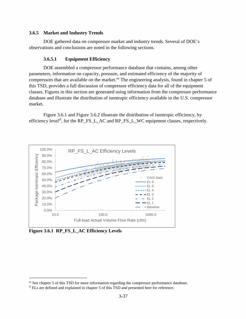
3-37

3.6.5 Market and Industry Trends

DOE gathered data on compressor market and industry trends. Several of DOE’s observations and conclusions are noted in the following sections.

3.6.5.1 Equipment Efficiency

DOE assembled a compressor performance database that contains, among other parameters, information on capacity, pressure, and estimated efficiency of the majority of compressors that are available on the market.ee The engineering analysis, found in chapter 5 of this TSD, provides a full discussion of compressor efficiency data for all of the equipment classes. Figures in this section are generated using information from the compressor performance database and illustrate the distribution of isentropic efficiency available in the U.S. compressor market.

Figure 3.6.1 and Figure 3.6.2 illustrate the distribution of isentropic efficiency, by efficiency levelff, for the RP_FS_L_AC and RP_FS_L_WC equipment classes, respectively.

Figure 3.6.1 RP_FS_L_AC Efficiency Levels

ee See chapter 5 of this TSD for more information regarding the compressor performance database. ff ELs are defined and explained in chapter 5 of this TSD and presented here for reference.

0.0%10.0%20.0%30.0%40.0%50.0%60.0%70.0%80.0%90.0%

100.0%

10.0 100.0 1000.0

Pack

age

Isen

tropi

c Ef

ficie

ncy

Full-load Actual Volume Flow Rate (cfm)

RP_FS_L_AC Efficiency Levels

CAGI DataEL 6EL 5EL 4EL 3EL 2EL 1Baseline

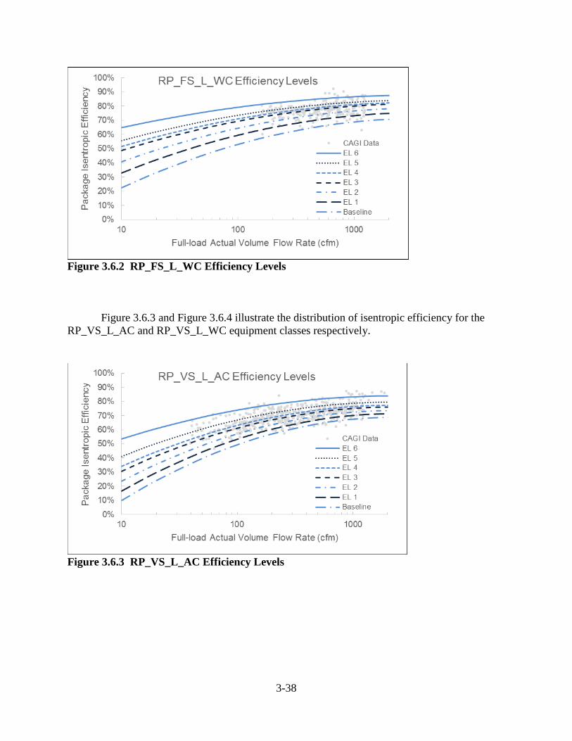
3-38

Figure 3.6.2 RP_FS_L_WC Efficiency Levels

Figure 3.6.3 and Figure 3.6.4 illustrate the distribution of isentropic efficiency for the RP_VS_L_AC and RP_VS_L_WC equipment classes respectively.

Figure 3.6.3 RP_VS_L_AC Efficiency Levels

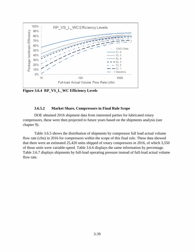
3-39

Figure 3.6.4 RP_VS_L_WC Efficiency Levels

3.6.5.2 Market Share, Compressors in Final Rule Scope

DOE obtained 2016 shipment data from interested parties for lubricated rotary compressors, these were then projected to future years based on the shipments analysis (see chapter 9).

Table 3.6.5 shows the distribution of shipments by compressor full load actual volume flow rate (cfm) in 2016 for compressors within the scope of this final rule. These data showed that there were an estimated 25,420 units shipped of rotary compressors in 2016, of which 3,550 of those units were variable-speed. Table 3.6.6 displays the same information by percentage. Table 3.6.7 displays shipments by full-load operating pressure instead of full-load actual volume flow rate.

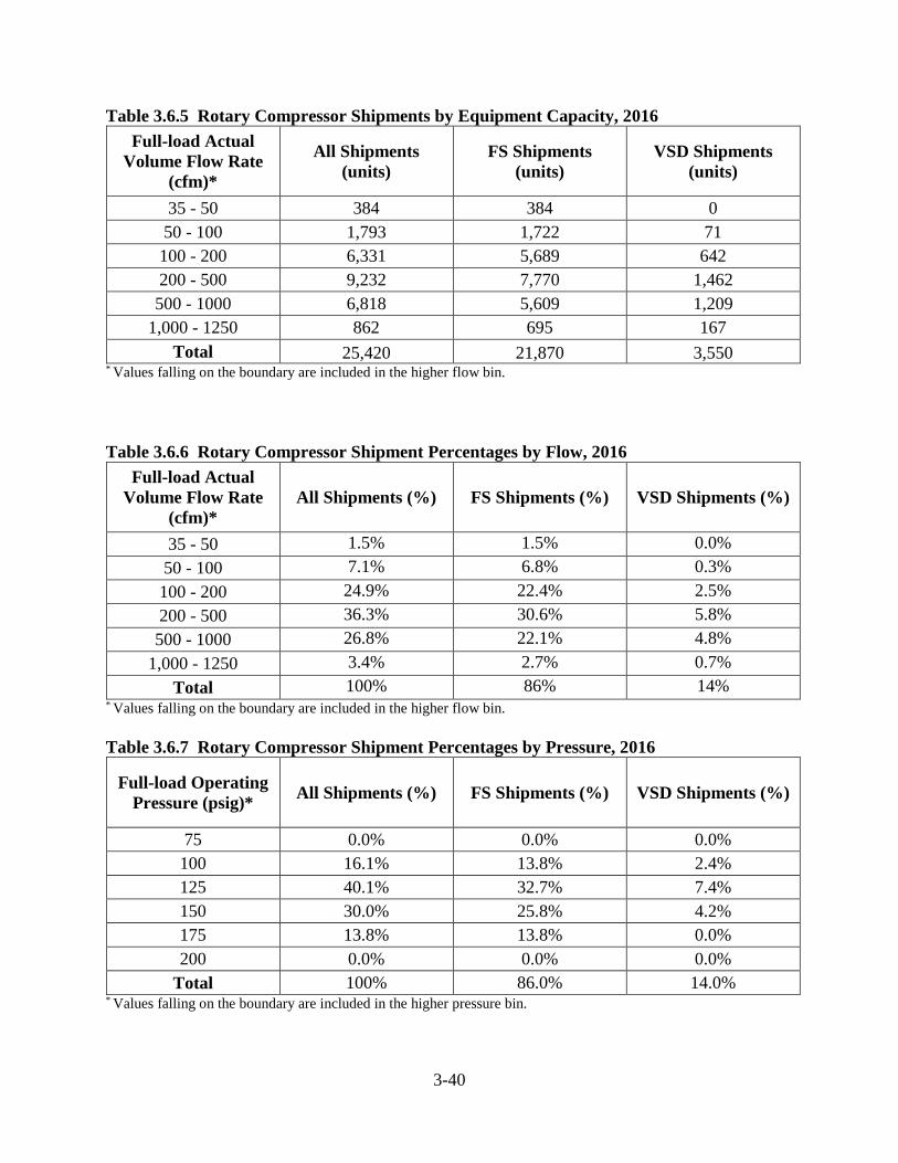
3-40

Table 3.6.5 Rotary Compressor Shipments by Equipment Capacity, 2016 Full-load Actual

Volume Flow Rate (cfm)*

All Shipments (units)

FS Shipments (units)

VSD Shipments (units)

35 - 50 384 384 0 50 - 100 1,793 1,722 71 100 - 200 6,331 5,689 642 200 - 500 9,232 7,770 1,462 500 - 1000 6,818 5,609 1,209

1,000 - 1250 862 695 167 Total 25,420 21,870 3,550

* Values falling on the boundary are included in the higher flow bin. Table 3.6.6 Rotary Compressor Shipment Percentages by Flow, 2016

Full-load Actual Volume Flow Rate

(cfm)* All Shipments (%) FS Shipments (%) VSD Shipments (%)

35 - 50 1.5% 1.5% 0.0% 50 - 100 7.1% 6.8% 0.3% 100 - 200 24.9% 22.4% 2.5% 200 - 500 36.3% 30.6% 5.8% 500 - 1000 26.8% 22.1% 4.8%

1,000 - 1250 3.4% 2.7% 0.7% Total 100% 86% 14%

* Values falling on the boundary are included in the higher flow bin. Table 3.6.7 Rotary Compressor Shipment Percentages by Pressure, 2016

Full-load Operating Pressure (psig)* All Shipments (%) FS Shipments (%) VSD Shipments (%)

75 0.0% 0.0% 0.0% 100 16.1% 13.8% 2.4% 125 40.1% 32.7% 7.4% 150 30.0% 25.8% 4.2% 175 13.8% 13.8% 0.0% 200 0.0% 0.0% 0.0%

Total 100% 86.0% 14.0% * Values falling on the boundary are included in the higher pressure bin.

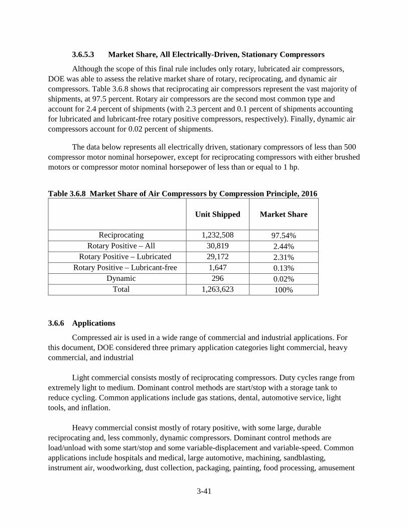
3-41

3.6.5.3 Market Share, All Electrically-Driven, Stationary Compressors

Although the scope of this final rule includes only rotary, lubricated air compressors, DOE was able to assess the relative market share of rotary, reciprocating, and dynamic air compressors. Table 3.6.8 shows that reciprocating air compressors represent the vast majority of shipments, at 97.5 percent. Rotary air compressors are the second most common type and account for 2.4 percent of shipments (with 2.3 percent and 0.1 percent of shipments accounting for lubricated and lubricant-free rotary positive compressors, respectively). Finally, dynamic air compressors account for 0.02 percent of shipments.

The data below represents all electrically driven, stationary compressors of less than 500 compressor motor nominal horsepower, except for reciprocating compressors with either brushed motors or compressor motor nominal horsepower of less than or equal to 1 hp.

Table 3.6.8 Market Share of Air Compressors by Compression Principle, 2016

Unit Shipped Market Share

Reciprocating 1,232,508 97.54% Rotary Positive – All 30,819 2.44%

Rotary Positive – Lubricated 29,172 2.31% Rotary Positive – Lubricant-free 1,647 0.13%

Dynamic 296 0.02% Total 1,263,623 100%

3.6.6 Applications

Compressed air is used in a wide range of commercial and industrial applications. For this document, DOE considered three primary application categories light commercial, heavy commercial, and industrial

Light commercial consists mostly of reciprocating compressors. Duty cycles range from

extremely light to medium. Dominant control methods are start/stop with a storage tank to reduce cycling. Common applications include gas stations, dental, automotive service, light tools, and inflation.

Heavy commercial consist mostly of rotary positive, with some large, durable reciprocating and, less commonly, dynamic compressors. Dominant control methods are load/unload with some start/stop and some variable-displacement and variable-speed. Common applications include hospitals and medical, large automotive, machining, sandblasting, instrument air, woodworking, dust collection, packaging, painting, food processing, amusement

3-42

parks, and construction.

Industrial consists mostly of medium and large rotary positive and dynamic. Dominant control methods are load/unload, with multi-compressor installations regulated by a master controller common for large sites. Compressors of multiple types may be employed in tandem. Common applications include painting, tool operations, injection molding, material conveying, soot blowing, electronic and semiconductor manufacturing, water and sewage treatment, glass manufacturing, pulp and paper, mining, and chemical production.

3.6.7 Controls Methods

Buyers of compressors may be able to save significant energy by using controls and heat recovery. Controls are used to match compressor output (flow) to air demand, which may occur in different patterns according to application.

The simplest demand pattern would be constant demand, wherein required air does not

vary over time. In this case, required compressor size is simple to determine, and no controls are needed other than an on/off switch. In practice, air demand as a function of time can be complicated. It may have sharp peaks, periods of zero demand, and even requirements for different pressure simultaneously. As a result, manufacturers have introduced several ways to match supply to demand. Broadly, they are “start/stop,” “load/unload,” “inlet modulation,” “variable-capacity,” “variable-speed,” and use of multiple compressors that incorporate these technologies.

Start/stop and load/unload can be considered cycling technologies, in the sense that they

adjust supply by switching compressor output on and off in a binary fashion. Often, these schemes will include compressed air storage to help the system serve large demand spikes and to allow the compressor to cycle on and off less frequently. A downside to storage is that air must be pressurized above the level that is ultimately required (and then regulated to a reduced pressure while leaving the storage), which consumes greater energy. In general, larger storage volume reduces the degree of over-pressurization required and, therefore, system energy consumption.

Start/stop is typically used to describe schemes in which the compressor driver is

depowered. Load/unload, by contrast, typically means that the motor is kept running and compressor output is eliminated by closing the air inlet. The unit still consumes power during unload periods. Load/unload is more commonly used in larger units where turning the compressor on and off would create secondary problems. For example, the motor may overheat if cycled beyond a certain frequency.

Inlet modulation provides the ability to operate a compressor in steady-state at partial

output. This is accomplished by modulating, or partially closing, the air intake, so that the compressor ingests less ambient air and generates correspondingly less output. Energy consumption per unit of output rises, however, because the compressor must work harder to intake each unit of air. Advantages of inlet modulation are simplicity, low cost, and possible reduced need for storage. The chief disadvantage is that inlet modulation tends to be less

3-43

efficient than other control schemes. The difference becomes even more pronounced at lower output levels.

Variable-capacity (sometimes called variable-displacement) and variable-speed both

work, respectively, either by effectively shrinking or by slowing the compressor, but still allowing it to operate relatively efficiently. Variable-capacity is normally used to describe an air-end with some type of variable geometry. The compression volumes shrink, so that less air is compressed during each stroke, turn, or cycle. Normally, the compressor still operates at full speed. Relative to inlet modulation, variable-capacity may cost more but perform better at lower output levels. Relative to variable-speed, variable-capacity may be simpler and less expensive but cede efficiency, especially at low outputs.

Variable-speed usually refers to compressors with the ability to continuously vary motor

speed to match demand. Normally, this is accomplished by using a motor controller with power electronics that can create a range of frequencies and voltages.gg Variable-speed is generally considered to be the most efficient control method, especially at lower output levels, and often also the most costly and complex. Because the motor controller introduces losses not present in other control schemes, however, variable-speed equipment may actually be less efficient at or near full output. Switching all compressors in an installation to variable-speed without carefully considering load patterns may increase overall system energy consumption. A load profile may be more efficiently served, for example, by using storage or employing multiple compressors as an ensemble.

Finally, using multiple compressors, or an ensemble, in place of one can be viewed as

final way to control output. Each compressor in the ensemble may employ any of the other control methods discussed in this section. Often, a master controller will be used to manage the ensemble, instead of allowing individual compressors to make their own decisions. Multi-compressor installations may have advantages of flexibility and robustness to failure in addition to potentially reduced energy consumption for suitable demand patterns. Disadvantages may include added cost and complexity.

3.7 TECHNOLOGY ASSESSMENT

The purpose of the technology assessment is to develop a preliminary list of technologies that

could improve the efficiency of compressors. The following assessment provides descriptions of technologies and designs that unless otherwise noted apply to all compressor equipment classes.

In the Framework document, DOE identified several technology options that could be

used to improve compressor package efficiency, including:

• improved controls, • improved bare compressor efficiency,

gg Sometimes called an inverter

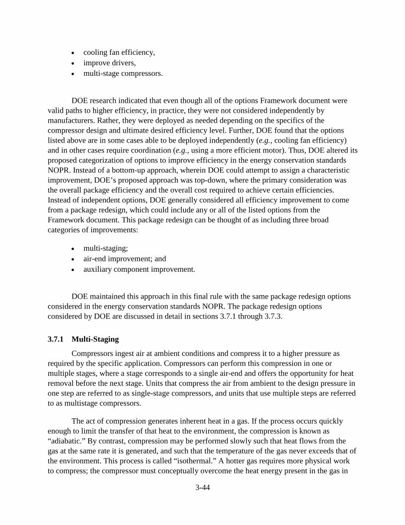
3-44

• cooling fan efficiency, • improve drivers, • multi-stage compressors.

DOE research indicated that even though all of the options Framework document were valid paths to higher efficiency, in practice, they were not considered independently by manufacturers. Rather, they were deployed as needed depending on the specifics of the compressor design and ultimate desired efficiency level. Further, DOE found that the options listed above are in some cases able to be deployed independently (e.g., cooling fan efficiency) and in other cases require coordination (e.g., using a more efficient motor). Thus, DOE altered its proposed categorization of options to improve efficiency in the energy conservation standards NOPR. Instead of a bottom-up approach, wherein DOE could attempt to assign a characteristic improvement, DOE’s proposed approach was top-down, where the primary consideration was the overall package efficiency and the overall cost required to achieve certain efficiencies. Instead of independent options, DOE generally considered all efficiency improvement to come from a package redesign, which could include any or all of the listed options from the Framework document. This package redesign can be thought of as including three broad categories of improvements:

• multi-staging; • air-end improvement; and • auxiliary component improvement.

DOE maintained this approach in this final rule with the same package redesign options considered in the energy conservation standards NOPR. The package redesign options considered by DOE are discussed in detail in sections 3.7.1 through 3.7.3.

3.7.1 Multi-Staging

Compressors ingest air at ambient conditions and compress it to a higher pressure as required by the specific application. Compressors can perform this compression in one or multiple stages, where a stage corresponds to a single air-end and offers the opportunity for heat removal before the next stage. Units that compress the air from ambient to the design pressure in one step are referred to as single-stage compressors, and units that use multiple steps are referred to as multistage compressors.

The act of compression generates inherent heat in a gas. If the process occurs quickly enough to limit the transfer of that heat to the environment, the compression is known as “adiabatic.” By contrast, compression may be performed slowly such that heat flows from the gas at the same rate it is generated, and such that the temperature of the gas never exceeds that of the environment. This process is called “isothermal.” A hotter gas requires more physical work to compress; the compressor must conceptually overcome the heat energy present in the gas in

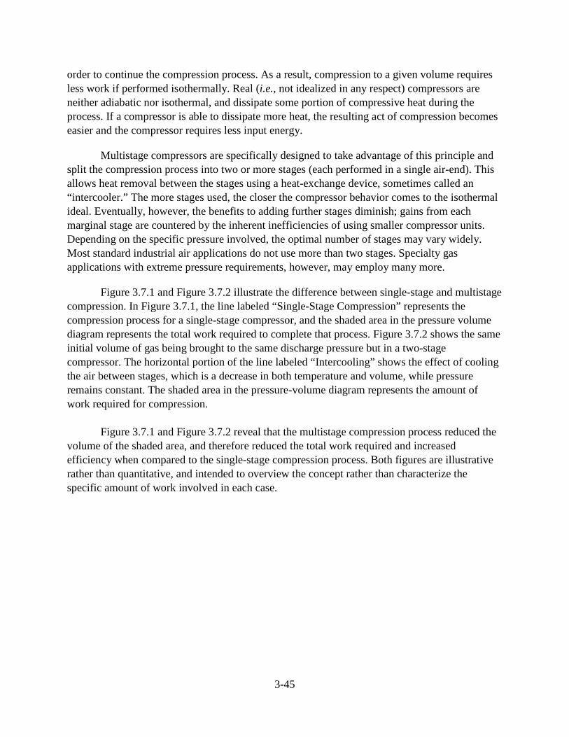
3-45

order to continue the compression process. As a result, compression to a given volume requires less work if performed isothermally. Real (i.e., not idealized in any respect) compressors are neither adiabatic nor isothermal, and dissipate some portion of compressive heat during the process. If a compressor is able to dissipate more heat, the resulting act of compression becomes easier and the compressor requires less input energy.

Multistage compressors are specifically designed to take advantage of this principle and split the compression process into two or more stages (each performed in a single air-end). This allows heat removal between the stages using a heat-exchange device, sometimes called an “intercooler.” The more stages used, the closer the compressor behavior comes to the isothermal ideal. Eventually, however, the benefits to adding further stages diminish; gains from each marginal stage are countered by the inherent inefficiencies of using smaller compressor units. Depending on the specific pressure involved, the optimal number of stages may vary widely. Most standard industrial air applications do not use more than two stages. Specialty gas applications with extreme pressure requirements, however, may employ many more.

Figure 3.7.1 and Figure 3.7.2 illustrate the difference between single-stage and multistage compression. In Figure 3.7.1, the line labeled “Single-Stage Compression” represents the compression process for a single-stage compressor, and the shaded area in the pressure volume diagram represents the total work required to complete that process. Figure 3.7.2 shows the same initial volume of gas being brought to the same discharge pressure but in a two-stage compressor. The horizontal portion of the line labeled “Intercooling” shows the effect of cooling the air between stages, which is a decrease in both temperature and volume, while pressure remains constant. The shaded area in the pressure-volume diagram represents the amount of work required for compression.

Figure 3.7.1 and Figure 3.7.2 reveal that the multistage compression process reduced the

volume of the shaded area, and therefore reduced the total work required and increased efficiency when compared to the single-stage compression process. Both figures are illustrative rather than quantitative, and intended to overview the concept rather than characterize the specific amount of work involved in each case.

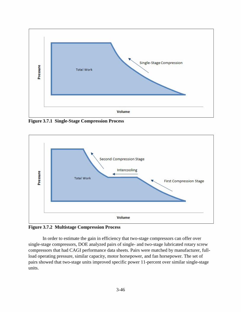
3-46

Figure 3.7.1 Single-Stage Compression Process

Figure 3.7.2 Multistage Compression Process

In order to estimate the gain in efficiency that two-stage compressors can offer over single-stage compressors, DOE analyzed pairs of single- and two-stage lubricated rotary screw compressors that had CAGI performance data sheets. Pairs were matched by manufacturer, full-load operating pressure, similar capacity, motor horsepower, and fan horsepower. The set of pairs showed that two-stage units improved specific power 11-percent over similar single-stage units.

3-47

3.7.2 Air-End Improvement

The efficiency of any given air-end depends upon a number of factors, including:

• rated compressor output capacity • compression chamber geometry • operating speed • surface finish • manufacturing precision • designed equipment tolerances

The effects of these different design decisions can be seen by comparing the performance curves for multiple air-ends. Every bare compressor can be characterized by a single performance curve, on which actual volume flow rate and isentropic efficiency are normally plotted on the x- and y-axes, respectively. Figure 3.7.3 provides an example design curve for a single-stage bare compressor, as detailed in the Lot 31 final report. hh

Figure 3.7.3 Representative Single-stage Bare Compressor Performance Curve

An individual bare compressor has a best efficiency point, represented by the dot at the

top of the curve. The decreases in efficiency seen on opposite sides of the curve are caused by conflicting effects, including leakage losses and increased friction experienced at high speeds.

hh See: Page 15 of https://www.regulations.gov/contentStreamer?documentId=EERE-2013-BT-STD-0040-0031&attachmentNumber=2&disposition=attachment&contentType=pdf

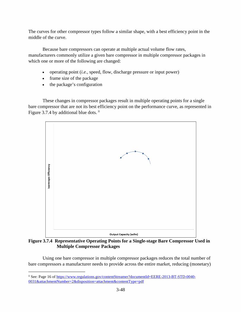
3-48

The curves for other compressor types follow a similar shape, with a best efficiency point in the middle of the curve.

Because bare compressors can operate at multiple actual volume flow rates,

manufacturers commonly utilize a given bare compressor in multiple compressor packages in which one or more of the following are changed:

• operating point (i.e., speed, flow, discharge pressure or input power) • frame size of the package • the package’s configuration

These changes in compressor packages result in multiple operating points for a single bare compressor that are not its best efficiency point on the performance curve, as represented in Figure 3.7.4 by additional blue dots. ii

Figure 3.7.4 Representative Operating Points for a Single-stage Bare Compressor Used in

Multiple Compressor Packages Using one bare compressor in multiple compressor packages reduces the total number of

bare compressors a manufacturer needs to provide across the entire market, reducing (monetary) ii See: Page 16 of https://www.regulations.gov/contentStreamer?documentId=EERE-2013-BT-STD-0040-0031&attachmentNumber=2&disposition=attachment&contentType=pdf

3-49

costs in exchange for reduced efficiency for those packages operating outside of the best efficiency point for each bare compressor. To minimize the effects of the reduced efficiency, manufacturers generally optimize bare compressor designs for the most common equipment applications. However, a manufacturer could redesign and optimize bare compressors for any given actual volume flow rate and discharge pressure, increasing the overall efficiency of the compressor package. Currently manufacturers do not provide an infinite number of optimized bare compressors for several reasons:

• Each new bare compressor requires expensive retooling of manufacturing equipment; • Increasing the number of bare compressors erases the economy of scale production

benefits; and • Each bare compressor must be kept as a spare part for approximately 15 years after

the end of production of the related packages.

3.7.3 Auxiliary Component Improvement

As discussed in the previous section, compressor manufacturers normally use one air-end in multiple compressor packages that are designed to operate at different discharge pressures and actual volume flow rates. Each compressor package consists of multiple design features that affect package efficiency, including valves, piping system, motor, capacity controls, fans, fan motors, filtration, drains, and driers. This equipment, for example, may control the flow of air, moisture, or oil, or the temperature and humidity of output air, or regulate temperature and operation. Compressor manufacturers do not normally provide the option to replace any individual part of a compressor package to increase efficiency, as each feature also has a direct effect on compressor performance. However, improving the operating characteristics of any of these “auxiliary” components may offer a chance to improve the overall efficiency of the compressor package.

For example, package isentropic efficiency can be increased by reducing the internal pressure drop of the package using improved valves and pipe systems, or by improving the efficiency of (1) both the drive and fan motors (if present), (2) the fan itself (if present), (3) condensate drains, (4) both air and lubricant filters, and (5) controls (if present). The improvement must be considered relative to a starting point, however. Even if the modifications could be deployed independently of each other, and not all can, the spread of efficiencies available in the market likely already reflects the more cost effective choice for improving efficiency at any given point. Perhaps one manufacturer, by virtue of features of its product lines, finds that reaching a given efficiency level in a particular equipment class is most cost effectively done by improving Technology X. Another may find that it is more cost effective to improve Technology Y. And both could be correct, because each may have had a different starting point.

DOE notes that, because the compressor packages function as an ensemble of complementary parts, changing one part often requires changing others. A special case may

3-50

come with more efficient electric motors. Compressors normally use induction motors, which generally vary operating speed as efficiency is improved. Using a more efficient (but otherwise identical) induction motor without considering the rest of the compressor design could be counterproductive if the gains in motor efficiency were more than offset by subsequent loss in performance of the air-end and other parts. DOE’s proposal assumes that the best-performing compressors on the market are built using the most-efficient available electric motors that are suited to the task. However, DOE could not confirm instances of a manufacturer using “super premium” or “IE4” induction motors, which appear to only recently have been made available commercially.jj These terms (“super premium” and “IE4”) have been used (in the United States and Europe, respectively) to describe the motor industry’s next tier of efficiency. Possible reasons for this include the motors not being suitable for use in compressors, manufacturers still exploring the relatively new motors and not having yet introduced equipment redesigned to make use of them, or that manufacturers are already using the motors in the most efficient compressor offerings.

As an example of the influence of auxiliary componentry on compressor efficiency, in the test procedure final rule, DOE presents two lists of components to describe compressor configuration requirements. The first includes components that must be included as part of a compressor package when testing, regardless of whether they are distributed in commerce with the basic model under test; the second list contains components that are only required if they are distributed in commerce with the basic model under test. Any component on these lists may affect efficiency, and these lists illustrate the set of componentry that needs to function harmoniously for the package to perform well.

jj One manufacturer, for example, describes its IE4 offerings here: www.regulations.gov/document?D=EERE-2013-BT-STD-0040-0073

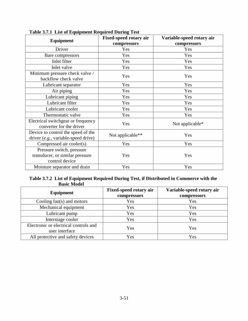
3-51

Table 3.7.1 List of Equipment Required During Test

Table 3.7.2 List of Equipment Required During Test, if Distributed in Commerce with the

Basic Model

Equipment Fixed-speed rotary air compressors

Variable-speed rotary air compressors

Driver Yes Yes Bare compressors Yes Yes

Inlet filter Yes Yes Inlet valve Yes Yes

Minimum pressure check valve / backflow check valve Yes Yes

Lubricant separator Yes Yes Air piping Yes Yes

Lubricant piping Yes Yes Lubricant filter Yes Yes

Lubricant cooler Yes Yes Thermostatic valve Yes Yes

Electrical switchgear or frequency converter for the driver Yes Not applicable*

Device to control the speed of the driver (e.g., variable-speed drive) Not applicable** Yes

Compressed air cooler(s) Yes Yes Pressure switch, pressure

transducer, or similar pressure control device

Yes Yes

Moisture separator and drain Yes Yes

Equipment Fixed-speed rotary air compressors

Variable-speed rotary air compressors

Cooling fan(s) and motors Yes Yes Mechanical equipment Yes Yes

Lubricant pump Yes Yes Interstage cooler Yes Yes

Electronic or electrical controls and user interface Yes Yes

All protective and safety devices Yes Yes

4-i

CHAPTER 4. SCREENING ANALYSIS

TABLE OF CONTENTS

4.1 INTRODUCTION ........................................................................................................... 4-1 4.2 SCREENED-OUT TECHNOLOGIES ............................................................................ 4-2 4.3 REMAINING TECHNOLOGIES ................................................................................... 4-2

4-1

CHAPTER 4. SCREENING ANALYSIS

4.1 INTRODUCTION

This chapter details the screening analysis that the U.S. Department of Energy (DOE) conducted in support of the energy conservation standards rulemakings for compressors.

In chapter 3, the market and technology assessment (MTA), DOE presented an initial list of technologies that can improve the energy efficiency of air compressors. The purpose of the screening analysis is to evaluate the technologies that improve equipment efficiency to determine which technologies to consider further and which to screen out. DOE consulted with a range of parties, including industry, technical experts, and others to develop a list of technologies for consideration. DOE evaluated the technologies pursuant to the criteria set out in the Energy Policy and Conservation Act (EPCA), as amended. (42 U.S.C. 6311-6317)

Section 325(o) EPCA establishes criteria for prescribing new or amended standards designed to achieve the maximum improvement in energy efficiency. Further, EPCA directs the Secretary of Energy to determine whether a standard is technologically feasible and economically justified. (42 U.S.C. 6295(o)(2)(A), as directed by 42 U.S.C. 6316(a)(1)-(3)). EPCA also establishes guidelines for determining whether a standard is economically justified. (42 U.S.C. 6295(o)(2)(B)) Appendix A to subpart C of Title 10, Code of Federal Regulations, Part 430 (10 CFR Part 430), “Procedures, Interpretations and Policies for Consideration of New or Revised Energy Conservation Standards for Consumer Products” (the Process Rule), sets forth procedures to guide DOE in its consideration and promulgation of new or revised equipment energy conservation standards. These procedures elaborate on the statutory criteria provided in 42 U.S.C. 6295(o) and, in part, eliminate problematic technologies early in the process of prescribing or amending an energy efficiency standard. In particular, sections 4(b)(4) and 5(b) of the Process Rule guide DOE in determining whether to eliminate from consideration any technology that presents unacceptable problems with respect to the following criteria:

• Technological feasibility. Technologies incorporated in commercial equipment or in working prototypes will be considered technologically feasible.

• Practicability to manufacture, install, and service. If mass production of a technology in commercial equipment and reliable installation and servicing of the technology could be achieved on the scale necessary to serve the relevant market at the time of the effective date of the standard, then that technology will be considered practicable to manufacture, install, and service.

• Impacts on equipment utility or equipment availability. If a technology is determined to have significant adverse impact on the utility of the equipment to significant subgroups of consumers, or result in the unavailability of any covered equipment type with performance characteristics (including reliability), features, sizes, capacities, and volumes that are substantially the same as equipment generally available in the United States at the time, it will not be considered further.

4-2

• Adverse impacts on health or safety. If it is determined that a technology will have significant adverse impacts on health or safety, it will not be considered further.

In sum, if DOE determines that a technology, or a combination of technologies, has unacceptable impacts on the policies stated in section 5(b) of the Process Rule, it will be eliminated from consideration. If a particular technology fails to meet one or more of the four criteria, it will be screened out. Section 4.2 documents the reasons for eliminating any technology.

4.2 SCREENED-OUT TECHNOLOGIES

Normally, this section describes the technologies that DOE eliminated for failure to meet one of the following four factors: (1) technological feasibility; (2) practicability to manufacture, install, and service; (3) impacts on equipment utility or equipment availability; and (4) adverse impacts on health or safety.

However, of the identified technology options, DOE was not able to identify any that fail the screening criteria.

4.3 REMAINING TECHNOLOGIES

After reviewing each technology, DOE concluded that all of the identified technologies listed in chapter 3 of the technical support document met all four screening criteria to be examined further as design options in DOE’s analysis. In summary, DOE did not screen out the following technology options, all of which are considered options in a compressor package redesign:

• multi-staging • air-end improvement • auxiliary component improvement

DOE determined that these technology options are technologically feasible because they

are used or have previously been used in commercially-available products or working prototypes. DOE also finds that all of the remaining technology options meet the other screening criteria (i.e., practicable to manufacture, install, and service and do not result in adverse impacts on consumer utility, equipment availability, health, or safety).

5-i

CHAPTER 5. ENGINEERING ANALYSIS

TABLE OF CONTENTS

5.1 INTRODUCTION ................................................................................... 5-1 5.2 METHODOLOGY OVERVIEW ............................................................ 5-1 5.3 SUMMARY OF DATA SOURCES ........................................................ 5-1

5.3.1 CAGI Data Sheets ........................................................................ 5-1 5.3.2 Lot 31 – European Union Ecodesign Preparatory Study on

Compressors ................................................................................. 5-3 5.3.3 Confidential Manufacturer Equipment Data ................................ 5-5

5.4 IMPACT OF SAMPLING PLAN ON CAGI DATA .............................. 5-6 5.4.1 Introduction .................................................................................. 5-6 5.4.2 General Approach ........................................................................ 5-6 5.4.3 Assumptions ................................................................................. 5-7

5.4.3.1 Variation of Compressor Performance for Each Basic Model ................................................................................. 5-8

5.4.3.2 Number of Compressors in Test Sample ............................ 5-9 5.4.3.3 Correlation Between Part-Load Specific Power

Measurements ................................................................... 5-10 5.4.4 Population of Compressors in Sampling Plan Analysis ............ 5-10 5.4.5 Results ........................................................................................ 5-11 5.4.6 Sensitivity Analysis ................................................................... 5-11

5.4.6.1 Assumed Distribution of Compressor Specific Power ..... 5-11 5.4.6.2 Number of Tested Compressors in Sample ...................... 5-12 5.4.6.3 Number of Trials Required for a Representative Result .. 5-12 5.4.6.4 Results of the Sensitivity Analyses .................................. 5-12

5.5 REPRESENTATIVE EQUIPMENT FOR ANALYSIS ....................... 5-17 5.6 DESIGN OPTIONS ............................................................................... 5-18 5.7 AVAILABLE EFFICIENCY IMPROVEMENTS ................................ 5-19 5.8 EFFICIENCY LEVELS......................................................................... 5-19

5.8.1 Efficiency Level Structure ......................................................... 5-19 5.8.1.1 Baseline ............................................................................ 5-20 5.8.1.2 Maximum Technologically Feasible Level ...................... 5-20

5.8.2 Methods Used to Determine Efficiency Levels ......................... 5-20 5.8.3 Air-Cooled Compressors ........................................................... 5-21

5.8.3.1 RP_FS_L_AC Efficiency Levels ..................................... 5-21 5.8.3.2 RP_VS_L_AC Efficiency Levels ..................................... 5-25

5.8.4 Liquid-Cooled Compressors ...................................................... 5-28 5.8.4.1 RP_FS_L_WC Efficiency Levels .................................... 5-29 5.8.4.2 RP_VS_L_WC Efficiency Levels .................................... 5-34

5.9 MANUFACTURER SELLING PRICE ................................................ 5-37 5.10 MANUFACTURER PRODUCTION COST ........................................ 5-47 5.11 OTHER ANALYTICAL OUTPUTS .................................................... 5-48

5-ii

LIST OF TABLES

Table 5.3.1 Lot 31 Regression Curve Coefficients .............................................. 5-4 Table 5.3.2 Lot 31 Draft Regulation Curve d-values........................................... 5-5 Table 5.3.3 Lot 31 List Price Curves ................................................................... 5-5 Table 5.4.1 Permissible Deviation of Specific Power and Package Isentropic

Efficiency During Customer Acceptance Test for Electrically Driven Packaged Displacement Compressors ....................... 5-9

Table 5.4.2 Impact of Specific Power Distribution and Sample Size to Average Change in Compressor Full-Load Package Isentropic Efficiency Rating ................................................................. 5-13

Table 5.4.3 Impact of Specific Power Distribution and Sample Size to Average Change in Compressor Part-Load Package Isentropic Efficiency Rating ................................................................. 5-13

Table 5.8.1 Efficiency at Representative Flow Rates for CAGI and Lot 31 Regression Curves for RP_FS_L_AC ................................. 5-22

Table 5.8.2 Efficiency Levels Analyzed for Rotary, Lubricated, Air-Cooled, Fixed-Speed, Three-Phase ................................................... 5-25

Table 5.8.3 Efficiency at Representative Flow Rates for CAGI and Lot 31 Regression Curves for RP_VS_L_AC ................................. 5-26

Table 5.8.4 Efficiency Levels Analyzed for Rotary, Lubricated, Air-Cooled, Variable-Speed, Three-Phase ............................................... 5-28

Table 5.8.5 Lubricated Fixed Speed Improvement in Package Isentropic Efficiency of Liquid-Cooled versus Air-Cooled from the CAGI Database ............................................................................... 5-29

Table 5.8.6 Lubricated Fixed Speed Improvement in Package Isentropic Efficiency of Liquid-Cooled versus Air-Cooled from the Updated CAGI Database...................................................... 5-30

Table 5.8.7 Efficiency Levels Analyzed for Rotary, Lubricated, Liquid-Cooled, Fixed-Speed, Three-Phase ................................................... 5-34

Table 5.8.8 Efficiency Levels Analyzed for Rotary, Lubricated, Liquid-Cooled, Variable-Speed, Three-Phase ............................................... 5-37

Table 5.9.1 Representative MSPs for the RP_FS_L_AC Equipment Class ...... 5-39 Table 5.9.2 Representative MSPs for the RP_VS_L_AC Equipment Class ..... 5-41 Table 5.9.3 Estimated Increase in Package Isentropic Efficiency from More-

Efficient Fan Motors for 25 hp Compressors ...................... 5-43 Table 5.9.4 Estimated Increase in Package Isentropic Efficiency from More-

efficient Fan Motors for 100 hp Compressors ..................... 5-44 Table 5.9.5 Estimated Increase in Package Isentropic Efficiency from More-

Efficient Fan Motors for 200 hp Compressors .................... 5-45 Table 5.9.6 Potential Air- and Liquid-Cooled Offset in Package Isentropic

Efficiency When Accounting for Fan Motor Efficiency Improvements ...................................................................... 5-46

Table 5.10.1 Baseline Markup Estimates .......................................................... 5-47 Table 5.10.2 Breakdown of MPC for Air Compressors .................................... 5-48

5-iii

LIST OF FIGURES

Figure 5.3.1 Example Rotary Variable-Speed Compressor Input Power vs. Flow Rate ........................................................................................ 5-3

Figure 5.4.1 Flowchart of Monte Carlo Simulation in Oracle Crystal Ball for Fixed-Speed Compressors ..................................................... 5-7

Figure 5.4.2 Average Decrement in Compressor Full-Load Package Isentropic Efficiency Rating Due to Sampling Plan for Normally Distributed Specific Power Variation, Sample Size of 3 ..... 5-13

Figure 5.4.3 Average Decrement in Compressor Full-Load Package Isentropic Efficiency Rating Due to Sampling Plan for Normally Distributed Specific Power Variation, Sample Size of 4 ..... 5-14

Figure 5.4.4 Average Decrement in Compressor Full-Load Package Isentropic Efficiency Rating Due to Sampling Plan for Uniformly Distributed Specific Power Variation, Sample Size of 3 ..... 5-14

Figure 5.4.5 Average Decrement in Compressor Full-Load Package Isentropic Efficiency Rating Due to Sampling Plan for Uniformly Distributed Specific Power Variation, Sample Size of 4 ..... 5-15

Figure 5.4.6 Average Decrement in Compressor Part-Load Package Isentropic Efficiency Rating Due to Sampling Plan for Normally Distributed Specific Power Variation, Sample Size of 3 ..... 5-15

Figure 5.4.7 Average Decrement in Compressor Part-Load Package Isentropic Efficiency Rating Due to Sampling Plan for Normally Distributed Specific Power Variation, Sample Size of 4 ..... 5-16

Figure 5.4.8 Average Decrement in Compressor Part-Load Package Isentropic Efficiency Rating Due to Sampling Plan for Uniformly Distributed Specific Power Variation, Sample Size of 3 ..... 5-16

Figure 5.4.9 Average Decrement in Compressor Part-Load Package Isentropic Efficiency Rating Due to Sampling Plan for Uniformly Distributed Specific Power Variation, Sample Size of 4 ..... 5-17

Figure 5.5.1 Histogram of Rotary Fixed-Speed Compressor Pressures in the CAGI Database ............................................................................... 5-18

Figure 5.5.2 Histogram of Rotary Variable-Speed Compressor Pressures in the CAGI Database .................................................................... 5-18

Figure 5.8.1 CAGI and Lot 31 Regression Curves for RP_FS_L_AC .............. 5-22 Figure 5.8.2 RP_FS_L_AC Baseline and Max-Tech......................................... 5-24 Figure 5.8.3 RP_FS_L_AC Efficiency Levels .................................................. 5-24 Figure 5.8.4 CAGI and Lot 31 Regression Curves for RP_VS_L_AC ............. 5-25 Figure 5.8.5 RP_VS_L_AC Baseline and Max-Tech ........................................ 5-27 Figure 5.8.6 RP_VS_L_AC Efficiency Levels .................................................. 5-28 Figure 5.8.7 Relationship Between Difference in Package Isentropic Efficiency

and Full-load Actual Volume Flow Rate for Pairs of Air-Cooled and Liquid-Cooled Compressors ............................. 5-31

Figure 5.8.8 Final Regression Curve for RP_FS_L_WC and CAGI Data ........ 5-32 Figure 5.8.9 RP_FS_L_WC Baseline and Max-Tech ........................................ 5-33 Figure 5.8.10 RP_FS_L_WC Efficiency Levels................................................ 5-33 Figure 5.8.11 Final Regression Curve for RP_VS_L_WC and CAGI Data ...... 5-35

5-iv

Figure 5.8.12 RP_VS_L_WC Baseline and Max-Tech ..................................... 5-36 Figure 5.8.13 RP_VS_L_WC Efficiency Levels ............................................... 5-36 Figure 5.9.1 RP_FS_L_AC U.S. Data Flow-Rate Efficiency Relationship ...... 5-38 Figure 5.9.2 RP_VS_L_AC U.S. Data Flow-Rate Efficiency Relationship ...... 5-40 Figure 5.11.1 Rotary Fixed-Speed Full-Load and No-Load Power................... 5-49

5-1

CHAPTER 5. ENGINEERING ANALYSIS

5.1 INTRODUCTION

The engineering analysis establishes the relationship between manufacturer selling price (MSP) and energy consumption for the air compressors examined in this rulemaking. The “price-efficiency” relationship serves as the basis for downstream cost-benefit calculations with respect to individual consumers, manufacturers, and the Nation.

5.2 METHODOLOGY OVERVIEW

This section describes the analytical methods the U.S. Department of Energy (DOE) used for the engineering analysis. In this rulemaking, DOE adopted an efficiency level approach to produce analytically derived curves representing the price-efficiency relationship for each equipment class analyzed. In an efficiency-level approach, DOE uses estimates of costs and efficiencies of equipment available on the market at distinct efficiency levels to develop the cost-efficiency relationship. The decision to use this approach was based on several factors, including the wide variety of equipment sizes analyzed, the availability of reliable performance data, the availability of a comparable European Union study, and the nature of the design options available for the equipment.

5.3 SUMMARY OF DATA SOURCES

For the engineering analysis, DOE utilized three principal data sources: (1) a database of air compressor performance data from the Compressed Air and Gas Institute (CAGI) data sheets, (2) results from the EU Lot 31 Ecodesign Preparatory Study on Compressors, and (3) a dataset of confidential manufacturer price data. The following subsections provide a brief description of each significant data source.

5.3.1 CAGI Data Sheets

CAGI’s Performance Verification Program provides manufacturers a standardized test method and performance data reporting format for rotary positive air compressors. CAGI uses ISO 1217:2009, Displacement compressors – Acceptance tests, Annex C Simplified acceptance test for electrically driven packaged displacement compressors, for its Performance Verification Program, which is similar to the method DOE adopted in the

5-2

compressors test procedure final rule (test procedure final rule).a In the energy conservation standards NOPR, DOE compiled the information contained in every CAGI Performance Verification data sheet found on the websites of ten individual manufacturers into one database, all of which are CAGI members. 81 FR 31680, 31704 (May 19, 2016). This was referred to this as the “CAGI database.” This resulted in data on 1,403 fixed-speed rotary compressors and 519 variable-speed rotary compressors which ranged from 4- to 700-hp.b,c As part of this final rule, DOE compiled information from newly available CAGI data sheets, as well as updated data sheets from the same compressor models, and compiled them into a new database; this is referred to as the “updated CAGI database” in this final rule. The updated CAGI database contains data on 1,372 fixed-speed rotary compressors and 963 variable-speed rotary compressors which ranged from 3 to 700 horsepower (hp). Package isentropic efficiency is not directly reported on CAGI data sheets; however, it was needed because it is the metric on which the standard is based. For all compressors, DOE calculated full-load package isentropic efficiency (i.e., package isentropic efficiency at 100 percent of full-load actual volume flow rate) using values of full-load operating pressure, full-load actual volume flow rate, and packaged compressor power input at full-load operating pressure per the test procedure final rule. These parameters were then used in subsequent analyses discussed in this chapter. Generally, variable-speed air compressors are rated by testing at multiple load points. The CAGI Performance Verification Program specifies testing at full-load operating pressure for fixed-speed compressors, and at a minimum of six test points for variable-speed compressors according to Annex E of ISO 1217:2009, including:

• maximum volume flow rate; • three or more volume flow rates evenly spaced between the minimum and

maximum volume flow rate; • minimum volume flow rate; and • no load power.

The test procedure final rule instructs testing at three points for variable-speed compressors, 40 percent, 70 percent, and 100 percent of full-load actual volume flow rate. Testing must then calculate package isentropic efficiency at each point, and weight those into a single metric. The variable-speed tested points in the CAGI data sheets may not necessarily line up with the test points in the test procedure final rule. Therefore, for variable-speed compressors, DOE linearly interpolated between values of flow rate and a For more information on the test procedure final rule, see www1.eere.energy.gov/buildings/appliance_standards/product.aspx/productid/78 b An example CAGI data sheet for fixed-speed compressors is available here: www.regulations.gov/document?D=EERE-2013-BT-STD-0040-0077 c An example CAGI data sheet for variable-speed compressors is available here: www.regulations.gov/document?D=EERE-2013-BT-STD-0040-0078

5-3

input power, to find values at 40 and 70 percent of maximum reported volume flow rate on the CAGI data sheet. Specifically, DOE interpolated between the closest tested values reported on the CAGI data sheet greater than and less than 40 and 70 percent of maximum reported volume flow rate. DOE notes that, for all variable-speed compressors considered, the relationship between flow rate and input power is well characterized by a linear regression. As shown in Figure 5.3.1, full-load actual volume flow rate in cubic feet per minute (cfm) and input power data from an example CAGI datasheet show a strong linear relationship, with an R2 (a statistical measure of goodness of fit) value of 0.9962 (where 1 represents a perfect match). Ultimately, DOE used the interpolated values for flow rate and input power to calculate package isentropic efficiency at each load point and weighted those results in a manner consistent with the test procedure final rule.

Figure 5.3.1 Example Rotary Variable-Speed Compressor Input Power vs. Flow

Rate

5.3.2 Lot 31 – European Union Ecodesign Preparatory Study on Compressors The Lot 31 Ecodesign Preparatory Study on Compressors (“Lot 31 study”) investigated the appropriateness and effectiveness of establishing an energy conservation standard for air compressors in the European Union.d The results of this study led the Commission of the European Communities to establish a working document proposing possible energy efficiency requirements for air compressors (“Lot 31 draft regulation”).e This working document represents an initial step towards establishing an Ecodesign energy conservation standard in the European Union. d VHK. Lot 31 – Ecodesign Preparatory Study on Compressors, 2014. Delft, Netherlands. www.regulations.gov/document?D=EERE-2013-BT-STD-0040-0031. e The Commission of the European Communities. Working Document on Possible requirements for compressors for standard air applications, 2013. Brussels, Belgium. www.regulations.gov/document?D=EERE-2013-BT-STD-0040-0031.

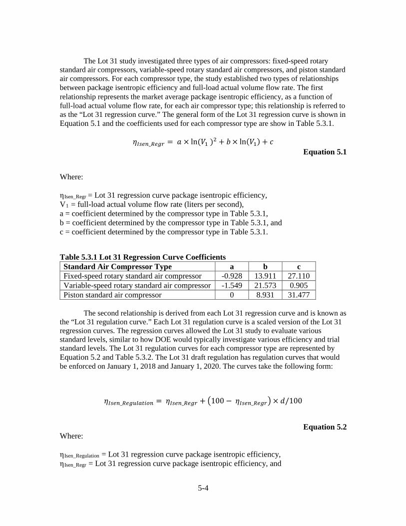
5-4

The Lot 31 study investigated three types of air compressors: fixed-speed rotary standard air compressors, variable-speed rotary standard air compressors, and piston standard air compressors. For each compressor type, the study established two types of relationships between package isentropic efficiency and full-load actual volume flow rate. The first relationship represents the market average package isentropic efficiency, as a function of full-load actual volume flow rate, for each air compressor type; this relationship is referred to as the “Lot 31 regression curve.” The general form of the Lot 31 regression curve is shown in Equation 5.1 and the coefficients used for each compressor type are show in Table 5.3.1.

𝜂𝜂𝐼𝐼𝐼𝐼𝐼𝐼𝐼𝐼_𝑅𝑅𝐼𝐼𝑅𝑅𝑅𝑅 = 𝑎𝑎 × ln (𝑉𝑉1 )2 + 𝑏𝑏× ln(𝑉𝑉1) + 𝑐𝑐 Equation 5.1

Where: ηIsen_Regr = Lot 31 regression curve package isentropic efficiency, V1 = full-load actual volume flow rate (liters per second), a = coefficient determined by the compressor type in Table 5.3.1, b = coefficient determined by the compressor type in Table 5.3.1, and c = coefficient determined by the compressor type in Table 5.3.1.

Table 5.3.1 Lot 31 Regression Curve Coefficients Standard Air Compressor Type a b c Fixed-speed rotary standard air compressor -0.928 13.911 27.110 Variable-speed rotary standard air compressor -1.549 21.573 0.905 Piston standard air compressor 0 8.931 31.477

The second relationship is derived from each Lot 31 regression curve and is known as the “Lot 31 regulation curve.” Each Lot 31 regulation curve is a scaled version of the Lot 31 regression curves. The regression curves allowed the Lot 31 study to evaluate various standard levels, similar to how DOE would typically investigate various efficiency and trial standard levels. The Lot 31 regulation curves for each compressor type are represented by Equation 5.2 and Table 5.3.2. The Lot 31 draft regulation has regulation curves that would be enforced on January 1, 2018 and January 1, 2020. The curves take the following form:

𝜂𝜂𝐼𝐼𝐼𝐼𝐼𝐼𝐼𝐼_𝑅𝑅𝐼𝐼𝑅𝑅𝑅𝑅𝑅𝑅𝑅𝑅𝑅𝑅𝑅𝑅𝑅𝑅𝐼𝐼 = 𝜂𝜂𝐼𝐼𝐼𝐼𝐼𝐼𝐼𝐼_𝑅𝑅𝐼𝐼𝑅𝑅𝑅𝑅 + �100 − 𝜂𝜂𝐼𝐼𝐼𝐼𝐼𝐼𝐼𝐼_𝑅𝑅𝐼𝐼𝑅𝑅𝑅𝑅� × 𝑑𝑑/100

Equation 5.2 Where: ηIsen_Regulation = Lot 31 regression curve package isentropic efficiency, ηIsen_Regr = Lot 31 regression curve package isentropic efficiency, and

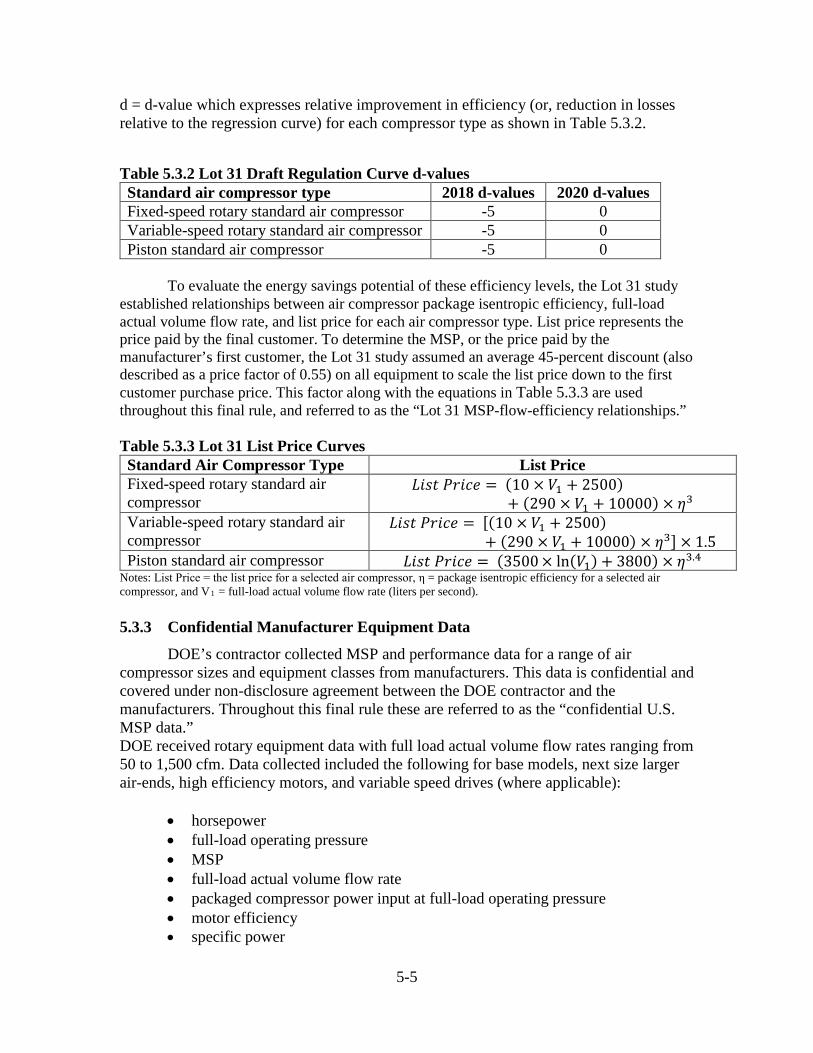
5-5

d = d-value which expresses relative improvement in efficiency (or, reduction in losses relative to the regression curve) for each compressor type as shown in Table 5.3.2.

Table 5.3.2 Lot 31 Draft Regulation Curve d-values Standard air compressor type 2018 d-values 2020 d-values Fixed-speed rotary standard air compressor -5 0 Variable-speed rotary standard air compressor -5 0 Piston standard air compressor -5 0

To evaluate the energy savings potential of these efficiency levels, the Lot 31 study established relationships between air compressor package isentropic efficiency, full-load actual volume flow rate, and list price for each air compressor type. List price represents the price paid by the final customer. To determine the MSP, or the price paid by the manufacturer’s first customer, the Lot 31 study assumed an average 45-percent discount (also described as a price factor of 0.55) on all equipment to scale the list price down to the first customer purchase price. This factor along with the equations in Table 5.3.3 are used throughout this final rule, and referred to as the “Lot 31 MSP-flow-efficiency relationships.” Table 5.3.3 Lot 31 List Price Curves Standard Air Compressor Type List Price Fixed-speed rotary standard air compressor

𝐿𝐿𝐿𝐿𝐿𝐿𝐿𝐿 𝑃𝑃𝑃𝑃𝐿𝐿𝑐𝑐𝑃𝑃 = (10 × 𝑉𝑉1 + 2500)+ (290 × 𝑉𝑉1 + 10000) × 𝜂𝜂3

Variable-speed rotary standard air compressor

𝐿𝐿𝐿𝐿𝐿𝐿𝐿𝐿 𝑃𝑃𝑃𝑃𝐿𝐿𝑐𝑐𝑃𝑃 = [(10 × 𝑉𝑉1 + 2500)+ (290 × 𝑉𝑉1 + 10000) × 𝜂𝜂3] × 1.5

Piston standard air compressor 𝐿𝐿𝐿𝐿𝐿𝐿𝐿𝐿 𝑃𝑃𝑃𝑃𝐿𝐿𝑐𝑐𝑃𝑃 = (3500 × ln(𝑉𝑉1) + 3800) × 𝜂𝜂3.4 Notes: List Price = the list price for a selected air compressor, η = package isentropic efficiency for a selected air compressor, and V1 = full-load actual volume flow rate (liters per second).

5.3.3 Confidential Manufacturer Equipment Data

DOE’s contractor collected MSP and performance data for a range of air compressor sizes and equipment classes from manufacturers. This data is confidential and covered under non-disclosure agreement between the DOE contractor and the manufacturers. Throughout this final rule these are referred to as the “confidential U.S. MSP data.” DOE received rotary equipment data with full load actual volume flow rates ranging from 50 to 1,500 cfm. Data collected included the following for base models, next size larger air-ends, high efficiency motors, and variable speed drives (where applicable):

• horsepower • full-load operating pressure • MSP • full-load actual volume flow rate • packaged compressor power input at full-load operating pressure • motor efficiency • specific power

5-6

5.4 IMPACT OF SAMPLING PLAN ON CAGI DATA

5.4.1 Introduction

In the energy conservation standards NOPR, DOE directly calculated the certified full- or part-load package isentropic efficiency of each compressor basic model using performance data in the updated CAGI Database (which is discussed further in section 5.3.1). DOE understands that the sampling plan defined in the test procedure final rule could result in certified full- or part-load package isentropic efficiency values that differ from the values that DOE calculated directly from the updated CAGI Database in the energy conservation standards NOPR analysis. Specifically, the sampling plan in the test procedure final rule requires a minimum of two tested compressors to calculate the full- or part-load package isentropic efficiency of a compressor basic model.

Ideally, to assess the impact of the sampling plan, DOE would directly calculate the certified full- or part-load package isentropic efficiency using the raw source data from each compressor test sample. However, such raw test is not available to DOE. In the absence of raw test data, DOE used a Monte Carlo analysis, built in the Crystal Ball risk-analysis software package, to assess if and how rated efficiency might differ under the test procedure final rule sampling plan, compared to those used in the energy conservation standards NOPR. Ultimately, based on the results of this model, DOE concludes that efficiency ratings will not differ. The following sections review DOE methods, results, and conclusions, in detail.

5.4.2 General Approach

A Monte Carlo analysis reflects the interactions between known “input” distributions and a resulting “output;” for the purposes of this analysis, the Monte Carlo analysis reflects the interaction between the distribution of specific power for each compressor, the known sampling plan adopted in the DOE test procedure, and the resulting compressor package isentropic efficiency rating. The flowchart in Figure 5.4.1 walks through the steps and calculations performed for each compressors in the updated CAGI database, as a part of the Monte Carlo analysis.

As shown in the flowchart, the Monte Carlo analysis simulates the process of testing each compressor in the updated CAGI database by first creating samples values for specific power, for each tested compressor. From those samples, the model calculates the rated package isentropic efficiency, according to the test procedure sampling plan. This process is iterated 10,000 times for each compressor in the updated CAGI database. After 10,000 iterations, the model assess the frequency that the simulated value for package isentropic efficiency was less than the directly calculated value for package isentropic efficiency. The model also assesses the average magnitude of the difference between the simulated value for package isentropic efficiency and the directly calculated value of package isentropic efficiency. These results were used to assess the impact of the sampling plan on the directly calculated efficiency for each compressor in the updated CAGI database.

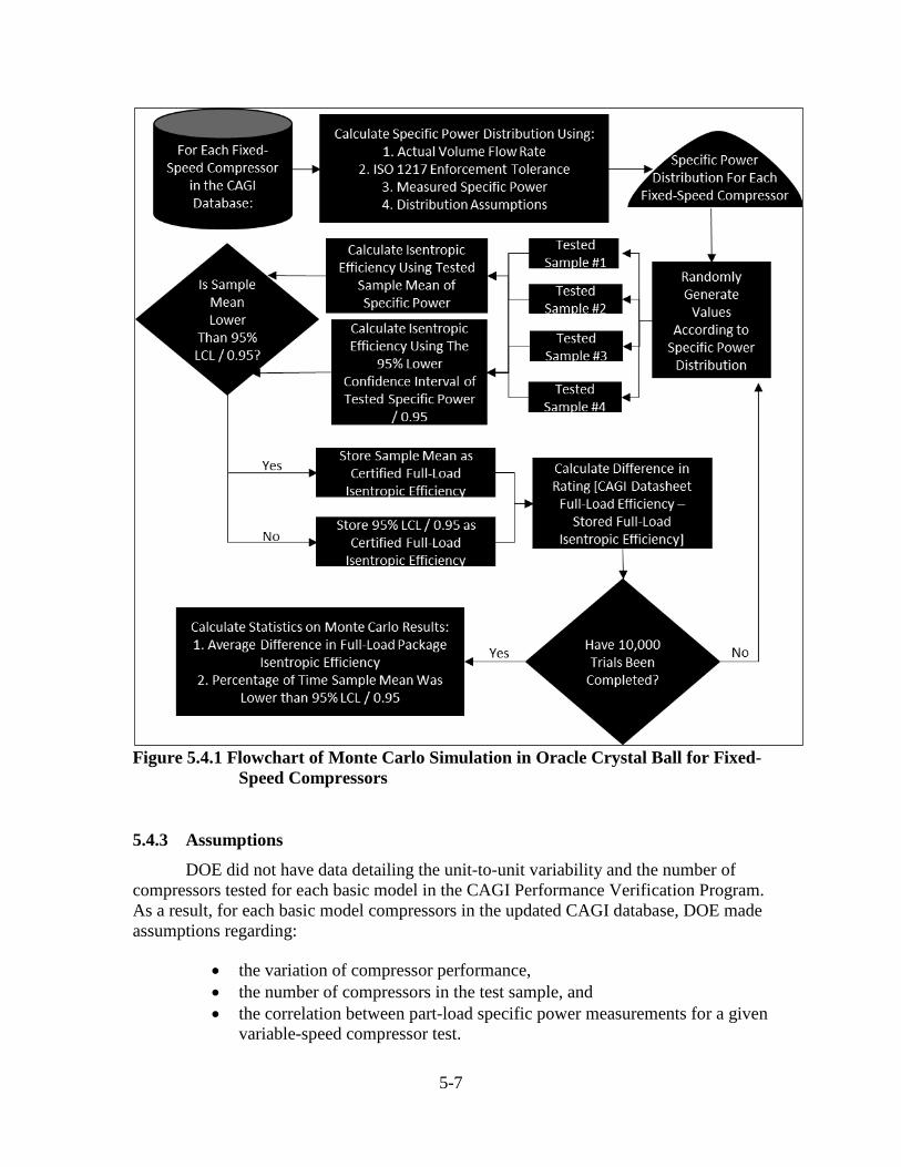
5-7

Figure 5.4.1 Flowchart of Monte Carlo Simulation in Oracle Crystal Ball for Fixed-

Speed Compressors

5.4.3 Assumptions

DOE did not have data detailing the unit-to-unit variability and the number of compressors tested for each basic model in the CAGI Performance Verification Program. As a result, for each basic model compressors in the updated CAGI database, DOE made assumptions regarding:

• the variation of compressor performance, • the number of compressors in the test sample, and • the correlation between part-load specific power measurements for a given

variable-speed compressor test.

5-8

Discussion of each assumption and rationale behind the assumptions are in the

preceding sections.

5.4.3.1 Variation of Compressor Performance for Each Basic Model

To characterize the variation of compressor performance, DOE made assumptions regarding the mean, bounds, and shape of the specific power distribution for each basic model. The following sections describe each tenant of the specific power distribution.

Mean of Specific Power Distribution. Based on comments provided by interested parties, DOE finds that the specific power data represented on CAGI performance verification data sheets are representative of the “true mean” of the population of each compressor basic model. Accordingly, for the purpose of the Monte Carlo analysis, DOE assumed that these specific power values represent the population mean.

Statistical Distribution of Specific Power. DOE considered two distributions that could characterize tested compressor specific power: (1) a uniform distribution that assumed equal probability of values between the lower and upper limit of specific power variation, and (2) a normal distribution.

A literature review conducted by DOE found that a uniform probability distribution, which has an equal probability of values between the lower and upper tolerance, does not commonly represent distributions that have continuous outcomes (such as specific power). Alternatively, literaturef states that of the commonly occurring probability distributions, a normal distribution is the most appropriate choice to represent the probability of a continuous outcome that is a function of the interaction between random and independent variables. Because tested specific power is indeed a function of random and independent variables, including manufacturing tolerances and test-to-test variation,g a normal probability distribution is the most representative of a compressor’s specific power distribution. For these reasons, DOE concludes that a normal distribution is the most appropriate to represent the unit-to-unit variability of compressor specific power. A sensitivity analysis of this assumption is in section 5.4.6.

Standard Deviation or Bounds of Specific Power Distribution. The CAGI Performance Verification Program guarantees that the tested specific power of any participating compressor will be within the bounds of Table 5.4.1.h

f Tennett, Geoff. Six Sigma: SPC and TQM in Manufacturing and Services. 2001. Gower Publishing Company: Burlington, VT. g Per Table C.2 of Annex C of ISO 1217:2009(E), the rationale for establishing a tolerance for specific power is to account for variation due to manufacturing and measurement tolerances. DOE interprets the statement to mean that the specific power tolerance accounts for unit-to-unit performance differences due to manufacturing tolerances as well as the inherent repeatability of the ISO 1217:2009(E) test procedure. h International Organization for Standardization (ISO), ISO 1217 (E), Displacement compressors— Acceptance tests, International Organization for Standardization (ISO), 2009, Annex H, Table H.3.

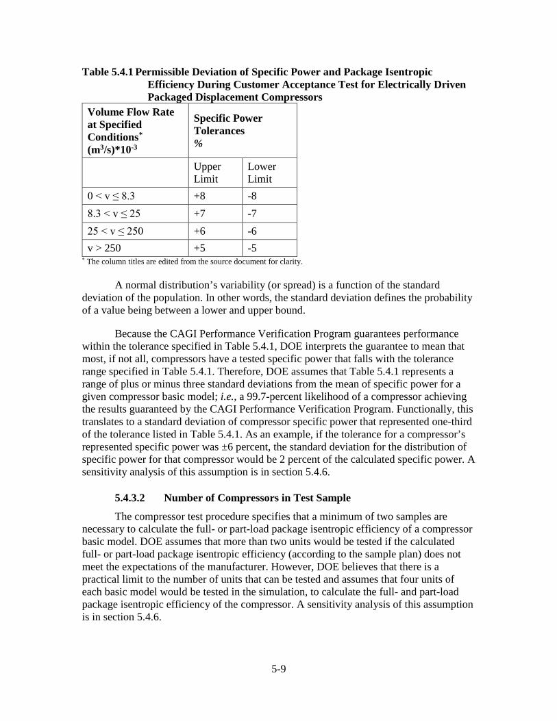
5-9

Table 5.4.1 Permissible Deviation of Specific Power and Package Isentropic Efficiency During Customer Acceptance Test for Electrically Driven Packaged Displacement Compressors

Volume Flow Rate at Specified Conditions* (m3/s)*10-3

Specific Power Tolerances %

Upper Limit

Lower Limit

0 < v ≤ 8.3 +8 -8 8.3 < v ≤ 25 +7 -7 25 < v ≤ 250 +6 -6 v > 250 +5 -5

* The column titles are edited from the source document for clarity. A normal distribution’s variability (or spread) is a function of the standard

deviation of the population. In other words, the standard deviation defines the probability of a value being between a lower and upper bound.

Because the CAGI Performance Verification Program guarantees performance within the tolerance specified in Table 5.4.1, DOE interprets the guarantee to mean that most, if not all, compressors have a tested specific power that falls with the tolerance range specified in Table 5.4.1. Therefore, DOE assumes that Table 5.4.1 represents a range of plus or minus three standard deviations from the mean of specific power for a given compressor basic model; i.e., a 99.7-percent likelihood of a compressor achieving the results guaranteed by the CAGI Performance Verification Program. Functionally, this translates to a standard deviation of compressor specific power that represented one-third of the tolerance listed in Table 5.4.1. As an example, if the tolerance for a compressor’s represented specific power was ±6 percent, the standard deviation for the distribution of specific power for that compressor would be 2 percent of the calculated specific power. A sensitivity analysis of this assumption is in section 5.4.6.

5.4.3.2 Number of Compressors in Test Sample

The compressor test procedure specifies that a minimum of two samples are necessary to calculate the full- or part-load package isentropic efficiency of a compressor basic model. DOE assumes that more than two units would be tested if the calculated full- or part-load package isentropic efficiency (according to the sample plan) does not meet the expectations of the manufacturer. However, DOE believes that there is a practical limit to the number of units that can be tested and assumes that four units of each basic model would be tested in the simulation, to calculate the full- and part-load package isentropic efficiency of the compressor. A sensitivity analysis of this assumption is in section 5.4.6.

5-10

5.4.3.3 Correlation Between Part-Load Specific Power Measurements

Part-load package isentropic efficiency is a function of package isentropic efficiency at 100, 70, and 40 percent of full-load actual volume flow rate. Section 5.4.3.1 discusses that a given compressor’s tested specific power has a variation defined by a normal distribution, yet does not discuss the relationship (if any) between performance at each part-load package isentropic efficiency load point. In other words, Section 5.4.3.1 does not discuss whether different load points are correlated (i.e., whether a higher than average measured specific power at 100 percent capacity will result in higher than average measured specific power at 70 percent and 40 percent capacity).

Before structuring the Monte Carlo analysis, DOE assessed two correlation scenarios: one with no correlation and one with a strong correlation. In the case of no correlation, specific power values at 100, 70, and 40 percent of full-load actual volume flow rate would be randomly drawn from their distribution, with no relationship to each other. Due to the random nature of this scenario, for each test sample, specific power values at each load point may fall above, below, or close to the mean (i.e., some may be high and some may be low). Ultimately, this scenario limits overall variation in part-load package isentropic efficiency, as individual high and low load point may cancel each other out, resulting in simulated part-load package isentropic efficiency values that are closer to the mean.

Alternatively, in the strongly correlated scenario, specific power values at 100, 70, and 40 percent of full-load actual volume flow rate would be tied together (i.e., all values might be high, or all might be low). Compared to the no correlation scenario, this scenario creates more variation in part-load package isentropic efficiency, and could be considered more conservative. In other words, assuming that the values of specific power at 100 percent, 70 percent, and 40 percent capacity have a positive correlation is a conservative assumption that is more likely to produce a change in compressor rating under the sampling plan.

DOE has no data to indicate whether or not the measured specific power of a compressor at 100, 70, and 40 percent of full-load actual volume flow rate have a correlation. In the absence of data, DOE pursued the more conservative option, and models a correlation of 1.0 for compressor specific power values from a given compressor sample. In practice, the simulation randomly generates a number for the probability distribution at 100 percent, 70 percent, and 40 percent capacity that is the same number of standard deviations from each distribution’s mean.

5.4.4 Population of Compressors in Sampling Plan Analysis

The updated CAGI database defines the population for the sampling plan analysis. Specifically, for each compressors in the database, the Monte Carlo analysis generates 10,000 unique, simulated package isentropic efficiencies, based on the rules of the sampling plan. DOE ran two unique simulations, one for fixed-speed compressors and

5-11

one for variable-speed compressors. Equipment that meets the definitioni of a variable-speed compressor (as established in the test procedure final rule) and with test data at, or below, 40 percent of full load actual volume flow rate is included in the part-load package isentropic efficiency simulation. Similarly, all of the compressors that meet the definition of a fixed-speed compressor are included in the fixed-speed compressors analysis, based on their performance at full-load actual volume flow rate.

5.4.5 Results

This section presents the results of the compressor test procedure sampling plan analysis. Sensitivity analyses on areas of uncertainty, including the type of distribution representing specific power, the number of compressor samples to certify the full- or part-load package isentropic efficiency, and the number of trials for the Monte Carlo analysis, are included in section 5.4.6.

The results of the sampling plan conclude that, on average, the certified efficiency of a random compressor sample of four units under the compressor test procedure sampling plan would not result in a lower value compared to the direct calculation of the certified efficiency from the CAGI Performance Verification data sheets. Put differently, for each iteration of the Monte Carlo simulation, given a random sample of four units, the mean of the sample was lower than the 95th lower confidence interval divided by 0.95 over 99.7 percent of the time.

5.4.6 Sensitivity Analysis

DOE conducted additional analyses with the Monte Carlo simulation to understand the sensitivity of three key assumptions that were made as part of the analysis:

1) The assumed distribution of compressor specific power, 2) The number of tested compressors, and 3) The number of trials required for a representative result.

The following sections discuss the changes made to the model as well as the results

of the sensitivity analyses.

5.4.6.1 Assumed Distribution of Compressor Specific Power

To determine the impact of the assumed distribution, DOE conducted the Monte Carlo analysis scenario with package specific power represented by a uniform distribution. The uniform distribution is defined by the allowable tolerances in Table 5.4.1 for each compressor in the Monte Carlo simulation. As noted in section 5.4.3.1, a uniform distribution represents the most conservative assumption for the distribution of compressor specific power as a uniform distribution assumes an equal probability of a compressor meeting any value of specific power within the bounds of the allowable tolerance. DOE asserts that this is unlikely given that most distributions of a continuous i DOE excludes variable-speed compressors that cannot reach 40 percent compressor capacity (approximately 140 compressors in the CAGI database).

5-12

outcome (i.e., manufacturing and testing tolerances) are of a normal distribution, which has a much higher probability that a value is closer to the mean. All other assumptions, including the number of trials, remain unchanged from the previous analysis.

5.4.6.2 Number of Tested Compressors in Sample

To determine the impact of the number of compressors assumed to be part of the tested sample, DOE reduced the sample size and conducted a Monte Carlo analysis scenario with three tested compressors comprising the sample (rather than four unit in the baseline case).

5.4.6.3 Number of Trials Required for a Representative Result

To determine the impact of the trials required in the Monte Carlo analysis to achieve a representative result, DOE ran up to 100,000 simulations for each of the results presented to evaluate whether 10,000 trials were sufficient to provide representative results. DOE defines the number of trials to be sufficient if the results of the simulation change by less than 0.005 points when incrementing the number of trials.

5.4.6.4 Results of the Sensitivity Analyses

The results of the specific power distribution and sample size sensitivity analyses are in Table 5.4.2 and Table 5.4.3. Table 5.4.2 and Table 5.4.3 refer to the average decrement in package isentropic efficiency, or the average difference between the calculated value from the CAGI data sheets and the rating from the Monte Carlo simulation in points of efficiency. For example, if the calculated full-load package isentropic efficiency from a direct calculation of data in the updated CAGI database was 70 percent and the Monte Carlo simulation calculated an average value of 69.5 percent, the average change in rating is -0.5 points.

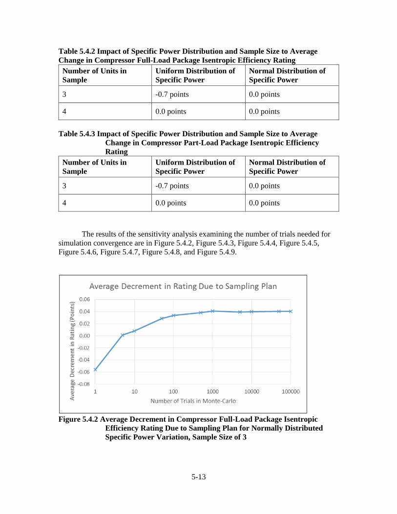
5-13

Table 5.4.2 Impact of Specific Power Distribution and Sample Size to Average Change in Compressor Full-Load Package Isentropic Efficiency Rating

Number of Units in Sample

Uniform Distribution of Specific Power

Normal Distribution of Specific Power

3 -0.7 points 0.0 points

4 0.0 points 0.0 points

Table 5.4.3 Impact of Specific Power Distribution and Sample Size to Average

Change in Compressor Part-Load Package Isentropic Efficiency Rating

Number of Units in Sample

Uniform Distribution of Specific Power

Normal Distribution of Specific Power

3 -0.7 points 0.0 points

4 0.0 points 0.0 points

The results of the sensitivity analysis examining the number of trials needed for simulation convergence are in Figure 5.4.2, Figure 5.4.3, Figure 5.4.4, Figure 5.4.5, Figure 5.4.6, Figure 5.4.7, Figure 5.4.8, and Figure 5.4.9.

Figure 5.4.2 Average Decrement in Compressor Full-Load Package Isentropic

Efficiency Rating Due to Sampling Plan for Normally Distributed Specific Power Variation, Sample Size of 3

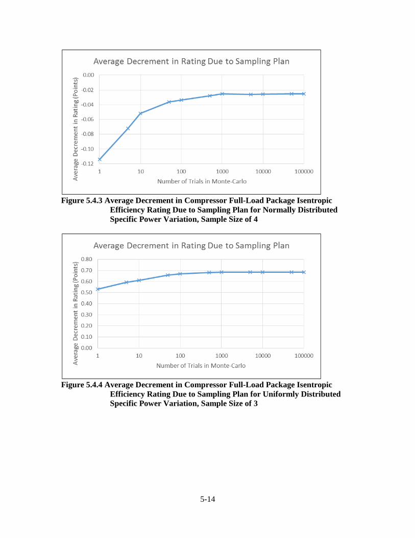
5-14

Figure 5.4.3 Average Decrement in Compressor Full-Load Package Isentropic

Efficiency Rating Due to Sampling Plan for Normally Distributed Specific Power Variation, Sample Size of 4

Figure 5.4.4 Average Decrement in Compressor Full-Load Package Isentropic

Efficiency Rating Due to Sampling Plan for Uniformly Distributed Specific Power Variation, Sample Size of 3

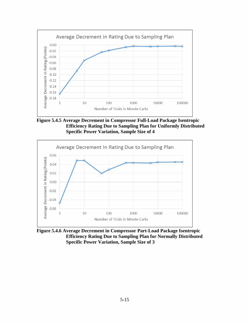
5-15

Figure 5.4.5 Average Decrement in Compressor Full-Load Package Isentropic

Efficiency Rating Due to Sampling Plan for Uniformly Distributed Specific Power Variation, Sample Size of 4

Figure 5.4.6 Average Decrement in Compressor Part-Load Package Isentropic

Efficiency Rating Due to Sampling Plan for Normally Distributed Specific Power Variation, Sample Size of 3

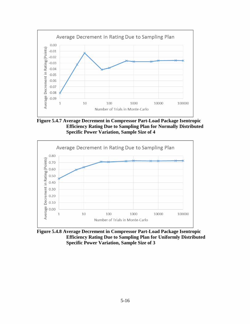
5-16

Figure 5.4.7 Average Decrement in Compressor Part-Load Package Isentropic

Efficiency Rating Due to Sampling Plan for Normally Distributed Specific Power Variation, Sample Size of 4

Figure 5.4.8 Average Decrement in Compressor Part-Load Package Isentropic

Efficiency Rating Due to Sampling Plan for Uniformly Distributed Specific Power Variation, Sample Size of 3

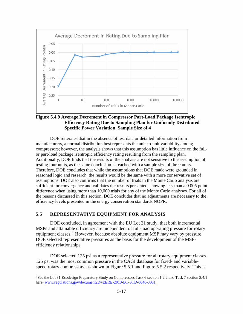
5-17

Figure 5.4.9 Average Decrement in Compressor Part-Load Package Isentropic

Efficiency Rating Due to Sampling Plan for Uniformly Distributed Specific Power Variation, Sample Size of 4

DOE reiterates that in the absence of test data or detailed information from manufacturers, a normal distribution best represents the unit-to-unit variability among compressors; however, the analysis shows that this assumption has little influence on the full- or part-load package isentropic efficiency rating resulting from the sampling plan. Additionally, DOE finds that the results of the analysis are not sensitive to the assumption of testing four units, as the same conclusion is reached with a sample size of three units. Therefore, DOE concludes that while the assumptions that DOE made were grounded in reasoned logic and research, the results would be the same with a more conservative set of assumptions. DOE also confirms that the number of trials in the Monte Carlo analysis are sufficient for convergence and validates the results presented, showing less than a 0.005 point difference when using more than 10,000 trials for any of the Monte Carlo analyses. For all of the reasons discussed in this section, DOE concludes that no adjustments are necessary to the efficiency levels presented in the energy conservation standards NOPR.

5.5 REPRESENTATIVE EQUIPMENT FOR ANALYSIS

DOE concluded, in agreement with the EU Lot 31 study, that both incremental MSPs and attainable efficiency are independent of full-load operating pressure for rotary equipment classes.j However, because absolute equipment MSP may vary by pressure, DOE selected representative pressures as the basis for the development of the MSP-efficiency relationships. DOE selected 125 psi as a representative pressure for all rotary equipment classes. 125 psi was the most common pressure in the CAGI database for fixed- and variable-speed rotary compressors, as shown in Figure 5.5.1 and Figure 5.5.2 respectively. This is j See the Lot 31 Ecodesign Preparatory Study on Compressors Task 6 section 1.2.2 and Task 7 section 2.4.1 here: www.regulations.gov/document?D=EERE-2013-BT-STD-0040-0031

5-18

consistent with the widespread use of 125 psi equipment and tools that are powered by these air compressors.

Figure 5.5.1 Histogram of Rotary Fixed-Speed Compressor Pressures in the CAGI

Database

Figure 5.5.2 Histogram of Rotary Variable-Speed Compressor Pressures in the

CAGI Database

5.6 DESIGN OPTIONS

After conducting the screening analysis and removing technologies that did not warrant inclusion on technical grounds, package redesign remained as the only design options to be considered in the final rule engineering analysis.

5-19

5.7 AVAILABLE EFFICIENCY IMPROVEMENTS

For each equipment class, DOE assessed the available energy efficiency improvements resulting from a package redesign. This assessment was informed by manufacturer performance and cost data, confidential manufacturer interview responses, general industry research, and stakeholder input. Potential improvements in efficiency are represented by the efficiency spread between the lowest efficiency and highest efficiency air compressors already offered in the marketplace. It is technically feasible for any air compressor of the baseline configuration to realize efficiency improvements in any increment, up to the highest efficiency currently present on the market, depending on the level of effort and capital a manufacturer chooses to invest in a redesign. Sections 5.8 and 5.9 discuss the relationship between efficiency gains and MSP in more detail.

5.8 EFFICIENCY LEVELS

For each equipment class, DOE established and analyzed six efficiency levels and a baseline to assess the relationship between MSP and package isentropic efficiency. As discussed previously, DOE’s efficiency levels have been established independent of full-load operating pressure. However, DOE concluded, in agreement with the Lot 31 study, that for the compressors within the scope of this rule, attainable package isentropic efficiency is a function of full-load actual volume flow rate.k As such, each efficiency level is defined by a mathematical relationship between full-load actual volume flow rate and package isentropic efficiency. Similar to the Lot 31 study, DOE defines a regression curve for each equipment class and uses specific “d-values” to shift the regression curve and establish efficiency levels for each equipment class, as discussed in this section.

5.8.1 Efficiency Level Structure

Similar to the Lot 31 study, DOE defines a regression curve (market average package isentropic efficiency, as a function of full-load actual volume flow rate) for each equipment class and uses specific d-values to shift the regression curve and establish efficiency levels for each equipment class; this is discussed in detail in in sections 5.8.3 and 5.8.4. Similar to the approach used by the Lot 31 study, DOE defined the d-value as a percentage improvement from the regression curve to theoretical 100 percent isentropic efficiency. A d-value of 100 would generate an efficiency level at 100 percent isentropic efficiency for all full-load actual volume flow rates. Alternatively, a d-value of 50 would generate a regulation curve that falls halfway between the regression curve and 100 percent isentropic efficiency for all full-load actual volume flow rates. This d-value represents the improvement of a product, expressed as the reduction of losses going from average (the regression curve) to 100 percent efficiency (theoretical). k Discussed often, e.g., Task 6 Section 1.3. See: www.regulations.gov/document?D=EERE-2013-BT-STD-0040-0031

5-20

5.8.1.1 Baseline

The baseline configuration represents the lowest efficiency level commonly available in the market. Because energy conservation standards did not currently exist for air compressors, DOE needed to establish a baseline configuration using available information. The baseline configuration defines the energy consumption and associated cost for the lowest efficiency equipment analyzed in each class. DOE performed an analysis on available air compressor data, and determined a d-value for each equipment class that represents the lowest efficiency equipment currently in the market. Although air compressors at this baseline level may have different physical designs, they all represent the baseline efficiency. Because there was no standard, baseline was not always the literal lowest-performing compressor at a given full-load actual volume flow rate. Manufacturers can (and sometimes do) produce performance outliers not representative of the common baseline performance level. The concept of a baseline is centered on describing the lowest-performing equipment that is sold with significant frequency. Further detail on what data was used, and what d-value was selected for each equipment class, is in sections 5.8.3 and 5.8.4.

5.8.1.2 Maximum Technologically Feasible Level

The maximum technologically feasible, or “max-tech,” is the efficiency level that provides the maximum improvement in energy efficiency that is technologically feasible. The max-tech level must be attainable across the entire scope of the equipment class. Generally, the max-tech level results from the combination of design options predicted to result in the highest efficiency level possible for an equipment class. For this rulemaking, package redesign was determined to be the only available design option. Air compressors are considered mature products with the highest levels of attainable efficiency already present in the marketplace. As such, the max-tech configuration represents the highest efficiency equipment commonly available in the market. DOE performed an analysis on available air compressor data, and determined a d-value for each equipment class that represents max-tech. Although air compressors at max-tech may have different physical designs, they all represent the max-tech. Further detail on what data was used, and what d-value was selected for each equipment class is in sections 5.8.3 and 5.8.4.

5.8.2 Methods Used to Determine Efficiency Levels

For each equipment class, DOE established and analyzed six efficiency levels and a baseline to assess the relationship between MSP and package isentropic efficiency. Efficiency levels were set using a d-value as described in section 5.8.1. As discussed previously, DOE’s efficiency levels have been established independent of full-load operating pressure. For each equipment class, DOE established efficiency levels at max-tech (EL 6) and a d-value of zero (EL 3). DOE also established two intermediary efficiency levels

5-21

between the baseline and a d-value of zero, and two efficiency levels between the d-value of zero level and max-tech. For all equipment classes, EL 6 represents the max-tech efficiency level. As discussed in section 5.8.1.2, the max-tech efficiency level coincides with the maximum available efficiency already offered in the marketplace. As a result, DOE performed market-based analyses to determine max-tech/max-available levels. As discussed in section 5.8.1.1, for all equipment classes the baseline defines the lowest efficiency equipment present in the market for each equipment class. DOE established baselines, represented by d-values, for each equipment class by reviewing available air compressor performance data. For all equipment classes EL 3 corresponds to a d-value of zero, which represents the mean efficiency available on the market. The EU Lot 31 draft regulation proposed a d-value of zero for a minimum energy efficiency requirement in 2020.l EL 1 and 2 are established as intermediary efficiency levels one-third and two-thirds of the way, respectively, between the baseline and EL 3. EL 4 is an efficiency level established slightly above EL 3 to evaluate the sensitivity of going above the EU Lot 31 draft regulation. EL 5 is an intermediary efficiency level established approximately halfway between EL 3 and EL 6. The actual numerical value of the d-values for EL 1, 2, 4, 5, and 6 vary for each equipment class. DOE pursued different analytical methods to establish efficiency levels for different equipment classes. For air-cooled equipment classes described in section 5.8.3, DOE used relationships established in the Lot 31 study as the basis for efficiency levels. For liquid-cooled equipment classes described in section 5.8.4, DOE used the CAGI database to develop relationship and scaled air-cooled efficiency levels to liquid-cooled efficiency levels.

5.8.3 Air-Cooled Compressors

When appropriate, DOE chose to use analogous EU Lot 31 regression curves for equipment classes. Specifically, DOE used the fixed-speed rotary standard air compressors Lot 31 regression curve for the rotary, lubricated, air-cooled, fixed-speed equipment class, and the variable-speed rotary standard air compressors Lot 31 regression curve for the rotary, lubricated, air-cooled, variable-speed equipment class. DOE verified the use of the Lot 31 regression curves for these equipment classes based on data in the CAGI database, as described in the following sections.

5.8.3.1 RP_FS_L_AC Efficiency Levels

The CAGI database contained 835 data points in the rotary, lubricated, air-cooled, fixed-speed equipment class. DOE used the CAGI data to create a regression curve, l See Draft Ecodesign Regulation Table 2: www.regulations.gov/document?D=EERE-2013-BT-STD-0040-0031

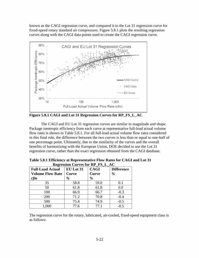
5-22

known as the CAGI regression curve, and compared it to the Lot 31 regression curve for fixed-speed rotary standard air compressors. Figure 5.8.1 plots the resulting regression curves along with the CAGI data points used to create the CAGI regression curve.

Figure 5.8.1 CAGI and Lot 31 Regression Curves for RP_FS_L_AC The CAGI and EU Lot 31 regression curves are similar in magnitude and shape. Package isentropic efficiency from each curve at representative full-load actual volume flow rates is shown in Table 5.8.1. For all full-load actual volume flow rates considered in this final rule, the difference between the two curves is less than or equal to one-half of one percentage point. Ultimately, due to the similarity of the curves and the overall benefits of harmonizing with the European Union, DOE decided to use the Lot 31 regression curve, rather than the exact regression obtained from the CAGI database. Table 5.8.1 Efficiency at Representative Flow Rates for CAGI and Lot 31

Regression Curves for RP_FS_L_AC Full-Load Actual Volume Flow Rate cfm

EU Lot 31 Curve %

CAGI Curve %

Difference %

35 58.8 59.0 0.1 50 61.8 61.8 0.0 100 66.9 66.7 -0.3 200 71.2 70.8 -0.4 500 75.4 74.9 -0.5

1,000 77.6 77.1 -0.5 The regression curve for the rotary, lubricated, air-cooled, fixed-speed equipment class is as follows:

5-23

𝜂𝜂𝐼𝐼𝐼𝐼𝐼𝐼𝐼𝐼_𝑅𝑅𝐼𝐼𝑅𝑅𝑅𝑅_𝑅𝑅𝑅𝑅_𝐹𝐹𝐹𝐹_𝐿𝐿_𝐴𝐴𝐴𝐴= −0.00928 × 𝑙𝑙𝑙𝑙2(0.4719 × 𝑉𝑉1) + 0.13911 × 𝑙𝑙𝑙𝑙(0.4719 × 𝑉𝑉1)+ 0.27110

Equation 5.3 Where: ηIsen_Regr_RP_FS_L_AC = regression curve package isentropic efficiency for the rotary, lubricated, air-cooled, fixed-speed equipment class, and V1 = full-load actual volume flow rate (cubic feet per minute).

Efficiency levels for the rotary, lubricated, air-cooled, fixed-speed equipment class are defined by the following equation, in conjunction with the d-values in Table 5.8.2: 𝜂𝜂𝐼𝐼𝐼𝐼𝐼𝐼𝐼𝐼_𝐹𝐹𝑆𝑆𝑆𝑆_𝑅𝑅𝑅𝑅_𝐹𝐹𝐹𝐹_𝐿𝐿_𝐴𝐴𝐴𝐴 = 𝜂𝜂𝐼𝐼𝐼𝐼𝐼𝐼𝐼𝐼_𝑅𝑅𝐼𝐼𝑅𝑅𝑅𝑅_𝑅𝑅𝑅𝑅_𝐹𝐹𝐹𝐹_𝐿𝐿_𝐴𝐴𝐴𝐴 + �1 − 𝜂𝜂𝐼𝐼𝐼𝐼𝐼𝐼𝐼𝐼_𝑅𝑅𝐼𝐼𝑅𝑅𝑅𝑅_𝑅𝑅𝑅𝑅_𝐹𝐹𝐹𝐹_𝐿𝐿_𝐴𝐴𝐴𝐴� × 𝑑𝑑/100

Equation 5.4

Where: ηIsen_STD_RP_FS_L_AC = package isentropic efficiency for the rotary, lubricated, air-cooled, fixed-speed equipment class, for a selected efficiency level, ηIsen_Regr_RP_FS_L_AC = regression curve package isentropic efficiency for the rotary, lubricated, air-cooled, fixed-speed equipment class, and d = d-value for each efficiency level, as specified in Table 5.8.2.

To select a baseline, in the energy conservation standards NOPR, DOE analyzed available performance data in the CAGI database that represented the lowest efficiency equipment available across the entire market. 81 FR 31680, 31705-31706. (May 19, 2016). Similarly, to select a max-tech level, in the energy conservation standards NOPR, DOE analyzed available performance data in the CAGI database to select a d-value that represented the highest efficiency equipment available across the entire market. 81 FR 31680, 31705-31706. In this final rule, DOE compared the NOPR baseline and max-tech levels to the updated CAGI database and concluded that the NOPR baselines and max-tech were still valid and accurately represent the new data. Figure 5.8.2 displays the curves that represent the baseline and max-tech levels for the rotary, lubricated, air-cooled, fixed-speed equipment class, as well as the updated CAGI database data used to confirm them.

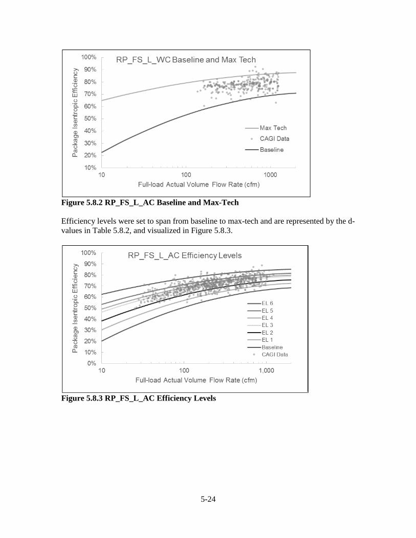
5-24

Figure 5.8.2 RP_FS_L_AC Baseline and Max-Tech Efficiency levels were set to span from baseline to max-tech and are represented by the d-values in Table 5.8.2, and visualized in Figure 5.8.3.

Figure 5.8.3 RP_FS_L_AC Efficiency Levels

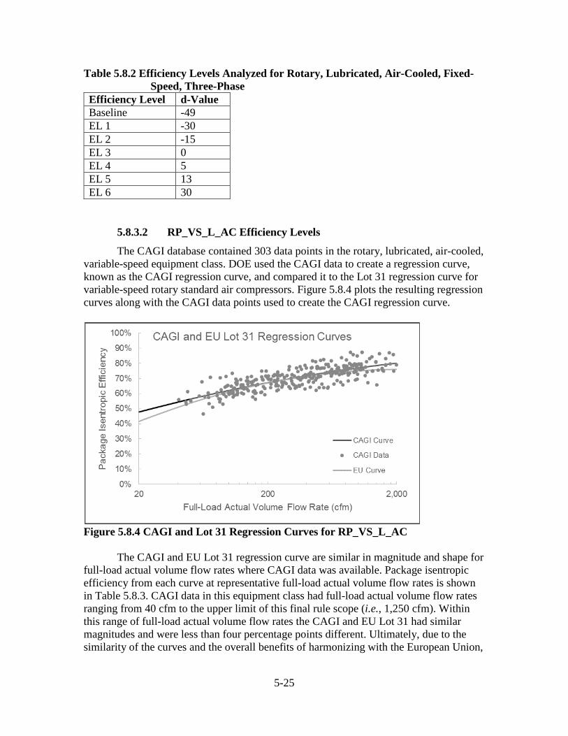
5-25

Table 5.8.2 Efficiency Levels Analyzed for Rotary, Lubricated, Air-Cooled, Fixed-Speed, Three-Phase

Efficiency Level d-Value Baseline -49 EL 1 -30 EL 2 -15 EL 3 0 EL 4 5 EL 5 13 EL 6 30

5.8.3.2 RP_VS_L_AC Efficiency Levels

The CAGI database contained 303 data points in the rotary, lubricated, air-cooled, variable-speed equipment class. DOE used the CAGI data to create a regression curve, known as the CAGI regression curve, and compared it to the Lot 31 regression curve for variable-speed rotary standard air compressors. Figure 5.8.4 plots the resulting regression curves along with the CAGI data points used to create the CAGI regression curve.

Figure 5.8.4 CAGI and Lot 31 Regression Curves for RP_VS_L_AC The CAGI and EU Lot 31 regression curve are similar in magnitude and shape for full-load actual volume flow rates where CAGI data was available. Package isentropic efficiency from each curve at representative full-load actual volume flow rates is shown in Table 5.8.3. CAGI data in this equipment class had full-load actual volume flow rates ranging from 40 cfm to the upper limit of this final rule scope (i.e., 1,250 cfm). Within this range of full-load actual volume flow rates the CAGI and EU Lot 31 had similar magnitudes and were less than four percentage points different. Ultimately, due to the similarity of the curves and the overall benefits of harmonizing with the European Union,

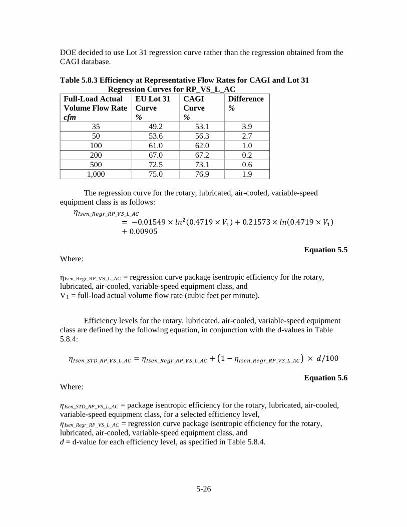
5-26

DOE decided to use Lot 31 regression curve rather than the regression obtained from the CAGI database. Table 5.8.3 Efficiency at Representative Flow Rates for CAGI and Lot 31

Regression Curves for RP_VS_L_AC Full-Load Actual Volume Flow Rate cfm

EU Lot 31 Curve %

CAGI Curve %

Difference %

35 49.2 53.1 3.9 50 53.6 56.3 2.7 100 61.0 62.0 1.0 200 67.0 67.2 0.2 500 72.5 73.1 0.6

1,000 75.0 76.9 1.9 The regression curve for the rotary, lubricated, air-cooled, variable-speed equipment class is as follows:

𝜂𝜂𝐼𝐼𝐼𝐼𝐼𝐼𝐼𝐼_𝑅𝑅𝐼𝐼𝑅𝑅𝑅𝑅_𝑅𝑅𝑅𝑅_𝑉𝑉𝐹𝐹_𝐿𝐿_𝐴𝐴𝐴𝐴= −0.01549 × 𝑙𝑙𝑙𝑙2(0.4719 × 𝑉𝑉1) + 0.21573 × 𝑙𝑙𝑙𝑙(0.4719 × 𝑉𝑉1)+ 0.00905

Equation 5.5

Where: ηIsen_Regr_RP_VS_L_AC = regression curve package isentropic efficiency for the rotary, lubricated, air-cooled, variable-speed equipment class, and V1 = full-load actual volume flow rate (cubic feet per minute).

Efficiency levels for the rotary, lubricated, air-cooled, variable-speed equipment class are defined by the following equation, in conjunction with the d-values in Table 5.8.4: 𝜂𝜂𝐼𝐼𝐼𝐼𝐼𝐼𝐼𝐼_𝐹𝐹𝑆𝑆𝑆𝑆_𝑅𝑅𝑅𝑅_𝑉𝑉𝐹𝐹_𝐿𝐿_𝐴𝐴𝐴𝐴 = 𝜂𝜂𝐼𝐼𝐼𝐼𝐼𝐼𝐼𝐼_𝑅𝑅𝐼𝐼𝑅𝑅𝑅𝑅_𝑅𝑅𝑅𝑅_𝑉𝑉𝐹𝐹_𝐿𝐿_𝐴𝐴𝐴𝐴 + �1 − 𝜂𝜂𝐼𝐼𝐼𝐼𝐼𝐼𝐼𝐼_𝑅𝑅𝐼𝐼𝑅𝑅𝑅𝑅_𝑅𝑅𝑅𝑅_𝑉𝑉𝐹𝐹_𝐿𝐿_𝐴𝐴𝐴𝐴� × 𝑑𝑑/100

Equation 5.6

Where: ηIsen_STD_RP_VS_L_AC = package isentropic efficiency for the rotary, lubricated, air-cooled, variable-speed equipment class, for a selected efficiency level, ηIsen_Regr_RP_VS_L_AC = regression curve package isentropic efficiency for the rotary, lubricated, air-cooled, variable-speed equipment class, and d = d-value for each efficiency level, as specified in Table 5.8.4.

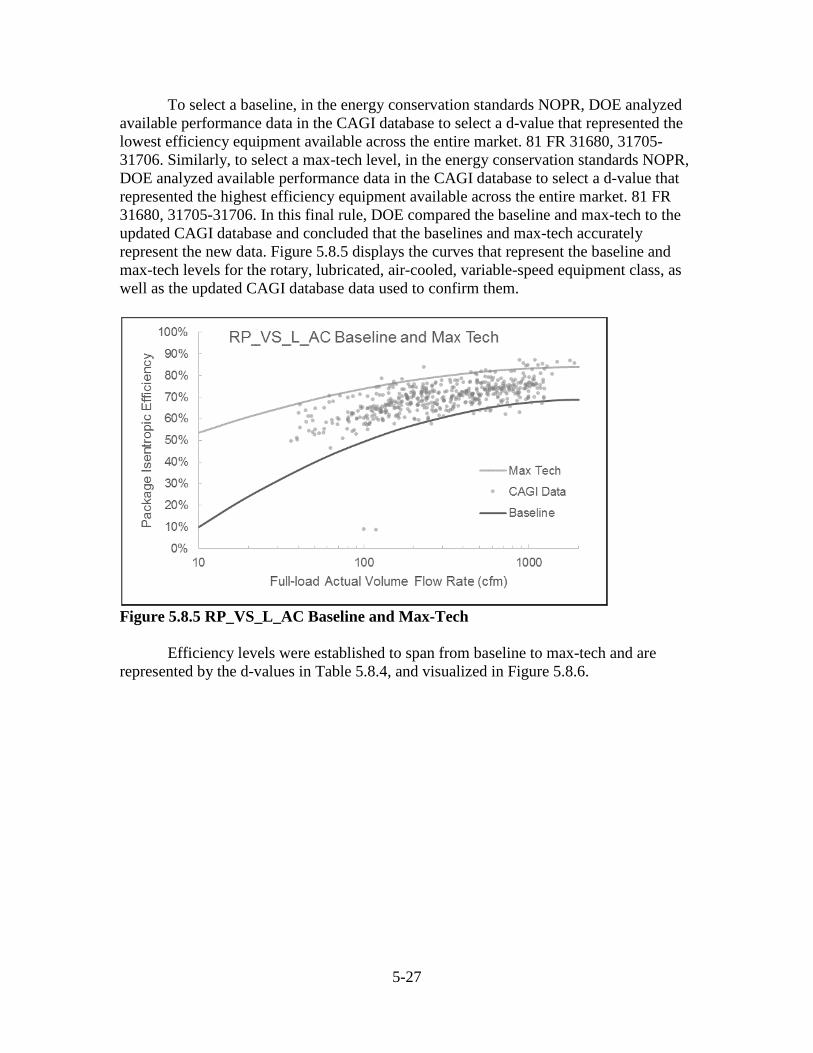
5-27

To select a baseline, in the energy conservation standards NOPR, DOE analyzed available performance data in the CAGI database to select a d-value that represented the lowest efficiency equipment available across the entire market. 81 FR 31680, 31705-31706. Similarly, to select a max-tech level, in the energy conservation standards NOPR, DOE analyzed available performance data in the CAGI database to select a d-value that represented the highest efficiency equipment available across the entire market. 81 FR 31680, 31705-31706. In this final rule, DOE compared the baseline and max-tech to the updated CAGI database and concluded that the baselines and max-tech accurately represent the new data. Figure 5.8.5 displays the curves that represent the baseline and max-tech levels for the rotary, lubricated, air-cooled, variable-speed equipment class, as well as the updated CAGI database data used to confirm them.

Figure 5.8.5 RP_VS_L_AC Baseline and Max-Tech Efficiency levels were established to span from baseline to max-tech and are represented by the d-values in Table 5.8.4, and visualized in Figure 5.8.6.

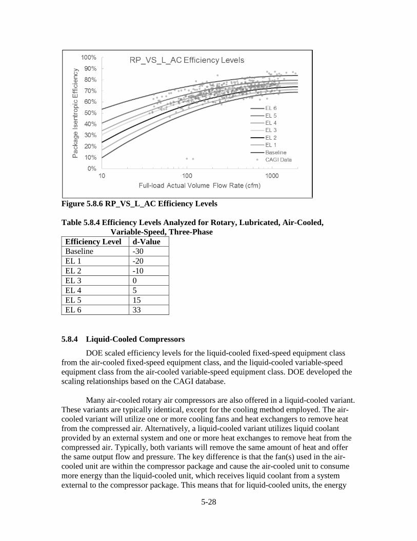
5-28

Figure 5.8.6 RP_VS_L_AC Efficiency Levels Table 5.8.4 Efficiency Levels Analyzed for Rotary, Lubricated, Air-Cooled,

Variable-Speed, Three-Phase Efficiency Level d-Value Baseline -30 EL 1 -20 EL 2 -10 EL 3 0 EL 4 5 EL 5 15 EL 6 33

5.8.4 Liquid-Cooled Compressors

DOE scaled efficiency levels for the liquid-cooled fixed-speed equipment class from the air-cooled fixed-speed equipment class, and the liquid-cooled variable-speed equipment class from the air-cooled variable-speed equipment class. DOE developed the scaling relationships based on the CAGI database. Many air-cooled rotary air compressors are also offered in a liquid-cooled variant. These variants are typically identical, except for the cooling method employed. The air-cooled variant will utilize one or more cooling fans and heat exchangers to remove heat from the compressed air. Alternatively, a liquid-cooled variant utilizes liquid coolant provided by an external system and one or more heat exchanges to remove heat from the compressed air. Typically, both variants will remove the same amount of heat and offer the same output flow and pressure. The key difference is that the fan(s) used in the air-cooled unit are within the compressor package and cause the air-cooled unit to consume more energy than the liquid-cooled unit, which receives liquid coolant from a system external to the compressor package. This means that for liquid-cooled units, the energy

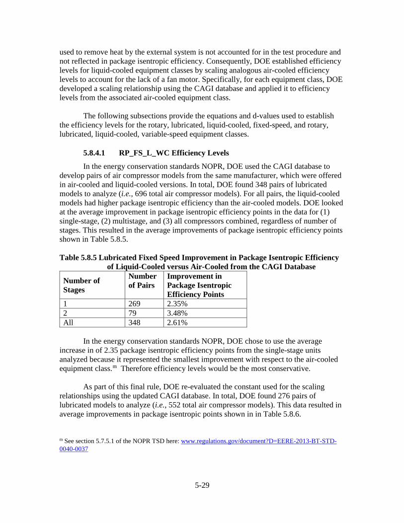
5-29

used to remove heat by the external system is not accounted for in the test procedure and not reflected in package isentropic efficiency. Consequently, DOE established efficiency levels for liquid-cooled equipment classes by scaling analogous air-cooled efficiency levels to account for the lack of a fan motor. Specifically, for each equipment class, DOE developed a scaling relationship using the CAGI database and applied it to efficiency levels from the associated air-cooled equipment class. The following subsections provide the equations and d-values used to establish the efficiency levels for the rotary, lubricated, liquid-cooled, fixed-speed, and rotary, lubricated, liquid-cooled, variable-speed equipment classes.

5.8.4.1 RP_FS_L_WC Efficiency Levels

In the energy conservation standards NOPR, DOE used the CAGI database to develop pairs of air compressor models from the same manufacturer, which were offered in air-cooled and liquid-cooled versions. In total, DOE found 348 pairs of lubricated models to analyze (i.e., 696 total air compressor models). For all pairs, the liquid-cooled models had higher package isentropic efficiency than the air-cooled models. DOE looked at the average improvement in package isentropic efficiency points in the data for (1) single-stage, (2) multistage, and (3) all compressors combined, regardless of number of stages. This resulted in the average improvements of package isentropic efficiency points shown in Table 5.8.5. Table 5.8.5 Lubricated Fixed Speed Improvement in Package Isentropic Efficiency

of Liquid-Cooled versus Air-Cooled from the CAGI Database

Number of Stages

Number of Pairs

Improvement in Package Isentropic Efficiency Points

1 269 2.35% 2 79 3.48% All 348 2.61%

In the energy conservation standards NOPR, DOE chose to use the average increase in of 2.35 package isentropic efficiency points from the single-stage units analyzed because it represented the smallest improvement with respect to the air-cooled equipment class.m Therefore efficiency levels would be the most conservative. As part of this final rule, DOE re-evaluated the constant used for the scaling relationships using the updated CAGI database. In total, DOE found 276 pairs of lubricated models to analyze (i.e., 552 total air compressor models). This data resulted in average improvements in package isentropic points shown in in Table 5.8.6. m See section 5.7.5.1 of the NOPR TSD here: www.regulations.gov/document?D=EERE-2013-BT-STD-0040-0037

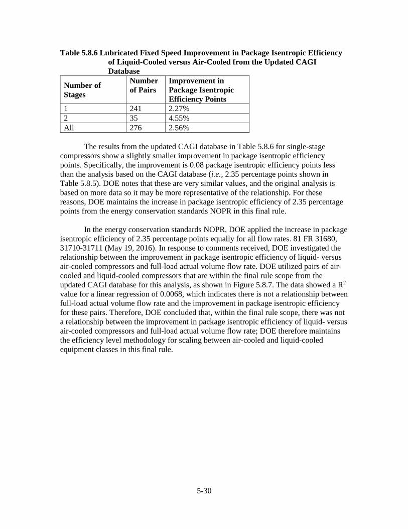
5-30

Table 5.8.6 Lubricated Fixed Speed Improvement in Package Isentropic Efficiency of Liquid-Cooled versus Air-Cooled from the Updated CAGI Database

Number of Stages

Number of Pairs

Improvement in Package Isentropic Efficiency Points

1 241 2.27% 2 35 4.55% All 276 2.56%

The results from the updated CAGI database in Table 5.8.6 for single-stage compressors show a slightly smaller improvement in package isentropic efficiency points. Specifically, the improvement is 0.08 package isentropic efficiency points less than the analysis based on the CAGI database (i.e., 2.35 percentage points shown in Table 5.8.5). DOE notes that these are very similar values, and the original analysis is based on more data so it may be more representative of the relationship. For these reasons, DOE maintains the increase in package isentropic efficiency of 2.35 percentage points from the energy conservation standards NOPR in this final rule. In the energy conservation standards NOPR, DOE applied the increase in package isentropic efficiency of 2.35 percentage points equally for all flow rates. 81 FR 31680, 31710-31711 (May 19, 2016). In response to comments received, DOE investigated the relationship between the improvement in package isentropic efficiency of liquid- versus air-cooled compressors and full-load actual volume flow rate. DOE utilized pairs of air-cooled and liquid-cooled compressors that are within the final rule scope from the updated CAGI database for this analysis, as shown in Figure 5.8.7. The data showed a R2 value for a linear regression of 0.0068, which indicates there is not a relationship between full-load actual volume flow rate and the improvement in package isentropic efficiency for these pairs. Therefore, DOE concluded that, within the final rule scope, there was not a relationship between the improvement in package isentropic efficiency of liquid- versus air-cooled compressors and full-load actual volume flow rate; DOE therefore maintains the efficiency level methodology for scaling between air-cooled and liquid-cooled equipment classes in this final rule.

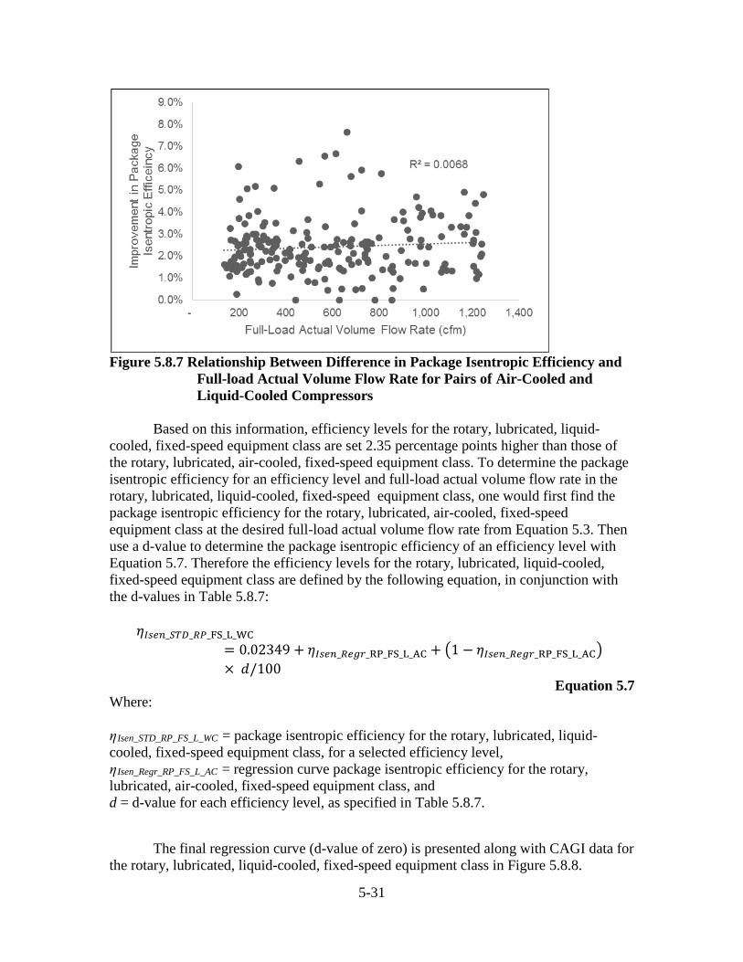
5-31

Figure 5.8.7 Relationship Between Difference in Package Isentropic Efficiency and

Full-load Actual Volume Flow Rate for Pairs of Air-Cooled and Liquid-Cooled Compressors

Based on this information, efficiency levels for the rotary, lubricated, liquid-cooled, fixed-speed equipment class are set 2.35 percentage points higher than those of the rotary, lubricated, air-cooled, fixed-speed equipment class. To determine the package isentropic efficiency for an efficiency level and full-load actual volume flow rate in the rotary, lubricated, liquid-cooled, fixed-speed equipment class, one would first find the package isentropic efficiency for the rotary, lubricated, air-cooled, fixed-speed equipment class at the desired full-load actual volume flow rate from Equation 5.3. Then use a d-value to determine the package isentropic efficiency of an efficiency level with Equation 5.7. Therefore the efficiency levels for the rotary, lubricated, liquid-cooled, fixed-speed equipment class are defined by the following equation, in conjunction with the d-values in Table 5.8.7:

𝜂𝜂𝐼𝐼𝐼𝐼𝐼𝐼𝐼𝐼_𝐹𝐹𝑆𝑆𝑆𝑆_𝑅𝑅𝑅𝑅_FS_L_WC= 0.02349 + 𝜂𝜂𝐼𝐼𝐼𝐼𝐼𝐼𝐼𝐼_𝑅𝑅𝐼𝐼𝑅𝑅𝑅𝑅_RP_FS_L_AC + �1 − 𝜂𝜂𝐼𝐼𝐼𝐼𝐼𝐼𝐼𝐼_𝑅𝑅𝐼𝐼𝑅𝑅𝑅𝑅_RP_FS_L_AC� × 𝑑𝑑/100

Equation 5.7 Where: ηIsen_STD_RP_FS_L_WC = package isentropic efficiency for the rotary, lubricated, liquid-cooled, fixed-speed equipment class, for a selected efficiency level, ηIsen_Regr_RP_FS_L_AC = regression curve package isentropic efficiency for the rotary, lubricated, air-cooled, fixed-speed equipment class, and d = d-value for each efficiency level, as specified in Table 5.8.7.

The final regression curve (d-value of zero) is presented along with CAGI data for the rotary, lubricated, liquid-cooled, fixed-speed equipment class in Figure 5.8.8.

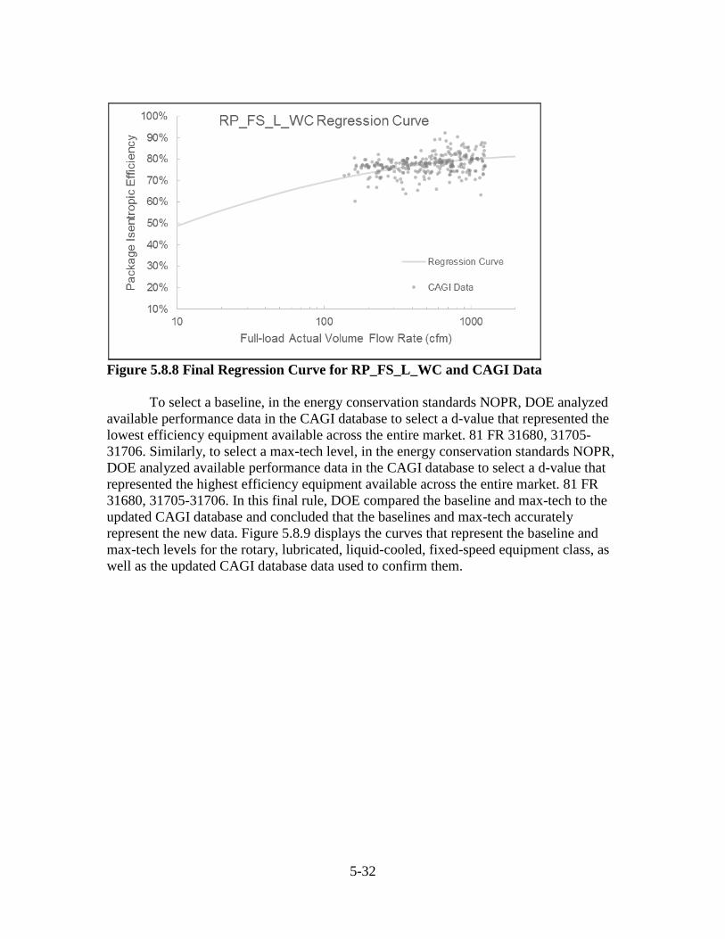
5-32

Figure 5.8.8 Final Regression Curve for RP_FS_L_WC and CAGI Data To select a baseline, in the energy conservation standards NOPR, DOE analyzed available performance data in the CAGI database to select a d-value that represented the lowest efficiency equipment available across the entire market. 81 FR 31680, 31705-31706. Similarly, to select a max-tech level, in the energy conservation standards NOPR, DOE analyzed available performance data in the CAGI database to select a d-value that represented the highest efficiency equipment available across the entire market. 81 FR 31680, 31705-31706. In this final rule, DOE compared the baseline and max-tech to the updated CAGI database and concluded that the baselines and max-tech accurately represent the new data. Figure 5.8.9 displays the curves that represent the baseline and max-tech levels for the rotary, lubricated, liquid-cooled, fixed-speed equipment class, as well as the updated CAGI database data used to confirm them.

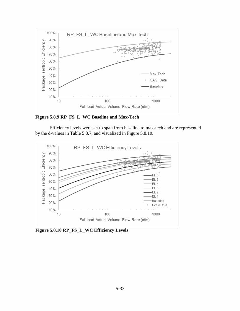
5-33

Figure 5.8.9 RP_FS_L_WC Baseline and Max-Tech Efficiency levels were set to span from baseline to max-tech and are represented by the d-values in Table 5.8.7, and visualized in Figure 5.8.10.

Figure 5.8.10 RP_FS_L_WC Efficiency Levels

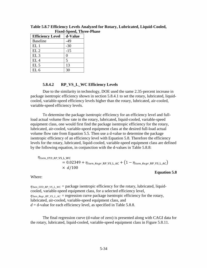
5-34

Table 5.8.7 Efficiency Levels Analyzed for Rotary, Lubricated, Liquid-Cooled, Fixed-Speed, Three-Phase

Efficiency Level d-Value Baseline -49 EL 1 -30 EL 2 -15 EL 3 0 EL 4 5 EL 5 13 EL 6 30

5.8.4.2 RP_VS_L_WC Efficiency Levels

Due to the similarity in technology, DOE used the same 2.35-percent increase in package isentropic efficiency shown in section 5.8.4.1 to set the rotary, lubricated, liquid-cooled, variable-speed efficiency levels higher than the rotary, lubricated, air-cooled, variable-speed efficiency levels. To determine the package isentropic efficiency for an efficiency level and full-load actual volume flow rate in the rotary, lubricated, liquid-cooled, variable-speed equipment class, one would first find the package isentropic efficiency for the rotary, lubricated, air-cooled, variable-speed equipment class at the desired full-load actual volume flow rate from Equation 5.5. Then use a d-value to determine the package isentropic efficiency of an efficiency level with Equation 5.8. Therefore the efficiency levels for the rotary, lubricated, liquid-cooled, variable-speed equipment class are defined by the following equation, in conjunction with the d-values in Table 5.8.8:

𝜂𝜂𝐼𝐼𝐼𝐼𝐼𝐼𝐼𝐼_𝐹𝐹𝑆𝑆𝑆𝑆_𝑅𝑅𝑅𝑅_VS_L_WC= 0.02349 + 𝜂𝜂𝐼𝐼𝐼𝐼𝐼𝐼𝐼𝐼_𝑅𝑅𝐼𝐼𝑅𝑅𝑅𝑅_RP_VS_L_AC + �1 − 𝜂𝜂𝐼𝐼𝐼𝐼𝐼𝐼𝐼𝐼_𝑅𝑅𝐼𝐼𝑅𝑅𝑅𝑅_RP_VS_L_AC� × 𝑑𝑑/100

Equation 5.8 Where: ηIsen_STD_RP_VS_L_WC = package isentropic efficiency for the rotary, lubricated, liquid-cooled, variable-speed equipment class, for a selected efficiency level, ηIsen_Regr_RP_VS_L_AC = regression curve package isentropic efficiency for the rotary, lubricated, air-cooled, variable-speed equipment class, and d = d-value for each efficiency level, as specified in Table 5.8.8.

The final regression curve (d-value of zero) is presented along with CAGI data for the rotary, lubricated, liquid-cooled, variable-speed equipment class in Figure 5.8.11.

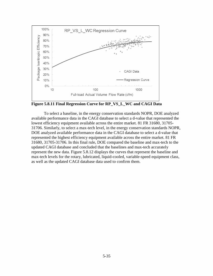
5-35

Figure 5.8.11 Final Regression Curve for RP_VS_L_WC and CAGI Data To select a baseline, in the energy conservation standards NOPR, DOE analyzed available performance data in the CAGI database to select a d-value that represented the lowest efficiency equipment available across the entire market. 81 FR 31680, 31705-31706. Similarly, to select a max-tech level, in the energy conservation standards NOPR, DOE analyzed available performance data in the CAGI database to select a d-value that represented the highest efficiency equipment available across the entire market. 81 FR 31680, 31705-31706. In this final rule, DOE compared the baseline and max-tech to the updated CAGI database and concluded that the baselines and max-tech accurately represent the new data. Figure 5.8.12 displays the curves that represent the baseline and max-tech levels for the rotary, lubricated, liquid-cooled, variable-speed equipment class, as well as the updated CAGI database data used to confirm them.

5-36

Figure 5.8.12 RP_VS_L_WC Baseline and Max-Tech Efficiency levels were set to span from baseline to max-tech and are represented by the d-values in Table 5.8.8, and visualized in Figure 5.8.13.

Figure 5.8.13 RP_VS_L_WC Efficiency Levels

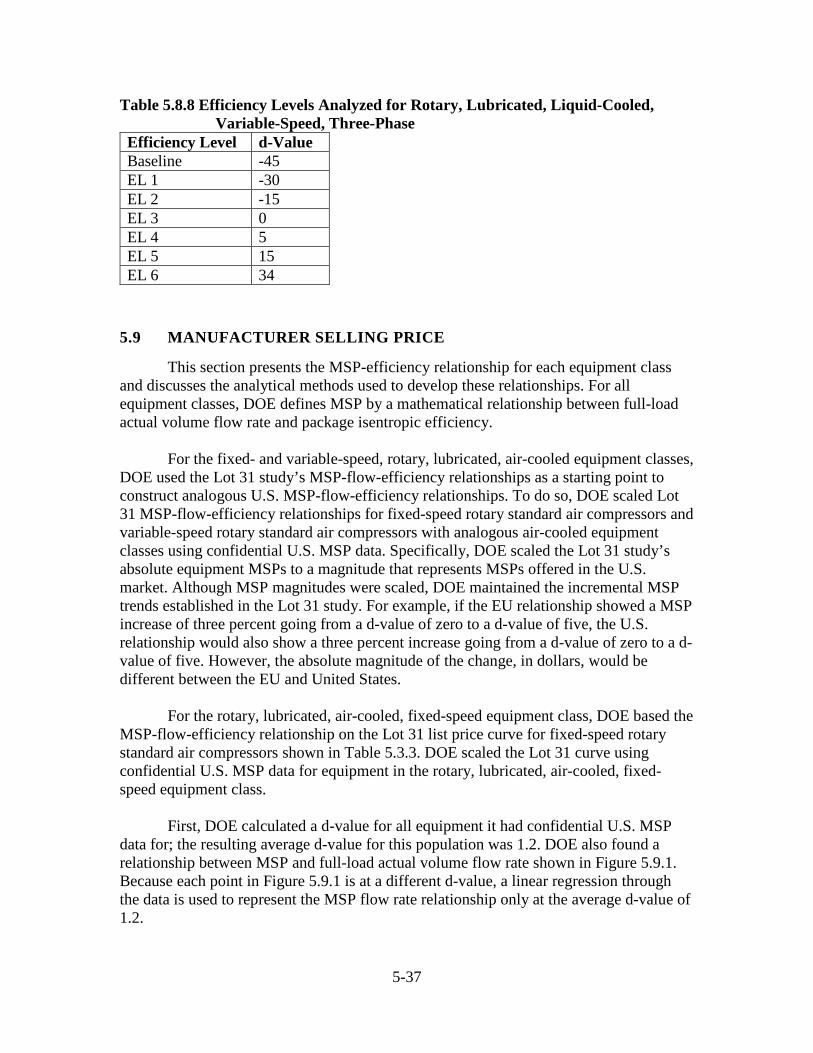
5-37

Table 5.8.8 Efficiency Levels Analyzed for Rotary, Lubricated, Liquid-Cooled, Variable-Speed, Three-Phase

Efficiency Level d-Value Baseline -45 EL 1 -30 EL 2 -15 EL 3 0 EL 4 5 EL 5 15 EL 6 34

5.9 MANUFACTURER SELLING PRICE

This section presents the MSP-efficiency relationship for each equipment class and discusses the analytical methods used to develop these relationships. For all equipment classes, DOE defines MSP by a mathematical relationship between full-load actual volume flow rate and package isentropic efficiency. For the fixed- and variable-speed, rotary, lubricated, air-cooled equipment classes, DOE used the Lot 31 study’s MSP-flow-efficiency relationships as a starting point to construct analogous U.S. MSP-flow-efficiency relationships. To do so, DOE scaled Lot 31 MSP-flow-efficiency relationships for fixed-speed rotary standard air compressors and variable-speed rotary standard air compressors with analogous air-cooled equipment classes using confidential U.S. MSP data. Specifically, DOE scaled the Lot 31 study’s absolute equipment MSPs to a magnitude that represents MSPs offered in the U.S. market. Although MSP magnitudes were scaled, DOE maintained the incremental MSP trends established in the Lot 31 study. For example, if the EU relationship showed a MSP increase of three percent going from a d-value of zero to a d-value of five, the U.S. relationship would also show a three percent increase going from a d-value of zero to a d-value of five. However, the absolute magnitude of the change, in dollars, would be different between the EU and United States. For the rotary, lubricated, air-cooled, fixed-speed equipment class, DOE based the MSP-flow-efficiency relationship on the Lot 31 list price curve for fixed-speed rotary standard air compressors shown in Table 5.3.3. DOE scaled the Lot 31 curve using confidential U.S. MSP data for equipment in the rotary, lubricated, air-cooled, fixed-speed equipment class. First, DOE calculated a d-value for all equipment it had confidential U.S. MSP data for; the resulting average d-value for this population was 1.2. DOE also found a relationship between MSP and full-load actual volume flow rate shown in Figure 5.9.1. Because each point in Figure 5.9.1 is at a different d-value, a linear regression through the data is used to represent the MSP flow rate relationship only at the average d-value of 1.2.

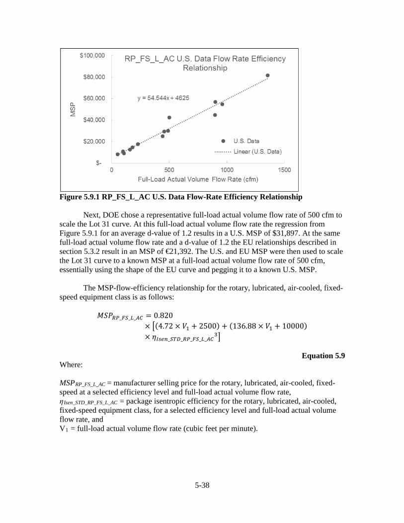
5-38

Figure 5.9.1 RP_FS_L_AC U.S. Data Flow-Rate Efficiency Relationship Next, DOE chose a representative full-load actual volume flow rate of 500 cfm to scale the Lot 31 curve. At this full-load actual volume flow rate the regression from Figure 5.9.1 for an average d-value of 1.2 results in a U.S. MSP of $31,897. At the same full-load actual volume flow rate and a d-value of 1.2 the EU relationships described in section 5.3.2 result in an MSP of €21,392. The U.S. and EU MSP were then used to scale the Lot 31 curve to a known MSP at a full-load actual volume flow rate of 500 cfm, essentially using the shape of the EU curve and pegging it to a known U.S. MSP. The MSP-flow-efficiency relationship for the rotary, lubricated, air-cooled, fixed-speed equipment class is as follows:

𝑀𝑀𝑀𝑀𝑃𝑃𝑅𝑅𝑅𝑅_𝐹𝐹𝐹𝐹_𝐿𝐿_𝐴𝐴𝐴𝐴 = 0.820× �(4.72 × 𝑉𝑉1 + 2500) + (136.88 × 𝑉𝑉1 + 10000)× 𝜂𝜂𝐼𝐼𝐼𝐼𝐼𝐼𝐼𝐼_𝐹𝐹𝑆𝑆𝑆𝑆_𝑅𝑅𝑅𝑅_𝐹𝐹𝐹𝐹_𝐿𝐿_𝐴𝐴𝐴𝐴

3�

Equation 5.9 Where: MSPRP_FS_L_AC = manufacturer selling price for the rotary, lubricated, air-cooled, fixed-speed at a selected efficiency level and full-load actual volume flow rate, ηIsen_STD_RP_FS_L_AC = package isentropic efficiency for the rotary, lubricated, air-cooled, fixed-speed equipment class, for a selected efficiency level and full-load actual volume flow rate, and V1 = full-load actual volume flow rate (cubic feet per minute).

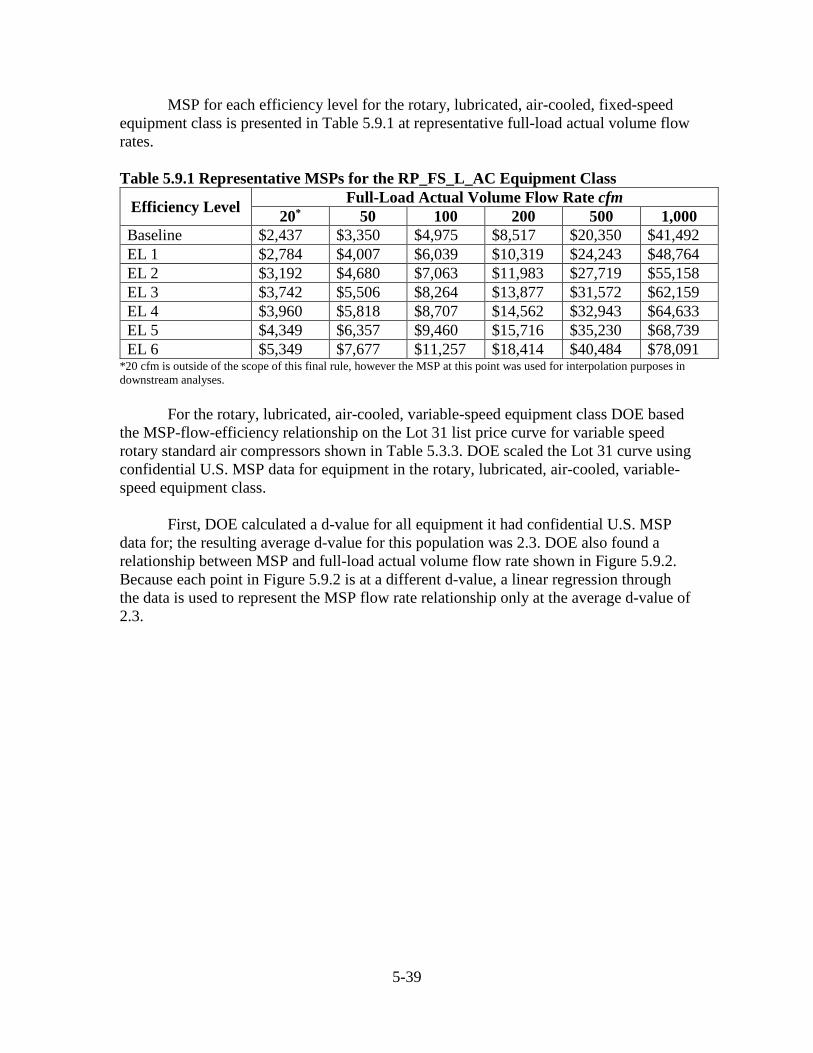
5-39

MSP for each efficiency level for the rotary, lubricated, air-cooled, fixed-speed equipment class is presented in Table 5.9.1 at representative full-load actual volume flow rates. Table 5.9.1 Representative MSPs for the RP_FS_L_AC Equipment Class

Efficiency Level Full-Load Actual Volume Flow Rate cfm 20* 50 100 200 500 1,000

Baseline $2,437 $3,350 $4,975 $8,517 $20,350 $41,492 EL 1 $2,784 $4,007 $6,039 $10,319 $24,243 $48,764 EL 2 $3,192 $4,680 $7,063 $11,983 $27,719 $55,158 EL 3 $3,742 $5,506 $8,264 $13,877 $31,572 $62,159 EL 4 $3,960 $5,818 $8,707 $14,562 $32,943 $64,633 EL 5 $4,349 $6,357 $9,460 $15,716 $35,230 $68,739 EL 6 $5,349 $7,677 $11,257 $18,414 $40,484 $78,091

*20 cfm is outside of the scope of this final rule, however the MSP at this point was used for interpolation purposes in downstream analyses. For the rotary, lubricated, air-cooled, variable-speed equipment class DOE based the MSP-flow-efficiency relationship on the Lot 31 list price curve for variable speed rotary standard air compressors shown in Table 5.3.3. DOE scaled the Lot 31 curve using confidential U.S. MSP data for equipment in the rotary, lubricated, air-cooled, variable-speed equipment class. First, DOE calculated a d-value for all equipment it had confidential U.S. MSP data for; the resulting average d-value for this population was 2.3. DOE also found a relationship between MSP and full-load actual volume flow rate shown in Figure 5.9.2. Because each point in Figure 5.9.2 is at a different d-value, a linear regression through the data is used to represent the MSP flow rate relationship only at the average d-value of 2.3.

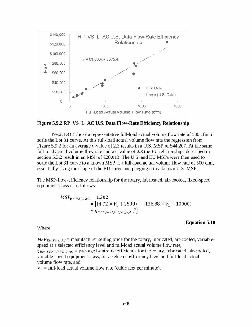
5-40

Figure 5.9.2 RP_VS_L_AC U.S. Data Flow-Rate Efficiency Relationship Next, DOE chose a representative full-load actual volume flow rate of 500 cfm to scale the Lot 31 curve. At this full-load actual volume flow rate the regression from Figure 5.9.2 for an average d-value of 2.3 results in a U.S. MSP of $44,207. At the same full-load actual volume flow rate and a d-value of 2.3 the EU relationships described in section 5.3.2 result in an MSP of €28,013. The U.S. and EU MSPs were then used to scale the Lot 31 curve to a known MSP at a full-load actual volume flow rate of 500 cfm, essentially using the shape of the EU curve and pegging it to a known U.S. MSP. The MSP-flow-efficiency relationship for the rotary, lubricated, air-cooled, fixed-speed equipment class is as follows:

𝑀𝑀𝑀𝑀𝑃𝑃RP_VS_L_AC = 1.302× �(4.72 × 𝑉𝑉1 + 2500) + (136.88 × 𝑉𝑉1 + 10000)× 𝜂𝜂𝐼𝐼𝐼𝐼𝐼𝐼𝐼𝐼_𝐹𝐹𝑆𝑆𝑆𝑆_RP_VS_L_AC

3�

Equation 5.10 Where: MSPRP_VS_L_AC = manufacturer selling price for the rotary, lubricated, air-cooled, variable-speed at a selected efficiency level and full-load actual volume flow rate, ηIsen_STD_RP_VS_L_AC = package isentropic efficiency for the rotary, lubricated, air-cooled, variable-speed equipment class, for a selected efficiency level and full-load actual volume flow rate, and V1 = full-load actual volume flow rate (cubic feet per minute).

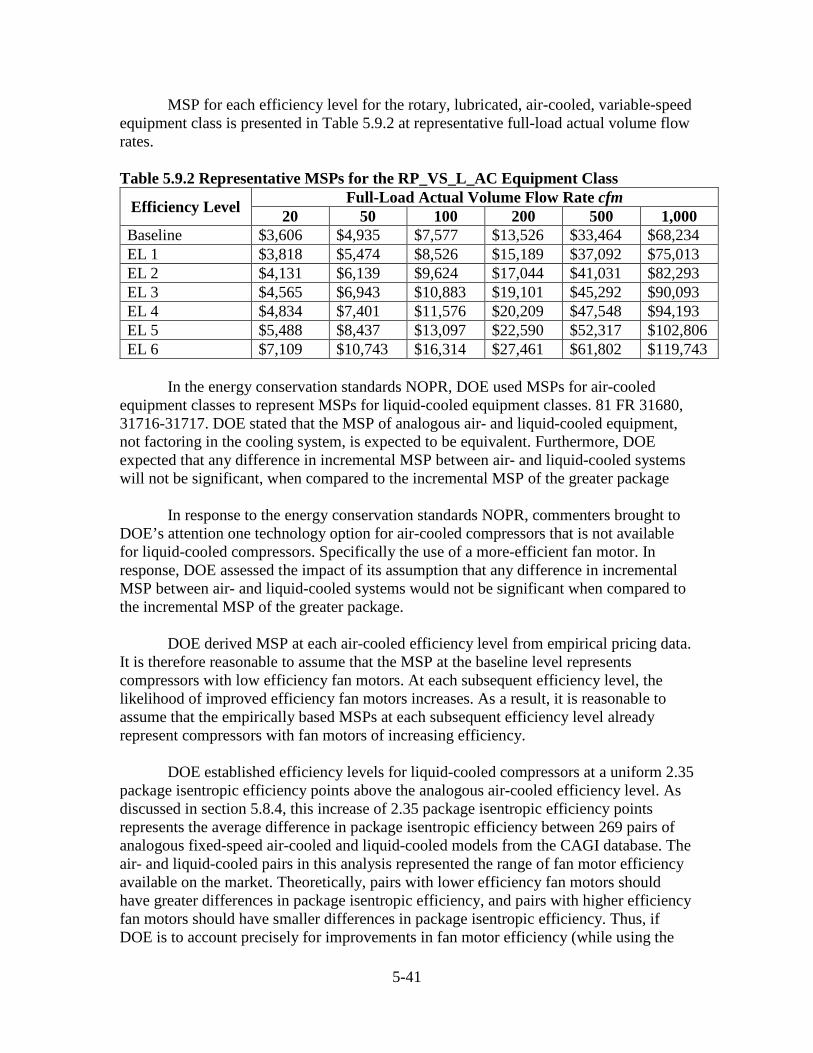
5-41

MSP for each efficiency level for the rotary, lubricated, air-cooled, variable-speed equipment class is presented in Table 5.9.2 at representative full-load actual volume flow rates. Table 5.9.2 Representative MSPs for the RP_VS_L_AC Equipment Class

Efficiency Level Full-Load Actual Volume Flow Rate cfm 20 50 100 200 500 1,000

Baseline $3,606 $4,935 $7,577 $13,526 $33,464 $68,234 EL 1 $3,818 $5,474 $8,526 $15,189 $37,092 $75,013 EL 2 $4,131 $6,139 $9,624 $17,044 $41,031 $82,293 EL 3 $4,565 $6,943 $10,883 $19,101 $45,292 $90,093 EL 4 $4,834 $7,401 $11,576 $20,209 $47,548 $94,193 EL 5 $5,488 $8,437 $13,097 $22,590 $52,317 $102,806 EL 6 $7,109 $10,743 $16,314 $27,461 $61,802 $119,743

In the energy conservation standards NOPR, DOE used MSPs for air-cooled equipment classes to represent MSPs for liquid-cooled equipment classes. 81 FR 31680, 31716-31717. DOE stated that the MSP of analogous air- and liquid-cooled equipment, not factoring in the cooling system, is expected to be equivalent. Furthermore, DOE expected that any difference in incremental MSP between air- and liquid-cooled systems will not be significant, when compared to the incremental MSP of the greater package In response to the energy conservation standards NOPR, commenters brought to DOE’s attention one technology option for air-cooled compressors that is not available for liquid-cooled compressors. Specifically the use of a more-efficient fan motor. In response, DOE assessed the impact of its assumption that any difference in incremental MSP between air- and liquid-cooled systems would not be significant when compared to the incremental MSP of the greater package. DOE derived MSP at each air-cooled efficiency level from empirical pricing data. It is therefore reasonable to assume that the MSP at the baseline level represents compressors with low efficiency fan motors. At each subsequent efficiency level, the likelihood of improved efficiency fan motors increases. As a result, it is reasonable to assume that the empirically based MSPs at each subsequent efficiency level already represent compressors with fan motors of increasing efficiency. DOE established efficiency levels for liquid-cooled compressors at a uniform 2.35 package isentropic efficiency points above the analogous air-cooled efficiency level. As discussed in section 5.8.4, this increase of 2.35 package isentropic efficiency points represents the average difference in package isentropic efficiency between 269 pairs of analogous fixed-speed air-cooled and liquid-cooled models from the CAGI database. The air- and liquid-cooled pairs in this analysis represented the range of fan motor efficiency available on the market. Theoretically, pairs with lower efficiency fan motors should have greater differences in package isentropic efficiency, and pairs with higher efficiency fan motors should have smaller differences in package isentropic efficiency. Thus, if DOE is to account precisely for improvements in fan motor efficiency (while using the

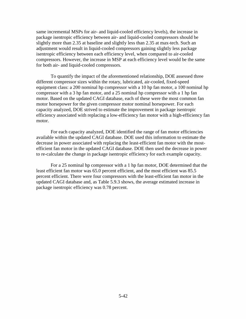
5-42

same incremental MSPs for air- and liquid-cooled efficiency levels), the increase in package isentropic efficiency between air- and liquid-cooled compressors should be slightly more than 2.35 at baseline and slightly less than 2.35 at max-tech. Such an adjustment would result in liquid-cooled compressors gaining slightly less package isentropic efficiency between each efficiency level, when compared to air-cooled compressors. However, the increase in MSP at each efficiency level would be the same for both air- and liquid-cooled compressors. To quantify the impact of the aforementioned relationship, DOE assessed three different compressor sizes within the rotary, lubricated, air-cooled, fixed-speed equipment class: a 200 nominal hp compressor with a 10 hp fan motor, a 100 nominal hp compressor with a 3 hp fan motor, and a 25 nominal hp compressor with a 1 hp fan motor. Based on the updated CAGI database, each of these were the most common fan motor horsepower for the given compressor motor nominal horsepower. For each capacity analyzed, DOE strived to estimate the improvement in package isentropic efficiency associated with replacing a low-efficiency fan motor with a high-efficiency fan motor. For each capacity analyzed, DOE identified the range of fan motor efficiencies available within the updated CAGI database. DOE used this information to estimate the decrease in power associated with replacing the least-efficient fan motor with the most-efficient fan motor in the updated CAGI database. DOE then used the decrease in power to re-calculate the change in package isentropic efficiency for each example capacity. For a 25 nominal hp compressor with a 1 hp fan motor, DOE determined that the least efficient fan motor was 65.0 percent efficient, and the most efficient was 85.5 percent efficient. There were four compressors with the least-efficient fan motor in the updated CAGI database and, as Table 5.9.3 shows, the average estimated increase in package isentropic efficiency was 0.78 percent.

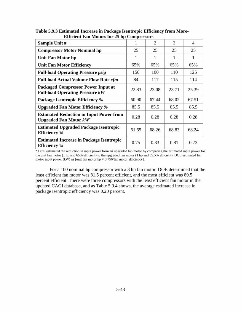
5-43

Table 5.9.3 Estimated Increase in Package Isentropic Efficiency from More-Efficient Fan Motors for 25 hp Compressors

Sample Unit # 1 2 3 4 Compressor Motor Nominal hp 25 25 25 25 Unit Fan Motor hp 1 1 1 1 Unit Fan Motor Efficiency 65% 65% 65% 65% Full-load Operating Pressure psig 150 100 110 125 Full-load Actual Volume Flow Rate cfm 84 117 115 114 Packaged Compressor Power Input at Full-load Operating Pressure kW 22.83 23.08 23.71 25.39

Package Isentropic Efficiency % 60.90 67.44 68.02 67.51 Upgraded Fan Motor Efficiency % 85.5 85.5 85.5 85.5 Estimated Reduction in Input Power from Upgraded Fan Motor kW* 0.28 0.28 0.28 0.28

Estimated Upgraded Package Isentropic Efficiency % 61.65 68.26 68.83 68.24

Estimated Increase in Package Isentropic Efficiency % 0.75 0.83 0.81 0.73

* DOE estimated the reduction in input power from an upgraded fan motor by comparing the estimated input power for the unit fan motor (1 hp and 65% efficient) to the upgraded fan motor (1 hp and 85.5% efficient). DOE estimated fan motor input power (kW) as [unit fan motor hp × 0.756/fan motor efficiency]. For a 100 nominal hp compressor with a 3 hp fan motor, DOE determined that the least efficient fan motor was 81.5 percent efficient, and the most efficient was 89.5 percent efficient. There were three compressors with the least efficient fan motor in the updated CAGI database, and as Table 5.9.4 shows, the average estimated increase in package isentropic efficiency was 0.20 percent.

5-44

Table 5.9.4 Estimated Increase in Package Isentropic Efficiency from More-efficient Fan Motors for 100 hp Compressors

Sample Unit # 1 2 3 Compressor Motor Nominal hp 100 100 100 Unit Fan Motor hp 3 3 3 Unit Fan Motor Efficiency % 81.5 81.5 81.5 Full-load Operating Pressure psig 125 100 110 Full-load Actual Volume Flow Rate cfm 436 495 495 Packaged Compressor Power Input at Full-load Operating Pressure kW 90.4 89 90.7

Package Isentropic Efficiency % 72.51 74.00 76.55 Upgraded Fan Motor Efficiency % 89.5 89.5 89.5 Estimated Reduction in Input Power from Upgraded Fan Motor kW* 0.25 0.25 0.25

Estimated Upgraded Package Isentropic Efficiency % 72.70 74.21 76.76

Estimated Increase in Package Isentropic Efficiency % 0.20 0.20 0.21

* DOE estimated the reduction in input power from an upgraded fan motor by comparing the estimated input power for the unit fan motor (3 hp and 81.5% efficient) to the upgraded fan motor (3 hp and 89.5% efficient). DOE estimated fan motor input power (kW) as [unit fan motor hp × 0.756/fan motor efficiency]. For a 200 nominal hp compressor with a 10 hp fan motor, DOE determined that the least efficient fan motor was 88.5 percent efficient, and the most efficient was 90.2 percent efficient. There were three compressors with the least efficient fan motor in the updated CAGI database, and as Table 5.9.5 shows, the average estimated increase in package isentropic efficiency was 0.18 percent.

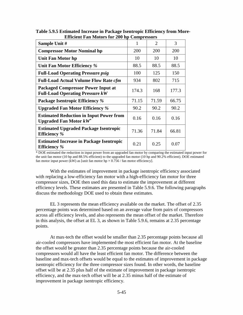
5-45

Table 5.9.5 Estimated Increase in Package Isentropic Efficiency from More-Efficient Fan Motors for 200 hp Compressors

Sample Unit # 1 2 3 Compressor Motor Nominal hp 200 200 200 Unit Fan Motor hp 10 10 10 Unit Fan Motor Efficiency % 88.5 88.5 88.5 Full-Load Operating Pressure psig 100 125 150 Full-Load Actual Volume Flow Rate cfm 934 802 715 Packaged Compressor Power Input at Full-Load Operating Pressure kW 174.3 168 177.3

Package Isentropic Efficiency % 71.15 71.59 66.75 Upgraded Fan Motor Efficiency % 90.2 90.2 90.2 Estimated Reduction in Input Power from Upgraded Fan Motor kW* 0.16 0.16 0.16

Estimated Upgraded Package Isentropic Efficiency % 71.36 71.84 66.81

Estimated Increase in Package Isentropic Efficiency % 0.21 0.25 0.07

* DOE estimated the reduction in input power from an upgraded fan motor by comparing the estimated input power for the unit fan motor (10 hp and 88.5% efficient) to the upgraded fan motor (10 hp and 90.2% efficient). DOE estimated fan motor input power (kW) as [unit fan motor hp × 0.756 / fan motor efficiency]. With the estimates of improvement in package isentropic efficiency associated with replacing a low-efficiency fan motor with a high-efficiency fan motor for three compressor sizes, DOE then used this data to estimate the improvement at different efficiency levels. These estimates are presented in Table 5.9.6. The following paragraphs discuss the methodology DOE used to obtain these estimates. EL 3 represents the mean efficiency available on the market. The offset of 2.35 percentage points was determined based on an average value from pairs of compressors across all efficiency levels, and also represents the mean offset of the market. Therefore in this analysis, the offset at EL 3, as shown in Table 5.9.6, remains at 2.35 percentage points. At max-tech the offset would be smaller than 2.35 percentage points because all air-cooled compressors have implemented the most efficient fan motor. At the baseline the offset would be greater than 2.35 percentage points because the air-cooled compressors would all have the least efficient fan motor. The difference between the baseline and max-tech offsets would be equal to the estimates of improvement in package isentropic efficiency for the three compressor sizes found. In other words, the baseline offset will be at 2.35 plus half of the estimate of improvement in package isentropic efficiency, and the max-tech offset will be at 2.35 minus half of the estimate of improvement in package isentropic efficiency.

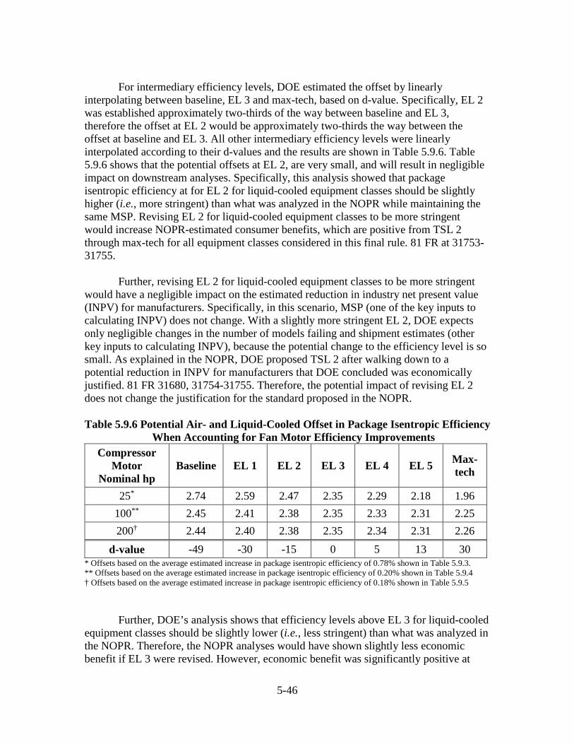
5-46

For intermediary efficiency levels, DOE estimated the offset by linearly interpolating between baseline, EL 3 and max-tech, based on d-value. Specifically, EL 2 was established approximately two-thirds of the way between baseline and EL 3, therefore the offset at EL 2 would be approximately two-thirds the way between the offset at baseline and EL 3. All other intermediary efficiency levels were linearly interpolated according to their d-values and the results are shown in Table 5.9.6. Table 5.9.6 shows that the potential offsets at EL 2, are very small, and will result in negligible impact on downstream analyses. Specifically, this analysis showed that package isentropic efficiency at for EL 2 for liquid-cooled equipment classes should be slightly higher (i.e., more stringent) than what was analyzed in the NOPR while maintaining the same MSP. Revising EL 2 for liquid-cooled equipment classes to be more stringent would increase NOPR-estimated consumer benefits, which are positive from TSL 2 through max-tech for all equipment classes considered in this final rule. 81 FR at 31753-31755. Further, revising EL 2 for liquid-cooled equipment classes to be more stringent would have a negligible impact on the estimated reduction in industry net present value (INPV) for manufacturers. Specifically, in this scenario, MSP (one of the key inputs to calculating INPV) does not change. With a slightly more stringent EL 2, DOE expects only negligible changes in the number of models failing and shipment estimates (other key inputs to calculating INPV), because the potential change to the efficiency level is so small. As explained in the NOPR, DOE proposed TSL 2 after walking down to a potential reduction in INPV for manufacturers that DOE concluded was economically justified. 81 FR 31680, 31754-31755. Therefore, the potential impact of revising EL 2 does not change the justification for the standard proposed in the NOPR. Table 5.9.6 Potential Air- and Liquid-Cooled Offset in Package Isentropic Efficiency

When Accounting for Fan Motor Efficiency Improvements Compressor

Motor Nominal hp

Baseline EL 1 EL 2 EL 3 EL 4 EL 5 Max-tech

25* 2.74 2.59 2.47 2.35 2.29 2.18 1.96 100** 2.45 2.41 2.38 2.35 2.33 2.31 2.25 200† 2.44 2.40 2.38 2.35 2.34 2.31 2.26

d-value -49 -30 -15 0 5 13 30 * Offsets based on the average estimated increase in package isentropic efficiency of 0.78% shown in Table 5.9.3. ** Offsets based on the average estimated increase in package isentropic efficiency of 0.20% shown in Table 5.9.4 † Offsets based on the average estimated increase in package isentropic efficiency of 0.18% shown in Table 5.9.5 Further, DOE’s analysis shows that efficiency levels above EL 3 for liquid-cooled equipment classes should be slightly lower (i.e., less stringent) than what was analyzed in the NOPR. Therefore, the NOPR analyses would have shown slightly less economic benefit if EL 3 were revised. However, economic benefit was significantly positive at

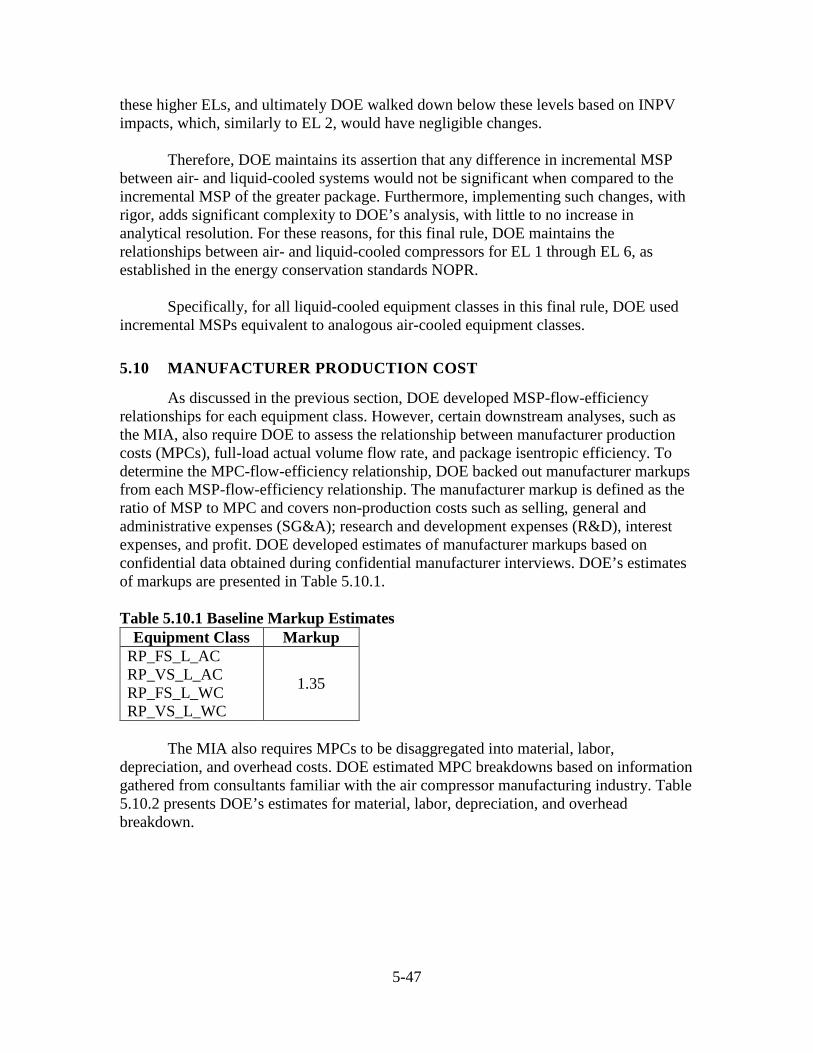
5-47

these higher ELs, and ultimately DOE walked down below these levels based on INPV impacts, which, similarly to EL 2, would have negligible changes. Therefore, DOE maintains its assertion that any difference in incremental MSP between air- and liquid-cooled systems would not be significant when compared to the incremental MSP of the greater package. Furthermore, implementing such changes, with rigor, adds significant complexity to DOE’s analysis, with little to no increase in analytical resolution. For these reasons, for this final rule, DOE maintains the relationships between air- and liquid-cooled compressors for EL 1 through EL 6, as established in the energy conservation standards NOPR. Specifically, for all liquid-cooled equipment classes in this final rule, DOE used incremental MSPs equivalent to analogous air-cooled equipment classes.

5.10 MANUFACTURER PRODUCTION COST

As discussed in the previous section, DOE developed MSP-flow-efficiency relationships for each equipment class. However, certain downstream analyses, such as the MIA, also require DOE to assess the relationship between manufacturer production costs (MPCs), full-load actual volume flow rate, and package isentropic efficiency. To determine the MPC-flow-efficiency relationship, DOE backed out manufacturer markups from each MSP-flow-efficiency relationship. The manufacturer markup is defined as the ratio of MSP to MPC and covers non-production costs such as selling, general and administrative expenses (SG&A); research and development expenses (R&D), interest expenses, and profit. DOE developed estimates of manufacturer markups based on confidential data obtained during confidential manufacturer interviews. DOE’s estimates of markups are presented in Table 5.10.1. Table 5.10.1 Baseline Markup Estimates

Equipment Class Markup RP_FS_L_AC RP_VS_L_AC RP_FS_L_WC RP_VS_L_WC

1.35

The MIA also requires MPCs to be disaggregated into material, labor, depreciation, and overhead costs. DOE estimated MPC breakdowns based on information gathered from consultants familiar with the air compressor manufacturing industry. Table 5.10.2 presents DOE’s estimates for material, labor, depreciation, and overhead breakdown.

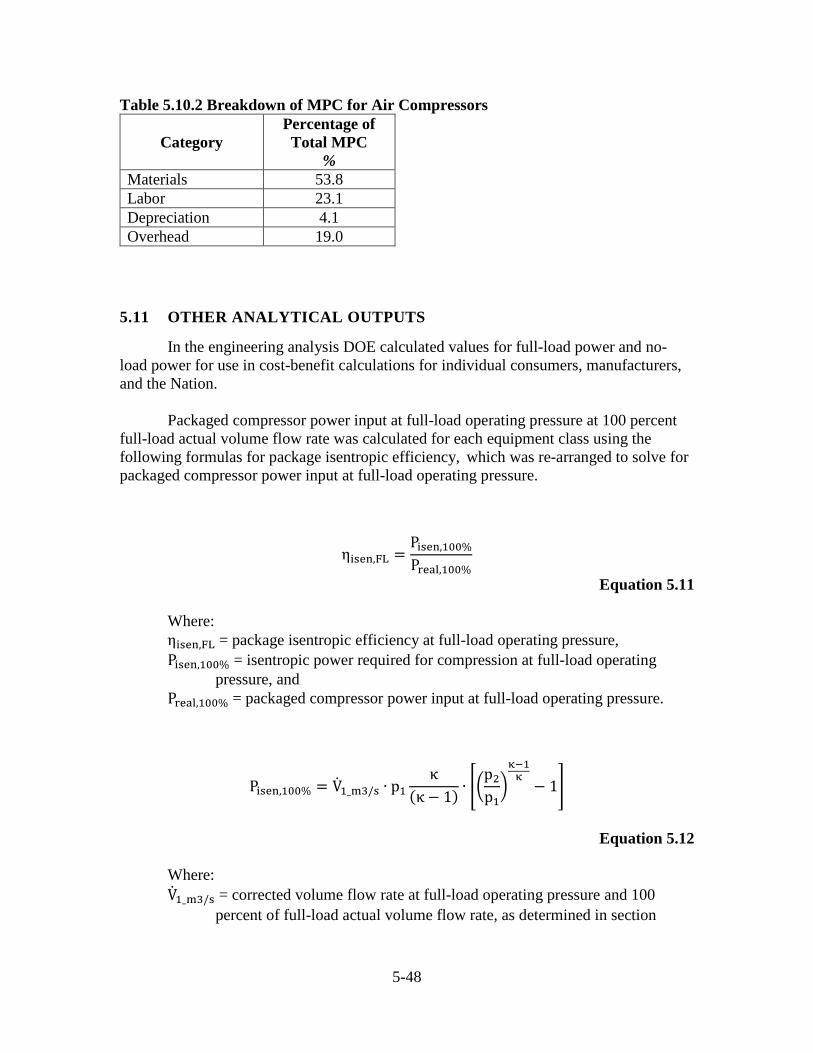
5-48

Table 5.10.2 Breakdown of MPC for Air Compressors

Category Percentage of Total MPC

% Materials 53.8 Labor 23.1 Depreciation 4.1 Overhead 19.0

5.11 OTHER ANALYTICAL OUTPUTS

In the engineering analysis DOE calculated values for full-load power and no-load power for use in cost-benefit calculations for individual consumers, manufacturers, and the Nation. Packaged compressor power input at full-load operating pressure at 100 percent full-load actual volume flow rate was calculated for each equipment class using the following formulas for package isentropic efficiency, which was re-arranged to solve for packaged compressor power input at full-load operating pressure.

ηisen,FL =Pisen,100%

Preal,100%

Equation 5.11

Where: ηisen,FL = package isentropic efficiency at full-load operating pressure, Pisen,100% = isentropic power required for compression at full-load operating

pressure, and Preal,100% = packaged compressor power input at full-load operating pressure.

Pisen,100% = V̇1_m3/s ∙ p1κ

(κ − 1) ∙ ��p2p1�κ−1κ− 1�

Equation 5.12

Where: V̇1_m3/s = corrected volume flow rate at full-load operating pressure and 100

percent of full-load actual volume flow rate, as determined in section

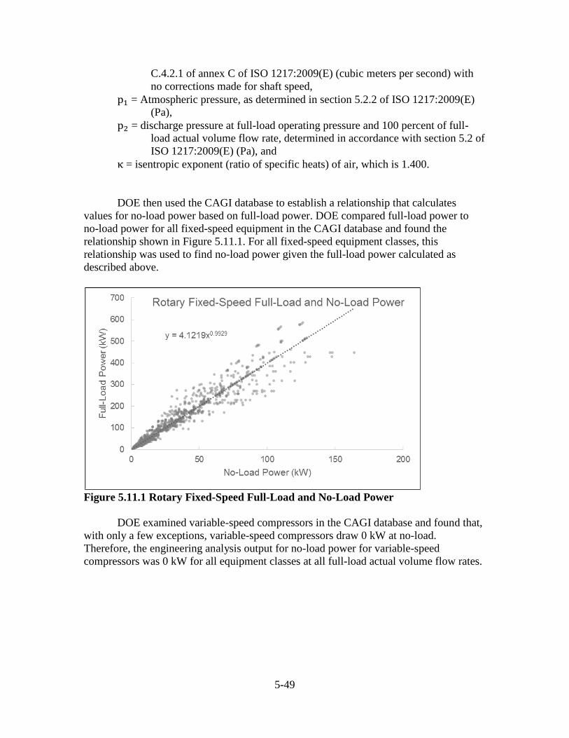
5-49

C.4.2.1 of annex C of ISO 1217:2009(E) (cubic meters per second) with no corrections made for shaft speed,

p1 = Atmospheric pressure, as determined in section 5.2.2 of ISO 1217:2009(E) (Pa),

p2 = discharge pressure at full-load operating pressure and 100 percent of full-load actual volume flow rate, determined in accordance with section 5.2 of ISO 1217:2009(E) (Pa), and

κ = isentropic exponent (ratio of specific heats) of air, which is 1.400. DOE then used the CAGI database to establish a relationship that calculates values for no-load power based on full-load power. DOE compared full-load power to no-load power for all fixed-speed equipment in the CAGI database and found the relationship shown in Figure 5.11.1. For all fixed-speed equipment classes, this relationship was used to find no-load power given the full-load power calculated as described above.

Figure 5.11.1 Rotary Fixed-Speed Full-Load and No-Load Power DOE examined variable-speed compressors in the CAGI database and found that, with only a few exceptions, variable-speed compressors draw 0 kW at no-load. Therefore, the engineering analysis output for no-load power for variable-speed compressors was 0 kW for all equipment classes at all full-load actual volume flow rates.

6-i

CHAPTER 6. MARKUPS ANALYSIS

TABLE OF CONTENTS

6.1 INTRODUCTION ........................................................................................................... 6-1 6.1.1 Distribution Channels .......................................................................................... 6-1

6.2 MARKUP CALCULATION METHODOLOGY ........................................................... 6-2 6.2.1 Assumptions ......................................................................................................... 6-3

6.3 APPROACH FOR ORIGINAL EQUIPMENT MANUFACTURER MARKUPS ........ 6-4 6.4 APPROACH FOR COMPRESSOR DISTRIBUTOR MARKUPS ................................ 6-5 6.5 CONTRACTOR OR INSTALLER MARKUP ............................................................... 6-8 6.6 SALES TAXES ............................................................................................................... 6-8 6.7 OVERALL MARKUPS................................................................................................... 6-8 REFERENCES .......................................................................................................................... 6-11

LIST OF TABLES

Table 6.1.1 Distribution Channels .................................................................................... 6-1 Table 6.1.2 Distribution Channels by Compressor Power Rating and Compression

Method ........................................................................................................... 6-2 Table 6.4.1 U.S. Census Business and Industry Annual Wholesale Trade Survey

Data Used to Calculate Distributor Markups ................................................. 6-7 Table 6.6.1 Average Sales Tax Rates by Census Division and Large State ..................... 6-8 Table 6.7.1 Summary of Markups for Three Primary Distribution Channels for

Compressors ................................................................................................... 6-9

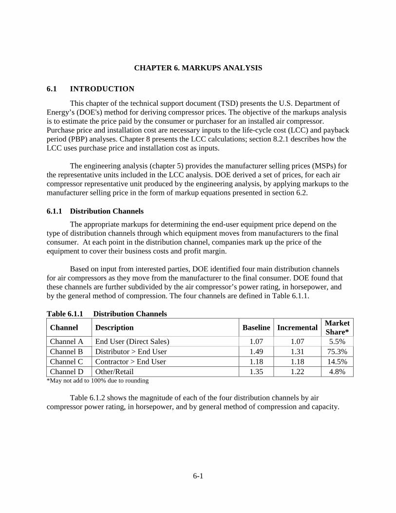
6-1

CHAPTER 6. MARKUPS ANALYSIS

6.1 INTRODUCTION

This chapter of the technical support document (TSD) presents the U.S. Department of Energy’s (DOE's) method for deriving compressor prices. The objective of the markups analysis is to estimate the price paid by the consumer or purchaser for an installed air compressor. Purchase price and installation cost are necessary inputs to the life-cycle cost (LCC) and payback period (PBP) analyses. Chapter 8 presents the LCC calculations; section 8.2.1 describes how the LCC uses purchase price and installation cost as inputs.

The engineering analysis (chapter 5) provides the manufacturer selling prices (MSPs) for

the representative units included in the LCC analysis. DOE derived a set of prices, for each air compressor representative unit produced by the engineering analysis, by applying markups to the manufacturer selling price in the form of markup equations presented in section 6.2.

6.1.1 Distribution Channels

The appropriate markups for determining the end-user equipment price depend on the type of distribution channels through which equipment moves from manufacturers to the final consumer. At each point in the distribution channel, companies mark up the price of the equipment to cover their business costs and profit margin.

Based on input from interested parties, DOE identified four main distribution channels

for air compressors as they move from the manufacturer to the final consumer. DOE found that these channels are further subdivided by the air compressor’s power rating, in horsepower, and by the general method of compression. The four channels are defined in Table 6.1.1.

Table 6.1.1 Distribution Channels

Channel Description Baseline Incremental Market Share*

Channel A End User (Direct Sales) 1.07 1.07 5.5% Channel B Distributor > End User 1.49 1.31 75.3% Channel C Contractor > End User 1.18 1.18 14.5% Channel D Other/Retail 1.35 1.22 4.8%

*May not add to 100% due to rounding Table 6.1.2 shows the magnitude of each of the four distribution channels by air

compressor power rating, in horsepower, and by general method of compression and capacity.

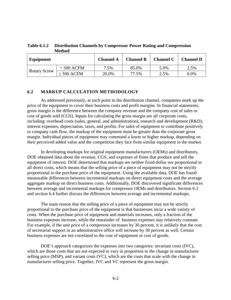
6-2

Table 6.1.2 Distribution Channels by Compressor Power Rating and Compression Method

Equipment Channel A Channel B Channel C Channel D

Rotary Screw < 500 ACFM 7.5% 85.0% 5.0% 2.5% ≥ 500 ACFM 20.0% 77.5% 2.5% 0.0%

6.2 MARKUP CALCULATION METHODOLOGY

As addressed previously, at each point in the distribution channel, companies mark up the price of the equipment to cover their business costs and profit margins. In financial statements, gross margin is the difference between the company revenue and the company cost of sales or cost of goods sold (CGS). Inputs for calculating the gross margin are all corporate costs, including: overhead costs (sales, general, and administration), research and development (R&D), interest expenses, depreciation, taxes, and profits. For sales of equipment to contribute positively to company cash flow, the markup of the equipment must be greater than the corporate gross margin. Individual pieces of equipment may command a lower or higher markup, depending on their perceived added value and the competition they face from similar equipment in the market.

In developing markups for original equipment manufacturers (OEMs) and distributors, DOE obtained data about the revenue, CGS, and expenses of firms that produce and sell the equipment of interest. DOE determined that markups are neither fixed-dollar nor proportional to all direct costs, which means that the selling price of a piece of equipment may not be strictly proportional to the purchase price of the equipment. Using the available data, DOE has found measurable differences between incremental markups on direct equipment costs and the average aggregate markup on direct business costs. Additionally, DOE discovered significant differences between average and incremental markups for compressor OEMs and distributors. Section 6.3 and section 6.4 further discuss the differences between average and incremental markups.

The main reason that the selling price of a piece of equipment may not be strictly

proportional to the purchase price of the equipment is that businesses incur a wide variety of costs. When the purchase price of equipment and materials increases, only a fraction of the business expenses increase, while the remainder of business expenses stay relatively constant. For example, if the unit price of a compressor increases by 30 percent, it is unlikely that the cost of secretarial support in an administrative office will increase by 30 percent as well. Certain business expenses are not correlated to the cost of equipment or cost of goods.

DOE’s approach categorizes the expenses into two categories: invariant costs (IVC),

which are those costs that are not expected to vary in proportion to the change in manufacturer selling price (MSP), and variant costs (VC), which are the costs that scale with the change in manufacturer selling price. Together, IVC and VC represent the gross margin.

6-3

For each step in equipment distribution, DOE estimated both a baseline markup and an incremental markup. For compressors, DOE understands that no increase in distribution labor is necessary for the distribution of more-efficient equipment, while the non-labor-scaling cost does increase with increasing equipment costs. This allowed DOE to estimate the incremental markup given a breakdown of distribution and manufacturing business expenses for a particular industry.

6.2.1 Assumptions

DOE derived the OEM and compressor distributor markups from three key assumptions about the costs associated with compressor-related industrial series. DOE used the financial data from the 2007 U.S. Economic Census’s Manufacturing Industry Series and 2012 Business and Industry Wholesale Trade Survey to determine OEM and compressor distributor markups, respectively.2,3 These income statements break down the components of all costs incurred by firms that assemble and distribute compressors. The key assumptions used to estimate markups using these financial data are:

1. The firm income statements faithfully represent the various average costs incurred by

firms designing, assembling, and distributing compressors. 2. These costs can be divided into two categories: (1) costs that vary in proportion to the

MSP of compressors (variant costs); and (2) costs that do not vary with the MSP of compressors (invariant costs).

3. Overall, OEM and distributor sales prices vary in proportion to OEM and distributor costs that are included in the balance sheets.

In support of the first assumption, the income statements itemize firm costs into a number

of expense categories, including CGS, operating labor and occupancy costs, and other operating costs and profit. Although OEMs and compressor distributors tend to handle multiple commodity lines, these data provide the most accurate indication that is available of the expenses associated with compressors.

In the following discussion, DOE assumes a division of costs between those that do not scale with the manufacturer price (labor and occupancy expenses), and those that do (operating expenses and profit). This division of costs led to the estimate of incremental markups addressed in the next section.

In support of the third assumption, the wholesaler industries are relatively competitive, and end-user demand for compressors is relatively inelastic—i.e., the demand is not expected to decrease significantly with a relatively small increase in price. Following standard economic theory, competitive firms facing inelastic demand either set prices in line with costs or quickly go out of business.1

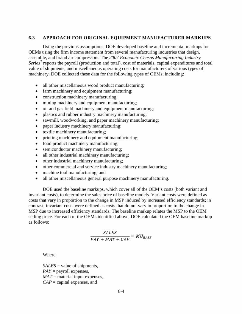
6-4

6.3 APPROACH FOR ORIGINAL EQUIPMENT MANUFACTURER MARKUPS

Using the previous assumptions, DOE developed baseline and incremental markups for OEMs using the firm income statement from several manufacturing industries that design, assemble, and brand air compressors. The 2007 Economic Census Manufacturing Industry Series2 reports the payroll (production and total), cost of materials, capital expenditures and total value of shipments, and miscellaneous operating costs for manufacturers of various types of machinery. DOE collected these data for the following types of OEMs, including:

• all other miscellaneous wood product manufacturing; • farm machinery and equipment manufacturing; • construction machinery manufacturing; • mining machinery and equipment manufacturing; • oil and gas field machinery and equipment manufacturing; • plastics and rubber industry machinery manufacturing; • sawmill, woodworking, and paper machinery manufacturing; • paper industry machinery manufacturing; • textile machinery manufacturing; • printing machinery and equipment manufacturing; • food product machinery manufacturing; • semiconductor machinery manufacturing; • all other industrial machinery manufacturing; • other industrial machinery manufacturing; • other commercial and service industry machinery manufacturing; • machine tool manufacturing; and • all other miscellaneous general purpose machinery manufacturing.

DOE used the baseline markups, which cover all of the OEM’s costs (both variant and

invariant costs), to determine the sales price of baseline models. Variant costs were defined as costs that vary in proportion to the change in MSP induced by increased efficiency standards; in contrast, invariant costs were defined as costs that do not vary in proportion to the change in MSP due to increased efficiency standards. The baseline markup relates the MSP to the OEM selling price. For each of the OEMs identified above, DOE calculated the OEM baseline markup as follows:

𝑆𝑆𝑆𝑆𝑆𝑆𝑆𝑆𝑆𝑆

𝑃𝑃𝑆𝑆𝑃𝑃 + 𝑀𝑀𝑆𝑆𝑀𝑀 + 𝐶𝐶𝑆𝑆𝑃𝑃= 𝑀𝑀𝑈𝑈𝐵𝐵𝐵𝐵𝐵𝐵𝐵𝐵

Where: SALES = value of shipments, PAY = payroll expenses, MAT = material input expenses, CAP = capital expenses, and

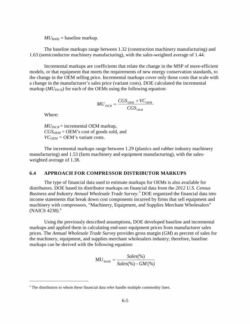
6-5

MUBASE = baseline markup. The baseline markups range between 1.32 (construction machinery manufacturing) and

1.63 (semiconductor machinery manufacturing), with the sales-weighted average of 1.44. Incremental markups are coefficients that relate the change in the MSP of more-efficient

models, or that equipment that meets the requirements of new energy conservation standards, to the change in the OEM selling price. Incremental markups cover only those costs that scale with a change in the manufacturer’s sales price (variant costs). DOE calculated the incremental markup (MUINCR) for each of the OEMs using the following equation:

OEM

OEMOEMINCR CGS

VCCGSMU

+=

Where: MUINCR = incremental OEM markup, CGSOEM = OEM’s cost of goods sold, and VCOEM = OEM’s variant costs.

The incremental markups range between 1.29 (plastics and rubber industry machinery

manufacturing) and 1.53 (farm machinery and equipment manufacturing), with the sales-weighted average of 1.38.

6.4 APPROACH FOR COMPRESSOR DISTRIBUTOR MARKUPS

The type of financial data used to estimate markups for OEMs is also available for distributors. DOE based its distributor markups on financial data from the 2012 U.S. Census Business and Industry Annual Wholesale Trade Survey.3 DOE organized the financial data into income statements that break down cost components incurred by firms that sell equipment and machinery with compressors, “Machinery, Equipment, and Supplies Merchant Wholesalers” (NAICS 4238).a

Using the previously described assumptions, DOE developed baseline and incremental

markups and applied them in calculating end-user equipment prices from manufacturer sales prices. The Annual Wholesale Trade Survey provides gross margin (GM) as percent of sales for the machinery, equipment, and supplies merchant wholesalers industry; therefore, baseline markups can be derived with the following equation:

(%)(%)(%)MUBASE GMSales

Sales−

=

a The distributors to whom these financial data refer handle multiple commodity lines.

6-6

DOE used financial data from the Annual Wholesale Trade Survey for the categories “Machinery, Equipment, and Supplies Merchant Wholesalers” to calculate incremental markups used by wholesalers of compressors. Incremental markups are coefficients that relate the change in the MSP of higher efficiency models to the change in the wholesaler selling price. Hence, incremental markups cover only those costs that scale with a change in the manufacturer’s sales price (i.e., variant costs). DOE considers higher efficiency models to be equipment sold under market conditions with new efficiency standards. It calculated the incremental markup (MUINCR) for distributors using the following equation:

RDISTRIBUTO

RDISTRIBUTORDISTRIBUTOINCR CGS

VCCGSMU +=

Where: MUINCR = incremental wholesaler markup, CGSDISTRIBUTOR = distributor’s cost of goods sold, and VCDISTRIBUTOR =distributor’s variant costs.

Table 6.4.1 shows the data from the Annual Wholesale Trade Survey and the markups

DOE estimated using the procedures described previously.

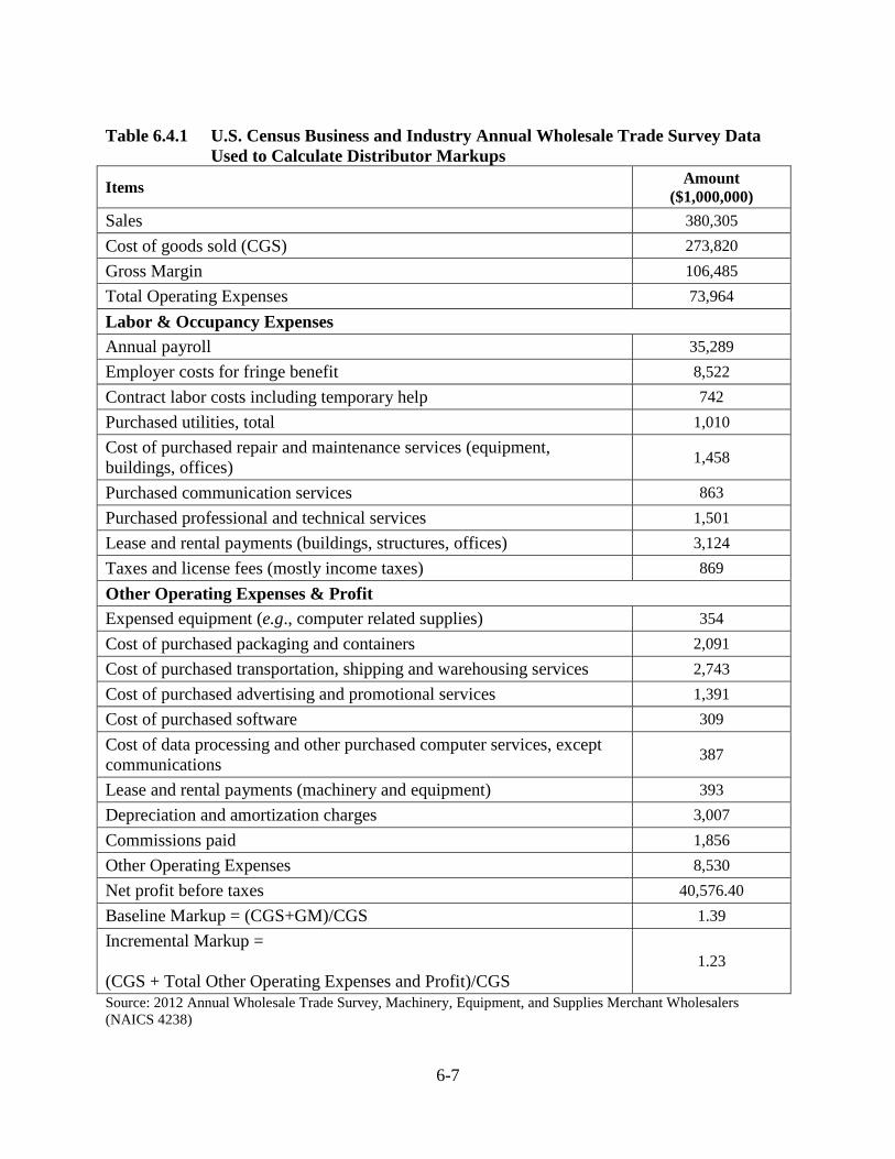
6-7

Table 6.4.1 U.S. Census Business and Industry Annual Wholesale Trade Survey Data Used to Calculate Distributor Markups

Items Amount ($1,000,000)

Sales 380,305 Cost of goods sold (CGS) 273,820 Gross Margin 106,485 Total Operating Expenses 73,964 Labor & Occupancy Expenses Annual payroll 35,289 Employer costs for fringe benefit 8,522 Contract labor costs including temporary help 742 Purchased utilities, total 1,010 Cost of purchased repair and maintenance services (equipment, buildings, offices) 1,458

Purchased communication services 863 Purchased professional and technical services 1,501 Lease and rental payments (buildings, structures, offices) 3,124 Taxes and license fees (mostly income taxes) 869 Other Operating Expenses & Profit Expensed equipment (e.g., computer related supplies) 354 Cost of purchased packaging and containers 2,091 Cost of purchased transportation, shipping and warehousing services 2,743 Cost of purchased advertising and promotional services 1,391 Cost of purchased software 309 Cost of data processing and other purchased computer services, except communications 387

Lease and rental payments (machinery and equipment) 393 Depreciation and amortization charges 3,007 Commissions paid 1,856 Other Operating Expenses 8,530 Net profit before taxes 40,576.40 Baseline Markup = (CGS+GM)/CGS 1.39 Incremental Markup = (CGS + Total Other Operating Expenses and Profit)/CGS

1.23

Source: 2012 Annual Wholesale Trade Survey, Machinery, Equipment, and Supplies Merchant Wholesalers (NAICS 4238)

6-8

6.5 CONTRACTOR OR INSTALLER MARKUP

DOE used information from RSMeans Electrical Cost Data4 to estimate markups used by contractors in the installation of equipment with compressors. RSMeans Electrical Cost Data estimates material expense markups for electrical contractors as 10 percent, leading to a markup factor of 1.10. DOE recognizes that contractors are not used in all installations, as some firms have in-house technicians who would install equipment or replace a compressor. However, DOE has no information on the extent to which this occurs, so it applied a markup of 1.10 in all cases.

6.6 SALES TAXES

The sales tax represents state and local sales taxes that are applied to the end-user equipment price. The sales tax is a multiplicative factor that increases the end-user equipment price.

DOE derived state and local taxes from data provided by the Sales Tax Clearinghouse.5

These data represent weighted averages that include county and city rates. DOE then derived population-weighted average tax values for each Census division and large state, as shown in Table 6.6.1 below. This provides a national average tax rate of 7.11 percent, which DOE used for each distribution channel.

Table 6.6.1 Average Sales Tax Rates by Census Division and Large State Census Division/State Population (2013) Tax Rate (2014) New England 14,618,806 5.69% Middle Atlantic 21,673,140 6.63% East North Central 46,662,180 6.91% West North Central 20,885,710 7.09% South Atlantic 42,230,787 6.07% East South Central 18,716,202 8.02% West South Central 11,435,411 8.65% Mountain 22,881,245 6.44% Pacific 13,040,657 5.30% New York 19,651,127 8.40% California 38,332,521 8.45% Texas 26,448,193 7.90% Florida 19,552,860 6.65%

Population Weighted Average 7.11%

6.7 OVERALL MARKUPS

The overall markup for each distribution channel is the product of the relevant markups, as well as the sales tax. DOE used the overall baseline markup to estimate the end-user equipment price of baseline models, given the MSP of the baseline models. As stated previously,

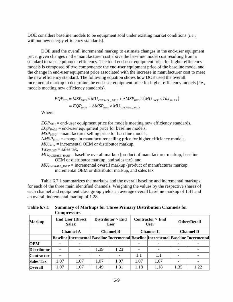
6-9

DOE considers baseline models to be equipment sold under existing market conditions (i.e., without new energy efficiency standards).

DOE used the overall incremental markup to estimate changes in the end-user equipment

price, given changes in the manufacturer cost above the baseline model cost resulting from a standard to raise equipment efficiency. The total end-user equipment price for higher efficiency models is composed of two components: the end-user equipment price of the baseline model and the change in end-user equipment price associated with the increase in manufacturer cost to meet the new efficiency standard. The following equation shows how DOE used the overall incremental markup to determine the end-user equipment price for higher efficiency models (i.e., models meeting new efficiency standards).

( )INCROVERALLMFGBASE

SALESINCRMFGBASEOVERALLMFGSTD

MUMSPEQPTaxMUMSPMUMSPEQP

_

_

×D+=

××D+×=

Where: EQPSTD = end-user equipment price for models meeting new efficiency standards, EQPBASE = end-user equipment price for baseline models, MSPMFG = manufacturer selling price for baseline models, ΔMSPMFG = change in manufacturer selling price for higher efficiency models, MUINCR = incremental OEM or distributor markup, TaxSALES = sales tax, MUOVERALL_BASE = baseline overall markup (product of manufacturer markup, baseline

OEM or distributor markup, and sales tax), and MUOVERALL_INCR = incremental overall markup (product of manufacturer markup,

incremental OEM or distributor markup, and sales tax

Table 6.7.1 summarizes the markups and the overall baseline and incremental markups for each of the three main identified channels. Weighting the values by the respective shares of each channel and equipment class group yields an average overall baseline markup of 1.41 and an overall incremental markup of 1.28. Table 6.7.1 Summary of Markups for Three Primary Distribution Channels for

Compressors

Markup End User (Direct Sales)

Distributor > End User

Contractor > End User Other/Retail

Channel A Channel B Channel C Channel D Baseline Incremental Baseline Incremental Baseline Incremental Baseline Incremental OEM - - - - - - Distributor - - 1.39 1.23 - - - - Contractor - - - - 1.1 1.1 - - Sales Tax 1.07 1.07 1.07 1.07 1.07 1.07 - - Overall 1.07 1.07 1.49 1.31 1.18 1.18 1.35 1.22

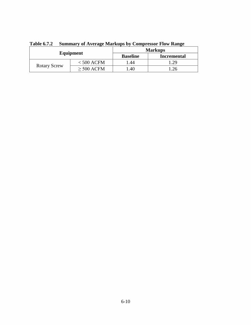
6-10

Table 6.7.2 Summary of Average Markups by Compressor Flow Range

Equipment Markups Baseline Incremental

Rotary Screw < 500 ACFM 1.44 1.29 ≥ 500 ACFM 1.40 1.26

6-11

REFERENCES

1 Pindyck, R.S. and D.L. Rubinfeld. (2000), Microeconomics, 5th ed., New Jersey: Prentice Hall.

2 U.S. Census Bureau (2007). Economic Census Manufacturing Industry Series (NAICS 33 Series) http://www.census.gov/manufacturing/asm

3 U.S. Census Bureau (2012). Annual Wholesale Trade Survey, Machinery, Equipment, and Supplies Merchant Wholesalers (NAICS 4238). http://www.census.gov/wholesale/index.html

4 RSMeans Construction Publishers & Consultants. (2013), Electrical Cost Data, 36th Annual Edition. 2013. ed. J.H. Chiang, Kingston, MA.

5 Sales Tax Clearinghouse, Inc. (last accessed on January 10, 2014), State sales tax rates along with combined average city and county rates, http://thestc.com/STrates.stm

7-i

CHAPTER 7. ENERGY USE ANALYSIS

TABLE OF CONTENTS

7.1 INTRODUCTION ........................................................................................................... 7-1 7.2 METHODOLOGY .......................................................................................................... 7-2

7.2.1 Annual Energy Use Calculation........................................................................... 7-2 7.2.2 Supply Side Inputs ............................................................................................... 7-3

Rated Operating Conditions ..................................................................... 7-3 7.2.2.1 Compressor Sizing ................................................................................... 7-4 7.2.2.2 Equipment Losses .................................................................................... 7-5 7.2.2.3

7.2.3 Demand Side Inputs ............................................................................................. 7-5 Compressor Applications ......................................................................... 7-5 7.2.3.1 Load Profiles ............................................................................................ 7-6 7.2.3.2 Assignment of Load Profiles to Applications .......................................... 7-7 7.2.3.3 Annual Hours of Operation ...................................................................... 7-8 7.2.3.4

7.2.4 Capacity Control Strategies ............................................................................... 7-10 Start/Stop................................................................................................ 7-12 7.2.4.1 Load/Unload .......................................................................................... 7-13 7.2.4.2 Inlet Valve Modulation .......................................................................... 7-13 7.2.4.3 Variable Displacement ........................................................................... 7-14 7.2.4.4 Variable Speed Drive ............................................................................. 7-14 7.2.4.5 Multiple Compressor Sequencing .......................................................... 7-15 7.2.4.6

7.2.5 Energy Use Factor.............................................................................................. 7-15 7.2.6 Compressed Air Storage .................................................................................... 7-16

7.3 ANNUAL ENERGY USE RESULTS .......................................................................... 7-16 REFERENCES .......................................................................................................................... 7-18

LIST OF TABLES

Table 7.2.1 Coefficients for Calculating Isentropic Power ..................................................... 7-4 Table 7.2.2 Fraction of Annual Operating Hours (%) as a Fraction of Rated Airflow ........... 7-7 Table 7.2.3 Assignment of Load Profiles to Applications ...................................................... 7-7 Table 7.2.4 Distribution of Annual Hours of Operation by Application and Flow Bin

for Rotary Positive Compressors Equipment Classes with Unload ..................... 7-9 Table 7.2.5 Distribution of Annual Hours of Operation by Application and Flow Bin

for Rotary Positive Compressors Equipment Classes without Unload .............. 7-10 Table 7.2.6 Capacity Control Strategies and Related Equipment Classes ........................... 7-11 Table 7.2.7 Variable Speed Drive Control Curve Regression Coefficients .......................... 7-15 Table 7.2.8 Energy Use Factors for All Control Types and Load Profiles ........................... 7-16 Table 7.3.1 Average Annual Hours of Operation per Fow Bin and Equipment Class ......... 7-16 Table 7.3.2 Sample Average Annual Energy Use by Equipment Class and Efficiency

Level (kWh) ....................................................................................................... 7-17

7-ii

LIST OF FIGURES

Figure 7.2.1 Control Strategy Part-Load Power Related to Part-Load Capacity Relationship ....................................................................................................... 7-12

7-1

CHAPTER 7. ENERGY USE ANALYSIS

7.1 INTRODUCTION

A key component of the life-cycle cost (LCC) and payback period (PBP) calculations described in chapter 8 is the savings in operating costs that customers would realize from more energy-efficient equipment. Energy costs are the most significant component of customer operating costs for air compressors. The U.S. Department of Energy (DOE) uses annual energy use, along with energy prices, to establish energy costs at various energy efficiency levels. This chapter describes how DOE determined the annual energy use of commercial and industrial compressors at the considered energy efficiency levels.

Compressors operation sees a compressor supplying compressed air in response to the demands of, what is usually, a dynamic system. As such, a compressor’s overall operational efficiency is a function of the compressor’s performance characteristics, the operating conditions of the system which it is connected to, and the method of matching compressor output to these operating conditions in the form of capacity controls. To capture the variability in compressor operation DOE separates its model into supply, demand, and capacity control inputs.

Supply side inputs consist of compressor performance characteristics. These are defined in the engineering analysis (see chapter 5) as the components affecting the overall efficiency of a compressor package according to the DOE test procedure (December 2016). For this analysis, compressor energy use is defined as the product of annual operating hours, compressor isentropic efficiency and isentropic power. The energy use calculation then considers the annual demand load profiles and methods to control the airflow to meet airflow demands.

Demand side inputs refer to operating conditions imposed on a compressor in the form of airflow and pressure demands of the system the compressor is connected to over a period of time (one year). Demand is determined by the tools and machinery connected to the compressed air system to which the compressor is supplying air. DOE modeled the variability of compressed air system airflow demand over time as an annual load profile. Load profiles contain the fraction of annual operating hours assigned to representative demand airflows (as a fraction of compressor capacity (Q)), while pressure is assumed to be held in a steady state. DOE developed several load profile types; these are discussed in section 7.2.3.2.

Capacity controls (henceforth referred to as controls) inputs refer to the means that is used to control how a compressor’s air supply is adjusted to meet operating condition demands. Part load performance is the change in efficiency from any controls that are used to match compressor output with varying system air demands that are seen in the field. The part-load performance of a compressor is wholly dependent on the type of capacity control employed. For today’s analysis DOE modeled the part-load performance using the power curves, which relate a

7-2

compressor’s part load capacity to its part-load power requirement, for several different control type configurations. Control types and power curves are discussed in section 7.2.4.

7.2 METHODOLOGY

7.2.1 Annual Energy Use Calculation

A compressor’s annual energy use (AEU), in kWh, is an integral of the instantaneous driver power (P) over time, as the compressor responds to system demand:

( )∫=

8760

1

dttPAEU Eq. 7.1

where: AEU = the compressor’s annual energy use,

1 [h] to 8760 [h] = a typical year in hourly timesteps,

t = time (in hours), and

P(t) = instantaneous compressor power (kW).

DOE calculates the AEU as a product of the annual energy use factor (EUF), compressor rated power (PRated) and annual hours of operation (AHO):

AHOPEUFAEU Rated ⋅⋅= Eq. 7.2

where: AEU = Annual Energy Use, see section 7.2.5

EUF = Energy Use Factor

PRated = Rated compressor power

The value of the energy use factor (EUF) is dependent on the compressor’s load profile,

load profiles are described in section 7.2.3.2, and the assigned control strategy, discussed in section 7.2.4. Section 7.2.4 provides equations to calculate EUF, and Table 7.3.2 shows the coefficients DOE used in today’s analysis.

Compressor rated power, PRated, depends on the rated operating conditions and the

isentropic efficiency, which are described in the following section, 7.2.2.

7-3

Section 7.2.3.4 provides information on AHO distributions for all equipment classes, as well as the utilized values.

7.2.2 Supply Side Inputs

Supply side inputs refer to the energy efficiency characterization of the compressor package. The supply side inputs are representative unit pressure, in pounds per square inch gauge (psig), representative unit airflow, in actual cubic feet per minute (acfm), and the isentropic efficiency. In this section DOE uses terms representative unit pressure and representative unit airflow as equivalents to representative unit full-load operating pressure and full-load actual volume flow ratea, respectively. For more information about the energy efficiency characteristic and the representative unit definition see the engineering analysis (TSD chapter 5).

Rated Operating Conditions 7.2.2.1

For this analysis DOE examined compressor isentropic efficiency and isentropic power. Compressor isentropic efficiency for each representative unit airflow and pressure combination is defined in the engineering analysis (chapter 5) for each equipment class (EC).

Rated compressor representative unit power equals the compressor isentropic power divided by the isentropic efficiency:

Isentropic

IsentropicRated

PP

η= Eq. 7.3

where:

PIsentropic = Compressor isentropic power

ηIsentropic = Compressor isentropic efficiency

The isentropic power depends on the airflow capacity and the inlet (considered to be atmospheric) and outlet air pressure. DOE calculated the isentropic power in kW as:

a See chapter 5, Engineering Analysis for a detailed description of full-load operating pressure, and full-load actual. volume flow rate

7-4

−

−

=

−

111000

11

γγ

γγ

atm

outoutatmIsentropic p

pQpP Eq. 7.4

Where, in addition to values provided in Table 7.2.1:

patm = atmospheric pressure, in Pa;

Qout = representative unit volumetric airflow at the compressor outlet, in m3/s;

γ = ratio between specific powers at constant pressure and constant volume for an ideal gas;

pout = absolute air pressure at the compressor outlet, in Pa.

Table 7.2.1 Coefficients for Calculating Isentropic Power Coefficient, unit Value

γ , - 1.4

patm , Pa 100000

Conversion factor, psi to Pa 14.503795

Conversion factor, acfm to m3/s 0.00047

Compressor Sizing 7.2.2.2

Rarely does the full-load operating condition (duty point) of an air compressor in the field match its rated duty point. To account for this effect, DOE introduced the oversize factor, which represents the ratio between its rated design point capacity and the peak airflow demand by the supplied facility:

DutyPoint

Rated

QQOF = Eq. 7.5

Where:

OF = overload factor;

QRated = rated compressor airflow capacity;

QDutyPoint = peak demand airflow capacity.

7-5

However, DOE did not receive any information in response to its request for information on this topic in the framework or NOPR to assume anything other than a perfect match between air compressor duty point and system demands. For this reason DOE assumed an oversize factor value of 1 (at which the peak demand equals the rated compressor capacity). However, to examine the potential impacts of equipment oversizing to consumers DOE conducted a sensitivity analysis utilizing an oversize factor of 1.1, the results of this sensitivity are presented in appendix 8A.

Equipment Losses 7.2.2.3

The total energy use calculated for the LCC depends on the sum total of losses within the compressor package, these include: compressor losses, motor losses, control losses, in addition to the losses of any transmission and ancillary equipment. This is explained in greater detail in engineering analysis (chapter 5). All of these losses represent energy that the compressor user must pay for as part of the operating costs.

Compressor and Capacity Control Losses Compressor losses account for the differences between compressor shaft horsepower and

pneumatic horsepower due to friction and other factors. DOE accounts for all the losses incurred by compressor package at both full- and part-load operating conditions; and these losses are captured in the full- and part-load compressor power consumption.

7.2.3 Demand Side Inputs

In the field, air compressors can be installed to operate as an individual compressor or in concert with multiple compressors under a unified control strategy to provide compressed air in response to system demands. For this analysis, DOE developed demand side inputs with enough variability to reflect the air demands placed upon an air compressor as if it were operated as an individual air compressor or part of a larger multi-air compressor system.

Compressor Applications 7.2.3.1

Compressors operate in response to system demands in three general ways, for today’s analysis these are classified as applications. DOE determined these applications after examining available field assessment data from two database sources: (1) a database of motor nameplate and field data compiled by the Washington State University (WSU) Extension Energy Program, Applied Proactive Technologies (APT), and New York State Energy Research and Development Authority (NYSERDA) (“WSU/NYSERDA database”);a and (2) the Northwest Industrial Motor

a The motors database is composed of information gathered by WSU and APT during 123 industrial motor surveys or assessments: 11 motor assessments were conducted between 2005 and 2011 and occurred in industrial plants; 112

7-6

Database (“Northwest Industrial database”).1,2 Based on the distribution of compressor specific assessments found in these databases DOE defined three applications in an effort to capture variations in air demand and control strategies. The three applications types are defined as:

Trim: are compressors equipped with controls configured to serve fluctuating air demand. The trim application is used to represent either the operation of an individual compressor, or a compressor within a compressor plant, that serves the fluctuating portion of the demand.

Baseload: are compressors equipped with controls configured to serve steady state air demands. The baseload application is used to represent a compressor within a compressor plant that serves the constant (baseload) portion of the demand, while the remaining fluctuating portion of demand is covered by a trim application.

Intermittent: are compressors equipped with controls configured to serve as a sporadic replacement for either baseload or trim compressors. They are thus assigned with significantly lower annual operating hours, as discussed further in section 7.2.3.4.

Load Profiles 7.2.3.2

Information on typical load profiles for compressors is not available in the public domain. DOE reviewed resources provided by stakeholders as well as commercial building assessments. Given the lack of data, DOE developed an array of representative load profiles based on the typical applications that compressors would likely be employed for in the field. Each compressor demand profile is approximated by weights that specify the percentage of time the compressor operates at one of five load points: 20, 40, 70, and 100 percent of its duty point airflow.a To capture the variation of compressor usage seen in the field DOE developed four load profile types. These are described as follows:

Flat load profile represents a constant maximum airflow demand, where all annual hours of operation are assigned to the compressors design duty point airflow (assuming that the compressor is sized such that it’s rated flow equals the design duty point airflow). The flat load profile is used for to represent most baseload applications.

High load profile represents a high fraction of annual operating hours spent at, or near the maximum airflow demand. Therefore the annual hours of operation are distributed across the

industrial motor surveys were conducted between 2005 and 2011 and were funded by NYSERDA and conducted in New York State. a DOE assumes that 20 percent is the lowest point at which a compressor will operate before being cycled by capacity controls into its Stop or Unload status. See section 7.2.4 for more information on capacity controls.

7-7

higher airflow load points, see Table 7.2.2. The high load profile is used to represent most trim applications, and some baseload applications.

Low load profile represents a low fraction of annual operating hours spent at maximum air flow, annual hours of operation are distributed across the lower airflow load points. Such load profile, although undesirable, is a representation of when a single compressor is supplying a wide range of small air demands, with only a small fraction of operating hours at maximum air demand. This profile is also used with both trim and intermittent applications.

Even load profile represents an even distribution of annual operating hours spent at each airflow load point. This load profile is a characteristic of trim and intermittent applications.

Table 7.2.2 shows the implemented load profiles and the fraction of annual hours of operations at each of the load points. The last two load profile in the Table 7.2.2 are DOE test procedure load profiles used to determine test procedure energy use and rebuttable payback period, as presented in chapter 8.

Table 7.2.2 Fraction of Annual Operating Hours (%) as a Fraction of Rated Airflow

Airflow Fraction Load Profile

Flat High Low Even TP FS TP VS 20% 0% 0% 30% 0% 0% 0% 40% 0% 10% 30% 33.3% 0% 25% 70% 0% 40% 30% 33.3% 0% 50%

100% 100% 50% 10% 33.3% 100% 25%

Assignment of Load Profiles to Applications 7.2.3.3

Due to the way DOE has defined the load profiles and the applications, not all load profiles occur in all application; Table 7.2.3 shows the distribution of load profiles across applications. For example, it is highly likely that the baseload application may have a constant full capacity load profile (flat load profile), but there is also some probability that a baseload compressor will need to slightly reduce its flow capacity for a fraction of the annual hours of operation (high load profile). On the other hand, the trim application, by definition (see section 7.2.3.1) does not serve the flat load profile and has most compressor units being assigned with the even and high load profile. Intermittent application, as it can represent a shorter term baseload or a trim application can be assigned with any of the loads.

Table 7.2.3 Assignment of Load Profiles to Applications

Application Load Profile Weight by Application

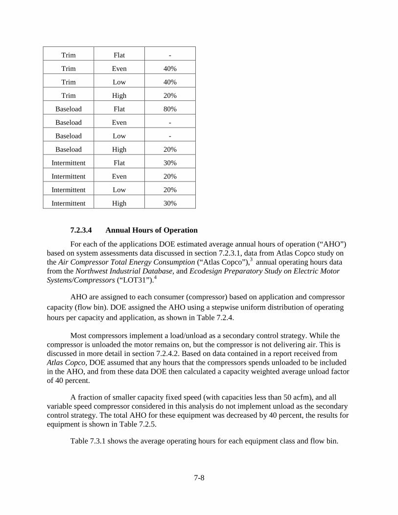
7-8

Trim Flat -

Trim Even 40%

Trim Low 40%

Trim High 20%

Baseload Flat 80%

Baseload Even -

Baseload Low -

Baseload High 20%

Intermittent Flat 30%

Intermittent Even 20%

Intermittent Low 20%

Intermittent High 30%

Annual Hours of Operation 7.2.3.4

For each of the applications DOE estimated average annual hours of operation (“AHO”) based on system assessments data discussed in section 7.2.3.1, data from Atlas Copco study on the Air Compressor Total Energy Consumption (“Atlas Copco”),3 annual operating hours data from the Northwest Industrial Database, and Ecodesign Preparatory Study on Electric Motor Systems/Compressors (“LOT31”).4

AHO are assigned to each consumer (compressor) based on application and compressor capacity (flow bin). DOE assigned the AHO using a stepwise uniform distribution of operating hours per capacity and application, as shown in Table 7.2.4.

Most compressors implement a load/unload as a secondary control strategy. While the compressor is unloaded the motor remains on, but the compressor is not delivering air. This is discussed in more detail in section 7.2.4.2. Based on data contained in a report received from Atlas Copco, DOE assumed that any hours that the compressors spends unloaded to be included in the AHO, and from these data DOE then calculated a capacity weighted average unload factor of 40 percent.

A fraction of smaller capacity fixed speed (with capacities less than 50 acfm), and all variable speed compressor considered in this analysis do not implement unload as the secondary control strategy. The total AHO for these equipment was decreased by 40 percent, the results for equipment is shown in Table 7.2.5.

Table 7.3.1 shows the average operating hours for each equipment class and flow bin.

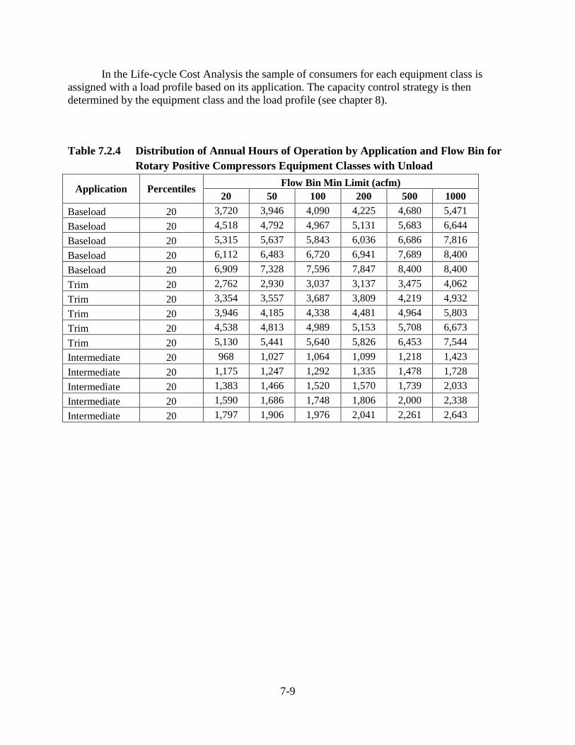
7-9

In the Life-cycle Cost Analysis the sample of consumers for each equipment class is assigned with a load profile based on its application. The capacity control strategy is then determined by the equipment class and the load profile (see chapter 8).

Table 7.2.4 Distribution of Annual Hours of Operation by Application and Flow Bin for Rotary Positive Compressors Equipment Classes with Unload

Application Percentiles Flow Bin Min Limit (acfm) 20 50 100 200 500 1000

Baseload 20 3,720 3,946 4,090 4,225 4,680 5,471 Baseload 20 4,518 4,792 4,967 5,131 5,683 6,644 Baseload 20 5,315 5,637 5,843 6,036 6,686 7,816 Baseload 20 6,112 6,483 6,720 6,941 7,689 8,400 Baseload 20 6,909 7,328 7,596 7,847 8,400 8,400 Trim 20 2,762 2,930 3,037 3,137 3,475 4,062 Trim 20 3,354 3,557 3,687 3,809 4,219 4,932 Trim 20 3,946 4,185 4,338 4,481 4,964 5,803 Trim 20 4,538 4,813 4,989 5,153 5,708 6,673 Trim 20 5,130 5,441 5,640 5,826 6,453 7,544 Intermediate 20 968 1,027 1,064 1,099 1,218 1,423 Intermediate 20 1,175 1,247 1,292 1,335 1,478 1,728 Intermediate 20 1,383 1,466 1,520 1,570 1,739 2,033 Intermediate 20 1,590 1,686 1,748 1,806 2,000 2,338 Intermediate 20 1,797 1,906 1,976 2,041 2,261 2,643

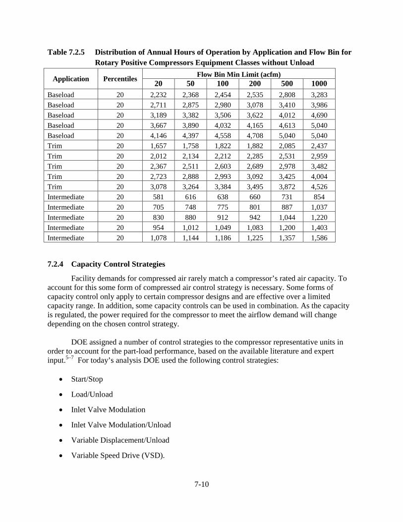
7-10

Table 7.2.5 Distribution of Annual Hours of Operation by Application and Flow Bin for Rotary Positive Compressors Equipment Classes without Unload

Application Percentiles Flow Bin Min Limit (acfm) 20 50 100 200 500 1000

Baseload 20 2,232 2,368 2,454 2,535 2,808 3,283 Baseload 20 2,711 2,875 2,980 3,078 3,410 3,986 Baseload 20 3,189 3,382 3,506 3,622 4,012 4,690 Baseload 20 3,667 3,890 4,032 4,165 4,613 5,040 Baseload 20 4,146 4,397 4,558 4,708 5,040 5,040 Trim 20 1,657 1,758 1,822 1,882 2,085 2,437 Trim 20 2,012 2,134 2,212 2,285 2,531 2,959 Trim 20 2,367 2,511 2,603 2,689 2,978 3,482 Trim 20 2,723 2,888 2,993 3,092 3,425 4,004 Trim 20 3,078 3,264 3,384 3,495 3,872 4,526 Intermediate 20 581 616 638 660 731 854 Intermediate 20 705 748 775 801 887 1,037 Intermediate 20 830 880 912 942 1,044 1,220 Intermediate 20 954 1,012 1,049 1,083 1,200 1,403 Intermediate 20 1,078 1,144 1,186 1,225 1,357 1,586

7.2.4 Capacity Control Strategies

Facility demands for compressed air rarely match a compressor’s rated air capacity. To account for this some form of compressed air control strategy is necessary. Some forms of capacity control only apply to certain compressor designs and are effective over a limited capacity range. In addition, some capacity controls can be used in combination. As the capacity is regulated, the power required for the compressor to meet the airflow demand will change depending on the chosen control strategy.

DOE assigned a number of control strategies to the compressor representative units in

order to account for the part-load performance, based on the available literature and expert input.5–7 For today’s analysis DOE used the following control strategies:

• Start/Stop

• Load/Unload

• Inlet Valve Modulation

• Inlet Valve Modulation/Unload

• Variable Displacement/Unload

• Variable Speed Drive (VSD).

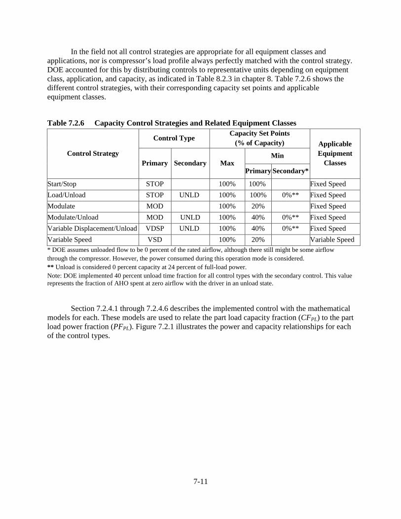
7-11

In the field not all control strategies are appropriate for all equipment classes and applications, nor is compressor’s load profile always perfectly matched with the control strategy. DOE accounted for this by distributing controls to representative units depending on equipment class, application, and capacity, as indicated in Table 8.2.3 in chapter 8. Table 7.2.6 shows the different control strategies, with their corresponding capacity set points and applicable equipment classes.

Table 7.2.6 Capacity Control Strategies and Related Equipment Classes

Control Strategy

Control Type Capacity Set Points

(% of Capacity) Applicable Equipment

Classes Primary Secondary Max Min

Primary Secondary*

Start/Stop STOP 100% 100% Fixed Speed Load/Unload STOP UNLD 100% 100% 0%** Fixed Speed Modulate MOD 100% 20%

Fixed Speed

Modulate/Unload MOD UNLD 100% 40% 0%** Fixed Speed Variable Displacement/Unload VDSP UNLD 100% 40% 0%** Fixed Speed Variable Speed VSD

100% 20%

Variable Speed

* DOE assumes unloaded flow to be 0 percent of the rated airflow, although there still might be some airflow through the compressor. However, the power consumed during this operation mode is considered. ** Unload is considered 0 percent capacity at 24 percent of full-load power. Note: DOE implemented 40 percent unload time fraction for all control types with the secondary control. This value represents the fraction of AHO spent at zero airflow with the driver in an unload state.

Section 7.2.4.1 through 7.2.4.6 describes the implemented control with the mathematical models for each. These models are used to relate the part load capacity fraction (CFPL) to the part load power fraction (PFPL). Figure 7.2.1 illustrates the power and capacity relationships for each of the control types.

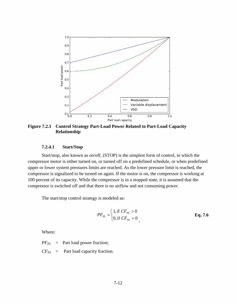
7-12

Figure 7.2.1 Control Strategy Part-Load Power Related to Part-Load Capacity

Relationship

Start/Stop 7.2.4.1

Start/stop, also known as on/off, (STOP) is the simplest form of control, in which the compressor motor is either turned on, or turned off on a predefined schedule, or when predefined upper or lower system pressures limits are reached. As the lower pressure limit is reached, the compressor is signalized to be turned on again. If the motor is on, the compressor is working at 100 percent of its capacity. While the compressor is in a stopped state, it is assumed that the compressor is switched off and that there is no airflow and not consuming power.

The start/stop control strategy is modeled as:

. Eq. 7.6

Where: PFPL = Part load power fraction;

CFPL = Part load capacity fraction.

=>

=0 if ,00 if ,1

PL

PLPL CF

CFPF

7-13

Load/Unload 7.2.4.2

Load/unload (UNLD) is a form of control similar to start/stop, which allows the compressor to operate either at its full capacity or at nearly no flow. The airflow through the compression chamber is limited when a predefined upper system pressure limit is reached putting the compressor into an unloaded state, instead of turning it off. This reduces the mass of air flow through the compressor resulting in reduced power requirements. While the compressor is unloaded the compressor motor runs continuously using 15- to 35-percent of its rated power. For this analysis DOE uses an average of 17-percent motor rated power as its unloaded power fraction, PFUnloaded.6 Compressors continue to consume power while they are unloaded; this is reflected in the AHO described in section 7.2.3.4.

The load/unload control strategy is modeled as:

Eq. 7.7

It should be noted that compressors can also be configured to unload at any part-load

capacity, and can be combined and used as a secondary control any of the control strategies shown in Table 7.2.6:

Inlet Valve Modulation 7.2.4.3

Inlet valve modulation (MOD) is a form of control in which the inlet valve is gradually closed in proportion to reduced system air demands. Similar to load/unload, the reduction in the mass of air flow through the compressor results in lower power requirements. DOE models this as a linear relationship between the part load capacity and power fractions:

Eq. 7.8

where:

PFmin and PFmax = the minimum and the maximum part load power fractions, DOE uses 0.7 and 1.0, respectively.6

For this analysis DOE considers 20-percent of airflow to be the lowest point at which

inlet valve modulation is used.5 The inlet valve modulation control strategy is generally most effective when modulating down to 40-percent of rated capacity, which DOE uses as unload point when inlet valve modulation is combined with the load/unload control strategy.6

≈>

=0 if ,0 if ,1

PLUnloaded

PLPL CFPF

CFPF

( )minmax

minminmaxmin CFCF

CFCFPFPFPFPF PLPL −

−−+=

7-14

Variable Displacement 7.2.4.4

Variable displacement (VDSP) is a form of control in which the volume of compression chamber is progressively adjusted to allow air to bypass compression in response to reduced system air demands thereby reducing power requirements. Variable displacement is effective from 40- and 50- to 100-percent of a compressor’s capacity.1 Though more efficient, variable displacement is similar to inlet valve modulation, whereby the reduction in required compressor power can be modeled as a quadratic function:2

Eq. 7.9

where: PFmin equals 0.6.7

For this analysis DOE considers 40-percent of airflow to be the lowest point at which this

control is used. Additionally, unload control is always required with variable displacement. Further, DOE grouped the following technologies as variable displacement, as they all have similar effects on reduced power requirements in relation to reduced air flow: slide, spiral, poppet, and turn values, and geometric lift.

Variable Speed Drive 7.2.4.5

Variable Speed Drive (VSD) is a form of control in which the speed of the prime mover of the air compressor can be progressively adjusted to match system air demands. While energy savings can be realized between 20- and 100-percent of a compressors capacity, the greatest energy saving potential lies in applications where the compressor is operated with the bulk of its hours at low to mid capacity.3 DOE generated the VSD control curve using manufacturer performance test data made publically available under the Compressed Air and Gas Institute’s (CAGI) performance verification program.a DOE used quadratic polynomial expression to approximate the relationship between part-load capacity and power for VSDs:

Eq. 7.10

Where a, b, and c are the coefficients obtained by averaging the regression coefficients based on the CAGI test data. The values for the coefficients are provided in Table 7.2.7.

a http://cagi.org/performance-verification/overview.aspx

( )2

minmax

minminmaxmin

−−

−+=CFCFCFCFPFPFPFPF PL

PL

cbCFaCFPF PLPLPL ++= 2

7-15

Table 7.2.7 Variable Speed Drive Control Curve Regression Coefficients Coefficient Value a 0.168603 b 0.709537 c 0.121266

Multiple Compressor Sequencing 7.2.4.6

Multiple compressor sequencing is used in larger compressed air systems where multiple compressors are programmed to operate together to meet a system’s air demands as efficiently as possible. This can be done by starting or stopping, loading or unloading individual compressors in response to a systems’ changing air demands. For this analysis, DOE estimates load profiles for individual compressors, and accounts for the loads of sequenced compressors within the scope of the applications defined in section 7.2.3.1.

7.2.5 Energy Use Factor

EUF is a dot product of AHO fractions spent at each loading point (AHOPL) and part load power fraction (PFPL) arrays:

∑ ⋅= ),,()( OFCTCFPFLPAHOEUF PLPLPL Eq. 7.11

Where:

AHOPL = fraction of AHO spent at each capacity loading points, see Table 7-2;

LP = load profile;

PFPL = part load power fractions, which result from applying the control type function to the part load capacity fractions;

CFPL = part load capacity fraction;

CT = control type;

OF = oversize factor.

The load profiles defined in section 7.2.3.2 consist of the fraction of annual operating

hours spent at each loading point. DOE then calculated the corresponding part load power fraction (PFPL) and for those hours where the compressor is operating in part-load DOE determined the appropriate control strategy combination. DOE then calculated the energy use of those part-load hours according to the control strategy. Table 7.2.8 provides the values implemented in the energy use analysis.

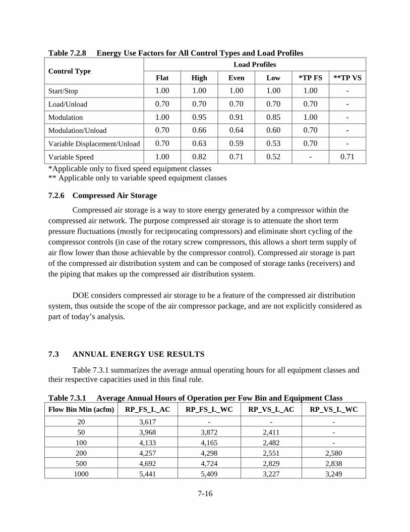
7-16

Table 7.2.8 Energy Use Factors for All Control Types and Load Profiles

Control Type Load Profiles

Flat High Even Low *TP FS **TP VS

Start/Stop 1.00 1.00 1.00 1.00 1.00 -

Load/Unload 0.70 0.70 0.70 0.70 0.70 -

Modulation 1.00 0.95 0.91 0.85 1.00 - Modulation/Unload 0.70 0.66 0.64 0.60 0.70 -

Variable Displacement/Unload 0.70 0.63 0.59 0.53 0.70 -

Variable Speed 1.00 0.82 0.71 0.52 - 0.71 *Applicable only to fixed speed equipment classes ** Applicable only to variable speed equipment classes

7.2.6 Compressed Air Storage

Compressed air storage is a way to store energy generated by a compressor within the compressed air network. The purpose compressed air storage is to attenuate the short term pressure fluctuations (mostly for reciprocating compressors) and eliminate short cycling of the compressor controls (in case of the rotary screw compressors, this allows a short term supply of air flow lower than those achievable by the compressor control). Compressed air storage is part of the compressed air distribution system and can be composed of storage tanks (receivers) and the piping that makes up the compressed air distribution system.

DOE considers compressed air storage to be a feature of the compressed air distribution

system, thus outside the scope of the air compressor package, and are not explicitly considered as part of today’s analysis.

7.3 ANNUAL ENERGY USE RESULTS

Table 7.3.1 summarizes the average annual operating hours for all equipment classes and their respective capacities used in this final rule. Table 7.3.1 Average Annual Hours of Operation per Fow Bin and Equipment Class Flow Bin Min (acfm) RP_FS_L_AC RP_FS_L_WC RP_VS_L_AC RP_VS_L_WC

20 3,617 - - - 50 3,968 3,872 2,411 - 100 4,133 4,165 2,482 - 200 4,257 4,298 2,551 2,580 500 4,692 4,724 2,829 2,838

1000 5,441 5,409 3,227 3,249

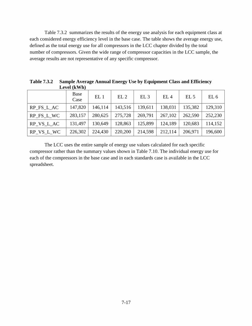
7-17

Table 7.3.2 summarizes the results of the energy use analysis for each equipment class at each considered energy efficiency level in the base case. The table shows the average energy use, defined as the total energy use for all compressors in the LCC chapter divided by the total number of compressors. Given the wide range of compressor capacities in the LCC sample, the average results are not representative of any specific compressor.

Table 7.3.2 Sample Average Annual Energy Use by Equipment Class and Efficiency Level (kWh)

Base Case EL 1 EL 2 EL 3 EL 4 EL 5 EL 6

RP_FS_L_AC 147,820 146,114 143,516 139,611 138,031 135,382 129,310

RP_FS_L_WC 283,157 280,625 275,728 269,791 267,102 262,590 252,230

RP_VS_L_AC 131,497 130,649 128,863 125,899 124,189 120,683 114,152

RP_VS_L_WC 226,302 224,430 220,200 214,598 212,114 206,971 196,600

The LCC uses the entire sample of energy use values calculated for each specific compressor rather than the summary values shown in Table 7.10. The individual energy use for each of the compressors in the base case and in each standards case is available in the LCC spreadsheet.

7-18

REFERENCES

1. Applied Proactive Technologies (APT), under contract with the New York State Energy Research and Development Authority (NYSERDA) & Washington State University Extension Energy Program (WSU). Database of motor nameplate and field measurements. (WSU, NYSERDA, 2011).

2. Strategic Energy Group. Northwest Industrial Motor Database Summary. (2009).

3. Wouters, C. Air Compressor Total Energy Consumption. (2016).

4. Prepared for the European Commission by Van Holsteijn en Kemna B.V. (VHK). Ecodesign Preparatory Study on Electric Motor Systems/Compressors. (2014).

5. McCulloh, D. M. Compressed Air and Gase Handbook. (Compressed Air and Gas Institute (CAGI), 2003).

6. Wheeler, G. M., Bessey, E. G. & McGill, R. D. Anlaysis Methodology Manual for AIRMaster Compressed Air System Audit and Analysis Software. (1997).

7. Maxwell, J. B. Improving Part Load Efficiency of Screw Air Compressors. (Oregon State University, 1992).

8-i

CHAPTER 8. LIFE-CYCLE COST AND PAYBACK PERIOD ANALYSIS

TABLE OF CONTENTS

8.1 INTRODUCTION ........................................................................................................... 8-1 8.1.1 General Approach for Life-Cycle Cost and Payback Period Analysis ................ 8-1 8.1.2 Overview of Life-Cycle Cost and Payback Period Inputs ................................... 8-1

8.2 DEFINITION OF THE LIFE-CYCLE COST SAMPLE ................................................ 8-3 8.2.1 Definition of the Weights..................................................................................... 8-3

8.2.1.1 Equipment Class Weights ........................................................................ 8-4 8.2.1.2 Sector Assignment ................................................................................... 8-4 8.2.1.3 Application, Control Type and Load Profile Assignment ....................... 8-4 8.2.1.4 Equipment Oversizing ............................................................................. 8-6

8.2.2 LCC Sampling Method ........................................................................................ 8-6 8.3 LIFE-CYCLE COST INPUTS ........................................................................................ 8-7

8.3.1 Total Installed Cost Inputs ................................................................................... 8-7 8.3.1.1 No-Standards Case Equipment Price ....................................................... 8-8 8.3.1.2 Standards Case Equipment Price ............................................................. 8-8 8.3.1.3 Projection of Future Equipment Prices .................................................... 8-9 8.3.1.4 Installation Cost ....................................................................................... 8-9

8.3.2 Operating Cost Inputs ........................................................................................ 8-10 8.3.2.1 Annual Energy Use ................................................................................ 8-10 8.3.2.2 Electricity Prices .................................................................................... 8-10 8.3.2.3 Maintenance Costs and Repair Costs ..................................................... 8-11 8.3.2.4 Equipment Lifetime ............................................................................... 8-11 8.3.2.5 Discount Rates ....................................................................................... 8-13

8.3.3 Base Case Efficiency Distribution ..................................................................... 8-16 8.4 REBUTTABLE PAYBACK PERIOD .......................................................................... 8-17

8.4.1 Inputs.................................................................................................................. 8-17 8.4.2 Results ................................................................................................................ 8-18

8.5 LIFE-CYCLE COST AND PAYBACK PERIOD RESULTS ...................................... 8-18 REFERENCES .......................................................................................................................... 8-25

LIST OF TABLES

Table 8.2.1 Air Compressor Sector Assignment............................................................... 8-4 Table 8.2.2 Distribution of Air Compressors by Application ........................................... 8-4 Table 8.2.3 Distribution of Control Types by Application and Equipment Class ............ 8-5 Table 8.2.4 Summary of additional inputs to each LCC sample row ............................... 8-7 Table 8.3.1 Initial Air Compressor Mechanical Lifetimes by Capacity ......................... 8-12 Table 8.3.2 Average Mechanical Lifetime and Service Lifetime by Equipment

Class ............................................................................................................. 8-12 Table 8.3.3 Risk Free Rate and Equity Risk Premium, 2004-2013 ................................ 8-15

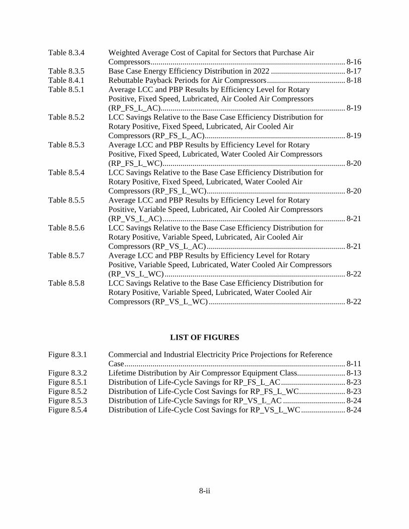
8-ii

Table 8.3.4 Weighted Average Cost of Capital for Sectors that Purchase Air Compressors ................................................................................................. 8-16

Table 8.3.5 Base Case Energy Efficiency Distribution in 2022 ..................................... 8-17 Table 8.4.1 Rebuttable Payback Periods for Air Compressors ....................................... 8-18 Table 8.5.1 Average LCC and PBP Results by Efficiency Level for Rotary

Positive, Fixed Speed, Lubricated, Air Cooled Air Compressors (RP_FS_L_AC)............................................................................................ 8-19

Table 8.5.2 LCC Savings Relative to the Base Case Efficiency Distribution for Rotary Positive, Fixed Speed, Lubricated, Air Cooled Air Compressors (RP_FS_L_AC) ...................................................................... 8-19

Table 8.5.3 Average LCC and PBP Results by Efficiency Level for Rotary Positive, Fixed Speed, Lubricated, Water Cooled Air Compressors (RP_FS_L_WC) ........................................................................................... 8-20

Table 8.5.4 LCC Savings Relative to the Base Case Efficiency Distribution for Rotary Positive, Fixed Speed, Lubricated, Water Cooled Air Compressors (RP_FS_L_WC) ..................................................................... 8-20

Table 8.5.5 Average LCC and PBP Results by Efficiency Level for Rotary Positive, Variable Speed, Lubricated, Air Cooled Air Compressors (RP_VS_L_AC) ........................................................................................... 8-21

Table 8.5.6 LCC Savings Relative to the Base Case Efficiency Distribution for Rotary Positive, Variable Speed, Lubricated, Air Cooled Air Compressors (RP_VS_L_AC) ..................................................................... 8-21

Table 8.5.7 Average LCC and PBP Results by Efficiency Level for Rotary Positive, Variable Speed, Lubricated, Water Cooled Air Compressors (RP_VS_L_WC) .......................................................................................... 8-22

Table 8.5.8 LCC Savings Relative to the Base Case Efficiency Distribution for Rotary Positive, Variable Speed, Lubricated, Water Cooled Air Compressors (RP_VS_L_WC) .................................................................... 8-22

LIST OF FIGURES

Figure 8.3.1 Commercial and Industrial Electricity Price Projections for Reference Case .............................................................................................................. 8-11

Figure 8.3.2 Lifetime Distribution by Air Compressor Equipment Class........................ 8-13 Figure 8.5.1 Distribution of Life-Cycle Savings for RP_FS_L_AC ................................ 8-23 Figure 8.5.2 Distribution of Life-Cycle Cost Savings for RP_FS_L_WC ....................... 8-23 Figure 8.5.3 Distribution of Life-Cycle Savings for RP_VS_L_AC ............................... 8-24 Figure 8.5.4 Distribution of Life-Cycle Cost Savings for RP_VS_L_WC ...................... 8-24

8-1

CHAPTER 8. LIFE-CYCLE COST AND PAYBACK PERIOD ANLAYSIS

8.1 INTRODUCTION

The life-cycle cost (LCC) and payback period (PBP) analysis evaluates the impact of proposed energy conservation standards on air compressor users, i.e., the consumers who purchase and operate air compressors. The LCC provides a measure of the total cost of ownership, consisting of the initial purchase price and installation costs, and energy, maintenance and repair costs over the lifetime of the air compressor. The Department of Energy (DOE) accounts for variability in energy use, discount rates, and energy costs by doing individual LCC calculations for a large sample of air compressors that are assigned different installation conditions. Installation conditions include customer attributes such as sector and application, and usage attributes such as annual hours of operation. This sample is used to generate national average LCC savings by efficiency level.

General Approach for Life-Cycle Cost and Payback Period Analysis 8.1.1

DOE conducted the LCC and PBP analysis by developing a large sample of air compressor installations, which represent the general population of air compressors that would be affected by proposed energy conservation standards. Separate analyses are conducted for each equipment class. Conceptually, the analysis distinguishes between the air compressor installation and the air compressor itself. The air compressor installation is characterized by a combination of customer attributes (sector, application, electricity price, discount rate) and usage attributes (equipment class, control type, load profile, annual hours of operation, mechanical lifetime) that do not change with each trial standard level (TSL). DOE conducted the LCC and PBP analysis by modeling both the uncertainty and variability in the inputs using probability distributions. The air compressor itself is the regulated equipment, so its efficiency and selling price do change with TSL. For each equipment class the LCC sample consists of 10,000 distinct air compressor installations.

In the base case, DOE assigns a specific air compressor to each installation. At each

efficiency level, an air compressor, that meets or exceeds the efficiency level being examined, is assigned to identical installation. Equivalently, for that installation, the LCC at the given efficiency level is the same as the LCC in the base case and the standard does not impact that user. If the compressor fails to meet the efficiency level (EL) considered in the standard-case, the compressor gets redesigned. The LCC savings at each efficiency level are defined as the difference between the LCC in the base case and the LCC for the more efficient air compressor. The LCC is calculated for each air compressor installation at each efficiency level. These calculations are presented in the LCC spreadsheet.

Overview of Life-Cycle Cost and Payback Period Inputs 8.1.2

DOE categorizes inputs to the LCC and PBP analysis as follows: (1) inputs for establishing the initial expense, otherwise known as the total installed cost; and (2) inputs for calculating the operating cost.

8-2

The primary inputs for establishing the total installed cost are:

• No-Standards case manufacturer selling price: The price at which the manufacturer sells the equipment, which includes the costs incurred by the manufacturer to produce equipment meeting existing standards. The no-standards case manufacture selling price is described in detail in chapter 5, Engineering Analysis

• Standard case manufacturer selling price: The manufacturer selling price associated with producing equipment to meet a particular standard level. The standards case manufacture selling price is described in detail in chapter 5, Engineering Analysis

• Markups and sales tax: The distribution channel markups and sales tax associated with converting the manufacturer cost to a consumer equipment price. The markups and sales tax are described in detail in chapter 6, Markups Analysis.

• Installation cost: The cost to the consumer of installing the equipment. The installation cost represents all costs required to install the equipment other than the marked-up consumer equipment price. The installation cost includes labor, overhead, and any miscellaneous materials and parts. Thus, the total installed cost equals the consumer equipment price plus the installation cost. Installation costs are described in section 8.3.1.4.

The primary inputs for calculating the operating cost are:

• Equipment energy consumption: The equipment energy consumption is the site energy use associated with operating the equipment. Chapter 7, Energy Use Characterization, details how DOE determined the equipment energy consumption based on various data sources.

• Energy prices: Energy prices are the prices paid by end-users for energy (i.e., electricity). DOE determined current energy prices based on data from the Energy Information Agency’s (EIA’s) Form EIA-861 database (based on “Annual Electric Power Industry Report”), Edison Electric Institute (EEI) Typical Bills and Average Rates Reports, and information from utility tariffs. a,b Electricity prices are described in section 8.3.2.2.

• Energy price trends: To estimate energy prices in future years, DOE multiplied the recent electricity prices by a projection of annual national-average industrial and commercial

a Available at: www.eia.gov/forecasts/aeo/

b Edison Electric Institute. Typical Bills and Average Rates Report. Winter 2014 published April 2014, Summer 2014 published October 2014: Washington, D.C. (Last accessed June 2, 2015.) www.eei.org/resourcesandmedia/products/Pages/Products.aspx.

8-3

electricity prices consistent with cases described on p. E-8 in AEO 2016.c Electricity price trends are described in section 8.3.2.2

• Repair and maintenance costs: Repair costs are associated with repairing or replacing components that have failed. Maintenance costs are associated with maintaining the operation of the equipment. Repair and maintenance costs are described in section 8.3.2.3.

• Lifetime: The age at which the equipment is retired from service. Equipment lifetimes are described in section 8.3.2.4

• Discount rate: The rate at which DOE discounted future expenditures to establish their present value. Discount rates are described in section 8.3.2.5.

8.2 DEFINITION OF THE LIFE-CYCLE COST SAMPLE

For each equipment class, an LCC sample presents a population of air compressors, defined such that its variability both in consumer and equipment side inputs represents the population of air compressors as utilized today. In this section DOE described the method of combining, assigning and quantifying these inputs.

DOE did not assign the customer attributes (sector, application, shipment weight, etc.) to

duty points randomly. DOE reviewed several data sources to incorporate correlations between sector, application, equipment class, load profile, control type and operating hours into the analysis. Each of these assignments is described below in section 8.2.1. DOE used these distributions to determine the relative weighting of different sectors and applications in the LCC sample.

Definition of the Weights 8.2.1

Each row of the LCC sample estimates a combination of consumer and equipment parameters which would likely be seen in the field, under assumption that the customer choses an appropriately dimensioned compressor to meet its demand load. The calculation of the frequency of each such unique combination in the LCC sample is defined in the following sections.

c The standards finalized in this rulemaking will take effect before the requirements of the Clean Power Plan (CPP) as modeled in the AEO 2016 Reference case, putting downward pressure on electricity prices relative to the projections in Reference case. Consequently, DOE used the more conservative (i.e., lower) price projections found in the AEO 2016 No-CPP case.

8-4

8.2.1.1 Equipment Class Weights

Estimates from the shipments analysis (chapter 9) are used to define the relative weightings of the representative units based on 2013 shipments. Each representative unit is defined as an air compressor that can substitute the operation of all air compressors available in the market, which operate within appropriate representative unit’s design point pressure and air flow bin. Pressure and flow design points for each representative unit are described in the Engineering analysis chapter, while the weight of each equipment class at each design point pressure and flow are described the chapter 9, Shipments, with the weights for each equipment class pressure and flow weight shown in appendix 9A.

8.2.1.2 Sector Assignment

The economic inputs to the LCC (discount rate and electricity price) depend on the sector, while usage criteria such as hours of operation depend on the application and capacity. Hence, each air compressor installation in the LCC sample must be assigned a sector and application. DOE considered two sectors: industrial and commercial. Air compressors have been assigned to a sector depending on their airflow capacity, as provided in Table 8.2.1. Based on stakeholder comments, fraction of industrial equipment increases with the compressor capacity.

Table 8.2.1 Air Compressor Sector Assignment

Flow Bin Min Limit, acfm

Sector Commercial Industrial

20 50% 50% 50 25% 75% 100 5% 95% 200 0% 100% 500 0% 100% 1000 0% 100%

8.2.1.3 Application, Control Type and Load Profile Assignment

DOE defined three application types to capture variations in air demand and control strategies, as explained in further detail in chapter 7 of this technical support document (TSD). The probability that a compressor gets assigned to a particular application type was derived based on motor system assessment data, as shown in Table 8.2.4.1

Table 8.2.2 Distribution of Air Compressors by Application Application Probability

Trim 50% Baseload 28% Intermittent 22%

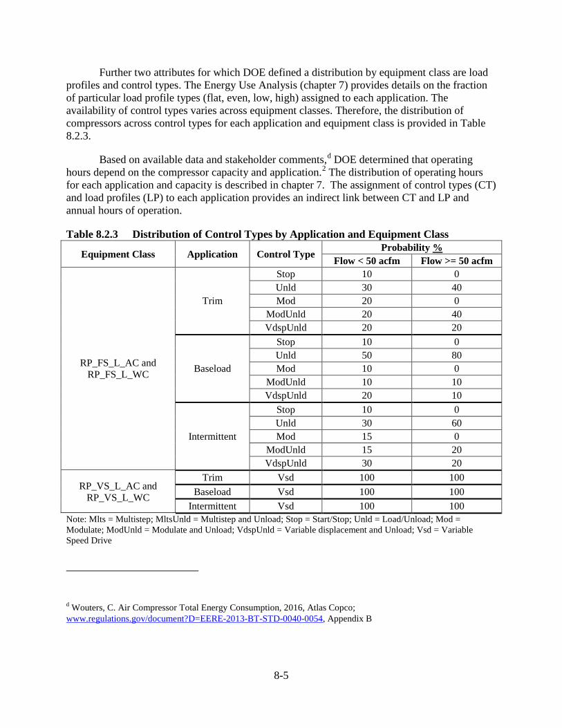
8-5

Further two attributes for which DOE defined a distribution by equipment class are load profiles and control types. The Energy Use Analysis (chapter 7) provides details on the fraction of particular load profile types (flat, even, low, high) assigned to each application. The availability of control types varies across equipment classes. Therefore, the distribution of compressors across control types for each application and equipment class is provided in Table 8.2.3.

Based on available data and stakeholder comments,d DOE determined that operating hours depend on the compressor capacity and application.2 The distribution of operating hours for each application and capacity is described in chapter 7. The assignment of control types (CT) and load profiles (LP) to each application provides an indirect link between CT and LP and annual hours of operation.

Table 8.2.3 Distribution of Control Types by Application and Equipment Class

Equipment Class Application Control Type Probability %

Flow < 50 acfm Flow >= 50 acfm

RP_FS_L_AC and RP_FS_L_WC

Trim

Stop 10 0 Unld 30 40 Mod 20 0

ModUnld 20 40 VdspUnld 20 20

Baseload

Stop 10 0 Unld 50 80 Mod 10 0

ModUnld 10 10 VdspUnld 20 10

Intermittent

Stop 10 0 Unld 30 60 Mod 15 0

ModUnld 15 20 VdspUnld 30 20

RP_VS_L_AC and RP_VS_L_WC

Trim Vsd 100 100 Baseload Vsd 100 100

Intermittent Vsd 100 100 Note: Mlts = Multistep; MltsUnld = Multistep and Unload; Stop = Start/Stop; Unld = Load/Unload; Mod = Modulate; ModUnld = Modulate and Unload; VdspUnld = Variable displacement and Unload; Vsd = Variable Speed Drive d Wouters, C. Air Compressor Total Energy Consumption, 2016, Atlas Copco; www.regulations.gov/document?D=EERE-2013-BT-STD-0040-0054, Appendix B

8-6

8.2.1.4 Equipment Oversizing

DOE did not receive any information that would require the analysis to consider compressor oversizing. The demand size load profile variability, as described in chapter 7, provides some compensation of this effect, assuming that only slight over or under dimensioning of the equipment occurs in existing installations. Despite this small effect, DOE considers that compressors are perfectly sized to the loads they are connected to .DOE conducted a sensitivity analysis with an oversize factor of 1.1,the results of this sensitivity can be found in appendix 8A.

LCC Sampling Method 8.2.2

The LCC sampling requires a weighting function, discussed in this section. The flow and pressure design points are indexed by i and j respectively, and total shipment weight at the points is defined as wij. As mentioned earlier in this chapter, the weight wij is defined as the number of compressors at point (i,j) divided by the total number of compressors in the shipments data for a given equipment class.e At each point, compressors are distributed across application a, load profile p, control type q.

The LCC process is (for each equipment class):

1) Create a list of installation types, indexed by (a,p,q,i,j) with a weighting wij , which defines the percentage of all air compressors (rows in the sample) this installation type is expected to represent.

2) Set a number, N, of rows in the LCC sample for each equipment class (DOE adopted N=10,000 in the results presented in this TSD).

3) Create an expanded list of N installations with each installation type sampled Nwij times.

4) For each row of the sample fill in the additional required information as defined in Table 8.2.4.

5) For each row, based on the assigned base case efficiency, for all ELs:

(a) Pull the MSP and isentropic efficiency from the engineering data for all ELs.

(b) Check whether the compressor representative unit passes of fails at each EL.

6) Calculate the annual operating cost, total installed cost and life-cycle cost for each row of the sample at each EL.

e The methodology for deriving the wij for each equipment class’ pressure and flow combination is described in chapter 9, Shipment Analysis.

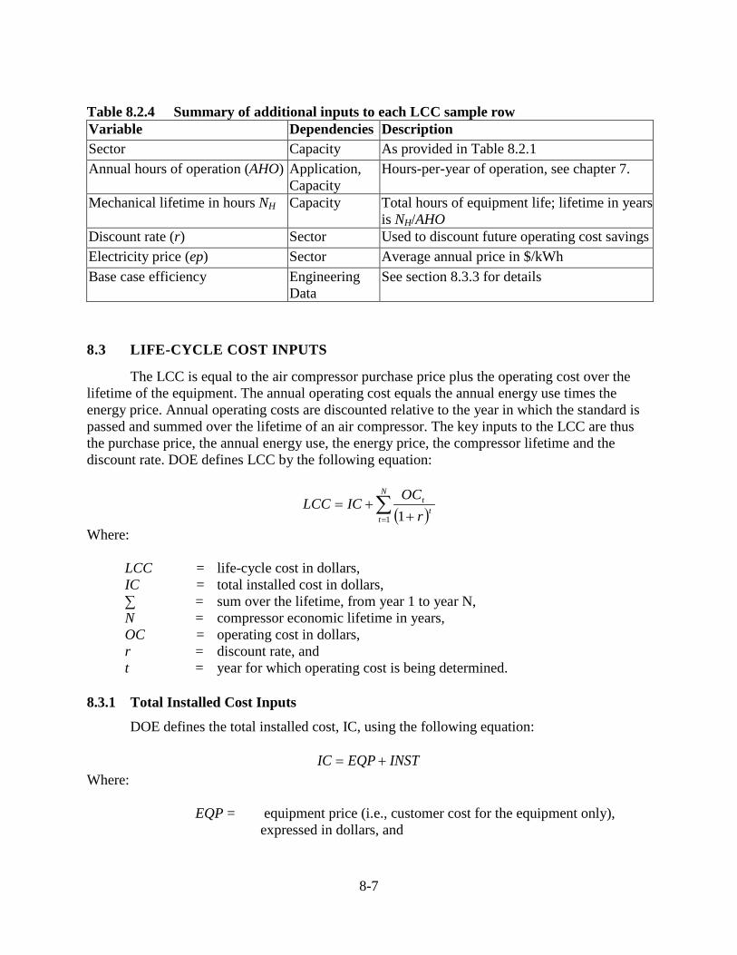
8-7

Table 8.2.4 Summary of additional inputs to each LCC sample row Variable Dependencies Description Sector Capacity As provided in Table 8.2.1 Annual hours of operation (AHO) Application,

Capacity Hours-per-year of operation, see chapter 7.

Mechanical lifetime in hours NH Capacity Total hours of equipment life; lifetime in years is NH/AHO

Discount rate (r) Sector Used to discount future operating cost savings Electricity price (ep) Sector Average annual price in $/kWh Base case efficiency Engineering

Data See section 8.3.3 for details

8.3 LIFE-CYCLE COST INPUTS

The LCC is equal to the air compressor purchase price plus the operating cost over the lifetime of the equipment. The annual operating cost equals the annual energy use times the energy price. Annual operating costs are discounted relative to the year in which the standard is passed and summed over the lifetime of an air compressor. The key inputs to the LCC are thus the purchase price, the annual energy use, the energy price, the compressor lifetime and the discount rate. DOE defines LCC by the following equation:

( )∑= +

+=N

tt

t

rOCICLCC

1 1

Where:

LCC = life-cycle cost in dollars, IC = total installed cost in dollars, ∑ = sum over the lifetime, from year 1 to year N, N = compressor economic lifetime in years, OC = operating cost in dollars, r = discount rate, and t = year for which operating cost is being determined.

Total Installed Cost Inputs 8.3.1

DOE defines the total installed cost, IC, using the following equation:

INSTEQPIC += Where:

EQP = equipment price (i.e., customer cost for the equipment only), expressed in dollars, and

8-8

INST = installation cost or the customer price to install equipment (i.e., the cost for labor and materials), also in dollars.

DOE found no evidence that installation costs would increase with an increase in the

compressor energy efficiency, as further explained in section 8.3.1.4. Thus, DOE did not incorporate changes in installation costs for air compressors that are more efficient than equipment selected in the no-standards case.

8.3.1.1 No-Standards Case Equipment Price

The manufacturer selling price (MSP) is the price charged by the manufacturer for the equipment. The price paid by air compressor users is equal to the MSP, plus any relevant distributor markup, plus the sales tax, plus installation costs markups. At each efficiency level, the MSP increases to reflect the additional costs incurred by the air compressor manufacturers to meet the standard. In the no-standards case, representing the market with no standard in place, DOE calculated the equipment price for no-standards case equipment based on the following equation:

𝐸𝐸𝐸𝐸𝐸𝐸𝑛𝑛𝑛𝑛−𝑠𝑠𝑠𝑠𝑠𝑠 = 𝑀𝑀𝑀𝑀𝐸𝐸𝑛𝑛𝑛𝑛−𝑠𝑠𝑠𝑠𝑠𝑠 × 𝑀𝑀𝑀𝑀𝑛𝑛𝑜𝑜𝑜𝑜𝑜𝑜𝑜𝑜𝑜𝑜𝑜𝑜_𝑏𝑏𝑜𝑜𝑠𝑠𝑜𝑜

Where: EQPno-std = consumer equipment price in the no-standards case,

MSPno-std = manufacturer selling price in the no-standards case, and MUoverall_base = baseline overall markup (product of baseline distribution channel

markup, and sales tax). The overall markups used in the LCC analyses are discussed in Chapter 6.

8.3.1.2 Standards Case Equipment Price

As discussed in the engineering analysis, the MSP in the standard-case is determined using an efficiency level approach. Costs associated with the increase in energy efficiency are based on (1) a database of air compressor performance data from the Compressed Air and Gas Institute (CAGI) data sheets,f (2) results from the EU Lot 31 - Ecodesign Preparatory Study on Compressors, (3) confidential data gained through manufacturer interviews, and (4) online publicly available retailer prices.3 For all equipment classes, DOE defines MSP by a mathematical relationship between flow rate and isentropic efficiency. DOE assumed that the MSP is independent of the operating pressure. f For more information regarding CAGI’s Performance Verification program, please see: www.cagi.org/performance-verification/

8-9

The LCC includes a pre-processing step that calculates the selling price of each compressor representative unit in the sample, at each EL. If the compressor design meets an efficiency level (EL) higher than the no-standards case, it gets assigned with MSP associated with its last passing EL. Therefore, standards case equipment price depends on the particular standards case MSP, no-standards case MSP, overall baseline markup and overall incremental markup:

𝐸𝐸𝐸𝐸𝐸𝐸𝑠𝑠𝑠𝑠𝑠𝑠 = 𝑀𝑀𝑀𝑀𝐸𝐸𝑛𝑛𝑛𝑛−𝑠𝑠𝑠𝑠𝑠𝑠 × 𝑀𝑀𝑀𝑀𝑛𝑛𝑜𝑜𝑜𝑜𝑜𝑜𝑜𝑜𝑜𝑜𝑜𝑜_𝑏𝑏𝑜𝑜𝑠𝑠𝑜𝑜 + (𝑀𝑀𝑀𝑀𝐸𝐸𝑠𝑠𝑠𝑠𝑠𝑠 − 𝑀𝑀𝑀𝑀𝐸𝐸𝑛𝑛𝑛𝑛−𝑠𝑠𝑠𝑠𝑠𝑠) × 𝑀𝑀𝑀𝑀𝑛𝑛𝑜𝑜𝑜𝑜𝑜𝑜𝑜𝑜𝑜𝑜𝑜𝑜_𝑖𝑖𝑛𝑛𝑖𝑖𝑜𝑜 Where:

𝐸𝐸𝐸𝐸𝐸𝐸𝑠𝑠𝑠𝑠𝑠𝑠 = consumer equipment price of the air compressor in the standards case,

MSPstd = manufacturer selling price in the standards case, MUoverall_incr = incremental overall markup (markup related to the change in

the MSP due to increasing the efficiencyof the model; product of incremental markup, and sales tax).

8.3.1.3 Projection of Future Equipment Prices

To project an equipment price trend, DOE derived an inflation-adjusted index of the Producer Price Index for air and gas compressor equipment manufacturing over the period 1984-2013.g These data show a slight decrease from 1989 through 2004. Since 2004, however, there has been an increase in the price index. Given the relatively slow global economic activity in 2009 through 2013, the extent to which the future trend can be predicted based on the last decade is uncertain. Because the observed data do not provide a firm basis for projecting future cost trends for compressor equipment, DOE used a constant price assumption as the default trend to project future compressor prices in 2022.h Thus, prices projected for the LCC and PBP analysis are equal to the 2014 values for each efficiency level in each equipment class.

8.3.1.4 Installation Cost

In the NOPR, DOE requested information on whether air compressor installation costs would be expected to change with efficiency.i Sullair further noted there might be an added cost of installation of equipment related to efficiency. Although stakeholders indicated that there may be differences in installation costs between the no-new-standards case and the standards case equipment, stakeholders did not provide an explanation, or data to indicate at what efficiency

g Series ID PCU333911333912; www.bls.gov/ppi/ h Compliance is planned for late 2021, as such this analysis is conducted in the first-full year after compliance, which is 2022. i www.regulations.gov/#!documentDetail;D=EERE-2013-BT-STD-0040-0001

8-10

level DOE may need to consider an increase in installation costs. For today’s analysis DOE considers water- and air-cooled compressors as a separate equipment class, thus any additional piping or plumbing required in the standards case would also be required in the no-new standards case, so for today’s analysis DOE has not estimated an installation cost for this analysis as they would be the same in both the standards and no-new standards cases.

Operating Cost Inputs 8.3.2

8.3.2.1 Annual Energy Use

DOE estimated the annual electricity consumed by each class of commercial and industrial air compressor, by efficiency level, based on the energy use analysis described in chapter 7 of the notice of proposed rulemaking (NOPR) TSD.

8.3.2.2 Electricity Prices

DOE derived average and marginal annual non-residential (commercial and industrial) electricity prices using data from EIA’s Form EIA-861 database (based on “Annual Electric Power Industry Report”)j, EEI Typical Bills and Average Rates Reports, and information from utility tariffs. 4 Electricity tariffs for non-residential consumers can be very complex, with the principal difference from residential rates being the incorporation of demand charges. The presence of demand charges means that two consumers with the same monthly electricity consumption may have very different bills, depending on their peak demand. For this analysis DOE used marginal electricity prices to estimate the impact of demand charges for consumers of air compressors. These prices are $0.1040/kWh and $0.0828/kWh, for commercial and industrial customers respectively. The methodology of use to calculate the marginal electricity rates can be found in appendix 8B of the final rule TSD.

To estimate energy prices in future years, DOE multiplied the average national energy prices by the forecast of annual change in national-average commercial and industrial energy price in the Reference case from AEO 2016, which has an end year of 2040.1 To estimate price trends after 2040, DOE used the average annual rate of change in prices from 2020 to 2040.

j Available at: www.eia.doe.gov/cneaf/electricity/page/eia861.html

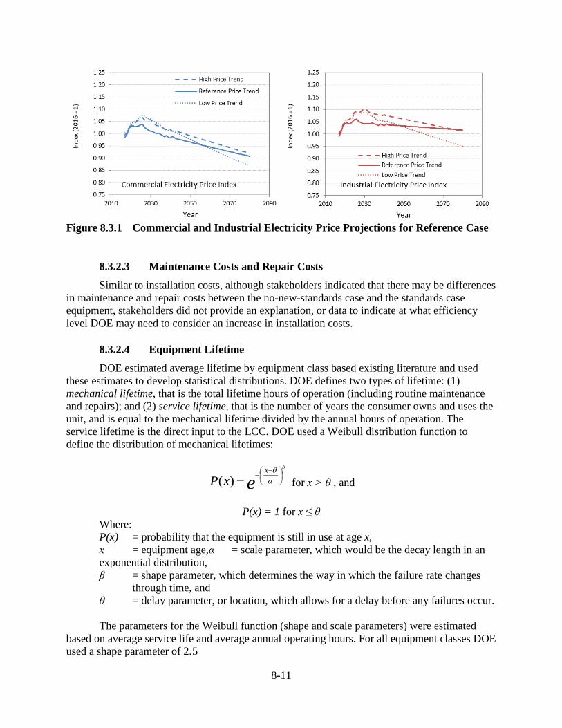
8-11

Figure 8.3.1 Commercial and Industrial Electricity Price Projections for Reference Case

8.3.2.3 Maintenance Costs and Repair Costs

Similar to installation costs, although stakeholders indicated that there may be differences in maintenance and repair costs between the no-new-standards case and the standards case equipment, stakeholders did not provide an explanation, or data to indicate at what efficiency level DOE may need to consider an increase in installation costs.

8.3.2.4 Equipment Lifetime

DOE estimated average lifetime by equipment class based existing literature and used these estimates to develop statistical distributions. DOE defines two types of lifetime: (1) mechanical lifetime, that is the total lifetime hours of operation (including routine maintenance and repairs); and (2) service lifetime, that is the number of years the consumer owns and uses the unit, and is equal to the mechanical lifetime divided by the annual hours of operation. The service lifetime is the direct input to the LCC. DOE used a Weibull distribution function to define the distribution of mechanical lifetimes:

ex

xPβ

αθ

−

−=)( for x > θ , and

P(x) = 1 for x ≤ θ Where: P(x) = probability that the equipment is still in use at age x, x = equipment age,α = scale parameter, which would be the decay length in an exponential distribution, β = shape parameter, which determines the way in which the failure rate changes

through time, and θ = delay parameter, or location, which allows for a delay before any failures occur.

The parameters for the Weibull function (shape and scale parameters) were estimated based on average service life and average annual operating hours. For all equipment classes DOE used a shape parameter of 2.5

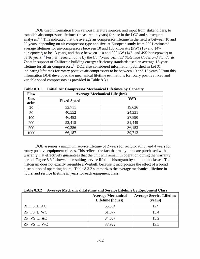
8-12

DOE used information from various literature sources, and input from stakeholders, to

establish air compressor lifetimes (measured in years) for use in the LCC and subsequent analyses.6, 7 This indicated that the average air compressor lifetime in the field is between 10 and 20 years, depending on air compressor type and size. A European study from 2001 estimated average lifetimes for air-compressors between 10 and 100 kilowatts (kW) (13- and 147-horsepower) to be 13 years, and those between 110 and 300 kW (147- and 495-horsepower) to be 16 years.10 Further, research done by the California Utilities' Statewide Codes and Standards Team in support of California building energy efficiency standards used an average 15-year lifetime for all air compressors.11 DOE also considered information published in Lot 31 indicating lifetimes for rotary positive air compressors to be between 10 and 15 years.3 From this information DOE developed the mechanical lifetime estimations for rotary positive fixed and variable speed compressors as provided in Table 8.3.1.

Table 8.3.1 Initial Air Compressor Mechanical Lifetimes by Capacity

Flow Bin, acfm

Average Mechanical Life (hrs)

Fixed Speed VSD

20 32,711 19,626 50 40,552 24,331 100 46,483 27,890 200 52,415 31,449 500 60,256 36,153 1000 66,187 39,712

DOE assumes a minimum service lifetime of 2 years for reciprocating, and 4 years for rotary positive equipment classes. This reflects the fact that many units are purchased with a warranty that effectively guarantees that the unit will remain in operation during the warranty period. Figure 8.3.2 shows the resulting service lifetime histogram by equipment classes. This histogram does not exactly resemble a Weibull, because it incorporates the effect of a broad distribution of operating hours. Table 8.3.2 summarizes the average mechanical lifetime in hours, and service lifetime in years for each equipment class.

Table 8.3.2 Average Mechanical Lifetime and Service Lifetime by Equipment Class

Average Mechanical Lifetime (hours)

Average Service Lifetime (years)

RP_FS_L_AC 55,394 12.9 RP_FS_L_WC 61,877 13.4 RP_VS_L_AC 34,657 13.2 RP_VS_L_WC 37,922 13.5

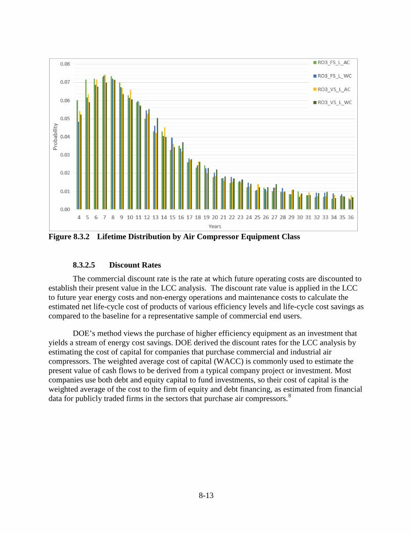
8-13

Figure 8.3.2 Lifetime Distribution by Air Compressor Equipment Class

8.3.2.5 Discount Rates

The commercial discount rate is the rate at which future operating costs are discounted to establish their present value in the LCC analysis. The discount rate value is applied in the LCC to future year energy costs and non-energy operations and maintenance costs to calculate the estimated net life-cycle cost of products of various efficiency levels and life-cycle cost savings as compared to the baseline for a representative sample of commercial end users.

DOE’s method views the purchase of higher efficiency equipment as an investment that yields a stream of energy cost savings. DOE derived the discount rates for the LCC analysis by estimating the cost of capital for companies that purchase commercial and industrial air compressors. The weighted average cost of capital (WACC) is commonly used to estimate the present value of cash flows to be derived from a typical company project or investment. Most companies use both debt and equity capital to fund investments, so their cost of capital is the weighted average of the cost to the firm of equity and debt financing, as estimated from financial data for publicly traded firms in the sectors that purchase air compressors.8

8-14

Damodaran Online is a widely used source of information about company debt and equity financing for most types of firms, and was the primary source of data for this analysis.9 Detailed sectors included in the Damondaran Online database were assigned to the aggregate categories of: buildings commercial and institutional.k

DOE estimated the cost of equity using the capital asset pricing model (CAPM).10 The

CAPM assumes that the cost of equity (ke) for a particular company is proportional to the systematic risk faced by that company, where high risk is associated with a high cost of equity and low risk is associated with a low cost of equity. The systematic risk facing a firm is determined by several variables: the risk coefficient of the firm (β), the expected return on risk-free assets (Rf), and the equity risk premium (ERP). The risk coefficient of the firm indicates the risk associated with that firm relative to the price variability in the stock market. The expected return on risk-free assets is defined by the yield on long-term government bonds. The ERP represents the difference between the expected stock market return and the risk-free rate. The cost of equity financing is estimated using the following equation, where the variables are defined as above:

𝑘𝑘𝑜𝑜 = 𝑅𝑅𝑓𝑓 + (𝛽𝛽 × 𝐸𝐸𝑅𝑅𝐸𝐸)

Where:

ke = cost of equity, Rf = expected return on risk-free assets, β = risk coefficient of the firm, and ERP = equity risk premium.

Several parameters of the cost of capital equations can vary substantially over time, and

therefore the estimates can vary with the time period over which data is selected and the technical details of the data averaging method. For guidance on the time period for selecting and averaging data for key parameters and the averaging method, DOE used Federal Reserve methodologies for calculating these parameters. In its use of the CAPM, the Federal Reserve uses a forty-year period for calculating discount rate averages, utilizes the gross domestic product price deflator for estimating inflation, and considers the best method for determining the risk free rate as one where “the time horizon of the investor is matched with the term of the risk-free security.”11

k http://pages.stern.nyu.edu/~adamodar/

8-15

By taking a forty-year geometric average of Federal Reserve data on annual nominal returns for 10-year Treasury bills, DOE estimated the following risk free rates for 2004-2015 (Table 8.3.3).12 DOE also estimated the ERP by calculating the difference between risk free rate and stock market return for the same time period, as estimated using Damodaran Online data on the historical return to stocks.13

Table 8.3.3 Risk Free Rate and Equity Risk Premium, 2004-2013

Year Risk free rate (%) ERP (%) 2004 7.10% 3.25% 2005 7.11% 3.68% 2006 7.10% 3.49% 2007 7.08% 3.36% 2008 7.01% 2.40% 2009 6.88% 3.07% 2010 6.74% 3.23% 2011 6.61% 2.94% 2012 6.41% 3.99% 2013 6.24% 5.30%

The cost of debt financing (kd) is the interest rate paid on money borrowed by a company.

The cost of debt is estimated by adding a risk adjustment factor (Ra) to the risk-free rate. This risk adjustment factor depends on the variability of stock returns represented by standard deviations in stock prices. So for firm i, the cost of debt financing is:

aifdi RRk +=

Where:

kd = cost of debt financing for firm, i, Rf = expected return on risk-free assets, and Rai = risk adjustment factor to risk-free rate for firm, i.

DOE estimates the WACC using the following equation:

𝑊𝑊𝑊𝑊𝑊𝑊𝑊𝑊 = 𝑘𝑘𝑜𝑜 × 𝑤𝑤𝑜𝑜 + 𝑘𝑘𝑠𝑠 × 𝑤𝑤𝑠𝑠 Where:

WACC = weighted average cost of capital, we = proportion of equity financing, and wd = proportion of debt financing.

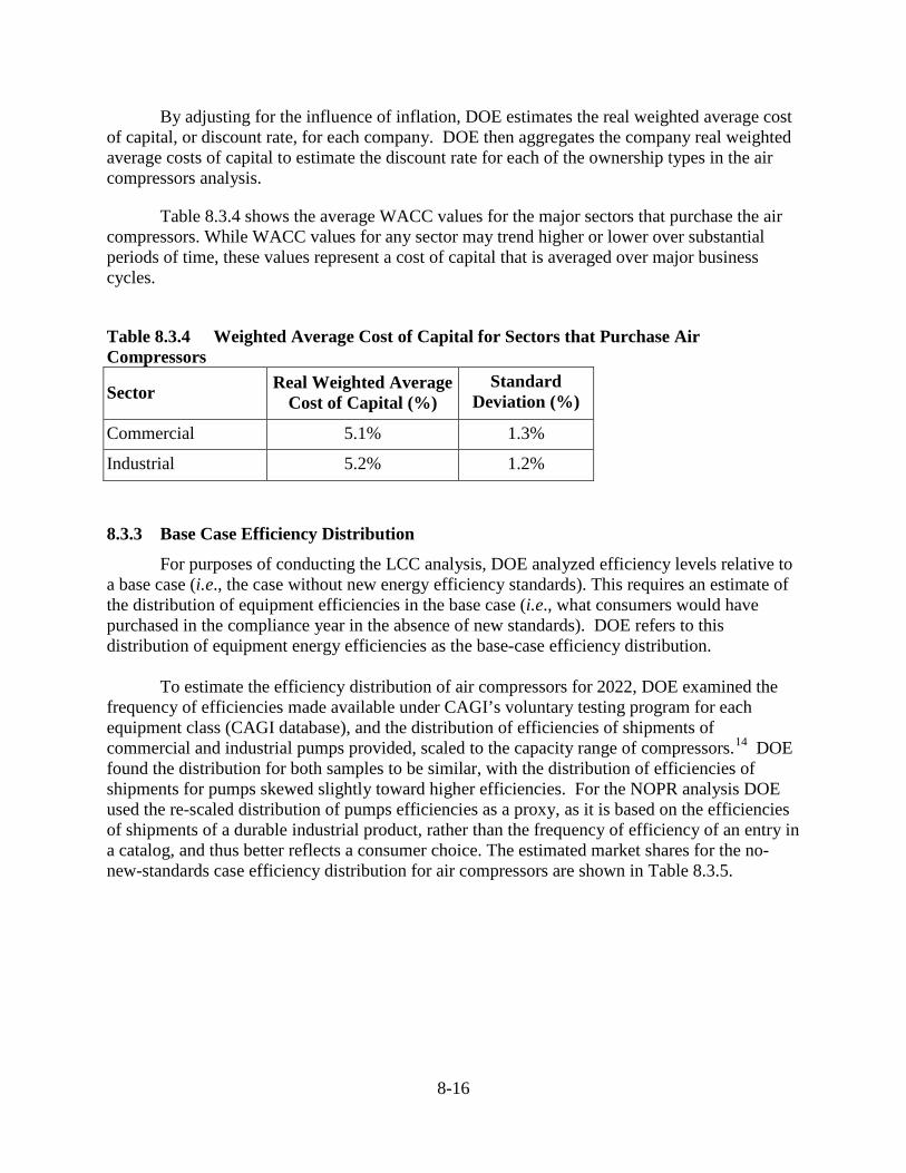
8-16

By adjusting for the influence of inflation, DOE estimates the real weighted average cost of capital, or discount rate, for each company. DOE then aggregates the company real weighted average costs of capital to estimate the discount rate for each of the ownership types in the air compressors analysis.

Table 8.3.4 shows the average WACC values for the major sectors that purchase the air compressors. While WACC values for any sector may trend higher or lower over substantial periods of time, these values represent a cost of capital that is averaged over major business cycles.

Table 8.3.4 Weighted Average Cost of Capital for Sectors that Purchase Air Compressors

Sector Real Weighted Average Cost of Capital (%)

Standard Deviation (%)

Commercial 5.1% 1.3%

Industrial 5.2% 1.2%

Base Case Efficiency Distribution 8.3.3

For purposes of conducting the LCC analysis, DOE analyzed efficiency levels relative to a base case (i.e., the case without new energy efficiency standards). This requires an estimate of the distribution of equipment efficiencies in the base case (i.e., what consumers would have purchased in the compliance year in the absence of new standards). DOE refers to this distribution of equipment energy efficiencies as the base-case efficiency distribution.

To estimate the efficiency distribution of air compressors for 2022, DOE examined the frequency of efficiencies made available under CAGI’s voluntary testing program for each equipment class (CAGI database), and the distribution of efficiencies of shipments of commercial and industrial pumps provided, scaled to the capacity range of compressors.14 DOE found the distribution for both samples to be similar, with the distribution of efficiencies of shipments for pumps skewed slightly toward higher efficiencies. For the NOPR analysis DOE used the re-scaled distribution of pumps efficiencies as a proxy, as it is based on the efficiencies of shipments of a durable industrial product, rather than the frequency of efficiency of an entry in a catalog, and thus better reflects a consumer choice. The estimated market shares for the no-new-standards case efficiency distribution for air compressors are shown in Table 8.3.5.

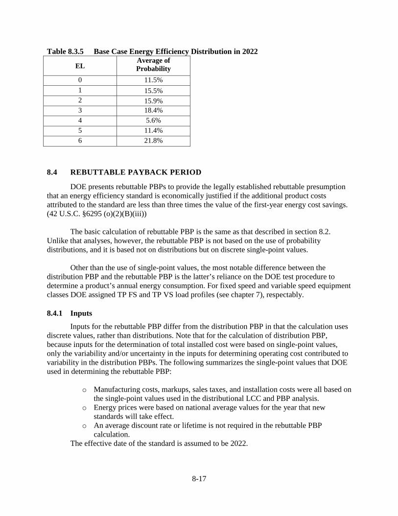
8-17

Table 8.3.5 Base Case Energy Efficiency Distribution in 2022

EL Average of Probability

0 11.5% 1 15.5% 2 15.9% 3 18.4% 4 5.6% 5 11.4% 6 21.8%

8.4 REBUTTABLE PAYBACK PERIOD

DOE presents rebuttable PBPs to provide the legally established rebuttable presumption that an energy efficiency standard is economically justified if the additional product costs attributed to the standard are less than three times the value of the first-year energy cost savings. (42 U.S.C. §6295 (o)(2)(B)(iii)) The basic calculation of rebuttable PBP is the same as that described in section 8.2. Unlike that analyses, however, the rebuttable PBP is not based on the use of probability distributions, and it is based not on distributions but on discrete single-point values.

Other than the use of single-point values, the most notable difference between the distribution PBP and the rebuttable PBP is the latter’s reliance on the DOE test procedure to determine a product’s annual energy consumption. For fixed speed and variable speed equipment classes DOE assigned TP FS and TP VS load profiles (see chapter 7), respectably.

Inputs 8.4.1

Inputs for the rebuttable PBP differ from the distribution PBP in that the calculation uses discrete values, rather than distributions. Note that for the calculation of distribution PBP, because inputs for the determination of total installed cost were based on single-point values, only the variability and/or uncertainty in the inputs for determining operating cost contributed to variability in the distribution PBPs. The following summarizes the single-point values that DOE used in determining the rebuttable PBP:

o Manufacturing costs, markups, sales taxes, and installation costs were all based on the single-point values used in the distributional LCC and PBP analysis.

o Energy prices were based on national average values for the year that new standards will take effect.

o An average discount rate or lifetime is not required in the rebuttable PBP calculation.

The effective date of the standard is assumed to be 2022.

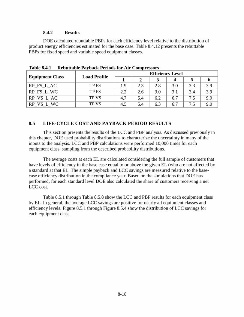
8-18

Results 8.4.2

DOE calculated rebuttable PBPs for each efficiency level relative to the distribution of product energy efficiencies estimated for the base case. Table 8.4.12 presents the rebuttable PBPs for fixed speed and variable speed equipment classes.

Table 8.4.1 Rebuttable Payback Periods for Air Compressors

Equipment Class Load Profile Efficiency Level 1 2 3 4 5 6

RP_FS_L_AC TP FS 1.9 2.3 2.8 3.0 3.3 3.9 RP_FS_L_WC TP FS 2.2 2.6 3.0 3.1 3.4 3.9 RP_VS_L_AC TP VS 4.7 5.4 6.2 6.7 7.5 9.0 RP_VS_L_WC TP VS 4.5 5.4 6.3 6.7 7.5 9.0

8.5 LIFE-CYCLE COST AND PAYBACK PERIOD RESULTS

This section presents the results of the LCC and PBP analysis. As discussed previously in this chapter, DOE used probability distributions to characterize the uncertainty in many of the inputs to the analysis. LCC and PBP calculations were performed 10,000 times for each equipment class, sampling from the described probability distributions.

The average costs at each EL are calculated considering the full sample of customers that have levels of efficiency in the base case equal to or above the given EL (who are not affected by a standard at that EL. The simple payback and LCC savings are measured relative to the base-case efficiency distribution in the compliance year. Based on the simulations that DOE has performed, for each standard level DOE also calculated the share of customers receiving a net LCC cost.

Table 8.5.1 through Table 8.5.8 show the LCC and PBP results for each equipment class by EL. In general, the average LCC savings are positive for nearly all equipment classes and efficiency levels. Figure 8.5.1 through Figure 8.5.4 show the distribution of LCC savings for each equipment class.

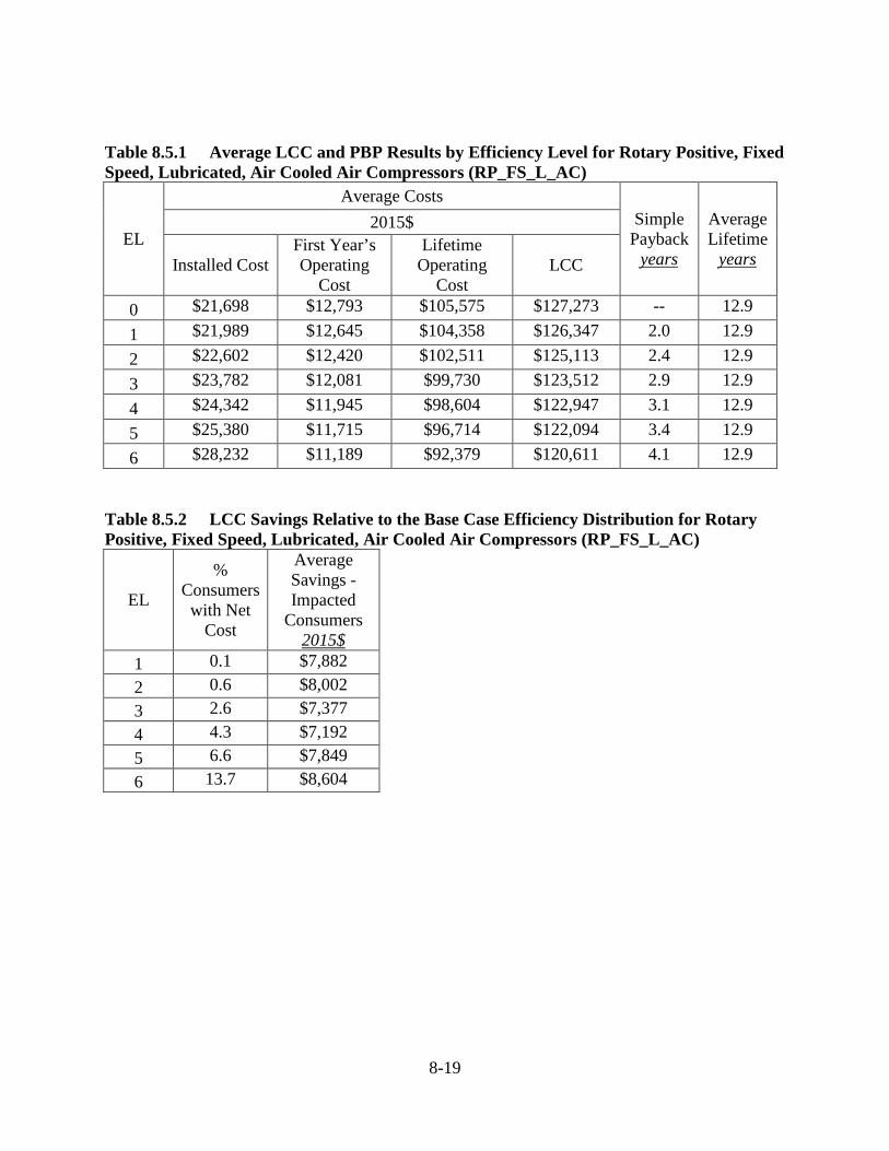
8-19

Table 8.5.1 Average LCC and PBP Results by Efficiency Level for Rotary Positive, Fixed Speed, Lubricated, Air Cooled Air Compressors (RP_FS_L_AC)

EL

Average Costs Simple

Payback years

Average Lifetime

years

2015$

Installed Cost First Year’s Operating

Cost

Lifetime Operating

Cost LCC

0 $21,698 $12,793 $105,575 $127,273 -- 12.9 1 $21,989 $12,645 $104,358 $126,347 2.0 12.9 2 $22,602 $12,420 $102,511 $125,113 2.4 12.9 3 $23,782 $12,081 $99,730 $123,512 2.9 12.9 4 $24,342 $11,945 $98,604 $122,947 3.1 12.9 5 $25,380 $11,715 $96,714 $122,094 3.4 12.9 6 $28,232 $11,189 $92,379 $120,611 4.1 12.9

Table 8.5.2 LCC Savings Relative to the Base Case Efficiency Distribution for Rotary Positive, Fixed Speed, Lubricated, Air Cooled Air Compressors (RP_FS_L_AC)

EL

% Consumers

with Net Cost

Average Savings - Impacted

Consumers 2015$

1 0.1 $7,882 2 0.6 $8,002 3 2.6 $7,377 4 4.3 $7,192 5 6.6 $7,849 6 13.7 $8,604

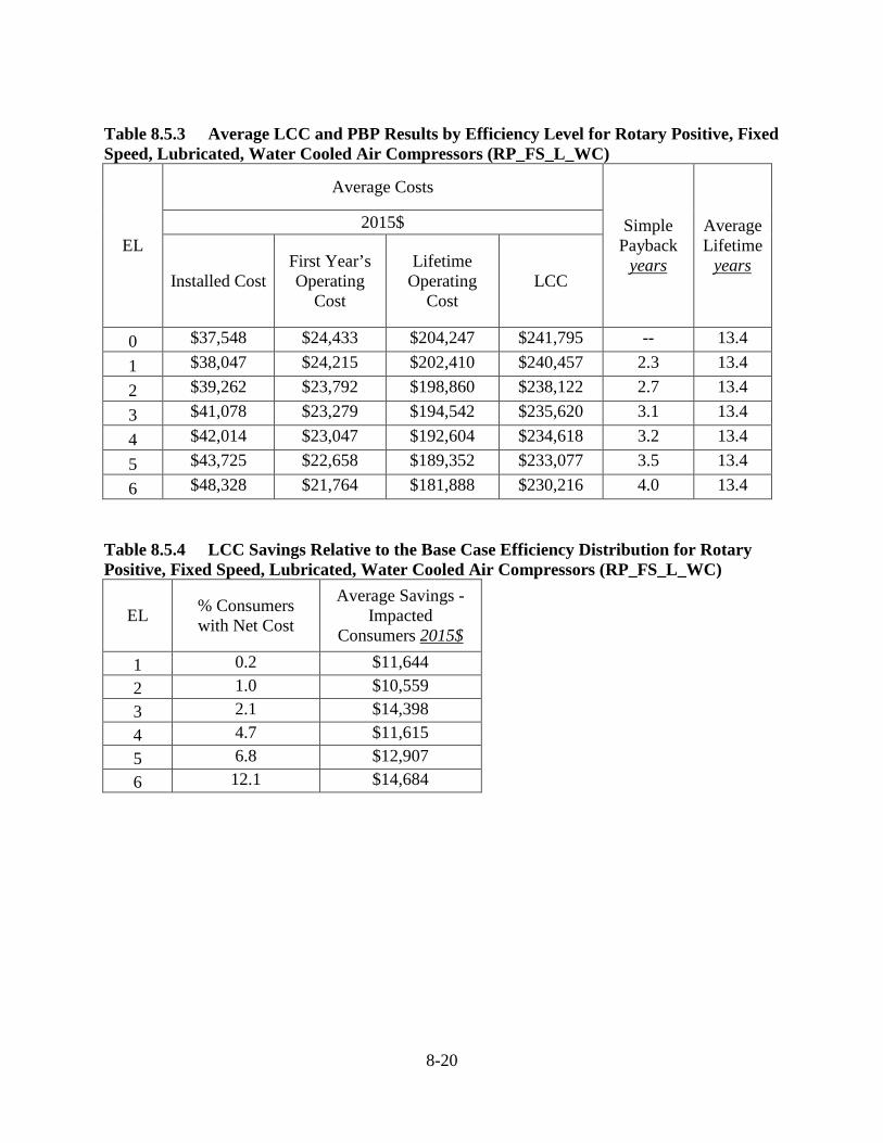
8-20

Table 8.5.3 Average LCC and PBP Results by Efficiency Level for Rotary Positive, Fixed Speed, Lubricated, Water Cooled Air Compressors (RP_FS_L_WC)

EL

Average Costs

Simple Payback

years

Average Lifetime

years

2015$

Installed Cost First Year’s Operating

Cost

Lifetime Operating

Cost LCC

0 $37,548 $24,433 $204,247 $241,795 -- 13.4 1 $38,047 $24,215 $202,410 $240,457 2.3 13.4 2 $39,262 $23,792 $198,860 $238,122 2.7 13.4 3 $41,078 $23,279 $194,542 $235,620 3.1 13.4 4 $42,014 $23,047 $192,604 $234,618 3.2 13.4 5 $43,725 $22,658 $189,352 $233,077 3.5 13.4 6 $48,328 $21,764 $181,888 $230,216 4.0 13.4

Table 8.5.4 LCC Savings Relative to the Base Case Efficiency Distribution for Rotary Positive, Fixed Speed, Lubricated, Water Cooled Air Compressors (RP_FS_L_WC)

EL % Consumers with Net Cost

Average Savings - Impacted

Consumers 2015$

1 0.2 $11,644 2 1.0 $10,559 3 2.1 $14,398 4 4.7 $11,615 5 6.8 $12,907 6 12.1 $14,684

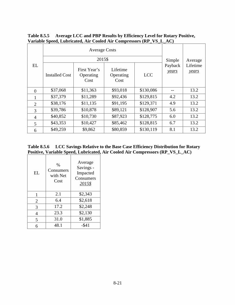
8-21

Table 8.5.5 Average LCC and PBP Results by Efficiency Level for Rotary Positive, Variable Speed, Lubricated, Air Cooled Air Compressors (RP_VS_L_AC)

EL

Average Costs

Simple Payback

years

Average Lifetime

years

2015$

Installed Cost First Year’s Operating

Cost

Lifetime Operating

Cost LCC

0 $37,068 $11,363 $93,018 $130,086 -- 13.2 1 $37,379 $11,289 $92,436 $129,815 4.2 13.2 2 $38,176 $11,135 $91,195 $129,371 4.9 13.2 3 $39,786 $10,878 $89,121 $128,907 5.6 13.2 4 $40,852 $10,730 $87,923 $128,775 6.0 13.2 5 $43,353 $10,427 $85,462 $128,815 6.7 13.2 6 $49,259 $9,862 $80,859 $130,119 8.1 13.2

Table 8.5.6 LCC Savings Relative to the Base Case Efficiency Distribution for Rotary Positive, Variable Speed, Lubricated, Air Cooled Air Compressors (RP_VS_L_AC)

EL

% Consumers

with Net Cost

Average Savings - Impacted

Consumers 2015$

1 2.1 $2,343 2 6.4 $2,618 3 17.2 $2,248 4 23.3 $2,130 5 31.0 $1,885 6 48.1 -$41

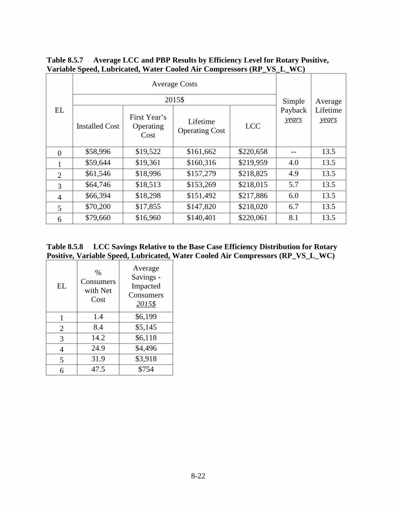
8-22

Table 8.5.7 Average LCC and PBP Results by Efficiency Level for Rotary Positive, Variable Speed, Lubricated, Water Cooled Air Compressors (RP_VS_L_WC)

EL

Average Costs

Simple Payback

years

Average Lifetime

years

2015$

Installed Cost First Year’s Operating

Cost

Lifetime Operating Cost LCC

0 $58,996 $19,522 $161,662 $220,658 -- 13.5 1 $59,644 $19,361 $160,316 $219,959 4.0 13.5 2 $61,546 $18,996 $157,279 $218,825 4.9 13.5 3 $64,746 $18,513 $153,269 $218,015 5.7 13.5 4 $66,394 $18,298 $151,492 $217,886 6.0 13.5 5 $70,200 $17,855 $147,820 $218,020 6.7 13.5 6 $79,660 $16,960 $140,401 $220,061 8.1 13.5

Table 8.5.8 LCC Savings Relative to the Base Case Efficiency Distribution for Rotary Positive, Variable Speed, Lubricated, Water Cooled Air Compressors (RP_VS_L_WC)

EL

% Consumers

with Net Cost

Average Savings - Impacted

Consumers 2015$

1 1.4 $6,199 2 8.4 $5,145 3 14.2 $6,118 4 24.9 $4,496 5 31.9 $3,918 6 47.5 $754

8-23

Figure 8.5.1 Distribution of Life-Cycle Savings for RP_FS_L_AC

Figure 8.5.2 Distribution of Life-Cycle Cost Savings for RP_FS_L_WC

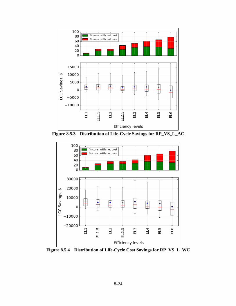
8-24

Figure 8.5.3 Distribution of Life-Cycle Savings for RP_VS_L_AC

Figure 8.5.4 Distribution of Life-Cycle Cost Savings for RP_VS_L_WC

8-25

REFERENCES 1 Strategic Energy Group. Northwest Industrial Motor Database Summary, 2009

2 Washington State University Extension Energy Program (WSU) and Applied Proactive Technologies (APT). Database of Motor Nameplate and Field Measurement Data. New York State Energy Research and Development Authority (NYSERDA), 2011

3 Van Holsteijn en Kemna B.V. (VHK). Ecodesign Preparatory Study on Electric Motor Systems/Compressors; 2014; Prepared for the European Commission by Van Holsteijn en Kemna B.V. (VHK); ENER/C3/413-2010-LOT 31-SI2.612161; http://www.eco-compressors.eu/index.html

4 Edison Electric Institute. Typical Bills and Average Rates Report. Winter 2014 published April 2014, Summer 2014 published October 2014: Washington, D.C. (Last accessed June 2, 2015.) http://www.eei.org/resourcesandmedia/products/Pages/Products.aspx.

5 Barringer & Associates. Weibull Reliability Database For Failure Data For Various Components. (Last accessed July 20, 2015.) http://www.barringer1.com/wdbase.htm.

6Peter Radgen and Edgar Blaustein, Compressed Air Systems in the European Union - Energy, Emissions, Sanvings Potential and Policy Acitions, Stuttgart, 2001,

7 San Diego Gas and Electric, Southern California Gas Company, Southern California Edison, and Pacific Gas and Electric Company, Compressed Air Systems - 2013 California Building Energy Efficiency Standards, 2011

8 Modigliani, F. and M. Miller, The Cost of Capital, Corporations Finance and the Theory of Investment. American Economic Review, 1958. 48(3): pp. 261-297 <http://www.jstor.org/stable/1809766>

9 Damodaran Online, Data Page: Costs of Capital by Industry Sector, 2012. Damodaran. (Last accessed July, 2013.) <http://pages.stern.nyu.edu/~adamodar/>

10 Ibbotson Associates, SBBI Valuation Edition 2009 Yearbook. 2009. Chicago, IL.

11 Federal Reserve Board, Federal Reserve Bank Services Private Sector Adjustment Factor, 2005, 2005. Washington, D.C. <http://www.federalreserve.gov/boarddocs/Press/other/2005/20051012/attachment.pdf>

12 Board of Governors of the Federal Reserve System, H.15 Historical Data Selected Interest Rates, 2013. (Last accessed February, 2013.) <http://www.federalreserve.gov/releases/h15/data.htm>

8-26

13 Damodaran Online, Data Page: Historical Returns on Stocks, Bonds and Bills-United States,

2012. Damodaran. (Last accessed July, 2013.) <http://pages.stern.nyu.edu/~adamodar/>

14 U.S. Department of Energy. Energy Efficiency and Renewable Energy Office. Energy Conservation Program: Energy Conservation Standards for Pumps; Notice of proposed rulemaking (NOPR), 2015. See: http://www.regulations.gov/#!documentDetail;D=EERE-2011-BT-STD-0031-0040

9-i

CHAPTER 9. SHIPMENTS ANALYSIS

TABLE OF CONTENTS

9.1 INTRODUCTION ........................................................................................................... 9-1 9.2 CURRENT SHIPMENTS ................................................................................................ 9-1 9.3 SHIPMENTS PROJECTION .......................................................................................... 9-2

9.3.1 Methodology ........................................................................................................ 9-2 9.3.2 Shipments in the No-new Standards Case ........................................................... 9-4 9.3.3 Shipments in Standards Cases ............................................................................. 9-6 9.3.4 Shipments Results ................................................................................................ 9-7

REFERENCES ............................................................................................................................ 9-8

LIST OF TABLES

Table 9.2.1 In-Scope Air Compressor Shipment Estimates: FY 2013 ............................. 9-2 Table 9.3.1 Rotary Positive Air Compressor Shipment by Capacity (ACFM) ................. 9-5 Table 9.3.3 Share of Rotary Positive Shipments by Capacity and Equipment Class ....... 9-6 Table 9.3.3 Representative Equipment Class Weight for Air Cooled, Oil Injected

Fixed Speed Rotary Positive (RP_FS_L_AC) ............................................... 9-6 Table 9.3.6 Annual and Cumulative Compressor Shipments Projections (thousand

units) .............................................................................................................. 9-7

LIST OF FIGURES

Figure 9.3.1 Medium Electric Motor Shipments Index vs. Private Fixed Investment Index in Selected Equipment and Structure ................................................... 9-3

Figure 9.3.2 Compressor Shipments Index vs. Private Fixed Investment Index in All Equipment ................................................................................................ 9-3

Figure 9.3.3 Shipments Projection by Scenario Case Based on Growth in Private Fixed Investment ............................................................................................ 9-4

Figure 9.3.5 Air Compressor Shipments Projection by Scenario Case .............................. 9-7

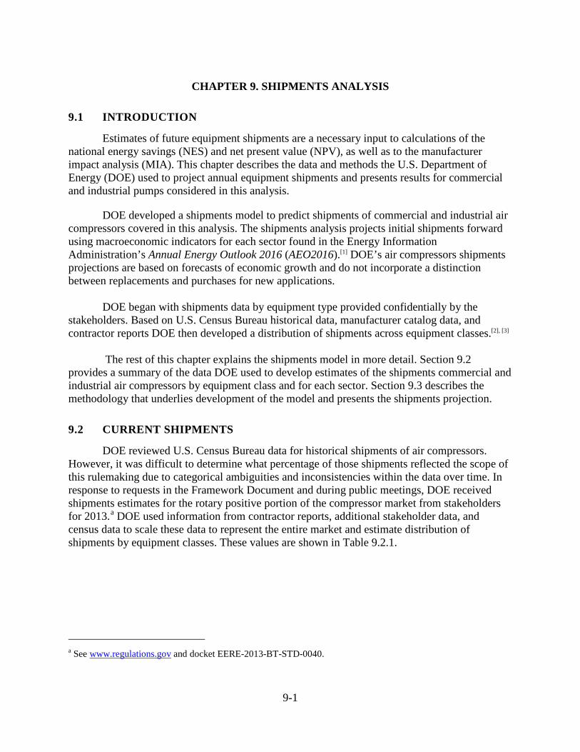
9-1

CHAPTER 9. SHIPMENTS ANALYSIS

9.1 INTRODUCTION

Estimates of future equipment shipments are a necessary input to calculations of the national energy savings (NES) and net present value (NPV), as well as to the manufacturer impact analysis (MIA). This chapter describes the data and methods the U.S. Department of Energy (DOE) used to project annual equipment shipments and presents results for commercial and industrial pumps considered in this analysis.

DOE developed a shipments model to predict shipments of commercial and industrial air compressors covered in this analysis. The shipments analysis projects initial shipments forward using macroeconomic indicators for each sector found in the Energy Information Administration’s Annual Energy Outlook 2016 (AEO2016).[1] DOE’s air compressors shipments projections are based on forecasts of economic growth and do not incorporate a distinction between replacements and purchases for new applications. DOE began with shipments data by equipment type provided confidentially by the stakeholders. Based on U.S. Census Bureau historical data, manufacturer catalog data, and contractor reports DOE then developed a distribution of shipments across equipment classes.[2], [3] The rest of this chapter explains the shipments model in more detail. Section 9.2 provides a summary of the data DOE used to develop estimates of the shipments commercial and industrial air compressors by equipment class and for each sector. Section 9.3 describes the methodology that underlies development of the model and presents the shipments projection.

9.2 CURRENT SHIPMENTS

DOE reviewed U.S. Census Bureau data for historical shipments of air compressors. However, it was difficult to determine what percentage of those shipments reflected the scope of this rulemaking due to categorical ambiguities and inconsistencies within the data over time. In response to requests in the Framework Document and during public meetings, DOE received shipments estimates for the rotary positive portion of the compressor market from stakeholders for 2013.a DOE used information from contractor reports, additional stakeholder data, and census data to scale these data to represent the entire market and estimate distribution of shipments by equipment classes. These values are shown in Table 9.2.1.

a See www.regulations.gov and docket EERE-2013-BT-STD-0040.

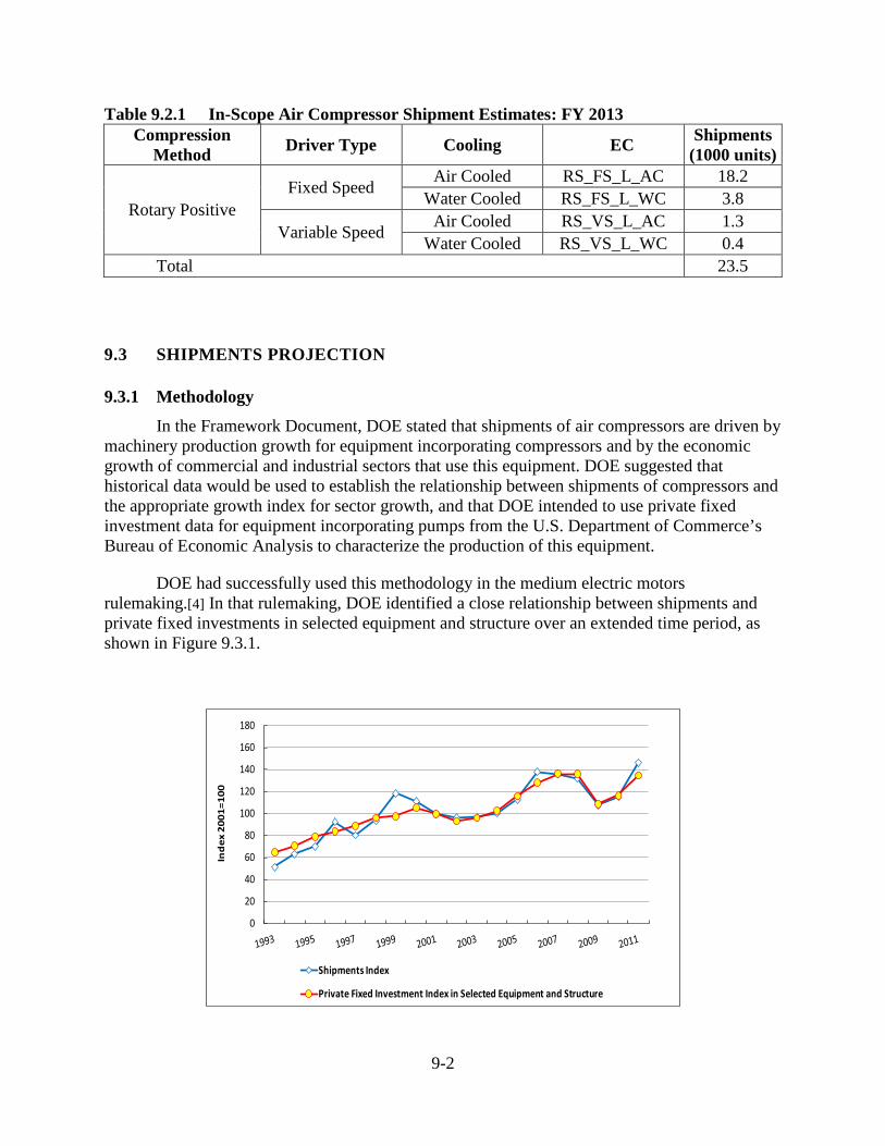
9-2

Table 9.2.1 In-Scope Air Compressor Shipment Estimates: FY 2013 Compression

Method Driver Type Cooling EC Shipments (1000 units)

Rotary Positive Fixed Speed Air Cooled RS_FS_L_AC 18.2

Water Cooled RS_FS_L_WC 3.8

Variable Speed Air Cooled RS_VS_L_AC 1.3 Water Cooled RS_VS_L_WC 0.4

Total 23.5

9.3 SHIPMENTS PROJECTION

9.3.1 Methodology

In the Framework Document, DOE stated that shipments of air compressors are driven by machinery production growth for equipment incorporating compressors and by the economic growth of commercial and industrial sectors that use this equipment. DOE suggested that historical data would be used to establish the relationship between shipments of compressors and the appropriate growth index for sector growth, and that DOE intended to use private fixed investment data for equipment incorporating pumps from the U.S. Department of Commerce’s Bureau of Economic Analysis to characterize the production of this equipment.

DOE had successfully used this methodology in the medium electric motors rulemaking.[4] In that rulemaking, DOE identified a close relationship between shipments and private fixed investments in selected equipment and structure over an extended time period, as shown in Figure 9.3.1.

0

20

40

60

80

100

120

140

160

180

Ind

ex 2

001=

100

Shipments Index

Private Fixed Investment Index in Selected Equipment and Structure

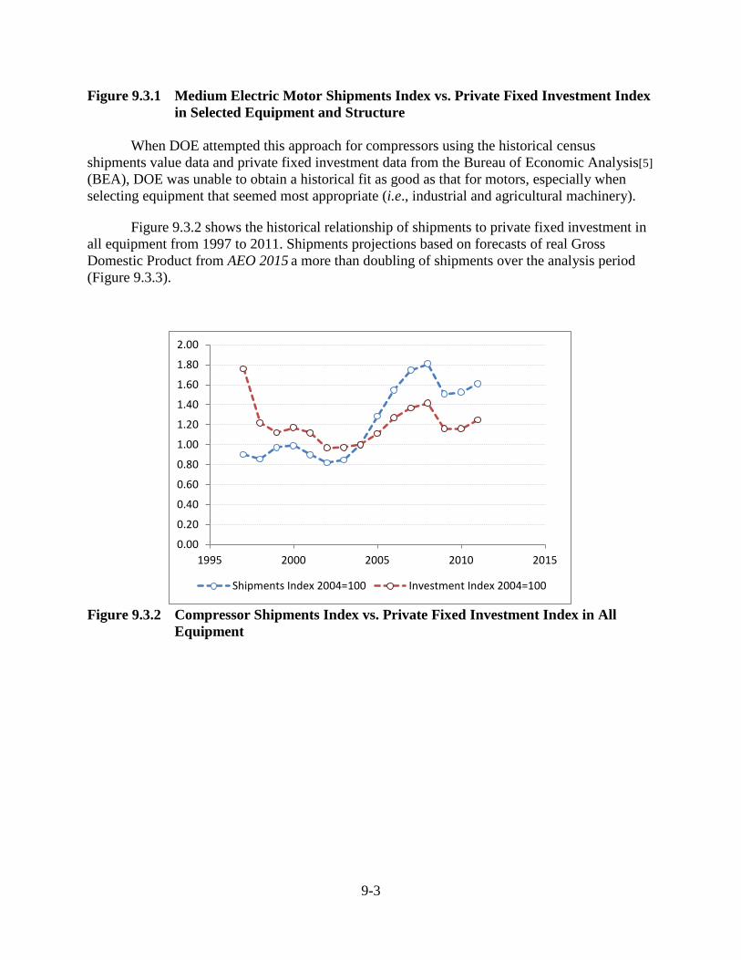
9-3

Figure 9.3.1 Medium Electric Motor Shipments Index vs. Private Fixed Investment Index in Selected Equipment and Structure

When DOE attempted this approach for compressors using the historical census

shipments value data and private fixed investment data from the Bureau of Economic Analysis[5]

(BEA), DOE was unable to obtain a historical fit as good as that for motors, especially when selecting equipment that seemed most appropriate (i.e., industrial and agricultural machinery).

Figure 9.3.2 shows the historical relationship of shipments to private fixed investment in all equipment from 1997 to 2011. Shipments projections based on forecasts of real Gross Domestic Product from AEO 2015 a more than doubling of shipments over the analysis period (Figure 9.3.3).

Figure 9.3.2 Compressor Shipments Index vs. Private Fixed Investment Index in All

Equipment

0.00

0.20

0.40

0.60

0.80

1.00

1.20

1.40

1.60

1.80

2.00

1995 2000 2005 2010 2015

Shipments Index 2004=100 Investment Index 2004=100

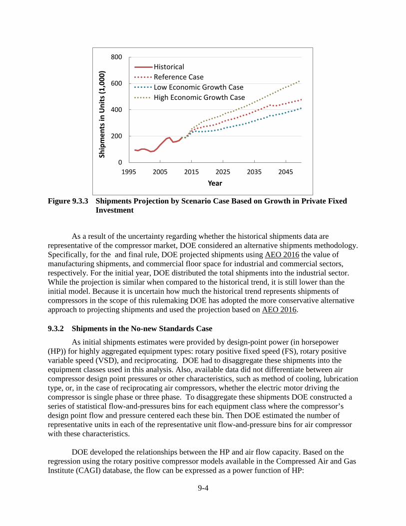
9-4

Figure 9.3.3 Shipments Projection by Scenario Case Based on Growth in Private Fixed

Investment

As a result of the uncertainty regarding whether the historical shipments data are representative of the compressor market, DOE considered an alternative shipments methodology. Specifically, for the and final rule, DOE projected shipments using AEO 2016 the value of manufacturing shipments, and commercial floor space for industrial and commercial sectors, respectively. For the initial year, DOE distributed the total shipments into the industrial sector. While the projection is similar when compared to the historical trend, it is still lower than the initial model. Because it is uncertain how much the historical trend represents shipments of compressors in the scope of this rulemaking DOE has adopted the more conservative alternative approach to projecting shipments and used the projection based on AEO 2016.

9.3.2 Shipments in the No-new Standards Case

As initial shipments estimates were provided by design-point power (in horsepower (HP)) for highly aggregated equipment types: rotary positive fixed speed (FS), rotary positive variable speed (VSD), and reciprocating. DOE had to disaggregate these shipments into the equipment classes used in this analysis. Also, available data did not differentiate between air compressor design point pressures or other characteristics, such as method of cooling, lubrication type, or, in the case of reciprocating air compressors, whether the electric motor driving the compressor is single phase or three phase. To disaggregate these shipments DOE constructed a series of statistical flow-and-pressures bins for each equipment class where the compressor’s design point flow and pressure centered each these bin. Then DOE estimated the number of representative units in each of the representative unit flow-and-pressure bins for air compressor with these characteristics.

DOE developed the relationships between the HP and air flow capacity. Based on the

regression using the rotary positive compressor models available in the Compressed Air and Gas Institute (CAGI) database, the flow can be expressed as a power function of HP:

0

200

400

600

800

1995 2005 2015 2025 2035 2045

Ship

men

ts in

Uni

ts (1

,000

)

Year

HistoricalReference CaseLow Economic Growth CaseHigh Economic Growth Case

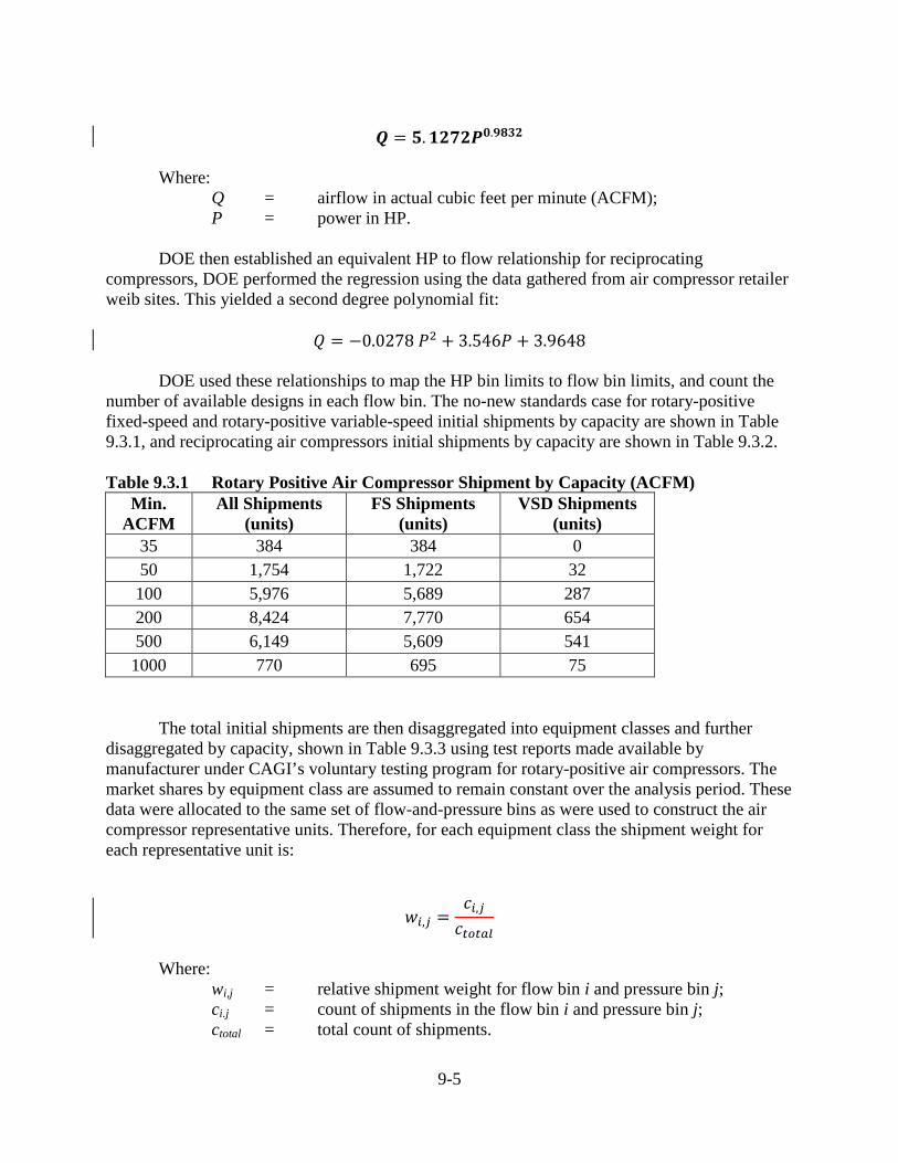
9-5

𝑸𝑸 = 𝟓𝟓.𝟏𝟏𝟏𝟏𝟏𝟏𝟏𝟏𝑷𝑷𝟎𝟎.𝟗𝟗𝟗𝟗𝟗𝟗𝟏𝟏

Where:

Q = airflow in actual cubic feet per minute (ACFM); P = power in HP.

DOE then established an equivalent HP to flow relationship for reciprocating

compressors, DOE performed the regression using the data gathered from air compressor retailer weib sites. This yielded a second degree polynomial fit:

𝑄𝑄 = −0.0278 𝑃𝑃2 + 3.546𝑃𝑃 + 3.9648

DOE used these relationships to map the HP bin limits to flow bin limits, and count the

number of available designs in each flow bin. The no-new standards case for rotary-positive fixed-speed and rotary-positive variable-speed initial shipments by capacity are shown in Table 9.3.1, and reciprocating air compressors initial shipments by capacity are shown in Table 9.3.2.

Table 9.3.1 Rotary Positive Air Compressor Shipment by Capacity (ACFM)

Min. ACFM

All Shipments (units)

FS Shipments (units)

VSD Shipments (units)

35 384 384 0 50 1,754 1,722 32 100 5,976 5,689 287 200 8,424 7,770 654 500 6,149 5,609 541 1000 770 695 75

The total initial shipments are then disaggregated into equipment classes and further disaggregated by capacity, shown in Table 9.3.3 using test reports made available by manufacturer under CAGI’s voluntary testing program for rotary-positive air compressors. The market shares by equipment class are assumed to remain constant over the analysis period. These data were allocated to the same set of flow-and-pressure bins as were used to construct the air compressor representative units. Therefore, for each equipment class the shipment weight for each representative unit is:

𝑤𝑤𝑖𝑖,𝑗𝑗 =

𝑐𝑐𝑖𝑖,𝑗𝑗𝑐𝑐𝑡𝑡𝑡𝑡𝑡𝑡𝑡𝑡𝑡𝑡

Where:

wi,j = relative shipment weight for flow bin i and pressure bin j; ci.j = count of shipments in the flow bin i and pressure bin j; ctotal = total count of shipments.

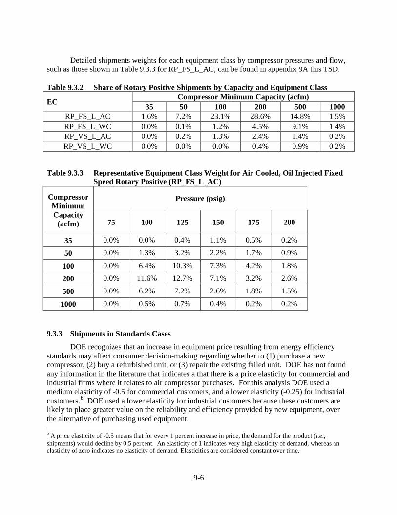
9-6

Detailed shipments weights for each equipment class by compressor pressures and flow,

such as those shown in Table 9.3.3 for RP_FS_L_AC, can be found in appendix 9A this TSD. Table 9.3.2 Share of Rotary Positive Shipments by Capacity and Equipment Class

EC Compressor Minimum Capacity (acfm) 35 50 100 200 500 1000

RP_FS_L_AC 1.6% 7.2% 23.1% 28.6% 14.8% 1.5% RP_FS_L_WC 0.0% 0.1% 1.2% 4.5% 9.1% 1.4% RP_VS_L_AC 0.0% 0.2% 1.3% 2.4% 1.4% 0.2% RP_VS_L_WC 0.0% 0.0% 0.0% 0.4% 0.9% 0.2%

Table 9.3.3 Representative Equipment Class Weight for Air Cooled, Oil Injected Fixed Speed Rotary Positive (RP_FS_L_AC)

Compressor Minimum Capacity

(acfm)

Pressure (psig)

75 100 125 150 175 200

35 0.0% 0.0% 0.4% 1.1% 0.5% 0.2%

50 0.0% 1.3% 3.2% 2.2% 1.7% 0.9%

100 0.0% 6.4% 10.3% 7.3% 4.2% 1.8%

200 0.0% 11.6% 12.7% 7.1% 3.2% 2.6%

500 0.0% 6.2% 7.2% 2.6% 1.8% 1.5%

1000 0.0% 0.5% 0.7% 0.4% 0.2% 0.2%

9.3.3 Shipments in Standards Cases

DOE recognizes that an increase in equipment price resulting from energy efficiency standards may affect consumer decision-making regarding whether to (1) purchase a new compressor, (2) buy a refurbished unit, or (3) repair the existing failed unit. DOE has not found any information in the literature that indicates a that there is a price elasticity for commercial and industrial firms where it relates to air compressor purchases. For this analysis DOE used a medium elasticity of -0.5 for commercial customers, and a lower elasticity (-0.25) for industrial customers.b DOE used a lower elasticity for industrial customers because these customers are likely to place greater value on the reliability and efficiency provided by new equipment, over the alternative of purchasing used equipment. b A price elasticity of -0.5 means that for every 1 percent increase in price, the demand for the product (i.e., shipments) would decline by 0.5 percent. An elasticity of 1 indicates very high elasticity of demand, whereas an elasticity of zero indicates no elasticity of demand. Elasticities are considered constant over time.

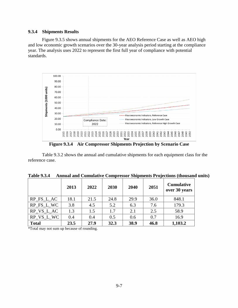
9-7

9.3.4 Shipments Results

Figure 9.3.5 shows annual shipments for the AEO Reference Case as well as AEO high and low economic growth scenarios over the 30-year analysis period starting at the compliance year. The analysis uses 2022 to represent the first full year of compliance with potential standards.

Figure 9.3.4 Air Compressor Shipments Projection by Scenario Case

Table 9.3.2 shows the annual and cumulative shipments for each equipment class for the

reference case.

Table 9.3.4 Annual and Cumulative Compressor Shipments Projections (thousand units)

2013 2022 2030 2040 2051 Cumulative over 30 years

RP_FS_L_AC 18.1 21.5 24.8 29.9 36.0 848.1 RP_FS_L_WC 3.8 4.5 5.2 6.3 7.6 179.3 RP_VS_L_AC 1.3 1.5 1.7 2.1 2.5 58.9 RP_VS_L_WC 0.4 0.4 0.5 0.6 0.7 16.9 Total 23.5 27.9 32.3 38.9 46.8 1,103.2

*Total may not sum up because of rounding.

9-8

REFERENCES

[1] U.S. Energy Information Administration, Annual Energy Outlook 2016, With Projections to

2040. Washington DC: U.S. Department of Energy, 2016.

[2] Manufacturing and Construction Division Census Bureau, “Pumps (except hydraulic) and Compressors - 1960 - 2000,” U.S. Department of Commerce, Washington, DC, 2000 1960.

[3] Manufacturing and Construction Division Census Bureau, “Pumps (except hydraulic) and Compressors - 2001 - 2010,” U.S. Department of Commerce, Washington, DC, 2010 2001.

[4] U.S. Department of Energy, “Technical Support Document: Energy Conservation Program: Energy Conservation Standards for Commercial and Industrial Electric Motors.” U.S. Department of Energy, 05-Dec-2013.

[5] Bureau of Economic Analysis, “Private Fixed Investment in Equipment by Type,” U.S. Department of Commerce, Washington DC.

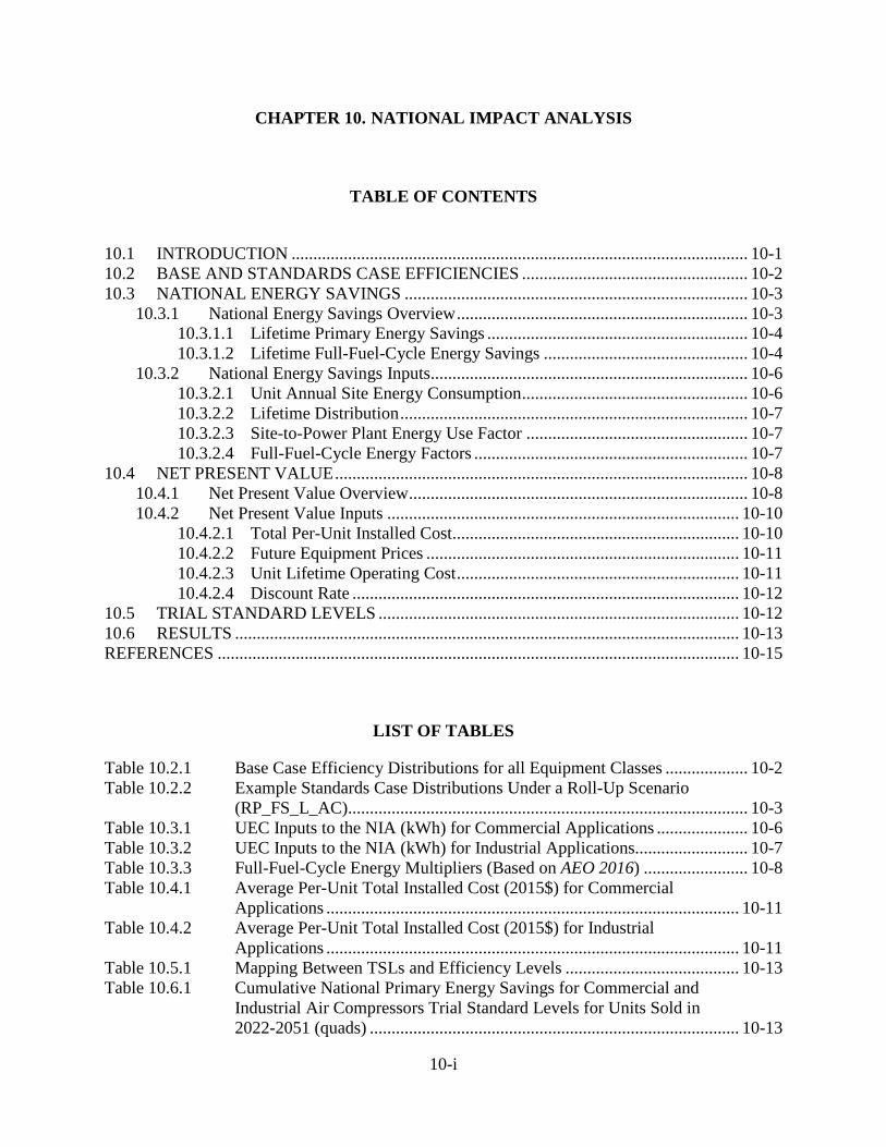
10-i

CHAPTER 10. NATIONAL IMPACT ANALYSIS

TABLE OF CONTENTS

10.1 INTRODUCTION ......................................................................................................... 10-1 10.2 BASE AND STANDARDS CASE EFFICIENCIES .................................................... 10-2 10.3 NATIONAL ENERGY SAVINGS ............................................................................... 10-3

10.3.1 National Energy Savings Overview ................................................................... 10-3 Lifetime Primary Energy Savings ............................................................ 10-4 10.3.1.1 Lifetime Full-Fuel-Cycle Energy Savings ............................................... 10-4 10.3.1.2

10.3.2 National Energy Savings Inputs......................................................................... 10-6 Unit Annual Site Energy Consumption .................................................... 10-6 10.3.2.1 Lifetime Distribution ................................................................................ 10-7 10.3.2.2 Site-to-Power Plant Energy Use Factor ................................................... 10-7 10.3.2.3 Full-Fuel-Cycle Energy Factors ............................................................... 10-7 10.3.2.4

10.4 NET PRESENT VALUE ............................................................................................... 10-8 10.4.1 Net Present Value Overview .............................................................................. 10-8 10.4.2 Net Present Value Inputs ................................................................................. 10-10

Total Per-Unit Installed Cost .................................................................. 10-10 10.4.2.1 Future Equipment Prices ........................................................................ 10-11 10.4.2.2 Unit Lifetime Operating Cost ................................................................. 10-11 10.4.2.3 Discount Rate ......................................................................................... 10-12 10.4.2.4

10.5 TRIAL STANDARD LEVELS ................................................................................... 10-12 10.6 RESULTS .................................................................................................................... 10-13 REFERENCES ........................................................................................................................ 10-15

LIST OF TABLES

Table 10.2.1 Base Case Efficiency Distributions for all Equipment Classes ................... 10-2 Table 10.2.2 Example Standards Case Distributions Under a Roll-Up Scenario

(RP_FS_L_AC)............................................................................................ 10-3 Table 10.3.1 UEC Inputs to the NIA (kWh) for Commercial Applications ..................... 10-6 Table 10.3.2 UEC Inputs to the NIA (kWh) for Industrial Applications.......................... 10-7 Table 10.3.3 Full-Fuel-Cycle Energy Multipliers (Based on AEO 2016) ........................ 10-8 Table 10.4.1 Average Per-Unit Total Installed Cost (2015$) for Commercial

Applications ............................................................................................... 10-11 Table 10.4.2 Average Per-Unit Total Installed Cost (2015$) for Industrial

Applications ............................................................................................... 10-11 Table 10.5.1 Mapping Between TSLs and Efficiency Levels ........................................ 10-13 Table 10.6.1 Cumulative National Primary Energy Savings for Commercial and

Industrial Air Compressors Trial Standard Levels for Units Sold in 2022-2051 (quads) ..................................................................................... 10-13

10-ii

Table 10.6.2 Cumulative National Full-Fuel-Cycle Energy Savings for Commercial and Industrial Air Compressors Trial Standard Levels for Units Sold in 2022-2051 (quads) ..................................................................................... 10-14

Table 10.6.3 Cumulative Net Present Value at a 3-percent Discount Rate of Customer Benefit for Commercial and Industrial Air Compressors Trial Standard Levels for Units Sold in 2022-2051 (billion 2015$) .......... 10-14

Table 10.6.4 Cumulative Net Present Value at a 7-percent Discount Rate of Customer Benefit for Commercial and Industrial Air Compressors Trial Standard Levels for Units Sold in 2022-2051 (billion 2015$) .......... 10-14

LIST OF FIGURES

Figure 10.4.1 Marginal Electricity Price Time Series ...................................................... 10-12

10-1

CHAPTER 10. NATIONAL IMPACT ANALYSIS

10.1 INTRODUCTION

This chapter examines national impacts attributable to each trial standard level (TSL) considered for commercial and industrial air compressors. For each equipment class, DOE evaluated the following impacts: national energy savings (NES) attributable to each potential standard level, monetary value of the lifetime energy savings to customers of the considered equipment, increased total lifetime cost of the equipment because of standards, and net-present value (NPV) resulting from increased energy efficiency (the difference between the energy cost savings and the increased total lifetime cost of the equipment).

To conduct its national impacts analysis (NIA), DOE determined the NES and NPV for each TSL being considered as the new standard for commercial and industrial air compressors. DOE performed all calculations for each considered equipment class using Microsoft Excel spreadsheet models, which are accessible on the Internet.a The spreadsheets combine the calculations for determining the NES and NPV for each considered equipment with input from the appropriate shipments model that DOE used to project future purchases of the considered equipment. Chapter 9 provides a detailed description of the shipments model. The NIA calculation started with the shipments model, which produces a projection of annual shipments of air compressors. DOE used the annual projection of shipments to produce an accounting of annual national energy savings, annual national energy cost savings, and annual national incremental non-energy costs resulting from purchasing, installing and operating the units projected to be shipped in each year of the analysis period during their estimated lifetime. To calculate the annual national energy savings, DOE first estimated the lifetime primary and fuel-fuel-cycleb (FFC) energy consumption at the unit level and for each year in the analysis period, for pumps of each equipment class. The unit’s lifetime primary and FFC energy consumptions were then scaled up to the national level based on the annual shipments projection. This produced, for each equipment class, two streams of annual national energy consumption, from which DOE derived two streams of annual NES from air compressors shipped in each year of the analysis period: one that accounts for primary energy savings, and one that accounts for the FFC energy savings. DOE followed a similar procedure to calculate the annual national energy cost savings and the annual national incremental non-energy costs. DOE first estimated the lifetime energy cost and the lifetime non-energy costs at unit level and for each year in the analysis period, for air compressors of each equipment class. The unit lifetime energy and non-energy costs, estimated for units shipped in each year in the analysis period, were then scaled up to the national level based on the annual shipments projection. This produced, for each equipment a See www.eere.energy.gov/buildings/appliance_standards/ b The full-fuel-cycle energy consumption adds to the primary energy consumption the energy consumed by the energy supply chain upstream to power plants.

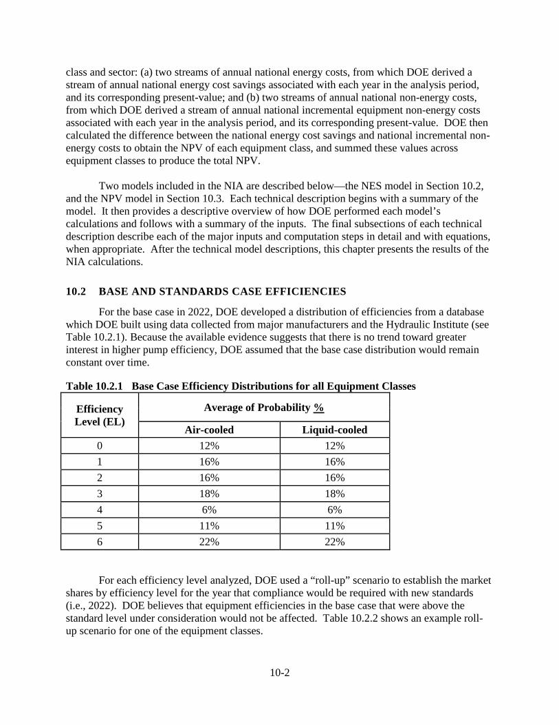
10-2

class and sector: (a) two streams of annual national energy costs, from which DOE derived a stream of annual national energy cost savings associated with each year in the analysis period, and its corresponding present-value; and (b) two streams of annual national non-energy costs, from which DOE derived a stream of annual national incremental equipment non-energy costs associated with each year in the analysis period, and its corresponding present-value. DOE then calculated the difference between the national energy cost savings and national incremental non-energy costs to obtain the NPV of each equipment class, and summed these values across equipment classes to produce the total NPV.

Two models included in the NIA are described below—the NES model in Section 10.2, and the NPV model in Section 10.3. Each technical description begins with a summary of the model. It then provides a descriptive overview of how DOE performed each model’s calculations and follows with a summary of the inputs. The final subsections of each technical description describe each of the major inputs and computation steps in detail and with equations, when appropriate. After the technical model descriptions, this chapter presents the results of the NIA calculations.

10.2 BASE AND STANDARDS CASE EFFICIENCIES

For the base case in 2022, DOE developed a distribution of efficiencies from a database which DOE built using data collected from major manufacturers and the Hydraulic Institute (see Table 10.2.1). Because the available evidence suggests that there is no trend toward greater interest in higher pump efficiency, DOE assumed that the base case distribution would remain constant over time.

Table 10.2.1 Base Case Efficiency Distributions for all Equipment Classes

Efficiency Level (EL)

Average of Probability %

Air-cooled Liquid-cooled 0 12% 12% 1 16% 16% 2 16% 16% 3 18% 18% 4 6% 6% 5 11% 11% 6 22% 22%

For each efficiency level analyzed, DOE used a “roll-up” scenario to establish the market shares by efficiency level for the year that compliance would be required with new standards (i.e., 2022). DOE believes that equipment efficiencies in the base case that were above the standard level under consideration would not be affected. Table 10.2.2 shows an example roll-up scenario for one of the equipment classes.

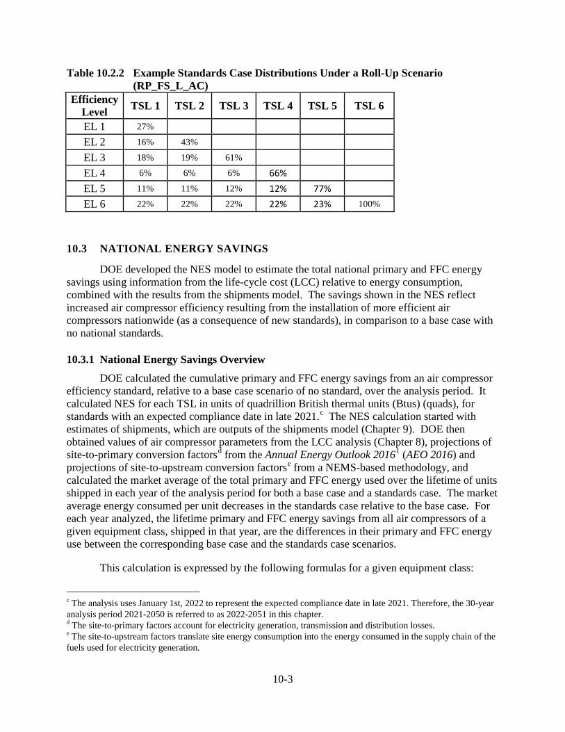
10-3

Table 10.2.2 Example Standards Case Distributions Under a Roll-Up Scenario (RP_FS_L_AC)

Efficiency Level TSL 1 TSL 2 TSL 3 TSL 4 TSL 5 TSL 6

EL 1 27%

EL 2 16% 43%

EL 3 18% 19% 61%

EL 4 6% 6% 6% 66%

EL 5 11% 11% 12% 12% 77%

EL 6 22% 22% 22% 22% 23% 100%

10.3 NATIONAL ENERGY SAVINGS

DOE developed the NES model to estimate the total national primary and FFC energy savings using information from the life-cycle cost (LCC) relative to energy consumption, combined with the results from the shipments model. The savings shown in the NES reflect increased air compressor efficiency resulting from the installation of more efficient air compressors nationwide (as a consequence of new standards), in comparison to a base case with no national standards.

10.3.1 National Energy Savings Overview

DOE calculated the cumulative primary and FFC energy savings from an air compressor efficiency standard, relative to a base case scenario of no standard, over the analysis period. It calculated NES for each TSL in units of quadrillion British thermal units (Btus) (quads), for standards with an expected compliance date in late 2021.c The NES calculation started with estimates of shipments, which are outputs of the shipments model (Chapter 9). DOE then obtained values of air compressor parameters from the LCC analysis (Chapter 8), projections of site-to-primary conversion factorsd from the Annual Energy Outlook 20161 (AEO 2016) and projections of site-to-upstream conversion factorse from a NEMS-based methodology, and calculated the market average of the total primary and FFC energy used over the lifetime of units shipped in each year of the analysis period for both a base case and a standards case. The market average energy consumed per unit decreases in the standards case relative to the base case. For each year analyzed, the lifetime primary and FFC energy savings from all air compressors of a given equipment class, shipped in that year, are the differences in their primary and FFC energy use between the corresponding base case and the standards case scenarios.

This calculation is expressed by the following formulas for a given equipment class:

c The analysis uses January 1st, 2022 to represent the expected compliance date in late 2021. Therefore, the 30-year analysis period 2021-2050 is referred to as 2022-2051 in this chapter. d The site-to-primary factors account for electricity generation, transmission and distribution losses. e The site-to-upstream factors translate site energy consumption into the energy consumed in the supply chain of the fuels used for electricity generation.

10-4

Lifetime Primary Energy Savings 10.3.1.1

𝑛𝑛𝑛𝑛𝑛𝑛𝑛𝑛(𝑦𝑦) = 𝑛𝑛𝑛𝑛𝑛𝑛𝑛𝑛𝑛𝑛𝑛𝑛(𝑦𝑦) − 𝑛𝑛𝑛𝑛𝑛𝑛𝑛𝑛𝑛𝑛𝑛𝑛𝑛𝑛(𝑦𝑦) 𝑛𝑛𝑛𝑛𝑛𝑛𝑛𝑛𝑛𝑛𝑛𝑛(𝑦𝑦) = 𝑛𝑛ℎ𝑝𝑝(𝑦𝑦) ∙ ∑ �𝑢𝑢𝑛𝑛𝑛𝑛𝑛𝑛𝑐𝑐(𝑦𝑦) ∙ 𝑀𝑀𝑛𝑛𝑛𝑛𝑐𝑐(𝑦𝑦)�𝑐𝑐 𝑛𝑛𝑛𝑛𝑛𝑛𝑛𝑛𝑛𝑛𝑛𝑛𝑛𝑛(𝑦𝑦) = 𝑛𝑛ℎ𝑝𝑝(𝑦𝑦) ∙ ∑ �𝑢𝑢𝑛𝑛𝑛𝑛𝑛𝑛𝑐𝑐(𝑦𝑦) ∙ 𝑀𝑀𝑛𝑛𝑛𝑛𝑛𝑛𝑐𝑐(𝑦𝑦)�𝑐𝑐 𝑢𝑢𝑛𝑛𝑛𝑛𝑛𝑛𝑐𝑐(𝑦𝑦) = ∑ 𝑎𝑎𝑛𝑛𝑛𝑛𝑛𝑛𝑐𝑐(𝑦𝑦, 𝑖𝑖)𝑖𝑖=1..𝐿𝐿𝐿𝐿 where: 𝑛𝑛𝑛𝑛𝑛𝑛𝑛𝑛(𝑦𝑦) = the lifetime primary energy savings of all air compressors shipped in year y, 𝑛𝑛𝑛𝑛𝑛𝑛𝑛𝑛𝑛𝑛𝑛𝑛(𝑦𝑦) = the base case, lifetime primary energy consumption of air compressors

shipped in year y, 𝑛𝑛𝑛𝑛𝑛𝑛𝑛𝑛𝑛𝑛𝑛𝑛𝑛𝑛(𝑦𝑦) = the standards case, lifetime primary energy consumption of air compressors

shipped in year y, 𝑛𝑛ℎ𝑝𝑝(𝑦𝑦) = the number of air compressors shipped in year y, 𝑢𝑢𝑛𝑛𝑛𝑛𝑛𝑛𝑐𝑐(𝑦𝑦) = the lifetime primary energy consumption of a unit with efficiency level at

EL c shipped in year y, 𝑎𝑎𝑛𝑛𝑛𝑛𝑛𝑛𝑐𝑐(𝑦𝑦, 𝑖𝑖) = the annual primary energy consumption in the 𝑖𝑖-th year of operation of a

unit with efficiency level at EL c, shipped in year y, 𝑀𝑀𝑛𝑛𝑛𝑛𝑐𝑐(𝑦𝑦) = the base case market share of units with efficiency level at EL c shipped in

year y, and 𝑀𝑀𝑛𝑛𝑛𝑛𝑛𝑛𝑐𝑐(𝑦𝑦) = the standards case market share of units with efficiency level at EL c

shipped in year y.

Lifetime Full-Fuel-Cycle Energy Savings 10.3.1.2

𝑛𝑛𝑛𝑛𝑛𝑛𝑛𝑛(𝑦𝑦) = 𝑛𝑛𝑛𝑛𝑛𝑛𝑛𝑛𝑛𝑛𝑛𝑛(𝑦𝑦) − 𝑛𝑛𝑛𝑛𝑛𝑛𝑛𝑛𝑛𝑛𝑛𝑛𝑛𝑛(𝑦𝑦) 𝑛𝑛𝑛𝑛𝑛𝑛𝑛𝑛𝑛𝑛𝑛𝑛(𝑦𝑦) = 𝑛𝑛ℎ𝑝𝑝(𝑦𝑦) ∙ ∑ �𝑢𝑢𝑛𝑛𝑛𝑛𝑛𝑛𝑐𝑐(𝑦𝑦) ∙ 𝑀𝑀𝑛𝑛𝑛𝑛𝑐𝑐(𝑦𝑦)�𝑐𝑐 𝑛𝑛𝑛𝑛𝑛𝑛𝑛𝑛𝑛𝑛𝑛𝑛𝑛𝑛(𝑦𝑦) = 𝑛𝑛ℎ𝑝𝑝(𝑦𝑦) ∙ ∑ �𝑢𝑢𝑛𝑛𝑛𝑛𝑛𝑛𝑐𝑐(𝑦𝑦) ∙ 𝑀𝑀𝑛𝑛𝑛𝑛𝑛𝑛𝑐𝑐(𝑦𝑦)�𝑐𝑐 𝑢𝑢𝑛𝑛𝑛𝑛𝑛𝑛𝑐𝑐(𝑦𝑦) = ∑ �𝑎𝑎𝑛𝑛𝑛𝑛𝑛𝑛𝑐𝑐(𝑦𝑦, 𝑖𝑖) ∙ 𝑓𝑓𝑓𝑓𝑛𝑛(𝑦𝑦 + 𝑖𝑖 − 1)�𝑖𝑖=1..𝐿𝐿𝐿𝐿

10-5

where:

𝑛𝑛𝑛𝑛𝑛𝑛𝑛𝑛(𝑦𝑦) = the lifetime FFC energy savings of all air compressors shipped in year y,

𝑛𝑛𝑛𝑛𝑛𝑛𝑛𝑛𝑛𝑛𝑛𝑛(𝑦𝑦) = the base case, lifetime FFC energy consumption of air compressors shipped in year y,

𝑛𝑛𝑛𝑛𝑛𝑛𝑛𝑛𝑛𝑛𝑛𝑛𝑛𝑛(𝑦𝑦) = the standards case, lifetime FFC energy consumption of air compressors shipped in year y,

𝑛𝑛ℎ𝑝𝑝(𝑦𝑦) = the number of air compressors shipped in year y, 𝑢𝑢𝑛𝑛𝑛𝑛𝑛𝑛𝑐𝑐(𝑦𝑦) = the lifetime FFC energy consumption of a unit with efficiency

level at EL c shipped in year y, 𝑎𝑎𝑛𝑛𝑛𝑛𝑛𝑛𝑐𝑐(𝑦𝑦, 𝑖𝑖) = the annual primary energy consumption in the 𝑖𝑖-th year of

operation of a unit with efficiency level at EL c, shipped in year y, 𝑓𝑓𝑓𝑓𝑛𝑛(𝑦𝑦) = the primary-to-FFC conversion factor in year y, 𝑀𝑀𝑛𝑛𝑛𝑛𝑐𝑐(𝑦𝑦) = the base case market share of units with efficiency level at EL c

shipped in year y, and 𝑀𝑀𝑛𝑛𝑛𝑛𝑛𝑛𝑐𝑐(𝑦𝑦) = the standards case market share of units with efficiency level at EL

c shipped in year y. DOE used the lifetime primary and FFC energy savings estimated for all air compressors shipped from 2022 through 2051 to calculate the total primary NES (𝑁𝑁𝑛𝑛𝑛𝑛𝑠𝑠𝑠𝑠𝑐𝑐) and the total FFC NES (𝑁𝑁𝑛𝑛𝑛𝑛𝐹𝐹𝐹𝐹𝐹𝐹) for the analysis period. The calculation used the following formulas: 𝑁𝑁𝑛𝑛𝑛𝑛𝑠𝑠𝑠𝑠𝑐𝑐 = ∑ 𝑛𝑛𝑛𝑛𝑛𝑛𝑛𝑛(𝑦𝑦)2051

𝑦𝑦=2022 𝑁𝑁𝑛𝑛𝑛𝑛𝐹𝐹𝐹𝐹𝐹𝐹 = ∑ 𝑛𝑛𝑛𝑛𝑛𝑛𝑛𝑛(𝑦𝑦)2051

𝑦𝑦=2022

where:

𝑛𝑛𝑛𝑛𝑛𝑛𝑛𝑛(𝑦𝑦) = the lifetime primary energy savings of all air compressors shipped in year y, and

𝑛𝑛𝑛𝑛𝑛𝑛𝑛𝑛(𝑦𝑦) = the lifetime FFC energy savings of all air compressors shipped in year y.

Once the shipments model provides the estimate of shipments, and the site-to-primary and site-to-upstream factors convert site energy consumption respectively into primary and upstream energy consumption, the key to the NES calculation is in calculating the unit annual site energy consumption and market share distributions using inputs from the LCC analysis. The next section summarizes the inputs necessary for the NES calculation and then presents them individually; the following sections detail, respectively, how the unit lifetime site energy consumption and the standards case efficiency distribution were calculated.

10-6

10.3.2 National Energy Savings Inputs

The NES model inputs include: (a) the unit site energy consumption, (b) the site-to-primary conversion factors, which enable the calculation of primary energy consumption from site energy use, (c) the site-to-upstream conversion factors which – in addition to the site-to-primary factors – enable the calculation of FFC energy consumption from site energy use, and (d) shipment efficiency distributions, which were discussed in the previous section. The list of NES model inputs is as follows:

• unit annual site energy consumption;

• lifetime (probability) distribution;

• electricity site-to-primary conversion factors; and

• electricity site-to-upstream conversion factors.

Unit Annual Site Energy Consumption 10.3.2.1

The unit annual site energy consumption expresses an estimate of the amount of site energy that an air compressors of a given equipment class, meeting the efficiency level of a given EL, and shipped in a given year will consume in each year of its lifetime.

The average per-unit annual energy consumption for each equipment class and efficiency level was calculated in the LCC. In the base case, the distribution of horsepower within each efficiency bin differs. As a result, average energy use may not decrease monotonically as efficiency level increases. In addition, in each standards case, the per-unit annual energy consumption at the minimum efficiency level differs from that in the base case.

DOE uses a shipment and air compressor capacity-weighted average annual UEC for both commercial and industrial applications in its calculation of the national AEC. This takes into account that the markets include shipments of equipment with a broad range of efficiencies and capacities (see chapter 5 for details on air compressor capacities), as shown in section 10.2. The capacity-weighted average UEC for each EC are shown in Table 10.3.1 and Table 10.3.2.

Table 10.3.1 UEC Inputs to the NIA (kWh) for Commercial Applications Equipment Class EL 0 EL 1 EL 2 EL 3 EL 4 EL 5 EL 6

RP_FS_L_AC 43,080 42,209 40,860 39,074 38,433 37,381 34,999

RP_FS_L_WC 52,671 51,965 50,274 48,299 47,383 45,935 42,996

RP_VS_L_AC 43,464 42,993 41,945 40,292 39,358 37,538 34,274

RP_VS_L_WC - - - - - - -

10-7

Table 10.3.2 UEC Inputs to the NIA (kWh) for Industrial Applications Equipment Class EL 0 EL 1 EL 2 EL 3 EL 4 EL 5 EL 6

RP_FS_L_AC 152,935 151,188 148,528 144,520 142,895 140,168 133,915

RP_FS_L_WC 284,457 281,915 277,000 271,040 268,342 263,812 253,410

RP_VS_L_AC 133,375 132,519 130,717 127,725 125,999 122,456 115,856

RP_VS_L_WC 226,302 224,430 220,200 214,598 212,114 206,971 196,600

Lifetime Distribution 10.3.2.2

For the NIA, DOE uses a distribution of air compressors lifetime in years as determined in the LCC (chapter 8). Each air compressors will consume its annual UEC in each year of its lifetime.

Site-to-Power Plant Energy Use Factor 10.3.2.3

In determining national annual energy consumption, DOE initially calculated the annual energy consumption at the site (for electricity, the energy in kWh consumed at the household. DOE then applied a conversion factor to site energy consumption to account for losses associated with the generation, transmission, and distribution of electricity. This multiplicative site-to-power-plant conversion factor converts site energy consumption into primary energy consumption, expressed in quadrillion Btus (quads).

DOE used annual site-to-power-plant conversion factors based on the version of the National Energy Modeling System (NEMS)f that corresponds to DOE’s Energy Information Administration’s (EIA’s) Annual Energy Outlook 2016 (AEO2016).1 The factors are marginal values, which represent the response of the system to an incremental decrease in consumption. For electricity, the conversion factors change over time in response to projected changes in generation sources (that is, the types of power plants projected to provide electricity to the Nation). The value AEO2016 reported for 2040 (the last year available in AEO2016) was extrapolated through the end of the projection period (2051).

Full-Fuel-Cycle Energy Factors 10.3.2.4

The full-fuel-cycle (FFC) includes point-of-use (site) energy; the energy losses associated with generation, transmission, and distribution of electricity; and the energy consumed in extracting, processing, and transporting or distributing primary fuels. To estimate the FFC by including the energy consumed in extracting, processing, and transporting or distributing primary fuels, which we refer to as “upstream” activities, DOE developed FFC multipliersg using the data f For more information on NEMS, refer to the U.S. Department of Energy, Energy Information Administration documentation. A useful summary is National Energy Modeling System: An Overview 2000, DOE/EIA-0581(2000), March 2000.

g FFC multipliers discussed in this chapter relate to the upstream part of the FFC process.

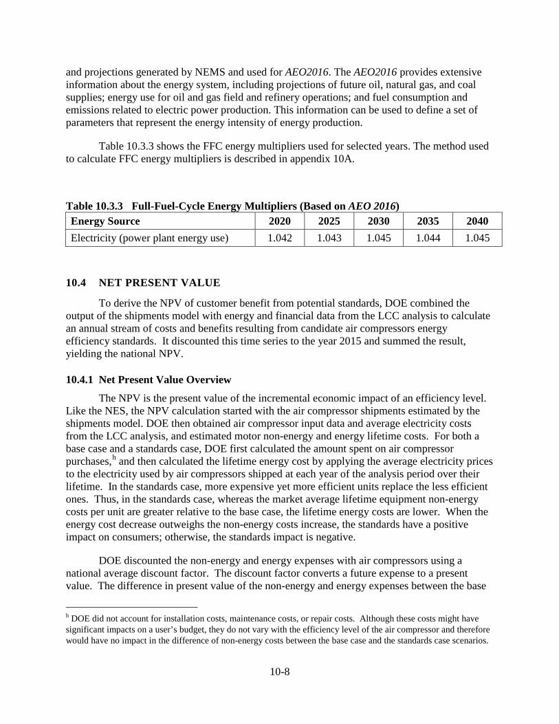
10-8

and projections generated by NEMS and used for AEO2016. The AEO2016 provides extensive information about the energy system, including projections of future oil, natural gas, and coal supplies; energy use for oil and gas field and refinery operations; and fuel consumption and emissions related to electric power production. This information can be used to define a set of parameters that represent the energy intensity of energy production.

Table 10.3.3 shows the FFC energy multipliers used for selected years. The method used to calculate FFC energy multipliers is described in appendix 10A.

Table 10.3.3 Full-Fuel-Cycle Energy Multipliers (Based on AEO 2016) Energy Source 2020 2025 2030 2035 2040 Electricity (power plant energy use) 1.042 1.043 1.045 1.044 1.045

10.4 NET PRESENT VALUE

To derive the NPV of customer benefit from potential standards, DOE combined the output of the shipments model with energy and financial data from the LCC analysis to calculate an annual stream of costs and benefits resulting from candidate air compressors energy efficiency standards. It discounted this time series to the year 2015 and summed the result, yielding the national NPV.

10.4.1 Net Present Value Overview

The NPV is the present value of the incremental economic impact of an efficiency level. Like the NES, the NPV calculation started with the air compressor shipments estimated by the shipments model. DOE then obtained air compressor input data and average electricity costs from the LCC analysis, and estimated motor non-energy and energy lifetime costs. For both a base case and a standards case, DOE first calculated the amount spent on air compressor purchases,h and then calculated the lifetime energy cost by applying the average electricity prices to the electricity used by air compressors shipped at each year of the analysis period over their lifetime. In the standards case, more expensive yet more efficient units replace the less efficient ones. Thus, in the standards case, whereas the market average lifetime equipment non-energy costs per unit are greater relative to the base case, the lifetime energy costs are lower. When the energy cost decrease outweighs the non-energy costs increase, the standards have a positive impact on consumers; otherwise, the standards impact is negative.

DOE discounted the non-energy and energy expenses with air compressors using a national average discount factor. The discount factor converts a future expense to a present value. The difference in present value of the non-energy and energy expenses between the base

h DOE did not account for installation costs, maintenance costs, or repair costs. Although these costs might have significant impacts on a user’s budget, they do not vary with the efficiency level of the air compressor and therefore would have no impact in the difference of non-energy costs between the base case and the standards case scenarios.

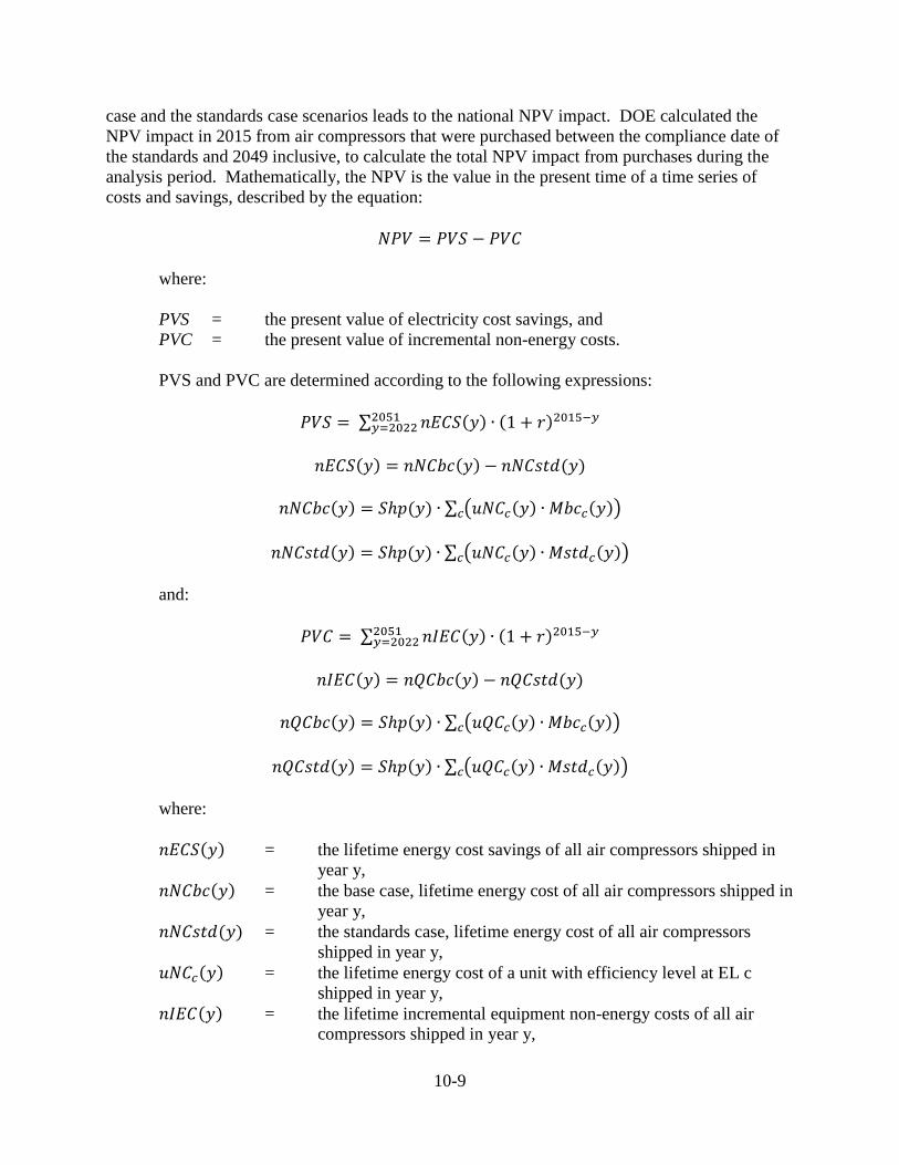
10-9

case and the standards case scenarios leads to the national NPV impact. DOE calculated the NPV impact in 2015 from air compressors that were purchased between the compliance date of the standards and 2049 inclusive, to calculate the total NPV impact from purchases during the analysis period. Mathematically, the NPV is the value in the present time of a time series of costs and savings, described by the equation: 𝑁𝑁𝑁𝑁𝑁𝑁 = 𝑁𝑁𝑁𝑁𝑛𝑛 − 𝑁𝑁𝑁𝑁𝑛𝑛

where:

PVS = the present value of electricity cost savings, and PVC = the present value of incremental non-energy costs.

PVS and PVC are determined according to the following expressions:

𝑁𝑁𝑁𝑁𝑛𝑛 = ∑ 𝑛𝑛𝑛𝑛𝑛𝑛𝑛𝑛(𝑦𝑦) ∙ (1 + 𝑟𝑟)2015−𝑦𝑦2051

𝑦𝑦=2022 𝑛𝑛𝑛𝑛𝑛𝑛𝑛𝑛(𝑦𝑦) = 𝑛𝑛𝑁𝑁𝑛𝑛𝑛𝑛𝑛𝑛(𝑦𝑦) − 𝑛𝑛𝑁𝑁𝑛𝑛𝑛𝑛𝑛𝑛𝑛𝑛(𝑦𝑦) 𝑛𝑛𝑁𝑁𝑛𝑛𝑛𝑛𝑛𝑛(𝑦𝑦) = 𝑛𝑛ℎ𝑝𝑝(𝑦𝑦) ∙ ∑ �𝑢𝑢𝑁𝑁𝑛𝑛𝑐𝑐(𝑦𝑦) ∙ 𝑀𝑀𝑛𝑛𝑛𝑛𝑐𝑐(𝑦𝑦)�𝑐𝑐 𝑛𝑛𝑁𝑁𝑛𝑛𝑛𝑛𝑛𝑛𝑛𝑛(𝑦𝑦) = 𝑛𝑛ℎ𝑝𝑝(𝑦𝑦) ∙ ∑ �𝑢𝑢𝑁𝑁𝑛𝑛𝑐𝑐(𝑦𝑦) ∙ 𝑀𝑀𝑛𝑛𝑛𝑛𝑛𝑛𝑐𝑐(𝑦𝑦)�𝑐𝑐

and: 𝑁𝑁𝑁𝑁𝑛𝑛 = ∑ 𝑛𝑛𝑛𝑛𝑛𝑛𝑛𝑛(𝑦𝑦) ∙ (1 + 𝑟𝑟)2015−𝑦𝑦2051

𝑦𝑦=2022 𝑛𝑛𝑛𝑛𝑛𝑛𝑛𝑛(𝑦𝑦) = 𝑛𝑛𝑛𝑛𝑛𝑛𝑛𝑛𝑛𝑛(𝑦𝑦) − 𝑛𝑛𝑛𝑛𝑛𝑛𝑛𝑛𝑛𝑛𝑛𝑛(𝑦𝑦) 𝑛𝑛𝑛𝑛𝑛𝑛𝑛𝑛𝑛𝑛(𝑦𝑦) = 𝑛𝑛ℎ𝑝𝑝(𝑦𝑦) ∙ ∑ �𝑢𝑢𝑛𝑛𝑛𝑛𝑐𝑐(𝑦𝑦) ∙ 𝑀𝑀𝑛𝑛𝑛𝑛𝑐𝑐(𝑦𝑦)�𝑐𝑐 𝑛𝑛𝑛𝑛𝑛𝑛𝑛𝑛𝑛𝑛𝑛𝑛(𝑦𝑦) = 𝑛𝑛ℎ𝑝𝑝(𝑦𝑦) ∙ ∑ �𝑢𝑢𝑛𝑛𝑛𝑛𝑐𝑐(𝑦𝑦) ∙ 𝑀𝑀𝑛𝑛𝑛𝑛𝑛𝑛𝑐𝑐(𝑦𝑦)�𝑐𝑐

where:

𝑛𝑛𝑛𝑛𝑛𝑛𝑛𝑛(𝑦𝑦) = the lifetime energy cost savings of all air compressors shipped in year y,

𝑛𝑛𝑁𝑁𝑛𝑛𝑛𝑛𝑛𝑛(𝑦𝑦) = the base case, lifetime energy cost of all air compressors shipped in year y,

𝑛𝑛𝑁𝑁𝑛𝑛𝑛𝑛𝑛𝑛𝑛𝑛(𝑦𝑦) = the standards case, lifetime energy cost of all air compressors shipped in year y,

𝑢𝑢𝑁𝑁𝑛𝑛𝑐𝑐(𝑦𝑦) = the lifetime energy cost of a unit with efficiency level at EL c shipped in year y,

𝑛𝑛𝑛𝑛𝑛𝑛𝑛𝑛(𝑦𝑦) = the lifetime incremental equipment non-energy costs of all air compressors shipped in year y,

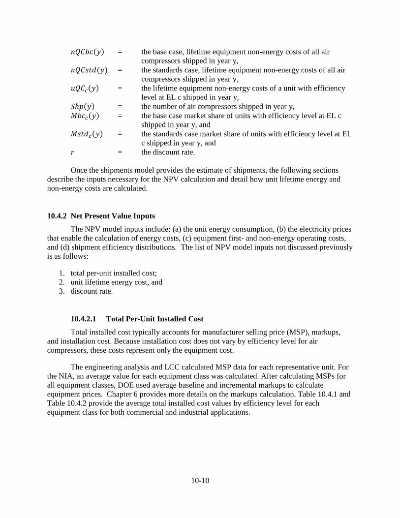
10-10

𝑛𝑛𝑛𝑛𝑛𝑛𝑛𝑛𝑛𝑛(𝑦𝑦) = the base case, lifetime equipment non-energy costs of all air compressors shipped in year y,

𝑛𝑛𝑛𝑛𝑛𝑛𝑛𝑛𝑛𝑛𝑛𝑛(𝑦𝑦) = the standards case, lifetime equipment non-energy costs of all air compressors shipped in year y,

𝑢𝑢𝑛𝑛𝑛𝑛𝑐𝑐(𝑦𝑦) = the lifetime equipment non-energy costs of a unit with efficiency level at EL c shipped in year y,

𝑛𝑛ℎ𝑝𝑝(𝑦𝑦) = the number of air compressors shipped in year y, 𝑀𝑀𝑛𝑛𝑛𝑛𝑐𝑐(𝑦𝑦) = the base case market share of units with efficiency level at EL c

shipped in year y, and 𝑀𝑀𝑛𝑛𝑛𝑛𝑛𝑛𝑐𝑐(𝑦𝑦) = the standards case market share of units with efficiency level at EL

c shipped in year y, and 𝑟𝑟 = the discount rate.

Once the shipments model provides the estimate of shipments, the following sections describe the inputs necessary for the NPV calculation and detail how unit lifetime energy and non-energy costs are calculated.

10.4.2 Net Present Value Inputs

The NPV model inputs include: (a) the unit energy consumption, (b) the electricity prices that enable the calculation of energy costs, (c) equipment first- and non-energy operating costs, and (d) shipment efficiency distributions. The list of NPV model inputs not discussed previously is as follows:

1. total per-unit installed cost; 2. unit lifetime energy cost, and 3. discount rate.

Total Per-Unit Installed Cost 10.4.2.1

Total installed cost typically accounts for manufacturer selling price (MSP), markups, and installation cost. Because installation cost does not vary by efficiency level for air compressors, these costs represent only the equipment cost.

The engineering analysis and LCC calculated MSP data for each representative unit. For the NIA, an average value for each equipment class was calculated. After calculating MSPs for all equipment classes, DOE used average baseline and incremental markups to calculate equipment prices. Chapter 6 provides more details on the markups calculation. Table 10.4.1 and Table 10.4.2 provide the average total installed cost values by efficiency level for each equipment class for both commercial and industrial applications.

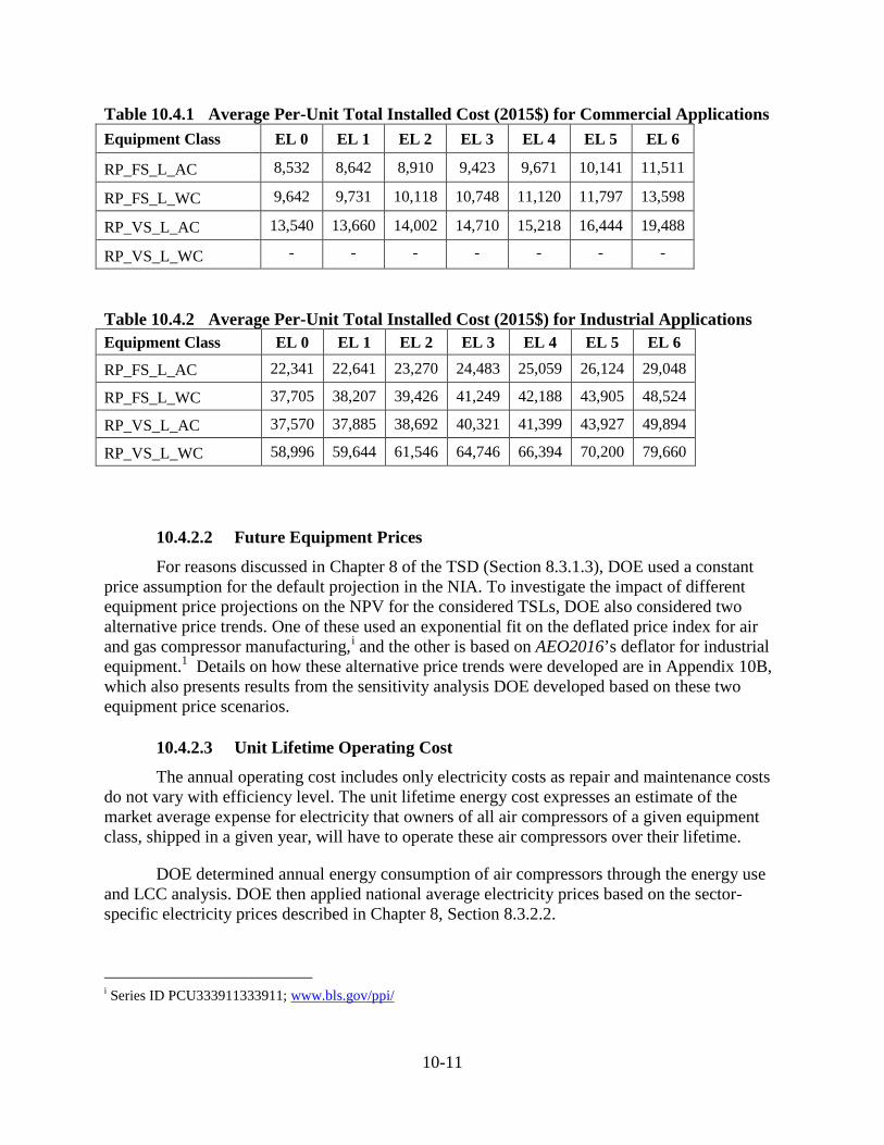
10-11

Table 10.4.1 Average Per-Unit Total Installed Cost (2015$) for Commercial Applications Equipment Class EL 0 EL 1 EL 2 EL 3 EL 4 EL 5 EL 6

RP_FS_L_AC 8,532 8,642 8,910 9,423 9,671 10,141 11,511

RP_FS_L_WC 9,642 9,731 10,118 10,748 11,120 11,797 13,598

RP_VS_L_AC 13,540 13,660 14,002 14,710 15,218 16,444 19,488

RP_VS_L_WC - - - - - - -

Table 10.4.2 Average Per-Unit Total Installed Cost (2015$) for Industrial Applications Equipment Class EL 0 EL 1 EL 2 EL 3 EL 4 EL 5 EL 6

RP_FS_L_AC 22,341 22,641 23,270 24,483 25,059 26,124 29,048

RP_FS_L_WC 37,705 38,207 39,426 41,249 42,188 43,905 48,524

RP_VS_L_AC 37,570 37,885 38,692 40,321 41,399 43,927 49,894

RP_VS_L_WC 58,996 59,644 61,546 64,746 66,394 70,200 79,660

Future Equipment Prices 10.4.2.2

For reasons discussed in Chapter 8 of the TSD (Section 8.3.1.3), DOE used a constant price assumption for the default projection in the NIA. To investigate the impact of different equipment price projections on the NPV for the considered TSLs, DOE also considered two alternative price trends. One of these used an exponential fit on the deflated price index for air and gas compressor manufacturing,i and the other is based on AEO2016’s deflator for industrial equipment.1 Details on how these alternative price trends were developed are in Appendix 10B, which also presents results from the sensitivity analysis DOE developed based on these two equipment price scenarios.

Unit Lifetime Operating Cost 10.4.2.3

The annual operating cost includes only electricity costs as repair and maintenance costs do not vary with efficiency level. The unit lifetime energy cost expresses an estimate of the market average expense for electricity that owners of all air compressors of a given equipment class, shipped in a given year, will have to operate these air compressors over their lifetime.

DOE determined annual energy consumption of air compressors through the energy use and LCC analysis. DOE then applied national average electricity prices based on the sector-specific electricity prices described in Chapter 8, Section 8.3.2.2.

i Series ID PCU333911333911; www.bls.gov/ppi/

10-12

As with the total installed cost data, DOE developed projected annual electricity expenses based on the annual projections of market share by efficiency level specified in the base case and standards cases. DOE multiplied the market share by efficiency level in each year by the per-unit electricity costs by efficiency level to calculate shipment-weighted average annual electricity costs. DOE then applied electricity price trends from AEO 2016 to scale the electricity expenses moving forward, as shown in Figure 10.4.1.

Figure 10.4.1 Marginal Electricity Price Time Series

Discount Rate 10.4.2.4

The discount rate expresses the time value of money. DOE used real discount rates of 3 percent and 7 percent, as established by the U.S. Office of Management and Budget (OMB) guidelines on regulatory analysis.2 The discount rates DOE used in the LCC are distinct from those it used in the NPV calculations, in that the NPV discount rates represent the societal rate of return on capital investment, whereas LCC discount rates reflect the owner cost of capital and the financial environment of electric utilities and commercial and industrial entities.

10.5 TRIAL STANDARD LEVELS

DOE analyzed the benefits and burdens of six TSLs for air compressors. These TSLs were developed by combining specific efficiency levels for each of the product classes analyzed by DOE. DOE presents the results for the TSLs in this document, while the results for all efficiency levels that DOE analyzed are in the TSD.

$0.00

$0.02

$0.04

$0.06

$0.08

$0.10

$0.12

2022 2027 2032 2037 2042 2047 2052 2057

$/kW

h

Industrial

Commercial

10-13

Table 10.5.1 presents the TSLs and the corresponding efficiency levels for air compressors. TSL 6 represents the maximum technologically feasible (“max-tech”) energy efficiency for all equipment classes. For the rotary positive lubricated equipment classes the TSL increase directly with the analyzed ELs from EL 1 through max-tech (EL 6). TSL 3 is of significance because it represents a combination of efficiency levels that are equivalent to the draft EU second tier minimum energy efficiency requirement for rotary lubricated air compressors.j For rotary positive lubricant-free equipment classes TSLs 1 through 5 are held at EL 0 (a new standard at baseline), while max-tech is represented at TSL 6. For reciprocating equipment classes TSLs 1 through 5 are held at EL 0 (no-new-standard), while max-tech is represented at TSL 6. Table 10.5.1 Mapping Between TSLs and Efficiency Levels

Equipment Class (EC) TSL 1 TSL 2 TSL 3 TSL 4 TSL 5 TSL 6

RP_FS_L_AC 1 2 3 4 5 6 RP_FS_L_WC 1 2 3 4 5 6

RP_VS_L_AC 1 2 3 4 5 6

RP_VS_L_WC 1 2 3 4 5 6

10.6 RESULTS

DOE evaluated NES and NPV for each equipment class and TSL using the inputs and methodologies described in Sections 10.3 and 10.4. Table 10.6.1 and Table 10.6.2 present the NES results; and Table 10.6.3 and Table 10.6.4 present the NPV results.

Table 10.6.1 Cumulative National Primary Energy Savings for Commercial and Industrial Air Compressors Trial Standard Levels for Units Sold in 2022-2051 (quads)

TSL 1 TSL 2 TSL 3 TSL 4 TSL 5 TLS 6

RP_FS_L_AC 0.02 0.10 0.30 0.41 0.59 1.08 RP_FS_L_WC 0.01 0.05 0.11 0.14 0.21 0.40 RP_VS_L_AC 0.00 0.00 0.02 0.02 0.04 0.08 RP_VS_L_WC 0.00 0.00 0.01 0.01 0.02 0.03 Total 0.03 0.15 0.43 0.59 0.87 1.59

Note: Components may not sum to total due to rounding.

j For more information regarding the draft regulation see: www.eup-network.de/product-groups/overview-ecodesign/

10-14

Table 10.6.2 Cumulative National Full-Fuel-Cycle Energy Savings for Commercial and Industrial Air Compressors Trial Standard Levels for Units Sold in 2022-2051 (quads)

TSL 1 TSL 2 TSL 3 TSL 4 TSL 5 TLS 6

RP_FS_L_AC 0.02 0.10 0.32 0.42 0.62 1.13 RP_FS_L_WC 0.01 0.05 0.11 0.15 0.22 0.41 RP_VS_L_AC 0.00 0.00 0.02 0.03 0.04 0.08 RP_VS_L_WC 0.00 0.00 0.01 0.01 0.02 0.04 Total 0.03 0.16 0.45 0.61 0.91 1.66

Note: Components may not sum to total due to rounding. Table 10.6.3 Cumulative Net Present Value at a 3-percent Discount Rate of Customer

Benefit for Commercial and Industrial Air Compressors Trial Standard Levels for Units Sold in 2022-2051 (billion 2015$)

TSL 1 TSL 2 TSL 3 TSL 4 TSL 5 TLS 6

RP_FS_L_AC 0.07 0.30 0.83 1.07 1.48 2.33 RP_FS_L_WC 0.02 0.13 0.29 0.38 0.54 0.89 RP_VS_L_AC 0.00 0.01 0.03 0.04 0.05 0.04 RP_VS_L_WC 0.00 0.01 0.01 0.01 0.02 0.01 Total 0.10 0.45 1.15 1.50 2.08 3.26

* Numbers in parentheses indicate negative NPV. Note: Components may not sum to total due to rounding. Table 10.6.4 Cumulative Net Present Value at a 7-percent Discount Rate of Customer

Benefit for Commercial and Industrial Air Compressors Trial Standard Levels for Units Sold in 2022-2051 (billion 2015$)

TSL 1 TSL 2 TSL 3 TSL 4 TSL 5 TLS 6

RP_FS_L_AC 0.03 0.11 0.29 0.37 0.50 0.72 RP_FS_L_WC 0.01 0.05 0.10 0.13 0.18 0.28 RP_VS_L_AC 0.00 0.00 0.01 0.01 0.01 (0.01) RP_VS_L_WC 0.00 0.00 0.00 0.00 0.00 (0.01) Total 0.04 0.16 0.40 0.51 0.68 0.98

* Numbers in parentheses indicate negative NPV. Note: Components may not sum to total due to rounding.

10-15

REFERENCES

1 U.S. Department of Energy-Energy Information Administration, Annual Energy Outlook 2016,

April, 2016. Washington, DC. Report No. DOE/EIA-0383(2016). http://www.eia.gov/forecasts/aeo/pdf/0383(2016).pdf.

2 U.S. Office of Management and Budget, Circular A-4: Regulatory Analysis, September 17, 2003. http://www.whitehouse.gov/omb/circulars/a004/a-4.pdf

11-i

CHAPTER 11. CUSTOMER SUBGROUP ANALYSIS

TABLE OF CONTENTS

11.1 INTRODUCTION ......................................................................................................... 11-1 11.2 SUBGROUPS DEFINITION ........................................................................................ 11-1

11.2.1 Small Businesses ................................................................................................ 11-1 11.3 RESULTS FOR AIR COMPRESSOR SUBGROUPS.................................................. 11-3

11.3.1 Small Business Subgroup .................................................................................. 11-3 REFERENCES .......................................................................................................................... 11-7

LIST OF TABLES

Table 11.2.1 Discount Rate Difference Between Small Company and Sector Average ........................................................................................................ 11-2

Table 11.3.1 Average LCC and PBP Results by Efficiency Level for Rotary Positive, Fixed Speed, Lubricated, Air Cooled Air Compressors (RP_FS_L_AC)............................................................................................ 11-3

Table 11.3.2 LCC Savings Relative to the Base Case Efficiency Distribution for Rotary Positive, Fixed Speed, Lubricated, Air Cooled Air Compressors (RP_FS_L_AC) ...................................................................... 11-3

Table 11.3.3 Average LCC and PBP Results by Efficiency Level for Rotary Positive, Fixed Speed, Lubricated, Water Cooled Air Compressors (RP_FS_L_WC) ........................................................................................... 11-4

Table 11.3.4 LCC Savings Relative to the Base Case Efficiency Distribution for Rotary Positive, Fixed Speed, Lubricated, Water Cooled Air Compressors (RP_FS_L_WC) ..................................................................... 11-4

Table 11.3.5 Average LCC and PBP Results by Efficiency Level for Rotary Positive, Variable Speed, Lubricated, Air Cooled Air Compressors (RP_VS_L_AC) ........................................................................................... 11-5

Table 11.3.6 LCC Savings Relative to the Base Case Efficiency Distribution for Rotary Positive, Variable Speed, Lubricated, Air Cooled Air Compressors (RP_VS_L_AC) ..................................................................... 11-5

Table 11.3.7 Average LCC and PBP Results by Efficiency Level for Rotary Positive, Variable Speed, Lubricated, Water Cooled Air Compressors (RP_VS_L_WC) .......................................................................................... 11-6

Table 11.3.8 LCC Savings Relative to the Base Case Efficiency Distribution for Rotary Positive, Variable Speed, Lubricated, Water Cooled Air Compressors (RP_VS_L_WC) .................................................................... 11-6

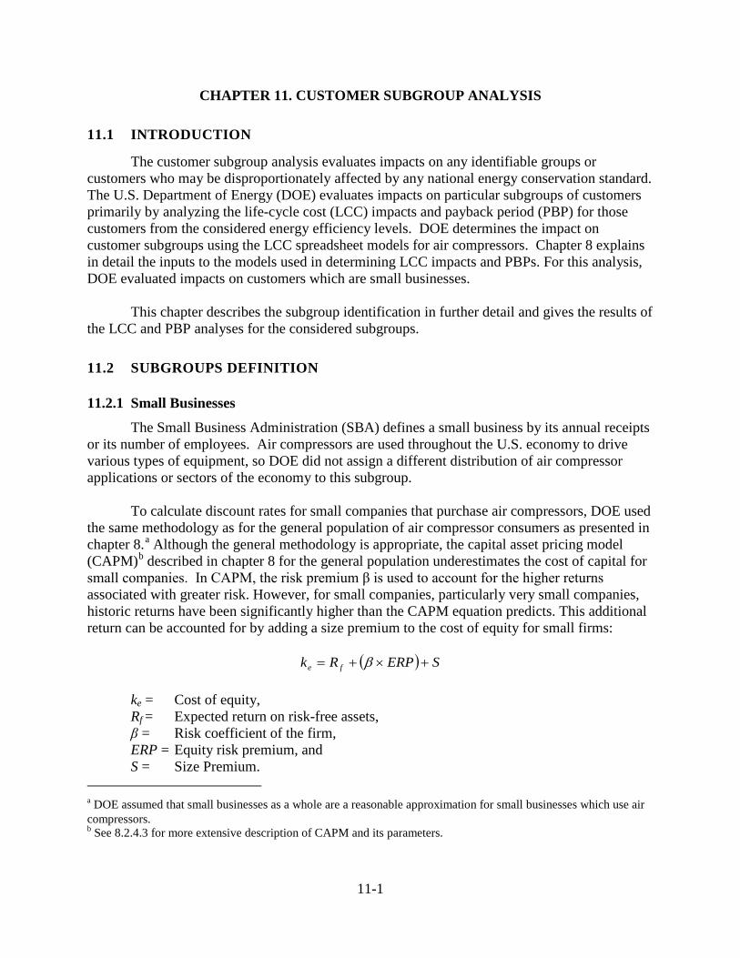
11-1

CHAPTER 11. CUSTOMER SUBGROUP ANALYSIS

11.1 INTRODUCTION

The customer subgroup analysis evaluates impacts on any identifiable groups or customers who may be disproportionately affected by any national energy conservation standard. The U.S. Department of Energy (DOE) evaluates impacts on particular subgroups of customers primarily by analyzing the life-cycle cost (LCC) impacts and payback period (PBP) for those customers from the considered energy efficiency levels. DOE determines the impact on customer subgroups using the LCC spreadsheet models for air compressors. Chapter 8 explains in detail the inputs to the models used in determining LCC impacts and PBPs. For this analysis, DOE evaluated impacts on customers which are small businesses. This chapter describes the subgroup identification in further detail and gives the results of the LCC and PBP analyses for the considered subgroups.

11.2 SUBGROUPS DEFINITION

11.2.1 Small Businesses

The Small Business Administration (SBA) defines a small business by its annual receipts or its number of employees. Air compressors are used throughout the U.S. economy to drive various types of equipment, so DOE did not assign a different distribution of air compressor applications or sectors of the economy to this subgroup. To calculate discount rates for small companies that purchase air compressors, DOE used the same methodology as for the general population of air compressor consumers as presented in chapter 8.a Although the general methodology is appropriate, the capital asset pricing model (CAPM)b described in chapter 8 for the general population underestimates the cost of capital for small companies. In CAPM, the risk premium β is used to account for the higher returns associated with greater risk. However, for small companies, particularly very small companies, historic returns have been significantly higher than the CAPM equation predicts. This additional return can be accounted for by adding a size premium to the cost of equity for small firms:

( ) SERPRk fe +×+= β ke = Cost of equity, Rf = Expected return on risk-free assets, β = Risk coefficient of the firm, ERP = Equity risk premium, and S = Size Premium. a DOE assumed that small businesses as a whole are a reasonable approximation for small businesses which use air compressors. b See 8.2.4.3 for more extensive description of CAPM and its parameters.

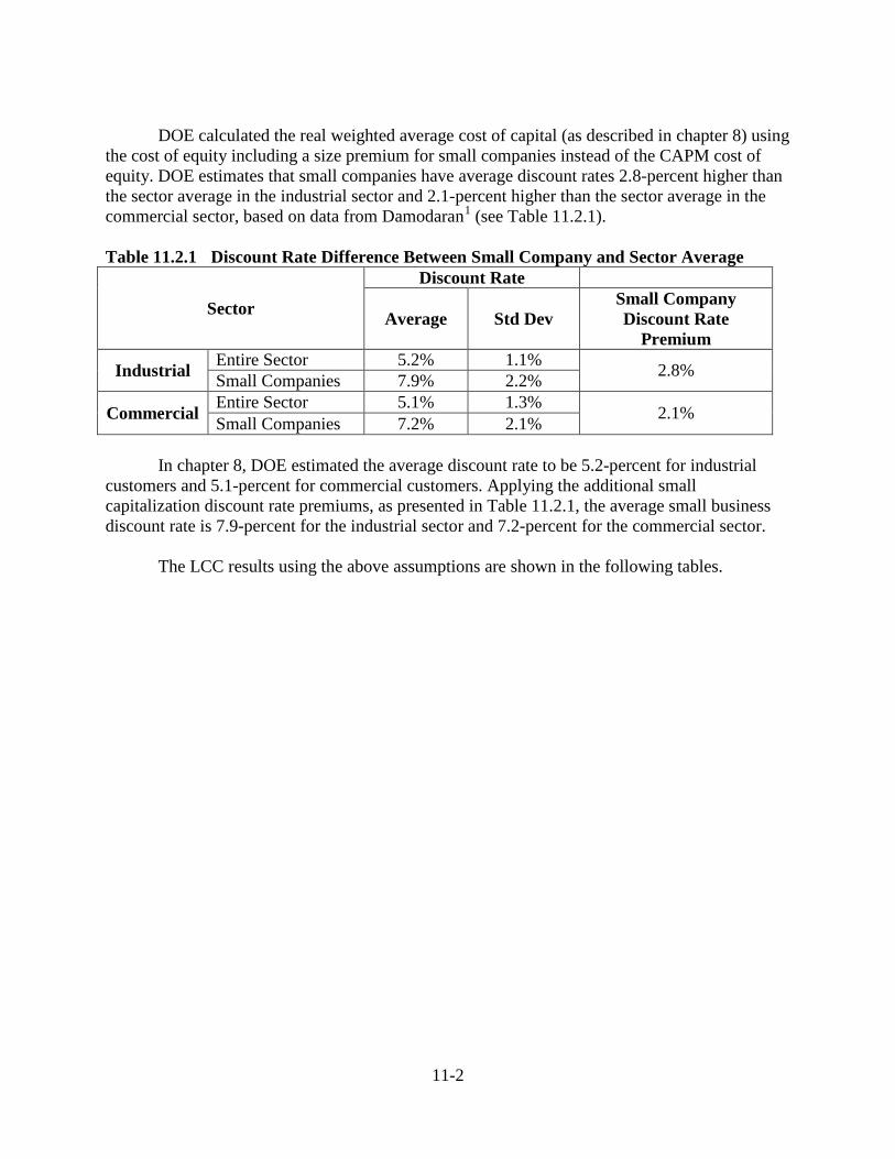
11-2

DOE calculated the real weighted average cost of capital (as described in chapter 8) using the cost of equity including a size premium for small companies instead of the CAPM cost of equity. DOE estimates that small companies have average discount rates 2.8-percent higher than the sector average in the industrial sector and 2.1-percent higher than the sector average in the commercial sector, based on data from Damodaran1 (see Table 11.2.1). Table 11.2.1 Discount Rate Difference Between Small Company and Sector Average

Sector

Discount Rate

Average Std Dev Small Company Discount Rate

Premium

Industrial Entire Sector 5.2% 1.1% 2.8% Small Companies 7.9% 2.2%

Commercial Entire Sector 5.1% 1.3% 2.1% Small Companies 7.2% 2.1% In chapter 8, DOE estimated the average discount rate to be 5.2-percent for industrial customers and 5.1-percent for commercial customers. Applying the additional small capitalization discount rate premiums, as presented in Table 11.2.1, the average small business discount rate is 7.9-percent for the industrial sector and 7.2-percent for the commercial sector. The LCC results using the above assumptions are shown in the following tables.

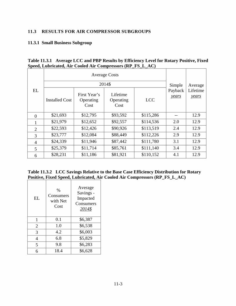
11-3

11.3 RESULTS FOR AIR COMPRESSOR SUBGROUPS

11.3.1 Small Business Subgroup

Table 11.3.1 Average LCC and PBP Results by Efficiency Level for Rotary Positive, Fixed Speed, Lubricated, Air Cooled Air Compressors (RP_FS_L_AC)

EL

Average Costs

Simple Payback

years

Average Lifetime

years

2014$

Installed Cost First Year’s Operating

Cost

Lifetime Operating

Cost LCC

0 $21,693 $12,795 $93,592 $115,286 -- 12.9 1 $21,979 $12,652 $92,557 $114,536 2.0 12.9 2 $22,593 $12,426 $90,926 $113,519 2.4 12.9 3 $23,777 $12,084 $88,449 $112,226 2.9 12.9 4 $24,339 $11,946 $87,442 $111,780 3.1 12.9 5 $25,379 $11,714 $85,761 $111,140 3.4 12.9 6 $28,231 $11,186 $81,921 $110,152 4.1 12.9

Table 11.3.2 LCC Savings Relative to the Base Case Efficiency Distribution for Rotary Positive, Fixed Speed, Lubricated, Air Cooled Air Compressors (RP_FS_L_AC)

EL

% Consumers

with Net Cost

Average Savings - Impacted

Consumers 2014$

1 0.1 $6,387 2 1.0 $6,538 3 4.2 $6,003 4 6.8 $5,829 5 9.8 $6,283 6 18.4 $6,628

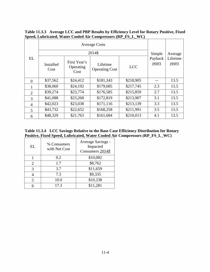
11-4

Table 11.3.3 Average LCC and PBP Results by Efficiency Level for Rotary Positive, Fixed Speed, Lubricated, Water Cooled Air Compressors (RP_FS_L_WC)

EL

Average Costs

Simple Payback

years

Average Lifetime

years

2014$

Installed Cost

First Year’s Operating

Cost

Lifetime Operating Cost LCC

0 $37,562 $24,412 $181,343 $218,905 -- 13.5 1 $38,060 $24,192 $179,685 $217,745 2.3 13.5 2 $39,274 $23,774 $176,585 $215,859 2.7 13.5 3 $41,088 $23,268 $172,819 $213,907 3.1 13.5 4 $42,023 $23,038 $171,116 $213,139 3.3 13.5 5 $43,732 $22,652 $168,258 $211,991 3.5 13.5 6 $48,329 $21,763 $161,684 $210,013 4.1 13.5

Table 11.3.4 LCC Savings Relative to the Base Case Efficiency Distribution for Rotary Positive, Fixed Speed, Lubricated, Water Cooled Air Compressors (RP_FS_L_WC)

EL % Consumers with Net Cost

Average Savings - Impacted

Consumers 2014$ 1 0.2 $10,082 2 1.7 $8,762 3 3.7 $11,659 4 7.3 $9,335 5 10.0 $10,238 6 17.3 $11,281

11-5

Table 11.3.5 Average LCC and PBP Results by Efficiency Level for Rotary Positive, Variable Speed, Lubricated, Air Cooled Air Compressors (RP_VS_L_AC)

EL

Average Costs

Simple Payback

years

Average Lifetime

years

2014$

Installed Cost First Year’s Operating

Cost

Lifetime Operating

Cost LCC

0 $37,087 $11,356 $82,714 $119,801 -- 13.3 1 $37,395 $11,282 $82,183 $119,579 4.2 13.3 2 $38,190 $11,129 $81,069 $119,259 4.9 13.3 3 $39,795 $10,873 $79,216 $119,011 5.6 13.3 4 $40,860 $10,725 $78,146 $119,007 6.0 13.3 5 $43,357 $10,424 $75,955 $119,313 6.7 13.3 6 $49,261 $9,861 $71,863 $121,124 8.1 13.3

Table 11.3.6 LCC Savings Relative to the Base Case Efficiency Distribution for Rotary Positive, Variable Speed, Lubricated, Air Cooled Air Compressors (RP_VS_L_AC)

EL

% Consumers

with Net Cost

Average Savings - Impacted

Consumers 2014$

1 2.4 $1,916 2 8.0 $1,982 3 21.0 $1,504 4 28.1 $1,289 5 36.7 $723 6 53.9 -$1,683

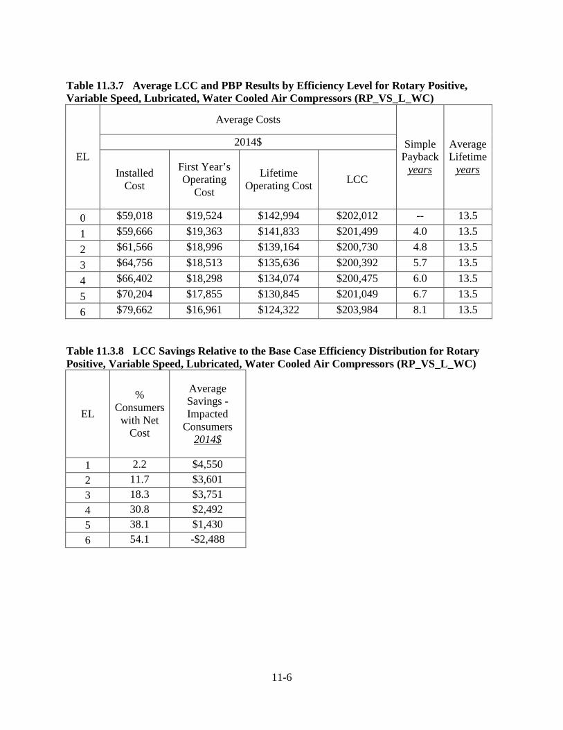
11-6

Table 11.3.7 Average LCC and PBP Results by Efficiency Level for Rotary Positive, Variable Speed, Lubricated, Water Cooled Air Compressors (RP_VS_L_WC)

EL

Average Costs

Simple Payback

years

Average Lifetime

years

2014$

Installed Cost

First Year’s Operating

Cost

Lifetime Operating Cost LCC

0 $59,018 $19,524 $142,994 $202,012 -- 13.5 1 $59,666 $19,363 $141,833 $201,499 4.0 13.5 2 $61,566 $18,996 $139,164 $200,730 4.8 13.5 3 $64,756 $18,513 $135,636 $200,392 5.7 13.5 4 $66,402 $18,298 $134,074 $200,475 6.0 13.5 5 $70,204 $17,855 $130,845 $201,049 6.7 13.5 6 $79,662 $16,961 $124,322 $203,984 8.1 13.5

Table 11.3.8 LCC Savings Relative to the Base Case Efficiency Distribution for Rotary Positive, Variable Speed, Lubricated, Water Cooled Air Compressors (RP_VS_L_WC)

EL

% Consumers

with Net Cost

Average Savings - Impacted

Consumers 2014$

1 2.2 $4,550 2 11.7 $3,601 3 18.3 $3,751 4 30.8 $2,492 5 38.1 $1,430 6 54.1 -$2,488

11-7

REFERENCES 1 Damodaran Online. The Data Page: Cost of Capital by Industry Sector, 2006.

<http://pages.stern.nyu.edu/~adamodar/>

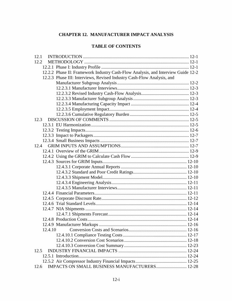
12-i

CHAPTER 12. MANUFACTURER IMPACT ANALYSIS

TABLE OF CONTENTS

12.1 INTRODUCTION ............................................................................................. 12-1 12.2 METHODOLOGY ............................................................................................ 12-1

12.2.1 Phase I: Industry Profile ............................................................................. 12-1 12.2.2 Phase II: Framework Industry Cash-Flow Analysis, and Interview Guide 12-2 12.2.3 Phase III: Interviews, Revised Industry Cash-Flow Analysis, and

Manufacturer Subgroup Analysis ............................................................... 12-2 12.2.3.1 Manufacturer Interviews ............................................................... 12-3 12.2.3.2 Revised Industry Cash-Flow Analysis.......................................... 12-3 12.2.3.3 Manufacturer Subgroup Analysis ................................................. 12-3 12.2.3.4 Manufacturing Capacity Impact ................................................... 12-4 12.2.3.5 Employment Impact...................................................................... 12-4 12.2.3.6 Cumulative Regulatory Burden .................................................... 12-5

12.3 DISCUSSION OF COMMENTS ...................................................................... 12-5 12.3.1 EU Harmonization ...................................................................................... 12-5 12.3.2 Testing Impacts ........................................................................................... 12-6 12.3.3 Impact to Packagers .................................................................................... 12-7 12.3.4 Small Business Impacts .............................................................................. 12-7

12.4 GRIM INPUTS AND ASSUMPTIONS ............................................................ 12-7 12.4.1 Overview of the GRIM ............................................................................... 12-9 12.4.2 Using the GRIM to Calculate Cash Flow ................................................... 12-9 12.4.3 Sources for GRIM Inputs .......................................................................... 12-10

12.4.3.1 Corporate Annual Reports .......................................................... 12-10 12.4.3.2 Standard and Poor Credit Ratings............................................... 12-10 12.4.3.3 Shipment Model.......................................................................... 12-10 12.4.3.4 Engineering Analysis .................................................................. 12-11 12.4.3.5 Manufacturer Interviews ............................................................. 12-11

12.4.4 Financial Parameters ................................................................................. 12-11 12.4.5 Corporate Discount Rate ........................................................................... 12-12 12.4.6 Trial Standard Levels ................................................................................ 12-14 12.4.7 NIA Shipments ......................................................................................... 12-14

12.4.7.1 Shipments Forecast ..................................................................... 12-14 12.4.8 Production Costs ....................................................................................... 12-14 12.4.9 Manufacturer Markups ............................................................................. 12-16 12.4.10 Conversion Costs and Scenarios ................................................... 12-16

12.4.10.1 Compliance Testing Costs ........................................................ 12-17 12.4.10.2 Conversion Cost Scenarios ....................................................... 12-18 12.4.10.3 Conversion Cost Summary ....................................................... 12-23

12.5 INDUSTRY FINANCIAL IMPACTS ............................................................ 12-24 12.5.1 Introduction ............................................................................................... 12-24 12.5.2 Air Compressor Industry Financial Impacts ............................................. 12-25

12.6 IMPACTS ON SMALL BUSINESS MANUFACTURERS ........................... 12-28

12-ii

12.7 OTHER IMPACTS .......................................................................................... 12-29 12.7.1 Employment .............................................................................................. 12-30

12.7.1.1 Methodology ............................................................................... 12-30 12.7.1.1 Direct Employment Impacts ....................................................... 12-30

12.7.2 Production Capacity .................................................................................. 12-32 12.7.3 Cumulative Regulatory Burden ................................................................ 12-32

12.8 CONCLUSION ................................................................................................ 12-35 12.8.1 Conclusions for Air Compressors ............................................................. 12-35

LIST OF TABLES

Table 12.4.1 GRIM Financial Parameters for the Air Compressor Industry ............... 12-11 Table 12.4.2 Cost of Equity Calculation ...................................................................... 12-12 Table 12.4.3 Cost of Debt Calculation......................................................................... 12-13 Table 12.4.4 Trial Standard Levels for Air Compressors ............................................ 12-14 Table 12.4.5 Guide to Equipment Class Abbreviations ............................................... 12-14 Table 12.4.6 Breakdown of MPC for Air Compressors for all Equipment Classes .... 12-15 Table 12.4.7 Manufacturer Production Cost Breakdown (2015$) for RP_FS_L_AC . 12-15 Table 12.4.8 Manufacturer Production Cost Breakdown (2015$) for R_FS_L_WC .. 12-15 Table 12.4.9 Manufacturer Production Cost Breakdown (2015$) for R_VS_L_AC .. 12-16 Table 12.4.10 Manufacturer Production Cost Breakdown (2015$) for R_VS_L_WC 12-16 Table 12.4.11 Estimated Basic Model Count for Each Equipment Class ................... 12-17 Table 12.4.12 Estimated Cost to Test One Basic Model ............................................. 12-18 Table 12.4.13 Aggregate Industry Compliance Testing Cost ...................................... 12-18 Table 12.4.14 Total Industry and Average Per-Manufacturer PCC at Max-Tech ....... 12-19 Table 12.4.15 Total Industry and Average Per-Manufacturer CCC at Max-Tech ...... 12-19 Table 12.4.16 Estimated Percentage of Models Failing at Each Efficiency Level...... 12-20 Table 12.4.17 Total Industry PCC* at Each Efficiency Level – High Conversion Cost Scenario........................................................................................................................ 12-20 Table 12.4.18 Total Industry CCC at Each Efficiency Level ...................................... 12-20 Table 12.4.19 Shipments Breakdowns Within Each Equipment Class Group ............ 12-20 Table 12.4.20 Disaggregated Total Industry PCC* at Each Efficiency Level – High Conversion Cost Scenario ............................................................................................ 12-21 Table 12.4.21 Disaggregated Total Industry CCC at Each Efficiency Level .............. 12-21 Table 12.4.22 Estimated Packager PCC at Each Efficiency Level – High Conversion Cost Scenario........................................................................................................................ 12-21 Table 12.4.23 Total Industry PCC* at Each Efficiency Level – Low Conversion Cost Scenario........................................................................................................................ 12-22 Table 12.4.24 Disaggregated Total Industry PCC* at Each Efficiency – Low Conversion Cost Scenario ............................................................................................................... 12-22 Table 12.4.25 Estimated Packager PCC at Each Efficiency Level – Low Conversion Cost Scenario........................................................................................................................ 12-22 Table 12.4.26 Summary of Total Industry PCC, Including Compliance Testing Cost, at each Efficiency Level – High and Low Scenario ........................................................ 12-23

12-iii

Table 12.4.27 Aggregate Industry Product Conversion Cost, Including Compliance and Testing Costs, at Each Efficiency Level ...................................................................... 12-23 Table 12.4.28 Aggregate Industry Capital Conversion Cost at Each Efficiency Level .. 12-23 Table 12.5.1 Manufacturer Impact Analysis Results for Air Compressors: Low Conversion Cost Scenario ............................................................................................ 12-25 Table 12.5.2 Manufacturer Impact Analysis Results for Air Compressors: High Conversion Cost Scenario ............................................................................................ 12-26 Table 12.7.1 Potential Changes ofCompressor Direct Employmentin 2022 ............... 12-31 Table 12.7.2 Compliance Dates and Expected Conversion Expenses and Federal Energy Conservation Standards Affecting Compressor Manufacturers .................................. 12-34 Table 12.8.1 Manufacturer Impact Analysis Results for Air Compressors ................. 12-35

LIST OF FIGURES

Figure 12.5.1 Annual Industry Net Cash Flows for Air Compressors (Low Conversion Cost Scenario) .............................................................................................................. 12-27 Figure 12.5.2 Annual Industry Net Cash Flows for Air Compressors (High Conversion Cost Scenario) .............................................................................................................. 12-27

12-1

CHAPTER 12. MANUFACTURER IMPACT ANALYSIS

12.1 INTRODUCTION

In determining whether a standard is economically justified, the U.S. Department of Energy (DOE) is required to consider “the economic impact of the standard on the manufacturers and on the consumers of the equipment subject to such a standard.” (42 U.S.C. 6313(a)(6)(B)(i)) The statute also calls for an assessment of the impact of any lessening of competition as determined in writing by the Attorney General. Id. DOE conducted a manufacturer impact analysis (MIA) to estimate the financial impact of proposed energy conservation standards on manufacturers of air compressors, and assessed the impact of such standards on direct employment and manufacturing capacity.

The MIA has both quantitative and qualitative aspects. The quantitative part of the MIA primarily relies on the Government Regulatory Impact Model (GRIM), an industry cash-flow model adapted for this rulemaking. The GRIM inputs include information on industry cost structure, shipments, and pricing strategies. The GRIM’s key output is the industry net present value (INPV). The model estimates the financial impact of more stringent energy conservation standards by comparing changes in INPV between a no-new-standards case and the various trial standard levels (TSLs) in the standards case. The qualitative part of the MIA addresses equipment characteristics, manufacturer characteristics, market and equipment trends, as well as the impact of standards on subgroups of manufacturers.

12.2 METHODOLOGY DOE conducted the MIA in three phases. The following sections provide a detailed

outline of each phase.

12.2.1 Phase I: Industry Profile

In Phase I of the MIA, DOE prepared a profile of the air compressors industry that built upon the market and technology assessment prepared for this rulemaking (refer to chapter 3 of the technical support document, TSD). Before initiating the detailed impact studies, DOE collected information on the market characteristics of the air compressors industry. This information included equipment shipments, manufacturer markups, and the cost structure for various manufacturers. The industry profile includes: (1) further detail on the overall market and equipment characteristics; (2) financial parameters such as net plant, property, and equipment; selling, general and administrative (SG&A) expenses; cost of goods sold, etc.; and (3) trends in the number of firms, market, and equipment characteristics. The industry profile included a top-down cost analysis of air compressors manufacturers that DOE used to derive the preliminary financial inputs for the GRIM (e.g., revenues, depreciation, SG&A, and research and development (R&D) expenses).

DOE also used public information to further calibrate its initial characterization of the industry, including Securities and Exchange Commission (SEC) 10-K reports, Standard & Poor’s (S&P) stock reports, industry trade association membership directories (e.g., the Compressed Air and Gas Institute), market research tools (e.g., Hoovers reports), corporate annual reports, and

12-2

the U.S. Census Bureau’s 2014 Annual Survey of Manufacturers (2014 ASM).a,b,c DOE also characterized the industry using information from its engineering analysis..

12.2.2 Phase II: Framework Industry Cash-Flow Analysis, and Interview Guide

In Phase 2 of the MIA, DOE prepared a framework industry cash-flow analysis to quantify the potential impacts of new energy conservation standards on manufacturers. In general, energy conservation standards can affect manufacturer cash flow in three distinct ways: (1) create a need for increased investment; (2) raise production costs per unit; and (3) alter revenue due to higher per-unit prices and changes in sales volumes. To quantify these impacts, DOE uses the GRIM to estimate a series of annual cash flows starting with the announcement of the standard and extending over a 30-year period following the compliance date of the standard. Inputs to the GRIM include annual expected revenues, costs of sales, SG&A expenses, R&D expenses, taxes, and capital expenditures.

In addition, DOE prepared a written interview guide to obtain targeted information from manufacturers during Phase III. Most of the information received from the interview guides is protected by non-disclosure agreements and resides with DOE’s contractors. Topics covered in the guide included: (1) key issues to this rulemaking; (2) company overview and organizational characteristics; (3) industry structure and competition; (4) financial parameters; (5) markups and profitability; (6) conversion costs; (7) direct employment, foreign competition, and outsourcing; (8) cumulative regulatory burden; and (9) impacts on small businesses.

12.2.3 Phase III: Interviews, Revised Industry Cash-Flow Analysis, and Manufacturer Subgroup Analysis

In Phase III, DOE interviewed a range of air compressors manufacturers, including small and large companies. The interviews provided DOE with valuable information for evaluating the impacts of energy conservation standards on manufacturer cash flows, investment requirements, and employment. Using information from Phase II and from the interviews, DOE refined its analysis for the equipment classes included in the GRIM. Additionally, DOE used information

a Securities and Exchange Commission, Annual 10-K Reports, Various Years, Washington DC. < www.sec.gov/index.htm>. b Standard and Poors Financial Services LLC, Company Credit Ratings, Various Companies, New York, NY. <www.standardandpoors.com/en_US/web/guest/home>. c U.S. Census Bureau, Annual Survey of Manufacturers: General Statistics: Statistics for Industry Groups and Industries (2014) (Available at: http://factfinder.census.gov/faces/tableservices/jsf/pages/productview.xhtml?pid=ASM_2014_31GS101&prodType=table)

12-3

from Phase II and from the interviews to assess small business impacts, manufacturing capacity, direct employment impacts, and cumulative regulatory burden.

12.2.3.1 Manufacturer Interviews

The information gathered in Phase I and the cash-flow analysis performed in Phase II are supplemented with information gathered from manufacturer interviews in Phase III. The interview process provides an opportunity for interested parties to privately express their views on important issues, thereby allowing confidential or sensitive information to be considered in the rulemaking process. As with the interview guides, most of the information received from these meetings is protected by non-disclosure agreements and resides with DOE’s contractors. DOE sought to obtain feedback from industry on the approaches used in the GRIM and to isolate key issues and concerns.

DOE used these interviews to tailor the GRIM to reflect unique financial characteristics of each equipment group. Interviews were scheduled well in advance to provide every opportunity for key individuals to be available for comment. Although a written response to the questionnaire was acceptable, DOE sought interactive interviews, which help clarify responses and identify additional issues. The resulting information provides valuable inputs to the GRIM developed for the equipment classes. DOE estimates that the interviewed manufacturers account for approximately 70 percent of the domestic rotary air compressor market.

12.2.3.2 Revised Industry Cash-Flow Analysis

In Phase III of the MIA, DOE provided manufacturers with preliminary GRIM input financial figures for review and evaluation. During the interviews, DOE requested comments on the values it selected for the parameters. DOE revised its industry cash-flow model based on this feedback. Section 12.4.4 provides more information on how DOE calculated the parameters.

12.2.3.3 Manufacturer Subgroup Analysis

Using average cost assumptions to develop an industry-cash-flow estimate may not adequately assess differential impacts of energy conservation standards among manufacturer subgroups. For example, small manufacturers, niche players, or manufacturers exhibiting a cost structure that largely differs from the industry average, could be more negatively affected. To address this possible impact, DOE used the results of the industry characterization analysis in Phase I to group manufacturers that exhibit similar characteristics.

Small-Business Manufacturer Subgroup. DOE investigated whether small business manufacturers should be analyzed as a manufacturer subgroup. DOE used the Small Business Administration (SBA) small business size standards effective on February 26, 2016, and the North American Industry Classification System (NAICS) code to determine whether any small

12-4

entities would be affected by the rulemaking.d The SBA defines a small business for “Air and Gas Compressor Manufacturing” as a company with 1,000 or fewer employees. The number of employees in a small business is rolled up with the total employees of the parent company; it does not represent the division manufacturing compressors. For compressors, the size standard is matched to NAICS code 333912, Air and Gas Compressor Manufacturing. During the NOPR stage, the SBA threshold for NAICS code 333912 was 500 or fewer employees. DOE has updated its final rule analysis to reflect the new size standards.

To estimate the number of small business manufacturers of equipment covered by this rulemaking, DOE conducted a market survey using available public information. DOE’s research involved industry trade association membership directories (including the Compressed Air and Gas Institute, CAGI), individual company and online retailer websites, and market research tools to create a list of companies that manufacture equipment covered by this rulemaking. DOE presented its list to manufacturers in MIA interviews and asked industry representatives if they were aware of any other small manufacturers during manufacturer interviews and at DOE public meetings. DOE reviewed publicly available data and contacted select companies on its list, as necessary, to determine whether they met the SBA’s definition of a small business manufacturer. DOE screened out companies that do not offer equipment covered by this rulemaking, do not meet the SBA definition of a small business, or are foreign-owned and operated.

12.2.3.4 Manufacturing Capacity Impact

One significant outcome of new energy conservation standards could be the obsolescence of existing manufacturing assets. The manufacturer interview guide included a series of questions to help identify impacts of new standards on manufacturing capacity, specifically capacity utilization and plant location decisions in the United States, with and without standards; the ability of manufacturers to upgrade or remodel existing facilities to accommodate the new requirements; the nature and value of any stranded assets; and estimates for any one-time changes to existing plant, property, and equipment (PPE). DOE’s estimates of the one-time capital changes affect the cash flow estimates in the GRIM. These estimates can be found in section 12.4.10. DOE’s discussion of the capacity impact can be found in section 12.7.2.

12.2.3.5 Employment Impact

The impact of energy conservation standards on employment is an important consideration in the rulemaking process. To assess how domestic direct employment patterns might be affected, the interviews explored current employment trends in the air compressors industry. The interviews also solicited manufacturer views on changes in employment patterns that may result from standards. The employment impacts are reported in section 12.7.1.

d The size standards are available on the SBA’s website at <www.sba.gov/sites/default/files/files/Size_Standards_Table.pdf>.

12-5

12.2.3.6 Cumulative Regulatory Burden

DOE seeks to mitigate the overlapping effects on manufacturers due to new energy conservation standards and other regulatory actions affecting the same equipment. DOE analyzed the impact on manufacturers of multiple, product-specific regulatory actions. Discussion of the cumulative regulatory burden can be found in section 12.7.3.

12.3 DISCUSSION OF COMMENTS

During the notice of proposed rulemaking (NOPR) public meeting, interested parties commented on the assumptions and results of the analyses. Verbal and written comments addressed several topics, including concerns regarding European Union (EU) harmonization, testing impacts, impacts on packagers, and small business impacts.

12.3.1 EU Harmonization

Several stakeholders commented that DOE should consider the cumulative regulatory burden of simultaneous energy conservation standards that the industry is currently facing, particularly with the European Union’s standards. In a joint comment, stakeholders stated that DOE should refine its analysis to include the cost effectiveness of full harmonization with the pending EU Compressor energy efficiency standards. Some manufacturers have already begun preparations for the proposed EU standard. Additionally, stakeholders commented that DOE should analyze the returns from the increased scale of production and a shared learning curve with international standards harmonization to consider the differential cost of development for products designed to comply. If U.S. and EU standards are not harmonized, these manufacturers noted they would either have to carry a greater number of equipment lines to comply with efficiency standards in both domestic and European markets, or sell a single set of high efficiency equipment in both markets. Either option will be cumbersome for manufacturers. (ASAP; ACEEE; NEEA; NRDC; NEEP; ASE, No. 60 at p. 3)

On the other hand, Sullivan-Palatek commented that some manufacturers only have U.S.

operations and cannot take advantage of harmonizing with EU standards. Therefore, it would not be beneficial for all manufacturers to harmonize with EU standards. (Sullivan-Palatek, Public Meeting Transcript No. 44 at p. 127)

In response, DOE acknowledges that harmonization with EU standards would reduce

cumulative regulatory burden for some manufacturers. In the test procedure final rule, DOE excluded non-lubricated rotary compressors from the scope of test procedures in part to help manufacturers harmonize with the EU’s standards. In this final rule, DOE modeled a low conversion cost scenario that accounts for potential synergies with the potential EU standard. In this scenario, industry has lower total conversion costs based synergies with the EU Standards, as proposed in EU’s “Lot 31” analysis, which set air compressor standards for both reciprocating and rotary air compressors. As such, EU standards were considered as a factor in DOE’s analysis. Further, to account for feedback that harmonization with EU standards would not be beneficial to industry, DOE modeled a high conversion cost scenario that reflects higher level of investments by manufacturers.

12-6

12.3.2 Testing Impacts

Sullivan-Palatek and Castair stated that a complex sampling and compliance program is a burden to such a low-volume specialty industry, particularly due to the staff, software and testing facilities required. These commenters were concerned that the test procedure, even with AEDMs, do not align with current testing methods used by the industry over the past 10 years. (Sullivan-Palatek, Public Meeting Transcript No. 0044 at p. 154-155; Castair, No. 45 at pp. 1-2) To address comments raised in both the test procedure rulemaking and the standards rulemaking, DOE amended the compressor test procedure to align as closely as possible to ISO 1217:2009 in order toreduce manufacturer burden. With these modifications, the test methods established in the final rule are intended to produce results equivalent to those produced historically under ISO 1217:2009. Consequently, if historical test data is consistent with values that will be generated when testing with the test methods established in this final rule, then manufacturers may use this data for the purposes of representing any metrics subject to representations requirements. (DOE, Public Meeting Transcript, No. 0016 at p. 136)

Jenny Products and Compressed Air Systems commented that the high cost to comply

with the test procedure and standard would place a significant burden on small manufacturers. (Jenny Products, No. 58 at p. 5; Compressed Air Systems, No. 61 at p. 4) Additionally, Jenny and CAGI raised concerns that the testing process would require technical resources that would come at the expense of other priorities, such as customer service. (Jenny Products, No. 58 at p. 5; CAGI, No. 52 at p. 3)

Compressed Air Systems noted that testing four to five units based on the NOPR test

procedure could cost up to $125,000 for a manufacturer. Most domestic small air compressor manufacturers produce small quantities of each model offered, which is a heavy cost burden to smaller companies with limited access to capital. (Compressed Air Systems, No. 61 at p. 4)

DOE understands the commenter’s concerns about the scope of the test procedure as

defined in the test procedure NOPR, which included many low-shipment volume or custom compressor models. In the test procedure final rule, DOE takes two key steps to address commenters’ concerns and to reduce the burden of testing, especially for low-volume equipment. First, DOE significantly limits the scope of the test procedure final rule, as compared to the scope proposed in the test procedure NOPR. Second, DOE adopts provisions allowing the use of an alternative efficiency determination method (AEDM), in lieu of testing.

The revised scope aligns with the scope recommended by CAGI and other manufacturers.

Further, the 10 to 200 hp scope established in the test procedure final rule falls within the scope of the CAGI Performance Verification Program for rotary compressors. A complete discussion can be found in the test procedure final rule.

In addition, the test procedure final rule adopts provisions allowing for the use of

AEDMs. AEDMs are mathematical calculations or models that manufacturers may use to predict the energy efficiency or energy consumption characteristics of a basic model. The use of AEDMs are intended to reduce the need for physical testing and to reduce the overall testing burden for manufacturers.

12-7

12.3.3 Impact to Packagers

During the NOPR public meeting, Sullivan-Palatek and Compressed Air Systems stated that packagers would incur engineering expenses as a result of the standard. They requested DOE incorporate cost estimates for packagers to comply with the standard in the revised analysis. (Compressed Air Systems; Sullivan-Palatek, Public Meeting Transcript No. 44 at p. 138-140) In written comments, Jenny Products stated that DOE should include in its cost estimate engineering redesign and certification costs for packagers. Jenny Products stated that the redesign of air ends by OEMs will only partially help packagers meet the standard. (Jenny Products, No. 58 at p. 4) In written comments, Sullivan-Palatek estimated packagers could have engineering redesign costs that exceed $1 million per company, depending on the number of models they offer. (Sullivan-Palatek, No. 51 at p. 1-2) Additionally, Castair requested that American air compressor packagers be exempt from this regulation (Castair, No. 18 at p. 2; CAGI, No. 52 at p. 3; Sullivan-Palatek, No. 51 at p. 2)

Sullivan-Palatek commented that contrary to DOE’s assumption, this standard will result

in significant production redesign costs for compressor packagers. They argue that the cost to packagers could in fact exceed $1 million per company because many of the energy gains required by this standard come not only from air end redesign, but also from packaging. (Sullivan-Palatek, No. 51 at p. 1-2) Additionally, Castair requested that American air compressor packagers be exempt from this regulation. (Castair, No. 18 at p. 2; CAGI, No. 52 at p. 3)

Although DOE is not exempting packagers from the analysis, DOE has revised its

analysis to calculate and include costs associated with packagers in its final rule analysis. DOE estimates that packagers will incur between $10.5 and $15.2 million in total engineering redesign costs to comply with the energy conservation standards of this final rule. As such, DOE has included this cost to packagers in total conversion costs estimated at TSL 2, which are between $98.1 million and $121.3 million for the industry. Details of the conversion cost methodology are described in section 12.4.10.

12.3.4 Small Business Impacts

Many manufacturers stated that small businesses will be negatively affected by the proposed regulation compared to their larger multinational counterparts. Sullivan-Palatek stated that it is difficult for small businesses to access capital compared to their larger competitors. (Sullivan-Palatek, Public Meeting Transcript No. 44 at p. 141-143) A few manufacturers also noted that a stringent standard can cause a disproportionate cost burden to small business. This burden will likely cause many small businesses to exit the rotary compressor business or to be acquired by larger companies. (Sullivan-Palatek, No. 51 at p. 2-9; Castair, No. 52 at p. 3; Compressed Air Systems, No. 61 at p. 4) Often times, these small businesses, both manufacturers and packagers, employ specialized workers that may not be able to find a new job where they can use their skills. (Sullivan-Palatek, No. 51 at p. 9; Castair, No. 45 at p. 1; CAGI, No. 52 at p. 3)

Consistent with the requirements of the Regulatory Flexibility Act (5 U.S.C. 601, et seq.),

as amended, the Department analyzed the expected impacts of an energy conservation standard on small business compressor manufacturers directly regulated by DOE’s standards. DOE

12-8

understands that small manufacturers may be significantly affected by an energy conservation standard. These impacts are discussed in detail in section 12.6. Furthermore, DOE analyzes the impacts of a compressors energy conservation standard on domestic direct employment in section VI.B.

Additionally, Sullivan-Palatek questioned how a smaller firm, such as their own, with the same number of models requiring conversion as a large manufacturer, would have fewer conversion costs. The company requested an independent analysis by the Department of Justice. (Sullivan-Palatek, No. 51 at p. 8-9)

In the NOPR, DOE reported an average conversion cost for small manufacturers. Depending on the number of models offered and equipment efficiencies, small manufacturers may find that their conversion costs fall either above or below the small business average. In the NOPR and final rule analyses, DOE identified two small OEMs. For those two small OEMs, DOE identified 23 failing models or models that do not comply with the standard. DOE notes that 21 of the 23 failing models are manufactured by one small business OEM, which is Sullivan-Palatek. Sullivan-Palatek has a significant portion of failing models is above the industry average failure rate. A more detailed analysis of small business impacts can be found in section VI.B.

During the notice of proposed rulemaking public meeting, DOE cautioned stakeholders that Small Business Administration (“SBA”) size standards may shift before the final rule is published. Sullair and CAGI commented that with an increased size standard, from 500 employees to 1,000 employees, the number of OEMs identified would increase as well. (CAGI, Public Meeting Transcript No. 44 at p. 141; Sullair, Public Meeting Transcript No. 44 at p. 140)

For the compressor manufacturing industry, the SBA sets size threshold, which defines

those entities classified as small businesses for the purpose of this statue. Compressor manufacturers are classified under NAICS 333912, “Air and Gas Compressor Manufacturing.” During the NOPR stage, the SBA set a threshold of 500 employees or less for an entity to be considered as a small business in this industry. In February 2016, as codified in 13 CFR part 121, the SBA changed size standards for NAICS code 333912 to 1,000 employees or less. Therefore, for the purpose of this final rule, DOE has identified 22 small manufacturers that meet the employee threshold defined by the SBA. The manufacturer impact analysis and regulatory flexibility analysis have been updated in the final rule to reflect the changes in SBA size standards.

Manufacturers stated that there are between 10-100 more small businesses affected by this rulemaking that were not previously identified by DOE during the NOPR stage. With a number of small businesses unidentified, many were not notified or contacted for feedback prior to the regulation. Jenny Products noted DOE did not contact them during the NOPR stage. (Sullivan-Palatek, No. 51 at p. 1-2; Jenny Products, No. 58 at p. 4-5; Compressed Air Systems, No. 61 at p. 2; Castair, No. 45 at p. 2) In a written comment, Compressed Air Systems provided a list of sixteen potential small businesses that could be affected by this final rule. They also noted that while DOE’s analysis shows that most units manufactured by small businesses can comply with the standards of this final rule, small businesses will still face high burdens testing

12-9

each model. (Compressed Air Systems, No. 61 at p. 2-5) As such, Compressed Air Systems asked that DOE conduct a more thorough survey of domestic small businesses to understand how a stringent standard will lessen their ability to remain competitive in the market. (Compressed Air Systems, No. 61 at p. 2-5)

DOE recognizes that small manufacturers may be substantially impacted by energy

conservation standards. Again, DOE notes in the Regulatory Flexibility Act, section VI.B of this final rule notice, that small manufacturers are not expected to face significantly higher conversion costs than their larger competitors. In response to the list of manufacturers provided by Compressed Air Systems, DOE reviewed this list and identified two additional entities that produce covered equipment. Of these two entities, one was a large manufacturer and the other was a domestic small business that packages and assembles covered equipment. DOE has updated its manufacturer count and analyses to reflect these additions. During the NOPR stage, DOE attempted to contact all small manufacturers identified at the time, including Jenny Products. Only two small manufacturers chose to participate in interviews with DOE.

12.4 GRIM INPUTS AND ASSUMPTIONS

The GRIM serves as the main tool for assessing the impacts on industry due to new energy conservation standards. DOE relies on several sources to obtain inputs for the GRIM. Data and assumptions from these sources are then fed into an accounting model that calculates industry cash flow both with and without new energy conservation standards.

12.4.1 Overview of the GRIM

The basic structure of the GRIM, illustrated in Error! Reference source not found., is an annual cash flow analysis that uses manufacturer prices, manufacturing costs, shipments, and industry financial information as inputs, and accepts a set of regulatory conditions such as changes in costs, investments, and associated margins. The GRIM spreadsheet uses a number of inputs to arrive at a series of annual cash flows, beginning with the base year of the analysis, 2016, and continuing to 2051. The model calculates the INPV by summing the stream of annual discounted cash flows during this period and adding a discounted terminal value.e

12.4.2 Using the GRIM to Calculate Cash Flow

The GRIM projects cash flows using standard accounting principles and compares changes in INPV between the no-new-standards case and the standard-case scenario induced by new energy conservation standards. The difference in INPV between the no-new-standards case and the standard case(s) represents the estimated financial impact of the new energy conservation standard on manufacturers.

e McKinsey & Company, Inc. Valuation: Measuring and Managing the Value of Companies, 3rd Edition, Copeland, Koller, Murrin. New York: John Wiley & Sons, 2000.

12-10

12.4.3 Sources for GRIM Inputs

The GRIM uses several different sources for data inputs in determining industry cash flow. These sources include corporate annual reports, company profiles, Census data, credit ratings, the shipments model, the engineering analysis, and manufacturer interviews.

12.4.3.1 Corporate Annual Reports

Corporate annual reports to the U.S. Securities and Exchange Commission (SEC) on Form 10-K (SEC 10-K) provided many of the initial financial inputs to the GRIM.f These reports exist for publicly held companies and are freely available to the general public. DOE developed initial financial inputs to the GRIM by examining the annual SEC 10-K reports filed by publicly traded manufacturers of air compressors. Because these companies do not provide detailed information about their individual equipment lines, DOE used the financial information for the entire companies as its initial estimates of the financial parameters in the GRIM analysis. These figures were later revised using feedback from manufacturer interviews. DOE used corporate annual reports to derive the following initial inputs to the GRIM:

• tax rate • working capital • SG&A • R&D • depreciation • capital expenditures • net PPE

12.4.3.2 Standard and Poor Credit Ratings

S&P provides independent credit ratings, research, and financial information. DOE relied on S&P reports to determine the industry’s average cost of debt when calculating the cost of capital.

12.4.3.3 Shipment Model

The GRIM used shipment projections derived from DOE’s shipments model in the national impact analysis (NIA). Chapter 9 of this TSD describes the methodology and analytical model DOE used to forecast shipments.

f www.sec.gov/answers/form10k.htm

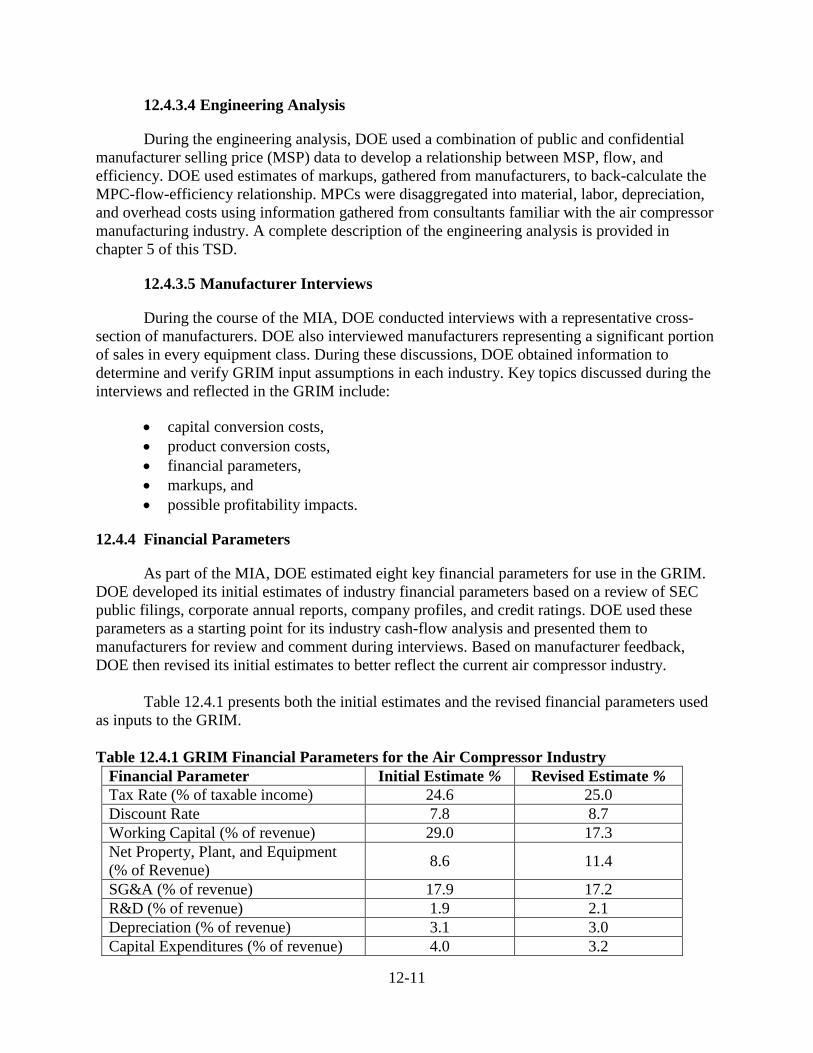
12-11

12.4.3.4 Engineering Analysis

During the engineering analysis, DOE used a combination of public and confidential manufacturer selling price (MSP) data to develop a relationship between MSP, flow, and efficiency. DOE used estimates of markups, gathered from manufacturers, to back-calculate the MPC-flow-efficiency relationship. MPCs were disaggregated into material, labor, depreciation, and overhead costs using information gathered from consultants familiar with the air compressor manufacturing industry. A complete description of the engineering analysis is provided in chapter 5 of this TSD.

12.4.3.5 Manufacturer Interviews

During the course of the MIA, DOE conducted interviews with a representative cross-section of manufacturers. DOE also interviewed manufacturers representing a significant portion of sales in every equipment class. During these discussions, DOE obtained information to determine and verify GRIM input assumptions in each industry. Key topics discussed during the interviews and reflected in the GRIM include:

• capital conversion costs, • product conversion costs, • financial parameters, • markups, and • possible profitability impacts.

12.4.4 Financial Parameters

As part of the MIA, DOE estimated eight key financial parameters for use in the GRIM. DOE developed its initial estimates of industry financial parameters based on a review of SEC public filings, corporate annual reports, company profiles, and credit ratings. DOE used these parameters as a starting point for its industry cash-flow analysis and presented them to manufacturers for review and comment during interviews. Based on manufacturer feedback, DOE then revised its initial estimates to better reflect the current air compressor industry.

Table 12.4.1 presents both the initial estimates and the revised financial parameters used

as inputs to the GRIM. Table 12.4.1 GRIM Financial Parameters for the Air Compressor Industry

Financial Parameter Initial Estimate % Revised Estimate % Tax Rate (% of taxable income) 24.6 25.0 Discount Rate 7.8 8.7 Working Capital (% of revenue) 29.0 17.3 Net Property, Plant, and Equipment (% of Revenue) 8.6 11.4

SG&A (% of revenue) 17.9 17.2 R&D (% of revenue) 1.9 2.1 Depreciation (% of revenue) 3.1 3.0 Capital Expenditures (% of revenue) 4.0 3.2

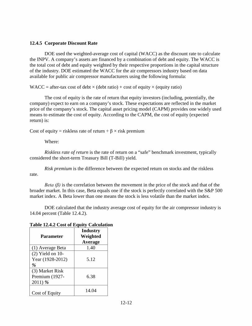
12-12

12.4.5 Corporate Discount Rate

DOE used the weighted-average cost of capital (WACC) as the discount rate to calculate the INPV. A company’s assets are financed by a combination of debt and equity. The WACC is the total cost of debt and equity weighted by their respective proportions in the capital structure of the industry. DOE estimated the WACC for the air compressors industry based on data available for public air compressor manufacturers using the following formula:

WACC = after-tax cost of debt × (debt ratio) + cost of equity × (equity ratio)

The cost of equity is the rate of return that equity investors (including, potentially, the company) expect to earn on a company’s stock. These expectations are reflected in the market price of the company’s stock. The capital asset pricing model (CAPM) provides one widely used means to estimate the cost of equity. According to the CAPM, the cost of equity (expected return) is:

Cost of equity = riskless rate of return + β × risk premium

Where:

Riskless rate of return is the rate of return on a “safe” benchmark investment, typically considered the short-term Treasury Bill (T-Bill) yield.

Risk premium is the difference between the expected return on stocks and the riskless rate.

Beta (β) is the correlation between the movement in the price of the stock and that of the broader market. In this case, Beta equals one if the stock is perfectly correlated with the S&P 500 market index. A Beta lower than one means the stock is less volatile than the market index.

DOE calculated that the industry average cost of equity for the air compressor industry is

14.04 percent (Table 12.4.2). Table 12.4.2 Cost of Equity Calculation

Parameter Industry Weighted Average

(1) Average Beta 1.40 (2) Yield on 10-Year (1928-2012) %

5.12

(3) Market Risk Premium (1927-2011) %

6.38

Cost of Equity 14.04

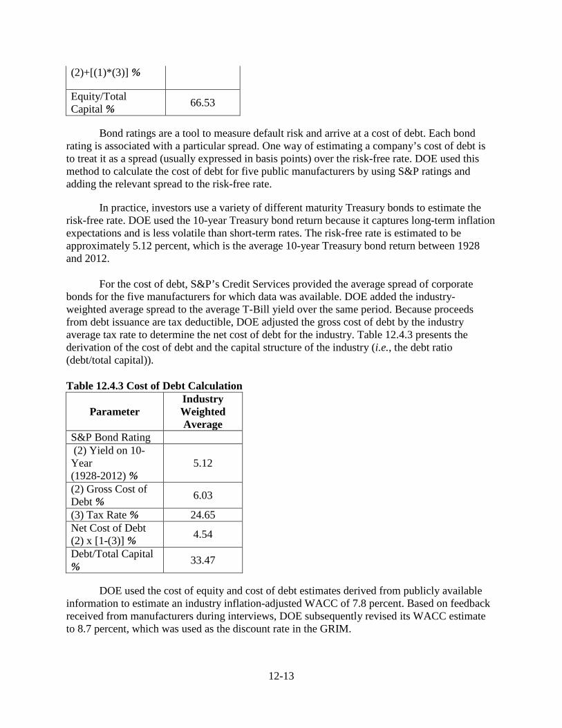
12-13

(2)+[(1)*(3)] %

Equity/Total Capital % 66.53

Bond ratings are a tool to measure default risk and arrive at a cost of debt. Each bond rating is associated with a particular spread. One way of estimating a company’s cost of debt is to treat it as a spread (usually expressed in basis points) over the risk-free rate. DOE used this method to calculate the cost of debt for five public manufacturers by using S&P ratings and adding the relevant spread to the risk-free rate.

In practice, investors use a variety of different maturity Treasury bonds to estimate the risk-free rate. DOE used the 10-year Treasury bond return because it captures long-term inflation expectations and is less volatile than short-term rates. The risk-free rate is estimated to be approximately 5.12 percent, which is the average 10-year Treasury bond return between 1928 and 2012.

For the cost of debt, S&P’s Credit Services provided the average spread of corporate bonds for the five manufacturers for which data was available. DOE added the industry-weighted average spread to the average T-Bill yield over the same period. Because proceeds from debt issuance are tax deductible, DOE adjusted the gross cost of debt by the industry average tax rate to determine the net cost of debt for the industry. Table 12.4.3 presents the derivation of the cost of debt and the capital structure of the industry (i.e., the debt ratio (debt/total capital)).

Table 12.4.3 Cost of Debt Calculation

Parameter Industry Weighted Average

S&P Bond Rating (2) Yield on 10-Year (1928-2012) %

5.12

(2) Gross Cost of Debt % 6.03

(3) Tax Rate % 24.65 Net Cost of Debt (2) x [1-(3)] % 4.54

Debt/Total Capital % 33.47

DOE used the cost of equity and cost of debt estimates derived from publicly available information to estimate an industry inflation-adjusted WACC of 7.8 percent. Based on feedback received from manufacturers during interviews, DOE subsequently revised its WACC estimate to 8.7 percent, which was used as the discount rate in the GRIM.

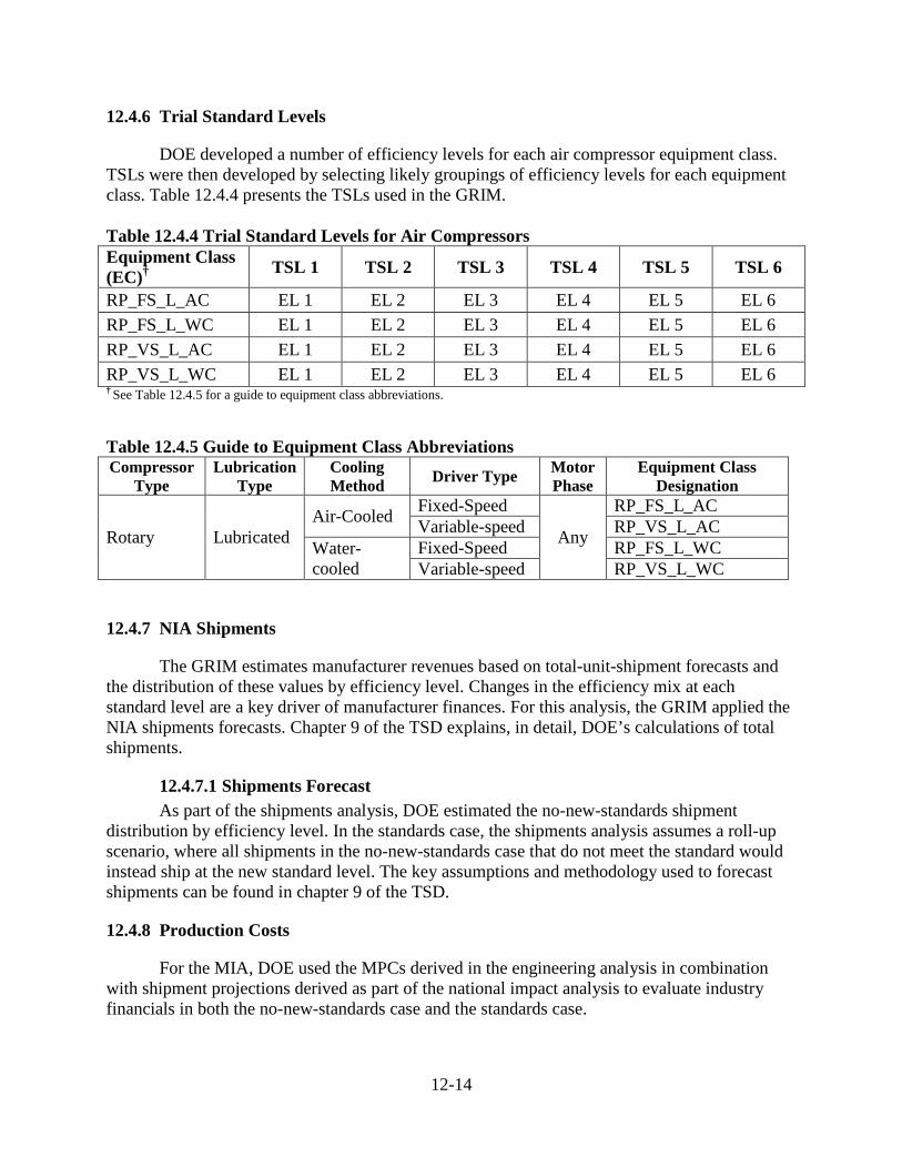
12-14

12.4.6 Trial Standard Levels

DOE developed a number of efficiency levels for each air compressor equipment class. TSLs were then developed by selecting likely groupings of efficiency levels for each equipment class. Table 12.4.4 presents the TSLs used in the GRIM. Table 12.4.4 Trial Standard Levels for Air Compressors Equipment Class (EC)† TSL 1 TSL 2 TSL 3 TSL 4 TSL 5 TSL 6

RP_FS_L_AC EL 1 EL 2 EL 3 EL 4 EL 5 EL 6 RP_FS_L_WC EL 1 EL 2 EL 3 EL 4 EL 5 EL 6 RP_VS_L_AC EL 1 EL 2 EL 3 EL 4 EL 5 EL 6 RP_VS_L_WC EL 1 EL 2 EL 3 EL 4 EL 5 EL 6 † See Table 12.4.5 for a guide to equipment class abbreviations. Table 12.4.5 Guide to Equipment Class Abbreviations Compressor

Type Lubrication

Type Cooling Method Driver Type Motor

Phase Equipment Class

Designation

Rotary Lubricated Air-Cooled Fixed-Speed

Any

RP_FS_L_AC Variable-speed RP_VS_L_AC

Water-cooled

Fixed-Speed RP_FS_L_WC Variable-speed RP_VS_L_WC

12.4.7 NIA Shipments

The GRIM estimates manufacturer revenues based on total-unit-shipment forecasts and the distribution of these values by efficiency level. Changes in the efficiency mix at each standard level are a key driver of manufacturer finances. For this analysis, the GRIM applied the NIA shipments forecasts. Chapter 9 of the TSD explains, in detail, DOE’s calculations of total shipments.

12.4.7.1 Shipments Forecast As part of the shipments analysis, DOE estimated the no-new-standards shipment

distribution by efficiency level. In the standards case, the shipments analysis assumes a roll-up scenario, where all shipments in the no-new-standards case that do not meet the standard would instead ship at the new standard level. The key assumptions and methodology used to forecast shipments can be found in chapter 9 of the TSD.

12.4.8 Production Costs

For the MIA, DOE used the MPCs derived in the engineering analysis in combination with shipment projections derived as part of the national impact analysis to evaluate industry financials in both the no-new-standards case and the standards case.

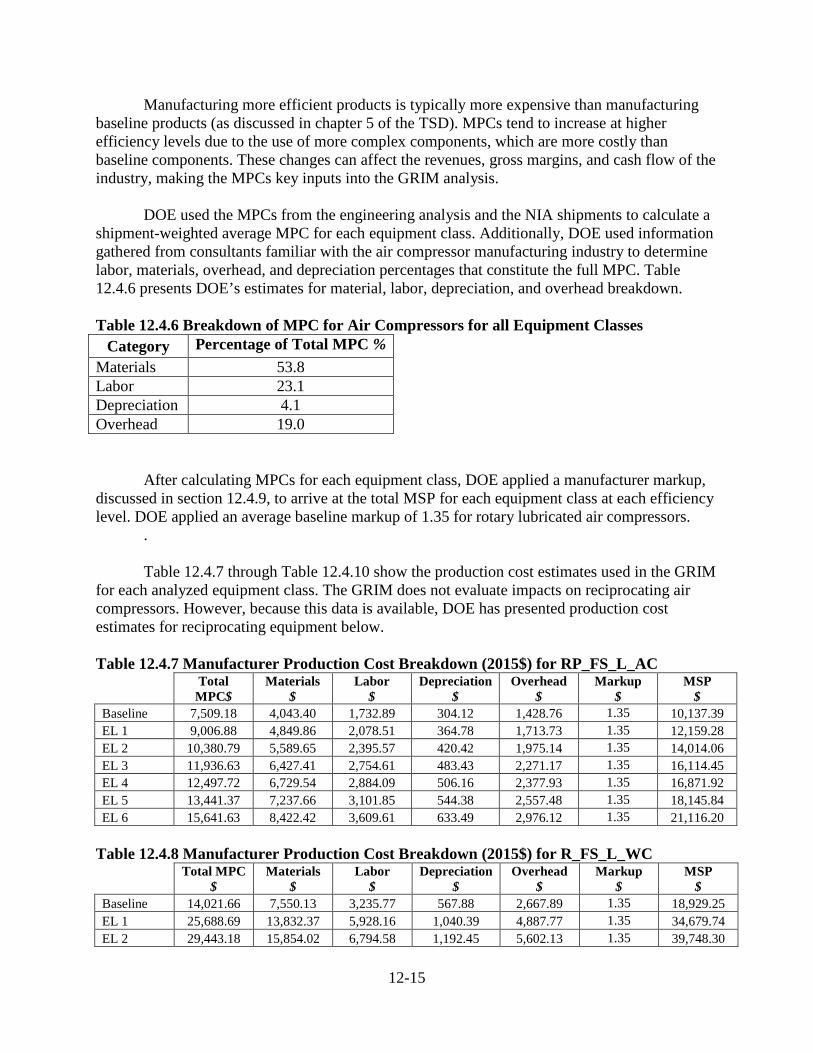
12-15

Manufacturing more efficient products is typically more expensive than manufacturing baseline products (as discussed in chapter 5 of the TSD). MPCs tend to increase at higher efficiency levels due to the use of more complex components, which are more costly than baseline components. These changes can affect the revenues, gross margins, and cash flow of the industry, making the MPCs key inputs into the GRIM analysis.

DOE used the MPCs from the engineering analysis and the NIA shipments to calculate a shipment-weighted average MPC for each equipment class. Additionally, DOE used information gathered from consultants familiar with the air compressor manufacturing industry to determine labor, materials, overhead, and depreciation percentages that constitute the full MPC. Table 12.4.6 presents DOE’s estimates for material, labor, depreciation, and overhead breakdown.

Table 12.4.6 Breakdown of MPC for Air Compressors for all Equipment Classes

Category Percentage of Total MPC % Materials 53.8 Labor 23.1 Depreciation 4.1 Overhead 19.0

After calculating MPCs for each equipment class, DOE applied a manufacturer markup,

discussed in section 12.4.9, to arrive at the total MSP for each equipment class at each efficiency level. DOE applied an average baseline markup of 1.35 for rotary lubricated air compressors.

. Table 12.4.7 through Table 12.4.10 show the production cost estimates used in the GRIM

for each analyzed equipment class. The GRIM does not evaluate impacts on reciprocating air compressors. However, because this data is available, DOE has presented production cost estimates for reciprocating equipment below.

Table 12.4.7 Manufacturer Production Cost Breakdown (2015$) for RP_FS_L_AC

Total MPC$

Materials $

Labor $

Depreciation $

Overhead $

Markup $

MSP $

Baseline 7,509.18 4,043.40 1,732.89 304.12 1,428.76 1.35 10,137.39 EL 1 9,006.88 4,849.86 2,078.51 364.78 1,713.73 1.35 12,159.28 EL 2 10,380.79 5,589.65 2,395.57 420.42 1,975.14 1.35 14,014.06 EL 3 11,936.63 6,427.41 2,754.61 483.43 2,271.17 1.35 16,114.45 EL 4 12,497.72 6,729.54 2,884.09 506.16 2,377.93 1.35 16,871.92 EL 5 13,441.37 7,237.66 3,101.85 544.38 2,557.48 1.35 18,145.84 EL 6 15,641.63 8,422.42 3,609.61 633.49 2,976.12 1.35 21,116.20

Table 12.4.8 Manufacturer Production Cost Breakdown (2015$) for R_FS_L_WC

Total MPC $

Materials $

Labor $

Depreciation $

Overhead $

Markup $

MSP $

Baseline 14,021.66 7,550.13 3,235.77 567.88 2,667.89 1.35 18,929.25 EL 1 25,688.69 13,832.37 5,928.16 1,040.39 4,887.77 1.35 34,679.74 EL 2 29,443.18 15,854.02 6,794.58 1,192.45 5,602.13 1.35 39,748.30

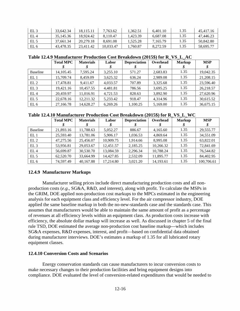
12-16

EL 3 33,642.34 18,115.11 7,763.62 1,362.51 6,401.10 1.35 45,417.16 EL 4 35,145.36 18,924.42 8,110.47 1,423.39 6,687.08 1.35 47,446.23 EL 5 37,661.34 20,279.18 8,691.08 1,525.28 7,165.79 1.35 50,842.80 EL 6 43,478.35 23,411.42 10,033.47 1,760.87 8,272.59 1.35 58,695.77

Table 12.4.9 Manufacturer Production Cost Breakdown (2015$) for R_VS_L_AC

Total MPC $

Materials $

Labor $

Depreciation $

Overhead $

Markup $

MSP $

Baseline 14,105.45 7,595.24 3,255.10 571.27 2,683.83 1.35 19,042.35 EL 1 15,709.74 8,459.09 3,625.32 636.24 2,989.08 1.35 21,208.15 EL 2 17,478.81 9,411.67 4,033.57 707.89 3,325.68 1.35 23,596.40 EL 3 19,421.16 10,457.55 4,481.81 786.56 3,695.25 1.35 26,218.57 EL 4 20,459.97 11,016.91 4,721.53 828.63 3,892.90 1.35 27,620.96 EL 5 22,678.16 12,211.32 5,233.42 918.47 4,314.96 1.35 30,615.52 EL 6 27,166.78 14,628.27 6,269.26 1,100.25 5,169.00 1.35 36,675.15

Table 12.4.10 Manufacturer Production Cost Breakdown (2015$) for R_VS_L_WC

Total MPC $

Materials $

Labor $

Depreciation $

Overhead $

Markup $

MSP $

Baseline 21,893.16 11,788.63 5,052.27 886.67 4,165.60 1.35 29,555.77 EL 1 25,593.40 13,781.06 5,906.17 1,036.53 4,869.64 1.35 34,551.09 EL 2 47,275.56 25,456.07 10,909.75 1,914.66 8,995.08 1.35 63,822.01 EL 3 53,956.81 29,053.67 12,451.57 2,185.25 10,266.32 1.35 72,841.69 EL 4 56,699.87 30,530.70 13,084.59 2,296.34 10,788.24 1.35 76,544.82 EL 5 62,520.70 33,664.99 14,427.85 2,532.09 11,895.77 1.35 84,402.95 EL 6 74,597.49 40,167.88 17,214.80 3,021.20 14,193.61 1.35 100,706.61

12.4.9 Manufacturer Markups

Manufacturer selling prices include direct manufacturing production costs and all non-production costs (e.g., SG&A, R&D, and interest), along with profit. To calculate the MSPs in the GRIM, DOE applied non-production cost markups to the MPCs estimated in the engineering analysis for each equipment class and efficiency level. For the air compressor industry, DOE applied the same baseline markup in both the no-new-standards case and the standards case. This assumes that manufacturers would be able to maintain the same amount of profit as a percentage of revenues at all efficiency levels within an equipment class. As production costs increase with efficiency, the absolute dollar markup will increase as well. As discussed in chapter 5 of the final rule TSD, DOE estimated the average non-production cost baseline markup—which includes SG&A expenses, R&D expenses, interest, and profit—based on confidential data obtained during manufacturer interviews. DOE’s estimates a markup of 1.35 for all lubricated rotary equipment classes. 12.4.10 Conversion Costs and Scenarios

Energy conservation standards can cause manufacturers to incur conversion costs to make necessary changes to their production facilities and bring equipment designs into compliance. DOE evaluated the level of conversion-related expenditures that would be needed to

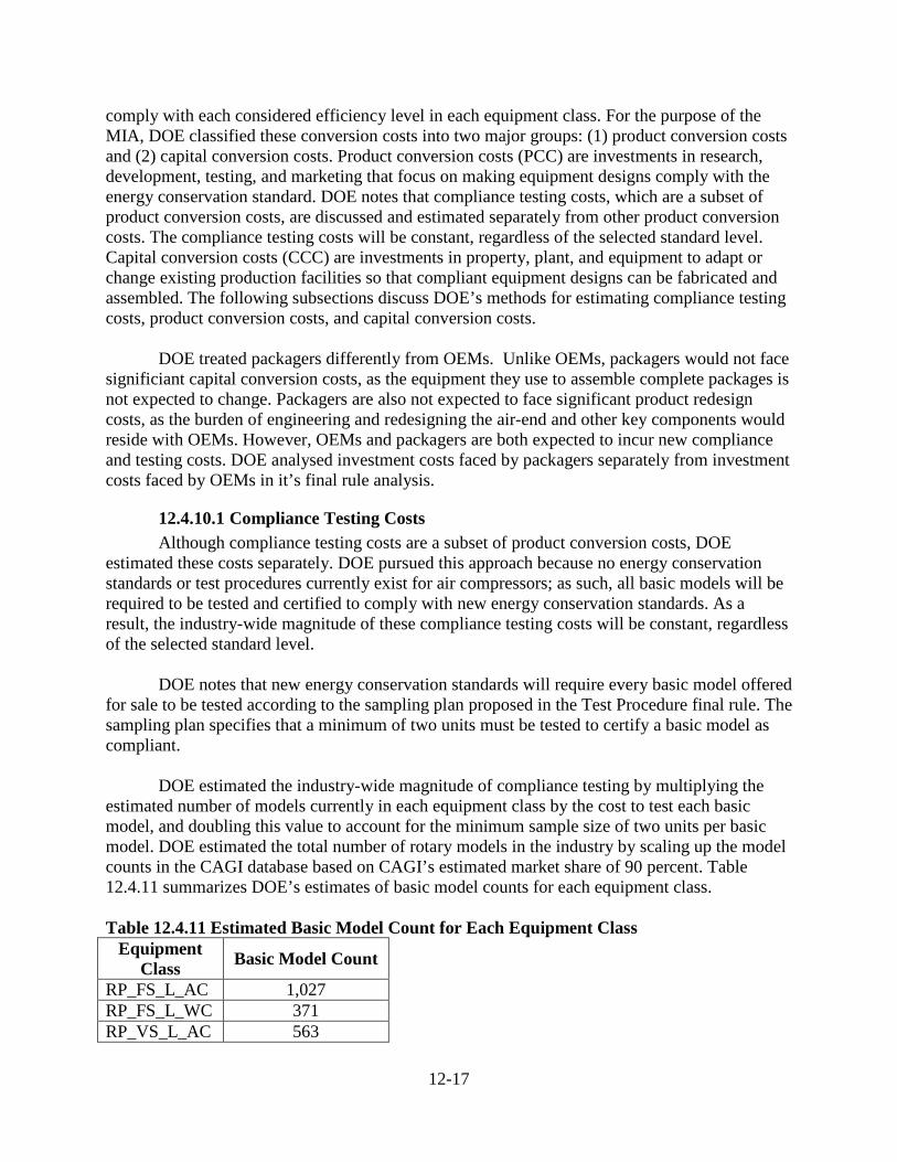
12-17

comply with each considered efficiency level in each equipment class. For the purpose of the MIA, DOE classified these conversion costs into two major groups: (1) product conversion costs and (2) capital conversion costs. Product conversion costs (PCC) are investments in research, development, testing, and marketing that focus on making equipment designs comply with the energy conservation standard. DOE notes that compliance testing costs, which are a subset of product conversion costs, are discussed and estimated separately from other product conversion costs. The compliance testing costs will be constant, regardless of the selected standard level. Capital conversion costs (CCC) are investments in property, plant, and equipment to adapt or change existing production facilities so that compliant equipment designs can be fabricated and assembled. The following subsections discuss DOE’s methods for estimating compliance testing costs, product conversion costs, and capital conversion costs.

DOE treated packagers differently from OEMs. Unlike OEMs, packagers would not face

significiant capital conversion costs, as the equipment they use to assemble complete packages is not expected to change. Packagers are also not expected to face significant product redesign costs, as the burden of engineering and redesigning the air-end and other key components would reside with OEMs. However, OEMs and packagers are both expected to incur new compliance and testing costs. DOE analysed investment costs faced by packagers separately from investment costs faced by OEMs in it’s final rule analysis.

12.4.10.1 Compliance Testing Costs Although compliance testing costs are a subset of product conversion costs, DOE

estimated these costs separately. DOE pursued this approach because no energy conservation standards or test procedures currently exist for air compressors; as such, all basic models will be required to be tested and certified to comply with new energy conservation standards. As a result, the industry-wide magnitude of these compliance testing costs will be constant, regardless of the selected standard level.

DOE notes that new energy conservation standards will require every basic model offered for sale to be tested according to the sampling plan proposed in the Test Procedure final rule. The sampling plan specifies that a minimum of two units must be tested to certify a basic model as compliant.

DOE estimated the industry-wide magnitude of compliance testing by multiplying the estimated number of models currently in each equipment class by the cost to test each basic model, and doubling this value to account for the minimum sample size of two units per basic model. DOE estimated the total number of rotary models in the industry by scaling up the model counts in the CAGI database based on CAGI’s estimated market share of 90 percent. Table 12.4.11 summarizes DOE’s estimates of basic model counts for each equipment class. Table 12.4.11 Estimated Basic Model Count for Each Equipment Class

Equipment Class Basic Model Count

RP_FS_L_AC 1,027 RP_FS_L_WC 371 RP_VS_L_AC 563

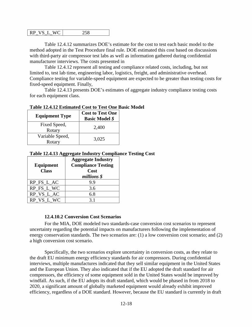
12-18

RP_VS_L_WC 258

Table 12.4.12 summarizes DOE’s estimate for the cost to test each basic model to the method adopted in the Test Procedure final rule. DOE estimated this cost based on discussions with third-party air compressor test labs as well as information gathered during confidential manufacturer interviews. The costs presented in

Table 12.4.12 represent all testing and compliance related costs, including, but not limited to, test lab time, engineering labor, logistics, freight, and administrative overhead. Compliance testing for variable-speed equipment are expected to be greater than testing costs for fixed-speed equipment. Finally,

Table 12.4.13 presents DOE’s estimates of aggregate industry compliance testing costs for each equipment class. Table 12.4.12 Estimated Cost to Test One Basic Model

Equipment Type Cost to Test One Basic Model $

Fixed Speed, Rotary 2,400

Variable Speed, Rotary 3,025

Table 12.4.13 Aggregate Industry Compliance Testing Cost

Equipment Class

Aggregate Industry Compliance Testing

Cost millions $

RP_FS_L_AC 9.9 RP_FS_L_WC 3.6 RP_VS_L_AC 6.8 RP_VS_L_WC 3.1

12.4.10.2 Conversion Cost Scenarios For the MIA, DOE modeled two standards-case conversion cost scenarios to represent

uncertainty regarding the potential impacts on manufacturers following the implementation of energy conservation standards. The two scenarios are: (1) a low conversion cost scenario; and (2) a high conversion cost scenario.

Specifically, the two scenarios explore uncertainty in conversion costs, as they relate to

the draft EU minimum energy efficiency standards for air compressors. During confidential interviews, multiple manufactures indicated that they sell similar equipment in the United States and the European Union. They also indicated that if the EU adopted the draft standard for air compressors, the efficiency of some equipment sold in the United States would be improved by windfall. As such, if the EU adopts its draft standard, which would be phased in from 2018 to 2020, a significant amount of globally marketed equipment would already exhibit improved efficiency, regardless of a DOE standard. However, because the EU standard is currently in draft

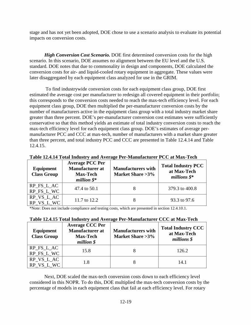
12-19

stage and has not yet been adopted, DOE chose to use a scenario analysis to evaluate its potential impacts on conversion costs.

High Conversion Cost Scenario. DOE first determined conversion costs for the high scenario. In this scenario, DOE assumes no alignment between the EU level and the U.S. standard. DOE notes that due to commonality in design and components, DOE calculated the conversion costs for air- and liquid-cooled rotary equipment in aggregate. These values were later disaggregated by each equipment class analyzed for use in the GRIM.

To find industrywide conversion costs for each equipment class group, DOE first

estimated the average cost per manufacturer to redesign all covered equipment in their portfolio; this corresponds to the conversion costs needed to reach the max-tech efficiency level. For each equipment class group, DOE then multiplied the per-manufacturer conversion costs by the number of manufacturers active in the equipment class group with a total industry market share greater than three percent. DOE’s per-manufacturer conversion cost estimates were sufficiently conservative so that this method yields an estimate of total industry conversion costs to reach the max-tech efficiency level for each equipment class group. DOE’s estimates of average per-manufacturer PCC and CCC at max-tech, number of manufacturers with a market share greater than three percent, and total industry PCC and CCC are presented in Table 12.4.14 and Table 12.4.15. Table 12.4.14 Total Industry and Average Per-Manufacturer PCC at Max-Tech

Equipment Class Group

Average PCC Per Manufacturer at

Max-Tech million $*

Manufacturers with Market Share >3%

Total Industry PCC at Max-Tech millions $*

RP_FS_L_AC RP_FS_L_WC 47.4 to 50.1 8 379.3 to 400.8

RP_VS_L_AC RP_VS_L_WC 11.7 to 12.2 8 93.3 to 97.6 *Note: Does not include compliance and testing costs, which are presented in section 12.4.10.1. Table 12.4.15 Total Industry and Average Per-Manufacturer CCC at Max-Tech

Equipment Class Group

Average CCC Per Manufacturer at

Max-Tech million $

Manufacturers with Market Share >3%

Total Industry CCC at Max-Tech

millions $

RP_FS_L_AC RP_FS_L_WC 15.8 8 126.2

RP_VS_L_AC RP_VS_L_WC 1.8 8 14.1

Next, DOE scaled the max-tech conversion costs down to each efficiency level

considered in this NOPR. To do this, DOE multiplied the max-tech conversion costs by the percentage of models in each equipment class that fail at each efficiency level. For rotary

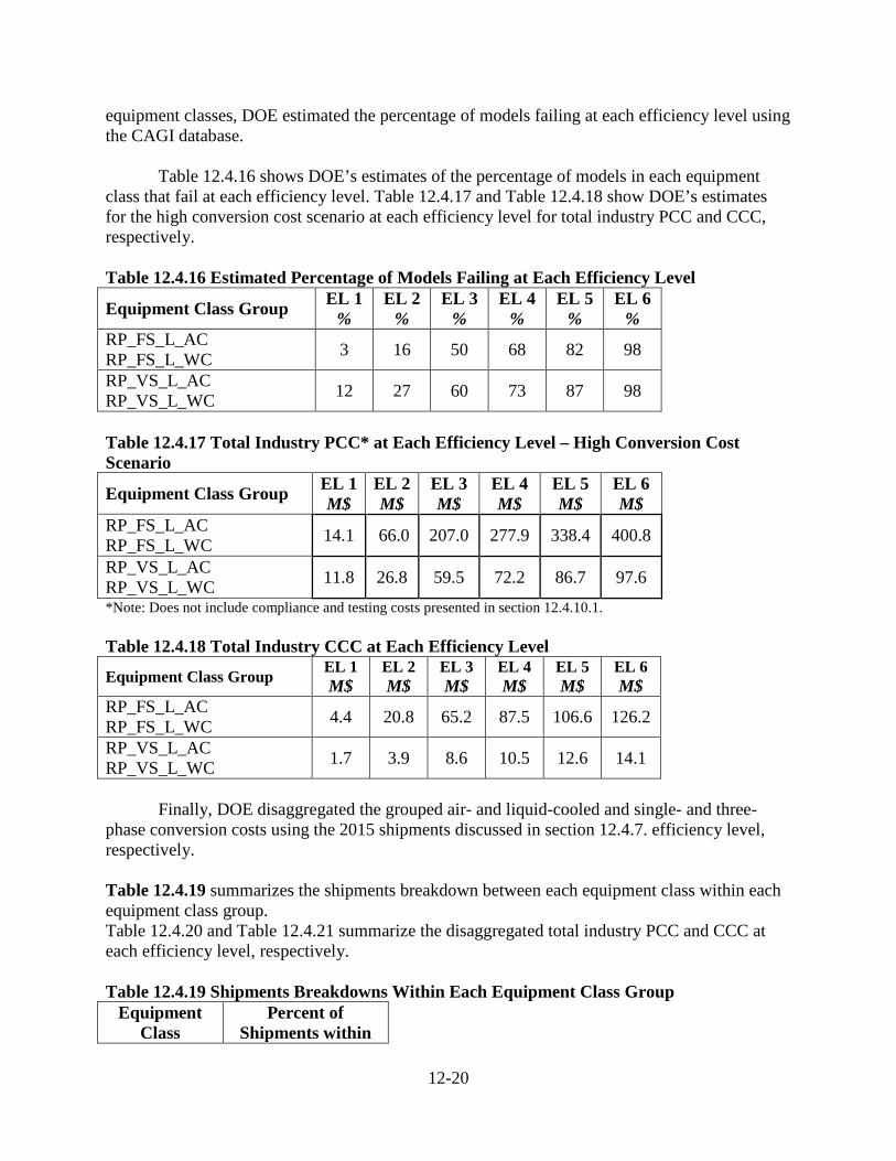
12-20

equipment classes, DOE estimated the percentage of models failing at each efficiency level using the CAGI database.

Table 12.4.16 shows DOE’s estimates of the percentage of models in each equipment class that fail at each efficiency level. Table 12.4.17 and Table 12.4.18 show DOE’s estimates for the high conversion cost scenario at each efficiency level for total industry PCC and CCC, respectively. Table 12.4.16 Estimated Percentage of Models Failing at Each Efficiency Level

Equipment Class Group EL 1 %

EL 2 %

EL 3 %

EL 4 %

EL 5 %

EL 6 %

RP_FS_L_AC RP_FS_L_WC 3 16 50 68 82 98

RP_VS_L_AC RP_VS_L_WC 12 27 60 73 87 98

Table 12.4.17 Total Industry PCC* at Each Efficiency Level – High Conversion Cost Scenario

Equipment Class Group EL 1 M$

EL 2 M$

EL 3 M$

EL 4 M$

EL 5 M$

EL 6 M$

RP_FS_L_AC RP_FS_L_WC 14.1 66.0 207.0 277.9 338.4 400.8

RP_VS_L_AC RP_VS_L_WC 11.8 26.8 59.5 72.2 86.7 97.6

*Note: Does not include compliance and testing costs presented in section 12.4.10.1. Table 12.4.18 Total Industry CCC at Each Efficiency Level

Equipment Class Group EL 1 M$

EL 2 M$

EL 3 M$

EL 4 M$

EL 5 M$

EL 6 M$

RP_FS_L_AC RP_FS_L_WC 4.4 20.8 65.2 87.5 106.6 126.2

RP_VS_L_AC RP_VS_L_WC 1.7 3.9 8.6 10.5 12.6 14.1

Finally, DOE disaggregated the grouped air- and liquid-cooled and single- and three-phase conversion costs using the 2015 shipments discussed in section 12.4.7. efficiency level, respectively. Table 12.4.19 summarizes the shipments breakdown between each equipment class within each equipment class group. Table 12.4.20 and Table 12.4.21 summarize the disaggregated total industry PCC and CCC at each efficiency level, respectively. Table 12.4.19 Shipments Breakdowns Within Each Equipment Class Group

Equipment Class

Percent of Shipments within

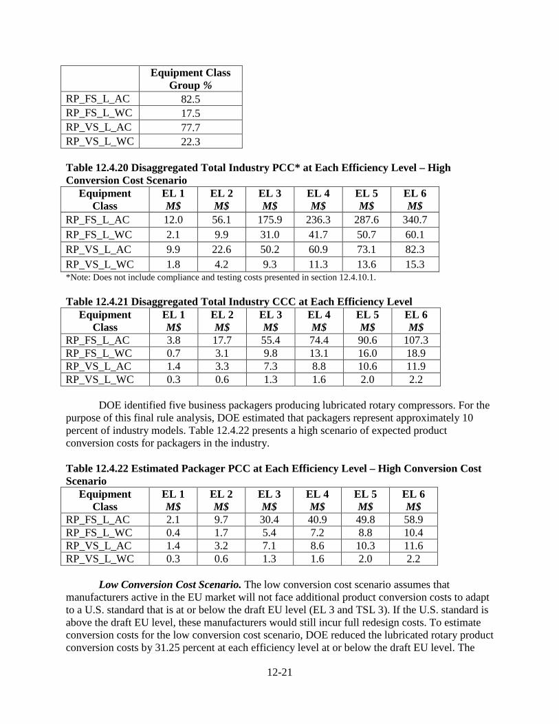
12-21

Equipment Class Group %

RP_FS_L_AC 82.5 RP_FS_L_WC 17.5 RP_VS_L_AC 77.7 RP_VS_L_WC 22.3 Table 12.4.20 Disaggregated Total Industry PCC* at Each Efficiency Level – High Conversion Cost Scenario

Equipment Class

EL 1 M$

EL 2 M$

EL 3 M$

EL 4 M$

EL 5 M$

EL 6 M$

RP_FS_L_AC 12.0 56.1 175.9 236.3 287.6 340.7 RP_FS_L_WC 2.1 9.9 31.0 41.7 50.7 60.1 RP_VS_L_AC 9.9 22.6 50.2 60.9 73.1 82.3 RP_VS_L_WC 1.8 4.2 9.3 11.3 13.6 15.3 *Note: Does not include compliance and testing costs presented in section 12.4.10.1. Table 12.4.21 Disaggregated Total Industry CCC at Each Efficiency Level

Equipment Class

EL 1 M$

EL 2 M$

EL 3 M$

EL 4 M$

EL 5 M$

EL 6 M$

RP_FS_L_AC 3.8 17.7 55.4 74.4 90.6 107.3 RP_FS_L_WC 0.7 3.1 9.8 13.1 16.0 18.9 RP_VS_L_AC 1.4 3.3 7.3 8.8 10.6 11.9 RP_VS_L_WC 0.3 0.6 1.3 1.6 2.0 2.2

DOE identified five business packagers producing lubricated rotary compressors. For the purpose of this final rule analysis, DOE estimated that packagers represent approximately 10 percent of industry models. Table 12.4.22 presents a high scenario of expected product conversion costs for packagers in the industry.

Table 12.4.22 Estimated Packager PCC at Each Efficiency Level – High Conversion Cost Scenario

Equipment Class

EL 1 M$

EL 2 M$

EL 3 M$

EL 4 M$

EL 5 M$

EL 6 M$

RP_FS_L_AC 2.1 9.7 30.4 40.9 49.8 58.9 RP_FS_L_WC 0.4 1.7 5.4 7.2 8.8 10.4 RP_VS_L_AC 1.4 3.2 7.1 8.6 10.3 11.6 RP_VS_L_WC 0.3 0.6 1.3 1.6 2.0 2.2

Low Conversion Cost Scenario. The low conversion cost scenario assumes that manufacturers active in the EU market will not face additional product conversion costs to adapt to a U.S. standard that is at or below the draft EU level (EL 3 and TSL 3). If the U.S. standard is above the draft EU level, these manufacturers would still incur full redesign costs. To estimate conversion costs for the low conversion cost scenario, DOE reduced the lubricated rotary product conversion costs by 31.25 percent at each efficiency level at or below the draft EU level. The

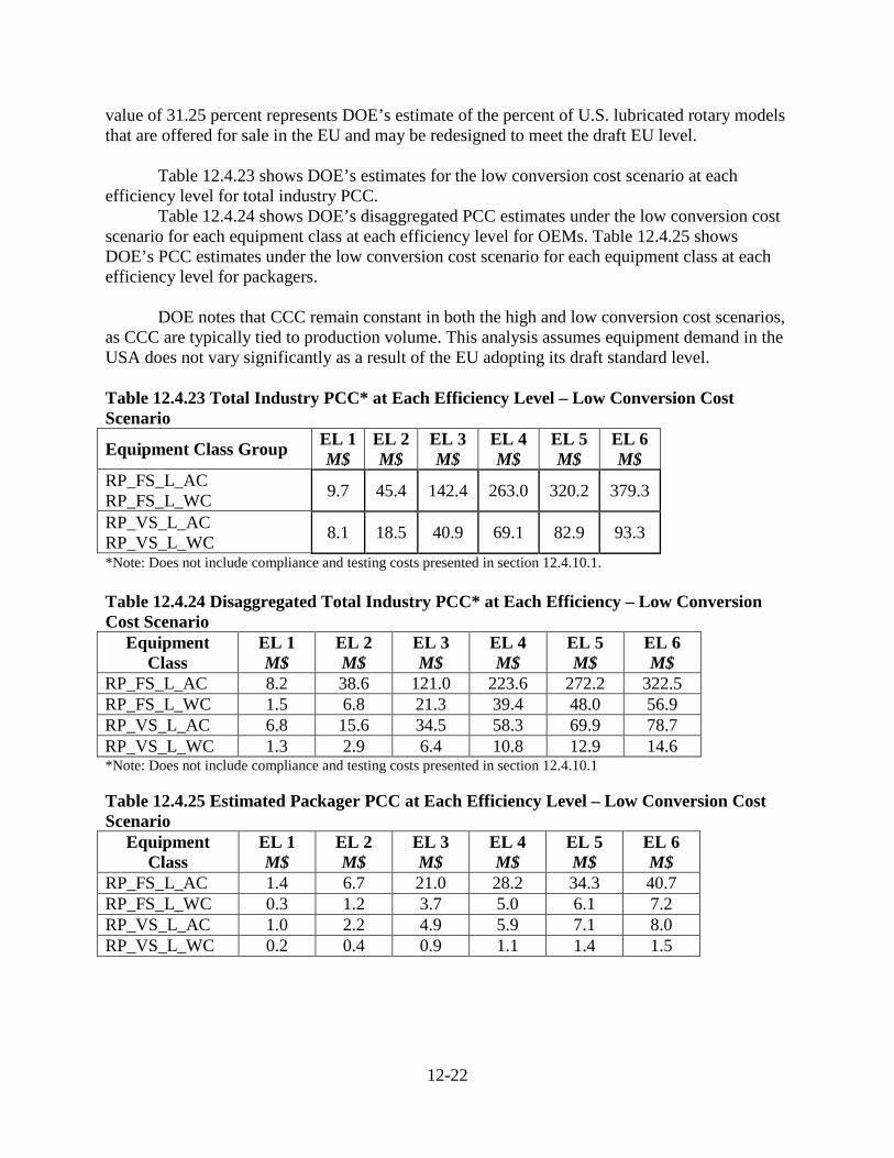
12-22

value of 31.25 percent represents DOE’s estimate of the percent of U.S. lubricated rotary models that are offered for sale in the EU and may be redesigned to meet the draft EU level.

Table 12.4.23 shows DOE’s estimates for the low conversion cost scenario at each

efficiency level for total industry PCC. Table 12.4.24 shows DOE’s disaggregated PCC estimates under the low conversion cost

scenario for each equipment class at each efficiency level for OEMs. Table 12.4.25 shows DOE’s PCC estimates under the low conversion cost scenario for each equipment class at each efficiency level for packagers.

DOE notes that CCC remain constant in both the high and low conversion cost scenarios,

as CCC are typically tied to production volume. This analysis assumes equipment demand in the USA does not vary significantly as a result of the EU adopting its draft standard level. Table 12.4.23 Total Industry PCC* at Each Efficiency Level – Low Conversion Cost Scenario

Equipment Class Group EL 1 M$

EL 2 M$

EL 3 M$

EL 4 M$

EL 5 M$

EL 6 M$

RP_FS_L_AC RP_FS_L_WC 9.7 45.4 142.4 263.0 320.2 379.3

RP_VS_L_AC RP_VS_L_WC 8.1 18.5 40.9 69.1 82.9 93.3

*Note: Does not include compliance and testing costs presented in section 12.4.10.1. Table 12.4.24 Disaggregated Total Industry PCC* at Each Efficiency – Low Conversion Cost Scenario

Equipment Class

EL 1 M$

EL 2 M$

EL 3 M$

EL 4 M$

EL 5 M$

EL 6 M$

RP_FS_L_AC 8.2 38.6 121.0 223.6 272.2 322.5 RP_FS_L_WC 1.5 6.8 21.3 39.4 48.0 56.9 RP_VS_L_AC 6.8 15.6 34.5 58.3 69.9 78.7 RP_VS_L_WC 1.3 2.9 6.4 10.8 12.9 14.6 *Note: Does not include compliance and testing costs presented in section 12.4.10.1 Table 12.4.25 Estimated Packager PCC at Each Efficiency Level – Low Conversion Cost Scenario

Equipment Class

EL 1 M$

EL 2 M$

EL 3 M$

EL 4 M$

EL 5 M$

EL 6 M$

RP_FS_L_AC 1.4 6.7 21.0 28.2 34.3 40.7 RP_FS_L_WC 0.3 1.2 3.7 5.0 6.1 7.2 RP_VS_L_AC 1.0 2.2 4.9 5.9 7.1 8.0 RP_VS_L_WC 0.2 0.4 0.9 1.1 1.4 1.5

12-23

12.4.10.3 Conversion Cost Summary Table 12.4.26 summarizes product conversion costs, including compliance testing costs,

at each efficiency level and conversion cost scenario, where applicable.

Table 12.4.26 Summary of Total Industry PCC, Including Compliance Testing Cost, at each Efficiency Level – High and Low Scenario

Equipment Class Scenario EL 1

M$ EL 2 M$

EL 3 M$

EL 4 M$

EL 5 M$

EL 6 M$

RP_FS_L_AC Low 18.1 48.4 130.9 233.5 282.1 332.3 High 21.8 65.9 185.8 246.1 297.5 350.6

RP_FS_L_WC Low 5.0 10.4 24.9 43.0 51.6 60.4 High 5.7 13.5 34.6 45.2 54.3 63.6

RP_VS_L_AC Low 13.7 22.4 41.3 65.1 76.7 85.6 High 16.8 29.5 57.0 67.8 79.9 89.2

RP_VS_L_WC Low 4.4 6.0 9.5 13.9 16.1 17.7 High 5.0 7.3 12.4 14.4 16.7 18.4

Finally, Table 12.4.27 and Table 12.4.28 present a summary of PCC and CCC at each efficiency

level for the following four major groupings of equipment classes: (1) rotary, lubricated, fixed-speed, air-cooled; (2) rotary, lubricated, fixed-speed, water-cooled; (3) rotary, lubricated, variable-speed, air-cooled; and (4) rotary, lubricated, variable-speed, liquid-cooled. These summaries are known commonalities of design and components within each group. Table 12.4.27 Aggregate Industry Product Conversion Cost, Including Compliance and Testing Costs, at Each Efficiency Level

Equipment Class Group* Scenario EL 1

M$ EL 2 M$

EL 3 M$

EL 4 M$

EL 5 M$

EL 6 M$

RP_FS_L_AC RP_VS_L_AC RP_FS_L_WC RP_VS_L_WC

Low 41.2 87.2 206.6 355.5 426.4 496.0

High 49.2 116.2 289.8 373.5 448.4 521.8

Table 12.4.28 Aggregate Industry Capital Conversion Cost at Each Efficiency Level

Equipment Class Group EL 1 M$

EL 2 M$

EL 3 M$

EL 4 M$

EL 5 M$

EL 6 M$

RP_FS_L_AC RP_VS_L_AC RP_FS_L_WC RP_VS_L_WC

6.1 24.7 73.8 98.0 119.1 140.4

In general, DOE assumes that all conversion-related investments occur between the year

of publication of the final rule and the year by which manufacturers must comply with the standard.

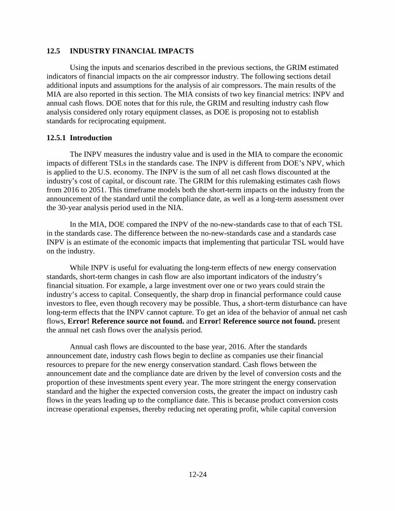
12-24

12.5 INDUSTRY FINANCIAL IMPACTS

Using the inputs and scenarios described in the previous sections, the GRIM estimated indicators of financial impacts on the air compressor industry. The following sections detail additional inputs and assumptions for the analysis of air compressors. The main results of the MIA are also reported in this section. The MIA consists of two key financial metrics: INPV and annual cash flows. DOE notes that for this rule, the GRIM and resulting industry cash flow analysis considered only rotary equipment classes, as DOE is proposing not to establish standards for reciprocating equipment.

12.5.1 Introduction

The INPV measures the industry value and is used in the MIA to compare the economic impacts of different TSLs in the standards case. The INPV is different from DOE’s NPV, which is applied to the U.S. economy. The INPV is the sum of all net cash flows discounted at the industry’s cost of capital, or discount rate. The GRIM for this rulemaking estimates cash flows from 2016 to 2051. This timeframe models both the short-term impacts on the industry from the announcement of the standard until the compliance date, as well as a long-term assessment over the 30-year analysis period used in the NIA.

In the MIA, DOE compared the INPV of the no-new-standards case to that of each TSL in the standards case. The difference between the no-new-standards case and a standards case INPV is an estimate of the economic impacts that implementing that particular TSL would have on the industry.

While INPV is useful for evaluating the long-term effects of new energy conservation standards, short-term changes in cash flow are also important indicators of the industry’s financial situation. For example, a large investment over one or two years could strain the industry’s access to capital. Consequently, the sharp drop in financial performance could cause investors to flee, even though recovery may be possible. Thus, a short-term disturbance can have long-term effects that the INPV cannot capture. To get an idea of the behavior of annual net cash flows, Error! Reference source not found. and Error! Reference source not found. present the annual net cash flows over the analysis period.

Annual cash flows are discounted to the base year, 2016. After the standards announcement date, industry cash flows begin to decline as companies use their financial resources to prepare for the new energy conservation standard. Cash flows between the announcement date and the compliance date are driven by the level of conversion costs and the proportion of these investments spent every year. The more stringent the energy conservation standard and the higher the expected conversion costs, the greater the impact on industry cash flows in the years leading up to the compliance date. This is because product conversion costs increase operational expenses, thereby reducing net operating profit, while capital conversion

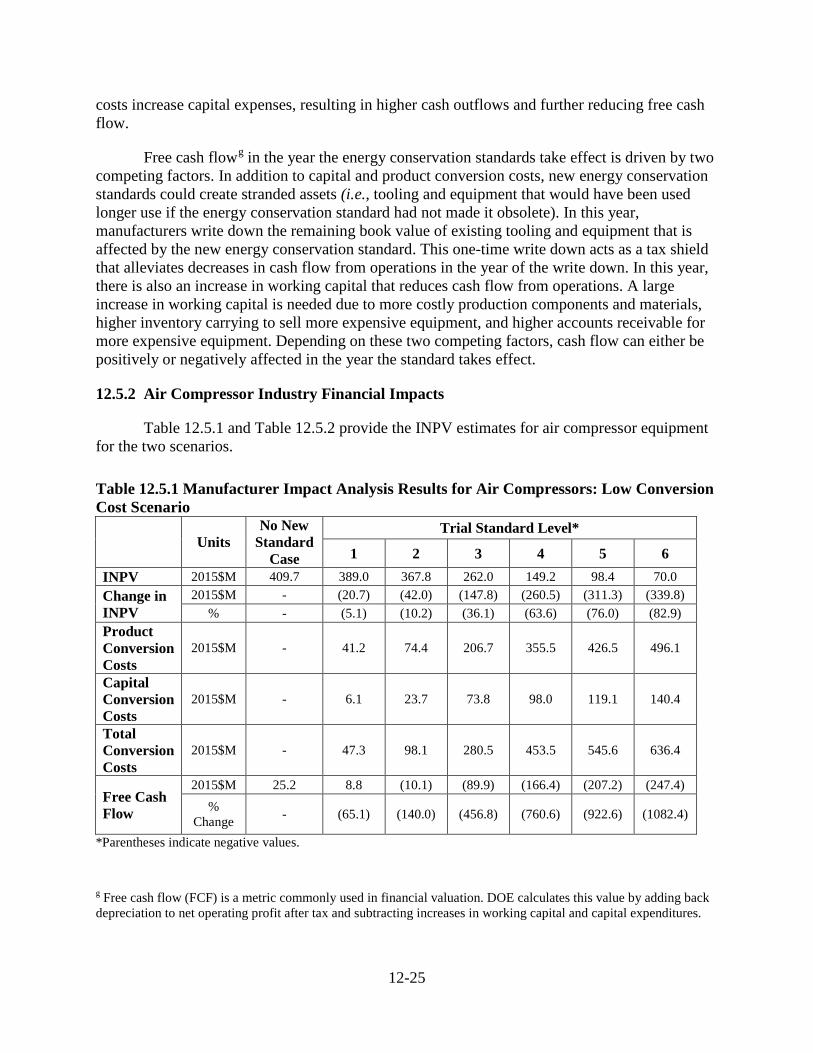
12-25

costs increase capital expenses, resulting in higher cash outflows and further reducing free cash flow.

Free cash flowg in the year the energy conservation standards take effect is driven by two competing factors. In addition to capital and product conversion costs, new energy conservation standards could create stranded assets (i.e., tooling and equipment that would have been used longer use if the energy conservation standard had not made it obsolete). In this year, manufacturers write down the remaining book value of existing tooling and equipment that is affected by the new energy conservation standard. This one-time write down acts as a tax shield that alleviates decreases in cash flow from operations in the year of the write down. In this year, there is also an increase in working capital that reduces cash flow from operations. A large increase in working capital is needed due to more costly production components and materials, higher inventory carrying to sell more expensive equipment, and higher accounts receivable for more expensive equipment. Depending on these two competing factors, cash flow can either be positively or negatively affected in the year the standard takes effect.

12.5.2 Air Compressor Industry Financial Impacts

Table 12.5.1 and Table 12.5.2 provide the INPV estimates for air compressor equipment for the two scenarios.

Table 12.5.1 Manufacturer Impact Analysis Results for Air Compressors: Low Conversion Cost Scenario

Units No New

Standard Case

Trial Standard Level*

1 2 3 4 5 6 INPV 2015$M 409.7 389.0 367.8 262.0 149.2 98.4 70.0 Change in INPV

2015$M - (20.7) (42.0) (147.8) (260.5) (311.3) (339.8) % - (5.1) (10.2) (36.1) (63.6) (76.0) (82.9)

Product Conversion Costs

2015$M - 41.2 74.4 206.7 355.5 426.5 496.1

Capital Conversion Costs

2015$M - 6.1 23.7 73.8 98.0 119.1 140.4

Total Conversion Costs

2015$M - 47.3 98.1 280.5 453.5 545.6 636.4

Free Cash Flow

2015$M 25.2 8.8 (10.1) (89.9) (166.4) (207.2) (247.4) %

Change - (65.1) (140.0) (456.8) (760.6) (922.6) (1082.4)

*Parentheses indicate negative values. g Free cash flow (FCF) is a metric commonly used in financial valuation. DOE calculates this value by adding back depreciation to net operating profit after tax and subtracting increases in working capital and capital expenditures.

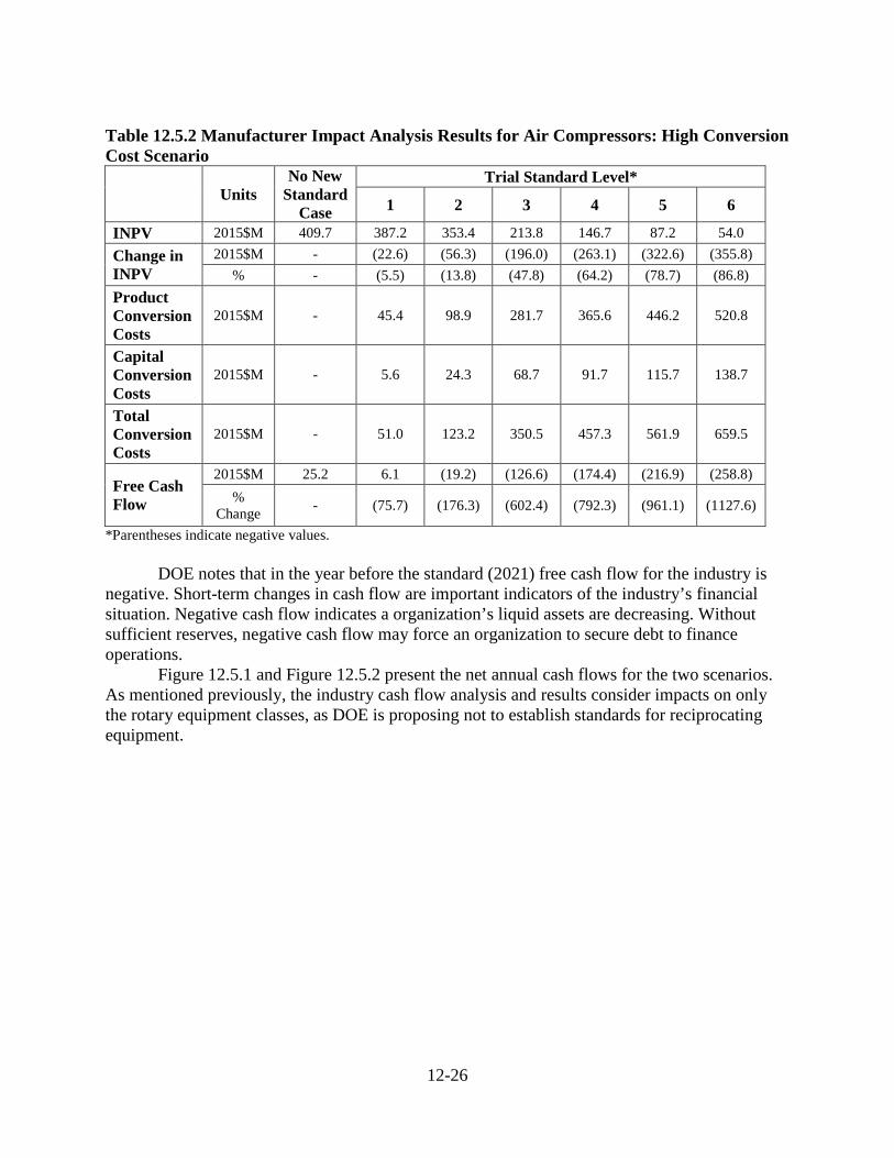
12-26

Table 12.5.2 Manufacturer Impact Analysis Results for Air Compressors: High Conversion Cost Scenario

Units No New

Standard Case

Trial Standard Level*

1 2 3 4 5 6

INPV 2015$M 409.7 387.2 353.4 213.8 146.7 87.2 54.0 Change in INPV

2015$M - (22.6) (56.3) (196.0) (263.1) (322.6) (355.8) % - (5.5) (13.8) (47.8) (64.2) (78.7) (86.8)

Product Conversion Costs

2015$M - 45.4 98.9 281.7 365.6 446.2 520.8

Capital Conversion Costs

2015$M - 5.6 24.3 68.7 91.7 115.7 138.7

Total Conversion Costs

2015$M - 51.0 123.2 350.5 457.3 561.9 659.5

Free Cash Flow

2015$M 25.2 6.1 (19.2) (126.6) (174.4) (216.9) (258.8) %

Change - (75.7) (176.3) (602.4) (792.3) (961.1) (1127.6)

*Parentheses indicate negative values. DOE notes that in the year before the standard (2021) free cash flow for the industry is

negative. Short-term changes in cash flow are important indicators of the industry’s financial situation. Negative cash flow indicates a organization’s liquid assets are decreasing. Without sufficient reserves, negative cash flow may force an organization to secure debt to finance operations.

Figure 12.5.1 and Figure 12.5.2 present the net annual cash flows for the two scenarios. As mentioned previously, the industry cash flow analysis and results consider impacts on only the rotary equipment classes, as DOE is proposing not to establish standards for reciprocating equipment.

12-27

Figure 12.5.1 Annual Industry Net Cash Flows for Air Compressors (Low Conversion Cost Scenario)

Figure 12.5.2 Annual Industry Net Cash Flows for Air Compressors (High Conversion Cost Scenario)

$(300.00)

$(250.00)

$(200.00)

$(150.00)

$(100.00)

$(50.00)

$-

$50.00

$100.00

2015

$ M

illio

ns

Net Free Cash Flow for Compressors

No STDs Case TSL 1 TSL 2 TSL 3 TSL 4 TSL 5 TSL 6

12-28

12.6 IMPACTS ON SMALL BUSINESS MANUFACTURERS

To estimate the number of small business manufacturers of equipment covered by this rulemaking, DOE reviewed publicly available data and contacted select companies on its list, as necessary, to determine whether they met the SBA’s definition of a small business manufacturer. DOE screened out companies that do not offer equipment covered by this rulemaking, do not meet the definition of a “small business,” or are foreign-owned and operated. DOE presented its list to manufacturers in MIA interviews and asked industry representatives if they were aware of any other small manufacturers during manufacturer interviews and at DOE public meetings.

Compressor manufacturers are classified under NAICS 333912, “Air and Gas

Compressor Manufacturing.” In February 2016, as codified in 13 CFR part 121, the SBA incrased size standards for NAICS code 333912 to 1,000 employees or fewer. Therefore, for the purpose of this final rule, DOE has identified 22 manufacturers of lubricated rotary compressor equipment sold in the United States and within the scope of this rulemaking. Seven of those manufacturers were under the 1,000-employee threshold defined by the SBA to qualify as a small business and are domestic companies.

Within the compressor industry, manufacturers are classified into two categories; original

equipment manufacturers (“OEMs”) and compressor packagers. OEMs manufacture their own air-ends and assemble them with other components to create complete package air compressors. Packagers assemble motors and other accessories with air-ends purchased from other companies, resulting in a complete air compressor.

Within the rotary air compressor industry, DOE identified 22 manufacturers; 15 are OEMs and seven are packagers of compressors. Of the 22 total manufacturers, seven large OEMs supply approximately 80 percent of shipments and revenues. Of the seven domestic small businesses identified, DOE’s research indicates that two are OEMs and five are packagers.

Of the seven domestic small rotary compressor manufacturers identified, DOE’s research

indicates that two are OEMs and five are packagers. Whereas OEMs would be expected to incur significant redesign and capital conversion costs in order to comply with new standards, packagers would not. Unlike OEMs, packagers would not face significant capital conversion costs, as the processes they use to assemble completed packages from purchased air-ends and components is not expected to change. Packagers are also not expected to face significant product redesign costs, as the burden of engineering and redesigning the air-end and other key components would reside with OEMs. However, as manufacturers OEMs and packagers are both expected to incur new compliance and testing costs, as any new energy conservation standard would require their equipment to be tested and certified to the standard, using a DOE test procedure.

As a result of these efforts, the following discussion of domestic small business impacts considers capital, redesign, and compliance cost impacts facing rotary OEMs, while only considering redesign and compliance cost impacts for rotary packagers.

DOE identified two small business OEMs producing lubricated rotary compressors.

Based on equipment listings data in the CAGI database, small business OEMs comprise

12-29

approximately three percent of industry listings. Excluding testing costs, DOE estimates that the average failing compressor model will cost between $0.29 million and $0.38 million in product and capital conversion costs. Using the CAGI database and manufacturer websites, DOE identified 23 failing models manufactured by small business OEMs. Therefore, DOE estimates that product and capital conversion costs, excluding testing costs, for small businesses to range from $6.6 million to $8.7 million. DOE notes that 21 of the 23 failing models are manufactured by one small business OEM. This small business OEM may incur disproportionate impacts relative to the industry because their percentage of failing models is above the industry average.

DOE identified five small business packagers producing lubricated rotary compressors. DOE estimates that the average packager will incur between $1.5 million and $2.2 million in engineering redesign costs at TSL2. DOE was unable to obtain equipment performance data for packagers. During the NOPR stage, DOE estimated the total number of rotary models in the industry by scaling the model counts in the CAGI database by CAGI’s estimated market share; 85 percent. In the final rule analysis, DOE updated the CAGI database with additional manufacturers and models. The CAGI database model count increased by approximately five percent and therefore, for the purposes of the final rule analysis, DOE estimates that packagers represent approximately 10 percent of industry models. Therefore, DOE calculated the industry testing cost to packagers at approximately $2.3 million. Further, using publicly available information, DOE calculated the average annual revenue of a small business packager at $14.5 million. With a conversion period of five years, 2017 to 2021, the average small business packager would have to commit between 2.5 percent and 3.5 percent of their conversion period revenue to cover the estimated engineering redesign and testing costs at TSL 2.

DOE’s conversion cost estimates were derived from total industry conversion costs discussed previously in section 12.4.10. DOE notes that the ranges shown here relate to the two conversion cost scenarios investigated in section 12.4.10.

However, as noted in section 12.5, the GRIM free cash flow results in 2021 indicated that

some manufacturers may need to access the capital markets in order to fund conversion costs directly related to the proposed standard. Given that small manufacturers may have greater difficulty securing outside capitalh and that the necessary conversion costs are not insignificant to the size of a small business, it is possible the domestic small OEMs may be forced to retire a greater portion of product models than large competitors. In addition, smaller companies often have a higher cost of borrowing due to higher risk on the part of investors, largely attributed to lower cash flows and lower per unit profitability. In these cases, small manufacturers may observe higher costs of debt than larger manufacturers.

12.7 OTHER IMPACTS

h Simon, Ruth, and Angus Loten, Small-Business Lending Is Slow to Recover, Wall Street Journal, August 14, 2014. Accessed August 2014, available at http://online.wsj.com/articles/small-business-lending-is-slow-to-recover-1408329562.

12-30

12.7.1 Employment

12.7.1.1 Methodology To quantitatively assess the potential impacts of energy conservation standards on direct

employment, DOE used the GRIM to estimate the domestic labor expenditures and number of direct employees in the no-new-standards case and at each TSL from 2016 through 2051. DOE used statistical data from the U.S. Census Bureau’s 2014 ASM, the results of the engineering analysis, and interviews with manufacturers to determine the inputs necessary to calculate industrywide labor expenditures and domestic direct employment levels. Labor expenditures related to producing the equipment are a function of the labor intensity of producing the equipment, the sales volume, and an assumption that wages remain fixed in real terms over time. The total labor expenditures in each year are calculated by multiplying the MPCs by the labor percentage of MPCs. DOE estimates that 50 percent of rotary air compressors are produced domestically.

The total labor expenditures in the GRIM were then converted to domestic production

employment levels by dividing production labor expenditures by the annual payment per production worker (production worker hours multiplied by the labor rate found in the ASM). The production worker estimates in this section only cover workers up to the line-supervisor level who are directly involved in fabricating and assembling equipment within an OEM facility. Workers performing services that are closely associated with production operations, such as materials-handling tasks using forklifts, are also included as production labor.

To calculate non-production workers, the GRIM assumes non-production workers

account for 42 percent of total direct employment, which is a ratio derived from 2014 ASM data. The total direct employment impacts calculated in the GRIM are the sum of the changes in the number of domestic production and non-production workers resulting from the new energy conservation standards for compressors, as compared to the no-new-standards case. In general, more efficient compressors are complex and more labor intensive. Per-unit labor requirements and production time requirements increase with higher energy conservation standards.

To estimate an upper bound to employment change, DOE assumes all domestic

manufacturers would choose to continue producing equipment in the U.S. and would not move production to foreign countries. To estimate a lower bound to employment, DOE considers the case where all manufacturers choose to relocate overseas the production of failing rotary compressors under 50 hp, rather than make the necessary conversions at domestic production facilities. To assess employment change under this scenario, DOE estimated the revenues attributed to compressors whose production would be relocated overseas, and adjusted employment numbers accordingly. Specifically, DOE found that approximately 45 percent of rotary, lubricated compressor revenues come from compressors that are under 50 hp. Therefore, to find the revenues attributed to compressors that would be relocated overseas, DOE multiplied the shipments failing at each TSL by 50 percent.

12.7.1.1 Direct Employment Impacts In the absence of energy conservation standards, DOE estimates that the rotary air

compressors industry would employ 2,275 total production and non-production workers in 2022.

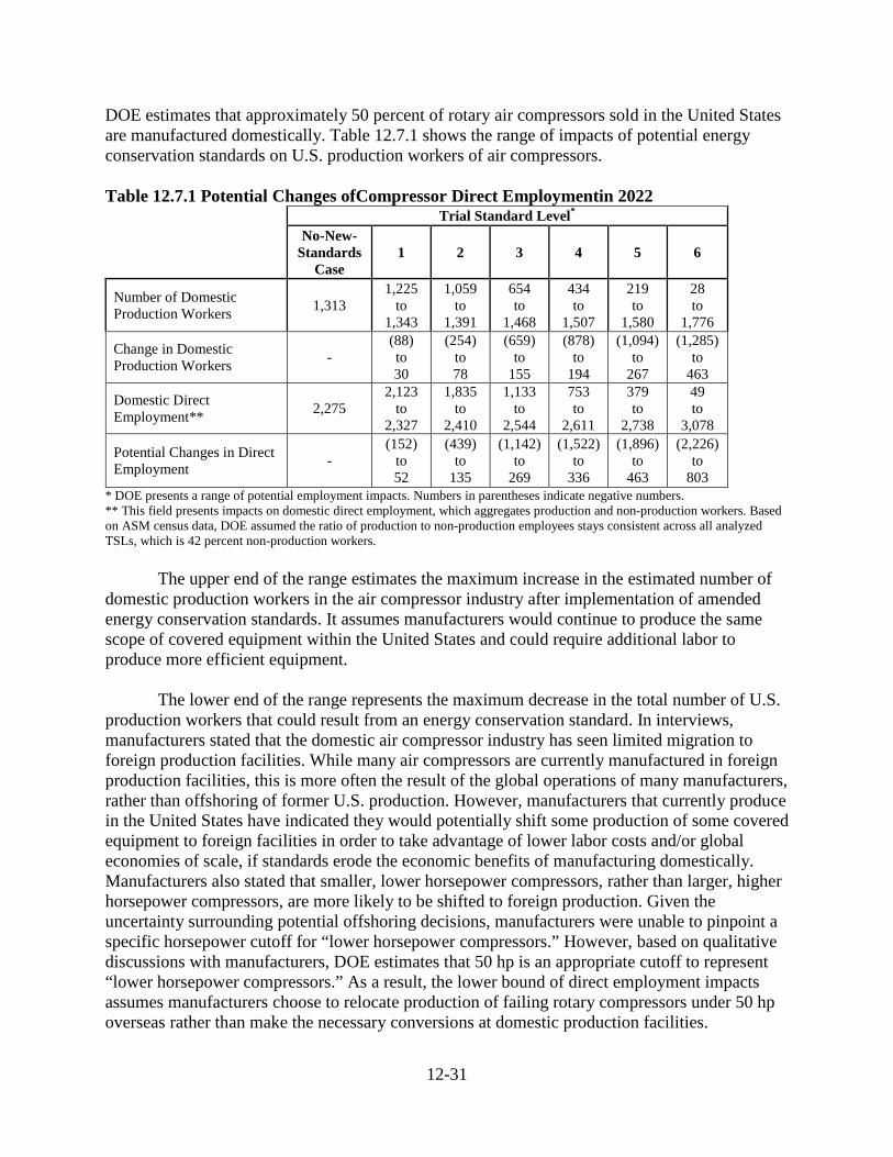
12-31

DOE estimates that approximately 50 percent of rotary air compressors sold in the United States are manufactured domestically. Table 12.7.1 shows the range of impacts of potential energy conservation standards on U.S. production workers of air compressors.

Table 12.7.1 Potential Changes ofCompressor Direct Employmentin 2022

Trial Standard Level*

No-New-Standards

Case 1 2 3 4 5 6

Number of Domestic Production Workers 1,313

1,225 to

1,343

1,059 to

1,391

654 to

1,468

434 to

1,507

219 to

1,580

28 to

1,776

Change in Domestic Production Workers -

(88) to 30

(254) to 78

(659) to

155

(878) to

194

(1,094) to

267

(1,285) to

463

Domestic Direct Employment** 2,275

2,123 to

2,327

1,835 to

2,410

1,133 to

2,544

753 to

2,611

379 to

2,738

49 to

3,078

Potential Changes in Direct Employment -

(152) to 52

(439) to

135

(1,142) to

269

(1,522) to

336

(1,896) to

463

(2,226) to

803 * DOE presents a range of potential employment impacts. Numbers in parentheses indicate negative numbers. ** This field presents impacts on domestic direct employment, which aggregates production and non-production workers. Based on ASM census data, DOE assumed the ratio of production to non-production employees stays consistent across all analyzed TSLs, which is 42 percent non-production workers. The upper end of the range estimates the maximum increase in the estimated number of domestic production workers in the air compressor industry after implementation of amended energy conservation standards. It assumes manufacturers would continue to produce the same scope of covered equipment within the United States and could require additional labor to produce more efficient equipment.

The lower end of the range represents the maximum decrease in the total number of U.S. production workers that could result from an energy conservation standard. In interviews, manufacturers stated that the domestic air compressor industry has seen limited migration to foreign production facilities. While many air compressors are currently manufactured in foreign production facilities, this is more often the result of the global operations of many manufacturers, rather than offshoring of former U.S. production. However, manufacturers that currently produce in the United States have indicated they would potentially shift some production of some covered equipment to foreign facilities in order to take advantage of lower labor costs and/or global economies of scale, if standards erode the economic benefits of manufacturing domestically. Manufacturers also stated that smaller, lower horsepower compressors, rather than larger, higher horsepower compressors, are more likely to be shifted to foreign production. Given the uncertainty surrounding potential offshoring decisions, manufacturers were unable to pinpoint a specific horsepower cutoff for “lower horsepower compressors.” However, based on qualitative discussions with manufacturers, DOE estimates that 50 hp is an appropriate cutoff to represent “lower horsepower compressors.” As a result, the lower bound of direct employment impacts assumes manufacturers choose to relocate production of failing rotary compressors under 50 hp overseas rather than make the necessary conversions at domestic production facilities.

12-32

The final rule analysis presents an updated set of total direct employment impacts that

range from a net loss of 439 to a gain of 135 jobs at the standard level. Therefore, DOE’s analysis agrees with the statements from the industry that there is a risk of decreasing the number of manufacturing jobs related to the covered equipment.

This conclusion is independent of any conclusions regarding indirect employment impacts in the broader U.S. economy, which are documented in chapter 15 of the TSD.

12.7.2 Production Capacity

In interviews, manufacturers of air compressors did not indicate that new energy conservation standards would significantly constrain manufacturing production capacity. However, as discussed in section 12.3.2, manufacturers expressed concern that they may face a bottleneck in the redesign process. In other words, manufacturers felt that if they could complete their redesigns within the compliance period, then they would not have a problem obtaining sufficient floor space, equipment, and manufacturing labor to meet the shipment demands of the market following an energy conservation standard.

Manufacturers indicated that most experienced air compressor design engineers are already employed within the industry, which limits their ability to rapidly expand their research and development teams if faced with a high volume of required compressor redesigns. Consequently, manufacturers typically commented that standard levels at or above the equivalent of TSL 3 could cause engineering constraints which might create time delays in complying with new standards. DOE notes that manufacturers typically discussed this constraint with respect to a three-year compliance period.

However, DOE is adopting a standard level at TSL 2, in conjunction with a 5-year compliance period. As such, DOE concludes that sufficient engineering resources are available to meet the proposed standard level over the 5-year compliance period.

12.7.3 Cumulative Regulatory Burden

While any one regulation may not impose a significant burden on manufacturers, the combined effects of recent or impending regulations may have serious consequences for some manufacturers, groups of manufacturers, or an entire industry. Assessing the impact of a single regulation may overlook this cumulative regulatory burden. In addition to energy conservation standards, other regulations can significantly affect manufacturers’ financial operations. Multiple regulations affecting the same manufacturer can strain profits and lead companies to abandon equipment lines or markets with lower expected future returns than competing equipment. For these reasons, DOE conducts an analysis of cumulative regulatory burden as part of its rulemakings pertaining to appliance efficiency.

For the cumulative regulatory burden analysis, DOE looks at other regulations that could

affect compressor manufacturers during the compliance period, from 2016 to 2022, or those that will take effect approximately 3 years after the 2022 compliance date of new energy

12-33

conservation standards for this equipment. The compliance years and expected industry conversion costs of relevant energy conservation standards are indicated in Table 12.7.2.

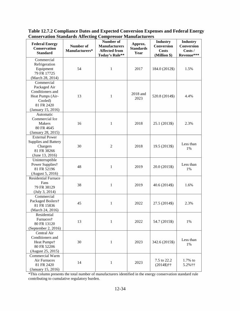
12-34

Table 12.7.2 Compliance Dates and Expected Conversion Expenses and Federal Energy Conservation Standards Affecting Compressor Manufacturers

Federal Energy Conservation

Standard

Number of Manufacturers*

Number of Manufacturers Affected from

Today’s Rule**

Approx. Standards

Year

Industry Conversion

Costs (Million $)

Industry Conversion

Costs / Revenue***

Commercial Refrigeration Equipment

79 FR 17725 (March 28, 2014)

54 1 2017 184.0 (2012$) 1.5%

Commercial Packaged Air

Conditioners and Heat Pumps (Air-

Cooled) 81 FR 2420

(January 15, 2016)

13 1 2018 and 2023 520.8 (2014$) 4.4%

Automatic Commercial Ice

Makers 80 FR 4645

(January 28, 2015)

16 1 2018 25.1 (2013$) 2.3%

External Power Supplies and Battery

Chargers 81 FR 38266

(June 13, 2016)

30 2 2018 19.5 (2013$) Less than 1%

Uninterruptible Power Supplies†

81 FR 52196 (August 5, 2016)

48 1 2019 20.0 (2015$) Less than 1%

Residential Furnace Fans

79 FR 38129 (July 3, 2014)

38 1 2019 40.6 (2014$) 1.6%

Commercial Packaged Boilers†

81 FR 15836 (March 24, 2016)

45 1 2022 27.5 (2014$) 2.3%

Residential Furnaces†

80 FR 13120 (September 2, 2016)

13 1 2022 54.7 (2015$) 1%

Central Air Conditioners and

Heat Pumps† 80 FR 52206

(August 25, 2015)

30 1 2023 342.6 (2015$) Less than 1%

Commercial Warm Air Furnaces 81 FR 2420

(January 15, 2016)

14 1 2023 7.5 to 22.2 (2014$)††

1.7% to 5.2%††

*This column presents the total number of manufacturers identified in the energy conservation standard rule contributing to cumulative regulatory burden.

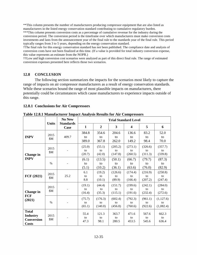
12-35

**This column presents the number of manufacturers producing compressor equipment that are also listed as manufacturers in the listed energy conservation standard contributing to cumulative regulatory burden. ***This column presents conversion costs as a percentage of cumulative revenue for the industry during the conversion period. The conversion period is the timeframe over which manufacturers must make conversion costs investments and lasts from the announcement year of the final rule to the standards year of the final rule. This period typically ranges from 3 to 5 years, depending on the energy conservation standard. †The final rule for this energy conservation standard has not been published. The compliance date and analysis of conversion costs have not been finalized at this time. (If a value is provided for total industry conversion expense, this value represents an estimate from the NOPR.) ††Low and high conversion cost scenarios were analyzed as part of this direct final rule. The range of estimated conversion expenses presented here reflects those two scenarios.

12.8 CONCLUSION The following section summarizes the impacts for the scenarios most likely to capture the

range of impacts on air compressor manufacturers as a result of energy conservation standards. While these scenarios bound the range of most plausible impacts on manufacturers, there potentially could be circumstances which cause manufacturers to experience impacts outside of this range.

12.8.1 Conclusions for Air Compressors

Table 12.8.1 Manufacturer Impact Analysis Results for Air Compressors

Units

No New Standards

Case

Trial Standard Level

1 2 3 4 5 6

INPV 2015 $M 409.7

384.8 to

389.0

354.6 to

367.8

204.6 to

262.0

136.6 to

149.2

83.2 to

98.4

52.0 to

70.0

Change in INPV

2015 $M -

(25.0) to

(20.7)

(55.1) to

(42.0)

(205.2) to

(147.8)

(273.1) to

(260.5)

(326.6) to

(311.3)

(357.7) to

(339.8)

% - (6.1)

to (5.1)

(13.5) to

(10.2)

(50.1) to

(36.1)

(66.7) to

(63.6)

(79.7) to

(76.0)

(87.3) to

(82.9)

FCF (2021) 2015 $M 25.2

6.1 to 8.8

(19.2) to

(10.1)

(126.6) to

(89.9)

(174.4) to

(166.4)

(216.9) to

(207.2)

(258.8) to

(247.4)

Change in FCF (2021)

2015 $M -

(19.1) to

(16.4)

(44.4) to

(35.3)

(151.7) to

(115.1)

(199.6) to

(191.6)

(242.1) to

(232.4)

(284.0) to

(272.6)

% - (75.7)

to (65.1)

(176.3) to

(140.0)

(602.4) to

(456.8)

(792.3) to

(760.6)

(961.1) to

(922.6)

(1,127.6) to

(1,082.4)

Total Industry Conversion Costs

2015 $M -

55.4 to

47.3

121.3 to

98.1

363.7 to

280.5

471.6 to

453.5

567.6 to

545.6

662.3 to

636.4

12-36

TSL 1 represents EL 1 for lubricated rotary compressors. At TSL 1, DOE estimates the impacts on INPV to range from -$25.0 million to -$20.7 million, or a change of -6.1 percent to -5.1 percent. Industry free cash flow is estimated to change by -$19.1 million to -$16.4 million, or a change of -75.7 percent to -65.1 percent compared to the no-new-standards case value of $25.2 million in the year before the compliance date (2021). DOE estimates industry conversion costs of as high as $55.4 million to $47.3 million at TSL 1.

TSL 2 represents EL 2 lubricated rotary compressors. At TSL 2, DOE estimates impacts

on INPV to range from -$55.1 million to -$42.0 million, or a change in INPV of -13.5 percent to -10.2 percent. At this level, industry free cash flow is estimated to change by -$44.4 million to -$35.3 million, or a change of -176.3 percent to -140.0 percent compared to the no-new-standards case value of $25.2 million in the year before the compliance date (2021). DOE estimates industry conversion costs of as high as $121.3 million to $98.1 million at TSL 2.

TSL 3 represents EL 3 for lubricated rotary compressors. At TSL 3, DOE estimates

impacts on INPV of -$205.2 million to -$147.8 million, or a change in INPV of -50.1 percent to -36.1 percent. At this level, industry free cash flow is estimated to change by -$151.7 million to -$115.1 million, or a change of -602.4 percent to -456.8 percent compared to the no-new-standards case value of $25.2 million in the year before the compliance date (2021). DOE estimates industry conversion costs of as high as $363.7 million to $280.5 million at TSL 3.

TSL 4 represents EL 4 for lubricated rotary compressors. At TSL 4, DOE estimates

impacts on INPV of -$273.1 million to -$260.5, or a change in INPV of -66.7 percent to -63.6 percent. At this level, industry free cash flow is estimated to change by -$199.6 million to -$191.6 million, or a change of -760.6 percent to -792.3 percent compared to the no-new-standards case value of $25.2 million in the year before the compliance date (2021). DOE estimates industry conversion costs of as high as $471.6 million to $453.5 million at TSL 4.

TSL 5 represents EL 5 for lubricated rotary compressors. At TSL 5, DOE estimates

impacts on INPV of -$326.6 million to -$311.3, or a change in INPV of -79.7 percent to -76. percent. Industry free cash flow is estimated to change by -$242.1 million to -$232.4 million or a change of -961.1 percent to -922.6 percent compared to the no-new-standards case value of $25.2 million in the year before the compliance date (2021). DOE estimates industry conversion costs of as high as $567.6 million to $545.6 million at TSL 5.

TSL 6 represents EL 6 for lubricated rotary compressors. At TSL 6, DOE estimates

impacts on INPV of -$357.7 to -$339.8 million, or a change in INPV of -87.3 percent to -82.9 percent. Industry free cash flow is estimated to change by -$284.0 million to -$272.6 million, or a change of -1,127.6 percent to -1,082.4 percent compared to the no-new-standards case value of $25.2 million in the year before the compliance date (2021). DOE estimates industry conversion costs of as high as $662.3 to $636.4 million at TSL 6.

13-i

CHAPTER 13. EMISSIONS IMPACT ANALYSIS

TABLE OF CONTENTS

13.1 INTRODUCTION ......................................................................................................... 13-1 13.2 AIR QUALITY REGULATIONS AND EMISSIONS IMPACTS ............................... 13-1 13.3 EMISSIONS IMPACT RESULTS ................................................................................ 13-3 REFERENCES .......................................................................................................................... 13-8

LIST OF TABLES

Table 13.3.1 Cumulative Emissions Reduction for Potential Standards for Commercial and Industrial Air Compressors .............................................. 13-3

LIST OF FIGURES

Figure 13.3.1 Commercial and Industrial Air Compressors: CO2 Total Emissions Reduction ..................................................................................................... 13-4

Figure 13.3.2 Commercial and Industrial Air Compressors: SO2 Total Emissions Reduction ..................................................................................................... 13-5

Figure 13.3.3 Commercial and Industrial Air Compressors: NOx Total Emissions Reduction ..................................................................................................... 13-5

Figure 13.3.4 Commercial and Industrial Air Compressors: Hg Total Emissions Reduction ..................................................................................................... 13-6

Figure 13.3.5 Commercial and Industrial Air Compressors: N2O Total Emissions Reduction ..................................................................................................... 13-6

Figure 13.3.6 Commercial and Industrial Air Compressors: CH4 Total Emissions Reduction ..................................................................................................... 13-7

13-1

CHAPTER 13. EMISSIONS IMPACT ANALYSIS

13.1 INTRODUCTION

The emissions analysis consists of two components. The first component estimates the effect of potential energy conservation standards on power sector emissions and, if present, site combustion emissions of carbon dioxide (CO2), nitrogen oxides (NOX), sulfur dioxide (SO2) and mercury (Hg). The second component estimates the impacts of potential standards on emissions of two additional greenhouse gases, methane (CH4) and nitrous oxide (N2O), as well as the impacts to emissions of all species due to “upstream” activities in the fuel production chain. These upstream activities comprise extraction, processing, and transporting fuels to the site of combustion. The associated emissions are referred to as upstream emissions. Together, these emissions account for the full-fuel-cycle (FFC), in accordance with DOE’s FFC Statement of Policy. 76 FR 51282 (Aug. 18, 2011).

The analysis of power sector emissions uses marginal emissions intensity factors calculated by DOE. The methodology is based on results published for the Annual Energy Outlook 2016 (AEO 2016), including a set of side cases that implement a variety of efficiency-related policies.1 The methodology is described in appendix 13A to this TSD, and in the report “Utility Sector Impacts of Reduced Electricity Demand” (Coughlin, 2014).4

The emissions intensity factors are expressed in terms of physical units per MWh or MMBtu of site energy savings. Total emissions reductions are estimated by multiplying the emissions intensity factor by the energy savings calculated in the national impact analysis (chapter 10). The emissions factors used in the calculations are provided in appendix 13A. For power sector emissions, the factors depend on the sector and end use. The results presented here use factors for the power plant types that supply electricity for general use in commercial buildings and industrial facilities.

13.2 AIR QUALITY REGULATIONS AND EMISSIONS IMPACTS

Each annual version of the Annual Energy Outlook (AEO) incorporates the projected impacts of existing air quality regulations on emissions. AEO 2016 generally represents current Federal and State legislation and final implementation regulations in place as of the end of February 2016. DOE’s estimation of impacts accounts for the presence of the emissions control programs discussed in the following paragraphs.

SO2 emissions from affected electric generating units (EGUs) are subject to nationwide and regional emissions cap and trading programs. Title IV of the Clean Air Act sets an annual emissions cap on SO2 for affected EGUs in the 48 contiguous states and the District of Columbia (D.C.). SO2 emissions from 28 eastern states and D.C. were also limited under the Clean Air Interstate Rule (CAIR), which created an allowance-based trading program that operates along with the Title IV program in those States and D.C. 70 FR 25162 (May 12, 2005). CAIR was remanded to EPA by the U.S. Court of Appeals for the District of Columbia Circuit (D.C.

13-2

Circuit) but parts of it remained in effect. On July 6, 2011 EPA issued a replacement for CAIR, the Cross-State Air Pollution Rule (CSAPR). 76 FR 48208 (August 8, 2011). On August 21, 2012, the D.C. Circuit issued a decision to vacate CSAPR.a The court ordered EPA to continue administering CAIR. On April 29, 2014, the U.S. Supreme Court reversed the judgment of the D.C. Circuit and remanded the case for further proceedings consistent with the Supreme Court's opinion.b On October 23, 2014, the D.C. Circuit lifted the stay of CSAPR.c Pursuant to this action, CSAPR went into effect (and CAIR ceased to be in effect) as of January 1, 2015.d AEO2016 assumes implementation of CSAPR.

The attainment of emissions caps is typically flexible among affected Electric Generating Units (EGUs) and is enforced through the use of emissions allowances and tradable permits. Under existing EPA regulations, any excess SO2 emissions allowances resulting from the lower electricity demand caused by the imposition of an efficiency standard could be used to permit offsetting increases in SO2 emissions by any regulated EGU. In past rulemakings, DOE recognized that there was uncertainty about the effects of efficiency standards on SO2 emissions covered by the existing cap-and-trade system, but it concluded that no reductions in power sector emissions would occur for SO2 as a result of standards.

Beginning in 2016, however, SO2 emissions will fall as a result of the Mercury and Air Toxics Standards (MATS) for power plants. 77 FR 9304 (Feb. 16, 2012). In the final MATS rule, EPA established a standard for hydrogen chloride as a surrogate for acid gas hazardous air pollutants (HAP), and also established a standard for SO2 (a non-HAP acid gas) as an alternative equivalent surrogate standard for acid gas HAP. The same controls are used to reduce HAP and non-HAP acid gas; thus, SO2 emissions will be reduced as a result of the control technologies installed on coal-fired power plants to comply with the MATS requirements for acid gas. AEO 2016 assumes that, in order to continue operating, coal plants must have either flue gas desulfurization or dry sorbent injection systems installed by 2016. Both technologies, which are used to reduce acid gas emissions, also reduce SO2 emissions. Under the MATS, emissions will be far below the cap established by CSAPR, so it is unlikely that excess SO2 emissions allowances resulting from the lower electricity demand would be needed or used to permit offsetting increases in SO2 emissions by any regulated EGU. Therefore, DOE believes that efficiency standards will reduce SO2 emissions in 2016 and beyond.

CSAPR established a cap on NOx emissions in 28 eastern States and the District of Columbia.e Energy conservation standards are expected to have little effect on NOx emissions in a See EME Homer City Generation, LP v. EPA, 696 F.3d 7, 38 (D.C. Cir. 2012). b See EPA v. EME Homer City Generation, 134 S.Ct. 1584, 1610 (U.S. 2014). The Supreme Court held in part that EPA's methodology for quantifying emissions that must be eliminated in certain States due to their impacts in other downwind States was based on a permissible, workable, and equitable interpretation of the Clean Air Act provision that provides statutory authority for CSAPR. c See Georgia v. EPA, Order (D.C. Cir. filed October 23, 2014) (No. 11-1302). d On July 28, 2015, the D.C. Circuit issued its opinion regarding CSAPR on remand from the Supreme Court. The court largely upheld CSAPR, but remanded to EPA without vacatur certain States’ emission budgets for reconsideration. EME Homer City Generation, LP v. EPA, 795 F.3d 118 (D.C. Cir. 2015).

e CSAPR also applies to NOX and it supersedes the regulation of NOX under CAIR.

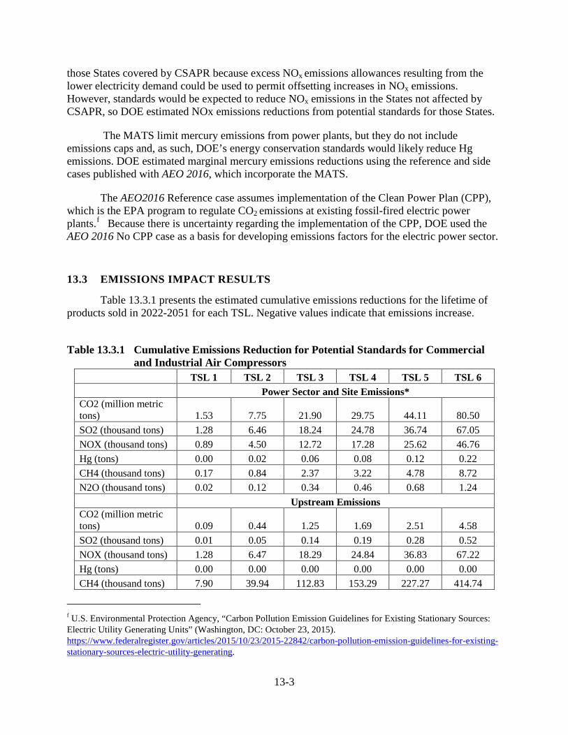
13-3

those States covered by CSAPR because excess NOx emissions allowances resulting from the lower electricity demand could be used to permit offsetting increases in NOx emissions. However, standards would be expected to reduce NOx emissions in the States not affected by CSAPR, so DOE estimated NOx emissions reductions from potential standards for those States.

The MATS limit mercury emissions from power plants, but they do not include emissions caps and, as such, DOE’s energy conservation standards would likely reduce Hg emissions. DOE estimated marginal mercury emissions reductions using the reference and side cases published with AEO 2016, which incorporate the MATS.

The AEO2016 Reference case assumes implementation of the Clean Power Plan (CPP), which is the EPA program to regulate CO2 emissions at existing fossil-fired electric power plants.f Because there is uncertainty regarding the implementation of the CPP, DOE used the AEO 2016 No CPP case as a basis for developing emissions factors for the electric power sector.

13.3 EMISSIONS IMPACT RESULTS

Table 13.3.1 presents the estimated cumulative emissions reductions for the lifetime of products sold in 2022-2051 for each TSL. Negative values indicate that emissions increase.

Table 13.3.1 Cumulative Emissions Reduction for Potential Standards for Commercial

and Industrial Air Compressors

TSL 1 TSL 2 TSL 3 TSL 4 TSL 5 TSL 6

Power Sector and Site Emissions*

CO2 (million metric tons) 1.53 7.75 21.90 29.75 44.11 80.50 SO2 (thousand tons) 1.28 6.46 18.24 24.78 36.74 67.05 NOX (thousand tons) 0.89 4.50 12.72 17.28 25.62 46.76 Hg (tons) 0.00 0.02 0.06 0.08 0.12 0.22 CH4 (thousand tons) 0.17 0.84 2.37 3.22 4.78 8.72 N2O (thousand tons) 0.02 0.12 0.34 0.46 0.68 1.24

Upstream Emissions

CO2 (million metric tons) 0.09 0.44 1.25 1.69 2.51 4.58 SO2 (thousand tons) 0.01 0.05 0.14 0.19 0.28 0.52 NOX (thousand tons) 1.28 6.47 18.29 24.84 36.83 67.22 Hg (tons) 0.00 0.00 0.00 0.00 0.00 0.00 CH4 (thousand tons) 7.90 39.94 112.83 153.29 227.27 414.74

f U.S. Environmental Protection Agency, “Carbon Pollution Emission Guidelines for Existing Stationary Sources: Electric Utility Generating Units” (Washington, DC: October 23, 2015). https://www.federalregister.gov/articles/2015/10/23/2015-22842/carbon-pollution-emission-guidelines-for-existing-stationary-sources-electric-utility-generating.

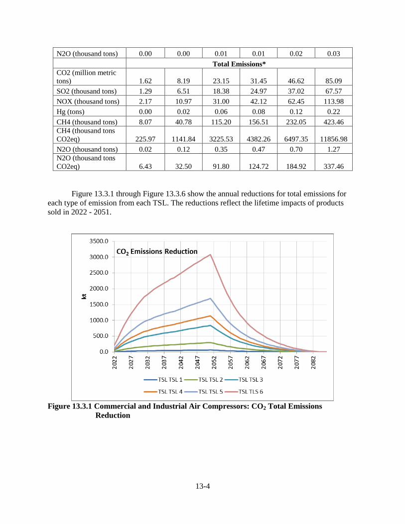
13-4

N2O (thousand tons) 0.00 0.00 0.01 0.01 0.02 0.03

Total Emissions*

CO2 (million metric tons) 1.62 8.19 23.15 31.45 46.62 85.09 SO2 (thousand tons) 1.29 6.51 18.38 24.97 37.02 67.57 NOX (thousand tons) 2.17 10.97 31.00 42.12 62.45 113.98 Hg (tons) 0.00 0.02 0.06 0.08 0.12 0.22 CH4 (thousand tons) 8.07 40.78 115.20 156.51 232.05 423.46 CH4 (thousand tons CO2eq) 225.97 1141.84 3225.53 4382.26 6497.35 11856.98 N2O (thousand tons) 0.02 0.12 0.35 0.47 0.70 1.27 N2O (thousand tons CO2eq) 6.43 32.50 91.80 124.72 184.92 337.46

Figure 13.3.1 through Figure 13.3.6 show the annual reductions for total emissions for each type of emission from each TSL. The reductions reflect the lifetime impacts of products sold in 2022 - 2051.

Figure 13.3.1 Commercial and Industrial Air Compressors: CO2 Total Emissions

Reduction

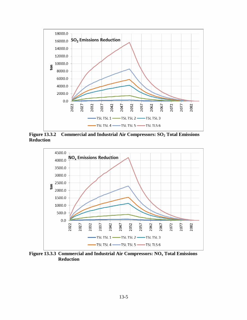
13-5

Figure 13.3.2 Commercial and Industrial Air Compressors: SO2 Total Emissions Reduction

Figure 13.3.3 Commercial and Industrial Air Compressors: NOx Total Emissions

Reduction

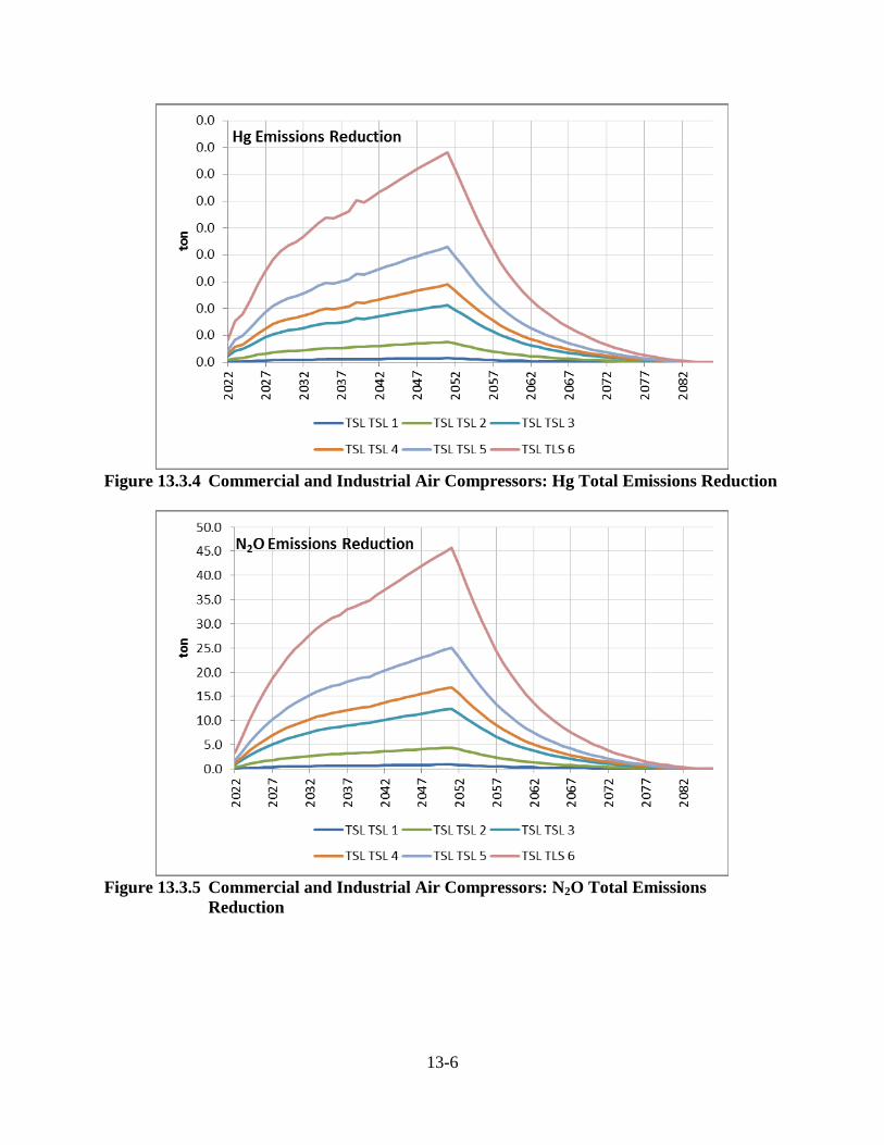
13-6

Figure 13.3.4 Commercial and Industrial Air Compressors: Hg Total Emissions Reduction

Figure 13.3.5 Commercial and Industrial Air Compressors: N2O Total Emissions

Reduction

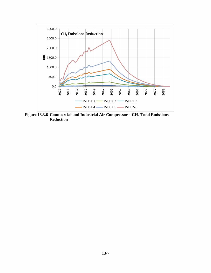
13-7

Figure 13.3.6 Commercial and Industrial Air Compressors: CH4 Total Emissions

Reduction

13-8

REFERENCES 1. Energy Information Administration, Annual Energy Outlook 2016 with Projections to

2040, September 2016. Washington, DC. http://www.eia.gov/forecasts/aeo/ 2. U.S. Environmental Protection Agency, Compilation of Air Pollutant Emission Factors,

AP-42, Fifth Edition, Volume I: Stationary Point and Area Sources. 1998. http://www.epa.gov/ttn/chief/ap42/index.html

3. Coughlin, K., Projections of Full-Fuel-Cycle Energy and Emissions Metrics, 2013.

Lawrence Berkeley National Laboratory. Report No. LBNL-6025E. http://ees.lbl.gov/sites/all/files/lbnl6025e_ffc.pdf.

4. Coughlin, K., Utility Sector Impacts of Reduced Electricity Demand, 2014. Lawrence

Berkeley National Laboratory. Report No. LBNL-6864E. http://www.osti.gov/scitech/biblio/1165372/

14-i

CHAPTER 14. MONETIZATION OF EMISSIONS REDUCTION BENEFITS

TABLE OF CONTENTS

14.1 INTRODUCTION ......................................................................................................... 14-1 14.2 MONETIZING CARBON DIOXIDE EMISSIONS ..................................................... 14-1

14.2.1 Social Cost of Carbon ........................................................................................ 14-1 14.2.2 Monetizing Carbon Dioxide Emissions ............................................................. 14-2 14.2.3 Current Approach and Key Assumptions .......................................................... 14-2

14.3 MONETIZING METHANE AND NITROUS OXIDE EMISSIONS .......................... 14-5 14.4 VALUATION OF OTHER EMISSIONS ..................................................................... 14-6 14.5 RESULTS ...................................................................................................................... 14-7 REFERENCES ........................................................................................................................ 14-10

LIST OF TABLES

Table 14.2.1 Annual SCC Values from 2013 Interagency Update (Revised July

2015), 2010–2050 (in 2007 dollars per metric ton CO2) ............................. 14-4 Table 14.3.1 Annual SC-CH4 and SC-N2O Estimates from 2016 IWG Addendum

(2007$ per Metric Ton CO2) ........................................................................ 14-6 Table 14.5.1 Global Present Value of CO2 Emissions Reduction for Potential

Standards for Commercial and Industrial Air Compressors ........................ 14-7 Table 14.5.2 Domestic Present Value of CO2 Emissions Reduction for Potential

Standards for Commercial and Industrial Air Compressors ........................ 14-8 Table 14.5.3 Present Value of Methane Emissions Reduction for Potential

Standards for Commercial and Industrial Air Compressors ........................ 14-8 Table 14.5.4 Present Value of Nitrous Oxide Emissions Reduction for Potential

Standards for Commercial and Industrial Air Compressors ........................ 14-9 Table 14.5.5 Present Value of NOX Emissions Reduction for Potential Standards for

Commercial and Industrial Air Compressors .............................................. 14-9

14-1

CHAPTER 14. MONETIZATION OF EMISSIONS REDUCTION BENEFITS

14.1 INTRODUCTION

As part of its assessment of energy conservation standards for commercial and industrial air compressors, the U.S. Department of Energy (DOE) estimated the monetary benefits likely to result from the reduced emissions of carbon dioxide (CO2), methane (CH4), nitrous oxide (N2O), and nitrogen oxides (NOX) that are expected to result from each trial standard level (TSL) considered for this rulemaking. This chapter summarizes the basis for the monetary values used for each of these emissions and presents the estimated benefits.

14.2 MONETIZATING CARBON DIOXIDE EMISSIONS

14.2.1 Social Cost of Carbon

The social cost of carbon (SCC) is an estimate of the monetized damages associated with an incremental increase in carbon emissions in a given year. It is intended to include (but is not limited to) changes in net agricultural productivity, human health, property damages from increased flood risk, and the value of ecosystem services. Estimates of the SCC are provided in dollars per metric ton of carbon dioxide. A domestic SCC value is meant to reflect the value of damages in the United States resulting from a unit change in carbon dioxide emissions, while a global SCC value is meant to reflect the value of damages worldwide.

Under section 1(b) of Executive Order 12866, agencies must, to the extent permitted by law, “assess both the costs and the benefits of the intended regulation and, recognizing that some costs and benefits are difficult to quantify, propose or adopt a regulation only upon a reasoned determination that the benefits of the intended regulation justify its costs.” The purpose of the SCC estimates presented here is to allow agencies to incorporate the monetized social benefits of reducing CO2 emissions into cost-benefit analyses of regulatory actions that have small, or “marginal,” impacts on cumulative global emissions. The estimates are presented with an acknowledgement of the many uncertainties involved and with a clear understanding that they should be updated over time to reflect increasing knowledge of the science and economics of climate impacts.

As part of the interagency process that developed these SCC estimates, technical experts from numerous agencies met on a regular basis to explore the technical literature in relevant fields, discuss key model inputs and assumptions, and consider public comments. The main objective of this process was to develop a range of SCC values using a defensible set of input assumptions grounded in the existing scientific and economic literatures. In this way, key uncertainties and model differences transparently and consistently inform the range of SCC estimates used in the rulemaking process.

14-2

14.2.2 Monetizing Carbon Dioxide Emissions

When attempting to assess the incremental economic impacts of carbon dioxide emissions, the analyst faces a number of serious challenges. A report from the National Research Council1 points out that any assessment will suffer from uncertainty, speculation, and lack of information about (1) future emissions of greenhouse gases, (2) the effects of past and future emissions on the climate system, (3) the impact of changes in climate on the physical and biological environment, and (4) the translation of these environmental impacts into economic damages. As a result, any effort to quantify and monetize the harms associated with climate change will raise serious questions of science, economics, and ethics and should be viewed as provisional.

Despite the limits of both quantification and monetization, SCC estimates can be useful in estimating the social benefits of reducing carbon dioxide emissions. Most Federal regulatory actions can be expected to have marginal impacts on global emissions. For such policies, the agency can estimate the benefits from reduced (or costs from increased) emissions in any future year by multiplying the change in emissions in that year by the SCC value appropriate for that year. The net present value of the benefits can then be calculated by multiplying each of these future benefits by an appropriate discount factor and summing across all affected years. This approach assumes that the marginal damages from increased emissions are constant for small departures from the baseline emissions path, an approximation that is reasonable for policies that have effects on emissions that are small relative to cumulative global carbon dioxide emissions.

In 2009, an interagency process was initiated to offer a preliminary assessment of how best to quantify the benefits from reducing carbon dioxide emissions. To ensure consistency in how benefits are evaluated across agencies, the Administration sought to develop a transparent and defensible method, specifically designed for the rulemaking process, to quantify avoided climate change damages from reduced CO2 emissions. The interagency group did not undertake any original analysis. Instead, it combined SCC estimates from the existing literature to use as interim values until a more comprehensive analysis could be conducted. These interim values represented the first sustained interagency effort within the U.S. government to develop an SCC for use in regulatory analysis. The results of this preliminary effort were presented in several proposed and final rules.

14.2.3 Current Approach and Key Assumptions

After the release of the interim values, the interagency group reconvened on a regular basis to generate improved SCC estimates. Specifically, the group considered public comments and further explored the technical literature in relevant fields. The interagency group relied on three integrated assessment models (IAMs) commonly used to estimate the SCC: the FUND, DICE, and PAGE models. These models are frequently cited in the peer-reviewed literature and were used in the last assessment of the Intergovernmental Panel on Climate Change. Each model was given equal weight in the SCC values that were developed.

Each model takes a slightly different approach to model how changes in emissions result in changes in economic damages. A key objective of the interagency process was to enable a consistent exploration of the three models while respecting the different approaches to quantifying damages taken by the key modelers in the field. An extensive review of the literature

14-3

was conducted to select three sets of input parameters for these models: (1) climate sensitivity; (2) socio-economic and emissions trajectories; and (3) discount rates. A probability distribution for climate sensitivity was specified as an input into all three models. In addition, the interagency group used a range of scenarios for the socio-economic parameters and a range of values for the discount rate. All other model features were left unchanged, relying on the model developers’ best estimates and judgments.

In 2010 the interagency group selected four SCC values for use in regulatory analyses.2 Three values are based on the average SCC from three integrated assessment models, at discount rates of 2.5, 3, and 5 percent. The fourth value, which represents the 95th percentile SCC estimate across all three models at a 3 percent discount rate, is included to represent higher-than-expected impacts from temperature change further out in the tails of the SCC distribution. The values grow in real terms over time. Additionally, the interagency group determined that a range of values from 7 percent to 23 percent should be used to adjust the global SCC to calculate domestic effects,a although preference is given to consideration of the global benefits of reducing CO2 emissions.

In 2013 the interagency working group issued revised SCC values that were generated using the most recent versions of the three integrated assessment models that have been published in the peer-reviewed literature. These values, which were slightly revised in July 2015, were used in the current analysis.3 Table 14.2.1 shows the updated sets of SCC estimates in five year increments from 2010 to 2050. Appendix 14A provides the full set of SCC estimates. The central value that emerges is the average SCC across models at the 3 percent discount rate. However, for purposes of capturing the uncertainties involved in regulatory impact analysis, the interagency group emphasizes the importance of including all four sets of SCC values.

a It is recognized that this calculation for domestic values is approximate, provisional, and highly speculative. There is no a priori reason why domestic benefits should be a constant fraction of net global damages over time.

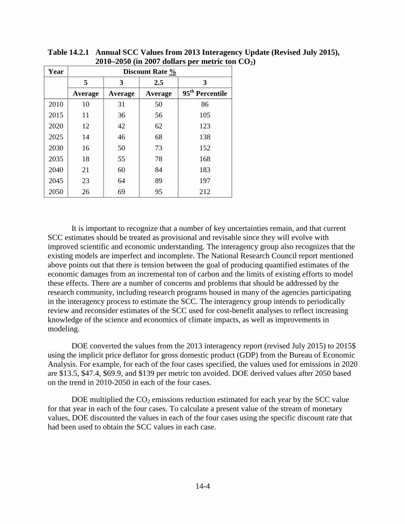
14-4

Table 14.2.1 Annual SCC Values from 2013 Interagency Update (Revised July 2015), 2010–2050 (in 2007 dollars per metric ton CO2)

Year Discount Rate %

5 3 2.5 3

Average Average Average 95th Percentile 2010 10 31 50 86 2015 11 36 56 105 2020 12 42 62 123 2025 14 46 68 138 2030 16 50 73 152 2035 18 55 78 168 2040 21 60 84 183 2045 23 64 89 197 2050 26 69 95 212

It is important to recognize that a number of key uncertainties remain, and that current SCC estimates should be treated as provisional and revisable since they will evolve with improved scientific and economic understanding. The interagency group also recognizes that the existing models are imperfect and incomplete. The National Research Council report mentioned above points out that there is tension between the goal of producing quantified estimates of the economic damages from an incremental ton of carbon and the limits of existing efforts to model these effects. There are a number of concerns and problems that should be addressed by the research community, including research programs housed in many of the agencies participating in the interagency process to estimate the SCC. The interagency group intends to periodically review and reconsider estimates of the SCC used for cost-benefit analyses to reflect increasing knowledge of the science and economics of climate impacts, as well as improvements in modeling.

DOE converted the values from the 2013 interagency report (revised July 2015) to 2015$ using the implicit price deflator for gross domestic product (GDP) from the Bureau of Economic Analysis. For example, for each of the four cases specified, the values used for emissions in 2020 are $13.5, $47.4, $69.9, and $139 per metric ton avoided. DOE derived values after 2050 based on the trend in 2010-2050 in each of the four cases.

DOE multiplied the CO2 emissions reduction estimated for each year by the SCC value for that year in each of the four cases. To calculate a present value of the stream of monetary values, DOE discounted the values in each of the four cases using the specific discount rate that had been used to obtain the SCC values in each case.

14-5

14.3 MONETIZING METHAND AND NITROUS OXIDE EMISSIONS

While carbon dioxide is the most prevalent greenhouse gas emitted into the atmosphere, other GHGs are also important contributors. These include methane and nitrous oxide. Global warming potentials (GWPs) are often used to convert emissions of non-CO2 GHGs to CO2-equivalents to facilitate comparison of policies and inventories involving different GHGs. While GWPs allow for some useful comparisons across gases on a physical basis, using the social cost of carbon to value the damages associated with changes in CO2-equivalent emissions is not optimal. This is because non-CO2 GHGs differ not just in their potential to absorb infrared radiation over a given time frame, but also in the temporal pathway of their impact on radiative forcing, which is relevant for estimating their social cost but not reflected in the GWP. Physical impacts other than temperature change also vary across gases in ways that are not captured by GWP.

In light of these limitations and the paucity of peer-reviewed estimates of the social cost of non-CO2 gases in the literature, the 2010 SCC Technical Support Document did not include an estimate of the social cost of non-CO2 GHGs and did not endorse the use of GWP to approximate the value of non-CO2 emission changes in regulatory analysis. Instead, the Interagency Working Group (IWG) noted that more work was needed to link non-CO2 GHG emission changes to economic impacts.

Since that time, new estimates of the social cost of non-CO2 GHG emissions have been developed in the scientific literature, and a recent study by Marten et al. (2015) provided the first set of published estimates for the social cost of CH4 and N2O emissions that are consistent with the methodology and modeling assumptions underlying the IWG SC-CO2 estimates.b Specifically, Marten et al. used the same set of three integrated assessment models, five socioeconomic and emissions scenarios, equilibrium climate sensitivity distribution, three constant discount rates, and the aggregation approach used by the IWG to develop the SC-CO2 estimates. An addendum to the IWG’s Technical Support Document on Social Cost of Carbon for Regulatory Impact Analysis under Executive Order 12866 summarizes the Marten et al. methodology and presents the social cost of methane (SC-CH4) and social cost of nitrous oxide (SC-N2O) estimates from that study as a way for agencies to incorporate the social benefits of reducing CH4 and N2O emissions into benefit-cost analyses of regulatory actions that have small, or “marginal,” impacts on cumulative global emissions.c

The methodology and estimates described in the addendum have undergone multiple stages of peer review and their use in regulatory analysis has been subject to public comment. b Marten, A.L., Kopits, E.A., Griffiths, C.W., Newbold, S.C., and A. Wolverton. 2015. Incremental CH4 and N2O Mitigation Benefits Consistent with the U.S. Government’s SC-CO2 Estimates. Climate Policy. 15(2): 272-298 (published online, 2014). c United States Government–Interagency Working Group on Social Cost of Greenhouse Gases. Addendum to Technical Support Document on Social Cost of Carbon for Regulatory Impact Analysis under Executive Order 12866: Application of the Methodology to Estimate the Social Cost of Methane and the Social Cost of Nitrous Oxide. August 2016. https://www.whitehouse.gov/sites/default/files/omb/inforeg/august_2016_sc_ch4_sc_n2o_addendum_final_8_26_16.pdf.

14-6

The estimates are presented with an acknowledgement of the limitations and uncertainties involved and with a clear understanding that they should be updated over time to reflect increasing knowledge of the science and economics of climate impacts, just as the IWG has committed to do for the SC-CO2. The OMB has determined that the use of the Marten et al. estimates in regulatory analysis is consistent with the requirements of OMB’s Information Quality Guidelines Bulletin for Peer Review and OMB Circular A-4.

The SC-CH4 and SC-N2O estimates are presented in Table 14.3.1. Following the same approach as with the SC-CO2 values for 2010, 2020, 2030, 2040, and 2050 are calculated by combining all outputs from all scenarios and models for a given discount rate. Values for the years in between are calculated using linear interpolation. The full set of annual SC-CH4 and SC-N2O estimates between 2010 and 2050 is reported in appendix 14A of the final rule TSD. DOE derived values after 2050 based on the trend in 2010–2050 in each of the four cases in the IWG addendum. Table 14.3.1 Annual SC-CH4 and SC-N2O Estimates from 2016 IWG Addendum (2007$

per Metric Ton CO2)

Year

SC-CH4 SC-N2O Discount Rate and Statistic Discount Rate and Statistic

5% 3% 2.5% 3% 5% 3% 2.5 % 3%

Average Average Average 95th percentile Average Average Average 95th

percentile 2010 370 870 1,200 2,400 3,400 12,000 18,000 31,000 2015 450 1,000 1,400 2,800 4,000 13,000 20,000 35,000 2020 540 1,200 1,600 3,200 4,700 15,000 22,000 39,000 2025 650 1,400 1,800 3,700 5,500 17,000 24,000 44,000 2030 760 1,600 2,000 4,200 6,300 19,000 27,000 49,000 2035 900 1,800 2,300 4,900 7,400 21,000 29,000 55,000 2040 1,000 2,000 2,600 5,500 8,400 23,000 32,000 60,000 2045 1,200 2,300 2,800 6,100 9,500 25,000 34,000 66,000 2050 1,300 2,500 3,100 6,700 11,000 27,000 37,000 72,000

DOE multiplied the CH4 and N2O emissions reduction estimated for each year by the SC-CH4 and SC-N2O estimates for that year in each of the four cases. To calculate a present value of the stream of monetary values, DOE discounted the values in each of the four cases using the specific discount rate that had been used to obtain the SC-CH4 and SC-N2O estimates in each case.

14.4 VALUATION OF OTHER EMISSIONS

As noted in chapter 13, new or amended energy conservation standards would reduce NOX emissions from electricity generation in those 22 States that are not affected by caps. For each of the considered TSLs, DOE estimated monetized values of NOX emissions reductions from electricity generation using benefit-per-ton estimates for NOX associated with PM2.5 from

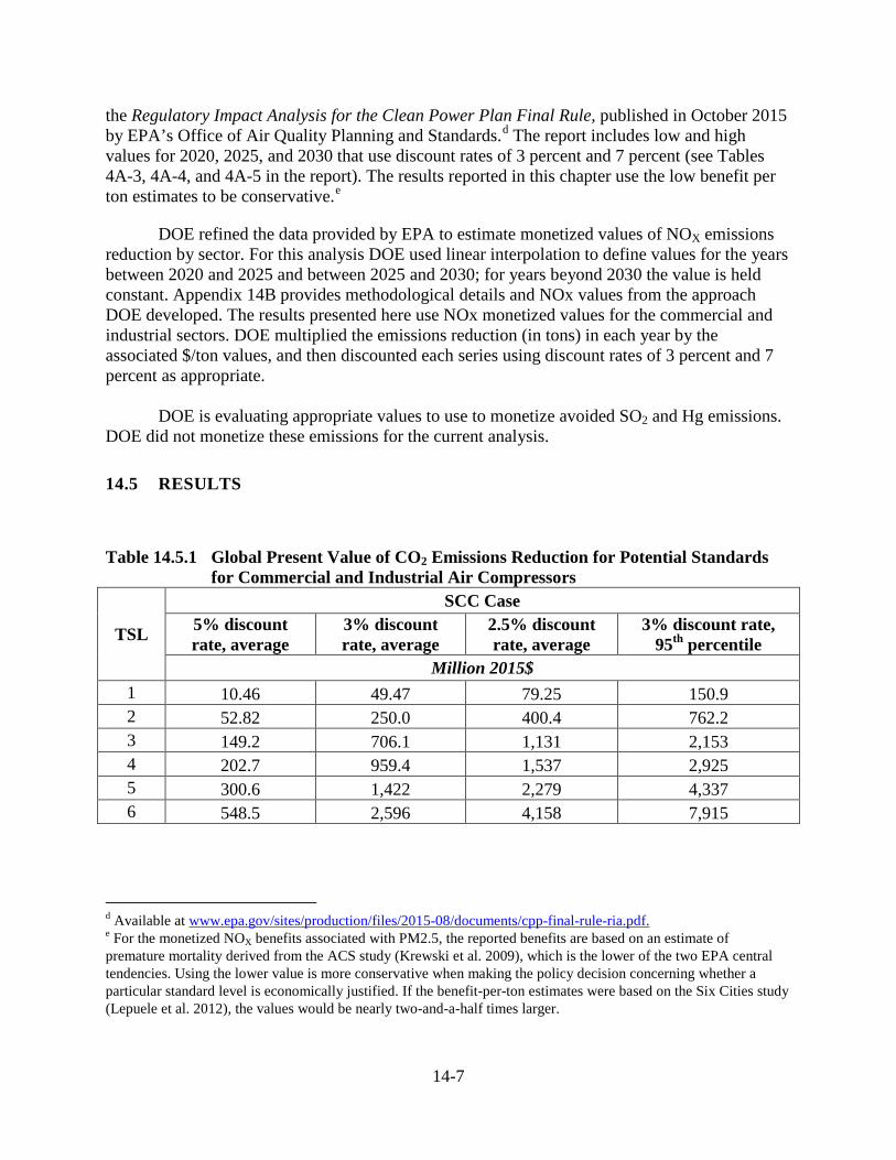
14-7

the Regulatory Impact Analysis for the Clean Power Plan Final Rule, published in October 2015 by EPA’s Office of Air Quality Planning and Standards.d The report includes low and high values for 2020, 2025, and 2030 that use discount rates of 3 percent and 7 percent (see Tables 4A-3, 4A-4, and 4A-5 in the report). The results reported in this chapter use the low benefit per ton estimates to be conservative.e

DOE refined the data provided by EPA to estimate monetized values of NOX emissions reduction by sector. For this analysis DOE used linear interpolation to define values for the years between 2020 and 2025 and between 2025 and 2030; for years beyond 2030 the value is held constant. Appendix 14B provides methodological details and NOx values from the approach DOE developed. The results presented here use NOx monetized values for the commercial and industrial sectors. DOE multiplied the emissions reduction (in tons) in each year by the associated $/ton values, and then discounted each series using discount rates of 3 percent and 7 percent as appropriate.

DOE is evaluating appropriate values to use to monetize avoided SO2 and Hg emissions.

DOE did not monetize these emissions for the current analysis.

14.5 RESULTS

Table 14.5.1 Global Present Value of CO2 Emissions Reduction for Potential Standards for Commercial and Industrial Air Compressors

TSL

SCC Case 5% discount rate, average

3% discount rate, average

2.5% discount rate, average

3% discount rate, 95th percentile

Million 2015$ 1 10.46 49.47 79.25 150.9 2 52.82 250.0 400.4 762.2 3 149.2 706.1 1,131 2,153 4 202.7 959.4 1,537 2,925 5 300.6 1,422 2,279 4,337 6 548.5 2,596 4,158 7,915

d Available at www.epa.gov/sites/production/files/2015-08/documents/cpp-final-rule-ria.pdf. e For the monetized NOX benefits associated with PM2.5, the reported benefits are based on an estimate of premature mortality derived from the ACS study (Krewski et al. 2009), which is the lower of the two EPA central tendencies. Using the lower value is more conservative when making the policy decision concerning whether a particular standard level is economically justified. If the benefit-per-ton estimates were based on the Six Cities study (Lepuele et al. 2012), the values would be nearly two-and-a-half times larger.

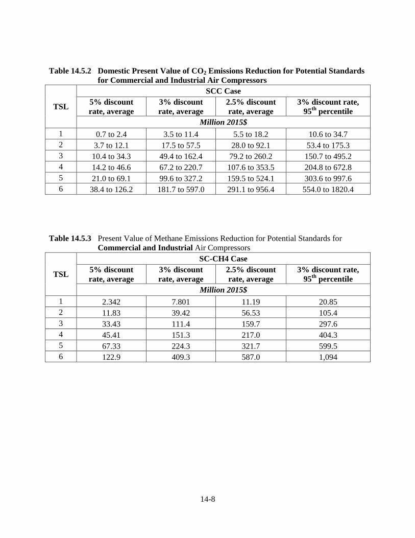
14-8

Table 14.5.2 Domestic Present Value of CO2 Emissions Reduction for Potential Standards

for Commercial and Industrial Air Compressors

TSL

SCC Case 5% discount rate, average

3% discount rate, average

2.5% discount rate, average

3% discount rate, 95th percentile

Million 2015$ 1 0.7 to 2.4 3.5 to 11.4 5.5 to 18.2 10.6 to 34.7 2 3.7 to 12.1 17.5 to 57.5 28.0 to 92.1 53.4 to 175.3 3 10.4 to 34.3 49.4 to 162.4 79.2 to 260.2 150.7 to 495.2 4 14.2 to 46.6 67.2 to 220.7 107.6 to 353.5 204.8 to 672.8 5 21.0 to 69.1 99.6 to 327.2 159.5 to 524.1 303.6 to 997.6 6 38.4 to 126.2 181.7 to 597.0 291.1 to 956.4 554.0 to 1820.4

Table 14.5.3 Present Value of Methane Emissions Reduction for Potential Standards for

Commercial and Industrial Air Compressors

TSL

SC-CH4 Case 5% discount rate, average

3% discount rate, average

2.5% discount rate, average

3% discount rate, 95th percentile

Million 2015$ 1 2.342 7.801 11.19 20.85 2 11.83 39.42 56.53 105.4 3 33.43 111.4 159.7 297.6 4 45.41 151.3 217.0 404.3 5 67.33 224.3 321.7 599.5 6 122.9 409.3 587.0 1,094

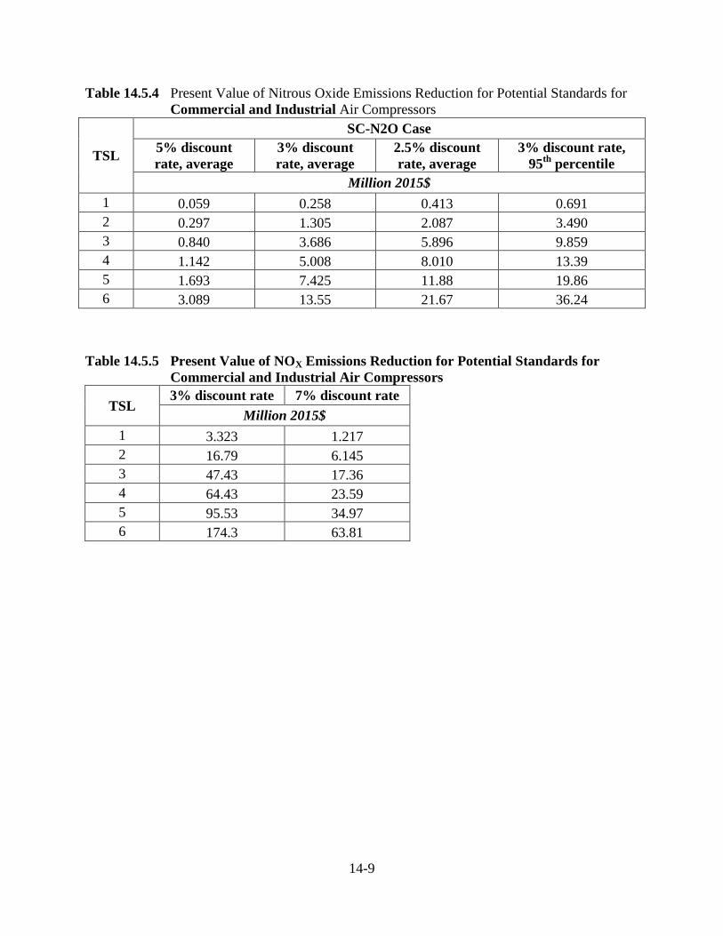
14-9

Table 14.5.4 Present Value of Nitrous Oxide Emissions Reduction for Potential Standards for Commercial and Industrial Air Compressors

TSL

SC-N2O Case 5% discount rate, average

3% discount rate, average

2.5% discount rate, average

3% discount rate, 95th percentile

Million 2015$ 1 0.059 0.258 0.413 0.691 2 0.297 1.305 2.087 3.490 3 0.840 3.686 5.896 9.859 4 1.142 5.008 8.010 13.39 5 1.693 7.425 11.88 19.86 6 3.089 13.55 21.67 36.24

Table 14.5.5 Present Value of NOX Emissions Reduction for Potential Standards for

Commercial and Industrial Air Compressors

TSL 3% discount rate 7% discount rate

Million 2015$ 1 3.323 1.217 2 16.79 6.145 3 47.43 17.36 4 64.43 23.59 5 95.53 34.97 6 174.3 63.81

14-10

REFERENCES 1. National Research Council. Hidden Costs of Energy: Unpriced Consequences of Energy

Production and Use. 2010. National Academies Press: Washington, D.C. (Last accessed October 16, 2015.) http://www.nap.edu/catalog/12794/hidden-costs-of-energy-unpriced-consequences-of-energy-production-and.

2. Interagency Working Group on Social Cost of Carbon. Social Cost of Carbon for Regulatory Impact Analysis under Executive Order 12866. 2010. United States Government. (Last accessed October 16, 2015.) http://www.whitehouse.gov/sites/default/files/omb/inforeg/for-agencies/Social-Cost-of-Carbon-for-RIA.pdf.

3. Interagency Working Group on Social Cost of Carbon. Technical Support Document: -Technical Update of the Social Cost of Carbon for Regulatory Impact Analysis -Under Executive Order 12866. 2015. United States Government. (Last accessed October 23, 2015.) https://www.whitehouse.gov/sites/default/files/omb/inforeg/scc-tsd-final-july-2015.pdf.

4. Krewski, D., M. Jerrett, R. T. Burnett, R. Ma, E. Hughes, Y. Shi, and et al. Extended Follow-Up and Spatial Analysis of the American Cancer Society Study Linking Particulate Air Pollution and Mortality. 2009. Health Effects Institute: Boston, MA. Report No. 140.

5. Lepuele, J., F. Laden, D. Dockery, and J. Schwartz. Chronic Exposure to Fine Particles and Mortality: An Extended Follow-Up of the Harvard Six Cities Study from 1974 to 2009. Environmental Health Perspectives. 2012. July, 120(7): pp. 965–970.

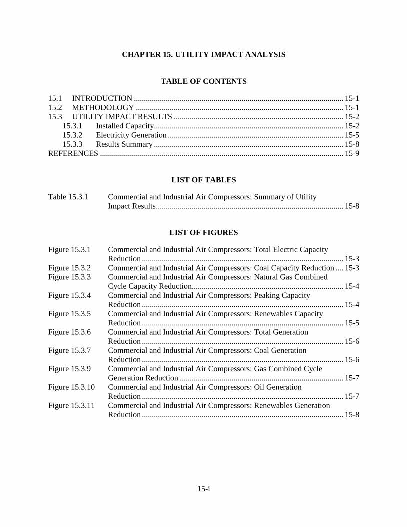
15-i

CHAPTER 15. UTILITY IMPACT ANALYSIS

TABLE OF CONTENTS

15.1 INTRODUCTION ......................................................................................................... 15-1 15.2 METHODOLOGY ........................................................................................................ 15-1 15.3 UTILITY IMPACT RESULTS ..................................................................................... 15-2

15.3.1 Installed Capacity............................................................................................... 15-2 15.3.2 Electricity Generation ........................................................................................ 15-5 15.3.3 Results Summary ............................................................................................... 15-8

REFERENCES .......................................................................................................................... 15-9

LIST OF TABLES

Table 15.3.1 Commercial and Industrial Air Compressors: Summary of Utility Impact Results .............................................................................................. 15-8

LIST OF FIGURES

Figure 15.3.1 Commercial and Industrial Air Compressors: Total Electric Capacity Reduction ..................................................................................................... 15-3

Figure 15.3.2 Commercial and Industrial Air Compressors: Coal Capacity Reduction .... 15-3 Figure 15.3.3 Commercial and Industrial Air Compressors: Natural Gas Combined

Cycle Capacity Reduction............................................................................ 15-4 Figure 15.3.4 Commercial and Industrial Air Compressors: Peaking Capacity

Reduction ..................................................................................................... 15-4 Figure 15.3.5 Commercial and Industrial Air Compressors: Renewables Capacity

Reduction ..................................................................................................... 15-5 Figure 15.3.6 Commercial and Industrial Air Compressors: Total Generation

Reduction ..................................................................................................... 15-6 Figure 15.3.7 Commercial and Industrial Air Compressors: Coal Generation

Reduction ..................................................................................................... 15-6 Figure 15.3.9 Commercial and Industrial Air Compressors: Gas Combined Cycle

Generation Reduction .................................................................................. 15-7 Figure 15.3.10 Commercial and Industrial Air Compressors: Oil Generation

Reduction ..................................................................................................... 15-7 Figure 15.3.11 Commercial and Industrial Air Compressors: Renewables Generation

Reduction ..................................................................................................... 15-8

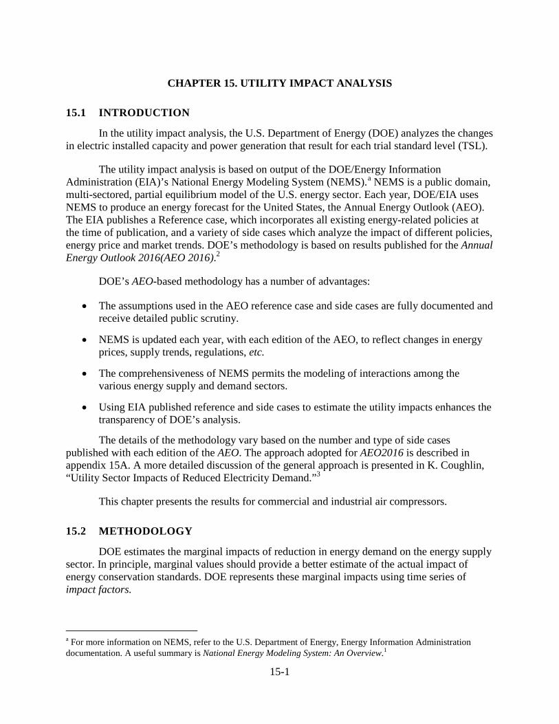
15-1

CHAPTER 15. UTILITY IMPACT ANALYSIS

15.1 INTRODUCTION

In the utility impact analysis, the U.S. Department of Energy (DOE) analyzes the changes in electric installed capacity and power generation that result for each trial standard level (TSL).

The utility impact analysis is based on output of the DOE/Energy Information Administration (EIA)’s National Energy Modeling System (NEMS).a NEMS is a public domain, multi-sectored, partial equilibrium model of the U.S. energy sector. Each year, DOE/EIA uses NEMS to produce an energy forecast for the United States, the Annual Energy Outlook (AEO). The EIA publishes a Reference case, which incorporates all existing energy-related policies at the time of publication, and a variety of side cases which analyze the impact of different policies, energy price and market trends. DOE’s methodology is based on results published for the Annual Energy Outlook 2016(AEO 2016).2

DOE’s AEO-based methodology has a number of advantages:

• The assumptions used in the AEO reference case and side cases are fully documented and receive detailed public scrutiny.

• NEMS is updated each year, with each edition of the AEO, to reflect changes in energy prices, supply trends, regulations, etc.

• The comprehensiveness of NEMS permits the modeling of interactions among the various energy supply and demand sectors.

• Using EIA published reference and side cases to estimate the utility impacts enhances the transparency of DOE’s analysis.

The details of the methodology vary based on the number and type of side cases published with each edition of the AEO. The approach adopted for AEO2016 is described in appendix 15A. A more detailed discussion of the general approach is presented in K. Coughlin, “Utility Sector Impacts of Reduced Electricity Demand.”3

This chapter presents the results for commercial and industrial air compressors.

15.2 METHODOLOGY

DOE estimates the marginal impacts of reduction in energy demand on the energy supply sector. In principle, marginal values should provide a better estimate of the actual impact of energy conservation standards. DOE represents these marginal impacts using time series of impact factors.

a For more information on NEMS, refer to the U.S. Department of Energy, Energy Information Administration documentation. A useful summary is National Energy Modeling System: An Overview.1

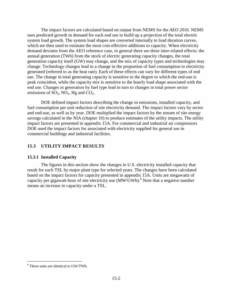
15-2

The impact factors are calculated based on output from NEMS for the AEO 2016. NEMS uses predicted growth in demand for each end use to build up a projection of the total electric system load growth. The system load shapes are converted internally to load duration curves, which are then used to estimate the most cost-effective additions to capacity. When electricity demand deviates from the AEO reference case, in general there are three inter-related effects: the annual generation (TWh) from the stock of electric generating capacity changes, the total generation capacity itself (GW) may change, and the mix of capacity types and technologies may change. Technology changes lead to a change in the proportion of fuel consumption to electricity generated (referred to as the heat rate). Each of these effects can vary for different types of end use. The change in total generating capacity is sensitive to the degree to which the end-use is peak coincident, while the capacity mix is sensitive to the hourly load shape associated with the end use. Changes in generation by fuel type lead in turn to changes in total power sector emissions of SO2, NOx, Hg and CO2.

DOE defined impact factors describing the change in emissions, installed capacity, and fuel consumption per unit reduction of site electricity demand. The impact factors vary by sector and end-use, as well as by year. DOE multiplied the impact factors by the stream of site energy savings calculated in the NIA (chapter 10) to produce estimates of the utility impacts. The utility impact factors are presented in appendix 15A. For commercial and industrial air compressors DOE used the impact factors for associated with electricity supplied for general use in commercial buildings and industrial facilities.

15.3 UTILITY IMPACT RESULTS

15.3.1 Installed Capacity

The figures in this section show the changes in U.S. electricity installed capacity that result for each TSL by major plant type for selected years. The changes have been calculated based on the impact factors for capacity presented in appendix 15A. Units are megawatts of capacity per gigawatt-hour of site electricity use (MW/GWh).b Note that a negative number means an increase in capacity under a TSL.

b These units are identical to GW/TWh.

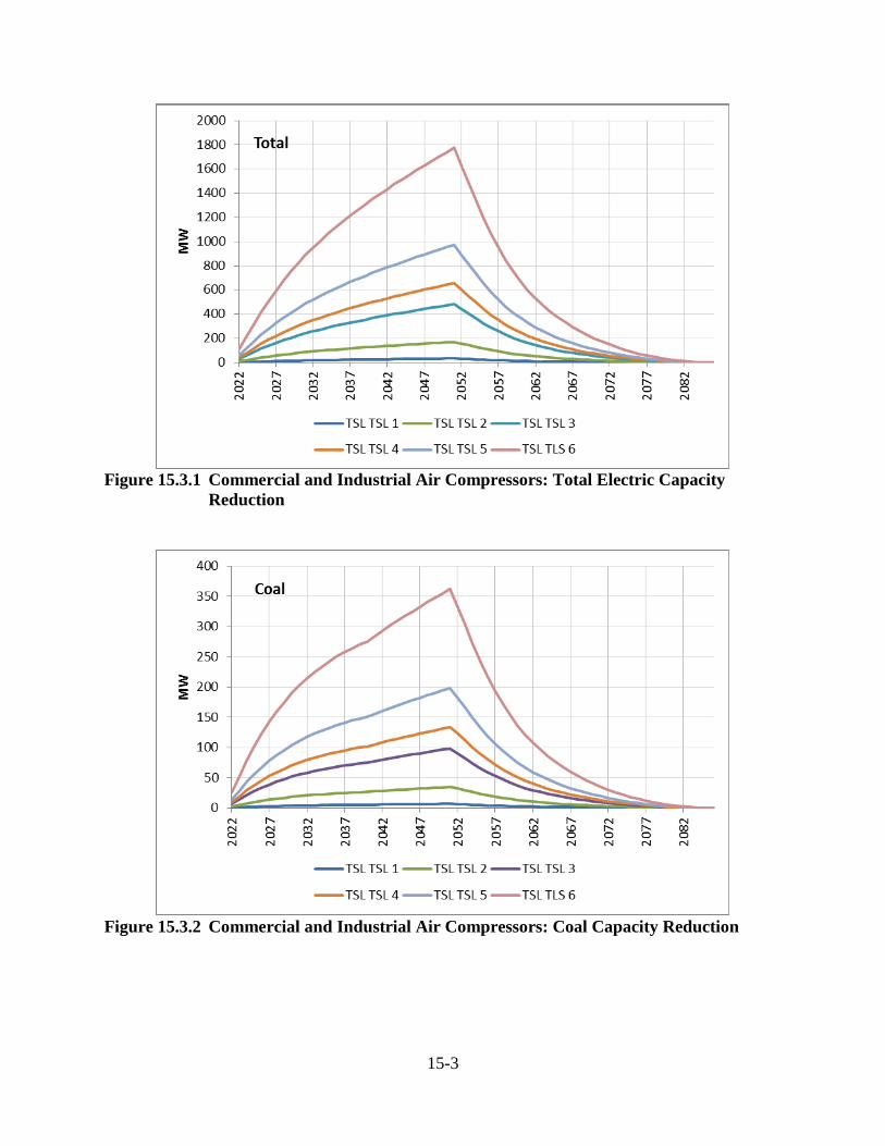
15-3

Figure 15.3.1 Commercial and Industrial Air Compressors: Total Electric Capacity

Reduction

Figure 15.3.2 Commercial and Industrial Air Compressors: Coal Capacity Reduction

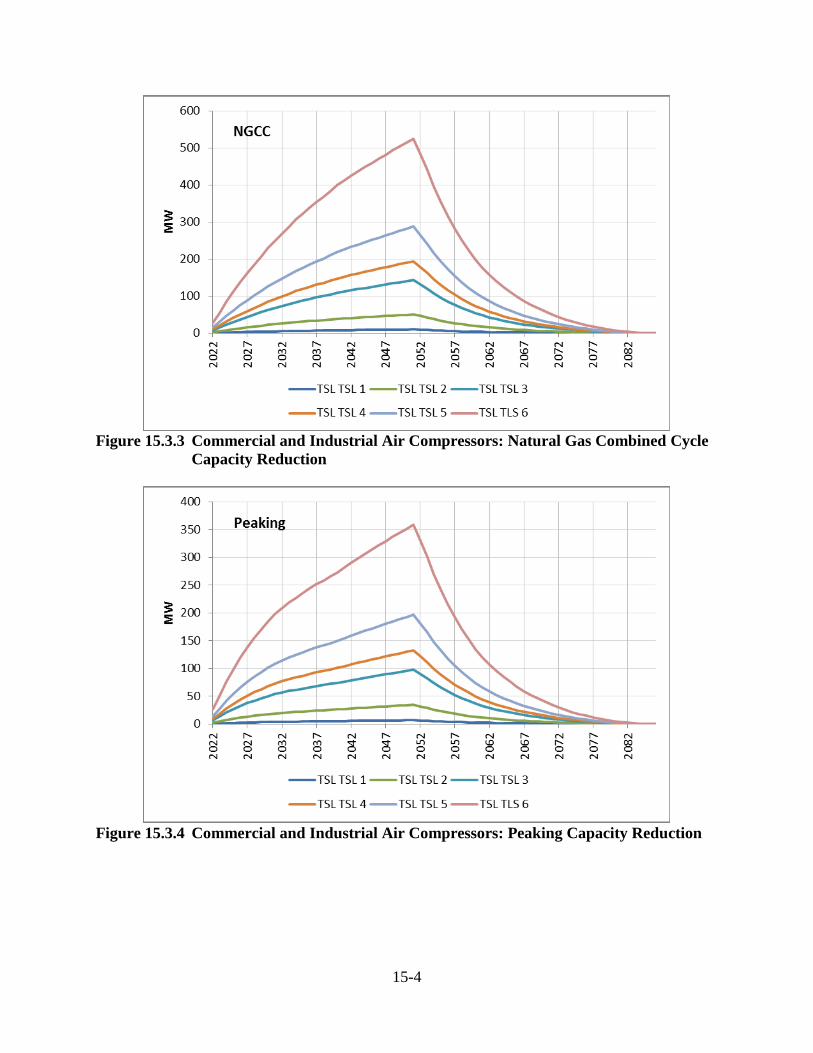
15-4

Figure 15.3.3 Commercial and Industrial Air Compressors: Natural Gas Combined Cycle

Capacity Reduction

Figure 15.3.4 Commercial and Industrial Air Compressors: Peaking Capacity Reduction

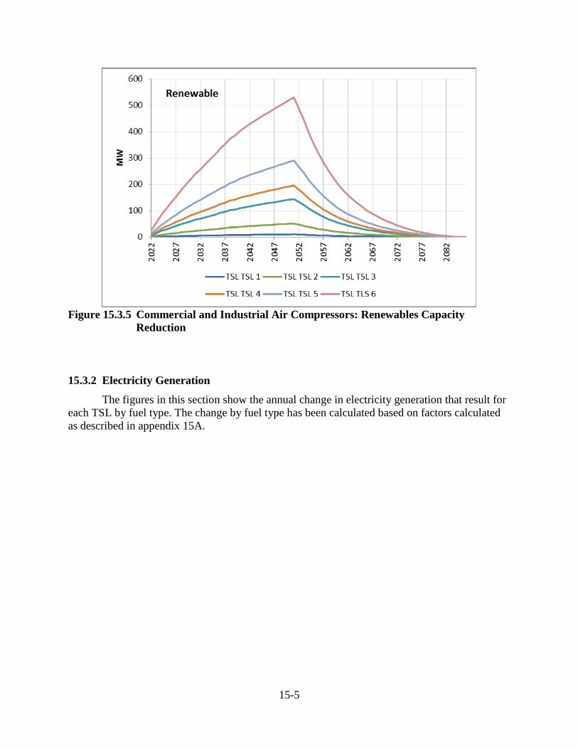
15-5

Figure 15.3.5 Commercial and Industrial Air Compressors: Renewables Capacity

Reduction

15.3.2 Electricity Generation

The figures in this section show the annual change in electricity generation that result for each TSL by fuel type. The change by fuel type has been calculated based on factors calculated as described in appendix 15A.

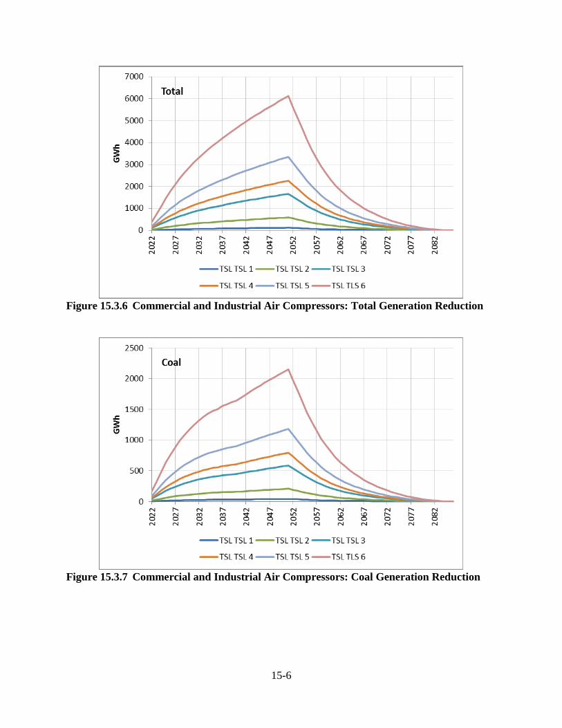
15-6

Figure 15.3.6 Commercial and Industrial Air Compressors: Total Generation Reduction

Figure 15.3.7 Commercial and Industrial Air Compressors: Coal Generation Reduction

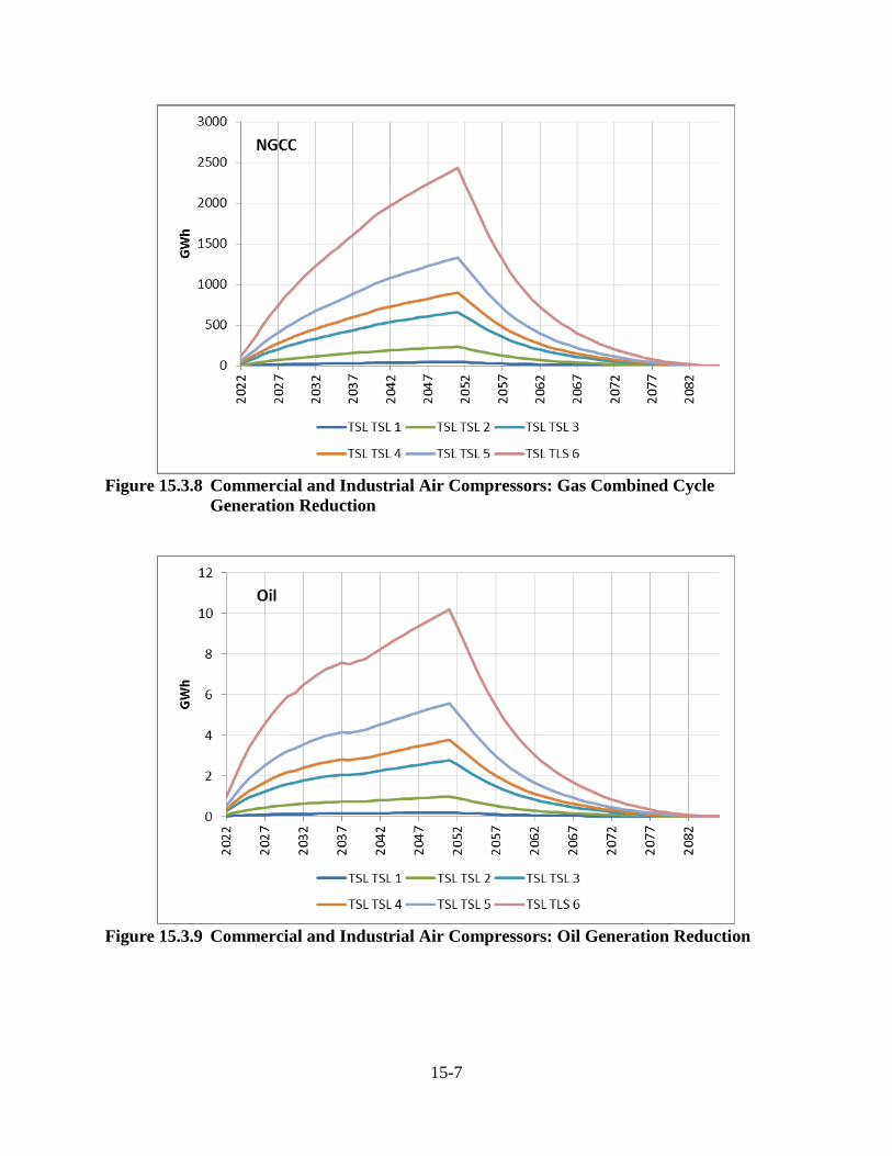
15-7

Figure 15.3.8 Commercial and Industrial Air Compressors: Gas Combined Cycle

Generation Reduction

Figure 15.3.9 Commercial and Industrial Air Compressors: Oil Generation Reduction

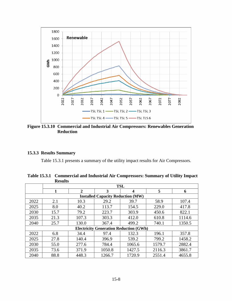
15-8

Figure 15.3.10 Commercial and Industrial Air Compressors: Renewables Generation

Reduction

15.3.3 Results Summary

Table 15.3.1 presents a summary of the utility impact results for Air Compressors.

Table 15.3.1 Commercial and Industrial Air Compressors: Summary of Utility Impact

Results

TSL 1 2 3 4 5 6

Installed Capacity Reduction (MW) 2022 2.1 10.3 29.2 39.7 58.9 107.4 2025 8.0 40.2 113.7 154.5 229.0 417.8 2030 15.7 79.2 223.7 303.9 450.6 822.1 2035 21.3 107.3 303.3 412.0 610.8 1114.6 2040 25.7 130.0 367.4 499.2 740.1 1350.5

Electricity Generation Reduction (GWh) 2022 6.8 34.4 97.4 132.3 196.1 357.8 2025 27.8 140.4 396.9 539.2 799.2 1458.2 2030 55.0 277.6 784.4 1065.6 1579.7 2882.4 2035 73.6 371.9 1050.8 1427.5 2116.3 3861.7 2040 88.8 448.3 1266.7 1720.9 2551.4 4655.8

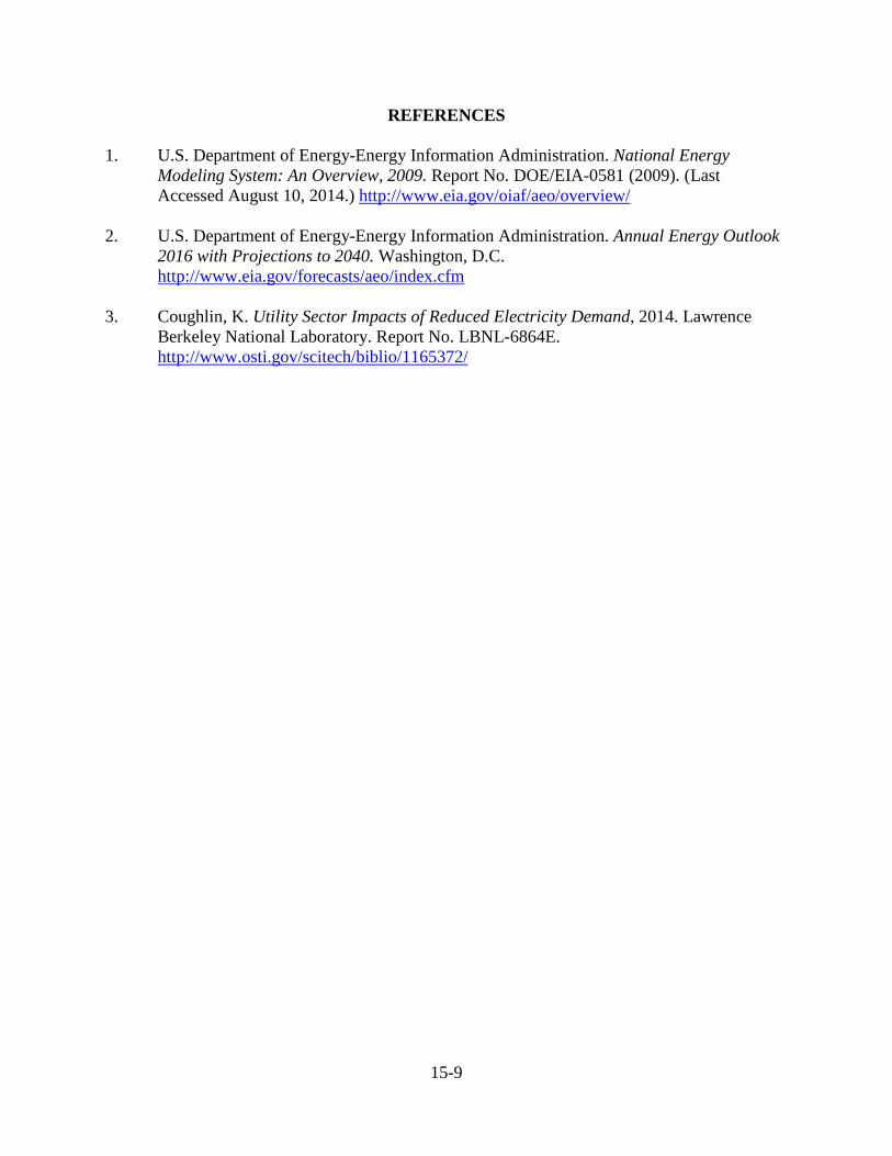
15-9

REFERENCES 1. U.S. Department of Energy-Energy Information Administration. National Energy

Modeling System: An Overview, 2009. Report No. DOE/EIA-0581 (2009). (Last Accessed August 10, 2014.) http://www.eia.gov/oiaf/aeo/overview/

2. U.S. Department of Energy-Energy Information Administration. Annual Energy Outlook

2016 with Projections to 2040. Washington, D.C. http://www.eia.gov/forecasts/aeo/index.cfm

3. Coughlin, K. Utility Sector Impacts of Reduced Electricity Demand, 2014. Lawrence

Berkeley National Laboratory. Report No. LBNL-6864E. http://www.osti.gov/scitech/biblio/1165372/

16-i

CHAPTER 16. EMPLOYMENT IMPACT ANALYSIS

TABLE OF CONTENTS 16.1 INTRODUCTION ......................................................................................................... 16-1 16.2 ASSUMPTIONS ............................................................................................................ 16-1 16.3 METHODOLOGY ........................................................................................................ 16-1 16.4 SHORT-TERM RESULTS ............................................................................................ 16-2 16.5 LONG-TERM IMPACTS .............................................................................................. 16-3 REFERENCES .......................................................................................................................... 16-5

LIST OF TABLES Table 16.4.1 Net National Short-Term Change in Employment (1000 Jobs) ......................... 16-3

16-1

CHAPTER 16. EMPLOYMENT IMPACT ANALYSIS

16.1 INTRODUCTION

The U.S. Department of Energy’s (DOE’s) employment impact analysis is designed to estimate indirect national job creation or elimination resulting from possible standards, due to reallocation of the associated expenditures for purchasing and operating compressors. Job increases or decreases reported in this chapter are separate from the direct manufacturing sector employment impacts reported in chapter 12 and reflect the employment impact of efficiency standards on all other sectors of the economy.

16.2 ASSUMPTIONS

DOE expects energy conservation standards to decrease energy consumption and, therefore, to reduce energy expenditures. The savings in energy expenditures may be spent on new investment or not at all (i.e., they may remain “saved”). The standards may alter the purchase price of appliances, including the retail price plus sales tax, and alter installation costs. Using an input/output econometric model of the U.S. economy, this analysis estimated the short-term effect of these expenditure impacts on net economic output and employment. DOE intends this analysis to quantify the indirect employment impacts of these expenditure changes. It evaluated direct employment impacts at manufacturers’ facilities in the manufacturer impact analysis (see chapter 12). DOE notes that ImSET is not a general equilibrium forecasting model and understands the uncertainties involved in projecting employment impacts, especially changes in the later years of the analysis.1 Because ImSET does not incorporate price changes, the employment effects predicted by ImSET would over-estimate the magnitude of actual job impacts over the long run for this rule. As input/output models do not allow prices to bring markets into equilibrium, they are best used for short-run analyses. DOE, therefore, includes a qualitative discussion of how labor markets are likely to respond in the longer term. In future rulemakings, DOE may consider the use of other modeling approaches for examining long-run employment impacts.

16.3 METHODOLOGY

The Department based its analysis on an input/output model of the U.S. economy that estimates the effects of standards on major sectors of the economy related to buildings and the net impact of standards on jobs. The Pacific Northwest National Laboratory developed the model, ImSET 3.1.12 (Impact of Sector Energy Technologies), as a successor to ImBuild3, a special-purpose version of the IMPLAN4 national input/output model. ImSET estimates the employment and income effects of building energy technologies. In comparison with simple economic multiplier approaches, ImSET allows for a more complete and automated analysis of the economic impacts of energy efficiency investments in buildings.

16-2

In an input/output model, the level of employment in an economy is determined by the relationship of different sectors of the economy and the spending flows among them. Different sectors have different levels of labor intensity, and changes in the level of spending (e.g., due to the effects of an efficiency standard) in one sector of the economy will affect flows in other sectors, which affect the overall level of employment. ImSET uses a 187-sector model of the national economy to predict the economic effects of residential and commercial building technologies. ImSET collects estimates of initial investments, energy savings, and economic activity associated with spending the savings resulting from standards (e.g., changes in final demand in personal consumption, business investment and spending, and government spending). It provides overall estimates of the change in national output for each input-output sector. The model applies estimates of employment and wage income per dollar of economic output for each sector and calculates impacts on national employment and wage income. Energy efficiency technology primarily affects the U.S. economy along three spending pathways. First, general investment funds are diverted to sectors that manufacture, install, and maintain energy-efficient appliances. Increased appliance costs lead to higher employment in the appliance manufacturing sectors and lower employment in other economic sectors; reduced appliance costs have the opposite effect. Second, commercial firm and residential spending are redirected from utilities toward other industries. Third, electric utility sector investment funds are released for use in other sectors of the economy. When consumers use less energy, electric utilities experience relative reductions in demand, which leads to reductions in utility sector investment and employment. DOE also notes that the employment impacts estimated with ImSET for the entire economy differ from the employment impacts in the compressor manufacturing sector estimated in chapter 12 using the Government Regulatory Impact Model (GRIM). The methodologies used and the sectors analyzed in the ImSET and GRIM models are different.

16.4 SHORT-TERM RESULTS

The results in this section refer to impacts of compressor standards relative to the base case. DOE disaggregated the impact of standards on employment into three component effects: altered capital investment costs, decreased energy costs, and changes in operations and maintenance costs. DOE presents the summary impact. Conceptually, one can consider the impact of the rule in its first year on three aggregate sectors: the compressor production sector, the energy generation sector, and the general consumer good sector (as mentioned previously, ImSET’s calculations are made at a much more disaggregate level). By raising energy efficiency, the rule alters the purchase price of compressors, in turn altering employment in this sector. At the same time, the improvements in energy efficiency reduce consumer expenditures on electricity. The reduction in electricity demand causes a reduction in employment in that sector. Finally, based on the net impact of altered expenditures on compressors and reduced expenditures on electricity, consumer

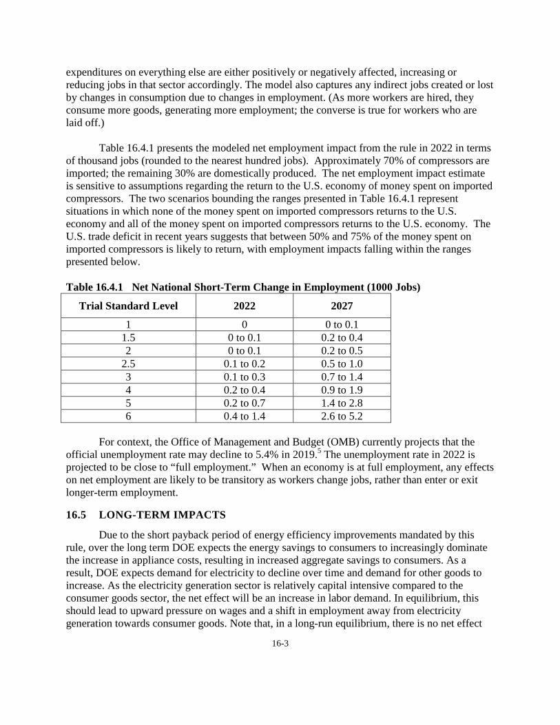
16-3

expenditures on everything else are either positively or negatively affected, increasing or reducing jobs in that sector accordingly. The model also captures any indirect jobs created or lost by changes in consumption due to changes in employment. (As more workers are hired, they consume more goods, generating more employment; the converse is true for workers who are laid off.) Table 16.4.1 presents the modeled net employment impact from the rule in 2022 in terms of thousand jobs (rounded to the nearest hundred jobs). Approximately 70% of compressors are imported; the remaining 30% are domestically produced. The net employment impact estimate is sensitive to assumptions regarding the return to the U.S. economy of money spent on imported compressors. The two scenarios bounding the ranges presented in Table 16.4.1 represent situations in which none of the money spent on imported compressors returns to the U.S. economy and all of the money spent on imported compressors returns to the U.S. economy. The U.S. trade deficit in recent years suggests that between 50% and 75% of the money spent on imported compressors is likely to return, with employment impacts falling within the ranges presented below. Table 16.4.1 Net National Short-Term Change in Employment (1000 Jobs)

Trial Standard Level 2022 2027

1 0 0 to 0.1 1.5 0 to 0.1 0.2 to 0.4 2 0 to 0.1 0.2 to 0.5

2.5 0.1 to 0.2 0.5 to 1.0 3 0.1 to 0.3 0.7 to 1.4 4 0.2 to 0.4 0.9 to 1.9 5 0.2 to 0.7 1.4 to 2.8 6 0.4 to 1.4 2.6 to 5.2

For context, the Office of Management and Budget (OMB) currently projects that the official unemployment rate may decline to 5.4% in 2019.5 The unemployment rate in 2022 is projected to be close to “full employment.” When an economy is at full employment, any effects on net employment are likely to be transitory as workers change jobs, rather than enter or exit longer-term employment.

16.5 LONG-TERM IMPACTS

Due to the short payback period of energy efficiency improvements mandated by this rule, over the long term DOE expects the energy savings to consumers to increasingly dominate the increase in appliance costs, resulting in increased aggregate savings to consumers. As a result, DOE expects demand for electricity to decline over time and demand for other goods to increase. As the electricity generation sector is relatively capital intensive compared to the consumer goods sector, the net effect will be an increase in labor demand. In equilibrium, this should lead to upward pressure on wages and a shift in employment away from electricity generation towards consumer goods. Note that, in a long-run equilibrium, there is no net effect

16-4

on total employment, because wages adjust to bring the labor market into equilibrium. Nonetheless, even to the extent that markets are slow to adjust, DOE anticipates that net labor market impacts will be negligible over time due to the small magnitude of the short-term effects presented in Table 16.4.1. The ImSET model projections, assuming no price or wage effects until 2027, are included in the second column of Table 16.4.1.

16-5

REFERENCES

1. Scott, M., JM Roop, RW Schultz, DM Anderson, KA Cort, The Impact of DOE Building

Technology Energy Efficiency Programs on U.S. Employment, Income, and Investment. Energy Economics, 2008. 30(5): pp. 2283-2301

2. Roop, J. M., M. J. Scott, and R. W. Schultz, ImSET: Impact of Sector Energy

Technologies. 2005. Pacific Northwest National Laboratory. Richland, WA. Report No. PNNL- 15273.

3. Scott, M. J., D. J. Hostick, and D. B. Belzer, ImBuild: Impact of Building Energy

Efficiency Programs. April, 1998. Pacific Northwest National Laboratory. Richland, WA. Report No. PNNL-11884.

4. Minnesota IMPLAN Group Inc., IMPLAN Professional: User's Guide, Analysis Guide,

Data Guide. 1997. Stillwater, MN. 5. Office of Management and Budget, Fiscal Year 2015 Mid-session Review Budget of the

U.S. Government. 2014. http://www.whitehouse.gov/sites/default/files/omb/budget/fy2015/assets/15msr.pdf

17-i

CHAPTER 17. REGULATORY IMPACT ANALYSIS

TABLE OF CONTENTS

17.1 INTRODUCTION ......................................................................................................... 17-1 17.2 NON-REGULATORY POLICIES ................................................................................ 17-2

17.2.1 Methodology ...................................................................................................... 17-2 17.2.2 Assumptions Regarding Non-Regulatory Policies ............................................ 17-3 17.2.3 Policy Interactions ............................................................................................. 17-4

17.3 NON-REGULATORY POLICY ASSUMPTIONS ...................................................... 17-4 17.3.1 No New Regulatory Action ............................................................................... 17-4 17.3.2 Consumer Rebates ............................................................................................. 17-5

17.3.2.1 Methodology ............................................................................................ 17-5 17.3.2.2 Analysis .................................................................................................... 17-6

17.3.3 Consumer Tax Credits ....................................................................................... 17-9 17.3.4 Manufacturer Tax Credits ................................................................................ 17-11 17.3.5 Voluntary Energy Efficiency Targets .............................................................. 17-12

17.4 IMPACTS OF NON-REGULATORY ALTERNATIVES ......................................... 17-14 REFERENCES ........................................................................................................................ 17-17

LIST OF TABLES

Table 17.1.1 Non-Regulatory Alternatives to National Standards ................................... 17-1 Table 17.2.1 Energy Efficiency by TSL for Rotary Positive, Fixed Speed,

Lubricated, Air-Cooled (%) ......................................................................... 17-3 Table 17.2.2 Energy Efficiency by TSL for Rotary Positive, Fixed Speed,

Lubricated, Water-Cooled (%)..................................................................... 17-4 Table 17.3.1 Benefit/Cost Ratios Without and With Rebates........................................... 17-6 Table 17.3.2 Market Penetrations in 2022 Attributable to Consumer Rebates................. 17-9 Table 17.3.3 Market Penetrations in 2022 Attributable to Consumer Tax Credits ........ 17-10 Table 17.3.4 Market Penetrations in 2022 Attributable to Manufacturer Tax Credits ... 17-12 Table 17.3.5 Market Barriers Changes Attributable to Voluntary Energy Efficiency

Targets (TSL 2) .......................................................................................... 17-13 Table 17.3.6 Market Penetrations in 2022 Attributable to Voluntary Energy

Efficiency Targets ...................................................................................... 17-13 Table 17.3.7 Market Penetrations in Selected Years Attributable to Voluntary

Energy Efficiency Targets for TSL 2 ......................................................... 17-14 Table 17.4.1 Impacts of Non-Regulatory Policy Alternatives (TSL 2) .......................... 17-16

LIST OF FIGURES

Figure 17.3.1 Market Penetration Curves for Air Compressors ......................................... 17-8 Figure 17.4.1 Market Penetration of Efficient RP_FS_L_AC (TSL 2) ........................... 17-15 Figure 17.4.2 Market Penetration of Efficient RP_FS_L_AC (TSL 2) ........................... 17-15

17-1

CHAPTER 17. REGULATORY IMPACT ANALYSIS

17.1 INTRODUCTION

The U.S. Department of Energy (DOE) has determined that the regulatory action described in the Federal Register notice associated with this TSD constitutes an “economically significant regulatory action” under Executive Order (E.O.) 12866, Regulatory Planning and Review. 58 FR 51735 (October 4, 1993). For such actions, E.O. 12866 requires Federal agencies to provide “an assessment, including the underlying analysis, of costs and benefits of potentially effective and reasonably feasible alternatives to the planned regulation, identified by the agencies or the public (including improving the current regulation and reasonably viable non-regulatory actions), and an explanation why the planned regulatory action is preferable to the identified potential alternatives.” 58 FR 51735, 51741.

To conduct this analysis, DOE used an integrated National Impact Analysis (NIA)-RIA model built on a modifieda version of the NIA model discussed in chapter 10. DOE identified four non-regulatory policy alternatives that possibly could provide incentives for the same energy efficiency levels as the ones in the selected trial standard levels (TSL) for the air compressors that are the subject of this rulemaking.b The non-regulatory policy alternatives are listed in Table 17.1.1, which also includes the “no new regulatory action” alternative. DOE evaluated each alternative in terms of its ability to achieve significant energy savings at a reasonable cost, and compared the effectiveness of each to the effectiveness of the selected standards for two of the equipment classes of air compressors covered by this rulemaking.c

Table 17.1.1 Non-Regulatory Alternatives to National Standards

No New Regulatory Action Consumer Rebates Consumer Tax Credits Manufacturer Tax Credits Voluntary Energy Efficiency Targets

Sections 17.2 and 17.3 discuss the analysis of five selected policies listed in Table 17.1.1

(excluding the alternative of “No New Regulatory Action”). Section 17.4 presents the results of the policy alternatives.

a For this RIA, DOE developed an alternative NIA model where shipments in the policy case do not account for any consumer-choice decision making. DOE believes that the national benefits from standards calculated this way are more comparable to the benefits from the alternative policies. b For this rulemaking, DOE is specifically focusing on industrial air compressors. Therefore, DOE is not analyzing effects of the bulk government purchases non-regulatory policy alternative. c For this RIA DOE analyzed the two equipment classes of air compressors that comprise 93% of shipments to the industrial sector. The two analyzed equipment classes are Rotary Positive, Fixed Speed, Lubricated, Air Cooled (RP_FS_L_AC) and Rotary Positive, Fixed Speed, Lubricated, Water Cooled (RP_FS_L_WC).

17-2

17.2 NON-REGULATORY POLICIES

This section describes the method DOE used to analyze the energy savings and cost effectiveness of the non-regulatory policy alternatives for air compressors. This section also describes the assumptions underlying the analysis.

17.2.1 Methodology

DOE used its integrated NIA-RIA spreadsheet model to calculate the national energy savings (NES) and net present value (NPV) associated with each non-regulatory policy alternative. Chapter 10 of this technical support document (TSD) describes the NIA spreadsheet model. Appendix 17A discusses the NIA-RIA integrated model approach.

DOE quantified the effect of each alternative on the purchase of equipment that meets the efficiency levels corresponding to each TSL. After establishing the quantitative assumptions underlying each alternative, DOE appropriately revised inputs to the NIA-RIA spreadsheet model. The primary model inputs revised were market shares of equipment meeting the target efficiency levels set for each TSL. The shipments of equipment for any given year reflect a distribution of efficiency levels. DOE assumed, for each TSL, that new energy efficiency standards would affect 100 percent of the shipments of products that did not meet the TSL target levels in the no-new-standards case, whereas the non-regulatory policies would affect a smaller percentage of those shipments. DOE made certain assumptions about the percentage of shipments affected by each alternative policy. DOE used those percentages to calculate the shipment-weighted average energy consumption and costs of air compressors attributable to each policy alternative.

Increasing the efficiency of a product often increases its average installed cost. However, operating costs generally decrease because energy consumption declines. DOE therefore calculated an NPV for each non-regulatory alternative in the same way it did for the selected standards. In some policy scenarios, increases in total installed cost are mitigated by government rebates or tax credits. Because DOE assumed that consumers would re-pay credits and rebates in some way (such as additional taxes), DOE did not include rebates or tax credits as a consumer benefit when calculating national NPV. DOE’s analysis also excluded any administrative costs for the non-regulatory policies; including such costs would decrease the NPVs slightly.

The following are key measures for evaluating the impact of each alternative.

• National Energy Savings (NES), given in quadrillion Btus (quads), describes the cumulative national energy saved over the lifetime of equipment purchased during the 30-year analysis period starting in the effective date of the policy (2022-2051).

• Net Present Value (NPV), represents the value of net monetary savings in 2016, expressed in 2015$, from equipment purchased during the 30-year analysis period starting in the effective date of the policy (2022-2051). DOE calculated the NPV as the difference between the present values of installed equipment cost and operating expenditures in the no-new-standards case and the present values of those costs in each policy case. DOE calculated operating expenses (including energy costs) for the life of the product.

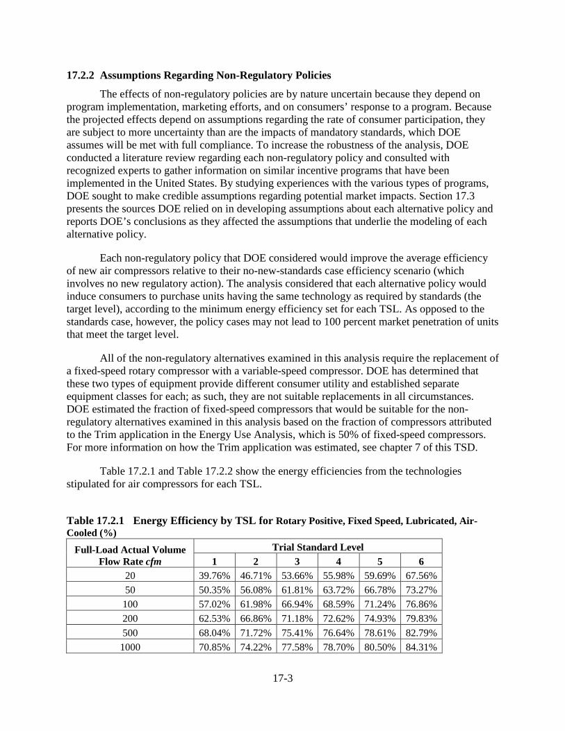
17-3

17.2.2 Assumptions Regarding Non-Regulatory Policies

The effects of non-regulatory policies are by nature uncertain because they depend on program implementation, marketing efforts, and on consumers’ response to a program. Because the projected effects depend on assumptions regarding the rate of consumer participation, they are subject to more uncertainty than are the impacts of mandatory standards, which DOE assumes will be met with full compliance. To increase the robustness of the analysis, DOE conducted a literature review regarding each non-regulatory policy and consulted with recognized experts to gather information on similar incentive programs that have been implemented in the United States. By studying experiences with the various types of programs, DOE sought to make credible assumptions regarding potential market impacts. Section 17.3 presents the sources DOE relied on in developing assumptions about each alternative policy and reports DOE’s conclusions as they affected the assumptions that underlie the modeling of each alternative policy.

Each non-regulatory policy that DOE considered would improve the average efficiency of new air compressors relative to their no-new-standards case efficiency scenario (which involves no new regulatory action). The analysis considered that each alternative policy would induce consumers to purchase units having the same technology as required by standards (the target level), according to the minimum energy efficiency set for each TSL. As opposed to the standards case, however, the policy cases may not lead to 100 percent market penetration of units that meet the target level.

All of the non-regulatory alternatives examined in this analysis require the replacement of a fixed-speed rotary compressor with a variable-speed compressor. DOE has determined that these two types of equipment provide different consumer utility and established separate equipment classes for each; as such, they are not suitable replacements in all circumstances. DOE estimated the fraction of fixed-speed compressors that would be suitable for the non-regulatory alternatives examined in this analysis based on the fraction of compressors attributed to the Trim application in the Energy Use Analysis, which is 50% of fixed-speed compressors. For more information on how the Trim application was estimated, see chapter 7 of this TSD.

Table 17.2.1 and Table 17.2.2 show the energy efficiencies from the technologies stipulated for air compressors for each TSL.

Table 17.2.1 Energy Efficiency by TSL for Rotary Positive, Fixed Speed, Lubricated, Air-Cooled (%)

Full-Load Actual Volume Flow Rate cfm

Trial Standard Level 1 2 3 4 5 6

20 39.76% 46.71% 53.66% 55.98% 59.69% 67.56% 50 50.35% 56.08% 61.81% 63.72% 66.78% 73.27% 100 57.02% 61.98% 66.94% 68.59% 71.24% 76.86% 200 62.53% 66.86% 71.18% 72.62% 74.93% 79.83% 500 68.04% 71.72% 75.41% 76.64% 78.61% 82.79%

1000 70.85% 74.22% 77.58% 78.70% 80.50% 84.31%

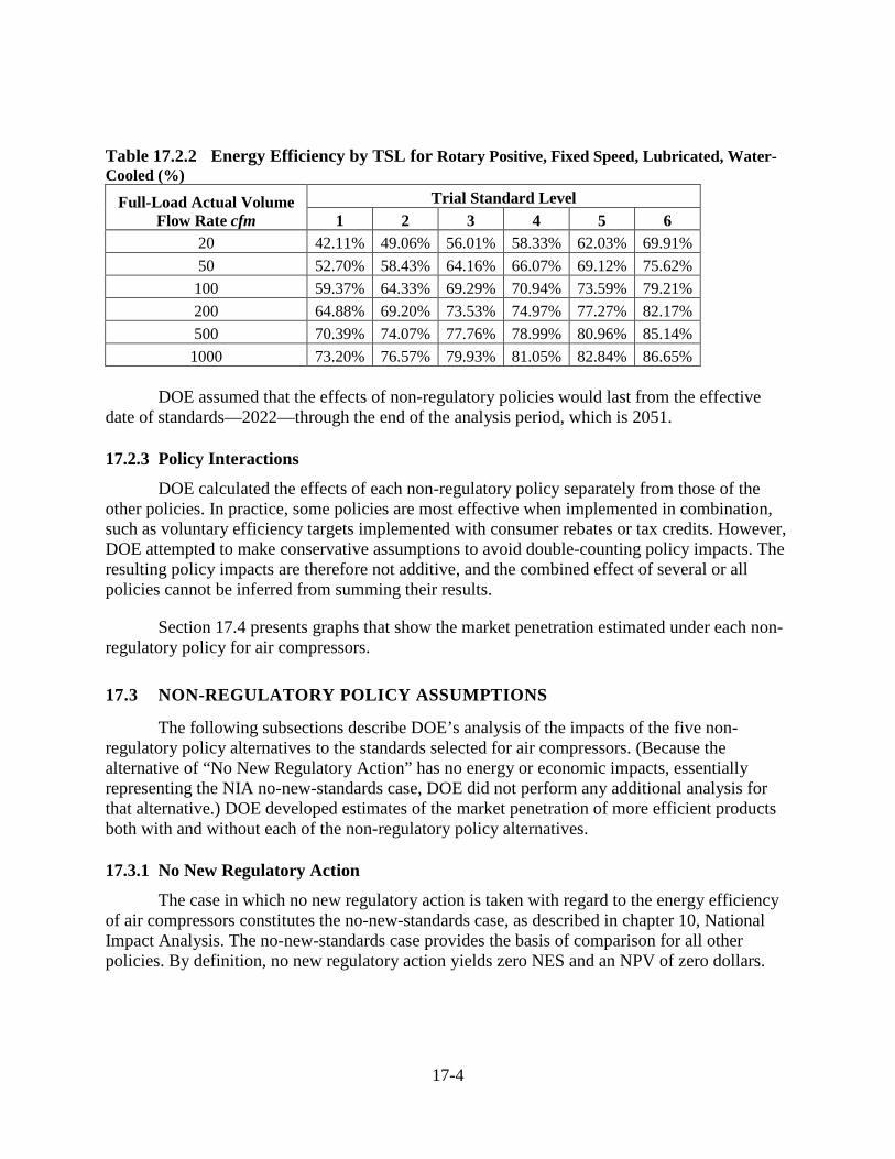
17-4

Table 17.2.2 Energy Efficiency by TSL for Rotary Positive, Fixed Speed, Lubricated, Water-Cooled (%)

Full-Load Actual Volume Flow Rate cfm

Trial Standard Level 1 2 3 4 5 6

20 42.11% 49.06% 56.01% 58.33% 62.03% 69.91% 50 52.70% 58.43% 64.16% 66.07% 69.12% 75.62% 100 59.37% 64.33% 69.29% 70.94% 73.59% 79.21% 200 64.88% 69.20% 73.53% 74.97% 77.27% 82.17% 500 70.39% 74.07% 77.76% 78.99% 80.96% 85.14%

1000 73.20% 76.57% 79.93% 81.05% 82.84% 86.65%

DOE assumed that the effects of non-regulatory policies would last from the effective date of standards—2022—through the end of the analysis period, which is 2051.

17.2.3 Policy Interactions

DOE calculated the effects of each non-regulatory policy separately from those of the other policies. In practice, some policies are most effective when implemented in combination, such as voluntary efficiency targets implemented with consumer rebates or tax credits. However, DOE attempted to make conservative assumptions to avoid double-counting policy impacts. The resulting policy impacts are therefore not additive, and the combined effect of several or all policies cannot be inferred from summing their results.

Section 17.4 presents graphs that show the market penetration estimated under each non-regulatory policy for air compressors.

17.3 NON-REGULATORY POLICY ASSUMPTIONS

The following subsections describe DOE’s analysis of the impacts of the five non-regulatory policy alternatives to the standards selected for air compressors. (Because the alternative of “No New Regulatory Action” has no energy or economic impacts, essentially representing the NIA no-new-standards case, DOE did not perform any additional analysis for that alternative.) DOE developed estimates of the market penetration of more efficient products both with and without each of the non-regulatory policy alternatives.

17.3.1 No New Regulatory Action

The case in which no new regulatory action is taken with regard to the energy efficiency of air compressors constitutes the no-new-standards case, as described in chapter 10, National Impact Analysis. The no-new-standards case provides the basis of comparison for all other policies. By definition, no new regulatory action yields zero NES and an NPV of zero dollars.

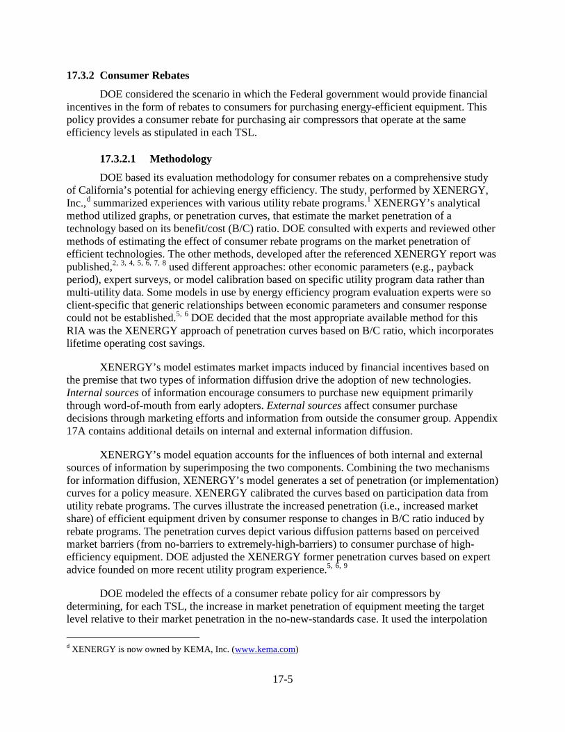
17-5

17.3.2 Consumer Rebates

DOE considered the scenario in which the Federal government would provide financial incentives in the form of rebates to consumers for purchasing energy-efficient equipment. This policy provides a consumer rebate for purchasing air compressors that operate at the same efficiency levels as stipulated in each TSL.

17.3.2.1 Methodology

DOE based its evaluation methodology for consumer rebates on a comprehensive study of California’s potential for achieving energy efficiency. The study, performed by XENERGY, Inc.,d summarized experiences with various utility rebate programs.1 XENERGY’s analytical method utilized graphs, or penetration curves, that estimate the market penetration of a technology based on its benefit/cost (B/C) ratio. DOE consulted with experts and reviewed other methods of estimating the effect of consumer rebate programs on the market penetration of efficient technologies. The other methods, developed after the referenced XENERGY report was published,2, 3, 4, 5, 6, 7, 8 used different approaches: other economic parameters (e.g., payback period), expert surveys, or model calibration based on specific utility program data rather than multi-utility data. Some models in use by energy efficiency program evaluation experts were so client-specific that generic relationships between economic parameters and consumer response could not be established.5, 6 DOE decided that the most appropriate available method for this RIA was the XENERGY approach of penetration curves based on B/C ratio, which incorporates lifetime operating cost savings.

XENERGY’s model estimates market impacts induced by financial incentives based on the premise that two types of information diffusion drive the adoption of new technologies. Internal sources of information encourage consumers to purchase new equipment primarily through word-of-mouth from early adopters. External sources affect consumer purchase decisions through marketing efforts and information from outside the consumer group. Appendix 17A contains additional details on internal and external information diffusion.

XENERGY’s model equation accounts for the influences of both internal and external sources of information by superimposing the two components. Combining the two mechanisms for information diffusion, XENERGY’s model generates a set of penetration (or implementation) curves for a policy measure. XENERGY calibrated the curves based on participation data from utility rebate programs. The curves illustrate the increased penetration (i.e., increased market share) of efficient equipment driven by consumer response to changes in B/C ratio induced by rebate programs. The penetration curves depict various diffusion patterns based on perceived market barriers (from no-barriers to extremely-high-barriers) to consumer purchase of high-efficiency equipment. DOE adjusted the XENERGY former penetration curves based on expert advice founded on more recent utility program experience.5, 6, 9

DOE modeled the effects of a consumer rebate policy for air compressors by determining, for each TSL, the increase in market penetration of equipment meeting the target level relative to their market penetration in the no-new-standards case. It used the interpolation d XENERGY is now owned by KEMA, Inc. (www.kema.com)

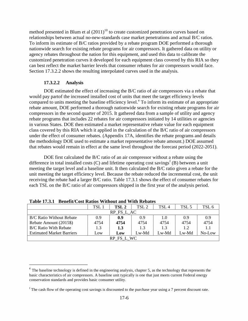
17-6

method presented in Blum et al (2011)10 to create customized penetration curves based on relationships between actual no-new-standards case market penetrations and actual B/C ratios. To inform its estimate of B/C ratios provided by a rebate program DOE performed a thorough nationwide search for existing rebate programs for air compressors. It gathered data on utility or agency rebates throughout the nation for this equipment, and used this data to calibrate the customized penetration curves it developed for each equipment class covered by this RIA so they can best reflect the market barrier levels that consumer rebates for air compressors would face. Section 17.3.2.2 shows the resulting interpolated curves used in the analysis.

17.3.2.2 Analysis

DOE estimated the effect of increasing the B/C ratio of air compressors via a rebate that would pay partof the increased installed cost of units that meet the target efficiency levels compared to units meeting the baseline efficiency level.e To inform its estimate of an appropriate rebate amount, DOE performed a thorough nationwide search for existing rebate programs for air compressors in the second quarter of 2015. It gathered data from a sample of utility and agency rebate programs that includes 22 rebates for air compressors initiated by 14 utilities or agencies in various States. DOE then estimated a market representative rebate value for each equipment class covered by this RIA which it applied in the calculation of the B/C ratio of air compressors under the effect of consumer rebates. (Appendix 17A, identifies the rebate programs and details the methodology DOE used to estimate a market representative rebate amount.) DOE assumed that rebates would remain in effect at the same level throughout the forecast period (2022-2051).

DOE first calculated the B/C ratio of an air compressor without a rebate using the difference in total installed costs (C) and lifetime operating cost savingsf (B) between a unit meeting the target level and a baseline unit. It then calculated the B/C ratio given a rebate for the unit meeting the target efficiency level. Because the rebate reduced the incremental cost, the unit receiving the rebate had a larger B/C ratio. Table 17.3.1 shows the effect of consumer rebates for each TSL on the B/C ratio of air compressors shipped in the first year of the analysis period.

Table 17.3.1 Benefit/Cost Ratios Without and With Rebates TSL 1 TSL 2 TSL 2 TSL 4 TSL 5 TSL 6

RP_FS_L_AC B/C Ratio Without Rebate 0.9 0.9 0.9 1.0 0.9 0.9 Rebate Amount (2015$) 4754 4754 4754 4754 4754 4754 B/C Ratio With Rebate 1.3 1.3 1.3 1.3 1.2 1.1 Estimated Market Barriers Low Low Lw-Md Lw-Md Lw-Md No-Low

RP_FS_L_WC

e The baseline technology is defined in the engineering analysis, chapter 5, as the technology that represents the basic characteristics of air compressors. A baseline unit typically is one that just meets current Federal energy conservation standards and provides basic consumer utility.

f The cash flow of the operating cost savings is discounted to the purchase year using a 7 percent discount rate.

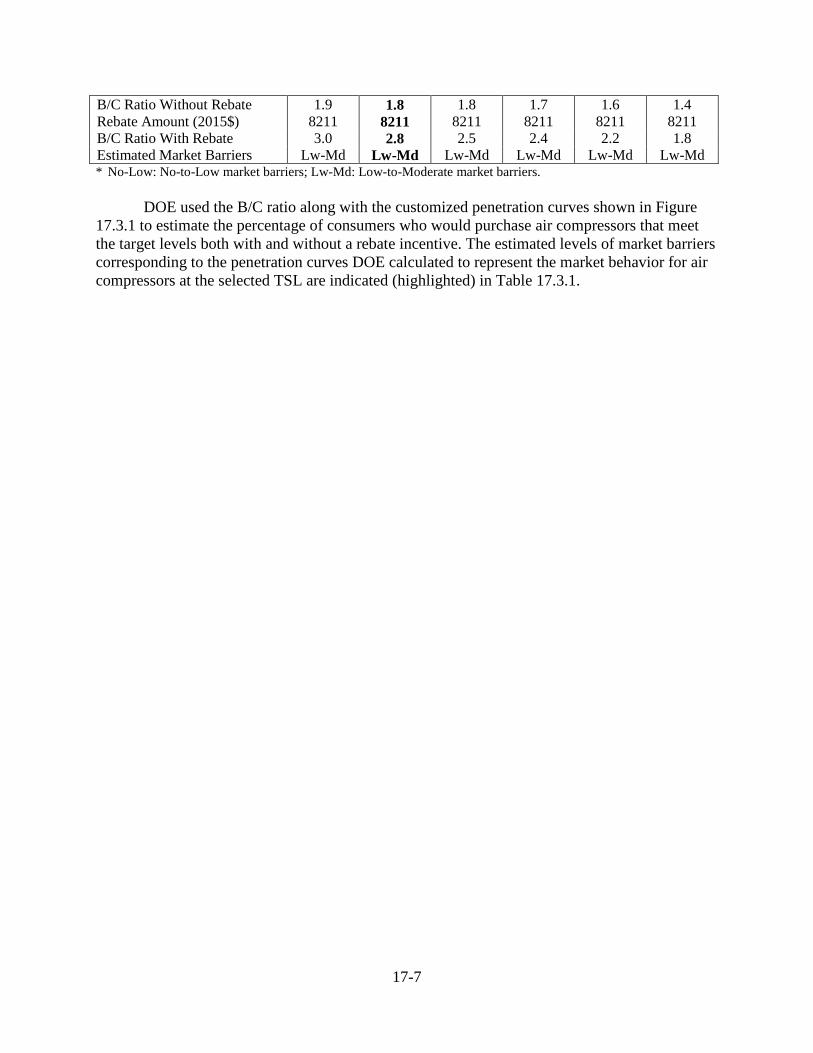
17-7

B/C Ratio Without Rebate 1.9 1.8 1.8 1.7 1.6 1.4 Rebate Amount (2015$) 8211 8211 8211 8211 8211 8211 B/C Ratio With Rebate 3.0 2.8 2.5 2.4 2.2 1.8 Estimated Market Barriers Lw-Md Lw-Md Lw-Md Lw-Md Lw-Md Lw-Md * No-Low: No-to-Low market barriers; Lw-Md: Low-to-Moderate market barriers.

DOE used the B/C ratio along with the customized penetration curves shown in Figure 17.3.1 to estimate the percentage of consumers who would purchase air compressors that meet the target levels both with and without a rebate incentive. The estimated levels of market barriers corresponding to the penetration curves DOE calculated to represent the market behavior for air compressors at the selected TSL are indicated (highlighted) in Table 17.3.1.

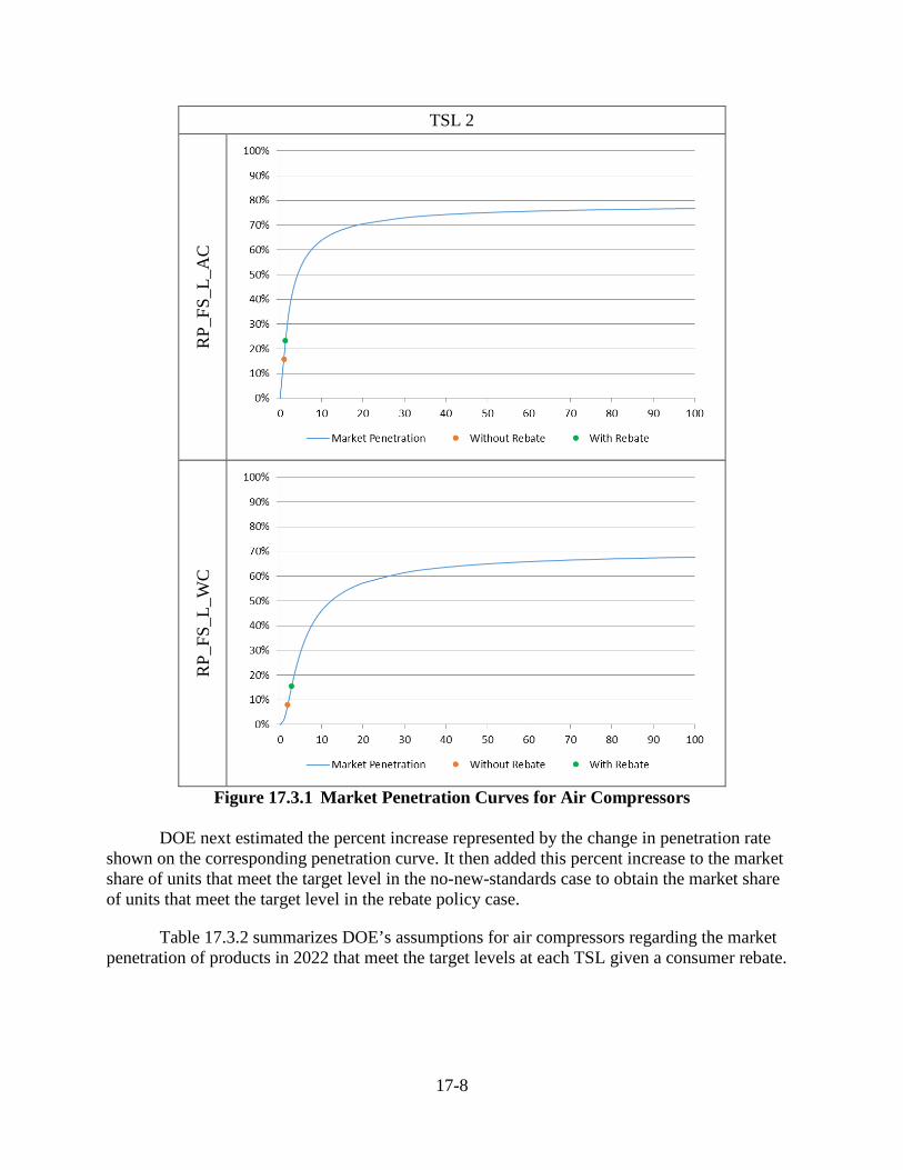
17-8

TSL 2

RP_

FS_L

_AC

RP_

FS_L

_WC

Figure 17.3.1 Market Penetration Curves for Air Compressors

DOE next estimated the percent increase represented by the change in penetration rate

shown on the corresponding penetration curve. It then added this percent increase to the market share of units that meet the target level in the no-new-standards case to obtain the market share of units that meet the target level in the rebate policy case.

Table 17.3.2 summarizes DOE’s assumptions for air compressors regarding the market penetration of products in 2022 that meet the target levels at each TSL given a consumer rebate.

17-9

Table 17.3.2 Market Penetrations in 2022 Attributable to Consumer Rebates TSL 1 TSL 2 TSL 2 TSL 4 TSL 5 TSL 6 RP_FS_L_AC Base-Case Market Share 15.5% 15.9% 9.2% 5.6% 11.4% 21.8% Policy Case Market Share 19.3% 19.5% 11.8% 7.4% 13.7% 23.9% Increased Market Share 3.9% 3.7% 2.6% 1.8% 2.3% 2.1% RP_FS_L_WC Base-Case Market Share 15.5% 7.9% 18.4% 5.6% 11.4% 21.8% Policy Case Market Share 20.8% 11.7% 22.6% 7.9% 14.3% 24.3% Increased Market Share 5.3% 3.8% 4.2% 2.3% 2.9% 2.5%

DOE used the resulting annual increases in market shares as inputs to represent the rebate

policy case scenario in its NIA-RIA model. Appendix 17A shows the annual market share increases due to this policy for the whole forecast period. Section 17.4 presents the resulting market penetration trends for the policy case of consumer rebates for air compressors.

17.3.3 Consumer Tax Credits

DOE estimated the effects of tax credits on consumer purchases based on its previous analysis of consumer participation in tax credits. DOE supported its approach using data from Oregon State’s tax credit program for energy-efficient appliances. DOE also incorporated previous research that disaggregated the effect of rebates and tax credits into a direct price effect, which derives from the savings in purchase price, and an announcement effect, which is independent of the amount of the incentive.11, 12 The announcement effect derives from the credibility that a technology receives from being included in an incentive program, as well as changes in product marketing and modifications in markup and pricing. DOE assumed that the rebate and consumer tax credit policies would encompass both direct price effects and announcement effects, and that half the increase in market penetration associated with either policy would be due to the direct price effect and half to the announcement effect.

In estimating the effects of a tax credit on purchases of consumer products that meet new efficiency standards, DOE assumed the amount of the tax credit would be the same as the corresponding rebate amount discussed above.

DOE estimated that fewer consumers would participate in a tax credit program than would take advantage of a rebate. Research has shown that the delay required for a consumer to receive a tax credit, plus the added time and cost in preparing the tax return, make a tax credit incentive less effective than a rebate received at the time of purchase. Based on previous analyses, DOE assumed that only 60 percent of the consumers who would take advantage of a rebate would take advantage of a tax credit.13

In preparing its assumptions to estimate the effects of tax credits on consumer purchases of air compressors, DOE also reviewed other tax credit programs that have been offered at both the Federal and State levels for energy-efficient appliances.

17-10

The Energy Policy Act of 2005 (EPACT 2005) included Federal tax credits for consumers who purchase energy-efficient products.14 Those tax credits were in effect in 2006 and 2007, expired in 2008, were reinstated for 2009–2010 by the American Recovery and Reinvestment Act of 2009 (ARRA), extended by Congress for 2011 with some modifications, and expired at the end of 2011.15, 16 The American Taxpayer Relief Act of 2012 extended, with some modifications, residential tax credits for air conditioners, heat pumps, furnaces, and water heaters placed in service between January 1, 2012 and December 31, 2013.17 DOE reviewed Internal Revenue Service data on the numbers of taxpayers who claimed the tax credits during tax years 2006 and 2007. DOE also reviewed data from an earlier Federal energy conservation tax credit program in place in the 1980s. However, DOE did not find data specific enough to air compressors to warrant adjusting its analysis method for the Consumer Tax Credits policy case. Appendix 17A contains more information on Federal consumer tax credits.

DOE also reviewed its previous analysis of Oregon’s tax credits for clothes washers to provide support for its assumptions.18 In that previous analysis, DOE compared the market shares of ultra-high efficiency (UHE) residential clothes washers in Oregon, which offered both State tax credits and utility rebates, with those in Washington State, which offered only utility rebates during the same period. Based on this analysis, DOE estimated that in Oregon the impact of tax credits was 62 percent of the impact of rebates for UHE clothes washers having equivalent efficiency. This finding supports its original assumption that participation in a tax credit program would be about 60 percent of participation in a rebate program. Additional discussion of State tax credits for Oregon and other states is in appendix 17A.

DOE applied the assumed 60 percent participation described above to the increase in penetration rates estimated for the rebate policy to estimate penetration rates attributable to consumer tax credits. In doing so, DOE incorporated the assumptions for consumer response to financial incentives from the customized penetration curves it developed for air compressors (See Figure 17.3.1).

Table 17.3.3 summarizes DOE’s assumptions for air compressors regarding the market penetration of products in 2022 that meet the target levels at each TSL given a consumer tax credit.

Table 17.3.3 Market Penetrations in 2022 Attributable to Consumer Tax Credits

TSL 1 TSL 2 TSL 2 TSL 4 TSL 5 TSL 6 RP_FS_L_AC Base-Case Market Share 15.5% 15.9% 9.2% 5.6% 11.4% 21.8% Policy Case Market Share 17.8% 18.1% 10.8% 6.7% 12.8% 23.0% Increased Market Share 2.3% 2.2% 1.6% 1.1% 1.4% 1.3% RP_FS_L_WC Base-Case Market Share 15.5% 7.9% 18.4% 5.6% 11.4% 21.8% Policy Case Market Share 18.7% 10.2% 20.9% 7.0% 13.1% 23.3% Increased Market Share 3.2% 2.3% 2.5% 1.4% 1.7% 1.5%

17-11

The increased market shares attributable to consumer tax credits shown in Table 17.3.3 were used as inputs in the NIA-RIA model. Appendix 17A shows the annual market share increases due to this policy for the whole forecast period. Section 17.4 presents the resulting market penetration trends for the policy case of consumer tax credits for air compressors that meet the efficiency level for the selected TSL.

17.3.4 Manufacturer Tax Credits

To analyze the potential effects of a policy that offers tax credits to manufacturers that produce air compressors that meet the target efficiency levels at each TSL, DOE assumed that a manufacturer tax credit would lower the consumer’s purchase cost by an amount equivalent to that provided by the consumer rebates or tax credits described above. DOE further assumed that manufacturers would pass on some of their reduced costs to consumers, causing a direct price effect. DOE assumed that no announcement effect would occur, because the program would not be visible to consumers.g Because the direct price effect is approximately equivalent to the announcement effect,11 DOE estimated that a manufacturer tax credit would induce half the number of consumers assumed to take advantage of a consumer tax credit to purchase more efficient products. Thus the assumed participation rate is equal to 30 percent of the number of consumers who would participate in a rebate program.

DOE attempted to investigate manufacturer response to the Energy Efficient Appliance Credits for manufacturers mandated by EPACT 2005.19 Those manufacturer tax credits have been in effect for dishwashers, clothes washers and refrigerators produced beginning in 2009. DOE was unable to locate data from the Internal Revenue Service or other sources on manufacturer response to the Federal credits. Appendix 17A presents details on Federal manufacturer tax credits.

DOE applied the assumption of 30 percent participation to the increase in penetration rates predicted for the rebate policy to estimate the effects of a manufacturer tax credit policy. In doing so, DOE incorporated the assumptions for consumer response to financial incentives from the customized penetration curves it developed for air compressors. (See Figure 17.3.1).

Table 17.3.4 summarizes DOE’s assumptions for air compressors regarding the market penetration of products in 2022 that meet the target levels at each TSL given a manufacturer tax credit.

g Note that this is a conservative assumption, since it is possible that manufacturers or utility/agency efficiency programs might promote the models for which manufacturers increase production due to the tax credits, which in turn might induce some announcement effect. However, DOE found no data on such programs on which to base an estimate of the magnitude of this possible announcement effect on consumer behavior.

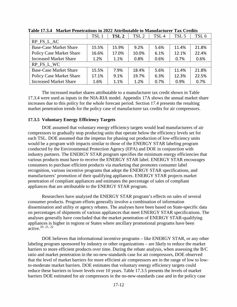
17-12

Table 17.3.4 Market Penetrations in 2022 Attributable to Manufacturer Tax Credits TSL 1 TSL 2 TSL 2 TSL 4 TSL 5 TSL 6 RP_FS_L_AC Base-Case Market Share 15.5% 15.9% 9.2% 5.6% 11.4% 21.8% Policy Case Market Share 16.6% 17.0% 10.0% 6.1% 12.1% 22.4% Increased Market Share 1.2% 1.1% 0.8% 0.6% 0.7% 0.6% RP_FS_L_WC Base-Case Market Share 15.5% 7.9% 18.4% 5.6% 11.4% 21.8% Policy Case Market Share 17.1% 9.1% 19.7% 6.3% 12.3% 22.5% Increased Market Share 1.6% 1.1% 1.2% 0.7% 0.9% 0.7%

The increased market shares attributable to a manufacturer tax credit shown in Table

17.3.4 were used as inputs in the NIA-RIA model. Appendix 17A shows the annual market share increases due to this policy for the whole forecast period. Section 17.4 presents the resulting market penetration trends for the policy case of manufacturer tax credits for air compressors.

17.3.5 Voluntary Energy Efficiency Targets

DOE assumed that voluntary energy efficiency targets would lead manufacturers of air compressors to gradually stop producing units that operate below the efficiency levels set for each TSL. DOE assumed that the impetus for phasing out production of low-efficiency units would be a program with impacts similar to those of the ENERGY STAR labeling program conducted by the Environmental Protection Agency (EPA) and DOE in conjunction with industry partners. The ENERGY STAR program specifies the minimum energy efficiencies that various products must have to receive the ENERGY STAR label. ENERGY STAR encourages consumers to purchase efficient products via marketing that promotes consumer label recognition, various incentive programs that adopt the ENERGY STAR specifications, and manufacturers’ promotion of their qualifying appliances. ENERGY STAR projects market penetration of compliant appliances and estimates the percentage of sales of compliant appliances that are attributable to the ENERGY STAR program.

Researchers have analyzed the ENERGY STAR program’s effects on sales of several consumer products. Program efforts generally involve a combination of information dissemination and utility or agency rebates. The analyses have been based on State-specific data on percentages of shipments of various appliances that meet ENERGY STAR specifications. The analyses generally have concluded that the market penetration of ENERGY STAR-qualifying appliances is higher in regions or States where ancillary promotional programs have been active.20, 21, 22

DOE believes that informational incentive programs – like ENERGY STAR, or any other labeling program sponsored by industry or other organizations – are likely to reduce the market barriers to more efficient products over time. During the rebate analysis, when assessing the B/C ratio and market penetration in the no-new-standards case for air compressors, DOE observed that the level of market barriers for more efficient air compressors are in the range of low to low-to-moderate market barriers. DOE estimates that voluntary energy efficiency targets could reduce these barriers to lower levels over 10 years. Table 17.3.5 presents the levels of market barriers DOE estimated for air compressors in the no-new-standards case and in the policy case

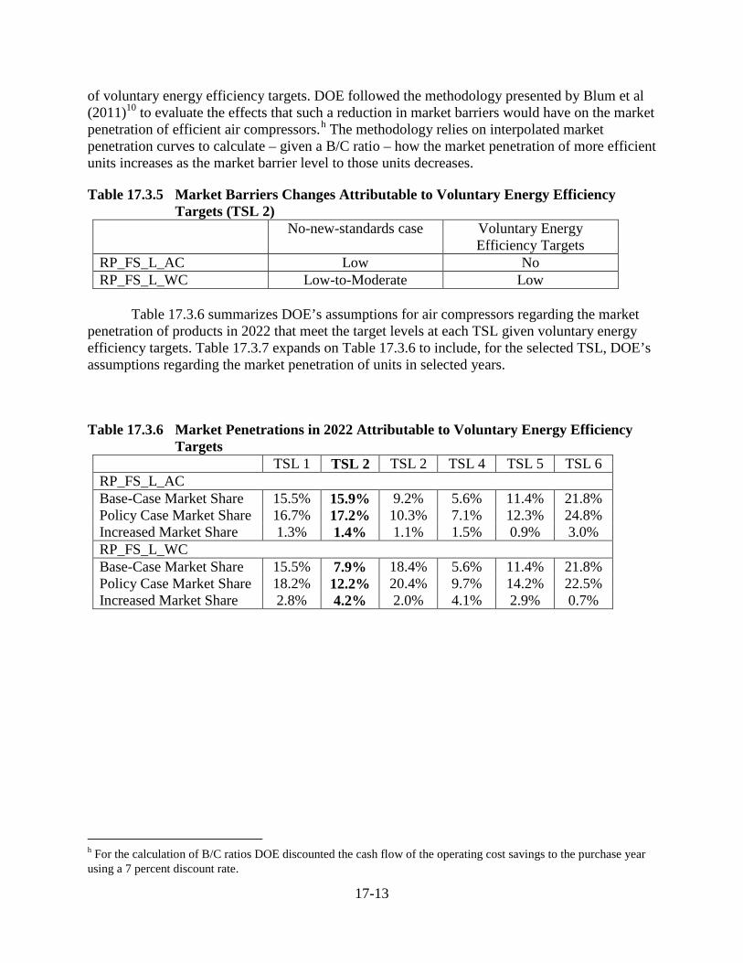
17-13

of voluntary energy efficiency targets. DOE followed the methodology presented by Blum et al (2011)10 to evaluate the effects that such a reduction in market barriers would have on the market penetration of efficient air compressors.h The methodology relies on interpolated market penetration curves to calculate – given a B/C ratio – how the market penetration of more efficient units increases as the market barrier level to those units decreases.

Table 17.3.5 Market Barriers Changes Attributable to Voluntary Energy Efficiency Targets (TSL 2)

No-new-standards case Voluntary Energy Efficiency Targets

RP_FS_L_AC Low No RP_FS_L_WC Low-to-Moderate Low

Table 17.3.6 summarizes DOE’s assumptions for air compressors regarding the market

penetration of products in 2022 that meet the target levels at each TSL given voluntary energy efficiency targets. Table 17.3.7 expands on Table 17.3.6 to include, for the selected TSL, DOE’s assumptions regarding the market penetration of units in selected years.

Table 17.3.6 Market Penetrations in 2022 Attributable to Voluntary Energy Efficiency

Targets TSL 1 TSL 2 TSL 2 TSL 4 TSL 5 TSL 6 RP_FS_L_AC Base-Case Market Share 15.5% 15.9% 9.2% 5.6% 11.4% 21.8% Policy Case Market Share 16.7% 17.2% 10.3% 7.1% 12.3% 24.8% Increased Market Share 1.3% 1.4% 1.1% 1.5% 0.9% 3.0% RP_FS_L_WC Base-Case Market Share 15.5% 7.9% 18.4% 5.6% 11.4% 21.8% Policy Case Market Share 18.2% 12.2% 20.4% 9.7% 14.2% 22.5% Increased Market Share 2.8% 4.2% 2.0% 4.1% 2.9% 0.7%

h For the calculation of B/C ratios DOE discounted the cash flow of the operating cost savings to the purchase year using a 7 percent discount rate.

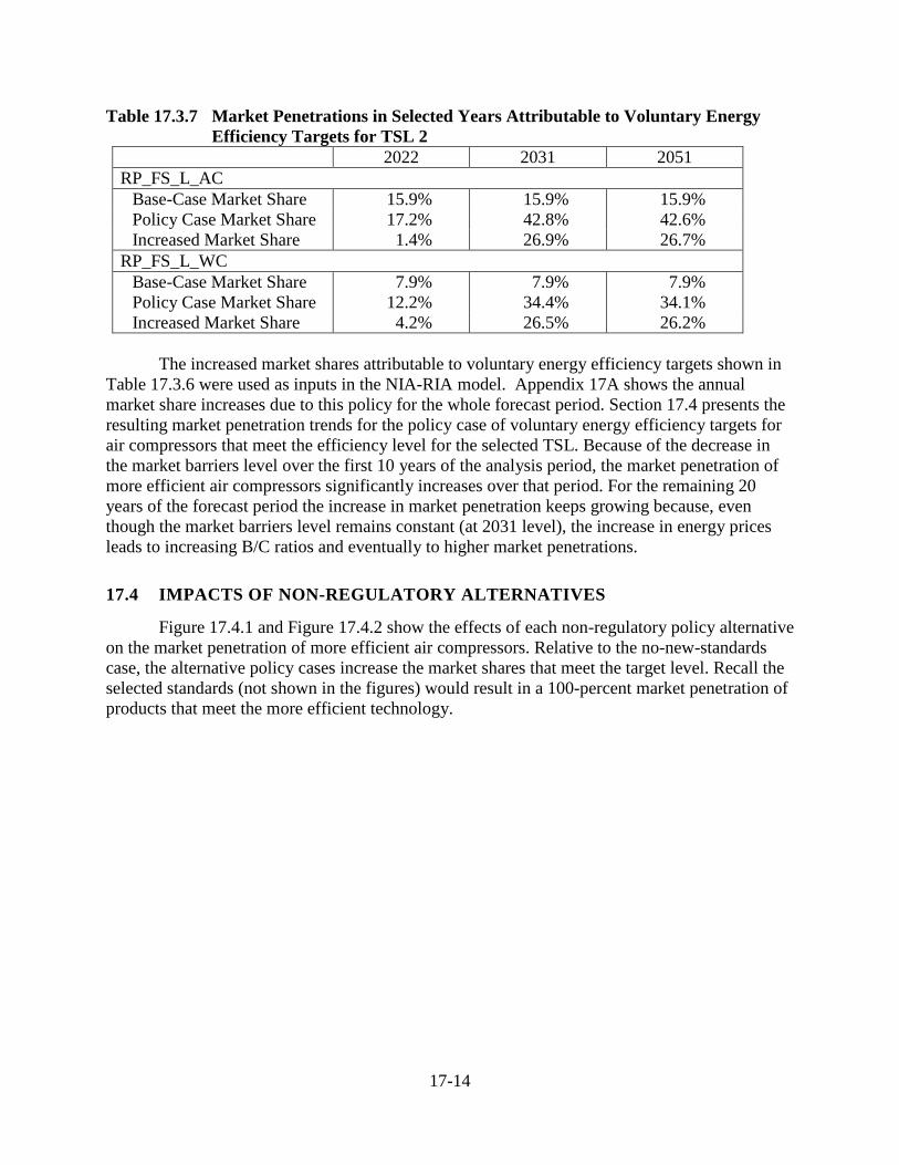
17-14

Table 17.3.7 Market Penetrations in Selected Years Attributable to Voluntary Energy Efficiency Targets for TSL 2

2022 2031 2051 RP_FS_L_AC

Base-Case Market Share 15.9% 15.9% 15.9% Policy Case Market Share 17.2% 42.8% 42.6% Increased Market Share 1.4% 26.9% 26.7%

RP_FS_L_WC Base-Case Market Share 7.9% 7.9% 7.9% Policy Case Market Share 12.2% 34.4% 34.1% Increased Market Share 4.2% 26.5% 26.2%

The increased market shares attributable to voluntary energy efficiency targets shown in

Table 17.3.6 were used as inputs in the NIA-RIA model. Appendix 17A shows the annual market share increases due to this policy for the whole forecast period. Section 17.4 presents the resulting market penetration trends for the policy case of voluntary energy efficiency targets for air compressors that meet the efficiency level for the selected TSL. Because of the decrease in the market barriers level over the first 10 years of the analysis period, the market penetration of more efficient air compressors significantly increases over that period. For the remaining 20 years of the forecast period the increase in market penetration keeps growing because, even though the market barriers level remains constant (at 2031 level), the increase in energy prices leads to increasing B/C ratios and eventually to higher market penetrations.

17.4 IMPACTS OF NON-REGULATORY ALTERNATIVES

Figure 17.4.1 and Figure 17.4.2 show the effects of each non-regulatory policy alternative on the market penetration of more efficient air compressors. Relative to the no-new-standards case, the alternative policy cases increase the market shares that meet the target level. Recall the selected standards (not shown in the figures) would result in a 100-percent market penetration of products that meet the more efficient technology.

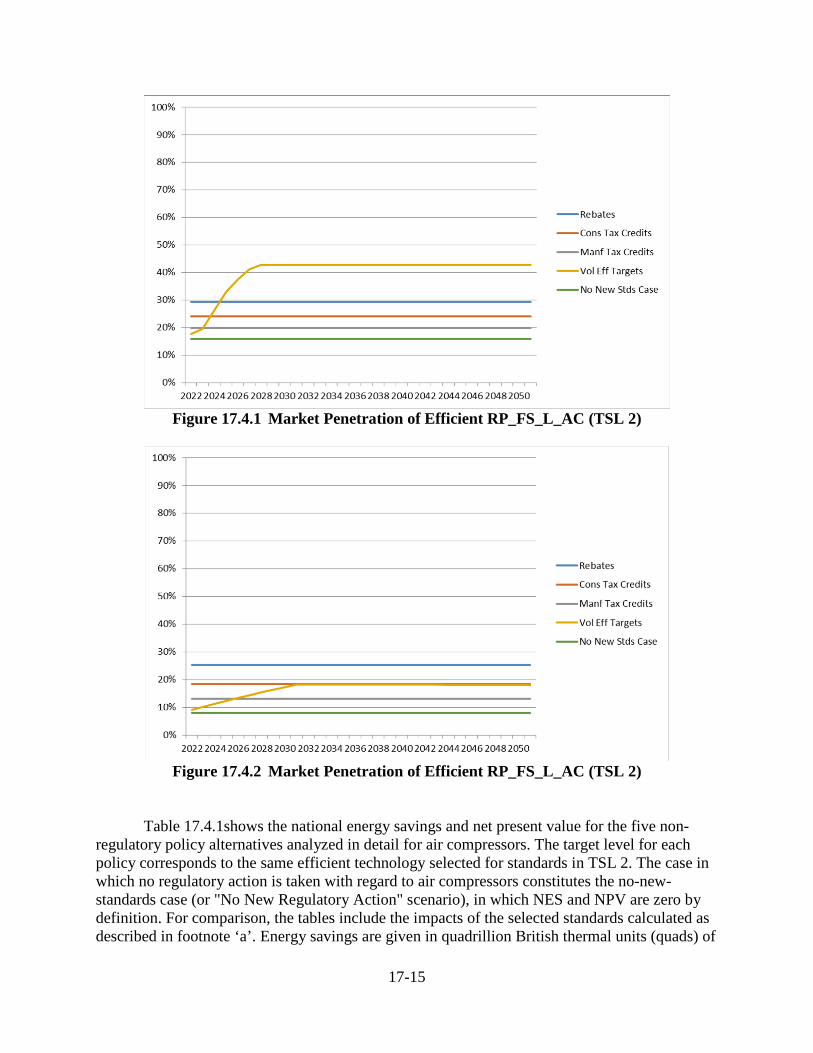
17-15

Figure 17.4.1 Market Penetration of Efficient RP_FS_L_AC (TSL 2)

Figure 17.4.2 Market Penetration of Efficient RP_FS_L_AC (TSL 2)

Table 17.4.1shows the national energy savings and net present value for the five non-regulatory policy alternatives analyzed in detail for air compressors. The target level for each policy corresponds to the same efficient technology selected for standards in TSL 2. The case in which no regulatory action is taken with regard to air compressors constitutes the no-new-standards case (or "No New Regulatory Action" scenario), in which NES and NPV are zero by definition. For comparison, the tables include the impacts of the selected standards calculated as described in footnote ‘a’. Energy savings are given in quadrillion British thermal units (quads) of

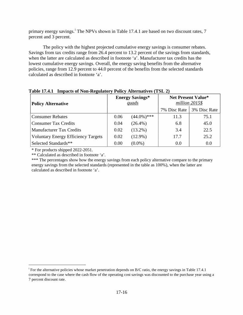
17-16

primary energy savings.i The NPVs shown in Table 17.4.1 are based on two discount rates, 7 percent and 3 percent.

The policy with the highest projected cumulative energy savings is consumer rebates. Savings from tax credits range from 26.4 percent to 13.2 percent of the savings from standards, when the latter are calculated as described in footnote ‘a’. Manufacturer tax credits has the lowest cumulative energy savings. Overall, the energy saving benefits from the alternative policies, range from 12.9 percent to 44.0 percent of the benefits from the selected standards calculated as described in footnote ‘a’. Table 17.4.1 Impacts of Non-Regulatory Policy Alternatives (TSL 2)

Policy Alternative Energy Savings*

quads Net Present Value*

million 2015$ 7% Disc Rate 3% Disc Rate

Consumer Rebates 0.06 (44.0%)*** 11.3 75.1 Consumer Tax Credits 0.04 (26.4%) 6.8 45.0 Manufacturer Tax Credits 0.02 (13.2%) 3.4 22.5 Voluntary Energy Efficiency Targets 0.02 (12.9%) 17.7 25.2 Selected Standards** 0.00 (0.0%) 0.0 0.0 * For products shipped 2022-2051. ** Calculated as described in footnote ‘a’. *** The percentages show how the energy savings from each policy alternative compare to the primary energy savings from the selected standards (represented in the table as 100%), when the latter are calculated as described in footnote ‘a’.

i For the alternative policies whose market penetration depends on B/C ratio, the energy savings in Table 17.4.1 correspond to the case where the cash flow of the operating cost savings was discounted to the purchase year using a 7 percent discount rate.

17-17

REFERENCES 1. Rufo, M. and F. Coito. California’s Secret Energy Surplus: The Potential for Energy

Efficiency. 2002. XENERGY Inc. (Last accessed December 17, 2015.) http://www.issuelab.org/resource/californias_secret_energy_surplus_the_potential_for_energy_efficiency.

2. ICF International. Arizona Public Service Energy Efficient Market Potential Study. 2007. Fairfax, VA.

3. Mosenthal, P. (Optimal Energy) and B. Atkinson (LBNL). Telephone conversation. January 2008.

4. Lee, A. (Quantec LLC) and B. Atkinson (LBNL). Telephone conversation. 2008.

5. Rufo, M. (Itron Inc.) and B. Atkinson (LBNL). Telephone conversation. January 2008.

6. Rufo, M. (Itron Inc.) and B. Atkinson (LBNL). Telephone conversation. March 2009.

7. Itron, Inc. and KEMA, Inc. California Energy Efficiency Potential Study. 2008. Pacific Gas & Electric Company: San Francisco, CA. Report No. PGE0264.01. (Last accessed December 17, 2015.) http://calmac.org/publications/PGE0264_Final_Report.pdf.

8. Global Energy Partners, LLC. AmerenUE DSM Market Research Report: Volume 2: Market Research, Results from the Saturation, Program Interest and Trade Ally Research. 2010. Walnut Creek, CA. Report No. 1287-2. (Last accessed December 17, 2015.) http://www.ameren.com/-/media/missouri-site/Files/Environment/Renewables/AmerenUEVolume2MarketResearchReport2.pdf.

9. Coito, F. (KEMA Inc.). Personal communication. E-mail to Barbara Atkinson, LBNL. June 2010.

10. Blum, H., B. A. Atkinson, and A. B. Lekov. A Framework for Comparative Assessments of Energy Efficiency Policy Measures. 2011. Lawrence Berkeley National Laboratory: Berkeley, CA. Report No. LBNL-4749E. (Last accessed December 17, 2015.) http://eetd.lbl.gov/publications/framework-comparative-assessments-energy-efficiency-policy-measures.

11. Lawrence Berkeley National Laboratory. Analysis of Tax Credits for Efficient Equipment. 1998. (Last accessed December 17, 2015.) http://enduse.lbl.gov/Projects/TaxCredits.html.

12. K. Train. Customer Decision Study: Analysis of Residential Customer Equipment Purchase Decisions. 1994. Prepared for Southern California Edison by Cambridge Systematics, Pacific Consulting Services, The Technology Applications Group, and California Survey Research Services.

17-18

13. U.S. Department of Energy–Office of Energy Efficiency and Renewable Energy. Energy Conservation Program for Consumer Products: Technical Support Document: Energy Efficiency Standards for Consumer Products: Refrigerators, Refrigerator-Freezers, and Freezers, Including Environmental Assessment and Regulatory Impact Analysis. 1995. Report No. DOE/EE-0064.

14. Energy Policy Act of 2005. 42 U.S. Code 15801. 2005. (Last accessed December 17, 2015.) http://energy.gov/sites/prod/files/2013/10/f3/epact_2005.pdf.

15. American Recovery and Reinvestment Act of 2009. Public Law 111-5. 2009. (Last accessed December 17, 2015.) http://www.gpo.gov/fdsys/pkg/BILLS-111hr1enr/pdf/BILLS-111hr1enr.pdf.

16. The Tax Incentives Assistance Project. Consumer Tax Incentives: Home Heating & Cooling Equipment. 2011. (Last accessed December 17, 2015.) http://www.energytaxincentives.org/consumers/heating-cooling.php.

17. The Tax Incentives Assistance Project. The Tax Incentives Assistance Project (TIAP). December 2014. (Last accessed December 17, 2015.) http://energytaxincentives.org/.

18. U.S. Department of Energy–Office of Energy Efficiency and Renewable Energy. Technical Support Document: Energy Efficiency Program for Consumer Products and Commercial and Industrial Equipment, Residential Dishwashers, Dehumidifiers, and Cooking Products, and Commercial Clothes Washers. 2008. Washington, D.C.

19. The Tax Incentives Assistance Project. Manufacturers Incentives. (Last accessed December 17, 2015.) http://energytaxincentives.org/builders/appliances.php.

20. Feldman, S., L. Hoegfen, L. Wilson-Wright, and A. Li. Modelling the Effects of U.S. ENERGY STAR® Appliance Programs. 2005. ECEEE 2005 Summer Study: Mandelieu La Napoule, France. (Last accessed December 17, 2015.) http://www.eceee.org/library/conference_proceedings/eceee_Summer_Studies/2005c/Panel_4/4228feldman/paper.

21. M. Rosenberg. The Impact of Regional Programs on the Market Share of Energy Star® Appliances. 2003. Seattle, WA.

22. Titus, E. and S. Feldman. Tracking the Effectiveness of Energy-Efficient Appliance Programs in the U.S. 2003. International Energy Program Evaluation Conference: Seattle, WA.

23. Smith, N. (National Association of State Procurement Officials) and B. Atkinson (LBNL). Telephone conversation. April 2008.

24. Responsible Purchasing Network. Responsible Purchasing Network. (Last accessed December 17, 2015.) www.responsiblepurchasing.org/.

17-19

25. Harris, J. and F. Johnson. Potential Energy, Cost, and CO2 Savings from Energy-Efficient Government Purchase. 2000. 2000 ACEEE Summer Study on Energy Efficiency in Buildings: Asilomar, CA. (Last accessed October 15, 2015.) http://aceee.org/files/proceedings/2000/data/papers/SS00_Panel4_Paper13.pdf.

26. U.S. Department of Energy–Energy Information Administration. 2009 RECS Survey Data. (Last accessed December 15, 2015.) http://www.eia.gov/consumption/residential/data/2009/.

27. U.S. Department of Energy–Energy Information Administration. 2012 CBECS Survey Data. (Last accessed December 17, 2015.) http://www.eia.gov/consumption/commercial/data/2012/index.cfm?view=microdata.

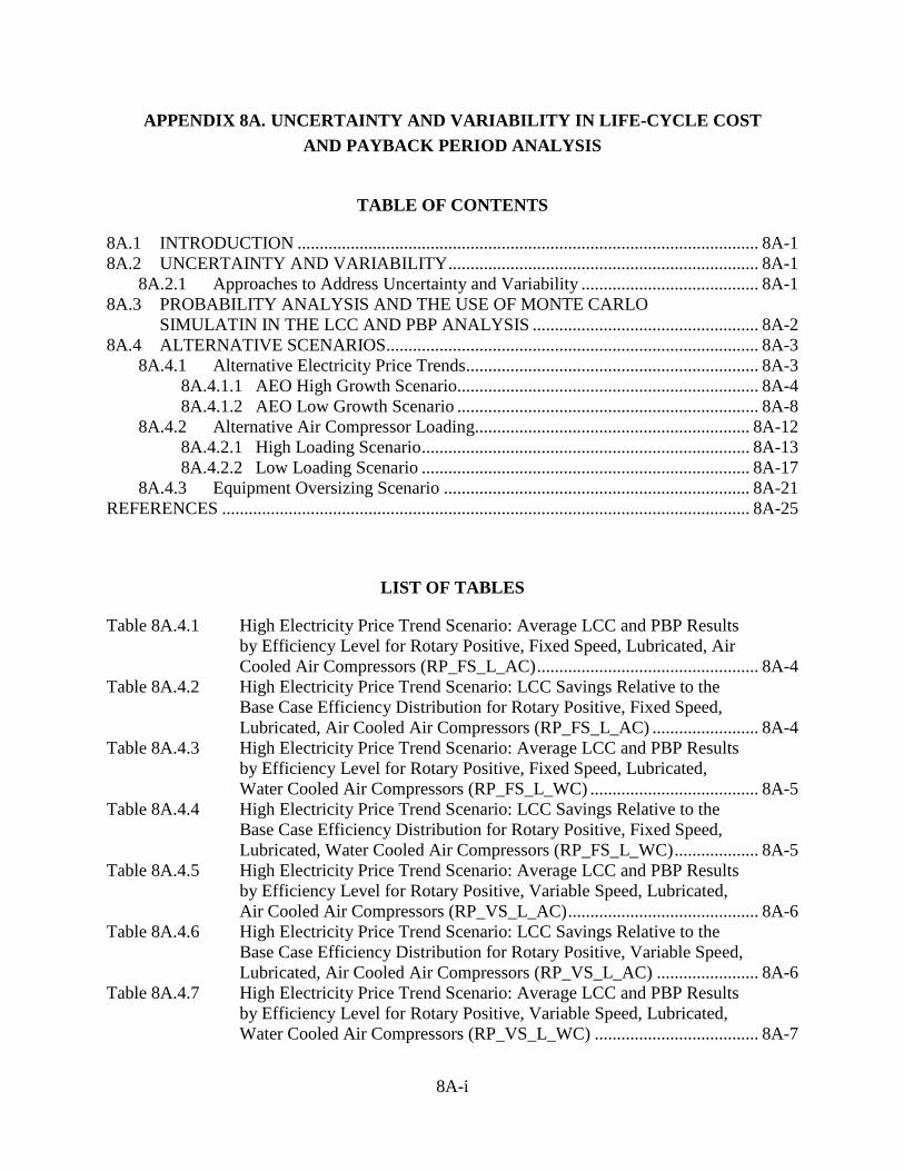
8A-i

APPENDIX 8A. UNCERTAINTY AND VARIABILITY IN LIFE-CYCLE COST AND PAYBACK PERIOD ANALYSIS

TABLE OF CONTENTS

8A.1 INTRODUCTION ........................................................................................................ 8A-1 8A.2 UNCERTAINTY AND VARIABILITY ...................................................................... 8A-1

8A.2.1 Approaches to Address Uncertainty and Variability ........................................ 8A-1 8A.3 PROBABILITY ANALYSIS AND THE USE OF MONTE CARLO

SIMULATIN IN THE LCC AND PBP ANALYSIS ................................................... 8A-2 8A.4 ALTERNATIVE SCENARIOS.................................................................................... 8A-3

8A.4.1 Alternative Electricity Price Trends .................................................................. 8A-3 8A.4.1.1 AEO High Growth Scenario.................................................................... 8A-4 8A.4.1.2 AEO Low Growth Scenario .................................................................... 8A-8

8A.4.2 Alternative Air Compressor Loading.............................................................. 8A-12 8A.4.2.1 High Loading Scenario .......................................................................... 8A-13 8A.4.2.2 Low Loading Scenario .......................................................................... 8A-17

8A.4.3 Equipment Oversizing Scenario ..................................................................... 8A-21 REFERENCES ....................................................................................................................... 8A-25

LIST OF TABLES

Table 8A.4.1 High Electricity Price Trend Scenario: Average LCC and PBP Results by Efficiency Level for Rotary Positive, Fixed Speed, Lubricated, Air Cooled Air Compressors (RP_FS_L_AC) .................................................. 8A-4

Table 8A.4.2 High Electricity Price Trend Scenario: LCC Savings Relative to the Base Case Efficiency Distribution for Rotary Positive, Fixed Speed, Lubricated, Air Cooled Air Compressors (RP_FS_L_AC) ........................ 8A-4

Table 8A.4.3 High Electricity Price Trend Scenario: Average LCC and PBP Results by Efficiency Level for Rotary Positive, Fixed Speed, Lubricated, Water Cooled Air Compressors (RP_FS_L_WC) ...................................... 8A-5

Table 8A.4.4 High Electricity Price Trend Scenario: LCC Savings Relative to the Base Case Efficiency Distribution for Rotary Positive, Fixed Speed, Lubricated, Water Cooled Air Compressors (RP_FS_L_WC) ................... 8A-5

Table 8A.4.5 High Electricity Price Trend Scenario: Average LCC and PBP Results by Efficiency Level for Rotary Positive, Variable Speed, Lubricated, Air Cooled Air Compressors (RP_VS_L_AC) ........................................... 8A-6

Table 8A.4.6 High Electricity Price Trend Scenario: LCC Savings Relative to the Base Case Efficiency Distribution for Rotary Positive, Variable Speed, Lubricated, Air Cooled Air Compressors (RP_VS_L_AC) ....................... 8A-6

Table 8A.4.7 High Electricity Price Trend Scenario: Average LCC and PBP Results by Efficiency Level for Rotary Positive, Variable Speed, Lubricated, Water Cooled Air Compressors (RP_VS_L_WC) ..................................... 8A-7

8A-ii

Table 8A.4.8 High Electricity Price Trend Scenario: LCC Savings Relative to the Base Case Efficiency Distribution for Rotary Positive, Variable Speed, Lubricated, Water Cooled Air Compressors (RP_VS_L_WC) .................. 8A-7

Table 8A.4.9 Low Electricity Price Trend Scenario: Average LCC and PBP Results by Efficiency Level for Rotary Positive, Fixed Speed, Lubricated, Air Cooled Air Compressors (RP_FS_L_AC) .................................................. 8A-8

Table 8A.4.10 Low Electricity Price Trend Scenario: LCC Savings Relative to the Base Case Efficiency Distribution for Rotary Positive, Fixed Speed, Lubricated, Air Cooled Air Compressors (RP_FS_L_AC) ........................ 8A-8

Table 8A.4.11 Low Electricity Price Trend Scenario: Average LCC and PBP Results by Efficiency Level for Rotary Positive, Fixed Speed, Lubricated, Water Cooled Air Compressors (RP_FS_L_WC) ...................................... 8A-9

Table 8A.4.12 Low Electricity Price Trend Scenario: LCC Savings Relative to the Base Case Efficiency Distribution for Rotary Positive, Fixed Speed, Lubricated, Water Cooled Air Compressors (RP_FS_L_WC) ................... 8A-9

Table 8A.4.13 Low Electricity Price Trend Scenario: Average LCC and PBP Results by Efficiency Level for Rotary Positive, Variable Speed, Lubricated, Air Cooled Air Compressors (RP_VS_L_AC) ......................................... 8A-10

Table 8A.4.14 Low Electricity Price Trend Scenario: LCC Savings Relative to the Base Case Efficiency Distribution for Rotary Positive, Variable Speed, Lubricated, Air Cooled Air Compressors (RP_VS_L_AC) ..................... 8A-10

Table 8A.4.15 Low Electricity Price Trend Scenario: Average LCC and PBP Results by Efficiency Level for Rotary Positive, Variable Speed, Lubricated, Water Cooled Air Compressors (RP_VS_L_WC) ................................... 8A-11

Table 8A.4.16 Low Electricity Price Trend Scenario: LCC Savings Relative to the Base Case Efficiency Distribution for Rotary Positive, Variable Speed, Lubricated, Water Cooled Air Compressors (RP_VS_L_WC) ................ 8A-11

Table 8A.4.17 Load Profile Scenario Definitions ........................................................... 8A-12 Table 8A.4.18 High Load Profile Scenario: Average LCC and PBP Results by

Efficiency Level for Rotary Positive, Fixed Speed, Lubricated, Air Cooled Air Compressors (RP_FS_L_AC) ................................................ 8A-13

Table 8A.4.19 High Load Profile Scenario: LCC Savings Relative to the Base Case Efficiency Distribution for Rotary Positive, Fixed Speed, Lubricated, Air Cooled Air Compressors (RP_FS_L_AC) ......................................... 8A-13

Table 8A.4.20 High Load Profile Scenario: Average LCC and PBP Results by Efficiency Level for Rotary Positive, Fixed Speed, Lubricated, Water Cooled Air Compressors (RP_FS_L_WC) ............................................... 8A-14

Table 8A.4.21 High Load Profile Scenario: LCC Savings Relative to the Base Case Efficiency Distribution for Rotary Positive, Fixed Speed, Lubricated, Water Cooled Air Compressors (RP_FS_L_WC) .................................... 8A-14

Table 8A.4.22 High Load Profile Scenario: Average LCC and PBP Results by Efficiency Level for Rotary Positive, Variable Speed, Lubricated, Air Cooled Air Compressors (RP_VS_L_AC) ............................................... 8A-15

Table 8A.4.23 High Load Profile Scenario: LCC Savings Relative to the Base Case Efficiency Distribution for Rotary Positive, Variable Speed, Lubricated, Air Cooled Air Compressors (RP_VS_L_AC) ..................... 8A-15

8A-iii

Table 8A.4.24 High Load Profile Scenario: Average LCC and PBP Results by Efficiency Level for Rotary Positive, Variable Speed, Lubricated, Water Cooled Air Compressors (RP_VS_L_WC) ................................... 8A-16

Table 8A.4.25 High Load Profile Scenario: LCC Savings Relative to the Base Case Efficiency Distribution for Rotary Positive, Variable Speed, Lubricated, Water Cooled Air Compressors (RP_VS_L_WC) ................ 8A-16

Table 8A.4.26 Low Loading Scenario: Average LCC and PBP Results by Efficiency Level for Rotary Positive, Fixed Speed, Lubricated, Air Cooled Air Compressors (RP_FS_L_AC) ................................................................... 8A-17

Table 8A.4.27 Low Loading Scenario: LCC Savings Relative to the Base Case Efficiency Distribution for Rotary Positive, Fixed Speed, Lubricated, Air Cooled Air Compressors (RP_FS_L_AC) ......................................... 8A-17

Table 8A.4.28 Low Loading Scenario: Average LCC and PBP Results by Efficiency Level for Rotary Positive, Fixed Speed, Lubricated, Water Cooled Air Compressors (RP_FS_L_WC) .................................................................. 8A-18

Table 8A.4.29 Low Loading Scenario: LCC Savings Relative to the Base Case Efficiency Distribution for Rotary Positive, Fixed Speed, Lubricated, Water Cooled Air Compressors (RP_FS_L_WC) .................................... 8A-18

Table 8A.4.30 Low Loading Scenario: Average LCC and PBP Results by Efficiency Level for Rotary Positive, Variable Speed, Lubricated, Air Cooled Air Compressors (RP_VS_L_AC) .................................................................. 8A-19

Table 8A.4.31 Low Loading Scenario: LCC Savings Relative to the Base Case Efficiency Distribution for Rotary Positive, Variable Speed, Lubricated, Air Cooled Air Compressors (RP_VS_L_AC) ..................... 8A-19

Table 8A.4.32 Low Loading Scenario: Average LCC and PBP Results by Efficiency Level for Rotary Positive, Variable Speed, Lubricated, Water Cooled Air Compressors (RP_VS_L_WC) ........................................................... 8A-20

Table 8A.4.33 Low Loading Scenario: LCC Savings Relative to the Base Case Efficiency Distribution for Rotary Positive, Variable Speed, Lubricated, Water Cooled Air Compressors (RP_VS_L_WC) ................ 8A-20

Table 8A.4.34 10% Oversizing Scenario: Average LCC and PBP Results by Efficiency Level for Rotary Positive, Fixed Speed, Lubricated, Air Cooled Air Compressors (RP_FS_L_AC) ................................................ 8A-21

Table 8A.4.35 10% Oversizing Scenario: LCC Savings Relative to the Base Case Efficiency Distribution for Rotary Positive, Fixed Speed, Lubricated, Air Cooled Air Compressors (RP_FS_L_AC) ......................................... 8A-22

Table 8A.4.36 10% Oversizing Scenario: Average LCC and PBP Results by Efficiency Level for Rotary Positive, Fixed Speed, Lubricated, Water Cooled Air Compressors (RP_FS_L_WC) ............................................... 8A-22

Table 8A.4.37 10% Oversizing Scenario: LCC Savings Relative to the Base Case Efficiency Distribution for Rotary Positive, Fixed Speed, Lubricated, Water Cooled Air Compressors (RP_FS_L_WC) .................................... 8A-22

Table 8A.4.38 10% Oversizing Scenario: Average LCC and PBP Results by Efficiency Level for Rotary Positive, Variable Speed, Lubricated, Air Cooled Air Compressors (RP_VS_L_AC) ............................................... 8A-23

8A-iv

Table 8A.4.39 10% Oversizing Scenario: LCC Savings Relative to the Base Case Efficiency Distribution for Rotary Positive, Variable Speed, Lubricated, Air Cooled Air Compressors (RP_VS_L_AC) ..................... 8A-23

Table 8A.4.40 10% Oversizing Scenario: Average LCC and PBP Results by Efficiency Level for Rotary Positive, Variable Speed, Lubricated, Water Cooled Air Compressors (RP_VS_L_WC) ................................... 8A-24

Table 8A.4.41 10% Oversizing Scenario: LCC Savings Relative to the Base Case Efficiency Distribution for Rotary Positive, Variable Speed, Lubricated, Water Cooled Air Compressors (RP_VS_L_WC) ................ 8A-24

LIST OF FIGURES

Figure 8A.3.1 Normal, Triangular, Uniform, Weibull, and Custom Probability Distributions ................................................................................................ 8A-3

8A-1

APPENDIX 8A. UNCERTAINTY AND VARIABILITY IN LIFE-CYCLE COST AND PAYBACK PERIOD ANALYSIS

8A.1 INTRODUCTION

This appendix discusses uncertainty and variability and describes how the U.S. Department of Energy (DOE) incorporated these into the life-cycle cost (LCC) and payback period (PBP) analysis in this notice of proposed rulemaking (NOPR) technical support document (TSD) for the air compressors energy conservation standards (ECS) rulemaking. The two key approaches are (1) to use distributions to capture uncertainties and variations in input variables when such distributions are reasonably well defined, and (2) to use scenarios that capture the bounds of uncertainty when the bounds are less well defined.

8A.2 UNCERTAINTY AND VARIABILITY

DOE develops mathematical models to analyze the impacts of proposed energy conservation standards. The models generate outputs (e.g., the LCC impact of proposed standards) based on inputs that are often uncertain, variable, or both.

Variability means that the quantity of interest takes on different values at different times or under different conditions. Variability may be caused by many factors. For example, the hours of use of a lamp depend on environmental factors (e.g., diurnal variations in light) and behavioral factors (e.g., the schedules and preferences of the inhabitants of a house). Manufacturing irregularities can also cause variability. For example, 10 lamps of the same model may each have slightly different power consumptions. DOE attempts to account for major sources of variability in its analyses.

Uncertainty has many sources. Variability may lead to uncertainty in model inputs, because analysts frequently must estimate the values of interest based on samples of a variable quantity (for example, the hours of use of lighting in a home). Measurement uncertainty is another source of uncertainty, which may result from instrumental uncertainties (resulting, for example, from drift, bias, and precision of resolution) and human factors (e.g., variations in experimental setup, errors in instrument readings or recordings). Uncertainty can also arise when there is limited data available to estimate a particular parameter. DOE attempts to address the major sources of uncertainties in its analyses.

8A.2.1 Approaches to Address Uncertainty and Variability

This section describes two approaches to address uncertainty and variability in numerical modeling that in practice are often used in tandem, as they are in this rulemaking: (1) probability analysis and (2) scenario analysis.

Probability analysis considers the probability that a variable has a given value over its range of possible values. For quantities with variability (e.g., electricity rates in different households), data from surveys or other forms of measurement can be used to generate a frequency distribution of numerical values to estimate the probability that the variable takes a given value. By sampling values from the resulting distribution, it is possible to quantify the

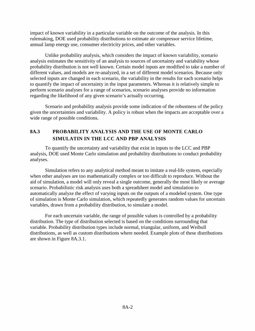
8A-2

impact of known variability in a particular variable on the outcome of the analysis. In this rulemaking, DOE used probability distributions to estimate air compressor service lifetime, annual lamp energy use, consumer electricity prices, and other variables.

Unlike probability analysis, which considers the impact of known variability, scenario analysis estimates the sensitivity of an analysis to sources of uncertainty and variability whose probability distribution is not well known. Certain model inputs are modified to take a number of different values, and models are re-analyzed, in a set of different model scenarios. Because only selected inputs are changed in each scenario, the variability in the results for each scenario helps to quantify the impact of uncertainty in the input parameters. Whereas it is relatively simple to perform scenario analyses for a range of scenarios, scenario analyses provide no information regarding the likelihood of any given scenario’s actually occurring.

Scenario and probability analysis provide some indication of the robustness of the policy given the uncertainties and variability. A policy is robust when the impacts are acceptable over a wide range of possible conditions.

8A.3 PROBABILITY ANALYSIS AND THE USE OF MONTE CARLO SIMULATIN IN THE LCC AND PBP ANALYSIS

To quantify the uncertainty and variability that exist in inputs to the LCC and PBP analysis, DOE used Monte Carlo simulation and probability distributions to conduct probability analyses.

Simulation refers to any analytical method meant to imitate a real-life system, especially when other analyses are too mathematically complex or too difficult to reproduce. Without the aid of simulation, a model will only reveal a single outcome, generally the most likely or average scenario. Probabilistic risk analysis uses both a spreadsheet model and simulation to automatically analyze the effect of varying inputs on the outputs of a modeled system. One type of simulation is Monte Carlo simulation, which repeatedly generates random values for uncertain variables, drawn from a probability distribution, to simulate a model.

For each uncertain variable, the range of possible values is controlled by a probability distribution. The type of distribution selected is based on the conditions surrounding that variable. Probability distribution types include normal, triangular, uniform, and Weibull distributions, as well as custom distributions where needed. Example plots of these distributions are shown in Figure 8A.3.1.

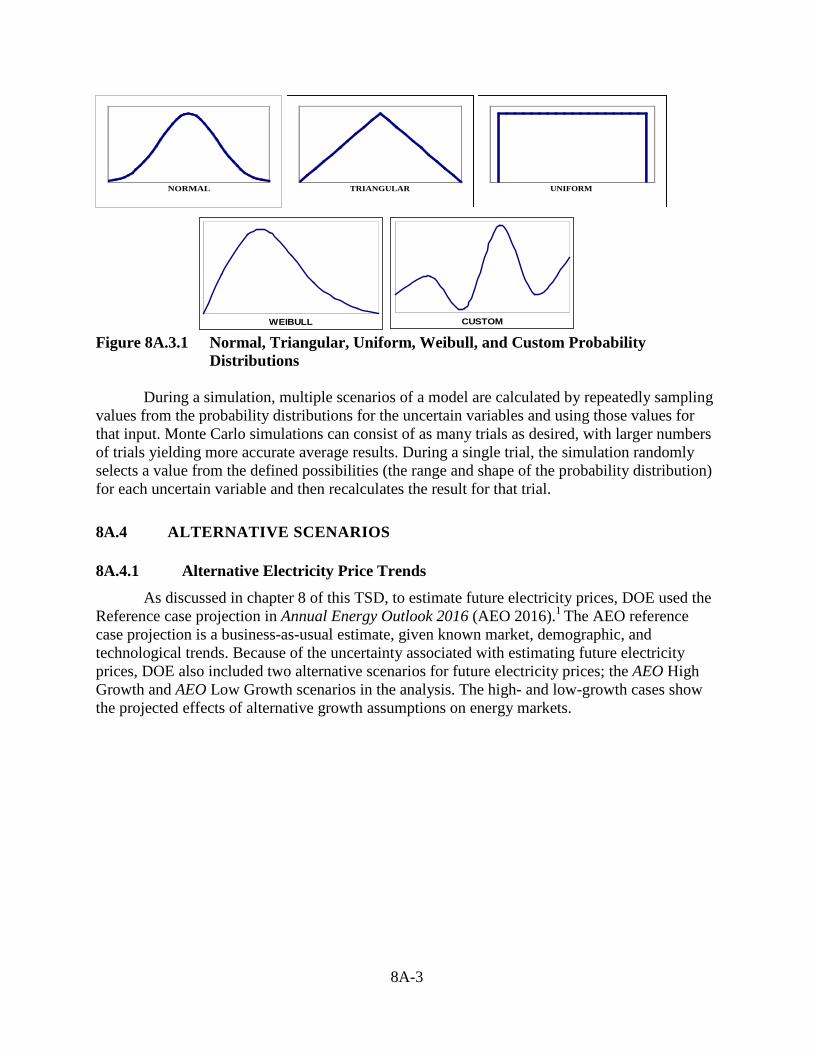
8A-3

Figure 8A.3.1 Normal, Triangular, Uniform, Weibull, and Custom Probability

Distributions

During a simulation, multiple scenarios of a model are calculated by repeatedly sampling values from the probability distributions for the uncertain variables and using those values for that input. Monte Carlo simulations can consist of as many trials as desired, with larger numbers of trials yielding more accurate average results. During a single trial, the simulation randomly selects a value from the defined possibilities (the range and shape of the probability distribution) for each uncertain variable and then recalculates the result for that trial.

8A.4 ALTERNATIVE SCENARIOS

8A.4.1 Alternative Electricity Price Trends

As discussed in chapter 8 of this TSD, to estimate future electricity prices, DOE used the Reference case projection in Annual Energy Outlook 2016 (AEO 2016).1 The AEO reference case projection is a business-as-usual estimate, given known market, demographic, and technological trends. Because of the uncertainty associated with estimating future electricity prices, DOE also included two alternative scenarios for future electricity prices; the AEO High Growth and AEO Low Growth scenarios in the analysis. The high- and low-growth cases show the projected effects of alternative growth assumptions on energy markets.

NORMAL UNIFORMTRIANGULAR

WEIBULL CUSTOM

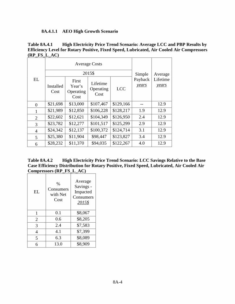
8A-4

8A.4.1.1 AEO High Growth Scenario

Table 8A.4.1 High Electricity Price Trend Scenario: Average LCC and PBP Results by Efficiency Level for Rotary Positive, Fixed Speed, Lubricated, Air Cooled Air Compressors (RP_FS_L_AC)

EL

Average Costs

Simple Payback

years

Average Lifetime

years

2015$

Installed Cost

First Year’s

Operating Cost

Lifetime Operating

Cost LCC

0 $21,698 $13,000 $107,467 $129,166 -- 12.9 1 $21,989 $12,850 $106,228 $128,217 1.9 12.9 2 $22,602 $12,621 $104,349 $126,950 2.4 12.9 3 $23,782 $12,277 $101,517 $125,299 2.9 12.9 4 $24,342 $12,137 $100,372 $124,714 3.1 12.9 5 $25,380 $11,904 $98,447 $123,827 3.4 12.9 6 $28,232 $11,370 $94,035 $122,267 4.0 12.9

Table 8A.4.2 High Electricity Price Trend Scenario: LCC Savings Relative to the Base Case Efficiency Distribution for Rotary Positive, Fixed Speed, Lubricated, Air Cooled Air Compressors (RP_FS_L_AC)

EL

% Consumers

with Net Cost

Average Savings - Impacted

Consumers 2015$

1 0.1 $8,067 2 0.6 $8,205 3 2.4 $7,583 4 4.1 $7,399 5 6.3 $8,089 6 13.0 $8,909

8A-5

Table 8A.4.3 High Electricity Price Trend Scenario: Average LCC and PBP Results by Efficiency Level for Rotary Positive, Fixed Speed, Lubricated, Water Cooled Air Compressors (RP_FS_L_WC)

EL

Average Costs

Simple Payback

years

Average Lifetime

years

2015$

Installed Cost

First Year’s

Operating Cost

Lifetime Operating

Cost LCC

0 $37,548 $24,829 $207,917 $245,465 -- 13.4 1 $38,047 $24,607 $206,048 $244,094 2.3 13.4 2 $39,262 $24,177 $202,434 $241,696 2.6 13.4 3 $41,078 $23,656 $198,038 $239,116 3.0 13.4 4 $42,014 $23,421 $196,066 $238,080 3.2 13.4 5 $43,725 $23,025 $192,755 $236,480 3.4 13.4 6 $48,328 $22,116 $185,157 $233,485 4.0 13.4

Table 8A.4.4 High Electricity Price Trend Scenario: LCC Savings Relative to the Base Case Efficiency Distribution for Rotary Positive, Fixed Speed, Lubricated, Water Cooled Air Compressors (RP_FS_L_WC)

EL % Consumers with Net Cost

Average Savings - Impacted

Consumers 2015$ 1 0.2 $11,932 2 1.0 $10,837 3 2.0 $14,805 4 4.4 $11,954 5 6.4 $13,303 6 11.5 $15,194

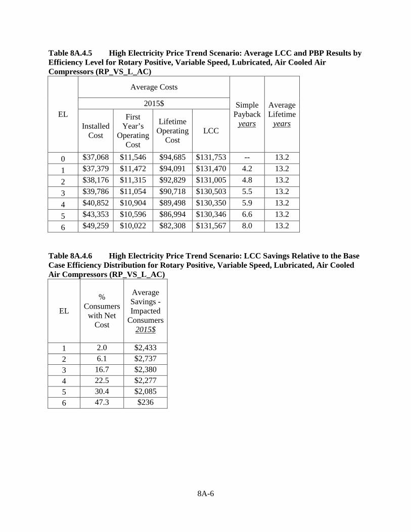
8A-6

Table 8A.4.5 High Electricity Price Trend Scenario: Average LCC and PBP Results by Efficiency Level for Rotary Positive, Variable Speed, Lubricated, Air Cooled Air Compressors (RP_VS_L_AC)

EL

Average Costs

Simple Payback

years

Average Lifetime

years

2015$

Installed Cost

First Year’s

Operating Cost

Lifetime Operating

Cost LCC

0 $37,068 $11,546 $94,685 $131,753 -- 13.2 1 $37,379 $11,472 $94,091 $131,470 4.2 13.2 2 $38,176 $11,315 $92,829 $131,005 4.8 13.2 3 $39,786 $11,054 $90,718 $130,503 5.5 13.2 4 $40,852 $10,904 $89,498 $130,350 5.9 13.2 5 $43,353 $10,596 $86,994 $130,346 6.6 13.2 6 $49,259 $10,022 $82,308 $131,567 8.0 13.2

Table 8A.4.6 High Electricity Price Trend Scenario: LCC Savings Relative to the Base Case Efficiency Distribution for Rotary Positive, Variable Speed, Lubricated, Air Cooled Air Compressors (RP_VS_L_AC)

EL

% Consumers

with Net Cost

Average Savings - Impacted

Consumers 2015$

1 2.0 $2,433 2 6.1 $2,737 3 16.7 $2,380 4 22.5 $2,277 5 30.4 $2,085 6 47.3 $236

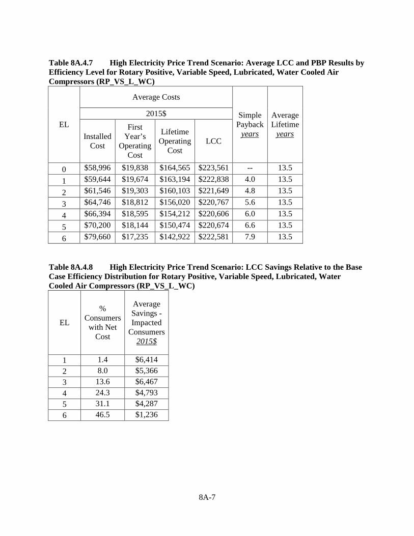
8A-7

Table 8A.4.7 High Electricity Price Trend Scenario: Average LCC and PBP Results by Efficiency Level for Rotary Positive, Variable Speed, Lubricated, Water Cooled Air Compressors (RP_VS_L_WC)

EL

Average Costs

Simple Payback

years

Average Lifetime

years

2015$

Installed Cost

First Year’s

Operating Cost

Lifetime Operating

Cost LCC

0 $58,996 $19,838 $164,565 $223,561 -- 13.5 1 $59,644 $19,674 $163,194 $222,838 4.0 13.5 2 $61,546 $19,303 $160,103 $221,649 4.8 13.5 3 $64,746 $18,812 $156,020 $220,767 5.6 13.5 4 $66,394 $18,595 $154,212 $220,606 6.0 13.5 5 $70,200 $18,144 $150,474 $220,674 6.6 13.5 6 $79,660 $17,235 $142,922 $222,581 7.9 13.5

Table 8A.4.8 High Electricity Price Trend Scenario: LCC Savings Relative to the Base Case Efficiency Distribution for Rotary Positive, Variable Speed, Lubricated, Water Cooled Air Compressors (RP_VS_L_WC)

EL

% Consumers

with Net Cost

Average Savings - Impacted

Consumers 2015$

1 1.4 $6,414 2 8.0 $5,366 3 13.6 $6,467 4 24.3 $4,793 5 31.1 $4,287 6 46.5 $1,236

8A-8

8A.4.1.2 AEO Low Growth Scenario

Table 8A.4.9 Low Electricity Price Trend Scenario: Average LCC and PBP Results by Efficiency Level for Rotary Positive, Fixed Speed, Lubricated, Air Cooled Air Compressors (RP_FS_L_AC)

EL

Average Costs

Simple Payback

years

Average Lifetime

years

2015$

Installed Cost

First Year’s

Operating Cost

Lifetime Operating

Cost LCC

0 $21,698 $13,027 $107,121 $128,819 -- 12.9 1 $21,989 $12,876 $105,885 $127,874 1.9 12.9 2 $22,602 $12,647 $104,011 $126,613 2.4 12.9 3 $23,782 $12,302 $101,189 $124,971 2.9 12.9 4 $24,342 $12,162 $100,047 $124,390 3.1 12.9 5 $25,380 $11,929 $98,129 $123,509 3.4 12.9 6 $28,232 $11,393 $93,730 $121,962 4.0 12.9

Table 8A.4.10 Low Electricity Price Trend Scenario: LCC Savings Relative to the Base Case Efficiency Distribution for Rotary Positive, Fixed Speed, Lubricated, Air Cooled Air Compressors (RP_FS_L_AC)

EL

% Consumers

with Net Cost

Average Savings - Impacted

Consumers 2015$

1 0.1 $8,035 2 0.6 $8,169 3 2.4 $7,546 4 4.2 $7,362 5 6.3 $8,046 6 13.2 $8,855

8A-9

Table 8A.4.11 Low Electricity Price Trend Scenario: Average LCC and PBP Results by Efficiency Level for Rotary Positive, Fixed Speed, Lubricated, Water Cooled Air Compressors (RP_FS_L_WC)

EL

Average Costs

Simple Payback

years

Average Lifetime

years

2015$

Installed Cost

First Year’s

Operating Cost

Lifetime Operating

Cost LCC

0 $37,548 $24,878 $207,211 $244,759 -- 13.4 1 $38,047 $24,655 $205,348 $243,395 2.2 13.4 2 $39,262 $24,225 $201,747 $241,008 2.6 13.4 3 $41,078 $23,703 $197,366 $238,444 3.0 13.4 4 $42,014 $23,467 $195,400 $237,414 3.2 13.4 5 $43,725 $23,070 $192,100 $235,826 3.4 13.4 6 $48,328 $22,160 $184,528 $232,856 4.0 13.4

Table 8A.4.12 Low Electricity Price Trend Scenario: LCC Savings Relative to the Base Case Efficiency Distribution for Rotary Positive, Fixed Speed, Lubricated, Water Cooled Air Compressors (RP_FS_L_WC)

EL % Consumers with Net Cost

Average Savings - Impacted

Consumers 2015$ 1 0.2 $11,875 2 1.0 $10,783 3 2.0 $14,726 4 4.5 $11,888 5 6.4 $13,226 6 11.6 $15,096

8A-10

Table 8A.4.13 Low Electricity Price Trend Scenario: Average LCC and PBP Results by Efficiency Level for Rotary Positive, Variable Speed, Lubricated, Air Cooled Air Compressors (RP_VS_L_AC)

EL

Average Costs

Simple Payback

years

Average Lifetime

years

2015$

Installed Cost

First Year’s

Operating Cost

Lifetime Operating

Cost LCC

0 $37,068 $11,570 $94,380 $131,449 -- 13.2 1 $37,379 $11,495 $93,789 $131,168 4.2 13.2 2 $38,176 $11,338 $92,530 $130,707 4.8 13.2 3 $39,786 $11,076 $90,426 $130,212 5.5 13.2 4 $40,852 $10,926 $89,210 $130,062 5.9 13.2 5 $43,353 $10,617 $86,713 $130,066 6.6 13.2 6 $49,259 $10,042 $82,043 $131,302 8.0 13.2

Table 8A.4.14 Low Electricity Price Trend Scenario: LCC Savings Relative to the Base Case Efficiency Distribution for Rotary Positive, Variable Speed, Lubricated, Air Cooled Air Compressors (RP_VS_L_AC)

EL

% Consumers

with Net Cost

Average Savings - Impacted

Consumers 2015$

1 2.0 $2,417 2 6.1 $2,716 3 16.8 $2,357 4 22.7 $2,251 5 30.5 $2,050 6 47.4 $187

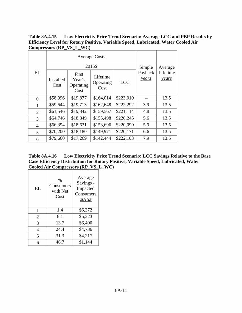
8A-11

Table 8A.4.15 Low Electricity Price Trend Scenario: Average LCC and PBP Results by Efficiency Level for Rotary Positive, Variable Speed, Lubricated, Water Cooled Air Compressors (RP_VS_L_WC)

EL

Average Costs

Simple Payback

years

Average Lifetime

years

2015$

Installed Cost

First Year’s

Operating Cost

Lifetime Operating

Cost LCC

0 $58,996 $19,877 $164,014 $223,010 -- 13.5 1 $59,644 $19,713 $162,648 $222,292 3.9 13.5 2 $61,546 $19,342 $159,567 $221,114 4.8 13.5 3 $64,746 $18,849 $155,498 $220,245 5.6 13.5 4 $66,394 $18,631 $153,696 $220,090 5.9 13.5 5 $70,200 $18,180 $149,971 $220,171 6.6 13.5 6 $79,660 $17,269 $142,444 $222,103 7.9 13.5

Table 8A.4.16 Low Electricity Price Trend Scenario: LCC Savings Relative to the Base Case Efficiency Distribution for Rotary Positive, Variable Speed, Lubricated, Water Cooled Air Compressors (RP_VS_L_WC)

EL

% Consumers

with Net Cost

Average Savings - Impacted

Consumers 2015$

1 1.4 $6,372 2 8.1 $5,323 3 13.7 $6,400 4 24.4 $4,736 5 31.3 $4,217 6 46.7 $1,144

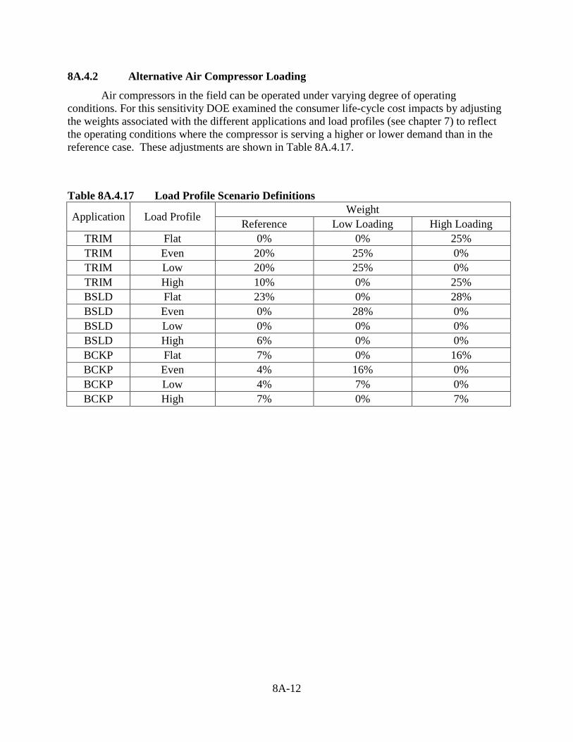
8A-12

8A.4.2 Alternative Air Compressor Loading

Air compressors in the field can be operated under varying degree of operating conditions. For this sensitivity DOE examined the consumer life-cycle cost impacts by adjusting the weights associated with the different applications and load profiles (see chapter 7) to reflect the operating conditions where the compressor is serving a higher or lower demand than in the reference case. These adjustments are shown in Table 8A.4.17.

Table 8A.4.17 Load Profile Scenario Definitions

Application Load Profile Weight Reference Low Loading High Loading

TRIM Flat 0% 0% 25% TRIM Even 20% 25% 0% TRIM Low 20% 25% 0% TRIM High 10% 0% 25% BSLD Flat 23% 0% 28% BSLD Even 0% 28% 0% BSLD Low 0% 0% 0% BSLD High 6% 0% 0% BCKP Flat 7% 0% 16% BCKP Even 4% 16% 0% BCKP Low 4% 7% 0% BCKP High 7% 0% 7%

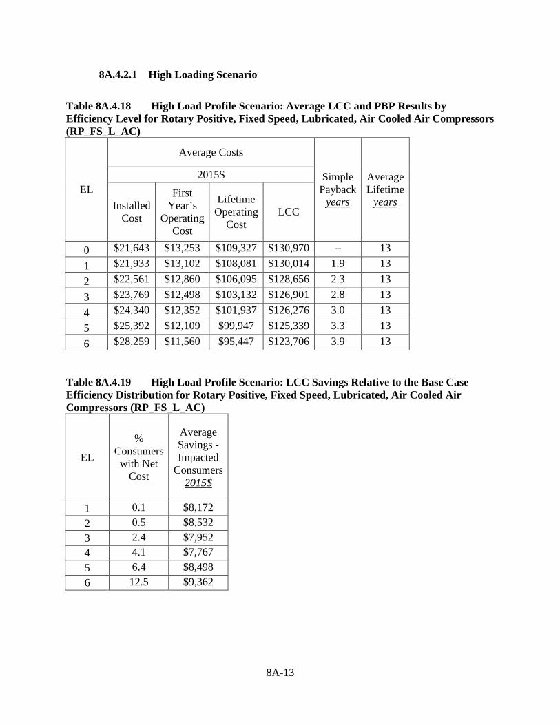
8A-13

8A.4.2.1 High Loading Scenario

Table 8A.4.18 High Load Profile Scenario: Average LCC and PBP Results by Efficiency Level for Rotary Positive, Fixed Speed, Lubricated, Air Cooled Air Compressors (RP_FS_L_AC)

EL

Average Costs

Simple Payback

years

Average Lifetime

years

2015$

Installed Cost

First Year’s

Operating Cost

Lifetime Operating

Cost LCC

0 $21,643 $13,253 $109,327 $130,970 -- 13 1 $21,933 $13,102 $108,081 $130,014 1.9 13 2 $22,561 $12,860 $106,095 $128,656 2.3 13 3 $23,769 $12,498 $103,132 $126,901 2.8 13 4 $24,340 $12,352 $101,937 $126,276 3.0 13 5 $25,392 $12,109 $99,947 $125,339 3.3 13 6 $28,259 $11,560 $95,447 $123,706 3.9 13

Table 8A.4.19 High Load Profile Scenario: LCC Savings Relative to the Base Case Efficiency Distribution for Rotary Positive, Fixed Speed, Lubricated, Air Cooled Air Compressors (RP_FS_L_AC)

EL

% Consumers

with Net Cost

Average Savings - Impacted

Consumers 2015$

1 0.1 $8,172 2 0.5 $8,532 3 2.4 $7,952 4 4.1 $7,767 5 6.4 $8,498 6 12.5 $9,362

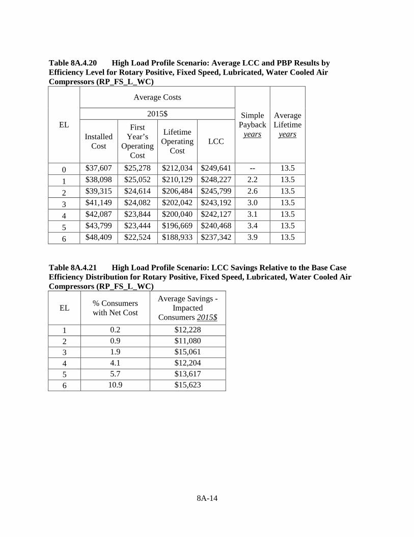
8A-14

Table 8A.4.20 High Load Profile Scenario: Average LCC and PBP Results by Efficiency Level for Rotary Positive, Fixed Speed, Lubricated, Water Cooled Air Compressors (RP_FS_L_WC)

EL

Average Costs

Simple Payback

years

Average Lifetime

years

2015$

Installed Cost

First Year’s

Operating Cost

Lifetime Operating

Cost LCC

0 $37,607 $25,278 $212,034 $249,641 -- 13.5 1 $38,098 $25,052 $210,129 $248,227 2.2 13.5 2 $39,315 $24,614 $206,484 $245,799 2.6 13.5 3 $41,149 $24,082 $202,042 $243,192 3.0 13.5 4 $42,087 $23,844 $200,040 $242,127 3.1 13.5 5 $43,799 $23,444 $196,669 $240,468 3.4 13.5 6 $48,409 $22,524 $188,933 $237,342 3.9 13.5

Table 8A.4.21 High Load Profile Scenario: LCC Savings Relative to the Base Case Efficiency Distribution for Rotary Positive, Fixed Speed, Lubricated, Water Cooled Air Compressors (RP_FS_L_WC)

EL % Consumers with Net Cost

Average Savings - Impacted

Consumers 2015$ 1 0.2 $12,228 2 0.9 $11,080 3 1.9 $15,061 4 4.1 $12,204 5 5.7 $13,617 6 10.9 $15,623

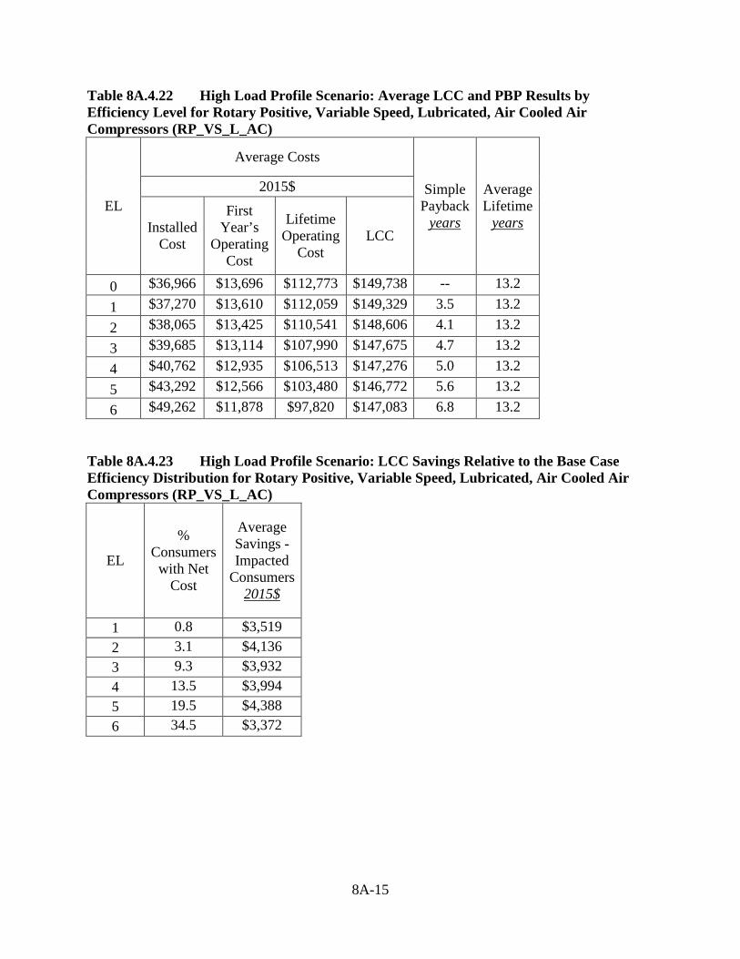
8A-15

Table 8A.4.22 High Load Profile Scenario: Average LCC and PBP Results by Efficiency Level for Rotary Positive, Variable Speed, Lubricated, Air Cooled Air Compressors (RP_VS_L_AC)

EL

Average Costs

Simple Payback

years

Average Lifetime

years

2015$

Installed Cost

First Year’s

Operating Cost

Lifetime Operating

Cost LCC

0 $36,966 $13,696 $112,773 $149,738 -- 13.2 1 $37,270 $13,610 $112,059 $149,329 3.5 13.2 2 $38,065 $13,425 $110,541 $148,606 4.1 13.2 3 $39,685 $13,114 $107,990 $147,675 4.7 13.2 4 $40,762 $12,935 $106,513 $147,276 5.0 13.2 5 $43,292 $12,566 $103,480 $146,772 5.6 13.2 6 $49,262 $11,878 $97,820 $147,083 6.8 13.2

Table 8A.4.23 High Load Profile Scenario: LCC Savings Relative to the Base Case Efficiency Distribution for Rotary Positive, Variable Speed, Lubricated, Air Cooled Air Compressors (RP_VS_L_AC)

EL

% Consumers

with Net Cost

Average Savings - Impacted

Consumers 2015$

1 0.8 $3,519 2 3.1 $4,136 3 9.3 $3,932 4 13.5 $3,994 5 19.5 $4,388 6 34.5 $3,372

8A-16

Table 8A.4.24 High Load Profile Scenario: Average LCC and PBP Results by Efficiency Level for Rotary Positive, Variable Speed, Lubricated, Water Cooled Air Compressors (RP_VS_L_WC)

EL

Average Costs

Simple Payback

years

Average Lifetime

years

2015$

Installed Cost

First Year’s

Operating Cost

Lifetime Operating

Cost LCC

0 $59,011 $23,468 $196,285 $255,296 -- 13.6 1 $59,671 $23,271 $194,607 $254,278 3.4 13.6 2 $61,577 $22,829 $190,904 $252,480 4.0 13.6 3 $64,781 $22,247 $186,018 $250,799 4.7 13.6 4 $66,427 $21,990 $183,864 $250,291 5.0 13.6 5 $70,223 $21,460 $179,422 $249,645 5.6 13.6 6 $79,665 $20,389 $170,449 $250,114 6.7 13.6

Table 8A.4.25 High Load Profile Scenario: LCC Savings Relative to the Base Case Efficiency Distribution for Rotary Positive, Variable Speed, Lubricated, Water Cooled Air Compressors (RP_VS_L_WC)

EL

% Consumers

with Net Cost

Average Savings - Impacted

Consumers 2015$

1 0.6 $9,050 2 4.6 $7,889 3 8.0 $10,409 4 15.1 $8,114 5 20.3 $8,402 6 34.6 $6,550

8A-17

8A.4.2.2 Low Loading Scenario

Table 8A.4.26 Low Loading Scenario: Average LCC and PBP Results by Efficiency Level for Rotary Positive, Fixed Speed, Lubricated, Air Cooled Air Compressors (RP_FS_L_AC)

EL

Average Costs

Simple Payback

years

Average Lifetime

years

2015$

Installed Cost

First Year’s

Operating Cost

Lifetime Operating

Cost LCC

0 $21,643 $12,637 $104,136 $125,779 -- 13 1 $21,933 $12,493 $102,947 $124,881 2.0 13 2 $22,561 $12,262 $101,056 $123,617 2.5 13 3 $23,769 $11,916 $98,236 $122,004 3.0 13 4 $24,340 $11,777 $97,097 $121,437 3.1 13 5 $25,392 $11,546 $95,202 $120,594 3.4 13 6 $28,259 $11,022 $90,917 $119,176 4.1 13

Table 8A.4.27 Low Loading Scenario: LCC Savings Relative to the Base Case Efficiency Distribution for Rotary Positive, Fixed Speed, Lubricated, Air Cooled Air Compressors (RP_FS_L_AC)

EL

% Consumers

with Net Cost

Average Savings - Impacted

Consumers 2015$

1 0.1 $7,680 2 0.6 $7,972 3 2.9 $7,376 4 5.0 $7,185 5 7.5 $7,825 6 14.6 $8,510

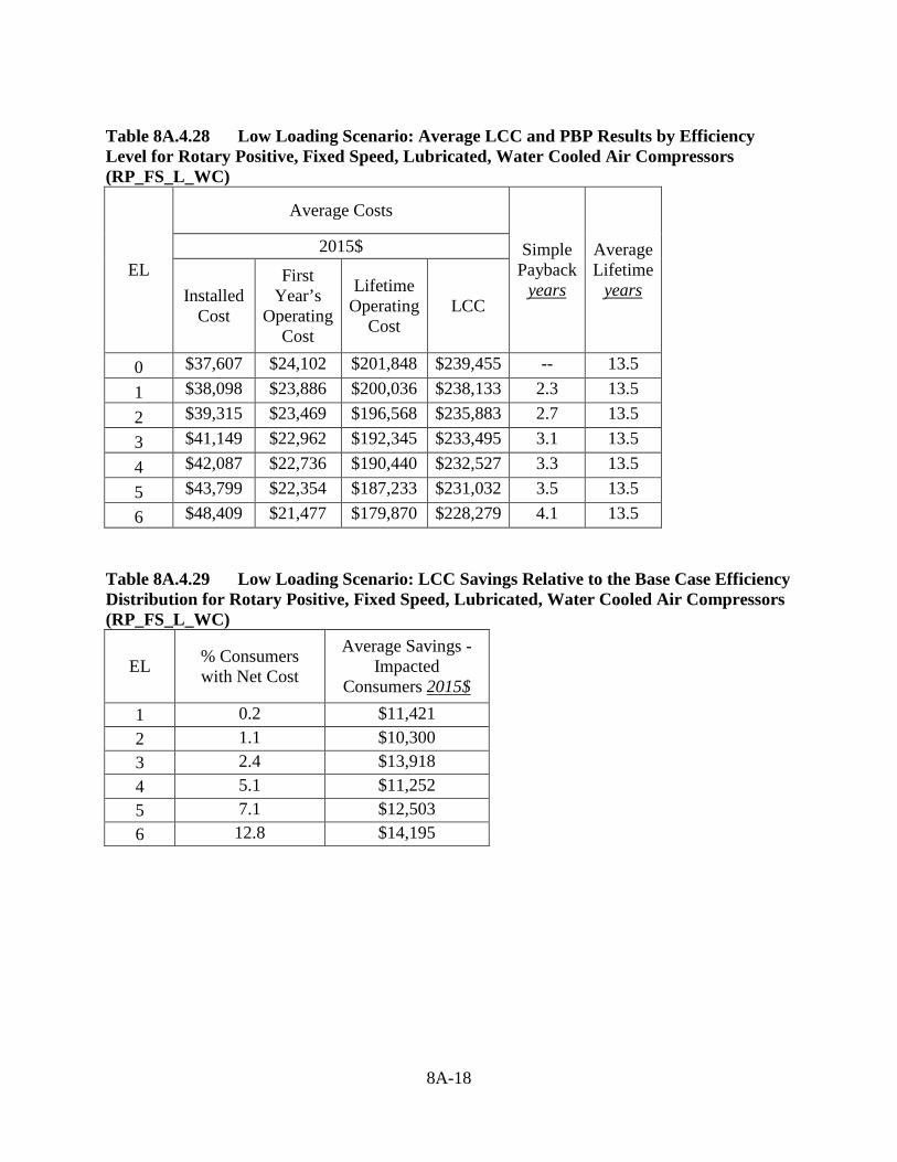
8A-18

Table 8A.4.28 Low Loading Scenario: Average LCC and PBP Results by Efficiency Level for Rotary Positive, Fixed Speed, Lubricated, Water Cooled Air Compressors (RP_FS_L_WC)

EL

Average Costs

Simple Payback

years

Average Lifetime

years

2015$

Installed Cost

First Year’s

Operating Cost

Lifetime Operating

Cost LCC

0 $37,607 $24,102 $201,848 $239,455 -- 13.5 1 $38,098 $23,886 $200,036 $238,133 2.3 13.5 2 $39,315 $23,469 $196,568 $235,883 2.7 13.5 3 $41,149 $22,962 $192,345 $233,495 3.1 13.5 4 $42,087 $22,736 $190,440 $232,527 3.3 13.5 5 $43,799 $22,354 $187,233 $231,032 3.5 13.5 6 $48,409 $21,477 $179,870 $228,279 4.1 13.5

Table 8A.4.29 Low Loading Scenario: LCC Savings Relative to the Base Case Efficiency Distribution for Rotary Positive, Fixed Speed, Lubricated, Water Cooled Air Compressors (RP_FS_L_WC)

EL % Consumers with Net Cost

Average Savings - Impacted

Consumers 2015$ 1 0.2 $11,421 2 1.1 $10,300 3 2.4 $13,918 4 5.1 $11,252 5 7.1 $12,503 6 12.8 $14,195

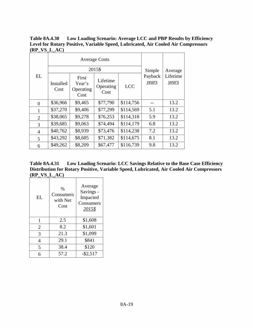
8A-19

Table 8A.4.30 Low Loading Scenario: Average LCC and PBP Results by Efficiency Level for Rotary Positive, Variable Speed, Lubricated, Air Cooled Air Compressors (RP_VS_L_AC)

EL

Average Costs

Simple Payback

years

Average Lifetime

years

2015$

Installed Cost

First Year’s

Operating Cost

Lifetime Operating

Cost LCC

0 $36,966 $9,465 $77,790 $114,756 -- 13.2 1 $37,270 $9,406 $77,299 $114,569 5.1 13.2 2 $38,065 $9,278 $76,253 $114,318 5.9 13.2 3 $39,685 $9,063 $74,494 $114,179 6.8 13.2 4 $40,762 $8,939 $73,476 $114,238 7.2 13.2 5 $43,292 $8,685 $71,382 $114,675 8.1 13.2 6 $49,262 $8,209 $67,477 $116,739 9.8 13.2

Table 8A.4.31 Low Loading Scenario: LCC Savings Relative to the Base Case Efficiency Distribution for Rotary Positive, Variable Speed, Lubricated, Air Cooled Air Compressors (RP_VS_L_AC)

EL

% Consumers

with Net Cost

Average Savings - Impacted

Consumers 2015$

1 2.5 $1,608 2 8.2 $1,601 3 21.3 $1,099 4 29.1 $841 5 38.4 $120 6 57.2 -$2,517

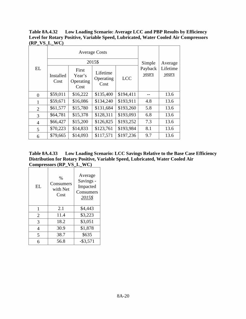
8A-20

Table 8A.4.32 Low Loading Scenario: Average LCC and PBP Results by Efficiency Level for Rotary Positive, Variable Speed, Lubricated, Water Cooled Air Compressors (RP_VS_L_WC)

EL

Average Costs

Simple Payback

years

Average Lifetime

years

2015$

Installed Cost

First Year’s

Operating Cost

Lifetime Operating

Cost LCC

0 $59,011 $16,222 $135,400 $194,411 -- 13.6 1 $59,671 $16,086 $134,240 $193,911 4.8 13.6 2 $61,577 $15,780 $131,684 $193,260 5.8 13.6 3 $64,781 $15,378 $128,311 $193,093 6.8 13.6 4 $66,427 $15,200 $126,825 $193,252 7.3 13.6 5 $70,223 $14,833 $123,761 $193,984 8.1 13.6 6 $79,665 $14,093 $117,571 $197,236 9.7 13.6

Table 8A.4.33 Low Loading Scenario: LCC Savings Relative to the Base Case Efficiency Distribution for Rotary Positive, Variable Speed, Lubricated, Water Cooled Air Compressors (RP_VS_L_WC)

EL

% Consumers

with Net Cost

Average Savings - Impacted

Consumers 2015$

1 2.1 $4,443 2 11.4 $3,223 3 18.2 $3,051 4 30.9 $1,878 5 38.7 $635 6 56.8 -$3,571

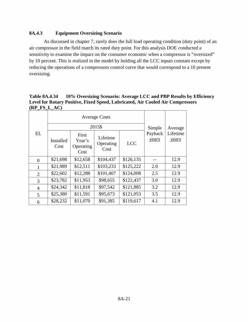
8A-21

8A.4.3 Equipment Oversizing Scenario

As discussed in chapter 7, rarely does the full load operating condition (duty point) of an air compressor in the field match its rated duty point. For this analysis DOE conducted a sensitivity to examine the impact on the consumer economic when a compressor is “oversized” by 10 percent. This is realized in the model by holding all the LCC inputs constant except by reducing the operations of a compressors control curve that would correspond to a 10 present oversizing.

Table 8A.4.34 10% Oversizing Scenario: Average LCC and PBP Results by Efficiency Level for Rotary Positive, Fixed Speed, Lubricated, Air Cooled Air Compressors (RP_FS_L_AC)

EL

Average Costs

Simple Payback

years

Average Lifetime

years

2015$

Installed Cost

First Year’s

Operating Cost

Lifetime Operating

Cost LCC

0 $21,698 $12,658 $104,437 $126,135 -- 12.9 1 $21,989 $12,511 $103,233 $125,222 2.0 12.9 2 $22,602 $12,288 $101,407 $124,008 2.5 12.9 3 $23,782 $11,953 $98,655 $122,437 3.0 12.9 4 $24,342 $11,818 $97,542 $121,885 3.2 12.9 5 $25,380 $11,591 $95,673 $121,053 3.5 12.9 6 $28,232 $11,070 $91,385 $119,617 4.1 12.9

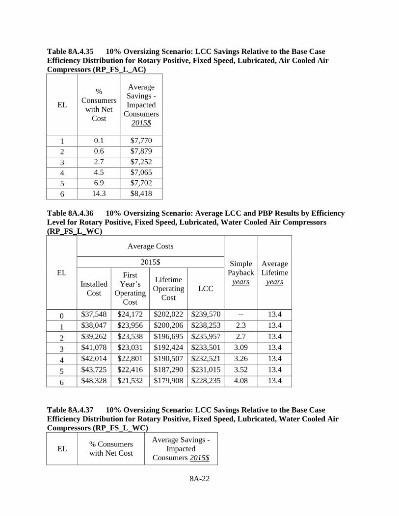
8A-22

Table 8A.4.35 10% Oversizing Scenario: LCC Savings Relative to the Base Case Efficiency Distribution for Rotary Positive, Fixed Speed, Lubricated, Air Cooled Air Compressors (RP_FS_L_AC)

EL

% Consumers

with Net Cost

Average Savings - Impacted

Consumers 2015$

1 0.1 $7,770 2 0.6 $7,879 3 2.7 $7,252 4 4.5 $7,065 5 6.9 $7,702 6 14.3 $8,418

Table 8A.4.36 10% Oversizing Scenario: Average LCC and PBP Results by Efficiency Level for Rotary Positive, Fixed Speed, Lubricated, Water Cooled Air Compressors (RP_FS_L_WC)

EL

Average Costs

Simple Payback

years

Average Lifetime

years

2015$

Installed Cost

First Year’s

Operating Cost

Lifetime Operating

Cost LCC

0 $37,548 $24,172 $202,022 $239,570 -- 13.4 1 $38,047 $23,956 $200,206 $238,253 2.3 13.4 2 $39,262 $23,538 $196,695 $235,957 2.7 13.4 3 $41,078 $23,031 $192,424 $233,501 3.09 13.4 4 $42,014 $22,801 $190,507 $232,521 3.26 13.4 5 $43,725 $22,416 $187,290 $231,015 3.52 13.4 6 $48,328 $21,532 $179,908 $228,235 4.08 13.4

Table 8A.4.37 10% Oversizing Scenario: LCC Savings Relative to the Base Case Efficiency Distribution for Rotary Positive, Fixed Speed, Lubricated, Water Cooled Air Compressors (RP_FS_L_WC)

EL % Consumers with Net Cost

Average Savings - Impacted

Consumers 2015$

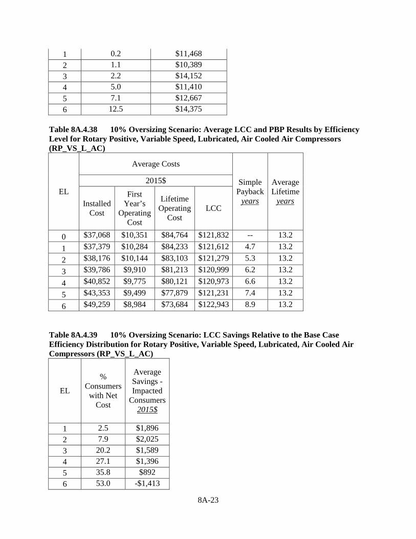
8A-23

1 0.2 $11,468 2 1.1 $10,389 3 2.2 $14,152 4 5.0 $11,410 5 7.1 $12,667 6 12.5 $14,375

Table 8A.4.38 10% Oversizing Scenario: Average LCC and PBP Results by Efficiency Level for Rotary Positive, Variable Speed, Lubricated, Air Cooled Air Compressors (RP_VS_L_AC)

EL

Average Costs

Simple Payback

years

Average Lifetime

years

2015$

Installed Cost

First Year’s

Operating Cost

Lifetime Operating

Cost LCC

0 $37,068 $10,351 $84,764 $121,832 -- 13.2 1 $37,379 $10,284 $84,233 $121,612 4.7 13.2 2 $38,176 $10,144 $83,103 $121,279 5.3 13.2 3 $39,786 $9,910 $81,213 $120,999 6.2 13.2 4 $40,852 $9,775 $80,121 $120,973 6.6 13.2 5 $43,353 $9,499 $77,879 $121,231 7.4 13.2 6 $49,259 $8,984 $73,684 $122,943 8.9 13.2

Table 8A.4.39 10% Oversizing Scenario: LCC Savings Relative to the Base Case Efficiency Distribution for Rotary Positive, Variable Speed, Lubricated, Air Cooled Air Compressors (RP_VS_L_AC)

EL

% Consumers

with Net Cost

Average Savings - Impacted

Consumers 2015$

1 2.5 $1,896 2 7.9 $2,025 3 20.2 $1,589 4 27.1 $1,396 5 35.8 $892 6 53.0 -$1,413

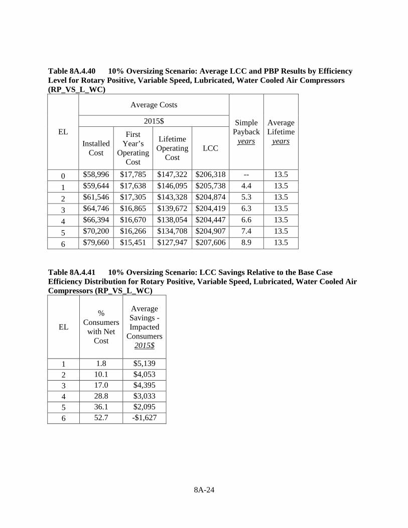
8A-24

Table 8A.4.40 10% Oversizing Scenario: Average LCC and PBP Results by Efficiency Level for Rotary Positive, Variable Speed, Lubricated, Water Cooled Air Compressors (RP_VS_L_WC)

EL

Average Costs

Simple Payback

years

Average Lifetime

years

2015$

Installed Cost

First Year’s

Operating Cost

Lifetime Operating

Cost LCC

0 $58,996 $17,785 $147,322 $206,318 -- 13.5 1 $59,644 $17,638 $146,095 $205,738 4.4 13.5 2 $61,546 $17,305 $143,328 $204,874 5.3 13.5 3 $64,746 $16,865 $139,672 $204,419 6.3 13.5 4 $66,394 $16,670 $138,054 $204,447 6.6 13.5 5 $70,200 $16,266 $134,708 $204,907 7.4 13.5 6 $79,660 $15,451 $127,947 $207,606 8.9 13.5

Table 8A.4.41 10% Oversizing Scenario: LCC Savings Relative to the Base Case Efficiency Distribution for Rotary Positive, Variable Speed, Lubricated, Water Cooled Air Compressors (RP_VS_L_WC)

EL

% Consumers

with Net Cost

Average Savings - Impacted

Consumers 2015$

1 1.8 $5,139 2 10.1 $4,053 3 17.0 $4,395 4 28.8 $3,033 5 36.1 $2,095 6 52.7 -$1,627

8A-25

REFERENCES 1. U.S. Energy Information Administration. Annual Energy Outlook 2016 with Projections

to 2040. 2016. Washington, D.C. Report No. DOE/EIA-0383(2016). (Last accessed November 9, 2016.) http://www.eia.gov/forecasts/aeo/pdf/0383(2016).pdf

8B-i

APPENDIX 8B. ELECTRICITY PRICES

TABLE OF CONTENTS

8B.1 INTRODUCTION .........................................................................................................8B-1 8B.2 DATA SOURCES .........................................................................................................8B-2 8B.3 RESIDENTIAL SECTOR .............................................................................................8B-5 8B.4 NON-RESIDENTIAL SECTOR ...................................................................................8B-7 REFERENCES ........................................................................................................................8B-13

LIST OF TABLES

Table 8D.2.1 Summary of Data Sources for Electricity Price Information .......................8B-3 Table 8D.2.2 Consumption and Demand Levels Included in the EEI Typical Bills

and Rates Reports ........................................................................................8B-5 Table 8D.3.1 Adjustment Factors by Region and Sector...................................................8B-7 Table 8D.3.2 Residential Sector Electricity Prices by Region ..........................................8B-7 Table 8D.4.1 Average Price for the US for each Bill Type, Sorted by Summer Price ......8B-9 Table 8D.4.2 Definition of Consumption Tiers for Averaging Across Bill Types ..........8B-11 Table 8D.4.3 Non-Residential Sector Prices by Region ..................................................8B-12

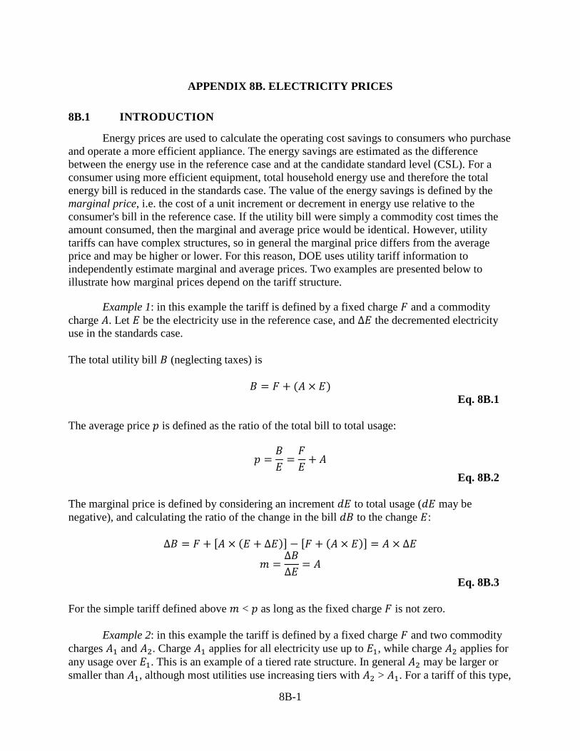
8B-1

APPENDIX 8B. ELECTRICITY PRICES

8B.1 INTRODUCTION

Energy prices are used to calculate the operating cost savings to consumers who purchase and operate a more efficient appliance. The energy savings are estimated as the difference between the energy use in the reference case and at the candidate standard level (CSL). For a consumer using more efficient equipment, total household energy use and therefore the total energy bill is reduced in the standards case. The value of the energy savings is defined by the marginal price, i.e. the cost of a unit increment or decrement in energy use relative to the consumer's bill in the reference case. If the utility bill were simply a commodity cost times the amount consumed, then the marginal and average price would be identical. However, utility tariffs can have complex structures, so in general the marginal price differs from the average price and may be higher or lower. For this reason, DOE uses utility tariff information to independently estimate marginal and average prices. Two examples are presented below to illustrate how marginal prices depend on the tariff structure.

Example 1: in this example the tariff is defined by a fixed charge 𝐹𝐹 and a commodity charge 𝐴𝐴. Let 𝐸𝐸 be the electricity use in the reference case, and ∆𝐸𝐸 the decremented electricity use in the standards case.

The total utility bill 𝐵𝐵 (neglecting taxes) is

𝐵𝐵 = 𝐹𝐹 + (𝐴𝐴 × 𝐸𝐸) Eq. 8B.1

The average price 𝑝𝑝 is defined as the ratio of the total bill to total usage:

𝑝𝑝 =𝐵𝐵𝐸𝐸

=𝐹𝐹𝐸𝐸

+ 𝐴𝐴 Eq. 8B.2

The marginal price is defined by considering an increment 𝑑𝑑𝐸𝐸 to total usage (𝑑𝑑𝐸𝐸 may be negative), and calculating the ratio of the change in the bill 𝑑𝑑𝐵𝐵 to the change 𝐸𝐸:

∆𝐵𝐵 = 𝐹𝐹 + [𝐴𝐴 × (𝐸𝐸 + ∆𝐸𝐸)] − [𝐹𝐹 + (𝐴𝐴 × 𝐸𝐸)] = 𝐴𝐴 × ∆𝐸𝐸

𝑚𝑚 =∆𝐵𝐵∆𝐸𝐸

= 𝐴𝐴 Eq. 8B.3

For the simple tariff defined above 𝑚𝑚 < 𝑝𝑝 as long as the fixed charge 𝐹𝐹 is not zero.

Example 2: in this example the tariff is defined by a fixed charge 𝐹𝐹 and two commodity charges 𝐴𝐴1 and 𝐴𝐴2. Charge 𝐴𝐴1 applies for all electricity use up to 𝐸𝐸1, while charge 𝐴𝐴2 applies for any usage over 𝐸𝐸1. This is an example of a tiered rate structure. In general 𝐴𝐴2 may be larger or smaller than 𝐴𝐴1, although most utilities use increasing tiers with 𝐴𝐴2 > 𝐴𝐴1. For a tariff of this type,

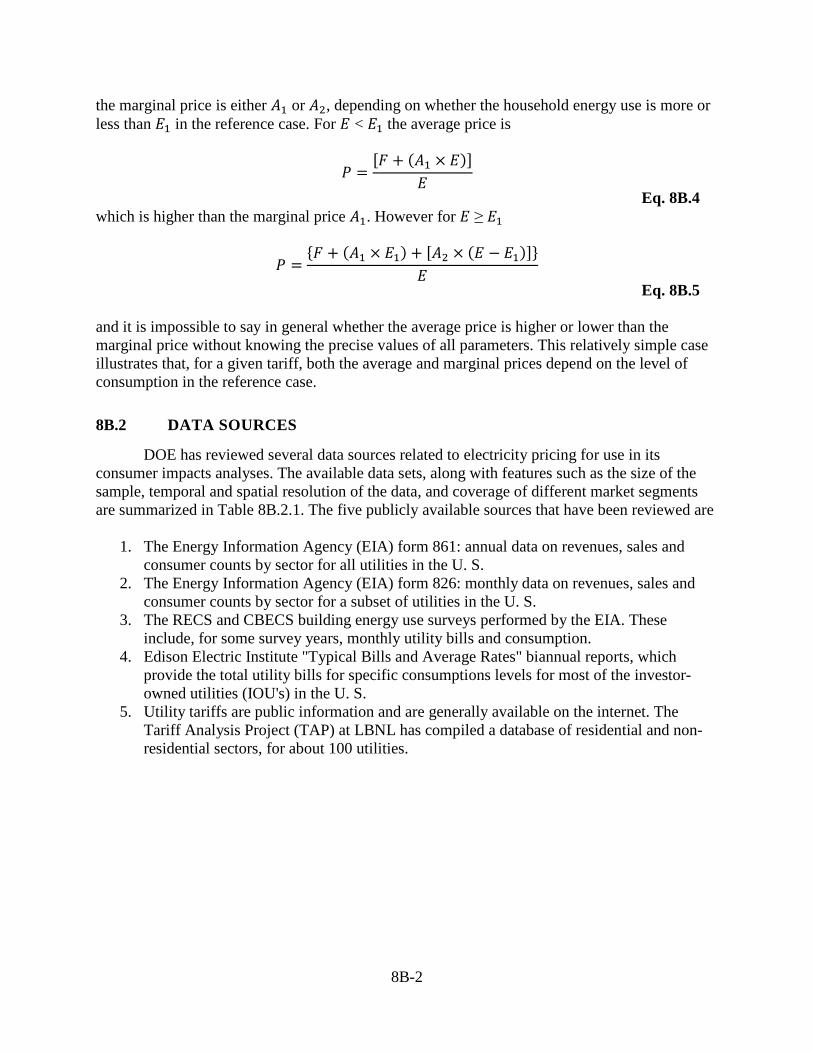
8B-2

the marginal price is either 𝐴𝐴1 or 𝐴𝐴2, depending on whether the household energy use is more or less than 𝐸𝐸1 in the reference case. For 𝐸𝐸 < 𝐸𝐸1 the average price is

𝑃𝑃 =[𝐹𝐹 + (𝐴𝐴1 × 𝐸𝐸)]

𝐸𝐸

Eq. 8B.4 which is higher than the marginal price 𝐴𝐴1. However for 𝐸𝐸 ≥ 𝐸𝐸1

𝑃𝑃 ={𝐹𝐹 + (𝐴𝐴1 × 𝐸𝐸1) + [𝐴𝐴2 × (𝐸𝐸 − 𝐸𝐸1)]}

𝐸𝐸

Eq. 8B.5 and it is impossible to say in general whether the average price is higher or lower than the marginal price without knowing the precise values of all parameters. This relatively simple case illustrates that, for a given tariff, both the average and marginal prices depend on the level of consumption in the reference case.

8B.2 DATA SOURCES

DOE has reviewed several data sources related to electricity pricing for use in its consumer impacts analyses. The available data sets, along with features such as the size of the sample, temporal and spatial resolution of the data, and coverage of different market segments are summarized in Table 8B.2.1. The five publicly available sources that have been reviewed are

1. The Energy Information Agency (EIA) form 861: annual data on revenues, sales and

consumer counts by sector for all utilities in the U. S. 2. The Energy Information Agency (EIA) form 826: monthly data on revenues, sales and

consumer counts by sector for a subset of utilities in the U. S. 3. The RECS and CBECS building energy use surveys performed by the EIA. These

include, for some survey years, monthly utility bills and consumption. 4. Edison Electric Institute "Typical Bills and Average Rates" biannual reports, which

provide the total utility bills for specific consumptions levels for most of the investor-owned utilities (IOU's) in the U. S.

5. Utility tariffs are public information and are generally available on the internet. The Tariff Analysis Project (TAP) at LBNL has compiled a database of residential and non-residential sectors, for about 100 utilities.

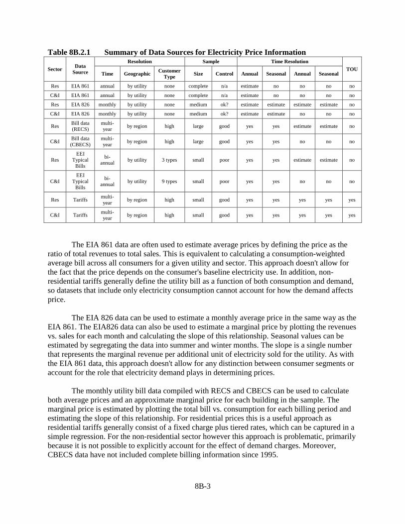
8B-3

Table 8B.2.1 Summary of Data Sources for Electricity Price Information

Sector Data Source

Resolution Sample Time Resolution TOU

Time Geographic Customer Type Size Control Annual Seasonal Annual Seasonal

Res EIA 861 annual by utility none complete n/a estimate no no no no

C&I EIA 861 annual by utility none complete n/a estimate no no no no

Res EIA 826 monthly by utility none medium ok? estimate estimate estimate estimate no

C&I EIA 826 monthly by utility none medium ok? estimate estimate no no no

Res Bill data (RECS)

multi-year by region high large good yes yes estimate estimate no

C&I Bill data (CBECS)

multi-year by region high large good yes yes no no no

Res EEI

Typical Bills

bi-annual by utility 3 types small poor yes yes estimate estimate no

C&I EEI

Typical Bills

bi-annual by utility 9 types small poor yes yes no no no

Res Tariffs multi-year by region high small good yes yes yes yes yes

C&I Tariffs multi-year by region high small good yes yes yes yes yes

The EIA 861 data are often used to estimate average prices by defining the price as the ratio of total revenues to total sales. This is equivalent to calculating a consumption-weighted average bill across all consumers for a given utility and sector. This approach doesn't allow for the fact that the price depends on the consumer's baseline electricity use. In addition, non-residential tariffs generally define the utility bill as a function of both consumption and demand, so datasets that include only electricity consumption cannot account for how the demand affects price.

The EIA 826 data can be used to estimate a monthly average price in the same way as the EIA 861. The EIA826 data can also be used to estimate a marginal price by plotting the revenues vs. sales for each month and calculating the slope of this relationship. Seasonal values can be estimated by segregating the data into summer and winter months. The slope is a single number that represents the marginal revenue per additional unit of electricity sold for the utility. As with the EIA 861 data, this approach doesn't allow for any distinction between consumer segments or account for the role that electricity demand plays in determining prices.

The monthly utility bill data compiled with RECS and CBECS can be used to calculate both average prices and an approximate marginal price for each building in the sample. The marginal price is estimated by plotting the total bill vs. consumption for each billing period and estimating the slope of this relationship. For residential prices this is a useful approach as residential tariffs generally consist of a fixed charge plus tiered rates, which can be captured in a simple regression. For the non-residential sector however this approach is problematic, primarily because it is not possible to explicitly account for the effect of demand charges. Moreover, CBECS data have not included complete billing information since 1995.

8B-4

The Edison Electric Institute publishes a "Typical Bills and Average Rates" report for summer and winter each year.1 The data in these reports consist of the total consumer bill at a set of fixed usage levels for most of the major investor-owned utilities (IOU's) in the country. The commercial and industrial usage levels specify both the electricity consumption (𝐸𝐸) and the peak electricity demand (𝐷𝐷). Usage levels are summarized in Table 8B.2.2. The EEI data can be used to estimate average prices for each of the typical bills, which helps to distinguish the effect of baseline energy use on the price. The EEI data also provide some ability to estimate the impact at the margin of changes in electricity consumption, as bills are provided with several levels of consumption for a fixed level of demand. The effect of demand can be evaluated to some extent with these data, by comparing bills for customers with the similar consumption but different demand levels, but the information provided is qualitative rather than quantitative.

The "Tariff Analysis Project" (TAP) database and calculation tools developed at LBNL2,3 have also been used in some DOE rulemakings.4 The TAP database consists of a complete set of residential and non-residential tariffs for approximately 100 utilities. The information in the tariffs is stored in a set of normalized data tables whose structure represents the most common tariff structures.2 The tariff database is the only electricity price dataset that allows the marginal value of changes in electricity demand and consumption to be separately estimated for the non-residential sector, and that can explicitly model time-of-use rate structures. Hence, it allows for the computation of exact marginal prices, assuming the consumer baseline energy use, and appropriate decrements to both consumption and demand are known. However, this database is infrequently updated.

For this analysis, DOE used the EEI Typical Bills and Rates reports for 2014, as these provide the most up-to-date information. This allows separate calculation of rates for summer and winter. The EEI data were supplemented as needed with information from EIA and the TAP database. DOE's calculation methods for the residential and non-residential sectors are described in the next section

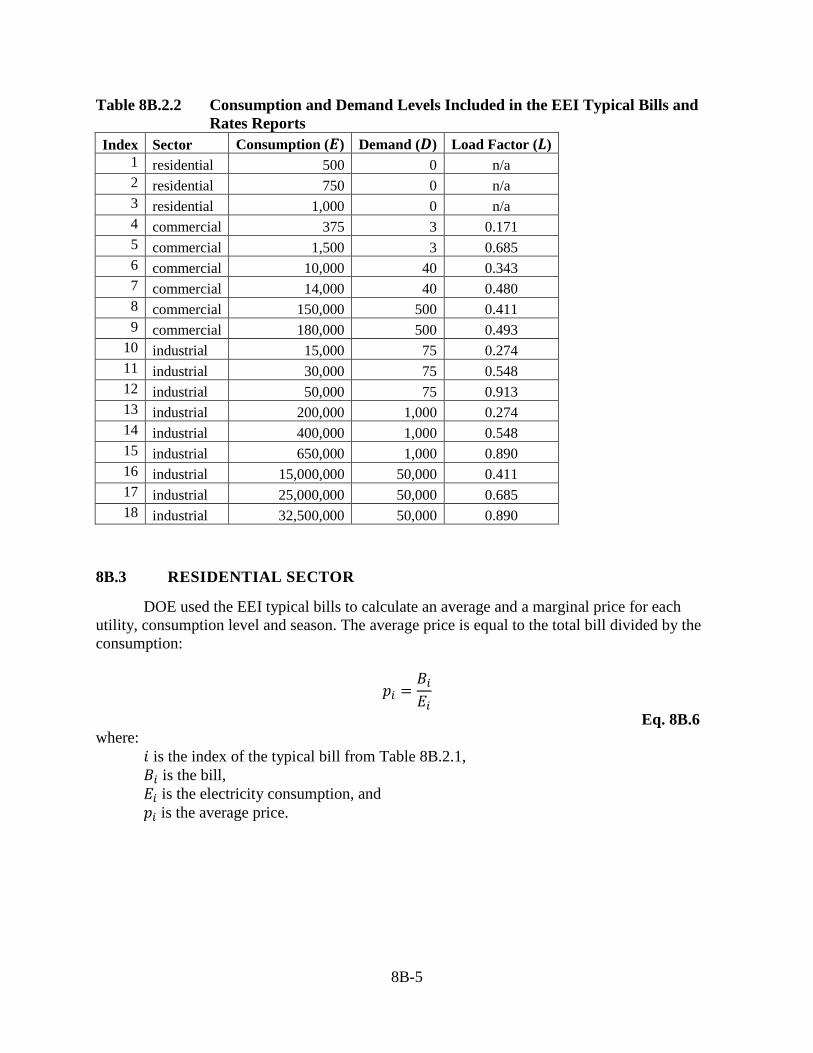
8B-5

Table 8B.2.2 Consumption and Demand Levels Included in the EEI Typical Bills and Rates Reports

Index Sector Consumption (𝑬𝑬) Demand (𝑫𝑫) Load Factor (𝑳𝑳) 1 residential 500 0 n/a 2 residential 750 0 n/a 3 residential 1,000 0 n/a 4 commercial 375 3 0.171 5 commercial 1,500 3 0.685 6 commercial 10,000 40 0.343 7 commercial 14,000 40 0.480 8 commercial 150,000 500 0.411 9 commercial 180,000 500 0.493

10 industrial 15,000 75 0.274 11 industrial 30,000 75 0.548 12 industrial 50,000 75 0.913 13 industrial 200,000 1,000 0.274 14 industrial 400,000 1,000 0.548 15 industrial 650,000 1,000 0.890 16 industrial 15,000,000 50,000 0.411 17 industrial 25,000,000 50,000 0.685 18 industrial 32,500,000 50,000 0.890

8B.3 RESIDENTIAL SECTOR

DOE used the EEI typical bills to calculate an average and a marginal price for each utility, consumption level and season. The average price is equal to the total bill divided by the consumption:

𝑝𝑝𝑖𝑖 =𝐵𝐵𝑖𝑖𝐸𝐸𝑖𝑖

Eq. 8B.6 where:

𝑖𝑖 is the index of the typical bill from Table 8B.2.1, 𝐵𝐵𝑖𝑖 is the bill, 𝐸𝐸𝑖𝑖 is the electricity consumption, and 𝑝𝑝𝑖𝑖 is the average price.

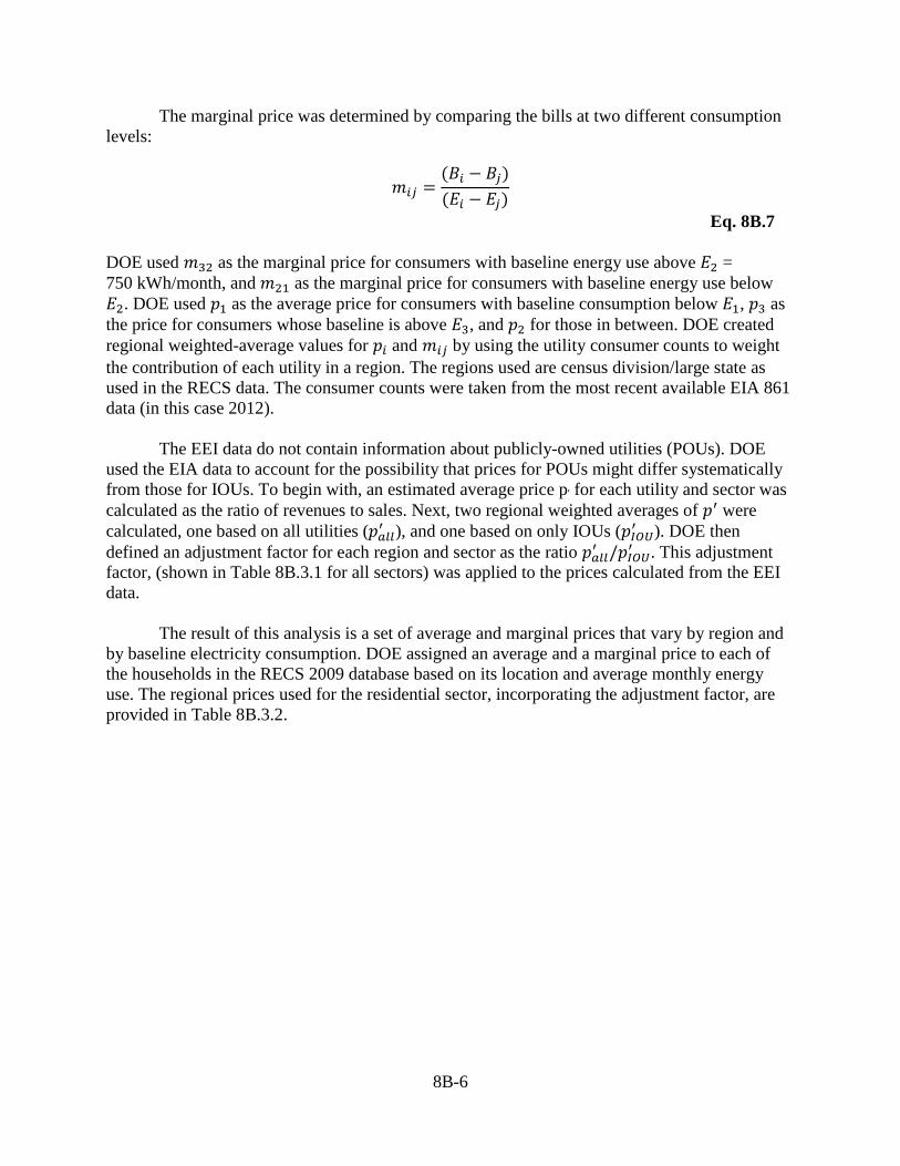
8B-6

The marginal price was determined by comparing the bills at two different consumption levels:

𝑚𝑚𝑖𝑖𝑗𝑗 =(𝐵𝐵𝑖𝑖 − 𝐵𝐵𝑗𝑗)(𝐸𝐸𝑖𝑖 − 𝐸𝐸𝑗𝑗)

Eq. 8B.7 DOE used 𝑚𝑚32 as the marginal price for consumers with baseline energy use above 𝐸𝐸2 = 750 kWh/month, and 𝑚𝑚21 as the marginal price for consumers with baseline energy use below 𝐸𝐸2. DOE used 𝑝𝑝1 as the average price for consumers with baseline consumption below 𝐸𝐸1, 𝑝𝑝3 as the price for consumers whose baseline is above 𝐸𝐸3, and 𝑝𝑝2 for those in between. DOE created regional weighted-average values for 𝑝𝑝𝑖𝑖 and 𝑚𝑚𝑖𝑖𝑗𝑗 by using the utility consumer counts to weight the contribution of each utility in a region. The regions used are census division/large state as used in the RECS data. The consumer counts were taken from the most recent available EIA 861 data (in this case 2012).

The EEI data do not contain information about publicly-owned utilities (POUs). DOE used the EIA data to account for the possibility that prices for POUs might differ systematically from those for IOUs. To begin with, an estimated average price p' for each utility and sector was calculated as the ratio of revenues to sales. Next, two regional weighted averages of 𝑝𝑝′ were calculated, one based on all utilities (𝑝𝑝𝑎𝑎𝑎𝑎𝑎𝑎′ ), and one based on only IOUs (𝑝𝑝𝐼𝐼𝐼𝐼𝐼𝐼′ ). DOE then defined an adjustment factor for each region and sector as the ratio 𝑝𝑝𝑎𝑎𝑎𝑎𝑎𝑎′ /𝑝𝑝𝐼𝐼𝐼𝐼𝐼𝐼′ . This adjustment factor, (shown in Table 8B.3.1 for all sectors) was applied to the prices calculated from the EEI data.

The result of this analysis is a set of average and marginal prices that vary by region and by baseline electricity consumption. DOE assigned an average and a marginal price to each of the households in the RECS 2009 database based on its location and average monthly energy use. The regional prices used for the residential sector, incorporating the adjustment factor, are provided in Table 8B.3.2.

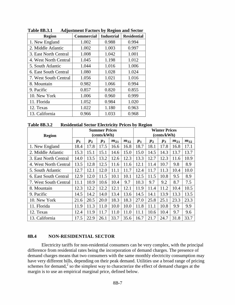
8B-7

Table 8B.3.1 Adjustment Factors by Region and Sector Region Commercial Industrial Residential

1. New England 1.002 0.988 0.994 2. Middle Atlantic 1.002 1.003 0.997 3. East North Central 1.008 1.042 1.001 4. West North Central 1.045 1.198 1.012 5. South Atlantic 1.044 1.016 1.006 6. East South Central 1.080 1.028 1.024 7. West South Central 1.056 1.021 1.016 8. Mountain 0.982 1.066 0.994 9. Pacific 0.857 0.820 0.855 10. New York 1.006 0.960 0.999 11. Florida 1.052 0.984 1.020 12. Texas 1.022 1.180 0.963 13. California 0.966 1.033 0.968

Table 8B.3.2 Residential Sector Electricity Prices by Region

Region Summer Prices

(cents/kWh) Winter Prices (cents/kWh)

𝒑𝒑𝟏𝟏 𝒑𝒑𝟐𝟐 𝒑𝒑𝟑𝟑 𝒎𝒎𝟐𝟐𝟏𝟏 𝒎𝒎𝟑𝟑𝟐𝟐 𝒑𝒑𝟏𝟏 𝒑𝒑𝟐𝟐 𝒑𝒑𝟑𝟑 𝒎𝒎𝟐𝟐𝟏𝟏 𝒎𝒎𝟑𝟑𝟐𝟐 1. New England 18.4 17.8 17.5 16.6 16.8 18.7 18.1 17.8 16.8 17.1 2. Middle Atlantic 15.3 15.1 15.1 14.6 15.0 15.0 14.5 14.3 13.7 13.7 3. East North Central 14.0 13.5 13.2 12.6 12.3 13.3 12.7 12.3 11.6 10.9 4. West North Central 13.5 12.8 12.5 11.6 11.6 12.1 11.4 10.7 9.8 8.9 5. South Atlantic 12.7 12.1 12.0 11.1 11.7 12.4 11.7 11.3 10.4 10.0 6. East South Central 12.9 12.0 11.5 10.1 10.1 12.5 11.5 10.8 9.5 8.9 7. West South Central 11.1 10.9 10.6 10.4 9.7 10.3 9.7 9.2 8.7 7.5 8. Mountain 12.3 12.2 12.2 12.1 12.1 11.9 11.4 11.2 10.4 10.5 9. Pacific 14.5 14.2 14.0 13.4 13.6 14.5 14.1 13.9 13.3 13.5 10. New York 21.6 20.5 20.0 18.3 18.3 27.0 25.8 25.1 23.3 23.3 11. Florida 11.9 11.3 11.0 10.0 10.0 11.8 11.1 10.8 9.9 9.9 12. Texas 12.4 11.9 11.7 11.0 11.0 11.1 10.6 10.4 9.7 9.6 13. California 17.5 22.9 26.1 33.7 35.6 16.7 21.7 24.7 31.8 33.7

8B.4 NON-RESIDENTIAL SECTOR

Electricity tariffs for non-residential consumers can be very complex, with the principal difference from residential rates being the incorporation of demand charges. The presence of demand charges means that two consumers with the same monthly electricity consumption may have very different bills, depending on their peak demand. Utilities use a broad range of pricing schemes for demand,2 so the simplest way to characterize the effect of demand charges at the margin is to use an empirical marginal price, defined below.

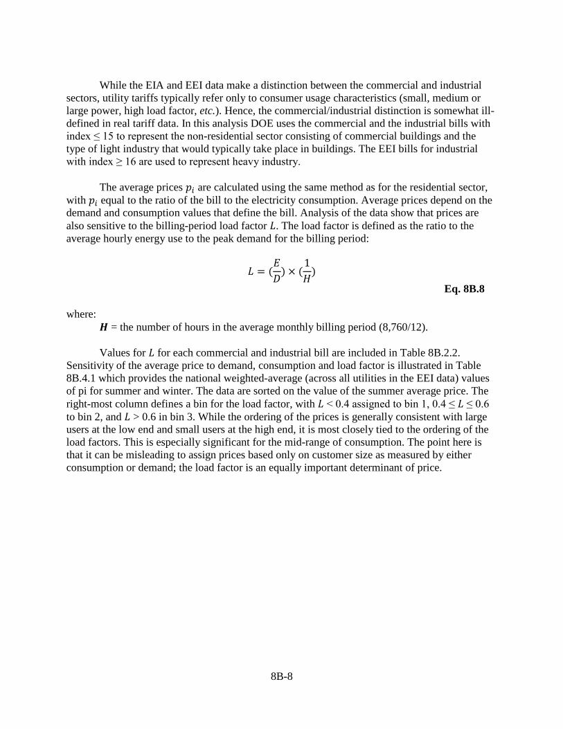
8B-8

While the EIA and EEI data make a distinction between the commercial and industrial

sectors, utility tariffs typically refer only to consumer usage characteristics (small, medium or large power, high load factor, etc.). Hence, the commercial/industrial distinction is somewhat ill-defined in real tariff data. In this analysis DOE uses the commercial and the industrial bills with index ≤ 15 to represent the non-residential sector consisting of commercial buildings and the type of light industry that would typically take place in buildings. The EEI bills for industrial with index ≥ 16 are used to represent heavy industry.

The average prices 𝑝𝑝𝑖𝑖 are calculated using the same method as for the residential sector, with 𝑝𝑝𝑖𝑖 equal to the ratio of the bill to the electricity consumption. Average prices depend on the demand and consumption values that define the bill. Analysis of the data show that prices are also sensitive to the billing-period load factor 𝐿𝐿. The load factor is defined as the ratio to the average hourly energy use to the peak demand for the billing period:

𝐿𝐿 = (𝐸𝐸𝐷𝐷

) × (1𝐻𝐻

) Eq. 8B.8

where:

𝑯𝑯 = the number of hours in the average monthly billing period (8,760/12).

Values for 𝐿𝐿 for each commercial and industrial bill are included in Table 8B.2.2. Sensitivity of the average price to demand, consumption and load factor is illustrated in Table 8B.4.1 which provides the national weighted-average (across all utilities in the EEI data) values of pi for summer and winter. The data are sorted on the value of the summer average price. The right-most column defines a bin for the load factor, with 𝐿𝐿 < 0.4 assigned to bin 1, 0.4 ≤ 𝐿𝐿 ≤ 0.6 to bin 2, and 𝐿𝐿 > 0.6 in bin 3. While the ordering of the prices is generally consistent with large users at the low end and small users at the high end, it is most closely tied to the ordering of the load factors. This is especially significant for the mid-range of consumption. The point here is that it can be misleading to assign prices based only on customer size as measured by either consumption or demand; the load factor is an equally important determinant of price.

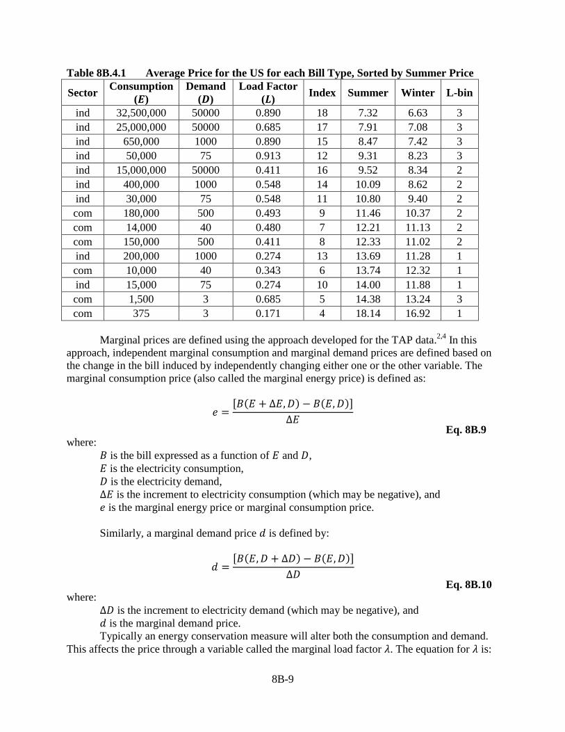
8B-9

Table 8B.4.1 Average Price for the US for each Bill Type, Sorted by Summer Price

Sector Consumption (𝑬𝑬)

Demand (𝑫𝑫)

Load Factor (𝑳𝑳) Index Summer Winter L-bin

ind 32,500,000 50000 0.890 18 7.32 6.63 3 ind 25,000,000 50000 0.685 17 7.91 7.08 3 ind 650,000 1000 0.890 15 8.47 7.42 3 ind 50,000 75 0.913 12 9.31 8.23 3 ind 15,000,000 50000 0.411 16 9.52 8.34 2 ind 400,000 1000 0.548 14 10.09 8.62 2 ind 30,000 75 0.548 11 10.80 9.40 2 com 180,000 500 0.493 9 11.46 10.37 2 com 14,000 40 0.480 7 12.21 11.13 2 com 150,000 500 0.411 8 12.33 11.02 2 ind 200,000 1000 0.274 13 13.69 11.28 1 com 10,000 40 0.343 6 13.74 12.32 1 ind 15,000 75 0.274 10 14.00 11.88 1 com 1,500 3 0.685 5 14.38 13.24 3 com 375 3 0.171 4 18.14 16.92 1

Marginal prices are defined using the approach developed for the TAP data.2,4 In this

approach, independent marginal consumption and marginal demand prices are defined based on the change in the bill induced by independently changing either one or the other variable. The marginal consumption price (also called the marginal energy price) is defined as:

𝑒𝑒 =[𝐵𝐵(𝐸𝐸 + ∆𝐸𝐸,𝐷𝐷) − 𝐵𝐵(𝐸𝐸,𝐷𝐷)]

∆𝐸𝐸

Eq. 8B.9 where:

𝐵𝐵 is the bill expressed as a function of 𝐸𝐸 and 𝐷𝐷, 𝐸𝐸 is the electricity consumption, 𝐷𝐷 is the electricity demand, ∆𝐸𝐸 is the increment to electricity consumption (which may be negative), and 𝑒𝑒 is the marginal energy price or marginal consumption price.

Similarly, a marginal demand price 𝑑𝑑 is defined by:

𝑑𝑑 =[𝐵𝐵(𝐸𝐸,𝐷𝐷 + ∆𝐷𝐷) − 𝐵𝐵(𝐸𝐸,𝐷𝐷)]

∆𝐷𝐷

Eq. 8B.10 where:

∆𝐷𝐷 is the increment to electricity demand (which may be negative), and 𝑑𝑑 is the marginal demand price. Typically an energy conservation measure will alter both the consumption and demand.

This affects the price through a variable called the marginal load factor 𝜆𝜆. The equation for 𝜆𝜆 is:

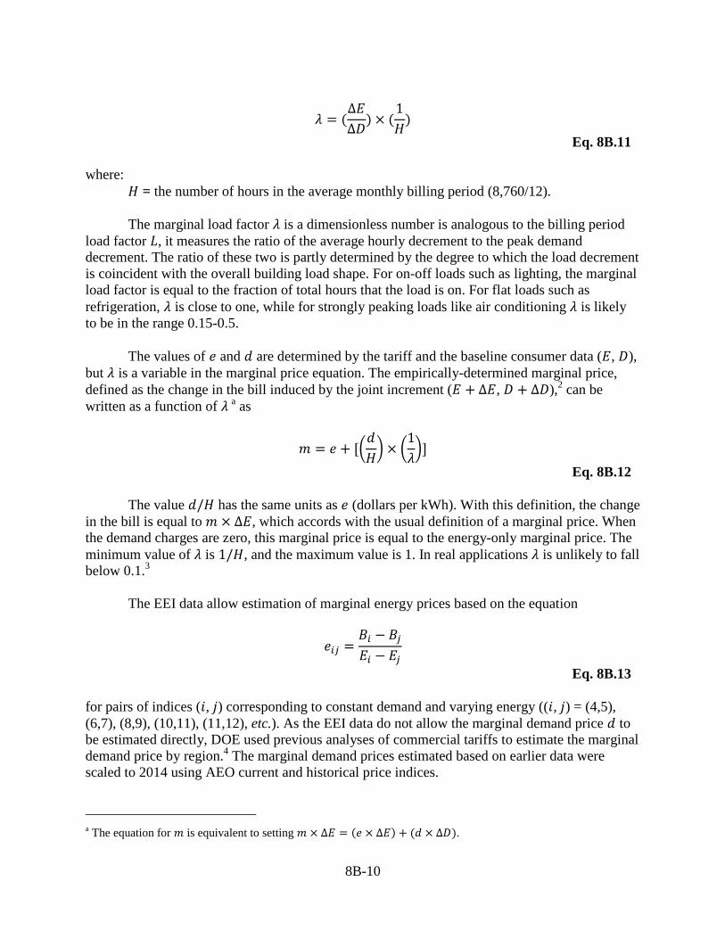
8B-10

𝜆𝜆 = (∆𝐸𝐸∆𝐷𝐷

) × (1𝐻𝐻

) Eq. 8B.11

where:

𝐻𝐻 = the number of hours in the average monthly billing period (8,760/12). The marginal load factor 𝜆𝜆 is a dimensionless number is analogous to the billing period

load factor 𝐿𝐿, it measures the ratio of the average hourly decrement to the peak demand decrement. The ratio of these two is partly determined by the degree to which the load decrement is coincident with the overall building load shape. For on-off loads such as lighting, the marginal load factor is equal to the fraction of total hours that the load is on. For flat loads such as refrigeration, 𝜆𝜆 is close to one, while for strongly peaking loads like air conditioning 𝜆𝜆 is likely to be in the range 0.15-0.5.

The values of 𝑒𝑒 and 𝑑𝑑 are determined by the tariff and the baseline consumer data (𝐸𝐸, 𝐷𝐷), but 𝜆𝜆 is a variable in the marginal price equation. The empirically-determined marginal price, defined as the change in the bill induced by the joint increment (𝐸𝐸 + ∆𝐸𝐸, 𝐷𝐷 + ∆𝐷𝐷),2 can be written as a function of 𝜆𝜆 a as

𝑚𝑚 = 𝑒𝑒 + [�𝑑𝑑𝐻𝐻� × �

1𝜆𝜆�]

Eq. 8B.12

The value 𝑑𝑑/𝐻𝐻 has the same units as 𝑒𝑒 (dollars per kWh). With this definition, the change in the bill is equal to 𝑚𝑚 × ∆𝐸𝐸, which accords with the usual definition of a marginal price. When the demand charges are zero, this marginal price is equal to the energy-only marginal price. The minimum value of 𝜆𝜆 is 1/𝐻𝐻, and the maximum value is 1. In real applications 𝜆𝜆 is unlikely to fall below 0.1.3

The EEI data allow estimation of marginal energy prices based on the equation

𝑒𝑒𝑖𝑖𝑗𝑗 =𝐵𝐵𝑖𝑖 − 𝐵𝐵𝑗𝑗𝐸𝐸𝑖𝑖 − 𝐸𝐸𝑗𝑗

Eq. 8B.13 for pairs of indices (𝑖𝑖, 𝑗𝑗) corresponding to constant demand and varying energy ((𝑖𝑖, 𝑗𝑗) = (4,5), (6,7), (8,9), (10,11), (11,12), etc.). As the EEI data do not allow the marginal demand price 𝑑𝑑 to be estimated directly, DOE used previous analyses of commercial tariffs to estimate the marginal demand price by region.4 The marginal demand prices estimated based on earlier data were scaled to 2014 using AEO current and historical price indices.

a The equation for 𝑚𝑚 is equivalent to setting 𝑚𝑚 × ∆𝐸𝐸 = (𝑒𝑒 × ∆𝐸𝐸) + (𝑑𝑑 × ∆𝐷𝐷).

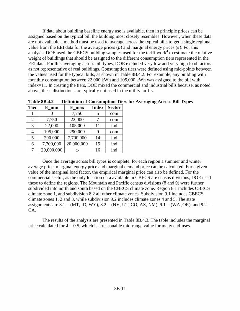
8B-11

If data about building baseline energy use is available, then in principle prices can be assigned based on the typical bill the building most closely resembles. However, when these data are not available a method must be used to average across the typical bills to get a single regional value from the EEI data for the average prices (𝑝𝑝) and marginal energy prices (𝑒𝑒). For this analysis, DOE used the CBECS building samples used for the tariff work4 to estimate the relative weight of buildings that should be assigned to the different consumption tiers represented in the EEI data. For this averaging across bill types, DOE excluded very low and very high load factors as not representative of real buildings. Consumption tiers were defined using mid-points between the values used for the typical bills, as shown in Table 8B.4.2. For example, any building with monthly consumption between 22,000 kWh and 105,000 kWh was assigned to the bill with index=11. In creating the tiers, DOE mixed the commercial and industrial bills because, as noted above, these distinctions are typically not used in the utility tariffs. Table 8B.4.2 Definition of Consumption Tiers for Averaging Across Bill Types Tier E_min E_max Index Sector

1 0 7,750 5 com 2 7,750 22,000 7 com 3 22,000 105,000 11 ind 4 105,000 290,000 9 com 5 290,000 7,700,000 14 ind 6 7,700,000 20,000,000 15 ind 7 20,000,000 ω 16 ind

Once the average across bill types is complete, for each region a summer and winter

average price, marginal energy price and marginal demand price can be calculated. For a given value of the marginal load factor, the empirical marginal price can also be defined. For the commercial sector, as the only location data available in CBECS are census divisions, DOE used these to define the regions. The Mountain and Pacific census divisions (8 and 9) were further subdivided into north and south based on the CBECS climate zone. Region 8.1 includes CBECS climate zone 1, and subdivision 8.2 all other climate zones. Subdivision 9.1 includes CBECS climate zones 1, 2 and 3, while subdivision 9.2 includes climate zones 4 and 5. The state assignments are 8.1 = (MT, ID, WY), 8.2 = (NV, UT, CO, AZ, NM), 9.1 = (WA ,OR), and 9.2 = CA.

The results of the analysis are presented in Table 8B.4.3. The table includes the marginal price calculated for 𝜆𝜆 = 0.5, which is a reasonable mid-range value for many end-uses.

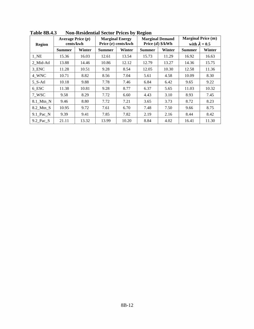
8B-12

Table 8B.4.3 Non-Residential Sector Prices by Region

Region Average Price (𝒑𝒑)

cents/kwh Marginal Energy

Price (𝒆𝒆) cents/kwh Marginal Demand Price (𝒅𝒅) $/kWh

Marginal Price (𝒎𝒎) with 𝝀𝝀 = 0.5

Summer Winter Summer Winter Summer Winter Summer Winter 1_NE 15.36 16.03 12.61 13.54 15.73 11.29 16.92 16.63 2_Mid-Atl 13.88 14.46 10.86 12.12 12.79 13.27 14.36 15.75 3_ENC 11.28 10.51 9.28 8.54 12.05 10.30 12.58 11.36 4_WNC 10.71 8.82 8.56 7.04 5.61 4.58 10.09 8.30 5_S-Atl 10.18 9.88 7.78 7.46 6.84 6.42 9.65 9.22 6_ESC 11.38 10.81 9.28 8.77 6.37 5.65 11.03 10.32 7_WSC 9.58 8.29 7.72 6.60 4.43 3.10 8.93 7.45 8.1_Mtn_N 9.46 8.80 7.72 7.21 3.65 3.73 8.72 8.23 8.2_Mtn_S 10.95 9.72 7.61 6.70 7.48 7.50 9.66 8.75 9.1_Pac_N 9.39 9.41 7.85 7.82 2.19 2.16 8.44 8.42 9.2_Pac_S 21.11 13.32 13.99 10.20 8.84 4.02 16.41 11.30

8B-13

REFERENCES 1. Coughlin, K., R. M. White, C. A. Bolduc, D. C. Fisher, and G. J. Rosenquist. The Tariff

Analysis Project: A Database and Analysis Platform for Electricity Tariffs. 2006. Lawrence Berkeley National Laboratory: Berkeley, CA. Report No. LBNL-55680. (Last accessed June 15, 2015.) http://eetd.lbl.gov/publications/tariff-analysis-project-database-and-analysis-platform-electricity-tariffs.

2. Coughlin, K., C. Bolduc, R. Van Buskirk, G. Rosenquist, and J. E. McMahon. Tariff-based Analysis of Commercial Building Electricity Prices. 2008. Lawrence Berkeley National Laboratory: Berkeley, CA. Report No. LBNL-55551. (Last accessed June 8, 2015.) https://escholarship.org/uc/item/9dv1m729.

3. Edison Electric Institute. Typical Bills and Average Rates Report. Winter 2014 published April 2014, Summer 2014 published October 2014: Washington, D.C. (Last accessed June 2, 2015.) http://www.eei.org/resourcesandmedia/products/Pages/Products.aspx.

4. U.S. Department of Energy. Commercial Unitary Air Conditioners and Heat Pumps Technical Support Document: Life-Cycle Cost and Pay-back Period Analysis. July 2004. Washington, D.C. (Last accessed June 15, 2015.) http://www1.eere.energy.gov/buildings/appliance_standards/commercial/pdfs/cuac_tsd_chp_8.pdf.

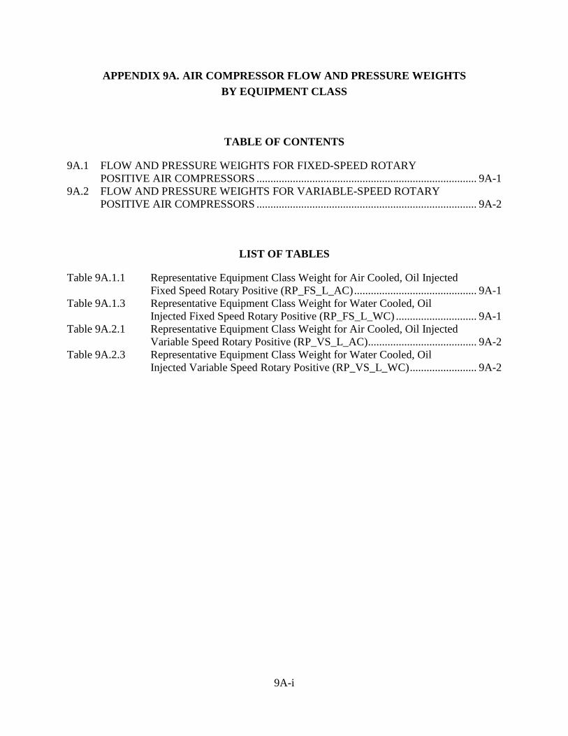
9A-i

APPENDIX 9A. AIR COMPRESSOR FLOW AND PRESSURE WEIGHTS BY EQUIPMENT CLASS

TABLE OF CONTENTS

9A.1 FLOW AND PRESSURE WEIGHTS FOR FIXED-SPEED ROTARY POSITIVE AIR COMPRESSORS ............................................................................... 9A-1

9A.2 FLOW AND PRESSURE WEIGHTS FOR VARIABLE-SPEED ROTARY POSITIVE AIR COMPRESSORS ............................................................................... 9A-2

LIST OF TABLES

Table 9A.1.1 Representative Equipment Class Weight for Air Cooled, Oil Injected Fixed Speed Rotary Positive (RP_FS_L_AC) ............................................ 9A-1

Table 9A.1.3 Representative Equipment Class Weight for Water Cooled, Oil Injected Fixed Speed Rotary Positive (RP_FS_L_WC) ............................. 9A-1

Table 9A.2.1 Representative Equipment Class Weight for Air Cooled, Oil Injected Variable Speed Rotary Positive (RP_VS_L_AC) ....................................... 9A-2

Table 9A.2.3 Representative Equipment Class Weight for Water Cooled, Oil Injected Variable Speed Rotary Positive (RP_VS_L_WC) ........................ 9A-2

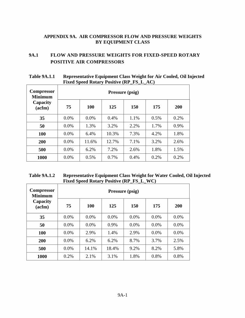
9A-1

APPENDIX 9A. AIR COMPRESSOR FLOW AND PRESSURE WEIGHTS BY EQUIPMENT CLASS

9A.1 FLOW AND PRESSURE WEIGHTS FOR FIXED-SPEED ROTARY POSITIVE AIR COMPRESSORS

Table 9A.1.1 Representative Equipment Class Weight for Air Cooled, Oil Injected

Fixed Speed Rotary Positive (RP_FS_L_AC)

Compressor Minimum Capacity

(acfm)

Pressure (psig)

75 100 125 150 175 200

35 0.0% 0.0% 0.4% 1.1% 0.5% 0.2%

50 0.0% 1.3% 3.2% 2.2% 1.7% 0.9%

100 0.0% 6.4% 10.3% 7.3% 4.2% 1.8%

200 0.0% 11.6% 12.7% 7.1% 3.2% 2.6%

500 0.0% 6.2% 7.2% 2.6% 1.8% 1.5%

1000 0.0% 0.5% 0.7% 0.4% 0.2% 0.2% Table 9A.1.2 Representative Equipment Class Weight for Water Cooled, Oil Injected

Fixed Speed Rotary Positive (RP_FS_L_WC)

Compressor Minimum Capacity

(acfm)

Pressure (psig)

75 100 125 150 175 200

35 0.0% 0.0% 0.0% 0.0% 0.0% 0.0%

50 0.0% 0.0% 0.9% 0.0% 0.0% 0.0%

100 0.0% 2.9% 1.4% 2.9% 0.0% 0.0%

200 0.0% 6.2% 6.2% 8.7% 3.7% 2.5%

500 0.0% 14.1% 18.4% 9.2% 8.2% 5.8%

1000 0.2% 2.1% 3.1% 1.8% 0.8% 0.8%

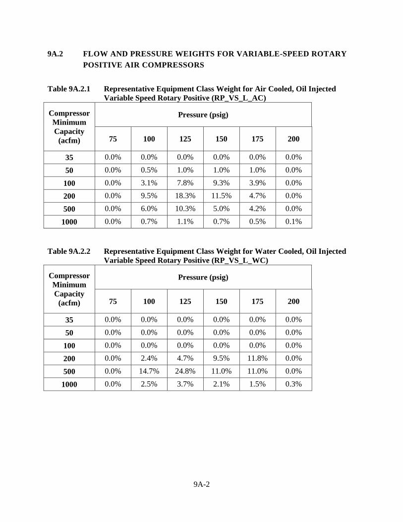
9A-2

9A.2 FLOW AND PRESSURE WEIGHTS FOR VARIABLE-SPEED ROTARY POSITIVE AIR COMPRESSORS

Table 9A.2.1 Representative Equipment Class Weight for Air Cooled, Oil Injected

Variable Speed Rotary Positive (RP_VS_L_AC)

Compressor Minimum Capacity

(acfm)

Pressure (psig)

75 100 125 150 175 200

35 0.0% 0.0% 0.0% 0.0% 0.0% 0.0%

50 0.0% 0.5% 1.0% 1.0% 1.0% 0.0%

100 0.0% 3.1% 7.8% 9.3% 3.9% 0.0%

200 0.0% 9.5% 18.3% 11.5% 4.7% 0.0%

500 0.0% 6.0% 10.3% 5.0% 4.2% 0.0%

1000 0.0% 0.7% 1.1% 0.7% 0.5% 0.1% Table 9A.2.2 Representative Equipment Class Weight for Water Cooled, Oil Injected

Variable Speed Rotary Positive (RP_VS_L_WC)

Compressor Minimum Capacity

(acfm)

Pressure (psig)

75 100 125 150 175 200

35 0.0% 0.0% 0.0% 0.0% 0.0% 0.0%

50 0.0% 0.0% 0.0% 0.0% 0.0% 0.0%

100 0.0% 0.0% 0.0% 0.0% 0.0% 0.0%

200 0.0% 2.4% 4.7% 9.5% 11.8% 0.0%

500 0.0% 14.7% 24.8% 11.0% 11.0% 0.0%

1000 0.0% 2.5% 3.7% 2.1% 1.5% 0.3%

10A-i

APPENDIX 10A. FULL-FUEL-CYCLE ANALYSIS

TABLE OF CONTENTS

10A.1 INTRODUCTION ...................................................................................................... 10A-1 10A.2 HEAT RATES ............................................................................................................ 10A-2 10A.3 FFC METHODOLOGY ............................................................................................. 10A-5 10A.4 ENERGY MULTIPLIERS FOR THE FULL FUEL CYCLE .................................... 10A-7 REFERENCES ....................................................................................................................... 10A-8

LIST OF TABLES

Table 10A.2.1 Electric Power Heat Rates (quads/TWh) by Sector and End-Use ............ 10A-5 Table 10A.3.1 Dependence of FFC Parameters on AEO Inputs ....................................... 10A-7 Table 10A.4.1 Energy Multipliers for the Full Fuel Cycle (Based on AEO 2016)........... 10A-7

LIST OF FIGURES

Figure 10A.2.1 Fuel Specific Heat Rates by Region ......................................................... 10A-4

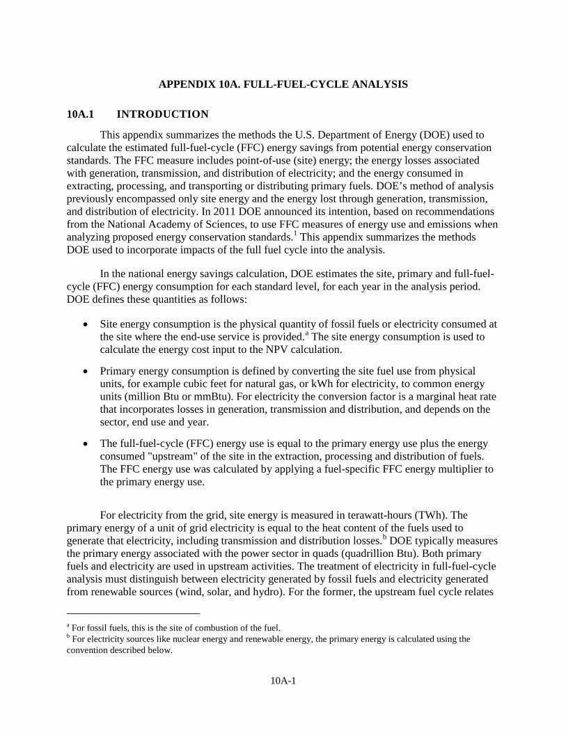
10A-1

APPENDIX 10A. FULL-FUEL-CYCLE ANALYSIS

10A.1 INTRODUCTION

This appendix summarizes the methods the U.S. Department of Energy (DOE) used to calculate the estimated full-fuel-cycle (FFC) energy savings from potential energy conservation standards. The FFC measure includes point-of-use (site) energy; the energy losses associated with generation, transmission, and distribution of electricity; and the energy consumed in extracting, processing, and transporting or distributing primary fuels. DOE’s method of analysis previously encompassed only site energy and the energy lost through generation, transmission, and distribution of electricity. In 2011 DOE announced its intention, based on recommendations from the National Academy of Sciences, to use FFC measures of energy use and emissions when analyzing proposed energy conservation standards.1 This appendix summarizes the methods DOE used to incorporate impacts of the full fuel cycle into the analysis.

In the national energy savings calculation, DOE estimates the site, primary and full-fuel-cycle (FFC) energy consumption for each standard level, for each year in the analysis period. DOE defines these quantities as follows:

• Site energy consumption is the physical quantity of fossil fuels or electricity consumed at the site where the end-use service is provided.a The site energy consumption is used to calculate the energy cost input to the NPV calculation.

• Primary energy consumption is defined by converting the site fuel use from physical units, for example cubic feet for natural gas, or kWh for electricity, to common energy units (million Btu or mmBtu). For electricity the conversion factor is a marginal heat rate that incorporates losses in generation, transmission and distribution, and depends on the sector, end use and year.

• The full-fuel-cycle (FFC) energy use is equal to the primary energy use plus the energy consumed "upstream" of the site in the extraction, processing and distribution of fuels. The FFC energy use was calculated by applying a fuel-specific FFC energy multiplier to the primary energy use.

For electricity from the grid, site energy is measured in terawatt-hours (TWh). The

primary energy of a unit of grid electricity is equal to the heat content of the fuels used to generate that electricity, including transmission and distribution losses.b DOE typically measures the primary energy associated with the power sector in quads (quadrillion Btu). Both primary fuels and electricity are used in upstream activities. The treatment of electricity in full-fuel-cycle analysis must distinguish between electricity generated by fossil fuels and electricity generated from renewable sources (wind, solar, and hydro). For the former, the upstream fuel cycle relates

a For fossil fuels, this is the site of combustion of the fuel. b For electricity sources like nuclear energy and renewable energy, the primary energy is calculated using the convention described below.

10A-2

to the fuel consumed at the power plant. There is no upstream component for the latter, because no fuel per se is used.

10A.2 HEAT RATES

DOE uses heat rates to convert site electricity savings in TWh to primary energy savings in quads. The heat rates are developed as a function of the sector, end-use and year of the analysis period. For this analysis DOE uses output of the DOE/Energy Information Administration (EIA)’s National Energy Modeling System (NEMS).2 EIA uses the NEMS model to produce the Annual Energy Outlook (AEO). DOE’s approach uses the most recently available edition, in this case AEO2016.3 The AEO publication includes a reference case and a series of side cases incorporating different economic and policy scenarios. DOE’s heat rate calculation methods depend on the scenarios available with the current AEO publication. When the data allow it, DOE calculates marginal heat rates as the ratio of the change in fuel consumption to the change in generation for each fossil fuel type, where the change is defined as the difference between the reference case and the side case. The marginal approach relies on the availability of side cases where the primary difference from the reference case is a reduction in demand for electricity, with relatively little change in the fuel mix and the economic and demographic drivers of electricity use. This approach was used with the AEO2014 and AEO2015, and is documented in the appendices to rules published in that time frame. The marginal methodology, and the conditions under which it applies, are also discussed in Coughlin (2014).4

The side cases published with AEO2016 do not allow for calculation of marginal heat rates, so DOE based its calculation of heat rates on grid-average data. DOE calculated heat rates in four steps:

1. DOE defined fuel-specific grid-average heat rates, as the ratio of primary energy consumed per unit of electricity generated for coal, natural gas and petroleum-based fuels. For renewable and nuclear generation, DOE adopted the EIA convention of assigning a constant heat rate of 10.5 Btu/Wh to nuclear power and 9.5 Btu/Wh to electricity from renewable sources. DOE calculated these heat rates for each of five geographic regions. The five regions consist of aggregations of the NERC reliability regions, which also map to aggregations of the NEMS Electricity Market Module regions as follows: region 1 consists of NERC regions NPCC and RFC, region 2 contains the SERC and FRCC regions, region 3 is MRO, region 4 ERCOT plus SPP, and region 5 is WECC. The fuel specific heat rates by region are shown in Figure 10A.2.1.

2. For each sector and end-use, DOE calculated regional weights based on the fraction of electricity consumption for that end-use in each of the five regions. DOE based this calculation on the AEO projection of end-use electricity consumption by census division, and a table matrix provided with the NEMS code that breaks down sectoral electricity use by both EMM region and census division. This calculation provides regional weights that vary by sector, end-use and year.

3. Within each region, DOE calculated the fraction of generation allocated to each fuel type based on AEO projections of generation by EMM region, for the major fuel types: coal, natural gas, nuclear, oil, and renewables. This grid-average calculation shows that

10A-3

approximately 15-20% of generation is allocated to nuclear. The grid-average calculation is being used as an approximation to the marginal calculation, and all DOE’s previous marginal calculations have shown that within NEMS nuclear power is never on the margin (i.e. total nuclear power generation is constant across all scenarios). To be consistent with previous marginal analyses, DOE zeroed out the nuclear portion of the generation fraction and redistributed the nuclear share proportionally across the other fuel types. The result is a set of factors defining the fraction of generation by fuel type for marginal reductions in demand that vary by region and year.

4. DOE multiplied the regional end-use weights by the product of the fraction of generation by fuel type and the fuel specific heat rates in each region, and summed over all regions and fuel types, to define a heat rate for each sector/end-use. This calculation also includes the transmission and distribution losses. In equation form:

h(u,y) = (1 + TDLoss)*∑r,f w(u,r) G(r,f,y) H(r,f,y) Where:

TDLoss = the fraction of total generation that is lost in transmission and distribution, equal to 0.07037

u = an index representing the sector/end-use (e.g. commercial cooling) r = the region y = the analysis year f = the fuel type w(u,r) = the regional weight H(r,f,y) = the fuel-specific heat rate plotted in Figure 10A.2.1 G(r,f,y) = the fraction of generation provided by fuel type f in region r and year y h(u,y) = the end-use specific marginal heat rate

The sector/end-use specific heat rates are shown in Table 10A.2.1. These heat rates convert site electricity to primary energy in quads; i.e., the units used in the table are quads per TWh.

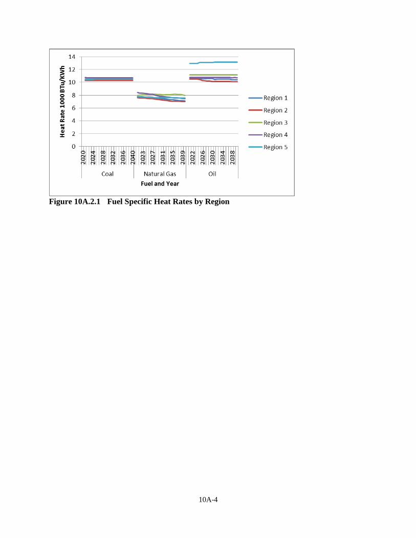
10A-4

Figure 10A.2.1 Fuel Specific Heat Rates by Region

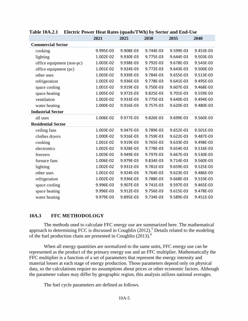
10A-5

Table 10A.2.1 Electric Power Heat Rates (quads/TWh) by Sector and End-Use

2021 2025 2030 2035 2040

Commercial Sector cooking 9.995E-03 9.908E-03 9.744E-03 9.599E-03 9.453E-03

lighting 1.002E-02 9.930E-03 9.775E-03 9.644E-03 9.503E-03 office equipment (non-pc) 1.003E-02 9.938E-03 9.792E-03 9.678E-03 9.543E-03 office equipment (pc) 1.001E-02 9.924E-03 9.772E-03 9.643E-03 9.500E-03 other uses 1.003E-02 9.939E-03 9.784E-03 9.655E-03 9.513E-03 refrigeration 1.002E-02 9.936E-03 9.778E-03 9.641E-03 9.495E-03 space cooling 1.001E-02 9.919E-03 9.750E-03 9.607E-03 9.468E-03 space heating 1.005E-02 9.972E-03 9.825E-03 9.701E-03 9.559E-03 ventilation 1.002E-02 9.933E-03 9.775E-03 9.640E-03 9.494E-03 water heating 1.000E-02 9.916E-03 9.757E-03 9.620E-03 9.480E-03

Industrial Sector all uses 1.006E-02 9.977E-03 9.826E-03 9.699E-03 9.560E-03

Residential Sector ceiling fans 1.003E-02 9.947E-03 9.789E-03 9.652E-03 9.501E-03

clothes dryers 1.000E-02 9.916E-03 9.759E-03 9.622E-03 9.487E-03 cooking 1.001E-02 9.919E-03 9.765E-03 9.633E-03 9.498E-03 electronics 1.002E-02 9.928E-03 9.778E-03 9.654E-03 9.516E-03 freezers 1.003E-02 9.949E-03 9.797E-03 9.667E-03 9.530E-03 furnace fans 1.006E-02 9.979E-03 9.834E-03 9.714E-03 9.560E-03 lighting 1.002E-02 9.931E-03 9.781E-03 9.659E-03 9.525E-03 other uses 1.001E-02 9.924E-03 9.764E-03 9.623E-03 9.486E-03 refrigeration 1.002E-02 9.936E-03 9.788E-03 9.668E-03 9.533E-03 space cooling 9.996E-03 9.907E-03 9.741E-03 9.597E-03 9.465E-03 space heating 9.996E-03 9.912E-03 9.756E-03 9.615E-03 9.478E-03 water heating 9.979E-03 9.895E-03 9.734E-03 9.589E-03 9.451E-03

10A.3 FFC METHODOLOGY

The methods used to calculate FFC energy use are summarized here. The mathematical approach to determining FCC is discussed in Coughlin (2012).5 Details related to the modeling of the fuel production chain are presented in Coughlin (2013).6

When all energy quantities are normalized to the same units, FFC energy use can be represented as the product of the primary energy use and an FFC multiplier. Mathematically the FFC multiplier is a function of a set of parameters that represent the energy intensity and material losses at each stage of energy production. Those parameters depend only on physical data, so the calculations require no assumptions about prices or other economic factors. Although the parameter values may differ by geographic region, this analysis utilizes national averages.

The fuel cycle parameters are defined as follows.

10A-6

• ax is the quantity of fuel x burned per unit of electricity produced for grid electricity. The calculation of ax includes a factor to account for losses incurred through the transmission and distribution systems.

• by is the amount of grid electricity used in producing fuel y, in MWh per physical unit of fuel y.

• cxy is the amount of fuel x consumed in producing one unit of fuel y.

• qx is the heat content of fuel x (MBtu/physical unit).

All the parameters are calculated as functions of an annual time step; hence, when evaluating the effects of potential new standards, a time series of annual values is used to estimate the FFC energy and emissions savings in each year of the analysis period and cumulatively.

The FFC multiplier is denoted µ (mu). A separate multiplier is calculated for each fuel used on site. Also calculated is a multiplier for electricity that reflects the fuel mix used in its generation. The multipliers are dimensionless numbers applied to primary energy savings to obtain the FFC energy savings. The upstream component of the energy savings is proportional to (µ-1). The fuel type is denoted by a subscript on the multiplier µ.

The method for performing the full-fuel-cycle analysis utilizes data and projections published in the AEO 2016.3 Table 10A.3.1 summarizes the data used as inputs to the calculation of various parameters. The column titled "AEO Table" gives the name of the table that provided the reference data.

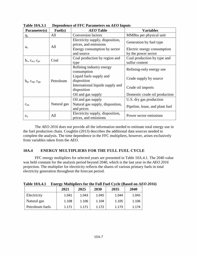
10A-7

Table 10A.3.1 Dependence of FFC Parameters on AEO Inputs Parameter(s) Fuel(s) AEO Table Variables qx All Conversion factors MMBtu per physical unit

ax All

Electricity supply, disposition, prices, and emissions Generation by fuel type

Energy consumption by sector and source

Electric energy consumption by the power sector

bc, cnc, cpc Coal Coal production by region and type

Coal production by type and sulfur content

bp, cnp, cpp Petroleum

Refining industry energy consumption Refining-only energy use

Liquid fuels supply and disposition Crude supply by source

International liquids supply and disposition Crude oil imports

Oil and gas supply Domestic crude oil production

cnn Natural gas Oil and gas supply U.S. dry gas production Natural gas supply, disposition, and prices Pipeline, lease, and plant fuel

zx All Electricity supply, disposition, prices, and emissions Power sector emissions

The AEO 2016 does not provide all the information needed to estimate total energy use in

the fuel production chain. Coughlin (2013) describes the additional data sources needed to complete the analysis. The time dependence in the FFC multipliers, however, arises exclusively from variables taken from the AEO.

10A.4 ENERGY MULTIPLIERS FOR THE FULL FUEL CYCLE

FFC energy multipliers for selected years are presented in Table 10A.4.1. The 2040 value was held constant for the analysis period beyond 2040, which is the last year in the AEO 2016 projection. The multiplier for electricity reflects the shares of various primary fuels in total electricity generation throughout the forecast period.

Table 10A.4.1 Energy Multipliers for the Full Fuel Cycle (Based on AEO 2016)

2021 2025 2030 2035 2040 Electricity 1.041 1.043 1.045 1.044 1.045 Natural gas 1.108 1.106 1.104 1.105 1.106 Petroleum fuels 1.171 1.171 1.172 1.173 1.174

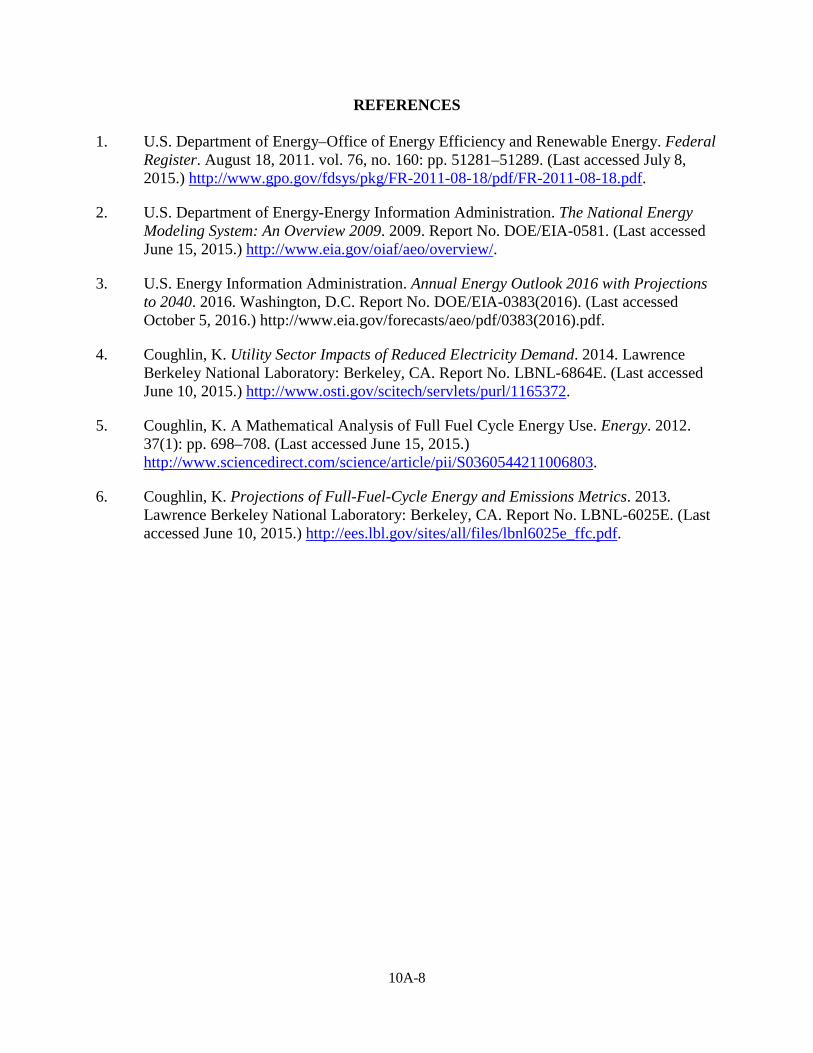
10A-8

REFERENCES 1. U.S. Department of Energy–Office of Energy Efficiency and Renewable Energy. Federal

Register. August 18, 2011. vol. 76, no. 160: pp. 51281–51289. (Last accessed July 8, 2015.) http://www.gpo.gov/fdsys/pkg/FR-2011-08-18/pdf/FR-2011-08-18.pdf.

2. U.S. Department of Energy-Energy Information Administration. The National Energy Modeling System: An Overview 2009. 2009. Report No. DOE/EIA-0581. (Last accessed June 15, 2015.) http://www.eia.gov/oiaf/aeo/overview/.

3. U.S. Energy Information Administration. Annual Energy Outlook 2016 with Projections to 2040. 2016. Washington, D.C. Report No. DOE/EIA-0383(2016). (Last accessed October 5, 2016.) http://www.eia.gov/forecasts/aeo/pdf/0383(2016).pdf.

4. Coughlin, K. Utility Sector Impacts of Reduced Electricity Demand. 2014. Lawrence Berkeley National Laboratory: Berkeley, CA. Report No. LBNL-6864E. (Last accessed June 10, 2015.) http://www.osti.gov/scitech/servlets/purl/1165372.

5. Coughlin, K. A Mathematical Analysis of Full Fuel Cycle Energy Use. Energy. 2012. 37(1): pp. 698–708. (Last accessed June 15, 2015.) http://www.sciencedirect.com/science/article/pii/S0360544211006803.

6. Coughlin, K. Projections of Full-Fuel-Cycle Energy and Emissions Metrics. 2013. Lawrence Berkeley National Laboratory: Berkeley, CA. Report No. LBNL-6025E. (Last accessed June 10, 2015.) http://ees.lbl.gov/sites/all/files/lbnl6025e_ffc.pdf.

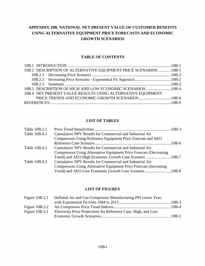
10B-i

APPENDIX 10B. NATIONAL NET PRESENT VALUE OF CUSTOMER BENEFITS USING ALTERNATIVE EQUIPMENT PRICE FORECASTS AND ECONOMIC

GROWTH SCENARIOS

TABLE OF CONTENTS

10B.1 INTRODUCTION .......................................................................................................10B-1 10B.2 DESCRIPTION OF ALTERNATIVE EQUIPMENT PRICE SCENARIOS .............10B-1

10B.2.1 Decreasing Price Scenario ...............................................................................10B-2 10B.2.2 Increasing Price Scenario - Exponential Fit Approach ....................................10B-2 10B.2.3 Summary ..........................................................................................................10B-3

10B.3 DESCRIPTION OF HIGH AND LOW ECONOMIC SCENARIOS .........................10B-4 10B.4 NET PRESENT VALUE RESULTS USING ALTERNATIVE EQUIPMENT

PRICE TRENDS AND ECONOMIC GROWTH SCENARIOS ................................10B-6 REFERENCES ........................................................................................................................10B-9

LIST OF TABLES

Table 10B.2.1 Price Trend Sensitivities ............................................................................10B-3 Table 10B.4.1 Cumulative NPV Results for Commercial and Industrial Air

Compressors Using Reference Equipment Price Forecast and AEO Reference Case Scenario............................................................................10B-6

Table 10B.4.2 Cumulative NPV Results for Commercial and Industrial Air Compressors Using Alternative Equipment Price Forecast (Decreasing Trend) and AEO High Economic Growth Case Scenario .........................10B-7

Table 10B.4.3 Cumulative NPV Results for Commercial and Industrial Air Compressors Using Alternative Equipment Price Forecast (Increasing Trend) and AEO Low Economic Growth Case Scenario ..........................10B-8

LIST OF FIGURES

Figure 10B.2.1 Deflated Air and Gas Compressor Manufacturing PPI versus Year, with Exponential Fit from 1984 to 2013 ....................................................10B-3

Figure 10B.2.2 Air Compressor Price Trend Indexes .........................................................10B-4 Figure 10B.3.1 Electricity Price Projections for Reference Case, High, and Low

Economic Growth Scenarios......................................................................10B-5

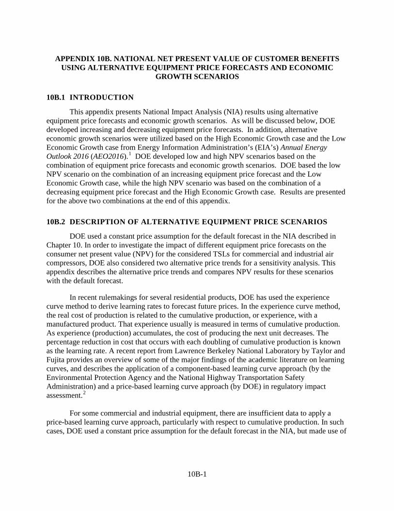
10B-1

APPENDIX 10B. NATIONAL NET PRESENT VALUE OF CUSTOMER BENEFITS USING ALTERNATIVE EQUIPMENT PRICE FORECASTS AND ECONOMIC

GROWTH SCENARIOS

10B.1 INTRODUCTION

This appendix presents National Impact Analysis (NIA) results using alternative equipment price forecasts and economic growth scenarios. As will be discussed below, DOE developed increasing and decreasing equipment price forecasts. In addition, alternative economic growth scenarios were utilized based on the High Economic Growth case and the Low Economic Growth case from Energy Information Administration’s (EIA’s) Annual Energy Outlook 2016 (AEO2016).1 DOE developed low and high NPV scenarios based on the combination of equipment price forecasts and economic growth scenarios. DOE based the low NPV scenario on the combination of an increasing equipment price forecast and the Low Economic Growth case, while the high NPV scenario was based on the combination of a decreasing equipment price forecast and the High Economic Growth case. Results are presented for the above two combinations at the end of this appendix.

10B.2 DESCRIPTION OF ALTERNATIVE EQUIPMENT PRICE SCENARIOS

DOE used a constant price assumption for the default forecast in the NIA described in Chapter 10. In order to investigate the impact of different equipment price forecasts on the consumer net present value (NPV) for the considered TSLs for commercial and industrial air compressors, DOE also considered two alternative price trends for a sensitivity analysis. This appendix describes the alternative price trends and compares NPV results for these scenarios with the default forecast.

In recent rulemakings for several residential products, DOE has used the experience curve method to derive learning rates to forecast future prices. In the experience curve method, the real cost of production is related to the cumulative production, or experience, with a manufactured product. That experience usually is measured in terms of cumulative production. As experience (production) accumulates, the cost of producing the next unit decreases. The percentage reduction in cost that occurs with each doubling of cumulative production is known as the learning rate. A recent report from Lawrence Berkeley National Laboratory by Taylor and Fujita provides an overview of some of the major findings of the academic literature on learning curves, and describes the application of a component-based learning curve approach (by the Environmental Protection Agency and the National Highway Transportation Safety Administration) and a price-based learning curve approach (by DOE) in regulatory impact assessment.2 For some commercial and industrial equipment, there are insufficient data to apply a price-based learning curve approach, particularly with respect to cumulative production. In such cases, DOE used a constant price assumption for the default forecast in the NIA, but made use of

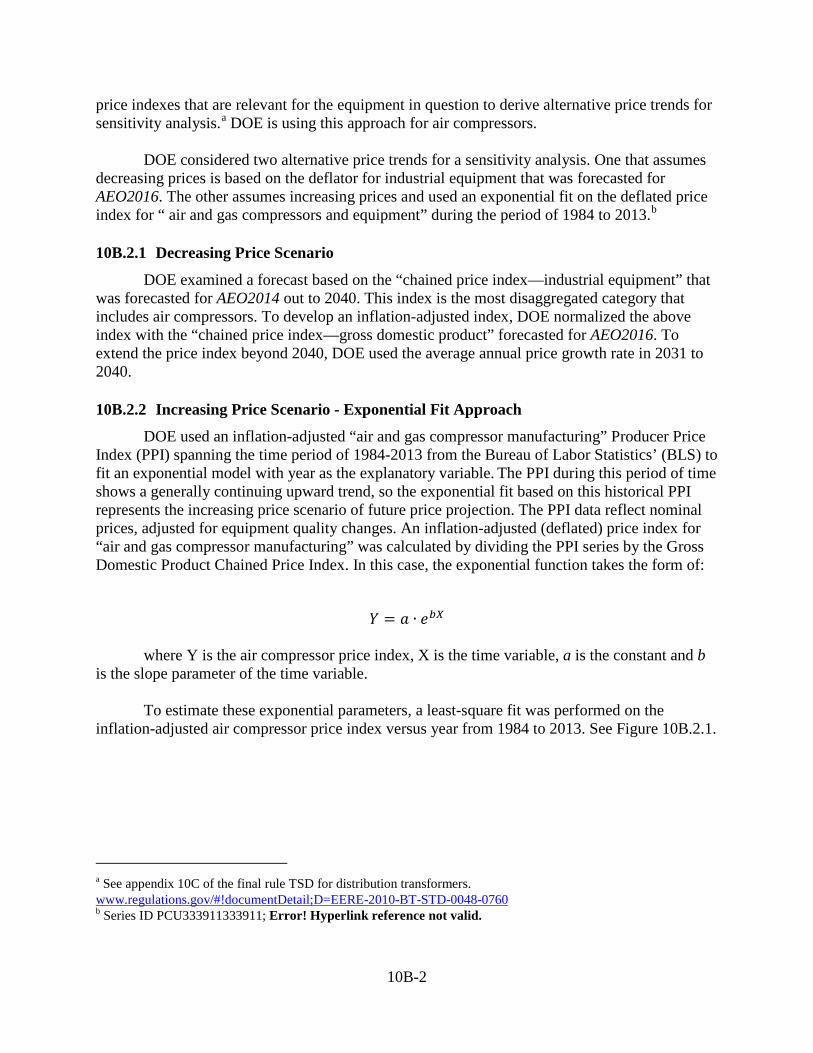
10B-2

price indexes that are relevant for the equipment in question to derive alternative price trends for sensitivity analysis.a DOE is using this approach for air compressors.

DOE considered two alternative price trends for a sensitivity analysis. One that assumes decreasing prices is based on the deflator for industrial equipment that was forecasted for AEO2016. The other assumes increasing prices and used an exponential fit on the deflated price index for “ air and gas compressors and equipment” during the period of 1984 to 2013.b

10B.2.1 Decreasing Price Scenario

DOE examined a forecast based on the “chained price index—industrial equipment” that was forecasted for AEO2014 out to 2040. This index is the most disaggregated category that includes air compressors. To develop an inflation-adjusted index, DOE normalized the above index with the “chained price index—gross domestic product” forecasted for AEO2016. To extend the price index beyond 2040, DOE used the average annual price growth rate in 2031 to 2040.

10B.2.2 Increasing Price Scenario - Exponential Fit Approach

DOE used an inflation-adjusted “air and gas compressor manufacturing” Producer Price Index (PPI) spanning the time period of 1984-2013 from the Bureau of Labor Statistics’ (BLS) to fit an exponential model with year as the explanatory variable. The PPI during this period of time shows a generally continuing upward trend, so the exponential fit based on this historical PPI represents the increasing price scenario of future price projection. The PPI data reflect nominal prices, adjusted for equipment quality changes. An inflation-adjusted (deflated) price index for “air and gas compressor manufacturing” was calculated by dividing the PPI series by the Gross Domestic Product Chained Price Index. In this case, the exponential function takes the form of:

𝑌𝑌 = 𝑎𝑎 ∙ 𝑒𝑒𝑏𝑏𝑏𝑏

where Y is the air compressor price index, X is the time variable, a is the constant and b

is the slope parameter of the time variable. To estimate these exponential parameters, a least-square fit was performed on the inflation-adjusted air compressor price index versus year from 1984 to 2013. See Figure 10B.2.1.

a See appendix 10C of the final rule TSD for distribution transformers. www.regulations.gov/#!documentDetail;D=EERE-2010-BT-STD-0048-0760 b Series ID PCU333911333911; Error! Hyperlink reference not valid.

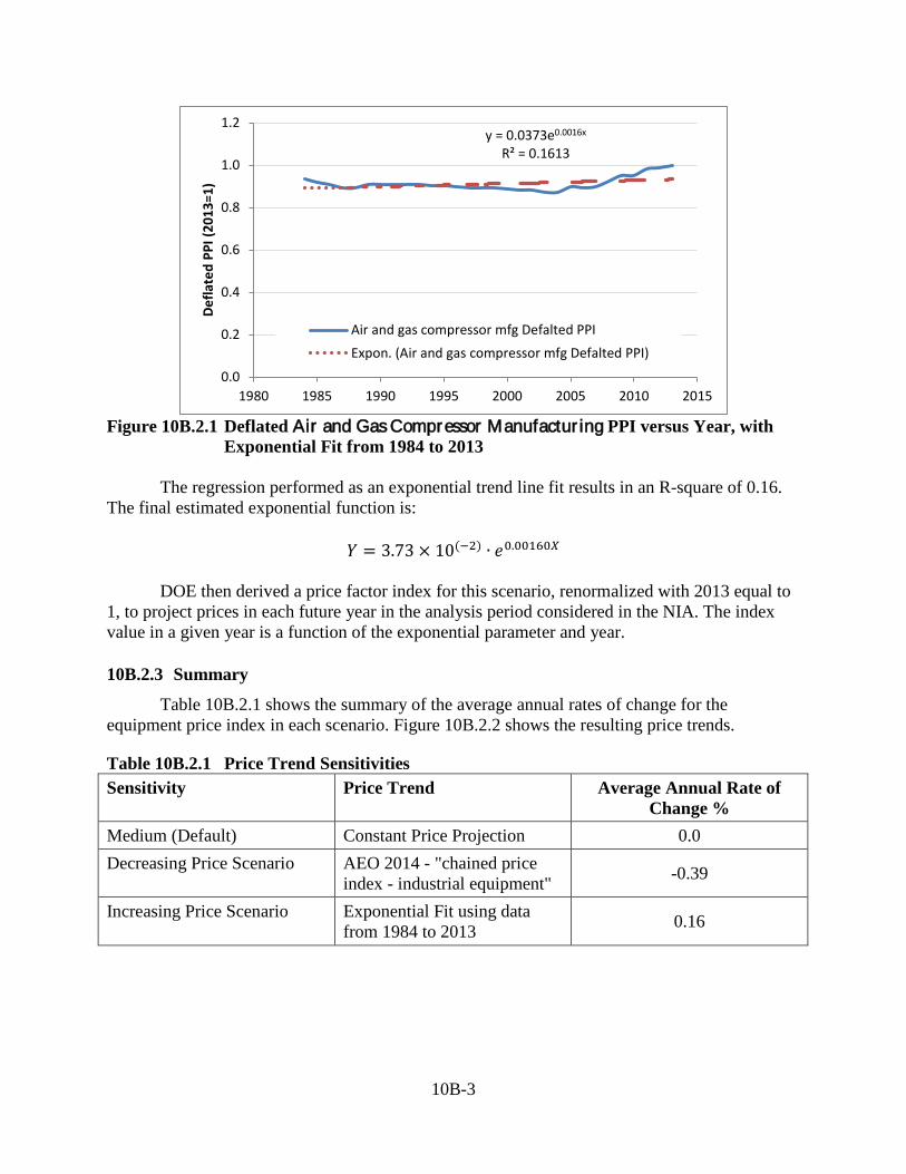
10B-3

Figure 10B.2.1 Deflated Air and Gas Compressor Manufactur ing PPI versus Year, with

Exponential Fit from 1984 to 2013 The regression performed as an exponential trend line fit results in an R-square of 0.16. The final estimated exponential function is:

𝑌𝑌 = 3.73 × 10(−2) ∙ 𝑒𝑒0.00160𝑏𝑏

DOE then derived a price factor index for this scenario, renormalized with 2013 equal to 1, to project prices in each future year in the analysis period considered in the NIA. The index value in a given year is a function of the exponential parameter and year.

10B.2.3 Summary

Table 10B.2.1 shows the summary of the average annual rates of change for the equipment price index in each scenario. Figure 10B.2.2 shows the resulting price trends.

Table 10B.2.1 Price Trend Sensitivities Sensitivity Price Trend Average Annual Rate of

Change % Medium (Default) Constant Price Projection 0.0 Decreasing Price Scenario AEO 2014 - "chained price

index - industrial equipment" -0.39

Increasing Price Scenario Exponential Fit using data from 1984 to 2013 0.16

y = 0.0373e0.0016x R² = 0.1613

0.0

0.2

0.4

0.6

0.8

1.0

1.2

1980 1985 1990 1995 2000 2005 2010 2015

Defla

ted

PPI (

2013

=1)

Air and gas compressor mfg Defalted PPIExpon. (Air and gas compressor mfg Defalted PPI)

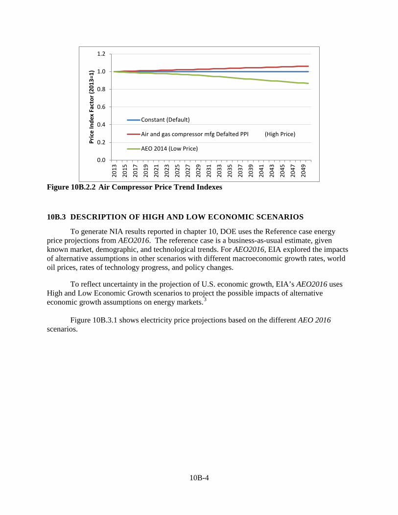
10B-4

Figure 10B.2.2 Air Compressor Price Trend Indexes

10B.3 DESCRIPTION OF HIGH AND LOW ECONOMIC SCENARIOS

To generate NIA results reported in chapter 10, DOE uses the Reference case energy price projections from AEO2016. The reference case is a business-as-usual estimate, given known market, demographic, and technological trends. For AEO2016, EIA explored the impacts of alternative assumptions in other scenarios with different macroeconomic growth rates, world oil prices, rates of technology progress, and policy changes.

To reflect uncertainty in the projection of U.S. economic growth, EIA’s AEO2016 uses High and Low Economic Growth scenarios to project the possible impacts of alternative economic growth assumptions on energy markets.3 Figure 10B.3.1 shows electricity price projections based on the different AEO 2016 scenarios.

0.0

0.2

0.4

0.6

0.8

1.0

1.2

2013

2015

2017

2019

2021

2023

2025

2027

2029

2031

2033

2035

2037

2039

2041

2043

2045

2047

2049

Pric

e In

dex

Fact

or (2

013=

1)

Constant (Default)

Air and gas compressor mfg Defalted PPI (High Price)

AEO 2014 (Low Price)

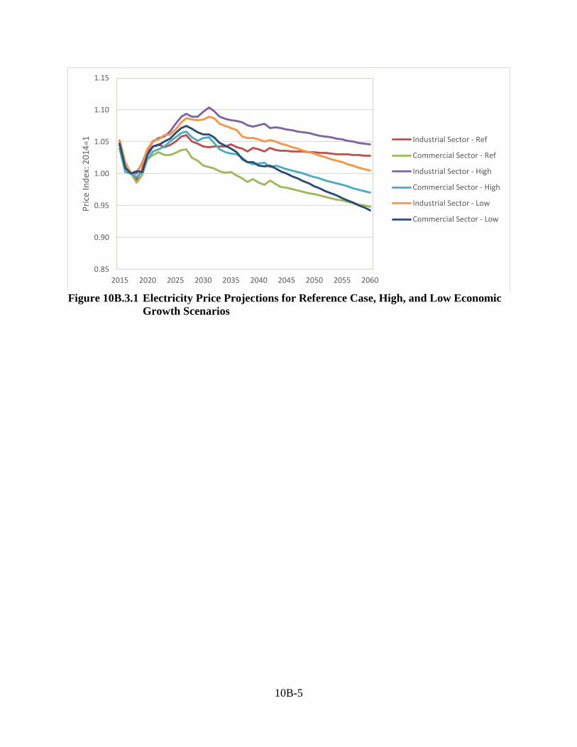
10B-5

Figure 10B.3.1 Electricity Price Projections for Reference Case, High, and Low Economic

Growth Scenarios

0.85

0.90

0.95

1.00

1.05

1.10

1.15

2015 2020 2025 2030 2035 2040 2045 2050 2055 2060

Pric

e In

dex:

201

4=1 Industrial Sector - Ref

Commercial Sector - Ref

Industrial Sector - High

Commercial Sector - High

Industrial Sector - Low

Commercial Sector - Low

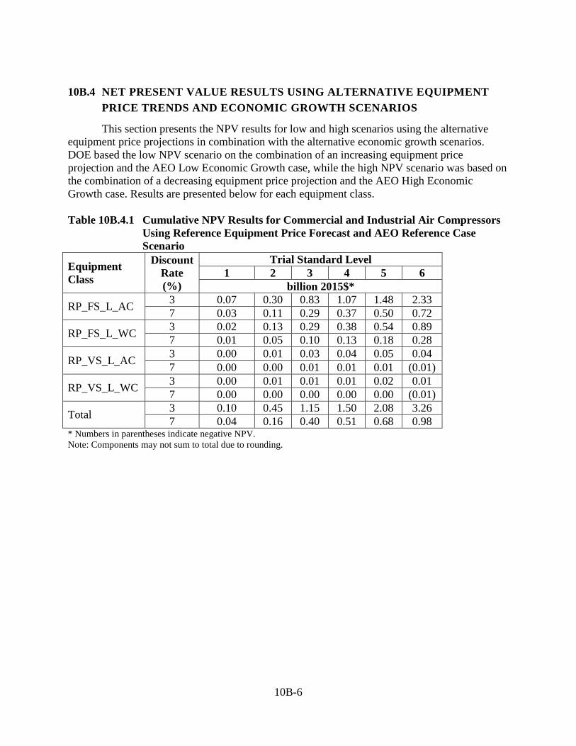
10B-6

10B.4 NET PRESENT VALUE RESULTS USING ALTERNATIVE EQUIPMENT PRICE TRENDS AND ECONOMIC GROWTH SCENARIOS

This section presents the NPV results for low and high scenarios using the alternative equipment price projections in combination with the alternative economic growth scenarios. DOE based the low NPV scenario on the combination of an increasing equipment price projection and the AEO Low Economic Growth case, while the high NPV scenario was based on the combination of a decreasing equipment price projection and the AEO High Economic Growth case. Results are presented below for each equipment class. Table 10B.4.1 Cumulative NPV Results for Commercial and Industrial Air Compressors

Using Reference Equipment Price Forecast and AEO Reference Case Scenario

Equipment Class

Discount Rate (%)

Trial Standard Level 1 2 3 4 5 6

billion 2015$*

RP_FS_L_AC 3 0.07 0.30 0.83 1.07 1.48 2.33 7 0.03 0.11 0.29 0.37 0.50 0.72

RP_FS_L_WC 3 0.02 0.13 0.29 0.38 0.54 0.89 7 0.01 0.05 0.10 0.13 0.18 0.28

RP_VS_L_AC 3 0.00 0.01 0.03 0.04 0.05 0.04 7 0.00 0.00 0.01 0.01 0.01 (0.01)

RP_VS_L_WC 3 0.00 0.01 0.01 0.01 0.02 0.01 7 0.00 0.00 0.00 0.00 0.00 (0.01)

Total 3 0.10 0.45 1.15 1.50 2.08 3.26 7 0.04 0.16 0.40 0.51 0.68 0.98

* Numbers in parentheses indicate negative NPV. Note: Components may not sum to total due to rounding.

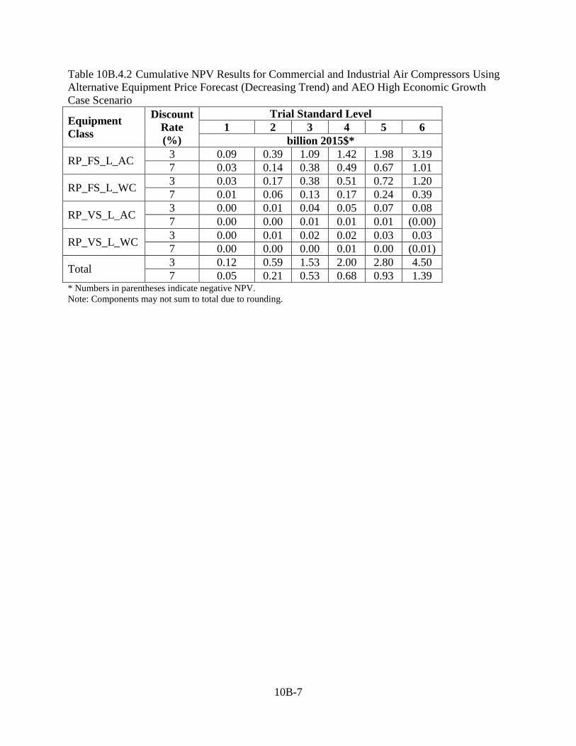
10B-7

Table 10B.4.2 Cumulative NPV Results for Commercial and Industrial Air Compressors Using Alternative Equipment Price Forecast (Decreasing Trend) and AEO High Economic Growth Case Scenario

Equipment Class

Discount Rate (%)

Trial Standard Level 1 2 3 4 5 6

billion 2015$*

RP_FS_L_AC 3 0.09 0.39 1.09 1.42 1.98 3.19 7 0.03 0.14 0.38 0.49 0.67 1.01

RP_FS_L_WC 3 0.03 0.17 0.38 0.51 0.72 1.20 7 0.01 0.06 0.13 0.17 0.24 0.39

RP_VS_L_AC 3 0.00 0.01 0.04 0.05 0.07 0.08 7 0.00 0.00 0.01 0.01 0.01 (0.00)

RP_VS_L_WC 3 0.00 0.01 0.02 0.02 0.03 0.03 7 0.00 0.00 0.00 0.01 0.00 (0.01)

Total 3 0.12 0.59 1.53 2.00 2.80 4.50 7 0.05 0.21 0.53 0.68 0.93 1.39

* Numbers in parentheses indicate negative NPV. Note: Components may not sum to total due to rounding.

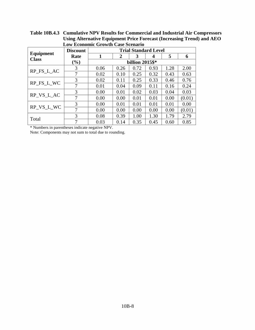
10B-8

Table 10B.4.3 Cumulative NPV Results for Commercial and Industrial Air Compressors Using Alternative Equipment Price Forecast (Increasing Trend) and AEO Low Economic Growth Case Scenario

Equipment Class

Discount Rate (%)

Trial Standard Level 1 2 3 4 5 6

billion 2015$*

RP_FS_L_AC 3 0.06 0.26 0.72 0.93 1.28 2.00 7 0.02 0.10 0.25 0.32 0.43 0.63

RP_FS_L_WC 3 0.02 0.11 0.25 0.33 0.46 0.76 7 0.01 0.04 0.09 0.11 0.16 0.24

RP_VS_L_AC 3 0.00 0.01 0.02 0.03 0.04 0.03 7 0.00 0.00 0.01 0.01 0.00 (0.01)

RP_VS_L_WC 3 0.00 0.01 0.01 0.01 0.01 0.00 7 0.00 0.00 0.00 0.00 0.00 (0.01)

Total 3 0.08 0.39 1.00 1.30 1.79 2.79 7 0.03 0.14 0.35 0.45 0.60 0.85

* Numbers in parentheses indicate negative NPV. Note: Components may not sum to total due to rounding.

10B-9

REFERENCES 1 Energy Information Administration, Annual Energy Outlook 2016 with Projections to 2040,

2016. Washington, DC. http://www.eia.gov/forecasts/aeo/pdf/0383(2016).pdf

2 Taylor, Margaret, and Sydny K. Fujita. Accounting for Technological Change in Regulatory Impact Analyses: The Learning Curve Technique. Berkeley: Lawrence Berkeley National Laboratory, 2013. LBNL-6195E

3 Energy Information Administration, Macroeconomic Activity Module for Annual Energy Outlook 2014, 2014. Washington, DC. <http://www.eia.gov/forecasts/aeo/assumptions/pdf/macroeconomic.pdf>

10C-i

APPENDIX 10C. NATIONAL IMPACTS ANALYSIS USING ALTERNATIVE EFFICIENCY TREND SCENARIOS

TABLE OF CONTENTS 10C.1 INTRODUCTION .................................................................................................10C-1 10C.2 RESULTS FOR THE 0.5 PERCENT EFFICIENCY SHIFT SCENARIO ...........10C-2 10C.3 RESULTS FOR THE 1 PERCENT EFFICIENCY SHIFT SCENARIO ..............10C-3

LIST OF TABLES

Table 10C.1.1 Distribution of Compressor Efficiencies in the No-New-Standards Case (2013) ................................................................................................10C-1

Table 10C.2.1 Distribution of Compressor Efficiencies in the No-New-Standards Case, 0.5 Percent Shift Scenario ................................................................10C-2

Table 10C.2.2 Cumulative National Full-Fuel-Cycle Energy Savings .............................10C-2 Table 10C.2.3 Net Present Value of Consumer Benefits at 3-Percent Discount Rate ......10C-2 Table 10C.2.4 Net Present Value of Consumer Benefits at a 7-Percent Discount Rate....10C-3 Table 10C.3.1 Distribution of Compressor Efficiencies in the No-New-Standards

Case, 1.0 Percent Shift Scenario ................................................................10C-3 Table 10C.3.2 Cumulative National Full-Fuel-Cycle Energy Savings .............................10C-3 Table 10C.3.3 Net Present Value of Consumer Benefits at 3-Percent Discount Rate ......10C-4 Table 10C.3.4 Net Present Value of Consumer Benefits at 7-Percent Discount Rate ......10C-4

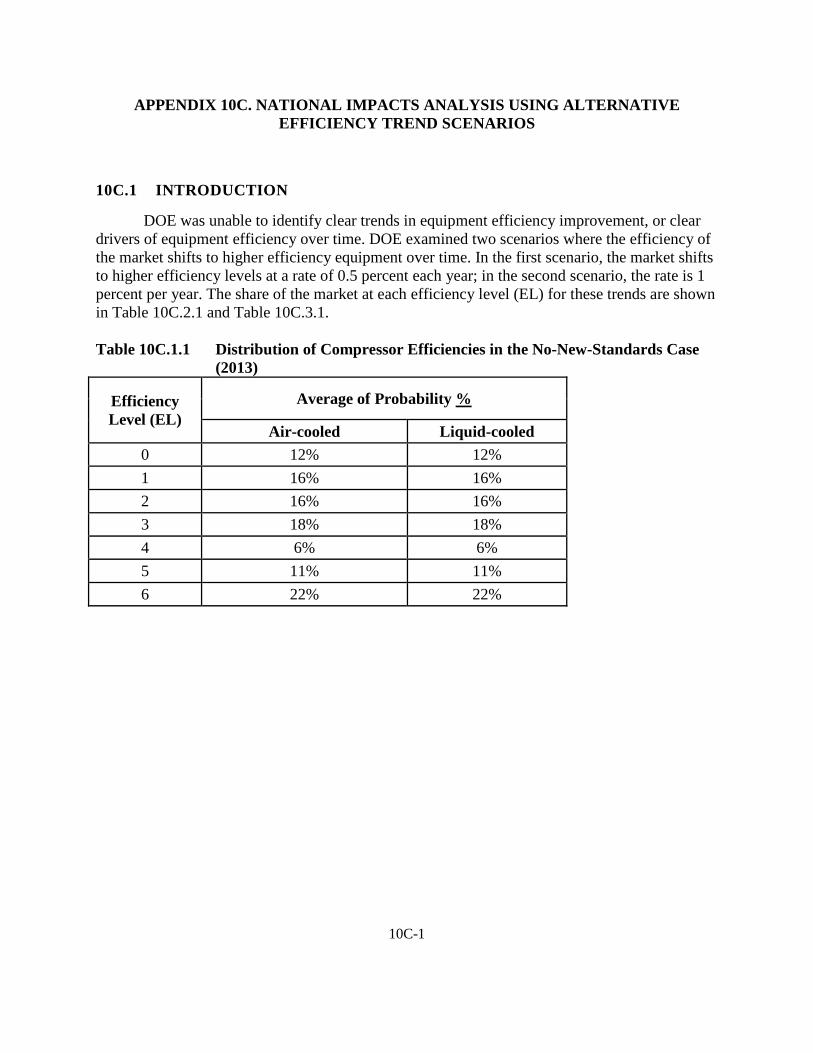
10C-1

APPENDIX 10C. NATIONAL IMPACTS ANALYSIS USING ALTERNATIVE EFFICIENCY TREND SCENARIOS

10C.1 INTRODUCTION

DOE was unable to identify clear trends in equipment efficiency improvement, or clear drivers of equipment efficiency over time. DOE examined two scenarios where the efficiency of the market shifts to higher efficiency equipment over time. In the first scenario, the market shifts to higher efficiency levels at a rate of 0.5 percent each year; in the second scenario, the rate is 1 percent per year. The share of the market at each efficiency level (EL) for these trends are shown in Table 10C.2.1 and Table 10C.3.1. Table 10C.1.1 Distribution of Compressor Efficiencies in the No-New-Standards Case

(2013)

Efficiency Level (EL)

Average of Probability %

Air-cooled Liquid-cooled 0 12% 12% 1 16% 16% 2 16% 16% 3 18% 18% 4 6% 6% 5 11% 11% 6 22% 22%

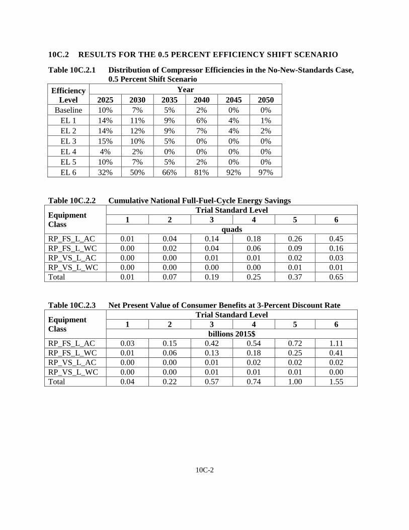
10C-2

10C.2 RESULTS FOR THE 0.5 PERCENT EFFICIENCY SHIFT SCENARIO

Table 10C.2.1 Distribution of Compressor Efficiencies in the No-New-Standards Case, 0.5 Percent Shift Scenario

Efficiency Level

Year 2025 2030 2035 2040 2045 2050

Baseline 10% 7% 5% 2% 0% 0% EL 1 14% 11% 9% 6% 4% 1% EL 2 14% 12% 9% 7% 4% 2% EL 3 15% 10% 5% 0% 0% 0% EL 4 4% 2% 0% 0% 0% 0% EL 5 10% 7% 5% 2% 0% 0% EL 6 32% 50% 66% 81% 92% 97%

Table 10C.2.2 Cumulative National Full-Fuel-Cycle Energy Savings

Equipment Class

Trial Standard Level 1 2 3 4 5 6

quads RP_FS_L_AC 0.01 0.04 0.14 0.18 0.26 0.45 RP_FS_L_WC 0.00 0.02 0.04 0.06 0.09 0.16 RP_VS_L_AC 0.00 0.00 0.01 0.01 0.02 0.03 RP_VS_L_WC 0.00 0.00 0.00 0.00 0.01 0.01 Total 0.01 0.07 0.19 0.25 0.37 0.65 Table 10C.2.3 Net Present Value of Consumer Benefits at 3-Percent Discount Rate

Equipment Class

Trial Standard Level 1 2 3 4 5 6

billions 2015$ RP_FS_L_AC 0.03 0.15 0.42 0.54 0.72 1.11 RP_FS_L_WC 0.01 0.06 0.13 0.18 0.25 0.41 RP_VS_L_AC 0.00 0.00 0.01 0.02 0.02 0.02 RP_VS_L_WC 0.00 0.00 0.01 0.01 0.01 0.00 Total 0.04 0.22 0.57 0.74 1.00 1.55

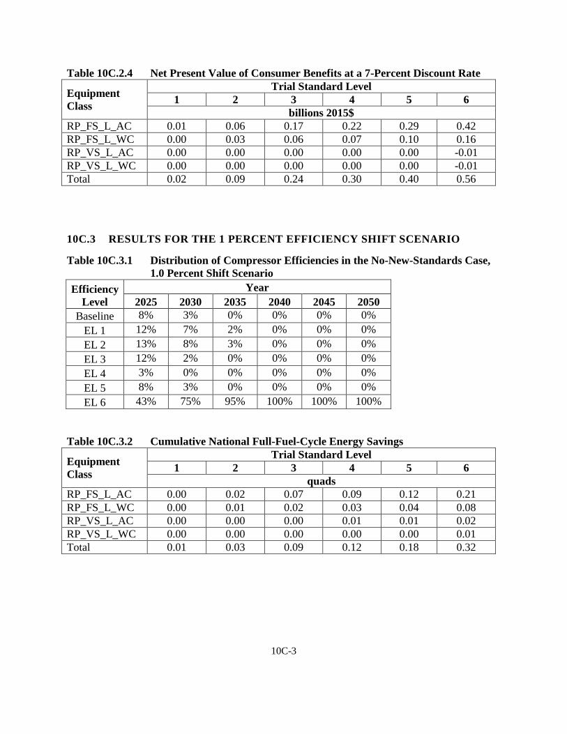
10C-3

Table 10C.2.4 Net Present Value of Consumer Benefits at a 7-Percent Discount Rate

Equipment Class

Trial Standard Level 1 2 3 4 5 6

billions 2015$ RP_FS_L_AC 0.01 0.06 0.17 0.22 0.29 0.42 RP_FS_L_WC 0.00 0.03 0.06 0.07 0.10 0.16 RP_VS_L_AC 0.00 0.00 0.00 0.00 0.00 -0.01 RP_VS_L_WC 0.00 0.00 0.00 0.00 0.00 -0.01 Total 0.02 0.09 0.24 0.30 0.40 0.56

10C.3 RESULTS FOR THE 1 PERCENT EFFICIENCY SHIFT SCENARIO

Table 10C.3.1 Distribution of Compressor Efficiencies in the No-New-Standards Case, 1.0 Percent Shift Scenario

Efficiency Level

Year 2025 2030 2035 2040 2045 2050

Baseline 8% 3% 0% 0% 0% 0% EL 1 12% 7% 2% 0% 0% 0% EL 2 13% 8% 3% 0% 0% 0% EL 3 12% 2% 0% 0% 0% 0% EL 4 3% 0% 0% 0% 0% 0% EL 5 8% 3% 0% 0% 0% 0% EL 6 43% 75% 95% 100% 100% 100%

Table 10C.3.2 Cumulative National Full-Fuel-Cycle Energy Savings

Equipment Class

Trial Standard Level 1 2 3 4 5 6

quads RP_FS_L_AC 0.00 0.02 0.07 0.09 0.12 0.21 RP_FS_L_WC 0.00 0.01 0.02 0.03 0.04 0.08 RP_VS_L_AC 0.00 0.00 0.00 0.01 0.01 0.02 RP_VS_L_WC 0.00 0.00 0.00 0.00 0.00 0.01 Total 0.01 0.03 0.09 0.12 0.18 0.32

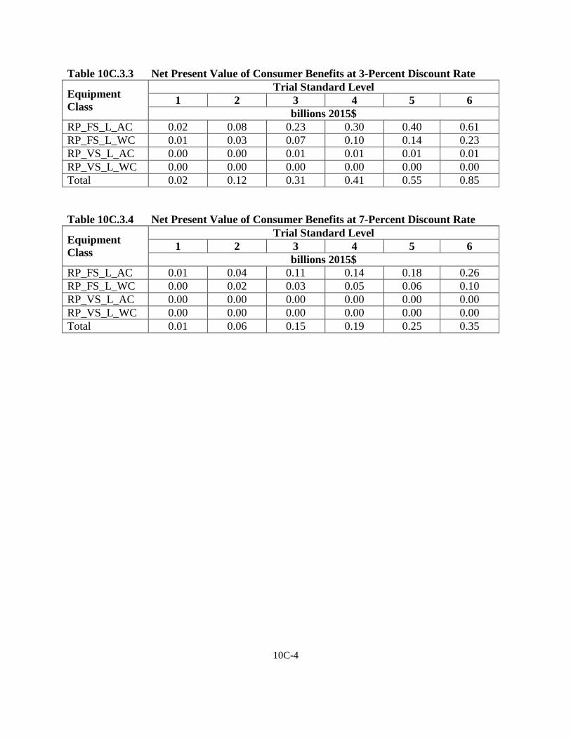
10C-4

Table 10C.3.3 Net Present Value of Consumer Benefits at 3-Percent Discount Rate

Equipment Class

Trial Standard Level 1 2 3 4 5 6

billions 2015$ RP_FS_L_AC 0.02 0.08 0.23 0.30 0.40 0.61 RP_FS_L_WC 0.01 0.03 0.07 0.10 0.14 0.23 RP_VS_L_AC 0.00 0.00 0.01 0.01 0.01 0.01 RP_VS_L_WC 0.00 0.00 0.00 0.00 0.00 0.00 Total 0.02 0.12 0.31 0.41 0.55 0.85 Table 10C.3.4 Net Present Value of Consumer Benefits at 7-Percent Discount Rate

Equipment Class

Trial Standard Level 1 2 3 4 5 6

billions 2015$ RP_FS_L_AC 0.01 0.04 0.11 0.14 0.18 0.26 RP_FS_L_WC 0.00 0.02 0.03 0.05 0.06 0.10 RP_VS_L_AC 0.00 0.00 0.00 0.00 0.00 0.00 RP_VS_L_WC 0.00 0.00 0.00 0.00 0.00 0.00 Total 0.01 0.06 0.15 0.19 0.25 0.35

12A-i

APPENDIX 12A. MANUFACTURER IMPACT ANALYSIS INTERVIEW GUIDE

TABLE OF CONTENTS

12A.1 MANUFACTURER IMPACT ANALYSIS INTERVIEW GUIDE FOR

COMPRESSORS ..............................................................................................................1

12A-1

CHAPTER 12. MANUFACTURER IMPACT ANALYSIS INTERVIEW GUIDE

12A.1 MANUFACTURER IMPACT ANALYSIS INTERVIEW GUIDE FOR COMPRESSORS

GENERAL INTRODUCTION Thank you for expressing interest in participating in The U.S. Department of Energy (DOE) Manufacturer Impact Analysis for the commercial and industrial compressors rulemaking. Currently, there are no established energy conservation standards for commercial and industrial compressors. DOE has initiated a rulemaking process to develop such standards based on the authority described below. For this rule, the process includes three major phases:

1. The publication of a framework document in which DOE describes the overall approach it is considering in developing potential energy conservation standards for a particular product or equipment;

2. The issuance of a notice of proposed rulemaking (NOPR); and 3. The issuance of a final rule.

At each of the first two steps, DOE holds a public meeting and solicits comments from the stakeholders on issues relevant to the development of potential standards. It should also be noted that a separate rulemaking process to establish a test procedure for the covered equipment will run in parallel to the energy conservation standards rulemaking. The resulting test procedure will establish both a metric and method for measuring the energy consumption of the equipment. (For more information on the test procedure rulemaking see: http://www1.eere.energy.gov/buildings/appliance_standards/product.aspx/productid/78) History of this rulemaking to date: The framework document for commercial and industrial compressors was published in January 2014 and comments on the framework were accepted through April 22, 2014. The next phase of the rulemaking is the preliminary analysis during which DOE will consider feedback on the approach presented in the framework and explore methods to establish trial standards levels (TSLs). TSLs span the range of efficiencies from the most basic equipment to the most efficient technology (max-tech) that is both feasible and cost effective. DOE conducts an engineering analysis to determine the costs associated with increasing efficiency from the baseline to various higher levels of efficiency. Authority:

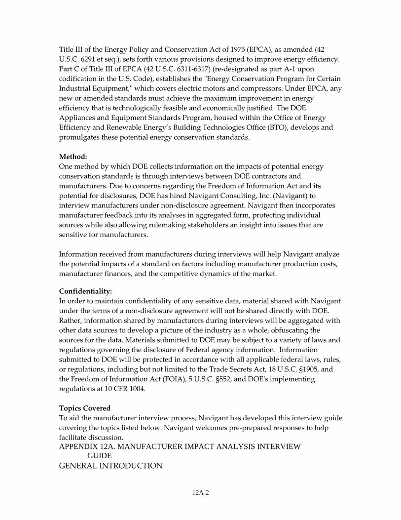
12A-2

Title III of the Energy Policy and Conservation Act of 1975 (EPCA), as amended (42 U.S.C. 6291 et seq.), sets forth various provisions designed to improve energy efficiency. Part C of Title III of EPCA (42 U.S.C. 6311-6317) (re-designated as part A-1 upon codification in the U.S. Code), establishes the "Energy Conservation Program for Certain Industrial Equipment," which covers electric motors and compressors. Under EPCA, any new or amended standards must achieve the maximum improvement in energy efficiency that is technologically feasible and economically justified. The DOE Appliances and Equipment Standards Program, housed within the Office of Energy Efficiency and Renewable Energy’s Building Technologies Office (BTO), develops and promulgates these potential energy conservation standards. Method: One method by which DOE collects information on the impacts of potential energy conservation standards is through interviews between DOE contractors and manufacturers. Due to concerns regarding the Freedom of Information Act and its potential for disclosures, DOE has hired Navigant Consulting, Inc. (Navigant) to interview manufacturers under non-disclosure agreement. Navigant then incorporates manufacturer feedback into its analyses in aggregated form, protecting individual sources while also allowing rulemaking stakeholders an insight into issues that are sensitive for manufacturers. Information received from manufacturers during interviews will help Navigant analyze the potential impacts of a standard on factors including manufacturer production costs, manufacturer finances, and the competitive dynamics of the market.

Confidentiality: In order to maintain confidentiality of any sensitive data, material shared with Navigant under the terms of a non-disclosure agreement will not be shared directly with DOE. Rather, information shared by manufacturers during interviews will be aggregated with other data sources to develop a picture of the industry as a whole, obfuscating the sources for the data. Materials submitted to DOE may be subject to a variety of laws and regulations governing the disclosure of Federal agency information. Information submitted to DOE will be protected in accordance with all applicable federal laws, rules, or regulations, including but not limited to the Trade Secrets Act, 18 U.S.C. §1905, and the Freedom of Information Act (FOIA), 5 U.S.C. §552, and DOE's implementing regulations at 10 CFR 1004. Topics Covered To aid the manufacturer interview process, Navigant has developed this interview guide covering the topics listed below. Navigant welcomes pre-prepared responses to help facilitate discussion. APPENDIX 12A. MANUFACTURER IMPACT ANALYSIS INTERVIEW

GUIDE GENERAL INTRODUCTION

12A-3

INTRODUCTION TO MANUFACTURER IMPACTS INTRODUCTION TO SCOPE AND ANALYTICAL STRUCTURE KEY ISSUES COMPANY OVERVIEW AND ORGANIZATIONAL

CHARACTERISTICS INDUSTRY STRUCTURE AND COMPETITION FINANCIAL PARAMETERS MARKUPS AND PROFITABILITY CONVERSION COSTS DIRECT EMPLOYMENT, FOREIGN COMPETITION, AND

OUTSOURCING CUMULATIVE REGULATORY BURDEN IMPACTS ON SMALL BUSINESS

Contact Information If you have any questions, please contact: Daniel Weintraub 781.270.8397 daniel.weintraub@navigant.com

12A-4

INTRODUCTION TO MANUFACTURER IMPACTS The Department of Energy (DOE) conducts the manufacturer impact analysis (MIA) as part of the rulemaking process for potential new energy conservation standards for air compressors. In this analysis, DOE uses publicly available information and information provided by manufacturers during interviews to assess possible impacts on manufacturers due to potential new energy conservation standards. INTRODUCTION TO SCOPE AND ANALYTICAL STRUCTURE Scope of this Interview Guide Although DOE has not established a scope of applicability (coverage) for this energy conservation standard, this interview guide will primarily focus on Air Compressors of the following types:

• Compression Type: Rotary Positive or Reciprocating, • Lubrication Type: Lubricated or Non-Lubricated, and • Speed Type: Fixed-Speed or Variable-Speed.

For these types of air compressors, this interview guide will consider air compressors within the following scope:

• Pressures >30 and <225 psig • Required shaft horsepower ≥1 and ≤500 horsepower.

Equipment Groups

For this energy conversation standard, DOE may choose to subdivide the covered population of air compressors into “Equipment Classes.” Equipment classes are often defined by differences in utility to the customer, ability to meet a certain efficiency level, or design features, and may ultimately be subject to different minimum efficiency standards. DOE has not yet established equipment classes for air compressors. In the absence of equipment classes, this analysis will subdivide the population of air compressors into discrete “equipment groups.” These equipment groups are for analytical purposes only. Ultimately, interview guide responses will be translated to the equipment classes selected by DOE. For these equipment groups, the top level differentiation is based on compression type: Rotary Positive or Reciprocating. The next level is grouped by lubrication type: Lubricated or Non-lubricated. The final level is grouped by speed type: Variable- or Fix-

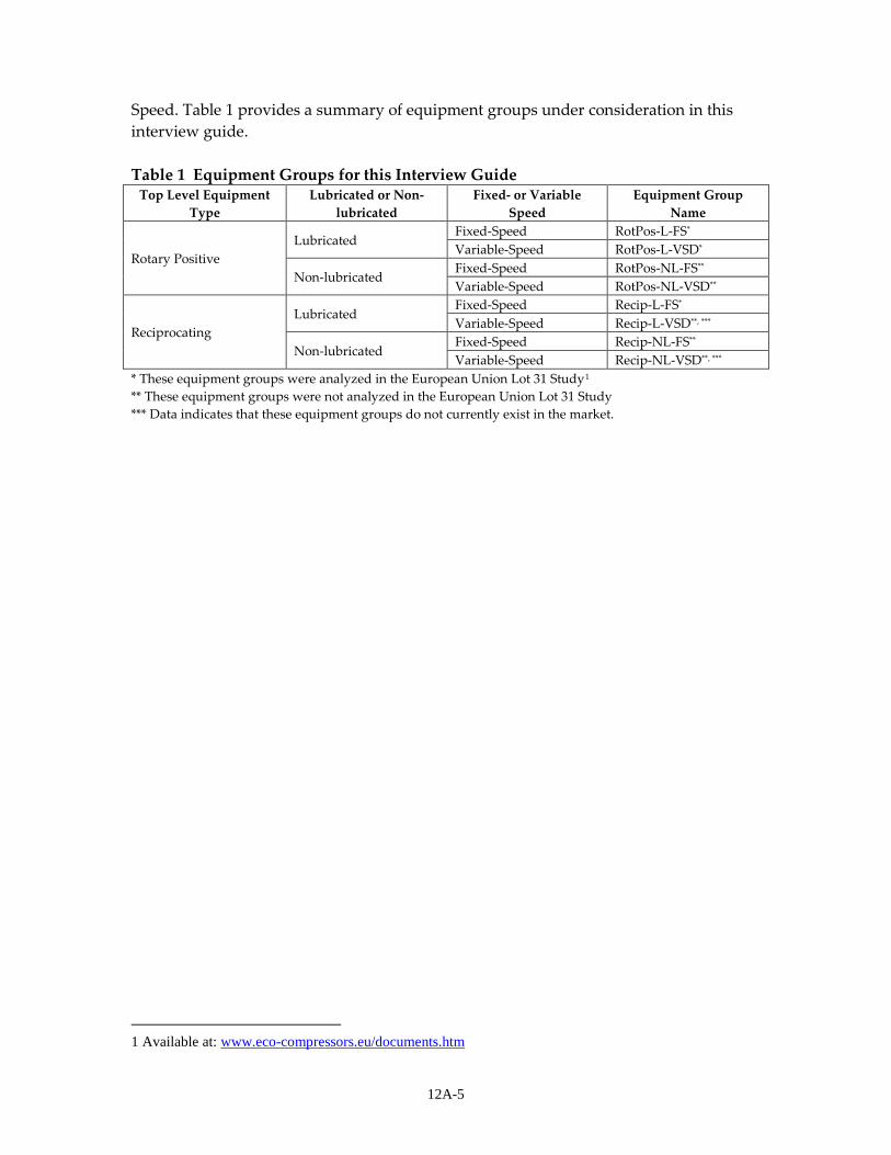
12A-5

Speed. Table 1 provides a summary of equipment groups under consideration in this interview guide. Table 1 Equipment Groups for this Interview Guide

Top Level Equipment Type

Lubricated or Non-lubricated

Fixed- or Variable Speed

Equipment Group Name

Rotary Positive Lubricated

Fixed-Speed RotPos-L-FS* Variable-Speed RotPos-L-VSD*

Non-lubricated Fixed-Speed RotPos-NL-FS** Variable-Speed RotPos-NL-VSD**

Reciprocating Lubricated

Fixed-Speed Recip-L-FS* Variable-Speed Recip-L-VSD**, ***

Non-lubricated Fixed-Speed Recip-NL-FS** Variable-Speed Recip-NL-VSD**, ***

* These equipment groups were analyzed in the European Union Lot 31 Study1 ** These equipment groups were not analyzed in the European Union Lot 31 Study *** Data indicates that these equipment groups do not currently exist in the market.

1 Available at: www.eco-compressors.eu/documents.htm

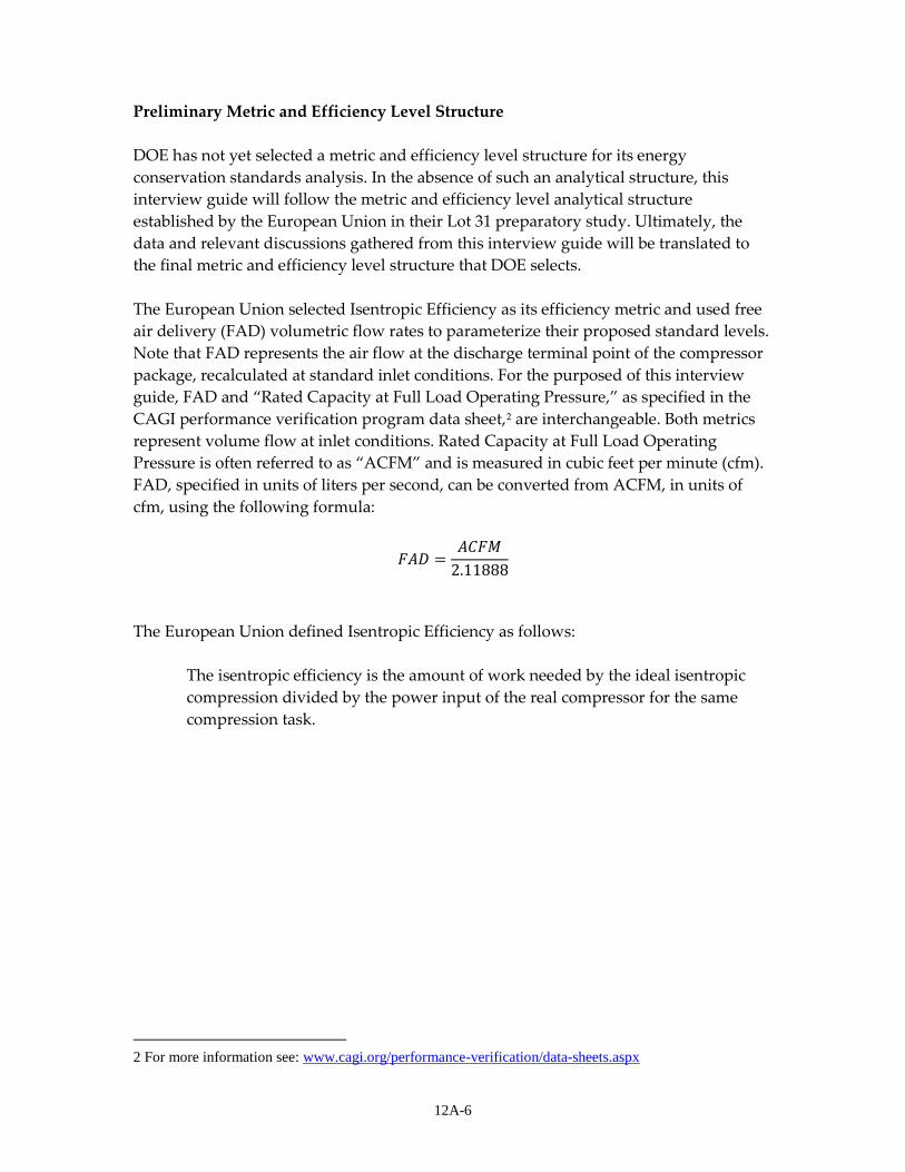
12A-6

Preliminary Metric and Efficiency Level Structure DOE has not yet selected a metric and efficiency level structure for its energy conservation standards analysis. In the absence of such an analytical structure, this interview guide will follow the metric and efficiency level analytical structure established by the European Union in their Lot 31 preparatory study. Ultimately, the data and relevant discussions gathered from this interview guide will be translated to the final metric and efficiency level structure that DOE selects. The European Union selected Isentropic Efficiency as its efficiency metric and used free air delivery (FAD) volumetric flow rates to parameterize their proposed standard levels. Note that FAD represents the air flow at the discharge terminal point of the compressor package, recalculated at standard inlet conditions. For the purposed of this interview guide, FAD and “Rated Capacity at Full Load Operating Pressure,” as specified in the CAGI performance verification program data sheet,2 are interchangeable. Both metrics represent volume flow at inlet conditions. Rated Capacity at Full Load Operating Pressure is often referred to as “ACFM” and is measured in cubic feet per minute (cfm). FAD, specified in units of liters per second, can be converted from ACFM, in units of cfm, using the following formula:

𝐹𝐹𝐹𝐹𝐹𝐹 =𝐹𝐹𝐴𝐴𝐹𝐹𝐴𝐴

2.11888

The European Union defined Isentropic Efficiency as follows:

The isentropic efficiency is the amount of work needed by the ideal isentropic compression divided by the power input of the real compressor for the same compression task.

2 For more information see: www.cagi.org/performance-verification/data-sheets.aspx

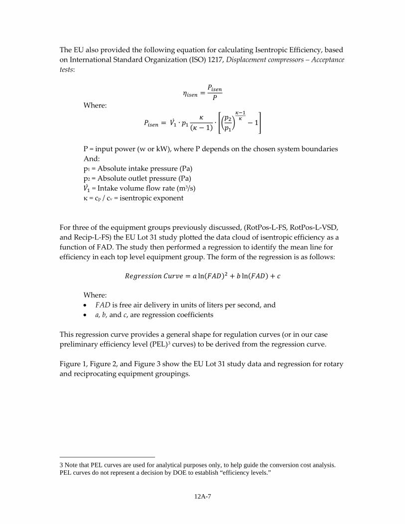
12A-7

The EU also provided the following equation for calculating Isentropic Efficiency, based on International Standard Organization (ISO) 1217, Displacement compressors – Acceptance tests:

𝜂𝜂𝑖𝑖𝑖𝑖𝑖𝑖𝑖𝑖 =𝑃𝑃𝑖𝑖𝑖𝑖𝑖𝑖𝑖𝑖𝑃𝑃

Where:

𝑃𝑃𝑖𝑖𝑖𝑖𝑖𝑖𝑖𝑖 = 𝑉𝑉1̇ ∙ 𝑝𝑝1𝜅𝜅

(𝜅𝜅 − 1) ∙ ��𝑝𝑝2𝑝𝑝1�𝜅𝜅−1𝜅𝜅− 1�

P = input power (w or kW), where P depends on the chosen system boundaries And: p1 = Absolute intake pressure (Pa) p2 = Absolute outlet pressure (Pa) 𝑉𝑉1̇ = Intake volume flow rate (m3/s) κ = cp / cv = isentropic exponent

For three of the equipment groups previously discussed, (RotPos-L-FS, RotPos-L-VSD, and Recip-L-FS) the EU Lot 31 study plotted the data cloud of isentropic efficiency as a function of FAD. The study then performed a regression to identify the mean line for efficiency in each top level equipment group. The form of the regression is as follows:

𝑅𝑅𝑅𝑅𝑅𝑅𝑅𝑅𝑅𝑅𝑅𝑅𝑅𝑅𝑅𝑅𝑅𝑅𝑅𝑅 𝐴𝐴𝐶𝐶𝑅𝑅𝐶𝐶𝑅𝑅 = 𝑎𝑎 ln(𝐹𝐹𝐹𝐹𝐹𝐹)2 + 𝑏𝑏 ln(𝐹𝐹𝐹𝐹𝐹𝐹) + 𝑐𝑐

Where: • FAD is free air delivery in units of liters per second, and • a, b, and c, are regression coefficients

This regression curve provides a general shape for regulation curves (or in our case preliminary efficiency level (PEL)3 curves) to be derived from the regression curve. Figure 1, Figure 2, and Figure 3 show the EU Lot 31 study data and regression for rotary and reciprocating equipment groupings.

3 Note that PEL curves are used for analytical purposes only, to help guide the conversion cost analysis. PEL curves do not represent a decision by DOE to establish “efficiency levels.”

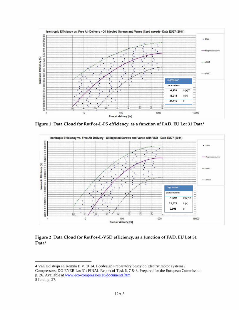
12A-8

Figure 1 Data Cloud for RotPos-L-FS efficiency, as a function of FAD. EU Lot 31 Data4

Figure 2 Data Cloud for RotPos-L-VSD efficiency, as a function of FAD. EU Lot 31 Data5

4 Van Holsteijn en Kemna B.V. 2014. Ecodesign Preparatory Study on Electric motor systems / Compressors; DG ENER Lot 31; FINAL Report of Task 6, 7 & 8. Prepared for the European Commission. p. 26. Available at www.eco-compressors.eu/documents.htm 5 Ibid., p. 27.

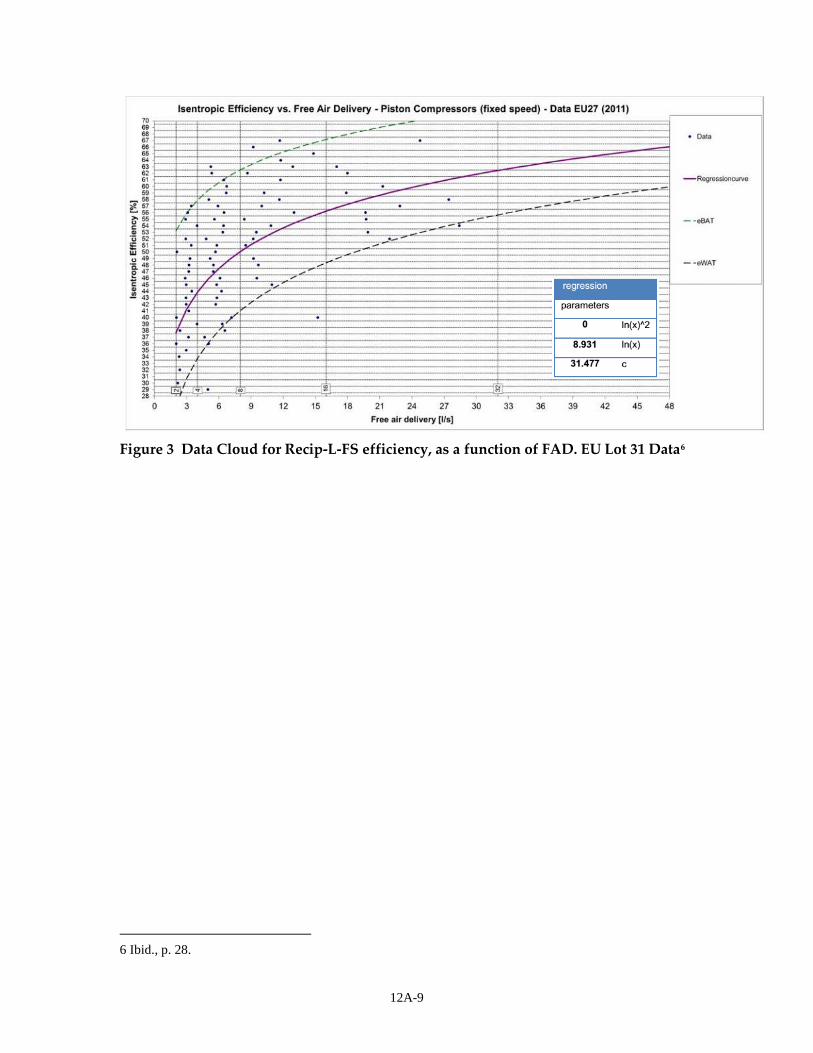
12A-9

Figure 3 Data Cloud for Recip-L-FS efficiency, as a function of FAD. EU Lot 31 Data6

6 Ibid., p. 28.

12A-10

The EU developed potential regulation curves (i.e., curves defining efficiency thresholds) that are derived from the regression curve. To do so, the EU defined the “d-value.” The d-value represents a percentage improvement from the regression curve to theoretical 100% isentropic efficiency. For example, a d-value of 100 would generate a regulation curve at 100% isentropic efficiency for all FAD flow rates. Alternatively, a d-value of 50 would generate a regulation curve that falls halfway between the regression curve and 100% isentropic efficiency, for all FAD flow rates. The d-value represents the improvement of a product, expressed as reduction of losses going from average (regression curve) to 100% efficiency (theoretical). Therefore, the formula to generate regulation curves (or PEL curves) is:

𝑃𝑃𝑃𝑃𝑃𝑃 𝐴𝐴𝐶𝐶𝑅𝑅𝐶𝐶𝑅𝑅 = 𝑅𝑅𝑅𝑅𝑅𝑅𝑅𝑅𝑅𝑅𝑅𝑅𝑅𝑅𝑅𝑅𝑅𝑅𝑅𝑅 𝐴𝐴𝐶𝐶𝑅𝑅𝐶𝐶𝑅𝑅 + �(100 − 𝑅𝑅𝑅𝑅𝑅𝑅𝑅𝑅𝑅𝑅𝑅𝑅𝑅𝑅𝑅𝑅𝑅𝑅𝑅𝑅 𝐴𝐴𝐶𝐶𝑅𝑅𝐶𝐶𝑅𝑅) ×𝑑𝑑

100�

Where d is the relative change in losses

For the interview guide analytical structure, the following PEL’s are being investigated:

1. the midpoint between the baseline7 and regression curve (lower 25th percentile),

2. the regression curve (lower 50th percentile), 3. the midpoint between the regression curve and maximum available

technology (lower 75th percentile),8 and 4. maximum available technology

Table 2 presents the d-values associated with each PEL for each equipment Group. As mentioned previously, the European Union only investigated RotPos-L-FS, RotPos-L-VSD, and Recip-L-FS equipment groups. For our analysis, the d-values for these three equipment groups will be applied to the remaining five equipment groups. Note: Navigant understands that non-lubricated and variable-speed units have inherently different efficiency characteristics than their counterparts. Additional data collection and analysis on all equipment groups is currently underway. Until that data collection is complete, proxy d-values for the five unanalyzed groups will be used.

7 Baseline is referred to as worst available technology (WAT) in the European Union Lot 31 study. 8 Maximum available technology is referred to as best available technology (BAT) in the European Union Lot 31 study.

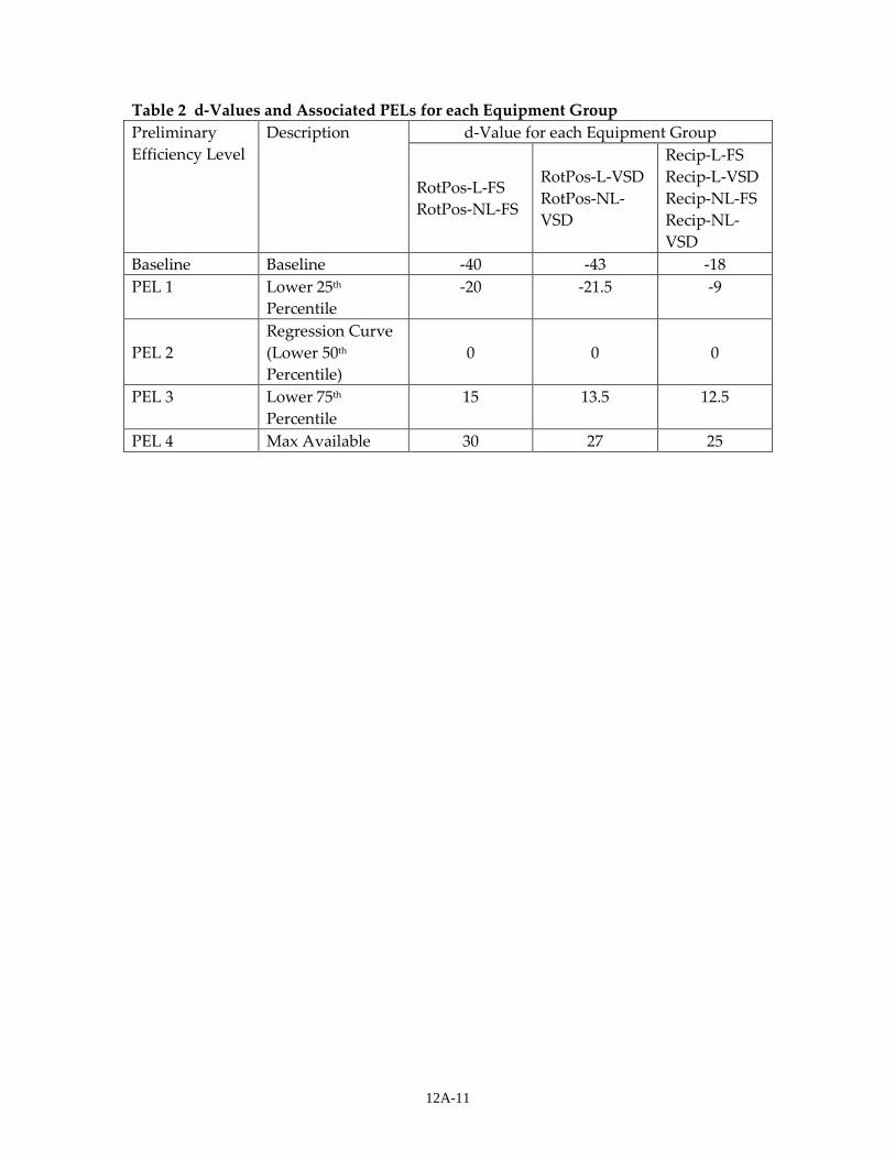
12A-11

Table 2 d-Values and Associated PELs for each Equipment Group Preliminary Efficiency Level

Description d-Value for each Equipment Group

RotPos-L-FS RotPos-NL-FS

RotPos-L-VSD RotPos-NL-VSD

Recip-L-FS Recip-L-VSD Recip-NL-FS Recip-NL-VSD

Baseline Baseline -40 -43 -18 PEL 1 Lower 25th

Percentile -20 -21.5 -9

PEL 2 Regression Curve (Lower 50th

Percentile) 0 0 0

PEL 3 Lower 75th Percentile

15 13.5 12.5

PEL 4 Max Available 30 27 25

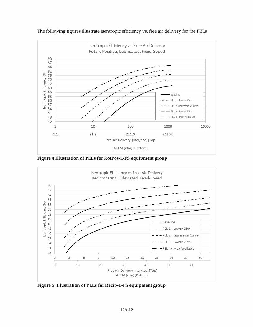
12A-12

The following figures illustrate isentropic efficiency vs. free air delivery for the PELs

Figure 4 Illustration of PELs for RotPos-L-FS equipment group

Figure 5 Illustration of PELs for Recip-L-FS equipment group

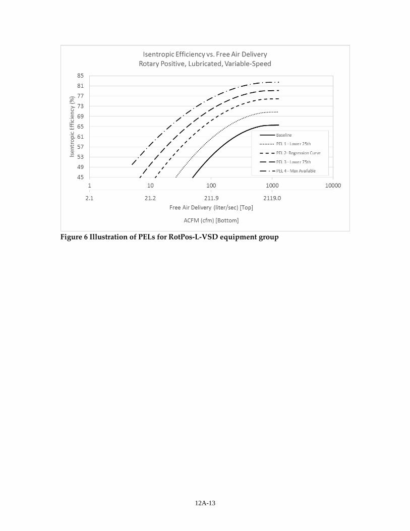
12A-13

Figure 6 Illustration of PELs for RotPos-L-VSD equipment group

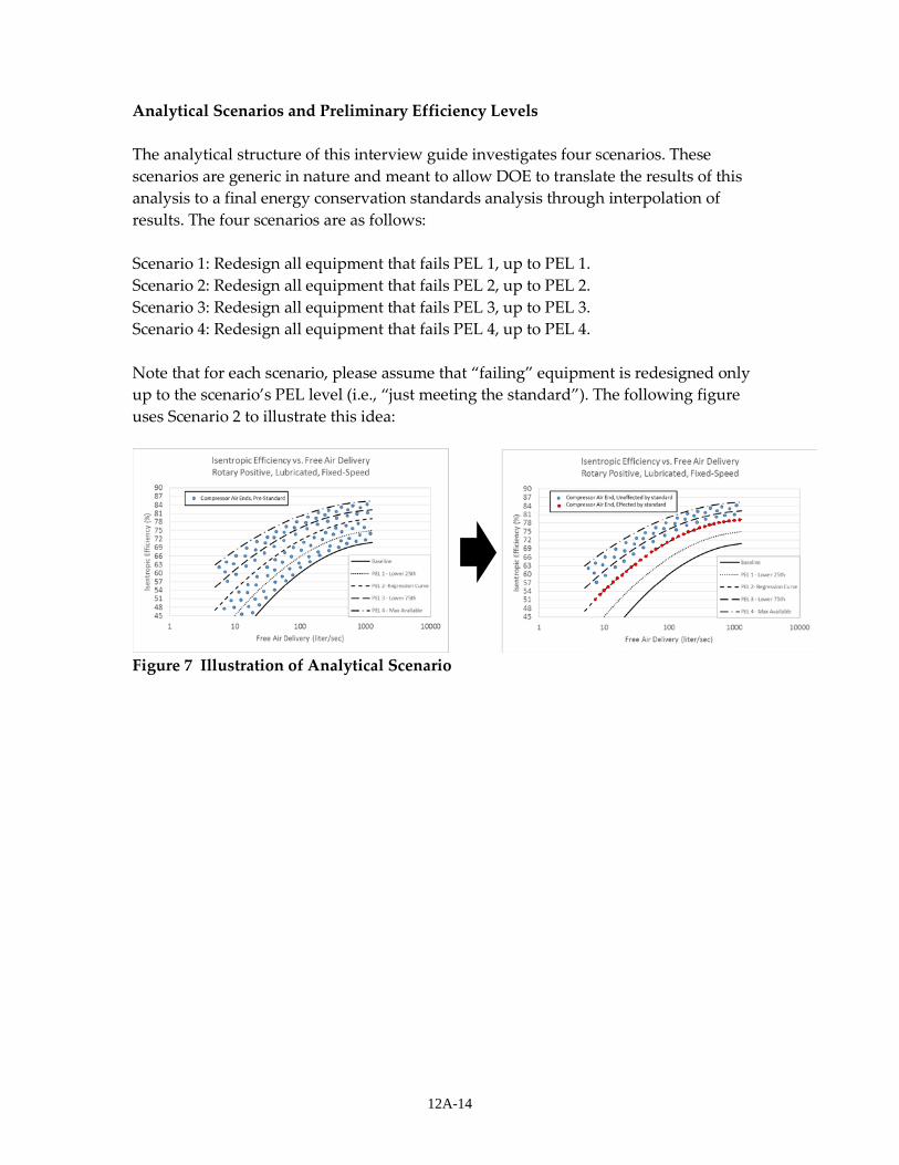
12A-14

Analytical Scenarios and Preliminary Efficiency Levels The analytical structure of this interview guide investigates four scenarios. These scenarios are generic in nature and meant to allow DOE to translate the results of this analysis to a final energy conservation standards analysis through interpolation of results. The four scenarios are as follows: Scenario 1: Redesign all equipment that fails PEL 1, up to PEL 1. Scenario 2: Redesign all equipment that fails PEL 2, up to PEL 2. Scenario 3: Redesign all equipment that fails PEL 3, up to PEL 3. Scenario 4: Redesign all equipment that fails PEL 4, up to PEL 4. Note that for each scenario, please assume that “failing” equipment is redesigned only up to the scenario’s PEL level (i.e., “just meeting the standard”). The following figure uses Scenario 2 to illustrate this idea:

Figure 7 Illustration of Analytical Scenario

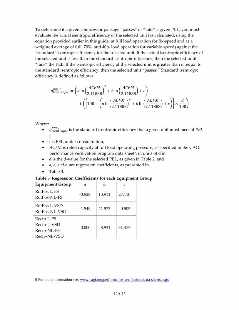
12A-15

To determine if a given compressor package “passes” or “fails” a given PEL, you must evaluate the actual isentropic efficiency of the selected unit (as calculated, using the equation provided earlier in this guide, at full load operation for fix-speed and as a weighted average of full, 70%, and 40% load operation for variable-speed) against the “standard” isentropic efficiency for the selected unit. If the actual isentropic efficiency of the selected unit is less than the standard isentropic efficiency, then the selected until “fails” the PEL. If the isentropic efficiency of the selected unit is greater than or equal to the standard isentropic efficiency, then the selected unit “passes.” Standard isentropic efficiency is defined as follows:

𝜂𝜂𝐼𝐼𝑖𝑖𝑖𝑖𝑖𝑖𝐼𝐼𝐼𝐼𝐼𝐼𝐼𝐼𝑖𝑖𝐼𝐼𝑃𝑃𝑃𝑃𝑃𝑃 𝑖𝑖 = �𝑎𝑎 ln �𝐹𝐹𝐴𝐴𝐹𝐹𝐴𝐴

2.11888�2

+ 𝑏𝑏 ln �𝐹𝐹𝐴𝐴𝐹𝐹𝐴𝐴

2.11888� + 𝑐𝑐�

+ ��100 − �𝑎𝑎 ln �𝐹𝐹𝐴𝐴𝐹𝐹𝐴𝐴

2.11888�2

+ 𝑏𝑏 ln �𝐹𝐹𝐴𝐴𝐹𝐹𝐴𝐴

2.11888� + 𝑐𝑐�� ×

𝑑𝑑100�

Where: • 𝜂𝜂𝐼𝐼𝑖𝑖𝑖𝑖𝑖𝑖𝐼𝐼𝐼𝐼𝐼𝐼𝐼𝐼𝑖𝑖𝐼𝐼𝑃𝑃𝑃𝑃𝑃𝑃 𝑖𝑖 is the standard isentropic efficiency that a given unit must meet at PEL

i, • i is PEL under consideration, • ACFM is rated capacity at full load operating pressure, as specified in the CAGI

performance verification program data sheet9, in units of cfm, • d is the d-value for the selected PEL, as given in Table 2, and • a, b, and c, are regression coefficients, as presented in • Table 3.

Table 3 Regression Coefficients for each Equipment Group Equipment Group a b c RotPos-L-FS RotPos-NL-FS

-0.928 13.911 27.110

RotPos-L-VSD RotPos-NL-VSD

-1.549 21.573 0.905

Recip-L-FS Recip-L-VSD Recip-NL-FS Recip-NL-VSD

0.000 8.931 31.477

9 For more information see: www.cagi.org/performance-verification/data-sheets.aspx

12A-16

KEY ISSUES DOE is interested in understanding the impact of energy conservation standards on manufacturers. This section provides an opportunity for manufacturers to identify high-priority issues that DOE should take into consideration when conducting the Manufacturer Impact Analysis. 1. In general, what are the key issues for your company regarding new energy conservation standards for air compressors?

2. Are any of the issues more or less significant for specific equipment groups?

3. Do any of the issues become more significant at higher Preliminary Efficiency Levels (PELs)?

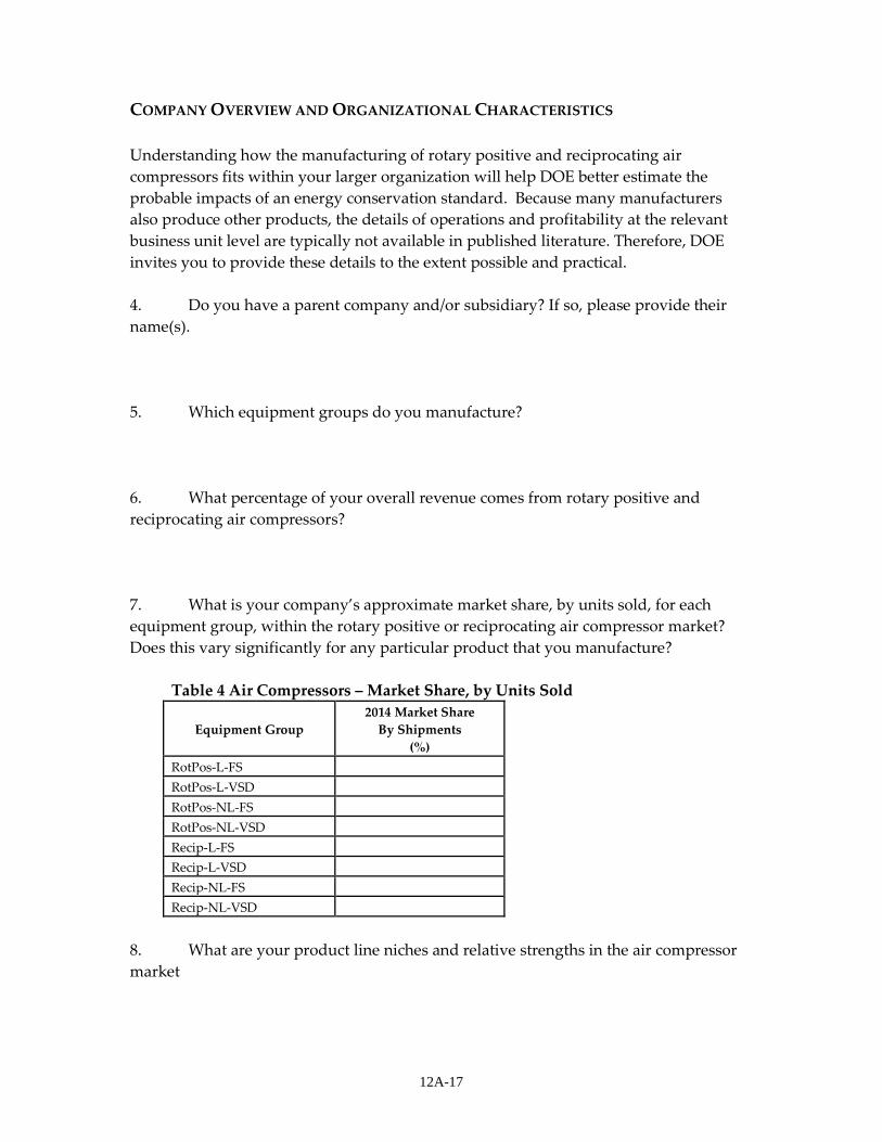
12A-17

COMPANY OVERVIEW AND ORGANIZATIONAL CHARACTERISTICS Understanding how the manufacturing of rotary positive and reciprocating air compressors fits within your larger organization will help DOE better estimate the probable impacts of an energy conservation standard. Because many manufacturers also produce other products, the details of operations and profitability at the relevant business unit level are typically not available in published literature. Therefore, DOE invites you to provide these details to the extent possible and practical. 4. Do you have a parent company and/or subsidiary? If so, please provide their name(s). 5. Which equipment groups do you manufacture? 6. What percentage of your overall revenue comes from rotary positive and reciprocating air compressors? 7. What is your company’s approximate market share, by units sold, for each equipment group, within the rotary positive or reciprocating air compressor market? Does this vary significantly for any particular product that you manufacture?

Table 4 Air Compressors – Market Share, by Units Sold

Equipment Group 2014 Market Share

By Shipments (%)

RotPos-L-FS RotPos-L-VSD RotPos-NL-FS RotPos-NL-VSD Recip-L-FS Recip-L-VSD Recip-NL-FS Recip-NL-VSD

8. What are your product line niches and relative strengths in the air compressor market

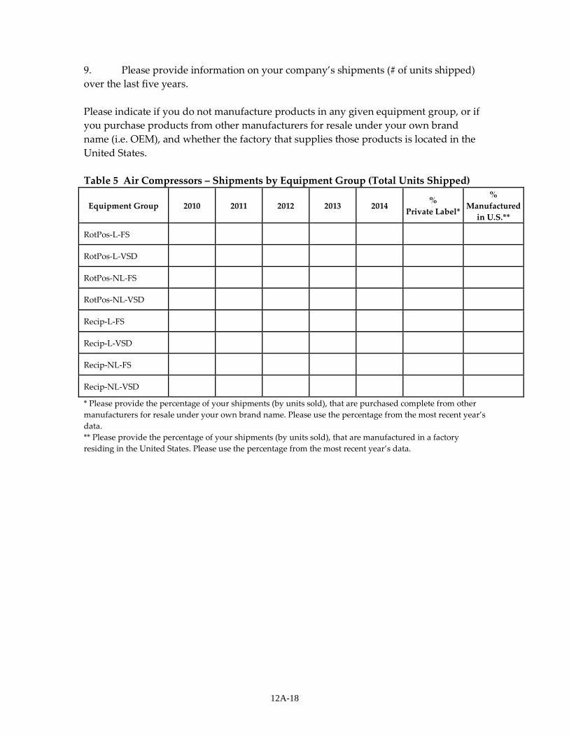
12A-18

9. Please provide information on your company’s shipments (# of units shipped) over the last five years. Please indicate if you do not manufacture products in any given equipment group, or if you purchase products from other manufacturers for resale under your own brand name (i.e. OEM), and whether the factory that supplies those products is located in the United States. Table 5 Air Compressors – Shipments by Equipment Group (Total Units Shipped)

Equipment Group 2010 2011 2012 2013 2014 % Private Label*

% Manufactured

in U.S.**

RotPos-L-FS

RotPos-L-VSD

RotPos-NL-FS

RotPos-NL-VSD

Recip-L-FS

Recip-L-VSD

Recip-NL-FS

Recip-NL-VSD

* Please provide the percentage of your shipments (by units sold), that are purchased complete from other manufacturers for resale under your own brand name. Please use the percentage from the most recent year’s data. ** Please provide the percentage of your shipments (by units sold), that are manufactured in a factory residing in the United States. Please use the percentage from the most recent year’s data.

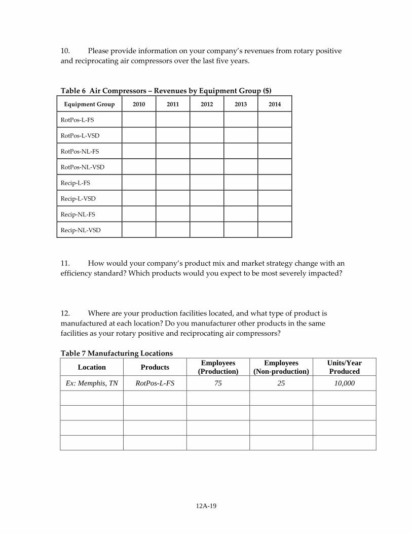
12A-19

10. Please provide information on your company’s revenues from rotary positive and reciprocating air compressors over the last five years. Table 6 Air Compressors – Revenues by Equipment Group ($)

Equipment Group 2010 2011 2012 2013 2014

RotPos-L-FS

RotPos-L-VSD

RotPos-NL-FS

RotPos-NL-VSD

Recip-L-FS

Recip-L-VSD

Recip-NL-FS

Recip-NL-VSD

11. How would your company’s product mix and market strategy change with an efficiency standard? Which products would you expect to be most severely impacted?

12. Where are your production facilities located, and what type of product is manufactured at each location? Do you manufacturer other products in the same facilities as your rotary positive and reciprocating air compressors? Table 7 Manufacturing Locations

Location Products Employees (Production)

Employees (Non-production)

Units/Year Produced

Ex: Memphis, TN RotPos-L-FS 75 25 10,000

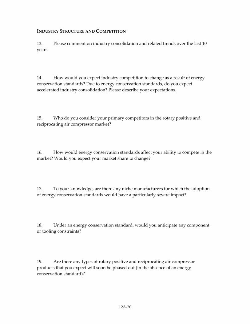
12A-20

INDUSTRY STRUCTURE AND COMPETITION 13. Please comment on industry consolidation and related trends over the last 10 years. 14. How would you expect industry competition to change as a result of energy conservation standards? Due to energy conservation standards, do you expect accelerated industry consolidation? Please describe your expectations. 15. Who do you consider your primary competitors in the rotary positive and reciprocating air compressor market? 16. How would energy conservation standards affect your ability to compete in the market? Would you expect your market share to change? 17. To your knowledge, are there any niche manufacturers for which the adoption of energy conservation standards would have a particularly severe impact? 18. Under an energy conservation standard, would you anticipate any component or tooling constraints? 19. Are there any types of rotary positive and reciprocating air compressor products that you expect will soon be phased out (in the absence of an energy conservation standard)?

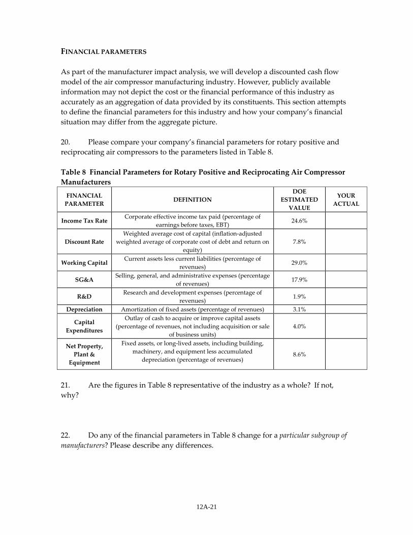
12A-21

FINANCIAL PARAMETERS As part of the manufacturer impact analysis, we will develop a discounted cash flow model of the air compressor manufacturing industry. However, publicly available information may not depict the cost or the financial performance of this industry as accurately as an aggregation of data provided by its constituents. This section attempts to define the financial parameters for this industry and how your company’s financial situation may differ from the aggregate picture.

20. Please compare your company’s financial parameters for rotary positive and reciprocating air compressors to the parameters listed in Table 8. Table 8 Financial Parameters for Rotary Positive and Reciprocating Air Compressor Manufacturers

FINANCIAL PARAMETER

DEFINITION DOE

ESTIMATED VALUE

YOUR ACTUAL

Income Tax Rate Corporate effective income tax paid (percentage of

earnings before taxes, EBT) 24.6%

Discount Rate Weighted average cost of capital (inflation-adjusted

weighted average of corporate cost of debt and return on equity)

7.8%

Working Capital Current assets less current liabilities (percentage of revenues)

29.0%

SG&A Selling, general, and administrative expenses (percentage

of revenues) 17.9%

R&D Research and development expenses (percentage of revenues)

1.9%

Depreciation Amortization of fixed assets (percentage of revenues) 3.1%

Capital Expenditures

Outlay of cash to acquire or improve capital assets (percentage of revenues, not including acquisition or sale

of business units) 4.0%

Net Property, Plant &

Equipment

Fixed assets, or long-lived assets, including building, machinery, and equipment less accumulated

depreciation (percentage of revenues) 8.6%

21. Are the figures in Table 8 representative of the industry as a whole? If not, why? 22. Do any of the financial parameters in Table 8 change for a particular subgroup of manufacturers? Please describe any differences.

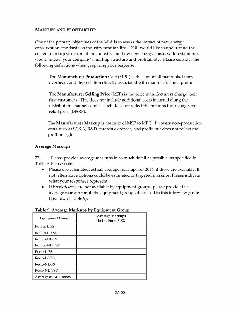
12A-22

MARKUPS AND PROFITABILITY One of the primary objectives of the MIA is to assess the impact of new energy conservation standards on industry profitability. DOE would like to understand the current markup structure of the industry and how new energy conservation standards would impact your company’s markup structure and profitability. Please consider the following definitions when preparing your response.

The Manufacturer Production Cost (MPC) is the sum of all materials, labor, overhead, and depreciation directly associated with manufacturing a product.

The Manufacturer Selling Price (MSP) is the price manufacturers charge their first customers. This does not include additional costs incurred along the distribution channels and as such does not reflect the manufacturer suggested retail price (MSRP).

The Manufacturer Markup is the ratio of MSP to MPC. It covers non-production costs such as SG&A, R&D, interest expenses, and profit, but does not reflect the profit margin.

Average Markups 23. Please provide average markups in as much detail as possible, as specified in Table 9. Please note:

• Please use calculated, actual, average markups for 2014, if those are available. If not, alternative options could be estimated or targeted markups. Please indicate what your responses represent.

• If breakdowns are not available by equipment groups, please provide the average markup for all the equipment groups discussed in this interview guide (last row of Table 9).

Table 9 Average Markups by Equipment Group

Equipment Group Average Markups (In the Form X.XX)

RotPos-L-FS

RotPos-L-VSD

RotPos-NL-FS

RotPos-NL-VSD

Recip-L-FS

Recip-L-VSD

Recip-NL-FS

Recip-NL-VSD

Average of All RotPos

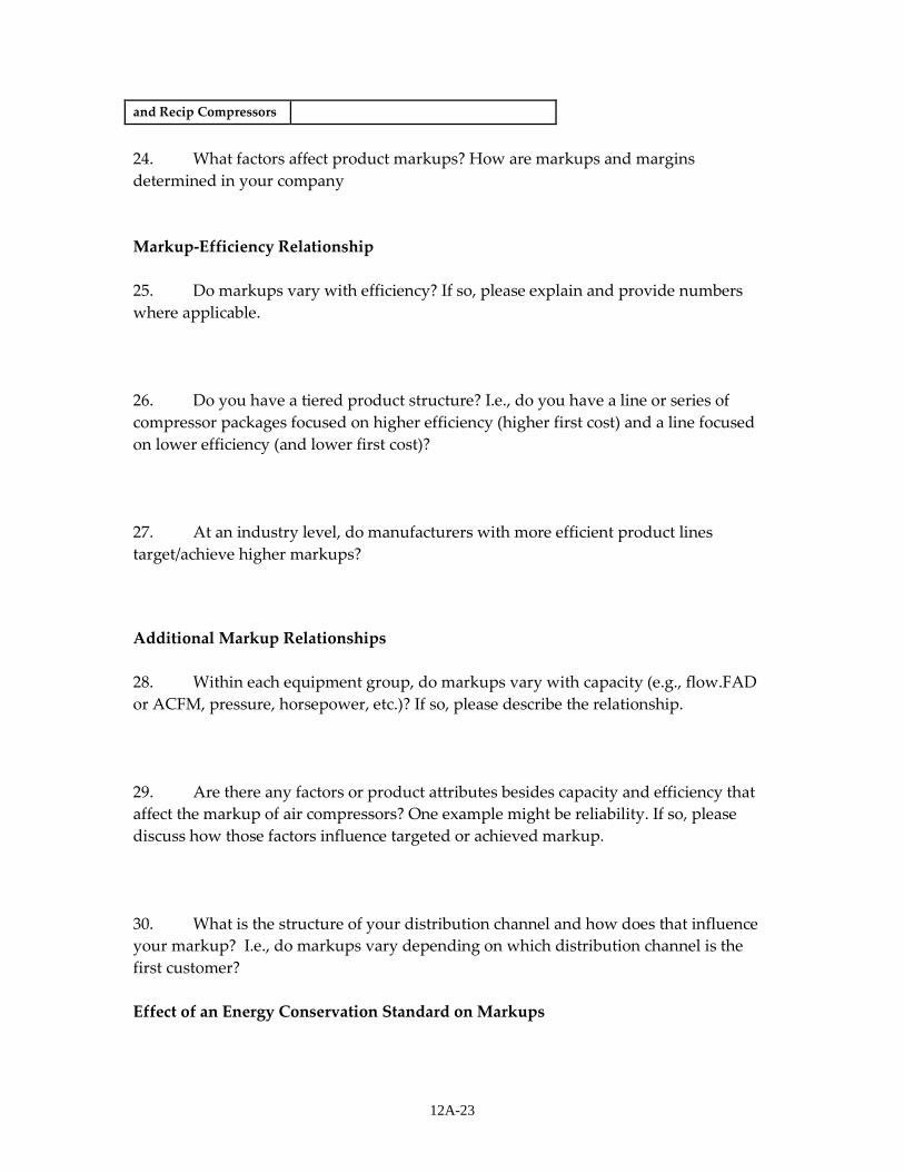
12A-23

and Recip Compressors

24. What factors affect product markups? How are markups and margins determined in your company Markup-Efficiency Relationship 25. Do markups vary with efficiency? If so, please explain and provide numbers where applicable. 26. Do you have a tiered product structure? I.e., do you have a line or series of compressor packages focused on higher efficiency (higher first cost) and a line focused on lower efficiency (and lower first cost)? 27. At an industry level, do manufacturers with more efficient product lines target/achieve higher markups?

Additional Markup Relationships 28. Within each equipment group, do markups vary with capacity (e.g., flow.FAD or ACFM, pressure, horsepower, etc.)? If so, please describe the relationship.

29. Are there any factors or product attributes besides capacity and efficiency that affect the markup of air compressors? One example might be reliability. If so, please discuss how those factors influence targeted or achieved markup.

30. What is the structure of your distribution channel and how does that influence your markup? I.e., do markups vary depending on which distribution channel is the first customer?

Effect of an Energy Conservation Standard on Markups

12A-24

31. Given the magnitude of potential conversion costs discussed in Section 6; following an energy conservation standard at one of the PELs discussed previously, do you anticipate increasing markups to recover your conversion cost investments and expenses?

32. If you answered “yes” to the previous question, please elaborate on how you expect to structure your markup increases following an energy conservation standard at one of the PELs discussed previously? For example, would you increase markups on only products that were redesigned? Or would you spread the markup increases across all models, both affected and unaffected? 33. Would you expect an energy conservation standards to affect your profitability? If so, please explain why. 34. In general, how do you expect standards to potentially impact the markup structure across the industry? Do you think other companies will take a path similar to yours?

12A-25

CONVERSION COSTS Definition of Conversion Costs Energy conservation standards may cause your company to incur capital and product conversion costs. These are the costs needed to redesign existing products and make changes or upgrades to production lines in order to comply with the energy conservation standard. With a detailed understanding of the conversion costs necessitated by different standard levels, DOE can more accurately model the impact of energy conservation standards on the industry. The MIA considers three types of conversion expenditures: Capital conversion costs (CCCs) are one-time investments in plant, property, and equipment (PPE) necessitated by an energy conservation standard. These may be incremental changes to existing PPE or the replacement of existing PPE. Included are expenditures on buildings, equipment, and tooling. Product conversion costs (PCCs) include the related research, product development, testing, marketing, and other non-capital costs necessary to bring products into compliance with a new energy conservation standard.

Stranded assets are assets replaced before the end of their useful lives as a direct result an energy conservation standard.

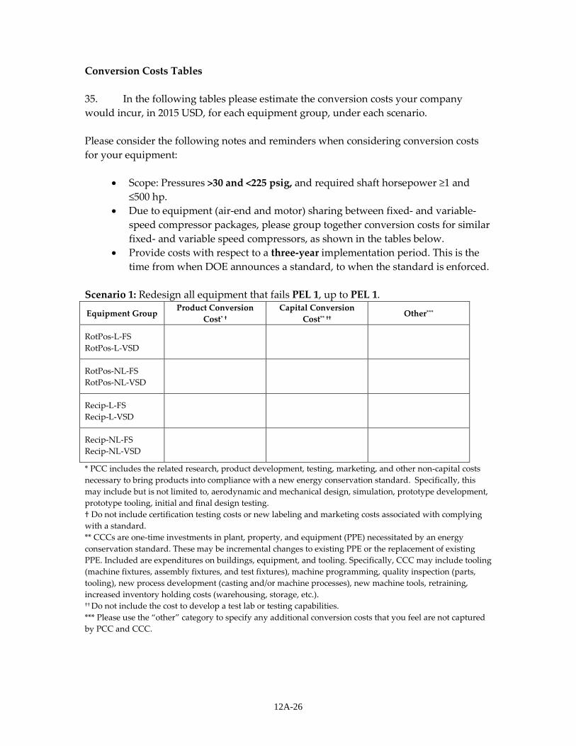
12A-26

Conversion Costs Tables 35. In the following tables please estimate the conversion costs your company would incur, in 2015 USD, for each equipment group, under each scenario. Please consider the following notes and reminders when considering conversion costs for your equipment:

• Scope: Pressures >30 and <225 psig, and required shaft horsepower ≥1 and ≤500 hp.

• Due to equipment (air-end and motor) sharing between fixed- and variable-speed compressor packages, please group together conversion costs for similar fixed- and variable speed compressors, as shown in the tables below.

• Provide costs with respect to a three-year implementation period. This is the time from when DOE announces a standard, to when the standard is enforced.

Scenario 1: Redesign all equipment that fails PEL 1, up to PEL 1.

Equipment Group Product Conversion

Cost* † Capital Conversion

Cost** †† Other***

RotPos-L-FS RotPos-L-VSD

RotPos-NL-FS RotPos-NL-VSD

Recip-L-FS Recip-L-VSD

Recip-NL-FS Recip-NL-VSD

* PCC includes the related research, product development, testing, marketing, and other non-capital costs necessary to bring products into compliance with a new energy conservation standard. Specifically, this may include but is not limited to, aerodynamic and mechanical design, simulation, prototype development, prototype tooling, initial and final design testing. † Do not include certification testing costs or new labeling and marketing costs associated with complying with a standard. ** CCCs are one-time investments in plant, property, and equipment (PPE) necessitated by an energy conservation standard. These may be incremental changes to existing PPE or the replacement of existing PPE. Included are expenditures on buildings, equipment, and tooling. Specifically, CCC may include tooling (machine fixtures, assembly fixtures, and test fixtures), machine programming, quality inspection (parts, tooling), new process development (casting and/or machine processes), new machine tools, retraining, increased inventory holding costs (warehousing, storage, etc.). †† Do not include the cost to develop a test lab or testing capabilities. *** Please use the “other” category to specify any additional conversion costs that you feel are not captured by PCC and CCC.

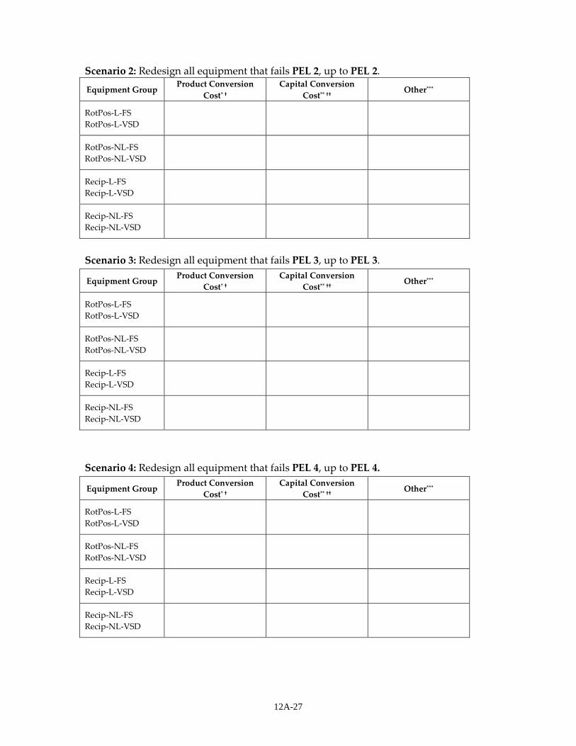
12A-27

Scenario 2: Redesign all equipment that fails PEL 2, up to PEL 2.

Equipment Group Product Conversion

Cost* † Capital Conversion

Cost** †† Other***

RotPos-L-FS RotPos-L-VSD

RotPos-NL-FS RotPos-NL-VSD

Recip-L-FS Recip-L-VSD

Recip-NL-FS Recip-NL-VSD

Scenario 3: Redesign all equipment that fails PEL 3, up to PEL 3.

Equipment Group Product Conversion Cost* †

Capital Conversion Cost** ††

Other***

RotPos-L-FS RotPos-L-VSD

RotPos-NL-FS RotPos-NL-VSD

Recip-L-FS Recip-L-VSD

Recip-NL-FS Recip-NL-VSD

Scenario 4: Redesign all equipment that fails PEL 4, up to PEL 4.

Equipment Group Product Conversion

Cost* † Capital Conversion

Cost** †† Other***

RotPos-L-FS RotPos-L-VSD

RotPos-NL-FS RotPos-NL-VSD

Recip-L-FS Recip-L-VSD

Recip-NL-FS Recip-NL-VSD

12A-28

Composition of Conversion Costs

36. Please discuss the specific types of capital conversion costs that you expect to encounter. If possible discuss the relative magnitude of these costs with respect to the total CCC.

For example, CCC may include tooling (machine fixtures, assembly fixtures, and test fixtures), machine programming, quality inspection (parts, tooling), new process development (casting and/or machine processes), new machine tools, retraining, increased inventory holding costs (warehousing, storage, etc).

37. If you specified costs in the “Other” category, please explain what these costs represent.

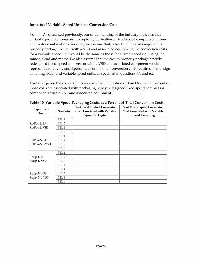
12A-29

Impacts of Variable Speed Units on Conversion Costs 38. As discussed previously, our understanding of the industry indicates that variable speed compressors are typically derivative of fixed-speed compressor air-end and motor combinations. As such, we assume that, other than the costs required to properly package the unit with a VSD and associated equipment, the conversion costs for a variable-speed unit would be the same as those for a fixed-speed unit using the same air-end and motor. We also assume that the cost to properly package a newly redesigned fixed-speed compressor with a VSD and associated equipment would represent a relatively small percentage of the total conversion costs required to redesign all failing fixed- and variable speed units, as specified in questions 6.1 and 6.2. That said, given the conversion costs specified in questions 6.1 and 6.2., what percent of those costs are associated with packaging newly redesigned fixed-speed compressor components with a VSD and associated equipment. Table 10 Variable Speed Packaging Costs, as a Percent of Total Conversion Costs

Equipment Group

Scenario % of Total Product Conversion Cost Associated with Variable

Speed Packaging

% of Total Capital Conversion Cost Associated with Variable

Speed Packaging

RotPos-L-FS RotPos-L-VSD

PEL 1 PEL 2 PEL 3 PEL 4

RotPos-NL-FS RotPos-NL-VSD

PEL 1 PEL 2 PEL 3 PEL 4

Recip-L-FS Recip-L-VSD

PEL 1 PEL 2 PEL 3 PEL 4

Recip-NL-FS Recip-NL-VSD

PEL 1 PEL 2 PEL 3 PEL 4

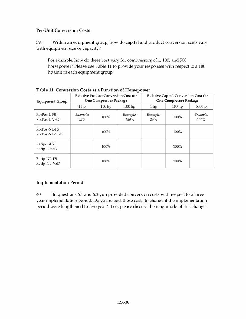
12A-30

Per-Unit Conversion Costs 39. Within an equipment group, how do capital and product conversion costs vary with equipment size or capacity?

For example, how do these cost vary for compressors of 1, 100, and 500 horsepower? Please use Table 11 to provide your responses with respect to a 100 hp unit in each equipment group.

Table 11 Conversion Costs as a Function of Horsepower

Equipment Group Relative Product Conversion Cost for

One Compressor Package Relative Capital Conversion Cost for

One Compressor Package 1 hp 100 hp 500 hp 1 hp 100 hp 500 hp

RotPos-L-FS RotPos-L-VSD

Example: 25%

100% Example:

150% Example:

25% 100%

Example: 150%

RotPos-NL-FS RotPos-NL-VSD

100% 100%

Recip-L-FS Recip-L-VSD

100% 100%

Recip-NL-FS Recip-NL-VSD

100% 100%

Implementation Period 40. In questions 6.1 and 6.2 you provided conversion costs with respect to a three year implementation period. Do you expect these costs to change if the implementation period were lengthened to five year? If so, please discuss the magnitude of this change.

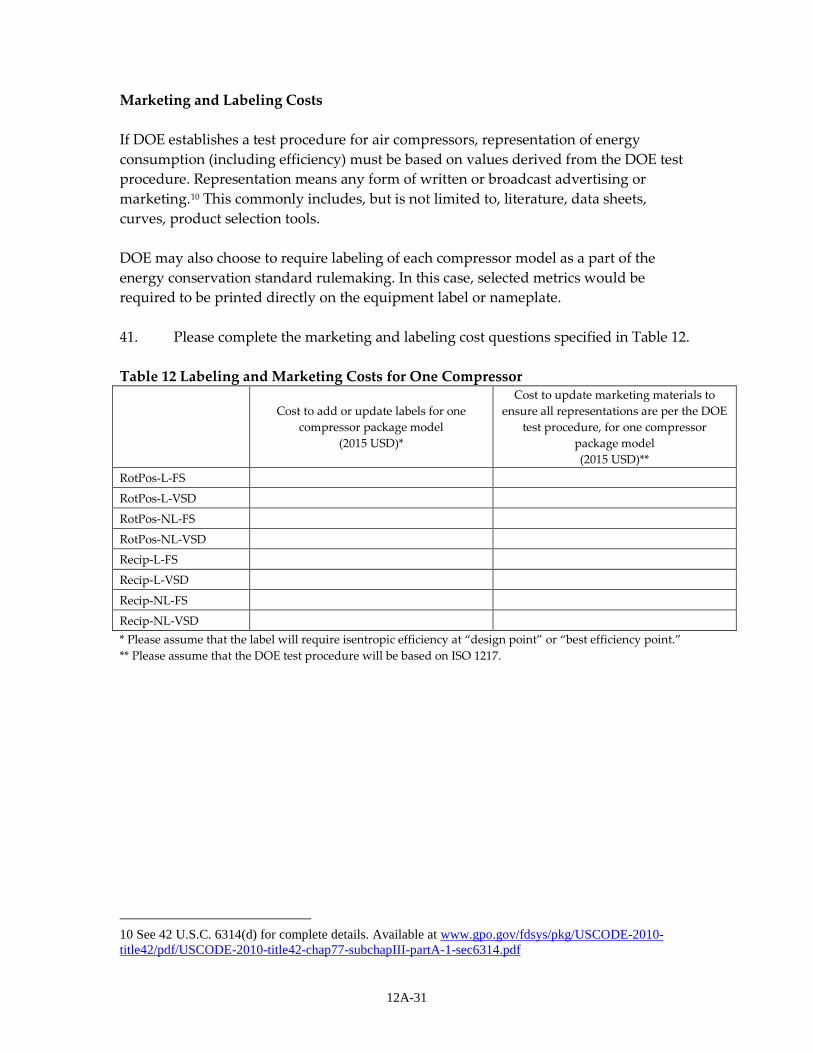
12A-31

Marketing and Labeling Costs If DOE establishes a test procedure for air compressors, representation of energy consumption (including efficiency) must be based on values derived from the DOE test procedure. Representation means any form of written or broadcast advertising or marketing.10 This commonly includes, but is not limited to, literature, data sheets, curves, product selection tools. DOE may also choose to require labeling of each compressor model as a part of the energy conservation standard rulemaking. In this case, selected metrics would be required to be printed directly on the equipment label or nameplate. 41. Please complete the marketing and labeling cost questions specified in Table 12. Table 12 Labeling and Marketing Costs for One Compressor

Cost to add or update labels for one compressor package model

(2015 USD)*

Cost to update marketing materials to ensure all representations are per the DOE

test procedure, for one compressor package model (2015 USD)**

RotPos-L-FS RotPos-L-VSD RotPos-NL-FS RotPos-NL-VSD Recip-L-FS Recip-L-VSD Recip-NL-FS Recip-NL-VSD * Please assume that the label will require isentropic efficiency at “design point” or “best efficiency point.” ** Please assume that the DOE test procedure will be based on ISO 1217.

10 See 42 U.S.C. 6314(d) for complete details. Available at www.gpo.gov/fdsys/pkg/USCODE-2010-title42/pdf/USCODE-2010-title42-chap77-subchapIII-partA-1-sec6314.pdf

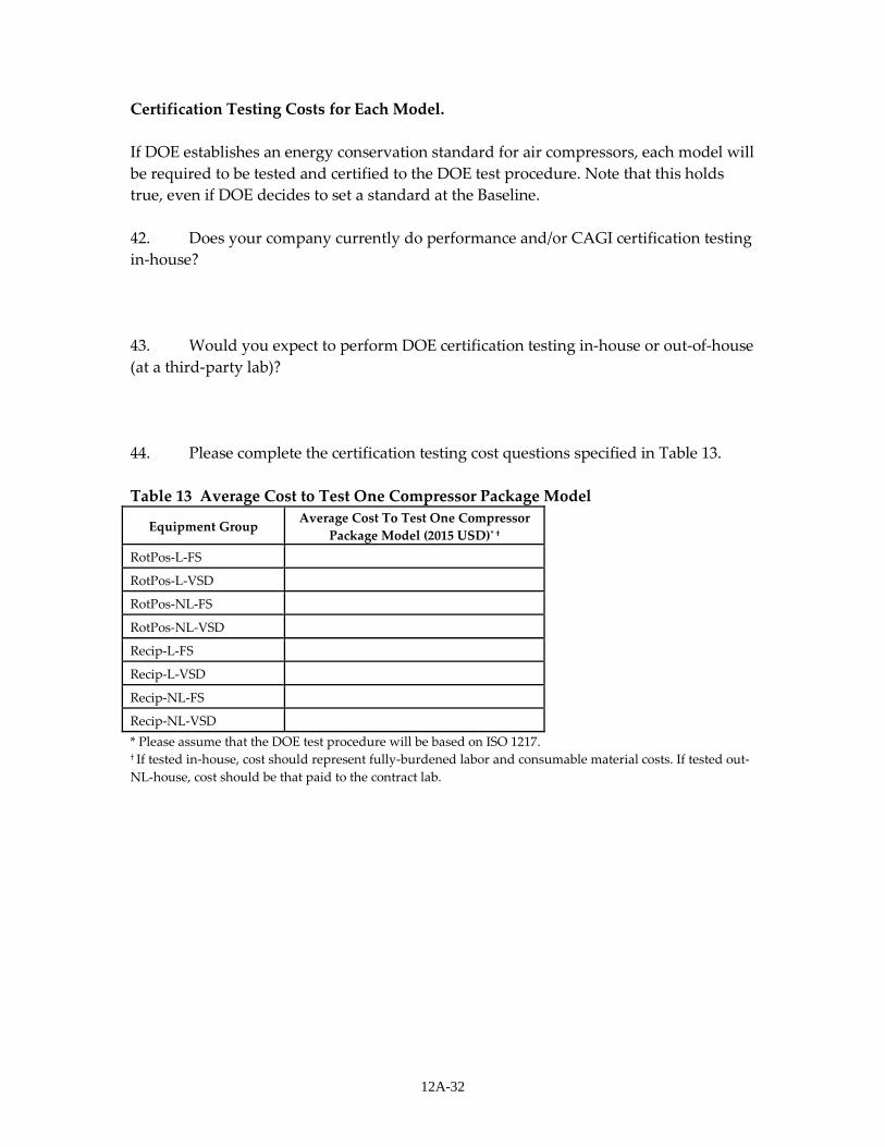
12A-32

Certification Testing Costs for Each Model. If DOE establishes an energy conservation standard for air compressors, each model will be required to be tested and certified to the DOE test procedure. Note that this holds true, even if DOE decides to set a standard at the Baseline. 42. Does your company currently do performance and/or CAGI certification testing in-house? 43. Would you expect to perform DOE certification testing in-house or out-of-house (at a third-party lab)? 44. Please complete the certification testing cost questions specified in Table 13. Table 13 Average Cost to Test One Compressor Package Model

Equipment Group Average Cost To Test One Compressor Package Model (2015 USD)* †

RotPos-L-FS

RotPos-L-VSD

RotPos-NL-FS

RotPos-NL-VSD

Recip-L-FS

Recip-L-VSD

Recip-NL-FS

Recip-NL-VSD

* Please assume that the DOE test procedure will be based on ISO 1217. † If tested in-house, cost should represent fully-burdened labor and consumable material costs. If tested out-NL-house, cost should be that paid to the contract lab.

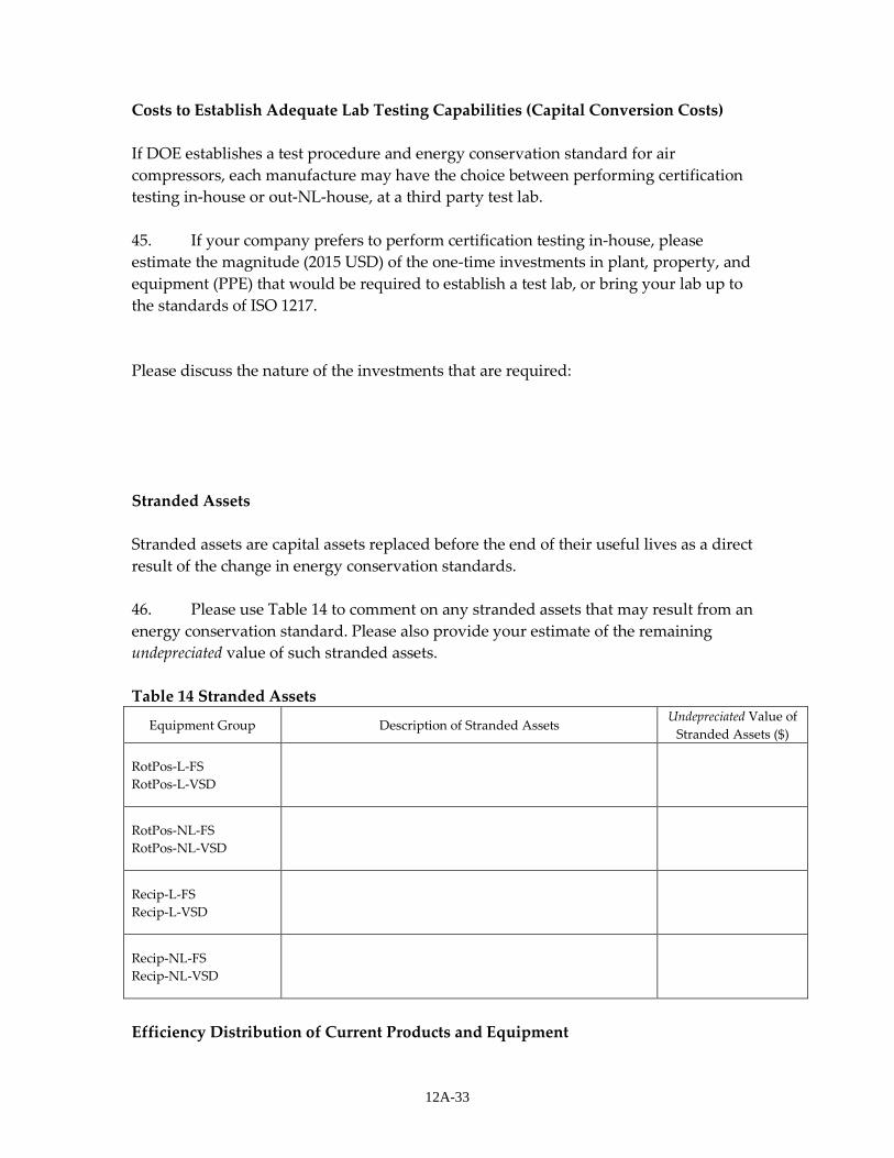
12A-33

Costs to Establish Adequate Lab Testing Capabilities (Capital Conversion Costs) If DOE establishes a test procedure and energy conservation standard for air compressors, each manufacture may have the choice between performing certification testing in-house or out-NL-house, at a third party test lab. 45. If your company prefers to perform certification testing in-house, please estimate the magnitude (2015 USD) of the one-time investments in plant, property, and equipment (PPE) that would be required to establish a test lab, or bring your lab up to the standards of ISO 1217. Please discuss the nature of the investments that are required: Stranded Assets Stranded assets are capital assets replaced before the end of their useful lives as a direct result of the change in energy conservation standards. 46. Please use Table 14 to comment on any stranded assets that may result from an energy conservation standard. Please also provide your estimate of the remaining undepreciated value of such stranded assets. Table 14 Stranded Assets

Equipment Group Description of Stranded Assets Undepreciated Value of

Stranded Assets ($)

RotPos-L-FS RotPos-L-VSD

RotPos-NL-FS RotPos-NL-VSD

Recip-L-FS Recip-L-VSD

Recip-NL-FS Recip-NL-VSD

Efficiency Distribution of Current Products and Equipment

12A-34

Please provide the following information related to the efficiency distribution of your current equipment catalogue. Relevant definitions: “Bare Compressor” refers to the singular machine responsible for the change in air

pressure and is sometimes referred to as an “air end,” which is the compression chamber where air is compressed. ISO 12942 refers to this level of equipment as the "mechanical compressor." 1

“Compressor Package” refers to a compressor made up of compression element (‘airend’), electric motor(s), and transmission or coupling to drive the compressor element, and which is fully piped and wired internally, including ancillary auxiliary items of equipment that are considered essential for safe operation and required for functioning as intended.

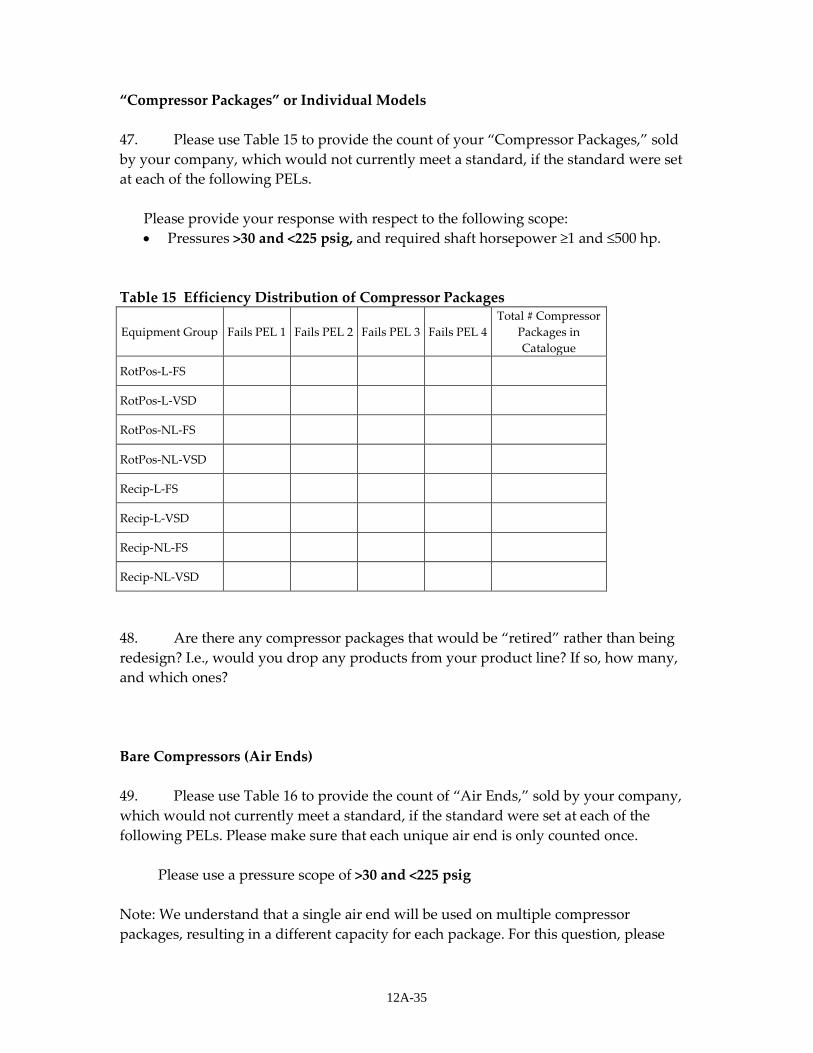
12A-35

“Compressor Packages” or Individual Models 47. Please use Table 15 to provide the count of your “Compressor Packages,” sold by your company, which would not currently meet a standard, if the standard were set at each of the following PELs.

Please provide your response with respect to the following scope: • Pressures >30 and <225 psig, and required shaft horsepower ≥1 and ≤500 hp.

Table 15 Efficiency Distribution of Compressor Packages

Equipment Group Fails PEL 1 Fails PEL 2 Fails PEL 3 Fails PEL 4 Total # Compressor

Packages in Catalogue

RotPos-L-FS

RotPos-L-VSD

RotPos-NL-FS

RotPos-NL-VSD

Recip-L-FS

Recip-L-VSD

Recip-NL-FS

Recip-NL-VSD

48. Are there any compressor packages that would be “retired” rather than being redesign? I.e., would you drop any products from your product line? If so, how many, and which ones? Bare Compressors (Air Ends) 49. Please use Table 16 to provide the count of “Air Ends,” sold by your company, which would not currently meet a standard, if the standard were set at each of the following PELs. Please make sure that each unique air end is only counted once.

Please use a pressure scope of >30 and <225 psig Note: We understand that a single air end will be used on multiple compressor packages, resulting in a different capacity for each package. For this question, please

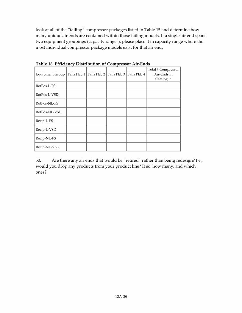
12A-36

look at all of the “failing” compressor packages listed in Table 15 and determine how many unique air ends are contained within those failing models. If a single air end spans two equipment groupings (capacity ranges), please place it in capacity range where the most individual compressor package models exist for that air end.

Table 16 Efficiency Distribution of Compressor Air-Ends

Equipment Group Fails PEL 1 Fails PEL 2 Fails PEL 3 Fails PEL 4 Total # Compressor

Air-Ends in Catalogue

RotPos-L-FS

RotPos-L-VSD

RotPos-NL-FS

RotPos-NL-VSD

Recip-L-FS

Recip-L-VSD

Recip-NL-FS

Recip-NL-VSD

50. Are there any air ends that would be “retired” rather than being redesign? I.e., would you drop any products from your product line? If so, how many, and which ones?

12A-37

DIRECT EMPLOYMENT, FOREIGN COMPETITION, AND OUTSOURCING The impact of energy conservation standards on employment and foreign competition is an important consideration in the rulemaking process. This section of the interview guide seeks to explore current trends in industry employment and to solicit manufacturer views on how domestic employment patterns might be affected by energy conservation standards. This section also considers the impacts of domestic energy conservation standards on imports, exports, and sourcing decisions. 51. Absent energy conservation standards, are production facilities being relocated to foreign countries? 52. Would energy conservation standards impact your domestic vs. foreign manufacturing decision? Please structure your response in terms of PELs 1 through 4, listed earlier. If so, please explain how they would change if higher efficiency levels are required. 53. Would your domestic employment levels be expected to change significantly under new energy conservation standards? Please structure your response in terms of PELs 1 through 4, listed earlier. If so, please explain how they would change if higher efficiency levels are required.

54. Would the workforce skills necessary under new energy conservation standards require extensive retraining or replacement of employees at your manufacturing facilities? 55. Would new energy conservation standards require extensive retraining of your service/field technicians? If so, could you expand on how your service infrastructure would be impacted in general as a result of new energy conservation standards?

12A-38

56. How would new energy conservation standards impact your company’s manufacturing capacity? 57. For any design changes that would require new production equipment, please describe how much downtime would be required. What impact would downtime have on your business? Are there any design changes that could not be implemented over a three-year implementation period? A five-year implementation period?

58. What percentage of your company’s air compressor sales are made within the United States? Please provide the percentage of units sold, and the percentage of revenues.

59. What percentage of your company’s air compressors are produced in the United States? Please provide the percentage of units sold, the percentage of models, and the percentage of revenues.

60. What percentage of your U.S.-produced air compressors are exported? Please provide the percentage of units sold, and the percentage of revenues.

61. Are there any foreign companies with North American production facilities? 62. Would new energy conservation standards impact your domestic versus foreign sourcing decisions?

12A-39

Overlap of the United States and European Union Markets 63. What percent of compressor packages sold by your company in the US are also sold in the EU? 64. What percent of air ends sold by your company in the US are also sold in the EU? 65. If overlap between US and EU air ends exists, will models redesigned for the EU market be introduced into the US market, regardless of potential US standards? How does this impact the conversion costs discussed in Section 6?

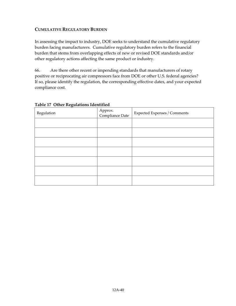
12A-40

CUMULATIVE REGULATORY BURDEN In assessing the impact to industry, DOE seeks to understand the cumulative regulatory burden facing manufacturers. Cumulative regulatory burden refers to the financial burden that stems from overlapping effects of new or revised DOE standards and/or other regulatory actions affecting the same product or industry. 66. Are there other recent or impending standards that manufacturers of rotary positive or reciprocating air compressors face from DOE or other U.S. federal agencies? If so, please identify the regulation, the corresponding effective dates, and your expected compliance cost. Table 17 Other Regulations Identified

Regulation Approx. Compliance Date

Expected Expenses / Comments

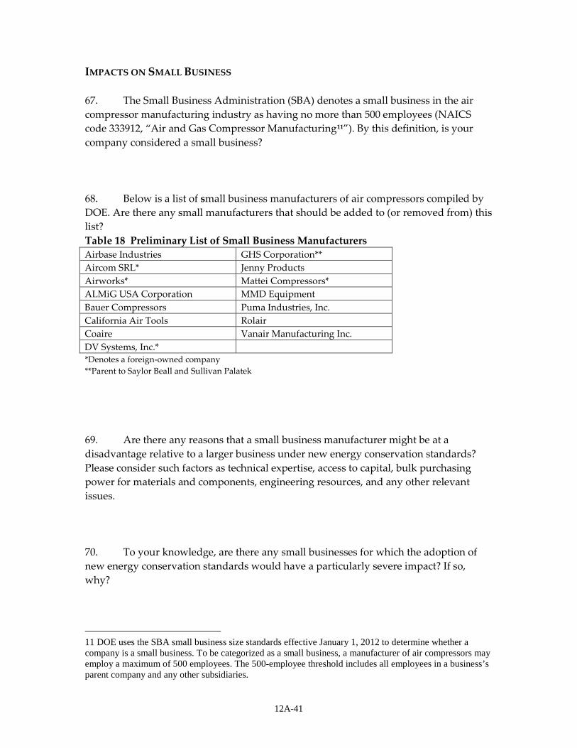
12A-41

IMPACTS ON SMALL BUSINESS 67. The Small Business Administration (SBA) denotes a small business in the air compressor manufacturing industry as having no more than 500 employees (NAICS code 333912, “Air and Gas Compressor Manufacturing11”). By this definition, is your company considered a small business? 68. Below is a list of small business manufacturers of air compressors compiled by DOE. Are there any small manufacturers that should be added to (or removed from) this list? Table 18 Preliminary List of Small Business Manufacturers Airbase Industries GHS Corporation** Aircom SRL* Jenny Products Airworks* Mattei Compressors* ALMiG USA Corporation MMD Equipment Bauer Compressors Puma Industries, Inc. California Air Tools Rolair Coaire Vanair Manufacturing Inc. DV Systems, Inc.* *Denotes a foreign-owned company **Parent to Saylor Beall and Sullivan Palatek 69. Are there any reasons that a small business manufacturer might be at a disadvantage relative to a larger business under new energy conservation standards? Please consider such factors as technical expertise, access to capital, bulk purchasing power for materials and components, engineering resources, and any other relevant issues. 70. To your knowledge, are there any small businesses for which the adoption of new energy conservation standards would have a particularly severe impact? If so, why?

11 DOE uses the SBA small business size standards effective January 1, 2012 to determine whether a company is a small business. To be categorized as a small business, a manufacturer of air compressors may employ a maximum of 500 employees. The 500-employee threshold includes all employees in a business’s parent company and any other subsidiaries.

12B-i

APPENDIX 12B. GOVERNMENT REGULATORY IMPACT MODEL OVERVIEW

TABLE OF CONTENTS 12B.1 INTRODUCTION AND PURPOSE ...............................................................................B-1 12B.2 MODEL DESCRIPTION ................................................................................................B-1

LIST OF TABLES

Table 12B.1 Detailed Cash Flow Example ..................................................................................B-4

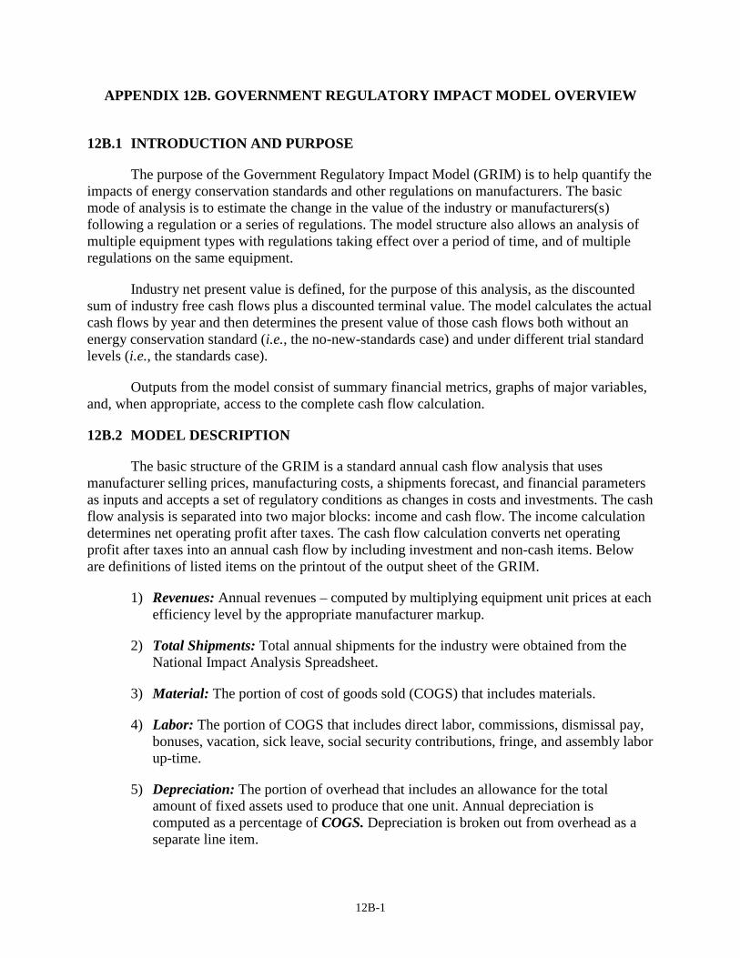
12B-1

APPENDIX 12B. GOVERNMENT REGULATORY IMPACT MODEL OVERVIEW

12B.1 INTRODUCTION AND PURPOSE

The purpose of the Government Regulatory Impact Model (GRIM) is to help quantify the impacts of energy conservation standards and other regulations on manufacturers. The basic mode of analysis is to estimate the change in the value of the industry or manufacturers(s) following a regulation or a series of regulations. The model structure also allows an analysis of multiple equipment types with regulations taking effect over a period of time, and of multiple regulations on the same equipment.

Industry net present value is defined, for the purpose of this analysis, as the discounted sum of industry free cash flows plus a discounted terminal value. The model calculates the actual cash flows by year and then determines the present value of those cash flows both without an energy conservation standard (i.e., the no-new-standards case) and under different trial standard levels (i.e., the standards case).

Outputs from the model consist of summary financial metrics, graphs of major variables, and, when appropriate, access to the complete cash flow calculation.

12B.2 MODEL DESCRIPTION

The basic structure of the GRIM is a standard annual cash flow analysis that uses manufacturer selling prices, manufacturing costs, a shipments forecast, and financial parameters as inputs and accepts a set of regulatory conditions as changes in costs and investments. The cash flow analysis is separated into two major blocks: income and cash flow. The income calculation determines net operating profit after taxes. The cash flow calculation converts net operating profit after taxes into an annual cash flow by including investment and non-cash items. Below are definitions of listed items on the printout of the output sheet of the GRIM.

1) Revenues: Annual revenues – computed by multiplying equipment unit prices at each efficiency level by the appropriate manufacturer markup.

2) Total Shipments: Total annual shipments for the industry were obtained from the National Impact Analysis Spreadsheet.

3) Material: The portion of cost of goods sold (COGS) that includes materials.

4) Labor: The portion of COGS that includes direct labor, commissions, dismissal pay, bonuses, vacation, sick leave, social security contributions, fringe, and assembly labor up-time.

5) Depreciation: The portion of overhead that includes an allowance for the total amount of fixed assets used to produce that one unit. Annual depreciation is computed as a percentage of COGS. Depreciation is broken out from overhead as a separate line item.

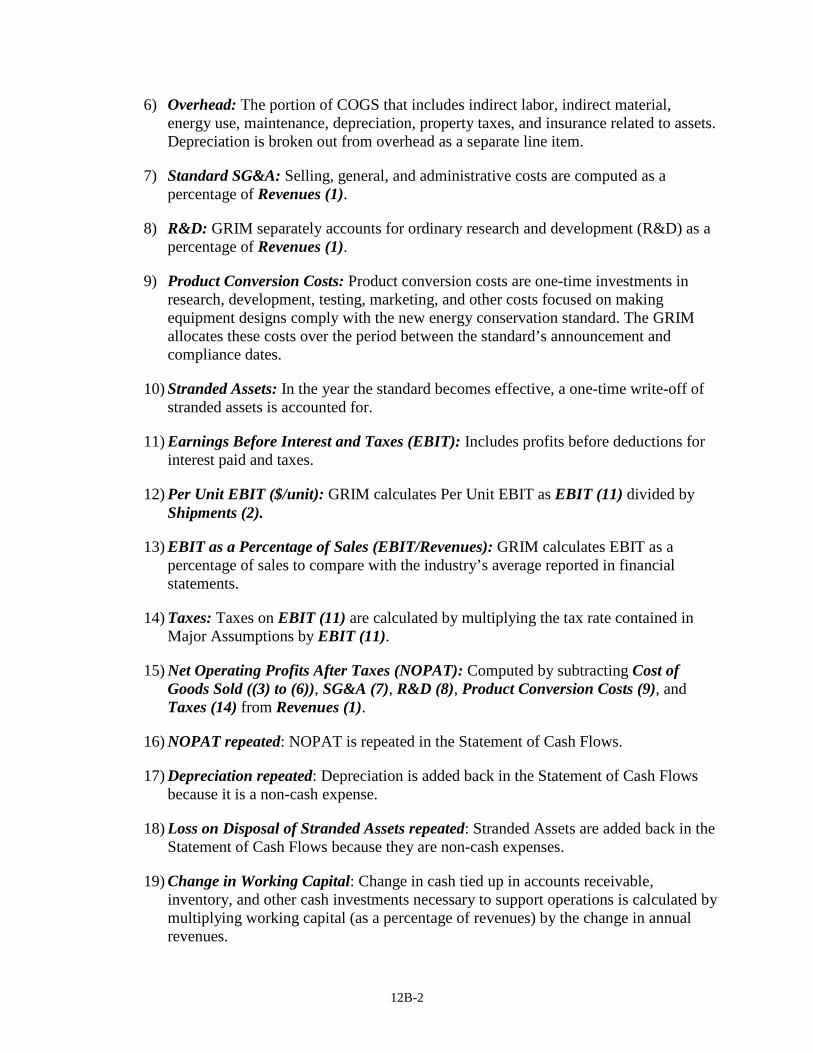
12B-2

6) Overhead: The portion of COGS that includes indirect labor, indirect material, energy use, maintenance, depreciation, property taxes, and insurance related to assets. Depreciation is broken out from overhead as a separate line item.

7) Standard SG&A: Selling, general, and administrative costs are computed as a percentage of Revenues (1).

8) R&D: GRIM separately accounts for ordinary research and development (R&D) as a percentage of Revenues (1).

9) Product Conversion Costs: Product conversion costs are one-time investments in research, development, testing, marketing, and other costs focused on making equipment designs comply with the new energy conservation standard. The GRIM allocates these costs over the period between the standard’s announcement and compliance dates.

10) Stranded Assets: In the year the standard becomes effective, a one-time write-off of stranded assets is accounted for.

11) Earnings Before Interest and Taxes (EBIT): Includes profits before deductions for interest paid and taxes.

12) Per Unit EBIT ($/unit): GRIM calculates Per Unit EBIT as EBIT (11) divided by Shipments (2).

13) EBIT as a Percentage of Sales (EBIT/Revenues): GRIM calculates EBIT as a percentage of sales to compare with the industry’s average reported in financial statements.

14) Taxes: Taxes on EBIT (11) are calculated by multiplying the tax rate contained in Major Assumptions by EBIT (11).

15) Net Operating Profits After Taxes (NOPAT): Computed by subtracting Cost of Goods Sold ((3) to (6)), SG&A (7), R&D (8), Product Conversion Costs (9), and Taxes (14) from Revenues (1).

16) NOPAT repeated: NOPAT is repeated in the Statement of Cash Flows.

17) Depreciation repeated: Depreciation is added back in the Statement of Cash Flows because it is a non-cash expense.

18) Loss on Disposal of Stranded Assets repeated: Stranded Assets are added back in the Statement of Cash Flows because they are non-cash expenses.

19) Change in Working Capital: Change in cash tied up in accounts receivable, inventory, and other cash investments necessary to support operations is calculated by multiplying working capital (as a percentage of revenues) by the change in annual revenues.

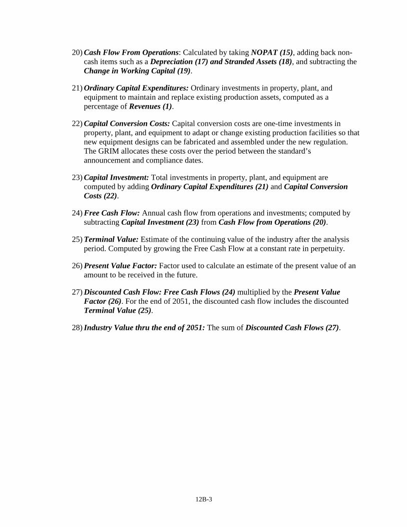
12B-3

20) Cash Flow From Operations: Calculated by taking NOPAT (15), adding back non-cash items such as a Depreciation (17) and Stranded Assets (18), and subtracting the Change in Working Capital (19).

21) Ordinary Capital Expenditures: Ordinary investments in property, plant, and equipment to maintain and replace existing production assets, computed as a percentage of Revenues (1).

22) Capital Conversion Costs: Capital conversion costs are one-time investments in property, plant, and equipment to adapt or change existing production facilities so that new equipment designs can be fabricated and assembled under the new regulation. The GRIM allocates these costs over the period between the standard’s announcement and compliance dates.

23) Capital Investment: Total investments in property, plant, and equipment are computed by adding Ordinary Capital Expenditures (21) and Capital Conversion Costs (22).

24) Free Cash Flow: Annual cash flow from operations and investments; computed by subtracting Capital Investment (23) from Cash Flow from Operations (20).

25) Terminal Value: Estimate of the continuing value of the industry after the analysis period. Computed by growing the Free Cash Flow at a constant rate in perpetuity.

26) Present Value Factor: Factor used to calculate an estimate of the present value of an amount to be received in the future.

27) Discounted Cash Flow: Free Cash Flows (24) multiplied by the Present Value Factor (26). For the end of 2051, the discounted cash flow includes the discounted Terminal Value (25).

28) Industry Value thru the end of 2051: The sum of Discounted Cash Flows (27).

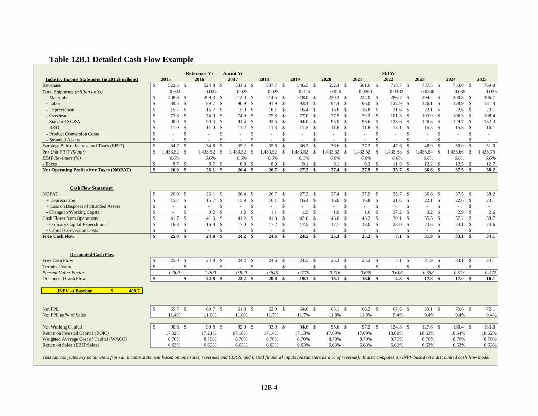
12B-4

Table 12B.1 Detailed Cash Flow Example

Reference Yr Ancmt Yr Std Yr Industry Income Statement (in 2015$ millions) 2015 2016 2017 2018 2019 2020 2021 2022 2023 2024 2025

Revenues 523.5$ 524.8$ 531.6$ 537.7$ 546.5$ 552.4$ 561.6$ 718.7$ 737.5$ 754.0$ 769.0$ Total Shipments (million units) 0.024 0.024 0.025 0.025 0.025 0.026 0.0260 0.0332 0.0340 0.035 0.035

- Materials 208.8$ 209.3$ 212.0$ 214.5$ 218.0$ 220.3$ 224.0$ 286.7$ 294.2$ 300.8$ 306.7$ - Labor 89.5$ 89.7$ 90.9$ 91.9$ 93.4$ 94.4$ 96.0$ 122.9$ 126.1$ 128.9$ 131.4$ - Depreciation 15.7$ 15.7$ 15.9$ 16.1$ 16.4$ 16.6$ 16.8$ 21.6$ 22.1$ 22.6$ 23.1$ - Overhead 73.8$ 74.0$ 74.9$ 75.8$ 77.0$ 77.9$ 79.2$ 101.3$ 103.9$ 106.3$ 108.4$ - Standard SG&A 90.0$ 90.3$ 91.4$ 92.5$ 94.0$ 95.0$ 96.6$ 123.6$ 126.8$ 129.7$ 132.3$ - R&D 11.0$ 11.0$ 11.2$ 11.3$ 11.5$ 11.6$ 11.8$ 15.1$ 15.5$ 15.8$ 16.1$ - Product Conversion Costs -$ -$ -$ -$ -$ -$ -$ -$ -$ -$ -$ - Stranded Assets -$ -$ -$ -$ -$ -$ -$ -$ -$ -$ -$

Earnings Before Interest and Taxes (EBIT) 34.7$ 34.8$ 35.2$ 35.6$ 36.2$ 36.6$ 37.2$ 47.6$ 48.9$ 50.0$ 51.0$ Per Unit EBIT ($/unit) 1,433.52$ 1,433.52$ 1,433.52$ 1,433.52$ 1,433.52$ 1,433.52$ 1,433.52$ 1,435.38$ 1,435.54$ 1,435.66$ 1,435.75$ EBIT/Revenues (%) 6.6% 6.6% 6.6% 6.6% 6.6% 6.6% 6.6% 6.6% 6.6% 6.6% 6.6%- Taxes 8.7$ 8.7$ 8.8$ 8.9$ 9.1$ 9.1$ 9.3$ 11.9$ 12.2$ 12.5$ 12.7$ Net Operating Profit after Taxes (NOPAT) 26.0$ 26.1$ 26.4$ 26.7$ 27.2$ 27.4$ 27.9$ 35.7$ 36.6$ 37.5$ 38.2$

Cash Flow Statement NOPAT 26.0$ 26.1$ 26.4$ 26.7$ 27.2$ 27.4$ 27.9$ 35.7$ 36.6$ 37.5$ 38.2$

+ Depreciation 15.7$ 15.7$ 15.9$ 16.1$ 16.4$ 16.6$ 16.8$ 21.6$ 22.1$ 22.6$ 23.1$ + Loss on Disposal of Stranded Assets -$ -$ -$ -$ -$ -$ -$ -$ -$ -$ -$ - Change in Working Capital -$ 0.2$ 1.2$ 1.1$ 1.5$ 1.0$ 1.6$ 27.2$ 3.2$ 2.9$ 2.6$

Cash Flows from Operations 41.7$ 41.6$ 41.2$ 41.8$ 42.0$ 43.0$ 43.2$ 30.1$ 55.5$ 57.2$ 58.7$ - Ordinary Capital Expenditures 16.8$ 16.8$ 17.0$ 17.2$ 17.5$ 17.7$ 18.0$ 23.0$ 23.6$ 24.1$ 24.6$ - Capital Conversion Costs -$ -$ -$ -$ -$ -$ -$ -$ -$ -$ -$

Free Cash Flow 25.0$ 24.8$ 24.2$ 24.6$ 24.5$ 25.3$ 25.2$ 7.1$ 31.9$ 33.1$ 34.1$

Discounted Cash FlowFree Cash Flow 25.0$ 24.8$ 24.2$ 24.6$ 24.5$ 25.3$ 25.2$ 7.1$ 31.9$ 33.1$ 34.1$ Terminal Value -$ -$ -$ -$ -$ -$ -$ -$ -$ -$ -$ Present Value Factor 0.000 1.000 0.920 0.846 0.779 0.716 0.659 0.606 0.558 0.513 0.472Discounted Cash Flow -$ 24.8$ 22.2$ 20.8$ 19.1$ 18.1$ 16.6$ 4.3$ 17.8$ 17.0$ 16.1$

INPV at Baseline 409.7$

Net PPE 59.7$ 60.7$ 61.8$ 62.9$ 64.0$ 65.1$ 66.2$ 67.6$ 69.1$ 70.6$ 72.1$ Net PPE as % of Sales 11.4% 11.6% 11.6% 11.7% 11.7% 11.8% 11.8% 9.4% 9.4% 9.4% 9.4%

Net Working Capital 90.6$ 90.8$ 92.0$ 93.0$ 94.6$ 95.6$ 97.2$ 124.3$ 127.6$ 130.4$ 133.0$ Return on Invested Capital (ROIC) 17.32% 17.21% 17.18% 17.14% 17.13% 17.09% 17.09% 18.61% 18.63% 18.64% 18.62%Weighted Average Cost of Capital (WACC) 8.70% 8.70% 8.70% 8.70% 8.70% 8.70% 8.70% 8.70% 8.70% 8.70% 8.70%Return on Sales (EBIT/Sales) 6.63% 6.63% 6.63% 6.63% 6.63% 6.63% 6.63% 6.63% 6.63% 6.63% 6.63%

This tab computes key parameters from an income statement based on unit sales, revenues and COGS, and initial financial inputs (parameters as a % of revenue). It also computes an INPV based on a discounted cash flow model.

13A-i

APPENDIX 13A. EMISSIONS ANALYSIS METHODOLOGY

TABLE OF CONTENTS

13A.1 INTRODUCTION ...................................................................................................... 13A-1 13A.2 POWER SECTOR AND SITE EMISSIONS FACTORS .......................................... 13A-1 13A.3 UPSTREAM FACTORS ............................................................................................ 13A-2 13A.4 DATA TABLES ......................................................................................................... 13A-3 REFERENCES ..................................................................................................................... 13A-11

LIST OF TABLES

Table 13A.4.1 Site Combustion Emissions Factors.......................................................... 13A-3 Table 13A.4.2 Power Sector Emissions Factors for CO2 (Tons of CO2 per MWh of

Site Electricity Use) .................................................................................. 13A-4 Table 13A.4.3 Power Sector Emissions Factors for Hg (tons/TWh) ................................ 13A-5 Table 13A.4.4 Power Sector Emissions Factors for NOx (tons/MWh) ............................ 13A-6 Table 13A.4.5 Power Sector Emissions Factors for SO2 (tons/MWh) ............................. 13A-7 Table 13A.4.6 Power Sector Emissions Factors for CH4 (tons/MWh)............................. 13A-8 Table 13A.4.7 Power Sector Emissions Factors for N2O (tons/MWh) ............................ 13A-9 Table 13A.4.8 Electricity Upstream Emissions Factors ................................................... 13A-9 Table 13A.4.9 Natural Gas Upstream Emissions Factors............................................... 13A-10 Table 13A.4.10 Fuel Oil Upstream Emissions Factors..................................................... 13A-10

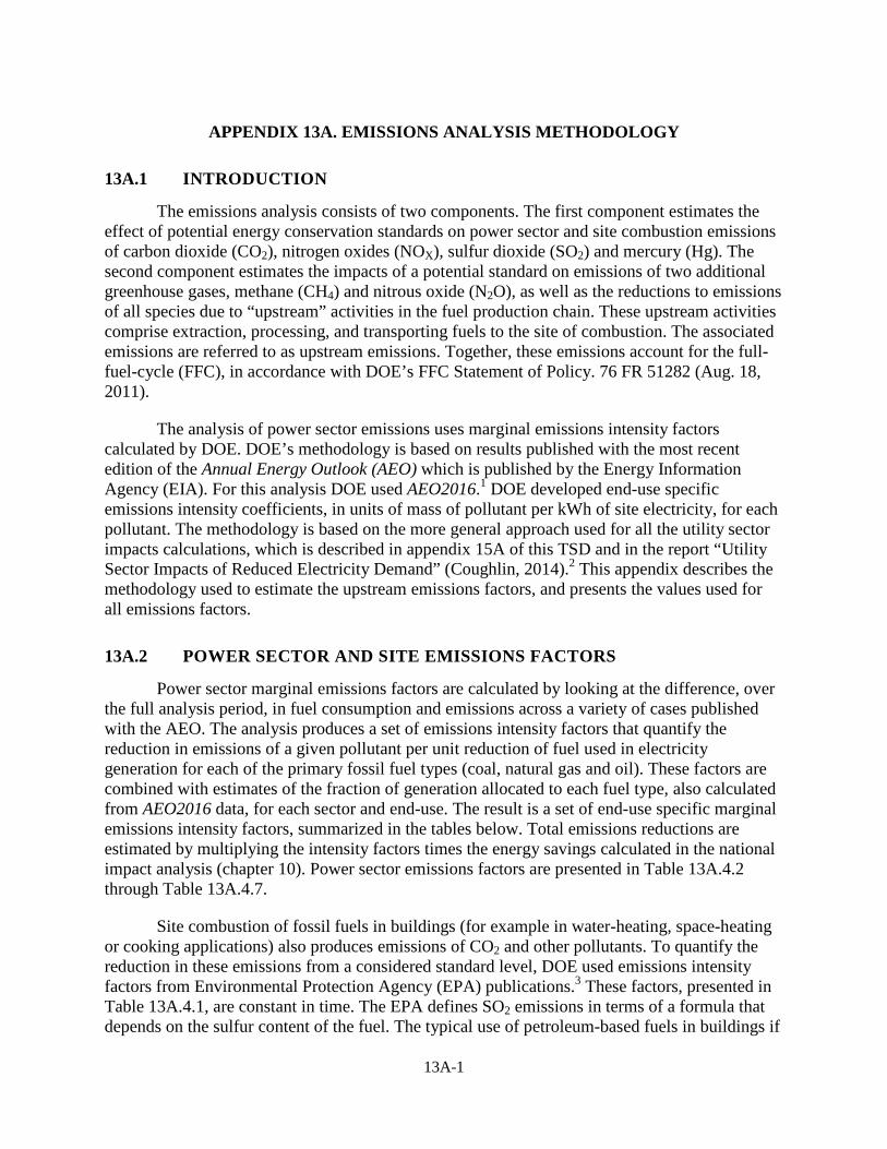
13A-1

APPENDIX 13A. EMISSIONS ANALYSIS METHODOLOGY

13A.1 INTRODUCTION

The emissions analysis consists of two components. The first component estimates the effect of potential energy conservation standards on power sector and site combustion emissions of carbon dioxide (CO2), nitrogen oxides (NOX), sulfur dioxide (SO2) and mercury (Hg). The second component estimates the impacts of a potential standard on emissions of two additional greenhouse gases, methane (CH4) and nitrous oxide (N2O), as well as the reductions to emissions of all species due to “upstream” activities in the fuel production chain. These upstream activities comprise extraction, processing, and transporting fuels to the site of combustion. The associated emissions are referred to as upstream emissions. Together, these emissions account for the full-fuel-cycle (FFC), in accordance with DOE’s FFC Statement of Policy. 76 FR 51282 (Aug. 18, 2011).

The analysis of power sector emissions uses marginal emissions intensity factors calculated by DOE. DOE’s methodology is based on results published with the most recent edition of the Annual Energy Outlook (AEO) which is published by the Energy Information Agency (EIA). For this analysis DOE used AEO2016.1 DOE developed end-use specific emissions intensity coefficients, in units of mass of pollutant per kWh of site electricity, for each pollutant. The methodology is based on the more general approach used for all the utility sector impacts calculations, which is described in appendix 15A of this TSD and in the report “Utility Sector Impacts of Reduced Electricity Demand” (Coughlin, 2014).2 This appendix describes the methodology used to estimate the upstream emissions factors, and presents the values used for all emissions factors.

13A.2 POWER SECTOR AND SITE EMISSIONS FACTORS

Power sector marginal emissions factors are calculated by looking at the difference, over the full analysis period, in fuel consumption and emissions across a variety of cases published with the AEO. The analysis produces a set of emissions intensity factors that quantify the reduction in emissions of a given pollutant per unit reduction of fuel used in electricity generation for each of the primary fossil fuel types (coal, natural gas and oil). These factors are combined with estimates of the fraction of generation allocated to each fuel type, also calculated from AEO2016 data, for each sector and end-use. The result is a set of end-use specific marginal emissions intensity factors, summarized in the tables below. Total emissions reductions are estimated by multiplying the intensity factors times the energy savings calculated in the national impact analysis (chapter 10). Power sector emissions factors are presented in Table 13A.4.2 through Table 13A.4.7.

Site combustion of fossil fuels in buildings (for example in water-heating, space-heating or cooking applications) also produces emissions of CO2 and other pollutants. To quantify the reduction in these emissions from a considered standard level, DOE used emissions intensity factors from Environmental Protection Agency (EPA) publications.3 These factors, presented in Table 13A.4.1, are constant in time. The EPA defines SO2 emissions in terms of a formula that depends on the sulfur content of the fuel. The typical use of petroleum-based fuels in buildings if

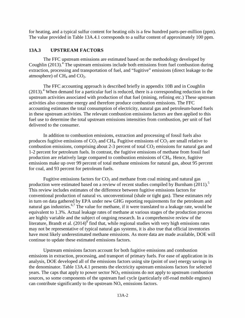
13A-2

for heating, and a typical sulfur content for heating oils is a few hundred parts-per-million (ppm). The value provided in Table 13A.4.1 corresponds to a sulfur content of approximately 100 ppm.

13A.3 UPSTREAM FACTORS

The FFC upstream emissions are estimated based on the methodology developed by Coughlin (2013).4 The upstream emissions include both emissions from fuel combustion during extraction, processing and transportation of fuel, and “fugitive” emissions (direct leakage to the atmosphere) of CH4 and CO2.

The FFC accounting approach is described briefly in appendix 10B and in Coughlin (2013).4 When demand for a particular fuel is reduced, there is a corresponding reduction in the upstream activities associated with production of that fuel (mining, refining etc.) These upstream activities also consume energy and therefore produce combustion emissions. The FFC accounting estimates the total consumption of electricity, natural gas and petroleum-based fuels in these upstream activities. The relevant combustion emissions factors are then applied to this fuel use to determine the total upstream emissions intensities from combustion, per unit of fuel delivered to the consumer.

In addition to combustion emissions, extraction and processing of fossil fuels also produces fugitive emissions of CO2 and CH4. Fugitive emissions of CO2 are small relative to combustion emissions, comprising about 2-3 percent of total CO2 emissions for natural gas and 1-2 percent for petroleum fuels. In contrast, the fugitive emissions of methane from fossil fuel production are relatively large compared to combustion emissions of CH4. Hence, fugitive emissions make up over 99 percent of total methane emissions for natural gas, about 95 percent for coal, and 93 percent for petroleum fuels.

Fugitive emissions factors for CO2 and methane from coal mining and natural gas production were estimated based on a review of recent studies compiled by Burnham (2011).5 This review includes estimates of the difference between fugitive emissions factors for conventional production of natural vs. unconventional (shale or tight gas). These estimates rely in turn on data gathered by EPA under new GHG reporting requirements for the petroleum and natural gas industries.6,7 The value for methane, if it were translated to a leakage rate, would be equivalent to 1.3%. Actual leakage rates of methane at various stages of the production process are highly variable and the subject of ongoing research. In a comprehensive review of the literature, Brandt et al. (2014)8 find that, while regional studies with very high emissions rates may not be representative of typical natural gas systems, it is also true that official inventories have most likely underestimated methane emissions. As more data are made available, DOE will continue to update these estimated emissions factors.

Upstream emissions factors account for both fugitive emissions and combustion emissions in extraction, processing, and transport of primary fuels. For ease of application in its analysis, DOE developed all of the emissions factors using site (point of use) energy savings in the denominator. Table 13A.4.1 presents the electricity upstream emissions factors for selected years. The caps that apply to power sector NOX emissions do not apply to upstream combustion sources, so some components of the upstream fuel cycle (particularly off-road mobile engines) can contribute significantly to the upstream NOx emissions factors.

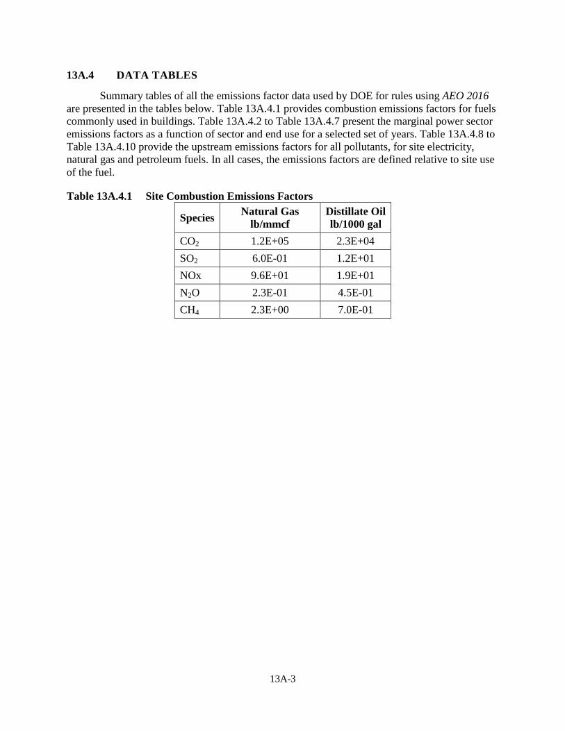
13A-3

13A.4 DATA TABLES

Summary tables of all the emissions factor data used by DOE for rules using AEO 2016 are presented in the tables below. Table 13A.4.1 provides combustion emissions factors for fuels commonly used in buildings. Table 13A.4.2 to Table 13A.4.7 present the marginal power sector emissions factors as a function of sector and end use for a selected set of years. Table 13A.4.8 to Table 13A.4.10 provide the upstream emissions factors for all pollutants, for site electricity, natural gas and petroleum fuels. In all cases, the emissions factors are defined relative to site use of the fuel.

Table 13A.4.1 Site Combustion Emissions Factors

Species Natural Gas lb/mmcf

Distillate Oil lb/1000 gal

CO2 1.2E+05 2.3E+04 SO2 6.0E-01 1.2E+01 NOx 9.6E+01 1.9E+01 N2O 2.3E-01 4.5E-01 CH4 2.3E+00 7.0E-01

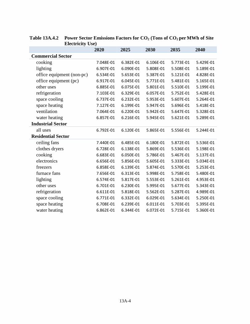
13A-4

Table 13A.4.2 Power Sector Emissions Factors for CO2 (Tons of CO2 per MWh of Site

Electricity Use)

2020 2025 2030 2035 2040

Commercial Sector cooking 7.048E-01 6.382E-01 6.106E-01 5.773E-01 5.429E-01

lighting 6.907E-01 6.090E-01 5.808E-01 5.508E-01 5.189E-01 office equipment (non-pc) 6.534E-01 5.653E-01 5.387E-01 5.121E-01 4.828E-01 office equipment (pc) 6.917E-01 6.045E-01 5.771E-01 5.481E-01 5.165E-01 other uses 6.885E-01 6.075E-01 5.801E-01 5.510E-01 5.199E-01 refrigeration 7.103E-01 6.329E-01 6.057E-01 5.752E-01 5.428E-01 space cooling 6.737E-01 6.232E-01 5.953E-01 5.607E-01 5.264E-01 space heating 7.127E-01 6.199E-01 5.947E-01 5.696E-01 5.418E-01 ventilation 7.064E-01 6.220E-01 5.942E-01 5.647E-01 5.328E-01 water heating 6.857E-01 6.216E-01 5.945E-01 5.621E-01 5.289E-01

Industrial Sector all uses 6.792E-01 6.120E-01 5.865E-01 5.556E-01 5.244E-01

Residential Sector ceiling fans 7.440E-01 6.485E-01 6.180E-01 5.872E-01 5.536E-01

clothes dryers 6.728E-01 6.138E-01 5.869E-01 5.536E-01 5.198E-01 cooking 6.683E-01 6.050E-01 5.786E-01 5.467E-01 5.137E-01 electronics 6.656E-01 5.856E-01 5.605E-01 5.333E-01 5.034E-01 freezers 6.858E-01 6.139E-01 5.874E-01 5.570E-01 5.253E-01 furnace fans 7.656E-01 6.313E-01 5.998E-01 5.758E-01 5.480E-01 lighting 6.574E-01 5.817E-01 5.553E-01 5.261E-01 4.953E-01 other uses 6.701E-01 6.230E-01 5.995E-01 5.677E-01 5.343E-01 refrigeration 6.611E-01 5.818E-01 5.562E-01 5.287E-01 4.989E-01 space cooling 6.771E-01 6.332E-01 6.029E-01 5.634E-01 5.250E-01 space heating 6.708E-01 6.239E-01 6.011E-01 5.703E-01 5.395E-01 water heating 6.862E-01 6.344E-01 6.072E-01 5.715E-01 5.360E-01

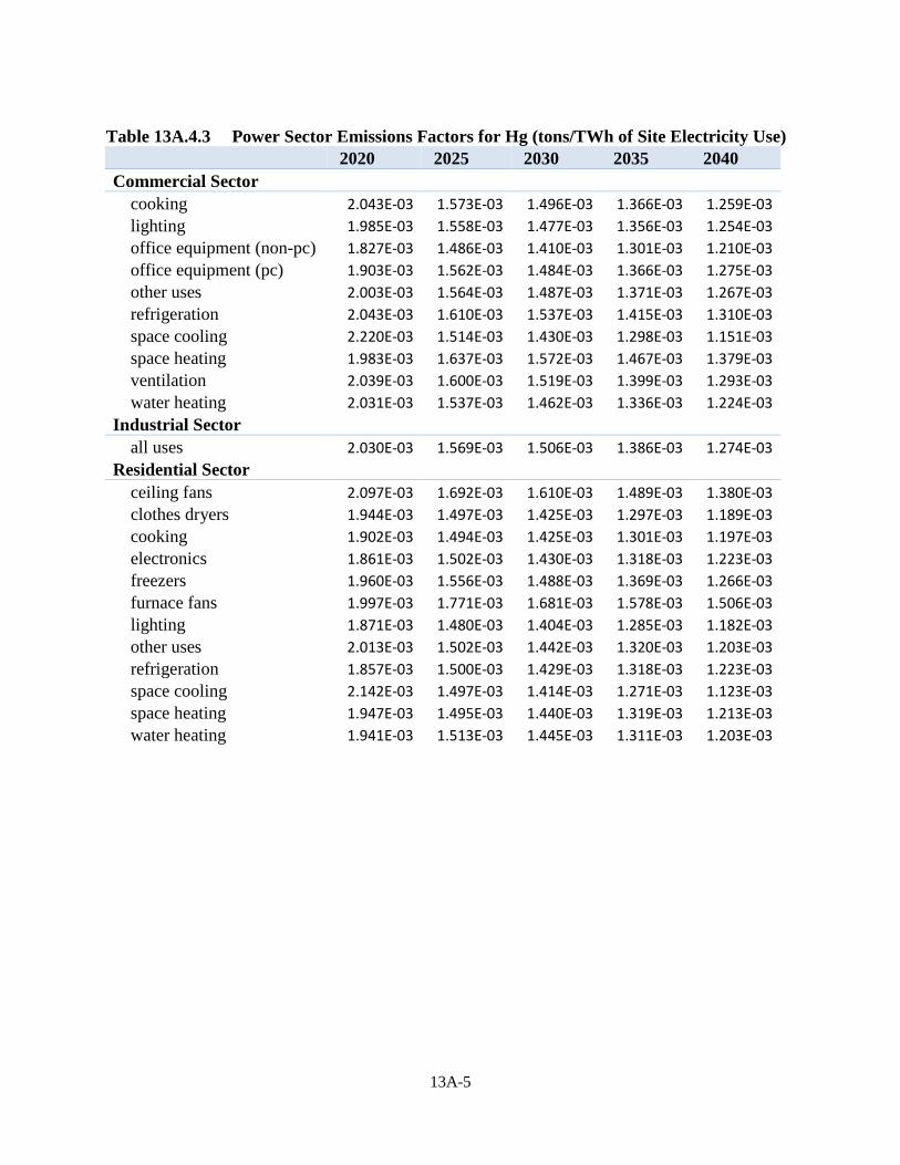
13A-5

Table 13A.4.3 Power Sector Emissions Factors for Hg (tons/TWh of Site Electricity Use)

2020 2025 2030 2035 2040

Commercial Sector cooking 2.043E-03 1.573E-03 1.496E-03 1.366E-03 1.259E-03

lighting 1.985E-03 1.558E-03 1.477E-03 1.356E-03 1.254E-03 office equipment (non-pc) 1.827E-03 1.486E-03 1.410E-03 1.301E-03 1.210E-03 office equipment (pc) 1.903E-03 1.562E-03 1.484E-03 1.366E-03 1.275E-03 other uses 2.003E-03 1.564E-03 1.487E-03 1.371E-03 1.267E-03 refrigeration 2.043E-03 1.610E-03 1.537E-03 1.415E-03 1.310E-03 space cooling 2.220E-03 1.514E-03 1.430E-03 1.298E-03 1.151E-03 space heating 1.983E-03 1.637E-03 1.572E-03 1.467E-03 1.379E-03 ventilation 2.039E-03 1.600E-03 1.519E-03 1.399E-03 1.293E-03 water heating 2.031E-03 1.537E-03 1.462E-03 1.336E-03 1.224E-03

Industrial Sector all uses 2.030E-03 1.569E-03 1.506E-03 1.386E-03 1.274E-03

Residential Sector ceiling fans 2.097E-03 1.692E-03 1.610E-03 1.489E-03 1.380E-03

clothes dryers 1.944E-03 1.497E-03 1.425E-03 1.297E-03 1.189E-03 cooking 1.902E-03 1.494E-03 1.425E-03 1.301E-03 1.197E-03 electronics 1.861E-03 1.502E-03 1.430E-03 1.318E-03 1.223E-03 freezers 1.960E-03 1.556E-03 1.488E-03 1.369E-03 1.266E-03 furnace fans 1.997E-03 1.771E-03 1.681E-03 1.578E-03 1.506E-03 lighting 1.871E-03 1.480E-03 1.404E-03 1.285E-03 1.182E-03 other uses 2.013E-03 1.502E-03 1.442E-03 1.320E-03 1.203E-03 refrigeration 1.857E-03 1.500E-03 1.429E-03 1.318E-03 1.223E-03 space cooling 2.142E-03 1.497E-03 1.414E-03 1.271E-03 1.123E-03 space heating 1.947E-03 1.495E-03 1.440E-03 1.319E-03 1.213E-03 water heating 1.941E-03 1.513E-03 1.445E-03 1.311E-03 1.203E-03

13A-6

Table 13A.4.4 Power Sector Emissions Factors for NOx (tons/MWh of Site Electricity

Use)

2020 2025 2030 2035 2040

Commercial Sector cooking 4.193E-04 3.306E-04 2.646E-04 2.546E-04 2.557E-04

lighting 3.937E-04 3.203E-04 2.612E-04 2.517E-04 2.522E-04 office equipment (non-pc) 3.547E-04 2.983E-04 2.458E-04 2.371E-04 2.372E-04 office equipment (pc) 3.785E-04 3.156E-04 2.582E-04 2.494E-04 2.496E-04 other uses 3.963E-04 3.220E-04 2.643E-04 2.545E-04 2.553E-04 refrigeration 4.171E-04 3.359E-04 2.770E-04 2.676E-04 2.684E-04 space cooling 4.303E-04 3.246E-04 2.538E-04 2.410E-04 2.434E-04 space heating 4.110E-04 3.408E-04 2.946E-04 2.879E-04 2.896E-04 ventilation 4.000E-04 3.272E-04 2.670E-04 2.574E-04 2.583E-04 water heating 4.133E-04 3.244E-04 2.611E-04 2.515E-04 2.533E-04

Industrial Sector all uses 4.350E-04 3.407E-04 2.910E-04 2.796E-04 2.780E-04

Residential Sector ceiling fans 4.198E-04 3.458E-04 2.866E-04 2.760E-04 2.756E-04

clothes dryers 4.172E-04 3.228E-04 2.615E-04 2.513E-04 2.515E-04 cooking 4.052E-04 3.184E-04 2.593E-04 2.495E-04 2.497E-04 electronics 3.749E-04 3.079E-04 2.529E-04 2.445E-04 2.453E-04 freezers 4.191E-04 3.322E-04 2.787E-04 2.689E-04 2.688E-04 furnace fans 3.792E-04 3.429E-04 2.965E-04 2.893E-04 2.894E-04 lighting 3.806E-04 3.075E-04 2.522E-04 2.428E-04 2.430E-04 other uses 4.358E-04 3.310E-04 2.709E-04 2.617E-04 2.626E-04 refrigeration 3.757E-04 3.086E-04 2.553E-04 2.466E-04 2.472E-04 space cooling 4.452E-04 3.298E-04 2.582E-04 2.447E-04 2.453E-04 space heating 4.300E-04 3.286E-04 2.689E-04 2.611E-04 2.643E-04 water heating 4.273E-04 3.280E-04 2.623E-04 2.524E-04 2.530E-04

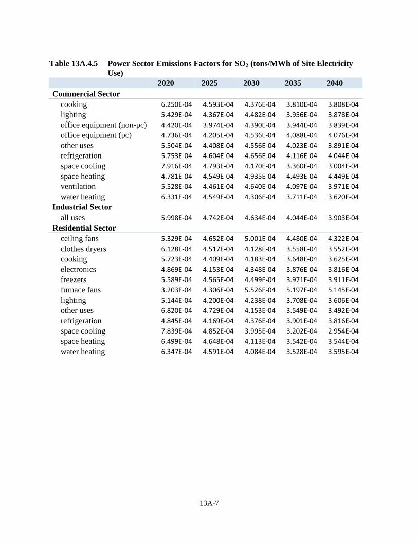
13A-7

Table 13A.4.5 Power Sector Emissions Factors for SO2 (tons/MWh of Site Electricity

Use)

2020 2025 2030 2035 2040

Commercial Sector cooking 6.250E-04 4.593E-04 4.376E-04 3.810E-04 3.808E-04

lighting 5.429E-04 4.367E-04 4.482E-04 3.956E-04 3.878E-04 office equipment (non-pc) 4.420E-04 3.974E-04 4.390E-04 3.944E-04 3.839E-04 office equipment (pc) 4.736E-04 4.205E-04 4.536E-04 4.088E-04 4.076E-04 other uses 5.504E-04 4.408E-04 4.556E-04 4.023E-04 3.891E-04 refrigeration 5.753E-04 4.604E-04 4.656E-04 4.116E-04 4.044E-04 space cooling 7.916E-04 4.793E-04 4.170E-04 3.360E-04 3.004E-04 space heating 4.781E-04 4.549E-04 4.935E-04 4.493E-04 4.449E-04 ventilation 5.528E-04 4.461E-04 4.640E-04 4.097E-04 3.971E-04 water heating 6.331E-04 4.549E-04 4.306E-04 3.711E-04 3.620E-04

Industrial Sector all uses 5.998E-04 4.742E-04 4.634E-04 4.044E-04 3.903E-04

Residential Sector ceiling fans 5.329E-04 4.652E-04 5.001E-04 4.480E-04 4.322E-04

clothes dryers 6.128E-04 4.517E-04 4.128E-04 3.558E-04 3.552E-04 cooking 5.723E-04 4.409E-04 4.183E-04 3.648E-04 3.625E-04 electronics 4.869E-04 4.153E-04 4.348E-04 3.876E-04 3.816E-04 freezers 5.589E-04 4.565E-04 4.499E-04 3.971E-04 3.911E-04 furnace fans 3.203E-04 4.306E-04 5.526E-04 5.197E-04 5.145E-04 lighting 5.144E-04 4.200E-04 4.238E-04 3.708E-04 3.606E-04 other uses 6.820E-04 4.729E-04 4.153E-04 3.549E-04 3.492E-04 refrigeration 4.845E-04 4.169E-04 4.376E-04 3.901E-04 3.816E-04 space cooling 7.839E-04 4.852E-04 3.995E-04 3.202E-04 2.954E-04 space heating 6.499E-04 4.648E-04 4.113E-04 3.542E-04 3.544E-04 water heating 6.347E-04 4.591E-04 4.084E-04 3.528E-04 3.595E-04

13A-8

Table 13A.4.6 Power Sector Emissions Factors for CH4 (tons/MWh of Site Electricity

Use)

2020 2025 2030 2035 2040

Commercial Sector Cooking 6.421E-05 6.242E-05 5.866E-05 5.520E-05 5.095E-05

Lighting 6.338E-05 6.141E-05 5.776E-05 5.451E-05 5.042E-05 office equipment (non-pc) 6.170E-05 5.960E-05 5.615E-05 5.310E-05 4.917E-05 office equipment (pc) 6.337E-05 6.143E-05 5.785E-05 5.466E-05 5.056E-05 other uses 6.329E-05 6.136E-05 5.779E-05 5.460E-05 5.055E-05 Refrigeration 6.439E-05 6.261E-05 5.900E-05 5.573E-05 5.159E-05 space cooling 6.272E-05 6.080E-05 5.700E-05 5.344E-05 4.923E-05 space heating 6.456E-05 6.277E-05 5.942E-05 5.649E-05 5.264E-05 Ventilation 6.393E-05 6.202E-05 5.839E-05 5.516E-05 5.103E-05 water heating 6.342E-05 6.157E-05 5.787E-05 5.447E-05 5.033E-05

Industrial Sector all uses 6.361E-05 6.195E-05 5.850E-05 5.523E-05 5.121E-05

Residential Sector ceiling fans 6.555E-05 6.367E-05 5.994E-05 5.668E-05 5.242E-05

clothes dryers 6.327E-05 6.137E-05 5.762E-05 5.413E-05 4.995E-05 cooking 6.299E-05 6.109E-05 5.741E-05 5.401E-05 4.987E-05 electronics 6.244E-05 6.044E-05 5.694E-05 5.380E-05 4.980E-05 freezers 6.375E-05 6.192E-05 5.835E-05 5.507E-05 5.101E-05 furnace fans 6.591E-05 6.394E-05 6.045E-05 5.767E-05 5.374E-05 lighting 6.221E-05 6.015E-05 5.657E-05 5.330E-05 4.927E-05 other uses 6.331E-05 6.162E-05 5.804E-05 5.465E-05 5.049E-05 refrigeration 6.230E-05 6.032E-05 5.684E-05 5.371E-05 4.975E-05 space cooling 6.336E-05 6.141E-05 5.737E-05 5.353E-05 4.915E-05 space heating 6.342E-05 6.174E-05 5.814E-05 5.476E-05 5.071E-05 water heating 6.397E-05 6.220E-05 5.834E-05 5.471E-05 5.041E-05

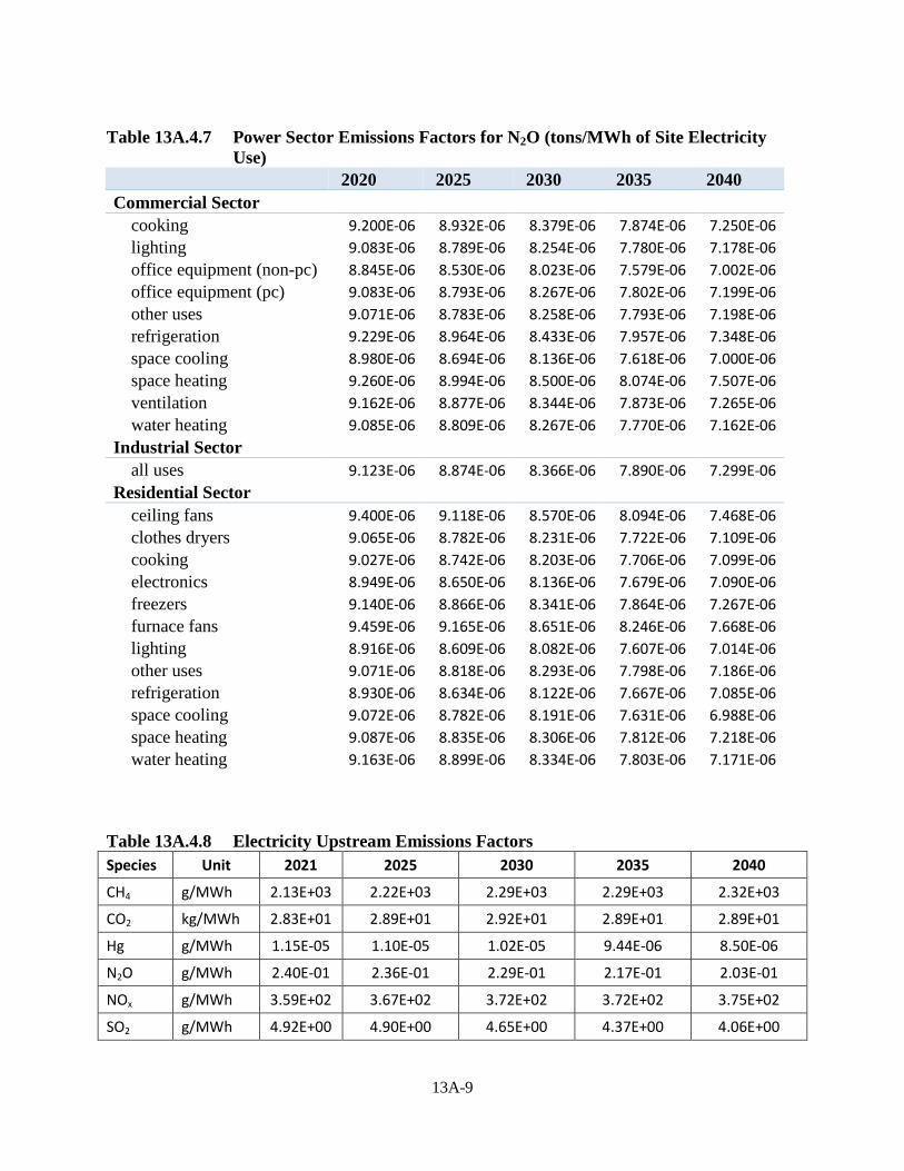
13A-9

Table 13A.4.7 Power Sector Emissions Factors for N2O (tons/MWh of Site Electricity

Use)

2020 2025 2030 2035 2040

Commercial Sector cooking 9.200E-06 8.932E-06 8.379E-06 7.874E-06 7.250E-06

lighting 9.083E-06 8.789E-06 8.254E-06 7.780E-06 7.178E-06 office equipment (non-pc) 8.845E-06 8.530E-06 8.023E-06 7.579E-06 7.002E-06 office equipment (pc) 9.083E-06 8.793E-06 8.267E-06 7.802E-06 7.199E-06 other uses 9.071E-06 8.783E-06 8.258E-06 7.793E-06 7.198E-06 refrigeration 9.229E-06 8.964E-06 8.433E-06 7.957E-06 7.348E-06 space cooling 8.980E-06 8.694E-06 8.136E-06 7.618E-06 7.000E-06 space heating 9.260E-06 8.994E-06 8.500E-06 8.074E-06 7.507E-06 ventilation 9.162E-06 8.877E-06 8.344E-06 7.873E-06 7.265E-06 water heating 9.085E-06 8.809E-06 8.267E-06 7.770E-06 7.162E-06

Industrial Sector all uses 9.123E-06 8.874E-06 8.366E-06 7.890E-06 7.299E-06

Residential Sector ceiling fans 9.400E-06 9.118E-06 8.570E-06 8.094E-06 7.468E-06

clothes dryers 9.065E-06 8.782E-06 8.231E-06 7.722E-06 7.109E-06 cooking 9.027E-06 8.742E-06 8.203E-06 7.706E-06 7.099E-06 electronics 8.949E-06 8.650E-06 8.136E-06 7.679E-06 7.090E-06 freezers 9.140E-06 8.866E-06 8.341E-06 7.864E-06 7.267E-06 furnace fans 9.459E-06 9.165E-06 8.651E-06 8.246E-06 7.668E-06 lighting 8.916E-06 8.609E-06 8.082E-06 7.607E-06 7.014E-06 other uses 9.071E-06 8.818E-06 8.293E-06 7.798E-06 7.186E-06 refrigeration 8.930E-06 8.634E-06 8.122E-06 7.667E-06 7.085E-06 space cooling 9.072E-06 8.782E-06 8.191E-06 7.631E-06 6.988E-06 space heating 9.087E-06 8.835E-06 8.306E-06 7.812E-06 7.218E-06 water heating 9.163E-06 8.899E-06 8.334E-06 7.803E-06 7.171E-06

Table 13A.4.8 Electricity Upstream Emissions Factors Species Unit 2021 2025 2030 2035 2040

CH4 g/MWh 2.13E+03 2.22E+03 2.29E+03 2.29E+03 2.32E+03

CO2 kg/MWh 2.83E+01 2.89E+01 2.92E+01 2.89E+01 2.89E+01

Hg g/MWh 1.15E-05 1.10E-05 1.02E-05 9.44E-06 8.50E-06

N2O g/MWh 2.40E-01 2.36E-01 2.29E-01 2.17E-01 2.03E-01

NOx g/MWh 3.59E+02 3.67E+02 3.72E+02 3.72E+02 3.75E+02

SO2 g/MWh 4.92E+00 4.90E+00 4.65E+00 4.37E+00 4.06E+00

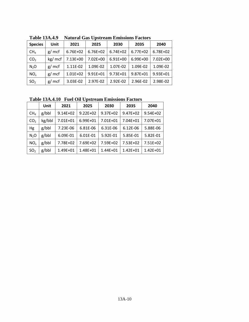
13A-10

Table 13A.4.9 Natural Gas Upstream Emissions Factors Species Unit 2021 2025 2030 2035 2040

CH4 g/ mcf 6.76E+02 6.76E+02 6.74E+02 6.77E+02 6.78E+02

CO2 kg/ mcf 7.13E+00 7.02E+00 6.91E+00 6.99E+00 7.02E+00

N2O g/ mcf 1.11E-02 1.09E-02 1.07E-02 1.09E-02 1.09E-02

NOx g/ mcf 1.01E+02 9.91E+01 9.73E+01 9.87E+01 9.93E+01

SO2 g/ mcf 3.03E-02 2.97E-02 2.92E-02 2.96E-02 2.98E-02 Table 13A.4.10 Fuel Oil Upstream Emissions Factors Unit 2021 2025 2030 2035 2040

CH4 g/bbl 9.14E+02 9.22E+02 9.37E+02 9.47E+02 9.54E+02

CO2 kg/bbl 7.01E+01 6.99E+01 7.01E+01 7.04E+01 7.07E+01

Hg g/bbl 7.23E-06 6.81E-06 6.31E-06 6.12E-06 5.88E-06

N2O g/bbl 6.09E-01 6.01E-01 5.92E-01 5.85E-01 5.82E-01

NOx g/bbl 7.78E+02 7.69E+02 7.59E+02 7.53E+02 7.51E+02

SO2 g/bbl 1.49E+01 1.48E+01 1.44E+01 1.42E+01 1.42E+01

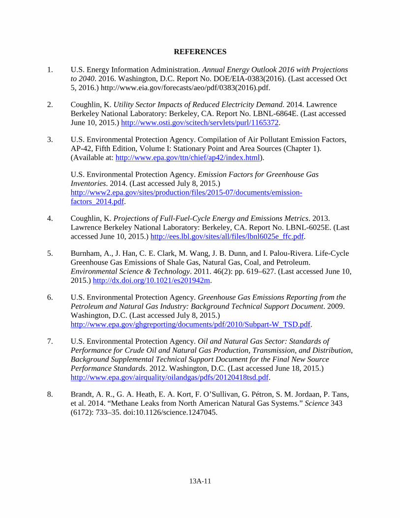
13A-11

REFERENCES 1. U.S. Energy Information Administration. Annual Energy Outlook 2016 with Projections

to 2040. 2016. Washington, D.C. Report No. DOE/EIA-0383(2016). (Last accessed Oct 5, 2016.) http://www.eia.gov/forecasts/aeo/pdf/0383(2016).pdf.

2. Coughlin, K. Utility Sector Impacts of Reduced Electricity Demand. 2014. Lawrence Berkeley National Laboratory: Berkeley, CA. Report No. LBNL-6864E. (Last accessed June 10, 2015.) http://www.osti.gov/scitech/servlets/purl/1165372.

3. U.S. Environmental Protection Agency. Compilation of Air Pollutant Emission Factors, AP-42, Fifth Edition, Volume I: Stationary Point and Area Sources (Chapter 1). (Available at: http://www.epa.gov/ttn/chief/ap42/index.html).

U.S. Environmental Protection Agency. Emission Factors for Greenhouse Gas Inventories. 2014. (Last accessed July 8, 2015.) http://www2.epa.gov/sites/production/files/2015-07/documents/emission-factors_2014.pdf.

4. Coughlin, K. Projections of Full-Fuel-Cycle Energy and Emissions Metrics. 2013. Lawrence Berkeley National Laboratory: Berkeley, CA. Report No. LBNL-6025E. (Last accessed June 10, 2015.) http://ees.lbl.gov/sites/all/files/lbnl6025e_ffc.pdf.

5. Burnham, A., J. Han, C. E. Clark, M. Wang, J. B. Dunn, and I. Palou-Rivera. Life-Cycle Greenhouse Gas Emissions of Shale Gas, Natural Gas, Coal, and Petroleum. Environmental Science & Technology. 2011. 46(2): pp. 619–627. (Last accessed June 10, 2015.) http://dx.doi.org/10.1021/es201942m.

6. U.S. Environmental Protection Agency. Greenhouse Gas Emissions Reporting from the Petroleum and Natural Gas Industry: Background Technical Support Document. 2009. Washington, D.C. (Last accessed July 8, 2015.) http://www.epa.gov/ghgreporting/documents/pdf/2010/Subpart-W_TSD.pdf.

7. U.S. Environmental Protection Agency. Oil and Natural Gas Sector: Standards of Performance for Crude Oil and Natural Gas Production, Transmission, and Distribution, Background Supplemental Technical Support Document for the Final New Source Performance Standards. 2012. Washington, D.C. (Last accessed June 18, 2015.) http://www.epa.gov/airquality/oilandgas/pdfs/20120418tsd.pdf.

8. Brandt, A. R., G. A. Heath, E. A. Kort, F. O’Sullivan, G. Pétron, S. M. Jordaan, P. Tans, et al. 2014. “Methane Leaks from North American Natural Gas Systems.” Science 343 (6172): 733–35. doi:10.1126/science.1247045.

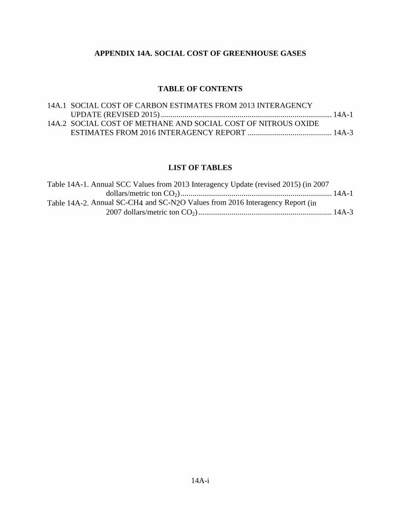
14A-i

APPENDIX 14A. SOCIAL COST OF GREENHOUSE GASES

TABLE OF CONTENTS

14A.1 SOCIAL COST OF CARBON ESTIMATES FROM 2013 INTERAGENCY UPDATE (REVISED 2015) ....................................................................................... 14A-1

14A.2 SOCIAL COST OF METHANE AND SOCIAL COST OF NITROUS OXIDE ESTIMATES FROM 2016 INTERAGENCY REPORT ........................................... 14A-3

LIST OF TABLES

Table 14A-1. Annual SCC Values from 2013 Interagency Update (revised 2015) (in 2007 dollars/metric ton CO2) ............................................................................. 14A-1

Table 14A-2. Annual SC-CH4 and SC-N2O Values from 2016 Interagency Report (in 2007 dollars/metric ton CO2) .................................................................... 14A-3

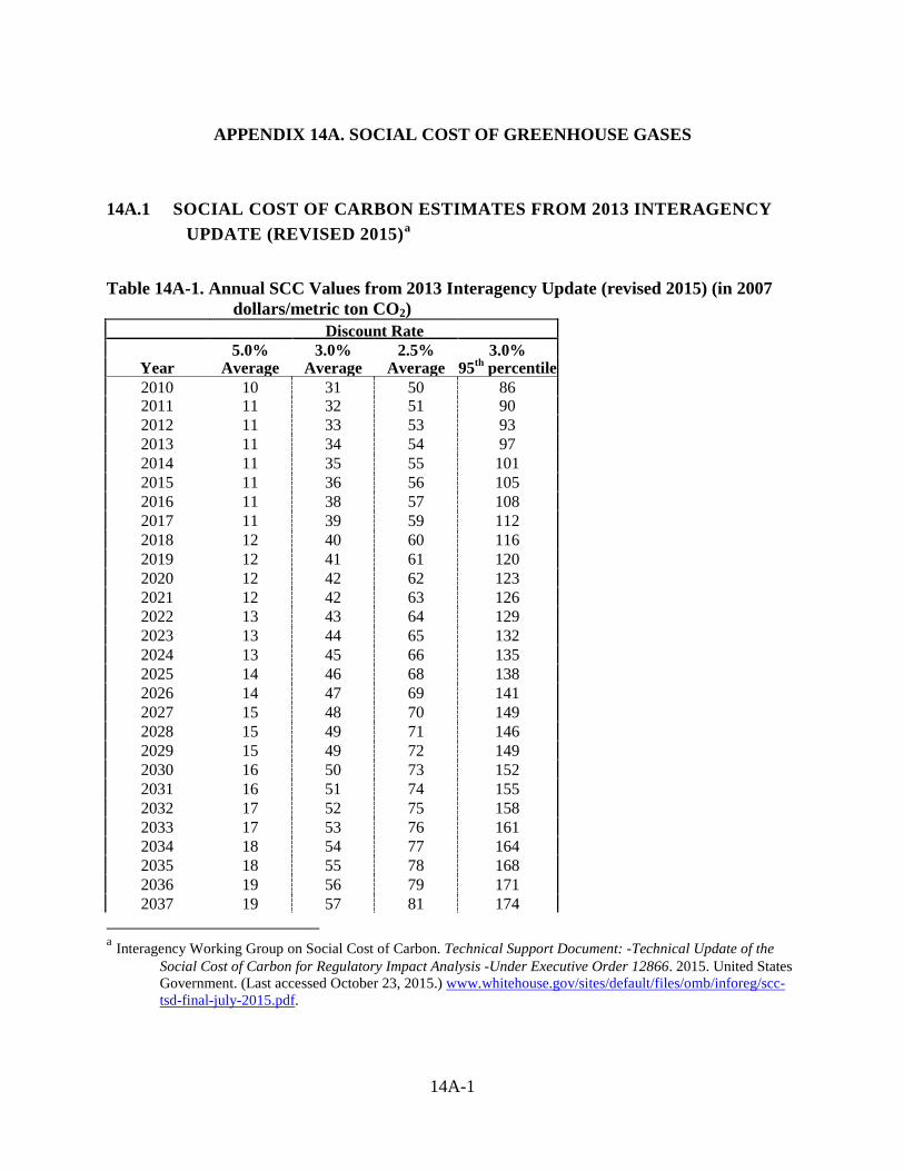
14A-1

APPENDIX 14A. SOCIAL COST OF GREENHOUSE GASES

14A.1 SOCIAL COST OF CARBON ESTIMATES FROM 2013 INTERAGENCY UPDATE (REVISED 2015)a

Table 14A-1. Annual SCC Values from 2013 Interagency Update (revised 2015) (in 2007

dollars/metric ton CO2)

a Interagency Working Group on Social Cost of Carbon. Technical Support Document: -Technical Update of the

Social Cost of Carbon for Regulatory Impact Analysis -Under Executive Order 12866. 2015. United States Government. (Last accessed October 23, 2015.) www.whitehouse.gov/sites/default/files/omb/inforeg/scc-tsd-final-july-2015.pdf.

Discount Rate

5.0% 3.0% 2.5% 3.0% Year Average Average Average 95th percentile 2010 10 31 50 86 2011 11 32 51 90 2012 11 33 53 93 2013 11 34 54 97 2014 11 35 55 101 2015 11 36 56 105 2016 11 38 57 108 2017 11 39 59 112 2018 12 40 60 116 2019 12 41 61 120 2020 12 42 62 123 2021 12 42 63 126 2022 13 43 64 129 2023 13 44 65 132 2024 13 45 66 135 2025 14 46 68 138 2026 14 47 69 141 2027 15 48 70 149 2028 15 49 71 146 2029 15 49 72 149 2030 16 50 73 152 2031 16 51 74 155 2032 17 52 75 158 2033 17 53 76 161 2034 18 54 77 164 2035 18 55 78 168 2036 19 56 79 171 2037 19 57 81 174

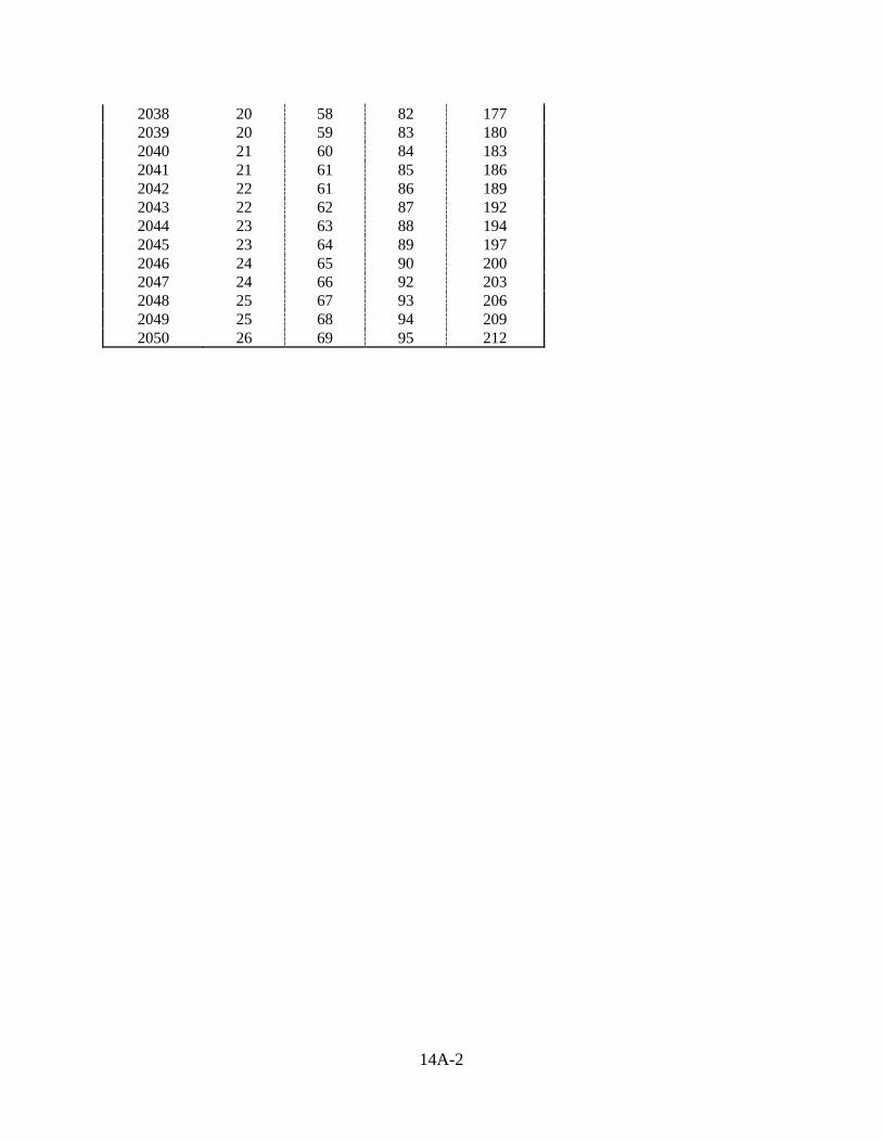
14A-2

2038 20 58 82 177 2039 20 59 83 180 2040 21 60 84 183 2041 21 61 85 186 2042 22 61 86 189 2043 22 62 87 192 2044 23 63 88 194 2045 23 64 89 197 2046 24 65 90 200 2047 24 66 92 203 2048 25 67 93 206 2049 25 68 94 209 2050 26 69 95 212

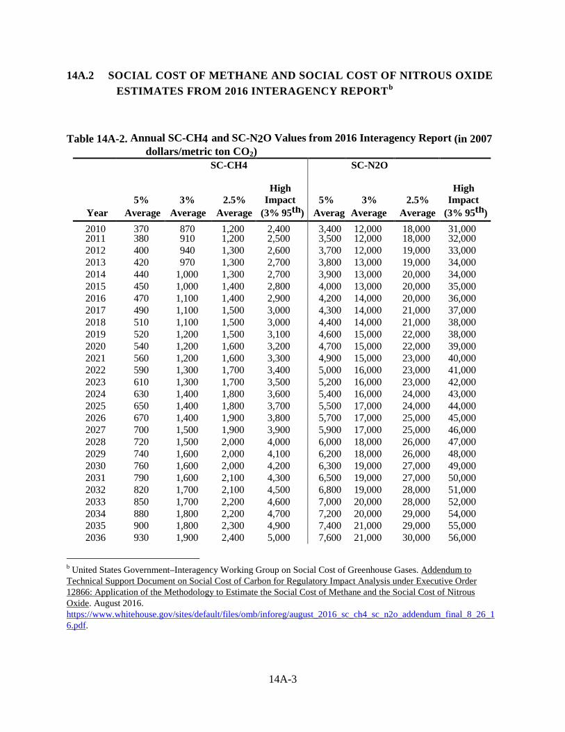
14A-3

14A.2 SOCIAL COST OF METHANE AND SOCIAL COST OF NITROUS OXIDE ESTIMATES FROM 2016 INTERAGENCY REPORTb

Table 14A-2. Annual SC-CH4 and SC-N2O Values from 2016 Interagency Report (in 2007

dollars/metric ton CO2) SC-CH4 SC-N2O

5%

3%

2.5%

High Impact

5%

3%

2.5%

High Impact

Year Average Average Average (3% 95th) Averag

Average Average (3% 95th) 2010 370 870 1,200 2,400 3,400 12,000 18,000 31,000 2011 380 910 1,200 2,500 3,500 12,000 18,000 32,000 2012 400 940 1,300 2,600 3,700 12,000 19,000 33,000 2013 420 970 1,300 2,700 3,800 13,000 19,000 34,000 2014 440 1,000 1,300 2,700 3,900 13,000 20,000 34,000 2015 450 1,000 1,400 2,800 4,000 13,000 20,000 35,000 2016 470 1,100 1,400 2,900 4,200 14,000 20,000 36,000 2017 490 1,100 1,500 3,000 4,300 14,000 21,000 37,000 2018 510 1,100 1,500 3,000 4,400 14,000 21,000 38,000 2019 520 1,200 1,500 3,100 4,600 15,000 22,000 38,000 2020 540 1,200 1,600 3,200 4,700 15,000 22,000 39,000 2021 560 1,200 1,600 3,300 4,900 15,000 23,000 40,000 2022 590 1,300 1,700 3,400 5,000 16,000 23,000 41,000 2023 610 1,300 1,700 3,500 5,200 16,000 23,000 42,000 2024 630 1,400 1,800 3,600 5,400 16,000 24,000 43,000 2025 650 1,400 1,800 3,700 5,500 17,000 24,000 44,000 2026 670 1,400 1,900 3,800 5,700 17,000 25,000 45,000 2027 700 1,500 1,900 3,900 5,900 17,000 25,000 46,000 2028 720 1,500 2,000 4,000 6,000 18,000 26,000 47,000 2029 740 1,600 2,000 4,100 6,200 18,000 26,000 48,000 2030 760 1,600 2,000 4,200 6,300 19,000 27,000 49,000 2031 790 1,600 2,100 4,300 6,500 19,000 27,000 50,000 2032 820 1,700 2,100 4,500 6,800 19,000 28,000 51,000 2033 850 1,700 2,200 4,600 7,000 20,000 28,000 52,000 2034 880 1,800 2,200 4,700 7,200 20,000 29,000 54,000 2035 900 1,800 2,300 4,900 7,400 21,000 29,000 55,000 2036 930 1,900 2,400 5,000 7,600 21,000 30,000 56,000

b United States Government–Interagency Working Group on Social Cost of Greenhouse Gases. Addendum to Technical Support Document on Social Cost of Carbon for Regulatory Impact Analysis under Executive Order 12866: Application of the Methodology to Estimate the Social Cost of Methane and the Social Cost of Nitrous Oxide. August 2016. https://www.whitehouse.gov/sites/default/files/omb/inforeg/august_2016_sc_ch4_sc_n2o_addendum_final_8_26_16.pdf.

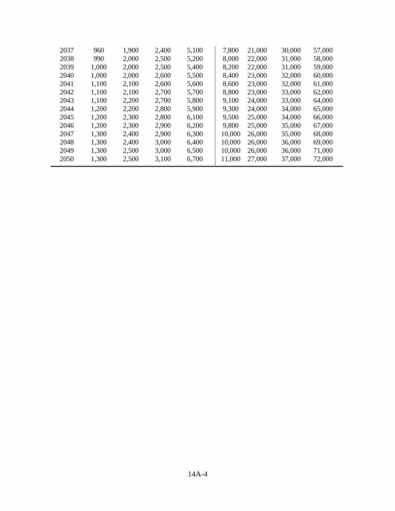
14A-4

2037 960 1,900 2,400 5,100 7,800 21,000 30,000 57,000 2038 990 2,000 2,500 5,200 8,000 22,000 31,000 58,000 2039 1,000 2,000 2,500 5,400 8,200 22,000 31,000 59,000 2040 1,000 2,000 2,600 5,500 8,400 23,000 32,000 60,000 2041 1,100 2,100 2,600 5,600 8,600 23,000 32,000 61,000 2042 1,100 2,100 2,700 5,700 8,800 23,000 33,000 62,000 2043 1,100 2,200 2,700 5,800 9,100 24,000 33,000 64,000 2044 1,200 2,200 2,800 5,900 9,300 24,000 34,000 65,000 2045 1,200 2,300 2,800 6,100 9,500 25,000 34,000 66,000 2046 1,200 2,300 2,900 6,200 9,800 25,000 35,000 67,000 2047 1,300 2,400 2,900 6,300 10,000 26,000 35,000 68,000 2048 1,300 2,400 3,000 6,400 10,000 26,000 36,000 69,000 2049 1,300 2,500 3,000 6,500 10,000 26,000 36,000 71,000 2050 1,300 2,500 3,100 6,700 11,000 27,000 37,000 72,000

14B-i

APPENDIX 14B. BENEFIT-PER-TON VALUES FOR NOX EMISSIONS FROM ELECTRICYT GENERATION

TABLE OF CONTENTS

14B.1 INTRODUCTION .......................................................................................................14B-1 14B.2 METHODOLOGY ......................................................................................................14B-1

14B.2.1 EPA Data .........................................................................................................14B-1 14B.2.2 AEO Data .........................................................................................................14B-2 14B.2.3 Equations..........................................................................................................14B-3

14B.3 RESULTS ....................................................................................................................14B-4 REFERENCES ........................................................................................................................14B-6

LIST OF TABLES

Table 14B-1 EPA Benefit-per-Ton Estimates for NOx (as PM2.5) for the Electricity Generating Utility Sector (2011$/short ton) ..............................................14B-2

Table 14B-2 NOX values based on the EPA price for low range, 7% discount rate (2011$/short ton) ........................................................................................14B-4

Table 14B-3 NOX values based on the EPA price for low range, 3% discount rate (2011$/short ton) ........................................................................................14B-4

Table 14B-4 NOX values based on the EPA price for high range, 7% discount rate (2011$/short ton) ........................................................................................14B-4

Table 14B-5 NOX values based on the EPA price for high range, 3% discount rate (2011$/short ton) ........................................................................................14B-5

LIST OF FIGURES

Figure 14B.2.1 Time series of the ratio of NOX tons/GWh of electricity sold by region ...14B-3

14B-1

APPENDIX 14B. BENEFIT-PER-TON VALUES FOR NOX EMISSIONS FROM ELECTRICITY GENERATION

14B.1 INTRODUCTION

This appendix describes the analytical methodology DOE uses to incorporate regional variability in NOX valuations into the emissions monetization. The regional values assigned to NOX emissions are taken from the EPA Clean Power Plan Final Rule,1 and summarized in Table 14B.2.1. EPA provides a range of estimates of the present value of NOX emissions reductions in three regions (East, West, and California) and three years (2020, 2025, and 2030). These data are combined with regional information on electricity consumption and NOX emissions to define a weighted-average national value for NOX as a function of end-use.

DOE’s methodology is based on results published with the most recent edition of the

Annual Energy Outlook (AEO) which is published by the Energy Information Agency (EIA). For this analysis DOE used AEO2016.2 In AEO2016 EIA incorporated the EPA Clean Power Plan (CPP) into the Reference case. The CPP plan period is 2020-2030, over which time states must achieve a mandated a limit on CO2 emissions from electricity generation. EIA also published a side case (No CPP) using the same assumptions as the Reference case but without implementation of the CPP. On February 9, 2016 the US Supreme Court granted a stay halting implementation of the CPP. Because the fate of the CPP is uncertain, DOE used the AEO2016 No CPP case as its reference projection for the energy sector.

The AEO2016 data are used to define two sets of factors that enter into the calculation: the distribution of end-use electricity consumption by region, and the relative NOX emissions intensity (in units of tons per MWh of electricity sales) in each region.

The rest of this appendix provides a more detailed description of the methodology and

results.

14B.2 METHODOLOGY

14B.2.1 EPA Data

The EPA Clean Power Plan Final Rule includes estimates of the present value of the benefits of NOX (as PM2.5) emissions reductions (benefit-per-ton estimates) in a given year, for three years (2020, 2025 and 2030). Because NOX, and other pollutants whose production is enhanced by the presence of NOX, persist in the atmosphere over a period of years, reductions in any given year will have benefits in subsequent years. These future benefits are discounted and summed to provide a single value for the reduction of one ton of emissions in the EPA model year. EPA publishes a range of values, defined by high and low, and using discount rates of 3% and 7% as mandated by OMB. These values are presented in Table 14B.2.1.

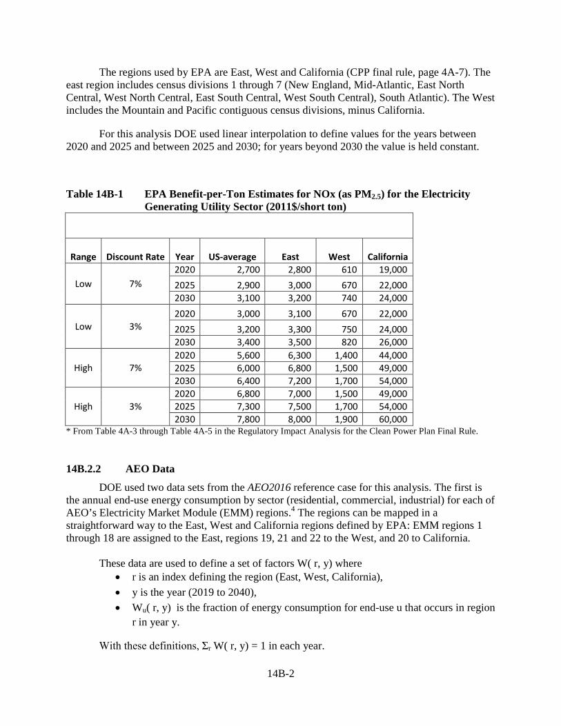
14B-2

The regions used by EPA are East, West and California (CPP final rule, page 4A-7). The east region includes census divisions 1 through 7 (New England, Mid-Atlantic, East North Central, West North Central, East South Central, West South Central), South Atlantic). The West includes the Mountain and Pacific contiguous census divisions, minus California.

For this analysis DOE used linear interpolation to define values for the years between 2020 and 2025 and between 2025 and 2030; for years beyond 2030 the value is held constant.

Table 14B-1 EPA Benefit-per-Ton Estimates for NOx (as PM2.5) for the Electricity Generating Utility Sector (2011$/short ton)

Range Discount Rate Year US-average East West California

Low 7% 2020 2,700 2,800 610 19,000 2025 2,900 3,000 670 22,000 2030 3,100 3,200 740 24,000

Low 3% 2020 3,000 3,100 670 22,000 2025 3,200 3,300 750 24,000 2030 3,400 3,500 820 26,000

High 7% 2020 5,600 6,300 1,400 44,000 2025 6,000 6,800 1,500 49,000 2030 6,400 7,200 1,700 54,000

High 3% 2020 6,800 7,000 1,500 49,000 2025 7,300 7,500 1,700 54,000 2030 7,800 8,000 1,900 60,000

* From Table 4A-3 through Table 4A-5 in the Regulatory Impact Analysis for the Clean Power Plan Final Rule.

14B.2.2 AEO Data

DOE used two data sets from the AEO2016 reference case for this analysis. The first is the annual end-use energy consumption by sector (residential, commercial, industrial) for each of AEO’s Electricity Market Module (EMM) regions.4 The regions can be mapped in a straightforward way to the East, West and California regions defined by EPA: EMM regions 1 through 18 are assigned to the East, regions 19, 21 and 22 to the West, and 20 to California.

These data are used to define a set of factors W( r, y) where

• r is an index defining the region (East, West, California), • y is the year (2019 to 2040), • Wu( r, y) is the fraction of energy consumption for end-use u that occurs in region

r in year y.

With these definitions, Σr W( r, y) = 1 in each year.

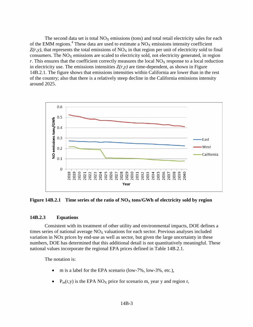
14B-3

The second data set is total NOX emissions (tons) and total retail electricity sales for each

of the EMM regions.4 These data are used to estimate a NOX emissions intensity coefficient Z(r,y), that represents the total emissions of NOX in that region per unit of electricity sold to final consumers. The NOX emissions are scaled to electricity sold, not electricity generated, in region r. This ensures that the coefficient correctly measures the local NOX response to a local reduction in electricity use. The emissions intensities Z(r,y) are time-dependent, as shown in Figure 14B.2.1. The figure shows that emissions intensities within California are lower than in the rest of the country; also that there is a relatively steep decline in the California emissions intensity around 2025.

Figure 14B.2.1 Time series of the ratio of NOX tons/GWh of electricity sold by region

14B.2.3 Equations

Consistent with its treatment of other utility and environmental impacts, DOE defines a times series of national average NOX valuations for each sector. Previous analyses included variation in NOx prices by end-use as well as sector, but given the large uncertainty in these numbers, DOE has determined that this additional detail is not quantitatively meaningful. These national values incorporate the regional EPA prices defined in Table 14B.2.1.

The notation is:

• m is a label for the EPA scenario (low-7%, low-3%, etc.),

• Pm(r,y) is the EPA NOX price for scenario m, year y and region r,

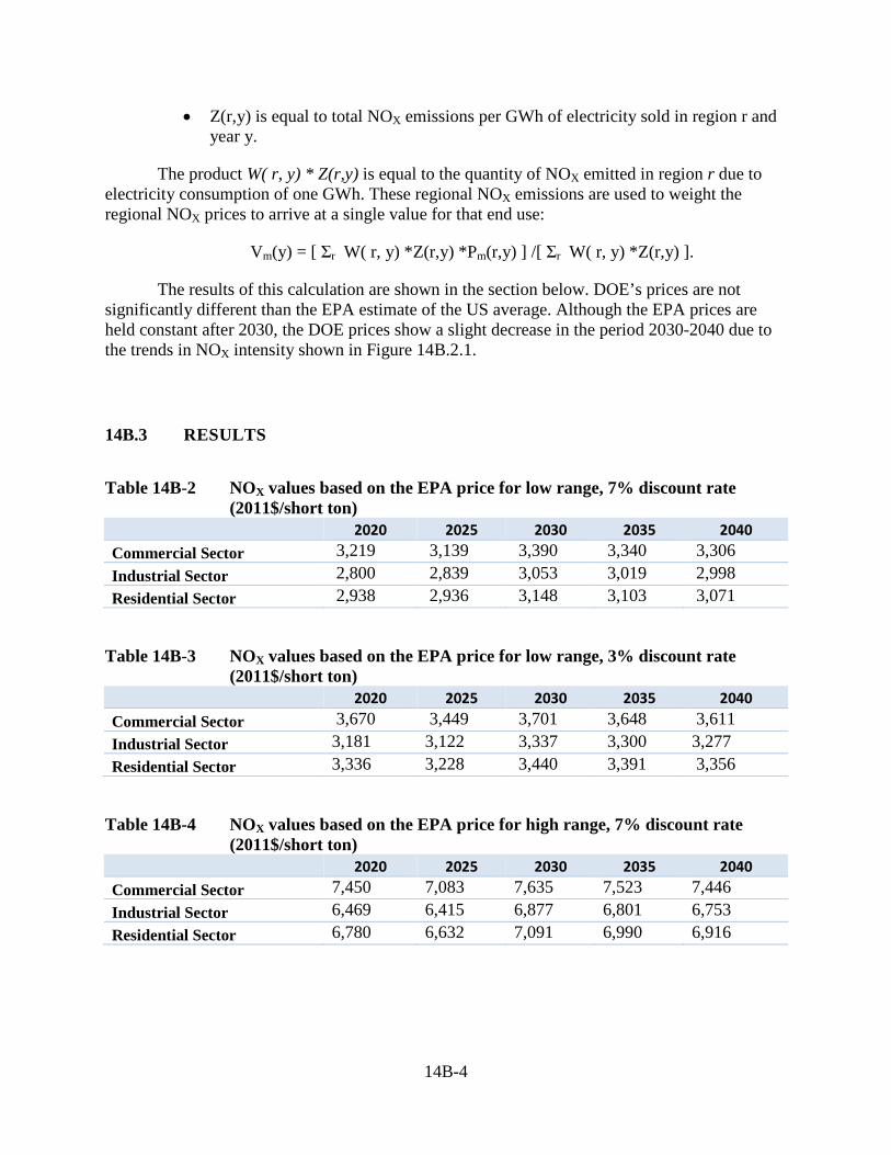
14B-4

• Z(r,y) is equal to total NOX emissions per GWh of electricity sold in region r and year y.

The product W( r, y) * Z(r,y) is equal to the quantity of NOX emitted in region r due to electricity consumption of one GWh. These regional NOX emissions are used to weight the regional NOX prices to arrive at a single value for that end use:

Vm(y) = [ Σr W( r, y) *Z(r,y) *Pm(r,y) ] /[ Σr W( r, y) *Z(r,y) ].

The results of this calculation are shown in the section below. DOE’s prices are not significantly different than the EPA estimate of the US average. Although the EPA prices are held constant after 2030, the DOE prices show a slight decrease in the period 2030-2040 due to the trends in NOX intensity shown in Figure 14B.2.1.

14B.3 RESULTS

Table 14B-2 NOX values based on the EPA price for low range, 7% discount rate

(2011$/short ton)

2020 2025 2030 2035 2040

Commercial Sector 3,219 3,139 3,390 3,340 3,306 Industrial Sector 2,800 2,839 3,053 3,019 2,998 Residential Sector 2,938 2,936 3,148 3,103 3,071

Table 14B-3 NOX values based on the EPA price for low range, 3% discount rate (2011$/short ton)

2020 2025 2030 2035 2040

Commercial Sector 3,670 3,449 3,701 3,648 3,611 Industrial Sector 3,181 3,122 3,337 3,300 3,277 Residential Sector 3,336 3,228 3,440 3,391 3,356

Table 14B-4 NOX values based on the EPA price for high range, 7% discount rate (2011$/short ton)

2020 2025 2030 2035 2040

Commercial Sector 7,450 7,083 7,635 7,523 7,446 Industrial Sector 6,469 6,415 6,877 6,801 6,753 Residential Sector 6,780 6,632 7,091 6,990 6,916

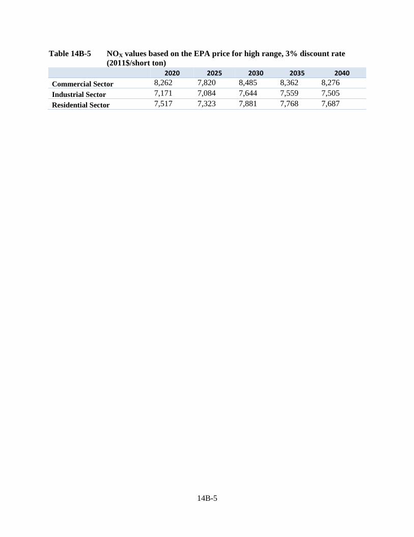
14B-5

Table 14B-5 NOX values based on the EPA price for high range, 3% discount rate (2011$/short ton)

2020 2025 2030 2035 2040

Commercial Sector 8,262 7,820 8,485 8,362 8,276 Industrial Sector 7,171 7,084 7,644 7,559 7,505 Residential Sector 7,517 7,323 7,881 7,768 7,687

14B-6

REFERENCES 1. U.S. Environmental Protection Agency. Carbon Pollution Emission Guidelines for

Existing Stationary Sources: Electric Utility Generating Units; Final Rule. Federal Register. October 23, 2015. vol. 80, no. 205: pp. 64662–64964. (Last accessed January 21, 2016.) https://www.gpo.gov/fdsys/pkg/FR-2015-10-23/pdf/2015-22842.pdf.

2. U.S. Energy Information Administration. Annual Energy Outlook 2015 with Projections to 2040. 2015. Washington, D.C. Report No. DOE/EIA-0383(2015). (Last accessed December 15, 2015.) http://www.eia.gov/forecasts/aeo/pdf/0383(2015).pdf.

3. U.S. Department of Energy–Energy Information Administration. Form EIA-861 Annual Electric Power Industry Report Database. (Last accessed December 15, 2015.) http://www.eia.gov/electricity/data/eia861/index.html.

4. U.S. Energy Information Administration. Assumptions to the Annual Energy Outlook 2015: Electricity Market Module. 2015. Washington, D.C. (Last accessed January 21, 2016.) https://www.eia.gov/forecasts/aeo/assumptions/pdf/electricity.pdf.

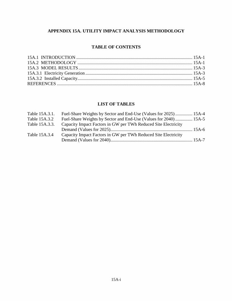
15A-i

APPENDIX 15A. UTILITY IMPACT ANALYSIS METHODOLOGY

TABLE OF CONTENTS

15A.1 INTRODUCTION ...................................................................................................... 15A-1 15A.2 METHODOLOGY ..................................................................................................... 15A-1 15A.3 MODEL RESULTS .................................................................................................... 15A-3 15A.3.1 Electricity Generation .............................................................................................. 15A-3 15A.3.2 Installed Capacity..................................................................................................... 15A-5 REFERENCES ....................................................................................................................... 15A-8

LIST OF TABLES

Table 15A.3.1. Fuel-Share Weights by Sector and End-Use (Values for 2025) ............... 15A-4 Table 15A.3.2 Fuel-Share Weights by Sector and End-Use (Values for 2040) ............... 15A-5 Table 15A.3.3. Capacity Impact Factors in GW per TWh Reduced Site Electricity

Demand (Values for 2025) ........................................................................ 15A-6 Table 15A.3.4 Capacity Impact Factors in GW per TWh Reduced Site Electricity

Demand (Values for 2040) ........................................................................ 15A-7

15A-1

APPENDIX 15A. UTILITY IMPACT ANALYSIS METHODOLOGY

15A.1 INTRODUCTION

In the utility impact analysis, the U.S. Department of Energy (DOE) analyzes the changes in electric installed capacity and power generation that result for each trial standard level (TSL). These changes are estimated by multiplying the site savings of electricity by a set of impact factors which measure the corresponding change in generation by fuel type, installed capacity, and power sector emissions. This Appendix describes the methods that DOE used to calculate these impact factors. The methodology is more fully described in Coughlin (2014).1

DOE’s analysis uses output of the DOE/Energy Information Administration (EIA)’s Annual Energy Outlook (AEO). The AEO includes a reference case and a set of side cases that implement a variety of economic and policy scenarios. In 2015 EIA announced the adoption of a two-year release cycle for the AEO, alternating between a full set of scenarios and a shorter edition containing only five scenarios.2 DOE adapts its calculation methodology according to the number and type of scenarios available with each AEO publication.

15A.2 METHODOLOGY

Marginal reductions in electricity demand lead to marginal reductions in power sector generation, emissions, and installed capacity. Generally, DOE quantifies these reductions using marginal impact factors, which are time series defining the change in some power sector quantity that results from a unit change in site electricity demand. Because load shapes affect the mix of generation types on the margin, these impact factors depend on end-use and sector.

DOE’s approach examines a series of AEO side cases related to efficiency policy to estimate the relationship between marginal demand reductions and power sector variables. In AEO2016 most published side cases do not incorporate changes in demand. Consequently DOE has adapted it’s methodology to use grid-average, rather than marginal, data for the utility impacts estimation. DOE continues to use marginal emissions intensity factors for the emissions analysis, as described in appendix 13A.

The purpose of the utility impacts analysis is to relate changes in electricity demand to the corresponding changes in three quantities: power sector generation (TWh) by fuel type, power sector fuel consumption (quads) by fuel type, and power sector installed capacity (GW) by fuel and technology type.

For this analysis, DOE used the AEO projections of generation, fuel consumption and installed capacity by Electricity Market Module (EMM) region. DOE aggregated the data for the 22 EMM regions into 5 regions which are also aggregations of the NERC reliability regions: region 1 consists of NERC regions NPCC and RFC, region 2 contains the SERC and FRCC regions, region 3 is MRO, region 4 ERCOT plus SPP, and region 5 is WECC.

The relationship between fuel consumption and generation is defined by the heat rate (quads/TWh). DOE’s approach to calculating heat rates is described in appendix 10B of this

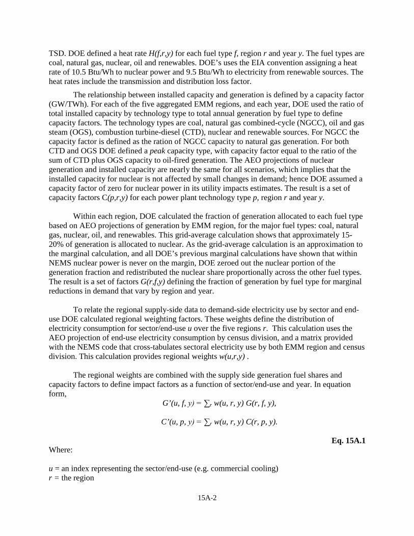
15A-2

TSD. DOE defined a heat rate H(f,r,y) for each fuel type f, region r and year y. The fuel types are coal, natural gas, nuclear, oil and renewables. DOE’s uses the EIA convention assigning a heat rate of 10.5 Btu/Wh to nuclear power and 9.5 Btu/Wh to electricity from renewable sources. The heat rates include the transmission and distribution loss factor. The relationship between installed capacity and generation is defined by a capacity factor (GW/TWh). For each of the five aggregated EMM regions, and each year, DOE used the ratio of total installed capacity by technology type to total annual generation by fuel type to define capacity factors. The technology types are coal, natural gas combined-cycle (NGCC), oil and gas steam (OGS), combustion turbine-diesel (CTD), nuclear and renewable sources. For NGCC the capacity factor is defined as the ration of NGCC capacity to natural gas generation. For both CTD and OGS DOE defined a peak capacity type, with capacity factor equal to the ratio of the sum of CTD plus OGS capacity to oil-fired generation. The AEO projections of nuclear generation and installed capacity are nearly the same for all scenarios, which implies that the installed capacity for nuclear is not affected by small changes in demand; hence DOE assumed a capacity factor of zero for nuclear power in its utility impacts estimates. The result is a set of capacity factors C(p,r,y) for each power plant technology type p, region r and year y. Within each region, DOE calculated the fraction of generation allocated to each fuel type based on AEO projections of generation by EMM region, for the major fuel types: coal, natural gas, nuclear, oil, and renewables. This grid-average calculation shows that approximately 15-20% of generation is allocated to nuclear. As the grid-average calculation is an approximation to the marginal calculation, and all DOE’s previous marginal calculations have shown that within NEMS nuclear power is never on the margin, DOE zeroed out the nuclear portion of the generation fraction and redistributed the nuclear share proportionally across the other fuel types. The result is a set of factors G(r,f,y) defining the fraction of generation by fuel type for marginal reductions in demand that vary by region and year. To relate the regional supply-side data to demand-side electricity use by sector and end-use DOE calculated regional weighting factors. These weights define the distribution of electricity consumption for sector/end-use u over the five regions r. This calculation uses the AEO projection of end-use electricity consumption by census division, and a matrix provided with the NEMS code that cross-tabulates sectoral electricity use by both EMM region and census division. This calculation provides regional weights w(u,r,y) . The regional weights are combined with the supply side generation fuel shares and capacity factors to define impact factors as a function of sector/end-use and year. In equation form,

G’(u, f, y) = ∑r w(u, r, y) G(r, f, y),

C’(u, p, y) = ∑r w(u, r, y) C(r, p, y).

Eq. 15A.1 Where: u = an index representing the sector/end-use (e.g. commercial cooling) r = the region

15A-3

y = the analysis year f = the fuel type p = the power plant technology type w(u,r,y) = the regional weight G(r,f,y) = the fraction of generation provided by fuel type f in region r and year y G’(u,f,y) = the fraction of generation provided by fuel type f for end-use u in year y C(r,f,y) = the capacity factor for plant type p in region r and year y C’(u,f,y) = the capacity factor for plant type p for end-use u in year

15A.3 MODEL RESULTS

Representative values of the impact factors for fuel share by fuel type, and capacity by technology type are provided in the tables below. The tables show the factors for two years, 2025 and 2040. The marginal heat rates are presented in appendix 10B and emissions factors are presented in in appendix 13A.

15A.3.1 Electricity Generation

Table 15A.3.1 and Table 15A.3.2 show the distribution across fuel types of a unit reduction in electricity demand by sector and end-use, referred to above as fuel-share weights. The fuel types are coal, natural gas, petroleum, renewables and nuclear. The values for cooling are representative of peaking loads, while the values for refrigeration are representative of flat loads. The data are shown for 2025 and 2040.

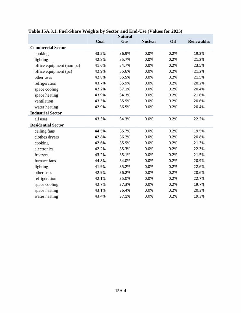
15A-4

Table 15A.3.1. Fuel-Share Weights by Sector and End-Use (Values for 2025)

Coal

Natural Gas Nuclear Oil Renewables

Commercial Sector cooking 43.5% 36.9% 0.0% 0.2% 19.3%

lighting 42.8% 35.7% 0.0% 0.2% 21.2% office equipment (non-pc) 41.6% 34.7% 0.0% 0.2% 23.5% office equipment (pc) 42.9% 35.6% 0.0% 0.2% 21.2% other uses 42.8% 35.5% 0.0% 0.2% 21.5% refrigeration 43.7% 35.9% 0.0% 0.2% 20.2% space cooling 42.2% 37.1% 0.0% 0.2% 20.4% space heating 43.9% 34.3% 0.0% 0.2% 21.6% ventilation 43.3% 35.9% 0.0% 0.2% 20.6% water heating 42.9% 36.5% 0.0% 0.2% 20.4%

Industrial Sector all uses 43.3% 34.3% 0.0% 0.2% 22.2%

Residential Sector ceiling fans 44.5% 35.7% 0.0% 0.2% 19.5%

clothes dryers 42.8% 36.2% 0.0% 0.2% 20.8% cooking 42.6% 35.9% 0.0% 0.2% 21.3% electronics 42.2% 35.3% 0.0% 0.2% 22.3% freezers 43.2% 35.1% 0.0% 0.2% 21.5% furnace fans 44.8% 34.0% 0.0% 0.2% 20.9% lighting 41.9% 35.2% 0.0% 0.2% 22.6% other uses 42.9% 36.2% 0.0% 0.2% 20.6% refrigeration 42.1% 35.0% 0.0% 0.2% 22.7% space cooling 42.7% 37.3% 0.0% 0.2% 19.7% space heating 43.1% 36.4% 0.0% 0.2% 20.3% water heating 43.4% 37.1% 0.0% 0.2% 19.3%

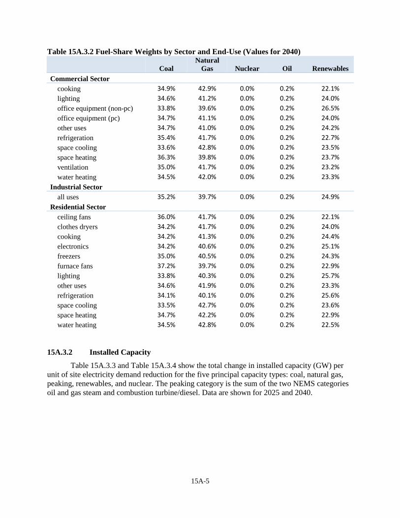
15A-5

Table 15A.3.2 Fuel-Share Weights by Sector and End-Use (Values for 2040)

Coal

Natural Gas Nuclear Oil Renewables

Commercial Sector cooking 34.9% 42.9% 0.0% 0.2% 22.1%

lighting 34.6% 41.2% 0.0% 0.2% 24.0% office equipment (non-pc) 33.8% 39.6% 0.0% 0.2% 26.5% office equipment (pc) 34.7% 41.1% 0.0% 0.2% 24.0% other uses 34.7% 41.0% 0.0% 0.2% 24.2% refrigeration 35.4% 41.7% 0.0% 0.2% 22.7% space cooling 33.6% 42.8% 0.0% 0.2% 23.5% space heating 36.3% 39.8% 0.0% 0.2% 23.7% ventilation 35.0% 41.7% 0.0% 0.2% 23.2% water heating 34.5% 42.0% 0.0% 0.2% 23.3%

Industrial Sector all uses 35.2% 39.7% 0.0% 0.2% 24.9%

Residential Sector ceiling fans 36.0% 41.7% 0.0% 0.2% 22.1%

clothes dryers 34.2% 41.7% 0.0% 0.2% 24.0% cooking 34.2% 41.3% 0.0% 0.2% 24.4% electronics 34.2% 40.6% 0.0% 0.2% 25.1% freezers 35.0% 40.5% 0.0% 0.2% 24.3% furnace fans 37.2% 39.7% 0.0% 0.2% 22.9% lighting 33.8% 40.3% 0.0% 0.2% 25.7% other uses 34.6% 41.9% 0.0% 0.2% 23.3% refrigeration 34.1% 40.1% 0.0% 0.2% 25.6% space cooling 33.5% 42.7% 0.0% 0.2% 23.6% space heating 34.7% 42.2% 0.0% 0.2% 22.9% water heating 34.5% 42.8% 0.0% 0.2% 22.5%

15A.3.2 Installed Capacity

Table 15A.3.3 and Table 15A.3.4 show the total change in installed capacity (GW) per unit of site electricity demand reduction for the five principal capacity types: coal, natural gas, peaking, renewables, and nuclear. The peaking category is the sum of the two NEMS categories oil and gas steam and combustion turbine/diesel. Data are shown for 2025 and 2040.

15A-6

Table 15A.3.3. Capacity Impact Factors in GW per TWh Reduced Site Electricity Demand (Values for 2025)

Coal

Natural Gas Nuclear Peaking Renewables

Commercial Sector cooking 6.99E-02 8.06E-02 0.00E+00 6.95E-02 6.42E-02

lighting 6.88E-02 7.90E-02 0.00E+00 6.83E-02 6.96E-02 office equipment (non-pc) 6.67E-02 7.79E-02 0.00E+00 6.66E-02 7.64E-02 office equipment (pc) 6.88E-02 7.87E-02 0.00E+00 6.82E-02 6.94E-02 other uses 6.87E-02 7.87E-02 0.00E+00 6.82E-02 7.04E-02 refrigeration 7.02E-02 7.89E-02 0.00E+00 6.91E-02 6.63E-02 space cooling 6.78E-02 8.20E-02 0.00E+00 6.92E-02 6.86E-02 space heating 7.05E-02 7.62E-02 0.00E+00 6.82E-02 7.00E-02 ventilation 6.95E-02 7.91E-02 0.00E+00 6.90E-02 6.76E-02 water heating 6.89E-02 8.03E-02 0.00E+00 6.88E-02 6.76E-02

Industrial Sector all uses 6.94E-02 7.68E-02 0.00E+00 6.76E-02 7.28E-02

Residential Sector ceiling fans 7.15E-02 7.83E-02 0.00E+00 6.99E-02 6.39E-02

clothes dryers 6.86E-02 7.98E-02 0.00E+00 6.81E-02 6.90E-02 cooking 6.83E-02 7.93E-02 0.00E+00 6.78E-02 7.03E-02 electronics 6.77E-02 7.85E-02 0.00E+00 6.73E-02 7.30E-02 freezers 6.94E-02 7.78E-02 0.00E+00 6.79E-02 7.04E-02 furnace fans 7.20E-02 7.52E-02 0.00E+00 6.93E-02 6.66E-02 lighting 6.73E-02 7.85E-02 0.00E+00 6.70E-02 7.42E-02 other uses 6.89E-02 8.00E-02 0.00E+00 6.83E-02 6.86E-02 refrigeration 6.75E-02 7.81E-02 0.00E+00 6.70E-02 7.42E-02 space cooling 6.85E-02 8.20E-02 0.00E+00 6.92E-02 6.65E-02 space heating 6.90E-02 8.01E-02 0.00E+00 6.84E-02 6.76E-02 water heating 6.96E-02 8.08E-02 0.00E+00 6.90E-02 6.45E-02

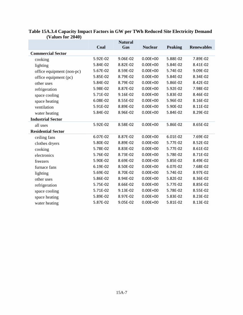
15A-7

Table 15A.3.4 Capacity Impact Factors in GW per TWh Reduced Site Electricity Demand (Values for 2040)

Coal

Natural Gas Nuclear Peaking Renewables

Commercial Sector cooking 5.92E-02 9.06E-02 0.00E+00 5.88E-02 7.89E-02

lighting 5.84E-02 8.82E-02 0.00E+00 5.84E-02 8.41E-02 office equipment (non-pc) 5.67E-02 8.59E-02 0.00E+00 5.74E-02 9.09E-02 office equipment (pc) 5.85E-02 8.79E-02 0.00E+00 5.84E-02 8.34E-02 other uses 5.84E-02 8.79E-02 0.00E+00 5.86E-02 8.42E-02 refrigeration 5.98E-02 8.87E-02 0.00E+00 5.92E-02 7.98E-02 space cooling 5.71E-02 9.16E-02 0.00E+00 5.83E-02 8.46E-02 space heating 6.08E-02 8.55E-02 0.00E+00 5.96E-02 8.16E-02 ventilation 5.91E-02 8.89E-02 0.00E+00 5.90E-02 8.11E-02 water heating 5.84E-02 8.96E-02 0.00E+00 5.84E-02 8.29E-02

Industrial Sector

all uses 5.92E-02 8.58E-02 0.00E+00 5.86E-02 8.65E-02 Residential Sector

ceiling fans 6.07E-02 8.87E-02 0.00E+00 6.01E-02 7.69E-02 clothes dryers 5.80E-02 8.89E-02 0.00E+00 5.77E-02 8.52E-02 cooking 5.78E-02 8.83E-02 0.00E+00 5.77E-02 8.61E-02 electronics 5.76E-02 8.73E-02 0.00E+00 5.78E-02 8.71E-02 freezers 5.90E-02 8.69E-02 0.00E+00 5.85E-02 8.49E-02 furnace fans 6.19E-02 8.50E-02 0.00E+00 6.07E-02 7.68E-02 lighting 5.69E-02 8.70E-02 0.00E+00 5.74E-02 8.97E-02 other uses 5.86E-02 8.94E-02 0.00E+00 5.82E-02 8.36E-02 refrigeration 5.75E-02 8.66E-02 0.00E+00 5.77E-02 8.85E-02 space cooling 5.71E-02 9.13E-02 0.00E+00 5.78E-02 8.55E-02 space heating 5.89E-02 8.97E-02 0.00E+00 5.83E-02 8.23E-02 water heating 5.87E-02 9.05E-02 0.00E+00 5.81E-02 8.13E-02

15A-8

REFERENCES 1. Coughlin, K. Utility Sector Impacts of Reduced Electricity Demand. 2014. Lawrence

Berkeley National Laboratory: Berkeley, CA. Report No. LBNL-6864E. (Last accessed June 10, 2015.) http://www.osti.gov/scitech/servlets/purl/1165372.

2. U.S. Energy Information Administration. Annual Energy Outlook 2016 with Projections to 2040. 2016. Washington, D.C. Report No. DOE/EIA-0383(2016). (Last accessed October 5, 2016.) http://www.eia.gov/forecasts/aeo/pdf/0383(2016).pdf.

3. U.S. Environmental Protection Agency. Emission Factors for Greenhouse Gas Inventories. 2014. (Last accessed July 8, 2015.) http://www.epa.gov/climateleadership/documents/emission-factors.pdf.

17A-i

APPENDIX 17A. REGULATORY IMPACT ANALYSIS: SUPPORTING MATERIALS

TABLE OF CONTENTS

17A.1 INTRODUCTION ...................................................................................................... 17A-1 17A.2 MARKET SHARE ANNUAL INCREASES BY POLICY ....................................... 17A-2 17A.3 NIA-RIA INTEGRATED MODEL ............................................................................ 17A-4 17A.4 MARKET PENETRATION CURVES ...................................................................... 17A-4

17A.4.1 Introduction ..................................................................................................... 17A-4 17A.4.2 Adjustment of XENERGY Penetration Curves .............................................. 17A-6 17A.4.3 Interpolation of Penetration Curves ................................................................ 17A-7

17A.5 CONSUMER REBATE PROGRAMS ....................................................................... 17A-8 17A.6 FEDERAL AND STATE TAX CREDITS................................................................. 17A-9

17A.6.1 Federal Tax Credits for Consumers ................................................................ 17A-9 17A.6.2 Federal Tax Credits for Manufacturers ......................................................... 17A-10 17A.6.3 State Tax Credits ........................................................................................... 17A-11

REFERENCES ..................................................................................................................... 17A-12

LIST OF TABLES

Table 17A.2.1 Annual Increases in Market Shares Attributable to Alternative Policy Measures for RP_FS_L_AC (TSL 2) ....................................................... 17A-2

Table 17A.2.2 Annual Increases in Market Shares Attributable to Alternative Policy Measures for RP_FS_L_WC (TSL 2) ...................................................... 17A-3

Table 17A.5.1 Rebates Programs for Air Compressors .................................................... 17A-8

LIST OF FIGURES

Figure 17A.4.1 S-Curves Showing Effects of External and Internal Sources on Adoption of New Technologies ................................................................ 17A-6

17A-1

APPENDIX 17A. REGULATORY IMPACT ANALYSIS: SUPPORTING MATERIALS

17A.1 INTRODUCTION

This appendix contains sections discussing the following topics:

• Projections of annual market share increases for the alternative policies; • NIA-RIA Integrated Model; • Market penetration curves used to analyze consumer rebates and voluntary energy

efficiency targets, including: o Background material on XENERGY’s approach, o DOE’s adjustment of these curves for this analysis, and o The method DOE used to derive interpolated, customized curves;

• Detailed table of rebates offered for the considered product, as well as DOE’s approach to estimate a market representative rebate value for this RIA; and

• Background material on Federal and State tax credits for appliances.

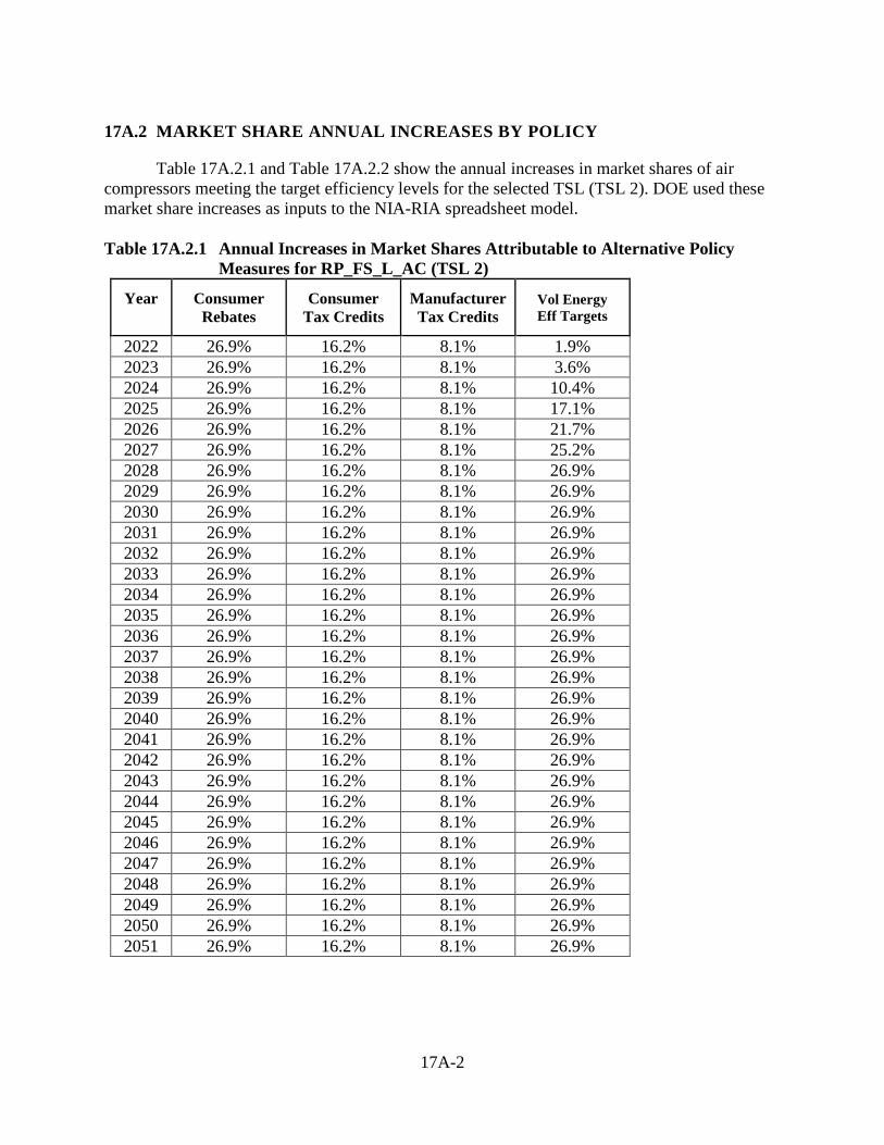
17A-2

17A.2 MARKET SHARE ANNUAL INCREASES BY POLICY

Table 17A.2.1 and Table 17A.2.2 show the annual increases in market shares of air compressors meeting the target efficiency levels for the selected TSL (TSL 2). DOE used these market share increases as inputs to the NIA-RIA spreadsheet model. Table 17A.2.1 Annual Increases in Market Shares Attributable to Alternative Policy

Measures for RP_FS_L_AC (TSL 2)

Year

Consumer Rebates

Consumer Tax Credits

Manufacturer Tax Credits

Vol Energy Eff Targets

2022 26.9% 16.2% 8.1% 1.9% 2023 26.9% 16.2% 8.1% 3.6% 2024 26.9% 16.2% 8.1% 10.4% 2025 26.9% 16.2% 8.1% 17.1% 2026 26.9% 16.2% 8.1% 21.7% 2027 26.9% 16.2% 8.1% 25.2% 2028 26.9% 16.2% 8.1% 26.9% 2029 26.9% 16.2% 8.1% 26.9% 2030 26.9% 16.2% 8.1% 26.9% 2031 26.9% 16.2% 8.1% 26.9% 2032 26.9% 16.2% 8.1% 26.9% 2033 26.9% 16.2% 8.1% 26.9% 2034 26.9% 16.2% 8.1% 26.9% 2035 26.9% 16.2% 8.1% 26.9% 2036 26.9% 16.2% 8.1% 26.9% 2037 26.9% 16.2% 8.1% 26.9% 2038 26.9% 16.2% 8.1% 26.9% 2039 26.9% 16.2% 8.1% 26.9% 2040 26.9% 16.2% 8.1% 26.9% 2041 26.9% 16.2% 8.1% 26.9% 2042 26.9% 16.2% 8.1% 26.9% 2043 26.9% 16.2% 8.1% 26.9% 2044 26.9% 16.2% 8.1% 26.9% 2045 26.9% 16.2% 8.1% 26.9% 2046 26.9% 16.2% 8.1% 26.9% 2047 26.9% 16.2% 8.1% 26.9% 2048 26.9% 16.2% 8.1% 26.9% 2049 26.9% 16.2% 8.1% 26.9% 2050 26.9% 16.2% 8.1% 26.9% 2051 26.9% 16.2% 8.1% 26.9%

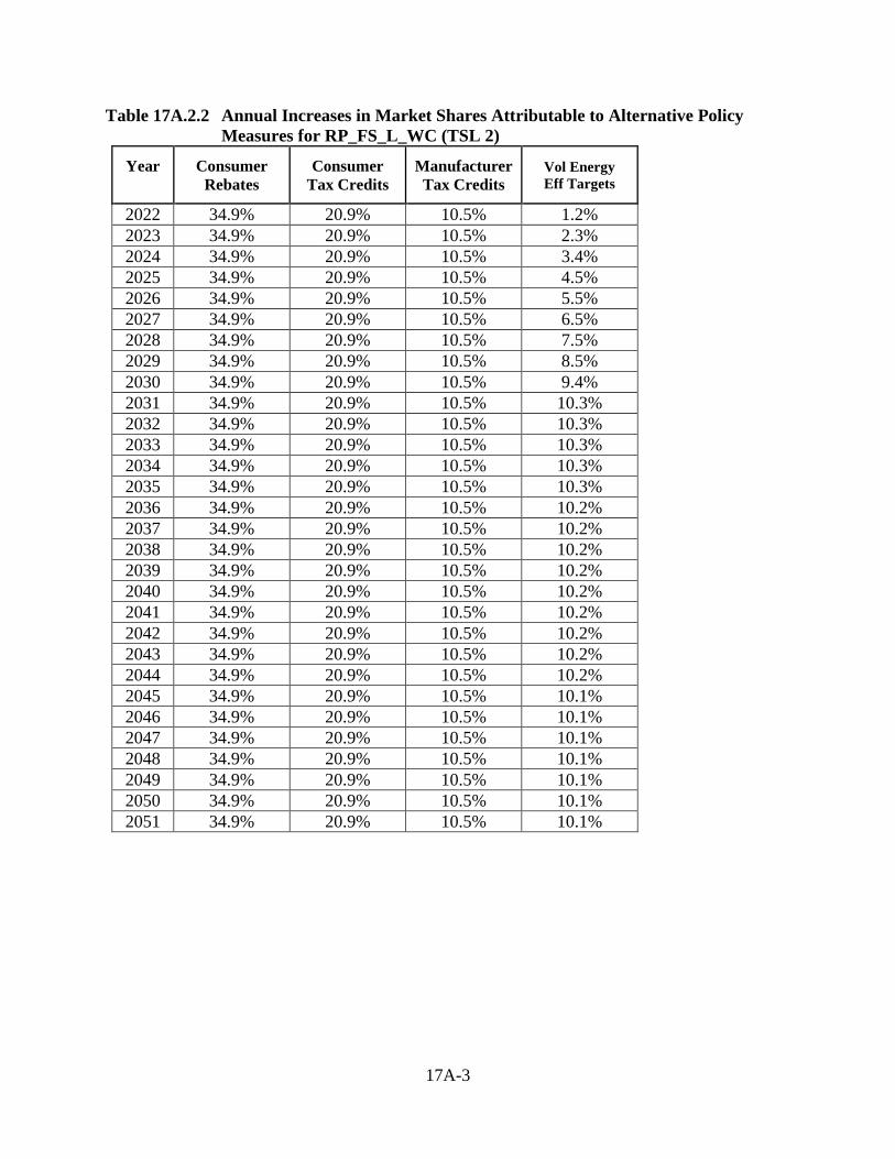
17A-3

Table 17A.2.2 Annual Increases in Market Shares Attributable to Alternative Policy Measures for RP_FS_L_WC (TSL 2)

Year

Consumer Rebates

Consumer Tax Credits

Manufacturer Tax Credits

Vol Energy Eff Targets

2022 34.9% 20.9% 10.5% 1.2% 2023 34.9% 20.9% 10.5% 2.3% 2024 34.9% 20.9% 10.5% 3.4% 2025 34.9% 20.9% 10.5% 4.5% 2026 34.9% 20.9% 10.5% 5.5% 2027 34.9% 20.9% 10.5% 6.5% 2028 34.9% 20.9% 10.5% 7.5% 2029 34.9% 20.9% 10.5% 8.5% 2030 34.9% 20.9% 10.5% 9.4% 2031 34.9% 20.9% 10.5% 10.3% 2032 34.9% 20.9% 10.5% 10.3% 2033 34.9% 20.9% 10.5% 10.3% 2034 34.9% 20.9% 10.5% 10.3% 2035 34.9% 20.9% 10.5% 10.3% 2036 34.9% 20.9% 10.5% 10.2% 2037 34.9% 20.9% 10.5% 10.2% 2038 34.9% 20.9% 10.5% 10.2% 2039 34.9% 20.9% 10.5% 10.2% 2040 34.9% 20.9% 10.5% 10.2% 2041 34.9% 20.9% 10.5% 10.2% 2042 34.9% 20.9% 10.5% 10.2% 2043 34.9% 20.9% 10.5% 10.2% 2044 34.9% 20.9% 10.5% 10.2% 2045 34.9% 20.9% 10.5% 10.1% 2046 34.9% 20.9% 10.5% 10.1% 2047 34.9% 20.9% 10.5% 10.1% 2048 34.9% 20.9% 10.5% 10.1% 2049 34.9% 20.9% 10.5% 10.1% 2050 34.9% 20.9% 10.5% 10.1% 2051 34.9% 20.9% 10.5% 10.1%

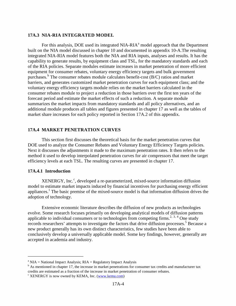
17A-4

17A.3 NIA-RIA INTEGRATED MODEL

For this analysis, DOE used its integrated NIA-RIAa model approach that the Department built on the NIA model discussed in chapter 10 and documented in appendix 10-A.The resulting integrated NIA-RIA model features both the NIA and RIA inputs, analyses and results. It has the capability to generate results, by equipment class and TSL, for the mandatory standards and each of the RIA policies. Separate modules estimate increases in market penetration of more efficient equipment for consumer rebates, voluntary energy efficiency targets and bulk government purchases.b The consumer rebates module calculates benefit-cost (B/C) ratios and market barriers, and generates customized market penetration curves for each equipment class; and the voluntary energy efficiency targets module relies on the market barriers calculated in the consumer rebates module to project a reduction in those barriers over the first ten years of the forecast period and estimate the market effects of such a reduction. A separate module summarizes the market impacts from mandatory standards and all policy alternatives, and an additional module produces all tables and figures presented in chapter 17 as well as the tables of market share increases for each policy reported in Section 17A.2 of this appendix.

17A.4 MARKET PENETRATION CURVES

This section first discusses the theoretical basis for the market penetration curves that DOE used to analyze the Consumer Rebates and Voluntary Energy Efficiency Targets policies. Next it discusses the adjustments it made to the maximum penetration rates. It then refers to the method it used to develop interpolated penetration curves for air compressors that meet the target efficiency levels at each TSL. The resulting curves are presented in chapter 17.

17A.4.1 Introduction

XENERGY, Inc.c, developed a re-parameterized, mixed-source information diffusion model to estimate market impacts induced by financial incentives for purchasing energy efficient appliances.1 The basic premise of the mixed-source model is that information diffusion drives the adoption of technology.

Extensive economic literature describes the diffusion of new products as technologies evolve. Some research focuses primarily on developing analytical models of diffusion patterns applicable to individual consumers or to technologies from competing firms.2, 3, 4 One study records researchers’ attempts to investigate the factors that drive diffusion processes.5 Because a new product generally has its own distinct characteristics, few studies have been able to conclusively develop a universally applicable model. Some key findings, however, generally are accepted in academia and industry.

a NIA = National Impact Analysis; RIA = Regulatory Impact Analysis b As mentioned in chapter 17, the increase in market penetrations for consumer tax credits and manufacturer tax credits are estimated as a fraction of the increase in market penetration of consumer rebates. c XENERGY is now owned by KEMA, Inc. (www.kema.com)

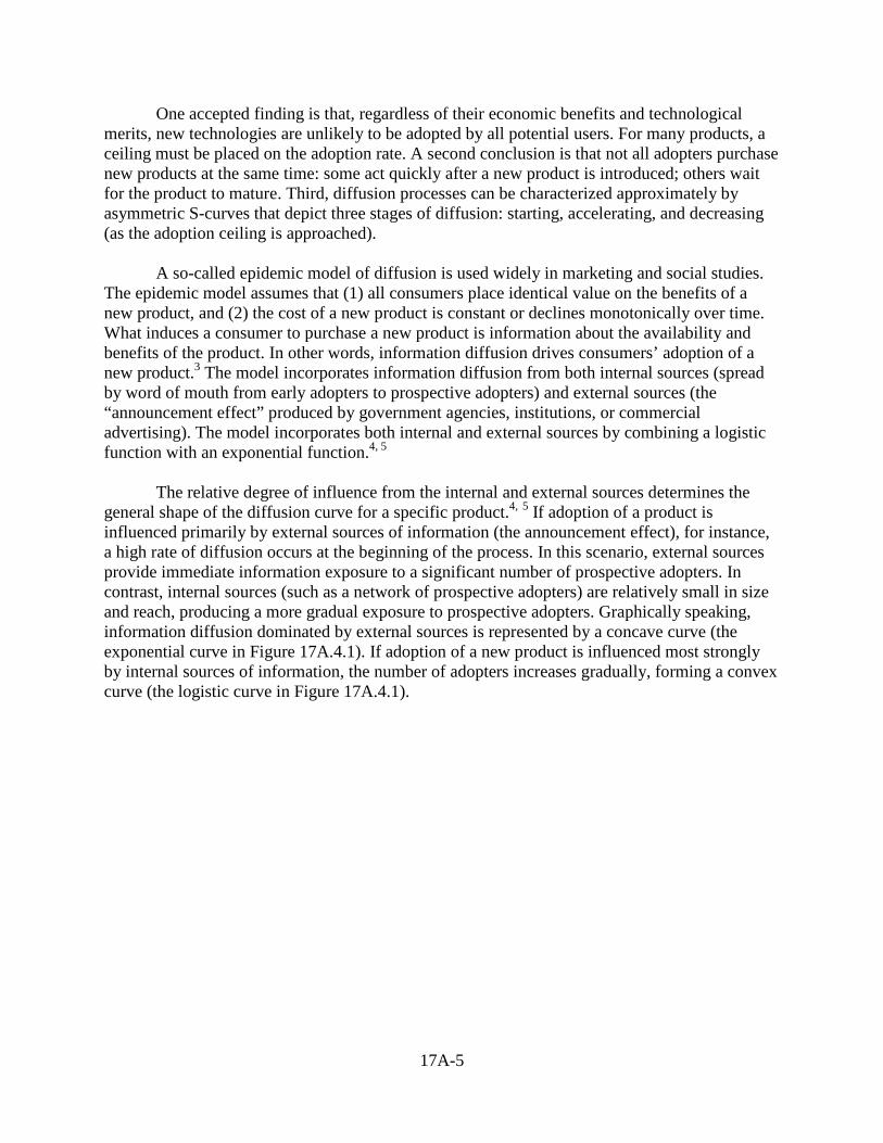
17A-5

One accepted finding is that, regardless of their economic benefits and technological merits, new technologies are unlikely to be adopted by all potential users. For many products, a ceiling must be placed on the adoption rate. A second conclusion is that not all adopters purchase new products at the same time: some act quickly after a new product is introduced; others wait for the product to mature. Third, diffusion processes can be characterized approximately by asymmetric S-curves that depict three stages of diffusion: starting, accelerating, and decreasing (as the adoption ceiling is approached). A so-called epidemic model of diffusion is used widely in marketing and social studies. The epidemic model assumes that (1) all consumers place identical value on the benefits of a new product, and (2) the cost of a new product is constant or declines monotonically over time. What induces a consumer to purchase a new product is information about the availability and benefits of the product. In other words, information diffusion drives consumers’ adoption of a new product.3 The model incorporates information diffusion from both internal sources (spread by word of mouth from early adopters to prospective adopters) and external sources (the “announcement effect” produced by government agencies, institutions, or commercial advertising). The model incorporates both internal and external sources by combining a logistic function with an exponential function.4, 5 The relative degree of influence from the internal and external sources determines the general shape of the diffusion curve for a specific product.4, 5 If adoption of a product is influenced primarily by external sources of information (the announcement effect), for instance, a high rate of diffusion occurs at the beginning of the process. In this scenario, external sources provide immediate information exposure to a significant number of prospective adopters. In contrast, internal sources (such as a network of prospective adopters) are relatively small in size and reach, producing a more gradual exposure to prospective adopters. Graphically speaking, information diffusion dominated by external sources is represented by a concave curve (the exponential curve in Figure 17A.4.1). If adoption of a new product is influenced most strongly by internal sources of information, the number of adopters increases gradually, forming a convex curve (the logistic curve in Figure 17A.4.1).

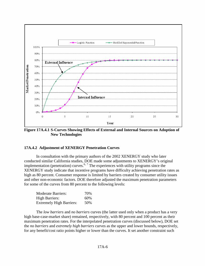
17A-6

Figure 17A.4.1 S-Curves Showing Effects of External and Internal Sources on Adoption of

New Technologies

17A.4.2 Adjustment of XENERGY Penetration Curves

In consultation with the primary authors of the 2002 XENERGY study who later conducted similar California studies, DOE made some adjustments to XENERGY’s original implementation (penetration) curves.6, 7 The experiences with utility programs since the XENERGY study indicate that incentive programs have difficulty achieving penetration rates as high as 80 percent. Consumer response is limited by barriers created by consumer utility issues and other non-economic factors. DOE therefore adjusted the maximum penetration parameters for some of the curves from 80 percent to the following levels: Moderate Barriers: 70% High Barriers: 60% Extremely High Barriers: 50% The low barriers and no barriers curves (the latter used only when a product has a very high base-case-market share) remained, respectively, with 80 percent and 100 percent as their maximum penetration rates. For the interpolated penetration curves (discussed below), DOE set the no barriers and extremely high barriers curves as the upper and lower bounds, respectively, for any benefit/cost ratio points higher or lower than the curves. It set another constraint such

17A-7

that the policy case market share cannot be great than 100 percent, as might occur for products with high no-new-standards case market shares of the target-level technology.

17A.4.3 Interpolation of Penetration Curves

As discussed above, the XENERGY penetration (implementation) curves followed a functional form to estimate the market implementation rate caused by energy efficiency measures such as consumer rebates.d The XENERGY report presents five reference market implementation curves that vary according to the level of market barriers to technology penetration.1 Such curves have been used by DOE in the Regulatory Impact Analyses for rulemakings for appliance energy efficiency standards to estimate market share increases in response to rebate programs.e They provide a framework for evaluating technology penetration, yet require matching the studied market to the curve that best represents it. This approximate matching can introduce some inaccuracy to the analysis.

Blum et al (2011, appendix A)8 presents an alternative approach to such evaluation: a method to estimate market implementation rates more accurately by performing interpolations of the reference curves. The referred report describes the market implementation rate function and the reference curves, the method to calibrate the function to a given market, and the limitations of the method.

DOE used the above referred method to interpolate market implementation curves, to generate customized curves that were used to estimate the effects of consumer rebates and voluntary energy efficiency targets for each equipment class covered by this RIA. For consumer rebates, DOE derived such curves based on an algorithm that finds the market implementation curve that best fits, for the first year of the analysis period, the B/C ratio of the target efficiency level and the market penetration of equipment with that level of energy efficiency in the no-new-standards case. For the analysis of voluntary energy efficiency targets, DOE departs from the market barriers level corresponding to the market implementation curve it derived for consumer rebates, to linearly decrease it over the ten initial years of the analysis period. For each year, as market barriers decline, the corresponding market implementation curve leads – for the same B/C ratio – to higher market penetrations.

d The RIA chapter refers to these curves as penetration curves. This section, in references to the original source, uses the term implementation curve. e DOE has also used this method to estimate market share increases resulting from consumer tax credit and manufacturer tax credit programs, since the effects of tax credits on markets are considered in this RIA proportional to the impacts from rebates.

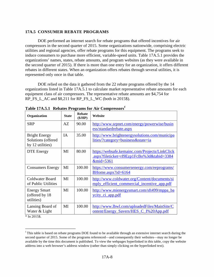
17A-8

17A.5 CONSUMER REBATE PROGRAMS

DOE performed an internet search for rebate programs that offered incentives for air compressors in the second quarter of 2015. Some organizations nationwide, comprising electric utilities and regional agencies, offer rebate programs for this equipment. The programs seek to induce consumers to purchase more efficient, variable-speed units. Table 17A.5.1 provides the organizations’ names, states, rebate amounts, and program websites (as they were available in the second quarter of 2015). If there is more than one entry for an organization, it offers different rebates in different states. When an organization offers rebates through several utilities, it is represented only once in that table. DOE relied on the data it gathered from the 22 rebate programs offered by the 14 organizations listed in Table 17A.5.1 to calculate market representative rebate amounts for each equipment class of air compressors. The representative rebate amounts are $4,754 for RP_FS_L_AC and $8,211 for RP_FS_L_WC (both in 2015$). Table 17A.5.1 Rebates Programs for Air Compressorsf

Organization State Rebate ($/HP) Website

SRP AZ 90.00 http://www.srpnet.com/energy/powerwise/business/standardrebate.aspx

Bright Energy Solutions (offered by 12 utilities)

IA 35.00 http://www.brightenergysolutions.com/municipalities/?category=business&state=ia

DTE Energy MI 80.00 https://websafe.kemainc.com/Projects/LinkClick.aspx?fileticket=rI9Ezp1FcBo%3d&tabid=3384&mid=5361

Consumers Energy MI 100.00 https://www.consumersenergy.com/eeprograms/BHome.aspx?id=6164

Coldwater Board of Public Utilities

MI 100.00 http://www.coldwater.org/Content/documents/simply_efficient_commercial_incentive_app.pdf

Energy Smart (offered by 18 utilities)

MI 100.00 http://www.mienergysmart.com/sft499/mppa_baycity_ci_app.pdf

Lansing Board of Water & Light

MI 100.00 http://www.lbwl.com/uploadedFiles/MainSite/Content/Energy_Savers/HES_C_I%20App.pdf

* In 2015$.

f This table is based on rebate programs DOE found to be available through an extensive internet search during the second quarter of 2015. Some of the programs referenced—and consequently their websites—may no longer be available by the time this document is published. To view the webpages hyperlinked in this table, copy the website address into a web browser’s address window (rather than simply clicking on the hyperlinked text).

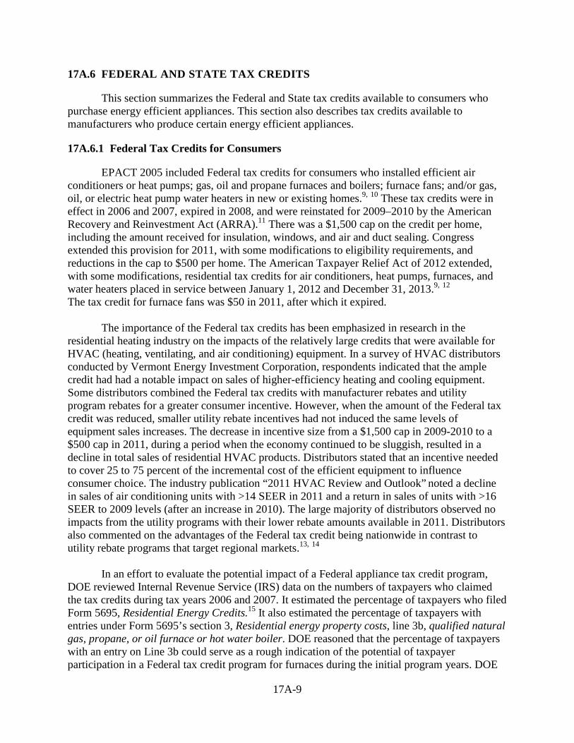
17A-9

17A.6 FEDERAL AND STATE TAX CREDITS

This section summarizes the Federal and State tax credits available to consumers who purchase energy efficient appliances. This section also describes tax credits available to manufacturers who produce certain energy efficient appliances.

17A.6.1 Federal Tax Credits for Consumers

EPACT 2005 included Federal tax credits for consumers who installed efficient air conditioners or heat pumps; gas, oil and propane furnaces and boilers; furnace fans; and/or gas, oil, or electric heat pump water heaters in new or existing homes.9, 10 These tax credits were in effect in 2006 and 2007, expired in 2008, and were reinstated for 2009–2010 by the American Recovery and Reinvestment Act (ARRA).11 There was a $1,500 cap on the credit per home, including the amount received for insulation, windows, and air and duct sealing. Congress extended this provision for 2011, with some modifications to eligibility requirements, and reductions in the cap to $500 per home. The American Taxpayer Relief Act of 2012 extended, with some modifications, residential tax credits for air conditioners, heat pumps, furnaces, and water heaters placed in service between January 1, 2012 and December 31, 2013.9, 12 The tax credit for furnace fans was $50 in 2011, after which it expired. The importance of the Federal tax credits has been emphasized in research in the residential heating industry on the impacts of the relatively large credits that were available for HVAC (heating, ventilating, and air conditioning) equipment. In a survey of HVAC distributors conducted by Vermont Energy Investment Corporation, respondents indicated that the ample credit had had a notable impact on sales of higher-efficiency heating and cooling equipment. Some distributors combined the Federal tax credits with manufacturer rebates and utility program rebates for a greater consumer incentive. However, when the amount of the Federal tax credit was reduced, smaller utility rebate incentives had not induced the same levels of equipment sales increases. The decrease in incentive size from a $1,500 cap in 2009-2010 to a $500 cap in 2011, during a period when the economy continued to be sluggish, resulted in a decline in total sales of residential HVAC products. Distributors stated that an incentive needed to cover 25 to 75 percent of the incremental cost of the efficient equipment to influence consumer choice. The industry publication “2011 HVAC Review and Outlook” noted a decline in sales of air conditioning units with >14 SEER in 2011 and a return in sales of units with >16 SEER to 2009 levels (after an increase in 2010). The large majority of distributors observed no impacts from the utility programs with their lower rebate amounts available in 2011. Distributors also commented on the advantages of the Federal tax credit being nationwide in contrast to utility rebate programs that target regional markets.13, 14

In an effort to evaluate the potential impact of a Federal appliance tax credit program, DOE reviewed Internal Revenue Service (IRS) data on the numbers of taxpayers who claimed the tax credits during tax years 2006 and 2007. It estimated the percentage of taxpayers who filed Form 5695, Residential Energy Credits.15 It also estimated the percentage of taxpayers with entries under Form 5695’s section 3, Residential energy property costs, line 3b, qualified natural gas, propane, or oil furnace or hot water boiler. DOE reasoned that the percentage of taxpayers with an entry on Line 3b could serve as a rough indication of the potential of taxpayer participation in a Federal tax credit program for furnaces during the initial program years. DOE

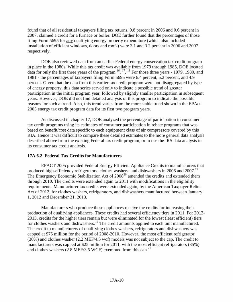
17A-10

found that of all residential taxpayers filing tax returns, 0.8 percent in 2006 and 0.6 percent in 2007, claimed a credit for a furnace or boiler. DOE further found that the percentages of those filing Form 5695 for any qualifying energy property expenditure (which also included installation of efficient windows, doors and roofs) were 3.1 and 3.2 percent in 2006 and 2007 respectively. DOE also reviewed data from an earlier Federal energy conservation tax credit program in place in the 1980s. While this tax credit was available from 1979 through 1985, DOE located data for only the first three years of the program.16, 17, 18 For those three years - 1979, 1980, and 1981 - the percentages of taxpayers filing Form 5695 were 6.4 percent, 5.2 percent, and 4.9 percent. Given that the data from this earlier tax credit program were not disaggregated by type of energy property, this data series served only to indicate a possible trend of greater participation in the initial program year, followed by slightly smaller participation in subsequent years. However, DOE did not find detailed analysis of this program to indicate the possible reasons for such a trend. Also, this trend varies from the more stable trend shown in the EPAct 2005 energy tax credit program data for its first two program years. As discussed in chapter 17, DOE analyzed the percentage of participation in consumer tax credit programs using its estimates of consumer participation in rebate programs that was based on benefit/cost data specific to each equipment class of air compressors covered by this RIA. Hence it was difficult to compare these detailed estimates to the more general data analysis described above from the existing Federal tax credit program, or to use the IRS data analysis in its consumer tax credit analysis.

17A.6.2 Federal Tax Credits for Manufacturers

EPACT 2005 provided Federal Energy Efficient Appliance Credits to manufacturers that produced high-efficiency refrigerators, clothes washers, and dishwashers in 2006 and 2007.19 The Emergency Economic Stabilization Act of 200820 amended the credits and extended them through 2010. The credits were extended again to 2011 with modifications in the eligibility requirements. Manufacturer tax credits were extended again, by the American Taxpayer Relief Act of 2012, for clothes washers, refrigerators, and dishwashers manufactured between January 1, 2012 and December 31, 2013.

Manufacturers who produce these appliances receive the credits for increasing their

production of qualifying appliances. These credits had several efficiency tiers in 2011. For 2012-2013, credits for the higher tiers remain but were eliminated for the lowest (least efficient) tiers for clothes washers and dishwashers.12 The credit amounts applied to each unit manufactured. The credit to manufacturers of qualifying clothes washers, refrigerators and dishwashers was capped at $75 million for the period of 2008-2010. However, the most efficient refrigerator (30%) and clothes washer (2.2 MEF/4.5 wcf) models was not subject to the cap. The credit to manufacturers was capped at $25 million for 2011, with the most efficient refrigerators (35%) and clothes washers (2.8 MEF/3.5 WCF) exempted from this cap.21

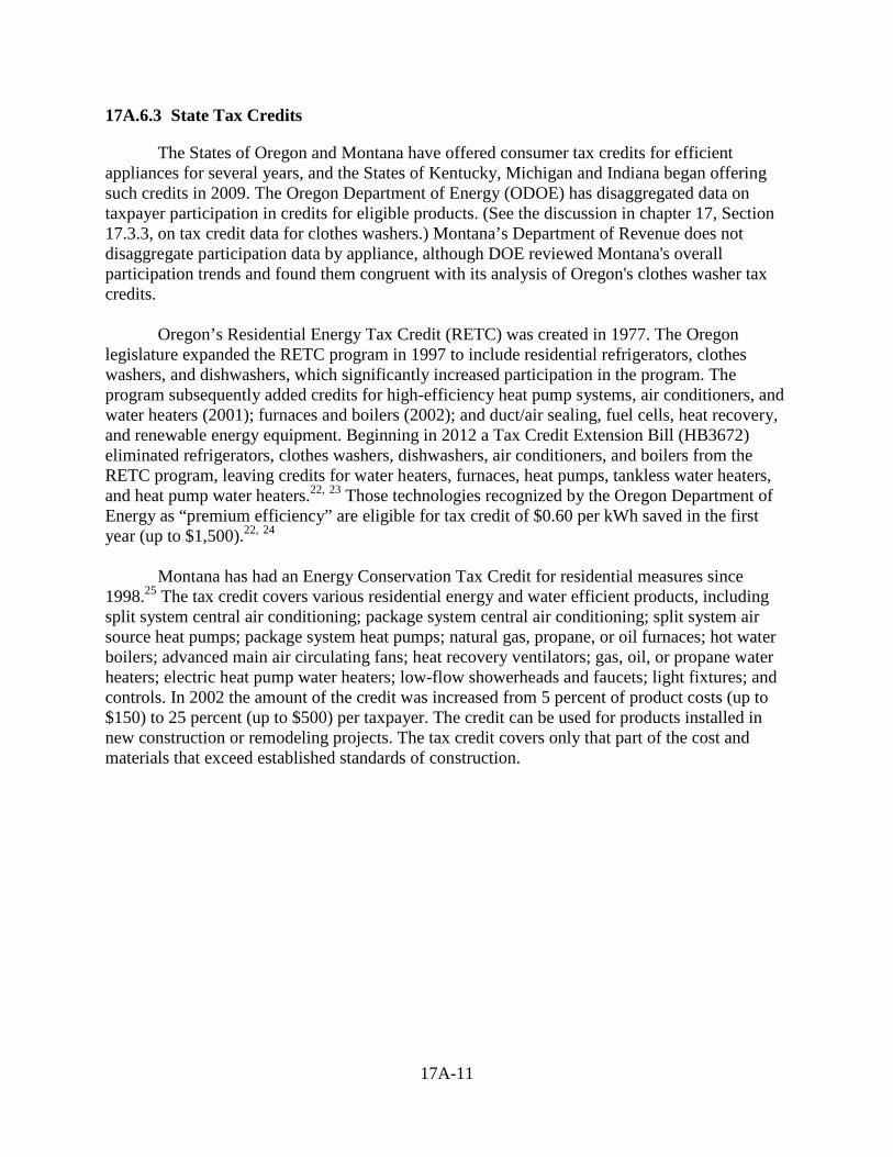
17A-11

17A.6.3 State Tax Credits

The States of Oregon and Montana have offered consumer tax credits for efficient appliances for several years, and the States of Kentucky, Michigan and Indiana began offering such credits in 2009. The Oregon Department of Energy (ODOE) has disaggregated data on taxpayer participation in credits for eligible products. (See the discussion in chapter 17, Section 17.3.3, on tax credit data for clothes washers.) Montana’s Department of Revenue does not disaggregate participation data by appliance, although DOE reviewed Montana's overall participation trends and found them congruent with its analysis of Oregon's clothes washer tax credits.

Oregon’s Residential Energy Tax Credit (RETC) was created in 1977. The Oregon

legislature expanded the RETC program in 1997 to include residential refrigerators, clothes washers, and dishwashers, which significantly increased participation in the program. The program subsequently added credits for high-efficiency heat pump systems, air conditioners, and water heaters (2001); furnaces and boilers (2002); and duct/air sealing, fuel cells, heat recovery, and renewable energy equipment. Beginning in 2012 a Tax Credit Extension Bill (HB3672) eliminated refrigerators, clothes washers, dishwashers, air conditioners, and boilers from the RETC program, leaving credits for water heaters, furnaces, heat pumps, tankless water heaters, and heat pump water heaters.22, 23 Those technologies recognized by the Oregon Department of Energy as “premium efficiency” are eligible for tax credit of $0.60 per kWh saved in the first year (up to $1,500).22, 24

Montana has had an Energy Conservation Tax Credit for residential measures since 1998.25 The tax credit covers various residential energy and water efficient products, including split system central air conditioning; package system central air conditioning; split system air source heat pumps; package system heat pumps; natural gas, propane, or oil furnaces; hot water boilers; advanced main air circulating fans; heat recovery ventilators; gas, oil, or propane water heaters; electric heat pump water heaters; low-flow showerheads and faucets; light fixtures; and controls. In 2002 the amount of the credit was increased from 5 percent of product costs (up to $150) to 25 percent (up to $500) per taxpayer. The credit can be used for products installed in new construction or remodeling projects. The tax credit covers only that part of the cost and materials that exceed established standards of construction.

17A-12

REFERENCES 1. Rufo, M. and F. Coito. California’s Secret Energy Surplus: The Potential for Energy

Efficiency. 2002. XENERGY Inc. (Last accessed December 17, 2015.) http://www.issuelab.org/resource/californias_secret_energy_surplus_the_potential_for_energy_efficiency.

2. Hall, B. H. and B. Khan. Adoption of New Technology. 2003. National Bureau of Economic Research, Inc. Report No. 9730. (Last accessed December 17, 2015.) https://ideas.repec.org/p/nbr/nberwo/9730.html.

3. Lekvall, P. and C. Wahlbin. A Study of Some Assumptions Underlying Innovation Diffusion Functions. The Swedish Journal of Economics. 1973. 75(4): pp. 362–377.

4. Geroski, P. A. Models of Technology Diffusion. Research Policy. 2000. 29(4–5): pp. 603–625.

5. Van den Bulte, C. Want to Know How Diffusion Speed Varies Across Countries and Products? Try a Bass Model. Product Development & Management Association Visions. 2002. 26(4): pp. 12–15.

6. Rufo, M. (Itron Inc.) and B. Atkinson (LBNL). Telephone conversation. January 2008.

7. Rufo, M. (Itron Inc.) and B. Atkinson (LBNL). Telephone conversation. March 2009.

8. Blum, H., B. A. Atkinson, and A. B. Lekov. A Framework for Comparative Assessments of Energy Efficiency Policy Measures. 2011. Lawrence Berkeley National Laboratory: Berkeley, CA. Report No. LBNL-4749E. (Last accessed December 17, 2015.) http://eetd.lbl.gov/publications/framework-comparative-assessments-energy-efficiency-policy-measures.

9. The Tax Incentives Assistance Project. Consumer Tax Incentives: Home Heating & Cooling Equipment. 2011. (Last accessed December 17, 2015.) http://www.energytaxincentives.org/consumers/heating-cooling.php.

10. Energy Policy Act of 2005. 42 U.S. Code 15801. 2005. (Last accessed December 17, 2015.) http://energy.gov/sites/prod/files/2013/10/f3/epact_2005.pdf.

11. American Recovery and Reinvestment Act of 2009. Public Law 111-5. 2009. (Last accessed December 17, 2015.) http://www.gpo.gov/fdsys/pkg/BILLS-111hr1enr/pdf/BILLS-111hr1enr.pdf.

12. The Tax Incentives Assistance Project. The Tax Incentives Assistance Project (TIAP). December 2014. (Last accessed December 17, 2015.) http://energytaxincentives.org/.

13. Foster, R., J. Grevatt, N. Lange, and T. Gee. Efficiency Programs and Distributors: Opportunities to Fully Leverage the Supply Chain for Greater Impact. 2012. 2012

17A-13

ACEEE Summer Study on Energy Efficiency in Buildings: Asilomar, CA. (Last accessed December 17, 2015.) http://www.aceee.org/files/proceedings/2012/data/papers/0193-000198.pdf.

14. Tusa, C. S., D. Pierson, P. Mammola, and J. P. Vora. JPM/HARDI 2011 HVAC Survey. 2011. J.P. Morgan. (Last accessed June 29, 2015.) http://hardinet.org/benchmarking/market-outlook-annual-report/.

15. U.S. Internal Revenue Service. SOI Tax Stats - Individual Income Tax Returns, Line Item Estimates. October 29, 2013. (Last accessed December 17, 2015.) http://www.irs.gov/uac/SOI-Tax-Stats-Individual-Income-Tax-Returns,-Line-Item-Estimates.

16. Commissioner of Internal Revenue. 1979 Annual Report. 1979. U.S. Internal Revenue Service: Washington, D.C. (Last accessed December 17, 2015.) http://www.irs.gov/pub/irs-soi/79dbfullar.pdf.

17. Commissioner of Internal Revenue. 1980 Annual Report. 1980. U.S. Internal Revenue Service: Washington, D.C. (Last accessed December 17, 2015.) http://www.irs.gov/pub/irs-soi/80dbfullar.pdf.

18. Commissioner of Internal Revenue and Chief Counsel for the Internal Revenue Service. 1981 Annual Report. 1981. U.S. Internal Revenue Service: Washington, D.C. (Last accessed December 17, 2015.) http://www.irs.gov/pub/irs-soi/81dbfullar.pdf.

19. U.S. Internal Revenue Service. Form 8909: Energy Efficient Appliance Credit. March 2014. (Last accessed December 17, 2015.) http://www.irs.gov/pub/irs-pdf/f8909.pdf.

20. Emergency Economic Stabilization Act of 2008. Public Law 110–343. 2008. (Last accessed December 17, 2015.) http://www.gpo.gov/fdsys/pkg/PLAW-110publ343/pdf/PLAW-110publ343.pdf.

21. The Tax Incentives Assistance Project. Manufacturers Incentives. (Last accessed December 17, 2015.) http://energytaxincentives.org/builders/appliances.php.

22. Database of State Incentives for Renewables and Efficiency (DSIRE). Oregon Incentives/Policies for Renewable Energy, Residential Energy Tax Credit. 2013. (Last accessed December 17, 2015.) http://programs.dsireusa.org/system/program/detail/638.

23. Oregon Department of Energy. HB 3672 (2011) Tax Credit Extension Bill. 2011. (Last accessed December 17, 2015.) http://www.oregon.gov/energy/CONS/docs/HB3672summary.pdf.

24. Oregon Department of Energy. ODOE: Residential Customers. (Last accessed October 15, 2015.) http://www.oregon.gov/energy/RESIDENTIAL/Pages/index.aspx.

25. Montana Department of Revenue. Energy Conservation Installation Credit. (Last accessed December 17, 2015.) http://revenue.mt.gov/home/individuals/taxrelief_energy.

17A-14

25. Montana Department of Revenue. Energy Conservation Installation Credit. (Last accessed December 17, 2015.) http://revenue.mt.gov/home/individuals/taxrelief_energy.