Review

Deep Learning for Lung Cancer Nodules Detectionand Classification in CT Scans

Diego Riquelme 1,2,† and Moulay A. Akhloufi 1,*,†

1 Perception, Robotics, and Intelligent Machines (PRIME), Department of Computer Science,Université de Moncton, Moncton, NB E1A3E9, Canada; diego.riquelme.13@sansano.usm.cl

2 Department of Electronic Engineering, Universidad Técnica Federico Santa Maria, Valparaiso, Chile* Correspondence: moulay.akhloufi@umoncton.ca; Tel.: +1-506-858-4120† These authors contributed equally to this work.

Received: 10 December 2019; Accepted: 3 January 2020; Published: 8 January 2020�����������������

Abstract: Detecting malignant lung nodules from computed tomography (CT) scans is a hard andtime-consuming task for radiologists. To alleviate this burden, computer-aided diagnosis (CAD)systems have been proposed. In recent years, deep learning approaches have shown impressiveresults outperforming classical methods in various fields. Nowadays, researchers are trying differentdeep learning techniques to increase the performance of CAD systems in lung cancer screening withcomputed tomography. In this work, we review recent state-of-the-art deep learning algorithmsand architectures proposed as CAD systems for lung cancer detection. They are divided into twocategories—(1) Nodule detection systems, which from the original CT scan detect candidate nodules;and (2) False positive reduction systems, which from a set of given candidate nodules classify theminto benign or malignant tumors. The main characteristics of the different techniques are presented,and their performance is analyzed. The CT lung datasets available for research are also introduced.Comparison between the different techniques is presented and discussed.

Keywords: lung cancer; deep learning; nodule detection; convolutional neural networks;computer-aided diagnosis

1. Introduction

Lung cancer is considered as the deadliest cancer worldwide. For this reason, many countriesare developing strategies for the early diagnosis of lung cancer. The NLST trial [1], showed thatthree annual screening rounds of high-risk subjects using low-dose Computed Tomography (CT)reduce the death rates considerably [2]. These measures mean that an overwhelming quantity ofCT scan images will have to be inspected by a radiologist. Since nodules are very difficult to detect,even for experienced doctors, the burden on radiologists increases heavily with the number of CTscans to analyze.

With the expected increase in the number of preventive/early-detection measures, scientists areworking in computerized solutions that help alleviate the work of doctors, improve diagnostics’precision by reducing the subjectivity factor, speedup the analysis and reduce medical costs.

In order to detect malignant nodules, specific features need to be recognized and measured.Based on the detected features and their combination, cancer probability can be assessed. However,this task is very difficult, even for an experienced medical doctor, since nodule presence and positivecancer diagnosis are not easily related. Common computer aided diagnosis (CAD) approaches usepreviously studied features which are somehow related to cancer suspiciousness, such as volume,shape, subtlety, solidity, spiculation, sphericity, among others. They use these features and MachineLearning (ML) techniques such as Support Vector Machine (SVM) to classify the nodule as benign or

AI 2020, 1, 28–67; doi:10.3390/ai1010003 www.mdpi.com/journal/ai

AI 2020, 1 29

malignant. Even though many works use similar machine learning frameworks [3–8], the problemwith these methods is that, in order for the system to work at its best performance, many parametersneed to be hand-crafted, thus making it difficult to reproduce state-of-the-art results. Additionally,this makes these approaches vulnerable to the variability between different CT scans and differentscreening parameters.

The advantage of using deep learning in CAD systems is that it can perform and end-to-enddetection by learning the most salient features during training. This allows the network to be robust tovariations as it captures nodules’ features in various CT scans with varying parameters. By havinga training set which is rich in variability, the system can inherently learn invariant features frommalignant nodules and enables better performances. Since no features are engineered, the network isable to learn, on its own, the relation between features and cancer using the provided ground-truth.Once the network is trained, it is expected to be able to generalize its learning and detect malignantnodules (or patient-level cancer) on new cases which have never been seen before by the system.

In this work, we present a review of recent deep learning techniques for lung cancer detection.Most of the proposed works are based on deep Convolutional Neural Networks (CNN). CNN are a classof neural networks designed to learn, during training, convolution parameters from a set of availabledata. In general, they are comprised of different layers such as convolutional layers, deconvolutionallayers, pooling layers and so forth. Different architectures were proposed in recent years to improvethe performance and overcome some limitations of the standard CNN. Among them ResidualNetworks (ResNets) [9], Inception [10,11], Xception [12] or Dense Networks [13,14]. CNN haveshown interesting performances in the tasks of classification, segmentation, object detection and soforth. Mainly applied to image data, they have been successfully used with other type of data such astext in NLP applications [15]. More details about deep learning and CNN are given in Reference [16]. Inthe following, we will present the main datasets used in lung cancer research (Section 2) and introducethe common metrics used to assess the deep learning models (Section 3). The techniques are dividedinto two categories—Nodule detection frameworks (Section 4) and false positive reduction models(Section 5). Comparative analysis of the different algorithms is presented and discussed (Section 6).

2. Datasets

Datasets are an important part of any machine learning or deep learning approach. The quality ofthe available data help develop, train and improve the algorithms. In medical imaging applications,the available data must be validated and labeled by experts in order to be useful in any development.This section present the datasets used in recent works related to deep learning for lung cancer detection.

2.1. The Lung Image Database Consortium (LIDC-IDRI)

The LIDC-IDRI dataset [17] consists of 1018 cases gathered from a collaboration of seven academiccenters and eight medical imaging companies. Each case includes an XML file containing annotationsof the CT scan. These annotations are performed by four experienced thoracic radiologists, in a 2-stageprocess. In the first stage, each radiologist independently categorizes findings into three categories(nodule ≥ 3 mm, nodule ≤ 3 mm and non-nodule ≥ 3 mm). Then, in the second stage, each radiologistreviews its classification and the classifications done by the other radiologists anonymously. So everynodule annotation is reviewed by all four radiologists independently.

The dataset consists of 1018 CT scans from 1010 patients, with a total of 244,527 images. With thisdataset, the diagnosis can be made at two levels. Diagnosis at the patient level (diagnosis associatedwith the patient) and diagnosis at the nodule level.

The CT scan DICOM images have a resolution of 512 × 512 × width, where the width varies from65 to 764 slices. The average number of slices width is 240 for this dataset.

The nodules are categorized into 4 levels. (1) Unknown (no data available), (2) Benign ornon-malignant disease, (3) A malignancy that is primary lung cancer, (4) A metastatic lesion thatis associated with an extra-thoracic primary malignancy. Furthermore, for each lesion, there is also

AI 2020, 1 30

information available about how the diagnosis was established. Including options as (1) Unknown(not clear how the diagnosis was established), (2) review of radiological images to show 2 years ofstable nodule, (3) biopsy, (4) surgical resection and (5) progression or response [18].

2.2. LUNA16

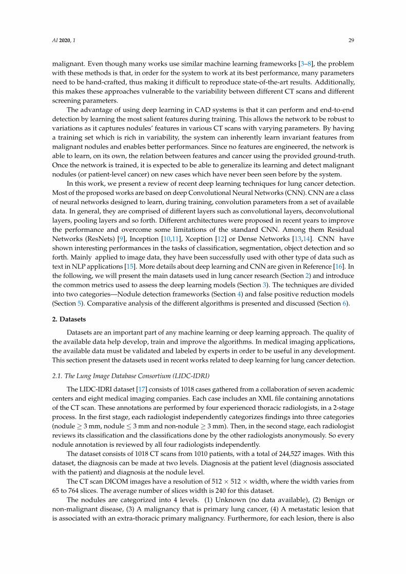
The LUNA16 dataset [19] is a subset of LIDC-IDRI dataset, in which the heterogeneous scans arefiltered by different criteria. Since pulmonary nodules can be very small, a thin slice should be chosen.Therefore scans with a slice thickness greater than 2.5 mm were discarded. Furthermore, scans withinconsistent slice spacing or missing slices were also excluded. This led to 888 CT scans, with a totalof 36,378 annotations by radiologists. In this dataset, only the annotations categorized as nodules ≥3 mm are considered relevant, as the other annotations (nodules ≤ 3 mm and non-nodules) are notconsidered relevant for lung cancer screening protocols [2]. Nodules found by different readers thatwere closer than the sum of their radii were merged. In this case, positions and diameters of thesemerged annotations were averaged. This results in a set of 2290, 1602, 1186 and 777 nodules annotatedby at least 1, 2, 3 or 4 radiologist, respectively.

In Figure 1, different slices from a LUNA16 CT scan with malignant nodules are shown as anexample of a Lung CT scan. For the other datasets, the same kind of image is obtained.

Figure 1. Computed tomography (CT) slices, with malignant nodules of different sizes.

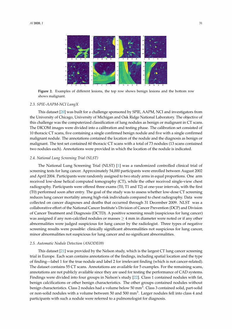
Figure 2 shows how similar are the benign and the malignant lesions. Thus, revealing the hardtask of classifying them.

AI 2020, 1 31

Figure 2. Examples of different lesions, the top row shows benign lesions and the bottom rowshows malignant.

2.3. SPIE-AAPM-NCI LungX

This dataset [20] was built for a challenge sponsored by SPIE, AAPM, NCI and investigators fromthe University of Chicago, University of Michigan and Oak Ridge National Laboratory. The objective ofthis challenge was the computerized classification of lung nodules as benign or malignant in CT scans.The DICOM images were divided into a calibration and testing phase. The calibration set consisted of10 thoracic CT scans, five containing a single confirmed benign nodule and five with a single confirmedmalignant nodule. The annotations contained the location of the nodule and the diagnosis as benign ormalignant. The test set contained 60 thoracic CT scans with a total of 73 nodules (13 scans containedtwo nodules each). Annotations were provided in which the location of the nodule is indicated.

2.4. National Lung Screening Trial (NLST)

The National Lung Screening Trial (NLST) [1] was a randomized controlled clinical trial ofscreening tests for lung cancer. Approximately 54,000 participants were enrolled between August 2002and April 2004. Participants were randomly assigned to two study arms in equal proportions. One armreceived low-dose helical computed tomography (CT), while the other received single-view chestradiography. Participants were offered three exams (T0, T1 and T2) at one-year intervals, with the first(T0) performed soon after entry. The goal of the study was to assess whether low-dose CT screeningreduces lung cancer mortality among high-risk individuals compared to chest radiography. Data werecollected on cancer diagnoses and deaths that occurred through 31 December 2009. NLST was acollaborative effort of the National Cancer Institute’s Division of Cancer Prevention (DCP) and Divisionof Cancer Treatment and Diagnosis (DCTD). A positive screening result (suspicious for lung cancer)was assigned if any non-calcified nodules or masses ≥ 4 mm in diameter were noted or if any otherabnormalities were judged suspicious for lung cancer by the radiologist. Three types of negativescreening results were possible: clinically significant abnormalities not suspicious for lung cancer,minor abnormalities not suspicious for lung cancer and no significant abnormalities.

2.5. Automatic Nodule Detection (ANODE09)

This dataset [21] was provided by the Nelson study, which is the largest CT lung cancer screeningtrial in Europe. Each scan contains annotations of the findings, including spatial location and the typeof finding—label 1 for the true nodule and label 2 for irrelevant finding (which is not cancer-related).The dataset contains 55 CT scans. Annotations are available for 5 examples. For the remaining scans,annotations are not publicly available since they are used for testing the performance of CAD systems.Findings were divided into four groups in Nelson’s study [22]. Class 1 contained nodules with fat,benign calcifications or other benign characteristics. The other groups contained nodules withoutbenign characteristics. Class 2 nodules had a volume below 50 mm3. Class 3 contained solid, part-solidor non-solid nodules with a volume between 50 and 500 mm3. Larger nodules fell into class 4 andparticipants with such a nodule were referred to a pulmonologist for diagnosis.

AI 2020, 1 32

2.6. The Danish Lung Cancer Screening Trial (DLCST)

The Danish Lung Cancer Screening Trial [23] assessed participants with high lung cancer risk.Two experienced chest radiologists evaluated the images, where size was manually measured.A nodule diameter of 3 mm was considered the lower limit of a positive finding in the initial evaluation.A chest radiologist, unaware of lung cancer diagnoses, recorded spiculation and malignancyobservations and categorized the nodules according to type—perifissural, solid, part-solid or non-solid(pure ground glass). This yielded to 823 patients with 1385 diagnosed nodules of which 233 noduleswere classified as benign calcification and excluded, leaving a total of 718 persons and 1152 nodules [24].

2.7. Data Science Bowl 2017 (DSB)

The Data Science Bowl 2017 (DSB), a challenge organized by Kaggle [25], released a databaseof CT scans on two stages, DSB1 and DSB2. This dataset provides annotations at a patient level,indicating whether the patient was diagnosed with cancer within one year after the scan was taken.It contains over a thousand low-dose CT scan images in a DICOM format from high-risk patients.This database is not publicly available at the moment due to usage restrictions. DSB scan resolutionsand scan parameters vary in source and quality. The source of the CT scans was not released. This mightgenerate problems when using this dataset, for both training or testing. Because, if the model is assessedon other datasets, it is not possible to know if samples from those data are already included in theDSB dataset.

Table 1 summarizes the datasets used for developing deep learning lung cancerdetection algorithms.t

Table 1. CT Scans datasets for lung cancer detection (* shows the datasets that have associatednodule annotations).

Dataset Number of CT Scans Annotations

LIDC-IDRI [17] 1018 *LUNA16 [19] 888 *SPIE-AAPM-NCI [20] 70 *NLST [1] 3410 *ANODE09 [21] 55 *DLCST [23] 612 *DSB [25] 1902 -

3. Performance Metrics

To analyze the performance of the developed deep learning algorithms for detecting andclassifying lung nodules, different metrics are used. In the reviewed papers, the authors use statisticalmeasures [26] such as sensitivity (SE), specificity (SP), accuracy (ACC), precision (PPV), F1-score,Receiver Operating Characteristic (ROC) curve, Free Response Operating Characteristic (FROC)and area under the ROC curve (AUC). Another measure was introduced in the ANODE09 challengeand was later used in the LUNA16 Challenge to assess the performance of the different models,this measure is the Competition Performance Metric (CPM) [21]. The different metrics used inassessing the performance of lung cancer algorithms are given in Table 2.

AI 2020, 1 33

Table 2. Metrics used in deep learning lung cancer detection literature.

Metric Definition Note

Sensitivity SE = TP/(TP + FN) True positive rate (TPR) or recall

Specificity SP = TN/(TN + FP) True negative rate (TNR)

Accuracy ACC = (TP + TN)/(TP + TN + FP + FN) Total true results

Precision PPV = TP/(TP + FP) Positive predicted value (PPV)

F1-Score F1 = 2TP/(2TP + FP + FN)Relates the sensitivity andprecision measures

ROCCurve depicting the relationship between the sensitivity andspecificity (Y-axis is the true positive rate and the X-axis is thefalse positive rate)

Receiver Operating Characteristic (ROC)curve

FROC Similar to the ROC curve, differing only in the X-axis. The X-axisis the false positive rate per image (or per scan)

Free Response Operating Characteristic(ROC) curve

AUC Total area under the ROC curve Area Under Curve (AUC)

CPM Average of the sensitivity at seven defined false positive rates inthe FROC curve: 1/8, 1/4, 1/2, 1, 2, 4 and 8 FPs/scan Competition Performance Metric (CPM)

TP = True Positives; TN = True Negatives; FP = False Positives; FN = False Negatives.

4. Deep Nodule Detection Frameworks

Due to the complexity of detecting pulmonary nodules and the importance of trying to detectall of them, the typical framework is divided into two main tasks. The first one focuses on detectingnodule candidates. This tries to detect from the CT scan volume all the true nodules, which usuallyincludes a high number of false positives. Then, the second task specializes in classifying the previouslygenerated candidates into benign nodules or malignant nodules. The second step basically aims toreduce the large number of false positives generated on the previous step. Some works do not use thisstrategy and from the CT scans they detect and classify nodules directly.

In this section, we present works which propose a whole pipeline from the CT scans to thefinal classification of the detected nodules. As aforementioned, some of them divide the taskinto candidate generation and false positive reduction, while other do not. Different works maydiffer in architecture, pre-processing of the images, training strategy, among others. A relevantdifference between approaches is if they are using a two-dimensional or three-dimensional approach.3D architectures demand the use of three-dimensional convolutions, which increases considerably thenumber of parameters, the computational cost and the training time. For this reason, some approachesuse 2D convolutions, which have fewer parameters and allow to train deeper and more complexarchitectures with less powerful hardware. 2D and 3D approaches are presented in the following.

4.1. 2D Deep Learning Approaches

Here we present works that are based on a 2D approach. This means that two-dimensionalkernels are convoluted with two-dimensional images or that the input of the deep neural networkis two-dimensional. This does not necessarily means that these architectures miss out all 3Dinformation. Some approaches make use of adjacent slices or different axial cuts in order to retainsome volumetric information.

Van Ginneken et al. [27] propose the use of transfer learning from OverFeat [28], a previouslytrained network for object detection in natural images. First, from the CT scan they extract 2Dsagittal, coronal and axial patches for each nodule candidate. Then, they extract 4096 features from thepenultimate layer of the network and classify them with linear SVM. Each patch is 50 × 50 mm andrescaled to 8-bit grayscale 221 × 221 pixels using Hounsfield unit rescaling and linear interpolation.They use 865 scans from the LIDC dataset, considering nodules≥ 3 mm labeled by 3 or 4 radiologists aspositive samples. Scan with a section thickness of more than 2.5 mm is excluded as well as scans withinconsistent or invalid DICOM. This results in 865 CT scans with 1147 pulmonary nodules and 3271excluded doubtful lesions. As the starting point of this framework, nodule candidate’s locations

AI 2020, 1 34

are extracted from an existing CAD system approved by the U.S. Food and Drug Administration(FDA) [29] and commercially available (MeVis Medical Solutions AG, Bremen, Germany). The CADsystem produces a list of candidates, each with a score indicating the likelihood that the location is anodule. The OverFeat network uses a 221× 221 RGB image patch as input. It consists of ConvolutionalLayers (CL) containing 96 to 1024 kernels of sizes 3 × 3 to 7 × 7. It uses half-wave rectificationand max-pooling kernels of sizes 3 × 3 and 5 × 5. The resulting 4096 features from the first FullyConnected (FC) layer are used as input to the linear Support Vector Machine (SVM) classifier withC optimized cross-validation [30]. The authors constructed three separate systems, one for eachorthogonal patch, designated x, y and z. To fuse these results, the best performing model was a latefusion approach using the CAD information. This was done by using the output of the three systems x,y, z plus the score reported by the CAD system. Then, they use a second stage classifier (linear SVM)to estimate the probability that the candidate is a nodule. The CAD system by itself generated 37,262candidate locations. Among those candidates 78% were true nodules (i.e, the maximum sensitivity thestudy could achieve). The complete model achieves a CPM of 0.71.

Kumar et al. [31] propose a CAD system that uses deep features extracted from an autoencoderto classify lung nodules. They use CT scans from patients with diagnostic data from the LIDCdataset. There are 157 patients with diagnostic information obtained from biopsy, surgical resection,progression or reviewing the radiological images to show 2 years of nodule state at two levels (thepatient level and the nodule level). They decided to use diagnostic data since it is the only way tojudge the certainty of malignancy. First, nodules are extracted from the 2D CT images using theannotations provided in the dataset. Then they are individually fed into a five-layered de-noisingautoencoder trained by L-BFGS [32]. Learned features are then extracted from the 4th layer. Thefeatures from the 4th layer were used to create a feature vector of 200 dimensions for each instance(instance meaning one slice containing nodules). Then this vector is fed into a binary decision tree toobtain the classification for nodules. For each nodule ≥ 3 mm in diameter, the annotations provided bythe radiologist are used to extract features from the autoencoder. They created an adaptive rectanglewindow based on the nodule size. Then each rectangular area is resized to a fixed dimension, to createa fixed length input for the autoencoder. Nodules with rating 0, 2, 3 are treated as malignant. Theyachieved an overall accuracy of 75.01% with a sensitivity of 0.8325 at a 0.39 FP/scan.

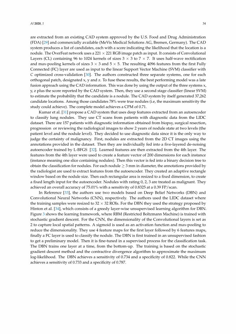
In Reference [33], the authors use two models based on Deep Belief Networks (DBN) andConvolutional Neural Networks (CNN), respectively. The authors used the LIDC dataset wherethe training samples were resized to 32 × 32 ROIs. For the DBN they used the strategy proposed byHinton et al. [34], which consists of a greedy layer-wise unsupervised learning algorithm for DBN.Figure 3 shows the learning framework, where RBM (Restricted Boltzmann Machine) is trained withstochastic gradient descent. For the CNN, the dimensionality of the Convolutional layers is set as2 to capture local spatial patterns. A sigmoid is used as an activation function and max-pooling toreduce the dimensionality. They use 4 feature maps for the first layer followed by 6 features maps,finally a FC layer is used to classify the nodule. The DBN is first trained in an unsupervised fashionto get a preliminary model. Then it is fine-tuned in a supervised process for the classification task.The DBN trains one layer at a time, from the bottom-up. The training is based on the stochasticgradient descent method and the contractive divergence algorithm to approximate the maximumlog-likelihood. The DBN achieves a sensitivity of 0.734 and a specificity of 0.822. While the CNNachieves a sensitivity of 0.733 and a specificity of 0.787.

AI 2020, 1 35

Figure 3. Deep belief network learning framework, illustration of the concept of training a noduleclassifier as in Reference [33].

Another work using DBNs and CNNs is proposed by Sun et al. [35]. In this work, the authorsimplement three different deep learning approaches. Using cropped 52 × 52 pixels patches from theLIDC database, they trained and tested CNN, DBNs and Stacked Denoising Autoencoder (SDAE) [36].The proposed CNN consists of 3 CL, each one with max-pooling. 5 × 5 kernels were used to generate12, 8 and 6 features maps, respectively. The second network is a DBN. It was obtained by training andstacking four layers of RBM in a greedy fashion. Each layer contained 100 RBM. The trained stack wasused to initialize a feed-forward neural network for classification. The hyperbolic tangent (tanh) wasused as an activation function. The last model was a three-layer SDAE, where each autoencoder wasstacked on top of each other. Each autoencoder has 2000, 1000 and 400 hidden neurons, with corruptionlevel of 0.5. From the 5 levels of malignancy available in the LIDC dataset (annotated by experts),they considered benign the ones with levels 1 and 2, while the 4 and 5 were considered malignantcases. The level 3 nodules were eliminated. For each nodule, they averaged the ratings from the fourradiologists. For every nodule, its area was segmented based on the union of the four radiologists’truth files. If the segmented area fits into 52 × 52 pixels, this ROI was placed at the center of the box.The ones that exceeded this size were downsampled to the reference size of 52 × 52 pixels. Then eachROI was rotated to four different directions and each rotated ROI was converted into four singlevectors. The pixel values were converted to 8 bits. With this preprocessing, from the 1018 cases 174,412vectors were generated. Each vector with 2704 elements. After discarding the level 3 nodules, 114,728vectors remained, consisting of 54,880 benign cases and 59,848 malignant cases. The performance ofthe proposed algorithms were assessed on accuracy where CNN, DBNs and SDAE achieved 0.7976,0.8119 and 0.7929, respectively.

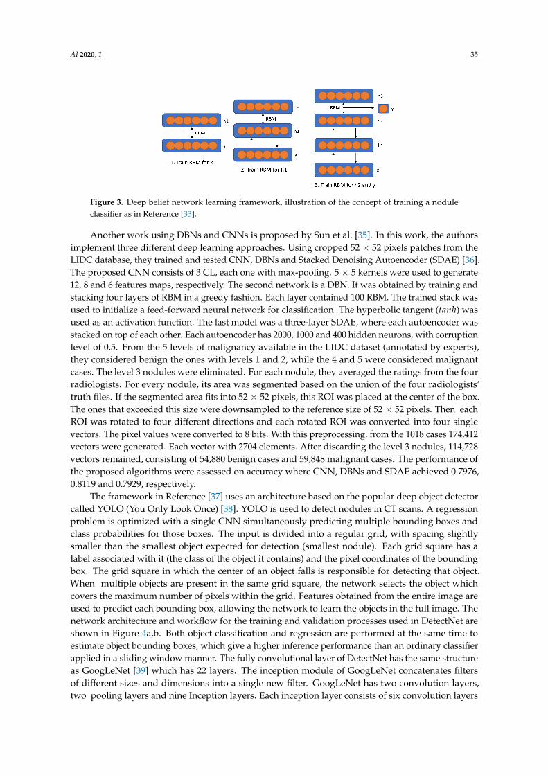
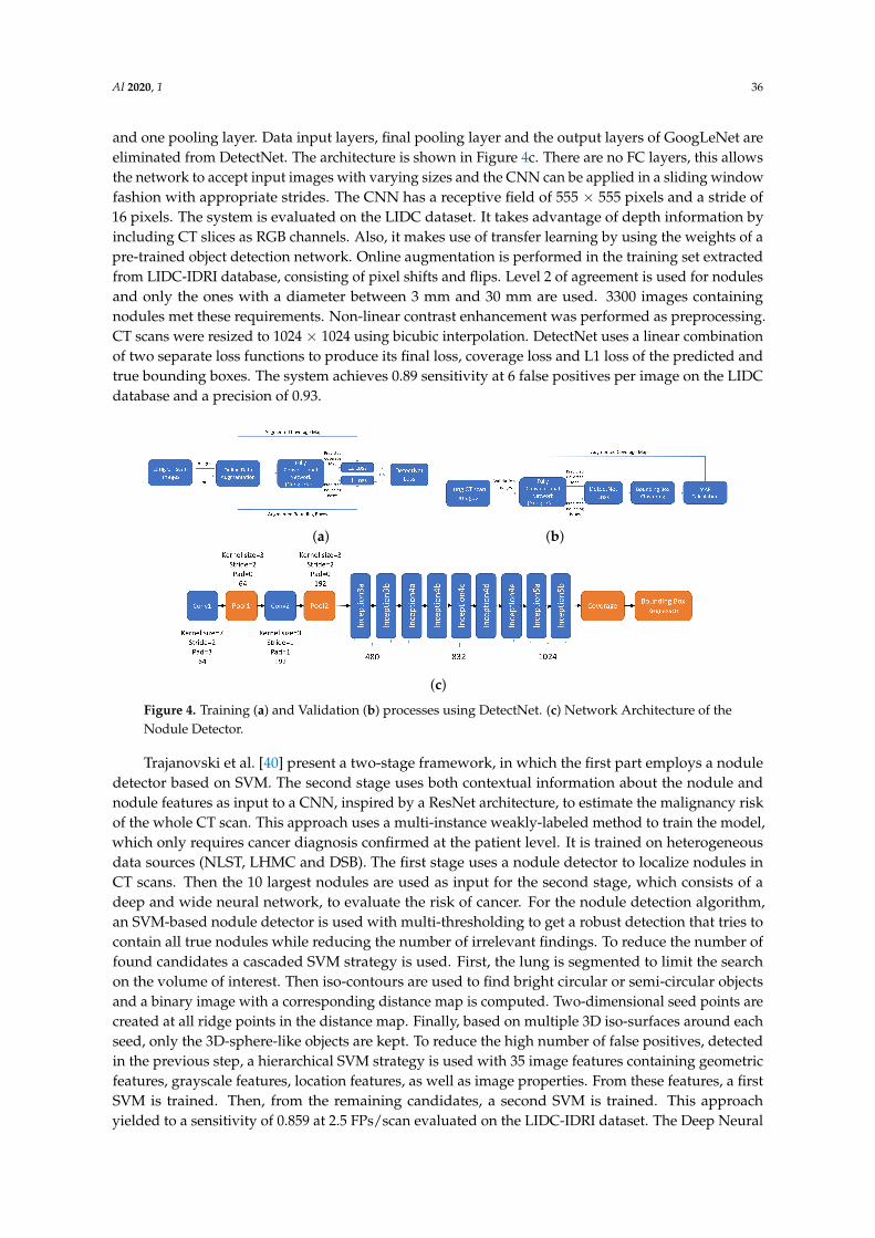
The framework in Reference [37] uses an architecture based on the popular deep object detectorcalled YOLO (You Only Look Once) [38]. YOLO is used to detect nodules in CT scans. A regressionproblem is optimized with a single CNN simultaneously predicting multiple bounding boxes andclass probabilities for those boxes. The input is divided into a regular grid, with spacing slightlysmaller than the smallest object expected for detection (smallest nodule). Each grid square has alabel associated with it (the class of the object it contains) and the pixel coordinates of the boundingbox. The grid square in which the center of an object falls is responsible for detecting that object.When multiple objects are present in the same grid square, the network selects the object whichcovers the maximum number of pixels within the grid. Features obtained from the entire image areused to predict each bounding box, allowing the network to learn the objects in the full image. Thenetwork architecture and workflow for the training and validation processes used in DetectNet areshown in Figure 4a,b. Both object classification and regression are performed at the same time toestimate object bounding boxes, which give a higher inference performance than an ordinary classifierapplied in a sliding window manner. The fully convolutional layer of DetectNet has the same structureas GoogLeNet [39] which has 22 layers. The inception module of GoogLeNet concatenates filtersof different sizes and dimensions into a single new filter. GoogLeNet has two convolution layers,two pooling layers and nine Inception layers. Each inception layer consists of six convolution layers

AI 2020, 1 36

and one pooling layer. Data input layers, final pooling layer and the output layers of GoogLeNet areeliminated from DetectNet. The architecture is shown in Figure 4c. There are no FC layers, this allowsthe network to accept input images with varying sizes and the CNN can be applied in a sliding windowfashion with appropriate strides. The CNN has a receptive field of 555 × 555 pixels and a stride of16 pixels. The system is evaluated on the LIDC dataset. It takes advantage of depth information byincluding CT slices as RGB channels. Also, it makes use of transfer learning by using the weights of apre-trained object detection network. Online augmentation is performed in the training set extractedfrom LIDC-IDRI database, consisting of pixel shifts and flips. Level 2 of agreement is used for nodulesand only the ones with a diameter between 3 mm and 30 mm are used. 3300 images containingnodules met these requirements. Non-linear contrast enhancement was performed as preprocessing.CT scans were resized to 1024 × 1024 using bicubic interpolation. DetectNet uses a linear combinationof two separate loss functions to produce its final loss, coverage loss and L1 loss of the predicted andtrue bounding boxes. The system achieves 0.89 sensitivity at 6 false positives per image on the LIDCdatabase and a precision of 0.93.

(a) (b)

(c)

Figure 4. Training (a) and Validation (b) processes using DetectNet. (c) Network Architecture of theNodule Detector.

Trajanovski et al. [40] present a two-stage framework, in which the first part employs a noduledetector based on SVM. The second stage uses both contextual information about the nodule andnodule features as input to a CNN, inspired by a ResNet architecture, to estimate the malignancy riskof the whole CT scan. This approach uses a multi-instance weakly-labeled method to train the model,which only requires cancer diagnosis confirmed at the patient level. It is trained on heterogeneousdata sources (NLST, LHMC and DSB). The first stage uses a nodule detector to localize nodules inCT scans. Then the 10 largest nodules are used as input for the second stage, which consists of adeep and wide neural network, to evaluate the risk of cancer. For the nodule detection algorithm,an SVM-based nodule detector is used with multi-thresholding to get a robust detection that tries tocontain all true nodules while reducing the number of irrelevant findings. To reduce the number offound candidates a cascaded SVM strategy is used. First, the lung is segmented to limit the searchon the volume of interest. Then iso-contours are used to find bright circular or semi-circular objectsand a binary image with a corresponding distance map is computed. Two-dimensional seed points arecreated at all ridge points in the distance map. Finally, based on multiple 3D iso-surfaces around eachseed, only the 3D-sphere-like objects are kept. To reduce the high number of false positives, detectedin the previous step, a hierarchical SVM strategy is used with 35 image features containing geometricfeatures, grayscale features, location features, as well as image properties. From these features, a firstSVM is trained. Then, from the remaining candidates, a second SVM is trained. This approachyielded to a sensitivity of 0.859 at 2.5 FPs/scan evaluated on the LIDC-IDRI dataset. The Deep Neural

AI 2020, 1 37

Network for cancer risk assessment uses the information obtained by the nodule detection step, whichprovides candidates with indications about the location, nodule size, nodule sphericity and confidenceof suggestion. These are referred to as metadata. Then, patches of size 32 × 32 × 32 mm3 areextracted around the nodule. Isotropic resampling was used to make every voxel correspond to 1mm3. During training, a random crop of 28 × 28 × 28 mm3 is extracted from the patch on every batchiteration to avoid overfitting. Finally, from the 3D patches, 3 different orthogonal 2D projections areextracted as channels, resulting on a 3 × 28 × 28 mm2 input for the network. To further improve theperformance, the metadata is added at the penultimate layer of the architecture. The deep network isa ResNet-like deep and wide model. It uses sigmoid activation function. At the end of the networka global max-pooling is performed, over the maximum of ten branches representing the differentnodules, to estimates the final cancer risk probability. The model was trained on a subset of the NLSTdata (3410 volumes, with 680 diagnosed cancer cases). It was verified on NLST and other datasets.AUC scores for the model, evaluated against confirmed cancer diagnosis, range from 0.82 to 0.88.The AUC on LHMC, UCM , NLST validation set, DSB 1 and DSB 2, are 0.87, 0.83, 0.88, 0.82 and 0.84,respectively.

The work in Reference [41] fuses texture, shape and deep model-learned information (Fuse-TSD)for automated classification of lung nodules. The algorithm uses three types of features extractedusing gray level co-occurrence matrix (GLCM) texture descriptors and Fourier shape descriptors tocharacterize the heterogeneity of nodules and a DCNN to learn features of nodules on a slice-by-slicebasis. An ensemble classifier based on back-propagation neural network (BPNN) and AdaBoost isconstructed. The decisions made by the different classifiers are fused by a weighted sum of likelihood,where the weights are proportional to the accuracy recorded on the validation set. A 64 × 64 squareregion centered on the nodule is cropped (the largest nodule is 64 mm). The area of the nodule isdefined as the intersection of the marked areas by the four radiologists. The non-nodule voxels are setto zero. For DCNN-based feature extraction, they needed to address size variability. The patches areresized to 32 × 32 using bicubic interpolation. They are used as input to a network made of three CLwith 32, 32, 64 kernels of size 5 × 5, respectively. Each CL is followed by a 3 × 3 average-pooling layerwith a stride of 2. Finally, two FC layers are used with 64 and 2 hidden units, respectively. Figure 5shows the DCNN architecture. Kernels were randomly initialized, ReLU activation function and 0.5dropout are used on the first FC layer to avoid overfitting. The GLCM-based texture feature extractionis used to evaluate the spatial dependence of voxel values by measuring energy, contrast, entropyand inverse difference, which proved to be effective for image classification. Four GLCMs computedat 0◦, 45◦, 90◦ and 135◦ are used to obtain a 16-dimensional GLCM texture descriptor for each imagepatch. For Fourier shape descriptor, 52 low-frequency coefficients are used as descriptors of the noduleboundary. For patch classification, the AdaBoost algorithm is used in which BPNN is the weak learner.To construct the one-hidden-layer BPNN weak learner, 90% of training data is sampled accordingto the distribution of their weights, which are initialized uniformly. The other 10% are used as avalidation set. In the BPNN, the number of neurons is set to D, which is the dimension of the inputdata that is, either the depth, texture or shape features of an image. The number of output units is 2,and the number of hidden neurons is set to log(D). The number of weak BPNN classifiers was set to10 empirically. Since there are three groups of image features, three AdaBoosted BPNNs are trained.On the LIDC-IDRI dataset, the nodules with a composite malignancy rate of 1 and 2 are consideredas benign, the ones with 4 and 5 as malignant, and the ones with 3 are left as uncertain. In this work,the authors assessed if including the uncertain nodules on one of the classes during training wouldincrease the performance. The best performance was achieved discarding the uncertain nodules. Thisprovided 1324 benign cases and 648 malignant nodules. Te best results achieved an AUC of 0.9665,an accuracy of 89.53%, a sensitivity of 0.8419 and a specificity of 0.9202.

AI 2020, 1 38

Figure 5. Structure of proposed eight-layer DCNN in Reference [41].

Xie et al. [42] propose a nodule detection framework using a 2D CNN. A modified version ofFaster R-CNN with two region proposal networks and a deconvolutional layer is designed to detectnodule candidates. Then, three models are trained for three different kind of slices. Their results arethen merged to integrate 3D information about the nodules. A boosting architecture based on 2D CNNis used for false positive reduction. Here, three models are sequentially trained, allowing the models tolearn different features each one having a finer discrimination than the previous one. The misclassifiedsamples are kept to retrain a model to achieve an improvement in the sensitivity of the nodule detectiontask. Due to computational cost, 2D axial slices are chosen as inputs instead of 3D images. This designcan be described as three sub-networks: feature extraction network, region proposal network and ROIclassifier. The feature extraction network is a VGG-16 with 5-group convolutions, which are sharedby the subsequent sub-networks. For the region proposal network, an image is set as input to anetwork composed of a FCN which outputs a set of rectangular object proposals. Each object witha particular objectness score. To generate region proposals, a small network is slid over the featuremap output by the feature extraction network. This small network uses a 3 × 3 spatial window asinput. Each sliding window is mapped to a feature vector (512-d for VGG). Then, this vector is fedto a box-classification and box-regression layers, consisting of two sibling FC layers. Seven anchors(12 × 12, 18 × 18, 27 × 27, 36 × 36, 51 × 51, 75 × 75 and 120 × 120) are used to predict multiple regionproposals, at each sliding window location. Two different region proposal networks are used, in orderto capture different information about the nodules. Both outputs are concatenated to a deconvolutionallayer and the middle convolution layer (conv3_3 according to the notation used in Reference [43]),respectively. The multitask loss for an image is defined as:

L(pi, ti, p1kj, t1

kj) = ∑i

L1(pi, ti) +2

∑k=1

∑j

L2(p1kj, t1

kj) (1)

where L1 and L2 are:L1(pi, ti) = Lcls(pi, p∗i ) + λp∗i Lreg(ti, t∗i ) (2)

L2(p1kj, t1

kj) =1

NclsLcls(p1

j , p∗j ) + λ1

Nregp∗j Lreg(t1

j , t∗j ) (3)

where i is the index of proposals produced by region proposal networks. pi is the predicted probabilityof proposal i being a nodule. The ground-truth label p∗i is 1 if the proposal is positive, otherwise 0.ti is a vector representing the 4 parameterized coordinates of the predicted bounding box and t∗i isthe vector of the ground-truth box associated with a positive proposal. The classification loss Lclsis a log-loss over two classes (nodule vs. non nodule). j is the index of an anchor which is chosenas a training sample in a region proposal network training mini-batch. k is the index of the tworegion proposal networks, p1

kj and t1kj are similar to the symbols mentioned above but in the kth region

proposal network.

AI 2020, 1 39

The regression loss is written as:

Lreg(ti, t∗i ) = R(ti − t∗i ), (4)

where R is a smooth L1 function defined in Reference [44]. The number of the training anchors N isused as a normalizing and balancing factor. Parameter λ controls the balance between Lcls and Lreg. λ

is set to 1 in all the experiments.To take advantage of the 3D information three networks are trained separately. Each one takes into

consideration 3 slices of the nodule as input. One network uses the middle slice and its two neighboringslices. The second one uses the top slice and its two neighboring slices. The third one takes the bottomslice and its two neighboring slices. Then, during the test, slices are input into the three networksseparately and their outputs are merged to obtain a final result. For the false positive reduction step,several CNNs are used to obtain a final result by voting. To further improve classification performance,a boosting-based algorithm [45] is used. As input, 35 × 35 patches are used, obtained by differentslices of the nodule. The size of the patch was based on the statistics about the nodules’ size. This patchsize allows to capture most nodules and also contextual information. The LUNA16 dataset is used toevaluate the system. Data augmentation is used to address the class imbalance issue. Image translationand horizontal flipping are used. Also, as pre-screening, randomly downsampling the negative class,help to even the number between classes. To tackle the problem of heterogeneity between different CTscans, isomorphic sampling is used to normalize all objects to 1 × 1 × 1 (mm) pixels. Nine patches areextracted corresponding to all symmetry planes of a cube. A hard negative mining strategy is used toobtain the training set. The training subset is divided into 3 parts, each part is used to independentlytrain the classification model. The first subset is employed to train a weak classification model1 andthen misclassified samples from model1 and a second subset are used to independently train a newmodel2 from scratch. Similarly, model 3 is independently trained with the wrong data form model1and model2 and a third subset. All models are based on the architecture of AlexNet. The weightsare initialized with the model pre-trained on ImageNet. For false positive reduction, pixel intensityof the image was clipped and scaled to [0,1]. The mean was subtracted. Weights were initializedby a Gaussian distribution. The candidate detection model achieved a sensitivity of 0.8642 and aCPM of 0.775, while the false positive reduction model obtained an AUC of 0.954, a CPM of 0.790and sensitivity of 0.734 and 0.744 at 1/8 and 1/4 FPs/scan, respectively.

4.2. 3D Deep Learning Approaches

3D deep learning approaches use 3D convolutions on 3D data. The use of 3D kernels allows thenetwork to learn volumetric features that may help in the task of nodule detection and classification.Some of the works presented make use of both 2D and 3D approaches, for different stages.

In Reference [46], the authors propose the use of a 3D CNN to learn key features from CT scanimages and properly detect malignant pulmonary nodules. Furthermore, they propose a strategyto relieve the duty of radiologists in making detailed nodule annotations by training the networkwith weakly labeled data. This task consists of simply annotating one voxel indicating the potentiallocation of the center of a nodule and its largest cross-sectional area. The results are tested on theAAPM-SPIE-LungX nodule classification dataset [20] . The images are preprocessed using 2D SLICsuperpixels [47] and 3D Gaussian filtering. These images capture the nodule and its neighborhoodwhich is given by the cross-sectional area indicated by the experts. Also, lung segmentation is appliedand for each voxel, enhancement is performed using a 3D Hessian filter. Then a threshold is used toreduce FP rates. After preprocessing the images, they train a network to discriminate whether theindicated voxel is likely to be a nodule or not. Given a location V(x, y, z) where V is an entire CTvolume, they crop a patch v = V(x−w : x + w, y−w : y + w, z− h : z + h) and use it as input volume,where w is the window size in X and Y planes and h in the Z plane. The values of w and h are in therange of 10–25 and 3.5, respectively. The designed network has 5 CL followed by ReLU activation,

AI 2020, 1 40

2 max-pooling layers and a final 2-way softmax layer for the classification. Dropout is also used toregularize the learning. Two of the five CL have a kernel size of 1× 1. In the proposed framework, theyuse 2 different networks to consider different contexts. Figure 6 shows the sizes for the larger context.For the smaller one, the same architecture is used, but the kernel sizes are modified accordingly. Thetwo considered context scales were 25 × 25 × 7 and 41 × 41 × 7, dimensions obtained experimentally.The training is done separately and the independent results of the two networks are merged to obtaina final result. As data augmentation strategy, they augment the positive class by centering the inputvolumes v in several different randomly sampled voxels and use them as different positive trainingsamples. For augmenting the negative samples, they chose patches from inside the lung which havean intensity above a threshold (≈400–500 on the Hounsfield scale). This resulted in about 15 K positivesamples and around 20 K negative samples. From the 70 scans available in the dataset, 20 were usedfor training and 47 for testing. Three scans were discarded because of ambiguity on the presence ofnodules. For a given threshold, a match is declared, if the estimation is around a small radius (typically5–10 mm) of the ground truth. For the best configuration, the system achieved a sensitivity of 0.80 for10 FP/scan.

Figure 6. Overall design of the 3D convolutional neural network trained for lung nodule detection.

Golan et al. [48] propose a 3D Deep Convolutional Neural Network to detect lung nodules insub-volumes of CT images. The proposed pipeline does not include an FP reduction step. The networkis composed of two parts. The first one is designed to extract valuable volumetric features from theinput data and is composed of 3D CL, ReLU activations and max-pooling layers. The second partconsists of the network responsible for the classification. Which is composed of multiple FC andthreshold layers, followed by a softmax layer. The CNN is composed of 5 × 20 × 20 − 96C3 × 9 × 9−MP1 × 2 × 2 − 256C2 × 4 × 4 −MP2 × 2 × 2 − 384C1 × 3 × 3 − 384C1 × 3 × 3 − 256C1 × 3 ×3 −MP1 × 2 × 2 − 4096FC − 4096FC − 2FC. From input to output. Where, for example, 96C3 × 9× 9 denotes a CL that have 96 kernels of size 3 × 9 × 9.The stride value is set to 1 for both CL andmax-pooling. ReLU activation is used and a threshold activation function set at 1 × 10−6 for the FClayers. Softmax is used for the output. Furthermore, in addition to the activation of its previous layer,the first FC layer of the CNN receives 7 additional values. They represent location information of thereceptive field in relation to the entire CT image for all three axes, slice thickness (in mm), pixel spacingin each of the two in-plane axes (in mm) and the image orientation. The receptive field was chosento be 5 × 20 × 20 empirically. During training, the sub-volumes were randomly extracted from theCT images of the training set and were normalized according to the estimated normal distributionof the voxel values in the dataset. Given a 3D CT image of size [65,764] × 512 × 512, the CNN isapplied in a sliding window approach which computes three-dimensional voting grid (of the samesize as the CT scan) by averaging the outputs of the CNN in various positions. Then by the use of2 thresholds, predicted nodules are obtained. A grouping procedure is then performed. Given theground-truth number of nodules in each CT scan and the number of nodules markings made by thefour radiologists in each CT scan, the closest pair of nodules are merged until the two numbers areequal. The framework achieves a sensitivity of 0.789 with 20 FP/scan or 0.71.2 at 10 FP/scan. Theauthors propose 4 ways to improve their system by using a larger dataset to learn more features,segmenting the lungs to reduce FP, adding an FP reduction step to the pipeline and, finally, since theframework generates a voting grid it is possible to use it with other methods.

AI 2020, 1 41

Ding et al. [49] make use of the deconvolution structure of the Faster R-CNN for the task ofcandidate detection on axial slices. Later, a 3D DCNN is used for the false positive reduction task.For the candidate detection, each slice of the CT scan is concatenated with its two neighbors andrescaled into 600 × 600 × 3 pixels. The network pipeline contains two steps. The first one is a RegionProposal Network (RPN), which generates different Regions of Interests (ROIs). These ROIs are fed intoan ROI classifier which discriminates whether the ROI is a nodule or not. To save the computationalcost of training two DCNNs, the two above-mentioned networks share the same feature extractionlayers. The RPN network takes a 3-channel image as input and outputs a set of rectangular objectproposals (ROIs), each with an objectness score. Since Faster R-CNN was trained on natural imagesand it did not perform well on pulmonary images, a deconvolution layer was added after the featureextractor (VGG-16). The kernel size, stride size, padding size and kernel number are 4, 4, 2 and 512for the deconvolution layer, respectively. This design choice led to a better performance. To generateROIs, a small network with a 3 × 3 window is slid through the feature map of the deconvolutionallayer, outputting a 512-dimensional feature vector. This is finally fed into two siblings FC layers forregressing the bounding box of the regions and predicting objectness score, respectively. In order tofit the different sizes of the nodules, six different anchor boxes are designed for each sliding window.The sizes are 4 × 4, 6 × 6, 10 × 10, 16 × 16, 22 × 22 and 32 × 32. For the ROI Classification withDCNN, a ROI pooling layer is used to map each ROI to a small feature map. It works by dividingthe ROI into a 7 × 7 grid and then max-pooling each sub-window into its corresponding output gridcell. This output is then fed into an FC network composed of two 4096-way FC layers, which map thefeature map into a feature vector. A regressor and a classifier based on the feature vector are used toobtain the bounding boxes of candidates and predict their confidence score. For training purposes,a loss which includes the RPN and ROI networks is defined in Equation (5).

Lt =1

Nc∑

iLc( pi, p∗i ) +

1Nr

∑i

Lr(ti, t∗i )

+1

N′c∑

jLc( pj, p∗j ) +

1N′r

∑j

Lr(tj, t∗j )(5)

where Nc, Nr, N′c and N′r denote the total number of inputs in Cls Layer, Reg Layer, BBox Cls andBBox Reg, respectively. The pi and p∗i respectively denotes the predicted and true probability ofanchor i being a nodule. ti is a vector representing the 4 parameterized coordinates of the predictedbounding box of RPN and t∗i is that of the ground-truth box associated with a positive anchor. In thesame fashion, pj, p∗j , tj and t∗j denote the corresponding concepts in the ROI classifier. The detaileddefinitions of classification loss Lc and regression loss Lr are the same as the corresponding definitionsin the literature [50], where Lc is log loss over two classes (object vs non-object), while Lr uses a robustloss function (smooth L1). To reduce the number of false positives, a 3D DCNN approach is chosen.This network contains six 3D CL, 3 max-pooling layers, three FC layers and a final 2-way softmaxactivation layer for the classification. All layers, except the last one uses ReLU activation. Dropout isused after max-pooling layers and FC layers to regularize the network. The initialization of parametersis determined by a Gaussian distribution with zero mean and standard deviation

√2/nl , where nl

denotes the number of connections of the response on the l-th layer [51]. As input, they first normalizeeach CT scan with a mean of -600 HU and a standard deviation of -300 HU. Then a 40 × 40 × 24 cubecentered on the nodules’ centroid is cropped. To train and test the architecture, the LUNA16 Datasetis used. As a data augmentation strategy, for each 40 × 40 × 24 patches, they crop smaller patchesof 36 × 36 × 20 from it, augmenting 125 times for each candidate. Moreover, each smaller patch isflipped in three orthogonal dimensions. Then, they duplicate positive patches by 8 times, to furtherbalance classes. The proposed model achieved a CPM of 0.891. Additionally, for the false positivereduction task, a sensitivity of 0.922 and 0.944 at 1 and 4 FPs/scan were obtained. Candidate detectionachieves a sensitivity of 0.946 with 15 candidates per scan.

AI 2020, 1 42

In Reference [52], the authors propose a 3D CNN for automatic detection of pulmonary nodulesin CT scans. This network is converted into a Fully Convolutional Network (FCN) which can generatea score map for the entire volume efficiently in a single pass, avoiding the sliding window approachwhich is time-consuming. The FCN approach leads to an 800-time speedup compared to the slidingwindow. The overall pipeline consists of the FCN for a fast candidate generation, which is followed bya CNN for the classification task. A subset of 509 cases from the LIDC database with slice thicknessbetween 1.5 mm and 3 mm was used to train the models. The model performance was assessed on25 additional cases. Nodules ≥3 mm that were detected by two or more radiologist were consideredas positive samples. This yields to a training and testing set with 833 and 104 nodules, respectively.Positive samples in the training set were further augmented by flipping and rotating copies of thepatches. The CAD system consists of two steps. First a screening where nodule candidates areproposed in Volumes of Interest (VoIs) and a discrimination step where the candidates are classified.For training, 3D patches containing nodules were cropped as positive samples and randomly selected3D patches without nodules were used as negative samples. The FCN [53] is used to generate a set ofhard negatives (negatives that are difficult for the network to distinguish from the positive samples)to train a second and more specialized CNN, which is again converted into a new FCN, and usedto generate candidates. Then, a third CNN is trained with the false positives generated by the newFCN, which is applied to 3D patches found during the previous screening in order to reduce the falsepositives and classify each candidate as a nodule or not. The network consists of three successive layersof convolution and max-pooling followed by an FC layer, and a final FC softmax layer. Padding wasset to zero. Nesterov momentum and dropouts were used. The output of the FCN is a score volume,where the intensity of each voxel indicates the probability of the voxel being a nodule. A threshold isused to reduce the number of false positives. The last CNN is trained with the same architecture butusing the FCN screened candidates patches as training to further reduce FP and classify nodules. TheFCN model reaches 0.80 sensitivity at 22.4 FPs/scan, and 0.95 sensitivity at 563 FPs/scan. The CNNreaches a sensitivity of 0.80 at 15.28 FPs/scan.

A 3D CNN for nodule detection is proposed in Reference [54]. Moreover, this work tested3 different models having different strategies for feeding the 3D nodule volume into the network.Independent 2D slices with nodule-level voting, simultaneous multi-slice input, and full 3D volumetricinput were used. The LIDC-IDRI dataset was used, both for training and testing. The nodules with ascore greater than 3 were considered malignant, while the samples with a score of less than 3 wereconsidered benign. The ones with score 3 were discarded. These criteria yielded to 1882 nodules. Dataaugmentation was used to balance classes. The configuration of the slice-level 2D CNN consists of thefollowing. First, the images are fed into 2D convolution layers with 20, 40, 80 and 80 filters of size 5 ×5, 5 × 5, 4 × 4 and 4 × 4, respectively. ReLU activation was used. Then the output feature maps arefed into a 2 × 2 max-pooling layers. Finally, an FC layer with 64 neurons with batch normalization,50% dropout and a softmax layer with two outputs were used. The weights were initialized randomly.Five patches of 64 × 64 pixels in the x-y plane were chosen as input. During testing, the majorityvote of the output from the network for the five patches was used for the final result. As the previousapproach processed each slice independently, it discarded all information along the z-axis. To addressthis problem, a Nodule-Level 2D CNN approach is proposed in order to consider different slices asdifferent channels of the same image. The network has the same architecture as the previous one.As input, the network takes a 64 × 64 × 5 patch. This allows the network to be trained and testedon a nodule basis, and eliminates the need for voting. To further take advantage of 3D information,three-dimensional convolutions are used in a 3D CNN. The network architecture consists of 4 sets of3D convolution-ReLU-pooling layers, followed by two FC layers with 50% dropout. The last layeris a two-way softmax. Each convolutional layer consists of 20, 40, 80 and 80 filters with kernels ofsize 5 × 5 × 2, 5 × 5 × 2, 4 × 4 × 2 and 4 × 4 × 2, respectively. 2 × 2 max-pooling layers are usedin x-y dimensions. The FC layers have 64 and 2 nodes, respectively. 300 nodules were randomlyselected as testing, and the remaining (over 1500 nodules) were used for training. To balance the

AI 2020, 1 43

classes, positive samples were doubled by adding a copy with a small random translation. To furtheraugment the training set, they added 4 rotated (90◦) and flipped copies, yielding to over 25,000 nodules.The 3D CNN approach outperformed the other models with an accuracy of 87.4%, a sensitivity of 0.894and an AUC of 0.947. The obtained results are shown in Table 3.

Table 3. Measured performance of the three different models.

Models Accuracy % Sensitivity % Specificity % AUC

2D CNN slice-level 86.7% 78.6% 91.2% 0.926 ± 0.0142D CNN nodule-level 87.3% 88.5% 86.0% 0.937 ± 0.0143D CNN 87.4% 89.4% 85.2% 0.947 ± 0.014

In Reference [55] a novel architecture is presented, which considers different scales at featurelevel in a single network instead of using many parallel networks which require more computationalpower. It is called Multi-Crop CNN (MC-CNN) and uses multi-crop pooling operations which producesmulti-scale features. Moreover this network besides detecting and classifying nodules, it adds semanticlabels and estimates the nodules’ diameter to further assist evaluation. The best performance of thenetwork was achieved with 32 neurons on the final hidden layer and 64 convolution kernels for eachof the three convolutional layers, with a multi-crop surrogating the first max-pooling layer. The inputwas a volume of 64 × 64 × 64 voxels. The network uses RReLU as activation function.This activationgives the advantage of being less prone to overfitting than ReLU [56,57]. This work proposes anextension of the max-pooling layer called Multi-crop pooling strategy, which allows the capture ofnodule-centric visual features. The concatenated nodule-centric feature f = [ f0, f1, f2] is formed fromthree nodule-centric feature patches R0, R1, R2 respectively. Specifically, let the size of R0 be l × l × n,where l × l is the dimension of the feature map and n is the number of feature maps:

fi = max− pool(2−i){Ri}, i = {0, 1, 2}, (6)

where R1, R2 are two center regions with a size of (l/2) × (l/2) × n and (l/4) × (l/4) × n.The superscript of "max-pool" indicates the frequency of the utilized max-pooling operation onRi. This strategy allows to feed a multi-scale nodule sensitive information into the convolutionallayers. The network also predicts nodule attributes including nodule subtlety, margin, and diameter.Malignancy suspiciousness, subtlety, and margin, were modeled as a binary classification problem.While for diameter estimation, the MC-CNN was modified to be a regression by replacing the lastsoftmax layer with a single neuron which predicts the estimated diameter. To assess the model,the LIDC-IDRI dataset was used. Spline interpolation was used to fix the resolution to 0.5 mm/voxelalong all three axes. The malignancy score for each nodule was averaged. For those scoring less than3 were labeled as low malignancy-suspicious nodules (LMNs), while for those greater than 3 werelabeled as high malignancy-suspicious (HMNs). This led to 880 LMN and 495 HMN. Those withrating 3 were considered as uncertain nodules (UN). Data augmentation was used by random imagetranslations (in the range of [−6,6] voxels), rotations and flip operations. Models with differentparameters were trained and the top 3 models were ensembled to make predictions on the test set.The final result was obtained by averaging the 3 outputs from each model. The model achieves anaccuracy of 87.14%, an AUC of 0.93, a sensitivity of 0.77 and a specificity of 0.93.

The framework proposed by Huang et al. [58] can be described in two steps. First nodulecandidates are generated by a local geometric-model-based filter. Then, the candidates are fed into a3D CNN oriented specifically to reduce structure variability, through candidate orientation estimationusing intensity-weighted PCA. For the model-based candidate generation, geometric model-basedmetric computed locally from the CT scans has proved to be effective. It uses the curvature basedmetric [59] and explicit local shape modeling of nodules, vessels, and vessel junctions in a Bayesianframework [60]. A neural network may be able to capture and learn orientation-invariant features.Nevertheless, to further assist the learning process, nodules are oriented using intensity-weighted

AI 2020, 1 44

PCA method [61]. This is encoded by a rotation matrix at the candidate voxel. Then a ROI is extractedfrom a 32 × 32 × 32 (30 mm × 30 mm × 30 mm) cube with a sampling grid aligned with the principaldirection. Also, the intensity is clipped to the range of [−1000 HU, 1000 HU] and scaled to a [0, 1]range. The oriented 32 × 32 × 32 nodule patches are fed into a 3D CNN. This network consists of threeconvolutional layers with 32, 16 and 16 kernels of size 3 × 3 × 3, respectively. Each convolutionallayer is followed by a max-pooling layer with overlapping 2 × 2 × 2 windows. Finally, three FC layerswith 64, 64, and 2 hidden units, respectively, are used for classification. ReLU activation is used inall CL and FC layers. l2 weight regularization and 50% dropout in the first two FC layers help avoidoverfitting. This architecture yields to about 34K parameters. The neural network is trained usingstochastic gradient descent algorithm with adaptive learning rate scheme Adadelta [62]. To initializethe network weights, normalized initialization is used as proposed in Reference [63]. The best modelwas chosen based on the lowest loss on the validation set. The data was obtained from the LIDCdatabase. 99 scans with ≤ 1.25 mm slice thickness were chosen. Ground Glass Opacity (GGO) andjuxta-pleural nodules were excluded from the experiment since the candidate generator model [60]was not developed to handle these nodules. To augment the data and balance classes, copies withrandomly perturbed estimated principal direction were obtained, with perturbations up to 18◦ alongeach axis. Randomly flipping the first principal direction was also used. For the non-nodule samples,a sampling grid is applied and also aligned with the local principal direction. A dense evaluation andpooling method is used as proposed in Reference [43]. Meaning that to classify a candidate, multiplecubes were densely sampled inside the candidates’ cluster and fed into the 3D CNN. Then the finalresult is given by the average of multiple predictions. The proposed method achieved a sensitivityof 0.90 at 5 FPs/scan. The authors noticed that 3D CNN outperformed 2D approaches and that thecandidate principal direction alignment and dense evaluation improved the performance.

The pipeline of the work presented in Reference [64] can be described in two steps, a candidatescreening, and a false positive reduction. First, a 3D FCN is trained with an online sample filteringscheme. Then in the next stage, a hybrid-loss residual network is designed which add location andsize information about the nodule to improve the classification performance. To tackle the classimbalance problem, a novel online sample filtering scheme is proposed. It selects highly informativesamples on-the-fly to effectively train the model and enhance its discrimination capability. In the3D FCN with online sample filtering for candidate screening, a binary classification 3D network isdesigned, which contains 5 CL and 1 max-pooling layer. The model was trained with small 3D patchescontaining positive and negative samples. It is built in a fully convolutional manner. Then candidatesare extracted from the output score volume, each position indicating a suspicious probability value.An online scheme is constructed to deal with the imbalance between easy and hard (to classify)samples. This is based on the observation that hard samples usually produce higher classificationlosses, compared to the easy ones. To implement the scheme, random samples are extracted from theinitial training set with large batch size. After forward propagation of each batch, samples are sorted bytheir loss, and the top 50% are extracted as hard samples. The scheme still retains half of the remaininglow-loss samples as easy samples. Finally, less informative samples are excluded from the currentiteration of the optimization phase. To obtain candidates, first 3D Non-Maximum Suppression (NMS)is used on the score volume. Due to the fact that the output and input dimensions are not the same,index-mapping [65] is used to get the estimate of the coordinates in the input dimension. Hybrid-loss3D residual learning for false positive reduction is used for reducing the false positives. A 3D residualnetwork is designed with a novel hybrid-loss objective function. First a modularized 3D residual unitis defined as xout = xin +F (xin, {Wk}), where the xin and xout are the input and output respectively.The F is a 3D residual transformation, that is, a stack of convolutional, batch normalization andReLU layers which are associated with the set of parameters {Wk}. The loss function considersclassification errors and localized information. With a set of N training pairs {(Xi, Yi, Gi)}i=1,...,N ,

AI 2020, 1 45

the shared early-layer parameters Ws and the classification branch weights Wcls in the residual network,the classification loss is computed as the negative log-likelihood as follows:

Lcls = −1N ∑

ilogp(Yi|Xi, Ws, Wcls) (7)

For the regression branch, considering that the target objects are three-dimensional,the localization ground truth named Gi = (Gi

x, Giy, Gi

z, Gid), where the first three are the centroid

position of the nodule and the fourth one being the diameter of the nodule. Denoting the 3D FCNproposal position by Pi = (Pi

x, Piy, Pi

z), and the second stage cropped patch size by S = (Sx, Sy, Sz),the continuous-valued regression target Ti = (Ti

x, Tiy, Ti

z, Tid) is defined in Equations (8) and (9).

Tik =

2(Gik − Pi

k)

Skk ∈ {x, y, z} (8)

Tid = log(

Gid√

S2x + S2

y + S2z

) (9)

where Ti specifies a scale-invariant translation and log-space size shift relative to the cropped patchsize S. Denoting the output of the regression branch by Ti = f (Xi, Ws, Wreg), the loss from locationinformation of a training sample i is:

Liloc = ∑

γ∈{x,y,z,d}1(Yi = 1)dist(Ti

γ − Yiγ) (10)

where the function dist(a) = 0.5a2 if |a| < 1, otherwise |a| − 0.5, which is a robust L1 loss less sensitiveto outliers than the L2 loss. The 1(Yi = 1) is the indicator function. Therefore, the hybrid loss objectivefunction is formulated as follows:

L = Lcls + λ1

Nreg∑

iLi

loc + β(||Ws||22 + ||Wcls||22 + ||Wreg||22) (11)

where Nreg represents the number of samples considered in the regularization. The third term isa weight decay of the shared, classification and regression parameters. The λ and β are balancingweights. The LUNA16 Database is used for evaluation, and augmentations are conducted for positivesamples including random translations within a radius region of the nodule, flipping, random scalingbetween [−0.9,+1.1], and random rotations of [90◦, 180◦, 270◦] in the transverse plane. A small trainingpatch size of 30 × 30 × 10 is used in the first stage for fast screening, then the second stage employed alarger size of 60 × 60 × 24 to include more contextual information. The 3D FCN model was initializedusing a Gaussian distribution N (0, 0.01). The score volume threshold for candidate screening wasset to 0.85, which was determined by a grid search on the validation set. For training the hybrid-lossresidual network, the first three CL were initialized from the FCN model, and the other parameterswere randomly initialized. The convolutions in the residual units used padding to preserve thedimension of feature maps. The λ and β of Equation (11) were set to 0.5 and 1 × 10−4, respectively.The system achieved a CPM of 0.839 and a sensitivity of 0.906 at 2 FPs/scan.

In Reference [66], the proposed framework is divided into two modules. The first part is a 3Dregion proposal network for nodule detection, which outputs all suspicious nodules for a subject.The second one selects the top five nodules based on their detection confidence, evaluates their cancerprobabilities and combines them with a leaky noisy-or gate to obtain the probability of lung cancer atthe patient level. Both networks are based on a modified U-Net. A 3D Region Proposal Network (RPN)is built to predict the bounding boxes for nodules. The noisy-or [67] is a local causal probability modelused in graph models, it assumes that an event can be caused by different factors, and the happening

AI 2020, 1 46

of any one of those can lead to the happening of the event with independent probability. A modifiedversion is called leaky noisy-or, which also allows a leakage probability for the event when none ofthe factors occur. A 3D CNN is designed for detecting suspicious nodules. It is a region proposalnetwork with a U-Net like architecture named N-Net. Due to GPU memory limitations, small 3Dpatches are extracted from lung scans and used as input for the network. The patch size is 128 × 128× 128 × 1. Two kinds of patches are randomly selected. First, 70% of the inputs are selected in sucha way they contain one or more nodules. Second, the remaining inputs are cropped randomly fromlung scans that may not contain any nodule. The network has a feedforward path and a feedbackpath. The first one has two 3 × 3 × 3 convolutional layers, both with 24 channels. Then, four 3Dresidual blocks interleaved with four 3D max-pooling layers with size 2 × 2 × 2 and stride 2, areused. Each 3D residual block is composed of three residual units. All the convolutional kernels in thefeedforward path have a kernel size of 3 × 3 × 3 and a padding of 1. The feedback path is composedof two deconvolutional layers with a stride of 2, a kernel size of 2, and two combining units whichconcatenates a feedforward block with a feedback block and send the output to a residual block. In theleft combining unit, the location information is introduced as an extra input. This feature map hasa size of 32 × 32 × 32 × 131. It is followed by two 1 × 1 × 1 convolutions with 64 and 15 channelsrespectively. Then, it is resized to 32 × 32 × 32 × 3 × 5. The last two dimensions correspond to theanchors and regressors respectively. The network has three anchors of different scales, correspondingto three bounding boxes with a length of 10, 30 and 60 mm, respectively. The five regression valuesare (o, dx, dy, dz, dr). A sigmoid activation function is used for the first one, and no activation functionis used for the others. For each image patch, a location crop sized 32 × 32 × 32 × 3 is outputted.The three channels correspond to coordinates in X, Y and Z axis, which are normalized between−1 and 1. For the loss function, Intersection over Union (IoU) is used. IoU evaluates performanceby comparing two areas. The intersection between the ground truth bounding box and the currentdetection bounding box is divided by the union of the ground truth and the detection bounding boxes.IoU is used to determine the label of each anchor box. In which the ones with an IoU larger than 0.5and smaller than 0.02 are treated as positive and negative samples, respectively. The classification lossfor a box is defined by:

Lcls = p log( p) + (1− p)log(1− p) (12)

where p and p are the ground truth label and predicted label, respectively. The total regression loss isdefined by:

Lreg = ∑k∈{x,y,z,r}

S(dk, dk) (13)

where d and d are the bounding box regression labels and their corresponding predictions, respectively.The loss metric S is a smoothed L1-norm function. The loss function for each anchor box is defined by:

L = Lcls + pLreg (14)

From Equation (14), it can be seen that the regression loss only applies to positive samples becauseonly in these cases p = 1. To balance the nodule samples, big nodules’ sampling frequencies areincreased, since these are less represented in the database. Also, hard negative mining is used to collecthard (to classify) samples. This is done by first feeding the network with patches to obtain proposedbounding boxes with different confidences. Then, N negative samples are randomly selected from acandidate pool. Finally, these are sorted in descending order based on their classification confidencescores, and the top N samples are selected as hard negatives. Since the network is an FCN, the entireCT scan can be fed as an input. However, due to memory limitations, CT scans are split into 208 × 208× 208 × 1 patches, which are processed independently and then combined. These patches have a 32pixels overlap margin. And Non-Maximum Suppression (NMS) is used to discriminate overlappingproposals. Once proposals are obtained, another model is used to predict their cancer probability. Forcancer classification, proposals are picked stochastically in training, where the probability of being

AI 2020, 1 47

picked, for a nodule, is proportional to its confidence score. During testing, top five proposals aredirectly chosen. The N-Net architecture is reused, where for each selected proposal, a 96 × 96 ×96 × 1 patch centered on the nodule is fed. Then the last convolutional layer whose size is 24 ×24 × 24 × 128 is extracted. Finally, the central 2 × 2 × 2 voxels of each proposal are extracted andmax-pooled, resulting in a 128-D feature. Features from the top five nodules are fed separately intothe same two-layer perceptron with 64 hidden units and one output which indicates the probability.The final cancer probability is given by the Leaky noisy-or method: P = 1− (1− Pd)∏i(1− Pi), wherePd is the probability of a hypothetical dummy nodule. Pd is learned automatically during training. Totrain the model, two lung scans datasets are used, the LUNA16 and the DSB. Data augmentation isused, by random left-right flipping and resizes with a ratio between 0.75 and 1.25, rotation and shifting.First, a mask extraction is performed to filter the image with a convex hull & dilation strategy for lungsegmentation. Then, intensity is normalized to a [0,255] interval. The training procedure has threestages: (1) transfer the weights from the trained detector and train the classifier in the standard mode,(2) train the classifier with gradient clipping, then freeze the Batch Normalization (BN) parameters, (3)train the network for classification and detection alternately with gradient clipping and the stored BNparameters. The model was assessed with the DSB validation set, consisting of 198 cases. A CPM of0.8562 and an AUC of 0.87 was achieved. With a threshold set to 0.5, a classification accuracy of 81.42%was obtained. Moreover, the cross-entropy loss for the Leaky noisy-or model was 0.4060.

The objective of the work proposed in Reference [68] is to develop and validate a reinforcementlearning approach on deep neural networks for early detection of lung nodules in thoracic CT images.A 3D CNN architecture with ReLU activation is used, where the input is a complete volume of 10× 512 × 512 pixels. Network details are shown in Figure 7. The LUNA16 database is used for bothtraining and validation. First, the data is normalized. The mean pixel value is subtracted and the resultdivided by the standard deviation of the pixel intensities of all images. Data augmentation is appliedby using a random combination of translations, rotations, horizontal/vertical flipping, and inversions,on each sample. To balance the nodule and non-nodule states, a state is defined as every 10 stackedaxial images. The balanced dataset contains a total of 2296 states, with an equal number of both states.For every epoch, 20% of the training set is left for cross-validation. The test sample consisted of 668nodules. These reported results are based on a cutoff value of 0.5. For training the network achievedmore than 99% in all the metrics (Accuracy, sensitivity, specificity, PPV and NPV). However, for testingthe results were very low, with an accuracy of 64.4%, a sensitivity of 0.589, a specificity of 0.553, a PPVof 0.542 and an NPV of 0.6. As the results show, there is overfitting, which is explained by the authorsto be the effect of the small dataset. Even though the model includes dropout and data augmentation,together barely damped the effect. It is worth noticing that one of the strengths of this approach isthe non use of preprocessing. Since CT scans vary in their parameters, preprocessing approaches addmore complexity in reproducing the experimental results.

Figure 7. The Convolutional Neural Network (CNN) architecture in Reference [68].

The pipeline of the work in Reference [69] is divided into nodule detection and noduleclassification. Two deep 3D Dual Path Networks (DPN) are designed for nodule detection andclassification, respectively. For nodule detection, a 3D Faster R-CNN is designed with 3D dual pathblocks and a U-Net-like encoder-decoder structure to learn nodule features. For nodule classification,Gradient Boosting Machine (GBM) with 3D dual path network features is proposed. Due to the

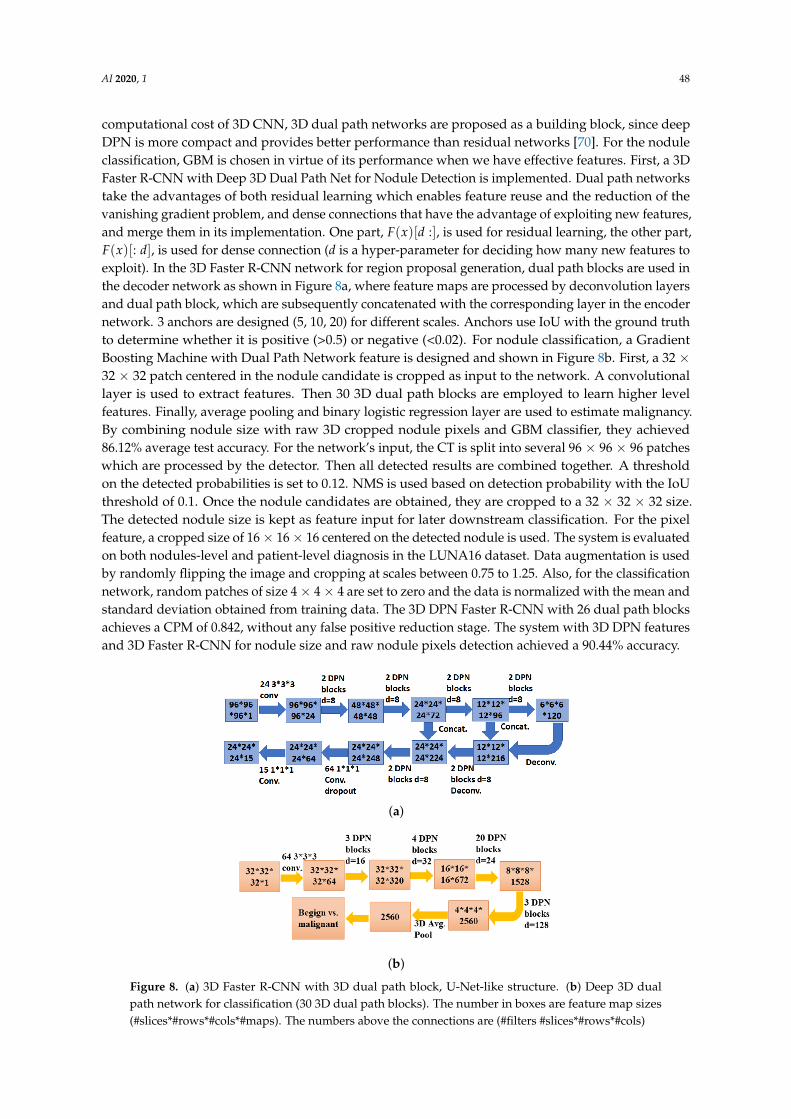
AI 2020, 1 48

computational cost of 3D CNN, 3D dual path networks are proposed as a building block, since deepDPN is more compact and provides better performance than residual networks [70]. For the noduleclassification, GBM is chosen in virtue of its performance when we have effective features. First, a 3DFaster R-CNN with Deep 3D Dual Path Net for Nodule Detection is implemented. Dual path networkstake the advantages of both residual learning which enables feature reuse and the reduction of thevanishing gradient problem, and dense connections that have the advantage of exploiting new features,and merge them in its implementation. One part, F(x)[d :], is used for residual learning, the other part,F(x)[: d], is used for dense connection (d is a hyper-parameter for deciding how many new features toexploit). In the 3D Faster R-CNN network for region proposal generation, dual path blocks are used inthe decoder network as shown in Figure 8a, where feature maps are processed by deconvolution layersand dual path block, which are subsequently concatenated with the corresponding layer in the encodernetwork. 3 anchors are designed (5, 10, 20) for different scales. Anchors use IoU with the ground truthto determine whether it is positive (>0.5) or negative (<0.02). For nodule classification, a GradientBoosting Machine with Dual Path Network feature is designed and shown in Figure 8b. First, a 32 ×32 × 32 patch centered in the nodule candidate is cropped as input to the network. A convolutionallayer is used to extract features. Then 30 3D dual path blocks are employed to learn higher levelfeatures. Finally, average pooling and binary logistic regression layer are used to estimate malignancy.By combining nodule size with raw 3D cropped nodule pixels and GBM classifier, they achieved86.12% average test accuracy. For the network’s input, the CT is split into several 96 × 96 × 96 patcheswhich are processed by the detector. Then all detected results are combined together. A thresholdon the detected probabilities is set to 0.12. NMS is used based on detection probability with the IoUthreshold of 0.1. Once the nodule candidates are obtained, they are cropped to a 32 × 32 × 32 size.The detected nodule size is kept as feature input for later downstream classification. For the pixelfeature, a cropped size of 16× 16× 16 centered on the detected nodule is used. The system is evaluatedon both nodules-level and patient-level diagnosis in the LUNA16 dataset. Data augmentation is usedby randomly flipping the image and cropping at scales between 0.75 to 1.25. Also, for the classificationnetwork, random patches of size 4× 4× 4 are set to zero and the data is normalized with the mean andstandard deviation obtained from training data. The 3D DPN Faster R-CNN with 26 dual path blocksachieves a CPM of 0.842, without any false positive reduction stage. The system with 3D DPN featuresand 3D Faster R-CNN for nodule size and raw nodule pixels detection achieved a 90.44% accuracy.

(a)

(b)

Figure 8. (a) 3D Faster R-CNN with 3D dual path block, U-Net-like structure. (b) Deep 3D dualpath network for classification (30 3D dual path blocks). The number in boxes are feature map sizes(#slices*#rows*#cols*#maps). The numbers above the connections are (#filters #slices*#rows*#cols)

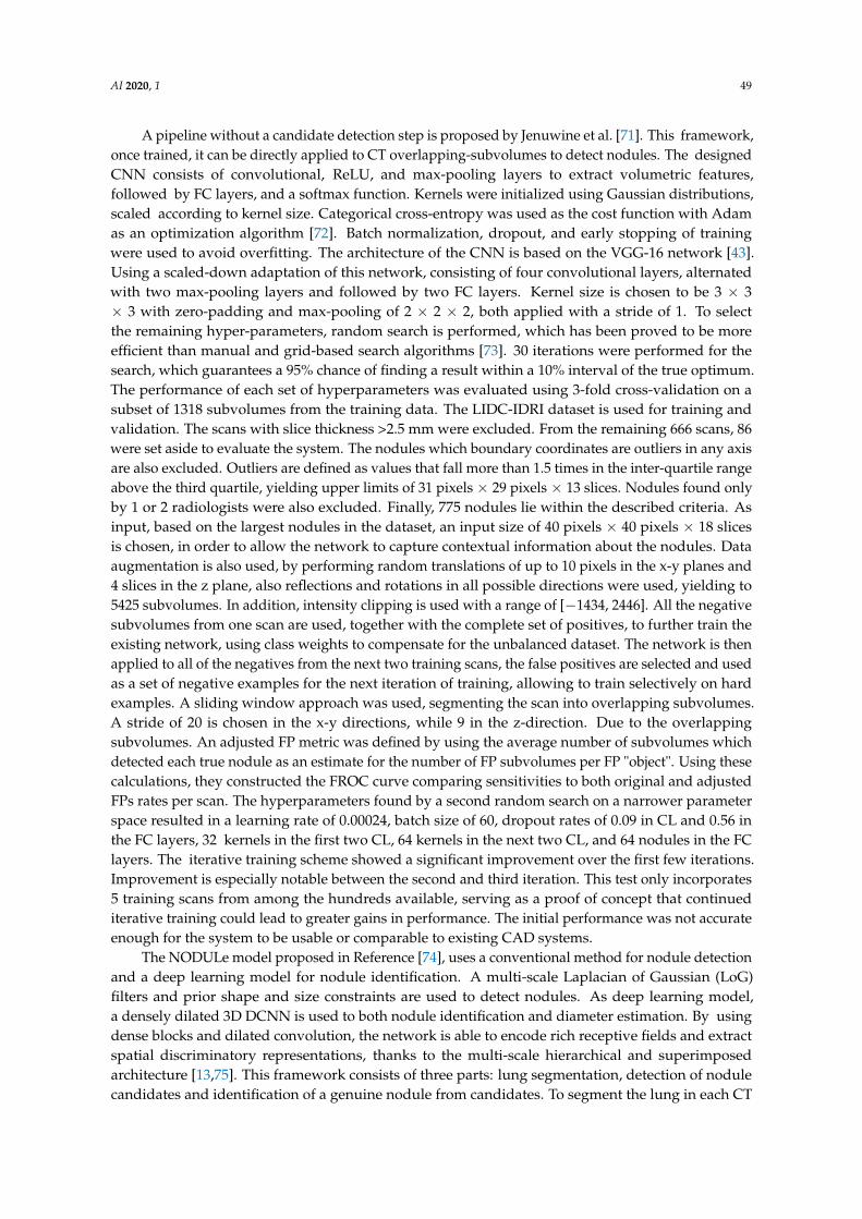
AI 2020, 1 49

A pipeline without a candidate detection step is proposed by Jenuwine et al. [71]. This framework,once trained, it can be directly applied to CT overlapping-subvolumes to detect nodules. The designedCNN consists of convolutional, ReLU, and max-pooling layers to extract volumetric features,followed by FC layers, and a softmax function. Kernels were initialized using Gaussian distributions,scaled according to kernel size. Categorical cross-entropy was used as the cost function with Adamas an optimization algorithm [72]. Batch normalization, dropout, and early stopping of trainingwere used to avoid overfitting. The architecture of the CNN is based on the VGG-16 network [43].Using a scaled-down adaptation of this network, consisting of four convolutional layers, alternatedwith two max-pooling layers and followed by two FC layers. Kernel size is chosen to be 3 × 3× 3 with zero-padding and max-pooling of 2 × 2 × 2, both applied with a stride of 1. To selectthe remaining hyper-parameters, random search is performed, which has been proved to be moreefficient than manual and grid-based search algorithms [73]. 30 iterations were performed for thesearch, which guarantees a 95% chance of finding a result within a 10% interval of the true optimum.The performance of each set of hyperparameters was evaluated using 3-fold cross-validation on asubset of 1318 subvolumes from the training data. The LIDC-IDRI dataset is used for training andvalidation. The scans with slice thickness >2.5 mm were excluded. From the remaining 666 scans, 86were set aside to evaluate the system. The nodules which boundary coordinates are outliers in any axisare also excluded. Outliers are defined as values that fall more than 1.5 times in the inter-quartile rangeabove the third quartile, yielding upper limits of 31 pixels × 29 pixels × 13 slices. Nodules found onlyby 1 or 2 radiologists were also excluded. Finally, 775 nodules lie within the described criteria. Asinput, based on the largest nodules in the dataset, an input size of 40 pixels × 40 pixels × 18 slicesis chosen, in order to allow the network to capture contextual information about the nodules. Dataaugmentation is also used, by performing random translations of up to 10 pixels in the x-y planes and4 slices in the z plane, also reflections and rotations in all possible directions were used, yielding to5425 subvolumes. In addition, intensity clipping is used with a range of [−1434, 2446]. All the negativesubvolumes from one scan are used, together with the complete set of positives, to further train theexisting network, using class weights to compensate for the unbalanced dataset. The network is thenapplied to all of the negatives from the next two training scans, the false positives are selected and usedas a set of negative examples for the next iteration of training, allowing to train selectively on hardexamples. A sliding window approach was used, segmenting the scan into overlapping subvolumes.A stride of 20 is chosen in the x-y directions, while 9 in the z-direction. Due to the overlappingsubvolumes. An adjusted FP metric was defined by using the average number of subvolumes whichdetected each true nodule as an estimate for the number of FP subvolumes per FP "object". Using thesecalculations, they constructed the FROC curve comparing sensitivities to both original and adjustedFPs rates per scan. The hyperparameters found by a second random search on a narrower parameterspace resulted in a learning rate of 0.00024, batch size of 60, dropout rates of 0.09 in CL and 0.56 inthe FC layers, 32 kernels in the first two CL, 64 kernels in the next two CL, and 64 nodules in the FClayers. The iterative training scheme showed a significant improvement over the first few iterations.Improvement is especially notable between the second and third iteration. This test only incorporates5 training scans from among the hundreds available, serving as a proof of concept that continuediterative training could lead to greater gains in performance. The initial performance was not accurateenough for the system to be usable or comparable to existing CAD systems.

The NODULe model proposed in Reference [74], uses a conventional method for nodule detectionand a deep learning model for nodule identification. A multi-scale Laplacian of Gaussian (LoG)filters and prior shape and size constraints are used to detect nodules. As deep learning model,a densely dilated 3D DCNN is used to both nodule identification and diameter estimation. By usingdense blocks and dilated convolution, the network is able to encode rich receptive fields and extractspatial discriminatory representations, thanks to the multi-scale hierarchical and superimposedarchitecture [13,75]. This framework consists of three parts: lung segmentation, detection of nodulecandidates and identification of a genuine nodule from candidates. To segment the lung in each CT

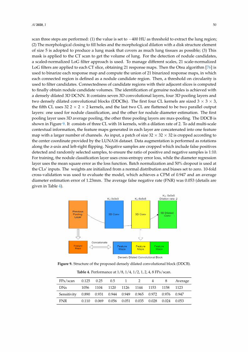
AI 2020, 1 50

scan three steps are performed: (1) the value is set to −400 HU as threshold to extract the lung region;(2) The morphological closing to fill holes and the morphological dilation with a disk structure elementof size 5 is adopted to produce a lung mask that covers as much lung tissues as possible; (3) Thismask is applied to the CT scan to get the volume of lung. For the detection of nodule candidates,a scaled-normalized LoG filter approach is used. To manage different scales, 21 scale-normalizedLoG filters are applied to each CT slice, obtaining 21 response maps. Then the Otsu algorithm [76] isused to binarize each response map and compute the union of 21 binarized response maps, in whicheach connected region is defined as a nodule candidate region. Then, a threshold on circularity isused to filter candidates. Connectedness of candidate regions with their adjacent slices is computedto finally obtain nodule candidate volumes. The identification of genuine nodules is achieved witha densely dilated 3D DCNN. It contains seven 3D convolutional layers, four 3D pooling layers andtwo densely dilated convolutional blocks (DDCBs). The first four CL kernels are sized 3 × 3 × 3,the fifth CL uses 32 2 × 2 × 2 kernels, and the last two CL are flattened to be two parallel outputlayers: one used for nodule classification, and the other for nodule diameter estimation. The firstpooling layer uses 3D average pooling, the other three pooling layers are max-pooling. The DDCB isshown in Figure 9. It consists of three CL with 16 kernels, with a dilation rate of 2. To add multi-scalecontextual information, the feature maps generated in each layer are concatenated into one featuremap with a larger number of channels. As input, a patch of size 32 × 32 × 32 is cropped according tothe center coordinate provided by the LUNA16 dataset. Data augmentation is performed as rotationsalong the z-axis and left-right flipping. Negative samples are cropped which include false positivesdetected and randomly selected samples, to ensure the ratio of positive and negative samples is 1:10.For training, the nodule classification layer uses cross-entropy error loss, while the diameter regressionlayer uses the mean square error as the loss function. Batch normalization and 50% dropout is used atthe CLs’ inputs. The weights are initialized from a normal distribution and biases set to zero. 10-foldcross-validation was used to evaluate the model, which achieves a CPM of 0.947 and an averagediameter estimation error of 1.23mm. The average false negative rate (FNR) was 0.053 (details aregiven in Table 4).

Figure 9. Structure of the proposed densely dilated convolutional block (DDCB).

Table 4. Performance at 1/8, 1/4, 1/2, 1, 2, 4, 8 FPs/scan.

FPs/scan 0.125 0.25 0.5 1 2 4 8 Average

DNs 1056 1104 1120 1126 1144 1153 1158 1123

Sensitivity 0.890 0.931 0.944 0.949 0.965 0.972 0.976 0.947

FNR 0.110 0.069 0.056 0.051 0.035 0.028 0.024 0.053

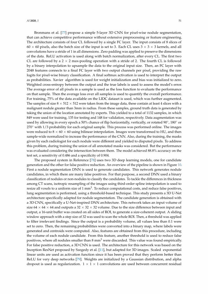
AI 2020, 1 51

Bronmans et al. [77] propose a simple 5-layer 3D CNN for pixel-wise nodule segmentation,that can achieve competitive performance without extensive preprocessing or feature engineering.The architecture consists of four CL followed by a single FC layer. The input consists of 8 slices of60 × 60 pixels, also the batch size of the input is set to 3. Each CL uses 3 × 3 × 3 kernels, and allconvolutions have a stride of 1 in all dimensions. Zero padding was applied to preserve the dimensionsof the data. ReLU activation is used along with batch normalization, after every CL. The first twoCL are followed by a 2 × 2 max-pooling operation with a stride of 2. The fourth CL is followedby a binary interpolation to upsample the data to the original input size. Then, an FC layer with2048 features connects to a final FC layer with two output channels per pixel, providing the rawlogits for pixel-wise binary classification. A final softmax activation is used to interpret the outputas probabilities. Xavier algorithm is used for weight initialization and bias was initialized to zero.Weighted cross-entropy between the output and the true labels is used to assess the model’s error.The average error of all pixels in a sample is used as the loss function to evaluate the performanceon that sample. Then the average loss over all samples is used to quantify the overall performance.For training, 75% of the data available on the LIDC dataset is used, which was further augmented.The samples of size 8 × 512 × 512 were taken from the image data, these contain at least 4 slices with amalignant nodule greater than 3mm in radius. From these samples, ground truth data is generated bytaking the union of the location annotated by experts. This yielded to a total of 1132 samples, in which849 were used for training, 135 for testing and 148 for validation, respectively. Data augmentation wasused by allowing in every epoch a 50% chance of flip horizontally, vertically, or rotated 90◦, 180◦ or270◦ with 1/3 probability for each original sample. This process was performed online. The imageswere reduced to 8 × 60 × 60 using bilinear interpolation. Images were transformed to HU, and thensample-wide normalized to increase the performance of the CNN. Also, during the training, the masksgiven by each radiologist for each nodule were different and yielded to disputed pixels. To addressthis problem, during training the union of all annotated masks was considered. But the performancewas evaluated considering the intersection between them. The model achieved 88.8% accuracy on thetest set, a sensitivity of 0.486 and a specificity of 0.904.

The proposed system in Reference [78] uses two 3D deep learning models, one for candidategeneration and the other for false positive reduction. An overview of the pipeline is shown in Figure 10.First a nodule segmentation DNN is used to generate candidates. This network generates nodulecandidates, in which there are many false positives. For that purpose, a second DNN used a binaryclassification of nodules or non-nodules to classify the candidates. To tackle the differences in thicknessamong CT scans, isotropic resampling of the images using third-order spline interpolation is used toresize all voxels to a uniform size of 1 mm3. To reduce computational costs, and reduce false positives,lung segmentation is performed, using a threshold-based technique. This study presents a 3D U-Netarchitecture specifically adapted for nodule segmentation. The candidate generation is obtained witha 3D CNN, specifically a U-Net-inspired DNN architecture. This network takes an input volume ofsize 64 × 64 × 64 and outputs a 32 × 32 × 32 volume. Due to the size difference between input andoutput, a 16-unit buffer was created on all sides of ROI, to generate a size-coherent output. A slidingwindow approach with a step size of 32 was used to scan the whole ROI. Then, a threshold was appliedto filter irrelevant findings. Since the output is a probability volume, all values less than 0.1 wereset to zero. Then, the remaining probabilities were converted into a binary map, where labels weregenerated and centroids were computed. Also, features are obtained from this procedure, includingthe volume of each nodule candidate. From this feature, another threshold is used to reduce falsepositives, where all nodules smaller than 8 mm3 were discarded. This value was found empirically.For false positive reduction, a 3D CNN is used. The architecture for this network was based on theInception ResNet proposed by Szegedy et al. [11], but adapted for 3D images. Scaled exponentiallinear units are used as activation function since it has been proved that they perform better thanReLU for very deep networks [79]. Weights are initialized by a Gaussian distribution, and alphadropout is used as regularization. 1 × 1 × 1 convolutions are used between concurrent residual

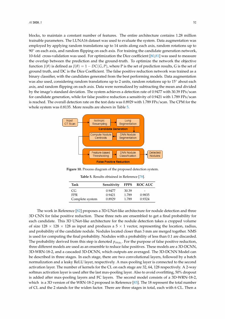
AI 2020, 1 52

blocks, to maintain a constant number of features. The entire architecture contains 1.28 milliontrainable parameters. The LUNA16 dataset was used to evaluate the system. Data augmentation wasemployed by applying random translations up to 14 units along each axis, random rotations up to90◦ on each axis, and random flipping on each axis. For training the candidate generation network,10-fold cross-validation was used. For optimization the Dice coefficient [80,81] was used to measurethe overlap between the prediction and the ground-truth. To optimize the network the objectivefunction J(θ) is defined as J(θ) = 1− DC(G, P), where P is the set of prediction results, G is the set ofground truth, and DC is the Dice Coefficient. The false positive reduction network was trained as abinary classifier, with the candidates generated from the best performing models. Data augmentationwas also used, considering random translations up to 2 units, random rotations up to 15◦ about eachaxis, and random flipping on each axis. Data were normalized by subtracting the mean and dividedby the image’s standard deviation. The system achieves a detection rate of 0.9477 with 30.39 FPs/scanfor candidate generation, while for false positive reduction a sensitivity of 0.9421 with 1.789 FPs/scanis reached. The overall detection rate on the test data was 0.8929 with 1.789 FPs/scan. The CPM for thewhole system was 0.8135. More results are shown in Table 5.

Figure 10. Process diagram of the proposed detection system.

Table 5. Results obtained in Reference [78].

Task Sensitivity FPPS ROC AUC

CG 0.9477 30.39 -FPR 0.9421 1.789 0.9835Complete system 0.8929 1.789 0.9324

The work in Reference [82] proposes a 3D-UNet-like architecture for nodule detection and three3D CNN for false positive reduction. These three nets are ensembled to get a final probability foreach candidate. This 3D UNet-like architecture for the nodule detection takes a cropped volumeof size 128 × 128 × 128 as input and produces a 5 × 1 vector, representing the location, radius,and probability of the candidate nodule. Nodules located closer than 3 mm are merged together. NMSis used for computing the final probability. Nodules with a probability of less than 0.1 are discarded.The probability derived from this step is denoted pstep1 . For the purpose of false positive reduction,three different models are used as an ensemble to reduce false positives. These models are a 3D-DCNN,3D-WRN-18-2, and a cascaded 3D-DCNN, which outputs are averaged. The 3D-DCNN Model canbe described in three stages. In each stage, there are two convolutional layers, followed by a batchnormalization and a leaky ReLU layer, respectively. A max-pooling layer is connected to the secondactivation layer. The number of kernels for the CL on each stage are 32, 64, 128 respectively. A 2-waysoftmax activation layer is used after the last max-pooling layer. Also to avoid overfitting, 50% dropoutis added after max-pooling layers and FC layers. The second model consists of a 3D-WRN-18-2,which is a 3D version of the WRN-18-2 proposed in Reference [83]. The 18 represent the total numberof CL and the 2 stands for the widen factor. There are three stages in total, each with 6 CL. Then a

AI 2020, 1 53

max-pooling layer is applied, and finally a 2-way softmax activation layer. 10% dropout is added aftermax-pooling layers and FC layers as regularization. The final model consists of a 5-stage cascaded3D-DCNN model, meaning that there are five 3D-DCNN just like the first model, cascaded oneafter the other. After each stage, the training set is reduced leaving samples that are hard to classify.This enables every network to learn different and specific features to better discriminate nodules.Once all the 3 probabilities from the different models are obtained, these are averaged and yield to aprobability for each nodule candidate, denoted as pstage2 . Finally, the ensemble probability is computedas p f inal = 0.4pstep1 + 0.6pstep2 . These weights were set empirically. The nodule detector network wasevaluated using 10-fold cross-validation on the LUNA16 dataset. The values of the CT scan wereset to [−1000, 1000] HU interval. Then data is interpolated to have the same voxel spacing betweendifferent CT scans (x:0.5556 mm, y:0.5556, z:1 mm). Finally, a 40 × 40 × 24 cubes are cropped around anodule. From that cube, a random crop of size 36 × 36 × 24 (20 mm × 20 mm × 20 mm) is obtained.Data augmentation is used to tackle the issue of imbalanced classes. Rotations of 90◦, 180◦, 270◦ areperformed, along with a shift within 2 pixels on the XY plane, zoom out, zoom in and flip along the xand y-axis. This increased by 7 times the number of positive samples. The weights of the networkswere initialized from a normal distribution and trained by minimizing the cross-entropy loss withAdam optimizer and a learning rate initialized to 0.0001. The recall for the nodule detection networkwas 0.991 with an FP/TP ratio of 16. A CPM of 0.966 is obtained in the false positive reduction task.This model obtained a second place on the false positive reduction task on the LUNA16 Challenge.The whole CAD system achieves a CPM of 0.947, yielding to the third place in the LUNA16 ChallengeLeaderboard on the complete nodule detection task.

Another proposed work [82] ranked first at the LUNA16 Challenge, at both nodule detection andfalse positive reduction categories. For Nodule detection, a network motivated by Feature PyramidNetworks (FPN) is used as architecture. False positive reduction is based on two 3D CNN classifiers.Focal loss [84] is used, since it has been proven to better manage the problem of class imbalance.Batch normalization and weight initialization by Xavier are used. Nodule detection is based on FPN.These type of networks have a similar architecture to U-Net, but leverages it as feature pyramid,with predictions made independently at all levels. The FPN network showed significant improvementcompared to existing methods. A volume of size 128 × 128 × 128 is cropped from the CT scan, and setas the input of the network. Also, adding hard negatives is used. First, N negative samples arerandomly selected from a candidate pool. The samples are sorted in descending order based on theirconfidence score, then the top n samples are chosen as hard negatives. This method showed to be moreeffective than focal loss alone. For false positive reduction, two 3D DCNN are used for the classificationpurpose. First, a 4-stage classifier network is proposed, which, in the first 3 stages contain two 3DCL followed by batch normalization, ReLU activation layers, and 3D max-pooling layers. Each stagecontains dropout to avoid overfitting. Finally, the last stage contains 3 FC layers with dropout. Thesecond network is based on a 3D U-Net architecture. It is first trained for nodule detection, thenchanged and fine-tuned for classification. This network also uses focal loss function, as it can focusthe training on the hard-to-class samples by reducing the weights of easy-to-class samples. The finaloutcome results from the fusion of both classification models. This work uses LUNA16 dataset toevaluate the model. First, a −600 HU threshold is used to get a 0–1 3D map and extract the lung area.Then, the final image pixels values are clipped to [−1200, 600] and normalized to [0, 255]. Pixels fora non-lung area are set to 170. Finally, a 128 × 128 × 128 cube is extracted. For the false positivereduction task, a multi-scale strategy is used, and two cubes of sizes 36 × 48 × 48 and 20 × 36 × 36,are cropped around the nodule, respectively. Oversampling over positive samples is used to tackle theclass imbalance. Methods like sliding window crop, flipping in all axes, rotations of 90◦, 180◦, 270◦,and multi-scale transform are used as data augmentation. This yielded to an expansion of positivesamples up to 300 times the original size. For the 3D DCNN, it was found empirically that usinga 36 × 48 × 48 cube for training and then fine-tuning it with 20 × 36 × 36 samples achieved goodresults. The U-Net classifier network uses a volume of size 32 × 32 × 32. 10-fold cross-validation

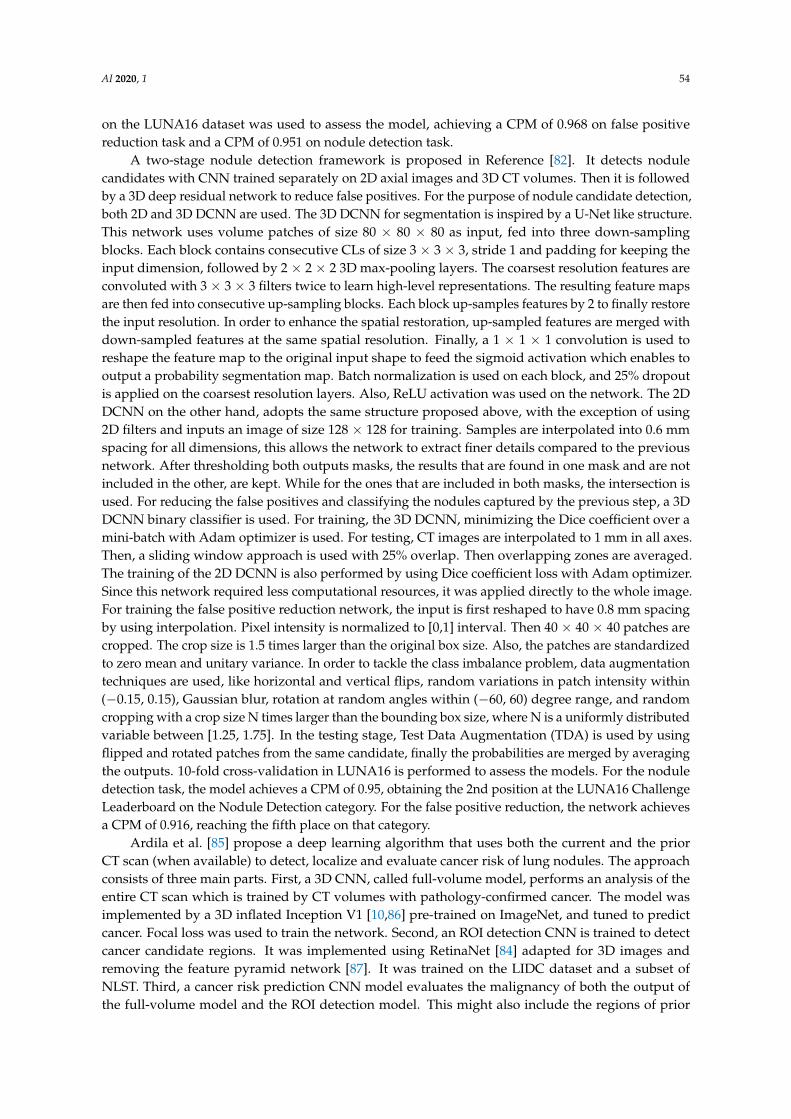
AI 2020, 1 54

on the LUNA16 dataset was used to assess the model, achieving a CPM of 0.968 on false positivereduction task and a CPM of 0.951 on nodule detection task.

A two-stage nodule detection framework is proposed in Reference [82]. It detects nodulecandidates with CNN trained separately on 2D axial images and 3D CT volumes. Then it is followedby a 3D deep residual network to reduce false positives. For the purpose of nodule candidate detection,both 2D and 3D DCNN are used. The 3D DCNN for segmentation is inspired by a U-Net like structure.This network uses volume patches of size 80 × 80 × 80 as input, fed into three down-samplingblocks. Each block contains consecutive CLs of size 3 × 3 × 3, stride 1 and padding for keeping theinput dimension, followed by 2 × 2 × 2 3D max-pooling layers. The coarsest resolution features areconvoluted with 3 × 3 × 3 filters twice to learn high-level representations. The resulting feature mapsare then fed into consecutive up-sampling blocks. Each block up-samples features by 2 to finally restorethe input resolution. In order to enhance the spatial restoration, up-sampled features are merged withdown-sampled features at the same spatial resolution. Finally, a 1 × 1 × 1 convolution is used toreshape the feature map to the original input shape to feed the sigmoid activation which enables tooutput a probability segmentation map. Batch normalization is used on each block, and 25% dropoutis applied on the coarsest resolution layers. Also, ReLU activation was used on the network. The 2DDCNN on the other hand, adopts the same structure proposed above, with the exception of using2D filters and inputs an image of size 128 × 128 for training. Samples are interpolated into 0.6 mmspacing for all dimensions, this allows the network to extract finer details compared to the previousnetwork. After thresholding both outputs masks, the results that are found in one mask and are notincluded in the other, are kept. While for the ones that are included in both masks, the intersection isused. For reducing the false positives and classifying the nodules captured by the previous step, a 3DDCNN binary classifier is used. For training, the 3D DCNN, minimizing the Dice coefficient over amini-batch with Adam optimizer is used. For testing, CT images are interpolated to 1 mm in all axes.Then, a sliding window approach is used with 25% overlap. Then overlapping zones are averaged.The training of the 2D DCNN is also performed by using Dice coefficient loss with Adam optimizer.Since this network required less computational resources, it was applied directly to the whole image.For training the false positive reduction network, the input is first reshaped to have 0.8 mm spacingby using interpolation. Pixel intensity is normalized to [0,1] interval. Then 40 × 40 × 40 patches arecropped. The crop size is 1.5 times larger than the original box size. Also, the patches are standardizedto zero mean and unitary variance. In order to tackle the class imbalance problem, data augmentationtechniques are used, like horizontal and vertical flips, random variations in patch intensity within(−0.15, 0.15), Gaussian blur, rotation at random angles within (−60, 60) degree range, and randomcropping with a crop size N times larger than the bounding box size, where N is a uniformly distributedvariable between [1.25, 1.75]. In the testing stage, Test Data Augmentation (TDA) is used by usingflipped and rotated patches from the same candidate, finally the probabilities are merged by averagingthe outputs. 10-fold cross-validation in LUNA16 is performed to assess the models. For the noduledetection task, the model achieves a CPM of 0.95, obtaining the 2nd position at the LUNA16 ChallengeLeaderboard on the Nodule Detection category. For the false positive reduction, the network achievesa CPM of 0.916, reaching the fifth place on that category.

Ardila et al. [85] propose a deep learning algorithm that uses both the current and the priorCT scan (when available) to detect, localize and evaluate cancer risk of lung nodules. The approachconsists of three main parts. First, a 3D CNN, called full-volume model, performs an analysis of theentire CT scan which is trained by CT volumes with pathology-confirmed cancer. The model wasimplemented by a 3D inflated Inception V1 [10,86] pre-trained on ImageNet, and tuned to predictcancer. Focal loss was used to train the network. Second, an ROI detection CNN is trained to detectcancer candidate regions. It was implemented using RetinaNet [84] adapted for 3D images andremoving the feature pyramid network [87]. It was trained on the LIDC dataset and a subset ofNLST. Third, a cancer risk prediction CNN model evaluates the malignancy of both the output ofthe full-volume model and the ROI detection model. This might also include the regions of prior

AI 2020, 1 55

CT scans, to evaluate cancer risk of the corresponding region in the previous scan and assigning acase-level malignancy score. The third part is also trained on case-level pathology-confirmed cancerlabels. For the lung segmentation, Mask-RCNN [88] was used and trained with the LUNA16 dataset.The network is used to find the center of the corresponding bounding box. All these deep learningmodels were trained, finetuned and tested with the NLST dataset. The proposed approach achievedan AUC of 0.944. Tests were also conducted in two phases to compare the performance of the approachagainst 6 radiologists on a different dataset. First, both model and radiologists evaluated a set ofCT scans. The model achieved an AUC of 0.959 outperforming all 6 radiologists. A second test wasconducted, where prior CT scans from the previous year was available for both radiologists and thedeep model. The model achieved an AUC of 0.926 which on average outperformed the radiologists.

Huang et al. [89] propose the use of a non-sharpening mask to help a deep learning architectureto learn the features of a malignant nodule. The deep learning framework consists of three 3D-CNNwhich detect malignant nodules. Each one focuses on different image sizes, 32 × 32 × 32, 64 × 64× 64, and 96 × 96 × 96, respectively. The output of each CNN is fused using an AdaBoost classifier.First, lung sections are segmented using an unsharp mask filter. Then as a data augmentation strategy,images are rotated 90◦, 180◦, 270◦ and some are downsampled from 96 × 96 size to 64 × 64 and 32 ×32, resulting in 326,570 images from which 18,125 are pulmonary nodules. The authors use RT-ReLU(Random Translation ReLU) [90] as an activation function to avoid dead neurons and overfittingduring training. ReLu is used for testing. Training is conducted using LUNA16 and Ali Tianchi [91]datasets. The model achieves a sensitivity of 0.817 and 0.851 at 0.125 and 0.25 false positives per scanon LUNA16 dataset. The dataset was divided into training, testing, and validation containing 14,674,1795 and 1656 nodules respectively. More results are shown in Table 6.

Table 6. Results of the Architecture on LUNA16 as in Reference [89].

FPs per scan 0.125 0.25 0.5 1 2 4 8

Sensitivity (%) 81.7 85.1 86.9 88.3 89.1 90.7 91.4

5. False Positive Reduction

In this section, we present the works which focus only on false positive reduction task without anodule detection step. Here, the input is a nodule candidate and the proposed model is a classifierthat outputs the label of the nodule as benign or malignant. These works are divided into 2D and3D approaches.

5.1. 2D Deep Learning Approaches

Two main works were proposed for 2D deep learning. They are presented in the following.In Reference [92], the authors propose two methods based on CNNs and Extreme Learning

Machines (ELM). They use an unsupervised method, proposing a deep Sparse Autoencoder (SAE) [93]called multi-SAE (MSAE), in order to obtain features characterizing the lung nodules. Moreover,they use staked SAE instead of one-dimensional higher SAE network to avoid feature dimensionissues. Using an MSAE network, feature extractors for different scales are learned from raw lungnodule image patches. These are then convoluted to produce feature vectors for SVM classification.The SAE is based on a feed-forward neural network, in which, the parameters of the network aretrained to generate an output equal to the input. In other words, trying to minimize the discrepancybetween the input and its reconstruction. This process allows the network to learn features that areimportant for the representation. To avoid a huge number of hidden nodes, which are harder to train,they use a deep SAE network stacked with multi-layer SAE to extract robust features. In order tolearn from the different sizes and morphologies of lung nodules, three different scale networks areused. The input is a 1024-dimension column vector that represents the 32 × 32 nodule patch. In theCNN of this framework, the convolutional layers are used as a feature extractor at the beginning

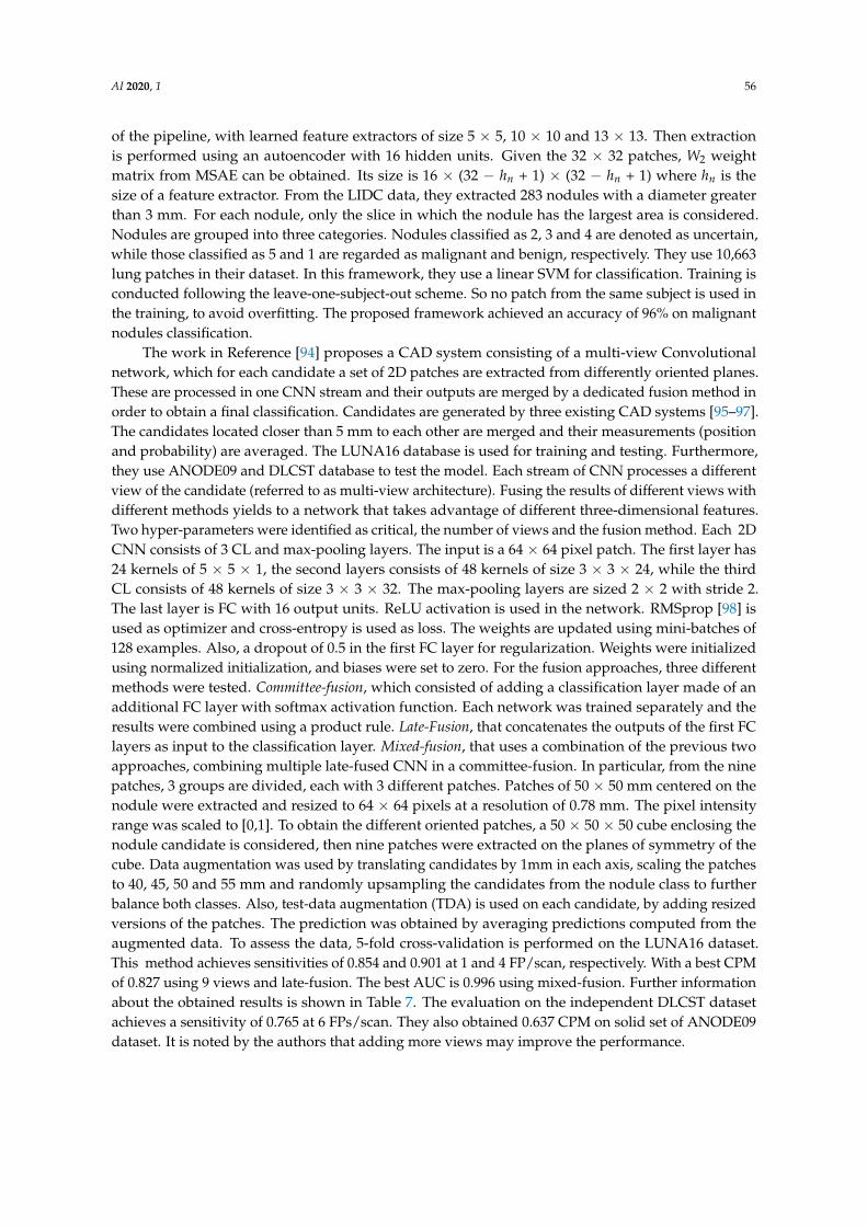
AI 2020, 1 56

of the pipeline, with learned feature extractors of size 5 × 5, 10 × 10 and 13 × 13. Then extractionis performed using an autoencoder with 16 hidden units. Given the 32 × 32 patches, W2 weightmatrix from MSAE can be obtained. Its size is 16 × (32 − hn + 1) × (32 − hn + 1) where hn is thesize of a feature extractor. From the LIDC data, they extracted 283 nodules with a diameter greaterthan 3 mm. For each nodule, only the slice in which the nodule has the largest area is considered.Nodules are grouped into three categories. Nodules classified as 2, 3 and 4 are denoted as uncertain,while those classified as 5 and 1 are regarded as malignant and benign, respectively. They use 10,663lung patches in their dataset. In this framework, they use a linear SVM for classification. Training isconducted following the leave-one-subject-out scheme. So no patch from the same subject is used inthe training, to avoid overfitting. The proposed framework achieved an accuracy of 96% on malignantnodules classification.

The work in Reference [94] proposes a CAD system consisting of a multi-view Convolutionalnetwork, which for each candidate a set of 2D patches are extracted from differently oriented planes.These are processed in one CNN stream and their outputs are merged by a dedicated fusion method inorder to obtain a final classification. Candidates are generated by three existing CAD systems [95–97].The candidates located closer than 5 mm to each other are merged and their measurements (positionand probability) are averaged. The LUNA16 database is used for training and testing. Furthermore,they use ANODE09 and DLCST database to test the model. Each stream of CNN processes a differentview of the candidate (referred to as multi-view architecture). Fusing the results of different views withdifferent methods yields to a network that takes advantage of different three-dimensional features.Two hyper-parameters were identified as critical, the number of views and the fusion method. Each 2DCNN consists of 3 CL and max-pooling layers. The input is a 64 × 64 pixel patch. The first layer has24 kernels of 5 × 5 × 1, the second layers consists of 48 kernels of size 3 × 3 × 24, while the thirdCL consists of 48 kernels of size 3 × 3 × 32. The max-pooling layers are sized 2 × 2 with stride 2.The last layer is FC with 16 output units. ReLU activation is used in the network. RMSprop [98] isused as optimizer and cross-entropy is used as loss. The weights are updated using mini-batches of128 examples. Also, a dropout of 0.5 in the first FC layer for regularization. Weights were initializedusing normalized initialization, and biases were set to zero. For the fusion approaches, three differentmethods were tested. Committee-fusion, which consisted of adding a classification layer made of anadditional FC layer with softmax activation function. Each network was trained separately and theresults were combined using a product rule. Late-Fusion, that concatenates the outputs of the first FClayers as input to the classification layer. Mixed-fusion, that uses a combination of the previous twoapproaches, combining multiple late-fused CNN in a committee-fusion. In particular, from the ninepatches, 3 groups are divided, each with 3 different patches. Patches of 50 × 50 mm centered on thenodule were extracted and resized to 64 × 64 pixels at a resolution of 0.78 mm. The pixel intensityrange was scaled to [0,1]. To obtain the different oriented patches, a 50 × 50 × 50 cube enclosing thenodule candidate is considered, then nine patches were extracted on the planes of symmetry of thecube. Data augmentation was used by translating candidates by 1mm in each axis, scaling the patchesto 40, 45, 50 and 55 mm and randomly upsampling the candidates from the nodule class to furtherbalance both classes. Also, test-data augmentation (TDA) is used on each candidate, by adding resizedversions of the patches. The prediction was obtained by averaging predictions computed from theaugmented data. To assess the data, 5-fold cross-validation is performed on the LUNA16 dataset.This method achieves sensitivities of 0.854 and 0.901 at 1 and 4 FP/scan, respectively. With a best CPMof 0.827 using 9 views and late-fusion. The best AUC is 0.996 using mixed-fusion. Further informationabout the obtained results is shown in Table 7. The evaluation on the independent DLCST datasetachieves a sensitivity of 0.765 at 6 FPs/scan. They also obtained 0.637 CPM on solid set of ANODE09dataset. It is noted by the authors that adding more views may improve the performance.

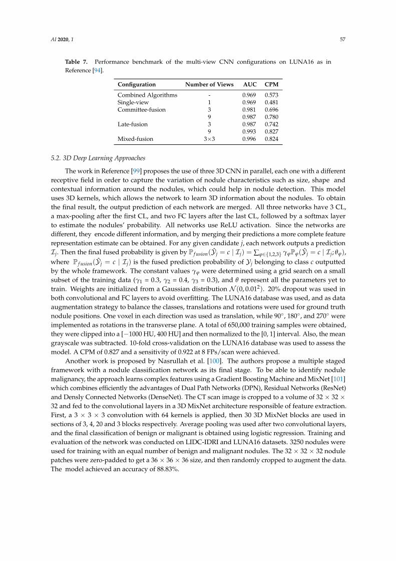
AI 2020, 1 57

Table 7. Performance benchmark of the multi-view CNN configurations on LUNA16 as inReference [94].

Configuration Number of Views AUC CPM

Combined Algorithms - 0.969 0.573Single-view 1 0.969 0.481Committee-fusion 3 0.981 0.696

9 0.987 0.780Late-fusion 3 0.987 0.742

9 0.993 0.827Mixed-fusion 3×3 0.996 0.824

5.2. 3D Deep Learning Approaches

The work in Reference [99] proposes the use of three 3D CNN in parallel, each one with a differentreceptive field in order to capture the variation of nodule characteristics such as size, shape andcontextual information around the nodules, which could help in nodule detection. This modeluses 3D kernels, which allows the network to learn 3D information about the nodules. To obtainthe final result, the output prediction of each network are merged. All three networks have 3 CL,a max-pooling after the first CL, and two FC layers after the last CL, followed by a softmax layerto estimate the nodules’ probability. All networks use ReLU activation. Since the networks aredifferent, they encode different information, and by merging their predictions a more complete featurerepresentation estimate can be obtained. For any given candidate j, each network outputs a predictionIj. Then the final fused probability is given by P f usion(Yj = c | Ij) = ∑ϕ∈{1,2,3} γϕPϕ(Yj = c | Ij; θϕ),where P f usion(Yj = c | Ij) is the fused prediction probability of Yj belonging to class c outputtedby the whole framework. The constant values γϕ were determined using a grid search on a smallsubset of the training data (γ1 = 0.3, γ2 = 0.4, γ3 = 0.3), and θ represent all the parameters yet totrain. Weights are initialized from a Gaussian distribution N (0, 0.012). 20% dropout was used inboth convolutional and FC layers to avoid overfitting. The LUNA16 database was used, and as dataaugmentation strategy to balance the classes, translations and rotations were used for ground truthnodule positions. One voxel in each direction was used as translation, while 90◦, 180◦, and 270◦ wereimplemented as rotations in the transverse plane. A total of 650,000 training samples were obtained,they were clipped into a [−1000 HU, 400 HU] and then normalized to the [0, 1] interval. Also, the meangrayscale was subtracted. 10-fold cross-validation on the LUNA16 database was used to assess themodel. A CPM of 0.827 and a sensitivity of 0.922 at 8 FPs/scan were achieved.

Another work is proposed by Nasrullah et al. [100]. The authors propose a multiple stagedframework with a nodule classification network as its final stage. To be able to identify nodulemalignancy, the approach learns complex features using a Gradient Boosting Machine and MixNet [101]which combines efficiently the advantages of Dual Path Networks (DPN), Residual Networks (ResNet)and Densly Connected Networks (DenseNet). The CT scan image is cropped to a volume of 32 × 32 ×32 and fed to the convolutional layers in a 3D MixNet architecture responsible of feature extraction.First, a 3 × 3 × 3 convolution with 64 kernels is applied, then 30 3D MixNet blocks are used insections of 3, 4, 20 and 3 blocks respectively. Average pooling was used after two convolutional layers,and the final classification of benign or malignant is obtained using logistic regression. Training andevaluation of the network was conducted on LIDC-IDRI and LUNA16 datasets. 3250 nodules wereused for training with an equal number of benign and malignant nodules. The 32 × 32 × 32 nodulepatches were zero-padded to get a 36 × 36 × 36 size, and then randomly cropped to augment the data.The model achieved an accuracy of 88.83%.

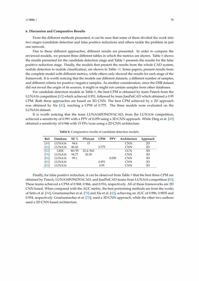
AI 2020, 1 58

6. Discussion and Comparative Results

From the different methods presented, it can be seen that some of them divided the work intotwo stages (candidate detection and false positive reduction) and others tackle the problem in justone network.

Due to these different approaches, different results are presented. In order to compare thereviewed models, we present three different tables in which the metrics are shown. Table 8 showsthe results presented for the candidate detection stage and Table 9 presents the results for the falsepositive reduction stage. Finally, the models that present the results from the whole CAD system,nodule detection to nodule classification, are shown in Table 10. Some papers, present results fromthe complete model with different metrics, while others only showed the results for each stage of theframework. It is worth noticing that the models use different datasets, a different number of samples,and different criteria for positive/negative samples. As another consideration, since the DSB datasetdid not reveal the origin of its sources, it might or might not contain samples from other databases.

For candidate detection models in Table 8, the best CPM is obtained by team Patech from theLUNA16 competition [82] which achieved 0.951, followed by team JianPeiCAD which obtained a 0.95CPM. Both these approaches are based on 3D CNN. The best CPM achieved by a 2D approachwas obtained by Xie [42], reaching a CPM of 0.775. The three models were evaluated on theLUNA16 dataset.

It is worth noticing that the team LUNA16FONOVACAD, from the LUNA16 competition,achieved a sensitivity of 0.991 with a PPV of 0.059 using a 3D CNN approach. While Ding et al. [49]obtained a sensitivity of 0.946 with 15 FPs/scan using a 2D CNN architecture.

Table 8. Comparative results of candidate detection models.

Ref. Database SE % FPs/scan CPM PPV Architecture Approach[49] LUNA16 94.6 15 CNN 2D[42] LUNA16 86.42 0.775 CNN 2D[52] LIDC 80/95 22.4/563 CCN 3D[78] LUNA16 94.77 30.39 CNN 3D[82] LUNA16 99.1 0.059 CNN 3D[82] LUNA16 0.951 CNN 3D[82] LUNA16 0.95 CNN 3D

Finally, for false positive reduction, it can be observed from Table 9 that the best three CPM areobtained by Patech, LUNA16FONOVACAD, and JianPeiCAD teams from LUNA16 competition [82].These teams achieved a CPM of 0.968, 0.966, and 0.916, respectively. All of these frameworks are 3DCNN based. When compared with the AUC metric, the best performing methods are from the worksof Setio et al. [94], Gruetzemacher et al. [78] and Xie et al. [42], achieving an AUC of 0.996, 0.9835 and0.954, respectively. Gruetzemacher et al. [78], used a 3D CNN approach, while the other two authorsused a 2D CNN based architecture.

AI 2020, 1 59

Table 9. Comparative results of false positive reduction models.

Ref. Database SE % FPs/scan ACC % CPM AUC Architecture Approach

[42] LUNA16 73.4/74.4 0.125/0.25 0.79 0.954 CNN 2D[92] LIDC 96 MSAE/CNN 2D[94] LUNA16 85.4/90.1 1.0/4.0 0.824 0.996 CNN 2D[94] ANODE09 0.637 CNN 2D[94] DLCST 76.5 6 CNN 2D[49] LUNA16 92.2/94.4 1.0/4.0 0.891 CNN 3D[52] LIDC 80 15.28 CNN 3D[78] LUNA16 94.21 1.789 0.983 CNN 3D[82] LUNA16 0.966 CNN 3D[82] LUNA16 0.968 CNN 3D[82] LUNA16 0.916 CNN 3D[99] LUNA16 92.2 8 0.827 CNN 3D[100] LUNA16/LIDC 88.83 CNN 3D

From Table 10 it can be seen that Zhang et al. [74] and the team of LUNA16FONOVACAD [82]presents the highest CPM with 0.947, obtained by testing on the LUNA16 dataset. Followed by a CPMof 0.876 achieved by Huang et al. [89] in the LUNA16/Ali Tianchi dataset. In third place, a CPM of0.856 was obtained by Liao et al. [66] on the DBS dataset. All the above-mentioned works were basedon 3D Convolutional Neural Networks. The closest performance in CPM that uses a 2D approach isSetio et al.’s work [94], reaching a CPM of 0.824 on the LUNA16 dataset. If AUC is used as a metric ofperformance, Setio et al. [94] achieve the best performance with 0.996 on the LUNA16 dataset. Then anAUC of 0.9665 is obtained by Xie [41] on the LIDC-IDRI dataset. Third, an AUC of 0.949 is achieved byArdila et al. [85] on the NLST dataset. In this case, the first two are 2D approaches, based on CNN andFuse-TSD respectively, while the third is a 3D CNN approach.

Overall, we can see that the best performing models used architectures based on three-dimensionalconvolutional neural networks. While 2D approaches are computationally less expensive, due tothe fact that CT volumes are 3D images, three-dimensional kernels can detect more details about thenodules, which are inherently a three-dimensional structure. However, since the different modelswere tested on different databases and with different augmentations, the comparison between theirperformances is not straight forward. Still the analysis help points out important characteristics forbuilding a robust deep learning architecture for lung cancer detection.

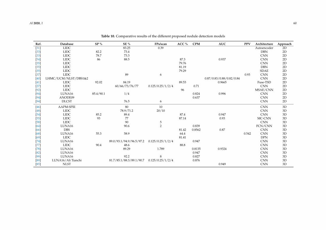
AI 2020, 1 60

Table 10. Comparative results of the different proposed nodule detection models

Ref. Database SP % SE % FPs/scan ACC % CPM AUC PPV Architecture Approach[31] LIDC 83.25 0.39 Autoencoder 2D[33] LIDC 82.2 73.4 DBN 2D[33] LIDC 78.7 73.3 CNN 2D[54] LIDC 86 88.5 87.3 0.937 CNN 2D[35] LIDC 79.76 CNN 2D[35] LIDC 81.19 DBN 2D[35] LIDC 79.29 SDAE 2D[37] LIDC 89 6 0.93 CNN 2D[40] LHMC/UCM/NLST/DBS1&2 0.87/0.83/0.88/0.82/0.84 CNN 2D[41] LIDC 92.02 84.19 89.53 0.9665 Fuse-TSD 2D[27] LIDC 60/66/73/76/77 0.125/0.25/1/2/4 0.71 CNN 2D[92] LIDC 96 MSAE/CNN 2D[94] LUNA16 85.4/90.1 1/4 0.824 0.996 CNN 2D[94] ANODE09 0.637 CNN 2D[94] DLCST 76.5 6 CNN 2D

[46] AAPM-SPIE 80 10 CNN 3D[48] LIDC 78.9/71.2 20/10 CNN 3D[54] LIDC 85.2 89.4 87.4 0.947 CNN 3D[55] LIDC 93 77 87.14 0.93 MC-CNN 3D[58] LIDC 90 5 CNN 3D[64] LUNA16 90.6 2 0.839 FCN/CNN 3D[66] DBS 81.42 0.8562 0.87 CNN 3D[68] LUNA16 55.3 58.9 64.4 0.542 CNN 3D[69] LIDC 81.41 DPN 3D[74] LUNA16 89.0/93.1/94.9/96.5/97.2 0.125/0.25/1/2/4 0.947 CNN 3D[77] LIDC 90.4 48.6 88.8 CNN 3D[78] LUNA16 89.29 1.789 0.8135 0.9324 CNN 3D[82] LUNA16 0.947 CNN 3D[99] LUNA16 92.2 8 0.827 CNN 3D[89] LUNA16/Ali Tianchi 81.7/85.1/88.3/89.1/90.7 0.125/0.25/1/2/4 0.876 CNN 3D[85] NLST 0.949 CNN 3D

AI 2020, 1 61

7. Conclusions

In this work, we presented different deep CAD systems and models that pursue the commonobjective of alleviating the work of radiologists in lung nodule detection. It is shown that deep learninghas achieved a level of precision that allows implementation, not only as a second opinion in diagnosisbut as a powerful tool that can be considered by physicians in their work.

The surveyed work shows that deep learning techniques have led to high performances forlung cancer detection using CT scans. The proposed techniques are based on deep ConvolutionalNeural Networks (CNN). Some of the proposed approaches used hybrid deep and classical machinelearning techniques. 3D convolutional neural network architectures showed their usefulness onobtaining representative features of malignant nodules, as most of the best-performing methods usedthem. In particular, densely connected networks and wide residual networks along with the U-Netarchitecture obtained very interesting results. While 3D CNN show the best performances overall, 2DCNN techniques also give some very interesting results.

Popular techniques such as U-Net, Faster R-CNN, Mask R-CNN, YOLO, VGG, ResNet, and soforth, were used to build the convolutional networks for nodule detection and false positive reduction.Future works can further improve convolutional architectures for the purpose of lung cancer detection.Both the design of new architectures and the study of the existing ones could improve the performanceand the computational cost especially for three-dimensional networks. Some recent deep learningtechniques have shown important improvements in the results of segmentation and classification. It isworth developing a new CAD system using such techniques. For example, for nodule detection wecan use the new YOLO v3 [102] which adds some scale invariance and can help detect lung nodulesof different sizes. New segmentation techniques such as DeepLabv3+ [103] and Gated-SCNN [104]can also be used to extract nodules candidates. The classification of the nodule into malignant orbenign can benefit from the performance of the recently proposed deep EfficientNet architectures [105].These recent techniques can be used for 2D or adapted to 3D data processing. Using multiple slicesas input in the 2D deep networks can also be considered. 2D networks are more efficient in term ofprocessing time and memory requirement, which makes them an interesting solution for processinglarge medical DICOM data.

A benchmarking of the most performing architectures on available datasets using similar metricscan help in their comparative analysis. Finally, one of the current limitations is the data and theirimbalanced nature. The use of new loss functions designed to tackle the problem of unbalancedclasses such as focal loss, could improve the existing results, and help achieve more efficient training.With more datasets and more balanced data, we think that better results can be achieved.

Author Contributions: Conceptualization, M.A.A. and D.R.; formal analysis, M.A.A. and D.R.; writing—originaldraft preparation, D.R.; writing—review and editing, M.A.A.; supervision, M.A.A.; project administration, M.A.A.;funding acquisition, M.A.A. All authors have read and agreed to the published version of the manuscript.

Funding: This work was partially supported by the New Brunswick Health Research Foundation (NBHRF),and the government of Canada under the Canada-Chile Leadership Exchange Scholarship.

Conflicts of Interest: The authors declare no conflict of interest.

References

1. Trial Summary—Learn—NLST—The Cancer Data Access System. Available online: https://biometry.nci.nih.gov/cdas/learn/nlst/trial-summary/ (accessed on 7 January 2020).

2. National Lung Screening Trial Research Team. Reduced Lung-Cancer Mortality with Low-Dose ComputedTomographic Screening. N. Engl. J. Med. 2011, 365, 395–409. [CrossRef] [PubMed]

3. Choi, W.J.; Choi, T.S. Automated Pulmonary Nodule Detection Based on Three-Dimensional Shape-BasedFeature Descriptor. Comput. Methods Progr. Biomed. 2014, 113, 37–54. [CrossRef] [PubMed]

4. Peña, D.M.; Luo, S.; Abdelgader, A.M.S. Auto Diagnostics of Lung Nodules Using Minimal CharacteristicsExtraction Technique. Diagnostics 2016, 6, 13. [CrossRef] [PubMed]

AI 2020, 1 62

5. Camarlinghi, N.; Gori, I.; Retico, A.; Bellotti, R.; Bosco, P.; Cerello, P.; Gargano, G.; Lopez Torres, E.; Megna, R.;Peccarisi, M.; et al. Combination of Computer-Aided Detection Algorithms for Automatic Lung NoduleIdentification. Int. J. Comput. Assist. Radiol. Surg. 2012, 7, 455–464. [CrossRef]

6. Teramoto, A.; Fujita, H. Fast Lung Nodule Detection in Chest CT Images Using CylindricalNodule-Enhancement Filter. Int. J. Comput. Assist. Radiol. Surg. 2013, 8, 193–205. [CrossRef]

7. Thomas, R.A.; Kumar, S.S. Automatic Detection of Lung Nodules Using Classifiers. In Proceedingsof the 2014 International Conference on Control, Instrumentation, Communication and ComputationalTechnologies (ICCICCT), Kanyakumari, India, 10–11 July 2014; pp. 705–710. [CrossRef]

8. Santos, A.M.; de Carvalho Filho, A.O.; Silva, A.C.; de Paiva, A.C.; Nunes, R.A.; Gattass, M. AutomaticDetection of Small Lung Nodules in 3D CT Data Using Gaussian Mixture Models, Tsallis Entropy and SVM.Eng. Appl. Artif. Intell. 2014, 36, 27–39. [CrossRef]

9. He, K.; Zhang, X.; Ren, S.; Sun, J. Deep Residual Learning for Image Recognition. In Proceedings of the2016 IEEE Conference on Computer Vision and Pattern Recognition (CVPR), Las Vegas, NV, USA, 27–30June 2016; pp. 770–778. [CrossRef]

10. Szegedy, C.; Vanhoucke, V.; Ioffe, S.; Shlens, J.; Wojna, Z. Rethinking the Inception Architecture for ComputerVision. In Proceedings of the 2016 IEEE Conference on Computer Vision and Pattern Recognition (CVPR),Las Vegas, NV, USA, 27–30 June 2016; pp. 2818–2826. [CrossRef]

11. Szegedy, C.; Ioffe, S.; Vanhoucke, V.; Alemi, A. Inception-v4, Inception-ResNet and the Impact of ResidualConnections on Learning. arXiv 2016, arXiv:1602.07261.

12. Chollet, F. Xception: Deep Learning with Depthwise Separable Convolutions. In Proceedings of the 2017IEEE Conference on Computer Vision and Pattern Recognition (CVPR), Honolulu, HI, USA, 21–26 July 2017;pp. 1800–1807. [CrossRef]

13. Huang, G.; Liu, Z.; van der Maaten, L.; Weinberger, K.Q. Densely Connected Convolutional Networks.In Proceedings of the 2017 IEEE Conference on Computer Vision and Pattern Recognition (CVPR), Honolulu,HI, USA, 21–26 July 2017; pp. 2261–2269. [CrossRef]

14. Huang, G.; Liu, Z.; Pleiss, G.; Van Der Maaten, L.; Weinberger, K. Convolutional Networks with DenseConnectivity. IEEE Trans. Pattern Anal. Mach. Intell. 2019, 1. [CrossRef]

15. Dauphin, Y.N.; Fan, A.; Auli, M.; Grangier, D. Language Modeling with Gated Convolutional Networks.In Proceedings of the 34th International Conference on Machine Learning, Sydney, Australia, 6–11 August2017; Volume 70, pp. 933–941.

16. Standford.edu. Deep Learning Tutorial. Available online: http://deeplearning.stanford.edu/tutorial/(accessed on 8 December 2019).

17. Armato Samuel, G., III; McLennan, G.; Bidaut, L.; McNitt-Gray, M.F.; Meyer, C.R.; Reeves, A.P.; Zhao, B.;Aberle, D.R.; Henschke, C.I.; Hoffman, E.A.; et al. Data From LIDC-IDRI. 2015. Available online: https://wiki.cancerimagingarchive.net/display/Public/LIDC-IDRI (accessed on 7 January 2020). [CrossRef]

18. Armato, S.G.; McLennan, G.; Bidaut, L.; McNitt-Gray, M.F.; Meyer, C.R.; Reeves, A.P.; Zhao, B.; Aberle, D.R.;Henschke, C.I.; Hoffman, E.A.; et al. The Lung Image Database Consortium (LIDC) and Image DatabaseResource Initiative (IDRI): A Completed Reference Database of Lung Nodules on CT Scans. Med. Phys. 2011,38, 915–931. [CrossRef]

19. Setio, A.A.A.; Traverso, A.; de Bel, T.; Berens, M.S.N.; van den Bogaard, C.; Cerello, P.; Chen, H.;Dou, Q.; Fantacci, M.E.; Geurts, B.; et al. Validation, Comparison, and Combination of Algorithmsfor Automatic Detection of Pulmonary Nodules in Computed Tomography Images: The LUNA16 Challenge.Med. Image Anal. 2017, 42, 1–13. [CrossRef]

20. Armato Samuel G., III; Hadjiiski, L.; Tourassi, G.D.; Drukker, K.; Giger, M.L.; Li, F.; Redmond, G.;Farahani, K.; Kirby, J.S.; Clarke, L.P. SPIE-AAPM-NCI Lung Nodule Classification Challenge Dataset.2015. Available online: https://wiki.cancerimagingarchive.net/display/Public/SPIE-AAPM+Lung+CT+Challenge (accessed on 7 January 2020).[CrossRef]

21. Van Ginneken, B.; Armato, S.G.; de Hoop, B.; van Amelsvoort-van de Vorst, S.; Duindam, T.; Niemeijer, M.;Murphy, K.; Schilham, A.; Retico, A.; Fantacci, M.E.; et al. Comparing and Combining Algorithms forComputer-Aided Detection of Pulmonary Nodules in Computed Tomography Scans: The ANODE09 Study.Med. Image Anal. 2010, 14, 707–722. [CrossRef] [PubMed]

22. Ru Zhao, Y.; Xie, X.; de Koning, H.J.; Mali, W.P.; Vliegenthart, R.; Oudkerk, M. NELSON Lung CancerScreening Study. Cancer Imaging 2011, 11, S79–S84. [CrossRef] [PubMed]

AI 2020, 1 63

23. Danish Lung Cancer Screening Trial (DLCST)—Full Text View— ClinicalTrials.Gov. Available online:https://clinicaltrials.gov/ct2/show/NCT00496977 (accessed on 7 January 2020).

24. Winkler Wille, M.M.; van Riel, S.J.; Saghir, Z.; Dirksen, A.; Pedersen, J.H.; Jacobs, C.; Thomsen, L.H.;Scholten, E.T.; Skovgaard, L.T.; van Ginneken, B. Predictive Accuracy of the PanCan Lung Cancer RiskPrediction Model -External Validation Based on CT from the Danish Lung Cancer Screening Trial. Eur. Radiol.2015, 25, 3093–3099. [CrossRef] [PubMed]

25. Data Science Bowl. 2017. Available online: https://www.kaggle.com/c/data-science-bowl-2017 (accessedon 7 January 2020).

26. Powers, D.M.W. Evaluation: From precision, recall and f-measure to roc., informedness, markedness &correlation. J. Mach. Learn. Technol. 2011, 2, 37–63.

27. Van Ginneken, B.; Setio, A.A.A.; Jacobs, C.; Ciompi, F. Off-the-Shelf Convolutional Neural Network Featuresfor Pulmonary Nodule Detection in Computed Tomography Scans. In Proceedings of the 2015 IEEE 12thInternational Symposium on Biomedical Imaging (ISBI), Brooklyn, NY, USA, 16–19 April 2015; pp. 286–289.[CrossRef]

28. Sermanet, P.; Eigen, D.; Zhang, X.; Mathieu, M.; Fergus, R.; LeCun, Y. OverFeat: Integrated Recognition,Localization and Detection Using Convolutional Networks. arXiv 2013, arXiv:1312.6229.

29. U S Food and Drug Administration Home Page. Available online: https://www.fda.gov/ (accessed on 7January 2020).

30. Burges, C.J.C. A Tutorial on Support Vector Machines for Pattern Recognition. Data Min. Knowl. Discov.1998, 2, 121–167.:1009715923555. [CrossRef]

31. Kumar, D.; Wong, A.; Clausi, D.A. Lung Nodule Classification Using Deep Features in CT Images.In Proceedings of the 2015 12th Conference on Computer and Robot Vision, Halifax, NS, Canada, 3–5June 2015; pp. 133–138. [CrossRef]

32. Liu, D.C.; Nocedal, J. On the Limited Memory BFGS Method for Large Scale Optimization. Math. Program.1989, 45, 503–528. [CrossRef]

33. Hua, K.L.; Hsu, C.H.; Hidayati, S.C.; Cheng, W.H.; Chen, Y.J. Computer-Aided Classification of LungNodules on Computed Tomography Images via Deep Learning Technique. OncoTargets Ther. 2015,8, 2015–2022. [CrossRef]

34. Hinton, G.E.; Osindero, S.; Teh, Y.W. A Fast Learning Algorithm for Deep Belief Nets. Neural Comput. 2006,18, 1527–1554. [CrossRef]

35. Sun, W.; Zheng, B.; Qian, W. Computer Aided Lung Cancer Diagnosis with Deep Learning Algorithms.In SPIE Medical Imaging; Tourassi, G.D., Armato, S.G., Eds.; International Society for Optics and Photonics:San Diego, CA, USA, 2016; p. 97850Z. [CrossRef]

36. Bengio, Y.; Lamblin, P.; Popovici, D.; Larochelle, H. Greedy Layer-wise Training of Deep Networks.In Proceedings of the 19th International Conference on Neural Information Processing Systems; MIT Press:Cambridge, MA, USA, 2006; pp. 153–160.

37. Ramachandran, S.; George, J.; Skaria, S.; VarunV. Using YOLO Based Deep Learning Network for Real TimeDetection and Localization of Lung Nodules from Low Dose CT Scans. In Proceedings of the MedicalImaging 2018: Computer-Aided Diagnosis, International Society for Optics and Photonics, Houston, TX,USA, 27 February 2018; Volume 10575, p. 105751I. [CrossRef]

38. Redmon, J.; Divvala, S.; Girshick, R.; Farhadi, A. You Only Look Once: Unified, Real-Time Object Detection.arXiv 2015, arXiv:1506.02640.

39. Szegedy, C.; Wei, L.; Jia, Y.; Sermanet, P.; Reed, S.; Anguelov, D.; Erhan, D.; Vanhoucke, V.; Rabinovich, A.Going Deeper with Convolutions. In Proceedings of the 2015 IEEE Conference on Computer Vision andPattern Recognition (CVPR), Boston, MA, USA, 7–12 June 2015; pp. 1–9. [CrossRef]

40. Trajanovski, S.; Mavroeidis, D.; Swisher, C.L.; Gebre, B.G.; Veeling, B.; Wiemker, R.; Klinder, T.; Tahmasebi, A.;Regis, S.M.; Wald, C.; et al. Towards Radiologist-Level Cancer Risk Assessment in CT Lung Screening UsingDeep Learning. arXiv 2018, arXiv:1804.01901.

41. Xie, Y.; Zhang, J.; Xia, Y.; Fulham, M.; Zhang, Y. Fusing Texture, Shape and Deep Model-Learned Informationat Decision Level for Automated Classification of Lung Nodules on Chest CT. Inf. Fusion 2018, 42, 102–110.[CrossRef]

42. Xie, H.; Yang, D.; Sun, N.; Chen, Z.; Zhang, Y. Automated Pulmonary Nodule Detection in CT Images UsingDeep Convolutional Neural Networks. Pattern Recognit. 2019, 85, 109–119. [CrossRef]

AI 2020, 1 64

43. Simonyan, K.; Zisserman, A. Very Deep Convolutional Networks for Large-Scale Image Recognition. arXiv2014, arXiv:1409.1556.

44. Girshick, R. Fast R-CNN. In Proceedings of the IEEE International Conference on Computer Vision, Santiago,Chile, 7–13 December 2015; pp. 1440–1448.

45. Schapire, R.E. A Brief Introduction to Boosting. In Proceedings of the 16th International Joint Conferenceon Artificial Intelligence; Morgan Kaufmann Publishers Inc.: San Francisco, CA, USA, 1999; Volume 2, pp.1401–1406.

46. Anirudh, R.; Thiagarajan, J.J.; Bremer, T.; Kim, H. Lung Nodule Detection Using 3D Convolutional NeuralNetworks Trained on Weakly Labeled Data. In SPIE Medical Imaging; Tourassi, G.D., Armato, S.G., Eds.;International Society for Optics and Photonics: San Diego, CA, USA, 2016; p. 978532. [CrossRef]

47. Achanta, R.; Shaji, A.; Smith, K.; Lucchi, A.; Fua, P.; Süsstrunk, S. SLIC Superpixels Compared toState-of-the-Art Superpixel Methods. IEEE Trans. Pattern Anal. Mach. Intell. 2012, 34, 2274–2282. [CrossRef][PubMed]

48. Golan, R.; Jacob, C.; Denzinger, J. Lung Nodule Detection in CT Images Using Deep Convolutional NeuralNetworks. In Proceedings of the 2016 International Joint Conference on Neural Networks (IJCNN),Vancouver, BC, Canada, 24–29 July 2016; pp. 243–250. [CrossRef]

49. Ding, J.; Li, A.; Hu, Z.; Wang, L. Accurate Pulmonary Nodule Detection in Computed TomographyImages Using Deep Convolutional Neural Networks. In Medical Image Computing and Computer-AssistedIntervention—MICCAI 2017; Lecture Notes in Computer Science; Descoteaux, M., Maier-Hein, L., Franz,A., Jannin, P., Collins, D.L., Duchesne, S., Eds.; Springer International Publishing: Berlin, Germany, 2017;pp. 559–567.

50. Ren, S.; He, K.; Girshick, R.; Sun, J. Faster R-CNN: Towards Real-Time Object Detection with Region ProposalNetworks. In Advances in Neural Information Processing Systems 28; Cortes, C., Lawrence, N.D., Lee, D.D.,Sugiyama, M., Garnett, R., Eds.; Curran Associates, Inc.: New York, NY, USA, 2015; pp. 91–99.

51. He, K.; Zhang, X.; Ren, S.; Sun, J. Delving Deep into Rectifiers: Surpassing Human-Level Performance onImageNet Classification. arXiv 2015, arXiv:1502.01852.

52. Hamidian, S.; Sahiner, B.; Petrick, N.; Pezeshk, A. 3D Convolutional Neural Network for AutomaticDetection of Lung Nodules in Chest CT. Proc. SPIE- Int. Soc. Opt. Eng. 2017, 10134. [CrossRef]

53. Long, J.; Shelhamer, E.; Darrell, T. Fully Convolutional Networks for Semantic Segmentation. ArXiv 2014,1411, arXiv:1411.4038.

54. Yan, X.; Pang, J.; Qi, H.; Zhu, Y.; Bai, C.; Geng, X.; Liu, M.; Terzopoulos, D.; Ding, X. Classification of LungNodule Malignancy Risk on Computed Tomography Images Using Convolutional Neural Network: AComparison Between 2D and 3D Strategies. In Computer Vision – ACCV 2016 Workshops; Lecture Notes inComputer Science; Chen, C.S., Lu, J., Ma, K.K., Eds.; Springer International Publishing: Berlin, Germany,2017; pp. 91–101.

55. Shen, W.; Zhou, M.; Yang, F.; Yu, D.; Dong, D.; Yang, C.; Zang, Y.; Tian, J. Multi-Crop Convolutional NeuralNetworks for Lung Nodule Malignancy Suspiciousness Classification. Pattern Recognit. 2017, 61, 663–673.[CrossRef]

56. Xu, B.; Wang, N.; Chen, T.; Li, M. Empirical Evaluation of Rectified Activations in Convolutional Network.2015. Available online: http://xxx.lanl.gov/abs/1505.00853 (accessed on 7 January 2020).

57. Maas, A.L.; Hannun, A.Y.; Ng, A.Y. Rectifier nonlinearities improve neural network acoustic models.Proc. ICML 2013, 30, 3.

58. Huang, X.; Shan, J.; Vaidya, V. Lung Nodule Detection in CT Using 3D Convolutional Neural Networks.In Proceedings of the 2017 IEEE 14th International Symposium on Biomedical Imaging (ISBI 2017),Melbourne, VIC, Australia, 18–21 April 2017; pp. 379–383. [CrossRef]

59. Mendonça, P.R.S.; Bhotika, R.; Sirohey, S.A.; Turner, W.D.; Miller, J.V.; Avila, R.S. Model-Based Analysis ofLocal Shape for Lesion Detection in CT Scans. In Medical Image Computing and Computer-Assisted Intervention– MICCAI 2005; Hutchison, D., Kanade, T., Kittler, J., Kleinberg, J.M., Mattern, F., Mitchell, J.C., Naor, M.,Nierstrasz, O., Pandu Rangan, C., Steffen, B., et al., Eds.; Springer: Berlin/Heidelberg, Germany, 2005;Volume 3749, pp. 688–695._85. [CrossRef]

60. Mendonça, P.R.S.; Bhotika, R.; Zhao, F.; Miller, J.V. Lung Nodule Detection Via Bayesian Voxel Labeling.In Information Processing in Medical Imaging; Karssemeijer, N., Lelieveldt, B., Eds.; Springer: Berlin/Heidelberg,Germany, 2007; Volume 4584, pp. 134–146._12. [CrossRef]

AI 2020, 1 65

61. Bai, J.; Huang, X.; Liu, S.; Song, Q.; Bhagalia, R. Learning Orientation Invariant Contextual Features forNodule Detection in Lung CT Scans. In Proceedings of the 2015 IEEE 12th International Symposium onBiomedical Imaging (ISBI), Brooklyn, NY, USA, 16–19 April 2015; pp. 1135–1138. [CrossRef]

62. Zeiler, M.D. ADADELTA: An Adaptive Learning Rate Method. CoRR 2012. Available online: http://xxx.lanl.gov/abs/1212.5701 (accessed on 7 January 2020).

63. Glorot, X.; Bengio, Y. Understanding the difficulty of training deep feedforward neural networks.In Proceedings of the Thirteenth International Conference on Artificial Intelligence and Statistics, Proceedingsof Machine Learning Research; Teh, Y.W., Titterington, M., Eds.; PMLR: Sardinia, Italy, 2010; Volume 9,pp. 249–256.

64. Dou, Q.; Chen, H.; Jin, Y.; Lin, H.; Qin, J.; Heng, P.A. Automated Pulmonary Nodule Detection via 3DConvNets with Online Sample Filtering and Hybrid-Loss Residual Learning. arXiv 2017, arXiv:1708.03867.

65. Dou, Q.; Chen, H.; Yu, L.; Zhao, L.; Qin, J.; Wang, D.; Mok, V.C.; Shi, L.; Heng, P. Automatic Detection ofCerebral Microbleeds From MR Images via 3D Convolutional Neural Networks. IEEE Trans. Med. Imaging2016, 35, 1182–1195. [CrossRef] [PubMed]

66. Liao, F.; Liang, M.; Li, Z.; Hu, X.; Song, S. Evaluate the Malignancy of Pulmonary Nodules Using the 3DDeep Leaky Noisy-or Network. arXiv 2017, arXiv:1711.08324.

67. Pearl, J. Probabilistic Reasoning in Intelligent Systems: Networks of Plausible Inference; Elsevier: Amsterdam,The Netherlands, 2014.

68. Ali, I.; Hart, G.R.; Gunabushanam, G.; Liang, Y.; Muhammad, W.; Nartowt, B.; Kane, M.; Ma, X.; Deng, J.Lung Nodule Detection via Deep Reinforcement Learning. Front. Oncol. 2018, 8. [CrossRef]

69. Zhu, W.; Liu, C.; Fan, W.; Xie, X. DeepLung: Deep 3D Dual Path Nets for Automated Pulmonary NoduleDetection and Classification. arXiv 2018, arXiv:1801.09555.

70. Chen, Y.; Li, J.; Xiao, H.; Jin, X.; Yan, S.; Feng, J. Dual Path Networks. In Advances in Neural InformationProcessing Systems 30; Guyon, I., Luxburg, U.V., Bengio, S., Wallach, H., Fergus, R., Vishwanathan, S.,Garnett, R., Eds.; Curran Associates, Inc.: New York, NY, USA, 2017; pp. 4467–4475.

71. Jenuwine, N.M.; Mahesh, S.N.; Furst, J.D.; Raicu, D.S. Lung Nodule Detection from CT Scans Using 3DConvolutional Neural Networks without Candidate Selection. In Proceedings of the Medical Imaging2018 Computer-Aided Diagnosis International Society for Optics and Photonics, Houston, TX, USA, 12–15February 2018; Volume 10575, p. 1057539. [CrossRef]

72. Kingma, D.P.; Ba, J. Adam: A Method for Stochastic Optimization. arXiv 2014, arXiv:1412.6980.73. Bergstra, J.; Bengio, Y. Random Search for Hyper-parameter Optimization. J. Mach. Learn. Res. 2012,

13, 281–305.74. Zhang, J.; Xia, Y.; Zeng, H.; Zhang, Y. NODULe: Combining Constrained Multi-Scale LoG Filters with

Densely Dilated 3D Deep Convolutional Neural Network for Pulmonary Nodule Detection. Neurocomputing2018, 317, 159–167. [CrossRef]

75. Yu, F.; Koltun, V. Multi-Scale Context Aggregation by Dilated Convolutions. arXiv 2015, arXiv:1511.07122.76. Otsu, N. A Threshold Selection Method from Gray-Level Histograms. IEEE Trans. Syst. Man Cybern. 1979,

9, 62–66. [CrossRef]77. Bronmans, B.; Haasdijk, E. Lung Nodule Segmentation Using 3D Convolutional Neural

Networks. Research Paper Business Analytics. 2018. p. 6. Available online: https://www.semanticscholar.org/paper/Lung-Nodule-Segmentation-Using-3-D-Convolutional-Bronmans-Haasdijk/e61d3b65664e0534229fed59daefd3532b151653 (accessed on 7 January 2020).

78. Gruetzemacher, R.; Gupta, A.; Paradice, D. 3D Deep Learning for Detecting Pulmonary Nodules in CT Scans.J. Am. Med. Inf. Assoc. 2018, 25, 1301–1310. [CrossRef]

79. Klambauer, G.; Unterthiner, T.; Mayr, A.; Hochreiter, S. Self-Normalizing Neural Networks. In Advancesin Neural Information Processing Systems 30; Guyon, I., Luxburg, U.V., Bengio, S., Wallach, H., Fergus, R.,Vishwanathan, S., Garnett, R., Eds.; Curran Associates, Inc.: New York, NY, USA, 2017; pp. 971–980.

80. Sørensen, T.J. A Method of Establishing Groups of Equal Amplitude in Plant Sociology Based on Similarity of SpeciesContent and Its Application to Analyses of the Vegetation on Danish Commons; I kommission hos E. Munksgaard:Copenhagen, Denmark, 1948.

81. Dice, L.R. Measures of the Amount of Ecologic Association Between Species. Ecology 1945, 26, 297–302.[CrossRef]

AI 2020, 1 66

82. LUNA16—Results. Available online: https://luna16.grand-challenge.org/Results/ (accessed on 7January 2020).

83. Zagoruyko, S.; Komodakis, N. Wide Residual Networks. arXiv 2016, arXiv:1605.07146.84. Lin, T.; Goyal, P.; Girshick, R.; He, K.; Dollar, P. Focal Loss for Dense Object Detection. In Proceedings

of the 2017 IEEE International Conference on Computer Vision (ICCV), Venice, Italy, 22–29 October 2018;pp. 2999–3007. [CrossRef]

85. Ardila, D.; Kiraly, A.P.; Bharadwaj, S.; Choi, B.; Reicher, J.J.; Peng, L.; Tse, D.; Etemadi, M.; Ye, W.; Corrado, G.;et al. End-to-End Lung Cancer Screening with Three-Dimensional Deep Learning on Low-Dose ChestComputed Tomography. Nat. Med. 2019, 25, 954–961. [CrossRef]

86. Carreira, J.; Zisserman, A. Quo Vadis, Action Recognition? A New Model and the Kinetics Dataset.In Proceedings of the 2017 IEEE Conference on Computer Vision and Pattern Recognition (CVPR), Honolulu,HI, USA, 21–26 July 2017; pp. 4724–4733. [CrossRef]

87. Lin, T.Y.; Dollar, P.; Girshick, R.; He, K.; Hariharan, B.; Belongie, S. Feature Pyramid Networks for ObjectDetection. In Proceedings of the 2017 IEEE Conference on Computer Vision and Pattern Recognition (CVPR),Honolulu, HI, USA, 21–26 July 2017; pp. 936–944. [CrossRef]

88. He, K.; Gkioxari, G.; Dollar, P.; Girshick, R. Mask R-CNN. In Proceedings of the 2017 IEEE InternationalConference on Computer Vision (ICCV), Venice, Italy, 22–29 October 2017; pp. 2980–2988. [CrossRef]

89. Huang, W.; Xue, Y.; Wu, Y. A CAD System for Pulmonary Nodule Prediction Based on DeepThree-Dimensional Convolutional Neural Networks and Ensemble Learning. PLoS ONE 2019, 14, e0219369.[CrossRef] [PubMed]

90. Krishnamurthy, S.; Narasimhan, G.; Rengasamy, U. An Automatic Computerized Model for CancerousLung Nodule Detection from Computed Tomography Images with Reduced False Positives. In Recent Trendsin Image Processing and Pattern Recognition; Santosh, K., Hangarge, M., Bevilacqua, V., Negi, A., Eds.; Springer:Singapore, 2017; Volume 709, pp. 343–355._31. [CrossRef]

91. Ali Tianchi Data. Available online: https://tianchi.aliyun.com/competition/entrance/231601/information(accessed on 7 January 2020).

92. Jia, T.; Zhang, H.; Bai, Y.K. Benign and Malignant Lung Nodule Classification Based on Deep LearningFeature. J. Med. Imaging Health Inf. 2015, 5, 1936–1940. [CrossRef]

93. Liou, C.Y.; Huang, J.C.; Yang, W.C. Modeling Word Perception Using the Elman Network. Neurocomputing2008, 71, 3150–3157. [CrossRef]

94. Setio, A.A.A.; Ciompi, F.; Litjens, G.; Gerke, P.; Jacobs, C.; van Riel, S.J.; Wille, M.M.W.; Naqibullah, M.;Sanchez, C.I.; van Ginneken, B. Pulmonary Nodule Detection in CT Images: False Positive Reduction UsingMulti-View Convolutional Networks. IEEE Trans. Med. Imaging 2016, 35, 1160–1169. [CrossRef]

95. Murphy, K.; van Ginneken, B.; Schilham, A.M.R.; de Hoop, B.J.; Gietema, H.A.; Prokop, M. A Large-ScaleEvaluation of Automatic Pulmonary Nodule Detection in Chest CT Using Local Image Features andk-Nearest-Neighbour Classification. Med. Image Anal. 2009, 13, 757–770. [CrossRef]

96. Jacobs, C.; van Rikxoort, E.M.; Twellmann, T.; Scholten, E.T.; de Jong, P.A.; Kuhnigk, J.M.; Oudkerk, M.;de Koning, H.J.; Prokop, M.; Schaefer-Prokop, C.; et al. Automatic Detection of Subsolid PulmonaryNodules in Thoracic Computed Tomography Images. Med. Image Anal. 2014, 18, 374–384. [CrossRef]

97. Setio, A.A.A.; Jacobs, C.; Gelderblom, J.; van Ginneken, B. Automatic Detection of Large Pulmonary SolidNodules in Thoracic CT Images. Med. Phys. 2015, 42, 5642–5653. [CrossRef] [PubMed]

98. Tieleman, T.; Hinton, G. RmsProp: Divide the gradient by a running average of its recent magnitude—Lecture6.5. COURSERA Neural Netw. Mach. Learn. 2012, 4, 26–31.

99. Dou, Q.; Chen, H.; Yu, L.; Qin, J.; Heng, P. Multilevel Contextual 3-D CNNs for False Positive Reduction inPulmonary Nodule Detection. IEEE Trans. Biomed. Eng. 2017, 64, 1558–1567. [CrossRef] [PubMed]

100. Nasrullah, N.; Sang, J.; Alam, M.S.; Xiang, H. Automated Detection and Classification for Early Stage LungCancer on CT Images Using Deep Learning. In Pattern Recognition and Tracking XXX; Alam, M.S., Ed.; SPIE:Baltimore, MD, USA, 2019; p. 27. [CrossRef]

101. Wang, W.; Li, X.; Yang, J.; Lu, T. Mixed Link Networks. IJCAI Int. Jt. Conf. Artif. Intell. 2018, 2819–2825,arXiv:1802.01808.

102. Redmon, J.; Farhadi, A. YOLOv3: An Incremental Improvement. CoRR 2018. Available online: http://xxx.lanl.gov/abs/1804.02767 (accessed on 7 January 2020).

AI 2020, 1 67

103. Chen, L.C.; Zhu, Y.; Papandreou, G.; Schroff, F.; Adam, H. Encoder-Decoder with Atrous SeparableConvolution for Semantic Image Segmentation. In Computer Vision—ECCV 2018; Ferrari, V., Hebert, M.,Sminchisescu, C., Weiss, Y., Eds.; Springer International Publishing: Cham, Germany, 2018; pp. 833–851.

104. Takikawa, T.; Acuna, D.; Jampani, V.; Fidler, S. Gated-SCNN: Gated Shape CNNs for Semantic Segmentation.In Proceedings of the ICCV, Seoul, Korea, 27 October–2 November 2019.

105. Tan, M.; Le, Q.V. EfficientNet: Rethinking Model Scaling for Convolutional Neural Networks. In Proceedingsof the ICML, Seoul, Korea, 27 October–2 November 2019.

© 2020 by the authors. Licensee MDPI, Basel, Switzerland. This article is an open accessarticle distributed under the terms and conditions of the Creative Commons Attribution(CC BY) license (http://creativecommons.org/licenses/by/4.0/).