Cojumping: Evidence from the US Treasury bond and futures markets
BIS CONFERENCE PAPERS
Vol. 8 – March 2000
INTERNATIONAL FINANCIAL MARKETS
AND THE IMPLICATIONS FOR
MONETARY AND FINANCIAL STABILITY
BANK FOR INTERNATIONAL SETTLEMENTSMonetary and Economic Department
Basel, Switzerland

Papers in this volume were prepared for the meeting of central bank economists held at the Bank forInternational Settlements in October 1999. The papers are on subjects of topical interest but are technical incharacter. The views expressed in them are those of their authors and not necessarily the views of the BIS or ofthe central banks represented at the meeting.
Copies of publications are available from:
Bank for International SettlementsInformation, Press & Library ServicesCH-4002 Basel, Switzerland
Fax: +41 61 / 280 91 00 and +41 61 / 280 81 00
© Bank for International Settlements 2000.All rights reserved. Brief excerpts may be reproduced or translated provided the source is stated.
ISSN 1026-3993ISBN 92-9131-099-9

BIS CONFERENCE PAPERS
Vol. 8 – March 2000
INTERNATIONAL FINANCIAL MARKETS
AND THE IMPLICATIONS FOR
MONETARY AND FINANCIAL STABILITY
BANK FOR INTERNATIONAL SETTLEMENTSMonetary and Economic Department
Basel, Switzerland

TABLE OF CONTENTS
Page
Foreword ................................................................................................................................. i
Participants in the meeting .................................................................................................... iii
Papers presented:
F Fornari and A Levy (Bank of Italy): “Global liquidity in the 1990s: geographicalallocation and long-run determinants” .................................................................................... 1
T Timmermans (National Bank of Belgium): “International diversification of investments inBelgium and its effects on the main Belgian securities markets” ............................................. 37
H Sasaki, S Yamaguchi and T Hisada (Bank of Japan): “The globalisation of financialmarkets and monetary policy” .................................................................................................. 57
N Cassola (European Central Bank): “Monetary policy implications of the international roleof the euro” ............................................................................................................................... 79
J Fidrmuc and F Schardax (Austrian National Bank): “Increasing integration of applicantcountries into international financial markets: implications for monetary and financialstability” ...................................................................................................................................
92
M Dahlquist (Stockholm School of Economics and CEPR), P Hördahl and P Sellin (Bank ofSweden): “Measuring international volatility spillovers” ....................................................... 110
D Domanski and M Kremer (Deutsche Bundesbank): “The dynamics of international assetprice linkages and their effects on German stock and bond markets” ....................................... 134
S Avouyi-Dovi and E Jondeau (Bank of France): “International transmission and volumeeffects in G5 stock market returns and volatility” .................................................................... 159
J Ayuso and R Blanco (Bank of Spain): “Has financial market integration increased duringthe 1990s?” ............................................................................................................................... 175
A Clare and I Lekkos (Bank of England): “Decomposing the relationship betweeninternational bond markets” ..................................................................................................... 196
M Loretan and W B English (Board of Governors of the Federal Reserve System):“Evaluating ‘correlation breakdowns’ during periods of market volatility” ........................... 214
A Vila (Bank of England): “Asset price crises and banking crises: some empirical evidence” 232
P J G Vlaar (Netherlands Bank): “Early warning systems for currency crises” ..................... 253
D Egli (Swiss National Bank): “How global are global financial markets? The impact ofcountry risk” ............................................................................................................................. 275
E van Wincoop and K Yi (Federal Reserve Bank of New York): “Asian crisis post-mortem:where did the money go and did the United States benefit?” ................................................... 281
L Ellis and E Lewis (Reserve Bank of Australia): “The response of financial markets inAustralia and New Zealand to news about the Asian crises” ................................................... 308
B Rime (Swiss National Bank): “The reaction of Swiss bank stock prices to the Russiancrisis” ....................................................................................................................................... 349
J Murray, M Zelmer and Z Antia (Bank of Canada): “International financial crises andflexible exchange rates: some policy lessons from Canada” ................................................... 359


i
Foreword
On 25–26 October 1999, the BIS hosted its annual autumn meeting of economists with representativesfrom a number of central banks. The topic of the meeting, “International Financial Markets and theImplications for Monetary and Financial Stability”, was chosen in recognition of the growing roleplayed by asset markets and financial factors in shaping the environment in which monetary policyoperates and in triggering episodes of financial instability. In order to stimulate further debate on andstudy of these questions, which are so important for central banks, the BIS is pleased to makeavailable the papers presented at the meeting.


iii
Participants in the meeting
Australia: Ms Luci ELLIS
Austria: Mr Franz SCHARDAX
Belgium: Mr Thierry TIMMERMANSMs Catherine RIGO
Canada: Mr John MURRAYMr Mark ZELMER
ECB: Mr Vincent BROUSSEAUMr Nuno CASSOLA
France: Mr Jean CORDIERMr Eric JONDEAU
Germany: Mr Dietrich DOMANSKIMr Manfred KREMER
Italy: Mr Aviram LEVYMr Marcello PERICOLI
Japan: Mr Takamasa HISADAMr Hitoshi SASAKI
Netherlands: Mr Peter J G VLAARMs Annemarie M C VAN DER ZWET
Spain: Mr José Luis ESCRIVÁ BELMONTEMr Roberto BLANCO
Sweden: Mr Hans DILLÉNMr Peter SELLIN
Switzerland: Mr Bertrand RIMEMr Dominik EGLI
United Kingdom: Ms Anne VILAMr Andrew CLARE
United States: Mr Kei-Mu YI (New York)Mr Bill ENGLISH (Washington)Mr Mico LORETAN (Washington)
BIS: Mr William WHITE (Chairman)Mr Renato FILOSAMr Joseph BISIGNANOMr Claudio BORIOMr Palle ANDERSEN

1
Global liquidity in the 1990s: geographicalallocation and long-run determinants
Fabio Fornari and Aviram Levy1
1. Introduction and main conclusions
One of the most significant aspects of financial globalisation has been the extremely rapid expansionof international liquidity. The enormous increase in liquid assets available to international marketparticipants is worrisome for several reasons: it erodes central banks’ ability to exercise monetarycontrol; it triggers potential inflationary pressures that could easily be triggered if expectations change;finally, it facilitates the opening of speculative positions and may cause the quality of credit to decline.These last two channels can create instability in the financial and real markets.
Other studies conducted by the Bank of Italy’s Research Department have analysed this phenomenon,2
focusing on the multiplication process of cross-border deposits to evaluate its stability, theimplications for monetary control by central banks and the risk of inflation. The analyses found thatthe international multiplier is broadly stable for cross-border deposits, which make up a small share ofthe money available to households and firms. They therefore pose a limited threat to the stability ofprices through the traditional channel whereby excess money leads to inflation. Alongside thisrelatively reassuring conclusion, however, the studies revealed important risks in two other areas.
First, in industrial nations there was evidence of a very rapid expansion in other types of financialassets held by households, especially bonds: the gross financial assets of the G6 doubled as aproportion of GDP between 1980 and 1994. Most of these assets could easily be sold and thereforerepresent an enormous reserve of potential liquidity that could fuel inflationary pressures throughchannels other than the traditional one linking prices only, or primarily, to the money supply. Second,the analyses reported evidence for the potential risks of the growth of cross-border interbank deposits:neglected by standard monetary analysis, these deposits have not only expanded very rapidly butunlike household deposits they have reached very high levels in relation to the corresponding measureof national liquidity. Cross-border interbank deposits are therefore a potential cause of financialinstability both because they can fuel speculative bubbles (an all too real possibility consideringcurrent levels of share and bond prices) and because they can play an important role in theinternational transmission of financial turbulence, as recent crises suggest.
This paper continues the research on international liquidity, aiming to improve understanding of thelatter by analysing cross-border financial flows differentiated by origin and destination. The approachis also a first step towards constructing a framework for international analysis that extends the analysisof the flow of funds within each financial system to the global level.
The examination of international liquidity by origin and destination is carried out in two stages, whichcorrespond to the two parts of this paper. The first part studies flows between large geographical areasin order to better understand the role that cross-border flows have played in the international allocationof financial resources and, more recently, in the transmission of turbulence. We have devotedparticular attention to Japan (where strong monetary expansion is said to have primarily translated into 1
This paper draws heavily on Liquidità internazionale: distribuzione geografica e determinanti di fondo, by F Fornari,A Levy and C Monticelli, preparatory paper for Bank of Italy’s 1998 Annual Report, April 1999, mimeo. The authorswish to thank the participants at the Autumn Meeting of Central Bank Economists, held at the BIS in Basel on 25-26October 1999, for their comments; the editorial assistance of Bianca Bucci and Giovanna Poggi is gratefullyacknowledged.
2The literature on international liquidity dates back to the early 1970s; see, for instance, Fratianni and Savona (1972).

2
capital outflows rather than domestic demand) and to the offshore banking centres and their role asinternational intermediaries, especially towards the emerging economies. The singularity of recentepisodes of financial instability has also prompted us to adopt a more cyclical viewpoint, focusing onthe phases of the preparation, explosion and re-absorption of the Asian and Russian crises.
The second part of this analysis utilises a higher degree of geographical differentiation and studies theflows to and from each of the G6 countries in order to understand fully the structural factors thatdetermine the allocation of funds in any given country. Using a longer time horizon makes it possibleto conduct econometric analysis to uncover the factors underlying the holdings of cross-borderdeposits.
The main conclusions are as follows:
• In the period between 1991 and 1994, which was characterised by the stagnation of cross-borderinterbank flows in conjunction with the economic slowdown in the industrial countries, a total of$170 billion flowed out of Japan towards other industrial nations and Asian offshore bankingcentres. The latter played a major role in intermediating flows at the international level, borrowingfunds from Japan and redirecting them to other industrial countries and the emerging economies.
• In the period between 1995 and 1997, global interbank activity expanded rapidly, characterisedonce again by net outflows from Japan. During this period, however, the banking system of theindustrial countries (excluding Japan) played the role of intermediary in the reallocation of flows,having made loans to offshore centres that were nearly equal to fund-raising from Japan($50 billion). The flows to emerging economies were enormous: $150 billion to banks and$130 billion to non-bank agents. Large capital flows (around $100 billion) were recorded in favourof non-bank agents located in offshore centres, among which some non-bank financialintermediaries such as hedge funds are also probably included.
• Following the outbreak of the Asian crisis in the first half of 1998, there was a generalisedcontraction in banks’ gross international exposure; the year as a whole witnessed sizeable netcapital outflows from offshore centres towards banks located in Japan and other OECD countries(around $190 billion) and a sharp reduction in loans to both banks ($53 billion) and non-bankborrowers (around $30 billion) in the emerging economies.
• An analysis of flows broken down by the nationality of the intermediaries’ parent company, ratherthan by the country of location, shows that flows between parent companies and the foreignbranches of Japanese banks represent a considerable share of international flows, suggesting thatthe evolution of the Japanese banking system is a key factor in analysing cross-border flows.
• Preliminary econometric estimates aimed at identifying the structural determinants of theinternational movement of bank capital - conducted for a longer time series (1985 to 1998) andusing a more detailed geographical breakdown of flows – suggest that financial variables (such asthe ratio of stock market capitalisation to GDP) have a greater explanatory power than moretraditional macroeconomic variables (output, international trade, interest rate differentials).However, the group of significant variables differs from country to country and also depends onthe criterion chosen for geographical disaggregation (that is, the depositor’s residence or theintermediary’s location). This suggests that other determinants that are specific to the country andto the nature of the cross-border relationship (with other banks or other subjects) can also besignificant.
2. Flows of bank capital between large economic areas
In this section we first identify the principal cycles that have characterised developments in theinternational banking sector in the 1990s. We then examine bank capital flows between the world’slarge economic areas, paying special attention to the hypothesis that between 1995 and 1997 theJapanese banking system furnished liquidity to the international banking system, which in turnreinvested these funds in the emerging market economies. The sudden unwinding of these positions
3
(de-leveraging) in 1998 seems to have amplified and propagated the effects of the internationalfinancial crisis.
2.1 International banking activity in the 1990s: cycles and underlying factors
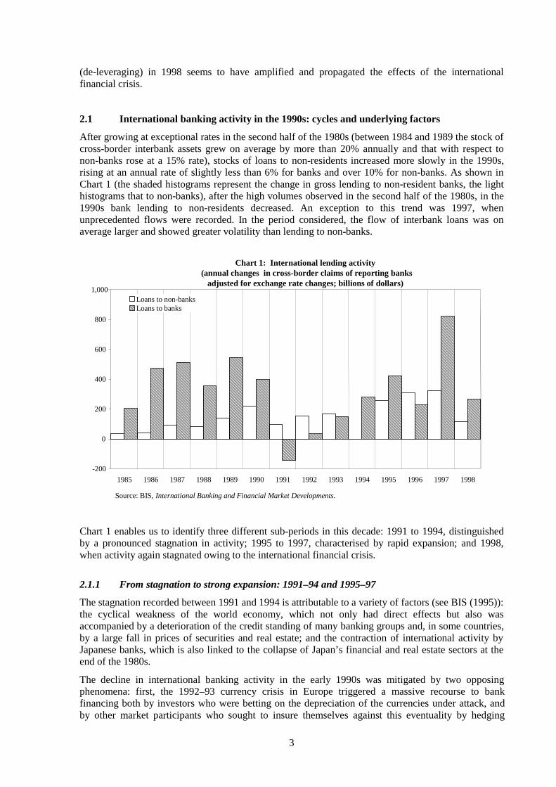
After growing at exceptional rates in the second half of the 1980s (between 1984 and 1989 the stock ofcross-border interbank assets grew on average by more than 20% annually and that with respect tonon-banks rose at a 15% rate), stocks of loans to non-residents increased more slowly in the 1990s,rising at an annual rate of slightly less than 6% for banks and over 10% for non-banks. As shown inChart 1 (the shaded histograms represent the change in gross lending to non-resident banks, the lighthistograms that to non-banks), after the high volumes observed in the second half of the 1980s, in the1990s bank lending to non-residents decreased. An exception to this trend was 1997, whenunprecedented flows were recorded. In the period considered, the flow of interbank loans was onaverage larger and showed greater volatility than lending to non-banks.
Chart 1 enables us to identify three different sub-periods in this decade: 1991 to 1994, distinguishedby a pronounced stagnation in activity; 1995 to 1997, characterised by rapid expansion; and 1998,when activity again stagnated owing to the international financial crisis.
2.1.1 From stagnation to strong expansion: 1991–94 and 1995–97
The stagnation recorded between 1991 and 1994 is attributable to a variety of factors (see BIS (1995)):the cyclical weakness of the world economy, which not only had direct effects but also wasaccompanied by a deterioration of the credit standing of many banking groups and, in some countries,by a large fall in prices of securities and real estate; and the contraction of international activity byJapanese banks, which is also linked to the collapse of Japan’s financial and real estate sectors at theend of the 1980s.
The decline in international banking activity in the early 1990s was mitigated by two opposingphenomena: first, the 1992–93 currency crisis in Europe triggered a massive recourse to bankfinancing both by investors who were betting on the depreciation of the currencies under attack, andby other market participants who sought to insure themselves against this eventuality by hedging
Chart 1: International lending activity (annual changes in cross-border claims of reporting banks
adjusted for exchange rate changes; billions of dollars)
-200
0
200
400
600
800
1,000
1985 1986 1987 1988 1989 1990 1991 1992 1993 1994 1995 1996 1997 1998
Loans to non-banksLoans to banks
Source: BIS, International Banking and Financial Market Developments.
4
against exchange rate risk; second, increased demand for bank funds was also created by the rise ininternational repurchase transactions, linked to the growth in global demand for government bonds.
By contrast, between 1995 and 1997 international banking activity expanded rapidly. It was driven byJapan’s robust monetary expansion, aimed at countering the slowdown in its economy and thedifficulties in its banking system, and more generally by favourable international economic conditions(see Giannini and Monticelli (1997); Tristani (1998)). As shown in Chart 1, banking activity wasespecially strong in 1997, with unprecedented growth in interbank lending (more than $800 billion)and lending to non-banks (over $300 billion). This enormous increase (some $400 billion was lent inthe fourth quarter alone) was the product of two factors in particular: (i) loans granted by the parentcompanies of Japanese banks to their foreign branch offices (over $80 billion in the fourth quarter),made necessary owing to the funding difficulties of the latter (induced by the deterioration in theircreditworthiness) and aided by the abundance of liquidity in Japan; (ii) the explosion of the Asiancrisis, which generated large transfers of interbank funds between geographical areas to accommodatechanges in portfolio composition and triggered a “flight to quality” that translated into a greaterpreference for liquidity.
An important phenomenon that characterised international banking activity in the period between 1995and 1997, and which was prolonged and accentuated with the crisis of 1998, is the trend of banks inthe industrial countries to employ a growing share of their external assets in the form of securitiesrather than traditional loans to customers: as can be seen in Table 1, between the end of 1995 (whenthe BIS began collecting data) and mid-1998, securities increased from 28% to 35% of the total stockof assets, and from 46% to almost 70% of flows.3
Table 1Securitisation of external assets of reporting banks (vis-à-vis non-bank sector)
(percentage share of securities in total assets)
Stocks Flows
1995 27.8
1996 29.9 46.4
1997 32.5 46.1
1998* 34.7 68.1
* At end-June.
Source: BIS, International Banking Statistics.
2.1.2 The 1998 financial crisis
Beginning in the summer of 1997, the international financial markets were hit by successive waves ofturbulence. In August 1998, what had appeared to be a regional crisis worsened and spread, becominga global crisis that hit economies – principally exporters of raw materials – with characteristics andproblems that were very different from those of the Asian countries. The Russian crisis, with the debtmoratorium, had a sharp impact on other emerging economies through contagion effects, linked tofears of additional moratoriums on foreign debt servicing.
The sudden and violent fluctuations in the prices of financial assets (exchange rates, bond and shareprices in emerging economies and industrial countries) recorded in the period signalled massivemovements of international bank and non-bank capital that had few precedents in terms of thevolumes traded, the range of financial instruments used and the countries involved. 3
This trend has already been observed for a considerable period of time in domestic banking in many industrial nations,but it is a relatively recent phenomenon in international banking and it could have negative side effects, such as: (i) anincrease in the instability of financial markets, since the stabilising role played by banks, whose “customer relations”make them less inclined to follow behaviour dictated by panic, will have diminished importance; (ii) a reduction in theeffectiveness of monetary policy, owing to the weakening of the traditional channels through which it operates.
5
During the first phase of the crisis, capital flowed out of the crisis-stricken Asian economies towardsthe industrial countries (the three largest benefited in virtually equal measure), but also towards LatinAmerica and eastern Europe. One indication of this was the sharp rise in stock and bond prices in theOECD countries, in the presence of broadly stable exchange rates.
With the intensification and the spread of the crisis in August 1998, financial asset prices reflected ageneralised outflow of capital from the emerging economies, this time including Latin America andeastern Europe, as well as the industrial countries that export raw materials (Norway, Australia, etc.),towards the industrial countries, with borrowers with the highest credit standing benefiting most (flightto quality). In this second phase of the crisis, the relative stability of exchange rates among the threelarge industrialised areas (the slight depreciation of the dollar mainly reflected changing expectationsfor US monetary policy) suggest that the capital flows were divided fairly equally between them.
It is widely believed that the closing-out of international arbitrage positions that were taken in thepreceding three-year period played an important role in the 1998 financial crisis. After internationalinvestors (typically hedge funds, see Eichengreen and Mathieson (1998)) made large profits by raisingfunds in yen and reinvesting in emerging markets between 1995 and 1997, the sudden unwinding ofthese positions in 1998 appeared to have contributed to the amplification and propagation of the crisis(see BIS (1999); IMF (1998)). There is ample empirical evidence on this phenomenon, althoughprecise estimates of the volumes of funds involved are not available. This is partly because investorscould borrow yen not only on the spot market (e.g. on the interbank market, for which data areavailable; see next section), but also with forward instruments and derivatives (for example, forwardexchange rates, futures, swaps and options), for which equally complete data sets are not available (seeGarber (1998)).
Below, this hypothesis will be tested utilising data on bank capital flows, paying particular attention tothe role of Japanese and offshore centre banks (which are respectively the principal “creators” and“reallocators” of international liquidity) and to non-bank agents located in offshore centres, whichpresumably include some hedge funds and other non-bank financial intermediaries.
2.2 Bank capital flows between large areas
BIS statistics on international banking activity make it possible to track the movements of bank capitalbetween the main geographical areas in recent years. It is important to note that the data on bank assetsand liabilities are available with greater detail only for the 24 reporting countries. For the rest of theworld, especially the emerging economies, information is only available to the extent that thesecountries have relations with banks in the reporting countries; hence data on bank relations betweenemerging economies are not included (for example, there are no data on the large movements of bankcapital which reportedly took place between banks in Korea and Thailand at the beginning of theAsian crisis).
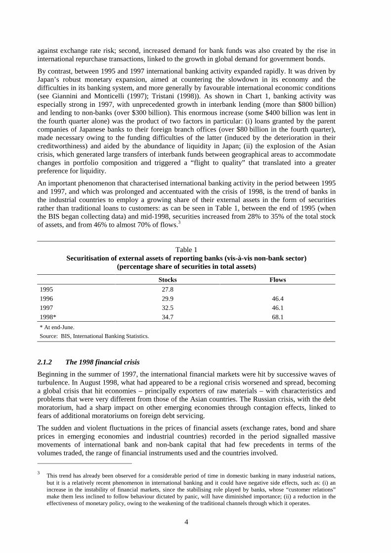
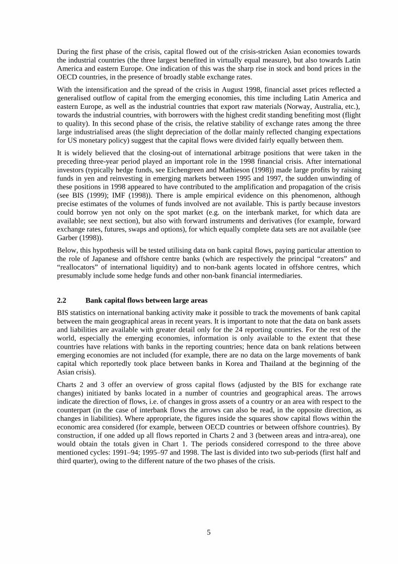
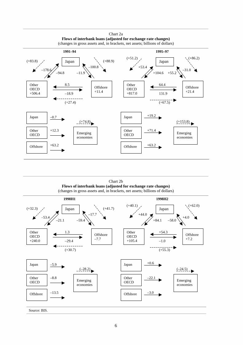
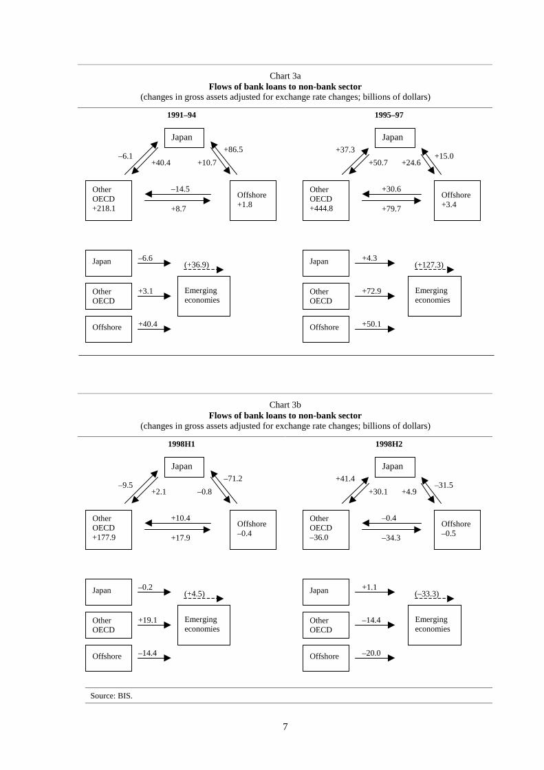
Charts 2 and 3 offer an overview of gross capital flows (adjusted by the BIS for exchange ratechanges) initiated by banks located in a number of countries and geographical areas. The arrowsindicate the direction of flows, i.e. of changes in gross assets of a country or an area with respect to thecounterpart (in the case of interbank flows the arrows can also be read, in the opposite direction, aschanges in liabilities). Where appropriate, the figures inside the squares show capital flows within theeconomic area considered (for example, between OECD countries or between offshore countries). Byconstruction, if one added up all flows reported in Charts 2 and 3 (between areas and intra-area), onewould obtain the totals given in Chart 1. The periods considered correspond to the three abovementioned cycles: 1991–94; 1995–97 and 1998. The last is divided into two sub-periods (first half andthird quarter), owing to the different nature of the two phases of the crisis.
6
(+83.8)
–178.6–94.8 –11.9
–100.8
(+88.9)
8.5
–18.9
(+27.4)
(+51.2)
+53.4
+104.6 +55.2–31.0
(+86.2)
64.4
131.9
(+67.5)
–0.7
+12.3
+63.2
(+74.8)
+19.2
+71.4
+63.2
(+153.8)
Source: BIS.
(+32.3)
–53.4–21.1 –59.4
–17.7
(+41.7)
1.3
–29.4
(+30.7)
(+40.1)
+44.0
+84.1 –58.0+4.0
(+62.0)
+54.3
–1.0
(+55.3)
–5.9
–8.8
–13.5
(–28.2)
+0.6
–22.1
–3.0
(–24.5)
Chart 2aFlows of interbank loans (adjusted for exchange rate changes)
(changes in gross assets and, in brackets, net assets; billions of dollars)
1991–94 1995–97
Chart 2bFlows of interbank loans (adjusted for exchange rate changes)
(changes in gross assets and, in brackets, net assets; billions of dollars)
1998H1 1998H2
Japan Japan
OtherOECD+506.4
Offshore+11.4
OtherOECD+817.0
Offshore+21.4
Japan Japan
OtherOECD
OtherOECD
Offshore Offshore
Emergingeconomies
Emergingeconomies
Japan Japan
OtherOECD+240.0
Offshore–7.7
OtherOECD+105.4
Offshore+7.2
Japan Japan
OtherOECD
OtherOECD
Offshore Offshore
Emergingeconomies
Emergingeconomies
7
–6.1+40.4 +10.7
+86.5
–14.5
+8.7
+37.3
+50.7 +24.6+15.0
+30.6
+79.7
–6.6
+3.1
+40.4
(+36.9)+4.3
+72.9
+50.1
(+127.3)
–9.5+2.1 –0.8
–71.2
+10.4
+17.9
+41.4
+30.1 +4.9–31.5
–0.4
–34.3
–0.2
+19.1
–14.4
(+4.5)+1.1
–14.4
–20.0
(–33.3)
Source: BIS.
Chart 3aFlows of bank loans to non-bank sector
(changes in gross assets adjusted for exchange rate changes; billions of dollars)
1991–94 1995–97
Chart 3bFlows of bank loans to non-bank sector
(changes in gross assets adjusted for exchange rate changes; billions of dollars)
1998H1 1998H2
Japan Japan
OtherOECD+218.1
Offshore+1.8
OtherOECD+444.8
Offshore+3.4
Japan Japan
OtherOECD
OtherOECD
Offshore Offshore
Emergingeconomies
Emergingeconomies
Japan Japan
OtherOECD+177.9
Offshore–0.4
OtherOECD–36.0
Offshore–0.5
Japan Japan
OtherOECD
OtherOECD
Offshore Offshore
Emergingeconomies
Emergingeconomies
8
The top part of the charts refers to the reporting area only, indicating movements between reportingcountries or areas (whose amount is given by the figures next to the arrows) and within reporting areas(figures inside the squares):
• Japan;
• other reporting industrial countries (henceforth “other OECD”): the United States, Canada, EUmembers (excluding Portugal and Greece), Switzerland and Norway;
• offshore centres: Hong Kong, Singapore, the Cayman Islands, the Bahamas and other minorcentres.
The lower part of the charts describes the relations between the reporting area and a group of non-reporting countries labelled as “emerging economies”: these include all Asia (excluding Japan, HongKong and Singapore), Latin America and central and eastern Europe.
2.2.1 Interbank capital movements
With reference to interbank flows (see Charts 2a and 2b), in the years 1991 to 1994 inside thereporting area there was a generalised withdrawal of funds between the three areas considered (closeto $400 billion), in part owing to the retrenchment of cross-border activity by the banks operating inJapan. The latter reduced their gross lending to the rest of the OECD area by nearly $100 billion andtheir gross borrowing by around $180 billion, and reduced their liabilities to offshore centres by morethan $100 billion. Reflecting the excess of saving over domestic investment, in the same period netcapital outflows from Japan amounted to around $170 billion (i.e. resident banks’ net external creditorposition increased by this amount). As to capital movements with countries outside the reporting area,i.e. with banks in the emerging economies, there was a substantial flow of funds towards the latter($75 billion) effected almost entirely by the offshore centres. At the global level, during the period inquestion banks in the offshore centres acted as international “reallocators” of funds; they were netborrowers from Japan in the order of $90 billion and net lenders of a virtually identical amount to theOECD area ($27 billion) and the emerging economies ($63 billion).
In the three years 1995–97, characterised by strong growth in international banking activity, inside thereporting area more than $400 billion of gross loans were granted across the three blocs. Japanesebanks granted new gross loans in large amounts to the rest of the OECD area ($105 billion) and tooffshore centres ($55 billion);4 the net capital outflow from Japan was also large ($137 billion),although slightly lower than that recorded in the previous period. Within the reporting area areallocative function was performed by the banks of the OECD area, which effected net funding inJapan ($50 billion) and net lending to the offshore centres ($65 billion). This development, in somerespects surprising, seems to imply an assumption of risk by OECD area banks resulting from amaturity and/or currency transformation in intermediation between the other two areas.5
As to business with countries outside the reporting area, in 1995–97 the reporting countries (mainlythe OECD countries and the offshore centres, in nearly equal measure) transferred some $150 billionto banks in emerging economies. Combining the information on cross-border activity inside andoutside the area, at the global level it was again the banks in offshore centres that reallocated interbankfunds with net fund-raising of around $150 billion from “other OECD” countries and Japan, and netlending of $63 billion to the emerging economies. It is worth noting that in terms of net flows, at aglobal interbank level, offshore centres were net borrowers for almost $90 billion: as will be seenbelow, part of this net funding was probably used to finance non-bank customers.
4
It should be borne in mind that these figures refer to the residence of the intermediaries, regardless of the nationality ofthe parent bank. As is detailed below, some of the interbank movements from Japan to offshore centres were actuallytransactions between parent banks and branches operating abroad.
5The BIS statistics are consistent with the hypothesis that in 1995–97 the banks of “other OECD” countries performedcurrency transformation: around 70% of the funds they raised from banks in Japan were in yen, while around 60% of theloans they granted to banks in offshore centres were in their own national currencies.

9
In 1998 the outbreak of the Asian crisis and, from August, its spread to other emerging economiescaused a virtually across-the-board cutback in cross-border interbank gross lending in the first half ofthe year, which was followed by a rebound of gross lending in the second half. In terms of net flows,inside the reporting area both halves of the year witnessed large net outflows of capital from offshorebanks to the other two areas (totalling roughly $190 billion); the repatriation of offshore capital toJapan (more than $100 billion net in 1998) is consistent with the hypothesis of de-leveraging. Outsidethe reporting area, Japan’s banks reduced their lending to banks in the emerging economies by morethan $50 billion.
2.2.2 Capital flows to non-bank customers
BIS statistics also allow tracking of cross-border bank capital movements in respect of non-bankcounterparts (see Charts 3a and 3b), even though the definition of the non-bank sector is not uniformacross countries and in some cases may include financial intermediaries such as hedge funds.
Inside the reporting area, in the four years 1991–94 the contraction in interbank activity was notaccompanied by one in business with non-bank customers, which is traditionally more stable. Capitalflows to the non-bank sector were positive in sign, albeit for relatively small amounts (more than$150 billion of gross loans were granted); exceptions were the large loans from offshore banks toJapanese non-banks, totalling $87 billion, and from Japanese banks to North American and Europeancompanies, amounting to $40 billion. Outside the area, there were substantial flows of nearly$40 billion from reporting area banks to non-banks in the emerging economies, perhaps compensatingfor the lower level of demand from the industrial countries during a period of cyclical weakness.Globally, in the same four years offshore banks were the largest lenders to the non-bank sector (for atotal, net of redemptions, of more than $110 billion); since offshore banks’ net interbank fund-raisingwas virtually nil (see the previous section), their net creditor position increased significantly.
In the period between 1995 and 1997 there was a generalised increase in international lending to non-banks. Inside the reporting area capital flowed across the three areas concerned; the largest flows werethose from Japanese banks to non-bank borrowers in “other OECD” ($51 billion) and from banks in“other OECD” to non-banks in offshore centres ($80 billion). Together with the inflow of capital frombanks in Japan ($25 billion), the latter brought the total inflow to the non-bank sector of the offshorecentres to more than $100 billion; considering the relatively modest GDP of those countries, it iscommon opinion (see BIS (1999)) that part of this borrowing was carried out by hedge funds locatedin those countries, where they are registered as non-banks. Outside the circuit of reporting countries,there were movements of nearly $130 billion from reporting banks to firms in the emergingeconomies; adding up these to the above mentioned interbank flows, total capital flows to theemerging economies amounted to around $280 billion.6 It is also worth emphasising that, globally,lending by offshore banks to foreign non-banks totalled around $95 billion, which is roughly the netborrowing by offshore centre banks in the interbank market (see above).
With the outbreak of the international financial crisis, in 1998 there was a slowdown in the flow ofbank credit to foreign firms, but not a generalised contraction in lending. In the first half of the yearthere were positive flows both within the reporting area (e.g. between “other OECD” and offshorecentres) and in activity external to it (“other OECD” provided nearly $20 billion to the emergingeconomies, diverting funds from Asia to Latin America). In the second half of 1998, with the spread ofthe crisis, there were further positive flows of credit within the reporting area, while loans to theemerging economies from all three reporting area blocs contracted by around $33 billion. It is worthnoting that in 1998 banks in the offshore centres drastically curtailed their lending to non-banks inJapan by around $100 billion and in the emerging economies by around $34 billion.
6
In order to measure the total inflow of resources to emerging economies, in addition to banks one would need to considercapital transferred by private investors, e.g. purchases of bonds and shares, and by public organisations.

10
2.2.3 Capital flows between parent banks and foreign branches(international banking statistics by “nationality”): the case of Japanese banks
The data on international banking activity used above are based on the concept of residence ofintermediaries. The BIS also collects and elaborates statistics based on banks’ nationality, byconsolidating data collected in all reporting countries, and provides a breakdown by counterpart (withthree categories: branches of the same group, other banks and non-banks) and by currency ofdenomination.
Chart 4External assets of reporting banks (with all sectors) by residence
(percentage share of total)
0
5
10
15
20
1992 1993 1994 1995 1996 1997 1998
JAP
GER
FRA
UK
USA
ITA
Source: BIS, International Banking Statistics. End-period data (1998: June).
Chart 5External assets of reporting banks (with all sectors) by nationality
(percentage share of total)
0
10
20
30
1992 1993 1994 1995 1996 1997 1998
USA
JAP
GER
FRA
ITA
UK
Source: BIS, International Banking Statistics. End-period data (1998: June).
11
The statistics based on nationality provide important additional information with respect to thosebased on residence particularly for countries where there is a large presence of foreign intermediaries(e.g. the United Kingdom) or, conversely, whose banks have a large presence abroad (e.g. Japan). Inthe latter case, the quantification of intragroup funds transfers yields indications about the strategypursued by a given banking system. This section takes a closer look at the behaviour of the Japanesebanking system in the past few years, first considering Japanese banks’ market shares and thenexamining their intragroup capital flows in the world.
Charts 4 and 5 show the gross external assets of the banks of each of the six leading industrialcountries as a percentage of the total for all reporting countries (the sum of the six shares is thereforeless than 100). While the market share of banks resident in Japan decreased from 14% to 12% between1992 and 1998, mainly to the benefit of the United Kingdom and Germany, the market share of banksof Japanese nationality (i.e. including branches abroad) fell much more markedly, from 28% to around18%, primarily to the benefit of German banks, whose market share grew from 11% to 18% and isnow nearly equal to that of Japanese institutions. This redistribution of market shares, which gainedpace in 1997 and 1998, is attributable to the crisis that has been plaguing the oversized andundercapitalised Japanese banking system since the start of the 1990s and to the policies of expansionand globalisation pursued in recent years by European and, above all, German banks (see BIS (1998)).
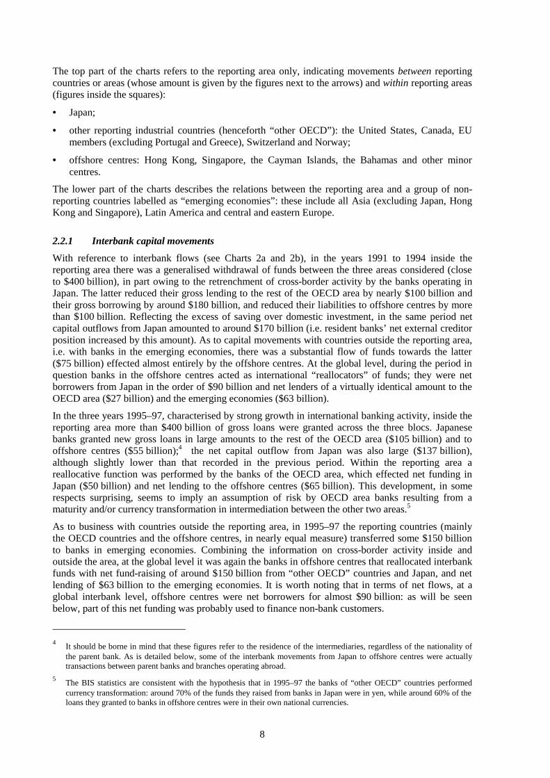
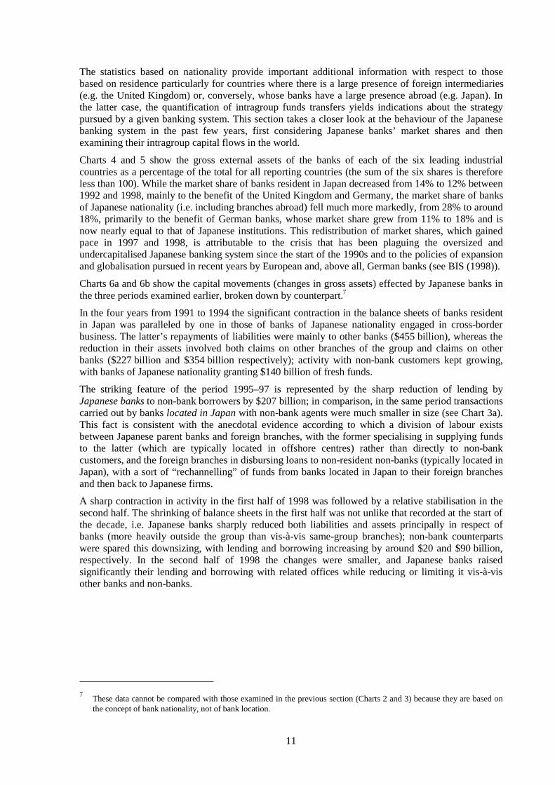
Charts 6a and 6b show the capital movements (changes in gross assets) effected by Japanese banks inthe three periods examined earlier, broken down by counterpart.7
In the four years from 1991 to 1994 the significant contraction in the balance sheets of banks residentin Japan was paralleled by one in those of banks of Japanese nationality engaged in cross-borderbusiness. The latter’s repayments of liabilities were mainly to other banks ($455 billion), whereas thereduction in their assets involved both claims on other branches of the group and claims on otherbanks ($227 billion and $354 billion respectively); activity with non-bank customers kept growing,with banks of Japanese nationality granting $140 billion of fresh funds.
The striking feature of the period 1995–97 is represented by the sharp reduction of lending byJapanese banks to non-bank borrowers by $207 billion; in comparison, in the same period transactionscarried out by banks located in Japan with non-bank agents were much smaller in size (see Chart 3a).This fact is consistent with the anecdotal evidence according to which a division of labour existsbetween Japanese parent banks and foreign branches, with the former specialising in supplying fundsto the latter (which are typically located in offshore centres) rather than directly to non-bankcustomers, and the foreign branches in disbursing loans to non-resident non-banks (typically located inJapan), with a sort of “rechannelling” of funds from banks located in Japan to their foreign branchesand then back to Japanese firms.
A sharp contraction in activity in the first half of 1998 was followed by a relative stabilisation in thesecond half. The shrinking of balance sheets in the first half was not unlike that recorded at the start ofthe decade, i.e. Japanese banks sharply reduced both liabilities and assets principally in respect ofbanks (more heavily outside the group than vis-à-vis same-group branches); non-bank counterpartswere spared this downsizing, with lending and borrowing increasing by around $20 and $90 billion,respectively. In the second half of 1998 the changes were smaller, and Japanese banks raisedsignificantly their lending and borrowing with related offices while reducing or limiting it vis-à-visother banks and non-banks.
7
These data cannot be compared with those examined in the previous section (Charts 2 and 3) because they are based onthe concept of bank nationality, not of bank location.
12
–227.1 –353.6 139.7 176.1 –35.2 –206.6
Assets
–234.3 –455.1 225.0 –30.6 –314.2 39.8
Source: BIS.
–122.4 –200.5 21.1 57.3 –27.4 –56.5
Assets
–91.8 –237.2 91.7 44.5 –75.8 12.0
Chart 6aLending by Japanese banks to non-residents
(exchange rate adjusted changes in gross stocks; billions of dollars)
1991–94 1995–97
Chart 6bLending by Japanese banks to non-residents
(exchange rate adjusted changes in gross stocks; billions of dollars)
1998H1 1998H2
Japanesebanks
Japanesebanks
Ownbranches Non-banks
Ownbranches Non-banks
Otherbanks
Otherbanks
LiabilitiesJapanesebanks
Japanesebanks
Ownbranches
Otherbanks Non-banks
Ownbranches
Otherbanks Non-banks
Japanesebanks
Japanesebanks
Ownbranches Non-banks
Ownbranches Non-banks
Otherbanks
Otherbanks
LiabilitiesJapanesebanks
Japanesebanks
Ownbranches
Otherbanks Non-banks
Ownbranches
Otherbanks Non-banks

13
3. The determinants of international liquidity
3.1 Introduction
The literature analysing the development of international liquidity is extremely limited, particularlywith regard to analysis of the geographical breakdown of cross-border flows. The most interestingcontribution is that of Alworth and Andresen (1992), who examine the dynamics of cross-borderdeposits in the 1980s in connection with competition between financial centres. A first part of thatstudy focuses on the development over time of cross-border deposits, classified according to thetraditional criteria of residence of the bank and residence of the deposit holder. The data used in thatwork are supplemented in the present study with more recent statistics and shown in Tables 2 and 3.Table 2 shows the share held by each country’s banking system in “hosting” cross-border deposits. Asin the preceding years, the United Kingdom is the leading financial centre, with cross-border depositsat the end of September 1998 totalling around $2,500 billion, equal to 21% of the total stock ofdeposits held with banks located in the reporting area. Shares approaching that of the United Kingdomwere held by the reporting offshore centres considered together (the Bahamas, Bahrain, the CaymanIslands, Hong Kong, the Netherlands Antilles and Singapore). Over the 15 years considered, the shareof deposits held with banks located in Germany rose from 2.7% to 9.7% and that held with banksresident in France from 5.7% to 7.1%, while that with banks in the United States diminished slightlyfrom 12.9% to 10.8%. The end-of-period share held with banks located in Japan fell sharply from12.5% to 6.0% from the peak recorded at the end of the 1980s.
Table 2Cross-border deposits held with banks of individual reporting countries
as a share of area’s total (billions of dollars and percentages)
End-December 1983 End-December 1990 End-December 1996 End-September 1998
Total
(1)
Non-banks
%share(1)/(2)
Total
(3)
Non-banks
%share(3)/(4)
Total
(5)
Non-banks
%share(5)/(6)
Total
(7)
Non-banks
%share(7)/(8)
AT 25.9 1.4 1.2 67.3 12.4 1.0 89.7 11.1 1.1 104.4 10.9 1.1
BE 72.6 8.5 3.4 217.3 36.4 3.4 266.4 70.9 3.3 278.6 82.3 2.9
LX 79.1 12.0 3.7 271.2 107.7 4.2 383.6 163.1 4.7 387.5 150.2 4.1
DK 5.1 0.4 0.2 43.8 2.5 0.6 38.8 7.7 0.5 278.6 9.9 3.0
SF 7.1 0.3 0.3 42.8 2.8 0.6 16.2 0.7 0.2 14.7 0.7 0.2
FR 138.7 15.1 6.5 482.1 46.9 7.5 617.0 56.3 7.6 712.0 61.7 7.6
DE 57.4 14.0 2.7 224.8 52.8 3.5 570.6 170.8 7.0 836.6 219.6 8.9
IE 5.0 2.5 0.2 17.8 5.6 0.3 64.2 18.3 0.8 128.3 38.8 1.4
IT 45.6 1.9 2.1 142.9 11.4 2.2 247.7 15.8 3.1 265.8 39.2 2.8
NL 55.5 12.1 2.6 148.0 42.7 2.3 217.9 55.5 2.7 331.6 60.8 3.5
NO 6.2 2.5 0.3 20.8 1.8 0.3 17.9 2.3 0.2 26.2 2.6 0.3
ES 18.5 8.4 0.9 64.0 26.7 1.0 128.0 43.4 1.6 189.2 52.1 2.0
SE 14.0 1.3 0.6 90.6 12.1 1.4 56.7 7.8 0.7 86.4 15.2 0.9
CH 117.5 90.0 5.5 312.7 217.0 4.9 404.0 242.6 4.9 509.2 261.3 5.4
UK 515.3 150.5 24.2 1,201.3 327.4 18.7 1,555.8 369.4 19.2 1,984.5 500.6 21.1
CA 62.2 25.1 2.9 81.0 35.9 1.3 98.8 36.7 1.2 120.0 36.5 1.3
JP 106.6 2.3 5.0 958.5 13.3 14.9 695.8 17.6 8.6 629.9 29.0 6.7
US 294.6 53.5 13.9 653.7 80.7 10.2 870.9 102.2 10.8 1,036.9 137.8 11.0
Off-shore
494.1 161.1 23.3 1,368.5 333.8 21.3 1,760.1 446.2 21.7 1,691.4 504.0 18.0
Total 2,121.0(2)
562.9 100.0 6,409.1(4)
1,369.9 100.0 8,100.1(6)
1,838.3 100.0 9,390.6(8)
1,506.0 100.0

14
Table 3Area of origin of deposits held by non-banks with banks located in reporting area
(billions of dollars; figures for banks plus non-banks in brackets)
Area of origin ofdeposit
End-December1983
End-December1990
End-December1996
End-September1998
Reporting area 371.3 1,247.8 1,377.9(6,296.7)
1,664.9(7,266.9)
Non-reportingindustrial countries
12.8 49.0 64.7(187.7)
66.9(202.6)
Offshore centres – – 285.0(1,127.4)
378.0(1,319.7)
of which:
Cayman Islands – – 66.9(321.4)
127.8(405.9)
Singapore – – 13.6(177.8)
16.6(221.6)
Eastern Europe 0.6 1.9 8.7(48.8)
11.8(49.1)
Asia 17.4 44.1 81.4(257.2)
107.3(287.4)
Latin America 37.3 85.2 110.1(228.2)
118.8(238.3)
of which:
Argentina 6.1 17.0 16.4(26.6)
16.8(35.3)
Brazil 7.0 17.5 16.2(71.4)
17.7(59.5)
Mexico 11.5 19.5 21.1(37.8)
24.7(47.4)
Table 3 shows the geographical origin of cross-border deposits held by non-banks with banks locatedin the reporting area (i.e. based on the residence of the depositor). It can be seen that most of thedeposits originate from agents located within the reporting area: roughly three quarters of the total inthe case of both bank and non-bank depositors. The other main areas of origin of the funds are theoffshore centres among which the Cayman Islands accounts for around one third and Latin America.Reflecting this characteristic of the geographical distribution of cross-border deposits, in theeconometric section more attention is devoted to analysing total deposits, which are largely held in theindustrial countries, rather than to their distribution by geographical area (eastern Europe, offshorecentres, Latin America).
3.2 The results of Alworth and Andresen
Alworth and Andresen (1992) identify a number of determinants of the behaviour of cross-borderdeposits. The reasons for depositing funds abroad include financing trade flows, investing in foreignfinancial assets and diversifying the default risk of one’s domestic banking system. Obviously, theamount of deposits held (like the size of trade flows between two countries) should be strictlydependent on the wealth of the two countries, as approximated by GDP. Alongside these main factors,the authors also consider other characteristics of the country where funds are deposited, such as thereserve requirement, the existence of regulatory constraints on interest rate movements, the efficiencyof the financial market and the financial and political riskiness of the country.
The econometric investigation conducted by the authors analyses a cross section of deposits classifiedaccording to the residence of the deposit holder. The dependent variable is the logarithm of deposits

15
(expressed in billions of dollars) held by non-bank residents in country i with banks located in countryj. The explanatory variables are:
• the output of the two countries (i, j), whose coefficients should be positive (GDP);
• the level of bilateral trade between the two countries (BITR), whose sign is expected to bepositive;
• the ratio of stock market capitalisation to output (CAP/GDP), whose sign is expected to bepositive;
• stock market turnover (TURN), whose sign is expected to be positive;
• the differential between the reserve ratio in the two countries (RR1–RR2), whose sign is expectedto be negative;
• the level of taxation (WT);
• the level of banking secrecy (BSECR);
• the rating of the financial centre in which the deposits are held (RAT);
• the degree of specialisation of the financial centres, i.e. the fact that some are mainly involved infund-raising, others in lending, as measured by the ratio between deposits held in the country bynon-banks and those held by banks (RATC).
The equations were estimated on the basis of end-year data for 1983, 1986 and 1990. A summary ofthe results is given in Table 4.
Table 4Summary of results
1983 1986 1990
Specialisation (RATC) –3.1057 –3.5429 –3.4216
Trade (BITR) 1.1278 1.2078 0.4438
GDP1 0.0024* 0.0047 0.0076
CAP/GDP2 0.0019* 0.0066 0.0072
RATING (RAT) 0.0048* 0.0023* 0.0050*
Reserves requirement, country 1(RR1)
0.0133* –0.0110* –0.0931
Reserves requirement, country 2(RR2)
–0.0916* –0.0545* –0.0907
Secrecy (BSECR) 0.4793 1.5869 0.9071
R2 0.4194 0.5075 0.5546
* Not significant at the 5% level.
The R-squared of the regressions, which range between 42% for 1983 and 55% for 1990, are fairlyhigh, especially considering the fact that the set of countries included in the study is heterogeneous(deposits held by non-bank residents of 17 countries with banks from 23 reporting countries). All ofthe main variables have the expected sign: domestic output is positively correlated with deposits, asare the ratio between market capitalisation in the bank’s country of residence and the GDP of thedeposit holder’s country of residence and the size of bilateral trade flows. The other variables alsohave the expected sign: the level of banking secrecy has a positive sign and the RATC variable (ratioof non-bank deposits to interbank deposits) is negative, and can be interpreted as a scale variable, suchthat financial centres where interbank loans predominate attract more deposits from non-bank non-residents.
16
3.3 New econometric evidence
The econometric analysis conducted in this paper differs from the Alworth-Andresen study in that itexamines a panel of data rather than a cross section. In addition, the range of cross-border depositsconsidered is broader in that it includes four categories of deposits: equations were estimated (over theperiod between the first quarter of 1985 and the second quarter of 1998) not only for cross-borderdeposits defined according to the residence of the holder (e.g. deposits held abroad by bank and non-bank residents of the United States) but also for deposits defined according to the location of the issueror “host” (e.g. deposits held with US-located banks by both banks and non-banks located abroad).
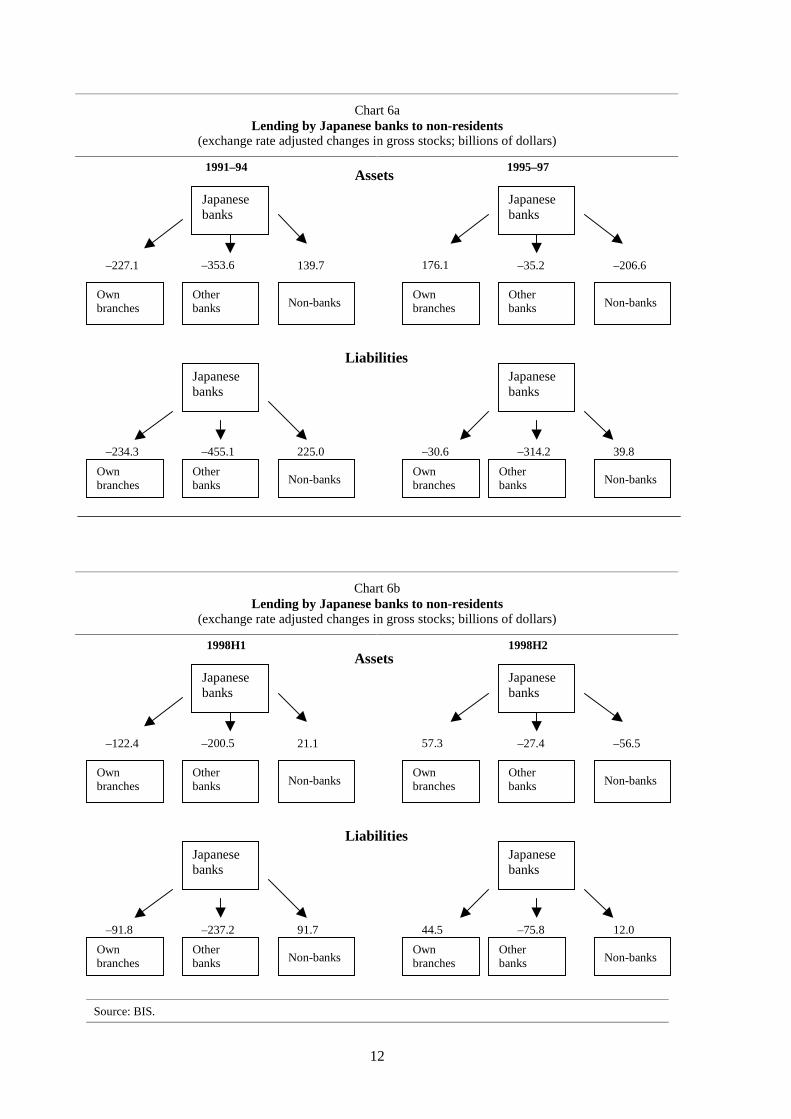
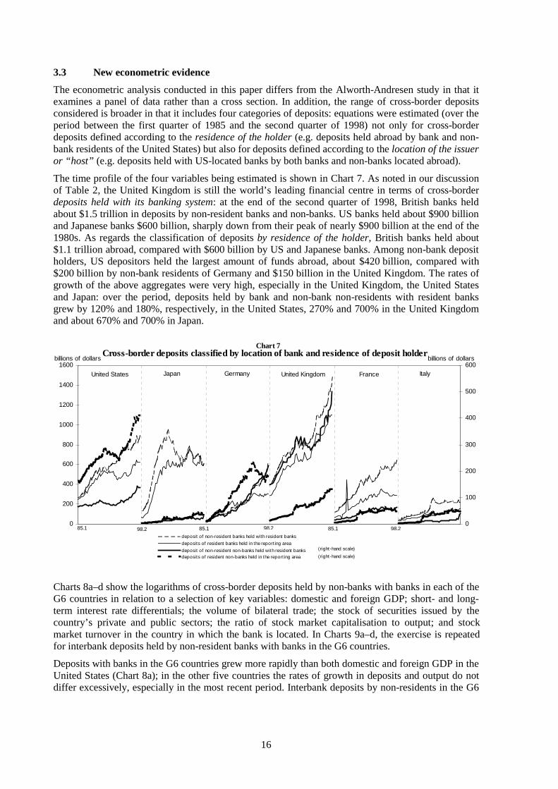
The time profile of the four variables being estimated is shown in Chart 7. As noted in our discussionof Table 2, the United Kingdom is still the world’s leading financial centre in terms of cross-borderdeposits held with its banking system: at the end of the second quarter of 1998, British banks heldabout $1.5 trillion in deposits by non-resident banks and non-banks. US banks held about $900 billionand Japanese banks $600 billion, sharply down from their peak of nearly $900 billion at the end of the1980s. As regards the classification of deposits by residence of the holder, British banks held about$1.1 trillion abroad, compared with $600 billion by US and Japanese banks. Among non-bank depositholders, US depositors held the largest amount of funds abroad, about $420 billion, compared with$200 billion by non-bank residents of Germany and $150 billion in the United Kingdom. The rates ofgrowth of the above aggregates were very high, especially in the United Kingdom, the United Statesand Japan: over the period, deposits held by bank and non-bank non-residents with resident banksgrew by 120% and 180%, respectively, in the United States, 270% and 700% in the United Kingdomand about 670% and 700% in Japan.
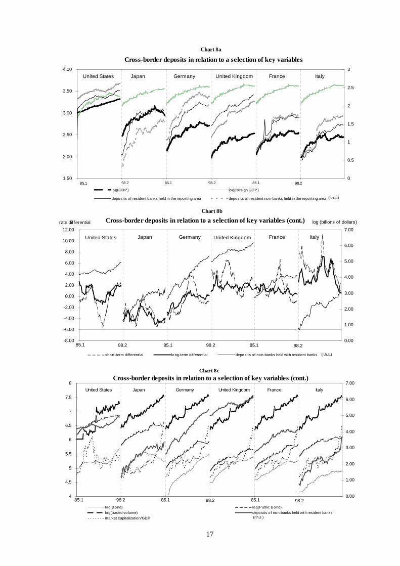
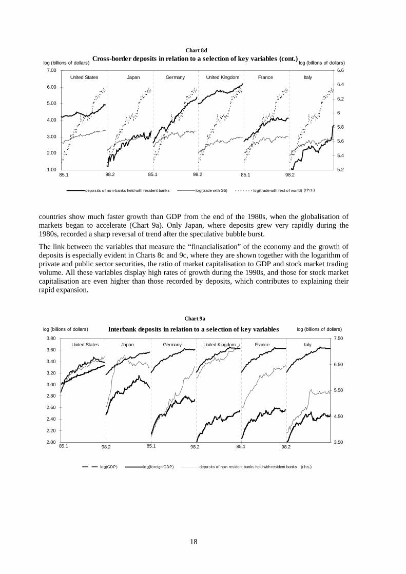
Charts 8a–d show the logarithms of cross-border deposits held by non-banks with banks in each of theG6 countries in relation to a selection of key variables: domestic and foreign GDP; short- and long-term interest rate differentials; the volume of bilateral trade; the stock of securities issued by thecountry’s private and public sectors; the ratio of stock market capitalisation to output; and stockmarket turnover in the country in which the bank is located. In Charts 9a–d, the exercise is repeatedfor interbank deposits held by non-resident banks with banks in the G6 countries.
Deposits with banks in the G6 countries grew more rapidly than both domestic and foreign GDP in theUnited States (Chart 8a); in the other five countries the rates of growth in deposits and output do notdiffer excessively, especially in the most recent period. Interbank deposits by non-residents in the G6
Cross-border deposits classified by location of bank and residence of deposit holder
0
200
400
600
800
1000
1200
1400
1600
0
100
200
300
400
500
600
deposit of non-res ident banks held with res ident banks
deposits of res ident banks held in the reporting area
deposit of non-res ident non-banks held with res ident banksdeposits of res ident non-banks held in the reporting area
United States Japan Germany United Kingdom France Italy
85.1 98.2 98.285.1 85.1 98.2
billions of dollars
(right-hand scale)
billions of dollars
Chart 7
(right-hand scale)
17
1.50
2.00
2.50
3.00
3.50
4.00
0
0.5
1
1.5
2
2.5
3
log(GDP ) log(foreign GDP )
depos its of res ident banks held in the reporting area depos its of res ident non-banks held in the reporting area
United States Japan Germany United Kingdom France Italy
85.1 98.2 85.1 98.2 85.1 98.2
Chart 8a
(r.h.s .)
Cross-border deposits in relation to a selection of key variables
-8.00
-6.00
-4.00
-2.00
0.00
2.00
4.00
6.00
8.00
10.00
12.00
0.00
1.00
2.00
3.00
4.00
5.00
6.00
7.00
s hort-term differential long-term differential depos its of non-banks held with res ident banks
United States Japan Germany United Kingdom France Italy
85.1 98.2 85.1 98.2 85.1 98.2
log (billions of dollars)rate differential
Chart 8b
Cross-border deposits in relation to a selection of key variables (cont.)
(r.h.s .)
4
4.5
5
5.5
6
6.5
7
7.5
8
0.00
1.00
2.00
3.00
4.00
5.00
6.00
7.00
log(B ond) log(P ublic B ond)log(traded volume) depos its of non-banks held with res ident banksmarket capitalization/GDP
United States Japan Germany United Kingdom France Italy
85.1 85.1 85.198.2 98.2 98.2
Chart 8c
(r.h.s .)
Cross-border deposits in relation to a selection of key variables (cont.)
18
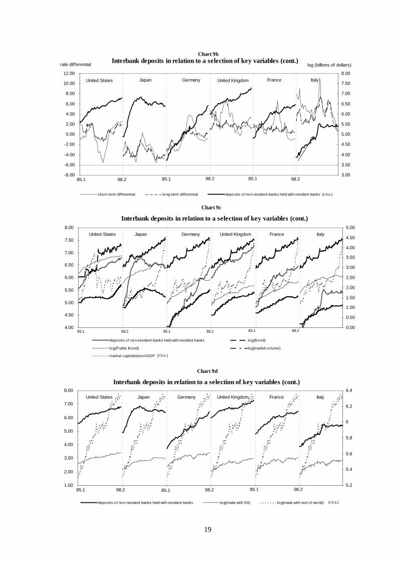
countries show much faster growth than GDP from the end of the 1980s, when the globalisation ofmarkets began to accelerate (Chart 9a). Only Japan, where deposits grew very rapidly during the1980s, recorded a sharp reversal of trend after the speculative bubble burst.
The link between the variables that measure the “financialisation” of the economy and the growth ofdeposits is especially evident in Charts 8c and 9c, where they are shown together with the logarithm ofprivate and public sector securities, the ratio of market capitalisation to GDP and stock market tradingvolume. All these variables display high rates of growth during the 1990s, and those for stock marketcapitalisation are even higher than those recorded by deposits, which contributes to explaining theirrapid expansion.
1.00
2.00
3.00
4.00
5.00
6.00
7.00
5.2
5.4
5.6
5.8
6
6.2
6.4
6.6
depos its of non-banks held with res ident banks log(trade with G5) log(trade with res t of world)
United States Japan Germany United Kingdom France Italy
85.1 85.1 85.198.2 98.2 98.2
log (billions of dollars)
Chart 8d
log (billions of dollars)
(r.h.s .)
Cross-border deposits in relation to a selection of key variables (cont.)
2.00
2.20
2.40
2.60
2.80
3.00
3.20
3.40
3.60
3.80
3.50
4.50
5.50
6.50
7.50
log(GDP ) log(foreign GDP ) depos its of non-res ident banks held with res ident banks
United States Japan Germany United Kingdom France Italy
85.1 98.2 85.1 98.2 85.1 98.2
log (billions of dollars) log (billions of dollars)
Chart 9a
Interbank deposits in relation to a selection of key variables
(r.h.s .)
19
-8.00
-6.00
-4.00
-2.00
0.00
2.00
4.00
6.00
8.00
10.00
12.00
3.00
3.50
4.00
4.50
5.00
5.50
6.00
6.50
7.00
7.50
8.00
s hort-term differential long-term differential depos its of non-res ident banks held with res ident banks
United States Japan Germany United Kingdom France Italy
85.1 98.2 85.1 98.2 85.1 98.2
log (billions of dollars)rate differential
Chart 9b
(r.h.s .)
Interbank deposits in relation to a selection of key variables (cont.)
4.00
4.50
5.00
5.50
6.00
6.50
7.00
7.50
8.00
0.00
0.50
1.00
1.50
2.00
2.50
3.00
3.50
4.00
4.50
5.00
depos its of non-res ident banks held with res ident banks log(B ond)
log(P ublic B ond) log(traded volume)
market capitalization/GDP
United States GermanyJapan United Kingdom France Italy
85.1 98.2 85.1 98.2 85.1 98.2
Chart 9c
Interbank deposits in relation to a selection of key variables (cont.)
(r.h.s .)
1.00
2.00
3.00
4.00
5.00
6.00
7.00
8.00
5.2
5.4
5.6
5.8
6
6.2
6.4
depos its of non-res ident banks held with res ident banks log(trade with G5) log(trade with res t of world)
85.1 98.2 85.1 85.198.2 98.2
United States Japan Germany United Kingdom France Italy
Chart 9d
Interbank deposits in relation to a selection of key variables (cont.)
(r.h.s .)
20
If the regressions should confirm that cross-border deposits are more closely linked to financialvariables than to macroeconomic determinants, we would be able to argue for a financial view of thegrowth of deposits. This position also finds support in a branch of the literature that in the last 10 yearshas focused on the so-called microstructure of financial markets and on the development of derivativesmarkets. The results obtained by this literature are based on direct observation of the foreign exchangemarket, the broadest and most active in the world. Trading volumes on this market are enormousbecause individual participants carry out repeated transactions to achieve a desired level of risk fortheir portfolio, selling foreign exchange forward for each asset position and buying foreign exchangeforward for each liability position. Such behaviour sharply amplifies the original transaction volume,consistently with so-called “hot potato” models of risk sharing. According to such models, banksexpand their original asset and liability positions with final investors on their balance sheets withpositions taken with other intermediaries to achieve the desired risk-return combination for theirportfolio.
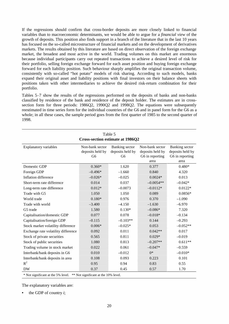
Tables 5–7 show the results of the regressions performed on the deposits of banks and non-banksclassified by residence of the bank and residence of the deposit holder. The estimates are in cross-section form for three periods: 1986Q2, 1990Q2 and 1998Q2. The equations were subsequentlyreestimated in time series form for the individual countries of the G6 and in panel form for the G6 as awhole; in all these cases, the sample period goes from the first quarter of 1985 to the second quarter of1998.
Table 5Cross-section estimate at 1986Q2
Explanatory variables Non-bank sectordeposits held by
G6
Banking sectordeposits held by
G6
Non-bank sectordeposits held byG6 in reporting
area
Banking sectordeposits held byG6 in reporting
area
Domestic GDP 0.360* 1.620 0.377 0.480*
Foreign GDP –0.496* –1.660 0.840 4.320
Inflation difference –0.026* –0.025 0.0024* 0.013
Short-term rate difference 0.014 0.037 –0.0054** –0.042*
Long-term rate difference 0.012* –0.0073 –0.0112* 0.0122*
Trade with G5 1.050 1.050 0.089 0.0856*
World trade 0.180* 0.976 0.370 –1.090
Trade with world –3.400 –4.150 –1.630 –6.970
G5 trade 1.580 0.130* –0.086* 7.320
Capitalisation/domestic GDP 0.077 0.078 –0.018* –0.134
Capitalisation/foreign GDP –0.115 –0.103** 0.144 –0.293
Stock market volatility difference 0.006* –0.025* 0.053 –0.052**
Exchange rate volatility difference 0.092 0.011 0.042** 0.017
Stock of private securities 0.565 0.811 0.029* –0.019
Stock of public securities 1.080 0.813 –0.207** 0.611**
Trading volume in stock market 0.022 0.061 –0.047* –0.559
Interbank/bank deposits in G6 0.010 –0.012 0* –0.010*
Interbank/bank deposits in area 0.108 0.093 0.223 0.101
R2 0.95 0.94 0.83 0.55
DW 0.37 0.45 0.57 1.70
* Not significant at the 5% level. ** Not significant at the 10% level.
The explanatory variables are:
• the GDP of country i;

21
• the GDP of the group of countries excluding i;
• the inflation differential between country i and the group of countries excluding i;
• the short-term interest rate differential between country i and the group of countries excluding i;
• the long-term interest rate differential between country i and the group of countries excluding i;
• the sum of exports and imports of country i with the group of countries excluding i;
• the sum of world exports and imports;
• the sum of exports and imports of the group of countries excluding i;
• the ratio of stock market capitalisation to the GDP of country i;
• the ratio of stock market capitalisation to the GDP of the group of countries excluding i;
• the differential between the volatility of the stock market of country i and that of the group ofcountries excluding i;
• the differential between the volatility of the nominal effective exchange rate of country i and thatof the nominal effective exchange rates of the group of countries excluding i;
• the stock of private sector securities in country i;
• the stock of public sector securities in country i;
• stock market trading volume in country i.
Table 6Cross-section estimate at 1990Q2
Explanatory variables Non-bank sectordeposits held by
G6
Banking sectordeposits held
by G6
Non-bank sectordeposits held byG6 in reporting
area
Banking sectordeposits held byG6 in reporting
area
Domestic GDP 1.210 0.415 –0.196* 0.044*
Foreign GDP –1.030 –0.383* 5.940 1.360
Inflation difference –0.021 –0.0011* 0.026 0.032*
Short-term rate difference 0.028 0.0083** –0.015 –0.036*
Long-term rate difference 0.010* 0.026 0.033* –0.016
Trade with G5 0.614 0.699 –0.870* 0.970
World trade 0.724 0.171* –1.400 0.130*
Trade with world –2.110** –2.090 –3.150* –1.940
G5 trade –0.614* 0.907* 5.850 0.350*
Capitalisation/domestic GDP 0.097 0.090 –0.137 –0.021*
Capitalisation/foreign GDP –0.075* –0.170 0.441 0.282
Stock market volatility difference –0.0049* 0.0230** –0.021* 0.047
Exchange rate volatility difference 0.0166 0.014 0.028 0.0035*
Stock of private securities 0.834 0.595 –0.058 0.029*
Stock of public securities 0.882 1.000 0.444 –0.100*
Trading volume in stock market –0.050* –0.017* –0.604 –0.086**
Interbank/bank deposits in G6 –0.011 0.011 0.0024* 0.00033*
Interbank/bank deposits in area 0.075 0.071 0.062* 0.238
R2 0.93 0.94 0.56 0.83
DW 0.39 0.31 1.71 0.57
* Not significant at the 5% level. ** Not significant at the 10% level.

22
Table 7Cross-section estimate at 1998Q2
Explanatory variables Non-bank sectordeposits held by
G6
Banking sectordeposits held by
G6
Non-bank sectordeposits held byG6 in reporting
area
Banking sectordeposits held byG6 in reporting
area
Domestic GDP 1.180 0.189* 1.400 –0.478
Foreign GDP –1.540 –0.505* 6.230 1.430
Inflation difference –0.032 –0.029 0.061 –0.011
Short-term rate difference 0.030 0.021 –0.018* 0.0072
Long-term rate difference –0.019 0.026 0.0002* –0.024
Trade with G5 0.379* 0.416* –2.210 0.919
World trade 0.949 0.529 –1.360 0.102*
Trade with world –0.866* –0.854* –1.080* –1.510
G5 trade –1.230* –0.198* 6.700 0.257*
Capitalisation/domestic GDP 0.145 0.099 –0.022* –0.026*
Capitalisation/foreign GDP 0.052* 0.245 –1.110 0.733
Stock market volatility difference 0* 0.026** 0.042** 0.038
Exchange rate volatility difference 0.013 0.015 0.0196 –0.0029*
Stock of private securities 1.190 0.824 –0.651 0.161
Stock of public securities 0.535 0.867 –0.184* –0.016*
Trading volume in stock market –0.271 –0.249 –0.277* –0.240
Interbank/bank deposits in G6 –0.012 0.012 0.0009* 0.0015
Interbank/bank deposits in area 0.061 0.056 0.102 0.234
R2 0.92 0.95 0.64 0.85
DW 0.40 0.42 1.68 0.65
* Not significant at the 5% level. ** Not significant at the 10% level.
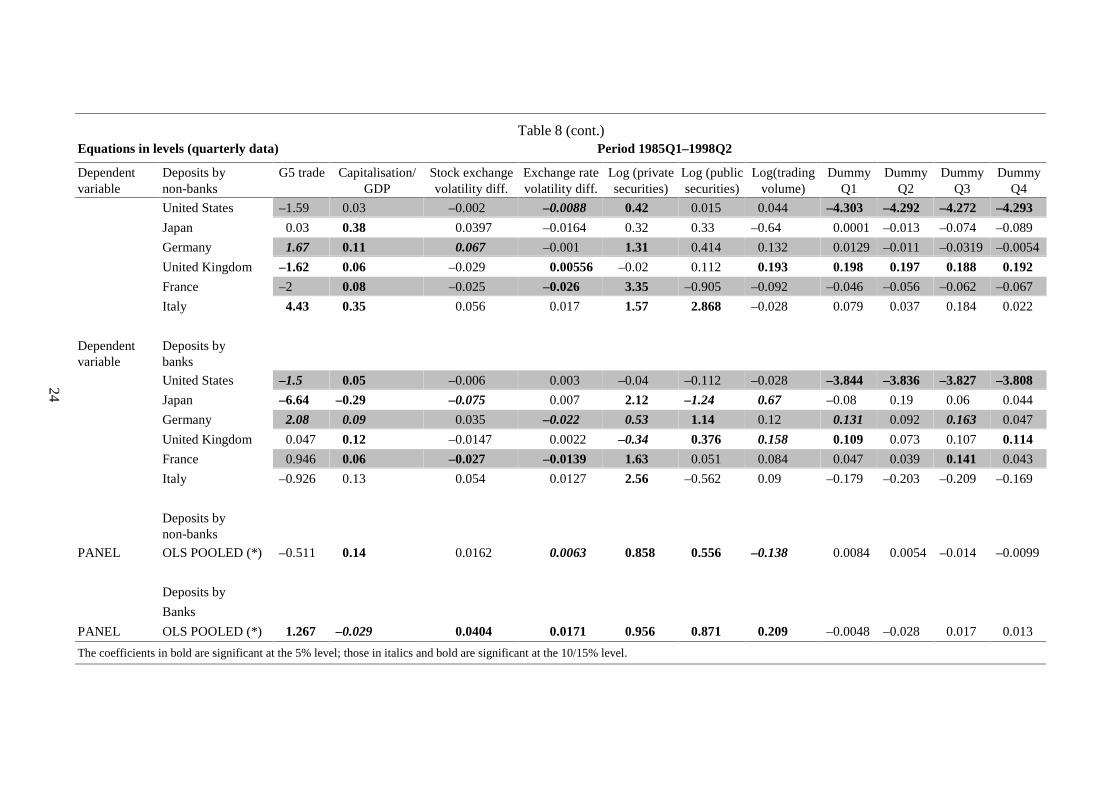
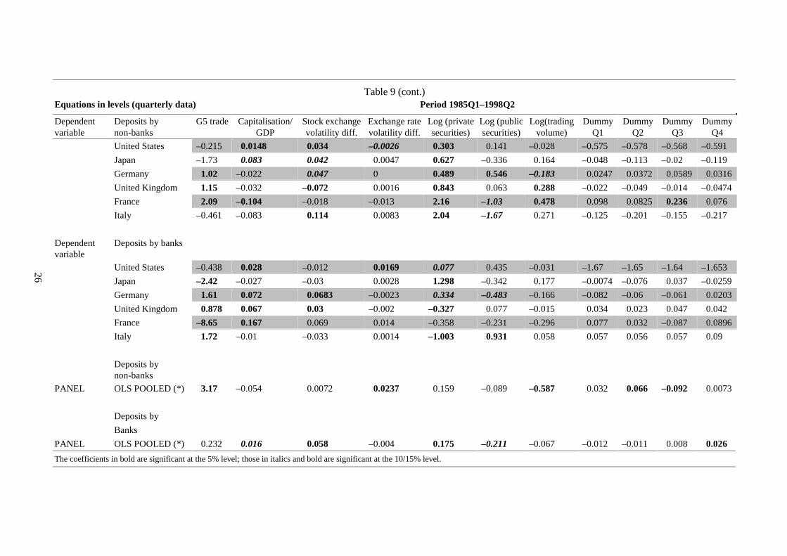
Tables 8 and 9 give the results of the regressions performed on the time series of cross-border depositsclassified by the residence of the bank and the residence of the deposit holder, respectively. The upperpart of each table reports the results of the time series estimates by country, whereas the lower partshows the results of the panel estimates.
As regards the estimates for the individual countries, cross-border deposits held by foreign non-bankswith resident banks in the country concerned (Table 8) are directly linked to the GDP of the country inwhich the bank is located in all cases except Italy; elasticities vary between 1.63 in France and 3.65 inthe United States, while the coefficient is not significant in Italy. Foreign GDP, which was expected tohave a positive sign, is negative in the United States, Germany and France and not significant in theother three. Short-term interest rate differentials were expected to be positive, as a higher short-termrate in country i than in country j should attract funds to country i. However, the hypothesis wasconfirmed only in the case of the United States and the United Kingdom, while the estimatedcoefficient is negative in Italy and zero in the remaining three cases.
By contrast, the coefficients of long-term rate differentials should be negative under the hypothesisthat they are a proxy for expected inflation rate differentials (i.e. for a given expected real rate in thetwo countries). The hypothesis is confirmed for the United States and France, while there is nosignificant relationship in Japan, Germany or Italy. The relation is significant but positive in theUnited Kingdom.
The current inflation differential is significant and negative, as expected, in two of the six cases(United States and France). In the other countries it is not significant.

23
Table 8Cross-border deposits held by non-residents with banks in the country concerned
Equations in levels (quarterly data) Period 1985Q1–1998Q2
Dependent Deposits by R2 Durbin Log Log Inflation Short-term rate Long-term rate Trade with G5 World trade Trade with
variable non-banks Watson (domestic GDP) (foreign GDP) diff. diff. diff. world
United States 0.961 1.72 3.65 –1.56 –0.026 0.0347 –0.0229 1.715 1.106 –2.24Japan 0.92 1.63 1.67 –1.74 0.023 0.0096 0.045 0.08 –1 4.46
Germany 0.993 1.38 3.01 –5.11 0.0168 –0.047 –0.0303 –1.82 0.53 1.35
United Kingdom 0.983 2.12 1.75 –0.06 –0.0077 0.0226 0.025 0.503 0.24 –0.073
France 0.987 1.67 1.63 –3.97 –0.114 0.017 –0.073 –0.187 0.525 1.86
Italy 0.958 1.43 –3.14 –4.15 –0.029 –0.048 0.018 1.6 –1.8 –1.218
Dependentvariable
Deposits bybanks
United States 0.99 1.72 2.38 1.07 0.005 0.018 0.02 0.2 0.09 1.05
Japan 0.953 1.71 2.08 –5.63 –0.03 –0.0027 0.0399 2.66 5.63 –6.81Germany 0.993 1.72 0.797 –4.57 0.014 0.0173 0.033 –0.61 0.741 0.744
United Kingdom 0.989 1.82 0.223 1.407 0.025 0 0.012 0.264 –0.382 0.452
France 0.996 2.15 0.043 –0.989 –0.057 –0.039 –0.037 0.161 –0.905 1.497Italy 0.947 1.22 –0.44 0.111 –0.079 0.0609 0.022 –0.233 –1.14 2.73
Deposits bynon-banks
PANEL OLS POOLED (*) 0.9 0.481 1.92 –1.51 –0.007 0.0117 –0.028 –0.703 0.554 0.929
Deposits by
banks
PANEL OLS POOLED (*) 0.908 0.228 –0.7 0.159 –0.0067 0.0113 0.0109 1.575 –0.174 –3.505
24
Table 8 (cont.)Equations in levels (quarterly data) Period 1985Q1–1998Q2
Dependentvariable
Deposits bynon-banks
G5 trade Capitalisation/GDP
Stock exchangevolatility diff.
Exchange ratevolatility diff.
Log (privatesecurities)
Log (publicsecurities)
Log(tradingvolume)
DummyQ1
DummyQ2
DummyQ3
DummyQ4
United States –1.59 0.03 –0.002 –0.0088 0.42 0.015 0.044 –4.303 –4.292 –4.272 –4.293
Japan 0.03 0.38 0.0397 –0.0164 0.32 0.33 –0.64 0.0001 –0.013 –0.074 –0.089
Germany 1.67 0.11 0.067 –0.001 1.31 0.414 0.132 0.0129 –0.011 –0.0319 –0.0054
United Kingdom –1.62 0.06 –0.029 0.00556 –0.02 0.112 0.193 0.198 0.197 0.188 0.192
France –2 0.08 –0.025 –0.026 3.35 –0.905 –0.092 –0.046 –0.056 –0.062 –0.067
Italy 4.43 0.35 0.056 0.017 1.57 2.868 –0.028 0.079 0.037 0.184 0.022
Dependentvariable
Deposits bybanks
United States –1.5 0.05 –0.006 0.003 –0.04 –0.112 –0.028 –3.844 –3.836 –3.827 –3.808
Japan –6.64 –0.29 –0.075 0.007 2.12 –1.24 0.67 –0.08 0.19 0.06 0.044
Germany 2.08 0.09 0.035 –0.022 0.53 1.14 0.12 0.131 0.092 0.163 0.047
United Kingdom 0.047 0.12 –0.0147 0.0022 –0.34 0.376 0.158 0.109 0.073 0.107 0.114
France 0.946 0.06 –0.027 –0.0139 1.63 0.051 0.084 0.047 0.039 0.141 0.043
Italy –0.926 0.13 0.054 0.0127 2.56 –0.562 0.09 –0.179 –0.203 –0.209 –0.169
Deposits bynon-banks
PANEL OLS POOLED (*) –0.511 0.14 0.0162 0.0063 0.858 0.556 –0.138 0.0084 0.0054 –0.014 –0.0099
Deposits by
Banks
PANEL OLS POOLED (*) 1.267 –0.029 0.0404 0.0171 0.956 0.871 0.209 –0.0048 –0.028 0.017 0.013
The coefficients in bold are significant at the 5% level; those in italics and bold are significant at the 10/15% level.

25
Table 9Cross-border deposits held by residents in the country concerned with non-resident banks
Equations in levels (quarterly data) Period 1985Q1–1998Q2
Dependent Deposits by R2 Durbin Log Log Inflation Short-term rate Long-term rate Trade with G5 World trade Trade with
variable non-banks Watson (domestic GDP) (foreign GDP) diff. diff. diff. World
United States 0.988 1.96 –0.233 –0.175 –0.0016 –0.007 0.004 –0.0014 0.411 0.016
Japan 0.953 1.14 0.831 –4.2 –0.005 –0.011 0.057 0.363 2.44 –0.453
Germany 0.989 1.53 1.08 –0.136 –0.026 0.031 0.042 1.54 –0.381 –4.11United Kingdom 0.979 1.35 0.263 –1.49 –0.007 0.00025 0.022 1.25 0.067 –3.11France 0.967 1.48 2.75 –4.85 –0.029 0.0021 –0.157 –2.28 –1.01 5.76Italy 0.917 0.817 2.77 –2.67 0.002 –0.047 0.04 –2.92 –0.419 7.31
Dependentvariable
Deposits by banks
United States 0.949 1.94 –0.211 0.009 0.0112 –0.0228 0.011 0.688 0.204 –0.564
Japan 0.963 1.77 1.514 –4.15 –0.019 –0.012 –0.0083 0.827 2.46 –2.57Germany 0.937 1.6 0.917 1.42 –0.0127 –0.041 0.059 0.367 –0.666 –2.03
United Kingdom 0.953 1.61 –0.378 1.573 0.0241 –0.0167 –0.006 –0.0688 –0.799 1.09France 0.746 1.98 –0.854 0.686 –0.101 0.046 0.125 3.32 3.1 –1.98
Italy 0.769 1.36 0.473 –1.77 0.0008 –0.0166 –0.017 1.32 1.65 –2.43
Deposits bynon-banks
PANEL OLS POOLED (*) 0.526 1.62 1.845 2.51 –0.0053 –0.017 0.025 –1.22 –0.248 –1.25
Deposits by
banks
PANEL OLS POOLED (*) 0.665 0.624 0.645 0.178 0.0098 –0.01 –0.036 0.702 –0.106 –0.938
26
Table 9 (cont.)Equations in levels (quarterly data) Period 1985Q1–1998Q2
Dependentvariable
Deposits bynon-banks
G5 trade Capitalisation/GDP
Stock exchangevolatility diff.
Exchange ratevolatility diff.
Log (privatesecurities)
Log (publicsecurities)
Log(tradingvolume)
DummyQ1
DummyQ2
DummyQ3
DummyQ4
United States –0.215 0.0148 0.034 –0.0026 0.303 0.141 –0.028 –0.575 –0.578 –0.568 –0.591
Japan –1.73 0.083 0.042 0.0047 0.627 –0.336 0.164 –0.048 –0.113 –0.02 –0.119
Germany 1.02 –0.022 0.047 0 0.489 0.546 –0.183 0.0247 0.0372 0.0589 0.0316
United Kingdom 1.15 –0.032 –0.072 0.0016 0.843 0.063 0.288 –0.022 –0.049 –0.014 –0.0474
France 2.09 –0.104 –0.018 –0.013 2.16 –1.03 0.478 0.098 0.0825 0.236 0.076
Italy –0.461 –0.083 0.114 0.0083 2.04 –1.67 0.271 –0.125 –0.201 –0.155 –0.217
Dependentvariable
Deposits by banks
United States –0.438 0.028 –0.012 0.0169 0.077 0.435 –0.031 –1.67 –1.65 –1.64 –1.653
Japan –2.42 –0.027 –0.03 0.0028 1.298 –0.342 0.177 –0.0074 –0.076 0.037 –0.0259
Germany 1.61 0.072 0.0683 –0.0023 0.334 –0.483 –0.166 –0.082 –0.06 –0.061 0.0203
United Kingdom 0.878 0.067 0.03 –0.002 –0.327 0.077 –0.015 0.034 0.023 0.047 0.042
France –8.65 0.167 0.069 0.014 –0.358 –0.231 –0.296 0.077 0.032 –0.087 0.0896
Italy 1.72 –0.01 –0.033 0.0014 –1.003 0.931 0.058 0.057 0.056 0.057 0.09
Deposits bynon-banks
PANEL OLS POOLED (*) 3.17 –0.054 0.0072 0.0237 0.159 –0.089 –0.587 0.032 0.066 –0.092 0.0073
Deposits by
Banks
PANEL OLS POOLED (*) 0.232 0.016 0.058 –0.004 0.175 –0.211 –0.067 –0.012 –0.011 0.008 0.026
The coefficients in bold are significant at the 5% level; those in italics and bold are significant at the 10/15% level.

27
The four measures of trade adopted in the study – world trade (the sum of exports and importsexpressed in billions of dollars), trade between the country concerned and the remaining G5 countries,trade between the reporting area and the country concerned, and trade between the rest of the worldand the country concerned – should be positively correlated with the behaviour of cross-borderdeposits but turn out to be so in only six of the 24 cases.
As could be expected on the basis of Charts 8 and 9, the variables that measure the “financialisation”of the six countries are more strongly correlated with deposits: the ratio of market capitalisation toGDP is positive and significantly different from zero in all cases except for the United States. Thestock of private sector securities is significant except in Japan and the United Kingdom, while thestock of public sector securities is significant only in Italy. The volatility differentials between thedomestic and foreign market and stock market trading volume are significant in only a few cases. Theseasonal dummies in the equations do not reveal any significant seasonality for any of the seriesconsidered.
The same conclusions can be drawn from the regressions by country performed on cross-borderdeposits held by banks located in the G6. Output has a positive sign in three out of six cases (UnitedStates, Japan and Germany), while it is not significant in the others. Foreign GDP is positive only forthe United States and the United Kingdom. The current inflation differential is negative only in Italyand France, while the expected inflation differential, measured by the long-term interest ratedifferential, is negative only in France. The short-term rate differential has the expected sign in theUnited States and Italy, whereas trade has the expected sign in one sixth of the cases, as before.
The aggregate regression performed on the panel of the six countries for the period between the firstquarter of 1985 and the second of 1998 produces similar results to those obtained for the individualcountries.
Table 9 gives the estimates performed on cross-border deposits held by bank and non-bank residentsof the countries concerned with banks located abroad. In this case, the expected sign of some variablesis the opposite of that in the previous regressions because we are studying deposits held abroad byresidents, not deposits held by non-residents in the country concerned. This is the case with the short-and long-term rate differentials, the current inflation differential and the differential in the volatility ofthe stock market and nominal effective exchange rates. Domestic GDP has the expected sign in fourcases (Japan, Germany, France and Italy) for deposits held by non-bank residents and two cases (Japanand Germany) for deposits held by banks. The short-term rate differential has the expected sign in twocases (United States and Italy) for non-banks and three cases for banks. Trade has the expected sign innine out of 24 cases for deposits held by non-banks, 10 out of 24 for those held by banks. The ratio ofstock market capitalisation to GDP is significant in two and four of the six cases respectively, whilethe stock of private-sector securities is significant in three of six. The stock of public sector securitiesis significant and has the expected sign only for Germany in the case of deposits held by non-banksand for Italy in the case of deposits held by banks.
The panel estimates provide good results, especially for deposits held by banks with non-residentbanks, where only the long-term rate differential and the stock of public sector securities do not havethe expected sign. In the case of deposits held by non-banks, it is primarily the financial scalevariables (capitalisation/GDP and the stock of securities) that are not significant.
Summing up, although the equations for the individual countries have R-squared close to unity, it isnecessary to bear in mind that this is the predictable result of regressions performed on time serieswith first-order autoregressive process with a coefficient not significantly different from unity. Undersuch conditions, the equation estimated must be considered a static, long-run equation. It is notpossible to introduce lags. The dynamic setting can only be studied in a second stage, estimating thesame equation in terms of first differences and introducing the residual of the static equation estimatedpreviously in order to take account of the constraints imposed by the long-run relationship on theshort-term dynamics.
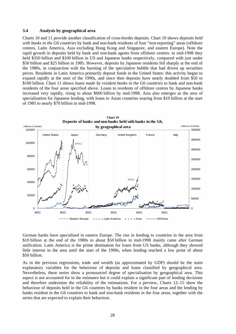
28
3.4 Analysis by geographical area
Charts 10 and 11 provide another classification of cross-border deposits. Chart 10 shows deposits heldwith banks in the G6 countries by bank and non-bank residents of four “non-reporting” areas (offshorecentres, Latin America, Asia excluding Hong Kong and Singapore, and eastern Europe). Note therapid growth in deposits held by bank and non-bank agents from offshore centres: in mid-1998 theyheld $350 billion and $100 billion in US and Japanese banks respectively, compared with just under$50 billion and $25 billion in 1985. However, deposits by Japanese residents fell sharply at the end ofthe 1980s, in conjunction with the bursting of the speculative bubble that had driven up securitiesprices. Residents in Latin America primarily deposit funds in the United States: this activity began toexpand rapidly at the start of the 1990s, and since then deposits have nearly doubled from $50 to$100 billion. Chart 11 shows loans made by resident banks in the G6 countries to bank and non-bankresidents of the four areas specified above. Loans to residents of offshore centres by Japanese banksincreased very rapidly, rising to about $600 billion by mid-1998. Asia also emerges as the area ofspecialisation for Japanese lending, with loans to Asian countries soaring from $10 billion at the startof 1985 to nearly $70 billion in mid-1998.
German banks have specialised in eastern Europe. The rise in lending to countries in the area from$10 billion at the end of the 1980s to about $50 billion in mid-1998 mainly came after Germanunification. Latin America is the prime destination for loans from US banks, although they showedlittle interest in the area until the start of the 1990s, when lending reached a low point of about$50 billion.
As in the previous regressions, trade and wealth (as approximated by GDP) should be the mainexplanatory variables for the behaviour of deposits and loans classified by geographical area.Nevertheless, these series show a pronounced degree of specialisation by geographical area. Thisaspect is not accounted for in the estimates but it could explain a significant part of lending decisionsand therefore undermine the reliability of the estimations. For a preview, Charts 12–15 show thebehaviour of deposits held in the G6 countries by banks resident in the four areas and the lending bybanks resident in the G6 countries to bank and non-bank residents in the four areas, together with theseries that are expected to explain their behaviour.
Deposits of banks and non-banks held with banks in the G6, by geographical area
0
20000
40000
60000
80000
100000
120000
8501 8501 8501 8501 8501 8501
0
50000
100000
150000
200000
250000
300000
350000
400000
Eastern Europe Latin America Asia Offshore
(r.h.s .)
United States Japan Germany United Kingdom France Italy
Chart 10
millions of dollars
(r.h.s .)
millions of dollars

29
Tables 10 and 11 report, respectively, the results of the regressions performed on deposits held bybank and non-bank agents resident in the four areas with banks resident in the G6 countries. As before,the estimates were performed for individual countries and for a panel of the six countries takentogether (only one subset of the variables used earlier has been used in the regressions performed forthe geographical areas). The R-squared of the panel regression performed for deposits by banks (Table10, last section) range between 0.62 for depositors resident in eastern Europe and 0.96 for those inAsia. Domestic GDP has the expected sign for Asia and eastern Europe, while foreign GDP has theexpected sign for eastern Europe and, marginally, for Latin America. The short-term interest ratedifferential is positive in all cases, while the long-term differential is negative but not significantlydifferent from zero for Asia only. World trade has the expected sign in all cases, while trade betweenthe individual areas and the G6 countries has a positive sign only for Latin America and easternEurope. The current inflation differential has a negative sign for Latin America and Asia and,marginally, the offshore countries. For the panel regressions performed on deposits by non-banks(Table 11, last section), domestic GDP has a positive sign in all cases, with elasticities that vary from0.39 for Asia to 1.0 for offshore countries (in other words, a 1% GDP growth prompts a 1% increasein deposits from the specified area).
Foreign GDP has the correct sign for offshore countries, Latin America and eastern Europe; it isnegative for Asia. The short-term interest rate differential is positive only for Asia, while the long-term differential has the expected negative sign for offshore countries and Asia. World trade directlyinfluences deposits by foreign non-banks in Latin America and Asia, while trade between the areasunder consideration and the G6 countries had an impact for Asia and eastern Europe.
As a follow-up to these estimates, one could specify the equations in a more complete fashion byadding other regressors, most important the stock of private sector securities and the volatilities ofexchange rates and stock markets, which strongly influenced investment decisions in these countries.In addition, one should also carry out regressions for loans granted by banks located in G6 countries tobank and non-bank residents of the four areas considered.
Lending by banks in the G6 to banks and non-banks, by geographical area (millions of dollars; from 1985Q1 to 1998Q2)
0
20000
40000
60000
80000
100000
120000
8501 8501 8501 8501 8501 8501
0
100000
200000
300000
400000
500000
600000
700000
Eastern Europe Latin America Asia Offshore
9802
Chart 11
United Kingdom
(r.h.s .)
United States Japan Germany France Italy
(r.h.s .)
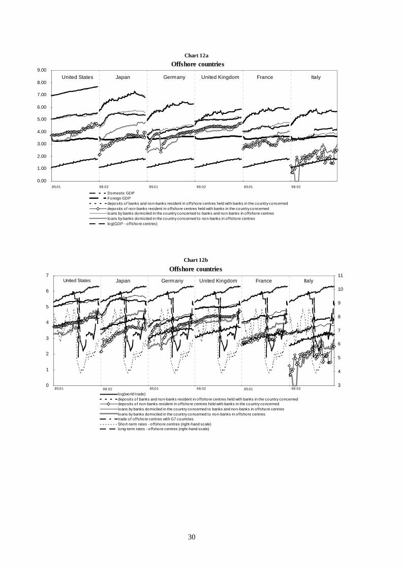
30
Offshore countries
0.00
1.00
2.00
3.00
4.00
5.00
6.00
7.00
8.00
9.00
Domes tic GDPF oreign GDPdepos its of banks and non-banks res ident in offs hore centres held with banks in the country concerned depos its of non-banks res ident in offs hore centres held with banks in the country concernedloans by banks domiciled in the country concerned to banks and non-banks in offs hore centresloans by banks domiciled in the country concerned to non-banks in offs hore centreslog(GDP - offs hore centres )
85.01 98.02 85.01 98.02 98.0285.01
United States Japan Germany United Kingdom France Italy
Chart 12a
Offshore countries
0
1
2
3
4
5
6
7
3
4
5
6
7
8
9
10
11
log(world trade)depos its of banks and non-banks res ident in offs hore centres held with banks in the country concerned depos its of non-banks res ident in offs hore centres held with banks in the country concernedloans by banks domiciled in the country concerned to banks and non-banks in offs hore centresloans by banks domiciled in the country concerned to non-banks in offs hore centrestrade of offs hore centres with G7 countriesS hort-term rates - offs hore centres (right-hand s cale)long-term rates - offs hore centres (right-hand s cale)
85.01 98.02 85.01 98.02 98.0285.01
United States Japan Germany United Kingdom France Italy
Chart 12b
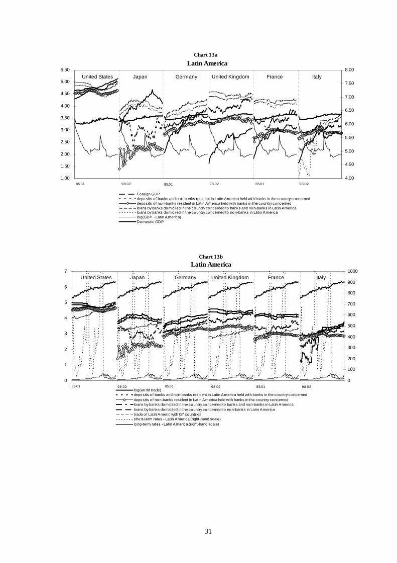
31
Latin America
1.00
1.50
2.00
2.50
3.00
3.50
4.00
4.50
5.00
5.50
4.00
4.50
5.00
5.50
6.00
6.50
7.00
7.50
8.00
F oreign GDPdepos its of banks and non-banks res ident in Latin America held with banks in the country concerned depos its of non-banks res ident in Latin America held with banks in the country concernedloans by banks domiciled in the country concerned to banks and non-banks in Latin Americaloans by banks domiciled in the country concerned to non-banks in Latin Americalog(GDP - Latin America)Domes tic GDP
85.01 98.02 85.01 98.02 98.0285.01
United States Japan Germany United Kingdom France Italy
Chart 13a
Latin America
0
1
2
3
4
5
6
7
0
100
200
300
400
500
600
700
800
900
1000
log(world trade)depos its of banks and non-banks res ident in Latin America held with banks in the country concerned depos its of non-banks res ident in Latin America held with banks in the country concernedloans by banks domiciled in the country concerned to banks and non-banks in Latin Americaloans by banks domiciled in the country concerned to non-banks in Latin Americatrade of Latin Americ with G7 countriess hort-term rates - Latin America (right-hand s cale)long-term rates - Latin America (right-hand s cale)
85.01 98.02 85.01 98.02 98.0285.01
United States Japan Germany United Kingdom France Italy
Chart 13b

32
Asia
1.00
1.50
2.00
2.50
3.00
3.50
4.00
4.50
5.00
5.50
4.00
4.50
5.00
5.50
6.00
6.50
7.00
7.50
8.00
F oreign GDPdepos its fof banks and non-banks res ident in As ia held with banks in the country concerneddepos its of non-banks res ident in As ia held with banks in the country concernedloans by banks domiciled in the country concerned to banks and non-banks in As ialoans by banks domiciled in the country concerned to non-banks in As ialog(GDP - As ia)Domes tic GDP
85.01 98.02 85.01 98.02 98.0285.01
United States Japan Germany United Kingdom France Italy
(right-hand s cale)
Chart 14a
Asia
0
1
2
3
4
5
6
7
5
10
15
20
25
30
log(world trade)depos its fof banks and non-banks res ident in As ia held with banks in the country concerneddepos its of non-banks res ident in As ia held with banks in the country concernedloans by banks domiciled in the country concerned to banks and non-banks in As ialoans by banks domiciled in the country concerned to non-banks in As ias hort-term rates - As ia (right-hand s cale)long-term rates - As ia (right-hand s cale)
85.01 98.02 85.01 98.02 98.0285.01
United States Japan Germany United Kingdom France Italy
Chart 14b
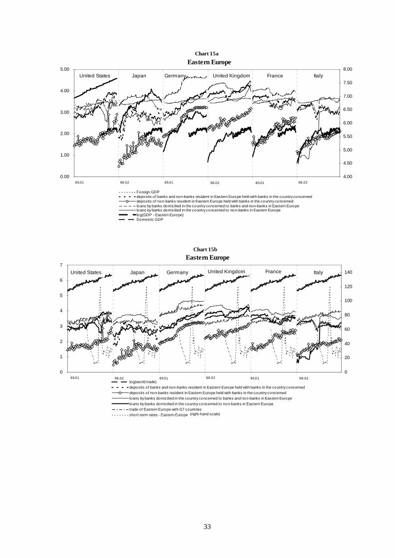
33
Eastern Europe
0.00
1.00
2.00
3.00
4.00
5.00
4.00
4.50
5.00
5.50
6.00
6.50
7.00
7.50
8.00
F oreign GDPdepos its of banks and non-banks res ident in Eas tern Europe held with banks in the country concerneddepos its of non-banks res ident in Eas tern Europe held with banks in the country concernedloans by banks domicilied in the country concerned to banks and non-banks in Eas tern Europeloans by banks domicilied in the country concerned to non-banks in Eas tern Europelog(GDP - Eas tern Europe)Domes tic GDP
85.01 98.02 85.01 98.02 98.0285.01
United States Japan Germany United Kingdom France Italy
Chart 15a
Eastern Europe
0
1
2
3
4
5
6
7
0
20
40
60
80
100
120
140
log(world trade)depos its of banks and non-banks res ident in Eas tern Europe held with banks in the country concerneddepos its of non-banks res ident in Eas tern Europe held with banks in the country concernedloans by banks domicilied in the country concerned to banks and non-banks in Eas tern Europeloans by banks domicilied in the country concerned to non-banks in Eas tern Europetrade of Eas tern Europe with G7 countriess hort-term rates - Eas tern Europe
85.01 98.02 85.01 98.02 98.0285.01
United States Japan Germany United Kingdom France Italy
Chart 15b
(right-hand s cale)
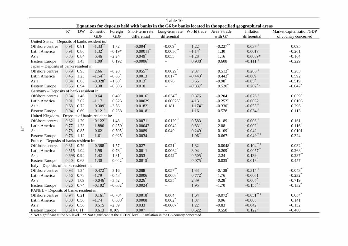
34
Table 10Equations for deposits held with banks in the G6 by banks located in the specified geographical areas
R2 DW DomesticGDP
ForeignGDP
Short-term ratedifferential
Long-term ratedifferential
World trade Area’s tradewith G7
Inflationdifferential
Market capitalisation/GDPof country concerned
United States – Deposits of banks resident in:Offshore centres 0.91 0.81 –1.33** 1.72 –0.004* –0.009* 1.22 –0.227** 0.037 1 0.095Latin America 0.91 0.86 1.32* –0.19* 0.00011* 0.0036** –1.14* 1.30 0.0017 –0.201Asia 0.85 0.84 5.46 –2.24 0.049* 0.055 –1.28 1.16 0.0039* –0.164Eastern Europe 0.96 1.43 1.00* 0.192 –0.0006* – 0.938* 0.608 –0.111 1 –0.229Japan – Deposits of banks resident in:Offshore centres 0.79 0.95 2.66 –8.20 0.055** 0.0029* 2.37 0.512* 0.280 1 0.283Latin America 0.45 1.23 –1.54** –0.06* 0.0013 0.017** –0.443* 0.442* –0.009 0.592Asia 0.84 0.65 –0.328* –1.30* 0.013* 0.076 3.55 –0.98* –0.05* –0.519Eastern Europe 0.56 0.94 3.38 –0.506 0.010 – –0.837* 0.520* 0.202* 1 –0.042*
Germany – Deposits of banks resident in:Offshore centres 0.84 1.46 0.64 0.49* 0.0016* –0.034** 0.376 –0.204 –0.076 1 0.059*
Latin America 0.91 2.02 –1.17 0.523 0.00029 0.00076* 4.13 –0.252* –0.0032 0.0103Asia 0.68 0.72 0.309* –3.56 0.0182* 0.181 1.174** –0.330* –0.055** 0.296Eastern Europe 0.94 0.69 –0.121* 0.268 0.0018** – 1.16 0.578 0.034 1 –0.113United Kingdom – Deposits of banks resident in:Offshore centres 0.82 1.20 –0.122** –1.48 –0.0071** 0.0129** 0.583 0.189 –0.003 1 0.161Latin America 0.77 1.23 –1.886 0.250* 0.00042 0.0042* 0.831* 2.08 –0.002* 0.116*
Asia 0.78 0.85 0.621 –0.595* 0.0089** 0.040 0.249* 0.109* –0.042 –0.0101Eastern Europe 0.76 1.12 –1.61 0.025* 0.0034 – 1.06** 0.667 0.049** 1 0.324France – Deposits of banks resident in:Offshore centres 0.81 0.79 0.388** –1.57 0.027 –0.021* 1.82 0.0048* 0.104** 1 0.032*
Latin America 0.515 1.04 –1.98 0.78** 0.0011 0.0064* 3.04 0.209* –0.0057** 0.268*
Asia 0.698 0.94 1.42 –1.31* 0.053 –0.042** –0.505* –2.24 –0.139 –0.237**
Eastern Europe 0.40 0.63 –1.30 –0.042* 0.0015* – –0.075* –0.035* 0.013 1 0.457Italy – Deposits of banks resident in:Offshore centres 0.93 1.34 –0.472** 3.16 0.088 0.057** 1.33 –0.138* –0.314 1 –0.043*
Latin America 0.56 0.78 –1.79 –0.43* 0.0006 0.0008* 0.772* 1.76 –0.0061 –0.232*
Asia 0.20 1.09 –0.046* –3.52 –0.026* 0.035* 2.39 –0.28* 0.005* –0.719Eastern Europe 0.26 0.74 –0.102* –0.032* 0.0024* – 1.95 –1.70 –0.155* 1 –0.132*
PANEL – Deposits of banks resident in:Offshore centres 0.94 0.21 0.161* –0.704 0.0018* 0.064 1.64 –0.072* –0.051** 1 0.054*
Latin America 0.88 0.56 –1.74 0.008* 0.0008 0.002* 1.37 0.96 –0.005 0.141Asia 0.96 0.56 0.515 –2.59 0.033 –0.0067* 1.22 –0.83 –0.042 –0.132Eastern Europe 0.614 0.11 0.613 0.109 0.007 – 0.622 0.558 0.122 1 –0.480* Not significant at the 5% level. ** Not significant at the 10/15% level. 1 Inflation in the G6 country concerned.

35
Table 11Equations for deposits held with banks in the G6 by banks located in the specified geographical areas
R2 DW DomesticGDP
ForeignGDP
Short-term ratedifferential
Long-term ratedifferential
World trade Area’s tradewith G7
Inflationdifferential
Market capitalisation/GDPof country concerned
United States – Deposits of non-banks resident in:Offshore centres 0.94 0.89 3.43 –3.33 0.0045* 0.011** 0.036* 0.286 –0.053** 1 –0.038**
Latin America 0.68 0.76 0.143* –0.019* –0.00005 0.0021 0.147* –0.113** 0.0006 0.0115*
Asia 0.89 0.67 0.097* 0.244* –0.005* 0.007* 0.359** 0.078* 0.0048* –0.030Eastern Europe 0.68 2.02 –0.912* 0.168 0.0028 – 1.14** –0.05* –0.204 1 0.074**
Japan – Deposits of non-banks resident in:Offshore centres 0.90 1.94 0.684 0.733* 0.015* 0.027* –0.147* 0.0086* 0.0286* 1 0.0854*
Latin America 0.54 1.57 –0.457** –0.05* 0* –0.0025* 1.19** –0.013* –0.0011* –0.166**
Asia 0.85 1.93 0.051* –0.419* –0.004* 0.0093* 0.496 –0.180** –0.002* –0.061**
Eastern Europe 0.76 1.90 0.76 –0.154 –0.0013* – 0.692** –0.533 0.009* 1 0.0073*
Germany – Deposits of non-banks resident in:Offshore centres 0.69 1.18 2.70 2.40 –0.058 –0.072** –2.68 –0.55 –0.068* 1 0.217**
Latin America 0.95 1.28 0.372 0.102 0.00003** 0.00011* 0.152* –0.063* –0.0002* 0.0242*
Asia 0.92 0.73 0.370 0.767 –0.0045* –0.0405 –0.157* –0.128* 0.0042* 0.036*
Eastern Europe 0.97 0.86 0.646 0.122 –0.0003* – –0.406** 0.579 0.077 1 –0.046*
United Kingdom – Deposits of non-banks resident in:Offshore centres 0.95 1.44 0.623 0.375 0.0069 –0.0054* –0.449 –0.052** 0.019 1 0.109Latin America 0.79 1.42 0.56 0.089 –0.0008 0.0008* –0.199** 0.027* 0.00015* –0.065Asia 0.86 1.04 0.442 –0.024* 0.0039** –0.015 –0.087* 0.0469* 0.0044* –0.0063*
Eastern Europe 0.89 1.60 –0.422** –0.019* 0.0011** – 0.672 0.408 0.0148* 1 0.049*
France – Deposits of non-banks resident in:Offshore centres 0.73 1.31 –0.007* –2.05 0.004 –0.048* 2.41 0.0049* 0.073** 1 –0.159Latin America 0.79 1.25 0.723 0.090** –0.00006 0.0014** –0.271** 0.071* 0.00013* –0.026*
Asia 0.92 1.23 0.526 0.019* 0.004* –0.036 0.064* –0.141* –0.007* –0.038*
Eastern Europe 0.90 1.33 0.167* 0.120 –0.0018** – 0.534** 0.499 0.011* 1 –0.178Italy – Deposits of non-banks resident in:Offshore centres 0.58 1.22 1.87 1.18** –0.035** –0.0089** –2.03 0.122* 0.084* 1 –0.027*
Latin America 0.92 1.82 0.561 0.122 –0.00006 0.0008** –0.156** 0.075** 0.0006 –0.041Asia 0.71 1.65 0.622 –0.262* –0.011** 0.017** –0.149* 0.071* 0.0086* 0.023*
Eastern Europe 0.91 1.86 0.751 0.083 0* – –0.593 0.256 0.045** 1 0.180PANEL – Deposits of non-banks resident in:Offshore centres 0.94 0.74 1.00 1.01 –0.0098** –0.028 –0.765 –0.052* 0.0173* 1 0.0067*
Latin America 0.99 1.28 0.510 0.138 –0.00007 0.0015 0.216 –0.194 0.00044 –0.0079*
Asia 0.99 0.77 0.390 –0.216 0.0017* –0.026 0.106** 0.200 0.00088* –0.0079*
Eastern Europe 0.91 1.03 0.813 0.117 –0.0011 – –0.631 0.351 0.037 1 0.063* Not significant at the 5% level. ** Not significant at the 10/15% level. 1 Inflation in the G6 country concerned.

36
Bibliography
Alworth, J S and S Andresen (1992): “The determinants of cross border non-bank deposits and thecompetitiveness of financial market centres”. Money Affairs, Vol. 5, pp. 105-33.
Banca d’Italia (1998a): Economic Bulletin, No. 30, February.
Banca d’Italia (1998b): Economic Bulletin, No. 31, October.
BIS (1995): International Banking and Financial Market Developments, February.
BIS (1998): International Banking and Financial Market Developments, August.
BIS (1999): International Banking and Financial Market Developments, March.
Eichengreen, B and D Mathieson (1998): “Hedge Funds and Financial Market Dynamics”. IMFOccasional Paper, No. 166, May.
Fratianni, M and P Savona (1972): “La liquidità internazionale – Proposta per la ridefinizione delproblema”. Il Mulino, Bologna.
Garber, P M (1998): “Derivatives in International Capital Flow”. NBER Working Paper, No. 6623,June.
Giannini, C and C Monticelli (1996): “Liquidità internazionale e depositi cross border”. Preparatorypaper for the Bank of Italy’s 1995 Annual Report, mimeo.
IMF (1998): “Interim Report on the World Economic Outlook and the International Capital Markets”.December.
La Porta, R, F Lopez-de-Silanes, A Shleifer and R W Vishny (1999): “Law and Finance”. Journal ofPolitical Economy, forthcoming.
Sheldon, G (1992): “Explaining the Cross-country Distribution of International Bank Deposits”, inM Blattner, H Gerber and A Swoboda (eds.), Competitiveness in banking.
Tristani, O (1998): “Liquidità ‘mondiale’ e controllo monetario”. Preparatory paper for the Bank ofItaly’s 1997 Annual Report, mimeo.
37
International diversification of investments in Belgiumand its effects on the main Belgian securities markets
Thierry Timmermans
1. Introduction
The international diversification of investments is far from being a recent phenomenon in Belgium.Over the past 20 years, individuals markedly stepped up their purchases of foreign currencydenominated assets such that, on the eve of EMU, these assets represented a greater share of privatewealth than in most other European countries. The introduction of the euro should, however, providefresh impetus to and a broader base for this process of diversifying out of domestic assets. This isbound to have profound repercussions on the Belgian financial markets, in particular the governmentsecurities market and the stock market. These markets will not be able to benefit to the same extent asin the past from a stable core of captive investors, and it is far from certain that this reduced interest onthe part of traditional customers can be fully offset by increased purchases by investors from othereuro area countries.
The first part of this note provides a snapshot of the current degree of international diversification offinancial assets and liabilities in Belgium. The second and third parts examine the present and futureimplications of the introduction of the euro on the government securities market and the stock marketrespectively, and briefly describe the adjustments envisaged by these two markets.
2. International diversification of financial assets and liabilities in Belgium
The very high saving rate among Belgian individuals has been reflected in an accumulation offinancial assets, which at end-1998 totalled close to three times GDP. How these savings are investedobviously exerts a powerful influence on the structure of Belgian financial markets.
In this context, there have been two major developments over the last 20 years. First, the overall shareof financial assets in foreign currency rose from 7% in 1980 to 23% in 1998 (Table 1). Second, therole of banks in attracting savings declined markedly during the same period, with banks’ market sharefalling from 60% to 37% in favour of direct purchases of securities and, above all, investments withinstitutional investors, in particular collective investment undertakings (UCITS).
It is interesting to note that these two developments were not independent but, on the contrary, wenthand in hand. The diversification of individuals’ investments into foreign currency occurred to a muchgreater extent via investments with institutional investors and direct purchases of securities than viamore traditional financial intermediaries such as banks.
This does not, however, mean that financial intermediaries have not played any accompanying role inthis development. Almost all UCITS are set up, administered and marketed by Belgian banks, whichthereby manage to recuperate, in the form of fee income, the falls in revenue resulting from thecontraction in their intermediation income. The diversification opportunities and professionalmanagement offered by these funds have greatly facilitated the growth of individuals’ foreign currencyinvestments. At the same time, however, this interest in foreign currency denominated assets has alsobeen reflected in a rise in direct purchases of securities.
This diversification of investments, be it by channel or currency, has not been driven by the purelyfinancial consideration of attaining a better risk-return combination. It has also had a fiscal motive as ameans of escaping the withholding tax on investment income. As individuals’ capital gains are not

38
taxed in Belgium, investments via UCITS are de jure exempt from withholding tax insofar as theUCITS do not distribute their income but capitalise it. A de facto exemption exists for direct purchasesof securities abroad in that the beneficiary can then easily omit to declare his income to the Belgianauthorities.
Table 1Structure of financial assets held by individuals1
(as a percentage of the total)
1980 1998
Investments with credit institutions 60.4 36.9of which: share in francs
share in foreign currency97.6
2.493.0
7.0
Investments with insurance companies and pension funds2 7.3 11.8of which: share in francs
share in foreign currency91.9
8.182.417.6
Investments with UCITS2 0.5 14.1of which: share in francs
share in foreign currency48.351.7
Direct purchases of securities 31.9 37.3of which: share in francs
share in foreign currency78.321.7
63.536.5
Total 100.0 100.0of which: share in francs
share in foreign currency92.6
7.476.723.3
1 Excluding shares held in unlisted companies.
2 The currency breakdown of investments by individuals with
institutional investors is assumed to be identical to that of financial assets held by these institutional investors.
Source: National Bank of Belgium (NBB).
Whatever the reasons, these foreign currency investments by individuals constituted a major source ofcapital outflows over the past 20 years and thereby a constraint on the balance of payments, as, toachieve its fixed exchange rate objective, Belgium had to counterbalance these outflows withoffsetting inflows. This requirement was obviously more difficult to meet at times when the currentaccount was in deficit, as in the early 1980s. The re-establishment of a surplus and its gradualwidening from 1986 onwards alleviated this constraint, without, however, eliminating it, as the currentaccount balance was often insufficient to counterbalance the capital outflows resulting frominvestments made abroad by individuals.
There have been two main types of offsetting inflows of capital. The first, autonomous in nature, hasbeen in the form of direct investments. The rest of the world’s holding of shares in Belgian companieshas increased steadily, from 12.6% to 29.1% (Table 2). This rise has not been limited to listed stocksbut has extended to unlisted equities, which in Belgium are by far the commonest means of raisingcapital.
The second major source of capital inflows has been the issuance of foreign currency denominatedbonds by the government. This activity has been endogenous in nature since its goal has beenprecisely to offset the balance on current and other capital account transactions.

39
Table 2Shareholder structure of Belgian companies
(as a percentage of the total)
1980 1998
Listed shares
IndividualsCompaniesOther residents*Rest of the world
Total
51.920.415.112.6
100.0
19.037.413.130.5
100.0
Unlisted shares
IndividualsCompaniesOther residents*Rest of the world
Total
63.622.4
1.512.6
100.0
39.930.9
1.228.0
100.0
Total shares
IndividualsCompaniesOther residents*Rest of the world
Total
61.222.0
4.212.6
100.0
30.833.7
6.429.1
100.0
* Including Belgian credit institutions and Belgian and foreign institutional investors operating in Belgium.
Source: NBB.
The volume of these inflows has thus been dictated by the exchange rate constraint. They wereconsiderable at the beginning of the 1980s, but declined progressively towards the end of the decade.As from 1990, the Treasury has been able to make repayments and thus reduce its foreign currencydenominated debt, except in 1993, a year marked by extreme tensions on the foreign exchange market.
This foreign currency borrowing has enabled foreign investors to play a role in the financing of theBelgian government (Table 3). Non-residents are, however, concentrated in the foreign currencysegment of the debt, holding more than 85% at end-1998. At that date over 80% of franc-denominateddebt was placed with Belgian financial intermediaries (banks and institutional investors). In thissecond segment, the share held by non-residents has actually risen, from 4% in 1980 to 11.3% in 1998,but this increase has been mainly at the expense of the share held by non-financial residents. It islargely the result of the recycling in Belgium of franc-denominated funds invested by Belgianindividuals with Luxembourg or Dutch banks for the fiscal reasons mentioned above.
The introduction of the euro has obviously altered this situation and, in particular, eliminated thebalance of payments constraint. This will, however, give way to a new imperative, namely that ofensuring an environment in which Belgian investors and borrowers alike will be able to benefit fromthe best possible investment and financing conditions within EMU, and which will at the same timemake it possible to preserve the source of revenue and activity which the existence of domesticfinancial markets and intermediaries represents for the national economy.
In this context, attention will no longer focus on investments by individuals. They will certainlycontinue to diversify their assets, but the introduction of the euro should above all prolong andreinforce a movement which, as just seen, has already been well under way for a number of years.
The real change will take effect at the level of financial intermediaries. Hitherto their role indiversification operations has been mainly indirect, consisting in the advice and services provided totheir private investor clientele. In operations for their own account, banks have been guided first andforemost by the (legitimate) concern of balancing their net Belgian franc and foreign currency

40
positions. This does not imply that they have been keeping their distance from the foreign exchangemarket. On the contrary, to satisfy a Belgian corporate clientele which depends largely on foreignmarkets for its business, Belgian banks have had to conduct a considerable volume of foreignexchange operations, both spot and forward. They have also accumulated a large amount of interbankforeign currency assets and liabilities on their balance sheets. However, these operations offset eachother, so that franc-denominated funds raised from individuals have until now, in the absence of asignificant euro-Belgian franc market, been almost exclusively devoted to financing Belgian debtors,principally the government.
Table 3Holding structure of Belgian public debt
(as a percentage of the total)
1980 1998
Franc-denominated debt
Credit institutionsInstitutional investorsOther residentsLuxembourgOther non-residents
67.15.8
23.03.10.9
59.319.110.4
7.14.2
Total 100.0 100.0
Foreign currency denominated debt
Credit institutionsInstitutional investorsOther residentsLuxembourgOther non-residents
63.7–––
36.3
14.3–––
85.7
Total 100.0 100.0
Total debt
Credit institutionsInstitutional investorsOther residentsLuxembourgOther non-residents
66.95.5
21.72.92.9
56.517.99.76.69.3
Total 100.0 100.0
Source: NBB.
It is this feature which is changing with the advent of EMU. Banks will no longer have to limit the useof their deposits, now denominated in euros, to purchasing domestic assets. Similarly, insurancecompanies and pension funds will see a relaxation of the constraint imposed by the obligation tomaintain a fairly strict balance in the currency composition of their assets and liabilities. Likewise,UCITS specialised in Belgian franc-denominated investments will be able to widen their investmentpolicy to cover the whole of the euro area. Finally, Dutch and Luxembourg banks which used torecycle in Belgium franc-denominated deposits received from Belgian individuals will obviously beable to invest these funds, now denominated in euros, on other markets.
This redeployment will have far-reaching repercussions for the two big borrowing sectors in theBelgian economy, the government and the corporate sector. The two main securities markets availableto these sectors, the government securities market and the stock market,1 will need to adapt. 1 The third potential market, that of corporate fixed income securities, is still very underdeveloped in Belgium. The
introduction of the euro will no doubt be a significant expansionary factor. This third market will not, however, beanalysed here as it raises issues very different from those concerning the future potential of the more mature governmentsecurities market and Brussels Stock Exchange.

41
3. Government securities market
Given its high degree of standardisation and its strong dependence on Belgian credit institutions, thegovernment securities market is likely to be the most rapidly affected by the introduction of the euro.In particular, dematerialised securities issued by the Belgian Treasury, either long-term (linear bondsor OLOs) or short-term (treasury certificates), will enter into direct competition with the euro-denominated securities offered by the other EMU member countries.
After only a few months of EMU, there has already been a significant change in the structure of OLOholdings (Table 4). Whereas the rest of the world’s share had fluctuated during the previous threeyears at around 10%, it climbed to almost 20% in the first six months of this year. It is mainly Belgiancredit institutions that have reduced their portfolios, as other Belgian holders do not seem to haverestructured to the same extent as yet. On the treasury certificate market, the trend towardsdiversification had started earlier, the rest of the world having already increased its share of the marketfrom 32.2% to 43.5% between end-1996 and end-1998.
Table 4Recent development of the holding structure of linear bonds and treasury certificates
As a percentage of the total, at end of period
1996 1998 1999
March June
Linear bonds (OLOs)Belgiumof which: Belgian credit institutions
Other holdersRest of the worldof which: EMU*
Other countries
87.491.983.981.159.961.6
55.351.027.530.328.630.1
12.68.1
16.118.9
n.a.n.a.
13.913.0
n.a.n.a.2.25.9
Total 100.0 100.0 100.0 100.0
Treasury certificatesBelgiumof which: Belgian credit institutions
Other holdersRest of the worldof which: EMU*
Other countries
67.856.559.556.750.541.2
48.845.617.315.310.611.1
32.243.540.543.3
n.a.n.a.
23.521.1
n.a.n.a.
17.122.2
Total 100.0 100.0 100.0 100.0
* Excluding Belgium.
Source: NBB.
It has to be noted that these figures do not take into account changes of ownership which are solelydue to repurchase agreements. These repos are extensively used by Belgian banks as a convenienttechnique to cover net borrowings of bonds in euros from abroad. While they result in a transfer ofBelgian government securities holdings from Belgium to the rest of the world, such operations are notmotivated by the economic purpose of portfolio diversification. By focusing on this economic concept,Table 4 underestimates the amount of Belgian government securities legally in the hands of the rest ofthe world. This restriction strengthens the significance of the changes in the ownership of OLOsrecorded in Table 4.
This quite naturally raises the question of the terms on which the Treasury has been able to attractforeign investors. A change in holding structure does not indicate whether or not it was necessary toincrease rates, be it to counter the declining interest of traditional investors or to attract new ones.

42
-0.5
0
0.5
1
1.5
2
1997 1998 1999-0.5
0
0.5
1
1.5
2
Belgium
France
Netherlands
Italy
Spain
-0.5
-0.4
-0.3
-0.2
-0.1
0
1997 1998 1999-0.5
-0.4
-0.3
-0.2
-0.1
0
3-months
6-months
12-months
RECENT EVOLUTION IN INTEREST RATE CONDITIONS ON THE BELGIAN GOVERNMENT
DEBT
Chart 1
²
²
INTEREST RATE DIFFERENTIALS WITH TEN YEAR GERMAN BONDS
INTEREST RATE DIFFERENTIALS BETWEEN BELGIAN TREASURY CERTIFICATES AND INTERBANK DEPOSITS ¹
Source: NBB.1. Bibor until 1998, Euribor thereafter.2. Average October and November.
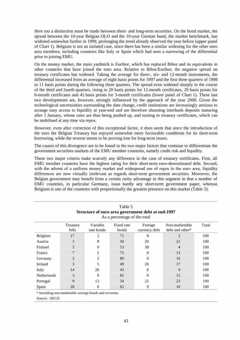
43
Here too a distinction must be made between short- and long-term securities. On the bond market, thespread between the 10-year Belgian OLO and the 10-year German bund, the market benchmark, haswidened somewhat further in 1999, prolonging the trend already observed the year before (upper panelof Chart 1). Belgium is not an isolated case, since there has been a similar widening for the other euroarea members, including countries like Italy or Spain which had seen a narrowing of the differentialprior to joining EMU.
On the money market, the main yardstick is Euribor, which has replaced Bibor and its equivalents inother countries that have joined the euro area. Relative to Bibor/Euribor, the negative spread ontreasury certificates has widened. Taking the average for three-, six- and 12-month instruments, thedifferential increased from an average of eight basis points for 1997 and the first three quarters of 1998to 11 basis points during the following three quarters. The spread even widened sharply in the courseof the third and fourth quarters, rising to 20 basis points for 12-month certificates, 29 basis points for6-month certificates and 45 basis points for 3-month certificates (lower panel of Chart 1). These lasttwo developments are, however, strongly influenced by the approach of the year 2000. Given thetechnological uncertainties surrounding the date change, credit institutions are increasingly anxious toarrange easy access to liquidity at year-end and are therefore shunning interbank deposits maturingafter 1 January, whose rates are thus being pushed up, and turning to treasury certificates, which canbe mobilised at any time via repos.
However, even after correction of this exceptional factor, it does seem that since the introduction ofthe euro the Belgian Treasury has enjoyed somewhat more favourable conditions for its short-termborrowing, while the reverse seems to be proving true for long-term issues.
The causes of this divergence are to be found in the two major factors that continue to differentiate thegovernment securities markets of the EMU member countries, namely credit risk and liquidity.
These two major criteria make scarcely any difference in the case of treasury certificates. First, allEMU member countries have the highest rating for their short-term euro-denominated debt. Second,with the advent of a uniform money market and widespread use of repos in the euro area, liquiditydifferences are now virtually irrelevant as regards short-term government securities. Moreover, theBelgian government may benefit from a certain rarity advantage in this segment in that a number ofEMU countries, in particular Germany, issue hardly any short-term government paper, whereasBelgium is one of the countries with proportionally the greatest presence on this market (Table 5).
Table 5Structure of euro area government debt at end-1997
As a percentage of the total
Treasurybills
Variablerate bonds
Fixed ratebonds
Foreigncurrency debt
Non-marketabledebt and other*
Total
Belgium 17 2 71 8 2 100
Austria 1 8 50 20 21 100
Finland 5 0 53 38 4 100
France 7 5 75 0 13 100
Germany 2 2 80 0 16 100
Ireland 3 5 49 26 17 100
Italy 14 26 45 6 9 100
Netherlands 3 0 82 0 15 100
Portugal 9 12 34 22 23 100
Spain 28 0 62 9 10 100
* Including non-marketable savings bonds and accounts.
Source: OECD.
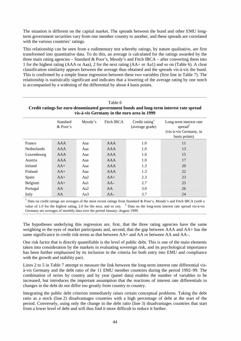
44
The situation is different on the capital market. The spreads between the bund and other EMU long-term government securities vary from one member country to another, and these spreads are correlatedwith the various countries’ ratings.
This relationship can be seen from a rudimentary test whereby ratings, by nature qualitative, are firsttransformed into quantitative data. To do this, an average is calculated for the ratings awarded by thethree main rating agencies – Standard & Poor’s, Moody’s and Fitch IBCA – after converting them into1 for the highest rating (AAA or Aaa), 2 for the next rating (AA+ or Aa1) and so on (Table 6). A clearclassification similarity appears between the average thus obtained and the spreads vis-à-vis the bund.This is confirmed by a simple linear regression between these two variables (first line in Table 7). Therelationship is statistically significant and indicates that a lowering of the average rating by one notchis accompanied by a widening of the differential by about 4 basis points.
Table 6Credit ratings for euro-denominated government bonds and long-term interest rate spread
vis-à-vis Germany in the euro area in 1999
Standard& Poor’s
Moody’s Fitch IBCA Credit rating1
(average grade)Long-term interest rate
spread2
(vis-à-vis Germany, inbasis points)
France AAA Aaa AAA 1.0 11
Netherlands AAA Aaa AAA 1.0 13
Luxembourg AAA Aaa AAA 1.0 15
Austria AAA Aaa AAA 1.0 17
Ireland AA+ Aaa AAA 1.3 20
Finland AA+ Aaa AAA 1.3 22
Spain AA+ Aa2 AA+ 2.3 23
Belgium AA+ Aa1 AA– 2.7 25
Portugal AA Aa2 AA 3.0 26
Italy AA Aa3 AA– 3.7 241 Data on credit ratings are averages of the most recent ratings from Standard & Poor’s, Moody’s and Fitch IBCA (with a
value of 1.0 for the highest rating, 2.0 for the next, and so on). 2 Data on the long-term interest rate spread vis-à-vis
Germany are averages of monthly data over the period January–August 1999.
The hypotheses underlying this regression are, first, that the three rating agencies have the sameweighting in the eyes of market participants and, second, that the gap between AAA and AA+ has thesame significance in credit risk terms as that between AA+ and AA or between AA and AA–.
One risk factor that is directly quantifiable is the level of public debt. This is one of the main elementstaken into consideration by the markets in evaluating sovereign risk, and its psychological importancehas been further emphasised by its inclusion in the criteria for both entry into EMU and compliancewith the growth and stability pact.
Lines 2 to 5 in Table 7 attempt to measure the link between the long-term interest rate differential vis-à-vis Germany and the debt ratio of the 11 EMU member countries during the period 1992–99. Thecombination of series by country and by year (panel data) enables the number of variables to beincreased, but introduces the important assumption that the reactions of interest rate differentials tochanges in the debt do not differ too greatly from country to country.
Integrating the public debt criterion immediately raises certain conceptual problems. Taking the debtratio as a stock (line 2) disadvantages countries with a high percentage of debt at the start of theperiod. Conversely, using only the change in the debt ratio (line 3) disadvantages countries that startfrom a lower level of debt and will thus find it more difficult to reduce it further.
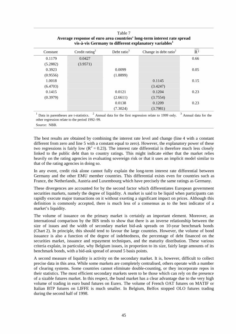
45
Table 7Average response of euro area countries’ long-term interest rate spread
vis-à-vis Germany to different explanatory variables1
Constant Credit rating2 Debt ratio3 Change in debt ratio2 ²R
0.1179 0.0427 0.66
(5.2882) (3.9571)
0.3923 0.0099 0.05
(0.9556) (1.8899)
1.0018 0.1145 0.15
(6.4703) (3.4247)
0.1415 0.0121 0.1204 0.23
(0.3979) (2.6611) (3.7554)
0.0138 0.1209 0.23
(7.3024) (3.7981)1 Data in parentheses are t-statistics.
2 Annual data for the first regression relate to 1999 only.
3 Annual data for the
other regression relate to the period 1992–99.
Source: NBB.
The best results are obtained by combining the interest rate level and change (line 4 with a constantdifferent from zero and line 5 with a constant equal to zero). However, the explanatory power of thesetwo regressions is fairly low (R2 = 0.23). The interest rate differential is therefore much less closelylinked to the public debt than to country ratings. This might indicate either that the market reliesheavily on the rating agencies in evaluating sovereign risk or that it uses an implicit model similar tothat of the rating agencies in doing so.
In any event, credit risk alone cannot fully explain the long-term interest rate differential betweenGermany and the other EMU member countries. This differential exists even for countries such asFrance, the Netherlands, Austria and Luxembourg which have precisely the same ratings as Germany.
These divergences are accounted for by the second factor which differentiates European governmentsecurities markets, namely the degree of liquidity. A market is said to be liquid when participants canrapidly execute major transactions on it without exerting a significant impact on prices. Although thisdefinition is commonly accepted, there is much less of a consensus as to the best indicator of amarket’s liquidity.
The volume of issuance on the primary market is certainly an important element. Moreover, aninternational comparison by the BIS tends to show that there is an inverse relationship between thesize of issues and the width of secondary market bid-ask spreads on 10-year benchmark bonds(Chart 2). In principle, this should tend to favour the large countries. However, the volume of bondissuance is also a function of the degree of indebtedness, the percentage of debt financed on thesecurities market, issuance and repayment techniques, and the maturity distribution. These variouscriteria explain, in particular, why Belgium issues, in proportion to its size, fairly large amounts of itsbenchmark bonds, with a bid-ask spread of around 5 basis points.
A second measure of liquidity is activity on the secondary market. It is, however, difficult to collectprecise data in this area. While some markets are completely centralised, others operate with a numberof clearing systems. Some countries cannot eliminate double-counting, or they incorporate repos intheir statistics. The most efficient secondary markets seem to be those which can rely on the presenceof a sizable futures market. In this respect, the bund market has a clear advantage due to the very highvolume of trading in euro bund futures on Eurex. The volume of French OAT futures on MATIF orItalian BTP futures on LIFFE is much smaller. In Belgium, Belfox stopped OLO futures tradingduring the second half of 1998.
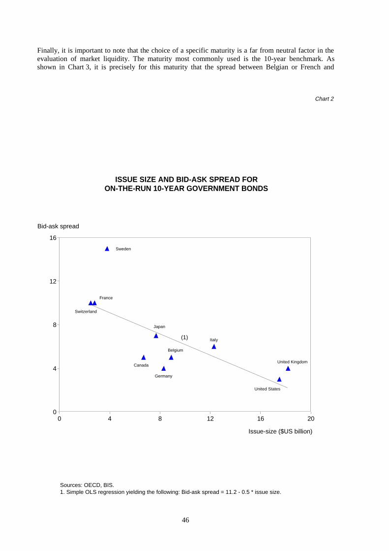
46
Finally, it is important to note that the choice of a specific maturity is a far from neutral factor in theevaluation of market liquidity. The maturity most commonly used is the 10-year benchmark. Asshown in Chart 3, it is precisely for this maturity that the spread between Belgian or French and
0
4
8
12
16
0 4 8 12 16 20
United Kingdom
United States
Italy
Belgium
Germany
Canada
Japan
Sweden
France
Switzerland
Bid-ask spread
Issue-size ($US billion)
(1)
Sources: OECD, BIS.1. Simple OLS regression yielding the following: Bid-ask spread = 11.2 - 0.5 * issue size.
Chart 2
ISSUE SIZE AND BID-ASK SPREAD FOR ON-THE-RUN 10-YEAR GOVERNMENT BONDS

47
German government bonds is the greatest.2 Although the bund has the lowest rates for maturitiesbetween nine and 12 years as well as for the 30-year maturity, it is the French OAT which constitutesthe benchmark for maturities from five to eight years, while, for other maturities, the rates on thesetwo categories of securities are very close.
-0.15
-0.1
-0.05
0
0.05
0.1
0.15
0.2
0.25
0.3
0 1 2 3 4 5 6 7 8 9 10 11 12 13 14 15 16 17 18 19 20 21 22 23 24 25 26 27 28 29 30
France
Chart 3
Belgium
Source: NBB.
Remaining period to maturity in years
YIELD DIFFERENTIAL OF FRENCH AND BELGIAN GOVERNMENT SECURITIES VIS-A-VIS GERMAN GOVERNMENT SECURITIES
(As at 1 June 1999-in percentages)
2 In order to correct the distortions which could result from slight differences in the exact maturities of bonds, Belgian and
French bond yields were compared with theoretical yields on German bonds of the same maturity calculated byinterpolating the two German bonds with the closest maturities.
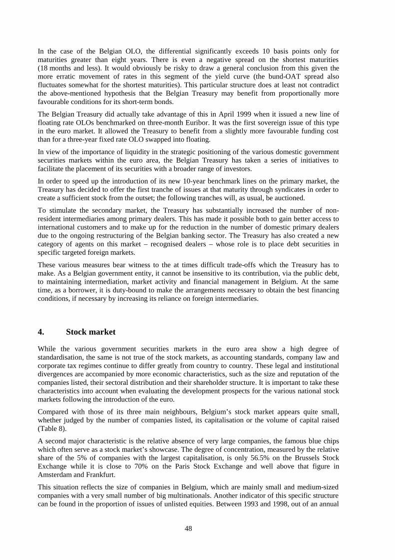
48
In the case of the Belgian OLO, the differential significantly exceeds 10 basis points only formaturities greater than eight years. There is even a negative spread on the shortest maturities(18 months and less). It would obviously be risky to draw a general conclusion from this given themore erratic movement of rates in this segment of the yield curve (the bund-OAT spread alsofluctuates somewhat for the shortest maturities). This particular structure does at least not contradictthe above-mentioned hypothesis that the Belgian Treasury may benefit from proportionally morefavourable conditions for its short-term bonds.
The Belgian Treasury did actually take advantage of this in April 1999 when it issued a new line offloating rate OLOs benchmarked on three-month Euribor. It was the first sovereign issue of this typein the euro market. It allowed the Treasury to benefit from a slightly more favourable funding costthan for a three-year fixed rate OLO swapped into floating.
In view of the importance of liquidity in the strategic positioning of the various domestic governmentsecurities markets within the euro area, the Belgian Treasury has taken a series of initiatives tofacilitate the placement of its securities with a broader range of investors.
In order to speed up the introduction of its new 10-year benchmark lines on the primary market, theTreasury has decided to offer the first tranche of issues at that maturity through syndicates in order tocreate a sufficient stock from the outset; the following tranches will, as usual, be auctioned.
To stimulate the secondary market, the Treasury has substantially increased the number of non-resident intermediaries among primary dealers. This has made it possible both to gain better access tointernational customers and to make up for the reduction in the number of domestic primary dealersdue to the ongoing restructuring of the Belgian banking sector. The Treasury has also created a newcategory of agents on this market – recognised dealers – whose role is to place debt securities inspecific targeted foreign markets.
These various measures bear witness to the at times difficult trade-offs which the Treasury has tomake. As a Belgian government entity, it cannot be insensitive to its contribution, via the public debt,to maintaining intermediation, market activity and financial management in Belgium. At the sametime, as a borrower, it is duty-bound to make the arrangements necessary to obtain the best financingconditions, if necessary by increasing its reliance on foreign intermediaries.
4. Stock market
While the various government securities markets in the euro area show a high degree ofstandardisation, the same is not true of the stock markets, as accounting standards, company law andcorporate tax regimes continue to differ greatly from country to country. These legal and institutionaldivergences are accompanied by more economic characteristics, such as the size and reputation of thecompanies listed, their sectoral distribution and their shareholder structure. It is important to take thesecharacteristics into account when evaluating the development prospects for the various national stockmarkets following the introduction of the euro.
Compared with those of its three main neighbours, Belgium’s stock market appears quite small,whether judged by the number of companies listed, its capitalisation or the volume of capital raised(Table 8).
A second major characteristic is the relative absence of very large companies, the famous blue chipswhich often serve as a stock market’s showcase. The degree of concentration, measured by the relativeshare of the 5% of companies with the largest capitalisation, is only 56.5% on the Brussels StockExchange while it is close to 70% on the Paris Stock Exchange and well above that figure inAmsterdam and Frankfurt.
This situation reflects the size of companies in Belgium, which are mainly small and medium-sizedcompanies with a very small number of big multinationals. Another indicator of this specific structurecan be found in the proportion of issues of unlisted equities. Between 1993 and 1998, out of an annual
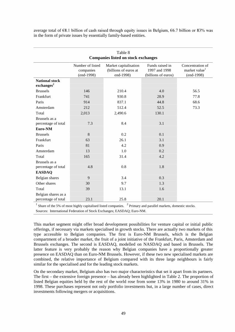
49
average total of ELOOLRQRIFDVKUDLVHGWKURXJKHTXLW\LVVXHVLQ%HOJLXP ELOOLRQRUZDVin the form of private issues by essentially family-based entities.
Table 8Companies listed on stock exchanges
Number of listedcompanies(end-1998)
Market capitalisation(billions of euros at
end-1998)
Funds raised in1997 and 1998
(billions of euros)
Concentration ofmarket value1
(end-1998)
National stockexchanges2
Brussels 146 210.4 4.0 56.5
Frankfurt 741 930.8 28.9 77.8
Paris 914 837.1 44.8 68.6
Amsterdam 212 512.4 52.5 73.3
Total 2,013 2,490.6 130.1
Brussels as apercentage of total 7.3 8.4 3.1
Euro-NMBrussels 8 0.2 0.1
Frankfurt 63 26.1 3.1
Paris 81 4.2 0.9
Amsterdam 13 1.0 0.2
Total 165 31.4 4.2
Brussels as apercentage of total 4.8 0.8 1.8
EASDAQBelgian shares 9 3.4 0.3
Other shares 30 9.7 1.3
Total 39 13.1 1.6
Belgian shares as apercentage of total 23.1 25.8 20.11 Share of the 5% of most highly capitalised listed companies.
2 Primary and parallel markets, domestic stocks.
Sources: International Federation of Stock Exchanges; EASDAQ; Euro-NM.
This market segment might offer broad development possibilities for venture capital or initial publicofferings, if necessary via markets specialised in growth stocks. There are actually two markets of thistype accessible to Belgian companies. The first is Euro-NM Brussels, which is the Belgiancompartment of a broader market, the fruit of a joint initiative of the Frankfurt, Paris, Amsterdam andBrussels exchanges. The second is EASDAQ, modelled on NASDAQ and based in Brussels. Thelatter feature is very probably the reason why Belgian companies have a proportionally greaterpresence on EASDAQ than on Euro-NM Brussels. However, if these two new specialised markets arecombined, the relative importance of Belgium compared with its three large neighbours is fairlysimilar for the specialised and for the leading stock markets.
On the secondary market, Belgium also has two major characteristics that set it apart from its partners.The first – the extensive foreign presence – has already been highlighted in Table 2. The proportion oflisted Belgian equities held by the rest of the world rose from some 13% in 1980 to around 31% in1998. These purchases represent not only portfolio investments but, in a large number of cases, directinvestments following mergers or acquisitions.
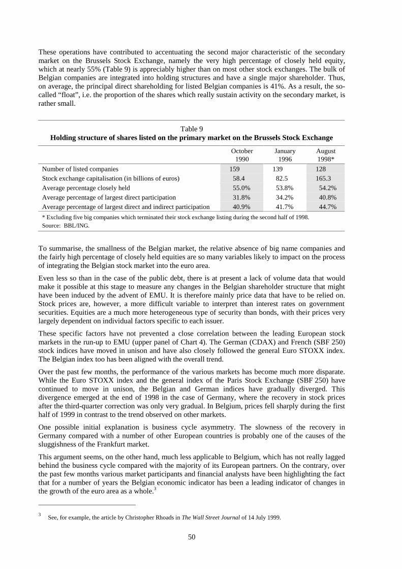
50
These operations have contributed to accentuating the second major characteristic of the secondarymarket on the Brussels Stock Exchange, namely the very high percentage of closely held equity,which at nearly 55% (Table 9) is appreciably higher than on most other stock exchanges. The bulk ofBelgian companies are integrated into holding structures and have a single major shareholder. Thus,on average, the principal direct shareholding for listed Belgian companies is 41%. As a result, the so-called “float”, i.e. the proportion of the shares which really sustain activity on the secondary market, israther small.
Table 9Holding structure of shares listed on the primary market on the Brussels Stock Exchange
October1990
January1996
August1998*
Number of listed companies 159 139 128
Stock exchange capitalisation (in billions of euros) 58.4 82.5 165.3
Average percentage closely held 55.0% 53.8% 54.2%
Average percentage of largest direct participation 31.8% 34.2% 40.8%
Average percentage of largest direct and indirect participation 40.9% 41.7% 44.7%
* Excluding five big companies which terminated their stock exchange listing during the second half of 1998.Source: BBL/ING.
To summarise, the smallness of the Belgian market, the relative absence of big name companies andthe fairly high percentage of closely held equities are so many variables likely to impact on the processof integrating the Belgian stock market into the euro area.
Even less so than in the case of the public debt, there is at present a lack of volume data that wouldmake it possible at this stage to measure any changes in the Belgian shareholder structure that mighthave been induced by the advent of EMU. It is therefore mainly price data that have to be relied on.Stock prices are, however, a more difficult variable to interpret than interest rates on governmentsecurities. Equities are a much more heterogeneous type of security than bonds, with their prices verylargely dependent on individual factors specific to each issuer.
These specific factors have not prevented a close correlation between the leading European stockmarkets in the run-up to EMU (upper panel of Chart 4). The German (CDAX) and French (SBF 250)stock indices have moved in unison and have also closely followed the general Euro STOXX index.The Belgian index too has been aligned with the overall trend.
Over the past few months, the performance of the various markets has become much more disparate.While the Euro STOXX index and the general index of the Paris Stock Exchange (SBF 250) havecontinued to move in unison, the Belgian and German indices have gradually diverged. Thisdivergence emerged at the end of 1998 in the case of Germany, where the recovery in stock pricesafter the third-quarter correction was only very gradual. In Belgium, prices fell sharply during the firsthalf of 1999 in contrast to the trend observed on other markets.
One possible initial explanation is business cycle asymmetry. The slowness of the recovery inGermany compared with a number of other European countries is probably one of the causes of thesluggishness of the Frankfurt market.
This argument seems, on the other hand, much less applicable to Belgium, which has not really laggedbehind the business cycle compared with the majority of its European partners. On the contrary, overthe past few months various market participants and financial analysts have been highlighting the factthat for a number of years the Belgian economic indicator has been a leading indicator of changes inthe growth of the euro area as a whole.3
3
See, for example, the article by Christopher Rhoads in The Wall Street Journal of 14 July 1999.
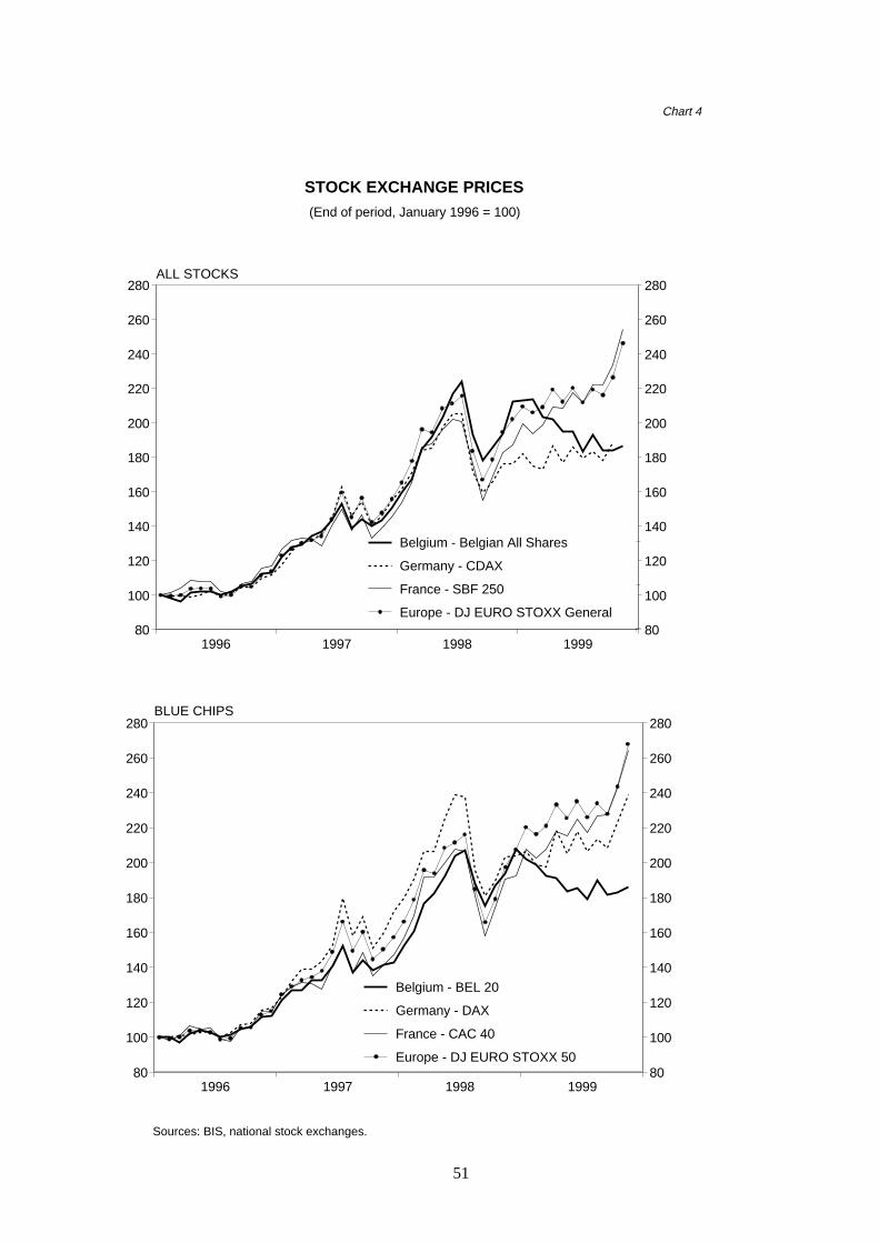
51
80
100
120
140
160
180
200
220
240
260
280
1996 1997 1998 199980
100
120
140
160
180
200
220
240
260
280
80
100
120
140
160
180
200
220
240
260
280
1996 1997 1998 199980
100
120
140
160
180
200
220
240
260
280
France - SBF 250
France - CAC 40
Europe - DJ EURO STOXX 50
Chart 4
(End of period, January 1996 = 100)
Belgium - Belgian All Shares
Germany - CDAX
Europe - DJ EURO STOXX General
Belgium - BEL 20
Germany - DAX
Sources: BIS, national stock exchanges.
STOCK EXCHANGE PRICES
BLUE CHIPS
ALL STOCKS
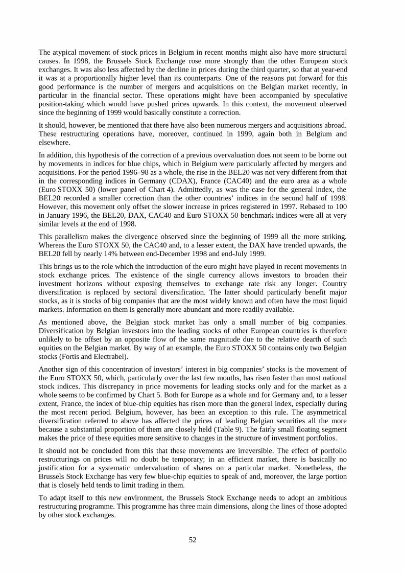
52
The atypical movement of stock prices in Belgium in recent months might also have more structuralcauses. In 1998, the Brussels Stock Exchange rose more strongly than the other European stockexchanges. It was also less affected by the decline in prices during the third quarter, so that at year-endit was at a proportionally higher level than its counterparts. One of the reasons put forward for thisgood performance is the number of mergers and acquisitions on the Belgian market recently, inparticular in the financial sector. These operations might have been accompanied by speculativeposition-taking which would have pushed prices upwards. In this context, the movement observedsince the beginning of 1999 would basically constitute a correction.
It should, however, be mentioned that there have also been numerous mergers and acquisitions abroad.These restructuring operations have, moreover, continued in 1999, again both in Belgium andelsewhere.
In addition, this hypothesis of the correction of a previous overvaluation does not seem to be borne outby movements in indices for blue chips, which in Belgium were particularly affected by mergers andacquisitions. For the period 1996–98 as a whole, the rise in the BEL20 was not very different from thatin the corresponding indices in Germany (CDAX), France (CAC40) and the euro area as a whole(Euro STOXX 50) (lower panel of Chart 4). Admittedly, as was the case for the general index, theBEL20 recorded a smaller correction than the other countries’ indices in the second half of 1998.However, this movement only offset the slower increase in prices registered in 1997. Rebased to 100in January 1996, the BEL20, DAX, CAC40 and Euro STOXX 50 benchmark indices were all at verysimilar levels at the end of 1998.
This parallelism makes the divergence observed since the beginning of 1999 all the more striking.Whereas the Euro STOXX 50, the CAC40 and, to a lesser extent, the DAX have trended upwards, theBEL20 fell by nearly 14% between end-December 1998 and end-July 1999.
This brings us to the role which the introduction of the euro might have played in recent movements instock exchange prices. The existence of the single currency allows investors to broaden theirinvestment horizons without exposing themselves to exchange rate risk any longer. Countrydiversification is replaced by sectoral diversification. The latter should particularly benefit majorstocks, as it is stocks of big companies that are the most widely known and often have the most liquidmarkets. Information on them is generally more abundant and more readily available.
As mentioned above, the Belgian stock market has only a small number of big companies.Diversification by Belgian investors into the leading stocks of other European countries is thereforeunlikely to be offset by an opposite flow of the same magnitude due to the relative dearth of suchequities on the Belgian market. By way of an example, the Euro STOXX 50 contains only two Belgianstocks (Fortis and Electrabel).
Another sign of this concentration of investors’ interest in big companies’ stocks is the movement ofthe Euro STOXX 50, which, particularly over the last few months, has risen faster than most nationalstock indices. This discrepancy in price movements for leading stocks only and for the market as awhole seems to be confirmed by Chart 5. Both for Europe as a whole and for Germany and, to a lesserextent, France, the index of blue-chip equities has risen more than the general index, especially duringthe most recent period. Belgium, however, has been an exception to this rule. The asymmetricaldiversification referred to above has affected the prices of leading Belgian securities all the morebecause a substantial proportion of them are closely held (Table 9). The fairly small floating segmentmakes the price of these equities more sensitive to changes in the structure of investment portfolios.
It should not be concluded from this that these movements are irreversible. The effect of portfoliorestructurings on prices will no doubt be temporary; in an efficient market, there is basically nojustification for a systematic undervaluation of shares on a particular market. Nonetheless, theBrussels Stock Exchange has very few blue-chip equities to speak of and, moreover, the large portionthat is closely held tends to limit trading in them.
To adapt itself to this new environment, the Brussels Stock Exchange needs to adopt an ambitiousrestructuring programme. This programme has three main dimensions, along the lines of those adoptedby other stock exchanges.
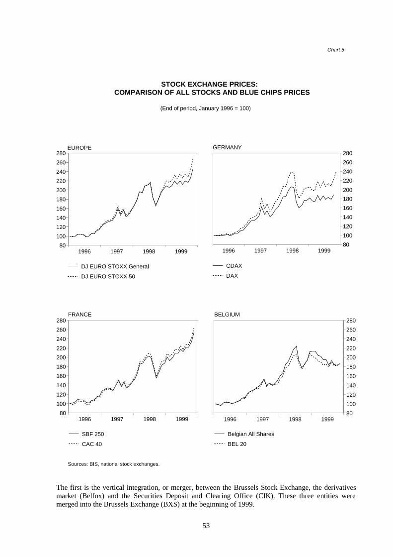
53
80
100
120
140
160
180
200
220
240
260
280
1996 1997 1998 199980
100
120
140
160
180
200
220
240
260
280
1996 1997 1998 1999
80
100
120
140
160
180
200
220
240
260
280
1996 1997 1998 199980
100
120
140
160
180
200
220
240
260
280
1996 1997 1998 1999
FRANCE
EUROPE
CDAX
DAXDJ EURO STOXX 50
SBF 250
CAC 40
Belgian All Shares
BEL 20
Chart 5
(End of period, January 1996 = 100)
GERMANY
BELGIUM
DJ EURO STOXX General
Sources: BIS, national stock exchanges.
STOCK EXCHANGE PRICES:COMPARISON OF ALL STOCKS AND BLUE CHIPS PRICES
The first is the vertical integration, or merger, between the Brussels Stock Exchange, the derivativesmarket (Belfox) and the Securities Deposit and Clearing Office (CIK). These three entities weremerged into the Brussels Exchange (BXS) at the beginning of 1999.
54
The second trend is that of demutualisation. The BXS has been set up as a public limited companywhose board is partly made up of independent directors. This structure protects the exchange againstthe risk of a fluctuation in capital, inherent in a cooperative setup, and allows a subsequent offering ofcapital to third parties, or even a listing.
The third trend is the establishment of ties between European exchanges. The Brussels StockExchange became involved in this process at a very early stage, first by participating in the foundingof Euro-NM (see above) and second by concluding a cross-membership agreement with the two otherBenelux exchanges in 1998. Finally, the Brussels Stock Exchange is party to the decision takenrecently by eight European exchanges to organise a common listing of leading European stocks.
It would, however, be wrong to concentrate exclusively on the locational aspect of stock markets. Thenew electronic trading systems are in any case likely to greatly reduce the relevance of geography. Theimportant thing is not the physical location of the quotation and trade processing systems. True addedvalue for an economy lies in intermediation, brokerage and particularly financial and market analysis.Much more than the existence of a stock exchange, maintaining and extending a market requires thepresence of institutional investors, venture capitalists and M&A consultancy and financing specialists.
In this respect, the handicap of the small number of very big companies listed on the Brussels StockExchange appears to be relative since the processing of transactions involving leading Europeanequities is eventually likely to become centralised on one dominant major exchange. The challenge istherefore to develop expertise that would make it possible to provide a broad range of financialservices to companies of comparable size to those which make up the major part of the Belgiancorporate structure.
5. Conclusions
Belgian individuals certainly did not wait for the introduction of the euro before purchasing financialassets abroad. Tax considerations in addition to the desire to diversify and the quest for higher returnsencouraged investors to invest in foreign currencies.
These capital movements were a significant constraint on the balance of payments, given Belgium’sfixed exchange rate objective. To counterbalance these outflows, the current account surplus had to besupplemented with offsetting capital inflows, which were of two main types. The first category wasdirect investments, which were reflected in an increase in the holding of Belgian equities by non-residents. The second consisted of government securities in foreign currency, issued principallyabroad, unlike franc-denominated public debt, which was almost exclusively placed in the domesticmarket.
The two big Belgian securities markets, the stock market and the government securities market, havethus been partly shaped by the exchange rate constraint. Although this has now been eliminated by theadvent of EMU, a new requirement has taken its place: ensuring the harmonious incorporation ofBelgian markets into the euro area or, more specifically, reconciling the double objective ofguaranteeing Belgian investors and borrowers the best financing conditions and preserving, inBelgium, the source of returns and activity provided by domestic markets and intermediaries.
As a government entity and principal borrower on the market, the Treasury is particularly affected bythis trade-off. A somewhat different trade-off arises with short- and long-term government securities.On the treasury certificate market, the Belgian Treasury benefits from a certain rarity factor in view ofthe insignificance of short-term public debt in most of the other euro area countries. With thisadvantage, it has been possible to slightly improve financing conditions owing to the advent of EMU,particularly since liquidity and credit risk are of little importance for this end of the maturity spectrum.
The same cannot be said for the long end, where the two criteria just mentioned are of majorimportance. It is on 10-year maturities, the bond markets’ benchmark, that these two variables havehad the most marked effects. The spreads between bunds and other euro area government paper

55
(including Belgian OLOs) are highest for 10-year bonds and have, moreover, tended to increase overthe last two years. A first possible measure for the Treasury is to seek out certain niches (floating rateinstruments, issues at other maturities, etc.). A second is to further open up the market to foreigninvestors, which leads back to the trade-off between improving financing conditions and promotingfinancial activity in Belgium.
On the stock market, securities are evidently more heterogeneous. The challenge posed by integrationinto the euro area is therefore presented in different terms. Interpreting recent price movements is alsomore complex and more hazardous to relate to the introduction of the single currency.
One fact emerges clearly. After varying in unison with European, German and French stock indicesfrom 1996 to 1998, Belgian indices diverged very markedly during the first half of 1999. Economic orstructural factors alone do not seem able to fully explain this divergence, so that its coinciding with thestart of EMU raises questions about the potential role of the euro.
The single currency has encouraged many Belgian investors, both private and institutional, to furtherdiversify their equity portfolios within the euro area. Although it is probable that a readjustment in theopposite direction has also been made by the residents of other European countries, this offsettingmovement has been dampened by a lack of major equities on the Brussels Stock Exchange. Thiswould partly explain why Belgian stock indices have moved much less favourably than thecorresponding indices elsewhere in the euro area. The asymmetry in diversification operationsweighed all the more on the prices of Belgian stocks since a substantial portion is closely held.
These developments are no doubt temporary, as systematic undervaluation is hardly conceivable in anefficient market. However, they do highlight some of the handicaps of the Brussels Stock Exchange interms of big name stocks and stock liquidity.
Reflections on the future of the Belgian stock market must therefore go beyond the problem of bluechips, which are in any case likely to end up listed on one dominant major stock exchange. They musteven go beyond the mere notion of a stock exchange. On the financial markets, added value is notobtained chiefly by maintaining a quotation and trade processing system, but first and foremost fromanalysis, consultancy and financing, activities which the existence of a local stock exchange can, atbest, serve to support and stimulate.

56
Bibliography
Abraham, J-P and A-F Pirard (1999): “Competition and cooperation among European exchanges: Theimpact of financial globalisation with special reference to smaller-sized exchanges”. Mimeo presentedat the 1999 Annual Meeting of the European Association of University Teachers in Banking andFinance, Lisbon, September.
Gehrig, T (1998): “Cities and the geography of financial centres”. Centre for Economic PolicyResearch, No. 1894, June.
Lefebvre, O (1999): “Bourses: entre fusions et alliances?” Revue de la Banque, pp. 251–4, June.
de Montpellier, L (1999): “La gestion de la dette publique belge dans la perspective de l’euro”. Revuede la Banque, pp. 192–7, May.
OECD, Economic Department (1999): “Public debt management in WP3 economies: recentdevelopments and policy considerations”. ECO/CPE/WP3, (99)8, September.
Padoa-Schioppa, T, K Lannoo and D Gros (1998): “Capital markets and EMU: Report of a CEPSWorking Party”. Center for European Policy Studies.
Rapport 1998 Fonds des Rentes (Belgium).
Revue économique de la Banque Nationale de Belgique (1998): “Le marché financier belge à la veillede l'Union économique et monétaire”, pp. 33–67, May.
Roëll, A (1998): “Competition among European Exchanges: Recent Developments”, in G Ferrarini(ed.); European Securities Markets: The Investment Services Directive and Beyond, Kluwer LawInternational, pp. 213–24.
Van Waterschoot, J (1998): “Het aandeelhouderschap na de veldslag”. BBL, Financiële berichtenNo. 2336, November.

57
The globalisation of financial markets and monetary policy
Hitoshi Sasaki, Satoshi Yamaguchi and Takamasa Hisada1
1. Introduction
It has been said that the recent globalisation of financial markets has been driven by increasing capitalmobility among countries. Hence, we should consider what kind of impact the globalisation offinancial markets has had on the effectiveness of monetary policy.
Looking at the movements of real long-term interest rates in the seven main industrialised countries,G72, it would seem that they have been equalising since the late 1980s.3 And if this phenomenonreflects the equalisation of asset returns because of the global integration of financial markets, wecannot deny the effect in respect of the conduct of monetary policy. This is because monetary policyaffects the real economy through various channels and, as one of these channels, the changing of theshort-term interest rate by the central bank has an effect on domestic real economic conditions throughits influence on the long-term interest rate. If the domestic real long-term interest rate converges tothose of other countries, it will be more difficult for monetary policy to affect the long-term interestrate, and consequently its effects on the domestic real economy will be weakened.
Table 1Difference in real long-term interest rate of each country and mean of the other countries
Sample period US JP DE UK FR IT CA
1993Q1–1997Q4 2.04 4.52 3.04 4.80 1.33 3.63 1.66
1980Q1–1989Q4 1.14 1.65 1.52 1.76 1.42 1.75 1.53
1990Q1–1997Q4 1.00 1.03 0.97 0.84 0.85 2.11 0.99
Note: Figures represent the standard deviation of the real long-term interest rate of each country minus the mean of theother countries.
However, some previous studies have indicated that world capital markets are still far from perfectlyintegrated. In fact, monetary policy has seemingly influenced domestic long-term interest rates. Inaddition, many studies have pointed out that the phenomenon of “home bias”, which means thepreference of domestic investors to hold domestic assets, has been observed in many countries’markets in spite of globalisation.4 The observations of home bias indicate that arbitrage transactions 1
Members of the Policy Research Division, Policy Planning Office, Bank of Japan. The views expressed in this paper arethose of the authors and do not necessarily reflect those of the Bank of Japan. The comments of our colleagues fromvarious sections materially improved this paper. Any remaining errors are of course our own.
2The United States, Japan, Germany, the United Kingdom, France, Italy and Canada (referred to as MI-7 in the graphs).
3The movements of G7 real long-term interest rates are plotted in Chart 1. The standard deviations of differences in thereal long-term interest rate of each country and the mean values of other countries’ rates are smaller in the 1980s and1990s than the 1970s, except for some countries and periods (Table 1).
4Most of the analyses dealing with home bias focus on the stock markets. For example, French and Poterba (1991) tried tomeasure investors’ portfolios and expected asset returns in three countries, the United States, Japan and the UnitedKingdom, based on several assumptions. Results indicate that (1) domestic stocks account for the greatest weight in theirportfolios: i.e. 94% for the United States, 98% for Japan and 82% for the United Kingdom, and (2) investors in thesecountries expect the highest returns from their own country’s stocks. For example, Japanese investors expect a return of6.6% from their domestic stock markets, which is about 3 points higher than the figures of 3.2% for US investors and3.8% for UK investors. Other analyses focusing on home bias include Tesar and Werner (1992), Frankel (1993) andKang and Stultz (1995).
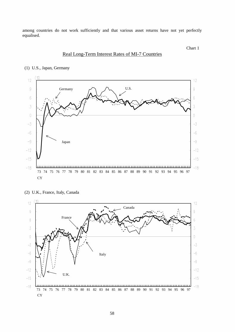
58
among countries do not work sufficiently and that various asset returns have not yet perfectlyequalised.
Real Long-Term Interest Rates of MI-7 CountriesChart 1
(1) U.S., Japan, Germany
Germany U.S.
Japan
73 74 75 76 77 78 79 80 81 82 83 84 85 86 87 88 89 90 91 92 93 94 95 96 97
CY
(2) U.K., France, Italy, Canada
France
Canada
U.K.
Italy
73 74 75 76 77 78 79 80 81 82 83 84 85 86 87 88 89 90 91 92 93 94 95 96 97
CY
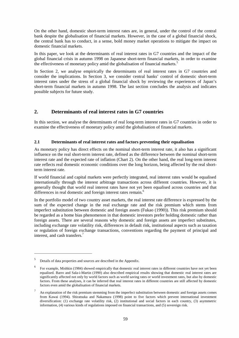
59
On the other hand, domestic short-term interest rates are, in general, under the control of the centralbank despite the globalisation of financial markets. However, in the case of a global financial shock,the central bank has to conduct, in a sense, bold money market operations to mitigate the impact ondomestic financial markets.
In this paper, we look at the determinants of real interest rates in G7 countries and the impact of theglobal financial crisis in autumn 1998 on Japanese short-term financial markets, in order to examinethe effectiveness of monetary policy amid the globalisation of financial markets.5
In Section 2, we analyse empirically the determinants of real interest rates in G7 countries andconsider the implications. In Section 3, we consider central banks’ control of domestic short-terminterest rates under the stress of a global financial shock by reviewing the experiences of Japan’sshort-term financial markets in autumn 1998. The last section concludes the analysis and indicatespossible subjects for future study.
2. Determinants of real interest rates in G7 countries
In this section, we analyse the determinants of real long-term interest rates in G7 countries in order toexamine the effectiveness of monetary policy amid the globalisation of financial markets.
2.1 Determinants of real interest rates and factors preventing their equalisation
As monetary policy has direct effects on the nominal short-term interest rate, it also has a significantinfluence on the real short-term interest rate, defined as the difference between the nominal short-terminterest rate and the expected rate of inflation (Chart 2). On the other hand, the real long-term interestrate reflects real domestic economic conditions over the long horizon, being affected by the real short-term interest rate.
If world financial and capital markets were perfectly integrated, real interest rates would be equalisedinternationally through the interest arbitrage transactions across different countries. However, it isgenerally thought that world real interest rates have not yet been equalised across countries and thatdifferences in real domestic and foreign interest rates remain.6
In the portfolio model of two country asset markets, the real interest rate difference is expressed by thesum of the expected change in the real exchange rate and the risk premium which stems fromimperfect substitution between domestic and foreign assets (Fukao (1990)). This risk premium shouldbe regarded as a home bias phenomenon in that domestic investors prefer holding domestic rather thanforeign assets. There are several reasons why domestic and foreign assets are imperfect substitutes,including exchange rate volatility risk, differences in default risk, institutional aspects such as taxationor regulation of foreign exchange transactions, conventions regarding the payment of principal andinterest, and cash transfers.7
5
Details of data properties and sources are described in the Appendix.
6For example, Mishkin (1984) showed empirically that domestic real interest rates in different countries have not yet beenequalised. Barro and Sala-i-Martin (1990) also described empirical results showing that domestic real interest rates aresignificantly affected not only by world factors such as world saving rates or world investment rates, but also by domesticfactors. From these analyses, it can be inferred that real interest rates in different countries are still affected by domesticfactors even amid the globalisation of financial markets.
7An explanation of the risk premium stemming from the imperfect substitution between domestic and foreign assets comesfrom Kawai (1994). Shiratsuka and Nakamura (1998) point to five factors which prevent international investmentdiversification: (1) exchange rate volatility risk, (2) institutional and social factors in each country, (3) asymmetricinformation, (4) various kinds of regulations imposed on financial transactions, and (5) sovereign risk.
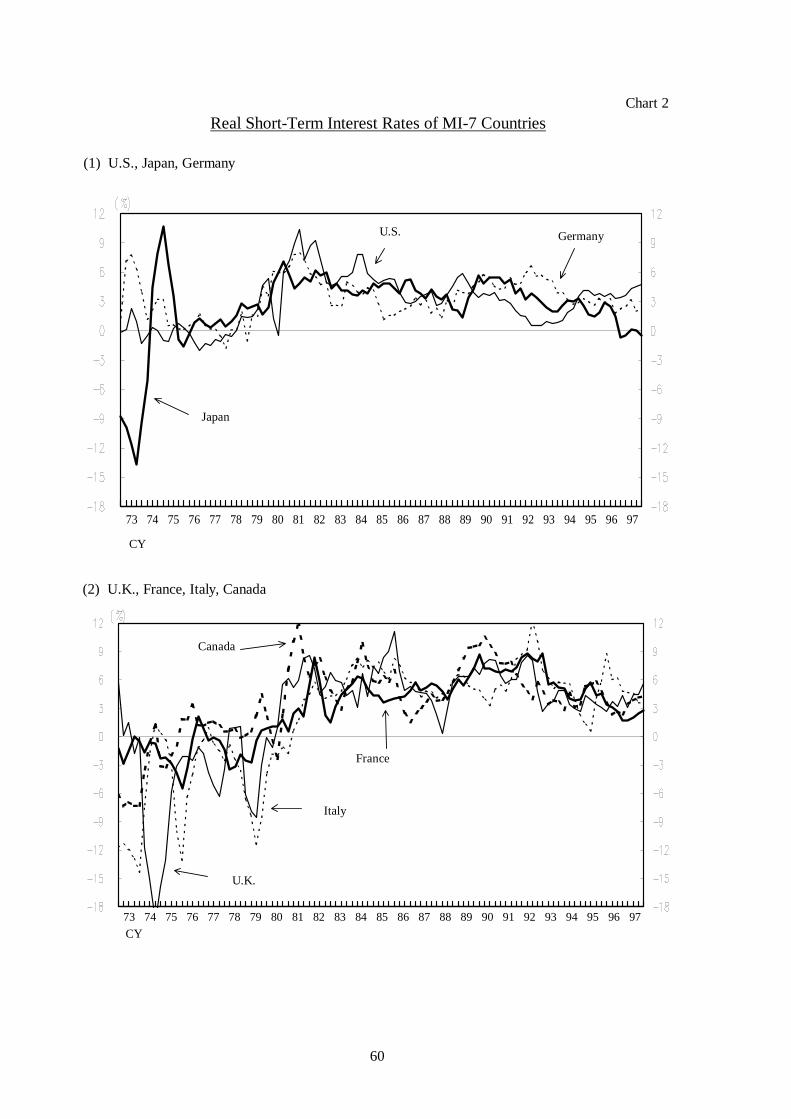
60
Chart 2
GermanyU.S.
Japan
73 74 75 76 77 78 79 80 81 82 83 84 85 86 87 88 89 90 91 92 93 94 95 96 97
CY
France
Canada
U.K.
Italy
73 74 75 76 77 78 79 80 81 82 83 84 85 86 87 88 89 90 91 92 93 94 95 96 97
CY
(1) U.S., Japan, Germany
Real Short-Term Interest Rates of MI-7 Countries
(2) U.K., France, Italy, Canada
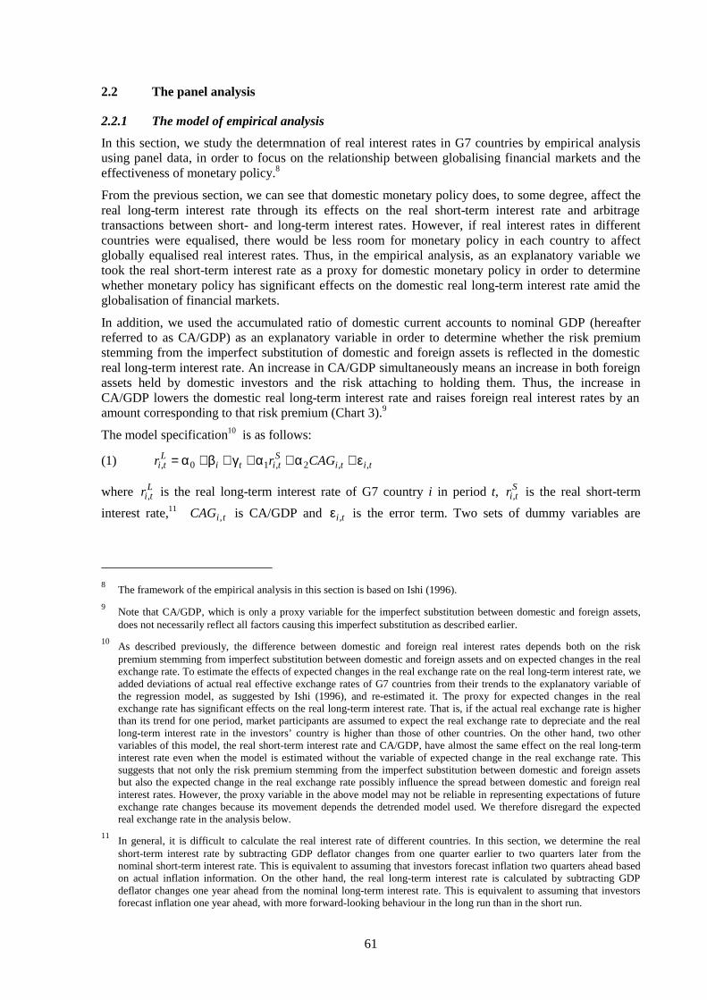
61
2.2 The panel analysis
2.2.1 The model of empirical analysis
In this section, we study the determnation of real interest rates in G7 countries by empirical analysisusing panel data, in order to focus on the relationship between globalising financial markets and theeffectiveness of monetary policy.8
From the previous section, we can see that domestic monetary policy does, to some degree, affect thereal long-term interest rate through its effects on the real short-term interest rate and arbitragetransactions between short- and long-term interest rates. However, if real interest rates in differentcountries were equalised, there would be less room for monetary policy in each country to affectglobally equalised real interest rates. Thus, in the empirical analysis, as an explanatory variable wetook the real short-term interest rate as a proxy for domestic monetary policy in order to determinewhether monetary policy has significant effects on the domestic real long-term interest rate amid theglobalisation of financial markets.
In addition, we used the accumulated ratio of domestic current accounts to nominal GDP (hereafterreferred to as CA/GDP) as an explanatory variable in order to determine whether the risk premiumstemming from the imperfect substitution of domestic and foreign assets is reflected in the domesticreal long-term interest rate. An increase in CA/GDP simultaneously means an increase in both foreignassets held by domestic investors and the risk attaching to holding them. Thus, the increase inCA/GDP lowers the domestic real long-term interest rate and raises foreign real interest rates by anamount corresponding to that risk premium (Chart 3).9
The model specification10 is as follows:
(1) titiStiti
Lti CAGrr ,,2,10, ε+α+α+γ+β+α=
where Ltir , is the real long-term interest rate of G7 country i in period t, S
tir , is the real short-term
interest rate,11 tiCAG , is CA/GDP and ti,ε is the error term. Two sets of dummy variables are
8
The framework of the empirical analysis in this section is based on Ishi (1996).
9Note that CA/GDP, which is only a proxy variable for the imperfect substitution between domestic and foreign assets,does not necessarily reflect all factors causing this imperfect substitution as described earlier.
10As described previously, the difference between domestic and foreign real interest rates depends both on the riskpremium stemming from imperfect substitution between domestic and foreign assets and on expected changes in the realexchange rate. To estimate the effects of expected changes in the real exchange rate on the real long-term interest rate, weadded deviations of actual real effective exchange rates of G7 countries from their trends to the explanatory variable ofthe regression model, as suggested by Ishi (1996), and re-estimated it. The proxy for expected changes in the realexchange rate has significant effects on the real long-term interest rate. That is, if the actual real exchange rate is higherthan its trend for one period, market participants are assumed to expect the real exchange rate to depreciate and the reallong-term interest rate in the investors’ country is higher than those of other countries. On the other hand, two othervariables of this model, the real short-term interest rate and CA/GDP, have almost the same effect on the real long-terminterest rate even when the model is estimated without the variable of expected change in the real exchange rate. Thissuggests that not only the risk premium stemming from the imperfect substitution between domestic and foreign assetsbut also the expected change in the real exchange rate possibly influence the spread between domestic and foreign realinterest rates. However, the proxy variable in the above model may not be reliable in representing expectations of futureexchange rate changes because its movement depends the detrended model used. We therefore disregard the expectedreal exchange rate in the analysis below.
11In general, it is difficult to calculate the real interest rate of different countries. In this section, we determine the realshort-term interest rate by subtracting GDP deflator changes from one quarter earlier to two quarters later from thenominal short-term interest rate. This is equivalent to assuming that investors forecast inflation two quarters ahead basedon actual inflation information. On the other hand, the real long-term interest rate is calculated by subtracting GDPdeflator changes one year ahead from the nominal long-term interest rate. This is equivalent to assuming that investorsforecast inflation one year ahead, with more forward-looking behaviour in the long run than in the short run.
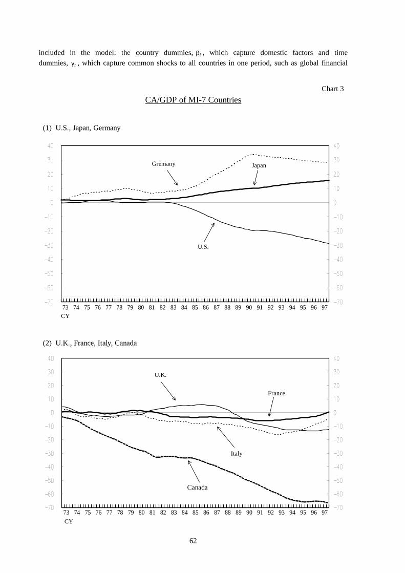
62
included in the model: the country dummies, iβ , which capture domestic factors and timedummies, tγ , which capture common shocks to all countries in one period, such as global financial
Gremany
U.S.
Japan
73 74 75 76 77 78 79 80 81 82 83 84 85 86 87 88 89 90 91 92 93 94 95 96 97
Chart 3
CY
France
Canada
U.K.
Italy
73 74 75 76 77 78 79 80 81 82 83 84 85 86 87 88 89 90 91 92 93 94 95 96 97
CY
CA/GDP of MI-7 Countries
(1) U.S., Japan, Germany
(2) U.K., France, Italy, Canada

63
shocks.12 The parameter for CA/GDP, 2α , is expected to be negative theoretically. In this empiricalanalysis, we estimate the above regression model for three periods using quarterly data.13 The firstperiod, 1973Q1–1980Q4, is characterised by acceleration of inflation, the second period, 1981Q1–1986Q4, by deceleration of inflation, and the third period, 1987Q1–1997Q4, by price stability. Wealso estimate the model using the rolling regression method with 10-year window to investigate howthe estimated parameters change in different sample periods.
2.2.2 Estimation results and implications
The results of the empirical analyses are shown in Table 2 and Chart 4-3. In the following, we discussthe main results and the implications.
(1) The real short-term interest rate, a proxy variable for monetary policy, significantly affects thereal long-term interest rate in all sample periods, which implies that domestic monetary policyalso has a significant effect on it even amid the globalisation of financial markets.
Table 2Estimation results of panel analysis(results for three sample periods)
Sample period from 1973Q1 to 1980Q4
Dependent variable: real long-term interest rate
Explanatory variable OLS One-way fixedeffect
One-wayrandom effect
Two-way fixedeffect
Two-wayrandom effect
Constant term 0.193 0.092 –0.085 0.029
(0.95) (0.30) (0.52) (0.08)
Real short-term interestrate
0.748**
(17.84)
0.622**
(13.02)
0.691**
(15.90)
0.515**
(12.62)
0.617**
(16.73)
CA/GDP 0.029 –0.105* –0.002 0.016 0.016
(1.11) (1.91) (0.04) (0.35) (0.51)
Lagrange multiplier test:One-and two-wayrandom effect vs OLS
13.86
(0.00)
61.42
(0.00)
Hausman test:One-way fixed vs one-way random effect
12.31
(0.00)
38.19
(0.00)
Adjusted R-squared 0.588 0.633 0.773
Hypothesis test (p-values are in parentheses)
Likelihoodratio test: x2
F-test
One-way fixed effectvs OLS
32.52(0.00)
5.51(0.00)
Two-way fixed effectvs OLS
176.35(0.00)
5.80(0.00)
Two-way fixed effectvs one-way fixed effect
144.30(0.00)
5.37(0.00)
12
The country and time dummies are included in all sample periods because statistical tests reject the null hypothesis thatthey are equal to zero.
13The historical movements of three variables in the model, the domestic real long-term interest rate, the real short-terminterest rate and CA/GDP of the relevant G7 country, are shown in Charts 1 to 3.
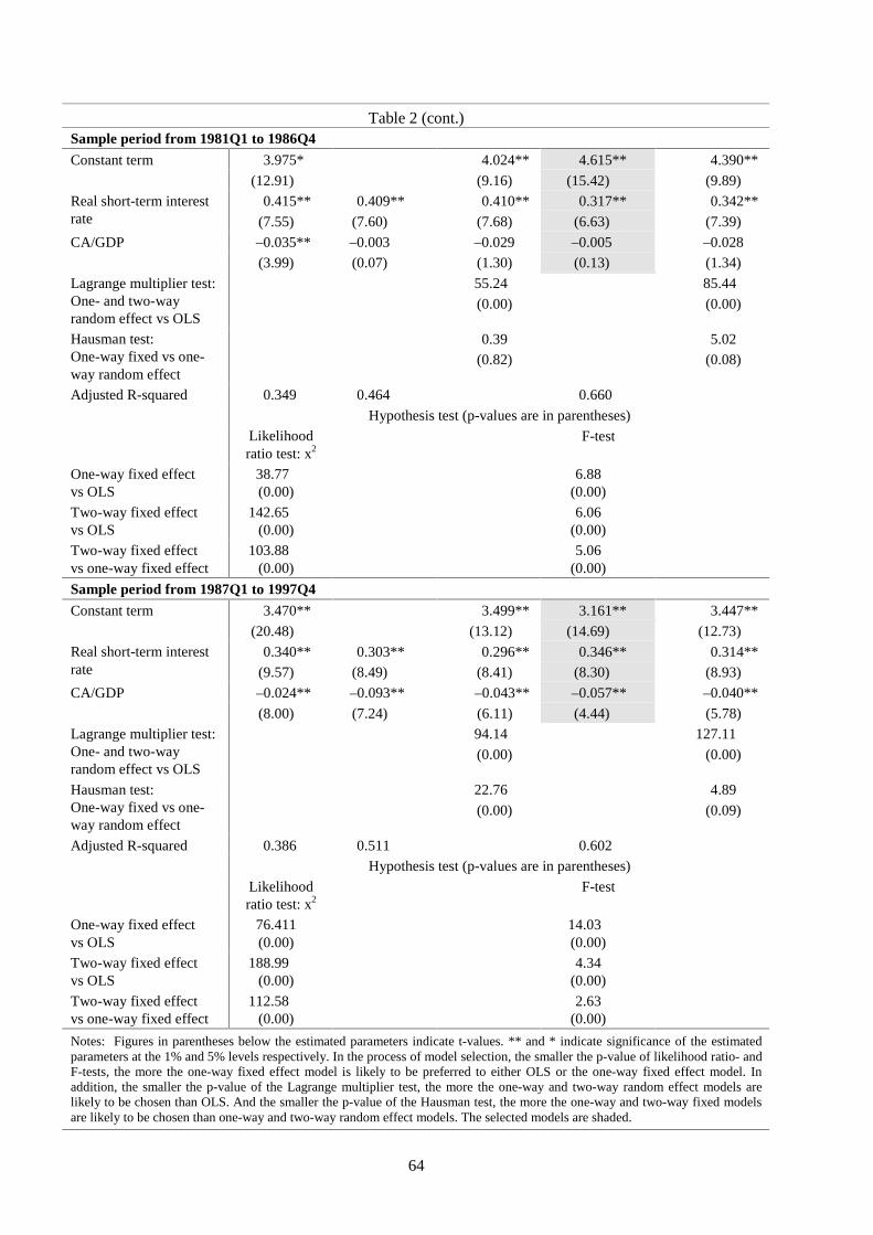
64
Table 2 (cont.)Sample period from 1981Q1 to 1986Q4
Constant term 3.975* 4.024** 4.615** 4.390**
(12.91) (9.16) (15.42) (9.89)
Real short-term interestrate
0.415**
(7.55)
0.409**
(7.60)
0.410**
(7.68)
0.317**
(6.63)
0.342**
(7.39)
CA/GDP –0.035** –0.003 –0.029 –0.005 –0.028
(3.99) (0.07) (1.30) (0.13) (1.34)
Lagrange multiplier test:One- and two-wayrandom effect vs OLS
55.24
(0.00)
85.44
(0.00)
Hausman test:One-way fixed vs one-way random effect
0.39
(0.82)
5.02
(0.08)
Adjusted R-squared 0.349 0.464 0.660
Hypothesis test (p-values are in parentheses)
Likelihoodratio test: x2
F-test
One-way fixed effectvs OLS
38.77(0.00)
6.88(0.00)
Two-way fixed effectvs OLS
142.65(0.00)
6.06(0.00)
Two-way fixed effectvs one-way fixed effect
103.88(0.00)
5.06(0.00)
Sample period from 1987Q1 to 1997Q4
Constant term 3.470** 3.499** 3.161** 3.447**
(20.48) (13.12) (14.69) (12.73)
Real short-term interestrate
0.340**
(9.57)
0.303**
(8.49)
0.296**
(8.41)
0.346**
(8.30)
0.314**
(8.93)
CA/GDP –0.024** –0.093** –0.043** –0.057** –0.040**
(8.00) (7.24) (6.11) (4.44) (5.78)
Lagrange multiplier test:One- and two-wayrandom effect vs OLS
94.14
(0.00)
127.11
(0.00)
Hausman test:One-way fixed vs one-way random effect
22.76
(0.00)
4.89
(0.09)
Adjusted R-squared 0.386 0.511 0.602
Hypothesis test (p-values are in parentheses)
Likelihoodratio test: x2
F-test
One-way fixed effectvs OLS
76.411(0.00)
14.03(0.00)
Two-way fixed effectvs OLS
188.99(0.00)
4.34(0.00)
Two-way fixed effectvs one-way fixed effect
112.58(0.00)
2.63(0.00)
Notes: Figures in parentheses below the estimated parameters indicate t-values. ** and * indicate significance of the estimatedparameters at the 1% and 5% levels respectively. In the process of model selection, the smaller the p-value of likelihood ratio- andF-tests, the more the one-way fixed effect model is likely to be preferred to either OLS or the one-way fixed effect model. Inaddition, the smaller the p-value of the Lagrange multiplier test, the more the one-way and two-way random effect models arelikely to be chosen than OLS. And the smaller the p-value of the Hausman test, the more the one-way and two-way fixed modelsare likely to be chosen than one-way and two-way random effect models. The selected models are shaded.
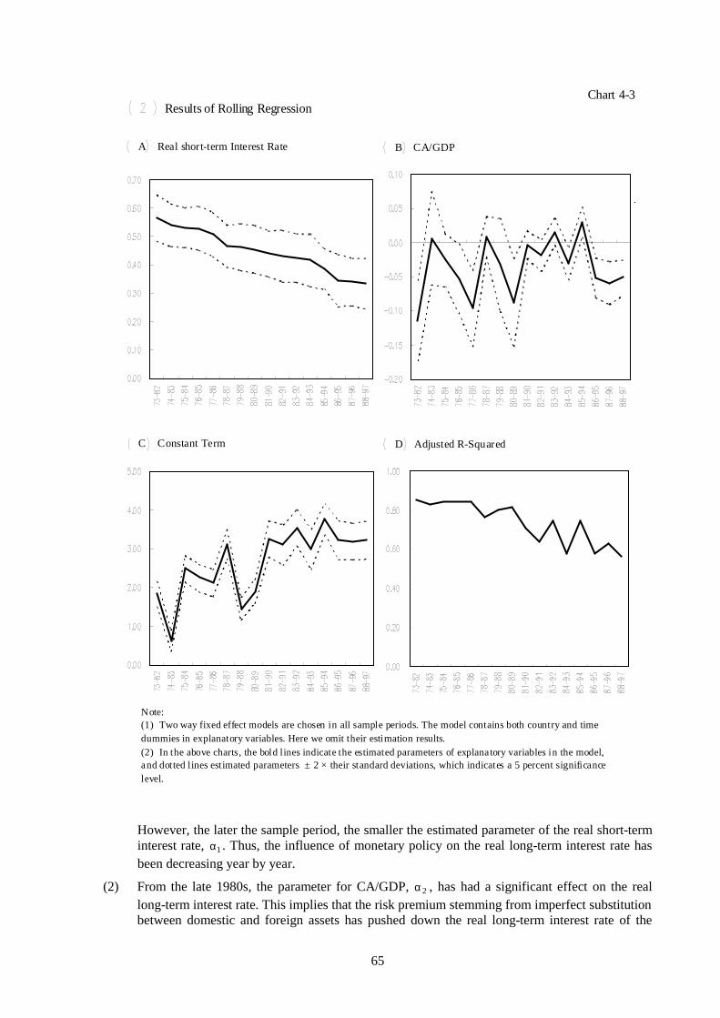
65
However, the later the sample period, the smaller the estimated parameter of the real short-terminterest rate, 1α . Thus, the influence of monetary policy on the real long-term interest rate hasbeen decreasing year by year.
(2) From the late 1980s, the parameter for CA/GDP, 2α , has had a significant effect on the reallong-term interest rate. This implies that the risk premium stemming from imperfect substitutionbetween domestic and foreign assets has pushed down the real long-term interest rate of the
Chart 4-3Results of Rolling Regression
Note:(1) Two way fixed effect models are chosen in all sample periods. The model contains both country and timedummies in explanatory variables. Here we omit their estimation results.(2) In the above charts, the bold lines indicate the estimated parameters of explanatory variables in the model,and dotted l ines estimated parameters ± 2 × their standard deviations, which indicates a 5 percent significancelevel.
A Real short-term Interest Rate B CA/GDP
C Constant Term D Adjusted R-Squared

66
country which holds net foreign assets, and pushed up that of the country which holds netforeign liabilities.14
In other words, this risk premium implies that the more foreign assets domestic investors have,the higher the returns they require for compensation for risks involved in holding such assets.
Note that the parameter for CA/GDP is significant only in the sample periods after the late1980s. This is because the current account imbalances in G7 countries were so small in the1970s and early 1980s that the effect of CA/GDP could not be extracted by empirical analysis,although the mechanism of home bias had possibly worked even in those periods. On the otherhand, as current account imbalances increased after the late 1980s, the phenomenon of homebias has become statistically significant.
(3) There seems to be little difference between the determinants of real long-term interest rates inJapan and the other G7 countries. This can be confirmed by decomposing the sum of squaredresiduals of the model into the part contributed by each country. Although the weightcontributed by Japan is higher than those of other countries except for the United Kingdom insample period 1, it is almost the same as them or rather lower in sample periods 2 and 3, asshown in Table 3. These facts suggest that the determinants of Japan’s real long-term interestrate are not necessarily much different from those in other G7 countries.
The fact that Japan’s real long-term interest rate is relatively lower than those of G7 countries inthe later periods is consistently explained by the following two factors: the low real short-terminterest rate, brought about by the Bank of Japan’s extremely easy monetary policy, and thelarge positive CA/GDP, which has held down Japan’s real long-term interest rate until now.
Table 3Analysis of sum of squared residuals of the model
Sample period US JP DE UK FR IT CA Sum of thesquared residuals
R-squared
(1) Contribution of each country1973Q1–1980Q4 0.84 4.46 1.83 7.04 0.81 2.33 1.28 18.59 81.41
1981Q1–1986Q4 2.39 4.05 2.43 5.29 3.77 3.02 6.55 27.50 72.50
1987Q1–1997Q4 2.49 2.69 3.11 5.46 4.03 12.10 3.14 33.02 66.98
Sample period US JP DE UK FR IT CA SUM
(2) Country weight1973Q1–1980Q4 4.54 23.98 9.86 37.85 4.37 12.53 6.87 100.00
1981Q1–1986Q4 8.68 14.73 8.82 19.24 13.72 10.98 23.82 100.00
1987Q1–1997Q4 7.53 8.16 9.42 16.53 12.22 36.64 9.51 100.00
Note: The contributions of each country to the sum of squared residuals of the model in (1) are multiplied by 100.
14
The risk premium imposed on holding foreign assets may include some sovereign risk of the country issuing theseforeign bonds. In this analysis, we tried to use the ratio of financial liability of general government to nominal GDP, as aproxy for sovereign risk, as the explanatory variable. However, we did not find evidence that the variable has asignificant effect on the real long-term interest rate.
67
3. Effects of the global financial crisis on Japanese financial markets inautumn 1998
Generally speaking, domestic short-term interest rates are likely to be under the control of the centralbank even given the globalisation of financial markets. However, can we say that the domestic short-term financial market is well controlled by the central bank in the event of global financial stress?
In autumn 1998, we observe that either a deterioration in the creditworthiness of Japanese financialinstitutions in the eyes of market participants or a credit contraction with a drying-up of dollarliquidity led to an increase in the Japan premium imposed on dollar fundings amid the global financialcrisis. As a result, Japanese short-term interest rates were exposed to upward pressure.
Below, we review the behaviour of Japanese financial institutions and arbitrage relationships amongsome financial markets in autumn 1998 (Section 3.1), and consider the Bank of Japan’s control overthe domestic short-term financial market (Section 3.2).
3.1 The Japan premium, market interest rates and the behaviour of financial institutions
The Japan premium15 (Chart 5), which reflects the differences in dollar funding costs of Japanese andforeign financial institutions, increased by 1 percentage point in autumn 1997, when the HokkaidoTakushoku Bank and Yamaichi Securities went bankrupt. Afterwards, although it decreased to 0.2points temporarily in May 1998, it began to quickly increase again and reached 0.91 points at thebeginning of November.16
According to market participants, the reason for the increase in the Japan premium in 1998 was thesame as in 1997 in that the creditworthiness of Japanese financial institutions had deteriorated, that is,solvency risk had heightened.17 However, the surge in autumn 1998 was probably affected by greaterdollar liquidity risk,18 which led to Japanese financial institutions finding it difficult to raise dollarfunds. Reasons were both a credit contraction and a drying-up of dollar liquidity in global financialmarkets that were caused by the Russian debt crisis – the depreciation of the Russian rouble andsubsequent debt moratorium – and the near-collapse of LTCM.
Faced with such a difficult financial situation, Japanese financial institutions tried to procure yen fundsin domestic and global financial markets and to convert them into dollar funds through yen/dollarswap transactions.19 Consequently, this added to the demand for yen funds, which were necessary foryen/dollar swap transactions. This, together with a rise in the risk premium attaching to yen fundingsof Japanese financial institutions, increased upward pressure on yen interest rates. The risk premiumfor raising yen funds, as given by the difference between the euroyen TIBOR and the risk-free yentreasury bill rate, widened from October to the beginning of November, as shown in Chart 6.
15
In this section, we define the Japan premium as three-month dollar TIBOR minus three-month dollar LIBOR.
16When Cosmo Credit Cooperative, Kizu Credit Cooperative and Hyogo Bank went bankrupt and the illegal transactions inthe New York branch of Daiwa Bank were exposed in 1995, the creditworthiness of Japanese financial institutionsdeteriorated and the Japan premium increased. For details of the Japan premium in autumn 1997, see Bank of Japan(1998).
17In 1998, the failure of LTCB, whose bankruptcy was rumoured in June and which was temporarily nationalised inOctober, and uncertainty over the passing of laws for the revitalisation of the financial system increased concerns aboutthe soundness of Japanese financial institutions and the entire Japanese financial system.
18Conceptually, the Japan premium is equal to the premium on the default risk of Japanese financial institutions comparedwith that of foreign financial institutions. The default risk is the sum of solvency risk and liquidity risk. However, it isquite difficult to directly observe solvency and liquidity risk.
19In this case, transactions in which Japanese financial institutions receive dollars and foreign financial institutions yen atthe start date, and Japanese financial institutions receive yen and foreign financial institutions dollars at thepredetermined forward exchange rate on the end date of the transactions.

68
The reason Japanese financial institutions engaged in a lot of yen/dollar swap transactions at that timeis that such transactions were easier than uncollateralised direct dollar fundings. This implies thatwhereas the supply side of dollar funds bears the counterparty’s default risk in uncollateralised
Japan PremiumDollar TIBOR Dollar LIBOR
Japan PremiumChart 5
Yen TIBOR Yen TB rate
Yen TIBOR
1998 1999
Chart 6Short-term Interest Rates
Note:3-month Dollar TIBOR and 3-month Dollar LIBOR.
Yen TB rate
Note:3-month Yen TIBOR and 3-month Dollar LIBOR.

69
transactions, in yen/dollar swap transactions, in which foreign financial institutions receive yen ascollateral, there is relatively less risk. Therefore, yen/dollar swap transactions provided a goodopportunity to raise dollar funds for Japanese financial institutions with relatively low credit ratings,which could hardly raise dollar funds without collateral.20
If Japanese financial institutions could have raised dollar funds smoothly through yen/dollar swaptransactions, the liquidity risk portion of the Japan premium would have been eliminated, although thesolvency risk portion would have partially remained. However, when the global financial crisisoccurred in autumn 1998, the suppliers of dollar funds, especially foreign financial institutions, tendedto restrict yen/dollar swap transactions with Japanese financial institutions.21 Hence, the difficultyfaced by Japanese financial institutions in procuring foreign currency was not eased immediately.
20
Chart 7 shows that yen/dollar swap turnover was more than yen/dollar spot turnover in autumn 1997 and autumn 1998, asHanajiri (1999) pointed out in his paper.
21Some possible factors explaining the behaviour of foreign financial institutions are as follows: first, profits of manyforeign financial institutions had deteriorated and their risk-taking capacity had weakened due to global financial shocksin autumn 1998. In addition, they experienced large volatility in the yen/dollar spot exchange rate, as shown in Chart 8,and had few opportunities to invest yen funds (obtained through yen/dollar exchange swap transactions with Japanesefinancial institutions) in risk-free assets (since there were insufficient risk-free assets, i.e. yen treasury and financing bills)in Japan’s short-term financial market (Hanajiri (1999)).
Yen/Dollar Spot Turnover Yen/Dollar Swap Tur nover
Billions dol lar
Yen/Dollar Spot and Yen/Dollar Swap Turnover
Chart 7

70
With the quantitative restriction, prices do not work efficiently to clear the markets. In autumn 1998,as foreign financial institutions restricted yen/dollar swap transactions, a distortion of arbitragetransactions between domestic and foreign interest rates was observed in short-term financial markets.As shown in Chart 9, the arbitrage relation between yen and the dollar risk-free rates, that is, yen and
Yen/Dollar Exchange Rate
Yen/ Dollar
Yen/Dollar Exchange Rate Volatili tyStandard Deviation from previous 20 days)
Yen/Dollar Exchange Rate and Volatility
Chart 8
Yen/Dollar Exchange rate
Yen/Dollar Exchange Rate Volatility
9/24News of Near Collapse of LTCM
8/17Russian Crisis
YenDepreciation
YenAppreciation
8/17Russian Crisis
9/24News of Near Collapse of LTCM
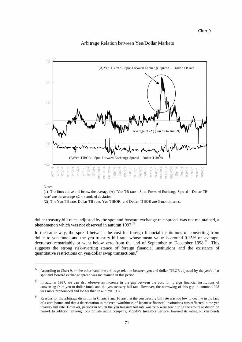
71
dollar treasury bill rates, adjusted by the spot and forward exchange rate spread, was not maintained, aphenomenon which was not observed in autumn 1997.22
In the same way, the spread between the cost for foreign financial institutions of converting fromdollar to yen funds and the yen treasury bill rate, whose mean value is around 0.15% on average,decreased remarkably or went below zero from the end of September to December 1998.23 Thissuggests the strong risk-averting stance of foreign financial institutions and the existence ofquantitative restrictions on yen/dollar swap transactions.24
22
According to Chart 9, on the other hand, the arbitrage relation between yen and dollar TIBOR adjusted by the yen/dollarspot and forward exchange spread was maintained in this period.
23In autumn 1997, we can also observe an increase in the gap between the cost for foreign financial institutions ofconverting from yen to dollar funds and the yen treasury bill rate. However, the narrowing of this gap in autumn 1998was more pronounced and longer than in autumn 1997.
24Reasons for the arbitrage distortion in Charts 9 and 10 are that the yen treasury bill rate was too low to decline in the faceof a zero bound and that a deterioration in the creditworthiness of Japanese financial institutions was reflected in the yentreasury bill rate. However, periods in which the yen treasury bill rate was zero were few during the arbitrage distortionperiod. In addition, although one private rating company, Moody’s Investors Service, lowered its rating on yen bonds
(A)Yen TB rate Spot-Forward Exchange Spread Dollar TB rate
(B)Yen TIBOR Spot-Forward Exchange Spread Dollar TIBOR
Average of (A) (Jan 97 to Jun 99)
Arbitrage Relation between Yen/Dollar Markets
Chart 9
Notes:(1) The lines above and below the average (A) "Yen TB rate Spot-Forward Exchange Spread Dollar TBrate" are the average ±2 × standard deviation.(2) The Yen TB rate, Dollar TB rate, Yen TIBOR, and Dollar TIBOR are 3-month terms.

72
issued and secured by the Japanese government from Aaa to Aa1 on 17 November 1998, distortion of the arbitragerelation had already been observed. Hence, we believe that this analysis are not affected by such factors.
(A) Conversion Cost from the Dollar to YenDollar LIBOR - Spot-Forward Exchange Spread
B) Yen TB rate
Average (Jan 97 to Jun 99)
Chart 10
Conversion Cost of Foreign Financial Institutions from the Dollar to Yen, and the Yen TB Rate.
Notes:(1) The lines above and below the average (A) "Conversion Cost of foreign financial institutions from theDollar to Yen" minus (B) "Yen TB rate" in the lower panel are average series ± 2 × standard deviation.(2) 3-month Yen TB rate and 3-month Dollar LIBOR.
Conversion Costs of Foreign Financial Institutionsfrom the Dollar to Yen and the Yen TB Rate
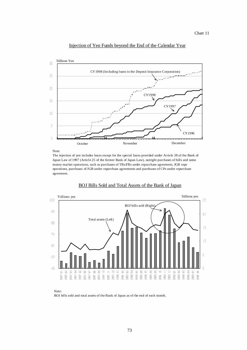
73
CY1998
CY1997
CY1996
Trillions Yen
CY1998 (Including loans to the Deposit Insurance Corporation)
Injection of Yen Funds beyond the End of the Calendar Year
Note:The injection of yen includes loans except for the special loans provided under Ar ticle 38 of the Bank ofJapan Law of 1997 (Article 25 of the former Bank of Japan Law), outright purchases of bills and somemoney mar ket operations, such as purchases of TBs/FBs under repurchase agreement, JGB repooperations, purchases of JGB under repurchase agreements and purchases of CPs under repurchaseagreement.
Chart 11
Trill ions yen Trillions yen
BOJ Bills Sold and Total Assets of the Bank of Japan
Note:BOJ bills sold and total assets of the Bank of Japan as of the end of each month.
BOJ bills sold (Right)
Total assets (Left)
October November December

74
3.2 Monetary policy operations of the Bank of Japan and their effects
In response to this tough financial situation, the Bank of Japan conducted money market operations byinjecting ample yen funds using instruments with relatively long maturities (beyond the end of thecalendar year) in order to mitigate the upward pressure on short-term yen interest rates.Simultaneously, the Bank absorbed excess yen funds by selling bills with short maturities in anattempt to prevent the overnight call rate, Japan’s interbank rate, from decreasing excessively(Chart 11; Bank of Japan (1999)). These money market operations had the following effects.
First, the injection of ample yen funds for conversion into dollar funds had a direct effect in mitigatingupward pressure on the short-term yen interest rates caused by the procurement of yen funds.
Second, the injection of ample yen funds implies that the Bank of Japan supplied these funds forJapanese financial institutions to convert into dollars. In this way, the Bank of Japan supportedJapanese financial institutions’ dollar financing. At this time, in fact, because foreign financialinstitutions restricted quantities in yen/dollar swap transactions, the difficulty of Japanese financialinstitutions in raising dollars was not completely eased. However, if it had not been for the Bank ofJapan’s money market operations, the Japanese financial situation might have been more confused.
Third, market participants complained that Japanese markets for risk-free yen assets, such as treasurybills and financing bills, were so small that foreign financial institutions were forced to restrictyen/dollar swap transactions (see footnote 21). In reality, excessive demand for treasury bills isevidenced by the fact that the treasury bill rate fell to zero at the beginning of November 1998. In thisrespect, the operations of the Bank of Japan to absorb excess yen by BOJ bill sales contributed toproviding risk-free yen assets to the market, and consequently led to the activation of yen/dollar swaptransactions. In fact, most of the buyers of these bills were foreign financial institutions (Shirakawa(1999)).
Lastly, the easing of dollar procurement by Japanese financial institutions, described above, seemed toreduce the default risk of Japanese financial institutions and the Japan premium. These effects alsoworked to reduce the short-term yen interest rate by decreasing the risk premium on yen funds.
From the above discussions, the money market operations of the Bank of Japan in autumn 1998, thatis, the aggressive injection of yen and BOJ bill sales, had some effect in mitigating upward pressure onyen interest rates induced by both the drying-up of dollar liquidity and the malfunction of swaptransactions. Nonetheless, it could not mitigate the increase in the Japan premium stemming fromsolvency risk.
In addition, global financial markets regaining stability after the interest rate reductions by the FederalReserve and increased confidence in Japan’s financial system following the enactment of financiallegislation enabled the short-term yen interest rate to decrease after mid-November.
4. Concluding remarks
In this paper, we analysed both the determinants of real interest rates in G7 countries and the impact ofthe global market crisis in autumn 1998 on Japan’s short-term financial market, in order to examinethe effectiveness of monetary policy amid the globalisation of financial markets.
From the empirical analysis of the determinants of real interest rates in G7 countries in Section 2, wefound that monetary policy has a significant effect on domestic real long-term interest rates, and thatthe risk premium stemming from the imperfect substitution between domestic and foreign assets alsohad a significant impact from the late 1980s. The latter indicates a home bias whereby domesticinvestors require higher returns for holding foreign assets. In addition, the determinants of Japan’s reallong-term interest rate are not much different from those in other countries. All this implies that thereal interest rates of different countries have not yet been equalised, and that monetary policy still hasa significant effect on the domestic economy through its influence on the real long-term interest ratesdespite the globalisation of financial markets.

75
However, it should be noted that the estimation results show that the direct effects of monetary policyon real long-term interest rates have been gradually weakening over time. In this respect, it isworthwhile to explore the effects of monetary policy on real long-term interest rates further, includingindirect effects through the risk premium.25
In Section 3, we considered the effects of the global financial crisis in autumn 1998 on Japan’s short-term financial market. The increase in the Japan premium and upward pressure on short-term yeninterest rates were aggravated by the contraction in dollar lending and swap transactions by foreignfinancial institutions, not to mention the erosion of Japanese financial institutions’ creditworthiness.These phenomena of credit contraction and the drying-up of dollar liquidity were observed in thedistortion of the arbitrage relation between Japanese and US short-term financial markets.
To tackle this situation, the Bank of Japan injected ample yen funds using instruments with relativelylong maturities (beyond the end of the calendar year) on one hand, and absorbed excess yen fundsthrough BOJ bill sales to prevent the overnight call rate from excessively decreasing on the other.These money market operations are likely to have contributed to mitigating upward pressures on theshort-term interest rate through the direct effect of the supply of yen funds and the indirect effect ofprompting Japanese financial institutions to convert yen into dollars, which consequently reduced theJapan premium and risk premium on yen funds.
25
According to the results of rolling regression, the adjusted-R squared falls from about 0.8 to 0.6 as in later sampleperiods. This suggests that the explanatory power of the real short-term interest rate and CA/GDP with respect to the reallong-term interest rate has been weakening. In this paper, we did not investigate further, however, it is important toconsider those factors amid the globalisation of financial markets.

76
Appendix
Determinants of the real interest rates in MI-7 countries
Data Content Source
Real long-terminterest rate
The real long-term interest rate is the nominal long-term interest rate minus inflation one year ahead.
Ltir , = L
tii , – [( 4, +tiP / tiP , ) – 1)]
where Ltir , is the real long-term interest rate of
country i in period t, Ltii , the nominal long-term
interest rate and tiP , the GDP deflator.
OECD, “NationalAccounts”, etc.
Real short-terminterest rate
The real short-term interest rate is the nominal short-term interest rate minus actual inflation from onequarter back to two quarters ahead.
Stir , = S
tii , – [( 2, +tiP / 1, −tiP ) 4 / 3 – 1)]
where Stir , is the real interest rate of country i in
period t, Stii , the nominal short-term interest rate and
tiP , the GDP deflator.
OECD, “NationalAccounts”, etc.
Nominal long-terminterest rate
United States: 10-year treasury notes.
Japan: 10-year government bonds.
Germany: 10-year government bonds
(before 1985Q4, government bonds with maturity of7–15 years).
United Kingdom: 20-year government bonds.
France: public and semi-public bonds.
Italy: 10-year government bonds.
Canada: over 10-year government bonds.
OECD, “Main EconomicIndicators”, etc.
Nominal short-terminterest rate
United States: three-month CD.
Japan: three-month CD. (before 1979Q2, two-monthbill rate)
Germany: three-month interbank rate.
United Kingdom: three-month interbank rate.
France: three-month PIBOR.
Italy: three-month interbank deposit rate.
Canada: 90-day deposit rate.
OECD, “Main EconomicIndicators”, etc.
Accumulated ratioof current accountsto nominal GDP
The accumulated ratio of each term’s currentaccounts to nominal GDP from 1970Q1.
IMF, “InternationalFinancial Statistics”,OECD, “Main EconomicIndicators”, etc.
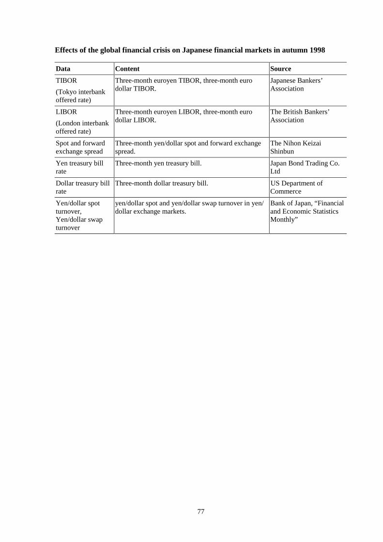
77
Effects of the global financial crisis on Japanese financial markets in autumn 1998
Data Content Source
TIBOR
(Tokyo interbankoffered rate)
Three-month euroyen TIBOR, three-month eurodollar TIBOR.
Japanese Bankers’Association
LIBOR
(London interbankoffered rate)
Three-month euroyen LIBOR, three-month eurodollar LIBOR.
The British Bankers’Association
Spot and forwardexchange spread
Three-month yen/dollar spot and forward exchangespread.
The Nihon KeizaiShinbun
Yen treasury billrate
Three-month yen treasury bill. Japan Bond Trading Co.Ltd
Dollar treasury billrate
Three-month dollar treasury bill. US Department ofCommerce
Yen/dollar spotturnover,Yen/dollar swapturnover
yen/dollar spot and yen/dollar swap turnover in yen/dollar exchange markets.
Bank of Japan, “Financialand Economic StatisticsMonthly”

78
Bibliography
Bank of Japan (1998): “Annual Review of Monetary and Economic Developments in Fiscal 1997”.Bank of Japan Annual Review, pp. 57-154.
Bank of Japan (1999): “Tsuuka Oyobi Kinyuu No Chousetsu Ni Kansuru Houkokusho (Report onMoney and Market Operations)”. June (in Japanese).
Barro R and X Sala-i-Martin (1990): “World Real Interest Rates”. NBER Macroeconomics Annual,pp. 15-74.
Frankel J (1993): “Quantifying International Capital Mobility in the 1980s”, in Frankel, J., OnExchange Rates, MIT Press.
French, K and J Poterba (1991): “Investor Diversification and International Equity Markets”.American Economic Review, 81, pp. 222-6, May.
Fukao, M (1990): “Jissen Zeminaru Kokusaikinyuu (International Economics and Finance)”. Toyo-keizai Sinposha, (in Japanese).
Hanajiri, T (1999): “Three Japan Premiums in Autumn 1997 and Autumn 1998 – Why did Premiumsdiffer between markets?” Financial Market Department Working Paper E-series 99-E-1, August.
Ishi, K (1996): “Jishitsukinri No Ketteiyouin Oyobi Kakkoku-Hikaku Ni Tsuite (The Determinants ofReal Interest Rate and Its Comparison among Countries)”. IMES Discussion Paper J-Series 96-J-18,Institute for Monetary and Economic Studies, Bank of Japan, (in Japanese).
Kang, J and R Stultz (1995): “Why is there a Home Bias? An Analysis of Foreign Portfolio EquityOwnership in Japan”. NBER Working Paper, No. 5166.
Kawai, M (1994): “Kinyuu Nyumon (Introduction to International Economics and Finance)”. TodaiShuppankai, (in Japanese).
Mishkin, F (1984): “Are Real Interest Rates Equal Across Countries? An Empirical Investigation ofInternational Parity Conditions”. Journal of Finance 39, pp. 1345-57, December.
Shirakawa, M (1999): “Nihon No Kokusaisijyou No Kinoukoujyou Ni Mukete (Suggestions for theImprovement of the JGB Market)”. Nihon Ginko Geppo (Bank of Japan Monthly Bulletin), June(in Japanese).
Shiratsuka, S and H Nakamura (1998): “Kokusai-Bunsantoushi Niokeru Homu-baiasu-pazuru WoMeguru Shoronten (The Home Bias Puzzle in International Investment Diversification)”. Monetaryand Economic Studies, 17(2), Institute for Monetary and Economic Studies, Bank of Japan,(in Japanese).
Tesar, L and I Werner (1992):: “Home Bias and the Globalisation of Securities Markets”. NBERWorking Paper, No. 4218.

79
Monetary policy implications of the international role of the euro
Nuno Cassola1
1. Introduction
The international role of the euro is drawing the attention of a growing number of academic andcentral bank economists. In fact, several studies have already been published focusing particularly onthe financial market implications of the emergence of the euro as an international currency.2 Theimplications that the internationalisation of the euro might have for the conduct of monetary policy bythe Eurosystem have received less attention. These are the focus of this paper.3 The main difficulty incarrying out such an analysis lies in clearly distinguishing the specific impact of theinternationalisation of the euro from other factors that may impact on monetary policy. Factors like theliberalisation and growing international integration of financial markets, and the changes resultingfrom Monetary Union itself affect the structure of the economy, the behaviour of the private sectorand, thus, may impact on monetary policy. Furthermore, technological changes in computing andtelecommunications, which occur largely independently but go hand in hand with the increasinginternational role of the euro, may also have implications for monetary policy. An additional difficultyis related to the lack of data, a fact that inhibits any reasonable empirical exploration of the subject atthe current stage. This study, thus, mainly focuses on conceptual and theoretical issues. The paper isorganised as follows. Section 2 briefly reviews the current use of the euro by non-euro area residentsand the factors that may affect the international use of the euro in the future. Section 3 addresses theimpact that the internationalisation of the euro might have on the transmission mechanism of monetarypolicy (Section 3.1) and on the monetary policy strategy of the Eurosystem (Section 3.2). The latterfocuses on money demand (Section 3.2.1), the role of the exchange rate (Section 3.2.2) and theinformation content of the yield curve (Section 3.2.3). Section 3.3 discusses some aspects relating tofinancial stability. The general implications of the internationalisation of the euro for monetary policyare summarised in Section 4.
2. The international role of the euro4
A currency that performs at least two of its three classical functions – unit of account, medium ofexchange and store of value – outside the country or area where it is issued, whether for private orofficial use, can be considered international money. The euro is the second most widely used currencyat the international level, behind the US dollar and ahead of the Japanese yen.5 This naturally reflectsthe legacy of the former national currencies of the euro area countries that have been replaced by the 1 Prepared by Nuno Cassola, of the Directorate Monetary Policy (DMP) in the Directorate General Economics (DG-E) of
the European Central Bank (ECB). Comments by Philippe Moutot, Wolfgang Schill, Hans-Joachim Klöckers, KlausMasuch and Nick Vidalis are gratefully acknowledged. The opinions expressed in this paper are those of the author anddo not necessarily represent those of the ECB.
2See, for example, IMF (1997a), Hartmann (1998) and Portes and Rey (1998).
3Discussions on this topic have mainly focused on the incentives to international policy coordination, as, for example,Alogoskoufis and Portes (1997) and Bergsten (1997), and on dollar/euro exchange rate volatility, as, for example,Bénassy-Quéré et al. (1997).
4 This section benefits from exchanges of views with Philipp Hartmann, in the Directorate General for Research (DG-R) of
the ECB, and Adrian Van Rixtel, in the DG-E of the ECB.
5For data on the current use of the euro by non-euro area residents, see ECB (1999d).

80
euro. There are four major factors determining the international role of a currency. The first is historyand inertia. One currency tends to be used internationally because others are expected to use it – thusthe analogy between the international use of a currency and the choice of English as the internationallanguage. This factor militates against a rapid expansion of the international role of the euro. Thesecond is the economic weight of the currency area, particularly in relation to world trade in goods andservices. Compared with the United States, the euro area accounts for a greater share of world exportsin goods and services, and in terms of GDP per capita the United States and the euro area arecomparable. These factors may contribute to the international role of the euro. The third factor isrelated to financial openness and development of the currency area. In this respect, although the euroarea has developed a larger banking sector, equity and debt securities markets are much larger in theUnited States. The introduction of the euro has fostered a process of structural change in the euro areafinancial and banking sectors that is expected to contribute to the international role of the euro. Thefourth factor is confidence in the value of the currency. The euro might have inherited the reputationof the most stable of the former currencies. Furthermore, the institutional design of the Eurosystem,granting it independence from political interference in pursuing stability-oriented monetary policy,enhances its credibility. Nevertheless, as the practice of central banking shows, only by developingand sustaining a track record of stability will the euro retain or enhance its attractiveness as aninternational currency.
The four factors mentioned above are related to two underlying economic determinants of theinternational role of a currency: size and risk. The first three – history, economic weight and financialdevelopment – are related to size and interact in a virtuous way to “perpetuate” the dominant positionof an international money. Stage Three of EMU acted as a catalyst for wide-ranging transformation inthe capital markets of the participating countries. Due to the interplay between network externalitiesand economies of scale, an integrated euro area capital market will surely exceed the sum of theconstituent parts in a fundamental way. In fact, through increased competitiveness and efficiency euroarea capital markets will become larger, with increasing liquidity, breadth and depth. This will tend tolower transaction costs (bid-ask spreads) and may facilitate the international use of the euro, which inturn will increase volume of trading in euro financial assets, further reduce transaction costs and,possibly, attract more market participants in a virtuous way. The fourth factor – monetary policyindependence and central bank credibility – interacting with the second and the third factors, will to alarge extent determine the volatility of returns of euro area financial assets and their correlation withreturns on investments denominated in other currencies. These characteristics create opportunities forportfolio diversification across currencies that contribute to reducing exposure to systemic risk andthus act like a “centrifugal” force counteracting the “centripetal” force of the size dimension.
Changes in invoicing and denomination practices in trade, and pricing in standardised and centralisedcommodity markets are likely to be very slow. Nevertheless, due to lower transaction costs in theforeign exchange market and, perhaps, the increasing ability of euro area exporters to use the euro forinvoicing and settlement, it is reasonable to expect a gradual expansion in the use of the euro as apayment/vehicle currency.
The factors mentioned above suggest that the international role of the euro will be determined bymarket forces in the context of increasing globalisation. There is a two-way relationship between thedepth and breadth of euro area financial markets and the international use of the euro.6 Theenlargement of the investor base provided by the internationalisation of the euro is likely to contributeto an expansion of both the quantity and diversity of securities issued by euro area residents.Consequently, trading activity in secondary financial markets could also be stimulated. Of particularrelevance could be the development of corporate bond markets and credit derivatives and the impetusgiven to securitisation. Such feedback from the internationalisation of the euro will contribute toenhancing overall liquidity in euro area capital markets, furthering the reduction of transaction costs.A mutually reinforcing process of financial development and internationalisation could take place.These phenomena may be additional factors in shaping the financial structure in the euro area. Inparticular, direct finance may gain relevance with a diminished role of banks.
6
See, for example, McCauley (1997).

81
3. Potential implications for monetary policy
Financial markets play a key role in the transmission mechanism, as they influence to a large extentthe effectiveness of the transmission mechanism of monetary policy. As indicated in Section 2, anenhanced international role of the euro may contribute to the creation of a broader, deeper and moreliquid financial market in the euro area. It will be characterised by lower transaction costs, furtherintegrated bond and to some extent equity markets, and possibly an enhanced role of direct financewith a larger role of private debt securities and equity markets. The impact of the international role ofthe euro on the transmission mechanism will also be determined by the impact of these features on thevarious channels of the transmission mechanism.
This section discusses the potential implications of the international role of the euro for the conduct ofmonetary policy by the Eurosystem. Two broad perspectives are taken. Firstly, we discuss the impactthat the international role of the euro may have on the transmission mechanism (Section 3.1).Secondly, we focus on whether the international role of the euro might affect the strategy of themonetary policy of the Eurosystem (Section 3.2). Financial stability issues, which are related to boththe transmission mechanism and the monetary policy strategy, are discussed in Section 3.3.
3.1 The transmission mechanism of monetary policy
Most economists agree that, in the short run, monetary policy actions can affect real output and otherreal economic variables. At the same time, in the long run, money is generally considered to beneutral. Nevertheless, there is broad agreement about the important contribution that monetary policyoriented towards maintaining price stability can make to improving economic prospects and raisingliving standards. There is, though, far less agreement on how precisely monetary policy exerts itsinfluence on the economy (i.e. the transmission mechanism). Due to the diversity of perspectives, thispaper does not follow any particular view about the transmission mechanism but, instead, tries to takeinto account the various approaches that have been put forward in the literature.7 After brieflyreviewing the theoretical basis for considering the different mechanisms, this section discusseswhether and how these might be affected by the internationalisation of the euro.
There are several channels through which changes in money and interest rates flow through toaggregate demand. These channels include interest rate effects, exchange rate effects and wealtheffects. Furthermore, one can make a distinction between the credit channel and the interest ratechannel that is mainly concerned with whether banks and bank lending play a special role in thetransmission mechanism.
Brief overview of the transmission mechanism
Monetary policy tightening is generally associated with a reduction of base money supply growth andhigher short-term nominal interest rates. Given price or inflation stickiness,8 following an increase innominal short-term interest rates real short-term interest rates rise as well. Additionally, longer-termreal interest rates might also rise slightly.9 These higher real interest rates change the opportunity cost
7
For a brief overview of the transmission mechanism, see, for example, Mishkin (1995) and the papers included in theJournal of Economic Perspectives, Vol. 9 (1995): 3-96. See also Dale and Haldane (1993) and IMF (1996). For a recentand comprehensive survey, see Walsh (1998).
8When prices are fully flexible, anticipated monetary policy might still impact on real activity. For example, anticipatedinflation, which acts like a tax on real balances, reduces the utility of the representative agent. Fully flexible price modelswill not be considered in this paper because of the weak empirical evidence supporting them. See Walsh (1998).
9Central bank credibility will be an important factor in the transmission mechanism. For example, if longer-run inflationexpectations are not firmly anchored, nominal interest rate changes may not be considered by the private sector aschanges in the real interest rate and consequently the private sector may not alter its demand for investment and/orconsumption. Furthermore, as central bank credibility may be subject to changes, the transmission mechanism may alsovary over time. This might be of particular relevance in the case of the internationalisation of the euro because theEurosystem’s policy actions will have to be understood by investors resident outside the euro area. These investors may

82
of borrowing funds to finance expenditure and will tend to lead to a decline in investment and,perhaps, consumption demand, which produces a decline in aggregate demand and output.10 Theintensity of these effects will depend on the extent of the transmission of official interest rate changesalong the yield curve and on the degree of the transmission of market interest rate changes to retaildeposit and loan interest rates.
An increase in official interest rates may also cause a decline in asset prices (equity, property), bychanging the discount rate of future earnings from holding assets. As a consequence, the market valueof firms will tend to fall in relation to the replacement cost of capital (Tobin’s q) and firms will haveless incentive to buy new investment goods because through takeovers they can buy existing capitalmore cheaply. Investment spending would thus be reduced. Wealth effects will also tend to lowerprivate consumption.
Furthermore, the quantitative importance of changes in interest rates via cash flow effects will dependon the leverage of the private sector and on the balance between short- and long-term debt in theliabilities of firms (and the asset of households) and the mixture of fixed versus floating rate debt.Generally, demand will be affected via cash flow effects of changes in interest rates in so far asborrowers and lenders have different marginal propensities to spend.
Banks may also play a special role in the transmission mechanism (credit channel) to the extent thatthey are particularly well suited to deal with the problem of screening and monitoring borrowers thathave limited access to capital markets (small or new firms and households).11 When monetary policytightening leads to decreasing bank reserves and higher funding costs, banks will reduce the supply oflending if loans and securities are not perfect substitutes.12 With banks reducing credit and firmsunable to easily substitute from bank loans to other sources of credit or retained earnings, theavailability of bank lending may have an independent impact on aggregate spending, reinforcing theimpact of interest rate increases. Spending in consumer durable goods and housing purchases may alsobe affected for similar reasons. The usual assumption in the literature is that if it exists, the banklending effect enhances the efficacy of monetary policy.
Asset price changes may lead to a decline in the net worth of firms, meaning that lenders, in effect,have less collateral for their loans. Consequently, banks will be less protected against shocks toborrowers’ balance sheets and against moral hazard, which may lead to decreased willingness of banksto lend to firms.13 An increase in official interest rates also causes deterioration in firms’ balancesheets because it reduces net cash flow, possibly at the time when retained earnings decline. Thebalance sheet effect will imply a more fragile financial position of the private sector and an increasedlikelihood of financial distress that leads to a decline in spending in investment.
The role of the exchange rate in the transmission mechanism can be briefly summarised. Higherdomestic (real) interest rates normally lead to an appreciation of the currency. The higher value of thecurrency makes goods produced in the country relatively more expensive than foreign goods, therebycausing a fall in net exports and hence in aggregate demand. Furthermore, currency appreciation willtend to lower import prices expressed in domestic currency, thus further dampening inflationarypressures in the economy.
have less information about euro area economic developments than residents or may have different views about theimplications of the Eurosystem’s monetary policy actions.
10The overall impact of interest rate changes on consumption is theoretically ambiguous due to offsetting income andsubstitution effects.
11In reality there is a spectrum of firms, from small to large, in the economy. With the deepening, broadening and greaterliquidity of euro capital markets, partly resulting from the internationalisation of the euro, more medium-sized firms mayactually gain access to capital markets.
12If they were perfect substitutes, banks would sell securities to maintain loan volumes.
13It does not imply quantitative credit rationing by banks. Price rationing through higher premiums over money marketinterest rates and/or other non-price borrowing terms (more collateral) may lead to a decrease in borrowing.

83
When discussing the implications of international capital market integration for US monetary policy, itis frequently emphasised that the internationalisation of finance changed the transmission mechanismby changing the effects of actual and anticipated exchange rate movements and thus enhancing the roleof the exchange rate.14
The impact of the internationalisation of the euro on the transmission mechanism: general aspects
(i) Quicker adjustment of market interest rates to official interest rate changes and morecompetition in banking
Should the internationalisation of the euro stimulate the development of a financial structure moredominated by direct finance, interest rates and wealth effects could gain more relevance in thetransmission mechanism, because financial market prices tend to react more rapidly to official interestrates than retail deposit and lending rates. Furthermore, facing increased competition, banks may haveto adjust their rates more promptly by changing interest rate spreads.
One can argue that it may become easier for domestic banks to attract funds from outside the euroarea, for example through the issuance of certificates of deposit, or to securitise their assets, forinstance mortgages. However, the ECB will continue to have sufficient control over short-term eurorates. Thus, banks would have to borrow in foreign currency if they would like to avoid higher rates,thus incurring exchange rate risks. Consequently, it is unlikely that the sensitiveness of banks’ assetsand liabilities to monetary policy actions will be significantly affected by availability of funds fromnon-residents.
Naturally, the internationalisation of the euro does not change the asymmetric information problemthat is at the root of the “special” role of banks. Thus, if the problems of screening and monitoringborrowers are not significantly affected by the internationalisation of the euro, small firms andhouseholds will continue to be constrained in their access to the (euro) capital markets. By contrast,for larger firms access to external finance will tend to be easier and less costly. Consequently, theinternationalisation of the euro may accentuate the differences in the ways in which the differentsectors of the economy react to changes in monetary policy. Additionally, for small firms andhouseholds, the international role of the euro is unlikely to be, in itself, a factor fostering major breaksin existing borrower-lender relationships.
(ii) Higher interest rate sensitivity of the economy
It also seems that the main factors that determine the strength of the interest rate channel in thetransmission mechanism are largely independent of the internationalisation of the euro. For example,increasing long-term borrowing at fixed rates by euro area firms might reflect expectations of pricestability or stem from structural changes in euro area capital markets resulting from Stage Three ofEMU.15
The internationalisation of the euro, however, may have an indirect effect on the interest rate channel.For example, if third countries successfully peg their exchange rates to the euro, there will be astronger impact of changes in euro area interest rates on interest rates outside the euro area. This inturn will have an impact on economic activity in these countries. Through its effect on euro areaexports to these countries, the interest rate channel will be reinforced, depending on the importance ofthe trade relations of the euro area with the countries that tie their exchange rates to the euro.
The transmission process of monetary policy via feedback effects through third countries will also beinfluenced by the role of the euro as an international investment currency and by the respective netasset position of other countries. For example, if a foreign country uses the euro mainly for thedenomination of short-term or floating debt, higher euro short-term rates would tend to dampendemand in that country. This effect will be compounded if borrowers or banks in these countries rely
14
See, for example, Friedman (1988), IMF (1997a) and Obstfeld and Rogoff (1995).
15Naturally, long-term borrowing at fixed interest rates will tend to shield debtors and creditors from changes in short-terminterest rates and thus, ceteris paribus, may reduce the efficacy of the cash flow effect of changes in interest rates.
84
heavily on the euro, whereas their assets are denominated in their local currency, in particular if thelatter significantly depreciates against the euro. The indirect impact of these developments on euroarea developments would again mainly depend on the degree of trade relations of the euro area withthe respective country.
(iii) Weaker exchange rate channel
An extensive use of the euro as invoice currency and as currency of denomination and settlement incommodity markets could make the euro area HICP less sensitive, in the short run, to US dollarexchange rate movements. Under these circumstances commodity price movements would convey abetter signalling of relative price changes for euro area producers and consumers and may help focusattention on the more fundamental and persistent factors underlying price trends. A widespread use ofthe euro as currency of denomination in commodity markets or as invoice currency could alsoinfluence the effects of exchange rate changes on the current account. If euro area exports and importsare increasingly invoiced in euros, the short-term effects of exchange rate changes on the trade balanceshould in general be reduced.
3.2 The monetary policy strategy of the Eurosystem
The primary objective of the Eurosystem is to maintain price stability in the euro area, as laid down inthe Treaty on European Union. To fulfil its mandate, the Governing Council of the European CentralBank has adopted a monetary policy strategy that is neither conventional monetary targeting nor directinflation targeting nor a simple mixture of the two.16 It is comprised of three elements: theannouncement of a quantitative definition of price stability (year-on-year increase of the HICP for theeuro area below 2%) and the so-called two pillars. The first pillar gives money a prominent role.17 Thesecond is a broadly based assessment of the outlook for price developments. Given that inflation isultimately a monetary phenomenon, monetary aggregates should provide a “nominal anchor” formonetary policy. Thus, a quantitative reference value of 4.5% for the growth rate of M3 wasannounced in December 1998. The second pillar of the strategy comprises an analysis of a wide rangeof indicator variables as well as the use of various forecasts of the outlook for price developments.18
In devising its strategy, the Eurosystem explicitly acknowledged that EMU represents an importantregime shift. Therefore, the uncertainty facing the Eurosystem concerning the indicator properties ofmonetary, financial and other economic variables for future price developments, and regarding privatesector reaction to monetary policy actions, is larger than has typically been the case in nationalcontexts in the past. Against this background, the Eurosystem eschews relying on a single indicator orintermediate target for the conduct of monetary policy.
The strategy aims at identifying those economic disturbances that threaten price stability andprompting a monetary policy response which is appropriate to both the prevailing economiccircumstances and the nature of the threat.
This section discusses whether the international role of the euro might affect the monetary policystrategy of the Eurosystem. It should be mentioned at the outset that the discussion does not aim atproviding a comprehensive review of the implications for all aspects of the strategy. Instead, thearguments reviewed have a narrower perspective centred on the monetary and financial aspects andimplications of the strategy. Therefore, a balanced review of the likely implications ofinternationalisation of the euro for the two pillars of the monetary policy strategy of the Eurosystem isnot undertaken in this paper.
16
For a detailed exposition of the monetary policy strategy of the Eurosystem, see ECB (1999a).
17See ECB (1999b).
18See ECB (1999c).
85
3.2.1 Stability of money demand
As mentioned in its monetary policy strategy, the ECB gives a prominent role to money with theannouncement of a reference value for the growth of a broad monetary aggregate (M3). A questionarises as to whether the growing internationalisation of the euro might have an impact on the stabilityand the information content of monetary aggregates, in particular of M3.
There is an extensive literature on the factors that may, in general, affect the indicator properties ofmoney and its implications for the conduct of monetary policy.19 Currency substitution and changes ineuro deposits held outside the euro area are factors that may impact on the signals of monetaryaggregates.
(i) Currency substitution in third countries
With its internationalisation the euro may play an enhanced role in some countries outside the euroarea, leading in particular to currency substitution in third countries. To the extent that it is held aseuro-denominated deposits by non-euro area residents, the broad aggregate M3 is not affected directly,as this aggregate only comprises holdings of euro area residents. Only the demand for euros in foreigncountries will directly impact on M3.20 However, as the M3 aggregate covers a broad range offinancial assets, the share of currency in circulation is relatively small. At the end of May 1999, itamounted to only 7%. While increases in banknotes in circulation abroad may affect the narrowmonetary aggregate M1, such currency substitution is less likely to be a major source of concernregarding the interpretation of the information content of the broad aggregate M3 in the euro areaunless it occurs very suddenly and, at the same time, no information on the reason for the highercurrency demand is available.
(ii) More holdings by residents abroad
The internationalisation of the euro may also take the form of increased holdings by residents of euro-denominated deposits abroad. Such holdings may be driven by differences in taxation or otherregulatory measures between euro area and non-euro area countries. It is a priori unclear whether suchholdings should be ideally considered to be part of M3. On the one hand, the fact that they havesimilar liquidity characteristics as holdings of comparable deposits within the euro area would call fortheir inclusion in a monetary aggregate. On the other hand, experience tells that such deposits are oftennot held for transaction purposes and may therefore be less relevant for the assessment of risks forprice stability. At the present stage, however, it is reassuring for the Eurosystem that the currentdefinition of M3 (i.e. deposits linked to holdings in the euro area) shows encouraging signs forstability and indicator properties. Hence, from this argument, it is unclear whether aggregates extendedto including deposits abroad would imply better empirical properties than that of the currentdevelopment of M3. Still, it is desirable that the Eurosystem have a good statistical basis on which toanalyse the implications of the international role of the euro.
(iii) Analysis of counterparts
Counterparts of M3, such as lending by domestic MFIs to euro area residents, may entail usefulinformation regarding prospective developments in activity and prices. Nonetheless, an increasedinternationalisation of the currency may impact on the relationship between domestic MFIs’ lending toeuro area residents and domestic activity. For instance, an increased international role of the euro maylead to increased lending by euro area MFIs to borrowers outside the euro area. This lending wouldappear under the external assets item in the balance sheet of the euro area MFIs.
19
See, for example, Friedman (1993) and Goodhart (1989).
20The demand by non-residents for money market fund shares/money market paper and debt securities up to two years,whose total share in M3 amounts to 10%, will also affect M3. Due to lack of detailed statistical information, it is notcurrently possible to separately identify and net out the amounts held outside the euro area by non-residents.

86
Conclusions on the role of money in the strategy
Overall, the role of money in the monetary policy strategy of the Eurosystem can well accommodatethe challenges that the growing international role of the euro might bring with respect to thedevelopment of monetary aggregates. Indeed, when devising its strategy, the Eurosystem took intoaccount that the growth of monetary aggregates might be affected by structural changes andbehavioural and statistical uncertainties, such as internationalisation, which are associated with theshift in regime that represents the move to Stage Three of EMU. Against this background, for thereference value a broad monetary aggregate (M3) was chosen that includes a wide spectrum ofdeposits, as well as close substitutes for them such as marketable short-term bank liabilities, and thusis less affected by portfolio shifts. Moreover, the concept of a reference value does not mean that theEurosystem will change its policy stance or react in a mechanical way to deviations of M3 growthfrom the reference value. A careful analysis of the reasons behind monetary developments alwaysneeds to be carried out before drawing policy conclusions. This analysis includes an investigation ofthe flow of funds, and of the counterparts and components of M3. One issue arising from theinternationalisation of the euro is therefore, probably, the availability of high-quality statistics oninternational, and in particular euro area residents’, holdings of euros abroad. Such statistics areessential for the thorough analysis of monetary developments that is needed to assess theappropriateness of current definitions of monetary aggregates and risks for future price stability.
3.2.2 The role of the exchange rate
(i) Exchange rate policy of the Eurosystem
From the perspective of monetary policy, there are two main lessons from the experience with floatingexchange rates. First, that flexibility in the exchange rates of the major currencies is needed to copewith the shocks that drive the dynamics of the world economy; and also because of the differences inthe structural characteristics of the major world economies. Secondly, that the most important factor inpromoting exchange rate stability is the maintenance of sound macroeconomic policies directedtowards non-inflationary long-run growth and avoiding large external imbalances.
While, in line with its strategy, the Eurosystem takes exchange rate developments into account, iteschews implicit or explicit exchange rate objectives and mechanistic reactions to exchange ratemovements. Rather, the strategy emphasises the need to analyse the nature of shocks hitting the euroarea economy, in order to decide on the appropriate monetary policy response aimed at maintainingprice stability. Any attempts to introduce certain types of exchange rate objectives would, in manycircumstances, constrain the pursuit of a stability-oriented monetary policy. In other words, theexchange rate policy cannot be separated in a meaningful way from monetary policy; rather, it has tobe consistent with the overall monetary policy strategy.
The Treaty sets a clear division of responsibilities between governments and monetary authorities inthe conduct of economic policy in the euro area. The Eurosystem is responsible for maintaining pricestability in the euro area.21 The Stability and Growth Pact and the “no bailout” clause set the rightincentives for the conduct of sound and disciplined fiscal policies across all participating MemberStates. The separation of responsibilities in policy-making and the clear emphasis on price stabilityand sound public finances greatly enhance the transparency and accountability of policy-making ingeneral, and in particular the credibility of the Eurosystem.
(ii) Pegging to the euro by third countries
It seems plausible that in the future additional countries will consider anchoring or decide to anchortheir currency either formally or informally to the euro or to a basket of currencies in which the euro isa major component. Given the prospects of EU enlargement, visible changes are likely to take place inthis area in the foreseeable future. It may even transpire that third countries decide to introduce the
21
The Treaty also states that general economic policies in the Community shall be supported by the Eurosystem, withoutprejudice to the objective of price stability.
87
euro as their legal tender, outside the procedure foreseen in the EC Treaty (“euroisation”). Against thisbackground, it is crucial that the Eurosystem’s focus on maintaining price stability in the euro area beabsolutely clear and credible, irrespective of the role the euro plays in third countries. If that were notthe case, i.e. if financial markets were to doubt the strict focus of the ECB on euro area price stability,any major economic development in those countries that peg to the euro (or even introduce it as legaltender) could have an immediate, and possibly undesirable, impact on euro interest and exchangerates. Such a spillover could be particularly severe if a major banking/financial crisis in countries witha currency board peg to the euro (or with the euro as legal tender) became likely or actually occurred.
Against this background, in line with the strategy, the policy of the Eurosystem should be designed ina way which shields the credibility of the Eurosystem against external shocks, thereby avoiding suchspillovers and continuing to provide the Eurosystem with as much room for manoeuvre as possible.For the pegs to the euro to be sustainable, these countries will have to have a sound banking system,follow credible and sound monetary and fiscal policies and enhance, through structural reforms, theflexibility of their product and labour markets. Normally, the closer the exchange rate link, the moreimportant it is that these preconditions be fulfilled. This is particularly the case for currency boards(and even more so for “euroisation”). Only in this way may euro anchoring by third countries allowthe benefits of price stability to be extended well beyond the euro area, based on a very credible focusof the ECB on price stability in the euro area.
3.2.3 The information content of the yield curve
The Eurosystem analyses interest rates in general and the yield curve in particular as one indicator inits broadly based assessment of the outlook for price developments in the euro area. Many authorsconsider the term structure of interest rates as a good indicator of market expectations or of the relativedegree of tightness of monetary policy.22 A few stylised facts can be drawn from the empiricalevidence for the US and European economies. Firstly, an increase in official interest rates tends toflatten the yield curve, and the extent of the flattening depends on the credibility of the central bank.Secondly, the slope of the yield curve has been shown to often possess leading indicator properties forturning points in the business cycles; and thirdly, the yield curve contains information about futureinflation. Moreover, interest rates and the yield curve are important determinants of the developmentsof monetary aggregates and their counterparts. Thus, the yield curve also plays an important role in theanalysis of monetary growth relative to the reference value.
Generally, the predictive power of the yield curve for output and inflation should be stronger forcountries that are large and have an independent monetary policy. A country that pegs or manages itsexchange rate within some (implicit) target zone may have much less influence on the term structurebecause domestic interest rates will be extremely sensitive to interest rates in the foreign country andto market perceptions of the credibility of the peg (or of the target zone). Therefore, given that theEurosystem has no exchange rate target, there is reason to assume, a priori, that the yield curve maycontain important information for monetary policy in the euro area.
Domestic and foreign investors may react in different ways to expected changes in real returns.Deviations from purchasing power parity may drive a wedge between the real rate of return ondomestic assets that is relevant for domestic residents and the real rate of return that is relevant froman international perspective. For a resident in the euro area, an expectation of lower ECB rates will notnecessarily lead to a decrease in the expected short-term real return on euro area assets measured interms of the domestic consumption bundle. This would happen, for example, if lower ECB rates wereaccompanied by lower short-term inflation expectations. For a non-resident, though, there may be adecrease in the expected real return of euro area assets measured in terms of the foreign consumptionbundle because the euro exchange rate may be expected to depreciate by more than the inflationdifferential. This may entail differentiated portfolio reactions of domestic and international investorsthat may impact on the reaction of the euro yield curve to expected monetary policy.
22
For a brief survey with particular reference to the ECB, see Estrella and Mishkin (1997).
88
However, these factors seem to be of second-order relevance also because an increased internationaluse of the euro as investment/financing currency would normally deepen the market for euro-denominated assets and thus increase liquidity. This implies that a portfolio shift of a given size (e.g. ifone big investor sells a certain large amount of euro bonds) would impact less on euro interest rates.The empirical evidence for the United States suggests that changes in the indicator properties of theyield curve are perhaps more related to changes in the strategy of monetary policy and credibility (e.g.October 1979) than to the international role of the dollar. Nevertheless, the Eurosystem’s policyactions will have to be understood by investors resident outside the euro area. These investors mayhave less information about euro area economic developments than residents or may hold differentviews on the implications of the Eurosystem’s monetary policy actions. Thus an extended internationalrole of the euro poses challenges to the communications policy and transparency of the Eurosystem.
3.3 Financial stability23
The strength of the financial system is an important feature of the economic environment in themonetary policy analysis. For example, a soundly capitalised banking sector will be able to provide“distress finance” for companies that suffer temporary cash flow problems, thereby stemming the tideof bankruptcy and stabilising the economy. In contrast, weak banks may be forced to ration credit andrecall loans, thereby increasing the risk of a deflationary spiral following a weakening in aggregatedemand. Thus, the strength of the banking sector and its ability to absorb the costs implied by a risingproportion of non-performing loans on its balance sheet, are a crucial determinant of the impact ofmonetary policy actions.
As mentioned, in the euro area the banking sector still has a predominant role in the financial system.Therefore, financial stability considerations in the euro area are closely linked to the stability of thebanking sector. Against this background, the structural changes in the banking sector fostered by theincreasing international role of the euro may impact on financial stability. It can be argued that adversedevelopments (boom and bust) might result from these expected structural changes. The factors thatmight contribute to such developments include changes in the financial system such as securitisation,disintermediation and the role of institutional investors and advances in computation and informationtechnology (e.g. internet banking). Also the fragmented nature of the euro area banking sector as wellas the likely overcapacity in the sector are further factors contributing to potential weakening of thebanking system in the euro area. The growing internationalisation of the euro works as a catalyst forthese pressures for change, and therefore may deepen these structural changes.
From the financial stability point of view, the most worrying scenario would be one in which banksrespond to these pressures by attempting to increase their revenues (that could otherwise decline) in anunsustainable manner. In practice, it could lead to more risk-taking, also in the form of more relaxedlending standards, which in turn would have the potential to fuel an asset price boom, and increase thevulnerability of the economy to asset price fluctuations. Indeed, if this kind of development were toget under way, it could lead to a boom-and-bust type of development in asset markets.
Financial stability may impinge on the effectiveness of monetary policy. If, for example, the balancesheets of the private sector are weak, the effectiveness of monetary policy will tend to be reinforced.Furthermore, changes in the strength of private sector balance sheets can lead to changes in the impactof a given level of interest rates. However, if a central bank indicates with its announcements or evenwith its actions that it is generally concerned about financial stability when it is setting interest rates,the private sector will take it into account ex ante. As the central bank is expected to react in anaccommodating way in the case of financial stress, effectively providing financial markets withinsurance against large losses, it can reinforce risk-taking by the private sector, producing asset price“bubbles”. It may also raise the probability that subsequent large corrections in asset prices will occur.
Against this background, a central bank should not push market participants into the belief that it willreact in an accommodating way to weakening private sector balance sheets and asset price volatility. 23
This section draws on joint work with Klaus Tuori of the DMP in the DG-E of the ECB.

89
In fact, incentives for market discipline would become ineffective, as it is already limited by thedeposit insurance system and explicit government guarantees for banks or implicit in the “too large tofail” problem.
Monetary policy, however, does not act in isolation. In certain circumstances, misguided structuralpolicies and/or fiscal policies create incentives for private sector behaviour that distort the allocationof resources and may lead to financial instability. For example, tax systems that create incentives forleveraged acquisition of real estate may generate unsustainable asset price movements. Similarly,failures in prudential regulatory policies or in the conduct of financial supervision can createincentives or allow excessive risk-taking among financial market participants, which could make themunduly exposed to asset price movements. Therefore stability-oriented monetary policy can only yieldits positive implications for financial stability if these other elements of the financial stabilityframework are in place.
4. Conclusions
At this stage it is difficult to evaluate the size and direction of the impact of the international role ofthe euro on the transmission mechanism. However, as the international role of the euro will enhancethe role of financial markets in the transmission mechanism, their rapid response to monetary policychanges might contribute to a reduction in the transmission mechanism lags.
Overall, it should be emphasised that it is very unlikely that the strategy of the Eurosystem would haveto be changed in response to the increasing international role of the euro, as it allows for these effectsto be taken into account.
An enhanced international role of the euro may increase the demand for euro banknotes in thirdcountries. Nevertheless, it may not significantly affect the growth of M3, given that the share ofcurrency in circulation in M3 is relatively small compared to other components. There are currently nosigns that the above disturbance is occurring. But should the information content of M3 orcounterparts be influenced by the international role of the euro, this would not be a major concern aslong as these influences could be taken into account in the regular analysis of monetary developmentsand be clearly explained to the public. Moreover, it should be considered that a monetary policy whichmaintains price stability in a credible way not only enhances the international role of the euro, but alsocontributes to the stability of money demand and makes it easier to assess the information content ofmonetary and financial indicators.24
Despite the role that the euro might play in third countries, it is crucial that the Eurosystem’s focus onmaintaining price stability in the euro area remain absolutely clear and credible. Otherwise moralhazard problems may emerge. If a central bank indicated either explicitly or implicitly that it intendedto react to asset price movements in the euro area fostered by the international role of the euro, thiswould encourage risk-taking, even leading to asset price bubbles.
The moral hazard problem discussed above does not imply that a central bank should not be concernedabout domestic financial price developments as well as economic and financial developments in thirdcountries. However, it should be made clear these developments are not monetary policy objectivesbut rather factors or constraints to be assessed and taken into account in the conduct of monetarypolicy. Clearly, in order to focus on price stability in the euro area, the Eurosystem would need toevaluate the impact of its own actions on third countries and financial markets.
To conclude, the international role of the euro would not alter the ability of the Eurosystem tomaintain price stability over the medium term. A key precondition for this conclusion is a continuationof the floating exchange rate regime for the euro, with the absence of intervention commitments.
24
See Issing (1997).

90
Bibliography
Alogoskoufis, George and Richard Portes (1997): “The Euro, the Dollar and the InternationalMonetary System”. Paper prepared for IMF (1997a): EMU and the International Monetary System,Conference, 17-18 March, Washington D.C.
Baliño, Tomás et al. (1997): Currency Board Arrangements, Issues and Experiences. OccasionalPaper, IMF.
Bank for International Settlements (1995): Financial Structure and the Monetary TransmissionMechanism. Basel.
Bénassy-Quéré, Agnès, Benoît Mojon and Jean Pisani-Ferry (1997): “The Euro and Exchange RateStability”. Paper prepared for IMF (1997a): EMU and the International Monetary System, Conference,17-18 March, Washington D.C.
Bergsten, Fred (1997): “The Impact of the Euro on Exchange Rates and International PolicyCoordination”. Paper prepared for IMF (1997a): EMU and the International Monetary System,Conference, 17-18 March, Washington D.C.
Dale, Spencer and Andrew Haldane (1993): “Bank Behaviour and the Monetary TransmissionMechanism”. Bank of England Quarterly Bulletin, November, pp. 478-91.
Dotsey, Michael (1996): “Changing Policy Orientation in the United States”, in Siebert, Horst (ed.),Monetary Policy in an Integrated World Economy, Symposium, 1995, Institut für Weltwirtschaft ander Universität Kiel, Mohr Tübingen, pp. 95-113.
Estrella, Arturo and Frederic Mishkin (1997): “The Predictive Power of the Term Structure of InterestRates in Europe and the United States: Implications for the European Central Bank”. EuropeanEconomic Review, 41(7), pp. 1375-1401.
European Central Bank (1999a): “The stability-oriented monetary policy of the Eurosystem”. MonthlyBulletin, January.
European Central Bank (1999b): “Euro area monetary aggregates and their role in the Eurosystem’smonetary policy strategy”. Monthly Bulletin, February.
European Central Bank (1999c): “The role of short-term economic indicators in the analysis of pricedevelopments in the euro area”. Monthly Bulletin, April.
European Central Bank (1999d): “The international role of the euro”. Monthly Bulletin, August.
Federal Reserve Bank of Kansas City (1989): Monetary Policy Issues in the 1990s. Symposium.
Federal Reserve Bank of Kansas City (1993): Changing Capital Markets: Implications for MonetaryPolicy. Symposium.
Friedman, Benjamin (1988): “Lessons on Monetary Policy from the 1980s”. Journal of EconomicPerspectives, 2(3), pp. 51-72.
Friedman, Benjamin (1993): “The Role of Judgement and Discretion in the Conduct of MonetaryPolicy: Consequences of Changing Financial Markets”, in Federal Reserve Bank of Kansas City,Changing Capital Markets: Implications for Monetary Policy. Symposium.
Goodhart, Charles A E (1989): “The Conduct of Monetary Policy”. Economic Journal, 99 (396),pp. 293-346; reprinted in Goodhart, Charles A E (1995): The Central Bank and the Financial System,Macmillan, London, Ch. 6, pp. 93-141.
Goodhart, Charles A E (1992): “The Objectives for, and Conduct of, Monetary Policy in the 1990s”,in Blundell-Wingnall, A (ed.), Inflation, Disinflation and Monetary Policy, Sydney, Reserve Bank ofAustralia: pp. 314-33; reprinted in Goodhart, Charles A E (1995): The Central Bank and the FinancialSystem, Macmillan, London, Ch. 10, pp. 216-35.
Goodhart, Charles A E (1995): The Central Bank and the Financial System. Macmillan, London.

91
Goodhart, Charles A E (1996): “Financial Globalisation, Derivatives, Volatility”, in Siebert, Horst(ed.), Monetary Policy in an Integrated World Economy, Symposium, 1995, Institut für Weltwirtschaftan der Universität Kiel, Mohr Tübingen, pp. 61-90.
Hartmann, Philipp (1998): Currency Competition and Foreign Exchange Markets: The Dollar, the Yenand the Euro. Cambridge University Press, Cambridge.
International Monetary Fund (1996): “Policy Challenges Facing Industrial Countries in the Late1990s”. World Economic Outlook, October, Ch. III, pp. 42-56.
International Monetary Fund (1997a): EMU and the International Monetary System. Conference,17-18 March, Washington D.C.
International Monetary Fund (1997b): “Meeting the Challenges of Globalisation in the AdvancedEconomies”. World Economic Outlook, May, Ch. III, pp. 59-71.
International Monetary Fund (1999): “International Financial Contagion”. World Economic Outlook,May, Ch. III, pp. 66-87.
Issing, Otmar (1996): “Is Monetary Targeting in Germany Still Adequate?” in Siebert, Horst (ed.),Monetary Policy in an Integrated World Economy, Symposium 1995, Institut für Weltwirtschaft ander Universität Kiel, Mohr Tübingen, pp. 117-30.
Issing, Otmar (1997): “Monetary Targeting in Germany: The Stability of Monetary Policy and of theFinancial System”. Journal of Monetary Economics 39, pp. 67-79.
Krugman, Paul (1984): “The international role of the dollar: theory and prospect”, in Bilson, J and RMarston (eds.): Exchange Rate Theory and Practice, Chicago University Press, Chicago, pp. 261-78.
McCauley, Robert N (1997): The Euro and the Dollar. BIS Working Papers No. 50, Basel.
Mishkin, Frederic S (1995): “Symposium on the Monetary Transmission Mechanism”. Journal ofEconomic Perspectives, 9(4), pp. 3-10.
Obstfeld, Maurice and Kenneth Rogoff (1995): “The Mirage of Fixed Exchange Rates”. Journal ofEconomic Perspectives, 9(4), pp. 73-96.
Portes, Richard and Hélène Rey (1998): “The Emergence of the Euro as an International Currency”.Economic Policy, 26, pp. 307-43.
Siebert, Horst (ed.) (1996): Monetary Policy in an Integrated World Economy, Symposium 1995,.Institut für Weltwirtschaft an der Universität Kiel, Mohr Tübingen.
Walsh, Carl E (1998): Monetary Theory and Policy. MIT Press, Cambridge (Mass.).
Williamson, John (1985): The Exchange Rate System. Institute for International Economics.Washington D.C.
Williamson, John (1995): What Role for Currency Boards? Institute for International Economics,Washington D.C.
Williamson, John and Marcus Miller (1987): Targets and Indicators: A Blueprint for the InternationalCoordination of Monetary Policy. Institute for International Economics, Washington D.C.
Wyplosz, Charles (1997): “An International Role for the Euro?” Report to European Capital MarketInstitute.

92
Increasing integration of applicant countries into internationalfinancial markets: implications for monetary and financial stability
Jarko Fidrmuc and Franz Schardax1
1. Introduction
Growing integration of international financial markets entails an increase in financial flows betweeneconomies. Deeper integration into international financial markets can provide important benefits:access to foreign capital eases financing constraints for investment projects and thus increaseseconomic growth. Besides the direct impact of additional resources, capital inflows often have positiveexternalities, such as spillovers of managerial and technical know-how, especially in the case of FDI.However, increasing capital flows also pose additional challenges for central banks. Capital inflowscan have inflationary effects and can increase the vulnerability of an economy’s financial system.Capital flow reversals may trigger financial crises. This paper analyses these aspects for four advancedtransition economies (the Czech Republic, Hungary, Poland and Slovenia), widely expected to beamong the first central and eastern European countries to join the European Union. The issue offinancial integration is thus highly relevant for this group of countries.
In this paper we define monetary stability as price stability, and financial stability as an absence offinancial crises. Our definition of financial crises is based on that of Kaminsky and Reinhart (1998),who distinguish between balance of payments crises2 and banking crises. Balance of payments crisesare characterised by “events” such as devaluations/flotations of the exchange rate and/or losses ofofficial reserves in connection with large increases in interest rates. Banking crises include the closure,merger or takeover by the state of one or more financial institutions as a consequence of bank runs. Ifno bank run occurs, the closure, merger or takeover of or provision of large-scale governmentassistance to an important financial institution (or group of institutions) that marks the start of a stringof similar outcomes for other financial institutions is also subsumed under the term “banking crisis”.On many occasions, both types of crisis are strongly interlinked, a situation we will call a “twincrisis”.
The paper is organised as follows. Section 2 deals with the impact of capital inflows on monetarydevelopments. It starts with a brief overview of macroeconomic effects of capital inflows, with anemphasis on the impact of capital inflows on the current account in the Czech Republic, Hungary,Poland and Slovenia. Based on this brief theoretical introduction, we present stylised facts on theinfluence of capital flows on exchange reserves and monetary aggregates in CEECs. Section 3investigates the impact of various kinds of capital inflows and other variables on the development ofinflation in Hungary. For reasons of data availability, this analysis could be undertaken only forHungary. Next, we turn to issues of financial stability (Section 4). We briefly discuss how capitalinflows can pose a threat to financial stability. Subsequently, we analyse the development of severalfinancial indicators in the accession countries that Kaminsky and Reinhart (1999) as well as Kaminskyet al. (1998) identified as the most reliable early warning signals of financial crisis. Finally, Section 5contains conclusions about monetary and financial stability.
1
We would like to thank Maria Dienst and Andreas Nader for excellent statistical support. We are also very grateful forhelpful comments from Peter Mooslechner, Peter Backe, Kurt Pribil and Doris Ritzberger-Grünwald.
2The term “currency crisis” is also often used for this kind of crisis in the literature.
93
2. Impact of capital flows on monetary development
2.1 Macroeconomic effects of capital flows
Whereas inflows of foreign direct investment had been small at the beginning of transition, an increasehas been recorded recently. According to the World Investment Report 1999 (UNCTAD (1999)), theCEECs have been catching up with the rest of the world since 1993. Moreover, other forms of capitalflows (portfolio investment) have started to develop dynamically in recent years. However, the capitalinflows are heavily concentrated on only a few countries in the region. It is no coincidence that theCzech Republic, Hungary, Poland and Slovenia are generally seen as the best-performing countries inthe region and the countries which are most likely to join the European Union in the near future.
From a balance of payments point of view, a surplus in the financial account (which is equivalent to acapital inflow) will automatically be accompanied by a deficit in the current account and/or anincrease in official reserves. A current account deficit can result from imports of investment goods,including modern equipment. In such a case, capital inflows finance an enlargement or upgrade ofproduction capacities, which has positive effects on the trade balance and the current account due toincreased export opportunities and/or import substitution after completion of the investment.Furthermore, imports of investment goods are expected to adjust relatively quickly to the changedeconomic situation in the event of a reversal of capital flows, without causing significant welfareeffects. Conversely, imports financed by capital inflows may be used for increased privateconsumption. Calvo et al. (1995) note that capital inflows to the CEECs were largely used to financeconsumption growth between 1990 and 1993. This is also documented in Table 1. The current accountdeficit is more frequently associated with real growth of private consumption than with an increase incapital formation. This can be seen in a relatively high and negative correlation between the currentaccount (as a share of GDP) and private consumption.
The development of the current account, consumption and investment exhibits different patterns in theCEECs covered by this study. In the Czech Republic, the real decline of both private consumption andinvestment led to surpluses of the current account at the beginning of economic transition. However,high private consumption growth fuelled a rapid rise in imports of consumption goods and resulted inburgeoning current account deficits (up to 7.6% of GDP in 1996) in the later phase of economicreforms. Simultaneously, capital formation slowed sharply and even declined in real terms from 1997.The current account deficits in Hungary can be traced to both imported investment and consumptiongoods, as reflected by a relatively high negative correlation between these variables between 1991 and1994. This indicates that increases in imports have been related to the growth of consumption andinvestment to about the same extent in Hungary. However, the recent period (1995 to 1998) ischaracterised by an improvement of growth driven by both private consumption and investment and asimultaneous reduction of the current account deficit. This positive development may have severalinternal and external reasons. Among them, Inotai (1999) argues that the early FDI has already creatednew export capacities, contributing both to GDP growth and a recent improvement of externalbalances in Hungary.
In Poland, there is a highly negative correlation of private consumption with the current account,indicating an important share of consumption products in Polish imports. As investment is negativelycorrelated with the current account too, investment and private consumption seem to have causedincreasing current account deficits in Poland recently. Contrary to other CEECs, Slovenia has beencharacterised by a balanced current account during the entire observation period.
As Calvo et al. (1995) note, the correlation of capital inflows with consumption rather than investmentmeans that CEECs have a greater similarity to Latin American than to Southeast Asian countries.However, this does not necessarily need to cause concern in the CEECs. As Calvo et al. (1995)conclude, private consumption is still relatively low given the level of resources in these countries.Therefore, the recent increase in consumption could reflect a shift towards the equilibrium level ofconsumption which would be consistent with efficient use of all available resources. However, there isa risk that capital inflows may not be available throughout the whole period of convergence tosafeguard the effective allocation of resources and an equilibrium level of consumption in line with
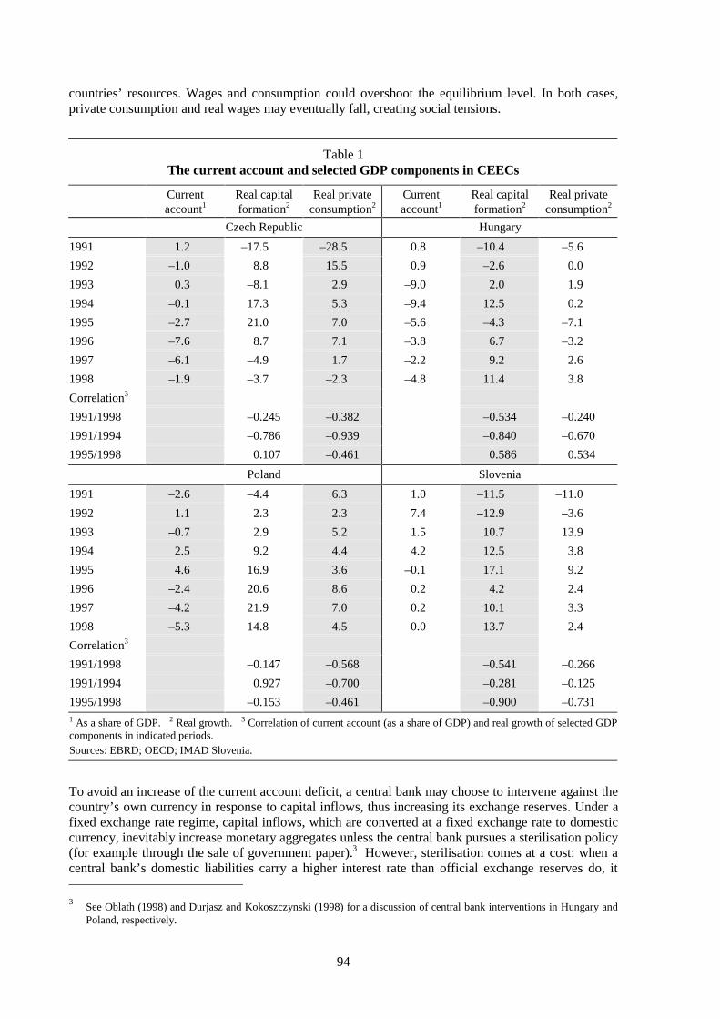
94
countries’ resources. Wages and consumption could overshoot the equilibrium level. In both cases,private consumption and real wages may eventually fall, creating social tensions.
Table 1The current account and selected GDP components in CEECs
Currentaccount1
Real capitalformation2
Real privateconsumption2
Currentaccount1
Real capitalformation2
Real privateconsumption2
Czech Republic Hungary
1991 1.2 –17.5 –28.5 0.8 –10.4 –5.6
1992 –1.0 8.8 15.5 0.9 –2.6 0.0
1993 0.3 –8.1 2.9 –9.0 2.0 1.9
1994 –0.1 17.3 5.3 –9.4 12.5 0.2
1995 –2.7 21.0 7.0 –5.6 –4.3 –7.1
1996 –7.6 8.7 7.1 –3.8 6.7 –3.2
1997 –6.1 –4.9 1.7 –2.2 9.2 2.6
1998 –1.9 –3.7 –2.3 –4.8 11.4 3.8
Correlation3
1991/1998 –0.245 –0.382 –0.534 –0.240
1991/1994 –0.786 –0.939 –0.840 –0.670
1995/1998 0.107 –0.461 0.586 0.534
Poland Slovenia
1991 –2.6 –4.4 6.3 1.0 –11.5 –11.0
1992 1.1 2.3 2.3 7.4 –12.9 –3.6
1993 –0.7 2.9 5.2 1.5 10.7 13.9
1994 2.5 9.2 4.4 4.2 12.5 3.8
1995 4.6 16.9 3.6 –0.1 17.1 9.2
1996 –2.4 20.6 8.6 0.2 4.2 2.4
1997 –4.2 21.9 7.0 0.2 10.1 3.3
1998 –5.3 14.8 4.5 0.0 13.7 2.4
Correlation3
1991/1998 –0.147 –0.568 –0.541 –0.266
1991/1994 0.927 –0.700 –0.281 –0.125
1995/1998 –0.153 –0.461 –0.900 –0.7311 As a share of GDP. 2 Real growth. 3 Correlation of current account (as a share of GDP) and real growth of selected GDPcomponents in indicated periods.Sources: EBRD; OECD; IMAD Slovenia.
To avoid an increase of the current account deficit, a central bank may choose to intervene against thecountry’s own currency in response to capital inflows, thus increasing its exchange reserves. Under afixed exchange rate regime, capital inflows, which are converted at a fixed exchange rate to domesticcurrency, inevitably increase monetary aggregates unless the central bank pursues a sterilisation policy(for example through the sale of government paper).3 However, sterilisation comes at a cost: when acentral bank’s domestic liabilities carry a higher interest rate than official exchange reserves do, it 3
See Oblath (1998) and Durjasz and Kokoszczynski (1998) for a discussion of central bank interventions in Hungary andPoland, respectively.

95
operates at a loss and thus increases the quasi-fiscal deficit. Under conditions of full capital mobility,sterilisation becomes ineffective, as any funds which are withdrawn from the money market by centralbank sterilisation operations will quickly be replaced by new capital inflows. The cost of sterilisationwill grow. As a consequence, in highly integrated financial markets, central banks have to accept someeffect of capital inflows on monetary aggregates, which may cause inflationary pressures.4
2.2 Capital flows and exchange reserves in CEECs
Figure 1 shows that, as far as data are available, the growth of official reserves (excluding gold) in theCEECs was largely determined by the surplus on the financial account, whereas the development ofthe current account did not play an important role (with the possible exception of Slovenia). TheCzech Republic, Hungary and Poland posted increasing exchange reserves financed by capital inflows.Declines in exchange reserves, for example in Hungary in 1996 and in the Czech Republic in 1996 and1997, were likewise largely caused by a decline (Czech Republic) or even a dramatic reversal(Hungary) of capital inflows. The capital flows to Hungary switched from a maximum surplus on thefinancial account of US$ 3.8 billion in the fourth quarter of 1995 to a deficit of US$ 0.6 billion in thefirst quarter of 1997, which subsequently increased to US$ 1.0 billion (minimum of the availableperiod). Contrary to the developments in the Czech Republic and Hungary, Poland largely succeededin avoiding outflows of capital and a resulting decline of exchange reserves. In Slovenia, both capitalflows and changes of reserves fluctuated strongly, with the average value relatively close to zero.
Figure 1
Financial account and the development of reserves in CEECs
Source: IMF, International Financial Statistics (IFS).
4
This effect on monetary aggregates can be avoided if capital inflows are utilised to repay foreign debt.
Czech Republic
-1500
-1000
-500
0
500
1000
1500
2000
2500
3000
3500
1990
Q1
1990
Q3
1991
Q1
1991
Q3
1992
Q1
1992
Q3
1993
Q1
1993
Q3
1994
Q1
1994
Q3
1995
Q1
1995
Q3
1996
Q1
1996
Q3
1997
Q1
1997
Q3
1998
Q1
1998
Q3
USD
mill
ion
financial account
change of reserves
Hungary
-2000
-1000
0
1000
2000
3000
4000
5000
1990
Q1
1990
Q3
1991
Q1
1991
Q3
1992
Q1
1992
Q3
1993
Q1
1993
Q3
1994
Q1
1994
Q3
1995
Q1
1995
Q3
1996
Q1
1996
Q3
1997
Q1
1997
Q3
1998
Q1
1998
Q3
USD
mill
ion
financial account
change of reserves
Poland
-6000
-5000
-4000
-3000
-2000
-1000
0
1000
2000
3000
4000
1990
Q1
1990
Q3
1991
Q1
1991
Q3
1992
Q1
1992
Q3
1993
Q1
1993
Q3
1994
Q1
1994
Q3
1995
Q1
1995
Q3
1996
Q1
1996
Q3
1997
Q1
1997
Q3
1998
Q1
1998
Q3
USD
mill
ion
financial account
change of reserves
Slovenia
-400
-200
0
200
400
600
800
1990
Q1
1990
Q3
1991
Q1
1991
Q3
1992
Q1
1992
Q3
1993
Q1
1993
Q3
1994
Q1
1994
Q3
1995
Q1
1995
Q3
1996
Q1
1996
Q3
1997
Q1
1997
Q3
1998
Q1
1998
Q3
USD
mill
ion
financial account
change of reserves
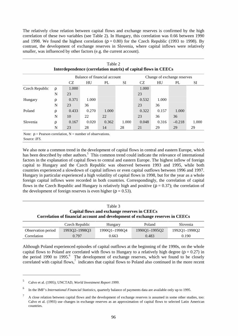
96
The relatively close relation between capital flows and exchange reserves is confirmed by the highcorrelation of these two variables (see Table 2). In Hungary, this correlation was 0.66 between 1990and 1998. We found the highest correlation (ρ = 0.80) for the Czech Republic (1993 to 1998). Bycontrast, the development of exchange reserves in Slovenia, where capital inflows were relativelysmaller, was influenced by other factors (e.g. the current account).
Table 2Interdependence (correlation matrix) of capital flows in CEECs
Balance of financial account Change of exchange reserves
CZ HU PL SI CZ HU PL SI
Czech Republic ρ 1.000 1.000
N 23 23
Hungary ρ 0.371 1.000 0.532 1.000
N 23 36 23 36
Poland ρ 0.433 0.270 1.000 0.322 0.157 1.000
N 10 22 22 23 36 36
Slovenia ρ 0.167 0.020 0.362 1.000 0.048 0.316 –0.218 1.000
N 23 28 14 28 21 29 29 29
Note: ρ = Pearson correlation, N = number of observations.Source: IFS.
We also note a common trend in the development of capital flows in central and eastern Europe, whichhas been described by other authors.5 This common trend could indicate the relevance of internationalfactors in the explanation of capital flows to central and eastern Europe. The highest inflow of foreigncapital to Hungary and the Czech Republic was observed between 1993 and 1995, while bothcountries experienced a slowdown of capital inflows or even capital outflows between 1996 and 1997.Hungary in particular experienced a high volatility of capital flows in 1998, but for the year as a wholeforeign capital inflows were recorded in both countries. Correspondingly, the correlation of capitalflows in the Czech Republic and Hungary is relatively high and positive (ρ = 0.37); the correlation ofthe development of foreign reserves is even higher (ρ = 0.53).
Table 3Capital flows and exchange reserves in CEECs
Correlation of financial account and development of exchange reserves in CEECs
Czech Republic Hungary Poland Slovenia
Observation period 1993Q2–1998Q3 1990Q1–1998Q4 1990Q1–1995Q2 1992Q1–1998Q2
Correlation 0.797 0.663 0.483 0.190
Although Poland experienced episodes of capital outflows at the beginning of the 1990s, on the wholecapital flows to Poland are correlated with flows to Hungary to a relatively high degree (ρ = 0.27) inthe period 1990 to 1995.6 The development of exchange reserves, which we found to be closelycorrelated with capital flows,7 indicates that capital flows to Poland also continued in the more recent
5
Calvo et al. (1995); UNCTAD, World Investment Report 1999.
6In the IMF’s International Financial Statistics, quarterly balance of payments data are available only up to 1995.
7A close relation between capital flows and the development of exchange reserves is assumed in some other studies, too:Calvo et al. (1993) use changes in exchange reserves as an approximation of capital flows to selected Latin Americancountries.
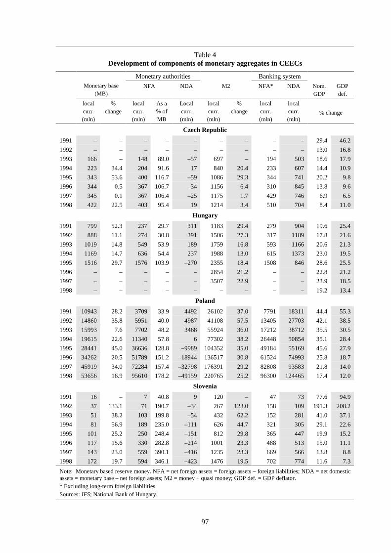
97
Table 4Development of components of monetary aggregates in CEECs
Monetary authorities Banking system
Monetary base(MB)
NFA NDA M2 NFA* NDA Nom.GDP
GDPdef.
localcurr.(mln)
%change
localcurr.(mln)
As a% ofMB
Localcurr.(mln)
localcurr.(mln)
%change
localcurr.(mln)
localcurr.(mln)
% change
Czech Republic
1991 – – – – – – – – – 29.4 46.2
1992 – – – – – – – – – 13.0 16.8
1993 166 – 148 89.0 –57 697 – 194 503 18.6 17.9
1994 223 34.4 204 91.6 17 840 20.4 233 607 14.4 10.9
1995 343 53.6 400 116.7 –59 1086 29.3 344 741 20.2 9.8
1996 344 0.5 367 106.7 –34 1156 6.4 310 845 13.8 9.6
1997 345 0.1 367 106.4 –25 1175 1.7 429 746 6.9 6.5
1998 422 22.5 403 95.4 19 1214 3.4 510 704 8.4 11.0
Hungary
1991 799 52.3 237 29.7 311 1183 29.4 279 904 19.6 25.4
1992 888 11.1 274 30.8 391 1506 27.3 317 1189 17.8 21.6
1993 1019 14.8 549 53.9 189 1759 16.8 593 1166 20.6 21.3
1994 1169 14.7 636 54.4 237 1988 13.0 615 1373 23.0 19.5
1995 1516 29.7 1576 103.9 –270 2355 18.4 1508 846 28.6 25.5
1996 – – – – – 2854 21.2 – – 22.8 21.2
1997 – – – – – 3507 22.9 – – 23.9 18.5
1998 – – – – – – – – – 19.2 13.4
Poland
1991 10943 28.2 3709 33.9 4492 26102 37.0 7791 18311 44.4 55.3
1992 14860 35.8 5951 40.0 4987 41108 57.5 13405 27703 42.1 38.5
1993 15993 7.6 7702 48.2 3468 55924 36.0 17212 38712 35.5 30.5
1994 19615 22.6 11340 57.8 6 77302 38.2 26448 50854 35.1 28.4
1995 28441 45.0 36636 128.8 –9989 104352 35.0 49184 55169 45.6 27.9
1996 34262 20.5 51789 151.2 –18944 136517 30.8 61524 74993 25.8 18.7
1997 45919 34.0 72284 157.4 –32798 176391 29.2 82808 93583 21.8 14.0
1998 53656 16.9 95610 178.2 –49159 220765 25.2 96300 124465 17.4 12.0
Slovenia
1991 16 – 7 40.8 9 120 – 47 73 77.6 94.9
1992 37 133.1 71 190.7 –34 267 123.0 158 109 191.3 208.2
1993 51 38.2 103 199.8 –54 432 62.2 152 281 41.0 37.1
1994 81 56.9 189 235.0 –111 626 44.7 321 305 29.1 22.6
1995 101 25.2 250 248.4 –151 812 29.8 365 447 19.9 15.2
1996 117 15.6 330 282.8 –214 1001 23.3 488 513 15.0 11.1
1997 143 23.0 559 390.1 –416 1235 23.3 669 566 13.8 8.8
1998 172 19.7 594 346.1 –423 1476 19.5 702 774 11.6 7.3
Note: Monetary based reserve money. NFA = net foreign assets = foreign assets – foreign liabilities; NDA = net domesticassets = monetary base – net foreign assets; M2 = money + quasi money; GDP def. = GDP deflator.* Excluding long-term foreign liabilities.Sources: IFS; National Bank of Hungary.

98
period. Capital flows to Slovenia developed relatively independently of those in other CEECs, as bothindicators show (Table 3).
2.3 Capital flows and monetary aggregates
In the previous section, we saw that capital flows fuelled sizeable increases in exchange reserves inmost CEECs. The aim of this section is to investigate to what degree this capital inflow-driven build-up of exchange reserves had an impact on the development of monetary aggregates, in order to assessthe inflationary potential arising from capital inflows.
Calvo et al. (1995) argue against sterilisation activities by CEE central banks in the early phase oftransition (until 1993), because they ascribe increasing capital flows in this phase to rising moneydemand. Therefore, capital flows would not pose a danger for price stability. The development ofinflation rates until 1995 lends support to this view. Although M2 was often growing more quicklythan nominal GDP in the CEECs during this period, inflation rates were declining (inflationary shockssuch as the devaluation in Hungary in 1995 are of course exceptions).
In about 1993, CEE central banks started to sterilise inflows, as documented by a sharp increase in theshare of net foreign assets in the monetary base, as central banks were trying to reduce net domesticassets in response to quickly growing net foreign assets. Table 4 provides an overview of the extent ofsterilisation operations in the CEECs: according to this table, the increase in net foreign assets wasmatched most closely by a decrease in net domestic assets in Slovenia. In Hungary and Poland,increases in net foreign assets were largely offset by declining net domestic assets while in the CzechRepublic the degree of sterilisation appears to be the lowest. However, one should be aware of theproblems involved in this simple comparison: As Oblath (1998, p. 197) points out, we are dealing withex post information. Thus, we cannot tell to what extent the sterilised funds would have contributed toan increase in the current account deficit and/or the monetary base. In addition, the reaction of capitalinflows in response to sterilisation measures is not captured.
The extent of sterilisation is also an indicator for the degree of integration into international financialmarkets. As stated above, under conditions of full capital mobility, sterilisation is ineffective. Thus,sterilisation operations would make little sense. One way to assess the effectiveness of sterilisation isto estimate offset coefficients. The change in the central bank’s net foreign assets is explained by achange in net domestic assets and other variables. A coefficient of –1 for net domestic assets wouldimply the total ineffectiveness of sterilisation (or full integration into financial markets), as anydecrease in net domestic assets would be met by an increase of equal size in net foreign assets. Buch etal. (1999) present a good overview of attempts to estimate offset coefficients in CEECs. They findthat, with the possible exception of Slovenia, which was not covered in their study, CEECs exhibit arather high degree of financial integration. Thus, the possibility of finding evidence of a relationshipbetween capital inflows and inflation in CEECs should not be ruled out ex ante, as sterilisationpolicies seem not to have succeeded in fully insulating monetary aggregates from capital inflows.
3. Capital flows and inflation: a case study of Hungary
Because of a lack of data on the other countries covered by this study, we are able to explore theserelationships in greater detail only for Hungary. This section discusses bivariate and multivariaterelations between various types of capital flows and selected monetary variables in Hungary between1992 (FDI) or 1994 (portfolio investment) and 1999.
Table 5 shows the result of Granger causality tests applied to capital flows (foreign direct investmentand portfolio investment in Hungary) and selected monetary variables, including various price indices,real and nominal effective exchange rate indices, and various interest rates. We can see that themotives of direct investors are substantially different to those of portfolio investors. Direct investorsare motivated mainly by real wages and exchange rates, while portfolio investors are attracted by theinterest rate level. Various price indices are the only variables which exhibit a statistically significant
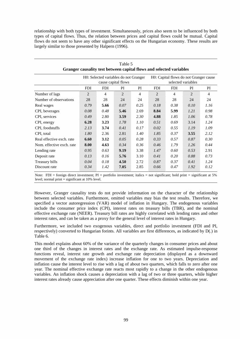
99
relationship with both types of investment. Simultaneously, prices also seem to be influenced by bothtypes of capital flows. Thus, the relation between prices and capital flows could be mutual. Capitalflows do not seem to have any other significant effects on the Hungarian economy. These results arelargely similar to those presented by Halpern (1996).
Table 5Granger causality test between capital flows and selected variables
H0: Selected variables do not Grangercause capital flows
H0: Capital flows do not Granger causeselected variables
FDI FDI PI PI FDI FDI PI PI
Number of lags 2 4 2 4 2 4 2 4
Number of observations 28 28 24 24 28 28 24 24
Real wages 0.79 5.66 0.07 0.25 0.18 0.38 0.10 1.16
CPI, beverages 0.08 0.48 5.46 2.69 8.84 5.99 1.21 0.98
CPI, services 0.49 2.80 3.59 2.30 4.88 1.85 1.06 0.78
CPI, energy 6.28 3.23 1.78 1.10 0.51 0.69 3.14 1.24
CPI, foodstuffs 2.13 3.74 0.41 0.17 0.02 0.55 1.19 1.09
CPI, total 1.80 2.36 2.81 1.40 1.85 0.37 3.55 2.12
Real effective exch. rate 6.60 3.12 0.05 0.28 0.33 0.57 0.87 0.30
Nom. effective exch. rate 8.00 4.63 0.34 0.36 0.46 1.79 1.26 0.44
Lending rate 0.95 0.63 9.19 3.38 1.47 0.60 0.53 2.91
Deposit rate 0.13 0.16 5.76 3.10 0.41 0.20 0.88 0.73
Treasury bills 0.04 0.18 4.50 2.72 0.87 0.37 0.41 1.24Discount rate 0.34 1.42 7.05 2.85 0.66 0.47 1.92 0.12
Note: FDI = foreign direct investment; PI = portfolio investment; italics = not significant; bold print = significant at 5%level; normal print = significant at 10% level.
However, Granger causality tests do not provide information on the character of the relationshipbetween selected variables. Furthermore, omitted variables may bias the test results. Therefore, wespecified a vector autoregression (VAR) model of inflation in Hungary. The endogenous variablesinclude the consumer price index (CPI), interest rates on treasury bills (TBR), and the nominaleffective exchange rate (NEER). Treasury bill rates are highly correlated with lending rates and otherinterest rates, and can be taken as a proxy for the general level of interest rates in Hungary.
Furthermore, we included two exogenous variables, direct and portfolio investment (FDI and PI,respectively) converted to Hungarian forints. All variables are first differences, as indicated by D(.) inTable 6.
This model explains about 60% of the variance of the quarterly changes in consumer prices and aboutone third of the changes in interest rates and the exchange rate. As estimated impulse-responsefunctions reveal, interest rate growth and exchange rate depreciation (displayed as a downwardmovement of the exchange rate index) increase inflation for one to two years. Depreciation andinflation cause the interest level to rise with a lag of about two quarters, which falls to zero after oneyear. The nominal effective exchange rate reacts most rapidly to a change in the other endogenousvariables. An inflation shock causes a depreciation with a lag of two or three quarters, while higherinterest rates already cause appreciation after one quarter. These effects diminish within one year.
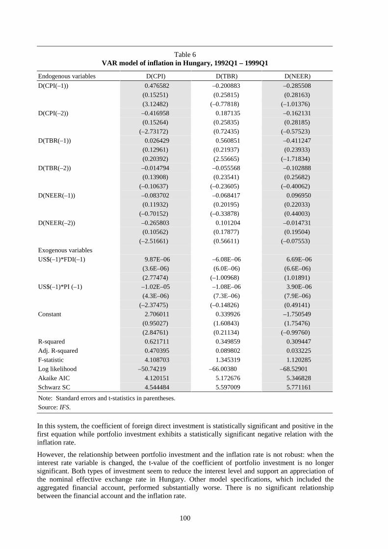
100
Table 6VAR model of inflation in Hungary, 1992Q1 – 1999Q1
Endogenous variables D(CPI) D(TBR) D(NEER)
D(CPI(–1)) 0.476582 –0.200883 –0.285508
(0.15251) (0.25815) (0.28163)
(3.12482) (–0.77818) (–1.01376)
D(CPI(–2)) –0.416958 0.187135 –0.162131
(0.15264) (0.25835) (0.28185)
(–2.73172) (0.72435) (–0.57523)
D(TBR(–1)) 0.026429 0.560851 –0.411247
(0.12961) (0.21937) (0.23933)
(0.20392) (2.55665) (–1.71834)
D(TBR(–2)) –0.014794 –0.055568 –0.102888
(0.13908) (0.23541) (0.25682)
(–0.10637) (–0.23605) (–0.40062)
D(NEER(–1)) –0.083702 –0.068417 0.096950
(0.11932) (0.20195) (0.22033)
(–0.70152) (–0.33878) (0.44003)
D(NEER(–2)) –0.265803 0.101204 –0.014731
(0.10562) (0.17877) (0.19504)
(–2.51661) (0.56611) (–0.07553)
Exogenous variables
US$(–1)*FDI(–1) 9.87E–06 –6.08E–06 6.69E–06
(3.6E–06) (6.0E–06) (6.6E–06)
(2.77474) (–1.00968) (1.01891)
US$(–1)*PI (–1) –1.02E–05 –1.08E–06 3.90E–06
(4.3E–06) (7.3E–06) (7.9E–06)
(–2.37475) (–0.14826) (0.49141)
Constant 2.706011 0.339926 –1.750549
(0.95027) (1.60843) (1.75476)
(2.84761) (0.21134) (–0.99760)
R-squared 0.621711 0.349859 0.309447
Adj. R-squared 0.470395 0.089802 0.033225
F-statistic 4.108703 1.345319 1.120285
Log likelihood –50.74219 –66.00380 –68.52901
Akaike AIC 4.120151 5.172676 5.346828
Schwarz SC 4.544484 5.597009 5.771161
Note: Standard errors and t-statistics in parentheses.
Source: IFS.
In this system, the coefficient of foreign direct investment is statistically significant and positive in thefirst equation while portfolio investment exhibits a statistically significant negative relation with theinflation rate.
However, the relationship between portfolio investment and the inflation rate is not robust: when theinterest rate variable is changed, the t-value of the coefficient of portfolio investment is no longersignificant. Both types of investment seem to reduce the interest level and support an appreciation ofthe nominal effective exchange rate in Hungary. Other model specifications, which included theaggregated financial account, performed substantially worse. There is no significant relationshipbetween the financial account and the inflation rate.

101
Figure 2VAR impulses to indicators’ shocks in Hungary
-2
-1
0
1
2
1 2 3 4 5 6 7 8 9 10 11 12
Response of D(CPI) to D(CPI)
-2
-1
0
1
2
1 2 3 4 5 6 7 8 9 10 11 12
Response of D(CPI) to D(TBR)
-2
-1
0
1
2
1 2 3 4 5 6 7 8 9 10 11 12
Response of D(CPI) to D(NEER)
-2
-1
0
1
2
3
1 2 3 4 5 6 7 8 9 10 11 12
Response of D(TBR) to D(CPI)
-2
-1
0
1
2
3
1 2 3 4 5 6 7 8 9 10 11 12
Response of D(TBR) to D(TBR)
-2
-1
0
1
2
3
1 2 3 4 5 6 7 8 9 10 11 12
Response of D(TBR) to D(NEER)
-2
-1
0
1
2
3
4
1 2 3 4 5 6 7 8 9 10 11 12
Response of D(NEER) to D(CPI)
-2
-1
0
1
2
3
4
1 2 3 4 5 6 7 8 9 10 11 12
Response of D(NEER) to D(TBR)
-2
-1
0
1
2
3
4
1 2 3 4 5 6 7 8 9 10 11 12
Response of D(NEER) to D(NEER)
Response to one SD innovation ± 2 SE
These effects are, incidentally, in accordance with the experiences of other countries (seeChristoffersen and Wescott (1999) and Calvo et al. (1993)).
4. Impact of capital inflows on financial stability
4.1 Theoretical considerations
Capital flows can pose a threat to financial stability via two main channels: first, capital flows maycause an excessive real appreciation of the exchange rate and, second, they may produce a currencyand maturity mismatch of assets and liabilities in the financial sector. While the first channel isrelevant for both flexible and fixed exchange rate systems the second is decidedly more relevant forfixed exchange rate systems. Such a system encourages borrowing at lower interest rates in foreigncurrency as long as the exchange rate target of the central bank remains credible, and this may result inhigh open foreign exchange positions of banks (i.e. a currency mismatch of assets and liabilities) andfirms. Even when capital inflows take the form of purchases of domestic currency-denominated assetsby foreigners rather than borrowing in foreign currency capital, inflows pose additional risks forfinancial stability. As explained above, under conditions of full capital mobility, the central bank hasno control over the monetary base under fixed exchange rates. If the monetary base increases because

102
of capital inflows, broader monetary aggregates will expand more than the amount of initial inflowsbecause of the money multiplier. Thus, there will be a rise in the ratio of M2/ official reserves, whichimplies that the gap between liquid domestic assets (which could be converted into foreign currency-denominated assets) and the stock of foreign exchange available for meeting this demand grows.Although this problem can be mitigated through the use of higher minimum reserves, it cannot beavoided altogether.
Under conditions of less than full capital mobility, when sterilisation is partly effective, there are stillsome unwanted side effects. Beside the fiscal costs of sterilisation, the structure of capital inflows islikely to change in response to sterilisation operations. Montiel and Reinhart (1999) find evidence fora change in the composition of capital inflows in favour of short-term and portfolio flows as a result ofsterilisation operations. At fixed exchange rates, capital inflows also tend to increase maturitymismatches in the banking sector, as foreigners’ deposits with domestic banks will often have shortermaturities than the credits which are funded by the deposits.
In the light of the preceding discussion, a floating exchange rate system seams a preferable solution. Itcertainly has the big advantage that it does not encourage quasi-arbitrage between domestic andforeign interest rates, which would increase the fragility of the financial system. However, a floatingregime is not entirely free from complications either. White (1999) gives a good overview ofchallenges for central banks which arise from the adoption of a floating exchange rate/direct inflationtargeting framework. For transition economies, the issue of exchange rate overshooting seems to be ofparticular relevance. The expectation of large FDI inflows as a result of privatisation projects mightalso attract short-term inflows, which could lead to an overvaluation of the exchange rate. Beside thenegative impact of an exchange rate misalignment on the real sector, strong expectations of exchangerate appreciation could induce banks and businesses to borrow excessively in foreign currency.
4.2 Development of economic and financial indicators
Given that we defined financial stability as the absence of financial crises, we analyse variables whichare associated in the literature with financial crises. Kaminsky et al. (1998), who conducted extensivestudies of a large number of balance of payments crises, identify the real exchange rate, bankingcrises, exports, stock prices, M2/reserves and output as the most reliable leading indicators of balanceof payments crises. The real exchange rate, stock prices, the M2 multiplier, output and exports arementioned by Reinhart (1999) as the most successful “predictors” of banking crises. As there areneither adequate time series of these indicators nor enough observations of crises available in CEECs,the empirical testing of the relevance of these indicators for transition countries is impossible atpresent. Thus, we have to stick to the presentation of “stylised facts” of the development of a set ofindicators of financial vulnerability which is based on the findings of Kaminsky et al. (1998) andReinhart (1999). We divided our set of financial indicators into two groups, monetary and realvariables. The first group of variables should be expected to reflect credit booms and asset bubblesfuelled by the strong money supply growth resulting from capital inflows. The second group tends tomirror symptoms of the excessive real appreciation of the exchange rate.
4.2.1 Monetary variables: M2/reserves, short-term debt/reserves, stock prices
When the reforms began, the Czech Republic and Poland had to cope with very low levels ofinternational reserves, resulting in high M2/reserves ratios. In about 1993, CEE central banks startedto sterilise capital inflows, resulting in a sharp fall in this ratio until 1995. By then, internationalreserves had accumulated to a level deemed sufficient and – as stated before – the management ofcontinuing capital inflows from the viewpoint of monetary and financial stability became an importantissue in the accession countries. Apart from Slovenia,8 all countries had started to follow a strategy ofexchange rate targeting by that time, and steps to liberalise the capital account had been taken, with the
8
Slovenia pursues a policy of monetary targeting but pays strong attention to exchange rate developments. Thus, inpractice this policy comes close to a strategy of exchange rate targeting.

103
Czech Republic leading in this respect. In the next two years, this ratio again worsened markedly inHungary and the Czech Republic, albeit starting from a low level. Although this indicator did not seemto have reached an alarming level by 1997, 9 the Czech Republic experienced a currency crisis. Thus,a capital inflow-driven credit boom does not seem to be the main cause of the crisis in the CzechRepublic. Comparing a measure of liquid domestic assets such as M2 with the amount of foreignassets available in the economy to satisfy the demand for domestic assets if there is a run on thecurrency may yield insights into the severity of an exchange rate correction in the event of a loss ofcredibility. This could explain why the fall of the Czech koruna was fairly limited and why thecurrency crisis did not develop into a twin crisis.10
Table 7M2/reserves
Czech Republic Hungary Poland Slovenia
1993 6.20 2.59 6.12 4.16
1994 4.98 2.65 5.26 3.30
1995 2.79 1.40 2.82 3.54
1996 3.30 1.78 2.64 3.08
1997 3.60 2.05 2.43 2.20
1998 3.38 1.97 2.30 2.51
Note: Since 1998, Hungary has not published figures for M2; the 1998 figure is based on the ratio of M2/M3 in 1997.
Sources: WIIW monthly reports; National Bank of Hungary.
0102030405060708090
100
Slovenia Poland CzechRep.
Korea Hungary Thailand M exico
Sources: BIS; IM F International Financial Statistics .
Figure 3 Ratio of outstanding short-term debt to
international reservesIn per cent, at end-1998
While Reinhart’s (1999) set of financial indicators includes the M2 multiplier, we include the ratio ofshort-term debt/reserves instead. Except for Poland, which experienced a noticeable growth trend ofthe M2 multiplier in the 1990s, in our view the development of this indicator does not yield many
9
Before the onset of the crisis, Korea’s and Mexico’s M2/reserves ratios reached levels of 6 to 7.
10Obviously, the Czech banking system has problems but they are a consequence of poor lending practices rather thanexchange rate losses.
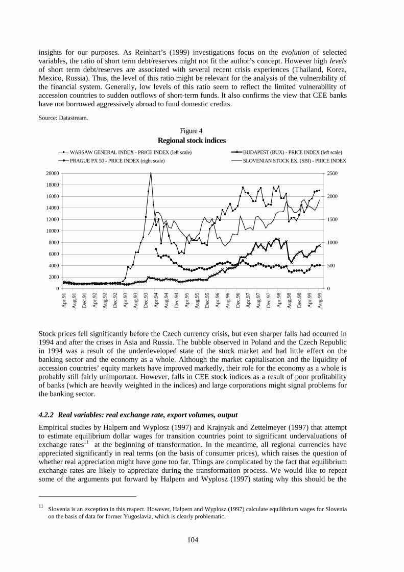
104
insights for our purposes. As Reinhart’s (1999) investigations focus on the evolution of selectedvariables, the ratio of short term debt/reserves might not fit the author’s concept. However high levelsof short term debt/reserves are associated with several recent crisis experiences (Thailand, Korea,Mexico, Russia). Thus, the level of this ratio might be relevant for the analysis of the vulnerability ofthe financial system. Generally, low levels of this ratio seem to reflect the limited vulnerability ofaccession countries to sudden outflows of short-term funds. It also confirms the view that CEE bankshave not borrowed aggressively abroad to fund domestic credits.
Source: Datastream.
Stock prices fell significantly before the Czech currency crisis, but even sharper falls had occurred in1994 and after the crises in Asia and Russia. The bubble observed in Poland and the Czech Republicin 1994 was a result of the underdeveloped state of the stock market and had little effect on thebanking sector and the economy as a whole. Although the market capitalisation and the liquidity ofaccession countries’ equity markets have improved markedly, their role for the economy as a whole isprobably still fairly unimportant. However, falls in CEE stock indices as a result of poor profitabilityof banks (which are heavily weighted in the indices) and large corporations might signal problems forthe banking sector.
4.2.2 Real variables: real exchange rate, export volumes, output
Empirical studies by Halpern and Wyplosz (1997) and Krajnyak and Zettelmeyer (1997) that attemptto estimate equilibrium dollar wages for transition countries point to significant undervaluations ofexchange rates11 at the beginning of transformation. In the meantime, all regional currencies haveappreciated significantly in real terms (on the basis of consumer prices), which raises the question ofwhether real appreciation might have gone too far. Things are complicated by the fact that equilibriumexchange rates are likely to appreciate during the transformation process. We would like to repeatsome of the arguments put forward by Halpern and Wyplosz (1997) stating why this should be the
11
Slovenia is an exception in this respect. However, Halpern and Wyplosz (1997) calculate equilibrium wages for Sloveniaon the basis of data for former Yugoslavia, which is clearly problematic.
Figure 4 Regional stock indices
0
2000
4000
6000
8000
10000
12000
14000
16000
18000
20000
Apr
.91
Aug
.91
Dec
.91
Apr
.92
Aug
.92
Dec
.92
Apr
.93
Aug
.93
Dec
.93
Apr
.94
Aug
.94
Dec
.94
Apr
.95
Aug
.95
Dec
.95
Apr
.96
Aug
.96
Dec
.96
Apr
.97
Aug
.97
Dec
.97
Apr
.98
Aug
.98
Dec
.98
Apr
.99
Aug
.99
0
500
1000
1500
2000
2500
WARSAW GENERAL INDEX - PRICE INDEX (left scale) BUDAPEST (BUX) - PRICE INDEX (left scale)
PRAGUE PX 50 - PRICE INDEX (right scale) SLOVENIAN STOCK EX. (SBI) - PRICE INDEX
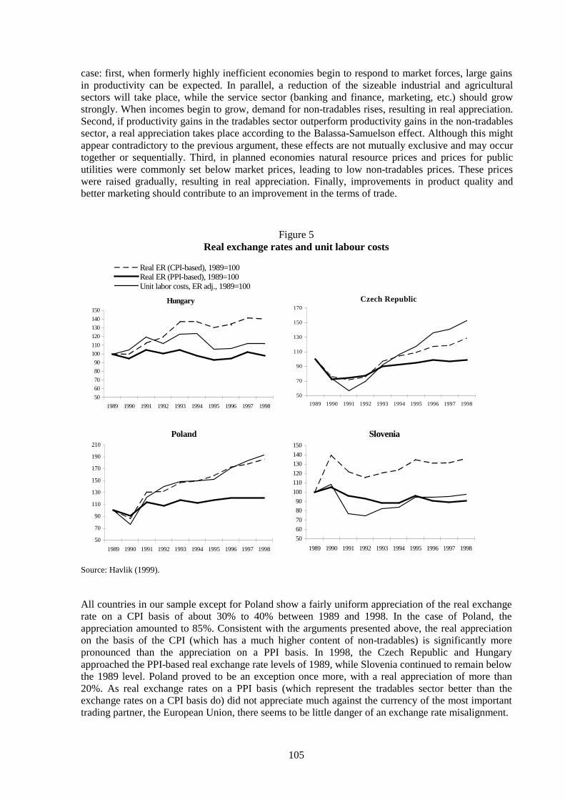
105
case: first, when formerly highly inefficient economies begin to respond to market forces, large gainsin productivity can be expected. In parallel, a reduction of the sizeable industrial and agriculturalsectors will take place, while the service sector (banking and finance, marketing, etc.) should growstrongly. When incomes begin to grow, demand for non-tradables rises, resulting in real appreciation.Second, if productivity gains in the tradables sector outperform productivity gains in the non-tradablessector, a real appreciation takes place according to the Balassa-Samuelson effect. Although this mightappear contradictory to the previous argument, these effects are not mutually exclusive and may occurtogether or sequentially. Third, in planned economies natural resource prices and prices for publicutilities were commonly set below market prices, leading to low non-tradables prices. These priceswere raised gradually, resulting in real appreciation. Finally, improvements in product quality andbetter marketing should contribute to an improvement in the terms of trade.
Figure 5Real exchange rates and unit labour costs
Hungary
50
60
70
80
90
100
110
120
130
140
150
1989 1990 1991 1992 1993 1994 1995 1996 1997 1998
Real ER (CPI-based), 1989=100Real ER (PPI-based), 1989=100Unit labor costs, ER adj., 1989=100
Czech Republic
50
70
90
110
130
150
170
1989 1990 1991 1992 1993 1994 1995 1996 1997 1998
Poland
50
70
90
110
130
150
170
190
210
1989 1990 1991 1992 1993 1994 1995 1996 1997 1998
Slovenia
50
60
70
80
90
100
110
120
130
140
150
1989 1990 1991 1992 1993 1994 1995 1996 1997 1998
Source: Havlik (1999).
All countries in our sample except for Poland show a fairly uniform appreciation of the real exchangerate on a CPI basis of about 30% to 40% between 1989 and 1998. In the case of Poland, theappreciation amounted to 85%. Consistent with the arguments presented above, the real appreciationon the basis of the CPI (which has a much higher content of non-tradables) is significantly morepronounced than the appreciation on a PPI basis. In 1998, the Czech Republic and Hungaryapproached the PPI-based real exchange rate levels of 1989, while Slovenia continued to remain belowthe 1989 level. Poland proved to be an exception once more, with a real appreciation of more than20%. As real exchange rates on a PPI basis (which represent the tradables sector better than theexchange rates on a CPI basis do) did not appreciate much against the currency of the most importanttrading partner, the European Union, there seems to be little danger of an exchange rate misalignment.

106
The analysis of unit labour costs yields a more mixed picture, however. Slovenia and Hungaryexperienced only small rises in exchange rate adjusted (ECU-based) unit labour costs of 6.8% and12.2% respectively, whereas unit labour costs in Poland and the Czech Republic shot up by 108% and56% respectively. Several observations seem to confirm the high relevance of unit labour costs forexplaining trade and current account deficits: first, Slovenia, which experienced the smallest rise inexchange rate adjusted unit labour costs, has traditionally had a balanced current account or evensurpluses. Second, episodes of very large current account deficits (Hungary 1994, Czech Republic in1996) occurred after sharp rises in exchange rate adjusted unit labour costs. At first glance, themassive rise in Polish exchange rate adjusted unit labour costs, which did not cause severemacroeconomic imbalances up to 1998, may appear difficult to explain. However, by far the largestrise in unit labour costs occurred in 1991, which caused a marked erosion of the previous trade balancesurplus. Nevertheless, the current account remained in check as a result of the debt relief granted toPoland. This debt relief caused a rise in the equilibrium exchange rate, as it reduced the need toachieve surpluses in the trade balance in order to service its foreign debt. Second, trade in US dollars,and in particular trade with CIS states, is more relevant for Poland than for the other countries coveredin this paper. Approximately 16% of (classified) Polish exports went to CIS countries before theRussian crisis.12 As the Russian rouble’s real appreciation before the crisis was in excess of the realappreciation of the Polish zloty, Poland’s trade-weighted (effective) exchange rate appreciated lessthan the ECU-based rate before the Russian crisis. As a result, until the outbreak of the Russian crisisthere were no visible symptoms of an overvalued exchange rate in Poland. However, if one perceivesthe loss of the CIS export markets for Poland as permanent (at least for the medium term), thepossibility exists that the zloty became overvalued at the end of 1998.
Figure 6Real GDP growth
Annual percentage changes
-15
-10
-5
0
5
10
1989 1990 1991 1992 1993 1994 1995 1996 1997 1998
C zech R epublic H ungary
Poland Slovenia
Source: WIIW monthly reports.
Output and export dynamics also support the view that no exchange rate misalignment occurred inPoland until 1998, while in the Czech case symptoms appeared which might point to a misalignmentof the Czech koruna under short-run considerations. Before the Czech koruna’s devaluation in 1997,Czech exports markedly lagged Polish exports, whereas the situation reversed after the devaluation ofthe Czech currency. GDP growth rates paint the same picture: continued high GDP growth rates inPoland contrasted with slowing growth rates and rising current account deficits in the Czech Republicbefore the Czech currency crisis. 12
Poland’s surplus in unclassified trade was also reduced significantly by the Russian crisis.
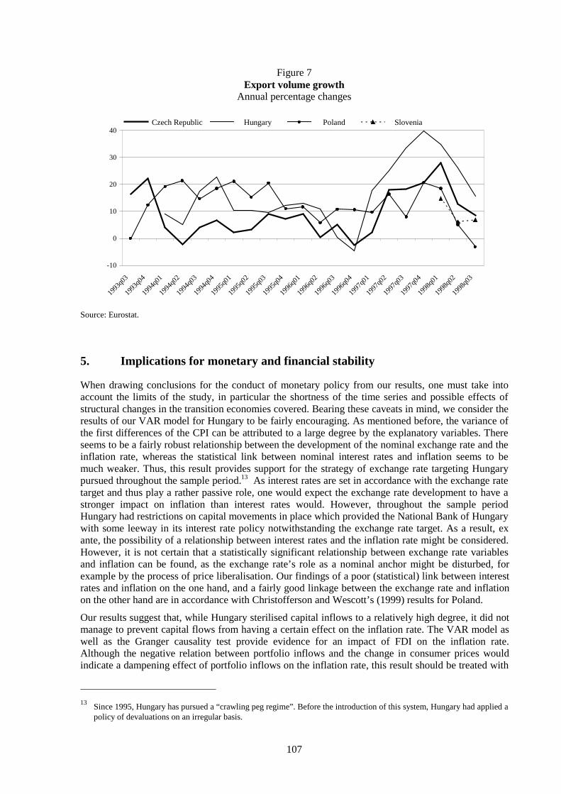
107
Figure 7Export volume growth
Annual percentage changes
-10
0
10
20
30
40
1993
q03
1993
q04
1994
q01
1994
q02
1994
q03
1994
q04
1995
q01
1995
q02
1995
q03
1995
q04
1996
q01
1996
q02
1996
q03
1996
q04
1997
q01
1997
q02
1997
q03
1997
q04
1998
q01
1998
q02
1998
q03
Czech Republic Hungary Poland Slovenia
Source: Eurostat.
5. Implications for monetary and financial stability
When drawing conclusions for the conduct of monetary policy from our results, one must take intoaccount the limits of the study, in particular the shortness of the time series and possible effects ofstructural changes in the transition economies covered. Bearing these caveats in mind, we consider theresults of our VAR model for Hungary to be fairly encouraging. As mentioned before, the variance ofthe first differences of the CPI can be attributed to a large degree by the explanatory variables. Thereseems to be a fairly robust relationship between the development of the nominal exchange rate and theinflation rate, whereas the statistical link between nominal interest rates and inflation seems to bemuch weaker. Thus, this result provides support for the strategy of exchange rate targeting Hungarypursued throughout the sample period.13 As interest rates are set in accordance with the exchange ratetarget and thus play a rather passive role, one would expect the exchange rate development to have astronger impact on inflation than interest rates would. However, throughout the sample periodHungary had restrictions on capital movements in place which provided the National Bank of Hungarywith some leeway in its interest rate policy notwithstanding the exchange rate target. As a result, exante, the possibility of a relationship between interest rates and the inflation rate might be considered.However, it is not certain that a statistically significant relationship between exchange rate variablesand inflation can be found, as the exchange rate’s role as a nominal anchor might be disturbed, forexample by the process of price liberalisation. Our findings of a poor (statistical) link between interestrates and inflation on the one hand, and a fairly good linkage between the exchange rate and inflationon the other hand are in accordance with Christofferson and Wescott’s (1999) results for Poland.
Our results suggest that, while Hungary sterilised capital inflows to a relatively high degree, it did notmanage to prevent capital flows from having a certain effect on the inflation rate. The VAR model aswell as the Granger causality test provide evidence for an impact of FDI on the inflation rate.Although the negative relation between portfolio inflows and the change in consumer prices wouldindicate a dampening effect of portfolio inflows on the inflation rate, this result should be treated with
13
Since 1995, Hungary has pursued a “crawling peg regime”. Before the introduction of this system, Hungary had applied apolicy of devaluations on an irregular basis.
108
some scepticism. First, it is contrary to theoretical expectations and, second, the relation is statisticallynot robust. As FDI inflows appear to be related to the inflation rate although this is not the case for thefinancial account as a whole, one may conclude that FDI causes some demand-driven inflation,whereas the danger of a credit boom as a result of a large total inflow amount channelled through thebanking system seems to be rather limited. This would suggest that growth in monetary aggregates is aweak link between capital inflows and inflation.
The levels and dynamics of financial indicators presented in this paper point to a relatively moderatevulnerability of the CEECs to financial crises at present. Few signs of a worsening of the indicatorswhich seem to be caused by increasing financial integration could be detected. This overall positiveassessment is supported by the relatively limited impact of the Russian crisis on the more advancedCEECs. On the contrary, there is no definitive answer as to how far the indicators applied in this studywere able to “predict” the balance of payments crises in Hungary in 1994/95 and in the CzechRepublic in 1997. However, it seems fair to conclude that the development of exchange rate adjustedunit labour costs was a relevant indicator in both cases. While the Hungarian crisis occurred underconditions of limited integration into international financial markets, the question of to what degreethe advanced state of integration of the Czech Republic contributed to the Czech crisis cannot be fullyanswered. Among the indicators which we presented in this paper, the “real variables” reflect theproblems in the Czech economy better than the “monetary variables”. If improper intermediation ofcapital inflows were the main factor behind the crisis, the “monetary indicators” should look worse.Thus, we would draw the conclusion that excessive real appreciation (measured by exchange rateadjusted unit labour costs) in the run-up to the crisis is more relevant for explaining the Czechcurrency crisis. However, the question of whether capital inflows contributed to the worsening ofexchange rate adjusted unit labour costs in the run-up to the crisis remains open.

109
Bibliography
Buch, Claudia M, Ralph P Heinrich and Christian Pierdzioch (1999): “Foreign Capital and EconomicTransformation: Risks and Benefits of Free Capital Flows”. Kieler Studien 295.
Christoffersen, Peter F and Robert F Wescott (1999): “Is Poland Ready for Inflation Targeting?”Working Paper, No. 99/41, International Monetary Fund, Washington D.C.
Calvo, Guillermo A, Ratna Sahay and Carlos A Végh (1995): “Capital Flows in Central and EasternEurope: Evidence and Policy Options”. Working Paper, No. 95/57, International Monetary Fund,Washington D.C.
Calvo, Guillermo A, Leonardo Leiderman and Carmen M Reinhart (1993): “Capital Inflows and RealExchange Rate Appreciation in Latin America”. IMF Staff Papers, No. 40 (1), pp. 108-51.
Durjasz, Pawel and Ryszard Kokoszczynski (1998): “Financial Inflows to Poland, 1990-96”.Empirica, 25 (2).
Halpern, László (1996): “Real Exchange Rate and Exchange Rate Policy in Hungary”. Economics ofTransition, 4 (1), pp. 211-28.
Halpern, László and Charles Wyplosz (1997): “Equilibrium Exchange Rates in TransitionEconomies”. IMF Staff Papers, 44 (4), pp. 430-61.
Havlik, Peter (1999): “The Transition Countries in 1999: A Further Weakening of Growth and SomeHopes for Later Recovery”. The Vienna Institute for Comparative Economic Studies (WIIW)Research Report, No. 257, pp. 1-42, June.
Inotai, Andras (1999): “Die beitrittswilligen Staaten auf dem Weg in die Europäische Union - Ungarnauf dem Vormarsch”, in BMwA: Österreichs Außenwirtschaft, 1998/1999, pp. 205-16.
Kaminsky, Graciela, Saul Lizondo and Carmen M Reinhart (1998): “Leading Indicators of CurrencyCrises”. IMF Staff Papers, 45 (1), pp. 1-48.
Kaminsky, Graciela and Carmen M Reinhart (1999): “The Twin Crises: The Causes of Banking andBalance-of-Payments Problems”. American Economic Review, 89(3), pp. 473-500, June.
Krajnyak, Kornelia, and Jeromin Zettelmeyer (1997): “Competitiveness in Transition Economies:What Scope for Real Appreciation?” Working Paper, WP/97/149. International Monetary Fund,Washington D.C.
Montiel, Peter and Carmen M Reinhart (1999): “Do Capital Controls and Macroeconomic PoliciesInfluence the Volume and Composition of Capital Flows? Evidence from the 1990s”. Journal ofInternational Money and Finance, forthcoming.
Oblath, Gabor (1998). “Capital Inflows to Hungary in 1995-96 and the Accompanying PolicyResponses”. Empirica, 25 (2).
Reinhart, Carmen M (1999): “The Anatomy of Financial Crises”. Seminar Paper for the Seminar“Capital Flow Volatility, Contagion and Crises Management’ at the University of Maryland.
UNCTAD (1999): “World Investment Report 1999: Foreign Direct Investment and the Challenge ofDevelopment”. United Nations.
White, William R (1999): “Evolving international financial markets: some implications for centralbanks”. BIS Working Papers, No. 66, April.

110
Measuring international volatility spillovers
Magnus Dahlquist, Peter Hördahl and Peter Sellin1
1. Introduction
Since the early 1980s, there has been a trend to globalisation in international financial markets asinvestors’ portfolios have become more internationally diversified.2 Perhaps as a result of this,volatility has been closely synchronised across national bond markets since the mid-1980s (Borio andMcCauley (1996)). Moreover, we have witnessed increased comovements of interest rates acrossnational markets that do not seem to be fully explicable by fundamental domestic determinants. As anexample, we have the increase in long-term rates in Europe and Japan following the Fed’s tighteningof monetary policy in early 1994 in spite of the fact that these economies were considerably weakerthan the US economy at that time.3
The observations made above raise (at least) two important questions. First, where do the shocksoriginate – in the large bond markets or in the small markets themselves – and how are theytransmitted from one market to another? Interest rates could move either in response to global eventsthat affect all national markets or they could be primarily driven by local events. Second, do marketsmove together at exactly those times when investors do not want them to, i.e. when volatility is high?If this were the case, the benefits of international portfolio diversification would be reduced.
In this paper we consider the transmission of shocks from the United States and German bond marketsto the Swedish bond market during the recent 1993–98 period of floating exchange rates. Morespecifically, we characterise the behaviour of conditional variances and covariances on German,Swedish and US bonds. The emphasis is on volatility spillovers from two larger markets– Germany and the United States – to a small market – Sweden. Furthermore, we address the questionof whether markets become more correlated during periods of high volatility. Another question is howpersistent are these correlations and what is of importance for longer horizon correlations?
It is well established that financial data, at least when sampled monthly or more frequently, exhibittime-varying second moments. The parsimonious autoregressive conditional volatility (ARCH)modelling seems to be able to capture this variation in second moments.4 Univariate time-seriesmodels of asset returns have emphasised stylised facts in the form of volatility clustering and thepersistence in volatility. More recently, there have also been studies employing multivariate ARCHmodels.5 Unlike these studies, our focus will not only be on the conditional variances of returns, butalso on the conditional covariation of returns. In addition, most previous studies have been concerned
1 Magnus Dahlquist is an assistant professor at the Stockholm School of Economics and the CEPR, and Peter Hördahl and
Peter Sellin are economists at the Bank of Sweden.
2 See, for example, Davis (1991), Frankel (1992), Mussa and Goldstein (1993) and Tesar and Werner (1995).
3 There is also anecdotal evidence that, at least in the short term, bond traders react to developments in the major markets
rather than to the fundamentals in the country of relevance.
4 See Bollerslev et al. (1992) for a survey of the empirical ARCH literature. An extensive review of the methodology is
given by Bollerslev et al. (1994).
5 Engle et al. (1990) employ factor ARCH models in their exploration of common features in returns on US bonds with
different maturities. Ng et al. (1992) investigate US stock returns in a similar setting. Furthermore, Diebold and Nerlove(1989) analyse exchange rate movements in this context. The interaction between volatility and the transmission ofvolatility across international stock markets is considered by Hamao et al. (1990), Engle et al. (1990), Lin et al. (1994),and King et al. (1994), among others.

111
with equity markets rather than fixed income markets. For portfolio managers, worldwide bondmarkets should be of equal or greater importance.
Often, the number of parameters in multivariate models increases dramatically with the dimension ofthe system, making them intractable. It is therefore necessary to use a specification that reduces thenumber of parameters to estimate, but is still flexible enough to capture the dynamics and features ofthe data. In this paper, we use an ARCH model which allows local as well as global influences. Theidea behind the parameterisation is that a few common economic factors determine asset prices. Thisis implemented on both covariances between returns and on the structure for the expected returns.Hence, this kind of model places restrictions – consistent with the basic idea – on the conditionalmeans and conditional variances for the returns.
The paper is organised as follows. In Section 2, we give a brief description of the data and apreliminary analysis which serves as a motivation for the paper. Our empirical model is formulated inSection 3. The results from the estimation of the basic model together with diagnostics are presentedin Section 4. A characterisation of conditional variances as well as the derived conditional correlationsis given in Section 5. Finally, we offer some concluding comments in Section 6.
2. Data and some preliminary analysis
2.1 Data
We consider holding returns for the period 20 October 1993 – 22 December 1998 on three nationalbond markets: Germany, the United States and Sweden. Ideally, we would like to consider morecountries but our parsimonious parameterisation, described in the next section, only allow for a smallset of countries. The choice of the larger markets, Germany and the United States, is meant to capturethe common global economic factors affecting returns.
The bonds have a maturity of 10 years. The sample is weekly and the holding period is one week. Theholding returns for the 10-year bonds are computed from constructed zero coupon bond rates obtainedusing Svensson’s (1995) extension of the Nelson and Siegel (1987) model. The rates are collected ataround European market closing time every Tuesday, or Wednesday if Tuesday is a holiday. Thesource is the Sveriges Riksbank.
Figure 1. Swedish, German and US 10-year interest rates
0
2
4
6
8
10
12
14
20.10
.1993
20.12
.1993
20.02
.1994
20.04
.1994
20.06
.1994
20.08
.1994
20.10
.1994
20.12
.1994
20.02
.1995
20.04
.1995
20.06
.1995
20.08
.1995
20.10
.1995
20.12
.1995
20.02
.1996
20.04
.1996
20.06
.1996
20.08
.1996
20.10
.1996
20.12
.1996
20.02
.1997
20.04
.1997
20.06
.1997
20.08
.1997
20.10
.1997
20.12
.1997
20.02
.1998
20.04
.1998
20.06
.1998
20.08
.1998
20.10
.1998
20.12
.1998
SE
DE
US

112
Figure 2c. Weekly returns on US 10-year bonds
-0.1
-0.08
-0.06
-0.04
-0.02
0
0.02
0.04
0.06
27.10
.1993
27.12
.1993
27.02
.1994
27.04
.1994
27.06
.1994
27.08
.1994
27.10
.1994
27.12
.1994
27.02
.1995
27.04
.1995
27.06
.1995
27.08
.1995
27.10
.1995
27.12
.1995
27.02
.1996
27.04
.1996
27.06
.1996
27.08
.1996
27.10
.1996
27.12
.1996
27.02
.1997
27.04
.1997
27.06
.1997
27.08
.1997
27.10
.1997
27.12
.1997
27.02
.1998
27.04
.1998
27.06
.1998
27.08
.1998
27.10
.1998
Figure 2b. Weekly returns on German 10-year bonds
-0.1
-0.08
-0.06
-0.04
-0.02
0
0.02
0.04
0.06
27.10
.1993
27.12
.1993
27.02
.1994
27.04
.1994
27.06
.1994
27.08
.1994
27.10
.1994
27.12
.1994
27.02
.1995
27.04
.1995
27.06
.1995
27.08
.1995
27.10
.1995
27.12
.1995
27.02
.1996
27.04
.1996
27.06
.1996
27.08
.1996
27.10
.1996
27.12
.1996
27.02
.1997
27.04
.1997
27.06
.1997
27.08
.1997
27.10
.1997
27.12
.1997
27.02
.1998
27.04
.1998
27.06
.1998
27.08
.1998
27.10
.1998
Figure 2a. Weekly returns on Swedish 10-year bonds
-0.1
-0.08
-0.06
-0.04
-0.02
0
0.02
0.04
0.06
27.10
.1993
27.12
.1993
27.02
.1994
27.04
.1994
27.06
.1994
27.08
.1994
27.10
.1994
27.12
.1994
27.02
.1995
27.04
.1995
27.06
.1995
27.08
.1995
27.10
.1995
27.12
.1995
27.02
.1996
27.04
.1996
27.06
.1996
27.08
.1996
27.10
.1996
27.12
.1996
27.02
.1997
27.04
.1997
27.06
.1997
27.08
.1997
27.10
.1997
27.12
.1997
27.02
.1998
27.04
.1998
27.06
.1998
27.08
.1998
27.10
.1998

113
Holding returns are constructed by taking the difference between the logarithm of the prices of theconstructed 10-year zero coupon bonds and the10-year-minus-one-week bonds one week later. We uselocal returns. That is, the returns are not converted to a specific currency, but can rather be seen as(perfectly) hedged returns. We are thus abstracting from influences due to variations in exchange rates.
The 10-year interest rates on Swedish, German and US bonds are shown in Figure 1. The Swedish10-year interest rate has clearly converged toward the lower paths followed by the German and USinterest rates. During the turbulence in early 1994, there was a strong increase in the Swedish 10-yearrate, which then remained at about 4 percentage points above the German and US rates for most of1994–95. But as Swedish economic policy gained credibility among investors, the interest rategradually declined. During most of 1998, the Swedish rate was close to the German rate and lowerthan the US rate.
In Figures 2a–c, we depict the weekly returns on 10-year bonds in Sweden, Germany and the UnitedStates. We use the same scales to facilitate comparisons. It is evident that the Swedish returns aremore volatile than the German and US returns, especially during the earlier part of the sample. It ismore difficult to see whether volatility is positively correlated across markets. We will study thisquestion more carefully below.
2.2 Some preliminary results
This section serves to illustrate some of the interdependencies among the three national bond markets.We are primarily interested in whether, and if so to what extent, volatility in one market spills overand contributes to volatility in another market. For investors, interested in diversifying the risk in theirportfolios internationally, it is of importance to know how correlations vary over time. It is especiallyimportant that markets are not more correlated in times of high volatility, since this would mitigate thebenefits of diversification.
In Figures 3a–b, we look at how the volatility of interest rates and returns in the three markets hasevolved over time. We do this by computing rolling standard deviations using 20 weeks of data foreach observation. There seems to be some positive covariation among the series depicted in Figures3a–b. There also seems to be a downward trend in volatility in the Swedish bond market during thisperiod.
To see if we can detect if and when there is a shift in volatility, in Figures 4–6 we present the
cumulative sum of squares, Ck, and the centred cumulative sum of squares, kDT 2/ , of the return
series for the three markets. These measures are defined as follows:
(1) ∑=
ε=k
ttkC
1
2
where t is the residual from a regression of the return on a constant and lagged return, and
(2)T
k
C
CD
T
kk −=
for k = 1,...,T, with D0 = DT = 0. The reason for de-meaning and filtering out autocorrelation in the
return series is that this makes possible correct statistical inference regarding kDT 2/ . This quantity
should oscillate around zero for series with homogeneous variance. If the maximum absolute value at
date k, maxk kDT 2/ , exceeds the critical boundary value of 1.3, we can with 95% confidence say
that there has been a shift in variance at date k.6 We have marked these boundaries in Figures 4–6. Apeak indicates a downward shift and a trough an upward shift in volatility.
6 The critical values for different sample sizes are tabulated in Inclán and Tiao (1994).
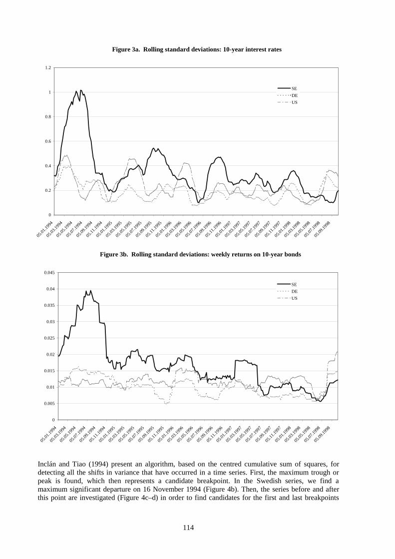
114
Inclán and Tiao (1994) present an algorithm, based on the centred cumulative sum of squares, fordetecting all the shifts in variance that have occurred in a time series. First, the maximum trough orpeak is found, which then represents a candidate breakpoint. In the Swedish series, we find amaximum significant departure on 16 November 1994 (Figure 4b). Then, the series before and afterthis point are investigated (Figure 4c–d) in order to find candidates for the first and last breakpoints
Figure 3a. Rolling standard deviations: 10-year interest rates
0
0.2
0.4
0.6
0.8
1
1.2
05.01
.1994
05.03
.1994
05.05
.1994
05.07
.1994
05.09
.1994
05.11
.1994
05.01
.1995
05.03
.1995
05.05
.1995
05.07
.1995
05.09
.1995
05.11
.1995
05.01
.1996
05.03
.1996
05.05
.1996
05.07
.1996
05.09
.1996
05.11
.1996
05.01
.1997
05.03
.1997
05.05
.1997
05.07
.1997
05.09
.1997
05.11
.1997
05.01
.1998
05.03
.1998
05.05
.1998
05.07
.1998
05.09
.1998
SE
DE
US
Figure 3b. Rolling standard deviations: weekly returns on 10-year bonds
0
0.005
0.01
0.015
0.02
0.025
0.03
0.035
0.04
0.045
05.01
.1994
05.03
.1994
05.05
.1994
05.07
.1994
05.09
.1994
05.11
.1994
05.01
.1995
05.03
.1995
05.05
.1995
05.07
.1995
05.09
.1995
05.11
.1995
05.01
.1996
05.03
.1996
05.05
.1996
05.07
.1996
05.09
.1996
05.11
.1996
05.01
.1997
05.03
.1997
05.05
.1997
05.07
.1997
05.09
.1997
05.11
.1997
05.01
.1998
05.03
.1998
05.05
.1998
05.07
.1998
05.09
.1998
SE
DE
US
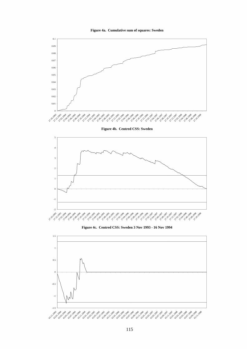
115
Figure 4a. Cumulative sum of squares: Sweden
0
0.01
0.02
0.03
0.04
0.05
0.06
0.07
0.08
0.09
0.1
27.10
.1993
27.12
.1993
27.02
.1994
27.04
.1994
27.06
.1994
27.08
.1994
27.10
.1994
27.12
.1994
27.02
.1995
27.04
.1995
27.06
.1995
27.08
.1995
27.10
.1995
27.12
.1995
27.02
.1996
27.04
.1996
27.06
.1996
27.08
.1996
27.10
.1996
27.12
.1996
27.02
.1997
27.04
.1997
27.06
.1997
27.08
.1997
27.10
.1997
27.12
.1997
27.02
.1998
27.04
.1998
27.06
.1998
27.08
.1998
27.10
.1998
Figure 4b. Centred CSS: Sweden
-2
-1
0
1
2
3
4
5
27.10
.1993
27.12
.1993
27.02
.1994
27.04
.1994
27.06
.1994
27.08
.1994
27.10
.1994
27.12
.1994
27.02
.1995
27.04
.1995
27.06
.1995
27.08
.1995
27.10
.1995
27.12
.1995
27.02
.1996
27.04
.1996
27.06
.1996
27.08
.1996
27.10
.1996
27.12
.1996
27.02
.1997
27.04
.1997
27.06
.1997
27.08
.1997
27.10
.1997
27.12
.1997
27.02
.1998
27.04
.1998
27.06
.1998
27.08
.1998
27.10
.1998
Figure 4c. Centred CSS: Sweden 3 Nov 1993 - 16 Nov 1994
-1.5
-1
-0.5
0
0.5
1
1.5
03.11
.1993
03.01
.1994
03.03
.1994
03.05
.1994
03.07
.1994
03.09
.1994
03.11
.1994
03.01
.1995
03.03
.1995
03.05
.1995
03.07.1
995
03.09
.1995
03.11
.1995
03.01
.1996
03.03
.1996
03.05
.1996
03.07
.1996
03.09
.1996
03.11
.1996
03.01
.1997
03.03
.1997
03.05
.1997
03.07
.1997
03.09
.1997
03.11
.1997
03.01
.1998
03.03
.1998
03.05
.1998
03.07
.1998
03.09
.1998
03.11
.1998
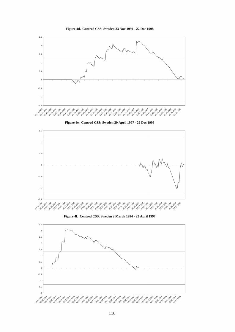
116
Figure 4d. Centred CSS: Sweden 23 Nov 1994 - 22 Dec 1998
-1.5
-1
-0.5
0
0.5
1
1.5
2
2.5
03.11
.1993
03.01
.1994
03.03
.1994
03.05
.1994
03.07
.1994
03.09
.1994
03.11
.1994
03.01
.1995
03.03
.1995
03.05
.1995
03.07.1
995
03.09
.1995
03.11
.1995
03.01
.1996
03.03
.1996
03.05
.1996
03.07
.1996
03.09
.1996
03.11
.1996
03.01
.1997
03.03
.1997
03.05
.1997
03.07
.1997
03.09
.1997
03.11
.1997
03.01
.1998
03.03
.1998
03.05
.1998
03.07
.1998
03.09
.1998
03.11
.1998
Figure 4e. Centred CSS: Sweden 29 April 1997 - 22 Dec 1998
-1.5
-1
-0.5
0
0.5
1
1.5
03.11
.1993
03.01
.1994
03.03
.1994
03.05
.1994
03.07
.1994
03.09
.1994
03.11
.1994
03.01
.1995
03.03
.1995
03.05
.1995
03.07.1
995
03.09
.1995
03.11
.1995
03.01
.1996
03.03
.1996
03.05
.1996
03.07
.1996
03.09
.1996
03.11
.1996
03.01
.1997
03.03
.1997
03.05
.1997
03.07
.1997
03.09
.1997
03.11
.1997
03.01
.1998
03.03
.1998
03.05
.1998
03.07
.1998
03.09
.1998
03.11
.1998
Figure 4f. Centred CSS: Sweden 2 March 1994 - 22 April 1997
-2
-1.5
-1
-0.5
0
0.5
1
1.5
2
2.5
3
3.5
03.11
.1993
03.01
.1994
03.03
.1994
03.05
.1994
03.07
.1994
03.09
.1994
03.11
.1994
03.01
.1995
03.03
.1995
03.05
.1995
03.07.1
995
03.09
.1995
03.11
.1995
03.01
.1996
03.03
.1996
03.05
.1996
03.07
.1996
03.09
.1996
03.11
.1996
03.01
.1997
03.03
.1997
03.05
.1997
03.07
.1997
03.09
.1997
03.11
.1997
03.01
.1998
03.03
.1998
03.05
.1998
03.07
.1998
03.09
.1998
03.11
.1998
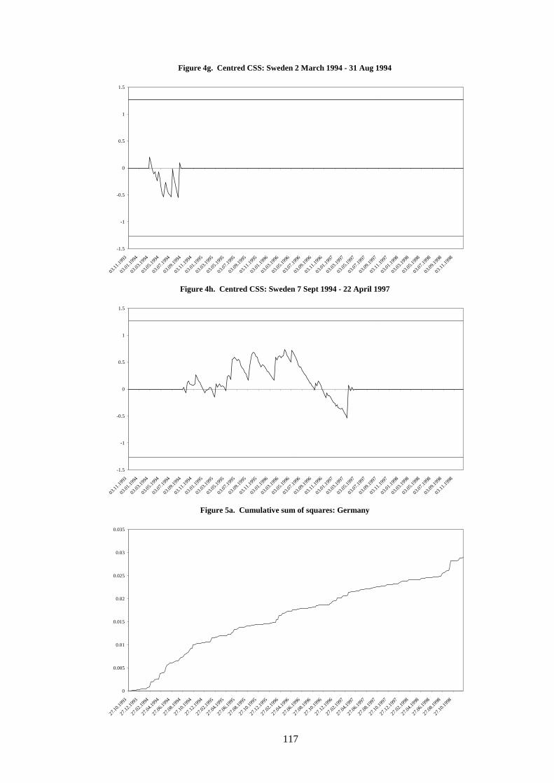
117
Figure 4g. Centred CSS: Sweden 2 March 1994 - 31 Aug 1994
-1.5
-1
-0.5
0
0.5
1
1.5
03.11
.1993
03.01
.1994
03.03
.1994
03.05
.1994
03.07
.1994
03.09
.1994
03.11
.1994
03.01
.1995
03.03
.1995
03.05
.1995
03.07.1
995
03.09
.1995
03.11
.1995
03.01
.1996
03.03
.1996
03.05
.1996
03.07
.1996
03.09
.1996
03.11
.1996
03.01
.1997
03.03
.1997
03.05
.1997
03.07
.1997
03.09
.1997
03.11
.1997
03.01
.1998
03.03
.1998
03.05
.1998
03.07
.1998
03.09
.1998
03.11
.1998
Figure 4h. Centred CSS: Sweden 7 Sept 1994 - 22 April 1997
-1.5
-1
-0.5
0
0.5
1
1.5
03.11
.1993
03.01
.1994
03.03
.1994
03.05
.1994
03.07
.1994
03.09
.1994
03.11
.1994
03.01
.1995
03.03
.1995
03.05
.1995
03.07.1
995
03.09
.1995
03.11
.1995
03.01
.1996
03.03
.1996
03.05
.1996
03.07
.1996
03.09
.1996
03.11
.1996
03.01
.1997
03.03
.1997
03.05
.1997
03.07
.1997
03.09
.1997
03.11
.1997
03.01
.1998
03.03
.1998
03.05
.1998
03.07
.1998
03.09
.1998
03.11
.1998
Figure 5a. Cumulative sum of squares: Germany
0
0.005
0.01
0.015
0.02
0.025
0.03
0.035
27.10
.1993
27.12
.1993
27.02
.1994
27.04
.1994
27.06
.1994
27.08
.1994
27.10
.1994
27.12
.1994
27.02
.1995
27.04
.1995
27.06
.1995
27.08
.1995
27.10
.1995
27.12
.1995
27.02
.1996
27.04
.1996
27.06
.1996
27.08
.1996
27.10
.1996
27.12
.1996
27.02
.1997
27.04
.1997
27.06
.1997
27.08
.1997
27.10
.1997
27.12
.1997
27.02
.1998
27.04
.1998
27.06
.1998
27.08
.1998
27.10
.1998
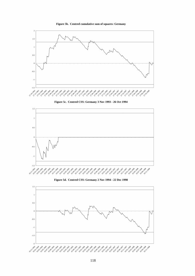
118
Figure 5b. Centred cumulative sum of squares: Germany
-1.5
-1
-0.5
0
0.5
1
1.5
2
27.10
.1993
27.12
.1993
27.02
.1994
27.04
.1994
27.06
.1994
27.08
.1994
27.10
.1994
27.12
.1994
27.02
.1995
27.04
.1995
27.06
.1995
27.08
.1995
27.10
.1995
27.12
.1995
27.02
.1996
27.04
.1996
27.06
.1996
27.08
.1996
27.10
.1996
27.12
.1996
27.02
.1997
27.04
.1997
27.06
.1997
27.08
.1997
27.10
.1997
27.12
.1997
27.02
.1998
27.04
.1998
27.06
.1998
27.08
.1998
27.10
.1998
Figure 5c. Centred CSS: Germany 3 Nov 1993 - 26 Oct 1994
-1.5
-1
-0.5
0
0.5
1
1.5
03.11
.1993
03.01
.1994
03.03
.1994
03.05
.1994
03.07
.1994
03.09
.1994
03.11
.1994
03.01
.1995
03.03
.1995
03.05
.1995
03.07.1
995
03.09
.1995
03.11
.1995
03.01
.1996
03.03
.1996
03.05
.1996
03.07
.1996
03.09
.1996
03.11
.1996
03.01
.1997
03.03
.1997
03.05
.1997
03.07
.1997
03.09
.1997
03.11
.1997
03.01
.1998
03.03
.1998
03.05
.1998
03.07
.1998
03.09
.1998
03.11
.1998
Figure 5d. Centred CSS: Germany 2 Nov 1994 - 22 Dec 1998
-2
-1.5
-1
-0.5
0
0.5
1
1.5
03.11
.1993
03.01
.1994
03.03
.1994
03.05
.1994
03.07
.1994
03.09
.1994
03.11
.1994
03.01
.1995
03.03
.1995
03.05
.1995
03.07.1
995
03.09
.1995
03.11
.1995
03.01
.1996
03.03
.1996
03.05
.1996
03.07
.1996
03.09
.1996
03.11
.1996
03.01
.1997
03.03
.1997
03.05
.1997
03.07
.1997
03.09
.1997
03.11
.1997
03.01
.1998
03.03
.1998
03.05
.1998
03.07
.1998
03.09
.1998
03.11
.1998
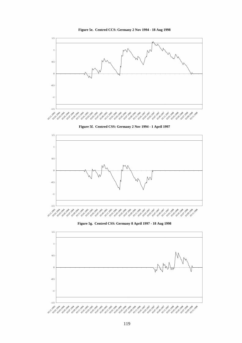
119
Figure 5e. Centred CCS: Germany 2 Nov 1994 - 18 Aug 1998
-1.5
-1
-0.5
0
0.5
1
1.5
03.11
.1993
03.01
.1994
03.03
.1994
03.05
.1994
03.07
.1994
03.09
.1994
03.11
.1994
03.01
.1995
03.03
.1995
03.05
.1995
03.07.1
995
03.09
.1995
03.11
.1995
03.01
.1996
03.03
.1996
03.05
.1996
03.07
.1996
03.09
.1996
03.11
.1996
03.01
.1997
03.03
.1997
03.05
.1997
03.07
.1997
03.09
.1997
03.11
.1997
03.01
.1998
03.03
.1998
03.05
.1998
03.07
.1998
03.09
.1998
03.11
.1998
Figure 5f. Centred CSS: Germany 2 Nov 1994 - 1 April 1997
-1.5
-1
-0.5
0
0.5
1
1.5
03.11
.1993
03.01
.1994
03.03
.1994
03.05
.1994
03.07
.1994
03.09
.1994
03.11
.1994
03.01
.1995
03.03
.1995
03.05
.1995
03.07.1
995
03.09
.1995
03.11
.1995
03.01
.1996
03.03
.1996
03.05
.1996
03.07
.1996
03.09
.1996
03.11
.1996
03.01
.1997
03.03
.1997
03.05
.1997
03.07
.1997
03.09
.1997
03.11
.1997
03.01
.1998
03.03
.1998
03.05
.1998
03.07
.1998
03.09
.1998
03.11
.1998
Figure 5g. Centred CSS: Germany 8 April 1997 - 18 Aug 1998
-1.5
-1
-0.5
0
0.5
1
1.5
03.11
.1993
03.01
.1994
03.03
.1994
03.05
.1994
03.07
.1994
03.09
.1994
03.11
.1994
03.01
.1995
03.03
.1995
03.05
.1995
03.07.1
995
03.09
.1995
03.11
.1995
03.01
.1996
03.03
.1996
03.05
.1996
03.07
.1996
03.09
.1996
03.11
.1996
03.01
.1997
03.03
.1997
03.05
.1997
03.07
.1997
03.09
.1997
03.11
.1997
03.01
.1998
03.03
.1998
03.05
.1998
03.07
.1998
03.09
.1998
03.11
.1998
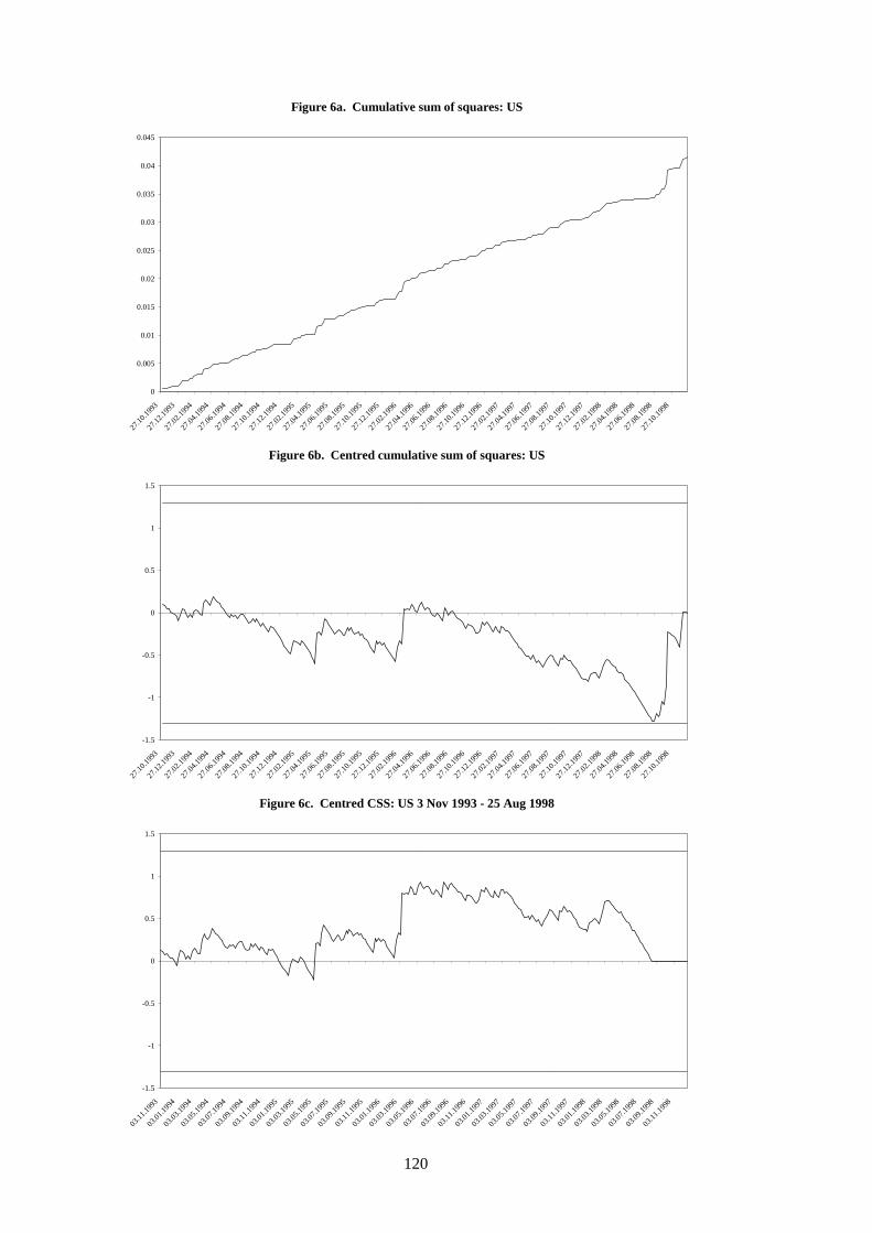
120
Figure 6a. Cumulative sum of squares: US
0
0.005
0.01
0.015
0.02
0.025
0.03
0.035
0.04
0.045
27.10
.1993
27.12
.1993
27.02
.1994
27.04
.1994
27.06
.1994
27.08
.1994
27.10
.1994
27.12
.1994
27.02
.1995
27.04
.1995
27.06
.1995
27.08
.1995
27.10
.1995
27.12
.1995
27.02
.1996
27.04
.1996
27.06
.1996
27.08
.1996
27.10
.1996
27.12
.1996
27.02
.1997
27.04
.1997
27.06
.1997
27.08
.1997
27.10
.1997
27.12
.1997
27.02
.1998
27.04
.1998
27.06
.1998
27.08
.1998
27.10
.1998
Figure 6b. Centred cumulative sum of squares: US
-1.5
-1
-0.5
0
0.5
1
1.5
27.10
.1993
27.12
.1993
27.02
.1994
27.04
.1994
27.06
.1994
27.08
.1994
27.10
.1994
27.12
.1994
27.02
.1995
27.04
.1995
27.06
.1995
27.08
.1995
27.10
.1995
27.12
.1995
27.02
.1996
27.04
.1996
27.06
.1996
27.08
.1996
27.10
.1996
27.12
.1996
27.02
.1997
27.04
.1997
27.06
.1997
27.08
.1997
27.10
.1997
27.12
.1997
27.02
.1998
27.04
.1998
27.06
.1998
27.08
.1998
27.10
.1998
Figure 6c. Centred CSS: US 3 Nov 1993 - 25 Aug 1998
-1.5
-1
-0.5
0
0.5
1
1.5
03.11
.1993
03.01
.1994
03.03
.1994
03.05
.1994
03.07
.1994
03.09
.1994
03.11
.1994
03.01
.1995
03.03
.1995
03.05
.1995
03.07.1
995
03.09
.1995
03.11
.1995
03.01
.1996
03.03
.1996
03.05
.1996
03.07
.1996
03.09
.1996
03.11
.1996
03.01
.1997
03.03
.1997
03.05
.1997
03.07
.1997
03.09
.1997
03.11
.1997
03.01
.1998
03.03
.1998
03.05
.1998
03.07
.1998
03.09
.1998
03.11
.1998
121
(23 February 1994 and 22 April 1997). We take 23 February 1994 as the first breakpoint, since thereare too few observations to allow us to find a possible earlier breakpoint. In Figure 4e, it is confirmedthat 22 April 1997 is the last breakpoint, since there are no violations of the 95% confidence intervals.The analysis is then repeated for the new series starting at the first breakpoint and ending at the lastbreakpoint. We iterate in this manner until all the breakpoints in the series are found. The sameprocedure is followed in investigating the German and US series in Figures 5 and 6 respectively. Wedetect a total of seven breaks in the three series: three (or possibly four) in the Swedish series, three inthe German series, and one in the US series (see Table 1).
Using the Inclán and Tiao algorithm, the first shift we detect is an upward shift in Swedish volatilityon 23 February 1994. This is followed by a downward shift later the same year, on 31 August. Thethird shift occurs in the German market on 26 October 1994, when volatility shifts down. In April1997, there is another downward shift in volatility in the German market in the first week of the month(1 April), followed by a downward shift in the Swedish market on 22 April. There is an upward shiftin volatility in the German market on 18 August 1998, immediately followed by an upward shift in theUS market on 25 August (at the 80% confidence level, there is also a shift in the Swedish market on1 September). These shifts took place in the wake of the Russian debt crisis. We note that some of theshifts in volatility occur at around the same time in at least two of the markets studied, while othershifts are market-specific.
Table 1Weeks with a shift in volatility
Sweden Germany United States
23 February 1994 (up)
31 August 1994 (down)
26 October 1994 (down)
22 April 1997 (down) 4 April 1997 (down)
1 September 1998 (up) 18 August 1998 (up) 25 August 1998 (up)
In addition to investigating concurrent shifts in volatility, it is also of interest to look at more short-term synchrony. Let us first focus on contemporaneous large interest rate shocks in the three markets.In Table 2, we report large changes in interest rates defined as greater than 30 basis points in absolutevalue, that is, if the change in interest rates during a week has been larger than 30 basis points in atleast one of the markets we enter the changes for all markets in that week in Table 2. However, forclarity of exposition we do not report changes of less than 15 basis points. For the same reason,changes greater than 30 basis points are in boldface. There is only one instance when a change in oneof the large markets is not associated with a large change in the smaller Swedish market(3 December 1998). In most cases, a large change in the Swedish interest rate is contemporaneouswith a large change in the US or German rate, or both. But this is not always the case, which suggeststhat domestic factors also play an important role. The most striking example of this is 11 August 1994,when the Swedish Riksbank announced an increase in its repo rate. This was the first rate increasefollowing a period of easing and came as something of a surprise to the market, resulting in the 102basis point increase in the 10-year interest rate in the following week.
Another way to investigate short-term synchrony is to use the same technique as above to computerolling correlations among the series. These are shown in Figures 7a–b. During most of the period, itlooks as if the Swedish market is more highly correlated with the German than with the US market.We also note that the correlations vary a great deal over time, which makes it more difficult todistinguish possible trends in the correlations. But with the exception of the period of high correlationbetween the Swedish and German markets in 1994, the correlations seem to have trended upwardsduring the period.
To investigate the question of a possible interaction between volatility and correlations, we sort rolling20-week return volatility from the lowest to the highest. Then, the correlations of the returns are

122
ordered correspondingly (so that the dates are matched). Finally, the averages of the correlations foreach quartile are computed. The results are shown in Figures 8a–c. The overall impression from thesefigures is that the correlation between the returns on a large and small bond market is decreasing in thevolatility of the small market but increasing in the volatility of the large market. In Figure 8a, thecorrelation between Swedish and US returns is negatively related to the volatility in the Swedishmarket. The relation regarding the correlation between Swedish and German returns is not as clear.When the German market is the reference market the negative relation is weaker, as seen in Figure 8b.The evidence presented in Figure 8c tells us that volatility in the US market is positively related to thecorrelations with returns in the other two (smaller) markets.
The above preliminary results warrant a further assessment of the time variation in second moments.We therefore continue our analysis with the estimation of a multivariate ARCH model, which ispotentially able to accommodate the features documented above.
Table 2Large changes in interest rates
Week Sweden Germany United States
2 March 1994 66 3230 March 1994 45 24
6 April 1994 –3020 April 1994 62 3818 May 1994 –30 –15
25 May 1994 67 311 June 1994 49 24
22 June 1994 3529 June 1994 –416 July 1994 96 16
10 August 1994 35 23 19
17 August 1994 102 17 –17
31 August 1994 –4328 September 1994 –40 –20
16 November 1994 –388 March 1995 419 May 1995 –43 –18 –406 June 1995 –51 –14 –18
12 September 1995 –4419 September 1995 –336 February 1996 50 26
20 February 1996 27 30 3112 March 1996 20 23 4526 March 1996 –30 –15
7 May 1996 39 17 20
17 September 1996 –33 –19
19 November 1996 –3118 March 1997 59 26
6 October 1998 –24 –17 –3413 October 1998 23 46 573 December 1998 –22 –43
Note: A large change is defined as a change greater than 30 basis points in absolute value. Changes smaller than 15 basispoints are not shown in the table.
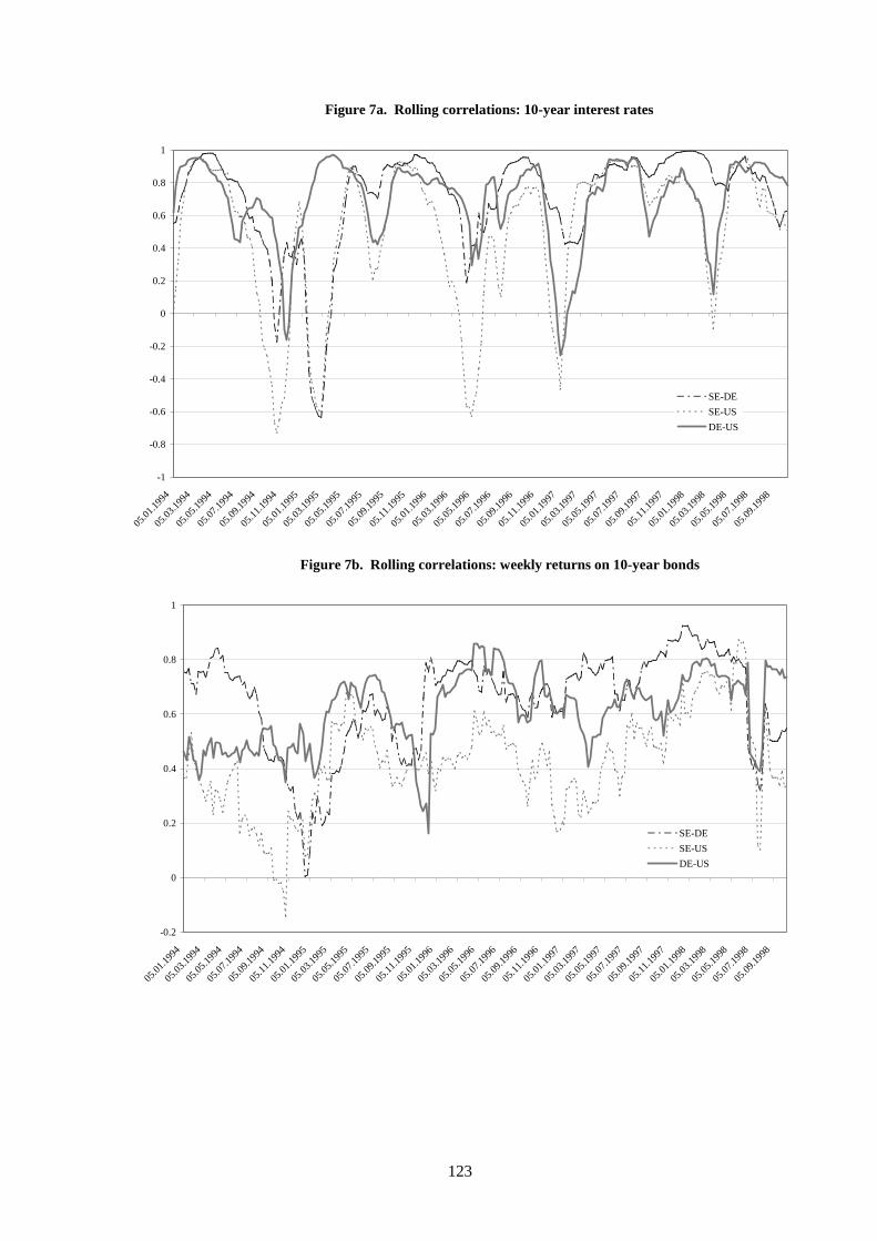
123
Figure 7a. Rolling correlations: 10-year interest rates
-1
-0.8
-0.6
-0.4
-0.2
0
0.2
0.4
0.6
0.8
1
05.01
.1994
05.03
.1994
05.05
.1994
05.07
.1994
05.09
.1994
05.11
.1994
05.01
.1995
05.03
.1995
05.05
.1995
05.07
.1995
05.09
.1995
05.11
.1995
05.01
.1996
05.03
.1996
05.05
.1996
05.07
.1996
05.09
.1996
05.11
.1996
05.01
.1997
05.03
.1997
05.05
.1997
05.07
.1997
05.09
.1997
05.11
.1997
05.01
.1998
05.03
.1998
05.05
.1998
05.07
.1998
05.09
.1998
SE-DE
SE-US
DE-US
Figure 7b. Rolling correlations: weekly returns on 10-year bonds
-0.2
0
0.2
0.4
0.6
0.8
1
05.01
.1994
05.03
.1994
05.05
.1994
05.07
.1994
05.09
.1994
05.11
.1994
05.01
.1995
05.03
.1995
05.05
.1995
05.07
.1995
05.09
.1995
05.11
.1995
05.01
.1996
05.03
.1996
05.05
.1996
05.07
.1996
05.09
.1996
05.11
.1996
05.01
.1997
05.03
.1997
05.05
.1997
05.07
.1997
05.09
.1997
05.11
.1997
05.01
.1998
05.03
.1998
05.05
.1998
05.07
.1998
05.09
.1998
SE-DE
SE-US
DE-US
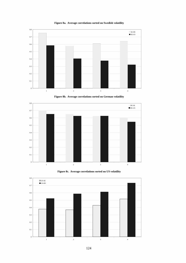
124
Figure 8a. Average correlations sorted on Swedish volatility
0
0.1
0.2
0.3
0.4
0.5
0.6
0.7
0.8
1 2 3 4
SE-DE
SE-US
Figure 8b. Average correlations sorted on German volatility
0
0.1
0.2
0.3
0.4
0.5
0.6
0.7
0.8
1 2 3 4
DE-SE
DE-US
Figure 8c. Average correlations sorted on US volatility
0
0.1
0.2
0.3
0.4
0.5
0.6
0.7
0.8
1 2 3 4
US-SE
US-DE

125
3. The empirical model
We need a model that is flexible enough to capture the time-varying nature of the interdependenciesbetween the bond markets, as indicated above. A multivariate ARCH model should be able to capturethe observed patterns to some extent.7
3.1 Conditional means
A straightforward linear model will be used for the conditional means. Let itR denote the return on the
ith bond market, where i = DE (Germany), US (United States) or SE (Sweden). We consider thefollowing moving average (MA) specification for Germany
(3) USt
DEDEt
DEDEt
DEDEtR 12110 −− εθ+εθ+ε+θ=
and for the United States
(4) USt
USDEt
USUSt
USUStR 12110 −− εθ+εθ+ε+θ=
This specification is consistent with the idea that price spillovers do not necessarily have to be relatedto volatility spillovers or the fact that shocks in the two markets are correlated. For Swedish returns,the model is formulated such that price shocks from all markets could be of importance,
(5) SEt
SEUSt
SEDEt
SESEt
SESEtR 1312110 −−− εθ+εθ+εθ+ε+θ=
In the next section, we will discuss how to model the error terms, allowing for time variation, and thelink to the conditional second moments in the above pricing equations.
3.2 Conditional variances
We will use a model suggested by Engle and Kroner (1995), known as the BEKK model. This modelis a special case of the more general VEC representation of a multivariate generalised ARCH model.The advantage of the BEKK model for conditional covariances is that it guarantees positive definiteconditional covariance matrices under weak conditions. Moreover, compared with other models it usesfew parameters, but still allows for conditional correlations and is able to capture potential cross-volatility interactions as well. For tractability, the model is here restricted to be of order (1,1). Thespecification below allows us to simultaneously model conditional variances, covariances andcorrelations.
Let [ ]′εεε=ε SEt
USt
DEtt denote a combined error term from the conditional mean specifications. In the
general BEKK model we consider, the dynamic for the conditional covariance matrix is given by
(6) ( ) BHBAAIEH ttttttt 1111 −−−− ′+ε′ε′+ΩΩ′=ε′ε≡
ZKHUH LVD x 3 upper triangular matrix of parameters, and A and B are 3 x 3 matrices of parameters.We can impose some additional restrictions on the model. We make the innocuous assumption thatthere is no spillover from the small Swedish bond market to the larger US and German markets. Thisresults in the following parameterisation of the A and B matrices
=
333231
232221
11 00
aaa
aaa
a
A and
=
333231
232221
11 00
bbb
bbb
b
B
7 We started by estimating univariate GARCH models for each market separately allowing for shifts in variance, in
agreement with the findings reported in the previous section. However, the shift coefficients turned out not to bestatistically significant in the GARCH framework.
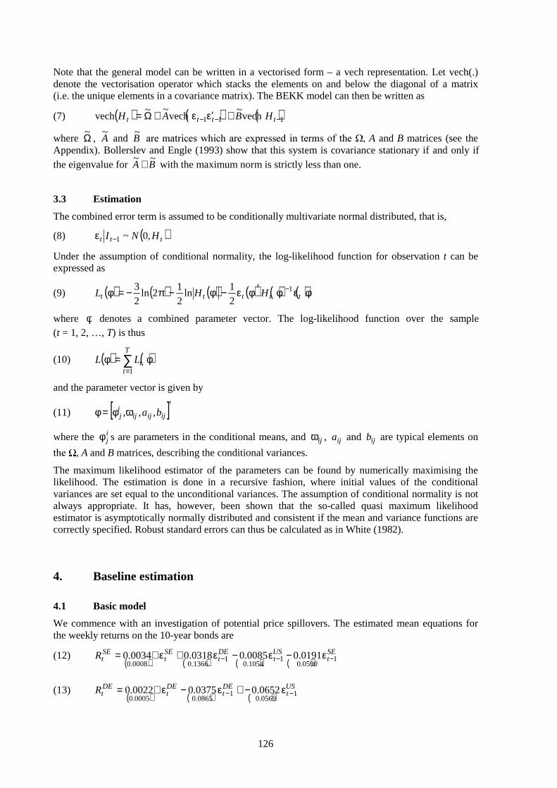
126
Note that the general model can be written in a vectorised form – a vech representation. Let vech(.)denote the vectorisation operator which stacks the elements on and below the diagonal of a matrix(i.e. the unique elements in a covariance matrix). The BEKK model can then be written as
(7) ( ) ( ) ( )111 vech~
vech~~
vech −−− +ε′ε+Ω= tttt HBAH
where Ω~ , A~
and B~DUHPDWULFHVZKLFKDUHH[SUHVVHGLQWHUPVRIWKH A and B matrices (see the
Appendix). Bollerslev and Engle (1993) show that this system is covariance stationary if and only ifthe eigenvalue for BA
~~ + with the maximum norm is strictly less than one.
3.3 Estimation
The combined error term is assumed to be conditionally multivariate normal distributed, that is,
(8) ( )ttt HNI ,0~1−ε
Under the assumption of conditional normality, the log-likelihood function for observation t can beexpressed as
(9) ( ) ( ) ( ) ( ) ( ) ( )φεφ′φε−φ−π−=φ −ttttt HHL 1
2
1ln
2
12ln
2
3
where φ denotes a combined parameter vector. The log-likelihood function over the sample(t = 1, 2, …, T) is thus
(10) ( ) ( )φ=φ ∑=
T
ttLL
1
and the parameter vector is given by
(11) [ ]′ωφ=φ ijijijij ba ,,,
where the ijφ s are parameters in the conditional means, and ijω , ija and ijb are typical elements on
WKH A and B matrices, describing the conditional variances.
The maximum likelihood estimator of the parameters can be found by numerically maximising thelikelihood. The estimation is done in a recursive fashion, where initial values of the conditionalvariances are set equal to the unconditional variances. The assumption of conditional normality is notalways appropriate. It has, however, been shown that the so-called quasi maximum likelihoodestimator is asymptotically normally distributed and consistent if the mean and variance functions arecorrectly specified. Robust standard errors can thus be calculated as in White (1982).
4. Baseline estimation
4.1 Basic model
We commence with an investigation of potential price spillovers. The estimated mean equations forthe weekly returns on the 10-year bonds are
(12)( ) ( ) ( ) ( )
SEt
USt
DEt
SEt
SEtR 1
0590.01
1054.01
1366.00008.00191.00085.00318.00034.0 −−− ε−ε−ε+ε+=
(13)( ) ( ) ( )
USt
DEt
DEt
DEtR 1
0569.01
0865.00005.00652.00375.00022.0 −− ε−+ε−ε+=
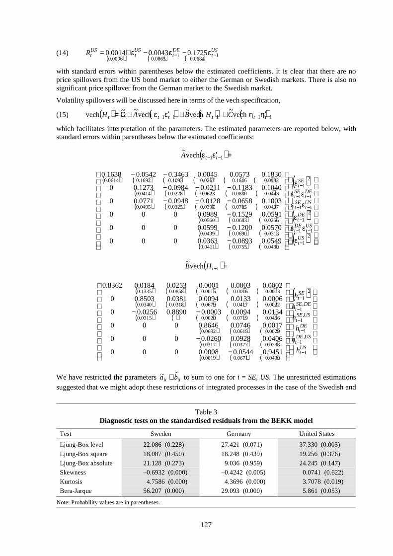
127
(14)( ) ( ) ( )
USt
DEt
USt
UStR 1
0684.01
0865.00006.01725.00043.00014.0 −− ε−ε−ε+=
with standard errors within parentheses below the estimated coefficients. It is clear that there are noprice spillovers from the US bond market to either the German or Swedish markets. There is also nosignificant price spillover from the German market to the Swedish market.
Volatility spillovers will be discussed here in terms of the vech specification,
(15) ( ) ( ) ( ) ( )11111 vech~
vech~
vech~~
vech −−−−− η′η++ε′ε+Ω= tttttt CHBAH
which facilitates interpretation of the parameters. The estimated parameters are reported below, withstandard errors within parentheses below the estimated coefficients:
( ) =ε′ε −− 11vech~
ttA
( ) ( ) ( ) ( ) ( ) ( )
( ) ( ) ( ) ( ) ( )
( ) ( ) ( ) ( ) ( )
( ) ( ) ( )
( ) ( ) ( )
( ) ( ) ( )
( )
( )
( )
ε
εεε
εεεε
ε
−
−
−
−−−
−−−
−−
−
−−
−
−−
−−
−
21
11
21
11
11
21
0430.00755.00411.0
0313.00690.00439.0
0256.00683.00560.0
0497.00705.00397.00325.00495.0
0443.00830.00623.00228.00414.0
0982.01616.00267.01093.01692.00614.0
0549.00893.00363.0000
0570.01200.00599.0000
0591.01529.00989.0000
1003.00658.00128.00948.00771.00
1040.01183.00211.00984.01273.00
1830.00573.00045.03463.00542.01638.0
USt
USt
DEt
DEt
USt
SEt
DEt
SEt
SEt
( ) =−1vech~
tHB
( ) ( ) ( ) ( ) ( )
( ) ( ) ( ) ( ) ( )
( ) ( ) ( ) ( ) ( )
( ) ( ) ( )
( ) ( ) ( )
( ) ( ) ( )
( )
−
−
−−
−
−
−
−
−
−
USt
USDEt
DEt
USSEt
DESEt
SEt
h
h
h
h
h
h
1
,1
1
,1
,1
21
0430.00671.00019.0
0338.00377.00317.0
0029.00619.00692.0
0456.00719.00020.00315.0
0022.00417.00679.00318.00340.0
0013.00016.00015.00858.01335.0
9451.00544.00008.0000
0406.00928.00260.0000
0017.00746.08646.0000
0134.00094.00003.08890.00256.00
0006.00133.00094.00381.08503.00
0002.00003.00001.00253.00184.08362.0
We have restricted the parameters iiii ba~~ + to sum to one for i = SE, US. The unrestricted estimations
suggested that we might adopt these restrictions of integrated processes in the case of the Swedish and
Table 3Diagnostic tests on the standardised residuals from the BEKK model
Test Sweden Germany United States
Ljung-Box level 22.086 (0.228) 27.421 (0.071) 37.330 (0.005)
Ljung-Box square 18.087 (0.450) 18.248 (0.439) 19.256 (0.376)
Ljung-Box absolute 21.128 (0.273) 9.036 (0.959) 24.245 (0.147)
Skewness –0.6932 (0.000) –0.4242 (0.005) 0.0741 (0.622)
Kurtosis 4.7586 (0.000) 4.3696 (0.000) 3.7078 (0.019)
Bera-Jarque 56.207 (0.000) 29.093 (0.000) 5.861 (0.053)
Note: Probability values are in parentheses.
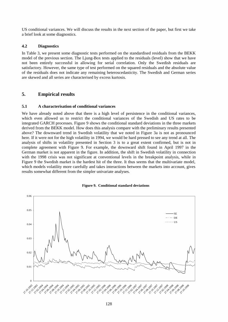
128
US conditional variances. We will discuss the results in the next section of the paper, but first we takea brief look at some diagnostics.
4.2 Diagnostics
In Table 3, we present some diagnostic tests performed on the standardised residuals from the BEKKmodel of the previous section. The Ljung-Box tests applied to the residuals (level) show that we havenot been entirely successful in allowing for serial correlation. Only the Swedish residuals aresatisfactory. However, the same type of test performed on the squared residuals and the absolute valueof the residuals does not indicate any remaining heteroscedasticity. The Swedish and German seriesare skewed and all series are characterised by excess kurtosis.
5. Empirical results
5.1 A characterisation of conditional variances
We have already noted above that there is a high level of persistence in the conditional variances,which even allowed us to restrict the conditional variances of the Swedish and US rates to beintegrated GARCH processes. Figure 9 shows the conditional standard deviations in the three marketsderived from the BEKK model. How does this analysis compare with the preliminary results presentedabove? The downward trend in Swedish volatility that we noted in Figure 3a is not as pronouncedhere. If it were not for the high volatility in 1994, we would be hard pressed to see any trend at all. Theanalysis of shifts in volatility presented in Section 3 is to a great extent confirmed, but is not incomplete agreement with Figure 9. For example, the downward shift found in April 1997 in theGerman market is not apparent in the figure. In addition, the shift in Swedish volatility in connectionwith the 1998 crisis was not significant at conventional levels in the breakpoint analysis, while inFigure 9 the Swedish market is the hardest hit of the three. It thus seems that the multivariate model,which models volatility more carefully and takes interactions between the markets into account, givesresults somewhat different from the simpler univariate analyses.
Figure 9. Conditional standard deviations
0
0.01
0.02
0.03
0.04
0.05
0.06
27.10
.1993
27.12
.1993
27.02
.1994
27.04
.1994
27.06
.1994
27.08
.1994
27.10
.1994
27.12
.1994
27.02
.1995
27.04
.1995
27.06
.1995
27.08
.1995
27.10
.1995
27.12
.1995
27.02
.1996
27.04
.1996
27.06
.1996
27.08
.1996
27.10
.1996
27.12
.1996
27.02
.1997
27.04
.1997
27.06
.1997
27.08
.1997
27.10
.1997
27.12
.1997
27.02
.1998
27.04
.1998
27.06
.1998
27.08
.1998
27.10
.1998
SE
DE
US
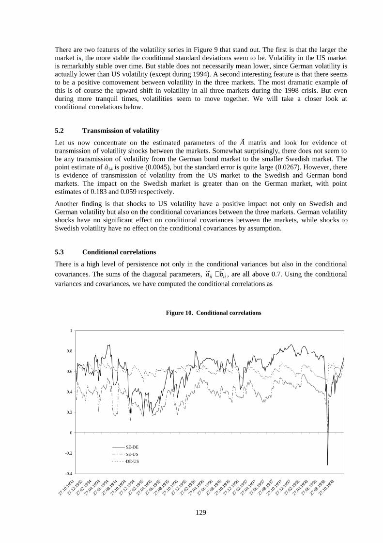
129
There are two features of the volatility series in Figure 9 that stand out. The first is that the larger themarket is, the more stable the conditional standard deviations seem to be. Volatility in the US marketis remarkably stable over time. But stable does not necessarily mean lower, since German volatility isactually lower than US volatility (except during 1994). A second interesting feature is that there seemsto be a positive comovement between volatility in the three markets. The most dramatic example ofthis is of course the upward shift in volatility in all three markets during the 1998 crisis. But evenduring more tranquil times, volatilities seem to move together. We will take a closer look atconditional correlations below.
5.2 Transmission of volatility
Let us now concentrate on the estimated parameters of the à matrix and look for evidence oftransmission of volatility shocks between the markets. Somewhat surprisingly, there does not seem tobe any transmission of volatility from the German bond market to the smaller Swedish market. Thepoint estimate of ã14 is positive (0.0045), but the standard error is quite large (0.0267). However, thereis evidence of transmission of volatility from the US market to the Swedish and German bondmarkets. The impact on the Swedish market is greater than on the German market, with pointestimates of 0.183 and 0.059 respectively.
Another finding is that shocks to US volatility have a positive impact not only on Swedish andGerman volatility but also on the conditional covariances between the three markets. German volatilityshocks have no significant effect on conditional covariances between the markets, while shocks toSwedish volatility have no effect on the conditional covariances by assumption.
5.3 Conditional correlations
There is a high level of persistence not only in the conditional variances but also in the conditional
covariances. The sums of the diagonal parameters, iiii ba~~ + , are all above 0.7. Using the conditional
variances and covariances, we have computed the conditional correlations as
Figure 10. Conditional correlations
-0.4
-0.2
0
0.2
0.4
0.6
0.8
1
27.10
.1993
27.12
.1993
27.02
.1994
27.04
.1994
27.06
.1994
27.08
.1994
27.10
.1994
27.12
.1994
27.02
.1995
27.04
.1995
27.06
.1995
27.08
.1995
27.10
.1995
27.12
.1995
27.02
.1996
27.04
.1996
27.06
.1996
27.08
.1996
27.10
.1996
27.12
.1996
27.02
.1997
27.04
.1997
27.06
.1997
27.08
.1997
27.10
.1997
27.12
.1997
27.02
.1998
27.04
.1998
27.06
.1998
27.08
.1998
27.10
.1998
SE-DE
SE-US
DE-US
130
(16)j
tit
ijtij
thh
h=ρ
for i, j ∈ SE,DE,US. These are shown in Figure 10. We can see that the conditional correlationbetween the two largest markets is the most stable. The correlation between the US and Germanreturns fluctuates within a narrow band around 0.6. It is also the case that the correlation between theSwedish and US markets is more stable than that between the Swedish and German markets. Thus, itseems that the larger the markets considered, the more stable the correlation between them will be. Wealso note that the Swedish and German markets are more highly correlated than the Swedish and USmarkets. Both of these correlations fluctuate quite a bit. The correlations with the Swedish market alsodrop drastically during the 1998 crisis, while the correlation between the US and German marketsactually increases.
6. Conclusion
The extent to which interest rates in a small national bond market are determined by domestic relativeto foreign factors is of considerable interest from an investment as well as from a monetary policyperspective. We have considered the transmission of shocks from the US and German bond markets tothe Swedish market during the recent period of floating exchange rates. We found evidence for theimportance of both local and global factors for the small Swedish bond market. We commenced withsome preliminary analyses that served to motivate the use of a multivariate GARCH model of theBEKK type. This approach enabled us to model time-varying conditional variances and covariances,which allows a great deal of flexibility in modelling the interaction between the three markets.
Several interesting facts emerged from the estimated multivariate model. The conditional variances inthe German and US markets were found to be more stable over time than the conditional variance inthe Swedish market. The conditional correlation between the large markets was also found to be quitestable over time, around 0.6, while the Swedish market’s correlations with these two markets weremuch more volatile (around 0.6 with the German market and 0.4 with the US market). We found noevidence that volatility shocks in the German bond market have any significant impact on thevolatility in the Swedish bond market the next week. However, there is clear evidence of transmissionof volatility shocks from the US market to the Swedish and German markets from one week to thenext. Thus, it appears that news from Germany is more rapidly incorporated into Swedish bond pricesthan news from the United States.
The more general conclusions that can be drawn from this paper are somewhat tentative because of thelimited number of countries investigated. Our main conclusion is that both local and global factorsplay important roles for a small bond market. We also conclude that larger markets are connected withmore stable second moments, that is, conditional variances are more stable, although not necessarilylower, over time in a large market compared with a smaller market. In addition, the larger the marketsinvestigated, the more stable the conditional correlations. It would be of great interest to see how thesegeneral conclusions hold up for other sets of countries.

131
Appendix
Vech representation
Let vec(.) and vech(.) denote the standard vectorisation operators. That is, let Ln denote the eliminationmatrix, defined so that for a square matrix M, vech(M) = Lnvec(M). Furthermore, let Dn denote theduplication matrix, defined so that for any symmetric matrix N, vec(N) = Dnvech(N). The dynamicscan first be rewritten in vec form as
(17) ( ) ( ) ( )1*
11** vecvecvec −−− +ε′ε+Ω= tttt HBAH
where ( )ΩΩ′=Ω vec* , AAA ′⊗′=* and BBB ′⊗′=* . In vech form, the dynamics can then beexpressed as
(18) ( ) ( ) ( )111 vech~
vech~~
vech −−− +ε′ε+Ω= tttt HBAH
where ( )ΩΩ′=Ω vech~
, nnnnn DAALDALA ′⊗′== *~ and nnnn DBBLDBLB ′⊗′== *~
.

132
Bibliography
Baba, Yasunori, Robert F Engle, D F Kraft and Kenneth F Kroner (1990): “Multivariate SimultaneousGeneralized ARCH”. Mimeo, Department of Economics, University of California, San Diego.
Bekaert, Geert and Guojun Wu (1997): “Asymmetric Volatility and Risk in Equity Markets”. WorkingPaper, Graduate School of Business, Stanford University.
Bollerslev Tim, Ray Y Chou and Kenneth F Kroner (1992): “ARCH Modeling in Finance: A Reviewof the Theory and Empirical Evidence”. Journal of Econometrics, 52, pp. 5-59.
Bollerslev, Tim and Robert F Engle (1993): “Common Persistence in Conditional Variances”.Econometrica, 61, pp. 167–86.
Bollerslev, Tim, Robert F Engle and Daniel B Nelson (1994): “ARCH Models”, in Robert F Engle andDaniel F McFadden (eds.), Handbook of Econometrics, Vol. 4, pp. 2951–3038.
Borio, Claudio E V and Robert N McCauley (1996): “The Economics of Recent Bond MarketVolatility”. BIS Economic Papers, No 45.
Davis, E P (1991): “International Diversification of Institutional Investors”. Bank of England,Discussion Papers No. 44.
Diebold, Francis X and Marc Nerlove (1989): “The Dynamics of Exchange Rate Volatility: AMultivariate Latent Factor ARCH Model”. Journal of Applied Econometrics, Vol. 4, pp. 1–21.
Engle, Robert F and Kenneth F Kroner (1995): “Multivariate Simultaneous Generalised ARCH”.Econometric Theory, Vol. 11, pp. 122-50.
Engle, Robert F, Takatoshi Ito and Wen-Ling Lin (1990): “Meteor Showers or Heat Waves?Heteroskedastic Intra-Daily Volatility in the Foreign Exchange Market”. Econometrica, Vol. 58,pp. 525–42.
Engle, Robert F and Victor K Ng (1993): “Measuring and Testing the Impact of News on volatility”.Journal of Finance, Vol. 48, pp. 1749–78.
Engle, Robert F, Victor K Ng, and Michael Rothschild (1990): “Asset Pricing with a Factor – ARCHCovariance Structure: Empirical Estimates for Treasury Bills”. Journal of Econometrics, Vol. 45,pp. 213–37.
Frankel, Jeffrey A (1992): “Measuring International Capital Mobility”. American Economic Review,Vol. 82, pp. 197–202.
Glosten, Lawrence R, Ravi Jagannathan and David E Runkle (1993): “On the Relation between theExpected Value and the Volatility of the Nominal Excess Return on Stocks”. Journal of Finance,Vol. 48, pp. 1779–801.
Hamao, Yasushi, Ronald W Masulis and Victor K Ng (1990): “Correlations in Price Changes andVolatility across International Stock Markets”. Review of Financial Studies, Vol. 3, pp. 281–307.
Inclán, Carla and George C Tiao (1994): “Use of Cumulative Sums of Squares for RetrospectiveDetection of Changes of Variance”. Journal of the American Statistical Association, Vol. 89,pp. 913-23.
King, Mervyn, Enrique Sentana and Sushil Wadhwani (1994): “Volatility and Links between NationalStock Markets”. Econometrica, Vol. 62, pp. 901–33.
Koutmos, Gregory and G Geoffrey Booth (1995): “Asymmetric Volatility Transmission inInternational Stock Markets”. Journal of International Money and Finance, Vol. 14, pp. 747-62.
Kroner, Kenneth F and Victor K Ng (1995): “Modeling the Time Varying Co-movements of AssetReturns”. Working Paper, Wells Fargo Nikko Investment Advisors.

133
Lin, Wen-Ling, Robert F Engle and Takatoshi Ito (1994): “Do Bulls and Bears Move across Borders?International Transmission of Stock Returns and Volatility”. Review of Financial Studies, Vol. 7,pp. 507–38.
Mussa, Michael and Morris Goldstein (1993): “The Integration of World Capital Markets”, inChanging Capital Markets, proceedings of a symposium sponsored by the Federal Reserve Bank ofKansas City.
Nelson, Charles R and Andrew F Siegel (1987): “Parsimonious Modelling of Yield Curves”. Journalof Business, Vol. 60, pp. 473–89.
Ng, Victor K, Robert F Engle and Michael Rothschild (1992): “A Multi-Dynamic-Factor Models forStock Returns”. Journal of Econometrics, Vol. 52, pp. 245–66.
Singleton, Kenneth (1994): “Persistence of International Interest Rate Correlations”. Preparation forthe Berkeley Program in Finance.
Svensson, Lars E O (1995): “Estimating Forward Interest Rates with the Extended Nelson and SiegelMethod”. Quarterly Review, Sveriges Riksbank, Vol. 3, pp. 13-26.
Tesar, Linda and Ingrid Werner (1995): “Home Bias and High Turnover”. Journal of InternationalMoney and Finance, Vol. 14, pp. 467–92.
White, Halbert (1982): “Maximum Likelihood Estimation of Misspecified Models”. Econometrica,Vol. 50, pp. 1–26.
134
The dynamics of international asset price linkages andtheir effects on German stock and bond markets
Dietrich Domanski and Manfred Kremer1
1. Introduction
The financial market turbulences in 1998, as other crises previously, produced strong price movementsin the securities markets worldwide. This reflected, first, a general reassessment of credit risk, and,second, a drying-up of liquidity even in some of the largest mature securities markets.2 As a result,cross-market return correlations temporarily underwent dramatic changes, challenging portfolioallocation and risk management strategies which rely on constant historical comovements of assetprices. Against this background, the immediate question arises of how asset price linkages can beproperly measured when they are subject to periodic changes as observed in times of market stress.The main purpose of the present paper is to address this question more thoroughly.
In order to measure the dynamics of international asset price linkages, we first employ bivariateGARCH models to analyse the comovements between weekly stock and bond market returns acrossthe G3 countries. GARCH models take account of the specific time-series properties of short-termasset returns, which is needed to obtain reliable estimates of the cross-country linkages. Next,switching-regime ARCH or “SWARCH” models are applied which can identify different volatilityregimes for short-term asset prices endogenously. We use this methodology to address two issues:first, “Are international short-term return linkages state-dependent?”, and second, “Do volatilityspillovers affect individual segments of the domestic bond or stock market differently (i.e. are theymarket-segment-dependent)?” The first question may also be referred to as the “contagionhypothesis”. This states that contagion leads to a significant increase in the cross-market correlationduring states of financial market turmoil. Hence, contagion differs from mere “interdependence” inthat it demands a stronger-than-normal market linkage during periods of stress.3
The paper is organised as follows: Section 2 presents some stylised facts on short-term asset returnsderived from summary statistics and simple cross-market correlations. In the third section, we outlinethe ARCH and SWARCH techniques employed to assess the comovements of weekly returns onvarious bond and stock price indices. In Section 4, the hypothesis of state-dependent internationalvolatility spillovers between the United States, Japan and Germany is tested. The fifth sectionexamines the question of market-segment-dependent contagion within the German financial system.Section 6 concludes by addressing some possible implications of the results.
2. Measuring international asset price linkages: some stylised facts
The asset universe considered in this paper comprises G3 bond and stock markets, the formerrepresented by the prices of 10-year benchmark government bonds, the latter by broad-market priceindices of Datastream (DS country indices).4 Additionally, the following segments of German
1
The views expressed in this paper are those of the authors and do not necessarily reflect the opinion of the DeutscheBundesbank.
2See International Monetary Fund (1998), p. 38.
3See Forbes and Rigobon (1999), p. 1, and Baig and Goldfajn (1999), p. 169.
4A detailed description of the data is given in the Appendix.
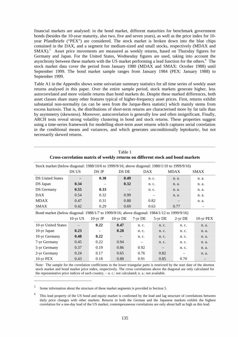
135
financial markets are analysed: in the bond market, different maturities for benchmark governmentbonds (besides the 10-year maturity, also two, five and seven years), as well as the price index for 10-year Pfandbriefe (“PEX”) are considered. The stock market is broken down into the blue chipscontained in the DAX, and a segment for medium-sized and small stocks, respectively (MDAX andSMAX).5 Asset price movements are measured as weekly returns, based on Thursday figures forGermany and Japan. For the United States, Wednesday figures are used, taking into account theasynchrony between these markets with the US market performing a lead function for the others.6 Thestock market data cover the period from January 1980 (MDAX and SMAX: October 1988) untilSeptember 1999. The bond market sample ranges from January 1984 (PEX: January 1988) toSeptember 1999.
Table A1 in the Appendix shows some univariate summary statistics for all time series of weekly assetreturns analysed in this paper. Over the entire sample period, stock markets generate higher, lessautocorrelated and more volatile returns than bond markets do. Despite these marked differences, bothasset classes share many other features typical of higher-frequency asset prices. First, returns exhibitsubstantial non-normality (as can be seen from the Jarque-Bera statistic) which mainly stems fromexcess kurtosis. That is, the distributions of short-term returns are characterised more by fat tails thanby asymmetry (skewness). Moreover, autocorrelation is generally low and often insignificant. Finally,ARCH tests reveal strong volatility clustering in bond and stock returns. These properties suggestusing a time-series framework for modelling short-term asset returns which captures serial correlationin the conditional means and variances, and which generates unconditionally leptokurtic, but notnecessarily skewed returns.
Table 1Cross-correlation matrix of weekly returns on different stock and bond markets
Stock market (below diagonal: 1988/10/6 to 1999/9/16; above diagonal: 1980/1/10 to 1999/9/16)
DS US DS JP DS DE DAX MDAX SMAX
DS United States – 0.38 0.49 n. c. n. a. n. a.
DS Japan 0.34 – 0.32 n. c. n. a. n. a.
DS Germany 0.55 0.33 – n. c. n. a. n. a.
DAX 0.54 0.32 0.99 – n. a. n. a.
MDAX 0.47 0.31 0.88 0.82 – n. a.
SMAX 0.42 0.29 0.69 0.63 0.77 –
Bond market (below diagonal: 1988/1/7 to 1999/9/16; above diagonal: 1984/1/12 to 1999/9/16)
10-yr US 10-yr JP 10-yr DE 7-yr DE 5-yr DE 2-yr DE 10-yr PEX
10-yr United States – 0.22 0.47 n. c. n. c. n. c. n. a.
10-yr Japan 0.23 – 0.28 n. c. n. c. n. c. n. a.
10-yr Germany 0.48 0.22 – n. c. n. c. n. c. n. a.
7-yr Germany 0.45 0.22 0.94 – n. c. n. c. n. a.
5-yr Germany 0.37 0.19 0.86 0.92 – n. c. n. a.
2-yr Germany 0.24 0.17 0.65 0.76 0.82 – n. a.
10-yr PEX 0.43 0.18 0.88 0.91 0.85 0.70 –
Note: The sample for the correlation coefficients in the lower triangular parts is restricted by the start date of the shorteststock market and bond market price index, respectively. The cross correlations above the diagonal are only calculated forthe representative price indices of each country. – n. c.: not calculated; n. a.: not available.
5
Some information about the structure of these market segments is provided in Section 5.
6This lead property of the US bond and equity market is confirmed by the lead and lag structure of correlations betweendaily price changes with other markets. Returns in both the German and the Japanese markets exhibit the highestcorrelation for a one-day lead of the US market; contemporaneous correlations are only about half as high as this lead.

136
Longer-term cross-market linkages are usually measured by the simple correlation coefficient betweenasset returns over a certain sample period. Table 1 displays cross-correlation coefficients for the stockand bond markets under study. The average stock and bond market linkages measured in this way aremuch stronger between the United States and Germany than they are between Japan and either theUnited States or Germany. Furthermore, international linkages seem to be somewhat closer acrossstock markets than across bond markets. Regarding German market segments, the almost identicalcorrelation structure of the DAX and the German DS index proves that the latter – being a broadvalue-weighted index – is, in fact, dominated by the prices of blue chip titles. The correlation of theDS index then decreases with the aggregate size of the stocks included in the MDAX and the SMAX,respectively. The correlation pattern between German government bond segments suggests that the“substitutability” of bonds decreases as the maturity difference becomes larger.
To assess possible time-variation or structural breaks, the correlation is often calculated over eithernon-overlapping sub-periods or a moving window.7 As an example, moving 52-week correlationsbetween German and US returns on bonds and stocks, respectively, are shown in Figure 1. Itdemonstrates how strongly moving correlations can change over time. However, the marked ups anddowns may only reflect the strong influence of single large price shocks on such “short-memory”correlations. This sensitivity renders a structural interpretation of this measure of international assetprice linkages rather doubtful.
7
See, for example, Deutsche Bundesbank (1997), p. 30 f.
Figure 1: Moving cross-country return correlation on stock and bond marketsGermany vs the United States; moving 52-week window
81 82 83 84 85 86 87 88 89 90 91 92 93 94 95 96 97 98 99-0.1
0.0
0.1
0.2
0.3
0.4
0.5
0.6
0.7
0.8
Stock marketBond market
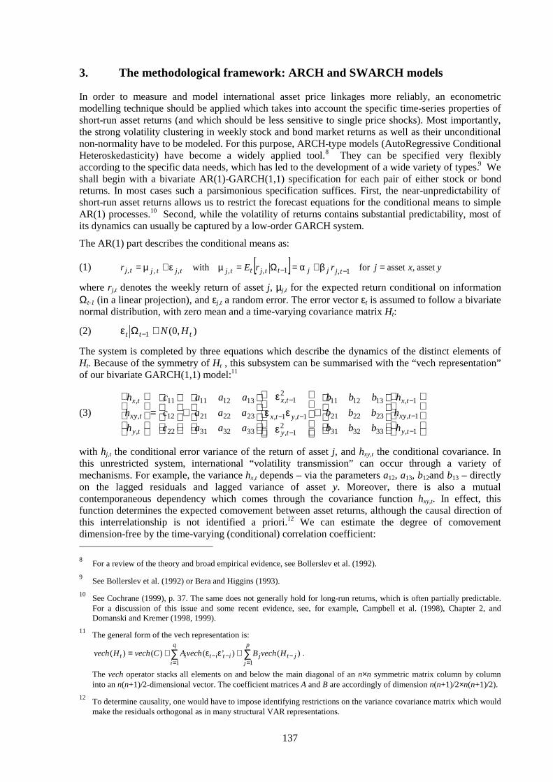
137
3. The methodological framework: ARCH and SWARCH models
In order to measure and model international asset price linkages more reliably, an econometricmodelling technique should be applied which takes into account the specific time-series properties ofshort-run asset returns (and which should be less sensitive to single price shocks). Most importantly,the strong volatility clustering in weekly stock and bond market returns as well as their unconditionalnon-normality have to be modeled. For this purpose, ARCH-type models (AutoRegressive ConditionalHeteroskedasticity) have become a widely applied tool.8 They can be specified very flexiblyaccording to the specific data needs, which has led to the development of a wide variety of types.9 Weshall begin with a bivariate AR(1)-GARCH(1,1) specification for each pair of either stock or bondreturns. In most cases such a parsimonious specification suffices. First, the near-unpredictability ofshort-run asset returns allows us to restrict the forecast equations for the conditional means to simpleAR(1) processes.10 Second, while the volatility of returns contains substantial predictability, most ofits dynamics can usually be captured by a low-order GARCH system.
The AR(1) part describes the conditional means as:
(1) [ ] yxjrrEr tjjjttjttjtjtjtj asset,assetforwith 1,1,,,,, =β+α=Ω=µε+µ= −−
where rj,t denotes the weekly return of asset j, µj,t for the expected return conditional on informationΩt-1 (in a linear projection), and εj,t a random error. The error vector εt is assumed to follow a bivariatenormal distribution, with zero mean and a time-varying covariance matrix Ht:
(2) ),0(1 ttt HN∼Ωε −
The system is completed by three equations which describe the dynamics of the distinct elements ofHt. Because of the symmetry of Ht , this subsystem can be summarised with the “vech representation”of our bivariate GARCH(1,1) model:11
(3)
+
εεε
ε
+
=
−
−
−
−
−−
−
1,
1,
1,
333231
232221
131211
21,
1,1,
21,
333231
232221
131211
22
12
11
,
,
,
ty
tyx
tx
ty
tytx
tx
ty
tyx
tx
h
h
h
bbb
bbb
bbb
aaa
aaa
aaa
c
c
c
h
h
h
with hj,t the conditional error variance of the return of asset j, and hxy,t the conditional covariance. Inthis unrestricted system, international “volatility transmission” can occur through a variety ofmechanisms. For example, the variance hx,t depends – via the parameters a12, a13, b12and b13 – directlyon the lagged residuals and lagged variance of asset y. Moreover, there is also a mutualcontemporaneous dependency which comes through the covariance function hxy,t. In effect, thisfunction determines the expected comovement between asset returns, although the causal direction ofthis interrelationship is not identified a priori.12 We can estimate the degree of comovementdimension-free by the time-varying (conditional) correlation coefficient: 8
For a review of the theory and broad empirical evidence, see Bollerslev et al. (1992).
9See Bollerslev et al. (1992) or Bera and Higgins (1993).
10See Cochrane (1999), p. 37. The same does not generally hold for long-run returns, which is often partially predictable.For a discussion of this issue and some recent evidence, see, for example, Campbell et al. (1998), Chapter 2, andDomanski and Kremer (1998, 1999).
11The general form of the vech representation is:
∑∑=
−=
−− +εε+=p
jjtj
q
iititit HvechBvechACvechHvech
11)()’()()( .
The vech operator stacks all elements on and below the main diagonal of an n×n symmetric matrix column by columninto an n(n+1)/2-dimensional vector. The coefficient matrices A and B are accordingly of dimension n(n+1)/2×n(n+1)/2).
12To determine causality, one would have to impose identifying restrictions on the variance covariance matrix which wouldmake the residuals orthogonal as in many structural VAR representations.

138
(4) ρt = hxy,t/(hx,t hy,t)0.5
This measure should be superior to the simple correlations as used in Section 2 since it is estimatedwithin a consistent econometric framework. Nevertheless, estimating the full vech representation facestwo serious drawbacks. First, positive definiteness of the variance covariance matrix is not guaranteed.Second, the system is heavily overparameterised (bivariate GARCH(1,1) models require 21coefficients to be estimated for the variance covariance process alone). To mitigate these problems,two restricted representations are applied: first, we impose zero-restrictions on all elements below andabove the main diagonal of the coefficient matrices A and B. This “diagonal representation” suggestedby Bollerslev et al. (1988) reduces the estimating burden to nine parameters. The conditional varianceprocesses equal those of univariate GARCH models since neither squared lagged residuals nor thelagged variance of one variable appear in the variance equation of the other. Hence, the internationalvolatility transmission can now occur only through the conditional covariance process. The diagonalrepresentation of the bivariate base model (with some convenient changes in notation) looks asfollows:
(5)
+
εεε
ε
+
=
−
−
−
−
−−
−
1,
1,
1,
21,
1,1,
21,
,
,
,
00
00
00
00
00
00
ty
tyx
tx
y
xy
x
ty
tytx
tx
y
xy
x
y
xy
x
ty
tyx
tx
h
h
h
b
b
b
a
a
a
c
c
c
h
h
h
Second, the model can be further simplified by assuming a constant correlation coefficient ρt = ρ asproposed by Bollerslev (1990). In this case, the conditional covariance function degenerates to theidentity:
(6) hxy,t = ρ (hx,t hy,t)0.5
Together with the two unchanged conditional variance processes, it forms the “constant correlationrepresentation” which leaves seven parameters to be estimated.13 Positive definiteness of the variancecovariance matrix can now be guaranteed. Despite its restrictive nature (it does not permit any laggedinternational volatility spillovers), the constant correlation representation renders it quite useful. First,it provides a simple summary measure of international asset price linkages, immediately challengingthe simple return correlation. Second, it offers an easy way of directly testing specific hypothesesabout possible determinants and the structural stability of the correlation coefficient. Concerning itspresumed dependence on volatility regimes, the parsimony of the constant correlation representationmakes it a natural candidate for multivariate switching-regime ARCH (SWARCH) models whichmultiply the number of parameters to be estimated.14
However, since multivariate SWARCH models soon become intractable when more than two or threeendogenous variables are involved, the present paper confines itself to univariate SWARCH modelswhich are used to identify volatility regimes in certain asset returns. SWARCH models date back tothe independent work of Cai (1994) and Hamilton and Susmel (1994). This model class allowsconditional volatility to be both time- and state-variant while the volatility regimes are identified andestimated endogenously. The appropriate number of states remains an empirical question and can betested statistically. We further the hypothesis of two states, i.e. periods of high and low volatility. Inthe univariate case, the variance equation when allowing for two different states St = 1 or 2 is givenby:15
13
The BEKK representation, as another variant of multivariate GARCH models, works without (a priori) imposing zero-restrictions upon the off-diagonal elements of the matrices A and B. Instead, it uses non-linear cross-equation restrictionsto reduce the estimating burden. A recent application to bond rates for the G3 countries is Herwartz and Reimers (1999).
14Ramchand and Susmel (1998) successfully applied univariate and bivariate SWARCH models to assess regime-dependent cross correlations between weekly stock returns of a broad set of countries.
15To save degrees of freedom, the AR(1) model for the mean return equation 1 remains state-independent as is the case inrelated work. This assumption is not very restrictive due to the near-unpredictability of weekly returns.
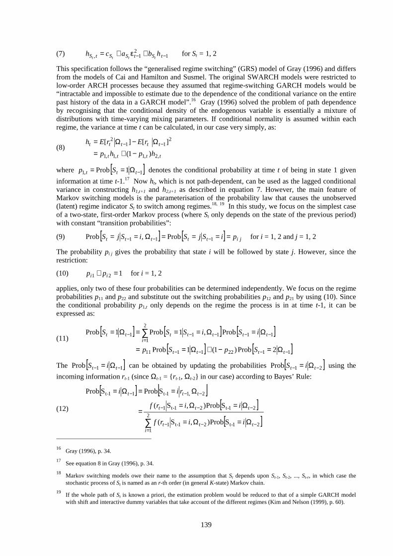
139
(7) 12
1, −− +ε+= tStSStS hbachtttt
for St = 1, 2
This specification follows the “generalised regime switching” (GRS) model of Gray (1996) and differsfrom the models of Cai and Hamilton and Susmel. The original SWARCH models were restricted tolow-order ARCH processes because they assumed that regime-switching GARCH models would be“intractable and impossible to estimate due to the dependence of the conditional variance on the entirepast history of the data in a GARCH model”.16 Gray (1996) solved the problem of path dependenceby recognising that the conditional density of the endogenous variable is essentially a mixture ofdistributions with time-varying mixing parameters. If conditional normality is assumed within eachregime, the variance at time t can be calculated, in our case very simply, as:
(8)tttt
ttttt
hphp
rErEh
,2,1,1,1
211
2
)1(
][][
−+=Ω−Ω= −−
where [ ]1,1 1Prob −Ω== ttt Sp denotes the conditional probability at time t of being in state 1 given
information at time t-1.17 Now ht, which is not path-dependent, can be used as the lagged conditionalvariance in constructing h1,t+1 and h2,t+1 as described in equation 7. However, the main feature ofMarkov switching models is the parameterisation of the probability law that causes the unobserved(latent) regime indicator St to switch among regimes.18, 19 In this study, we focus on the simplest caseof a two-state, first-order Markov process (where St only depends on the state of the previous period)with constant “transition probabilities”:
(9) [ ] [ ] jittttt piSjSiSjS ====Ω== −−− 111 Prob,Prob for i = 1, 2 and j = 1, 2
The probability pi j gives the probability that state i will be followed by state j. However, since therestriction:
(10) 121 =+ ii pp for i = 1, 2
applies, only two of these four probabilities can be determined independently. We focus on the regimeprobabilities p11 and p22 and substitute out the switching probabilities p12 and p21 by using (10). Sincethe conditional probability p1,t only depends on the regime the process is in at time t-1, it can beexpressed as:
(11)[ ] [ ] [ ]
[ ] [ ]11221111
11
2
1111
2Prob)1(1Prob
Prob,1Prob1Prob
−−−−
−−=
−−−
Ω=−+Ω==
Ω=Ω===Ω= ∑
tttt
tti
ttttt
SpSp
iSiSSS
The [ ]11Prob −− Ω= tt iS can be obtained by updating the probabilities [ ]21Prob −− Ω= tt iS using the
incoming information rt-1 (since Ωt-1 = rt-1, Ωt-2 in our case) according to Bayes’ Rule:
(12)
[ ] [ ][ ]
[ ]∑=
−−−
−−−
−−−
Ω=Ω=
Ω=Ω==
Ω==Ω=
2
121-t21-t1
21-t21-t1
2,11-t11-t
SProb),S(
SProb),S(
SProbSProb
ittt
ttt
ttt
iirf
iirf
rii
16
Gray (1996), p. 34.
17See equation 8 in Gray (1996), p. 34.
18Markov switching models owe their name to the assumption that St depends upon St-1, St-2, ..., St-r, in which case thestochastic process of St is named as an r-th order (in general K-state) Markov chain.
19If the whole path of St is known a priori, the estimation problem would be reduced to that of a simple GARCH modelwith shift and interactive dummy variables that take account of the different regimes (Kim and Nelson (1999), p. 60).
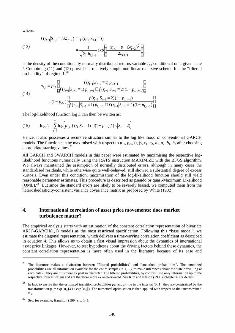
140
where:
(13)
β−α−−
π=
==Ω=
−
−−
−
−−−
1,
221
1,
1-t121-t1
2
)(exp
2
1
)S(),S(
ti
tt
ti
ttt
h
rr
h
irfirf
is the density of the conditionally normally distributed returns variable rt-1 conditional on a given statei. Combining (11) and (12) provides a relatively simple non-linear recursive scheme for the “filteredprobability” of regime 1:20
(14)
−=+=−=
−+
−=+==
=
−−−−−−
−−−
−−−−−−
−−−
)1()2()1(
)1()2()1(
)1()2()1(
)1(
1,1111,111
1,11122
1,1111,111
1,11111,1
tttttt
ttt
tttttt
tttt
pSrfpSrf
pSrfp
pSrfpSrf
pSrfpp
The log-likelihood function log L can then be written as:
(15) [ ]∑=
=−+==T
ttttttt SrfpSrfpL
1,1,1 )2()1()1(loglog
Hence, it also possesses a recursive structure similar to the log likelihood of conventional GARCHmodels. The function can be maximised with respect to p11, p22, α, β, c1, c2, a1, a2, b1, b2 after choosingappropriate starting values.21
All GARCH and SWARCH models in this paper were estimated by maximising the respective log-likelihood functions numerically using the RATS instruction MAXIMIZE with the BFGS algorithm.We always maintained the assumption of normally distributed errors, although in many cases thestandardised residuals, while otherwise quite well-behaved, still showed a substantial degree of excesskurtosis. Even under this condition, maximisation of the log-likelihood function should still yieldreasonable parameter estimates. This procedure is described as pseudo or quasi-Maximum Likelihood(QML).22 But since the standard errors are likely to be severely biased, we computed them from theheteroskedasticity-consistent variance covariance matrix as proposed by White (1982).
4. International correlation of asset price movements: does marketturbulence matter?
The empirical analysis starts with an estimation of the constant correlation representation of bivariateAR(1)-GARCH(1,1) models as the most restricted specification. Following this “base model”, weestimate the diagonal representation, which delivers a time-varying correlation coefficient as describedin equation 4. This allows us to obtain a first visual impression about the dynamics of internationalasset price linkages. However, to test hypotheses about the driving factors behind these dynamics, theconstant correlation representation is more often used in the literature because of its ease and 20
The literature makes a distinction between “filtered probabilities” and “smoothed probabilities”. The smoothedprobabilities use all information available for the entire sample t = 1,...,T to make inferences about the state prevailing ateach date t. They are thus more ex post in character. The filtered probabilities, by contrast, use only information up to therespective forecast origin and are therefore more ex ante-oriented. See Kim and Nelson (1999), chapter 4, for details.
21In fact, to ensure that the estimated transition probabilities p11 and p22 lie in the interval (0, 1), they are constrained by thetransformation pii = expπ ii/(1+ expπ ii). The numerical optimisation is then applied with respect to the unconstrainedπ ii.
22See, for example, Hamilton (1994), p. 145.
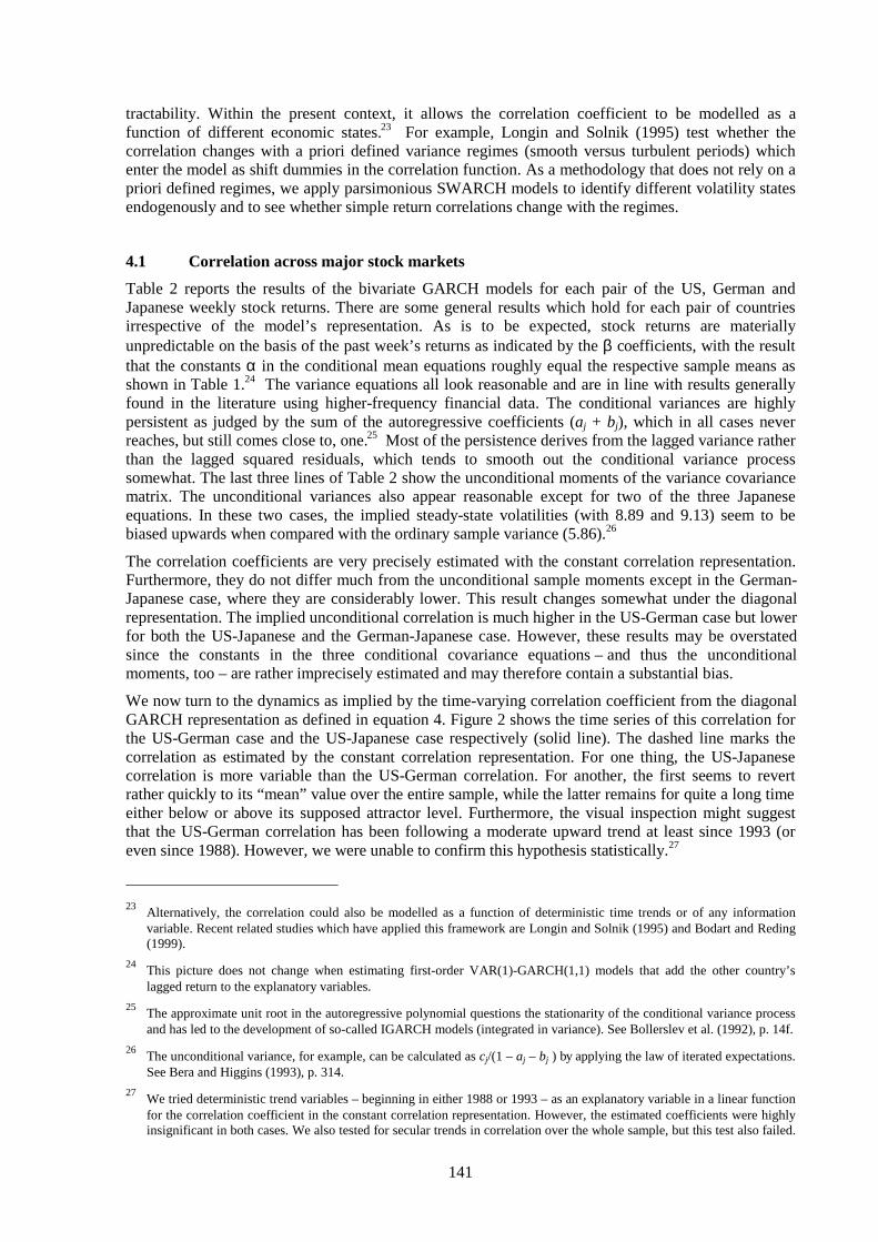
141
tractability. Within the present context, it allows the correlation coefficient to be modelled as afunction of different economic states.23 For example, Longin and Solnik (1995) test whether thecorrelation changes with a priori defined variance regimes (smooth versus turbulent periods) whichenter the model as shift dummies in the correlation function. As a methodology that does not rely on apriori defined regimes, we apply parsimonious SWARCH models to identify different volatility statesendogenously and to see whether simple return correlations change with the regimes.
4.1 Correlation across major stock markets
Table 2 reports the results of the bivariate GARCH models for each pair of the US, German andJapanese weekly stock returns. There are some general results which hold for each pair of countriesirrespective of the model’s representation. As is to be expected, stock returns are materiallyunpredictable on the basis of the past week’s returns as indicated by the β coefficients, with the resultthat the constants α in the conditional mean equations roughly equal the respective sample means asshown in Table 1.24 The variance equations all look reasonable and are in line with results generallyfound in the literature using higher-frequency financial data. The conditional variances are highlypersistent as judged by the sum of the autoregressive coefficients (aj + bj), which in all cases neverreaches, but still comes close to, one.25 Most of the persistence derives from the lagged variance ratherthan the lagged squared residuals, which tends to smooth out the conditional variance processsomewhat. The last three lines of Table 2 show the unconditional moments of the variance covariancematrix. The unconditional variances also appear reasonable except for two of the three Japaneseequations. In these two cases, the implied steady-state volatilities (with 8.89 and 9.13) seem to bebiased upwards when compared with the ordinary sample variance (5.86).26
The correlation coefficients are very precisely estimated with the constant correlation representation.Furthermore, they do not differ much from the unconditional sample moments except in the German-Japanese case, where they are considerably lower. This result changes somewhat under the diagonalrepresentation. The implied unconditional correlation is much higher in the US-German case but lowerfor both the US-Japanese and the German-Japanese case. However, these results may be overstatedsince the constants in the three conditional covariance equations – and thus the unconditionalmoments, too – are rather imprecisely estimated and may therefore contain a substantial bias.
We now turn to the dynamics as implied by the time-varying correlation coefficient from the diagonalGARCH representation as defined in equation 4. Figure 2 shows the time series of this correlation forthe US-German case and the US-Japanese case respectively (solid line). The dashed line marks thecorrelation as estimated by the constant correlation representation. For one thing, the US-Japanesecorrelation is more variable than the US-German correlation. For another, the first seems to revertrather quickly to its “mean” value over the entire sample, while the latter remains for quite a long timeeither below or above its supposed attractor level. Furthermore, the visual inspection might suggestthat the US-German correlation has been following a moderate upward trend at least since 1993 (oreven since 1988). However, we were unable to confirm this hypothesis statistically.27
23
Alternatively, the correlation could also be modelled as a function of deterministic time trends or of any informationvariable. Recent related studies which have applied this framework are Longin and Solnik (1995) and Bodart and Reding(1999).
24This picture does not change when estimating first-order VAR(1)-GARCH(1,1) models that add the other country’slagged return to the explanatory variables.
25The approximate unit root in the autoregressive polynomial questions the stationarity of the conditional variance processand has led to the development of so-called IGARCH models (integrated in variance). See Bollerslev et al. (1992), p. 14f.
26The unconditional variance, for example, can be calculated as cj/(1 – aj – bj ) by applying the law of iterated expectations.See Bera and Higgins (1993), p. 314.
27We tried deterministic trend variables – beginning in either 1988 or 1993 – as an explanatory variable in a linear functionfor the correlation coefficient in the constant correlation representation. However, the estimated coefficients were highlyinsignificant in both cases. We also tested for secular trends in correlation over the whole sample, but this test also failed.

142
Table 2Bivariate AR(1)-GARCH(1,1) models for major stock markets
tionrepresenta diagonal(5b)
tionrepresentan correlatioconstant )((6)
(5a)
y)country vs(country x,for(1)
1,1,1,,
5.01,1,,
1,2
1,,
,1,,
−−−
−−
−−
−
+εε+=
ρ=
+ε+=
=ε+β+α=
txyxytytxxyxytxy
tytxtxy
tjjtjjjtj
tjtjjjtj
hbach
hhh
hbach
yxjrr
Constant correlation representation Diagonal representationUS vs DE US vs JP DE vs JP US vs DE US vs JP DE vs JP
α x 0.267 (0.057)2 0.297 (0.055)2 0.263 (0.062)2 0.286 (0.058)2 0.303 (0.051)2 0.274 (0.065)2
β x –0.035 (0.031) –0.042 (0.034) 0.044 (0.035) –0.046 (0.032) –0.039 (0.029) 0.049 (0.036)
α y 0.249 (0.057)2 0.249 (0.053)2 0.235 (0.051)2 0.244 (0.047)2 0.245 (0.055)2 0.249 (0.059)2
β y 0.030 (0.030) 0.039 (0.031) 0.043 (0.034) 0.037 (0.028) 0.048 (0.030) 0.031 (0.032)
cx 0.245 (0.153) 0.250 (0.229) 0.351 (0.133)2 0.232 (0.135) 0.208 (0.106)1 0.387 (0.165)1
cy 0.367 (0.115)2 0.143 (0.062)1 0.130 (0.070) 0.351 (0.156)1 0.155 (0.070)2 0.175 (0.069)1
cxy – – – – – – 0.126 (0.076) 0.104 (0.054) 0.209 (0.123)
ax 0.099 (0.041)1 0.098 (0.056) 0.170 (0.046)2 0.088 (0.036)1 0.087 (0.029)2 0.165 (0.051)2
ay 0.161 (0.038)2 0.141 (0.030)2 0.136 (0.029)2 0.148 (0.047)1 0.154 (0.028)2 0.133 (0.024)2
axy – – – – – – 0.087 (0.037)1 0.115 (0.026)2 0.129 (0.051)1
bx 0.845 (0.064)2 0.845 (0.098)2 0.758 (0.057)2 0.858 (0.053)2 0.865 (0.042)2 0.752 (0.069)2
by 0.761 (0.045)2 0.842 (0.033)2 0.849 (0.032)2 0.776 (0.066)2 0.829 (0.032)2 0.842 (0.028)2
bxy – – – – – – 0.846 (0.065)2 0.813 (0.061)2 0.679 (0.148)2
ρ 0.457 (0.019)2 0.352 (0.028)2 0.273 (0.033)2 – – – – – –
hx* 4.395 – 4.374 – 4.878 – 4.280 – 4.392 – 4.680 –
hy* 4.692 – 8.575 – 8.890 – 4.597 – 9.126 – 6.798 –
ρ* – – – – – – 0.578 – 0.227 – 0.194 –
Note: The table gives the estimated coefficients calculated by Maximum Likelihood using the BFGS algorithm.Heteroskedasticity-consistent standard errors in parentheses. Effective sample: 24 January 1980 to 16 September 1999(1,026 usable observations). 1 (2) indicates significance at the 5% (1%) level. hj* is the unconditional variance of country j’sunexpected return, and ρ* is the unconditional correlation coefficient, both calculated as the steady-state solutions to thevariance and covariance equations 5a and 5b and using the definition of the correlation coefficient.
It is often argued that international stock market correlations increase in periods of stress with highconditional return volatilities. Figure A1 in the Appendix gives a visual impression of why thishypothesis is raised so often. The conditional variance series for both the United States and Germanyare shown in the lower part, while the corresponding correlation coefficient appears in the upper part.Obviously, the correlation jumps upwards when both markets are hit by large shocks, as in October1987 and August 1990. Empirical evidence in favour of this hypothesis is provided, for instance, byKoch and Koch (1991), and Longin and Solnik (1995). However, these studies did not find astatistically fully convincing solution to the problem of separating volatility regimes. Lacking a propermethodology, they had to define the sub-periods of high versus low volatilities exogenously in an adhoc fashion. SWARCH models now provide a technology for doing this job endogenously. They werefirst applied in this context by Ramchand and Susmel (1998), who find strong evidence for state-dependent correlations across weekly stock returns for a large set of countries.
This result does not necessarily contradict the findings in Longin and Solnik (1995), who used a much larger sample(1960 to 1990) with monthly stock returns for their bivariate GARCH models.

143
Table 3 presents our results of univariate SWARCH specifications. The model produces similarestimates for all of the stock returns. Most noticeable are the clear-cut and highly significantdifferences in the two identified, country-specific variance regimes.28 The unconditional variances ofthe high volatility state are three to five times larger than those of the low volatility state. Moreover,the use of the generalised regime-switching model specification of Gray (1996) proves to beadvantageous since it allows the persistence parameter aSt to differ between regimes in contrast to theoriginal SWARCH specifications. Within the low volatility state, the variances remain virtuallyconstant due to the negligible (and insignificant) autoregression coefficients a1. In the high volatilitystate, however, lagged squared residuals do have a significant and materially important influence oncurrent conditional variances via parameters a2. This makes large initial shocks, as typically observedin market crashes, persist for some time.
Furthermore, each regime itself is highly persistent as evidenced by the large (and, in general, highlysignificant) constant regime probabilities p11 and p22, respectively.29 This result is consistent withapplications of Markov switching in many other contexts. Accordingly, the time series for theconditional regime probabilities look quite reasonable. As an example, Figure 3 presents theconditional probability of German stock returns being in state 1 (p1,t), the low variance regime. This
28
We have to admit that individual standard errors of the parameters of the state-dependent variance equations do onlyprovide an informal test of the two-state model against a simple one-state specification, since under the null hypothesis ofno-regime switching the parameters of the second state’s variance equation are not identified. However, we regard theevidence in favour of the two-state model as so strong that we dispensed with a proper non-standard test such as thatdeveloped by Hansen (1992).
29Table 3 does not show standard errors for the “constrained” transition probabilities since standard errors were onlyobtained for the unconstrained probability parameters which are not directly interpretable and thus not shown in the table.
Figure 2: International stock return correlations from bivariate GARCH modelsConstant correlation representation (dashed) and diagonal representation (solid)
United States vs Germany
80 81 82 83 84 85 86 87 88 89 90 91 92 93 94 95 96 97 98 99-0.4
-0.2
0.0
0.2
0.4
0.6
0.8
United States vs Japan
80 81 82 83 84 85 86 87 88 89 90 91 92 93 94 95 96 97 98 99-0.30
0.00
0.30
0.60
0.90
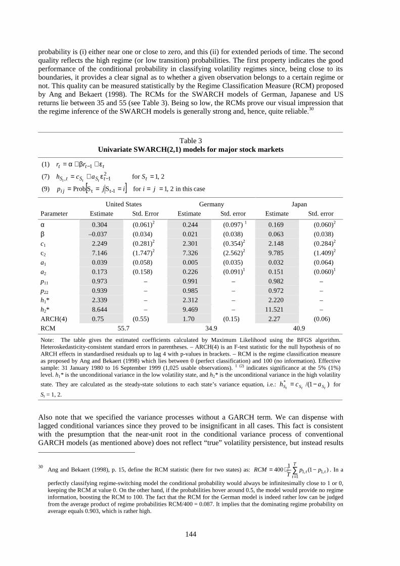
144
probability is (i) either near one or close to zero, and this (ii) for extended periods of time. The secondquality reflects the high regime (or low transition) probabilities. The first property indicates the goodperformance of the conditional probability in classifying volatility regimes since, being close to itsboundaries, it provides a clear signal as to whether a given observation belongs to a certain regime ornot. This quality can be measured statistically by the Regime Classification Measure (RCM) proposedby Ang and Bekaert (1998). The RCMs for the SWARCH models of German, Japanese and USreturns lie between 35 and 55 (see Table 3). Being so low, the RCMs prove our visual impression thatthe regime inference of the SWARCH models is generally strong and, hence, quite reliable.30
Table 3Univariate SWARCH(2,1) models for major stock markets
[ ] case in this2,1for SSProb(9)
2,1for(7)
(1)
1-tt
21,
1
=====
=ε+=
ε+β+α=
−
−
j iijp
Sach
rr
ji
ttSStS
ttt
ttt
United States Germany Japan
Parameter Estimate Std. Error Estimate Std. error Estimate Std. error
α 0.304 (0.061)2 0.244 (0.097) 1 0.169 (0.060)2
β –0.037 (0.034) 0.021 (0.038) 0.063 (0.038)
c1 2.249 (0.281)2 2.301 (0.354)2 2.148 (0.284)2
c2 7.146 (1.747)2 7.326 (2.562)2 9.785 (1.409)2
a1 0.039 (0.058) 0.005 (0.035) 0.032 (0.064)
a2 0.173 (0.158) 0.226 (0.091)1 0.151 (0.060)1
p11 0.973 – 0.991 – 0.982 –
p22 0.939 – 0.985 – 0.972 –
h1* 2.339 – 2.312 – 2.220 –
h2* 8.644 – 9.469 – 11.521 –
ARCH(4) 0.75 (0.55) 1.70 (0.15) 2.27 (0.06)
RCM 55.7 34.9 40.9
Note: The table gives the estimated coefficients calculated by Maximum Likelihood using the BFGS algorithm.Heteroskedasticity-consistent standard errors in parentheses. – ARCH(4) is an F-test statistic for the null hypothesis of noARCH effects in standardised residuals up to lag 4 with p-values in brackets. – RCM is the regime classification measureas proposed by Ang and Bekaert (1998) which lies between 0 (perfect classification) and 100 (no information). Effectivesample: 31 January 1980 to 16 September 1999 (1,025 usable observations). 1 (2) indicates significance at the 5% (1%)level. h1* is the unconditional variance in the low volatility state, and h2* is the unconditional variance in the high volatility
state. They are calculated as the steady-state solutions to each state’s variance equation, i.e.: )1/(*ttt SSS ach −= for
St = 1, 2.
Also note that we specified the variance processes without a GARCH term. We can dispense withlagged conditional variances since they proved to be insignificant in all cases. This fact is consistentwith the presumption that the near-unit root in the conditional variance process of conventionalGARCH models (as mentioned above) does not reflect “true” volatility persistence, but instead results
30Ang and Bekaert (1998), p. 15, define the RCM statistic (here for two states) as: ∑
=−⋅=
T
ttt pp
TRCM
1,1,1 )1(
1400 . In a
perfectly classifying regime-switching model the conditional probability would always be infinitesimally close to 1 or 0,keeping the RCM at value 0. On the other hand, if the probabilities hover around 0.5, the model would provide no regimeinformation, boosting the RCM to 100. The fact that the RCM for the German model is indeed rather low can be judgedfrom the average product of regime probabilities RCM/400 = 0.087. It implies that the dominating regime probability onaverage equals 0.903, which is rather high.
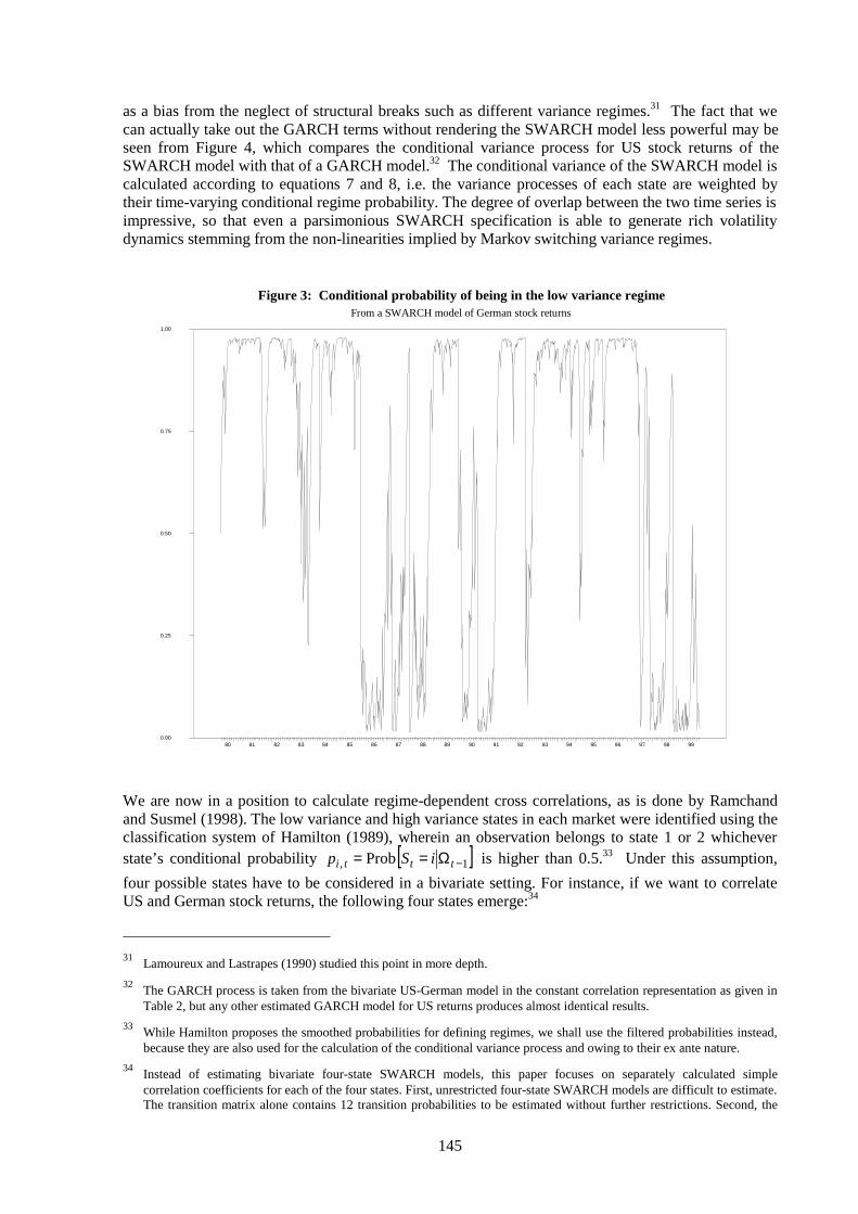
145
as a bias from the neglect of structural breaks such as different variance regimes.31 The fact that wecan actually take out the GARCH terms without rendering the SWARCH model less powerful may beseen from Figure 4, which compares the conditional variance process for US stock returns of theSWARCH model with that of a GARCH model.32 The conditional variance of the SWARCH model iscalculated according to equations 7 and 8, i.e. the variance processes of each state are weighted bytheir time-varying conditional regime probability. The degree of overlap between the two time series isimpressive, so that even a parsimonious SWARCH specification is able to generate rich volatilitydynamics stemming from the non-linearities implied by Markov switching variance regimes.
We are now in a position to calculate regime-dependent cross correlations, as is done by Ramchandand Susmel (1998). The low variance and high variance states in each market were identified using theclassification system of Hamilton (1989), wherein an observation belongs to state 1 or 2 whicheverstate’s conditional probability [ ]1, Prob −Ω== ttti iSp is higher than 0.5.33 Under this assumption,
four possible states have to be considered in a bivariate setting. For instance, if we want to correlateUS and German stock returns, the following four states emerge:34
31
Lamoureux and Lastrapes (1990) studied this point in more depth.
32The GARCH process is taken from the bivariate US-German model in the constant correlation representation as given inTable 2, but any other estimated GARCH model for US returns produces almost identical results.
33While Hamilton proposes the smoothed probabilities for defining regimes, we shall use the filtered probabilities instead,because they are also used for the calculation of the conditional variance process and owing to their ex ante nature.
34Instead of estimating bivariate four-state SWARCH models, this paper focuses on separately calculated simplecorrelation coefficients for each of the four states. First, unrestricted four-state SWARCH models are difficult to estimate.The transition matrix alone contains 12 transition probabilities to be estimated without further restrictions. Second, the
Figure 3: Conditional probability of being in the low variance regimeFrom a SWARCH model of German stock returns
80 81 82 83 84 85 86 87 88 89 90 91 92 93 94 95 96 97 98 990.00
0.25
0.50
0.75
1.00

146
St = 1: US variance low, German variance low
St = 2: US variance low, German variance high
St = 3: US variance high, German variance low
St = 4: US variance high, German variance high35
The results of the return correlations across these four states are given in Table 4.36 They confirm thegeneral hypothesis of correlations increasing along with volatility. Hence, “market turbulence matters”indeed. For example, the US-German correlation increases to 0.63 when both countries experiencehigh volatilities (state 4) compared with 0.40 in the case of low volatilities (state 1). The same patternholds for the remaining country pairs. The intermediate states suggest the following interpretation: theUS market seems to dictate the degree of international stock price synchronisation. If US returns are inthe high volatility state, the correlation with German and Japanese returns is also high, regardless ofwhether foreign returns belong to the high or to the low volatility state. Conversely, if US returns arein the low volatility state, the correlation with foreign returns also diminishes. Furthermore, thecorrelation between German and Japanese returns is minor except when both returns become more
two-step, “system-free” procedure provides a tractable way of obtaining state-dependent correlations even when a largerset of countries or asset classes is considered. However, this entails the disadvantage of not obtaining an independentestimate of the conditional regime probabilities which could be used for forecasting purposes.
35Comparing the conditional variance series of different countries suggests that the distinction between four states doesmake sense. Figure 3, for example, shows volatility hikes in Germany which occur independently of volatilitymovements in the United States, and vice versa. Thus, volatility cycles are generally not fully synchronised, which arguesagainst the general validity of the contagion hypothesis.
36We also calculated the correlations between the residuals from the SWARCH models instead of total returns, but theresults were absolutely unchanged to the first and second decimal place.
Figure 4: Conditional variance from a SWARCH and GARCH modelUS stock returns
80 81 82 83 84 85 86 87 88 89 90 91 92 93 94 95 96 97 98 990
8
16
24
32
40
48
56
SWARCHGARCH
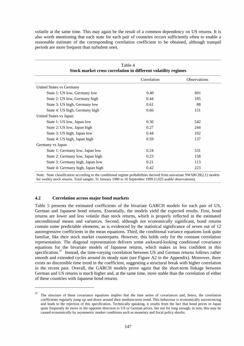
147
volatile at the same time. This may again be the result of a common dependency on US returns. It isalso worth mentioning that each state for each pair of countries occurs sufficiently often to enable areasonable estimate of the corresponding correlation coefficient to be obtained, although tranquilperiods are more frequent than turbulent ones.
Table 4Stock market cross correlation in different volatility regimes
Correlation Observations
United States vs Germany
State 1: US low, Germany low 0.40 601
State 2: US low, Germany high 0.44 185
State 3: US high, Germany low 0.61 88
State 4: US high, Germany high 0.66 151
United States vs Japan
State 1: US low, Japan low 0.30 542
State 2: US low, Japan high 0.27 244
State 3: US high, Japan low 0.44 102
State 4: US high, Japan high 0.59 137
Germany vs Japan
State 1: Germany low, Japan low 0.24 531
State 2: Germany low, Japan high 0.23 158
State 3: Germany high, Japan low 0.21 113
State 4: Germany high, Japan high 0.42 223
Note: State classification according to the conditional regime probabilities derived from univariate SWARCH(2,1) modelsfor weekly stock returns. Total sample: 31 January 1980 to 16 September 1999 (1,025 usable observations).
4.2 Correlation across major bond markets
Table 5 presents the estimated coefficients of the bivariate GARCH models for each pair of US,German and Japanese bond returns. Essentially, the models yield the expected results. First, bondreturns are lower and less volatile than stock returns, which is properly reflected in the estimatedunconditional means and variances. Second, although not economically significant, bond returnscontain some predictable elements, as is evidenced by the statistical significance of seven out of 12autoregressive coefficients in the mean equations. Third, the conditional variance equations look quitefamiliar, like their stock market counterparts. However, this holds only for the constant correlationrepresentation. The diagonal representation delivers some awkward-looking conditional covarianceequations for the bivariate models of Japanese returns, which makes us less confident in thisspecification.37 Instead, the time-varying correlation between US and German returns follows rathersmooth and extended cycles around its steady state (see Figure A2 in the Appendix). Moreover, thereexists no discernible time trend in the coefficient, suggesting a structural break with higher correlationin the recent past. Overall, the GARCH models prove again that the short-term linkage betweenGerman and US returns is much higher and, at the same time, more stable than the correlation of eitherof these countries with Japanese bond returns.
37
The structure of these covariance equations implies that the time series of covariances and, hence, the correlationcoefficients regularly jump up and down around their medium-term trend. This behaviour is economically unconvincingand leads to the rejection of this specification. Technically speaking, it results from the fact that bond prices in Japanquite frequently do move in the opposite direction to US or German prices, but not for long enough; in turn, this may becaused economically by asymmetric market conditions such as monetary and fiscal policy shocks.

148
Table 5Bivariate AR(1)-GARCH(1,1) models for major bond markets
tionrepresenta diagonal(5b)
tionrepresentan correlatioconstant )((6)
(5a)
y)country vs(country x,for(1)
1,1,1,,
5.01,1,,
1,2
1,,
,1,,
−−−
−−
−−
−
+εε+=
ρ=
+ε+=
=ε+β+α=
txyxytytxxyxytxy
tytxtxy
tjjtjjjtj
tjtjjjtj
hbach
hhh
hbach
yxjrr
Constant correlation representation Diagonal representation
US vs DE US vs JP DE vs JP US vs DE US vs JP DE vs JP
α x 0.047 (0.038) 0.038 (0.035) 0.051 (0.021)1 0.046 (0.031) 0.042 (0.031) 0.049 (0.022)1
β x –0.038 (0.031) –0.016 (0.038) 0.077 (0.039)1 –0.046 (0.039) –0.019 (0.033) 0.081 (0.027)2
α y 0.047 (0.025) 0.067 (0.031)1 0.073 (0.026)2 0.044 (0.026) 0.068 (0.024)2 0.074 (0.025)2
β y 0.077 (0.034)1 0.086 (0.037)1 0.090 (0.036)1 0.069 (0.039) 0.091 (0.039)1 0.095 (0.044)1
cx 0.087 (0.035)1 0.075 (0.043) 0.019 (0.007)2 0.080 (0.033)1 0.074 (0.035)2 0.022 (0.007)2
cy 0.028 (0.011)1 0.076 (0.023)2 0.075 (0.021)2 0.033 (0.016)1 0.074 (0.020)2 0.080 (0.022)2
cxy – – – – – – 0.018 (0.006)2 0.296 (0.052)2 0.225 (0.051)2
ax 0.078 (0.028)2 0.072 (0.024)2 0.114 (0.027)2 0.079 (0.025)2 0.072 (0.022)2 0.108 (0.022)2
ay 0.116 (0.031)2 0.143 (0.037)2 0.135 (0.036)2 0.105 (0.032)2 0.139 (0.033)2 0.126 (0.034)2
axy – – – – – – 0.053 (0.011)2 –0.026 (0.021)2 –0.034 (0.026)2
bx 0.839 (0.047)2 0.856 (0.054)2 0.855 (0.026)2 0.844 (0.043)2 0.857 (0.045)2 0.853 (0.024)2
by 0.832 (0.040)2 0.756 (0.054)2 0.763 (0.047)2 0.831 (0.055)2 0.762 (0.042)2 0.763 (0.049)2
bxy – – – – – – 0.893 (0.016)2 –0.805 (0.121)2 –0.627 (0.240)2
ρ 0.472 (0.026)2 0.215 (0.036)2 0.267 (0.032)2 – – – – – –
hx* 1.040 – 1.042 – 0.624 – 1.040 – 1.041 – 0.580 –
hy* 0.549 – 0.745 – 0.733 – 0.523 – 0.744 – 0.719 –
ρ* – – – – – – 0.451 – 0.183 – 0.210 –
Note: The table gives the estimated coefficients calculated by Maximum Likelihood using the BFGS algorithm.Heteroskedasticity-consistent standard errors in parentheses. Effective sample: 26 January 1984 to 16 September 1999 (817usable observations). 1 (2) indicates significance at the 5% (1%) level. hj* is the unconditional variance of country j’sunexpected return, and ρ* is the unconditional correlation coefficient, both calculated as the steady-state solutions to thevariance and covariance equations 5a and 5b and using the definition of the correlation coefficient.
In testing for regime dependency of bond market correlation, our two-state SWARCH model failed toidentify different volatility regimes in the US case.38 We therefore have recourse to the “threshold”approach, where an exogonenously defined threshold value separates high from low volatilityobservations.39 Accordingly, an observation belongs to the high (low) volatility regime when squaredreturns are higher (lower) than the threshold value. While in most cases the threshold is set to thesample standard deviation, we apply different scaling parameters to the unconditional standarddeviation in order to mitigate the problem of ad-hocery. The corresponding regime-dependent crosscorrelations are presented in Table 6. Again, the results strongly confirm the positive relation betweenmarket turbulence and international correlation. For example, irrespective of the scaling parameter, theUS-German correlation more than doubles when both countries move together from a low volatility toa high variance state. In the US-Japanese case, correlation even increases about five times on average,although it never reaches the absolute values of the US-German linkage. The mixed states 2 and 3 onlymatter for the relationship between US and German bond returns. The correlation is higher than in the
38
For Germany and Japan, instead, we obtained reasonable results.
39See Longin and Solnik (1995).
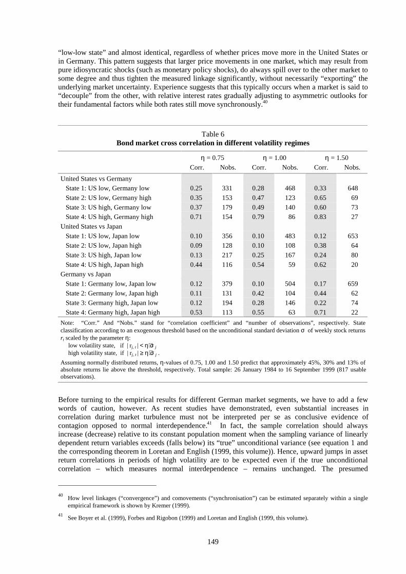
149
“low-low state” and almost identical, regardless of whether prices move more in the United States orin Germany. This pattern suggests that larger price movements in one market, which may result frompure idiosyncratic shocks (such as monetary policy shocks), do always spill over to the other market tosome degree and thus tighten the measured linkage significantly, without necessarily “exporting” theunderlying market uncertainty. Experience suggests that this typically occurs when a market is said to“decouple” from the other, with relative interest rates gradually adjusting to asymmetric outlooks fortheir fundamental factors while both rates still move synchronously.40
Table 6Bond market cross correlation in different volatility regimes
η = 0.75 η = 1.00 η = 1.50
Corr. Nobs. Corr. Nobs. Corr. Nobs.
0.25 331 0.28 468 0.33 648
0.35 153 0.47 123 0.65 69
0.37 179 0.49 140 0.60 73
0.71 154 0.79 86 0.83 27
0.10 356 0.10 483 0.12 653
0.09 128 0.10 108 0.38 64
0.13 217 0.25 167 0.24 80
0.44 116 0.54 59 0.62 20
0.12 379 0.10 504 0.17 659
0.11 131 0.42 104 0.44 62
0.12 194 0.28 146 0.22 74
United States vs Germany
State 1: US low, Germany low
State 2: US low, Germany high
State 3: US high, Germany low
State 4: US high, Germany high
United States vs Japan
State 1: US low, Japan low
State 2: US low, Japan high
State 3: US high, Japan low
State 4: US high, Japan high
Germany vs Japan
State 1: Germany low, Japan low
State 2: Germany low, Japan high
State 3: Germany high, Japan low
State 4: Germany high, Japan high 0.53 113 0.55 63 0.71 22
Note: “Corr.” And “Nobs.” stand for “correlation coefficient” and “number of observations”, respectively. Stateclassification according to an exogenous threshold based on the unconditional standard deviation σ of weekly stock returnsrt scaled by the parameter η: low volatility state, if | rj, t | < η⋅σ j high volatility state, if | rj, t | ≥ η⋅σ j .
Assuming normally distributed returns, η-values of 0.75, 1.00 and 1.50 predict that approximately 45%, 30% and 13% ofabsolute returns lie above the threshold, respectively. Total sample: 26 January 1984 to 16 September 1999 (817 usableobservations).
Before turning to the empirical results for different German market segments, we have to add a fewwords of caution, however. As recent studies have demonstrated, even substantial increases incorrelation during market turbulence must not be interpreted per se as conclusive evidence ofcontagion opposed to normal interdependence.41 In fact, the sample correlation should alwaysincrease (decrease) relative to its constant population moment when the sampling variance of linearlydependent return variables exceeds (falls below) its “true” unconditional variance (see equation 1 andthe corresponding theorem in Loretan and English (1999, this volume)). Hence, upward jumps in assetreturn correlations in periods of high volatility are to be expected even if the true unconditionalcorrelation – which measures normal interdependence – remains unchanged. The presumed
40
How level linkages (“convergence”) and comovements (“synchronisation”) can be estimated separately within a singleempirical framework is shown by Kremer (1999).
41See Boyer et al. (1999), Forbes and Rigobon (1999) and Loretan and English (1999, this volume).
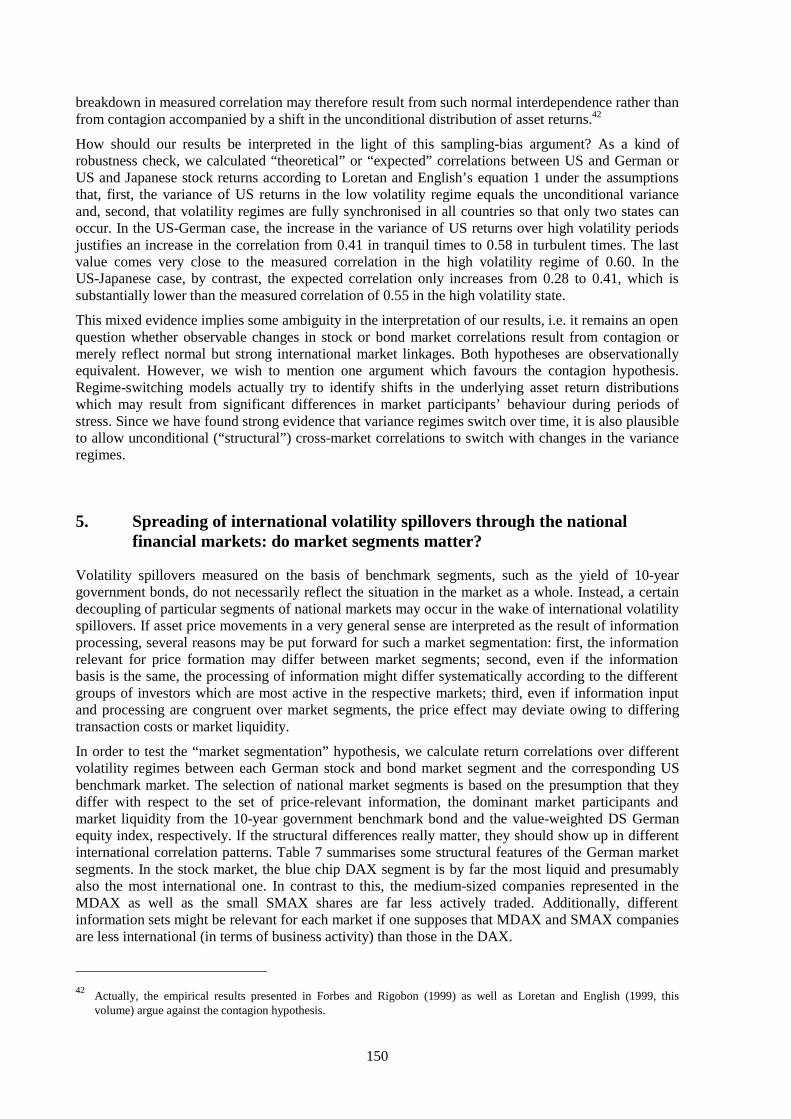
150
breakdown in measured correlation may therefore result from such normal interdependence rather thanfrom contagion accompanied by a shift in the unconditional distribution of asset returns.42
How should our results be interpreted in the light of this sampling-bias argument? As a kind ofrobustness check, we calculated “theoretical” or “expected” correlations between US and German orUS and Japanese stock returns according to Loretan and English’s equation 1 under the assumptionsthat, first, the variance of US returns in the low volatility regime equals the unconditional varianceand, second, that volatility regimes are fully synchronised in all countries so that only two states canoccur. In the US-German case, the increase in the variance of US returns over high volatility periodsjustifies an increase in the correlation from 0.41 in tranquil times to 0.58 in turbulent times. The lastvalue comes very close to the measured correlation in the high volatility regime of 0.60. In theUS-Japanese case, by contrast, the expected correlation only increases from 0.28 to 0.41, which issubstantially lower than the measured correlation of 0.55 in the high volatility state.
This mixed evidence implies some ambiguity in the interpretation of our results, i.e. it remains an openquestion whether observable changes in stock or bond market correlations result from contagion ormerely reflect normal but strong international market linkages. Both hypotheses are observationallyequivalent. However, we wish to mention one argument which favours the contagion hypothesis.Regime-switching models actually try to identify shifts in the underlying asset return distributionswhich may result from significant differences in market participants’ behaviour during periods ofstress. Since we have found strong evidence that variance regimes switch over time, it is also plausibleto allow unconditional (“structural”) cross-market correlations to switch with changes in the varianceregimes.
5. Spreading of international volatility spillovers through the nationalfinancial markets: do market segments matter?
Volatility spillovers measured on the basis of benchmark segments, such as the yield of 10-yeargovernment bonds, do not necessarily reflect the situation in the market as a whole. Instead, a certaindecoupling of particular segments of national markets may occur in the wake of international volatilityspillovers. If asset price movements in a very general sense are interpreted as the result of informationprocessing, several reasons may be put forward for such a market segmentation: first, the informationrelevant for price formation may differ between market segments; second, even if the informationbasis is the same, the processing of information might differ systematically according to the differentgroups of investors which are most active in the respective markets; third, even if information inputand processing are congruent over market segments, the price effect may deviate owing to differingtransaction costs or market liquidity.
In order to test the “market segmentation” hypothesis, we calculate return correlations over differentvolatility regimes between each German stock and bond market segment and the corresponding USbenchmark market. The selection of national market segments is based on the presumption that theydiffer with respect to the set of price-relevant information, the dominant market participants andmarket liquidity from the 10-year government benchmark bond and the value-weighted DS Germanequity index, respectively. If the structural differences really matter, they should show up in differentinternational correlation patterns. Table 7 summarises some structural features of the German marketsegments. In the stock market, the blue chip DAX segment is by far the most liquid and presumablyalso the most international one. In contrast to this, the medium-sized companies represented in theMDAX as well as the small SMAX shares are far less actively traded. Additionally, differentinformation sets might be relevant for each market if one supposes that MDAX and SMAX companiesare less international (in terms of business activity) than those in the DAX.
42
Actually, the empirical results presented in Forbes and Rigobon (1999) as well as Loretan and English (1999, thisvolume) argue against the contagion hypothesis.

151
Table 7Features of German securities markets
Market segment Marketcapitalisation
(euro bn)
Numberof
issues
Average market valueper issue outstanding
(euro bn)
Futurescontracts
traded
Turnover/market
capitalisation1
Foreignparticipation2
Stock market
DS Germany 965.4 no derivative n.a. n.a.
DAX 791.2 30 26.4 1.0883 0.68 n.a.
MDAX 116.7 70 1.7 743 0.24 n.a.
SMAX 19.9 107 0.2 no derivative 0.29 n.a.
Bond market
Bund 10-yr 54.1 4 13.5 99.0934 n.a.
Bund 7-yr 22.5 2 11.3 no derivative n.a.
Bund 5-yr 47.6 7 6.8 32.5094 n.a.
130%
Bund 2-yr 50.6 8 6.3 10.9784 n.a. 75%
Pfandbriefe 10-yr 177.3 2.94 0.1 no derivative n.a. 30%
Note: Figures are as of August 1999 or as indicated.1 Average monthly turnover from September 1998 to August 1999 divided by market capitalisation as of end-August 1999.2 Cumulated net purchases by foreigners from January 1994 to June 1999 related to total net issues. 3 In billions of euros.4 Number of contracts traded from January 1999 to August 1999 in thousands.
Sources: Deutsche Börse; Deutsche Bundesbank; Eurex Germany; own calculations.
For the bond market, the 10-year government bond segment is clearly the most liquid one (as isindicated by the average size of issues and the availability of one of the most actively traded futurescontracts worldwide as a hedging instrument) and also the most “international” one. (The availablestatistics do not allow for a separation of ownership for individual issues. However, anecdotalevidence suggests that international participation – and particularly short-term position-taking – isconcentrated in this segment.) The five- and two-year maturities can also be assessed as very liquidand “international”, although less so than the 10-year segment. A stark contrast exists between thestructure of the 10-year bund and bank bond segment. The latter is relatively scattered andinternational participation is only a fraction of that of the bund market (the picture would be differentfor the liquid Jumbo Pfandbriefe; however, it is not possible to separate them statistically). Comparedwith the stock market, the information relevant for bond prices could mainly depend on the maturity ofthe instrument (giving domestic monetary policy a particularly strong and more direct impact at theshort end of the yield curve).
5.1 Stock market
The correlation of stock returns between the US market and the different segments of the Germanmarket supports the presumption sketched out above that less liquid and less international marketsegments may be less prone to international turbulence (see Table 8). The correlation pattern betweenthe US market and the DAX is again (see Table 1) very similar to that of the DS index due to thedominance of the blue chips in the latter. The correlation increases by about 50% if both marketsswitch from a low volatility regime to a high volatility regime at the same time. By contrast, thecorrelation of MDAX and SMAX shares with the US stock market is significantly lower than that ofthe DAX if market conditions are calm in Germany. However, all German markets exhibit a similarcomovement with US stock prices if Germany is in a high volatility regime. But, in both cases,MDAX and SMAX correlation is broadly unaffected by a switch in the volatility regime in the UnitedStates.

152
Table 8Cross correlation with the US stock market for different market segments
in Germany over different volatility regimes
Correlation with DS United States: German market segment
Volatility regime DS Germany DAX MDAX SMAX
Germany low
US low (364) 0.46 0.44 0.39 0.28
US high (13) 0.51 0.54 0.31 0.26
Germany high
US low (99) 0.58 0.54 0.54 0.53
US high (94) 0.65 0.65 0.54 0.55
Note: Volatility regimes identified by univariate SWARCH(2,1) models for US and German total market returns(DS indices). Effective sample: 21 October 1988 to 16 September 1999. Number of regime observations in parentheses.
5.2 Bond market
For the bond market, the level of return correlations under different volatility regimes and the impactof a volatility regime shift in the US bond market on the various German market segments support theview that market segments matter (see Figure 5). If both the domestic and the US market are in a lowvolatility regime, correlation is generally low but increases with longer maturities of Germangovernment bonds. This correlation pattern may simply be explained by the fact that thesubstitutability of 10-year US government bonds and German bonds decreases with shorter maturities
of the latter. From the viewpoint of the information contained in bond prices, this may be a reflectionof cyclical differences in domestic factors – namely monetary policies – becoming less important with
0,1
0,2
0,3
0,4
0,5
0,6
0,7
0,8
0,9
PEX PEX
Bund
10 y7 y
5 y
2y
Bund
10 y7 y5 y2y
Figure 5: Volatility regime shifts in the US bond market andtheir impact on the correlation with the German bond market*
*Correlation of weekly returns on 10- year US government bonds and the return in the respectiveGerman market segment. Volatility regimes identified by exogenous threshold for unconditionalstandard deviation (UStd) with low variance regime: |r(t)| < 1.0*UStd, and high variance regime:|r(t) | > 1.0*UStd.
Germany: low volatility Germany: high volatility
: low US volatility: high US volatility

153
increasing maturities relative to long-term expectations about growth and inflation. The correlationbetween the highly liquid 10-year bunds and the less liquid Pfandbriefe, on the one hand, and USbonds, on the other, differs only slightly. This may be seen as an indication that arbitrage between bothdomestic market segments works well during calm periods. A reason for this could be that marketliquidity plays a minor role in calm periods.
This picture changes during episodes of high volatility: if the US market switches to a high volatilityregime (while Germany remains in the low volatility state), correlation between German governmentbonds and US Treasuries almost doubles, irrespective of the maturity of the former. The Pfandbriefsegment, in contrast, exhibits only a slightly higher correlation. An explanation for this phenomenonmight be that the German government bond market, as the most liquid and international segment, isdirectly affected by the reallocation of international bond portfolios induced by the US market. ThePfandbrief segment might remain relatively unaffected by these transactions because domesticportfolios do not need to be reallocated against a background of still-low domestic volatility. Thisview changes dramatically if the domestic market switches to a high volatility regime, too. In thiscase, the correlation between the Pfandbriefe and US Treasuries jumps to 0.81, about the level of thebunds’ correlation.
6. Conclusion and outlook
The purpose of this paper is twofold. First, we suggest GARCH techniques to measure internationalasset price linkages when higher-frequency data are used. The proposed measure is either a constant ora time-varying correlation coefficient of (unexpected) weekly asset returns. Second, we investigatewhether correlations between German and US bond and stock returns depend on different volatilityregimes and, moreover, whether they vary across benchmark products and minor market segments inGermany. The results generally support the view that both the volatility regime and the marketstructure are important for the strength of international price linkages. Given these results, twoquestions arise: first, “How can the empirical evidence presented in this paper be interpreted andexplained economically?”, and second, “What are the policy implications at the micro and the macrolevel?”.
GARCH models are essentially descriptive in nature. As in most applications, the models employedhere were not derived from first economic principles and thus lack a straightforward theoreticalinterpretation. Consequently, the theory behind the model has to be superimposed a posteriori.Furthermore, the forces that drive short-term asset prices are modelled as “latent” and henceunobservable variables. Both issues leave a wide range of options among competing theories for themodel’s interpretation. Unless the theory imposes a certain structure on the model which leads totestable restrictions, this choice will always be ad hoc and somewhat arbitrary.
A very general approach to interpretation is to view asset price movements as the result of aninformation-processing activity, comprising the arrival of new information, its analysis by marketparticipants and the interplay of market transactions carried out on the basis of this new information.In this perspective, ARCH effects in high-frequency data can be seen as a manifestation of serialcorrelation or “time dependence” in the amount of information or the quality of information arriving tothe market per period of time, i.e. short-term asset returns are driven by the amount or quality of newsreaching the market in clusters.43 This view can be broadened to include the time it takes marketparticipants to assess the information fully (information-processing hypothesis) and the pricedynamics created by the responses of market agents to news. For example, traders with heterogeneous
43
For different interpretations of ARCH models, see Bera and Higgins (1993), pp. 322-30, and Bollerslev et al. (1992),p. 40f.
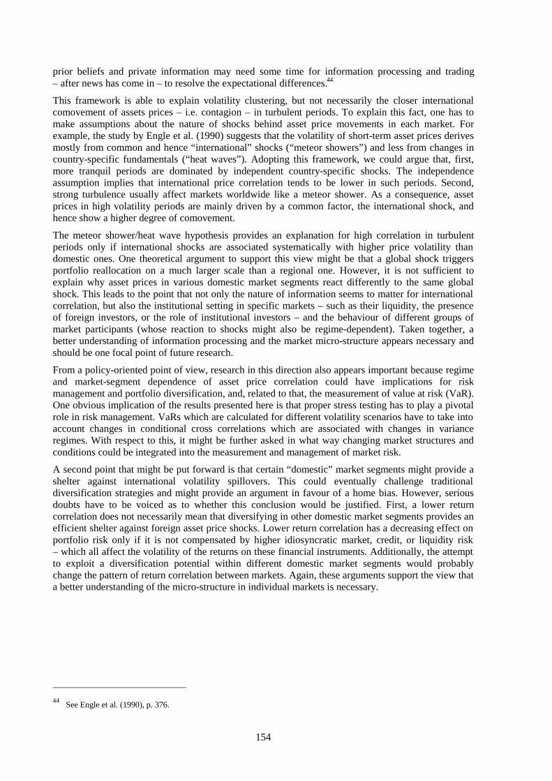
154
prior beliefs and private information may need some time for information processing and trading– after news has come in – to resolve the expectational differences.44
This framework is able to explain volatility clustering, but not necessarily the closer internationalcomovement of assets prices – i.e. contagion – in turbulent periods. To explain this fact, one has tomake assumptions about the nature of shocks behind asset price movements in each market. Forexample, the study by Engle et al. (1990) suggests that the volatility of short-term asset prices derivesmostly from common and hence “international” shocks (“meteor showers”) and less from changes incountry-specific fundamentals (“heat waves”). Adopting this framework, we could argue that, first,more tranquil periods are dominated by independent country-specific shocks. The independenceassumption implies that international price correlation tends to be lower in such periods. Second,strong turbulence usually affect markets worldwide like a meteor shower. As a consequence, assetprices in high volatility periods are mainly driven by a common factor, the international shock, andhence show a higher degree of comovement.
The meteor shower/heat wave hypothesis provides an explanation for high correlation in turbulentperiods only if international shocks are associated systematically with higher price volatility thandomestic ones. One theoretical argument to support this view might be that a global shock triggersportfolio reallocation on a much larger scale than a regional one. However, it is not sufficient toexplain why asset prices in various domestic market segments react differently to the same globalshock. This leads to the point that not only the nature of information seems to matter for internationalcorrelation, but also the institutional setting in specific markets – such as their liquidity, the presenceof foreign investors, or the role of institutional investors – and the behaviour of different groups ofmarket participants (whose reaction to shocks might also be regime-dependent). Taken together, abetter understanding of information processing and the market micro-structure appears necessary andshould be one focal point of future research.
From a policy-oriented point of view, research in this direction also appears important because regimeand market-segment dependence of asset price correlation could have implications for riskmanagement and portfolio diversification, and, related to that, the measurement of value at risk (VaR).One obvious implication of the results presented here is that proper stress testing has to play a pivotalrole in risk management. VaRs which are calculated for different volatility scenarios have to take intoaccount changes in conditional cross correlations which are associated with changes in varianceregimes. With respect to this, it might be further asked in what way changing market structures andconditions could be integrated into the measurement and management of market risk.
A second point that might be put forward is that certain “domestic” market segments might provide ashelter against international volatility spillovers. This could eventually challenge traditionaldiversification strategies and might provide an argument in favour of a home bias. However, seriousdoubts have to be voiced as to whether this conclusion would be justified. First, a lower returncorrelation does not necessarily mean that diversifying in other domestic market segments provides anefficient shelter against foreign asset price shocks. Lower return correlation has a decreasing effect onportfolio risk only if it is not compensated by higher idiosyncratic market, credit, or liquidity risk– which all affect the volatility of the returns on these financial instruments. Additionally, the attemptto exploit a diversification potential within different domestic market segments would probablychange the pattern of return correlation between markets. Again, these arguments support the view thata better understanding of the micro-structure in individual markets is necessary.
44
See Engle et al. (1990), p. 376.
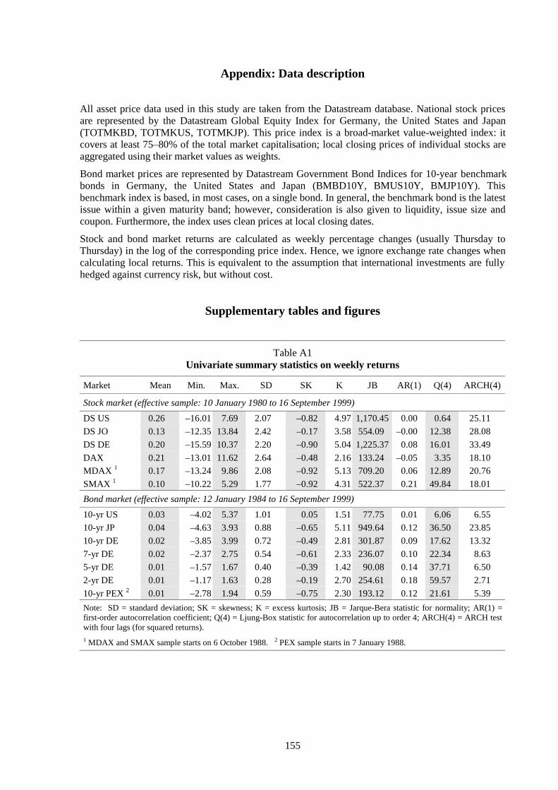
155
Appendix: Data description
All asset price data used in this study are taken from the Datastream database. National stock pricesare represented by the Datastream Global Equity Index for Germany, the United States and Japan(TOTMKBD, TOTMKUS, TOTMKJP). This price index is a broad-market value-weighted index: itcovers at least 75–80% of the total market capitalisation; local closing prices of individual stocks areaggregated using their market values as weights.
Bond market prices are represented by Datastream Government Bond Indices for 10-year benchmarkbonds in Germany, the United States and Japan (BMBD10Y, BMUS10Y, BMJP10Y). Thisbenchmark index is based, in most cases, on a single bond. In general, the benchmark bond is the latestissue within a given maturity band; however, consideration is also given to liquidity, issue size andcoupon. Furthermore, the index uses clean prices at local closing dates.
Stock and bond market returns are calculated as weekly percentage changes (usually Thursday toThursday) in the log of the corresponding price index. Hence, we ignore exchange rate changes whencalculating local returns. This is equivalent to the assumption that international investments are fullyhedged against currency risk, but without cost.
Supplementary tables and figures
Table A1Univariate summary statistics on weekly returns
Market Mean Min. Max. SD SK K JB AR(1) Q(4) ARCH(4)
Stock market (effective sample: 10 January 1980 to 16 September 1999)
DS US 0.26 –16.01 7.69 2.07 –0.82 4.97 1,170.45 0.00 0.64 25.11
DS JO 0.13 –12.35 13.84 2.42 –0.17 3.58 554.09 –0.00 12.38 28.08
DS DE 0.20 –15.5910.37 2.20 –0.90 5.041,225.37 0.08 16.01 33.49
DAX 0.21 –13.0111.62 2.64 –0.48 2.16 133.24 –0.05 3.35 18.10
MDAX 1 0.17 –13.24 9.86 2.08 –0.92 5.13 709.20 0.06 12.89 20.76
SMAX 1 0.10 –10.22 5.29 1.77 –0.92 4.31 522.37 0.21 49.84 18.01
Bond market (effective sample: 12 January 1984 to 16 September 1999)
10-yr US 0.03 –4.02 5.37 1.01 0.05 1.51 77.75 0.01 6.06 6.55
10-yr JP 0.04 –4.63 3.93 0.88 –0.65 5.11 949.64 0.12 36.50 23.85
10-yr DE 0.02 –3.85 3.99 0.72 –0.49 2.81 301.87 0.09 17.62 13.32
7-yr DE 0.02 –2.37 2.75 0.54 –0.61 2.33 236.07 0.10 22.34 8.63
5-yr DE 0.01 –1.57 1.67 0.40 –0.39 1.42 90.08 0.14 37.71 6.50
2-yr DE 0.01 –1.17 1.63 0.28 –0.19 2.70 254.61 0.18 59.57 2.71
10-yr PEX 2 0.01 –2.78 1.94 0.59 –0.75 2.30 193.12 0.12 21.61 5.39
Note: SD = standard deviation; SK = skewness; K = excess kurtosis; JB = Jarque-Bera statistic for normality; AR(1) =first-order autocorrelation coefficient; Q(4) = Ljung-Box statistic for autocorrelation up to order 4; ARCH(4) = ARCH testwith four lags (for squared returns).1 MDAX and SMAX sample starts on 6 October 1988. 2 PEX sample starts in 7 January 1988.

156
US varianceGerman variance
Correlation
Figure A1: Conditional variances and correlation between US and German stock returnsBivariate AR(1)-GARCH(1,1), diagonal representation: variances (left scale), correlation (right scale)
80 81 82 83 84 85 86 87 88 89 90 91 92 93 94 95 96 97 98 990
8
16
24
32
40
48
56
-0.4
-0.2
0.0
0.2
0.4
0.6
0.8
Figure A2: US–German bond return correlation from bivariate GARCH modelsConstant correlation representation (dashed line) and diagonal representation (solid line)
84 85 86 87 88 89 90 91 92 93 94 95 96 97 98 99-0.1
0.0
0.1
0.2
0.3
0.4
0.5
0.6
0.7
0.8
157
Bibliography
Ang, A and G Bekaert (1998): “Regime switches in interest rates”. NBER Working Paper, No. 6508,April.
Baig, T and I Goldfajn (1999): “Financial market contagion in the Asian crisis”. IMF Staff Papers, 46,pp. 167-95.
Bera, A K and M L Higgins (1993): “ARCH models: properties, estimation and testing”. Journal ofEconomic Surveys, 7, pp. 305-62.
Bodart, V and P Reding (1999): “Exchange rate regimes, volatility and international correlations onbond and stock markets”. Journal of International Money and Finance, 18, pp. 133-51.
Bollerslev, T (1990): “Modelling the coherence in short-run nominal exchange rates: a multivariategeneralised ARCH approach”. Review of Economics and Statistics, 72, pp. 498-505.
Bollerslev, T, R F Engle and J M Wooldridge (1988): “A capital asset pricing model with time-varying covariances”. Journal of Political Economy, 96, pp. 116-31.
Bollerslev, T, R Y Chou and K F Kroner (1992): “ARCH modeling in finance”. Journal ofEconometrics, 52, pp. 5-59.
Cai, J (1994): “A Markov model of switching-regime ARCH”. Journal of Business and EconomicStatistics, 12, pp. 309-16.
Campbell, J Y, A W Lo and A C MacKinlay (1998): The econometrics of financial markets. PrincetonUniversity Press, Princeton, N.J.
Cochrane, J H (1999): “New facts in finance”. Federal Reserve Bank of Chicago, EconomicPerspectives, 23, pp. 36-58.
Deutsche Bundesbank (1997): “The implications of international influences for capital market rates”.Monthly Report, Vol. 49, No. 7, pp. 23-40, July.
Domanski, D and M Kremer (1998): “What do asset price movements in Germany tell monetarypolicy makers?” Bank for International Settlements, BIS Conference Papers, Vol. 3, pp. 24-44.
Domanski, D and M Kremer (1999): “What is behind equity price movements in Germany?” inE Baltensperger (ed.), Transmissionsmechanismen der Geldpolitik, Schriften des Vereins fürSozialpolitik, Neue Folge Band 264, Duncker und Humbolt, Berlin, pp. 111-41.
Engle, R F, T Ito and W-L Lin (1990): “Meteor showers or heat waves? Heteroskedastic intra-dailyvolatility in the foreign exchange market”. Econometrica, 58, pp. 525-542, reprinted in R F Engle(ed.), ARCH. Selected readings, Oxford University Press, Oxford (1995), pp. 375-94.
Forbes, K and R Rigobon (1999): “No contagion, only interdependence”. NBER Working Paper,No. 7267, July.
Gray, S F (1996): “Modeling the conditional distribution of interest rates as a regime-switchingprocess”. Journal of Financial Economics, 42, pp. 27-62.
Hamilton, J (1989): “A new approach to the economic analysis of nonstationary time series and thebusiness cycle”. Econometrica, 57, pp. 357-84.
Hamilton, J (1994): Time series analysis. Princeton University Press, Princeton, N.J.
Hamilton, J and R Susmel (1994): “Autoregressive conditional heteroskedasticity and changes inregime”. Journal of Econometrics, 64, pp. 307-33.
Hansen, B E (1992): “The likelihood ratio test under non-standard conditions: testing the Markovtrend model of GNP”. Journal of Applied Econometrics, 7, pp. S61-S82.

158
Herwartz, H and H-E Reimers (1999): “Dynamic relationships between international bond markets”.Mimeo.
International Monetary Fund (1998): World economic outlook and international capital markets –interim assessment. Washington, D.C.
Kim, C-J and C R Nelson (1999): State-space models with regime switching. The MIT Press,Cambridge, MA, and London, England.
Koch, P D and T W Koch (1991): “Evolution in dynamic linkages across daily national stockindexes”. Journal of International Money and Finance, 10, pp. 231-51.
Kremer, M (1999): “Die Kapitalmarktzinsen in Deutschland und den USA: Wie eng ist derZinsverbund? Eine Anwendung der multivariaten Kointegrationsanalyse”. Economic Research Groupof the Deutsche Bundesbank, Discussion Paper 2/99, February.
Lamoureux, C G and W D Lastrapes (1990): “Persistence in variance, structural change and theGARCH model”. Journal of Business and Economic Statistics, 5, pp. 121-29.
Longin, F and B Solnik (1995): “Is the correlation in international equity returns constant: 1960–1990?” Journal of International Money and Finance, 14, pp. 3-26.
Loretan, M and W B English (1999): “Evaluating ‘correlation breakdowns’ during periods of marketvolatility”. Bank for International Settlements, BIS Conference Papers, this volume.
Ramchand, L and R Susmel (1998): “Volatility and cross correlation across major stock markets”.Journal of Empirical Finance, 5, pp. 397-416.
White, H (1982): “Maximum likelihood estimation of misspecified models”. Econometrica, 50,pp. 1-25.
159
International transmission and volume effects inG5 stock market returns and volatility
Sanvi Avouyi-Dovi and Eric Jondeau1
1. Introduction
An extensive literature has studied stock market returns and volatility. The attempts to clarify linksbetween return and its theoretical determinants have led researchers to investigate several areas.Return-volatility interactions, trading volume effects and international transmission mechanismsappear to be the most promising of these.
Seminal papers by Mandelbrot (1963) and Fama (1965) have shown that volatility is time varying.Portfolio models suggest that volatility may play a central role in the determination of return, since ariskier asset is supposed to yield a higher return. This link has been studied through ARCH-in-Meanmodels, in which volatility is directly introduced as an explanatory variable of return (as in Engle et al.(1987) or French et al. (1987)). Conversely, Schwert (1990), among others, has shown that a shock toreturns may have an asymmetric (or leverage) effect on volatility, depending on the sign of the shock:a negative shock on return generally implies a greater increase of volatility than a positive shock does,everything else being equal. These interactions between return and risk appear to be robust inexplaining price dynamics of most financial assets (stock markets, exchange markets, etc.).
International transmission mechanisms were first identified between stock returns (Eun and Shim(1989)). Subsequently, interest has focused on volatility transmission between stock markets. Indeed,work on volatility spillovers on currency markets (Engle et al. (1990)) has recently been extended tostock markets by Hamao et al. (1990), Koutmos and Booth (1995) and Booth et al. (1997).
The role of trading volumes in return formation has been pointed out by many authors (see Tauchenand Pitts (1983) and Karpoff (1987) for surveys). Such a relation may be based on theoreticalarguments (Copeland (1976) or Epps and Epps (1976) for a volume-volatility relation; Epps (1975) orJennings et al. (1981) for a volume-return relation); but it is more often based on empirical evidence(Karpoff (1987)). Most studies have shown a positive correlation between volume and absolutereturns, or volatility, on most asset markets: for instance, Schwert (1989) or Gallant et al. (1992) onstock markets, or Bessembinder and Seguin (1993) on futures markets. Moreover, as suggested inHarris and Gurel (1986) and Karpoff (1988), trading volumes and returns may be positively correlated(although this correlation is often weak). Lastly, Gallant et al. (1992) conducted a systematic long-runanalysis of possible correlations between returns, volatility and trading volume. They have shown thatvolume plays a central role in explaining links between returns and volatility: indeed, they obtain anegative link between returns and volatility without including volume in the relation, but a positivelink when volume is taken into account; moreover, the asymmetric effect decreases when volume isintroduced in the dynamics of volatility. This empirical evidence on the links between volume, returnand volatility suggests including volume as an explanatory variable in both return and volatilityequations. But these three variables should actually be determinated simultaneously. This appears tobe a difficult task. However, Jacobs and Onochie (1998) estimate a bivariate GARCH-in-Mean model,for stock market return and trading volume. To overcome this difficulty, we adopt a sequentialapproach in order to estimate return-volatility links (as in Davidian and Carroll (1987) andBessembinder and Seguin (1993)). First of all, we filter the volume series in order to take account ofthe endogeneity of volume with respect to return and volatility (Gallant et al. (1992)).
1
Research Department, Bank of France. The views expressed in this paper are those of the authors and do not necessarilyrepresent those of the Bank of France.
160
This paper analyses the links between stock market return, volatility and trading volume. Thisframework is used to study the daily returns of the reference stock market indices of the G5 countriesover the period 1988–98. The model is composed of three equations (for volume, return andvolatility), in which the aforementioned effects are introduced. To measure the effect of laggedvariables, we also included a sequence of lags for all explanatory variables except trading volumes.
The remainder of the paper is organised as follows. Section 2 presents our model and the estimationmethodology. Section 3 describes the data and outlines adjustments made to the data. Section 4provides our main empirical results. Section 5 offers concluding remarks.
2. Methodology
2.1 The model
The model proposed in this paper generalises previous models, in particular those proposed by Hamaoet al. (1990) or Bessembinder and Seguin (1993). It is written in the following form:
(1) ttttttt mFDvQLCRLBLAI ε++++σ+∆+ε=∆ − ˆ)()()( 11
(2) tttttt DvLL η+σ+ϕ+γ+εβ+σα=σ −− 011 ˆ)()(
where A(L), B(L), C(L), α(L) and β(L) are lag polynomial matrices with ∑ = α=α pi
ii LL 0)( . ∆It is the
vector of returns of stock market indices at time t, where It denotes the index price in logarithm. εt isthe vector of innovations of the process ∆It (εt = ∆It-Et-1 ∆It). Conditionally on the information setavailable at time t, εt is assumed to be normally distributed. ∆Rt is the vector of changes in the 10-yearrates. σt is the vector of conditional volatilities of returns. ηt is the vector of innovations of σt. tv is the
vector of trading volumes.
The vector )’,...,,,,,...,( 11141 Kttttttt dumdumHHJJD +−= groups all 0-1 variables: ‘day’ variables (Jjt,j=1,...,4) are equal to 1 on the given day in the week (Monday,..., Thursday), and 0 otherwise; the‘holiday’ variable (Ht) is equal to 1 when date t is a holiday, and 0 otherwise; Kkktdum ,...,1= groups
the dummy variables for major shocks on the stock markets.2
To allow for the current domestic interest rate and current domestic volatility in the return equation,but to exclude contemporaneous foreign variables, we introduce the following additional constraints:Bij(0)=Cij(0)=0, for all i≠j.
Return equation (1) has the following features:
• The return of the country i index at time t is a function of past unexpected returns in that marketand in other markets. Actually returns in all stock market indices are not introduced into equationsfor all stock returns. In fact, we apply a predefined ranking of countries by financial market size:US variables are systematically introduced to explain other stock market indices; Germanvariables are systematically introduced into equations for other European stock market indices.3
2
Dummy variables used are consistent across markets. They capture the main exogenous events that affected theinternational environment: the fall of the Berlin Wall (October 1989), German reunification (October 1990), the Gulf war(April 1990), and the attempted putsch in Moscow (1991). Because of time zone differences, the variables maysometimes have a one-day lag.
3The ranking of European markets recognises Germany as the European leader. This choice is based on the relative sizesof the national economies, rather than on the relative weight as financial markets. Assuming the United Kingdom asdriving European markets does not improve our results.

161
To ensure consistency with the volatility equation, unexpected returns – rather than total returns –are introduced as explanatory variables.4
• The return of the country i index depends on changes in bond yields (present and past yields incountry i and past yields in the driving foreign countries). Introducing long-term interest ratesallows us to evaluate the impact of other variables – in particular, trading volumes and volatilities– independently of the strong direct effect of interest rates. Interest rates are undoubtedly thestrongest explanatory variables for stock returns, and omitting this effect would bias the estimatesof other effects. Besides, given the relative weights of bond and stock markets, long-term ratesappear to be exogenous with respect to parameters of stock return equations.
• The return of the country i index is a function of present and past volatilities in that market, andpast volatilities in the driving foreign markets. Engle et al. (1987) have shown the role of volatilityas a risk-proxy variable in modelling returns. Volatility is introduced into the return equationsystematically with past unexpected returns.
• The influence of domestic trading volumes in the return equation is measured in two ways: the logof unexpected trading volume; and a breakdown between positive and negative unexpectedvolume, allowing measurement of asymmetric effects on return and volatility equations.
The main features of the volatility equation (2) are the following:
• The volatility of the country i index at time t is a function of past volatilities in that market and indriving foreign markets.
• Introducing unexpected returns makes it possible to measure the possible asymmetry of returnshocks on volatility.
• The influence of volumes in the volatility equation is tested under the same alternative forms as inthe return equation: the unexpected volume, and the unexpected volume broken down into positiveand negative shocks.
2.2 Estimating unexpected trading volumes
A large number of papers have shown the central role played by trading volumes in explaining thedynamics of stock market indices. Theoretical arguments have been proposed in order to introducevolumes into the return equation (Karpoff (1987)) and into the volatility equation (Epps and Epps(1976) and Admati and Pfleiderer (1988)). Trading volumes can be interestingly interpreted in termsof market “depth”. Kyle (1985) defined market depth as the unexpected order flow required to movethe stock market index by 1%. This definition is also chosen by Bessembinder and Seguin (1993) intheir study of the impact of volume on volatility.
However, trading volume is strongly endogenous with respect to return and volatility. But the jointestimation of price equations (i.e. return and volatility) and of volume equations would be ratherdifficult due to the complexity of our specifications. One commonly adopted solution (Gallant et al.(1992), Bessembinder and Seguin (1993) and Campbell et al. (1993)) consists in filtering the volumeseries beforehand. This preliminary step also allows total volume to be broken down into expectedvolume and unexpected volume. 4
Accordingly, if countries are ranked in the following order (United States, Japan Germany, France and United Kingdom),matrices Ai, Bi, Ci, i=1,...,p, in equation (1) as well as αi and βi, i=1,...,p, in equation (2) have the following structure:
xxx
xxx
xx
xx
x
00
00
000
000
0000
For France, for example, this allows the presence of US, German and French variables in return and volatility equations.
162
Trading volume is broken down in two steps:
First, systematic effects (deterministic trend, day-of-the-week effects and holiday effects) are extractedfrom trading volume:
(3) itititj
jjit vHfHfJfttV ++++γ+β+α= +−=
∑ 1615
4
1
2log
Second, the non-systematic trading volume, itv , is then broken down into an expected and anunexpected part. Some authors (including Gallant et al. (1992)) have identified a significantcorrelation between past volatility and trading volume, largely responsible for the endogeneity ofvolume with respect to price index. itv is therefore regressed on its lagged values, on past volatility,and on past return. Volatility is defined here as the absolute value of the stock return
( 2/π∆= itit Is ). Therefore, we estimate the following regression:
(4) nait
jjitj
jjitj
jjitjit vIsvv +∆ψ+π+λ+α= ∑∑∑
=−
=−
=−
4
1
4
1
4
1
ˆˆ
In what follows, the unexpected volume is defined as the estimated residual from the second step naitv .
This breakdown is based on the idea that market participants react differently to a shock on volume,depending on whether this shock is expected. More precisely, it may be that only unexpected volumeaffects return and volatility. In the following, we consider two ways of introducing unexpectedvolume. In the first model, we introduce unexpected volume directly; in the second model, we allowfor an asymmetric effect of volume on both return and volatility equations.
2.3 Estimating the model
Given the large number of parameters to be estimated in return and volatility equations, it wouldappear very difficult to estimate this model using a direct maximum-likelihood approach. Toovercome this problem, we follow the methodology proposed by Schwert (1990) and Bessembinderand Seguin (1993). First, as suggested by Schwert and Seguin (1990), volatility is estimated as:
(5) 2/ˆˆ πε=σ tt
where tε is the estimated residual of the return equation. This definition is based on the result that
( ) πσ= /2xE if ( )2,0 σ→ Nx .5 Volatility therefore depends on both unexpected returns and the
absolute value of unexpected returns. A shock on the unexpected return will affect volatility in adifferent way, depending on whether the shock is positive or negative, according to the followingrelation:
(6)
<επα+β−
>επα+β=
ε∂σ∂
−
−
− .0ˆif2/
0ˆif2/
ˆ
ˆ
ljtijlijl
ljtijlijl
ljt
it
Second, the econometric estimation of the model is carried out using the convergent sequentialestimation method proposed by Davidian and Carroll (1987):
1. A return equation is first estimated by replacing domestic unexpected returns observed returnsbut without domestic and foreign volatilities. Moreover, the vector of past unexpected returns (denoted
5
Other volatility indicators may be used. The standard deviation of the return-equation residuals over n trading days is oneof the indicators most widely used by traders, but it is largely unsatisfactory because it implies an overlapping bias. Usingimplied volatilities would also have been an interesting alternative but, owing to the lack of adequate data, we wereunable to implement it.

163
)0(1ˆ −εt ) is composed of foreign unexpected returns and domestic observed return:
)1(1
)0(1 ˆ)(ˆ)( ititi
naitititiit mDFvQRLBLAI ε++++∆+ε=∆ −
from which one obtains unexpected returns )1(ˆ tε .
2. Volatility is then computed using equation (3)
2/ˆˆ )1()1( πε=σ itit
and a preliminary estimation of the volatility equation is performed: volatility is regressed on pastdomestic and foreign volatilities and on past domestic and foreign unexpected returns (the unexpecteddomestic return is the residual of the first-step regression):
)1(0
)1(1
)1(1
)1( ˆˆ)(ˆ)(ˆ ititinaitititiit DvLL η+σ+ϕ+γ+εβ+σα=σ −−
from which one obtains expected volatilities )1()1()2( ˆˆˆ ttt η−σ=σ
3. Return equation (1) is finally estimated, with domestic and foreign expected volatilities anddomestic and foreign unexpected returns:
)2(1
)2()1(1 ˆˆ)()(ˆ)( ititi
naititititiit mDFvQLCRLBLAI ε++++σ+∆+ε=∆ −
from which one obtains unexpected returns )2(ˆ tε .
4. Volatility is calculated once again as
2/ˆˆ )2()3( πε=σ tt
and the volatility equation (2) is finally estimated:
)2(0
)2(1
)3(1
)3( ˆˆ)(ˆ)(ˆ ititinaitititiit DvLL η+σ+ϕ+γ+εβ+σα=σ −− .
This sequential estimation method requires the variance-covariance matrix of residuals to be diagonal.The covariance between errors associated with the return equation ( tε ) and volatility equation ( tη ) isassumed to be zero. However, volatility is allowed to have an instantaneous effect on return. Similarly,correlations between errors associated with different markets ( itε and jtε for return equations, itη
and jtη for volatility equations) are assumed to be zero. This constraint, however, is relaxed by the
introduction into return and volatility equations of the most recent errors on other stock markets.
3. Data and preliminary analysis
3.1 Data
The data used in this paper are leading G5 stock market indices (Dow Jones in New York, DAX inFrankfurt, CAC 40 in Paris, FTSE 100 in London and Nikkei in Tokyo),6 trading volumes for eachmarket, and 10-year benchmark interest rates. The database has a daily frequency over the period from1 January 1988 to 31 December 1998 (2,870 observations), recorded at the close of each trading day(source: Datastream). The choice of 1988 as the first year in our sample is intended to eliminate theOctober 1987 crash, which greatly disturbed stock markets.
6
The stock market indices used are not necessarily consistent with one another: there are differences in methods used forweighting individual stocks and in the portion of total market capitalisation captured by each index. Nevertheless, theseindices have been chosen because they are the most widely used indicators of aggregate prices in the different markets.

164
As far as trading volumes are concerned, we face two problems: first, reported trading volume is thenumber of securities traded during the session in the United States, Japan and the United Kingdom, butit is expressed in monetary units in Germany and France. Statistics on the number of securities tradedare also available for German and French markets, but for a too short period to be used here. Second,some data had to be adjusted before any statistical analysis. In some cases, volumes were stated forholidays, trading days were left blank, and some entries were clearly aberrant. For the entire database,we corrected four observations in the United States, four in Germany, 21 in France, two in the UnitedKingdom, and four in Japan.
Opening and closing times of stock markets are reported in GMT in Datastream. If the market closesduring the afternoon of day t in Europe, it closes during the morning of day t in Japan and during theevening of day t-1 in the United States.7
Non-trading days were treated as follows:8
When day t-1 is closed on the market examined, the variables of day t in change form (log of the indexor interest rate) are defined as the change between two trading days (irrespective of the number of non-trading days between them); variables stated in levels (trading volume, volatility) are not adjustedsince they are provided only for trading days; foreign variables in the domestic index equation areadjusted in the following way: first, if day t is a non-trading day for the foreign market, the foreignvariables in change form are set to zero, and the variables in levels are assigned the value of theprevious day; second, if day t is a trading day, we use the observed variations and levels.
If day t is a trading day for the market studied, but a non-trading day for the foreign market, foreignvariables in change form are set to zero, and variables in levels are assigned the value of the previousday.
3.2 Preliminary analysis
Table 1 reports summary statistics on stock returns, trading volumes and 10-year interest rates in theG5 countries over the period under study. Stock returns exhibit an asymmetric distribution (negative inthe United States, Germany and France; positive in the United Kingdom and Japan) and havesignificant fat tails (Table 1a). The excess kurtosis is rather high, from 2.3 for the FTSE 100 to 10.4for the DAX. The Jarque-Bera test therefore rejects the normality hypothesis for each return series.The Ljung-Box statistics for serial correlation (LBQ, calculated with 20 lags) give mixed results sincethe null hypothesis of no serial correlation is rejected for the FTSE 100 and the Nikkei, but not forother stock market indices. Finally, the Ljung-Box statistics on the squared returns (LBQ2) indicatestrong heteroskedasticity for all series. The statistical properties of the return series therefore require aspecific model for stock returns and their volatility – at least as regards to the strong dependence ofsquared returns.
Concerning 10-year interest rates, normality is rejected for each country (Table 1b). The nullhypothesis of no serial correlation is accepted only for French rates only. Besides, all interest ratesexhibit significant serial correlation of squared returns.
As regards the growth rate of trading volume, we reject the hypothesis of normality, but not thehypothesis that the residuals are serially correlated, and homoskedasticity (Table 1c). 7
There is a large overlap between European market opening times. In the case of the link between Frankfurt and Paris, forinstance, introducing the current German return into the French return equation could be misleading: a significant effectof the German return may be interpreted as a causal link, whereas it may actually reflect a “news” effect only. Topreclude this potential source of bias, we have estimated two types of models: in the first, we introduce lagged Germanvariables only (in both French and UK equations, Tables 3 and 4); in the second, we introduce current German variables.Moreover, it is worth noting that New York opens after the closing of Frankfurt but before the closing of Paris. Thus theCAC 40 closing price may reflect some information from first transactions of New York that cannot be reflected in theclosing price of DAX.
8The number of non-trading days differs considerably between countries. Over the period studied (1988–98), we identified88 non-trading days in the United States, 116 in Germany, 129 in France, 89 in the United Kingdom, and 155 in Japan.

165
Table 1aStatistics for stock returns
Dow Jones Nikkei DAX CAC 40 FTSE 100
Mean (%) 0.056 –0.017 0.058 0.051 0.045
Std dev. (%) 0.907 1.429 1.248 1.197 0.873
Skewness –0.700 a 0.328 a –0.871 a –0.185 a 0.028 a
Kurtosis 7.565 a 4.843 a 10.440 a 2.812 a 2.309 a
Jarque-Bera 4,614.100 a 3,307.700 a 21,375.000 a 726.300 a 391.400 a
LBQ(20) 35.000 b 48.380 a 30.920 c 34.420 b 61.960 a
LBQ2(20) 253.390 a 617.110 a 295.330 a 601.730 a 922.550 a
Table 1bStatistics for changes of 10-year rates
United States Japan Germany France United Kingdom
Mean (%) –0.002 –0.001 –0.001 –0.002 –0.002
Std dev. (%) 0.059 0.046 0.047 0.057 0.067
Skewness 0.236 a 0.209 a 0.658 a –0.018 –0.292 a
Kurtosis 2.866 a 6.172 a 5.013 a 2.682 a 5.473 a
Jarque-Bera 523.700 a 2,737.600 a 1,927.000 a 533.100 a 2,821.000 a
LBQ(20) 43.540 a 30.780 c 43.960 c 17.860 34.220 b
LBQ2(20) 89.990 a 122.770 a 403.250 a 398.790 a 172.710 a
Table 1cStatistics on trading volumes (rate of change)
New York Tokyo Frankfurt Paris London
Mean (%) 0.049 –0.054 0.076 –0.014 0.012
Std dev. (%) 20.303 30.437 24.277 30.872 22.295
Skewness –0.179 a –0.092 a 0.032 0.047 –0.103 b
Kurtosis 6.099 a 1.847 a 1.924 a 2.745 a 2.480 a
Jarque-Bera 1,972.800 a 235.200 a 1,783.400 a 437.950 a 251.300 a
LBQ(20) 615.600 a 817.770 a 358.270 a 437.950 a 769.530 a
LBQ2(20) 350.500 a 174.700 a 176.890 a 425.790 a 118.580 a
Note: a, b and c indicate that the statistics are significant at a 1%, 5% and 10% level respectively. Under the null ofnormality, the Jarque-Bera statistics are chi-square distributed with 2 degrees of freedom. LBQ are the Ljung-Box statistics(computed with 20 lags) for the residuals; LBQ2 are the Ljung-Box statistics for the squared residuals; under the null of nocorrelation of the series considered, these statistics are chi-square distributed with 20 degrees of freedom.
Another issue concerns stationarity of the variables (Table 2). Stock-market indices (in log) andinterest rates can be considered as difference-stationary processes. Indeed, autoregressive coefficientsof variables in levels are very close to 1 and DF and ADF tests do not reject the null hypothesis ofnon-stationarity. On the other hand, variables in change form appear to be stationary. Furthermore, wefind no evidence of non-stationarity for trading volumes. In all cases, volumes display a deterministic– not a stochastic – trend. Therefore, in what follows, trading volumes are treated as stationary arounda deterministic trend.
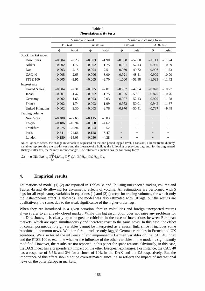
166
Table 2Non-stationarity tests
Variable in level Variable in change form
DF test ADF test DF test ADF test
φ t-stat φ t-stat φ t-stat φ t-stat
Stock market index
Dow Jones –0.004 –2.23 –0.003 –1.90 –0.988 –52.00 –1.111 –11.74
Nikkei –0.002 –1.77 –0.002 –1.75 –0.991 –52.13 –0.980 –10.89
Dax –0.003 –2.15 –0.004 –2.51 –0.950 –49.72 –0.996 –11.73
CAC 40 –0.005 –2.65 –0.006 –3.00 –0.921 –48.51 –0.909 –10.90
FTSE 100 –0.005 –2.95 –0.005 –2.70 –1.000 –51.98 –1.033 –11.42
Interest rate
United States –0.004 –2.31 –0.005 –2.81 –0.937 –49.54 –0.878 –10.27
Japan –0.001 –1.47 –0.002 –1.75 –0.965 –50.61 –0.875 –10.76
Germany –0.002 –1.63 –0.003 –2.03 –0.997 –52.13 –0.929 –11.28
France –0.002 –1.74 –0.003 –1.99 –0.953 –50.01 –0.942 –11.37
United Kingdom –0.002 –2.30 –0.003 –2.76 –0.970 –50.41 –0.737 –9.48
Trading volume
New York –0.400 –27.60 –0.115 –5.83 − − − −Tokyo –0.186 –16.94 –0.060 –4.62 − − − −Frankfurt –0.275 –20.94 –0.054 –3.52 − − − −Paris –0.341 –24.66 –0.128 –6.47 − − − −London –0.150 –15.05 –0.050 –4.38 − − − −
Note: For each series, the change in variable is regressed on the one-period lagged level, a constant, a linear trend, dummyvariables representing the day-in-week and the presence of a holiday the following or previous day, and, for the augmentedDickey-Fuller test, the 20 most recent changes. The estimated equation has the following form:
ttti
iii
ititt HfHfJfXXtX ε++++∆θ+φ+β+α=∆ +−==
−− ∑∑ 1615
4
1
20
11
4. Empirical results
Estimations of model (1)-(2) are reported in Tables 3a and 3b using unexpected trading volume andTables 4a and 4b allowing for asymmetric effects of volume. All estimations are performed with 5lags for all explanatory variables in equations (1) and (2) (except for trading volumes, for which onlythe instantaneous effect is allowed). The model was also estimated with 10 lags, but the results arequalitatively the same, due to the weak significance of the higher-order lags.
When they are introduced in a given equation, foreign volatilities and foreign unexpected returnsalways refer to an already closed market. While this lag assumption does not raise any problems forthe Dow Jones, it is clearly open to greater criticism in the case of interactions between Europeanmarkets, which are open simultaneously and therefore react to the same news. In this case, the effectof contemporaneous foreign variables cannot be interpreted as a causal link, since it includes somereactions to common news. We therefore introduce only lagged German variables in French and UKequations. We also tested the influence of contemporaneous German variables on the CAC 40 indexand the FTSE 100 to examine whether the influence of the other variables in the model is significantlymodified. However, the results are not reported in this paper for space reasons. Obviously, in this case,the DAX index has a preponderant impact on the other European exchanges. For instance, the CAC 40has a response of 5.5% and 3% for a shock of 10% in the DAX and the DJ respectively. But theimportance of this effect should not be overestimated, since it also reflects the impact of internationalnews on the other European markets.
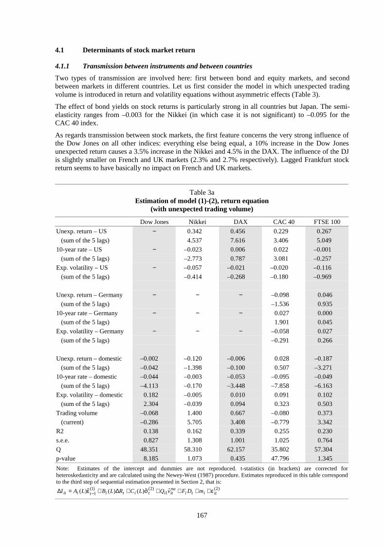
167
4.1 Determinants of stock market return
4.1.1 Transmission between instruments and between countries
Two types of transmission are involved here: first between bond and equity markets, and secondbetween markets in different countries. Let us first consider the model in which unexpected tradingvolume is introduced in return and volatility equations without asymmetric effects (Table 3).
The effect of bond yields on stock returns is particularly strong in all countries but Japan. The semi-elasticity ranges from –0.003 for the Nikkei (in which case it is not significant) to –0.095 for theCAC 40 index.
As regards transmission between stock markets, the first feature concerns the very strong influence ofthe Dow Jones on all other indices: everything else being equal, a 10% increase in the Dow Jonesunexpected return causes a 3.5% increase in the Nikkei and 4.5% in the DAX. The influence of the DJis slightly smaller on French and UK markets (2.3% and 2.7% respectively). Lagged Frankfurt stockreturn seems to have basically no impact on French and UK markets.
Table 3aEstimation of model (1)-(2), return equation
(with unexpected trading volume)
Dow Jones Nikkei DAX CAC 40 FTSE 100
Unexp. return – US − 0.342 0.456 0.229 0.267
(sum of the 5 lags) 4.537 7.616 3.406 5.049
10-year rate – US − –0.023 0.006 0.022 –0.001
(sum of the 5 lags) –2.773 0.787 3.081 –0.257
Exp. volatility – US − –0.057 –0.021 –0.020 –0.116
(sum of the 5 lags) –0.414 –0.268 –0.180 –0.969
Unexp. return – Germany − − − –0.098 0.046
(sum of the 5 lags) –1.536 0.935
10-year rate – Germany − − − 0.027 0.000
(sum of the 5 lags) 1.901 0.045
Exp. volatility – Germany − − − –0.058 0.027
(sum of the 5 lags) –0.291 0.266
Unexp. return – domestic –0.002 –0.120 –0.006 0.028 –0.187
(sum of the 5 lags) –0.042 –1.398 –0.100 0.507 –3.271
10-year rate – domestic –0.044 –0.003 –0.053 –0.095 –0.049
(sum of the 5 lags) –4.113 –0.170 –3.448 –7.858 –6.163
Exp. volatility – domestic 0.182 –0.005 0.010 0.091 0.102
(sum of the 5 lags) 2.304 –0.039 0.094 0.323 0.503
Trading volume –0.068 1.400 0.667 –0.080 0.373
(current) –0.286 5.705 3.408 –0.779 3.342
R2 0.138 0.162 0.339 0.255 0.230
s.e.e. 0.827 1.308 1.001 1.025 0.764
Q 48.351 58.310 62.157 35.802 57.304
p-value 8.185 1.073 0.435 47.796 1.345
Note: Estimates of the intercept and dummies are not reproduced. t-statistics (in brackets) are corrected forheteroskedasticity and are calculated using the Newey-West (1987) procedure. Estimates reproduced in this table correspondto the third step of sequential estimation presented in Section 2, that is:
)2(1
)2()1(1
ˆˆ)()(ˆ)( ititinaititititiit mDFvQLCRLBLAI ε++++σ+∆+ε=∆ −

168
The influence of foreign bond yields is generally rather weak on domestic stock returns. Note,however, that the US interest rate seems to replace the Japanese long-term rate that has no significanteffect on the Nikkei return equation.
4.1.2 Effects of volatility on return
Expected domestic volatility has no significant impact on domestic returns in any country. This resultappears to conflict with the results obtained by French et al. (1987) on US data. More recent studies,however, have cast doubt on the robustness of the conclusions of those authors. Using the samemethodology, Poon and Taylor (1992), for example, found no significant effect of volatility onreturns; Hamao et al. (1990), in most of their estimations, also failed to find any significant impact ofvolatility.
In the framework of our study, this result could also be explained by the introduction of volumes intothe return equation. Indeed, estimating model (1)-(2) without trading volume gives, for almost allindices, a significant effect of expected volatility (results are not reproduced here).
4.1.3 Volume effects
Volume effects are analysed in three stages: the unexpected volume effect on the return equation, theunexpected volume effect on the volatility equation, and the effect of allowing asymmetric effects inreturn and volatility equations.
Table 3bEstimation of model (1)-(2), volatility equation
(with unexpected trading volume)
Dow Jones Nikkei DAX CAC 40 FTSE 100
Exp. volatility – US − 0.162 0.549 0.133 0.056
(sum of the 5 lags) 1.238 3.472 0.751 0.549
Unexp. return – US − –0.221 –0.173 –0.032 –0.025
(sum of the 5 lags) –4.249 –3.505 –0.625 –0.681
Exp. volatility – Germany − − − 0.519 0.303
(sum of the 5 lags) 6.234 4.355
Unexp. return – Germany − − − –0.074 –0.059
(sum of the 5 lags) –1.452 –1.605
Exp. volatility – domestic 0.431 0.548 0.462 0.186 0.299
(sum of the 5 lags) 8.218 16.386 11.500 4.217 6.922
Unexp. return – domestic –0.214 –0.197 –0.058 –0.071 –0.070
(sum of the 5 lags) –4.361 –5.189 –1.324 –1.818 –1.308
Trading volume 1.240 1.036 0.958 0.250 0.337
(current) 8.735 7.720 10.596 3.905 4.136
R2 0.162 0.207 0.236 0.125 0.134
s.e.e. 0.669 1.008 0.761 0.791 0.584
Q 129.352 124.534 125.913 61.172 136.369
p-value 0.000 0.000 0.000 0.551 0.000
Note: Estimates of the intercept and of parameters associated to dummies are not reproduced here. t-statistics (in brackets)are corrected for heteroskedasticity and are calculated using the Newey-West (1987) procedure. Estimates reproduced in thistable correspond to the third step of sequential estimation presented in Section 2, that is:
)2(0
)2(1
)3(1
)3( ˆˆ)(ˆ)(ˆ ititinaitititiit DvLL η+σ+ϕ+γ+εβ+σα=σ −−
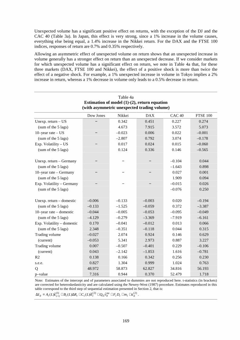
169
Unexpected volume has a significant positive effect on returns, with the exception of the DJ and theCAC 40 (Table 3a). In Japan, this effect is very strong, since a 1% increase in the volume causes,everything else being equal, a 1.4% increase in the Nikkei return. For the DAX and the FTSE 100indices, responses of return are 0.7% and 0.35% respectively.
Allowing an asymmetric effect of unexpected volume on return shows that an unexpected increase involume generally has a stronger effect on return than an unexpected decrease. If we consider marketsfor which unexpected volume has a significant effect on return, we note in Table 4a that, for thesethree markets (DAX, FTSE 100 and Nikkei), the effect of a positive shock is more than twice theeffect of a negative shock. For example, a 1% unexpected increase in volume in Tokyo implies a 2%increase in return, whereas a 1% decrease in volume only leads to a 0.5% decrease in return.
Table 4aEstimation of model (1)-(2), return equation
(with asymmetric unexpected trading volume)
Dow Jones Nikkei DAX CAC 40 FTSE 100
Unexp. return – US − 0.342 0.451 0.227 0.274
(sum of the 5 lags) 4.673 7.915 3.572 5.073
10–year rate – US − –0.023 0.006 0.022 –0.001
(sum of the 5 lags) –2.807 0.792 3.074 –0.178
Exp. Volatility – US − 0.017 0.024 0.015 –0.060
(sum of the 5 lags) 0.124 0.336 0.146 –0.565
Unexp. return – Germany − − − –0.104 0.044
(sum of the 5 lags) –1.643 0.898
10–year rate – Germany − − − 0.027 0.001
(sum of the 5 lags) 1.909 0.094
Exp. Volatility – Germany − − − –0.015 0.026
(sum of the 5 lags) –0.076 0.250
Unexp. return – domestic –0.006 –0.133 –0.003 0.020 –0.194
(sum of the 5 lags) –0.133 –1.525 –0.059 0.372 –3.387
10–year rate – domestic –0.044 –0.005 –0.053 –0.095 –0.049
(sum of the 5 lags) –4.129 –0.279 –3.369 –7.919 –6.161
Exp. Volatility – domestic 0.170 –0.041 –0.012 0.013 0.066
(sum of the 5 lags) 2.348 –0.351 –0.118 0.044 0.315
Trading volume –0.027 2.074 0.924 0.146 0.629
(current) –0.053 5.341 2.973 0.887 3.227
Trading volume 0.007 –0.507 –0.401 0.229 –0.106
(current) 0.043 –2.142 –1.853 1.616 –0.781
R2 0.138 0.166 0.342 0.256 0.230
s.e.e. 0.827 1.304 0.999 1.024 0.763
Q 48.972 58.873 62.827 34.816 56.193
p–value 7.316 0.944 0.370 52.479 1.718
Note: Estimates of the intercept and of parameters associated to dummies are not reproduced here. t-statistics (in brackets)are corrected for heteroskedasticity and are calculated using the Newey-West (1987) procedure. Estimates reproduced in thistable correspond to the third step of sequential estimation presented in Section 2, that is:
)2(1
)2()1(1
ˆˆ)()(ˆ)( ititinaititititiit mDFvQLCRLBLAI ε++++σ+∆+ε=∆ − .

170
4.2 Determinants of stock market volatility
While volatility exhibits significant autoregressive dynamics, it is clearly stationary in all markets. Theindex with the most persistent volatility is the Nikkei, with a cumulated impact of 0.55 for the fivelagged volatilities. For the other indices, the cumulated impact is between 0.18 and 0.46. However, inmost previous studies (e.g. Hamao et al. (1990)), the conditional variance appears to be stronglyautoregressive, or even non-stationary. This result may be linked to the method used for calculatingthe conditional variance.
Table 4bEstimation of model (1)-(2), volatility equation(with asymmetric unexpected trading volume)
Dow Jones Nikkei DAX CAC 40 FTSE 100
Exp. volatility – US − 0.141 0.522 0.111 0.042
(sum of the 5 lags) 1.125 3.653 0.711 0.520
Unexp. return – US − –0.220 –0.168 –0.026 –0.029
(sum of the 5 lags) –4.247 –3.347 –0.500 –0.792
Exp. volatility – Germany − − − 0.532 0.304
(sum of the 5 lags) 6.346 4.463
Unexp. return – Germany − − − –0.076 –0.059
(sum of the 5 lags) –1.476 –1.588
Exp. volatility – domestic 0.421 0.552 0.470 0.177 0.297
(sum of the 5 lags) 7.979 16.927 13.156 4.049 6.629
Unexp. return – domestic –0.216 –0.194 –0.060 –0.074 –0.068
(sum of the 5 lags) –4.367 –5.438 –1.372 –1.937 –1.283
Trading volume 2.033 1.629 1.292 0.263 0.343
(current) 6.476 6.820 7.685 2.274 2.656
Trading volume –0.546 –0.400 –0.558 –0.206 –0.365
(current) –4.376 –2.700 –4.042 –2.347 –2.727
R2 0.173 0.218 0.241 0.123 0.133
s.e.e. 0.665 1.000 0.760 0.791 0.584
Q 135.617 136.453 136.954 63.623 135.190
p-value 0.000 0.000 0.000 0.304 0.000
Note: Estimates of the intercept and of parameters associated to dummies are not reproduced here. t-statistics (in brackets)are corrected for heteroskedasticity and are calculated using the Newey-West (1987) procedure. Estimates reproduced in thistable correspond to the third step of sequential estimation presented in Section 2, that is:
)2(0
)2(1
)3(1
)3( ˆˆ)(ˆ)(ˆ ititinaitititiit DvLL η+σ+ϕ+γ+εβ+σα=σ −−
4.2.1 “Leverage” effects
In all equations, unexpected returns has a negative impact on volatility. This effect is stronglysignificant for the Dow Jones and the Nikkei. The reaction of volatility to a return shock appears to belargely asymmetric (Table 5): in the case of the Dow Jones, for example, a positive 10% shockincreases volatility by only 3.2%, whereas a negative 10% shock increases volatility by 7.4%. Thisasymmetric behaviour also turns out to be significant for the Nikkei: volatility increases by 5.0% aftera positive return shock and by 8.9% after a negative shock.

171
Table 5Impact of a 1% return shock on volatility (from estimation of Table 3)
Dow Jones Nikkei DAX CAC 40 FTSE 100
Positive shock 0.32 0.51 0.16 0.30 0.50
Negative shock 0.74 0.64 0.29 0.45 0.89
Note: Figures reported in this figure measure the total effect on volatility of a 1% shock on all lagged domestic returns:
<επα+β−
>επα+β=
ε∂σ∂
−
−
− 0ˆif2/
0ˆif2/
ˆ
ˆ
ljtijlijl
ljtijlijl
ljt
it .
4.2.2 Volatility transmission
International volatility transmission gives contrasting results. The expected volatility of the Dow Joneshas a positive effect on the volatility of other markets, but this effect is significant for the DAX indexonly: a 10% increase in the DJ volatility implies, everything else being equal, a 5.6% increase in theDAX volatility. Moreover, the US unexpected return has a strong negative effect on DAX and Nikkeivolatility. Therefore a negative shock on the US market leads to a larger increase of German and Japanvolatilities than a positive shock does.
As regards European markets, the CAC 40 and the FTSE 100 volatilities are significantly affected bythe German market. Indeed, the DAX expected volatility has a strong positive effect, whereas theunexpected return has a weak negative effect. Once again, a negative shock on the German marketimplies a larger increase of French and UK volatilities than a positive shock does. We obtain such aresult whether or not current German variables are introduced in the CAC 40 and FTSE 100 equations.
To conclude, it is worth noting that we obtain some asymmetric effects for all market volatilities.
4.2.3 Volume effects
The effect of unexpected volume on volatility is strongly significant for all indices (Table 3b):between 0.96 and 1.12 for the Dow Jones, the DAX and the Nikkei; between 0.23 and 0.34 for theCAC 40 and the FTSE 100. These results can be interpreted in terms of market depth (along the linesof Kyle (1985)): a 1% change in the index is obtained by an unexpected change in volume by 0.89%(1/1.124) for Dow Jones, 1.04% for the DAX, 4.24% for the CAC 40, 2.99% for the FTSE 100 and0.99% for the Nikkei. The relative magnitudes are comparable to those found by Bessembinder andSeguin (1993) for exchange rates.
Besides, we obtain for the Dow Jones, the DAX and the Nikkei a strong asymmetric effect of volumeon volatility. For these three indices a 1% increase in unexpected volume implies an increase ofvolatility by more than 1.3%. Conversely a 1% decrease in unexpected volume leads to a decrease ofvolatility by less than 0.6%.
To conclude, all stock market indices are affected in one way by volumes: unexpected volumespositively affect most returns and all volatilities. Asymmetric effects of volume on return andvolatility are particularly strong in Japan and, to a lesser extent, Germany.
5. Conclusion
The model proposed in this paper provides a framework to measure different types ofinterdependence: the interactions between return and volatility for a given index, transmissionmechanisms between stock markets for return as well as for volatility, and the effect of tradingvolumes on return and volatility.

172
Several findings are of interest.
First, interest rates are found to have a strong negative effect on all stock returns. All returns exhibitspillover effects from the New York stock exchange. The German index has basically no impact onFrench and UK indices at the return level. International transmission mechanisms are also strong forthe volatility equation: US expected volatility and/or unexpected return have a clear-cut effect on theDAX and Nikkei volatility. In addition, German variables play a similar role for the CAC 40 and theFTSE 100. The Dow Jones does not seem to have a direct effect in terms of volatility on the Frenchand UK markets.
Volatility is not found to play a significant role in explaining returns. This confirms the difficulty ofdetecting the presence of an ARCH-in-Mean effect in stock return equations. By contrast, asymmetriceffects – i.e. the effect of unexpected return on volatility – are significant for the US and Japaneseindices. Overall, there is some kind of asymmetry for each stock market. This effect can come fromthe domestic unexpected return (as in the US and Japan) or from foreign unexpected return (DAX,CAC 40, FTSE 100 and Nikkei). We can conclude that, for all stock markets, a negative shock (badnews) has a larger effect on the volatility than a positive shock (good news).
Finally, unexpected trading volume has a strong positive impact on all indices. In the return equation,this influence is more pronounced for the DAX, the FTSE 100 and the Nikkei. Moreover, allvolatilities are strongly influenced by volume effects. Unexpected volume appears to have asymmetriceffects on return as well as on volatility. A positive shock on volume affects German, UK andJapanese returns more strongly than a negative shock does. Similarly, a positive shock on volumeaffects US, German and Japanese volatility more strongly than a negative shock does.

173
Bibliography
Admati, A R and P Pfleiderer (1988): “Selling and Trading on Information in Financial Markets”.American Economic Review, 78(2), pp. 96-103.
Bessembinder, H and P J Seguin (1993): “Price Volatility, Trading Volume, and Market Depth:Evidence from Futures Markets”. Journal of Financial and Quantitative Analysis, 28, pp. 21-39.
Booth, G G, T Martikainen and Y Tse (1997): “Price and Volatility Spillovers in Scandinavian StockMarkets”. Journal of Banking and Finance, 21, pp. 811-23.
Campbell, J Y, S J Grossman and J Wang (1993): “Trading Volume and Serial Correlation on StockReturns”. Quarterly Journal of Economics, 435, pp. 905-39.
Copeland, T E (1976): “A Model of Asset Trading under the Assumption of Sequential InformationArrival”. Journal of Finance, 31, pp. 1149-68.
Davidian, M, and R J Carroll (1987): “Variance Function Estimation”. Journal of the AmericanStatistical Association, 82, pp. 1079-91.
Engle, R F, T Ito and W L Lin (1990): “Meteor Showers or Heat Waves?: Heteroskedastic Intra-DailyVolatility in the Foreign Exchange Market”. Econometrica, 58, pp. 525-42.
Engle, R F, R M Lilien and R P Robins (1987): “Estimating Time Varying Risk Premia in the TermStructure: The ARCH-M Model”. Econometrica, 55, pp. 391-407.
Epps, T W (1975): “Security Price Changes and Transaction Volumes: Theory and Evidence”.American Economic Review, 65, pp. 586-97.
Epps, T W and M L Epps (1976): “The Stochastic Dependence of Security Price Changes andTransaction Volumes: Implications for the Mixture-of-Distributions Hypothesis”. Econometrica, 44,pp. 305-21.
Eun, C and S Shim (1989): “International Transmission of Stock Market Movements”. Journal ofFinancial and Quantitative Analysis, 24, pp. 241-56.
Fama, E F (1965): “The Behavior of Stock Market Prices”. Journal of Business, 38, pp. 34-105.
French, K R, G W Schwert and R F Stambaugh (1987): “Expected Stock Returns and Volatility”.Journal of Financial Economics, 19, pp. 3-30.
Gallant, A R, P E Rossi and G Tauchen (1992): “Stock Prices and Volume”. Review of FinancialStudies, 5, pp. 199-242.
Hamao, Y, R W Masulis and V Ng (1990): “Correlations in Price Changes and Volatility AcrossInternational Stock Markets”. Review of Financial Studies, 3, pp. 281-307.
Harris, L and E Gurel (1986): “Price and Volume Effects Associated with Changes in the S&P 500List: New Evidence for the Existence of Price Pressures”. Journal of Finance, 41, pp. 815-29.
Jacobs, M and J Onochie (1998): “A Bivariate Generalized Autoregressive ConditionalHeteroscedasticity-in-Mean Study of the Relationship between Return Variability and TradingVolume in International Futures Markets”. Journal of Futures Markets, 18(4), pp. 379-97.
Jennings, R H, L T Starks and J C Fellingham (1981): “An Equilibrium Model of Asset Trading withSequential Information Arrival”. Journal of Finance, 36, pp. 143-61.
Karpoff, J M (1987): “The Relation between Price Changes and Trading Volume”. Journal ofFinancial and Quantitative Analysis, 22, pp. 109-26.
Karpoff, J M (1988): “Costly Short Sales and the Correlation of Returns with Volume”. Journal ofFinancial Research, 11, pp. 173-88.
174
Koutmos, G and G G Booth (1995): “Asymmetric Volatility Transmission in International StockMarkets”. Journal of International Money and Finance, 14(6), pp. 747-62.
Kyle, A S (1985): “Continuous Auctions and Insider Trading”. Econometrica, 53, pp. 1315-35.
Mandelbrot, B (1963): “The Variation of Certain Speculative Prices”. Journal of Business, 36,pp. 394-19.
Newey, W K and K D West (1987): “A Simple, Positive Definite, Heteroscedasticity andAutocorrelation Consistent Covariance Matrix”. Econometrica, 55, pp. 703-8.
Poon, S H and S J Taylor (1992): “Stock Returns and Volatility: An Empirical Study of the UK StockMarket”. Journal of Banking and Finance, 16, pp. 37-59.
Schwert, G W (1989): “Why Does Stock Volatility Change Over Time?” Journal of Finance, 44,pp. 1115-54.
Schwert, G W (1990): “Stock Volatility and the Crash of '87”. Review of Financial Studies, 3,pp. 77-102.
Schwert, G W and P J Seguin (1990): “Heteroskedasticity in Stock Returns”. Journal of Finance, 45,pp. 1129-56.
Tauchen, G E and M Pitts (1983): “The Price Variability-Volume Relationship on SpeculativeMarkets”. Econometrica, 51, pp. 485-505.
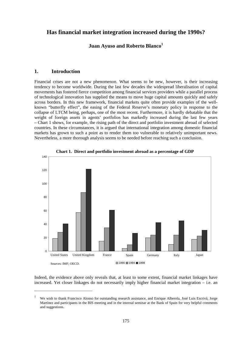
175
Has financial market integration increased during the 1990s?
Juan Ayuso and Roberto Blanco1
1. Introduction
Financial crises are not a new phenomenon. What seems to be new, however, is their increasingtendency to become worldwide. During the last few decades the widespread liberalisation of capitalmovements has fostered fierce competition among financial services providers while a parallel processof technological innovation has supplied the means to move huge capital amounts quickly and safelyacross borders. In this new framework, financial markets quite often provide examples of the well-known “butterfly effect”, the easing of the Federal Reserve’s monetary policy in response to thecollapse of LTCM being, perhaps, one of the most recent. Furthermore, it is hardly debatable that theweight of foreign assets in agents’ portfolios has markedly increased during the last few years– Chart 1 shows, for example, the rising path of the direct and portfolio investment abroad of selectedcountries. In these circumstances, it is argued that international integration among domestic financialmarkets has grown to such a point as to render them too vulnerable to relatively unimportant news.Nevertheless, a more thorough analysis seems to be needed before reaching such a conclusion.
Indeed, the evidence above only reveals that, at least to some extent, financial market linkages haveincreased. Yet closer linkages do not necessarily imply higher financial market integration – i.e. an
1 We wish to thank Francisco Alonso for outstanding research assistance, and Enrique Alberola, José Luis Escrivá, Jorge
Martínez and participants in the BIS meeting and in the internal seminar at the Bank of Spain for very helpful commentsand suggestions.
0
20
40
60
80
100
120
140
United States United Kingdom France Spain Germany Italy Japan
1990 1994 1998
Chart 1. Direct and portfolio investment abroad as a percentage of GDP
Sources: IMF; OECD.

176
additional removal of barriers of any kind to cross-border financial transactions. Thus, it could beargued that not only financial markets but also economies, as a whole, have reached a higher level ofinternationalisation. Cross-border commercial linkages have increased as well. Moreover, it should beborne in mind that the same technological innovations that have paved the way for cross-borderfinancial transactions have also increased the worldwide diffusion of information in real time.Accordingly, it could be the case that the main driving force behind the apparent increase in financialmarket linkages is the globalisation of the news that affects financial prices instead of a higher degreeof market integration.
In our view, it is important to determine whether there has been a genuine increase in financial marketintegration. It is worth noting that the assessment of a hypothetical increase in financial marketlinkages will depend on the causes of the increase. In terms of welfare, for example, it should be clearthat whereas a removal of barriers implies an increase in diversification opportunities – thus reducingthe levels of risk that agents have to accept to obtain a given return – a greater globalisation of therelevant information set would mean exactly the opposite. Similarly, the implications of each scenarioregarding the need for a global supervisor would be different if information, instead of markets, ismore global.
The main goal of this paper is to investigate whether there has been a genuine increase in the degree offinancial market integration during the 1990s. To do this, we focus on stock markets and compute,first, a number of standard measures of financial market integration that, in our view, only measurefinancial market linkages. This allows us to make a more formal assessment of the actual increase infinancial market linkages and, at the same time, the shortcomings of these measures as indicators offinancial market integration become clearer. Second, we analyse whether there has been any notableadvance in the degree of “pure” financial market integration by computing two alternative measures ofmarket integration based on a refinement of the approach suggested in Chen and Knez (1995).
The paper is organised as follows. After this introduction, Section 2 computes standard measures ofmarket linkages that reveal a higher degree of linkage but are unable to show whether this is due tohigher market integration or to other factors. Section 3 addresses this question and computes directmeasures of the changes in market integration during the 1990s that show an increasing degree ofmarket integration over this decade. Finally, Section 4 summarises the main results and points outsome of their potential policy implications.
2. Standard measures of linkages between international stock prices
Perhaps the simplest approach in the literature to analyse the degree of market integration is that basedon the computation of the correlation between returns on those markets that are thought to be moreintegrated than previously.2 This approach is based on rather simple intuition: the more integratedmarkets are, the higher the comovement between their prices. In this connection, Table 1 shows thecorrelation between weekly returns on seven selected stock exchanges (New York, London, Paris,Madrid, Frankfurt, Milan and Tokyo)3 during the 1990–94 and 1995–99 periods. In 15 out of the 21possible combinations, the correlation has increased in the second half of the 1990s, with the Japanesestock exchange accounting for the remaining six cases. On average, the correlation between the returnson these stock exchanges increased from 0.42 during the period 1990–94 to 0.54 during 1995–99.
Although this evidence can be considered as supporting the view of a higher degree of financialmarket linkages, it is well known that higher correlation is neither a necessary nor a sufficient
2
See, for example, Taylor and Tonks (1989) or Le (1991).
3 Returns have been obtained as the first difference of the logarithm of a representative index for each stock exchange:these are, respectively, S&P 500, FTSE All-Share, CAC 40, IGBM, DAX 30, MIB all shares and Nikkei 225. See theAnnex for details about the data used.
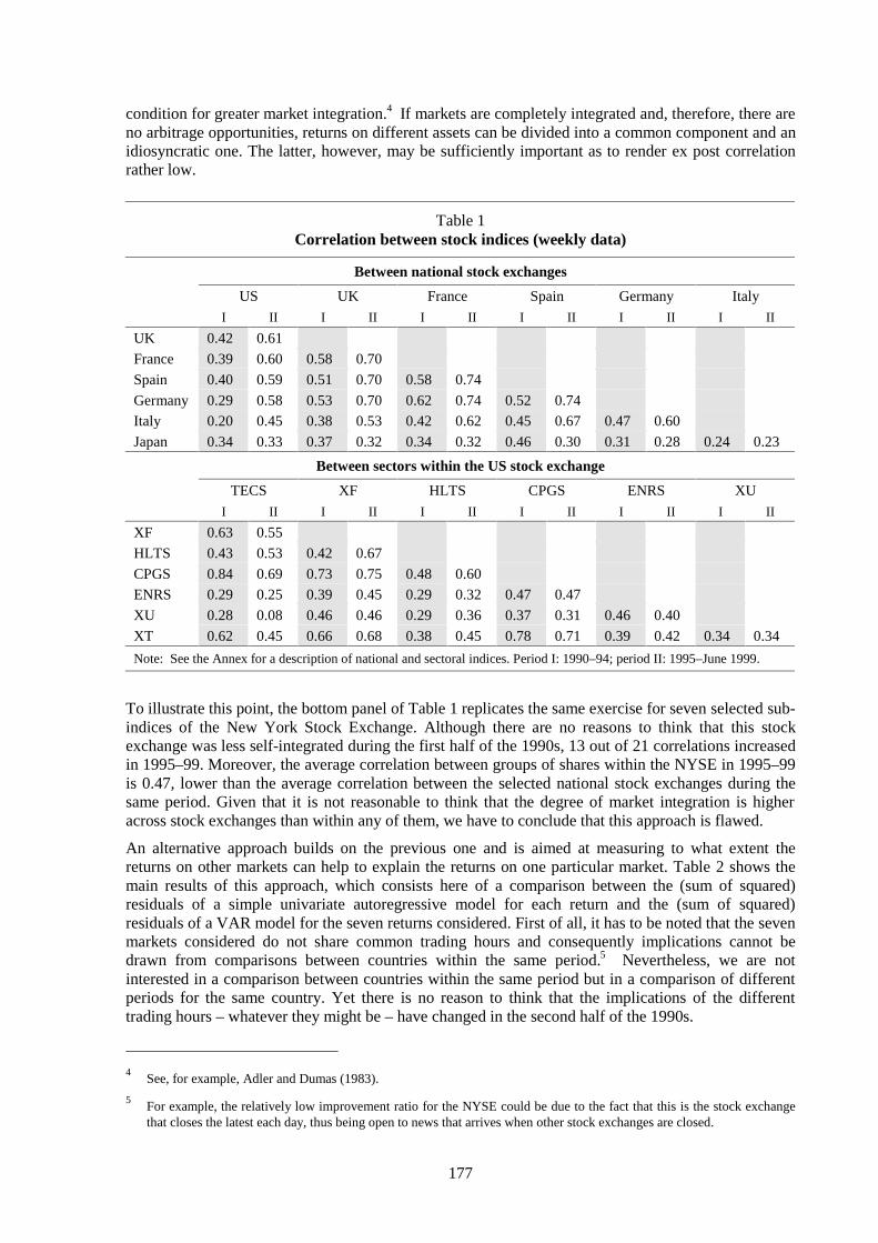
177
condition for greater market integration.4 If markets are completely integrated and, therefore, there areno arbitrage opportunities, returns on different assets can be divided into a common component and anidiosyncratic one. The latter, however, may be sufficiently important as to render ex post correlationrather low.
Table 1Correlation between stock indices (weekly data)
Between national stock exchanges
US UK France Spain Germany Italy
I II I II I II I II I II I II
UK 0.42 0.61
France 0.39 0.60 0.58 0.70
Spain 0.40 0.59 0.51 0.70 0.58 0.74
Germany 0.29 0.58 0.53 0.70 0.62 0.74 0.52 0.74
Italy 0.20 0.45 0.38 0.53 0.42 0.62 0.45 0.67 0.47 0.60
Japan 0.34 0.33 0.37 0.32 0.34 0.32 0.46 0.30 0.31 0.28 0.24 0.23
Between sectors within the US stock exchange
TECS XF HLTS CPGS ENRS XU
I II I II I II I II I II I II
XF 0.63 0.55
HLTS 0.43 0.53 0.42 0.67
CPGS 0.84 0.69 0.73 0.75 0.48 0.60
ENRS 0.29 0.25 0.39 0.45 0.29 0.32 0.47 0.47
XU 0.28 0.08 0.46 0.46 0.29 0.36 0.37 0.31 0.46 0.40
XT 0.62 0.45 0.66 0.68 0.38 0.45 0.78 0.71 0.39 0.42 0.34 0.34
Note: See the Annex for a description of national and sectoral indices. Period I: 1990–94; period II: 1995–June 1999.
To illustrate this point, the bottom panel of Table 1 replicates the same exercise for seven selected sub-indices of the New York Stock Exchange. Although there are no reasons to think that this stockexchange was less self-integrated during the first half of the 1990s, 13 out of 21 correlations increasedin 1995–99. Moreover, the average correlation between groups of shares within the NYSE in 1995–99is 0.47, lower than the average correlation between the selected national stock exchanges during thesame period. Given that it is not reasonable to think that the degree of market integration is higheracross stock exchanges than within any of them, we have to conclude that this approach is flawed.
An alternative approach builds on the previous one and is aimed at measuring to what extent thereturns on other markets can help to explain the returns on one particular market. Table 2 shows themain results of this approach, which consists here of a comparison between the (sum of squared)residuals of a simple univariate autoregressive model for each return and the (sum of squared)residuals of a VAR model for the seven returns considered. First of all, it has to be noted that the sevenmarkets considered do not share common trading hours and consequently implications cannot bedrawn from comparisons between countries within the same period.5 Nevertheless, we are notinterested in a comparison between countries within the same period but in a comparison of differentperiods for the same country. Yet there is no reason to think that the implications of the differenttrading hours – whatever they might be – have changed in the second half of the 1990s.
4
See, for example, Adler and Dumas (1983).
5For example, the relatively low improvement ratio for the NYSE could be due to the fact that this is the stock exchangethat closes the latest each day, thus being open to news that arrives when other stock exchanges are closed.

178
Table 2The explanatory power of other market returns on the own market return (daily data)
Period National stock indices
Japan UK Germany France Italy Spain US
I SSR univ (1) 3,020.51 855.27 1,680.48 1,747.90 1,868.50 1,455.96 732.30
SSR VAR (2) 2,840.19 779.88 1,480.46 1,625.46 1,730.57 1,366.60 719.86
((1)–(2)) / (1) 5.97% 8.81% 11.90% 6.96% 7.38% 6.14% 1.70%
No. of observ. 1,299
q 12
II SSR univ (1) 2,404.09 736.37 2,001.04 1,798.24 2,071.64 1,631.90 1,093.83
SSR VAR (2) 2,174.19 624.65 1,494.08 1,611.14 1,519.17 1,480.80 1,073.12
((1)–(2)) / (1) 9.56% 15.17% 25.33% 10.40% 26.67% 9.26% 1.89%
No. of observ. 1,150
q 6
Sectoral indices
TECS XF HLTS CPGS ENRS XU XT
I SSR univ (1) 1,330.51 1,404.80 1,614.32 929.67 982.95 902.14 1,431.88
SSR VAR (2) 1,315.97 1,387.38 1,597.42 916.96 973.79 894.95 1,397.45
((1)–(2)) / (1) 1.09% 1.24% 1.05% 1.37% 0.93% 0.80% 2.40%
No. of observ. 1,299
q 6
II SSR univ (1) 3,133.84 2,066.84 1,804.60 1,306.17 1,705.21 688.91 1,556.00
SSR VAR (2) 3,102.66 2,056.92 1,780.77 1,284.77 1,681.02 655.91 1,530.38
((1)–(2)) / (1) 0.99% 0.48% 1.32% 1.64% 1.42% 4.79% 1.65%
No. of observ. 1,150
q 6
Note: See the Annex for a description of national and sectoral indices. Period I: 1990–94; period II: 1995–June 1999. q isthe number of new regressors in the VAR when compared with the univariate model.
According to Table 2, during the first half of the 1990s the sum of the squared residuals is reduced, onaverage, by 6.98% when other market returns are taken into account to explain the behaviour of stockreturns. During the second half of the decade, the reduction amounts to 14.04%, thus revealing ahigher average degree of linkage between the markets considered. This increased linkage is, moreover,uniform across the seven countries and could even be underestimated in Table 2 given that the VARapproach adds only six parameters to each univariate model in the 1995–99 period whereas12 parameters are added in the 1990–94 period.6
In order to evaluate the magnitude of the recorded increases in linkages, the bottom panel of Table 2replicates the exercise for the same seven sub-indices of the NYSE as in Table 1, thus offering a usefulyardstick. During the second half of the decade there is also an increase in the explanatory power ofthe other market returns. Nevertheless, this increase has three interesting features. First, it is clearlylower (1.27% compared to 1.76%) than that in the upper panel. Second, it is not uniform across sectors(only four out of seven show an improvement). And third, the levels of the reduction in the sum ofsquared residuals in each period are somewhat lower than those corresponding to the seven countrycase (1.27% and 1.76% versus 6.98% and 14.04%). Accordingly, it could be concluded that theincrease in the linkages between the returns on the stock exchanges chosen is quite genuine. 6
In 1990–94 the VAR model includes two lags, whereas in 1995–99 a single lag is sufficient to eliminate any residualautocorrelation. Accordingly, when compared to the univariate model, the VAR adds 12 more parameters (2 lags x 6countries) during the first period and only six (1 lag x 6 countries) during the second.
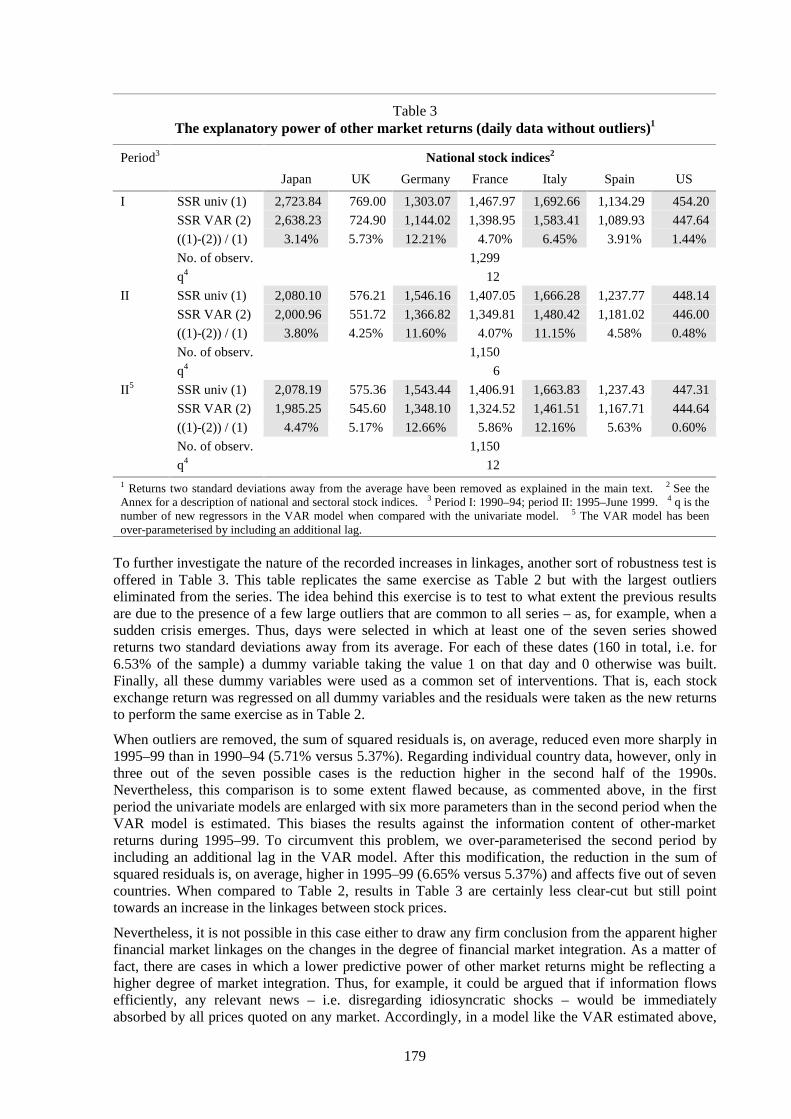
179
Table 3The explanatory power of other market returns (daily data without outliers)1
Period3 National stock indices2
Japan UK Germany France Italy Spain US
I SSR univ (1) 2,723.84 769.00 1,303.07 1,467.97 1,692.66 1,134.29 454.20
SSR VAR (2) 2,638.23 724.90 1,144.02 1,398.95 1,583.41 1,089.93 447.64
((1)-(2)) / (1) 3.14% 5.73% 12.21% 4.70% 6.45% 3.91% 1.44%
No. of observ. 1,299
q4 12
II SSR univ (1) 2,080.10 576.21 1,546.16 1,407.05 1,666.28 1,237.77 448.14
SSR VAR (2) 2,000.96 551.72 1,366.82 1,349.81 1,480.42 1,181.02 446.00
((1)-(2)) / (1) 3.80% 4.25% 11.60% 4.07% 11.15% 4.58% 0.48%
No. of observ. 1,150
q4 6
II5 SSR univ (1) 2,078.19 575.36 1,543.44 1,406.91 1,663.83 1,237.43 447.31
SSR VAR (2) 1,985.25 545.60 1,348.10 1,324.52 1,461.51 1,167.71 444.64
((1)-(2)) / (1) 4.47% 5.17% 12.66% 5.86% 12.16% 5.63% 0.60%
No. of observ. 1,150
q4 121 Returns two standard deviations away from the average have been removed as explained in the main text. 2 See theAnnex for a description of national and sectoral stock indices. 3 Period I: 1990–94; period II: 1995–June 1999. 4 q is thenumber of new regressors in the VAR model when compared with the univariate model. 5 The VAR model has beenover-parameterised by including an additional lag.
To further investigate the nature of the recorded increases in linkages, another sort of robustness test isoffered in Table 3. This table replicates the same exercise as Table 2 but with the largest outlierseliminated from the series. The idea behind this exercise is to test to what extent the previous resultsare due to the presence of a few large outliers that are common to all series – as, for example, when asudden crisis emerges. Thus, days were selected in which at least one of the seven series showedreturns two standard deviations away from its average. For each of these dates (160 in total, i.e. for6.53% of the sample) a dummy variable taking the value 1 on that day and 0 otherwise was built.Finally, all these dummy variables were used as a common set of interventions. That is, each stockexchange return was regressed on all dummy variables and the residuals were taken as the new returnsto perform the same exercise as in Table 2.
When outliers are removed, the sum of squared residuals is, on average, reduced even more sharply in1995–99 than in 1990–94 (5.71% versus 5.37%). Regarding individual country data, however, only inthree out of the seven possible cases is the reduction higher in the second half of the 1990s.Nevertheless, this comparison is to some extent flawed because, as commented above, in the firstperiod the univariate models are enlarged with six more parameters than in the second period when theVAR model is estimated. This biases the results against the information content of other-marketreturns during 1995–99. To circumvent this problem, we over-parameterised the second period byincluding an additional lag in the VAR model. After this modification, the reduction in the sum ofsquared residuals is, on average, higher in 1995–99 (6.65% versus 5.37%) and affects five out of sevencountries. When compared to Table 2, results in Table 3 are certainly less clear-cut but still pointtowards an increase in the linkages between stock prices.
Nevertheless, it is not possible in this case either to draw any firm conclusion from the apparent higherfinancial market linkages on the changes in the degree of financial market integration. As a matter offact, there are cases in which a lower predictive power of other market returns might be reflecting ahigher degree of market integration. Thus, for example, it could be argued that if information flowsefficiently, any relevant news – i.e. disregarding idiosyncratic shocks – would be immediatelyabsorbed by all prices quoted on any market. Accordingly, in a model like the VAR estimated above,

180
other market (lagged) returns should not contain any relevant information provided that the ownmarket (lagged) returns are taken into account. From this standpoint, the results in Tables 2 and 3might even be seen as pointing towards less efficiency in the transmission of information – i.e. greaterbarriers to financial trade and therefore less integration.
Tables 1 to 3 address the issue of market linkages by focusing on stock return levels. Nevertheless,there are also other statistical moments that could be analysed to elicit further relevant information onthe relationships between financial markets. In particular, it is also of interest to analyse whether thereis greater linkage between stock price volatilities. In Engle et al. (1988), volatility linkages areexplored to draw conclusions on market efficiency from the way information arrives in financialmarkets and is transmitted between them.
As is well known, the question of how volatility should be measured has received an almostunanimous answer in the literature: by estimating the conditional variance of the series considered.There are, however, several models available to make such an estimate.7 In this paper, we estimate themodel proposed in Glosten, Jagannathan and Runkle (GJR) (1989). This model consists of a small buthighly significant variation to the GARCH model proposed by Bollerslev (1986) which allows it tocapture an important feature of stock returns: the leverage or asymmetric effect first noted by Black(1976). The importance of this innovation is highlighted in Engle and Ng (1993), who perform aninteresting horse race between several conditional variance models to explain the behaviour of theconditional variance of Japanese stock returns and conclude that “the best model is the one proposedby Glosten, Jagannathan and Runkle”.
In this paper, we first estimate a GJR model for each of the residual series of the VAR model. Thesemodels are next enlarged to include the lagged (squared) residuals corresponding to the remainingmarkets as new explanatory variables. In particular, as we are interested in testing whether the role ofthe other market residuals has increased, we include as new regressors each other market (squared)residual and the product of each other market (squared) residual times a step dummy variable whichtakes the value 1 during the period 1995–99 and 0 otherwise. Consequently, a positive and significantvalue of the coefficient of the latter would imply an increasing role of the corresponding other marketvolatility to explain the volatility of the own market.
Formally,
(1) ∑ ∑∑∑∑∑≠ =
−−=
−=
−=
−−−
=−
+++++=
ij
q
kktktjkj
q
kktjkj
q
kktik
q
kktiktik
q
kktikti SSeddedhbSegeaah
1
1
2,,
1
1
2,,
2
1,
1
1,
2,
1
1
2,0,
where
)( ,1, tititi rEre −−= ; ( )titti hNe ,1, ,0~| −Ω and )( ,1 tit rE − – i.e. the conditional expectation on tir , – is
computed from the VAR model,
i, j = Japan (JP), the United Kingdom (GB), Germany (DE), France (FR), Italy (IT), Spain (ES) andthe United States (US),
1, =−tiS if 01, ≤=tie and 0 otherwise,
1=tSS from 1995 to 1999 and 0 otherwise.
It is worth noting that the VAR model includes the levels of the other market returns as explanatoryvariables for each own market return. Accordingly, the possibility can be ruled out that squaredresiduals from other markets appear as significant in the conditional variance equation only as aconsequence of (level) residuals being an omitted variable in the conditional mean equation.
Table 4 shows the main results of the exercise. First of all, it has to be noted that the GJR models fitreasonably well, as shown by the standard goodness-of-fit tests reported in the table (CH1, CH5, T1,T2 and T3). The leverage effect – that is, the coefficient g1 – is also important in all but one country.
7 See, for example, Engle and Ng (1993) for an extensive comparison among alternative methods.
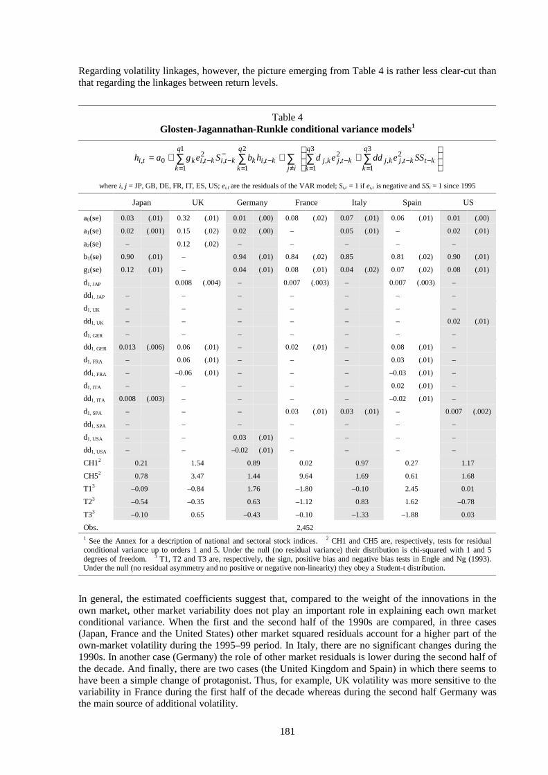
181
Regarding volatility linkages, however, the picture emerging from Table 4 is rather less clear-cut thanthat regarding the linkages between return levels.
Table 4Glosten-Jagannathan-Runkle conditional variance models1
+++= −−
=−
=≠−
==
−−− ∑∑∑∑∑ ktktj
q
kkjktj
q
kkj
ijkti
q
kk
q
kktiktikti SSeddedhbSegah 2
,
3
1,
2,
3
1,,
2
1
1
1,
2,0,
where i, j = JP, GB, DE, FR, IT, ES, US; ei,t are the residuals of the VAR model; Si,t = 1 if ei,t is negative and SSt = 1 since 1995
Japan UK Germany France Italy Spain US
a0(se) 0.03 (.01) 0.32 (.01) 0.01 (.00) 0.08 (.02) 0.07 (.01) 0.06 (.01) 0.01 (.00)
a1(se) 0.02 (.001) 0.15 (.02) 0.02 (.00) – 0.05 (.01) – 0.02 (.01)
a2(se) – 0.12 (.02) – – – – –
b1(se) 0.90 (.01) – 0.94 (.01) 0.84 (.02) 0.85 0.81 (.02) 0.90 (.01)
g1(se) 0.12 (.01) – 0.04 (.01) 0.08 (.01) 0.04 (.02) 0.07 (.02) 0.08 (.01)
d1, JAP 0.008 (.004) – 0.007 (.003) – 0.007 (.003) –
dd1, JAP – – – – – – –
d1, UK – – – – – – –
dd1, UK – – – – – – 0.02 (.01)
d1, GER – – – – – – –
dd1, GER 0.013 (.006) 0.06 (.01) – 0.02 (.01) – 0.08 (.01) –
d1, FRA – 0.06 (.01) – – – 0.03 (.01) –
dd1, FRA – –0.06 (.01) – – – –0.03 (.01) –
d1, ITA – – – – – 0.02 (.01) –
dd1, ITA 0.008 (.003) – – – – –0.02 (.01) –
d1, SPA – – – 0.03 (.01) 0.03 (.01) – 0.007 (.002)
dd1, SPA – – – – – – –
d1, USA – – 0.03 (.01) – – – –
dd1, USA – – –0.02 (.01) – – – –
CH12 0.21 1.54 0.89 0.02 0.97 0.27 1.17
CH52 0.78 3.47 1.44 9.64 1.69 0.61 1.68
T13 –0.09 –0.84 1.76 –1.80 –0.10 2.45 0.01
T23 –0.54 –0.35 0.63 –1.12 0.83 1.62 –0.78
T33 –0.10 0.65 –0.43 –0.10 –1.33 –1.88 0.03
Obs. 2,4521 See the Annex for a description of national and sectoral stock indices. 2 CH1 and CH5 are, respectively, tests for residualconditional variance up to orders 1 and 5. Under the null (no residual variance) their distribution is chi-squared with 1 and 5degrees of freedom. 3 T1, T2 and T3 are, respectively, the sign, positive bias and negative bias tests in Engle and Ng (1993).Under the null (no residual asymmetry and no positive or negative non-linearity) they obey a Student-t distribution.
In general, the estimated coefficients suggest that, compared to the weight of the innovations in theown market, other market variability does not play an important role in explaining each own marketconditional variance. When the first and the second half of the 1990s are compared, in three cases(Japan, France and the United States) other market squared residuals account for a higher part of theown-market volatility during the 1995–99 period. In Italy, there are no significant changes during the1990s. In another case (Germany) the role of other market residuals is lower during the second half ofthe decade. And finally, there are two cases (the United Kingdom and Spain) in which there seems tohave been a simple change of protagonist. Thus, for example, UK volatility was more sensitive to thevariability in France during the first half of the decade whereas during the second half Germany wasthe main source of additional volatility.

182
Thus, once the effects of other market return levels are used to explain the level of returns in eachmarket, the evidence in Table 4 does not offer clear support to the view of an increasing volatilitylinkage during the 1990s. Nevertheless, it has to be borne in mind that, as commented above, a moreprominent role of innovations in a market to explain the volatility of other market returns might beinterpreted as a sign of informational inefficiency. Accordingly, the evidence in Table 4 could also beseen, at least to some extent, as a sign of a high degree of market integration.
All in all, the results in this section seem to give mild support to the existence of an increase in stockmarket linkages, which is clearer in the case of levels than in that of volatility. Nevertheless, it remainsto be seen whether these greater linkages are the consequence of a genuine higher degree of marketintegration or merely reflect the greater globalisation of the main sources of the news which drivesstock prices. Addressing this question is the main goal of the rest of this paper.
3. Measuring financial market integration
3.1 Conceptual framework
Perfect cross-market integration is generally understood as a situation in which there is no barrier ofany kind to cross-border financial transactions, such as tariffs, taxes, restrictions on the trading offoreign assets, information costs or any other cost that makes it more difficult to trade across countriesthan within them. With perfect cross-market integration there are no cross-market arbitrageopportunities and the law of one price – i.e. portfolios with the same payoffs should have the sameprice in different markets – holds. It is worth noting, however, that, as suggested above, the law of oneprice or the absence of arbitrage opportunities cannot be assessed from the analysis of the comovementof the levels of financial asset prices or of their volatilities.
Although this point can be made without reference to any specific asset pricing model, it is easier toillustrate it if a particular model is considered. Thus, for the sake of simplicity, let us assume thatassets are priced according to the well-known APT model. Under this model each (ex post) asset priceis equal to the sum of the products of a number of random factors (the sources of risk) multiplied bytheir coefficients (generally called risk prices) plus the realisation of an idiosyncratic shock. If marketsare perfectly integrated these random factors have to be equally priced in each market. Accordingly, anincrease in the degree of integration between markets that were previously segmented should increasethe comovements of their prices due to the reduction in the differences between the prices of thecommon risk factors. Nevertheless, increases in the comovements may also be the result of a greaterintersection of the sets of risk factors affecting prices in both markets – possibly as a result of a greaterglobalisation of news – while differences in the risk prices remain. Similarly, a reduction of the weightof the idiosyncratic shocks would also result in a higher (ex post) comovement independently of thedegree of market integration.
Against this background, Chen and Knez (1995) developed a measurement theory of marketintegration that relies directly on the concept of the law of one price and the condition of absence ofarbitrage opportunities and does not depend on any particular asset pricing model.8 Following theseminal work of Hansen and Jagannathan (1991, 1997), the measures they proposed exploit certainproperties of the stochastic discount factors. The latter are random variables d, which are implicitlydefined in the following unconditional moment restriction:
(2) ( ) NidxEpE ii ∈∀=)(
8
In the literature other approaches that test for integration based on the notion of absence of arbitrage have been developed(for instance, Adler and Dumas (1983) use an international CAPM). However, as pointed out by Chen and Knez (1995),the main shortcoming of these approaches is that any test of market integration is, at the same time, a test of the particularasset pricing model used.

183
where E(.) is the expectation operator, pi is the price of asset i, xi is the future payoff of that asset,9 andN is the number of assets traded in the market studied. Expression (2) is derived by applying the law ofiterated expectations to the equilibrium condition of a generic asset pricing model: prices of a futurepayoff on any traded security have to be equal to the expected product of the payoff and theintertemporal marginal rate of substitution.10 All random variables d satisfying equation (2) make upthe family of admissible stochastic discount factors. It is found that under certain conditions thepricing structure of a market can be completely summarised by these discount factors.
Chen and Knez (1995) showed that the law of one price holds across two markets if and only if theintersection between their sets of admissible stochastic discount factors is not empty.11 Based on thisresult, they proposed to measure the degree of market integration as the (square of the) minimumsquare distance between the sets of the admissible stochastic discount factors in the two markets.12
Note that this measure is zero if and only if the two markets are perfectly integrated. A strictly positivevalue for this measure indicates the degree of segmentation: the lower the measure, the more closelyintegrated the two markets. Applying a result taken from Hansen and Jagannathan (1997),13 thismeasure can be interpreted as the maximum (squared) difference between the prices assigned by twomarkets to any unit-norm common payoff.14 Thus, this measure reflects the magnitude of pricingdiscrepancy between the two markets and, to some extent, indicates the minimum costs necessary toprevent investors from taking advantage of the pricing discrepancy.
In order to implement the measure empirically, Chen and Knez (1995) proposed to use data on pricesand payoffs for a sample of securities in two markets and to approximate population moments withsample moments. Formally, the set of admissible discount factors d in market j – Dj – is made up ofany vectors of dimension T – the number of time series observations – that satisfy the following Nj
restrictions.15
(3) jj dXOP =
where O is a vector of ones with dimension T, Pj is the matrix of the prices of the Nj securities tradedin market j and Xj is the matrix of the payoffs of the same securities.
It is worth noting that the value of the estimated integration measure depends on the combination ofthe values chosen for T and NA + NB. In particular, it is straightforward to show that if T is higher thanNA + NB and the rank of XA+B is NA + NB
16 – i.e. two portfolios with equal payoffs, one from eachmarket, cannot be constructed – the intersection between DA and DB will be non-empty because thesystem resulting from jointly considering (3) in both markets does have a solution. In this case theestimated integration measure will always be equal to zero. Note that in this situation cross-marketarbitrage is not possible because we cannot form two portfolios with the same payoffs in both markets,
9
This model assumes the existence of only two periods. In the first one, assets are traded; in the second, investors obtainthe payoffs.
10This is the so-called Euler equation, which is common to all existing asset pricing models. Particular models differ in thespecification of consumers’ preferences and, therefore, of the marginal rate of substitution.
11They also proved that cross-market arbitrage opportunities do not exist if and only if the intersection between the sets ofnon-negative admissible stochastic discount factors is not empty.
12They called this the weak integration measure. They also proposed another measure – the strong integration measure –which computes the same distance when only the non-negative elements of those sets are taken into account.
13Hansen and Jagannathan (1997) showed that the least square distance between a random variable and the set ofadmissible stochastic discount factors of one particular market gives the maximum pricing error in using that randomvariable to price any unit-norm payoffs traded on that market.
14The strong integration measure can be interpreted as the mini-max bound on the (squared) pricing differences when usingthe non-negative stochastic discount factors of the two markets to price any conceivable unit-norm payoff.
15These restrictions are the sample counterparts of the population restrictions of expression (2).
16In our data set this tends to occur in (almost) all cases.

184
not because both portfolios are equally priced. Thus, under these circumstances, the integrationmeasure will be uninformative.17
Two lessons can be drawn from the previous comments. First, when implementing the integrationmeasure, attention has to be paid to the selection of T, NA and NB. Second, the absolute value of theintegration measure is difficult to interpret. In other words, it would be preferable to use it incomparing pairs of markets or periods.
In this paper, we apply the methodology described above to assess how market integration haschanged during the 1990s. More specifically, we compute two different integration measures – bothbased on this theory – for pairs of markets in the period 1990–94 and compare them with thoseobtained for the period 1995–99. To undertake this exercise we use daily data on prices and payoffs18
denominated in US dollars for a sample of securities traded in three out of the seven stock exchangesconsidered in Section 2 – New York, Frankfurt and Madrid.
Unfortunately, in our data set the aggregate number of securities in any pair of markets is much lowerthan the number of time series observations in each of the periods studied. In order to avoid theuninformative solution mentioned above, we followed two alternative approaches. Under the first one,we compute the (square root of the) integration measure proposed by Chen and Knez (1995) usingonly monthly data, which leaves us with only 53 observations in each period.19 This figure is lowerthan the total available number of assets on the US stock exchange, which overcomes the trivialsolution. The problem with this approach is, first, that we lose some of the available information. Also,it should be recognised that this is a “tricky” approach since we force data to guarantee the existenceof two portfolios – one from each market – with common payoffs. In fact, both portfolios might havedifferent payoffs if we considered more periods.
The second approach relies on weekly data, which gives us 230 observations in each period. In thiscase, the problem of getting an uninformative zero value is overcome by computing mean distancesbetween the sets of admissible discount factors instead of minimum distances. Of course, the meandistance between two sets could be strictly positive even if they do intersect.20 Note that this measurehas a different pricing error interpretation as it computes the mean – instead of the minimum – of themaximum absolute pricing errors when using the pricing rules implied by one market to price anyunit-norm payoffs marketed on the other market.21 Thus, this measure could be interpreted as theexpected maximum pricing discrepancy between two markets.
Alternatively, the latter measure can be interpreted in terms of the expected minimum distancebetween the sets of discount factors in markets A and B (DA and DB) when expanding these markets toinclude all assets traded. To see this, note first that the higher the number of assets, the more reducedthe size of the sets DA and DB. Nevertheless, given that information is always limited these sets willtend to be too large and we will find a non-empty intersection – and, therefore, a zero minimumdistance. Yet in this case we can still distinguish between cases like those in Chart 2. In general, as theinformation set expands and sets DA and DB reduce, the minimum distance will tend to increase. If itbecomes finally non-negative, it can be expected to be higher in the left-hand situation. That is, thehigher the mean distance between DA and DB, the higher the expected minimum distance, provided the
17
Chen and Knez (1995) estimated the degree of integration between the NASDAQ and the NYSE computing theirintegration measures, but they did not take into account this observation. The estimated figures they obtained are verylow but non-zero probably as a result of the algorithm they applied, which cannot produce a zero value as it stops whenconvergence is supposed to be reached.
18The payoffs are computed taking into account splits, dividends and capital increases in addition to capital gains – i.e.price changes. See the Annex for more details about the data used.
19The number of observations in the first period (1990–94) is higher than 53, but we have reduced the size to 53 in order tomake the comparison between the periods fairer, given that, as we have shown, the sample size could affect the results.
20To be more precise, as will be clear later, we introduce some restrictions that affect the value of the discount factors inorder to simplify computation and to guarantee the existence of the mean.
21This interpretation follows after applying the result of Hansen and Jagannathan (1997). See footnote 13.

185
information set is large enough. Or put in a different way, the lower the mean distance, the higher theprobability of having a non-empty intersection when the information set is large enough.
Chart 2. Mean distance between sets of admissible discount factors as a measure of integration
DA DB DA DB
Low degree of integration High degree of integration
The procedure we followed to implement the two integration measures introduced in the previousparagraphs has two important features. First, for each of the three markets studied we form a numberof sub-markets by taking different samples of assets, each one having its associated set of admissiblediscount factors. This allows us to have – in each period – a set of integration measures, instead ofpoint estimates, which varies according to the particular stocks included in each sub-market. Second,we not only estimate the integration measures between different markets, but we also estimate themwithin the same market22 – the benchmark market. This allows us to have values of the integrationmeasure for a market which is thought to be self-integrated. By construction these figures willgenerally be strictly positive in spite of the fact that the market is perfectly self-integrated. So, we canhave a set of values for the measures which could be used as reference values for perfectly integratedmarkets. Thus, the relative measures of integration – defined as the difference between the absoluteintegration measure between two different markets and that within the benchmark market – will beeasier to interpret as integration measures – i.e. a significant positive value for this relative measurewill suggest that markets are not perfectly integrated.
More specifically, the procedure we followed involves – in both approaches and in each period – thefollowing five steps:
i) One market is taken as a benchmark.
ii) A random group of NA securities is selected from among the assets available in the benchmarkmarket. In what follows, this group of assets will be referred to as sub-market A and DA willstand for the set of discount factors that price assets in that sub-market.
iii) 100 random combinations of groups of NB securities are selected in each of the three marketsstudied. In what follows, any of these groups of assets will be referred to as sub-market B, andDB will stand for the set of discount factors that price assets in those sub-markets. So, we have300 sub-markets B – 100 sub-markets for each of the three markets. For the benchmark market,stocks in sub-markets B are restricted to being different to those selected in step ii).
iv) Distances23 between the fixed set DA and the sets DB are computed. So, we get 100 distances foreach of the three pairs of markets. These 100 distances are then averaged for each pair ofmarkets. Thus, we finally have 3 average distances.
v) Steps ii) to iv) are repeated 100 times.
22
In other words, in this case sub-markets A and B are made up of stocks belonging to the same market.
23Under the first approach the minimum distances are computed, and under the second approach mean distances arecomputed.
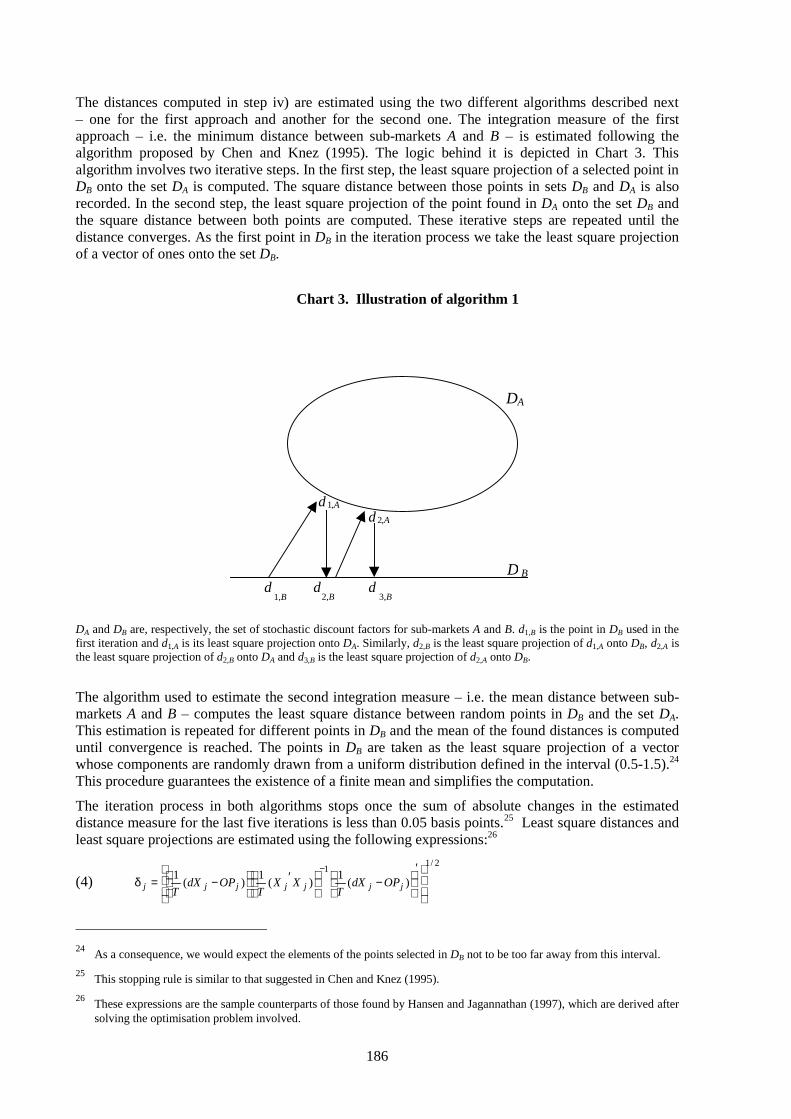
186
The distances computed in step iv) are estimated using the two different algorithms described next– one for the first approach and another for the second one. The integration measure of the firstapproach – i.e. the minimum distance between sub-markets A and B – is estimated following thealgorithm proposed by Chen and Knez (1995). The logic behind it is depicted in Chart 3. Thisalgorithm involves two iterative steps. In the first step, the least square projection of a selected point inDB onto the set DA is computed. The square distance between those points in sets DB and DA is alsorecorded. In the second step, the least square projection of the point found in DA onto the set DB andthe square distance between both points are computed. These iterative steps are repeated until thedistance converges. As the first point in DB in the iteration process we take the least square projectionof a vector of ones onto the set DB.
DA and DB are, respectively, the set of stochastic discount factors for sub-markets A and B. d1,B is the point in DB used in thefirst iteration and d1,A is its least square projection onto DA. Similarly, d2,B is the least square projection of d1,A onto DB, d2,A isthe least square projection of d2,B onto DA and d3,B is the least square projection of d2,A onto DB.
The algorithm used to estimate the second integration measure – i.e. the mean distance between sub-markets A and B – computes the least square distance between random points in DB and the set DA.This estimation is repeated for different points in DB and the mean of the found distances is computeduntil convergence is reached. The points in DB are taken as the least square projection of a vectorwhose components are randomly drawn from a uniform distribution defined in the interval (0.5-1.5).24
This procedure guarantees the existence of a finite mean and simplifies the computation.
The iteration process in both algorithms stops once the sum of absolute changes in the estimateddistance measure for the last five iterations is less than 0.05 basis points.25 Least square distances andleast square projections are estimated using the following expressions:26
(4)2/1
1
)(1
)(1
)(1
′
−
′
−=δ
−
jjjjjjj OPdXT
XXT
OPdXT
24
As a consequence, we would expect the elements of the points selected in DB not to be too far away from this interval.
25This stopping rule is similar to that suggested in Chen and Knez (1995).
26These expressions are the sample counterparts of those found by Hansen and Jagannathan (1997), which are derived aftersolving the optimisation problem involved.
Chart 3. Illustration of algorithm 1
D A
d 1 ,A d 2 ,A
D B
d 1,B
d 2,B
d 3,B
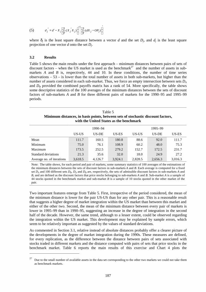
187
(5)′
−
′−′=′
−)(
1)(
11
jjjjjj OPdXT
XXT
Xdd
where δj is the least square distance between a vector d and the set Dj, and dj is the least squareprojection of one vector d onto the set Dj.
3.2 Results
Table 5 shows the main results under the first approach – minimum distances between pairs of sets ofdiscount factors – when the US market is used as the benchmark27 and the number of assets in sub-markets A and B is, respectively, 44 and 10. In these conditions, the number of time seriesobservations – 53 – is lower than the total number of assets in both sub-markets, but higher than thenumber of assets considered in each sub-market. Thus, we force an empty intersection between sets DA
and DB provided the combined payoffs matrix has a rank of 54. More specifically, the table showssome descriptive statistics of the 100 averages of the minimum distances between the sets of discountfactors of sub-markets A and B for three different pairs of markets for the 1990–95 and 1995–99periods.
Table 5Minimum distances, in basis points, between sets of stochastic discount factors,
with the United States as the benchmark
1990–94 1995–99
US-US US-DE US-ES US-US US-DE US-ES
Mean 111.7 160.5 180.8 88.6 92.0 111.7
Minimum 75.0 76.1 108.9 60.2 48.0 75.3
Maximum 173.5 252.5 279.2 152.7 172.5 231.7
Standard deviations 21.3 35.6 32.0 18.0 24.9 27.2
Average no. of iterations 3,618.5 4,126.7 3,924.1 2,828.5 2,656.3 3,016.3
Note: The table shows, for each period and pair of markets, some summary statistics of 100 averages of the estimations ofthe minimum distances between the sets of discount factors in sub-markets A and B. Each average is computed for a fixedset DA and 100 different sets DB. DA and DB are, respectively, the sets of admissible discount factors in sub-markets A andB, and are defined as the discount factors that price stocks belonging to sub-markets A and B. Sub-market A is a sample of44 stocks quoted in the benchmark market and sub-market B is a sample of 10 stocks quoted in the other market of thepair.
Two important features emerge from Table 5. First, irrespective of the period considered, the mean ofthe minimum distance is lower for the pair US-US than for any other pair. This is a reasonable resultthat suggests a higher degree of market integration within the US market than between this market andeither of the other two. Second, the mean of the minimum distance between every pair of markets islower in 1995–99 than in 1990–95, suggesting an increase in the degree of integration in the secondhalf of the decade. However, the same trend, although to a lesser extent, could be observed regardingthe integration within the US market. This development may be explained by sample errors, whichseem to be relatively important as suggested by the values of standard deviations.
As commented in Section 3.1, relative instead of absolute distances probably offer a clearer picture ofthe developments in the degree of market integration during the 1990s. These measures are defined,for every replication, as the difference between the distance between pairs of sets associated withstocks traded in different markets and the distance computed with pairs of sets that price stocks in thebenchmark market. Table 6 reports the main results of this exercise and Chart 4 plots the 27
Due to the small number of available assets in the data set corresponding to the other two markets we could not take themas benchmark markets.
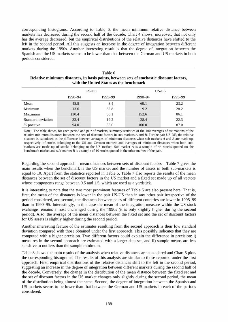
188
corresponding histograms. According to Table 6, the mean minimum relative distance betweenmarkets has decreased during the second half of the decade. Chart 4 shows, moreover, that not onlyhas the average decreased, but the empirical distributions of the relative distances have shifted to theleft in the second period. All this suggests an increase in the degree of integration between differentmarkets during the 1990s. Another interesting result is that the degree of integration between theSpanish and the US markets seems to be lower than that between the German and US markets in bothperiods considered.
Table 6Relative minimum distances, in basis points, between sets of stochastic discount factors,
with the United States as the benchmark
US-DE US-ES
1990–94 1995–99 1990–94 1995–99
Mean 48.8 3.4 69.1 23.2
Minimum –13.6 –32.8 9.2 –28.2
Maximum 130.4 66.1 152.6 86.1
Standard deviation 33.4 19.2 28.4 22.3
% positive 94.0 55.0 100.0 87.0
Note: The table shows, for each period and pair of markets, summary statistics of the 100 averages of estimations of therelative minimum distances between the sets of discount factors in sub-markets A and B. For the pair US-DE, the relativedistance is calculated as the difference between averages of minimum distances when sub-markets A and B are made up,respectively, of stocks belonging to the US and German markets and averages of minimum distances when both sub-markets are made up of stocks belonging to the US market. Sub-market A is a sample of 44 stocks quoted on thebenchmark market and sub-market B is a sample of 10 stocks quoted in the other market of the pair.
Regarding the second approach – mean distances between sets of discount factors – Table 7 gives themain results when the benchmark is the US market and the number of assets in both sub-markets isequal to 10. Apart from the statistics reported in Table 5, Table 7 also reports the results of the meandistances between the set of discount factors in the US market and a fixed set made up of all vectorswhose components range between 0.5 and 1.5, which are used as a yardstick.
It is interesting to note that the two most prominent features of Table 5 are also present here. That is,first, the mean of the distances is lower in the pair US-US than in any other pair irrespective of theperiod considered, and second, the distances between pairs of different countries are lower in 1995–99than in 1990–95. Interestingly, in this case the mean of the integration measure within the US stockexchange remains almost unchanged during the 1990s (it is only slightly higher during the secondperiod). Also, the average of the mean distances between the fixed set and the set of discount factorsfor US assets is slightly higher during the second period.
Another interesting feature of the estimates resulting from the second approach is their low standarddeviation compared with those obtained under the first approach. This possibly indicates that they arecomputed with a higher precision. Two different factors could explain the difference in precision: i)measures in the second approach are estimated with a larger data set, and ii) sample means are lesssensitive to outliers than the sample minimum.
Table 8 shows the main results of the analysis when relative distances are considered and Chart 5 plotsthe corresponding histograms. The results of this analysis are similar to those reported under the firstapproach. First, empirical distributions of the relative distances shift to the left in the second period,suggesting an increase in the degree of integration between different markets during the second half ofthe decade. Conversely, the change in the distribution of the mean distance between the fixed set andthe set of discount factors in the US market changes only slightly during the second period, the meanof the distribution being almost the same. Second, the degree of integration between the Spanish andUS markets seems to be lower than that between the German and US markets in each of the periodsconsidered.
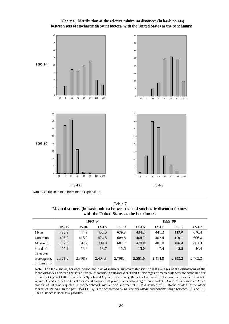
189
Note: See the note to Table 6 for an explanation.
Table 7Mean distances (in basis points) between sets of stochastic discount factors,
with the United States as the benchmark
1990–94 1995–99
US-US US-DE US-ES US-FIX US-US US-DE US-ES US-FIX
Mean 432.9 444.9 452.0 639.3 434.2 441.2 443.0 640.4
Minimum 403.2 413.0 424.3 609.6 404.7 402.4 410.1 606.8
Maximum 479.6 497.9 489.0 687.7 470.8 481.0 486.4 681.3
Standarddeviation
15.2 18.8 13.7 15.6 15.0 17.4 15.5 16.4
Average no.of iterations
2,376.2 2,396.3 2,404.5 2,706.4 2,381.0 2,414.0 2,393.2 2,702.3
Note: The table shows, for each period and pair of markets, summary statistics of 100 averages of the estimations of themean distances between the sets of discount factors in sub-markets A and B. Averages of mean distances are computed fora fixed set DA and 100 different sets DB. DA and DB are, respectively, the sets of admissible discount factors in sub-marketsA and B, and are defined as the discount factors that price stocks belonging to sub-markets A and B. Sub-market A is asample of 10 stocks quoted in the benchmark market and sub-market. B is a sample of 10 stocks quoted in the othermarket of the pair. In the pair US-FIX, DB is the set formed by all vectors whose components range between 0.5 and 1.5.This distance is used as a yardstick.
Chart 4. Distribution of the relative minimum distances (in basis points)between sets of stochastic discount factors, with the United States as the benchmark
US-DE US-ES
0
5
10
15
20
25
30
35
40
-20 0 20 40 60 80 100 > 100
1990–94
0
5
10
15
20
25
30
35
40
-20 0 20 40 60 80 100 > 100
1995–99
0
5
10
15
20
25
30
35
40
-20 0 20 40 60 80 100 > 100
0
5
10
15
20
25
30
35
40
-20 0 20 40 60 80 100 > 100
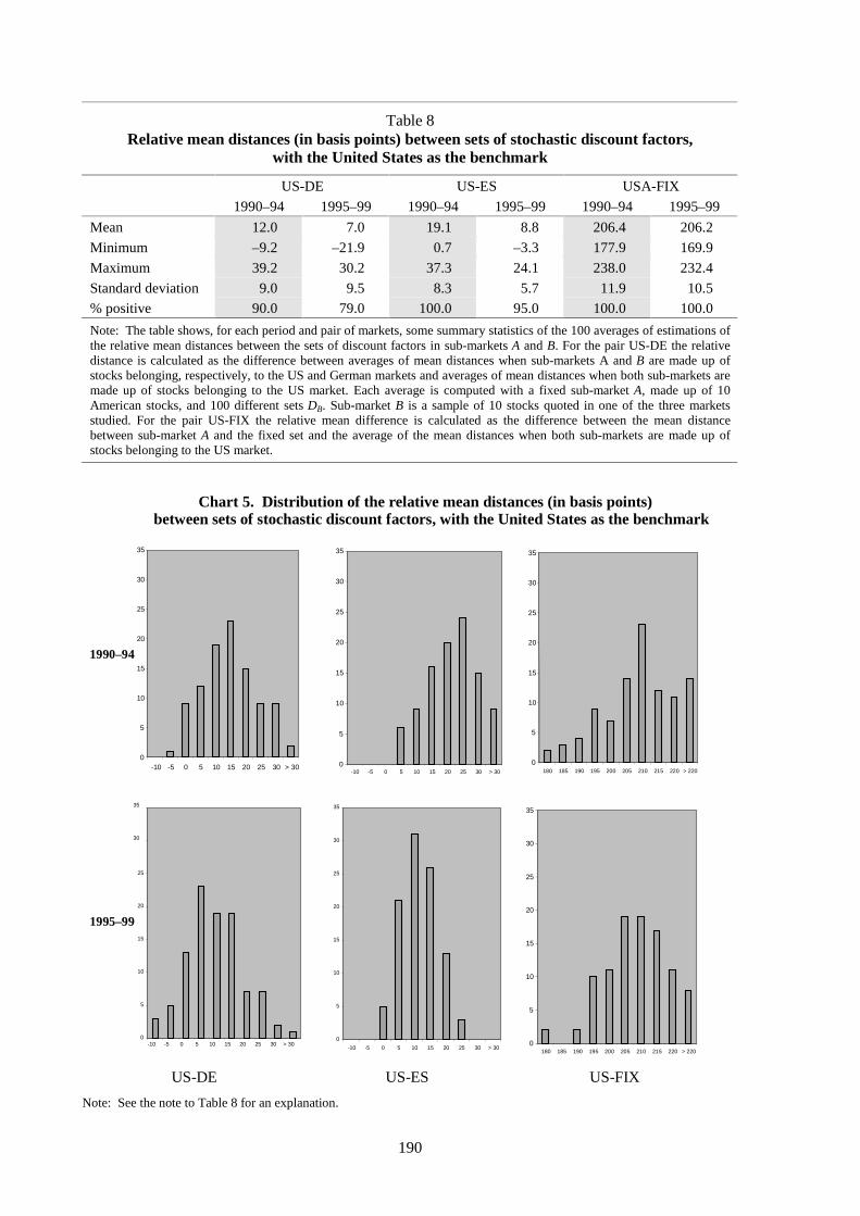
190
Table 8Relative mean distances (in basis points) between sets of stochastic discount factors,
with the United States as the benchmark
US-DE US-ES USA-FIX
1990–94 1995–99 1990–94 1995–99 1990–94 1995–99
Mean 12.0 7.0 19.1 8.8 206.4 206.2
Minimum –9.2 –21.9 0.7 –3.3 177.9 169.9
Maximum 39.2 30.2 37.3 24.1 238.0 232.4
Standard deviation 9.0 9.5 8.3 5.7 11.9 10.5
% positive 90.0 79.0 100.0 95.0 100.0 100.0
Note: The table shows, for each period and pair of markets, some summary statistics of the 100 averages of estimations ofthe relative mean distances between the sets of discount factors in sub-markets A and B. For the pair US-DE the relativedistance is calculated as the difference between averages of mean distances when sub-markets A and B are made up ofstocks belonging, respectively, to the US and German markets and averages of mean distances when both sub-markets aremade up of stocks belonging to the US market. Each average is computed with a fixed sub-market A, made up of 10American stocks, and 100 different sets DB. Sub-market B is a sample of 10 stocks quoted in one of the three marketsstudied. For the pair US-FIX the relative mean difference is calculated as the difference between the mean distancebetween sub-market A and the fixed set and the average of the mean distances when both sub-markets are made up ofstocks belonging to the US market.
Note: See the note to Table 8 for an explanation.
Chart 5. Distribution of the relative mean distances (in basis points)between sets of stochastic discount factors, with the United States as the benchmark
US-FIXUS-ESUS-DE
0
5
10
15
20
25
30
35
-10 -5 0 5 10 15 20 25 30 > 30
1990–94
0
5
10
15
20
25
30
35
-10 -5 0 5 10 15 20 25 30 > 30
0
5
10
15
20
25
30
35
180 185 190 195 200 205 210 215 220 > 220
0
5
10
15
20
25
30
35
-10 -5 0 5 10 15 20 25 30 > 30
1995–99
0
5
10
15
20
25
30
35
-10 -5 0 5 10 15 20 25 30 > 300
5
10
15
20
25
30
35
180 185 190 195 200 205 210 215 220 > 220
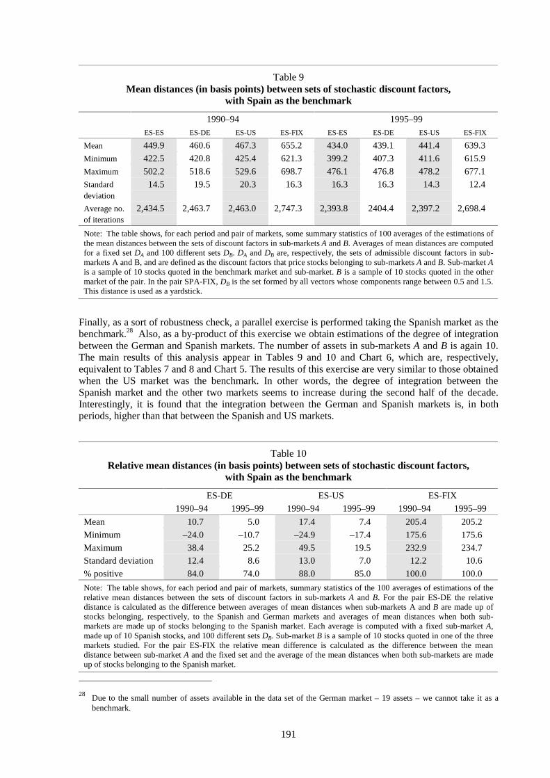
191
Table 9Mean distances (in basis points) between sets of stochastic discount factors,
with Spain as the benchmark
1990–94 1995–99
ES-ES ES-DE ES-US ES-FIX ES-ES ES-DE ES-US ES-FIX
Mean 449.9 460.6 467.3 655.2 434.0 439.1 441.4 639.3
Minimum 422.5 420.8 425.4 621.3 399.2 407.3 411.6 615.9
Maximum 502.2 518.6 529.6 698.7 476.1 476.8 478.2 677.1
Standarddeviation
14.5 19.5 20.3 16.3 16.3 16.3 14.3 12.4
Average no.of iterations
2,434.5 2,463.7 2,463.0 2,747.3 2,393.8 2404.4 2,397.2 2,698.4
Note: The table shows, for each period and pair of markets, some summary statistics of 100 averages of the estimations ofthe mean distances between the sets of discount factors in sub-markets A and B. Averages of mean distances are computedfor a fixed set DA and 100 different sets DB. DA and DB are, respectively, the sets of admissible discount factors in sub-markets A and B, and are defined as the discount factors that price stocks belonging to sub-markets A and B. Sub-market Ais a sample of 10 stocks quoted in the benchmark market and sub-market. B is a sample of 10 stocks quoted in the othermarket of the pair. In the pair SPA-FIX, DB is the set formed by all vectors whose components range between 0.5 and 1.5.This distance is used as a yardstick.
Finally, as a sort of robustness check, a parallel exercise is performed taking the Spanish market as thebenchmark.28 Also, as a by-product of this exercise we obtain estimations of the degree of integrationbetween the German and Spanish markets. The number of assets in sub-markets A and B is again 10.The main results of this analysis appear in Tables 9 and 10 and Chart 6, which are, respectively,equivalent to Tables 7 and 8 and Chart 5. The results of this exercise are very similar to those obtainedwhen the US market was the benchmark. In other words, the degree of integration between theSpanish market and the other two markets seems to increase during the second half of the decade.Interestingly, it is found that the integration between the German and Spanish markets is, in bothperiods, higher than that between the Spanish and US markets.
Table 10Relative mean distances (in basis points) between sets of stochastic discount factors,
with Spain as the benchmark
ES-DE ES-US ES-FIX
1990–94 1995–99 1990–94 1995–99 1990–94 1995–99
Mean 10.7 5.0 17.4 7.4 205.4 205.2
Minimum –24.0 –10.7 –24.9 –17.4 175.6 175.6
Maximum 38.4 25.2 49.5 19.5 232.9 234.7
Standard deviation 12.4 8.6 13.0 7.0 12.2 10.6
% positive 84.0 74.0 88.0 85.0 100.0 100.0
Note: The table shows, for each period and pair of markets, summary statistics of the 100 averages of estimations of therelative mean distances between the sets of discount factors in sub-markets A and B. For the pair ES-DE the relativedistance is calculated as the difference between averages of mean distances when sub-markets A and B are made up ofstocks belonging, respectively, to the Spanish and German markets and averages of mean distances when both sub-markets are made up of stocks belonging to the Spanish market. Each average is computed with a fixed sub-market A,made up of 10 Spanish stocks, and 100 different sets DB. Sub-market B is a sample of 10 stocks quoted in one of the threemarkets studied. For the pair ES-FIX the relative mean difference is calculated as the difference between the meandistance between sub-market A and the fixed set and the average of the mean distances when both sub-markets are madeup of stocks belonging to the Spanish market.
28
Due to the small number of assets available in the data set of the German market – 19 assets – we cannot take it as abenchmark.
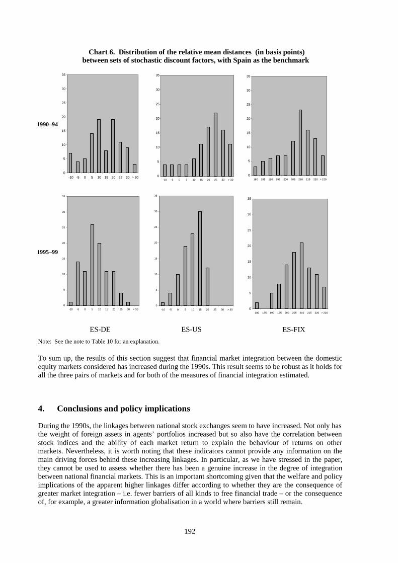
192
Note: See the note to Table 10 for an explanation.
To sum up, the results of this section suggest that financial market integration between the domesticequity markets considered has increased during the 1990s. This result seems to be robust as it holds forall the three pairs of markets and for both of the measures of financial integration estimated.
4. Conclusions and policy implications
During the 1990s, the linkages between national stock exchanges seem to have increased. Not only hasthe weight of foreign assets in agents’ portfolios increased but so also have the correlation betweenstock indices and the ability of each market return to explain the behaviour of returns on othermarkets. Nevertheless, it is worth noting that these indicators cannot provide any information on themain driving forces behind these increasing linkages. In particular, as we have stressed in the paper,they cannot be used to assess whether there has been a genuine increase in the degree of integrationbetween national financial markets. This is an important shortcoming given that the welfare and policyimplications of the apparent higher linkages differ according to whether they are the consequence ofgreater market integration – i.e. fewer barriers of all kinds to free financial trade – or the consequenceof, for example, a greater information globalisation in a world where barriers still remain.
Chart 6. Distribution of the relative mean distances (in basis points)between sets of stochastic discount factors, with Spain as the benchmark
ES-FIXES-USES-DE
0
5
10
15
20
25
30
35
-10 -5 0 5 10 15 20 25 30 > 30
1990–94
0
5
10
15
20
25
30
35
-10 -5 0 5 10 15 20 25 30 > 30
0
5
10
15
20
25
30
35
180 185 190 195 200 205 210 215 220 > 220
0
5
10
15
20
25
30
35
-10 -5 0 5 10 15 20 25 30 > 30
1995–99
0
5
10
15
20
25
30
35
-10 -5 0 5 10 15 20 25 30 > 30 0
5
10
15
20
25
30
35
180 185 190 195 200 205 210 215 220 > 220

193
Accordingly, we propose two refinements of a direct measure of financial market integrationoriginally proposed by Chen and Knez (1995) and compute them for the US, German and Spanishstock exchanges in the 1990s. Our analysis shows that during the 1990s there has been an increase inthe degree of integration among the markets considered.
This result has important implications when assessing the closer relationships observed between stockexchanges. Thus, for example, due to the entailed elimination of obstacles to free trade, greaterfinancial market integration means higher financial market efficiency and an improvement in the risk-and-return combinations available to investors. This has to be viewed as a counterargument to thosewho believe that markets are now too vulnerable to news due to their excessive links.
Greater market integration, on the other hand, reduces the ability of domestically focused policies todeal with the new problems arising in financial markets. It might be argued that the closer we are to asingle world market, the greater the need for worldwide supervision, particularly if this greaterintegration is the result of solid structural trends, as seems to be the case. Whether such worldwidesupervision should be provided by a single supervisor or by a very closely linked group of supervisorsis, however, a different question.

194
Annex
In Section 2, we use overall indices for seven stock exchanges and sector indices for the US stockexchange. The overall indices are the following:
S&P 500 for New York.29
FTSE All-Share for London.CAC 40 for Paris.IGBM for Madrid.DAX 30 for Frankfurt.MIB all shares for Milan.Nikkei 225 for Tokyo.
In all these indices, stocks are weighted by their capitalisation and are calculated on a price-returnbasis – i.e. they only reflect capital gains. The source is the BIS, with the exception of the IGBM,where the source is the Bank of Spain.
The sector indices for the US exchange are seven of the sector indices of the S&P 500. They are thefollowing:
XF: financial sector.TECS: technology sector.HLTS: healthcare sector.CPGS: capital goods sector.ENRS: energy sector.XU: utility sector.XT: transportation sector.
This data set is taken from Bloomberg.
In Section 3, we use information on prices and payoffs for a sample of portfolios of assets in each ofthree different markets – New York, Frankfurt and Madrid. The payoffs are indices calculated on atotal-return basis representing the performance of portfolios of assets, and prices are the same seriesbut lagged one period. For the Frankfurt market we take the 19 CDAX sector indices. These indicesare calculated by the Deutsche Börse with the gross dividends reinvested in the index and withcorrection for capital increases. For the NYSE we construct total-return indices for 80 of the industryindices of the S&P 500. The computation is performed reinvesting gross dividends into those industryindices. More formally, we use the following expression:
∏=
+=t
it
i
it I
I
dTRI
0
)1(
where TRIt stands for total return index in period t, di is the sum of all gross dividends – expressed inindex points – paid in period i by stocks belonging to the index, and Ij for j = i,t is the price index inperiod j. The information needed to construct the previous data set was taken from Bloomberg.
Finally, for the Madrid exchange, we construct 43 indices representing the total return on 43 of thestocks which have been listed throughout the period studied. The total return is computed applying theprevious expression, when the price index has been corrected for capital increases. The latter index iscalculated after eliminating the impact of the correction for dividends made by the Bolsa de Madrid30
in its individual price indices. The source of the data we use to compute these indices is the Bank ofSpain for individual indices and the Bolsa de Madrid for dividends. 29
In fact, the S&P 500 index also includes stocks quoted on other exchanges such NASDAQ and AMEX. However, thenumber of assets quoted on the NYSE represents more than 90% of the total.
30The Bolsa de Madrid calculates individual price indices for those stocks belonging to the global index IGBM. Theseindices are corrected for dividends in such a way that the drop in price on the ex-dividend day is eliminated, but as theyare not reinvested into the index this correction was not useful for our purpose. That is why we have eliminated theimpact of this correction.
195
Bibliography
Adler, M and B Dumas (1983): “International Portfolio Choice and Corporation Finance: ASynthesis”. Journal of Finance, 38, pp. 925-84.
Black, F (1976): “Studies in stock price volatility changes”. Proceedings of the 1976 Business Meetingof the Business and Economics Statistics Section, American Statistical Association, pp. 177-81.
Bollerslev, T (1986): “Generalised autoregressive conditional heteroskedasticity”. Journal ofEconometrics, 31, pp. 307-27.
Chen, Z and P J Knez (1995): “Measurement of Market Integration and Arbitrage”. Review ofFinancial Studies, 8 (2), pp. 287-325.
Engle, R F , T Ito and W L Lin (1988): “Meteor showers or heat waves?: intra-daily volatility in theforeign exchange market”. NBER Working Paper.
Engle, R F and V K Ng (1993): “Measuring and Testing the Impact of News on Volatility”. Journal ofFinance, 5, 1749-78.
Glosten, L, R Jagannathan and D Runkle (1989): “Relationship between the expected value and thevolatility of the nominal excess return on stocks”. Working Paper, Department of Finance, ColumbiaUniversity.
Hansen, L P and R Jagannathan (1991): “Implications of Security Market Data for Models of DynamicEconomies”. Journal of Political Economy, 99, pp. 225-62.
Hansen, L P and R Jagannathan (1997): “Assessing Specification Errors in Stochastic Discount FactorModels”. The Journal of Finance, 52 (2), pp. 557-90.
Le, S V (1991): “International investment diversification before and after the October 19, 1987 stockmarket crisis”. Journal of Business Research, 22, pp. 305-10.
Taylor, M P and I Tonks (1989): “The Internationalisation of Stock Markets and the Abolition of UKExchange Control”. Review of Economics and Statistics, 71, pp. 332-6.

196
Decomposing the relationship betweeninternational bond markets
Andrew Clare and Ilias Lekkos1
1. Introduction
The correlations between major asset classes are of concern and interest to monetary authorities andfinancial regulators alike – the potential for a worldwide decline in consumption which might resultfrom a dramatic fall in equity market wealth could have serious implications for both the health offinancial institutions and that of the real economy. This concern is reflected in the academic literature,where an increasing number of researchers have tried to understand the characteristics of theselinkages and the nature of the processes by which information flows between markets. Perhaps themain catalyst for this concern in recent years was the equity market crash of October 1987. This eventmore than any other highlighted the high levels of correlation between national equity markets at timesof extreme market stress.
However, of equal importance is the relationship between international bond markets. Typically,monetary authorities are able to influence directly only the very short end of the term structure.Nevertheless, given that the long bond rate is determined by expectations about future short-term realinterest rates and inflation, a credible monetary policy should trigger a transmission mechanismthrough which monetary policy actions are passed through to the whole of the term structure. As thecovariation between government bond rates in different countries increases, the ability of monetaryauthorities to influence the term structure may decline, and hence their ability to control domesticinflation may also decline.
Correlation between bond markets may arise through a number of channels, for example: if there is aworld price of risk; if real rates are determined by global factors; or if there is a “flight to quality” intimes of financial stress. Unconditional measures of the correlations between major international bondmarkets showed that the linkages between these markets increased from the 1960s until the early1980s, but, according to Solnik et al. (1996) and Christiansen and Pigott (1997), these correlationshave not exhibited a clear trend since this time. However, while simple unconditional, rollingmeasures of international bond market correlations may not have been trending up in recent times, thequestion of how much control monetary authorities can bring to bear upon the shape of the yield curvethrough changes in short rates still remains. Another issue relates to the extent (in terms of durationand magnitude) to which the slope of the yield curve is influenced by international factors duringperiods of financial crisis. Finally, another important and related issue is the extent to whichcomovements in long bond rates, or indeed the components of these comovements, change duringperiods of financial market stress. This paper addresses all of these issues.
Using the intuition from the rational expectations hypothesis of the term structure (REHTS), wedecompose the long bond rates of Germany, the United Kingdom and the United States into theirrespective “fundamental” and risk premium components.2 The decomposition is achieved by using the
1
We would like to thank Roger Clews, Nicola Anderson, James Proudman, Nikolaos Panigirtzoglou and participants at theBIS Autumn 1999 Meeting of Central Bank Economists for comments on an earlier draft of this paper. We would like topoint out that the views expressed in this paper are those of the authors and do not necessarily represent those of the Bankof England. E-mails: [email protected] and [email protected]
2Our technique does not allow us to distinguish between more permanent risk premium components and temporarycontagion effects. However, for expositional simplicity we use the term risk premium in this paper to mean somecombination of the two.
197
Campbell and Shiller (1987) VAR methodology. Each VAR which we estimate contains bothdomestic and foreign conditioning variables, which means that we can separate that portion of thevariance of the slope of the yield curve which is influenced by domestic factors from that portionwhich is driven by international factors. We then turn our attention to calculating a conditionalmeasure of international bond market covariation, decomposing this measure into its fundamental andrisk premia components, by invoking the REHTS. We extend our analysis to consider the relationshipsbetween sterling and US dollar swap markets, a relationship which to our knowledge has not beenconsidered in this context by previous researchers. Finally, because we estimate each of the VARs ona rolling basis, we can monitor the time variation in both the variance and the covariancedecompositions.
Our results suggest that there have been periods associated with financial market crises when theslopes of the government yield curves studied here are determined more by international than bydomestic factors, for example during the sterling exchange rate crisis of 1992. However, our evidencesuggests in general that once the crisis has passed, the yield curves become dominated by domesticfactors once again. With respect to the covariance between bond yields, we find that while the totalcovariance between the markets is fairly stable over time, the components of this covariance can varyconsiderably over time. The rest of the paper is organised as follows: in Section 2 we briefly outlinerelevant academic literature on the topic of financial market linkages; in Section 3 we describe ourmethodology; in Section 4 we present the data used here; in Section 5 we present our results; andfinally, Section 6 concludes the paper.
2. Brief literature review
One of the main spurs to research into financial market linkages was the October 1987 stock marketcrash. Koutmos and Booth (1995) (amongst others) find evidence to suggest that interdependenciesbetween the world’s three major stock markets – London, New York and Tokyo – increased after the1987 crash. This apparent increase in the linkages between national equity markets could be due to theglobalisation of finance, and hence to an increase in the presence of “international investors”.Alternatively, volatility transmission could be the result of contagion, as proposed by King andWadhwani (1990), where, for example, agents do not assess the economic implications of news froman overseas market for their own and simply respond by “shooting first and asking questions later”(see Shiller et al. (1991)).
While some early studies of the informational linkages between markets investigated theinterdependencies between conditional first moments (see, for example, Eun and Shim (1989), Kingand Wadhwani (1990) or Koch and Koch (1991)), more recent studies have focused upon therelationships between conditional first and second moments. Engle et al. (1990) examine thephenomenon of volatility clustering in foreign exchange markets, making the distinction between whatthey term to be “heat wave” and “meteor shower” effects: the former referring to volatility which isnot transmitted to other markets, the latter referring to volatility which is transferred between markets.The Engle et al. study finds more evidence for meteor shower than for heat wave behaviour in theforeign exchange data in their study. Using daily data on London, New York and Tokyo stock indices,Koutmos and Booth (1995) estimate a multivariate E-GARCH model to test for spillover effectsbetween the conditional first and second moments of returns in these markets. While they find clearevidence of such spillovers, they also find that the volatility transmission is asymmetric, with negativeshocks from one market having a larger impact upon the volatility of another market than equivalentpositive shocks. Following King and Wadhwani (1990), other studies have couched the volatilitytransmission issue as a signal extraction problem, where agents in the local market have to extractfrom any news event that portion of the news which is relevant to their market. For example, Lin et al.(1994) decompose return surprises from one market into its global and local components usingKalman filtering techniques.
198
An alternative approach to the analysis of the relationship between national equity markets can befound in Ammer and Mei (1996), who use a variant of the Campbell and Shiller (1987) variancedecomposition for equities to analyse the relationship between US and UK stock returns. From 1957 to1989 they find that there was an increase in the correlation both between expected dividends andbetween risk premiums in these two countries, but that these correlations have changed little since1989.
Finally, some researchers have also considered the relationship between bond and stock markets.Shiller and Beltratti (1992) and Campbell and Ammer (1993) investigate the relationship betweenbond and stock markets using the VAR approach of Campbell and Shiller (1987) to decompose assetreturns. Shiller and Beltratti find that the negative relationship observed between real stock prices andlong-term interest rates is much bigger in magnitude compared to the relationship implied by thesimple rational expectations present value model. Using a similar VAR decomposition for US data,Campbell and Ammer (1993) find that stock returns are driven mainly by news about future stockreturns, while bond returns are predominantly driven by inflation, thus explaining the low correlationbetween the returns on these two long-term assets.
To our knowledge, far fewer researchers have investigated the relationships between internationalbond markets (for an exception to this general rule, see Dahlquist et al. (1999)). The purpose of thispaper, then, is to add to the literature on financial market linkages by considering the links betweenfixed income markets.
3. Methodology
3.1 Structural decomposition of bond market covariation
We begin by outlining a decomposition of the covariation between long-term bond rates. To achievethis more structural approach to the linkages between international bond markets, we make use of theREHTS. In its original form the REHTS defines current long-term interest rates as an average ofexpected future short-term rates plus a constant risk premium. Given the overwhelming empiricalevidence against the pure expectations hypothesis, we adopt a more general version of the REHTS thatallows for a time-varying, risk premium (see Evans and Lewis (1994)). For pure discount bonds wecan write:
(1) tke
tktk RPRR ,,, +=
where tkR , is the yield on a k-maturity pure discount bond and tkRP , is the risk premium at time t
associated with buying a long bond relative to rolling over one-period bonds. etkR , is the theoretical
k-maturity rate according to the expectations hypothesis given by:
(2) ∑−
=+=
1
0,1,
1 k
iitt
etk rE
kR
where tE denotes the market’s expectations conditional upon information available at time t and itr +,1
is the one-period rate at time t+i.
Similarly we can define foreign bond rates as:
(3) *,
*,
*, tk
etktk RPRR +=
Given equations (1) and (3), the covariance between domestic and foreign interest rates can be writtenas:
(4)),(),(),(),(
),(),(****
***
RPRPCovRRPCovRPRCovRRCov
RPRRPRCovRRCoveeee
ee
+++=
++=

199
How can we interpret these components? The first component in expression (4) measures that part ofthe covariation between two bond markets which can be attributed to the covariation in investors’expectations about future short-term interest rates in the two countries. Given that these expectationswill reflect considerations about the future path of inflation, real interest rates and the monetary policystance in each country, we assume that this component reflects the part of the total covariation due to“economic fundamentals” between the two economies. If the two economies track each other throughthe business cycle, we might expect the links between the two bond markets to be quite strong. Theremaining components are a direct result of our use of the REHTS. In the absence of a bond marketrisk premium the fully anticipated rational expectation of the long rate will equal the actual long rate.
We can therefore interpret the difference between kR and ekR as the risk premium required for
holding government bonds, RP. The second (third) component then represents the covariation betweendomestic (foreign) fundamentals and the foreign (domestic) interest rate risk premium. Finally, thefourth component measures the covariation between domestic and foreign risk premia.
3.2 Generating expectations of future long rates
One difficulty in calculating the covariance decomposition given by expression (4) is that none of thelong-term interest rate components are directly observable. Since the components of expression (4)depend upon long-horizon expectations of short-term interest rates, we need some way to conditionthese expectations. To this end we use the vector autoregression (VAR) methodology to calculatemultiperiod expectations of the long rate (see Campbell and Shiller (1987)).3
Having chosen this VAR methodology, the next issue relates to the choice of conditioning variables.Campbell and Shiller (1987) use a two-dimensional vector of state variables, which includes thechanges in the short rate and the slope of the term structure, in undertaking this exercise using USdata. An assumption inherent in such a formulation is that investors’ expectations about future short-term rates are affected only by information concerning domestic fundamentals as reflected in the shortrate and the slope of the term structure. However, since the aim of this paper is to investigate thelinkages between national bond markets, we condition expectations about future long rates on bothdomestic and international measures of the short rate and the slope of the term structure. Our intentionthen is to formulate a VAR using information from the bond markets of Germany, the UnitedKingdom and the United States in such a way that interest rate expectations are jointly determined,thus allowing for possible interactions between domestic and international fundamentals. In order toachieve this interaction, we expand the information set to include information on three different termstructures.4 As a result the vector of state variables is defined as:
(5) ],,,,,[ *****,1,1
*,1 ′∆∆∆= ttttyeartyeartyeart SlopeSlopeSloperrrz
where the superscripts * and ** relate to the first and second “foreign” markets respectively.
Having chosen the information set, we can follow Campbell and Shiller (1987) and define the
theoretical slope of the term structure under the expectations hypothesis, etks , , as:
(6) te
tke
tk rRs ,1,, −=
Substituting (2) into (5), we get:
(7) ∑−
=++∆−=
1
11,1, )()(
1 k
iitt
etk rEik
ks
where ∆ denotes the one-period backward difference operator defined as ititit rrr +++++ −=∆ ,11,11,1 .
3
For a more detailed discussion on alternative methodologies used to evaluate multiperiod expectations of unobservedvariables and their shortcomings relative to the VAR approach, see Campbell and Ammer (1993).
4The number of countries included in the vector of state variables is limited only by data availability.
200
Similar expressions to (6) and (7) hold for *,
etks and **
,e
tks .
To estimate the expectations of future short-rate changes, we assume that the vector of state variablesdefined by (5) follows a first-order VAR process:
(8) ttt wzz += −1A
where zt is the vector of state variables given by (5), A is the matrix of the VAR coefficients and wt isthe vector of residuals. By including the interest rate changes rather than the levels, we ensurestationarity in the VAR. Furthermore, for reasons of notational simplicity and computationalconvenience, we demean the variables before including them in the VAR. Finally, we note that theassumption of the first-order VAR process is not restrictive.5
Based on this formulation, the long-horizon expectations of changes in one-period interest ratesj-periods in the future, j=1,...,k-1, can be estimated by:
(9) tT1 zAh j
jtt rE =∆ + )( ,1
(10) tT2 zAh j
jtt rE =∆ + )( *,1 and
(11) tT3 zAh j
jtt rE =∆ + )( **,1
where ,...]0,0,0,1[=T1h , ,...]0,0,1,0[=T
2h and ,...]0,1,0,0[=T3h are used to pick out the first, second
and third element of the state vector.
Once the matrix A of VAR coefficients is estimated then for each t, t=1,...,T, the expectations of futurechanges in interest rates can be generated using expressions (9), (10) and (11), and the theoretical termstructure slopes by using expression (7). We can calculate the theoretical long-term interest rate by
solving (6) with respect to etkR , . The differences between the theoretical and actual long-term rates
provide an estimate of the domestic and foreign bond market risk premium, tkRP , . Estimates of *,
etkR ,
*,tkRP and **
,e
tkR , **,tkRP are produced by a similar procedure.6 Given the estimated theoretical long
rates and the risk premia, then, for each pair of countries, components of the covariance betweenactual interest rates can be calculated according to expression (4).
Our intention is not only to identify the covariance components and the importance of domestic andinternational factors in determining interest rates, but also to examine how these derived variables varyover our sample period. To capture this effect, we adopt a rolling estimation procedure where the VARdescribed above is estimated using one year’s worth of data. We then roll forward the estimationwindow by one week and repeat the procedure outlined above until the end of the sample period. Bydoing this, we can generate a time series of the components of expression (4).
Finally, the estimation of a VAR allows us to decompose the variance of the slopes of both thedomestic and foreign term spreads, a procedure which is now common practice in papers usingunrestricted VARs of the kind used here (see Sims (1980) for a description of the technique). Thevariance decomposition provides us with an estimate of the proportion of the movement in onevariable which can be attributed to shocks in other variables in the VAR. Since we estimate the VARson a rolling basis, we also create a time series of this variance decomposition allowing us, forexample, to gauge the time-varying impact of shocks to overseas interest rates on the slope of the UKyield curve.
5
Campbell and Shiller (1988) demonstrate that it is straightforward to modify the model to allow for a higher VAR order.
6These estimates of the risk premia will be accurate provided that we include in our model all the relevant information thatinvestors use to form their expectations about future interest rates and that the dynamics of the VAR are correctlyspecified. If these conditions are not met, estimates of risk premia will be biased upwards.
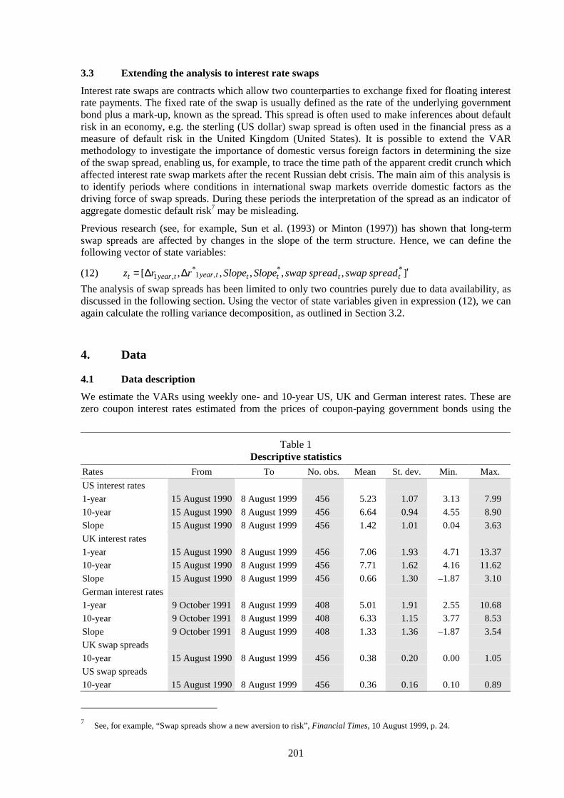
201
3.3 Extending the analysis to interest rate swaps
Interest rate swaps are contracts which allow two counterparties to exchange fixed for floating interestrate payments. The fixed rate of the swap is usually defined as the rate of the underlying governmentbond plus a mark-up, known as the spread. This spread is often used to make inferences about defaultrisk in an economy, e.g. the sterling (US dollar) swap spread is often used in the financial press as ameasure of default risk in the United Kingdom (United States). It is possible to extend the VARmethodology to investigate the importance of domestic versus foreign factors in determining the sizeof the swap spread, enabling us, for example, to trace the time path of the apparent credit crunch whichaffected interest rate swap markets after the recent Russian debt crisis. The main aim of this analysis isto identify periods where conditions in international swap markets override domestic factors as thedriving force of swap spreads. During these periods the interpretation of the spread as an indicator ofaggregate domestic default risk7 may be misleading.
Previous research (see, for example, Sun et al. (1993) or Minton (1997)) has shown that long-termswap spreads are affected by changes in the slope of the term structure. Hence, we can define thefollowing vector of state variables:
(12) ] , ,,,,[ **,1
*,1 ′∆∆= tttttyeartyeart spreadswapspreadswapSlopeSloperrz
The analysis of swap spreads has been limited to only two countries purely due to data availability, asdiscussed in the following section. Using the vector of state variables given in expression (12), we canagain calculate the rolling variance decomposition, as outlined in Section 3.2.
4. Data
4.1 Data description
We estimate the VARs using weekly one- and 10-year US, UK and German interest rates. These arezero coupon interest rates estimated from the prices of coupon-paying government bonds using the
Table 1Descriptive statistics
Rates From To No. obs. Mean St. dev. Min. Max.
US interest rates
1-year 15 August 1990 8 August 1999 456 5.23 1.07 3.13 7.99
10-year 15 August 1990 8 August 1999 456 6.64 0.94 4.55 8.90
Slope 15 August 1990 8 August 1999 456 1.42 1.01 0.04 3.63
UK interest rates
1-year 15 August 1990 8 August 1999 456 7.06 1.93 4.71 13.37
10-year 15 August 1990 8 August 1999 456 7.71 1.62 4.16 11.62
Slope 15 August 1990 8 August 1999 456 0.66 1.30 –1.87 3.10
German interest rates
1-year 9 October 1991 8 August 1999 408 5.01 1.91 2.55 10.68
10-year 9 October 1991 8 August 1999 408 6.33 1.15 3.77 8.53
Slope 9 October 1991 8 August 1999 408 1.33 1.36 –1.87 3.54
UK swap spreads
10-year 15 August 1990 8 August 1999 456 0.38 0.20 0.00 1.05
US swap spreads
10-year 15 August 1990 8 August 1999 456 0.36 0.16 0.10 0.89
7
See, for example, “Swap spreads show a new aversion to risk”, Financial Times, 10 August 1999, p. 24.

202
Svensson methodology (Svensson (1994, 1995)).8 The zero coupon data available for the threecountries begin on different dates: from January 1979 for the United Kingdom, from August 1990 forthe United States and from October 1991 for Germany.9 Given that the VARs are jointly estimated forthree countries at a time, the estimation period for each VAR is set equal to the period over whichoverlapping data between the three countries are available. Descriptive statistics for the data used aregiven in Table 1.
In addition, we extend our analysis to interest rate swap spreads. Only sterling and US dollar swaprates were available to us for a sufficient span of time. The swap data span the period from August1990 to August 1999. From zero coupon swap rates10 we subtract the equivalent maturity zero-couponinterest rate estimated from the appropriate Svensson yield curve to provide estimates of the sterlingand dollar swap spreads.
5. Results
We now present the results relating to various versions of the VAR outlined in Section 4 above. ThisVAR is estimated using government bond market data for Germany, the United Kingdom and theUnited States. We also estimate the VAR given in expression (12) using swap market data. We beginby discussing the results of the variance decompositions of these VARs and then move on to discussthe decomposition of the covariance.
5.1 Variance decomposition results
5.1.1 Government bond market results
In Figure 1 we present the variance decomposition for the slope of the US yield curve, based upon aVAR which includes German, UK and US variables. The figure reports the proportion of the varianceof the slope of the term structure that can be attributed to shocks in the variables of the VAR, 26weeks into the future.11 One known shortcoming of the VAR methodology is that the variancedecomposition results may be influenced by the ordering of the variables in the VAR. In our VAR thefirst variable in the state vector is the change in short-term US interest rates, followed by the change inGerman and then UK short-term rates, which are followed in turn by the slopes of the US, German andUK yield curves. The raison d’être for this ordering is that shocks to short-term rates should affect theslopes of the yield curves. The ordering of the countries, with the United States first then Germany andthen the United Kingdom, reflects our priors of the importance of these economies and their respectivebond markets in a global sense.
8
More details on the implementation of the Svensson methodology and the estimation of zero coupon term structures areprovided in Appendix A.
9From January 1999 the German rates are replaced by euro interest rates.
10Appendix B gives more details about the estimation of zero coupon interest rates estimated from swap rates.
11The variance decomposition results presented here could be based upon coefficients which are poorly determined. To testfor this possibility, and to test for causation between foreign influences on the domestic term structure, we test a nullhypothesis that the VAR coefficients relating to the foreign variables are jointly insignificant, i.e. that they do not help topredict the domestic slope and interest rate change. We undertake this test on a rolling basis. In the interests of brevity,we do not report the results in detail here; however, we find that for all of the VARs presented in this paper the nullhypothesis of no foreign influence on domestic interest rates can be rejected for the majority of the sample periodconsidered here, and in particular for the “crisis” periods. An alternative way of interpreting these results is that dualcausality, in the Granger causality sense of the term, exists between these markets. These results are of course availableon request from the authors.
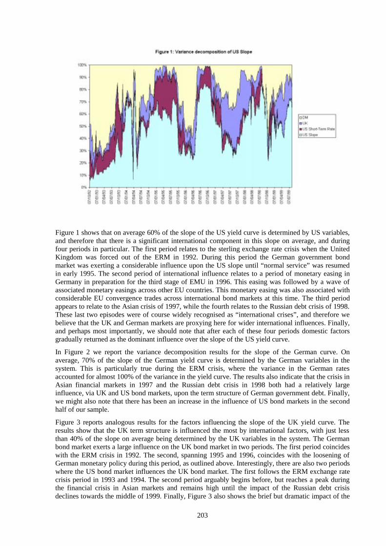
203
Figure 1 shows that on average 60% of the slope of the US yield curve is determined by US variables,and therefore that there is a significant international component in this slope on average, and duringfour periods in particular. The first period relates to the sterling exchange rate crisis when the UnitedKingdom was forced out of the ERM in 1992. During this period the German government bondmarket was exerting a considerable influence upon the US slope until “normal service” was resumedin early 1995. The second period of international influence relates to a period of monetary easing inGermany in preparation for the third stage of EMU in 1996. This easing was followed by a wave ofassociated monetary easings across other EU countries. This monetary easing was also associated withconsiderable EU convergence trades across international bond markets at this time. The third periodappears to relate to the Asian crisis of 1997, while the fourth relates to the Russian debt crisis of 1998.These last two episodes were of course widely recognised as “international crises”, and therefore webelieve that the UK and German markets are proxying here for wider international influences. Finally,and perhaps most importantly, we should note that after each of these four periods domestic factorsgradually returned as the dominant influence over the slope of the US yield curve.
In Figure 2 we report the variance decomposition results for the slope of the German curve. Onaverage, 70% of the slope of the German yield curve is determined by the German variables in thesystem. This is particularly true during the ERM crisis, where the variance in the German ratesaccounted for almost 100% of the variance in the yield curve. The results also indicate that the crisis inAsian financial markets in 1997 and the Russian debt crisis in 1998 both had a relatively largeinfluence, via UK and US bond markets, upon the term structure of German government debt. Finally,we might also note that there has been an increase in the influence of US bond markets in the secondhalf of our sample.
Figure 3 reports analogous results for the factors influencing the slope of the UK yield curve. Theresults show that the UK term structure is influenced the most by international factors, with just lessthan 40% of the slope on average being determined by the UK variables in the system. The Germanbond market exerts a large influence on the UK bond market in two periods. The first period coincideswith the ERM crisis in 1992. The second, spanning 1995 and 1996, coincides with the loosening ofGerman monetary policy during this period, as outlined above. Interestingly, there are also two periodswhere the US bond market influences the UK bond market. The first follows the ERM exchange ratecrisis period in 1993 and 1994. The second period arguably begins before, but reaches a peak duringthe financial crisis in Asian markets and remains high until the impact of the Russian debt crisisdeclines towards the middle of 1999. Finally, Figure 3 also shows the brief but dramatic impact of the
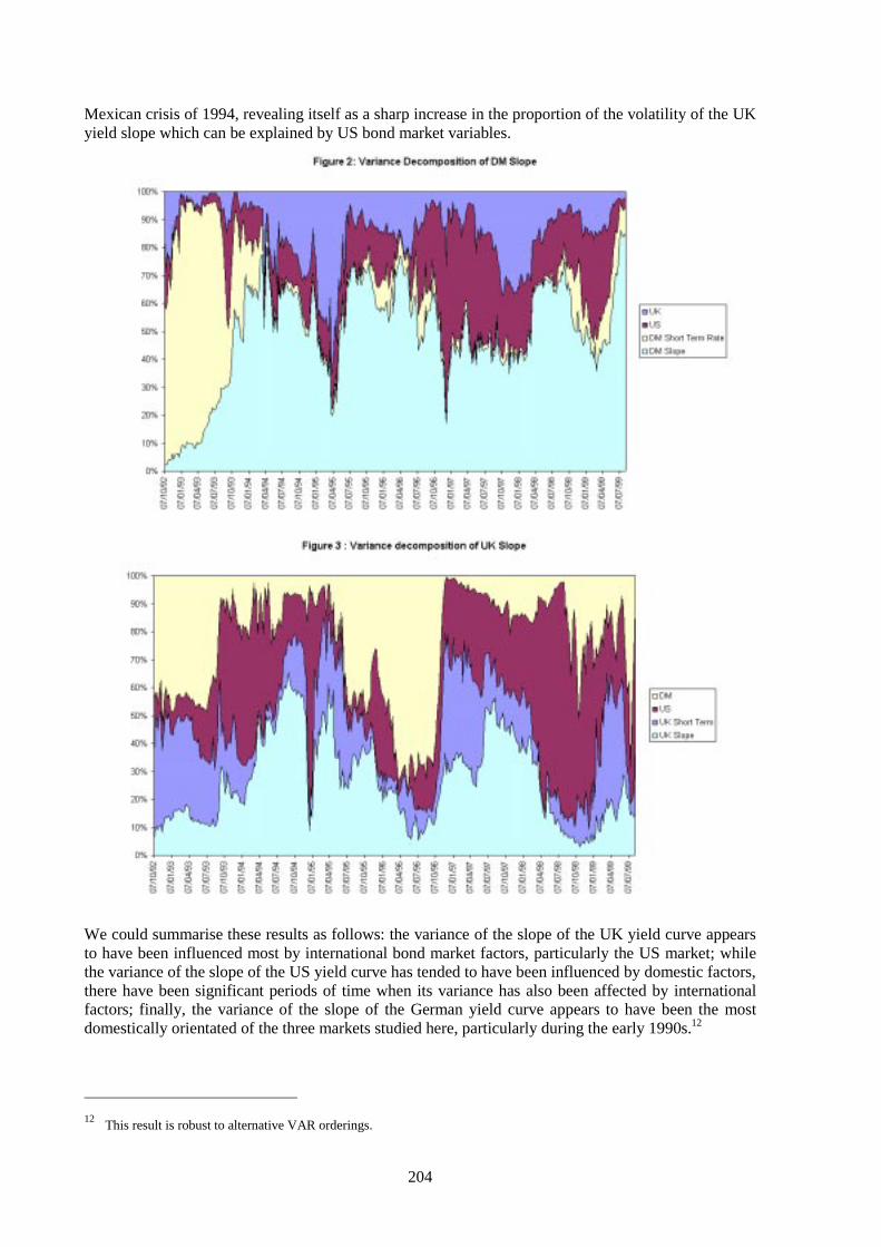
204
Mexican crisis of 1994, revealing itself as a sharp increase in the proportion of the volatility of the UKyield slope which can be explained by US bond market variables.
We could summarise these results as follows: the variance of the slope of the UK yield curve appearsto have been influenced most by international bond market factors, particularly the US market; whilethe variance of the slope of the US yield curve has tended to have been influenced by domestic factors,there have been significant periods of time when its variance has also been affected by internationalfactors; finally, the variance of the slope of the German yield curve appears to have been the mostdomestically orientated of the three markets studied here, particularly during the early 1990s.12
12
This result is robust to alternative VAR orderings.
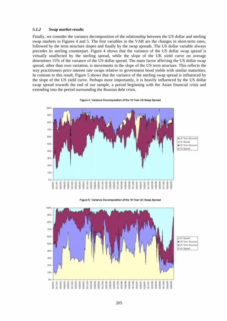
205
5.1.2 Swap market results
Finally, we consider the variance decomposition of the relationship between the US dollar and sterlingswap markets in Figures 4 and 5. The first variables in the VAR are the changes in short-term rates,followed by the term structure slopes and finally by the swap spreads. The US dollar variable alwaysprecedes its sterling counterpart. Figure 4 shows that the variance of the US dollar swap spread isvirtually unaffected by the sterling spread, while the slope of the UK yield curve on averagedetermines 15% of the variance of the US dollar spread. The main factor affecting the US dollar swapspread, other than own variation, is movements in the slope of the US term structure. This reflects theway practitioners price interest rate swaps relative to government bond yields with similar maturities.In contrast to this result, Figure 5 shows that the variance of the sterling swap spread is influenced bythe slope of the US yield curve. Perhaps more importantly, it is heavily influenced by the US dollarswap spread towards the end of our sample, a period beginning with the Asian financial crisis andextending into the period surrounding the Russian debt crisis.

206
The results with respect to the sterling swap spread should act as a potential warning for those whobelieve that swap spreads are an indicator of domestic financial conditions. While this might be truefor the US dollar swap market, clearly at the end of our sample the sterling swap spread was beingmore heavily influenced by developments in the US bond and US dollar swap markets than by UKfactors.
5.2 Covariance decomposition results
We now turn to the results of decomposing the covariances between the major government bondmarkets. In Figure 6 we present the unconditional covariance between UK and US long bond rates. Inkeeping with the results of Christiansen and Pigott (1997) and Solnik et al. (1996), we find no sign ofan obvious increase in the total covariation between these two markets during the 1990s, which isalways positive, although very close to zero for much of the period. Interestingly this covariancemeasure reaches a peak during 1994, not during the sterling, Asian or Russian crises. Figure 6 alsoshows the covariance over time between the REHTS-derived measures of expected long rates. The factthat this measure of covariance does not always track the total covariance closely indicates that attimes the covariance between these markets is influenced very strongly by risk premium effects. Thiscorroborates our previous findings that at times international factors exert considerable influence onthe determination of the domestic interest rates, overriding in many cases considerations aboutdomestic fundamentals. There are two such periods. Firstly, during the sterling exchange rate crisis inlate 1992. The covariance between the REHTS-derived expectations of the two long rates indicatesthat the relationship should be strongly negative, reflecting the fact that the two economies were atdifferent stages in the business cycle. However, since the total covariance is positive, this indicatesthat there were strong risk premium effects present at this time offsetting the influence of respectivedomestic economic conditions. The second notable deviation between the two series occurs during theAsian economic crisis, where domestic economic fundamentals were implying a negative covariance,but the impact of the crisis, which raised the total covariance between the two markets over thisperiod, combined to produce a positive relationship. Finally, we might also note that there are alsotimes when the REHTS-derived covariance term suggests a more positive relationship between thetwo markets than can be seen from the total covariance measure.
In Figure 7 we present analogous results for the US-German covariance decomposition. The totalcovariance between these two markets peaks in 1994. There is a noticeable, but small increase in this
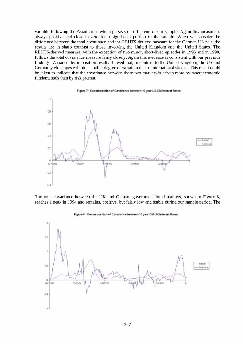
207
variable following the Asian crisis which persists until the end of our sample. Again this measure isalways positive and close to zero for a significant portion of the sample. When we consider thedifference between the total covariance and the REHTS-derived measure for the German-US pair, theresults are in sharp contrast to those involving the United Kingdom and the United States. TheREHTS-derived measure, with the exception of two minor, short-lived episodes in 1995 and in 1998,follows the total covariance measure fairly closely. Again this evidence is consistent with our previousfindings. Variance decomposition results showed that, in contrast to the United Kingdom, the US andGerman yield slopes exhibit a smaller degree of variation due to international shocks. This result couldbe taken to indicate that the covariance between these two markets is driven more by macroeconomicfundamentals than by risk premia.
The total covariance between the UK and German government bond markets, shown in Figure 8,reaches a peak in 1994 and remains, positive, but fairly low and stable during our sample period. The
208
sterling, Asian and Russian crises again seem to have had little impact upon total covariance over thisperiod. There appear to be at least three periods where the REHTS-derived covariance componentdiverges substantially from the total measure. The first of these periods occurs after the UnitedKingdom’s exit from the ERM in 1992, when the REHTS measure is strongly positive, while the totalcovariance measure remains positive, but small. This divergence suggests that the covariance betweenforeign risk premia and the REHTS measure of interest rate expectations is very negative over thisperiod and analysis of this series confirms this to be true. During 1994, when the total covariancemeasure is at its maximum, the REHTS-derived measure is negative for a period, indicating strongpositive correlations between risk premia. Finally, towards the end of our sample we see that theREHTS measure is indicating that the markets should be positively correlated while the total measureremains low, once again indicating that the risk-premia-related covariance components are negativelycorrelated with one another, and with the REHTS measure.
6. Conclusions
In this paper we examine the significance of domestic and international factors in determining theslopes of the US, German and UK yield curves, and how the magnitude of their impact fluctuates overthe business cycle. Our main finding is that at times of global financial turmoil, like the sterlingexchange rate crisis of 1992, the Asian financial crisis of 1997 and the Russian debt crisis of 1998,these slopes respond mainly to international factors, presumably as global investors reallocate theirbond portfolio holdings and local investors readjust their expectations about domestic interest rates.We also examine the decomposition of the covariances between the US, German and UK long-terminterest rates. Our decomposition of the covariance between these government bond markets indicatesthat risk premia and/or contagion effects have played an important role during these periods, movingthe covariance between the markets away from where we might have expected it to be if internationalbond rates were determined solely by the REHTS arbitrage.

209
Appendix A
The estimation of the term structure of interest rates13
The term structures of US Treasury zero coupon bonds are provided by the Bank of England. Here we
provide a brief discussion of the relevant issues. GtiP , , i=1,...,n, is the price (clean price plus accrued
interest) of an ith maturity bond at time t. The bond GtiP , pays a stream of cash flows, ijc , (including
redemption payments) at times ijm . The vector of discount bonds corresponding to the coupon-paying
bonds can be estimated from the following non-linear model:
(A1) nimcP ijj
ijijGti ,...,1),( ,, =ε+δ= ∑
where ),( ijmδ is a parametric discount function with parameter vector ),,,,,( 213210 ττββββ= .
The functional form selected by the Bank of England is based on the Svensson (1994, 1995)generalisation of the Nelson and Siegel (1987) model. According to Svensson the term structure ofzero coupon yields is given by:
(A2)
−τ
−β+
−τ
−β+
τ−β+
β=
τ−τ
−
τ−τ
−
τ−
22
11
1
23
12
11
0
/
1
/
1
/
1
),(
mm
mm
m
em
e
em
e
m
e
my
and the discount function is:
(A3)
−=δ m
mym
100
),(exp),(
Equations (A2) and (A3) are substituted in equation (A1) and the parameter vector is estimated viaa non-linear maximisation algorithm.
13
This appendix is largely based on the work undertaken by the Monetary Instruments and Markets division at the Bank ofEngland. See Bianchi (1997) and Anderson et al. (1996) for more details.

210
Appendix B
Swap market data
The most common type of interest rate swap is the fixed-to-floating par swap. This is a contractbetween two counterparties to exchange future cash flows or equivalently to exchange interest rate riskpositions. One party of the swap, namely the fixed payer, agrees to pay, on each payment day until thematurity of the swap, an amount equal to a fixed interest rate applied on a notional principal. In return,the fixed payer receives from the other counterparty, the floating payer, cash flows based on the samenotional principal but calculated with respect to a floating interest rate, e.g. Libor. The payments ofthese cash flows usually occur either annually or semiannually.
The technique used to infer the prices of zero coupon bonds from swap rates is called bootstrappingand is based on the fact that interest rate swaps are par instruments with zero net present value. In thecase of US dollars, where the swap cash flows occur annually, the prices of discount bonds implied bythe swap market are given by:
(B1)( )
ttt
ti iiit
t s
bsb
,1
11 ,0,1
,0 1
1
−
−= −
α+α−
= ∑
where ts is the swap rate, ti ,,2,1 K= and the accrual factor is ii ,1−α .14 The only problem is that
swaps are available only for one, two, three, four, five, seven and 10 years of maturity. Thus, a linearinterpolation has to be used to get an estimate of the missing swap rates.
In the case of pound sterling swaps, where the swap cash flows occur semiannually, the calculationsare slightly more complicated.15 If the swaps make semiannual payments, then we have to use swaprates every half a year in order to calculate the zero bond prices for the corresponding period. Again alinear interpolation has to be used to get an estimate of the missing swap rates. The only swap rate weare not able to calculate using linear interpolation is the 5.1s swap rate since the one-year swap rate isnot available and the corresponding one-year rate available from the money market is quoted on adifferent basis. As a result an adjustment has to be made:
(B2)1,01,5.05.0,05.0.0
1,01
1
bb
bs
α+α−
=
and 5.1s can be calculated by interpolating between 1s and 2s .
Finally, the zero bond prices can be calculated using the bootstrap method as in equation (B1) but nowthe index i in the summation is being done semiannually such that i = 1, 1.5, 2, 2.5, …, t.
Based on those zero coupon bond prices, we can estimate the implied annualised yields as:16
(B3) 11
,0
,0,0 −
=
α− t
tt b
r
14In the case of US dollar interest rate swaps, the accrual factor is defined as
360
30,1 =α − ii .
15In the case of sterling swap markets, the swap day-count convention is 365 days per year. Thus, the accrual factor is
defined as 365
1,1
−−
−=α ii
iitt
.
16The accrual factors now refer to bonds and are defined a
3651
,1−
−−
=α iiii
tt.

211
One-year forward rates can be estimated by:
(B4) 112,
12,0
,012,,0 −
=
+α−
++
mtt
mt
tmtt b
bf

212
Bibliography
Ammer, J and J Mei (1996): “Measuring international economic linkages with stock market data”.Journal of Finance, 51(5), pp. 1743-63, December.
Anderson, N, F Breedon, A Deacon, M Derry and G Murphy (1996): Estimating and interpreting theyield curve. John Wiley & Sons, London.
Bianchi, M (1997): Estimation of forward yield curves from conventional and index-linked bonds.Mimeo, Bank of England.
Campbell, J Y and J Ammer (1993): “What moves the stock and bond markets? A variancedecomposition for long-term asset returns”. Journal of Finance; 48(1), pp. 3-37, March.
Campbell, J Y and R J Shiller (1987): “Cointegration and tests of present value models”. Journal ofPolitical Economy; 95, pp. 1062-88.
Campbell, J Y and R J Shiller (1988): “Stock prices, earnings, and expected dividends”. Journal ofFinance; 43(3), pp. 661-76 July.
Christiansen, H and C Pigott (1997): “Long-term interest rates in globalised markets”. OECDWorking Paper Series, Paris.
Dahlquist, M, P Hördahl and P Sellin (1999): “Measuring international volatility spillovers”. Thisvolume.
Engle, R F, T Ito and W Lin (1990): “Meteor showers or heat waves? Heteroskedastic intra-dailyvolatility in the foreign exchange market”. Econometrica, 58, pp. 525-42.
Eun, C S and S Shim (1989): “International transmission of stock market movements”. Journal ofFinancial and Quantitative Analysis, 24, pp. 241-56.
Evans, M D D and K K Lewis (1994): “Do stationary premia explain it all? Evidence from the termstructure”. Journal of Monetary Economics, 33, pp. 285-318.
King, M A and S Wadhwani (1990): “Transmission of volatility between stock markets”. Review ofFinancial Studies, 3(1), pp. 5-33.
Koch, P D and T W Koch (1991): “Evolution in dynamic linkages across daily national stockindexes”. Journal of International Money and Finance, 10(2), pp. 231-51, June.
Koutmos, G and G G Booth (1995): “Asymmetric volatility transmission in international stockmarkets”. Journal of International Money and Finance, 14, pp. 747-62.
Lin, W, R F Engle and T Ito (1994): “Do bulls and bears move across borders? Internationaltransmission of stock returns and volatility”. Review of Financial Studies, 7, pp. 507-38.
Minton, B A (1997): “An empirical examination of basic valuation models for plain vanilla U.S.interest rate swaps”. Journal of Financial Economics, 44, pp. 251-77.
Nelson, C R and A F Siegel (1987): “Parsimonious Modeling of Yield Curves”. Journal of Business,60(4), pp. 473-89, October.
Shiller, R J, F Konya and Y Tsutsui (1991): “Investor behaviour in the October 1987 stock marketcrash: The case of Japan”. Journal of the Japanese and International Economy, 5(1), pp. 1-13, March.
Shiller, R J and A E Beltratti (1992): “Stock prices and bond yields: Can their comovements beexplained in terms of present value models?” Journal of Monetary Economics, 30(1), pp. 25-46,October.
Sims, C A (1980): “Macroeconomics and reality”. Econometrica, 48(1), pp. 1-48, January.
Solnik, B, C Boucrelle and Y Le Fur (1996): “International market correlation and volatility”.Financial Analysts’ Journal, pp. 17-34, September/October.

213
Sun, T S, S Sundaresun and C Wang (1993): “Interest rates swaps. An empirical investigation”.Journal of Financial Economics, 34, pp. 77-99.
Svensson, L (1994): “Estimating and interpreting forward rates: Sweden 1992–1994”. Working paper114, International Monetary Fund.
Svensson, L (1995): “Estimating forward rates with the extended Nelson and Siegel method”.Quarterly Review, Sveriges Riksbank.

214
Evaluating “correlation breakdowns” duringperiods of market volatility
Mico Loretan and William B English1
1. Introduction
In order to measure and manage market risks, financial analysts take account of the variability andcorrelation of the returns on assets held in their portfolios. One difficulty they encounter in doing so isthat in periods of heightened market volatility, correlations between asset returns can differsubstantially from those seen in quieter markets. The problem of “correlation breakdown” duringperiods of greater volatility is well known. For example, the former global risk manager of a majorfinancial firm notes that, “during major market events, correlations change dramatically” (Bookstaber(1997)). A recent example of this phenomenon occurred following the Russian default in August 1998.One prominent money center bank attributed larger than expected losses in late summer and early falllast year to higher volatility, illiquidity and “breakdowns in historical correlations” (JP Morgan(1999)). Indeed, a comprehensive study found that the average correlation between five-day changesin yield spreads for 26 instruments in 10 economies rose from 0.11 in the first half of 1998 to 0.37between mid-August and mid-September, but then fell back to 0.12 after mid-October (Bank forInternational Settlements (1999), Table A18).
It is tempting to explain the increased correlation of returns during hectic market periods as the resultof a shift in the joint distribution of asset returns owing to contagion of some markets by others, theparticular nature of the shocks, or changes in market structures and practices.2 However, unless onehas a model of when such periods are likely to arise, or at least how often, and what particular patternof correlations will ensue, this approach makes it extraordinarily difficult to manage risk because therelationship between asset returns in some future situations is essentially unknown.3
Moreover, the inference that changes in measured correlations imply that the joint distribution of assetreturns changes in volatile periods may not be warranted. Even if the behavior of asset returns isgoverned by an unchanged process, one would expect a link between volatility and measures ofcorrelation. Indeed, a model of asset returns as simple as the bivariate normal can explain why periodsof increased (sampling) volatility will also be periods of relatively high (sampling) correlations. Thepossible importance for economics and finance of this result has only been realized recently(Ronn (1995); Boyer, Gibson and Loretan (1999); Forbes and Rigobon (1999)).4 In this paper, wedemonstrate that a significant portion of shifts in correlations over time – including those that occurredin the fall of 1998 – may reflect nothing more than the predictable effect of differences in samplevolatilities on measured correlations, rather than breaks in the data generating process for asset returns.
To explore this possibility, we select three asset classes – equities, bonds and foreign exchange – intwo representative countries and look at the quarterly correlations between daily returns over the
1 The analysis and conclusions in this paper are those of the authors and do not indicate concurrence by other members of
the research staff, by the Board of Governors, or by the Federal Reserve Banks. We thank Jim Clouse, Mike Gibson,Michael Gordy, Brian Madigan, Matt Prisker and Vince Reinhart for helpful comments and discussions. All remainingerrors are ours.
2Recent discussions of possible routes for contagion include Drazen (1998), Eichengreen, Rose and Wyplosz (1996) andGerlach and Smets (1995). The CGFS report on the events of the fall of 1998 (Bank for International Settlements (1999))presents a narrative account of how the effects of shocks were reinforced and spread to other markets by market practices.
3One advance along these lines is the structural model of contagion-like transmission of shocks presented in Kodres andPritsker (1999).
4Ronn (1995) attributes the insight to a conference discussion by Stambaugh.
215
1990s. Our calculations suggest that quarters with high correlations tend also to be quarters withhigher than average volatility. Moreover, actual correlations during periods of relatively high volatilityappear to be fairly close to the correlations one would expect conditional on the level of volatility andbased on an unchanged process for asset returns. Our findings generalize the results reported for stockprices in Forbes and Rigobon (1999), and suggest that correlation breakdowns may reflect time-varying volatility of financial markets rather than a change in the relationships between asset returns.
Since the link between market volatility and in-sample correlations between asset prices appears to beempirically important, we go on to consider the implications of this link for risk managementpractices, the supervision of financial firms and the conduct of monetary policy. We note that the useof data for a relatively short period when calculating correlations for use in risk management modelsmay lead to poor measurements of market risks. We also point to the need to use appropriateconditional correlations when examining the riskiness of a portfolio under high volatility scenarios.Finally, because monetary policy can affect the volatility of markets, monetary policymakers may findit useful to incorporate the effect of unexpected changes in policy on market participants’ assessmentof their risk exposures. Indeed, some monetary policymakers may, in practice, make this link: there issome evidence that monetary policy in the United States was initially adjusted relatively slowly inearly 1994 because of concern that the long period of interest rate stability that preceded the rate hikehad led some market participants to underestimate the riskiness of their positions.
2. The theoretical link between volatility and correlation
To see the link between volatility and correlation, consider the unrealistically simple case of tworandom variables, x and y, that are independently and identically distributed bivariate normal, withmeans equal to zero, variances equal to unity and a correlation of 0.5. A large sample of draws of such(x,y) pairs is shown in Figure 1. Now consider splitting the full sample into two subsamples based onthe value of x: a “low volatility” subsample, including all (x,y) pairs with an absolute value of x lessthan 1.96; and a “high volatility” subsample, including all (x,y) pairs with an absolute value of xgreater than or equal to 1.96.5 Intuitively, the effect of trimming the ends off the joint distribution inthe low volatility subsample should be to reduce the sample correlation between x and y. By contrast,the correlation for the high volatility subsample should be enhanced because the support of itsdistribution is disjointed, with one portion picking up the large positive values of both variables whilethe other portion of the distribution picks up the large negative values of the variables. Indeed, asnoted in the figure, the correlation for the high volatility subsample is 0.81, while that for the lowvolatility sample is 0.45. Note that the correlation in the latter subsample is close to the populationvalue of 0.5; this latter result may not be surprising since the low volatility subsample includes 95% ofthe data.
2.1 Theoretical result
This intuitive result can be derived formally. Boyer, Gibson and Loretan (1999) provide the followingtheorem:
Theorem: consider a pair of bivariate normal random variables x and yZLWKYDULDQFHV x2 DQG y
2 ,respectively, and covariance xy/HW xy/( x y)) be the unconditional correlation between x and y.The correlation between x and y conditional on an event x∈A, for any A⊂ with 0 < Prob(A) < 1, isgiven by:
(1) )A)Var(x|x
Var(x))-( + ( = -‰22
A ∈ρρρρ 1
5
The marginal distributions of x and y are (univariate) standard normal, hence Prob(|x|>1.96) is equal to 0.05.
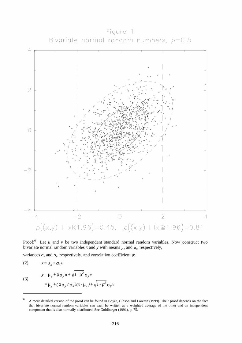
216
Proof:6 Let u and v be two independent standard normal random variables. Now construct twobivariate normal random variables x and y with means x and y, respectively,
variances x and yUHVSHFWLYHO\DQGFRUUHODWLRQFRHIILFLHQW
(2) u + = x xx σµ
(3)v-1 + )-)(x/( + =
v-1 +u + =y
y2
xxyy
y2
yy
σρµσσρµ
σρσρµ
6
A more detailed version of the proof can be found in Boyer, Gibson and Loretan (1999). Their proof depends on the factthat bivariate normal random variables can each be written as a weighted average of the other and an independentcomponent that is also normally distributed. See Goldberger (1991), p. 75.
217
Consider any event x∈A such that 0 < Prob(x∈A) < 1. By definition, the conditional correlationcoefficient between x and y, A, is given by:
(4)A)x|Var(y A)x|Var(x
A)x|yCov(x, = A ∈∈
∈ρ
By substituting for u in (3) using equation (2), then substituting the resulting expression for y into (4),and using the fact that x and v are independent by construction, one can rewrite this as:
(5)σρ∈σσρ∈
∈σσρρ
2y
22x
2y
2
xyA
)-( + A)x|)Var(x/( A)x|Var(x
A)x|)Var(x/( =
1
which can, in turn, be simplified to yield the expression in (1).
Thus, the conditional correlation between x and y LV ODUJHU VPDOOHU WKDQ LQ DEVROXWH YDOXH LI WKHconditional variance of x given x∈A is larger (smaller) than the unconditional variance of x.7
2.2 Some generalizations
This theorem is based on several assumptions that are unrealistic in empirical practice, such as that thedata are i.i.d. and are drawn from a bivariate normal distribution. In the present case, bivariatenormality of x and y is used – see equation (3) in the proof above – only to re-express the variable y as
an affine function of x y + ( y/ x)(x- x), plus a component that is independent of x, νσρ 2y
2-1 .
Therefore, the main result of the theorem is not limited to cases where the data are bivariate normal,but holds in any situation where y can be stated as a linear (or, more generally, an affine) function of xplus an independent component (the “error term”), a framework which encompasses the familiarbivariate linear regression model with independent (but not necessarily normally distributed) errors.
Economic data are often observed as time series, and it is of interest to understand how measuredcorrelations are affected by sampling variability in the data. Time series also pose the question of howserial dependence in the data affects the correlations. Assuming the general linear regression model,y = xt + ut , with Cov(xt ,ut ) = 0 and t = 1,2,…, one may write the sampling correlation coefficientbetween x and y, for a sample of size n, as
(6) (y)Var(x)Var
y)(x,Cov = y)(x,Corrnn
nn
which can be rewritten as
(7) u)(x,Cov + (u)Var + (x)Var (x)Var
u)(x,Cov + (x)Var =y)(x,Corrnnn
2n
nnn
ββ
β
where the subscript n denotes sampling, as opposed to population, moments.8
Of primary interest to our paper is how this correlation coefficient will vary across subsamples oftime. It will differ from the population moment for two reasons: the sampling covariance between xt
7
Henri Pagès has provided the following heuristic interpretation of the result given in (1): if conditioning on an event x∈Abrings about an increase in the conditional variance of x, Var(x| x0A), it also raises the population conditional correlationbetween x and y because of a concomitant increase in the ratio Var(x|x0A)/Var(x), which can be rewritten as(Var(v)/Var(x))(Var(x|x0A)/Var(v), where the first term is a constant and the second term is a signal to noise ratio; it isthis increase in the signal to noise ratio that raises the conditional correlation.
8 7KH FRQQHFWLRQ IURP HTXDWLRQ WR LV PDGH E\ VHWWLQJ y/ x and ut= νσρ ty2 -1 , and by dividing the
numerator and denominator on the right-hand side of (6) by Var(x) x2, the population unconditional variance of x.

218
and the “error” term ut may be non-zero, or the sampling variance of ut may be time-varying (andcorrelated with Varn (x)).
In financial time series, we often find that the mean of yt is close to a linear function of xt, and thatCovn (xt ,ut ) ≈ 0 is a reasonable assumption to make. However, even if the levels of x and u areapproximately uncorrelated, their variances may well be serially, as well as contemporaneously,correlated. Hence, the term Varn (u) may move systematically across subsamples with the samplingvariance of x6XSSRVHIRUH[DPSOH WKDW > 0 and that the contemporaneous volatilities of x and u(and hence the contemporaneous volatilities of x and y) are positively correlated. Then, time intervalsexhibiting a high sampling variability of x will also tend to have larger than average values for Varn
(u). As a result, the sampling correlation between x and y will tend to deviate less from its populationvalue, on average, than would be suggested by equation (1). (The possible practical importance ofcontemporaneous dependence in volatilities is discussed below; see footnote 17.)
While the preceding discussion establishes that the simple expression stated in equation (1) for therelationship between conditional and unconditional correlations may have to be modified suitablywhen some of the maintained assumptions of the theorem are not met by the data, it is clear thatconditioning on volatility will, in general, have strong systematic effects on the correlation between xand y.
2.3 A simple example
As an example of a time series application of that theorem, consider subdividing a bivariate time series(xt ,yt) that is observed daily into equally sized subsamples (“quarters”) of 60 daily observations each,and then ordering the quarters by the level of the within-quarter variance of x. For each subsample, wemay also calculate the correlation between x and y. Table 1 shows the results of such an exercise underthe assumption that x and y are i.i.d. bivariate normal with unit variances and a population correlationcoefficient equal to 0.5 (as in Figure 1). The rows of the table show ranges for the ratio of the quarterlyvariance in x to its population value, while the columns show the distribution of the values of thequarterly correlation given the ranges. For values of the within-quarter variance of x close to itspopulation value (0.9 to 1.1), the median value of the correlation is 0.50, although the range of valuesis fairly wide, with a 90% confidence interval running from 0.34 to 0.64. However, for quarters within-sample variance of x between 1.7 and 1.9 times the population value, the median correlation is 0.61,with the 90% confidence interval running from 0.48 to 0.72.
Table 1In-sample correlations when conditioning on volatility
Conditional correlation of x and yRange of variances of xrelative to itspopulation value Bottom 5% Median Top 5%
0.3–0.5 0.17 0.36 0.53
0.5–0.7 0.24 0.43 0.58
0.7–0.9 0.29 0.47 0.61
0.9–1.1 0.34 0.50 0.64
1.1–1.3 0.38 0.54 0.67
1.3–1.5 0.41 0.57 0.69
1.5–1.7 0.45 0.59 0.71
1.7–1.9 0.48 0.61 0.72
Note: The values of x and y are i.i.d. bivariate normal with a population correlation of 0.5. Reported values for theCorr(x,y) are based on 2.5 million random draws of 60 observations (“quarters”). There were too few observations withthe variance of x less than 0.3 or greater than 1.9 times its population value for values of Corr(x,y) to be reported withconfidence.

219
3. An empirical application
3.1 The data
In order to assess the empirical importance of the relationship between volatility and correlation overtime, we need to study specific pairs of asset prices. We consider a relatively broad set of assets, ratherthan focus on a single type of asset (e.g. equity prices, as in Forbes and Rigobon (1999)). As shown inTable 2, we settled on equities, bonds and foreign exchange. The Financial Times and DAX stockprice indexes are as of the close of the stock markets in London and Frankfurt, respectively, and aretaken from Bloomberg. The German and British government bond yields are those on 10-yearinstruments. They are also as of market close and are from Bloomberg. The dollar/mark and dollar/yenexchange rates are those prevailing around noon in the New York market and are collected by FederalReserve staff. We selected these particular series because they represent large and liquid markets andthe data reflect market conditions at roughly the same time, and so we do not have to be concernedabout the implications of non-synchronous data collection.9
Table 2Data series used
Asset prices Quote time Quote location Source
Equity pricesFinancial Times 100DAX
Market closeMarket close
LondonFrankfurt
BloombergBloomberg
Government bond yieldsUK 10-year noteGerman 10-year note
Market closeMarket close
LondonFrankfurt
BloombergBloomberg
Exchange ratesUS dollar / Japanese yenUS dollar / Deutsche mark
About noon New York timeAbout noon New York time
New YorkNew York
Federal ReserveFederal Reserve
Note: The London and Frankfurt markets now close at the same time, although in the past their closing times havediffered by one hour.
The returns on foreign exchange and equity holdings are simply the daily percentage changes in theirrespective prices. Calculating the returns on government bonds is more complicated, since theavailable data relate to bond yields rather than bond prices. The return we use is an estimate of thepercentage daily gain or loss from holding the 10-year bellwether government bonds, based on thereported yields and under the assumption that the bonds have maturities of exactly 10 years, havecoupon payments twice a year, and are trading at par.10
Figures 2–4 show time series plots of the within-quarter variances (panels a and b) and correlations(panel c) of daily returns for the three pairs of assets. In the case of stock prices (Figure 2), it is clearthat last fall was a period of high volatility and, just as the theorem presented earlier would suggest,there was a high correlation between the two returns. The returns on bond investments were alsosomewhat volatile last fall (Figure 3), and the correlation between the two returns in 1998 Q3 and1998 Q4 was at the high end of its range. By contrast, movements in the dollar/yen and dollar/mark
9
For a discussion of the problems associated with non-synchronous data collection, see RiskMetrics (1996), pp. 184–96.
10The approximation is excellent for small changes in yields on bonds trading near par. Even for large movements in yieldson bonds priced far from par, the approximation is fairly good. For example, on October 9, 1998 (the day of the largestone-day loss on UK bonds in the sample), the UK 10-year bond maturing in October 2008 was selling near 130. Based onbond price and yield data from the Financial Times, the actual loss on the bond for that day was 2.33%, while theapproximation yields a loss of 2.55%.

220
exchange rates were not particularly highly correlated last fall (Figure 4), despite the extraordinarilyhigh volatility in the dollar/yen rate in 1998 Q4.

221

222
3.2 Using the theorem
Before using the theorem to try to explain the variation in quarterly correlations between returns, weneed to examine whether the data satisfy its assumptions to ensure that its use is appropriate. Then, foreach pair of returns, we need to determine the anticipated relationship between volatility and
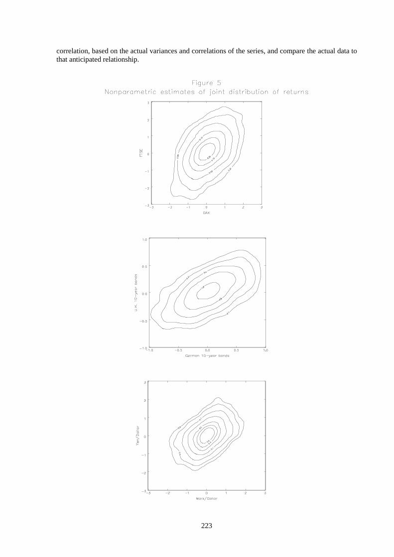
223
correlation, based on the actual variances and correlations of the series, and compare the actual data tothat anticipated relationship.

224
Figure 5 shows non-parametrically estimated level curves of the joint distributions of the pairs of assetreturns.11 These concentric curves are loci of constant height of the joint densities, and so they showthe shape of the distribution of the observations. Recall that the theorem’s main requirements are thoseof a linear regression model, which are satisfied if the joint distribution of the data is elliptic, that is, ifthe level curves of the joint density are ellipses (see Spanos (1986), pp. 457–8). The estimated levelcurves appear to be reasonably close to elliptic, although those for the exchange rates are somewhatmore “rectangular” than the other two sets. We view these level curves as suggesting that theassumption of an elliptical distribution is reasonable for our empirical work, and hence that it isworthwhile to proceed comparing the empirical variance/correlation pairs with values predicted bythat theorem.
To evaluate the importance of the theoretical link between volatility and correlation, we plot inFigure 6 the quarterly in-sample correlations against the in-sample volatility of one of the two assetreturns.12 In all three cases, a generally increasing relationship between conditional variances andconditional correlations is observable. However, the data also show a considerable dispersion in the in-sample correlation for a given level of volatility. In order to assess how close the points are to thelocations indicated by the theorem, we also show in Figure 6 the theoretical relationship between assetreturn volatility and the correlation between asset returns, the dashed line (derived from equation (1)),and a 90% confidence contour around this theoretical locus, derived under the maintained assumptionsthat the data are i.i.d. bivariate normal, and that the population correlation is equal to the full-sampleempirical correlation.13
The theoretical relationships appear to fit the data fairly well. In the case of equity prices, the increasein correlation late last year was very large and, as shown by the two points to the top right in the chart,these relatively high correlations were roughly consistent with what the theorem would lead one toexpect given the increase in volatility at that time. The events of last fall left a much smaller imprinton the correlations between returns on government bonds and foreign exchange. In the case of foreignexchange, this may not be surprising given that the volatility of the dollar/mark exchange rate was notelevated. Over the entire period plotted, however, the empirical relationship between volatility andcorrelation seems to fit the theorem fairly well, although, in the case of the bond and foreign exchangereturns, the fractions of observations falling outside the 90% confidence contours considerably exceed10%.14
However, the stated 90% confidence intervals in Figure 6 will not be correct if the data are not wellapproximated by a bivariate normal distribution. For example, it is well known that the (unconditional)distribution of asset returns is strongly leptokurtic, resulting in far more “outlier” observations thanone would expect under normality.15 One way to obtain improved confidence intervals is to use abootstrap. We select random samples of a quarter’s worth of observations (60 pairs of returns) from
11
The non-parametric estimates of the joint densities are based on a bivariate normal kernel and a standard window width(Silverman (1986), pp. 86–7).
12The correlations could be plotted relative to the volatility of either return, but we have chosen the volatility of the Germanasset as the variable for the x-axis in all three cases. While this choice is immaterial theoretically, in the cases of the bondand foreign exchange returns, the results are somewhat better when the German asset volatility is selected. Note that thevariances of the German asset returns have been expressed relative to their full-sample values.
13Ronn (1995) plots average measures of comovement stratified by volatility for a number of interest rate measures and(separately) for a large number of US equity prices. He finds that, consistent with the theorem, large moves in asset pricesare associated with a higher average degree of comovement. However, he does not try to match the empiricalrelationships with those implied by the theorem.
14The confidence contours are shown over a relatively narrow range of quarterly variances because, under the assumptionof an i.i.d. bivariate normal distribution of returns, there are too few observations outside this range (given our choice of2.5 million repetitions) to allow the calculation of confidence intervals. The number of points on the left and right of theconfidence contours shown reflects the fact that the actual distribution of returns has fatter tails than does the normal,resulting in greater dispersion of sampling variances.
15See, for example, Mandelbrot (1963). For more recent discussions, see Jansen and de Vries (1991) and Loretan andPhillips (1994).
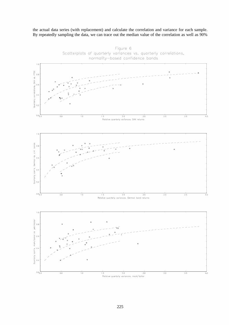
225
the actual data series (with replacement) and calculate the correlation and variance for each sample.By repeatedly sampling the data, we can trace out the median value of the correlation as well as 90%

226
confidence intervals based on the actual distributions of the data series.16 These Monte Carlo resultsare shown in Figure 7.
16
This bootstrap procedure preserves the contemporaneous correlation structure of the data, as well as the unconditionallyheavy-tailed nature of the distributions, but it does not take account of serial dependence features such as GARCH which,as discussed in footnote 14, appear to be present in the data.
227
The improved methodology yields confidence contours that encompass a larger fraction of thequarterly data points.17 It appears that the equity data fit the theory relatively well, with only three ofthe 34 observations outside the 90% confidence contours. The bond return volatilities and correlationsalso appear to be roughly what one would expect given the theorem, although with some evidence of alarger than expected clustering of observations to the upper left of the chart. The foreign exchangereturns generally match the upward slope predicted by the theorem, but the range of correlations stillappears to be considerably wider than would be expected. The three outlier observations at the top ofthis panel are from 1994 Q4 to 1995 Q3, that is, the period during and after the Mexican crisis ofDecember 1994. The location of these points may suggest that the sharp fluctuations of the dollaragainst the mark and yen that occurred following the Mexican crisis, and the associated increase in thecorrelation of these asset returns relative to long-term norms, may have been caused by a genuine,though temporary, change in the data generating process.18 For example, there were several episodesof concerted central bank intervention during this period, which would tend to boost daily correlationsirrespective of changes in within-quarter volatility.
3.3 Summary
While there is some evidence in the case of foreign exchange suggesting the possibility of a temporarychange in correlations following the Mexican crisis in late 1994, in general the link between highmarket volatility and high correlations between asset returns is remarkably close to what the theoremwould suggest.19 While a more comprehensive test of the proposition of stationarity, including abroader array of asset prices, is beyond the scope of this paper, our results suggest that one should notbe too quick to conclude that correlation breakdowns, including those observed last year, representtrue changes in the distribution of asset returns. Rather, they may be nothing more than the predictableconsequences of observing certain (low probability) draws from an unchanged distribution. Theseresults need not imply that “contagion” does not occur; rather, they suggest that if one definescontagion to mean elevated correlations between asset returns, then contagion is a natural by-productof temporal variation in volatilities.
3.4 Implications
The statistical link between the volatility and correlation of asset returns discussed here has importantimplications for the evaluation of portfolio risk by market participants and investors, for thesupervision of financial firms’ risk management practices, and for monetary policy.
In empirical practice, risk managers sometimes use data from a relatively short interval whencalculating correlations and volatilities for use in risk management models. For example, one majorbanking company reports that they use the most recent 264 trading days’ changes in market prices intheir calculations of value at risk, or VaR (Chase Manhattan (1999), p. 36). RiskMetrics uses 550 daily
17
The bootstrap also reveals that the location of the median correlation coefficient, for a given value of Varn (x)/Var(x), is(slightly) below the value predicted by equation 1 when Varn(x)/Var(x) is large, say greater than 2.5. This finding isconsistent with our conjecture, advanced in Section 2 above, that a positive contemporaneous correlation between thevolatilities of x and u could bring about lower bivariate correlations between the returns, on average, than the equationwould suggest whenever Varn(x) – and hence Varn(u) – is large. We caution that the discrepancy we detect between thebootstrapped median value and the value predicted by equation (1) for the (subsample) correlations is quite small in allcases, and does not exceed 0.05. Hence, while the dependence between volatilities may bring about a slight deviationfrom the relationship stated in equation (1), the equation is still very useful for predicting the average location of thesubsample correlations.
18Recall also that the estimated joint distribution of returns on foreign exchange shown in Figure 5 appeared to be lesselliptical than those of the equity and bond returns.
19Our results are based on the volatility of asset returns with no distinction made between increases and decreases. In arelated study, Longin and Solnik (1998) find that measured correlations between equity returns in different countriesbehave as the theorem would suggest when there are large positive stock market returns but are higher than the theoremwould suggest when there are large negative returns. We leave an examination of this issue for future research.
228
return observations in the calculation of variances and correlations of returns, but becauseexponentially declining weights are applied, the effective number of daily returns employed is just 75for estimates of daily correlations and volatilities and 150 for monthly values (RiskMetrics (1996),Table 5.9, p. 100). The use of a relatively short period for these calculations has some desirablefeatures. Since financial markets can change over time, one may not want to depend on data from thedistant past.20 Moreover, the emphasis RiskMetrics puts on recent data allows it to take account oftime-varying volatility, which appears to be a feature of actual returns (RiskMetrics (1996), pp. 55 and79–80).
Nonetheless, the theoretical and empirical results presented here suggest that the use of a relativelyshort interval of data for estimating correlations and volatilities may be dangerous. If the interval istypically stable, then not only may the estimated volatilities be too low, depending on whether theassumed level of exponential decay captures the autocorrelation in volatility correctly, but, perhapsmore importantly, the estimated correlations between returns will be lower than average. As a result,assessments of market risk may overstate the amount of diversification in a portfolio, leading theinvesting firm to take on excessive risk. Conversely, if the interval of data employed is a relativelyvolatile one, then the resulting estimates of correlations will be atypically high, and could lead the firmto take positions that are excessively risk-averse.
Another way in which the link between in-sample volatility and correlation could cause problems forrisk managers is in the calculation of worst case scenarios and in stress testing. Put simply, riskmanagers should not consider the possible effects of a period of high volatility without also taking intoaccount the likely effect that elevated volatility would have on the correlations between asset returns(see Ronn (1995), for a related discussion). Instead, risk managers may need to include informationfrom historical periods of high volatility to form estimates of correlations conditional on theheightened volatility.21 These conditional correlations could then be used to evaluate the likelydistribution of returns under a high volatility scenario. Put differently, the method used for stresstesting a model must not (inadvertently) exclude the feature that periods of high volatility will also beperiods of elevated correlations.
Supervisors of financial institutions also need to be aware of the link between volatilities andcorrelations when assessing firms’ risk management. For example, under Federal Reserve regulations,an institution applying the market risk capital rules must hold capital based on its internal model’sestimates of VaR. The internal model must be based on a minimum observation period of one year,and must be subjected to stress tests appropriate to the institution’s particular situation. The VaRcalculation should be based on a 99% (one-tailed) confidence level of estimated maximum loss(Federal Reserve (1999), pp. 11–2). In evaluating such internal models, supervisors need to keep inmind the difficulties noted earlier with relying on a relatively short interval of data for information oncorrelations and the need to form appropriate conditional correlations for stress tests.
Finally, monetary policymakers may also need to be aware of the link between volatility andcorrelations. Most obviously, correlation breakdowns during periods of financial market turbulencecould lead policymakers to reassess the stance of policy in light of the apparent shift in correlations.So long as in-sample changes in correlations only reflect the movements in volatility, however, suchreassessment would not be warranted unless private agents’ adjustments to the volatility made achange in the stance of monetary policy desirable.
Perhaps more importantly, changes in the stance of monetary policy, particularly if they follow anextended period during which policy has remained unchanged, have the potential to cause volatility infinancial markets to increase. Since such an increase in volatility is likely to be associated with
20
Similarly, if the assets under consideration are firm-specific (rather than indexes), the behavior of firms can change overtime as managers or business strategies are changed, making older information less useful.
21Alternatively, firms might want to use actual data from earlier periods of high volatility to stress test their portfolios.Chase Manhattan indicates that they use asset price movements during the bond market sell-off in 1994, the 1994Mexican peso crisis and the 1997 Asian markets crisis, as well as internally developed scenarios, when assessing the riskof their portfolio (Chase Manhattan (1999), p. 37).

229
increases in correlations between asset returns, a change in policy could impose substantialunanticipated risks on market participants if – as discussed earlier – their risk management were basedon movements in asset prices during the previous period of relative stability. The resulting adjustmentsof portfolios by the affected firms could generate outsize effects of policy on asset prices.22 Theserelatively large effects may lead policymakers to move more gradually than they otherwise would insuch situations, providing a possible explanation for the interest rate smoothing behavior noted bySack and Wieland (forthcoming). Moreover, uncertainties about the size and timing of such portfolioadjustments would make the likely effects of policy more difficult than usual to assess. Thisuncertainty would also suggest that a gradual approach would be desirable (Brainard (1967)).23
Indeed, the Federal Reserve found that its tightening of monetary policy in 1994, which followed asubstantial period of unchanged policy, led market participants to trim their risk profiles. It noted thatuncertainty about the policy outlook, as well as “the capital losses following the tightenings,encouraged investors to shorten the maturity of their investments and reduce their degree of leverage”(Federal Reserve (1995), pp. 21–2). While this reaction may only have reflected the revision of overlyoptimistic beliefs about monetary policy and market volatility, it is also what one would expect tohappen if the increase in volatility by itself caused correlations between asset returns to increase.There is some evidence that this was the case; for example, Bankers Trust indicated in its 1994 annualreport that movements in interest rates in early 1994 (and also at the end of 1994, when the Mexicanpeso devaluation occurred) were “unusual in the degree to which interest rates across internationalmarkets moved together” (Bankers Trust (1995), p. 23).24 It went on to note that “this phenomenon ofincreased correlation among interest rates reduced the risk management benefits derived fromdiversification across interest-sensitive instruments” (Bankers Trust (1995), p. 23). The bankresponded to this unexpected situation by withdrawing from substantial market positions (BankersTrust (1995), p. 24).
In fact, the possibility that a change in monetary policy could affect market volatility and correlations,and thereby influence the desired risk profiles of market participants, may have been taken intoaccount by the Federal Reserve. In its discussion of the 1994 tightening, the February 1995Humphrey-Hawkins report noted that:
“The FOMC, at its meeting in early February 1994, agreed that policy should be moved to a lessstimulative stance. The pace at which the adjustment to policy should be made was less clear: A rapidshift in policy stance would minimise the risk of allowing inflation pressures to build, while a moregradual move would allow financial markets time to adjust to the changed environment. Althoughmany market participants seemed to anticipate a firming move fairly soon … some investors wouldundoubtedly reconsider their portfolio strategies.” (Federal Reserve (1995), p. 21).
Taking account of these factors, the FOMC agreed to move slowly at first. As a result, the first threepolicy moves were relatively small (25 basis points), and spread over three months. However, theFederal Reserve also reported that “once market participants seemed to have made substantialadjustments to the new direction of policy, a larger tightening move [of 50 basis points] wasimplemented in May” (Federal Reserve (1995), p. 21).
22
This mechanism could provide an alternative explanation for the larger effects on asset prices of monetary policy movesthat represent a change in the direction of policy, noted by Goodfriend (1991).
23In addition, these effects could be reduced by increased transparency about the outlook for policy in advance of a policymove.
24The effect of increased volatility on conditional correlations is, of course, only one possible reason for the increase incorrelations of asset returns at this time. For example, a structural model of asset returns might suggest that changes inmonetary policy should generate relatively highly correlated movements in many asset prices.

230
Bibliography
Bank for International Settlements, Committee on the Global Financial System (1999): A Review ofFinancial Market Events in Autumn 1998. Basel, October.
Bankers Trust (1994): Annual Report 1994. New York.
Bookstaber, Richard (1997): “Global Risk Management: Are We Missing the Point?” Journal ofPortfolio Management, pp. 102–7.
Boyer, Brian H, Michael S Gibson and Mico Loretan (1999): “Pitfalls in Tests for Changes inCorrelations”. Federal Reserve Board, IFS Discussion Paper, No. 597R, March.
Brainard, William (1967): “Uncertainty and the Effectiveness of Policy”. American Economic Review,Papers and Proceedings, Vol. 57, pp. 411–25.
Chase Manhattan Corp. (1999): Annual Report 1998. New York.
Drazen, Alan (1998): “Political Contagion in Currency Crises”. Mimeo, University of Maryland.
Eichengreen, Barry, Andrew Rose and C Wyplosz (1996): “Contagious Currency Crises”. NBERWorking Paper, No. 5681.
Forbes, Kristin and Roberto Rigobon (1999): “No Contagion, Only Interdependence: Measuring stockmarket co-movements”. NBER Working Paper, No. 7267, July.
Federal Reserve Board (1995): Monetary Policy Report to the Congress Pursuant to the FullEmployment and Balanced Growth Act of 1978. February 21.
Federal Reserve Board (1999): Trading and Capital Markets Activities Manual: Capital Adequacy.Washington, D.C.
Gerlach, Stefan and Frank Smets (1995): “Contagious Speculative Attacks”. European Journal ofPolitical Economy.
Goldberger, Arthur S (1991): A Course in Econometrics. Cambridge, MA: Harvard University Press.
Goodfriend, Marvin (1991): “Interest Rates and the Conduct of Monetary Policy”. Carnegie-Rochester Conference Series on Public Policy, Vol. 34, pp. 7–30.
JP Morgan and Co. (1999): Annual Report 1998. New York.
Jansen, D W and C G de Vries (1991): “On the Frequency of Large Stock Returns: Putting Booms andBusts into Perspective”. Review of Economics and Statistics, Vol. 73, pp. 18–24.
Kodres, Laura E and Matthew Pritsker (1999): “A Rational Expectations Model of FinancialContagion”. Mimeo, Federal Reserve Board.
Longin, François and Bruno Solnik (1998): “Correlation Structure of International Equity MarketsDuring Extremely Volatile Periods”. Mimeo, Group HEC.
Loretan, Mico and Peter C B Phillips (1994): “Testing the Covariance Stationarity of Heavy-TailedTime Series”. Journal of Empirical Finance, Vol. 1, pp. 211–48.
Mandelbrot, B B (1963): “The Variation of Certain Speculative Prices”. Journal of Business, Vol. 36,pp. 394–419.
RiskMetrics (1996): RiskMetrics–Technical Document. 4th ed. New York: JP Morgan/Reuters.
Ronn, Ehud I (1995): “The Impact of Large Changes in Asset Prices on Intra-Market Correlations inthe Stock and Bond Markets”. Mimeo, Department of Finance, University of Texas at Austin.
Sack, Brian and Volker Wieland: “Interest-Rate Smoothing and Optimal Monetary Policy: A Reviewof Recent Empirical Evidence”. Journal of Economics and Business (forthcoming).

231
Silverman, B W (1986): Density Estimation for Statistics and Data Analysis. London: Chapman andHall.
Spanos, Aris (1986): Statistical Foundations of Econometric Modelling. Cambridge: CambridgeUniversity Press.
232
Asset price crises and banking crises:some empirical evidence
Anne Vila1
1. Introduction
The aim of this paper is to see whether, for a range of countries and time periods, there is anysystematic relationship between stock market collapses and banking system crises. This is intended tobe a first step in a larger study, one which aims ultimately to see whether asset price movements haveany implications for the stability of the banking system in developed countries. The present paper,however, largely confines itself to an atheoretical examination of the data, so as to explore what thereis to be explained. Three decades of equity and banking data, drawn from 14 countries, are examined.
Three questions in particular are put to these data. First, is there any evidence of association betweenstock market crashes and banking crises? Second, insofar as there is any association, does the depth orthe length of stock market falls affect the severity of banking sector problems? Third, have the sizeand frequency of either stock market crashes or banking crises shown any sign of varying over time?
With this paper, we hope to contribute to the debate on the role of central banks with respect to assetprice volatility. While it is generally acknowledged that central banks should focus in the first instanceon price stability in product markets, there is now a growing acceptance that they should at leastmonitor price developments in asset markets.2 One reason for doing so is that asset prices can affectaggregate demand directly or via the balance sheet channel (i.e. through their effects on household andbusiness balance sheets). A second reason is that overvaluation in asset markets could lead to financialfragility. In particular, there is widespread concern that the growth of asset price bubbles and theirsubsequent bursting could create systemic risk. A third reason for central banks to be concerned aboutasset price volatility is that this may be a manifestation of poorly implemented financial reforms thatlead to excessive lending and risk-taking, and to asset price booms and subsequent collapses.3
Financial institutions in particular are vulnerable to asset price collapses, because of the decline in thevalue of collateral they hold, and also because of the general increase in uncertainty that may lead to aflight to quality and to a widespread reduction in lending that could affect even solvent financialinstitutions.4 If asset price collapses were to lead to bank failures, further financial stability problemscould arise as a result of contagion. This in turn could lead to business failures, unemployment and afully fledged economic downturn. Moreover, the costs associated with banking crises are high, both interms of declines in real output and in terms of transfers from the public to distressed banks and theircreditors (Kaufman (1999)). For example, recent research by the IMF (1998) into the occurrence ofbanking crises estimates that the cumulative actual and potential losses in output associated with 54banking crises across developed and emerging markets (pre-dating the Asia crisis) averaged 11.6% ofGDP.
1
Financial Intermediaries Division, Bank of England. Comments from Phil Davis, Ian Michael, Paul Tucker, GeoffreyWood and from participants of a Bank of England financial stability workshop and from the BIS autumn meeting ofcentral bank ecomonists greatly improved the present paper. I also thank Faysal Maruf for his outstanding researchassistance. The views expressed in this paper are mine and not necessarily those of the Bank of England. Any errors andomissions are of course my own.
2See, for example, Greenspan (1999), Vickers (1999), Bernanke and Gertler (1999) and Gertler et al. (1998).
3See, for example, Borio et al. (1994) and Schinasi and Hargraves (1993).
4See, for example, Kaufman (1998).

233
Recently, significant progress has been made towards studying the relationship between banking andcurrency crises in a more systematic way.5 In contrast, the study of the relationship between bankingand equity crises is largely limited to case studies. Hence, we do not know whether banking crisessystematically precede or follow equity market crises. Likewise, we do not know how severe a crisishas to be in order to spill over into other parts of the financial sector. As a result, we remain quiteuncertain when asked to define the financial stability consequences of a sharp fall in equity valuations.
The main results of this paper can be summarised as follows. First, we do not find any evidence of asystematic association between equity market crises and banking crises within countries. In particular,we cannot establish that equity price collapses necessarily lead to banking crises. Second, we find thatif there is an association, the length or severity of the equity price decline is irrelevant. Third, we findthat both equity market and banking crises have become less severe over time: crises in the 1970swere on average longer and led, in the case of the former, to bigger price falls than in the followingdecades. Fourth, we cannot establish that periods of large stock market increases are more likely tolead to simultaneous crises in either the equity market or the banking sector.
When looking at the effect of banking crises on the equity market, we observe mixed evidence ofbanking crises leading to large equity price falls. But we cannot conclude that banking crisessystematically cause large-scale liquidations of equity. Finally, we find weak evidence of increasedbank lending prior to equity market crises.
The paper further illustrates the difficulty of accurately measuring banking crises. Qualitativemeasures used in the currency crisis literature are not without flaws, yet alternative measures proposedin the present paper turn out to be inconsistent with existing measures in several instances. This in turnaffects the observed relationship between banking and equity market crises.
The remainder of the paper is organised as follows. In Section 2, we review the recent literature on therelationship between asset market crises and banking crises. Then in Section 3, the data are outlined,and the method by which equity market crises and banking crises can be identified are set out. InSection 4, we present our main results regarding the relationships between equity price and bankingcrises. Section 5 concludes.
2. Literature review
2.1 Theoretical models of banking crises and asset price crises
The views expressed in the literature on banking crises fall broadly into two groups. The first view isthat banking crises are random events, unrelated to changes in the real economy. Banking crises canarise from self-fulfilling expectations, as modelled by Diamond and Dybvig (1983), among others. Intheir model, two possible equilibria can emerge. In the first equilibrium, a depositor may believe that abanking crisis is about to occur and that all other depositors will try to obtain liquid funds. As a result,his optimal strategy is to withdraw his own liquid assets immediately. A speculative attack follows andbanks run out of liquid funds. An alternative equilibrium is one in which no one believes that a bankrun will occur and banks have sufficient funds to meet true liquidity demands, such that no crisisdevelops. Unfortunately, while conceptually quite plausible, these multiple equilibrium models havereceived weak support from historical data (see e.g. Gorton (1988)).
The second view is that banking crises are related to the real business cycle and are triggered bysudden changes in aggregate risk. 6 As an economic downturn is likely to reduce the value of a bank’sassets, signals about an impending downturn may induce depositors to consider withdrawing theirfunds. For example, Kaufman (1998) argues that banks fail through exposure to the same commonshock (e.g. downturns in the economy or in the stock and real estate markets) rather than through 5
See, for example, Kaminsky et al. (1998) and Berg and Pattillo (1999).
6See Allen and Gale (1998a) for a review of business cycle papers.

234
exposure to other bank failures that were the result of idiosyncratic factors. Relying on historical casestudies rather than a formal model, he concludes that “to the extent contagion exists in the bankingsector, at least in the United States, it appears to be rational and information based ignited by acommon shock.”
Recent papers combine the speculative attack view and the business cycle view. Chari andJagannathan (1988) consider a model where informed agents observe a negative signal about theperformance of a risky investment. Uninformed agents, however, are unclear about the motivation forthese withdrawals (i.e. whether they are information-based or not) and may make decisions similar tothe ones described in Diamond and Dybvig (1983). Hence, bank runs can occur either because thefundamentals look bad or because investors believe liquidity demands to be excessive.
Common to all papers is the insight that asymmetric information is a key factor in triggering a bankingcrisis. At the same time, asymmetric information problems (both adverse selection and moral hazard)are generally intensified during periods of sharp asset price falls, as lenders’ collateral values andborrowing firms’ net worth decline. This in turn increases the possibility of a banking crisis. Mishkin(1994) argues that a large number of US financial crises that occurred in the 19th and early 20thcenturies can be explained using this asymmetric information framework, and that they typicallystarted with stock market crashes.
In a series of theoretical papers, Allen and Gale formally relate asset price declines and banking crises.In Allen and Gale (1998b), they model a representative bank which holds illiquid assets with riskyreturns. A bank run will occur if depositors expect low returns on the risky asset. The crisis will spillover into asset markets if banks attempt to sell their risky assets in order to meet depositors’ demandsfor liquidity. In a related model, Allen and Gale (1999) consider banks with cross-holdings of deposits.In this model, contagion and eventually bankruptcies occur when banks liquidate their claims on otherbanks in order to meet liquidity demands from their customers.
Marshall (1998) argues that asset price declines may lead to banking crises if investors believe stockprices to be a function of the probability of future crises. As in Diamond and Dybvig (1983), Marshallconsiders a model with two equilibria, with the “bad one” leading to a self-fulfilling liquidity crisis inthe banking sector. Contagion arises when defaults are viewed as a signal that the economy is about toshift to the bad equilibrium. Of course, a single default could be a firm-specific event and should notnecessarily lead to a reduction in capital provision by investors. Yet, when investors are imperfectlyinformed, they may erroneously attribute the default of a single firm to a widespread reduction ininvestor confidence. This mechanism could in turn lead to a (further) decline in equity prices.
The above models show how problems in the banking sector can affect asset prices or how signalsabout lower future asset returns may cause bank runs. But the banking crisis literature does notincorporate the possibility of a bubble in asset prices, nor does it model the mechanism by which thebursting of the bubble would lead to a full-blown liquidity crisis. This is clearly a gap in the theoreticalliterature. Allen and Gale (1998a) go some way towards modelling this issue, by linking suddenchanges in credit availability and asset price movements. In their model, investors build theirexpectations about future credit supply into their decisions about how much to borrow from arepresentative bank and how much to pay for a risky asset. An agency problem exists becauseinvestors can default on their debt when asset returns are low, but keep the surplus when returns arehigh. A bubble develops when investors are willing to bid up the price of the risky asset above theprice they would be willing to pay if they were not able to shift the risk as described. If the creditexpansion is suddenly less than expected, investors may not be able to repay their loans, and may haveto sell their risky assets instead. This may lead to a collapse in asset prices. Allen and Gale (1998a) donot, however, model the generalised collapse of the banking sector described in the multipleequilibrium models mentioned above.
A further criticism is that the banking crisis models are less relevant in countries where the bankingsector has relatively low holdings of risky assets, such as equity or property. But, arguably, banks’exposure to corporate or household defaults through their loan books could give rise to qualitativelysimilar transmission mechanisms. A sharp fall in equity or property prices could also cause banks to

235
liquidate relatively liquid assets such as bonds. In this case, the association between asset price andbanking crises could result from a flight to quality or to liquidity.
2.2 Empirical questions raised by the theory
The theoretical papers mentioned in the previous section suggest a number of empirical questionsworth examining:
(i) Are bank runs preceded by periods of deteriorating equity returns?
(ii) Do bank runs contribute to a further fall in equity prices (as banks attempt to sell their assetsin order to meet the sudden liquidity demands)?
(iii) Are equity price bubbles associated with rapidly expanding credit provision by banks (whichin the long run could make the latter more vulnerable to default risk)?
The literature is unclear, however, on the exact timing of these events, or on the severity of the fall inequity prices required for a bank run to occur. The literature also does not provide any empiricalpredictions regarding the impact of equity price bubbles (both their growth and their subsequentbursting) on the banking sector. Based on these observations, we put the following questions to thedata:
(Q1) Are banking crises preceded by equity price crises, or are equity price crises preceded bybanking crises?
(Q2) Insofar as there is any association, does the nature of the equity price crisis (length, intensity)matter?
(Q3) Do equity prices decline during a banking crisis?
(Q4) Has the size or frequency of either equity crises or banking crises shown any sign of varyingover time?
(Q5) Are equity market crises preceded by periods of unusually large equity price increases(possible evidence of asset price bubbles)?
(Q6) Is there evidence of an increase in bank lending prior to equity price crises (possibleevidence of asset price bubbles)?
3. Data and methodology
3.1 Identifying equity market crises
We use a data set of monthly price data for Morgan Stanley Capital International (MSCI) stock indicesof 14 developed countries.7 For most countries, they span the period January 1970 to July 1999. Toidentify equity crises, we closely follow the methodology of Patel and Sarkar (1998). First, we willwork with the ratio CMAX, defined as follows:
CMAXt = index level at time t/maximum index over the past 24 months.
The advantage of using this measure is that sharp price declines are more visible, and as such easier todate, than if we were to work with the raw index data. The rolling maximum in the denominator wasdefined over a relatively short period (24 months) to avoid losing too many data points. Weexperimented with periods of up to five years. While the resulting series looks smoother, theidentification of the key dates ((i) to (iv) below) was unaffected.
7
We also collected data for 14 emerging markets that we plan to examine in future research.

236
Also following Patel and Sarkar (1998), we define the following concepts:
(i) The beginning of the crisis: this is the month in which the CMAX reaches its (local)maximum prior to the month in which the crash (defined in (ii) below) was triggered.
(ii) The beginning of the crash: this is the month in which the CMAX falls below a trigger level,defined below.
(iii) The trough: this is the month in which the CMAX reaches its minimum during the crisis.
(iv) The recovery: this is the month in which the CMAX reaches its pre-crash maximum.
We used two trigger points, defined as 1.5 and 2 standard deviations below the mean of the CMAXseries. We further calculate the length of the crisis, measured from the beginning of the crisis to theend, and the magnitude of the price decline between the beginning of the crisis and the trough.
An example of these definitions is given below, where we calculated CMAX for the US market. Usingthe 2 standard deviation trigger, we identify two crisis periods, from December 1972 to January 1976and from August 1987 to July 1989. Crashes occurred in April 1974 and November 1987 (seeFigure 1).8 The crises lasted 36 and 22 months, respectively, and the respective price declines were48% and 30%. A 1.5 standard deviation crisis is registered in the early 1980s, from November 1980to November 1982. In this instance, the market crashed in September 1981 and prices fell by 23%.This crisis lasted for 23 months. Using the CMAX method and a trigger of 2 standard deviations, weidentified a total of 28 equity market crises. When using the 1.5 standard deviation trigger, weidentified a further 10 crises. The full list of equity crises is reproduced in Appendix A.
3.2 Identifying banking crises
In contrast to equity crises, banking crises are more difficult to measure precisely. This follows fromthe difficulty in capturing the complexity of a crisis with a single variable and from a lack of suitabledata.9 In this section, we first consider the measures that have been used in the fast growing empirical
8
Recall that we are using monthly returns (based on beginning-of-month prices) to construct the CMAX series. So themarket fall of 19–20 October 1987 will show up in the November 1987 return.
9Davis (1999) discusses the difficulty of measuring financial instability in general.
Figure 1 US equity market index
0
200
400
600
800
1000
1200
1400
1600
Dec
.71
Oct
.72
Aug
.73
Jun.
74
Apr
.75
Feb.
76
Dec
.76
Oct
.77
Aug
.78
Jun.
79
Apr
.80
Feb.
81
Dec
.81
Oct
.82
Aug
.83
Jun.
84
Apr
.85
Feb.
86
Dec
.86
Oct
.87
Aug
.88
Jun.
89
Apr
.90
Feb.
91
Dec
.91
Oct
.92
Aug
.93
Jun.
94
Apr
.95
Feb.
96
Dec
.96
Oct
.97
Aug
.98
Jun.
990.000
0.200
0.400
0.600
0.800
1.000
1.200
Index
CMAX
Trigger(2sd)
Trigger (1.5sd)
Source: Datastream.

237
literature on the determinants of banking and currency crises. It should be noted that this literature isprimarily concerned with assessing the probability of a crisis. As such, its objective is to develop a setof indicators that could predict a banking or currency crisis, and less time is devoted to defining thecrisis itself. For example, a number of studies define the onset of a banking crisis by the first officialintervention, even though the banking sector may have become increasingly fragile in the precedingmonths or years.10 In addition to these qualitative measures, we propose two alternative indicators,one based on bank equity prices and one based on aggregate bank balance sheet data.
The banking and currency crisis literature starting with Kaminsky and Reinhart (1999) typicallyemploys a combination of events to define the beginning of a banking crisis. These may include:i) bank runs that lead to a closure, merger or takeover by the public sector of one or more financialinstitutions; and ii) in the absence of runs, the closure, merger, takeover or large-scale governmentassistance of an important financial institution that marks the beginning of a string of similar outcomesfor similar institutions. More recent papers combine this qualitative approach with a limited number ofquantitative criteria. Examples are Lindgren et al (1996), Demirgüç-Kunt and Detragiache (1998a) and(1998b), and Glick and Hutchinson (1999). They define a banking crisis as a situation where at leastone of the following conditions holds: i) the ratio of non-performing assets to total assets is greaterthan 2% of GDP; ii) the cost of the rescue operation is at least 2% of GDP; iii) banking sectorproblems result in large-scale nationalisation of banks; and iv) extensive bank runs lead to emergencymeasures.
In this paper, we use the Glick and Hutchinson list as it is more selective than those produced byearlier studies.11 A drawback is that they limit themselves to reporting annual data. In their view, it isnot possible to date banking crises with more precision. For our sample, the Glick and Hutchinsonmethod produces 13 banking crises, listed in Appendix B. Unfortunately, the qualitative methods donot always distinguish between problems encountered by single banks that have no systemicimplications and banking crises that involve several banks of systemic importance. From Appendix Bit can be seen that Glick and Hutchinson correctly identify the banking crises in the Nordic countriesin the early 1990s, but fail elsewhere. For example, the 1984 UK banking crisis reported by themreflects the failure of an individual bank rather than a systemic banking crisis.12
An alternative way of defining a banking crisis is to use aggregate balance sheet data. If a bankingcrisis were the result of bank runs, namely the simultaneous withdrawal of deposits from one or morebanks, then one could interpret a sharp fall in aggregate bank deposits as the beginning of a bankingcrisis. But Glick and Hutchinson (1999) point out that in recent years most banking problems indeveloped countries have not been associated with bank runs, but rather with problems on the assetside of the balance sheet. Moreover, a bank run (or a large-scale government intervention to prevent apotential bank run) is likely to have been preceded by a period of deterioration in the quality of abank’s assets. This is confirmed by Hardy and Pazarbasioglu (1998), who find that bank deposits intheir large sample of banking crises in both developed and emerging markets start falling in real termsbefore a banking crisis is fully acknowledged, and continue to fall during the crisis. Another problemwith using deposits is that changes in aggregate deposit growth may reflect macroeconomic factorsrather than critical problems in the banking sector.
The banking and currency crisis literature frequently uses two other measures to identify bank balancesheet problems: the stock of non-performing loans as a percentage of total assets and bank lending as apercentage of GDP. With respect to the latter, it is assumed that if bank lending expands rapidly in arelatively short period of time, banks’ screening is likely to be imperfect. This in turn may lead to arelatively high proportion of non-performing loans in the future (see, for example, Sachs et al. (1996)).Hardy and Pazarbasioglu (1998) report a boom and bust pattern in bank lending to the private sector
10
See, for example, Kaminsky and Reinhart (1999) and Hardy and Pazarbasioglu (1998).
11For banking distress to be included in their study, it has to be mentioned in both Lindgren et al. (1996) and Demirgüç-Kunt and Detragiache (1998a).
12See, for example, Davis (1995).
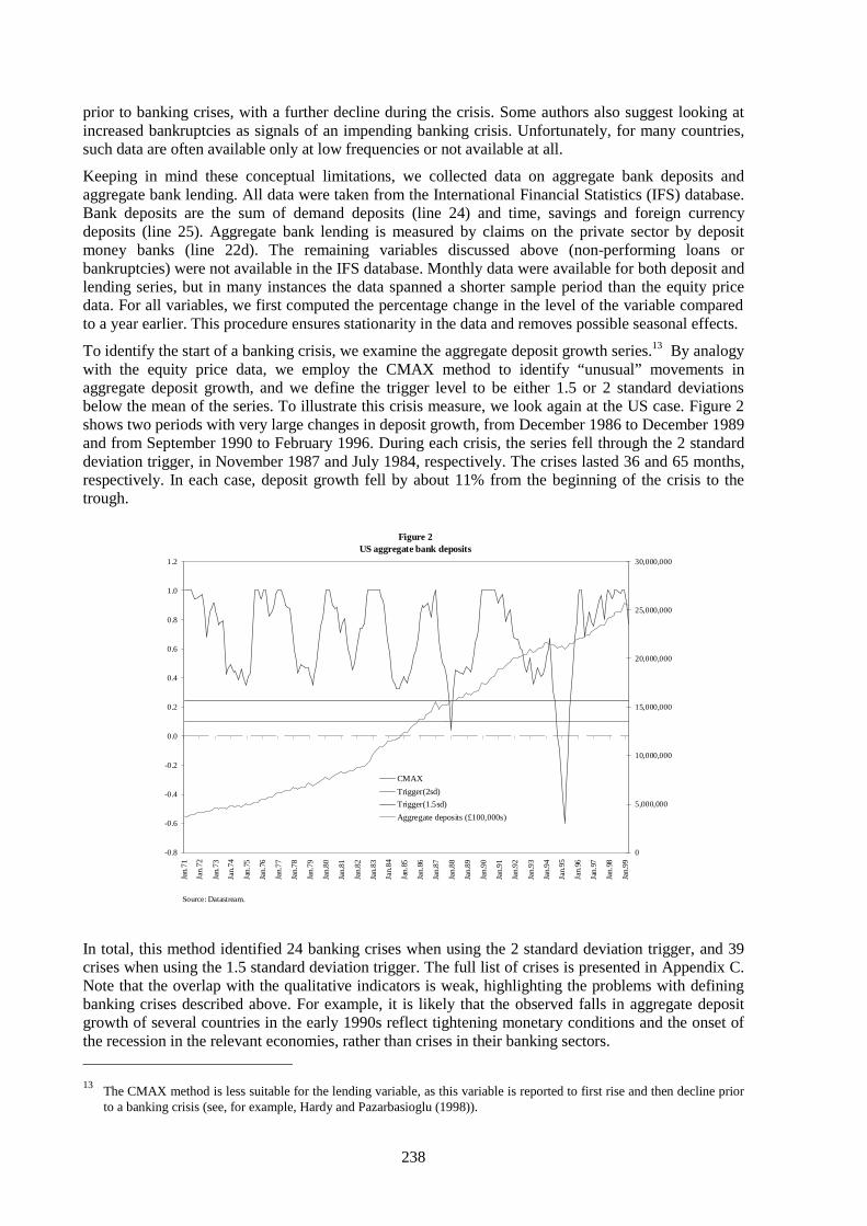
238
prior to banking crises, with a further decline during the crisis. Some authors also suggest looking atincreased bankruptcies as signals of an impending banking crisis. Unfortunately, for many countries,such data are often available only at low frequencies or not available at all.
Keeping in mind these conceptual limitations, we collected data on aggregate bank deposits andaggregate bank lending. All data were taken from the International Financial Statistics (IFS) database.Bank deposits are the sum of demand deposits (line 24) and time, savings and foreign currencydeposits (line 25). Aggregate bank lending is measured by claims on the private sector by depositmoney banks (line 22d). The remaining variables discussed above (non-performing loans orbankruptcies) were not available in the IFS database. Monthly data were available for both deposit andlending series, but in many instances the data spanned a shorter sample period than the equity pricedata. For all variables, we first computed the percentage change in the level of the variable comparedto a year earlier. This procedure ensures stationarity in the data and removes possible seasonal effects.
To identify the start of a banking crisis, we examine the aggregate deposit growth series.13 By analogywith the equity price data, we employ the CMAX method to identify “unusual” movements inaggregate deposit growth, and we define the trigger level to be either 1.5 or 2 standard deviationsbelow the mean of the series. To illustrate this crisis measure, we look again at the US case. Figure 2shows two periods with very large changes in deposit growth, from December 1986 to December 1989and from September 1990 to February 1996. During each crisis, the series fell through the 2 standarddeviation trigger, in November 1987 and July 1984, respectively. The crises lasted 36 and 65 months,respectively. In each case, deposit growth fell by about 11% from the beginning of the crisis to thetrough.
In total, this method identified 24 banking crises when using the 2 standard deviation trigger, and 39crises when using the 1.5 standard deviation trigger. The full list of crises is presented in Appendix C.Note that the overlap with the qualitative indicators is weak, highlighting the problems with definingbanking crises described above. For example, it is likely that the observed falls in aggregate depositgrowth of several countries in the early 1990s reflect tightening monetary conditions and the onset ofthe recession in the relevant economies, rather than crises in their banking sectors. 13
The CMAX method is less suitable for the lending variable, as this variable is reported to first rise and then decline priorto a banking crisis (see, for example, Hardy and Pazarbasioglu (1998)).
Figure 2US aggregate bank deposits
-0.8
-0.6
-0.4
-0.2
0.0
0.2
0.4
0.6
0.8
1.0
1.2
Jan.
71
Jan.
72
Jan.
73
Jan.
74
Jan.
75
Jan.
76
Jan.
77
Jan.
78
Jan.
79
Jan.
80
Jan.
81
Jan.
82
Jan.
83
Jan.
84
Jan.
85
Jan.
86
Jan.
87
Jan.
88
Jan.
89
Jan.
90
Jan.
91
Jan.
92
Jan.
93
Jan.
94
Jan.
95
Jan.
96
Jan.
97
Jan.
98
Jan.
99
0
5,000,000
10,000,000
15,000,000
20,000,000
25,000,000
30,000,000
CMAX
Trigger(2sd)
Trigger(1.5sd)
Aggregate deposits (£100,000s)
Source: Datastream.
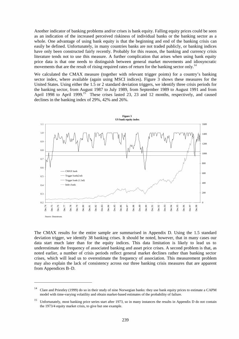
239
Another indicator of banking problems and/or crises is bank equity. Falling equity prices could be seenas an indication of the increased perceived riskiness of individual banks or the banking sector as awhole. One advantage of using bank equity is that the beginning and end of the banking crisis caneasily be defined. Unfortunately, in many countries banks are not traded publicly, or banking indiceshave only been constructed fairly recently. Probably for this reason, the banking and currency crisisliterature tends not to use this measure. A further complication that arises when using bank equityprice data is that one needs to distinguish between general market movements and idiosyncraticmovements that are the result of rising required rates of return for the banking sector only.14
We calculated the CMAX measure (together with relevant trigger points) for a country’s bankingsector index, where available (again using MSCI indices). Figure 3 shows these measures for theUnited States. Using either the 1.5 or 2 standard deviation triggers, we identify three crisis periods forthe banking sector, from August 1987 to July 1989, from September 1989 to August 1991 and fromApril 1998 to April 1999.15 These crises lasted 23, 23 and 12 months, respectively, and causeddeclines in the banking index of 29%, 42% and 26%.
The CMAX results for the entire sample are summarised in Appendix D. Using the 1.5 standarddeviation trigger, we identify 38 banking crises. It should be noted, however, that in many cases ourdata start much later than for the equity indices. This data limitation is likely to lead us tounderestimate the frequency of associated banking and asset price crises. A second problem is that, asnoted earlier, a number of crisis periods reflect general market declines rather than banking sectorcrises, which will lead us to overestimate the frequency of association. This measurement problemmay also explain the lack of consistency across our three banking crisis measures that are apparentfrom Appendices B–D.
14
Clare and Priestley (1999) do so in their study of nine Norwegian banks: they use bank equity prices to estimate a CAPMmodel with time-varying volatility and obtain market-based estimates of the probability of failure.
15Unfortunately, most banking price series start after 1973, so in many instances the results in Appendix D do not containthe 1973/4 equity market crisis, to give but one example.
Figure 3 US bank equity index
0.2
0.3
0.4
0.5
0.6
0.7
0.8
0.9
1.0
1.1
Dec
.74
Dec
.75
Dec
.76
Dec
.77
Dec
.78
Dec
.79
Dec
.80
Dec
.81
Dec
.82
Dec
.83
Dec
.84
Dec
.85
Dec
.86
Dec
.87
Dec
.88
Dec
.89
Dec
.90
Dec
.91
Dec
.92
Dec
.93
Dec
.94
Dec
.95
Dec
.96
Dec
.97
Dec
.98
0
200
400
600
800
1000
1200
1400
1600
CMAX bank
Trigger bank(2sd)
Trigger bank (1.5sd)
Index bank
Source: Datastream.

240
4. Equity price crises and banking crises: empirical results
In this section, we present the empirical results for hypotheses (Q1) to (Q6) as identified in Section 2.Unless otherwise specified, we employ the broadest definition of a crisis (i.e. based on the 1.5 standarddeviation trigger). To identify twin asset price and banking crises, it is useful to examine the followingmatrix, adapted from the banking and currency crisis literature.
Asset price crisis at t No asset price crisis at tBank crisis at t At, t Bt, t
No bank crisis at t Ct, t Dt, t
For example, we can use this matrix to learn in how many instances an asset price crisis occurringduring period t was accompanied by a banking crisis in period t (At, t), or not accompanied by abanking crisis (Ct, t). A similar matrix could be constructed to tabulate the number of instances inwhich an asset price crisis in period t was preceded or followed by a banking crisis in period t–1 ort+1, respectively. In what follows, we look for within-country associations only, but a similar matrixcould be constructed to identify associations across countries.
Table 1 sheds light on the first question, using all three criteria to define a banking crisis. In each case,the table presents the number of twin banking and equity market crises, defined as episodes where theonset of an equity market crisis is either followed or preceded by the onset of a banking crisis within12 months. We also looked at instances where the banking crisis began within a 24-month periodsurrounding the start of the stock market crisis. Unless otherwise specified, our discussion focuses onthe former window.
Table 1Measuring the association between banking and equity price crises (Q1)
12-month window 24-month window
Number1 Number1
Total number of equity crises 38
Panel I: Using bank equityTotal number of banking crises 38 38
Asset price crises associated with banking crisis2 16 18
Asset price crises not associated with banking crisis 6 4
Banking crises associated with asset price crisis3 17 19
Banking crises not associated with asset price crisis 21 19
Panel II: Using qualitative dataTotal number of banking crises 13 13
Asset price crises associated with banking crisis2 4 5
Asset price crises not associated with banking crisis 34 33
Banking crises associated with asset price crisis3 4 5
Banking crises not associated with asset price crisis 8 6
Panel III: Using balance sheet dataTotal number of banking crises 39
Asset price crises associated with banking crisis2 9 11
Asset price crises not associated with banking crisis 27 25
Banking crises associated with asset price crisis3 9 11
Banking crises not associated with asset price crisis 29 281 When comparing isolated and twin crises, two numbers may not add up because of the later start of many bank data.2 Frequency with which asset price crisis at t is accompanied by banking crisis in either t+k or t–k, where k = 12 or 24months. 3 Frequency with which banking crisis at t is accompanied by asset price crisis in either t+k or t–k, where k = 12 or24 months.

241
When using bank equity as our criterion, we find that 16 out of 38 equity market crises could beassociated with a banking crisis (At, t), while six other equity crises were isolated occurrences (Ct, t).
16
Twin crises occurred in Hong Kong and Sweden in the 1990s, Australia, Canada, Denmark, Italy,Japan, Spain, the United Kingdom and the United States in the 1980s and the United Kingdom in the1970s. When looking at banking crises first, we find similar numbers of banking crises associated withequity price crises (At, t: 17), but a larger number of banking crises which neither resulted in nor werepreceded by equity crises (Bt, t: 21).
The association becomes even weaker when using the qualitative criteria, as can be seen from panel II.The Glick and Hutchinson criterion returned four twin crises (Norway, Sweden, the United Kingdomand the United States). Recall, however, that the latter method employed years rather than months todate the banking crisis. In any case, the disparity between the results from this and the previousmethod suggest that a fair amount of measurement error is present.
Panel III repeats the exercise, this time using the balance sheet method to identify banking crises. Thistime, we find that nine out of 38 equity price crises were associated with banking crises (At, t). Theyoccurred in Australia in the 1970s, Japan, Norway, Sweden and the United States in the 1980s andDenmark, Finland, Germany and Sweden in the 1990s. This number goes up to 11 when we consider a24-month window either way (Canada and Spain). When looking at banking crises first, we find thatout of the 36 banking crises identified by the balance sheet method, nine are in fact twin crises (At, t),with the remaining 29 being banking crises that were neither preceded nor followed by asset pricecrises (Bt, t).
To conclude, Table 1 shows that irrespective of our methodology, the association between equity andbanking crises is weak. In particular, the empirical evidence is too weak to provide support for theview that stock price declines always lead to banking crises.
Table 2 looks at the nature of equity price crises, namely their length (number of months) and the totalprice decline that occurred in the equity market. We are interested in learning whether or not twincrises are systematically preceded by more severe equity price crises. For the total sample, the averageequity crisis lasted 38 months and prices fell by 43% on average. Crises varied both in their length andtheir intensity, however, with the longest crisis lasting 82 months (Spain, April 1974 – March 1981),and the most severe crisis entailing an 89% price decline (Hong Kong, 1973).
Table 2Does the nature of the equity crisis affect the likelihood of twin crises (Q2)?
12-month window 24-month window
Length of equitycrisis (months)
Price decline(%)
Length of equitycrisis (months)
Price decline(%)
All equity crises 37 –42.9
Panel I: Using bank equityEquity crises associated with banking crisis 35 –39.5 36 –39.1
Equity crises not associated with banking crisis 33 –32.2 28 –33
Panel II: Using qualitative dataEquity crises associated with banking crisis 22 –33.2 24 –29.6
Equity crises not associated with banking crisis 38 –44 36 –42.03
Panel III: Using balance sheet dataEquity crises associated with banking crisis 33 –40.65 34 –40.66
Equity crises not associated with banking crisis 38 –41.27 38 –41.32
16
For the remaining 16 asset price crisis episodes, no bank equity data were available.

242
When using bank equity data to identify banking crises, we see that equity crises associated withbanking crises tend to last longer than those not associated with banking crises, and to result in largerprice declines. But when using qualitative or balance sheet data to identify banking crises, we obtainthe opposite result: equity price crises not associated with banking crises last longer and witness largerprice declines. Hence, we cannot conclude that the more severe the equity price crisis, the more likelya banking crisis is to follow. Arguably, the results in this section are affected by the small number oftwin crises that were identified in the first place.
Table 3 looks at the behaviour of equity prices during a banking crisis, both those occurring inisolation and those associated with equity price crises. Large falls in equity prices during an isolatedbanking crisis might suggest that investors are liquidating their equity holdings because of reducedconfidence in the banking sector and/or reduced access to bank credit. Significant equity price fallsduring a twin crisis could reflect concerns about both overvaluation of the equity market and increasedfragility in the banking sector.
Table 3 measures the percentage fall in the overall equity index from the beginning of the bankingcrisis to the trough. The table provides a very mixed picture. When using the bank equity criterion(panel I), we find that equity returns were indeed negative during banking crises, and even more soduring twin crises. But since this method does not make an accurate distinction between generalmarket and bank equity movements, we cannot unambiguously interpret these negative returns as amanifestation of banking sector problems. When using the bank balance sheet method (panel III), wereport negative returns during twin crises only. Finally, the qualitative method (panel II) yieldspositive returns during both isolated and twin crises. It should be noted that since this method does notprovide a trough date, the price decline was measured from the beginning of the crisis to the end. Thereported positive returns may therefore mask an actual decline during the first phase of the crisis (fromthe beginning until the trough). Overall, the evidence seems too weak to conclude that bankingproblems lead to a spillover into asset markets as modelled by, for example, Allen and Gale (1998b).
Table 3Do equity prices decline further during a banking crisis (Q3)?
From beginning of crisis to trough
12-month window 24-month window
% decline of equity index
Panel I: Bank equityAll banking crises –26.03
Banking crises associated with equity crisis –34.121 –29.00
Banking crises not associated with equity crisis –16.78 –21.58
Panel II: Qualitative data2
All banking crises 51.17
Banking crises associated with equity crisis 109.07 117.561
Banking crises not associated with equity crisis 25.44 9.68
Panel III: Bank balance sheet dataAll banking crises 23.12
Banking crises associated with equity crisis –4.701 16.32
Banking crises not associated with equity crisis 32.06 26.60
Benchmarks
Total sample 12.85
1970s 6.08
1980s 19.56
1990s 10.981 Denotes that results for twin crisis are significantly different from those during other crises (95%). 2 Uses end-date instead.

243
Table 4 documents the changing nature of both equity and banking crises over time. Panel I shows thatstock market crises in the 1970s were on average longer and led to bigger price falls than in thesubsequent decades. In contrast, declines in bank equity prices (panel II) were longer and morepronounced in the 1980s, although this result is possibly biased because many of the data series werenot available for the 1970s. Finally, panel III shows that when considering bank balance sheet data,banking crises have become shorter and characterised by smaller falls in deposit growth over time.
Table 4Changing nature of crises (Q4)
Total period 1970s 1980s 1990s
Panel I: Equity crises
Number of crises 38 15 18 5
Average length of crisis 37 41 33 36
% decline to trough –42.89 –49.97 –37.44 –41.29
Panel II: Banking crises using bank equityNumber of crises 38 4 19 15
Average length of crisis 31 30 34 23*
% decline to trough –39.84 –35.03 –42.09 –38.15
Panel III: Banking crises using bank balance sheet dataNumber of crises 39 6 12 21
Average length of crisis 40 53 41 37
% change in deposits 8.20 15.42 12.74 3.88
% change in deposit growth –20.32 –34.19 –27.51 –12.91
(beginning to trough)
* Most banking crises of the 1990s have not yet ended, according to this definition.
Table 5 addresses the question of whether equity market crises are preceded by periods of unusuallylarge price increases which could be interpreted as possible evidence of asset price bubbles. Theempirical literature on bubbles argues that if bubbles lead to very large price movements, both duringthe final periods of the bubble growth and after it has burst, the distribution of asset prices will exhibitnegative skewness and large kurtosis. Unfortunately, many of the empirical tests in this literature haveproved inconclusive, primarily because market fundamentals and bubbles could be characterised bysimilar statistical properties, and it is now widely acknowledged that asset price bubbles cannot beidentified unambiguously. While keeping the shortcomings of these tests in mind, it is still worthwhileto examine the distributional properties of asset price returns before the onset of an equity price crisis,and compare them with benchmarks for “normal” periods.17
When considering the entire sample of 38 equity price crises, we see that average returns were higherthan historical benchmarks in the three years preceding the start of the crisis, though the differencesare not statistically significant. But neither skewness nor kurtosis was particularly high. Skewnessmeasures were positive though, as one would expect in a rising market but, except for the two-yearperiod before the crisis, remained close to zero. The kurtosis did not indicate significant departurefrom normality and therefore did not point to a preponderance of very large market movements in theperiod preceding the stock market crisis. Hence, while stock price crises seem to occur after periods ofrapid price increases, insufficient evidence is available to designate these as bubble periods.
17
Assuming normality for equity returns, negative skewness points to the occurrence of a larger number of negative returnsthan indicated by the symmetric normal distribution (which has zero skewness). The benchmark for our kurtosis measure(i.e. the occurrence of a larger number of very large positive or negative returns than characteristic for a normaldistribution) is 0. A negative number indicates that the actual distribution of returns is flatter (has more weight in thetails) than the normal distribution.

244
Table 5Are equity crises preceded by large price movements (Q5)?
Returns before crisis Skewness before crisis Kurtosis before crisis
1 year 2 years 3 years 1 year 2 years 3 years 1 year 2 years 3 years
All equity crises 31.83 22.40 21.61 0.29 0.44 0.52 –0.21 –0.09 –0.13
Panel I: using bank equity
12-month window:
Equity crises associated withbanking crisis
37.67 25.73 24.85 0.05 0.62 0.35 0.14 0.08 0.17
Equity crises not associated withbanking crisis
15.31 17.45 13.35 0.56 0.29 0.17 –0.28 –0.47 –0.92
24-month window:
Equity crises associated withbanking crisis
34.01 24.45 24.16 0.72 0.43 0.35 0.08 0.04 0.02
Equity crises not associated with28.22 23.19 13.07 –0.03 0.62 0.42 –0.47 –0.68 –0.81
banking crisis
Panel II: Using qualitative data
12-month window:
Equity crises associated withbanking crisis
23.08 13.26 8.60 0.48 0.43 0.50 –0.58 –0.45 0.04
Equity crises not associated with32.86 23.48 23.47 0.27 0.44 0.53 –0.17 –0.05 –0.16
banking crisis
24-month window:
Equity crises associated withbanking crisis
21.48 15.21 14.57 0.14 0.51 0.56 –0.26 –0.24 –0.04
Equity crises not associated withbanking crisis
33.40 23.49 22.92 0.31 0.43 0.51 –0.21 –0.07 –0.15
Panel III: Using bank balancesheets
12-month window:
Equity crises associated withbanking crisis
17.55* 18.27 17.88 0.43 0.30 0.37 0.18 –0.44 –0.70
Equity crises not associated with35.33 22.40 21.90 0.21 0.47 0.58 –0.36 –0.07 –0.05
banking crisis
24-month window:
Equity crises associated withbanking crisis
18.55* 18.80 18.88 0.55 0.47 0.39 0.19 –0.03 –0.50
Equity crises not associated withbanking crisis
36.31 22.50 21.75 0.13 0.41 0.59 –0.41 –0.23 –0.09
Benchmarks Returns SkewnessKurtosis
Total sample 12.85 0.87 2.65
1970s 6.08 0.67 1.41
1980s 19.56 0.48 0.20
1990s 10.98 0.35 –0.11
*Indicates that results for twin crisis are significantly different from those during other crises (95%).
We repeat the same exercise for the twin crises identified earlier. In general, equity price increases inthe period preceding the twin asset and banking crises were significantly higher than during ourchosen benchmark periods. When using bank equity as our identification method, we find that equityprice increases were slightly higher when a twin equity and banking crisis followed than when anisolated equity crisis followed, but again the difference was statistically insignificant. In contrast,

245
when using the qualitative or the balance sheet methods, we obtain the opposite result, with twin crisesfollowing weaker equity price increases. No remarkable pattern is observed in either skewness orkurtosis. Hence, the available evidence is too weak to conclude that bubble periods are more likely tocause simultaneous problems in both stock markets and the banking sector.
Finally, Table 6 examines bank lending in the three years prior to the onset of an asset price crisis.Evidence of expanding bank lending prior to asset crises might be an indication of a developing assetprice bubble. As suggested by Allen and Gale (1998a), this bubble could burst if investors suddenlybelieved future credit to be lower than previously expected.
The table shows that, on average, aggregate lending growth is higher one, two and three years beforethe start of the asset price crisis when compared with historical benchmarks. None of the differencesare statistically significant, however. When comparing twin and non-twin crises, we observe someevidence of higher lending growth prior to the former. Note, however, that both the qualitative and thebalance sheet criteria yield the opposite result when using a 12-month window, and that thedifferences are rarely significant. Hence, our evidence to support the theoretical result of Allen andGale (1998a) is rather weak.
Table 6Is there evidence of increased bank lending prior to an equity price crisis (Q6)?
Average lending growth prior to crisis
One year Two years Three years
All equity crises 14.31 14.62 14.18
Panel I: Using bank equity12-month window:
Equity crises associated with banking crisis 13.70 14.86 13.94
Equity crises not associated with banking crisis 11.03 11.70 11.94
24-month window:
Equity crises associated with 13.24 14.70 14.01
banking crisis
Equity crises not associated with banking crisis 11.28 10.67 10.71
Panel II: Using qualitative data12-month window:
Equity crises associated with 19.26 21.49 20.98
banking crisis
Equity crises not associated with banking crisis 13.78 13.88 13.45
24-month window:
Equity crises associated with banking crisis 19.26 21.49 20.98
Equity crises not associated with banking crisis 13.78 13.88 13.45
Panel III: Using bank balance sheets12-month window:
Equity crises associated with banking crisis 13.01 13.32 13.61
Equity crises not associated with banking crisis 14.76 15.07 14.38
24-month window:
Equity crises associated with banking crisis 15.31 15.41 15.62
Equity crises not associated with banking crisis 14.43 14.55 13.86
Benchmarks
Total sample 11.48
1970s 15.07
1980s 14.20
1990s 6.05

246
5. Conclusions
This paper examined the association between equity market crises and banking crises for 14 developedcountries over the period 1970–99. We find the association to be relatively weak and not to besystematically related to the severity of the equity price collapse. Our empirical results do not permitus to conclude that periods of sharp equity price increases cause problems in both equity markets andthe banking sector.
When looking at the effect of banking crises on the equity market, we observe mixed evidence ofbanking crises leading to large equity price falls, but cannot conclude that banking crisessystematically cause large-scale liquidations of equity. Finally, we find only weak evidence ofincreased bank lending prior to equity market crises, as suggested by theoretical models of asset pricebubbles and banking crises.
An important caveat pertains to all our results, which stems from the relatively small number ofbanking crises that have occurred in developed countries over the past three decades, the incompletenature of our data set and the limitations of our methodology to accurately identify banking crises.Extending our sample to emerging market economies may yield stronger associations. For example,Glick and Hutchinson (1999) find that the association between banking and currency crises is strongerfor financially liberalised emerging market economies than for the remaining countries (including bothdeveloped and less developed emerging countries). It will be equally important in future research torefine our banking crisis indicators.
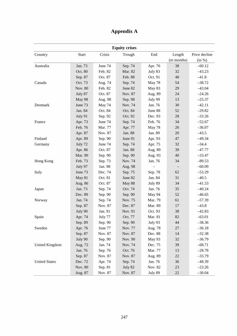
247
Appendix A
Equity crises
Country Start Crisis Trough End Length Price decline
(in months) (in %)
Australia Jan. 73 June 74 Sep. 74 Apr. 76 38 –60.12
Oct. 80 Feb. 82 Mar. 82 July 83 32 –43.23
Sep. 87 Oct. 87 Feb. 88 Oct. 91 48 –41.8
Canada Oct. 73 Aug. 74 Sep. 74 May 78 54 –38.72
Nov. 80 Feb. 82 June 82 May 83 29 –43.04
July 87 Oct. 87 Nov. 87 Aug. 89 24 –24.26
May 98 Aug. 98 Sep. 98 July 99 13 –25.37
Denmark June 73 May 74 Nov. 74 Jan. 76 30 –42.11
Jan. 84 Oct. 84 Oct. 84 June 88 52 –29.82
July 91 Sep. 92 Oct. 92 Dec. 93 28 –33.26
France Apr. 73 June 74 Sep. 74 Feb. 76 34 –52.67
Feb. 76 Mar. 77 Apr. 77 May 78 26 –36.07
Apr. 87 Nov. 87 Jan. 88 Jan. 89 20 –43.5
Finland Apr. 89 Sep. 90 June 91 Apr. 93 47 –49.34
Germany July 72 June 74 Sep. 74 Apr. 75 32 –34.4
Apr. 86 Oct. 87 Jan. 88 Aug. 89 39 –47.77
Mar. 90 Sep. 90 Sep. 90 Aug. 93 40 –33.47
Hong Kong Feb. 73 Sep. 73 Nov. 74 Jan. 76 34 –89.53
July 97 Jan. 98 Aug. 98 – – –60.09
Italy June 73 Dec. 74 Sep. 75 Sep. 78 62 –53.29
May 81 Oct. 81 June 82 Jan. 84 31 –40.5
Aug. 86 Oct. 87 May 88 July 89 34 –41.53
Japan Jan. 73 Sep. 74 Oct. 74 Jan. 76 35 –40.24
Dec. 89 Sep. 90 Sep. 90 May 94 52 –46.65
Norway Jan. 74 Sep. 74 Nov. 75 Mar. 79 61 –57.39
Sep. 87 Nov. 87 Dec. 87 Mar. 89 17 –43.8
July 90 Jan. 91 Nov. 91 Oct. 93 38 –42.83
Spain Apr. 74 July 77 Oct. 77 Mar. 81 82 –63.01
Sep. 89 Sep. 90 Sep. 90 July 93 44 –38.36
Sweden Apr. 76 June 77 Nov. 77 Aug. 78 27 –36.18
Sep. 87 Nov. 87 Nov. 87 Dec. 88 14 –32.38
July 90 Sep. 90 Nov. 90 May 93 32 –36.79
United Kingdom Aug. 72 Jan. 74 Nov. 74 Dec. 75 39 –68.71
Jan. 76 Sep. 76 Oct. 76 Mar. 77 13 –28.78
Sep. 87 Nov. 87 Nov. 87 Aug. 89 22 –33.79
United States Dec. 72 Apr. 74 Sep. 74 Jan. 76 36 –48.39
Nov. 80 Sep. 81 July 82 Nov. 82 23 –23.26
Aug. 87 Nov. 87 Nov. 87 July 89 22 –30.04
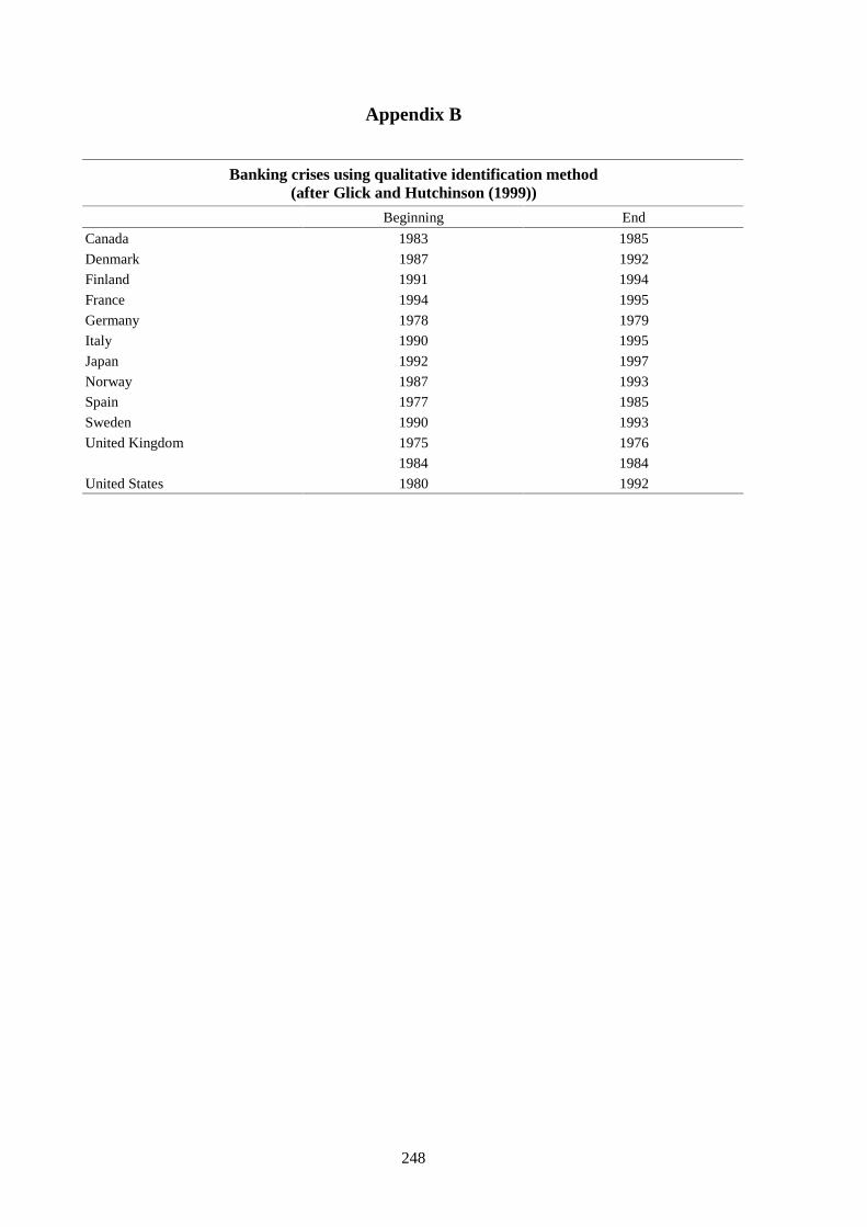
248
Appendix B
Banking crises using qualitative identification method(after Glick and Hutchinson (1999))
Beginning End
Canada 1983 1985
Denmark 1987 1992
Finland 1991 1994
France 1994 1995
Germany 1978 1979
Italy 1990 1995
Japan 1992 1997
Norway 1987 1993
Spain 1977 1985
Sweden 1990 1993
United Kingdom 1975 1976
1984 1984
United States 1980 1992
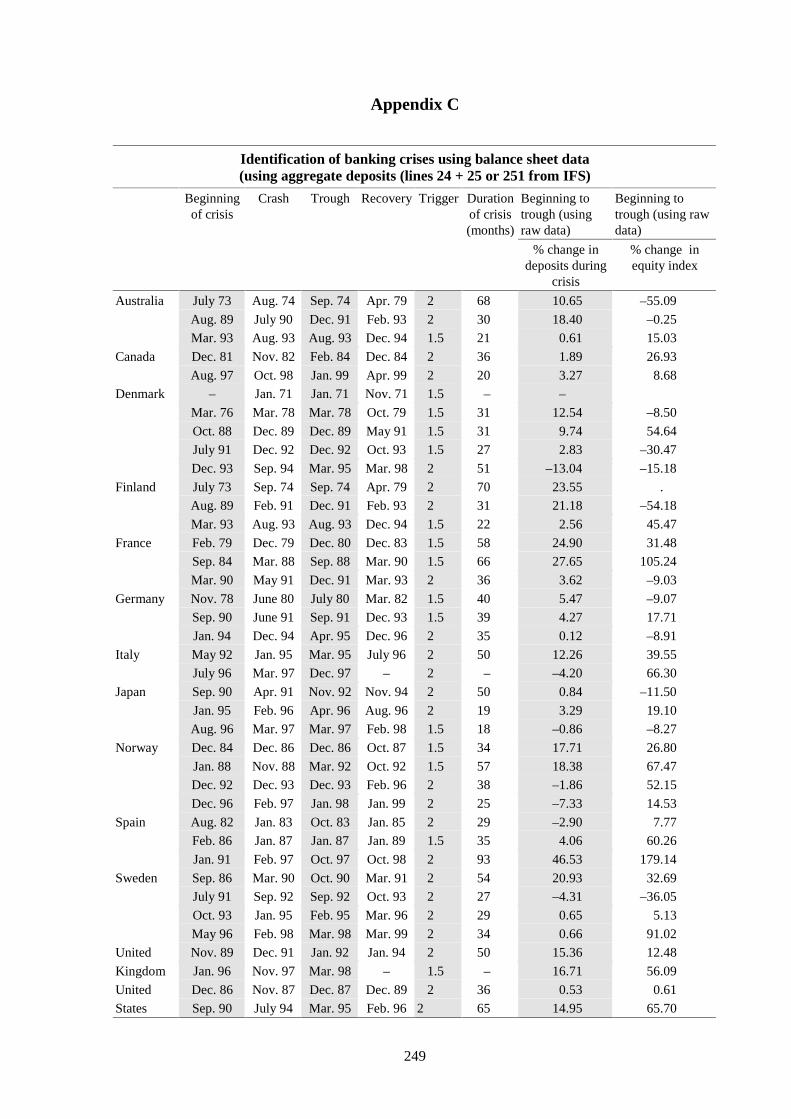
249
Appendix C
Identification of banking crises using balance sheet data(using aggregate deposits (lines 24 + 25 or 251 from IFS)
Beginningof crisis
Crash Trough Recovery Trigger Durationof crisis(months)
Beginning totrough (usingraw data)
Beginning totrough (using rawdata)
% change indeposits during
crisis
% change inequity index
Australia July 73 Aug. 74 Sep. 74 Apr. 79 2 68 10.65 –55.09
Aug. 89 July 90 Dec. 91 Feb. 93 2 30 18.40 –0.25
Mar. 93 Aug. 93 Aug. 93 Dec. 94 1.5 21 0.61 15.03
Canada Dec. 81 Nov. 82 Feb. 84 Dec. 84 2 36 1.89 26.93
Aug. 97 Oct. 98 Jan. 99 Apr. 99 2 20 3.27 8.68
Denmark – Jan. 71 Jan. 71 Nov. 71 1.5 – –
Mar. 76 Mar. 78 Mar. 78 Oct. 79 1.5 31 12.54 –8.50
Oct. 88 Dec. 89 Dec. 89 May 91 1.5 31 9.74 54.64
July 91 Dec. 92 Dec. 92 Oct. 93 1.5 27 2.83 –30.47
Dec. 93 Sep. 94 Mar. 95 Mar. 98 2 51 –13.04 –15.18
Finland July 73 Sep. 74 Sep. 74 Apr. 79 2 70 23.55 .
Aug. 89 Feb. 91 Dec. 91 Feb. 93 2 31 21.18 –54.18
Mar. 93 Aug. 93 Aug. 93 Dec. 94 1.5 22 2.56 45.47
France Feb. 79 Dec. 79 Dec. 80 Dec. 83 1.5 58 24.90 31.48
Sep. 84 Mar. 88 Sep. 88 Mar. 90 1.5 66 27.65 105.24
Mar. 90 May 91 Dec. 91 Mar. 93 2 36 3.62 –9.03
Germany Nov. 78 June 80 July 80 Mar. 82 1.5 40 5.47 –9.07
Sep. 90 June 91 Sep. 91 Dec. 93 1.5 39 4.27 17.71
Jan. 94 Dec. 94 Apr. 95 Dec. 96 2 35 0.12 –8.91
Italy May 92 Jan. 95 Mar. 95 July 96 2 50 12.26 39.55
July 96 Mar. 97 Dec. 97 – 2 – –4.20 66.30
Japan Sep. 90 Apr. 91 Nov. 92 Nov. 94 2 50 0.84 –11.50
Jan. 95 Feb. 96 Apr. 96 Aug. 96 2 19 3.29 19.10
Aug. 96 Mar. 97 Mar. 97 Feb. 98 1.5 18 –0.86 –8.27
Norway Dec. 84 Dec. 86 Dec. 86 Oct. 87 1.5 34 17.71 26.80
Jan. 88 Nov. 88 Mar. 92 Oct. 92 1.5 57 18.38 67.47
Dec. 92 Dec. 93 Dec. 93 Feb. 96 2 38 –1.86 52.15
Dec. 96 Feb. 97 Jan. 98 Jan. 99 2 25 –7.33 14.53
Spain Aug. 82 Jan. 83 Oct. 83 Jan. 85 2 29 –2.90 7.77
Feb. 86 Jan. 87 Jan. 87 Jan. 89 1.5 35 4.06 60.26
Jan. 91 Feb. 97 Oct. 97 Oct. 98 2 93 46.53 179.14
Sweden Sep. 86 Mar. 90 Oct. 90 Mar. 91 2 54 20.93 32.69
July 91 Sep. 92 Sep. 92 Oct. 93 2 27 –4.31 –36.05
Oct. 93 Jan. 95 Feb. 95 Mar. 96 2 29 0.65 5.13
May 96 Feb. 98 Mar. 98 Mar. 99 2 34 0.66 91.02
United Nov. 89 Dec. 91 Jan. 92 Jan. 94 2 50 15.36 12.48
Kingdom Jan. 96 Nov. 97 Mar. 98 – 1.5 – 16.71 56.09
United Dec. 86 Nov. 87 Dec. 87 Dec. 89 2 36 0.53 0.61
States Sep. 90 July 94 Mar. 95 Feb. 96 2 65 14.95 65.70

250
Appendix D
Identification of banking crises using bank equity data
Beginningof crisis
Crash Trough Recovery Trigger Duration ofcrisis (months)
% price declineduring crisis
% price declineduring crisis
Bank equity Total equity
Australia Aug. 87 Oct. 87 Nov. 87 May 88 1.5 9 –28.63 –36.65
Jan. 90 Sep. 90Dec. 90 June 93 2 41 –38.30 –20.41
Canada Aug. 75 Apr. 77May 77 Apr. 78 1.5 32 –20.06 50.20
Nov. 80 Jan. 82June 82 Feb. 83 2 27 –41.16 –43.04
Apr. 83 May 84June 84 May 85 1.5 25 –24.97 –4.54
June 87 Oct. 87Nov. 87 Jan. 89 1.5 19 –20.92 –20.98
July 89 Apr. 90 Oct. 90 Nov. 81 2 28 –29.87 –19.97
May 98 Aug. 98Sep. 98 – 2 – –38.02
Denmark Dec. 83 Mar. 84June 84 June 85 1.5 18 –29.37 –19.64
Dec. 85 July 86 July 86 June 88 1.5 30 –29.51 –17.90
Nov. 89 Dec. 90Oct. 92 Sep. 93 2 46 –55.19 –26.20
France Apr. 90 Sep. 90Dec. 90 Nov. 92 1.5 31 –36.71 –26.13
Dec. 93 Aug. 95 Sep. 95 Feb. 97 1.5 50 –34.93 –16.92
July 98 Sep. 98Sep. 98 – 2 – –51.31
Germany Apr. 86 May 87 Jan. 88 Nov. 89 2 43 –49.47 –47.77
May 98 Sep. 98Sep. 98 – 2 – –35.05
Hong Kong July 81 Sep. 82Nov. 82 Dec. 84 2 41 –55.79 –57.97
Sep. 87 Nov. 87Nov. 87 Dec. 89 1.5 27 –41.93 –45.78
Jan. 94 Jan. 95 Jan. 95 Jan. 96 1.5 24 –42.32 –36.72
July 97 May 98Sep. 98 – 2 – –54.52
Italy May 81 Oct. 81June 82 July 85 2 49 –51.09 –40.50
Mar. 86 Dec. 87May 88 May 89 1.5 37 –51.75 –33.43
Japan Dec. 89 Sep. 90Sep. 90 June 96 2 77 –47.75 –46.65
June 96 Oct. 97Sep. 98 – 2 – –62.98
Spain Aug. 89 Mar. 90 Sep. 92 July 93 2 47 –48.01 –42.33
July 98 Sep. 98Sep. 98 – 2 – –42.85
Sweden Aug. 89 June 92Nov. 92 Aug. 93 2 48 –87.00 –21.43
June 96 Oct. 97 Sep. 98 – 1.5 – –
United Jan. 69 July 69Mar. 70 Mar. 71 1.5 26 –25.35
Kingdom Dec. 72 Feb. 74Nov. 74 Nov. 75 2 35 –69.68 –67.76
Jan. 76 Nov. 76Nov. 76 Apr. 78 1.5 27 –25.03 –24.10
Sep. 87 Oct. 87Nov. 87 Nov. 89 2 26 –35.29 –33.79
Jan. 90 Sep. 90Oct. 90 Mar. 91 1.5 9 –26.28 –12.14
Jan. 94 May 94 May 95 Sep. 95 1.5 20 –8.83 –6.07
Feb. 98 Aug. 98Sep. 98 Mar. 99 2 13 –35.57 –12.29
United Aug. 87 Oct. 97Nov. 87 July 89 2 23 –29.35 –30.04
States Sep. 89 Apr. 90 Oct. 90 Aug. 91 2 23 –42.63 –12.27
Apr. 98 Aug. 98Sep. 98 Apr. 99 1.5 12 –26.62 –7.68

251
Bibliography
Allen, Franklin and Douglas Gale (1998a): “Bubbles and Crises”. Mimeo, University of Pennsylvania.
Allen, Franklin and Douglas Gale (1998b): “Optimal Financial Crises”. Journal of Finance, 53(4),pp. 1245-84.
Allen, Franklin and Douglas Gale (1999): “Financial Contagion”. Mimeo, University of Pennsylvania.
Berg, Andrew and Catherine Pattillo (1999): “Are Currency Crises Predictable? A Test”. IMF StaffPapers, 46, pp. 107-38.
Bernanke, Ben and Mark Gertler (1999): “Monetary Policy and Asset Price Volatility”. Paperpresented at Jackson Hole Conference on “New Challenges for Monetary Policy,” 26–28 August.
Borio, Claudio E V, N Kennedy and S Prowse (1994): “Exploring aggregate asset price fluctuationsacross countries: measurement, determinants and monetary policy implications”. BIS EconomicPapers, No. 40.
Chari, V V and Ravi Jagannathan (1988): “Banking panics, information, and rational expectationsequilibrium”. Journal of Finance, 43(3), pp. 749-61.
Clare, Andrew and Richard Priestley (1999): Mimeo, Norwegian School of Management.
Davis, E Philip (1999): “Financial Data Needs for Macroprudential Surveillance – What are the KeyIndicators of Risks to Domestic Financial Stability?” Bank of England, Handbooks in Central BankingLecture Series, No 2.
Davis, E Philip (1995): Debt, Financial Fragility and Systemic Risk. Clarendon Press, 2nd edition.
Demirgüç-Kunt, Asli and Enrica Detragiache (1998a): “The Determinants of Banking Crises inDeveloping and Developed Countries”. IMF Staff Papers, 45(1), pp. 81-109.
Demirgüç-Kunt, Asli and Enrica Detragiache (1998b): “Financial Liberalization and FinancialFragility”. IMF Working Paper 98/83.
Diamond, Douglas W and Philip H Dybvig (1983): “Bank runs, deposit insurance, and liquidity”.Journal of Political Economy, 91(3), pp. 401-19.
Eichengreen, Barry, Andrew K Rose and Charles Wyplosz (1996): “Contagious Currency Crises”.NBER Working Paper No. 5681.
Gertler, Marc, Marvin Goodfriend, Otmar Issing and Luigi Spaventa (1998): “Asset prices andmonetary policy. Four views”. CEPR and BIS.
Glick and Hutchinson (1999): “Banking and Currency Crises: How Common Are Twins?” Mimeo,IMF.
Gorton, Gary (1988): “Banking panics and business cycles”. Oxford Economic Papers, 40(4),pp. 751-81.
Greenspan, Alan (1999): “New challenges for monetary policy”. Speech at Jackson Hole conferenceon “New Challenges for Monetary Policy”, August 27.
Hardy, Daniel C and Ceyla Pazarbasioglu (1998): “Leading Indicators of Banking Crises: Was AsiaDifferent?” IMF Working Paper 98/91.
International Monetary Fund (1998): “World Economic Outlook”. Washington DC.
Kaminsky, Graciela, Saul Lizondo and Carmen Reinhart (1998): “Leading Indicators of CurrencyCrises”. IMF Staff Papers, 45, pp. 1-48.
Kaminsky, Graciela and Carmen Reinhart (1999): “The Twin Crises. The Causes of Banking andBalance-of-Payment Problems”. American Economic Review, 89(3), pp. 473-500.

252
Kaufman, George G (1999): “Banking and Currency Crises and Systemic Risk: A Taxonomy andReview”. Mimeo, Loyola University Chicago.
Kaufman, George G (1998): “Central Banks, Asset Bubbles, and Financial Stability”. Working Paper98-12, Federal Reserve Bank of Chicago.
Lindgren, Carl-Johan, Gillian Garcia and Matthew I Saal (1996): Bank soundness and MacroeconomicPolicy. IMF.
Marshall, David (1998): “Understanding the Asian crisis: Systemic risk as co-ordination failure”.Economic Perspectives, Federal Reserve Bank of Chicago, pp. 13-28.
Mishkin, Frederic S (1994): “Preventing Financial Crises: An International Perspective”. NBERWorking Paper, No. 4636.
Patel and Sarkar (1998): “Crises in Developed and Emerging Stock Markets”. Financial AnalystsJournal, pp. 50-61, November/December.
Sachs, Jeffrey, Aaron Tornell and Andres Velasco (1996): “Financial Crises In Emerging Markets:The Lessons From 1995”. Brookings Papers On Economic Activity: 1, pp. 147-215.
Schinasi, Garry J and Monica Hargraves (1993): “Boom and Bust in Asset markets in the 1980s:Causes and Consequences”. Staff Studies for the World Economic Outlook, IMF, pp. 1-27.
Vickers, John (1999): “Monetary Policy and Asset Prices”. Bank of England Quarterly Bulletin,November.

253
Early warning systems for currency crises
Peter J G Vlaar1
1. Introduction
In recent years, the frequency of currency crises in developing countries seems to have increased.Moreover, the consequences of these financial crises have probably worsened, not only for the countryconcerned, but also for other countries in the region, due to increased international trade and capitalflows. This has encouraged research on the prediction of currency crises. In this paper, this research issummarised and a new approach to modelling currency crises is proposed.
In order to predict currency crises, it is of course essential to define what a currency crisis is. In thetheoretical literature, currency crises are defined only for fixed exchange rate regimes. A crisis isidentified as an official devaluation or revaluation, or a flotation of the currency. This definition isprobably too strict to be useful for our purposes. Many currency crises involve currencies that are notformally fixed to one currency or a basket of currencies, but are allowed to float within certainmargins. Even currencies that are allowed to float freely might be subject to a disruptive depreciationdue to a speculative attack. Moreover, a small official devaluation in a tranquil period does not have tobe disruptive as it may bring the real exchange rate more into line with fundamentals. Such an actionmight very well preclude future speculative attacks, and should not be identified as a crisis. For mostpurposes, the size of the depreciation is what matters, not so much whether this depreciation is causedby an official policy move or otherwise. Therefore, many empirical studies define a currency crisis asa large (either nominal or real) depreciation. Here, the problem arises of deriving the appropriatethreshold above which a depreciation should be labelled a crisis. Another issue concerning thedefinition of a crisis is whether or not to include unsuccessful speculative attacks. Authorities mayreact to a currency attack by means of direct intervention in the foreign exchange market, or by raisinginterest rates. These attacks might also be included in the crisis definition as the necessary policyactions might be disruptive for the economy as well. In addition, from an investor’s point of view,including unsuccessful speculative attacks might be useful as unsuccessful attacks also indicatevulnerability.
In this paper, a currency crisis indicator, based on monthly nominal exchange rate depreciationsrelative to the US dollar and depletions of official reserves, is constructed for emerging marketseconomies. Interest rates are not included in the index as interest rate data for emerging countries arenot always available and/or reliable. The main innovation in our modelling approach is that we modelthe crisis index itself, instead of a zero-one variable representing index values below or above a certainthreshold. The proposed model has two regimes – one for tranquil and one for crisis episodes – wherethe probability of ending up in the crisis regime depends on the economic circumstances. In the crisisregime, both the mean depreciation and the volatility are larger. The modelling technique resemblesthe one introduced in Vlaar (1998), where a two-regime model was used to predict weekly exchangerate changes within the European Monetary System, but is extended in two respects. First, not only theprobability to end up in the crisis regime, but also the mean depreciation and the volatility in thisregime are allowed to differ with economic conditions. Second, the model is adjusted to allow forpanel data estimation.
1
Econometric Research and Special Studies Department, Netherlands Bank. I thank Peter van Els and seminar participantsat the Netherlands Bank and the Autumn Meeting of Central Bank Economists at the BIS for valuable comments anddiscussions.

254
The continuous modelling approach has several advantages. First, by using the index itself, we do notdiscard information regarding the severity of a crisis. Therefore, large index values have more impacton the model than values just above the (arbitrarily set) crisis threshold. Second, as the continuouscrisis variable varies between observations, there is no need to include many crisis episodes in thesample in order to estimate the model. Consequently, we can concentrate on emerging markets withouthaving to include developed countries in the sample as well. Finally, the continuous modellingapproach makes it possible to distinguish between variables that have an effect on the probability of acrisis and those that affect the severity of crises.
The rest of this paper is organised as follows. In Section 2, some theoretical background on currencycrises is given. Section 3 summarises the main results from the empirical literature. In Section 4, thenew modelling approach is described. Section 5 contains the estimation and forecast results, andSection 6 concludes. The Appendix describes the data.
2. Theoretical considerations
As to the reasons for currency crises, the “first generation” models of, for example, Krugman (1979)focus on inconsistencies between an exchange rate commitment and domestic economic fundamentals,such as excess creation of domestic credit, typically prompted by a fiscal imbalance. In these models,currency crises occur because international reserves are gradually depleted. The model fixes the timingof a currency attack such that the remaining reserves before the attack are just enough to satisfy theforeign currency demands of market participants during the attack.
The “second generation” models of, for example, Obstfeld (1986) view currency crises as shiftsbetween multiple monetary equilibria in response to self-fulfilling speculative attacks. Consequently,the timing of the attack can no longer be determined, as it is no longer unique. In these secondgeneration models, currency attacks can take place even though current policy is not inconsistent withthe exchange rate commitment. The attacks can nevertheless be successful because the costs ofmaintaining a currency peg, in the form of high domestic interest rates, rise in response to the attack.In this framework, speculative attacks become more likely if high interest rates become moreproblematic. One reason for this might be economic slowdown or high unemployment rates. Anothermight be a weak domestic banking sector (Obstfeld (1995)). Raising interest rates increases short-termfunding costs for banks, whereas the higher proceeds from loans might be of little importance to bankprofits due to the longer maturity on average of loans relative to deposits and the increased probabilityof bad loans triggered by the rise in the interest rate.
This is one way banking and currency crises might be related. If there is an implicit governmentcommitment to bail out troubled banks, bank runs might also lead directly to a currency crisis if theincreased liquidity which results from the government bailout is inconsistent with the fixed parity(Velasco (1987), Calvo (1998)). The causality between banking and currency crises might also run inthe other direction, however, for instance if the domestic banking sector is exposed to exchange raterisk due to short-term foreign lending (Chang and Velasco (1998)). Indeed, Kaminsky and Reinhart(1996) find evidence of both directions, although during most twin crises the banking crisis ispreceded by the currency crisis.
3. Empirical literature
Kaminsky et al. (1998) summarise the results of 28 empirical studies on currency crises that haveappeared over the last 20 years. Although the studies differ widely in crisis episodes considered andmethodologies used, some general conclusions can be drawn. First, in order to explain all currencycrises a wide variety of variables is needed. This is because crises can have many different causes.Some variables do seem to have predictive power for many crises, however. In particular, real
255
exchange rates and international reserves are included in many studies and found significant most ofthe time. Other variables that seem to do well, although the limited number of studies consideringthem precludes firm statements, are the domestic inflation rate and domestic credit growth. Currentaccount deficits on the other hand are usually not found to have a significant impact. Rather thanreplicating the results by Kaminsky et al., we choose to highlight just a few typical studies and toconcentrate on emerging market economies. The studies will be categorised by the methodology used.
3.1 The signal approach
The signal approach is primarily a bivariate method. For each variable the average level (or growth) inthe period preceding the crises is compared to that in tranquil periods. If the variable behavesdifferently before a crisis, an extreme value for this variable provides a warning signal. The questionof what value should be considered extreme in this context is solved by weighing the percentage ofcrises predicted against the percentage of false signals. The threshold level can either be the same forall countries, or be based on the country-specific empirical distribution of the variable. Given thewarning signals of the individual variables, a composite leading indicator can be constructed as aweighted average of the individual signals.
In this procedure, both the crisis indicator and the explanatory variables are transformed into dummies,namely larger or smaller than a given threshold. This procedure probably gives the best results if thereis a clear distinction between crisis episodes and periods of tranquillity. Regarding the crisis indicator,this is probably true if only the most severe crises are above the threshold or if the crisis definition isrelated to a currency peg. However, in most studies the number of severe currency crises is limited,and less serious depreciations are also labelled as crises. In that case, there is no clear distinctionbetween observations just above and those below the crisis threshold. Concerning the explanatoryvariables, disregarding the exact value of the variable seems inefficient as, for instance, a currentaccount deficit twice the value of the threshold seems to provide a stronger signal than a deficit justabove it. If the individual signals are combined to compute a composite leading indicator, thisinefficiency leads to inferior results. Another problem that arises in combining the signals is that theoptimal weights for the individual signals cannot easily be assessed if the signals are correlated. If,however, one is primarily interested in finding vulnerabilities, without being particularly interested inexact probabilities, this method may be appropriate since it immediately points to the most importantvariables. This is particularly helpful for determining appropriate economic policy actions.
Kaminsky et al. (1998) use a signals approach to predict currency crises using monthly data for asample of 15 developing and five industrial countries during 1970–95. In their study, a currency crisisis defined to occur when a weighted average of monthly percentage nominal depreciations (either withrespect to the US dollar or the Deutsche mark) and monthly percentage declines in reserves exceeds itsmean by more than three standard deviations for that country.2 For 15 variables, based on economicpriors and data availability, they compare the levels in the 24 months prior to the crises with values intranquil periods. For each variable, an optimal threshold value is computed, above which the variablegives a signal for a crisis in the coming 24 months. The threshold levels are computed as a percentileof the distribution of the variable by country in such a way that the noise-to-signal ratio is optimal. Thevariables that have most explanatory power are (1) the real exchange rate deviation from adeterministic trend, (2) the occurrence of a banking crisis, (3) the export growth rate, (4) the stockprice index growth rate, (5) M2/reserves growth rate, (6) output growth, (7) excess M1 balances, (8)growth of international reserves, (9) M2 multiplier growth, and (10) the growth rate of the domesticcredit to GDP ratio.
Country-specific threshold levels for the economic variables have the advantage that national elementsare taken into account. However, as the same percentile is used for all countries, it also implies that,within sample, all variables signal the same number of crises per country. Although only countries thatexperienced currency crises are included in the sample, this artefact seems undesirable. The real 2
Weights, mean depreciations and volatility are calculated separately for high inflation episodes, defined as monthspreceded by a six month period with more than 150% inflation.

256
exchange rate is by far the most successful indicator. However, this result might be partly spurious asthe deviation of the bilateral real exchange rate from a deterministic trend is used. Consequently, anyreal overvaluation according to this definition has to lead to either a depreciation or a lower inflationrate at home than in the reference country.
Berg and Pattillo (1998) evaluated their approach with respect to predicting the Asian crisis out ofsample, and found mixed results. Most (68%) crises were not signalled in advance, and most (60%) ofthe signals were false. Nevertheless, the predictions were better than random guesses, botheconomically and statistically. The results improve slightly (also in-sample) if the current accountrelative to GDP and the level of the M2/reserves ratio are included. They also compare the ranking ofseverity of currency crises in 1997 with the ranking of vulnerability according to predictedprobabilities of crisis. The composite leading indicator can explain 28% of the variance. If the currentaccount/GDP and M2/reserves ratios are also included, this rises to 36%.
3.2 Limited dependent regressions
In the limited dependent regression models (logit or probit models), the currency crisis indicator ismodelled as a zero-one variable, as in the signals approach. The explanatory variables are nottransformed into dummy variables however, but are usually included in a linear fashion. The logit orprobit functions ensure that the predicted outcome of the model is always between zero and one. Theregression approach has several advantages compared with the signals approach. First of all, theprediction of the model is easily interpreted as the probability of a crisis. Moreover, as the methodconsiders the significance of all the variables simultaneously, the additional information of newvariables is easily checked. A disadvantage of this approach might be that the impact of an individualvariable is less easily detected. Due to the non-linear logit or probit function, the contribution of aparticular variable depends on all the other variables as well. A practical problem of using this strategyto model currency crises is that the number of crises is usually limited. Consequently, there are only afew ones in the sample, compared with a large number of zeros, resulting in poor estimation results. Inorder to increase the number of ones, many studies combine data from industrialised and emergingmarket economies.
Frankel and Rose (1996) use the probit model to estimate the probability of crisis in an annual sampleof 105 developing countries covering 1971–92. A crisis is defined as a depreciation of at least 25%,exceeding the previous year’s depreciation by at least 10%. The use of annual data has the advantagethat more variables are available, for instance regarding fiscal positions and external debt. Moreover,compared with monthly data, the balance between zeros and ones in the sample is probably better.They find 69 crashes in 780 observations. They present several specifications, and conclude that theprobability of crisis increases when output growth is low, domestic credit growth is high, foreigninterest rates are high, foreign direct investment as a proportion of total debt is low, reserves are low,or the real exchange rate is overvalued. The results for output growth, the real exchange rate andreserves were not robust across specifications, however. Berg and Pattillo (1998) evaluate the resultsof Frankel and Rose. Using a cutoff probability of 25% , only 17 out of 69 crises are rightly predictedwithin sample, whereas 33 out of 711 tranquil periods are wrongly predicted. They argue that one ofthe reasons for these rather poor results might be that the country group is too diverse. They proceedwith a smaller group of larger (emerging) markets over the sample 1970–96. Given results in otherstudies, the reserves/M2 and reserves/short-term debt ratios are also included as explanatory variables,where only the former shows significant results. For this specification, 38 out of 60 crises and 342 outof 383 tranquil periods are rightly predicted. The out-of-sample results are still disappointing,however. According to the definition of Frankel and Rose, there were no crises in 1997! This clearlyindicates one of the problems with yearly data if a crisis takes place around the end of the year. If theranking of their crisis index in 1997 is compared with the ranking of predicted probabilities of crisis,only 6% of the variance is explained in the original specification. For the modified model thepercentage is even lower, 5%. In both cases, the model does not perform significantly better thanrandom guesses.
257
Berg and Pattillo (1998) also use a probit model to study currency crises. They base themselves on thedata and crisis definition of Kaminsky et al (1998), augmented by the current account and the ratio ofM2 over reserves, as described above. In their regression model, not only the crises themselves arelabelled “one”, but also the 23 months prior to the crisis. Economically, this procedure has theadvantage that the optimal model is sought that signals a crises two years in advance. Of course, thisalso means that the origins of a crisis are supposed to be visible two years in advance. Statistically, theprocedure strongly improves the balance between the zeros and the ones in their monthly data set.They investigate whether a threshold value for the explanatory variables, as in the signals approach,improves on a linear specification. This turns out not to be the case. The variables that have mostexplanatory power are (1) the deviation of the real exchange rate from trend, (2) the current account,(3) reserve growth, (4) export growth, and (5) the ratio of M2 to reserves. In the model, not thevariables themselves but the percentiles of the country-specific distribution of the variables areincluded. Using a cutoff probability of 25%, the model signals 48% of crises and 84% of tranquilperiods correctly, within sample. Out of sample, the results are even better: 80% of crises and 79% oftranquil periods are correctly called. The prediction of the ranking of crisis severity in 1997 is not verysuccessful. Only 23% of the variance is explained, slightly worse than the signals approach ofKaminsky et al. (1998), though still significantly better than random guesses.
The “Event Risk Indicator” by JP Morgan (1998) is based on a logit regression on monthlyobservations for 25 industrial or emerging countries over the sample 1980–97. Their crisis indicator isdefined as a monthly real depreciation of the key bilateral exchange rate of over 10%. Consequently,this crisis definition excludes unsuccessful speculative attacks. As their basic goal is to find a modelthat can be used to predict profitable months to invest in weak currencies, this choice is reasonable.They balance the number of crises and tranquil periods in their sample by including only three tranquilperiods per country. The explanatory variables for these three periods are calculated as: first, theaverage value of the variables over the estimation sample (1980–94), excluding the months in whichthere was a crisis, the month before, and the month after these crises; second, the average plus onestandard deviation over the same sample; and third, the average minus one standard deviation. As aconsequence, the predictions of the model are not directly interpretable as probabilities of a currencycrash. The key factor behind currency crashes is supposed to be lack of competitiveness, included inthe model as an overvalued real exchange rate (a dummy variable that can take the values one to four,based on the average value of the real exchange rate in the last two years, relative to the average valuein the ten years before). As the model is used to select profitable investment months in weakcurrencies, predicting the exact timing of a crisis is extremely important. This timing is supposed todepend on two factors. First, the credibility of the government’s commitment to defend the exchangerate, which is related to expected economic growth (modelled by means of the three-month rise instock prices) and the size of foreign exchange reserves (relative to foreign debt). Second, the force offinancial contagion, reflected in global risk appetite and local currency crash clustering. Global riskappetite is measured as the correlation between return and risk (reflected in high interest rates and anovervalued currency) over the last three months. Both the one month lagged and the seven monthslagged six-month changes in this variable are included, as currency crashes are most likely if riskappetite changes from positive to negative. The local currency crashes variable is computed as aweighted number of currency crashes in the relevant currency block (Deutsche mark or US dollar) inthe last six months, where recent crashes are given a higher weight than earlier ones.
The regression results show that the six-month change in risk appetite is the most importantexplanatory variable, followed by the number of local crashes and the reserves/debt ratio. The realexchange rate is just significant at the 5% level, the six-month change in risk appetite lagged sevenmonths at the 10% level, and the change in stock prices at the 15% level. Using a cutoff level of 40%,3
31 out of 37 crises and 69 out of 74 quiet periods are correctly predicted within sample. The modelalso seems to predict quite well out of sample, as an investment strategy based on the modelpredictions outperforms a passive, or random, investment strategy on average. According to theauthors, the results of the model are most sensitive for the clustering variable, followed by the current
3
Over the period January 1988 to September 1997, this cutoff point would signal the risk of a crisis 29% of the time.
258
and lagged changes in risk appetite. Notwithstanding the importance of current sentiment, they alsoclaim that the model signals all the major first crashes, including Mexico (December 1994), the ERM(September 1992), and Thailand (July 1997). This is surprising as only lagged variables are used in themodel, and some of these crises came as a complete surprise to the market, thereby precluding theimportance of contagion variables.
3.3 Severity of crisis indicators
A third category of models is not directly aimed at predicting the timing of currency crises, but atpredicting which countries are going to be hit hardest, given the occurrence of a crisis somewhere inthe world. If the timing of currency crises is largely unpredictable, for instance due to the importanceof market sentiment, and the behaviour of financial markets during an international crisis is supposedto be different from normal behaviour, this strategy might be most fruitful. The idea is to define acrisis index (for instance based on depreciations and international reserve losses), spanning the wholeperiod during which international markets were under stress, for a cross-section of countries. Thedifferences between countries in the magnitude of this crisis index are subsequently explained byvariables representing the economic situation at the onset of the crisis. This can be done by simplecross-section regression analysis. Usually, only one crisis episode is considered at a time, but a panelof crisis episodes can be used as well.
Sachs et al. (1996) use this framework to explain the severity of currency crises during the Mexicancrisis of December 1994 (the so-called Tequila effect). They examine data on a cross-section of 20emerging markets. Their crisis index is defined as a weighted average of the percentage decrease inreserves and the percentage depreciation of the exchange rate, from November 1994 to April 1995.They claim that only countries that were already vulnerable were hit by the Mexican crisis. Only threefactors are essential for measuring vulnerability: an overvalued real exchange rate, measured as thereal appreciation between the average 1986–89 level and the one over 1990–94; a weak bankingsystem, measured by the four-year growth in credit to the private sector; and low levels ofinternational reserves relative to M2. It turns out that only the combination of weak fundamentals (realovervaluation or weak banks) and relatively low reserves induced a crisis. They also investigate theinfluence of investment, savings, current accounts, the size of capital inflows, and fiscal policystances, but these variables do not improve the results. Depending on the window over which the crisisindex is calculated, their model can explain 51% to 71% of the variation in the crisis index over theMexican crisis. Berg and Pattillo (1998) investigate whether the same equation can explain variationsin the severity of crises during the Asian crisis. Unfortunately this is not the case. Even the results forthe Mexican crisis turn out to be sensitive to minor revisions. Including three more countries changesthe coefficients significantly. This sensitivity is probably due to small-sample problems. They estimatea model with seven variables, whereas they have only 20 observations. When the original equation, orslightly modified versions estimated on the Mexican crisis, is applied to the Asian crisis, at most 5%of the rankings are explained. When the same specification is re-estimated with data from the Asiancrisis, the coefficients change significantly, and the real exchange rate is no longer significant. Thisequation can explain 21% of the variance in rankings (within sample). Tornell (1999) challenges thesepoor results. Using a model very similar to the one in Sachs et al. (1996), he concludes that bankingweakness, real appreciation and international liquidity can explain both crises.4 When estimated ondata of the Mexican crisis only, the out-of-sample prediction of the Asian crisis still explains 24% ofthe variance in ranking. The fact that this result is not robust for minor changes in, for instance, thedefinition of the explanatory variables, raises serious doubts about the applicability of the model as aprediction device, however.
These problems are again confirmed by Bussière and Mulder (1999). They investigate the factorsbehind the depth of the 1994 and 1997 crises, and whether these can explain the 1998 Russian crisis.
4
Both models include dummy variables for weak verses strong fundamentals (based on the real exchange rate and creditgrowth), and high verses low reserves. The results are especially sensitive to changes in the definition of the thresholdlevels for these dummy variables.

259
For this purpose they estimate a model using a panel of 22 emerging markets for the 1994 and 1997crises. As explanatory variables they compare those used by Tornell (1999) with the ones included inthe early warning system (EWS) model of the IMF (Borenzstein et al. (1999)).5 The results stronglyfavour the variables of the latter study. Within sample, the explanatory power of the two models isabout the same. Out of sample, however, the ranking of vulnerability according to Tornell’s modelturns out to be negatively correlated with the severity of crises in the aftermath of the Russianmoratorium in August 1998. The EWS-based model results in a significant positive correlation (0.56).This model only includes three variables: the four-year growth in the real exchange rate, the currentaccount/GDP ratio, and the short-term debt/reserves ratio, with the latter being by far the mostsignificant. Other variables that were investigated, but found insignificant, are export growth, reservechanges (both are included in the EWS model), credit growth, current account minus foreign directinvestment over GDP, M0, M1 or M2 over reserves, and short-term debt over GDP. The one variablethat does have a positive impact is the availability of an IMF programme. The presence of an IMF-supported programme significantly reduces the depth of a crisis. From these results, the authorsconclude that all three crises are primarily liquidity-driven, as opposed to solvency-driven. Whetherthe model can also be used to predict the next crisis remains to be seen. One of the problems relates tothe availability of data. The authors include the last available observation of the explanatory variablesbefore the starting point of the crises. This practice results in data being included that were notavailable to the market before the crisis. Especially with respect to short-term debt, the inclusion of theend-June 1997 and end-June 1998 positions is dubious as these figures only became available inNovember, whereas the crises started in July/August.
Glick and Rose (1998) use cross-sectional data on both industrial and developing countries (161countries in total) for five different currency crises (1971, 1973, 1992, 1994 and 1997) to explaincontagion. The inclusion of a large number of countries reduces the small-sample problem, but at theexpense of allowing for more heterogeneity in the sample. The crisis episodes are investigatedseparately, not as a panel. They find strong evidence that trade linkages explain regional patterns ofcurrency crises for all five periods. Domestic macroeconomic factors do not consistently help inexplaining the cross-country incidence of speculative attack.6 As no regional variable other than traderelations is included in the regressions, it is not clear whether trade relations really cause contagion, orwhether the trade variable simply picks up the regional preferences of international investors. If thelatter phenomenon is indeed dominant, diversifying trade patterns won’t shelter countries fromregional currency crises.
4. A new approach
The three approaches just discussed all have their disadvantages. The signals and limited dependentapproaches define a currency crisis as a discrete event, which is doubtful for marginal crises, anddisregards the depth of the crisis. The severity of crisis method only uses crisis observations, therebycompletely disregarding the timing of a crisis, and possible information from tranquil periods. In thischapter, we propose a method that combines elements of the limited dependent and severity of crisismethods. As in the latter approach, we model a continuous crisis index, in this case a weighted averageof the monthly depreciation of the exchange rate and of the monthly percentage decline ininternational reserves. In contrast to these models however, we consider not only crisis episodes but allavailable observations. Thus, it is assumed that tranquil periods also provide information regarding the
5
This model is based on Berg and Pattillo’s (1998) model. The main difference is that the short-term debt/reserves ratio isincluded instead of the M2/reserves ratio.
6Only inflation seems to matter during all five crises. Real growth significantly increased the severity of all but the 1992crisis. Other variables included are credit growth (significant in 1994), government budget over GDP (significant in 1971and 1973), current account over GDP (significant in 1994), and M2 over reserves (some influence in 1973 and 1994). Allcoefficients widely vary across crisis periods. In a probit regression, none of the macroeconomic variables is significantin any of the five crisis episodes considered.

260
vulnerability of individual currencies. The fact that vulnerabilities materialise primarily during crisesis modelled by means of a model with two regimes, one for normal and one for unexpectedly volatileperiods, where the latter regime is characterised by, on average, larger depreciations and extravolatility, which are common to crises. Unlike than with the limited dependent models, the definitionof crisis periods is not imposed beforehand, but is the outcome of a stochastic process. The weaker thefundamentals of a country, the higher the probability of entering the volatile regime.
The empirical model can be described by the following six equations:
(1) ititititit XI ε+ϑλ+β= 11
(2) ),)1((),()1(~ itititititititititit hNhN δ+ϑλ−λ+ϑλ−λ−ε
(3) 22 β= itit Xh
(4) ))3exp(1/()3exp( 33 β+β=λ ititit XX
(5) 44 β=ϑ itit X
(6) 55 β=δ itit X
The first equation describes the evolution of the crisis indicator )( itI for country i at time t. It consistsof three parts: a linear part for normal periods, a non-linear part related to crisis episodes, and astochastic error term. The distribution of the error term is described in equation (2). Conditional onbeing in the normal regime, which has probability )1( itλ− , the innovation is normally distributed
with expectation ititϑλ− and variance ith , whereas in the volatile regime the mean and variance are
higher by itϑ and itδ respectively. Note that the expectation of the combined process is zero. Thevolatility in the normal regime is described by equation (3). The probability of entering the volatileregime is estimated in the familiar logit form (equation (4)). Equations (5) and (6) describe,respectively, the additional expected depreciation ( itϑ ) and variance ( itδ ) in the volatile regime. Theparameters in this model (the is) are estimated by maximum likelihood. In order to ensure that theconditional variances are always positive, 2β and 5β and the corresponding economic variables itX 2
and itX 5 are restricted to being non-negative.
Apart from the second equation, economic variables, denoted by itX1 to itX 5 , might enter allequations. The interpretation of their influence differs between equations, however. The economicvariables in the first equation describe the evolution of the crisis indicator in normal periods.Candidate variables are past changes in exchange rates and international reserves; this enables us tomodel the positive autocorrelation in these series, and inflation rates and (changes in) the realexchange rate, as many countries allow their currency to depreciate gradually in order to maintaincompetitiveness. The volatility in normal periods (equation (3)) is explained by its own past, asvolatility is correlated through time- and country-specific as well as area-wide past volatility in orderto account for international aspects of volatility. Consequently, once a crisis has occurred, volatility isexpected to stay high temporarily, even if the probability of entering the volatile regime drops to zero.The fourth equation describing the probability of entering the volatile regime might involve a range ofvariables that increase the probability of a currency crisis. Variables that are found to be significant inother studies on currency crises could be included in our model via this equation. The additionalexpected change ( itϑ , equation (5)) and volatility ( itδ , equation (6)) in the crisis regime are mostlikely driven by indicators of current inequalities, such as deviations of the real exchange rate fromtrend, indicators of contagion, such as the number or depth of crises in neighbouring countries, andliquidity-related variables, which influence the probability to overshoot an equilibrium value due tocapital flight.
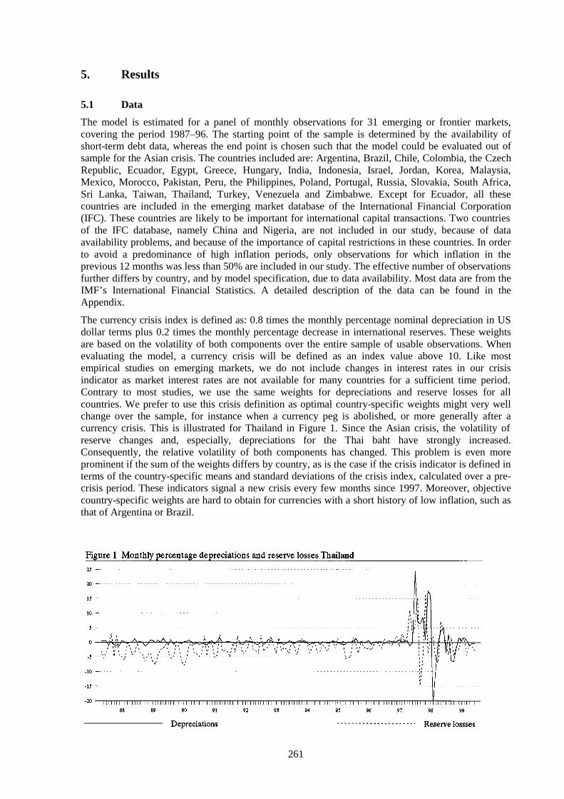
261
5. Results
5.1 Data
The model is estimated for a panel of monthly observations for 31 emerging or frontier markets,covering the period 1987–96. The starting point of the sample is determined by the availability ofshort-term debt data, whereas the end point is chosen such that the model could be evaluated out ofsample for the Asian crisis. The countries included are: Argentina, Brazil, Chile, Colombia, the CzechRepublic, Ecuador, Egypt, Greece, Hungary, India, Indonesia, Israel, Jordan, Korea, Malaysia,Mexico, Morocco, Pakistan, Peru, the Philippines, Poland, Portugal, Russia, Slovakia, South Africa,Sri Lanka, Taiwan, Thailand, Turkey, Venezuela and Zimbabwe. Except for Ecuador, all thesecountries are included in the emerging market database of the International Financial Corporation(IFC). These countries are likely to be important for international capital transactions. Two countriesof the IFC database, namely China and Nigeria, are not included in our study, because of dataavailability problems, and because of the importance of capital restrictions in these countries. In orderto avoid a predominance of high inflation periods, only observations for which inflation in theprevious 12 months was less than 50% are included in our study. The effective number of observationsfurther differs by country, and by model specification, due to data availability. Most data are from theIMF’s International Financial Statistics. A detailed description of the data can be found in theAppendix.
The currency crisis index is defined as: 0.8 times the monthly percentage nominal depreciation in USdollar terms plus 0.2 times the monthly percentage decrease in international reserves. These weightsare based on the volatility of both components over the entire sample of usable observations. Whenevaluating the model, a currency crisis will be defined as an index value above 10. Like mostempirical studies on emerging markets, we do not include changes in interest rates in our crisisindicator as market interest rates are not available for many countries for a sufficient time period.Contrary to most studies, we use the same weights for depreciations and reserve losses for allcountries. We prefer to use this crisis definition as optimal country-specific weights might very wellchange over the sample, for instance when a currency peg is abolished, or more generally after acurrency crisis. This is illustrated for Thailand in Figure 1. Since the Asian crisis, the volatility ofreserve changes and, especially, depreciations for the Thai baht have strongly increased.Consequently, the relative volatility of both components has changed. This problem is even moreprominent if the sum of the weights differs by country, as is the case if the crisis indicator is defined interms of the country-specific means and standard deviations of the crisis index, calculated over a pre-crisis period. These indicators signal a new crisis every few months since 1997. Moreover, objectivecountry-specific weights are hard to obtain for currencies with a short history of low inflation, such asthat of Argentina or Brazil.

262
As explanatory variables, a wide range of variables is considered. In the first instance, all possiblecandidates are included at the same time. Subsequently, variables that have the wrong sign or areinsignificant are excluded. Regarding the time lag for explanatory variables, we included at least aone-month lag for (real) exchange rates, international reserves, inflation rates and the currency regime,two months for GDP, exports, imports, M2 and bank credit, and five months for international debtdata. These relatively long time lags reflect the idea that economic variables become especiallyimportant if market participants become aware of them. Also, in order to be useful as early warningindicators, long time lags are necessary.
5.2 Estimation results
Table 1 shows the estimation results for the model selected for the 1987–96 period. Three numbers aregiven for most parameters. The first is the value of the estimated coefficient. As the model containshighly non-linear parts, this value is not always very informative. The second number is aheteroskedasticity-consistent t-value. The last number, between square brackets, gives the averagechange in the probability that the crisis indicator will exceed 10% if the specific variable is changedone standard deviation in the theoretically dangerous direction. This number gives some idea about theeconomic relevance of the variables, although it should be noted that no allowance is made for thecorrelation between the explanatory variables. Moreover, it only gives the average change.
Economic variables do have a significant impact on the crisis index in various ways. In the linear part,positive autocorrelation of reserve losses and depreciations is prominent. Moreover, domestic inflationand real overvaluation have a significant direct effect on the crisis index. This is in accordance withthe assumption that most countries allow their currency to depreciate gradually, if necessary, in orderto remain competitive. Autocorrelation is also important for the variance. A quite disturbing result isthat the most important factors predicting a crisis are the recent developments in reserves andexchange rates themselves. Nevertheless, other factors matter as well. The influence on the variance ofpast local volatility, defined as the cross-sectional variance computed over all other countries on thesame continent, can be explained by the correlation between exchange rate changes in neighbouringcountries, combined with the correlation in volatility over time. Freely floating currencies have aslightly higher volatility in normal periods.
Domestic inflation, an overvalued real exchange rate and reserve losses not only have a direct (linear)effect on the crisis indicator, but they also have an impact through the probability of entering thevolatile regime. For the probability of a crisis, defined as a crisis index of at least 10, this indirecteffect dominates the direct effect. Other variables that have a significant impact on the probability arethe import/export ratio, the reserves/M2 ratio, and the annual growth rate in short-term debt overreserves. Consequently, a crisis may be triggered by solvency problems (high import/export ratio or anovervalued currency) as well as liquidity-related problems. Regarding liquidity, note that over the1987–96 sample, the reserves/M2 ratio is economically and statistically more important than the short-term debt/reserves ratio. The latter variable is, however, very important for explaining the depth of acrisis, as the additional variance in the crisis regime is completely dominated by this variable. Thisresult might explain why the influence of the M2/reserves ratio is absent in Bussière and Mulder(1999), as they only investigated the depth of a crisis. The additional expected depreciation in thecrisis regime is only limited. The only economic variable for which some influence was found is theaverage depreciation in neighbouring countries in the previous month. This variable reflects contagioneffects in currency markets. In the absence of local depreciations in the previous month, the crisisindicator is only expected to grow by an additional 0.21 percentage points in the crisis regime. Themain reason is probably that the timing of currency depreciations, or reserve losses, is not easilypredictable, otherwise market participants could make arbitrage profits. The influence of uncertainty ismuch more important.
In order to investigate parameter stability, the same model that was selected for our 1987–96 samplewas also estimated for our full sample (May 1987–June 1999), and for the most recent period only(1997–99). Unfortunately, most parameters are not stable. The most notable changes concern theprobability of entering the crisis regime. The liquidity-related variables have become much more
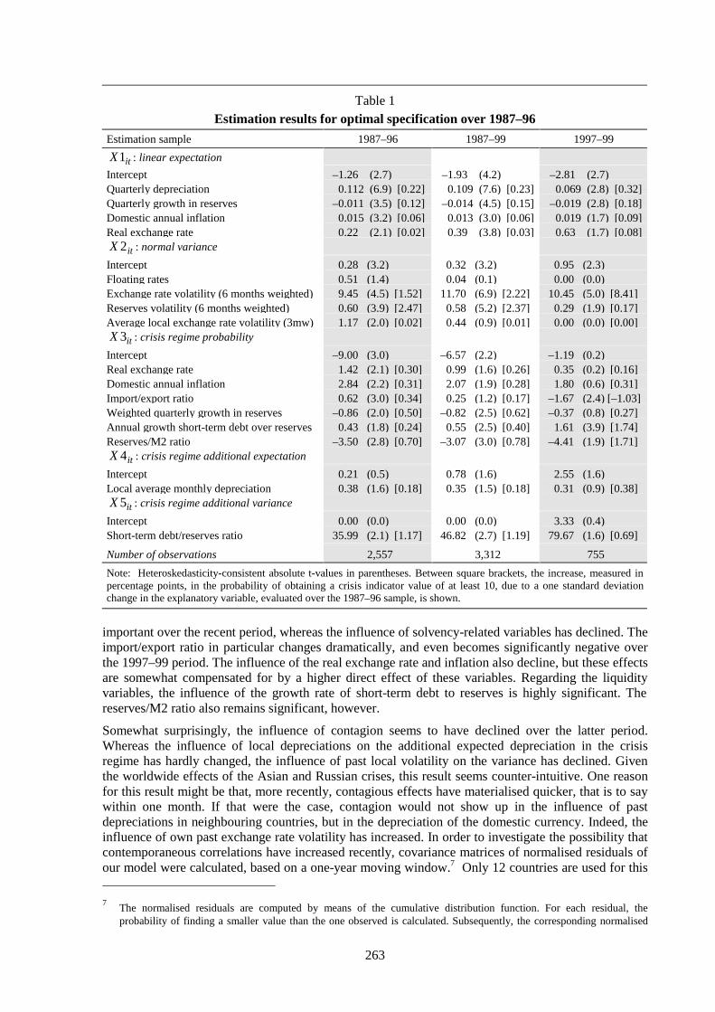
263
Table 1Estimation results for optimal specification over 1987–96
Estimation sample 1987–96 1987–99 1997–99
itX1 : linear expectation
Intercept –1.26 (2.7) –1.93 (4.2) –2.81 (2.7)Quarterly depreciation 0.112 (6.9) [0.22] 0.109 (7.6) [0.23] 0.069 (2.8) [0.32]Quarterly growth in reserves –0.011 (3.5) [0.12] –0.014 (4.5) [0.15] –0.019 (2.8) [0.18]Domestic annual inflation 0.015 (3.2) [0.06] 0.013 (3.0) [0.06] 0.019 (1.7) [0.09]Real exchange rate 0.22 (2.1) [0.02] 0.39 (3.8) [0.03] 0.63 (1.7) [0.08]
itX 2 : normal variance
Intercept 0.28 (3.2) 0.32 (3.2) 0.95 (2.3)Floating rates 0.51 (1.4) 0.04 (0.1) 0.00 (0.0)Exchange rate volatility (6 months weighted) 9.45 (4.5) [1.52] 11.70 (6.9) [2.22] 10.45 (5.0) [8.41]Reserves volatility (6 months weighted) 0.60 (3.9) [2.47] 0.58 (5.2) [2.37] 0.29 (1.9) [0.17]Average local exchange rate volatility (3mw) 1.17 (2.0) [0.02] 0.44 (0.9) [0.01] 0.00 (0.0) [0.00]
itX 3 : crisis regime probability
Intercept –9.00 (3.0) –6.57 (2.2) –1.19 (0.2)Real exchange rate 1.42 (2.1) [0.30] 0.99 (1.6) [0.26] 0.35 (0.2) [0.16]Domestic annual inflation 2.84 (2.2) [0.31] 2.07 (1.9) [0.28] 1.80 (0.6) [0.31]Import/export ratio 0.62 (3.0) [0.34] 0.25 (1.2) [0.17] –1.67 (2.4) [–1.03]Weighted quarterly growth in reserves –0.86 (2.0) [0.50] –0.82 (2.5) [0.62] –0.37 (0.8) [0.27]Annual growth short-term debt over reserves 0.43 (1.8) [0.24] 0.55 (2.5) [0.40] 1.61 (3.9) [1.74]Reserves/M2 ratio –3.50 (2.8) [0.70] –3.07 (3.0) [0.78] –4.41 (1.9) [1.71]
itX 4 : crisis regime additional expectation
Intercept 0.21 (0.5) 0.78 (1.6) 2.55 (1.6)Local average monthly depreciation 0.38 (1.6) [0.18] 0.35 (1.5) [0.18] 0.31 (0.9) [0.38]
itX 5 : crisis regime additional variance
Intercept 0.00 (0.0) 0.00 (0.0) 3.33 (0.4)Short-term debt/reserves ratio 35.99 (2.1) [1.17] 46.82 (2.7) [1.19] 79.67 (1.6) [0.69]
Number of observations 2,557 3,312 755
Note: Heteroskedasticity-consistent absolute t-values in parentheses. Between square brackets, the increase, measured inpercentage points, in the probability of obtaining a crisis indicator value of at least 10, due to a one standard deviationchange in the explanatory variable, evaluated over the 1987–96 sample, is shown.
important over the recent period, whereas the influence of solvency-related variables has declined. Theimport/export ratio in particular changes dramatically, and even becomes significantly negative overthe 1997–99 period. The influence of the real exchange rate and inflation also decline, but these effectsare somewhat compensated for by a higher direct effect of these variables. Regarding the liquidityvariables, the influence of the growth rate of short-term debt to reserves is highly significant. Thereserves/M2 ratio also remains significant, however.
Somewhat surprisingly, the influence of contagion seems to have declined over the latter period.Whereas the influence of local depreciations on the additional expected depreciation in the crisisregime has hardly changed, the influence of past local volatility on the variance has declined. Giventhe worldwide effects of the Asian and Russian crises, this result seems counter-intuitive. One reasonfor this result might be that, more recently, contagious effects have materialised quicker, that is to saywithin one month. If that were the case, contagion would not show up in the influence of pastdepreciations in neighbouring countries, but in the depreciation of the domestic currency. Indeed, theinfluence of own past exchange rate volatility has increased. In order to investigate the possibility thatcontemporaneous correlations have increased recently, covariance matrices of normalised residuals ofour model were calculated, based on a one-year moving window.7 Only 12 countries are used for this 7
The normalised residuals are computed by means of the cumulative distribution function. For each residual, theprobability of finding a smaller value than the one observed is calculated. Subsequently, the corresponding normalised
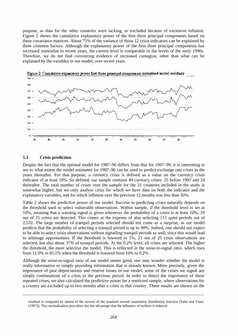
264
purpose, as data for the other countries were lacking, or excluded because of excessive inflation.Figure 2 shows the cumulative explanatory power of the first three principal components based onthese covariance matrices. About 75% of the variance of those 12 crisis indicators can be explained bythree common factors. Although the explanatory power of the first three principal components hasincreased somewhat in recent years, the current level is comparable to the levels of the early 1990s.Therefore, we do not find convincing evidence of increased contagion, other than what can beexplained by the variables in our model, over recent years.
5.3 Crisis prediction
Despite the fact that the optimal model for 1987–96 differs from that for 1997–99, it is interesting tosee to what extent the model estimated for 1987–96 can be used to predict exchange rate crises in theyears thereafter. For that purpose, a currency crisis is defined as a value on the currency crisisindicator of at least 10%. So defined, our sample contains 49 currency crises: 25 before 1997 and 24thereafter. The total number of crises over the sample for the 31 countries included in the study issomewhat higher, but we only analyse crisis for which we have data on both the indicator and theexplanatory variables, and for which inflation over the previous 12 months was less than 50%.
Table 2 shows the predictive power of our model. Success in predicting crises naturally depends onthe threshold used to select vulnerable observations. Within sample, if the threshold level is set at10%, meaning that a warning signal is given whenever the probability of a crisis is at least 10%, 10out of 25 crises are detected. This comes at the expense of also selecting 111 quiet periods out of2,532. The large number of tranquil periods selected should not come as a surprise, as our modelpredicts that the probability of selecting a tranquil period is up to 90%. Indeed, one should not expectto be able to select crisis observations without signalling tranquil periods as well, since this would leadto arbitrage opportunities. If the threshold is lowered to 1%, 23 out of 25 crisis observations areselected, but also about 37% of tranquil periods. At the 0.2% level, all crises are selected. The higherthe threshold, the more selective the model. This is reflected in the noise-to-signal ratio, which risesfrom 11.0% to 65.1% when the threshold is lowered from 10% to 0.2%.
Although the noise-to-signal ratio of our model seems good, one may wonder whether the model isreally informative or simply providing information that is already known. More precisely, given theimportance of past depreciations and reserve losses in our model, some of the crises we signal aresimply continuations of a crisis in the previous period. In order to detect the importance of theserepeated crises, we also calculated the predictive power for a restricted sample, where observations fora country are excluded up to two months after a crisis in that country. These results are shown on the
residual is computed by means of the inverse of the standard normal cumulative distribution function (Palm and Vlaar,(1997)). This normalisation procedure has the advantage that the influence of outliers is reduced.
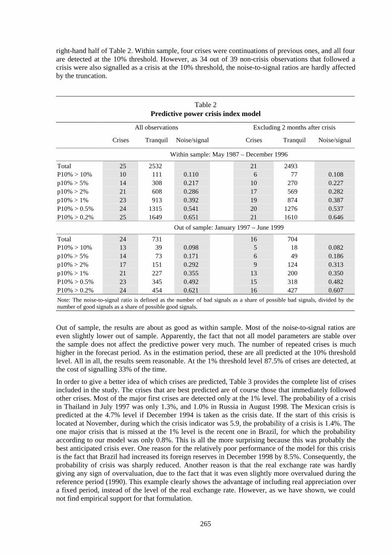
265
right-hand half of Table 2. Within sample, four crises were continuations of previous ones, and all fourare detected at the 10% threshold. However, as 34 out of 39 non-crisis observations that followed acrisis were also signalled as a crisis at the 10% threshold, the noise-to-signal ratios are hardly affectedby the truncation.
Table 2Predictive power crisis index model
All observations Excluding 2 months after crisis
Crises Tranquil Noise/signal Crises Tranquil Noise/signal
Within sample: May 1987 – December 1996
Total 25 2532 21 2493P10% > 10% 10 111 0.110 6 77 0.108p10% > 5% 14 308 0.217 10 270 0.227p10% > 2% 21 608 0.286 17 569 0.282p10% > 1% 23 913 0.392 19 874 0.387P10% > 0.5% 24 1315 0.541 20 1276 0.537P10% > 0.2% 25 1649 0.651 21 1610 0.646
Out of sample: January 1997 – June 1999
Total 24 731 16 704P10% > 10% 13 39 0.098 5 18 0.082p10% > 5% 14 73 0.171 6 49 0.186p10% > 2% 17 151 0.292 9 124 0.313p10% > 1% 21 227 0.355 13 200 0.350P10% > 0.5% 23 345 0.492 15 318 0.482P10% > 0.2% 24 454 0.621 16 427 0.607
Note: The noise-to-signal ratio is defined as the number of bad signals as a share of possible bad signals, divided by thenumber of good signals as a share of possible good signals.
Out of sample, the results are about as good as within sample. Most of the noise-to-signal ratios areeven slightly lower out of sample. Apparently, the fact that not all model parameters are stable overthe sample does not affect the predictive power very much. The number of repeated crises is muchhigher in the forecast period. As in the estimation period, these are all predicted at the 10% thresholdlevel. All in all, the results seem reasonable. At the 1% threshold level 87.5% of crises are detected, atthe cost of signalling 33% of the time.
In order to give a better idea of which crises are predicted, Table 3 provides the complete list of crisesincluded in the study. The crises that are best predicted are of course those that immediately followedother crises. Most of the major first crises are detected only at the 1% level. The probability of a crisisin Thailand in July 1997 was only 1.3%, and 1.0% in Russia in August 1998. The Mexican crisis ispredicted at the 4.7% level if December 1994 is taken as the crisis date. If the start of this crisis islocated at November, during which the crisis indicator was 5.9, the probability of a crisis is 1.4%. Theone major crisis that is missed at the 1% level is the recent one in Brazil, for which the probabilityaccording to our model was only 0.8%. This is all the more surprising because this was probably thebest anticipated crisis ever. One reason for the relatively poor performance of the model for this crisisis the fact that Brazil had increased its foreign reserves in December 1998 by 8.5%. Consequently, theprobability of crisis was sharply reduced. Another reason is that the real exchange rate was hardlygiving any sign of overvaluation, due to the fact that it was even slightly more overvalued during thereference period (1990). This example clearly shows the advantage of including real appreciation overa fixed period, instead of the level of the real exchange rate. However, as we have shown, we couldnot find empirical support for that formulation.

266
Table 3Characteristics of the currency crises in our sample
Date Country Crisis index Probability of crisis Annual inflation
8801 Jordan 11.4 3.07 13.4 –1.88802 Poland 14.6 5.13 24.6 46.78804 Jordan 14.7 22.62 82.3 1.78806 Jordan 15.0 32.05 86.1 0.38903 Venezuela 121.7 9.01 53.9 43.59010 Pakistan 13.3 4.59 27.5 10.69101 Ecuador 10.4 0.92 2.3 49.59103 Portugal 11.1 2.08 14.9 12.99103 Zimbabwe 12.5 2.71 6.7 18.89106 Zimbabwe 13.3 19.59 49.0 22.29107 India 13.6 17.24 65.3 13.09109 Zimbabwe 17.8 35.32 0.0 22.09205 Ecuador 11.0 2.69 15.6 49.69301 Zimbabwe 12.9 10.82 24.9 46.39303 India 11.1 0.33 11.5 5.79307 Pakistan 13.9 15.15 61.8 9.69309 Pakistan 11.5 20.50 3.4 9.89401 Zimbabwe 11.3 1.14 5.7 18.69405 Venezuela 35.7 1.38 18.7 48.19412 Mexico 53.7 4.69 30.6 6.99501 Mexico 11.4 42.21 78.0 7.19503 Mexico 18.9 40.38 4.3 14.39510 Mexico 11.7 3.11 10.6 43.59604 South Africa 14.9 8.14 28.2 6.39610 Pakistan 15.7 9.14 45.2 9.89707 Philippines 10.8 0.69 19.0 5.79707 Thailand 20.7 1.33 14.5 4.49708 Indonesia 14.4 1.53 8.3 5.49709 Zimbabwe 12.9 10.55 48.1 18.09710 Indonesia 11.6 16.63 6.3 7.39711 Korea 20.5 2.26 9.9 4.29711 Zimbabwe 19.7 12.51 38.4 16.09712 Indonesia 23.6 12.16 7.8 8.89712 Korea 39.8 20.85 14.8 4.39712 Philippines 15.0 5.82 15.8 7.59712 Thailand 13.5 11.93 9.6 7.69801 Indonesia 96.6 32.55 6.0 10.39801 Malaysia 14.9 10.89 7.9 2.99801 Thailand 13.2 21.55 6.4 7.69805 Indonesia 30.7 25.54 5.7 42.59806 Indonesia 33.5 34.73 2.5 49.79806 Pakistan 10.3 3.31 15.9 5.69806 South Africa 13.5 1.89 11.1 5.19808 Mexico 10.6 0.49 7.5 15.49808 Russia 29.5 1.01 7.9 5.69809 Ecuador 14.0 3.85 28.0 34.29809 Russia 81.0 30.36 38.6 9.59901 Brazil 55.2 0.82 9.1 1.79902 Ecuador 25.0 10.37 24.9 42.3
Note: represents the probability of entering the crisis regime of our model. Annual inflation denotes theinflation rate over the 12 months before the crisis.
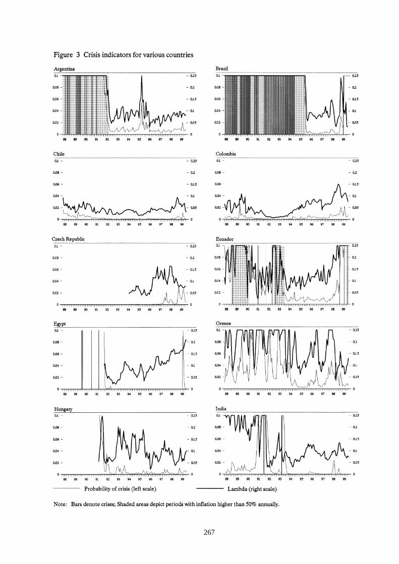
267

268
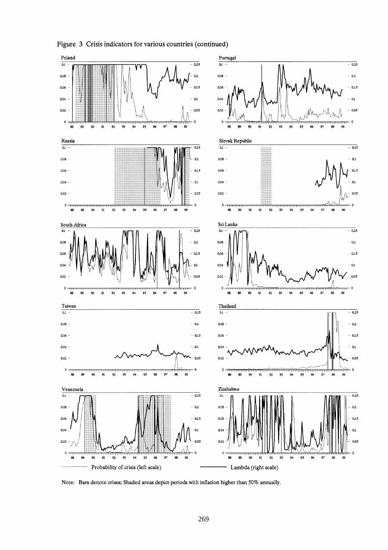
269
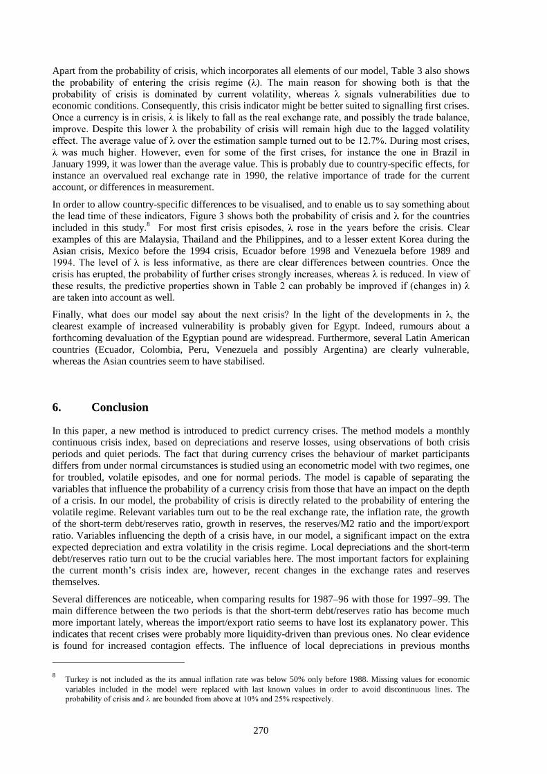
270
Apart from the probability of crisis, which incorporates all elements of our model, Table 3 also showsWKH SUREDELOLW\ RI HQWHULQJ WKH FULVLV UHJLPH 7KH PDLQ UHDVRQ IRU VKRZLQJ ERWK is that theSUREDELOLW\ RI FULVLV LV GRPLQDWHG E\ FXUUHQW YRODWLOLW\ ZKHUHDV VLJQDOV YXOQHUDELOLWLHV GXH WReconomic conditions. Consequently, this crisis indicator might be better suited to signalling first crises.2QFHDFXUUHQF\LVLQFULVLV LVOLNHO\WRIDOODVWKHUHDOH[FKDQJHUDWHDQGSRVVLEO\WKHWUDGHEDODQFHLPSURYH'HVSLWH WKLV ORZHU WKHSUREDELOLW\RI FULVLVZLOO UHPDLQ KLJK GXH WR WKH ODJJHG YRODWLOLW\HIIHFW7KHDYHUDJHYDOXHRI RYHUWKHHVWLPDWLRQVDPSOHWXUQHGRXWWREH'XULQJPRVWFULVHV ZDV PXFK KLJKHU +RZHYHU HYHQ IRU VRPH RI WKH ILUVW FULVHV IRU LQVWDQFH WKH RQH LQ %UD]LO LQ
January 1999, it was lower than the average value. This is probably due to country-specific effects, forinstance an overvalued real exchange rate in 1990, the relative importance of trade for the currentaccount, or differences in measurement.
In order to allow country-specific differences to be visualised, and to enable us to say something aboutthe OHDGWLPHRIWKHVHLQGLFDWRUV)LJXUHVKRZVERWKWKHSUREDELOLW\RIFULVLVDQG IRUWKHFRXQWULHVincluded in this study.8 )RU PRVW ILUVW FULVLV HSLVRGHV URVH LQ WKH \HDUV EHIRUH WKH FULVLV &OHDUexamples of this are Malaysia, Thailand and the Philippines, and to a lesser extent Korea during theAsian crisis, Mexico before the 1994 crisis, Ecuador before 1998 and Venezuela before 1989 and7KH OHYHORI LV OHVV LQIRUPDWLYH DV WKHUH DUH FOHDUGLIIHUHQFHVEHWZHHQ FRXQWULHV2QFH WKHFULVLVKDVHUXSWHGWKHSUREDELOLW\RIIXUWKHUFULVHVVWURQJO\LQFUHDVHVZKHUHDV LVUHGXFHG,QYLHZRIWKHVHUHVXOWV WKHSUHGLFWLYHSURSHUWLHVVKRZQLQ7DEOHFDQSUREDEO\EHLPSURYHG LIFKDQJHV LQare taken into account as well.
)LQDOO\ ZKDW GRHV RXUPRGHO VD\ DERXW WKH QH[W FULVLV" ,Q WKH OLJKW RI WKH GHYHORSPHQWV LQ WKHclearest example of increased vulnerability is probably given for Egypt. Indeed, rumours about aforthcoming devaluation of the Egyptian pound are widespread. Furthermore, several Latin Americancountries (Ecuador, Colombia, Peru, Venezuela and possibly Argentina) are clearly vulnerable,whereas the Asian countries seem to have stabilised.
6. Conclusion
In this paper, a new method is introduced to predict currency crises. The method models a monthlycontinuous crisis index, based on depreciations and reserve losses, using observations of both crisisperiods and quiet periods. The fact that during currency crises the behaviour of market participantsdiffers from under normal circumstances is studied using an econometric model with two regimes, onefor troubled, volatile episodes, and one for normal periods. The model is capable of separating thevariables that influence the probability of a currency crisis from those that have an impact on the depthof a crisis. In our model, the probability of crisis is directly related to the probability of entering thevolatile regime. Relevant variables turn out to be the real exchange rate, the inflation rate, the growthof the short-term debt/reserves ratio, growth in reserves, the reserves/M2 ratio and the import/exportratio. Variables influencing the depth of a crisis have, in our model, a significant impact on the extraexpected depreciation and extra volatility in the crisis regime. Local depreciations and the short-termdebt/reserves ratio turn out to be the crucial variables here. The most important factors for explainingthe current month’s crisis index are, however, recent changes in the exchange rates and reservesthemselves.
Several differences are noticeable, when comparing results for 1987–96 with those for 1997–99. Themain difference between the two periods is that the short-term debt/reserves ratio has become muchmore important lately, whereas the import/export ratio seems to have lost its explanatory power. Thisindicates that recent crises were probably more liquidity-driven than previous ones. No clear evidenceis found for increased contagion effects. The influence of local depreciations in previous months
8
Turkey is not included as the its annual inflation rate was below 50% only before 1988. Missing values for economicvariables included in the model were replaced with last known values in order to avoid discontinuous lines. TheSUREDELOLW\RIFULVLVDQG DUHERXQGHGIURPDERYHDWDQGUHVSHFWLYHO\

271
seems to have declined somewhat, whereas the contemporaneous correlations of the normalisedresiduals of our model rose only slightly. This result seems surprising given the worldwide impact ofthe Asian crisis. However, the domino effects of this crisis, as well as the large impact on the worldeconomy, might also be explained by the fact that these countries are much more open and moredeveloped than most previous targets of currency attacks. Consequently, large initial depreciationsimmediately affected the economic growth potential for neighbouring countries, as they werecompeting to a large extent on the same markets, and relied on exports for their growth.
The model is reasonably successful in predicting currency crises, including out of sample. If thethreshold above which the model gives a warning signal for an impending crisis is set at 1%, 21 out of24 crises are predicted out of sample. However, this comes at the cost of also giving a warning signal35% of the time when no crisis is about to occur. The clearest signals are provided for crises thatfollowed other crises. First crises are better detected by changes in the probability of entering the crisisUHJLPH 7KHVHSURYLGHDJRRGVXPPDU\RIFKDQJHVLQWKHHFRQRPLFYXOQHUDELOLW\RIFXUUHQFLHV$Vthe link between vulnerabilities and currency crises is far from perfect, however, one cannot expect todetect all currency crises with the help of just one econometric model.

272
Appendix: Data sources
General: The countries included in this study are: Argentina, Brazil, Chile, Colombia, the CzechRepublic, Ecuador, Egypt, Greece, Hungary, India, Indonesia, Israel, Jordan, Korea, Malaysia,Mexico, Morocco, Pakistan, Peru, the Philippines, Poland, Portugal, Russia, Slovakia, South Africa,Sri Lanka, Taiwan, Thailand, Turkey, Venezuela and Zimbabwe. The database consists of monthlyobservations for the period January 1970 to June 1999. Observations for countries with an annualinflation rate above 50% in the previous month are excluded from the estimation and evaluationprocedures. Most data come from the August 1999 International Financial Statistics CD-ROM of theIMF. Additional data are from Datastream or taken from the internet. For Taiwan, which is not an IMFmember, most data come from the Directorate General of Budgeting and Accounting Statistics(DGBAS). All explanatory variables are lagged at least one month, and more if the publication lag ofthe data is likely to be longer. In order to limit the influence of large reserve changes or nominalexchange rates, explanatory variables involving these two variables are bounded to their mean plus orminus five standard deviations. Local variables are calculated over usable observations of the includedcountries per continent (Asia, Latin America, Europe, or Africa plus the Middle East), excluding thecountry concerned. Global variables are calculated over the usable observations of all includedcountries, again excluding the country concerned. Whenever a weighted average of variable X over imonths is used, it is calculated as:
∑∑ =−= −−= i
jij jtWi jXjiX 1
10 /)( .
Exchange rates: line ae of the IFS, end-of-period local currency per US dollar, except for Taiwan(London exchange market). As explanatory variable, the variable is lagged in our model at least onemonth.
International reserves: line 1..ld of the IFS, international reserves excluding gold in millions of USdollars, except for South Africa, for which total reserves including gold (line 1..sf) are used. ForTaiwan, official reserves in US dollars, provided by DGBAS. As explanatory variable, the variable islagged in our model at least one month.
Currency crisis index: 0.8 * monthly percentage depreciation + 0.2 * monthly percentage reservelosses. In the estimation process, this variable is bounded at 50%, in order to limit the influence of anextreme observation (Venezuela, March 1989).
Consumer price index: line 64 of the IFS. For Taiwan, the urban CPI provided by DGBAS is used. Asexplanatory variable, the variable is lagged in our model at least one month.
Real exchange rates: CPI-based trade-weighted real exchange rates. Three different sources are used:the measure of JP Morgan for Argentina, Brazil, Chile, Colombia, Ecuador, Greece, India, Indonesia,Korea, Malaysia, Mexico, Morocco, Pakistan, Peru, the Philippines, South Africa, Taiwan, Thailand,Turkey and Venezuela; the IFS measure (line rece) for Hungary, Israel, Poland, Portugal, Russia andSlovakia; and own calculations based on trade weights with Japan, the European Union and the UnitedStates for the Czech Republic, Egypt, Jordan, Sri Lanka and Zimbabwe. For our own calculations,period average US dollar exchange rates (line af of IFS) and CPIs of Japan, Germany, the UnitedStates and the countries concerned are used. The trade weights are from various issues of the Directionof Trade Statistics. As explanatory variable, the variable is lagged in our model at least one month.
M2: Sum of lines 34 and 35 of the IFS. For Hungary, monthly observations provided by the NationalBank of Hungary are used. For Taiwan, monthly figures are from DGBAS. As explanatory variable,the variable is lagged in our model at least two months.
Credit: line 32d of the IFS, domestic credit to private sector. For Taiwan, domestic credit to privatesector collected by DGBAS; for Hungary, monthly consumer credit from the National Bank ofHungary. As explanatory variable, the variable is lagged in our model at least two months.
Short-term foreign debt and total foreign debt: BIS database. Semiannual reports of foreign lending ofBIS reporting banks by country and remaining maturity. Short-term debt is defined as debt with a

273
remaining maturity of less than one year. As explanatory variables, these variables are lagged in ourmodel at least five months as there is a five-month publication lag. This means using theend-December positions for the months May to October of the next year, and the end-June positionsfor the months November to April.
Exports and imports: lines 70..d and 71..d of the IFS, exports and imports in millions of US dollars. Asexplanatory variables, the variables are lagged in our model at least two months.
Gross domestic product: line 99b of the IFS, GDP in current prices. This quarterly series istransformed into a monthly series, using CPI and industrial production (line 66 of the IFS) asindicators. The quarterly GDP series for Taiwan is from DGBAS. If the IFS database did not providemonthly industrial production series, other sources were used as well. The alternative sources forindustrial production are: OECD (Hungary, Poland, Portugal and Russia), Macroeconomica(Argentina), Lopes Filho & Associates (Brazil), National Statistical Service of Greece, Biro PusatStatistik (Indonesia), Statistics South Africa, DGBAS (Taiwan), Bank of Thailand, State Institute ofStatistics (Turkey) and Veneconomia (Venezuela). As explanatory variable, the variable is lagged inour model at least two months.
Exchange rate regime: Annual report on exchange arrangements and exchange restrictions, IMF,various issues.

274
Bibliography
Berg, A and C Pattillo (1998): “Are Currency Crises Predictable? A Test”. IMF Working Paper,98/154.
Borenzstein, E, A Berg, G-M Millesi-Ferretti and C Pattillo (1999): “Anticipating Balance ofPayments Crises – The Role of Early Warning Systems”. IMF Occasional Paper, forthcoming.
Bussière, M and C Mulder (1999): “External Vulnerability in Emerging Market Economies: HowHigh Liquidity Can Offset Weak Fundamentals and the Effects of Contagion”. IMF Working Paper,99/88.
Calvo, G (1998): “Varieties of Capital-Market Crises”, in Calvo, G and M King (eds.) The debtburden and its consequences for monetary policy. IEA Conference Volume, No. 118. New York: St.Martin’s Press; London: Macmillan Press; in association with the International Economic Association.
Chang, R and A Velasco (1998): “Financial Fragility and the Exchange Rate Regime”. NBER WorkingPaper, 6469.
Frankel, J A and A K Rose (1996): “Currency Crashes in Emerging Markets: An EmpiricalTreatement”. Journal of International Economics, 41, pp. 351-66.
Glick, R and A K Rose (1998): “Contagion and Trade: Why are Currency Crises Regional?” NBERWorking Paper, 6806.
Kaminsky, G L, S Lizondo and C M Reinhart (1998): “Leading Indicators of Currency Crises”. IMFStaff Papers, 45, pp. 1-48.
Kaminsky, G L and C M Reinhart (1996): “The Twin Crises: The Causes of Banking and Balance-of-Payments Problems”. International Finance Discussion Papers, 544, Board of Governors of theFederal Reserve System.
Krugman, P (1979): “A Model of Balance-of-Payments Crises”. Journal of Money, Credit andBanking, 11, pp. 311-25.
JP Morgan (1998): “Event Risk Indicator Handbook”. JP Morgan, London (can be downloaded from:www.jpmorgan.com).
Obstfeld, M (1986): “Rational and Self-Fulfilling Balance-of-Payments Crises”. American EconomicReview, 76, pp. 72-80.
Obstfeld, M (1995): “The Logic of Currency Crises”, in Eichengreen, B, J Frieden and J von Hagen(eds.) Monetary and fiscal policy in an integrated Europe. European and Transatlantic Studies,Heidelberg; New York and London: Springer, pp. 62-90.
Palm, F C and P J G Vlaar (1997): “Simple Diagnostic Procedures for Modelling Financial TimeSeries”. Allgemeines Statistisches Archiv, 81, pp. 85-101.
Sachs, J D, A Tornell and A Velasco (1996): “Financial Crises in Emerging Markets: The Lessonsfrom 1995”. Brookings Papers on Economic Activity, pp. 147-98.
Tornell, A (1999): “Common Fundamentals in the Tequila and Asian Crises”. NBER Working Paper,7139.
Velasco, A (1987): “Financial Crises and Balance-of-Payments Crises”. Journal of DevelopmentEconomics, 27, pp. 263-83.
Vlaar, P J G (1998): “Target Zones and Realignment Risk: An Integrated Approach”. De Economist,146, pp. 91-116.
275
How global are global financial markets?The impact of country risk
Dominik Egli1
1. Introduction
Financial transactions are costly. On the one hand, processing a transaction requires resources, on theother hand the regulatory framework is costly as well. In both areas there have been dramatic changesrecently. Computerisation and advances in telecommunications lead to considerably lower technicalcosts. Furthermore, deregulation has eliminated many barriers to trade. Financial markets have becomeand still are in the process of becoming more open, and one often hears of the “globalisation offinancial markets”. As already mentioned in the title, I will investigate the question of what this meansin geographical terms. International transactions which lead to a net debtor position of countries resultin an additional type of transaction cost: country risk. Unlike domestic borrowers, sovereign countriescannot be forced to perform their contracts by legal action against them. Instead, creditors have to relyon indirect mechanisms. In the following, I describe the consequences of country risk in detail anddiscuss the main mechanism for dealing with it. It will become clear that country risk is the maintransaction cost for countries which should actually be large debtors given the potential of theireconomies. Country risk, therefore, considerably hampers the globalisation of financial markets.
2. Country risk
A creditor-debtor relationship typically consists of three types of actions. At the beginning of therelationship, the creditor lends money to the debtor. At the end, the debtor pays back the money lent.In between, the debtor pays interest on the loan. How much money has to flow on which date isusually written into a contract. The strategic situation is as simple as it is explosive: whereas thecreditor would like to get back as much as possible, the debtor prefers to pay back as little as possible.
Basically, payments are voluntary. Depending on the legal system, a damaged party has several meansby which to impose sanctions on the defaulting party. When payments become due, a debtor weighsthe costs of honouring the contract against the costs of defaulting on the loan. A simple model mightclarify the situation. On one side there is a debtor, on the other side there are many potential lenders.Let us assume that each lender is very wealthy.2 In this type of scenario, we can analyse the situationof a lender and a debtor in which the debtor has all the bargaining power. By combining interestpayments and repayment of principle, we have a two-stage strategic game. First, a contract (D, r) issigned, where D is the amount the lender hands over to the debtor and r is the interest rate. D thengoes to the debtor. Subsequently, repayment S = (1 + r) D becomes due. If the debtor does not payback S, sanctions can be imposed on him, which cost him P, an exogenous amount. The debtor’sdecision is now simple: if S < P he honours the debt, if S > P he defaults, and if S = P he is indifferent(we assume that he honours the debt in this case). When negotiating the contract at the first stage, theparties anticipate the debtor’s decision rule. Since there is no other risk than default risk, the debtoronly signs a contract with r* = i, where i is the world market interest rate. According to the debtor’sdecision in the second stage, the maximum repayment the debtor is willing to make is P. The
1 I would like to thank Bernhard Emunds for valuable suggestions. The views expressed in this article are those of the
author and should not be interpreted as reflecting those of the Swiss National Bank or other members of its staff.
2 Alternatively, we could assume that the lenders can form lending syndicates without incurring any expenses.

276
maximum money flow D the lender is willing to lend is computed from the condition P = (1 + i) D,
leading to D = P/(1 + i) (Eaton et al. (1986)).
It is worth mentioning that this result applies to both domestic and international debt contracts. In thedomestic area, the sanctioning costs P consist of costs the debtor incurs from bankruptcy. Inbankruptcy proceedings, the receiver seizes the tangible assets of the debtor. If the debtor has to bear apositive share of the costs of the bankruptcy proceedings, he only defaults if he is unable to pay.3
Nonetheless, the willingness to pay is the driving force. Faced with the threat of bankruptcy, thedebtor is willing to pay whenever he is able to do so. At the international level, the willingness to payis also the driving force. Since it is much more difficult to enforce performance of a contract throughbankruptcy proceedings, however, this fact is more apparent than at the domestic level.
In the absence of bankruptcy proceedings, the maximum debt amount is not determined by theprofitability of the project the debtor wants to carry out with the funds lent, but by the sanctioningcosts P. The lender is willing to lend any amount up to D . This can lead to credit rationing (Allen(1983)). In this case, the debtor would benefit from higher sanctioning costs. For each additional dollarof sanctioning costs, he gets 1/(1 + i) additional dollars of debt D. The lender does not care how thedebtor uses the money he gets, as long as the use does not influence the sanctioning costs P.
In sum, it can be said that the costs sanctions impose on the debtor determine the maximum amount ofdebt. The severity of the bankruptcy threat as the main penalty in the domestic realm causes thewillingness and the ability to repay to coincide. There are, however, no international bankruptcyproceedings. This constitutes the main difference between domestic and international debt contracts.In order to analyse the determinants of international debt, we have to take a closer look at the sanctionslenders can impose on defaulting international debtors.
3. The costs of sanctions
In what follows, I will present and discuss sanctions and their costs. There are two main types ofsanctions. In the vernacular, there are two approaches to induce a certain behaviour, referred to as“carrot and stick”. This approach can easily be applied to sanctions. Under the “carrot” approach, alender threatens to exclude the debtor from future access to international financial markets, and underthe “stick” approach, a lender threatens to impose direct sanctions. Exclusion from internationalmarkets leads to costs in the future, while direct sanctions lead to immediate costs.
3.1 Access to international financial markets
In the two-stage game of the previous section, market access cannot act as a disciplining device sincethe game ends after the repayment decision of the debtor. If the two-stage game is repeated “many”times, two incentives to preserve market access arise. First, credits can be used to smooth consumptionin case of income fluctuations. In bad times, the country imports more than it exports, thereby gettinginto debt, and in good times it repays by running a trade surplus. Second, credits can be used tofinance profitable projects. I will start with the latter.
3.1.1 Investment
In the public discussion, investment are probably the most prominent reason for international debt. Atransfer of savings from rich countries to poor countries will enable the latter to finance projects andthereby grow. The proceeds of the project will allow the debtor country to repay its debt and still keepsomething for itself. Under the threat of being denied access to international financial markets, the
3 In cases where the receiver is not able to seize all assets or the debtor is able to “take the money and run”, default can
occur even though the debtor would be able to honour the contract.
277
country repays in order to receive international funds to finance additional projects in the future.International lending for financing investments takes place when the return on investment is higherabroad than at home. As long as this is the case, the debtor country has no reason to prove its honestysince the creditors will grant additional loans out of profit considerations. This reasoning no longermakes sense when the investment prospects are the same in both countries. If this point is reached,however, firms in the debtor country no longer need access to international markets since they canfinance their projects on the home market at equal cost. Therefore, the threat of an exclusion frominternational financial markets has no bite. Sooner or later, the debtor country will no longer needaccess to international markets to finance valuable projects. Anticipating this, rational creditors are notwilling to lend at all. From the debtor countries’ point of view, the worst possible situation becomes areality.
The models of Kletzer (1984) and Cole and English (1991) show two possible ways to handle thisproblem. Basically, in both papers the existence of a last period, which triggers the backwardinducement argument used above, is assumed away. Kletzer (1984) assumes that projects financed byforeign lending enhance productivity, but only for one period. These productivity gains are lost in theevent of exclusion from the international financial markets. Cole and English (1991) model aneconomy with a growing amount of infinitely living individuals. They assume that internationaltransfers are necessary to guarantee optimal per capita consumption. A default triggers exclusion fromthe international financial markets and leads to a decline of per capita consumption. This threat makesinternational lending possible.
3.1.2 Consumption smoothing
Instead of financing projects, international credits can be used for consumption smoothing. Theinternational capital markets work as an insurance against income fluctuations. Income fluctuationscan be triggered by crop fluctuations or by changes in the terms of trade. If income is uncertain foreach period and the country prefers stable consumption to unstable consumption, it must always allowfor the possibility of using international credits in the future. As Eaton and Gersovitz (1981) show, thethreat of being cut off from receiving additional funds is enough to explain international debt. In goodtimes, the debtor country honours its obligations voluntarily in order to receive financing in bad times.Bulow and Rogoff (1989b) question the conclusion of Eaton and Gersovitz. They point out that acountry has other possibilities to perform consumption smoothing. The debtor country may just aseasily pay in advance for state-contingent future payments by international investors. The countrythereby signs an insurance contract. The premium is paid in advance, and the contract designatespayments in the case of unfavourable events in the future. According to Bulow and Rogoff (1989b), inequilibrium loans should not be granted, since the country would strictly profit from a switch from acredit contract to an insurance contract. Potential insurers have no incentives not to accept a contractsince they get paid in advance. In this case, the threat of exclusion from the international financialmarkets is not enough to discipline a sovereign debtor.
3.2 Direct sanctions
3.2.1 Bankruptcy
Of course, a lender always has the possibility to sue a defaulting foreign debtor. The debtor then riskslosing his assets. However, governments have several options to prevent the threat of seizing theirassets taking effect. For instance, a government can restrict the access of foreigners to bankruptcyproceedings. It can also directly change the bankruptcy procedure such that it becomes too costly.Quite a different possibility is to restrict capital mobility. Winning a lawsuit is of limited value if thelender is not allowed to export the proceeds. Yet another possibility is to add an official provision toguarantee the debt contract and to forbid payments. A government which is unwilling to repay a loanalways has means to undermine the credibility of the bankruptcy proceedings (Niehans (1986)).

278
3.2.2 Confiscation of foreign assets
The lenders can threaten to seize the foreign assets of a defaulting debtor country. In order for thisthreat to have an impact, there have to be clearly assignable assets. In addition, these assets need to bein the country in case a default occurs. This means that confiscation is only a threat to the country if itis not able to repatriate the assets in time. Moreover, lenders need the cooperation of their governmentor jurisdiction. According to Bulow and Rogoff (1989a), the law of most lender countries permits theseizure of foreign assets in order to satisfy domestic lenders.
3.2.3 Trade credits
Banks usually act as intermediaries for international transactions. In this way, delivery and paymentneed not coincide perfectly. Denying trade credits increases the cost of international trade since thedebtor country now has to build up reserves in order to pay instantly for imported goods.
3.2.4 Trade sanctions
Lenders can impose a trade embargo. Such an embargo only works if all trading partners cooperate.Since the debtor country is still interested in international trade, an embargo leads to losses by theforeign exporters. Since exporters usually are not lenders, the losers and the winners are not the same.Therefore, the losers have to be paid. If they are not, they participate in the political process to havethe embargo lifted. An individual country has an incentive to break an embargo since it can gain aslong as all other countries stick to the embargo. A debtor country can also mitigate the consequencesof an embargo by substitution. Therefore, the goods for which an embargo applies have to be adjustedon a regular basis.
Enforcing an embargo requires considerable determination. It must be monitored and adjustedcontinuously. Any slackening of efforts quickly leads to a deterioration of the embargo (Frey (1985)).The basic problems with an embargo are that where there is trade there is profit to be made and that itis very difficult to intervene in this process.
3.2.5 Costly sanctions
In summarising the analysis, the lenders’ attitude can be characterised as follows: as long as the debtorcountry honours its obligations, nothing happens. If it does not, the lenders impose sanctions. Thedebtor country pays as long as the costs incurred by the sanctions are lower than the obligations.Bulow and Rogoff (1989a) show that this analysis is unsatisfactory if the sanctions also result in costsfor the lenders. If this happens, it is not only necessary to resort to the possibility of imposingsanctions; lenders must also be willing to impose them.
Let us consider a debt contract with debt amount D and repayment obligation S = (1 + r) D. Weassume that the lenders can seize assets worth Y. Obviously, the debtor country faces punishment costsP = Y. The debtor country now has two possibilities. It either pays S or it offers a new contract withrepayment 0 S′ < S. Since S′ can be zero, default is already factored in. If the debtor country repaysS, the contractual relationship ends. If the debtor country offers S′ instead, and the lenders accept, thecountry pays S′ and the contractual relationship ends. If instead the lenders reject the offer, they canimpose sanctions. We assume that this leads to costs C for the lenders. On the one hand, C representsthe costs of the renegotiation procedure, on the other hand it represents the possibly different valuationof the sanction. If the debtor country defaults and the lenders impose the sanction, the net gain for thelenders is Y – C. The debtor country, however, is left with nothing. If the debtor country offersS′ = Y – C, the lenders are as well off and therefore agree. The country now is left with C. The debtorcountry therefore offers a renegotiated contract whenever Y – C < S. Anticipating this behaviour, thelenders are only willing to lend up to D* = (Y – C)/(1 + i) = (P – C)/(1 + i). The assumed strategicadvantage of the debtor country affects it negatively ex ante since the lenders anticipate its strength.The lower the bargaining power of the debtor country, the weaker is the effect. In the extreme case offull bargaining power of the lenders, renegotiation has no influence on the initial contract. The
279
possibility to renegotiate contracts strengthens the debtor country’s position ex post and has negativeconsequences ex ante since the lenders protect themselves against the strength of the debtor.
As already mentioned, this result is driven by the sanctioning costs C. Note that these costs are puredead weight losses. The bargaining procedure ensures that the sanctions do not take place, therebyleading to gain C. In fact, the parties bargain over how to split this gain. Assuming the information issymmetrical, this gain is always achieved (Coase Theorem). Since the bargaining solution isanticipated, it is implicitly incorporated in the original contract. Bargaining and sanctioning never takeplace. Bargaining power turns out to be a boomerang for the debtor country.
3.3 Reputation
Reputation as a disciplining mechanism constitutes a mixture of the carrot and stick approaches. Aerniand Egli (1999) analyse reputation as a basis for international lending. As in the standard reputationmodels (for an overview, see Fudenberg and Tirole (1991), Chapter 9), reputation effects areintroduced by adding uncertainty. Aerni and Egli assume that some debtor countries pay their debtobligations in any case, whereas other countries weigh the pros and cons of contract fulfilment againstrepudiation. Trade restrictions, such as embargoes or the denying of trade credits, can serve as a threatto discipline the behaviour of the debtor. The assumption implies that for some countries trade is soimportant that they are vulnerable, and hence always willing to pay. Another possible explanation forthe willingness to pay could be the different attitudes towards the future on the part of the government.Some regimes may be myopic and therefore maximise utility over short-term periods, whereas othersmay be more future-oriented, and are willing to bear costs today in order to profit tomorrow. While adebtor country knows whether or not it can successfully default on its debt, the creditor country isuncertain as to the type of debtor country it is dealing with. It only knows the strictly positive priorprobability that the debtor will always pay. A so-called “bad” debtor country may have an incentive tobuild up a reputation of being a reliable debtor by mimicking the behaviour of a “good” country.Under some parameter constellations, reputation leads to contracts in a two-period game which wouldbe irrational if only one period were considered.
The result also sheds light on the question of how and why international debt relationships areconnected with default. In a reputational equilibrium, default has to be a possibility. If a bad debtordoes not repay with a probability of less than one, there will be no lending. Default occurs as part ofoptimal play and is therefore simply a necessary by-product of international lending relationships.Whereas in the literature default occurs either due to unfavourable exogenous factors which the partiescannot write into a contract (see, for instance, Eaton et al. (1986) or Grossman and Van Huyck (1988))or due to falsely high debt (Bulow and Rogoff (1989b), among others), in the model of Aerni and Eglidefault arises endogenously and is, as just mentioned, both necessary and unavoidable.
4. How global are global financial markets?
Sovereign countries can default on their debt. As the discussion so far has shown, the sovereignty ofcountries leads to a misallocation of capital, especially to countries which, based on their economicpotential, should be debtors. For these countries, country risk is the major transaction cost.“Globalisation of financial markets” is based on the reduction of other transaction costs. For thecountries for which country risk is the major cost, the reduction of other costs plays only a secondaryrole. Globalisation will stop at their borders. The analysis, however, also shows ways to integratecountries despite country risk. As we have seen, punishments are the driving force behind internationallending. Industrial countries have access to international financial markets not only because most ofthem are small borrowers at best, but also because they are extremely vulnerable owing to their closetrade relations. Integrating emerging market countries into world trade makes them vulnerable too,thereby enabling them to participate in international financial markets.

280
Bibliography
Aerni, Peter and Dominik Egli (1999): “Overcoming Time-Inconsistency in Sovereign Debt”. Mimeo.
Allen, Franklin (1983): “Credit Rationing and Payment Incentives”. Review of Economic Studies, 50,pp. 639-46.
Bulow, Jeremy and Kenneth Rogo (1989a): “A Constant Recontracting Model of Sovereign Debt”.Journal of Political Economy, 97, pp. 155-78.
Bulow, Jeremy and Kenneth Rogo (1989b): “Sovereign Debt: Is to Forgive to Forget?”. AmericanEconomic Review, 97, pp. 43-50.
Cole, Harold and William English (1991): “Expropriation and Direct Investment”. Journal ofInternational Economics, 30, pp. 201-27.
Eaton, Jonathan and Mark Gersovitz (1981): “Debt with Potential Repudiation: Theoretical andEmpirical Analysis”. Review of Economic Studies, 48, pp. 289-309.
Eaton, Jonathan, Mark Gerosvitz and Joseph Stiglitz (1986): “The Pure Theory of Country Risk”.European Economic Review, 30, pp. 481-513.
Fudenberg, Drew and Jean Tirole (1991): Game theory. MIT Press, Cambridge, Mass. and London.
Frey, Bruno (1985): Internationale Politische Oekonomie, München.
Grossman, Herschel I and John B Van Huyck (1988): “Sovereign Debt as a Contingent Claim:Excusable Default, Repudiation, and Reputation”. American Economic Review, 78(5), pp. 1088-97.
Kletzer, Kenneth (1984): “Asymmetries of Information and LDC Borrowing with Sovereign Risk”.Economic Journal, 94, pp. 287-307.
Niehans, Jürg (1986): “Internationale Kredite mit undurchsetzbaren Forderungen”. Schriftenreihe desVereins für Socialpolitik, 155, pp. 151-79, Berlin.

281
Asian crisis post-mortem: where did the money goand did the United States benefit?
Eric van Wincoop and Kei-Mu Yi1
1. Introduction
The recent currency crises in Asia have raised important questions about the sensitivity ofindustrialized economies to financial crises in faraway emerging markets. In late 1997 and 1998,Indonesia, Korea, Malaysia, the Philippines and Thailand (Asia-5) experienced net capital outflows ofabout $80 billion, plunging them from “growth miracle” status into the worst recession they had seenin decades. GDP growth rates for 1998 in Korea and Malaysia were –5.8% and –7.5%, respectively,and in Indonesia and Thailand the GDP declines exceeded 10%. In the United States, however, 1998turned out to be a strong year, with GDP growth coming in at +4.1%.
Is there a connection between the crisis in Asia and the strong US growth performance? Sequentialcorrelation, of course, does not imply causation. The US economy could have been robust for manyreasons, including the “new” productivity revolution and the reductions in the federal funds rate in late1998. In addition, most economists thought the downturn in Asia would exert a negative effect on theUS economy. Recessions in the crisis countries, in conjunction with sharply depreciated currencies,would reduce their demand for imports from the United States. Moreover, the currency depreciationswould lead to an export surge to the United States. Hence, through this international trade channel, USnet exports were predicted to contribute more negatively to growth than had been expected prior to thecrisis. Indeed, the US trade deficit did increase, contributing –1.1% to US GDP growth in 1998.However, the increase in the deficit was more than offset by continued strong increases in employmentand production, in conjunction with continued robust spending on consumer goods and on producers’durable equipment. Quarter by quarter, US GDP growth in 1998 consistently exceeded projections.
In our view, these (apparently) surprising outcomes reflect the fact that the original way of thinkingabout the crisis was flawed. First, the depreciation of the Asian currencies against the dollar and therecessions in the Asian crisis countries were endogenous responses to a large and sharp reallocation ofcapital out of the Asian crisis region. From the point of view of the United States, this reallocation ofcapital is the appropriate starting point – not the depreciations and recessions – when thinking aboutthe implications of the crisis for the US economy.2 Second, the original way of thinking focused onlyon demand-side channels, ignoring the supply side.
While the reallocation of capital towards the United States generated the above-mentioned negativetrade effects on US GDP, the capital inflows also generated a positive effect on US GDP by financingan increase in US spending, both directly and indirectly by generating a drop in interest rates. Thecapital inflows also led to an appreciating dollar, which made imported inputs cheaper. These cheaperinputs generated a positive effect on GDP similar to the effect of a positive productivity shock. Forthese two reasons then, rather than viewing the strong US growth performance in 1998 as having
1
The views expressed in the paper are those of the authors and are not necessarily reflective of views at the FederalReserve Bank of New York or the Federal Reserve System. We thank Barbara Berman, Chris Gorband and Russ Schollof the Bureau of Economic Analysis, and Dan Kinney, Sydney Ludvigson, Therese Melfo, Don Morgan, Dick Peach,Monica Posen, Charles Steindel and participants at two Research Department brown bags for very helpful comments.Scott Nicholson and Stefan Papaioannou provided outstanding research assistance.
2One can of course go a step further and say that the analysis should start with the factors that led to the capital outflowfrom Asia in the first place. But from the point of view of the US economy, the exact cause of the reallocation of capitalis not critical.

282
occurred despite the Asian crisis, we view the strong performance as having occurred because of theAsian crisis.
As the crisis proceeded, and US growth remained strong, a new story along the lines sketched above,with capital inflows into the United States as the centerpiece, became increasingly popular. Yetsurprisingly, there is very little documentation of this story. This paper aims to at least partially fillthat gap. Specifically, we first attempt to document the trail of capital out of Asia and into the UnitedStates. We then analyze and quantify the implications for short-run US GDP growth of the (direct andindirect) reallocation of capital from Asia to the United States.
It is not difficult to document the “beginning” and the “end” of the money trail insofar as it involvesthe Asian countries and the United States. Capital outflows from the Asia-5 from the start of the crisis(1997Q2) to the end of 1998 amounted to about $80 billion. The United States ran a current accountdeficit in 1998 of $221 billion, an increase of $77 billion over the 1997 current account deficit. Theincreased deficit was obviously financed by increased capital inflows.
It is more difficult, however, to document the precise trail of money from these Asian countries to theUnited States. Using Bank for International Settlements (BIS) data, and data drawn from the USTreasury Department’s Treasury International Capital (TIC) system, we are able to follow the trail to acertain extent. We find that banking flows were the major source of the outflows, and that theseoutflows were dispersed all over the world, including Japan, Europe, the United States and offshorebanking centers. The majority of the flows went to the offshore centers. Our findings also suggest thatmost of the offshore centers funneled their money to European banks. From there the trail runs cold,but we do conclude that banks clearly played an important role at the beginning of the reallocationprocess, and the money clearly came to the United States in a roundabout fashion.
It is difficult to ascertain exactly in what form (banking, portfolio or direct investment) and fromexactly what countries the Asian crisis money entered the United States. We assume that the initial“rounds” of bilateral international money flows – the flows from the Asian crisis countries to the restof the world and from the offshore centers to the rest of the world – arise directly from the Asiancrisis, but this assumption clearly becomes more untenable as the money trail gets longer. In addition,the net errors and omissions component of the US balance of payments is typically large and, moreimportantly, it tends to spike during crises. At times, the change in errors and omissions is often largeenough to cancel out even the largest changes in reported capital flows.
In analyzing the impact of the crisis on short-run US GDP growth, we consider three channels. Thefirst is the trade channel, which has a negative impact on growth. The second is a domestic demandchannel. The capital inflows finance an increase in domestic demand. The third is a supply channel.The appreciation of the dollar against the Asian currencies leads to a decrease in prices of importedinputs. We illustrate these effects in the context of a simple model of goods market and balance ofpayments equilibrium. We then provide evidence consistent with each of these channels and quantifytheir impact on US GDP growth. We find that the net effect of the Asian crisis on US growth wassmall but positive, +0.2 percentage points, confirming the newer wisdom.
The remainder of the paper is organized as follows. Section 2 documents the trail of money out of theAsian crisis countries. Section 3 examines the inflow of capital to the United States. Section 4analyzes and quantifies the impact of the crisis on US growth. Section 5 concludes.
2. Outflow of capital from Asian crisis countries
Figure 1 illustrates the sharp and sudden net capital outflow from the “Asian-4” crisis countries, whichare Indonesia, Korea, the Philippines and Thailand.3 The Asia-4 countries experienced positive net
3
Although Malaysia is often included as one of the crisis countries, we do not include it in the figures because ofincomplete data, particularly the breakdown of the financial account into portfolio investment, foreign direct investment
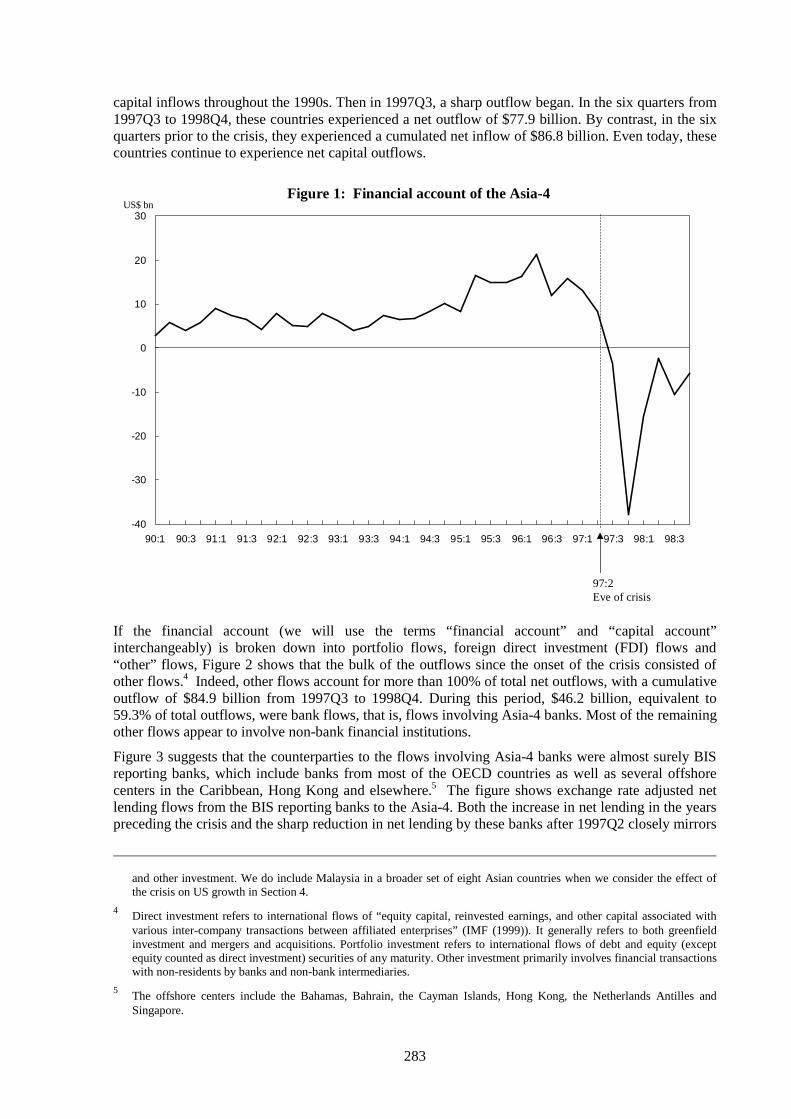
283
capital inflows throughout the 1990s. Then in 1997Q3, a sharp outflow began. In the six quarters from1997Q3 to 1998Q4, these countries experienced a net outflow of $77.9 billion. By contrast, in the sixquarters prior to the crisis, they experienced a cumulated net inflow of $86.8 billion. Even today, thesecountries continue to experience net capital outflows.
-40
-30
-20
-10
0
10
20
30
90:1 90:3 91:1 91:3 92:1 92:3 93:1 93:3 94:1 94:3 95:1 95:3 96:1 96:3 97:1 97:3 98:1 98:3
Figure 1: Financial account of the Asia-4US$ bn
97:2Eve of crisis
If the financial account (we will use the terms “financial account” and “capital account”interchangeably) is broken down into portfolio flows, foreign direct investment (FDI) flows and“other” flows, Figure 2 shows that the bulk of the outflows since the onset of the crisis consisted ofother flows.4 Indeed, other flows account for more than 100% of total net outflows, with a cumulativeoutflow of $84.9 billion from 1997Q3 to 1998Q4. During this period, $46.2 billion, equivalent to59.3% of total outflows, were bank flows, that is, flows involving Asia-4 banks. Most of the remainingother flows appear to involve non-bank financial institutions.
Figure 3 suggests that the counterparties to the flows involving Asia-4 banks were almost surely BISreporting banks, which include banks from most of the OECD countries as well as several offshorecenters in the Caribbean, Hong Kong and elsewhere.5 The figure shows exchange rate adjusted netlending flows from the BIS reporting banks to the Asia-4. Both the increase in net lending in the yearspreceding the crisis and the sharp reduction in net lending by these banks after 1997Q2 closely mirrors
and other investment. We do include Malaysia in a broader set of eight Asian countries when we consider the effect ofthe crisis on US growth in Section 4.
4Direct investment refers to international flows of “equity capital, reinvested earnings, and other capital associated withvarious inter-company transactions between affiliated enterprises” (IMF (1999)). It generally refers to both greenfieldinvestment and mergers and acquisitions. Portfolio investment refers to international flows of debt and equity (exceptequity counted as direct investment) securities of any maturity. Other investment primarily involves financial transactionswith non-residents by banks and non-bank intermediaries.
5The offshore centers include the Bahamas, Bahrain, the Cayman Islands, Hong Kong, the Netherlands Antilles andSingapore.
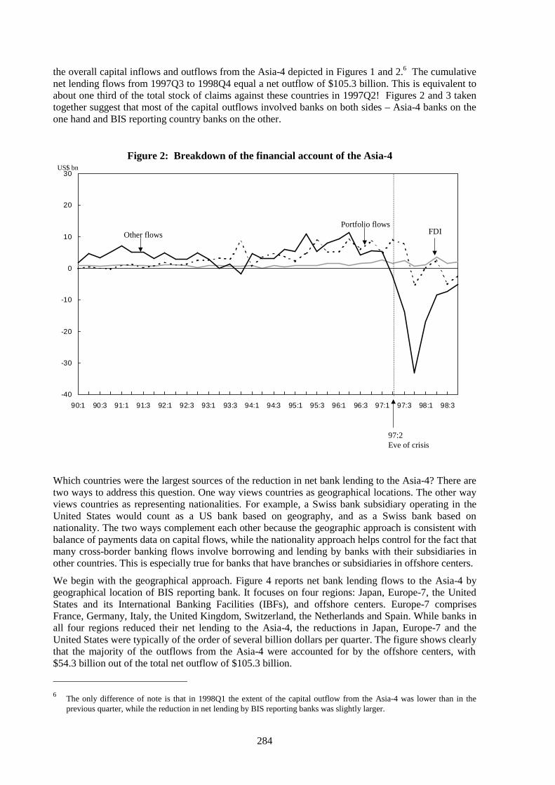
284
the overall capital inflows and outflows from the Asia-4 depicted in Figures 1 and 2.6 The cumulativenet lending flows from 1997Q3 to 1998Q4 equal a net outflow of $105.3 billion. This is equivalent toabout one third of the total stock of claims against these countries in 1997Q2! Figures 2 and 3 takentogether suggest that most of the capital outflows involved banks on both sides – Asia-4 banks on theone hand and BIS reporting country banks on the other.
Which countries were the largest sources of the reduction in net bank lending to the Asia-4? There aretwo ways to address this question. One way views countries as geographical locations. The other wayviews countries as representing nationalities. For example, a Swiss bank subsidiary operating in theUnited States would count as a US bank based on geography, and as a Swiss bank based onnationality. The two ways complement each other because the geographic approach is consistent withbalance of payments data on capital flows, while the nationality approach helps control for the fact thatmany cross-border banking flows involve borrowing and lending by banks with their subsidiaries inother countries. This is especially true for banks that have branches or subsidiaries in offshore centers.
We begin with the geographical approach. Figure 4 reports net bank lending flows to the Asia-4 bygeographical location of BIS reporting bank. It focuses on four regions: Japan, Europe-7, the UnitedStates and its International Banking Facilities (IBFs), and offshore centers. Europe-7 comprisesFrance, Germany, Italy, the United Kingdom, Switzerland, the Netherlands and Spain. While banks inall four regions reduced their net lending to the Asia-4, the reductions in Japan, Europe-7 and theUnited States were typically of the order of several billion dollars per quarter. The figure shows clearlythat the majority of the outflows from the Asia-4 were accounted for by the offshore centers, with$54.3 billion out of the total net outflow of $105.3 billion.
6 The only difference of note is that in 1998Q1 the extent of the capital outflow from the Asia-4 was lower than in the
previous quarter, while the reduction in net lending by BIS reporting banks was slightly larger.
-40
-30
-20
-10
0
10
20
30
90:1 90:3 91:1 91:3 92:1 92:3 93:1 93:3 94:1 94:3 95:1 95:3 96:1 96:3 97:1 97:3 98:1 98:3
Figure 2: Breakdown of the financial account of the Asia-4
97:2Eve of crisis
FDIPortfolio flows
Other flows
US$ bn
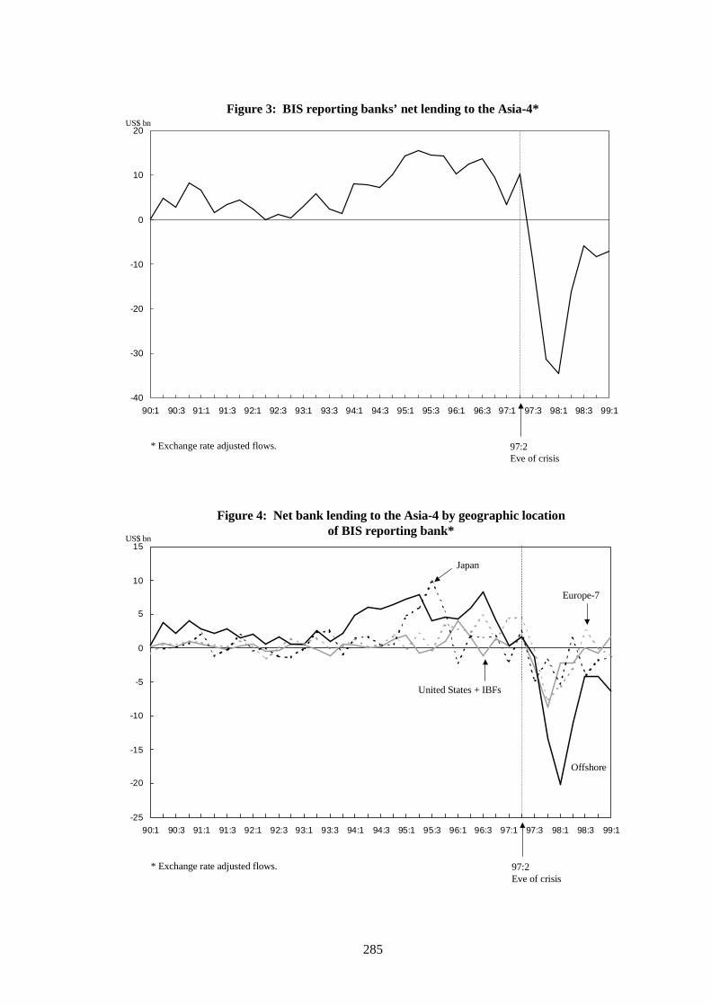
285
-40
-30
-20
-10
0
10
20
90:1 90:3 91:1 91:3 92:1 92:3 93:1 93:3 94:1 94:3 95:1 95:3 96:1 96:3 97:1 97:3 98:1 98:3 99:1
Figure 3: BIS reporting banks’ net lending to the Asia-4*
97:2Eve of crisis
* Exchange rate adjusted flows.
US$ bn
-25
-20
-15
-10
-5
0
5
10
15
90:1 90:3 91:1 91:3 92:1 92:3 93:1 93:3 94:1 94:3 95:1 95:3 96:1 96:3 97:1 97:3 98:1 98:3 99:1
Figure 4: Net bank lending to the Asia-4 by geographic locationof BIS reporting bank*
97:2Eve of crisis
United States + IBFs
Europe-7
Japan
Offshore
* Exchange rate adjusted flows.
US$ bn

286
Because the economies of the offshore centers are relatively small, we presume that most of theirinflows must generate corresponding outflows. To a large extent, one can therefore view these centersas “pass-through stations”.7 Figure 5 illustrates this in the form of a flow diagram. The figure reportsnet cumulative bank lending of BIS reporting countries over the 1997Q3-1998Q4 period. Banks inoffshore centers received $112.0 billion in net inflows from the Asia-4 and Japan between June 1997and December 1998. Most of this money went to banks in the Europe-7, which experienced a $121.1billion net inflow from the offshore centers.
What is also striking from Figure 5 is the minimal amount of banking inflows to the US originatingdirectly from the Asia-4 or mediated through the offshore centers. The money associated with theAsia-4 capital outflow could of course have reached the US banks via more indirect channels, such asthrough Europe, or even from Japan by way of the offshore centers and Europe. Once the flowsbecome so indirect, however, it becomes difficult to trace the original source of the money. This isalready apparent in Figure 5. More money entered the offshore centers from Japan than from theAsia-4. Therefore, we cannot conclude that the money exiting the offshore centers is directlyconnected to the Asia-4 outflows. This exiting offshore money could also be the result of net capitaloutflows from Japan connected to its own economic downturn.
The top row of Table 1 shows that of the $105.3 billion reduction in lending, $98.5 billion representeddeclines in claims on the Asia-4. Hence, we find that most of the adjustment is on the claims side. Wealso find that, even though a not insignificant fraction of the BIS bank loans were denominated indomestic currencies, the exchange rate adjusted flows are almost identical to the change in the stock of
7
In other words, we assume that these countries typically have small current accounts and small net changes in centralbank reserves. This is a reasonable assumption for all of the offshore centers except Hong Kong and Singapore. Total netcumulative external lending of the offshore centers was $29 billion during this period. However, this is a relatively smallfraction of the gross flows in and out of these centers. By contrast, during the crisis, the Asian crisis-country gross flowswere similar in magnitude to the net flows.
Figure 5: Flow diagram of net lending of BIS reporting banks: June 1997 to December 1998
Banks inoffshorecountries
Asia-4United States
Japan
Europe-7
121.1
16.2
57.7
14.1
US$ 54.3bn
17.0
15.5
Notes: The flows out of Asia-4 correspond to an increase in net liabilities vis-à-vis Asia-4 of the BIS reporting banks in the offshore countries, the United States, Europe-7 and Japan. The flows of the offshore countries vis-à-vis the United States, Europe-7 and Japan correspond to net lending by banks in the offshore countries to both banks and non-banks in the United States, Europe-7 and Japan.

287
claims less liabilities. This is shown in the second row of Table 1. The reduction in stocks was $106.3billion and the reduction in claims was $99.4 billion. These two findings are useful, because theyallow comparisons to be made between the geography-based data and the nationality-based data. Thenationality-based data are only available for claims (not liabilities) and are only available for stocks ofclaims (rather than exchange rate adjusted flows).
Table 1Change in assets and liabilities of BIS reporting banks vis-à-vis the Asia-4
(June 1997 to December 1998; in billions of US dollars)
Assets Liabilities Net claims
Geographical breakdown
Cumulative exchange rate adjusted flows –98.5 6.8 –105.3Change in stocks: All BIS countries –99.4 6.9 –106.3
Offshore countries –51.3 2.8 –54.1
United States –14.9 2.1 –17.1
Europe–7 –11.4 2.6 –14.0
Japan –18.4 –0.8 –17.6
Nationality breakdown
Change in stocks All nationalities –79.7 - -
United States –7.6 - -
Europe-6 –11.2 - -
Japan –28.6 - -
Other nationalities –32.3 - -
Notes: The geographical breakdown refers to all banks located in BIS reporting countries. The nationality breakdownrefers to all banks located in non-offshore BIS reporting countries, plus the foreign affiliates of these banks if they havethe nationality of one of the non-offshore BIS reporting countries. This means that banks in offshore countries withnationalities other than those of the non-offshore BIS countries are not included in the nationality breakdown, even thoughthey are included in the geographical breakdown. This accounts for the small discrepancy between the totals based on thegeographical and nationality breakdowns. The nationality data are only available for claims. Europe-7 comprises theUnited Kingdom, Germany, France, Italy, the Netherlands, Spain and Switzerland. Europe-6 excludes Switzerland. Banksof Swiss nationality in Switzerland are included in the total for the nationality breakdown, but are not included in theEuropean nationality subcategory.
The bottom panel of Table 1 provides a summary of bank lending to the Asia-4 by nationality. Timeseries of both the geographical and nationality data are shown in Figure 6 as well. Of the $79.7 billionreduction in assets that can be assigned to nationalities, only $47.6 billion involves the United States,the Europe-6 (Europe-7 less Switzerland) and Japan. This is surprising. The remaining $32.3 billion isaccounted for by banks of other nationalities operating in the BIS countries, which would include Thaiand Korean banks operating in the United States, for example. A detailed breakdown of this remainderis unavailable. Note that the outflows based on the nationality data are $19.7 billion less than theoutflows based on the geographical breakdown. The reason is that banks operating in the offshorecenters are not included in the nationality breakdown if their nationality is not that of one of thenon-offshore BIS reporting countries. For example, banks of Hong Kong nationality operating inHong Kong are not included in the nationality breakdown, while they are included in the geographicalbreakdown. The same is true for a Saudi Arabian bank operating in Hong Kong. In summary, less thanhalf of the total banking outflow from the Asia-4 is accounted for by US, Japanese or Europe-6-ownedbanks. Only $7.6 billion is associated with banks of US nationality.
We note parenthetically that the Asia-4 current account was initially buffered from the large capitaloutflows by IMF credit and a rundown of reserves. This is illustrated in Figure 7. It is worthwhilerecalling that from a balance of payments perspective, a rundown of central bank foreign exchangereserves is a net official capital inflow, which accounts for about half of the rise in reserves. The other

288
half is associated with the increase in IMF credit. Figure 7 shows that the full current accountadjustment did not take place until the first quarter of 1998.
-40
-30
-20
-10
0
10
20
30
40
50
90:1 90:3 91:1 91:3 92:1 92:3 93:1 93:3 94:1 94:3 95:1 95:3 96:1 96:3 97:1 97:3 98:1 98:3
Figure 7: The Asia-4 current account versus the financial account
97:2Eve of crisis
Reserves
Financial account
Current account
US$ bn
Figure 6: Source of BIS reporting bank claims on the Asia-4
By geographic location of banks
0
20
40
60
80
100
120
140
160
Jun-94 Dec-94 Jun-95 Dec-95 Jun-96 Dec-96 Jun-97 Dec-97 Jun-98 Dec-98
By nationality of banks
01020304050
60708090
100
Jun-94 Dec-94 Jun-95 Dec-95 Jun-96 Dec-96 Jun-97 Dec-97 Jun-98 Dec-98
Japan
Other nationalities
Eve of crisis
Offshore
Japan Europe-7
United States + IBFs
US$ bn
US$ bn
United States
Europe-6
Eve of crisis
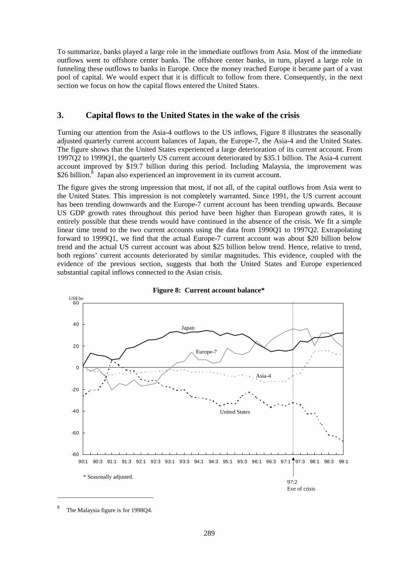
289
To summarize, banks played a large role in the immediate outflows from Asia. Most of the immediateoutflows went to offshore center banks. The offshore center banks, in turn, played a large role infunneling these outflows to banks in Europe. Once the money reached Europe it became part of a vastpool of capital. We would expect that it is difficult to follow from there. Consequently, in the nextsection we focus on how the capital flows entered the United States.
3. Capital flows to the United States in the wake of the crisis
Turning our attention from the Asia-4 outflows to the US inflows, Figure 8 illustrates the seasonallyadjusted quarterly current account balances of Japan, the Europe-7, the Asia-4 and the United States.The figure shows that the United States experienced a large deterioration of its current account. From1997Q2 to 1999Q1, the quarterly US current account deteriorated by $35.1 billion. The Asia-4 currentaccount improved by $19.7 billion during this period. Including Malaysia, the improvement was$26 billion.8 Japan also experienced an improvement in its current account.
The figure gives the strong impression that most, if not all, of the capital outflows from Asia went tothe United States. This impression is not completely warranted. Since 1991, the US current accounthas been trending downwards and the Europe-7 current account has been trending upwards. BecauseUS GDP growth rates throughout this period have been higher than European growth rates, it isentirely possible that these trends would have continued in the absence of the crisis. We fit a simplelinear time trend to the two current accounts using the data from 1990Q1 to 1997Q2. Extrapolatingforward to 1999Q1, we find that the actual Europe-7 current account was about $20 billion belowtrend and the actual US current account was about $25 billion below trend. Hence, relative to trend,both regions’ current accounts deteriorated by similar magnitudes. This evidence, coupled with theevidence of the previous section, suggests that both the United States and Europe experiencedsubstantial capital inflows connected to the Asian crisis.
8
The Malaysia figure is for 1998Q4.
-80
-60
-40
-20
0
20
40
60
90:1 90:3 91:1 91:3 92:1 92:3 93:1 93:3 94:1 94:3 95:1 95:3 96:1 96:3 97:1 97:3 98:1 98:3 99:1
Figure 8: Current account balance*
97:2Eve of crisis
Asia-4
United States
Japan
Europe-7
* Seasonally adjusted.
US$ bn
290
From the previous section, we also know that very little of the Asian crisis-related capital flows to theUnited States took the form of direct flows from the Asia-4 to the United States. This is furtherillustrated in Figure 9. US banks’ net lending to the Asia-4 fell by about $10 billion from 1997Q2 to1997Q4, but the reduction in net lending was relatively short-lived as negative net lending was lessthan $2 billion from 1998Q1 onwards. By contrast, total net US capital inflows averaged $68 billionquarterly between 1997Q3 and 1998Q4. Figure 9 also illustrates net portfolio flows during this period.The portfolio flows include both long-term portfolio flows and changes in the holdings of US Treasurybills by the Asian countries. Interestingly, the portfolio flows move in the opposite direction to thebank flows. The net portfolio outflow from the United States to the Asia-4 in the midst of the crisis(at the end of 1997) is probably the result of the sale of treasury securities by central banks in theAsian countries.
Our evidence, then, indicates that there were large capital flows to the United States (and Europe) as aresult of the Asian crisis, but that they reached the United States in a roundabout fashion, goingthrough several countries before eventually ending up in the United States. To the extent that theseflows were intermediated through banks, we would expect to see a surge in net flows to US banks (orequivalently, a decrease in net external lending by the US banks). The top panel of Figure 10 showsthat this was not the case. While inflows to the United States increased by about $40 billion in1997Q4, there was an equally large outflow in 1998Q1. The cumulative net inflow over the entireperiod between 1997Q3 and 1998Q4 was only $8.4 billion. The bottom panel of the figure breaksdown the net lending by region (Europe-7, offshore and Japan). Although there was an increase in netflows from Japan to US banks from the beginning of the crisis, there was also a similarly largeincrease in net flows from US banks to Europe.
Hence, while BIS banks accounted for virtually all of the net outflows from Asia, we also know thatthe net capital flows into the United States were not intermediated through US banks. Otherintermediation channels exist. European banks, for example, could have shifted lending from Asia tolocal institutions, which could then have used the money for foreign direct investment or portfolioinvestment in the United States. Indeed, cumulative net inflows to the United States from 1997Q3 to1998Q4 associated with foreign direct investment and portfolio investment were $326.9 billion. Ofcourse, given the large US current account deficits, a substantial portion of these flows would haveoccurred anyway.
A key difficulty with using the US balance of payments data is that errors and omissions (thestatistical discrepancy) were very large and volatile subsequent to the crisis. Between 1997Q2 and1998Q4, cumulative errors and omissions were –$92.6 billion, implying that net capital inflows were$92.6 billion less than actually reported during this period.9 Also, from 1997 to 1998, net errors andomissions rose by $152.7 billion, suggesting that actual capital inflows increased by $152.7 billionmore than reported. Because the current account deficit increased by $76.7 billion from 1997 to 1998,capital inflows should have shown a similar increase. Instead, reported capital inflows showed adecrease of $70.8 billion.
Figure 11 shows that changes in net errors and omissions were also very important in many of the keyquarters. For example, in 1997Q4 the United States experienced a net capital inflow of $114 billiondollars, an increase of about $40 billion from the previous quarter. The current account deficit was $41billion, a $4 billion decrease over the 1997Q3 deficit. The errors and omissions of –$73 billion thusrepresented a change of –$44 billion relative to the previous quarter. This suggests that the increase inUS capital inflows in 1997Q4 might not have happened. Similarly, the data show a sharp drop incapital inflows in 1998Q1, but this drop is again offset by a movement in errors and omissions in theopposite direction. There are several other episodes, such as during the Mexican crisis in 1994 and1995, where changes in errors and omissions are of the opposing sign to changes in the financialaccount. It is difficult to infer much from the US capital flows data.
9
This assumes that all the errors occur because of misreporting of the capital account data. In other words, we assume thatthe current account data are accurately represented.

291
-10
-8
-6
-4
-2
0
2
4
6
8
10
90:1 90:3 91:1 91:3 92:1 92:3 93:1 93:3 94:1 94:3 95:1 95:3 96:1 96:3 97:1 97:3 98:1 98:3 99:1
Figure 9: Net lending of the United States to the Asia-4*
97:2Eve of crisis
Net bank lending
Net portfolioflows
* Exchange rate-adjusted flows.
US$ bn
-50-40
-30-20
-100
1020
3040
50
90:1 90:3 91:1 91:3 92:1 92:3 93:1 93:3 94:1 94:3 95:1 95:3 96:1 96:3 97:1 97:3 98:1 98:3 99:1
-50-40
-30-20
-100
1020
3040
50
90:1 90:3 91:1 91:3 92:1 92:3 93:1 93:3 94:1 94:3 95:1 95:3 96:1 96:3 97:1 97:3 98:1 98:3 99:1
Figure 10: Net lending by US banks*
To BIS reporting countries
Eve of crisis
Eve of crisis
Europe-7
Offshore Japan
* Exchange rate-adjusted flows.
Total net lending by regionUS$ bn
US$ bn

292
-80
-60
-40
-20
0
20
40
60
80
100
120
90:1 90:3 91:1 91:3 92:1 92:3 93:1 93:3 94:1 94:3 95:1 95:3 96:1 96:3 97:1 97:3 98:1 98:3 99:1
Figure 11: US balance of payments*
97:2Eve of crisis
Current account
Net errors& omissions
Financial account
US$ bn
* Not seasonally adjusted.
0.6
0.65
0.7
0.75
0.8
0.85
0.9
0.95
1
Jan-90 Jan-91 Jan-92 Jan-93 Jan-94 Jan-95 Jan-96 Jan-97 Jan-98 Jan-99
80
90
100
110
120
130
140
150
160
Figure 12: Euro/$ and Yen/$Euro/$ Yen/$
Euro/$
Yen/$
97:2Eve of crisis
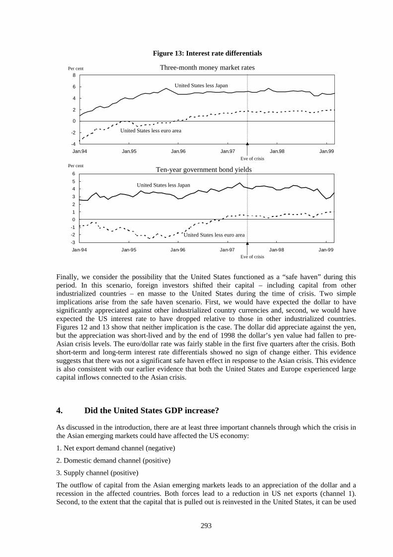
293
Finally, we consider the possibility that the United States functioned as a “safe haven” during thisperiod. In this scenario, foreign investors shifted their capital – including capital from otherindustrialized countries – en masse to the United States during the time of crisis. Two simpleimplications arise from the safe haven scenario. First, we would have expected the dollar to havesignificantly appreciated against other industrialized country currencies and, second, we would haveexpected the US interest rate to have dropped relative to those in other industrialized countries.Figures 12 and 13 show that neither implication is the case. The dollar did appreciate against the yen,but the appreciation was short-lived and by the end of 1998 the dollar’s yen value had fallen to pre-Asian crisis levels. The euro/dollar rate was fairly stable in the first five quarters after the crisis. Bothshort-term and long-term interest rate differentials showed no sign of change either. This evidencesuggests that there was not a significant safe haven effect in response to the Asian crisis. This evidenceis also consistent with our earlier evidence that both the United States and Europe experienced largecapital inflows connected to the Asian crisis.
4. Did the United States GDP increase?
As discussed in the introduction, there are at least three important channels through which the crisis inthe Asian emerging markets could have affected the US economy:
1. Net export demand channel (negative)
2. Domestic demand channel (positive)
3. Supply channel (positive)
The outflow of capital from the Asian emerging markets leads to an appreciation of the dollar and arecession in the affected countries. Both forces lead to a reduction in US net exports (channel 1).Second, to the extent that the capital that is pulled out is reinvested in the United States, it can be used
-3
-2
-1
0
1
2
3
4
5
6
Jan-94 Jan-95 Jan-96 Jan-97 Jan-98 Jan-99
Figure 13: Interest rate differentials
Three-month money market rates
-4
-2
0
2
4
6
8
Jan.94 Jan.95 Jan.96 Jan.97 Jan.98 Jan.99
United States less Japan
United States less euro area
Ten-year government bond yields
United States less Japan
United States less euro area
Eve of crisis
Eve of crisis
Per cent
Per cent

294
to finance an increase in US consumption and investment (channel 2). In the process, US interest ratesare likely to fall. Finally, the dollar appreciation and the emerging markets’ recessions lead to lowerUS import prices for intermediate and capital goods, which exerts a positive supply effect (channel 3).
These three effects are obviously interrelated. The capital inflow that leads to a lower interest rate alsoleads to the exchange rate appreciation that is responsible for lower exports. Moreover, supply mustequal demand, so that the third channel cannot be examined in isolation from the other two. We beginwith a miniature model that illustrates the forces at work within the context of equilibrium in thegoods market and the balance of payments. For illustrative purposes, the model is extremely simple.However, we argue that the model’s implications generalize under a variety of extensions. Afterdiscussing the model, we record that the evidence is broadly consistent with the model, and then wequantify the effect on GDP growth of each of the three channels. In the quantification, we make onlyminimal assumptions, much less strong than those of the model (and even its generalizations).
4.1 A miniature model
The model is illustrative and is designed to capture the essence of the response to the capital inflows.The open economy, which can be thought of as either the United States or all non-Asian crisiscountries, is characterized by two equations:
(1) )()()(__
RERNXrDDRERY s +=+
(2) 0),()(_
=γ+++
rKARERNX
where Ys = supply = GDP, DD = domestic demand, NX = net exports, KA = capital account (net capitalinflows), RER = real exchange rate, r UHDOLQWHUHVWUDWHDQG DEDODQFHRISD\PHQWVVKLIWYDULDEOHThe first equation represents goods market equilibrium, while the second represents balance ofpayments equilibrium. In equation (1), the supply of goods is written as a positive function of the realexchange rate. A real appreciation (rise in RER) implies that the prices of imported inputs fall, whichhas a positive supply effect. Supply is equated to demand, which is the sum of domestic demand andnet exports. Domestic demand decreases in response to a rise in the real interest rate, and net exportsdecrease in response to a real exchange rate appreciation.
Equation (2) represents balance of payments equilibrium. Net exports plus net capital inflows must beequal to zero. Net capital inflows are written as a positive function of the real interest rate. They alsoGHSHQG RQ WKH VKLIW YDULDEOH ZKLFK FRUUHVSRQGV WR DQ DXWRQRPRXV GHPDQG IRUUS (and otherLQGXVWULDOL]HG FRXQWU\ DVVHWV:HPRGHO WKH VWDUW RI WKH$VLDQ FULVLV DV DQ LQFUHDVH LQ WKDW LV Ddesired shift in capital from the Asian countries to the United States and other industrialized countries.For our purposes, it is not important to know the exact cause of this desired reallocation of capital; wecan think of the cause as a general decline in financial and macroeconomic conditions in the crisiscountries.
This simple model is diagramatically represented in Figure 14. The top diagram represents goodsmarket equilibrium. Output is on the y-axis and the real exchange rate is on the x-axis. The demandschedule is drawn for a given interest rate. The bottom diagram represents balance of paymentsequilibrium (equation (2)). The reallocation of capital to the United States (or non-Asian countries inJHQHUDO ± UHSUHVHQWHG E\ DQ LQFUHDVH LQ ± OHDGV WR D GRZQZDUG VKLIW LQ WKH EDODQFH RI SD\PHQWVequilibrium schedule. At a given real exchange rate, the new balance of payments equilibrium isreached at a lower interest rate. This lower interest rate leads to an increase in demand, shown by arightward shift in the demand curve in the top diagram. Output increases and the real exchange rateappreciates. The figure illustrates the pre-crisis and post-crisis levels of output, interest rate and realexchange rate.
The figure also permits a clean decomposition of the domestic demand and net export demand effects.The distance AC captures the increase in domestic demand engendered by the lower interest rate,while BC captures the reduced net exports caused by the real appreciation (corresponding to a
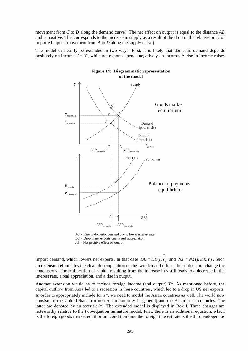
295
movement from C to D along the demand curve). The net effect on output is equal to the distance ABand is positive. This corresponds to the increase in supply as a result of the drop in the relative price ofimported inputs (movement from A to D along the supply curve).
The model can easily be extended in two ways. First, it is likely that domestic demand dependspositively on income Y = Ys, while net export depends negatively on income. A rise in income raises
import demand, which lowers net exports. In that case ),(_ +
= YrDDDD and ),(__YRERNXNX = . Such
an extension eliminates the clean decomposition of the two demand effects, but it does not change theconclusions. The reallocation of capital resulting from the increase in still leads to a decrease in theinterest rate, a real appreciation, and a rise in output.
Another extension would be to include foreign income (and output) Y*. As mentioned before, thecapital outflow from Asia led to a recession in these countries, which led to a drop in US net exports.In order to appropriately include for Y*, we need to model the Asian countries as well. The world nowconsists of the United States (or non-Asian countries in general) and the Asian crisis countries. Thelatter are denoted by an asterisk (*). The extended model is displayed in Box I. Three changes arenoteworthy relative to the two-equation miniature model. First, there is an additional equation, whichis the foreign goods market equilibrium condition (and the foreign interest rate is the third endogenous
Demand(post-crisis)
Rpost-crisis
RER
RERpre-crisis RERpost-crisis
Demand(pre-crisis)
SupplyY
Rpre-crisis
A
C
DB
R Post-crisisPre-crisis
Goods market equilibrium
Balance of payments equilibrium
Figure 14: Diagrammatic representationof the model
AC = Rise in domestic demand due to lower interest rateBC = Drop in net exports due to real appreciationAB = Net positive effect on output
RERRERpre-crisis RERpost-crisis
Ypre-crisis
Ypost-crisis
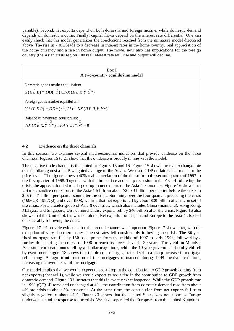
296
variable). Second, net exports depend on both domestic and foreign income, while domestic demanddepends on domestic income. Finally, capital flows depend on the interest rate differential. One caneasily check that this model generalizes the conclusions reached from the miniature model discussedabove. The rise in still leads to a decrease in interest rates in the home country, real appreciation ofthe home currency and a rise in home output. The model now also has implications for the foreigncountry (the Asian crisis region). Its real interest rate will rise and output will decline.
Box IA two-country equilibrium model
Domestic goods market equilibrium
*),,()()(___ +++
+= YYRERNXYrDDRERY
Foreign goods market equilibrium:
*),,(*)*,(*)(*____ ++
−= YYRERNXYrDDRERY
Balance of payments equilibrium:
0)*,(*),,(__
=γ±+++
rrKAYYRERNX
4.2 Evidence on the three channels
In this section, we examine several macroeconomic indicators that provide evidence on the threechannels. Figures 15 to 21 show that the evidence is broadly in line with the model.
The negative trade channel is illustrated in Figures 15 and 16. Figure 15 shows the real exchange rateof the dollar against a GDP-weighted average of the Asia-4. We used GDP deflators as proxies for theprice levels. The figure shows a 40% real appreciation of the dollar from the second quarter of 1997 tothe first quarter of 1998. Together with the immediate and sharp recession in the Asia-4 following thecrisis, the appreciation led to a large drop in net exports to the Asia-4 economies. Figure 16 shows thatUS merchandise net exports to the Asia-4 fell from about $2 to 3 billion per quarter before the crisis to$–5 to –7 billion per quarter soon after the crisis. Summing over the four quarters preceding the crisis(1996Q3–1997Q2) and over 1998, we find that net exports fell by about $30 billion after the onset ofthe crisis. For a broader group of Asia-8 countries, which also includes China (mainland), Hong Kong,Malaysia and Singapore, US net merchandise exports fell by $46 billion after the crisis. Figure 16 alsoshows that the United States was not alone. Net exports from Japan and Europe to the Asia-4 also fellconsiderably following the crisis.
Figures 17–19 provide evidence that the second channel was important. Figure 17 shows that, with theexception of very short-term rates, interest rates fell considerably following the crisis. The 30-yearfixed mortgage rate fell by 150 basis points from the middle of 1997 to early 1998, followed by afurther drop during the course of 1998 to reach its lowest level in 30 years. The yield on Moody’sAaa-rated corporate bonds fell by a similar magnitude, while the 10-year government bond yield fellby even more. Figure 18 shows that the drop in mortgage rates lead to a sharp increase in mortgagerefinancing. A significant fraction of the mortgages refinanced during 1998 involved cash-outs,increasing the overall size of the mortgage.
Our model implies that we would expect to see a drop in the contribution to GDP growth coming fromnet exports (channel 1), while we would expect to see a rise in the contribution to GDP growth fromdomestic demand. Figure 19 illustrates that this is exactly what happened. While the GDP growth ratein 1998 (Q/Q–4) remained unchanged at 4%, the contribution from domestic demand rose from about4% pre-crisis to about 5% post-crisis. At the same time, the contribution from net exports fell fromslightly negative to about –1%. Figure 20 shows that the United States was not alone as Europeunderwent a similar response to the crisis. We have separated the Europe-6 from the United Kingdom.

297
50
60
70
80
90
100
110
93:1 93:3 94:1 94:3 95:1 95:3 96:1 96:3 97:1 97:3 98:1 98:3 99:1
97:2Eve of crisis
Note: Real exchange rate is P/eP*, where P and P* are the GDP-weighted GDPdeflators of the Asian countries and the US GDP deflator respectively, and e isthe nominal exchange rate. GDP weights are 1994-96 average GDP shares.
Figure 15: Asia-4/US GDP-weighted real exchange rate1997:2 = 100
-15
-10
-5
0
5
10
15
90:1 90:3 91:1 91:3 92:1 92:3 93:1 93:3 94:1 94:3 95:1 95:3 96:1 96:3 97:1 97:3 98:1 98:3 99:1
Figure 16: Net exports to the Asia-4
97:2Eve of crisis
United States
Europe-7
Japan
World
US$ bn

298
2
3
4
5
6
7
8
9
10
94:1 94:3 95:1 95:3 96:1 96:3 97:1 97:3 98:1 98:3 99:1
Figure 17: US interest rates
30-year mortgage rates
97:2Eve of crisis
Moody’s seasoned Aaacorporate bond yield
10-year governmentbond yield
3-month moneymarket rate
Per cent
0
500
1000
1500
2000
2500
3000
3500
Jan-90 Jan-91 Jan-92 Jan-93 Jan-94 Jan-95 Jan-96 Jan-97 Jan-98 Jan-99
Figure 18: United States mortgage refinancing16 March 1990 = 100
June 1997Eve of crisis
Source: Mortgage Banker’s Association.
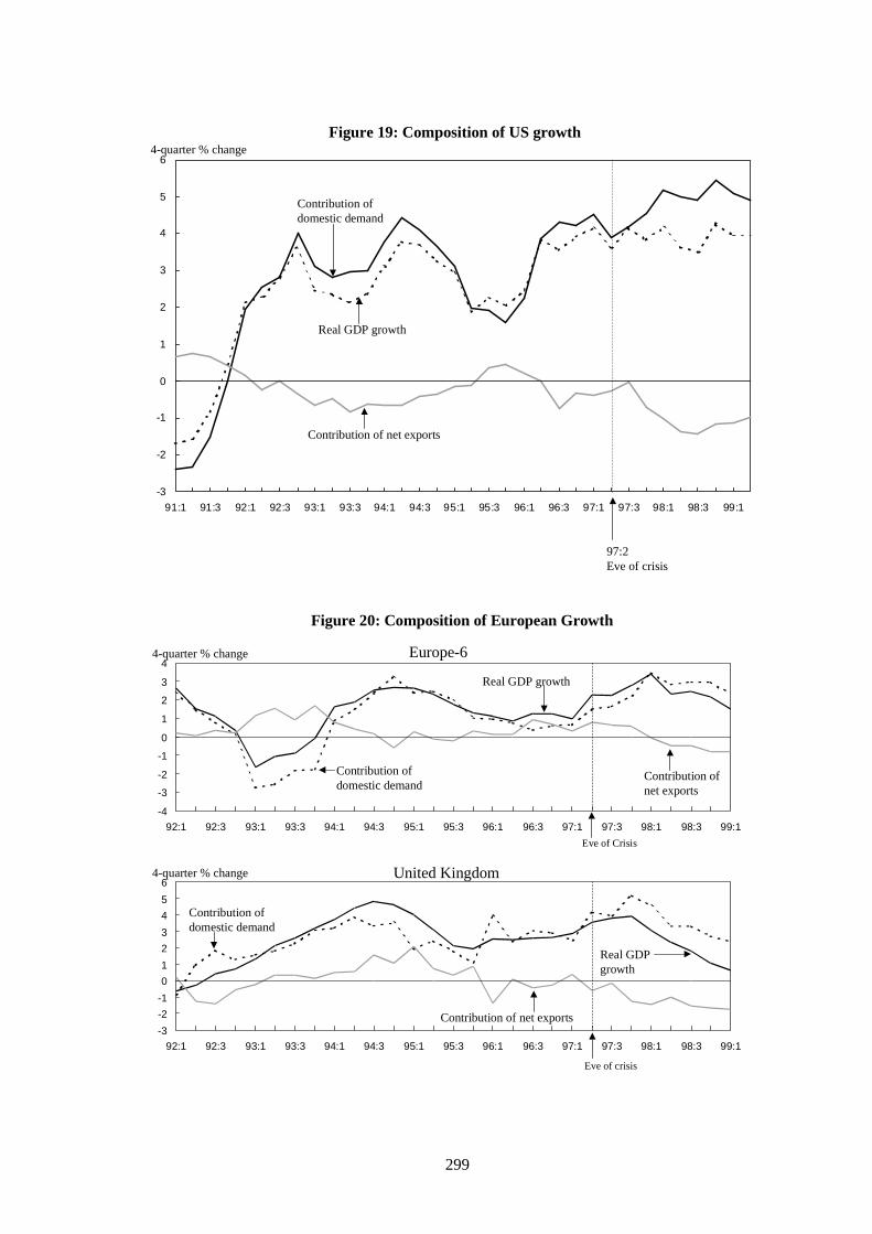
299
-3
-2
-1
0
1
2
3
4
5
6
91:1 91:3 92:1 92:3 93:1 93:3 94:1 94:3 95:1 95:3 96:1 96:3 97:1 97:3 98:1 98:3 99:1
Figure 19: Composition of US growth4-quarter % change
97:2Eve of crisis
Real GDP growth
Contribution ofdomestic demand
Contribution of net exports
Figure 20: Composition of European Growth
Europe-64-quarter % change
-4
-3
-2
-1
0
1
2
3
4
92:1 92:3 93:1 93:3 94:1 94:3 95:1 95:3 96:1 96:3 97:1 97:3 98:1 98:3 99:1
Real GDP growth
Contribution of net exports
Contribution of domestic demand
United Kingdom4-quarter % change
-3
-2
-1
0
1
2
3
4
5
6
92:1 92:3 93:1 93:3 94:1 94:3 95:1 95:3 96:1 96:3 97:1 97:3 98:1 98:3 99:1
Real GDP growth
Contribution of net exports
Contribution of domestic demand
Eve of crisis
Eve of Crisis

300
The United Kingdom is a special case because significant fiscal consolidation and a tightening ofmonetary conditions dampened domestic demand growth. For the Europe-6, we see that thecontribution of domestic demand growth rose from about 1% pre-crisis to a level between 2% and 3%post-crisis. At the same time, the contribution of net exports to GDP growth fell from slightly below1% to slightly above –1%.
The third channel depends on both the change in the relative price of imports (the reciprocal of the realexchange rate) and on the elasticity of supply with respect to the relative price of imports. Here, weprovide evidence on the relative price of imports; the next section derives the elasticity of supply.Figure 21 shows the import price index for total imports, and for merchandise imports from the Asia-4and the Asia-8.10 All import price indices are shown relative to the US GDP deflator, and are indexedto 100 in 1997Q2. The Asia-8 index represents a broader view of the impact of the Asian crisis on USimport prices. The import price indices show a sharp decrease for both sets of countries. From thepre-crisis period 1996Q3–1997Q2 to 1998, the relative import price index dropped by 18% for theAsia-4 and 12% for the Asia-8.11
4.3 Quantifying the three channels
We now attempt to quantify the effect on GDP growth of each of the three channels. In so doing, weimpose only minimal assumptions, in contrast to the strong structure imposed by the model. We canestimate the trade effect without making any model-specific assumptions. By directly examiningbilateral trade data, we can estimate how much the contribution to US GDP growth from net exports 10
We have proxied the US import price index from each Asian country by each country’s overall export price index(expressed in US dollars).
11These numbers are consistent with those reported in Barth and Dinmore (1999).
80
85
90
95
100
105
110
115
90:1 90:3 91:1 91:3 92:1 92:3 93:1 93:3 94:1 94:3 95:1 95:3 96:1 96:3 97:1 97:3 98:1 98:3 99:1
97:2Eve of crisis
Overall index
From Asia-4
* Seasonally adjusted.
Figure 21: Real US import price indexes, relative to GDP deflator*1997:2 = 100
From Asia-8

301
fell as a result of the Asian crisis. We do not need to know precisely what factors gave rise to the dropin net exports to the Asian crisis countries. In estimating the supply effect, we assume that firmsmaximize profits by choosing optimal levels of labor input and imported intermediate goods. Tofacilitate our calculations of the supply effect, we make three auxiliary assumptions. First, we hold thecapital stock constant. This assumption is not very restrictive, because it simply reflects the fact thatour analysis is short-term. Second, we assume that the real wage rate is constant. This implies that thelabor supply schedule is perfectly elastic. We argue below that this assumption is not essential to ourmain findings. As long as the labor supply schedule is not perfectly inelastic we will obtainqualitatively similar results. Third, we make assumptions about the production technology; these aredescribed in detail below. The essential assumption is that firms are profit-maximizing, so that outputis not simply demand-determined.
We estimate the domestic demand effect as the residual. The difference between the supply effect andthe trade effect equals the domestic demand effect. It would be difficult to calculate the domesticdemand effect directly. For example, we would need to know the size of the increase in capital flowsto the United States that can be traced to the crisis. We would need to know the effect of these inflowson the interest rate. We would need to know the elasticity of investment demand and savings demandwith respect to the interest rate. To know the savings demand and investment demand elasticities, wewould need to have a model of consumption behavior and of investment behavior, with itscorresponding set of assumptions. Hence, by treating the domestic demand effect as the residual, weavoid making the large number of assumptions necessary to calculate it.
In computing the trade and supply effects, we consider both the Asia-4 countries and the broader set ofAsia-8 countries. The advantage of looking at the broader set of Asia-8 countries is that we take intoaccount spillovers of the crisis to some important neighboring countries. We do not consider indirectsupply channels operating through oil prices or commodity prices, however. The recessions in theAsia-8 countries clearly had some negative effect on oil prices in 1998. These indirect channels wouldtend to raise the estimates of our supply effect.
We define the pre-crisis and post-crisis periods as we did above: 1996Q3–1997Q2 and 1998Q1–1998Q4. It is not appropriate to simply compare 1997 and 1998 because the crisis had already startedin 1997. Another unattractive alternative would be to compare the four quarters before the crisis to thefour following the start of the crisis (1996Q3–1997Q2 compared to 1997Q3–1998Q2), because thecrisis did not fully take effect until 1998. As shown in Figure 16, it took two to three quarters for netexports to drop to their lower post-crisis level. As discussed in Section 2, the effect of the capitaloutflows on the current account of the Asian countries was initially buffered by IMF credit and a dropin reserve assets. The full adjustment of the current account did not take place until 1998Q1.
In computing the trade effect, we focus on merchandise trade. This is a reasonable approximationbecause 79% of total US trade in 1998 was merchandise trade, which is also considerably morevolatile than services trade. The contribution to real GDP growth of net exports can be written as
)()(
M
MM
X
XXMXMX
P
P
Y
MP
P
P
Y
XP
Y
MPXP
M
M
Y
MP
X
X
Y
XP ∆−−
∆−
−∆=∆−∆
where Y is nominal GDP, PM and PX are import and export price indices vis-a-vis the Asian countries,and X and M are quantities of bilateral exports and imports. The first term on the right-hand sidemeasures the change in the nominal trade balance relative to GDP. The second term measures the priceeffects. The price effects are subtracted from the nominal trade effect to get the overall real tradeeffect. We approximate the US export price index to the Asian countries by the overall US exportprice index. The import price index is approximated by an import weighted-index of the Asian countryexport price indices.
Box II shows details of the firms’ profit maximization problem that underlies our calculation of thesupply effect. Firms maximize the difference between the value of gross output and costs. The variablecosts are labor costs and the costs of imported inputs. We are interested in the effect of a decrease inintermediate input prices on supply. After computing the first-order conditions for imported inputs andlabor, the supply effect can be written as:

302
(3)PP
PP
GDP
GDP
M
M
/
)/(
11
∆−αα
β−β=∆
where β is the share of imported inputs in total production costs in the pre-crisis period and α is theshare of labor income in domestic valued added. PM/P is the price of intermediate inputs relative to theprice of output. Real GDP is equal to gross output minus intermediate inputs, measured at pre-crisisprice levels. We compute the change in the overall PM/P as the merchandise import share from theAsia-4 or Asia-8 multiplied by the percentage change of PM/P for the Asia-4 or Asia-8.12 Notice thatthe supply effect is independent of the elasticity of substitution between imported inputs and domesticvalue added. The labor income share of GDP in 1997 was 58%, so we set α = 0.58. We set β equal toUS imports of intermediate and capital goods in 1998 (about 60% of total merchandise imports)divided by the sum of those imports and US GDP. This yields approximately 0.06.
Box IIFirms’ decision problems:
Maximise MPWLYP M−−_
where:_Y = gross output
L = labor
K = capital = constant
M = imported intermediates and imported capital goods
P = price of imported inputs
PM = price of imported inputs
)),,((_
MLKFY φ= (production function)
=φ ),( LK Cobb-Douglas index of K and L (labor share = α)
F &(6LQGH[ZLWKHODVWLFLW\RIVXEVWLWXWLRQ
The results of these computations are reported in Table 2. If we interpret the Asian crisis broadly ascorresponding to developments in the Asia-8 countries, US GDP fell by 0.8 percentage points as aresult of a drop in net exports to those countries, while it rose by 1.0 percentage points as a result ofthe increase in domestic demand. The net effect, which is also the supply effect, is +0.2 percentagepoints of GDP. The numbers are slightly smaller for the Asia-4. Our supply effect calculations suggestthat the net effect of the Asian crisis is small, but positive.
These results do not change in a major way if labor supply is not perfectly elastic. In this case, theincreased demand for labor (which results from lower prices of imported goods) leads to a rise in realwages. In the extreme case where labor supply is completely inelastic, the supply effect is zero. Whilethe lower prices of imported inputs lead to an increase in demand for imported inputs, which raisesgross output, domestic value added remains unaltered because both the capital stock and labor inputare unchanged. In general, when labor supply’s elasticity is finite, the supply effect will be somewherebetween 0% and 0.2%.13
Our findings correspond well with Figure 19. It shows that real GDP growth remained virtuallyunchanged following the crisis. The negative effect from lower net exports was almost exactly offset
12
We approximate P with the GDP deflator, as in Figure 15. This is not exactly correct because P is the price of grossoutput. But it gives a very close approximation as β is quite small.
13As noted earlier, we abstract from indirect supply effects, such as those resulting from oil prices. If the decline in oilprices in 1998 were entirely attributable to declining demand in the Asia-8 countries, then the supply effect would beconsiderably larger, close to 1.0 percentage points of GDP.
303
by the rise in domestic demand. The increase in the contribution of domestic demand to GDP growthfrom the pre-crisis to the post-crisis period (Figure 19) was about 1.0%. Hence, the Asian crisis couldhave accounted for all of the increase in US domestic demand.
Table 2Growth effect of Asian crisis
Asia-4 Asia-8
Trade effect –0.5% –0.8%
Domestic demand effect +0.6% +1.0%
Total effect +0.1% +0.2%
Notes: The table reports the contribution to GDP growth of lower trade and higher domestic demand as the result of theAsian crisis, as well as the total effect on GDP growth (which is also the supply effect). Results are reported both whenthinking of the Asian crisis as narrowly associated with four countries: Korea, Thailand, Indonesia and the Philippines(Asia-4) and when it is associated with a broader set of eight countries that also includes Hong Kong, Malaysia, Singaporeand China (mainland).
Other explanations have been put forward for the increase in US domestic demand during the Asiancrisis. However, we believe that such alternative explanations are less plausible, particularly to theextent that they relate to US-specific developments. For example, it has been pointed out that the USstock market rise could be responsible for the recent surge in US consumption. It has also beensuggested that US domestic demand increased in response to the new productivity revolution, which isushering in an era of permanently higher GDP growth rates. Both of these stories are specific to theUnited States, because the continental European stock market is much smaller by comparison, andEurope is not undergoing such a productivity revolution. Any US-specific increase in domesticdemand unrelated to the Asian crisis should have led to an increase in US interest rates, particularlyrelative to those in Europe and Japan. Moreover, we should have seen an exchange rate appreciationagainst the euro and the yen. Our earlier evidence showed that these events did not occur. In addition,we showed that the increase in the contribution of domestic demand to GDP growth in Europe was ofsimilar magnitude to that for the United States. That this pickup in domestic demand on both sides ofthe Atlantic also occurred in exactly the same time period strongly suggests a causal link to the Asiancrisis.
5. Conclusion
In the 1990s, many emerging market countries facilitated access for foreign investors to their financialmarkets by liberalizing controls on international capital flows. This has had benefits for both theemerging markets and for investors from industrialized countries. But there have also been risksassociated with the increased exposure of foreign investors to these new markets, because capitalinflows can be easily reversed in a short period of time. Assessing the causes of the crisis and theconsequences for the crisis countries themselves has been the focus of much of the literature on theAsian crisis. In this paper we shift the focus, examining the implications for industrialized countries,and for the United States in particular, of such far away economic crises.
While early in the crisis the negative trade effects for industrialized economies were emphasized, itsoon became clear that the trade channel was not the only transmission channel. By definition, acapital outflow from Asia is a capital inflow somewhere else. Capital inflows can finance an increasein domestic demand, which leads to an increase in GDP. One of our goals in this paper, therefore, hasbeen to follow the trail of money out of Asia in order to ascertain its final destination. We have foundit difficult to follow the trail very far, and to identify exactly how much ended up in the United States.We also found that large errors and omissions in the US balance of payments complicate thedocumentation of capital inflows to the United States.
304
Several stylized facts do emerge though:
1. The Asian crisis countries experienced net capital outflows close to $100 billion from the start ofthe crisis to the end of 1998.
2. The counterparties to the Asian outflows were essentially BIS reporting country banks.
3. About half of the outflows went to offshore center banks.
4. About half of the outflows went to banks whose nationality was neither US, Japanese norEuropean.
5. Very little money reached the United States directly from the crisis countries or through theoffshore centers.
6. Most of the outflows from the Asian crisis countries, as well as from Japan, did eventually reachboth the United States and Europe, probably through channels other than banks.
These facts highlight the importance of banks as the initial propagation mechanisms of the Asiancrisis, as well as the “roundaboutness” of the banking flows. One extension for future research is toexplore why banks played such a role.
The second goal of the paper was to analyze and quantify the short-run effect on US GDP growth. Weidentified three channels through which US growth was affected. First, the recessions in the Asiancountries and depreciated Asian currencies imply fewer US exports and more US imports. Second, thelower US interest rates that are the result of the increased inflows imply greater domestic demand.Third, appreciation of the dollar implies lower prices for imported intermediates and imported capitalgoods, reducing the cost of production. Our calculations that quantify these effects suggest that thenegative trade response is –0.8% of GDP, while the positive supply response is +0.2% of GDP. Thesetwo responses imply that the domestic demand response is about +1.0% of GDP. Thus, the overalleffect on the US economy in 1998 is about +0.2% of GDP, or $15–$20 billion.
Going forward, as the Asian economies recover we can expect these effects to go in the oppositedirection. If our findings are correct, however, a reversal of capital flows to the Asian countries willgenerate only a small net effect on US growth. However, it could generate large compositional effectson domestic demand and net exports.
305
Appendix
Figure 1: Sum across Korea, Thailand, Indonesia and the Philippines (henceforth known as the“Asia-4”) of the “financial account” as reported by the IFS. The IFS did not yet report the Koreanfinancial account in 1998Q4, so the “financial account” from McGraw-Hill’s DRI Asia CEIC databaseis used for Korea.
Figure 2: Sum across the Asia-4 of “portfolio investment (liabilities +assets)”, “direct investmentabroad + direct investment in rep. econ =”, and “other investment (liabilities + assets)” in the IFS. Dueto missing 1998Q4 Korean data, the CEIC database is used to complete the “balance of directinvestment”, “balance of portfolio investment”, and “balance of other investment” series.
Figure 3: Exchange rate adjusted flows, assets minus liabilities (including non-bank), as reported inthe BIS block M database. Vis-à-vis area is the Asia-4 and the reporting area “grand total” of BISreporting countries.
Figure 4: Exchange rate adjusted flows, assets minus liabilities (including non-bank), as reported inthe BIS block M database. Vis-à-vis area is the Asia-4, while reporting areas are Japan, Offshore,United States + IBFs and Europe-7 = United Kingdom + Germany + France + Italy + Netherlands +Spain +Switzerland (henceforth known as the “Europe-7”).
Figure 6: The top chart shows the stock of total assets vis-à-vis the Asia-4 with geographical origin ofa bank being the reporting area. BIS block M is the source. The bottom chart also shows the stock oftotal assets vis-à-vis the Asia-4, but by nationality of ownership. These data come from the publication“The BIS Consolidated International Banking Statistics”. Due to data unavailability, Switzerland isleft out of the Europe series in the bottom chart.
Figure 7: “Financial account” series are the same as that from Figure 1. Other series: sum across theAsia-4 of “reserves and related items” and “current account” as reported by the IFS. The IFS did notyet report the Korean financial or current account in 1998Q4, so 1998Q4 data for the Korean currentaccount come from Bank of Korea External Economic Indicators, Table P.F.2b, while “changes inreserve assets” from the CEIC database was used for Korea for that quarter.
Figure 8: With some exceptions in the most recent quarters, current account balance data forGermany, France, the Netherlands, the United Kingdom, Switzerland and Spain are from the BIS;Italian data are from the Bank of Italy; Japanese, US, Korean, Philippine, Thai and Indonesian data arefrom the IFS. The exceptions are: Spanish current account in 1999Q1 is from Bloomberg; Koreannumbers for 1998Q4 and 1999Q1 come from JP Morgan International Data Watch, as does theIndonesian value for 1999Q1. Data from the BIS are converted to US dollars using period averageexchange rates. All series are seasonally adjusted using the X11 additive filter in Eviews 3.0.
Figure 9: The “net bank lending” series is the same as in Figure 4. The “net portfolio flows” series isderived from Treasury International Capital (TIC) data. Long-term net sales by foreigners to USresidents are calculated from the TIC table “US Transactions with Foreigners in Long-TermSecurities”. Short-term treasury obligations from the TIC table “Liabilities to Foreigners Reported byBanks in the United States” are also included. Quarterly data are calculated using monthly sums.
Figure 10: These data are exchange rate adjusted flows, assets minus liabilities (including non-bank),as reported in the BIS block M database. The top chart is the United States + IBFs reporting vis-à-visall BIS reporting countries, while the bottom chart is the United States + IBFs reporting vis-à-visJapan, Offshore and the Europe-7.
Figure 11: US “financial account”, “current account” and “net errors and omissions” are from the IFS.
Figure 12: Exchange rates are monthly averages of the daily BIS series QBCAXM02 andQBBAJP02.
Figure 13: All data are from the European Central Bank’s website athttp://www.ecb.int/stats/mb/eastats.htm. The top chart data are three-month deposit rates for the
306
United States, Japan and euro area from Table 3.1. The bottom chart data are 10-year governmentbond yields for the United States, Japan and euro area from Table 3.2.
Figure 15: Quarterly average exchange rates for the Asia-4 are from the IFS. GDP deflators arecalculated using nominal and real GDP series from the CEIC database. After indexing all series to1997Q2 = 100, a GDP-weighted (1994–96 average GDP shares) average of the real exchange ratesyields the Asia-4/US real exchange rate.
Figure 16: Data are from the IMF’s Direction of Trade Statistics database. Asia-4 countries are theprimary country, i.e. Asia-4 countries report data on exports and imports, while secondary countriesare World, the United States, Japan and Europe-7 countries. To construct each series, the quantity (netexports * –1) was summed across the Asia-4 countries and across the Europe-7.
Figure 17: Three-month money market rates and 10-year government bond yields come from theEuropean Central Bank’s Euro Area Statistics Monthly Data, Tables 3.1 and 3.2, respectively (seeFigure 13). The Moody’s Seasoned Aaa Corporate Bond Yield series and 30-year mortgage ratesseries (Contract Rates on Commitments: Conventional 30-Yr Mortgages, FHLMC (%)) are both fromHaver Analytics’ USECON database. The money market rate is an end-of-period rate, and the otherinterest rates are monthly averages of daily rates.
Figure 18: This series is the refinancing index from the Mortgage Bankers’ Association weeklysurvey. Data are seasonally adjusted and weekly observations have been converted to monthlyaverages.
Figure 19: All data are from USECON. Contribution of domestic demand = [nominalDD(Q-4)/nominal GDP(Q-4)] *Real DD growth Q/Q-4. Nominal domestic demand is the sum of theC, I and G (consumption, investment and government) series. Real domestic demand is the sum of theCH, IH and GH (1992 chain-type dollar of the C, I and G series) series. Nominal GDP is simply theseries “GDP”. The “Real GDP growth” series is GDPH (seasonally adjusted, 1992 chain-type dollar).The “Contribution of net export” series is the difference between “Real GDP growth” and“Contribution of domestic demand”.
Figure 20: For the top chart, contribution of domestic demand = (sum nominal domestic demand(Q-4) across Europe-6/sum nominal GDP(Q-4) across Europe-6)*(Europe-6 real domestic demandgrowth (Q/Q-4).
In the above formula, nominal domestic demand and nominal GDP series are from the BIS database,where nominal domestic demand is reported in local currency and Nominal GDP is reported in dollars.Nominal domestic demand is converted to dollars (for the purpose of summing) using the period-average quarterly exchange rates from the IFS. Real domestic demand growth for the individualEurope-6 countries is from the following BIS series and corresponding countries: Italy (RHWBIT01),France (RHWBFR01), Germany (RHWBDE01), Switzerland (RHWACH01), the Netherlands(RHWBNL01), and Spain (RHWBES01). The BIS did not yet report Italy’s 1998Q4 real domesticdemand growth, so Bloomberg (original source is ISTAT) provided the data. Europe-6 real domesticdemand growth for each quarter is constructed as the weighted average (a country’s weight was theindividual country’s nominal domestic demand four quarters ago) of the individual countries’ real(Q/Q-4) domestic demand growth rates.
Europe-6 real GDP growth is calculated as the weighted average (a country’s weight was theindividual country’s nominal GDP four quarters ago) of the individual countries’ real (Q/Q-4) GDPgrowth rates. The nominal GDP data used in the weighting are the same BIS series used in theconstruction of “contribution of domestic demand” (see above). The individual countries’ real GDPdata are from the following BIS series and corresponding countries: Italy (RHGBIT01), France(RHGBFR01), Germany (RHGBDE09), Switzerland (RHGACH01), the Netherlands (RHGBNL01),Spain (RHGBES01). Italy’s 1998Q4 real domestic demand is from Bloomberg (original source isISTAT).
For the bottom chart, the United Kingdom’s contribution of domestic demand = [nominalDD(Q-4)/Nominal GDP(Q-4)] *real DD growth Q/Q-4. In the above formula, nominal domesticdemand and nominal GDP series are from the BIS, where nominal domestic demand is reported in

307
pounds sterling and nominal GDP in dollars. Nominal domestic demand is converted to dollars (for thepurpose of summing) using IFS quarterly period average exchange rates. Real domestic demandgrowth is from the BIS series RHWBGB01.
UK real GDP growth is from the BIS series RHFBGB01.
In both charts in this figure, the “contribution of net exports” series is the difference between “realGDP growth” and “contribution of domestic demand”.
Figure 21: US import price indices from the Asian countries are approximated using export priceindices of the Asian countries (from Oxford Economics) in dollar terms. Indices are deflated using theUS GDP deflator. After calculating real import price indices from the eight Asian countries, 1995 USimport shares yield weighted averages for the Asia-4 and Asia-8.
Bibliography
International Monetary Fund, International Financial Statistics. Various issues.
Barth, Marvin and Trevor Dinmore (1999): “Trade Prices and Volumes in East Asia Through theCrisis”. Board of Governors IFDP, No. 643, August.
308
The response of financial markets in Australia andNew Zealand to news about the Asian crisis
Luci Ellis and Eleanor Lewis1
1. Introduction
As financial markets become more integrated, shocks can be transmitted quickly between them. Intimes of market turmoil, this implies that the effects of negative shocks might be felt in markets farremoved from the originating market. In this paper, we investigate the spillover of financial-marketvolatility, specifically the impact of recent news from Asia (Korea, Thailand and Indonesia, as well asMalaysia and the Philippines), on financial markets in Australia and New Zealand. We examine theinitial impact of key events and announcements in the Asian crisis period and the spillover of theseeffects, as measured by both financial prices and proxies of their volatility.
We find that realisations of news – both positive and negative – that came out of Asia during the crisisclearly had repercussions for financial markets that were not directly affected by these events. Butthese effects must be put in perspective: developments in the US market generally had a much greaterinfluence on price movements and volatility than cross-market shocks originating in the Asian crisiseconomies. This result is in line with previous work on the importance of overseas returns inAustralian markets (Kortian and O’Regan (1996)). We also find evidence indicating that stock marketsreacted to developments in Asia with a lag, after the United States reacted, rather than reacting directlyto the news itself.
Our results indicate that the volatility in Australian and New Zealand financial markets in late 1998– which we term the “world crisis” period – was generally as great as or greater than in the 1997–98period, when the main news events of the Asian financial crisis occurred. We also find that theapparent spillover of financial market returns from Asia to Australia and New Zealand was small and– for some asset classes – smaller in the Asian crisis period than previously. This implies that theshocks originating in Asia were less important for Australian and New Zealand markets than were theglobal “common” shocks affecting all of these markets simultaneously.
The evidence suggests that the volatility seen in Australian and New Zealand markets was not affectedby the different stances of monetary policy, or the differing natures of the monetary policy regimes inthe two countries. The effects of developments in Asia on volatility in Australian and New Zealandfinancial markets were remarkably similar, despite the distinctly different methods used to conductmonetary policy over that period. These results reflect the short-run measure of volatility that we adoptin this paper, however. The levels of the financial market variables in Australia and New Zealanddisplay differing profiles: there were large divergences in stock and bond prices over the period. Onthe other hand, the exchange rates of the two currencies against the US dollar moved together,reflecting that these currencies are generally traded as a bloc.
This paper draws on the literature on contagion (Eichengreen et al. (1996) is a key empirical paper; seeDungey (1999) for a survey). Calvo and Mendoza (1999) show that contagion of financial marketvolatility might increase as world markets become more integrated. In certain circumstances, the costsof gathering and analysing information about unfamiliar foreign markets may outweigh the perceivedbenefits. This can result in investors choosing to act on the basis of rumours unrelated to market 1 Luci Ellis is a member of the Economic Analysis Department and Eleanor Lewis of the International Department. We are
indebted to colleagues at the Reserve Bank of Australia and to Mardi Dungey for invaluable comments and suggestions.We are also grateful to Adam Cagliarini for technical advice and Clare Padua for assistance with the data. Any errors areours alone. The opinions expressed in this paper are those of the authors and should not be attributed to the Reserve Bankof Australia.

309
fundamentals, instead of on complete information. In addition, fund managers may face incentives thatencourage herd behaviour in portfolio allocation decisions. Both of these effects can result incontagion of financial volatility from markets in one country to those in other countries.
Masson (1998) has defined contagion as the portion of financial market volatility that cannot beexplained by normal factors such as domestic fundamentals and global common shocks. However,much of the contagion literature focuses on the propagation of exchange rate crises and does not dealexplicitly with the transmission of volatility outside crisis periods (Dungey and Martin (1998) is anexception). In this sense, this paper has more in common with the literature on “meteor showers andheat waves”, which studies geographic (time zone) patterns in the volatility of particular securities(Engle et al. (1990); Fleming and Lopez (1999) is a recent example). We seek to identify the effect of“meteors” – as measured by news events or volatility in one market – on returns and volatility in othermarkets.
Previous work on the effects of macroeconomic “news” on Australian financial market prices andvolatility has focused on announcements made at pre-scheduled times, such as Australian CPI releases(Campbell and Lewis (1998) and Kim (1996)). In these cases, the content of an announcement may bea surprise, but its timing is not. Therefore, it is possible for market participants to plan their contingenttrading strategies in advance. If the timing of an announcement is not known in advance, however,traders have less opportunity to plan for its effects. Previous empirical work for other countries hassuggested that unscheduled announcements tend to have more persistent effects on financial returnsthan do scheduled announcements (Almeida et al. (1998)), although the difference can be measured inhours. In general, studies of this kind examine the impact of economic announcements on “own”financial markets. The present paper, however, focuses on the effects of unscheduled (thoughpotentially anticipated) announcements relating to one group of countries on the financial markets ofother countries.
The paper proceeds as follows. In Section 2, we discuss the reasons why financial markets in Australiaand New Zealand might have been affected by the financial crisis in Asia. We also discuss ourmeasure of news events and the financial market data to be analysed. Section 3 contains the empiricalevidence on the response of financial markets in Australia and New Zealand to these news events, interms of both volatility and price movements. In Section 4, we examine whether the spillover offinancial market returns is greater in times of crisis than in more normal times, using results fromvector autoregressions (VARs). Section 5 provides a brief conclusion.
2. Motivation and data
2.1 Why Australian and New Zealand financial markets might be affected
There are a number of reasons why negative events relating to the Asian financial crisis might beexpected to have a negative effect on financial markets in countries such as Australia and NewZealand. Firstly, to the extent that financial crises in some countries result in a generalised increase inuncertainty in world financial markets, we should expect increased volatility in financial markets innon-crisis countries, which usually results in lower returns.
Secondly, the Asian crisis countries are important markets for Australian and New Zealand exports.As such, a pronounced recession in the crisis countries might be expected to have a negative effect onactivity in Australia and New Zealand via the current account; these expectations would then flowthrough to financial market returns.2
Thirdly, some market participants might have factored in some possibility – however remote – thatcontagion of the crisis could have spread as far as Australia and New Zealand, perhaps relating tofinancial institutions’ debt exposures to the crisis countries. 2
This vector of contagion is essentially the economic linkages model of Lowell et al. (1998).

310
Finally, even if financial market participants do not expect that countries such as Australia andNew Zealand will experience financial crises, they may expect that portfolio rebalancing behaviourcould result in sharp declines in asset markets of countries with unrelated fundamentals. Kaminskyand Schmukler (1999) describe how market participants, in responding to a crisis in country A byselling country-A assets and buying country-B assets, may rebalance their portfolios by sellingcountry-C assets, where country C is similar to country B. This ensures that the share of B and Cassets in the portfolio remains at the desired level. This results in an apparent contagion of the crisisfrom country A to the unrelated country C. The effect is also consistent with the portfolio adjustmentmodel of contagion in Lowell et al. (1998). In addition, the effect might be compounded if there is asignificant number of uninformed traders in the market, as they may also sell country-C assets if theyinterpret the sell-off as reflecting a change in fundamentals.
The factors listed above could explain some co-movement between Asian financial markets and thosein Australia and New Zealand. On the other hand, there may be reasons for Australian andNew Zealand markets to move in the opposite direction to their Asian counterparts. If a financial crisisin one region caused overseas investors to repatriate or otherwise reallocate their funds, it is possiblethat markets such as Australia and New Zealand could have received them, putting upward pressure onasset prices in those countries. That is, Australia and New Zealand could have been country B, notcountry C, in the portfolio rebalancing scenario of Kaminsky and Schmukler (1999).
Further reactions to crisis events may occur, related to the actual or expected response by monetarypolicymakers. For example, if the authorities raise short-term interest rates in response to an exchangerate depreciation – or market participants expect that they will do so – this may result in a fall in stockprices and movements in long-term bond rates.
2.2 The impact of news on financial markets
A large literature exists on the impact of macroeconomic news on financial market prices sampled athigh frequencies (Campbell and Lewis (1998), Fleming and Remolona (1997), Almeida et al. (1998),Kim and Sheen (1998) and Kim (1999) are some recent examples).
One distinction between most of this “event study” literature and the present paper is that the formergenerally examines the effects of news events on financial markets in the country in which the newsoriginated. We focus on the effects of news on third-country markets. In addition, most of the previousliterature examines the effect of official macroeconomic data releases, which generally haveprescheduled release dates and times. Exceptions to this are releases of German macroeconomic data,which do not follow a predetermined schedule. In this case, market participants are less likely to beable to plan reaction strategies upon the release of the data. Almeida et al. (1998) find that theresponse of the US dollar/Deutsche mark bilateral exchange rate to German releases is somewhat moredrawn out than the response to US releases, which are pre-scheduled (although the difference can bemeasured in hours).
The set of news events we consider goes even further than this, however. Although the precise timingof German macroeconomic releases is not known in advance, they are approximately regular. Soalthough market participants may not know the exact timing of the German CPI release, they knowthat a release will occur each month. By contrast, news events during the Asian financial crisis werenot always predictable. This would tend to increase the “surprise” value of news about the Asiancrisis, relative to the surprise value embodied in regular releases of macroeconomic data.
Limitations of the available data, described in the next section, prevent us from examining theresponse of Australian and New Zealand financial markets to news at ultra-high frequencies of hoursor minutes. Also, since we do not have information on the times that most of the news eventsoccurred, we are restricted to examining news effects on a daily frequency.
Asian time zones largely overlap the Australian and New Zealand domestic trading zones. We would,therefore, expect that in most cases the reaction of Australian and New Zealand markets would beginon the same day that the Asian news events occurred. There will be some instances, however, in which

311
the news events in Asia occurred after the market closes in Australia and New Zealand, and so thereaction will have occurred on the following day.
2.3 Identifying the timing of news events
The first step in assessing how news about the Asian financial crisis affected other countries’ financialmarkets is to identify the events that constitute news. We use a combination of two pre-existingchronologies, one from the BIS and the other from the IMF (BIS (1998) Table VII.6, page 131; IMF(1998) Box 2.12, page 49), as well as the RBA’s daily market reports. A table listing the events fromthese sources is shown in the Appendix. It should be noted that in some cases the dates cited in theIMF chronology differ from other IMF papers (e.g. IMF (1999)). Where possible, we verified thedates using newswire stories and other sources. The IMF and BIS chronologies end in June and March1998 respectively; we extended the chronology in this paper to end-August 1998 using the RBA’sdaily market reports.
Positive news will have the opposite effect on markets to negative news, suggesting that we shoulddistinguish between events that are considered “good” or “bad” news. We classify events relating toagreements between international agencies and crisis countries, announcements of rollovers of debtand certain reforms as “good news”; all other news events listed in the Appendix are considered to be“bad news”. The classification of events as positive or negative is shown in the right-most column inthe table. Our listing is similar to the classification used by Kaminsky and Schmukler (1999), based onthe chronology compiled by Roubini (1999), and to that of Baig and Goldfajn (1998), compiled fromnewswire stories.3
Kaminsky and Schmukler (1999) report that days on which some of the most volatile movements inAsian financial markets occurred were not necessarily associated with specific news events relating tothe crisis. There are a number of possible explanations for this. Firstly, markets might react tocumulations of news, so that a seemingly “small” or unimportant news event can engender a greaterresponse if it follows a series of news events (the “straw that broke the camel’s back” effect).Secondly, there may be some herding behaviour by traders, so that sudden changes in financial pricescan occur even in the absence of significant news. Thirdly, the news events considered may be lessrelevant to asset markets than the trading strategies used by market participants. To maximise returnsfrom these trading strategies, it may be necessary to take advantage of particular market conditions,such as thin volume, which may not occur on news event days.
2.4 The financial market data, episodes and volatility
The data used to measure financial market returns and volatility for Australia and New Zealand in thisstudy are: the broad indices of stock prices – the All Ordinaries Index (AOI) for Australia and theNZSE40 for New Zealand; bilateral exchange rates for the Australian and New Zealand dollars againstthe US dollar; and the prices on futures contracts for Australian and New Zealand 10-year bonds,which trade on the Sydney Futures Exchange (SFE) and the New Zealand Futures and OptionsExchange (NZFOE).4
We use daily market-close data for stock prices and bond futures prices, and 4 pm (AEST) readingsfor the bilateral exchange rates. Given these data series, we need to derive an appropriate measure ofvolatility: for daily data, the usual approach is to take the absolute value of daily percentage changes inprices (returns), or squared percentage changes. To avoid introducing spurious autocorrelation into ourmeasure of financial market volatility, we do not use measures such as rolling standard deviations of
3
Although this classification is somewhat arbitrary, it did not seem to be crucial to our results.
4The bonds data are for the “next” contract to be delivered, which is a very close substitute for the underlying spotinstrument, i.e. physical 10-year bonds. The markets in these instruments on the futures exchanges are deep and liquidand provide reliable price readings. These markets are generally considered to be more liquid than those for thecorresponding physical securities.
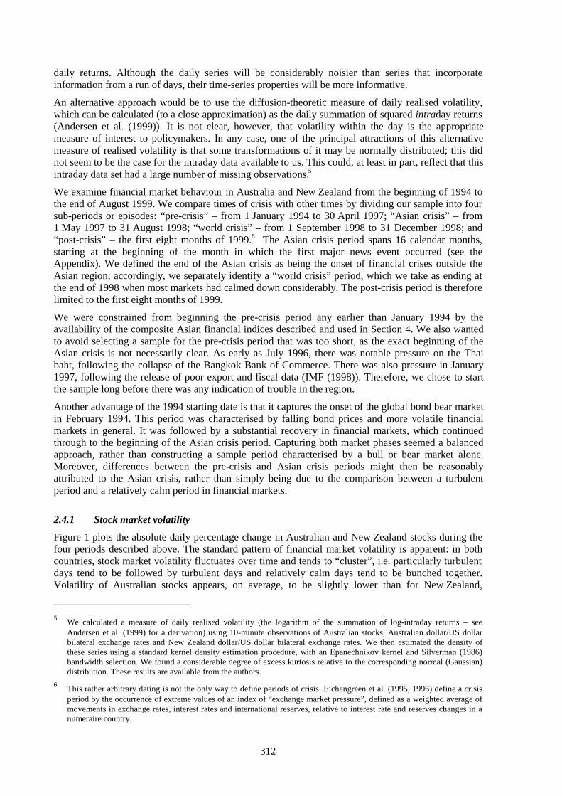
312
daily returns. Although the daily series will be considerably noisier than series that incorporateinformation from a run of days, their time-series properties will be more informative.
An alternative approach would be to use the diffusion-theoretic measure of daily realised volatility,which can be calculated (to a close approximation) as the daily summation of squared intraday returns(Andersen et al. (1999)). It is not clear, however, that volatility within the day is the appropriatemeasure of interest to policymakers. In any case, one of the principal attractions of this alternativemeasure of realised volatility is that some transformations of it may be normally distributed; this didnot seem to be the case for the intraday data available to us. This could, at least in part, reflect that thisintraday data set had a large number of missing observations.5
We examine financial market behaviour in Australia and New Zealand from the beginning of 1994 tothe end of August 1999. We compare times of crisis with other times by dividing our sample into foursub-periods or episodes: “pre-crisis” – from 1 January 1994 to 30 April 1997; “Asian crisis” – from1 May 1997 to 31 August 1998; “world crisis” – from 1 September 1998 to 31 December 1998; and“post-crisis” – the first eight months of 1999.6 The Asian crisis period spans 16 calendar months,starting at the beginning of the month in which the first major news event occurred (see theAppendix). We defined the end of the Asian crisis as being the onset of financial crises outside theAsian region; accordingly, we separately identify a “world crisis” period, which we take as ending atthe end of 1998 when most markets had calmed down considerably. The post-crisis period is thereforelimited to the first eight months of 1999.
We were constrained from beginning the pre-crisis period any earlier than January 1994 by theavailability of the composite Asian financial indices described and used in Section 4. We also wantedto avoid selecting a sample for the pre-crisis period that was too short, as the exact beginning of theAsian crisis is not necessarily clear. As early as July 1996, there was notable pressure on the Thaibaht, following the collapse of the Bangkok Bank of Commerce. There was also pressure in January1997, following the release of poor export and fiscal data (IMF (1998)). Therefore, we chose to startthe sample long before there was any indication of trouble in the region.
Another advantage of the 1994 starting date is that it captures the onset of the global bond bear marketin February 1994. This period was characterised by falling bond prices and more volatile financialmarkets in general. It was followed by a substantial recovery in financial markets, which continuedthrough to the beginning of the Asian crisis period. Capturing both market phases seemed a balancedapproach, rather than constructing a sample period characterised by a bull or bear market alone.Moreover, differences between the pre-crisis and Asian crisis periods might then be reasonablyattributed to the Asian crisis, rather than simply being due to the comparison between a turbulentperiod and a relatively calm period in financial markets.
2.4.1 Stock market volatility
Figure 1 plots the absolute daily percentage change in Australian and New Zealand stocks during thefour periods described above. The standard pattern of financial market volatility is apparent: in bothcountries, stock market volatility fluctuates over time and tends to “cluster”, i.e. particularly turbulentdays tend to be followed by turbulent days and relatively calm days tend to be bunched together.Volatility of Australian stocks appears, on average, to be slightly lower than for New Zealand,
5
We calculated a measure of daily realised volatility (the logarithm of the summation of log-intraday returns – seeAndersen et al. (1999) for a derivation) using 10-minute observations of Australian stocks, Australian dollar/US dollarbilateral exchange rates and New Zealand dollar/US dollar bilateral exchange rates. We then estimated the density ofthese series using a standard kernel density estimation procedure, with an Epanechnikov kernel and Silverman (1986)bandwidth selection. We found a considerable degree of excess kurtosis relative to the corresponding normal (Gaussian)distribution. These results are available from the authors.
6This rather arbitrary dating is not the only way to define periods of crisis. Eichengreen et al. (1995, 1996) define a crisisperiod by the occurrence of extreme values of an index of “exchange market pressure”, defined as a weighted average ofmovements in exchange rates, interest rates and international reserves, relative to interest rate and reserves changes in anumeraire country.
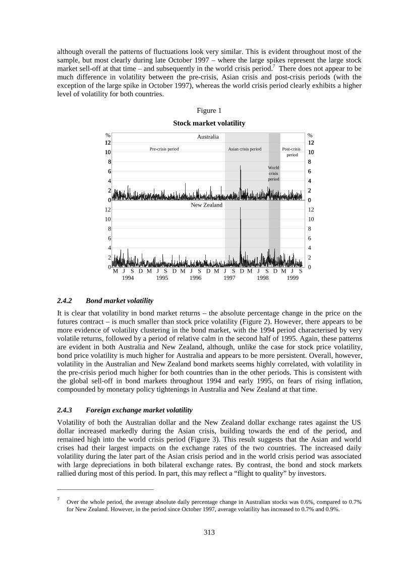
313
although overall the patterns of fluctuations look very similar. This is evident throughout most of thesample, but most clearly during late October 1997 – where the large spikes represent the large stockmarket sell-off at that time – and subsequently in the world crisis period.7 There does not appear to bemuch difference in volatility between the pre-crisis, Asian crisis and post-crisis periods (with theexception of the large spike in October 1997), whereas the world crisis period clearly exhibits a higherlevel of volatility for both countries.
Figure 1
Stock market volatility
M J S D M J S D M J S D M J S D M J S D M J
%
1994 1995 1996 1997 1998 1999
%
New Zealand
S
Asian crisis periodPre-crisis period Post-crisisperiod
l l l l l l l l l l l l l l l l l l l l l l0
2
4
6
8
10
12
0
2
4
6
8
10
12
Australia
0
2
4
6
8
10
12
0
2
4
6
8
10
12
0
2
4
6
8
10
12
0
2
4
6
8
10
12
Worldcrisisperiod
2.4.2 Bond market volatility
It is clear that volatility in bond market returns – the absolute percentage change in the price on thefutures contract – is much smaller than stock price volatility (Figure 2). However, there appears to bemore evidence of volatility clustering in the bond market, with the 1994 period characterised by veryvolatile returns, followed by a period of relative calm in the second half of 1995. Again, these patternsare evident in both Australia and New Zealand, although, unlike the case for stock price volatility,bond price volatility is much higher for Australia and appears to be more persistent. Overall, however,volatility in the Australian and New Zealand bond markets seems highly correlated, with volatility inthe pre-crisis period much higher for both countries than in the other periods. This is consistent withthe global sell-off in bond markets throughout 1994 and early 1995, on fears of rising inflation,compounded by monetary policy tightenings in Australia and New Zealand at that time.
2.4.3 Foreign exchange market volatility
Volatility of both the Australian dollar and the New Zealand dollar exchange rates against the USdollar increased markedly during the Asian crisis, building towards the end of the period, andremained high into the world crisis period (Figure 3). This result suggests that the Asian and worldcrises had their largest impacts on the exchange rates of the two countries. The increased dailyvolatility during the later part of the Asian crisis period and in the world crisis period was associatedwith large depreciations in both bilateral exchange rates. By contrast, the bond and stock marketsrallied during most of this period. In part, this may reflect a “flight to quality” by investors.
7
Over the whole period, the average absolute daily percentage change in Australian stocks was 0.6%, compared to 0.7%for New Zealand. However, in the period since October 1997, average volatility has increased to 0.7% and 0.9%.

314
Figure 2
Bond market volatility
M J S D M J S D M J S D M J S D M J S D M J
%
1994 1995 1996 1997 1998 1999
%
New Zealand
S
Asian crisis periodPre-crisis period Post-crisisperiod
l l l l l l l l l l l l l l l l l l l l l l0.0
0.1
0.2
0.3
0.4
0.5
0.0
0.1
0.2
0.3
0.4
0.5
Australia
0.0
0.1
0.2
0.3
0.4
0.5
0.0
0.1
0.2
0.3
0.4
0.5
0.0
0.1
0.2
0.3
0.4
0.5
0.0
0.1
0.2
0.3
0.4
0.5
World crisisperiod
Although the volatility in the exchange rates of the two currencies against the US dollar variedconsiderably in the crisis periods, the volatility in the Australian dollar/new Zealand dollar cross ratewas relatively stable (Figure 4), despite the differences in the operational regimes and stances ofmonetary policy between the two countries. During the Asian and world crises, the monetary policyinstrument was the cash rate in Australia, whereas in New Zealand it was a monetary conditions index(MCI), based on the trade-weighted index for the New Zealand dollar and the three-month bank billinterest rate. The relatively constant volatility of the cross rate reflects that the two currencies aregenerally traded as a bloc.
Figure 3
Foreign exchange market volatility
M J S D M J S D M J S D M J S D M J S D M J
%
1994 1995 1996 1997 1998 1999
%
New Zealand
S
Asian crisis periodPre-crisis period Post-crisisperiod
l l l l l l l l l l l l l l l l l l l l l l0
1
2
3
4
0
1
2
3
4
Australia
0
1
2
3
4
0
1
2
3
4
0
1
2
3
4
0
1
2
3
4
Worldcrisisperiod

315
Figure 4
Volatility of the Australian dollar/New Zealand dollar cross rate
l l l l l l l l l l l l l l l l l l l l l l0
1
2
3
4
0
1
2
3
4
% %
M J S D M J S D M J S D M J S D M J S D M J1994 1995 1996 1997 1998 1999
S
Asian crisis periodPre-crisis period Post-crisis
period
World crisisperiod
3. The response to news
In this section, we use some simple summary statistics and econometric techniques to measure theimpact of news on financial market volatility and returns during the Asian crisis.
Within the Asian crisis period, we distinguish between “news” days and “no-news” days, defined asdays on which a news event did not occur, and which neither preceded nor followed a news day. Dayson which a news event did not occur, but which were adjacent to a news day, are identified separatelyas “pre-news” and “post-news” days.
3.1 Summary statistics
3.1.1 Stock prices
The first two rows of Table 1 summarise volatility in the Australian and New Zealand stock markets –as measured by the average absolute percentage change in Australian and New Zealand stocks – for allnews event days (pre-news, news and post-news days) and no-news days during the Asian crisisperiod. The table also shows the corresponding measures for the world crisis, pre-crisis and post-crisisperiods, as well as the Asian crisis period taken as a whole. Table 2 and Table 3 present meandifference tests of the significance of the differences between these measures.
Several facts stand out. Firstly, during the Asian crisis, all news event days were noticeably morevolatile for both Australian and New Zealand stock indices than were days when news events did notoccur. Secondly, volatility in both stock indices in the pre-crisis period was significantly lower (in astatistical sense) than during the Asian crisis, but similar to no-news days during the crisis. It was alsolower than in both subsequent periods (world crisis and post-crisis). Thirdly, volatility in the worldcrisis period was similar to the Asian crisis for Australian stocks, but for New Zealand stocks theworld crisis period exhibited significantly higher volatility.
3.1.2 Bond futures prices
The variation in bond market volatility was much smaller than for the other financial marketsconsidered. For both Australia and New Zealand, there was seldom more than 0.01 percentage points

316
difference between the mean absolute movements in the bond futures prices across the sub-periods(Table 1). The mean difference tests shown in Table 2 and Table 3 do not indicate any significantnews effects during the Asian crisis period for Australia or New Zealand. Pre-news days, news daysand post-news days did not engender any greater volatility in Australian and New Zealand bondmarkets, on average, than days when news events did not occur. Reflecting the severe sell-off in bondmarkets in 1994, mean volatility in the pre-crisis period was significantly greater than for the Asianand post-crisis periods for both the Australian and New Zealand markets, but not greater than in theworld crisis period. Although these are statistically significant differences, they are very small from aneconomic perspective.
Table 1Daily financial market volatility:
average absolute daily percentage returns
News days during Asian crisis
Pre-news News Post-news No newsPre-crisis Asian crisis World crisis Post-crisis
Stock prices
Australia 0.77 0.91 1.00 0.59 0.55 0.70 0.77 0.62
New Zealand 1.01 0.97 1.24 0.63 0.55 0.79 1.03 0.74
Bond prices
Australia 0.06 0.06 0.06 0.06 0.08 0.06 0.07 0.07
New Zealand 0.05 0.05 0.07 0.05 0.06 0.05 0.06 0.05
Exchange rates
Australia 0.59 0.67 0.66 0.46 0.33 0.52 0.62 0.52
New Zealand 0.56 0.63 0.62 0.44 0.26 0.51 0.65 0.52
Note: There are 868 pre-crisis days, 348 Asian crisis days, 88 world crisis days and 173 post-crisis days. During the crisisperiod, there are 65 news days, 196 no-news days, 65 pre-news and 64 post-news days. There are 42 days that fall into morethan one category.
3.1.3 Exchange rates
The effect of the Asian crisis on Australian and New Zealand financial markets is particularly evidentfor exchange rates. There was an apparent news effect: the mean absolute returns on all news eventdays were significantly greater than for no-news days for both exchange rates. In the Asian crisis,world crisis and post-crisis periods, both exchange rates were significantly more volatile, on average,than in the pre-crisis period. This suggests that these differences reflected a generalised increase involatility stemming from heightened uncertainty triggered by the crises. Moreover, the world crisisperiod exhibited greater volatility than the Asian crisis period in both countries, although notsignificantly so for Australia.
3.1.4 Comparing Australia and New Zealand
In Section 2.1 above, we discussed a number of reasons why financial markets in Australia andNew Zealand might react to news events in Asia. The degree of the responses, however, may not bethe same. For example, there may be differing degrees of macroeconomic integration with the crisiscountries. There could be different expectations about the likelihood of the crisis spreading to theseeconomies. The reactions could also reflect differences in markets’ expectations of the potentialresponses by the monetary authorities in each country, or market reactions to different monetary policyactions that actually occurred. (Australia and New Zealand were conducting monetary policy usingdifferent operational regimes at the time of the crisis.) Finally, there is a possibility that financialmarkets in different countries react differently to policy actions that appear identical.
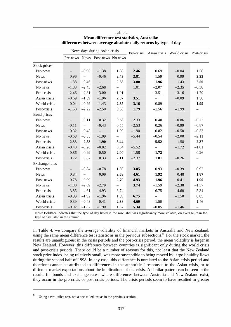
317
Table 2Mean difference test statistics, Australia:
differences between average absolute daily returns by type of day
News days during Asian crisis
Pre-news News Post-news No newsPre-crisis Asian crisis World crisis Post-crisis
Stock prices
Pre-news – –0.96 –1.38 1.88 2.46 0.69 –0.04 1.58
News 0.96 – –0.46 2.43 2.81 1.59 0.99 2.22Post-news 1.38 0.46 – 2.68 3.00 1.96 1.43 2.50No news –1.88 –2.43 –2.68 – 1.01 –2.07 –2.35 –0.58
Pre-crisis –2.46 –2.81 –3.00 –1.01 – –3.51 –3.16 –1.79
Asian crisis –0.69 –1.59 –1.96 2.07 3.51 – –0.89 1.56
World crisis 0.04 –0.99 –1.43 2.35 3.16 0.89 – 1.99Post-crisis –1.58 –2.22 –2.50 0.58 1.79 –1.56 –1.99 –
Bond prices
Pre-news – 0.11 –0.32 0.68 –2.33 0.40 –0.86 –0.72
News –0.11 – –0.43 0.55 –2.53 0.26 –0.99 –0.87
Post-news 0.32 0.43 – 1.09 –1.90 0.82 –0.50 –0.33
No news –0.68 –0.55 –1.09 – –5.44 –0.54 –2.00 –2.11
Pre-crisis 2.33 2.53 1.90 5.44 – 5.52 1.58 2.37Asian crisis –0.40 –0.26 –0.82 0.54 –5.52 – –1.72 –1.81
World crisis 0.86 0.99 0.50 2.00 –1.58 1.72 – 0.26
Post-crisis 0.72 0.87 0.33 2.11 –2.37 1.81 –0.26 –
Exchange rates
Pre-news – –0.84 –0.78 1.80 3.85 0.93 –0.39 0.92
News 0.84 – 0.09 2.69 4.61 1.92 0.48 1.87Post-news 0.78 –0.09 – 2.79 4.93 1.96 0.41 1.90No news –1.80 –2.69 –2.79 – 3.74 –1.59 –2.38 –1.37
Pre-crisis –3.85 –4.61 –4.93 –3.74 – –6.75 –4.60 –5.34
Asian crisis –0.93 –1.92 –1.96 1.59 6.75 – –1.50 0.05
World crisis 0.39 –0.48 –0.41 2.38 4.60 1.50 – 1.46
Post-crisis –0.92 –1.87 –1.90 1.37 5.34 –0.05 –1.46 –
Note: Boldface indicates that the type of day listed in the row label was significantly more volatile, on average, than thetype of day listed in the column.
In Table 4, we compare the average volatility of financial markets in Australia and New Zealand,using the same mean difference test statistic as in the previous subsections.8 For the stock market, theresults are unambiguous: in the crisis periods and the post-crisis period, the mean volatility is larger inNew Zealand. However, this difference between countries is significant only during the world crisisand post-crisis periods. There could be a number of reasons for this, not least that the New Zealandstock price index, being relatively small, was more susceptible to being moved by large liquidity flowsduring the second half of 1998. In any case, this difference is unrelated to the Asian crisis period andtherefore cannot be attributed to differences in the authorities’ responses to the Asian crisis, or todifferent market expectations about the implications of the crisis. A similar pattern can be seen in theresults for bonds and exchange rates: where differences between Australia and New Zealand exist,they occur in the pre-crisis or post-crisis periods. The crisis periods seem to have resulted in greater
8
Using a two-tailed test, not a one-tailed test as in the previous section.
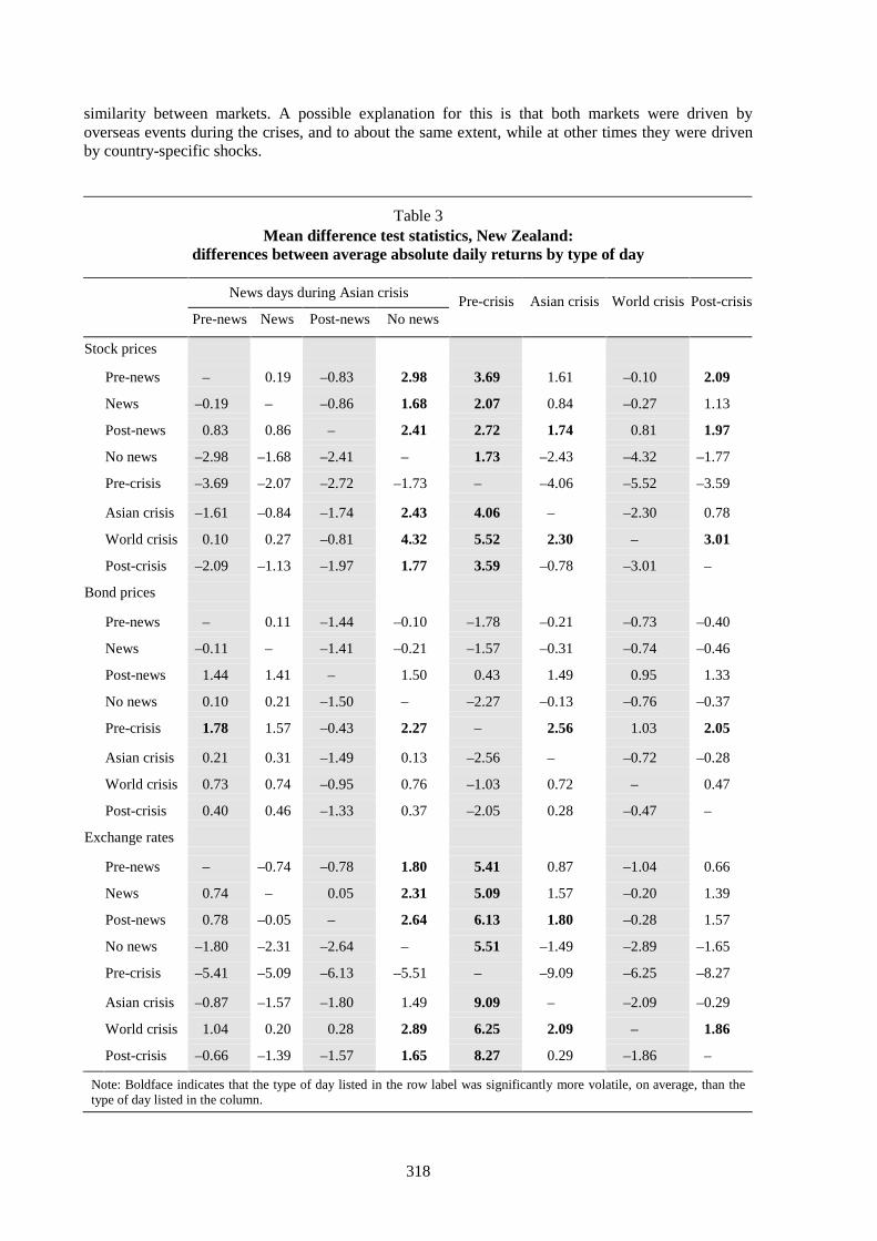
318
similarity between markets. A possible explanation for this is that both markets were driven byoverseas events during the crises, and to about the same extent, while at other times they were drivenby country-specific shocks.
Table 3Mean difference test statistics, New Zealand:
differences between average absolute daily returns by type of day
News days during Asian crisis
Pre-news News Post-news No newsPre-crisis Asian crisis World crisis Post-crisis
Stock prices
Pre-news – 0.19 –0.83 2.98 3.69 1.61 –0.10 2.09
News –0.19 – –0.86 1.68 2.07 0.84 –0.27 1.13
Post-news 0.83 0.86 – 2.41 2.72 1.74 0.81 1.97
No news –2.98 –1.68 –2.41 – 1.73 –2.43 –4.32 –1.77
Pre-crisis –3.69 –2.07 –2.72 –1.73 – –4.06 –5.52 –3.59
Asian crisis –1.61 –0.84 –1.74 2.43 4.06 – –2.30 0.78
World crisis 0.10 0.27 –0.81 4.32 5.52 2.30 – 3.01
Post-crisis –2.09 –1.13 –1.97 1.77 3.59 –0.78 –3.01 –
Bond prices
Pre-news – 0.11 –1.44 –0.10 –1.78 –0.21 –0.73 –0.40
News –0.11 – –1.41 –0.21 –1.57 –0.31 –0.74 –0.46
Post-news 1.44 1.41 – 1.50 0.43 1.49 0.95 1.33
No news 0.10 0.21 –1.50 – –2.27 –0.13 –0.76 –0.37
Pre-crisis 1.78 1.57 –0.43 2.27 – 2.56 1.03 2.05
Asian crisis 0.21 0.31 –1.49 0.13 –2.56 – –0.72 –0.28
World crisis 0.73 0.74 –0.95 0.76 –1.03 0.72 – 0.47
Post-crisis 0.40 0.46 –1.33 0.37 –2.05 0.28 –0.47 –
Exchange rates
Pre-news – –0.74 –0.78 1.80 5.41 0.87 –1.04 0.66
News 0.74 – 0.05 2.31 5.09 1.57 –0.20 1.39
Post-news 0.78 –0.05 – 2.64 6.13 1.80 –0.28 1.57
No news –1.80 –2.31 –2.64 – 5.51 –1.49 –2.89 –1.65
Pre-crisis –5.41 –5.09 –6.13 –5.51 – –9.09 –6.25 –8.27
Asian crisis –0.87 –1.57 –1.80 1.49 9.09 – –2.09 –0.29
World crisis 1.04 0.20 0.28 2.89 6.25 2.09 – 1.86
Post-crisis –0.66 –1.39 –1.57 1.65 8.27 0.29 –1.86 –
Note: Boldface indicates that the type of day listed in the row label was significantly more volatile, on average, than thetype of day listed in the column.

319
Table 4Mean difference tests between Australia and New Zealand
News days during Asian crisis
Pre-news News Post-news No newsPre-crisis Asian crisis World crisis Post-crisis
Stock prices
Australia
– Mean volatility 0.77 0.91 1.00 0.59 0.55 0.70 0.77 0.62
– Sample variance 0.47 1.05 1.42 0.25 0.24 0.52 0.39 0.20
New Zealand
– Mean volatility 1.01 0.97 1.24 0.63 0.55 0.79 1.03 0.74
– Sample variance 0.97 2.57 4.05 0.29 0.26 1.11 0.61 0.39
Test statistic –1.64 –0.23 –0.82 –0.67 –0.07 –1.35 –2.39 –1.97
Decision Same Same Same Same Same Same Aust<NZ Aust<NZ
Bond prices
Australia
– Mean volatility 0.06 0.06 0.06 0.06 0.08 0.06 0.07 0.07
– Sample variance 0.003 0.003 0.003 0.002 0.006 0.002 0.003 0.003
New Zealand
– Mean volatility 0.05 0.05 0.07 0.05 0.06 0.05 0.06 0.05
– Sample variance 0.002 0.003 0.004 0.003 0.004 0.003 0.002 0.002
Test statistic 1.12 1.01 –0.07 0.80 5.11 1.46 1.73 2.56
Decision Same Same Same Same Aust>NZ Same Same Aust>NZ
Exchange rates
Australia
– Mean volatility 0.59 0.67 0.66 0.46 0.33 0.52 0.62 0.52
– Sample variance 0.27 0.33 0.27 0.19 0.10 0.23 0.33 0.19
New Zealand
– Mean volatility 0.56 0.63 0.62 0.44 0.26 0.51 0.65 0.52
– Sample variance 0.20 0.34 0.23 0.22 0.06 0.24 0.34 0.16
Test statistic 0.31 0.39 0.39 0.30 5.87 0.41 –0.29 0.04
Decision Same Same Same Same Aust>NZ Same Same Same
Note: The null hypothesis is that the mean volatility in the two markets is the same on that category of day. The two-sidedalternative is that they are different.
While the volatility in the two countries’ financial markets was very similar during the Asian crisis,the levels of the financial-market variables suggest that conditions in Australian and New Zealandstock and bond markets were rather different during this period (Figure 5).
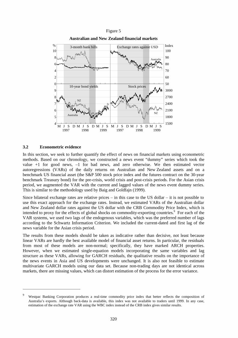
320
Figure 5
Australian and New Zealand financial markets
l l l l l l l l l l0
2
4
6
8
10
%
NZ
Australia
l l l l l l l l l l 50
60
70
80
90
100
Index
l l l l l l l l l l 1500
1800
2100
2400
2700
3000
NZ
Australia
Australia
NZ
l l l l l l l l l l4
5
6
7
8
9
Australia
NZ
Exchange rates against USD3-month bank bills
10-year bond yields Stock prices
M J S D M J S D M J S M J S D M J S D M J S1997 1998 1999 1997 1998 1999
3.2 Econometric evidence
In this section, we seek to further quantify the effect of news on financial markets using econometricmethods. Based on our chronology, we constructed a news event “dummy” series which took thevalue +1 for good news, –1 for bad news, and zero otherwise. We then estimated vectorautoregressions (VARs) of the daily returns on Australian and New Zealand assets and on abenchmark US financial asset (the S&P 500 stock price index and the futures contract on the 30-yearbenchmark Treasury bond) for the pre-crisis, world crisis and post-crisis periods. For the Asian crisisperiod, we augmented the VAR with the current and lagged values of the news event dummy series.This is similar to the methodology used by Baig and Goldfajn (1999).
Since bilateral exchange rates are relative prices – in this case to the US dollar – it is not possible touse this exact approach for the exchange rates. Instead, we estimated VARs of the Australian dollarand New Zealand dollar rates against the US dollar with the CRB Commodity Price Index, which isintended to proxy for the effects of global shocks on commodity-exporting countries.9 For each of theVAR systems, we used two lags of the endogenous variables, which was the preferred number of lagsaccording to the Schwartz Information Criterion. We included the current-dated and first lag of thenews variable for the Asian crisis period.
The results from these models should be taken as indicative rather than decisive, not least becauselinear VARs are hardly the best available model of financial asset returns. In particular, the residualsfrom most of these models are non-normal; specifically, they have marked ARCH properties.However, when we estimated single-equation models incorporating the same variables and lagstructure as these VARs, allowing for GARCH residuals, the qualitative results on the importance ofthe news events in Asia and US developments were unchanged. It is also not feasible to estimatemultivariate GARCH models using our data set. Because non-trading days are not identical acrossmarkets, there are missing values, which can distort estimation of the process for the error variance.
9
Westpac Banking Corporation produces a real-time commodity price index that better reflects the composition ofAustralia’s exports. Although back-data is available, this index was not available to traders until 1999. In any case,estimation of the exchange rate VAR using the WBC index instead of the CRB index gives similar results.
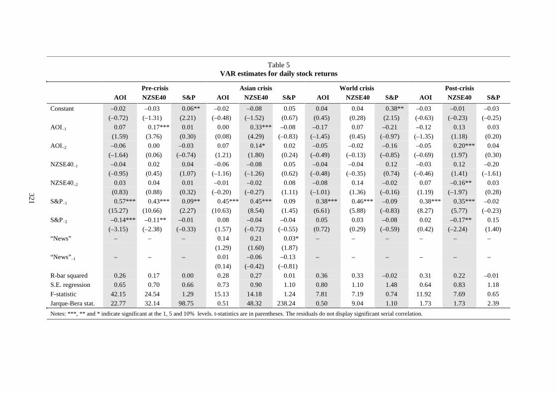
321
Table 5VAR estimates for daily stock returns
Pre-crisis Asian crisis World crisis Post-crisisAOI NZSE40 S&P AOI NZSE40 S&P AOI NZSE40 S&P AOI NZSE40 S&P
Constant –0.02 –0.03 0.06** –0.02 –0.08 0.05 0.04 0.04 0.38** –0.03 –0.01 –0.03
(–0.72) (–1.31) (2.21) (–0.48) (–1.52) (0.67) (0.45) (0.28) (2.15) (-0.63) (–0.23) (–0.25)
AOI–1 0.07 0.17*** 0.01 0.00 0.33*** –0.08 –0.17 0.07 –0.21 –0.12 0.13 0.03
(1.59) (3.76) (0.30) (0.08) (4.29) (–0.83) (–1.45) (0.45) (–0.97) (–1.35) (1.18) (0.20)
AOI–2 –0.06 0.00 –0.03 0.07 0.14* 0.02 –0.05 –0.02 –0.16 –0.05 0.20*** 0.04
(–1.64) (0.06) (–0.74) (1.21) (1.80) (0.24) (–0.49) (–0.13) (–0.85) (–0.69) (1.97) (0.30)
NZSE40–1 –0.04 0.02 0.04 –0.06 –0.08 0.05 –0.04 –0.04 0.12 –0.03 0.12 –0.20
(–0.95) (0.45) (1.07) (–1.16) (–1.26) (0.62) (–0.48) (–0.35) (0.74) (–0.46) (1.41) (–1.61)
NZSE40–2 0.03 0.04 0.01 –0.01 –0.02 0.08 –0.08 0.14 –0.02 0.07 –0.16** 0.03
(0.83) (0.88) (0.32) (–0.20) (–0.27) (1.11) (–1.01) (1.36) (–0.16) (1.19) (–1.97) (0.28)
S&P–1 0.57*** 0.43*** 0.09** 0.45*** 0.45*** 0.09 0.38*** 0.46*** –0.09 0.38*** 0.35*** –0.02
(15.27) (10.66) (2.27) (10.63) (8.54) (1.45) (6.61) (5.88) (–0.83) (8.27) (5.77) (–0.23)
S&P–2 –0.14*** –0.11** –0.01 0.08 –0.04 –0.04 0.05 0.03 –0.08 0.02 –0.17** 0.15
(–3.15) (–2.38) (–0.33) (1.57) (–0.72) (–0.55) (0.72) (0.29) (–0.59) (0.42) (–2.24) (1.40)
“News” – – – 0.14 0.21 0.03* – – – – – –
(1.29) (1.60) (1.87)
“News”–1 – – – 0.01 –0.06 –0.13 – – – – – –
(0.14) (–0.42) (–0.81)
R-bar squared 0.26 0.17 0.00 0.28 0.27 0.01 0.36 0.33 –0.02 0.31 0.22 –0.01
S.E. regression 0.65 0.70 0.66 0.73 0.90 1.10 0.80 1.10 1.48 0.64 0.83 1.18
F-statistic 42.15 24.54 1.29 15.13 14.18 1.24 7.81 7.19 0.74 11.92 7.69 0.65
Jarque-Bera stat. 22.77 32.14 98.75 0.51 48.32 238.24 0.50 9.04 1.10 1.73 1.73 2.39
Notes: ***, ** and * indicate significant at the 1, 5 and 10% levels. t-statistics are in parentheses. The residuals do not display significant serial correlation.

322
Table 6VAR estimates for daily bond returns
Pre-crisis Asian crisis World crisis Post-crisisAustralia NZ US Australia NZ US Australia NZ US Australia NZ US
Constant 0.00 0.00 0.00 0.02 0.00 0.04 0.01 0.01* –0.07 –0.01 –0.01** –0.09*
(0.55) (–0.43) (–0.18) (0.52) (0.91) (1.34) (1.47) (1.75) (–0.86) (–1.15) (–2.02) (–1.94)
Australia–1 –0.14*** 0.06 0.24 –0.02 0.04 –0.12 –0.41*** –0.02 –1.18 –0.25** –0.02 –0.08
(–3.31) (1.40) (0.80) (–0.32) (0.58) (–0.25) (–2.74) (–0.19) (–0.85) (–2.50) (–0.24) (–0.07)
Australia–2 0.00 0.21 0.03 –0.10 0.01 –0.51 –0.13 –0.05 –0.82 0.19** 0.19*** 0.62
(–0.02) (0.58) (0.12) (–1.61) (0.18) (–1.18) (–0.96) (–0.45) (–0.65) (2.02) (2.63) (0.61)
NZ–1 –0.11** –0.19*** 0.45 0.05 –0.10 0.15 0.14 –0.13 0.34 –0.16 –0.18* 0.13
(–2.31) (–4.20) (1.34) (0.79) (–1.52) (0.34) (0.79) (–0.84) (0.21) (–1.19) (–1.75) (0.08)
NZ–2 –0.04 –0.04 0.12 0.01 –0.03 0.01 0.04 0.00 0.32 –0.44*** –0.31*** –1.69
(–0.76) (–0.79) (0.37) (0.16) (–0.54) (0.02) (0.28) (0.01) (0.21) (–3.72) (–3.32) (–1.29)
US–1 0.12*** 0.08*** –0.04 0.09*** 0.07** 0.06 0.06*** 0.06*** 0.28** 0.14*** 0.11*** –0.02
(19.21) (14.03) (–0.87) (10.67) (6.96) (0.99) (4.53) (5.42) (2.27) (16.96) (17.17) (–0.32)
US–2 0.01* 0.00 –0.08 –0.01 –0.02 –0.01 0.03 0.03** 0.23 0.04*** 0.02* 0.02
(1.68) (0.48) (–1.40) (–1.02) (–1.57) (–0.09) (1.51) (2.19) (1.38) (2.98) (1.73) (0.15)
“News” – – – –0.01 0.01 0.00 – – – – – –
(–1.27) (0.53) (0.01)
“News”–1 – – – 0.01 0.01 –0.04 – – – – – –
(0.57) (0.71) (–0.66)
R-bar squared 0.39 0.26 0.00 0.29 0.14 –0.02 0.24 0.30 0.03 0.67 0.67 –0.02
SE regression 0.09 0.08 0.60 0.06 0.07 0.45 0.07 0.06 0.65 0.05 0.04 0.56
F-statistic 64.20 36.14 0.72 15.38 6.86 0.44 4.57 5.95 1.30 49.92 50.96 0.47
Jarque-Bera stat. 189.44 32.58 29.98 37.42 103.58 30.18 8.31 1.30 0.64 1.03 1.42 6.02
Notes: ***, ** and * indicate significant at the 1, 5 and 10% levels. t-statistics are in parentheses. The residuals do not display significant serial correlation.
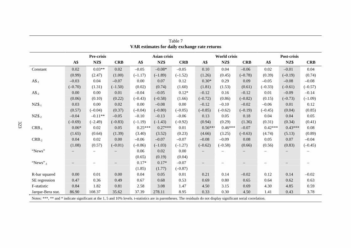
323
Table 7VAR estimates for daily exchange rate returns
Pre-crisis Asian crisis World crisis Post-crisisA$ NZ$ CRB A$ NZ$ CRB A$ NZ$ CRB A$ NZ$ CRB
Constant 0.02 0.03** 0.02 –0.05 –0.08* –0.05 0.10 0.04 –0.06 0.02 –0.01 0.04
(0.99) (2.47) (1.00) (–1.17) (–1.89) (–1.52) (1.26) (0.45) (–0.78) (0.39) (–0.19) (0.74)
A$-1 –0.03 0.04 –0.07 0.00 0.07 0.12 0.30* 0.29 0.09 –0.05 –0.08 –0.08
(–0.70) (1.31) (–1.50) (0.02) (0.74) (1.60) (1.81) (1.53) (0.61) (–0.33) (–0.61) (–0.57)
A$-2 0.00 0.00 0.01 –0.04 –0.05 0.12* –0.12 0.16 –0.12 0.01 –0.09 –0.14
(0.06) (0.10) (0.22) (–0.43) (–0.58) (1.66) (–0.72) (0.86) (–0.82) (0.15) (–0.73) (–1.09)
NZ$-1 0.03 0.00 0.02 0.00 –0.08 0.00 –0.12 –0.10 –0.02 –0.06 0.01 0.12
(0.57) (–0.04) (0.37) (–0.04) (–0.80) (–0.05) (–0.85) (–0.62) (–0.19) (–0.45) (0.04) (0.85)
NZ$-2 –0.04 –0.11** –0.05 –0.10 –0.13 –0.06 0.13 0.05 0.18 0.04 0.04 0.05
(–0.69) (–2.49) (–0.83) (–1.19) (–1.43) (–0.92) (0.94) (0.29) (1.36) (0.31) (0.34) (0.41)
CRB-1 0.06* 0.02 0.05 0.25*** 0.27*** 0.01 0.56*** 0.46*** –0.07 0.42*** 0.43*** 0.08
(1.65) (0.64) (1.39) (3.40) (3.52) (0.23) (4.66) (3.25) (–0.63) (4.74) (5.13) (0.89)
CRB-2 0.04 0.02 0.00 –0.06 –0.07 –0.07 –0.08 –0.09 0.08 0.05 0.07 –0.04
(1.08) (0.57) (–0.01) (–0.86) (–1.03) (–1.27) (–0.62) (–0.58) (0.66) (0.56) (0.83) (–0.45)
“News” – – – 0.06 0.02 0.00 – – – – – –
(0.65) (0.19) (0.04)
“News”-1 – – – 0.17* 0.17* –0.07 – – – – – –
(1.85) (1.77) (–0.87)
R-bar squared 0.00 0.01 0.00 0.04 0.05 0.01 0.21 0.14 –0.02 0.12 0.14 –0.02
SE regression 0.47 0.36 0.49 0.67 0.68 0.53 0.69 0.80 0.65 0.64 0.62 0.63
F-statistic 0.84 1.82 0.81 2.58 3.08 1.47 4.50 3.15 0.69 4.30 4.85 0.59
Jarque-Bera stat. 86.90 108.37 35.62 37.39 278.11 8.95 0.33 0.30 4.50 1.41 0.43 3.78
Notes: ***, ** and * indicate significant at the 1, 5 and 10% levels. t-statistics are in parentheses. The residuals do not display significant serial correlation.
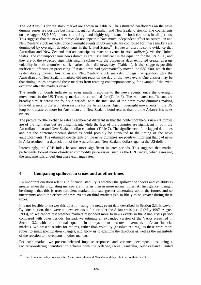
324
The VAR results for the stock market are shown in Table 5. The estimated coefficients on the newsdummy series are positive but insignificant for Australian and New Zealand stocks. The coefficientson the lagged S&P 500, however, are large and highly significant for both countries in all periods.This suggests that the news dummies do not appear to have much independent effect on Australian andNew Zealand stock markets, once overnight events in US markets are controlled for; these markets aredominated by overnight developments in the United States.10 However, there is some evidence thatAustralian and New Zealand market participants react to events in Asia indirectly via the UnitedStates. The contemporaneous news dummies are just significant in the equation for the S&P 500, andthey are of the expected sign. This might explain why the post-news days exhibited greater averagevolatility in both countries’ stock markets than did news days (Table 1). It also suggests possibleinefficient information processing. If Asian news had systematically moved the S&P 500, which thensystematically moved Australian and New Zealand stock markets, it begs the question why theAustralian and New Zealand markets did not react on the day of the news event. One answer may bethat timing issues prevented these markets from reacting contemporaneously, for example if the eventoccurred after the markets closed.
The results for bonds indicate an even smaller response to the news events, once the overnightmovements in the US Treasury market are controlled for (Table 6). The estimated coefficients arebroadly similar across the four sub-periods, with the inclusion of the news event dummies makinglittle difference to the estimation results for the Asian crisis. Again, overnight movements in the USlong bond mattered more for Australian and New Zealand bond returns than did the Asian-crisis newsevents.
The picture for the exchange rates is somewhat different in that the contemporaneous news dummiesare of the right sign but are insignificant, while the lags of the dummies are significant in both theAustralian dollar and New Zealand dollar equations (Table 7). The significance of the lagged dummiesand not the contemporaneous dummies could possibly be attributed to the timing of the newsannouncements. The estimated coefficients on the news dummies are positive, implying that bad newsin Asia resulted in a depreciation of the Australian and New Zealand dollars against the US dollar.
Interestingly, the CRB index became more significant in later periods. This suggests that marketparticipants looked more closely at commodity price series, such as the CRB index, when assessingthe fundamentals underlying these exchange rates.
4. Comparing spillover in crises and at other times
An important question relating to financial stability is whether the spillover of shocks and volatility isgreater when the originating markets are in crisis than in more normal times. At first glance, it mightbe thought that this is true: turbulent markets indicate greater uncertainty about the future, and souncertainty about the effects of news events on third markets is also likely to be greater during thesetimes.
It is not feasible to answer this question using the news event data described in Section 2.3, however.By construction, there were no news events before or after the Asian crisis period (May 1997–August1998), so we cannot test whether markets responded more to news events in the Asian crisis periodcompared with other periods. Instead, we estimate an expanded version of the VARs presented inSection 3.2, with an additional equation in the system to measure movements in Asian financialmarkets. We present results for returns, rather than volatility (absolute returns), as these were morerobust to small specification changes, and allow us to examine the direction as well as the magnitudeof the reaction to movements in other markets.
For each market, we present selected impulse responses and variance decompositions, using arecursive-ordering identification scheme with the ordering (Asia, Australia, New Zealand, United 10
The US market’s day t occurs after Asian, Australian and New Zealand day t, but before their day t+1.
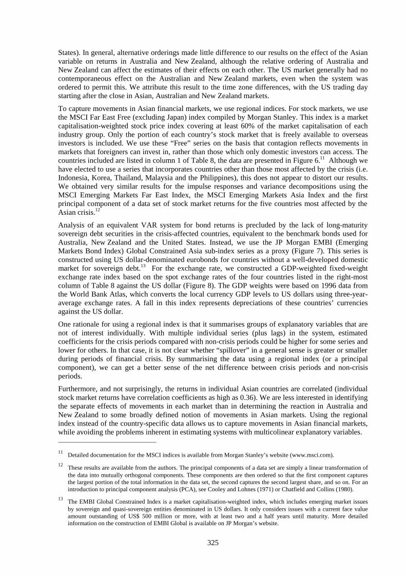
325
States). In general, alternative orderings made little difference to our results on the effect of the Asianvariable on returns in Australia and New Zealand, although the relative ordering of Australia andNew Zealand can affect the estimates of their effects on each other. The US market generally had nocontemporaneous effect on the Australian and New Zealand markets, even when the system wasordered to permit this. We attribute this result to the time zone differences, with the US trading daystarting after the close in Asian, Australian and New Zealand markets.
To capture movements in Asian financial markets, we use regional indices. For stock markets, we usethe MSCI Far East Free (excluding Japan) index compiled by Morgan Stanley. This index is a marketcapitalisation-weighted stock price index covering at least 60% of the market capitalisation of eachindustry group. Only the portion of each country’s stock market that is freely available to overseasinvestors is included. We use these “Free” series on the basis that contagion reflects movements inmarkets that foreigners can invest in, rather than those which only domestic investors can access. Thecountries included are listed in column 1 of Table 8, the data are presented in Figure 6.11 Although wehave elected to use a series that incorporates countries other than those most affected by the crisis (i.e.Indonesia, Korea, Thailand, Malaysia and the Philippines), this does not appear to distort our results.We obtained very similar results for the impulse responses and variance decompositions using theMSCI Emerging Markets Far East Index, the MSCI Emerging Markets Asia Index and the firstprincipal component of a data set of stock market returns for the five countries most affected by theAsian crisis.12
Analysis of an equivalent VAR system for bond returns is precluded by the lack of long-maturitysovereign debt securities in the crisis-affected countries, equivalent to the benchmark bonds used forAustralia, New Zealand and the United States. Instead, we use the JP Morgan EMBI (EmergingMarkets Bond Index) Global Constrained Asia sub-index series as a proxy (Figure 7). This series isconstructed using US dollar-denominated eurobonds for countries without a well-developed domesticmarket for sovereign debt.13 For the exchange rate, we constructed a GDP-weighted fixed-weightexchange rate index based on the spot exchange rates of the four countries listed in the right-mostcolumn of Table 8 against the US dollar (Figure 8). The GDP weights were based on 1996 data fromthe World Bank Atlas, which converts the local currency GDP levels to US dollars using three-year-average exchange rates. A fall in this index represents depreciations of these countries’ currenciesagainst the US dollar.
One rationale for using a regional index is that it summarises groups of explanatory variables that arenot of interest individually. With multiple individual series (plus lags) in the system, estimatedcoefficients for the crisis periods compared with non-crisis periods could be higher for some series andlower for others. In that case, it is not clear whether “spillover” in a general sense is greater or smallerduring periods of financial crisis. By summarising the data using a regional index (or a principalcomponent), we can get a better sense of the net difference between crisis periods and non-crisisperiods.
Furthermore, and not surprisingly, the returns in individual Asian countries are correlated (individualstock market returns have correlation coefficients as high as 0.36). We are less interested in identifyingthe separate effects of movements in each market than in determining the reaction in Australia andNew Zealand to some broadly defined notion of movements in Asian markets. Using the regionalindex instead of the country-specific data allows us to capture movements in Asian financial markets,while avoiding the problems inherent in estimating systems with multicolinear explanatory variables. 11
Detailed documentation for the MSCI indices is available from Morgan Stanley’s website (www.msci.com).
12These results are available from the authors. The principal components of a data set are simply a linear transformation ofthe data into mutually orthogonal components. These components are then ordered so that the first component capturesthe largest portion of the total information in the data set, the second captures the second largest share, and so on. For anintroduction to principal component analysis (PCA), see Cooley and Lohnes (1971) or Chatfield and Collins (1980).
13The EMBI Global Constrained Index is a market capitalisation-weighted index, which includes emerging market issuesby sovereign and quasi-sovereign entities denominated in US dollars. It only considers issues with a current face valueamount outstanding of US$ 500 million or more, with at least two and a half years until maturity. More detailedinformation on the construction of EMBI Global is available on JP Morgan’s website.
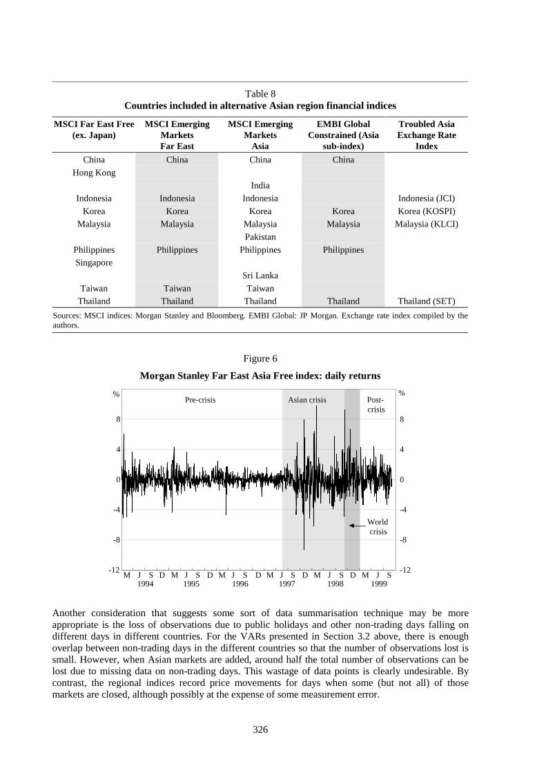
326
Table 8Countries included in alternative Asian region financial indices
MSCI Far East Free(ex. Japan)
MSCI EmergingMarketsFar East
MSCI EmergingMarkets
Asia
EMBI GlobalConstrained (Asia
sub-index)
Troubled AsiaExchange Rate
Index
China China China China
Hong Kong
India
Indonesia Indonesia Indonesia Indonesia (JCI)
Korea Korea Korea Korea Korea (KOSPI)
Malaysia Malaysia Malaysia Malaysia Malaysia (KLCI)
Pakistan
Philippines Philippines Philippines Philippines
Singapore
Sri Lanka
Taiwan Taiwan Taiwan
Thailand Thailand Thailand Thailand Thailand (SET)
Sources: MSCI indices: Morgan Stanley and Bloomberg. EMBI Global: JP Morgan. Exchange rate index compiled by theauthors.
Figure 6
Morgan Stanley Far East Asia Free index: daily returns
M J S D M J S D M J S D M J S D M J S D M J S1994 1995 1996 1997 1998 1999
% %
l l l l l l l l l l l l l l l l l l l l l l-12
-8
-4
0
4
8
-12
-8
-4
0
4
8
Asian crisisPre-crisis Post-crisis
Worldcrisis
Another consideration that suggests some sort of data summarisation technique may be moreappropriate is the loss of observations due to public holidays and other non-trading days falling ondifferent days in different countries. For the VARs presented in Section 3.2 above, there is enoughoverlap between non-trading days in the different countries so that the number of observations lost issmall. However, when Asian markets are added, around half the total number of observations can belost due to missing data on non-trading days. This wastage of data points is clearly undesirable. Bycontrast, the regional indices record price movements for days when some (but not all) of thosemarkets are closed, although possibly at the expense of some measurement error.

327
Figure 7
EMBI Global Constrained Asia sub-index: daily returns
M J S D M J S D M J S D M J S D M J S D M J S1994 1995 1996 1997 1998 1999
% %
l l l l l l l l l l l l l l l l l l l l l l-6
-4
-2
0
2
4
-6
-4
-2
0
2
4
Asian-crisisPre-crisis Post-crisis
Worldcrisis
Figure 8
Troubled Asia Exchange Rate Index: daily returns
M J S D M J S D M J S D M J S D M J S D M J S1994 1995 1996 1997 1998 1999
% %
l l l l l l l l l l l l l l l l l l l l l l-15
-10
-5
0
5
10
15
-15
-10
-5
0
5
10
15
Asian crisisPre-crisis Post-crisis
Worldcrisis
4.1 Stock markets
Within each sub-period (pre-crisis, Asian crisis, world crisis and post-crisis), our VAR results forstock returns were largely as expected. Much of the variation in Australian and New Zealand returnswas driven by overnight developments in US markets. Movements in the Australian and New Zealandmarkets did not have an independent effect on US markets. There was some minor persistence inAustralasian markets, with lagged own price changes being significant in some cases. The previousday’s return in the Australian market also had a significant positive effect on the New Zealand market;we attribute this to time zone differences.14
14
We do not present the estimation results in the paper; they are available from the authors. To save space, we also showonly the first, second and fifth days in the variance decompositions.
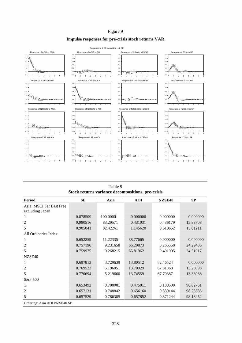
328
Figure 9
Impulse responses for pre-crisis stock returns VAR
-0.2
0.0
0.2
0.4
0.6
0.8
1.0
1 2 3 4 5 6 7 8
Response of ASIA to ASIA
-0.2
0.0
0.2
0.4
0.6
0.8
1.0
1 2 3 4 5 6 7 8
Response of ASIA to AOI
-0.2
0.0
0.2
0.4
0.6
0.8
1.0
1 2 3 4 5 6 7 8
Response of ASIA to NZSE40
-0.2
0.0
0.2
0.4
0.6
0.8
1.0
1 2 3 4 5 6 7 8
Response of ASIA to SP
-0.2
0.0
0.2
0.4
0.6
0.8
1 2 3 4 5 6 7 8
Response of AOI to ASIA
-0.2
0.0
0.2
0.4
0.6
0.8
1 2 3 4 5 6 7 8
Response of AOI to AOI
-0.2
0.0
0.2
0.4
0.6
0.8
1 2 3 4 5 6 7 8
Response of AOI to NZSE40
-0.2
0.0
0.2
0.4
0.6
0.8
1 2 3 4 5 6 7 8
Response of AOI to SP
-0.2
0.0
0.2
0.4
0.6
0.8
1 2 3 4 5 6 7 8
Response of NZSE40 to ASIA
-0.2
0.0
0.2
0.4
0.6
0.8
1 2 3 4 5 6 7 8
Response of NZSE40 to AOI
-0.2
0.0
0.2
0.4
0.6
0.8
1 2 3 4 5 6 7 8
Response of NZSE40 to NZSE40
-0.2
0.0
0.2
0.4
0.6
0.8
1 2 3 4 5 6 7 8
Response of NZSE40 to SP
-0.2
0.0
0.2
0.4
0.6
0.8
1 2 3 4 5 6 7 8
Response of SP to ASIA
-0.2
0.0
0.2
0.4
0.6
0.8
1 2 3 4 5 6 7 8
Response of SP to AOI
-0.2
0.0
0.2
0.4
0.6
0.8
1 2 3 4 5 6 7 8
Response of SP to NZSE40
-0.2
0.0
0.2
0.4
0.6
0.8
1 2 3 4 5 6 7 8
Response of SP to SP
Response to 1 SD innovation, ± 2 SE
Table 9Stock returns variance decompositions, pre-crisis
Period SE Asia AOI NZSE40 SP
Asia: MSCI Far East Freeexcluding Japan
1 0.878509 100.0000 0.000000 0.000000 0.000000
2 0.980516 83.29571 0.431031 0.436179 15.83708
5 0.985841 82.42261 1.145628 0.619652 15.81211
All Ordinaries Index
1 0.652259 11.22335 88.77665 0.000000 0.000000
2 0.757196 9.231658 66.20873 0.265550 24.29406
5 0.759975 9.268215 65.81962 0.401995 24.51017
NZSE40
1 0.697813 3.729639 13.80512 82.46524 0.000000
2 0.769523 5.196051 13.70929 67.81368 13.28098
5 0.770694 5.219660 13.74559 67.70387 13.33088
S&P 500
1 0.653492 0.708081 0.475811 0.188500 98.62761
2 0.657131 0.748842 0.656160 0.339144 98.25585
5 0.657529 0.786385 0.657852 0.371244 98.18452
Ordering: Asia AOI NZSE40 SP.

329
Figure 10Impulse responses for Asian crisis stock returns VAR
-0.5
0.0
0.5
1.0
1.5
2.0
1 2 3 4 5 6 7 8
Response of ASIA to ASIA
-0.5
0.0
0.5
1.0
1.5
2.0
1 2 3 4 5 6 7 8
Response of ASIA to AOI
-0.5
0.0
0.5
1.0
1.5
2.0
1 2 3 4 5 6 7 8
Response of ASIA to NZSE40
-0.5
0.0
0.5
1.0
1.5
2.0
1 2 3 4 5 6 7 8
Response of ASIA to SP
-0.2
0.0
0.2
0.4
0.6
0.8
1 2 3 4 5 6 7 8
Response of AOI to ASIA
-0.2
0.0
0.2
0.4
0.6
0.8
1 2 3 4 5 6 7 8
Response of AOI to AOI
-0.2
0.0
0.2
0.4
0.6
0.8
1 2 3 4 5 6 7 8
Response of AOI to NZSE40
-0.2
0.0
0.2
0.4
0.6
0.8
1 2 3 4 5 6 7 8
Response of AOI to SP
-0.2
0.0
0.2
0.4
0.6
0.8
1.0
1 2 3 4 5 6 7 8
Response of NZSE40 to ASIA
-0.2
0.0
0.2
0.4
0.6
0.8
1.0
1 2 3 4 5 6 7 8
Response of NZSE40 to AOI
-0.2
0.0
0.2
0.4
0.6
0.8
1.0
1 2 3 4 5 6 7 8
Response of NZSE40 to NZSE40
-0.2
0.0
0.2
0.4
0.6
0.8
1.0
1 2 3 4 5 6 7 8
Response of NZSE40 to SP
-0.2
0.0
0.2
0.4
0.6
0.8
1.0
1.2
1 2 3 4 5 6 7 8
Response of SP to ASIA
-0.2
0.0
0.2
0.4
0.6
0.8
1.0
1.2
1 2 3 4 5 6 7 8
Response of SP to AOI
-0.2
0.0
0.2
0.4
0.6
0.8
1.0
1.2
1 2 3 4 5 6 7 8
Response of SP to NZSE40
-0.2
0.0
0.2
0.4
0.6
0.8
1.0
1.2
1 2 3 4 5 6 7 8
Response of SP to SP
Response to 1 SD innovation, ± 2 SE
Table 10Stock returns variance decompositions, Asian crisis
Period SE Asia AOI NZSE40 S&P 500
Asia: MSCI Far East Freeexcluding Japan
1 1.663163 100.0000 0.000000 0.000000 0.000000
2 1.788953 91.58451 0.102682 0.008993 8.303816
5 1.799454 90.55363 0.216412 0.312136 8.917818
All Ordinaries Index
1 0.719485 18.65428 81.34572 0.000000 0.000000
2 0.873748 16.27916 55.15806 0.007574 28.55521
5 0.883768 15.96006 54.22948 0.237500 29.57297
NZSE40
1 0.882700 3.579450 11.56667 84.85388 0.000000
2 1.049160 9.988225 11.59553 60.09029 18.32595
5 1.065953 10.74370 11.47999 58.34329 19.43302
S&P 500
1 1.085633 6.496993 0.331497 1.459383 91.71213
2 1.091870 6.663517 0.485786 1.559626 91.29107
5 1.085633 6.496993 0.331497 1.459383 91.71213
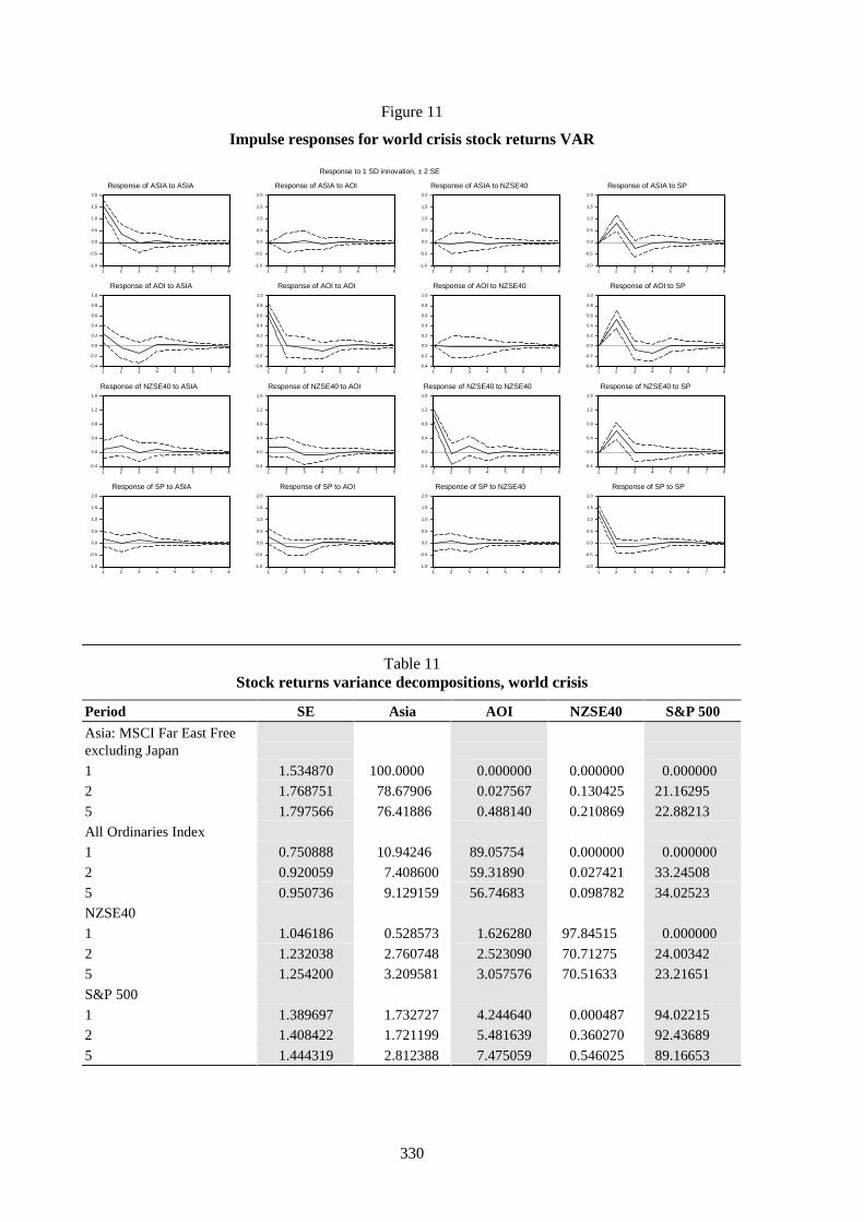
330
Figure 11
Impulse responses for world crisis stock returns VAR
-1.0
-0.5
0.0
0.5
1.0
1.5
2.0
1 2 3 4 5 6 7 8
Response of ASIA to ASIA
-1.0
-0.5
0.0
0.5
1.0
1.5
2.0
1 2 3 4 5 6 7 8
Response of ASIA to AOI
-1.0
-0.5
0.0
0.5
1.0
1.5
2.0
1 2 3 4 5 6 7 8
Response of ASIA to NZSE40
-1.0
-0.5
0.0
0.5
1.0
1.5
2.0
1 2 3 4 5 6 7 8
Response of ASIA to SP
-0.4
-0.2
0.0
0.2
0.4
0.6
0.8
1.0
1 2 3 4 5 6 7 8
Response of AOI to ASIA
-0.4
-0.2
0.0
0.2
0.4
0.6
0.8
1.0
1 2 3 4 5 6 7 8
Response of AOI to AOI
-0.4
-0.2
0.0
0.2
0.4
0.6
0.8
1.0
1 2 3 4 5 6 7 8
Response of AOI to NZSE40
-0.4
-0.2
0.0
0.2
0.4
0.6
0.8
1.0
1 2 3 4 5 6 7 8
Response of AOI to SP
-0.4
0.0
0.4
0.8
1.2
1.6
1 2 3 4 5 6 7 8
Response of NZSE40 to ASIA
-0.4
0.0
0.4
0.8
1.2
1.6
1 2 3 4 5 6 7 8
Response of NZSE40 to AOI
-0.4
0.0
0.4
0.8
1.2
1.6
1 2 3 4 5 6 7 8
Response of NZSE40 to NZSE40
-0.4
0.0
0.4
0.8
1.2
1.6
1 2 3 4 5 6 7 8
Response of NZSE40 to SP
-1.0
-0.5
0.0
0.5
1.0
1.5
2.0
1 2 3 4 5 6 7 8
Response of SP to ASIA
-1.0
-0.5
0.0
0.5
1.0
1.5
2.0
1 2 3 4 5 6 7 8
Response of SP to AOI
-1.0
-0.5
0.0
0.5
1.0
1.5
2.0
1 2 3 4 5 6 7 8
Response of SP to NZSE40
-1.0
-0.5
0.0
0.5
1.0
1.5
2.0
1 2 3 4 5 6 7 8
Response of SP to SP
Response to 1 SD innovation, ± 2 SE
Table 11Stock returns variance decompositions, world crisis
Period SE Asia AOI NZSE40 S&P 500
Asia: MSCI Far East Freeexcluding Japan
1 1.534870 100.0000 0.000000 0.000000 0.000000
2 1.768751 78.67906 0.027567 0.130425 21.16295
5 1.797566 76.41886 0.488140 0.210869 22.88213
All Ordinaries Index
1 0.750888 10.94246 89.05754 0.000000 0.000000
2 0.920059 7.408600 59.31890 0.027421 33.24508
5 0.950736 9.129159 56.74683 0.098782 34.02523
NZSE40
1 1.046186 0.528573 1.626280 97.84515 0.000000
2 1.232038 2.760748 2.523090 70.71275 24.00342
5 1.254200 3.209581 3.057576 70.51633 23.21651
S&P 500
1 1.389697 1.732727 4.244640 0.000487 94.02215
2 1.408422 1.721199 5.481639 0.360270 92.43689
5 1.444319 2.812388 7.475059 0.546025 89.16653

331
Figure 12
Impulse responses for post-crisis stock returns VAR
-0.5
0.0
0.5
1.0
1.5
1 2 3 4 5 6 7 8
Response of ASIA to ASIA
-0.5
0.0
0.5
1.0
1.5
1 2 3 4 5 6 7 8
Response of ASIA to AOI
-0.5
0.0
0.5
1.0
1.5
1 2 3 4 5 6 7 8
Response of ASIA to NZSE40
-0.5
0.0
0.5
1.0
1.5
1 2 3 4 5 6 7 8
Response of ASIA to SP
-0.4
-0.2
0.0
0.2
0.4
0.6
0.8
1 2 3 4 5 6 7 8
Response of AOI to ASIA
-0.4
-0.2
0.0
0.2
0.4
0.6
0.8
1 2 3 4 5 6 7 8
Response of AOI to AOI
-0.4
-0.2
0.0
0.2
0.4
0.6
0.8
1 2 3 4 5 6 7 8
Response of AOI to NZSE40
-0.4
-0.2
0.0
0.2
0.4
0.6
0.8
1 2 3 4 5 6 7 8
Response of AOI to SP
-0.4
-0.2
0.0
0.2
0.4
0.6
0.8
1.0
1 2 3 4 5 6 7 8
Response of NZSE40 to ASIA
-0.4
-0.2
0.0
0.2
0.4
0.6
0.8
1.0
1 2 3 4 5 6 7 8
Response of NZSE40 to AOI
-0.4
-0.2
0.0
0.2
0.4
0.6
0.8
1.0
1 2 3 4 5 6 7 8
Response of NZSE40 to NZSE40
-0.4
-0.2
0.0
0.2
0.4
0.6
0.8
1.0
1 2 3 4 5 6 7 8
Response of NZSE40 to SP
-0.5
0.0
0.5
1.0
1.5
1 2 3 4 5 6 7 8
Response of SP to ASIA
-0.5
0.0
0.5
1.0
1.5
1 2 3 4 5 6 7 8
Response of SP to AOI
-0.5
0.0
0.5
1.0
1.5
1 2 3 4 5 6 7 8
Response of SP to NZSE40
-0.5
0.0
0.5
1.0
1.5
1 2 3 4 5 6 7 8
Response of SP to SP
Response to 1 SD innovation, ± 2 SE
Table 12Stock returns variance decompositions, post-crisis
Period SE Asia AOI NZSE40 S&P 500
Asia: MSCI Far East Freeexcluding Japan
1 1.255178 100.0000 0.000000 0.000000 0.000000
2 1.449960 80.50739 0.143763 0.203534 19.14531
5 1.472692 78.52142 0.186564 2.505483 18.78654
All Ordinaries Index
1 0.621094 14.28146 85.71854 0.000000 0.000000
2 0.767114 9.491655 56.85340 0.477399 33.17755
5 0.773912 10.18582 56.00659 0.523479 33.28412
NZSE40
1 0.807679 7.041972 6.734723 86.22330 0.000000
2 0.911771 5.691949 7.033684 68.24758 19.02679
5 0.936746 5.708620 7.430989 67.55056 19.30983
S&P 500
1 1.146743 0.013412 0.067533 0.349749 99.56931
2 1.157855 0.176475 0.087614 2.041724 97.69419
5 1.168442 0.773487 0.299874 2.054634 96.87200

332
The impulse responses shown in Figures 9–12, and the variance decompositions in Tables 9–12, arebased on the recursive identification scheme discussed above. We cannot be completely certain thatwe have identified true structural innovations using this scheme. However, we are confident that adifferent ordering within a recursive scheme would not appreciably affect the results. The impulseresponses and variance decompositions derived using other possible orderings are very similar to thosepresented here.15 In particular, even when the US variable (S&P 500) was ordered before the othervariables, allowing it to affect all other variables contemporaneously, the impulse responses of theother variables to an innovation in the S&P 500 were still tent-shaped, with the contemporaneousresponses being close to (and almost always insignificantly different from) zero. A similar resultapplied for the bond and foreign exchange market results presented in the following sections.
The variance decompositions for the four periods show that own market innovations are the mostimportant, although the S&P 500 has a significant impact on the Australian and New Zealand indicesin all periods. The effect of the Asian market variable on Australian and New Zealand stocks was alsofairly important, particularly during the Asian crisis period. There was some apparent cross-determination between the Australian and New Zealand markets, although this was not robust todifferent relative orderings. As expected, the S&P 500 was virtually entirely driven by own marketinnovations, although the contribution of the Asian variable in the crisis period was higher than atother times.16
When we examine each of the sub-periods individually, however, we obtain results that conflict withthe usual intuition about the spillover of financial market volatility, i.e. that transmission of volatilityfrom one market to another should be greater in times of crisis than in more normal times. The impliedresponse of Australian and New Zealand stocks to an innovation from the Asian series wasproportionately smaller in both the Asian and world crisis periods than in the pre-crisis period. Theimpulse response peaked at around 0.2 percentage points in both the pre-crisis and Asian crisisperiods, even though the size of a one-standard-deviation innovation in the Asian series wassubstantially larger in the Asian crisis period than the pre-crisis period. Moreover, the reaction in thepost-crisis period was similar to the reaction in the Asian crisis, and greater than in the world crisisperiod.
4.2 Bond markets
Figure 14 suggests that EMBI Global Constrained had a small and marginally significant impact onAustralian and New Zealand bond returns during the Asian crisis period. However, the greatestreaction of Australian and New Zealand bond returns to the Asian series was in the pre-crisis period.17
This result may be due to the EMBI series picking up the effects of the Japanese and Europeanmarkets on Australian and New Zealand bond yields. Previous work has suggested some role for theseother markets, independent of the US market, in explaining bond market movements in Australia(Kortian and O’Regan (1996)). Since these markets are omitted from our estimates, it may be that theEMBI series is picking up innovations from those markets during the 1994 bond market sell-off. If theJapanese and European market had affected Asian markets as well as the Australian and New Zealandmarkets, then our identification approach will capture this as Australian and New Zealand returnsbeing affected by Asian returns.
There does not appear to be an indirect response to Asia via the US market. Overnight developmentsin US bond markets had a strong effect on Australian and New Zealand bond returns, accounting for
15
There are 4!=24 possible orderings for a four-variable VAR; if Australia and New Zealand are treated as a block (i.e.,kept together but with potentially different ordering within the block) there are twelve. The results for the other orderingsare available from the authors.
16We have omitted the responses of the S&P 500 to other variables from the impulse response graphs as they are very closeto zero.
17In both the pre-crisis and the Asian crisis period, the point estimate is around 0.01, although the size of a one-standard-deviation EMBI shock in the Asian crisis period was somewhat larger.

333
15–30% of their variability in the Asian crisis period, 40% in the world crisis period and 66% in thepost-crisis period. However, during the Asian crisis (and the world crisis), bond market volatility in
Figure 13
Impulse responses for pre-crisis bond returns VAR
-0.04
-0.02
0.00
0.02
0.04
0.06
0.08
1 2 3 4 5 6 7 8
Response of AUST to EMBI
-0.04
-0.02
0.00
0.02
0.04
0.06
0.08
1 2 3 4 5 6 7 8
Response of AUST to US
-0.02
0.00
0.02
0.04
0.06
1 2 3 4 5 6 7 8
Response of NZ to EMBI
-0.02
0.00
0.02
0.04
0.06
1 2 3 4 5 6 7 8
Response of NZ to US
Table 13Bonds variance decompositions, pre-crisis
Period SE AUST NZ US EMBI
Australian bond futures
1 0.085200 98.22205 0.000000 0.000000 1.777947
2 0.109599 59.72717 0.232840 35.65331 4.386683
5 0.110739 58.56773 0.303433 36.10057 5.028259
New Zealand bond futures
1 0.080857 18.26934 81.40192 0.000000 0.328740
2 0.094819 13.60097 60.79360 23.90294 1.702492
5 0.095185 13.52368 60.36892 24.11231 1.995087
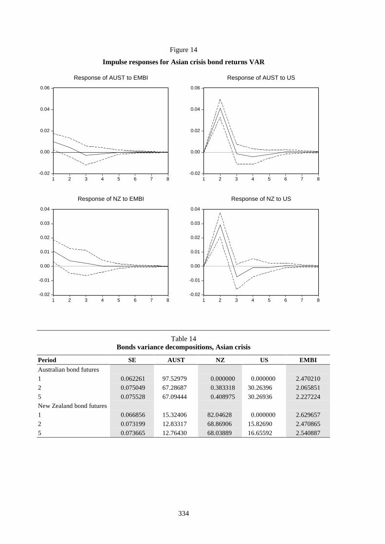
334
Figure 14
Impulse responses for Asian crisis bond returns VAR
-0.02
0.00
0.02
0.04
0.06
1 2 3 4 5 6 7 8
Response of AUST to EMBI
-0.02
0.00
0.02
0.04
0.06
1 2 3 4 5 6 7 8
Response of AUST to US
-0.02
-0.01
0.00
0.01
0.02
0.03
0.04
1 2 3 4 5 6 7 8
Response of NZ to EMBI
-0.02
-0.01
0.00
0.01
0.02
0.03
0.04
1 2 3 4 5 6 7 8
Response of NZ to US
Table 14Bonds variance decompositions, Asian crisis
Period SE AUST NZ US EMBI
Australian bond futures
1 0.062261 97.52979 0.000000 0.000000 2.470210
2 0.075049 67.28687 0.383318 30.26396 2.065851
5 0.075528 67.09444 0.408975 30.26936 2.227224
New Zealand bond futures
1 0.066856 15.32406 82.04628 0.000000 2.629657
2 0.073199 12.83317 68.86906 15.82690 2.470865
5 0.073665 12.76430 68.03889 16.65592 2.540887

335
Figure 15
Impulse responses for world crisis bond returns VAR
-0.04
-0.02
0.00
0.02
0.04
0.06
1 2 3 4 5 6 7 8
Response of AUST to EMBI
-0.04
-0.02
0.00
0.02
0.04
0.06
1 2 3 4 5 6 7 8
Response of AUST to US
-0.04
-0.02
0.00
0.02
0.04
0.06
1 2 3 4 5 6 7 8
Response of NZ to EMBI
-0.04
-0.02
0.00
0.02
0.04
0.06
1 2 3 4 5 6 7 8
Response of NZ to US
Table 15Bonds variance decompositions, world crisis
Period SE AUST NZ US EMBI
Australian bond futures
1 0.064735 99.99992 0.000000 0.000000 7.96E-05
2 0.078880 74.58906 0.275470 23.01557 2.119898
5 0.081283 70.27160 0.514577 25.74554 3.468275
New Zealand bond futures
1 0.056596 34.44071 64.26665 0.000000 1.292638
2 0.069234 23.40149 44.42332 30.81652 1.358669
5 0.075197 20.23925 37.71642 39.95933 2.084998
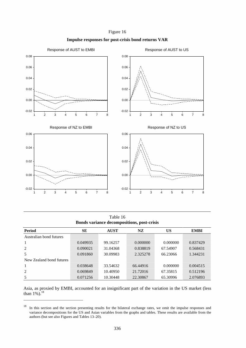
336
Figure 16
Impulse responses for post-crisis bond returns VAR
-0.02
0.00
0.02
0.04
0.06
0.08
1 2 3 4 5 6 7 8
Response of AUST to EMBI
-0.02
0.00
0.02
0.04
0.06
0.08
1 2 3 4 5 6 7 8
Response of AUST to US
-0.02
0.00
0.02
0.04
0.06
1 2 3 4 5 6 7 8
Response of NZ to EMBI
-0.02
0.00
0.02
0.04
0.06
1 2 3 4 5 6 7 8
Response of NZ to US
Table 16Bonds variance decompositions, post-crisis
Period SE AUST NZ US EMBI
Australian bond futures
1 0.049935 99.16257 0.000000 0.000000 0.837429
2 0.090021 31.04368 0.838819 67.54907 0.568431
5 0.091860 30.09983 2.325278 66.23066 1.344231
New Zealand bond futures
1 0.038648 33.54632 66.44916 0.000000 0.004515
2 0.069849 10.40950 21.72016 67.35815 0.512196
5 0.071256 10.30448 22.30867 65.30996 2.076893
Asia, as proxied by EMBI, accounted for an insignificant part of the variation in the US market (lessthan 1%).18
18
In this section and the section presenting results for the bilateral exchange rates, we omit the impulse responses andvariance decompositions for the US and Asian variables from the graphs and tables. These results are available from theauthors (but see also Figures and Tables 13–20).

337
There are a number of possible reasons for this smaller response to Asian crisis events than is the casefor stocks. In particular, bond yields are determined primarily by expectations of inflation and(domestic) real interest rates. Therefore, bond returns should be less affected by corporate sector andtrade developments than are other markets, and so the economic linkages rationale for contagionbetween asset markets (Lowell et al. (1998)) is not as important. This would tend to result in a moremuted reaction in bond markets than for stocks and, particularly, exchange rates.
4.3 Exchange rates
There was a clear reaction of the Australian dollar/US dollar and New Zealand dollar/US dollar tomovements in Asian markets during the Asian crisis (Figure 18). This response was much moreobvious than in the other two markets. Exchange market movements in Asia were significant duringthe Asian crisis, accounting for just under 8% of the variation in the Australian dollar/US dollar rate,and around 5.5% of the New Zealand dollar/US dollar.19 There was also a significant impact on theNew Zealand dollar/US dollar rate in the pre-crisis period. In the other periods, the impulse responseswere not more than two standard deviations from zero (although nearly so for the Australian dollar/USdollar in the world crisis; see also Figures and Tables 17–20). While this might partly reflect the poorfit of the linear model – evidenced by the large error bands in most periods – it makes the contrast withthe Asian crisis period even more striking.
As might be expected from the results in Section 3.2, another feature of these results is the increasingimportance of the CRB index in explaining daily movements in both the Australian dollar/US dollarand New Zealand dollar/US dollar exchange rates. Since Australia’s and New Zealand’s exports havetended to become more diverse over time, rather than more concentrated in commodities, this resultcannot reflect changing fundamentals. In any case, the extent of the change in exchange rate behaviouris probably too dramatic to be explained by a shift in the composition of exports. Moreover, thecomposition of the CRB index is not a particularly good match with the commodities exported byAustralia and New Zealand, perhaps suggesting that short-term movements in these exchange rateshave become less aligned with genuine fundamentals over time. This type of development may beevidence that financial market integration brings an increased proportion of less-informed traders toregional markets, who may look to indicator variables with little information content – but high-frequency availability – in forming their views and trading strategies. In this context, the theoreticalfindings of Calvo and Mendoza (1999) seem particularly pertinent. On the other hand, the increasingimportance of the CRB index may simply reflect that the shocks to commodity prices wereconcentrated in the components of the index most relevant to Australian and New Zealand exports,despite the index as a whole being an imperfect measure of prices of these exports.
4.4 Interpretation
Our results indicate that responses to crises can vary between asset classes. There is not a uniformnotion of increased uncertainty driving a uniform result: rather, each asset class is influenced by bothcommon and market-specific factors. In addition, there are differences between the results in the Asiancrisis and world crisis periods, which may reflect the different nature of shocks hitting Australian andNew Zealand financial markets in the two periods. The Asian crisis countries are largely commodityimporters and significant trading partners of Australia and New Zealand; the countries in financialdistress in the world crisis period – primarily Russia and Brazil – are commodity exporters with littlebilateral trade with Australia and New Zealand, although they are competitors in third markets.
The VAR estimates imply that Australian and New Zealand stock and (to a lesser extent) bondmarkets were less affected by movements in Asian markets during the crises than at other times. Thatis, spillover from these markets in crisis to unrelated markets appears to be weaker than it is between 19
The large fraction of New Zealand dollar/US dollar variability accounted for by the Australian dollar/US dollar rate is anartefact of our recursive ordering identification scheme, and may reflect that the Australian and New Zealand dollars tendto be traded as a bloc.
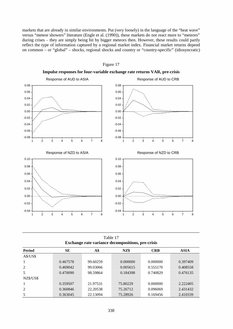
338
markets that are already in similar environments. Put (very loosely) in the language of the “heat wave”versus “meteor showers” literature (Engle et al. (1990)), these markets do not react more to “meteors”during crises – they are simply being hit by bigger meteors then. However, these results could partlyreflect the type of information captured by a regional market index. Financial market returns dependon common – or “global” – shocks, regional shocks and country or “country-specific” (idiosyncratic)
Figure 17
Impulse responses for four-variable exchange rate returns VAR, pre-crisis
-0.08
-0.06
-0.04
-0.02
0.00
0.02
0.04
0.06
0.08
1 2 3 4 5 6 7 8
Response of AUD to ASIA
-0.08
-0.06
-0.04
-0.02
0.00
0.02
0.04
0.06
0.08
1 2 3 4 5 6 7 8
Response of AUD to CRB
-0.04
-0.02
0.00
0.02
0.04
0.06
0.08
0.10
1 2 3 4 5 6 7 8
Response of NZD to ASIA
-0.04
-0.02
0.00
0.02
0.04
0.06
0.08
0.10
1 2 3 4 5 6 7 8
Response of NZD to CRB
Table 17Exchange rate variance decompositions, pre-crisis
Period SE A$ NZ$ CRB ASIA
A$/US$
1 0.467578 99.60259 0.000000 0.000000 0.397409
2 0.469042 99.03066 0.005615 0.555170 0.408558
5 0.470090 98.59864 0.184398 0.740829 0.476135
NZ$/US$
1 0.359507 21.97531 75.80229 0.000000 2.222405
2 0.360846 22.20538 75.26712 0.096069 2.431432
5 0.363045 22.13094 75.28926 0.169456 2.410339
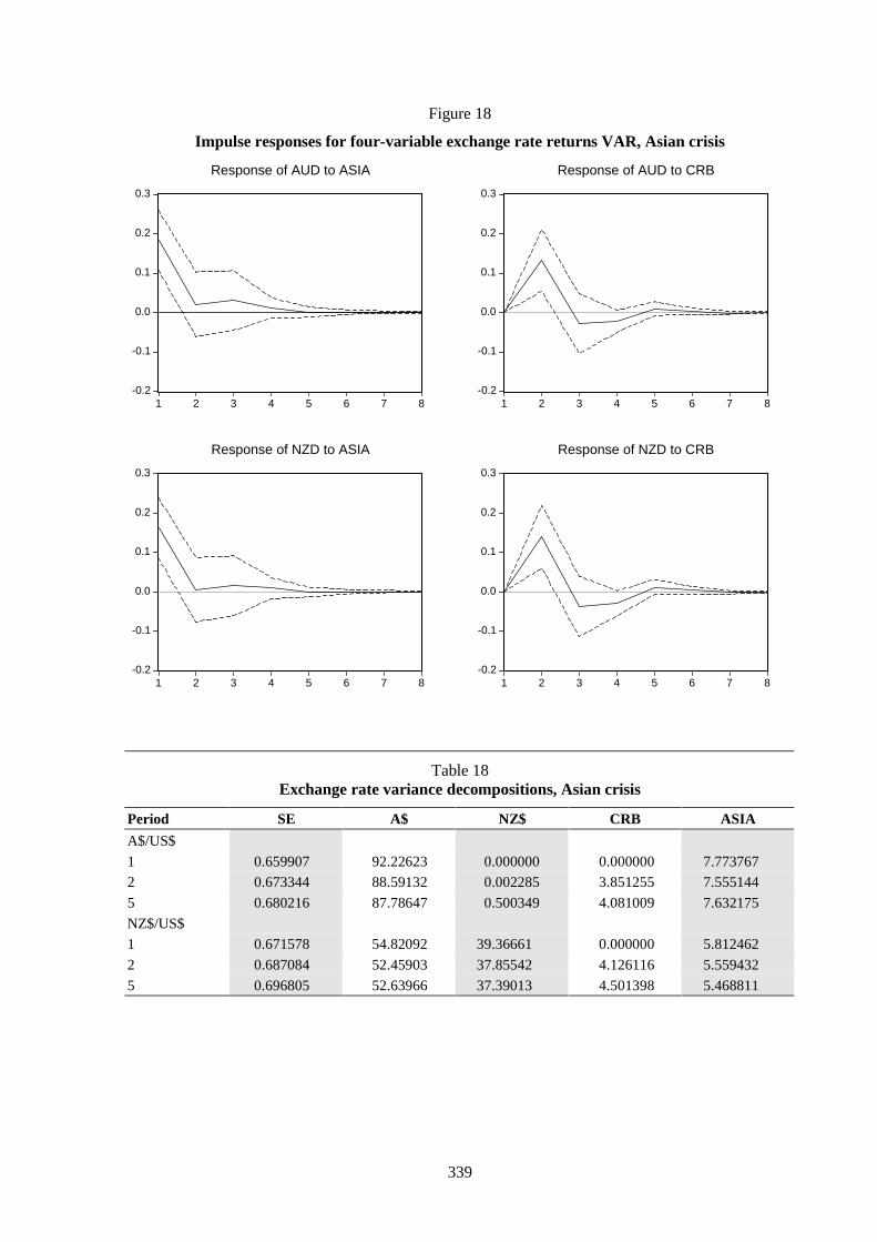
339
Figure 18
Impulse responses for four-variable exchange rate returns VAR, Asian crisis
-0.2
-0.1
0.0
0.1
0.2
0.3
1 2 3 4 5 6 7 8
Response of AUD to ASIA
-0.2
-0.1
0.0
0.1
0.2
0.3
1 2 3 4 5 6 7 8
Response of AUD to CRB
-0.2
-0.1
0.0
0.1
0.2
0.3
1 2 3 4 5 6 7 8
Response of NZD to ASIA
-0.2
-0.1
0.0
0.1
0.2
0.3
1 2 3 4 5 6 7 8
Response of NZD to CRB
Table 18Exchange rate variance decompositions, Asian crisis
Period SE A$ NZ$ CRB ASIA
A$/US$
1 0.659907 92.22623 0.000000 0.000000 7.773767
2 0.673344 88.59132 0.002285 3.851255 7.555144
5 0.680216 87.78647 0.500349 4.081009 7.632175
NZ$/US$
1 0.671578 54.82092 39.36661 0.000000 5.812462
2 0.687084 52.45903 37.85542 4.126116 5.559432
5 0.696805 52.63966 37.39013 4.501398 5.468811

340
Figure 19
Impulse responses for four-variable exchange rate returns VAR, world crisis
-0.2
0.0
0.2
0.4
0.6
1 2 3 4 5 6 7 8
Response of AUD to ASIA
-0.2
0.0
0.2
0.4
0.6
1 2 3 4 5 6 7 8
Response of AUD to CRB
-0.2
0.0
0.2
0.4
0.6
1 2 3 4 5 6 7 8
Response of NZD to ASIA
-0.2
0.0
0.2
0.4
0.6
1 2 3 4 5 6 7 8
Response of NZD to CRB
Table 19Exchange rate variance decompositions, world crisis
Period SE A$ NZ$ CRB ASIA
A$/US$
1 0.645511 95.02422 0.000000 0.000000 4.975782
2 0.753993 70.71614 0.618036 22.94515 5.720675
5 0.761877 70.34418 1.233740 22.60467 5.817406
NZ$/US$
1 0.759300 58.14465 40.80457 0.000000 1.050773
2 0.821129 50.83597 35.23830 12.35003 1.575700
5 0.850081 52.00823 32.95247 12.61087 2.428423
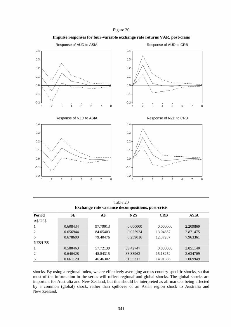
341
Figure 20
Impulse responses for four-variable exchange rate returns VAR, post-crisis
-0.2
-0.1
0.0
0.1
0.2
0.3
0.4
1 2 3 4 5 6 7 8
Response of AUD to ASIA
-0.2
-0.1
0.0
0.1
0.2
0.3
0.4
1 2 3 4 5 6 7 8
Response of AUD to CRB
-0.2
-0.1
0.0
0.1
0.2
0.3
0.4
1 2 3 4 5 6 7 8
Response of NZD to ASIA
-0.2
-0.1
0.0
0.1
0.2
0.3
0.4
1 2 3 4 5 6 7 8
Response of NZD to CRB
Table 20Exchange rate variance decompositions, post-crisis
Period SE A$ NZ$ CRB ASIA
A$/US$
1 0.608434 97.79013 0.000000 0.000000 2.209869
2 0.656944 84.05403 0.025924 13.04857 2.871475
5 0.678600 79.40476 0.259016 12.37287 7.963361
NZ$/US$
1 0.588463 57.72139 39.42747 0.000000 2.851140
2 0.640428 48.84315 33.33962 15.18252 2.634709
5 0.661120 46.46302 31.55317 14.91386 7.069949
shocks. By using a regional index, we are effectively averaging across country-specific shocks, so thatmost of the information in the series will reflect regional and global shocks. The global shocks areimportant for Australia and New Zealand, but this should be interpreted as all markets being affectedby a common (global) shock, rather than spillover of an Asian region shock to Australia andNew Zealand.
342
During the crisis periods, however, the Asian market variables incorporate idiosyncratic (country-specific) and regional shocks that were much larger than in non-crisis periods. Also, although country-specific shocks would ordinarily tend to average out and thus not show up in a regional index, thismay not have been the case during the Asian crisis, as shocks were disproportionately negative in thatperiod. These Asia-specific shocks may be less important to Australian and New Zealand markets thanthe global shocks also captured in the Asian data. Therefore, the estimated coefficients on the stockprice indices during the Asian crisis period might have been smaller because the series containedproportionally less information relevant to markets in Australia and New Zealand.
By contrast, spillover of financial market volatility to exchange rates was greater during the crisesthan at other times. This difference is an example of the tendency for the asset class to matter more indetermining spillover than did the country where the market was located. Indeed, the importance ofAsian export markets for Australia and New Zealand may imply that Asia-specific shocks are moreimportant than other shocks for exchange rates.
These results are not necessarily conclusive, as they might have some limitations. In particular, byusing linear VAR econometric models, we have ignored the well-documented ARCH characteristicsseen in most financial data sets, including the ones used in this paper. On the other hand, ourinvestigations suggest that accounting for these characteristics does not affect the essential results.
5. Conclusion
Our results represent a first pass at examining the spillover of financial returns across markets,specifically the reactions by Australian and New Zealand markets to news about financial crises inother countries. We find that news events and movements in Asian financial markets had noticeableeffects on financial markets in Australia and New Zealand. These events were not the primarydeterminant of Australian and New Zealand financial returns during the crises, however. During theAsian crisis, domestic developments generally accounted for more than half of the variation inAustralian and New Zealand returns. The few cases where domestic shocks accounted for less thanhalf of the total variation in daily returns reflected the apparent common shock affecting both theAustralian dollar and New Zealand dollar exchange rates. In the post-crisis period, the US bondmarket also had a strong influence on its Australian and New Zealand counterparts.
Developments in US markets were more important than Asian market returns for Australian and NewZealand stocks and bonds. This result may be another example of the close relationship between USand Australian economic variables seen in other studies (Gruen and Shuetrim (1994), de Roos andRussell (1996) and Kortian and O’Regan (1996)). Moreover, the results from Section 3 suggest thatstock markets in Australia and New Zealand seem to have reacted to Asian news with a lag. This mayindicate that market participants wait until they observe the reaction in the United States beforeresponding to the news. If true, this finding suggests that participants in financial markets do notprocess information efficiently. On the other hand, the reactions to movements in Asian financialmarkets, shown in Section 4, did indicate a contemporaneous relationship.
The results show that different asset classes can react differently to the same events. The bond marketswere little affected by developments in Asia, while the stock markets displayed a (sometimes delayed)clear reaction; exchange rates were the most affected by events in Asia. These differences probablyreflect that, even though financial markets react to the same set of information about fundamentals, therelative importance of particular aspects of fundamentals can vary greatly across asset classes. Forexample, returns on bonds are largely driven by expectations of future developments in inflation andmonetary policy. The implications of the Asian news events for Australian and New Zealand inflation(via exchange rate depreciations) may have been offset by a “flight to quality”, and by expectationsthat the world real interest rate had fallen in response to the contraction in Asian demand. In additionto expected inflation and interest rates, stock market returns reflect corporate profitability andindicators of world demand such as commodity prices. Therefore, a downturn in Asia and elsewherewould reduce expected returns on Australian and New Zealand stocks.

343
The currencies of the two countries were the asset class most affected by Asian news events. Thissupports the idea that trade developments, such as recessions in trading partner nations, affectexchange rates more than they affect returns on other assets. The economic contractions in Asia wouldhave reduced demand for differentiated products exported to Asia, and also tended to reducecommodity prices. Consequently the bilateral exchange rates of the Australian dollar and New Zealanddollar against the US dollar depreciated through the Asian crisis period.
The world crisis period, on the other hand, was characterised by small appreciations in the currencies.These were despite the large falls at the end of August 1998, which largely reflected developments inglobal financial markets and the positions of highly leveraged traders. This seems in line with thedifferent implications of the world crisis for commodity prices, given that the countries newly affectedthen tended to be commodity exporters. We would therefore expect smaller depreciations in othercommodity exporters’ currencies, since depreciation of a competitor’s currency will only affectcommodity prices in US dollar or own currency terms if the competitor responds by increasing itssupply of commodities onto the world market. This effect was offset by the effects of marketparticipants unwinding the short positions in the Australian dollar and New Zealand dollar built uptowards the end of the Asian crisis period, resulting in a net appreciation.
We did not find any evidence of significant differences between the reactions of Australian andNew Zealand markets, despite the differences in the monetary policy stances and operational regimesin those countries. This may reflect the similarities in their other fundamentals and in particular thatthe two currencies tend to be traded as a bloc.
In essence, our results suggest that financial markets may be buffeted by shocks spilling over fromother markets in crisis. Even when markets are not dragged into crises, some spillover of shocksclearly occurs for at least some asset classes. This can sometimes occur regardless of domesticfundamentals, as evidenced by the exchange rate volatility in the world crisis period being at least ashigh as – if not higher than – in the Asian crisis period. This occurred even though the Asian crisiscountries are more important trade partners for Australia and New Zealand than the countries draggedinto the world financial crisis of late 1998, and, again, probably reflects the turmoil in marketsgenerally, rather than reactions to crises in specific countries.

344
Appendix: Chronology of major events in the Asian crisis
Date Event Type ofnews
1997
15 May Thailand, after a week of selling pressure and massive intervention in the forward markets,announces wide-ranging capital controls aimed at segmenting the onshore and offshoremarkets.
bad
27 June The BoT suspends the operations of 16 troubled finance companies and orders them tosubmit merger or consolidation plans.
bad
2 July Floating of the Thai baht (baht devalues by 15% in onshore markets, 20% in offshoremarkets). Pressure spreads to the Philippine peso, Malaysian ringgit and Indonesian rupiah.
bad
11 July BSP announces the peso will float in a wider range, abandoning the de facto peg. BIwidens the rupiah trading band from 8% to 12%.
bad
14 July BNM is reported as abandoning the defence of the ringgit. bad
28 July Thai government requests IMF assistance. bad
5 August Thailand suspends a further 42 troubled finance companies. bad
14 August Indonesia abandons the rupiah trading band. The rupiah depreciates by 4%. bad
20 August Thailand and the IMF agree on a US$ 17 billion financial stabilisation package. good
27 August Malaysia imposes trading restrictions on the stock market including an effective ban onshort selling.
bad
29 August BI introduces selective credit controls on rupiah trading. bad
8 October Indonesia announces it will seek IMF assistance. bad
17 October Malaysia announces an austerity budget. Authorities stop supporting the new Taiwandollar, which falls by 6%. Pressure on Hong Kong dollar and equity markets intensifies.Review of Thai emergency funding.
bad
20–23 October Financial turbulence in Hong Kong. Hang Seng index falls by 23% in four days. Overnightinterest rates rise from 7% to around 250%. S&P downgrades Korea’s and Thailand’ssovereign ratings.
bad
27 October The Dow Jones loses 554 points, following the crash in the Hang Seng. Equity markets inBrazil, Argentina and Mexico see their biggest single-day losses, as the crisis ripplesacross the globe.
bad
28 October Russian equity prices decline by 23%. bad
31 October Bank resolution package announced in Indonesia, resulting in the closure of 16 troubledprivate banks. Leads to a depositor run on others. After intense pressure on the real, theCentral Bank of Brazil doubles the central bank intervention rate to 43%.
bad
5 November IMF standby credit for Indonesia of US$ 10.1 billion approved; US$ 3 billion madeavailable immediately.
good
10 November In Thailand, opposition leader Chuan Leekpai takes over as Prime Minister. In Russia,interest rates raised by 7 percentage points and authorities announce that the interventionband for the rouble will be widened from ±5% to ±15%.
bad
17 November Korea abandons defence of the won. bad
18 November Korean finance minister resigns. Authorities announce a reform package. bad
20 November Daily fluctuation band for the Korean won widened from ±2¼% to ±10%. bad
21 November Korea requests IMF assistance. bad
3 December Korea and the IMF agree on a US$ 57 billion financial assistance package. good
8 December Thai authorities close 56 of the suspended finance companies. bad
16 December Floating of the Korean won. bad
23 December Rating agencies downgrade Korea’s sovereign rating to speculative grade. The won falls tonearly 2,000 to the US dollar.
bad

345
24 December IMF and other lenders announce speeding-up of disbursement of financial assistance andthat international commercial banks will roll over short-term debts owed by Koreanfinancial institutions.
good
30 December Foreign banks agree to roll over Korean debt. good
1998
2 January Indonesia announces plans to merge four out of seven state-owned banks. Malaysiaannounces plans for mergers of finance companies.
good
6 January Indonesian budget introduced: badly received by financial markets. bad
13 January Thailand amends law for foreign investors in banks to be reclassified as domesticcompanies, allowing them to hold property.
good
15 January Indonesia and the IMF announce agreement on revised economic programme aimed atstrengthening and reinforcing the ongoing IMF-supported programme.
good
16 January International lenders officially agree to roll over Korean short-term bank debt. good
20 January Thailand allows full foreign ownership of securities firms. good
27 January Indonesia guarantees commercial bank obligations, allows overseas investments in localbanks and announces a freeze on debt payments.
good
29 January Agreement between Korea and its external creditors to exchange $US 24 billion of short-term debt for government-guaranteed loans at 2¼–2¾ percentage points over six-monthLIBOR.
good
30 January Thailand lifts currency restrictions, reunifying the spot market. good
9–10 February Indonesia’s plan to create a currency board is opposed by the IMF and several creditorgovernments, which threaten to withdraw financial assistance.
bad
13 February IMF Managing Director Camdessus expresses further concern over Indonesia’s move to acurrency board. He is of the “strong view” that the time for a currency board in Indonesiahas “not yet come” because of a number of preconditions.
bad
4 March In a second review of Thailand’s economic programme, the IMF relaxes certainmacroeconomic policy targets and approves disbursement of second tranche.
good
10 April Indonesia signs new letter of intent on economic programme with IMF. good
21 May Indonesia’s president Suharto resigns. bad
25 May The Korean stock market falls to an 11-year low. bad
1 June The Thai stock market index, continuing its slide from early March, falls to a 10-year low. bad
4 June Indonesian authorities reach an agreement to restructure the external debt of Indonesia’sbanking and corporate sectors.
good
10 June Third Quarterly Review of Thailand’s assistance programme: indicated restructuring ontrack.
good
2 July World Bank approves a US$ 1 billion loan to Indonesia. Loan is part of US$ 4.5 billionpledged by the World Bank in 1997.
good
8 July S&P affirms its CCC+ rating on the Republic of Indonesia’s US$ 400 million yankee bonddue in 2006, and the CCC+ long-term foreign currency and B– long-term local currencyissuer credit ratings. Outlook is now described as negative.
bad
10 July Malaysian stock index hits nine-year low. bad
16 July IMF approves US$ 1 billion payment and promises another US$ 6 billion to Indonesia. good
24 July Moody’s cuts Malaysia’s foreign currency debt rating to Baa2 from A2. Reasons cited are:the country’s recession, its growing debt and lack of clear policy direction in response tothe Asian crisis.
bad
4 August Philippines benchmark stock index slides to its lowest level since April 1993 on continuingloss of confidence in the region.
bad
6 August Malaysia’s sovereign risk rating cut to BBB from A by Thomson BankWatch. bad
7 August Singapore stock index reaches a 9.5-year low. bad
11 August Agence France-Presse (AFP) reports that the Indonesian government is in default on someof its sovereign debt. The government denies this.
bad
13 August Moody’s and S&P cut ratings for Russian sovereign debt. bad

346
14 August Hong Kong government intervenes in the stock market, purchasing an estimatedHK$3 billion in stocks and futures, in an attempt to stop the speculation against thecurrency.
bad
17 August Russia allows the rouble to float freely within a corridor between 6.00/9.50 to the USdollar and makes some other changes to Russian financial markets. S&P cuts Russia’slong-term foreign currency debt rating to CCC from B–.
bad
25 August IMF Executive Board approves extended funding arrangement for Indonesia. good
31 August S&P downgrades Hong Kong’s sovereign credit rating to A, with a negative outlook. Therating agency also cites a decline in Hong Kong’s financial strength because of the Asiancrisis.
bad
Sources: BIS (1998), Table VII.6, p. 131 and IMF (1998), Box 2.12, p. 49.

347
Bibliography
Almeida, A, C A E Goodhart and R Payne (1998): “The Effects of Macroeconomic News on HighFrequency Exchange Rate Behaviour”. Journal of Financial and Quantitative Analysis, 33(3),pp. 383–408.
Andersen, T G, T Bollerslev, F X Diebold and P Labys (1999): “The Distribution of Exchange RateVolatility”. Wharton Financial Institutions Center, Working Paper, No. 99–08, University ofPennsylvania.
Bank for International Settlements (1998): 68th Annual Report.
Baig, T and I Goldfajn (1998): “Financial Market Contagion in the Asian Crisis”. IMF WorkingPaper, WP/98/155, November.
Baig, T and I Goldfajn (1999): “Financial Market Contagion in the Asian Crisis”. IMF Staff Papers,46(2) pp. 167–95.
Calvo, G A and E G Mendoza (1999): “Rational Contagion and the Globalisation of SecuritiesMarkets”. NBER Working Paper, No. 7153.
Campbell, F and E Lewis (1998): “What Moves Yields in Australia?” Reserve Bank of Australia,Research Discussion Paper, No. 9808.
Chatfield, C and A J Collins (1980): Introduction to Multivariate Analysis. London, Chapman andHall Ltd.
Cooley, W W and P R Lohnes (1971): Multivariate Data Analysis. New York, John Wiley and Sons.
De Roos, N and W Russell (1996): “Towards an Understanding of Australia’s Co-movement withForeign Business Cycles”. Reserve Bank of Australia, Research Discussion Paper, No. 9607.
Dungey, M (1999): “Contagion in Currency Crises: What do We Mean?” La Trobe University,mimeo. Available from http://www.business.latrobe.edu.au/staffhp/mardihp/mardi3~1.htm (accessed7 September 1999).
Dungey, M and V Martin (1998): “Contagion in the East Asian Currency Crisis”. La Trobe University,mimeo. Available from http://www.business.latrobe.edu.au/staffhp/mardihp/mardi3~1.htm (accessed7 September 1999).
Eichengreen, B, A Rose and C Wyplosz (1995): “Exchange Market Mayhem: The Antecedents andAftermath of Speculative Attacks”. Economic Policy: A European Forum, 21, pp. 251–312.
Eichengreen, B, A Rose and C Wyplosz (1996): “Contagious Currency Crises: First Tests”.Scandinavian Journal of Economics, 98(4), pp. 463–84.
Engle, R F, T Ito and W Lin (1990): “Meteor Showers or Heat Waves? Heteroskedastic Intra-DailyVolatility in the Foreign Exchange Market”. Econometrica, 58(3), pp 525–42.
Fleming, M and J A Lopez (1999): “Heat Waves, Meteor Showers and Trading Volume: An Analysisof Volatility Spillovers in the U.S. Treasury Market”. Federal Reserve Bank of San Francisco WorkingPapers in Applied Economic Theory, 99–09.
Fleming, M and E Remolona (1997): “What Moves the Bond Market?” Federal Reserve Bank of NewYork Economic Policy Review, 3(4) pp. 31–50.
Gruen, D W R and G Shuetrim, (1994): “Internationalisation and the Macroeconomy”, in P Lowe andJ Dwyer (eds.), International Integration of the Australian Economy, Proceedings of a Conference,Reserve Bank of Australia, Sydney, pp. 309–63.
International Monetary Fund (1998): “The Asian Crisis: Capital Markets Dynamics and Spillover,Chronology of Major Events in the Asian Crisis and its Spillover”. IMF World Economic Outlook,September.

348
International Monetary Fund (1999): “IMF-Supported Programs in Indonesia, Korea and Thailand: APreliminary Assessment”. Prepared by T Lane and others, January.
Kaminsky, G L and S L Schmukler (1999): “What triggers market jitters? A chronicle of the AsianCrisis”. Journal of International Money and Finance, 18(4), pp. 537–60.
Kim, S-J (1996): “Inflation News in Australia: Its Effects on Exchange Rates and Interest Rates”.Applied Financial Economics, 6, pp. 225–31.
Kim, S-J and J Sheen (1998): “International Linkages and Macroeconomic News Effects on InterestRate Volatility – Australia and the US”. University of Sydney, Working Papers in Economics,No. 98–11.
Kim, S-J (1999): “The Short-Term Dynamics of Bond Futures Market Response to New Information:Australian Evidence”. University of New South Wales School of Banking and Finance, WorkingPaper, 1999–03.
Kortian, T and J O’Regan (1996): “Australian Financial Market Volatility: An Exploration of Cross-Country and Cross-Market Linkages”. Reserve Bank of Australia, Research Discussion Paper,No. 9609.
Lowell, J, C R Neu and D Tong (1998): “Financial Crisis and Contagion in Emerging MarketCountries”. RAND MR–962, available from: http://ftp.rand.org/publications/MR/MR962/MR962.pdf/(accessed 13 September 1999).
Masson, P (1998): “Contagion: Monsoonal Effects, Spillovers, and Jumps between MultipleEquilibria”. IMF Working Paper, WP-98/142.
Roubini, N (1999): “Asia Chronology: Chronology of the Asian Currency Crisis and its GlobalContagion”. Available from http://www.stern.nyu.edu/~nroubini/asia/AsiaChronology1.html andhttp://www.stern.nyu.edu/~nroubini/asia/AsiaChronology1998.html (accessed 20 August 1999).
Silverman, B W (1986): Density Estimation for Statistics and Data Analysis. London, Chapman andHall Ltd.
World Bank (1998): World Bank Atlas. Washington DC.

349
The reaction of Swiss bank stock prices to the Russian crisis
Bertrand Rime1
1. Introduction
On 17 August 1998 Russia announced a debt moratorium after several weeks of pressure on the roubleexchange rate and tension on the Russian treasury bill markets. The Russian financial collapserepresented one more episode in the financial turmoil that had been affecting emerging marketeconomies since the floating of the Thai baht in mid-1997. The spreading crisis in emerging marketsraised concerns about the financial stability of a number of western and Japanese creditor banks. Crisisfears culminated in September 1998 with the near-collapse of the hedge fund LTCM. Some analystspointed to the risk of contagion among international banks and to the systemic repercussions that thefailure of a large creditor bank might have on the domestic banking sector of its home country. Theloss of investor confidence led to a 30% fall in the stock markets of the developed countries during thethird quarter of 1998.
The issues of contagion and systemic risk have a particular dimension in Switzerland for two reasons.First, the Swiss banking sector is highly concentrated by international standards. This is especially truefor the domestic interbank market, where the two big banks represent about 65% of total liabilities.Secondly, the two big Swiss banks are highly involved in international banking and have beensignificantly affected by the Russian crisis and the LTCM debacle.
In this paper, we try to assess the impact of the Russian moratorium on Swiss banks. Using eventstudy methodology, we compute Swiss bank stock returns for a number of events related to theRussian moratorium. In a second step, we regress each bank’s stock returns against dummy variablesreflecting the bank’s category.
The paper is organised as follows. Section 2 provides a detailed chronology of the Russian crisis. InSection 3 we introduce the event study methodology and the cross-sectional regression model. InSection 4 we present the results of the event study and of the regression analysis. Section 5 concludes.
2. Chronology of the Russian crisis
In this section, we try to identify the events related to the Russian moratorium that are most likely tohave affected Swiss bank stocks.
The 69th Annual Report of the Bank for International Settlements (1999, pp. 50–2) provides a well-structured chronology of the Russian crisis: “Difficulties in controlling public finances, the rising paceof short-term government debt issuance, falling commodity prices and real exchange rate appreciationcast increasing doubt on Russia’s debt servicing capabilities in late 1997 and the first half of 1998. Asa result, the exchange rate suffered repeated attacks which were met by successive increases ininterest rates to 150% by end-May... To buttress rouble stability, which had been a centrepiece ofmonetary policy for some years, a two-year international financial package of almost $23 billion wasoffered to Russia in July... However, given strong parliamentary opposition to key revenue-raisingmeasures, implementing IMF’s adjustment programme proved difficult… Reserve losses continuedand an attempt to lengthen the very short-term maturity of marketable government debt effectively
1
Banking Studies Section, Swiss National Bank. The opinions expressed are the author’s and do not necessarily reflectthose of the Swiss National Bank.
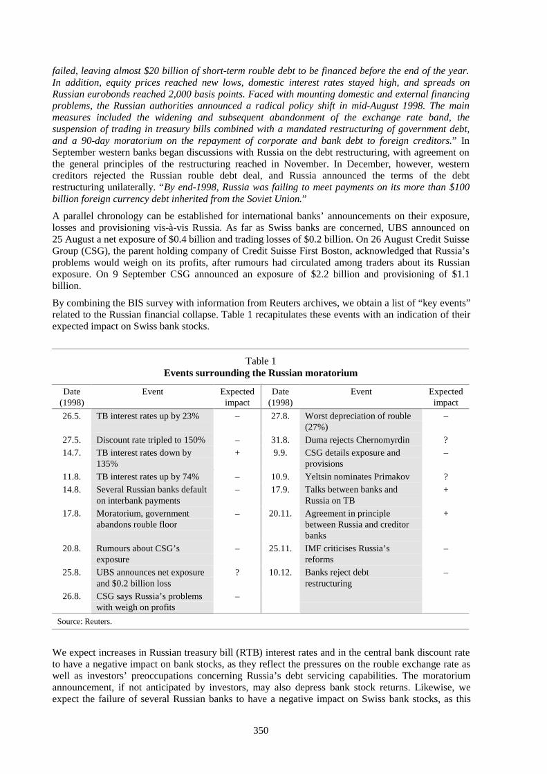
350
failed, leaving almost $20 billion of short-term rouble debt to be financed before the end of the year.In addition, equity prices reached new lows, domestic interest rates stayed high, and spreads onRussian eurobonds reached 2,000 basis points. Faced with mounting domestic and external financingproblems, the Russian authorities announced a radical policy shift in mid-August 1998. The mainmeasures included the widening and subsequent abandonment of the exchange rate band, thesuspension of trading in treasury bills combined with a mandated restructuring of government debt,and a 90-day moratorium on the repayment of corporate and bank debt to foreign creditors.” InSeptember western banks began discussions with Russia on the debt restructuring, with agreement onthe general principles of the restructuring reached in November. In December, however, westerncreditors rejected the Russian rouble debt deal, and Russia announced the terms of the debtrestructuring unilaterally. “By end-1998, Russia was failing to meet payments on its more than $100billion foreign currency debt inherited from the Soviet Union.”
A parallel chronology can be established for international banks’ announcements on their exposure,losses and provisioning vis-à-vis Russia. As far as Swiss banks are concerned, UBS announced on25 August a net exposure of $0.4 billion and trading losses of $0.2 billion. On 26 August Credit SuisseGroup (CSG), the parent holding company of Credit Suisse First Boston, acknowledged that Russia’sproblems would weigh on its profits, after rumours had circulated among traders about its Russianexposure. On 9 September CSG announced an exposure of $2.2 billion and provisioning of $1.1billion.
By combining the BIS survey with information from Reuters archives, we obtain a list of “key events”related to the Russian financial collapse. Table 1 recapitulates these events with an indication of theirexpected impact on Swiss bank stocks.
Table 1Events surrounding the Russian moratorium
Date(1998)
Event Expectedimpact
Date(1998)
Event Expectedimpact
26.5. TB interest rates up by 23% – 27.8. Worst depreciation of rouble(27%)
–
27.5. Discount rate tripled to 150% – 31.8. Duma rejects Chernomyrdin ?
14.7. TB interest rates down by135%
+ 9.9. CSG details exposure andprovisions
–
11.8. TB interest rates up by 74% – 10.9. Yeltsin nominates Primakov ?
14.8. Several Russian banks defaulton interbank payments
– 17.9. Talks between banks andRussia on TB
+
17.8. Moratorium, governmentabandons rouble floor
– 20.11. Agreement in principlebetween Russia and creditorbanks
+
20.8. Rumours about CSG’sexposure
– 25.11. IMF criticises Russia’sreforms
–
25.8. UBS announces net exposureand $0.2 billion loss
? 10.12. Banks reject debtrestructuring
–
26.8. CSG says Russia’s problemswith weigh on profits
–
Source: Reuters.
We expect increases in Russian treasury bill (RTB) interest rates and in the central bank discount rateto have a negative impact on bank stocks, as they reflect the pressures on the rouble exchange rate aswell as investors’ preoccupations concerning Russia’s debt servicing capabilities. The moratoriumannouncement, if not anticipated by investors, may also depress bank stock returns. Likewise, weexpect the failure of several Russian banks to have a negative impact on Swiss bank stocks, as this
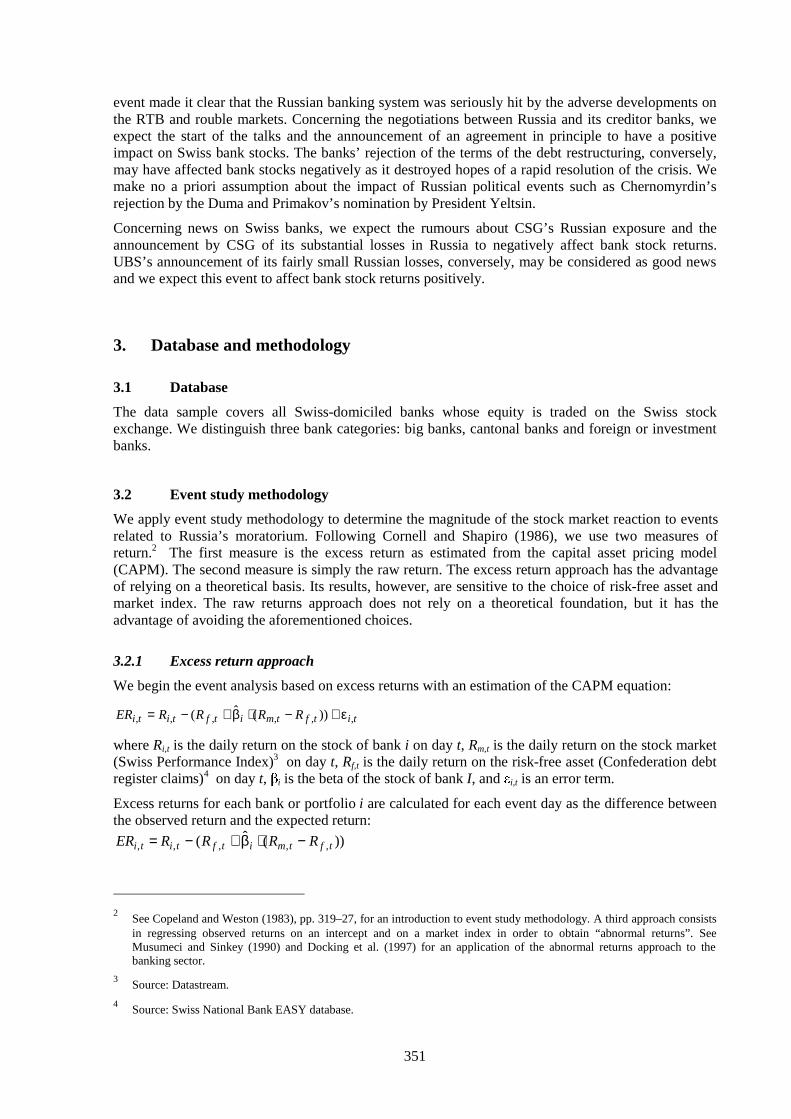
351
event made it clear that the Russian banking system was seriously hit by the adverse developments onthe RTB and rouble markets. Concerning the negotiations between Russia and its creditor banks, weexpect the start of the talks and the announcement of an agreement in principle to have a positiveimpact on Swiss bank stocks. The banks’ rejection of the terms of the debt restructuring, conversely,may have affected bank stocks negatively as it destroyed hopes of a rapid resolution of the crisis. Wemake no a priori assumption about the impact of Russian political events such as Chernomyrdin’srejection by the Duma and Primakov’s nomination by President Yeltsin.
Concerning news on Swiss banks, we expect the rumours about CSG’s Russian exposure and theannouncement by CSG of its substantial losses in Russia to negatively affect bank stock returns.UBS’s announcement of its fairly small Russian losses, conversely, may be considered as good newsand we expect this event to affect bank stock returns positively.
3. Database and methodology
3.1 Database
The data sample covers all Swiss-domiciled banks whose equity is traded on the Swiss stockexchange. We distinguish three bank categories: big banks, cantonal banks and foreign or investmentbanks.
3.2 Event study methodology
We apply event study methodology to determine the magnitude of the stock market reaction to eventsrelated to Russia’s moratorium. Following Cornell and Shapiro (1986), we use two measures ofreturn.2 The first measure is the excess return as estimated from the capital asset pricing model(CAPM). The second measure is simply the raw return. The excess return approach has the advantageof relying on a theoretical basis. Its results, however, are sensitive to the choice of risk-free asset andmarket index. The raw returns approach does not rely on a theoretical foundation, but it has theadvantage of avoiding the aforementioned choices.
3.2.1 Excess return approach
We begin the event analysis based on excess returns with an estimation of the CAPM equation:
titftmitftiti RRRRER ,,,,,, ))(ˆ( ε+−⋅β+−=
where Ri,t is the daily return on the stock of bank i on day t, Rm,t is the daily return on the stock market(Swiss Performance Index)3 on day t, Rf,t is the daily return on the risk-free asset (Confederation debtregister claims)4 on day t, i is the beta of the stock of bank I, and i,t is an error term.
Excess returns for each bank or portfolio i are calculated for each event day as the difference betweenthe observed return and the expected return:
))(ˆ( ,,,,, tftmitftiti RRRRER −⋅β+−=
2
See Copeland and Weston (1983), pp. 319–27, for an introduction to event study methodology. A third approach consistsin regressing observed returns on an intercept and on a market index in order to obtain “abnormal returns”. SeeMusumeci and Sinkey (1990) and Docking et al. (1997) for an application of the abnormal returns approach to thebanking sector.
3Source: Datastream.
4Source: Swiss National Bank EASY database.

352
Standardised excess returns SERi,be or t-values are obtained by dividing the excess return on day i bythe standard deviation of excess returns over the estimation period:
)( ,
,,
bei
beibei ERSD
ERSER =
Cumulative returns CERi,be over a particular time interval are computed as
∑=
=e
bttibei ERCER ,,
for the interval beginning on day t = b and ending on day t = e. The cumulative standardised excessreturn SCERi,be or t-value equals:
)( ,
,,
bei
beibei CERSD
CERSCER =
The standard deviation SD(CERi,be) is estimated as:
5.01,,, )],()1(2)([)( −⋅−+⋅= titiibei ERERCovTERVarTCERSE
where T represents the number of trading days in the interval T = e–b+1. This standard deviationmeasurement controls for the autocorrelation of returns that may result from event clustering.5
3.2.2 Raw returns methodology
Within this approach, we look directly at the raw return Ri,t occurring on a given day or over a giventime interval. To determine whether the raw return is significant or not, we calculate raw standardisedreturns as
)( ,
,,
bei
beibei RSD
RSR =
where SD(Ri,be) is the standard deviation of raw returns over the estimation period.
Cumulative raw returns CRi,be and cumulative standard raw returns SCRi,be are calculated following theprocedure described above for excess returns.
3.3 Cross-sectional regression analysis
In the absence of accurate information on each bank’s exposure, we can imagine that investorsconsider that banks belonging to the same category are equally exposed to the Russian crisis. In theSwiss case, investors may consider that the big banks and foreign/investment banks, because of theirinternational orientation, have a larger exposure to Russia than the cantonal banks, whose corebusiness is domestic. Under that assumption, we would expect a sell-off of all big and foreign/invest-ment bank stocks following bad news from Russia.
To test the hypothesis of category-based discrimination, we regress each bank’s raw or excess returnsagainst dummy variables reflecting the bank’s category:
beiiiibeibei FICANBIGERR ,321,, or υ+⋅γ+⋅γ+⋅γ=
where BIGi is unity for big banks and zero otherwise, CANi is unity for cantonal banks and zerootherwise, and FIi is unity for foreign/investment banks and zero otherwise.
The finding of significant differences between the dummy variables would indicate that investorsmainly discriminate between banks according to their category. 5
See Ruback (1982), Brunner and Simms (1987) and Madura et al. (1991).

353
4. Results
4.1 Stock event analysis
In this section, we compute daily and cumulative bank equity returns for each key event inventoried inour chronology of Russia’s financial collapse. The purpose of this stock event analysis is to determinewhether the Russian financial collapse coincided with significant moves in Swiss bank stock pricesand to identify the categories of bank that were most affected.
To save space, we limit our discussion of the results to the stock event analysis based on raw returns.Table 2 presents the raw returns both by event day and cumulated from the start of the tensions on theRTB market. Their standardised values are in parentheses. The results are presented separately forUBS, CSG, a portfolio of cantonal banks and a portfolio of foreign/investment banks (equallyweighted portfolios).
Table 2Event analysis: raw returns
Date Event Daily returns Cumulative returns(1998) CSG UBS CAN FI CSG UBS CAN FI
26.5. TB interest rates up by 23% 0.008 0.004 0.003 0.009(0.39) (0.25) (0.50) (0.95)
27.5. Discount rate tripled to –0.020 –0.023 –0.002 –0.005150% (–1.01) (–1.49) (–0.45) (–0.52)
14.7. TB interest rates down by –0.001 –0.014 0.001 0.020*135% (–0.07) (–0.90) (0.16) (2.13)
11.8. TB interest rates up by –0.051* –0.048* –0.011* –0.047* –0.051* –0.048* –0.011* –0.047*74% (–2.66) (–3.05) (–2.02) (–5.15) (–2.66) (–3.05) (–2.02) (–5.15)
14.8. Several Russian banks default0.011 0.032* –0.002 0.033* –0.027 –0.008 –0.009 –0.025on interbank payments (0.55) (2.04) (–0.40) (3.56) (–0.70) (–0.24) (–0.84) (–1.24)
17.8. Moratorium, government –0.002 –0.014 0.003 –0.017 –0.028 –0.022 –0.006 –0.042abandons rouble floor (–0.08) (–0.88) (0.58) (–1.91) (–0.66) (–0.57) (–0.50) (–1.90)
20.8. Rumours about CSG’s –0.046* –0.040* 0.000 –0.007 –0.087 –0.062 0.010 –0.038exposure (–2.38) (–2.56) (–0.08) (–0.75) (–1.62) (–1.26) (0.61) (–1.34)
25.8. UBS announces net exposure0.019 0.035* 0.000 0.013 –0.129* –0.086 –0.014 –0.088*and $0.2 billion loss (0.97) (2.22) (0.02) (1.45) (–2.03) (–1.50) (–0.75) (–2.65)
26.8. CSG says Russia’s problems–0.045* –0.024 –0.007 –0.048* –0.174* –0.110 –0.021 –0.136*will weigh on profits (–2.35) (–1.55) (–1.25) (–5.23) (–2.63) (–1.84) (–1.07) (–3.92)
27.8. Worst depreciation of –0.082* –0.052* –0.011 –0.061* –0.257* –0.161* –0.031 –0.197*rouble (27%) (–4.28) (–3.30) (–1.93) (–6.63) (–3.73) (–2.59) (–1.54) (–5.44)
31.8. Duma rejects –0.032 –0.027 0.000 –0.025* –0.287* –0.223* –0.039 –0.221*Chernomyrdin (–1.68) (–1.73) (–0.04) (–2.68) (–3.88) (–3.32) (–1.79) (–5.70)
9.9. CSG details exposure and –0.131* –0.045* –0.001 0.004 –0.445* –0.194* –0.037 –0.238*provisions (–6.80) (–2.89) (–0.21) (0.46) (–4.97) (–2.38) (–1.40) (–5.06)
10.9. Yeltsin nominates –0.066* –0.084* –0.011* –0.048* –0.511* –0.278* –0.048 –0.286*Primakov (–3.42) (–5.37) (–1.97) (–5.21) (–5.58) (–3.34) (–1.77) (–5.94)
17.9. Talks between banks and –0.108* –0.068* –0.001 –0.014 –0.562* –0.324* –0.049 –0.259*Russia on TB (–5.58) (–4.32) (–0.21) (–1.51) (–5.56) (–3.53) (–1.62) (–4.86)
20.11. Agreement in principle 0.050* 0.041* –0.002 0.035* –0.331* –0.262 –0.056 –0.129between Russia and banks (2.60) (2.62) (–0.35) (3.82) (–2.02) (–1.75) (–1.15) (–1.49)
25.11. IMF criticises Russia’s –0.029 –0.022 –0.002 –0.005 –0.279 –0.258 –0.051 –0.117reforms (–1.49) (–1.41) (–0.33) (–0.50) (–1.66) (–1.69) (–1.02) (–1.32)
10.12. Banks reject debt –0.070* –0.013 0.000 0.000 –0.443* –0.324* –0.062 –0.133restructuring (–3.61) (0.33) (–0.04) (–1.36) (–2.47) (–1.99) (–1.16) (–1.41)
The standardised values or t-values are in parentheses. * significant at the 5% level.

354
Concerning the commencement of the crisis, our results indicate that early increases in RTB rates andthe tripling of the central bank discount rate in May 1998 did not significantly affect Swiss bank stockprices. The 74% rise in RTB rates in August, however, coincided with significant negative returns forall Swiss bank categories.
The default of several major Russian banks on the interbank market and the announcement of themoratorium had no significant impact on Swiss bank stocks. A possible interpretation for this absenceof reaction is that investors anticipated the moratorium and the disruption of the interbank market,given the tensions observed on the RTB and rouble markets. The 17% depreciation of the rouble inlate August coincided with significant negative returns for the two big Swiss banks.
Surprisingly, the start of the discussions between Russia and its creditor banks coincided withsignificant negative returns for the two big banks. A possible explanation for this reaction could bethat investors interpreted the announcement of the negotiations as a confirmation of the gravity of thecrisis. The announcement of an agreement in principle between Russia and its creditors in Novembercoincided with significant positive returns for the two big banks. Conversely, CSG shares wereaffected negatively by western banks’ rejection of the debt restructuring and by Russia’s unilateralannouncement of the restructuring terms in December.
As far as political events are concerned, Chernomyrdin’s rejection by the Duma did not affect Swissbank stocks, while Primakov’s nomination by President Yeltsin coincided with significant negativereturns for all Swiss bank categories. Investors’ reaction may be explained by Primakov’s intention toreturn to a planned economy.
Proceeding to bank-specific news, our results indicate that rumours concerning CSG’s exposure toRussia were accompanied by significant negative returns on the two big banks’ shares. UBS’sannouncement of its quite moderate exposure was followed by a significant positive return on itsshares. Conversely, CSG’s first announcement that Russia’s problems would weigh on its profitscoincided with a significant negative return on the bank’s stock. CSG’s release of details on itsRussian exposure and provisioning was followed by a very large negative return on the bank’s ownshares, while UBS also experienced a significant, although smaller, negative return.
A cross-category comparison of the results of the stock event analysis indicates that CSG shares werethe most affected by the Russian financial collapse. UBS and foreign/investment bank stock returnswere affected less often and less significantly than CSG shares. Cantonal bank shares reacted only ontwo occasions, and by little. This differentiation in market reaction seems at first sight reasonable,given that CSG experienced more substantial losses than UBS in Russia and that cantonal banks,because of their domestic orientation, are unlikely to have a significant exposure to Russia.
The last four columns of Table 2 present raw returns cumulated as from 11 August. Cumulated rawreturns reached their minimum at –0.576 for CSG (significant at the 1% level), –0.440 for UBS(significant at the 1% level), –0.321 for the foreign/investment bank portfolio (significant at the 1%level) and 0.066 (significant at the 5% level) for the cantonal bank portfolio. For three bank categories,the minimum coincides with the start of the talks between Russia and its creditor banks. The figuresobtained for CSG and UBS indicate that the equity value of the two big banks measured at marketprices was nearly halved during the most turbulent phase of the Russian crisis. This seems quiteimpressive when compared to the losses announced by the two big banks for their Russian operations,as they represented “only” 7% of CSG’s equity and 1% of UBS’s equity.
The findings of our stock event analysis can be summarised as follows. First, Swiss bank stocks didnot react to the announcement of the Russian moratorium itself, but were negatively affected by thetensions in the RTB and rouble markets. Here, a plausible interpretation is that the moratorium cameas no surprise to investors, given the adverse financial and economic context. Secondly, the Russianfinancial collapse affected CSG shares more than those of UBS and the cantonal banks; a priori, thisresult seems consistent with the respective losses announced by the two big banks and with the lowinternational profile of the cantonal banks. Thirdly, the cumulated negative stock returns observed forthe two big banks are much larger than the announced losses vis-à-vis Russia. Here a possibleexplanation is that investors, in a context of financial instability, feared that large banks could alsosuffer considerable losses on their exposures to other emerging market countries.

355
4.2 Results of the cross sectional analysis
In this subsection we present the results of the cross-sectional regression analysis. The model isestimated for each event characterised by a significant raw return or excess return. Given theheteroscedasticity in raw returns and excess returns, the t-statistics of the estimated coefficients maybe biased. To cope with this problem, we use the White (1980) heteroscedasticity-consistentcovariance matrix estimator, which provides correct t-statistics for the coefficient estimates in thepresence of heteroscedasticity of unknown form.
Table 3 presents the model estimates based on raw returns. The big bank dummy is negative andsignificant for all events, except for the announcement of the agreement in principle, where it ispositive and significant. The cantonal bank dummy is negative and significant for two events only.The foreign/investment bank dummy is significant and negative for seven events, and positive andsignificant for the announcement of the agreement in principle. Differences between the bank categorydummies are highly significant for the great majority of events.
Table 3Model estimates based on raw returns
Date (1998) Event BIG CAN FI R2
11.8. TB interest rates up by 74% –0.05* –0.02 –0.04* 0.16
(0.01) (0.06) (0.00)
20.8. Rumours about CSG’s exposure –0.04* 0.00 –0.01 0.49
(0.00) (0.55) (0.25)
25.8. UBS announces net exposure and 0.03* 0.00 0.02* 0.36
$0.2 billion loss (0.01) (0.94) (0.01)
26.8. CSG announces Russia’s problems –0.03* –0.01* –0.03* 0.06
will weigh on profits (0.04) (0.05) (0.01)
27.8. Worst depreciation of rouble (27%) –0.07* –0.02* –0.06* 0.33
(0.01) (0.05) (0.00)
31.8. Duma rejects Chernomyrdin –0.03* 0.00 –0.03* 0.36
(0.02) (0.55) (0.00)
9.9. CSG details exposure and provisions –0.09* 0.00 0.01 0.63
(0.00) (0.63) (0.30)
10.9. Yeltsin nominates Primakov –0.08* –0.02 –0.04* 0.30
(0.00) (0.06) (0.01)
17.9. Talks between banks and –0.09* 0.00 –0.02* 0.79
Russia on TB (0.00) (0.44) (0.03)
20.11. Agreement in principle between 0.05* 0.00 0.02* 0.50
Russia and creditor banks (0.00) (0.72) (0.01)
10.12. Banks reject debt restructuring –0.04* 0.00 0.00 0.34
(0.01) (0.96) (0.93)
In parentheses: p-values derived from a t-Student test based on White’s coefficient covariance matrix. * significant at the5% level.
Table 4 presents the model estimates based on excess returns. The big bank dummy is negative andsignificant for four events, and positive and significant for the announcement of the agreement inprinciple. The cantonal bank dummy is never significant. The foreign/investment bank dummy issignificant and negative for three events, and positive and significant for one event. Differencesbetween the bank category dummies are highly significant for the great majority of events.

356
Table 4Model estimates based on excess returns
Date (1998) Event BIG CAN FI R2
11.8. TB interest rates up by 74% –0.01 –0.01 –0.02* –0.09
(0.54) (0.11) (0.05)
17.8. Moratorium 0.00 0.00 –0.01 0.01
(0.79) (0.63) (0.18)
20.8. Rumours about CSG’s exposure –0.03* 0.00 0.00 0.36
(0.00) (0.86) (0.93)
25.8. UBS announces net exposure and 0.01 0.00 0.01 0.03
$0.2 billion loss (0.49) (0.54) (0.21)
26.8. CSG announces Russia woes –0.01 –0.01 –0.02* –0.05
weigh on profits (0.51) (0.06) (0.02)
27.8. Worst depreciation of rouble (27%) –0.01 –0.01 –0.04* 0.26
(0.47) (0.06) (0.00)
31.8. Duma rejects Chernomyrdin –0.01 0.00 –0.02* 0.22
(0.21) (0.82) (0.01)
9.9. CSG details exposure and provisions –0.06* 0.00 0.03* 0.60
(0.00) (0.90) (0.01)
10.9. Yeltsin nominates Primakov –0.03 –0.01 –0.01 –0.07
(0.07) (0.11) (0.15)
17.9. Talks between banks and –0.04* 0.00 0.01 0.67
Russia on TB (0.00) (0.36) (0.24)
20.11. Agreement in principle between 0.02* 0.00 0.01 0.24
Russia and creditor banks (0.03) (0.66) (0.18)
10.12. Banks reject debt restructuring –0.02 0.00 0.01 0.19
(0.06) (0.72) (0.30)
In parentheses: p-values derived from a t-Student test based on White’s coefficient covariance matrix. *significant at the5% level.
Overall, the results of the-cross sectional regression analysis provide strong evidence in favour of thehypothesis that in the absence of official information on bank’ individual exposures to Russia,investors discriminated mainly according to bank category.
5. Conclusions
In this paper, we have studied the impact of the Russian crisis on Swiss bank stock prices. In a firststep, using stock event analysis, we tried to determine the events related to the Russian moratoriumthat coincided with significant returns on Swiss bank shares. Our results indicate that Swiss bankstocks were negatively affected by the tensions in the RTB and rouble markets, but that they did notreact to the Russian debt moratorium itself. Here, a possible interpretation is that the moratorium wasnot a surprise for investors, given the adverse financial and economic context. In a second step, weregressed each bank’s stock against dummy variables reflecting the category of the bank. Ourestimates provide strong evidence in favour of the hypothesis that in the absence of officialinformation on banks’ individual exposures to Russia, investors discriminated mainly according tobank category.

357
Bibliography
Bank for International Settlements (1999): 69th Annual Report, June, pp. 50-2.
Bruner, Robert F and John M Simms Jr. (1987): “The International Debt Crisis and Bank SecurityReturns in 1982”. Journal of Money Credit and Banking, Vol. 19, No. 1, pp. 47-55.
Copeland, Thomas E and J Fred Weston (1983): Financial Theory and Corporate Policy, SecondEdition, by Addison-Wesley Publishing Company, Inc.
Cornell, Bradford and Alan C Shapiro (1986): “The Reaction of Bank Stock Prices to the InternationalDebt Crisis”. Journal of Banking and Finance 10, pp. 55-73.
Docking, Diane Scott, Mark Hirschey and Elaine Jones (1997): “Information and contagion effects ofbank loan-loss reserve announcements”. Journal of Financial Economics 43, pp. 219-39.
Karafiath, Imre, Ross Mynatt and Kenneth L Smith (1991): “The Brazilian default announcement andthe contagion effect hypothesis”. Journal of Banking and Finance 15, pp. 699-716.
Kaufman, George (1994): “Bank Contagion: a Review of the theory and Evidence”. Journal ofFinancial Services Research 8(2), pp. 123-50.
Madura, Jeff, Anne Marie White and William R McDaniel (1991): “Reaction of British bank shareprices to Citicorp’s announced $3 billion increase in loan-loss reserves”. Journal of Banking andFinance 15, pp. 151-63.
Musumeci, James J and Joseph F Sinkey, Jr. (1990): “The International Debt Crisis, InvestorContagion, and Bank Security Returns in 1987: The Brazilian Experience”. Journal of Money, Credit,and Banking, pp. 209-20.
Wall, Larry D and David R Peterson (1990): “The effect of Continental Illinois’ failure on thefinancial performance of other banks”. Journal of Monetary Economics 26, pp. 77-99.


358
International financial crises and flexible exchange rates:some policy lessons from Canada
John Murray, Mark Zelmer and Zahir Antia1
“In other words, for cyclical as well as for more fundamental reasons, the prospects aregood for a stronger Canadian currency.” 2
1. Introduction
The near-term prospects for the Canadian economy and the Canadian dollar looked very promising inearly 1997. Canada’s current account balance had swung into surplus for the first time in 11 years; thefederal government deficit had finally been eliminated; public sector debt was now on a cleardownward track; world commodity prices had recovered from their 1992–93 lows; and inflation hadremained steady at 1 to 2% for more than five years.
While the Governor’s exchange rate forecast may seem optimistic in retrospect, this positive outlookwas shared by many other observers. Canadian interest rates had fallen below comparable US ratesacross the yield curve, suggesting that most investors believed the Canadian dollar would soonappreciate and continue to strengthen for several years to come. The only question was how high itwould go. Some market analysts were concerned that the dollar might strengthen too much,undermining Canada’s new-found competitiveness and throwing the economy back into recession.
“Can Canada compete with a higher currency?... C$ bulls may soon be pointing to 80cents US as a fair evaluation of C$ fundamentals... [However] without an extraordinaryresponse from Canadian consumers growth in our borderline economy could easily cometo a standstill or worse.”3
While there was widespread agreement among analysts and most forecasting groups that the Canadiandollar would soon appreciate, few of them shared Buchanan’s and Rubin’s concerns about the“borderline” growth prospects in Canada (or the world economy more generally). Both the IMF andthe OECD predicted that growth in Canada would be higher than in any other G7 country, reaching3.5% in 1997 and 3.3% in 1998. World output was expected to grow by more than 4% a year, andworld trade was expected to increase by more than 9% – continuing a trend that had started in 1994.
In the event, none of these optimistic predictions came true. Although the Canadian economy did postrespectable growth rates in 1997 and 1998, they were not the highest in the G7.4 (That honor belongedto the United States, which grew by 3.9% in both years.) The performance of the Canadian dollar waseven more disappointing. It fell from an average level of US 74 cents in the first quarter of 1997 to a
1 The views expressed in this paper are those of the authors. No responsibility for them should be attributed to the Bank of
Canada. John Murray works in the International Department of the Bank of Canada, while Mark Zelmer and Zahir Antiawork in the Financial Markets Department. The authors would like to thank Robert Amano, David Laidler, James Powelland Lawrence Schembri for their helpful comments. They are also grateful for the invaluable technical assistanceprovided by Jason Daw and Francine Rioux.
2 Excerpted from “Flexible Exchange Rates in a World of Low Inflation”. Remarks by Gordon Thiessen, Governor of the
Bank of Canada, to the FOREX ’97 Conference in Toronto, 30 May 1997.
3See Rubin and Buchanan (1996).
4Real economic growth in Canada was 3.3% in 1997 and 2.8% in 1998.
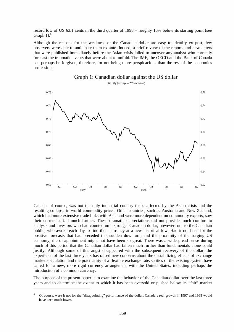
359
record low of US 63.1 cents in the third quarter of 1998 – roughly 15% below its starting point (seeGraph 1).5
Although the reasons for the weakness of the Canadian dollar are easy to identify ex post, fewobservers were able to anticipate them ex ante. Indeed, a brief review of the reports and newslettersthat were published immediately before the Asian crisis failed to uncover any analyst who correctlyforecast the traumatic events that were about to unfold. The IMF, the OECD and the Bank of Canadacan perhaps be forgiven, therefore, for not being more perspicacious than the rest of the economicsprofession.
Weekly (average of Wednesdays)
Q1 Q2 Q3 Q4 Q1 Q2 Q3 Q4 Q1 Q21997 1998
0.62
0.64
0.66
0.68
0.70
0.72
0.74
0.76
0.62
0.64
0.66
0.68
0.70
0.72
0.74
0.76
Graph 1: Canadian dollar against the US dollar
Canada, of course, was not the only industrial country to be affected by the Asian crisis and theresulting collapse in world commodity prices. Other countries, such as Australia and New Zealand,which had more extensive trade links with Asia and were more dependent on commodity exports, sawtheir currencies fall much further. These dramatic depreciations did not provide much comfort toanalysts and investors who had counted on a stronger Canadian dollar, however; nor to the Canadianpublic, who awoke each day to find their currency at a new historical low. Had it not been for thepositive forecasts that had preceded this sudden downturn, and the proximity of the surging USeconomy, the disappointment might not have been so great. There was a widespread sense duringmuch of this period that the Canadian dollar had fallen much further than fundamentals alone couldjustify. Although some of this angst disappeared with the subsequent recovery of the dollar, theexperience of the last three years has raised new concerns about the destabilizing effects of exchangemarket speculation and the practicality of a flexible exchange rate. Critics of the existing system havecalled for a new, more rigid currency arrangement with the United States, including perhaps theintroduction of a common currency.
The purpose of the present paper is to examine the behavior of the Canadian dollar over the last threeyears and to determine the extent to which it has been oversold or pushed below its “fair” market 5
Of course, were it not for the “disappointing” performance of the dollar, Canada’s real growth in 1997 and 1998 wouldhave been much lower.

360
value. The principal tool for our analysis is a simple exchange rate equation that was first developed atthe Bank of Canada in the early 1990s. Extensive testing with the equation during the past nine yearshas shown that it is able to explain most of the broad movements in the dollar over the post-BrettonWoods period.
Three major conclusions can be drawn from the evidence that is presented below. First, any differencebetween the actual and predicted values of the Canadian dollar over the past three years has been smalland generally short-lived. Overshooting has not been a major problem. Second, the dollar’s currentvalue is very close to the fitted values predicted by our simple exchange rate equation and is notsignificantly undervalued. Most of its recent weakness can be explained by two or three criticalvariables. Third, periods of market turbulence and increased exchange rate volatility, like the onesassociated with the Asian and Russian crises, are typically dominated by fundamentalists rather thandestabilizing speculators. Efforts by the Bank of Canada to resist these movements through exchangemarket intervention or higher interest rates are therefore likely to reduce market efficiency. Tacticalmanoeuvres to support the exchange rate and calm market expectations should be used sparingly,where there is clear evidence of market failure and the remedial interest rate increases can be quicklyreversed.
The rest of the paper is organized as follows. Section 2 describes the basic exchange rate equation thatis used in our analysis and presents the results of a number of simulations designed to measure theextent to which the dollar has been undervalued. Section 3 extends the analysis by adding two newvariables to the exchange rate equation – differences in Canadian-US productivity and the level ofpublic debt – to see if they improve its explanatory power. The role of speculative bubbles anddestabilizing currency traders is investigated in Section 4 with the aid of a regime-switching model.The final section of the paper provides a summary of the main results and some suggestions for futurework.
2. The basic exchange rate equation
The Bank of Canada’s exchange rate equation is based on a simple error-correction model that wasfirst developed by Robert Amano and Simon van Norden in 1991. The dependent variable is the realCanadian-US exchange rate, and its equilibrium value is determined by two independent variables: theenergy terms of trade, and the commodity terms of trade (ex-energy). Short-run dynamics are capturedby changes in the Canadian-US interest rate differential.
The equation can be written as follows:
(1) ln(rfx) = α(ln(rfx)t–1 – β0 – βc comtott–1–βe enetott–1) + γintdift–1 + εt
where rfx = real Canadian-US exchange rate, comtot = non-energy commodity terms of trade,enetot = energy terms of trade and intdif = Canadian-US interest rate differential.
The dependent variable, rfx, is simply the nominal Canadian-US exchange rate deflated by either theCPI or the GDP price index. The choice of deflator makes little difference to the resulting time seriessince the CPI and GDP price indices move in a very similar manner over the sample periods relevantfor our study. The two independent variables, enetot and comtot, are obtained by dividing the USdollar price of energy and non-energy commodities by the US GDP deflator. The effects of Canadianand US monetary policies on the real exchange rate are proxied by intdif, which is simply thedifference between Canadian and US short-term interest rates.6
6
The specification described above differs from the original Amano-van Norden equation in three respects. First, theenergy and commodity terms of trade are deflated by the GDP price index rather than the price of US manufacturedgoods. Second, oil prices are used as a proxy for all energy prices. Third, the interest rate differential is just the spreadbetween Canadian and US short-term interest rates rather than the difference between long-term and short-term interestrates in the two countries. These changes have no significant effect on the performance of the equation and wereintroduced simply to reduce the number of data series that were required to use it.

361
)( usst
cast iiintdif −=
While equation (1) contains many of the variables that one would expect to find in a Canadian-USexchange rate relationship, and has performed surprisingly well over the past nine years, it isimportant to note that Amano and van Norden only arrived at this simple specification after testingover a much larger set of explanatory variables. The fact that the relationship has remained stablethrough time and has retained much of its explanatory power is remarkable, particularly for anexchange rate equation, and is testament to the important influence that comtot, enetot and entdif exerton the Canadian dollar.7
2.1 Regression results
Representative results for the basic exchange rate equation estimated over four different sampleperiods are shown in Table 1. As the reader can see, most of the parameters are statistically significantand have their expected signs. Since the dependent variable is defined in a way that associatesdownward movements in the exchange rate with appreciations (and upward movements withdepreciations), the results suggest that increases in comtot and intdif cause the exchange rate tostrengthen, while increases in enetot cause it to weaken. Although the latter may seem counter-intuitive, and was not expected when Amano and van Norden first ran their regressions, it has provento be a remarkably robust result. Indeed, it was only when energy and non-energy commodity priceswere separated into two variables, and allowed to affect rfx in different ways, that the equation wasable to work. Earlier results, based on a single commodity price variable which combined the twoeffects, proved disappointing.
The unexpected result on the energy price term can be explained by noting that Canada is only amarginal net exporter of energy products, but has other industries which are very energy-intensive. Asa consequence, the benefits realized from larger energy exports when the price of energy increases aremore than offset by the additional costs borne by other Canadian industries.8 Higher energy prices,therefore, cause the real exchange rate to depreciate.
Table 1Standard exchange rate equation
Variable 1973Q1–1986Q1 1973Q1–1991Q3 1973Q1–1996Q1 1973Q1–1998Q4
Speed of adjustment –0.198 –0.167 –0.141 –0.125
(–3.251) (–3.917) (–4.149) (–3.752)
Constant 2.419 1.807 2.728 3.040
(4.585) (5.306) (7.566) (7.672)
comtot –0.454 –0.368 –0.524 –0.580
(–4.794) (–5.713) (–6.558) (–6.328)
enetot 0.059 0.119 0.070 0.057
(1.442) (2.916) (1.769) (1.298)
intdif –0.540 –0.519 –0.604 –0.576
(–2.442) (–3.105) (–3.682) (–4.040)
R2 0.218 0.227 0.204 0.194
Durbin-Watson 1.197 1.159 1.265 1.311
Note: t-statistics in parentheses.
7
The unit root and cointegration tests that were used to check the original specification are described in Appendix 1.
8Macklem (1993) has constructed a three-sector general equilibrium model of the Canadian economy which generatesresults very similar to those described above.
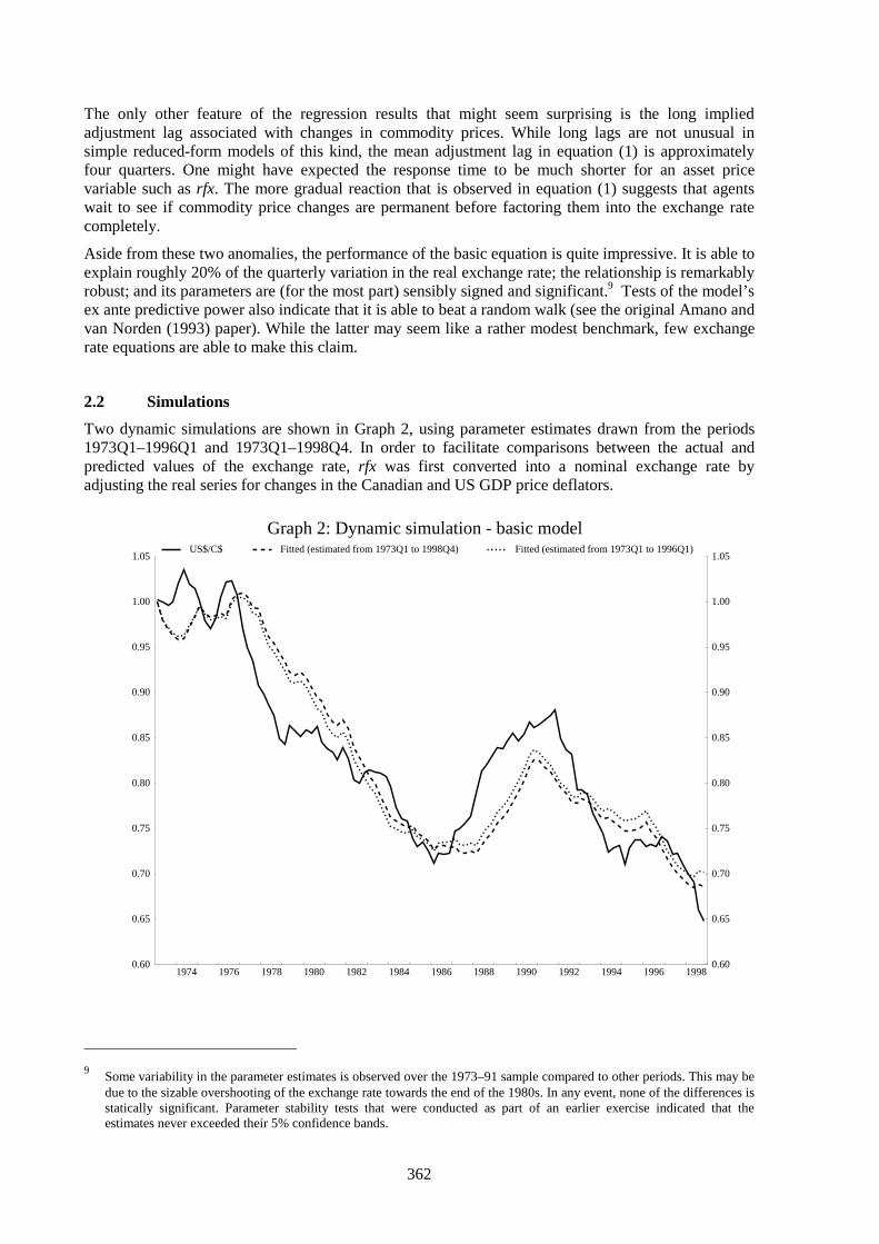
362
The only other feature of the regression results that might seem surprising is the long impliedadjustment lag associated with changes in commodity prices. While long lags are not unusual insimple reduced-form models of this kind, the mean adjustment lag in equation (1) is approximatelyfour quarters. One might have expected the response time to be much shorter for an asset pricevariable such as rfx. The more gradual reaction that is observed in equation (1) suggests that agentswait to see if commodity price changes are permanent before factoring them into the exchange ratecompletely.
Aside from these two anomalies, the performance of the basic equation is quite impressive. It is able toexplain roughly 20% of the quarterly variation in the real exchange rate; the relationship is remarkablyrobust; and its parameters are (for the most part) sensibly signed and significant.9 Tests of the model’sex ante predictive power also indicate that it is able to beat a random walk (see the original Amano andvan Norden (1993) paper). While the latter may seem like a rather modest benchmark, few exchangerate equations are able to make this claim.
2.2 Simulations
Two dynamic simulations are shown in Graph 2, using parameter estimates drawn from the periods1973Q1–1996Q1 and 1973Q1–1998Q4. In order to facilitate comparisons between the actual andpredicted values of the exchange rate, rfx was first converted into a nominal exchange rate byadjusting the real series for changes in the Canadian and US GDP price deflators.
1974 1976 1978 1980 1982 1984 1986 1988 1990 1992 1994 1996 19980.60
0.65
0.70
0.75
0.80
0.85
0.90
0.95
1.00
1.05
0.60
0.65
0.70
0.75
0.80
0.85
0.90
0.95
1.00
1.05US$/C$ Fitted (estimated from 1973Q1 to 1998Q4) Fitted (estimated from 1973Q1 to 1996Q1)
Graph 2: Dynamic simulation - basic model
9
Some variability in the parameter estimates is observed over the 1973–91 sample compared to other periods. This may bedue to the sizable overshooting of the exchange rate towards the end of the 1980s. In any event, none of the differences isstatically significant. Parameter stability tests that were conducted as part of an earlier exercise indicated that theestimates never exceeded their 5% confidence bands.

363
The correspondence between the simulated values of the nominal exchange rate and its actual value isvery close. Most of the broad movements in the exchange rate are captured by the three explanatoryvariables. Sizeable deviations do occur on occasion, but they typically disappear after a short period oftime. The 1987–90 episode is an example of this. While 1998 may provide another example ofspeculative overshooting, the deviations that were recorded over this “crisis” period appear to berelatively modest compared to earlier episodes. Moreover, the actual exchange rate has now returnedto a level that is very close to what the equation would predict. In other words, very little of anexceptional or potentially troubling nature was observed during this period of international turbulence.
Table 2 provides a decomposition of one of the simulations shown in Graph 2, and indicates therelative contribution of each variable to changes in the actual Canadian-US exchange rate.
Table 2Relative importance of the explanatory variables 1973Q1–1998Q4
Variable Percentage share
comtot 56.20
enetot 1.85
intdif –6.52
Inflation 23.00
Lags 11.51
Other* 13.76
Total 100.00
* Includes error term.
Over the 1973Q1–1998Q4 period, the nominal bilateral exchange rate depreciated by roughly 44 cents(Canadian). Of this, more than 56% was the result of a trend decline in the relative price of non-energycommodities; 23% was caused by higher inflation in Canada than in the United States (purchasingpower parity); 2% came from higher energy prices; and 25% was related to other unidentified factors(including the lagged adjustment term and the residual error). Short-term interest rate differentialsprovided some offset to the depreciation and raised the value of the dollar by roughly 7%.
3. An extended equation
The results reported in the previous section suggest that most of the movements in the exchange ratehave been driven by two or three fundamental variables, and that it would be possible to predict thegeneral direction of the exchange rate, if not its exact level, provided one had prior knowledge of theseforcing variables. Nevertheless, independent of which sample period is used to estimate the equation,it tends to overpredict the actual value of the exchange rate over most of the 1990s. Is this evidence ofovershooting or is there a chance that other explanatory variables might be uncovered that could helpexplain these discrepancies?
Amano and van Norden (1993) ended their estimations in 1992Q2. While the regressions reportedabove in Table 1 extend their results to 1998Q4, no new variables have been added to the originalequation. The same specification has simply been applied to more data. Although the new results areessentially unchanged vis-à-vis those of Amano and van Norden, the longer sample that is nowavailable might allow us to uncover additional variables that could help explain the “undervalued”dollar over the 1992–98 period.

364
3.1 Canadian-US differences in productivity and government debt
Several new variables have been examined as part of an effort to find a new and improved exchangerate equation for the Canadian dollar. A complete list of the variables that have been tested iscontained in a recent paper written by two colleagues, David Tessier and Ramdane Djoudad, who haveconducted a more exhaustive study of this issue.10
Rather than reproduce all of the results of Tessier and Djoudad, we have decided to focus our attentionon two variables: the difference in Canadian and US labor force productivity, and the difference inCanadian and US general government debt. These variables are of particular interest owing to thepublic attention that they have attracted in recent months. Moreover, the results that we obtain arebroadly similar to those reported by Tessier and Djoudad using a number of other specifications.
(i) Productivity
Sagging productivity has been the focus of a lively public debate in Canada since late last year, whenthe OECD published a report suggesting that the level of labor productivity in Canada’s manufacturingsector was well below that in the United States, and was also growing at a much slower rate. Althoughthe data on which these results were based have now been revised, and the productivity growth puzzleseems to have largely disappeared, the debate continues. As a result, there is considerable interest inseeing if any evidence of a productivity slowdown can be detected in the exchange rate equation.Since Canada is not a large enough producer to materially affect the world price of most commodities,and is unlikely to suffer from “immiserizing growth”, one would expect lower productivity growth tocause the Canadian dollar to depreciate. (It is important to note, however, that the exchange rateeffects of a (relative) decline in productivity are in theory ambiguous.)
(ii) Government debt
The high level of government debt in Canada relative to that in the United States has also been asource of concern in recent years. As with slow productivity growth, one would also expect it to leadto an exchange rate depreciation, since countries must eventually pay for any excess absorption withhigher net exports. (This assumes that the counterpart of higher domestic debt is higher foreignindebtedness.) In the short run, however, the net effect of higher government debt on the exchange ratecould be ambiguous. The positive demand shock generated by higher government spending andreduced taxes might be expected to put upward pressure on the exchange rate, in part through higherinterest rates.11 On the other hand, if the outstanding debt were to approach levels that raised concernsabout the government’s ability to service it, the positive Keynesian effect described above could easilybe outweighed by risk considerations, causing domestic interest rates to rise and the exchange rate todepreciate. Whether the statistical techniques employed below will be able to disentangle theseconflicting effects, and the sudden changes in market sentiment that might occur once certain debtthresholds are breached, is unclear.
3.2 Regression results
Preliminary tests which were run on the new variables prior to estimating the extended model suggestthat any results one might obtain should be treated with caution, since it was impossible to identify astable cointegrating relationship between the new variables and the exchange rate.12 Nevertheless, it isinteresting to see how the results compare with those of the original specification reported in Table 1.
10
See Tessier and Djoudad (1999). Some of the variables that Tessier and Djoudad considered were (1) differences inCanadian-US unemployment rates, (2) differences in Canadian-US productivity, (3) differences in Canadian-USgovernment spending, (4) differences in Canadian-US foreign indebtedness, and (5) differences in the levels ofCanadian and US government debt.
11Although Canadian-US interest rate differentials are entered as a separate variable, the stimulative short-run effects ofincreased government spending and lower taxes could still lead to an appreciation of the exchange rate through otherchannels.
12Unit root and cointegration tests for the extended model are reported in Appendix 2.
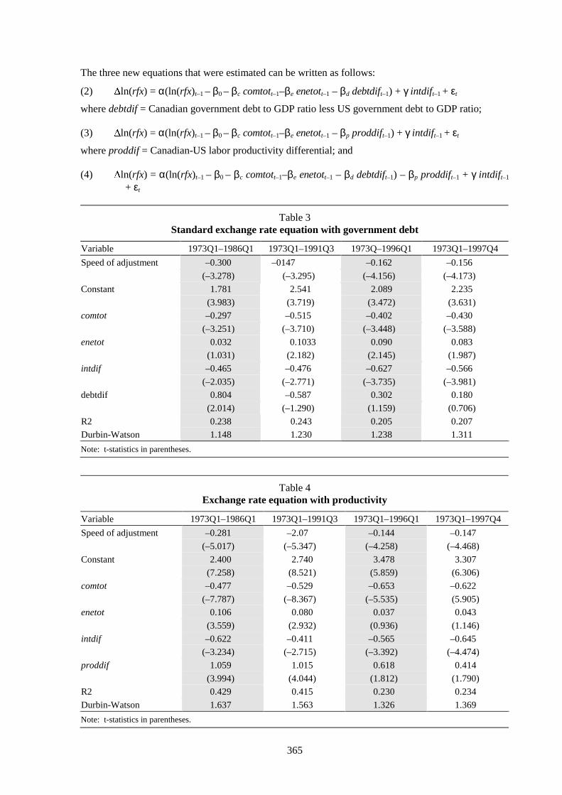
365
The three new equations that were estimated can be written as follows:
(2) ln(rfx) = α(ln(rfx)t–1 – β0 – βc comtott–1–βe enetott–1 – βd debtdift–1) + γ intdift–1 + εt
where debtdif = Canadian government debt to GDP ratio less US government debt to GDP ratio;
(3) ln(rfx) = α(ln(rfx)t–1 – β0 – βc comtott–1–βe enetott–1 – βp proddift–1) + γ intdift–1 + εt
where proddif = Canadian-US labor productivity differential; and
(4) ln(rfx) = α(ln(rfx)t–1 – β0 – βc comtott–1–βe enetott–1 – βd debtdift–1) – βp proddift–1 + γ intdift–1
+ εt
Table 3Standard exchange rate equation with government debt
Variable 1973Q1–1986Q1 1973Q1–1991Q3 1973Q–1996Q1 1973Q1–1997Q4
Speed of adjustment –0.300 –0147 –0.162 –0.156
(–3.278) (–3.295) (–4.156) (–4.173)
Constant 1.781 2.541 2.089 2.235
(3.983) (3.719) (3.472) (3.631)
comtot –0.297 –0.515 –0.402 –0.430
(–3.251) (–3.710) (–3.448) (–3.588)
enetot 0.032 0.1033 0.090 0.083
(1.031) (2.182) (2.145) (1.987)
intdif –0.465 –0.476 –0.627 –0.566
(–2.035) (–2.771) (–3.735) (–3.981)
debtdif 0.804 –0.587 0.302 0.180
(2.014) (–1.290) (1.159) (0.706)
R2 0.238 0.243 0.205 0.207
Durbin-Watson 1.148 1.230 1.238 1.311
Note: t-statistics in parentheses.
Table 4Exchange rate equation with productivity
Variable 1973Q1–1986Q1 1973Q1–1991Q3 1973Q1–1996Q1 1973Q1–1997Q4
Speed of adjustment –0.281 –2.07 –0.144 –0.147
(–5.017) (–5.347) (–4.258) (–4.468)
Constant 2.400 2.740 3.478 3.307
(7.258) (8.521) (5.859) (6.306)
comtot –0.477 –0.529 –0.653 –0.622
(–7.787) (–8.367) (–5.535) (5.905)
enetot 0.106 0.080 0.037 0.043
(3.559) (2.932) (0.936) (1.146)
intdif –0.622 –0.411 –0.565 –0.645
(–3.234) (–2.715) (–3.392) (–4.474)
proddif 1.059 1.015 0.618 0.414
(3.994) (4.044) (1.812) (1.790)
R2 0.429 0.415 0.230 0.234
Durbin-Watson 1.637 1.563 1.326 1.369
Note: t-statistics in parentheses.

366
The first thing to note from the results reported in Table 3 for the government debt variable is that,while debtdif often enters equation (2) with the expected positive sign (i.e. higher debt leads to aweaker exchange rate), it is seldom significant. Indeed, the only period in which it has a t-statisticgreater than 2.0 is 1973Q1 to 1986Q1, when Canada’s debt-to-GDP ratio was growing but still muchlower than that of the United States. The productivity variable, in contrast, is significant at the 10%level in all four sample periods (see Table 4), but always has the wrong sign (i.e. higher relativeproductivity leads to a weaker exchange rate). When both variables are entered into the equationsimultaneously, they become highly significant over the last two sample periods, but proddif still hasthe wrong sign. Interestingly, none of the other variables in the original equation is affected by theaddition of the new variables, though their t-statistics are sometimes slightly higher (see Table 5).
Table 5Exchange rate equation with government debt and productivity
Variable 1973Q1–1986Q1 1973Q1–1991Q3 1973Q1–1996Q1 1973Q1–1997Q4
Speed of adjustment –0.262 –0.216 –0.211 –0.199
(–3.25)1 (–5.100) (–5.374) (–5.178)
Constant 2.568 2.580 2.162 2.206
(3.879) (6.222) (4.917) (4.801)
comtot –0.520 –0.491 –0.401 –0.412
(–3.277) (–6.075) (–4.781) (–4.666)
enetot 0.118 0.084 0.081 0.801
(2.365) (3.055) (2.701) (2.552)
intdif –0.844 –0.417 –0.557 –0.685
(–3.141) (–2.732) (–3.484) (–4.847)
debtdif –0.205 0.137 0.782 0.637
(–0.309) (0.560) (3.640) (2.932)
proddif 1.183 1.031 0.898 0.605
(2.363) (4.217) (3.564) (3.205)
R2 0.418 0.409 0.296 0.273
Durbin-Watson 1.672 1.559 1.366 1.367
Note: t-statistics in parentheses.
3.3 Simulations
Graphs 3, 4 and 5 compare the actual value of the nominal Canadian-US exchange rate with thesimulated value from the original equation and those of equations (2), (3) and (4). Unfortunately, thesimulations have to end in 1997Q4 since the debt and productivity variables that we use are notavailable for 1998 or 1999. While the extra variables seem to improve the explanatory power of theequation, the overshooting that was noted in earlier simulations over much of the 1990s is still evident.
Differences in national debt and labor productivity do not seem to provide the missing link that wewere looking for. Neither do they represent a very reliable addition to the basic model that we firstexamined. Perhaps the overshooting that we have observed has been driven by other forces, such asthe destabilizing behavior of noise traders and speculators who, popular wisdom suggests, regularlycause exchange rates to become disconnected from market fundamentals.
4. Excess volatility and speculative bubbles
Chartists and noise traders are often cast as the villains in any discussion of sudden or unwantedexchange rate movements. This is not to suggest that the stories are untrue, or that speculative activity
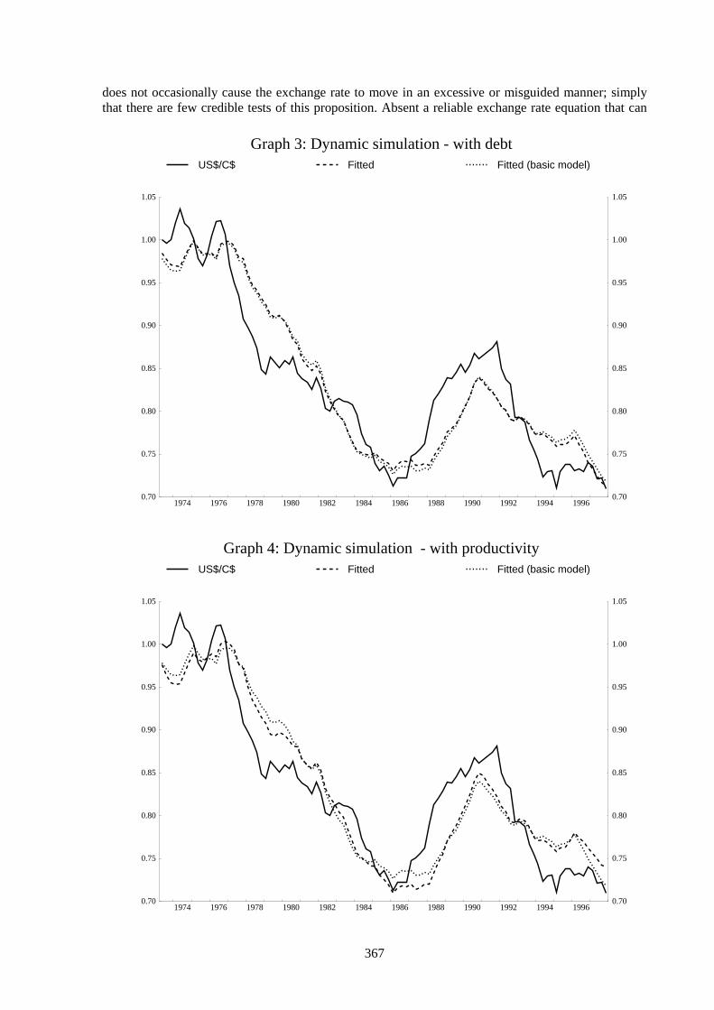
367
does not occasionally cause the exchange rate to move in an excessive or misguided manner; simplythat there are few credible tests of this proposition. Absent a reliable exchange rate equation that can
1974 1976 1978 1980 1982 1984 1986 1988 1990 1992 1994 19960.70
0.75
0.80
0.85
0.90
0.95
1.00
1.05
0.70
0.75
0.80
0.85
0.90
0.95
1.00
1.05
US$/C$ Fitted Fitted (basic model)
Graph 3: Dynamic simulation - with debt
1974 1976 1978 1980 1982 1984 1986 1988 1990 1992 1994 19960.70
0.75
0.80
0.85
0.90
0.95
1.00
1.05
0.70
0.75
0.80
0.85
0.90
0.95
1.00
1.05
US$/C$ Fitted Fitted (basic model)
Graph 4: Dynamic simulation - with productivity

368
tell the authorities exactly where the currency should be at every point in time, it is impossible to makeanything other than informed guesses about whether or not the exchange rate has deviated from its fairmarket value and what might have caused it.
1974 1976 1978 1980 1982 1984 1986 1988 1990 1992 1994 19960.70
0.75
0.80
0.85
0.90
0.95
1.00
1.05
0.70
0.75
0.80
0.85
0.90
0.95
1.00
1.05
US$/C$ Fitted Fitted (basic model)
Graph 5: Dynamic simulation - with productivity and debt
The issue of exchange rate overshooting is of critical concern to policymakers, who often worry thatexcessive volatility in exchange markets will spill over into domestic interest rates and prejudice thecentral bank’s ability to control monetary conditions. Even when exchange rate movements arebelieved to be driven by fundamentals, there is a risk that sharp currency depreciations might becomeself-reinforcing, causing interest rates to jump and pushing monetary conditions much higher at a timewhen easier conditions would clearly be called for.13, 14
In periods such as this, it may be necessary for central banks to raise official short-term interest ratesin a pre-emptive manner, in order to calm exchange markets and dampen extrapolative expectations. Atactical manoeuvre like this is undertaken, not because tighter monetary conditions are desired, but toavoid the more dramatic tightening that might otherwise occur if market expectations were to becomedestabilizing. 13
Given Canada’s past record of exchange rate depreciation and uncertainty associated with financial market volatility, theBank of Canada has been concerned for many years that there is little firm conviction in financial markets about theappropriate level for the Canadian dollar exchange rate. Consequently, when the Canadian dollar depreciated rapidly, theBank often raised its Bank Rate in order to provide “comfort” to exchange market participants and contain the potentialfeedback effects on domestic interest rates. See Zelmer (1996) and Clinton and Zelmer (1997) for a more completediscussion of the tactical challenges confronting Canadian monetary policy.
14In the past the Bank also feared that a marked exchange rate depreciation would spark an increase in inflationexpectations, thereby putting upward pressure on nominal interest rates – see the 1985 Bank of Canada Annual Report.However, the introduction of inflation targets, and more importantly their achievement, appears to be providing a firmerfooting for inflation expectations. The significant depreciation of the Canadian dollar in 1998 was accompanied by anarrowing of the spread between nominal and real return bond yields in Canada and longer-term private sector forecastsof inflation remained firmly rooted around the mid-part of the inflation central target range.
369
The Bank of Canada engaged in such an exercise in late August 1998, shortly after the collapse of theRussian rouble. The depreciation of the Canadian dollar had started to accelerate, domestic interestrates across the yield curve had moved sharply higher, and there was a growing sense of unease amongmarket analysts and traders. During this episode, the overnight rate was raised by a full percentagepoint, after which financial markets appeared to calm and the overnight rate was gradually reduced.15
The key to any successful operation of this type is to know when destabilizing expectations arebeginning to take hold and to apply just enough contractionary medicine to reverse the process. Onceconditions have improved, interest rates can be lowered and authorities can guide the economy back tothe desired monetary policy track. Ideally, central banks would like to have a model that could tellthem exactly when these destabilizing episodes were about to occur. The model would be able tocapture the joint effects of fundamentalists and speculative noise traders in the exchange market, andallow the central bank to gauge which group was exerting a stronger influence on the exchange rate atdifferent points in time.
Robert Vigfusson, an economist at the Bank of Canada, developed such a model in 1996, based on aMarkov-switching procedure. According to the model, the exchange rate that is actually observed inthe market at any time is the result of a complex interaction between two types of agents –fundamentalists, who try to keep the exchange rate close to its true equilibrium value, and noisetraders (or chartists), who often cause it to deviate from its fair market value. The actions offundamentalists are assumed to be guided by the basic exchange rate equation described in Section 2.The fitted values that the equation provides represent the exchange rates that one would observe if themarket were dominated by these equilibrating agents. Noise traders or chartists, in contrast, areassumed to operate on the basis of a simple rule of thumb, designed to detect shifts in marketsentiment and the emergence of new support levels or trends in the exchange rate.
This joint exchange rate determination process is captured by the following equation, in which theexpected change in the exchange rate is modeled as a weighted average of the expectations of thesetwo groups:
(5) ctt
fttt sEsEsE 111 )1( +++ ∆ω−+∆ω=∆
where E¨s = expected change in s, s = log of the nominal Canadian-US exchange rate,f,c = superscripts indicating fundamentalists and chartists, and ω = weight assigned to fundamentalists.
The equations describing the behavior of fundamentalists and chartists can be written as:
(6) ftttt
fft intdifsss ε+γ+−φ+α=∆ −−− 111 )~(
where s~ = fundamentalists’ forecast of s, αf = a constant, and
(7) ctt
cct intdifmamas ε+Γ+ψ+ψ+α=∆ −12002001414
where ma14 and ma200 = moving averages used by the chartists to forecast changes in s, and αc = aconstant.
The variables guiding the fundamentalists have already been discussed in detail in earlier sections ofthe paper. The only change that was introduced by Vigfusson was to convert quarterly data into a dailyfrequency using a cubic spline technique. The chartists’ equation that he used assumes the followingsimple (but not unrealistic) behavioral pattern. Whenever the 14-day (short-term) moving average ofexchange rates exceeds the 200-day (long-term) moving average, chartists are assumed to buy the
15
It must be conceded that on the day the Bank acted there were no immediate salutary effects on markets. The exchangerate remained weak that day and interest rate spreads across the yield curve widened out even further (see the empiricalresults contained in Muller and Zelmer (1999)). However, the situation improved shortly thereafter as expectations of amonetary easing by the Federal Reserve began to emerge and as commodity prices showed signs of stabilizing.
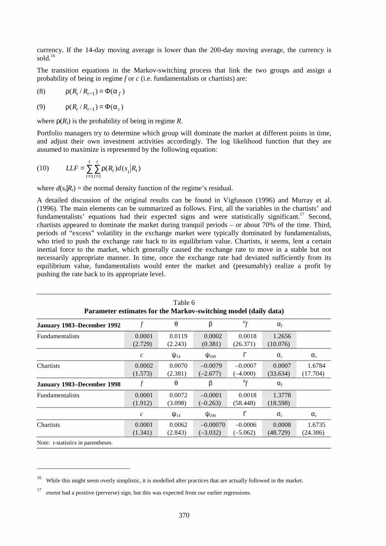
370
currency. If the 14-day moving average is lower than the 200-day moving average, the currency issold.16
The transition equations in the Markov-switching process that link the two groups and assign aprobability of being in regime f or c (i.e. fundamentalists or chartists) are:
(8) )()/( 1 ftt RR αΦ=ρ −
(9) )()/( 1 ctt RR αΦ=ρ −
where ρ(Rt) is the probability of being in regime R.
Portfolio managers try to determine which group will dominate the market at different points in time,and adjust their own investment activities accordingly. The log likelihood function that they areassumed to maximize is represented by the following equation:
(10) ∑∑= =
ρ=t
t
t
tttt RsdRLLF
1 1
)()(
where d(st|Rt) = the normal density function of the regime’s residual.
A detailed discussion of the original results can be found in Vigfusson (1996) and Murray et al.(1996). The main elements can be summarized as follows. First, all the variables in the chartists’ andfundamentalists’ equations had their expected signs and were statistically significant.17 Second,chartists appeared to dominate the market during tranquil periods – or about 70% of the time. Third,periods of “excess” volatility in the exchange market were typically dominated by fundamentalists,who tried to push the exchange rate back to its equilibrium value. Chartists, it seems, lent a certaininertial force to the market, which generally caused the exchange rate to move in a stable but notnecessarily appropriate manner. In time, once the exchange rate had deviated sufficiently from itsequilibrium value, fundamentalists would enter the market and (presumably) realize a profit bypushing the rate back to its appropriate level.
Table 6Parameter estimates for the Markov-switching model (daily data)
January 1983–December 1992 f θ β σf αf
Fundamentalists 0.0001(2.729)
0.0119(2.243)
0.0002(0.381)
0.0018(26.371)
1.2656(10.076)
c ψ14 ψ200 Γ σc αc
Chartists 0.0002(1.573)
0.0070(2.381)
–0.0079(–2.677)
–0.0007(–4.000)
0.0007(33.634)
1.6784(17.704)
January 1983–December 1998 f θ β σf αf
Fundamentalists 0.0001(1.912)
0.0072(3.098)
–0.0001(–0.263)
0.0018(58.448)
1.3778(18.598)
c ψ14 ψ200 Γ σc αc
Chartists 0.0001(1.341)
0.0062(2.843)
–0.00070(–3.032)
–0.0006(–5.062)
0.0008(48.729)
1.6735(24.386)
Note: t-statistics in parentheses.
16
While this might seem overly simplistic, it is modelled after practices that are actually followed in the market.
17enetot had a positive (perverse) sign, but this was expected from our earlier regressions.
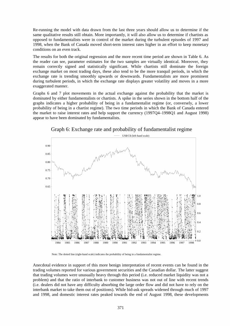
371
Re-running the model with data drawn from the last three years should allow us to determine if thesame qualitative results still obtain. More importantly, it will also allow us to determine if chartists asopposed to fundamentalists were in control of the market during the turbulent episodes of 1997 and1998, when the Bank of Canada moved short-term interest rates higher in an effort to keep monetaryconditions on an even track.
The results for both the original regression and the more recent time period are shown in Table 6. Asthe reader can see, parameter estimates for the two samples are virtually identical. Moreover, theyremain correctly signed and statistically significant. While chartists still dominate the foreignexchange market on most trading days, these also tend to be the more tranquil periods, in which theexchange rate is trending smoothly upwards or downwards. Fundamentalists are more prominentduring turbulent periods, in which the exchange rate displays greater volatility and moves in a moreexaggerated manner.
Graphs 6 and 7 plot movements in the actual exchange against the probability that the market isdominated by either fundamentalists or chartists. A spike in the series shown in the bottom half of thegraphs indicates a higher probability of being in a fundamentalist regime (or, conversely, a lowerprobability of being in a chartist regime). The two time periods in which the Bank of Canada enteredthe market to raise interest rates and help support the currency (1997Q4–1998Q1 and August 1998)appear to have been dominated by fundamentalists.
Graph 6: Exchange rate and probability of fundamentalist regime
0.65
0.70
0.75
0.80
0.85
0.90
US$/C$ (left-hand scale)
1984 1985 1986 1987 1988 1989 1990 1991 1992 1993 1994 1995 1996 1997 19980.0
0.2
0.4
0.6
0.8
1.0
Note: The dotted line (right-hand scale) indicates the probability of being in a fundamentalist regime.
Anecdotal evidence in support of this more benign interpretation of recent events can be found in thetrading volumes reported for various government securities and the Canadian dollar. The latter suggestthat trading volumes were unusually heavy through this period (i.e. reduced market liquidity was not aproblem) and that the ratio of interbank to customer business was not out of line with recent trends(i.e. dealers did not have any difficulty absorbing the large order flow and did not have to rely on theinterbank market to take them out of positions). While bid-ask spreads widened through much of 1997and 1998, and domestic interest rates peaked towards the end of August 1998, these developments

372
were not peculiar to Canada and may have simply reflected a normal adjustment of the real riskpremium during a period of increased uncertainty. (Graphs A1 through A9 in Appendix 3 documentthese changes in greater detail.)
It is important to note that this evidence and the empirical results reported above are only suggestiveand cannot speak to the issue of whether or not the Bank of Canada’s actions over this period werenecessary or helpful. Had it not been for the tactical operations that were undertaken, it is possible thatmarkets would have become seriously destabilized after the collapse of the Russian rouble. Since wecannot perform a true counterfactual experiment, we will never know. In the end, such tacticalmanoeuvres must always rely on judgment and gut instinct. Given the uncertain nature of the marketthrough the latter part of August and early September 1998, one could regard the 1% increase inofficial interest rates as prudent insurance, which was unwound shortly thereafter and had little effecton the real economy. It also provided cover for the severe dislocations that were experienced in worldfinancial markets immediately after the problems of Long-Term Capital Management became public.
Graph 7: Exchange rate and probability of fundamentalist regime
0.65
0.70
0.75
0.80
0.85
0.90
US$/C$ (left-hand scale)
Q1 Q2 Q3 Q4 Q1 Q2 Q3 Q41997 1998
0.0
0.2
0.4
0.6
0.8
1.0
Note: The dotted line (right-hand scale) indicates the probability of being in a fundamentalist regime.
Another question that might be asked regarding the results of our work is how fundamentalists couldbe seen dominating the market at a time when the actual exchange rate appears to have been somewhatlower than the value predicted by our exchange rate equation (see, for example, Graph 2). Morespecifically, if the equation that the fundamentalists were using to guide their activities suggests thatthe dollar was undervalued, why, according to the regime-switching model, were they in the marketdriving it even lower? The answer hinges on the distinction between short-run and long-run equilibria.While the exchange rate equation captures the average speed of adjustment of rfx to external shocks,and indicates where the real exchange rate is expected to be at time t, there may be times when thespeed of adjustment accelerates or becomes non-linear. The turbulent episodes described above mayrepresent such periods. To give the reader a better idea of how this might operate, Graph 8 plots theactual exchange rate, its predicted short-run value, and its long-run equilibrium value. Viewed in thisway, the seeming inconsistency between the results reported above and those reported in Sections 2
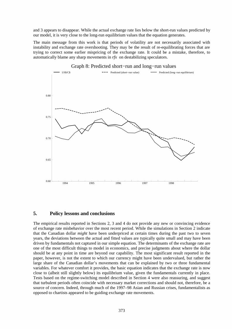
373
and 3 appears to disappear. While the actual exchange rate lies below the short-run values predicted byour model, it is very close to the long-run equilibrium values that the equation generates.
The main message from this work is that periods of volatility are not necessarily associated withinstability and exchange rate overshooting. They may be the result of re-equilibrating forces that aretrying to correct some earlier mispricing of the exchange rate. It could be a mistake, therefore, toautomatically blame any sharp movements in rfx on destabilizing speculators.
1994 1995 1996 1997 19980.60
0.65
0.70
0.75
0.80
US$/C$ Predicted (short−run value) Predicted (long−run equilibrium)
Graph 8: Predicted short−run and long−run values
5. Policy lessons and conclusions
The empirical results reported in Sections 2, 3 and 4 do not provide any new or convincing evidenceof exchange rate misbehavior over the most recent period. While the simulations in Section 2 indicatethat the Canadian dollar might have been underpriced at certain times during the past two to sevenyears, the deviations between the actual and fitted values are typically quite small and may have beendriven by fundamentals not captured in our simple equation. The determinants of the exchange rate areone of the most difficult things to model in economics, and precise judgments about where the dollarshould be at any point in time are beyond our capability. The most significant result reported in thepaper, however, is not the extent to which our currency might have been undervalued, but rather thelarge share of the Canadian dollar’s movements that can be explained by two or three fundamentalvariables. For whatever comfort it provides, the basic equation indicates that the exchange rate is nowclose to (albeit still slightly below) its equilibrium value, given the fundamentals currently in place.Tests based on the regime-switching model described in Section 4 were also reassuring, and suggestthat turbulent periods often coincide with necessary market corrections and should not, therefore, be asource of concern. Indeed, through much of the 1997–98 Asian and Russian crises, fundamentalists asopposed to chartists appeared to be guiding exchange rate movements.

374
The lessons that policymakers might take from this analysis are threefold. First, and most obviously,international financial crises are difficult, if not impossible, to predict. Any exchange rate forecast isrisky and subject to a large margin of error, no matter how reliable the underlying equation might be.Second, most movements in the Canadian dollar (and, one hopes, other exchange rates) are guided byfundamentals as opposed to animal spirits. In an environment where inflation expectations are firmlyanchored, policymakers should be wary of resisting them, and should instead consider adjusting theirdesired monetary policy track rather than automatically raising interest rates in response to anyexchange rate pressure. Third, market turbulence does not necessarily imply exchange rate instability.Tactical manoeuvres, in which official interest rates are temporarily increased to support the exchangerate and calm market expectations, should be used sparingly, where such insurance is clearly necessaryand the remedial interest rate increases can be quickly reversed.
Our future work in this area will concentrate on two topics. The first will involve a morecomprehensive search for alternative explanatory variables that might improve the performance of ourexchange rate equation. The second will involve further extensions and testing of Robert Vigfusson’sregime-switching model, to see if it can be used to provide reliable real-time guidance to the Bank ofCanada in its day-to-day operations.

375
Appendix 1
Unit root and cointegration tests on the original specification
Amano and van Norden began their search for a new and more reliable exchange rate equation in 1990by first testing the dependent variable for stationarity. Their results showed that the real exchange ratewas non-stationary in levels and was characterized by a unit root. Similar tests conducted over asomewhat longer sample period for purposes of the present paper appear to confirm these earlierresults. Based on the Augmented Dickey-Fuller (ADF) tests shown in Table A1, we cannot reject thenull hypothesis of a unit root for rfx.18
The fact that the dependent variable has a unit root is significant for at least three reasons. First, itimplies that purchasing power parity does not hold – even in the long run. Second, it implies thatcointegration techniques must be used in the analysis to avoid drawing incorrect and misleadinginferences from the regression results. Third, it implies that only variables that are also integrated oforder one, I(1), can play a role in determining the long-run behavior of the real exchange rate.
Unit root tests conducted on the three explanatory variables in our equation suggest that only enetotand comtot are I(1), while intdif is stationary in levels. As a result, only the first two variables canappear in the error-correction term. intdif has to be left outside the parentheses, influencing the short-term dynamics of the real exchange rate but not its long-run value.
Table A1Tests for unit roots(1973Q1–1997Q4)
Variable No. of lags ADF
rfx 3 –1.040
comtot 5 –1.801
enetot 3 –1.360
intdif 6 –3.280
5% critical value –2.890
10% critical value –2.580
If enetot and comtot are to play a critical role in determining the value of rfx, it is not sufficient simplyto show that they have a unit root. We must also demonstrate that the dependent variable and theprospective explanatory variables are linked by a stable long-run relationship (or are cointegrated).Although several different approaches can be used to test for cointegration, the most popular andreliable method is the Johansen-Juselius test, which applies maximum likelihood estimationtechniques to a full vector-autoregressive system of equations. The results of this test, estimated overthe sample period 1973Q1 to 1997Q4, are shown below in Table A2.
Based on the λmax statistics reported in Table A2, only one cointegrating vector can be identified atthe 5% critical value. (More specifically, we cannot reject the hypothesis that there are fewer than twocointegrating vectors.) There is no guarantee, however, that this vector links enetot and comtot to rfx.It is possible that the two explanatory variables are cointegrated with one another, and have noinfluence on the long-run behavior of rfx.
To check for this possibility, a separate Johansen-Juselius test was run just on enetot and comtot. Sinceno cointegrating vector was identified for these two variables (see Table A3), it appears that they are
18
This is indicated by the fact that the ADF value shown opposite rfx is less than both the 5% and 10% critical values forthe ADF test statistic.
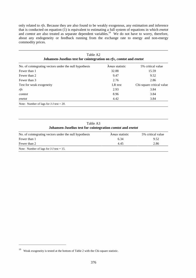
376
only related to rfx. Because they are also found to be weakly exogenous, any estimation and inferencethat is conducted on equation (1) is equivalent to estimating a full system of equations in which enetotand comtot are also treated as separate dependent variables.19 We do not have to worry, therefore,about any endogeneity or feedback running from the exchange rate to energy and non-energycommodity prices.
Table A2Johansen-Juselius test for cointegration on rfx, comtot and enetot
No. of cointegrating vectors under the null hypothesis λmax statistic 5% critical value
Fewer than 1 32.88 15.59
Fewer than 2 9.47 9.52
Fewer than 3 2.76 2.86
Test for weak exogeneity LR test Chi-square critical value
rfx 2.93 3.84
comtot 8.96 3.84
enetot 4.42 3.84
Note: Number of lags for J-J test = 20.
Table A3Johansen-Juselius test for cointegration comtot and enetot
No. of cointegrating vectors under the null hypothesis λmax statistic 5% critical value
Fewer than 1 6.34 9.52
Fewer than 2 4.45 2.86
Note: Number of lags for J-J test = 15.
19
Weak exogeneity is tested at the bottom of Table 2 with the Chi-square statistic.
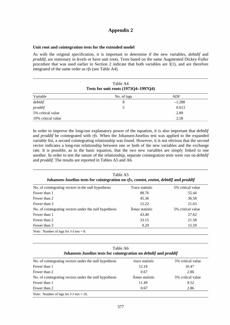
377
Appendix 2
Unit root and cointegration tests for the extended model
As with the original specification, it is important to determine if the new variables, debtdif andproddif, are stationary in levels or have unit roots. Tests based on the same Augmented Dickey-Fullerprocedure that was used earlier in Section 2 indicate that both variables are I(1), and are thereforeintegrated of the same order as rfx (see Table A4).
Table A4Tests for unit roots (1973Q4–1997Q4)
Variable No. of lags ADF
debtdif 8 –1.288
proddif 5 0.613
5% critical value 2.89
10% critical value 2.58
In order to improve the long-run explanatory power of the equation, it is also important that debtdifand proddif be cointegrated with rfx. When the Johansen-Juselius test was applied to the expandedvariable list, a second cointegrating relationship was found. However, it is not obvious that the secondvector indicates a long-run relationship between one or both of the new variables and the exchangerate. It is possible, as in the basic equation, that the two new variables are simply linked to oneanother. In order to test the nature of the relationship, separate cointegration tests were run on debtdifand proddif. The results are reported in Tables A5 and A6.
Table A5Johansen-Juselius tests for cointegration on rfx, comtot, enetot, debtdif and proddif
No. of cointegrating vectors in the null hypothesis Trace statistic 5% critical value
Fewer than 1 88.76 55.44
Fewer than 2 45.36 36.58
Fewer than 3 12.22 21.63
No. of cointegrating vectors under the null hypothesis λmax statistic 5% critical value
Fewer than 1 43.40 27.62
Fewer than 2 33.15 21.58
Fewer than 3 9.29 15.59
Note: Number of lags for J-J test = 8.
Table A6Johansen-Juselius tests for cointegration on debtdif and proddif
No. of cointegrating vectors under the null hypothesis trace statistic 5% critical value
Fewer than 1 12.16 10.47
Fewer than 2 0.67 2.86
No. of cointegrating vectors under the null hypothesis λmax statistic 5% critical value
Fewer than 1 11.49 9.52
Fewer than 2 0.67 2.86
Note: Number of lags for J-J test = 16.

378
Based on the trace and λmax statistics, the two new variables appear to be related to one another asopposed to rtf. While there was not enough time to explore the nature of this relationship in any detail,it would not be surprising if the two were negatively correlated and if higher government debt wasseen to cause lower productivity. Pierre St-Amant and David Tessier (1998) have shown in an earlierBank of Canada Working Paper that higher trend rates of government spending in Canada than in theUnited States can explain much of the difference in the long-run rates of unemployment in the twocountries. Although higher unemployment does not necessarily translate into lower productivity,productivity is known to be procyclical, and increased government regulation and spending are oftenbelieved to reduce potential output.

379
Appendix 3
Trading volumes and ratios of customer to interbank business for government of Canadasecurities and the Canadian dollar
Jan Feb Mar Apr May Jun Jul Aug Sep Oct Nov Dec10
20
30
40
50
60
70
80
90
1997
1998
Graph A1: Customer FX transaction volumes against the C$Outright (billions of C$)
Note: Vertical line corresponds to the August 1998 Bank Rate increase.Source: Weekly transaction volumes reported by Canadian banks each Wednesday.
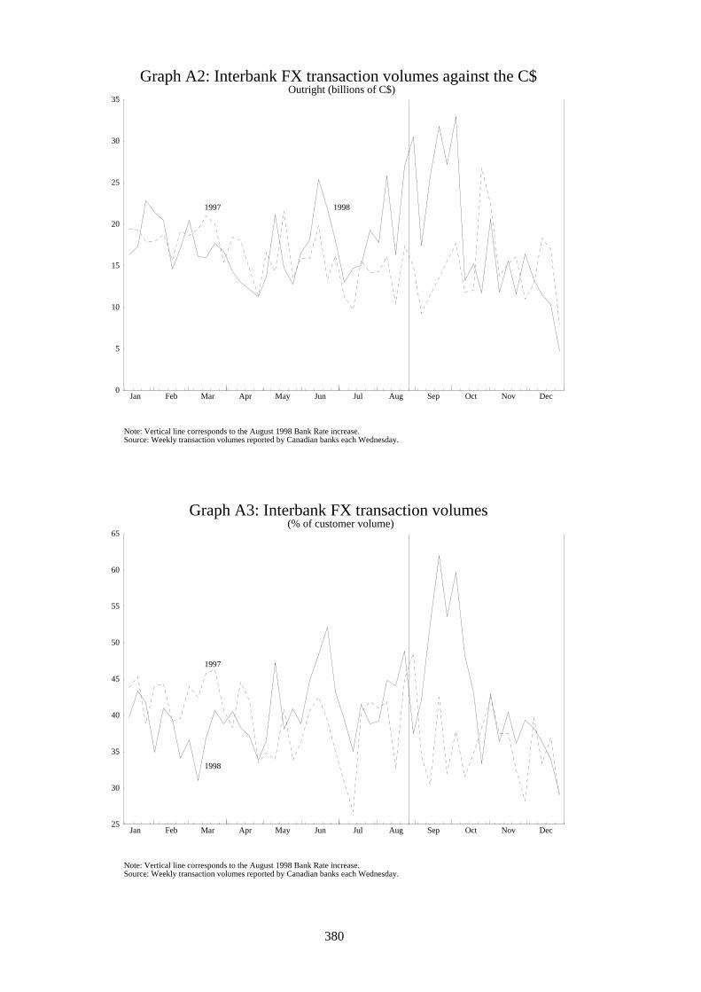
380
Jan Feb Mar Apr May Jun Jul Aug Sep Oct Nov Dec0
5
10
15
20
25
30
35
1997 1998
Graph A2: Interbank FX transaction volumes against the C$Outright (billions of C$)
Note: Vertical line corresponds to the August 1998 Bank Rate increase.Source: Weekly transaction volumes reported by Canadian banks each Wednesday.
Jan Feb Mar Apr May Jun Jul Aug Sep Oct Nov Dec25
30
35
40
45
50
55
60
65
1997
1998
Graph A3: Interbank FX transaction volumes(% of customer volume)
Note: Vertical line corresponds to the August 1998 Bank Rate increase.Source: Weekly transaction volumes reported by Canadian banks each Wednesday.

381
Q1 Q2 Q3 Q4 Q1 Q2 Q3 Q4 Q1 Q2 Q31997 1998 1999
40
50
60
70
80
90
100
110
120
40
50
60
70
80
90
100
110
120
Total weekly trading volumeFour-week moving average
Graph A4: Government of Canada weekly T-bill trading volumeCustomer (billions of dollars)
Vertical line refers to August 1998 Bank Rate increase
Q1 Q2 Q3 Q4 Q1 Q2 Q3 Q4 Q1 Q2 Q31997 1998 1999
0
5
10
15
20
25
30
35
40
0
5
10
15
20
25
30
35
40
Total weekly trading volumeFour-week moving average
Graph A5: Government of Canada weekly T-bill trading volumeInterdealer (billions of dollars)
Vertical line refers to August 1998 Bank Rate increase

382
Q1 Q2 Q3 Q4 Q1 Q2 Q3 Q4 Q1 Q2 Q31997 1998 1999
0.05
0.10
0.15
0.20
0.25
0.30
0.35
0.40
0.05
0.10
0.15
0.20
0.25
0.30
0.35
0.40
Weekly trading volume ratioFour-week moving average
Graph A6: Government of Canada weekly T-bill trading volumeRatio of interdealer to customer trading volume
Vertical line refers to August 1998 Bank Rate increase
Q1 Q2 Q3 Q4 Q1 Q2 Q3 Q4 Q1 Q2 Q31997 1998 1999
0.5
1.0
1.5
2.0
2.5
3.0
3.5
4.0
4.5
5.0
5.5
0.5
1.0
1.5
2.0
2.5
3.0
3.5
4.0
4.5
5.0
5.5
Total weekly trading volumeFour-week moving average
Graph A7: Government of Canada weekly bond trading volumeCustomer (billions of dollars)
Vertical line refers to August 1998 Bank Rate increase

383
Q1 Q2 Q3 Q4 Q1 Q2 Q3 Q4 Q1 Q2 Q31997 1998 1999
0.0
0.5
1.0
1.5
2.0
2.5
0.0
0.5
1.0
1.5
2.0
2.5
Total weekly trading volumeFour-week moving average
Graph A8: Government of Canada weekly bond trading volumeInterdealer (billions of dollars)
Vertical line refers to August 1998 Bank Rate increase
Q1 Q2 Q3 Q4 Q1 Q2 Q3 Q4 Q1 Q2 Q31997 1998 1999
0.0
0.1
0.2
0.3
0.4
0.5
0.6
0.7
0.8
0.9
0.0
0.1
0.2
0.3
0.4
0.5
0.6
0.7
0.8
0.9
Weekly trading volume ratioFour-week moving average
Graph A9: Government of Canada weekly bond trading volumeRatio of interdealer to customer trading volumes
Vertical line refers to August 1998 Bank Rate increase

384
Bibliography
Amano, R and S van Norden (1993): “A Forecasting Equation for the Canada-U.S. Dollar ExchangeRate”, in The Exchange Rate and the Economy, proceedings of a conference held at the Bank ofCanada, 22–23 June 1992, Bank of Canada.
Clinton, K and M Zelmer (1997): “Constraints on the Conduct of Canadian Monetary Policy in the1990s: Dealing with Uncertainty in Financial Markets”. Bank of Canada Technical Report, No. 80.
Dickey, D A and W A Fuller (1979): “Distributions of the Estimators for Autoregressive Time Serieswith a Unit Root”. Journal of the American Statistical Association, 74, pp. 427-31, June.
Dornbusch, R (1979): “Monetary Policy Under Exchange Rate Flexibility”, in Managed Exchange-Rate Flexibility: The Recent Experience, Federal Reserve Bank of Boston Conference Series No. 20,Federal Reserve Bank of Boston.
International Monetary Fund: “World Economic Outlook”. October 1996, May 1997 and August1999.
Johansen, S (1988): “Statistical Analysis of Cointegration Vectors”. Journal of Economic Dynamicsand Control, 12, pp. 231-54, June-September.
Johansen, S and K Juselius (1990): “Maximum Likelihood Estimation and Inference on Cointegrationwith Applications to the Demand for Money”. Oxford Bulletin of Economics and Statistics, 52,pp. 169-210, May.
McCallum, J (1998): “Government Debt and the Canadian Dollar”. Royal Bank of Canada CurrentAnalysis, Vol. 2, No. 10, September.
Macklem, T (1993): “Terms of Trade Shocks, Real Exchange Rates Adjustment, and Sectoral andAggregate Dynamics”, in The Exchange Rate and the Economy, proceedings of a conference held atthe Bank of Canada, 22–23 June 1992, Bank of Canada.
Muller, P and M Zelmer (1999): “Greater Transparency in Monetary Policy: Impact on FinancialMarkets”. Bank of Canada Technical Report, No. 86.
Murray, J, S van Norden and R Vigfusson (1996): “Excess Volatility and Speculative Bubbles in theCanadian Dollar: Real or Imagined?” Bank of Canada Technical Report, No. 76.
Orr, D (1999): “Why Do Such Bad Things Happen to Such a Good Economy?” WEFA Canada, May.
Rubin, J and P Buchanan (1996): “Do Fundamentals Justify An 80 Cent C$?” Wood GundyEconomics Occasional Report, No. 16, 3 December.
St-Amant, P and D Tessier (1998): “Tendance des dépenses publiques et de l’inflation et évolutioncomparative du taux de chômage au Canada et aux États-Unis”. Bank of Canada Working Paper,No. 98-3.
Tessier, D and R Djoudad (1999): “Certaines évidences empiriques relatives à l’évolution du taux dechange Canada/É.U.” Bank of Canada, February.
Vigfusson, R (1996): “Switching Between Chartists and Fundamentalists: A Markov–SwitchingApproach”. Bank of Canada Working Paper, No. 96-1.
Zelmer, M (1996): “Strategies Versus Tactics for Monetary Policy Operations”, in Money Marketsand Central Bank Operations, proceedings of a conference held by the Bank of Canada, November.

ISSN 1026-3993ISBN 92-9131-099-9
Copyright © 2022 FDOKUMEN