Extending Fama–French Factors to Corporate Bond Markets

Demir Bektić a

Josef-Stefan Wenzler b

Michael Wegener b

Dirk Schiereck c

Timo Spielmann b

This version: July 2017

First version: January 2016

aDarmstadt University of Technology, Department of Law and Economics, Hochschulstrasse 1,64289 Darmstadt, Germany, Deka Investment GmbH and IQ-KAP, Mainzer Landstraße 16, 60325Frankfurt am Main, Germany. Views expressed in this paper are those of the authors and do notnecessarily reflect those of Deka Investment or its employees. We are very grateful for commentsfrom Hsiu-Lang Chen, Victor DeMiguel, Daniel Giamouridis, Amit Goyal, Patrick Jahnke, AndrewKarolyi, Harald Lohre, Felix Miebs, Paolo Porchia (discussant), Tobias Regele, Olivier Scaillet(discussant), Björn Strauß, Michael Weber and Andrew Zhang as well as seminar participants atthe 6th International Conference of the Financial Engineering and Banking Society, 13th Citi GlobalQuant Research Conference, 24th Spanish Finance Forum, 2016 Financial Management AssociationAnnual Meeting and Northfield’s 29th Annual Research Conference. Parts of this research projecthave been conducted while the first author was at the University of Chicago Booth School ofBusiness. Corresponding author: demir.bektic@gmail.com, (+49) 69 7147 5779.

bDeka Investment GmbH and IQ-KAP.cDarmstadt University of Technology, Department of Law and Economics.

Extending Fama–French Factors to Corporate Bond Markets

This version: July 2017

First version: January 2016

ABSTRACT

The explanatory power of size, value, profitability and investment has been exten-

sively studied for equity markets. Yet, the relevance of these factors in global credit

markets is less explored although equities and bonds should be related according to

structural credit risk models. We investigate the impact of the four Fama–French

factors in the U.S. and European credit space. While all factors exhibit economically

and statistically significant excess returns in the U.S. high yield market, we find

mixed evidence for U.S. and European investment grade markets. Nevertheless, we

show that investable multi-factor portfolios outperform the corresponding corporate

bond benchmarks on a risk-adjusted basis. Finally, our results highlight the impact

of company level characteristics on the joint return dynamics of equities and corpo-

rate bonds.

JEL classification: G11, G12, G14.

Keywords: corporate bonds, risk premia, factors, size, value, profitability, investment

1. Introduction

Do equity market factors explain corporate bond return dynamics? This empirical relation-

ship is of substantial importance to investors (interested in return and diversification char-

acteristics), economists (want to know the mechanisms that connect these markets) and not

least policymakers (concerned about the stability of the financial system). As long as some

investors have access to both equity and corporate bond markets, the absence of arbitrage op-

portunities imposes cross-market restrictions on the stochastic discount factor (SDF)1. While

the relevant empirical studies can be traced back to the seminal work by Fama and French

(1993), there is limited direct evidence in the literature concerning the pricing of risk across

stock and bond markets. On the theoretical side, besides the contingent-claim approach to

corporate bond pricing (see Merton, 1974), we still lack helpful guidance about which risk

factors are necessary to achieve consistent risk pricing in stock and credit markets. We aim

to fill this gap by examining whether the four risk factors in the Fama and French (2015)

framework - size (SMB), value (HML), profitability (RMW) and investment (CMA) - are

priced in the corporate bond market.

Analyzing the link between equity and corporate bond factors is a tempting propo-

sition for at least the following three reasons. First, over the years evidence has mounted

that alternative risk premia beyond the traditional asset class risk premia (e.g., equity and

term premium) do indeed exist. Harvey et al. (2016) provide an excellent summary on fac-

tors in the equity space and recount more than 300 papers on cross-sectional return patterns

published in various journals. According to structural credit risk models both equity and

corporate debt are driven by the fundamentals of the same underlying corporation implying

that stock prices and credit spread changes must be related to ensure the absence of arbi-1The stochastic discount factor is sometimes referred to as the pricing kernel and reflects the fact that the

price of an asset can be computed by discounting the future cash flow by a stochastic factor.

1

trage. Consequently, risk premia in equity and corporate bond markets should be related.2

Second, with the increasing size of the Credit Default Swap (CDS) market, capital structure

arbitrage grew in popularity and aims to profit from temporal mispricing between firm’s

equity and corporate bonds or CDS’s (see Yu, 2006 or Duarte et al., 2007). Third, while the

relationship between firm’s default risk and equity risk premia has been analyzed in numer-

ous studies (see Vassalou and Yuhang, 2004 or more recently Chava and Purnanandam, 2010

and Friewald et al., 2014), there is little evidence that investigates if corporate bond returns

exhibit anomalies similar to those in stock markets.

To alleviate this shortcoming and to provide a more comprehensive insight into return

dynamics between equity and debt, we explore the proposition that size, value, profitability

and investment, as originally defined by Fama and French (2015) for equity markets, do

indeed extend their explanatory power to U.S. high yield (HY) as well as U.S. and European

investment grade (IG) credit markets.

We contribute to the literature in several ways. First, we depart from previous

research by employing the original Fama and French (2015) equity factor definitions of size,

value, profitability and investment for corporate cash bonds. Thus, we form portfolios by

sorting the cross-section of bonds into deciles based on corresponding company characteristics

and then we examine their time series performance. If these factors are rational pricing

factors (or mispricings caused by behavioral biases), their factor risk premia estimated in

one market should be consistent with those estimated in the other, according to theory.

We formalize this intuition by combining the Merton (1974) model with the Miller and

Modigliani (1961) valuation model, which serves as a motivation of Fama and French’s five-2Kapadija and Pu (2012) argue that there is cross-sectional variation in the correlation of equity and

credit markets and that short-horizon pricing discrepancies across equities and corporate bonds are commonand predominantly anomalous due to limited arbitrage activity. However, these authors also suggest thatMerton’s (1974) model is appropriate for longer time scales.

2

factor model for equities. Second, in addition to U.S. IG and HY corporate bonds, we

extend our findings to a market not previously studied (European IG credits) shedding some

light on the debate whether country-specific or global versions of Fama–French factors better

explain international asset returns (see Griffin, 2002 for equity markets) and if corporate

bond risk premia can be harvested internationally. Given the recent interest in studying

equity factors in the U.S. corporate bond market, analysis of if and how such factors carry

their explanatory power into other corporate bond markets seems warranted. Third, we

contribute to the growing literature on capital structure arbitrage where mispricings between

equity and debt are of crucial concern. Our results point up the importance of company level

characteristics on the joint return dynamics of equities and corporate bonds. Finally, the

recent shift towards factor-based investment strategies in general (sometimes referred to as

smart beta), has led to a revived interest into risk factors.

Our paper relates to the recent literature that examines factors in credit markets and

closest to our paper are Houweling and van Zundert (2017) and Israel et al. (2016). Our paper

differs in two ways. The key difference between these papers and ours is that both examine

discretionary bond-specific factor definitions, whereas we focus on well-documented equity

factor definitions as well as the link between equities and corporate bonds. Our article is also

related to Choi and Kim (2016) and Chordia et al. (2016). Since properties of alternative risk

premia in credit markets have mostly been studied in isolation, these authors focus solely on

the cross-section of separate anomalies and do not study the benefits of investable multi-factor

portfolios. Furthermore, all four related papers only consider U.S. corporate bond markets

in their analysis while we also take into account the European IG market. Unfortunately,

empirical evidence on factors in credit markets is mixed and inconclusive. Some evidence

supports positive risk premia, other evidence suggests a negative relation, and a third strand

of the literature finds that the relation is unstable. For instance, while Collin-Dufresne et al.

3

(2001) do not find strong explanatory power of the equity factors and uncover evidence of a

missing factor, Avramov et al. (2007) document that common factors play a much large role

for investment grade bonds while firm level characteristics are much stronger determinants

for high yield credit spreads.

In addition to individual factor portfolios, we investigate the performance of in-

vestable equal-weighted multi-factor portfolios by combining size, value, profitability and in-

vestment. While we concede that a long-short portfolio might lead to superior risk-adjusted

returns in theory, we consider long-short credit portfolios somewhat impractical due to op-

erational difficulties and high transaction costs associated with shorting corporate bonds

(especially for lower-rated or illiquid securities). Moreover, the majority of corporate bond

investors is restricted to long-only portfolios. However, performance and diversification ben-

efits can be achieved by combining all four factors which improves investor’s overall portfo-

lio return. Interestingly, the Sharpe ratios of multi-factor portfolios are up to 30% higher

compared to those of the market. These results remain robust even after accounting for

transaction costs.

Finally, our results suggest that corporate bond returns cannot be fully subsumed by

traditional equity risk factors as corporate bond factor risk premia are not the same across

the two markets. These findings indicate that the four Fama and French equity risk factors

are priced differently in credit markets, a puzzle for modern asset-pricing theory that implies

market segmentation (see Choi and Kim, 2016) and needs further investigation. As we con-

duct an out-of-sample study only (we use established equity factor definitions), it is ensured

that our results do not suffer from in-sample bias.

Related Literature In the past, empirical research on relevant pricing factors focused

predominantly on equity markets. In the early 1990s Fama and French (1992; 1993) introduce

4

a factor model based on firm-specific factors to explain cross-sectional stock returns. They

demonstrate that size, value and beta factors can account for up to 95% of variability in U.S.

stock market returns. A stunning result that opened the door for a lot of extensive studies on

factor-based investing, leading to a multitude of new factors (sometimes referred to as “the

factor zoo”)3 and factor models in the equity space.4 A substantial amount of these studies

suggest that size, value, profitability and investment have explanatory power to describe the

cross-section of future stock returns.5 Moreover, Hou et al. (2015) present a “q-factor” model

containing size, profitability and investment which is able to explain a significant amount

of stock market anomalies. Finally, Fama and French (2015) enrich their traditional three-

factor model by adding a measure of firm profitability and investment, showing that the new

five-factor model performs better than their three-factor model.6

Despite the apparent success of factor-based investing, the abundance of academic

research on factor-based investing in equity markets and the fact that global fixed-income

markets are bigger than global equity markets (see Crawford et al., 2015, Goldstein et al., 2015

or Israel et al., 2016), similar research for fixed-income securities is less mature. However,

documented corporate bond factors in the literature include low volatility (Ilmanen et al.,

2004 or Frazzini and Pedersen, 2014), momentum (Pospisil and Zhang, 2010 or Jostova et al.,

2013), value (Correia et al., 2012) and size (Houweling and van Zundert, 2017). Moreover,

Choi and Kim (2016) note that asset growth and investment anomalies exist in corporate

bond markets and Chordia et al. (2016) state that size, profitability and past equity returns3See Cochrane (2011).4See Harvey et al. (2016).5See Banz (1981) for size, Basu (1977) for value, Haugen and Baker (1996) or Novy-Marx (2013) for

profitability and Titman et al. (2004) or Watanabe et al. (2013) for investment, to name a few.6By adding profitability and investment to their model, the value factor of the three-factor model becomes

redundant for describing average returns in the U.S. stock market. Nevertheless, investors interested in port-folio tilts towards size, value, profitability and investment premia should consider all five factors recommendedby Fama and French (2015).

5

are strong predictors of corporate bond returns. Additionally, Crawford et al. (2015) examine

the predictive power of over thirty accounting-based fundamental variables related to equity

returns on corporate bond returns. Finally, Israel et al. (2016) find that carry, low volatility,

momentum and value explain nearly 15% of the cross-sectional variation in U.S. corporate

bond excess returns.

The remainder of this paper is structured as follows: In section 2 we describe the

models, in section 3 the data and empirical methodology, and in section 4 we introduce the

four factors. In sections 5 and 6 we document the empirical results and the robustness of

these findings. Section 7 is the discussion followed by our conclusion in section 8.

2. Return dynamics between equity and debt

Relating equity and corporate bond returns is not trivial but represents a natural starting

point. Rational asset pricing models suggest that risk premia in the equity market should

be consistent with those of the corporate bond market, assuming that the two markets are

integrated. The earliest formalized structural credit risk model developed by Merton (1974)

provides important intuition why changes in equity and corporate bond returns should be

related as they represent contingent claims against the assets of the same company.

The only state variable in the model is the value of the firm V and one of the main

assumptions is that the value of a company’s assets follows a geometric Brownian motion

W under the risk neutral martingale measure Q where µ and σ are the drift and volatility,

respectively.

(1) dVt = Vtµdt+ VtσdWQt

6

It is assumed that the company issues only a single zero-coupon bond with face value F

payable at T where the payoff to the creditors at date T is:

(2) D(VT , T ) = min(VT , F ) = F − (F − VT )+

To relate equity and debt in the Merton model, equity is valued as a call option on the value

of assets and applying the accounting identity or put-call parity equates the value of debt D

and equity E:

(3) E(Vt, t) = CallBS(Vt, F, µ, T − t, σ)

(4) D(Vt, t) = P (t, T ) − PutBS(Vt, F, µ, T − t, σ)

The model makes it clear that the spread between risky credit debt and risk-free debt is the

value of the put option.7 Consequently, possible determinants of credit spreads and hence

the key factors that influence credit spreads are: Company’s business risk of the assets σ,

Maturity of the debt T and the leverage F .

The theoretical link that equities and corporate bonds of a company are connected

through their exposure to the underlying company value is an important insight from the

formalized Merton model. Therefore, equity market factors are relevant for pricing corporate7CallBS(Vt, F, µ, T - t, σ) denotes the value of a call option and PutBS(Vt, F, µ, T - t, σ) is the value

of a put option according to Black and Scholes (1973).

7

debt only if they capture changes in firm value or changes in risk neutral probabilities. Fama

and French (2015) motivate their five-factor model for equities from the Miller and Modigliani

(1961) valuation model:

(5) Pit =∞∑τ=1

E[Dit+τ ]/(1 + ri)τ

The dividend discount model assumes that the market value of firm i’s stock, Pit, is the

present value of its expected dividends where Dit denotes dividends and ri the internal

rate of return (or firm’s long-term average expected stock return). According to the clean

surplus relation, dividends equal to the earnings minus the change in book equity: Dit+τ =

Yit+τ − ∆Bit+τ , where ∆Bit+τ = Bit+τ − Bit+τ−1. The dividend discount model can then be

written as:

(6) PitBit

=∑∞τ=1 E[Yit+τ − ∆Bit+τ ]/(1 + ri)τ

Bit

In their paper, Fama and French (2015) claim that equation (6) makes three predictions:

First, fixing everything except the current market value (Pit) and the expected stock return

(ri), a low Pit or a high book-to-market equity (Bit/Pit) implies a high expected return.

Second, fixing everything except the expected profitability and the expected stock return,

high expected profitability implies a high expected return. Finally, fixing everything except

the expected growth in book equity and the expected return, high expected growth in book

equity implies a low expected return. This is in the spirit of Fama and French (2015): "Most

asset pricing research focuses on short-horizon returns–we use a one-month horizon in our

tests".

8

3. Data and methodology

3.1. Data

Similar to Israel et al. (2016), we use monthly data of the Bank of America Merrill Lynch

(BAML) for this analysis. Prices are provided by BAML traders and are used as primary

pricing source. The data set includes monthly data of all senior U.S. HY, U.S. IG and

European IG corporate bond issues rated by at least one of the three major rating agencies

(S&P, Moody’s and Fitch), issued in Euro (EUR) or U.S. Dollar (USD). The employed BAML

indices only include bonds with a minimum amount outstanding of 250 million for IG and 100

million for HY in local currency terms8, a fixed coupon schedule, and a minimum remaining

time to maturity of one year. Newly issued bonds must exhibit a time to maturity of at least

18 months.9

European HY bonds are not included in this analysis due to insufficient size of the

European HY market until 2013. As in Elton et al. (2001) puttable bonds are excluded.

We further eliminate subordinated and contingent capital securities (“cocos”) as well as tax-

able and tax-exempt U.S. municipal, equity-linked, securitized, DRD-eligible10 and legally

defaulted securities as these have distinctly different payout characteristics compared to stan-

dard senior coupon bonds.

The data set covers the period from December 1996 to December 2016 for U.S.

HY and IG bonds and the period from December 2000 to December 2016 for European8This is similar to equity market anomaly literature where too small stocks are typically removed to ensure

that results are not driven by market microstructure or liquidity.9Removing bonds that have less than one year to maturity is applied to all major corporate bond indices

like Citi Fixed Income Indices, Barclays Capital Corporate Bond Index as well as BAML Corporate MasterIndex. The 18 month cutoff for newly issued bonds is a standard choice of BAML.

10A dividends received deduction (DRD) is a tax deduction received by a corporation on the dividendspaid by companies in which it has an ownership stake.

9

IG bonds.11 Since the adoption of the Euro in 1999, BAML gradually introduced Euro

denominated bonds into their indices. EUR denominated IG indices reached critical mass

of at least 100 unique publicly traded issuers to be included in this study in December of

2000. Since all four factors are based on financial statement ratios and equity market data

obtained from FactSet Fundamentals, only publicly traded corporations are considered in this

analysis.12 Furthermore, we use a 6-month lag to ensure that financial statement information

is completely priced in by bond market participants and to avoid a forward-looking bias in

our analysis (see Bhojraj and Swaminathan, 2009).

In total, our sample contains 1,272,900 unique bond-month observations: 248,820 in

U.S. HY and 849,684 (174,396) in U.S. IG (European IG). Table 1 reports the descriptive

statistics of the time-series averages. The average number of observations per month is 1,036

in U.S. HY markets and 3,540 (855) in U.S. IG (European IG) markets.

Table 1 provides further summary statistics of our data set including the most im-

portant bond characteristics such as duration, spread and rating.

[Please insert Table 1 here]

The total return of corporate bonds is predominantly driven by two components: interest

rates (term premium) and credit spreads (default premium). Only the latter component is

relevant in the context of factor-based investing in credit markets, as interest rate changes are

usually independent of credit spreads and the main purpose of investing in credit securities

is to additionally earn the default premium. Therefore, to evaluate unbiased factor returns11Trade Reporting and Compliance Engine (TRACE) transaction data is available for U.S. bonds only and

starts not before July 2002.12Typically between 85% and 90% of the companies considered for this study publish accounting data and

between 50% and 55% are publicly traded firms.

10

of credit portfolios one must consider excess returns of corporate bonds versus duration-

matched sovereign bond returns. These returns, which are provided by BAML as well, are

net of interest rate effects and thus reflect the credit premium component of corporate bonds

only. Futhermore, BAML accounts for all defaults in its monthly excess returns, thereby

freeing the data set of survivorship bias.

3.2. Empirical methodology

The factors at the heart of this study require equity data, therefore only publicly traded

issuers are included in this analysis. The resulting number of issuers in the universe are

further subdivided into three subsamples according to their ratings and issuance currencies

(USD HY, USD IG and EUR IG) to accommodate the fact that bonds with varying credit

risks and currencies exhibit different market behavior (see Merton, 1974) and transaction

costs (see Chen et al., 2007). A separation that also prevails in practice as most investors

are looking for either HY or IG bonds denominated in a particular currency. Moreover,

leading index providers as well as regulation authorities consequently split these two market

segments.13 Therefore, our U.S. HY & IG subsamples consist of all USD denominated HY

& IG bonds included in the data set. Similarly, the European IG universe contains all EUR

denominated IG bonds.

As suggested by Jegadeesh and Titman (1993) for equities and by Jostova et al.

(2013) for corporate bonds, we investigate the existence of factor premia for each of the

three bond subsamples via decile analysis. That is, issuers are ranked and grouped into

ten deciles according to their size, value, profitability and investment scores. The weighting

scheme for each bond in each decile is based on the total number of issuers in the particular13Chen et al. (2014) provide empirical evidence that credit ratings segment the corporate bond market in

IG and HY securities.

11

bond subsample. Similar to Baker and Wurgler (2012) and Choi and Kim (2016) we ensure

that decile portfolios are not dominated by single large issuers and weigh each issuer equally

rather than employing a market-capitalization weighting scheme. Accordingly, we use equal-

weighted benchmarks for each market and segment we study.

Let N be the number of unique issuers in the universe and let M(n) be the total

number of bonds corresponding to issuer n. Then the weight for each issuer is given by 1/N

and the weight for each bond m of issuer n by 1/N × 1/M(n) = ωnm. The total weight is

then given by ∑Nn=1

∑M(n)m=1 ωnm = 1 which is distributed equally among all deciles to ensure

that each decile accounts for 10% of the total weight. The decile portfolios are rebalanced

on a monthly basis (see Israel et al., 2016). Given the weighting scheme and monthly excess

returns of each bond, the performance of each decile for each factor portfolio and bond

subsample can be computed.

4. Defining corporate bond factors

In general, a factor can be any characteristic that explains a security’s return and/or risk

component. However, to be deemed relevant a factor should a) exhibit significant explanatory

power for cross-sectional returns and must be supported by a sound economic rationale,

b) have exhibited significant premia that are expected to persist in the future, where the

mentioned rationale can be motivated by an economic or behavioral explanation, c) have

return history available in non-U.S. countries and regions including drawdowns, and d) be

implementable in liquid instruments (see Ang et al., 2009 and Amenc et al., 2012).

In the context of equity markets, size, value, profitability and investment conform

with these requirements. In the tradition of Merton (1974), changes in equity and corporate

bond prices should be related as they represent claims against the assets of the same company

12

according to equations (3) and (4). For instance, if the equity price increases to incorporate

positive news, the probability of default decreases and this should affect the bond price

positively, and vice versa. The correlation in this relationship suggests, that any factor

which has predictive power for equity returns is in principle an eligible candidate to forecast

corporate bond returns as well due to the no-arbitrage principle. However, the question if

equity factors indeed extend into the corporate bond space still remains open.

We employ the original equity factor definitions rather than using proprietary bond

factor definitions. However, we assume that using bond-only information for factor defini-

tions in credit markets could probably lead to different results.

Size

From an economic point of view, smaller companies are typically associated with lower liquid-

ity, higher distress, and more downside risk than larger firms. Therefore, smaller companies

should outperform larger firms to compensate investors for taking on the additional risk

(see Banz, 1981). The behavioral bias argument for a size risk premium is given by limited

investor attention to smaller companies.14

As empirical evidence for size premia in credit markets is relatively sparse and its

definition less consensual than for the other three factors analyzed in this paper15, we follow

Banz (1981) and Fama and French (1993; 2015) and define size in the corporate bond space14See, for exapmle, Carlson et al. (2006) for rational explanations and Stambaugh et al. (2012) for behavioral

explanations of cross-sectional equity returns.15Houweling and van Zundert (2017) use the index weight of each company from the Barclays U.S. Cor-

porate IG index and the Barclays U.S. Corporate HY index suggesting that the size of a company’s publicdebt in a given index represents the size factor in credit markets.

13

as the market capitalization of the company’s equity:

(7) Sizet = SOt × PPSt

where SOt denotes the number of shares outstanding and PPSt the price per share in month

t. The same arguments for a size premium in the equity space apply to the realm of credit

markets, as investor should demand higher returns for the additional risks inherent to smaller

issuers. As firm size decreases, equity volatility increases and so does the probability of default

(see Merton, 1974). From a bondholder’s perspective these firms are likely to be more risky

and should therefore offer higher risk premia.

To harvest the size premium in credit markets, we construct the decile portfolio

containing the bonds of the smallest 10% of the companies as measured by equity market

capitalization and rebalance it on a monthly basis.

Value

Fama and French (1992) use the book-to-market ratio (BE/ME) as a measure of equity value.

A high BE/ME is indicative of a cheap stock in relative terms while a low BE/ME suggests

the opposite. According to Zhang (2005), a rationale for the value premium is based on costly

reversibility of investments. Hence, companies with high sensitivity to economic shocks in

bad times should offer higher returns. A behavioral based explanation suggests that investors

overreact to bad news and extrapolate recent price movements into the future, which results

in underpricing.

We use the Fama and French (1993; 2015) definition of value and adjust it according

14

to Asness and Frazzini (2013), using the last available share price:16

(8) V aluet = BEt−6

MEt

where BEt−6 and MEt denote book equity and market equity in month t − 6 and t, re-

spectively. Fama and French (1995) and Chen and Zhang (1998) show that firms with a

high book-to-market equity ratio are more likely to exhibit persistently low earnings, more

earnings uncertainty, high financial leverage, and are more likely to cut their dividend, which

in turn leads to an increased volatility. High equity volatility implies a higher probability of

default in the Merton (1974) model and hence value should have the same directional impact

on equity and bond prices.

We construct the decile portfolio containing the bonds of the most valuable 10% of

the issuers as measured by book-to-market value and rebalance it on a monthly basis.

Profitability

Fama and French (2015) use the dividend discount model to show that firms with high

earnings relative to book equity have higher expected returns. The behavioral explanation

suggests that investors do not differentiate between high and low profitability in growth firms

and therefore bonds of companies with high profitability have higher returns. Chordia et al.

(2016) note that highly profitable companies generate healthy cashflows and thus have a

smaller probability of default.

We measure operating profitability, OP, using accounting data available at end of

month t-6 and define it as earnings before taxes, EBT (revenues minus cost of goods sold,16See Correia et al. (2012), Houweling and van Zundert (2017), or Israel et al. (2016) for other definitions

of value in credit markets.

15

minus selling, general, and administrative expenses, minus interest expenses) divided by book

equity, BE (see Fama and French, 2015).

(9) OPt = EBTt−6

BEt−6

We construct the decile portfolio containing the bonds of the most profitable 10% of the firms

as measured by operating profitability and rebalance it on a monthly basis.

Investment

Fama and French (2015) motivate the existence of an investment premium in equity markets

using the dividend discount model and define the investment factor as the change in total

assets, TA, from the fiscal year ending in t-18 to the fiscal year ending in t-6, divided by total

assets in t-18. A risk-based explanation of the investment factor is linked to the fact that

corporations with low levels of investment tend to have higher costs of capital, and therefore

only engage in projects that are most likely to lead to future earnings and ultimately to

higher returns for equity investors. The behavioral explanation is based on the premise

that investors misprice low investment companies due to expectation errors. According to

Kahneman and Tversky’s (1979) prospect theory, investors prefer and overprice firms that

engage in excessive investment strategies due to their lottery-like payoffs which could explain

the low average returns of such lotteries. Conversely, they tend to underprice companies that

pick their investments wisely.

Based on the definition of Fama and French (2015), we define the investment factor,

16

Inv, for credit markets in month t as:

(10) Invt = TAt−6 − TAt−18

TAt−18

We construct the decile portfolio every month which contains the bonds of the 10% of the

companies with the lowest investment and rebalance it on a monthly basis.

4.1. Comparing Corporate Bond Factor Portfolio Returns

To compare factor portfolios, we compute risk-adjusted returns for all portfolios. Further-

more, we regress factor portfolio returns on corporate bond market excess returns (DEF )

representing the credit default premium, and equity returns of Fama–French factors market

(MKT), size (SMB), value (HML), profitability (RMW) and investment (CMA)17 as well as

the bond factor TERM representing the term premium that can be harvested by invest-

ing in interest rate securities like Treasury bonds. For the U.S. HY and IG credit markets,

the Term factor is constructed as the total return of the BAML US Treasuries 1-10 year

index minus the 1-month T-bill rate which is also available on Kenneth French’s website.

For the European IG corporate bond market this factor is constructed as the total return of

the BAML German Federal Government 1-10 year index minus the 1-month Euro Interbank

Offered Rate (EURIBOR) as the T-bill equivalent for European money markets. For each

currency (EUR and USD) and rating segment (HY and IG), we calculate corporate bond

market excess returns by computing the equal-weighted average of excess returns of each

decile to ensure comparability. Accordingly, we compute three benchmarks and therefore

three DEF factors.17The data on MKT, SMB, HML, RMW, and CMA is obtained from Kenneth French’s website:

http://mba.tuck.dartmouth.edu/pages/faculty/ken.french/data_library.html.

17

We adjust for risk in three ways to extract the added value (intercept or alpha) of

each factor portfolio in credit markets, as is commonly done in literature (see Fama and

French, 1993, Gebhardt et al., 2005, Bhojraj and Swaminathan, 2009, Bessembinder et al.,

2009 or Jostova et al., 2013):

First, we use the Sharpe ratio (SR) to measure returns for each factor portfolio i relative to

its total risk:

(11) SRi = riσi

where ri is the annual average excess return (based on monthly returns) of factor portfolio i

divided by the annual average standard deviation σi of these returns.

Second, we correct for systematic risk of factor portfolio i by regressing its returns on the

Default premium:

(12) Rit = αit + βiDEFt + εit

where Rit is the return of factor portfolio i and DEFt is the default premium in month t.

The intercept in this regression is the equivalent to the CAPM-alpha for the corporate bond

market with the default premium being the market factor.

Third, we correct for systematic risk using the Fama–French five factor model, the default

18

premium and the term premium. We run the following regression:

Rit = αit + βi1MKTt + βi2SMBt + βi3HMLt + βi4RMWt + βi5CMAt+

βi6DEFt + βi7TERMt + εit

(13)

where MKT (market), SMB (small minus big), HML (high minus low), RMW (robust minus

weak) and CMA (conservative minus aggressive) are the equity market, equity size, equity

value, equity profitability and equity investment premium, respectively. The idea behind this

approach is to analyze the impact of and dynamics between traditional equity factors and

corresponding factors in corporate bond markets.

5. Empirical results

In Table 2 we report annualized mean returns, standard deviations (volatilities), Sharpe ra-

tios, excess returns, tracking errors, maximum drawdowns and information ratios for size,

value, profitability and investment factor-portfolios for all three corporate bond subsamples

as well as the corresponding market characteristics. Regression intercepts (or alphas) and

their t-statistics of the regression analysis as described above for each factor are also provided

in Table 2 for each market segment.

[Please insert Table 2 here]

5.1. Single-factor performance

Panel A of Table 2 reports results for each of the individual factors across markets and

segments. Average top-decile size returns are 6.94% per year in U.S. HY, 1.41% in U.S. IG,

and 1.27% in European IG credit markets. Value generates average returns of 5.99% (U.S.

19

HY), 1.37% (U.S. IG), and 1.01% (European IG) compared to 4.28% (U.S. HY), 0.97% (U.S.

IG), and 0.99% (European IG) of the market. The annualized returns for the profitability

factor are 5.86% (U.S. HY), 0.78% (U.S. IG), and 0.77% (European IG). Average investment

returns are 7.21% (U.S. HY), 1.19% (U.S. IG), and 1.68% (European IG). Corresponding

volatilites (annualized standard deviations) and maximum drawdowns differ across factors.

For instance, size and value exhibit the highest volatilities across markets and rating segments.

Maximum drawdowns are also largest in size and value for U.S. HY and EUR IG corporate

bonds while size and investment have the largest drawdowns in U.S. IG markets. Sharpe

ratios are up to 30% higher compared to market. For instance, in U.S. HY markets the

Sharpe ratio ranges from 0.46 (value) to 0.62 (profitability) compared to 0.45 of the market.

In U.S. IG markets the Sharpe ratio ranges from 0.24 (profitability) to 0.33 (size) and in

European IG markets from 0.27 (value) to 0.68 (investment). For completeness, bottom-

decile factor portfolio returns are also included in Table 2 and are described in more detail

in the robustness section in the context of long-short portfolios.

Panel B reports the excess returns over benchmark returns. In the U.S. HY segment,

all factors exhibit statistically significant premia in both U.S. credit segments. However, for

U.S. IG markets only size is significant at the 10% level. For European IG credit markets

only the investment factor generates economically and statistically significant returns. Inter-

estingly, profitability is negatively priced in both IG credit markets and this is in line with

the findings of Chordia et al. (2016) and Campbell et al. (2016).18

Panel C reports the excess returns versus DEF (CAPM alpha) and Panel D reports

the excess return statistics after controlling for Fama–French equity factors MKT, SMB,

HML, RMW and CMA as well as the bond market factors TERM and DEF. Here, for18In contrast, Choi and Kim (2016) report that profitability has no explanatory power for the U.S. IG

credit market.

20

U.S. HY markets, profitability and investment are still significant factors while for U.S. IG

markets none factor exhibits statistical significance. In European IG markets investment

generates economically and statistically significant returns also after controlling for DEF as

well as the 7-factor model. In addition, it is not surprising that DEF carries the majority of

the explanatory power for long-only factor portfolios due to the common market exposure

incorporated in long-only portfolios.

However, single-factor tracking errors suggest that investing in factor portfolios can

be risky in relative terms.19

Tracking errors range from 3.45% (profitability) to 7% (size) for U.S. HY, 0.88%

(profitability) to 2.01% (value) for the U.S. IG, and 0.94% (profitability) to 1.87% (value) for

European IG top-decile corporate bond factor portfolios and thus are quite large compared

to the market volatilities of 9.47%, 3.59%, and 2.36%, respectively. The information ratios

range from 0.28 (value) to 0.52 (investment) in the U.S. HY market, from -0.21 (profitability)

to 0.29 (size) in the U.S. IG market, and from -0.23 (profitability) to 0.58 (investment) in

the European IG market. The Sharpe ratios in combination with the relatively high active

risk imply that factor portfolios may underperform the benchmark on shorter investment

horizons (see Houweling and van Zundert, 2017). Hence, single-factor portfolios are rather

unattractive for portfolio managers as well as investors looking for benchmark-oriented port-

folio management. Instead, investors who consider factor investing with corporate bonds

should strategically allocate to factors in order to harvest risk premia on a consistent basis

(see Ang et al., 2009). Figures 1, 2, and 3 show the top decile single-factor portfolio perfor-19Information ratio (IRi) is defined as the active return of a portfolio i divided by tracking error, where

active return is the difference between the return of the portfolio (Ri) and the return of a selected benchmarkindex (Rb), and tracking error is the standard deviation of the active return (σRi−Rb

i ).

(14) IRi = Ri −Rb

σRi−Rbi

21

mance versus the benchmark.

[Please insert Figure 1, 2, and 3 here]

5.2. Multi-factor performance

It is well documented that a portfolio constructed of different assets (here factors) will, on

average, generate higher risk-adjusted returns than any individual security within the invest-

ment universe (only true if the assets or factors in the portfolio are not perfectly correlated).

Table 3 shows the outperformance correlations between our four analyzed factors size, value,

OP and Inv for U.S. HY as well as U.S. and European IG credit markets and the original

Fama–French equity factors MKT, SMB, HML, RMW, CMA as well as the bond factors

TERM and DEF. For U.S. HY markets, the corporate bond factor correlations range from

-0.15 (OP and DEF) to 0.56 (Size and Inv). For U.S. IG markets, the corporate bond factor

correlations range from -0.44 (OP and DEF) to 0.58 (Size and DEF). Finally, for European

IG markets, the corporate bond factor correlations range from -0.67 (OP and DEF) to 0.51

(Value and DEF). Low and negative correlations between equity and bond factors suggest

that the single factors capture different aspects across asset classes.20 However, these low

and negative correlations suggest that a combination of two or more factors offers significant

diversification benefits.

[Please insert Table 3 here]

20Interestingly, CMA and HML exhibit a relatively high positive correlation of 0.63 for the period from Dec1996 to Dec 2016 and this is probably the reason why Fama–French argue that the HML factor of the three-factor model becomes redundant for describing average returns in the U.S. stock market when incorporatingCMA and RMW, respectievly.

22

Therefore, we also construct equal-weighted long-only multi-factor portfolios by combining

size, value, profitability and investment, as described by:

(15) rMultiFactort = 0.25rSizet + 0.25rV aluet + 0.25rOPt + 0.25rInvt

where rt denotes the return of each corresponding sinlge-factor portfolio as well as the multi-

factor portfolio in month t. These equal-weighted portfolios are another way to examine the

efficacy of the four analyzed factors across markets and segments. Table 4 reports the multi-

factor portfolio statistics. The multi-factor portfolios deliver annual average excess returns

of 2.33% in the U.S. HY market (t-stat 3.12), 0.23% in the U.S. IG market (t-stat 1.63), and

0.21% in the European IG market (t-stat 1.39). Moreover, the equal-weighted combination of

size, value, profitability and investment within the different markets and segments generates

higher Sharpe ratios than the equal-weighted market index. Sharpe ratios are still up to 30%

higher compared to market. One possible explanation is that multi-factor portfolios are more

diversified because more securities in the cross section have nonzero weights and the weights

are less extreme than in single-factor portfolios. However, when controlling for Fama–French

equity factors MKT, SMB, HML, RMW and CMA as well as the bond market factors TERM

and DEF, the alphas of multi-factor portfolios are still economically and statistically signifi-

cant for U.S. HY markets while U.S. and European IG markets cannot withstand the test.

[Please insert Table 4 here]

These findings suggest that the combination of all four factors leads to diversification benefits.

The equal-weighted multi-factor portfolios demonstrate an annualized Sharpe ratio of 0.59%

23

for U.S. HY, 0.31% for U.S. IG, and 0.45% for European IG corporate bonds while Sharpe

ratios of their corresponding markets are 0.45%, 0.23%, and 0.42%, respectively. Maximum

drawdowns are comparable to those of the market and thus similar to the results of Lettau

et al. (2014), we find that downside risk is not able to explain corporate bond returns. Fig-

ures 4, 5, and 6 show the multi-factor portfolio performance versus the benchmark as well as

the cumulative outperformance.

[Please insert Figure 4, 5, and 6 here]

6. Robustness checks

In this section we check the robustness of our results. On the one hand, we consider transac-

tion costs and on the other hand, we look at long-short factor portfolios which is common in

the academic literature. In addition, we analyze correlations between long-short corporate

bond factor returns and the original Fama and French equity factor returns as well as bond

factors TERM and DEF.

Corporate bonds are typically traded less frequently than stocks. Therefore, most

academic research focuses on low turnover strategies in order to avoid high transaction costs.

Edwards et al. (2007) find that bid/ask spreads for U.S. corporates vary significantly through

time and depend on the bond’s quality and transaction size. However, the majority of the

existing literature either ignores costs completely or assumes transaction costs to be a fixed

amount of 13bp (Gebhardt et al., 2005) or 12bp (Jostova et al., 2013). According to Amenc

et al. (2012) it is possible to achieve lower turnover by setting a rebalancing treshold where a

portfolio is not rebalanced until two-way turnover reaches 70% in a quarter. The main idea is

24

to avoid rebalancing when new weights deviate from the current weights by a relatively small

amount. By applying this rule, portfolio turnover and corresponding trading costs can be

reduced. Novy-Marx and Velikov (2016) confirm that most factor-based strategies continue

to generate statistically significant alphas despite low turnover. Nevertheless, we estimate

transaction costs as a function of issue rating, maturity and total turnover associated with

each factor portfolio similar to Chen et al. (2007).

[Please insert Table 5 here]

We document that our results remain unchanged after accounting for transaction costs. Thus,

the factors studied here are not only properly motivated, theoretically sound but can also be

implemented. However, the specific implementation design21 has an impact on performance

and explains why two portfolios based on the same factor may perform differently.

As our definitions are based on existing academic literature, our selection is not

based on ex post results and we refrain from optimizing portfolio constituents weights, we

argue that the results of our analyzed four factors are largely free of data mining.22

Panels A, B and C of Table 6 report results for each of the individual long-short

decile factor portfolios as well as the multi-factor portfolios across markets and segments.

In particular, the multi-factor portfolios still exhibit higher Sharpe ratios than the market.

Sharpe ratios are 0.51 (U.S. HY), 0.34 (U.S. IG) and 0.56 (European IG). However, the re-

sults of our long-short single-factor portfolios suggest that not all of the analyzed four factors21Investment universe, rebalancing frequency, weighting scheme and definition of portfolio configuration

(e.g., decile, quintile etc.)22In this study, we do not control for rating, duration or spread. However, additional tests show that

our results remain unchanged if we control for duration. Furthermore, our results remain robust if we usemarket-capitalization-weighted rather than equal-weighted portfolios. In addition, our results are unchangedduring subperiods or if financials are excluded, indicating robust findings.

25

represent usable investment solutions. Panel C reports the excess returns of the long-short

portfolios versus DEF (CAPM alpha) and Panel D reports the excess return statistics of

long-short portfolios after controlling for Fama–French equity factors MKT, SMB, HML,

RMW and CMA as well as the bond market factors TERM and DEF. For U.S. HY markets,

profitability and investment again exhibit economically and statistically significant returns

while for U.S. IG markets none factor exhibits statistical significance. In European IG mar-

kets investment again generates economically and statistically significant returns also after

controlling for DEF as well as the 7-factor model. As expected, DEF carries much less of

the explanatory power compared to long-only factor portfolios as common market exposure

is lower in multi-factor portfolios.

[Please insert Table 6 here]

Table 7 shows the correlations between long-short decile factor portfolios and corresponding

Fama and French (1993; 2015) equity factors as well as bond factors TERM and DEF. For

U.S. HY markets, the corporate bond factor correlations range from -0.54 (OP and DEF)

to 0.43 (Size and Inv). For U.S. IG markets, the corporate bond factor correlations range

from -0.53 (Size and OP) to 0.48 (Value and DEF). Finally, for European IG markets, the

corporate bond factor correlations range from -0.58 (Value and Inv) to 0.60 (Value and DEF).

[Please insert Table 7 here]

We find that investing in certain single-factor portfolios as well as in multi-factor portfolios

can substantially improve performance compared to investing in the market index. Our

main inferences, especially when viewed in a long-only as well as a multi-factor context, is

26

unaffected even after accounting for transaction costs or long-short portfolio construction

techniques. These robustness checks imply that factor-based investing in credit markets does

indeed offer additional benefit to corporate bond investors.

7. Discussion and interpretation of the results

Frazier and Liu (2016) show that risk aversion is still a fundamental concept in theory as well

as in practice and state that, all else equal, investors require additional reward for bearing

additional risk. The relationship between equities and corporate bonds in general is explained

by Merton (1974) who claims that a corporate bond, in essence, consists of a default-free

bond and a short put on the issuer’s equity. As such each corporate bond is described by a

risk free component (for example government bond) and an equity component (equity put).

For higher rated IG bonds, the probability of default (PD) is small and hence the value of

the put is small compared to the risk free component of the credit security, leading to a more

risk-free-bond like behavior of IG bonds. In contrast, the elevated PD of issuers of HY debt,

increases the value of the put and hence leads to a more equity-like behavior of HY debt. In

other words, just like equity investors, HY bond investors bet on the future prosperity of the

issuer by writing at the money puts. If the issuer’s stock price increases, so does the value

of the put and hence the value of the bond and vice versa.

In the following paragraphs we discuss our findings for each factor and compare

these to extant literature. First, our results agree with Choi and Kim (2016) who show

that cross-sectional return premia in U.S. corporate bonds are not equal to those in equity

markets implying market segmentation. Second, our profitability findings in the U.S. IG

corporate bond market are in agreement with Chordia et al. (2016), Franke et al. (2016)

and Campbell et al. (2016), who note that this factor is negatively priced within this market

27

segment due to the fact that bonds of more profitable firms tend to underperform while higher

performance of low profitability firms compensates for default risk. Moreover, we extend this

finding to European IG credit markets. In contrast to the cited papers above, we find that

profitability is a statistically significant factor but positively priced for the U.S. HY corporate

bond market which we attribute to the more equity-like features of HY debt. However, our

results suggest that there is no equity value risk premium for corporate bonds. Furthermore,

we provide empirical evidence that the equity size factor is not statistically significant for IG

credit markets. One possible explanation for this finding is given by Shumway and Warther

(1999), who show that the small-cap anomaly in the equity space is a data phenomenon only.

Finally, while Chordia et al. (2016) and Franke et al. (2016) report that investment

is not statistically significant for U.S. IG corporate bonds, we find that indeed investment is

significant for U.S. HY and European IG credit markets. One possible explanation for the

significance of investment in Europe is a structural break in the market structure after the

bailout announcement by the European Central Bank (ECB) and the subsequent quantitative

easing of monetary policy followed by the so-called trash rally where risky assets outperformed

the market. This effect might have been enhanced by the debt crisis in Greece as well as in

Portugal, Ireland, Italy and Spain (also known as the PIIGS-crisis), as due to this crisis an

additional country spread significantly impacted the performance of corporate bonds. Finally,

we conjecture that the heterogeneity of the European IG corporate bond market additionally

leads to an imbalance especially in terms of broker coverage, taxation and liquidity.

However, we cannot entirely disentangle whether our results can be considered an

anomaly in the corporate bond market or whether it is just bond prices adjusting for equity

prices due to the correlation of the two markets. The lead-lag relationship between stock

returns and corporate bond returns (especially HY bonds) has been debated in the litera-

ture, yet findings are still inconclusive. Subrahmanyam and Titman (1999) find that stock

28

markets usually incorporate new information faster due to its greater liquidity and larger

clientele, despite the fact that on average bond market investors are more sophisticated than

those in the stock market. However, Hotchkiss and Ronen (2002) find no evidence that

stocks lead HY bonds. In contrast, Downing et al. (2009) find that the bond market is less

informationally efficient than the stock market and show that stocks do not lead high qual-

ity non-convertible bonds (rated AAA-A) but do indeed lead non-convertible bonds rated

BBB or lower. Moreover, Hong et al. (2012) report that stocks lead HY bonds and to a

lesser degree IG bonds as well. In addition, Bao and Hou (2014) find that the comovement

between bonds and equities is stronger for firms with higher credit risk. Finally, Li et al.

(2016) state that heterogeneous agents are constantly revising their investment portfolios by

taking into account the time-varying stock-bond return comovements and market conditions.

This collective investment behavior impacts the stock-bond interlinkage and has an effect

on capital allocations of these agents. Especially when the market volatility is high during

periods of extreme market uncertainty, flight-to-quality is empirically observable.

In general, these conflicting results might imply suboptimal factor definitions be-

cause well-defined and robust factors should exhibit explanatory power regardless of market

segment and region. According to Hodrick and Vassalou (2002) the dynamics of fixed-income

assets in globalized markets should be affected mainly by international rather than domestic

factors. Interestingly, the results are stronger for HY markets. We conjecture that this ob-

servation is due to the more equity-like features of HY bond markets compared to IG bond

markets. As the Fama–French factors have shown to hold significant explanatory power for

equity market returns, it is not surprising that these equity factors perform better in more

equity-like bond markets, though further research is needed to support this hypothesis.

29

8. Conclusion

In this analysis, we investigate if the Fama–French equity factors size, value, profitability

and investment, factors well known for their robust risk premia in the equity space, can be

extended to corporate bond markets. Although bonds and stocks are driven by the same

firm fundamentals and therefore should react to the same factors, our empirical results show

that these factors do not fully translate into fixed-income markets as suggested by structural

equity-bond relations like Merton’s (1974). On the one hand, a possible explanation could

be market segmentation as bonds occupy a different position in a firm’s capital structure

(see Choi and Kim, 2016). On the other hand, market segmentation could also be caused

by institutional investors who in fact dominate the corporate bond market and perceive risk

differently compared to individual investors (see Chordia et al., 2016). Therefore, corporate

bond markets seem to have its own unique features.

Nevertheless, after controlling for corresponding equity factor exposures, some fac-

tors do add value to corporate bond investors. In particular, our results suggest that the

examined factors exhibit stronger returns in HY corporate bond markets (especially prof-

itability and investment) probably due to the equity-like features of HY bonds, which is in

line with theory. In contrast, no factor is significant for U.S. IG securities while the invest-

ment factor generates economically and statistically significant returns in the European IG

market. Interestingly, profitability is negatively priced in both IG markets. While the orig-

inal Fama and French (1993) factors size and value do not seem to add significant value to

corporate bond investors, the two newly proposed Fama and French (2015) factors profitabil-

ity and investment do offer return potential to investor portfolios. Finally, our results show

that an investable equal-weighted long-only multi-factor portfolio reduces tracking error and

drawdown, while higher risk-adjusted returns are preserved.

30

These empirical phenomena are a first step towards identifying factors in credit

markets, yet a theoretical framework to underpin these results is still needed. Therefore,

new implications about factor-based investing in credit markets, the finding of asset-pricing

factors that are able to consistently price cross-asset returns as well as the investigation of

additional significant and robust factors in global corporate bond markets should remain a

fruitful area for future research.

31

ReferencesAmenc, N., F. Goltz, A. Lodh, and L. Martellini, 2012, Diversifying the diversifiers andtracking the tracking error: Outperforming cap-weighted indices with limited risk of un-derperformance, The Journal of Portfolio Management 38 (3), 72–89.

Ang, A., W.N. Goetzmann, and S.M. Schaefer, 2009, Evaluation of active management of thenorwegian government pension fund - global, Report to the Norwegian Ministry of Finance,2009.

Asness, C., and A. Frazzini, 2013, The devil in HML’s details, Journal of Portfolio Manage-ment 114, 49–69.

Avramov, D., G. Jostova, and A. Philipov, 2007, Understanding changes in corporate creditspreads, Financial Analysts Journal 63, 90–105.

Baker, M., and J. Wurgler, 2012, Comovement and predictability relationships between bondsand the cross-section of stocks, Review of Asset Pricing Studies 2, 57–87.

Banz, R.W., 1981, The relationship between return and market value of common stocks,Journal of Financial Economics 9, 3–18.

Bao, J., and K. Hou, 2014, Comovement of corporate bonds and equities, Working Paper,Ohio State University.

Basu, S., 1977, Investment performance of common stocks in relation to their price-earningsratios: A test of the efficient market hypothesis, Journal of Finance 32, 663–682.

Bessembinder, H., K. Kahle, W. Maxwell, and D. Xu, 2009, Measuring abnormal bondperformance, Review of Financial Studies 22, 4220–4258.

Bhojraj, S., and B. Swaminathan, 2009, How does the corporate bond market value capitalinvestments and accruals?, Review of Accounting Studies 14, 31–62.

Black, F., and M.S. Scholes, 1973, The pricing of options and corporate liabilities, Journalof Political Economy 81, 637–654.

Campbell, T.C., D. Chichernea, and A. Petkevich, 2016, Dissecting the bond profitabilitypremium, Journal of Financial Markets 27, 102–131.

32

Carlson, M., A. Fisher, and R. Giammarino, 2006, Corporate investment and asset pricedynamics: Implications for seo event studies and long-run performance, Journal of Finance61, 1009–1034.

Chava, S., and A. Purnanandam, 2010, Is default risk negatively related to stock returns?,Review of Financial Studies 23, 2523–2559.

Chen, L., D. A. Lesmond, and J. Wei, 2007, Corporate yield spread and bond liquidity,Journal of Finance 62, 119–149.

Chen, N.-F., and F. Zhang, 1998, Risk and return of value stocks, Journal of Business 71,501–535.

Chen, Z., A. A. Lookman, N. Schürhoff, and D.J. Seppi, 2014, Rating-based investmentpractices and bond market segmentation, Review of Asset Pricing Studies 4, 162–205.

Choi, J., and Y. Kim, 2016, Anomalies and market (dis)integration, Working Paper, Univer-sity of Illinois at Urbana–Champaign.

Chordia, T., A. Goyal, Y. Nozawa, A. Subrahmanyam, and Q. Tong, 2016, Are capitalmarket anomalies common to equity and corporate bond markets?, Working Paper, EmoryUniversity.

Cochrane, J. H., 2011, Presidential address: Discount rates, Journal of Finance 66, 1047–1108.

Collin-Dufresne, P., R.S. Goldstein, and J.S. Martin, 2001, The determinants of credit spreadchanges, Journal of Finance 56, 2177–2207.

Correia, M., S. Richardson, and I. Tuna, 2012, Value investing in credit markets, Review ofAccounting Studies 17 (3), 572–609.

Crawford, S., P. Perotti, R. Price, and C.J. Skousen, 2015, Accounting-based anomalies inthe bond market, Working Paper, University of Houston, University of Bath and UtahState University.

Downing, C., S. Underwood, and Y. Xing, 2009, The relative informational efficiency ofstocks and bonds: An intraday analysis, Journal of Financial and Quantitative Analysis44, 1081–1122.

33

Duarte, J., F.A. Longstaff, and F.Yu, 2007, Risk and return in fixed-income arbitrage: Nickelsin front of a steamroller?, Review of Financial Studies 20, 769–811.

Edwards, A., L. Harris, and M.S. Piwowar, 2007, Corporate bond market transaction costsand transparency, Journal of Finance 62, 1–21.

Elton, E., M. Gruber, D. Agrawal, and C. Mann, 2001, Explaining the rate spread on cor-porate bonds, Journal of Finance 56, 247–277.

Fama, E.F., and K.R. French, 1992, The cross-section of expected stock returns, Journal ofFinance 47, 427–465.

Fama, E.F., and K.R. French, 1993, Common risk factors in the returns on stocks and bonds,Journal of Financial Economics 33, 3–56.

Fama, E.F., and K.R. French, 1995, Size and book-to-market factors in earnings and returns,Journal of Finance 50, 131–155.

Fama, E.F., and K.R. French, 2015, A five-factor asset pricing model, Journal of FinancialEconomics 116, 1–22.

Franke, B., S. Müller, and S. Müller, 2016, New asset pricing factors and expected bondreturns, Working Paper, University of Mannheim.

Frazier, D.T., and X. Liu, 2016, A new approach to risk-return trade-off dynamics via de-composition, Journal of Economic Dynamics & Control 62, 43–55.

Frazzini, A., and L.H. Pedersen, 2014, Betting against beta, Journal of Financial Economics111, 1–25.

Friewald, N., C. Wagner, and J. Zechner, 2014, The cross-section of credit risk premia andequity returns, Journal of Finance 69, 2419–2469.

Gebhardt, W.R., S. Hvidkjaer, and B. Swaminathan, 2005, Stock and bond market interac-tion: Does momentum spill over?, Journal of Financial Economics 75, 651–690.

Goldstein, I., H. Jiang, and D. T. Ng, 2015, Investor flows and fragility in corporate bondfunds, Working Paper, The Wharton School.

Griffin, J.M., 2002, Are the fama and french factors global or country specific, Review ofFinancial Studies 15, 783–803.

34

Harvey, C. R., Y. Liu, and H. Zhu, 2016, ...and the cross-section of expected returns, Reviewof Financial Studies 29, 5–68.

Haugen, R.A., and N.L. Baker, 1996, Commonality in the determinants of expected stockreturns, Journal of Financial Economics 41, 401–439.

Hodrick, R., and M. Vassalou, 2002, Do we need multi-country models to explain exchangerate and interest rate and bond return dynamics?, Journal of Economic Dynamics &Control 26, 1275–1299.

Hong, Y.M., H. Lin, and C.C. Wu, 2012, Are corporate bond market returns predicable?,Journal of Banking and Finance 36, 2216–2232.

Hotchkiss, E.S., and T. Ronen, 2002, The informational efficiency of the corporate bondmarket: An intraday analysis, Review of Financial Studies 15, 1325–1354.

Hou, K., C. Xue, and L. Zhang, 2015, Digesting anomalies: An investment approach, Reviewof Financial Studies 28, 650–705.

Houweling, P., and J. van Zundert, 2017, Factor investing in the corporate bond market,Financial Analyst Journal, forthcoming.

Ilmanen, A., R. Byrne, H. Gunasekera, and R. Minikin, 2004, Which risks have been bestrewarded?, Journal of Portfolio Management 30 (2), 53–57.

Israel, R., D. Palhares, and S. Richardson, 2016, Common factors in corporate bond andbond fund returns, Working Paper, AQR Capital Management.

Jegadeesh, N., and S. Titman, 1993, Returns to buying winners and selling losers: Implica-tions for stock market efficiency, Journal of Finance 48, 65–91.

Jostova, G., S. Nikolova, A. Philipov, and C.W. Stahel, 2013, Momentum in corporate bondreturns, Review of Financial Studies 26, 1649–1693.

Kahneman, D., and A. Tversky, 1979, Prospect theory: An analysis of decision under risk,Econometrica 47 (2), 263–292.

Kapadija, N., and X. Pu, 2012, Limited arbitrage between equity and credit markets, Journalof Financial Economics 105, 542–564.

Lettau, M., M. Maggiori, and M. Weber, 2014, Conditional risk premia in currency marketsand other asset classes, Journal of Financial Economics 114, 197–225.

35

Li, M., H. Zheng, T.T.L. Chong, and Y. Zhang, 2016, The stock-bond comovements andcross-market trading, Journal of Economic Dynamics & Control 73, 417–438.

Merton, R., 1974, On the pricing of corporate debt: The risk structure of interest rates,Journal of Finance 29, 449–470.

Miller, M.H., and F. Modigliani, 1961, Dividend policy, growth, and the valuation of shares,Journal of Business 34, 411–433.

Novy-Marx, R., 2013, The other side of value: The gross profitability premium, Journal ofFinancial Economics 108, 1–28.

Novy-Marx, R., and M. Velikov, 2016, A taxonomy of anomalies and their trading costs,Review of Financial Studies 29, 104–147.

Pospisil, L., and J. Zhang, 2010, Momentum and reversal effects in corporate bond pricesand credit cycles, Journal of Fixed Income 20 (2), 101–115.

Shumway, T., and V.A. Warther, 1999, The delisting bias in CRSP’s Nasdaq data and itsimplications for the size effect, Journal of Finance 54, 2361–2379.

Stambaugh, R. F., J. Yu, and Y. Yuan, 2012, The short of it: Investor sentiment andanomalies, Journal of Financial Economics 104, 288–302.

Subrahmanyam, A., and S. Titman, 1999, The going-public decision and the development offinancial markets, Journal of Finance 54, 1045–1082.

Titman, S., J. Wei, and F. Xie, 2004, Capital investments and stock returns, Journal ofFinancial and Quantitative Analysis 39, 677–700.

Vassalou, M., and X. Yuhang, 2004, Default risk in equity returns, Journal of Finance 59,831–868.

Watanabe, A., Y. Xu, T. Yao, and T. Yu, 2013, The asset growth effect: Insights frominternational equity markets, Journal of Financial Economics 108, 529–563.

Yu, F., 2006, How profitable is capital structure arbitrage?, Financial Analyst Journal 62,47–62.

Zhang, L., 2005, The value premium, Journal of Finance 60, 67–103.

36

Tab

le1:

Summaryof

UniverseStatistics

Averagemon

thly

numbe

rof

totalfi

rms,

public

firms,

privatefirmsan

dbo

ndsas

wellas

theaveragedu

ratio

n,spread

andratin

gforeach

year.

U.S.H

ighYield

Universe

YEA

RAv

g.#

Firm

sAv

g.#

Public

Firm

sAv

g.#

PrivateFirm

sAv

g.#

Bond

sAv

g.Mod

ified

Duration

Avg.

Option

AdjustedSp

read

Avg.

Rating

1997

333

151

182

324

4.18

285

13.65

1998

381

173

208

337

4.38

405

13.65

1999

465

220

245

406

4.37

579

13.73

2000

485

239

246

503

4.2

660

13.81

2001

501

259

242

611

3.89

1110

14.06

2002

511

293

218

779

3.92

1369

14.12

2003

615

361

255

980

4.13

802

14.14

2004

719

410

309

1036

4.28

411

14.04

2005

745

420

325

1021

4.16

360

14.00

2006

757

424

334

965

4.15

329

13.97

2007

709

404

305

798

4.25

330

13.76

2008

819

460

359

890

4.09

921

13.84

2009

782

477

305

981

3.68

1639

14.26

2010

876

529

346

1106

3.94

662

14.12

2011

1054

619

435

1278

4.18

605

13.95

2012

1124

677

447

1412

3.84

682

14.04

2013

1231

742

489

1570

3.89

559

14.24

2014

1314

799

514

1722

3.89

494

14.21

2015

1347

869

478

1963

3.95

761

14.19

2016

1292

876

415

2053

3.74

946

14.29

Ratingdescrip

tion:

AAA=1,

AA+=2,

AA=3,

AA-=

4,A+=5,

A=6,

A-=

7,BB

B+=8,

BBB=

9,BB

B-=10,B

B+=11,B

B=12,B

B-=13,B

+=14,B

=15,B

-=16,C

CC+=17,C

CC=18,C

CC-=

19

37

Table1-C

ontin

ued

U.S.Inv

estm

entGrade

Universe

YEA

RAv

g.#

Firm

sAv

g.#

Public

Firm

sAv

g.#

PrivateFirm

sAv

g.#

Bond

sAv

g.Mod

ified

Duration

Avg.

Option

AdjustedSp

read

Avg.

Rating

1997

816

563

253

2516

5.61

626.72

1998

909

619

290

3026

5.65

101

6.86

1999

860

609

251

3004

5.61

139

6.90

2000

738

560

178

2595

5.29

181

6.91

2001

736

578

158

2785

5.19

201

7.11

2002

756

620

136

2939

5.21

208

7.25

2003

752

621

131

3019

5.38

151

7.38

2004

799

647

152

3186

5.48

100

7.44

2005

700

548

152

2399

5.68

917.22

2006

717

559

158

2484

5.70

101

7.21

2007

759

594

165

2267

6.06

124

7.40

2008

809

649

160

2751

5.64

332

7.46

2009

789

640

149

3036

5.41

435

7.58

2010

855

700

155

3396

5.69

192

7.60

2011

928

765

163

3894

5.86

194

7.67

2012

994

820

175

4388

5.94

219

7.78

2013

1117

922

195

5021

6.08

174

7.86

2014

1220

1000

220

5545

6.00

142

7.85

2015

1294

1055

239

6055

6.00

172

7.85

2016

1306

1057

249

6501

5.89

186

7.87

Ratingdescrip

tion:

AAA=1,

AA+=2,

AA=3,

AA-=

4,A+=5,

A=6,

A-=

7,BB

B+=8,

BBB=

9,BB

B-=10,B

B+=11,B

B=12,B

B-=13,B

+=14,B

=15,B

-=16,C

CC+=17,C

CC=18,C

CC-=

19

38

Table1-C

ontin

ued

Europe

anInvestmentGrade

Universe

YEA

RAv

g.#

Firm

sAv

g.#

Public

Firm

sAv

g.#

PrivateFirm

sAv

g.#

Bond

sAv

g.Mod

ified

Duration

Avg.

Option

AdjustedSp

read

Avg.

Rating

2000

221

142

79289

4.73

104

5.73

2001

266

173

93402

4.39

113

6.01

2002

320

225

96551

4.09

128

6.33

2003

319

230

90591

3.95

906.41

2004

340

245

95624

4.01

566.59

2005

325

233

92569

4.3

466.48

2006

324

237

87602

4.46

516.4

2007

350

263

87567

4.84

646.46

2008

388

293

95725

4.17

199

6.4

2009

383

292

91918

3.81

288

6.47

2010

385

293

921034

3.98

154

6.63

2011

386

292

941069

3.96

174

6.82

2012

387

295

921125

3.88

181

7.19

2013

395

300

951187

4.32

121

7.35

2014

436

322

113

1270

4.72

102

7.41

2015

486

362

124

1415

5.17

109

7.44

2016

545

411

134

1595

5.18

121

7.54

Ratingdescrip

tion:

AAA=1,

AA+=2,

AA=3,

AA-=

4,A+=5,

A=6,

A-=

7,BB

B+=8,

BBB=

9,BB

B-=10,B

B+=11,B

B=12,B

B-=13,B

+=14,B

=15,B

-=16,C

CC+=17,C

CC=18,C

CC-=

19

39

Tab

le2:

Per

form

ance

sum

mar

yof

fact

orpo

rtfo

lios

Results

formarket,

size,

value,

profi

tabilityan

dinvestmentfactor

portfolio

sfortheU.S.HY

aswellas

theU.S.an

dEu

rope

anIG

corporatebo

ndmarkets.Atthebe

ginn

ingof

each

calend

ermon

thequa

l-weigh

tedpo

rtfolio

sareconstruc

tedfrom

the10%

issue

rswith

thehigh

est(top

)an

dlowest

(bottom)factor

expo

sure

tosiz

e,value,

profi

tabilityan

dinvestment.

Pane

lAsummarizes

riskan

dreturn

statist

ics.

Pane

lBshow

stheexcess

return

statist

ics.

Pane

lCdisplays

theCAPM

-alpha

and-beta.

InPa

nelD

alph

asareestim

ated

from

thetim

e-serie

sregressio

nusing

DEF

asthecred

itde

fault

prem

ium,

MK

T(m

inus

theris

k-free

rateRF)as

theequity

marketprem

ium

inad

ditio

nto

theFa

ma–Fren

chfactors

SMB

(size)

and

HM

L(value

),R

MW

(profitab

ility),

CM

A(in

vestment)

and

TER

Min

the7-factor

mod

el.Means,v

olatilitie

s,Sh

arpe

ratio

s,excess

returns,

tracking

errors,m

axim

umdraw

downs,inform

ationratio

san

dalph

asarean

nualized

.Wetest

whe

ther

theou

tperform

ance

ofafactor

compa

redto

themarketis

larger

than

0(P

anel

B,t

-test),a

ndwhe

ther

thealph

asof

afactor

portfolio

arelarger

than

0(t-testin

Pane

lC,a

ndD).

Statist

ical

signific

ance

isde

notedby

*,**

and***correspo

ndingto

the90%,9

5%an

d99%

confi

denc

elevels,

respectiv

ely.

U.S

.H

YM

arke

tSi

zeV

alue

OP

Inv

Pane

lA:R

isk/R

eturn

Top

Bottom

Top

Bottom

Top

Bottom

Top

Bottom

Mean

4.28%

6.94%

6.77%

5.99%

5.49%

5.86%

2.10%

7.21%

3.00%

Volatility

9.47%

13.88%

9.95%

13.00%

9.49%

9.53%

13.23%

11.77%

12.43%

Max

imum

Drawdo

wn

-38.21%

-47.78%

-33.03%

-41.15%

-35.93%

-40.65%

-49.99%

-39.50%

-47.01%

Sharpe

ratio

0.45

0.50

0.68

0.46

0.58

0.62

0.16

0.61

0.24

Pane

lB:E

xcessReturn

alph

a2.66%**

2.5%

**1.71%*

1.21%

1.59%**

-2.17%

*2.93%***

-1.27%

t-stat

1.95

2.01

1.49

1.22

1.97

1.39

2.41

0.82

Tracking

Error

7.00%

5.35%

6.20%

4.27%

3.45%

5.38%

5.60%

4.81%

Inform

ationRatio

0.38

0.47

0.28

0.28

0.46

-0.40

0.52

-0.26

Pane

lC:C

APM

alph

aalph

a1.63%

2.9%

**1.00%

1.61%*

1.79%**

-3.12%

***

2.55%**

-1.96%

**be

ta1.30

0.89

1.23

0.90

0.94

1.32

1.10

1.23

t-stat

1.14

2.45

0.76

1.72

2.34

3.10

2.05

2.04

AdjustedR

20.79

0.72

0.80

0.81

0.87

0.89

0.78

0.88

Pane

lD:7

-Factoralph

aalph

a1.09%

-0.19%

2.66%***

2.99%**

t-stat

0.70%

0.13

3.14

2.06

MKT-R

F0.00

0.06

0.00

-0.02

SMB

0.05

0.05

0.03

0.04

HML

-0.01

-0.08

-0.05

-0.01

RMW

0.18

0.09

0.05

0.05

CMA

0.05

0.06

0.07

0.09

TER

M0.24

0.60

-0.14

0.02

DEF

1.28

1.19

0.86

1.03

40

Tab

le2-C

ontin

ued

U.S

.IG

Mar

ket

Size

Val

ueO

PIn

v

Pane

lA:R

isk/R

eturn

Top

Bottom

Top

Bottom

Top

Bottom

Top

Bottom

Mean

0.97%

1.41%

0.59%

1.37%

0.76%

0.78%

1.17%

1.19%

0.95%

Volatility

3.59%

4.22%

2.93%

4.59%

3.11%

3.30%

4.38%

4.15%

4.19%

Max

imum

Drawdo

wn

-21.47%

-27.23%

-14.85%

-23.31%

-17.96%

-18.08%

-27.12%

-24.37%

-24.75%

Sharpe

ratio

0.27

0.33

0.20

0.30

0.24

0.24

0.27

0.29

0.23

Pane

lB:E

xcessReturn

alph

a0.45%*

-0.37%

0.41%

-0.20%

-0.19%

0.20%

0.22%

-0.01%

t-stat

1.33

1.18

1.00

1.02

1.01

0.72

0.98

0.06

Tracking

Error

1.57%

1.48%

2.01%

0.95%

0.88%

1.43%

1.10%

0.91%

Inform

ationRatio

0.29

-0.25

0.20

-0.21

-0.21

0.14

0.20

-0.01

Pane

lC:C

APM

alph

aalph

a0.37%

-0.13%

0.28%

-0.05%

-0.09%

0.06%

0.11%

-0.14%

beta

1.10

0.75

1.16

0.84

0.89

1.17

1.12

1.15

t-stat

1.08

0.5

0.65

0.31

0.49

0.20

0.50

0.88

AdjustedR

20.87

0.84

0.82

0.94

0.94

0.91

0.94

0.97

Pane

lD:7

-Factoralph

aalph

a0.55%

-0.33%

-0.07%

0.16%

t-stat

1.49

0.72

0.37

0.64

MKT-R

F-0.01

0.03

0.00

0.00

SMB

0.00

0.00

0.01

0.01

HML

0.03

-0.02

0.00

0.00

RMW

-0.02

0.01

0.01

0.00

CMA

-0.02

0.04

-0.03

0.00

TER

M-0.01

0.13

0.01

-0.01

DEF

1.10

1.16

0.89

1.12

41

Tab

le2-C

ontin

ued

Eur

opea

nIG

Mar

ket

Size

Val

ueO

PIn

v

Pane

lA:R

isk/R

eturn

Top

Bottom

Top

Bottom

Top

Bottom

Top

Bottom

Mean

0.99%

1.27%

0.53%

1.01%

0.86%

0.77%

0.95%

1.68%

0.47%

Volatility

2.36%

3.47%

2.34%

3.68%

2.04%

1.87%

3.12%

2.48%

3.10%

Max

imum

Drawdo

wn

-11.91%

-17.98%

-10.24%

-17.54%

-10.59%

-9.04%

-15.10%

-10.36%

-16.25%

Sharpe

ratio

0.42

0.37

0.23

0.27

0.42

0.41

0.30

0.68

0.15

Pane

lB:E

xcessReturn

alph

a0.29%

-0.46%

**0.02%

-0.13%

-0.22%

-0.04%

0.69%***

-0.52%

**t-stat

0.70

1.65

0.14

0.54

0.96

0.05

2.31

1.63

Tracking

Error

1.80%

1.10%

1.87%

0.98%

0.94%

1.47%

1.19%

1.21%

Inform

ationRatio

0.16

-0.42

0.01

-0.13

-0.23

-0.03

0.58

-0.43

Pane

lC:C

APM

alph

aalph

a0.02%

-0.33%

-0.34%

0.08%

0.04%

-0.20%

0.76%***

-0.72%

***

beta

1.29

0.88

1.4

0.79

0.73

1.18

0.92

1.23

t-stat

0.05

1.24

0.82

0.38

0.25

0.55

2.57

2.37

AdjustedR

20.77

0.79

0.81

0.83

0.86

0.79

0.78

0.88

Pane

lD:7

-Factoralph

aalph

a-0.20%

-0.52%

-0.14%

0.80%**

t-stat

0.44

1.15

0.72

2.47

MKT-R

F0.00

0.02

0.01

0.00

SMB

0.02

0.01

0.00

-0.02

HML

0.03

0.00

0.00

0.01

RMW

0.02

0.02

0.01

-0.01

CMA

-0.02

-0.03

0.01

0.02

TER

M-0.01

0.03

0.03

0.00

DEF

1.28

1.36

0.72

0.95

42

Tab

le3:

Cor

rela

tion

sum

mar

yof

fact

orpo

rtfo

lios

Returncorrelations

betw

eentheFa

ma–Fren

chfactorsMKT,S

MB,H

ML,

RMW

,CMA

andthebo

ndmarketfactorsTER

Man

dDEF

aswella

sthe

outperform

ance

ofthean

alyzed

bond

factorssiz

e,value,

profi

tabilityan

dinvestmentfortheU.S.H

Yan

dIG

universe

over

thepe

riodDecem

ber1996

toDecem

ber2016

(Decem

ber2000

toDecem

ber2016

forEu

rope

anIG

bond

s).

U.S.H

YSize

Value

OP

Inv

Mkt-R

FSM

BHML

RMW

CMA

TER

MDEF

Size

1.00

Value

0.23

1.00

OP

0.06

-0.08

1.00

Inv

0.56

-0.12

0.17

1.00

Mkt-R

F0.17

0.28

-0.15

-0.01

1.00

SMB

0.07

0.13

0.00

0.07

0.22

1.00

HML

0.15

-0.06

0.01

0.12

-0.14

-0.11

1.00

RMW

0.07

-0.11

0.10

0.04

-0.49

-0.50

0.46

1.00

CMA

0.04

-0.10

0.10

0.12

-0.34

0.01

0.63

0.31

1.00

TER

M-0.14

0.03

-0.03

-0.08

-0.30

-0.19

-0.04

0.24

0.02

1.00

DEF

0.41

0.35

-0.15

0.14

0.61

0.28

0.03

-0.35

-0.14

-0.52

1.00

U.S.IG

Size

Value

OP

Inv

Mkt-R

FSM

BHML

RMW

CMA

TER

MDEF

Size

1.00

Value

-0.08

1.00

OP

-0.30

-0.05

1.00

Inv

0.42

-0.06

-0.34

1.00

Mkt-R

F0.37

-0.06

-0.22

0.17

1.00

SMB

0.21

-0.05

-0.01

0.14

0.22

1.00

HML

0.15

-0.23

-0.09

0.03

-0.14

-0.11

1.00

RMW

-0.24

-0.03

0.12

-0.10

-0.49

-0.50

0.46

1.00

CMA

-0.05

-0.13

-0.13

-0.03

-0.34

0.01

0.63

0.31

1.00

TER

M-0.31

0.02

0.22

-0.20

-0.30

-0.19

-0.04

0.24

0.02

1.00

DEF

0.58

-0.07

-0.44

0.40

0.50

0.24

0.02

-0.26

-0.11

-0.42

1.00

EUR

IGSize

Value

OP

Inv

Mkt-R

FSM

BHML

RMW

CMA

TER

MDEF

Size

1.00

Value

0.19

1.00

OP

-0.26

-0.40

1.00

Inv

-0.04

-0.42

-0.03

1.00

Mkt-R

F0.23

0.36

-0.36

-0.13

1.00

SMB

0.20

0.14

-0.13

-0.14

0.32

1.00

HML

0.18

0.01

0.05

0.12

0.06

0.22

1.00

RMW

-0.04

-0.15

0.24

0.08

-0.59

-0.30

0.16

1.00

CMA

0.02

-0.14

0.18

0.18

-0.14

0.11

0.58

0.20

1.00

TER

M-0.15

-0.17

0.30

0.06

-0.42

-0.16

-0.03

0.24

0.07

1.00

DEF

0.38

0.51

-0.67

-0.15

0.61

0.20

0.05

-0.32

-0.11

-0.36

1.00

43

Tab

le4:

Per

form

ance

sum

mar

yof

long

-onl

ym

ulti

-fac

tor

port

folio

s

Results

fortheU.S.H

Yas

wella

stheU.S.a

ndEu

rope

anIG

benchm

arks

(BM)as

wella

slong

-onlymulti-factor

corporatebo

ndpo

rtfolio

s(M

F).A

tthebe

ginn

ingof

each

calend

ermon

thequa

l-weigh

tedpo

rtfolio

sareconstruc

tedfrom

the10%

issue

rswith

thehigh

estfactor

expo

sure

tosiz

e,value,

profi

tabilityan

dinvestment.

Pane

lAsummarizes

riskan

dreturn

statist

ics.

Pane

lBshow

sthe

excess

return

statist

ics.

Pane

lCdisplays

theCAPM

-alpha

and-beta.

InPa

nelD

alph

asareestim

ated

from

thetim

e-serie

sregressio

nusing

DEF

asthecred

itde

faultprem

ium,M

KT

(minus

theris

k-free

rate

RF)as

theequity

marketprem

ium

inad

ditio

nto

theFa

ma–Fren

chfactors

SMB

(size)

and

HM

L(value

),R

MW

(profitab

ility),

CM

A(in

vestment)

and

TER

Min

the7-factor

mod

el.Means,volatilities,Sh

arpe

ratio

s,excess

returns,

tracking

errors,max

imum

draw

downs,inform

ationratio

san

dalph

asarean

nualized

.Wetest

whe

ther

theou

tperform

ance

ofafactor

compa

redto

themarketis

larger

than

0(P

anel

B,t

-test),a

ndwhe

ther

thealph

asof

afactor

portfolio

arelarger

than

0(t-testin

Pane

lC,a

ndD).Statist

ical

signific

ance

isde

notedby

*,**

and***correspo

ndingto

the90%,9

5%an

d99%

confi

denc

elevels,

respectiv

ely. U

.S.

HY

BM

U.S

.H

YM

FU

.S.

IGB

MU

.S.

IGM

FE

ur.

IGB

ME

ur.

IGM

F

Pane

lA:R

isk/R

eturn

Long

Only

Long

Only

Long

Only

Mean

4.28%

6.61%

0.97%

1.20%

0.99%

1.19%

Volatility

9.47%

11.27%

4.22%

3.88%

2.36%

2.64%

Max

imum

Drawdo

wn

-38.21%

-41.76%

-21.47%

-23.18%

-11.91%

-13.22%

Sharpe

ratio

0.45

0.59

0.23

0.31

0.42

0.45

Pane

lB:E

xcessReturn

alph

a2.33%***

0.23%*

0.21%*

t-stat

3.12

1.63

1.39

Tracking

Error

3.46%

0.66%

0.61%

Inform

ationRatio

0.67

0.35

0.34

Pane

lC:C

APM

alph

aalph

a1.74%**

0.17%

0.12%

beta

1.14

1.07

1.09

t-stat

2.43

0.14

0.85

AdjustedR

20.92

0.98

0.95

Pane

lD:7

-Factoralph

aalph

a1.65%**

0.08%

-0.01%

t-stat

1.96

0.52

0.09

MKT-R

F0.01

0.00

0.01

SMB

0.04

0.00

0.00

HML

-0.04

0.00

0.01

RMW

0.09

0.00

0.01

CMA

0.07

0.00

0.00

TER

M0.18

0.03

0.01

DEF

1.09

1.07

1.08

44

Table 5: Performance summary of factor portfolios after transaction costs

Performance results of the market, size, value, profitability, investment and multi-factor portfolios for theU.S. HY as well as the U.S. and European IG corporate bond markets after transaction costs. Transactioncosts are calculated according to Chen, Lesmond, and Wei (2007). Gross returns, transaction costs, netreturns, volatilities and Sharpe ratios are annualized.

U.S. High Yield Market Size Value OP Inv Multi-Factor

Gross return 4.28% 6.94% 5.99% 5.86% 7.21% 6.61%Transaction costs 0.35% 0.41% 0.52% 0.44% 0.47% 0.46%Net return 3.93% 6.53% 5.47% 5.42% 6.74% 6.15%Volatility 9.47% 13.88% 13.00% 9.53% 11.77% 11.27%Net Sharpe ratio 0.41 0.47 0.42 0.57 0.57 0.55

U.S. Investment Grade Market Size Value OP Inv Multi-Factor

Gross return 0.97% 1.41% 1.37% 0.78% 1.19% 1.20%Transaction costs 0.14% 0.15% 0.21% 0.17% 0.19% 0.18%Net return 0.83% 1.26% 1.16% 0.61% 1.00% 1.02%Volatility 4.22% 4.22% 4.59% 3.30% 4.15% 3.88%Net Sharpe ratio 0.20 0.30 0.25 0.18 0.24 0.26

European Investment Grade Market Size Value OP Inv Multi-Factor

Gross return 0.99% 1.27% 1.01% 0.77% 1.68% 1.19%Transaction costs 0.16% 0.18% 0.23% 0.19% 0.21% 0.20%Net return 0.83% 1.09% 0.78% 0.58% 1.47% 0.99%Volatility 2.36% 3.47% 3.68% 1.87% 2.48% 2.64%Net Sharpe ratio 0.35 0.31 0.21 0.31 0.59 0.37

45

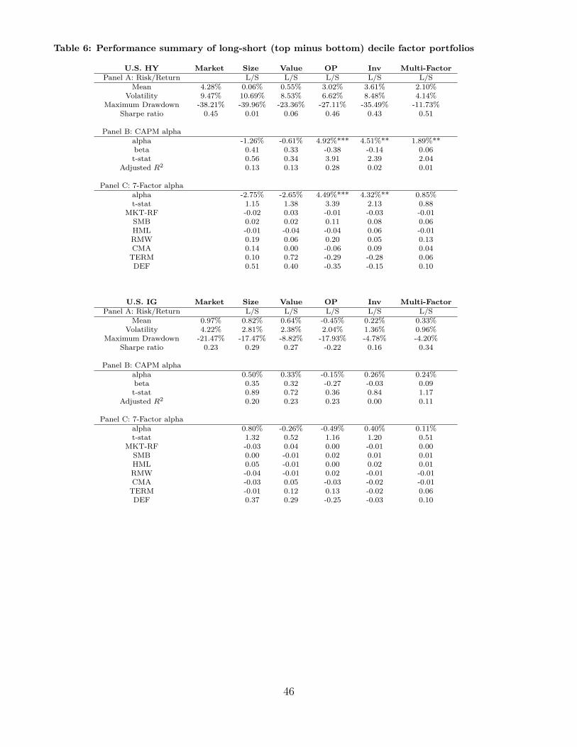
Table 6: Performance summary of long-short (top minus bottom) decile factor portfolios

U.S. HY Market Size Value OP Inv Multi-FactorPanel A: Risk/Return L/S L/S L/S L/S L/S

Mean 4.28% 0.06% 0.55% 3.02% 3.61% 2.10%Volatility 9.47% 10.69% 8.53% 6.62% 8.48% 4.14%

Maximum Drawdown -38.21% -39.96% -23.36% -27.11% -35.49% -11.73%Sharpe ratio 0.45 0.01 0.06 0.46 0.43 0.51

Panel B: CAPM alphaalpha -1.26% -0.61% 4.92%*** 4.51%** 1.89%**beta 0.41 0.33 -0.38 -0.14 0.06t-stat 0.56 0.34 3.91 2.39 2.04

Adjusted R2 0.13 0.13 0.28 0.02 0.01

Panel C: 7-Factor alphaalpha -2.75% -2.65% 4.49%*** 4.32%** 0.85%t-stat 1.15 1.38 3.39 2.13 0.88

MKT-RF -0.02 0.03 -0.01 -0.03 -0.01SMB 0.02 0.02 0.11 0.08 0.06HML -0.01 -0.04 -0.04 0.06 -0.01RMW 0.19 0.06 0.20 0.05 0.13CMA 0.14 0.00 -0.06 0.09 0.04

TERM 0.10 0.72 -0.29 -0.28 0.06DEF 0.51 0.40 -0.35 -0.15 0.10

U.S. IG Market Size Value OP Inv Multi-FactorPanel A: Risk/Return L/S L/S L/S L/S L/S

Mean 0.97% 0.82% 0.64% -0.45% 0.22% 0.33%Volatility 4.22% 2.81% 2.38% 2.04% 1.36% 0.96%

Maximum Drawdown -21.47% -17.47% -8.82% -17.93% -4.78% -4.20%Sharpe ratio 0.23 0.29 0.27 -0.22 0.16 0.34

Panel B: CAPM alphaalpha 0.50% 0.33% -0.15% 0.26% 0.24%beta 0.35 0.32 -0.27 -0.03 0.09t-stat 0.89 0.72 0.36 0.84 1.17

Adjusted R2 0.20 0.23 0.23 0.00 0.11

Panel C: 7-Factor alphaalpha 0.80% -0.26% -0.49% 0.40% 0.11%t-stat 1.32 0.52 1.16 1.20 0.51

MKT-RF -0.03 0.04 0.00 -0.01 0.00SMB 0.00 -0.01 0.02 0.01 0.01HML 0.05 -0.01 0.00 0.02 0.01RMW -0.04 -0.01 0.02 -0.01 -0.01CMA -0.03 0.05 -0.03 -0.02 -0.01

TERM -0.01 0.12 0.13 -0.02 0.06DEF 0.37 0.29 -0.25 -0.03 0.10

46

Table 6 - Continued

EUR IG Market Size Value OP Inv Multi-FactorPanel A: Risk/Return L/S L/S L/S L/S L/S

Mean 0.99% 0.74% 0.17% -0.22% 1.16% 0.48%Volatility 2.36% 2.49% 2.42% 1.98% 2.11% 0.85%

Maximum Drawdown -11.91% -11.46% -8.61% -11.81% -4.70% -3.18%Sharpe ratio 0.42 0.30 0.07 -0.11 0.55 0.56

Panel B: CAPM alphaalpha 0.36% -0.42% 0.24% 1.49%*** 0.41%**beta 0.41 0.61 -0.44 -0.31 0.07t-stat 0.61 0.85 0.56 2.97 1.99

Adjusted R2 0.15 0.36 0.27 0.11 0.03

Panel C: 7-Factor alphaalpha 0.10% -0.43% -0.06% 1.50%*** 0.27%t-stat 0.16 0.80 0.13 2.73 1.23

MKT-RF -0.01 0.01 0.01 -0.02 0.00SMB 0.04 0.02 0.01 -0.03 0.01HML 0.05 0.00 0.03 0.02 0.02RMW 0.03 0.01 0.01 -0.02 0.01CMA -0.02 -0.03 -0.03 0.04 -0.01

TERM -0.05 -0.01 0.06 0.01 0.00DEF 0.40 0.55 -0.47 -0.23 0.06

47

Tab

le7:

Cor

rela

tion

sum

mar

yof

long

-sho

rtde

cile

fact

orpo

rtfo

lios

Returncorrelations

betw

eentheFa

ma–

Fren

chfactorsMKT,S

MB,H

ML,

RMW

,CMA

andthebo

ndmarketfactorsTER

Man

dDEF

aswella

sthelong

-sho

rtde

cile

size,

value,

profi

tabilityan

dinvestmentpo

rtfolio

sfortheU.S.H

Yan

dIG

universe

over

thepe

riodDecem

ber

1996

toDecem

ber20

16(D

ecem

ber20

00to

Decem

ber20

16forEu

rope

anIG

bond

s).

U.S.H

YSize

Value

OP

Inv

Mkt-R

FSM

BHML

RMW

CMA

TER

MDEF

L/SSize

1.00

L/SVa

lue

0.05

1.00

L/SOP

-0.23

-0.22

1.00

L/SInv

0.43

-0.40

0.01

1.00

Mkt-R

F0.13

0.25

-0.40

-0.18

1.00

SMB

0.05

0.10

-0.10

0.02

0.22

1.00

HML

0.16

-0.02

0.01

0.16

-0.14

-0.11

1.00

RMW

0.06

-0.09

0.34

0.14

-0.49

-0.50

0.46

1.00

CMA

0.10

-0.09

0.07

0.20

-0.34

0.01

0.63

0.31

1.00

TER

M-0.17

0.00

0.20

0.01

-0.30

-0.19

-0.04

0.24

0.02

1.00

DEF

0.38

0.36

-0.54

-0.17

0.61

0.28

0.03

-0.35

-0.14

-0.52

1.00

U.S.IG

Size

Value

OP

Inv

Mkt-R

FSM

BHML

RMW

CMA

TER

MDEF

L/SSize

1.00

L/SVa

lue

0.24

1.00

L/SOP

-0.53

-0.21

1.00

L/SInv

0.30

-0.19

-0.20

1.00

Mkt-R

F0.14

0.38

-0.22

-0.11

1.00

SMB

0.14

0.11

-0.05

0.09

0.22

1.00

HML

0.12

0.00

-0.07

0.06

-0.14

-0.11

1.00

RMW

-0.13

-0.19

0.13

-0.01

-0.49

-0.50

0.46

1.00

CMA

0.01

-0.02

-0.05

0.04

-0.34

0.01

0.63

0.31

1.00

TER

M-0.20

-0.10

0.36

-0.01

-0.30

-0.19

-0.04

0.24

0.02

1.00

DEF

0.45

0.48

-0.48

-0.08

0.50

0.24

0.02

-0.26

-0.11

-0.42

1.00

EUR

IGSize

Value

OP

Inv

Mkt-R

FSM

BHML

RMW

CMA

TER

MDEF

L/SSize

1.00

L/SVa

lue

0.31

1.00

L/SOP

-0.16

-0.36

1.00

L/SInv

-0.10

-0.58

-0.10

1.00

Mkt-R

F0.22

0.41

-0.28

-0.28

1.00

SMB

0.23

0.19

-0.04

-0.15

0.32

1.00

HML

0.22

-0.01

0.10

0.12

0.06

0.22

1.00

RMW

-0.05

-0.22

0.20

0.15

-0.59

-0.30

0.16

1.00

CMA

0.05

-0.15

0.07

0.20

-0.14

0.11

0.58

0.20

1.00

TER

M-0.18

-0.25

0.24

0.16

-0.42

-0.16

-0.03

0.24

0.07

1.00

DEF

0.39

0.60

-0.53

-0.34

0.61

0.20

0.05

-0.32

-0.11

-0.36

1.00

48

Figure 1: Cumulative U.S. HY Single-Factor Long-Only Portfolio Returns (Dec 1996 - Dec 2016)

60

100

140

180

220

260

300

340

380

420

Per

form

ance

U.S. HY BenchmarkSize DECILE1Value DECILE 10OP DECILE 10Inv DECILE 1

Figure 2: Cumulative U.S. IG Single-Factor Long-Only Portfolio Returns (Dec 1996 - Dec 2016)

75

80

85

90

95

100

105

110

115

120

125

130

135

140

Per

form

ance

Size DECILE 1Value DECILE 10OP DECILE 10Inv DECILE 1U.S. IG Benchmark

Figure 3: Cumulative European IG Single-Factor Long-Only Portfolio Returns (Dec 2000 - Dec 2016)

85

90

95

100

105

110

115

120

125

130

135

Per

form

ance

Size DECILE 1Value DECILE 10OP DECILE 10Inv DECILE 1European IG Benchmark

49

Figure 4: Cumulative U.S. HY Multi-Factor Long-Only Portfolio Returns (Dec 1996 - Dec 2016)

-20%

0%

20%

40%

60%

80%

100%

120%

140%

50

100

150

200

250

300

350

400

Cu

mu

lative Ou

tperfo

rman

ce

Per

form

ance

Outperformance

Multi-Factor U.S. HY

U.S. HY Benchmark

Figure 5: Cumulative U.S. IG Multi-Factor Long-Only Portfolio Returns (Dec 1996 - Dec 2016)

-2%

-1%

0%

1%

2%

3%

4%

5%

6%

7%

80

85

90

95

100

105

110

115

120

125

130

Cu

mu

lative Ou

tperfo

rman

ce

Per

form

ance

Outperformance

Multi-Factor U.S. IG

U.S. IG Benchmark

Figure 6: Cumulative European IG Multi-Factor Long-Only Portfolio Returns (Dec 2000 - Dec 2016)

-3%

-2%

-1%

0%

1%

2%

3%

4%

5%

90

95

100

105

110

115

120

125

Cu

mu

lative Ou

tperfo

rman

ce

Per

form

ance

Outperformance

Multi-Factor European IG

European IG Benchmark

50