NCER Working Paper SeriesNCER Working Paper Series

Cojumping: Evidence from the US Treasury Bond and Futures Markets

Mardi DungeyMardi Dungey Lyudmyla HvozdykLyudmyla Hvozdyk

Working Paper #56Working Paper #56 July 2010July 2010

Cojumping: Evidence from the US Treasury Bondand Futures Markets∗

Mardi Dungey∗+ and Lyudmyla Hvozdyk+

∗ University of Tasmania+ CFAP, University of Cambridge

14 July 2010

Abstract

The basis between spot and future prices will be affected by jump behavior ineach asset price, challenging intraday hedging strategies. Using a formal cojump-ing test this paper considers the cojumping behavior of spot and futures prices inhigh frequency US Treasury data. Cojumping occurs most frequently at shortermaturities and higher sampling frequencies. We find that the presence of an an-ticipated macroeconomic news announcement, and particularly non-farm payrolls,increases the probability of observing cojumps. However, a negative surprise innon-farm payrolls, also increases the probability of the cojumping tests being un-able to determine whether jumps in spots and futures occur contemporaneously,or alternatively that one market follows the other. On these occasions the marketdoes not clearly signal its short term pricing behavior.

JEL Categories: C1, C32, G14

Keywords: US Treasury markets, high frequency data, cojump test

∗We are grateful to Ross Adams for managing the database. We would like to thank Brett In-der, Petko Kalev, Michael McKenzie and Hashem Pesaran for constructive comments on this paperas well as participants at the Cambridge Finance Workshop, seminars at the Judge Business School,Monash University and the University of Tasmania, conferences at Warwick Business School and Prince-ton University for helpful discussions. Author contacts: Dungey, mardi.dungey@utas.edu.au, Hvozdyk,l.hvozdyk@cerf.cam.ac.uk.

1 Introduction

The joint behavior of spot and future prices for a single asset is an area of considerable

interest to financial markets. Research into hedging using spot and futures includes

papers by Stein (1961), those surveyed by Lien and Tse (2002) and recently Lee (2010).

The literature on price discovery in these markets generally favours information flowing

from futures markets to spot, see for example, Rosenberg and Traub (2006), Mizrach

and Neely (2008) and Chen and Gau (2010). Information arrival is often associated

with price discontinuities, known as jumps, and evidence from high frequency data now

strongly suggests that these may occur at the same time across a number of different asset

prices, see particularly Andersen et al. (2007a), Dungey et al. (2009a) and Lahaye et al.

(2010). An intraday portfolio management strategy involves recognizing and responding

to such jumps. In particular, a speculative positioning on the basis between spot and

futures prices requires a view of whether jumps in the two prices are matched in time, or

indeed matched at all on an intraday frequency.

This paper examines the joint behavior of the spot and futures markets for US Trea-

sury bonds using a formal joint test of cojumping recently developed by Jacod and

Todorov (2009). The spot and futures prices for US Treasuries are already known to

jump individually; see for example Jiang and Yan (2009), Dungey et al. (2009a), Lahaye

et al. (2010), Andersen et al. (2007a).1 However, to our knowledge, the question of

cojumping across spot and futures markets for the same assets is previously unstudied.

In addition to considering the evidence for spot and futures cojumping, we additionally

consider the jumping behavior across the term structure for each of the assets, extending

the univariate test results in Dungey et al. (2009a). Contemporaneous jumps across the

term structure are consistent with liquidity preference theory, while more idiosyncratic

jumps support segmented markets.

The Jacod and Todorov procedure comprises two tests, conducted on individual price

series in which jumps are already known to occur. One test has the null hypothesis of

contemporaneous jumps across multiple asset prices (cojumping), while the other has the

null hypothesis of disjoint jumps (or no cojumping). The tests build on the standard

assumptions of a continuous price process with discrete interruptions (the jumps), where

the multipower quadratic variation of the returns for the chosen time period, usually one

day, can be consistently estimated by realized variance. Jacod and Todorov recognize

that under the null of common jumps the ratio of realized variances at different sampling

frequencies will be the same, so that the hypothesis can be rejected when this is not

the case. Alternatively, in the case of a null of disjoint jumps, the ratio of the realized

variance to the square root of product of the quadratic returns of the individual asset

1The particular univariate testing frameworks include Barndorff-Nielsen and Shephard (2004, 2006),Aït-Sahalia and Jacod (2009) and Lee and Mykland (2008).

1

returns tends to zero (that is there is no evidence that the movements occur together).

High frequency US Treasury spot prices are drawn from eSpeed, one of the two dom-

inant ECNs trading these assets in the post-2000 era. Earlier work, such as Mizrach and

Neely (2008) use data from the now superseded GovPX platform, which operated a voice

over protocol. Corresponding data for the futures sample are obtained from the Chicago

Mercantile Exchange, suitably transformed for nearest contract.

Working with 2, 5, 10 and 30 year maturity contracts we find evidence of cojumping

between spot and futures prices, and that cojumping often occurs in response to the

surprise component of scheduled US macroeconomic news announcements. There are

more jumps in the futures contracts than the spot contracts, however, there are also

periods when the spot market jumps but the futures market does not. The results also

clearly show that the evidence for cojumping increases monotonically with maturity (that

is longer dated securities are more likely to cojump than short-dated) and also increases

with sampling frequency.

Given that the cojumping test proposed by Jacod and Todorov (2009) have two com-

ponents, we find some periods where these tests are in conflict, so that one test suggests

a cojump in the two assets and the other rejects its presence. The extent of this is far

greater than anticipated. We therefore confirm the sample properties of the tests via an

extension of the Monte Carlo study of Jacod and Todorov (2009) which takes into account

the highly correlated nature of spot and futures prices. As we find that the contradictory

test results are not an artefact of the test behavior, we consider the influence of news.

Simple tabulations suggest that the conflicting results in the spot and futures pairs oc-

cur predominantly in the presence of negative surprises for US non-farm payrolls data.

Formal regression analysis confirms that macroeconomic news arrival influences not only

the probability of a jump, a result found in previous papers, but also the probability of

observing an contradictory result. In these contradictory instances the hedging signals

are unclear, as the tests are unable to reveal whether the basis has changed due to a

jump in one asset, implying a potential arbitrage opportunity in the other asset, or due

to different sized contemporaneous jumps in both assets. This likely reflects uncertainty

around the news announcement, leading to moves which are inconsistent with the un-

derlying continuous data generating process as the market attempts to establish a new

equilibrium. For an intraday speculator or portfolio manager, it is potentially important

to recognize that these periods of confusion, and hence opportunity, occur primarily in

association with news releases, and particularly in response to the release of negative

surprises in non-farm payrolls data.

The paper is organized as follows. Section 2 presents formal jump test methodologies.

The data are described in Section 3 and the results of the cojumping test applied to

maturity pairs of futures and spot data are discussed in Section 4. In Section 5 the small

sample properties of the jumps test are examined in a Monte Carlo with correlated prices.

2

The relationships between cojumping and news, and contradictory test result occurrences

and news are analyzed in Section 6. Finally, Section 7 concludes.

2 Methodology

2.1 Univariate Jump Test

The jump days for each series are determined using the univariate jumps test of Barndorff-

Nielsen and Shephard (2006), henceforth BNS, which is a specific case of the more general

proposal of Aït-Sahalia and Jacod (2009)2. Assume that an individual asset price, xit, is

an Itô semi-martingale process

xit =

∫ t

0

bsds+

∫ t

0

σsdWs +N∑

j=1

cjt, (1)

where xt represents the price of the asset at time t, and the right hand side terms represent

a continuous, locally bounded variation process, bt, a strictly positive stochastic volatility

process, σt, Wt is Brownian motion and the final term is a jump process where cjt assumes

a Poisson arrivals process with N possible jump occurrences. Returns for δ intervals are

given by rt+jδ,δ = xt+iδ − xt+(j−1)δ. The realized variance for each period t (one day in

the application here) is sum of squared δ period returns which converges as δ → 0 to the

true quadratic variation and squared jumps,

RVt+1(δ) =

1/δ∑

i=1

r2t+iδ,δ →t∫

0

σ2sds+∑

0<s≤tc2s, (2)

while the product of absolute adjacent δ period returns, or bipower variation converges

to quadratic variation,

BVt+1(δ) = µ−21

1/δ∑

i=2

|rt+iδ,δ|∣∣rt+(i−1)δ,δ

∣∣→t∫

0

σ2sds,

where µ1 =√2/π is a normalizing coefficient.

The BNS test recognizes that as δ → 0 the difference between realized volatility and

bipower variation converges to a jumps only component

RVt+1(δ)−BVt+1(δ)→∑

0<s≤tc2s,

2We also applied Aït-Sahalia and Jacod (2009) univariate jump test but found that it has poorsmall sample properties for our case and is not reported here. See also footnote 4 on the small sampleproperties.

3

which is modified to account for potential negative observations and serial correlation

following Huang and Tauchen (2005) as

JSt+1(δ) = (RVt+1(δ)−BVt+1(δ)) /

(µ−41 + 2µ−21 − 5)δt+1∫

t

σ4(s)ds

−1/2

∼ N(0, 1).

(3)

2.2 Bivariate Jump Test

While Barndorff-Nielsen and Shephard (2004) extend the concepts of bipower variation

and realized variance to multivariate equivalents, the corresponding multivariate test is

currently incomplete. An alternative is the extension to the bivariate case presented in

Jacod and Todorov (2009). The assumed structure for the pricing process of the financial

market assets is now expressed for a vector, xt, where for convenience xt represents the

bivariate case of the current paper. Formally,

xt = x0 +

∫ t

0

bsds+

∫ t

0

σsdWs +

∫ t

0

∫κ′ θ (s, x) (µ− v) (ds, dx)

+

∫ t

0

∫κ′

θ (s, x)µ (ds, dx) , (4)

where bt is the deterministic drift coefficient, Wt a Wiener process, and µ a Poisson

random measure (the jumps). The intensity of the jumps is v with a truncation function

κ (x) = x on a neighborhood of 0. Both bt and θ are 2-dimensional processes in the 2

asset case and the 2 × 2 variance-covariance matrix of the returns, σt, is non-trivially

assumed to evolve with the same Itô semimartingale form as (4), that is there are drift

and jump terms in the evolution of the volatility.

There are three complementary sets to which the observed price paths may belong:

ΩJt , when the series cojump (that is both series jump contemporaneously), ΩDt when the

individual series jump but do not cojump, known as disjoint jumps and ΩCt , when at least

one of the series is continuous, that is displays no jumps. Jacod and Todorov eliminate

ΩCt from consideration by pretesting individual series for the presence of jumps using

univariate jump test series — so that interest is focussed purely on the jumping series.

The formal tests of jumps across multiple series are based on the use of the power

variation estimators, where rt+jδ,δ is the vector of return series:

V (f, δ)t =

[1/δ]∑

j=1

f(rt+jδ,δ) and V (g, δ)t =

[1/δ]∑

j=1

g(rt+jδ,δ).

The first test uses a null of common jumps, and compares the power variation of the

returns series at two different sampling frequencies (scales), δ and kδ where k is a positive

integer. The test statistic, Φ(J)t converges to one under the null of common jumps:

Φ(J)t =

V (f, kδ)tV (f, δ)t

P−→ 1,

4

where

V (f, δ)tP−→ Bt =

∑

s≤t(r1,s)

2(r2,s)2.

The second test has a null of disjoint jumps (or equivalently there are no common

jumps) and the test statistic, Φ(D)t , has the form

Φ(D)t =

V (f, δ)t√V (g1, δ)tV (g2, δ)t

P−→ 0

where

V (gi, δ)tP−→ B′

i,t =∑

s≤t(ri,s)

4.

The tests have critical regions based on C(J)t =

∣∣∣Φ(J)t − 1∣∣∣ ≥ c

(J)t = zα

√δ

V (f,δ)t

and C

(D)t =

Φ(D)t ≥ δ

(Z(D)t

(α)+At)

√V (g1,δ)tV (g2,δ)t

> 0

where Z

(D)t (α) is the normalized order statistic based on

the normalized truncated power variation and At is an alternative truncated power esti-

mator (Jacod and Todorov, 2009).

3 Data Description

US Treasury markets are large in terms of turnover per trading day. Futures trade volume

is greater than spot, but the turnover in the spot market itself is substantial; an average

trade volume of $US524.7 billion per day was recorded in 2006 (see Spiegel, 2008). In

this paper the data set for spot trade in US Treasury bonds is drawn from the Cantor-

Fitzgerald eSpeed trade file and comprises tick by tick transaction prices for the 2, 5,

10 and 30 year US Treasury bonds. The eSpeed platform is one of two dominant ECNs

in this market, the other being ICAP’s BrokerTec, and the characteristics of the trading

volume on the two platforms are not significantly different (compare the data in Dungey

et al., 2009a and Jiang et al., 2010). Futures contracts on the same maturity Treasury

bonds are sourced from the Chicago Mercantile Exchange and are also tick by tick data

for transactions on that platform. The common span of these data sets is from January

2, 2002 to December 31, 2006 with a trading day defined as the period from 7:30a.m. to

5:30p.m. New York time. Weekends and public holidays are excluded from the sample.

The market is very liquid — for example only 4 percent of the 5 minute intervals contain

no spot trade in the 5 year bond.

Discretized spot and futures data are constructed such that the last transaction in an

interval indicates the price at the end of the interval. A number of different sampling

frequencies have been applied in studies of jumps thus far. Lahaye et al. (2010) use 15

minutes, Huang and Tauchen (2005) and Andersen et al. (2007a) sample at 5 minute

intervals, while Dungey et al. (2009a) produce results for a number of different frequen-

cies. Unfortunately, the optimal sampling frequency tests proposed by Bandi and Russell

5

(2006) give no guidance on the appropriate means of choosing sampling frequency for

multiple series considered contemporaneously, particularly in the case of different trade

intensities as in the current problem. Consequently, we consider three sampling frequen-

cies, namely 1, 5 and 10 minute intervals.

Examples of the intraday returns and potential jump behavior of the data are given

in Figure 1, which presents 5 minute returns in 5 year spot and futures data for two

particular days where US non-farm payrolls data were released to the market. The

Figure shows that there are clear disruptions in the price processes at the time of those

announcements.

Descriptive statistics for the intraday returns data are presented in Table 1. The

largest average returns are obtained for the 30 year bonds (0.0003%) at 10 minute inter-

vals. As the sampling frequency increases, the average returns decrease, with the futures

returns approaching 0 faster than the corresponding spot transactions. Futures returns

tend to be more volatile than spot returns. For example, at 5 minute intervals, the stan-

dard deviation of the 5 year and 10 year maturity futures is almost 8 times the standard

deviation of the spot return (0.024 versus 0.170 and 0.040 versus 0.276). The highest

standard deviation is obtained for the 30 year securities with the volatility in the futures

again higher than that in the spot returns.

4 Empirical Tests

4.1 Univariate Test

The appropriate sample period to search for jumps is taken to be one trading day. The

filter for days where individual series jump is the BNS univariate jump test.

The application of the univariate jumps tests reveals a considerable number of days

when both spot and futures contracts of the same maturity exhibit jumps. The results

are summarized in Table 2, which gives the number of days on which a jump is detected

and the corresponding rejection frequency for the null hypothesis of no univariate jumps

for each series. The rejection frequencies of the null hypothesis of no univariate jumps are

generally higher for futures contracts than for the corresponding maturity spot contracts

(except for the 30 year futures at the 10 minute interval). It is also apparent that

as sampling frequency increases the number of test rejections increases. This result is

especially striking for the 1 minute sampling frequency where rejection rates are all over

85%. An increased prevalence of microstructure noise in more frequently sampled data

may be behind this result, although it is difficult to differentiate on statistical criteria

between noise and information. The rejection rates for the null of no jumping in the

futures contracts decrease monotonically as the maturity increases from the 2 year to 30

year. This also holds for spot contracts at 10 minute intervals but is mixed at higher

6

frequencies.

When both spot and futures series in the maturity pair jump individually, this day

is defined as a common jump day. (Note that a common jump day is a day on which

jumps in both series occur, but not necessarily contemporaneously.) The number of these

days is recorded in the penultimate column of Table 2, and the proportion of the total

sample days this represents in the final column. The numbers vary depending on the

sampling frequency: for the 30 year maturity pair the common days are 87 at the 10

minute sampling frequency and 1106 at the 1 minute frequency. Common jump days are

taken as the sample for the cojumping tests.

4.2 Bivariate Test: Bond and Futures Maturity Pairs

The cojumping tests apply to days where both series exhibit jumps individually. We

test for cojumping behavior across spot and futures contracts of the same maturity, and

secondly on pairs of assets of differing maturity within the term structure of the spot

or futures markets. Hence there are 4 maturity pairs in the spot and futures matched

maturity sample: 2, 5, 10 and 30 year contracts, and 6 maturity pair combinations

within each of the spot and futures datasets: 2 and 5, 2 and 10, 2 and 30, 5 and 10, 5

and 30, and 10 and 30 year maturities.

The findings of the two cojumping tests, Φ(J)t and Φ

(D)t , for each bond and futures

maturity pair are presented in Table 3 for 1, 5, and 10 minute sampling frequencies.

Column (1) gives the number of days on which the null of cojumping is rejected using

the Φ(J)t test, and column (3) gives the number of days when the null of no cojumping is

rejected using theΦ(D)t test. When Φ

(J)t is accepted andΦ

(D)t rejected the tests consistently

find cojumping, as shown in column (5). The occurrences when the tests consistently find

no cojumps, when Φ(J)t is accepted and Φ(D)t rejected, are shown in column (7).

Consider first the results of the tests for spot and futures maturity pairs. Rejection of

the null of cojumping increases monotonically with increasing maturity in the Treasury

bonds — which means there is more evidence of cojumping at shorter maturities. To

illustrate consider the 1 minute frequency in Table 3. The null of cojumping, using Φ(J)t ,

is rejected in 4.4% of the total 1230 days for the 2 year maturity, and 61.5% of 1230 days

for the 30 year maturity. The 5 and 10 year maturities lie between these extremes. The

same pattern may be found for other sampling frequencies. The rejection frequency for

the null of common jumps also seems to largely decline with sampling frequency, although

this is not strongly evident in the 2 year maturity. In summary there is more evidence

of cojumping at shorter maturities and higher sampling frequencies using the cojumping

test.

The disjoint test, however, based on the null of disjoint jumps, Φ(D)t , does not display

a monotonicity with maturity. For example, at the 1 minute frequency in Table 3 the

7

null of disjoint jumping is rejected in 88.5% of 1230 days for the 2 year maturity, and

71.4% of 1230 days for the 5 year maturity — but for the 30 year maturity the disjoint

jumps are rejected in 73.2% jump days. However, there is evidence of monotonicity with

the sampling frequency. Using the 5 year maturity as an example, the rejection of the

disjoint null decreases from 71.4% of days at 1 minute sampling to 9.6% of days at

10 minute sampling. Thus there is less evidence of disjoint jumps at higher sampling

frequencies.

Thus the cojumping and disjoint tests both support the existence of more common

jumping (fewer disjoint jumps) at higher frequency of sampling, and less cojumping at

lower sampling frequencies. A direct relationship with maturity is not as clear in the

disjoint test. Jacod and Todorov present evidence that the Φ(D)t test is undersized.

The two cojumping tests have an area of disagreement, when either both reject

their respective null hypotheses or both accept. The prevalence of these occurrences

are recorded in columns (9) and (11) of the tables, and are clearly well in excess of the

type I and type II errors expected. The prevalence of both tests rejecting the null hypoth-

esis (that is a rejection of the null of cojumping using Φ(CJ)t and a rejection of the null

of disjoint jumping using Φ(D)t ) is monotonic with maturity structure and sampling fre-

quency, with the exception of the 2 year spot and futures contracts at 1 minute sampling

frequency. We consider this issue more fully in Section 5.

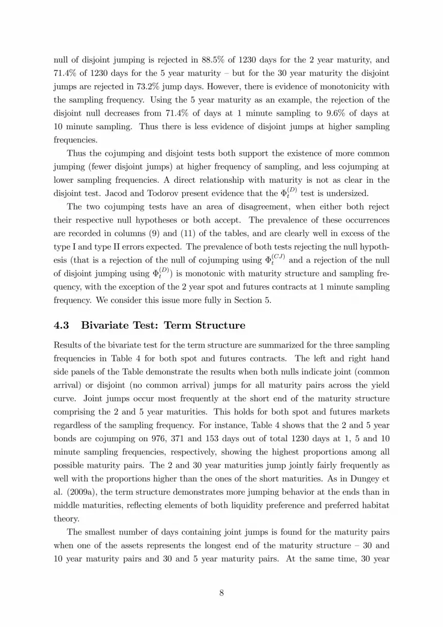
4.3 Bivariate Test: Term Structure

Results of the bivariate test for the term structure are summarized for the three sampling

frequencies in Table 4 for both spot and futures contracts. The left and right hand

side panels of the Table demonstrate the results when both nulls indicate joint (common

arrival) or disjoint (no common arrival) jumps for all maturity pairs across the yield

curve. Joint jumps occur most frequently at the short end of the maturity structure

comprising the 2 and 5 year maturities. This holds for both spot and futures markets

regardless of the sampling frequency. For instance, Table 4 shows that the 2 and 5 year

bonds are cojumping on 976, 371 and 153 days out of total 1230 days at 1, 5 and 10

minute sampling frequencies, respectively, showing the highest proportions among all

possible maturity pairs. The 2 and 30 year maturities jump jointly fairly frequently as

well with the proportions higher than the ones of the short maturities. As in Dungey et

al. (2009a), the term structure demonstrates more jumping behavior at the ends than in

middle maturities, reflecting elements of both liquidity preference and preferred habitat

theory.

The smallest number of days containing joint jumps is found for the maturity pairs

when one of the assets represents the longest end of the maturity structure — 30 and

10 year maturity pairs and 30 and 5 year maturity pairs. At the same time, 30 year

8

maturity in conjunction with the 5 or 10 year maturities tend to jump disjointly more

often than other pairs. The cases when both nulls disagree have patterns similar to the

ones in Section 4.2.

To examine the results of the Sections 4.2 and 4.3 more carefully the next two sec-

tions explore first, the sampling properties of the tests by extending the Monte Carlo

experiment of Jacod and Todorov (2009) to more closely resemble the characteristics of

the current problem, and second, the relationship of the cojumping behavior with news

announcements in US markets. This builds on a large existing body of work on the re-

lationship between price changes in US Treasury markets and scheduled macroeconomic

news releases; see Fleming and Remolona (1999), Green (2004), Simpson and Ramchan-

der (2004), Andersen et al. (2007b).

5 Finite Sample Properties

5.1 Simulation Design

Jacod and Todorov (2009) examine the finite sample properties of their test under the

assumption that the two series are uncorrelated and have the same jump intensity. The

data considered in this paper are highly correlated and have different jump intensities.

Consequently, we extend the Monte Carlo of Jacod and Todorov (2009) accordingly. Two

data generating processes for the log price process, Xt are implemented. The first is a

constant volatility jump diffusion model originally designed by Jacod and Todorov (2009),

and the second a stochastic volatility jump diffusion model, as in Andersen et al. (2010),

Chernov et al. (2003), Andersen et al. (2002). The constant volatility process, CVP, is

defined as:

CVP: dXi,t = σidWi,t + αi∫Rxiλi(dt, dxi) + α3

∫Rx3λ3(dt, dx3), i = 1, 2, (5)

where W it is a Brownian motion, cor(W 1,W 2) = ρ1; λ1, λ2 and λ3 are the Poisson

measures; σi is a constant volatility factor.

The stochastic volatility jump diffusion model, SVP, has the form:

SVP: dXi,t = exp(β0 + βivi,t)dWi,t + αi∫Rxiλi(dt, dxi) + α3

∫Rx3λ3(dt, dx3)

dvi,t = αvvi,tdt+ dWvi,t, i = 1, 2,(6)

where Wt is the standard Brownian motion; cor(Wi,Wv1) = ρi is the leverage correlation;

cor(W1,W2) = ρ is the correlation between returns; vt is the stochastic volatility compo-

nent and λ1, λ2 and λ3 are the Poisson measures. Following Jacod and Todorov (2009)

we set αv = 0.1, β0 = 0, βi = 0.125 and in line with Veraart (2010), ρi = −0.62.The three jump components of the process (5) are represented by two disjoint jump

components and a common jump component premultiplied by α1, α2 and α3, respectively.

9

The number of jumps in each component is simulated from a Poisson distribution with

parameter λ and is uniformly distributed on the whole time interval. The parameter λ is

chosen to reflect the lowest of the rejection frequencies in the univariate tests of the data

given in Table 2. The jump sizes are drawn from a N(0, 1) distribution. As US Treasury

futures and spot prices are characterized by high correlations we trial values of ρ, the

correlation of the continuous part of the process, of 1.00 and 0.95. The results were not

qualitatively different and only the ρ = 1 outcomes are reported here. We simulate 5000

replications from the processes (5) and (6) with one increment per minute for a trading

day of 600 minutes, consistent with the dataset in Section 4.3

The first three columns of Table 5 shows the parameter values of the 16 cases we

consider when ρ = 1. Intensities λ1 and λ2 corresponding to the disjoint components of

the DGP (5) are 1:1 (this is the case studied by Jacod and Todorov, 2009), 2:1, 5:1 and

10:1, and the intensity λ3 is equal to λ1 in all simulation scenarios. Constant volatility

factors σ1 and σ2 are equal to 8× 10−5 in all simulations.

5.2 Size and Power

Table 5 reports results for the case of the 1% true size tests. This significance level is

reported for consistency with the application, but simulations at higher significance levels

produce similar analytical results. The BNS univariate jumps test reported in columns

(4) and (7) of Table 5 is oversized, consistent with literature on the univariate jump test

properties (e.g. Huang and Tauchen, 2005), and more so in the SVP than CVP, which

may be due to a volatility feedback effect when negative returns are associated with

higher volatility. As the intensity of the jumps increases, the test size rises, indicating

that the relatively small jumps are difficult to distinguish from the Wiener process.4

Under the null of cojumping the bivariate test is oversized for both DGPs as reported

in columns (5) and (8) of Table 5. This improves with smaller values of the α parameters.

The disjoint jumping test is undersized, as reported in columns (6) and (9).

Table 5 also presents the power properties of the three test statistics. Larger jump

size and higher jump intensity have a positive effect on the univariate test power as shown

in Columns (10) and (13). The cojumping test has relatively low power for high values

of the α parameters, and as with the size results for this test, power improves as the

sizes of the jump, the α parameters, increase. The disjoint test has good power in all

experiments, columns (12) and (15).

The results of the Monte Carlo experiment have confirmed earlier work that the BNS

3To make the CVP and SVP processes comparable across simulations the Brownian motion innova-tions to the price process of equation (6) are rescaled by a factor of 120.

4A further Monte Carlo examined the small sample properties of the univariate jump test of Aït-Sahalia and Jacod (2009). The test consistently overrejects the null of no jumps, which is a consequenceof the far fewer sample observations per day in our scenario than the 1, 4 and 15 second samplingfrequencies suggested in Aït-Sahalia and Jacod (2009). Results are available on request.

10

univariate test is somewhat oversized. The Jacod and Todorov common jumps test is

also oversized with both size and power improved by higher jump sizes, while the disjoint

test has good power properties, but is somewhat undersized. These results are consistent

with those at 5% and 10% significance levels. These Monte Carlo results do not suggest

that the contradictory results between the two tests observed in Section 4.2 are the result

of test performance. Consequently, we next turn to relating the occurrence of jumps, and

contradictory results in the bivariate jumps tests, to the presence of news announcements.

6 Cojumps and News

It is well known that jumps often occur in association with a news event, in particular

with surprises associated with prescheduled US news releases, see Lahaye et al. (2010),

Andersen et al (2007a,b). We use a set of 23 major US macroeconomic news announce-

ments, consistent with Simpson and Ramchander (2004) and Dungey et al. (2009a).5

Of the 1230 trading days, 702 days, or 57%, contain scheduled macroeconomic news

announcements.

The news surprise data for the announcements are drawn from Bloomberg and stan-

dardized across the sample. A simple cross tabulation with the jump test results suggests

a strong correlation between the jump behavior and the announcement of non-farm pay-

rolls data. Non-farm payroll releases are known to be the news release which most affects

US Treasury markets; Fleming and Remolona (1999) and Dungey et al. (2009a), although

Jiang and Yan (2009) find PPI as their most important event. Hence it is not surprising

that if arbitrage opportunities exist between futures and spot markets they are likely to

occur around surprises emanating from non-farm payrolls data. In the current sample

the non-farm payrolls data were released 59 times, producing a distribution of surprises

shown in Figure 2. There were more negative than positive surprises, but no particularly

large negative outlier is detected.

To formally evaluate the relationship between jump days and prescheduled news an-

nouncements, we estimate a panel logit model on the probability of observing either a

jump day, JDit, or the probability of observing a conflicting day, CDit, (i.e. the day

when two bivariate nulls disagree) for maturities i = 2, 5, 10, 30 for t = 1, ..., 1230. In the

initial specification we examine whether the presence of news, denoted by the variable

Newst which takes the value of 1 in the presence of news and 0 otherwise, is significant as

a determinant of the probability of jumps or conflicting results. To account for possible

effects of futures contract rollovers a dummy, Expi,t equals one on the last day of trade

for a given futures contract and zero otherwise. Two such dummies are necessary as

5The news announcements are: auto sales, business inventory, capacity utilization, constructionspending, consumer credit, CPI, durable goods orders, factory orders, GDP, hourly earnings, housingstarts, industrial production, leading indicators, new home sales, non-farm payrolls, personal consump-tion, personal income, PPI, retail sales, trade balance, unemployment, US NAPM, US Treasury Budget.

11

expiry dates are the same for 10 and 30 year contracts and for 2 and 5 year contracts6.

Day of the week dummies variables Djt, j = 1, 2, 3, 4 are included, normalizing on Friday.

Different maturities have different jump activities therefore we specify a random effects

model that accounts for heterogeneity between different maturities7:

JD(CD)it = β0 + β1Newst + β3Expit|i=2,5 (7)

+β4Expit|i=10,30 +Σ8j=5βjDjt + εit,

εit = τ i + eit, (8)

where τ i and eit are two iid series with zero mean and constant variances. To extend this

further, the Newst variable is supplemented by the standardized surprise in non-farm

payrolls releases, NFPt (shown in Figure 2), and the standardized news surprise for all

other news announcements, Surpt.

JD(CD)it = β0 + β1Newst + β2NFPt + β3Surpt + β4Expit|i=2,5

+β5Expit|i=10,30 +Σ9j=6βjDjt + εit,

εit = τ i + eit, (9)

Similarly, we estimate two panel logit models for the term structure of US Treasury bonds

and futures, where the dependent variable JDit denotes cojumps between maturities i

and l. An additional independent variable in equation (10) is a set of maturity dummies,

Mjt, j = i, l, with the 30 year bond taken as the omitted category. These take the of

value 1 when either of the maturity pair under consideration involves that maturity, so

for jumps considered in the combination of the 2 and 5 year contracts, M2,t = M5,t = 1.

Futures contract expiry dummies are also included in the specification for futures only:

JDit(CDit) = β0 + β1Newst + β2NFPt + β3Surpt + β4Expit|i=2,5

+β5Expit|i=10,30 +Σ9j=6βjDjt +Σ

12j=10βjMjt + εilt,

εit = τ i + eit, (10)

Panel I of Table 6 reports results of estimating equations (7) and (10) with the bivari-

ate Newst dummy. They reveal a significant positive relationship between the presence

of scheduled macroeconomic news and cojump days in both the maturity matched spot

and futures pairs, and in the term structure of either spot or futures. In the case of the

6The 2 and 5 year contracts expire on the last business day of the contract month, the 10 and30 year contracts expire 7 business days before the last business day of the contract month. Seewww.cmegroup.com for further details. A number of robustness checks were conducted for the expirydummy. Examination of the trade data suggests increased volume and volatility some 20 ± 2 tradingdays before the expiry of the 2 and 5 year contracts and some 15 ± 2 days before the expiry of the 10and 30 year maturity contracts. Dummies based on these timings were also insignificant, and are notreported in the paper.

7The Hausman test confirms the choice of a random effects specification.

12

spot and future maturity pairs the probability of observing a jump day increases by 2.8%

given there is a prescheduled macroeconomic news announcement. For the term struc-

ture results the probability of a common jump is increased by 4.4% in the spot market

and 1.0% in the futures market. The presence of macroeconomic news also results in a

statistically significant 2.3% increase in the probability of the bivariate tests disagreeing

for spot and futures pairs.

The presence of the long end futures expiry date is significant for the maturity pairs

specification in Panel I. The significance of the day of the week dummies varies, but in

general Mondays have a positive impact on the probability of observing a common jump,

confirming the information that arrives after the weekend is important in explaining the

jumps.

When the Newst dummy is augmented by the news surprise for all news announce-

ments, as in equations (9) and (10) it retains its statistical significance. However, a

further decomposition, reported in Panel II of Table 6 reveals greater detail, by allowing

for asymmetric responses to positive and negative non-farm payroll surprises (asymmetric

responses to general news surprises were not empirically supported). In each of the cases

examined in Table 6 Panel II the presence of a negative or positive non-farm payrolls

surprise statistically increases the probability of observing cojumps, and of observing a

conflicting result in the jumps tests. In the case of maturity pairs of spot and futures

contracts a positive and a negative non-farm payrolls news surprises increase the proba-

bility of a cojump by 22.2% and 19.5%, respectively. The probability of a contradictory

test result is increased by 6.4% and 6.3% in the case of a positive or a negative non-farm

payroll surprise. Thus, the presence of a non-farm payroll surprise is more likely to cause

a cojump, than a conflicting day. For the term structure, both positive and negative

surprises are statistically significant. For the futures term structure the magnitude of the

positive non-farm payroll surprise effect is more than two times higher than that of the

negative surprise and statistically different. In the case of the bond term structure there

is a significant effect of the macro news of around 20% for either positive or negative

surprises, confirming findings in the existing literature (see Dungey et al., 2009a). Wald

tests indicate significant differences between the coefficients on positive and negative

surprises in the specifications for the futures term structure, but not for the remaining

specifications.

While the finding that news results are important in the univariate jumps literature

is not unusual, here the emphasis is on how the news impacts significantly on the cases

where the market data are not clearly signalling the jump behavior of the prices. These

cases, which seem to be associated with the case of worse than anticipated news releases,

are interesting in that they represent periods when hedging may be difficult.8

8Jiang, Lo and Verdhalan (2010) suggest that liquidity factors may also be important in these circum-stances, however, the expandable limit order nature of the eSpeed database makes the construction of

13

7 Conclusions

The presence of price discontinuities in high frequency financial market data is well docu-

mented in the univariate case. However, many interesting questions concern the presence

of contemporaneous price disruptions across multiple assets. In a hedging framework an

obvious question is the extent to which spot and future prices exhibit such behavior.

Recently, Jacod and Todorov (2009) have developed a bivariate test for contemporaneous

jumps across two series using a pair of tests — one of which has a null of cojumping and

one of which the null of disjoint jumps. This paper considers the cojumping behavior

of spot and future contracts for US Treasury contracts in maturity pairs, and across the

term structure. The bivariate tests indicate that the detection of cojumping is increasing

with sampling frequency. The test with the null of cojumping finds a monotonic relation-

ship between cojumping and maturity structure — more cojumps are detected for lower

maturity contracts in both futures and spot contracts for maturity pairs, or within the

same market across the term structure. However, the test with a null of disjoint jumps

(that is jumps on the same day but different time intervals within that day) find no clear

relationship with maturity structure.

As the two cojumping tests disagree more than statistically expected, the small sample

properties of the tests were confirmed under the conditions of highly correlated series of

different intensities present in this data. The disjoint test is found to be slightly undersized

but with good power.

Prescheduled macroeconomic news events increase the probability of cojumping be-

havior, and more specifically negative surprises in non-farm payrolls data increase the

probability of observing a cojump in maturity matched pairs of spot and futures con-

tracts for US Treasuries. The presence of negative surprises in non-farm payrolls is also

associated with a lesser increase in the probability of the cojumping tests being unable

to distinguish whether the two price series are jumping contemporaneously or with some

time separation. Non-farm payroll surprises increase the probability of jump behavior in

both spot and futures contracts for US Treasuries. They also increase the probability of

a lack of clear signal as to whether a jump in one asset price is likely to be immediately

accompanied by a jump in the other. The increase in probability of cojumping is higher

than the probability of observing a conflicting result. Overall, the results indicate the

importance of non-farm payrolls releases to active portfolio management.

an order book similar to that used in their analysis uniformative in this case, see Dungey et al. (2009b)and Boni and Leach (2004) for a description of the expandable limit order book.

14

References

[1] Aït-Sahalia, Y. and J. Jacod (2009), “Testing for Jumps in a Discretely ObservedProcess”, Annals of Statistics, 37, 184-222.

[2] Andersen, T. G., T. Bollerslev, P. Frederiksen and M. Ø. Nielsen (2010),“Continuous-Time Models, Realized Volatilities, and Testable Distributional Impli-cations for Daily Stock Returns”, Journal of Applied Econometrics, 25(2), 233-261.

[3] Andersen, T. G., T. Bollerslev and F. X. Diebold (2007a), “Roughing it Up: Includ-ing Jump Components in the Measurement, Modelling and Forecasting of ReturnVolatility”, The Review of Economics and Statistics, 89, 4, 701-720.

[4] Andersen, T. G. and Bollerslev, T., Diebold, X. and Vega, C. (2007b), “Real-TimePrice Discovery in Global Stock, Bond and Foreign Exchange Markets”, Journal ofInternational Economics, 73, 251-277.

[5] Andersen, T. G., L. Benzoni and J. Lund (2002), “An Empirical Investigation ofContinuous-Time Equity Return Models”, Journal of Finance, 57, 1047-1091.

[6] Bandi, F. M., and J. R. Russell (2006), “Separating Micro Structure Noise fromVolatility”, Journal of Financial Economics, 79, 655-692.

[7] Barndorff-Nielsen, O. E. and N. Shephard (2006), “Econometrics of Testing forJumps in Financial Economics Using Bipower Variation”, Journal of FinancialEconometrics, 4, 1-30.

[8] Barndorff-Nielsen, O. E. and N. Shephard (2004), “Measuring the Impact of Jumpsin Multivariate Price Process Using Bi-Power Covariation”, manuscript.

[9] Boni, L. and C. Leach (2004), “Expandable Limit Order Markets”, Journal of Fi-nancial Markets, 7, 145-185.

[10] Chen, Y. and Y. Gau (2010), "News Announcements and Price Discovery in ForeignExchange Spot and Futures Markets", Journal of Banking and Finance, 34, 1628-1636.

[11] Chernov, M., A. R. Gallant, E. Ghysels and G. Tauchen (2003), “Alternative Modelsfor Stock Price Dynamics”, Journal of Econometrics, 116, 225-257.

[12] Dungey, M., M. McKenzie and V. Smith (2009a), “News, No-News and Jumps inthe US Treasury Market”, Journal of Empirical Finance, 16, 430-445.

[13] Dungey, M., Henry, O. and M. McKenzie (2009b), “From Trade-to-Trade in USTreasuries”, manuscript.

[14] Fleming M. J. and E. M. Remolona (1999), “What Moves Bond Prices?”, Journalof Portfolio Management, 25, 28-38.

[15] Green, T. C. (2004), “Economic News and the Impact of Trading on Bond Prices”,The Journal of Finance, 59 (3), 1201-1233.

[16] Huang, X. and G. Tauchen (2005), “The Relative Contribution of Jumps to TotalPrice Variance”, Journal of Financial Econometrics, 3, 4, 456 — 499.

[17] Jacod, J. and V. Todorov (2009), “Testing for Common Arrivals of Jumps for Dis-cretely Observed Multidimensional Processes”, Annals of Statistics, 37 (4).

[18] Jiang, G. and Yan, S. (2009), “Linear-quadratic term structure models — Towardthe understanding of jumps in interest rates”, Journal of Banking and Finance, 33,473-485.

15

[19] Jiang, G., I. Lo. and A. Verdelhan (2010), “Information Shocks, Liquidity Shocks,Jumps and Price Discovery: Evidence from the U.S. Treasury Market”, Journal ofFinancial and Quantitative Analysis, forthcoming.

[20] Lahaye, L., S. Laurent and C. Neely (2010), “Jumps, Cojumps and Macro Announce-ments”, Journal of Applied Econometrics, forthcoming (available in early view).

[21] Lee, H.-T. (2010), “Regime Switching Correlation Hedging”, Journal of Banking andFinance, forthcoming (available in early view).

[22] Lee, S. S. and P. A. Mykland (2008), “Jumps in Financial Markets: A New Nonpara-metric Test and Jump Dynamics”, Review of Financial Studies, 21(6), 2535-2563.

[23] Lien, D. and Tse, Y. (2002), “Some Recent Developments in Futures Hedging”,Journal of Economic Surveys, 16, 357-396.

[24] Mizrach, B. and C. Neely (2008), “Information Shares in the US Treasury Market”,Journal of Banking and Finance, 32, 1221-1233.

[25] Spiegel, M. (2008), “Patterns in Cross Market Liquidity”, Financial Research Letters,5, 2-10.

[26] Simpson, M. W. and S. Ramchander (2004), “An Examination of the Impact ofMacroeconomic News on the Spot and Futures Treasuries Markets”, Journal of Fu-tures Markets, 24 (5), 453-478.

[27] Stein, J. L. (1961), “The Simultaneous Determination of Spot and Future Prices”,American Economic Review, 51, 1012-1025.

[28] Rosenberg, J. V. and L. G. Traub (2006), “Price Discovery in the Foreign CurrencyFutures and Spot Market”, Federal Reserve Bank of New York Staff Report, No. 262.

[29] Veraart, A.E.D. (2010), “Inference for the Jump Part of Quadratic Variation of ItôSemimartingales”, Econometric Theory, 26 (2), 331-368.

16

Table 1:Descriptive Statistics for Bond and Futures Returns Across Maturities and Frequencies,

2002 — 2006

BONDS FUTURESMaturity Mean St Dev Min Max Mean St Dev Min Max

1 Minute Sampling

2 year 0.0000 0.006 -2.032 2.032 0.0000 0.054 -0.968 1.1405 year 0.0000 0.012 —2.866 2.913 0.0000 0.151 -1.534 1.95110 year 0.0000 0.018 -1.787 1.703 0.0000 0.260 -2.872 2.89030 year 0.0000 0.033 -9.564 9.550 0.0000 0.271 -5.249 4.234

5 Minute Sampling

2 Year 0.0000 0.010 -0.517 0.470 0.0000 0.077 -0.968 1.1405 Year 0.0001 0.024 -0.870 1.234 0.0000 0.170 -1.667 2.02210 Year 0.0001 0.040 -1.723 1.509 0.0000 0.276 -2.604 2.63930 Year 0.0002 0.071 -9.535 9.550 0.0000 0.290 -4.234 4.180

10 Minute Sampling

2 Year 0.001 0.014 -0.548 0.544 0.0000 0.084 -0.968 1.1405 Year 0.002 0034 -1.103 1.326 0.0001 0.176 -1.693 200410 Year 0.002 0.056 -1.549 1.583 0.0000 0.286 -2.406 2.63330 Year 0.003 0.086 -1.979 1.902 0.0001 0.300 -4.234 4.180

Figure 1: 5 Minute Returns for 5 Year Maturity US Treasury Bonds and Futures:1 April 2005 7 February 2003

17

Table 2:Results of the Univariate Test for the US Treasury Bond and Futures, January 2002 —

December 2006BOND FUTURES No. of Prop. of

No. of Rejection No. of Rejection Common CommonMaturity Jump Days Frequency Jump Days Frequency Jump Days Jump Days1 Minute Sampling:

2 Year 1213 0.986 1222 0.993 1207 0.9815 Year 1073 0.872 1198 0.974 1052 0.85510 Year 1104 0.898 1166 0.948 1048 0.85230 Year 1207 0.981 1128 0.917 1106 0.899

5 Minute Sampling:

2 Year 916 0.745 1104 0.898 813 0.6615 Year 451 0.367 728 0.592 293 0.23810 Year 484 0.393 652 0.530 287 0.23330 Year 574 0.467 586 0.476 298 0.242

10 Minute Sampling:

2 Year 564 0.459 778 0.633 365 0.2975 Year 298 0.242 347 0.282 142 0.11510 Year 271 0.220 281 0.228 86 0.07030 Year 273 0.222 250 0.203 87 0.071

Figure 2: Distribution of the Standardised Non-Farm Payroll Surprises, 2001 — 2006

.0169 .0169

.0508

.1356

.2373

.1525

.1356

.1017

.0678

.0508

.0339

0.0

5.1

.15

.2.2

5F

ract

ion

-4 -2 0 2Standardised Non-Farm Payroll Surprises

18

Table 3:Results of the Bivariate Test for the Maturity Pairs of US Treasury Bond and Futures,

January 2002 — December 2006Common No Common Both Nulls Both NullsArrival Arrival Cannot be Can be

Reject Ho: of Jumps: of Jumps: Rejected Rejected

Joint Disjoint Accept Φ(j)t Reject Φ

(j)t Accept Φ

(j)t Reject Φ

(j)t

Maturity Jumps, Φ(j)t Jumps, Φ

(d)t Reject Φ

(d)t Accept Φ

(d)t Accept Φ

(d)t Reject Φ

(d)t

No. Prop. No. Prop. No. Prop. No. Prop. No. Prop. No. Prop.(1) (2) (3) (4) (5) (6) (7) (8) (9) (10) (11) (12)

1 minute sampling

2 year 54 0.044 1089 0.885 1047 0.851 12 0.010 106 0.086 42 0.0345 year 189 0.154 878 0.714 749 0.609 60 0.049 114 0.093 129 0.10510 year 466 0.379 806 0.655 471 0.383 131 0.107 111 0.090 335 0.27230 year 756 0.615 900 0.732 308 0.250 164 0.133 42 0.034 592 0.481

5 minute sampling

2 year 34 0.028 708 0.576 683 0.555 9 0.007 96 0.078 25 0.0205 year 77 0.063 243 0.198 187 0.152 21 0.017 29 0.024 56 0.04610 year 158 0.128 226 0.184 111 0.090 43 0.035 18 0.015 115 0.09330 year 241 0.196 246 0.200 52 0.042 47 0.038 5 0.004 194 0.158

10 minute sampling

2 year 43 0.035 328 0.267 290 0.236 5 0.004 32 0.026 38 0.0315 year 65 0.053 118 0.096 69 0.056 16 0.013 8 0.007 49 0.04010 year 53 0.043 75 0.061 30 0.024 8 0.007 3 0.002 45 0.03730 year 74 0.060 71 0.058 12 0.010 15 0.012 1 0.001 59 0.048

19

Table 4:Results of the Bivariate Test for the Maturity Pairs Spot and Futures markets, January

2002 — December 2006Spot Futures

Common No Common Both Nulls Common No Common Both NullsArrival Arrival Can Be Cannot be Can be Can Be

of Jumps: of Jumps: Rejected Rejected Rejected Rejected

Accept Φ(j)t Reject Φ

(j)t Reject Φ

(j)t Accept Φ

(j)t Reject Φ

(j)t Reject Φ

(j)t

Maturity Reject Φ(d)t Accept Φ

(d)t Reject Φ

(d)t Accept Φ

(d)t Reject Φ

(d)t Reject Φ

(d)t

No. Prop. No. Prop. No. Prop. No. Prop. No. Prop. No. Prop.1 minute sampling

2 and 5 976 0.793 5 0.004 42 0.034 857 0.697 26 0.021 242 0.1972 and 10 981 0.798 6 0.005 52 0.042 650 0.528 63 0.051 328 0.2672 and 30 983 0.799 23 0.019 106 0.086 557 0.453 86 0.070 377 0.3075 and 10 822 0.668 17 0.014 116 0.094 427 0.347 133 0.108 493 0.4015 and 30 784 0.637 27 0.022 207 0.168 346 0.281 151 0.123 508 0.41310 and 30 644 0.524 44 0.036 378 0.307 219 0.178 166 0.135 635 0.516

5 minute sampling

2 and 10 371 0.302 0 0.000 33 0.027 428 0.348 51 0.041 122 0.0992 and 10 369 0.300 0 0.000 46 0.037 283 0.230 52 0.042 190 0.1542 and 30 371 0.302 2 0.002 56 0.046 254 0.207 55 0.045 175 0.1425 and 10 211 0.172 0 0.000 94 0.076 161 0.131 69 0.056 198 0.1615 and 30 173 0.141 2 0.002 107 0.087 129 0.105 43 0.035 191 0.15510 and 30 137 0.111 6 0.005 158 0.128 66 0.054 60 0.049 212 0.172

10 minute sampling

2 and 5 153 0.124 0 0.000 76 0.062 142 0.115 6 0.005 74 0.0602 and 10 122 0.099 0 0.000 68 0.055 93 0.076 18 0.015 71 0.0582 and 30 98 0.080 1 0.001 69 0.056 73 0.059 13 0.011 67 0.0545 and 10 91 0.074 0 0.000 96 0.078 49 0.040 10 0.008 71 0.0585 and 30 59 0.048 0 0.000 91 0.074 28 0.023 12 0.010 65 0.05310 and 30 51 0.041 0 0.000 110 0.089 20 0.016 6 0.005 69 0.056

20

Table 5:Size and Power Properties of the Univariate and Bivariate Jump Tests Based on anAsymptotic Size of 1%, Constant and Stochastic Volatility Models, Equivalent to 1

Minute Sampling Frequency, 5,000 Replications.Parameters Size Powerρ = 1 CVP SVP CVP SVP

α3 α1,2 λ1:2 JSt T(j)t T

(d)t JSt T

(j)t T

(d)t JSt T

(j)t T

(d)t JSt T

(j)t T

(d)t

(1) (2) (3) (4) (5) (6) (7) (8) (9) (10) (11) (12) (13) (14) (15)0.6 0.6 1:1 0.018 0.334 0.001 0.114 0.340 0.001 0.959 0.666 0.999 0.855 0.660 0.9990.6 0.6 2:1 0.020 0.333 0.000 0.108 0.343 0.000 0.963 0.667 1.000 0.898 0.657 1.0000.6 0.6 5:1 0.028 0.354 0.000 0.110 0.364 0.000 0.958 0.646 1.000 0.933 0.636 1.0000.6 0.6 10:1 0.030 0.347 0.000 0.106 0.357 0.000 0.956 0.653 1.000 0.946 0.643 1.0000.6 0.2 1:1 0.018 0.333 0.001 0.114 0.336 0.001 0.911 0.667 0.999 0.829 0.664 0.9990.6 0.2 2:1 0.020 0.333 0.000 0.108 0.343 0.000 0.917 0.667 1.000 0.882 0.657 1.0000.6 0.2 5:1 0.028 0.355 0.000 0.110 0.362 0.000 0.915 0.645 1.000 0.923 0.638 1.0000.6 0.2 10:1 0.030 0.346 0.000 0.106 0.356 0.000 0.907 0.654 1.000 0.940 0.644 1.0000.2 0.6 1:1 0.018 0.086 0.001 0.114 0.097 0.001 0.912 0.914 0.999 0.816 0.903 0.9990.2 0.6 2:1 0.020 0.092 0.000 0.108 0.105 0.001 0.918 0.908 1.000 0.859 0.895 0.9990.2 0.6 5:1 0.028 0.103 0.001 0.110 0.111 0.001 0.922 0.897 0.999 0.892 0.889 0.9990.2 0.6 10:1 0.030 0.102 0.000 0.106 0.107 0.000 0.914 0.898 1.000 0.902 0.893 1.0000.2 0.2 1:1 0.018 0.071 0.001 0.114 0.076 0.001 0.858 0.929 0.999 0.786 0.924 0.9990.2 0.2 2:1 0.020 0.085 0.000 0.108 0.091 0.000 0.868 0.915 1.000 0.840 0.909 1.0000.2 0.2 5:1 0.028 0.092 0.000 0.110 0.098 0.000 0.871 0.908 1.000 0.876 0.902 1.0000.2 0.2 10:1 0.030 0.093 0.000 0.106 0.095 0.000 0.861 0.907 1.000 0.891 0.905 1.000

Note: λ3 = λ1 in all experiments.

21

Table 6:Results of the Panel Logit Random Effects Model Estimation, Marginal Effects, 5

Minute Sampling FrequencyCommon Jump Days Conflicting Jump Days

Maturity Pairs Term Structure Maturity Pairs Term StructureSpot and Futures Spot Futures Spot and Futures Spot Futures

Panel I:

News 0.028*** 0.044* 0.010 0.023** 0.029* 0.026*(0.017) (0.012) (0.013) (0.011) (0.006) (0.009)

DMo 0.086* 0.007 0.123* 0.000 -0.034* 0.028***(0.029) (0.019) (0.022) (0.011) (0.006) (0.016)

DTue -0.010 -0.063* 0.027 -0.020*** -0.027* 0.011(0.023) (0.016) (0.019) (0.011) (0.005) (0.014)

DWed -0.011 -0.078* 0.056* -0.005 -0.028* 0.027**(0.023) (0.015) (0.019) (0.009) (0.005) (0.014)

DThu -0.070* -0.069* -0.015 -0.028** -0.035* -0.013(0.024) (0.015) (0.019) (0.013) (0.005) (0.013)

Expiry10,30 0.121*** - 0.014 0.033 - 0.026(0.064) - (0.049) (0.029) - (0.037)

Expiry2,5 -0.017 - 0.033 - - -0.047(0.079) - (0.059) - - (0.034)

M2 - 0.107* 0.210* - -0.069* -0.036*- (0.013) (0.014) - (0.007) (0.010)

M5 - -0.014 0.092* - -0.030* -0.026*- (0.013) (0.014) - (0.006) (0.010)

M10 - 0.002 0.048* - -0.008 0.009- (0.013) (0.014) - (0.006) (0.010)

Panel II:

News 0.023 0.038* 0.007 0.020** 0.022* 0.023*(0.017) (0.012) (0.013) (0.010) (0.006) (0.009)

Surp_exl_nfp -0.003 -0.012 -0.006 -0.001 0.006** -0.003(0.012) (0.009) (0.009) (0.005) (0.003) (0.006)

Non− farm pos 0.221* 0.190* 0.222* 0.064** 0.098* 0.141*(0.069) (0.046) (0.054) (0.029) (0.013) (0.027)

Non− farm neg -0.195* -0.208* -0.107* -0.063* -0.085* -0.059*(0.050) (0.033) (0.032) (0.026) (0.009) (0.018)

DMo 0.126* 0.044** 0.149* 0.017 -0.015** 0.049*(0.032) (0.021) (0.022) (0.014) (0.008) (0.018)

DTue 0.029 -0.027 0.055* -0.004 -0.005 0.033**(0.025) (0.017) (0.020) (0.010) (0.007) (0.015)

DWed 0.029 -0.042* 0.084* 0.013 -0.006 0.050*(0.025) (0.017) (0.020) (0.012) (0.007) (0.016)

DThu -0.033 -0.033** 0.011 -0.014 -0.013** 0.007(0.024) (0.017) (0.020) (0.010) (0.007) (0.015)

Expiry10,30 0.134** - 0.211* 0.040 - -0.036*(0.065) - (0.014) (0.031) - (0.010)

Expiry2,5 -0.016 - 0.092* - - -0.026*(0.079) - (0.014) - - (0.010)

M2 - 0.108* 0.049* - -0.071* 0.009- (0.013) (0.014) - (0.007) (0.010)

M5 - -0.014 0.030 - -0.030* -0.048- (0.013) (0.059) - (0.006) (0.033)

M10 - 0.002 0.023 - -0.008 0.033- (0.013) (0.050) - (0.006) (0.038)

Note: ***, ** and * indicate statistical significance at 10%, 5% and 1%. (Standard errors). Exp2,5, isexcluded from the conflicting maturity pairs due to no conflicting days on expiry dates for these

maturities. Surp, Non− farm pos and Non− farm neg represent standardized surprises from: newsreleases other than non-farm payrolls, positive non-farm payrolls and negative non-farm payrolls.

22

List of NCER Working Papers No. 55 (Download full text) Martin G. Kocher, Marc V. Lenz and Matthias Sutter Psychological pressure in competitive environments: Evidence from a randomized natural experiment: Comment No. 54 (Download full text) Adam Clements and Annastiina Silvennoinen Estimation of a volatility model and portfolio allocation No. 53 (Download full text) Luis Catão and Adrian Pagan The Credit Channel and Monetary Transmission in Brazil and Chile: A Structured VAR Approach No. 52 (Download full text) Vlad Pavlov and Stan Hurn Testing the Profitability of Technical Analysis as a Portfolio Selection Strategy No. 51 (Download full text) Sue Bridgewater, Lawrence M. Kahn and Amanda H. Goodall Substitution Between Managers and Subordinates: Evidence from British Football No. 50 (Download full text) Martin Fukac and Adrian Pagan Structural Macro‐Econometric Modelling in a Policy Environment No. 49 (Download full text) Tim M Christensen, Stan Hurn and Adrian Pagan Detecting Common Dynamics in Transitory Components No. 48 (Download full text) Egon Franck, Erwin Verbeek and Stephan Nüesch Inter‐market Arbitrage in Sports Betting No. 47 (Download full text) Raul Caruso Relational Good at Work! Crime and Sport Participation in Italy. Evidence from Panel Data Regional Analysis over the Period 1997‐2003. No. 46 (Download full text) (Accepted) Peter Dawson and Stephen Dobson The Influence of Social Pressure and Nationality on Individual Decisions: Evidence from the Behaviour of Referees No. 45 (Download full text) Ralf Becker, Adam Clements and Christopher Coleman‐Fenn Forecast performance of implied volatility and the impact of the volatility risk premium

No. 44 (Download full text) Adam Clements and Annastiina Silvennoinen On the economic benefit of utility based estimation of a volatility model No. 43 (Download full text) Adam Clements and Ralf Becker A nonparametric approach to forecasting realized volatility No. 42 (Download full text) Uwe Dulleck, Rudolf Kerschbamer and Matthias Sutter The Economics of Credence Goods: On the Role of Liability, Verifiability, Reputation and Competition No. 41 (Download full text) Adam Clements, Mark Doolan, Stan Hurn and Ralf Becker On the efficacy of techniques for evaluating multivariate volatility forecasts No. 40 (Download full text) Lawrence M. Kahn The Economics of Discrimination: Evidence from Basketball No. 39 (Download full text) Don Harding and Adrian Pagan An Econometric Analysis of Some Models for Constructed Binary Time Series No. 38 (Download full text) Richard Dennis Timeless Perspective Policymaking: When is Discretion Superior? No. 37 (Download full text) Paul Frijters, Amy Y.C. Liu and Xin Meng Are optimistic expectations keeping the Chinese happy? No. 36 (Download full text) Benno Torgler, Markus Schaffner, Bruno S. Frey, Sascha L. Schmidt and Uwe Dulleck Inequality Aversion and Performance in and on the Field No. 35 (Download full text) T M Christensen, A. S. Hurn and K A Lindsay Discrete time‐series models when counts are unobservable No. 34 (Download full text) Adam Clements, A S Hurn and K A Lindsay Developing analytical distributions for temperature indices for the purposes of pricing temperature‐based weather derivatives No. 33 (Download full text) Adam Clements, A S Hurn and K A Lindsay Estimating the Payoffs of Temperature‐based Weather Derivatives

No. 32 (Download full text) T M Christensen, A S Hurn and K A Lindsay The Devil is in the Detail: Hints for Practical Optimisation No. 31 (Download full text) Uwe Dulleck, Franz Hackl, Bernhard Weiss and Rudolf Winter‐Ebmer Buying Online: Sequential Decision Making by Shopbot Visitors No. 30 (Download full text) Richard Dennis Model Uncertainty and Monetary Policy No. 29 (Download full text) Richard Dennis The Frequency of Price Adjustment and New Keynesian Business Cycle Dynamics No. 28 (Download full text) Paul Frijters and Aydogan Ulker Robustness in Health Research: Do differences in health measures, techniques, and time frame matter? No. 27 (Download full text) Paul Frijters, David W. Johnston, Manisha Shah and Michael A. Shields Early Child Development and Maternal Labor Force Participation: Using Handedness as an Instrument No. 26 (Download full text) Paul Frijters and Tony Beatton The mystery of the U‐shaped relationship between happiness and age. No. 25 (Download full text) T M Christensen, A S Hurn and K A Lindsay It never rains but it pours: Modelling the persistence of spikes in electricity prices No. 24 (Download full text) Ralf Becker, Adam Clements and Andrew McClelland The Jump component of S&P 500 volatility and the VIX index No. 23 (Download full text) A. S. Hurn and V.Pavlov Momentum in Australian Stock Returns: An Update No. 22 (Download full text) Mardi Dungey, George Milunovich and Susan Thorp Unobservable Shocks as Carriers of Contagion: A Dynamic Analysis Using Identified Structural GARCH No. 21 (Download full text) (forthcoming) Mardi Dungey and Adrian Pagan Extending an SVAR Model of the Australian Economy

No. 20 (Download full text) Benno Torgler, Nemanja Antic and Uwe Dulleck Mirror, Mirror on the Wall, who is the Happiest of Them All? No. 19 (Download full text) Justina AV Fischer and Benno Torgler Social Capital And Relative Income Concerns: Evidence From 26 Countries No. 18 (Download full text) Ralf Becker and Adam Clements Forecasting stock market volatility conditional on macroeconomic conditions. No. 17 (Download full text) Ralf Becker and Adam Clements Are combination forecasts of S&P 500 volatility statistically superior? No. 16 (Download full text) Uwe Dulleck and Neil Foster Imported Equipment, Human Capital and Economic Growth in Developing Countries No. 15 (Download full text) Ralf Becker, Adam Clements and James Curchin Does implied volatility reflect a wider information set than econometric forecasts? No. 14 (Download full text) Renee Fry and Adrian Pagan Some Issues in Using Sign Restrictions for Identifying Structural VARs No. 13 (Download full text) Adrian Pagan Weak Instruments: A Guide to the Literature No. 12 (Download full text) Ronald G. Cummings, Jorge Martinez‐Vazquez, Michael McKee and Benno Torgler Effects of Tax Morale on Tax Compliance: Experimental and Survey Evidence No. 11 (Download full text) Benno Torgler, Sascha L. Schmidt and Bruno S. Frey The Power of Positional Concerns: A Panel Analysis No. 10 (Download full text) Ralf Becker, Stan Hurn and Vlad Pavlov Modelling Spikes in Electricity Prices No. 9 (Download full text) A. Hurn, J. Jeisman and K. Lindsay Teaching an Old Dog New Tricks: Improved Estimation of the Parameters of Stochastic Differential Equations by Numerical Solution of the Fokker‐Planck Equation

No. 8 (Download full text) Stan Hurn and Ralf Becker Testing for nonlinearity in mean in the presence of heteroskedasticity. No. 7 (Download full text) (published) Adrian Pagan and Hashem Pesaran On Econometric Analysis of Structural Systems with Permanent and Transitory Shocks and Exogenous Variables. No. 6 (Download full text) (published) Martin Fukac and Adrian Pagan Limited Information Estimation and Evaluation of DSGE Models. No. 5 (Download full text) Andrew E. Clark, Paul Frijters and Michael A. Shields Income and Happiness: Evidence, Explanations and Economic Implications. No. 4 (Download full text) Louis J. Maccini and Adrian Pagan Inventories, Fluctuations and Business Cycles. No. 3 (Download full text) Adam Clements, Stan Hurn and Scott White Estimating Stochastic Volatility Models Using a Discrete Non‐linear Filter. No. 2 (Download full text) Stan Hurn, J.Jeisman and K.A. Lindsay Seeing the Wood for the Trees: A Critical Evaluation of Methods to Estimate the Parameters of Stochastic Differential Equations. No. 1 (Download full text) Adrian Pagan and Don Harding The Econometric Analysis of Constructed Binary Time Series.