Decomposing the productivity index in its main factors, applied ...

18th LACCEI International Multi-Conference for Engineering, Education, and Technology: “Engineering, Integration, and Alliances for a Sustainable

Development” “Hemispheric Cooperation for Competitiveness and Prosperity on a Knowledge-Based Economy”, July 27-31, 2020, Virtual Edition.1

Decomposing the productivity index in its main

factors, applied at the MSME of graphic arts. Case

study.

Juan Victor Bernal - Olvera, M. A.1, Eduardo Oliva - López, Ph. D.2 1Tecnológico de Estudios Superiores de Cuautitlán Izcalli, and Instituto Politécnico Nacional, Mexico, [email protected],

2Instituto Politécnico Nacional, Mexico, [email protected]

Abstract– It is limited the information provided by the

productivity index, which only measures the relationship between

production and the resources used to obtain it; in addition, this

index is a relative measure and in the past tense. How can a

MSME improve productivity with this number? This work shows

the decomposition of the productivity index in its mains factors,

Labor and Capital, through applying Cobb – Douglas Production

Function, into a study case over a graphic arts Mexican

manufacturer of equipment. The results show that it is possible to

use the proposed productivity index in this work, doing the

validation with de typical Sumanth mathematical expression,

finding no significant difference between both equations.

Keywords—Productivity, MSME, Labor, Capital,

measurement.

I. INTRODUCTION

There are many way to get the productivity index, but all

of them coincide in relating the production outputs with the

resources used to achieve them. Nevertheless, the question is

what is the utility of this result for MSME? How are the

resources of the MSME being used at this time, according to

this result?

The importance of this point is around of global

competitiveness, as a consequence, the manufacturing

industry is constantly under tough pressure to increase its

competitiveness [1]. To be able to maintain and develop their

ability to compete on a global market, manufacturing

companies need to be successful in developing innovative and

high – quality products with short lead times, as well as in

designing robust and flexible systems providing the best

preconditions for operational excellence [2].

Productivity accounts for half of the differences in GDP

per capita across countries. Identifying policies to stimulate it

is thus critical to alleviating poverty and fulfilling the rising

aspirations of global citizens. Yet productivity growth has

slowed globally in recent decades, and the lagging

productivity performance in developing countries constitutes

a major barrier to convergence with advanced-economy levels

of income [3].

Because it is a core part in the growth of the countries,

their increase of competitiveness level, and affect to the

inflation rate and improve life quality, one of relevant concept

in the economic processes is the productivity [4]. Increasing it

in a company or organization is essential to decrease the cost of production, to produce more efficiently and, therefore,

to be able to compete with others in today's highly

challenging market conditions [5]. But, in the first step, it is

necessary to understand the productivity index, identifying its

main factors to develop the best way to improve its final

result.

A. Evolution of Productivity concept

Productivity is a concept that has been present in the

analysis of many people from different professions, including

engineers and economists and it has developed historically.

Thus, for Sumanth [6], the first time that reference was made

to this concept was in 1766 in the work of François Quesnay,

French economist, who affirmed that the rule of fundamental

conduct is to achieve the greatest satisfaction with the least

expense or fatigue, whose approach is directly related to

utilitarianism and in it are present the antecedents that point

to productivity and competitiveness.

From the economic perspective, Adam Smith in his

work, The Wealth of Nations, alludes to the term, when he

points out that the annual product of the land and labor of the

nation, can only be increased by two procedures: or with an

advance in the productive faculties of the nation useful work

that is maintained within them, or by some increase in the

amount of that work. In 1883, Littre defined productivity as

the power to produce. In 1898, Wright studied the behavior of

productivity in the manufacturing sector and in 1900, Early

defined productivity as the relationship between production

and the means used to achieve it [4].

David Ricardo, an English economist, who raised the

theory of value, absolute advantages and comparative

advantages, relates productivity to the competitiveness of

countries in the international market, incorporating the idea

of decreasing returns in the use of factors [7]. Marx [8]

defines labor productivity as an increase in production from

the development of the productive capacity of labor without

changing the use of labor power, while the intensity of labor

is an increase in production at starting from increasing the

effective time of work, reducing downtime and/or increasing

the workday. An important element in the concept of

productivity of Marx is that it incorporates in its definition, in

addition to the skills of workers, the characteristics of science

and technology incorporated in the production process [4]. Digital Object Identifier (DOI): http://dx.doi.org/10.18687/LACCEI2020.1.1.302 ISBN: 978-958-52071-4-1 ISSN: 2414-6390

mailto:[email protected]


Development” “Hemispheric Cooperation for Competitiveness and Prosperity on a Knowledge-Based Economy”, 29-31 July 2020, Buenos Aires, Argentina. 2

In 1924 the Hawthorne Studios began an attempt to

improve worker productivity at the Hawthorne Works of the

Western Electric Company in Cicero, Illinois. However,

ultimately, many managers and academics considered this

exhaustive study, whose results were published in 1939

during the Great Depression, under the title Management and

the Worker, as a manifesto that offered a new vision to

rebuild a shattered world of meanings for the management

grant and organizational life [9]. It became evident from

these studies that the informal associations found in

organizations profoundly affect the motivation, the level of

production and the quality of individual work [10].

The Total Productivity of Factors (TFP), defined as the

relationship between the real product and the actual use of

factors or inputs, it was introduced into the economic

literature by J. Tinbergen at the beginning of the forty’s

decade. Independently, this concept was developed by J.

Stigler, and later used and reformulated in the fifties and

sixties by various authors, including J. W. Kendrick, R.

Solow, and E. F. Denison. More recently, the contributions of

H. Lydall, W. E. Diewert, L. R. Christensen and D. Jorgenson

stand out in this line of research [11].

Until 1950, the European Organization for Economic

Cooperation, provides a much more formal definition: the

quotient obtained by dividing the output by one of the factors

of production. As of this decade, the managers of some

companies in North America emphasized the production

function. In the following decade, the study of markets was

positioned as the main strategy. Between the '70s and the

beginning of the '80s, corporate acquisitions and mergers

depended to a large extent on the power of finance. In 1979

Sumanth [6] proposes a model of total productivity that

relates quality, technology and productivity. In the second

half of the 80s and the beginning of the 90s, management

began to highlight the importance of quality at the

managerial level.

In 1984 Goldratt [12] published his advances in the

theory of restrictions, which bases his work on labor

efficiency through the detection and elimination of

bottlenecks, improving the production and efficient use of

resources, in a methodology that has a sequence of recursive

application and business application.

B. The Mexican MSME of graphic arts

SAB is an MSME in Mexico’s Valley, at the northwest

limit with Mexico City. It is a manufacturer of different kinds

of machinery and equipment for the silk screen printing

process. It was founded in 1976, and now it lives its second

management generation. It has as a leader product in sales, a

printer machine, although its operation covers the sale of

supplies related to this printing way. It has a familiar

structure, with a traditional technology in its process of

manufacture production.

II. FRAME OF REFERENCE

A. Productivity in the literature

Even though productivity is an extremely common

measure, there is no commonly used definition on an

operationalized level [1]. The high industrial application rate

has therefore resulted in many definitions of productivity

concept, all of them basically emanating from the general

definition given by Sumanth [6]: Productivity is the quotient

between outputs and entries.

This definitely must be operationalized in order to be

useful. A variety of partial and total productivity measures are

used in the industry. The use of partial measure has the

drawback is that the impact from only one parameter is

viewed, which might lead to a false indication about overall

productivity [1].

Kaplan and Cooper [13] define productivity as the ratio

of what is produced to what is required to produce it.

Productivity measures the relationship between output such as

goods and services produced, and inputs, which include labor,

capital, material and other resources.

For Bernolak [14], productivity is a comparison of the

physical inputs to a factory with the physical output from a

factory. It means, Grünberg says, how much and how well

produced from the resources used. By resources it means all

the physical and human resources, including the people who

produce the goods or provide the services, and the assets with

which the people can produce or provide the services. He

notes that performance measures sometimes turn out to

resemble productivity measures, sometimes making it difficult

to identify whether a measure is a performance measure or a

productivity measure [15]. This is in contradiction to White

[16], who includes several productivity measures in his array

of performance measures.

Huang et al. [17] claim that productivity measures

including Overall Throughput Effectiveness (OTE) and Cycle

Time Effectiveness (CTE) can be derived based on Overall

Equipment Efficiency (OEE). Chakravarthy et al. [18] present

the measure Overall Equipment Productivity (OEP), also

based on OEE together with an X – factor that determines the

cycle time share of the total process time. In fact, OEE could

be considered a subset of productivity since OEE

improvements also improve the productivity level.

B. Some Productivity indexes

There are some productivity indexes applies in the

enterprises; among the most prominent are the following.

Total Factor Productivity (TFP) is an index number

representing technology shifts from output growth that is

unexplained by input growth [19]. Over the last decades,

consciousness has developed that ignoring inefficiency may

bias TFP measures. Nishimizu and Page [20] decomposing

TFP into a technical change component and a technical

efficiency change component.

Digital Object Identifier: (only for full papers, inserted by LACCEI).

ISSN, ISBN: (to be inserted by LACCEI).



Caves, Christensen and Diewert [21] analyze discrete

time Malmquist input, output and productivity indices using

distance functions as general representations of technology.

This index is related to the Törnqvist productivity index that

uses both price and quantity information but needs no

knowledge on the technology [22]. Färe, Grosskopf, Norris,

and Zhang propose a procedure to estimate the Shephardian

distance functions in the Malmquist productivity index by

exploiting their inverse relation with the radial efficiency

measures computed relative to multiple inputs and outputs

nonparametric technologies [23]. They also integrate the two

parts Nishimizu and Page decomposition. The underlying

distance functions of this Malmquist productivity index have

also been parametrically estimated [24].

Bjurek proposes a Hicks–Moorsteen TFP index that can

be defined as the ratio of a Malmquist output- over a

Malmquist input-index [25]. These Malmquist and Hicks-

Moorsteen productivity indexes are known to be identical

under two strong conditions: (i) inverse homotheticity of

technology; and (ii) constant returns to scale [26]. Therefore,

both indices are in general expected to differ, since the

conditions needed for their equality are unlikely to be met in

empirical work.

Chambers, Färe and Grosskopf [27] introduce the

Luenberger productivity. These directional distance functions

generalize the Shephardian distance functions by allowing

simultaneous input reductions and output augmentations and

they are dual to the profit function indicator as a

differencebased index of directional distance functions [28].

Briec, Kerstens and Vanden Eeckaut define a Luenberger-

HicksMoorsteen TFP indicator using the same directional

distance functions [29]. Luenberger output, or input, oriented

productivity indicators and Luenberger-Hicks-Moorsteen

productivity indicators coincide under two demanding

properties: (i) inverse translation homotheticity of technology;

and (ii) graph translation homotheticity. Though not as

popular as the Malmquist productivity index, the Luenberger

productivity indicator has recently been used rather widely as

a tool for empirical analysis [22].

C. Cobb – Douglas Production Function

It is possible to know the level of competitiveness and

productivity of a MSME, in terms of investment of labor and

capital, adapting a model through of the production function

of Cobb - Douglas [30]; it is a form that has been studied and

applied to model the productive process of the company [31 to

34]. Its basic formulation is presented in Equation 1.

(1)

Where x is the Labor quantity, in hours per year; y is the

Capital; A is a productivity constant; α is the elasticity factor,

and p is the production volume. Equation 1 has the following

properties:

1. To say p represents the actual production volume is to

give particular expression to a well – known theory.

2. p approaches zero as either Labor or Capital

approaches zero.

3. p approximates actual production over the period.

4. The first derivative of p with respect to Labor is ∝p/x.

5. The first derivative of p with respect to Capital is

(1 -∝)p/y.

6. The elasticity of the product with respect to small

changes in Labor alone is ∝.

7. The elasticity of the product with respect to small

changes in Capital alone is 1-∝.

Depending on the values of ∝, small changes will be

more significant in the volume of production p attributable to

Labor or Capital, that is, if the value of ∝ is greater for the

Labor, then small changes will have more impact on the

value of p.

This theory of production relates the values of Capital

and labor through a level of efficiency in the use of resources,

individually and collectively, making interpretation easier, as

well as the possibility of generating strategies for

improvement in these two vectors

D. Productivity index using Cobb – Douglas production

function

Productivity is a quotient that relates the volume of

production with the inputs to achieve it; so, in this case, the

Cobb - Douglas production function can define this

production volume, then it is divided between the inputs to

achieve it. In this manner, the productivity index can be

expressed in terms of Capital and Labor. Then, the index

that involves this math expression is shown in Equation 2.

(2)

Where c is the cost per hour in the Labor, in Mexican

money.

E. Mexican MSME and the graphic arts

According to Statistical Information of Population from

Mexico, INEGI [35], the Graphic Arts Industry represents a

total national GDP of 1.033%, with approximately 24,654

registered economic units, which have employed 173,122

people, of which 65% are men and 35% women.

Screen printing is a branch of graphic arts that consists

of the technique of reproducing ideas through the pass of ink

through a mesh prepared to deposit it on a surface.

Within the graphic arts industry, there is a manufacturer

of screen printing equipment and machinery located on the

northwest of Mexico Valley. It was founded in 1976, and now



it lives its second management generation. It has as a leader

product in sales, a printer machine, although its operation

covers the sale of supplies related to this printing way. It has

a familiar structure, with a traditional technology in its

process of manufacture production. This MSME, named

SAB, will be the study case.

III. METHODOLOGY

A. General procedure

This work is made with a general procedure with an

exploratory scope, since there is no relevant information in

the literature on the decomposition of the productivity index

into its main factors, labor and capital, which are important

to expand its usefulness to serve as a guide to MSME. First,

company information is collected, using official sources, in

this case, sales data and costs reported in tax payments. Next,

a descriptive statistical analysis is performed with this

information, applied in the proposed formula and then, an

inferential analysis of the significance with respect to a

classical mathematical equation, which is that of Sumanth.

B. Statement of the Hypothesis.

The hypothesis to be tested is stated as follows: The

productivity index of the MSME of graphic arts can be

expressed in terms of the reason for the Cobb - Douglas

production function and the values of the resources used.

IV. DISCUSSION

A. Collect information and analysis

SAB reported the information with respect to the last

fiscal year, which is shown in Table I; the values are in

Mexican money. Into a first analysis and applying the

mathematical expression of Sumanth productivity, it is

obtains a result of 0.5955. This means that, for every peso

invested, the MSME only gets 59 cents as a return. Here, it

cannot be determined whether it is good or bad, because it

does not offer more information. If it is wants to compare

with another company, however similar they may be, the

comparison criteria would not be fair. However, more

information can be obtained if the production volume is

separating in their main factors with the Cobb-Douglas

production function.

TABLE I

SPECIFIC VALUES FOR THE MSME, ACCORDING TO ITS LAST YEAR

PERFORMANCE

In the last year, the MSME obtained incomes for

equivalent to 25 printer machines, each one with a unit cost

of $37,013.74; with the information of Table 1, investment of

$1,132,584.75 in Capital, 4, 200 Labor hours, at a cost per

hour of $100.31, equal to $421,303.91, and the value for

productivity constant A = 0.5955, the elasticity constant (α)

can obtain with a simple math operation, and it is equal to

0.5887. These values are harnessed to determine the

production index , using the Cobb - Douglas production

function, summarized in Table II. TABLE II

SPECIFIC VALUES USED IN THE DETERMINATION OF THE PRODUCTIVITY

INDEX ip WITH THE COBB – DOUGLAS FUNTION

With these data, the Cobb – Douglas function to MSME is

defined by Equation 4, and its productivity index by Equation

5.

(4)

(5)

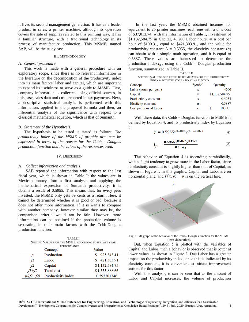
The behavior of Equation 4 is ascending parabolically,

with a slight tendency to grow more in the Labor factor, since

its elasticity constant is slightly higher than that of Capital, as

shown in Figure 1. In this graphic, Capital and Labor are on

horizontal plane, and is on the vertical line.

Fig. 1. 3D graph of the behavior of the Cobb - Douglas function for the MSME

(own elaboration).

But, when Equation 5 is plotted with the variables of

Capital and Labor, then a behavior is observed that is better at

lower values, as shown in Figure 2. Due Labor has a greater

impact on the productivity index, since this is indicated by its

elasticity constant, it is convenient to initiate improvement

actions for this factor.

With this analysis, it can be seen that as the amount of

Labor and Capital increases, the volume of production



increases with a range up to infinity, only limited by the

restrictions of the resources available to the MSME. However,

the productivity index prevents the inappropriate use of

resources, so it is necessary to consider each increment in

terms of its impact on said productivity index.

Fig. 2. 3D graph of the behavior of the productivity index using Cobb -

Douglas function for the MSME (own elaboration).

B. Model Validation

The model validation is through Equation 5, where x is

expressed in hundreds of hours per year, y in thousands of

Mexican pesos, A= 0.5955, α=0.5887, and c=0.1 thousand

Mexican pesos per hour. Eight capital values are established,

from $ 1,000 thousand Mexican pesos, to $ 1,700, with

increases of $ 100. In the same way, 3.7 hundreds of hours

per year are considered up to 7.2, with increments of 0.5 until

to have 8 strata of study; a combination of 64 values is

generated for the different amounts of Capital and Labor.

These results are shown in Table III.

TABLE III

MATRIX OF THE PRODUCTIVITY INDICES CALCULATED FOR DIFFERENT

VALUES OF AMOUNT OF WORK AND CAPITAL (OWN ELABORATION).

The form used to validate the model is through statistical

analysis using hypothesis tests. A sample of 25% of the values

is taken, it is mean, 16 of the 64 productivity indices in Table

III. The cells are listed from 1 to 64 as shown in Table IV,

forming 8 horizontal rows. Two numbers are extracted from

each row using the “randbetween” Excel function; so, to

validate the random numbers that are used in this work, the

test procedure of the , Chi square test, because the generator

is expected to produce discretely distributed numbers evenly.

The frequency observed and expected are located in two

columns, getting of either their differences or errors and

square error. The sum of these square errors is necessary for

Chi-square test, as shown in Table V.

TABLE IV

NUMBERING OF THE MATRIX CELLS FOR THE RANDOM SAMPLE

INSACULATION PROCESS (OWN ELABORATION)

TABLE V

FREQUENCY VALUES EXPECTED AND OBSERVED, AS WELL AS ERRORS

FOR THE TEST OF (OWN ELABORATION).

If the numbers come from a random number generator

that works properly, a uniform discrete distribution must be

manifested, which implies that each of the integers generated

between 1 and 64 must be presented 8 times. Using a 95%

confidence level, that is α = 5%, the null hypothesis is

established as the form of the random number distribution is

the uniform discrete it is not possible to reject it, since Figure

3 shows the eight-step hypothesis-testing procedure for

random numbers in the validation process, as Montgomery

proposes [36].



Fig. 3 The eight-step hypothesis-testing procedure for random numbers in

the validation process (own elaboration).

The selected numbers are in Table VI together with their

Labor, Capital and values.

Once the randomness is confirmed, Table IV is made with

the values of the proposal calculated with Equation 2,

agreeing the results of the productivity index as determined

by Sumanth mathematical expression, that is, production

obtained among the resources used to obtain it. The values of

the mean, standard deviation and variance for each sample

have also been calculated, with which the test of differences

of means for two populations is applied. It is based on the

assumption that both samples should not have a significant

variation when a 95% confidence level is used.

TABLE VI FREQUENCY VALUES EXPECTED AND OBSERVED, AS WELL AS ERRORS FOR

THE TEST (OWN ELABORATION).

To prove that there is no significant difference, a

hypothesis test is performed, following the procedure that

Montgomery establishes [36]. So, using data of Table VI,

with two samples, proposal equation, and Sumanth

mathematical expression, production divided by resources, it

is possible to get values for productivity index for both ways.

Then, the sample 1 has the index productivity by the

proposal, and the sample 2 is with the Sumanth expression.

In every sample, are calculated the means and variances,

considering every sample independent. Now, to test their

significance, the hypothesis test of difference of means is

considered, in which both samples are considered to be equal,

and therefore, their difference is zero. The null hypothesis is

defined bay this condition, the difference between two

samples mean is zero.

Using α = 0.05 as level of significance, the test statistic

is to, since it is not certain that both samples have normal

behavior. Too, it seems reasonable to combine the two sample

variances with a pooled estimator, Sp. The procedure is shown

in the Figure 4, using the eight-step hypothesis-testing

procedure for a Difference in Means of productivity indexes,

by Montgomery.

Fig. 4. The eight-step hypothesis-testing procedure for a Difference in Means

of productivity indexes (own elaboration).

Due, the null hypothesis cannot be rejected, It is verified

that the Equation proposed in (2), is valid and can be used to

calculate and productivity index.

V. CONCLUSIONS

Through this work, it has been found that it is possible to

express the productivity index in terms of the Cobb - Douglas

production function. The advantage of using this expression

in this index is due to finding the factors that affect it, such as

labor and capital, to determine the values that guide MSMEs

to improve this systemic indicator.

Since an analysis of descriptive and inferential statistics,

you can specify the way in which work and capital are

behaving at this time, and decide on strategies that directly

impact a better result in the productivity index. When



comparing this proposed equation with the classic model, it is

concluded that there is no significant difference, so it can be

used in the company.

ACKNOWLEDGMENT

Special thanks are made to the SAB enterprise, especially Mr.

Ramón Bernal (†) for his valuable support in allowing his

company's information to be considered. Likewise, to

CONACYT for the support granted in the realization of this

work, and to ESIME of the IPN, headquarters of the

Doctorate in Systems Engineering. Special thanks to TESCI

for the facilities granted.

REFERENCES

[1] C. Andersson and M. Bellgran. “On the complexity of using performance

measures: Enhancing sustained production improvement capability by

combining OEE and productivity”. Journal of Manufacturing Systems. Vol.

35, pp.144 – 154, 2015.

[2] M. Bellgran and K. Säfsten. “Production development: design and operation

of production systems. London: Springer Verlag, 2010.

[3] A. P. Cusolito and W. Maloney. Productivity Revisited Shifting Paradigms

in Analysis and Policy. International Bank for Reconstruction and

Development / The World Bank, 2018.

[4] M. Martínez. The concept of productivity in economic analysis. Aportes.

Vol. 3, 7, 1998, pp 95 – 118.

[5] D. Sumanth, and M. Dedeoglu. Application of expert systems to

productivity measurement in companies/organizations. Computers industrial

engineers. Vol. 13, No 1-4, 1987, pp.21-25.

[6] D. Sumanth. Total Productivity Management. A systemic and quantitative

approach to compete in quality, price and time. USA: St. Lucie Press.

1998..

[7] P. Sraffa. The works and correspondence of David Ricardo Vol 1. On the

principles of Political economy and Taxation. London: Cambridge

University Press. 1950.

[8] Marx, C. El Capital, Siglo XXI editores, México, España, Argentina, Tomo

I/Vol.2, Cap. XV. 1980.

[9] M. Anteby, and R. Khurana. A new vision. Baker Library. Historical

Collections. Harvard Business Review. (s/f).

[10]W. French and C. Bell. Organizational development: Interventions of

behavioral science for the improvement of the organization. USA: Pearson.

2007.

[11]E. Hernández Laos, Evolución de la productividad total de los factores en la

economía mexicana 1970-1989, México: STPS. 1993.

[12]E. Goldratt and J. Cox. The goal: A Process of Ongoing Improvement. USA:

The North River Press, P. C. 1984

[13]R. Kaplan and R. Cooper. Cost and effect: using integrated systems to drive

profitability and performance. Boston: Harvard Business School Press.

1998.

[14]I. Bernolak. Effective measurement and successful elements of company

productivity: the basis of competitiveness and world prosperity. Int J Prod

Econ; Vol. 52, 1 – 2, 1997, pp203 – 213.

[15]T. Grünberg. Performance improvement: a method to support performance

improvement in industrial operations. Sweden: Dept of production

Engineering, Royal Institute of Technology. 2007.

[16]P. White. A survey and taxonomy of strategy – related performance

measures for manufacturing. Int J Operation Production Management, vol

16, 3, 1996, pp 42 – 61.

[17]H. Huang, J. Dismukes, J. Shi, and E Robinson. Manufacturing system

modeling for productivity improvement. Journal manufacturing Systems,

Vol. 21, 4, 2002, pp. 249 – 259.

[18]G. Chakravarthy, P. Keller, B. Wheeler and S. Van Oss. A methodology for

measuring reporting, navigating and analyzing overall equipment efficiency

(OEE). Proceedings from IEEE/SEMI advanced semiconductor

manufacturing conference. 2007, pp 3026 – 3012.

[19]C. Hulten. Total Factor Productivity: A Short Biography. New

Developments in Productivity Analysis, Chicago, University of Chicago

Press, 1–47. 2001.

[20]M. Nishimizu and J. Page. Total Factor Productivity Growth, Technological

Progress and Technical Efficiency Change: Dimensions of Productivity

Change in Yugoslavia, 1965–1978, Economic Journal, Vol. 92, 368, 1982,

pp. 920–936.

[21]D. Caves, L. Christensen and W. Diewert (1982). The Economic Theory of

Index Numbers and the Measurement of Inputs, Outputs and Productivity,

Econometrica. Vol. 50, 6, 1982, pp 1393 – 1414.

[22]K. Kerstens, Z, Shen and I: Van de Woestyne. Comparing Luenberger and

Luenberger-Hicks-Moorsteen Productivity Indicators: How Well is Total

Factor Productivity Approximated? International Journal of Production

Economics. Vol. 195, pp. 311 – 318, January 2018.

[23]R. Färe, S. Grosskopf, M. Norris, and Z. Zhang. Productivity Growth,

Technical Progress, and Efficiency Change in Industrialized Countries,

American Economic Review. Vol 84, 1, 1994, pp. 66 – 83.

[24]S. Atkinson, C. Cornwell, O. Honerkamp. Measuring and Decomposing

Productivity Change: Stochastic Distance Function Estimation Versus Data

Envelopment Analysis. Journal of Business and Economic Statistics. Vol.

21, 2. 2003, pp. 284 – 294.

[25]H. Bjurek. The Malmquist Total Factor Productivity Index. Scandinavian

Journal of Economics. Vol. 98, 2. 1996, pp. 303 – 313.

[26]R. Färe, S. Grosskopf and P. Roos. On Two Definitions of Productivity,

Economics Letters. Vol. 53, 3. 1996, pp. 269 - 274.

[27]R. Chambers, R. Färe and S. Grosskopf. Input and Output Indicators. Index

Numbers: Essays in Honour of Sten Malmquist. Boston, Kluwer, pp. 241-

271. 1998.

[28]R.Chambers, Exact Nonradial Input, Output, and Productivity

Measurement, Economic Theory. Vol. 20, 4. 2002, pp. 751 – 765.

[29]W. Briec, K. Kerstens, and P. Vanden Eeckaut. Non-convex Technologies

and Cost Functions: Definitions, Duality and Nonparametric Tests of

Convexity. Journal of Economics. Vol. 81, 2. 2004, pp. 155-192.

[30]C. Cobb and P. Douglas. A theory of Production. The American Economic

Review, Vol. 18, No. 1, Supplement, Papers and Proceedings of the Fortieth

Annual Meeting of the American Economic. 1928, pp. 139 - 165.

[31]R. Solow. Technical Change and the Aggregate Production Function. The

Review of Economics and Statistics. Vol. 39, No. 3. 1957, pp. 312320.

[32]H. Arrow, B. Chenery, B. Minhas, and R. Solow. Capital -Labor

Substitution and Economic Efficiency. The Review of Economics and

Statistics, Vol. 43, No. 3, 1961, pp. 225 - 250.

[33]X. Wang and Y. Fu. Some Characterizations of the Cobb-Douglas and CES

Production Functions in Microeconomics. Hindawi Publishing Corporation.

Abstract and Applied Analysis Vol. 2013, Article ID 761832, 6 pages,

2013.

[34]J. Cadil, K. Vltsaka, I. Krejci, D. Hartman and M. Brabec. Aggregate

production function and income identity– empirical analysis. International

Journal of Economic Sciences. Vol. VI, No. 1, 2017.

[35]INEGI. Encuesta nacional sobre productividad y competitividad de las

Micro, Pequeñas y Medianas Empresas. 2016.

[36]D. Montgomery and G. Runger. Applied statistics and probability for

engineers. USA: John Wiley & Sons.

Decomposing the productivity index in its main factors, applied ...

Documents

Transcript of Decomposing the productivity index in its main factors, applied ...