1 23

Journal of Productivity Analysis ISSN 0895-562XVolume 43Number 3 J Prod Anal (2015) 43:281-293DOI 10.1007/s11123-015-0437-z

Decomposing the productivity differencesbetween hospitals in the Nordic countries

Sverre A. C. Kittelsen, Benny AdamWinsnes, Kjartan S. Anthun, FannyGoude, Øyvind Hope, Unto Häkkinen,Birgitte Kalseth, et al.

1 23

Your article is published under the Creative

Commons Attribution license which allows

users to read, copy, distribute and make

derivative works, as long as the author of

the original work is cited. You may self-

archive this article on your own website, an

institutional repository or funder’s repository

and make it publicly available immediately.

Decomposing the productivity differences between hospitalsin the Nordic countries

Sverre A. C. Kittelsen • Benny Adam Winsnes • Kjartan S. Anthun •

Fanny Goude • Øyvind Hope • Unto Hakkinen • Birgitte Kalseth •

Jannie Kilsmark • Emma Medin • Clas Rehnberg • Hanna Ratto

Published online: 26 February 2015

� The Author(s) 2015. This article is published with open access at Springerlink.com

Abstract Previous studies indicate that Finnish hospitals

have significantly higher productivity than in the other

Nordic countries. Since there is no natural pairing of ob-

servations between countries we estimate productivity

levels rather than a Malmquist index of productivity dif-

ferences, using a pooled set of all observations as refer-

ence. We decompose the productivity levels into technical

efficiency, scale efficiency and country specific possibility

sets (technical frontiers). Data have been collected on op-

erating costs and patient discharges in each diagnosis re-

lated group for all hospitals in the four major Nordic

countries, Denmark, Finland, Norway and Sweden. We

find that there are small differences in scale and technical

efficiency between countries, but large differences in pro-

duction possibilities (frontier position). The country-

specific Finnish frontier is the main source of the Finnish

productivity advantage. There is no statistically significant

association between efficiency and status as a university or

capital city hospital. The results are robust to the choice of

bootstrapped data envelopment analysis or stochastic

frontier analysis as frontier estimation methodology.

Keywords Productivity � Hospitals � Efficiency � DEA �SFA

JEL Classification C14 � I12

1 Introduction

In previous studies (Kittelsen et al. 2009; Kittelsen et al.

2008; Linna et al. 2006, 2010) one has found persistent

evidence that the somatic hospitals in Finland have a sig-

nificantly higher average productivity level than hospitals

in the other major Nordic countries (Sweden, Denmark and

Norway).1 These results indicate that there could be sig-

nificant gains from learning from the Finnish example,

especially in the other Nordic countries, but potentially

also in other similar countries. The policy implications

could however be very different depending on the source of

the productivity differences. This paper extends earlier

work by, (1) decomposing the productivity differences into

those that stem from technical efficiency, scale efficiency

and differences in the possibility set (the technology) be-

tween periods and countries, and (2) exploring the statis-

tical associations between the technical efficiency and

various hospital-level indicators such as case-mix, outpa-

tient share and status as a university or capital city hospital.

S. A. C. Kittelsen (&) � B. A. Winsnes

Frisch Centre, Oslo, Norway

e-mail: sverre.kittelsen@frisch.uio.no

B. A. Winsnes

Oslo University Hospital, Oslo, Norway

K. S. Anthun � Ø. Hope � B. KalsethSINTEF, Trondheim, Norway

F. Goude � E. Medin � C. RehnbergKarolinska Institutet, Stockholm, Sweden

U. Hakkinen � H. RattoNational Institute for Health and Welfare – THL, Helsinki,

Finland

J. Kilsmark

Danish Institute of Health Research, Copenhagen, Denmark

1 Although the Nordic countries also include Iceland, comparable

data on Icelandic hospitals have not been available. In this article we

will therefore use the term Nordic countries about the four largest

countries.

123

J Prod Anal (2015) 43:281–293

DOI 10.1007/s11123-015-0437-z

Finally, (3) we examine the robustness of the results to the

choice of method.

International comparisons of productivity and efficiency

of hospitals are few, primarily because of the difficulty of

getting comparable data on output (Derveaux et al. 2004;

Linna et al. 2006; Medin et al. 2013; Mobley and Mag-

nussen 1998; Steinmann et al. 2004; Varabyova and

Schreyogg 2013). Such analyses often find quite substantial

differences in performance between countries. Differences

may be due to the dissimilar hospital structures and fi-

nancing schemes, e.g. whether hospitals exploit economies

of scale, have an optimal level of specialisation, or face

high-powered incentive schemes that would encourage

efficient production. Differences may also result from

methodological problems. Cross-national analyses are

often based on data sets that only to a limited extent are

comparable—in the sense that inputs and outputs are de-

fined and measured differently across countries. Our

comparison gains validity from the existence of a Nordic

standard for diagnosis related groups (DRGs) (Linna and

Virtanen 2011). As described in the data section, the

structure of the hospital sectors are broadly similar in the

Nordic countries and the main differences are handled by

assuming country specific production frontiers and vari-

ables in the analysis. It is, however, well known that the

way we measure hospital performance may influence the

empirical efficiency measures (Halsteinli et al. 2010;

Magnussen 1996). In this article we will therefore use both

the non-parametric data envelopment analysis (DEA)

method and the stochastic frontier analysis (SFA) method,

and provide evidence of the robustness of our results.

2 Methods

2.1 Efficiency and productivity

Efficiency and productivity are often used interchangeably.

In our terminology productivity denotes the ratio of inputs

and outputs, while efficiency is a relative measure com-

paring actual to optimal productivity. Since productivity is

a ratio, it is by definition a concept that is homogenous of

degree zero in inputs and outputs, i.e. a constant returns to

scale (CRS) concept. This does not imply that the under-

lying technology is CRS. Indeed, the technology may well

exhibit variable returns to scale (VRS), and equally effi-

cient units may well have different productivity depending

on their scale of operation, as well as other differences in

their production possibility sets.

Most productivity indexes rely on prices to weigh sev-

eral inputs and/or outputs, but building on Malmquist

(1953), Caves et al. (1982) recognised that (lacking prices)

one can instead use properties of the production function,

i.e. rates of transformation and substitution along the

frontier of the production possibility set, for an implicit

weighting of inputs and outputs. We will use the term

technical productivity to denote such a ratio of inputs to

outputs where the weights are not input and output prices

but rather derived from the estimated technologies.

This analysis departs from Farrell (1957) who defined

(the input-oriented) technical efficiency as:

ETtc

i ¼ Min h ðhxi; yiÞ 2 Ttcjf g ð1Þ

Where ðxi; yiÞ is the input/output vector for an observation

i, and Ttc is the technology or production possibility set for

year t and country c. For an input/output-vector ðx; yÞ to be

part of the production possibility set, we need to be able to

produce y using x. As shown in Fare and Lovell (1978),

this is equivalent to the inverse of the Shephard (1970)

input distance function.

If there are variable returns to scale, Farrell’s measure of

technical efficiency depends on the size of the observation,

so that we can account for (dis)economies of scale. The

measure of technical productivity can, following Førsund

and Hjalmarsson (1987), be defined by rescaling inputs and

outputs:2

EkTtc

i ¼ Minh;k h ðhxi; yiÞj 2 kTtcf g; ð2Þ

where the convex cone of the technology kTtc, contains allinput–output combinations that are a proportionate rescal-

ing of a feasible point in the technology set Ttc. While this

is formally identical to a ‘‘CRS technical efficiency’’

measure, our definition here is instead that the reference

surface is a homogenous envelopment of the underlying

technology. This is the same assumption normally used in

Malmquist indices of productivity change, see e.g. Grifell-

Tatje and Lovell (1995).

Furthermore, it is not necessary to assume that the

technologies of different countries and time periods are

identical in order to compare productivity, as long as one

has a common reference set. It is common to use a specific

(base) time period as a reference, as in Berg et al. (1992):

Mtcij ¼

EkTtc

i

EkTtc

j

; ð3Þ

which compares the productivity of two observations i and

j using a fixed time period t as the reference, even if the

observations i and j are from different time periods. A

widespread alternative method is to construct geometric

averages of indices based on consecutive time periods, as

2 Førsund and Hjalmarsson (1987) used the symbols e1 for input

technical efficiency, as did Farrell (1957), and e3 for technical

productivity which they call ‘‘overall scale efficiency’’.

282 J Prod Anal (2015) 43:281–293

123

in Fare et al. (1994), which avoids the arbitrary choice of

reference period t, but instead introduces a circularity

problem. The approach followed here is instead to use

information from all time periods for the country specific

productivity reference:

Tc ¼ Envt

Ttcð Þ ð4Þ

where Env() is the convex envelopment of the time specific

technologies. Furthermore, to compare the productivity

across countries we will need the envelopment of all time

and country specific technologies:

T ¼ Envc

Tcð Þ ð5Þ

The reference sets (4) and (5) are not themselves tech-

nologies, only envelopment of technologies, as are the

convex cones (rescaled sets) kTc; k�T . Analogous to (2), it isthen possible to define the productivity levels relative to the

country specific references and the pooled references as

EkTC

i and respectively.

The country c specific Malmquist index of productivity

change over time can then be defined as.

Mcij ¼

EkTc

i

EkTc

j

; ð6Þ

which normally is reported for two observation i and j of

the same unit at two points in time. In this analysis we are

primarily concerned with comparing observations from

different units in different countries, and there is no natural

pairing of i and j. Edvardsen and Førsund (2003) develop

and report geometric means of Malmquist indices between

a unit in one country and all units in another country. We

will instead take a simpler approach and report the pro-

ductivity and efficiency levels of each unit and their

country means.

2.2 Decomposition

As discussed e.g. in Fried et al. (2008), the Malmquist

index can be decomposed in various ways, where the ori-

ginal decomposition is into frontier shift and efficiency

change. When working in productivity and efficiency

levels, the starting point is instead the decomposition of

technical productivity into technical efficiency and scale

efficiency:

EkTtc

i ¼ ETtc

i

EkTtc

i

ETtc

i

¼ ðTPi ¼ TEi � SEiÞ; ð7Þ

where the parenthesis denotes the conventional way of

writing the technical productivity (TP) as the product of

technical efficiency (TEi ¼ ETtc

i ) and scale efficiency

(SEi ¼ EkTtci

ETtc

i

). By including the possibility of comparing

productivity across both time and countries, this decom-

position naturally expands into:

Ek �Ti ¼ ETtc

i

EkTtc

i

ETtc

i

EkTc

i

EkTtc

i

Ek �Ti

EkTc

i

¼ ðTTPi ¼ TEi � SEi � PPi � CPiÞ;ð8Þ

where we have decomposed the now total technical pro-

ductivity (TTP) into technical efficiency (TEi ¼ ETtc

i ), scale

efficiency (SEi ¼ EkTtci

ETtc

i

), period productivity (PPi ¼ EkTci

EkTtci

)

and country productivity (CPi ¼ Ek �Ti

EkTci

). Each of these is

specific to the observation i.

Note that dividing this decomposition for two observa-

tions of one unit at different points in time, and ignoring

the country productivity, one gets the common Malmquist

decomposition of technical efficiency change, scale effi-

ciency change and frontier change. As with the Malmquist

index, the decomposition is not easily extended to com-

parisons between countries, as there is no natural pairing of

observations. Asmild and Tam (2007) develop a global

index of frontier shifts which they note would be useful for

international comparisons, but does not extend this to a full

decomposition.

These concepts are illustrated in Fig. 1, where we ignore

the time dimension and concentrate on country differences.

For an observation A in country 1 with a production pos-

sibility set bounded by the production function Frontier 1,

we can define the technical efficiency by (1) above as the

ratio BC/BA of necessary inputs to actual inputs for a given

output. The productivity of A is the slope of the diagonal

OA, but we can normalise this in (2) by comparing it to the

maximal productivity given by the slope of the diagonal

OD. The technical productivity of A is then the ratio BD/

BA. Using the definition implicit in (7), scale efficiency is

Fig. 1 The components of hospital total technical productivity in

input–output space. For observation A in country 1, Total technical

productivity (TTP) = BE/BA, Technical efficiency (TE) = BC/BA,

Technical productivity (TP) = BD/BA, Scale efficiency (SE) = BD/

BC and Country productivity (CP) = BE/BD

J Prod Anal (2015) 43:281–293 283

123

BD/BC. Assume that country 2 has a production possibility

set bounded by Frontier 2, and that the maximal produc-

tivity of country 2 given by the slope OE is also the

maximal for all countries, i.e. bounding the convex cone of

all possibility sets k�T . This slope OE will serve as the

reference for the total technical productivity in (8), which

for observation A is given by BE/BA. The country pro-

ductivity for observation A is then the ratio BE/BD.

With only one input and one output as in Fig. 1, one

country will define the reference and all observations in each

country will have the same country productivity. With two

outputs as in Fig. 2, the convex cone of each country’s

frontier kTC can be drawn as the curved lines for a given levelof the single input. The convex cone of all the country fron-

tiers k�T is represented by the dashed line which serves as the

reference for total technical productivity defined in (8). If the

country frontiers cross as in this example, the country pro-

ductivities will depend on the output mix of the observation.

2.3 Cost efficiency and productivity

Finally note that since we have only one input in our data,

cost minimization for a given input price is formally

equivalent to input minimization. Thus cost efficiency,

which is defined as the ratio of necessary costs to input costs,

is also equivalent to technical efficiency. The decomposition

of productivity and the Malmquist index is most often

shown in terms of technical efficiency and technical pro-

ductivity but could easily have been developed in terms of

cost efficiency and cost productivity. Note that in the general

multi-input case the numbers will differ in technical and cost

productivity decompositions, but in our one-input case, the

actual numbers will be identical.3 Thus, we may view the

terms technical efficiency and cost efficiency as equivalent

in discussing the results in this analysis.

2.4 Estimation method

The DEA and SFA methodologies build upon the same

basic production theory basis. In both cases one estimates

the production frontier (the boundry of the production

possibility set or technology) or the dual formulation in the

cost frontier, but the methods are quite different in their

approach to estimating the frontiers and in the measures

that are easily calculated and therefore commonly reported

in the literature (Coelli et al. 2005; Fried et al. 2008). While

the major strengths of DEA has been the lack of strong

assumptions beyond those basic in theory (free disposal

and convexity) and the fact that the frontier fits closely

around the data, SFA has had a superior ability to handle

the prescense of measurement error and to perform statis-

tical inference. The latter shortcoming of DEA has been

allieviated somewhat with the bootstrapping techniques

introduced by Simar and Wilson (1998, 2000).

In our data there are good reasons to choose either

method. While the prescense of measurement error is

probably limited for those activities that are actually

measured, there is a strong case for omitted variable (i.e.

quality) bias that may be more severe in DEA. The DEA

method can easily estimate the country specific frontiers

without strong assumptions, thereby making country dif-

ferences dependent on the input–output mix, while the SFA

formulation generally introduces a constant difference be-

tween country frontiers. The prescense of country dummies

in SFA implies however, that information from other

countries are used to increase the precision of the estimates

and therefore the power of the statistical tests.

In the DEA analysis the frontiers have been estimated

using the homogenous bootstrapping algorithm from Simar

and Wilson (1998), while the second stage analysis of the

statistical association of technical efficiency and the envi-

ronmental variables has been conducted using ordinary

least square (OLS) regressions. The SFA analysis has used

the simultanous estimation of the frontier component and

the (in)efficiency component proposed in Battese and

Coelli (1995).4

2.5 Data

Data has been collected for inputs and outputs of all public

sector acute somatic hospitals. The hospital structure of the

four Nordic countries is broadly similar. The structure

Fig. 2 The components of hospital total technical productivity in

output–output space. For observation A in country 1, Total technical

productivity (TTP) = OA/OD, Technical efficiency (TE) = OA/OC,

and CP Country productivity (CP) = OC/OD

3 In the general case with more than one output, cost efficiency and

technical efficiency would be equal only if all units are allocatively

efficient.

4 The DEA bootstrap estimations have been done in FrischNonPara-

metric, while second stage regressions and the SFA analysis has been

done in STATA 12 (StataCorp 2011).

284 J Prod Anal (2015) 43:281–293

123

consists of mostly publicly financed and governed somatic

hospitals with only a very few commercial hospitals, al-

most no specialization in medicine, surgical, cancer care

etc., and no specialization to cater for specific groups such

as veterans/military, childrens hospitals etc. Only in Fin-

land are there a number of Health Centres with inpatient

beds that serve less severe patients, and these are excluded

from our analysis, as are the few commercial hospitals.

Some non-profit private hospitals that are under contract

with the public sector are included, however. The data

includes almost the whole population of somatic hospitals

in the Nordic countries, which due to a natural geographic

monopoly usually serve a catchment area covering all

residents. Differences in patient mix will mainly reflect

demographic differences across the geographic areas, fac-

tors that are partly included in the second stage regression.

While the hospital sectors in all four countries are based

on public ownership and tax-based financing, there are

administrative and incentive differences. In Norway, all

hospitals are state-owned, but the provision of hospital

services is delegated to five (reduced to four during 2007)

regional health enterprises (RHF). Each of these own be-

tween four and thirteen health enterprices (HF) which are

the administrative units of hospital production, but a

number of the health enterprises are multi-location insti-

tutions and the extent of integration between the actual

physical hospitals varies considerably. In Denmark and

Sweden hospitals are owned by the intermediate govern-

ment level regions or counties (‘‘regioner’’ and ‘‘landst-

ing’’), but single-location hospitals are still mainly separate

institutions. The Finnish hospital sector is owned by health

districts that are federations of municipalities. Norway and

some counties in Sweden use partial activity based fi-

nancing (ABF) based on the DRG-system, but with most of

the payment made by block grants. In Denmark ABF was

used only to a limited extent during the period. The Finnish

hospital districts use various case-based classification sys-

tems (including DRGs) as a method of collecting payments

from municipalities, but the Finnish payment system does

not create similar incentives as ABF used in other countries

(Kautiainen et al. 2011). However, since hospitals can be

described by the same input–output vectors the produc-

tivity of the hospitals in our sample should be comparable

even though they may not face the same production pos-

sibility sets.

Inputs are measured as operating costs, which for rea-

sons of data availability are exclusive of capital costs. It

was not possible to get ethical permission for the use of

data for 2007 in Sweden. The Swedish data is further

limited by the lack of cost information at the hospital level,

nescessitating the use of the administrative county

(‘‘landsting’’) level as the unit of observation, each en-

compassing from one to five physical hospitals. The

difference in level of observational unit between the

countries (counties, health enterprises or hospitals) is one

of the reasons why we estimate different technologies or

production possibility sets in each country.

Since we do not have data on teaching and research

output, the associated costs are also excluded. Costs are

initially measured in nominal prices in each country’s na-

tional currency, but to estimate productivity and efficiency

one needs a comparable measure of ‘‘real costs’’ that is

corrected for differences in input prices.

To harmonize the cost level between the four countries

over time we have constructed wage indices for physicians,

nurses and four other groups of hospital staff, as well as

one for ‘‘other resources’’. This removes a major source of

nominal cost and productivity differences between the

countries, a difference that can not be influenced by the

hospitals themselves, nor by the hospital sector as a whole.

The wage indices are based on official wage date and in-

clude all personnel costs, i.e. pension costs and indirect

labour taxes (Kittelsen et al. 2009). The index for ‘‘other

resources’’ is the purchaser parity corrected GDP price

index from OECD. The indices are weighted together with

Norwegian cost shares in 2007. Thus we construct a

Paasche-index using Norway in 2007 as reference point.

Note that this represents an approximation, the index will

only hold exactly if the relative use of inputs is constant

over time and country.

Outputs are measured by using the Nordic version of the

diagnosis related groups (DRGs). Each hospital discharge

is assigned to one of about 500 DRGs on the basis of di-

agnosis and procedure codes. When activity is measured by

DRG-points, discharges are weighed by a factor that is an

estimate of the average cost of patients in that DRG. Thus

the weighting is implicitly by patient severity or com-

plexity as reflected in average costs. We define three broad

output categories; inpatient care, day care and outpatient

visits. Within each category patients are weighted with the

Norwegian cost weights from 2007, where the weights are

calculated from accounting data from a sample of major

Norwegian hospitals.5 Outpatient visits were not weighted.

Considerable work has gone into reducing problems asso-

ciated with differences in coding practice, including mov-

ing patients between DRGs, eliminating double counting

etc. The problem of DRG-creep, where hospitals that face

strong incentives to upcode from simple to more severe

DRGs based on the number of co-morbidities has been

reduced by aggregating these groups. In the DEA analysis

this had the effect of reducing the mean productivity level

5 From a common initial starting point, the Danish DRG system has

diverged significantly from the other Nordic systems after 2002.

Danish DRG-weights were used for the specific Danish DRG groups,

while the level was normalized using those DRG-groups that were

common in the two systems.

J Prod Anal (2015) 43:281–293 285

123

of Norwegian hospitals by 2 % points while the other

countries were not affected, presumably because activity

based financing is a more entrenched feature in Norway.

In addition to the single input and the three outputs, we

have collected data for some characteristics that vary be-

tween hospitals within each country or over time, and that

may be associated with efficiency. These include dummies

for university hospital status which may capture any scope

effects of teaching and research. This must be effects be-

yond the costs attributed to these activities which are al-

ready deducted from the cost variable, but the sign of the

effect on productivity would depend on whether there are

economies or diseconomies of scope between patient

treatment and teaching and research. University hospitals

may also have a more severe mix of patients within each

DRG-group, which may bias estimated productivity

downwards. The main case-mix effect should presumably

already be captured by the DRG weighting scheeme.

University hospitals are located in major cities. We also

include a dummy for capital city hospitals, which may have

a less favourable patient mix due to the socio-economic

composition of the catchment area, so that one would ex-

pect the capital city hospitals to have lower productivity.

However, university and capital city hospitals could also

have lower costs due to shorter travelling times and a

greater potential for daypatient or outpatient treatment, so

the net effect is not obvious. Allthough all hospitals are

located in towns, the university and capital city dummies

should capture the main differences that may be due to

urban or rural catchment areas.

The case-mix index (CMI) is calculated as the average

DRG-weight per patient, and may again capture patient

severity if the average severity within each DRG-group is

correlated with the average severity as measured by the

DRG-system itself, in which case one should expect a high

CMI to be correlated with low productivity. The length of

stay (LOS) deviation variable is calculated as the DRG-

weighted average LOS in each DRG for each hospital di-

vided by the average LOS in each DRG across the whole

sample (i.e. expected LOS). Again this could capture dif-

ferences in severity within each DRG group, but may also

indicate excessive, and therefore inefficient, LOS. Finally,

the outpatient share is an indicator of diffences in treatment

practices across hospitals, where a high outpatient share

may indicate lower costs per discharge. These variables are

collectively termed ‘‘environmental variables’’, although

they are not always strictly exogenous to the hospital.

In earlier studies, the extent of activity based financing

(ABF) has been an important explanatory variable, but in

the period covered by our dataset there has been too little

variation in ABF within each country. If a variable is or

highly correlated with the country then it is not possible to

statistically separate the effect from other country specific

fixed effects. This also holds for structural variables such as

ownership structure, financing system etc. Travelling time

to hospital can be an important cost driver but is not in-

cluded here due to lack of data.6 Finally, no indicators of

the quality of treatment have been available for this

analysis.

Table 1 shows the distribution of hospitals between

countries and summary statistics for the varibles in the

analyses. When interpreting the size of the Swedish ob-

servations, remember that these are not physical hospitals

but the larger administrative ‘‘Landsting’’ units. To a lesser

extent, the Norwegian observations of health enterprises

can also encompass several physical hospitals.

3 Results

3.1 DEA results

In the DEA analysis, the total technical productivity level

is calculated with reference to a homogenous frontier es-

timated from the pooled set of observations for all coun-

tries and periods. Figure 3 show that the considerable

productivity superiority of the Finnish hospitals found in

previous studies is also present and highly significant in

this dataset. The other Nordic countries are in some periods

significantly different from each other, but in general have

a similar productivity level.

Figure 3 also shows a slight time trend towards declin-

ing productivity. However, the DEA bootstrap tests did not

reject a hypothesis of constant technology across time pe-

riods. This implies that we can ignore the time dimension

and report the simpler three-way decomposition

Ek �Ti ¼ ETc

i

EkTc

i

ETc

i

Ek �Ti

EkTc

i

¼ ðTTPi ¼ TEi � SEi � CPiÞ; ð9Þ

The productivity estimates for the individual observa-

tions are shown in Fig. 4. The hypothetical full produc-

tivity frontier is represented by productivity equal to 1.0,

but since these numbers are bootstrapped estimates no

observation is on the frontier. Clearly, the Finnish pro-

ductivity level is consistently higher, with all Finnish ob-

servations doing better than most observations in Denmark

and Norway and almost all in Sweden. Confidence inter-

vals are quite narrow so this is a robust result. In all

countries one can see that smaller units tend to be more

productive, while comparisons between countries are

6 While we do not have data for travelling time in Denmark, we have

calculated the average travelling time for the catchment area of

emergency hospitals in the other countries. A separate analysis

reported in Kalseth et al. (2011) indicate that travelling time can

explain some of the cost differences between the Norwegian regions,

but not a significant amount of the differences between countries.

286 J Prod Anal (2015) 43:281–293

123

confounded by the fact that the Swedish units are not

hospitals but observations on the administrative ‘‘Landst-

ing’’ level.

Table 2 reports the mean country productivity results

and its decomposition. The first line reports the of pro-

ductivity of each country’s hospital sector relative to the

Table 1 Descriptive statistics. Observation means and SD

Variable Finland Sweden Denmark Norway Total

Observation type Hospital Landsting/County Hospital Health enterprise

Number of observations 96 40 105 75 316

Period 2005–2007 2005–2006 2005–2007 2005–2007

Variables in production frontier function (deterministic part)

Real Costs in billion NOK# 1112 4812 1516 1864 1893

SD 1563 5178 1167 1248 2488

Outpatient visits 150,128 368,134 178,620 129,609 182,321

SD 170,646 445,542 125,012 70,008 212,219

DRG points inpatients 22,516 65,262 22,517 31,447 30,047

SD 27,834 68,200 17,647 18,414 34,440

DRG points daypatients 3119 18,000 2651 4044 5067

SD 4092 18,207 2028 2532 8576

Variables in SFA efficiency part or DEA second stage (environmental variables)

University hospital dummy 0.156 0.250 0.381 0.200 0.253

SD 0.365 0.439 0.488 0.403 0.436

Capital city dummy 0.031 0.050 0.257 0.160 0.139

SD 0.175 0.221 0.439 0.369 0.347

Case mix index DRG patients 0.848 0.655 0.915 0.918 0.862

SD 0.089 0.096 0.166 0.083 0.146

Length of stay deviation 0.968 1.118 1.017 0.859 0.977

SD 0.092 0.111 0.193 0.082 0.156

Outpatient share 0.841 0.731 0.865 0.773 0.819

SD 0.028 0.049 0.044 0.026 0.061

# 2007 price level

Fig. 3 DEA bootstrapped

productivity estimates by

country and year with common

reference frontier. Mean of

observations and 95 % CI

J Prod Anal (2015) 43:281–293 287

123

envelopment of the bootstrapped estimates of the country-

specific production possibility sets, i.e. an estimate largely

based on pooling the best hospitals. While Finland has an

average productivity of around 80 % measured relative to

the pooled frontier, the decomposition reveals that this is

wholly due to lack of scale efficiency and technical effi-

ciency, which are at around 90 % each. The country pro-

ductivity mean is almost precisely 100 %, which means

that it is the Finnish hospitals that define the pooled ref-

erence frontier alone.

For Sweden and Norway the picture is quite different;

here the country productivity is the major component in the

lack of total productivity. In fact, the cost efficiency and

scale efficiency components are quite similar for Finland,

Norway and Sweden. This implies that the hospitals in each

country has a similar dispersion from the best to the worst

performers both in terms of technical and scale efficiencies,

but that the best performing hospitals in Norway and

Sweden are significantly less productive than the best

performers in Finland.

Denmark is in between, with significantly higher coun-

try productivity than Sweden and Norway, but still lagging

far behind Finland. On the other hand, Denmark has clearly

the lowest technical efficiency level of the Nordic coun-

tries, which means that the dispersion behind the frontier is

largest in Denmark.

Fig. 4 Hecksher–Salter diagram of DEA bootstrapped total technical productivity estimates with pooled common reference frontier. Height of

each bar is productivity estimate for each observation with 95 % CI, and width is proportional to the observation size measured by real costs

Table 2 Mean bootstrapped productivity in each country as measured against the pooled reference frontier in DEA

Finland Sweden Denmark Norway

Productivity with pooled reference frontier,

TPP

79.1 % (77.0–81.0) 52.6 % (49.8–54.2) 57.7 % (55.4–59.6) 56.6 % (53.0–58.6)

Decomposition of productivity:

• Productivity of country specific frontier, CP 100.0 % (99.8–100.0) 65.1 % (62.3–68.7) 78.5 % (75.8–81.4) 68.6 % (66.1–72.7)

• Scale efficiency, SE 89.7 % (87.8–91.8) 94.3 % (91.9–96.3) 93.7 % (91.9–95.2) 94.2 % (93.1–95.1)

• Technical efficiency, TE 89.8 % (88.9–90.6) 84.1 % (81.7–86.2) 77.1 % (75.4–78.6) 89.7 % (88.6–90.6)

Scale elasticity 0.935 (0.917–0.956) 1.137 (1.000–1.255) 0.940 (0.911–0.982) 0.941 (0.884–0.982)

Decomposition of total technical productivity into productivity of country specific frontier, scale efficiency and technical efficiency respectively.

The mean scale elasticity is also shown

Geometric mean with 95 % CI for observations in each country

288 J Prod Anal (2015) 43:281–293

123

Table 2 also reports the scale elasticities in the last line.

Scale properties can be different across geographical units,

as also found in a study on hospitals in two Canadian pro-

vinces by Asmild et al. (2013). Since the DEA numbers are

based on separate frontier estimates for each country, the

fact that the units are of a different nature represents no

theoretical problem but must be reflected in the interpreta-

tion of the results. For Finland, Denmark and Norway,

where the units are hospitals or low-level health enterprises,

the scale elasticities below 1 indicate decreasing returns to

scale on average, a result that is often found in estimates of

hospital scale properties. Thus, optimal size is smaller than

the median size. For Sweden, however, the scale elasticity is

larger than one, although only just significantly. Thus, even

though the units of observation are clearly larger in Sweden,

the optimal size is even larger. The natural interpretation of

this paradox is that while the optimal size of a hospital is

quite small, the optimal size of an administrative region (or

purchaser), such as the Swedish Landsting, is quite large. Of

course, other national differences that are not captured by

our variables may also explain this result.

3.2 SFA results

The testing tree for the SFA model is shown in Table 3.

The formulation by Battese and Coelli (1995) implies that

factors that determine the position of the frontier function

in the deterministic part of the equation are estimated

Table 3 Simplified test tree in the SFA analysis

Log-likelihood ratio Critical value (df) Result

Should country enter the frontier function? 287.952 7.05 (3) Yes

Is translog better than Cobb–Douglas? 42.892 11.91 (6) Yes

Should year enter frontier function? 2.798 5.14 (2) No

Should environmental variables enter efficiency term? 22.867 10.37 (5) Yes

Should country enter efficiency term? 57.751 7.05 (3) Yes

Should year enter efficiency term? 1.821 5.14 (2) No

The Log-likelihood ratio indicator is distributed as v2 with degrees of freedom equal to the number of additional variables

Table 4 Marginal normalized effects on productivity in SFA and DEA, 95 % CI

Parameter SFA DEA

Frontier (deterministic

component)

Efficiency

component

Frontier

distance

Technical efficiency in

second stage regression

Finland 0.300*** 0.049 0.322*** -0.029

(0.233–0.361) (-0.085–0.183) (0.295–0.370) (-0.083–0.025)

Sweden 0.071 -0.024 -0.021 -0.004

(-0.020–0.154) (-0.085–0.037) (-0.068–0.061) (-0.072–0.064)

Denmark 0.208*** -0.118*** 0.050*** -0.160***

(0.132–0.277) (-0.174–(-0.062)) (0.010–0.094) (-0.246–(-0.075))

Outpatient share 0.658*** 0.666**

(0.259–1.057) (0.014–1.319)

Length of stay deviation -0.063 -0.138**

(-0.142–0.015) (-0.263–(-0.013))

Case mix index -0.048 -0.064

(-0.160–0.064) (-0.204–0.075)

Capital city dummy 0.030 0.040

(-0.015–0.075) (-0.021–1.101)

University hospital dummy –0.010 0.012

(-0.049–0.029) (-0.040–0.064)

Constant -0.216 0.533**

(-0.504–0.072) (0.104–1.002)

*, **, *** Significant coefficients at 10, 5 and 1 % level respectively. Reference units are hospitals in Norway in 2007 that are not in the capital

and not university hospitals. The reference unit in SFA has a technical efficiency estimate of 0.9176. In the DEA model the distance between the

frontiers is measured at the average product mix of Norwegian hospitals

J Prod Anal (2015) 43:281–293 289

123

simultaneously as the variables in the ‘‘explanation’’ of the

inefficiency term. Right hand side variables can potentially

enter both components.

Clearly, the strongest result is that country dummies

should enter the frontier term. This implies that there are

highly significant fixed country effects that are not ex-

plained by any of our other variables, and that by the as-

sumptions of the model specification the country dummy

should primarily shift the frontier term. The functional

form of the inefficiency term is not easily tested but the

exponential distribution is the one that fits the data most

closely. The functional form of the frontier function itself

is, however, testable, and the simple Cobb-Douglas form is

rejected in favour of the flexible Translog form. The time

period dummies are also rejected in both terms, which

mean that the period can be ignored as in the DEA case.

The normalized marginal effects are shown in Table 4

together with the corresponding DEA results. The full es-

timation results for the preferred model are included in

Appendix 2. The normalization in Table 4 is done so that a

positive coefficient shows the percentage point increase in

the productivity level (or decrease in costs) stemming from

a one per cent increase in the explanatory variable. The

frontier and efficiency terms are shown in separate col-

umns. For the DEA results, the marginal effects are de-

pendent on the input–output mix, and the numbers shown

are for the average Norwegian observation.

The results are generally very robust across methods.

The Finnish hospitals are strongly more productive than the

other countries. The Swedish and Norwegian frontiers are

not significantly different from each other, while the

Danish frontier is in between the Finnish and the Swedish/

Norwegian. In the efficiency term, the only significant

country effect is that the Danish hospitals are less efficient.

Of the environmental variables, the outpatient share has a

significant positive effect on productivity while the LOS

deviation has a weaker negative effect. The case-mix index

and the dummies for university and capital city hospitals

have no effect on costs. There seems to be no sign that the

central hospitals have a more costly case mix than what is

accounted for by the DRG system.

4 Conclusion

International comparisons can reveal more about the cost

and productivity structure of a sector such as the somatic

hospitals than a country specific study alone. In addition to

an increase in the number of observations and therefore in

the degrees of freedom, one gets more variation in ex-

planatory variables and stronger possibilities for exploring

causal mechanisms. This study has found evidence of a

positive association between efficiency and outpatient

share, a negative association with LOS, and no association

with the case-mix index or university and capital city

dummies. We have further found evidence of decreasing

returns to scale at the hospital level, with a possibility of

increasing returns to scale at the administrative or pur-

chaser level. There is also evidence of cost/technical in-

efficiency, particularly in Denmark.

As so often, the strongest results are not what we can

explain, but what we cannot explain. There is strong evi-

dence, independent of method, that there are large country

specific differences that are not correlated with any of our

other variables. Finland is consistently more productive

than the other Nordic countries. There are systematic dif-

ferences between countries that do not vary between hos-

pitals within each country. Without observations from

more countries, or more variables that vary over time or

across hospitals within each country, such mechanisms

cannot be revealed by statistical methods.

On the other hand, qualitative information can give

some speculations and plausible explanations. Interesting-

ly, the stronger incentives that are supposed to be provided

by ABF in Norway and some counties of Sweden does not

seem to increase productivity. These data are from before

the financial crisis, but Finland was still suffering the after-

effects of a local recession after the collapse of the Soviet

Union, with increased budget restraint in the public sector.

Based on interviews of 8 hospitals in Nordic countries

(Kalseth et al. 2011) some of the possible reasons for the

Finnish good results can be the good coordination between

somatic hospitals and primary care, including inpatient

departments of health centres. This coordination is pri-

marily due to the common ownership by the municipalities

of both hospitals and primary care institutions.7 Finland

also had a smaller number of personnel as well as better

organization of work and team work between different

personnel groups inside hospitals (Kalseth et al. 2011).

However, these findings are still preliminary. An important

research and policy question is whether the higher pro-

ductivity in Finland is related to differences in quality.

Our claim is that the country productivity differences are

consistent with possible differences in system characteris-

tics that vary systematically between countries. Such

characteristics may include the financing structure, own-

ership structure, regulation framework, quality differences,

standards, education, professional interest groups, work

culture, etc. Some of these characteristics, such as quality,

7 As mentioned, Finland has low-speciality health centres that are

excluded from study. If these treat the least severe patients then the

Finnish hospitals would have a more severe case-mix. Most of this

should be captured in the DRG-system, but if hospital patients are

more severe within each DRG the potential bias is that the Finnish

hospitals are actually even more productive than estimated here.

290 J Prod Anal (2015) 43:281–293

123

may also vary between hospitals in each country and

should be the subject of further research.

Differences in estimated country productivity are also

consistent with data definition differences, but the ana-

lysis in Kalseth et al. (2011) does not support this. In

summary, these country effects are essentially not caused

by factors that can be changed by the individual hospitals

to become more efficient, but rather factors that must be

tackled by relevant organizations and authorities at the

national level.

Acknowledgments We acknowledge the contribution of other

participants in the Nordic Hospital Comparison Study Group (http://

www.thl.fi/en_US/web/en/research/projects/nhcsg) in the collection

of data and discussion of study design and results. During this study

the NHCSG consisted of Mikko Peltola and Jan Christensen in ad-

dition to the authors listed. The data has been processed by Anthun,

with input from Kalseth and Hope, while Kittelsen and Winsnes

have performed the DEA and SFA analysis respectively and drafted

the manuscript. All authors have critically reviewed the manuscript

and approved the final version. We thank the Norwegian board of

health and the Health Economics Research Programme at the

University of Oslo (HERO—www.hero.uio.no), the Research

Council of Norway under grant 214338/H10, as well as the re-

spective employers, for financial contributions. We finally thank the

participants of the Conference in Memory of Professor Lennart

Hjalmarsson in December 2012 in Gothenburg for helpful comments

and suggestions.

Open Access This article is distributed under the terms of the

Creative Commons Attribution License which permits any use, dis-

tribution, and reproduction in any medium, provided the original

author(s) and the source are credited.

Appendix 1: Estimated models

Let xi denote the level of the single input for each hospital i

and yi is the vector of yni, the level of output n for hospital

i. The environmental variables that enter the frontier

function are denoted zkia , and the environmental variables

that enter the (in)efficiency function zlib. After the tests

described in Table 3, zkia only consists of country dummies

(with Norway as the dropped reference), while zlibconsists

of all variables in the first column of Table 4.

The set of observed hospitals i in each country c and

period t is denoted Hct, the intertemporal set in each

country is Hc ¼S

t

Hct, and the full set of all observations

across all countries is �H ¼S

c

Hc.

DEA estimates

For an input–output vector ðx0; y0Þ, the basic estimates of

country-and period-specific technical input efficiencies

used in Table 1 are bootstrapped estimates using the

standard DEA variable returns to scale (VRS) formulation:

ETtc

0 ¼ Min h hx0 �X

i2Htc

kixi; y0 �X

i2Htc

kiyi;X

i2Htc

ki ¼ 1

�����

( )

ð10Þ

Where the restrictions represent the DEA estimate of the

production possibility set Ttc. The period- and country-

specific technical productivity is then the measured relative

to the homogenous envelopment kTtcof the set:

EkTtc

0 ¼ Min h hx0 �X

i2Htc

kixi; y0 �X

i2Htc

kiyi

�����

( )

ð11Þ

The estimate of productivity of an observation relative

to the intertemporal country-specific frontier is calculated

relative to a reference set pooling all observations in each

country across periods:

EkTc

0 ¼ Min h hx0 �X

i2Hc

kixi; y0 �X

i2Hc

kiyi

�����

( )

ð12Þ

The estimate of productivity of an observation relative to

the intertemporal and cross-country frontier, i.e. the total

technical productivity is calculated relative to a reference set

pooling all observations across all countries and periods:

Ek �T0 ¼ Min h hx0 �

X

i2 �H

kixi; y0 �X

i2 �H

kiyi

�����

( )

ð13Þ

After elimination of the assumption of period-specific

frontiers from the decomposition (9), technical efficiency is

calculated with the intertemporal pooled country reference

sets:

ETc

0 ¼ Min h hx0 �X

i2Hc

kixi; y0 �X

i2Hc

kiyi;X

i2Hc

ki ¼ 1

�����

( )

ð14Þ

All estimates are bootstrapped using the homogenous

procedure in Simar and Wilson (1998), with 2000 bootstrap

iterations and kernel estimates of the inefficiency distri-

butions based on the technical efficiency scores (10) and

(14) respectively.

The second stage regression in the DEA analysis is an OLS

regression with bootstrapped technical efficiency estimates

ETc

i for each hospital i as the dependent variable and envi-

ronmental variables zlibas independent variables of the form:

ETc

i ¼ c0 þXL

l¼1

clzbli þ ei ð15Þ

SFA estimates

The stochastic frontier analysis is based on maximum

likelihood estimation of the Battese and Coelli (1995) type

J Prod Anal (2015) 43:281–293 291

123

of model with the variance of the inefficiency term is a

function of the environmental variables. The model is es-

timated using the ‘‘cost function’’ procedure in Stata 13 as

our only input is total operating costs. After the tests in

Table 3, the reported results are from a model with a

translog functional form for the deterministic part and ex-

ponential distribution for the inefficiency term.

ln xi ¼ b0 þXN

n¼1

bn ln yni þ 0:5XN

n¼1

XN

m¼1

bnm ln yni ln ymi

þXK

k¼1

gkz1ki þ vi � uivi �Normalð0; r2vÞ

ui �Exponentialðrui Þ; lnðr2uiÞ ¼ d0 þXL

l¼1

dlzbli ð16Þ

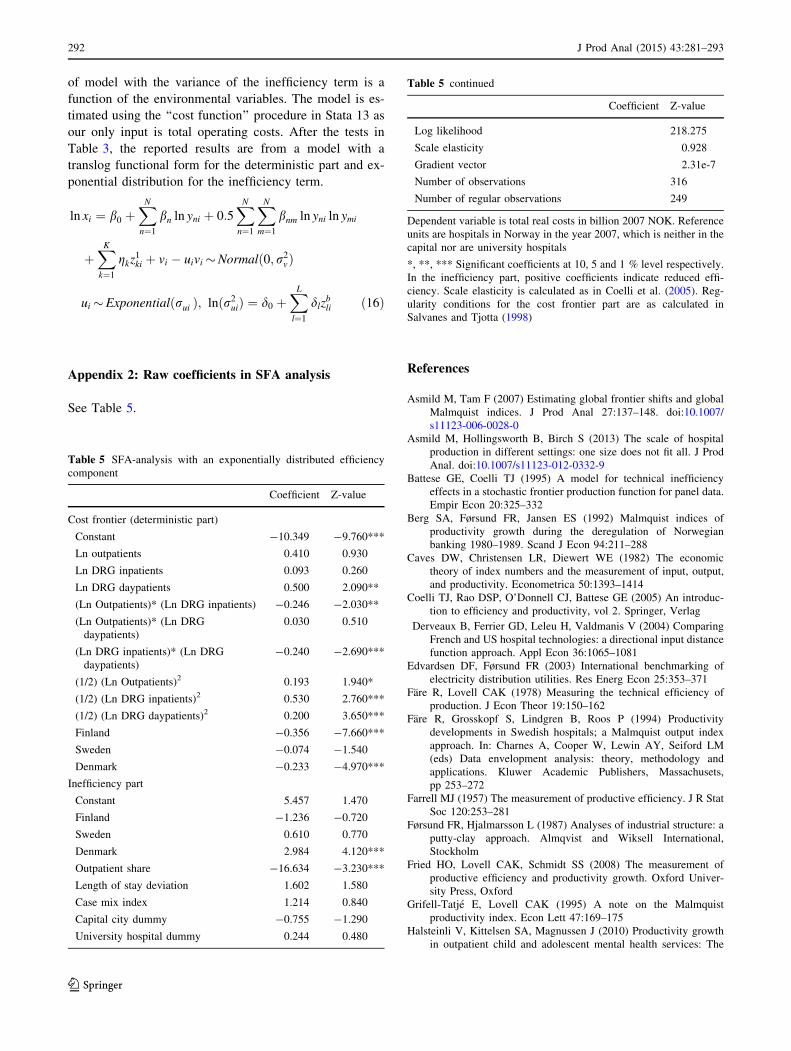
Appendix 2: Raw coefficients in SFA analysis

See Table 5.

References

Asmild M, Tam F (2007) Estimating global frontier shifts and global

Malmquist indices. J Prod Anal 27:137–148. doi:10.1007/

s11123-006-0028-0

Asmild M, Hollingsworth B, Birch S (2013) The scale of hospital

production in different settings: one size does not fit all. J Prod

Anal. doi:10.1007/s11123-012-0332-9

Battese GE, Coelli TJ (1995) A model for technical inefficiency

effects in a stochastic frontier production function for panel data.

Empir Econ 20:325–332

Berg SA, Førsund FR, Jansen ES (1992) Malmquist indices of

productivity growth during the deregulation of Norwegian

banking 1980–1989. Scand J Econ 94:211–288

Caves DW, Christensen LR, Diewert WE (1982) The economic

theory of index numbers and the measurement of input, output,

and productivity. Econometrica 50:1393–1414

Coelli TJ, Rao DSP, O’Donnell CJ, Battese GE (2005) An introduc-

tion to efficiency and productivity, vol 2. Springer, Verlag

Derveaux B, Ferrier GD, Leleu H, Valdmanis V (2004) Comparing

French and US hospital technologies: a directional input distance

function approach. Appl Econ 36:1065–1081

Edvardsen DF, Førsund FR (2003) International benchmarking of

electricity distribution utilities. Res Energ Econ 25:353–371

Fare R, Lovell CAK (1978) Measuring the technical efficiency of

production. J Econ Theor 19:150–162

Fare R, Grosskopf S, Lindgren B, Roos P (1994) Productivity

developments in Swedish hospitals; a Malmquist output index

approach. In: Charnes A, Cooper W, Lewin AY, Seiford LM

(eds) Data envelopment analysis: theory, methodology and

applications. Kluwer Academic Publishers, Massachusets,

pp 253–272

Farrell MJ (1957) The measurement of productive efficiency. J R Stat

Soc 120:253–281

Førsund FR, Hjalmarsson L (1987) Analyses of industrial structure: a

putty-clay approach. Almqvist and Wiksell International,

Stockholm

Fried HO, Lovell CAK, Schmidt SS (2008) The measurement of

productive efficiency and productivity growth. Oxford Univer-

sity Press, Oxford

Grifell-Tatje E, Lovell CAK (1995) A note on the Malmquist

productivity index. Econ Lett 47:169–175

Halsteinli V, Kittelsen SA, Magnussen J (2010) Productivity growth

in outpatient child and adolescent mental health services: The

Table 5 SFA-analysis with an exponentially distributed efficiency

component

Coefficient Z-value

Cost frontier (deterministic part)

Constant -10.349 -9.760***

Ln outpatients 0.410 0.930

Ln DRG inpatients 0.093 0.260

Ln DRG daypatients 0.500 2.090**

(Ln Outpatients)* (Ln DRG inpatients) -0.246 -2.030**

(Ln Outpatients)* (Ln DRG

daypatients)

0.030 0.510

(Ln DRG inpatients)* (Ln DRG

daypatients)

-0.240 -2.690***

(1/2) (Ln Outpatients)2 0.193 1.940*

(1/2) (Ln DRG inpatients)2 0.530 2.760***

(1/2) (Ln DRG daypatients)2 0.200 3.650***

Finland -0.356 -7.660***

Sweden -0.074 -1.540

Denmark -0.233 -4.970***

Inefficiency part

Constant 5.457 1.470

Finland -1.236 -0.720

Sweden 0.610 0.770

Denmark 2.984 4.120***

Outpatient share -16.634 -3.230***

Length of stay deviation 1.602 1.580

Case mix index 1.214 0.840

Capital city dummy -0.755 -1.290

University hospital dummy 0.244 0.480

Table 5 continued

Coefficient Z-value

Log likelihood 218.275

Scale elasticity 0.928

Gradient vector 2.31e-7

Number of observations 316

Number of regular observations 249

Dependent variable is total real costs in billion 2007 NOK. Reference

units are hospitals in Norway in the year 2007, which is neither in the

capital nor are university hospitals

*, **, *** Significant coefficients at 10, 5 and 1 % level respectively.

In the inefficiency part, positive coefficients indicate reduced effi-

ciency. Scale elasticity is calculated as in Coelli et al. (2005). Reg-

ularity conditions for the cost frontier part are as calculated in

Salvanes and Tjotta (1998)

292 J Prod Anal (2015) 43:281–293

123

impact of case-mix adjustment. Soc Sci Med 70:439–446.

doi:10.1016/j.socscimed.2009.11.002

Kalseth B, Anthun KS, Hope Ø, Kittelsen SAC, Persson B (2011)

Spesialisthelsetjenesten i Norden. Sykehusstruktur, styringsstruk-

tur og lokal arbeidsorganisering som mulig forklaring pa kost-

nadsforskjeller mellom landene. SINTEF Report A19615,

SINTEF Health Services Research, Trondheim

Kautiainen K, Hakkinen U, Lauharanta J (2011) Finland: DRGs in a

decentralized health care system. In: Busse R, Geissler A,

Quentin W, Wiley M (eds) Diagnosis-related groups in Europe:

Moving towards transparency, efficiency and quality in hospi-

tals. European Observatory on Health Systems and Policies

Series. McGraw-Hill, Maidenhead, pp 321–338

Kittelsen SAC, Anthun KS, Kalseth B, Halsteinli V, Magnussen J

(2009) En komparativ analyse av spesialisthelsetjenesten i

Finland, Sverige, Danmark og Norge: Aktivitet, ressursbruk og

produktivitet 2005–2007. SINTEF Report A12200, SINTEF

Health Services Research, Trondheim

Kittelsen SAC, Magnussen J, Anthun KS, Hakkinen U, Linna M,

Medin E, Olsen K, Rehnberg C (2008) Hospital productivity and

the Norwegian ownership reform—a Nordic comparative study.

STAKES discussion paper 2008:8, STAKES, Helsinki

Linna M, Virtanen M (2011) NordDRG: the benefits of coordination.

In: Busse R, Geissler A, Quentin W, Wiley M (eds) Diagnosis-

related groups in Europe: moving towards transparency, efficien-

cy and quality in hospitals. Open University Press, Maidenhead

Linna M, Hakkinen U, Magnussen J (2006) Comparing hospital cost

efficiency between Norway and Finland. Health Policy

77:268–278. doi:10.1016/j.healthpol.2005.07.019

Linna M, Hakkinen U, Peltola M, Magnussen J, Anthun KS, Kittelsen

S, Roed A, Olsen K, Medin E, Rehnberg C (2010) Measuring

cost efficiency in the Nordic Hospitals-a cross-sectional

comparison of public hospitals in 2002. Health Care Manag

Sci 13:346–357. doi:10.1007/s10729-010-9134-7

Magnussen J (1996) Efficiency measurement and the operationaliza-

tion of hospital production. Health Serv Res 31:21–37

Malmquist S (1953) Index numbers and indifference surfaces.

Trabajos de estadistica 4:209–224

Medin E, Hakkinen U, Linna M, Anthun KS, Kittelsen SAC,

Rehnberg C (2013) International hospital productivity compar-

ison: experiences from the Nordic countries. Health Policy

112:80–87. doi:10.1016/j.healthpol.2013.02.004

Mobley L, Magnussen J (1998) An international comparison of

hospital efficiency. Does institutional environment matter? Appl

Econ 30:1089–1100

Salvanes KG, Tjøtta S (1998) A note on the importance of testing for

regularities for estimated flexible functional forms. J Prod Anal

9:133–143

Shephard RW (1970) Theory of cost and production functions, 2nd

edn. Princeton University Press, Princeton

Simar L, Wilson PW (1998) Sensitivity analysis of efficiency scores:

how to bootstrap in nonparametric frontier models. Manag Sci

44:49–61

Simar L, Wilson PW (2000) Statistical inference in nonparametric

frontier models: the state of the art. J Prod Anal 13:49–78

StataCorp (2011) Stata: Release 12. Statistical Software. StataCorp

LP, College Station

Steinmann L, Dittrich G, Karmann A, Zweifel P (2004) Measuring

and comparing the (in)effciency of German and Swiss Hospitals.

Eur J Health Econ 5:216

Varabyova Y, Schreyogg J (2013) International comparisons of the

technical efficiency of the hospital sector: panel data analysis of

OECD countries using parametric and non-parametric approach-

es. Health policy. doi:10.1016/j.healthpol.2013.03.003

J Prod Anal (2015) 43:281–293 293

123