Database Solutions to Sports Applications - NTNU Open
96
NTNU Norwegian University of Science and Technology Faculty of Information Technology and Electrical Engineering Department of Computer Science Master’s thesis Oscar Thån Conrad Database Solutions to Sports Applications A Comparison and Performance Test of Graph Databases and Relational Databases Master’s thesis in Master of Informatics Supervisor: Svein Erik Bratsberg June 2019
-
Upload
khangminh22 -
Category
Documents
-
view
4 -
download
0
Transcript of Database Solutions to Sports Applications - NTNU Open

NTN
UN
orw
egia
n U
nive
rsity
of S
cien
ce a
nd T
echn
olog
yFa
cult
y of
Info
rmat
ion
Tech
nolo
gy a
nd E
lect
rica
lEn
gine
erin
gD
epar
tmen
t of C
ompu
ter
Scie
nce
Mas
ter’
s th
esis
Oscar Thån Conrad
Database Solutions to SportsApplications
A Comparison and Performance Test of GraphDatabases and Relational Databases
Master’s thesis in Master of InformaticsSupervisor: Svein Erik Bratsberg
June 2019

Oscar Thån Conrad
Database Solutions to SportsApplications
A Comparison and Performance Test of GraphDatabases and Relational Databases
Master’s thesis in Master of InformaticsSupervisor: Svein Erik BratsbergJune 2019
Norwegian University of Science and TechnologyFaculty of Information Technology and Electrical EngineeringDepartment of Computer Science


Summary
The amount of data generated today is enormous. It is estimated that we generate 2,5billion gigabytes of data every day. As a result of this, new trends in data analysishave emerged along with new methods and technologies within data storage, processing,management, search and visualization. Sports is a field that is known to use data analysis inorder to improve athletes’ performance and to analyze competitors. In addition, bookmakersrely heavily on data analysis to predict results and provide betting odds.
In this thesis, we developed an application that analyzes sports data provided by an externalAPI. The data retrieved from the API is stored in two different databases, a graph databaseand a relational database. The application is then used to determine which databasetechnology performs best for the given use case of analyzing sports data. For the graphdatabase we used Neo4j and for the relational database we used MySQL by Oracle.
Our results suggest that relational databases perform better for small datasets, but as soonas the number of records surpasses a certain size, graph databases perform better. For ourexperiments, that size was approximately 1670 records. That size will differ dependingupon the exact structure of the dataset, but our conclusion is that for larger datasets, therewill be a performance advantage in storing the data in a graph database rather than in arelational database for our kind of data analysis.
i

ii

Sammendrag
Hver eneste dag genereres det enorme mengder data. Det estimeres at vi genererer 2.5milliarder gigabyte med data hver eneste dag. Det har resultert i at en ny trend harutviklet seg, en trend som har brakt med seg nye metoder og teknologier innen lagring,prosessering, søk og visualisering av data. Idrett er et felt som har tatt i bruk mange avdisse metodene og teknologiene. I dag brukes de blant annet til a forbedre en idrettsutøversytelse og til a analysere motstandere. En annen bransje som ogsa har tatt i bruk dissemetodene er pengespillbransjen. De bruker datanalyse til a forutse resultater og produsereodds til idrettsarrangement.
I denne avhandlingen utvikler vi en applikasjon som analyserer sportsdata levert av eteksternt API. Dataen hentes fra API-et og lagres i to forskjellige databaser, en grafdatabaseog en relasjonsdatabase. Applikasjonen benyttes sa til a undersøke hvilken database somegner seg best til analyse av denne type data. Vi benyttet oss av grafdatabasen til Neo4j ogOracle sin relasjonsdatabase MySQL.
Resultatene vare indikerer at relasjonsdatabaser yter bedre for sma datamengder, menettersom antall poster passerer en viss størrelse, vil en grafdatabase yte bedre. Undervare forsøk gikk den grensen ved cirka 1670 poster. Denne grensen vil endre seg avhengigav datasettet sin struktur, men var konklusjon er at det vil være en ytelsesmessing fordel alagre dataen i en grafdatabase, i stedet for en relasjonsdatabase for var type datanalyse.
iii

iv
Preface
This thesis was written at the Department of Computer and Information Science (IDI) atthe Norwegian University of Science and Technology (NTNU) in Trondheim, in collaborationwith the technology firm Sportradar AG. The research was conducted by Oscar ThanConrad, under the supervision of Professor Svein Erik Bratsberg. It is assumed that thereader has a basic knowledge of database systems, algorithms, and data structures whenreading this thesis.
The project was designed as a performance and usability test of two database managementsystems, Neo4j’s graph database and Oracle’s relational database MySQL. Both databaseswere populated with sports data from the English top division in soccer, the PremierLeague. Sportradar AG provided us with all the data through their developer APIs.
I would like to thank Svein Erik for his guidance and valuable feedback throughout theyear. In addition, I would like to thank my father Mark Allan Conrad for being a valuablediscussion partner and for helping me improve my work by proofreading and solvinglinguistic challenges. Lastly, I would like to thank Sportradar for providing me with data,by giving me access to their developer API.
v

vi
Table of Contents
Summary i
Sammendrag iii
Preface v
Table of Contents ix
List of Tables xi
List of Figures xiii
List of Listings xv
Abbreviations xvi
1 Introduction 11.1 Project Description . . . . . . . . . . . . . . . . . . . . . . . . . . . . . 11.2 Background . . . . . . . . . . . . . . . . . . . . . . . . . . . . . . . . . 11.3 Motivation . . . . . . . . . . . . . . . . . . . . . . . . . . . . . . . . . . 2
1.3.1 Extended Friends Experiment . . . . . . . . . . . . . . . . . . . 31.4 Personal Motivation . . . . . . . . . . . . . . . . . . . . . . . . . . . . . 31.5 Sportradar AG . . . . . . . . . . . . . . . . . . . . . . . . . . . . . . . . 41.6 Scope . . . . . . . . . . . . . . . . . . . . . . . . . . . . . . . . . . . . 41.7 Research Strategy . . . . . . . . . . . . . . . . . . . . . . . . . . . . . . 51.8 Structure . . . . . . . . . . . . . . . . . . . . . . . . . . . . . . . . . . . 6
2 Related Work 92.1 World Cup As a Graph . . . . . . . . . . . . . . . . . . . . . . . . . . . 9
2.1.1 The World Cup Graph Domain Model . . . . . . . . . . . . . . . 102.2 Medhi’s Study . . . . . . . . . . . . . . . . . . . . . . . . . . . . . . . . 10
vii

2.3 Import Time . . . . . . . . . . . . . . . . . . . . . . . . . . . . . . . . . 11
3 Background 153.1 Application Programming Interface . . . . . . . . . . . . . . . . . . . . 15
3.1.1 Sportradar Developer API . . . . . . . . . . . . . . . . . . . . . 153.2 Graph . . . . . . . . . . . . . . . . . . . . . . . . . . . . . . . . . . . . 17
3.2.1 Use Cases . . . . . . . . . . . . . . . . . . . . . . . . . . . . . . 173.3 Graph Storage . . . . . . . . . . . . . . . . . . . . . . . . . . . . . . . . 193.4 Neo4j . . . . . . . . . . . . . . . . . . . . . . . . . . . . . . . . . . . . 19
3.4.1 Choosing Neo4j . . . . . . . . . . . . . . . . . . . . . . . . . . 193.4.2 The Property Graph Model . . . . . . . . . . . . . . . . . . . . . 203.4.3 Neo4j Browser . . . . . . . . . . . . . . . . . . . . . . . . . . . 203.4.4 Cypher . . . . . . . . . . . . . . . . . . . . . . . . . . . . . . . 213.4.5 APOC . . . . . . . . . . . . . . . . . . . . . . . . . . . . . . . . 22
3.5 Alternative Graph Database Management Systems . . . . . . . . . . . . . 223.5.1 Amazon Neptune . . . . . . . . . . . . . . . . . . . . . . . . . . 233.5.2 OrientDB . . . . . . . . . . . . . . . . . . . . . . . . . . . . . . 233.5.3 ArangoDB . . . . . . . . . . . . . . . . . . . . . . . . . . . . . 23
3.6 Oracle . . . . . . . . . . . . . . . . . . . . . . . . . . . . . . . . . . . . 243.6.1 MySQL . . . . . . . . . . . . . . . . . . . . . . . . . . . . . . . 243.6.2 Structured Query Language . . . . . . . . . . . . . . . . . . . . 243.6.3 Support . . . . . . . . . . . . . . . . . . . . . . . . . . . . . . . 253.6.4 Choosing MySQL . . . . . . . . . . . . . . . . . . . . . . . . . 253.6.5 InnoDB . . . . . . . . . . . . . . . . . . . . . . . . . . . . . . . 253.6.6 B+-Tree . . . . . . . . . . . . . . . . . . . . . . . . . . . . . . . 263.6.7 MySQL Workbench . . . . . . . . . . . . . . . . . . . . . . . . 26
3.7 Python . . . . . . . . . . . . . . . . . . . . . . . . . . . . . . . . . . . . 273.8 Premier League . . . . . . . . . . . . . . . . . . . . . . . . . . . . . . . 27
4 Design & Implementation 294.1 Approach . . . . . . . . . . . . . . . . . . . . . . . . . . . . . . . . . . 294.2 Database Design . . . . . . . . . . . . . . . . . . . . . . . . . . . . . . 324.3 Neo4j Graph Database . . . . . . . . . . . . . . . . . . . . . . . . . . . 36
4.3.1 Neo4j Driver . . . . . . . . . . . . . . . . . . . . . . . . . . . . 394.3.2 Neo4j Configuration . . . . . . . . . . . . . . . . . . . . . . . . 39
4.4 MySQL Relational Database . . . . . . . . . . . . . . . . . . . . . . . . 394.4.1 Design . . . . . . . . . . . . . . . . . . . . . . . . . . . . . . . 394.4.2 MySQL Server . . . . . . . . . . . . . . . . . . . . . . . . . . . 414.4.3 MySQL Workbench . . . . . . . . . . . . . . . . . . . . . . . . 41
4.5 Data Mapper Application . . . . . . . . . . . . . . . . . . . . . . . . . . 414.5.1 Neo4j Data Mapper . . . . . . . . . . . . . . . . . . . . . . . . . 424.5.2 MySQL Data Mapper . . . . . . . . . . . . . . . . . . . . . . . 424.5.3 Data Aggregation . . . . . . . . . . . . . . . . . . . . . . . . . . 43
4.6 Hardware . . . . . . . . . . . . . . . . . . . . . . . . . . . . . . . . . . 45
5 Results & Discussion 47
viii
5.1 Expectations . . . . . . . . . . . . . . . . . . . . . . . . . . . . . . . . . 475.2 Results . . . . . . . . . . . . . . . . . . . . . . . . . . . . . . . . . . . . 47
5.2.1 Execution Time Neo4j . . . . . . . . . . . . . . . . . . . . . . . 485.2.2 Execution Time MySQL . . . . . . . . . . . . . . . . . . . . . . 49
5.3 Analysis . . . . . . . . . . . . . . . . . . . . . . . . . . . . . . . . . . . 505.3.1 Single Match . . . . . . . . . . . . . . . . . . . . . . . . . . . . 505.3.2 Team Season . . . . . . . . . . . . . . . . . . . . . . . . . . . . 515.3.3 Complete Season . . . . . . . . . . . . . . . . . . . . . . . . . . 52
5.4 Discussion . . . . . . . . . . . . . . . . . . . . . . . . . . . . . . . . . . 525.4.1 Response time . . . . . . . . . . . . . . . . . . . . . . . . . . . 53
5.5 Database Querying . . . . . . . . . . . . . . . . . . . . . . . . . . . . . 565.5.1 Query Performance . . . . . . . . . . . . . . . . . . . . . . . . . 57
5.6 Visualization . . . . . . . . . . . . . . . . . . . . . . . . . . . . . . . . 585.7 Data Import . . . . . . . . . . . . . . . . . . . . . . . . . . . . . . . . . 605.8 Data Model . . . . . . . . . . . . . . . . . . . . . . . . . . . . . . . . . 61
6 Conclusion & Future Work 636.1 Conclusion . . . . . . . . . . . . . . . . . . . . . . . . . . . . . . . . . 646.2 Future work . . . . . . . . . . . . . . . . . . . . . . . . . . . . . . . . . 66
6.2.1 Hardware & Architecture . . . . . . . . . . . . . . . . . . . . . . 666.2.2 Memory Consumption . . . . . . . . . . . . . . . . . . . . . . . 666.2.3 Import time . . . . . . . . . . . . . . . . . . . . . . . . . . . . . 666.2.4 Different dataset . . . . . . . . . . . . . . . . . . . . . . . . . . 676.2.5 Mitigate Cold Start . . . . . . . . . . . . . . . . . . . . . . . . . 67
6.3 Threats to Validity & Limitations . . . . . . . . . . . . . . . . . . . . . . 676.4 Contribution . . . . . . . . . . . . . . . . . . . . . . . . . . . . . . . . . 67
Bibliography 69
Appendix 75
ix

x

List of Tables
1.1 Results in seconds from extended friends experiment . . . . . . . . . . . 3
2.1 Execution time for different queries based on database and size of database 11
5.1 Execution times for Neo4j database in seconds . . . . . . . . . . . . . . 485.2 Neo4j test case results in seconds . . . . . . . . . . . . . . . . . . . . . . 495.3 Execution times for MySQL database in seconds . . . . . . . . . . . . . 495.4 MySQL test case results in seconds . . . . . . . . . . . . . . . . . . . . . 505.5 Results for Neo4j un-optimized Neo4j queries in seconds . . . . . . . . . 58
6.1 The median processing time in seconds . . . . . . . . . . . . . . . . . . 656.2 The average processing time in seconds . . . . . . . . . . . . . . . . . . 65
xi

xii

List of Figures
1.1 Research process model . . . . . . . . . . . . . . . . . . . . . . . . . . . 5
2.1 World Cup graph model . . . . . . . . . . . . . . . . . . . . . . . . . . . 102.2 Relational model of dataset . . . . . . . . . . . . . . . . . . . . . . . . . 122.3 Graph model of dataset . . . . . . . . . . . . . . . . . . . . . . . . . . . 132.4 Data import time results . . . . . . . . . . . . . . . . . . . . . . . . . . . 14
3.1 Sportradar API map . . . . . . . . . . . . . . . . . . . . . . . . . . . . . 163.2 Graph examples . . . . . . . . . . . . . . . . . . . . . . . . . . . . . . . 173.3 Graph use cases . . . . . . . . . . . . . . . . . . . . . . . . . . . . . . . 183.4 Property Graph Model . . . . . . . . . . . . . . . . . . . . . . . . . . . 203.5 Relationship between two nodes . . . . . . . . . . . . . . . . . . . . . . 213.6 B+-tree example . . . . . . . . . . . . . . . . . . . . . . . . . . . . . . 26
4.1 System design . . . . . . . . . . . . . . . . . . . . . . . . . . . . . . . . 314.2 Visualized subset of the graph database . . . . . . . . . . . . . . . . . . 374.3 Relational database design . . . . . . . . . . . . . . . . . . . . . . . . . 404.4 Output from executing each of the test cases . . . . . . . . . . . . . . . . 44
5.1 Graphed results of the first test case . . . . . . . . . . . . . . . . . . . . 505.2 Graphed results of the second test case . . . . . . . . . . . . . . . . . . . 515.3 Graphed results of the third test case . . . . . . . . . . . . . . . . . . . . 525.4 Complete overview of execution times . . . . . . . . . . . . . . . . . . . 555.5 Returned results from SQL query . . . . . . . . . . . . . . . . . . . . . . 595.6 Returned results from Cypher query . . . . . . . . . . . . . . . . . . . . 60
xiii

xiv
Listings
3.1 Cypher query used to create graph from Figure 3.5 . . . . . . . . . . . . 214.1 Result from calling the Tournament List API . . . . . . . . . . . . . . . . 324.2 Result from calling the Tournament Info API . . . . . . . . . . . . . . . 334.3 Result from calling the Tournament Schedule API . . . . . . . . . . . . . 344.4 Result from calling the Match Timeline API . . . . . . . . . . . . . . . . 354.5 Query for importing all teams to the graph database . . . . . . . . . . . . 384.6 Cypher statement for connecting home teams with matches . . . . . . . . 384.7 Cypher statement for connecting a match with its corresponding events . . 394.8 Python function that temporary stores team attributes . . . . . . . . . . . 404.9 Python function that writes each team with attributes to database . . . . . 414.10 Cypher query that returns relevant information for a given matchId . . . . 424.11 Cypher query that returns name for home and away team for a given matchId 424.12 SQL query that returns relevant information for a given matchId . . . . . 424.13 SQL query used to retrieve name of home team . . . . . . . . . . . . . . 435.1 SQL query that returns all offsides that Chelsea have produced on home
ground . . . . . . . . . . . . . . . . . . . . . . . . . . . . . . . . . . . . 565.2 Cypher query that returns all offsides that Chelsea have produced on home
ground . . . . . . . . . . . . . . . . . . . . . . . . . . . . . . . . . . . . 575.3 Un-optimized cypher query not utilizing relationships . . . . . . . . . . . 57
xv

Abbreviations
ACID = Atomicity, Consistency, Isolation, DurabilityAPI = Application Programming InterfaceAPOC = Awesome Procedures on CypherCAP = Consistency, Availability, Partition, ToleranceCRUD = Create, Read, Update, DeleteDB = DatabaseDBTG = Data Base Task GroupGDB = Graph DatabaseGDBMS = Graph database management systemHTTP = Hypertext Transfer ProtocolI/O = Input/OutputJSON = JavaScript Object NotationNoSQL = Not Only Structured Query LanguageNFL = National Football LeagueNHL = National Hockey LeagueRDBMS = Relational database management systemREST = REpresentational State TransferRQ = Research QuestionSQL = Structured Query LanguageXML = Extensible Markup Language
xvi

Chapter 1Introduction
This chapter introduces the project for this thesis. In addition, this chapter will presentits relevance and context to the research community. Research goals, research questionsare also presented in this chapter, together with a short description of the chosen researchstrategy.
1.1 Project Description
This project is a result of a Master’s thesis in Informatics written at the Norwegian Universityof Science and Technology in the city of Trondheim. The research was conducted incooperation with the technology firm Sportradar AG. The starting point for the projectwas the following description drafted by Sportradar AG:
Currently, we host all our sports and betting data in various relational databases.Google and Facebook have successfully structured a lot of their data as graphs,and we have seen several other interesting use cases for graph databases.Graph databases provide a different way of structuring our data that allowsfor different kinds of data queries. We would be interested in researchingstrategies for structuring sports data as graphs, and if this will allow us tosearch and aggregate our sports data.
1.2 Background
A database management system is a system where users can organize, store, and retrievedata through a computer, and is a way of communicating with a computer’s internalstorage. In the 1950s, the early days of computers, computers were essentially huge
1
Chapter 1. Introduction
calculators, and punch cards were used to store data. Computers were quickly adopted bypeople and became available for commercial use. People adapted them to solve real-worldproblems, which made the demands regarding data processing and storage to skyrocket. In1960 the American computer scientist Charles Bachman designed what is known as “TheIntegrated Data Store” (IDS), on behalf of General Electric. IDS is considered the world’sfirst database management system [16].
By the middle of the 1960s, the development of computers was booming, and many kindsof databases became available for consumers. Resulting in a wide range of systemsand standards. At the same time, Bachman formed the Database Task Group (DBTG),which took responsibility for creating a common standard for databases. In 1971 DTBGpresented their new standard called Common Business Oriented Language (COBOL) [16].
COBOL was based on a model known as the network model, which represented data asdifferent kinds of objects with relations between them. The Network Model was conceivedas a graph and known for being schemaless. Many databases were built on this concept,and the COBOL standard came to be known as the CODASYL-approach [16].
There is, in many ways, a direct resemblance between the network model and graphdatabases as we know them today. However, there is one crucial element that separates thetwo. The CODASYL approach is a complex system, which makes it very hard to searchand query data. Graph databases usually have their own query language which makesthese kinds of operations much easier [8].
Due to the CODASYL approach’s failing abilities to search for records, it eventually lostits popularity. A developer from IBM was not satisfied with the search engine in theCODASYL approach. Therefore he started to look at alternative ways to manage data.So in 1970, he published a series of papers describing a different way of constructing adatabase and storing data as rows in tables. This evolved into the relational database modelas we know it today [16].
1.3 Motivation
Today, enormous amounts of data are collected. According to Forbes, we produce 2.5quintillion bytes of data every year. During the last two years, 90% of all measured data inthe world was generated [25]. According to a publication from the advisory firm EY [15],we will by 2020, generate about 1.7 megabytes of new information every second for everyhuman being on the planet. Buzz words like ”Big data” are often in found tech-blogs andother publications, which points to a trend, where enormous amounts of data go throughcomprehensive analytic processes.
The relational database model has been around since the 1970s. Relational databasetechnology has been the choice for most traditional applications that require both datastorage and retrieval. A relational database consists of tables with rows and columns.These tables can have thousands or even millions of rows, known as records.
2

1.4 Personal Motivation
With these vast amounts of data, both practical and ethical questions arise on how can weprocess and take advantage of this? What kind of data management systems can we utilizein order to process this data, and meet the new demands of analyzing data.
For decades traditional relational database management systems have been used in orderto store and manage data. For a very long time they have worked well, and they have beenrather easy to use and implement. With the massive data we produce today, we expectmore from the data, and we are continually looking for new ways to apply all this data, inorder to find new trends and patterns. For this kind of data processing, traditional RDBMSmay come to short. Processing queries that output the kind of data that we often wish fortoday is usually very costly and may require many join operations. Besides, the queriescan be complicated to write and may not very intuitive for people to interpret.
Meanwhile, many other database models and providers have come to the surface. Today,document, key-value and graph model databases have challenged the traditional relationaldatabase with different properties. A popular database that has emerged is the graphdatabase Neo4j. Neo4j has grown quickly, and many big corporations have implementedtheir database.
1.3.1 Extended Friends Experiment
Partner and Vukotic present a very interesting experiment in their book [63]. The experimentis known as the extended friends experiment and is widely used to demonstrate the powerof a graph database. The experiment seeks to find friends of friends in a social network,consisting of 1.000.000 people, where each person has 50 friends. The experiment is donein four iterations, seeking to find friends of friends in depth one to four. The social networkis modeled as a graph in Neo4j and a relational database in MySQL. The results can beseen in Table 1.1 and it clearly shows how Neo4j outperforms MySQL for this kind ofquery.
Depth MySQLExecution Time
Neo4jExecution Time Records returned
2 0,016 0,01 ∼25003 20,267 0,168 ∼110.0004 1543.305 1,359 ∼600.0005 Unfinished 2,132 ∼800.000
Table 1.1: Results in seconds from extended friends experiment
1.4 Personal Motivation
The authors of this thesis have a great interest in both analyzation and management ofdata. The interest increased while completing a bachelor’s degree in informatics priorto this thesis, which included several subjects within data management and information
3

Chapter 1. Introduction
retrieval. Discovering the extended friends experiment, revealing how powerful a graphdatabase can be, supplemented to that curiosity. Also, the idea of working together witha firm, which is world-leading in its area and founded by two earlier computer sciencestudents from NTNU was highly motivating.
The background study, presented in Chapter 2, revealed that the research regarding theuse of graph databases to manage sports data was somewhat limited. Therefore this thesiswill also contribute to the research community within data management, processing andanalyzation.
1.5 Sportradar AG
Sportradar AG hereafter, referred to as Sportradar, is a company founded in Trondheim inthe year of 2000. It all started with two computer science students’ master’s thesis hereat NTNU. Together they designed a high accuracy wrapper that could crawl the web, andgather betting odds and information from 25 different sports across 300 different onlinebookmaking platforms [5].
One of the co-founders of the company had been following different bookmakers’ onlinebetting platforms. He discovered the fact that the odds to a given sporting event tendedto differ between different betting platforms depending on in which country the oddswere determined. Knowing this, he could predict score results better than most otherbookmakers. Further, he discovered that the different bookmakers tended to provide betterodds for teams that represented their interests. For example, a Spanish bookmaker wouldgive better odds to Spain’s national soccer team for a given soccer match, than what anAmerican bookmaker would do. Knowing all this and subsequently making more moneyon betting, than what he considered normal. The idea of developing an application that therest of the world’s bookmakers could have enormous use of emerged [52].
Today, Sportradar is a leading company providing live sports results, sports statistics, odds,and sports integrity services. They cover the entire value chain of collecting, processing,marketing and monitoring of sports-related live data as well as sports-related services.They consist of about 1700 employees and serve customers in approximately 100 countries[14].
Sportradar is in partnership with many international sporting federations, for example, theNHL, NFL and NASCAR and German Bundesliga where they are the leading provider ofsporting statistics. Furthermore, they provide several bookmakers like Bet365, Ladbrokes,Svenska Spel and Norsk Tipping with betting services [55] [59].
1.6 Scope
Based on the description above, the goal of this research was to investigate how sportsdata from Sportradar performed when structured in a graph database. Since this was a
4

1.7 Research Strategy
comprehensive problem, we had to narrow down our scope, in order to make the researchfeasible. One of the sports that Sportradar had excellent data coverage for was soccer, andespecially the English Premier League. In combination with good data coverage and thefact that many people have a relationship with soccer, we chose to use that as our domainfor our research. Therefore we developed out a pair of research questions with the purposeof supporting the overall goal. The research questions were as follows:
• RQ1: Identify a use case which is representative for the data and applications ofSportradar.
• RQ2: How does the Neo4j graph database management system compare againstOracle’s MySQL relational database management system, in regard to target theproblem?
1.7 Research Strategy
The findings we present in this thesis was a result of planning, implementing and conductinga research strategy. B. J. Oates [39] presents a model in his book, Figure 1.1 whichhighlights important elements of research.
Figure 1.1: Model of research process [39]
Our Research strategy was rooted in this model. We developed our research questionsbased on experiences, motivation and previous work. We mainly used quantitative research
5

Chapter 1. Introduction
methods through experiments to generate data for our analysis. However, qualitativemethods were also used in order to assess aspects of a DBMS that are not measurableby numbers. Babbie, Earl R [3] defines both quantitative and qualitative research methodsas follows:
• Quantitative methods emphasize objective measurements and the statistical,mathematical, or numerical analysis of data collected through polls,questionnaires, and surveys, or by manipulating pre-existing statisticaldata using computational techniques. Quantitative research focuses ongathering numerical data and generalizing it across groups of people orto explain a particular phenomenon
• Qualitative research is a scientific method of observation to gather non-numericaldata. This type of research ”refers to the meanings, concepts definitions,characteristics, metaphors, symbols, and description of things” and notto their ”counts or measures.
In our research, we designed two different databases, based on two different technologies,Neo4j and MySQL. Both databases were populated with identical data, provided by Sportradar.We collected numerical data by having the databases execute three different test cases each.Then we analyzed the databases’ performance by comparing and analyzing the executiontimes for each of the test cases. The test cases were the same for both databases andconsisted of different kinds of queries. However, they differed in the way that they werewritten and customized in order to meet the requirements of both database technologies.After obtaining results from our database performance testing, they were discussed withregards to previous related work, presented in Chapter 2. In the discussion, aspects suchas documentation, durability and usability were enlightened.
1.8 Structure
This section presents a list, which in short, describes each chapter and its content.
• Chapter 1 - Introduction introduces the thesis as a whole and presents how thisproject came to life. Furthermore, it introduces Sportradar and gives a brief introductionto the history of databases.
• Chapter 2 - Related Work presents related work and studies which have played animportant role in this research.
• Chapter 3 - Background introduces central concepts within graph databases andrelational databases. The database management systems Neo4j and MySQL arepresented, along with other related tools and technologies.
• Chapter 4 - Design & Implementation delves into how our solution was implementedstep by step. By explaining how the databases import data from Sportradar’s API,and how our Python scripts and queries interact with the databases.
6

1.8 Structure
• Chapter 5 - Results & Discussion presents all results and findings achieved throughcarrying out our different experiments. In addition, results are discussed in light ofprevious related work.
• Chapter 6 - Conclusion & Future Work summarizes the thesis, and evaluates howthe project can be improved. Also, it presents advantages and disadvantages withboth MySQL and Neo4j. Lastly, it discusses future work that may verify or discreditthe results achieved through this project.
7

Chapter 1. Introduction
8

Chapter 2Related Work
Graph database theory has been around for a pretty long time, compared to other computerscience concepts. However, they have only been practiced to a small degree, until recently.Therefore the amount of relevant research and work within this topic is limited. Nevertheless,there has been significant research on graph database usage in other domains. Some of it isrelevant to our research and can be adapted for our domain. This chapter will summarizethat literature.
2.1 World Cup As a Graph
During the FIFA Soccer World Cup In 2014, the team behind Neo4j built two differentgraph data sets. One based on historic World Cup data, and the other on data from the2014 World Cup in Brazil. With both databases, they were able to explore the World Cupdata in new and different ways [29].
When graphing the historical data, and later querying the database, the developer teamdiscovered many interesting findings. Some examples are as following:
• After losing to France, it took Mexico 82 years to get their revenge. Mexico lost in1930 and did not beat France until 2012.
• During the tournament in 1954 Hungary met West Germany in the initial round, butthen lost to them in the final.
• The following five players were all drafted to play in the World Cup three times, butwere kept as substitutes and never brought on the field.
– Anthony Seric (Croatia)
– Antonio Juliano (Italy)
9
Chapter 2. Related Work
– Marek Kusto (Poland)
– Borislav Mikhailov (Bulgaria)
– Francisco Urruticoechea (Spain)
This list is an example of things that one can do with graph databases.
2.1.1 The World Cup Graph Domain Model
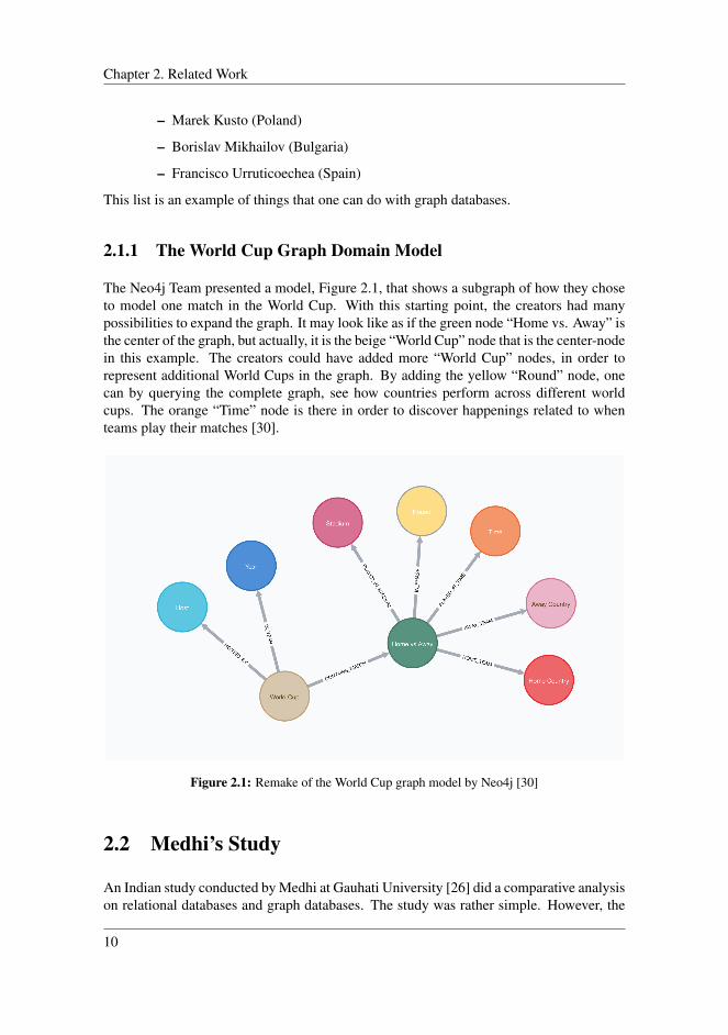
The Neo4j Team presented a model, Figure 2.1, that shows a subgraph of how they choseto model one match in the World Cup. With this starting point, the creators had manypossibilities to expand the graph. It may look like as if the green node “Home vs. Away” isthe center of the graph, but actually, it is the beige “World Cup” node that is the center-nodein this example. The creators could have added more “World Cup” nodes, in order torepresent additional World Cups in the graph. By adding the yellow “Round” node, onecan by querying the complete graph, see how countries perform across different worldcups. The orange “Time” node is there in order to discover happenings related to whenteams play their matches [30].
Figure 2.1: Remake of the World Cup graph model by Neo4j [30]
2.2 Medhi’s Study
An Indian study conducted by Medhi at Gauhati University [26] did a comparative analysison relational databases and graph databases. The study was rather simple. However, the
10

2.3 Import Time
results were conclusive. Medhi used a dataset based on three different cricket tournaments,the Test Cricket Tournament, One Day International Tournament (ODI) and the Twenty-TwentyTournament (T20). The dataset consisted of all the cricket players’ information, team andwhich player had played which matches.
This dataset was modeled in both a relational database and a graph database. For therelational database MySQL version 5.1.0 was used, and for the graph database Neo4jversion 2.0.3 was used. PHP and Cypher were respectively used as languages to query thedatabase. A relational database consisting of three tables were then created, based on datafrom the dataset. Furthermore, a graph based on the same data was modeled. With thetwo different databases containing the exact same data. They executed the three followingqueries:
• Find the names of the teams.
• Find the names of the cricketers who have played in both the One Day InternationalTournament and the Test Tournament.
• Find the Cricket players who belong to team India.
These the queries were executed three times each. During each iteration the databases weremodified to respectively contain 100, 300 and 400 objects. The results of these queries canbe seen in Table 2.1:
No. ofobjects
Query 1MySQL
Query 1Neo4j
Query 2MySQL
Query 2Neo4j
Query 3MySQL
Query 3Neo4j
100 12.56ms 5ms 18.52ms 7.32ms 15.75ms 6ms300 153ms 7ms 212.53ms 13ms 180.24ms 9.32ms400 164.43ms 8.32ms 387.34ms 15.67ms 302.44ms 13.32ms
Table 2.1: Execution time for different queries based on database and size of database
As Table 2.1 shows, there were significant differences in the time it took to execute theabove queries. As the size of the dataset increased, the execution time increased at a muchfaster rate with the MySQL database than with the Neo4j database. The study concludedthat the graph database performed much better than the relational database concerningtime. Also, it added that it was easier to model, maintain and expand the graph databasedue to the high connectivity of the data.
2.3 Import Time
Many studies have been conducted that assess the pros and cons of both graph databasesand relational databases. A study [45] published in August 2018 compares the architecturalstructure between Neo4j, MySQL and the NoSQL database MongoDB. In this study, theyfocus on how the different databases perform while importing data. They performedan experiment using a dataset containing details on vehicle transactions between a car
11

Chapter 2. Related Work
dealership and their customers, consisting of about 100.000 records. The dataset had thefollowing structure:
• transaction id
• counter id
• branch id
• date of transaction
• hour
• high level territory
• staff id
• product id
• payment amount
• bea admin
• cust id
• name
Before the dataset was imported, it was restructured into the respective schemas accordingto the database’s requirements. For the relational database, the dataset was modeled intoseven tables, containing six foreign-key relationships between them. Six tables containedactual data, while the last table only contained links between the different entities in themodel, as shown in Figure 2.3.
Figure 2.2: Relational model of dataset
12

2.3 Import Time
Figure 2.3 shows how the graph database was modeled. By using six different nodes thatrepresented the data, and seven different connections, that represented the relationshipsbetween the nodes.
Figure 2.3: Graph model of dataset
During this experiment, they imported parts of the dataset at the time. They tested thedifferent databases’ abilities to import datasets containing 10.000, 30.000, 60.000, and100.000 records. Figure 2.4 shows how the databases performed concerning time.
13

Chapter 2. Related Work
Figure 2.4: Data import time results adopted from [45]
From Pandey’s study [45] we saw that the size of the dataset that was imported, affectedhow the different databases performed. We also noticed that MongoDB and Neo4j performedalmost constant, only decreasing in performance with a few milliseconds as the datasetgrew. On the other side, we found MySQL, when the dataset was smaller than 20.000records, MySQL performed better than Neo4j, with regard to import time. Lastly, weobserved that data import time grew close to exponentially as the dataset increased in size.
14
Chapter 3Background
This chapter introduces central concepts related to graphs, graph theory and graph databases.In addition, other graph database management systems will be introduced to better evaluateand compare Neo4j against other providers of graph databases. Furthermore, this chapterwill present one of Neo4j’s biggest competitors, Oracle with its database managementsystem MySQL, and relevant theory behind it. As graph database theory is a newer andless known concept than relational database theory, the focus in this chapter will mainlybe on graph database theory.
3.1 Application Programming Interface
An Application Programming Interface (API) allows software applications to communicatewith one another. It is a well defined set of functions and procedures that allow oneapplication to interface with another [54]. Commonly used is the Web-API that usesRESTful methods, meaning that it uses HTTP requests to GET, PUT, POST and DELETEdata. Communication is done via a defined request–response message system, that can bepublicly available or restricted to certain users. The response from the endpoints is usuallyexpressed in either JSON or XML. Developers typically build applications based on thedata returned by calling the different endpoints [6].
3.1.1 Sportradar Developer API
The API developed by Sportradar delivers enormous amounts of data in both JSON formatand XML format. It is Sportradar’s main product, and their customers have to purchasea subscription in order to use the API. With the API, users can access sports statisticsfeeds, which contain vast amounts of data for different leagues, conferences, teams, games,
15
Chapter 3. Background
and players in their database. The API uses RESTful methods, making it possible fordevelopers to integrate Sportradar’s services directly into their application.
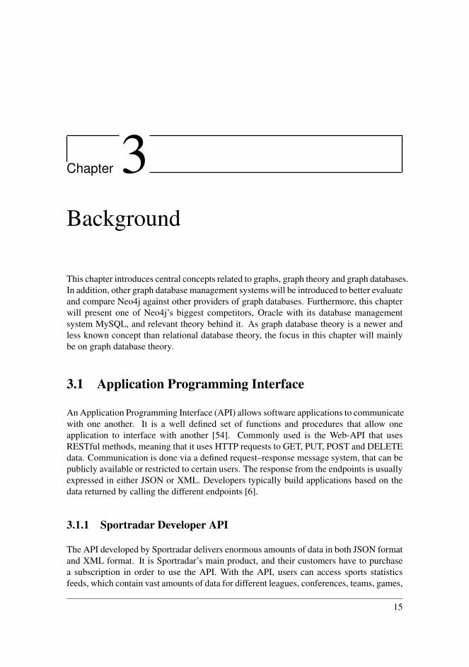
With regard to soccer, Sportradar covers almost all leagues and tournaments. Big leaguessuch as the Premier League is broader covered than less popular leagues such as the highestNorwegian league Eliteserien. Figure 3.1 is a mapping of the Soccer API that shows howall the different soccer APIs are connected and what kind of data they return.
Figure 3.1: API map from Sportradar [56]
16
3.2 Graph
3.2 Graph
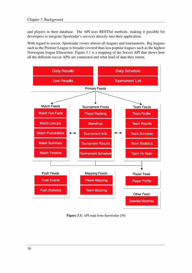
A graph is a way of representing a collection of vertices and edges and how they areconnected to each other. Graph theory is the study of mathematical objects known asgraphs, which consist of vertices (or nodes) connected by edges [10]. Figure 3.2a shows asimple graph where the vertices are the numbered circles, and the edges join the vertices.
(a) Undirected graph (b) Directed graph
Figure 3.2: Graph examples
Edges in a graph are either directed as the edges are in Figure 3.2b or undirected as theedges are in Figure 3.2a. An edge (u, v) is directed from u to v if the pair (u, v) is ordered,with u preceding v. If all the edges in a graph are undirected, then the graph is undirected,and directed if all the edges are directed. Both graphs can also be weighted, which meansthat edges can be assigned either with a positive or negative value. Graphs are typicallyvisualized by drawing the vertices as ovals or rectangles and the edges as segments orcurves connecting pairs of ovals and rectangles. An undirected graph can be convertedinto a directed graph by replacing every undirected edge with a directed edge. It is oftenuseful to keep undirected and mixed graphs represented as they are, for such graphs haveseveral properties that can have different areas of use [20].
3.2.1 Use Cases
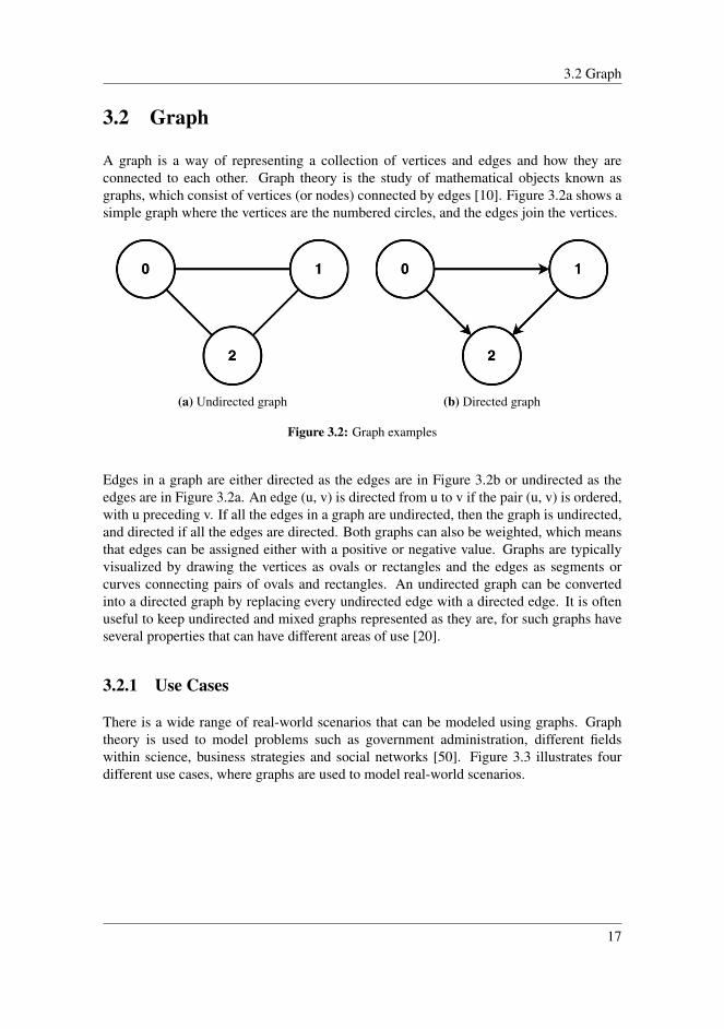
There is a wide range of real-world scenarios that can be modeled using graphs. Graphtheory is used to model problems such as government administration, different fieldswithin science, business strategies and social networks [50]. Figure 3.3 illustrates fourdifferent use cases, where graphs are used to model real-world scenarios.
17
Chapter 3. Background
(a) Social network graph derived from [23](b) Fraud detection graph derived from [49]
(c) Recommendation System graph derived from[64] (d) Insurance Fraud graph derived from [49]
Figure 3.3: Graph use cases
There is a wide range of well-developed graph algorithms that perform many kinds ofgraph operations such as clustering, pattern matching, shortest path calculations, depthsearch and other graphing functions. Some well-known examples are the following:
• Depth & Breadth First Search: A simple search algorithm used to find the shortestpath from one node to another. Depth first search begins by inspecting the deepestnodes first. Breadth first search begins with inspecting the closest node first [7].
• Belleman-Ford: An algorithm used to find the shortest path to all other nodes froma given starting point. Used in graphs that have negatively weighted edges [17].
• Dijkstra: Algorithm used to find the shortest path between two nodes in a networkwith weighted edges [24].
• K-means: A clustering algorithm used to discover underlying patterns by groupingsimilar data points together [19].
18
3.3 Graph Storage
3.3 Graph Storage
The term “Graph Storage” refers to the internal graph database structure, and how the datastorage is actually implemented. Different systems use different ways of storing graphs.However, systems built specifically for storing graph data are called native graph storage.Native graph storage means that the system is optimized for graphs in every aspect, andconsiderations for other aspects may be down-prioritized [9]. A native graph storageenables traversal of connected nodes in constant time. It makes it possible to traverse,for example, a dataset consisting of one billion nodes, just as fast as a one million nodedataset.
In order to achieve native storage, graph databases utilize an architecture known as“index-free adjacency”, which is designed explicitly for graph databases. “Index-freeadjacency” means that a data element is directly connected and points to another dataelement or relationship. This makes lookups extremely fast because there is no need tolook up and follow index pointers [21].
The term non-native storage is used for systems where other sources handle how the graphis stored. If a relational or a different kind of NoSQL database has to store a graph, nodesand relationships may end up being placed far from each other, and performance will bedrastically affected [9].
3.4 Neo4j
Neo4j is a native graph database management system written in Java and Scala, developedby Neo4j. Inc. The development of the system began in 2003 and was released forcommercial use in 2007. Neo4j is an open-source, NoSQL, native graph database. Thesource code can be found on GitHub1, and the service can also be used through a user-friendlydesktop application. Neo4j is available in two different versions, a community editionand an enterprise edition. The enterprise edition includes all the same features as thecommunity edition, but it also includes services to back up data and features clustering andfailover abilities. Today, Neo4j is used by many big corporations, for example, Telenor,Nettbus(Vy), Volvo, Walmart, eBay, IBM and Microsoft [33].
3.4.1 Choosing Neo4j
The rationale behind choosing Neo4j as service for this project was mostly because Sportradaralready used Neo4j for parts of their data. Furthermore, Neo4j is one of the most usedgraph database management systems. Naturally, there exists more documentation forNeo4j compared to other graph databases. The research and use of graph databases arequite limited; therefore choosing a well-known provider was important.
1https://github.com/neo4j/neo4j
19

Chapter 3. Background
Community
Neo4j has a large online community with more than one thousand users. The communityconsists of a global forum for online discussion on how graphs work. Furthermore, Neo4jhas its own workspace on Slack2; “neo4j-users.slack.com” where users can register. Todaythere are 10.000 active users on Neo4j’s Slack. Both the forum and the workspace on Slackare two reliable sources to explore when looking for documentation and answers regardingNeo4j.
3.4.2 The Property Graph Model
Neo4j has its own unique object model, called The Property Graph Model, which describeshow its system works in terms of objects, classes and the relationships between them. Itis shown in Figure 3.4. The Property Graph Model organizes data as nodes, relationshipsand properties. Nodes and relationships are the graph’s vertices and edges. Properties arevarious kinds of information that are stored on both the nodes and the relationships [36].
Figure 3.4: Property Graph Model by Neo4j [36]
3.4.3 Neo4j Browser
The Neo4j Browser is Neo4j’s graphical user interface. The browser is easy to use andcan be run through the web browser. With the Neo4j Browser, users can query, visualize,administer and monitor a graph database.
2https://slack.com
20

3.4 Neo4j
3.4.4 Cypher
Cypher is Neo4j’s own query language created for describing visual patterns in graphs. Itis a declarative language and is highly inspired by SQL. Cypher supports the use of allCRUD-operations on a graph without having to explicitly describe how to do it. CRUDstands for create, read, update and delete, and together they make up the basic operations ofa database. As mentioned earlier in this chapter, a graph consists of nodes and relationships.Both nodes and relationships can have additional info known as labels. Figure 3.5 showsa simple graph containing two nodes and one relationship. Cypher makes it possible toask and answer complex questions on datasets by lay or application users and not justdevelopers [31].
Figure 3.5: Relationship between two nodes
Cypher’s syntax is quite simple. Nodes are enclosed by parentheses, “(node)”, relationshipsby straight brackets, “[relationship]” and properties by curly brackets, “{property}”. Therelationships must be directed, meaning they have to point from one node to another.Arrows such as “->” and “<-” are used to indicate the direction of the relationship. Listing3.1 shows how the graph in Figure 3.5 can be created.
1 CREATE(:John{name:"John Doe"})2 -[:LIKES]->(:Julie{name:"Julie Doe"})
Listing 3.1: Cypher query used to create graph from Figure 3.5
The CREATE statement above displays a query that can be used to create the graph shownin Figure 3.5. The graph contains two kinds of nodes (:John) and (:Julie). Eachnode has been given the property name which is respectively set to “John Doe” and “JulieDoe”. The node types are used for accessing and referencing the nodes. For example,we can use MATCH(person:John), which gives all nodes of type (:John) the labelperson. Then we can use RETURN person.name to access John Doe’s full name.If the graph contained other nodes of the type (:John) representing different Johns, itwould also return their full names.
21

Chapter 3. Background
3.4.5 APOC
APOC stands for Awesome Procedures on Cypher and is a utility library for Neo4j basedon Cypher. It contains more than 450 different functions and procedures for different kindsof tasks including:
• Graph algorithms
• Metadata
• Manual indexes and relationship indexes
• Full-text search
• Integration with other databases like MongoDB, ElasticSearch, Cassandra and relationaldatabases
• Loading of XML and JSON from APIs and files
• Collection and map utilities
• Date and time functions
• String and text functions
• Import and export
• Concurrent and batched Cypher execution
• Spatial functions
• Path expansion
Today, APOC is the largest literary developed for Neo4j. Before APOC was implemented,developers had to write their own methods for all the functions and procedures mentionedabove, and the result was a lot of duplicated and poor quality code [22]. APOC madeit possible for developers to only focus on writing business-logic and use-case specificcode without having to deal with platform limitations. All functions and procedures arewell-supported and easy to use by themselves, or in combination with other methods [37].
3.5 Alternative Graph Database Management Systems
There are many providers of graph database management systems out on the market.Some are open source, and public licensed and others are commercially licensed. Thenext following sections will present a few other alternatives to Neo4j.
22
3.5 Alternative Graph Database Management Systems
3.5.1 Amazon Neptune
Amazon Neptune3 is a commercially licensed cloud-based GDBMS, and it is one of thebiggest providers of graph databases on the commercial market. Amazon released it 2017so that users could create sophisticated, interactive graph applications that could querybillions of relationships with minimum latency. Amazon Neptune supports a variety ofthe most popular graph models and their query languages. Along with complete ACIDcompliance, Amazon Neptune is fully managed, which means that users do not have toworry about database management tasks such as hardware provisioning, software patching,setup, configuration or backups. All of these tasks are completed automatically [53][61].
Amazon created the database with a high focus on availability, recoverability and durability.Amazon Neptune supports point-in-time recovery, which means an administrator can rollback the database to any given timestamp. Continuous backups are made automaticallyand stored using Amazon’s S3 cloud storage services. Highly secure and encrypted storageis also offered using Amazon’s own encryption algorithms [53].
3.5.2 OrientDB
OrientDB is an open source NoSQL database management system, developed by OrientDBLtd and released in 2010. The database is a “multi-model” database, which means itsupports various models such as key/value, document, object and graph model. In OrientDB,all connections between records are managed as relationships as in a graph database.Orient is written in Java and is designed to perform very fast. With the ability to storeand process 220.000 records per second, it is according to their own website4, the graphdatabase with the highest performance available [44].
OrientDB comes in two different versions, a free community edition and an enterpriseedition with professional support service. Furthermore, OrientDB has an enormous capacity.It can store up to 302,231,454,903,657 billion ( 278) records with the maximum capacityof 19.807.040.628.566.084 Terabytes of data on a single server or multiple nodes [44].
3.5.3 ArangoDB
ArangoDB is also a native multi-model database developed by ArangoDB Inc. The databasewas released in 2011 under the name AvocadoDB, but one year later in, 2012, it waschanged to ArangoDB. On their website5, they market themselves as a GDBMS with ahigh focus on search and index algorithms. Natively integrated into ArangoDB, is a C++based full-text search engine, with included similarity ranking capabilities. This searchengine utilizes two kinds of information retrieval techniques: boolean and generalizedranking retrieval. It enables ArangoDB to perform complex federated searches over awhole complex graph [1].
3https://aws.amazon.com/neptune/4https://orientdb.com5https://www.arangodb.com
23
Chapter 3. Background
The developers behind ArangoDB have also created a query language, ArangoDB QueryLanguage (AQL), which is similar to SQL. AQL supports CRUD, aggregations, complexfilter conditions, secondary indexes and real JOIN operations, which makes it possible forthe users to alter their data access strategy just by changing a query [2].
3.6 Oracle
Oracle is a world-leading software company. According to an analysis [47], by the advisoryfirm PwC, Oracle was the second-largest software company by revenue in 2014 and is aglobal corporation that develops software and applications used for business. The companyis best known for its relational database software. Oracle was founded in 1977 in theUnited States in Santa Clara, California. Today, Oracle has its headquarters in RedwoodShores, California [60]. They have about half a million customers in 173 different countriesand 25.000 partners [40].
3.6.1 MySQL
MySQL is the world’s most popular open source RDBMS [43]. It is based on SQL and canrun on many different platforms including Linux, UNIX and Windows. MySQL is used ina wide range of applications, both small and large applications, but it is commonly foundin web applications. Originally MySQL was a Swedish product, but was acquired by SunMicrosystems in 2008, and later taken over by Oracle in 2010. Today, MySQL is used inmany top large scale websites such as Facebook, Google, Twitter and YouTube [51].
MySQL is based on a client-server model. The core of MySQL is a server, which handlesall commands to the database. In order to communicate with the server, one typicallyuses a MySQL client to send commands. The client can be downloaded and installed onmost computers today. Originally MySQL was designed to handle large databases quickly.However, most users only install MySQL on one machine, but the client can be installedon several machines and the database can be accessed through a broad range of clientinterfaces. Through the client, users can send SQL statements to the server and have itreturn the results.
3.6.2 Structured Query Language
SQL stands for Structured Query Language, which is the standard programming languagefor relational data manipulation and data management. The language was developed in theearly 1970s at IBM by Raymond Boyce and Donald Chamberlin. Today, most RDBMSsupport SQL, including MySQL, and it is used to query, insert, update and modify data inrelational databases. In 1979 Oracle adapted SQL and released its own modified version.Since then, SQL has played an important role in modern database development [38].
24

3.6 Oracle
3.6.3 Support
An important aspect of MySQL is the fact that MySQL can store data across many differentstorage engines. Furthermore, MySQL has algorithms for replicating data and partitioningtables in order to increase performance and durability. Not only is MySQL free to downloadand use, but equally important is the fact that Oracle has a large technical support teamfocused just on MySQL. Oracle offers direct access to expert MySQL Support engineerswho are capable of helping with development, deployment, and management of MySQLapplications. Support is available 24 hours a day and 365 days a year [28]. Since MySQLhas been around for a decade, a large community around it has emerged. On StackOverflow6, one can find over half a million posts that are tagged with MySQL [12].
Through their website7, MySQL provides a broad array of different support and educationalservices. Users of MySQL can sign up for comprehensive MySQL training courses, whicheducate developers on how to build efficient database solutions. Followed by a certificationprogram that developers can take in order to prove their knowledge within MySQL.
On the support side, MySQL offers a consulting service, which can assist developers tooptimize or scale an existing solution, or it can be used to get help with setting up anew project. Lastly, the MySQL technical support team aid developers with their specificneeds, helping them achieve higher levels of performance, reliability, and uptime.
3.6.4 Choosing MySQL
MySQL is the world’s most used database [4]. It is Neo4j biggest competitor, and it is alsothe database that Sportradar primarily uses. Thus it was natural to select it as the relationaldatabase to use for this project.
3.6.5 InnoDB
MySQL 8.0 is powered by InnoDB, a general purpose storage-engine created by Oracle.Today, InnoDB is the storage-engine used by default in MySQL, unless other configurationsare made. Until December 2010, MySQL was powered by an engine called MyISAM, butwas replaced by InnoDB. InnoDB serves the purpose of balancing high reliability withhigh performance within MySQL. In addition, InnoDB follows the standard ACID model,which features transactions with commit, rollback, and crash-recovery capability in orderto protect user data. Based on primary keys, InnoDB arranges data on disk in order tooptimize queries. This means that each table has a primary key index that is used toorganize data so that the amount I/O lookups for primary keys are reduced [41].
6https://stackoverflow.com/7https://www.mysql.com/services/
25
Chapter 3. Background
3.6.6 B+-Tree
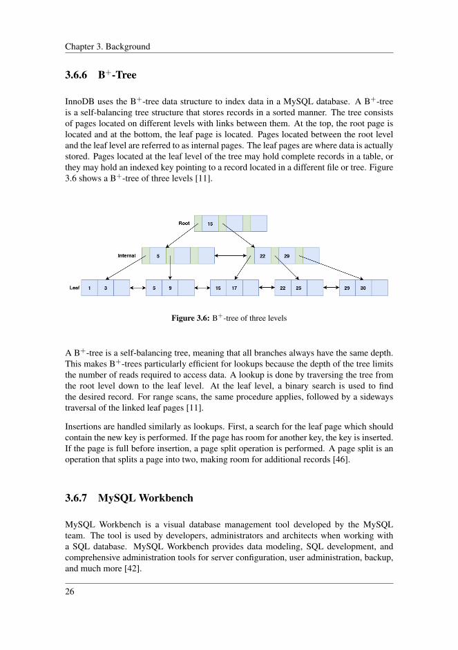
InnoDB uses the B+-tree data structure to index data in a MySQL database. A B+-treeis a self-balancing tree structure that stores records in a sorted manner. The tree consistsof pages located on different levels with links between them. At the top, the root page islocated and at the bottom, the leaf page is located. Pages located between the root leveland the leaf level are referred to as internal pages. The leaf pages are where data is actuallystored. Pages located at the leaf level of the tree may hold complete records in a table, orthey may hold an indexed key pointing to a record located in a different file or tree. Figure3.6 shows a B+-tree of three levels [11].
Figure 3.6: B+-tree of three levels
A B+-tree is a self-balancing tree, meaning that all branches always have the same depth.This makes B+-trees particularly efficient for lookups because the depth of the tree limitsthe number of reads required to access data. A lookup is done by traversing the tree fromthe root level down to the leaf level. At the leaf level, a binary search is used to findthe desired record. For range scans, the same procedure applies, followed by a sidewaystraversal of the linked leaf pages [11].
Insertions are handled similarly as lookups. First, a search for the leaf page which shouldcontain the new key is performed. If the page has room for another key, the key is inserted.If the page is full before insertion, a page split operation is performed. A page split is anoperation that splits a page into two, making room for additional records [46].
3.6.7 MySQL Workbench
MySQL Workbench is a visual database management tool developed by the MySQLteam. The tool is used by developers, administrators and architects when working witha SQL database. MySQL Workbench provides data modeling, SQL development, andcomprehensive administration tools for server configuration, user administration, backup,and much more [42].
26
3.7 Python
3.7 Python
Python is a high-level programming language. It is an interpreted language which meansthat its code is executed directly without the need of a compiler to first translate or compilethe program into machine language instructions. Python was released in 1990 and hasbeen continuously updated and improved ever since. The language is easy to learn and hasmany areas of use. Most programming paradigms such as object-oriented, functional andprocedural programming are well supported [48].
3.8 Premier League
The Premier League is the top level of English soccer. The league was founded in 1992after numerous conflicts and discussions between soccer authorities, players, televisionbroadcasters and the previous top-level league management [62]. This season, the 2018/2019season, is the 27th season of the Premier League. Today the league consists of 20 competingteams, and is the most followed sports league in the world. The League is broadcasted in212 territories and to 643 million homes which potentially can reach 4.7 billion people. Aseason starts in August and lasts until May. In the course of that time period, 387 soccermatches are played [13]. According to BBC [57] the television rights for a three yearperiod 2016-2019 are worth £5.14bn.
27

Chapter 3. Background
28
Chapter 4Design & Implementation
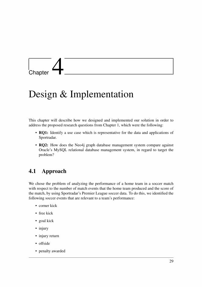
This chapter will describe how we designed and implemented our solution in order toaddress the proposed research questions from Chapter 1, which were the following:
• RQ1: Identify a use case which is representative for the data and applications ofSportradar.
• RQ2: How does the Neo4j graph database management system compare againstOracle’s MySQL relational database management system, in regard to target theproblem?
4.1 Approach
We chose the problem of analyzing the performance of a home team in a soccer matchwith respect to the number of match events that the home team produced and the score ofthe match, by using Sportradar’s Premier League soccer data. To do this, we identified thefollowing soccer events that are relevant to a team’s performance:
• corner kick
• free kick
• goal kick
• injury
• injury return
• offside
• penalty awarded
29

Chapter 4. Design & Implementation
• penalty missed
• red card
• score change
• shot off target
• shot on target
• shot saved
• throw in
• yellow card
• yellow red card
For each event type, we calculated the number of events created per minute for each of thethree possible states a soccer match can be in with respect to home team score:
• Score is tied
• Home team is winning
• Home team is losing
In order to performance test Neo4j and MySQL, we developed two databases, one graphdatabase and one relational database. Both databases contained the exact same data, butstructured differently. With all this information, we developed an application that retrievedevent information from a database, and analyzed it according to our preferences. Wedefined three test cases, described below, in order to compare performance between thegraph and the relational database. The application was by turn connected to each of thedatabases, and for each database, each test case was executed 25 times.
• Single Match - Select a random soccer match and calculate events produced perminute by the home team based on score.
• Team Season - Calculate events produced per minute based on the score for allsoccer matches played on home ground during the season for a specific team.
• Complete Season - Calculate events produced per minute based on the score for thehome team for all matches that have been played during the season.
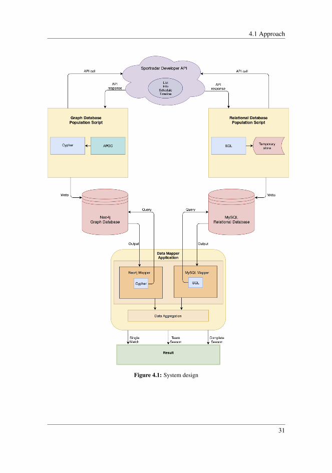
Figure 4.1 shows a complete overview of the system design. The remainder of this chapterwill describe what the different elements in the figure are, and how they work together.
30
4.1 Approach
Figure 4.1: System design
31

Chapter 4. Design & Implementation
4.2 Database Design
As previously mentioned, we created two databases for this project. To retrieve the necessarydata to populate our databases, we used four specific Sportradar API calls:
• Tournament List API
• Tournament Info API
• Tournament Schedule API
• Match Timeline API
These API calls are represented in Figure 4.1 as the purple cloud on top named “SportradarDeveloper API”.
The Tournament List API returns a list of all major soccer tournaments in Europe. Wecalled that first to retrieve the necessary information regarding the Premier League, hereidentified by the “tournament id” field, shown in Listing 4.1, which is a fragment of theresults we received when we called the Tournament List API.
1 {2 "id": "sr:tournament:17",3 "name": "Premier League",4 "sport": {5 "id": "sr:sport:1",6 "name": "Soccer"7 },8 "category": {9 "id": "sr:category:1",
10 "name": "England",11 "country_code": "ENG"12 },13 "current_season": {14 "id": "sr:season:54571",15 "name": "Premier League 18/19",16 "start_date": "2018-08-10",17 "end_date": "2019-05-13",18 "year": "18/19"19 }
Listing 4.1: Result from calling the Tournament List API
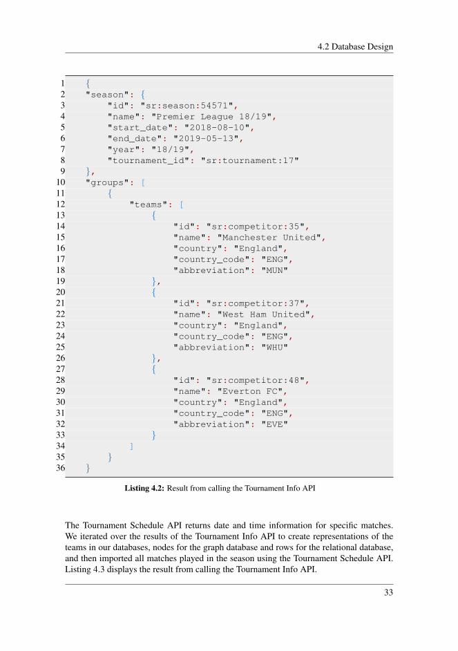
The Tournament Info API returns a complete overview of all teams that participate in aspecific tournament, along with information about the tournament such as season, nameand start and end date. Listing 4.2 shows a selection of the result from calling the TournamentInfo API using the “tournament id” received from the Tournament List API.
32
4.2 Database Design
1 {2 "season": {3 "id": "sr:season:54571",4 "name": "Premier League 18/19",5 "start_date": "2018-08-10",6 "end_date": "2019-05-13",7 "year": "18/19",8 "tournament_id": "sr:tournament:17"9 },
10 "groups": [11 {12 "teams": [13 {14 "id": "sr:competitor:35",15 "name": "Manchester United",16 "country": "England",17 "country_code": "ENG",18 "abbreviation": "MUN"19 },20 {21 "id": "sr:competitor:37",22 "name": "West Ham United",23 "country": "England",24 "country_code": "ENG",25 "abbreviation": "WHU"26 },27 {28 "id": "sr:competitor:48",29 "name": "Everton FC",30 "country": "England",31 "country_code": "ENG",32 "abbreviation": "EVE"33 }34 ]35 }36 }
Listing 4.2: Result from calling the Tournament Info API
The Tournament Schedule API returns date and time information for specific matches.We iterated over the results of the Tournament Info API to create representations of theteams in our databases, nodes for the graph database and rows for the relational database,and then imported all matches played in the season using the Tournament Schedule API.Listing 4.3 displays the result from calling the Tournament Info API.
33

Chapter 4. Design & Implementation
12 {3 "sport_evnts": {4 "id": "sr:match:14735957",5 "scheduled": "2018-08-10T19:00:00+00:00",6 "tournament": {7 "id": "sr:tournament:17"8 }9 "competitors": [
10 {11 "id": "sr:competitor:35",12 "name": "Manchester United",13 "country": "England",14 "country_code": "ENG",15 "abbreviation": "MUN",16 "qualifier": "home"17 },18 {19 "id": "sr:competitor:31",20 "name": "Leicester City",21 "country": "England",22 "country_code": "ENG",23 "abbreviation": "LEI",24 "qualifier": "away"25 }26 ]27 }
Listing 4.3: Result from calling the Tournament Schedule API
The Match Timeline API returns information regarding each soccer event for a given matchor game: event type, clock time, period and team type (home or visiting). Listing 4.3 abovedisplays the results for a single soccer match. We received the results for 387 matches, andeach one resulted in a new match node or row in our databases. For each match, we calledthe Match Timeline API in order to collect all its game events, and each individual eventresulted in a new node or row in our databases. Listing 4.4 shows parts of a timeline fromcalling the Match Timeline API.
34

4.2 Database Design
1 {2 "sport_event": {3 "id": "sr:match:14735957"4 },5 "competitors": [6 {7 "id": "sr:competitor:35",8 "name": "Manchester United"9 },
10 {11 "id": "sr:competitor:31",12 "name": "Leicester City"13 }14 ],15 "timeline": [16 {17 "id": 447784954,18 "type": "match_started",19 "time": "2018-08-10T19:00:10+00:00"20 },21 {22 "id": 447785488,23 "type": "penalty_awarded",24 "match_clock": "1:27",25 "team": "home",26 "period": 127 },28 {29 "id": 447785902,30 "type": "score_change",31 "match_clock": "2:28",32 "team": "home",33 "period": 134 },35 {36 "id": 447786246,37 "type": "throw_in",38 "match_clock": "3:16",39 "team": "home",40 "period": 141 }42 ]43 }
Listing 4.4: Result from calling the Match Timeline API
35
Chapter 4. Design & Implementation
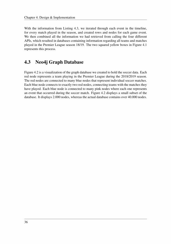
With the information from Listing 4.3, we iterated through each event in the timeline,for every match played in the season, and created rows and nodes for each game event.We then combined all the information we had retrieved from calling the four differentAPIs, which resulted in databases containing information regarding all teams and matchesplayed in the Premier League season 18/19. The two squared yellow boxes in Figure 4.1represents this process.
4.3 Neo4j Graph Database
Figure 4.2 is a visualization of the graph database we created to hold the soccer data. Eachred node represents a team playing in the Premier League during the 2018/2019 season.The red nodes are connected to many blue nodes that represent individual soccer matches.Each blue node connects to exactly two red nodes, connecting teams with the matches theyhave played. Each blue node is connected to many pink nodes where each one representsan event that occurred during the soccer match. Figure 4.2 displays a small subset of thedatabase. It displays 2.000 nodes, whereas the actual database contains over 40.000 nodes.
36

4.3 Neo4j Graph Database
Figure 4.2: Visualized subset of the graph database
When creating our database, we started with importing all the data that we needed. Inorder to import data from the APIs, we had to use the APOC plugin, described in Section3.4.5. APOC contained a function that let us directly import JSON formatted data into
37

Chapter 4. Design & Implementation
our graph database. This process was wrapped inside a script which is represented by theyellow box called “Graph Database Population Scrip” in Figure 4.1.
12 :param tournament_info:"https://api.sportradar.us3 /soccer-t3/eu/en/tournaments/sr:tournament:17/info.json?4 api_key={your_api_key}"56 CALL apoc.load.json(tournament_info,'.groups')7 YIELD value unwind value.teams as t8 CREATE (team:Team)9 SET team.name = t.name, team.id = t.id, team.abbreviation
10 = t.abbreviation
Listing 4.5: Query for importing all teams to the graph database
Listing 4.5 shows how we used APOC in a Cypher query to populate the database with allthe teams. First, we declared the parameter tournament_info and assigned it to theAPI call, which returned information regarding all soccer teams competing in the PremierLeague. Then we called APOC’s load procedure and passed in our newly createdtournament_info parameter together with a parameter called .groups. We includedthe .groups parameter because we were only interested in the contents of the groupsproperty shown on line 10 in Listing 4.2. Next, we used the YIELD keyword, whichenabled us to create new internal variables for fields that were within the groups property.By using the unwind clause, we reduced the newly created variables into a list consistingof team-objects. Finally, we used the CREATE statement together with the SET statementto create “(team:Team)”-nodes containing information for each team.
In order to populate the database with nodes representing soccer matches and in-gameevents, we set the Tournament Schedule API and the Match Timeline API as parameters,and executed very similar procedures as the one explained above with the new parameters.
The final part of populating the database was to create relationships between the nodes.After all the nodes where created, we made sure that they had a unique identification andthat they had an identifier that pointed to either their parent or child node. Team nodescontained the team’s name, abbreviation and an identification number. The Match nodeswere given an identifier that consisted of the playing team’s abbreviations. For example,the match between Newcastle and Chelsea FC was identified with “NEW-CHE”, wherethe team listed first was also the home team. Listing 4.6 and Listing 4.7 shows how theCypher statements connected teams to matches and matches to events.
1 MATCH (t:Team), (s:SportEvent) WHERE t.name = s.homeTeam2 CREATE (t)-[played:PLAYED]->(s)
Listing 4.6: Cypher statement for connecting home teams with matches
38

4.4 MySQL Relational Database
1 MATCH (se:SportEvent),(ge:GameEvent) WHERE se.sportEventId2 = ge.sportEventId CREATE (ge)-[part_of:PART_OF]->(se)
Listing 4.7: Cypher statement for connecting a match with its corresponding events
4.3.1 Neo4j Driver
There are many ways to interact with a Neo4j database and many different drivers tochoose from. For this research, we chose Neo4j’s official driver, as this was the onerecommended when working with Python as a programming language, according to thecommunity on Neo4j’s own Slack workspace. The driver is built on the “Bolt-protocol”,which is a binary protocol used for communication between client applications and databaseservers [34]. The driver provided us with a connection setup, which we needed to usewhen connecting to the database. Additionally, the driver gave us access to functions thatwe used to read and write to the database.
4.3.2 Neo4j Configuration
The graph database solution was created by using version 3.5.3 of Neo4j, together withversion 3.5.0.2 of the APOC plugin. Not all versions of Neo4j and APOC are compatiblewith each other, so it is important to be sure that the correct versions are being used. Forvisualization and administration of the graph database, we used version 1.1.13 of Neo4j’sdesktop application.
4.4 MySQL Relational Database
To better evaluate our graph database results, we created a relational MySQL database forcomparison, and populated with the same data from the same Sportradar APIs.
4.4.1 Design
The MySQL database was designed similarly to the Neo4j database. The schema consistedof three tables shown in figure 4.3. The “Team” table contained a row for each team thatplayed in Premier League 18/19. The “SportEvent” table contained a row for all soccermatches that had been played during the season. The “GameEvent” table contained a rowfor each event that took place in a match.
39

Chapter 4. Design & Implementation
Figure 4.3: Relational database design
To populate the different tables we wrote scripts in Python. They imported data fromthe APIs, retrieved relevant information and applied string operations to clean the data.Lastly, the scripts wrote the data into the correct tables. In order to write data to thedatabase, we created an SQL statement similar to the Cypher statement from Listing 4.5.Populating the Team table in MySQL was, however, a more complex process. Insteadof writing to the database directly from the Tournament Info API, we had to store alldata temporarily. This was done in our Python scripts. To import the teams we definedthe function getTeamInformation(jsonObject) seen in Listing 4.8. Receivingthe results from the Tournament Info API (Listing 4.2) as input, the function temporarilystored each team’s details in different lists.
tempTeamId = []tempTeamName = []tempTeamAbbreviation = []def getTeamInformation(jsonObject):groups = jsonObject["groups"]for group in groups:
teams = (group["teams"])for team in teams:
tempTeam.append(team["id"])tempTeamName.append(team["name"])tempTeamAbbreviation.append(team["abbreviation"])
Listing 4.8: Python function that temporary stores team attributes
Upon completion of getTeamInformation(jsonObject), we were able to populatethe Team table using the function updateTeamTable(db) shown in Listing 4.9. Ititeratively wrote the contents of each temporary attribute list to the table. The variablesqlString, was the actual SQL statement that was processed by the database.
40

4.5 Data Mapper Application
def populateTeamTable(db):cursor = db.cursor()for x in range(0, len(teamId)):
idTeam = tempTeamId[x]name = tempTeamName[x]abbreviation = tempTeamAbbreviation[x]sqlString = "INSERT INTO Team VALUES(" + "'" + str(idTeam) + "'" + ", " + '"' +str(name) + '"' + ", " + '"' +str(abbreviation) + '"' + ")"cursor.execute(sqlString)
print("Team table updated")
Listing 4.9: Python function that writes each team with attributes to database
This procedure was repeated in a similar way for writing soccer matches and in-gameevents to the database. The table population is indicated by the yellow box named “RelationalDatabase Population Script” in Figure 4.1.
4.4.2 MySQL Server
We used MySQL version 8.0.15 for the database. The database was hosted on localhost.Having the database hosted locally made it simple to handle, and we were not dependenton third-party vendors, which gave us complete control over the database.
4.4.3 MySQL Workbench
When creating the database, we used Oracle’s MySQL Workbench version 8.0.15. MySQLWorkbench provided us with a graphical user interface for our relational database. Thiswas a useful tool for testing and debugging the database. Also, MySQL Workbench wasused to define the schema for the relational database.
4.5 Data Mapper Application
A mapper is a layer that moves or separates data between an object and a database [18].In this case, we needed an application that could calculate the score and number of eventsoccurring in each match, based on data returned from querying the databases. We wroteour mapping application in Python. The application consisted of two parts; the firstpart separately performed the mapping for databases and the second part aggregated themapping results. This part is illustrated in Figure 4.1 as the yellow box with roundededges.
41
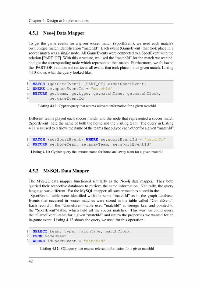
Chapter 4. Design & Implementation
4.5.1 Neo4j Data Mapper
To get the game events for a given soccer match (SportEvent), we used each match’sown unique match identification “matchId”. Each event (GameEvent) that took place in asoccer match was a single node. All GameEvents were connected to a SportEvent with therelation [PART OF]. With this structure, we used the “matchId” for the match we wanted,and got the corresponding node which represented that match. Furthermore, we followedthe [PART OF] relation and retrieved all events that took place in that given match. Listing4.10 shows what the query looked like.
1 MATCH (ge:GameEvent)-[PART_OF]->(se:SportEvent)2 WHERE se.sportEventId = "matchId"3 RETURN ge.team, ge.type, ge.matchTime, ge.matchClock,4 ge.gameEventId
Listing 4.10: Cypher query that returns relevant information for a given matchId
Different teams played each soccer match, and the node that represented a soccer match(SportEvent) held the name of both the home and the visiting team. The query in Listing4.11 was used to retrieve the name of the teams that played each other for a given “matchId”.
1 MATCH (se:SportEvent) WHERE se.sportEventId = "matchId"2 RETURN se.homeTeam, se.awayTeam, se.sportEventId"
Listing 4.11: Cypher query that returns name for home and away team for a given matchId
4.5.2 MySQL Data Mapper
The MySQL data mapper functioned similarly as the Neo4j data mapper. They bothqueried their respective databases to retrieve the same information. Naturally, the querylanguage was different. For the MySQL mapper, all soccer matches stored in the“SportEvent”-table were identified with the same “matchId” as in the graph database.Events that occurred in soccer matches were stored in the table called “GameEvent”.Each record in the “GameEvent”-table used “matchId” as foreign key, and pointed tothe “SportEvent”-table, which held all the soccer matches. This way we could querythe “GameEvent”-table for a given “matchId” and return the properties we wanted for anin-game event. Listing 4.12 shows the query we used for this operation.
1 SELECT team, type, matchTime, matchClock2 FROM GameEvent3 WHERE idSportEvent = "matchId"
Listing 4.12: SQL query that returns relevant information for a given matchId
42
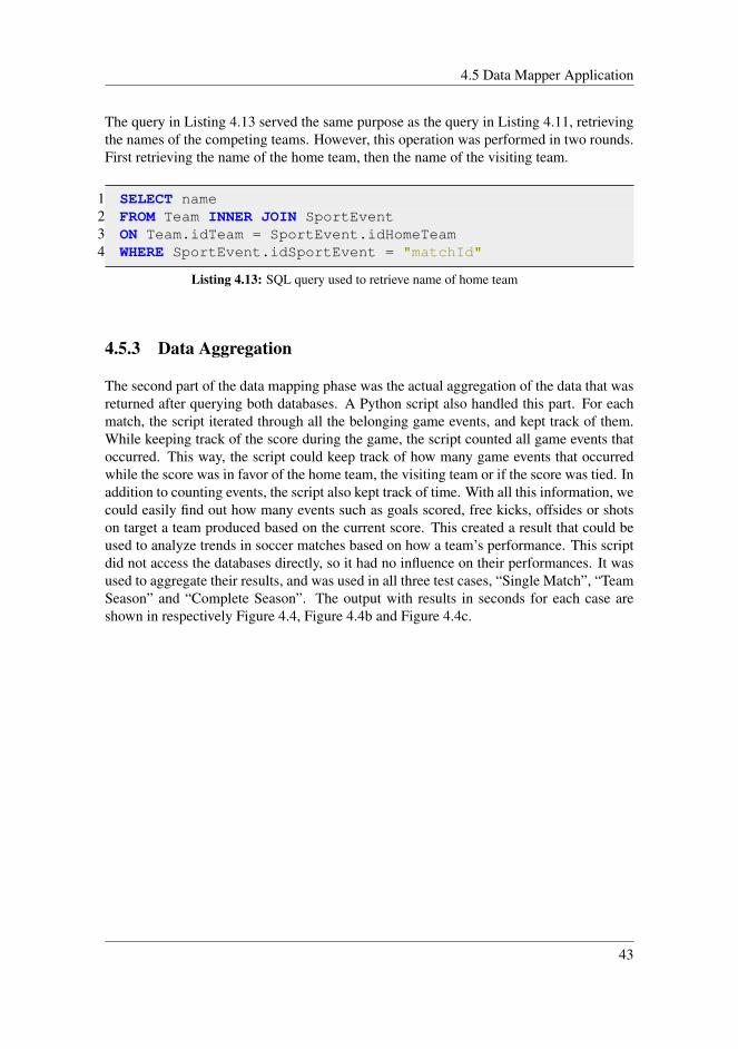
4.5 Data Mapper Application
The query in Listing 4.13 served the same purpose as the query in Listing 4.11, retrievingthe names of the competing teams. However, this operation was performed in two rounds.First retrieving the name of the home team, then the name of the visiting team.
1 SELECT name2 FROM Team INNER JOIN SportEvent3 ON Team.idTeam = SportEvent.idHomeTeam4 WHERE SportEvent.idSportEvent = "matchId"
Listing 4.13: SQL query used to retrieve name of home team
4.5.3 Data Aggregation
The second part of the data mapping phase was the actual aggregation of the data that wasreturned after querying both databases. A Python script also handled this part. For eachmatch, the script iterated through all the belonging game events, and kept track of them.While keeping track of the score during the game, the script counted all game events thatoccurred. This way, the script could keep track of how many game events that occurredwhile the score was in favor of the home team, the visiting team or if the score was tied. Inaddition to counting events, the script also kept track of time. With all this information, wecould easily find out how many events such as goals scored, free kicks, offsides or shotson target a team produced based on the current score. This created a result that could beused to analyze trends in soccer matches based on how a team’s performance. This scriptdid not access the databases directly, so it had no influence on their performances. It wasused to aggregate their results, and was used in all three test cases, “Single Match”, “TeamSeason” and “Complete Season”. The output with results in seconds for each case areshown in respectively Figure 4.4, Figure 4.4b and Figure 4.4c.
43

Chapter 4. Design & Implementation
(a) Results of data aggregation for a single match (Cardiff City - Wolverhampton Wanderers)
(b) Results of data aggregation for all of Liverpool’s home matches
(c) Results of data aggregation of all home matches played so far at the time in the Premier Leagueseason 18/19
Figure 4.4: Output from executing each of the test cases
44

4.6 Hardware
4.6 Hardware
All development and test case execution were conducted on a single computer, a MacBookPro Early 2013, running macOS Mojave Version 10.14.4 with these components:
• Processor: 2.6 Ghz Intel Core i5 (2 cores)
• Memory: 8 GB 1600 MHz DDR3
• Storage: Apple SSD 256 GB
• Graphics: Intel HD Graphics 4000 1536 MB
45

Chapter 4. Design & Implementation
46

Chapter 5Results & Discussion
Our research project consisted of three different test cases. The test cases were eachperformed on a graph database and a relational database. This chapter will first presentthe results of our research. It will then analyze and discuss them in light of previous workand our own expectations.
5.1 Expectations
Based on the project description from Sportradar, we had high expectations for Neo4j.In addition, most of the related work we studied indicated that Neo4j would outperformMySQL for most of our test cases. The index-free adjacency property was also a factorthat contributed to raising the expectations of Neo4j. We therefore assumed that our graphdatabase would tackle the three test cases without any problems. Based on the long lifetimeof MySQL and its widespread use, we assumed that MySQL also would perform well allover.
5.2 Results
We produced the results in this project by measuring the time it took to complete each ofthe three test cases for each of the two databases. To ensure accurate and unbiased timingresults, the test cases were executed one at a time on the same computer, described inSection 4.6, with only the most minimal services running. The database servers were alsoboth hosted locally so that there would not be bias from network irregularities.
The processing time was different for every individual execution. Therefore all experimentswere performed 25 times for each test case in order to give representative results, and
47
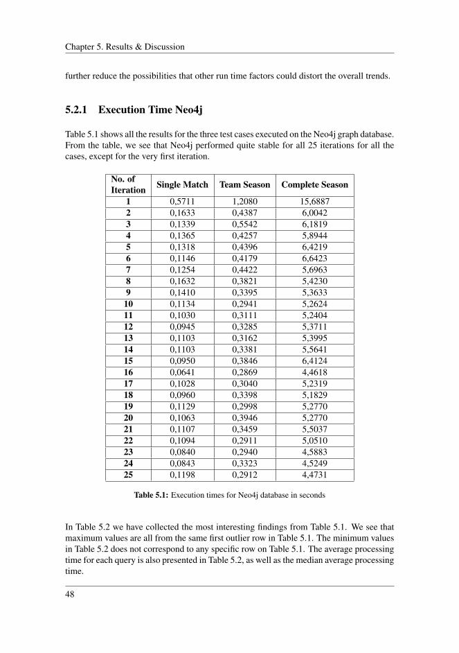
Chapter 5. Results & Discussion
further reduce the possibilities that other run time factors could distort the overall trends.
5.2.1 Execution Time Neo4j
Table 5.1 shows all the results for the three test cases executed on the Neo4j graph database.From the table, we see that Neo4j performed quite stable for all 25 iterations for all thecases, except for the very first iteration.
No. ofIteration Single Match Team Season Complete Season
1 0,5711 1,2080 15,68872 0,1633 0,4387 6,00423 0,1339 0,5542 6,18194 0,1365 0,4257 5,89445 0,1318 0,4396 6,42196 0,1146 0,4179 6,64237 0,1254 0,4422 5,69638 0,1632 0,3821 5,42309 0,1410 0,3395 5,3633
10 0,1134 0,2941 5,262411 0,1030 0,3111 5,240412 0,0945 0,3285 5,371113 0,1103 0,3162 5,399514 0,1103 0,3381 5,564115 0,0950 0,3846 6,412416 0,0641 0,2869 4,461817 0,1028 0,3040 5,231918 0,0960 0,3398 5,182919 0,1129 0,2998 5,277020 0,1063 0,3946 5,277021 0,1107 0,3459 5,503722 0,1094 0,2911 5,051023 0,0840 0,2940 4,588324 0,0843 0,3323 4,524925 0,1198 0,2912 4,4731
Table 5.1: Execution times for Neo4j database in seconds
In Table 5.2 we have collected the most interesting findings from Table 5.1. We see thatmaximum values are all from the same first outlier row in Table 5.1. The minimum valuesin Table 5.2 does not correspond to any specific row on Table 5.1. The average processingtime for each query is also presented in Table 5.2, as well as the median average processingtime.
48
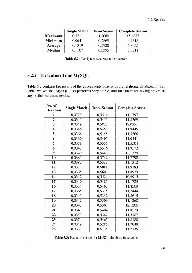
5.2 Results
Single Match Team Season Complete SeasonMaximum 0,5711 1,2080 15,6887Minimum 0,0641 0,2869 4,4618Average 0,1319 0,3920 5,8455Median 0,1107 0,3395 5,3711
Table 5.2: Neo4j test case results in seconds
5.2.2 Execution Time MySQL
Table 5.2 contains the results of the experiments done with the relational database. In thistable, we see that MySQL also performs very stable, and that there are no big spikes inany of the test cases results.
No. ofIteration Single Match Team Season Complete Season
1 0,0775 0,5514 11,17972 0,0345 0,5455 11,83693 0,0349 0,5823 12,02514 0,0346 0,5457 11,94455 0,0366 0,5455 11,53666 0,0360 0,5407 11,04417 0,0378 0,5355 11,55048 0,0342 0,5516 11,95729 0,0349 0,5447 12,1375
10 0,0381 0,5742 11,729011 0,0382 0,5533 11,131212 0,0374 0,6088 11,918313 0,0365 0,5601 11,897914 0,0342 0,5524 10,991515 0,0340 0,5485 11,172516 0,0334 0,5463 11,850917 0,0365 0,5378 11,744418 0,0343 0,5352 11,861519 0,0342 0,5509 11,126820 0,0343 0,5301 12,120621 0,0347 0,5404 11,857922 0,0357 0,5382 11,518723 0,0374 0,5467 11,818024 0,0349 0,5285 11,704825 0,0331 0,6135 11,2135
Table 5.3: Execution times for MySQL database in seconds
49

Chapter 5. Results & Discussion
Table 5.4 sums up the most interesting findings from Table 5.3, presenting the fastestand slowest processing time for each test case. In addition, the table presents the regularaverage and median average for processing time.
Single Match Team Season Complete SeasonMaximum 0,0775 0,6135 12,1375Minimum 0,0331 0,5285 10,9915Average 0,0371 0,5523 11,6348Median 0,0349 0,5463 11,7444
Table 5.4: MySQL test case results in seconds
5.3 Analysis
With the results presented in the previous section we have created three graphs, one foreach test case. The graphs consist of two plots showing how the two databases comparedwith respect to each other. In this section, we will use the plots to analyze these results.
5.3.1 Single Match
The “Single Match” test case computed the number of events produced by the home teamper minute based on the score of a single soccer match.
Figure 5.1: Graphed results of the first test case
50
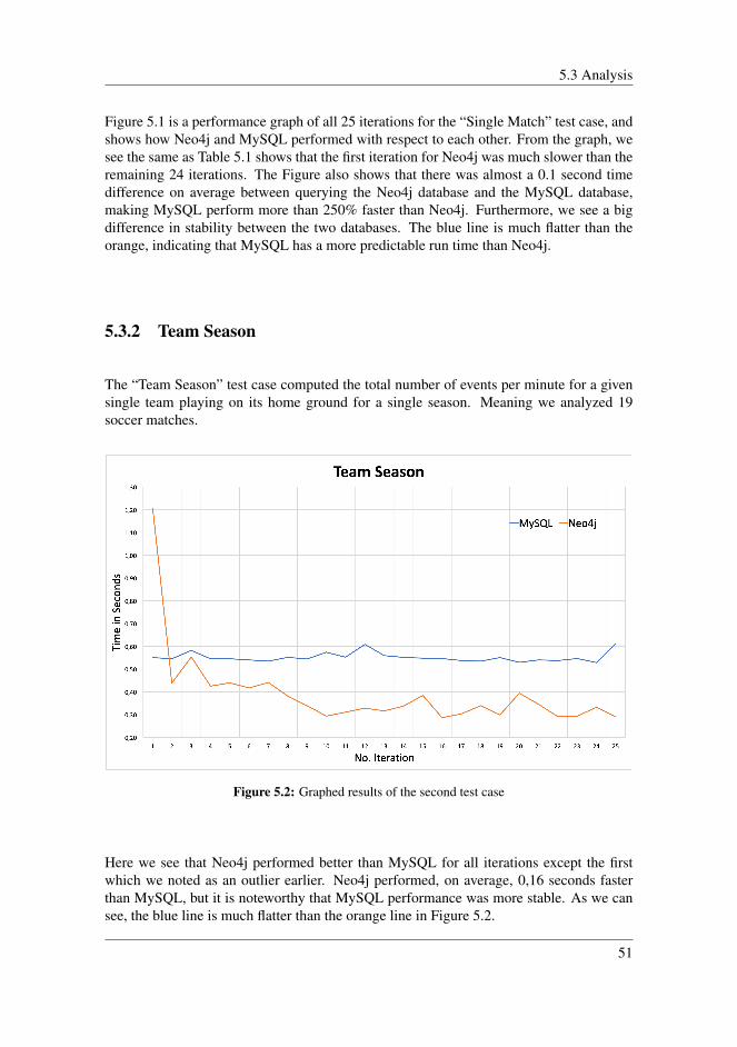
5.3 Analysis
Figure 5.1 is a performance graph of all 25 iterations for the “Single Match” test case, andshows how Neo4j and MySQL performed with respect to each other. From the graph, wesee the same as Table 5.1 shows that the first iteration for Neo4j was much slower than theremaining 24 iterations. The Figure also shows that there was almost a 0.1 second timedifference on average between querying the Neo4j database and the MySQL database,making MySQL perform more than 250% faster than Neo4j. Furthermore, we see a bigdifference in stability between the two databases. The blue line is much flatter than theorange, indicating that MySQL has a more predictable run time than Neo4j.
5.3.2 Team Season
The “Team Season” test case computed the total number of events per minute for a givensingle team playing on its home ground for a single season. Meaning we analyzed 19soccer matches.
Figure 5.2: Graphed results of the second test case
Here we see that Neo4j performed better than MySQL for all iterations except the firstwhich we noted as an outlier earlier. Neo4j performed, on average, 0,16 seconds fasterthan MySQL, but it is noteworthy that MySQL performance was more stable. As we cansee, the blue line is much flatter than the orange line in Figure 5.2.
51
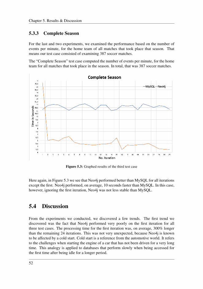
Chapter 5. Results & Discussion
5.3.3 Complete Season
For the last and two experiments, we examined the performance based on the number ofevents per minute, for the home team of all matches that took place that season. Thatmeans our test case consisted of examining 387 soccer matches.
The “Complete Season” test case computed the number of events per minute, for the hometeam for all matches that took place in the season. In total, that was 387 soccer matches.
Figure 5.3: Graphed results of the third test case
Here again, in Figure 5.3 we see that Neo4j performed better than MySQL for all iterationsexcept the first. Neo4j performed, on average, 10 seconds faster than MySQL. In this case,however, ignoring the first iteration, Neo4j was not less stable than MySQL.
5.4 Discussion
From the experiments we conducted, we discovered a few trends. The first trend wediscovered was the fact that Neo4j performed very poorly on the first iteration for allthree test cases. The processing time for the first iteration was, on average, 300% longerthan the remaining 24 iterations. This was not very unexpected, because Neo4j is knownto be affected by a cold start. Cold start is a reference from the automotive world. It refersto the challenges when starting the engine of a car that has not been driven for a very longtime. This analogy is applied to databases that perform slowly when being accessed forthe first time after being idle for a longer period.
52
5.4 Discussion
An article written by the developers of Neo4j [35] revealed that cold start is a knownchallenge when utilizing graph databases in Neo4j. Cold start occurs when the databasehas just recently been booted up, and indexes have not yet been cached. When this isthe case, the database needs to look up all records directly on the disk which is a costlyoperation. However, after the first disk lookup, all indices are cached, which makesupcoming queries much faster. Because cold start has become a common phenomenon,there now exists workarounds and patches that keep the database warm, reducing theimpact of cold start.
Another interesting finding was the fact that MySQL performed better than Neo4j for thefirst test case, but not in the two other. By looking at this in the light of the study by Medhipresented in Chapter 2 this result was on one side unexpected. Medhi’s study concludedthat Neo4j perform better when querying densely connected sports related data. However,the difference in performance between the two databases increases as the dataset grows.The same trend we can see in our results, but the significant difference is the fact thatMySQL performed best for the most uncomplicated query.
On the other side, it was not unexpected that MySQL performed better than Neo4j for the“Single Match” test case. MySQL utilizes B+-trees in order to index its data. B+-treeindexation facilitates for very fast read operations. For queries on small tables or queriesthat require most of the rows in a larger table, it is often faster to read sequentially throughthe table instead of working through an index. This can explain why MySQL performsbetter than Neo4j for the test case that required the lookup of the smallest amount of data.Neo4j utilizes index-free adjacency, which provides lightning-fast lookups. This meansthat only the index for the starting node of the query needs to be looked up. From there on,each node has a pointer pointing to its neighboring node, supporting a time complexity ofO(n), where “n” equals the number of nodes in the graph. This lets Neo4j perform betterfor the last two test cases, which required the lookup of larger amounts of data.
5.4.1 Response time
A trend that was harder to account for was the fact that MySQL’s response time seemedto be much more stable than Neo4j’s. Especially in Figure 5.1 and Figure 5.2, the bluelines are smoother than the orange ones. This could be explained by the fact that MySQLis more memory efficient than Neo4j because MySQL does not cache indices in the sameway as Neo4j. Keeping all pointers in memory as Neo4j does, requires a lot of memory.A lack of memory will affect Neo4j’s performance. On the other hand we noticed thatMySQL performed very stable for the first test case, but as the the test cases became morechallenging, the blue line became more and more rocky. For the “Complete Season” it ishard to tell which database performed the most stable by looking at the plots in Figure 5.3.
Because of the way we chose to model our databases, using three different tables for therelational database and using three different types of nodes. The number of records in therelational database equaled the number of nodes in the graph database. With this in mind,we discovered some interesting findings regarding the overall response time. We used theaverage processing time and the number of records accessed for each of the three test cases
53

Chapter 5. Results & Discussion
to estimate the difference in performance between the two databases. Table 5.4a shows theestimation of how Neo4j and MySQL compare to each other with regard to executiontime. We see that it corresponds with Table 5.2 and Table 5.4. Although the graphs onlyconsisted of three points each, we can still see a clear difference in performance. FromTable 5.4b, which is an enlarged selected area from Table 5.4a, we see that the blue andorange lines intersect after 0.236 seconds when the amount of records is about 1670. Thismeans that Neo4j and MySQL performed equally well when the number of records thathad to be processed approached 1670.
54
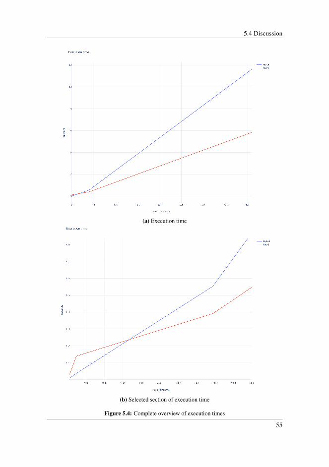
5.4 Discussion
(a) Execution time
(b) Selected section of execution time
Figure 5.4: Complete overview of execution times
55
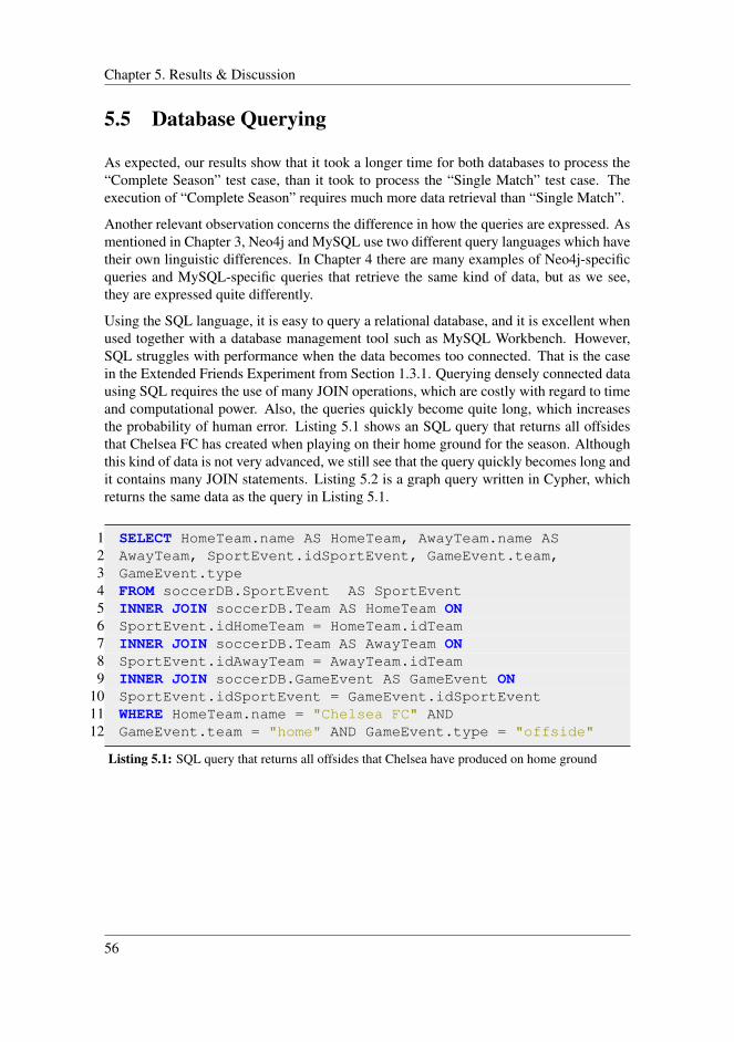
Chapter 5. Results & Discussion
5.5 Database Querying
As expected, our results show that it took a longer time for both databases to process the“Complete Season” test case, than it took to process the “Single Match” test case. Theexecution of “Complete Season” requires much more data retrieval than “Single Match”.
Another relevant observation concerns the difference in how the queries are expressed. Asmentioned in Chapter 3, Neo4j and MySQL use two different query languages which havetheir own linguistic differences. In Chapter 4 there are many examples of Neo4j-specificqueries and MySQL-specific queries that retrieve the same kind of data, but as we see,they are expressed quite differently.
Using the SQL language, it is easy to query a relational database, and it is excellent whenused together with a database management tool such as MySQL Workbench. However,SQL struggles with performance when the data becomes too connected. That is the casein the Extended Friends Experiment from Section 1.3.1. Querying densely connected datausing SQL requires the use of many JOIN operations, which are costly with regard to timeand computational power. Also, the queries quickly become quite long, which increasesthe probability of human error. Listing 5.1 shows an SQL query that returns all offsidesthat Chelsea FC has created when playing on their home ground for the season. Althoughthis kind of data is not very advanced, we still see that the query quickly becomes long andit contains many JOIN statements. Listing 5.2 is a graph query written in Cypher, whichreturns the same data as the query in Listing 5.1.
1 SELECT HomeTeam.name AS HomeTeam, AwayTeam.name AS2 AwayTeam, SportEvent.idSportEvent, GameEvent.team,3 GameEvent.type4 FROM soccerDB.SportEvent AS SportEvent5 INNER JOIN soccerDB.Team AS HomeTeam ON6 SportEvent.idHomeTeam = HomeTeam.idTeam7 INNER JOIN soccerDB.Team AS AwayTeam ON8 SportEvent.idAwayTeam = AwayTeam.idTeam9 INNER JOIN soccerDB.GameEvent AS GameEvent ON
10 SportEvent.idSportEvent = GameEvent.idSportEvent11 WHERE HomeTeam.name = "Chelsea FC" AND12 GameEvent.team = "home" AND GameEvent.type = "offside"
Listing 5.1: SQL query that returns all offsides that Chelsea have produced on home ground
56
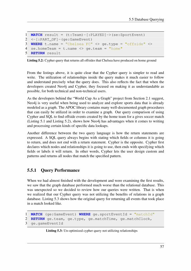
5.5 Database Querying
1 MATCH result = (t:Team)-[:PLAYED]->(se:SportEvent)2 <-[:PART_OF]-(ge:GameEvent)3 WHERE t.name = "Chelsea FC" <> ge.type = "offside" <>4 se.homeTeam = t.name <> ge.team = "home"5 RETURN result
Listing 5.2: Cypher query that returns all offsides that Chelsea have produced on home ground
From the listings above, it is quite clear that the Cypher query is simpler to read andwrite. The utilization of relationships inside the query makes it much easier to followand understand precisely what the query does. This also reflects the fact that when thedevelopers created Neo4j and Cypher, they focused on making it as understandable aspossible, for both technical and non-technical users.
As the developers behind the “World Cup As a Graph” project from Section 2.1 suggest,Neo4j is very useful when being used to analyze and explore sports data that is alreadymodeled as a graph. The APOC library contains many well-documented graph proceduresthat can easily be utilized in order to examine a graph. Our query comparison of usingCypher and SQL to find offside events created by the home team for a gives soccer match(Listing 5.1 and Listing 5.2), shows how Neo4j has advantages when it comes to writingand processing certain kinds of specific data lookups.
Another difference between the two query language is how the return statements areexpressed. A SQL query always begins with stating which fields or columns it is goingto return, and does not end with a return statement. Cypher is the opposite. Cypher firstdeclares which nodes and relationships it is going to use, then ends with specifying whichfields or labels it will return. In other words, Cypher lets the user design custom andpatterns and returns all nodes that match the specified pattern.
5.5.1 Query Performance
When we had almost finished with the development and were examining the first results,we saw that the graph database performed much worse than the relational database. Thiswas unexpected so we decided to review how our queries were written. That is whenwe realized that our Cypher query was not utilizing the benefits of relations in a graphdatabase. Listing 5.3 shows how the original query for returning all events that took placein a match looked like.
1 MATCH (ge:GameEvent) WHERE ge.sportEventId = "matchId"2 RETURN ge.team, ge.type, ge.matchTime, ge.matchClock,3 ge.gameEventId
Listing 5.3: Un-optimized cypher query not utilizing relationships
57

Chapter 5. Results & Discussion
The query produced the results shown in Table 5.5. After updating to our final query(Listing 4.10), we achieved the much better results displayed earlier in Table 5.2.
Single Match Team Season Complete SeasonMaximum 0,1842 1,9833 38,7823Minimum 0,0973 0,7915 15,1158Average 0,1349 1,0626 21,0334Median 0,1302 0,9065 16,8275
Table 5.5: Results for Neo4j un-optimized Neo4j queries in seconds
Table 5.5 shows the result of writing Cyber queries with an SQL mindset. The un-optimizedquery had to iterate through all the GameEvent-nodes in order to join them with a matchId.When the graph database consisted of 40.0000 GameEvent-nodes, the query was destinedto take a long time with almost 400 soccer matches. However, our final query tookadvantage of the [PART OF] relation between SportEvents and GameEvents. By that,it was utilizing the properties of index-free adjacency. This meant that when requestingthe same data, the only thing that needed to be looked up was the SportEvent-node whichcontained the corresponding matchId. This was because all the GameEvents were connectedto that SportEvent-node through the [PART OF] relation. By making this change in thequery, we were able to reduce the average execution time by 360%. Results for all 25iterations of the three test-cases with the un-optimized query can be found in a table locatedin the appendix.
5.6 Visualization
When working with queries and databases, it is beneficial to see the data that one isworking with. Also other people involved in the project, such as stakeholders, businessowners and analysts, can benefit greatly from good data visualization. Then they canuse the visualization to determine areas of interest or assess easily the current state andorganization of the data [32]. Neo4j provides with its desktop application a browser thatis excellent for data visualization along with query creation. MySQL Workbench providesmany of the query creation tools, but the data visualization is limited to table format.Figure 5.5 illustrates how MySQL Workbench returns the Listing 5.1 query. Figure 5.6shows the Neo4j browser results for the same query.
The graph visualization is simple and makes it intuitive for most people to understandwhat data is returned and how it is connected. The process of creating the graph, however,is very costly. Whenever the results are more than 100 nodes, for instance, our computerstruggled to render the graph and it took a very long time. With more than 1000 nodes,there was no point of even trying to render the graph. That would not be a problem,however, with MySQL Workbench.
58
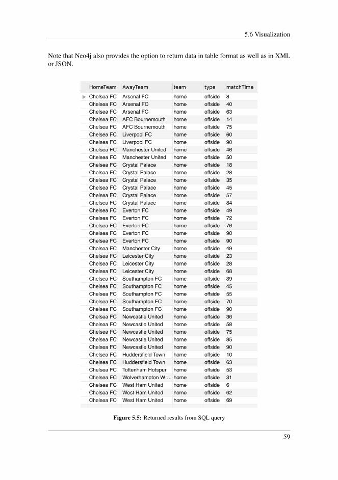
5.6 Visualization
Note that Neo4j also provides the option to return data in table format as well as in XMLor JSON.
Figure 5.5: Returned results from SQL query
59

Chapter 5. Results & Discussion
Figure 5.6: Returned results from Cypher query
5.7 Data Import
When evaluating different database technologies and database management systems, dataimport can be an important aspect. In the study by Pandey [45], presented in Chapter 2,we see that there are big differences in how MySQL and Neo4j perform with respect todata size and time. Neo4j clearly outperforms MySQL as the size of the dataset grows.
The time aspect of data import does not always have to play such an important role. It isvery dependent on how the database is used and what it is being used for. If a companywanted to migrate their database from their existing solution to either MySQL or Neo4j,the time aspect of data import would probably not be a decisive factor. Because such amigration is usually a one-time thing and other factors would play a more important role.Nonetheless, if the database were to be used as explained in the World Cup Model fromChapter 2, import time can be an essential factor. With projects where the database iscontinuously being updated or expanded with new records, it is more important that thedatabase can perform well while importing data. The same issue would be applicable
60

5.8 Data Model
to our experiment as well, if we were to expand the scope of our project. It would beinteresting to conduct the same experiments, as explained in Chapter 4, with significantlylarger datasets. Then more would be required from the database technologies with regardto import time.
5.8 Data Model
With the property graph model that Neo4j provides, it is simple to alter the graph database’sdata model. Nodes, relationships and properties can continually be added without affectingthe performance of the database. This makes Neo4j suitable for handling a database thatmay often change its data model. On the other hand, MySQL’s data model is much stricterin order to guarantee ACID properties. This makes MySQL less flexible with regard todata model alterations.
For databases containing live updates, historical data and other sports related data, it maybe hard to predict how the database should be modeled. The methods for generating suchdata are constantly changing, and the requirements from clients who are using the data arealso changing. Thus it is hard to determine in advance how the data model should looklike. This is an important aspect where Neo4j has a great advantage with its flexible model.
61

Chapter 5. Results & Discussion
62

Chapter 6Conclusion & Future Work
This chapter summarizes the thesis, and presents pros and cons with using Neo4j andMySQL for the application we developed. The goal of our research was to explore howgraph databases can be used together with the Sportradar developer API, and to investigatepotential advantages or disadvantages. In order to approach this problem we formulatedthe two following research questions:
• RQ1: Identify a use case which is representative for the data and applications ofSportradar.
• RQ2: How does the Neo4j graph database management system compare againstOracle’s MySQL relational database management system, in regard to target theproblem?
To answer RQ1, we created an application that calculated how the home team performedin a soccer match, from the English Premier League, based on the score. The applicationcalculated performance based on how many events the home team produced. The followingevents were defined:
• corner kick
• free kick
• goal kick
• injury
• injury return
• offside
• penalty awarded
• penalty missed
63

Chapter 6. Conclusion & Future Work
• red card
• score change
• shot off target
• shot on target
• shot saved
• throw in
• yellow card
• yellow red card
For the application, we created two databases; a Neo4j graph database and a MySQLrelational database. The databases varied in structure, but contained the exact same data.The application retrieved the event information from the databases. During runtime, theapplication kept track of occurred events based on score and time played. For each soccermatch, the application returned the total number of events that the home team produced.In addition, the application calculated events produced per minute while the match wastied or if the home team was either winning or losing.
To address RQ2, we created three different test cases for our application, which we usedto performance test our databases. First, we executed and timed each test case 25 timeshaving the application connected to the graph database. Then we disconnected the graphdatabase and connected the relational database, and executed all three test cases another25 times. The test cases were defined as the following:
• Single Match - Select a random soccer match and calculate events produced perminute by the home team based on score.
• Team Season - Calculate events produced per minute based on the score for allsoccer matches played on home ground during the season for a specific team.
• Complete Season - Calculate events produced per minute based on the score for thehome team for all matches that have been played during the season.
6.1 Conclusion
We found that both Neo4j and MySQL were suitable for our application to measure soccerteams’ performance with respect to match events. Both databases have their advantagesand disadvantages, but for this project, none of them serious enough to play a major role.If the dataset was significantly larger, however, our research indicates that Neo4j would bea better choice of a database management system with regard to processing time.
Table 6.2 shows the average processing of out test cases, while Table 6.1 shows themedian processing time. The median processing time is more interesting than the averageprocessing time because it is not affected by cold start.
64

6.1 Conclusion
Test Case Neo4j MySQLSingle Match 0,1107 0,0349Team Season 0,3395 0,5463
Complete Season 5,3711 11,7444
Table 6.1: The median processing time in seconds
Test Case Neo4j MySQLSingle Match 0,1319 0,0371Team Season 0,3920 0,5523
Complete Season 5,8455 11,6348
Table 6.2: The average processing time in seconds
Our results indicate that MySQL performs better for queries that require the lookup ofabout 1670 or fewer records, in databases based on our design. When the amount ofrequired records that need to be looked up exceeds 1670, Neo4j performs much better.This explains why MySQL performs better for the “Single Match” test case than Neo4j,but Neo4j outperforms MySQL for the other two test cases. Besides, previous workalso suggests that the more connected the data is, the better a graph database performscompared to a relational database. This corresponds with our results indicating that themore advanced a query is, requiring the lookup of denser connected data, the better agraph database performs compared to a relational database.
When setting up and populating the databases with data from Sportradar’s API, MySQLhas a significant advantage because it is so widely used. MySQL is heavily documentedand is a more stable database, whereas Neo4j has some issues with compatibility andintegration with other frameworks and services.
Regarding query languages, both databases have strong and well-functioning query languages.SQL is a traditional, well-known land widely used language. Cypher is Neo4j specificand much less used, but is intuitive and easy to learn. Where SQL uses advanced JOINstatements, Cypher takes advantage of relationships instead, which are less complicated,easier to understand and require shorter queries, reducing the possibility of human error.It is important that Cypher statements are expressed in the correct way, in order to fullyutilize the power of a graph database.
With regard to data administration and data visualization, both providers have powerfultools. The Neo4j Browser is an excellent tool for visualizing a graph database. However,it is highly demanding regarding hardware. MySQL Workbench is a useful tool whenit comes to monitoring a database, and designing a data model. However, it does notvisualize data as neat as the Neo4j Browser.
65

Chapter 6. Conclusion & Future Work
6.2 Future work
There are a lot of areas in this project that could benefit from further research. First of all,it would be interesting if more studies similar to this one were conducted to see if theyidentified the same or different trends than this project found. Using other studies as aform of verification, we could feel more confident about our results.
This project only compared performance between the two databases that we have created,based on data from Sportradar’s API. The next step for Sportradar would be to conduct asimilar study on Sportradar’s internal data storage, where the API gets its data from. Ourresults give an indication of which prerequisites that are important in order for a databaseto function optimally. Such a study could also verify if our design and implementation areapplicable to a real-world scenarios.
6.2.1 Hardware & Architecture
Since the design and experiments described Chapter 4 and Chapter 5 in this project, allhave been completed on one single computer, it would be interesting to perform the sameexperiments on different hardware, both less and more powerful. This would generateresults that are more representative.
A typical architecture for this kind application is the client-server architecture [58]. Byhosting our database on one or more external servers instead of hosting it locally, wewould achieve this architecture. The application and database would then run on differentresources, which could impact the results of our experiments.
6.2.2 Memory Consumption
Graph databases are known to require a lot of memory to function optimally [27]. Thisresearch does not investigate how the use of memory affects the performance of Neo4j.Memory consumption is an essential factor when choosing database technology. Therefore,researching how the amount of available memory affects the performance of Neo4j andMySQL would be very helpful.
6.2.3 Import time
Limitations on how often we were allowed to call Sportradar’s API per second, made itimpossible for us to investigate how our two databases compared to each other regardingimport time. Even though previous work indicates that there is a big difference betweenNeo4j and MySQL regarding import time [45], it would be useful to see if that applies toour databases as well when populated with sports data from Sportradar.
66

6.3 Threats to Validity & Limitations
6.2.4 Different dataset
Another way to validate our results would be to perform similar experiments on a different,but similar dataset. For example, using data from the National Hockey League (NHL). Theleague is structured differently from the Premier League, consisting of a different matchsetup, more teams and more players. The difference between the sports is significantenough to create a completely different data model with regard to connections and relationshipsbetween the data. In addition, one could do even heavier performance testing by designingtest cases that are more complex in terms of queries.
6.2.5 Mitigate Cold Start
Cold start is a well-known challenge with Neo4j, and there exist many ways to workaround it. Modern implementations of Neo4j, depending on use, usually have implementedworkarounds keeping the database warm. Implementing such a workaround could makethe database perform different, thus affecting the results.
6.3 Threats to Validity & Limitations
Both databases have been modeled to the best of our abilities. We have followed thestandards in the field of our research when modeling both the relational database and thegraph database. As with most research, there exists a possibility for human error. There isalways a chance that we have misinterpreted something when it comes to database designor query design, which may have affected our results.
Since we only conducted experiments on three different test cases. It was hard to determineexact for how many records the two databases performed equally well. Therefore, thenumber 1670, which we presented earlier, must be considered as an estimate for whenNeo4j and MySQL perform evenly.
6.4 Contribution
This thesis has identified a relevant field of use for Sportradar’s Developer API, anddeveloped an application for analysis of soccer matches. The application alternated betweenusing a graph database and relational database as a means of data source. The applicationwas used to do a performance test and a comparison of the two databases. Three test caseswere developed for the application in order to measure the databases’ performance. Otheraspects such as maintainability, compatibility and query language were also taken intoconsideration.
We have presented a solution to how the two databases can be structured and organized toserve the purpose of the application. In addition, we have identified which circumstances
67

Chapter 6. Conclusion & Future Work
the different databases require in order to perform best, based on theory, previous workand our own results with regard to the target problem.
68
Bibliography
[1] ArangoDB, Unknown. Arangosearch: Full-text search engine including similarityranking capabilities. Accessed May 6, 2019.URL https://www.arangodb.com/why-arangodb/full-text-search-engine-arangosearch/
[2] ArangoDB, Unknown. Sql / aql - comparison. Accessed May 6, 2019.URL https://www.arangodb.com/why-arangodb/sql-aql-comparison/
[3] Babbie, R., 2012. The Practice of Social Research. Cengage Learning, pp. 414–416.URL https://books.google.no/books?id=k-aza3qSULoC
[4] Babeni, S., 2019. https://ormuco.com/blog/most-popular-databases. Accessed May31, 2019.URL https://ormuco.com/blog/most-popular-databases
[5] Bazilchuk, N., 2005. Student programming project becomes multi-million dollarcompany. Accessed September 19, 2018.URL https://www.ercim.eu/publication/Ercim News/enw61/bazilchuk.html
[6] Berlind, D., 2015. Why did they put the web in web apis? Accessed April 19, 2019.URL https://www.programmableweb.com/news/why-did-they-put-web-web-apis/analysis/2015/12/03
[7] Bettilyon, E., 2019. Breadth first search and depth first search. Accessed May 14,2019.URL https://medium.com/tebs-lab/breadth-first-search-and-depth-first-search-4310f3bf8416
[8] bitn!ne, 2016. History of databases and graph database. Accessed 8 May, 2019.URL https://bitnine.net/blog-graph-database/history-of-databases-and-graph-database/
69

[9] Chao, J., 2018. Graph databases for beginners: Native vs. non-native graphtechnology. Accessed March 11, 2019.URL https://neo4j.com/blog/native-vs-non-native-graph-technology/?ref=blog
[10] Chiou, L., 2019. Graph theory. Accessed May 14, 2019.URL https://brilliant.org/wiki/graph-theory/
[11] Cole, J., 2014. B+tree index structures in innodb. Accessed June 1, 2019.URL https://blog.jcole.us/2013/01/10/btree-index-structures-in-innodb/
[12] Community, S. O., 2018. Questions tagged [mysql]. Accessed November 7, 2018.URL https://stackoverflow.com/questions/tagged/mysql
[13] Ebner, S., 2013. History and time are key to power of football, says premier leaguechief. Accessed March 27, 2019.URL https://www.thetimes.co.uk/article/history-and-time-are-key-to-power-of-football-says-premier-league-chief-3d3zf5kb35m
[14] EQT, 2018. Sportradar. Accessed September 19, 2018.URL http://www.eqtpartners.com/Investments/Current-Portfolio/Sportradar/
[15] Ernst & Young, A., 2017. Big Data: Beyond the buzzword. Ernst & Young Australia,p. 3.
[16] Foote, K. D., 2017. A brief history of database management. Accessed May 8, 2019.URL https://www.dataversity.net/brief-history-database-management/#
[17] for Geeks, G., 2018. Bellman–ford algorithm — dp-23. Accessed May 14, 2019.URL https://www.geeksforgeeks.org/bellman-ford-algorithm-dp-23/
[18] Fowler, M., Rice, D., 2003. Patterns of Enterprise Application Architecture. A MartinFowler signature book. Addison-Wesley, pp. 165–167.URL https://books.google.no/books?id=FyWZt5DdvFkC
[19] Garbade, D. M. J., 2018. Understanding k-means clustering in machine learning.Accessed May 14, 2019.URL https://towardsdatascience.com/understanding-k-means-clustering-in-machine-learning-6a6e67336aa1
[20] Goodrich, M. T., Tamassia, R., Goldwasser, M. H., 2004. Data structures andalgorithms in Java Fourth Edition. John Wiley & Sons, p. 793.
[21] GraphGrid, 2016. Native graph databases versus non-native graph databases.Accessed March 28, 2019.
70

URL https://www.graphgrid.com/native-graph-databases-versus-non-native-graph-databases/
[22] Hunger, M., 2016. Apoc: An introduction to user-defined procedures and apoc.Accessed October 7, 2018.URL https://neo4j.com/blog/intro-user-defined-procedures-apoc/
[23] Jones, C., 2014. How to visualize your facebook friend network. Accessed May 6,2019.URL http://allthingsgraphed.com/2014/08/28/facebook-friends-network/
[24] Joshi, V., 2017. Finding the shortest path, with a little help from dijkstra. AccessedMay 14, 2019.URL https://medium.com/basecs/finding-the-shortest-path-with-a-little-help-from-dijkstra-613149fbdc8e
[25] Marr, B., 2018. How much data do we create every day? the mind-blowing statseveryone should read. Accessed September 20, 2018.URL https://www.forbes.com/sites/bernardmarr/2018/05/21/how-much-data-do-we-create-every-day-the-mind-blowing-stats-everyone-should-read/#7bbb1ccd60ba
[26] Medhi, S., Baruah, H. K., 2017. Relational database and graph database: Acomparative analysis. Journal of Process Management. New Technologies 5 (2), 1–9.
[27] Mendel-Gleason, G., 2018. Databases of the future: How changes in hardware aredriving a revolution. Accessed May 28, 2019.URL https://www.datachemist.com/blog/databases-of-the-future-how-changes-in-hardware-are-driving-a-revolution
[28] MySQL, 2018. Mysql technical support. Accessed November 6, 2018.URL https://www.mysql.com/support/
[29] Neo4j-Team, 2014. 5 things you didn’t know about the world cup. Accessed March8, 2019.URL http://worldcup.neo4j.org/5-things-you-didnt-know-about-the-world-cup/
[30] Neo4j-Team, 2014. The world cup graph domain model. Accessed March 9, 2019.URL http://worldcup.neo4j.org/the-world-cup-graph-domain-model/
[31] Neo4j-Team, 2019. Cypher basics i. Accessed May 28, 2019.URL https://neo4j.com/developer/cypher-query-language/
[32] Neo4j-Team, 2019. Graph visualization. Accessed April 28, 2019.URL https://neo4j.com/developer/graph-visualization/
71

[33] Neo4j-Team, 2019. Neo4j customers. Accessed April 28, 2019.URL https://neo4j.com/customers/
[34] Neo4j-Team, 2019. The neo4j drivers manual v1.7 for python. Accessed April 19,2019.URL https://neo4j.com/docs/pdf/neo4j-driver-manual-1.7-python.pdf
[35] Neo4j-Team, 2019. Warm the cache to improve performance from cold start.Accessed May 26, 2019.URL https://neo4j.com/developer/kb/warm-the-cache-to-improve-performance-from-cold-start/
[36] Neo4j-Team, 2019. What is a graph database? Accessed May 6, 2019.URL https://neo4j.com/developer/graph-database/
[37] Neo4j-Team, Unknown. Neo4j apoc library. Accessed October 7, 2018.URL https://neo4j.com/developer/apoc/
[38] {ntc}, 2019. Sql (structured query language). Accessed May 9, 2019.URL https://www.ntchosting.com/encyclopedia/databases/structured-query-language/
[39] Oates, B. J., 2005. Researching information systems and computing. Sage, pp.32–33.URL https://books.google.no/books?id=ztrj8aph-4sC
[40] Oracle, 2018. Create tomorrow, today. Accessed November 5, 2018.URL http://www.oracle.com/us/corporate/oracle-fact-sheet-079219.pdf
[41] Oracle, 2019. Introduction to innodb. Accessed April 26, 2019.URL https://dev.mysql.com/doc/refman/8.0/en/innodb-introduction.html
[42] Oracle, 2019. Mysql workbench. Accessed March 28, 2019.URL https://www.mysql.com/products/workbench/
[43] Oralce, 2019. Top 10 reasons to choose mysql for next generation web applications.Accessed May 7, 2019.URL https://www.mysql.com/why-mysql/white-papers/top-10-reasons-to-choose-mysql-for-next-generation-web-applications/
[44] Orientechnologies, 2016. Orientdb. Accessed November 13, 2018.URL https://github.com/orientechnologies/orientdb
[45] Pandey, S., Joshi, E., Maharjan, M., Karki, N., 08 2018. A research on architecturaland performance comparison of relational database, nosql and graph database(neo4j).
72
[46] Pollari-Malmi, K., 2010. B+-trees. Accessed June 1, 2019.URL https://www.cs.helsinki.fi/u/mluukkai/tirak2010/B-tree.pdf
[47] Pwc, 2014. Global 100 software leaders by revenue. Accessed May 31, 2019.URL https://www.pwc.com/gx/en/industries/technology/publications/global-100-software-leaders/explore-the-data.html
[48] Python-Software-Foundation, 2019. What is python? executive summary. AccessedMarch 28, 2019.URL https://www.python.org/doc/essays/blurb/
[49] Rathle, G. S. . P., 2017. Fraud detection: Discovering connections with graphdatabases. Accessed May 6, 2019.
[50] Robinson, I., Webber, J., Eifrem, E., 2015. Graph databases: new opportunities forconnected data. ” O’Reilly Media, Inc.”, pp. 105–109.URL https://books.google.no/books?id=RTvcCQAAQBAJ&printsec=frontcover&redir esc=y#v=onepage&q&f=false
[51] Rouse, M., 2081. Mysql. Accessed November 5, 2018.URL https://searchoracle.techtarget.com/definition/MySQL
[52] Sellæg, A., 2011. Perleporten apen for petter smart. Accessed September 19, 2018.URL https://www.ntnu.no/documents/304978/0/IG+i+Ukeadressa+08+10+11+(3).pdf/b7900abd-c0d5-4e62-bfee-e17b32b1c6e7
[53] Services, A. W., 2018. Amazon neptune. Accessed November 12, 2018.URL https://aws.amazon.com/neptune/
[54] Soft, M., 2019. What is an api? (application programming interface). Accessed April19, 2019.URL https://www.mulesoft.com/resources/api/what-is-an-api
[55] Soshnick, S., 2015. Jordan, cuban, leonsis put millions on sports betting’s future.Accessed September 19, 2018.URL https://www.bloomberg.com/news/articles/2015-10-27/jordan-cuban-leonsis-put-millions-on-sports-betting-s-future
[56] Sportradar, 2019. Soccer extended v3. Accessed May 15, 2019.URL https://developer.sportradar.com/docs/read/football soccer/Soccer Extended v3#soccer-extended-v3-api-map
[57] Sports, B., 2018. Premier league tv rights: Five of seven live packages sold for£4.464bn. Accessed March 27, 2019.URL https://www.bbc.com/sport/football/43002985
73
[58] Techopedia, 2019. Client/server architecture. Accessed May 12, 2019.URL https://www.techopedia.com/definition/438/clientserver-architecture
[59] Trondheimsregionen, N., 2017. Sportradar ble Arets bedrift! Accessed September19, 2018.URL https://www.nitr.no/no/aktuelt/sportradar+ble+arets+bedrift+2017.html
[60] Unknon, 2017. Oracle corporation. Accessed November 5, 2018.URL http://www.orafaq.com/wiki/Oracle Corporation#WHO
[61] Unknown, 2018. System properties comparison amazon neptune vs. neo4j. AccessedNovember 12, 2018.URL https://db-engines.com/en/system/Amazon+Neptune%3BNeo4j
[62] Unknown, 2019. Discover the origins and history of the top tier of english football.Accessed March 27, 2019.URL https://www.premierleague.com/history
[63] Vukotic, A., Watt, N., Abedrabbo, T., Fox, D., Partner, J., 2014. Neo4j in action.Manning Publications Co., pp. 12–13.URL https://books.google.no/books?id=61GdmgEACAAJ
[64] Webber, J., 2018. Powering real-time recommendations with graph databasetechnology. Accessed May 6, 2019.
74

Appendix
Below is a table containing execution times in seconds from querying the graph databaseusing un-optimized queries.
No. ofIteration Single match Team Season Complete Season
1 0,1386 1,9833 38,78232 0,1392 1,5113 31,06923 0,1302 1,4360 30,73044 0,1541 1,2986 29,83885 0,1334 1,3195 28,64996 0,1317 1,3570 25,56337 0,1277 1,2485 25,69668 0,1373 1,1795 24,49269 0,1439 1,4090 24,2195
10 0,1287 0,9569 22,557511 0,1299 0,8489 20,334012 0,1359 0,8491 16,701213 0,1280 0,8377 16,800214 0,1278 0,8545 16,827515 0,1034 0,8262 15,581816 0,1842 0,8711 16,346017 0,1671 0,9101 15,115818 0,1488 0,8292 15,570119 0,1297 0,8587 15,268820 0,1286 0,8529 15,407521 0,1247 0,8249 16,209422 0,1216 0,7915 17,089023 0,0973 0,9065 16,220424 0,1565 0,9317 15,180925 0,1243 0,8721 15,5813
75

NTN
UN
orw
egia
n U
nive
rsity
of S
cien
ce a
nd T
echn
olog
yFa
cult
y of
Info
rmat
ion
Tech
nolo
gy a
nd E
lect
rica
lEn
gine
erin
gD
epar
tmen
t of C
ompu
ter
Scie
nce
Mas
ter’
s th
esis
Oscar Thån Conrad
Database Solutions to SportsApplications
A Comparison and Performance Test of GraphDatabases and Relational Databases
Master’s thesis in Master of InformaticsSupervisor: Svein Erik Bratsberg
June 2019