Data Mining to Support Anaerobic WWTP Monitoring

1

DATA MINING TO SUPPORT ANAEROBIC WWTP MONITORING

Maurice Dixon **, Julian R. Gallop*, Simon C. Lambert*,

Laurent Lardon***, Jerome V. Healy**, and Jean-Philippe Steyer***

*e-Science Department, CCLRC Rutherford Appleton Laboratory,

Chilton, Didcot, Oxon. OX11 0QX, UK

**CCTM, London Metropolitan University, 31 Jewry Street, LONDON, EC3N 2EY, UK

*** Laboratoire de Biotechnologie de l'Environnement - INRA, Avenue des etangs, 11100 Narbonne,

France

Corresponding author : Maurice Dixon

fax: +44 207 320 3009 – email : M.Dixon@Londonmet.ac.uk

Abstract

The stable and efficient operation of anaerobic WWTPs (Waste Water

Treatment Plants) is a major challenge for monitoring and control systems.

Support for distributed anaerobic WWTPs through remotely monitoring their

data was investigated in the TELEMAC framework. This paper describes how

the accumulating filtered sensor data was mined to contribute to the refining

of expert experience for insights into digester states. Visualisation techniques

were used to present cluster analyses of digester states. A procedure for

determining prediction intervals is described together with its application for

volatile fatty acid concentrations; this procedure enables prediction risk

assessment.

Keywords: Water pollution, Waste treatment, Prediction interval, Reactor

modelling, Reactor states.

Please cite this article as: Dixon, M., et al. Data mining to support anaerobic WWTP monitoring. Control Engineering Practice, (2007), doi:10.1016/j.conengprac.2006.11.010

Data Mining to Support Anaerobic WWTP Monitoring

2

1. Introduction

1.1 Background

The treatment of waste water by an anaerobic digestion process has several significant advantages.

(Gujer and Zender, 1983). It can be done at a rapid rate with a high volume throughput yet it can be

deployed in small local treatment plants. Anaerobic digestion can degrade concentrated and difficult

substrates while producing very little sludge. Good overall water quality output can be obtained. A bonus

is that energy can be recovered from some of the by-products such as methane.

In practice a digester based on these principles may enter an unstable state which leads to a

breakdown of the process with the requirement of a shutdown followed by a lengthy restart process. For

reasons of caution therefore, an anaerobic digester is typically operated with a low throughput whereas

the ideal would be to run a plant at higher efficiency, while maintaining stability. The biological/chemical

variables are difficult to measure so an expert is required to advise in the running of a plant. Fig.1 shows

the two stage process of conversion. Firstly the organic carbon is converted rapidly to organic volatile

fatty acids, VFA. A slower conversion of the VFA to methane and carbon dioxide then proceeds;

however this second stage can be inhibited by the build up of VFAs. Thus knowledge of the VFA

concentration is pivotal to understanding the digester behaviour. Carrasco, Rodriguez, Punal, Roca, and

Lema (2004) have noted the difficulty of achieving good process representations using mathematical

models and proposed advanced knowledge based control systems based on fuzzy logic as an alternative.

Data mining has been carried out within the context of work (within an EU-funded project,

TELEMAC) to support a variety of Waste Water Treatment Plants (WWTP) in a way that does not

require local expertise (Bernard et al, 2005). There is considerable diversity between plants in terms of

digester volumes, of underlying biological principles, and of sensor sets available. The business impetus

comes from the requirements for waste water treatment in the alcoholic beverages industry which has

many small widely dispersed treatment sites. The lengthy restart process means that the systematic

exploration of abnormal operating conditions is done on small pilot reactors rather than industrial sized

reactors. The data collected from WWTPs vary considerably between different installations. Also,

because of the harsh conditions of WWTPs, the data collected for a given digester varies from time to

time. In the present paper, the focus is on a pilot scale (~1m3), extensively instrumented fixed bed

digester for which there has been an extensive series of experiments carried out at the Institut National de

la Reserche Agronomique, Laboratoire de Biotechnologie de l'Environnement, INRA-LBE (Steyer,

Bouvier, Conte, Gras, and Sousbie, 2002a). At INRA-LBE Fault Detection and Isolation, FDI, has been

developed for this well instrumented process and is working well. A filtered dataset from one of these

experiments forms the input to the data mining reported here.

Data Mining to Support Anaerobic WWTP Monitoring

3

1.2 Scope of Data Mining

Data mining is used in TELEMAC to aid remote experts as data was accumulated from the industrial

digesters. It provides guidance that plant parameters are in normal range as well as predictions when

sensors indicate aberrant conditions. Some sensors are expensive and others are unreliable so one role of

data mining is to determine which sensors are required for predictions. Another role of data mining is to

gain a better understanding of the current and imminent state of a digester. Expert judgement is used to

provide guidance in ranking sensors on availability, reliability and expense for the small scale industrial

anaerobic digestion process. This ranking is given in Fig. 2 as a Venn diagram. If a sensor stops working

or is too expensive to deploy initially then the Venn diagram is the starting point for determining the best

sensor combinations to support the modelling of the missing sensor. This enables a narrowing of the data

mining input search space. The innermost space shown in the Venn diagram corresponds to sensors that

are ranked Level 1 because they are judged to be the most available, or least expensive or most reliable

sensors.

1.3 Determination of Sensors for Prediction

If a sensor stops working or is unavailable then data mining is needed to determine the best

combination of the other sensors for monitoring. Where the linear regression approximation holds,

forward stepping can be used to rank the benefits of adding sensors. However linear regression has been

seen to be applicable only to the more fully instrumented digesters (Gallop, Dixon, Healy, Lambert,

Laurent, and Steyer, 2004). For regression involving neural nets then sensitivity analysis can be used to

rank the sensors. Useful measures of model accuracy can be derived for the out-of-sample test data set

from the summary statistics such as mean error, mean squared error, prediction risk, and R2; however

prediction intervals can provide a guide on a point basis to the quality of the prediction across the sensor

range and so will be given here also (Healy, Dixon, Read, and Cai, 2003a).

1.4 State Estimation

One of the aspects of the Fault Detection and Isolation procedure (FDI) is the detection of the

biological state of the digestion process itself. On the basis of expert knowledge, a typology of the

different states has been established. Several sets of rules have been written; these provide the

correspondence between measured values and the state. Experts had identified some characteristic states

of the digester which trigger alarms eg hydraulic overload, and organic overload based on combinations

of sensor readings (Lardon, Punal, and Steyer, 2004). Data mining clustering is targeted at identifying the

range of states and their characteristic spread. Inclusion measures can be used to show that a classification

of a record set into a state remains stable when the number of states is varied.

1.5 Deployment of Data Mining Findings

Data mining results are used to support aspects of fault detection and isolation. This support may take

the form of assistance with set-up and calibration of an FDI module running at a particular plant, or may

Data Mining to Support Anaerobic WWTP Monitoring

4

itself provide additional information in real time about conditions on the plant. In the latter case, the data

mining need not run at each local plant, but could run at a remote plant monitoring telecontrol centre,

designed within the TELEMAC framework.

1.6 Data Mining Tools

A standard commercial data mining tool, SPSS Clementine, described in (SPSS, 2003), was used for

the investigations which involved rule induction, clustering, linear regression and neural net regression.

Models can be exported from Clementine as C-code and as Predictive Model Markup Language (PMML)

code, an XML-based language (DMG, 2003). The XMDV multidimensional visualization tool (Ward,

1994) was used to inspect inputs and predictions as scatter plots.

1.7 Structure of Paper

Section 2 describes and discusses the sensor data selected for this data mining study derived from

experiments on the pilot digester at INRA-LBE. In section 3 the theory and procedure for the modelling

of prediction intervals for heteroskedastic data using neural net regression is considered. Linear and

neural net regression results are reported in section 4. The cluster analysis and rule induction is presented

in section 5. Section 6 details the overall conclusions and discusses further work.

2. Sensor data from pilot digester

2.1 Background

INRA-LBE has operated a 1m3 fixed-bed anaerobic digester for the treatment of industrial distillery

waste water over several years. This process is fully instrumented and there is substantial documentation

of both normal and abnormal operation in Steyer et al (2002a) and Hilgert, Harmand, Steyer, and Vila

(2000). Data from these experiments have been used within TELEMAC to inform fault identification and

correction. Parameters of simulation models have been based upon sets of these data (Bernard, Hadj-

Sadok, Dochain, Genovesi, and Steyer, 2001); Dixon, Gallop, Lambert, and Healy (2007) have shown

that data mining can recover VFA concentrations from the simulated output.

2.2 Sensors

The digester has available classical on-line instrumentation (i.e. pH denoted as pHdig, temperature as

tempdig, liquid flow-rate as qin, biogas flow-rate as qgas, pressure as pressdig, and biogas composition in

terms of percentage methane as ch4gas, percentage carbon dioxide as co2gas and percentage of hydrogen

as ppmH2). The following are the advanced sensors:

• a TOCmeter (commercially available from Zellweger Inc.,) providing measurements on total

organic carbon (tocdig),

• an INRA-LBE constructed titrimetric sensor for the measurement of partial and total alkalinity

(padig and tadig), volatile fatty acids (vfadig) and bicarbonate (bicdig) in the liquid phase,

Data Mining to Support Anaerobic WWTP Monitoring

5

• a mid infra-red spectrometer modified by INRA-LBE for additional measures of padig, tadig,

dissolved CO2, vfadig, tocdig and chemical oxygen demand (coddig). (Steyer et al 2002b).

The suffix dig indicates that the sensor refers to data for samples drawn from the digester.

2.3 Data Selection

This study has focussed on 88 days of data measurements sampled at approximately 0.5 hour

intervals giving ~4000 time stamped records. There are missing data in the elapsed time ranges, {(0.6 to

4.6), (15.6 to 18.4), (28 to 29), (67.7 to 76.8), (83.6 to 84.4)} days.

Table 1 shows basic statistics for the subset of 8 sensors selected by experts for detailed consideration;

each sensor has been assigned to a level in the Venn diagram in Fig.2. The data values from the sensors

had been pre-processed and filtered, to remove obvious outliers.

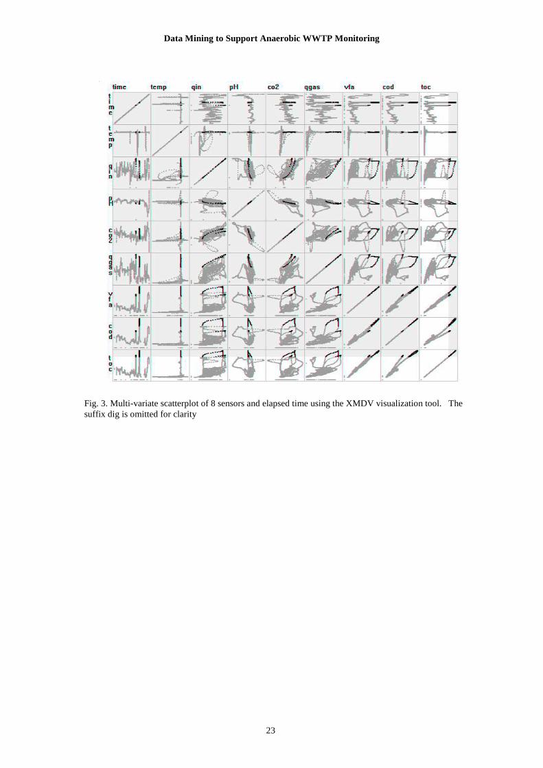
An overview of the characteristics of the data is shown in Fig. 3. It shows a matrix of scatterplots of

elapsed time and the 8 sensors, using the XMDV multidimensional visualization tool (Ward, 1994).

Every pair of the 9 variables is represented by a scatterplot. For instance the box which is in the column

labelled pH and the row labelled temp contains a scatterplot with pH and temp as the x- and y-axes

respectively.

For each of the sensors which measure a quantity in the digester, the suffix “dig” has been removed

for clarity and similarly co2gas is labelled as co2. There is redundancy in the diagram as a whole since

there is a symmetry about the major diagonal, which contains each variable plotted against itself.

Although detail such as axis labelling is sacrificed in favour of displaying 9 variables, some trends

can be noted. The leftmost column shows plots of all the sensors against elapsed time. Thus temperature

is steady all the time, except for a few short intervals, but other quantities exhibit frequent fluctuation

against time. The plot of any sensor value against another is independent of time. In several of these

scatter plots, some peaks are more readily distinguished from each other. This can be seen in the plots

which involve qin, pH and vfa.

3. Modelling error bounds

3.1 Introduction

When using a regression model to estimate expected data values from one of the missing or faulting

sensors it is necessary to know how reliable the estimate is. A robust method for estimating local error

bars has been developed by Healy et al (2003a, b) and shown to be effective for a range of synthetic and

multivariate data. The method’s main theoretical advantage was that it maintained the integrity of

statistical inference. The method is related to a proposal of Nix and Weigend (1995) who were studying a

laser intensity series problem. Their proposal offered advantages since it avoids the need for bootstrap re-

sampling or the problems arising from the need to invert a Hessian matrix. Nix and Weigend required a

special neural net (NN) architecture whereas this method can be used for a wide range of non-linear

regression techniques. In particular it can use a standard neural net architecture rather than a customised

Data Mining to Support Anaerobic WWTP Monitoring

6

one. Prediction intervals can be estimated directly by extending the work of Hwang and Ding (1997) to

the heteroskedastic case which is where the error term has non constant variance. White’s test confirmed

that the data used here was heteroskedastic. Prediction risk, as defined by Moody (1994), can be obtained

as a by-product for unseen targets using the predicted local error bars.

3.2 Outline of Theory

Hornik, Stichcombe, and White (1990) have shown that neural nets can be universal approximators to

continuous functions. This strength can be a problem in modelling if there are too many parameters and

these lead to the derived model being over-fitted to the specific characteristics of the data with consequent

poor outcome for the out-of-sample performance. Hwang and Ding (1997) reported that the

nonidentifiability of weights in neural net models meant that previous statistical theory for determining

confidence intervals was inappropriate. However they showed that it was indeed possible to construct

asymptotically valid prediction intervals; their derivation assumed a constant variance. Nix and Weigend

(1995) proposed a practical method for computing the local error bars for a derived model; their method

involved a Gaussian noise assumption, a special neural net architecture and a weighted regression, which

emphasised the low noise contributions in the target.

Healy et al (2003b) showed that an NN with two output nodes can produce an estimate of the mean

and variance of the conditional distribution of the target; one node is trained to fit a target value and the

other is trained to fit squared residuals. The proof depended on minimising a least squares cost function

and does not depend specifically on the deployment of neural nets. This gave the prediction interval as:

)1(

)x(*)x(*)x( i

2

)1(),2/1(ii −−±≈ −−− kn

ntdPI kna

σ (1)

where d*(xi) is the estimated target for input row xi, t is the Student’s t-distribution; n is the number of

rows used in training, k is the number of applicable degrees of freedom, a is the significance level, σ*2(x i)

is the estimate of the variance of d for row xi.

The prediction risk is

( ))(/11

2*i

N

i

xNEPR ∑=

= σ (2)

where σ*2(xi) is the estimate of the variance of d for row xi by the neural net when the corresponding

target d for the estimate d* is not known. The PR is derived from applying the training model on the new

input data xi .

3.3 Procedure for Modelling Error Estimates

The data set is split randomly into three equal sized sets called here TRAIN1, TRAIN2, and

TESTSET. Only filtered complete records are retained for training and testing. In Phase1 a model is

constructed using dataset TRAIN1 to fit the target variable for the required input variables. In Phase2 the

model from Phase1 is applied to dataset TRAIN2 to derive an estimate of the target; using the target

Data Mining to Support Anaerobic WWTP Monitoring

7

values and the estimated values a set of residuals is calculated and the square of the residuals is appended

to the dataset. A new model is now trained on the pair of targets consisting of the target variable and the

corresponding squared residual.

In the Phase1 modelling, TRAIN1 is randomly split into equal sized training and validation sets.

Early stopping on the validation set is used to reduce over- fitting. The same applies to Phase2 with

TRAIN2. TESTSET data values are the ‘out-of-sample’ data; they are used so that model performance is

estimated on the basis of values that have not been used in the model construction.

4. Model implementation

4.1 Expert Judgement

Input variable selection was based upon the four-tier ranking of sensors shown above in Fig. 2. The

full set of INRA-LBE sensors is not expected to be available in industrial WWTPs. In the current work

the focus is on the prediction of: a) volatile fatty acid concentrations in the digester, vfadig, from Level

2,1 sensors; and b) chemical oxygen demand in the digester, coddig, from Level 4,3,2,1 sensors and from

Level 2,1 sensors.

4.2 Linear Regression

Linear regression was used to perform preliminary investigations. There were high Pearson

correlations between vfadig, tocdig, and coddig. Specifically the correlation between vfadig and tocdig

was 0.988, between vfadig and coddig was 0.95, and between tocdig and coddig was 0.97.

For the prediction of coddig, a value of R2=0.979 was obtained by linear regression using all sensors

except tempdig, which was eliminated as insignificant on an F* test. Omitting tocdig from the inputs gave

a value of R2=0.972. The omission of vfadig as well as tocdig reduced the value of R2 to 0.288 and a

variance that was less than half the experimental value. More extended details were reported by Gallop et

al (2004).

For prediction of vfadig a value of R2=0.45 was obtained using Level 2 and Level 1 sensors alone; the

sensor data for co2gas and qin were eliminated as insignificant on an F* test in the forward stepping

regression. The predicted variance was less than a third of the experimental value. By comparison with

the extended set of sensors introduced in section 2.2 Sensors, restriction by expert judgement involved

removing total and partial digester alkalinities, tadig and padig, from Level 3 and pressdig from Level 1;

inclusion of these sensors’ data in the linear model gave R2~0.75. On a different, though similar, dataset it

was seen that the linear model for the prediction of vfadig with inputs of bicdig (digester bicarbonate

concentration) and tadig alone gave R2 ~1.

Overall it appears that Level 4 and Level 3 variables require at least Level 3 sensor data for linear

regression to be effective in predicting the correlation and variance.

Data Mining to Support Anaerobic WWTP Monitoring

8

4.3 Regression with neural nets

Some manual and automatic sensitivity exploration was undertaken prior to choosing the neural net

architecture. The first stage was the creation of a set of simple models using an NN architecture with one

hidden layer and with a fixed number of inputs. A logistic function and early stopping on the validation

set were used for modelling. These gave useful qualitative guidance for the fits that might be achieved.

For the results reported here for both vfadig and coddig a Phase 1 neural net model of 10 logistic

functions were arranged in one hidden layer of neurons. The gross fitting trends noted for linear

regression were followed for the NN regressions with the notable exception of cases where neither Level

3 nor Level 4 sensor data are used as input to the model formation when it was clear that neural nets were

giving much better fits. Overall the Phase 1 model generation was straightforward although the residuals

were notably larger than when the higher Venn Level sensor data were included in the modelling. The

reported accuracy for vfadig prediction was 96.9% and for coddig it was 96.8%.

The creation of Phase 2 models was relatively straightforward when the inputs included Level 3 and

Level 4 sensor data. However when the inputs omitted Level 3 and Level 4 sensor data there were much

larger residuals from Phase 1. For the results reported here for both vfadig and coddig a Phase 2 neural

net model of 11 logistic functions were arranged in one hidden layer of neurons. The Phase2 reported

accuracy for the combined targets was 98.0% and 98.2% respectively.

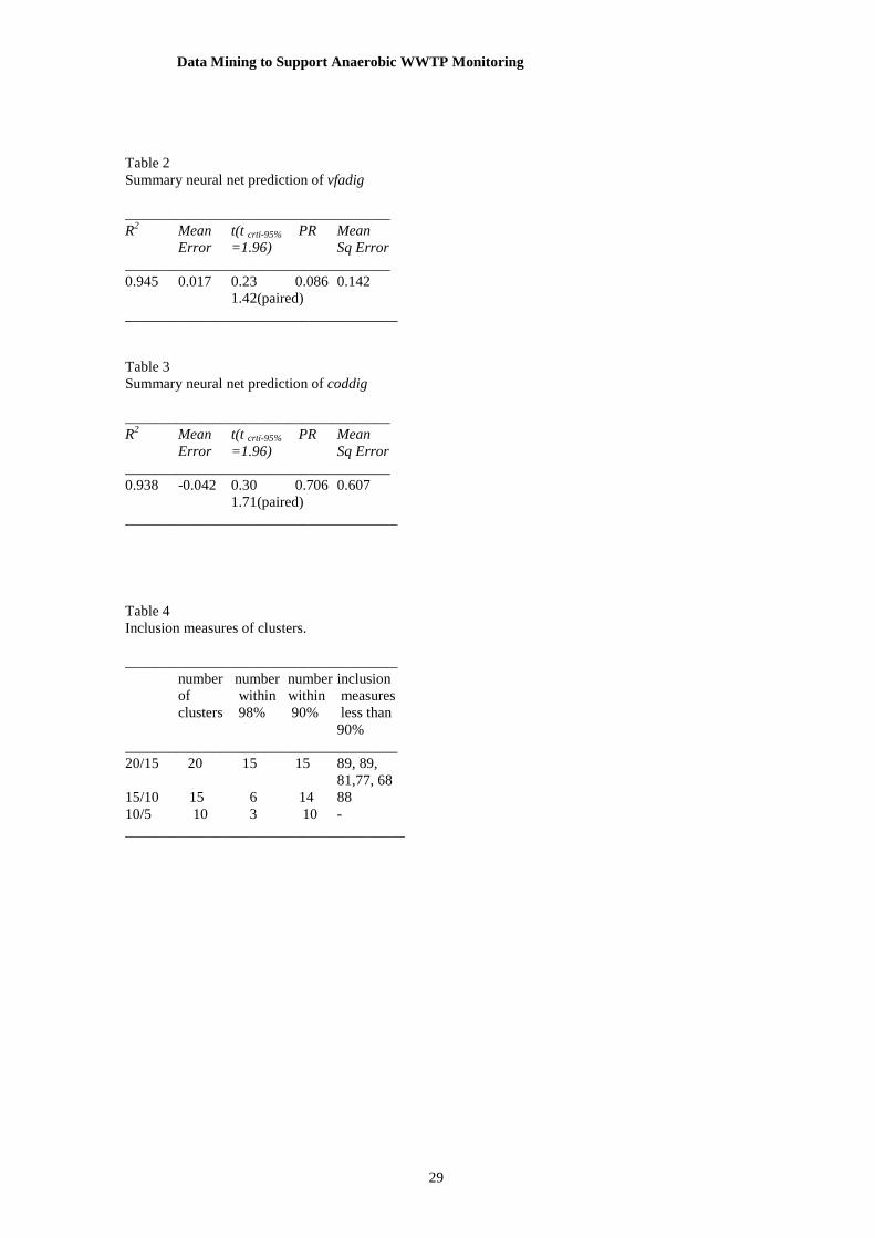
Table 2 and Table 3 report summary data from applying the models to the data values in TESTSET,

for the prediction of vfadig and coddig with the filtered experimental values. TESTSET values have not

been used for training the neural net. R2 is the square of the Pearson correlation; a value close to 1

indicates the model is giving a good prediction. The mean error is the mean of the difference between the

TESTSET data values and the neural net prediction. The value of t< t crit-95% indicates that the mean

value of the sensor data and the predictions are indistinguishable at the 95% level. Prediction Risk, PR, is

defined in equation 2; it is the expectation of the mean squared error from the Phase 2 NN model without

knowing the target value. Mean Sq Error is the actual mean squared error based upon knowing the target

data values as well as the prediction.

4.4 Estimates of vfadig and coddig

From Table 2 it can be seen that the predicted value of vfadig, is very well correlated to the

experimental values since R2 = 0.945; this compares very favourably with the linear regression’s R2~0.45.

The t-value indicates that the mean values are consistent with a 95% confidence interval. The paired t-

value, 1.42, is well within the critical value range also. The predicted variance of $N-vfadig is 2.4

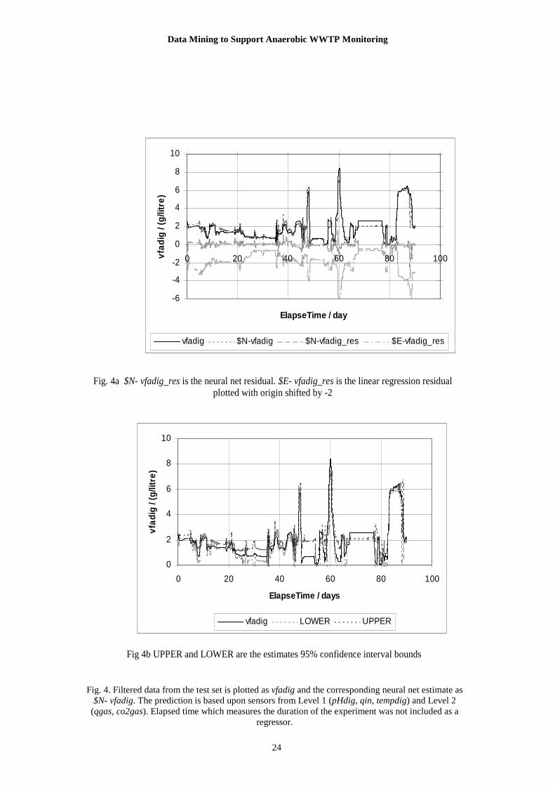
(g/litre)2 which has a probability of 0.28 of not being different from the experimental data. Fig. 4a shows

the filtered data from the test set as vfadig and the neural net estimate as $N-vfadig both plotted against

experimental duration – called elapsed time here; the corresponding residual is $N-vfadig_res while $E-

vfadig_res (ordinate shifted) is the linear regression residual. (Straight lines are an artefact of the drawing

tool and represent simple interpolation across gaps in the data which were identified in Section 2.3.). It

can be seen that there is reasonable qualitative agreement between both the location and magnitude of the

Data Mining to Support Anaerobic WWTP Monitoring

9

peaks in the neural net case; the linear regression errors are much larger. The upper and lower prediction

bands are shown in Fig. 4b as UPPER and LOWER. 66% of the experimental filtered vfadig data values

in TESTSET fell between the 95% prediction interval bands; if the band was widened by 30% of vfadig

then 93% fell in the band. Using the XMVD tool enabled the identification of the disparity as arising

from the model underestimating small squared errors across the range. Also the main peak around 60.3

days is under estimated and the data lies above the upper bound by ~0.5 g/litre.

In Table 3 the value of R2 = 0.938 shows the fit of coddig from Level 1 and Level 2 sensor data is not

quite as well estimated compared to vfadig, however it compares very favourably with the linear

regression’s R2~0.28. The t-value indicates that the mean values are consistent with a 95% confidence

interval. The paired t-value of 1.71 is within the critical range. The predicted variance of $N-coddig is 9.4

(g/litre)2 which has a probability of 0.47 of not being different from the experimental data. Fig. 5a shows

qualitatively good agreement between the experimental data and the neural net prediction from $N-coddig

for the location and magnitude of peaks. As expected the residual curves show that the neural net estimate

is much better than the linear regression estimate over the full time range. Fig. 5b shows the

corresponding prediction intervals for coddig. 57% of the filtered coddig data values in TESTSET fell

between the 95% prediction interval bands; if the band was widened by 30% of coddig then 85% fell in

the band while widening it by 40% gave 89% in band.

4.5 Summary

It has been shown that it is possible to estimate the concentration of volatile fatty acids and of chemical

oxygen demand in an anaerobic digester from Level 1 and Level 2 sensor data using neural net modelling;

satisfactory values of mean and variance were obtained. This is a significant step towards modelling the

process state and this is markedly better than can be achieved with linear regression models for the same

inputs. High accuracy seems to require data from Level 3 and Level 4 sensors. Prediction intervals have

been estimated for unseen targets although for the models reported here their width is under estimated and

it is not a matter of simple linear scaling; the modelling is underestimating small squared errors.

5. Cluster analysis and rule induction

5.1 Introduction

As a complementary technique, it is also desirable to investigate whether the multi-sensor space

which records the digester process can be characterised by a set of process states, which are small in

number, intelligible and have some stability, are robust and are sufficiently accurate. To this end, the

experimental data is analysed by using clustering techniques and rule induction.

Data Mining to Support Anaerobic WWTP Monitoring

10

5.2 Respective roles of each technique in sensor data analysis

In outline, cluster analysis can be used to identify coherent subsets of data. Within a subset (a

cluster), data records are similar to each other, but data records in different subsets are dissimilar.

Rule induction can be used to identify relationships between variables and these are inferred by

analysing the available data. A rule is a Boolean relationship accompanied by information that provides

guidance as to the reliability of the rule, which can be useful even if not 100% true on the available

evidence.

Cluster analysis and rule induction used together offer a potential of useful relationships relating the

digester sensors. Relationships need to be established between sensors that are absent and those, which

are more reliable or more likely to be present, as discussed in section 1.2.

A rule induction algorithm (Hand, 2001) requires the prior specification of:

• a variable T1 which is to be used as the target

• and a set of predictor variables (P1, … Pn) which are to be used to infer a set of relationships

with T1

It generates a set of induced rules, of which an example can be of the form:

if P1<0.7 and P4>5.6 then T1=3

The antecedent – the if clause – is already in a form which is suitable for variables corresponding to

sensor measurements. In general, rules produced in this way are relatively straightforward to interpret,

unless the number of variables used in the antecedent becomes unwieldy.

However the right hand side – the consequent - of an induced rule involves a single target variable

T1. Since existing work on the FDI (as outlined in section 1.5) shows that some digester conditions

require more than one sensor to diagnose, a method of expressing this state as a single state is required.

One possible such single variable is a cluster identifier, a discrete variable which is produced by a

cluster algorithm. In most such algorithms, the clusters are inferred by using a multivariate distance

criterion. Such a method has an advantage of not requiring prior estimates of how the multidimensional

sensor space is to be partitioned. A disadvantage of a cluster algorithm is that the cluster identifier is not

straightforward to interpret, but since it is subsequently entered as a target of rule induction, the

possibility of interpretation is restored.

5.3 Cluster analysis

Clustered data.

The dataset used is the same as that described earlier in the document (section 2) and it includes

elapsed time and the 8 sensor variables.

Data Mining to Support Anaerobic WWTP Monitoring

11

Since it is important to analyse the process state and any recurrence of a similar process state at any

time, elapsed time is excluded from consideration by the algorithm. However it is required for

subsequent visual post-processing of the output results.

Using the cluster algorithm

The cluster algorithm used here is one that is mature and is available on the market - the Two Step

algorithm from the Clementine data mining system (SPSS, 2003) and results are then analysed with post-

processing techniques that are described below. The phrase Two Step refers to the phases of the

algorithm where the first groups the raw data into manageable groups and the second progressively

improves that grouping. The algorithm as provided can standardise numeric variables before clustering,

to prevent one cause of bias in distance calculation. Like other cluster algorithms, the process is

unsupervised.

If a number of clusters M is specified by the user, the algorithm generates an identifier which is a

number from 1 up to and including M. The result of the algorithm is that each complete record is

assigned to a cluster.

The state estimation work outlined earlier (section 1.4) uses up to 5 discrete bands for some sensor

variables. The possibility of requiring more bands is considered. Separate iterations of the algorithm

were executed, specifying in turn, 5, 10, 15 and 20 clusters, and following this with partly manual

postprocessing investigations as described below. A much larger number of clusters could be specified

but this tends towards the extreme of a cluster per data point, which tends to lose the benefit of

summarising the process state.

Postprocessing

For postprocessing purposes, the sensor variables are combined with elapsed time and the cluster

identifier, for each iteration of the algorithm. Furthermore the Two Means algorithm provides the centre

of each cluster.

Fig 6 shows a multivariate scatter plot, similar to Fig 3, but this time with a cluster identifier included

for a 20-cluster iteration (c20). The discrete property of the identifiers is apparent from the plot of c20

against time. Here, time, the cluster number (c20) and a subset of sensor variables are used. Although

all sensor variables could have been plotted here, slightly clearer results can be obtained by excluding

some, such as tempdig, held steady in this cluster, and tocdig and coddig which show similar patterns to

vfadig. The data corresponding to one of the values of the cluster identifier (in this case, 8) is shown in

black and the others in grey. It can be seen from this figure that in this case the range of each variable in

cluster c20 is comparatively small compared with the whole dataset.

One of the goals of data mining is not only that it can assist analysts to infer patterns, but that those

patterns should also have significance. Since clusters do not conform to a predefined, simple condition,

some examination is needed before the expert can be convinced of their significance. Therefore

properties of the cluster sets, which can be calculated simply or visually inferred, are a potentially useful

tool. Here are defined and discussed two properties, inclusion and compactness.

Data Mining to Support Anaerobic WWTP Monitoring

12

Inclusion

The first property described is that of inclusion, which can be calculated where there are multiple

iterations of the cluster algorithm. A dataset that does not fall readily into clusters may reveal some lack

of stability when results for different numbers of clusters are compared. To use the example of a 15-

cluster and a 20-cluster model, it is desirable to determine whether each of the 20 clusters is largely

contained within just one of the clusters in the 15-cluster model.

More generally, for a given number M, an M-cluster model is described as consisting of M clusters

CM,i for i=1,M, where the union of all the CM,i is the complete set of records and each of the pairwise

intersections is the empty set. Two values of M are described: i.e. M1 and M2 such that M1<M2.

Then the inclusion measure of cluster CM1,k within the cluster set CM2 is:

))(max( ,2,1 iMkM CCcount ∩ (3)

where max is calculated over I=1,M2

An inclusion measure of 100% would imply that CM1,k is wholly contained within just one of the

clusters CM2,j

Having defined it, the inclusion measure is readily determined using straightforward calculation and

information processing such as can easily be handled by a DBMS. Table 4 summarises the results of

applying this to 4 models with 20, 15, 10 and 5 clusters, considered pairwise 20/15, 15/10 and 10/5. Thus

the first row summarises the inclusion measures of each cluster C20,i within the cluster set C15. Out of the

20 clusters, 15 have an inclusion measure of 98% or greater and the remaining clusters range from 89%

down to 68%.

The figures 77% and 68% for the 20 cluster case within the larger 15-cluster model prompt the

suggestion that subdivision to this many clusters may be causing some arbitrariness in the partitioning,

but some further investigation of this would be profitable.

Compactness

The second property indicates how compact the clusters are. If some variables have a narrow

variance within a particular cluster, it is possible to suggest that certain variables and certain ranges of

those variables are a significant influence in that cluster being inferred by the cluster algorithm. To begin

to determine this, for each variable within a given cluster, a per-cluster width measure is used and is

expressed as a percentage. This is based on the standard deviation of that variable within that cluster, by

comparison with the standard deviation of that variable within the whole dataset. A measure of 100%

would indicate that within a cluster, a variable has the same standard deviation as over the whole dataset.

Since a cluster is designed to minimise distances within a cluster, a low percentage could be expected for

at least some variables within a cluster. However some caution needs to be exercised here since a

sausage shape not parallel to an axis is a plausible cluster.

This measure has been calculated for all the clusters in the four cluster models identified (5, 10, 15,

20 clusters). To use a 20-cluster model as an example, the following characteristics have been found.

Data Mining to Support Anaerobic WWTP Monitoring

13

The variable which consistently (17 out of 20) scores the lowest per-cluster width measure in a

cluster is tempdig and, in all but one cluster, the measure for tempdig is <8%. This appears to be

consistent with the observation that this sensor is held at a steady value for all but four short periods,

which is also apparent from the temperature against time scatterplot in Fig. 3. Furthermore tempdig does

not figure as an influence at all in the linear regression results.

After tempdig, every cluster has at least one variable that has a per-cluster width measure of <25%,

except for just one cluster where this measure scores >40% for all variables.

The next stage is to use the cluster identifier as input to rule induction. Currently there is no single

preferred number of clusters. A development of this work could use a range of possible numbers of

clusters and test the effectiveness of rule induction with a different number in turn. Here, for illustrative

purposes, the result of the 20-cluster model is used.

5.4 Rule induction

The cluster identifier, an integer, is used as the target variable for rule induction. The cluster

identifier is chosen that results from the iteration which specifies 20 clusters.

The C5.0 algorithm in the Clementine data mining software was used here. It is based on the widely

used C4.5 algorithm developed by Quinlan (Quinlan, 1993) which is based in turn on his previous ID3. It

first of all produces a decision tree which embodies a sequence of decision points which are each based

on a comparison involving a single variable. A number of criteria are used to avoid excessive

subdivision, which would result in overfitting. A consequence of using a decision tree is that the number

of thresholds for each single variable is reduced to a manageable number.

On any given iteration of the rule induction algorithm, the sensor variables can be divided into

indicators and predictors. A set of indicator variables is considered to consist of those sensors that, in

combination, if available, are believed to provide effective information about the digester condition. A

set of predictor variables is an alternative set that is considered to consist of those sensors that, in

combination, may plausibly provide effective information and may have certain attractions, based on the

sensor ranking, as a substitute for the indicator set.

Thus vfadig (a level 3 sensor) could be considered to be a possible indicator in combination with

others and co2dig, qgas and qin (level 2 and 1 sensors) to be a possible set of predictors.

Postprocessing criteria for rule acceptability

It is important to know how effective a given set of rules may be. A rule induction algorithm such as

C5.0 provides control over the maximum complexity and the predictive power of the generated rules.

The purpose of this is to reduce the quantity and complexity of rules that turn out to be ineffective when

presented to a domain expert.

In general, these criteria are provided as controls on or output from an induction algorithm:

• Support: this is the number of records for which the Boolean antecedent holds

• Confidence: the proportion of those records for which the target variable takes the required value

Data Mining to Support Anaerobic WWTP Monitoring

14

While useful, these are insufficient. Therefore the approach here is to apply a richer set of criteria in a

post-processing stage. Each of the criteria has a threshold which, depending on the application, can be

controlled to include or exclude rules.

To describe this, suppose there is a rule of the form:

if P then T

where P could be of the form P1<4.2 and P3>1.2 and T could be T2. Thus denoting terms:

• P+ to refer to the number of records for which the antecedent (or prediction) is true,

• P- to refer the number of records for which the antecedent is false,

• similarly T+ and T- refer to the target,

• and the concatenation P+T- refers to the intersection of P+ and T- .

The relationship of these to each other is shown in Fig. 7.

So (making use of the same notation to denote the size of a subset) the support is P+, and the

confidence is P+T+/P+ .

However, being able to control how rules are postprocessed, means that further criteria can be applied

automatically, such as:

• T- and T+ should both be high enough. If T+ refers to one of several unusual digester conditions that

require separate investigation, sufficient experimental measurements need to be available for results to

be significant.

• The proportion of false positives P+T-/T- and false negatives P-T+/T+ should both be small enough.

For a given application, it may be necessary to control these independently.

• It can occasionally happen that a generated rule is a better predictor of the reverse case than the

unreversed case. Thus even if P+T+/T+ is high, it is possible for P+T-/T- to be even higher and a rule

with this characteristic may not be useful.

Since a few of the criteria are equivalent to a combination of others, not all need be applied. By

using a suitable postprocessing procedure, the choice of criteria and thresholds can be controlled by the

user. For example in this case, the generated rules were written to an XML file by Clementine, using the

PMML language (DMG, 2003). From that description, software independent of any specific data mining

software was used. An XML transformer using XSLT converted the rules to a CSV file. Using a

relational DBMS, every rule was applied to every data record and suitable counts accumulated.

Criteria of this form already exist in the literature on rule induction (An and Cercone, 2001). Here

they are expressed in a straightforward form and conventional, readily available software (XML

transformers and DBMS) can be used to apply the criteria.

Data Mining to Support Anaerobic WWTP Monitoring

15

An example

Table 5 and Table 6 show an example of the results of rule scoring in tabular form reduced from 30

rules to 9 by applying suitable criteria.

In these tables, the flow rates, qin and qgas, are normalised by dividing by their respective maximum

value in the dataset. This is to produce numbers which are comparable between different digester plants.

The other variables are already in comparable units. The target value is transformed from the cluster

identifier, to a number which is representative of vfadig in the cluster, specifically the mean of this

variable multiplied by 1000.

The two tables result from a vertical cut applied to a single wider table leaving the target value

column in both portions: the cut has been made here for ease of layout. Each row in the single, wide

table corresponds to a rule.

For each row:

• In the centre is a value corresponding to the cluster identifier. Here the small integer number is

converted to a target value representative of the values of one of the indicator variables (in this case

vfadig) in the cluster.

• On the left side, a rule relating the given indicator variables to that cluster is shown. This provides a

characterisation of the cluster in terms already understood by the human expert to indicate the condition

of the plant. In this case, the indicator variables were chosen to be vfadig and qin

• On the right hand side is a rule relating the given predictor variables to that same cluster. Inspection

of both sides gives a relationship between the indicators and predictors. In this case, the predictor

variables were chosen to be qgas, co2gas, pHdig and qin (level 2 and 1 variables). The sensor qin

appears in both categories.

In the table, the initials lb and ub are the lower and upper bounds of the range of values for each

variable for each rule and are not necessarily the same as the minimum and maximum of the variable

within the complete cluster. Where a lower bound is blank, that bound is the minimum of the entire

dataset; a blank upper bound indicates the maximum.

As an example, consider the row containing the target value 3436. The condition in this row

involving the indicators (Table 5) qin and vfadig has a high (99%) of correctly predicted true positives

and true negative. The number of records with positive predictions is not high (148) because here the

values of vfadig are high and it is difficult to run a digester for long in that condition.

Turning to the predictors qgas, qin, co2gas and pHdig, for the same target value (Table 6), it can be

seen that only two of those four sensors are required (the entries for qin and pHdig are blank so these

sensors do not influence the rule), which makes the rule easier to interpret. The number of true negatives

is high (100%) but the false positives are 27%. Taking the indicator and predictor sides together, this

suggests that the predictor rule (involving level 1 and 2 sensors) will correctly predict conditions where

the level 3 and 4 variables are within the specified bounds, but there will also be cases where the

prediction is made, but it will turn out that the digester state is not within the predicted state.

Data Mining to Support Anaerobic WWTP Monitoring

16

6. Conclusions

6.1 Findings

Neural nets and linear regression

Good estimates of volatile fatty acid concentration and chemical oxygen demand concentration can

be obtained using neural nets from Level 1 (pHdig, qin, tempdig) and Level 2 sensors (qgas, co2gas)

alone. The corresponding linear regressions are unsatisfactory having poor correlation and variance.

A robust method for determining prediction intervals for models derived by neural nets has been

applied. This aimed at determining the reliability of the estimates of sensor values in terms of other sensor

readings. It was based on simultaneously modelling the mean and variance, using a standard NN-

architecture. Specifically, using a NN regression, it has been feasible to estimate for an anaerobic digester

the concentration of volatile fatty acids and chemical oxygen demand with the corresponding prediction

intervals. There is a performance limit to the prediction interval in the case of small residuals and around

sharp peaks. Prediction risk for a set of unseen targets was estimated as a summary statistic of the

prediction interval calculation; the increase in prediction risk as input sensors were removed anticipated

the qualitative deterioration in the mean squared error on known targets.

Cluster analysis and rule induction

Adopting an approach of postprocessing cluster models and induced rules sets allows some freedom

to adopt properties and criteria which have relevance to the application domain, instead of relying on

controls supported in the available data mining software.

Although exporting cluster information for post-processing purposes is relatively straightforward,

exporting rule sets requires correct treatment of the rule structure. The adoption of a common XML-

based language for this purpose (PMML) allows the data mining and post-processing software to be

independent of each other.

In a situation where models may be constructed and then applied in an operational situation,

techniques which here are used to assess the initial quality of rule sets can also be adopted for assessing

the continued applicability in new operational situations.

The identification and analysis of clusters in the multidimensional state space of the digester offers

potential for simplifying the digester state. It is then also necessary to determine how the clusters can be

characterised in a straightforward way. Analysis of clustering results suggested that: (i) cluster

membership is stable, as the number of clusters varies, reducing the chances of arbitrary clusters; (ii)

clusters can be shown to have a subset of variables which have a narrow spread within the cluster and this

subset may differ from one cluster to another.

In the above studies the use off-the-shelf software proved to be very effective for the purposes

required.

Data Mining to Support Anaerobic WWTP Monitoring

17

6.2 Further Work

Fault Detection and Isolation

Although FDI has been developed for one well instrumented process and is working well it would

require some efforts to extrapolate it to other processes so a further data mining objective is to generalise

the FDI results by finding for example (i) what are the possible models to be used across several

processes to validate sensor information (eg, linear and NN models)? (ii) what are the best indicators over

several processes to detect the faults or process states (eg clustering)? (iii) what are the rules of the FDI

that are general and possibly used for many processes? This link between FDI and data mining requires

further strengthening and embodying in an operational procedure.

Other Further Work

Future work will proceed in a number of directions. It is planned to use lagged variables from the

basic set of sensors in a vector regression to provide predictions of imminent states of the plant while

sensors are unavailable. Although auto-regression will provide high accuracy for one-step ahead

predictions it is not seen as so useful in the TELEMAC context where sensor maintenance will be on a

longer time scale; Young (2004) has emphasised the inappropriateness of applying iteration in these

circumstances. Further study of the estimation of the prediction interval is needed since the proportion of

the test set data points laying outside the bands is high and seems to arise from under-estimation of the

squared residuals. Further investigation of clustering of states will concentrate on sequencing of states,

which is expected to provide an interesting complement to expert knowledge.

The work of Lardon et al (2004) on sensor consistency and process states will be improved by using

data mining to repeatedly check the validity of both the clustering and the expert rules.

Acknowledgements

Support from the European Commission’s IST programme under the TELEMAC project (IST-2000-

28156) is acknowledged. J V Healy was supported by a teaching research bursary from the London

Metropolitan University’s CCTM. The authors are grateful to Professor R Soncini Sessa and an

anonymous referee for guidance in restructuring an original workshop presentation paper for this journal.

References

An, A., and Cercone, N., (2001). Rule Quality Measures for Rule Induction Systems: Description and

Evaluation. Computational Intelligence, 17( 3), pp 409-424

Bernard, O., Hadj-Sadok, Z., Dochain, D., Genovesi A., Steyer J. P. (2001). Dynamical model

development and parameter identification for an anaerobic waste water treatment process.

Biotechnology and Bioengineering, 75(4) pp 424-438.

Data Mining to Support Anaerobic WWTP Monitoring

18

Bernard, O., et al. (2005). An integrated system to remote monitor and control anaerobic wastewater

treatment plants through the Internet, Water Science and Technology,52,(1-2), pp 457-464 see also

http://www.ERCIM.org/TELEMAC/

Carrasco, E.F., Rodriguez, J., Punal, A., Roca, E., and Lema, J.M. (2004). Diagnosis of acidification

states in an anaerobic wastewater treatment plant using a fuzz-based expert system. Control

Engineering Practice 12, pp 59-64.

Dixon M., Gallop J.R., Lambert S.C., Healy J.V. (2007). Experience with data mining for the anaerobic

waste water treatment process. Environmental Modelling and Software 22, pp315-322.

DMG (Data Mining Group). (2003). web pages on PMML at http://www.dmg.org/v2-

0/GeneralStructure.html.

Gallop, J. R., Dixon, M., Healy, J.V., Lambert, S.C., Laurent, L., and Steyer, J.P. (2004). The use of data

mining for the monitoring and control of anaerobic waste water plants. Presented to 4th International

Workshop on Environmental Applications of Machine Learning at the 4th European Conference on

Ecological Modelling. The associated technical report is available from

http://epubs.cclrc.ac.uk/bitstream/1150/EAMLpaper.pdf

Gujer W. and Zender A.J.B. (1983). Conversion processes in anaerobic digestion. Wat. Sci. Tech. 15:pp

127-167.

Hand, D., Mannila, H., and Smyth, P. (2001) Principles of Data Mining, The MIT Press

Healy, J. V., Dixon, M., Read, B.J., and Cai F.F. (2003a). Confidence in Data Mining Model Predictions

from Option Prices. Proceedings of the IEEE, IECON03, ISBN 0780379063/03 pp 1926-1931.

Healy, J. V., Dixon, M., Read, B.J., and Cai F.F. (2003b) Confidence and prediction in generalised non

linear models: an application to option pricing, International Capital Markets Discussion Paper,

London Metropolitan University. 03-6 pp 1-42.

Hilgert N., Harmand J., Steyer, J. P., and Vila, J. P. (2000). Nonparametric identification and adaptive

control of an anaerobic fluidized bed digester. Control Engineering Practice 8, pp 367-376.

Hornik, K., Stinchcombe, M., and White H. (1990). Universal Approximation of an unknown Mapping

and its derivatives using multilayer feedfoward networks. Neural Networks,3, pp551-560.

Hwang, J.T.G. and A.A. Ding (1997). Prediction Intervals for Artificial Neural Networks. Journal of the

American Statistical Association, 92, pp748-757.

Lardon, L., Punal, A., and Steyer, J.P. (2004) On-line diagnosis and uncertainty management using

evidence theory––experimental illustration to anaerobic digestion processes, Journal of Process

Control, Volume 14, Issue 7, October 2004, pp747-763.

Moody, J.E. (1994) Prediction Risk and Architecture Selection for Neural Networks : From Statistics to

Neural Networks:Theory and Pattern Recognition Applications (Eds: Cherkassky, V., J.H. Friedman,

and H. Wechsler.) NATO ASI Series F, Springer Verlag.

Data Mining to Support Anaerobic WWTP Monitoring

19

Nix, D.A. and Weigend, A.S. (1995). Learning Local Error Bars for Nonlinear Regression. In: Advances

in Neural Information Processing Systems (NIPS*94) (G. Tesauro, D.S. Touretsky, and T.K. Leen.

(Ed)), pp 489-496. MIT Press, Cambridge MA.

Quinlan, J.R., (1993) C4.5: Programs for Machine Learning, Morgan Kaufmann Publishers , ISBN

1558602380

SPSS, (2003) Clementine 8.0 User’s Guide.

Steyer, J.P., Bouvier, J.C., Conte, T. Gras, P. and Sousbie, P. (2002a). Evaluation of a four year

experience with a fully instrumented anaerobic digestion process. Water Science and Technology,

45(4-5), pp 495-502.

Steyer, J.P., Bouvier, J.C., Conte, T. , Gras, P., Harmand, J., and Delgenes, J.P. (2002b) On-line

measurements of COD, TOC, VFA, total and partial alkalinity in anaerobic digestion processes using

infra-red spectrometry. Water Science and Technology, 45(10), pp 133-138.

Ward, M.O.,(1994) XmdvTool: integrating multiple methods for visualizing multivariate data,

Proceedings IEEE Visualization 1994, pp 326-333.

Young, P.C., (2004). The Data-based mechanistic approach to the modelling, forecasting and control of

environmental systems. Proceedings of IFAC Workshop on Modelling and Control for Participatory

Planning and Managing Water Systems. Venice.

Data Mining to Support Anaerobic WWTP Monitoring

20

Figure Legends

Fig. 1. Two stage process of conversion

Fig. 2. Venn diagram showing sensor ranking. The sensors are defined in section 2

Fig. 3. Multi-variate scatterplot of 8 sensors and elapsed time using the XMDV visualization tool. The suffix dig is omitted for clarity

Fig.4 . Filtered data from the test set is plotted as vfadig and the corresponding neural net estimate as $N- vfadig. The prediction is based upon sensors from Level 1 (pHdig, qin, tempdig) and Level 2 (qgas, co2gas). Elapsed time which measures the duration of the experiment was not included as a regressor

Fig. 4a $N-vfadig_res is the neural net residual. $E-vfadig_res is the linear regression residual plotted with origin shifted by -2 Fig. 4b UPPER and LOWER are estimates 95% confidence interval bounds

Fig. 5. Filtered data from the test set is plotted as coddig and the corresponding neural net estimate as $N-coddig. The prediction is based upon sensors from Level 1 (pHdig, qin, tempdig) and Level 2 (qgas, co2gas). Elapsed time which measures the duration of the experiment was not included as a regressor

Fig. 5a $N-coddig_res is the neural net residual. $E-coddig_res is the linear regression residual plotted with origin shifted by -5 Fig. 5b UPPER and LOWER are estimates 95% confidence interval bounds

Fig. 6. Multiway scatter plot showing a cluster identifier c20

Fig. 7. Predictions and targets

Data Mining to Support Anaerobic WWTP Monitoring

21

Fig. 1. Two stage process of conversion.

Organic Carbon

VFA + CO2

CH4 + CO2

Fast Slow

Inhibition

Data Mining to Support Anaerobic WWTP Monitoring

22

Fig. 2. Venn diagram showing sensor ranking. The sensors are defined in section 2

tempdig, qin, phdig Level 1

qgas, co2gas

Level 2

vfadig

Level 3

coddig, tocdig

Level 4

Data Mining to Support Anaerobic WWTP Monitoring

23

Fig. 3. Multi-variate scatterplot of 8 sensors and elapsed time using the XMDV visualization tool. The suffix dig is omitted for clarity

Data Mining to Support Anaerobic WWTP Monitoring

24

Fig. 4a $N- vfadig_res is the neural net residual. $E- vfadig_res is the linear regression residual

plotted with origin shifted by -2

Fig 4b UPPER and LOWER are the estimates 95% confidence interval bounds

-6

-4

-2

0

2

4

6

8

10

0 20 40 60 80 100

ElapseTime / day

vfad

ig /

(g/li

tre)

vfadig $N-vfadig $N-vfadig_res $E-vfadig_res

0

2

4

6

8

10

0 20 40 60 80 100

ElapseTime / days

vfad

ig /

(g/li

tre)

vfadig LOWER UPPER

Fig. 4. Filtered data from the test set is plotted as vfadig and the corresponding neural net estimate as $N- vfadig. The prediction is based upon sensors from Level 1 (pHdig, qin, tempdig) and Level 2 (qgas, co2gas). Elapsed time which measures the duration of the experiment was not included as a

regressor.

Data Mining to Support Anaerobic WWTP Monitoring

25

-10

-5

0

5

10

15

20

0 20 40 60 80 100

ElapseTime / day

codd

ig /

(g/li

tre)

coddig $N-coddig $N-coddig_res $E-coddig_res

Fig. 5a $N- coddig_res is the neural net residual. $E- coddig_res is the linear regression residual

plotted with origin shifted by -5

0

5

10

15

20

25

30

0 20 40 60 80 100

ElapseTime / day

cod

dig

/ (g

/litr

e)

coddig LOWER UPPER

Fig 5b UPPER and LOWER are the estimates 95% confidence interval bounds

Fig. 5. Filtered data from the test set is plotted as vfadig and the corresponding neural net estimate as $N-coddig. The prediction is based upon sensors from Level 1 (pHdig, qin, tempdig) and Level 2 (qgas, co2gas). Elapsed time which measures the duration of the experiment was not included as a regressor

Data Mining to Support Anaerobic WWTP Monitoring

26

.

Fig. 6. Multiway scatterplot showing a cluster identifier c20

Data Mining to Support Anaerobic WWTP Monitoring

27

P+T- false

positives P-T-

T-

P+T+

P-T+

false

negatives T+

t

a

r

g

e

t

P+

P-

prediction

Fig. 7. Predictions and targets

Data Mining to Support Anaerobic WWTP Monitoring

28

Table 1 Descriptive Statistics for Filtered Sensor Data

________________________________________ Sensor Venn Mean Min Max Level ________________________________________ tempdig / oC 1 35.2 27.3 37.5 qin/ (litre/hr) 1 24 0 54 pHdig 1 7.2 5.3 8.8 co2gas /% 2 33 3 55 qgas/(litre/hr) 2 204 0 481 vfadig/(g/litre) 3 1.84 0 8.37 tocdig/(g/litre) 4 1.18 0 4.53 coddig/(g/litre) 4 3.95 0 17.2 ________________________________________

Data Mining to Support Anaerobic WWTP Monitoring

29

Table 2 Summary neural net prediction of vfadig ____________________________________ R2 Mean t(t crti-95% PR Mean

Error =1.96) Sq Error ____________________________________ 0.945 0.017 0.23 0.086 0.142 1.42(paired) _____________________________________

Table 3 Summary neural net prediction of coddig ____________________________________ R2 Mean t(t crti-95% PR Mean

Error =1.96) Sq Error ____________________________________ 0.938 -0.042 0.30 0.706 0.607 1.71(paired) _____________________________________

Table 4 Inclusion measures of clusters. _____________________________________ number number number inclusion

of within within measures clusters 98% 90% less than

90% _____________________________________ 20/15 20 15 15 89, 89,

81,77, 68 15/10 15 6 14 88 10/5 10 3 10 - ______________________________________

Data Mining to Support Anaerobic WWTP Monitoring

30

Table 5. Rule Induction scoring (a)

_______________________________________________________________________

indicators Target Value

_______________________________________________________________________ qin vfadig lb ub lb ub P+ T+ T- (P+T+) / (P-T-) / T+ T- 0.15 0.079 0.259 83 79 3197 0.52 0.99 126 0.37 0.758 265 366 2910 0.62 0.99 716 0.47 0.938 294 366 2910 0.66 0.98 906 0.37 0.69 0.938 1.530 520 408 2868 0.96 0.95 1407 0.40 1.530 2.690 273 235 3041 0.97 0.98 1817 0.61 1.530 624 203 3073 0.99 0.86 2622 0.91 1.930 3.920 42 39 3237 0.54 0.99 2921 0.40 0.48 2.100 118 131 3145 0.61 0.99 2568 0.61 2.690 4.640 148 116 3160 0.99 0.99 3436 _______________________________________________________________________

Table 6 Rule Induction scoring (b) _____________________________________________________________________________________ Target predictors Value ____________________________________________________________________________________ qgas qin co2gas pHdig lb ub lb ub lb ub lb ub P+ T+ T- (P+T+) (P-T-) / T+ /T- _____________________________________________________________________________________ 126 0.05 118 80 3196 0.98 0.99 716 0.05 0.28 0.34 6.89 471 430 2846 0.92 0.97 906 0.28 0.54 0.38 32.0 7.38 341 366 2910 0.91 1.00 1407 0.28 0.54 0.19 32.0 7.38 310 412 2864 0.64 0.98 1817 0.28 0.66 34.6 7.19 94 119 3157 0.73 1.00 2622 0.63 33.8 7.19 124 131 3145 0.92 1.00 2921 0.54 33.8 7.19 151 203 3073 0.59 0.99 2568 0.28 45.6 102 104 3172 0.89 1.00 3436 0.28 22.8 33 41 3235 0.73 1.00 _____________________________________________________________________________________