American University in Cairo American University in Cairo

AUC Knowledge Fountain AUC Knowledge Fountain

Theses and Dissertations

6-1-2018

Anaerobic digestion of organic waste: A kitchen waste case study Anaerobic digestion of organic waste: A kitchen waste case study

Charles Sendaaza

Follow this and additional works at: https://fount.aucegypt.edu/etds

Recommended Citation Recommended Citation

APA Citation Sendaaza, C. (2018).Anaerobic digestion of organic waste: A kitchen waste case study [Master’s thesis, the American University in Cairo]. AUC Knowledge Fountain. https://fount.aucegypt.edu/etds/434

MLA Citation Sendaaza, Charles. Anaerobic digestion of organic waste: A kitchen waste case study. 2018. American University in Cairo, Master's thesis. AUC Knowledge Fountain. https://fount.aucegypt.edu/etds/434

This Thesis is brought to you for free and open access by AUC Knowledge Fountain. It has been accepted for inclusion in Theses and Dissertations by an authorized administrator of AUC Knowledge Fountain. For more information, please contact mark.muehlhaeusler@aucegypt.edu.

1

ANAEROBIC DIGESTION OF ORGANIC WASTE:

A KITCHEN WASTE CASE STUDY

A Thesis Submitted to

Center for Sustainable Development

in partial fulfillment of the requirements for

the degree of Master of Science in Sustainable Development

by

CHARLES SENDAAZA

Under the supervision of:

Dr. Salah El-Haggar

Prof. of Energy and Sustainable Development

Mechanical Engineering Department

&

Dr. Hani Sewilam

Director Center for Sustainable Development

Mechanical engineering department

Spring 2018

2

Dedication

To my family

I would like to dedicate this thesis and all my life achievements to this stage, to my beloved

parents, Mr. Bayiga Richard Francis and Mrs. Nakisendo Gloria. Without their immeasurable

love, efforts, support and care, I wouldn’t have made it this far. I am eternally indebted to them.

I also would like to express my sincere gratitude to my dear brothers and sisters for their

continued guidance throughout the course of my research.

Last, but never the least, I am eternally indebted to my soul mate, best friend and best counsel,

Luzige Shaima for her encouragement. Thank you for believing in me, being with me through

this journey and for being proud of my achievements. Thank you for your love and patience.

3

Acknowledgements

I am in the first place very grateful to the Almighty God for blessing me with this opportunity

and many other opportunities that have made my life a success and His continued guidance.

This journey has been made possible by a number of people whose contributions and heartless

support I would like to appreciate in a special way.

I would in the first place like to thank the Ford Foundation for their generous contribution to the

African Graduate Fellowship which I was granted for my master’s degree studies. Their

generosity has afforded students from African countries, including myself, the privilege to study

at the American University in Cairo.

I would like to express my sincere gratitude to my supervisor and mentor Prof. Dr. Salah El

Haggar for his continued advice, guidance and support throughout my master studies. Thank you

for the encouragement and for the faith you always had in me. You have been a very good

compass, putting me back on track when lost and thank you for being available and for all you

always had to give up to meet with me and read every detail of my work. I pray that the Good

Lord rewards you abundantly.

I would also like to thank my co-supervisors, Dr. Yehia I. M. Zain and Dr. Mohamed M. Afifi

from the Soil, Water and Environmental Research Institute at the Agricultural Research Center,

and Dr. Hani Sewilam, Director Center for Sustainable Development in the American University

in Cairo. Thank you all for your guidance, time and patience throughout the research. Special

thanks to Dr. Mohamed Afifi and Dr. Yehia for all the technical support, dedication and

expertise at analyzing my samples and generating data for the research. I am deeply grateful for

all your efforts.

Mr. Mohamed Mahdy and Mr. Aboual Kasem Sayed from the Sustainable Development Lab,

your support cannot be forgotten. I am sincerely grateful for the cold nights you had to spend in

the lab to collect data on my behalf and enduring the terrible smell of the digesters when

monitoring progress of the experiments. May the good Lord reward you abundantly.

Finally, I would like to thank my team at the Research Institute for a Sustainable Environment

(RISE), thank you all for the encouragement, support and love. Every day in your company gave

me a sense of purpose and enabled me to focus more on completing this research. Thank you

Abdallah Tawfik for helping on my presentation, Rouba Dagher for helping with technical

drawings, Tina, for reading and editing my work, Amira for affording me time off work to

complete this research, and everyone else for the contribution. May you all live to see your

dreams come true.

4

Abstract.

Rapid population growth, urbanization, improved living standards and a shift in the consumption

patterns have accordingly escalated the intensity of waste generation. The 2012 World Bank

report on solid waste estimated the annual municipal solid waste generation at 1.3 billion tons

per year with a projection of over a 40% increase in the annual generation rate by 2025 and a

300% increase by 2100 worldwide. Nearly half of the generated municipal solid waste is organic,

including food wastes. About 30% of the food produced annually is wasted at different stages

along the food supply chain before human consumption. Kitchens serving the food needs of The

American University in Cairo’s New campus haven’t performed any different in their yield of

food waste, with on campus kitchens producing up to 150kg of food waste, mainly a composition

of fruit and vegetable waste daily.

Agricultural development mainly driven by extensive mechanization, continued incentivization

and growing demand for food on the other hand is also a significant organic waste generator.

Recent data estimates the annual production of agricultural waste at close to 1000 million tons.

Animal and poultry wastes in form of manure have been reported by different researchers for

their negative environmental impacts resulting from their direct application in agriculture or

mismanagement, raising concern over possible alternative means of sustainable management.

Anaerobic digestion stands out as the most viable means of sustainable management thanks to

the high moisture content and nutrient composition of the manures.

This study carried out in two phases aimed at investigating anaerobic digestion of the American

University in Cairo’s kitchen waste, market vegetable waste and animal and chicken manure. In

Phase I of the experiment, batch setups of 100% animal manure (A), 100% chicken manure (B),

1:1 animal to chicken manure (C) and 1:4 animal to market vegetable waste (D) were digested

for nine weeks. Biogas yield at the end of digestion was 285.33L, 300.54L, 329.95L and 0.00L

respectively. Average methane composition in digesters A, B and C was 43.54%, 52.59% and

45.58% respectively.

Phase II of the experiment was exclusive to The American University in Cairo’s kitchen waste.

Three batch set ups; KW1, KW2 and KW3 of uniform amounts of kitchen waste were prepared.

KW1 was inoculated with digested animal manure from A, KW2 with digested chicken manure

5

from B and KW3 inoculated with Chinese bokashi. Results of accumulated biogas yield at the

end of a six weeks’ psychrophilic digestion period were in the order KW2 > KW3 > KW1;

498.64L, 284.58L, and 65.54L respectively. Average methane composition was 41.63%, 40.33%

and 25.55% in KW3, KW2 and KW1 respectively.

Following confirmation of the biological feasibility of anaerobic digestion of the University’s

kitchen waste, technical and economic studies make the project even a more daring venture for

the university’s engagement. A biogas production project satisfactorily blends into the

university’s sustainability goals with the potential to offset up to an equivalent of over 4% of the

CO2 emissions from the combustion of natural gas for on campus domestic and lab purposes. The

many strengths and opportunities listed in the SWOT analysis of the project make it a viable step

towards sustainable development. However, the noted weaknesses and threats demand for close

collaboration of the University’s offices overseeing food services, campus sustainability,

landscape, and facilities and operation with technical help from the Center for Sustainable

Development and the Research Institute for a Sustainable Environment if the project is to come

to life.

6

TABLE OF CONTENTS

ABSTRACT. 2

GLOSSARY OF WORDS 13

Chapter 1: INTRODUCTION 17

1.1. Agricultural organic waste 22

1.1.1. Classification of agricultural waste 22

1.1.2. Agricultural waste in Egypt 25 1.1.3. Potential benefits of agricultural waste management in Egypt 27

1.2. Selected agricultural organic wastes. 28

1.2.1. Animal (cow) manure 28 1.2.2. Chicken/poultry manure 30

1.3. Research motivation and objectives 36

1.3.1. Kitchen waste from AUC New Cairo Campus and its potential impacts 36 1.3.2. Alternatives for on campus kitchen waste recycling. 37

1.3.3. Research aim and objectives 37 1.3.4. Research methodology 38

Chapter 2: LITERATURE REVIEW 39

2.1. Anaerobic digestion of organic waste 39

2.2. Factors affecting the Anaerobic Digestion (AD) process 41

2.3. Advantages of anaerobic digestion 46

2.4. Types of anaerobic digesters 47

2.4.1. Covered lagoon digester 47

2.4.2. Plug-flow digester 48 2.4.3. Complete mix digester 48 2.4.4. Floating dome/ Indian type digester 49

2.4.5. Fixed dome/Chinese type biogas digesters 50

7

2.5. Enhancement of biogas yield 52

2.5.1. Pretreatment of organic waste 52 2.5.2. Anaerobic co-digestion of organic waste 55 2.5.3. Use of anaerobic digestion starters 56

2.6. Anaerobic digestion of animal manure 58

2.7. Anaerobic Digestion of kitchen waste 59

2.7.1. Co-digestion of kitchen waste with animal manure 62

2.8. Anaerobic digestion of poultry manure 63

2.8.1. Co-digestion of chicken manure with animal manure 66

2.9. Utilization of products from anaerobic digestion 68

Chapter 3: EXPERIMENTAL WORK 69

3.1. Experimental model 69

3.2. Phase I Feedstock Material and preparation 71

3.3. Analytical methods 73

3.3.1. Chemical analyses 73

3.3.2. Biological analysis 78

3.4. Phase II of the experiment. 79

3.4.1. Raw materials preparation 81

3.5. Experimental Limitations 82

Chapter 4: RESULTS AND DISCUSSION 83

4.1. Results from experimental phase I 83

4.1.1. Phase I biogas analysis 89 4.1.2. Organic material decomposition inside the digester. 90

4.1.3. Cumulative biogas production predictive mode 93

4.2. Results from experimental Phase II 94

4.2.1. Phase II biogas analysis 98

4.3. Slurry characterization at the end of phase I experiment. 100

8

Chapter 5: A SCENARIO OF AUC BIOGAS PRODUCTION 103

5.1. Feasibility of biogas production 103

5.1.1. Calculations of digester size and biogas yield 105

5.1.2. Biogas utilization 107 5.1.3. Digester construction cost 110 5.1.4. Biogas appliances costs 112

5.2. Benefits to AUC 112

5.3. SWOT analysis for the project 114

Chapter 6: CONCLUSIONS AND RECOMMENDATIONS 117

6.1. Conclusions 117

6.2. Recommendations 118

REFERENCES 120

APPENDIX 136

9

TABLE OF FIGURES

Figure 1. 1: Part of the initial fruits and vegetables production wasted at different supply chain

stages in Sub-Saharan Africa, North Africa, the West and Central Asia. 19

Figure 1. 2: U.S. Annual municipal solid waste composition 2013. 20

Figure 1. 3: Organic materials recycled, diverted and disposed in Washington between 1992 and

2013. 21

Figure 1. 4: Generated solid waste in Egypt, 2010. 26

Figure 1. 5: Generated solid waste in Egypt, 2001, 2006 and 2012. 26

Figure 1. 6: Total per capita consumption of poultry products in the United States. 30

Figure 1. 7: Waste collection and disposal methods in most poultry farms. 35

Figure 2. 1: Anaerobic digestion process flow diagram. 42

Figure 2. 2: Relative biogas yields depending on temperature and hydraulic retention time. 43

Figure 2. 3: Covered lagoon digester. 48

Figure 2. 4: Plug-flow digester. 48

Figure 2. 5: Complete mix digester. 49

Figure 2. 6: Floating dome biogas digester. 50

Figure 2. 7: Fixed dome biogas digester. 51

Figure 2. 8: Flow chart for the utilization of anaerobic digestion products. 68

Figure 3. 1: Schematic diagram of Experimental setup 70

Figure 3. 2: Experimental setup. 71

Figure 3. 3: pH meter used in the experiments 74

Figure 3. 4: Combined pH/mV and EC/TDS/NaCl meter used during the experiments 74

Figure 3. 5: Varian CP 3800 chromatograph used in the chemical analysis of biogas samples 78

Figure 3. 6: Phase II experimental setup 80

Figure 4. 1: Weekly and cumulative biogas production from digester A 86

Figure 4. 2: Weekly and cumulative biogas production from digester B 87

10

Figure 4. 3: Weekly and cumulative biogas production from digester C 88

Figure 4. 4: Cumulative biogas production from three of the digesters throughout the retention

time. 88

Figure 4. 5: CO2 and CH4 production from digester A 89

Figure 4. 6: CO2 and CH4 production from digester B 90

Figure 4. 7: CO2 and CH4 production from digester C 90

Figure 4. 8: Daily biogas production from KW1, KW2 and KW3 95

Figure 4. 9: Cumulative biogas production from KW1, KW2 and KW3. 96

Figure 4.10: Methane yield in the biogas in phase II experiment 96

Figure 5. 1: Schematic layout of proposed biogas energy production and conversion system 104

Figure 5. 2: Sketch of the of digester proposed for use in AD of AUC kitchen waste 109

Figure 5. 3: Sustainability benefits of anaerobic digestion of AUC’s kitchen waste 113

11

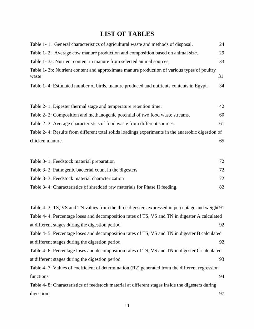
LIST OF TABLES

Table 1- 1: General characteristics of agricultural waste and methods of disposal. 24

Table 1- 2: Average cow manure production and composition based on animal size. 29

Table 1- 3a: Nutrient content in manure from selected animal sources. 33

Table 1- 3b: Nutrient content and approximate manure production of various types of poultry

waste 31

Table 1- 4: Estimated number of birds, manure produced and nutrients contents in Egypt. 34

Table 2- 1: Digester thermal stage and temperature retention time. 42

Table 2- 2: Composition and methanogenic potential of two food waste streams. 60

Table 2- 3: Average characteristics of food waste from different sources. 61

Table 2- 4: Results from different total solids loadings experiments in the anaerobic digestion of

chicken manure. 65

Table 3- 1: Feedstock material preparation 72

Table 3- 2: Pathogenic bacterial count in the digesters 72

Table 3- 3: Feedstock material characterization 72

Table 3- 4: Characteristics of shredded raw materials for Phase II feeding. 82

Table 4- 3: TS, VS and TN values from the three digesters expressed in percentage and weight 91

Table 4- 4: Percentage loses and decomposition rates of TS, VS and TN in digester A calculated

at different stages during the digestion period 92

Table 4- 5: Percentage loses and decomposition rates of TS, VS and TN in digester B calculated

at different stages during the digestion period 92

Table 4- 6: Percentage loses and decomposition rates of TS, VS and TN in digester C calculated

at different stages during the digestion period 93

Table 4- 7: Values of coefficient of determination (R2) generated from the different regression

functions 94

Table 4- 8: Characteristics of feedstock material at different stages inside the digesters during

digestion. 97

12

Table 4- 10: Slurry chemical characterization after a 10 weeks’ digestion period 101

Table 4- 11: Pathogenic bacterial count in the slurry after a 10 weeks’ digestion period 101

Table 5- 1: Estimated costs of constructing a biogas digester on AUC campus 110

Table 5- 2: Estimated costs of biogas appliances to utilize produced biogas 112

Table 5- 3: A SWOT analysis for AD of AUC kitchen waste 115

13

Glossary of Words

Ammonia nitrogen

A parameter used to express the amount of ammonia present in the organic waste sample.

Ammonia is produced from the digestion of protein containing compounds such as proteins and

lipids. When certain levels of concentration are exceeded, ammonia inhibits anaerobic digestion.

Anaerobic bacteria

A consortia of bacteria that breakdown organic materials under oxygen-free environments to

produce biogas.

Anaerobic digester

An enclosed vessel/container/tank with the connected accessories designed specifically to

contain organic materials undergoing anaerobic digestion. The digester provides an oxygen-free

atmosphere, a constant temperature and other conditions optimal for microbial activity.

Anaerobic digestion (AD)

A biological process where anaerobic microbes breakdown organic material in the absence of

oxygen. Biogas is produced a by-product of the process.

Animal manure (AM)

Organic matter derived from a combination of animal feces and urine that can be used as an

organic fertilizer in agriculture and a feedstock in anaerobic digestion.

Batch digestion

An anaerobic digestion process where biomass is added to digester once at the start of the

process and the digester sealed for the whole duration of the anaerobic degradation process.

Biogas production is not constant.

Biogas

A mixture of gases produced from the anaerobic digestion of organic matter. Main components

of the gas are methane and carbon dioxide present in ranges of 60 – 80% and 30 – 40%

respectively.

14

Carbon to nitrogen ratio (C/N)

The relation between organic carbon and nitrogen essential for anaerobic digestion and biogas

production. A C/N ratio of 20 – 30:1 is generally considered optimum for biogas production

where other conditions are in their favorable ranges.

Chicken/poultry manure (CM)

Organic matter, a combination of chicken feces and urine used as an organic fertilizer in

agriculture and in this case as an anaerobic digestion substrate.

Co-digestion

The anaerobic digestion of more than one organic materials together in the same digester. The

practice increases digestion efficiency, biogas yield and methane content in the biogas

Composting

Microbial breakdown of organic material in the presence of oxygen to produce compost.

Compost is used as an organic fertilizer and soil amendment in agriculture and landscape

applications.

Continuous flow digestion

An anaerobic digestion process where biomass is either continually added to the digester or

added at different stages of the process. There is continuous biogas production.

Digestate

Effluent material remaining after completion of the anaerobic digestion process. Digestate can be

applied on agricultural lands as an organic fertilizer or further processed to extract humic and

fulvic substances.

Effective Microorganisms (EM)

A mixed culture of fermentative, soil-based, beneficial micro-organisms which can be applied in

many environments to break down organic matter

Feedstock material

Organic material in a liquid or solid state with biogas production potential fed to the digester.

Greenhouse gases (GHGs)

A combination of gases that are responsible for the greenhouse effect by absorbing infrared

radiations. Carbon dioxide and methane are examples of GHGs

15

Hydraulic Retention Time (HRT)

The amount of time that an anaerobic digestion feedstock material stays inside the digester. HRT

depends on the volume of the digester and volume of feedstock material.

Hydrolysis

Breakdown of complex organic compounds such as carbohydrates, fats and proteins into simpler

soluble molecules due to reaction with water.

Kitchen waste (KW)

Left over organic matter from cooking activities in kitchens in restaurants, households and

hotels. In this study, vegetable residues from local markets were also classified under KW.

Mesophilic digestion

Anaerobic digestion under temperature conditions between 20 and 450C

Organic carbon

The amount of carbon existing in different organic forms found in an organic compound

Organic loading rates (OLR)

Amount of organic matter added to the digester every day, expressed in Kg VS/m3/day

Psychrophilic digestion

Anaerobic digestion under temperature conditions less than 200C

Slurry

The digestate.

Thermophilic digestion

Anaerobic digestion under temperature conditions between 45 and 550C

Total nitrogen (TN)

Sum total of all the forms of nitrogen present in the sample; including nitrate, organic and

ammonia nitrogen. Nitrogen is an essential nutrient required for microbial activity.

Total solids (TS)

Weight of dry matter in present in an AD feedstock material.

16

Volatile Fatty Acids (VFA)

A group of acids; acetic acid, propionic acid, butyric and valeric acid produced as intermediate

compounds during anaerobic digestion. VFA concentration in the optimal amounts increases

biogas yield, however, over accumulation inhibits the process.

Volatile solids (VS)

Portion of organic solids in the digestion raw material that can be anaerobically broken down to

produce biogas. VS are lost when sample is incubated at 5500C.

17

Chapter 1

INTRODUCTION

Rapid population growth, urbanization, improved living standards and a shift in the consumption

patterns have accordingly escalated the intensity of waste generation. The 2012 World Bank

report on solid waste estimated the annual municipal solid waste generation at 1.3 billion tons

per year with a projection of over a 40% increase in the annual generation rate by 2025

(Hoornweg & Perinaz, 2012) and a 300% increase by 2100 (Hoornweg et al.,2013). The report

also showed that 46% of the global solid waste generated in 2009 was organic. In this study,

organic municipal solid waste (OMSW) is used as a point of reference to reflect the food waste

generation.

OMSW is that biodegradable portion of municipal solid waste. Based on the composition of

OMSW, different countries have adopted different definitions; for example, the United States of

America defines OMSW as a composition of food, garden waste and paper, whereas by OMSW,

Europe refers to waste from parks, gardens and kitchens (Campuzano & González, 2016). In

general, OMSW has been used to refer to food waste from kitchens, cafeterias, institutional

lunch rooms, and markets. Composition and quantity of OMSW varies between countries,

geographical regions, cultures, seasons of the year, food habits, social and economic status of the

population, and the social and economic activities in the region among others.

Food waste, which forms part of the organic portion of municipal solid waste has also followed

an incremental trend through the years. About 30% of the food produced annually is wasted at

different stages along the food supply chain before human consumption, resulting from

inefficiencies in harvesting, storage, packing houses, transportation, marketing constraints, and

weaknesses in the prevailing institutional and legal frameworks (FAO, 2017). The United States

generate over 38 million tons of food waste annually. Only 5% of the waste is recycled through

composting, 76% is landfilled with no record of the quantity of food waste recycled through

anaerobic digestion (EPA, 2016). China generates almost three times the amount of food waste

generated by the United States of America (over 90 million tons) (EPA, 2016). In the European

18

union, besides the health and environmental hazards associated with the close to 88 million tons

of food wasted annually, a huge economic cost of close to 1.5 billion euros is faced in managing

food wastage (Stenmarck et al., 2016).

According to (Gustavsson et al., 2011) causes of food wastage differ among countries, their

levels of development and consequently standards of living. Among the causes studied are;

excess production than demanded, premature harvesting common in developing countries, poor

post-harvest food handling infrastructure, absence of food processing facilities and poorly

established marketing systems among others. These causes can respectively be remedied through

establishment of good communication channels among famers to reduce excess production,

organizing farmers and setting in place initiatives to enable them upscale their production,

prioritization of transportation and post-harvest food handling infrastructural development and

establishment of farmer cooperatives along with improvement of marketing channels

(Gustavsson et al., 2011).

Food wastage at the different stages along the food supply chain differs. Taking Sub-Saharan

Africa, North Africa, West and Central Asia as examples, food wastage at the different stages of

the supply chain of fruits and vegetables is illustrated in the figure 1.1 below. From the figure,

most of the wastage in Sub-Saharan Africa is during processing, possibly due to poor processing

facilities. Whereas in North Africa, West and Central Asia, wastage during agricultural

production is dominant. This loss could be associated with the post-harvest grading of the fruits

and vegetables to meet retailer quality standards.

19

Figure 1. 1: Part of the initial fruits and vegetables production wasted at different supply chain stages in

Sub-Saharan Africa, North Africa, the West and Central Asia. Extracted from (Gustavsson et al., 2011).

Food waste as a subset of OMSW contributes to about 15% of the total load of generated

municipal solid waste (MSW) in the United States (“Municipal Solid Waste Factsheet,” 2016).

Making it the second largest municipal solid waste stream after paper (figure 1.2). Through time,

a number of technologies have evolved targeting the diversion of food waste from landfill, to

recover and utilize this precious resource for other applications. The most common of

technologies include composting (nutrient recovery), anaerobic digestion (renewable energy

production) and further processing into animal feed.

0%

5%

10%

15%

20%

25%

Sub-Saharan Africa North Africa, West and Central Asia

Chart Title

Agriculture Post-Harvest Processing Distribution Consumption

20

Figure 1. 2: U.S. Annual municipal solid waste composition 2013 (“Municipal Solid Waste Factsheet,”

2016)

With the recovery technologies in place and of course the allocation of incentives to waste

sustainable management, significant reductions have been recorded in the tonnage of OMSW

and all forms of MSW in general being sent to landfill in different parts of the world. Taking the

United States as an example, data collected from the state of Washington (figure 1.3) shows the

progressive increase in the amount of organic materials being successfully recycled and diverted

from landfills. Food waste being part of these organic materials, it goes without saying that the

same fate directly applies to food waste as well.

The interest in finding sustainable OMSW management solutions among researchers and policy

makers has increased in recent years because of the high risk of the possible environmental

impacts that can result from its poor management. The high moisture content and ease of

biodegradation characteristic to OMSW account for its adverse environmental impacts in

landfills. These impacts include ground water contamination from the leachate, volatile organic

compounds produced from the waste, climate change, toxic odors and fires (Alibardi & Cossu,

2015). As a result, different diversion channels have been created to tap into the numerous

21

benefits in sustainable management of OMSW without sending it to traditional landfills.

Anaerobic digestion falls into one of these many channels that have been designed.

Figure 1. 3: Organic materials recycled, diverted and disposed in Washington between 1992 and 2013

(Newman, 2016)

In this study, kitchen or food waste is generically used to refer to all uneaten food (parts) that is

discarded as waste during domestic food preparation for consumption. Sources of kitchen waste

are not restricted to residential streams but rather include all food waste from restaurants,

commercial and institutional cafeterias and lunchrooms. It is however important to note that food

waste from different sources varies in its composition and characteristics. In many regions,

composition of the generated kitchen waste is a function of the existent food habits, season of the

year, culture, social class, type of diet and other related demographic factors.

Without prior separation, kitchen waste is a composition of both organic and inorganic

(biodegradable and non-biodegradable) waste materials. Unsorted food waste contains plastics,

glass ware, spoilt foods, fruit and vegetable skin, peels and trimmings, rotten fruits and

vegetables, bones, egg-shells, teabags, bread and other pastries, oils, cooked and uncooked meat,

leftover food, tissue paper, packing materials, and water among others (Ramzan, et al., 2010).

This study focused on kitchen waste from two different sources; vegetable waste collected from

a local market and fruit and vegetable waste collected from kitchens on The American University

in Cairo (AUC) New Cairo campus.

22

1.1. Agricultural organic waste

On the other hand, due to the extensive mechanization, continued incentivization of the sector

and growing demand for food which have fueled the global agricultural intensity, the agricultural

sector has emerged a relatively large generator of waste materials. In many developing countries,

agriculture is among, if not the largest contributor of any resource sector to the countries’

economy. Agricultural development is credited for increasing the economic development of

developing countries (UNEP, 2009). As developing countries struggle to leap to better living

standards, it is very likely that farming systems in these countries will be intensified. At this level

significant increases in agricultural waste generation will be far from avoidable. Recent data

estimates the annual production of agricultural waste at close to 1000 million tons (Agamuthu,

2009).

Agricultural waste is a general term used to refer to organic and inorganic byproducts of the

different farming activities taking place on agricultural farms (Ashworth and Pablo., 2009). On-

farm activities entail although are not limited to dairy farming, field crop production,

horticulture, nursery production, crop and livestock breeding, seed growing, market gardens,

aquaculture and woodlands. Byproducts of agro-based industries are also categorized under

agricultural waste. Typically, agricultural waste comprises of; wet organic matter (food waste,

sludge), dry organic matter (wood and straw), inert material (sand and soil), recyclable materials

(plastic, glass, paper, and metal), and hazardous material (chemicals, asbestos). The hazardous

part of agricultural waste is mainly due to surface runoff of pesticides and chemical fertilizers

during rains and drifts during application. Therefore, the careful handling and management of

agricultural based waste needs to be sustainably addressed to protect the environment and to save

the neighboring societies from pollution and irritating odors stemming from rotting organic

waste. It is worth noting that the nature of waste generated varies from one agricultural activity

to another.

1.1.1. Classification of agricultural waste

The agricultural industry, being a vast industrial sector, is associated with almost all types of

waste. Common examples of waste as shown in Table 1-1 can be generated from farming

activities. From the table, it is evident that agricultural waste comprises not only the organic

residues of farming, but also municipal waste and other types of waste related to the processing

23

industry. The table also provides an overview of the conventional disposal methods of different

types of agricultural waste. Based on this and other criteria, agricultural waste is further

classified into hazardous and nonhazardous waste.

Hazardous agricultural waste is any sort of waste generated directly from agriculture or related

activities that may pose a potential threat to public or environmental health (US EPA, 2016).

Hazardous waste has the uniqueness that it requires special treatments before being disposed of.

This pre-treatment is intended to reduce their harmful environmental effects, i.e. they require

special disposal methods. Common agricultural hazardous wastes result from fertilizer run-off,

pesticide drift and runoff, dust from both soil and dried manures, and livestock manure. Careful

management of hazardous wastes is imperative given the many streams through which such

waste can make its way into the ecosystem, for example; pesticides from crop fields can reach

water streams in a number of ways, which include drifting during their application and runoff

due to rains through soil erosion and leaching into the ground water supplies.

Pesticides are poisons by nature that affect insects and animals, and their intrusion into domestic

water sources may cause serious health and environment damages. The US Department of

agriculture points out that manure runoff from agricultural fields contributes to food-borne

disease outbreaks when food crop fields are polluted by animal waste. Similar to manure,

fertilizers may have devastating consequences on the environment and human health if not used

in the appropriate quantities, especially regarding its concentration of phosphorous and nitrogen

(Harmel et al., 2009). Fertilizer runoff, according to the North Carolina State University

contributes to aquatic dead zones through eutrophication processes. Nonhazardous agricultural

waste, on the other hand, includes types of waste that are not defined as injurious or of potential

threat to human life and the environment. This research focuses on the non-hazardous part of

agricultural waste.

24

Table 1- 1: General characteristics of agricultural waste and methods of disposal (Loehr, 1978)

Agricultural

activity

Type of solid

waste

generated

Common method of

solid waste disposal

Pertinent components in

the solid waste

Crop

production and

harvest

Straw

Stover

Land application

Plowing under the soil

Burning

Biodegradable organics

Bacteria, Residues of

fertilizers and pesticides.

Grain

processing

Biological

sludge

Spilled grains

Animal feeds

Byproduct recovery

Landfills

Biodegradable organics,

Residues of fertilizers and

pesticides

Fruit and

vegetable

processing

Biological

sludge

Trimmings,

Soil, Seeds,

peels, leaves

&stems

Landfills, animal feeds,

land application,

burning

Biodegradable organics,

bacteria, nutrients, salts,

pesticides, Residues of

fertilizers and pesticides

Sugar

processing

(sugar canes,

sugar beet, cane

sugar refining)

Biological

sludge, bagasse,

soil, pulp, lime,

mud

Composting, animal

feed, burning, landfill

Biodegradable organics,

bacteria, nutrients

Animal

production

Manures Land application,

processed feeds

Biodegradable organics,

nutrients, bacteria, salts,

medicinal, inorganic

additives e.g. Copper

Dairy product

processing

Biological

sludge

Landfill, land spreading Biodegradable organics

Meat

processing

Biological

sludge, feathers,

Rendering, byproduct

recovery, landfill

Biodegradable organics,

nitrogen, bacteria,

25

Agricultural

activity

Type of solid

waste

generated

Common method of

solid waste disposal

Pertinent components in

the solid waste

product

trimmings,

hides, bones,

grease

chlorides

Leather tanning Fleshings, hair,

raw and tanned

hide trimmings,

lime and chrome

sludge,

biological

sludge, grease

Rendering, byproduct

recovery, landfill, land

spreading

Biodegradable organics,

chromium grease, tannins,

sulphide, nitrogen,

bacteria, chlorides

Timber

production

Branches,

leaves, small

trees

Left in place, burned in

place, crushed

Slowly biodegradable

organics

Wood

processing

Bark, sawdust,

small pieces

Burned, pulp, particle

boards, landfill

Slowly biodegradable

organics

1.1.2. Agricultural waste in Egypt

As is the case in many other countries of the world, rapid population increase, urbanization,

industrialization and improved standards of living in Egypt have changed the country’s

consumption patterns and have consequently led to an increased demand for agricultural

products. In addition, a considerable number of industries in Egypt are agriculture based, which

is reflected in the percentage of workforce employed in agriculture, estimated at 27%, ( Fadl,

2015). This percentage of workforce is the highest among all industrial sectors in Egypt.

Consequentially, there are escalations in the amounts of agricultural solid waste generated in the

country annually. According to a report by the Ministry of State for Local Development, MoLD,

in 2010 (Zaki et al., 2013), of the approximately 95 million tons of solid waste generated in the

26

country, agricultural waste came second after construction and demolition waste. Agricultural

waste accounted for over a third of the generated solid waste as shown in figure 1.4 below.

Figure 1. 4: Generated solid waste in Egypt, 2010 ( Zaki et al., 2013)

Figure 1. 5: Generated solid waste in Egypt, 2001, 2006 and 2012, EEAA. (Zaki et al., 2013)

The Egyptian Environmental Affairs Agency (EAA) reports an increase of over 30% e in the

amount of agricultural waste generated over the years from 2001 to 2012, as indicated in figure

27

1.5. The current devastatingly high amounts of agricultural waste in Egypt are a consequence of

both the introduction and increased use of artificially synthesized materials that are not

biodegradable, as well as the lack of sustainable management practices for the waste.

Agricultural waste continues to increase in Egypt for many other reasons. First, the government

intervention in waste management is still low, which leaves the whole responsibility to

individual farmers to manage their waste. Secondly, there is inadequacy in the required

machinery to handle and prepare the crop residues. Thirdly, there is lack of awareness on the

potential uses of agricultural residues. For this reason, especially rural farmers find no reason but

to handle their residues in ways that they find most suitable. The other contributor to waste

buildup is the poor unpaved dirty feeder roads between farms, which make it a ‘mission

impossible’ to transport agricultural wastes to either processing stations, market centers or

government handling sites as the case with straw (Zaki et al., 2013).

Unlike in Egypt’s past, when crop residues were being utilized as fuel sources, re-used on the

farm as fodder, fertilizer or as mulch, the increased use of gas stoves, ovens and artificial

fertilizers today has decreased the reuse of farm waste and rendered its use impractical because

of the low heating value compared to fossil fuels. As a result, there has been an increase in the

open burning of agricultural residue and its accumulation in landfills (Zayani, 2010). The largest

portion of agriculture generated waste in Egypt today is either being burned or illegally dumped.

Inefficient collection of waste and illegal disposal of agricultural waste are among the major

sources of land, air and water pollution and pose catastrophic effects on the environment and

human health (Zaki et al., 2013). Illegal dumping of agricultural residues on the canal banks

creates barriers to water flow and endangers water quality. Crop residues block irrigation

systems and contribute to eutrophication.

1.1.3. Potential benefits of agricultural waste management in Egypt

Despite their tremendous damage to both the environment and human health, agricultural

residues could be employed in the income generation struggle and could be holistic in the

conservation of other nonrenewable resources. Some of the results of proper management

agricultural wastes as discussed are;

28

A number of small agro industries can be established in the rural areas based on

agricultural residue recycling, which in turn would create employment opportunities.

Compost from organic agricultural waste can be used in the land reclamation process.

This would facilitate in the extension of agricultural lands, and as a result increase

agricultural production.

Proper agricultural waste management can lead to a reduction in the expenditure on

chemical fertilizer and their consequential negative impacts

Proper waste handling reduces the adverse impacts on the environment and has the

potential to provide alternative sources of clean energy production. Biogas produced from

the anaerobic digestion of organic waste is one of such energies.

Crop residue can be used as fodder for the animals. This lowers dependence on imported

feeds and supplements.

Anaerobic digestion of biodegradable agricultural waste material such as manure, crop

residue, and sewage sludge produces biogas, a sustainable energy source.

1.2. Selected agricultural organic wastes.

From the agricultural waste stream, this research focuses on energy recovery from the dairy and

poultry sub waste streams using animal (cow) and chicken manure. Energy recovery in the form

of biogas through anaerobic digestion was investigated. In the study, a brief insight into the dairy

and poultry sectors and their contribution to environmental pollution is given together, and the

anaerobic digestion of both manure streams as mono ad co-substrates was explored.

1.2.1. Animal (cow) manure

The increasing global demand for livestock products as protein sources, income growth,

improvement in livestock production technologies and the rapidly growing world population

have been the main drivers to the steady growth of the livestock industry. It is estimated that at

least a third of the earth’s ice-free terrestrial surface area is dedicated to livestock production,

with systems valued at $1.4 trillion in 2010. For this reason, the industry ranks among the fastest

growers in developing countries (Thornton, 2010).

This fast growth has however come not without demerits. The consequential increase in animal

manure produced has raised environmental concerns and demanded sustainable management

29

approaches to keep the potential damage under check. Average cow manure production and

composition based on animal size is shown in table 1-2. Amount of manure production remains a

function of the digestibility of the diet, animal stocking density, yard cleaning frequency,

moisture content, climatic conditions, age and size of the animal.

Table 1- 2: Average cow manure production and composition based on animal size (Department of

Agriculture and Fisheries, 2011).

Animal

size (kg)

Manure

production

(kg/day)

Total

solids

(kg/day)

Volatile

solids

(kg/day)

BOD*

(kg/day)

Nutrient content (kg/day)

N P K

220 13.2 1.54 1.32 0.35 0.075 0.024 0.052

300 18.0 2.08 1.06 0.48 0.104 0.034 0.076

450 27.0 3.10 2.70 0.72 0.153 0.050 0.108

600 36.0 4.18 3.56 0.96 0.206 0.068 0.149

BOD* = Biochemical oxygen demand

Because of the rising costs and environmental impacts of commercial inorganic fertilizers,

organic animal manure is being widely adopted to cover the gap. A number of studies in the past

have been dedicated to the use of animal manure as a fertilizer (Seefeldt & Jerry, 2013), (Zhang,

n.d.), (Araji et al, 2001), (Rosen & Peter, 2017). Preference for the use of animal manure is

preferred for in crop fields is because of its wealth in nutrient composition. Animal manure as

indicated in the table 2 above contains considerable amounts of the three major plant nutrient

elements; nitrogen, phosphorous and potassium in addition to other essential micronutrients.

Besides its nutrient contribution, animal manure also has positive effects on the soil organic

matter content, water and nutrient holding capacity, fertility and tilth.

While applying animal manure as a fertilizer, caution should be taken to apply only the right

dose. Application of dry manure during strong winds should be avoided, application should as

well not be in the vicinity of water bodies and the manure should be free of grass and weed

seeds. Incautious handling of animal manure has been reported to bear huge costs to the

environment, animal and human health. (Sören & F., 2012) and (Brandjes, & H., 1996) detail the

environmental impacts of manure storage and its use in soil amendment. Among those listed are

30

surface water pollution, air pollution from the ammonia emissions, ground water pollution from

nutrient leaching.

1.2.2. Chicken/poultry manure

Globally, the poultry industry is one of the largest and fast growing agro-based industries.

Growth of the industry is attributed to the increasing demands for poultry products in forms of

meat and eggs. Statistics indicate that global production and consumption of poultry meat

increased at a rate of over 5% annually between 1991 and 2001 (F.A.O., 2006). A report by

OECD-FAO shows that per capita consumption of poultry products between 2005 and 2017

increased at a rate of 2% (“OECD-FAO Agricultural Outlook 2017-2026,” 2017). Data plotted in

figure 1.6 below adopted from the United States Department of Agriculture (USDA) also shows

an average increase rate in the consumption of poultry products of about 2% between 2008 and

2018 in the United States. Consequently, compared to the 15% contribution to the world meat

production three decades ago, the poultry industry as of 2006 contributed to over 30% of the

global livestock meat supply (F.A.O., 2006).

Figure 1. 6: Total per capita consumption of poultry products in the United States (USDA, 2017)

90

95

100

105

110

115

2008 2009 2010 2011 2012 2013 2014 2015 2016 2017 2018

Tota

l per

cap

ita

con

sum

pti

on

(p

ou

nd

s)

Years

31

Egypt not being an exception has also experienced a steady increase in this industrial expansion.

Credit for this increase has been given to the fact that red meat consumption alone cannot cover

human protein needs in the country(Attia & Abd El-Hamid, 2005). Indirectly, the rapid

population growth and resultant nutritional requirements could as well be held accountable. As

of 2014, the commercial poultry industry of Egypt was valued at 2.5 billion Egyptian Pounds

with the annual growth projected at a rate between 3-4%. On per capita basis, poultry products

consumption in Egypt is 100 eggs and 10 birds annually, with the figures expected to double or

even triple once considerations are taken for the growing national population, per capital income

and the high quality vis-à-vis being a cheap protein source (Hassan, 2014).

However, the main challenge of the industrial expansion is the increased accumulation of waste

from the different industrial activities. Waste from poultry farms comprises of poultry excreta

(manure), spilled feed, feathers and bedding materials used in poultry houses.

1.2.2.1. Poultry Manure production and nutrient contents

The quantity of poultry manure produced varies from one farm to another (Chastain et al., 2014).

On the other hand, the quantity of manure produced from a poultry farm generally depends on

the type and amount of material used for bedding, feed formulation, stocking density, type of

housing being employed and litter management techniques in practice (Coufal & C, 2006).

One of the major concerns of the poultry manure is its high mineral nutrient concentration.

Nutrients in poultry manure are mainly derived from the poultry feed, supplements, medications,

and water consumed by the birds. For any given sample of manure, nutrient composition is

dependent on the ration digestibility, age of the birds, amount of feed and water that goes to

waste, the frequency of cleaning the poultry house and the type and amount of bed used

(Chastain et al., 2014). Poultry manure ideally contains 13 nutrient elements; nitrogen (N)

phosphorous (P) potassium (K) calcium (Ca) magnesium (Mg) sulfur (S) manganese (Mn)

copper (C) zinc (Zn) chlorine (Cl) boron (B) iron (Fe) and molybdenum (Mo) all of which

happen to be essential to plant growth (Nnabuchi et al., 2012). Therefore, the use of poultry

manure as a fertilizer in plant growth could be a potential source for all or a considerable part of

the plant nutrient requirements. It is worth noting that the fecal discharge from chicken is a

composition of both feces and urine. Therefore, the nutrient composition of the manure is not

affected by either the urine or feces as the two are the same (Chastain et al., 2014).

32

On average, fresh manure from poultry has a higher nutrient content in relation to manure from

other animals as shown in table 1-3a. In comparison with other manure sources, poultry manure

has significantly higher amounts of potassium, nitrogen, phosphorous, calcium and magnesium.

This makes poultry manure a better source of plant nutrition. Table 1-3b also gives an overview

of the disparity in nutrient contents and approximations of manure production from the two

different sources of poultry waste. From the table, laying chicken produce almost twice the dry

matter produced by chicken raised for meat production. Layers also on average produce more

nutrients as do broilers. This could be because of the difference in dietary requirements of both

classes of chicken.

Despite the nutritive suitability of the manure as a fertilizer, the mineral composition of

poultry manure has high negative amenities to the environment. The nutrients are

reported to pollute both the soil and water. In addition, the pathogens from the manure

and heavy metals that accumulate in the manure from the poultry feed and water cause

soil, ground and surface water pollution. This is normally a consequence of poor

manure handling practices and manure storage. The manure is also known to be a

source of bad odors, a hub for flies, rodents and a lot of other disease carriers. The odors

from manure storage or disposal facilities are a composition of ammonia, volatile

organic compounds (VOCs) and Hydrogen Sulphide (H2S) which are very toxic to

human health. Leaching of the heavy metals into the ground water from the manure

storage facilities is a common occurrence which pollutes ground water reservoirs and

also compromises aquatic life in the nearby streams when residual water flows from the

manure piles to the streams. This is because of the resultant eutrophication which claims

a big percentage of aquatic lives (Maheshwari, 2013).

33

Table 1- 3a: Nutrient content in manure from selected animal sources. (“Manure is an excellent

fertilizer,” 2017.)

Nitroge

n

(N)

Phosphoro

us

(P2O5)

Potassiu

m

(K2O)

Calciu

m

(Ca)

Magnesiu

m

(Mg)

Organi

c

matter

Moistur

e

content

FRESH

MANUR

E

% % % % % % %

Cattle 0.5 0.3 0.5 0.3 0.1 16.7 81.3

Sheep 0.9 0.5 0.8 0.2 0.3 30.7 64.8

Poultry 0.9 0.5 0.8 0.4 02 30.7 64.8

Horse 0.5 0.3 0.6 0.3 0.12 7.0 68.8

Swine 0.6 0.5 0.4 0.2 0.03 15.5 77.6

TREATE

D DRIED

MANUR

E

% % % % % % %

Cattle 2.0 1.5 2.2 2.9 0.7 69.9 7.9

Sheep 1.9 1.4 2.9 3.3 0.8 53.9 11.4

Poultry 4.5 2.7 1.4 2.9 0.6 58.6 9.2

Table 1-3b: Nutrient content and approximate manure production of various types of poultry waste (

Attia & Abd El-Hamid, 2005)

Type of manure Chemical composition (%) Manure nutrient content \bird

\year (g)

N P2O5 K2O Na DM N P2O5 K2O Na

Broiler 4.88 4.86 3.0 0.6 4890 239 229 129 29.5

Layer hens 4.80 6.73 3.92 0.6 7000 336 471 275 42.0

**DM – Dry matter

From the poultry industry in Egypt, Nitrogen and phosphorous represent the highest amount of

nutrients excreted with the chicken manure, (table 1-4) (Attia & Abd El-Hamid, 2005). Although

34

these nutrients are essential for animal and plant growth and nutrition, there extreme abundance

in the ecosystem poses adverse ecological threats. According to the soil conditions in the Egypt,

these two nutrients account for the high pollution levels in the newly reclaimed desert

agricultural areas where poultry manure is excessively used as a fertilizer and/or soil amendment

( Attia & Abd El-Hamid, 2005). Nitrogen and phosphorous stand high chances of being leached

to the ground water causing ground water pollution, a result of which is human and animal health

problems.

Excessive Nitrogen build up in drinking water (ground water) in form of nitrates is very harmful

to infants and livestock. They inhibit oxygen transportation in the blood stream which results in a

condition commonly known as blue baby syndrome (Perlman, 2017). High phosphorous

concentration on the other hand impairs micronutrient availability in the top layers of the soil for

plant absorption and accelerates growth of algal blooms in water bodies causing eutrophication

and death of aquatic animals (Busman et al., 2009). Given the aforementioned impacts of the

high concentrations of nitrogen, phosphorous and heavy metals in poultry manure on the

ecosystem, it is worth adding that their excessive accumulation in the soil also negatively

impacts its agricultural abilities.

Table 1- 4: Estimated number of birds, manure produced and nutrients contents in Egypt (Attia & Abd

El-Hamid, 2005)

Type of birds No. of

birds

(M)

Manure

produced

g/b/yr.

Amount of nutrients produced annually,

tons

N P2O5 K2O Na

Broilers 800 4890 191200 183200 103200 23600

Broiler

breeders 5 10500 2520 3533 2058 315

Layers 15 7500 5040 7065 4125 523

Laying

breeders 0.25 8140 98 137 80 12.2

Turkeys 2 10860 1060 1056 652 108.6

Waterfowl 20 6500 6344 6318 3900 780

Total 541 206262 201309 114015 26426

35

Despite the earlier quoted disastrous impacts that accompany poor handling of poultry waste,

management of this waste has still proven a very big challenge to the industry especially the

manure and the poultry litter. Figure 1.7 below shows some of the common poultry waste

handling and management practices in most of the poultry farms.

From the figure, almost 89% of the waste generated from the poultry farms is in the solid form.

Data from the table also shows that over 90% of the poultry waste is open dumped. As earlier

explained in this chapter, open dumping of poultry waste has grave effects to both human health

and the environment mainly due to the nutrient content carried in the waste. For this reason, there

is need for legislative, and Research and development intervention to effectively regulate proper

and sustainable handling and/or disposal of the waste.

Figure 1. 7: Waste collection and disposal methods in most poultry farms (Mary et al., 2015).

36

1.3. Research motivation and objectives

The major aspects behind the motivation for this research have been (1) the grave closely similar

environmental impacts associated with the unsustainable handling of kitchen waste, chicken and

animal manure waste stream in general, (2) the increasing agricultural systems’ intensification

especially in the developing world, with an aim of closing the loop - producing bio-fertilizers in

the end to replace the chemical fertilizers especially in the newly reclaimed agricultural lands as

the need to expand cultivable lands increases, (3) absence of sustainable and strategic measures

put in place to manage the huge amount of organic waste generated from the kitchens of the food

outlets operating on AUC New Cairo campus, and (4) the world’s increasing demand for cleaner

and renewable energy resources, in response to the rising global awareness of the likely

environmental impacts associated with the use of fossil based fuels and the need to decouple

food prices from fuel prices

1.3.1. Kitchen waste from AUC New Cairo Campus and its potential impacts

The food needs of The American University in Cairo’s (AUC) New Cairo campus are served by

eight food vendors. These serve fast foods, fresh vegetable and juices, complete meals, snacks

and hot beverages. Fortunately, all vendors have kitchens on campus. However, these kitchens

generate considerable amounts of organic waste daily. Waste from the kitchens is largely a

composition of spoilt food, fruit and vegetable peelings, offcuts and low quality undesired fruits

or vegetables.

The current KW management hierarchy in place is only a three stage process. (1) The unsorted

waste is collected in bins present in the kitchens, (2) the bins are collected by the campus

services to the university waste collection facility where it is mixed with waste from other

streams on the university campus that will not be recycled and (3) the waste is all together sent to

the Zabaleen area/landfill.

Landfilling of organic waste has been linked to serious environmental impacts. This is mainly

because of the high moisture content, biodegradability and methane production potentials of the

waste in the landfills. Because of this, under the uncontrolled anaerobic conditions inside the

landfills, organic wastes can be broken down through microbial activity releasing gases (40-70%

methane) and leachates (El-Fadel et al., 1997). Methane is a combustible and greenhouse gas

37

with the potential to cause fires hazards and contribute to global warming and climate change. In

addition, other components in the gas produced in landfills, may contribute to air pollution

causing health and more specifically respiratory hazards. The leachate on the other hand

contributes to ground water pollution as it seeps through the soil. (El-Fadel et al., 1997)

1.3.2. Alternatives for on campus kitchen waste recycling.

Owing to its high moisture content, composting (aerobic digestion) and/or anaerobic digestion

are the most feasible means of recycling kitchen waste on campus. The process of composting

produces compost; a rich organic soil amendment. With AUC’s devotion to sustainable

landscaping, on campus compost production from the kitchen waste presents a complement to

the many efforts undertaken in that pursuit. Similar efforts are already being taken by the

university’s landscaping department, which composts over 80% of the waste it generates from its

usual maintenances. However, the downsides of the practice are; (1) the process consumes a lot

of water especially during the summers to maintain the necessary moisture content inside the

compost pile, (2) the process requires mechanization to turn the pile to ensure uniform air

circulation inside the pile for effective microbial breakdown and (3) if not properly controlled,

the process of compost production may take up to eight weeks. All these make the process

somewhat costly when related to the cheap price of compost on the Egyptian market, where a ton

is only about 26$.

Anaerobic digestion on the other hand yields both biogas and an organic bio fertilizer at the end

of the process. Biogas is a sustainable energy source with a considerable potential to cover some

of the university’s energy needs. Besides, the production of biogas on campus may open gates

for new cutting edge research in this field of sustainable energy under the auspices of the

university’s accredited school of engineering and sciences’ programs.

1.3.3. Research aim and objectives

The main aim of this research is (1) to investigate the production of biogas from animal manure,

chicken manure and kitchen waste, (2) to explore the biogas production potential of organic

waste generated by kitchens on AUC New Cairo campus. and (3) to achieve an environmentally

sound zero waste on campus food production system.

To reach this aim, the study was divided into a list of main objectives as stated here below;

38

Experimental anaerobic degradation of different combinations of animal manure, chicken

manure and kitchen waste to produce biogas and a bio fertilizer from the slurry at the end

of the digestion process.

Experimental anaerobic digestion of kitchen waste from AUC kitchens for biogas

production with the aim of closing the cycle of waste generation to reach a zero waste

food production system.

Proposing avenues to achieving an organic waste free food service system on AUC New

Cairo campus – proposing a feasible anaerobic digester design to digest the food waste

produced on campus.

1.3.4. Research methodology

A combination of different research methodologies was employed to ensure adherence to

meeting the target research objectives. Literature review in the early stages of the study was the

most important method employed to align the research with the scope of action. Preliminary

baseline data was also obtained through literature review. Secondary data sources were journal

articles, conference papers, books, government published reports, published international

statistics and websites.

A pilot scale experiment was set up in two phases (I and II) to investigate biogas production

from animal manure, chicken manure and kitchen waste. Primary data was collected from the

experiments. Results of the experiment were used as in put to recommend anaerobic digestion as

a very viable organic kitchen waste management strategy for AUC.

39

Chapter 2

Literature Review

2.1. Anaerobic digestion of organic waste

Anaerobic digestion (AD) is a naturally occurring microbial process in which organic matter is

broken down into simpler chemical compounds in an oxygen free environment under ideal

conditions (Monnet, 2003). The process aims at biologically transforming almost all forms of

organic waste from one form to another (Khalid et al., 2011). Anaerobic digestion process

naturally takes place in many anaerobic environments such as the marine water sediments, peat

bogs, mammalian guts and water courses (Al Seadi et al., 2008), (Ward et al., 2008). During the

process, a mixture of gases including; methane, carbon dioxide, hydrogen sulfide and ammonia

in varying percentages is produced. This mixture of gasses is what is called Biogas.

Biogas is a mixture of gases, primarily methane and carbon dioxide along with traces of other

gases. Biogas is combustible and it is for this reason that the gas is used as a fuel in gas engines,

heating and lighting. Chemically, biogas from the anaerobic digestion of agricultural waste

comprises of 60-75% methane (CH4), 19-33% Carbon dioxide (CO2), 0-1% Nitrogen (N2) and

less than 0.5% Oxygen (O2). This chemical composition however varies according to the type of

feed (The Biogas, 2009). Besides biogas, an organic residue (digestate) is left at the end of the

digestion process. The residue is highly rich in nitrogen. For this reason, coupled with its low

moisture content, the digestate has been applied as a soil amendment/fertilizer (Li et al., 2011).

Anaerobic digestion (biogas production) is a four-stage process (figure 2.1), which starts with

hydrolysis, followed by acidogenesis, acetogenesis and completed by methanognesis. The

chemical reaction below summarizes the anaerobic digestion process.

C6H12O6 → 3CO2 + 3CH4 Glucose Carbon dioxide Methane

40

2.1.1. Hydrolysis

Hydrolysis is the first stage of the anaerobic digestion process, where the hydrolytic bacteria

break down the complex organic compounds such as carbohydrates, fats and proteins into

simpler soluble molecules (Monnet, 2003). The stage is enzyme controlled; the hydrolytic

microorganisms release enzymes that breakdown the complex polymers into soluble monomers

setting pace for the acidogenic microorganisms in the next stage (Al Seadi et al., 2008).

Substrate-specific enzymes break down the complex polysaccharides, proteins, lipids or proteins

in the presence of water (moisture) to simpler soluble monosaccharaides, amino acids or fatty

acids respectively. Hydrolysis follows the reaction below.

2.1.2. Acidogenesis

The second stage of the process is acidogenesis, usually the fastest stage of an anaerobic

digestion process (Chen & Howard, 2014). The acid forming bacteria (acidogens) convert the

products of hydrolysis (fatty acids, amino acids, simple sugars) into simple organic acids,

hydrogen and carbon dioxide (methanogenic substrates). The principal organic acids produced

during this stage are acetic acid, butyric acid, propionic acid and ethanol, an alcohol (volatile

fatty acids) (Monnet, 2003).

2.1.3. Acetogenesis

Acetogenesis is the second last stage before methanogenesis. During acetogenesis, products of

acidogenesis that could not be directly converted are converted into methanogenic substrates

along with minor production of H2 and CO2. Methanogenic substrates being referred to are

acetate, hydrogen and carbon dioxide (Al Seadi et al., 2008). The last stage of the anaerobic

degradation process is methanogenesis. This stage is accomplished by methanogenic bacteria

which convert the methanogenic (intermediate) substrates into CH4 and CO2. Methanogenesis is

the slowest yet most critical of all anaerobic digestion biochemical processes (Adekunle &

Okolie, 2015).

41

2.2. Factors affecting the Anaerobic Digestion (AD) process

The efficiency of an anaerobic digestion reaction similar to any biochemical reaction is a factor

of a number of parameters. For successful microbial growth and activity therefore, certain

conditions must be ideal to keep the many different microorganisms involved in balance. Critical

parameters affecting microbial activity and growth are temperature, pH, nutrient supply (C/N

ratio), complete absence of oxygen, presence of toxic compounds and inhibitor concentration

during the digestion process.

2.2.1. Temperature

The anaerobic digestion process can be operated at three different temperature ranges;

psychrophilic range (<250C), mesophilic (25-450C) or thermophilic ranges (45-700C) (Al Seadi

et al., 2008). Mesophilic (32-430C) and thermophilic (49-600C) temperature ranges are however

the most preferred for biogas production. These respectively offer the optimum working

environments for the mesophilic and thermophilic bacteria involved in the process (Chen &

Howard, 2014). Digester operation temperature is largely dictated by the feedstock. Temperature

stability during operation is very critical for optimum results since different digestion stages have

different optimum temperature ranges. For example, most of the acidogens grow and perform

well under mesophilic temperatures whereas the methanogens prefer higher temperatures

(Adekunle & Okolie, 2015).

The temperature of the process is directly linked to the hydraulic retention time (the average time

a given volume of digestion feedstock stays in the digester.) (Table 2-1) Running the digester at

thermophilic temperatures gives a higher biogas yield with a lower retention time as opposed to

mesophilic temperatures (Krich et al., 2005). Figure 2.2 shows the relation between

temperatures, hydraulic retention time and biogas yield.

42

Figure 2. 1: Anaerobic digestion process flow diagram (Adekunle & Okolie, 2015)

Table 2- 1: Digester thermal stage and temperature retention time (Al Seadi et al., 2008)

Thermal stage Process temperatures (0C) Minimum retention time (days)

Psychrophilic Less than 20 70 to 80

Mesophilic 30-42 30-40

Thermophilic 43-55 15-20

Operating the biogas digester at thermophilic temperature ranges has a number of advantages

over mesophilic conditions as listed below.

High temperatures in thermophilic ranges kill all pathogens in the sludge

Shorter retention time with an increase in process efficiency and biogas yield

More effective substrate digestion with better substrate utilization

There is a direct relation between higher temperature and growth of methanogenic

bacteria

43

Improved digestibility and substrate availability

Higher possibilities of solid and liquid fractional separation

The main disadvantages of operating the biogas digester at thermophilic temperatures are; the

high energy demand to maintain high temperatures, secondly at high temperatures, there are

higher risks of ammonia inhibition and there is a large degree of imbalance in the system (Al

Seadi et al., 2008).

Figure 2. 2: Relative biogas yields depending on temperature and hydraulic retention time (Al Seadi et

al., 2008)

2.2.2. pH

A near neutral pH is ideal for most AD process (Rapport et al., 2008). However, pH

requirements vary across the different process stages and thermal stages at which the process is

conducted. A pH of 7.0-8.0 is optimum for the methanogens. Acidogenic bacteria require lower

pH values for optimum performance. Optimum pH for mesophilic bacteria is 6.5-8.0. A slight

drop to 6.0 or rise to 8.3 triggers an inhibitory effect to the process. The pH in thermophilic

digesters is lower as a result of the formation of carbonic acid upon reaction of the dissolved CO2

with water. This is a reaction initiated by an increase in temperature (Al Seadi et al., 2008).

44

2.2.3. C/N ratio

Carbon and Nitrogen are the main nutrient sources for anaerobic bacterial growth and stability

during digestion. A balance in availability of these two nutritional sources is very critical for

efficient degradation while preventing ammonia build up and inhibition (Rapport et al., 2008). A

C/N ratio of 20-30:1 has generally been considered optimum for microbial activity, and largely

dependent on the feedstock and inoculum (Zhang et al., 2014).

2.2.4. Presence of process inhibitors (ammonia)

In the digester, ammonia exists in two forms, free ammonia (NH3) and ammonium (NH4+) both

forms resulting from the breakdown of proteins and other nitrogen-rich organic substrates

present in the feedstock (Zhang et al., 2014). Free ammonia is a good nutrient source for the AD

bacteria; however, its high concentration during digestion inhibits the process. Ammonia

inhibition is common in the AD of animal manure coming from the high ammonia concentration

in their urine (Al Seadi et al., 2008).

2.2.5. Total solids

Total solids (TS) refer to the weight of the dry matter of an anaerobic digestion substrate. This

weight is expressed as a percentage of the total weight of the substrate sample (Schmidt, 2005).

TS content of the substrate can be used to define two different anaerobic digestion processes; wet

and dry digestion. The wet digestion process occurs at a substrate TS content of less than 15%

whereas dry digestion occurs at a TS content between 15% and 20% (Karthikeyan &

Visvanathan, 2013). The TS content of any given biogas feedstock directly contributes to the

performance of the system and yield of biogas during microbial degradation. There is an inverse

relation between the TS content and biogas yield (Ugwuoke et al., 2015). There is an optimum

value of TS for each feedstock to maximize biogas production.

2.2.6. Volatile solids

Volatile solids (VS) refers to that percentage of the solid material of the digestion raw materials

inside the digester that can be broken down by the bacteria to produce biogas. This portion varies

from one organic waste material to another. VS content is calculated by diving the weight of

volatile solids in the raw material by the total weight of solids in raw material and normally

expressed as a percentage of the total solids content (IRENA, 2016). VS content of an anaerobic

45

digestion substrate is often an essential parameter in predicting methane production from the

substrate (Schmidt, 2005).

2.2.7. Volatile fatty acids (VFA)

VFA are the main intermediate compounds formed during the anaerobic digestion process. They

are the main product of the acidogenesis stage in the anaerobic digestion process of organic

wastes. They include acetic acid, propionic acid, butyric acid, and valeric acid (Monnet, 2003),

(Zhang et al., 2014). Of these acids, acetic and propionic acid play the most significant roles in

biogas production, and therefore tracking their concentration could be basis for determining the

success of an anaerobic digestion process (Zhang et al., 2014). Under ideal conditions, the VFA

are transformed into CO2 and CH4 by the methanogenic bacteria. Under high organic loading

rates, as the common case in fruit and vegetable wastes, the VFA could accumulate inside the

digester. As a result of their amplified accumulation, the pH inside the digester is lowered, which

may eventually inhibit the whole digestion process (Alvarez et al., 2000; Zhang et al., 2014). It

therefore right to conclude that VFA have the potential to determine the pH inside the digester.

2.2.8. Hydraulic Retention/Residence Time

Hydraulic Retention Time (HRT) refers to the amount of time that the digestion substrate

material stays in the digester. HRT depends on the volume of the digester and the volume of the

substrate fed to the digester in a given time period. The HTR can be calculated from the formula

below.

𝐻𝑅𝑇 𝐷𝑖𝑔𝑒𝑠𝑡𝑒𝑟 𝑣𝑜𝑙𝑢𝑚𝑒 (𝑚3)

𝑆𝑢𝑏𝑠𝑡𝑟𝑎𝑡𝑒 𝑓𝑒𝑒𝑑𝑖𝑛𝑔 𝑟𝑎𝑡𝑒 (𝑚3

𝑑𝑎𝑦)

The HRT is based on the biological oxygen demand (BOD) of the feedstock material and the

slurry at the end of the process, and the chemical oxygen demand (COD), which is the measure

for the average time needed for the organic to reach full decomposition (Arsova, 2010). Substrate

feeding rate can also be referred to as the organic loading rate (OLR). OLR is a very important

parameter in digester operation. It is a measure of the efficiency of an anaerobic digestion system

at biomass conversion. OLR is important in determining the right volatile solids loading into an

anaerobic digestion system for optimum biogas yield. Overloading the system has been reported

46

to contribute to the accumulation of inhibitory substrates in the digester which result into low

biogas yields (Arsova, 2010).

From the equation above, knowing the HRT and OLR it is easy calculating the required digester

volume. Also from the equation, increasing the OLR decreases the HRT. Depending on the

substrate under digestion, the HRT must be long enough to maintain a balance between the

bacterial population in the digestate (effluent) and the amount of bacteria being reproduced. The

reproduction cycle of the bacteria is usually 10 or more days (Adekunle & Okolie, 2015; Al

Seadi et al., 2008). A short HRT would mean a good flow of substrates through the digester, but

with a low biogas yield. It is therefore imperative to align the HRT with the COD of the substrate

under digestion (Al Seadi et al., 2008).

2.3. Advantages of anaerobic digestion

AD as listed below has a number of social, economic and environmental benefits.

a. AD cuts back on the irritating odor emissions from decayed agricultural waste,

indirectly improving air quality

b. The use of biogas greatly reduces on the GHG emissions into the environment coming

from the use of fossil fuels in the same applications.

c. Use of manure in AD preserves soil and water quality by preventing the pathogens in the

manure from directly entering these resources upon unsustainable disposal.

d. The energy generated (biogas) in the process has numerous applications and can also be

sold to provide a source of income

e. The manure produced at the end of the process is free of pathogens and weed seeds yet

rich in nutrients. This saves fertilizer costs and the negative impacts of synthetic

fertilizers.

f. Use of agricultural waste saves the costs of waste storage and disposal

g. According to the Kyoto protocol, biogas generation has the potential of earning carbon

credits based on its potential towards reducing GHG emissions.

h. AD also has the potential of reducing VOC emissions into the environment.

The one possible downside of AD lies with the digesters that burn biogas. During the combustion

of biogas, oxides of nitrogen (NOx) are given off. These negatively impact the environment due

47

their ozone formation potential (Krich et al., 2005). Ozone is an irritant and upon reaction with

water forms nitric acid. This process is responsible for the acidic rain formation.

2.4. Types of anaerobic digesters

Four types of anaerobic digester designs are commonly used for large scale on-farm biogas

production; the covered lagoon digester, complex mix, plug-flow and temperature phased

anaerobic digesters (Chen & Howard, 2014), (Pillars, n.d.). For on-farm/household small scale

production, the Indian (fixed dome) and Chinese (floating drum) biogas digesters are the most

widely adopted. However, the technology and design of biogas (anaerobic) digesters varies from

country to country and is influenced by factors such as local climate, legal frameworks, energy

policies, availability and affordability(Al Seadi et al., 2008).

Anaerobic digesters can further be classified basing on the substrate feeding schedule; into batch,

continuous and semi –continuous feed digesters. In the batch type of digesters, the digester is

loaded once with a batch of fresh substrate and closed. Substrate is left to digest to/close to a

stage of no further reaction and completely removed for a new batch to be loaded and the process

continues. Batch digesters have the advantage in their simplicity of design. In continuous feed

digesters, feedstock is continuously added to the digester without any interruptions to the

digestion process. In such type of digesters, substrate flow through the digester is by means of

either mechanical force or pressure from the newly applied feedstock which forces out the

already digested feedstock. Unlike the batch type, there is steady and continuous biogas

production in the continuous feed digester (Al Seadi et al., 2008).

2.4.1. Covered lagoon digester

A covered lagoon is a large, in-ground, earthen or lined lagoon with a flexible or floating

impermeable gas-tight cover (Chen & Howard, 2014) (Figure 2.3). The cover acts to trap the

biogas. This design is most suitable for feedstock in liquid form with <2% solids (Pillars, n.d.).

Such digesters do not have the potential to be heated. For this reason, they have longer hydraulic

retention times (30-45days) and suitable for warmer regions; where atmospheric heat can assist

in stabilizing digester temperature (Chen & Howard, 2014).

48

Figure 2. 3: Covered lagoon digester (“lagoon covers | Ieccovers’s Blog,” 2010)

2.4.2. Plug-flow digester

The plug-flow type is the most suitable for solid substrates with 11-14% solids content (Pillars,

n.d.). The system comprises a cylindrical tank and a hot water piping network to maintain a

stable temperature in the tank. New in-fed manure from one end pushes the biogas and slurry

through the other end (Chen & Howard, 2014) (Figure 2.4).

Figure 2. 4: Plug-flow digester ((“lagoon covers | Ieccovers’s Blog,” 2010)

2.4.3. Complete mix digester

The complete mix design of digester exists in two forms, either as cylindrical tanks above the

ground or below the ground as rectangular pits (Chen & Howard, 2014). The design consists of

an enclosure from a rigid or flexible material and a heated tank with a mechanical, hydraulic, or

gas mixing system (“lagoon covers | Ieccovers’s Blog,” 2010) (figure 2.5). This type of digester

can be operated at both mesophilic and thermophilic temperature ranges (Chen & Howard,

2014). Best results are reached when the feedstock manure is diluted with water to 3-10% solids

(Chen & Howard, 2014), (“lagoon covers | Ieccovers’s Blog,” 2010).

49

Figure 2. 5: Complete mix digester (Chen & Howard, 2014)

2.4.4. Floating dome/ Indian type digester

The floating dome/drum (figure 13) type of digesters is the mostly commonly used in India. This

is primarily because the first digester of this type to ever be built was in India in the 1950s by

Joshbai Patel (Abbasi et al., 2012). The principal of biogas production in this type of digesters is

gas production at a constant digester pressure with variations in volume inside the digester

(Rajendran et al., 2012).

The design comprises mainly of a cylindrical dome-shaped digester and a movable inverted

floating drum. The drum moves up and down depending on the amount of gas produced inside

the digester, also from this movement the amount of gas accumulated in the digester can be

detected. The drum moves up when there is gas production and down when the gas is being

consumed. In majority of the cases, the drum is made of steel. This drum is also vital in

regulating biogas flow during use.

The digester is a construction of bricks and sand. The inside walls of the digester are plastered

with sand and cement to seal the digester from any gas leaks during production. In high volume

digesters, there is a partition wall in the middle of the digester (figure 2.6) which is in most cases

50

absent in low volume digester (below 4m3). The gas produced is stored in the gas holder and let

out for use through the outlet pipe on the gas holder.

This reactor model is preferred because of the ease in utilizing the gas produced since it is

produced at a constant pressure. The demerits of these digesters are the high maintenance costs

e.g. the timely painting of the drum to prevent it from rusting, the high initial cost of constructing

the reactor and the short service life of the reactor.

Figure 2. 6: Floating dome biogas digester (Kumar et al., 2015)

2.4.5. Fixed dome/Chinese type biogas digesters

According to (Marchaim, 1992), the fixed dome, also called the constant volume digester is the

most widely used biogas digester in developing countries. From their name, they are also the

most used type in China (Rajendran et al., 2012). The digestion principal is gas production at

constant slurry volume inside the digester. As a result, the gas is produced at varying pressures.

The typical design of a fixed dome biogas digester is shown in figure 2.7

51

Figure 2. 7: Fixed dome biogas digester (Gupta & Rahul, 2017)

Different from the floating dome type, this mode has the gas collection dome fixed. Digester

construction is normally with bricks, sand and masonry. The top and bottom ends of the reactor

are in most cases dome shaped, although flat bottom ends are also being used. The digester walls

are plastered from the inside with sand and cement to seal the digester making it air tight. During

digestion, the gas produced is stored under the dome at the top end of the digester. Gas buildup

in the dome creates a pressure which displaces off some of the slurry into the outlet chamber.

The gas outlet valve or pipe in the dome is used to collect the gas into a storage balloon or to any

point for direct use.

The advantages of fixed dome digesters are their low initial costs, long service life, compact

design that is space saving, high methane yield and the lack of moving parts or parts prone to

rusting as the case in floating models. The downside of these digesters is the high technical skills

needed to ensure a gas tight seal, difficulties in using the produced gas because of its inconsistent

pressure, occasional gas leakages that may occur if the digester wasn’t properly sealed, and the

cost of excavation in case of systems failure.

52

2.5. Enhancement of biogas yield

The unceasing efforts undertaken by scientists to increase the efficiency of energy recovery from

organic waste products have continuously revealed that AD of pre-treated and co-composted

organic feedstock significantly increases the biogas yield. This binary approach is based on the

chemical, physical and biological properties of the respective organic waste sources.

2.5.1. Pretreatment of organic waste

Pretreatment of AD feedstock has been widely adopted in the biogas production processes

because of a number of reasons such as;

Some feedstock material contains chemical compounds that inhibit AD microbial activity

The cellular structure of lignocellulosic feedstock from agricultural and forestry waste for

example, makes it difficult for microbial breakdown during AD. For successful digestion,

the chemical and physical bonds in the plant cell wall constituents have to be broken to

fasten the hydrolysis process (Jönsson & Martín, 2016).

Increase biogas yield

Optimize biogas production from the new or locally available organic substrates.

Biological, thermal, chemical, and mechanical pretreatment technologies have until today been

exhaustively investigated. Results show that efficiency of the different pretreatment methods

varies depending on the nature of organic waste, temperature range at which the digester is

operated, type of digester, physico-chemical properties of the waste and method of digestion.

(Whether mono-substrate digestion or co-digestion)

2.5.1.1. Biological pretreatment

Biological pretreatment of AD substrates is done under both aerobic and anaerobic conditions

along with addition of specific enzymes such as lipases, peptidases, cellulases among others to

the AD process (Jönsson & Martín, 2016). Biological pretreatment primarily aims at amplifying

the hydrolysis stage of main digestion (Liqian, 2011). In the case of lignocellulosic biomass,

biological pretreatments have been proved to be the most sustainable alternatives of breaking

down their lignin structure compared to the high energy physical-chemical conventional methods

(Maurya et al., 2015). Besides enzymes, micro-organisms such as white, brown and soft rot-

fungi have also been used for their degradative action on lignin and hemicellulose (Harmsen et

53

al., 2010). Biological pretreatment in many cases has been preferred over other pretreatment

methods because it can be carried out at low temperatures without any chemical additions.

However, the downside is the relatively slow treatment rate (Montgomery & Bochmann, 2014).

2.5.1.2. Thermal pretreatment

Thermal treatment acts to break the cell membranes to increase the solubility of organic

compounds during AD (Ariunbaatar et al, 2014). Heat treatments aid in the hydrolysis of

complex organic compounds in organic wastes. This improves their solubility while enhancing

their biological conversion into biogas under anaerobic conditions (Salihu & Alam, 2016).

Temperatures between 60-1800C have been reported to give optimum results. Above 1800C,

compounds with an inhibitory effect are formed, slowing down the process (Salihu & Alam,

2016). Temperature requirements for pretreatment vary from one substrate to the other. Thermal

pretreatment of organic waste is in most cases done together with chemicals or mechanical

agitation (Montgomery & Bochmann, 2014).

2.5.1.3. Chemical pretreatment

Chemical pretreatment is accomplished by strong organic acids, alkalis and oxidants which are

added to organic substrates during AD with the objective of breaking down the complex organic

compounds (Ariunbaatar et al., 2014). The efficiency of a chemical pretreatment is a function of

the chemical pretreatment method and chemical characteristics of the AD substrate. This

pretreatment method is ideal for lignocellulosic and other lignin rich substrates as opposed to

substrates with high carbohydrates and easily biodegradable molecular structures. Amplified

biodegradation in the later state accompanied by an accumulation of volatile fatty acids

negatively affect the methanogenic stage and consequently the entire AD process (Ariunbaatar et

al., 2014).

Acid pretreatment plays to chemically hydrolyze lignin and hemicellulose, increasing their

solubility and eventually availing cellulose for enzyme degradation (Maurya et al., 2015). In

acidic pretreatments, strong and dilute acids vary in their applications with dilute acids preferred

over strong acid solutions. Sulfuric and hydrochloric acids have been the most widely used in

concentrated pretreatments. Despite being strong hydrolysis agents, concentrated acids are not

suitable for the job mainly because of their high corrosiveness, toxicity, and hazardous nature.

For that reason, working with strong acids requires equipment that are resistant to corrosion,

54

which hikes the costs of the process. This is in contrast with the high dilute acids applications on

industrial scale.

Alkali pretreatments of biomass involve the addition of alkali solutions mainly hydroxides of

sodium, potassium, calcium and ammonium at ambient temperature and pressure (Maurya et al.,

2015). This pretreatment approach aims at the removal of lignin from mainly the lignocellulosic

biomass. The first stage of the alkali pretreatment reaction process results in the swelling of the

lignocelluloses and partial solubilization of lignin (Montgomery & Bochmann, 2014).Two

reactions; solvation and saponification occur during this stage (Ariunbaatar et al., 2014). Alkali

pretreatment is credited for its ability to significantly increase cellulose solubility, flexibility in

operation temperature, pressure, and time ranges, the alkalis being inexpensive and its provision

of protecting cellulose and hemicellulose from total solubilization (Maurya et al., 2015).

Although (Kumar & Wyman, 2009) suggest that sodium hydroxide is the most efficient of the

alkali solutions for biomass pretreatment, (Liqian, 2011) reports study that discovered a 66% in

methane yield with treatment of digested manure biofibers with calcium oxide. The kink in using

alkali pretreatments exits in the huge amounts of water needed to wash the salts of sodium and

calcium, and the high costs of materials and mineral recovery at the end of the process (Maurya

et al., 2015).

Oxidative pretreatment is accomplished with the application of hydrogen peroxide or ozone. The

action of these two compounds is very similar in their lignin degradation effects to alkali

pretreatments. Oxidative pretreatment is not widely applied because of high costs and the high

CO2 content in the biogas produced from feedstock subjected to this pretreatment. The high CO2

is a result of the extra oxygen added into the system from the decomposition of hydrogen

peroxide (Montgomery & Bochmann, 2014).

2.5.1.4. Mechanical pretreatment

Mechanical or physical pretreatment of organic waste aims at particle size reduction through

grinding, shredding and milling of organic solid waste and feedstock homogenization in organic

sludge (Salihu & Alam, 2016). The grinding, milling as well as homogenization processes act to

increase the specific surface area and expose the cellular components of the organic waste for

microbial breakdown. An elaborate surface area increases the substrate-bacteria contact which

speeds up the AD process (Ariunbaatar et al., 2014). A particle size in the range of 1 to 2 mm has

55

been found most ideal for AD of lignocellulosic material (Montgomery & Bochmann, 2014).

Mechanical pretreatment of sludge is most commonly applied through high pressure

homogenization (Salihu & Alam, 2016). The main disadvantage of mechanical treatment in the

high energy requirements in running the pretreatment equipment, which make the process

expensive.

2.5.2. Anaerobic co-digestion of organic waste

In the anaerobic digestion, co-digestion has been employed to mainly enhance biogas yield and

reduce the inhibitory effects by some substrates during the process. Co-digestion is also very

helpful in the adjustment of the C/N ratio to the optimum ranges for efficient digestion (Ward et

al., 2008). This is because feedstocks vary in their carbon and nitrogen contents. Organic

materials higher in lipids and fats have higher methane production potentials than organic

materials richer in carbohydrates and fats (Atandi & Rahman, 2012). Therefore to harness

methane yield, co-digestion if of both organic materials is of absolute importance.

During anaerobic co-digestion, organic substrates with higher biogas production potentials per

unit mass are co-digested with the base (main) substrate to increase the overall biogas production

per unit volume of the digester (Atandi & Rahman, 2012). The mixture of the two co-digestates

creates a positive synergism between the two substrates, since they complement each other in

terms of nutrients, moisture, pH, and buffer action among others (Alvarez et al., 2000). Co-

digestion offers a number of primary benefits, including dilution of toxic compounds that may be

present in any of the substrates, adjust the moisture content and pH of the feedstock, supply the

necessary buffer capacity to the feedstock and diversifying the bacterial population taking part

the process (Esposito et al., 2012). Secondary benefits include the reduction on greenhouse gas

emissions, enhanced efficiency in biogas production, reduction in quantities of organic waste

sent to landfills, savings on costs related to organic waste handling and disposal, saving on costs

related to substrate pretreatment before anaerobic digestion, and improved quality of the

fertilizer produced at the end of the process.

According to (Esposito et al., 2012) all organic substrates with carbohydrates, cellulose,

hemicellulose, proteins ad lipids as the main chemical structural compositions can be

anaerobically digested and therefore make good co-digestion substrates. Success of co-digestion

is largely dependent on the quality and quantity of the co-substrates (Atandi & Rahman, 2012).

56

To best achieve the objective of increasing biogas and methane yield from co-digestion, it is

imperative to mix the co-substrates in the most optimal ratios. There are no standard ratios for

co-digestion substrates, but rather this can be achieved through prior experimentation (both lab

and pilot) with different ratios of the substrates under study. Other factors behind the success of

anaerobic digestion are; full homogenization of substrates, absence of inhibitory conditions,

optimum operation temperature and optimization of other anaerobic digestion process parameters

earlier explained under factors that affect anaerobic digestion.

Animal manure is most preferred among anaerobic co-digestion substrates because of its

abundance and physical, chemical and biological properties such as the high moisture content,

good buffering action and its wealth of the essential elements and nutrients as required to

successfully steer the anaerobic digestion process (Atandi & Rahman, 2012).

2.5.3. Use of anaerobic digestion starters

The use of starters (starter cultures) has for a long time been employed in both aerobic and

anaerobic degradation process to hasten organic materials breakdown. In anaerobic digestion

particularly, the use of starters is aimed at enhancing biogas production from the process. An

anaerobic digestion starter, also called inoculum is a substrate with low concentration of

biodegradable organic matter but with a wealth of various essential bacteria required for the

anaerobic degradation process (Rojas et al., 2010).

In most anaerobic digestion studies, animal manures have been the most commonly used as

starters mainly because of their high populations of essential anaerobic microorganisms. Impacts

of animal manures as starters on the progress of anaerobic fermentation processes, biogas and

methane yield from different substrates have also been studied. For example; (Phetyim et al.,

2015) experimented biogas production from vegetable waste using dog manure mixed with cow

manure as starters. Results of their experiment concluded that a higher percentage of dog manure

recorded the highest methane. Besides the direct use of animal manures, starters can also be

derived from digested slurry of a biogas plant or sewage sludge (Rojas et al., 2010).

In their experiment to determine the efficacies of various anaerobic starter seeds for biogas

production from different types of wastewater, (Chaiprasert et al., 2017) used five starter seeds;

rubber starter seed, cassava starch seed, palm oil starter seed, swine starter seed and soymilk

57

starter seed sourced from fully established waste water treatment plants (anaerobic reactors)

with five years of operation. Results of the experiment showed that all starter seeds showed the

potential to produce methane from waste water of different sources. (Halim et al., 2017)

investigated the anaerobic digestion of palm oil mill effluent with lampung natural zeolite as

microbe immobilization medium using digested cow manure as a starter. In his experiment to

study the possibility of biogas production through the use of seas water to dilute organic wastes,

(Gamal-El-Din, 1986) used a starter prepared from effluent of a cattle manure fed actively

running lab-scale digester. Other starter cultures being used in anaerobic digestion are; activated

carbon (charcoal) with a buffer acetate under guidelines outlined by (Geluk et al., 1992), yeast in

the fermentation of food waste (Suwannarat & Ritchie, 2015) and effective microorganisms

(Widjaja et al., 2016), (Maalim et al., 2015) and (Gates et al., 2014).

Effective Microorganisms (EMs) have earned different definitions based on their application. In

gardening, EMs are defined by (The Recycle Works Ltd, 2017) as “a mixed culture of

fermentative, soil-based, beneficial micro-organisms which can be applied in many environments

to break down organic matter”. (Higa & Wididana, 2017) explain theories of the positive

impacts of EM administration to the soil, including the increase in crop yield, plant protection

from diseases and pathogens and induction of disease resistance in soils. (Permaculture Research

institute, 2016) also adds that EMs in the soil increase soil fertility in addition to improvement in

the availability of essential mineral nutrients and other organic compounds required for plant

health, through enhancement of organic matter breakdown. In municipal waste management,

EMs have been applied in composting and anaerobic fermentation of food waste. During

anaerobic methanization, the co-existent groups of microorganisms in the EMs breakdown the

complex organic matter to release CO2 and CH4 (Shalaby, 2011).

EMs exist under different brand names in the commercial markets, for example; (Randjawali &

Waris, 2016) used Green Phoskko as the starter in their experiment to produce biogas when

designing and testing mini-biogas plants. Green Phoskko is a brand name for an EM sold in

Indonesia. Bokashi is one of the many such brands of EM, developed by Prof. Teruo Higa in

1982. Bokashi is developed by combining a EM-1 (a group of microorganisms particularly lactic

acid bacteria, photosynthetic bacteria, yeasts, actinomycenes and fermenting fungi derived from

naturally decomposing systems into a water-based product) with a high carbon material

58

preferably saw dust or rice bran and addition of a suitable nutrient source before subject to

fermentation (Merfield, 2012). Despite its wealth of essential anaerobic digestion microbes and

over all suitability for anaerobic fermentation, a lot of research has focused on the use of Bokashi

in composting and little efforts have been invested in exploring the its use in anaerobic digestion

to produce biogas.

2.6. Anaerobic digestion of animal manure

Because of the high risks of environmental pollution associated with the application of animal

manure as a fertilizer and the high moisture content of fresh manure, AD of animal manure has

proved an economically yet environmentally efficient and effective mitigative measure in

reducing these risks. Use of animal manure as both a mono-substrate and co-digestate in AD has

been widely studied. (Recebli et al, 2015) investigated the production of biogas from a breeding

farm. Results of the study showed a daily 6.33 m3 of biogas production obtained from

fermentation of bovine animal manure from 70 cattle with a heating value of 21,000 KJ/m3. The

slurry at the end of the AD process was applied to the farm fields as a fertilizer. (Abubakar &

Ismail, 2012) investigated the effectiveness of cow dung for biogas production using a 10L

laboratory scale bioreactor operating at both batch and semi continuous modes. Results of their

investigation established the feasibility of cow dung as an AD feedstock with biogas production

of 0.15 L/kg VS added and a 47% methane content at 1.7 kg volatile solids (VS)/L d organic

loading in a 10 days’ hydraulic retention time during the semi continuous phase.

Despite the undoubted suitability and performance of animal manure as an anaerobic digestion

substrate, (Atandi & Rahman, 2012) report that biogas digesters run on dairy manure as a mono-

substrate have a low biogas yield per unit mass of manure which keeps their returns on

investment low. Therefore, to optimize biogas production from dairy manure and consequently

the returns on investment from the venture, considerations for anaerobic co-digestion with other

organic substrates are indispensable. Co-digestion of animal manure with substrates such as

chicken manure, food waste, and agricultural waste has also been extensively studied.

Research conducted by (Gashaw & Libsu, 2016) concluded that anaerobic co-digestion of food

waste and cow dung ameliorates biogas potential when compared to digestion of cow dung as a

mono substrate. (Eyalarasan et al, 2013) studied anaerobic co-digestion of Eritrea’s cafeteria

59

food waste with cow dung under mesophilic conditions in a batch mode. Results of their study

showed the highest methane yield with the 1:1 cow dung to cafeteria waste mixture at TS of 8%.

Highest biogas was recorded when the organic loading rate was 0.34m3/kgVS added.

This study seeks to investigate and build on this previous research to assess the feasibility of

biogas production from animal manure in three states, as a mono-substrate, as a co-substrate with

kitchen waste, and as a starter for kitchen waste digestion.

2.7. Anaerobic Digestion of kitchen waste

The use of food/kitchen waste as both a mono and co-digested substrate in the production of

biogas has been extensively experimented and reported. Kitchen waste is a widely used

feedstock in AD because of its wealth in calorific value, nutrients and high biodegradability.

Food waste has been quoted to have a composition of 7 to 31 weight percentage of total solids

with a biomethane production potential estimated at 0.44-0.48 m2 CH4/kg of the added volatile

solids (Baky et al, 2014). Compared to biosolids, food waste has three times the methane

production potential (Kuo et al., 2017). Besides, the relatively high moisture content in kitchen

waste estimated at 74-90% (Zhang et al., 2007) qualifies AD as the most suitable way of energy

recovery from the waste when compared to other conversion technologies such as gasification

and combustion (Zhang et al., 2007) (Ramzan et al., 2010).

Kitchen waste from different sources varies widely in its chemical, physical and biological

composition. For example, composition of food waste from a university cafeteria would most

unlikely be similar to that from residential sources. Similarly, different foodstuffs vary in their

biogas production potentials. Composition and methane production potential of two different

food waste streams reported by (Xu et al., 2018) is shown in table 2-2 below.

An experiment conducted by (Cho et al., 1995)concluded that at the same temperature and

retention time, methane yield was different for all the food wastes studied. The observed

methane yields for cooked meat, boiled rice, fresh cabbage and mixed food wastes were 482,

294, 277, and 472 mL/g VS respectively (Cho et al., 1995). In the same manner, a number of

other scientists have studied kitchen waste from different sources for its biogas production

abilities. Results of their chemical, physical and biological analytical characterization of the

60

waste are shown in table 2-3 below. Characterization of food waste before AD is a very crucial

step after the collection and separation of food waste for a number of reasons;

1- For prior assessment of the suitability of food waste as an AD feedstock

2- To appropriately adjust process parameters for optimal microbial activity

3- To best examine the feasibility of converting the collected food waste into biogas

production.

Table 2- 2: Composition and methanogenic potential of two food waste streams (Xu et al., 2018)

Stream Components TS (%) VS/TS

(%) C/N ratio pH

Methane

yield

(m3/kgVSfeed)

Fruit and

vegetable

waste

Leaves, peels,

pomace, skins,

rinds, cores, pits,

pulp, stems, seeds,

twigs, and spoiled

fruits and

vegetables.

7.4–17.9 83.4–95.3 15.2–18.9 3.7–

4.2 0.16 - 0.35

Household

and

restaurant

food waste

Nonedible

portions of food

(e.g. banana peels,

egg shales) and

uneaten food such

as plate waste.

4.0–41.5 88.7–95.1 11.4–36.4 3.3–

5.7 0.46 – 0.53

To balance the efficiency of the AD process within the acceptable retention time period while

maintaining the right digester volumes may be a challenge in cases of direct digester feeding

without prior feedstock pretreatment. Extensive research into AD food waste preparation

methods and their feasibility has been conducted to probe into the unusually long retention times,

increase biogas yield and aid in proper designing of AD digesters.

61

Table 2- 3: Average characteristics of food waste from different sources

Parameter Source Averages

Moisture content (MC) % (Ramzan et al., 2010) 85.6

(R. Zhang et al., 2007) 70

(Thenabadu, 2010) 77.9 - 92

C/N ratio (Ramzan et al., 2010) 23.3

(R. Zhang et al., 2007) 14.8

(Thenabadu, 2010) -

Volatile Solids (VS) % (Ramzan et al., 2010) 89.5

(R. Zhang et al., 2007) 26.35

(Thenabadu, 2010) 14.6

Total Solids (TS) % (Ramzan et al., 2010) 14.4

(R. Zhang et al., 2007) 30.9

(Thenabadu, 2010) 15.23

pH (Ramzan et al., 2010) 6.3

(R. Zhang et al., 2007) -

(Thenabadu, 2010) 5.7

Mechanical pretreatment is an important preliminary step especially in non-source-separated

kitchen waste to sort the organic component for AD from other impurities such as plastics, glass,

and paper among others. This step also plays to maintain stability of the digestion process and

protect the digester from unanticipated mechanical failures (Ramzan et al., 2010). The use of

catalysis to enhance biogas yield from vegetable waste was studied by (Das & Chanchal, 2013).

Results of their study confirmed an increase in production of biogas which was mainly a result of

the increase in the rate of bacterial growth and consequently the rate of biomass degradation into

biogas.

Vegetable wastes, because of their high carbohydrates content are characterized by a tendency of

fast production and accumulation of volatile fatty acids (VFA), which lower the pH inside the

digester (Alvarez et al., 2000). This greatly affects the anaerobic digestion of vegetable waste as

a result of rapid acidification during the process. Lowering the pH in the digester most

62

specifically affects the methanogenesis stage of reaction, causing process inhibition

(Velmurugan & Ramanujam, 2011).

In their research, (Raynal et al., 1998) characterized fruit and vegetable waste to be a

composition of 75% hemicellulose, 9% cellulose and 5% lignin. All these carbohydrates are rich

in energy, which is good for the anaerobic digestion process. However, for successful

biodegradation a balance in the C/N ratio has to be achieved, which is hard in the case of

vegetable wastes with a very high carbohydrate content. In this case, co-digestion of vegetable

waste with other materials rich in nitrogen is necessary. The second phase of this study is

entirely focused on kitchen waste because of its higher biogas production potential in relation to

other substrates such as animal manure, crop residues and other organic streams (Paritosh et al.,

2017).

However, in the anaerobic digestion of fruit and vegetable wastes, a common challenge has been

reported by a number of researchers; process inhibition resulting from a decrease in pH inside

the digester caused by an accumulation of organic acids. High organic loading rates have been

pointed out as the main causes of this phenomenon (Sridevi et al., 2015) (Bouallagui et al.,

2009). Derived from the cause, the most recommended remedy to volatile fatty acid

accumulation has been the reduction in organic loading rates.

2.7.1. Co-digestion of kitchen waste with animal manure

In their experiment, (Callaghan et al., 2002) found out that in the co-digestion of cattle slurry

with a mixture of fruit and vegetable waste, increasing the concentration of the fruit and

vegetable waste to over 30%, increased the volatile fatty acids production in the digester. In the

same experiment they also established that despite the VFA accumulation, with fruit and

vegetable waste concentrations of up to 50%, methane production yield was still good although

with a slight decrease in the volatile solids reduction rate. (Li et al., 2009) experimented the

anaerobic co-digestion of kitchen waste and cattle manure at both batch and semi-continuous

reaction modes on five different feed stocks under mesophilic conditions. The five feed stocks

were mixtures of kitchen waste with cattle manure at different ratios; 0:1, 1:1, 2:1, 3:1, and 1:0

labelled R1, R2, R3, R4 and R5 respectively. Results of their experiments showed that R2, 3 and

4 exhibited the highest specific methane potential and biodegradability in the batch tests

resulting from the addition of kitchen waste. In the semi-continuous tests, the highest methane

63

yield was 233 ml/g volatile solid obtained from R4. Their study recommends a kitchen waste to

cattle manure ratio of 3:1 as the optimum for the co-digestion of kitchen waste and cattle

manure.

(Zhang et al., 2013) studied anaerobic co-digestion of food waste and cattle manure in search for

the key parameters responsible for the production of biogas and methane during the process at

both batch and continuous modes. They established that at both modes, co-digestion increased

total methane yield while the enhanced biogas production is a result of the C/N ratio and higher

lipids breakdown. They also suggested 2:1 as the optimal food waste to cattle manure ratio for

enhanced methane production at both batch and continuous modes of digestion.

2.8. Anaerobic digestion of poultry manure

Poultry manure can be utilized in biogas production in two different ways. The manure could be

used alone without addition of any other organic materials to produce biogas, or could be used

along with other organic wastes to enhance the biogas production potential of the system. The

latter approach is called co-digestion. During co-digestion, organic waste from crop residue,

sludge, animal manure and other similar organic sources could be used along with the poultry

manure in the digestion process. Utilization of poultry manure in anaerobic digestion is based on

the biodegradability of the organic matter component of the manure. In this study, chicken

manure is considered because, chicken among the poultry are the most intensively raised and

have for a long time been the main manure sources for biogas production from the industry

(House, 2010).

On a daily basis, chicken excrete between 80-125g (wet) per chicken. The excreta contain over

25% dry matter, around 20-25% total solids (TS) and 55-65% volatile solids (VS) of total solids.

These are the essential parts of the excreta for energy production (Abouelenien et al., 2009).

Anaerobic digestion of chicken manure to produce energy is mainly inhibited by the low C/N

ratio of the manure and the high ammonia levels in the digester. The organic matter is rich in

nitrogen compared to manure from other animals which makes it hard for anaerobic digestion of

the chicken manure as a substrate in comparison to other manure substrates (Abouelenien et al.,

2009). During the anaerobic degradation, ammonia is produced from the degradation of the

proteinaceous composition of the organic matter (Dalkılıc & Ugurlu, 2015) which is very toxic

64

and has an inhibitory effect (Ripley et al., 1984). The C/N ratio of chicken manure is between 8-

10, which range is lower than the optimum range of 15-30 (Dalkılıc & Ugurlu, 2015) To steadily

operate the digester, measures such as dilution of the manure to reduce TS content, maintaining a

neutral digester pH, increasing the temperature of the process and other countermeasures like

supplementary buffering or maintenance of a longer retention time are essential to keeping the

digester in stable operation (Ripley et al., 1984). Co-digestion of the manure with carbon rich

substrates to raise the C/N ratio is also essential in the enhancement of biogas digestion from

chicken manure.

Temperature is one of the environmental factors that affects anaerobic digestion. Experiments

have proved more efficiency with thermophilic (50-550C) anaerobic digestion as compared to

mesophilic (37-400C) anaerobic digestion. Thermophilic anaerobic digestion is more effective at

destroying the volatile solids which guarantees improved biogas production and removal of

pathogens. The advantage of mesophilic digestion over the thermophilic one is the tolerance of

the mesophilic bacteria to environmental conditions and high total ammonia nitrogen

concentrations.

There is an inverse relationship between the rate of biogas production and the levels of total

solids loading during the digestion process. As the levels of total solids in the manure increase, a

reduction in the biogas production rates are observed. It is written that the threshold value for

chicken manure is 5% total solids (Abouelenien et al., 2009). Experiments conducted by

(Bujoczek et al., 2000) indicated that the feasibility of anaerobic digestion at total solids loadings

higher than 10% was inhibited. This is because at loadings higher than 10%, a longer acclimation

period is needed even after which the digestion process could still be inhibited. On the other

hand, dilution of the of the manure to 0.5%-3% total solids as commonly practiced is an effective

approach at blocking the inhibitory effect of ammonia during digestion, but uneconomical due to

the resultant large volumes of wastes (Asyraf, 2010). A summary of results from previous

research conducted on the total solids concentration in chicken manure for anaerobic digestion is

shown in table 2-4. From their experiments, (Bujoczek et al., 2000) concluded that optimum

digestion was most feasible at total solids loadings between 4%-6%.

65

Table 2- 4: Results from different total solids loadings experiments in the anaerobic digestion of chicken

manure (Asyraf, 2010).

Total solids loading Author Results

20-25% Hill, 1983; Jewell &

Loehr, 1977; Morris et

al., 1975

Reduction in process performance

caused by ammonia accumulation

11.4% Converse et al. (1981) High volatile acid content of the

digestate and low volatile solids

(VS) reductions obtained

indicated the need for

optimization of the digester's

biogasification efficiency

5.9% Safley et al. (1985) Reported better performance of

their full-scale digester

Different total solids

levels; 21.7 %, 10%,

5%.

Bujoczek et al. (2000) The highest total solids at which

the digestion was still feasible

was around 10% total solids.

30-35% Jantrania and White

(1985)

Hydrogen sulphide to inhibitory

levels in most of the reactors and

overall reduced conversion

efficiency very long retention

times employed pointed out the

limitation of the application

Broad range of solids

from 1 to 10%

Webb and

Hawkes (1985)

showed optimum substrate

Bioconversion to methane at 4-

6% influent TS

Diluted manure at

different solids

concentrations

Huang and Shih (1981) Maximum CH4 production can be

obtained at 6% VS

66

An alternative to successful anaerobic digestion of chicken manure is the two stage systems

approach (Dalkılıc & Ugurlu, 2015). This approach is primarily aimed at accelerating the

degradation of volatile solids and methane production in anaerobic processes (Carrère et al.,

2010). In the approach, the first stage of the system is the pre-digestion. During this 1-2 days’

stage, the organic matter is biologically pre-treated to increase acetate production at a pH of 5.5-

6.5 (Yadvika et al., 2004). Hydrolysis and acidification of the organic matter are the main

processes that take place during this stage. In the second stage of the system (the methanogenic

phase) production of intense high volatile fatty acids is suppressed which enhances the activity of

the free methanogens (Carrère et al., 2010)

2.8.1. Co-digestion of chicken manure with animal manure

In their research, (Callaghan et al., 2002) point out that the co-digestion of chicken manure and

diary manure could be among the most promising alternatives for anaerobic co-digestion. Co-

digestion has been in many cases suggested in the digestion of chicken manure as an alternative

to prevent ammonia inhibition (Chen et al., 2008). (Chomini et al., 2015, p.) investigated the

effect of co-digestion of cow dung and poultry manure on biogas yields along with the proximate

and amino acid compositions of the by-products. In their study, triplicates of mixtures of cow

dung and poultry manure in ratios of 1:0, 0:1, 1:1, 3:1 and 1:3 were named A, B, C, D and E

respectively and loaded in 13.6L locally fabricated digesters. Results of their research concluded

that after an eight weeks’ retention period, ratio C (1:1) yielded the highest biogas significantly

influenced by co-digestion as well as mixture ratios. They concluded that order of cumulative

average volume of biogas production after the 8 weeks across the mixtures was highest in C

followed by E, B, A and least in D.

(Miah et al., 2016) experimented the biogas production from the co-digestion of poultry litter

with cow dung. In their experiments, four digesters were fed with blends of poultry litter, poultry

droppings and manure in ratios of 100% poultry litter, 75% poultry litter with 25% cow dung,

50% poultry litter with 50% cow dung and 70% poultry litter with 30% poultry droppings. The

reactors were respectively branded R1, R2, R3 and R4. Results of cumulative biogas yield after a

50 days’ retention period showed that R2 gave the highest biogas yield, followed by R3, R1 and

R4 recorded the least gas yield. This difference in gas yield was linked to the differences in VS

67

destruction efficiencies in the respective reactors. VS destruction efficiencies for the four

reactors respectively were 46%, 51.99%, 51.96% and 43%.

Research conducted by (Nnabuchi et al., 2012) in Nigeria on the effect of co-digestion of

chicken manure and cow dung on biogas generation concluded that maximum biogas yield was

attained at a ratio of 1:4. In their experiments, they also tested a series of regression models to

derive one that best described cumulative biogas production from animal waste streams. Their

research concluded that the polynomial function with R2 = 0.78 was most accurate when

predicting biogas yield from animal derived wastes.

Various other studies have been conducted on the co-digestion of chicken manure with animal

waste (Bujoczek et al., 2000), (Ofoefule et al, 2010) and (Sadaka & S., 2000). However, little

research has been published in Egypt as regards to energy recovery from chicken litter despite

the country’s very large and fast growing poultry industry. The objective of this research is to

experimentally investigate the feasibility of poultry and animal manure co-digestion in Egypt

building on literature from research conducted around the world in this field under Egyptian

conditions.

68

2.9. Utilization of products from anaerobic digestion

The flowchart in figure 2.8 summarizes potential benefits from a successfully operated anaerobic

digestion plant. From the chart, the main products of a biogas plant are power and an organic

fertilizer. The power is fed into the electricity grid whereas the fertilizer is applied on agriculture

fields and in landscape. In the chart, C02 a waste product from the process can also be utilized to

improve growth of crops grown under greenhouses, culturing of algae and in power-to-gas plants

(Rutz, 2015). This research focuses on the use of biogas in heating and electricity production.

Figure 2. 8: Flow chart for the utilization of anaerobic digestion products (extracted from (Rutz, 2015)).

69

Chapter 3

Experimental Work

This chapter presents the experimental work carried out to confirm biogas production from the

selected organic waste streams. The experimental model is based on lab scale biogas production

process models. This is the first experimental setup of the kind to be used for the same

investigation in the American University in Cairo. Because of its fairly simple structure of

locally fabricated metallic digesters and plastic bottles as gas collection chambers, the model

showed an acceptable degree of accuracy in terms of gas production. As for use in biogas

experimentation, the model needs to be studied and adjustments made to meet the scope of future

research. The model design will be discussed in details in this chapter.

3.1. Experimental model

The experiment was carried out in two phases, I and II. In both phases, experiments were carried

out in batch pilot scale digesters of volume 88L under mesophilic conditions. The digesters were

made of steel sheets and painted black on the outside for maximum heat absorption. In

experimental phase I, the effective working volume of the digesters was maintained at 80L,

whereas in phase II a working volume of 75L was used. Figures 3.1 and 3.2 illustrate phase I

experimental setup in two different views; schematic diagram of the experimental digesters with

the parts labeled and an actual visual of the final setup.

As illustrated in figure 3.1, the four digesters were fitted with suitable accessories for feeding,

gas collection, sample collection and drainage of residues at the end of the process. The top

plates of the digesters support the feeding and gas collection valves. The sample collection

valves were fitted along the digester height while the drainage valve was fixed at the bottom end

of the digester. Each digester was connected to two 19L plastic bottles by silicone tubes. Each of

the digesters was fed with a different feedstock as labeled in figure 3.1. Of the two plastic bottles

attached to the digesters, one bottle contains a solution which is a mixture of 15L of water,

250ml of 1.00N standard potassium dichromate solution and 50ml of 95% concentrated sulfuric

acid, while the second bottle was kept empty.

70

The digesters were operated by a draw and fill method. Biogas production was monitored daily

by solution displacement method. During anaerobic digestion, the biogas produced inside the

digester flows through the gas outlet valve into the solution filled plastic bottle. Here the gas

exerts a pressure on the solution and by displacement action, the solution overflows through a

silicone tube into the empty plastic bottle. The over flown solution volume was recorded on a

daily basis for ten weeks. Each time, after recording the volume, the solution was poured back

into the solution filled bottle. The experimental theory is that the volume of displaced solution at

any specific time represents the volume of biogas produced.

Figure 3. 1: Schematic diagram of Experimental setup

71

Figure 3. 2: Experimental setup.

3.2. Phase I Feedstock Material and preparation

Animal manure (cow dung) (AM), chicken manure (CM) and kitchen waste (KW) were used in

the experiment. AM and CM were collected from a local dairy and poultry farm respectively in

Banha, Qalyubia governorate of Egypt. KW was 100% composition of vegetable market waste

from a local market in Kattameya, Cairo governorate. Vegetable waste consisted of tomatoes,

cabbage leaf scrap, arugula, pepper, onion scraps, parsley, and mint among other components.

Basing on the literature review, KW was first sorted to remove inorganic impurities and then

mechanically pretreated by shredding to reduce particle size before feeding. Four feedstock

materials were prepared for the experiment as summarized in table 3-1 below. The AM in

digester 4 was added as a starter to facilitate the anaerobic digestion process of the vegetable

waste.

72

Table 3- 1: Table 3-1: Feedstock material preparation

Digester Description Ratios

A Animal Manure (AM) 1 : 0

B Chicken manure (CM) 1 : 0

C AM + CM 1 : 1

D AM + Kitchen waste (KW) 1 : 4

Building on the significance of raw materials characterization in any anaerobic digestion process,

initial characterization of the raw materials under experiment was conducted to determine the

composition of the respective feedstock materials. Also a pathogenic bacterial count in the raw

materials with respect to coliform forming bacteria (total and fecal), salmonella and shigella was

done to establish the population of these pathogenic bacteria in the feedstock material. Results of

the initial biological and chemical raw material characterization are shown in tables 3-2 and 3-3

respectively.

Table 3- 2: Pathogenic bacterial count in the digesters

Digester T. Coli (cfu/ml) F. Coli (cfu/ml) S & S (cfu/ml)

A 113 X 10-2 13 X 102 12 X 102

B 53 X 102 7 X 102 13 X 102

C 92 X 102 11 X 102 3 X 102

D Not detected Not detected Not detected

Table 3- 3: Feedstock material characterization

Test Units A B C D

Total Solids (TS) % 8.60 8.00 7.60 1.80

pH 6.84 6.87 7.59 5.97

EC dS/m 7.12 22.00 16.98 12.28

Total nitrogen % 2.04 2.32 2.06 1.59

Ammonia nitrogen ppm 156 3619 2134 564

Nitrate nitrogen ppm Nil 53 26 6

73

Test Units A B C D

Organic matter % 62.38 52.95 58.0 44.75

Organic carbon % 36.18 30.71 33.64 25.96

C/N ratio 18:1 13:1 16:1 16:1

Total phosphorus % 0.45 2.09 1.7 0.7

Volatile Solids % 47.36 39.71 40.50 33.56

Volatile Fatty Acids mg/L 5 0.00 0.00 0.00

3.3. Analytical methods

Volatile Solids (VS), Total solids (TS), Ammonia nitrogen, Nitrate Nitrogen, Volatile Fatty

Acids (VFAs) Organic matter, Organic carbon, total phosphorous and potassium tests were

carried out in the microbiology lab at the Soils, Water and Environment Research Institute

(SWERI) in the Agricultural Research Center (ARC), Giza – Egypt following standard test

procedures as detailed below. All tests but the TS, pH and EC on feedstock samples during

characterization were carried out based on dry weight. Temperature inside the digesters was

recorded by inserting a clinical thermometer inside the digester (slurry) and taking readings at

the respective intervals.

3.3.1. Chemical analyses

3.3.1.1. pH

As explained in section 2.2.2 of chapter 2, pH is an important parameter in AD for its role in

creating ideal conditions for microbial activity. A near neutral pH is optimum for the process.

During the experiment, pH was measured using a laboratory bench top pH/mV meter model CP-

511 shown in figure 3.3. Samples for pH measurement were prepared in ratios of 1:10 feedstock

material to distilled water.

3.3.1.2. Electrolytic conductivity (EC)

EC measurements were carried out on samples prepared from feedstock material and distilled

water mixed in ratios of 1:1. In each of the tests, the mixture was filtered using a filter paper, and

the EC of the filtrate measured using a combined pH/mV and EC/TDS/NaCl meter model HI 255

as shown in figure 3.4.

74

Figure 3. 3: pH meter used in the experiments

Figure 3. 4: Combined pH/mV and EC/TDS/NaCl meter used during the experiments

75

3.3.1.3. Total and Volatile solids

As earlier discussed in sections 2.2.5 and 2.2.6 of chapter 2, total and volatile solids play a

significant role in biogas production. Total solids refer to the dry matter weight on an AD

substrate expressed as a percentage of the total weight of a substrate sample, whereas volatile

solids are the solid parts of the anaerobic digestion material that are broken down to produce

biogas. In the determination of total and volatile solids content in the AD material, standard

procedures outlined by (Water Pollution Control Federation, 1985).

Determination of VS content was by evaporation of a weighed sample of AD material on an

evaporating dish in a muffle furnace. When working out the TS and VS composition of the

substrate material, initially, fresh weight of 30ml of an evenly mixed AD sample was recorded.

Then the sample was dried under a steam bath by evaporation at 1030C for an hour before being

cooled to be weighed again. From this the TS content was computed from the differences in

weights.

The cooled substrate sample was used to determine the VS content of the feedstock material by

placing it in a muffle furnace at 5500C until sample completely burned out. The crucible after the

furnace was allowed to partially cool in air and then returned to the desiccator to be cooled to

room temperature. The crucible was then weighed and the difference in weight calculated. This

loss in weight represents the VS content from which the VS percentage was computed.

3.3.1.4. Ammonia nitrogen

Ammonia in the digester originates from the biological degradation of nitrogen –containing

matter such as proteins and lipids present in the digestion substrate (Ghyselbrecht et al., 2017).

Nitrogen present in the form of ammonia is essential in process monitoring. As discussed in

section 2.2.4 of chapter 2, when the concentration of ammonia inside the digester exceeds a

certain level, it becomes a process inhibitor. For this reason, it is important to closely monitor its

concentration inside the digester.

Ammonia nitrogen content was determined following procedures outlined in (Water Pollution

Control Federation, 1985). 100ml of the sample were clarified by addition of 1ml zinc sulfate

solution followed by 0.5ml sodium hydroxide solution, mixed and filtered. 30ml of the filtrate

were diluted in a Nessler tube to 50ml with distilled water. 3 drops of Rochelle salt solution were

76

added to the solution in the Nessler tube followed by Nessler’s reagent. the content of ammonia

nitrogen was determined by spectrophotometric from comparisons with a series of standards.

3.3.1.5. Total nitrogen

Total Nitrogen refers to the sum total of all the forms of nitrogen present in the sample; including

nitrate, organic and ammonia nitrogen. Kjeldahl nitrogen is another term that refers to the

summation of ammonia and organic nitrogen present in the sample. Total nitrogen was

determined using the Kjeldahl sulfuric acid digestion method following procedures detailed in

(Jackson M.L., 1973).

In this method, three gram samples were digested using concentrated sulfuric acid and a

digestion mixture, which consisted of potassium sulfate, copper sulfate and selenium in a ratio of

100: 10: 1. During digestion, the organic nitrogen present in the samples was converted to

ammonium ions. (NH4+) Distillation was then carried out with a 40 % sodium hydroxide solution

to convert the ammonium ions into ammonia (NH3). The evolved ammonia was absorbed in 10

ml boric acid (2%) with few drops of mixed indicator containing bromo-cresol green and methyl

red indicator. Nitrogen content was determined from the concentration of the trapped ammonium

ions obtained by titration with a standard solution of sulfuric acid.

3.3.1.6. Nitrate nitrogen

Biological nitrification happens inside the digester producing nitrites which are rapidly oxidized

to nitrates. The oxidative conversion of nitrites to nitrates is very rapid process that in some case

not even traces of nitrites can be observed during the process. Nitrates are good indicators of

process progress and stability (Water Pollution Control Federation, 1985). To determine nitrate

nitrogen content in the samples, standard procedures of the Ultraviolet Spectrophotometric

Screening Method detailed in (A.P.H.A.., 1998).

In this method, 1ml of hydrochloric acid solution was added to 50ml of a clear filtered sample

and the two mixed thoroughly. Nitrate standard calibration curves were prepared in the range of

0 to 7mg NO3–-N/L by diluting a range of volumes of intermediate nitrate solutions from 0,

1.00, up to 35.0 l to 50 ml. Standard Nitrates (NO3-) were also treated in a manner similar to

samples. This process was followed by the spectrophotometric measurement. Nitrates were read

using the 220nm wavelength whereas for the case of dissolved organic matter interference, the

275nm wavelength was used.

77

3.3.1.7. Total phosphorous

Phosphorous content in the digester was measured following procedures listed in (EPA, 1978, p.

365). A mixture of 50ml sample, 1 ml sulfuric acid and 0.4 g ammonium persulfate was gently

boiled in an Erlenmeyer flask for 30 minutes. After boiling, the mixture was cooled, diluted to

40ml and filtered. To the filtrate, 2 ml of ascorbic acid solution were added and the solution left

to stand for 5 minutes. Total phosphorous content was then determined through

spectrophotometry from the standard curve.

3.3.1.8. Organic carbon content

Total organic carbon is a composition of different organic compounds existing in range of

oxidation states, some of which can undergo further oxidation while others cannot (A.P.H.A.,

1998). Analysis of organic carbon content was conducted with employment of the wet-oxidation

method outlined by the (A.P.H.A., 1998).

In this method, the AD sample was first acidified, purged to expel the inorganic carbon from the

sample and then autoclaved with persulfate starting with a temperature of 1160C and then

increasing gradually to 1300C. The resulting carbon dioxide was then measured by non-

dispersive infrared spectrometry (A.P.H.A., 1998). This represented the organic carbon present

in the AD feedstock material.

3.3.1.9. Volatile fatty acids (VFA)

As earlier discussed in section 2.2.7 of chapter 2, VFA play a significant role in biogas

production yet as well have an inhibitory potential to the process should their concentration

inside the digester exceed the desired limits. VFA are the main precursors of methane formation

in AD. VFA concentration was determined by the distillation method following standard

procedures outlined in (A.P.H.A, 1998).

During analysis, 200ml of AD samples containing various known concentrations of acetic acid

were steam distilled following steps detailed in (A.P.H.A., 1998). The distillate was titrated with

standards 0.1 sodium hydroxide solution to determine the VFA composition which was

expressed as the acetic acid portion in the sample.

Biogas chemical composition tests were done at the central labs of the Egyptian Petroleum

Research Institute in Nasr City, Cairo – Egypt by Gas Chromatography method. Gas samples

were analyzed using a CP 3800 Varian - Gas Chromatograph shown in figure 3.5 below. Gas

78

samples were collected using 60ml clinical syringes. Rubber stoppers were used to seal the tips

of the syringes to prevent the collected gas from escaping. Gas samples were taken for analysis

on the same day of collection in all cases.

During analysis, standard test procedures for chromatographic natural gas analysis were followed

in reference to (ASTM D1945, 2017). During the analysis, only CO2 and CH4 gases were

specifically studied. The rest of the sample component gases were labeled as other gases –

including nitrogen, hydrogen sulfide, oxygen and hydrogen. The GC method used measured CO2

present only in the range of 0.01 Mol% to 20 Mol% and CH4 in the range of 0.01 Mol% to 100

Mol%. TS and VS were determined according to Standard Methods reported by (Clesceri et al.,

1989)

Figure 3. 5: Varian CP 3800 chromatograph used in the chemical analysis of biogas samples

3.3.2. Biological analysis

Coliform bacteria, salmonella and shigella were the main only bacteria studied during the

biological characterization of the AD samples. These three forms of bacteria are normally

present in manures, but have pathogenic effects on human, animal and plant health. Direct

application of untreated manures to farm land as an organic fertilizer greatly increases these

pathogen loads in the soil, which in the long run affects yields, and encourages proliferation of

animal diseases. In this study, the populations of coliforming bacteria (fecal and total),

salmonella and shigella are studied before and after AD purposely to investigate the effect of AD

79

on the bacterial loads in the slurry. The levels of pathogenic bacteria in the slurry could also be

used as a parameter to define slurry quality for its application as an organic fertilizer in

agricultural and landscape operations.

Coliform bacteria (total, T. Coli and fecal, F. Coli); Six plates were inoculated with 1 ml of the

suitable dilution and poured with Mac Conekey's medium. Half of them were incubated at 35 –

370C for 24 hours for counting total coliform bacteria while the other plates were incubated at

440C for 48 hours for counting fecal coliform bacteria. Red, pink or nearly colorless with a pink

center colonies were considered as coliform group bacteria (Difco laboratories, 1977)

Salmonella and Shigella (S & S); The inoculated plates containing Salmonella and Shigella agar

medium were incubated at 35 – 370C for 24 hours. Black centered colonies were counted as

Salmonella and Shigella microorganisms. (Difco laboratories, 1977)

3.4. Phase II of the experiment.

The second phase of the experiment was prepared after completion of phase I digestion period

and data collection. The experimental setup was exactly the same as in Phase I. However, in this

phase different starter materials were investigated and only three reactors were operated. Unlike

phase I, where the experiment was conducted outdoors, experiments in phase II were conducted

indoors under psychrophilic condition. Experimental setup is shown in figure 3.6 below.

80

Figure 3. 6: Phase II experimental setup

Phase II of the experiment mainly focused on KW material from three kitchens to three food

outlets on AUC New Cairo campus. The kitchen waste, mainly a composition of fruit and

vegetable waste and other impurities was collected from Catering Co., Formula Onederful and

Tarwe2a kitchens located in the University’s Parcel 17. Catering Co. has a diverse menu, serving

fast foods, fresh vegetables, whole meal plates and fresh beverages. Formula Onderful serves

fresh beverages and fast foods whereas Tarwe2a serves fast foods (sandwiches). As can be

derived from the menus of the respective outlets, the biggest percentage of waste from formula

Onederful was fruit waste, waste from Catering Co. was dominated by vegetable peelings, rotten

fruit and vegetables while waste from Tarwe2a was mainly vegetable offcuts and other

byproducts.

81

3.4.1. Raw materials preparation

Mixed waste after collection was sorted to remove all inorganic impurities such as used surgical

gloves, used tissue paper, foil and stored at 50C before further preparation for feeding. Before

mechanical pretreatment, the waste was again secondarily sorted to separate vegetable from fruit

waste. Vegetable waste was peelings from potatoes, onions, pepper, rotten tomatoes, carrots,

lettuce, squash, cauliflower and broccoli. Fruit waste was a composition of orange pomace, apple

offcuts, watermelon and cantaloupe pericarps, mango peels and rotten mangoes. The fruit and

vegetable wastes were then each mechanically processed by shredding without addition of water.

At feeding, mixtures of equal portions of fruit and vegetable waste were prepared for each of the

three digesters; KW1, KW2 and KW3 (ratio 1:1). Residual material from the digested feedstock

of digesters A and B in phase I of the experiment were used as starters for digesters KW1 and

KW2 in phase II setup respectively. A Chinese starter of the Bokashi type was used for digester

KW3. pH of the raw materials after preparation was found to be 3.5, 3.7 and 3.4 respectively.

The acidic pH of the feedstock material after preparation was adjusted using Calcium Carbonate.

The experiment was run for a digestion period of six weeks. With all other conditions similar

across the three digester, the only variables in this phase were the different starter materials used

to inoculate the digesters as explained above.

Results of the initial characterization of the feedstock material are shown in table 3-4 below. In

this phase, only chemical characterization of the material was conducted. Same analytical

procedures as in phase I of the experiment were followed. The digesters were operated at

psychrophilic temperatures (inside the digesters) fluctuating between 20 and 220C. The main

reason for operating the digesters under psychrophilic temperatures was because, the experiment

was conducted in winter. No extra provision of heating was attempted given the excess energy

requirements to heat the setup and difficulty in maintaining and operating thermophilic systems

(Arsova, 2010). Active digester volume was maintained at 75L.

82

Table 3- 4: Characteristics of shredded raw materials for Phase II feeding.

Tests Units KW1 KW2 KW3

Total solids (TS) % 10.5 11.2 10.8

pH 5.21 5.15 4.77

EC ds/m 11.32 14.24 9.79

Total nitrogen (TN) % 0.65 1.13 0.64

Ammonia nitrogen (NH4+) ppm 531 2258 148

Nitreate nitrogen (NO3-) ppm 67 Nil 54

Organic matter (VS) % 38.58 14.25 50.39

Organic carbon % 22.78 8.27 29.23

Ash % 61.42 85.75 49.71

C/N ratio 34:1 27:1 45:1

Total phosphorous % 0.14 0.43 0.18

Volatile Fatty Acids

(VFA) mq/l 6.2 5.9 3.8

3.5. Experimental Limitations

Since the experiment was carried out at a batch mode, the possibility of studying the effect of

kinetic parameters on the progress of the process was very minimal. Therefore, in this

experiment only biogas production rate could be measured on a daily basis. Chemical and

biological composition analyses on the slurry during the process were limited to keep the degrees

of error as low as possible.

83

Chapter 4

Results and discussion

As elaborated in the preceding chapter, the experiment was conducted in two phases. The main

aim of phase I setup was to investigate the feasibility of producing biogas on a small scale from

AM, CM and KW while as well testing the efficiency of low tech locally fabricated digesters at

biogas production. Phase II on the other hand concentrated on producing biogas from AUC

kitchen waste through three digesters KW1, KW2 and KW3 inoculated with digested AM,

digester CM and Chinese bokashi respectively. Basing on the experimental assumption, record

for the volumes of overflown solution in all the seven different digester was taken to represent

the amount of biogas produced. Pathogenic microbial population counts done herein were aimed

at studying the effect of methanogenesis on the respective microbes. This in turn would be used

to grade the quality of organic fertilizer (slurry) building on its freedom from E. coli, salmonella

and shigella. This chapter discuses results from both phases of the experiment.

4.1. Results from experimental phase I

During the experiment, record of weekly biogas production from the respective digesters was

taken. Results of biogas production recorded over the ten weeks of experimental phase I

digestion for three of the feedstock materials are shown in table 4-1 in the appendix. Besides

biogas yield, included in the table is the cumulative biogas production from the three reactors

through the experimental digestion period.

Relations between weekly and cumulative biogas production in all the digesters were plotted as

in the chats shown in figures 4.1, 4.2 and 4.3 below to better track the behavior of all raw

materials with respect to their biogas yield during the digestion process. Figure 4.4 compares the

cumulative biogas yields from the three digesters throughout the experimental detention time.

Data collected revealed that in the first week of the experiment, the highest amount of biogas

produced was recorded in digester A at 34.48L of biogas (figure 4.1). The quantity of biogas

produced from the same digester varied weekly as the process advanced, reaching a maximum of

84

44.62L in the fifth week of the experiment as shown in figure 4.1. After attaining peak, the

following weeks recorded a gradual decline in gas production reaching the lowest mark at

14.79L during the last week of the experiment (figure 4.1).

On the other hand, digester B recorded the least biogas yield (0.49L) in the first experimental

week as indicated in figure 4.2. Gas production then increased drastically through the second and

third weeks, a production peak of 49.24L (figure 4.2) of biogas in week five of the experiment.

The peak record as was the case in digester A was followed by a gradual and steady decline in

biogas production reaching 23.83L in the last experimental week as shown in figure 4.2. Biogas

yield from digester C in the first week of the experiment in figure 4.3 was second to digester A

recording only 32.74L of gas. Successive weeks witnessed a steady increase in biogas yield

reaching the highest recorded figure in the fifth week of the experiment (50.46L) (figure 4.3).

Although this was the most superior yield of biogas recorded from any of the digesters in

experimental week five, the trend of biogas yield in digester C wasn’t any different from that of

both A and B. There was also a decline in biogas yield through the successive weeks of digester

C experimental activity until the last week of the experiment. In the last week of the experiment,

biogas yield from digester C was 13.31L (figure 4.3) and also the lowest among the three

digesters in the same week.

As observed from the results in figures 4.1 – 4.3, anaerobic degradation in all the three digesters

followed a similar trend; gradually increasing at the start of the process, reaching a peak and then

gradually decreasing until the end of the experiment. The reason for such behavior is the direct

relation between biogas yield and specific growth rate of methanogenic bacteria in batch

anaerobic digesters (Nordberg & Edström, 2005). The initial general increase in biogas

production is in conformity with a research conducted by (Li et al., 2011) which attributed the

change to the presence of readily biodegradable organic matter and a considerable population of

methanogens in all the digestion substrates. The gradual decline in gas production recorded

between the sixth and tenth week meshes well with research conducted by (Xie et al., 2011).

This is partly due to the low content readily biodegradable organic compounds in the slurry.

The highest biogas yield from all the digesters was reached in the fifth week. In the first half of

the experiment (between week one and five), average increase in biogas yield was highest in

digester B and least in digester A. One conclusion that can be drawn from this is that although

85

initial biogas yield was very low in digester B, the degradative microbial population in digester B

showed the highest corporation in the first half of the digestion process. The average decrease in

the second half of the process (between week five and ten) on the contrary was highest in

digester C and least in B.

A step further to calculate, tabulate and plot (figure 4.4) the cumulative biogas production during

the ten-week digestion period best elaborates the total gas yield from the respective reactors

while giving account for the gas accumulation in each successive week. Similar to the records for

the daily biogas production from each digester, calculations of the cumulative gas yield also

show highest biogas production from all reactors to have been reached in the week five of the

experiment. From the cumulative biogas graph in figure 4.4, digester C accumulated the highest

biogas at 329.95L. This was followed by B with 300.54L. Digester A accumulated the least gas

at 285.33L. These results are in agreement with results reached in the experiments conducted by

(Chomini et al., 2015) as detailed in the literature, which showed that a 1:1 mix of poultry

manure and cow dung gave better yield of biogas than each digested singly as a monosubstrate.

As in (Chomini et al., 2015) experiment, digestion of CM as a monosubstrate showed better

results when compared to the digestion of AM also as a mono substrate. Achieving similar

results in their experiments, (Hobson et al., 1981) ascribed the inferior yield in biogas from AM

to a low biodegradable materials composition. Research by (Nnabuchi et al., 2012) credits the

superior biogas yield from CM to a presence of special micro flora characteristic of the manure.

86

Figure 4. 1: Weekly and cumulative biogas production from digester A

There was no gas production observed/recorded from digester D throughout the experimental

period. A number of factors could be pinned for this. From literature, the particle size of the

feedstock material plays a big role in orienting the success of a kitchen waste degradation

process. (Yadvika et al., 2004) mention that large particle size of the material makes it difficult

for the bacteria to perform their digestive role, and therefore affecting the hydrolysis and

acidogenesis stages of the process (Basaria & Priadi, 2016) and consequently the overall

progress.

Secondly, the TS level in the prepared sample was lower than the optimum TS recommendations

from (Babaee & Shayegan, 2011a) who established that running a vegetable waste digester at 8%

TS gave good and stable results. The uneven improper shredding of the kitchen waste material

during preparation could as well have contributed to the low TS percentage. (Li et al., 2016)

point that higher pungency degrees (PDs) in kitchen waste originating mainly from capsaicinoids

present in peppers and chilies may exhibit inhibitory effects to microbial activity during

digestion. Higher PDs according to the research showed a negative impact on the anaerobic

degradability of kitchen waste. Therefore, existence of considerable amounts of peppers and

chilies in kitchen waste is very likely to affect the kinetics of the anaerobic digestion process.

0

50

100

150

200

250

300

0

5

10

15

20

25

30

35

40

45

50

1 2 3 4 5 6 7 8 9 10

Cu

mu

lati

ve

bio

ga

s y

ield

(L

)

Bio

ga

s y

ield

(L

)

Retention time (weeks)

Digester A

Weekly Biogas yield Cumulative biogas yield

87

Another assumed cause of the failure to produce biogas in digester D was the possibility that the

vegetable waste from the market was contaminated by chemicals which may have killed the

anaerobic bacteria, hindering the anaerobic digestion process. The chemical contaminants may

have been from two main sources, residues of pesticides applied during production or foliar

applied fertilizers. Owing to the sensitivity of anaerobic bacteria to any forms of toxicity,

presence of chemicals in such levels that induce toxicity would very much account for a failed

digestion process.

Figure 4. 2: Weekly and cumulative biogas production from digester B

0

50

100

150

200

250

300

350

0

10

20

30

40

50

60

1 2 3 4 5 6 7 8 9 10

Cu

mu

lati

ve

bio

ga

s y

ield

(L

)

Bio

ga

s y

ield

(L

)

Retention time (weeks)

Digester B

Weekly biogas yield Cumulative biogasyield

88

Figure 4. 3: Weekly and cumulative biogas production from digester C

Figure 4. 4: Cumulative biogas production from three of the digesters throughout the retention time.

0

50

100

150

200

250

300

350

0

10

20

30

40

50

60

1 2 3 4 5 6 7 8 9 10

Cu

mu

lati

ve

bio

ga

s y

ield

(L

)

Bio

ga

s y

ield

(L

)

Retention time (weeks)

Digester C

Weekly biogas yield Cumulative biogas yield

0

50

100

150

200

250

300

350

1 2 3 4 5 6 7 8 9 10

CU

MU

LA

TIV

E B

IOG

AS

YIE

LD

(L

)

RETENTION TIME (WEEKS)

Cumulative biogas production from digesters A, B and C

A B C

89

4.1.1. Phase I biogas analysis

The biogas produced during the experiment was analyzed for its chemical composition with

respect to CH4 and CO2. Only the two gases were studied because these are the principle gases of

which biogas is composed. Three gas samples taken in the fourth, seventh and tenth weeks of the

experiment respectively were analyzed. The results are shown in table 4-2 in the appendix.

Relations between CO2 and CH4 in the respective digesters are also graphed in figures 4.5, 4.6

and 4.7.

CH4 yield in all digesters followed an increasing trend from the first to the last month of the

experiment. CO2 on the other hand follows a decreasing trend throughout the experimental

period with the accumulation of CH4. Digester B showed superior methane yield, with the peak

reached at 81.94% methane followed by C with 68.5% methane and A with 63.55%. Peaks in all

the reactors were recorded in the last week of the experiment. (Nelson, 2005) credits superior

methane yield to high TS/VS values. Table 4-3 reflects the role of TS/VS ratio the high methane

yield from digester B relative to C and A. From the table, average TS/VS ratio through the

experiment is higher in reactor B than in C and A. Gas analysis shows that the peaks in gas

accumulation were not reached until the last week of the experiment.

Figure 4. 5: CO2 and CH4 production from digester

0

10

20

30

40

50

60

70

0

10

20

30

40

50

60

70

4 7 10

Met

ha

ne

(Mo

l.%

)

Ca

rbo

nd

ioxid

e (M

ol.

%)

Retention time (weeks)

Digester A

Carbondioxide Methane

90

Figure 4. 6: CO2 and CH4 production from digester B

Figure 4. 7: CO2 and CH4 production from digester C

4.1.2. Organic material decomposition inside the digester.

The rate of organic matter decomposition inside the digester at different digestion stages was

traced with reference to the changes in TS, VS (organic matter) and Total Nitrogen (TN)

0

10

20

30

40

50

60

70

80

90

0

10

20

30

40

50

60

4 7 10

Met

ha

ne

(Mo

l.%

)

Ca

rbo

nd

ioxid

e (M

ol.

%)

Retention time (weeks)

Digester B

Carobondioxide Methane

0

10

20

30

40

50

60

70

80

0

5

10

15

20

25

30

35

40

45

4 7 10

Met

ha

ne

(Mo

l. %

)

Ca

rbo

nd

ioxid

e (M

ol.

%)

Retention time (weeks)

Digester C

Carbondioxide Methane

91

concentration inside the digester. Values of TS, VS and TN by weight in kilograms were

calculated as a function of the total solids concentration in the digester using formulas (1), (2)

and (3) respectively and the results tabulated in table 4.3 below.

𝑇𝑆 (𝐾𝑔) = 𝑇𝑆% 𝑋 𝑆𝑢𝑏𝑠𝑡𝑟𝑎𝑡𝑒 𝑤𝑒𝑖𝑔ℎ𝑡

100… … … … … … … … (1)

𝑉𝑆 (𝐾𝑔) = 𝑇𝑆(𝑘𝑔) 𝑋 𝑉𝑆%

100… … … … … … … … … … … … … . (2)

𝑇𝑁 (𝐾𝑔) = 𝑇𝑆(𝑘𝑔) 𝑋 𝑇𝑁%

100… … … … … … … … … … … … … (3)

Decomposition rates and percentage losses in TS, VS and TN by weight at different stages of the

degradation process were calculated following equation (4) and (5) below. Results of the

deductions from mathematical application of formulas 4 and 5 are tabulated in tables 4-4, 4-5

and 4-6 below.

𝐷𝑒𝑐𝑜𝑚𝑝𝑜𝑠𝑖𝑡𝑖𝑜𝑛 𝑟𝑎𝑡𝑒

= 𝑜𝑟𝑖𝑔𝑖𝑛𝑎𝑙 𝑣𝑎𝑙𝑢𝑒 − 𝑛𝑒𝑤 𝑣𝑎𝑙𝑢𝑒

𝑜𝑟𝑖𝑔𝑖𝑛𝑎𝑙 𝑣𝑎𝑙𝑢𝑒 𝑋 𝑡𝑖𝑚𝑒 𝑏𝑒𝑡𝑤𝑒𝑒𝑛 𝑣𝑎𝑙𝑢𝑒𝑠 (𝑤𝑒𝑒𝑘𝑠) 𝑋 1000. . (4)

𝑃𝑒𝑟𝑐𝑒𝑛𝑡𝑎𝑔𝑒 𝑙𝑜𝑠𝑠 =𝑖𝑛𝑖𝑡𝑖𝑎𝑙 𝑣𝑎𝑙𝑢𝑒 − 𝑣𝑎𝑙𝑢𝑒 𝑎𝑡 𝑠𝑝𝑒𝑐𝑖𝑓𝑖𝑐 𝑡𝑖𝑚𝑒

𝑖𝑛𝑖𝑡𝑖𝑎𝑙 𝑣𝑎𝑙𝑢𝑒 𝑋 100% … … … … … (5)

Table 4- 1: TS, VS and TN values from the three digesters expressed in percentage and weight

Time

(weeks) TS % TS (kg) VS % VS (kg)

TS/VS

ratio TN % TN (kg)

Digester A

1 8.6 1.72 62.38 1.07 1.61 2.04 0.035

4 7.3 1.46 58.68 0.86 1.70 1.53 0.022

7 4.1 0.82 53.88 0.44 1.86 0.33 0.003

10 2.7 0.54 53.14 0.29 1.86 0.02 0.000

Digester B

1 8.0 1.60 52.95 0.85 1.88 2.32 0.037

92

Table 4- 2: Percentage loses and decomposition rates of TS, VS and TN in digester A calculated at

different stages during the digestion period

Digestion

time

(weeks)

TS % loss TS DR

(g/week) VS % loss

VS DR

(g/week) TN % loss

TN DR

(g/week)

1 - - - - - -

4 15.12 604.65 19.63 785.05 37.1 1485.7

7 52.33 1315.07 58.88 1465.12 91.4 2590.9

10 68.60 1024.39 72.9 1022.73 100.0 3000.0

Table 4- 3: Percentage loses and decomposition rates of TS, VS and TN in digester B calculated at

different stages during the digestion period

Digestion

time

(weeks)

TS % loss TS DR

(g/week)

VS %

loss

VS DR

(g/week)

TN %

loss

TN DR

(g/week)

1 - - - - - -

4 7.50 300.00 14.12 564.71 35.14 1405.4

7 25.00 567.57 37.65 821.92 94.59 2750.0

10 36.25 450.00 48.24 509.43 100.0 3000.0

4 7.4 1.48 49.55 0.73 2.03 1.65 0.024

7 6.0 1.20 44.45 0.53 2.26 0.15 0.002

10 5.1 1.02 42.96 0.44 2.32 0.02 0.000

Digester C

1 7.6 1.52 58.00 0.88 1.73 2.06 0.031

4 6.8 1.36 55.30 0.75 1.81 1.30 0.018

7 5.2 1.04 53.50 0.56 1.86 0.28 0.003

10 4.1 0.82 52.45 0.43 1.91 0.02 0.000

93

Table 4- 4: Percentage loses and decomposition rates of TS, VS and TN in digester C calculated at

different stages during the digestion period

Digestion

time

(weeks)

TS % loss TS DR

(g/week)

VS %

loss

VS DR

(g/week)

TN %

loss

TN DR

(g/week)

1 - - - - - -

4 10.53 421.05 14.77 590.91 41.94 1677.4

7 31.58 705.88 36.36 760.00 90.32 2500.0

10 46.05 634.62 51.14 696.43 100.0 3000.0

There was a uniform decreasing trend in the concentrations of TS, VS and TN inside the

respective digesters through the digestion period. This can be linked to the increasing microbial

population and activity inside the digesters at the different stages of digestion. At the start of the

experiment, the level of volatile solids is high in all the three digester, but rather falls gradually

as the anaerobic digestion process progresses. Relating results of table 4-3 with the methane

production through the detention time, there is an inverse relation between methane yield and

TS, VS and TN reduction during the process. The negative relation between TS reduction and

methane yield was also observed by (Liotta et al., 2014).

Although the percentage losses and decomposition rates for all the three parameters increase

through the digestion period, the percentage decrease of TS, VS inside the digester only

increased until the seventh week, after which they started declining. This was a signal of

digestion process failure. Relating results of tables 4-4 to 4-6 to methane production, increase in

the decomposition rate of VS seems to have an impact on the methane yield. The inverse relation

between methane yield and VS loses and destruction is also reported by (Gray et al., 2008).

4.1.3. Cumulative biogas production predictive mode

Cumulative biogas produced and recorded from the different digesters was used to derive

statistical predictive models for biogas production from the respective substrates at different

retention times. Regression analysis models were used to observe the nature of relationship

between biogas production and retention time as a basis to establish a mechanism for predicting

or forecasting biogas yield (Ali & Rundong, 2016). Regression functions including linear,

94

polynomial, exponential, power and logarithmic were studied using Microsoft excel software.

While analyzing biogas production using regression models, models with the highest level of

coefficient of determination (R2) between the model type and the actual data generated from the

experiments are sought (Nnabuchi et al., 2012). R2 statistically expresses how close the

experimental data is to the fitted regression line. The value of R2 ranges from 0 to 100%; the

closer to 100% the better the model fits the experimental data (Frost, 2013). When conducting

the regression analyses in this research, CBP stood for the Cumulative Biogas Production,

whereas T represented the Retention Time.

R2 values generated from the respective regression functions to predict the cumulative biogas

yield are shown in table 4-7 below. After conducting regression analyses, a comparative study

was done for R2 values generated to obtain the highest values, which would be selected as the

best fits to the experimental data. It was observed that R2 values in all cases but the exponential

function in digester B were high. However, in all digesters the polynomial function showed the

highest level of reliability when compared to the rest because of its very high R2 values. In the

prediction of cumulative gas production based on the data from this research therefore, the

polynomial function would be most genuine.

Table 4- 5: Values of coefficient of determination (R2) generated from the different regression functions

Digester Polynomial Linear Logarithmic Power Exponential

A R2 = 0.9879 R2 = 0.9835 R2 = 0.9038 R2 = 0.9833 R2 = 0.9137

B R2 = 0.9935 R2 = 0.9887 R2 = 0.9157 R2 = 0.8904 R2 = 0.6461

C R2 = 0.9932 R2 = 0.9725 R2 = 0.9420 R2 = 0.9903 R2 = 0.8541

4.2. Results from experimental Phase II

The experiment only focused on kitchen waste sourced from AUC kitchens. Three different

samples were prepared, each inoculated with a different starter. Figures 4.8 and 4.9 below show

results of the daily and cumulative biogas production respectively from the three digesters. In

addition to the initial characterization of the feedstock materials, two other samples for material

95

characterization were taken in second and sixth weeks of the experiment. Table 4-8 shows

changes in material characteristics inside the digesters during the digestion process.

Biogas production in all three reactors started right from the first day of experimental set up.

Production then decreased before again rising to hit the highest marks in the respective digesters.

The decrease periods and time to reach maximum gas yield were different in the three digesters.

Figure 4. 8: Daily biogas production from KW1, KW2 and KW3

0

50

100

150

200

250

1 3 6 9 12 15 18 21 24 27 30 33 36 39 42

BIO

GA

S Y

IEL

D (

L)

RETENTION TIME (DAYS)

Daily biogas yield from KW1, KW2 and KW3

KW1 KW2 KW3

96

Figure 4. 9: Cumulative biogas production from KW1, KW2 and KW3.

From figure 4.9, on the first day of the experiment, KW3 recorded the highest biogas yield of

94L yet the least gas production on the same day was observed in KW1 at only 20L of gas. Until

the third day, gas production decreased in KW2, after which it gradually increased through day

six. A drastic increase in gas production was then observed after the sixth day of digestion to

reach the highest biogas yield in KW2 (211L) on day nine of digestion. This was followed by a

gradual and then rapid decline in gas production before again gradually declining at the end of

the second week of digestion. Gradual decrease in gas production continued in KW2 up to day

24 of the experiment when production died out.

Biogas production from KW1 similar the behavior in KW2, also decreased through day three

followed by a gradual rise to the highest recorded mark of 25L immediately after which

production died out completely for the rest of the experimental detention time. KW3 displayed

quite a different gas production pattern than did KW1 and KW2. Despite the high initial gas

yield, gas production gradually decreased through the first two weeks of digestion. Production

then fluctuates until the end of the experiment without any significant peaks or troughs.

0

100

200

300

400

500

600

1 3 6 9 12 15 18 21 24 27 30 33 36 39 42

BIO

GA

S Y

IEL

D (

L)

RETENTION TIME (DAYS)

Cumulative biogas yield from KW1, KW2 and KW3

KW1 KW2 KW3

97

Table 4- 6: Characteristics of feedstock material at different stages inside the digesters during digestion.

Tests

KW1 KW2 KW3

Initial 2nd

week

6th

week Initial

2nd

week

6th

week Initial

2nd

week

6th

week

Total Solids (TS) % 10.5 10.6 10.5 11.2 8.1 13.0 10.8 7.8 9.1

pH 5.21 5.4 5.17 5.15 5.54 5.29 4.77 5.11 5.35

EC (dS/m) 11.32 10.79 12.84 14.24 14.35 14.97 9.79 10.158 11.17

Total Nitrogen (%) 0.65 1.2 2.12 1.13 1.18 2.59 0.64 0.92 1.95

Ammonia Nitrogen

(ppm) 531 - - 2258 - - 148 - -

Nitrate Nitrogen

(ppm) 67 - - Nil Nil Nil 54 - -

Organic Matter (%) 38.58 44.97 43.72 32.89 14.25 32.87 50.39 50.45 71.01

Organic Carbon (%) 22.78 26.8 25.36 8.27 19.08 19.07 29.23 29.26 41.19

Ash (%) 61.42 61.42 85.75 85.75 49.71 49.71

C/N Ratio 34:1 22:1 12:1 7:1 16:1 8:1 45:1 32:1 21:1

Total Phosphorous

(%) 0.14 0.17 0.46 0.43 0.41 0.36 0.18 0.17 0.39

VFA (mq/l) 62 266 32.5 59.2 312 32.0 37.6 69 13.6

Results of VFA in table 4-8 show that there was a rapid accumulation of VFAs in the second

week of the experiment. In KW2 for example, the concentration of VFA increased over fivefold

from 59 to 312mq/l. This rapid accumulation of VFA as was mentioned in the literature may

have constituted an inhibitory effect which may have slowed down the process at the end of the

second week of the experiment in all digesters. The accumulation of VFA in KW3 however was

much lower than in KW1 and KW2, it could be for this reason that biogas production continued

in KW3 even when production died out in KW1 and KW2.

Plotting the cumulative gas production (figure 4.9) shows that, KW2 accumulated the highest gas

production through the experiment even though production stopped only three weeks after

feeding. KW3 on the other hand produced biogas throughout the experimental period. In KW1

98

and KW2, highest gas production was recorded between day 2 and 15 of the experiment. This

suggests that the best retention time in the digestion of AUC kitchen waste should be between 7

and 15 days. For its high biogas yield, the use of digested chicken manure as a starter in

anaerobic digestion of AUC kitchen waste would be most viable. Under conditions identical to

those observed during the experiment, the use of bokashi as the starter would require longer

retention times and consequently a larger digester. All this translates into higher capital and

operation costs, which makes the starter undesirable.

Anaerobic digestion of kitchen food waste has not been alien to low retention times as observed

from this study. In their experiment (Gray et al., 2008) suggested a 10 days retention as ideal.

4.2.1. Phase II biogas analysis

Four gas samples collected in the first, second, third and sixth weeks of the experiment were

analyzed using Gas Chromatography for their composition of CH4 and CO2 respectively. Results

of the analyses are shown in table 4-9 in the appendix.

Figure 4.10: Methane yield in the biogas in phase II experiment

99

From figure 4.10 above, there was no methane yield in the first two days of the experiment. This

was because of the slow growth rate of methanogens (Bajpai, 2017) and the low initial digester

pH which affects methane formation (Nelson, 2005). This form of lag phase is followed by an

exponential methane production phase in the second week of the experiment, which may be

attributed to the stable pH and temperature conditions inside the digesters at the time.

Fluctuations in temperature that followed this period could as well have been the causes of the

sudden declines in methane production in all digesters, owing to the sensitivity of methanogens

to such sudden changes (Bajpai, 2017). Also the survival of methanogens is exclusively

dependent on the continued proliferation of acetogens and acidogens - these convert the products

of hydrolysis into substrates required by the methanogens in the methane forming stage (Bajpai,

2017). A reduction in their population observed from the reduction in biogas production would

also provide a valid account for the drop in methane production mainly in KW1 and KW2.

The superior performance of KW2 in biogas production may be credited to the quality of the

starter inoculum (digested CM). (Nnabuchi et al., 2012) reports that CM contains special

microflora essential to methanogenesis, whose collective effect may have contributed to the high

methane yield in KW2. Although KW3 had an inferior methane yield compared to KW1 and

KW2, the rate of decline in methane yield after the second week was also the least. The sustained

methane yield in KW3 routes from the rich and seemingly tolerant microbial consortium in the

Chinese bokashi starter used as inoculum. From its composition, Chinese Bokashi constitutes a

population of essential anaerobic bacteria and other effective microorganisms all which play

significant roles in the anaerobic degradation process. Low temperature and pH may have

retarded the efficiency of methane production by either inhibiting the multiplication of

methanogens or setting stage for growth and multiplication of some undesirable microorganisms

inside the digester which negatively impacts methanogenesis.

Although (Das & Chanchal, 2013) argue that fruit and vegetable wastes have the highest

methane potential when compared with other organic municipal solid wastes, the observed

average methane yields from all three digesters do not conform with the statement. Methane

yields from the experiment as can be seen in table 4-9 (appendix) are slightly below that reported

in most of the literature from the digestion of other organic materials - take for example in phase

I of this very experiment, where methane yield was up to 82% in the digestion of chicken

100

manure. The low methane yield may have resulted from both the low temperature at which the

reactors were operated, which affects the methane forming microbial consortia and hence the

process itself (Kashyap et al., 2003) (Dhaked et al., 2010), and the fluctuations in temperature

which have a significant negative impact on the reaction kinetics and yield of methane (Khalil et

al., 2016) (Bouallagui et al., 2004).

Methanogensis under psychrophilic conditions is presumably accomplished by mesophilic

bacteria which adapted to the low temperatures to facilitate methane formation (Kashyap et al.,

2003) (Dhaked et al., 2010). For this reason, (Kashyap et al., 2003) charges the low methane

yield on the inability of the methanogens to adapt to the low temperatures. (Kashyap et al., 2003)

also point out that at temperatures below those optimum to their kind for growth, micro bacteria

lose the ability to ingest materials from their surrounding because of impaired affinity, causing

starvation and lowered performance. The role of this phenomenon in the low recorded methane

yield from the experiment cannot therefore be ruled out. However, literature also notes that a

mere increase in digester temperature from psychrophilic to mesophilic or thermophilic ranges

would significantly increase both biogas and methane yields (Bouallagui et al., 2004). Therefore,

biogas and methane production potentials of the same setups under mesophilic or thermophilic

conditions would be significantly higher than observed from the experiment.

Despite the complexity in biogas and methane yield under low temperatures, anaerobic digestion

at psychrophilic temperatures is hailed by (Khalil et al., 2016) for its lower operation cost

relative to mesophilic and thermophilic systems given that no heating is required and their

suitability for use in warmer climates let alone their very high methane yields in temperatures

between 220C and 280C while digesting food wastes.

4.3. Slurry characterization at the end of phase I experiment.

Results from the analyses to characterize the slurry at the end of the digestion period are shown

in table 4-10 and 4-11 below. Table 4-10 focuses in the chemical analysis of the slurry whereas

4-11 focuses on the biological composition of the slurry in terms of pathogenic bacterial

population. Similar experimental procedures during slurry characterization were followed as was

the case in feedstock characterization. Comparing results of slurry and feed stock analysis, there

was an overall reduction in the TS and VS percentages from all digesters. This was expected

101

because as a result of microbial degradation, both TS and VS are broken down during anaerobic

digestion to produce biogas.

Table 4- 10: Slurry chemical characterization after a 10 weeks’ digestion period

Test Units A B C D

Total Solids (TS) % 2.70 5.1 4.10 0.7

pH 7.18 7.90 7.60 7.42

EC dS/m 6.17 18.65 14.18 9.07

Total nitrogen % 0.02 0.02 0.02 0.16

Ammonia nitrogen ppm 156 3619 2134 564

Organic matter % 53.14 42.96 52.45 24.43

Organic carbon % 36.62 24.92 30.42 13.93

Total phosphorus % 0.61 2.32 1.88 0.29

Total potassium % 0.93 1.21 1.24 1.53

Volatile Fatty Acids mg/L 5.50 3.00 5.00 1.40

Table 4- 11: Pathogenic bacterial count in the slurry after a 10 weeks’ digestion period

Digester T. Coli (cells/ml) F. Coli (cells/ml) S & S (cells/ml)

A Not detected Not detected Not detected

B Not detected Not detected Not detected

C Not detected Not detected Not detected

D Not detected Not detected Not detected

Pathogenic bacterial analyses on the slurry detected no presence of any of the principle

pathogens. This was as well expected following findings by (Extension, 2013) which concluded

that anaerobic digestion of manures has an efficiency of up to 98% in reducing pathogenic

bacteria populations under mesophilic digester conditions.

Judging from the wealth of slurry from all digesters in terms of the primary nutrients required for

health plant growth; nitrogen, phosphorous and potassium, and absence of pathogenic bacteria in

the slurry, the slurry is ideal for use as a bio fertilizer. Nitrogen, phosphorous and potassium

102

under this study are expressed as ammonia nitrogen and nitrate nitrogen for nitrogen, total

phosphorous and total potassium. Studies for other micro and macro plant nutrients were not

studied during this research. However, since not only the nutrient and pathogenic bacteria

compositions determine the fertilizer value of the slurry, concluding that the bio slurry from the

experiment can substitute any form of fertilizer would be incorrect. Further studies on the bio

slurry itself backed up by results of its field application would offer the best conclusion on its

quality.

103

Chapter 5

A scenario of AUC biogas production

5.1. Feasibility of biogas production

After a successful demonstration of the potential of biogas production from AUC’s kitchen

waste, the study went ahead to attempt a cost-benefit analysis for the project under AUC budget

financing. The purpose of the analysis was to review the feasibility of incorporating the facility

in the campus’ electric, heating and cooking energy generation processes. The generated energy

in all three forms as discussed in this chapter is to be utilized by the kitchens in the main kitchen

area in the University’s Parcel 17. The cost benefit analysis was based on information from

literature around the world, material prices available in Egypt and raw data collected during the

experiment. A few assumptions were made to reach the final figures displayed in this section of

the study. Figure 5.1 represents the schematic layout of the proposed system.

A scouting done to establish the total amount of kitchen waste generated on the AUC New Cairo

campus concluded that the kitchens on campus combined produced 450Kg of waste daily

(Sunday to Thursday) in the spring 2018 academic semester. The waste is mainly a composition

of fruit and vegetable waste in forms as described in section 1.3.1 above. To reach this figure, a

week long survey of the waste collected from the kitchens on campus was conducted; where

waste was continually collected at a designated site close to the waste collection point in parcel

17, sorted and weighed. Waste collected from Sunday to Thursday was considered for the

experiment, since the university is closed on Fridays, yet less than half of the students are on

campus on Saturdays. Monthly waste generation therefore was estimated at 450 X 22 =

9900Kg/month.

According to information provided by the University Registrar’s office, the Fall and Spring

semesters register the highest number of students compared to the winter and summer semester.

Therefore, since student population in Spring and Fall semesters is almost the same, the above

monthly figure recorded in the Spring semester (9900Kg/month) has been as well assumed to

apply to the Fall semester.

104

Figure 5. 1: Schematic layout of proposed biogas energy production and conversion system

From figure 5.1 above, waste collected from the kitchens on campus is sent to the digester to be

located in the Parcel 17 area. Anaerobic breakdown of the waste yields biogas which directly

flows to the piping network through a desulfurizer to remove the H2S gas, before flowing to the

gas water heater, generator to be converted into electric energy or the biogas stoves to be utilized

in cooking. The study focused on biogas utilization in electricity energy for lighting and cooking.

At the end of the digestion process, the slurry at the outlet shall be collected into a storage pool

before being applied as a fertilizer in landscape and other agricultural applications available on

campus.

During application, the slurry would be first buried in trenches along the trees for about a month,

after which it can be dug out and applied as a soil amendment in landscape. The storage pool is

covered and vented to prevent attraction of flies and other bugs yet as well allowing for air

circulation within the pool. The leachate from the storage pool is to be sent back to the digester

since it contains high loads of nutrients which may be dangerous to the environment if their

disposal or application is not carefully managed. The trees around the site would act as wind

breakers to reduce the nuisance from bad odors.

105

5.1.1. Calculations of digester size and biogas yield

The size of an anaerobic digester (digester volume, Vm) is a function of two main factors – the

retention time (RT) and the daily amount of feedstock material (FD) added to the digester. The

amount of feedstock material in this case will be a combination of the kitchen waste collected

mixed with water in a ratio of 1:1. A continuous flow digester is most ideal for the job so as to

minimize digester volume. This is because of the shorter retention times in continuous flow

reactors compared to batch reactors and therefore relatively smaller digester volume

requirements (Arsova, 2010).

5.1.1.1. Feedstock flow rate (FR)

FD = 450kg (wet weight), TS = 20%

If the material is mixed with water in a ratio of 1:1,

FR = (1 X 450) + (1 X 450) = 900kg/day

Assuming that 1kg of waste = 1L, FR = 900L/day, also = 0.9m3/day

5.1.1.2. Retention time (RT)

From the second phase of the experiment, a RT of 15 days was found ideal under all the three

starter cases for maximum biogas production. Different researchers have established varying RT

values for optimum methane and biogas yield from food wastes. (Oliveira, 2015) for example

obtained maximum biogas yield from digestion of food waste after a 10 day RT and the highest

methane yield after 28 days of the experiment, (Kim et al., 2006) recorded their highest biogas

yield at a RT of 10 days and the maximum methane yield was reached two days later.

Therefore, until the first day of gas collection, the amount of feedstock material inside the

digester will be;

Vm = FR X RT = 0.9m3/day X 15 days = 13.5m3 of material.

Vm is also called the Active digester volume of the unit.

5.1.1.3. Feedstock Quality (QT)

Dry matter (DM) content = FD X TS

DM = 450kg X 20% = 90kg of dry matter.

106

At a Volatile Solids (VS) content of 40%, QT = VS X DM,

QT = 40% VS X 90kg = 36kgVS/day per 0.9m3

QT (kgVS/m3) = 36kgVS / 0.9m3 = 40kgVS/m3

40%VS was obtained from the average of the initial VS values obtained from KW1, KW2 and

KW3.

5.1.1.4. Organic loading rate (OLR)

𝑂𝐿𝑅 = 𝐹𝑅 𝑋 𝑄𝑇

𝑉𝑚=

0.9𝑋40

13.5= 2.67𝑘𝑔𝑉𝑆/𝑚3

However, according to research conducted by (Paritosh et al., 2017), (Xu et al., 2018), (Liu et al.,

2017), and (Babaee & Shayegan, 2011b), this is a very high OLR for successful digestion of

food waste, recommending OLRs between 1.4 and 22 KgVS/m3. (Xu et al., 2018) generally

encourages operation of food waste digesters at low OLRs as a remedy to system’s instability

that may result from either the rapid formation and accumulation of volatile fatty acid or

ammonia formation from the proteins and lipids inside the digester. (Liu et al., 2017) concluded

that under mesophilic digestion of food waste, an OLR of 1.5KgVS/m3 is optimum for steady

methane production, whereas experiments conducted by (Babaee & Shayegan, 2011b) on

methane production from vegetable waste concluded that an OLR of 1.4KgVS/m3 was ideal for

the highest and stable methane and biogas yield.

The above recommendations suggest a reducktion in the OLR for the proposed system. This

could be reached through either of three steps; (a) Reduction in substrate concentration, (b)

improvement in the concentration of the inoculum and (c) increase the alkalinity inside the

digester to prevent acidification due to accumulation of VFA. This study assumes that the OLR

shall be maintained at 1.5KgVS/m3 to ensure maximum digester performance.

5.1.1.5. Expected amount of gas production (G)

In their publication, (Patil & Deshmukh, 2015) conclude that the range of biogas yield from

vegetable waste reached by a number of researchers under different conditions was between

0.360 m3/kg of VS to 0.9 m3/kg VS added. In this study, the average of the range of biogas yield

reported by (Patil & Deshmukh, 2015) is used, which is 0.63 m3/kg of VS added.

107

Therefore, G = OLR X Vm X 0.63 m3/kgVS = 12.76m3 of gas per day

5.1.1.6. Total digester unit volume (Vt)

The Vt is a summation of active slurry volume (Vm) and gas storage (holder) volume (Vg).

It is assumed that, the ratio of Vm to Vg is 3:1 in a fixed dome anaerobic digester.

Therefore, if Vm represents 75% of Vt, Vg = 4.5m3

Vt = Vm + Vg = 4.5m3 + 13.5m3 = 18m3.

5.1.1.7. Digester dimensions

The most critical dimensions of the digester are its height (H) and diameter (D). The ratio

between H and D is usually 2:1 (Kaur et al., 2017) (Ogur & Mbatia, 2013). Therefore, D = 2H.

From the mathematical formula of cylinder volume calculation,

𝑉𝑚 = 𝜋 𝑋 𝐻 𝑋 𝐷2

4=

𝜋 𝑋 𝐻 𝑋 (2𝐻)2

4

𝐻 = (𝑉𝑚

𝜋)

1/3

= (13.5

3.14)

1

3

𝐻 = 1.63𝑚

𝐷 = 2 𝑋 1.63 = 3.26𝑚

Slurry displacement inside the digester is dependent on the schedule of gas usage (Kaur et al.,

2017). Displacement is caused by the accumulated gas pressure in the gas holder section which

pushes down the slurry, usage of the gas relieves the pressure from the gas allowing the slurry

volume to retract back to its original height. From the formulas derived by (Kaur et al., 2017),

the d value can be calculated.

5.1.2. Biogas utilization

Assuming that utilization of biogas produced daily from the system was to be equally split

between cooking and lighting, i.e. 50% to be used in cooking and the other half for lighting,

sections 5.1.2.1 and 5.1.2.2 below enumerate the performance in either cases.

108

5.1.2.1. Lighting

One cubic meter of biogas has an electric energy potential of about 2 - 2.5KWh (Uddin et al.,

2016) (Banks, 2009). Using 50% of the daily biogas production for conversion into electric

energy for lighting, available energy is 0.5 X 12.76m3/day = 6.38 ≈ 6.4m3/day. Kitchens in

parcel 17 area use 40W fluorescent bulbs for lighting. If the lights are to be operated for 10 hours

daily, each would consume 40W X 10hrs = 400Wh per day which is equivalent to 0.4 KWh per

day.

Electrical energy content in the 6.4m3 of gas available for lighting everyday = 6.4 X 2.5KWh =

16KWh. This amount of energy can run; 16KWh/0.4KWh = 40 fluorescent bulbs in the kitchen

area for 10 hours daily.

5.1.2.2. Cooking.

One cubic meter of biogas has a thermal energy potential of upto 22 MJ (Banks, 2009). Most of

the cooking in the AUC kitchens is with gas ovens. With 50% of the biogas energy produced

available for cooking, the gas ovens would have; 0.5 X 12.76 = 6.38 m3 in biogas and 140.36 MJ

of thermal energy to complement the daily kitchen cooking needs. Another assumption would be

that; if six kitchens in Parcel 17 each employed a gas oven that consumed 1m3 of gas per hour

and operated for only one hour every day, the available biogas for cooking would sufficiently

serve the daily gas requirements for the six ovens.

109

**All measurements are recorded in meters

Figure 5. 2: Sketch of the of digester proposed for use in AD of AUC kitchen waste

110

5.1.3. Digester construction cost

Table 5- 1: Estimated costs of constructing a biogas digester on AUC campus

Item Units Estimated cost/Unit, LE

Excavation in ground other than rock to

foundation levels as indicated in drawings, soil

investigation report or as directed by the engineer.

m3 15

Excavation in ground other than rock to

foundation levels as indicated in drawings, soil

investigation report or as directed by the engineer.

(Manual Excavation)

m2 / 20 cm

layer 12

Supply and install Plain concrete with

Characteristic strength 200 Kg/cm2 for

foundations including formwork, Casting, Curing,

Testing and surface finishes according to

drawings & specification.

m3 850

Supply and Install Solid Brick size 25 cm for

walls including mortar for bedding and all

requirements as per drawings and specifications.

m3 700

Backfilling with approved selected Excavated soil

on layers 250 mm thick. Including compaction to

not less than 95% of the maximum dry density of

the selected soil.

m3 30

Supply and application Gravel layer 50:100 mm

thick for upper roof. m3 150

Reinforced cast-in-place concrete with type I

cement, Grade 250 including formwork, steel

reinforcement, movement joints, and construction

joints, concrete surface repair, water stop

wherever necessary and concrete tests all as per

drawings and in accordance with specifications

m3 1500

111

Item Units Estimated cost/Unit, LE

Supply and apply 2 layers of Waterproofing for

foundation by Oxidized Bitumen (bituminous

emulsion) for foundation (footings, smells, and

backfilling masonry and neck columns) including

all necessary preparation works and protection

works.

m2 22

Supply, install and test of Galvanized pipes PN10

(ASTM D3034) for sanitary sewage and Storm

drainage networks, the item includes all pipes,

fittings, accessories, concrete works, rock soil,

backfilling using suitable materials, compaction,

dewatering, shoring, removal of excess materials,

bedding, non-woven geotextile 300gm/m2 and

gravel type A (size 1-2 inches) aggregate

surround pipes as per the drawings and technical

specifications.

Meter Length 1000

Supply, install and test of uPVC perforated pipes

PN10 (ASTM D3034) for sanitary sewage and

Storm drainage networks, the item includes all

pipes, fittings, accessories, concrete works, rock

soil, backfilling using suitable materials,

compaction, dewatering, shoring, removal of

excess materials, bedding, non-woven geotextile

300gm/m2 and gravel type A (size 1-2 inches)

aggregate surround pipes as per the drawings

and technical specifications.

Meter length 570

Damp proofing and Waterproofing for Roof, Rate

includes light weight concrete with 60 mm thick,

water proof membrane 4 mm, metal flashing,

mastic sealant, 50 mm screed, 50-100 gravel

m2 250

112

Item Units Estimated cost/Unit, LE

layer, as per drawings, specifications and

approved sample.

(Internal Walls) Cement plaster applied directly

on surfaces of concrete or masonry including

metal beads, metal reveals and other fixing

accessories all in accordance with the

specifications

m2 55

Manual labor All above items

include

workmanship

If labor costs / Around

20,000.00 EGP

Technical fee (consultant)

2.5 % from total

construction cost

5.1.4. Biogas appliances costs

Table 5- 2: Estimated costs of biogas appliances to utilize produced biogas

Item Amount Estimated cost, LE

Biogas generator 01 12,000

Gas flow meter 01 1,000

Pressure regulator 02 1,000

Desulfurizer 01 350

Food waste shredder 01 12,000

Gas storage balloon 02 3,500

Total cost 29,850 LE

5.2. Benefits to AUC In addition to the merits of anaerobic digestion listed in chapter 2.3, AUC as a global university

committed to sustainable development and more specifically environmental conservation has a

lot more to benefit from anaerobic digestion. The range of benefits cuts across the societal,

economic and environmental scopes of sustainability. Summarized in figure 5.3 are benefits of

an anaerobic digestion initiative to AUC.

113

Figure 5. 3: Sustainability benefits of anaerobic digestion of AUC’s kitchen waste

As AUC struggles to remain true to its goals of decreasing the University's carbon footprint,

promoting environmental research and education, implementing recycling programs and raising

public awareness, anaerobic digestion of kitchen waste comes in handy. Employing a greenhouse

gas calculator available on https://watchmywaste.com.au/food-waste-greenhouse-gas-calculator/,

the 450kg of kitchen waste generated on campus daily emit 855 Kg CO2-e. On a four months

semester basis where only a 22 days/month waste generation is considered, emissions from

kitchen waste alone would amount to over 75 MT CO2-e, which is over 4% of the CO2

emissions from the combustion of natural gas for on campus domestic and lab purposes in the

University’s 2016 academic year alone (AUC, 2017). Extrapolating the amount of KW

production to the end of an academic year, AUC pumps a tremendous load of CO2 into the

atmosphere by falling short of a sustainable KW management strategy. The conversion of this

114

seemingly invaluable waste into a sustainable source of energy would therefore offset a great

deal of CO2 emissions from AUC’s account.

In the 2016 academic year, the university consumed 32,308,600KWh of electricity and 847,272

m3 of natural gas to meet its electrical and heating needs (AUC, 2017). With this very huge

amount of energy consumption, an energy offset of a couple of bulbs and gas ovens may not

seem of tangible significance. However, the significance lies in the nature of energy. Biogas

being a sustainable form of energy with a high environmental pollution mitigative potential

should be afforded a more attentive audience if the University is to honor its commitment to

sustainable development.

To maintain the University’s elegant landscape through the 2016 academic year, 6.28 metric tons

and 2105 liters of solid and liquid synthetic fertilizers respectively had to be injected into the

soil. The two forms of synthetic fertilizers combined emitted 9.2 MT CO2e into the atmosphere

(AUC, 2017). On the other hand, CO2 emissions from the 150 metric tons of organic fertilizers

(both locally produced and purchased compost) applied alongside the synthetic fertilizers only

totaled to 4.5 MTCO2e (AUC, 2017). Comparing emissions potential of inorganic and organic

fertilizers, there is a significant difference in favor of inorganics. The use of organic fertilizers

therefore offsets an enormous amount of CO2 emissions. Anaerobic digestion is not alien to

production of organic fertilizers itself. The slurry at the end of the AD process as discussed

earlier is a good source of pathogen free organic fertilizers, whose application in addition to the

locally produced compost will not only contribute to CO2 emissions reductions but also aid to

reduce the amount spent on procuring extra compost.

5.3. SWOT analysis for the project Despite the attractiveness of the venture, to create grounds for fair decision making into whether

the path is worth taking, this study took the extra step to conduct a strength, weakness,

opportunities and threats (SWOT) analysis about on campus anaerobic digestion. The results of a

brainstorming process are shown in table 5-3 below.

115

Table 5- 3: A SWOT analysis for AD of AUC kitchen waste

Strengths Weaknesses

1. Biogas is a sustainable energy source

2. AD solves the organic waste disposal

problem

3. Availability of space to establish the

facility

4. Organic waste from other on-campus

sources could as well be digested

5. KW can be easily digestible with help of a

starter

6. No need for extra waste collection and

transportation infrastructure

7. AD would reduce AUC’s carbon footprint

8. Low operation and maintenance costs

9. University is responsible for waste

collection on campus

10. Kitchen services are overseen by the

university’s food services office

11. Presence of a campus sustainability office

1. High initial investment costs

2. Not enough space available for waste

collection in the kitchens

3. Limited awareness about AD among food

vendors

4. Individual food vendors handle their

wastes differently

5. Lack of a designated place for organic

waste collection and sorting

6. Absence of a clearly documented strategy

for organic waste management

7. Limited collaboration between offices

regulating food, campus services and

sustainability

8. Hard to justify the financial viability of

the project

9. The need to establish special required

pipes and systems for utilizing the biogas

10. Need for special safety inspections and/or

permits

11. Process requires biological starter none of

which is readily available on campus

12. Inefficiency of the at-the-source waste

separation system currently in place

13. Biogas can only be used in limited

applications

14. Methane use has to be controlled to

reduce emissions into the atmosphere

116

Opportunities Threats

1. AUC’s dedication to a reduction in its

carbon footprint

2. Presence of a sustainable environment

research institute on campus

3. Organic wastes from the landscape and

other departments can be used as co-

substrates

4. Existence of at-the-source waste

separation infrastructure on campus

5. No special governmental permits required

for the establishment of small scale plants

6. In some cases natural gas infrastructure

can use biogas without any prior

modifications

7. Biogas production and energy conversion

is a well-developed technology

8. Existence of avenues to utilize all

intended AD products

1. Composting of landscape waste

2. Existence of an on-campus central utility

power generation plant

3. Absence of a clear guideline for KW

waste collection channels

4. Contracted waste disposal services

5. Fatalities linked to gas leaks

6. Unfavorable weather conditions

7. Difficulty in acquiring loans from banks

for AD as the field is considered risky

8. Upscaling of the digester is difficult

9. Organic fertilizer application requires

extra effort, skills and precaution

10. Inconsistence in amount of waste –

dependent on student population

117

Chapter 6

Conclusions and Recommendations

6.1. Conclusions In the current study, anaerobic digestion was investigated as a sustainable strategy to managing

organic waste from kitchens on the AUC New Cairo campus. The experiments were carried out

in two phases with different substrates - phase I utilized market vegetable waste, animal and

chicken manure whereas phase II relied exclusively on AUC kitchen waste inoculated with

different starters. Four setups were prepared in the first phase of the experiment; 100% animal

manure(A), 100% chicken manure (B), animal manure mixed with chicken manure in ratio 1:1

(C) and animal manure mixed with kitchen (market vegetable) waste in a ratio of 1:4 (D).

Mesophilic AD of these substrates for 9 weeks accumulated 285.33L, 300.54L, 329.95L and 0L

of biogas respectively. Average composition of methane in biogas produced from digesters A, B

and C was 43.54%,52.59% and 45.58% respectively.

In the second experimental phase, AUC kitchen waste (KW) – a mixture of vegetable and fruit

waste, was the sole AD substrate. Three setups KW1, KW2 and KW3 with equal amounts of

KW were prepared, each inoculated with a different starter. KW1 was inoculated with digested

animal manure (AM) from digester A, KW2 with digester chicken manure (CM) from digester B

whereas KW3 was inoculated with Chinese bokashi, a form of effective microorganisms.

Inoculation with digested CM showed superior biogas yield accumulating 498.64L of biogas at

the end of the six weeks’ psychrophilic digestion period. KW2 was followed by KW3 in biogas

yield producing 284.58L. Least biogas accumulation was in KW1 with only 65.54L at the end of

the digestion process. Average methane yield was 25.55%, 40.33% and 41.63% in KW1, KW2

and KW3 respectively. Considering its yield of the highest biogas with a considerable methane

composition, the use of digested CM as the starter in AD of AUC KW would be considered most

suitable under psychrophilic conditions.

In addition to the biological feasibility of AD of AUC kitchen waste, the process is also both

technically and economically feasible for AUC. On campus biogas production comes in handy

118

with a multitude of benefits satisfying the three pillars of sustainability. Through their

applications, the potential in use of AD products to offset CO2 emissions stands out. For

example, AD of KW produced in a four-month semester would intercept an equivalent of over

4% of the CO2 emissions from the combustion of natural gas for on campus domestic and lab

purposes from being pumped into the vulnerable atmosphere.

A SWOT analysis of the project revealed the many strengths and opportunities making the

project such an attractive venture for university sustainability. Although the venture is not

without weaknesses and threats, integration of an anaerobic digestion facility into the existent

campus waste management architecture stands imperative. Close collaboration of the

University’s offices overseeing food services, campus sustainability, landscape, and facilities and

operation with technical help from the Center for Sustainable Development and the Research

Institute for a Sustainable Environment is the key to making the project a possibility.

6.2. Recommendations

Basing on the results and establishments of this study, it is recommended to incorporate

anaerobic digestion into AUC’s sustainable waste management programs. Sensitization of the

kitchens on campus should be prioritized to achieve a considerable degree of sorted organic

waste and performance of the overall anaerobic digestion strategy. It is also recommended that a

fourth waste category be introduced in addition to the existing at-the-source waste separation

categories to have food waste from secondary sources accounted for.

Since all food vendors on campus are under contracts, it is recommended that their adherence to

some of the University values such as sustainability and research be stressed to create a healthy

atmosphere for their mandatory collaboration in on campus research projects. It is imperative to

promote the necessary awareness of merits of waste recycling among all stake holders for the

many efforts undertaken in this direction to bear fruit.

This research has been conducted with the aim of providing supporting information about

anaerobic digestion as a strategy for recycling kitchen and food waste in general. However, to

provide stronger supporting information for the concerned stakeholders, there is need to conduct

119

research into the feasibility and viability of other recycling methods for kitchen waste such as

composting.

In light of research, this study aimed at setting stage for applied research in the field anaerobic

digestion. However, experiments on AUC’s kitchen waste were only carried out under

psychrophilic conditions. Therefore, research under mesophilic and thermophilic conditions is

recommended to reach conclusive data about the most viable conditions for optimum results

from the project. In the current study, priority was given to biogas yield and its quality as

opposed to slurry and its quality. Therefore, further research dedicated to the slurry, its quality,

applications and sustainability impacts is also recommended.

Active involvement and/or collaboration of the different organs dedicated to sustainable

development and food chain management on campus is also highly required. In their respective

capacities, the Center for Sustainable Development, the Sustainability and Food Services

Offices, and the Research Institute for a Sustainable Environment have vital roles to play in

diverting the 450kg of food waste per day from landfills and significantly cutting back on the

associated environmental risks as is the case currently. Involvement could be but not limited to

research, ensuring food-vendor adherence to waste management policies, and technical support

among others.

120

References

1. Abbasi, T., Tauseef, S. M., & Abbasi, S. A. (2012). A Brief History of Anaerobic

Digestion and “Biogas.” In T. Abbasi, S. M. Tauseef, & S. A. Abbasi, Biogas Energy

(pp. 11-23). New York, NY: Springer New York.

2. Abouelenien, F., Nakashimada, Y., & Nishio, N. (2009). Dry mesophilic fermentation

of chicken manure for production of methane by repeated batch culture. Journal of

Bioscience and Bioengineering, 107(3), 293-295.

3. Abubakar, B., & Ismail, N. (2012). Anaerobic digestion of cow dung for biogas

tproduction. ARPN Journal of Engineering and Applied Sciences, 7(2), 169-172.

4. Adekunle, K. F., & Okolie, J. A. (2015). A review of biochemical process of anaerobic

digestion. Advances in Bioscience and Biotechnology, 06(03), 205-212.

5. Agamuthu, P. (2009). Challenges and opportunities in agro-waste management: An

Asian perspective. In Inaugural Meeting of First Regional 3R Forum in Asia. Tokyo,

Japan. Retrieved from

http://www.uncrd.or.jp/content/documents/Session2_Agamuthu.pdf

6. Al Seadi, T., Rutz, D., Prassl, H., Köttner, M., Finsterwalder, T., Volk, S., & Janssen,

R. (2008). Biogas Handbook. Esbjerg: University of Southern Denmark Esbjerg.

7. Ali, A., & Rundong, L. (2016). Predictive modeling of biogas production from

anaerobic digestion of mixed kitchen waste at mesophilic temperature. International

Journal of Waste Resources, 6(3).

8. Alibardi, L., & Cossu, R. (2015). Composition variability of the organic fraction of

municipal solid waste and effects on hydrogen and methane production potentials.

Waste Management, 36, 147-155.

121

9. Alvarez, M., J., Macé, S., & Llabrés, P. (2000). Anaerobic digestion of organic solid

wastes. An overview of research achievements and perspectives. Bioresource

Technology, 74(1), 3-16.

10. Araji, A. A., Abdo, Z. O., & Joyce, P. (2001). Efficient use of animal manure on

cropland–economic analysis. Bioresource Technology, 79(2), 179-191.

11. Ariunbaatar, J., Panico, A., Esposito, G., Pirozzi, F., & Lens, P. N. L. (2014).

Pretreatment methods to enhance anaerobic digestion of organic solid waste. Applied

Energy, 123, 143-156.

12. Arsova, L. (2010). Anaerobic digestion of food waste: Current status, problems and an

alternative product. Department of Earth and Environmental Engineering Foundation

of Engineering and Applied Science Columbia University. Retrieved from

http://www.seas.columbia.edu/earth/wtert/newwtert/Research/sofos/arsova_thesis.pdf

13. Ashworth, G. S., & Pablo A. (2009). Agricultural Wastes. Nova Science Publishers:

Agriculture Issues and Policies. Retrieved from

https://www.novapublishers.com/catalog/product_info.php?products_id=9698

14. A. P. H. A. (1998). Standard Methods for the Examination of Water and Wastewater,

American Water Works Association and Water Environment Federation. 39-42.

15. ASTM D1945 (2017). ASTM D1945 - 14 Standard Test Method for Analysis of

Natural Gas by Gas Chromatography. ASTM International, West Conshohocken, PA,

19428-2959 USA.

16. Asyraf, A. (2010). Production of biogas from poultry manure. Universiti Malaysia

Pahang. Retrieved from http://umpir.ump.edu.my/3179/

17. Atandi, E., & Rahman, S. (2012). Prospect of anaerobic co-digestion of dairy manure:

a review. Environmental Technology Reviews, 1(1), 127-135.

18. Attia, & Abd El-Hamid E. A. (2005). Control of Environmental Pollution Related to

Poultry Production in Egypt. J. Agric. & Env. Sci. Alex. Univ, Egypt, Vol.4 (1).

19. AUC. (2017). AUC Carbon Footprint. Cairo: The American University in Cairo.

122

20. Babaee, A., & Shayegan, J. (2011a). Anaerobic digestion of vegetable waste.

Chemical Engineering Transactions, 24, 1291-1296.

21. Babaee, A., & Shayegan, J. (2011b). Effect of organic loading rates (OLR) on

production of methane from anaerobic digestion of vegetables waste.

22. Bajpai, P. (2017). Basics of anaerobic digestion process. In Springer Briefs in Applied

Sciences and Technology, (pp. 7-12). Singapore.

23. Baky, M. A. H., Nazmul, M., Khan, H., Kader, M. F., & Amin, H. (2014). Production

of biogas by anaerobic digestion of food waste and process simulation. In ASME 2014

8th International Conference on Energy Sustainability collocated with the ASME 2014

12th International Conference on Fuel Cell Science, Engineering and Technology,

American Society of Mechanical Engineers. (p. V002T04A018–V002T04A018)

24. Banks, C. (2009). Optimizing anaerobic digestion - Evaluating the Potential for

Anaerobic Digestion to Provide Energy and Soil Amendment, University of Reading

25. Basaria, P., & Priadi, C. R. (2016). Influence of organic fraction of municipal solid

waste particle size on biogas production. International Journal of Technology, 7(8),

1430.

26. Bouallagui, H., Haouari, O., Touhami, Y., Ben Cheikh, R., Marouani, L., & Hamdi,

M. (2004). Effect of temperature on the performance of an anaerobic tubular reactor

treating fruit and vegetable waste. Process Biochemistry, 39(12), 2143–2148.

27. Bouallagui, H., Lahdheb, H., Ben Romdan, E., Rachdi, B., & Hamdi, M. (2009).

Improvement of fruit and vegetable waste anaerobic digestion performance and

stability with co-substrates addition. Journal of Environmental Management, 90(5),

1844–1849.

28. Brandjes, J. de Wit, & H.G. van der Meer. (1996). Environmental impact of animal

manure management. H. Van Keulen International Agriculture Centre, Wageningen,

The Netherlands: Retrieved from

http://www.fao.org/WAIRDOCS/LEAD/X6113E/x6113e06.htm

123

29. Bujoczek, G., Oleszkiewicz, J., Sparling, R., & Cenkowski, S. (2000). High solid

anaerobic digestion of chicken manure. Journal of Agricultural Engineering Research,

76(1), 51–60.

30. Busman, L., Lamb, J., Randall, G., Rehm, G., & Schmitt, M.. (2009). The nature of

phosphorus in soils: nitrogen.  University of Minnesota Extension. Retrieved March

10, 2017, from http://www.extension.umn.edu/agriculture/nutrient-

management/phosphorus/the-nature-of-phosphorus/

31. Callaghan, F. J., Wase, D. A. J., Thayanithy, K., & Forster, C. F. (2002). Continuous

co-digestion of cattle slurry with fruit and vegetable wastes and chicken manure.

Biomass and Bioenergy, 22(1), 71–77.

32. Campuzano, R., & González-Martínez, S. (2016). Characteristics of the organic

fraction of municipal solid waste and methane production: A review. Waste

Management, 54, 3–12.

33. Carrère, H., Dumas, C., Battimelli, A., Batstone, D. J., Delgenès, J. P., Steyer, J. P., &

Ferrer, I. (2010). Pretreatment methods to improve sludge anaerobic degradability: A

review. Journal of Hazardous Materials, 183(1-3), 1-15.

34. Chaiprasert, P., Hudayah, N., & Auphimai, C. (2017). Efficacies of various anaerobic

starter seeds for biogas production from different types of wastewater. BioMed

Research International, 2017, 1-13.

35. Chastain, J., Camberato, J.J. & Skewes, P. (2014). Poultry manure production and

nutrient content, Clemson University.

36. Chen, L. & Howard N. (2014). Anaerobic digestion basics. University of Idaho.

Retrieved from https://www.cals.uidaho.edu/edcomm/pdf/CIS/CIS1215.pdf

37. Cho, J. K., Park, S. C., & Chang, H. N. (1995). Biochemical methane potential and

solid state anaerobic digestion of Korean food wastes. Bioresource Technology, 52(3),

245-253.

124

38. Chomini, M.S., Ogbonna, C.I.C., Falemara, B.C., & Micah (2015). Effect of co-

digestion of cow dung and poultry manure on biogas yield, proximate and amino acid

contents of their effluents. OSR Journal of Agriculture and Veterinary Science (IOSR -

JAVS), 8(1 1 Ver. I), 48-56.

39. Clesceri, L.S., Greenberg, A.E., Trussell, R. R. (1989). Standard methods for the

examination of water and wastewater (17th ed.). American Public Health Association:

Wahington, DC.

40. Coufal, C. D., & C, C. (2006). Measurement of broiler litter production rates and

nutrient content using recycled litter. Department of Poultry Science, Texas A&M

University, College.

41. Dalkılıc, K., & Ugurlu, A. (2015). Biogas production from chicken manure at different

organic loading rates in a mesophilic-thermopilic two stage anaerobic system. Journal

of Bioscience and Bioengineering, 120(3), 315-322.

42. Das, A. & Chanchal M. (2013). Catalytic enhancement of biogas yield from mixed

fruit and vegetable waste by anaerobic digestion. The Journal of Bioprocess

Technology.

43. Department of Agriculture and Fisheries, (2011), Manure production data. Retrieved

from https://www.daf.qld.gov.au/environment/intensive-livestock/cattle-

feedlots/managing-environmental-impacts/manure-production-data.

44. Dhaked, R. K., Singh, P., & Singh, L. (2010). Biomethanation under psychrophilic

conditions. Waste Management, 30(12), 2490-2496.

45. Difco Laboratories (1977). Difco manual. Detroit, Michigan: Difco Labratories.

46. El-Fadel, M., Findikakis, A. N., & Leckie, J. O. (1997). Environmental impacts of

solid waste landfilling. Journal of Environmental Management, 50(1), 1-25.

47. EPA. (1978). Method 365.3: Phosphorous, all forms (Colorimetric, Ascorbic Acid,

Two Reagent). United States Environmental Protection Agency.

125

48. EPA. (2016). Advancing sustainable materials management: 2014 fact sheet. United

States Environmental Protection Agency Office of Land and Emergency Management

(5306P). Retrieved from https://www.epa.gov/sites/production/files/2016-

11/documents/2014_smmfactsheet_508.pdf

49. Esposito, G., Frunzo, L., Giordano, A., Liotta, F., Panico, A., & Pirozzi, F. (2012).

Anaerobic co-digestion of organic wastes. Reviews in Environmental Science and

Bio/Technology, 11(4), 325-341.

50. Extension (2013). Pathogen Reduction in Anaerobic Digestion of Manure - eXtension.

Retrieved November 17, 2017, from

http://articles.extension.org/pages/30309/pathogen-reduction-in-anaerobic-digestion-

of-manure

51. Eyalarasan, K., Tewelde, S., Yohannes, A., Habteslasie, T. & Karthikeyan, K.. (2013).

Anaerobic co-digestion of cafeteria wastes and cow dung mixtures for biogas

production. International Journal of Engineering Research & Technology (IJERT),

2(3).

52. F.A.O. (2006). Prospects for food, nutrition, agriculture World agriculture towards

2030/2050. Global Perspective Studies Unit, Rome.

53. Fadl, N. (2015). The labor market in Egypt (No. Policy Brief 033).

54. FAO. (2017). Food loss and food waste. Retrieved December 15, 2017, from

http://www.fao.org/food-loss-and-food-waste/en/

55. Frost. (2013). Regression analysis: how do I interpret R-squared and assess the

doodness-of-fit? Retrieved December 24, 2017, from

http://blog.minitab.com/blog/adventures-in-statistics-2/regression-analysis-how-do-i-

interpret-r-squared-and-assess-the-goodness-of-fit

56. Gamal-El-Din, H. (1986). Biogas from organic waste diluted with seawater: Biogas

Technology, Transfer and Diffusion. Springer, (pp. 417–423). Egypt.

126

57. Gashaw, A., & Libsu, S. (2016). Biodiesel, Bio-Ethanol and Biogas as an Alternative

Fuels. American Academic Press.

58. Gates, R.S., Batista, M.D., Souza, C.F., Tinoco, I.F.F., Miranda, S., & Álvares, F.F.

(2014). Using cultures of “effective microorganisms” (EM) as inoculum in substrates

for anaerobic digestion (Vol. 7, pp. 4817–4827). Presented at the American Society of

Agricultural and Biological Engineers Annual International Meeting, ASABE,

Montreal; Canada: American Society of Agricultural and Biological Engineers.

59. Geluk, M. A., Norde, W., Van Kalsbeek, H., & Van’t Riet, K. (1992). Adsorption of

lipase from Candida rugosa on cellulose and its influence on lipolytic activity. Enzyme

and Microbial Technology, 14(9), 748-754.

60. Ghyselbrecht, K., Monballiu, A., Somers, M. H., Sigurnjak, I., Meers, E., Appels, L.,

& Meesschaert, B. (2017). The fate of nitrite and nitrate during anaerobic digestion.

Environmental Technology, 1-14.

61. Gray, D. M., Suto, P., & Peck, C. (2008). Anaerobic digestion of food waste. East Bay

Muncipal Utility District.

62. Gupta R and Rahul J, (2017). Fixed dome type biogas plant. Retrieved June 9, 2017,

from http://www.funscience.in/study-

zone/Physics/NonRenewableSourcesOfEnergy/FixedDomeTypeBioGasPlant.php

63. Gustavsson, J., Cederberg, C., & Sonesson, U. (2011). Global food losses and food

waste: extent, causes and prevention; study conducted for the International Congress

Save Food! at Interpack 2011, [16 - 17 May], Düsseldorf, Germany. Food and

Agriculture Organization of the United Nations. Rome:

64. Halim, L., Mellyanawaty, M., Cahyono, R. B., Sudibyo, H., & Budhijanto, W. (2017).

Anaerobic digestion of palm oil mill effluent with lampung natural zeolite as microbe

immobilization medium and digested cow manure as starter (p. 110003).

127

65. Harmel, R. D., Smith, D. R., Haney, R. L., & Dozier, M. (2009). Nitrogen and

phosphorus runoff from cropland and pasture fields fertilized with poultry litter.

Journal of Soil and Water Conservation, 64(6), 400-412.

66. Harmsen, P. F. H., Huijgen, W., Bermudez, L., & Bakker, R. (2010). Literature review

of physical and chemical pretreatment processes for lignocellulosic biomass.

Wageningen UR Food & Biobased Research. Retrieved from

http://library.wur.nl/WebQuery/wurpubs/396201

67. Hassan, M. K. (2014). Promising future for the Egyptian poultry industry. VIV

EUROPE: Talking Poultry.

68. Higa, T. & Wididana, G. N.. (2017). The concept and theories of effective

microorgaisms. University of the Ryukyus, Okinawa, Japan.

69. Hoornweg D. & Perinaz B. T. (2012). What a waste: A global review of solid waste

management (urban development series knowledge papers No. 15). Urban

Development & Local Government Unit: The World Bank. Washington, DC

70. Hoornweg D., Perinaz B. T., Chris K. (2013). Waste Production Must Peak This

Century. Comment, 502, 615-617.

71. House D. W. (2010). The complete biogas handbook. Alternative House Information.

72. IRENA. (2016). Measuring small-scale biogas capacity and production. International

Renewable Energy Agency (IRENA). Abu Dhabi:

73. Jackson M.L. (1973). Soil chemical analysis. Prentice Hall of Englewood Cliffs. New

Jersey:

74. Jönsson, L. J., & Martín, C. (2016). Pretreatment of lignocellulose: Formation of

inhibitory by-products and strategies for minimizing their effects. Bioresource

Technology, 199, 103-112.

128

75. Karthikeyan, O. P., & Visvanathan, C. (2013). Bio-energy recovery from high-solid

organic substrates by dry anaerobic bio-conversion processes: a review. Reviews in

Environmental Science and Bio/Technology, 12(3), 257-284.

76. Kashyap, D. R., Dadhich, K. S., & Sharma, S. K. (2003). Biomethanation under

psychrophilic conditions: a review. Bioresource Technology, 87(2), 147-153.

77. Kaur, Sachin K. & Vipan K. S. (2017). Designing of small scale fixed dome biogas

digester for paddy straw. International Journal of Renewable Energy Research 7(1)

78. Khalid, A., Arshad, M., Anjum, M., Mahmood, T., & Dawson, L. (2011). The

anaerobic digestion of solid organic waste. Waste Management, 31(8), 1737-1744.

79. Khalil, C. A., Ibrahim, L., Ibrahim, E., & Ghanimeh, S. (2016). Clean energy

generation through psychrophilic anaerobic digestion of food and landscape wastes. In

Renewable Energies for Developing Countries (REDEC), 2016 3rd International

Conference on (pp. 1–6). IEEE.

80. Khalid, Wan N. W. N., Noorazlin R., & Norzaidi M. D. (2016). Producing Fertilizer

from Food Waste Recycling Using Berkeley and Bokashi Method. International

Scientific Researches Journal, 72(4), 75-83.

81. Kim, J. K., Oh, B. R., Chun, Y. N., & Kim, S. W. (2006). Effects of temperature and

hydraulic retention time on anaerobic digestion of food waste. Journal of Bioscience

and Bioengineering, 102(4), 328-332.

82. Krich, K., Augenstein, D., Batmale, J. P., Benemann, J., Rutledge, B., & Salour, D.

(2005). Biomethane from dairy waste. A Sourcebook for the Production and Use of

Renewable Natural Gas in California, 147-162.

83. Kumar, A., Mandal, B., & Sharma, A. (2015). Advancement in biogas digester. In A.

Sharma & S. K. Kar (Eds.), Energy sustainability through green energy (pp. 351–

382). New Delhi: Springer India.

129

84. Kumar, R., & Wyman, C. E. (2009). Effects of cellulase and xylanase enzymes on the

deconstruction of solids from pretreatment of poplar by leading technologies.

Biotechnology Progress, 25(2), 302-314.

85. Kuo, Jason, & Jeff & Dow. (2017). Biogas production from anaerobic digestion of

food waste and relevant air quality complications. Journal of the Air & Waste

Management Association

86. Lagoon covers | Ieccovers’s Blog. (2010). Retrieved February 12, 2017, from

https://floatingcovers.wordpress.com/tag/lagoon-covers/

87. Li, J., Jha, A. K., He, J., Ban, Q., Chang, S., & Wang, P. (2011). Assessment of the

effects of dry anaerobic co-digestion of cow dung with waste water sludge on biogas

yield and biodegradability. International Journal of Physical Sciences, 6(15), 3723-

3732.

88. Li, R., Chen, S., & Li, X. (2009). Anaerobic co-digestion of kitchen waste and cattle

manure for methane production. Energy Sources, Part A: Recovery, Utilization, and

Environmental Effects, 31(20), 1848-1856.

89. Li, Y., Jin, Y., Li, J., Li, H., & Yu, Z. (2016). Effects of pungency degree on

mesophilic anaerobic digestion of kitchen waste. Applied Energy, 181, 171-178.

90. Li, Y., Park, S. Y., & Zhu, J. (2011). Solid-state anaerobic digestion for methane

production from organic waste. Renewable and Sustainable Energy Reviews, 15(1),

821-826.

91. Liotta, F., d’Antonio, G., Esposito, G., Fabbricino, M., Van Hullebusch, E. D., Lens,

P. N., Pontoni, L. (2014). Effect of total solids content on methane and volatile fatty

acid production in anaerobic digestion of food waste. Waste Management & Research,

32(10), 947-953.

92. Liqian, (2011). Different pretreatments to enhance biogas production. Halmstad

University, Retrieved from

https://xa.yimg.com/kq/groups/3004572/1168378956/name/FULLTEXT01.pdf

130

93. Liu, C., Wang, W., Anwar, N., Ma, Z., Liu, G., & Zhang, R. (2017). Effect of organic

loading rate on anaerobic digestion of food waste under mesophilic and thermophilic

conditions. Energy & Fuels, 31(3), 2976-2984.

94. Loehr, R. C. (1978). Hazardous solid waste from agriculture. Environmental Health

Perspectives, 27, 261.

95. Maalim M.K, Mgana S.M, Mbuligwe S.E, Kassenga G.R, & Mohamed S.M. (2015).

Effect of EM on Biogas Production in UASB Reactor Treating Domestic Wastewater

Under Tropical Conditions. In Proceedings of the 14th International Conference on

Environmental Science and Technology. Rhodes, Greece.

96. Maheshwari, S. (2013). Environmental impacts of poultry production. Poultry,

Fisheries & Wildlife Sciences.

97. Manure is an excellent fertilizer. Retrieved March 10, 2017, from

http://www.ecochem.com/t_manure_fert.html

98. Marchaim, U. (1992). Biogas processes for sustainable development. Food and

Agriculture Organization of the United Nations, Rome

99. Mary, B. O., Ewesumbo, F. A., & Sifau, A. A. (2015). Poultry litter management in

Lagos and effects of its soil application on the growth of okra (Abelmoschus

esculentus). African Journal of Plant Science, 9(11), 427-438.

100. Maurya, D. P., Singla, A., & Negi, S. (2015). An overview of key pretreatment

processes for biological conversion of lignocellulosic biomass to bioethanol. 3

Biotech, 5(5), 597-609.

101. Merfield, C. N. (2012). Treating food preparation ‘waste’by Bokashi fermentation vs.

composting for crop land application: A feasibility and scoping review. Report

Commissioned by Gisborne District Council. Canterbury: Lincoln University: The

BHU Future Farming Centre.

131

102. Miah, M. R., Rahman, A. K. M. L., Akanda, M. R., Pulak, A., & Rouf, M. A. (2016).

Production of biogas from poultry litter mixed with the co-substrate cow dung.

Journal of Taibah University for Science, 10(4), 497-504.

103. Monnet, F. (2003). An introduction to anaerobic digestion. Remade, Scotland.

104. Montgomery, L. F., & Bochmann, G. (2014). Pretreatment of feedstock for enhanced

biogas production. IEA Bioenergy, 1–20.

105. Municipal Solid Waste Factsheet. (2016). Center for sustainable systems, University of

Michigan.

106. Nelson, R. (2005). Methane generation from the anaerobic digesters: Considering

different substrates.

107. Newman G. (2016). Beyond Waste Progress Report - Organic Materials Recycled and

Disposed. Retrieved August 4, 2017, from

http://www.ecy.wa.gov/beyondwaste/bwprogOrganics.html

108. Nnabuchi, M. N., Akubuko, F. O, Augustine, C., & Ugwu, G.Z.. (2012). Assessment

of the effect of co-digestion of chicken dropping and cow dung on biogas generation.

Global Journal of Science Frontier Research Physics and Space Sciences, 12(7), Page

numbers. Retrieved from

http://citeseerx.ist.psu.edu/viewdoc/summary?doi=10.1.1.349.3196

109. Nordberg, Å. & Edström, M. (2005). Co-digestion of energy crops and the source-

sorted organic fraction of municipal solid waste. Water Science and Technology, 52(1-

2), 217–222.

110. OECD-FAO (2017). Agricultural outlook 2017-2026. Retrieved August 9, 2017, from

http://stats.oecd.org/Index.aspx?datasetcode=HIGH_AGLINK_2017

132

111. Ofoefule, E.O. Uzodinma, & C.N. Anyanwu. (2010). Studies on the effect of

anaerobic digestion on the microbial flora on animal wastes 2: digestion and modelling

of process parameters. Trends in Applied Sciences Research.

112. Ogur, E. O., & Mbatia, S. (2013). Conversion of kitchen waste into biogas. The

International Journal of Engineering and Science (IJES), 11(2), 70-76.

113. Oliveira F., Doelle K, (2015). Anaerobic digestion of food waste to produce biogas: a

comparison of bioreactors to increase methane content: A Review. Journal of Food

Processing & Technology, 06(08).

114. P. N. Hobson, S. Bousfield, & R. Summers. (1981). Methane Production from

Agricultural and Domestic Wastes. UK: Applied Science Publishers.

115. Paritosh, K., Kushwaha, S. K., Yadav, M., Pareek, N., Chawade, A., & Vivekanand,

V. (2017). Food waste to energy: an overview of sustainable approaches for food

waste management and nutrient recycling. BioMed Research International, 2017,

Issue 1-19.

116. Patil V.S., & Deshmukh H.V. (2015). Anaerobic digestion of Vegetable waste for

Biogas generation: A Review. International Research Journal of Environment

Sciences, 4(6), 80-83.

117. Perlman, H. (2017). Nitrogen and water: USGS Water Science School. Retrieved

March 10, 2017, from https://water.usgs.gov/edu/nitrogen.html

118. Permaculture Research Institute (2016). What are effective microorganisms? Retrieved

September 12, 2017, from https://permaculturenews.org/2016/01/19/what-are-

effective-microorganisms/

119. Phetyim, N., Wanthong, T., Kannika, P., & Supngam, A. (2015). Biogas production

from vegetable waste by using dog and cattle manure. Energy Procedia, 79, 436–441.

133

120. Pillars, R. (n.d.). Farm-based anaerobic digesters. Michigan State University,

Extension.

121. Rajendran, K., Aslanzadeh, S., & Taherzadeh, M. J. (2012). Household Biogas

Digesters - A Review. Energies, 5(12), 2911-2942.

122. Ramzan, N., Naveed, S., Latif, N., & Saleemi, A. R. (2010). Characterization of

kitchen waste as a feedstock for biogas generation by thermophilic anaerobic

digestion. NUST Journal of Engineering Sciences (NJES), 3(1), 15-21.

123. Randjawali, E., & Waris, A. (2016). Design and testing of mini-size biogas plant.

Journal of Physics: Conference Series, 739, 012038.

124. Rapport, J., Zhang, R., Jenkins, B.M.& Williams, R.B. (2008). Current anaerobic

digestion technologies used for treatment of municipal organic solid waste.

Agricultural Engineering University of California, Davis. California.

125. Raynal, J., Delgenes, J. P., & Moletta, R. (1998). Two-phase anaerobic digestion of

solid wastes by a multiple liquefaction reactors process. Bioresource Technology,

65(1–2), 97-103.

126. Recebli, Z., Selimli, S., Ozkaymak, M., & Gonc, O. (2015). Biogas Production from

Animal Manure. Journal of Engineering Science and Technology, 10(6), 722-729.

127. Ripley, Leonard E., Kmet, N.M., Boyle, W.C. (1984). The effects of ammonia

nitrogen on the anaerobic digestion of poultry manure. Industrial Waste Conference,

Purdue University

128. Rojas, C., Fang, S., Uhlenhut, F., Borchert, A., Stein, I., & Schlaak, M. (2010).

Stirring and biomass starter influences the anaerobic digestion of different substrates

for biogas production. Engineering in Life Sciences, 10(4), 339-347.

129. Rosen, C. J. & Peter M. B. (2017). Using manure and compost as nutrient sources for

fruit and vegetable crops. Retrieved April 9, 2017, from

http://www.extension.umn.edu/garden/fruit-vegetable/using-manure-and-compost/

134

130. Rutz, D. (2015). Sustainable heat use of biogas plants a handbook. WIP Renewable

Energies, Munich, Germany.

131. Sadaka, & S. E. (2000). Effects of mixing on anaerobic composting of beef manure. In

Engineering solutions for a new century.

132. Salihu, A., & Alam, M. Z. (2016). Pretreatment Methods of Organic Wastes for

Biogas Production. Journal of Applied Sciences, 16(3), 124-137.

133. Schmidt, D. (2005). Anaerobic digestion overview. University of Minnesota-

Extension, Department of Biosystem and Agricultural Engineering. Minnesota. USA.

Retrieved from http://www.extension.umn.edu/agriculture/manure-management-and-

air-quality/manure-treatment/docs/anaerobic-digestion-overview.pdf

134. Seefeldt, S. & Purser, P. (2013). Animal manure as fertilizer. University of Alaska

Fairbanks Cooperative Extension Service.

135. Shalaby, E. A. (2011). Prospects of effective microorganisms technology in wastes

treatment in Egypt. Asian Pacific Journal of Tropical Biomedicine, 1(3), 243-248.

136. Sören, & F. Wilhelmsson. (2012). Biogas production from manure. Agrifood

Economics Center. Retrieved from

http://www.agrifood.se/files/agrifood_wp20121.pdf

137. Sridevi, D., V., Rema, T., & Srinivasan, S. V. (2015). Studies on biogas production

from vegetable market wastes in a two-phase anaerobic reactor. Clean Technologies

and Environmental Policy, 17(6), 1689-1697.

138. Stenmarck, Å., Jensen, C., Quested, T., Moates, G., Buksti, M., Cseh. Östergren, K.

(2016). Estimates of European food waste levels. IVL Swedish Environmental

Research Institute, Stockholm.

139. Suwannarat, J., & Ritchie, R. J. (2015). Anaerobic digestion of food waste using yeast.

Waste Management, 42, 61-66.

135

140. The Biogas, (2009). Biogas composition. Retrieved February 11, 2017, from

http://www.biogas-renewable-energy.info/biogas_composition.html

141. The Recycle Works Ltd. (2017). Using the garden yoghurt maker. Retrieved from

https://www.recycleworks.co.uk/pdf/16177/Using_the_Garden_Yoghurt_Maker.pdf

142. Thenabadu, M. (2010). Anaerobic digestion of food and market waste; Waste

characterization, Bio methane potential and Bio reactor design: A Case study in Sri

Lanka. Retrieved from http://www.diva-portal.org/smash/record.jsf?pid=diva2:854121

143. Thornton, P. K. (2010). Livestock production: recent trends, future prospects.

Philosophical Transactions of the Royal Society B: Biological Sciences, 365(1554),

2853-2867.

144. Uddin, W., Khan, B., Shaukat, N., Majid, M., Mujtaba, G., Mehmood, A., …??

Almeshal, A. M. (2016). Biogas potential for electric power generation in Pakistan: A

survey. Renewable and Sustainable Energy Reviews, 54, 25-33.

145. Ugwuoke, Nwachukwu N.P, Ude M.U, Ofili I, & Abur F.F. (2015). The Effect of

Total Solid Concentration on Biogas Production. International Journal of Science,

Engineering and Technology Research (IJSETR), 4(9)

146. UNEP (2009). Agriculture and economic development. Our Planet The Magazine of

the United Nations Environment Special Edition Programme.

147. US EPA (2016). Municipal solid waste. Retrieved March 8, 2017, from

https://archive.epa.gov/epawaste/nonhaz/municipal/web/html/

148. USDA (2017). Per capita consumption of poultry and livestock, 1965 to estimated

2018, in pounds. Retrieved November 4, 2017, from

http://www.nationalchickencouncil.org/about-the-industry/statistics/per-capita-

consumption-of-poultry-and-livestock-1965-to-estimated-2012-in-pounds/

136

149. Velmurugan, B., & Ramanujam, R. A. (2011). Anaerobic digestion of vegetable

wastes for biogas production in a fed-batch reactor. International Journal of Emerging

Sciences, 1(3), 478-487.

150. Ward, A. J., Hobbs, P. J., Holliman, P. J., & Jones, D. L. (2008). Optimisation of the

anaerobic digestion of agricultural resources. Bioresource Technology, 99(17), 7928-

7940.

151. Water Pollution Control Federation. (1985). Simplified laboratory procedures for

wastewater examination (Special Publication Series) 3rd Edition. Water Environment

Federation.

152. Widjaja, T., Noviyanto, A. A., & Gunawan, S. (2016). The effect of rumen and mixed

microorganism (Rumen and Effective Microorganism) on biogas production from rice

straw waste. ARPN J Eng Appl Sci., 11(4), 2702-2710.

153. Xie, S., Lawlor, P. G., Frost, J. P., Hu, Z., & Zhan, X. (2011). Effect of pig manure to

grass silage ratio on methane production in batch anaerobic co-digestion of

concentrated pig manure and grass silage. Bioresource Technology, 102(10), 5728-

5733.

154. Xu, F., Li, Y., Ge, X., Yang, L., & Li, Y. (2018). Anaerobic digestion of food waste –

Challenges and opportunities. Bioresource Technology, 247, 1047-1058.

155. Yadvika, Santosh, Sreekrishnan, T. R., Kohli, S., & Rana, V. (2004). Enhancement of

biogas production from solid substrates using different techniques––a review.

Bioresource Technology, 95(1), 1-10.

156. Zaki, T., Kafafi, A.G., Mina, M.B. & Abd El-Halim, A. M. (2013). Annual report on

waste management in Egypt. Ministry of State for Environmental Affairs, Egypt.

157. Zayani, A. (2010). Solid Waste Management: Overview and current state in Egypt.

Cairo: Tri-Ocean Carbon.

158. Zhang. (n.d.). Fertilizer nutrients in animal manure. Oklahoma Cooperative Extension

Service, Division of Agricultural Sciences and Natural Resources, Oklahoma State

137

University. Retrieved from http://poultrywaste.okstate.edu/Publications/files/PSS-

2228.pdf

159. Zhang, C., Su, H., Baeyens, J., & Tan, T. (2014). Reviewing the anaerobic digestion of

food waste for biogas production. Renewable and Sustainable Energy Reviews, 38,

383-392.

160. Zhang, C., Xiao, G., Peng, L., Su, H., & Tan, T. (2013). The anaerobic co-digestion of

food waste and cattle manure. Bioresource Technology, 129, 170-176.

161. Zhang, R., Elmashad, H., Hartman, K., Wang, F., Liu, G., Choate, C., & Gamble, P.

(2007). Characterization of food waste as feedstock for anaerobic digestion.

Bioresource Technology, 98(4), 929-935.

138

Appendix

Table 4- 7: Weekly and cumulative biogas production during anaerobic digestion of AM, CM and mixture

of AM and CM.

Digestion

period (weeks)

Lb / Digester / week (liters) Cumulative Lb / digester (liters)

A B C A B C

1 34.48 00.49 32.74 34.48 00.49 32.74

2 18.67 18.91 35.43 53.15 19.40 68.17

3 24.66 37.32 37.15 77.81 56.72 105.32

4 35.32 46.75 46.20 113.13 103.47 151.52

5 44.62 49.24 50.46 157.75 152.71 201.98

6 41.23 36.97 43.60 198.98 189.68 245.58

7 28.50 32.83 31.91 227.48 222.51 277.49

8 25.00 28.80 21.79 252.48 251.31 299.28

9 18.06 25.40 17.36 270.54 276.71 316.64

10 14.79 23.83 13.31 285.33 300.54 329.95

Lb – Volume of biogas produced,

Table 4- 8: Biogas chemical composition during experimental phase I

Digester Digestion

period (weeks) CH4% CO2% Other gases %

A

4 21.50 59.15 15.30

7 45.66 35.14 19.20

10 63.55 23.27 13.18

B

4 19.30 48.12 32.58

7 56.52 39.01 04.47

10 81.94 06.15 11.92

C

4 25.55 42.22 36.28

7 42.68 31.66 25.66

10 68.50 27.11 04.39

139

Table 4- 9: Results from the chemical analysis of biogas in phase II experiment

Digester Digestion period

(days) CH4 (%) CO2 (%) Other gases (%)

KW1

2 Nil 96.067 3.933

12 53.603 43.196 3.201

20 15.042 78.875 6.083

40 08.001 81.428 10.571

KW2

2 Nil 96.594 3.406

12 62.148 33.839 4.013

20 48.610 46.161 5.229

40 10.237 82.422 7.341

KW3

2 Nil 94.076 5.924

12 49.822 45.367 4.811

20 39.049 56.449 4.502

40 36.008 58.165 5.827