Daily Wind Speed Forecasting Through Hybrid AR-ANN and AR-KF Models

72:5 (2015) 89–95 | www.jurnalteknologi.utm.my | eISSN 2180–3722 |

Full paper Jurnal

Teknologi

Daily Wind Speed Forecasting Through Hybrid AR-ANN and AR-KF Models Osamah Basheer Shukura,b, Muhammad Hisyam Leea*

aDepartment of Mathematical Sciences, Universiti Teknologi Malaysia, 81310 UTM Johor Bahru, Johor, Malaysia bDepartment of Statistics and Informatics, College of Computer Science and Mathematics, University of Mosul, Iraq

*Corresponding author: [email protected]; [email protected]

Article history

Received : 15 August 2014

Received in revised form : 15 October 2014

Accepted :15 November 2014

Graphical abstract

The framework of the study

Abstract

The nonlinearity and the chaotic fluctuations in the wind speed pattern are the reasons of inaccurate wind

speed forecasting results using a linear autoregressive integrated moving average (ARIMA) model. The inaccurate forecasting of ARIMA model is a problem that reflects the uncertainty of modelling process.

This study aims to improve the accuracy of wind speed forecasting by suggesting more appropriate

approaches. An artificial neural network (ANN) and Kalman filter (KF) will be used to handle nonlinearity and uncertainty problems. Once ARIMA model was used only for determining the inputs

structures of KF and ANN approaches, using an autoregressive (AR) Instead of ARIMA may be resulted

in more simplicity and more accurate forecasting. ANN and KF based on the AR model are called hybrid AR-ANN model and hybrid AR-KF model, respectively. In this study, hybrid AR-ANN and hybrid AR-

KF models are proposed to improve the wind speed forecasting. The performance of ARIMA, hybrid AR-

ANN, and hybrid AR-KF models will be compared to determine which had the most accurate forecasts. A case study will be carried out that used daily wind speed data from Iraq and Malaysia. Hybrid AR-ANN

and AR-KF models performed better than ARIMA model while the hybrid AR-KF model was the most

adequate and provided the most accurate forecasts. In conclusion, the hybrid AR-KF model will result in better wind speed forecasting accuracy than other approaches, while the performances of both hybrid

models will be provided acceptable forecasts compared to ARIMA model that will provide ineffectual

wind speed forecasts.

Keywords: Wind speed forecasting; ARIMA; KF; ANN; hybrid forecasting

© 2015 Penerbit UTM Press. All rights reserved.

1.0 INTRODUCTION

Extreme wind speeds and the nonlinear nature of wind speed data

makes forecasting a complex process. Some authors have

proposed using ARIMA models to forecast wind speeds. Benth

and Benth proposed an ARIMA model for estimating and

forecasting wind speeds for three different wind farms in New

York State [1]. Shi et al. adopted a simplified ARIMA model for

direct and indirect short-term forecasting methods then compared

the performances of both approaches using the wind speed and

power production data [2]. Zhu and Genton reviewed statistical

short-term wind speed forecasting models, including AR model

and traditional time series approaches, used in wind power

developments to determine which model provided the most

accurate forecasts [3].

An ANN can be used to handle the nonlinear nature of wind

speed data. Many recent papers have proposed using ANNs to

improve the forecasting accuracy of nonlinear data. Cadenas and

Rivera presented a comparison of ARIMA and ANN approaches

for wind speed forecasting using seven years of wind speed data

[4].

The nonlinear pattern of wind speed data is the reason for the

inaccuracy of ARIMA forecasting, which is a linear model [5].

Pourmousavi-Kani and Ardehali used ANN to develop very short-

term wind speed forecasts after creating a hybrid ANN–MC

model [6]. Assareh, et al. forecasted wind speeds using twelve

years of data. They proposed ANN as a way to represent the

relationship between wind speed, and other meteorological data

[7]. Bilgili and Sahin used ANN to forecast daily, weekly, and

monthly wind speeds using data from four different measuring of

Turkey [8]. They obtained successful forecasting results. Peng et

al. [9] suggested an individual ANN and hybrid strategy based on

physical and statistical approaches for short term wind power

forecasting [9]. The individual ANN approach resulted in highly

accurate forecasts.

In this study, an ANN based on AR was proposed to improve

the forecasting accuracy. This method is called a hybrid AR-ANN

model. Li and Shi compared one hour ahead forecasts for hourly

wind speeds using three different types of artificial neural

networks [10]. They used an autocorrelation function (ACF) and a

partial autocorrelation function (PACF) to determine the ANN

inputs. Guo, et al. proposed many methods for wind speed

forecasting [11]. One of these methods was a feed-forward neural

network whose inputs were determined based on the AR order.

Liu, et al. proposed new ARIMA-ANN and ARIMA-Kalman

hybrid methods [12]. Their new hybrid ARIMA-ANN method

was similar to hybrid AR-ANN model that will be studied in the

current study. They confirmed that the performance of their

hybrid method in terms of its predictions was consistently better

than that of ARIMA.

90 Osamah Basheer Shukur & Muhammad Hisyam Lee / Jurnal Teknologi (Sciences & Engineering) 72:5 (2015) 89–95

Although an ARIMA is a preferable statistical model for

forecasting, it leads to inaccurate wind speed forecasting. The KF

model can be used for wind speed forecasting. To obtain the best

initial parameters for the KF, an AR will be used to create the

structure of the KF model to handle the stochastic uncertainty and

improve forecasting. An AR will be depended to construct the

structure of the state equation (SE) of KF. This model is called a

hybrid AR-KF that is proposed in the current study. In the

proposed AR-KF model, the SE and the observation equation

(OE) will be created based on AR model.

Malmberg, et al. used the KF model based on AR to forecast

the large scale component of bounded areas of near-surface ocean

wind speeds [13]. Galanis, et al. proposed implementing non-

linear polynomial functions in classical linear KF algorithm as a

new methodology that would improve regional weather forecasts

[14]. Louka, et al. applied the KF model for numerical wind speed

forecasting and employed two limited area atmospheric models

with different horizontal resolution to improve forecasts [15].

Cassola and Burlando proposed a mixed approach based on the

use of a NWP model coupled with a statistical model based on the

KF model to forecast wind speed and wind power data collected

from two anemometric stations [16]. Liu, et al. proposed two new

hybrid ARIMA-ANN and ARIMA-KF methods for wind speed

forecasting, and compared their performance [12]. Their hybrid

ARIMA-KF method was similar to hybrid AR-KF model in the

current study. The performance of their method in terms of its

predictions was consistently better than that of ARIMA. Zhu and

Genton suggested using traditional statistical models of wind

speed forecasting, including a KF method, to handle uncertainty

[3]. Tatinati and Veluvolu proposed many approaches for short

term wind speed forecasting [17]. One of these approaches was a

hybrid AR-KF model to improve forecasting accuracy.

AR, ARIMA, or seasonal ARIMA models have been used

for comparing and determining KF and ANN inputs structures

such by several researchers [4, 5, 11, 12, 17, 18]

This paper is organized as follows: Section 2 states the

framework of this study and presents the proposed hybrid AR-

ANN and AR-KF models theoretically. Section 3 displays and

discusses the forecasting results of the methods in Section 2.

Section 4 provides the conclusions of this study.

2.0 MATERIAL AND METHOD

2.1 Data and Framework Used in the Study

In this study, daily wind speed data from two meteorological

stations was collected. The first data set was collected from the

Mosul Dam Meteorological Station in Mosul, Iraq. It covered four

hydrological years (1 October 2000–30 September 2004) which

was used for training. Another four months’ of hydrological data

(1 October 2004–31 January 2005) was reserved for testing. The

other data set was collected from the Muar Meteorological Station

in Johor, Malaysia. It covered four hydrological years (1 October

2006–30 September 2010) which was used for training. An

additional three months’ of hydrological data (1 October 2010–

31December 2010) was used for testing. The framework of this

study includes the following:

a. Determining the most appropriate ARIMA model

following Box-Jenkins methodology.

b. Constructing the most appropriate ANN based on AR.

c. Constructing the most appropriate KF based on AR.

d. Comparing the studied approaches to determine what

model would provide the best forecasts. Figure 1

demonstrates the framework of this study.

Figure 1 The framework of the study

2.2 Mathematical Models

2.2.1 ARIMA Model

An ARIMA model was used to forecast wind speed. The

modelling strategy followed Box-Jenkins methodology. A general

expression of the seasonal ARIMA(p,d,q)(P,D,Q)s model is

shown in Equation (1).

2 2

1 2 1 2

( )( )

2 2

1 2 1 2

( ) ( )

(1 ) (1 )

(1 ) (1 )

s

s

p s s Ps

p P t

AR PAR p

q s Qs

q Q t

MA q MA Q

B B B B B B W

B B B B B B a

(1)

where

( ) ( )

(1 ) (1 )

s

d s D

t t

I d I D

W B B Y

where tY is the time series variable,

tW is the time series variable

after the successive and seasonal differences, ta is the residual

series at the current time, where AR(p) is a pth order of the

autoregressive component, MA(q) is a qth order of moving average

component, I(d) is a dth non-seasonal difference, ( )AR Ps

is a Pth

order of seasonal autoregressive component, ( )MA Qs

is a Qth

order of seasonal moving average component, ( )I Ds

is a Dth

seasonal difference, s is a period of the seasonal pattern, iB is an

ith order of backshift operator, and , , , are the parameters

of the ARIMA model.

The Box–Jenkins methodology steps were developed by

[19]. An ARIMA expression in Equation (1) can be reformulated

after performing many computational processes as per Equation

(2).

2 2

1 2 1 2

2 2

1 2 1 2

2 2

1 2 1 2

2 2

1 2 1 2

2 2

1 2 1 2

(1 )(1 ) ( )

( ) ( )

( )(

p s s Ps

p P

t tp s s Ps

p P

p s s Ps

p P t t

q s Qs

q Q

q s

q

B B B B B BY Y

B B B B B B

B B B B B B W Y

B B B B B B

B B B B B

)t tQs

Q

a aB

(2)

2.2.2 Hybrid AR-ANN Model

ANN will be proposed to handle the nonlinearity of wind speed

data and to improve the forecasting accuracy. Use of the

multilayer feed-forward back propagation neural network for time

series forecasting was supported by the ANN toolbox in

MATLAB software. Determining the training function, transfer


functions types of hidden and output layers, and other

requirements was necessary to create the most appropriate ANN

structure.

The types of transfer functions are tan-sigmoid, which

generates nonlinear outputs between -1 and +1, log-sigmoid

which generates nonlinear outputs between 0 and 1, and linear

transfer functions which generates linear outputs between -1 and

+1. Selecting a suitable transfer function is important for

obtaining good results. The best training functions for back

propagation algorithms are Levenberg-Marquardt and Bayesian

regularization. The number of neurons in a hidden layer must be

correctly calculated to create an appropriate ANN.

The nonlinearity of wind speed data is obligated to choose a

nonlinear transfer function such as tan-sigmoid and log-sigmoid

for hidden layer to filter the nonlinearity. In these situations,

determining a linear transfer function for an output layer is

preferable, especially after the nonlinearity filtration. Figure 2

demonstrates the structure of feed-forward back propagation and

the differences among the types of transfer functions.

Figure 2 ANN structure and transfer function types

AR variables, which are those on the right side of Equation

(2) regardless of the parameters and signs, will be used to

determine the inputs structure of the ANN. This approach can just

be called ANN [20, 21] or it can also be called hybrid AR-ANN

model [12]. Using an AR model Instead of ARIMA model,

regardless of several time series conditions, resulted in a simple

input structure for the ANN. Hybrid AR-ANN model has been

proposed in the current study to improve the accuracy of

forecasting.

Hybrid AR-ANN model combines the regularity of the pure

statistical AR model with the high forecasting accuracy of

nonlinear ANN. In the first stage, the AR model will be

constructed. An AR model was used to determine the inputs

structure of the ANN.

2.2.3 Hybrid AR-KF Model

To handle the stochastic uncertainty, a KF model was used for

more accuracy of wind speed forecasting. Due to its good

performance in meteorological applications, it was used for wind

speed forecasting [13-15]. The KF model can be introduced as a

statistical approach for estimating and forecasting the unmeasured

state space. In this study, the KF model will be initialized based

on AR model to obtain a hybrid AR-KF model. A hybrid AR-KF

model is proposed instead of hybrid ARIMA-KF model to

maintain simplicity when the parameters of moving average (MA)

part become zero [12, 17, 18]. The SE inputs of the KF model

were the same as the AR variables, which are those on the right

side of Equation (2) regardless of the parameters. Based on the

AR model, SE and OE of the KF model can be written in state

space form as per Equation (30) and Equation (4) [22]:

1t t

T

tX AX C a (3)

t tY CX (4)

where tX is m-dimensional state vector

1 2

T

,t m,tt ,tX X ... XX ;

A is m m state transition matrix

1 2 3

1 0 0 0

0 1 0 0

0 0 0 1 0

m

m m

K K

A

K K

and C is 1 m observation transition matrix

11 0 0 0

mC

where 1 2 3 mK , K , K , , K are all AR parameter values,

which are those on the right side of Equation (2) after seasonal

and non-seasonal differencing, and m is the number of these

parameters. tY and

ta are the observation and the residual

transpose vectors, respectively.

After initializing the SE and OE, the KF model will be used

for wind speed forecasting using KF recursive steps such as the

one found in [14, 15, 23]. The output of OE represented the fitted

series or the forecasting series. The difference t tY CX is the error

forecasting of KF. The mean absolute percentage error (MAPE)

will be computed for the error forecasting of the KF model to

evaluate the accuracy of the forecasts.

3.0 RESULTS AND DISCUSSION

The wind speed data from Iraq for the period spanning (1 October

2000–31 January 2005) and the wind speed data from Malaysia

for the period spanning (1 October 2006–31 December 2010) are

plotted in Figure 3.

Figure 3 Time series plot of wind speed for Iraq and Malaysia

Figure 3 shows monthly seasonal periods based on data line

behaviour. The data was recorded daily and it exhibited monthly

peaks or valleys. As a result, the order of seasonality was equalled

to 12.


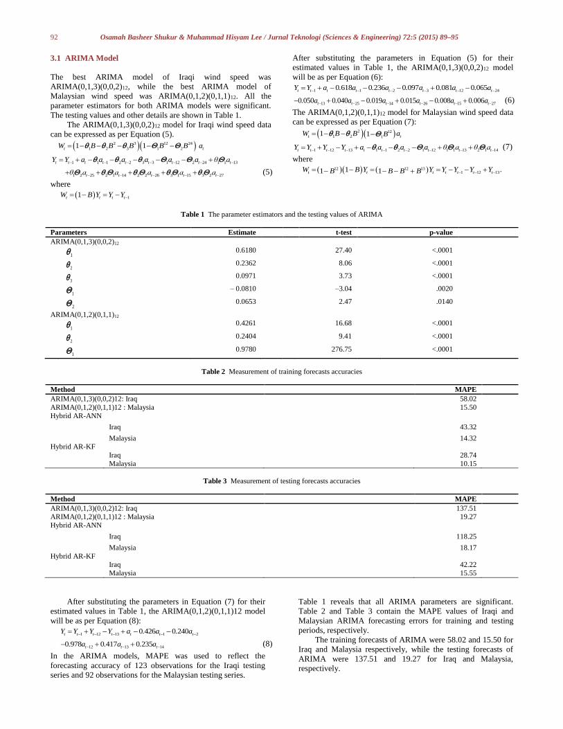
3.1 ARIMA Model

The best ARIMA model of Iraqi wind speed was

ARIMA(0,1,3)(0,0,2)12, while the best ARIMA model of

Malaysian wind speed was ARIMA(0,1,2)(0,1,1)12. All the

parameter estimators for both ARIMA models were significant.

The testing values and other details are shown in Table 1.

The ARIMA(0,1,3)(0,0,2)12 model for Iraqi wind speed data

can be expressed as per Equation (5).

2 3 12 24

1 2 3 1 21 1t tW B B B B B a

1 1 1 2 2 3 3 1 12 2 24 1 1 13t t t t t t t t tY Y a a a a a a θ a

1 2 25 2 1 14 2 2 26 3 1 15 3 2 27t t t t tθ a a a a a (5)

where

11t t t tW B Y Y Y

After substituting the parameters in Equation (5) for their

estimated values in Table 1, the ARIMA(0,1,3)(0,0,2)12 model

will be as per Equation (6):

1 1 2 3 12 240 618 0 236 0 097 0 081 0 065t t t t t t t tY Y a . a . a . a . a . a

13 25 14 26 15 270 050 0 040 0 019 0 015 0 008 0 006t t t t t t. a . a . a . a . a . a (6)

The ARIMA(0,1,2)(0,1,1)12 model for Malaysian wind speed data

can be expressed as per Equation (7):

2

1 12121 1t tW B B B a

1 12 13 1 1 2 2 1 12 1 1 13 2 1 14t t t t t t t t t tY Y Y Y a a a a θ a θ a (7)

where

12 12 13

1 12 131 1 1t t t t t t t .B B BW B Y Y Y Y Y YB

Table 1 The parameter estimators and the testing values of ARIMA

Parameters Estimate t-test p-value

ARIMA(0,1,3)(0,0,2)12

1

0.6180 27.40 <.0001

2

0.2362 8.06 <.0001

3

0.0971 3.73 <.0001

1

– 0.0810 –3.04 .0020

2

0.0653 2.47 .0140

ARIMA(0,1,2)(0,1,1)12

1

0.4261 16.68 <.0001

2

0.2404 9.41 <.0001

1

0.9780 276.75 <.0001

Table 2 Measurement of training forecasts accuracies

Method MAPE

ARIMA(0,1,3)(0,0,2)12: Iraq 58.02

ARIMA(0,1,2)(0,1,1)12 : Malaysia 15.50

Hybrid AR-ANN

Iraq 43.32

Malaysia 14.32 Hybrid AR-KF

Iraq 28.74

Malaysia 10.15

Table 3 Measurement of testing forecasts accuracies

Method MAPE

ARIMA(0,1,3)(0,0,2)12: Iraq 137.51 ARIMA(0,1,2)(0,1,1)12 : Malaysia 19.27

Hybrid AR-ANN

Iraq 118.25

Malaysia 18.17

Hybrid AR-KF Iraq 42.22

Malaysia 15.55

After substituting the parameters in Equation (7) for their

estimated values in Table 1, the ARIMA(0,1,2)(0,1,1)12 model

will be as per Equation (8):

1 12 13 1 20 426 0 240t t t t t t tY Y Y Y a . a . a

12 13 140 978 0 417 0 235t t t. a . a . a (8)

In the ARIMA models, MAPE was used to reflect the

forecasting accuracy of 123 observations for the Iraqi testing

series and 92 observations for the Malaysian testing series.

Table 1 reveals that all ARIMA parameters are significant.

Table 2 and Table 3 contain the MAPE values of Iraqi and

Malaysian ARIMA forecasting errors for training and testing

periods, respectively.

The training forecasts of ARIMA were 58.02 and 15.50 for

Iraq and Malaysia respectively, while the testing forecasts of

ARIMA were 137.51 and 19.27 for Iraq and Malaysia,

respectively.


3.2 Hybrid AR-ANN Model

Neural network toolboxes in MATLAB can use many types of

training algorithms and training functions. Feed forward and

back-propagation algorithm with the Levenberg Marquardt and

the Bayesian regularization training algorithms were used in this

study to improve forecasting accuracy.

The partial autocorrelation function (PACF) for the original

series reflected the number of significant orders for the AR

model. The stationarity conditions were omitted in this stage,

because the AR model was used only for determining the

structure of the input layer for the ANN. Figure 4 illustrates the

ACF and PACF of the original Iraqi and Malaysian wind speed

data set.

Figure 4 ACF and PACF for Iraqi and Malaysian wind speeds

From Figure 4, ACF exhibited the slow dying out style of

the Iraqi and Malaysian non-stationary data. The PACF in

Figure 4 illustrates the cutting off style after 12 for the Iraqi data

set and after 7 for the Malaysian data set. Therefore, AR(12) and

AR(7) can be proposed based on the ACF and PACF results for

the Iraqi and Malaysian data sets, respectively. The Akaike

information criterion (AIC) will be plotted to measure the

adequacy of the best AR model. AIC was used to confirm these

results (Figure 5) for the original Iraqi and Malaysian data set

series for AR(1), AR(2), …, AR(20).

Figure 5 AIC of the ARIMA for Iraqi and Malaysian data sets

Figure 5 shows the quick dying out style of the AIC values

that stabilized after the 12th and 7th values for the Iraqi and

Malaysian data sets, respectively. The AIC plots confirmed that

the selection of AR(12) and AR(7) was performed correctly.

The input structure of the ANN for both data sets can be

considered based on the autoregressive order of the AR(12) and

AR(7) models. In other words, the ANN inputs are equalled to

12 and 7 for the Iraqi and Malaysian data sets, respectively.

Figure 6 outlines the consistency between the original and

testing forecast series obtained by using the hybrid AR-ANN

model for Iraqi and Malaysian wind speed data sets,

respectively.

Figure 6 Hybrid AR-ANN testing forecast and the original plots for

Iraq and Malaysia

Figure 6 demonstrates that the consistence between the

testing forecasts series and original data sets was acceptable for

Iraq and Malaysia with some of over forecasting situation for

Iraqi data set. Table 2 and Table 3explains the MAPE values for

Iraqi and Malaysian hybrid AR-ANN forecasting errors for the

training and testing periods, respectively. From Table 2 and

Table 3, the MAPE values for the hybrid AR-ANN training

forecasts were 43.32 and 14.32 for Iraqi and Malaysian wind

speed data, respectively, while the MAPE values for the testing

forecasts of the hybrid AR-ANN were 118.25 and 18.17 for

Iraqi and Malaysian wind speed data sets, respectively. Table 2

and Table 3 shows that for both the Iraqi and Malaysian data

sets, the wind speed forecasting values for training and testing

periods found using AR-ANN were better than those found

using the ARIMA model. These results confirm that the hybrid

AR-ANN model improved the forecasting accuracy compared to

the ARIMA model.

3.3 Hybrid AR-KF Model

To handle stochastic uncertainty, the KF model was used for

more accurate forecasting. AR modelling has been performed in

the previous section successfully. Therefore, the state vector

inputs of the KF for both data sets can be considered based on

AR(12) and AR(7) models. In other words, the state vector

inputs are equalled to 12 and 7 for the Iraqi and Malaysian data

sets, respectively.

Based on the AR model after applying t i i ,tY Y , SE and OE

of the KF model in Equations (3) and (4) can be formulated for

Iraqi wind speed as follows:


0.426 0.025 0.034 0.001 0.072 0.055 0.027 0.044 0.034 0.087 0.035 0.128

1 0 0 0 0 0 0 0 0 0 0 0

0 1 0 0 0 0 0 0 0 0 0 0

0 0 1 0 0 0 0 0 0 0 0 0

0 0 0 1 0 0 0 0 0 0 0 0

1

2

3

4

5

6

7

8

9

10

11

12

Y ,t

Y ,t

Y ,t

Y ,t

Y ,t

Y ,t

Y ,t

Y ,t

Y ,t

Y ,t

Y ,t

Y ,t

0 0 0 0 1 0 0 0 0 0 0 0

0 0 0 0 0 1 0 0 0 0 0 0

0 0 0 0 0 0 1 0 0 0 0 0

0 0 0 0 0 0 0 1 0 0 0 0

0 0 0 0 0 0 0 0 1 0 0 0

0 0 0 0 0 0 0 0 0 1 0 0

0 0 0 0 0 0 0 0 0 0 1 0

1

2

3

4

5

6

7

8

9

10

11

12

1

0

0

0

0

0

0

0

0

0

0

0

,t

,t

,t

,t

,t

,t

t

,t

,t

,t

,t

,t

,t

Y

Y

Y

Y

Y

Y

Y

Y

Y

Y

Y

Y

a

(9)

1 12

12 1

1 0 0 0 0 0 0 0 0 0 0 0

1

2

3

4

5

6

7

8

9

10

11

12

Y ,tY ,tY ,tY ,tY ,tY ,tYYt ,tY ,tY ,tY ,tY ,tY ,t

(10)

Based on the AR, after applying t i i,tY Y , SE and OE of KF

process in Equations (3) and (4) can be formulated for

Malaysian wind speed as follows:

0 615 0 068 0 081 0 0359 0 062 0 010 0 140

1 0 0 0 0 0 0

0 1 0 0 0 0 0

0 0 1 0 0 0 0

0 0 0 1 0 0 0

0 0 0 0 1 0 0

0 0 0 0 0 1 0

1

2

3

4

5

6

7

. . . . . . .Y ,t

Y ,t

Y ,t

Y ,t

Y ,t

Y ,t

Y ,t

1

0

0

0

0

0

0

1 1

2 1

3 1

4 1

5 1

6 1

7 1

ta

Y ,t

Y ,t

Y ,t

Y ,t

Y ,t

Y ,t

Y ,t

(11)

1

2

3

41 7

5

6

7 7 1

1 0 0 0 0 0 0

,t

,t

,t

,tt

,t

,t

,t

YYYYYYYY

(12)

After initializing the SE and OE for Iraq and Malaysia, the

hybrid AR-KF model will be used for forecasting by using KF

recursive steps, such as the one found in [14, 15, 23]. The

outputs tY of OE in Equation (10) and (12) represent the Iraqi

and Malaysian hybrid AR-KF fitted or forecasting series

respectively. The difference t tY CX is the forecasting errors for

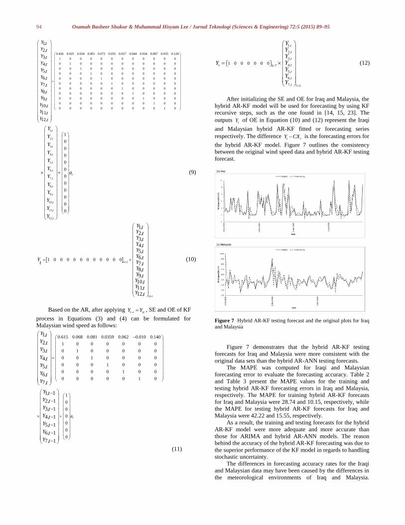
the hybrid AR-KF model. Figure 7 outlines the consistency

between the original wind speed data and hybrid AR-KF testing

forecast.

Figure 7 Hybrid AR-KF testing forecast and the original plots for Iraq

and Malaysia

Figure 7 demonstrates that the hybrid AR-KF testing

forecasts for Iraq and Malaysia were more consistent with the

original data sets than the hybrid AR-ANN testing forecasts.

The MAPE was computed for Iraqi and Malaysian

forecasting error to evaluate the forecasting accuracy. Table 2

and Table 3 present the MAPE values for the training and

testing hybrid AR-KF forecasting errors in Iraq and Malaysia,

respectively. The MAPE for training hybrid AR-KF forecasts

for Iraq and Malaysia were 28.74 and 10.15, respectively, while

the MAPE for testing hybrid AR-KF forecasts for Iraq and

Malaysia were 42.22 and 15.55, respectively.

As a result, the training and testing forecasts for the hybrid

AR-KF model were more adequate and more accurate than

those for ARIMA and hybrid AR-ANN models. The reason

behind the accuracy of the hybrid AR-KF forecasting was due to

the superior performance of the KF model in regards to handling

stochastic uncertainty.

The differences in forecasting accuracy rates for the Iraqi

and Malaysian data may have been caused by the differences in

the meteorological environments of Iraq and Malaysia.


Additionally, Iraq has four seasons yearly, whereas Malaysia

has only two, making the Iraqi wind speed more complex.

4.0 CONCLUSION

Hybrid AR-ANN and AR-KF models were proposed to improve

the wind speed forecasting accuracy. Two wind speed data sets

from different meteorological environments were used. The

results showed that the hybrid AR-ANN and AR-KF models

were effective. However, the MAPE results indicated that the

hybrid AR-KF model was the most effective tool for improving

the forecasting accuracy. The hybrid AR-KF forecasting was

more accurate than those for ARIMA and AR-ANN models. The

advantage of the hybrid AR-KF model was due to the superior

performance of the KF model in regards to handling stochastic

uncertainty.

References

[1] Benth, J. Š., and F. E. Benth. 2010. Analysis and Modelling of Wind

Speed in New York. J. Appl. Stat. 37(6): 893–909.

[2] Shi, J., X. Qu, and S. Zeng. 2011. Short-term Wind Power Generation Forecasting: Direct Versus Indirect ARIMA-based Approaches. Int. J.

Green Energy. 8(1): 100–112.

[3] Zhu, X., and M. G. Genton. 2012. Short-term Wind Speed Forecasting

for Power System Operations. Int. Stat. Rev. 80(1): 2–23.

[4] Cadenas, E., and W. Rivera. 2007. Wind Speed Forecasting in the

South Coast of Oaxaca, México. Renew. Energy. 32(12): 2116–2128.

[5] Cadenas, E., and W. Rivera. 2010. Wind Speed Forecasting in Three

Different Regions of Mexico, Using a Hybrid ARIMA–ANN Model. Renew. Energy. 35(12): 2732–2738.

[6] Pourmousavi-Kani, S. A., and M. M. Ardehali. 2011. Very Short-term

Wind Speed Prediction: A New Artificial Neural Network–Markov

Chain Model. Energy Conv. Manag. 52(1): 738–745.

[7] Assareh, E., M. Behrang, M. Ghalambaz, A. Noghrehabadi, and A.

Ghanbarzadeh. 2012. An Analysis of Wind Speed Prediction Using

Artificial Neural Networks: A Case Study in Manjil, Iran. Energy Sources, Part A: Recovery, Utilization, and Environmental Effects.

34(7): 636–644.

[8] Bilgili, M., and B. Sahin. 2013. Wind Speed Prediction of Target

Station from Reference Stations Data. Energy Sources Part A-Recovery

Util. Environ. Eff. 35(5): 455–466.

[9] Peng, H., F. Liu, and X. Yang. 2013. A Hybrid Strategy of Short Term

Wind Power Prediction. Renew. Energy. 50: 590–595. [10] Li, G., and J. Shi. 2010. On Comparing Three Artificial Neural

Networks for Wind Speed Forecasting. Appl. Energy. 87: 2313–2320.

[11] Guo, Z., W. Zhao, L. Haiyan, and J. Wang. 2012. Multi-step

Forecasting for Wind Speed Using A Modified EMD-based Artificial

Neural Network Model. Renew. Energy. 37: 241–249.

[12] Liu, H., H. Tian, and Y. Li. 2012. Comparison of Two New ARIMA-

ANN and ARIMA-Kalman Hybrid Methods for Wind Speed Prediction. Appl. Energy. 98: 415–424.

[13] Malmberg, A., U. Holst, and J. Holst. 2005. Forecasting Near-surface

Ocean Winds with Kalman Filter Techniques. Ocean Eng. 32(3): 273–

291.

[14] Galanis, G., P. Louka, P. Katsafados, I. Pytharoulis, and G. Kallos.

2006. Applications of Kalman Filters Based on Non-linear Functions to

Numerical Weather Predictions. Ann. Geophys. 24(10): 2451–2460.

[15] Louka, P., G. Galanis, N. Siebert, G. Kariniotakis, P. Katsafados, I. Pytharoulis, and G. Kallos. 2008. Improvements in Wind Speed

Forecasts for Wind Power Prediction Purposes Using Kalman Filtering.

J. Wind Eng. Ind. Aerodyn. 96(12): 2348–2362.

[16] Cassola, F., and M. Burlando. 2012. Wind Speed and Wind Energy

Forecast Through Kalman Filtering of Numerical Weather Prediction

Model Output. Appl. Energy. 99: 154–166.

[17] Tatinati, S., and K. C. Veluvolu. 2013. A Hybrid Approach for Short-

term Forecasting Of Wind Speed. Sci. World J. 2013. [18] Chen, K., and J. Yu. 2014. Short-term Wind Speed Prediction Using

an Unscented Kalman Filter Based State-space Support Vector

Regression Approach. Appl. Energy. 113: 690–705.

[19] Liu, L.-M. 2006. Time Series Analysis and Forecasting. 2nd ed.

Illinois, USA: Scientific Computing Associates Corp.

[20] Zhang, G. P. 2003. Time Series Forecasting Using A Hybrid ARIMA

and Neural Network Model. Neurocomputing. 50: 159–175. [21] Khashei, M., and M. Bijari. 2010. An Artificial Neural Network

(P,D,Q) Model for Time Series Forecasting. Expert Syst. Appl. 37(1):

479–489.

[22] Gould, P. G., A. B. Koehler, J. K. Ord, R. D. Snyder, R. J. Hyndman,

and F. V. Araghi. 2008. Forecasting Time Series with Multiple

Seasonal Patterns. Eur. J. Oper. Res. 191: 207–222.

[23] Madsen, H. 2007. Time Series Analysis. CRC Press.

Daily Wind Speed Forecasting Through Hybrid AR-ANN and AR-KF Models

Documents

Transcript of Daily Wind Speed Forecasting Through Hybrid AR-ANN and AR-KF Models