D-brane gauge theories from toric singularities and toric duality ☆ ☆ Research supported in part...

arX

iv:h

ep-t

h/00

0516

6v2

17

Oct

200

0

hep-th/0005166

TIFR/TH/00-22

May, 2000

D-brane gauge theories from toricsingularities of the form C3/Γ and C4/Γ

Tapobrata Sarkar1

Department of Theoretical Physics,

Tata Institute of Fundamental Research,

Homi Bhabha Road, Mumbai 400 005, India

Abstract

We discuss examples of D-branes probing toric singularities, andthe computation of their world-volume gauge theories from the geo-metric data of the singularities. We consider several such examples ofD-branes on partial resolutions of the orbifolds C

3/Z2 × Z2,C3/Z2 × Z3

and C4/Z2 × Z2 × Z2.

1Email: [email protected]

http://arxiv.org/abs/hep-th/0005166v2

http://arxiv.org/abs/hep-th/0005166

1 Introduction

In the last few years, a lot of progress has been made in the study of D-branesas probes of sub-stringy geometry. While the usual picture of space-time issupposed to be valid upto the string scale, it was argued in [1] that D-branesare the natural candidates to probe the geometry of space-time beyond thestring scale. As has been widely accepted by now, the standard conceptsof space-time appears, from the D-brane perspective, as the vacuum modulispace of its world volume gauge theory. Indeed, it has been found that thespace-time appearing in D-brane probes at ultra-short distance scales hasqualitatively different features from that probed by bulk strings [2].

Of particular interest has been the study of D-branes on Calabi-Yau man-ifolds. In [3],[4], the moduli space of Calabi-Yau manifolds was studied usingfundamental strings. A rich underlying geometric structure was discovered,and the moduli space was shown to contain topologically distinct geometric(Calabi-Yau) phases, as well as non-geometric (Landau-Ginzburg) phases.The Kahler sector of the vacuum moduli space was shown to consist of sev-eral domains (separated by singular Calabi-Yau spaces), whose union is iso-morphic to the complex structure moduli space of the mirror manifold. Itwas also shown, that using mirror symmetry as in [3] or the approach ofgauged linear sigma models as in [4], one can interpolate smoothly betweenthe topologically distinct points in the Kahler moduli space. In the funda-mental string picture, the geometric and non-geometric phases of Calabi-Yaumanifolds appear as two distinct possibilities, with the latter being thoughtof as an analytic continuation of the geometric phases in the presence of anon-zero theta angle in the language of [4]. It was, however, shown in [5] thatthe presence of additional open string sectors change this picture consider-ably, and that the D-brane linear sigma model probes only a part of the fulllinear sigma model vacuum moduli space, namely the geometric phase. Itwas explicitly demonstrated in [5] that D-branes (in the particular examplesof the orbifold C3/Z3 and C3/Z5) ‘project out’ the non-geometric phase, inagreement with the results obtained in [6]. This was found to be generallytrue for Calabi-Yau orbifolds of the form C3/Zn [7].

Since the pioneering work of [8], which dealt with D-branes on Abelianorbifold singularities of the form C2/Zn that was generalised to arbitrarynon-Abelian singularities of the form C2/Γ (Γ being a subgroup of SU(2)),D-branes on Abelian and non-Abelian orbifold backgrounds have been ex-

1

tensively studied in [7],[9], [10],[11],[12],[13]. D-branes at orbifolded conifoldsingularities have been considered in [14]. (See also [15] for an analysis of ablowup of the four-dimensional N = 1, Z3 orientifold). Of particular inter-est has been the applications of methods of toric geometry [16],[17] to thestudy of D-brane gauge theories on such singularities. In the approach pio-neered in [5], the matter content and the interactions of the D-brane gaugetheory, which are specified by the D-terms and the F-terms of the gaugetheory respectively, are treated on the same footing, and the gauge theoryinformation can be encoded as algebraic equations of the toric variety. It isan interesting question to ask, if this procedure can be reversed, i.e, givena particular toric singularity, is there a way of consistently reading off theworld volume gauge theory data for a D-brane that probes this singularity.A step in this direction has been recently taken in [21]. The authors of [21]have given an algorithm by which the geometrical data encoded in a toricdiagram can be used to construct the matter content and superpotentialinteraction of the D-brane gauge theory that probes it, and have demon-strated this in the cases of the suspended pinch point (SPP) singularity ofthe blowup of the C3/Z2 × Z2 orbifold and the various partial resolutions ofthe C3/Z3 × Z3 orbifold analysed in [22]. In the present paper, we criticallyexamine this procedure in several other examples. We first consider this algo-rithm, which we call the inverse toric procedure, for partial resolutions of theorbifold C3/Z2 × Z2. Further, we consider several blowups of the orbifoldsC3/Z2 × Z3 and C4/Z2 × Z2 × Z2 and present results on the extraction ofthe D-brane gauge theory data from the given toric geometric data.

The organisation of the paper is as follows. In section 2, we first recapit-ulate the essential details of the construction of the D-brane gauge theory onpartial resolutions of the orbifold C3/Z2 × Z2 [19],[20] that will also set thenotation and conventions to be used in the rest of the paper and then demon-strate the inverse toric algorithm to construct the gauge theory of a D-braneprobing the Z2 and the conifold singularities obtained by partially resolv-ing the C3/Z2 × Z2 orbifold. Section 3 deals with the orbifold C3/Z2 × Z3

and its various partial resolutions. In section 4, we consider the exampleof the orbifold C4/Z2 × Z2 × Z2 and consider some resolutions of the same.Section 5 contains discussions and directions for future work.

2

2 D-branes on C3/Z2 × Z2 and its blowups

We begin this section by recapitulating the essential details of the applica-tion of toric methods to the construction of D3-branes on C3/Z2 × Z2 andsome of its partial resolutions which will also set the notations and conven-tions to be followed in the rest of the paper. Recall that the world volumesupersymmetric gauge theory of D-branes probing a toric singularity arecharacterised by its matter content and interactions. While the former aregiven by the D-term equations, the latter are specified, via the superpoten-tial, as the F-term equations. These two sets of equations, in conjunction,define the moduli space of the theory. In order to define the D-brane modulispace by toric methods, the standard procedure [5] is to re-express the Fand D-term constraints in terms of a set of homogeneous variables pα, anda concatenation of these two sets of equations give rise to the toric data.Let us briefly review this construction for the example of D-3 branes on theorbifold C3/(Z2 × Z2).

We start by considering the field theory of a set of D-3 branes at aC3/(Z2 × Z2) singularity. Generically, a single D-p brane of type II stringtheory at a point in the orbifold C3/Γ is constructed by considering thetheory of |Γ| D-p branes in C3 and then projecting to C3/Γ where the pro-jection is defined by a combined action of Γ on C3 as well as the D-braneChan-Paton index. The unbroken supersymmetry in d = 4 would then beN = 2 in the closed string sector while the open string sector will have N = 1supersymmetry. In our example, a generator g of the discrete group Z2 × Z2

acts simultaneously on the coordinates of C3 and also the D-3 brane Chan-Paton factors. The surviving fields in the theory are the ones that are leftinvariant by a combination of these two actions. Specifically, denoting theaction of the quotienting group on C3 by R(g) and that on the Chan-Patonindices by γ(g) (where γ denotes a regular representation of g), the survivingcomponents of the scalars X that live on the brane world volume are thosefor which X = R(g)γ(g)Xγ(g)−1, and the components of the gauge fields Athat survive the projection are those that satisfy A = γ(g)Aγ(g)−1. Afterimposing these projections, the N = 1 matter multiplet of the theory consistsof the twelve fields

(X13, X31, X24, X42) , (Y12, Y21, Y34, Y43) , (Z14, Z41, Z23, Z32) (1)

Where we have denoted the complex bosonic fields corresponding to the

3

position coordinates tangential to C3 by X1 = X, X2 = Y, X3 = Z. Afterprojection of the gauge field, the unbroken gauge symmetry in this case is thesubgroup U(1)4 of U(4), and, apart from an overall U(1), we have a U(1)3

theory. The total charge matrix is given by

d =

−1 0 0 1 −1 1 0 0 −1 0 1 00 −1 1 0 1 −1 0 0 0 −1 0 10 1 −1 0 0 0 −1 1 1 0 −1 01 0 0 −1 0 0 1 −1 0 1 0 −1

(2)

With the last row of d signifying the overall U(1). The D-term constraintsare now given by

∑

µ

dβ(i)µ|X

µβ |

2 − ζi = 0 (3)

where dβ(i)µ is the charge of Xµ

β under the i’th U(1) and β signifies the matrixindices of the surviving components of Xµ.

∑

i ζi = 0 is the condition for theexistence of supersymmetric vacua.

The superpotential of the theory is given by the expression

W = Tr[

X1, X2]

X3 (4)

With the vacuum satisfying

∂W

∂Xµ= 0; i.e [Xµ, Xν ] = 0 (5)

Using the expressions for the Xµ’s from eq.(1) in eq. (5), one can derivetwelve constraints on the twelve fields Xij, Yij, Zij, out of which six are seento be independent, hence the twelve initial fields can be solved in termsof six independent fields. Denoting the twelve matter fields collectively byXi, i = 1 · · ·12, and the set of six independent fields (which we take to beX13, X24, Y21, Y34, Z14, Z32) by xb, (b = 1 · · ·6), the solution, which is of theform

Xi =6

∏

b=1

xKib

b (6)

4

can be encoded in the columns of the matrix K, given by

K =

X13 X24 X31 X42 Y12 Y21 Y34 Y43 Z14 Z23 Z32 Z41

X13 1 0 0 1 1 0 0 1 0 0 0 0X24 0 1 1 0 −1 0 0 −1 0 0 0 0Y21 0 0 0 0 0 1 0 1 0 1 0 1Y34 0 0 0 0 1 0 1 0 0 −1 0 −1Z14 0 0 −1 −1 0 0 0 0 1 1 0 0Z32 0 0 1 1 0 0 0 0 0 0 1 1

(7)

The columns of the above matrix are vectors in the lattice N = Z6,and define the edges of a cone σ. In order to make the description of thetoric variety explicit, we consider the dual cone σ∨, which is defined in thedual lattice M = Hom(N,Z). The dual cone σ∨ is defined to be the set ofvectors in the dual lattice M which have non-negative inner products withthe vectors of σ, i.e

σ∨ = {m ∈ M : 〈m,n〉 ≥ 0 ∀n ∈ σ} (8)

The dual cone corresponds to defining a new set of fields pα(α = 1 · · · c),in terms of which the variables xb are solved, in a way that is consistent withthe relation (6). In this example, c = 9 and the dual cone is generated bythe columns of the matrix

T =

p1 p2 p3 p4 p5 p6 p7 p8 p9

X13 1 1 0 0 0 0 0 0 1X24 0 1 1 0 0 0 0 0 1Y21 0 0 1 1 1 0 0 0 0Y34 0 0 1 0 1 1 0 0 0Z14 0 0 0 0 0 1 1 0 1Z32 0 0 0 0 0 1 1 1 0

(9)

The relationship between pα and xb are then of the form

xb =∏

α

pTbαα (10)

Thus, there are nine variables pα in terms of which we parametrize the sixindependent variables xb. This parametrization, however, has redundancies,and in order to eliminate these, we introduce a new set of C∗ actions on

5

the pα’s, with the condition that under these actions, the fields xb are leftinvariant. This can be equivalently described by the introduction of a new setof U(1) gauge symmetries, such that the xb’s are gauge invariant [3]. In ourexample, since there are nine fields pα and six independent variables xb, weintroduce a gauge group U(1)3, such that the pα’s are charged with respectto these, with charges Qnα for the nth U(1). The gauge invariance conditiondemands that the charge matrix Q must obey

TQt = 0 (11)

where Qt is the transpose of Q. From the matrix T given above, the chargematrix is given by

Q =

p1 p2 p3 p4 p5 p6 p7 p8 p9

U(1)1 0 0 0 1 −1 1 −1 0 0U(1)2 0 1 0 0 0 0 1 −1 −1U(1)3 1 −1 1 0 −1 0 0 0 0

(12)

We now consider the constraints imposed on the original fields Xi via theD-flatness conditions, and impose these conditions in terms of the new fieldspα. The charges of the fields xb under the original U(1) charge assignmentsare given by the matrix

V =

x1 x2 x3 x4 x5 x6

1 0 −1 0 1 00 1 1 0 0 −1−1 0 0 1 0 1

(13)

From the relationship xb =∏

α pTbαα , it is clear that in order for the charge

assignment qpiα for pα (corresponding to the original set of (i = 3) U(1)

symmetries) to reproduce that for the xb’s, we must have qpT t = V , andone possible choice for the matrix qp is qp

iα = (V U)iα with the matrix Usatisfying TU t = Id. The matrix U is thus the inverse of the matrix T t.However, since T t is a rectangular matrix the usual definition of its inverse(as in the case of a square matrix) is not applicable and there are severalchoices for U . In particular, for a rectangular matrix A, using the rules ofsingle value decomposition, we can compute the Moore-Penrose inverse ofA which is defined in a way that the sum of the squares of all the entries

6

in the matrix (AA−1 − Id) is minimised, where Id is the identity matrix inappropriate dimensions. For any choice of the inverse of T t, the final toricdata will of course be identical, and in this section and the next, we simplyuse the results of [23] in defining the matrix U . For this case, the matrix Uis

U = (T t)−1 =

1 0 0 0 0 0 0 0 0−1 1 0 0 0 0 0 0 00 0 0 1 0 0 0 0 00 0 0 0 0 1 −1 0 00 −1 0 0 0 0 0 0 10 0 0 0 0 0 0 1 0

Now, multiplying by V and concatenating Q and V U we obtain the totalcharge matrix,

Qt =

0 0 0 1 −1 1 −1 0 0 00 1 0 0 0 0 1 −1 −1 01 −1 1 0 −1 0 0 0 0 01 −1 0 −1 0 0 0 0 1 ζ1

−1 1 0 1 0 0 0 −1 0 ζ2

−1 0 0 0 0 1 −1 1 0 ζ3

(14)

where the ζi are the Fayet-Illiapoulos parameters for the original U(1)’s,there being three independent ζi’s because of the constraint

∑4i=1 ζi = 0. The

toric data can now be calculated from the cokernel of the transpose of Qt,which (after a few row operations) become

T =

0 1 0 0 −1 0 1 1 11 1 1 0 1 0 −1 0 11 1 1 1 1 1 1 1 1

(15)

Now from the dual cone T , we can, via the matrix K, find expressions forall the twelve initial fields in terms of the fields pα. These are then used todefine invariant variables in the following way

X13X31 = x = p1p22p3p8p9

Y12Y21 = y = p1p3p4p25p6

Z14Z41 = z = p4p6p27p8p9

X13Y34Z41 = w = p1p2p3p4p5p6p7p8p9 (16)

7

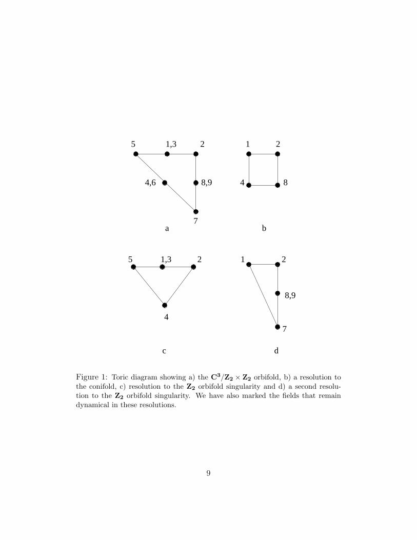
which follow the relation xyz = w2. The toric diagram of the orbifoldC3/Z2 × Z2 is shown in figure 1(a). Let us now consider some examples ofthe possible partial resolutions of this space. We will discuss three possiblepartial blowups as in [23],[25].

The first example corresponds to blowing up the orbifold C3/Z2 × Z2

by a P1 parametrised by w′ = wz. This gives the suspended pinch point

(SPP) singularity given by xy = zw′2. The SPP can be further blown upby introducing a second P1. One possibility is to parametrise this P1 byy′ = y

w′(or x′ = x

w′) and the remaining singularity is the conifold x′y = zw′

(or xy′ = zw′) of figure 1(b). One can also introduce a P1 parametrised bysay x′ = x

zwhence the resulting blowup is a C2/Z2 × C. Two possible toric

diagrams of the latter are shown in fig. 1(c) and fig. 1(d).Let us now come to the description of the inverse toric problem. Suppose

we are given with a singularity depicted by a toric diagram of the form givenin fig. 1(b), 1(c) or 1(d). We wish to extract the gauge theory data of aD-brane that probes such a singularity, starting from figure 1(a). This issuewas addressed in [21], and let us review the basic steps in their algorithm.

Recall that the toric data for a given singularity that a D-brane probesis given by the matrix T which is the transpose of the kernel of the totalcharge matrix (obtained by concatenating the F and D-term constraints ex-pressed in terms of the homogeneous coordinates pα). Hence, the solutionto the inverse problem would imply the construction of an appropriately re-duced total charge matrix Qred

t , the cokernel of the transpose of which is thereduced matrix Tred obtained by deleting the appropriate columns (corre-sponding to the fields that have been resolved) from T . However, althoughTred is known, there is no unique way of specifying the reduced charge ma-trix Qred

t from a knowledge of Tred. Further, there is no guarantee apriorithat such a Qred

t , if obtained, would continue to describe the world volumetheory of a D-brane that probes the given singularity. The algorithm of [21]gives a canonical method by which these issues can be addressed. It con-sists of determining the fields to be resolved by tuning the Fayet-Illiopoulosparameters appropriately (so that the resulting theory at the end is still aphysical D-brane gauge theory) and then reading off the the matrix Qred

t

which can be separated into the F and D-terms and thus can be used toobtain the matter content and the superpotential determining the gaugetheory. Let us discuss this in some more details. The toric diagrams for thepartially resolved singularities are obtained by the deletion of of a subset of

8

��

��

��

��

��

��

��

��

��

��

��

��

��

��

��

��

��

��

��

��

��

��

��

��

��

��

��

��

��

��

��

��

��

��

��

��

��

��

��

��

��

��

��

��

��

��

��

4

8,9

7

5 1,3 2 1 2

5 1,3 2 1 2

4,6 8,9 4 8

7 a b

c d

Figure 1: Toric diagram showing a) the C3/Z2 × Z2 orbifold, b) a resolution to

the conifold, c) resolution to the Z2 orbifold singularity and d) a second resolu-tion to the Z2 orbifold singularity. We have also marked the fields that remaindynamical in these resolutions.

9

nodes from the original one. Conversely, a given toric diagram of dimen-sion k can be embedded into a singularity of the form Ck/Γ(k, n) whereΓ(k, n) = Zn × Zn× · · · (k − 1 times) · · ·Zn. In our case, the singularitiesmentioned above can be embedded into the toric diagram for the singularityC3/Γ(3, 2). For example, the SPP, and the conifold singularity can both beembedded into the C3/Z2 × Z2 singularity, as is obvious from their toric di-agrams. We shall henceforth refer to these singularities, in which we embedthe partially resolved ones as the parent singularities. A toric diagram cor-responding to a partial resolution can of course be embedded in more thanone parent singularity and according to the algorithm of [21], one can choosethe minimal embedding. We will return to this issue in a while.

We now determine the fields to be resolved from the parent singularityin order to reach the given toric diagram, by appropriately choosing thevalues of ζi. The difficulty that arises here is that given the toric diagram ofthe singularity that we are interested in, there is no unique way of knowingexactly which fields (in the toric data of the parent singularity) have to beresolved in order to reach the toric singularity of interest. Given a toricdiagram for the parent singularity, a particular resolution, along with theelimination of one or more nodes, might also require a subset of fields fromsome other nodes to be resolved. Hence, we have to carefully tune the FIparameters for a consistent blowup of the parent singularity to the one thatwe are interested in. We now illustrate this procedure by the example of theblowup of the C3/Z2 × Z2 singularity to the C2/Z2 × C orbifold illustratedin fig. 1(c). This example is, in a sense, straightforward, because from thetoric diagram of fig. 1(c), it is clear that this being the Z2 singularity, we candirectly read off the matter content and the interactions from the standardresults for D3-branes on the Z2 orbifold [8]. However, note that this is thesimplest example where the inverse procedure of calculating the D-branegauge theory has to be valid. The Z2 orbifold can be thought of as partialresolutions of the orbifolds C3/Z2 × Z2, or C3/Z2 × Z3, and the inverse toricprocedure must give familiar results for both in agreement with [8],[23]. Alower dimensional toric orbifold can always be embedded in the toric diagramof one of higher dimension, and the inverse toric procedure must consistentlyreproduce the D-brane gauge theory on the former, starting from the latterdata. As we will see, this is indeed the case.

We proceed by embedding the Z2 singularity in C3/Z2 × Z2. In order todetermine the fields to be resolved, we perform Gaussian row reduction on

10

the the matrix Qt to obtain

−1 0 0 0 0 1 −1 0 1 ζ1 + ζ2 + ζ3

0 −1 0 0 0 0 −1 0 2 ζ1 + ζ2

0 0 −1 0 0 1 −1 0 1 ζ1

0 0 0 −1 0 1 0 0 0 ζ1 + ζ3

0 0 0 0 −1 2 −1 0 0 ζ1 + ζ3

0 0 0 0 0 0 0 −1 1 ζ1 + ζ2

The above set of equations imply the constraints

− x1 + x6 − x7 + x9 = (ζ1 + ζ2 + ζ3)

−x2 − x7 + 2x9 = (ζ1 + ζ2)

−x3 + x6 − x7 + x9 = ζ1

−x4 + x6 = (ζ1 + ζ3)

−x5 + 2x6 − x7 = (ζ1 + ζ3)

−x8 + x9 = (ζ1 + ζ2) (17)

Where, for convenience of notation, we have labelled p2i = xi. This set of

equations is now solved in terms of the fields that we know would definitelyget resolved. From the toric diagram, three such fields are p7, p8, p9. However,from the relation between x8 and x9 above, it suffices to solve the above setof equations in terms of x7 and x9, say. This gives the solution set,

[x1, · · ·x9] = [x1, (2x9 − x7 − ζ1 − ζ2), (x1 + ζ2 + ζ3), (x1 + x7 − x9 + ζ2),

(2x1 + x7 − 2x9 + ζ1 + 2ζ2 + ζ3)(x1 + x7 − x9 + ζ1 + ζ2 + ζ3),

x7, (x9 − ζ1 − ζ2), x9] (18)

Now, from the toric diagram of fig.1(c), we choose the fields [p1, p2, p3, p5]to have zero vev i.e these fields continue to remain dynamical. Thus, in theabove solution set, we impose x1, x2, x3, x5 = 0 to obtain

[x1, · · ·x9] = [0, 0, 0, (x9 − ζ1), 0, (x7 − x9 + ζ1), x7, (x9 − ζ1 − ζ2), x9] (19)

We further set x9 = ζ1 in order to make x4 = 0. Hence, x6 = x7 = ζ1−ζ2.Also, x8 = −ζ2. Therefore, the fields to be resolved are [p6, p7, p8, p9], all ofwhich have positive vevs.

11

We now need to obtain the reduced charge matrix for this choice of vari-ables to be resolved. The method of doing this essentially consists of per-forming row operations on the full charge matrix Qt in eq. (14), such thatthe columns corresponding to the resolved fields [p6, p7, p8, p9] are set to zero.The reduced charge matrix Qred

t thus obtained must be in the nullspace of thereduced toric matrix Tred, that can be directly evaluated from the full toricmatrix in eq. (15) by removing the columns 6, 7, 8, 9. Let us first discuss thegeneral formalism for achieving this, which can then be easily applied to ourpresent example. Consider a general parent theory that has a total chargematrix Qt of dimensions (a × b), and suppose we wish to eliminate d fieldsfrom the parent theory in order to reach the theory of interest. This impliesthat we have to perform row operations on Qt so that the given d columnswill have zero entries and thus be eliminated. The latter can be achieved byconstructing the nullspace of the transpose of a submatrix that is formed byprecisely the d columns that need to be eliminated. Further, since the toricdata T was initially in the nullspace of Qt, removal of the d columns from Qt

to obtain Qredt would mean that the reduced toric data Tred with the same

d columns removed would be in the nullspace of Qredt . Thus, the expression

for Qredt is given by [21]

Qredt =

[

NullSpace(Qtd) · Qr

]

(20)

where Qtd is the transpose of the matrix obtained from Q containing as its

columns, the deleted columns of Q and Qr is the remaining matrix.In our example, we evaluate Qred directly, by writing Qt

d as the transposeof the matrix that contains columns 6, 7, 8, 9 of the charge matrix Qt, and Qr

being the matrix containing the columns 1, 2, 3, 4, 5, 6, 10 of Qt. This impliesthat the reduced charge matrix is

Qredt =

(

1 −1 1 0 −1 0−2 1 0 0 1 ζ2 + ζ3

)

(21)

From this, the reduced charge matrices corresponding to the F and D-termsare

Qred = (1 − 1 1 0 − 1) ; (V U)red = (−2 1 0 0 1) (22)

Denoting the kernel of the charge matrix by Tred, the transpose of its dual is

12

the reduced Kt matrix,

Ktred =

0 1 0 1 01 0 0 0 00 1 1 0 00 0 1 0 1

Now, From eq. (6), the charge matrix for the initial fields Xi are given,via the charge matrix for the independent fields xb by the relation

∆ = V · Kt (23)

Hence, in this case, making use of the identity Ured · T tred = Id, the matter

content for the D-brane gauge theory on the resolved space is obtained as∆red = (V U)red(T

tredK

tred). From which in this case we obtain the matrix

dred =

(

0 1 1 −1 −10 −1 −1 1 1

)

(24)

where we have included an extra row corresponding to the redundant U(1).Hence, the gauge group is seen to be U(1)2, with four bifundamentals, inagreement with the result of [23]. Also note that one adjoint field has ap-peared in our expression. This signals an ambiguity that exists in the toricprocedure with regards to handling chargeless fields. Consider, for exam-ple, the superpotential interaction, which can be determined from the ma-trix K that encodes the F-flatness conditions. The number of columns inthe matrix Kt

red is the number of fields that appear in the interactions andthe terms in the superpotential are read off as linear relations between thecolumns of Kt

red. In this example, from the matrix K, we have the relationX2X5 = X3X4, and from the d matrix, we can see that each of these havecharge zero. Hence, we try as an ansatz for the superpotential,

W = (X1 + φ) (X2X5 − X3X4) (25)

where φ is a field uncharged for both the U(1)’s. This agrees with [23] afterthe identification x13 → X2; Y34 → X5; X24 → X3; X13 → X4; Z41 →X1; Z23 → −φ. As is clear, however, there is an ambiguity in writing the su-perpotential due to the presence of fields that are chargeless under both theU(1)’s [21]. Let us also mention that we can carry out the inverse procedurejust outlined for the case of the alternative blowup to C3/Z2 ×C shown in

13

figure 1(d). This gives exactly the same matter content and superpotentialas the case just analysed, in the region of moduli space given by ζ1 + ζ3 = 0,ζ2 >> 0.

• We now discuss the example of the blowup of the C3/Z2 × Z2 singularityto the conifold. Proceeding in the same way as above, we now find that inthe region of the FI parameters determined by ζ2 = 0; ζ1,3 >> 0, the fieldsto be resolved are [p3, p5, p6, p7, p9], when the fields [p1, p2, p4, p8] are chosendynamical, i.e continue to have zero vev. Therefore, from eq. (20), we obtainthe reduced charge matrix to be

Qredt = (−1 1 1 − 1 ζ2) (26)

Note that in this, case, there are no F-terms and we have Qred = 01×4,moreover, the kernel of this matrix is the 4 × 4 identity matrix, i.e Tred =Id4×4, which implies that (since the dual matrix of Tred is also the 4 × 4identity matrix) ∆ = Qred, with the charge matrix given in this case (byadding the extra column corresponding to the overall U(1)) as

dred =

(

−1 1 1 −11 −1 −1 1

)

(27)

In this case, the matrix Qred being zero, there are no F-terms and the entiregauge theory information is contained in the D-term.

3 D-branes on C3/Z2 × Z3 and its blowups

Let us now consider D3-branes on the orbifold C3/Z2 × Z3. In this case, thebosonic fields corresponding to the D3-brane coordinates tangential to theC3 are 6 × 6 matrices, and the components that survive the projection bythe quotienting group constitute the N = 1 matter multiplet, given by theset

(X12, X23, X34, X45, X56, X61)

(Y13, Y24, Y35, Y46, Y51, Y62)

(Z14, Z25, Z36, Z41, Z52, Z63) (28)

The F-flatness condition (5) in this case imply 18 constraints out of which 8are seen to be independent. Further, there are 17 homogeneous coordinates

14

pα, (α = 1 · · · 17), corresponding to the physical fields in terms of which thedual cone may be described.

The total charge matrix of the homogeneous coordinates pα is defined byintroducing a set of 9 C∗ actions that remove the redundancy in expressingthe original independent fields in terms of the homogeneous coordinates anda further set of U(1)5 charges expressing the D-term constraints in terms ofthe pα. (The 6th U(1) is redundant because of the relation

∑

i ζi = 0). Thetotal charge matrix can then be obtained by concatenating these two sets ofcharge matrices as in our earlier example, and is given (with the inclusion ofa column specifying the 5 independent Fayet-Illiopoulos parameters) by [23]

Qt =

1 0 −1 0 0 0 0 0 0 0 −1 0 0 0 1 0 0 00 1 0 0 0 0 −1 0 0 0 0 0 0 −1 0 0 1 00 0 1 −1 0 0 0 0 0 −1 1 0 0 0 0 0 0 00 0 0 1 −1 0 0 0 0 0 0 0 −1 1 0 0 0 00 0 0 0 1 0 0 0 −1 0 −1 0 0 0 1 −1 1 00 0 0 0 0 1 0 0 0 −1 0 0 −1 0 1 −1 1 00 0 0 0 0 0 1 0 0 −1 −1 0 0 0 1 0 0 00 0 0 0 0 0 0 1 −1 0 0 1 −1 0 −1 0 1 00 0 0 0 0 0 0 0 0 0 0 1 0 −1 −1 1 0 00 −1 0 0 1 0 0 0 0 0 0 0 0 0 0 0 0 ζ1

−1 −1 0 0 0 1 1 0 0 0 0 0 0 0 0 0 0 ζ2

1 0 −1 0 −1 0 0 0 1 0 0 0 0 0 0 0 0 ζ3

0 1 0 1 −1 0 −1 0 0 0 0 0 0 0 0 0 0 ζ4

−1 1 1 0 0 −1 0 0 0 0 0 0 0 0 0 0 0 ζ5

The toric data is the co-kernel of the transpose of this charge matrix (whenthe FI parameters are set to zero) and is given by

T =

1 0 1 1 0 0 1 1 0 1 1 0 0 −1 1 0 00 0 1 −1 0 1 −1 0 1 0 −2 0 0 1 −1 0 01 1 1 1 1 1 1 1 1 1 1 1 1 1 1 1 1

(29)

The invariant variables are defined by

X12X23X34X45X56X61 = x = p41p2p

63p

24p5p

36p

27p

48p

39p

410p12p13p

215p16p17

Y24Y46Y62 = y = p1p2p24p5p

27p8p10p

311p12p13p

215p16p17

Z14Z41 = z = p2p5p6p9p12p13p214p16p17

X12Y24Z41 = w = p1p2p3p4p5p6p7p8p9p10p11p12p13

p14p15p16p17 (30)

15

16,17

14 6,9 3 9 3

4,7,15 4,7,15

11 11

2,5,12,13, 1,8,10 17 1,8

Figure 2: Toric diagram showing a resolution of the C3/Z2 × Z3 orbifold along

with the choice of fields to be resolved.

From which it can be seen that

xy2z3 = w6 (31)

Let us now discuss some examples of blowups of this space that will illustratethe procedure outlined in section 2. We will use the notation xi = p2

i in whatfollows.

• Our first example is illustrated in figure 2. From the diagram, we see thatthe field p14 will definitely be resolved. Hence, after performing Gaussianrow reduction on the charge matrix Qt, which gives

1 0 0 0 0 0 0 0 0 0 1 0 0 0 −2 0 0 −ζ1 − 2ζ2 − ζ4 − 2ζ5

0 1 0 0 0 0 0 0 0 0 0 0 0 0 0 0 −1 −ζ1 − ζ2 − ζ3

0 0 1 0 0 0 0 0 0 0 2 0 0 0 −3 0 0 −ζ1 − 2ζ2 − ζ4 − 2ζ5

0 0 0 1 0 0 0 0 0 0 0 0 0 0 −1 0 0 −ζ2 − ζ5

0 0 0 0 1 0 0 0 0 0 0 0 0 0 0 0 −1 −ζ2 − ζ3

0 0 0 0 0 1 0 0 0 0 1 0 0 0 −1 0 −1 −ζ1 − ζ2 − ζ3 − ζ5

0 0 0 0 0 0 1 0 0 0 0 0 0 0 −1 0 0 −ζ1 − ζ2 − ζ4 − ζ5

0 0 0 0 0 0 0 1 0 0 1 0 0 0 −2 0 0 −ζ2 − ζ5

0 0 0 0 0 0 0 0 1 0 1 0 0 0 −1 0 −1 −ζ2

0 0 0 0 0 0 0 0 0 1 1 0 0 0 −2 0 0 −ζ1 − ζ2 − ζ4 − ζ5

0 0 0 0 0 0 0 0 0 0 0 1 0 0 0 0 −1 ζ4 + ζ5

0 0 0 0 0 0 0 0 0 0 0 0 1 0 0 0 −1 ζ4

0 0 0 0 0 0 0 0 0 0 0 0 0 1 1 0 −2 −ζ3 + ζ4 + ζ5

0 0 0 0 0 0 0 0 0 0 0 0 0 0 0 1 −1 −ζ3

(32)

16

we use this matrix to solve for all the fields in terms of x14, the solutionset being given by

[x1 · · ·x17] = [x1, x2, (2x1 − 2x2 + x14 − ζ1 − ζ3 + ζ5),

(2x2 − x14 + 2ζ1 + ζ2 + ζ3 + ζ4), (x2 + ζ1),

(x1 − x2 + x14 − ζ1 − ζ3), (2x2 − x14 + ζ1 + ζ2 + ζ3),

(x1 + ζ1 + ζ2 + ζ4 + ζ5), (x1 − x2 + x14 + ζ5),

(x1 + ζ2 + ζ5), (−x1 + 4x2 − 2x14 + 3ζ1 + 2ζ2 + 2ζ3 + ζ4),

(x2 + ζ1 + ζ2 + ζ3 + ζ4 + ζ5), (x2 + ζ1 + ζ2 + ζ3 + ζ4),

x14, (2x2 − x14 + 2ζ1 + 2ζ2 + ζ3 + ζ4 + ζ5),

(x2 + ζ1 + ζ2), (x2 + ζ1 + ζ2 + ζ3)] (33)

Now, we choose the fields [p1, p3, p4, p11] as the ones that continue tohave zero vev, and in eq. (33) set the values of these to zero. We thusobtain conditions on the FI parameters, ζ1 + ζ2 + ζ4 = 0, ζ2 = 2ζ5. Inthe new solution set obtained with these conditions, we choose ζ5 = 0 whichmakes x8 = 0. This also imples that ζ2 = 0 (since ζ2 = 2ζ5). We also setx2 = x14 = −ζ3 − ζ1 to obtain x7, x9, x15, x17 = 0. Our choice of ζ2 = ζ5 = 0implies that x10 = 0. This gives the solution set

[x1 · · ·x17] = [0, (−ζ3 − ζ1), 0, 0,−ζ3, (−ζ1 − ζ3),

0, 0, 0, 0, 0,−ζ1,−ζ1, (−ζ3 − ζ1), 0,−ζ3, 0] (34)

Thus the fields to be resolved are [p2, p5, p6, p12, p13, p14, p16]. Hence, from(20), we obtain the reduced charge matrix,

Qredt =

0 0 1 0 −1 0 0 −1 1 0 00 0 0 1 0 0 −1 −1 1 0 00 1 −1 0 0 0 −1 1 0 0 01 −1 0 0 0 0 0 −1 1 0 0−1 0 1 0 0 −1 1 −1 0 1 ζ2

0 0 1 −1 0 0 0 0 0 0 ζ1 + ζ4

−1 1 −1 1 0 1 −1 1 0 −1 ζ5

In the usual way, we calculate the kernel of the charge matrix Tred, and

17

the transpose of its dual matrix is

Ktred =

0 1 0 0 0 0 0 00 0 1 1 0 1 0 00 0 1 1 1 0 0 00 0 0 1 0 1 1 01 0 0 0 0 0 0 00 0 1 0 0 1 0 1

from the matrices Tred, Ktred and (V U)red, we can read off the matter

content and gauge group of the D-brane gauge theory from the matrix

dred =

1 −1 0 1 0 0 0 −10 0 1 −1 0 0 −1 1−1 1 0 0 −1 1 0 00 0 −1 0 1 −1 1 0

This is an U(1)4 gauge theory with 8 matter fields, in agreement with[23],[24]. To calculate the superpotential, we first note that the relationsbetween the columns of the matrix Kt, which can be written as X3X7 =X5X6 = X4X8. All these combinations are seen to be chargeless, as is thecombination X1X2. Hence, our ansatz for the superpotential in this case is

W = X1X2 (X3X7 − X5X6)+φ1 (X3X7 − X4X8)+φ2 (X5X6 − X4X8) (35)

which agrees with that calculated in [23] after the identification with theirnotation, Z25 → X1, Z52 → X2; X23 → X3; Y62 → X7; Y51 → X5; X45 → X6;Y → X4; X61 → X8; Z36 → −φ1; Z14 → φ2.

In terms of the original variables of (28), this blowup corresponds togiving a vev to the fields Z63, Z41. The invariant variables are in this casedefined by

x′ = p21p

33p4p7p

28p9p

210p15; x = x′2z

y = p1p24p

27p8p10p

311p

215p17

z = p9p17

w′ = p1p3p4p7p8p10p11p15; w = w′z (36)

In terms of these variables, the blown up space is given by x′y = zw′3.

18

• We now consider the second example which is depicted in figure 3(a).In this case, we start from the matrix (32), and in the solution set of eq.(33), keeping in mind the toric diagram of the blowup, we select the set offields [x7, x9] that remain dynamical, with zero vev. This gives the solutionx1 = ζ1 + ζ4. From the resulting solution set, we now select x17 = 0, in orderto obtain x2 = x14 = −ζ1 − ζ2 − ζ3 and after imposing this condition, wemake the choice ζ1 + ζ4 + ζ5 = 0 in order for p9 to have zero vev. The finalsolution is given by

[x1 · · ·x17] = [(ζ1 + ζ4), (−ζ1 − ζ2 − ζ3), (ζ1 + ζ2 + ζ4), (ζ1 + ζ4),

(ζ2 − ζ3), (ζ4 − ζ3), 0, (ζ1 + ζ2 + ζ4), 0, ζ2, 0,−ζ1, ζ4,

(−ζ1 − ζ2 − ζ3), ζ2,−ζ3, 0] (37)

Hence, the fields to be resolved are [p1, p2, p3, p4, p5, p6, p8, p10, p12, p13, p14,p15, p16] and the dynamical fields are [p7, p9, p11, p17]. We can thus directlyevaluate the reduced charge matrix from (20) which is given by

Qredt = (−1 1 1 − 1 ζ1 + ζ4 + ζ5) (38)

Defining the invariant variables from eq. (28) in this case as

x′ = p7p9; x = x′2z

y′ = p11p17; y = y′w′2

z = p9p17

w′ = p7p11; w = w′z (39)

this blownup space can be seen to be the conifold x′y′ = zw′ by using theredefined variables in (31). The gauge theory living on the D-brane is ofcourse the same as in eq. (27). In terms of the original variables in eq.(28), this blowup can be shown to correspond to giving vevs to the fieldsX45, X23, Z63, Z41. Since there are no F-terms in this case, all the informa-tion about the gauge theory is contained in the D-term constraint.

• Let us now consider the toric diagram given by figure 3(b). From the toricdiagram of fig. 3(b), we choose the fields p1, p2, p3, p4, p11 to have zero vev.These conditions imply that ζ1 + ζ4 = 0 and also ζ2 + ζ5 = 0. Substituting

19

this in the solution set (33), we obtain

[x1 · · ·x17] = [0, 0, 0, 0, ζ1, ζ2, 0, 0, (ζ1 + ζ3), 0, 0, ζ3, (ζ2 + ζ3),

(ζ1 + ζ3 − ζ5), 0, (ζ1 + ζ2), (ζ1 + ζ2 + ζ3)] (40)

Now, we have a choice. We put ζ1 = 0 and obtain x5 = 0 which alsoimplies that ζ4 = 0. Hence, from the final solution set, we see that the fieldsthat continue to have zero vev and are dynamical are, in this case, given bythe set [p1, p2, p3, p4, p5, p7, p8, p10, p11, p15] and the fields that pick up non-zerovev and hence are resolved are [p6, p9, p12, p13, p14, p16, p17]. Hence, accordingto (20), we obtain the reduced charge matrix as

Qredt =

0 0 0 1 0 0 −1 0 −1 1 00 0 0 0 0 1 0 −1 −1 1 00 0 1 −1 0 0 0 −1 1 0 01 0 −1 0 0 0 0 0 −1 1 0−2 0 1 0 0 1 0 0 0 0 ζ2 + ζ5

0 1 0 1 −1 −1 0 0 0 0 ζ4

0 −1 0 0 1 0 0 0 0 0 ζ1

and the dual of the kernel of the charge matrix Qred is

Ktred =

1 0 0 0 0 1 1 01 0 0 0 0 1 0 11 0 0 0 1 0 1 00 0 0 1 0 1 1 00 0 1 0 0 0 0 00 1 0 0 0 0 0 0

As before, in order to calculate the matter content, we use the matrix T tred ·

Ktred, from which the matrix ∆, which specifies the matter content and gauge

group of the D-brane gauge theory is calculated to be

dred =

1 0 0 −1 0 0 1 −1−1 1 −1 1 −1 1 0 00 −1 1 0 0 0 0 00 0 0 0 1 −1 −1 1

Hence, the gauge group is U(1)4 and there are 8 matter fields. Using therelations X1X4 = X5X6 = X7X8 with total charge zero and the chargelesscombination X2X3, we write the superpotential in this case as

W = X2X3 (X1X4 − X5X6)+φ1 (X1X4 − X7X8)+φ2 (X5X6 − X7X8) (41)

20

where the fields φ1, φ2 are possible adjoints. The invariant variables (30) aredefined by

x′ = p21p

33p4p7p

28p

210p15

y′ = p1p24p

27p8p10p

311p

215

z = p2p5

w′ = p1p3p4p7p8p10p11p15 (42)

with the relations x = x′2z; y = y′z; w = w′z. The remaining singularity isseen from eq. (31) to be the equation x′y′ = w′3 in C3, which is recognisedas corresponding to blowing up the C3/Z2 × Z3 orbifold to the singularityC2/Z3 × C. Let us also mention that in terms of the original variables ineq. (28), this blowup corresponds to giving vevs to the fields Y13, Z14, Z52, Z63.

• We now come to the example shown in figure 3(c). In this case, fromthe Gaussian row-reduced matrix of eq. (33), we choose the set of fields[p10, p7, p11] to have zero vev. This implies that ζ1 + ζ2 + ζ4 + ζ5 = 0 andalso that x1 = ζ1 + ζ4. Substituting this in the solution set implies that inaddition x15 = 0, and further setting x2 = −ζ3 + ζ4 + ζ5, so that x17 is zero,we obtain the full solution set in this case as

[x1 · · ·x17] = [(−ζ2 − ζ5), (−ζ3 + ζ4 + ζ5), (−ζ2 − ζ5), (−ζ2 − ζ5),

(−ζ2 − ζ3), (ζ4 − ζ5), 0, (−ζ2 − ζ5),−ζ2, 0, 0, (ζ4 + ζ5), ζ4,

(−ζ3 + ζ4 + ζ5), 0,−ζ3, 0] (43)

Hence, the fields that are dynamical and have zero vev is given by the set[p7, p10, p11, p15, p17] and the set to be resolved is given by [p1, p2, p3, p4, p5, p6,p8, p9, p12, p13, p14, p16]. Using this, the reduced charge matrix is calculatedfrom (20) to be

Qredt =

(

1 −1 −1 1 0 00 −1 −1 2 0 ζ1 + ζ2 + ζ4 + ζ5

)

From which the F and the D-terms as

Qred = (1 − 1 − 1 1 0) (V U)red = (0 − 1 − 1 2 0) (44)

21

17

7 4,7,15

11 11

7,15

11

2 1

17 10 6 3

2,5 1,8,10

c d

a b

9 3

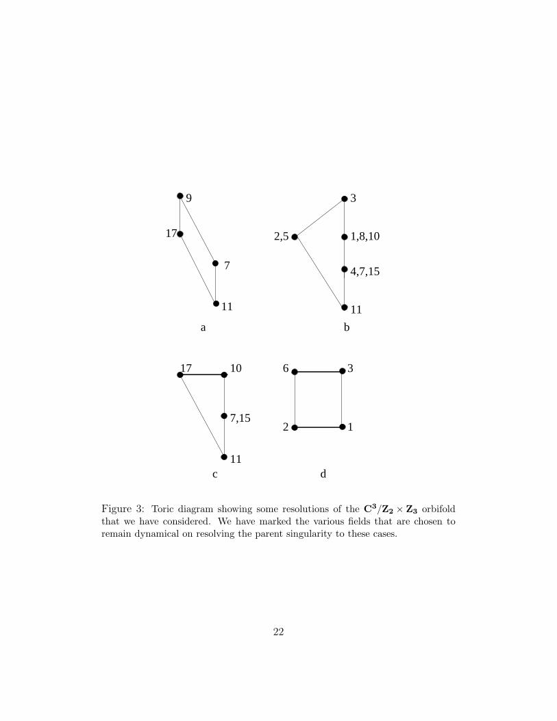
Figure 3: Toric diagram showing some resolutions of the C3/Z2 × Z3 orbifold

that we have considered. We have marked the various fields that are chosen toremain dynamical on resolving the parent singularity to these cases.

22

The dual of the kernel of Qred is given by

Ktred =

1 0 0 0 00 1 1 0 00 1 0 1 00 0 1 0 1

and the matter content and gauge group of the D-brane gauge theory isobtained as

dred =

(

0 1 1 −1 −10 −1 −1 1 1

)

The superpotential is written down, after noting that the field X1 is charge-less, and the relations X2X5 = X3X4 from the matrix Kt. It is given by

W = (X1 + φ) (X2X5 − X3X4) (45)

where φ is a possible adjoint. The matter content and the superpotential areexactly the same as in (24) and (25). This is of course as expected becauseboth describe the world volume theory of a D3-brane on the C2/Z2 singular-ity. This blowup corresponds to giving vevs to the fields X12, X23, X45. Theinvariant variables (30) are in this case

x′ = p7p210p15

y′ = p7p211p15

z = p17

w′ = p7p10p11p15 (46)

where x = x′2z; y = y′w′z; w = w′z. The blown up space is, from eq.(31), given by the equation x′y′ = w′2 in C3, which describes the blowup toC2/Z3 × C. Let us pause to comment here that the toric diagram of figure3(c) can be embedded both into that of C3/Z2 × Z3 and C3/Z2 × Z2; infact, this diagram is identical to that in figure 1(d). The fact that either em-bedding gives correct results for the D-brane gauge theory data shows thatthe inverse toric procedure is indeed consistent.

• Finally, let us discuss the toric diagram of figure 3(d). which is the conifoldobtained by partially resolving the C2/Z2 × Z3 singularity. Following the

23

same procedure as outlined in the previous examples, we start from thesolution set of (33) and select the fields [p1, p3, p6] which we set to zero. Fromthis, we obtain the solution x2 = ζ5 and x14 = (ζ1 + ζ2 + ζ5). Substitutingthis in the solution set and further setting ζ5 = 0 so that x2 = 0, we finallyobtain the full solution set to be

[x1 · · ·x17] = [0, 0, 0, (ζ1 + ζ2 + ζ4), ζ1, 0, ζ2, (ζ1 + ζ2 + ζ3 + ζ4), (ζ1 + ζ3),

ζ2, (ζ1 + 2ζ2 + ζ4)(ζ1 + ζ2 + ζ3 + ζ4), (ζ1 + ζ2 + ζ3 + ζ4),

(ζ1 + ζ3), (ζ1 + 2ζ2 + ζ4), (ζ1 + ζ2), (ζ1 + ζ2 + ζ3)] (47)

Hence, the fields that are dynamical are given by the set [p1, p2, p3, p6] whilethe rest acquire non-zero vev and hence are resolved, and in this case thereduced charge matrix is obtained from (20) to be

Q = (−1 1 1 − 1 ζ5) (48)

This blowup corresponds to the conifold. To see this, we define the in-variant variables (30) in this case by

x′ = p1p3 =w

z; y = p1p2; z = p2p6; w′ = p3p6 (49)

In this case, from (31), we can see that the remaining singularity is givenby the conifold x′y = zw′. Let us also mention that in terms of the originalvariables in eq. (28), this blowup corresponds to giving vevs to Y13, Y24, Z36.

4 D-branes on C4/Z2 × Z2 × Z2 and its blowups

We now consider D-branes on the orbifold C4/Z2 × Z2 × Z2 and some of itsblowups [26]. We will consider a D1-brane at this singularity, and the worldvolume theory is an N = (0, 2) SYM theory in two dimensions. The methodof construction of the moduli space of the D-1 brane is similar to the methodoutlined in sections 2 and 3. The unbroken gauge symmetry in this case is(apart from a redundant U(1)), U(1)7. The matter multiplet, after imposingthe appropriate projections consist of 32 surviving fields,

(X18, X27, X36, X45, X54, X63, X72, X81) , (Y15, Y26, Y37, Y48, Y51, Y62, Y73, Y84)

(Z13, Z24, Z31, Z42, Z57, Z68, Z75, Z86) , (W12, W21, W34, W43, W56, W65, W78, W87)(50)

24

The F-term constraints of eq. (5), in this case imply that out of the 32 fields,11 are independent, and the 32 initial fields can be solved in terms of these11, and the solutions can be denoted as vectors in the lattice Z11. The dualcone in this case has 34 homogeneous coordinates (matter fields) pα, and theredundancy in the definition of the initial independent coordinates in termsof these can be eliminated by introducing a set of 23 C∗ actions. The chargematrix Q for the C∗ actions is given in [26]. For the matrix denoting theoriginal U(1) charges expressed in terms of the homogeneous coordinates pα,we use the Moore-Penrose inverse of the matrix defining the dual cone, andconcatenate these two matrices to obtain the total charge matrix given inthe appendix. The toric diagram is given by the columns of the matrix

p1 p2 p3 p4 p5 p6 p7 p8 p9 p10 p11 p12 p13 p14 p15 p16 p17

1 0 1 0 1 2 1 0 0 1 0 1 1 1 1 1 11 1 1 1 0 0 0 0 0 0 2 1 0 1 1 1 11 0 0 1 1 0 0 1 2 1 0 0 0 1 1 1 10 0 0 −1 0 1 1 0 −1 0 −1 0 1 0 0 0 0

· · · · · ·

· · ·


1 0 0 0 1 1 1 1 1 1 0 1 1 1 1 1 11 1 0 0 1 1 1 1 1 1 1 1 1 1 1 1 11 1 0 1 1 1 1 1 1 1 0 1 1 1 1 1 10 −1 1 0 0 0 0 0 0 0 0 0 0 0 0 0 0

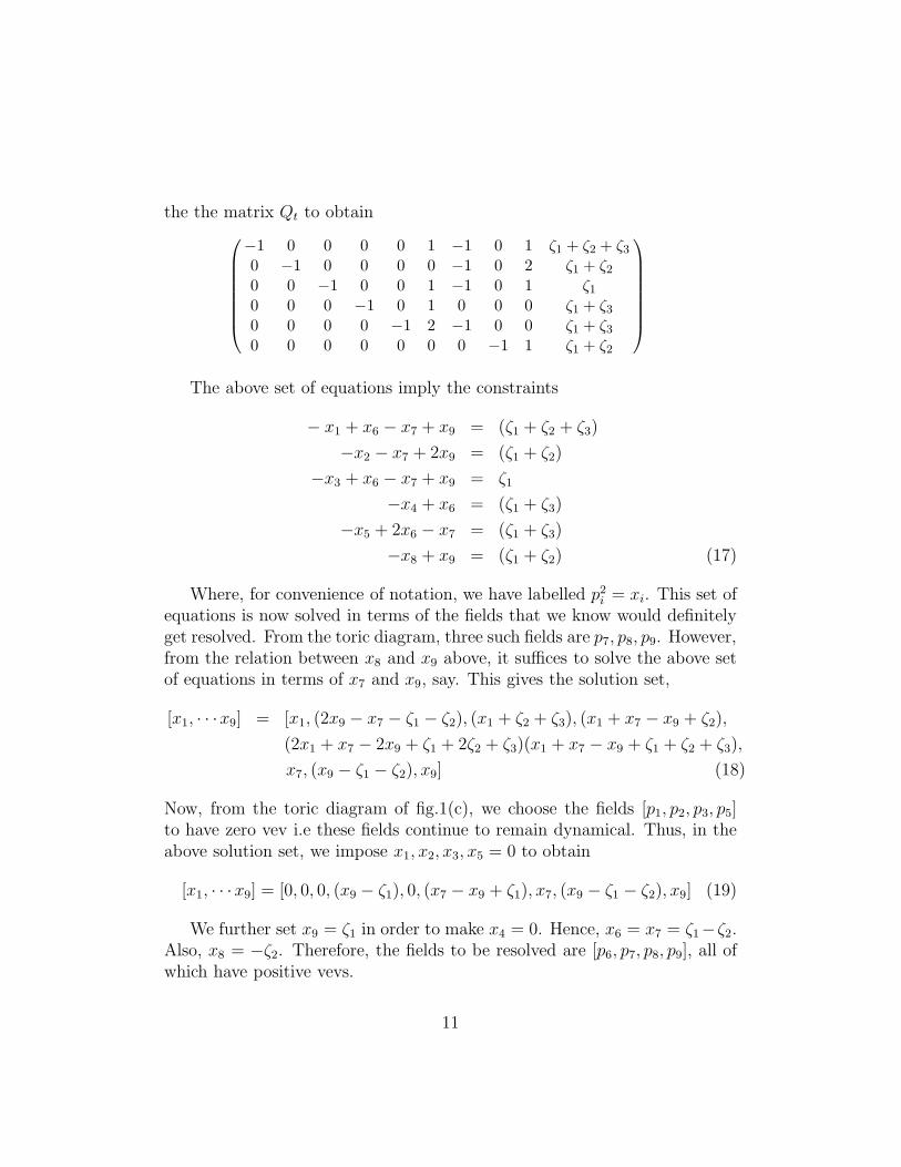
The distinct columns in the toric data are shown in fig. 4. The labelling ofthe vectors and the corresponding pα are as follows

a (2 0 0 1) [p6]

b (1 0 0 1) [p7, p13]

c (1 0 1 0) [p5, p10]

d (1 1 1 0) [p1, p14, p15, p16, p17, p18, p22, p23,

p24, p25, p26, p27, p29, p30, p31, p32, p33, p34]

e (1 1 0 0) [p3, p12]

f (0 0 0 1) [p20]

g (0 0 1 0) [p8, p21]

h (0 0 2 − 1) [p9]

25

��

��

��

��

��

��

��

��

��

��

��

��

��

��

��

��

��

��

��

��

��

��

��

��

��

��

��

��

��

��

��

��

��

��

��

��

��

��

��

��

��

��

��

��

��

��

��

��

��

��

��

��

��

��

��

��

��

��

��

��

a

fg

hi

j

k

(a)

h

g

f

k

ji

(b) (c)

b

c d e

h c a

Figure 4: Toric data for the orbifold C4/Z2 × Z2 × Z2 and two of its blowups to

the Z2 × Z2 singularity and the Z2 singularity.

26

i (0 1 1 − 1) [p4, p19]

j (0 2 0 − 1) [p11]

k (0 1 0 0) [p11] (51)

The invariant variables, in this case denoted by x = (X18X81); y = (Y15Y51);z = (Z13Z31); w = (W12W21); v = (X18Y84Z42W21), are

x = p1p2p7p8p13p14p15p16p17p18p220p21p22p23p24

p25p26p27p28p29p30p31p32p33p34

y = p1p2p3p4p211p12p14p15p16p17p18p19p22p23p24

p25p26p27p28p29p30p31p32p33p34

z = p1p4p5p8p29p10p14p15p16p17p18p19p21p22p23p24

p25p26p27p29p30p31p32p33p34

w = p1p3p5p26p7p10p12p13p14p15p16p17p18p22p23p24

p25p26p27p29p30p31p32p33p34

v = p21p2p3p4p5p6p7p8p9p10p11p12p13p

214p

215p

216p

217

p218p19p20p21p

222p

223p

224p

225p

226p

227p28p

229p

230p

231p

232p

233p

234 (52)

In terms of these variables, the space is defined by the surface xyzw = v2

in C5. Two of its resolutions (corresponding to cases (Vb and VIb of [26])are shown in figure 4.This singularity has to be analysed in the lines of [22] in order to determinewhether its partial resolutions are realised in the moduli space of the D-braneworld volume gauge theory. We leave this issue for future work, and for themoment analyse the blowups of this singularity into lower dimensional orb-ifold singularities, using the inverse toric procedure.

• Let us consider the blowup illustrated in fig. 4(b). Performing Gaus-sian row reduction on the total charge matrix, we find that for the rangeof the FI parameters ζ1 + ζ2 = 0; ζ3 + ζ4 = 0; ζ5 + ζ6 = 0, an appro-priate initial choice determines the fields that retain zero vev as the set[p2, p4, p8, p9, p11, p19, p20, p21, p28], while all others have non-zero vev and are

27

hence resolved. The reduced charge matrix is

Qredt =

0 1 0 −1 −1 1 0 0 0 0−1 0 0 0 1 0 1 0 −1 0−1 0 1 −1 1 0 0 1 −1 05 5 −5 0 −4 −1 0 1 −1 ζ5 + ζ6

−5 5 5 −4 0 −1 0 −1 1 ζ3 + ζ4

−1 −5 −5 4 0 1 0 1 5 ζ1 + ζ2

From the kernel of the charge matrix Qred, the transpose of its dual isobtained as

Kt =

1 1 0 1 0 1 0 0 0 0 0 01 0 1 0 0 0 1 0 1 0 0 01 0 0 1 0 0 0 0 1 0 1 00 1 1 0 1 0 0 0 0 1 0 00 1 0 0 0 1 0 0 0 1 0 10 0 1 0 1 0 1 1 0 0 0 0

From these matrices, we can extract the gauge theory data which is nowgiven by the matrix

dred =

0 −1 0 −1 −1 0 1 0 1 0 0 10 0 −1 1 0 1 0 1 −1 −1 0 01 1 1 0 0 0 0 −1 0 0 −1 −1−1 0 0 0 1 −1 −1 0 0 1 1 0

The gauge group is as expected, U(1)4 with 12 matter fields, and the super-potential is given by

W = X1X5X12 − X3X4X12 + X2X8X9 − X2X7X11 + X3X6X11

− X5X6X9 + X10X4X7 − X1X8X10 (53)

From the definition of the invariant variables in eq. (52), it can be seen thatthis space is C3/Z2 × Z2 defined by the equation xyz = v2 in C4. In termsof the original fields, it corresponds to giving vevs to the fields W12 and W21.

• Finally, we come to the example of fig. 4(c). In this case, in the region ofmoduli space given by ζ2 + ζ3 + ζ6 + ζ7 = 0, we find that the dynamical fieldsare given by the set [p5, p6, p9, p10], while the rest acquire non-zero vev andare resolved. The reduced charge matrix is

Qredt =

(

1 −1 −1 1 05 −2 −2 −1 ζ2 + ζ3 + ζ6 + ζ7

)

28

The matrix Kt is in this case given by

Kt =

1 1 0 01 0 1 00 1 0 1

Which specifies the matter content as a U(1)2 gauge theory with the chargematrix given, as expected, by

dred =

(

−1 −1 1 11 1 −1 −1

)

With a superpotential W = φ (X1X4 − X2X3) with φ being a possiblechargeless field. In terms of the original fields in the theory, this resolu-tion corresponds to giving vevs to X18, X81, Y15, Y51, and the resulting spaceis the C2/Z2 orbifold zw = v2 that we have discussed earlier.

5 Discussions

In this paper, we have critically examined the inverse procedure of obtainingthe world volume gauge theory data of D-branes probing certain toric singu-larities and their blowups from the geometric data of the resolution. We haveshown that the algorithm of [21] gives consistent results, for a given singu-larity that can be reached by partial resolutions of different parent theories.We have explicitly checked several partial resolutions of orbifolds of the formC3/Γ and C4/Γ and found the results to be in agreement with field theorycalculations. However, as pointed out in [21], in the presence of chargelessfields in the matter multiplet, the procedure cannot be used to specify thesuperpotential interaction uniquely, because of the inherent problem in thehandling of such fields by toric methods.

We have treated the simplest examples of the resolution of theC4/Z2 × Z2 × Z2 singularity in this paper. It would be interesting to inves-tigate the various partial resolutions of the moduli space of D-branes on thissingularity the lines of [22] and determine the gauge theory data thereof.

Finally, as noted in [21], the ambiguities that exist in the inverse algorithmseem to imply that in some cases, different gauge theories, in the infra redlimit flow to theories with identical moduli space. We have not dealt withthis aspect in the present paper, and it would be an interesting direction forfuture work.

29

Acknowledgements

I would like to thank I. Biswas, S. Bhattacharjee, P. Chatterjee and D. Sur-yaramana for helpful discussions.

30

Appendix

Charge matrix for the partial resolutions of C3/Z2 × Z2 × Z2:

Qt =


0 0 0 0 1 −1 0 0 −1 1 0 0 0 0 0 0 0

0 0 1 0 0 −1 0 0 0 0 −1 1 0 0 0 0 0

−1 0 0 0 1 0 0 1 −1 0 0 0 −1 1 0 0 0

1 −1 0 −1 −1 0 −1 0 0 0 0 0 0 0 1 0 0

1 −1 −1 0 −1 0 0 −1 0 0 0 0 0 0 0 1 0

1 −1 0 −1 0 −1 0 −1 0 0 0 0 0 0 0 0 1

−1 0 1 1 1 −1 0 0 −1 0 −1 0 0 0 0 0 0

0 0 0 1 0 0 0 0 −1 0 −1 0 0 0 0 0 0

0 0 0 0 0 1 −1 0 0 0 0 0 −1 0 0 0 0

0 0 0 0 0 1 −1 1 −1 0 0 0 −1 0 0 0 0

−2 1 1 1 1 0 0 1 −1 0 −1 0 −1 0 0 0 0

1 0 −1 −1 0 0 −1 −1 0 0 0 0 0 0 0 0 0

1 −1 −1 0 0 0 −1 0 −1 0 0 0 0 0 0 0 0

−1 1 1 0 0 0 0 0 0 0 −1 0 −1 0 0 0 0

−1 0 1 1 0 0 0 1 −1 0 −1 0 −1 0 0 0 0

2 −1 −1 −1 −1 0 −1 −1 0 0 0 0 0 0 0 0 0

0 1 0 0 0 1 −1 0 0 0 −1 0 −1 0 0 0 0

1 0 −1 −1 −1 1 −1 0 0 0 0 0 −1 0 0 0 0

−1 1 0 1 0 1 −1 1 −1 0 −1 0 −1 0 0 0 0

−1 1 1 0 1 0 −1 1 −1 0 −1 0 −1 0 0 0 0

−1 1 0 1 1 0 0 0 −1 0 −1 0 −1 0 0 0 0

1 0 0 0 −1 0 −1 −1 0 0 −1 0 0 0 0 0 0

1 0 0 0 0 0 −1 0 −1 0 −1 0 −1 0 0 0 0

−5 −2 −2 −2 −2 0 −2 −2 0 2 0 2 2 1 −3 −3 −1

−1 −2 2 −2 2 0 2 −2 0 −2 0 −2 −2 −3 1 1 −5

−1 −2 −2 2 2 0 −2 2 0 −2 0 2 2 −3 1 1 3

3 −2 2 2 −2 0 2 2 0 2 0 −2 −2 1 −3 −3 −1

−1 2 2 2 −2 0 −2 −2 0 2 0 −2 2 5 1 1 3

3 2 −2 2 2 0 2 −2 0 −2 0 2 −2 1 5 −3 −1

3 2 2 −2 2 0 −2 2 0 −2 0 −2 2 1 −3 5 −1

· · · · · ·

· · ·

p18 p19 p20 p21 p22 p23 p24 p25 p26 p27 p28 p29 p30 p31 p32 p33 p34 p35

0 0 0 0 0 0 0 0 0 0 0 0 0 0 0 0 0 0

0 0 0 0 0 0 0 0 0 0 0 0 0 0 0 0 0 0

0 0 0 0 0 0 0 0 0 0 0 0 0 0 0 0 0 0

0 0 0 0 0 0 0 0 0 0 0 0 0 0 0 0 0 0

0 0 0 0 0 0 0 0 0 0 0 0 0 0 0 0 0 0

0 0 0 0 0 0 0 0 0 0 0 0 0 0 0 0 0 0

1 0 0 0 0 0 0 0 0 0 0 0 0 0 0 0 0 0

0 1 0 0 0 0 0 0 0 0 0 0 0 0 0 0 0 0

0 0 1 0 0 0 0 0 0 0 0 0 0 0 0 0 0 0

0 0 0 1 0 0 0 0 0 0 0 0 0 0 0 0 0 0

0 0 0 0 1 0 0 0 0 0 0 0 0 0 0 0 0 0

0 0 0 0 0 1 0 0 0 0 0 0 0 0 0 0 0 0

0 0 0 0 0 0 1 0 0 0 0 0 0 0 0 0 0 0

0 0 0 0 0 0 0 1 0 0 0 0 0 0 0 0 0 0

0 0 0 0 0 0 0 0 1 0 0 0 0 0 0 0 0 0

0 0 0 0 0 0 0 0 0 1 0 0 0 0 0 0 0 0

0 0 0 0 0 0 0 0 0 0 1 0 0 0 0 0 0 0

0 0 0 0 0 0 0 0 0 0 0 1 0 0 0 0 0 0

0 0 0 0 0 0 0 0 0 0 0 0 1 0 0 0 0 0

0 0 0 0 0 0 0 0 0 0 0 0 0 1 0 0 0 0

0 0 0 0 0 0 0 0 0 0 0 0 0 0 1 0 0 0

0 0 0 0 0 0 0 0 0 0 0 0 0 0 0 1 0 0

0 0 0 0 0 0 0 0 0 0 0 0 0 0 0 0 1 0

1 2 0 2 2 −3 −1 1 3 −2 2 −1 1 3 3 −1 5 ζ1−3 2 0 2 −2 1 3 −3 −1 2 2 3 5 −1 −1 3 1 ζ2−3 −2 0 −2 −2 1 −5 5 −1 2 2 3 −3 −1 −1 3 1 ζ31 −2 0 −2 2 5 −1 1 −5 −2 2 −1 1 3 3 −1 −3 ζ4−3 −2 0 2 −2 1 3 −3 −1 2 −2 3 −3 −1 −1 −5 1 ζ51 −2 0 2 2 −3 −1 1 3 −2 −2 −1 1 3 −5 −1 −3 ζ61 2 0 −2 2 −3 −1 1 3 −1 −1 −1 1 −5 3 −1 −3 ζ7

References

31

[1] M. R. Douglas, D. Kabat, P. Pouliot, S. Shenker, “D-branes andShort Distances in String Theory,” Nucl. Phys. B485 (1997) 85,hep-th/9608024.

[2] B. Greene, Y. Kanter, “Small Volumes in Compactified String Theory,”Nucl. Phys. B497 (1997) 127, hep-th/9612181.

[3] P. Aspinwall, B. Greene, D. Morrison, “Calabi-Yau Moduli Space, Mir-ror Manifolds and Space-time Topology Change in String Theory,” Nucl.Phys. B416 (1994) 78, hep-th/9309097.

[4] E. Witten, “Phases of N = 2 Theories in Two Dimensions,” Nucl. Phys.B403 (1993) 159, hep-th/9301042.

[5] M. Douglas, B. Greene, D. Morrison, “Orbifold Resolution by D-branes,”Nucl. Phys. B506 (1997) 84, hep-th/9704151.

[6] E. Witten, “Phase Transitions in M Theory and F Theory,” Nucl. Phys.B471 (1996) 195, hep-th/9603150.

[7] T. Muto, “D-branes on Orbifolds and Topology Change,” Nucl.Phys.B521 (1998) 183, hep-th/9711090.

[8] M. Douglas, G. Moore, “D-branes, Quivers, and ALE Instantons.”hep-th/9603167.

[9] C. Johnson, R. Myers, “Aspects of Type IIB Theory on ALE Spaces,”Phys. Rev. D55 (1997) 6382, hep-th/9610140.

[10] M. Douglas, B. Greene, “Metrics on D-brane Orbifolds,” Adv. Theor.Math. Phys. 1 (1998) 184, hep-th/9707214.

[11] M. Douglas, A. Kato, H. Ooguri, Adv. Theor. Math. Phys. 1 (1998) 237,hep-th/9708012.

[12] T. Muto, “Brane Configurations for Three-Dimensional NonabelianOrbifolds,” hep-th/9905230.

[13] B. Feng, A. Hanany, Y. He, “Z-D-brane Box Models and NonchiralDihedral Quivers,” hep-th/9909125.

32














[14] K. Oh, R. Tatar, “Branes at Orbifolded Conifold Singularities andSupersymmetric Gauge Field Theories,” JHEP 9910i (1999) 0319,hep-th/9906012

[15] M. Cvetic, L. Everett, P. Langacker, J. Wang, “Blowing upthe Four-Dimensional Z(3) Orientifold,” JHEP 9904 (1999) 020,hep-th/9903051

[16] W. Fulton, Introduction to Toric Varieties, Princeton UniversityPress, 1993.

[17] D. Cox, alg-geom/9606016.

[18] E. Gimon, J. Polchinski, “Consistency Conditions for Orientifolds andD Manifolds,” Phys. Rev. D54 (1996) 1667, hep-th/9601038.

[19] B. Greene, “D-brane Topology Changing Transitions,” Nucl.Phys. B525

(1998) 284, hep-th/9711124.

[20] S. Mukhopadhay, K. Ray, “Conifolds from D-branes,” Phys. Lett. B423

(1998) 247, hep-th/9711131.

[21] B. Feng, A. Hanany, Y. He, hep-th/0003085.

[22] C. Beasley, B. Greene, C. Lazaroiu, M. Plesser, “D3-branes on PartialResolutions of Abelian Quotient Singularities of Calabi-Yau Threefolds,”Nucl. Phys. B553 (1999) 711, hep-th/9907186.

[23] J. Park, R. Rabadan, A. M. Uranga, hep-th/9907086, “Orientifoldingthe Conifold,” Nucl.Phys. B570 (2000) 38, hep-th/9907086.

[24] A. Uranga, “Brane Configurtions for Branes at Conifolds,” JHEP 9901

(1999) 022, hep-th/9811004

[25] D. Morrison, R. Plesser, “Nonspherical Horizons 1,” Adv. Theor. Math.Phys. 3 (1999) 1, hep-th/9810201.

[26] A. Ahn, H. Kim, “Branes at C4/Γ Singularity from Toric Geometry,”JHEP 9904 (1999) 012, hep-th/9903181.

[27] K. Mohri, “D-branes and Quotient Singularities of Calabi-Yau Four-folds,”, Nucl. Phys. B521 (1998) 161, hep-th/9707012

33



http://arxiv.org/abs/alg-geom/9606016












D-brane gauge theories from toric singularities and toric duality ☆ ☆ Research supported in part...

Documents

Transcript of D-brane gauge theories from toric singularities and toric duality ☆ ☆ Research supported in part...