Cross-Modality Feature Learning for Three-Dimensional Brain ...
164
Cross-Modality Feature Learning for Three-Dimensional Brain Image Synthesis Yawen Huang Department of Electronic and Electrical Engineering University of Sheffield This dissertation is submitted for the degree of Doctor of Philosophy August 2018
-
Upload
khangminh22 -
Category
Documents
-
view
2 -
download
0
Transcript of Cross-Modality Feature Learning for Three-Dimensional Brain ...

Cross-Modality Feature Learning forThree-Dimensional Brain Image
Synthesis
Yawen Huang
Department of Electronic and Electrical EngineeringUniversity of Sheffield
This dissertation is submitted for the degree ofDoctor of Philosophy
August 2018


I would like to dedicate this thesis to my loving parents.

Declaration
I hereby declare that the work contained in this thesis are original and have not been submittedin whole or in part for any other degree or qualification. This thesis is my own work andincludes nothing which is the outcome of work done in collaboration except where specificallyclarified in the texts and acknowledgements. Some parts of the work presented in this thesishave been, or are due to be published in the following articles.
• Y. Huang, and L. Shao. Task-Driven Bidirectional Fault-Aware Adversarial Networksfor Three-dimensional Brain Image Analysis. To be submitted, 2018.
• Y. Huang, and L. Shao. Simultaneous Super-Resolution and Cross-Modality Synthesisin Magnetic Resonance Imaging. To be submitted, 2018.
• Y. Huang, L. Shao, and A. F. Frangi. Cross-Modality Image Synthesis via Weakly-Coupled and Geometry Co-Regularized Joint Dictionary Learning. IEEE Transactionson Medical Imaging (TMI), 2017.
• Y. Huang, L. Shao, and A. F. Frangi. Simultaneous Super-Resolution and Cross-ModalitySynthesis of 3D Medical Images using Weakly-Supervised Joint Convolutional SparseCoding. In Proceedings of the IEEE Conference on Computer Vision and PatternRecognition (CVPR), July 2017.
• Y. Huang, L. Shao, and A. F. Frangi. DOTE: Dual Convolutional Filter Learning forSuper-Resolution and Cross-Modality Synthesis in MRI. In International Conference onMedical Image Computing and Computer-Assisted Intervention (MICCAI), pages 89–98,2017.
• Y. Huang, F. Zhu, L. Shao, and A. F. Frangi. Color Object Recognition via Cross-Domain Learning on RGB-D Images. In IEEE International Conference on Roboticsand Automation (ICRA) (oral), 2016, pp. 1672–1677.
• Y. Huang, L. Beltrachini, L. Shao, and A. F. Frangi. Geometry Regularized Joint Dictio-nary Learning for Cross-Modality Image Synthesis in Magnetic Resonance Imaging. In
vi
MICCAI Workshop on Simulation and Synthesis in Medical Imaging (SASHIMI) (oral),Springer, 2016, pp. 118–126.
• Y. Huang, L. Beltrachini, L. Shao, and A. F. Frangi. Magnetic Resonance ImagingCross-Modality Synthesis. In International Society for Magnetic Resonance in Medicine(ISMRM), no. 4220, 2016.
• D. Wang, Y. Huang, and A. F. Frangi. Region-Enhanced Joint Dictionary Learningfor Cross-Modality Synthesis in Diffusion Tensor Imaging. In MICCAI Workshop onSimulation and Synthesis in Medical Imaging (SASHIMI), Springer, 2017, pp. 41–48.
Yawen HuangAugust 2018
Acknowledgements
I would like to acknowledge my supervisors Prof. Ling Shao and Prof. Geraint W Jewell fortheir expert supervisions and continuous encouragements over the past four years. It has been agreat pleasure and honor working under the guidance of Prof. Ling, whose profession, foresightand patience for works pulling at me. I am very grateful to him for teaching me not just aboutsome technical skills or the art of communicating ideas, but for teaching me how to think.
A special thanks to Prof. Alejandro F. Frangi for shaping how I think about research andbeing able to provide considerable intellectual input into the research that I have done to date.
I would like to thank my friends and colleges: Dr. Simon Jones, Dr. Ruomei Yan, Dr. DiWu, Dr. Fan Zhu, Dr. Mengyang Yu, Dr. Yang Long, Dr. Ziyun Cai, Dr. Feng Zheng, Dr. ZeikeTaylor, Dr. Ali Gooya, Dr. Leandro Beltrachini, Dr. Jose Pozo, Dr. Nishant Ravikumar, Dr.Marco Pereanez, Dr. Serkan Cimen, Dr. Bo Dong, Redzuan Bin Abdul Manap, BingzhangHu, Yi Zhou, Yunbai Wang, Le Zhang, Yuanjun Lu, Junyu Jiang, Tiantian Dou, and DanyangWang (who is my best friend). I would also like to thank many other reviewers for their helpfulcomments and discussions.
I am also very grateful to my thesis examiners Prof. Jianguo Zhang and Dr. Wei Liu, whooffered insightful discussions and constructive suggestions for my research. Many specialthanks are due to them for serving on reading my thesis, chairing my oral examination andproviding valuable feedbacks to refine my thesis.
I would like to thank my assessors Dr. Charith Abhayaratne and Dr. Xiaoli Chu for theirinvaluable suggestions and comments for assessing my confirmation review report and vivaduring my first year PhD study.
I specially thank Dr. Thomas Walther in our department for his kind support and suggestions.I also owe a great deal to the postgraduate administrators, Ms. Hilary J. Levesley and Ms.Frances G. Bright.
Thank you to the head of the department Prof. Geraint W Jewell, who has supported meand helped me when I was in trouble. I am very grateful to Prof. Geraint for his continuedsupport and explicit decision during the most difficult times.
I also would like to thank the departmental Learned Society Fund and the British MachineVision Association for their financial support of my conference trips through my PhD.

viii
Finally, I would like to thank my parents for their selfless love, unconditional support andimmense encouragement in the past 26 years.
Abstract
Multi-modality medical imaging is increasingly used for comprehensive assessment of complexdiseases in either diagnostic examinations or as part of medical research trials. Differentimaging modalities provide complementary information about living tissues. However, multi-modal examinations are not always possible due to adversary factors such as patient discomfort,increased cost, prolonged scanning time and scanner unavailability. In addition, in large imagingstudies, incomplete records are not uncommon owing to image artifacts, data corruption or dataloss, which compromise the potential of multi-modal acquisitions. Moreover, independently ofhow well an imaging system is, the performance of the imaging equipment usually comes toa certain limit through different physical devices. Additional interferences arise (particularlyfor medical imaging systems), for example, limited acquisition times, sophisticated and costlyequipment and patients with severe medical conditions, which also cause image degradation.The acquisitions can be considered as the degraded version of the original high-quality images.
In this dissertation, we explore the problems of image super-resolution and cross-modalitysynthesis for one Magnetic Resonance Imaging (MRI) modality from an image of anotherMRI modality of the same subject using an image synthesis framework for reconstructing themissing/complex modality data. We develop models and techniques that allow us to connect thedomain of source modality data and the domain of target modality data, enabling transformationbetween elements of the two domains. In particular, we first introduce the models that projectboth source modality data and target modality data into a common multi-modality featurespace in a supervised setting. This common space then allows us to connect cross-modalityfeatures that depict a relationship between each other, and we can impose the learned associationfunction that synthesizes any target modality image. Moreover, we develop a weakly-supervisedmethod that takes a few registered multi-modality image pairs as training data and generatesthe desired modality data without being constrained a large number of multi-modality imagescollection of well-processed (e.g., skull-stripped and strictly registered) brain data. Finally, wepropose an approach that provides a generic way of learning a dual mapping between source andtarget domains while considering both visually high-fidelity synthesis and task-practicability.We demonstrate that this model can be used to take any arbitrary modality and efficientlysynthesize the desirable modality data in an unsupervised manner.

x
We show that these proposed models advance the state-of-the-art on image super-resolutionand cross-modality synthesis tasks that need jointly processing of multi-modality images andthat we can design the algorithms in ways to generate the practically beneficial data to medicalimage analysis.
Table of contents
List of figures xv
List of tables xix
Nomenclature xxi
1 Introduction and Literature Review 11.1 Background . . . . . . . . . . . . . . . . . . . . . . . . . . . . . . . . . . . 11.2 Imaging Modalities . . . . . . . . . . . . . . . . . . . . . . . . . . . . . . . 21.3 Challenges . . . . . . . . . . . . . . . . . . . . . . . . . . . . . . . . . . . . 41.4 Dictionary Learning . . . . . . . . . . . . . . . . . . . . . . . . . . . . . . . 61.5 Convolutional Sparse Coding . . . . . . . . . . . . . . . . . . . . . . . . . . 81.6 Datasets . . . . . . . . . . . . . . . . . . . . . . . . . . . . . . . . . . . . . 101.7 Related Work . . . . . . . . . . . . . . . . . . . . . . . . . . . . . . . . . . 12
1.7.1 Nature Image Domain . . . . . . . . . . . . . . . . . . . . . . . . . 121.7.2 Medical Image Domain . . . . . . . . . . . . . . . . . . . . . . . . . 13
1.8 Thesis Outline . . . . . . . . . . . . . . . . . . . . . . . . . . . . . . . . . . 151.9 Contributions . . . . . . . . . . . . . . . . . . . . . . . . . . . . . . . . . . 15
2 Feature-Clustered and Normalized Joint Sparse Representation 172.1 Introduction . . . . . . . . . . . . . . . . . . . . . . . . . . . . . . . . . . . 182.2 Background . . . . . . . . . . . . . . . . . . . . . . . . . . . . . . . . . . . 21
2.2.1 Image Degradation Model . . . . . . . . . . . . . . . . . . . . . . . 212.2.2 Dictionary Learning . . . . . . . . . . . . . . . . . . . . . . . . . . 22
2.3 Method . . . . . . . . . . . . . . . . . . . . . . . . . . . . . . . . . . . . . 222.3.1 Data Description . . . . . . . . . . . . . . . . . . . . . . . . . . . . 232.3.2 Gradient Feature Representation . . . . . . . . . . . . . . . . . . . . 232.3.3 Cross-Modality Dictionary Learning . . . . . . . . . . . . . . . . . . 252.3.4 Clustering-based Globally Redundant Codes . . . . . . . . . . . . . 26
xii Table of contents
2.4 Experiments . . . . . . . . . . . . . . . . . . . . . . . . . . . . . . . . . . . 292.4.1 Dictionary Size . . . . . . . . . . . . . . . . . . . . . . . . . . . . . 302.4.2 Sparsity . . . . . . . . . . . . . . . . . . . . . . . . . . . . . . . . . 312.4.3 MRI Super-Resolution . . . . . . . . . . . . . . . . . . . . . . . . . 322.4.4 Simultaneous Super-Resolution & Cross-Modality Synthesis . . . . . 32
2.5 Conclusions . . . . . . . . . . . . . . . . . . . . . . . . . . . . . . . . . . . 34
3 Dual Convolutional Filter Learning 393.1 Introduction . . . . . . . . . . . . . . . . . . . . . . . . . . . . . . . . . . . 393.2 Background . . . . . . . . . . . . . . . . . . . . . . . . . . . . . . . . . . . 40
3.2.1 Convolutional Sparse Coding . . . . . . . . . . . . . . . . . . . . . 403.2.2 Dual Learning . . . . . . . . . . . . . . . . . . . . . . . . . . . . . 413.2.3 Problem Formulation . . . . . . . . . . . . . . . . . . . . . . . . . . 41
3.3 Method . . . . . . . . . . . . . . . . . . . . . . . . . . . . . . . . . . . . . 423.3.1 Dual Convolutional Filter Learning . . . . . . . . . . . . . . . . . . 423.3.2 Optimization . . . . . . . . . . . . . . . . . . . . . . . . . . . . . . 433.3.3 Synthesis . . . . . . . . . . . . . . . . . . . . . . . . . . . . . . . . 45
3.4 Experimental Results . . . . . . . . . . . . . . . . . . . . . . . . . . . . . . 453.4.1 Experimental Setup . . . . . . . . . . . . . . . . . . . . . . . . . . . 45
3.5 Conclusions . . . . . . . . . . . . . . . . . . . . . . . . . . . . . . . . . . . 47
4 Weakly-Supervised Joint Convolutional Sparse Coding 514.1 Introduction . . . . . . . . . . . . . . . . . . . . . . . . . . . . . . . . . . . 524.2 Preliminaries . . . . . . . . . . . . . . . . . . . . . . . . . . . . . . . . . . 53
4.2.1 Problem Formulation . . . . . . . . . . . . . . . . . . . . . . . . . . 544.2.2 Notation . . . . . . . . . . . . . . . . . . . . . . . . . . . . . . . . 55
4.3 Weakly-Supervised Joint Convolutional Sparse Coding . . . . . . . . . . . . 554.3.1 Hetero-Domain Image Alignment . . . . . . . . . . . . . . . . . . . 554.3.2 Objective Function . . . . . . . . . . . . . . . . . . . . . . . . . . . 564.3.3 Optimization . . . . . . . . . . . . . . . . . . . . . . . . . . . . . . 584.3.4 Synthesis . . . . . . . . . . . . . . . . . . . . . . . . . . . . . . . . 61
4.4 Experimental Results . . . . . . . . . . . . . . . . . . . . . . . . . . . . . . 624.4.1 Brain MRI Super-Resolution . . . . . . . . . . . . . . . . . . . . . . 634.4.2 Simultaneous Super-Resolution and Cross-Modality Synthesis . . . . 63
4.5 Conclusions . . . . . . . . . . . . . . . . . . . . . . . . . . . . . . . . . . . 67
Table of contents xiii
5 Geometry Constrained Dictionary Learning 695.1 Geometry Regularized Joint Dictionary Learning . . . . . . . . . . . . . . . 69
5.1.1 Introduction . . . . . . . . . . . . . . . . . . . . . . . . . . . . . . . 705.1.2 Method . . . . . . . . . . . . . . . . . . . . . . . . . . . . . . . . . 715.1.3 Experiments . . . . . . . . . . . . . . . . . . . . . . . . . . . . . . 755.1.4 Summary . . . . . . . . . . . . . . . . . . . . . . . . . . . . . . . . 77
5.2 Weakly-Coupled and Geometry Co-Regularized Joint Dictionary Learning . . 785.2.1 Introduction . . . . . . . . . . . . . . . . . . . . . . . . . . . . . . . 785.2.2 Method . . . . . . . . . . . . . . . . . . . . . . . . . . . . . . . . . 805.2.3 Experiments . . . . . . . . . . . . . . . . . . . . . . . . . . . . . . 915.2.4 Discussions . . . . . . . . . . . . . . . . . . . . . . . . . . . . . . . 995.2.5 Conclusions . . . . . . . . . . . . . . . . . . . . . . . . . . . . . . . 100
6 Task-Driven Bidirectional Fault-Aware Adversarial Networks 1036.1 Introduction . . . . . . . . . . . . . . . . . . . . . . . . . . . . . . . . . . . 1046.2 Related Work . . . . . . . . . . . . . . . . . . . . . . . . . . . . . . . . . . 106
6.2.1 Cross-Modality Synthesis . . . . . . . . . . . . . . . . . . . . . . . 1066.2.2 Medical Image Analysis . . . . . . . . . . . . . . . . . . . . . . . . 108
6.3 Task-Driven Bidirectional Fault-Aware Adversarial Networks . . . . . . . . . 1096.3.1 Preliminaries . . . . . . . . . . . . . . . . . . . . . . . . . . . . . . 1096.3.2 Problem Formulation . . . . . . . . . . . . . . . . . . . . . . . . . . 1096.3.3 Jointly-Adapted Bidirectional Loss . . . . . . . . . . . . . . . . . . 1106.3.4 Fault-Aware Discriminator . . . . . . . . . . . . . . . . . . . . . . . 1126.3.5 Objective Function . . . . . . . . . . . . . . . . . . . . . . . . . . . 113
6.4 Implementation . . . . . . . . . . . . . . . . . . . . . . . . . . . . . . . . . 1146.4.1 Network Structures . . . . . . . . . . . . . . . . . . . . . . . . . . . 1146.4.2 Training Details . . . . . . . . . . . . . . . . . . . . . . . . . . . . . 115
6.5 Experiments . . . . . . . . . . . . . . . . . . . . . . . . . . . . . . . . . . . 1156.5.1 Experimental Setup . . . . . . . . . . . . . . . . . . . . . . . . . . . 1156.5.2 Segmentation-Driven Synthesis . . . . . . . . . . . . . . . . . . . . 119
6.6 Conclusions . . . . . . . . . . . . . . . . . . . . . . . . . . . . . . . . . . . 120
7 Conclusions and Future Directions 1237.1 Conclusions . . . . . . . . . . . . . . . . . . . . . . . . . . . . . . . . . . . 1237.2 Future Works . . . . . . . . . . . . . . . . . . . . . . . . . . . . . . . . . . 124
7.2.1 Discrimination Capability . . . . . . . . . . . . . . . . . . . . . . . 1257.2.2 Conditional GAN . . . . . . . . . . . . . . . . . . . . . . . . . . . . 125

xiv Table of contents
7.2.3 4D Cardiac Data . . . . . . . . . . . . . . . . . . . . . . . . . . . . 126
References 127
Appendix A Parallel Contrast Experiment 141
List of figures
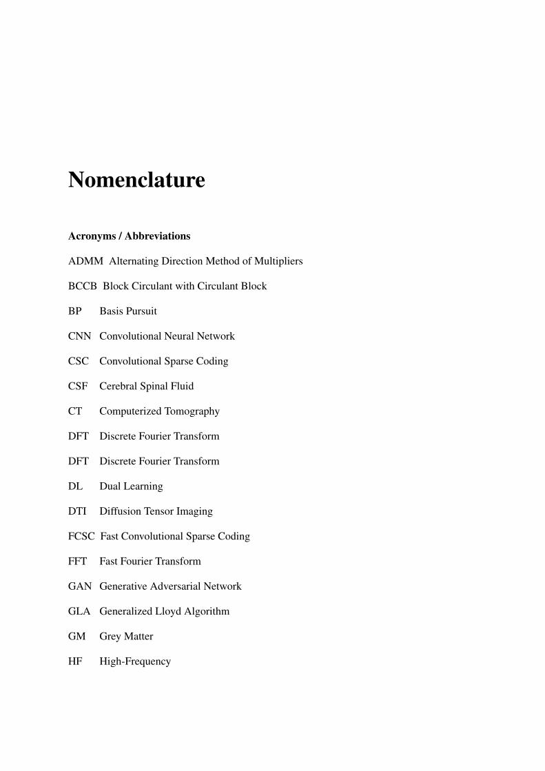
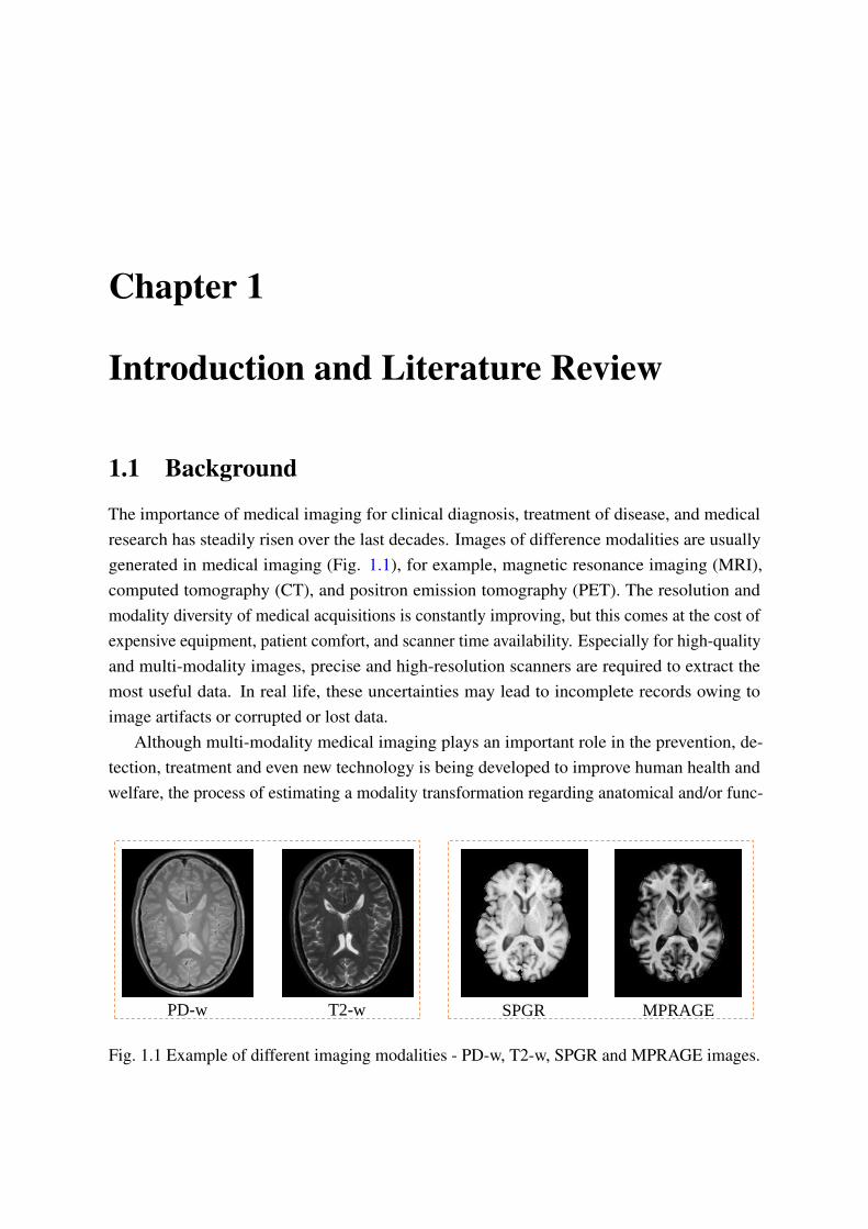
1.1 Example of different imaging modalities - PD-w, T2-w, SPGR and MPRAGEimages. . . . . . . . . . . . . . . . . . . . . . . . . . . . . . . . . . . . . . 1
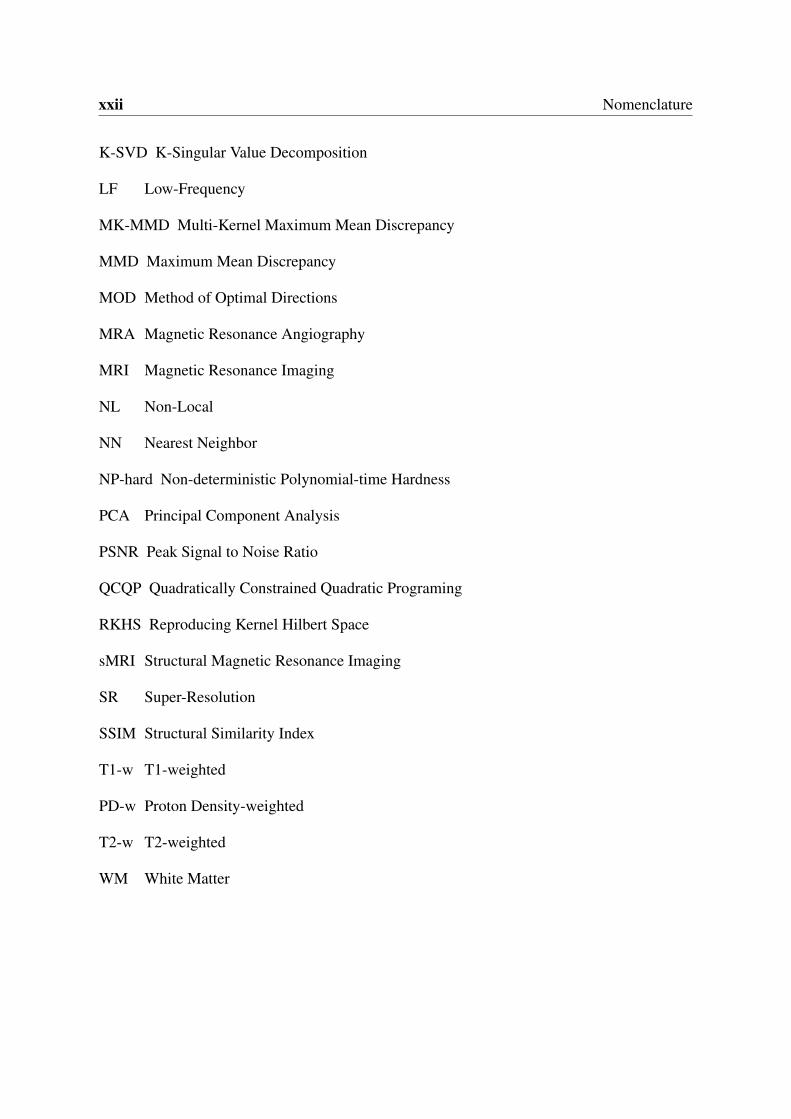
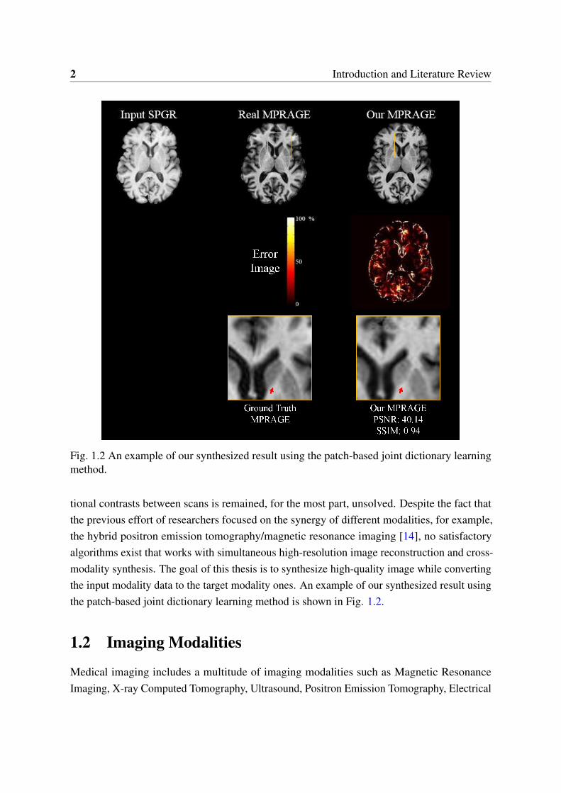
1.2 An example of our synthesized result using the patch-based joint dictionarylearning method. . . . . . . . . . . . . . . . . . . . . . . . . . . . . . . . . 2
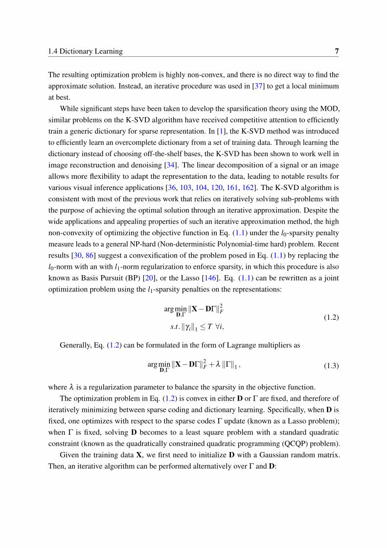
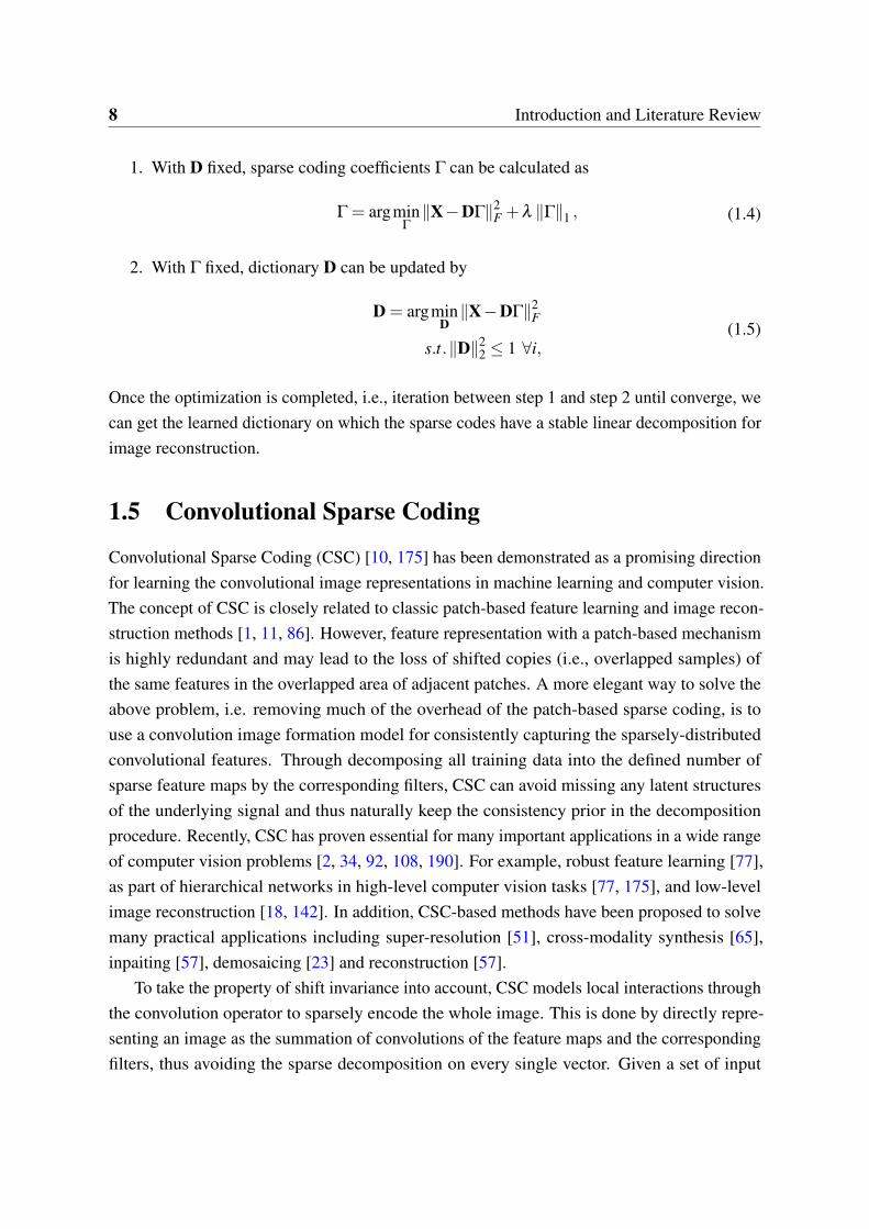
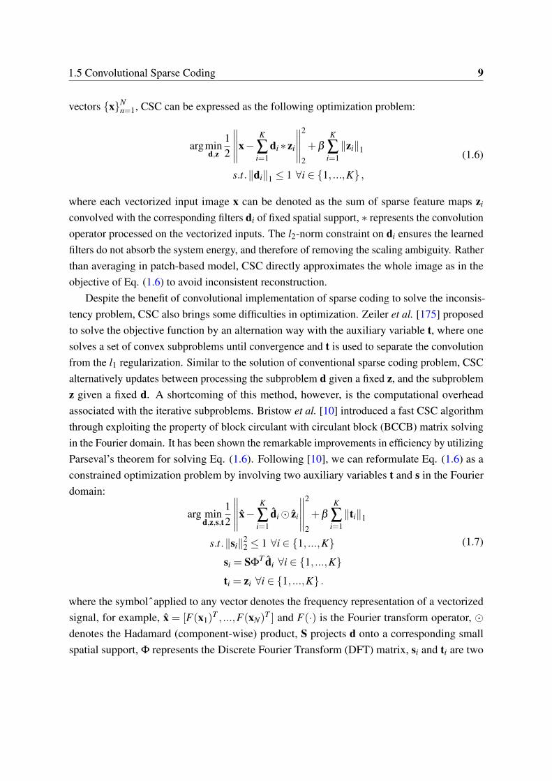
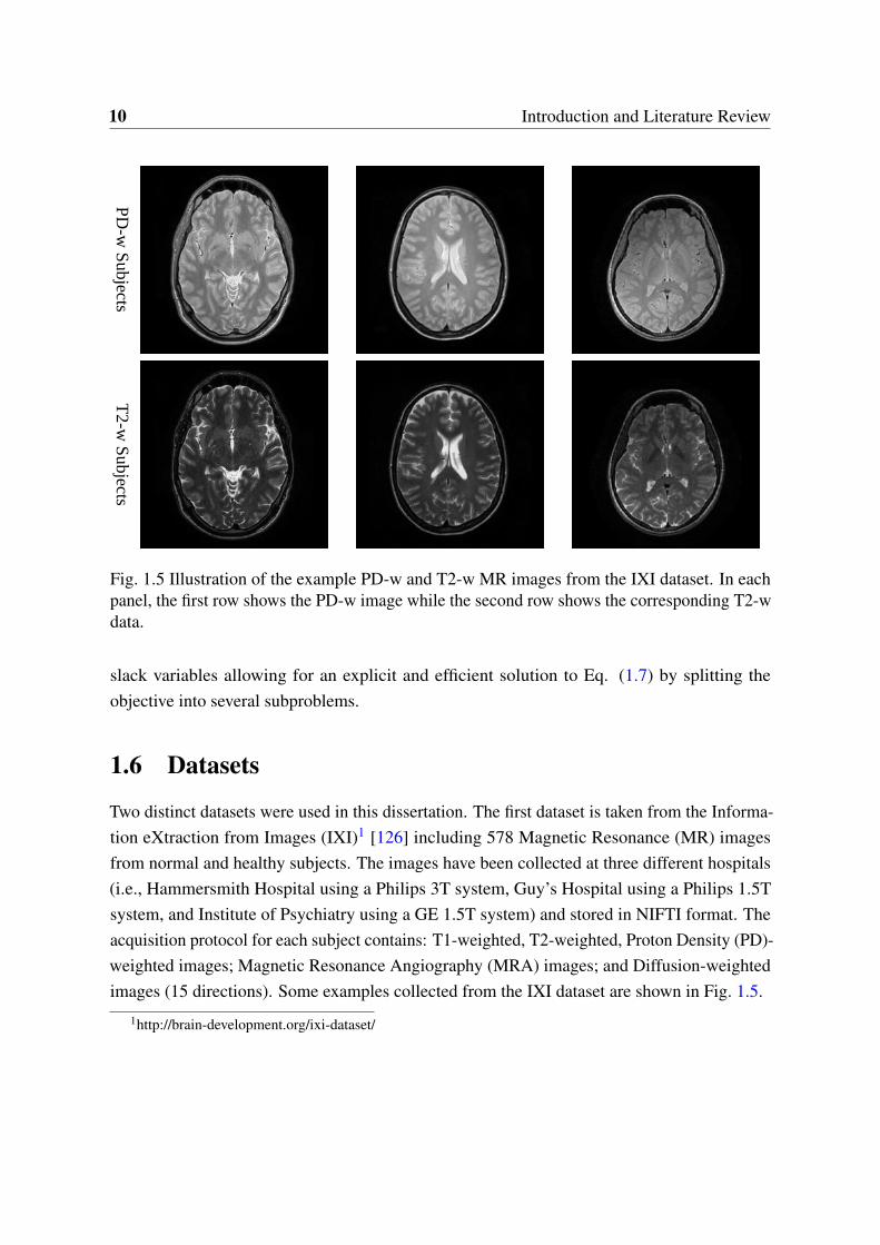
1.3 histogram matching model. . . . . . . . . . . . . . . . . . . . . . . . . . . . 41.4 A patch-based cross-modality synthesis schema. . . . . . . . . . . . . . . . . 51.5 Illustration of the example PD-w and T2-w MR images from the IXI dataset.
In each panel, the first row shows the PD-w image while the second row showsthe corresponding T2-w data. . . . . . . . . . . . . . . . . . . . . . . . . . . 10
1.6 Illustration of the example T1-w and T2-w MR images from the NAMICdataset. In each panel, the first row shows the T1-w image while the secondrow shows the corresponding T2-w data. . . . . . . . . . . . . . . . . . . . . 11
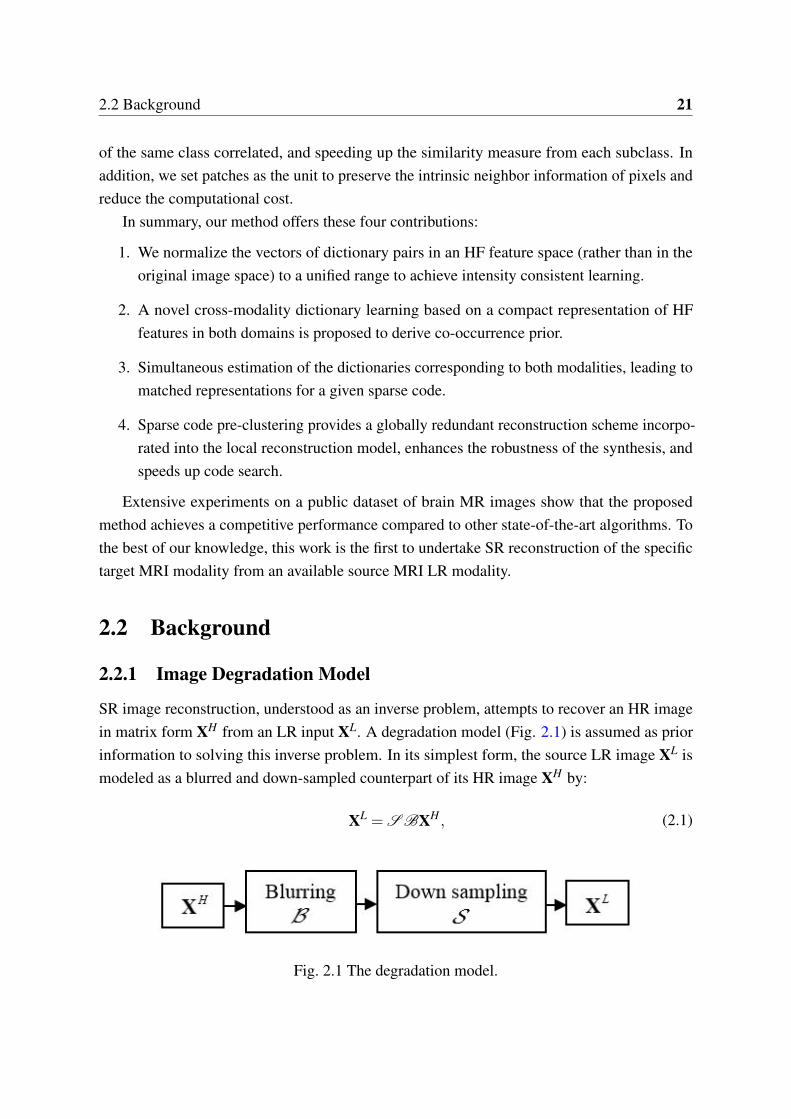
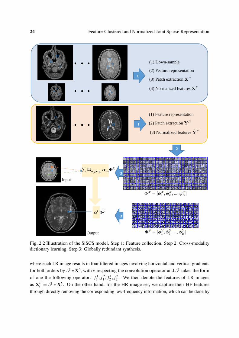
2.1 The degradation model. . . . . . . . . . . . . . . . . . . . . . . . . . . . . . 212.2 Illustration of the SiSCS model. Step 1: Feature collection. Step 2: Cross-
modality dictionary learning. Step 3: Globally redundant synthesis. . . . . . 242.3 Example of the clustering-based global redundancy model including cross-
modal matching and self-similarity. For each reference patch in the test image,groups of similar patches including cross-modal matching and self-similaritycan be found based on K-means clustering (we collect three clusters here). . . 27
2.4 Comparison of the SR results with ground truth. . . . . . . . . . . . . . . . . 312.5 Axial views of synthesized HR T2-w examples based on the LR PD-w inputs
using different methods (zoom in for details). . . . . . . . . . . . . . . . . . 332.6 Visual comparison of synthesized results using different methods on the
NAMIC dataset (zoom in for details). . . . . . . . . . . . . . . . . . . . . . 342.7 Synthesis result of a pathological case comparison between SiSCS and other
stat-of-the-art methods. . . . . . . . . . . . . . . . . . . . . . . . . . . . . . 34
xvi List of figures
2.8 Boxplots of error measures (PSNRs, SSIMs) for SR reconstructions withdifferent methods. . . . . . . . . . . . . . . . . . . . . . . . . . . . . . . . . 36
2.9 Synthesis performance comparison between SiSCS and other stat-of-the-artmethods on the NAMIC dataset. . . . . . . . . . . . . . . . . . . . . . . . . 37
3.1 Flowchart of the proposed method for MRI cross-modality synthesis. . . . . . 423.2 Example SR results and the corresponding PSNRs and SSIMs. . . . . . . . . 483.3 Error measures of SR results on the IXI dataset. . . . . . . . . . . . . . . . . 493.4 Visual comparison of synthesized results using MIMECS and DOTE. . . . . 503.5 CMS results: DOTE vs. MIMECS on the IXI dataset. . . . . . . . . . . . . . 50
4.1 Flowchart of the proposed method (WEENIE) for simultaneous SR and cross-modality synthesis. . . . . . . . . . . . . . . . . . . . . . . . . . . . . . . . 55
4.2 Example SR results and corresponding PSNRs, SSIMs (zoom in for details). . 634.3 Performance comparisons of different SR approaches. . . . . . . . . . . . . . 644.4 Visual comparison of synthesized results using different methods. . . . . . . 654.5 SRCMS results: WEENIE vs. MIMECS on IXI dataset. . . . . . . . . . . . . 66
5.1 Comparison of the synthesized results with ground truth. . . . . . . . . . . . 775.2 Overview of the proposed cross-modality image synthesis method. Squares
within the 3D images represent the extracted 3D patches with size of 5×5×5.The first step is to project the extracted paired/unpaired patches into a commonfeature space denoted by circles for source modality data and triangles fortarget modality data respectively. Then, we measure the divergence of thedistribution of the maximum mean discrepancy (MMD) over all matched pairsfrom the first step to seek the intrinsic pairs in the reproducing kernel Hilbertspace (RKHS). After that, to better preserve the modality-specific information,we adopt the Laplacian eigenmaps to capture the local geometric structure foreach domain and denoted by geometric co-regularization term. Finally, theexpected dictionary pairs can be trained based on the processed features. . . . 81
5.3 Synthesized results generated using SC, MIMECS, WAG-0, WAG-GC, WAG-MMD and WAG (zoom in for details). . . . . . . . . . . . . . . . . . . . . . 93
5.4 Cross-modality synthesis results: MIMECS, SC, WAG, WAG-MMD, WAG-GCand WAG-0 on the IXI dataset. . . . . . . . . . . . . . . . . . . . . . . . . . 94
5.5 Example cross-modality synthesis results generated by MIMECS, SC, Ve-S,Ve-US and WAG on the NAMIC dataset. . . . . . . . . . . . . . . . . . . . . 97
5.6 Cross-modality synthesis results: MIMECS, SC, WAG, Ve-S and Ve-US onthe NAMIC dataset. . . . . . . . . . . . . . . . . . . . . . . . . . . . . . . . 98
List of figures xvii
6.1 Flowchart of the proposed method (T-GAN) for cross-modality synthesis. Gand F are the dual mapping functions which are used to establish domainexchange among the source domain X and the target domain Y , X and Y arethe 3D volumes belongs to X and Y respectively, X and Y represent the firstgenerated results while X and Y are their dual generations, DCG and DCF arethe discriminators corresponding to G and F , Lc denotes the cycle-consistentGAN, dk is the MK-MMD-based jointly-adapted regularizer, CX and CY arethe task-driven results. . . . . . . . . . . . . . . . . . . . . . . . . . . . . . 110
6.2 Visual comparison for PD-w→ T2-w with/without skull stripping MRI brainimage cross-modality synthesis. . . . . . . . . . . . . . . . . . . . . . . . . 117
6.3 Quantitative performance of PD-w→ T2-w with/without skull stripping MRIbrain image cross-modality synthesis. . . . . . . . . . . . . . . . . . . . . . 118
6.4 Visual comparison for PD-w→ T2-w with/without skull stripping MRI brainimage cross-modality synthesis. . . . . . . . . . . . . . . . . . . . . . . . . 120
6.5 Quantitative analysis of T2-w→ T1-w MRI brain image cross-modality syn-thesis on the NAMIC dataset. . . . . . . . . . . . . . . . . . . . . . . . . . . 121

List of tables
2.1 Effects of Dictionary Size on SR Reconstruction and Simultaneous Super-Resolution and Cross-Modality Synthesis using All Slices of the IXI dataset. . 30
2.2 Performance Measures of SR Resolution and Simultaneous Super-Resolutionand Cross-Modality Synthesis for Different Sparsity Values using All slices ofthe IXI dataset. . . . . . . . . . . . . . . . . . . . . . . . . . . . . . . . . . 31
2.3 Average Assessment Measures for Image Synthesis of Nine Pathological Cases 35
3.1 Quantitative evaluation: DOTE vs. other SR methods. . . . . . . . . . . . . . 463.2 Quantitative evaluation: DOTE vs. DOTEnodual. . . . . . . . . . . . . . . . . 463.3 CMS results: DOTE vs. other synthesis methods on the NAMIC dataset. . . . 47
4.1 Quantitative evaluation (PSNR and SSIM): WEENIE vs. other SR methods on95 subjects of the IXI dataset. . . . . . . . . . . . . . . . . . . . . . . . . . . 65
4.2 Quantitative evaluation (PSNR and SSIM): WEENIE vs. other synthesismethods on the IXI dataset. . . . . . . . . . . . . . . . . . . . . . . . . . . . 67
4.3 Quantitative evaluation (PSNR and SSIM): WEENIE vs. other synthesismethods on the NAMIC dataset. . . . . . . . . . . . . . . . . . . . . . . . . 67
5.1 Performance measures of the synthetic images using JDL, GRiDLE (δ = 0),and GRiDLE. . . . . . . . . . . . . . . . . . . . . . . . . . . . . . . . . . . 76
5.2 Comparison of methods used for synthesizing MPRAGE based on SPGR. . . 775.3 The number of selected paired/unpaired images. . . . . . . . . . . . . . . . . 925.4 PSNRs and SSIMs of the WAG-synthesized images resulting from different
paired/full set ratios during dictionary training. . . . . . . . . . . . . . . . . 955.5 Performance measures of the WAG-synthesized images resulting from different
paired/full set ratios during dictionary training. . . . . . . . . . . . . . . . . 955.6 Performance measures of the WAG-synthesized images resulting from different
paired/full set ratios during dictionary training. . . . . . . . . . . . . . . . . 96
xx List of tables
5.7 Averaged PSNRs and SSIMs of the synthesized images using different methodson the NAMIC dataset. . . . . . . . . . . . . . . . . . . . . . . . . . . . . . 96
5.8 Paired t-test on the WAG improvements using the IXI dataset. . . . . . . . . 995.9 Independent t-test on the performance benefits using the IXI dataset. . . . . . 995.10 Independent t-test on the performance benefits using the NAMIC dataset. . . 99
6.1 Quantitative evaluation (PSNR (dB) and SSIM): T-GAN vs. other synthesismethods on the IXI dataset. . . . . . . . . . . . . . . . . . . . . . . . . . . . 119
6.2 Quantitative evaluation (PSNR (dB) and SSIM): T-GAN vs. other synthesismethods on the NAMIC dataset. . . . . . . . . . . . . . . . . . . . . . . . . 119
A.1 Quantitative evaluation (PSNR (dB) and SSIM): SiSCS, DOTE, WEENIE,WAG, and T-GAN on the IXI dataset. . . . . . . . . . . . . . . . . . . . . . 142
Nomenclature
Acronyms / Abbreviations
ADMM Alternating Direction Method of Multipliers
BCCB Block Circulant with Circulant Block
BP Basis Pursuit
CNN Convolutional Neural Network
CSC Convolutional Sparse Coding
CSF Cerebral Spinal Fluid
CT Computerized Tomography
DFT Discrete Fourier Transform
DFT Discrete Fourier Transform
DL Dual Learning
DTI Diffusion Tensor Imaging
FCSC Fast Convolutional Sparse Coding
FFT Fast Fourier Transform
GAN Generative Adversarial Network
GLA Generalized Lloyd Algorithm
GM Grey Matter
HF High-Frequency
xxii Nomenclature
K-SVD K-Singular Value Decomposition
LF Low-Frequency
MK-MMD Multi-Kernel Maximum Mean Discrepancy
MMD Maximum Mean Discrepancy
MOD Method of Optimal Directions
MRA Magnetic Resonance Angiography
MRI Magnetic Resonance Imaging
NL Non-Local
NN Nearest Neighbor
NP-hard Non-deterministic Polynomial-time Hardness
PCA Principal Component Analysis
PSNR Peak Signal to Noise Ratio
QCQP Quadratically Constrained Quadratic Programing
RKHS Reproducing Kernel Hilbert Space
sMRI Structural Magnetic Resonance Imaging
SR Super-Resolution
SSIM Structural Similarity Index
T1-w T1-weighted
PD-w Proton Density-weighted
T2-w T2-weighted
WM White Matter
Chapter 1
Introduction and Literature Review
1.1 Background
The importance of medical imaging for clinical diagnosis, treatment of disease, and medicalresearch has steadily risen over the last decades. Images of difference modalities are usuallygenerated in medical imaging (Fig. 1.1), for example, magnetic resonance imaging (MRI),computed tomography (CT), and positron emission tomography (PET). The resolution andmodality diversity of medical acquisitions is constantly improving, but this comes at the cost ofexpensive equipment, patient comfort, and scanner time availability. Especially for high-qualityand multi-modality images, precise and high-resolution scanners are required to extract themost useful data. In real life, these uncertainties may lead to incomplete records owing toimage artifacts or corrupted or lost data.
Although multi-modality medical imaging plays an important role in the prevention, de-tection, treatment and even new technology is being developed to improve human health andwelfare, the process of estimating a modality transformation regarding anatomical and/or func-
PD-w T2-w
Introd
SPGR MPRAGE
Fig. 1.1 Example of different imaging modalities - PD-w, T2-w, SPGR and MPRAGE images.
2 Introduction and Literature Review
Fig. 1.2 An example of our synthesized result using the patch-based joint dictionary learningmethod.
tional contrasts between scans is remained, for the most part, unsolved. Despite the fact thatthe previous effort of researchers focused on the synergy of different modalities, for example,the hybrid positron emission tomography/magnetic resonance imaging [14], no satisfactoryalgorithms exist that works with simultaneous high-resolution image reconstruction and cross-modality synthesis. The goal of this thesis is to synthesize high-quality image while convertingthe input modality data to the target modality ones. An example of our synthesized result usingthe patch-based joint dictionary learning method is shown in Fig. 1.2.
1.2 Imaging Modalities
Medical imaging includes a multitude of imaging modalities such as Magnetic ResonanceImaging, X-ray Computed Tomography, Ultrasound, Positron Emission Tomography, Electrical
1.2 Imaging Modalities 3
Impedance Tomography, etc. Recently, researches have been focused on recovering themissing modalities potentially existing in different modalities of MRI to capture diversifiedcharacteristics of the underlying anatomy, especially in the brain research [127, 153].
MRI is a non-ionizing, non-invasive and in vivo medical imaging technique used in radiologyto create a detailed cross-sectional image of the anatomy and the physiological processes ofhuman body. The acquisitions are generated by forming strong magnetic fields, electric fieldgradients, and radio waves while avoiding ionizing radiation that can be potentially harmfulto the patient. MRI has various modalities for providing useful anatomical and functionaldiagnostic information, where the contrast of each modality depends on the magnetic propertiesand number of hydrogen nuclei. By acquiring the comprehensive information, both cliniciansand researchers are all likely to benefit from the advances in multi-modality MRI. The clinicalapplications of such multi-modality MRI exist, containing the assessment of active lesions inmultiple sclerosis with MRI.
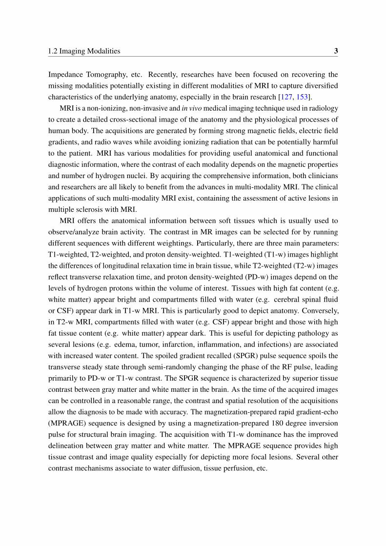
MRI offers the anatomical information between soft tissues which is usually used toobserve/analyze brain activity. The contrast in MR images can be selected for by runningdifferent sequences with different weightings. Particularly, there are three main parameters:T1-weighted, T2-weighted, and proton density-weighted. T1-weighted (T1-w) images highlightthe differences of longitudinal relaxation time in brain tissue, while T2-weighted (T2-w) imagesreflect transverse relaxation time, and proton density-weighted (PD-w) images depend on thelevels of hydrogen protons within the volume of interest. Tissues with high fat content (e.g.white matter) appear bright and compartments filled with water (e.g. cerebral spinal fluidor CSF) appear dark in T1-w MRI. This is particularly good to depict anatomy. Conversely,in T2-w MRI, compartments filled with water (e.g. CSF) appear bright and those with highfat tissue content (e.g. white matter) appear dark. This is useful for depicting pathology asseveral lesions (e.g. edema, tumor, infarction, inflammation, and infections) are associatedwith increased water content. The spoiled gradient recalled (SPGR) pulse sequence spoils thetransverse steady state through semi-randomly changing the phase of the RF pulse, leadingprimarily to PD-w or T1-w contrast. The SPGR sequence is characterized by superior tissuecontrast between gray matter and white matter in the brain. As the time of the acquired imagescan be controlled in a reasonable range, the contrast and spatial resolution of the acquisitionsallow the diagnosis to be made with accuracy. The magnetization-prepared rapid gradient-echo(MPRAGE) sequence is designed by using a magnetization-prepared 180 degree inversionpulse for structural brain imaging. The acquisition with T1-w dominance has the improveddelineation between gray matter and white matter. The MPRAGE sequence provides hightissue contrast and image quality especially for depicting more focal lesions. Several othercontrast mechanisms associate to water diffusion, tissue perfusion, etc.
4 Introduction and Literature Review
Prior Work
Histogram Matching
Fig. 1.3 histogram matching model.
Although the abundance of multiple MRI is clinically advantageous, acquisitions sufferfrom a number of practical problems. In addition, we investigated most of the multi-modalityMRI datasets mainly from the brain imaging. To increase diagnosis capabilities and producemore reliable results, synthesizing the desirable modality MRI from the available brain data isthe subject of this thesis.
1.3 Challenges
Synthesizing the unavailable data from the available MRI studies is a common necessity inthe medical imaging community and hence attracted the considerable amount of research inthe past [121, 127]. Nonetheless, such a cross-modality synthesis problem is not satisfactorilysolved in many real-life cases and also poses some challenges. Many applications [150] usesubject-specific knowledge to synthesize the desired target modality data from the given sourcemodality images. One common criticism is that in a supervised setting the training processbecomes more difficult since collecting multi-modality medical images is both time consumingand expensive. These methods are usually restricted to just considering strictly paired data tothe entire dataset. Unfortunately, most datasets are non-normalized (containing unpaired singlemodality data) and it is imperative to apply them to supply auxiliary support about the trainingrequirement. A more recent, but harder, problem, is the cross-modality synthesis in a weakly-supervised or an unsupervised manner. This is a difficult route and challenge arising when the
1.3 Challenges 5
Problem
PD-w
Input
T2-w
Output
Cross-
Modality
Learning
Fig. 1.4 A patch-based cross-modality synthesis schema.
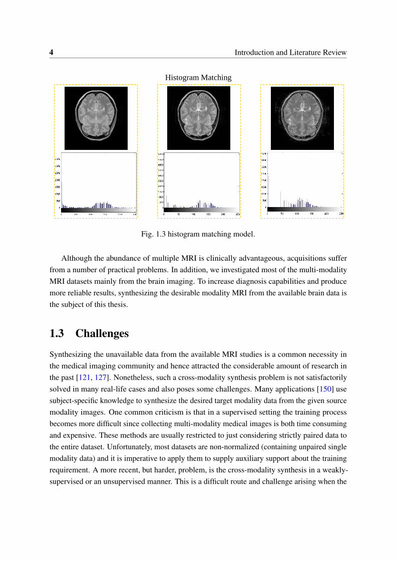
methods attempt to correlate the source modality data and the target modality data. It may feelnatural to learn two modalities data in isolation and then compose them to form a relationship.In other words, addressing cross-modality feature learning task jointly needs to formulate anintegrated framework that automatically explores the intermediate representations betweenboth modalities during training, without having to explicitly define which two subjects shouldbe aligned while processing the modality-specific image to support the synthesis task. Besidesthe interplay between different modality subjects and the quantity of data collected, additionalproblems contain the imaging conditions, the use of histogram matching model (shown inFig. 1.3), the use of patch-based approaches (shown in Fig. 1.4), effective cross-modalityfeature representations, and method complexity. Also, how might the researcher even want toutilize the synthesized results in the following applications, e.g., registration, and segmentation.Making the synthesized data not only work but actually be effective of key consideration. Ahigh-level overview of the challenges are given in the following:
1. the lacking of modality-specific information (i.e., missing certain modality data is criticalto the feature learning of an algorithm)
2. the lacking of paired data
3. domain discrepancy
4. the relationship between different modality data
5. cross-modality feature learning
6. the fidelity of the synthesized results
7. higher-resolution requirement
6 Introduction and Literature Review
8. the validity and effectiveness of the synthesized data
1.4 Dictionary Learning
In computer vision, feature representation is a crucial problem for understanding and learningimages. To capture the compact and succinct representation in visual data, a popular way is toadopt dictionary learning to achieve sparse representation using only a few active code elementsfor representing images. Dictionary leaning for sparse coding has shown promising results innumerous tasks, such as image reconstruction [22, 102, 105, 121, 164], object recognition [66,71, 180, 185], image super-resolution [43, 167, 171, 178], image denoising [28, 89, 130, 166],and visual classification [81, 169, 170, 181] to name a few.
Dictionary learning-based sparse and redundant representation was first introduced byOlshausen and Field [116] for modeling the spatial receptive fields of simple cells in themammalian visual cortex. It assumes an ability to represent natural signals (like images) as alinear combination of a few non-zero coefficients of an overcomplete (i.e. the number of basisatoms is greater than the dimension of the data) dictionary. The property of overcomplete isto provide the flexibility in matching data leading to a better approximation of the statisticaldistribution of the signal. Subsequently, extensive works on the dictionary learning model(according to different criteria) have been investigated in an attempt to understand it betterand achieve or improve upon state-of-the-art results. Referring to the most classical ones ofdictionary learning, the method of optimal directions (MOD) [37] and the K-Singular ValueDecomposition (K-SVD) [1] algorithms have led to the dramatical improvements in infillingmissing pixels and image compression tasks.
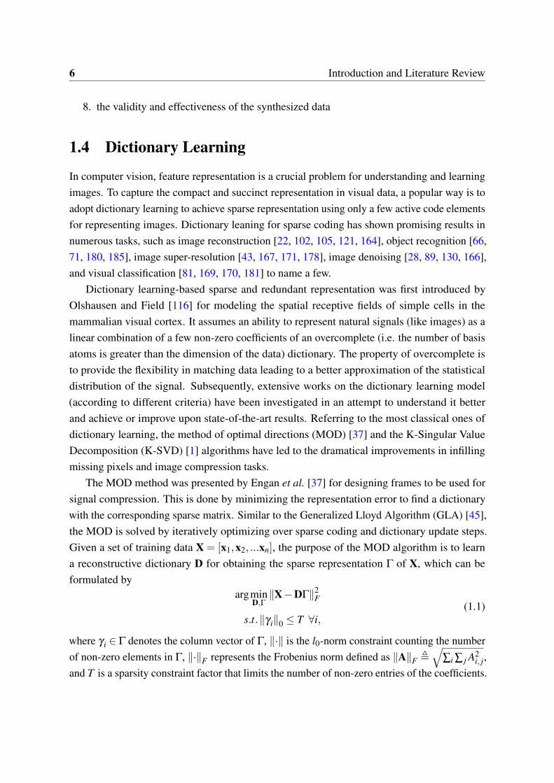
The MOD method was presented by Engan et al. [37] for designing frames to be used forsignal compression. This is done by minimizing the representation error to find a dictionarywith the corresponding sparse matrix. Similar to the Generalized Lloyd Algorithm (GLA) [45],the MOD is solved by iteratively optimizing over sparse coding and dictionary update steps.Given a set of training data X = [x1,x2, ...xn], the purpose of the MOD algorithm is to learna reconstructive dictionary D for obtaining the sparse representation Γ of X, which can beformulated by
argminD,Γ∥X−DΓ∥2
F
s.t.∥γ i∥0 ≤ T ∀i,(1.1)
where γ i ∈ Γ denotes the column vector of Γ, ∥·∥ is the l0-norm constraint counting the numberof non-zero elements in Γ, ∥·∥F represents the Frobenius norm defined as ∥A∥F ,
√∑i ∑ j A2
i, j,and T is a sparsity constraint factor that limits the number of non-zero entries of the coefficients.
1.4 Dictionary Learning 7
The resulting optimization problem is highly non-convex, and there is no direct way to find theapproximate solution. Instead, an iterative procedure was used in [37] to get a local minimumat best.
While significant steps have been taken to develop the sparsification theory using the MOD,similar problems on the K-SVD algorithm have received competitive attention to efficientlytrain a generic dictionary for sparse representation. In [1], the K-SVD method was introducedto efficiently learn an overcomplete dictionary from a set of training data. Through learning thedictionary instead of choosing off-the-shelf bases, the K-SVD has been shown to work well inimage reconstruction and denoising [34]. The linear decomposition of a signal or an imageallows more flexibility to adapt the representation to the data, leading to notable results forvarious visual inference applications [36, 103, 104, 120, 161, 162]. The K-SVD algorithm isconsistent with most of the previous work that relies on iteratively solving sub-problems withthe purpose of achieving the optimal solution through an iterative approximation. Despite thewide applications and appealing properties of such an iterative approximation method, the highnon-convexity of optimizing the objective function in Eq. (1.1) under the l0-sparsity penaltymeasure leads to a general NP-hard (Non-deterministic Polynomial-time hard) problem. Recentresults [30, 86] suggest a convexification of the problem posed in Eq. (1.1) by replacing thel0-norm with an with l1-norm regularization to enforce sparsity, in which this procedure is alsoknown as Basis Pursuit (BP) [20], or the Lasso [146]. Eq. (1.1) can be rewritten as a jointoptimization problem using the l1-sparsity penalties on the representations:
argminD,Γ∥X−DΓ∥2
F
s.t.∥γ i∥1 ≤ T ∀i,(1.2)
Generally, Eq. (1.2) can be formulated in the form of Lagrange multipliers as
argminD,Γ∥X−DΓ∥2
F +λ ∥Γ∥1 , (1.3)
where λ is a regularization parameter to balance the sparsity in the objective function.The optimization problem in Eq. (1.2) is convex in either D or Γ are fixed, and therefore of
iteratively minimizing between sparse coding and dictionary learning. Specifically, when D isfixed, one optimizes with respect to the sparse codes Γ update (known as a Lasso problem);when Γ is fixed, solving D becomes to a least square problem with a standard quadraticconstraint (known as the quadratically constrained quadratic programming (QCQP) problem).
Given the training data X, we first need to initialize D with a Gaussian random matrix.Then, an iterative algorithm can be performed alternatively over Γ and D:
8 Introduction and Literature Review
1. With D fixed, sparse coding coefficients Γ can be calculated as
Γ = argminΓ∥X−DΓ∥2
F +λ ∥Γ∥1 , (1.4)
2. With Γ fixed, dictionary D can be updated by
D = argminD∥X−DΓ∥2
F
s.t.∥D∥22 ≤ 1 ∀i,
(1.5)
Once the optimization is completed, i.e., iteration between step 1 and step 2 until converge, wecan get the learned dictionary on which the sparse codes have a stable linear decomposition forimage reconstruction.
1.5 Convolutional Sparse Coding
Convolutional Sparse Coding (CSC) [10, 175] has been demonstrated as a promising directionfor learning the convolutional image representations in machine learning and computer vision.The concept of CSC is closely related to classic patch-based feature learning and image recon-struction methods [1, 11, 86]. However, feature representation with a patch-based mechanismis highly redundant and may lead to the loss of shifted copies (i.e., overlapped samples) ofthe same features in the overlapped area of adjacent patches. A more elegant way to solve theabove problem, i.e. removing much of the overhead of the patch-based sparse coding, is touse a convolution image formation model for consistently capturing the sparsely-distributedconvolutional features. Through decomposing all training data into the defined number ofsparse feature maps by the corresponding filters, CSC can avoid missing any latent structuresof the underlying signal and thus naturally keep the consistency prior in the decompositionprocedure. Recently, CSC has proven essential for many important applications in a wide rangeof computer vision problems [2, 34, 92, 108, 190]. For example, robust feature learning [77],as part of hierarchical networks in high-level computer vision tasks [77, 175], and low-levelimage reconstruction [18, 142]. In addition, CSC-based methods have been proposed to solvemany practical applications including super-resolution [51], cross-modality synthesis [65],inpaiting [57], demosaicing [23] and reconstruction [57].
To take the property of shift invariance into account, CSC models local interactions throughthe convolution operator to sparsely encode the whole image. This is done by directly repre-senting an image as the summation of convolutions of the feature maps and the correspondingfilters, thus avoiding the sparse decomposition on every single vector. Given a set of input
1.5 Convolutional Sparse Coding 9
vectors xNn=1, CSC can be expressed as the following optimization problem:
argmind,z
12
∥∥∥∥∥x−K
∑i=1
di ∗ zi
∥∥∥∥∥2
2
+β
K
∑i=1∥zi∥1
s.t.∥di∥1 ≤ 1 ∀i ∈ 1, ...,K ,
(1.6)
where each vectorized input image x can be denoted as the sum of sparse feature maps zi
convolved with the corresponding filters di of fixed spatial support, ∗ represents the convolutionoperator processed on the vectorized inputs. The l2-norm constraint on di ensures the learnedfilters do not absorb the system energy, and therefore of removing the scaling ambiguity. Ratherthan averaging in patch-based model, CSC directly approximates the whole image as in theobjective of Eq. (1.6) to avoid inconsistent reconstruction.
Despite the benefit of convolutional implementation of sparse coding to solve the inconsis-tency problem, CSC also brings some difficulties in optimization. Zeiler et al. [175] proposedto solve the objective function by an alternation way with the auxiliary variable t, where onesolves a set of convex subproblems until convergence and t is used to separate the convolutionfrom the l1 regularization. Similar to the solution of conventional sparse coding problem, CSCalternatively updates between processing the subproblem d given a fixed z, and the subproblemz given a fixed d. A shortcoming of this method, however, is the computational overheadassociated with the iterative subproblems. Bristow et al. [10] introduced a fast CSC algorithmthrough exploiting the property of block circulant with circulant block (BCCB) matrix solvingin the Fourier domain. It has been shown the remarkable improvements in efficiency by utilizingParseval’s theorem for solving Eq. (1.6). Following [10], we can reformulate Eq. (1.6) as aconstrained optimization problem by involving two auxiliary variables t and s in the Fourierdomain:
arg mind,z,s,t
12
∥∥∥∥∥x−K
∑i=1
di⊙ zi
∥∥∥∥∥2
2
+β
K
∑i=1∥ti∥1
s.t.∥si∥22 ≤ 1 ∀i ∈ 1, ...,K
si = SΦT di ∀i ∈ 1, ...,K
ti = zi ∀i ∈ 1, ...,K .
(1.7)
where the symbolˆapplied to any vector denotes the frequency representation of a vectorizedsignal, for example, x = [F(x1)
T , ...,F(xN)T ] and F(·) is the Fourier transform operator, ⊙
denotes the Hadamard (component-wise) product, S projects d onto a corresponding smallspatial support, Φ represents the Discrete Fourier Transform (DFT) matrix, si and ti are two
10 Introduction and Literature Review
PD
-w S
ub
jectsT
2-w
Su
bjects
Fig. 1.5 Illustration of the example PD-w and T2-w MR images from the IXI dataset. In eachpanel, the first row shows the PD-w image while the second row shows the corresponding T2-wdata.
slack variables allowing for an explicit and efficient solution to Eq. (1.7) by splitting theobjective into several subproblems.
1.6 Datasets
Two distinct datasets were used in this dissertation. The first dataset is taken from the Informa-tion eXtraction from Images (IXI)1 [126] including 578 Magnetic Resonance (MR) imagesfrom normal and healthy subjects. The images have been collected at three different hospitals(i.e., Hammersmith Hospital using a Philips 3T system, Guy’s Hospital using a Philips 1.5Tsystem, and Institute of Psychiatry using a GE 1.5T system) and stored in NIFTI format. Theacquisition protocol for each subject contains: T1-weighted, T2-weighted, Proton Density (PD)-weighted images; Magnetic Resonance Angiography (MRA) images; and Diffusion-weightedimages (15 directions). Some examples collected from the IXI dataset are shown in Fig. 1.5.
1http://brain-development.org/ixi-dataset/
1.6 Datasets 11
T1
-w S
ub
jectsT
2-w
Su
bjects
Fig. 1.6 Illustration of the example T1-w and T2-w MR images from the NAMIC dataset. Ineach panel, the first row shows the T1-w image while the second row shows the correspondingT2-w data.
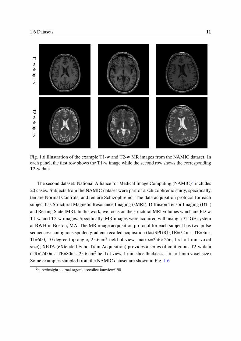
The second dataset: National Alliance for Medical Image Computing (NAMIC)2 includes20 cases. Subjects from the NAMIC dataset were part of a schizophrenic study, specifically,ten are Normal Controls, and ten are Schizophrenic. The data acquisition protocol for eachsubject has Structural Magnetic Resonance Imaging (sMRI), Diffusion Tensor Imaging (DTI)and Resting State fMRI. In this work, we focus on the structural MRI volumes which are PD-w,T1-w, and T2-w images. Specifically, MR images were acquired with using a 3T GE systemat BWH in Boston, MA. The MR image acquisition protocol for each subject has two pulsesequences: contiguous spoiled gradient-recalled acquisition (fastSPGR) (TR=7.4ms, TE=3ms,TI=600, 10 degree flip angle, 25.6cm2 field of view, matrix=256×256, 1×1×1 mm voxelsize); XETA (eXtended Echo Train Acquisition) provides a series of contiguous T2-w data(TR=2500ms, TE=80ms, 25.6 cm2 field of view, 1 mm slice thickness, 1×1×1 mm voxel size).Some examples sampled from the NAMIC dataset are shown in Fig. 1.6.
2http://insight-journal.org/midas/collection/view/190
12 Introduction and Literature Review
1.7 Related Work
With the goal to transfer the modality information from the source domain to the target domain,recent developments in cross-modality synthesis, such as texture synthesis [32, 44, 59], facephoto-sketch synthesis [42, 158], and multi-modal retrieval [110, 138], have shown promisingresults. In this thesis, we focus on the problems of image super-resolution and cross-modalitysynthesis, so only review related methods on these two aspects. To synthesize a target modalityimage from a source modality image, several approaches have been suggested in the literaturewith state-of-the-art results [14, 72, 153]. Most of these methods can be broadly referred to asthe nature image domain and the medical image domain roughly subdivided based on the typeof images.
1.7.1 Nature Image Domain
In the nature image domain, the purpose of image super-resolution (SR) is to reconstructan high-resolution (HR) image from its low-resolution (LR) counterpart. According to theimage priors, image SR methods can be grouped into two main categories: interpolation-based,external or internal data driven learning methods. Interpolation-based SR works, includingthe classic bilinear [90], bicubic [78], and some follow-up methods [131, 179], interpolatemuch denser HR grids by the weighted average of the local neighbors. Most modern image SRmethods have shifted from interpolation to learning based. These methods focus on learning acompact dictionary or manifold space to relate LR/HR image pairs, and presume that the losthigh-frequency (HF) details of LR images can be predicted by learning from either externaldatasets or internal self-similarity. The external data driven SR approaches [16, 40, 168] exploita mapping relationship between LR and HR image pairs from a specified external dataset. Inthe pioneer work of Freeman et al. [40], the NN of an LR patch is found, with the correspondingHR patch, and used for estimating HF details in a Markov network. Chang et al. [16] projectedmultiple NNs of the local geometry from the LR feature space onto the HR feature spaceto estimate the HR embedding. Furthermore, sparse coding-based methods [128, 168] wereexplored to generate a pair of dictionaries for LR and HR patch pairs to address the image SRproblem. Wang et al. [155] and Huang et al. [60] further suggested modeling the relationshipbetween LR and HR patches in the feature space to relax the strong constraint. Recently, anefficient CNN based approach was proposed in [27], which directly learned an end-to-endmapping between LR and HR images to perform complex nonlinear regression tasks. Forinternal dataset driven SR methods, this can be built using the similarity searching [125] and/orscale-space pyramid of the given image itself [61].
1.7 Related Work 13
In parallel, various cross-modality synthesis methods have been proposed for synthesizingunavailable modality data from available source images. One of the well-established modalitytransformation approaches is the example-based learning method generated by Freeman etal. [41]. Given a patch of a test image, several NNs with similar properties are picked fromthe source image space to reconstruct the target one using Markov random fields. In addition,Hertzmann et al. provided image analogies [59], which transfers the texture information froma source modality space onto a target modality space. Gatys et al. [44] introduced a CNNalgorithm of artistic style, that new images can be generated by performing an image pre-searchin high-level image content to match generic feature representations of example images.
1.7.2 Medical Image Domain
In the medical imaging community [127, 150, 153], synthesis algorithms can be summarizedinto a main family, i.e., example-based methods roughly subdivided in accordance with the sizeof the training set. Particularly, image SR can be treated as a way of synthesis which attemptsto improve image resolution by algorithms instead of carrying out during the acquisitionstage. Image SR effectively solved the problem of long acquisition and breath-hold fromthe requirement of high quality images, therefore the accuracy of clinical diagnosis can beincreased while the images are acquired in a reasonable time.
Example-based methods learn the source-target mapping from a very small number ofsource-target image pairs (e.g. several or even a pair of images) by extracting multiple imagepatches from the source image and assuming the same sparse codes are shared between sourceand target modality spaces. One of the well-established cross-modality synthesis approaches inthis category is applied to facilitate multi-modal image registration in correlative microscopy[15]. Kroon et al. [82] mapped between T1-w and T2-w magnetic resonance images bysimply using the peaks in a joint histogram of registered image pairs to transform betweensource and target image representations. Techniques based on sparse representations have beenpresented, which separately learn two corresponding dictionaries from registered image pairsand synthesize the target MRI modality data from the patches of the source MRI modality[127]. Specifically, Roy et al. [127] used sparse coding for desirable MR contrast synthesisassuming that cross-modality patch pairs have same representations and can be directly usedfor training dictionaries to estimate the contrast of the target modality. Similar work was alsoused in [67]. In [4], a canonical correlation analysis-based approach was proposed to yielda feature space that can get underlying common structures of co-registered data for bettercorrelation of dictionary pairs. Recently, Jog et al. [72] proposed a nonlinear regression-basedimage synthesis approach that used registered image pairs to train a random forest regressor forpredicting the target from the source image intensity.
14 Introduction and Literature Review
Some example-based methods learn the source-target mapping assuming that a large setof source-target modality image pairs (e.g. the whole dataset) is available. These approachesvary on how to generate a model (e.g. learning a dictionary, a manifold or a network) thatrelates to the number of the patches of the registered image pairs. In measuring the similaritybetween training and test data of the same modality, Ye et al. [172] proposed an iterativepatch-based modality propagation approach. For each patch of the test image, a global searchwas performed comparing the input patch with each patch in the training dataset. The nearestneighbors to the input patch were found in the source domain; the target modality imagewas synthesized with the corresponding target modality patches. Rather than learning themapping between both domains in the original data space, coupled dictionary learning [168] canalleviate simple cross-modality heterogeneity in the projected feature space. As an extension,semi-coupled dictionary learning was presented by advancing a linear mapping to model therelationship on the sparse representations from both domains. Burgos et al. [14] introducedanother framework called pseudo CT synthesis for generating CT-like image from the T1-wor T2-w input using multi-atlas deformable registration and tissue contrast fusion. In [150],a location-sensitive deep network [150] has been put forward to explicitly utilize the voxelimage coordinates by incorporating image intensities and spatial information into a deepnetwork for synthesizing purposes. Instead of using coupled image pairs as training data,matching feature representations and learning spatial relations with joint sparse coding [153]has shown great potential in synthesizing images across modalities. To improve the quality ofthe synthesized images across different modalities, Huang et al. [65] proposed to first alignweakly-supervised data and then generate super-resolution cross-modality data simultaneouslyusing joint convolutional sparse coding scheme. Inspired by this strategy, we integrate pairedand unpaired training data by constructing correspondences across different modalities andleverage weakly-coupled data effectively.
As argued in [153], collecting a large number of multi-modality images is both time-consuming and expensive, and sometimes even impractical in medical imaging. It would bepreferable to use an unsupervised approach to deal with input data instead of ensuring data to becoupled invariably. Most of the methods, especially the full-set-based approaches, require con-siderable amounts of co-registered training data in both source and target domains. Motivatedby this and the above works, we propose several more practical cross-modality image synthesissolutions that link source-target domains in either a fully supervised setting or a weakly-coupledfashion, which outperform existing state-of-the-art methods on our experiments.
1.8 Thesis Outline 15
1.8 Thesis Outline
This dissertation begins with works that address the core algorithmic problem of designingcross-modality synthesis methods to assist comprehensive assessment of complex diseases ineither diagnostic examinations or as part of medical research trials. In particular, we developboth supervised and weakly-supervised approaches that process and align the two modalitiesand train their parameters on datasets of multi-modality brain MRI acquisitions. The rest ofthis thesis is organized as follows.
In Chapter 2, we consider the problem of collecting features in MRI by their modality-specific properties learned with full supervision. Chapter 3 presents a novel dual convolutionalfilter learning algorithm for the cross-modality synthesis of brain MRI data, with the keycontribution being an algorithm for bringing state-of-the-art 3D method for robust synthesis.Chapter 4 deals with the challenging task of weakly-supervised learning useful for both imagesuper-resolution and cross-modality synthesis. In Chapter 5, we first introduce a geometryregularized joint dictionary learning method in a supervised setting, which is designed towork on brain image for synthesizing the missing/complex modality data. Another part of themodel included in Chapter 5 extends the proposed geometrical regularization approach to aweakly-supervised scheme for cross-modality synthesis. Chapter 6 constructs an unsuperviseddeep learning architecture for automatically synthesize the application/post processing-efficienthigh-resolution or required modality data with dual learning during training. Finally, Chapter 7concludes this thesis and discusses future works. The parallel contrast experiments are involvedin Appendix A.
1.9 Contributions
In this dissertation, we develop models for the cross-modality synthesis of the three-dimensionalbrain image. In particular, we develop several learning-based architectures that process andalign the two modalities and train models on different public multi-modality brain datasets.Most contributions in this dissertation have first appeared as my publications, which aresummarized below3:
1. Chapter 2: Simultaneous super-resolution and cross-modality synthesis in magneticresonance imaging.
2. Chapter 3: Dual convolutional filter learning for super-resolution and cross-modalitysynthesis in MRI [64].
3A more detailed account of contributions appears in Section 7.1. Other publications such as [66] are beyondthe scope of this dissertation and thus not discussed here.
16 Introduction and Literature Review
3. Chapter 4: Simultaneous super-resolution and cross-modality synthesis of 3D medicalimages using weakly-supervised joint convolutional sparse coding [65].
4. Chapter 5: Geometry regularized joint dictionary learning for cross-modality imagesynthesis in magnetic resonance imaging [62]. Cross-Modality Image synthesis viaweakly-coupled and geometry co-regularized joint dictionary learning [63].
5. Chapter 6: Task-driven bidirectional fault-aware adversarial networks for three-dimensionalbrain image analysis.
Chapter 2
Feature-Clustered and Normalized JointSparse Representation
Multi-modality Magnetic Resonance Imaging (MRI) has enabled significant progress to bothclinical diagnosis and medical research. Applications range from different diagnosis to novelinsights into disease mechanisms and phenotypes. However, there exist many practical sce-narios where acquiring high-quality multi-modality MRI is restricted, for instance, owingto limited scanning time. This imposes constraints on multi-modality MRI processing tools,e.g. segmentation and registration. Such limitations are not only recurrent in prospective dataacquisition, but also when dealing with existing databases with either missing or low qualityimaging data. In this chapter, we explore the problem of synthesizing high-resolution imagescorresponding to one MRI modality from a low-resolution image of another MRI modalityof the same subject. This is achieved by introducing the cross-modality dictionary learningscheme and a patch-based globally redundant model based on sparse representations. Weuse high-frequency multi-modality image features to train dictionary pairs, which are robust,compact, and correlated in this multimodal feature space. A feature clustering step is inte-grated into the reconstruction framework speeding up the search involved in the reconstructionprocess. Images are partitioned into a set of overlapping patches to maintain the consistencybetween neighboring pixels and increase speed further.Extensive experimental validationson two multi-modality databases of real brain MR images show that the proposed methodoutperforms state-of-the-art algorithms in two challenging tasks: image super-resolution andsimultaneous SR and cross-modality synthesis. Our method was assessed on both healthysubjects and patients suffering from schizophrenia with excellent results.
18 Feature-Clustered and Normalized Joint Sparse Representation
2.1 Introduction
Magnetic Resonance Imaging (MRI) has advanced both clinical diagnosis and biomedicalresearch in the neurosciences. MRI has widely been used given its non-invasiveness and theversatility associated with multi-modality imaging protocols that unravel both brain structureand function. Each MRI sequence (hereafter called an MRI modality) is based upon differentimage contrast mechanisms that relate to complementary properties of brain tissue structureand function and help to unravel anatomical differences and physiologic alterations of braintissue in health and disease [121].
Despite these benefits, acquiring a full battery of MRI modalities faces constraints associatedwith increased scanning costs, limited availability of scanning time, and patient comfort, amongothers. Also, as MRI technologies improve, enhanced resolution or new contrast mechanismscan be utilized. However, in longitudinal imaging cohorts, its benefits will not be availableretrospectively for earlier time points in the study, imposing a natural limitation on the dataset.This brings an additional complexity to image analysis and interpretation as the imagingprotocol can change. Finally, many reasons can lead to incomplete records for a subject whotook part in a large imaging study owing to imaging artifacts, acquisition errors, and lostor corrupted data sets. In all such scenarios, it would be desirable to have a mechanism tosynthesize the high-resolution missing data in a different modality with the available MRImodality. However, most of the existing methods tackling this problem either focuses on imagesuper-resolution (SR) or cross-modality synthesis, but not on solving both problems jointly.
Image SR aims to reconstruct a high-resolution (HR) image from a low-resolution (LR)counterpart. It is an under determined inverse problem since a multiplicity of solutions existfor the LR input. To solve such a problem, solution space is often constrained by involvingstrong prior information. In the early years of studies, some simple interpolation-based smoothmethods [50, 58, 87, 140] were proposed to zoom up LR images. However, Van Ouwerkerk[151] pointed out that such interpolation methods cannot recover detailed information lostin the down-sampling procedure, and even may blur sharp edges. SR techniques were thenproposed [16, 47, 117, 124, 128, 133, 168], which take the degradation model (e.g. blurring,noise, and down-sampling effects) into account, to reconstruct the image with much higheraccuracy. Such methods estimate the HR image by learning co-occurrence priors between theLR and HR image pairs [168]. For instance, Freeman et al. [41] presented a learning-basedapproach to estimate an HR image from an LR input via Markov Network and Bayesian BeliefPropagation. Although the resolution can generally be improved effectively, corners, edges,and ridges are still blurred. Based on such a strategy, Sun et al. [141] addressed the aboveproblem by a computationally intensive process of analysis of millions of LR-HR patch pairs.Neighbor Embedding was then proposed for single-image SR [16]. This consists of projecting
2.1 Introduction 19
the local geometry from the LR feature space onto the HR feature space to estimate the HRembedding. Although a small dataset was used in the training process (partly to solve themassive computational load) results were confined to the small number of neighbors. Toadequately recover the general image structure and its details, Non-Local Means (NL means)[106, 107] was presented to reconstruct the HR image with noise suppression exploitingimage self-similarities. However, for strong denoising levels, images are visually over-smooth.Recently, sparse representations were exploited for solving the SR problem. For example, Yanget al. [168] adopted a joint dictionary learning framework for mapping LR and HR imagepairs into a common representation space. Rueda et al. [128] took advantage of this modeland applied it to address the SR problem in brain MRI. A common drawback shared by bothmethods is that they only consider local image information in the image synthesis leading tosuboptimal reconstructions.
In parallel to the SR technique, researchers have been developing methods to solve theproblem of cross-modality image synthesis. This problem can be tackled either by transformingMRI intensities across modalities or by synthesizing tissue contrast in the target domain basedon patches of the source domain. Histogram matching is a simple way of transforming imageintensities from one modality onto another or to normalize histogram ranges across subjects[7, 24, 113, 123, 134]. Applications such as segmentation and registration can benefit fromhistogram normalization and/or transformation to reduce the dependency of the results tointensity variations across individuals or imaging protocols. Although this method is widelyused in neuroimaging (e.g. [7, 24, 113, 123, 134]), it has demonstrated its weakness forconverting data with inconsistent intensities and apparent errors [127]. An alternative approachto reconstruct a target MRI modality from a source MRI modality (or more generally, fromany other imaging modality) is the example-based image synthesis [127]. In this approach,two dictionaries are independently trained on corresponding patches from registered imagepairs of the source and target modalities, respectively. Then the target image is synthesizedfrom the source data based on a reconstruction algorithm that links the patches to reconstructthe source image to the corresponding patches in the target dictionary. Such approacheshave also been applied with very promising results to the related problems of label fusion[145] and image hallucination [124]. The procedure to reconstruct the target image imposesthat the same code that optimally reconstructs the source patches from the source dictionarymust be applied directly to reconstruct the target patches from the target dictionary basedon a mapping learned from a set of image pairs. To do so, the most common procedureis to train two dictionaries via random sampling of the registered image patches from twodomains and build the correspondence between patches of two modalities. Such methodsconcatenate both domains according to the intensities of the paired patches, leading to two
20 Feature-Clustered and Normalized Joint Sparse Representation
separate dictionary learning processes in their respective modalities. In this context, the jointrepresentation of the two domains (juxtaposing the two independently-computed codes) issuboptimal regarding a jointly learned code that exploits the cross-modality correlations. Inaddition, example-based methods rely on the given cross-modality exemplar pairs, and doesnot capture the rich variability in image texture across a population of subjects. Accordingto the similarity measurement between training and test data of the same modality, Ye et al.[172] proposed a patch-based modality propagation method. Through global search, the inputpatch was compared against the training patches in the dataset. Several nearest neighborswith similar properties were picked from the source domain and corresponding patches inthe target modality used for image synthesis. In [14], a pseudo CT synthesis algorithm wasproposed, which aims at generating CT-like images from T1-w / T2-w inputs, using multi-atlasregistration and tissue contrast fusion. Nguyen et al. [150] proposed a location-sensitive deepnetwork method to integrate image intensities and spatial information into a deep networkfor cross-modality image synthesis. To verify the effectiveness of synthesized data, Tulder etal. used restricted Boltzmann machines to learn abstract representations from training datafor synthesizing the missing image sequences. More recently, a nonlinear regression-basedimage synthesis approach [72] was proposed to predict the intensities in the target modality.While training, this method used registered image pairs from source and target modalities tolearn a random forest regressor for regressing the target modality data. Besides these methods,Vemulapalli et al. proposed an unsupervised approach which relaxed needing registered imagepairs during training, to deal with the synthesis problem.
In this chapter, we present a novel MRI Simultaneous Super-Resolution and Cross-ModalitySynthesis (SiSCS) method for reconstructing the HR version of the target modality based onan LR image of the source modality while treating each 3D volume as a stack of 2D images.We simultaneously train a cross-modality dictionary pair based on registered patches of theLR source modality and the HR target modality. For an accurate image synthesis, the sparsecodes of the LR source modality should be the same as those of the HR ground truth onthe premise of high correlation between the paired LR source data and HR target data. Wemap high-frequency (HF) features of the registered image pairs between source and targetmodalities into a common feature space to fit the style-specific local structures and resolutions.We introduce patch-based global redundancy, consisting of cross-modal matching and self-similarity, to enhance the quality of image reconstruction based on sparse representations. Priorpapers such as [12, 34] and follow-up studies [29, 106, 107, 187] have shown that self-similarimage properties were used for enabling exact local image reconstruction. However, classicalNL means [165] are computationally expensive. To overcome such problem, we present anintegrated clustering algorithm into the original redundancy framework for making the data
2.2 Background 21
of the same class correlated, and speeding up the similarity measure from each subclass. Inaddition, we set patches as the unit to preserve the intrinsic neighbor information of pixels andreduce the computational cost.
In summary, our method offers these four contributions:
1. We normalize the vectors of dictionary pairs in an HF feature space (rather than in theoriginal image space) to a unified range to achieve intensity consistent learning.
2. A novel cross-modality dictionary learning based on a compact representation of HFfeatures in both domains is proposed to derive co-occurrence prior.
3. Simultaneous estimation of the dictionaries corresponding to both modalities, leading tomatched representations for a given sparse code.
4. Sparse code pre-clustering provides a globally redundant reconstruction scheme incorpo-rated into the local reconstruction model, enhances the robustness of the synthesis, andspeeds up code search.
Extensive experiments on a public dataset of brain MR images show that the proposedmethod achieves a competitive performance compared to other state-of-the-art algorithms. Tothe best of our knowledge, this work is the first to undertake SR reconstruction of the specifictarget MRI modality from an available source MRI LR modality.
2.2 Background
2.2.1 Image Degradation Model
SR image reconstruction, understood as an inverse problem, attempts to recover an HR imagein matrix form XH from an LR input XL. A degradation model (Fig. 2.1) is assumed as priorinformation to solving this inverse problem. In its simplest form, the source LR image XL ismodeled as a blurred and down-sampled counterpart of its HR image XH by:
XL = S BXH , (2.1)
Fig. 2.1 The degradation model.
22 Feature-Clustered and Normalized Joint Sparse Representation
where B and S represent the blurring and down-sampling operators, respectively [151].
2.2.2 Dictionary Learning
Dictionary learning has been successfully applied to a number of problems in image pro-cessing, such as image restoration [1, 104, 129], denoising [29, 34, 165], and enhancement[39, 129, 168]. In image reconstruction based on dictionary learning, an image is nor-mally treated as the combination of many patches [1, 34, 104, 129, 168] and denoted asX = [x1,x2, ...,xN ] ∈ Rk×N . An image is approximated as X ≈ ΦA, where X is the targetmatrix being approximated, Φ = [φ 1,φ 2, ...,φ K] ∈ Rk×K denotes a projection dictionary withK atoms, and A = [α1,α2, ...,αN ] ∈ RK×N is a set of N K-dimensional sparse codes of Xwith ∥A∥0≪ K. Representing Eq. (2.1) for sparse reconstruction of XL regarding Φ
L can beachieved by:
XL ≈ΦLA = BS (ΦHA), (2.2)
where ΦL and Φ
H denotes an LR dictionary and an HR dictionary, respectively. For each image,the sparse decomposition is obtained by solving:
minA∥A∥0 s.t. X = ΦA (or∥X−ΦA∥p ≤ ε), (2.3)
where ∥·∥0 controls the number of non-zero elements in A, and ε is used for managing thereconstruction errors. As shown in [26], the minimization problem as stated in Eq. (2.3) is anNP-hard problem under the l0-norm with the l1-norm to obtain a near-optimal solution [20].The estimation is then accomplished by minimizing a least squares problem with a quadraticconstraint, whose Lagrange multiplier formulation is:
< Φ,A >= argminΦ,A∥X−ΦA∥2
2 +λ ∥A∥1 , (2.4)
where λ is a regularization factor trading off the parametric sparsity and the reconstructionerror of the solution.
2.3 Method
The proposed SiSCS method computes an estimation of an HR version of a target MRImodality based on an LR version of a source MRI modality using jointly learned dictionary.SR reconstruction in this work is inspired in earlier work on brain hallucination [124], with anassumption that an HR image can be reconstructed from the LR input with the help by another
2.3 Method 23
HR image using dictionaries of paired data in a sparse representation framework [76, 127].In this work, we partition the images in the training database into a set of overlapping imagepatches. These image patches are built simultaneously on the source and target spaces byregistered source-target image pairs. We propose a cross-modality dictionary learning thatenforces the computation of joint sparse codes. Instead of working with the original data ofthe paired patches, we choose an HF representation of the data in the gradient domain, so thesparse codes promote a high correlation between the two modalities regarding the LR and HR,respectively. In brief, given the test image in matrix form Xt (with modality M1), the proposedmethod will synthesize an SR image Yt with modality M2 from Xt through a patch-basedglobal redundant reconstruction model regarding the learned cross-modality dictionary pair.The entire framework of SiSCS model is summarized in Fig. 2.2.
2.3.1 Data Description
Let X = X1,X2, ...,Xm be m training images of modality M1 in the source domain, andY = Y1,Y2, ...,Ym be m training images of modality M2 in the target domain. We denotecross-modality image pairs as Xi,Yi, while Xi and Yi are registered. In this work, weconsider the LR input and HR output and define the observed LR counterparts based on the HRimages in X as Eq. (2.1). X = X1,X2, ...,Xm is then updated as X L =
XL
1 ,XL2 , ...,X
Lm
,and cross-modality image pairs can be rewritten as XL
i ,Yi. After that, we build our algorithmbased on these data.
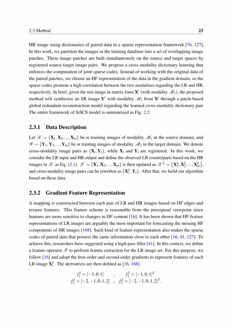
2.3.2 Gradient Feature Representation
A mapping is constructed between each pair of LR and HR images based on HF edges andtexture features. This feature scheme is reasonable from the perceptual viewpoint sincehumans are more sensitive to changes in HF content [16]. It has been shown that HF featurerepresentations of LR images are arguably the most important for forecasting the missing HFcomponents of HR images [168]. Such kind of feature representation also makes the sparsecodes of paired data that possess the same information close to each other [16, 41, 127]. Toachieve this, researchers have suggested using a high-pass filter [41]. In this context, we definea feature operator F to perform feature extraction for the LR image set. For this purpose, wefollow [16] and adopt the first-order and second-order gradients to represent features of eachLR image XL
i . The derivatives are then defined as [16, 168]
f 11 = [−1,0,1] , f 2
1 = [−1,0,1]T
f 12 = [−2,−1,0,1,2] , f 2
2 = [−2,−1,0,1,2]T .
24 Feature-Clustered and Normalized Joint Sparse Representation
1
(1) Feature representation
(2) Patch extraction
(3) Normalized features
2
3
3
1
(1) Down-sample
(2) Feature representation
(3) Patch extraction
(4) Normalized features
Input
Output
Fig. 2.2 Illustration of the SiSCS model. Step 1: Feature collection. Step 2: Cross-modalitydictionary learning. Step 3: Globally redundant synthesis.
where each LR image results in four filtered images involving horizontal and vertical gradientsfor both orders by F ∗XL, with ∗ respecting the convolution operator and F takes the formof one the following operator: f 1
1 , f 21 , f 1
2 , f 22 . We then denote the features of LR images
as XFi = F ∗XL
i . On the other hand, for the HR image set, we capture their HF featuresthrough directly removing the corresponding low-frequency information, which can be done by
2.3 Method 25
subtracting the mean value of HR data for Yi [16], i.e. YFi =Yi−mean(Yi). Further, images are
treated as the collection of n patches and denoted as the matrices X =[xL
1 ,xL2 , ...,x
Ln]
and Y =
[y1,y2, ...,yn], and the corresponding HF features can be represented as XF =[xF
1 ,xF2 , ...,x
Fn]
and YF =[yF
1 ,yF2 , ...,y
Fn]
in the source and target domains, respectively.
2.3.3 Cross-Modality Dictionary Learning
Following the dictionary learning procedure described in Section II, instead of considering therelationship between two sets of training data, we can learn two independent dictionaries [124]regarding the source domain and the target domain:
ΦX = arg min
ΦX ,AX
∥∥∥XF −ΦX AX
∥∥∥2
2+λ
∥∥∥AX∥∥∥
1,
ΦY = arg min
ΦY ,AY
∥∥∥YF −ΦY AY
∥∥∥2
2+λ
∥∥∥AY∥∥∥
1.
(2.5)
However, such a strategy is time-consuming and results in two sets of independent sparsecodes. To solve a similar problem, Yang et al. [168] explored an image SR method that usesjoint dictionary learning to correlate the sparse codes of LR data with those correspondingHR data. This is done by mapping LR and HR patch pairs into a common space to enforcethe sparse codes of paired data possess the same value. Based on this method, we developa cross-modality dictionary learning algorithm using the features of registered patch pairsto build the mapping relationship for highly dissimilar training data. To proceed with thesynthesis, a dictionary pair Φ
X and ΦY should be simultaneously trained from data relating
both modalities and resolutions. For doing this, we first capture the HF features of both sets andthen project them into a common space to achieve an effective correlation. Once the LR and HRpatch pairs are incorporated in the feature space, we proceed with the joint dictionary learning.However, such a strategy fails to consider different modalities involving inconsistent intensityscales in the feature space. To solve this problem, we introduce a normalization function so wecan handle dissimilar features within the same range. The maximum l2-norm values are thencomputed for both feature sets:
σX = max
∥∥xFi∥∥
2
, σ
Y = max∥∥yF
i∥∥
2
. (2.6)
Once σX and σY are obtained, we use them for intensity normalization of all patchfeatures, i.e.
xFi =
xFi
σX, yF
i =yF
iσY
. (2.7)
26 Feature-Clustered and Normalized Joint Sparse Representation
To maximize the correlation between normalized feature pairs in both modalities, we mapthem into a common high-dimensional space and propose a cross-modality dictionary learningmethod to simultaneously train two dictionaries for both datasets, leading to
arg minΦ
X ,ΦY ,A
1P
∥∥∥XF −ΦX A
∥∥∥2
2+
1Q
∥∥∥YF −ΦY A∥∥∥2
2
+λ (1P+
1Q)∥A∥1 s.t.
∥∥∥ΦXi
∥∥∥2
2≤ 1,
∥∥∥ΦYi
∥∥∥2
2≤ 1,
(2.8)
where 1P and 1
Q are the regularization parameters for balancing two error terms, and P andQ represent the sizes of LR and HR patches, respectively. The above formulation is convexregarding each dictionary (or sparse codes) assuming the other one fixed. Constructing Φ
X
and ΦY is achieved by alternating the computation of the sparse codes and the update of the
dictionary pairs. We summarize the training part of our SiSCS method in Algorithm 1.
Algorithm 1: SiSCS TrainingInput: Training data X and Y, parameters λ , µ , h, γ .
1 Down sample and blur X by Eq. (2.1) to obtain XL.2 Extract HF features and treat images as patches: XF , YF .3 Normalize patches by Eq. (2.7).4 Initialize Φ
X0 , Φ
Y0 , A0.
5 while not converged do6 Update Ai+1 by sparse coding in Eq. (2.8) with Φ
Xi and Φ
Yi fixed.
7 Update ΦXi+1 and Φ
Yi+1 by dictionary learning in Eq. (2.8) with Ai+1.
8 endOutput: Φ
X , ΦY .
2.3.4 Clustering-based Globally Redundant Codes
Once ΦX and Φ
Y have been obtained from Eq. (2.8), we seek to reconstruct a test image Xt
by sparsely representing the normalized features of Xt and ΦX . This is done by solving Eq.
(2.4) as
argminAt
∥∥∥Xt−ΦX At
∥∥∥2
2+λ
∥∥At∥∥1 , (2.9)
where each patch of Xt is treated as its feature representation and normalized following Eq.(2.7) regarding LR and M1 modality by Xt = F∗Xt
σX , and At indicates the sparse coefficientsof Xt . The estimated sparse codes can be directly used to synthesize the image Yt of ourdesired modality M2 and HR by a linear combination of elements in the dictionary Φ
Y , namelyYt = Φ
Y At .
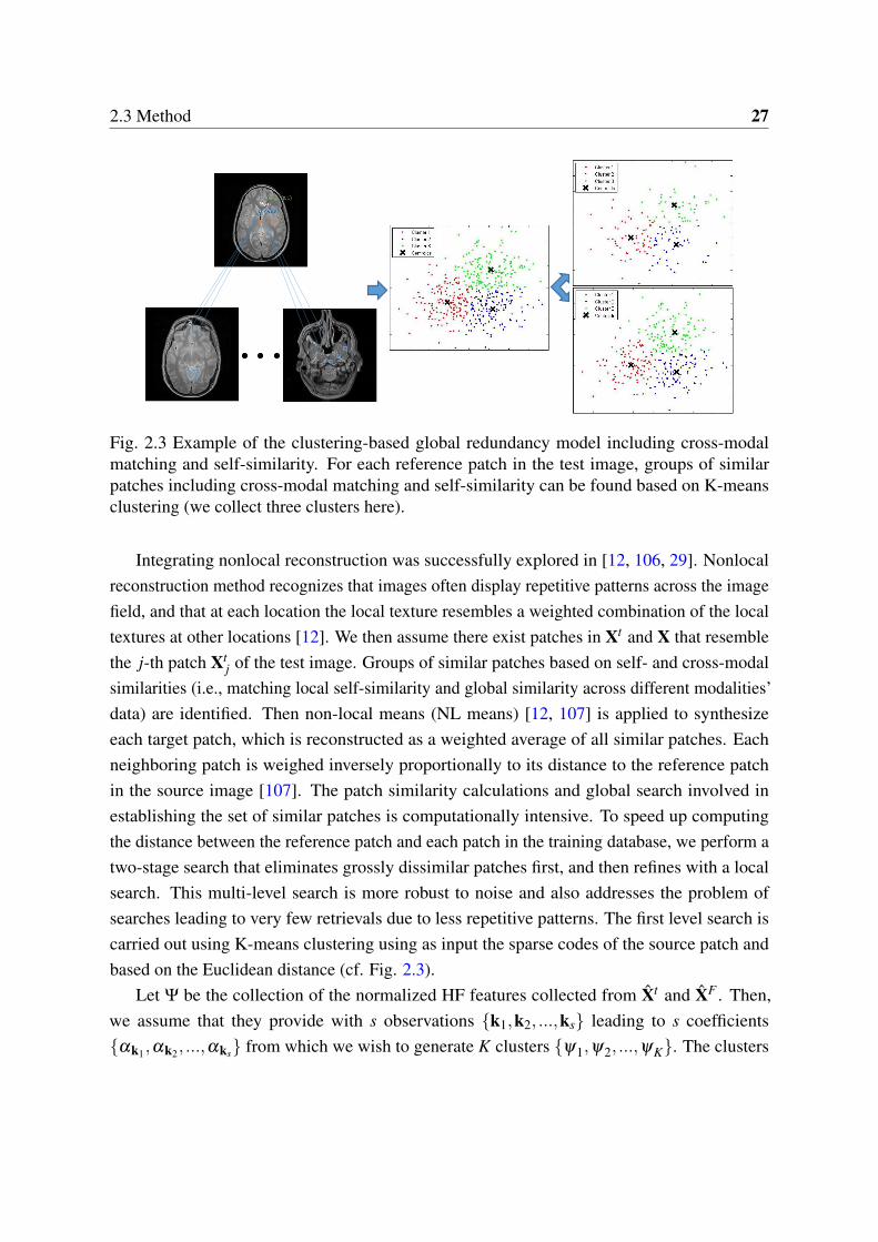
2.3 Method 27
Fig. 2.3 Example of the clustering-based global redundancy model including cross-modalmatching and self-similarity. For each reference patch in the test image, groups of similarpatches including cross-modal matching and self-similarity can be found based on K-meansclustering (we collect three clusters here).
Integrating nonlocal reconstruction was successfully explored in [12, 106, 29]. Nonlocalreconstruction method recognizes that images often display repetitive patterns across the imagefield, and that at each location the local texture resembles a weighted combination of the localtextures at other locations [12]. We then assume there exist patches in Xt and X that resemblethe j-th patch Xt
j of the test image. Groups of similar patches based on self- and cross-modalsimilarities (i.e., matching local self-similarity and global similarity across different modalities’data) are identified. Then non-local means (NL means) [12, 107] is applied to synthesizeeach target patch, which is reconstructed as a weighted average of all similar patches. Eachneighboring patch is weighed inversely proportionally to its distance to the reference patchin the source image [107]. The patch similarity calculations and global search involved inestablishing the set of similar patches is computationally intensive. To speed up computingthe distance between the reference patch and each patch in the training database, we perform atwo-stage search that eliminates grossly dissimilar patches first, and then refines with a localsearch. This multi-level search is more robust to noise and also addresses the problem ofsearches leading to very few retrievals due to less repetitive patterns. The first level search iscarried out using K-means clustering using as input the sparse codes of the source patch andbased on the Euclidean distance (cf. Fig. 2.3).
Let Ψ be the collection of the normalized HF features collected from Xt and XF . Then,we assume that they provide with s observations k1,k2, ...,ks leading to s coefficientsαk1,αk2, ...,αks from which we wish to generate K clusters ψ1,ψ2, ...,ψK. The clusters
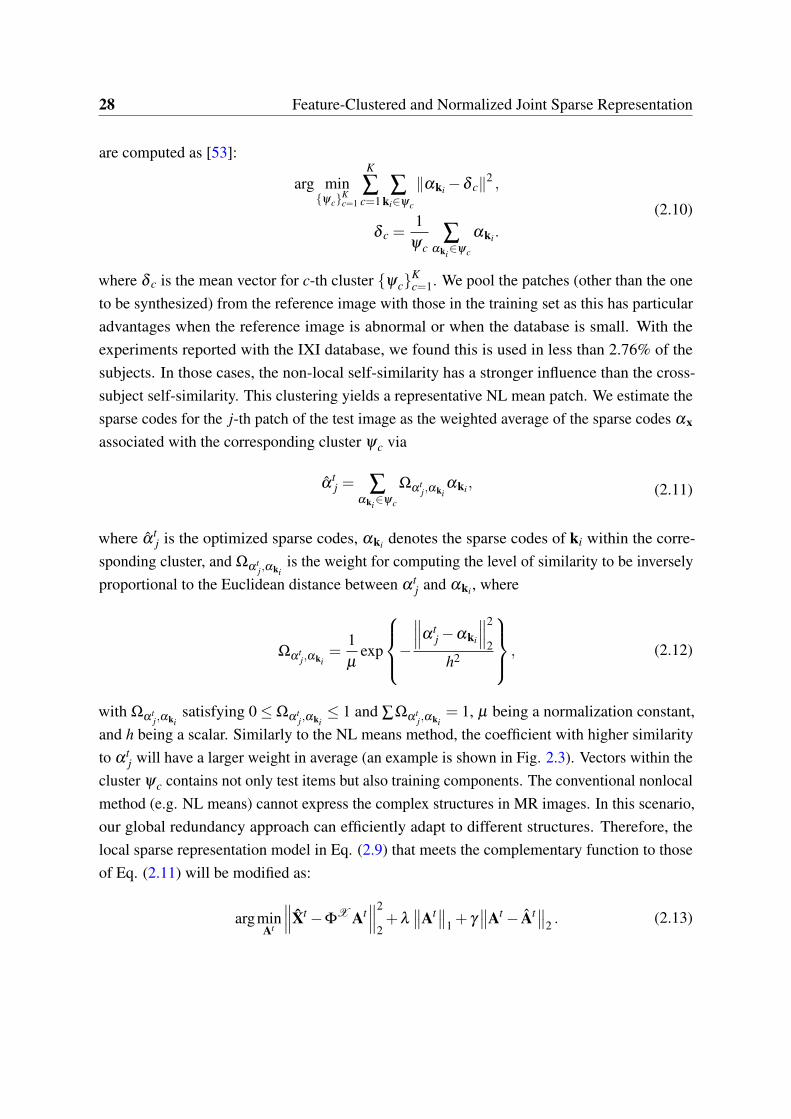
28 Feature-Clustered and Normalized Joint Sparse Representation
are computed as [53]:
arg minψc
Kc=1
K
∑c=1
∑ki∈ψc
∥αki−δ c∥2 ,
δ c =1
ψc∑
αki∈ψc
αki.
(2.10)
where δ c is the mean vector for c-th cluster ψcKc=1. We pool the patches (other than the one
to be synthesized) from the reference image with those in the training set as this has particularadvantages when the reference image is abnormal or when the database is small. With theexperiments reported with the IXI database, we found this is used in less than 2.76% of thesubjects. In those cases, the non-local self-similarity has a stronger influence than the cross-subject self-similarity. This clustering yields a representative NL mean patch. We estimate thesparse codes for the j-th patch of the test image as the weighted average of the sparse codes αx
associated with the corresponding cluster ψc via
αtj = ∑
αki∈ψc
Ωαtj,αki
αki, (2.11)
where αtj is the optimized sparse codes, αki denotes the sparse codes of ki within the corre-
sponding cluster, and Ωαtj,αki
is the weight for computing the level of similarity to be inverselyproportional to the Euclidean distance between α t
j and αki , where
Ωαtj,αki
=1µ
exp
−∥∥∥α t
j−αki
∥∥∥2
2h2
, (2.12)
with Ωαtj,αki
satisfying 0≤Ωαtj,αki≤ 1 and ∑Ωαt
j,αki= 1, µ being a normalization constant,
and h being a scalar. Similarly to the NL means method, the coefficient with higher similarityto α t
j will have a larger weight in average (an example is shown in Fig. 2.3). Vectors within thecluster ψc contains not only test items but also training components. The conventional nonlocalmethod (e.g. NL means) cannot express the complex structures in MR images. In this scenario,our global redundancy approach can efficiently adapt to different structures. Therefore, thelocal sparse representation model in Eq. (2.9) that meets the complementary function to thoseof Eq. (2.11) will be modified as:
argminAt
∥∥∥Xt−ΦX At
∥∥∥2
2+λ
∥∥At∥∥1 + γ
∥∥At− At∥∥2 . (2.13)
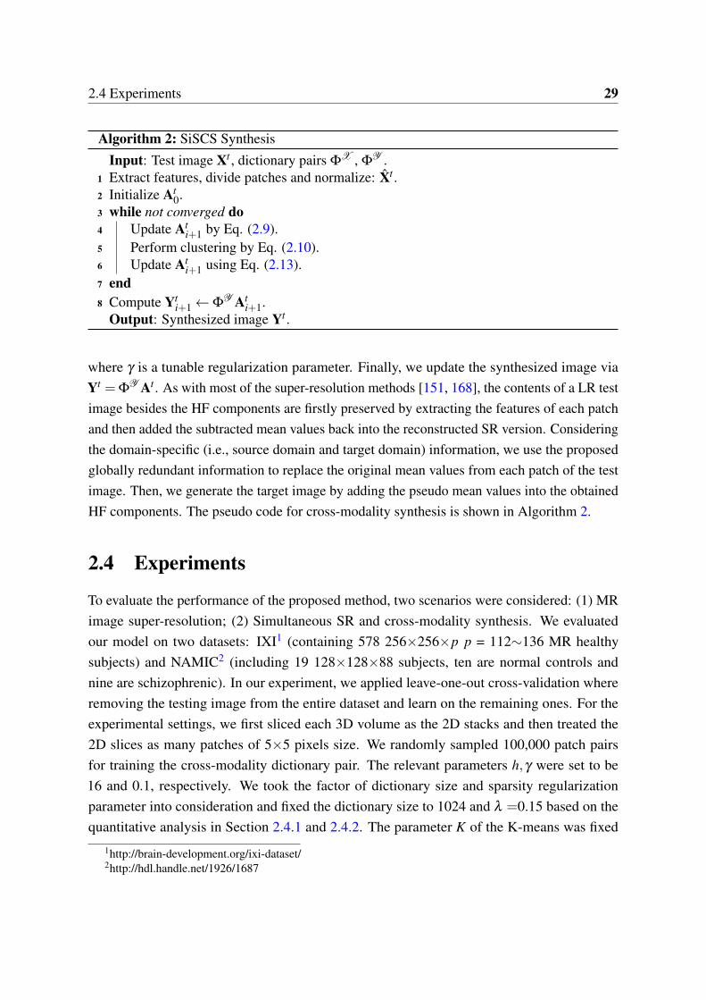
2.4 Experiments 29
Algorithm 2: SiSCS Synthesis
Input: Test image Xt , dictionary pairs ΦX , Φ
Y .1 Extract features, divide patches and normalize: Xt .2 Initialize At
0.3 while not converged do4 Update At
i+1 by Eq. (2.9).5 Perform clustering by Eq. (2.10).6 Update At
i+1 using Eq. (2.13).7 end8 Compute Yt
i+1←ΦY At
i+1.Output: Synthesized image Yt .
where γ is a tunable regularization parameter. Finally, we update the synthesized image viaYt = Φ
Y At . As with most of the super-resolution methods [151, 168], the contents of a LR testimage besides the HF components are firstly preserved by extracting the features of each patchand then added the subtracted mean values back into the reconstructed SR version. Consideringthe domain-specific (i.e., source domain and target domain) information, we use the proposedglobally redundant information to replace the original mean values from each patch of the testimage. Then, we generate the target image by adding the pseudo mean values into the obtainedHF components. The pseudo code for cross-modality synthesis is shown in Algorithm 2.
2.4 Experiments
To evaluate the performance of the proposed method, two scenarios were considered: (1) MRimage super-resolution; (2) Simultaneous SR and cross-modality synthesis. We evaluatedour model on two datasets: IXI1 (containing 578 256×256×p p = 112∼136 MR healthysubjects) and NAMIC2 (including 19 128×128×88 subjects, ten are normal controls andnine are schizophrenic). In our experiment, we applied leave-one-out cross-validation whereremoving the testing image from the entire dataset and learn on the remaining ones. For theexperimental settings, we first sliced each 3D volume as the 2D stacks and then treated the2D slices as many patches of 5×5 pixels size. We randomly sampled 100,000 patch pairsfor training the cross-modality dictionary pair. The relevant parameters h,γ were set to be16 and 0.1, respectively. We took the factor of dictionary size and sparsity regularizationparameter into consideration and fixed the dictionary size to 1024 and λ =0.15 based on thequantitative analysis in Section 2.4.1 and 2.4.2. The parameter K of the K-means was fixed
1http://brain-development.org/ixi-dataset/2http://hdl.handle.net/1926/1687
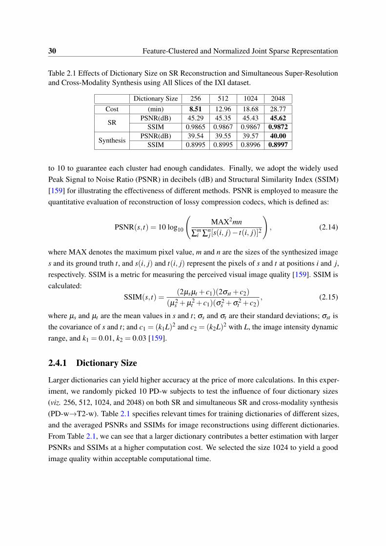
30 Feature-Clustered and Normalized Joint Sparse Representation
Table 2.1 Effects of Dictionary Size on SR Reconstruction and Simultaneous Super-Resolutionand Cross-Modality Synthesis using All Slices of the IXI dataset.
Dictionary Size 256 512 1024 2048Cost (min) 8.51 12.96 18.68 28.77
SRPSNR(dB) 45.29 45.35 45.43 45.62
SSIM 0.9865 0.9867 0.9867 0.9872
SynthesisPSNR(dB) 39.54 39.55 39.57 40.00
SSIM 0.8995 0.8995 0.8996 0.8997
to 10 to guarantee each cluster had enough candidates. Finally, we adopt the widely usedPeak Signal to Noise Ratio (PSNR) in decibels (dB) and Structural Similarity Index (SSIM)[159] for illustrating the effectiveness of different methods. PSNR is employed to measure thequantitative evaluation of reconstruction of lossy compression codecs, which is defined as:
PSNR(s, t) = 10 log10
(MAX2mn
∑mi ∑
nj [s(i, j)− t(i, j)]2
), (2.14)
where MAX denotes the maximum pixel value, m and n are the sizes of the synthesized images and its ground truth t, and s(i, j) and t(i, j) represent the pixels of s and t at positions i and j,respectively. SSIM is a metric for measuring the perceived visual image quality [159]. SSIM iscalculated:
SSIM(s, t) =(2µsµt + c1)(2σst + c2)
(µ2s +µ2
t + c1)(σ2s +σ2
t + c2), (2.15)
where µs and µt are the mean values in s and t; σs and σt are their standard deviations; σst isthe covariance of s and t; and c1 = (k1L)2 and c2 = (k2L)2 with L, the image intensity dynamicrange, and k1 = 0.01, k2 = 0.03 [159].
2.4.1 Dictionary Size
Larger dictionaries can yield higher accuracy at the price of more calculations. In this exper-iment, we randomly picked 10 PD-w subjects to test the influence of four dictionary sizes(viz. 256, 512, 1024, and 2048) on both SR and simultaneous SR and cross-modality synthesis(PD-w→T2-w). Table 2.1 specifies relevant times for training dictionaries of different sizes,and the averaged PSNRs and SSIMs for image reconstructions using different dictionaries.From Table 2.1, we can see that a larger dictionary contributes a better estimation with largerPSNRs and SSIMs at a higher computation cost. We selected the size 1024 to yield a goodimage quality within acceptable computational time.
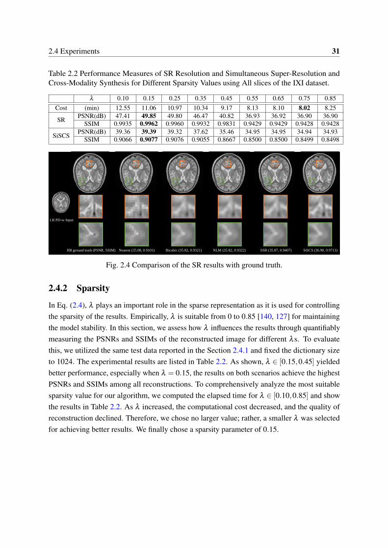
2.4 Experiments 31
Table 2.2 Performance Measures of SR Resolution and Simultaneous Super-Resolution andCross-Modality Synthesis for Different Sparsity Values using All slices of the IXI dataset.
λ 0.10 0.15 0.25 0.35 0.45 0.55 0.65 0.75 0.85Cost (min) 12.55 11.06 10.97 10.34 9.17 8.13 8.10 8.02 8.25
SR PSNR(dB) 47.41 49.85 49.80 46.47 40.82 36.93 36.92 36.90 36.90SSIM 0.9935 0.9962 0.9960 0.9932 0.9831 0.9429 0.9429 0.9428 0.9428
SiSCS PSNR(dB) 39.36 39.39 39.32 37.62 35.46 34.95 34.95 34.94 34.93SSIM 0.9066 0.9077 0.9076 0.9055 0.8667 0.8500 0.8500 0.8499 0.8498
HR ground truth (PSNR, SSIM) Bicubic (35.82, 0.9321)Nearest (35.08, 0.9101) NLM (35.82, 0.9322) SiSCS (36.90, 0.9713)SSR (35.87, 0.9407)
LR PD-w Input
HR ground truth (PSNR, SSIM) Bicubic (35.82, 0.9321)Nearest (35.08, 0.9101) NLM (35.82, 0.9322) SiSCS (36.90, 0.9713)SSR (35.87, 0.9407)
LR PD-w Input
Fig. 2.4 Comparison of the SR results with ground truth.
2.4.2 Sparsity
In Eq. (2.4), λ plays an important role in the sparse representation as it is used for controllingthe sparsity of the results. Empirically, λ is suitable from 0 to 0.85 [140, 127] for maintainingthe model stability. In this section, we assess how λ influences the results through quantifiablymeasuring the PSNRs and SSIMs of the reconstructed image for different λ s. To evaluatethis, we utilized the same test data reported in the Section 2.4.1 and fixed the dictionary sizeto 1024. The experimental results are listed in Table 2.2. As shown, λ ∈ [0.15,0.45] yieldedbetter performance, especially when λ = 0.15, the results on both scenarios achieve the highestPSNRs and SSIMs among all reconstructions. To comprehensively analyze the most suitablesparsity value for our algorithm, we computed the elapsed time for λ ∈ [0.10,0.85] and showthe results in Table 2.2. As λ increased, the computational cost decreased, and the quality ofreconstruction declined. Therefore, we chose no larger value; rather, a smaller λ was selectedfor achieving better results. We finally chose a sparsity parameter of 0.15.
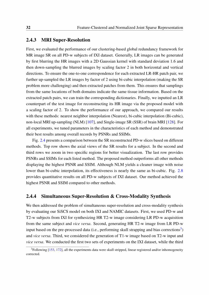
32 Feature-Clustered and Normalized Joint Sparse Representation
2.4.3 MRI Super-Resolution
First, we evaluated the performance of our clustering-based global redundancy framework forMR image SR on all PD-w subjects of IXI dataset. Generally, LR images can be generatedby first blurring the HR images with a 2D Gaussian kernel with standard deviation 1.6 andthen down-sampling the blurred images by scaling factor 2 in both horizontal and verticaldirections. To ensure the one-to-one correspondence for each extracted LR-HR patch pair, wefurther up-sampled the LR images by factor of 2 using bi-cubic interpolation (making the SRproblem more challenging) and then extracted patches from them. This ensures that samplingsfrom the same locations of both domains indicate the same tissue information. Based on theextracted patch pairs, we can train the corresponding dictionaries. Finally, we inputted an LRcounterpart of the test image for reconstructing its HR image via the proposed model witha scaling factor of 2. To show the performance of our approach, we compared our resultswith these methods: nearest neighbor interpolation (Nearest), bi-cubic interpolation (Bi-cubic),non-local MRI up-sampling (NLM) [107], and Single-image SR (SSR) of brain MRI [128]. Forall experiments, we tuned parameters in the characteristics of each method and demonstratedtheir best results among overall records by PSNRs and SSIMs.
Fig. 2.4 presents a comparison between the SR reconstructed PD-w slices based on differentmethods. Top row shows the axial views of the SR results for a subject. In the second andthird rows we zoom in two specific regions for better visualization. The last row providesPSNRs and SSIMs for each listed method. The proposed method outperforms all other methodsdisplaying the highest PSNR and SSIM. Although NLM yields a cleaner image with noiselower than bi-cubic interpolation, its effectiveness is nearly the same as bi-cubic. Fig. 2.8provides quantitative results on all PD-w subjects of IXI dataset. Our method achieved thehighest PSNR and SSIM compared to other methods.
2.4.4 Simultaneous Super-Resolution & Cross-Modality Synthesis
We then addressed the problem of simultaneous super-resolution and cross-modality synthesisby evaluating our SiSCS model on both IXI and NAMIC datasets. First, we used PD-w andT2-w subjects from IXI for synthesizing HR T2-w image considering LR PD-w acquisitionfrom the same subject and vice versa. Second, generating HR T2-w image from LR PD-winput based on the pre-processed data (i.e., performing skull strapping and bias corrections3)and vice versa. Third, we considered the generation of T1-w image based on T2-w input andvice versa. We conducted the first two sets of experiments on the IXI dataset, while the third
3Following [153, 172], all the experiments data were skull stripped, linear registered and/or inhomogeneitycorrected.
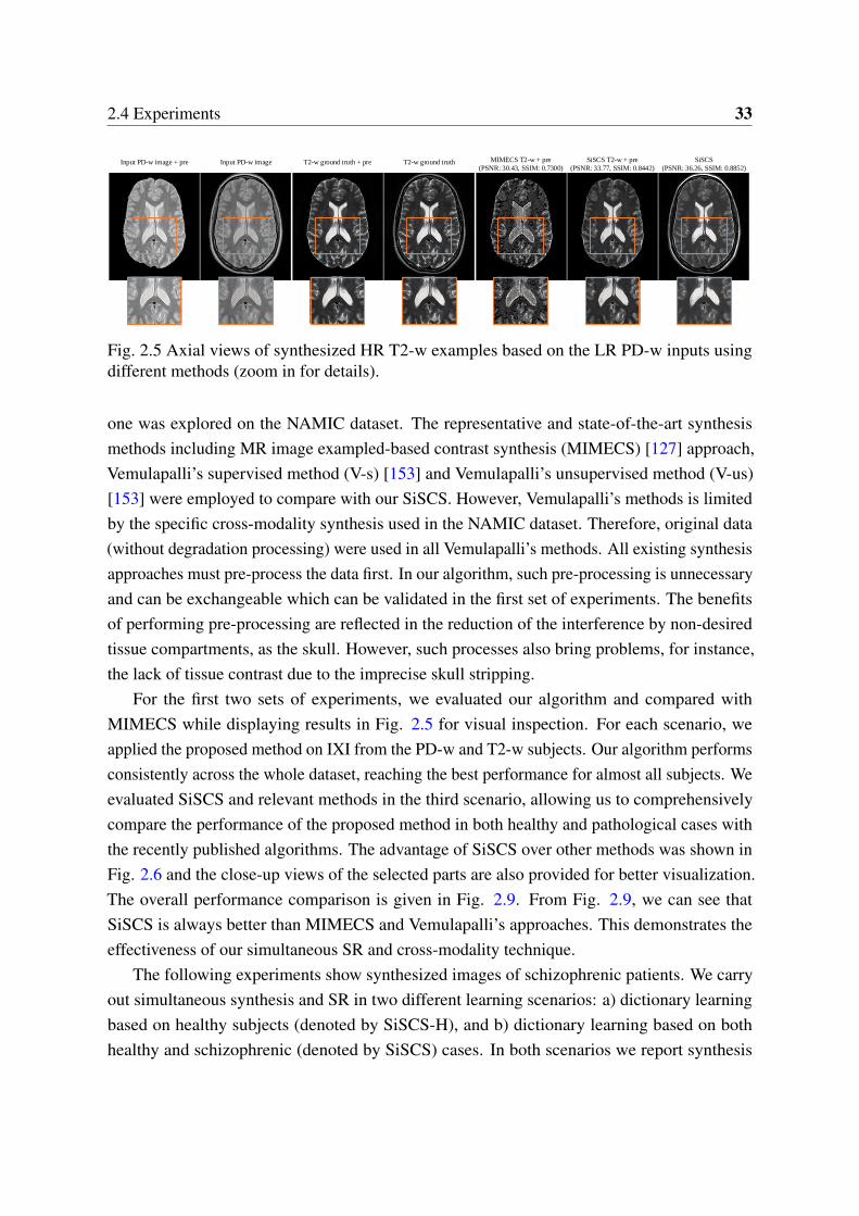
2.4 Experiments 33
Input PD-w image + pre Input PD-w image T2-w ground truth + pre T2-w ground truth MIMECS T2-w + pre
(PSNR: 30.43, SSIM: 0.7300)
SiSCS T2-w + pre
(PSNR: 33.77, SSIM: 0.8442)
SiSCS
(PSNR: 36.26, SSIM: 0.8852)
Fig. 2.5 Axial views of synthesized HR T2-w examples based on the LR PD-w inputs usingdifferent methods (zoom in for details).
one was explored on the NAMIC dataset. The representative and state-of-the-art synthesismethods including MR image exampled-based contrast synthesis (MIMECS) [127] approach,Vemulapalli’s supervised method (V-s) [153] and Vemulapalli’s unsupervised method (V-us)[153] were employed to compare with our SiSCS. However, Vemulapalli’s methods is limitedby the specific cross-modality synthesis used in the NAMIC dataset. Therefore, original data(without degradation processing) were used in all Vemulapalli’s methods. All existing synthesisapproaches must pre-process the data first. In our algorithm, such pre-processing is unnecessaryand can be exchangeable which can be validated in the first set of experiments. The benefitsof performing pre-processing are reflected in the reduction of the interference by non-desiredtissue compartments, as the skull. However, such processes also bring problems, for instance,the lack of tissue contrast due to the imprecise skull stripping.
For the first two sets of experiments, we evaluated our algorithm and compared withMIMECS while displaying results in Fig. 2.5 for visual inspection. For each scenario, weapplied the proposed method on IXI from the PD-w and T2-w subjects. Our algorithm performsconsistently across the whole dataset, reaching the best performance for almost all subjects. Weevaluated SiSCS and relevant methods in the third scenario, allowing us to comprehensivelycompare the performance of the proposed method in both healthy and pathological cases withthe recently published algorithms. The advantage of SiSCS over other methods was shown inFig. 2.6 and the close-up views of the selected parts are also provided for better visualization.The overall performance comparison is given in Fig. 2.9. From Fig. 2.9, we can see thatSiSCS is always better than MIMECS and Vemulapalli’s approaches. This demonstrates theeffectiveness of our simultaneous SR and cross-modality technique.
The following experiments show synthesized images of schizophrenic patients. We carryout simultaneous synthesis and SR in two different learning scenarios: a) dictionary learningbased on healthy subjects (denoted by SiSCS-H), and b) dictionary learning based on bothhealthy and schizophrenic (denoted by SiSCS) cases. In both scenarios we report synthesis
34 Feature-Clustered and Normalized Joint Sparse Representation
Input T1-w T2-w ground truth MIMECS T2-w V-us T2-w SiSCS T2-wV-s T2-w
Input T2-w T1-w ground truth MIMECS T1-w V-us T1-w SiSCS T1-wV-s T1-w
Input T1-w T2-w ground truth MIMECS T2-w V-us T2-w SiSCS T2-wV-s T2-w
Input T2-w T1-w ground truth MIMECS T1-w V-us T1-w SiSCS T1-wV-s T1-w
Fig. 2.6 Visual comparison of synthesized results using different methods on the NAMICdataset (zoom in for details).
Ground Truth MIMECS V-us SiSCS-H SiSCSV-sGround Truth MIMECS V-us SiSCS-H SiSCSV-s
Fig. 2.7 Synthesis result of a pathological case comparison between SiSCS and other stat-of-the-art methods.
results corresponding to schizophrenia cases only. Fig. 2.7 provides visual results of varioussynthesis methods of an illustrative patient. Table 2.3 summarizes key quantitative performancemetrics over the total set of 9 schizophrenic subjects. Both visual and quantitative results showthat, compared to earlier methods, our approach provides the best results. Our experiments alsoshow that SiSCS-H is outperformed by SiSCS trained on both control and pathologic cases andtested using cross-validation.
2.5 Conclusions
We present a novel approach to simultaneous super-resolution and cross-modality synthesis(SiSCS) in brain MRI. SiSCS first learns a cross-modality dictionary in a high-frequency space.
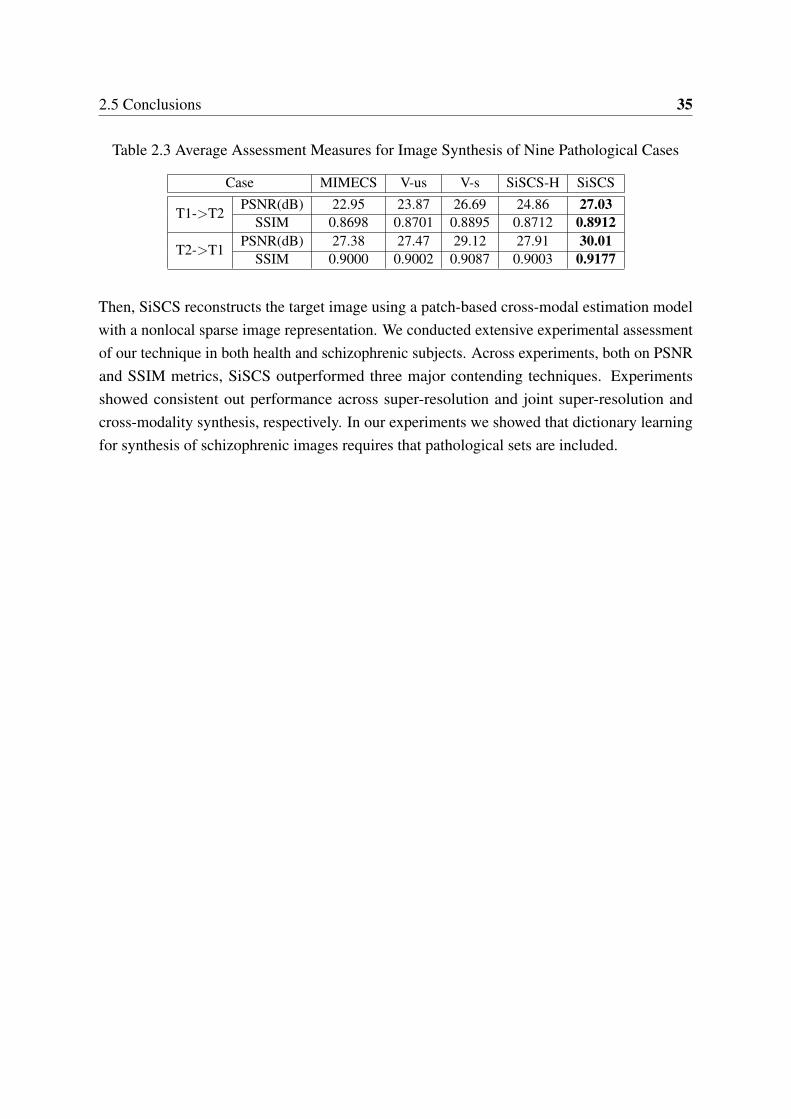
2.5 Conclusions 35
Table 2.3 Average Assessment Measures for Image Synthesis of Nine Pathological Cases
Case MIMECS V-us V-s SiSCS-H SiSCS
T1->T2PSNR(dB) 22.95 23.87 26.69 24.86 27.03
SSIM 0.8698 0.8701 0.8895 0.8712 0.8912
T2->T1PSNR(dB) 27.38 27.47 29.12 27.91 30.01
SSIM 0.9000 0.9002 0.9087 0.9003 0.9177
Then, SiSCS reconstructs the target image using a patch-based cross-modal estimation modelwith a nonlocal sparse image representation. We conducted extensive experimental assessmentof our technique in both health and schizophrenic subjects. Across experiments, both on PSNRand SSIM metrics, SiSCS outperformed three major contending techniques. Experimentsshowed consistent out performance across super-resolution and joint super-resolution andcross-modality synthesis, respectively. In our experiments we showed that dictionary learningfor synthesis of schizophrenic images requires that pathological sets are included.
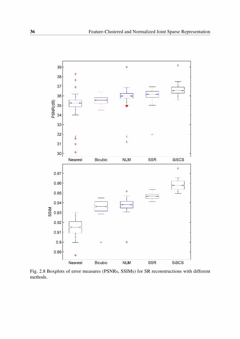
36 Feature-Clustered and Normalized Joint Sparse Representation
Fig. 2.8 Boxplots of error measures (PSNRs, SSIMs) for SR reconstructions with differentmethods.
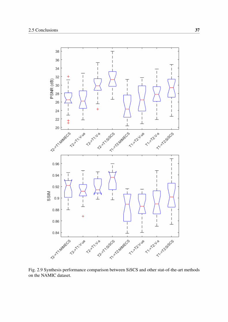
2.5 Conclusions 37
Fig. 2.9 Synthesis performance comparison between SiSCS and other stat-of-the-art methodson the NAMIC dataset.

Chapter 3
Dual Convolutional Filter Learning
Cross-modal image synthesis is a topical problem in medical image computing. Existingmethods for image synthesis are either tailored to a specific application, require large scaletraining sets, or are based on partitioning images into overlapping patches. In this chapter,we propose a novel Dual cOnvolutional filTer lEarning (DOTE) approach to overcome thedrawbacks of these approaches. We construct a closed loop joint filter learning strategy thatgenerates informative feedback for model self-optimization. Our method can leverage datamore efficiently thus reducing the size of the required training set. We extensively evaluateDOTE in two challenging tasks: image super-resolution and cross-modality synthesis. Theexperimental results demonstrate superior performance of our method over other state-of-the-artmethods.
3.1 Introduction
In medical image analysis, it is sometimes convenient or necessary to infer an image from onemodality or resolution from another image modality or resolution for better disease visualization,prediction and detection purposes. A major challenge of cross-modality image segmentationor registration comes from the differences in tissue appearance or spatial resolution in imagesarising from different physical acquisition principles or parameters, which translates into thedifficulty to represent and relate these images. Some existing methods tackle this problem bylearning from a large amount of registered images and constraining pairwise solutions in acommon space. In general, one would desire to have high-resolution (HR) three-dimensionalMagnetic Resonance Imaging (MRI) with near isotropic voxel resolution as opposed to themore common image stacks of multiple 2D slices for accurate quantitative image analysis anddiagnosis. Multi-modality imaging can generate tissue contrast arising from various anatomical
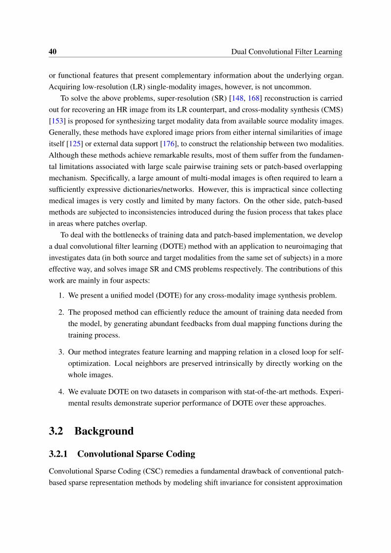
40 Dual Convolutional Filter Learning
or functional features that present complementary information about the underlying organ.Acquiring low-resolution (LR) single-modality images, however, is not uncommon.
To solve the above problems, super-resolution (SR) [148, 168] reconstruction is carriedout for recovering an HR image from its LR counterpart, and cross-modality synthesis (CMS)[153] is proposed for synthesizing target modality data from available source modality images.Generally, these methods have explored image priors from either internal similarities of imageitself [125] or external data support [176], to construct the relationship between two modalities.Although these methods achieve remarkable results, most of them suffer from the fundamen-tal limitations associated with large scale pairwise training sets or patch-based overlappingmechanism. Specifically, a large amount of multi-modal images is often required to learn asufficiently expressive dictionaries/networks. However, this is impractical since collectingmedical images is very costly and limited by many factors. On the other side, patch-basedmethods are subjected to inconsistencies introduced during the fusion process that takes placein areas where patches overlap.
To deal with the bottlenecks of training data and patch-based implementation, we developa dual convolutional filter learning (DOTE) method with an application to neuroimaging thatinvestigates data (in both source and target modalities from the same set of subjects) in a moreeffective way, and solves image SR and CMS problems respectively. The contributions of thiswork are mainly in four aspects:
1. We present a unified model (DOTE) for any cross-modality image synthesis problem.
2. The proposed method can efficiently reduce the amount of training data needed fromthe model, by generating abundant feedbacks from dual mapping functions during thetraining process.
3. Our method integrates feature learning and mapping relation in a closed loop for self-optimization. Local neighbors are preserved intrinsically by directly working on thewhole images.
4. We evaluate DOTE on two datasets in comparison with stat-of-the-art methods. Experi-mental results demonstrate superior performance of DOTE over these approaches.
3.2 Background
3.2.1 Convolutional Sparse Coding
Convolutional Sparse Coding (CSC) remedies a fundamental drawback of conventional patch-based sparse representation methods by modeling shift invariance for consistent approximation
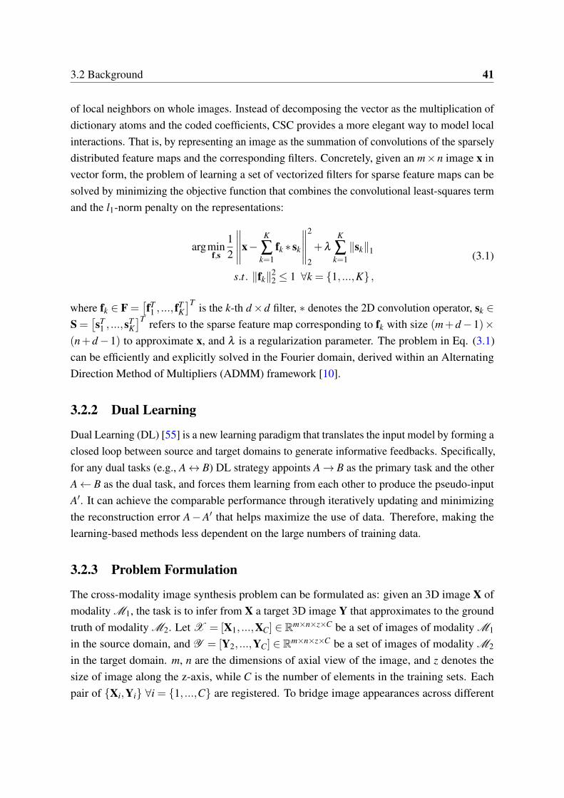
3.2 Background 41
of local neighbors on whole images. Instead of decomposing the vector as the multiplication ofdictionary atoms and the coded coefficients, CSC provides a more elegant way to model localinteractions. That is, by representing an image as the summation of convolutions of the sparselydistributed feature maps and the corresponding filters. Concretely, given an m×n image x invector form, the problem of learning a set of vectorized filters for sparse feature maps can besolved by minimizing the objective function that combines the convolutional least-squares termand the l1-norm penalty on the representations:
argminf,s
12
∥∥∥∥∥x−K
∑k=1
fk ∗ sk
∥∥∥∥∥2
2
+λ
K
∑k=1∥sk∥1
s.t. ∥fk∥22 ≤ 1 ∀k = 1, ...,K ,
(3.1)
where fk ∈ F =[fT1 , ..., f
TK]T is the k-th d×d filter, ∗ denotes the 2D convolution operator, sk ∈
S =[sT
1 , ...,sTK]T refers to the sparse feature map corresponding to fk with size (m+d−1)×
(n+d−1) to approximate x, and λ is a regularization parameter. The problem in Eq. (3.1)can be efficiently and explicitly solved in the Fourier domain, derived within an AlternatingDirection Method of Multipliers (ADMM) framework [10].
3.2.2 Dual Learning
Dual Learning (DL) [55] is a new learning paradigm that translates the input model by forming aclosed loop between source and target domains to generate informative feedbacks. Specifically,for any dual tasks (e.g., A↔ B) DL strategy appoints A→ B as the primary task and the otherA← B as the dual task, and forces them learning from each other to produce the pseudo-inputA′. It can achieve the comparable performance through iteratively updating and minimizingthe reconstruction error A−A′ that helps maximize the use of data. Therefore, making thelearning-based methods less dependent on the large numbers of training data.
3.2.3 Problem Formulation
The cross-modality image synthesis problem can be formulated as: given an 3D image X ofmodality M1, the task is to infer from X a target 3D image Y that approximates to the groundtruth of modality M2. Let X = [X1, ...,XC] ∈ Rm×n×z×C be a set of images of modality M1
in the source domain, and Y = [Y2, ...,YC] ∈ Rm×n×z×C be a set of images of modality M2
in the target domain. m, n are the dimensions of axial view of the image, and z denotes thesize of image along the z-axis, while C is the number of elements in the training sets. Eachpair of Xi,Yi ∀i = 1, ...,C are registered. To bridge image appearances across different
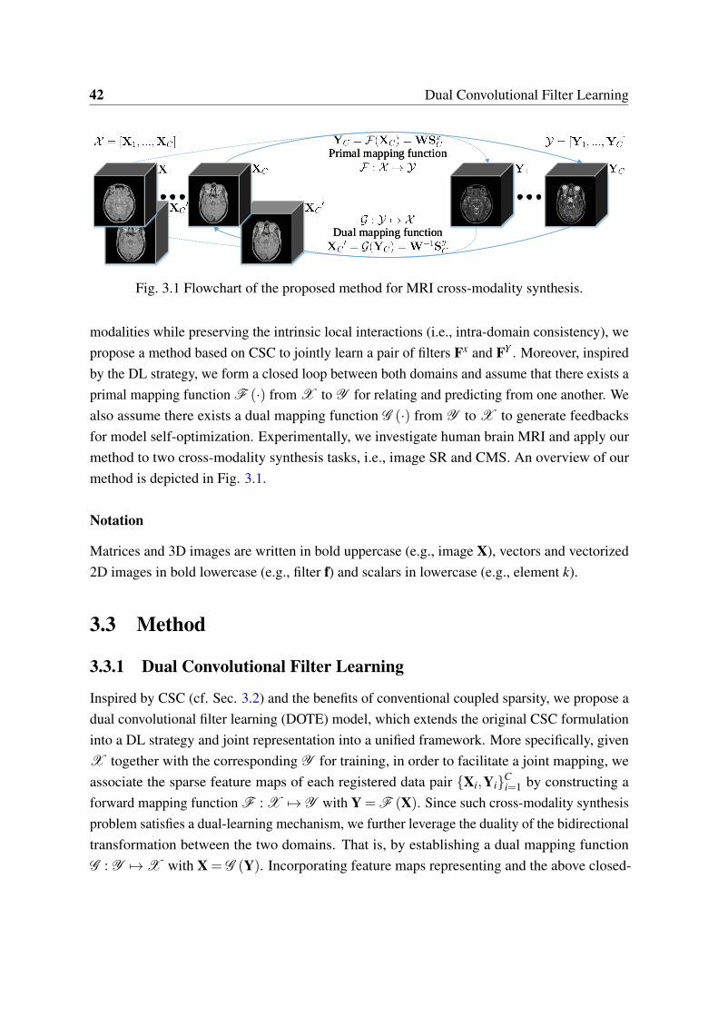
42 Dual Convolutional Filter Learning
Dual mapping functionDual mapping function
Primal mapping functionPrimal mapping function
Fig. 3.1 Flowchart of the proposed method for MRI cross-modality synthesis.
modalities while preserving the intrinsic local interactions (i.e., intra-domain consistency), wepropose a method based on CSC to jointly learn a pair of filters Fx and FY . Moreover, inspiredby the DL strategy, we form a closed loop between both domains and assume that there exists aprimal mapping function F (·) from X to Y for relating and predicting from one another. Wealso assume there exists a dual mapping function G (·) from Y to X to generate feedbacksfor model self-optimization. Experimentally, we investigate human brain MRI and apply ourmethod to two cross-modality synthesis tasks, i.e., image SR and CMS. An overview of ourmethod is depicted in Fig. 3.1.
Notation
Matrices and 3D images are written in bold uppercase (e.g., image X), vectors and vectorized2D images in bold lowercase (e.g., filter f) and scalars in lowercase (e.g., element k).
3.3 Method
3.3.1 Dual Convolutional Filter Learning
Inspired by CSC (cf. Sec. 3.2) and the benefits of conventional coupled sparsity, we propose adual convolutional filter learning (DOTE) model, which extends the original CSC formulationinto a DL strategy and joint representation into a unified framework. More specifically, givenX together with the corresponding Y for training, in order to facilitate a joint mapping, weassociate the sparse feature maps of each registered data pair Xi,YiCi=1 by constructing aforward mapping function F : X 7→ Y with Y = F (X). Since such cross-modality synthesisproblem satisfies a dual-learning mechanism, we further leverage the duality of the bidirectionaltransformation between the two domains. That is, by establishing a dual mapping functionG : Y 7→X with X = G (Y). Incorporating feature maps representing and the above closed-

3.3 Method 43
loop mapping functions, we can thus derive the following objective function:
arg minFx,Fy,Sx,Sy,W
12
∥∥∥∥∥X−K
∑k=1
Fxk ∗Sx
k
∥∥∥∥∥2
F
+12
∥∥∥∥∥Y−K
∑k=1
Fyk ∗Sy
k
∥∥∥∥∥2
F
+ γ
K
∑k=1∥Wk∥2
F
+λ
(K
∑k=1∥Sx
k∥1 +K
∑k=1
∥∥Syk
∥∥1
)+β
(K
∑k=1
∥∥Syk−WkSx
k
∥∥2F +
K
∑k=1
∥∥Sxk−W−1
k Syk
∥∥2F
)s.t. ∥fx
k∥22 ≤ 1
∥∥fyk
∥∥22 ≤ 1 ∀k = 1, ...,K .
(3.2)
where Sxk and Sy
k take the role of the k-th sparse feature maps that approximate data X and Ywhen convolved with the k-th filters Fx
k and Fyk of a fixed spatial support, k = 1, ...,K. ∥·∥F
is a Frobenius norm chosen to induce the convolutional least squares approximation, and ∗is represented as a 3D convolution operator, while λ , β , γ are the regularization parameters.Particularly, dual mapping functions F
(Sx
k,Wk)= WkSx
k and G(Sy
k,W−1k
)= W−1
k Syk are used
to relate the sparse feature maps of X and Y over Fx and Fy. They are done by solving two setsof least squares terms (i.e., ∑
Kk=1(
∥∥Syk−WkSx
k
∥∥2F +∑
Kk=1
∥∥Sxk−W−1
k Syk
∥∥2F) with respect to the
linear projections.
3.3.2 Optimization
Similar to classical dictionary learning methods, the objective function in Eq. (3.2) is notsimultaneously convex with respect to the learned filter pairs,the sparse feature maps and themapping. Instead, we divide the proposed method into three sub-problems: learning Sx, Sy,training Fx, Fy, and updating W.
Computing sparse feature maps
We first initialize the filters Fx, Fy as two random matrices and the mapping W as an identitymatrix, then fix them for calculating the solutions of sparse feature maps Sx, Sy. As a result, theproblem of Eq. (3.2) can be converted into two optimization sub-problems. Unfortunately, thiscannot be solved under l1 penalty without breaking rotation invariance. The resulting alternatingalgorithms [10] by introducing two auxiliary variables U and V enforce the constraint inherentin the splitting. In this work, we follow [10] and solve the convolution subproblems in the
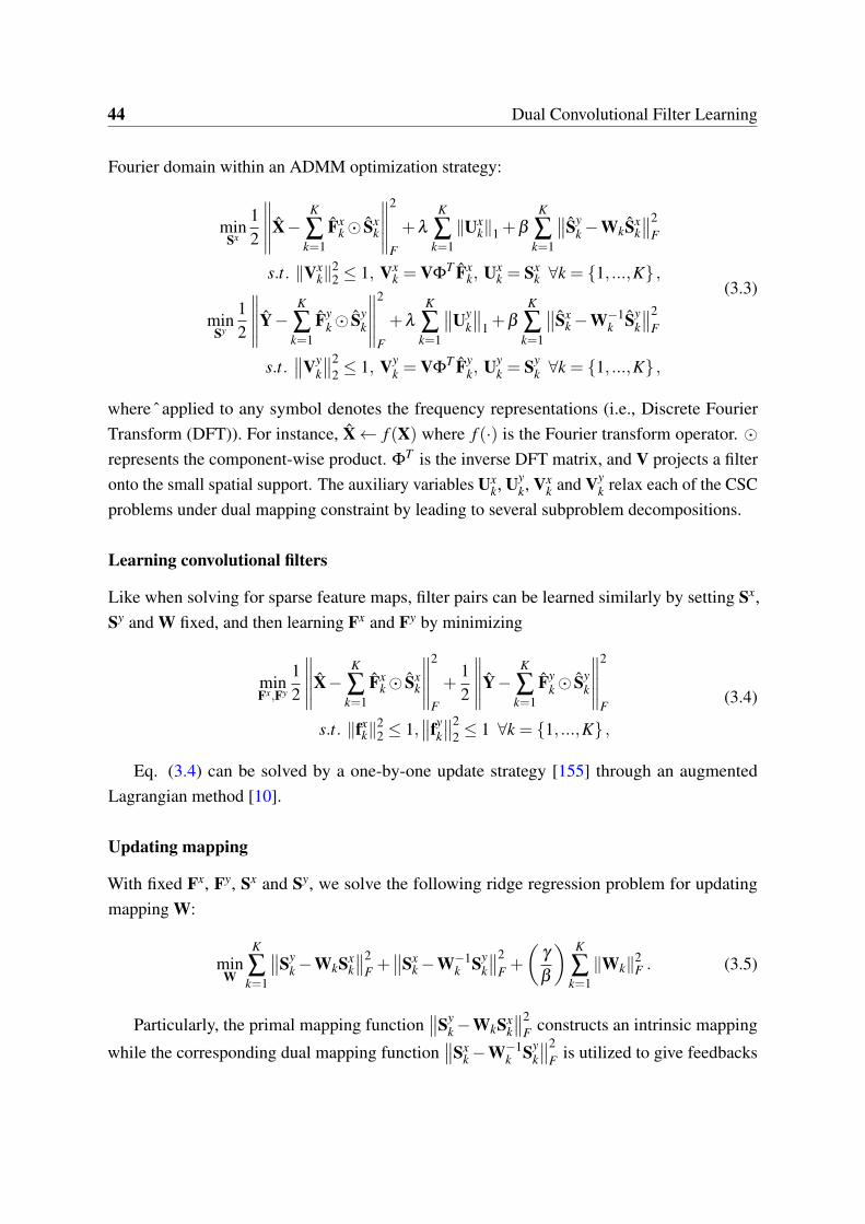
44 Dual Convolutional Filter Learning
Fourier domain within an ADMM optimization strategy:
minSx
12
∥∥∥∥∥X−K
∑k=1
Fxk⊙ Sx
k
∥∥∥∥∥2
F
+λ
K
∑k=1∥Ux
k∥1 +β
K
∑k=1
∥∥Syk−WkSx
k
∥∥2F
s.t. ∥Vxk∥
22 ≤ 1, Vx
k = VΦT Fx
k, Uxk = Sx
k ∀k = 1, ...,K ,
minSy
12
∥∥∥∥∥Y−K
∑k=1
Fyk⊙ Sy
k
∥∥∥∥∥2
F
+λ
K
∑k=1
∥∥Uyk
∥∥1 +β
K
∑k=1
∥∥Sxk−W−1
k Syk
∥∥2F
s.t.∥∥Vy
k
∥∥22 ≤ 1, Vy
k = VΦT Fy
k, Uyk = Sy
k ∀k = 1, ...,K ,
(3.3)
where ˆ applied to any symbol denotes the frequency representations (i.e., Discrete FourierTransform (DFT)). For instance, X← f (X) where f (·) is the Fourier transform operator. ⊙represents the component-wise product. Φ
T is the inverse DFT matrix, and V projects a filteronto the small spatial support. The auxiliary variables Ux
k, Uyk, Vx
k and Vyk relax each of the CSC
problems under dual mapping constraint by leading to several subproblem decompositions.
Learning convolutional filters
Like when solving for sparse feature maps, filter pairs can be learned similarly by setting Sx,Sy and W fixed, and then learning Fx and Fy by minimizing
minFx,Fy
12
∥∥∥∥∥X−K
∑k=1
Fxk⊙ Sx
k
∥∥∥∥∥2
F
+12
∥∥∥∥∥Y−K
∑k=1
Fyk⊙ Sy
k
∥∥∥∥∥2
F
s.t. ∥fxk∥
22 ≤ 1,
∥∥fyk
∥∥22 ≤ 1 ∀k = 1, ...,K ,
(3.4)
Eq. (3.4) can be solved by a one-by-one update strategy [155] through an augmentedLagrangian method [10].
Updating mapping
With fixed Fx, Fy, Sx and Sy, we solve the following ridge regression problem for updatingmapping W:
minW
K
∑k=1
∥∥Syk−WkSx
k
∥∥2F +
∥∥Sxk−W−1
k Syk
∥∥2F +
(γ
β
) K
∑k=1∥Wk∥2
F . (3.5)
Particularly, the primal mapping function∥∥Sy
k−WkSxk
∥∥2F constructs an intrinsic mapping
while the corresponding dual mapping function∥∥Sx
k−W−1k Sy
k
∥∥2F is utilized to give feedbacks
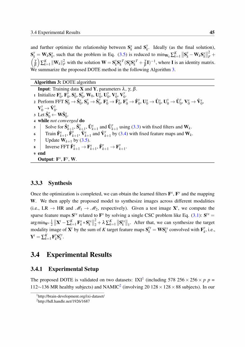
3.4 Experimental Results 45
and further optimize the relationship between Sxk and Sy
k. Ideally (as the final solution),Sy
k = WkSxk, such that the problem in Eq. (3.5) is reduced to minWk ∑
Kk=1
∥∥Syk−WkSx
k
∥∥2F +(
γ
β
)∑
Kk=1 ∥Wk∥2
F with the solution W = SykSx
kT (Sx
kSxk
T + γ
βI)−1, where I is an identity matrix.
We summarize the proposed DOTE method in the following Algorithm 3.
Algorithm 3: DOTE algorithmInput: Training data X and Y, parameters λ , γ , β .
1 Initialize Fx0, Fy
0, Sx0, Sy
0, W0, Ux0, Uy
0, Vx0, Vy
0.2 Perform FFT Sx
0→ Sx0, Sy
0→ Sy0, Fx
0→ Fx0, Fy
0→ Fy0, Ux
0→ Ux0, Uy
0→ Uy0, Vx
0→ Vx0,
Vy0→ Vy
0.3 Let Sy
0←WSx0.
4 while not converged do5 Solve for Sx
k+1, Syk+1, Ux
k+1 and Uyk+1 using (3.3) with fixed filters and Wk.
6 Train Fxk+1, Fy
k+1, Vxk+1 and Vy
k+1 by (3.4) with fixed feature maps and Wk.7 Update Wk+1 by (3.5).8 Inverse FFT Fx
k+1→ Fxk+1, Fy
k+1→ Fyk+1.
9 endOutput: Fx, Fy, W.
3.3.3 Synthesis
Once the optimization is completed, we can obtain the learned filters Fx, Fy and the mappingW. We then apply the proposed model to synthesize images across different modalities(i.e., LR → HR and M1 →M2, respectively). Given a test image Xt , we compute thesparse feature maps Stx related to Fx by solving a single CSC problem like Eq. (3.1): Stx =
argminStx12
∥∥Xt−∑Kk=1 Fx
k ∗Stxk
∥∥22 + λ ∑
Kk=1
∥∥Stxk
∥∥1. After that, we can synthesize the target
modality image of Xt by the sum of K target feature maps Styk = WStx
k convolved with Fyk, i.e.,
Yt = ∑Kk=1 Fy
kStyk .
3.4 Experimental Results
3.4.1 Experimental Setup
The proposed DOTE is validated on two datasets: IXI1 (including 578 256× 256× p p =112∼136 MR healthy subjects) and NAMIC2 (involving 20 128×128×88 subjects). In our
1http://brain-development.org/ixi-dataset/2http://hdl.handle.net/1926/1687
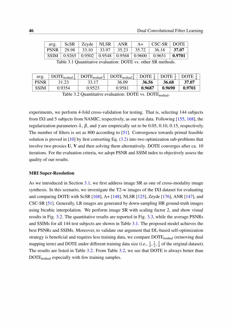
46 Dual Convolutional Filter Learning
avg. ScSR Zeyde NLSR ANR A+ CSC-SR DOTEPSNR 29.98 33.10 33.97 35.23 35.72 36.18 37.07SSIM 0.9265 0.9502 0.9548 0.9568 0.9600 0.9651 0.9701
Table 3.1 Quantitative evaluation: DOTE vs. other SR methods.
avg. DOTEnodual14 DOTEnodual
12 DOTEnodual
34 DOTE 1
4 DOTE 12 DOTE 3
4PSNR 31.23 33.17 36.09 36.56 36.68 37.07SSIM 0.9354 0.9523 0.9581 0.9687 0.9690 0.9701
Table 3.2 Quantitative evaluation: DOTE vs. DOTEnodual.
experiments, we perform 4-fold cross-validation for testing. That is, selecting 144 subjectsfrom IXI and 5 subjects from NAMIC, respectively, as our test data. Following [155, 168], theregularization parameters λ , β , and γ are empirically set to be 0.05, 0.10, 0.15, respectively.The number of filters is set as 800 according to [51]. Convergence towards primal feasiblesolution is proved in [10] by first converting Eq. (3.2) into two optimization sub-problems thatinvolve two proxies U, V and then solving them alternatively. DOTE converges after ca. 10iterations. For the evaluation criteria, we adopt PSNR and SSIM index to objectively assess thequality of our results.
MRI Super-Resolution
As we introduced in Section 3.1, we first address image SR as one of cross-modality imagesynthesis. In this scenario, we investigate the T2-w images of the IXI dataset for evaluatingand comparing DOTE with ScSR [168], A+ [148], NLSR [125], Zeyde [176], ANR [147], andCSC-SR [51]. Generally, LR images are generated by down-sampling HR ground-truth imagesusing bicubic interpolation. We perform image SR with scaling factor 2, and show visualresults in Fig. 3.2. The quantitative results are reported in Fig. 3.3, while the average PSNRsand SSIMs for all 144 test subjects are shown in Table 3.1. The proposed model achieves thebest PSNRs and SSIMs. Moreover, to validate our argument that DL-based self-optimizationstrategy is beneficial and requires less training data, we compare DOTEnodual (removing dualmapping term) and DOTE under different training data size (i.e., 1
4 ,12 ,
34 of the original dataset).
The results are listed in Table 3.2. From Table 3.2, we see that DOTE is always better thanDOTEnodual especially with few training samples.

3.5 Conclusions 47
Metric(avg.)NAMIC
T1−>T2 T2−>T1MIMECS Vemulapalli DOTE MIMECS Vemulapalli DOTE
PSNR 24.98 27.22 29.83 27.13 28.95 32.03SSIM 0.8821 0.8981 0.9013 0.9198 0.9273 0.9301
Table 3.3 CMS results: DOTE vs. other synthesis methods on the NAMIC dataset.
Cross-Modality Synthesis
For the problem of CMS, we evaluate DOTE and the relevant algorithms on both datasetsinvolving four groups of experiments: (1) synthesizing T2-w image from PD-w acquisition and(2) vice versa; (3) generating T1-w image from T2-w input, and (4) vice versa. We conduct(1-2) experiments on the IXI dataset, while (3-4) are explored on the NAMIC dataset. Therepresentative and state-of-the-art CMS methods, including Vemulapalli’s method [153] andMIMECS [127] are employed to compare with our DOTE approach. We demonstrate visualand quantitative results in Fig. 3.4, Fig. 3.5 and Table. 3.3, respectively. Our algorithm yieldsthe best results against MIMECS and Vemulapalli for two datasets validating our claim ofbeing able to synthesize better results through the expanded dual optimization.
3.5 Conclusions
We presented a dual convolutional filter learning (DOTE) method which directly decomposesthe whole image based on CSC, such that local neighbors are preserved consistently. Theproposed dual mapping functions integrated with joint learning model form a closed loop thatleverages the training data more efficiently and keeps a very stable mapping between imagemodalities. We applied DOTE to both image SR and CMS problems. Extensive results showedthat our method outperforms other state-of-the-art approaches. Future work could concentrateon extending DOTE to higher-order imaging modalities like diffusion tensor MRI and to othermodalities beyond MRI.
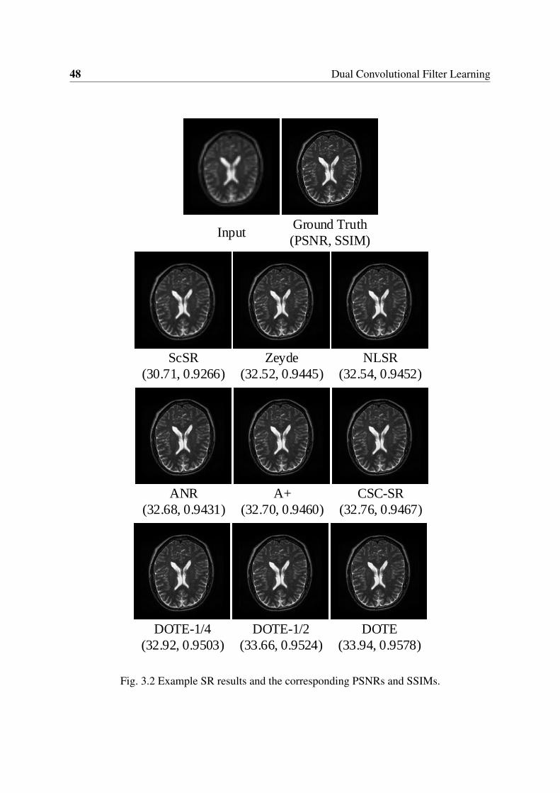
48 Dual Convolutional Filter Learning
InputGround Truth
(PSNR, SSIM)
ScSR
(30.71, 0.9266)
Zeyde
(32.52, 0.9445)
NLSR
(32.54, 0.9452)
ANR
(32.68, 0.9431)
A+
(32.70, 0.9460)
CSC-SR
(32.76, 0.9467)
DOTE-1/4
(32.92, 0.9503)
DOTE-1/2
(33.66, 0.9524)
DOTE
(33.94, 0.9578)
Fig. 3.2 Example SR results and the corresponding PSNRs and SSIMs.
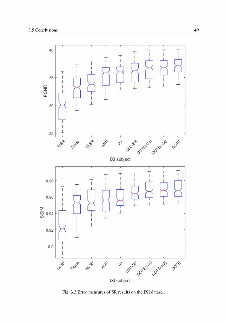
3.5 Conclusions 49
Fig. 3.3 Error measures of SR results on the IXI dataset.
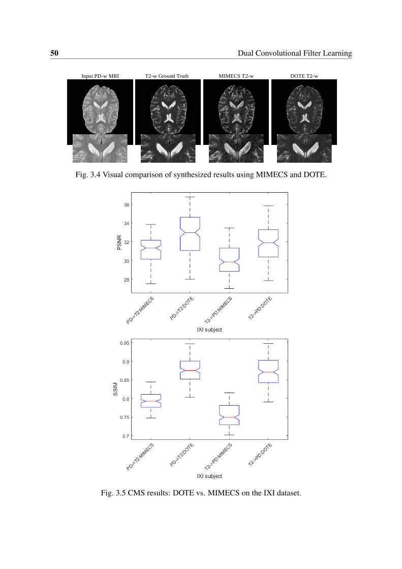
50 Dual Convolutional Filter Learning
Input PD-w MRI T2-w Ground Truth MIMECS T2-w DOTE T2-w
Fig. 3.4 Visual comparison of synthesized results using MIMECS and DOTE.
Fig. 3.5 CMS results: DOTE vs. MIMECS on the IXI dataset.
Chapter 4
Weakly-Supervised Joint ConvolutionalSparse Coding
Magnetic Resonance Imaging (MRI) offers high-resolution in vivo imaging and rich functionaland anatomical multimodality tissue contrast. In practice, however, there are challengesassociated with considerations of scanning costs, patient comfort, and scanning time thatconstrain how much data can be acquired in clinical or research studies. In this chapter,we explore the possibility of generating high-resolution and multimodal images from low-resolution single-modality imagery. We propose the weakly-supervised joint convolutionalsparse coding to simultaneously solve the problems of super-resolution (SR) and cross-modalityimage synthesis. The learning process requires only a few registered multimodal image pairsas the training set. Additionally, the quality of the joint dictionary learning can be improvedusing a larger set of unpaired images1. To combine unpaired data from different imageresolutions/modalities, a hetero-domain image alignment term is proposed. Local imageneighborhoods are naturally preserved by operating on the whole image domain (as opposed toimage patches) and using joint convolutional sparse coding. The paired images are enhanced inthe joint learning process with unpaired data and an additional maximum mean discrepancyterm, which minimizes the dissimilarity between their feature distributions. Experiments showthat the proposed method outperforms state-of-the-art techniques on both SR reconstructionand simultaneous SR and cross-modality synthesis.
1Unpaired data/images: acquisitions are from different subjects without registration. Paired data/images:acquisitions of the same subject obtained from different modalities are registered.
52 Weakly-Supervised Joint Convolutional Sparse Coding
4.1 Introduction
With the rapid progress in Magnetic Resonance Imaging (MRI), there are a multitude ofmechanisms to generate tissue contrast that are associated with various anatomical or functionalfeatures. However, the acquisition of a complete multimodal set of high-resolution imagesfaces constraints associated with scanning costs, scanner availability, scanning time, and patientcomfort. In addition, long-term longitudinal studies such as ADNI [111] imply that changesexist in the scanner or acquisition protocol over time. In these situations, it is not uncommonto have images of the same subject but obtained from different sources, or to be confrontedwith missing or corrupted data from earlier time points. In addition, high-resolution (HR) 3Dmedical imaging usually requires long breath-hold and repetition times, which lead to long-termscanning times that are challenging or unfeasible in clinical routine. Acquiring low-resolution(LR) images and/or skipping some imaging modalities altogether from the acquisition are thennot uncommon. In all such scenarios, it is highly desirable to be able to generate HR data fromthe desired target modality from the given LR modality data.
The relevant literature in this area can be divided into either super-resolution (SR) recon-struction from single/multiple image modalities or cross-modality (image) synthesis (CMS). Onthe one hand, SR is typically concerned with achieving improved visual quality or overcomingthe resolution limits of the acquired image data. Such a problem is generally under-determinedand ill-posed, hence, the solution is not unique. To mitigate this fact, the solution space needs tobe constrained by incorporating strong priors. Prior information comes in the form of smooth-ness assumptions as in, for example, interpolation-based SR [78, 131]. State-of-the-art methodsmostly adopt either external data or internal data to guide the learning algorithms [125, 144].On the other hand, due to variations in optimal image representations across modalities, thelearned image model from one modality data may not be the optimal model for a differentmodality. How to reveal the relationship between different representations of the underlyingimage information is a major research issue to be explored. In order to synthesize one modalityfrom another, recent methods in CMS proposed utilizing non-parametric methods like nearestneighbor (NN) search [41], nonlinear regression forests [73], coupled dictionary learning [127],and convolutional neural network (CNN) [44], to name a few. Although these algorithmsachieve remarkable results, most of them suffer from the fundamental limitations associatedwith supervised learning and/or patch-based synthesis. Supervised approaches require a largenumber of training image pairs, which is impractical in many medical imaging applications.Patch-based synthesis suffers from inconsistencies introduced during the fusion process thattakes place in areas where patches overlap.
In this chapter, we propose a weakly-supervised convolutional sparse coding method withan application to neuroimaging that utilizes a small set of registered multimodal image pairs
4.2 Preliminaries 53
and solves the SR and CMS problems simultaneously. Rather than factorizing each patch into alinear combination of patches drawn from a dictionary built under sparsity constraints (sparsecoding), or requiring a training set with fully registered multimodal image pairs, or requiring thesame sparse code to be used for both modalities involved, we generate a unified learning modelthat automatically learns a joint representation for heterogeneous data (e.g., different resolutions,modalities and relative poses). This representation is learned in a common feature space thatpreserves the local consistency of the images. Specifically, we utilize the co-occurrence oftexture features across both domains. A manifold ranking method picks features of the targetdomain from the most similar subjects in the source domain. Once the correspondence betweenimages in different domains is established, we directly work on a whole image representationthat intrinsically respects local neighborhoods. Furthermore, a mapping function is learned thatlinks the representations between the two modalities involved. We call the proposed methodWEakly-supErvised joiNt convolutIonal sparsE coding (WEENIE), and perform extensiveexperiments to verify its performance.
The main contributions of this chapter are as follows:
1. This is the first attempt to jointly solve the SR and CMS problems in 3D medical imagingusing weakly-supervised joint convolutional sparse coding.
2. To exploit unpaired images from different domains during the learning phase, a hetero-domain image alignment term is proposed, which allows identifying correspondencesacross source and target domains and is invariant to pose transformations.
3. To map LR and HR cross-modality image pairs, joint learning based on convolutionalsparse coding is proposed that includes a maximum mean discrepancy term.
4. Finally, extensive experimental results show that the proposed model yields better per-formance than state-of-the-art methods in both reconstruction error and visual qualityassessment measures.
4.2 Preliminaries
Convolutional Sparse Coding (CSC) was introduced in the context of modeling receptive fieldspreciously, and later generalized to image processing, in which the representation of an entireimage is computed by the sum of a set convolutions with dictionary filters. The goal of CSC is toremedy the shortcoming of conventional patch-based sparse coding methods by removing shiftvariations for consistent approximation of local neighbors on whole images. Concretely, giventhe vectorized image x, the problem of generating a set of vectorized filters for sparse feature
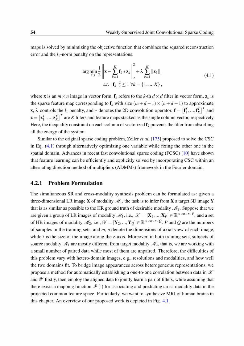
54 Weakly-Supervised Joint Convolutional Sparse Coding
maps is solved by minimizing the objective function that combines the squared reconstructionerror and the l1-norm penalty on the representations:
argminf,z
12
∥∥∥∥∥x−K
∑k=1
fk ∗ zk
∥∥∥∥∥2
2
+λ
K
∑k=1∥zk∥1
s.t. ∥fk∥22 ≤ 1 ∀k = 1, ...,K ,
(4.1)
where x is an m×n image in vector form, fk refers to the k-th d×d filter in vector form, zk isthe sparse feature map corresponding to fk with size (m+d−1)× (n+d−1) to approximatex, λ controls the l1 penalty, and ∗ denotes the 2D convolution operator. f =
[fT1 , ..., f
TK]T and
z =[zT
1 , ...,zTK]T are K filters and feature maps stacked as the single column vector, respectively.
Here, the inequality constraint on each column of vectorized fk prevents the filter from absorbingall the energy of the system.
Similar to the original sparse coding problem, Zeiler et al. [175] proposed to solve the CSCin Eq. (4.1) through alternatively optimizing one variable while fixing the other one in thespatial domain. Advances in recent fast convolutional sparse coding (FCSC) [10] have shownthat feature learning can be efficiently and explicitly solved by incorporating CSC within analternating direction method of multipliers (ADMMs) framework in the Fourier domain.
4.2.1 Problem Formulation
The simultaneous SR and cross-modality synthesis problem can be formulated as: given athree-dimensional LR image X of modality M1, the task is to infer from X a target 3D image Ythat is as similar as possible to the HR ground truth of desirable modality M2. Suppose that weare given a group of LR images of modality M1, i.e., X = [X1, ...,XP] ∈ Rm×n×t×P, and a setof HR images of modality M2, i.e., Y = [Y2, ...,YQ] ∈ Rm×n×t×Q. P and Q are the numbersof samples in the training sets, and m, n denote the dimensions of axial view of each image,while t is the size of the image along the z-axis. Moreover, in both training sets, subjects ofsource modality M1 are mostly different from target modality M2, that is, we are working witha small number of paired data while most of them are unpaired. Therefore, the difficulties ofthis problem vary with hetero-domain images, e.g., resolutions and modalities, and how wellthe two domains fit. To bridge image appearances across heterogeneous representations, wepropose a method for automatically establishing a one-to-one correlation between data in X
and Y firstly, then employ the aligned data to jointly learn a pair of filters, while assuming thatthere exists a mapping function F (·) for associating and predicting cross-modality data in theprojected common feature space. Particularly, we want to synthesize MRI of human brains inthis chapter. An overview of our proposed work is depicted in Fig. 4.1.
4.3 Weakly-Supervised Joint Convolutional Sparse Coding 55
RKHS
Mapping W
Common SpacePaired Unpaired
Convolutional
Decomposition
Feature Convert via W
Convolution
Convolutional
Decomposition
Feature Convert via W
Convolution
Convolutional
Decomposition
Feature Convert via W
Convolution
Convolutional
Decomposition
Feature Convert via W
Convolution
Fig. 4.1 Flowchart of the proposed method (WEENIE) for simultaneous SR and cross-modalitysynthesis.
4.2.2 Notation
For simplicity, we denote matrices and 3D images as upper-case bold (e.g., image X), vectorsand vectorized 2D images as lower-case bold (e.g., filter f), and scalars as lower-case (e.g.,the number of filter k). Image with modality M1 called source modality belongs to the sourcedomain, and with modality M2 called target modality belongs to the target domain.
4.3 Weakly-Supervised Joint Convolutional Sparse Coding
4.3.1 Hetero-Domain Image Alignment
The design of an alignment A (·) from X to Y requires a combination of extracting commoncomponents from LR/HR images and some measures of correlation between both modalities.In SR literature, common components are usually accomplished by extracting high-frequency(HF) edges and texture features from LR/HR images, respectively [16, 168]. In this chapter,we adopt first- and second-order derivatives involving horizontal and vertical gradients as
the features for LR images by Xh fp = G ∗Xp. G =
[G1
1, G21
G12, G2
2
], and each gradient G has the
same length of z-axis as input image while g11 = [−1,0,1], g2
1 = g11
T , and g12 = [−2,−1,0,1,2],
g22 = g1
2T . For HR images, HF features are obtained through directly subtracting mean value,
i.e., Yh fp = Yp−mean(Yp). To define the hetero-domain image alignment term A (·), we
assume that the intrinsic structures of brain MRI of a subject across image modalities are alsosimilar in the HF space since images of different modalities are more likely to be describeddifferently by features. When HF features of both domains are obtained, it is possible to build away for cross-modality data alignment (in particular, a unilateral cross-modality matching canbe thought as a special case in [66]). To this end, we define a subject-specific transformation
56 Weakly-Supervised Joint Convolutional Sparse Coding
matrix A as
A=
K(Xh f
1 ,Yh f1 ) · · · K(Xh f
1 ,Yh fQ )
... . . . ...K(Xh f
P ,Yh f1 ) · · · K(Xh f
P ,Yh fQ )
, (4.2)
where K(Xh fp ,Yh f
q ) is used for measuring the distances between each pair of HF data in X andY computed by the Gaussian kernel as
K(Xh fp ,Yh f
q ) =1
(√
2πσ)3e−
∣∣∣Xh fp −Yh f
q∣∣∣2
2σ2 , (4.3)
where σ determines the width of Gaussian kernel. In order to establish a one-to-one corre-spondence across different domains, for each element of X , the most relevant image withmaximum K from Y is preserved while discarding the rest of the elements:
A=
max(K (1, :)). . .
max(K (P, :))
, (4.4)
where max(K (p, :)) denotes the maximum element of the p-th row of A. We further setmax(K (p, :)) to 1, and all the blank elements to 0. Therefore, A is a binary matrix. Since Ais calculated in a subject-specific manner, each subject of X can only be connected to onetarget of the most similar brain structures. Hence, images under a hetero-domain can be treatedas being the registered pairs, i.e., Pi = Xi,YiP
i=1, by constructing virtual correspondence:A (X ,Y ) =
∥∥Xh f −AYh f∥∥2
2.
4.3.2 Objective Function
For image modality transformation, coupled sparse coding [70, 168] has important advantages,such as reliability of correspondence dictionary pair learning and less memory cost. However,the arbitrarily aligned bases related to the small part of images may lead to shifted versions ofthe same structures or inconsistent representations based on the overlapped patches. CSC [175]was then proposed to generate a global decomposition framework based on the whole imagefor solving the above problem. In spired by CSC and the benefits of coupled sparsity [70],we introduce a joint convolutional sparse coding method in a weakly-supervised setting forhetero-domain images. The small number of originally registered pairs are used to carry theintrinsic relationship between X and Y while the majority of unpaired data are introduced toexploit and enhance the diversity of the original learning system.
4.3 Weakly-Supervised Joint Convolutional Sparse Coding 57
Assume that the aforementioned alignment approach leads to a perfect correspondenceacross X and Y , such that each aligned pair of images possesses approximately identical (orthe same for co-registered data) information. Moreover, to facilitate image mappings in a jointmanner, we require sparse feature maps of each pair of corresponding source and target imagesto be associated. That is, suppose that there exists a mapping function F (·), where the featuremaps of LR M1 modality images can be converted to their HR M2 versions. Given X and Y ,we propose to learn a pair of filters with corresponding feature maps and a mapping functionpre-processed with the aligned term
∥∥Xh f −AYh f∥∥2
2 by
arg minFx,Fy,Zx,Zy,W
12
∥∥∥∥∥X−K
∑k=1
Fxk ∗Zx
k
∥∥∥∥∥2
F
+12
∥∥∥∥∥Y−K
∑k=1
Fyk ∗Zy
k
∥∥∥∥∥2
F
+β
K
∑k=1
∥∥Zyk−WkZx
k
∥∥2F
+λ
(K
∑k=1∥Zx
k∥1 +K
∑k=1
∥∥Zyk
∥∥1
)+ γ
K
∑k=1∥Wk∥2
F
s.t. ∥fxk∥
22 ≤ 1,
∥∥fyk
∥∥22 ≤ 1∀k,
(4.5)
where Zxk and Zy
k are the k-th sparse feature maps that estimate the aligned data terms X andY when convolved with the k-th filters Fx
k and Fyk of a fixed spatial support, ∀k = 1, ...,K.
Concretely, X denotes the aligned image from P with LR and M1 modality; Y denotes thealigned image from P containing HR and M2 modality. A convolution operation is representedas ∗ operator, and ∥·∥F denotes a Frobenius norm chosen to induce the convolutional leastsquares approximate solution. Fx and Fy are adopted to list all K filters, while Zx and Zy
represent corresponding K feature maps for source and target domains, respectively. A (X ,Y )
is combined to enforce the correspondence for unpaired auxiliary subjects. The mappingfunction F
(Zx
k,Wk)= WkZx
k is modeled as a linear projection Wk of Zxk and Zy
k by solvinga set of the least squares problem (i.e., minW ∑
Kk=1
∥∥Zyk−WkZx
k
∥∥2F ). Parameters λ , β and γ
balance sparsity, feature representation and association mapping.It is worth noting that Pi = Xi,Yi may not be perfect since HF feature alignment in
Eq. (4.4) is not good enough for very heterogeneous domain adaptation by matching the first-and second-order derivatives of X and means of Y , which leads to suboptimal filter pairsand inaccurate results. To overcome such a problem, we need additional constraints to ensurethe correctness of registered image pairs produced by the alignment. Generally, when featuredifference is substantially large, there always exists some subjects of the source domain thatare not particularly related to target ones even in the HF subspace. Thus, a registered subject
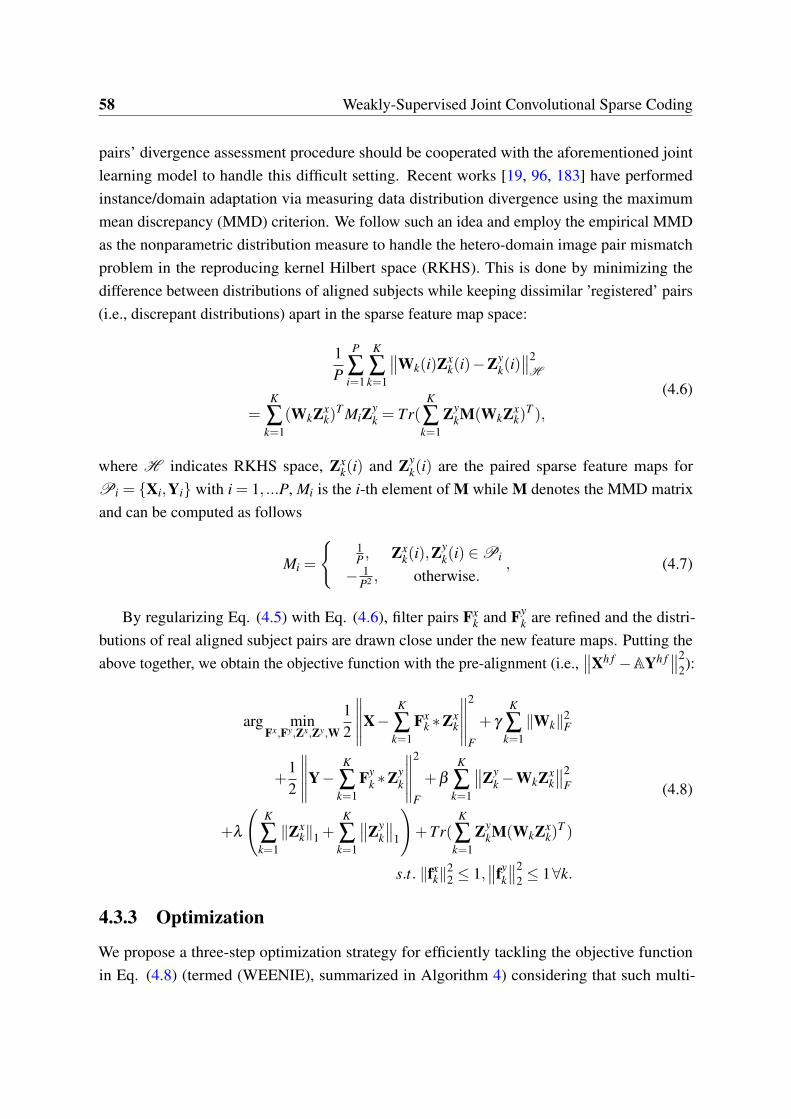
58 Weakly-Supervised Joint Convolutional Sparse Coding
pairs’ divergence assessment procedure should be cooperated with the aforementioned jointlearning model to handle this difficult setting. Recent works [19, 96, 183] have performedinstance/domain adaptation via measuring data distribution divergence using the maximummean discrepancy (MMD) criterion. We follow such an idea and employ the empirical MMDas the nonparametric distribution measure to handle the hetero-domain image pair mismatchproblem in the reproducing kernel Hilbert space (RKHS). This is done by minimizing thedifference between distributions of aligned subjects while keeping dissimilar ’registered’ pairs(i.e., discrepant distributions) apart in the sparse feature map space:
1P
P
∑i=1
K
∑k=1
∥∥Wk(i)Zxk(i)−Zy
k(i)∥∥2
H
=K
∑k=1
(WkZxk)
T MiZyk = Tr(
K
∑k=1
ZykM(WkZx
k)T ),
(4.6)
where H indicates RKHS space, Zxk(i) and Zy
k(i) are the paired sparse feature maps forPi = Xi,Yi with i = 1, ...P, Mi is the i-th element of M while M denotes the MMD matrixand can be computed as follows
Mi =
1P , Zx
k(i),Zyk(i) ∈Pi
− 1P2 , otherwise.
, (4.7)
By regularizing Eq. (4.5) with Eq. (4.6), filter pairs Fxk and Fy
k are refined and the distri-butions of real aligned subject pairs are drawn close under the new feature maps. Putting theabove together, we obtain the objective function with the pre-alignment (i.e.,
∥∥Xh f −AYh f∥∥2
2):
arg minFx,Fy,Zx,Zy,W
12
∥∥∥∥∥X−K
∑k=1
Fxk ∗Zx
k
∥∥∥∥∥2
F
+ γ
K
∑k=1∥Wk∥2
F
+12
∥∥∥∥∥Y−K
∑k=1
Fyk ∗Zy
k
∥∥∥∥∥2
F
+β
K
∑k=1
∥∥Zyk−WkZx
k
∥∥2F
+λ
(K
∑k=1∥Zx
k∥1 +K
∑k=1
∥∥Zyk
∥∥1
)+Tr(
K
∑k=1
ZykM(WkZx
k)T )
s.t. ∥fxk∥
22 ≤ 1,
∥∥fyk
∥∥22 ≤ 1∀k.
(4.8)
4.3.3 Optimization
We propose a three-step optimization strategy for efficiently tackling the objective functionin Eq. (4.8) (termed (WEENIE), summarized in Algorithm 4) considering that such multi-
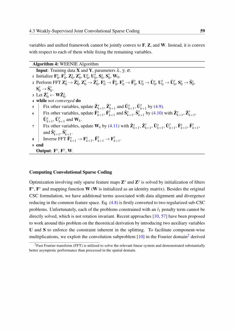
4.3 Weakly-Supervised Joint Convolutional Sparse Coding 59
variables and unified framework cannot be jointly convex to F, Z, and W. Instead, it is convexwith respect to each of them while fixing the remaining variables.
Algorithm 4: WEENIE AlgorithmInput: Training data X and Y, parameters λ , γ , σ .
1 Initialize Fx0, Fy
0, Zx0, Zy
0, Ux0, Uy
0, Sx0, Sy
0, W0.2 Perform FFT Zx
0→ Zx0, Zy
0→ Zy0, Fx
0→ Fx0, Fy
0→ Fy0, Ux
0→ Ux0, Uy
0→ Uy0, Sx
0→ Sx0,
Sy0→ Sy
0.3 Let Zy
0←WZx0.
4 while not converged do5 Fix other variables, update Zx
k+1, Zyk+1 and Ux
k+1, Uyk+1 by (4.9).
6 Fix other variables, update Fxk+1, Fy
k+1 and Sxk+1, Sy
k+1 by (4.10) with Zxk+1, Zy
k+1,Ux
k+1, Uyk+1 and Wk.
7 Fix other variables, update Wk by (4.11) with Zxk+1, Zy
k+1, Uxk+1, Uy
k+1, Fxk+1, Fy
k+1,and Sx
k+1, Syk+1.
8 Inverse FFT Fxk+1→ Fx
k+1, Fyk+1→ Fy
k+1.9 end
Output: Fx, Fy, W.
Computing Convolutional Sparse Coding
Optimization involving only sparse feature maps Zx and Zy is solved by initialization of filtersFx, Fy and mapping function W (W is initialized as an identity matrix). Besides the originalCSC formulation, we have additional terms associated with data alignment and divergencereducing in the common feature space. Eq. (4.8) is firstly converted to two regularized sub-CSCproblems. Unfortunately, each of the problems constrained with an l1 penalty term cannot bedirectly solved, which is not rotation invariant. Recent approaches [10, 57] have been proposedto work around this problem on the theoretical derivation by introducing two auxiliary variablesU and S to enforce the constraint inherent in the splitting. To facilitate component-wisemultiplications, we exploit the convolution subproblem [10] in the Fourier domain2 derived
2Fast Fourier transform (FFT) is utilized to solve the relevant linear system and demonstrated substantiallybetter asymptotic performance than processed in the spatial domain.
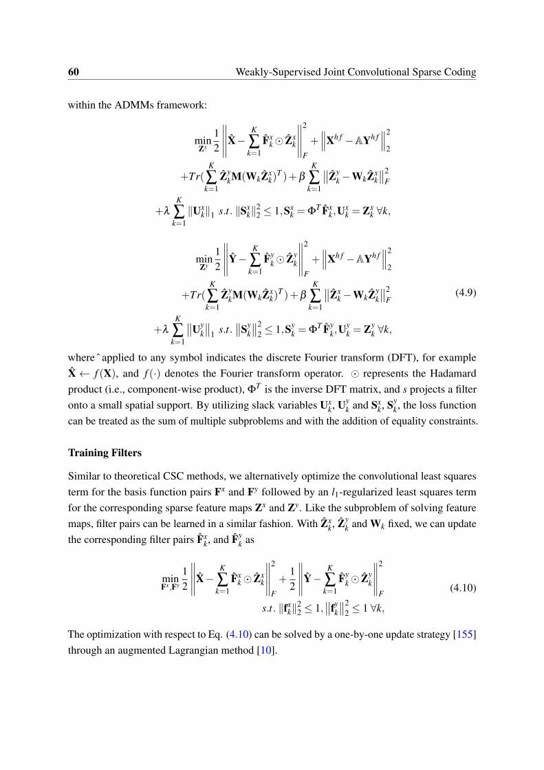
60 Weakly-Supervised Joint Convolutional Sparse Coding
within the ADMMs framework:
minZx
12
∥∥∥∥∥X−K
∑k=1
Fxk⊙ Zx
k
∥∥∥∥∥2
F
+∥∥∥Xh f −AYh f
∥∥∥2
2
+Tr(K
∑k=1
ZykM(WkZx
k)T )+β
K
∑k=1
∥∥Zyk−WkZx
k
∥∥2F
+λ
K
∑k=1∥Ux
k∥1 s.t. ∥Sxk∥
22 ≤ 1,Sx
k = ΦT Fx
k,Uxk = Zx
k ∀k,
minZy
12
∥∥∥∥∥Y−K
∑k=1
Fyk⊙ Zy
k
∥∥∥∥∥2
F
+∥∥∥Xh f −AYh f
∥∥∥2
2
+Tr(K
∑k=1
ZykM(WkZx
k)T )+β
K
∑k=1
∥∥Zxk−WkZy
k
∥∥2F
+λ
K
∑k=1
∥∥Uyk
∥∥1 s.t.
∥∥Syk
∥∥22 ≤ 1,Sy
k = ΦT Fy
k,Uyk = Zy
k ∀k,
(4.9)
where ˆ applied to any symbol indicates the discrete Fourier transform (DFT), for exampleX← f (X), and f (·) denotes the Fourier transform operator. ⊙ represents the Hadamardproduct (i.e., component-wise product), Φ
T is the inverse DFT matrix, and s projects a filteronto a small spatial support. By utilizing slack variables Ux
k, Uyk and Sx
k, Syk, the loss function
can be treated as the sum of multiple subproblems and with the addition of equality constraints.
Training Filters
Similar to theoretical CSC methods, we alternatively optimize the convolutional least squaresterm for the basis function pairs Fx and Fy followed by an l1-regularized least squares termfor the corresponding sparse feature maps Zx and Zy. Like the subproblem of solving featuremaps, filter pairs can be learned in a similar fashion. With Zx
k, Zyk and Wk fixed, we can update
the corresponding filter pairs Fxk, and Fy
k as
minFx,Fy
12
∥∥∥∥∥X−K
∑k=1
Fxk⊙ Zx
k
∥∥∥∥∥2
F
+12
∥∥∥∥∥Y−K
∑k=1
Fyk⊙ Zy
k
∥∥∥∥∥2
F
s.t. ∥fxk∥
22 ≤ 1,
∥∥fyk
∥∥22 ≤ 1 ∀k,
(4.10)
The optimization with respect to Eq. (4.10) can be solved by a one-by-one update strategy [155]through an augmented Lagrangian method [10].
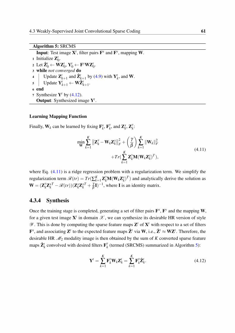
4.3 Weakly-Supervised Joint Convolutional Sparse Coding 61
Algorithm 5: SRCMSInput: Test image Xt , filter pairs Fx and Fy, mapping W.
1 Initialize Zt0.
2 Let Zt0←WZt
0, Yt0← FyWZt
0.3 while not converged do4 Update Zt
k+1 and Ztk+1 by (4.9) with Yt
k, and W.5 Update Yt
k+1←WZtk+1.
6 end7 Synthesize Yt by (4.12).
Output: Synthesized image Yt .
Learning Mapping Function
Finally, Wk can be learned by fixing Fxk, Fy
k, and Zxk, Zy
k:
minW
K
∑k=1
∥∥Zyk−WkZx
k
∥∥2F +
(γ
β
) K
∑k=1∥Wk∥2
F
+Tr(K
∑k=1
ZykM(WkZx
k)T ),
(4.11)
where Eq. (4.11) is a ridge regression problem with a regularization term. We simplify theregularization term R(tr) = Tr(∑K
k=1 ZykM(WkZx
k)T ) and analytically derive the solution as
W = (ZykZx
kT −R(tr))(Zx
kZxk
T + γ
βI)−1, where I is an identity matrix.
4.3.4 Synthesis
Once the training stage is completed, generating a set of filter pairs Fx, Fy and the mapping W,for a given test image Xt in domain X , we can synthesize its desirable HR version of styleY . This is done by computing the sparse feature maps Zt of Xt with respect to a set of filtersFx, and associating Zt to the expected feature maps Zt via W, i.e., Zt ≈WZt . Therefore, thedesirable HR M2 modality image is then obtained by the sum of K converted sparse featuremaps Zt
k convolved with desired filters Fyk (termed (SRCMS) summarized in Algorithm 5):
Yt =K
∑k=1
FykWkZt
k =K
∑k=1
FykZt
k. (4.12)
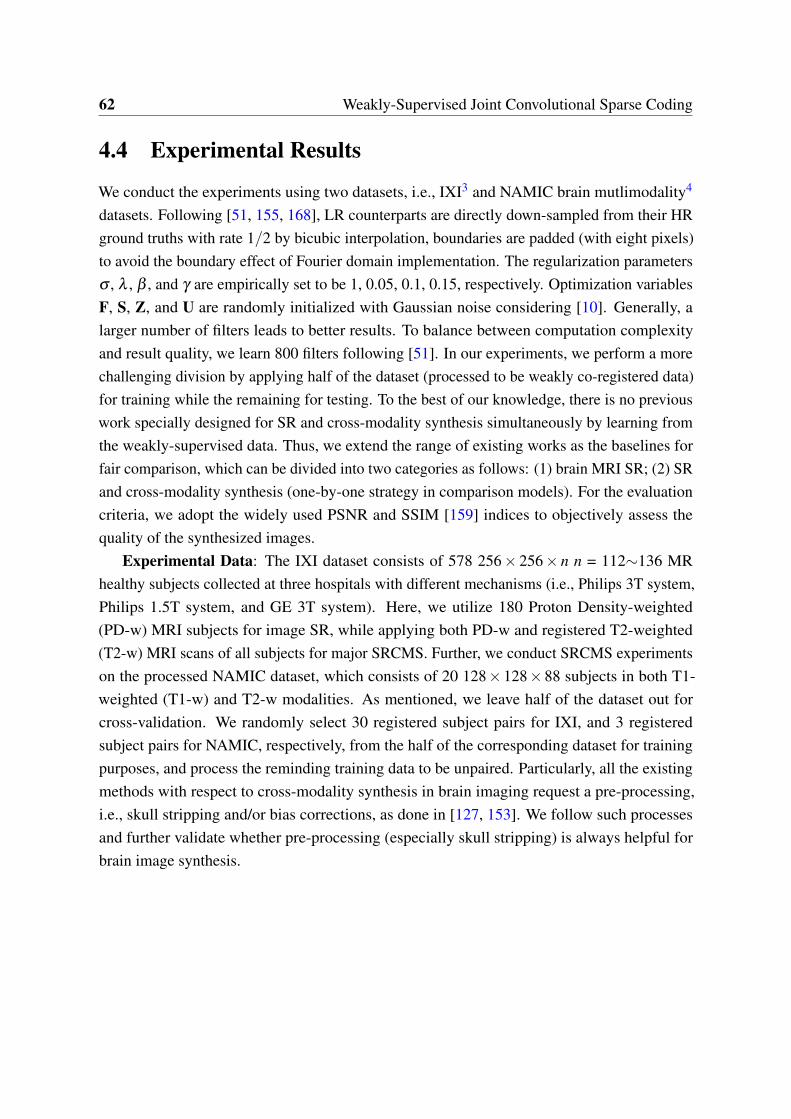
62 Weakly-Supervised Joint Convolutional Sparse Coding
4.4 Experimental Results
We conduct the experiments using two datasets, i.e., IXI3 and NAMIC brain mutlimodality4
datasets. Following [51, 155, 168], LR counterparts are directly down-sampled from their HRground truths with rate 1/2 by bicubic interpolation, boundaries are padded (with eight pixels)to avoid the boundary effect of Fourier domain implementation. The regularization parametersσ , λ , β , and γ are empirically set to be 1, 0.05, 0.1, 0.15, respectively. Optimization variablesF, S, Z, and U are randomly initialized with Gaussian noise considering [10]. Generally, alarger number of filters leads to better results. To balance between computation complexityand result quality, we learn 800 filters following [51]. In our experiments, we perform a morechallenging division by applying half of the dataset (processed to be weakly co-registered data)for training while the remaining for testing. To the best of our knowledge, there is no previouswork specially designed for SR and cross-modality synthesis simultaneously by learning fromthe weakly-supervised data. Thus, we extend the range of existing works as the baselines forfair comparison, which can be divided into two categories as follows: (1) brain MRI SR; (2) SRand cross-modality synthesis (one-by-one strategy in comparison models). For the evaluationcriteria, we adopt the widely used PSNR and SSIM [159] indices to objectively assess thequality of the synthesized images.
Experimental Data: The IXI dataset consists of 578 256× 256× n n = 112∼136 MRhealthy subjects collected at three hospitals with different mechanisms (i.e., Philips 3T system,Philips 1.5T system, and GE 3T system). Here, we utilize 180 Proton Density-weighted(PD-w) MRI subjects for image SR, while applying both PD-w and registered T2-weighted(T2-w) MRI scans of all subjects for major SRCMS. Further, we conduct SRCMS experimentson the processed NAMIC dataset, which consists of 20 128×128×88 subjects in both T1-weighted (T1-w) and T2-w modalities. As mentioned, we leave half of the dataset out forcross-validation. We randomly select 30 registered subject pairs for IXI, and 3 registeredsubject pairs for NAMIC, respectively, from the half of the corresponding dataset for trainingpurposes, and process the reminding training data to be unpaired. Particularly, all the existingmethods with respect to cross-modality synthesis in brain imaging request a pre-processing,i.e., skull stripping and/or bias corrections, as done in [127, 153]. We follow such processesand further validate whether pre-processing (especially skull stripping) is always helpful forbrain image synthesis.
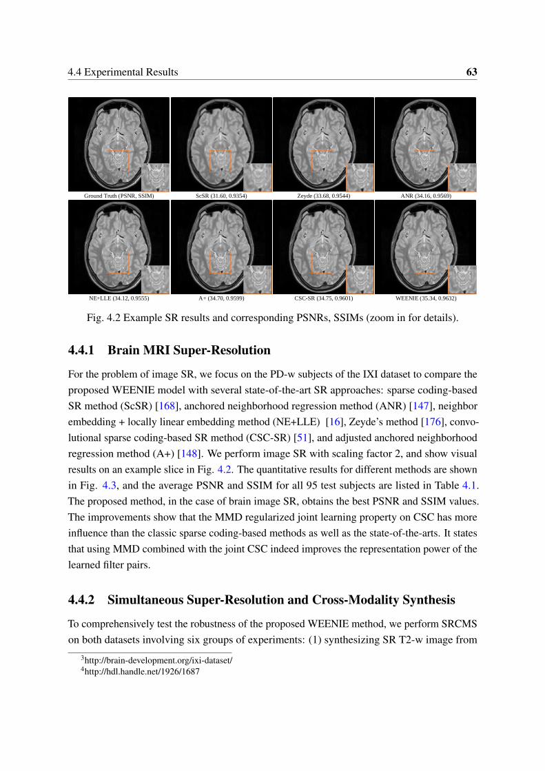
4.4 Experimental Results 63
Ground Truth (PSNR, SSIM) ScSR (31.60, 0.9354) Zeyde (33.68, 0.9544) ANR (34.16, 0.9569)
NE+LLE (34.12, 0.9555) A+ (34.70, 0.9599) CSC-SR (34.75, 0.9601) WEENIE (35.34, 0.9632)
Fig. 4.2 Example SR results and corresponding PSNRs, SSIMs (zoom in for details).
4.4.1 Brain MRI Super-Resolution
For the problem of image SR, we focus on the PD-w subjects of the IXI dataset to compare theproposed WEENIE model with several state-of-the-art SR approaches: sparse coding-basedSR method (ScSR) [168], anchored neighborhood regression method (ANR) [147], neighborembedding + locally linear embedding method (NE+LLE) [16], Zeyde’s method [176], convo-lutional sparse coding-based SR method (CSC-SR) [51], and adjusted anchored neighborhoodregression method (A+) [148]. We perform image SR with scaling factor 2, and show visualresults on an example slice in Fig. 4.2. The quantitative results for different methods are shownin Fig. 4.3, and the average PSNR and SSIM for all 95 test subjects are listed in Table 4.1.The proposed method, in the case of brain image SR, obtains the best PSNR and SSIM values.The improvements show that the MMD regularized joint learning property on CSC has moreinfluence than the classic sparse coding-based methods as well as the state-of-the-arts. It statesthat using MMD combined with the joint CSC indeed improves the representation power of thelearned filter pairs.
4.4.2 Simultaneous Super-Resolution and Cross-Modality Synthesis
To comprehensively test the robustness of the proposed WEENIE method, we perform SRCMSon both datasets involving six groups of experiments: (1) synthesizing SR T2-w image from
3http://brain-development.org/ixi-dataset/4http://hdl.handle.net/1926/1687

64 Weakly-Supervised Joint Convolutional Sparse Coding
Fig. 4.3 Performance comparisons of different SR approaches.
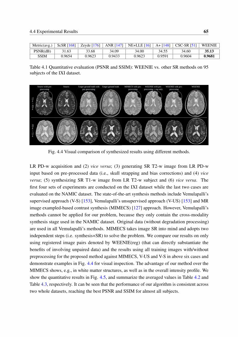
4.4 Experimental Results 65
Metric(avg.) ScSR [168] Zeyde [176] ANR [147] NE+LLE [16] A+ [148] CSC-SR [51] WEENIEPSNR(dB) 31.63 33.68 34.09 34.00 34.55 34.60 35.13
SSIM 0.9654 0.9623 0.9433 0.9623 0.9591 0.9604 0.9681
Table 4.1 Quantitative evaluation (PSNR and SSIM): WEENIE vs. other SR methods on 95subjects of the IXI dataset.
Source with pre-
processing
Source Target ground truth with
pre-processing
Target ground truth MIMECS with pre-
processing
WEENIE with pre-
processing + reg only
WEENIE with pre-
processing
WEENIE
T2-w
-> P
D-w
PD
-w ->
T2-w
Fig. 4.4 Visual comparison of synthesized results using different methods.
LR PD-w acquisition and (2) vice versa; (3) generating SR T2-w image from LR PD-winput based on pre-processed data (i.e., skull strapping and bias corrections) and (4) viceversa; (5) synthesizing SR T1-w image from LR T2-w subject and (6) vice versa. Thefirst four sets of experiments are conducted on the IXI dataset while the last two cases areevaluated on the NAMIC dataset. The state-of-the-art synthesis methods include Vemulapalli’ssupervised approach (V-S) [153], Vemulapalli’s unsupervised approach (V-US) [153] and MRimage exampled-based contrast synthesis (MIMECS) [127] approach. However, Vemulapalli’smethods cannot be applied for our problem, because they only contain the cross-modalitysynthesis stage used in the NAMIC dataset. Original data (without degradation processing)are used in all Vemulapalli’s methods. MIMECS takes image SR into mind and adopts twoindependent steps (i.e. synthesis+SR) to solve the problem. We compare our results on onlyusing registered image pairs denoted by WEENIE(reg) (that can directly substantiate thebenefits of involving unpaired data) and the results using all training images with/withoutpreprocessing for the proposed method against MIMECS, V-US and V-S in above six cases anddemonstrate examples in Fig. 4.4 for visual inspection. The advantage of our method over theMIMECS shows, e.g., in white matter structures, as well as in the overall intensity profile. Weshow the quantitative results in Fig. 4.5, and summarize the averaged values in Table 4.2 andTable 4.3, respectively. It can be seen that the performance of our algorithm is consistent acrosstwo whole datasets, reaching the best PSNR and SSIM for almost all subjects.
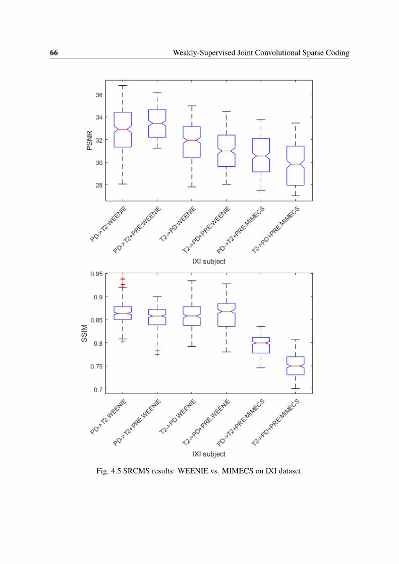
66 Weakly-Supervised Joint Convolutional Sparse Coding
Fig. 4.5 SRCMS results: WEENIE vs. MIMECS on IXI dataset.
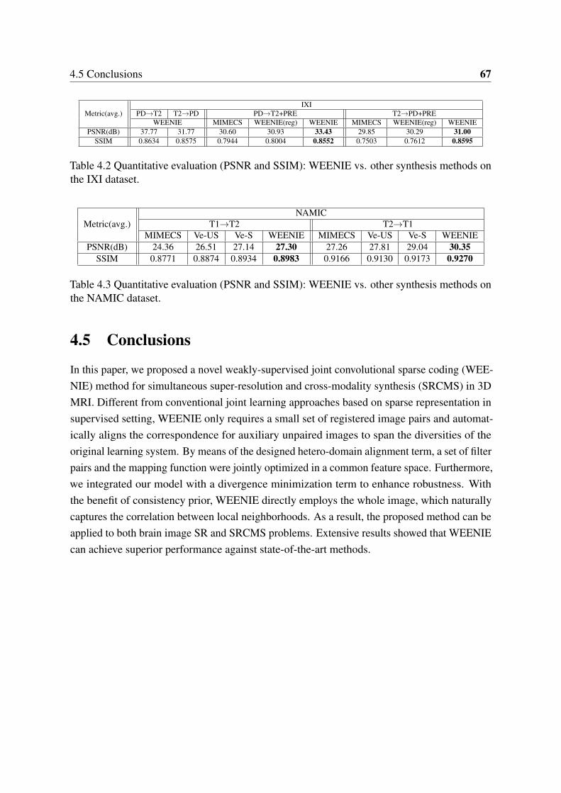
4.5 Conclusions 67
Metric(avg.)IXI
PD→T2 T2→PD PD→T2+PRE T2→PD+PREWEENIE MIMECS WEENIE(reg) WEENIE MIMECS WEENIE(reg) WEENIE
PSNR(dB) 37.77 31.77 30.60 30.93 33.43 29.85 30.29 31.00SSIM 0.8634 0.8575 0.7944 0.8004 0.8552 0.7503 0.7612 0.8595
Table 4.2 Quantitative evaluation (PSNR and SSIM): WEENIE vs. other synthesis methods onthe IXI dataset.
Metric(avg.)NAMIC
T1→T2 T2→T1MIMECS Ve-US Ve-S WEENIE MIMECS Ve-US Ve-S WEENIE
PSNR(dB) 24.36 26.51 27.14 27.30 27.26 27.81 29.04 30.35SSIM 0.8771 0.8874 0.8934 0.8983 0.9166 0.9130 0.9173 0.9270
Table 4.3 Quantitative evaluation (PSNR and SSIM): WEENIE vs. other synthesis methods onthe NAMIC dataset.
4.5 Conclusions
In this paper, we proposed a novel weakly-supervised joint convolutional sparse coding (WEE-NIE) method for simultaneous super-resolution and cross-modality synthesis (SRCMS) in 3DMRI. Different from conventional joint learning approaches based on sparse representation insupervised setting, WEENIE only requires a small set of registered image pairs and automat-ically aligns the correspondence for auxiliary unpaired images to span the diversities of theoriginal learning system. By means of the designed hetero-domain alignment term, a set of filterpairs and the mapping function were jointly optimized in a common feature space. Furthermore,we integrated our model with a divergence minimization term to enhance robustness. Withthe benefit of consistency prior, WEENIE directly employs the whole image, which naturallycaptures the correlation between local neighborhoods. As a result, the proposed method can beapplied to both brain image SR and SRCMS problems. Extensive results showed that WEENIEcan achieve superior performance against state-of-the-art methods.

Chapter 5
Geometry Constrained DictionaryLearning
5.1 Geometry Regularized Joint Dictionary Learning
Multi-sequence MRI protocols are used in comprehensive examinations of various pathologiesin both clinical diagnosis and medical research. Various MRI techniques provide comple-mentary information about living tissue. However, a comprehensive examination coveringall modalities is rarely achieved due to considerations of cost, patient comfort, and scannertime availability. This may lead to incomplete records owing to image artifacts or corruptedor lost data. In this chapter, we explore the problem of synthesizing images for one MRImodality from an image of another MRI modality of the same subject using a novel geometryregularized joint dictionary learning framework for non-local patch reconstruction. Firstly,we learn a cross-modality joint dictionary from a multi-modality image database. Trainingimage pairs are first co-registered. A cross-modality dictionary pair is then jointly learnedby minimizing the cross-modality divergence via a Maximum Mean Discrepancy term in theobjective function of the learning scheme. This guarantees that the distribution of both imagemodalities is taken jointly into account when building the resulting sparse representation. Inaddition, in order to preserve intrinsic geometrical structure of the synthesized image patches,we further introduced a graph Laplacian regularization term into the objective function. Finally,we present a patch-based non-local reconstruction scheme, providing further fidelity of thesynthesized images. Experimental results demonstrate that our method achieves significantperformance gains over previously published techniques.
70 Geometry Constrained Dictionary Learning
5.1.1 Introduction
Magnetic Resonance Imaging (MRI) is a versatile and noninvasive imaging technique exten-sively used in neuroimaging studies. MRI comes in many different flavors (viz. MRI sequences,or henceforth also referred as MRI modalities1), each providing diverse and complementaryimage contrast mechanisms unraveling structural and functional information about brain tissue.Multi-modality MRI are nowadays very common in many pharmaceutical clinical trials, inresearch studies of neurosciences, or in population imaging cohorts targeted to understandneurodegeneration and cognitive decline. The acquisitions of a full battery of all these MRimages can face constraints associated with their cost, limited availability of scanning time,patient com-fort or safety considerations. Moreover, in large scale studies it is not uncommonto face incomplete datasets due to the presence of imaging artifacts, acquisition errors orcorrupted data. While many such studies use imputation techniques to compensate for theselatter issues, this is usually only at the level of the derived imaging biomarkers and not of thedata itself. Finally, in longitudinal imaging studies where image data is collected over severalyears, evolution of imaging technology may lead to the appearance of new MRI sequences thatare added to an existing imaging protocol at some point in time but for which are not availableas part of the imaging battery acquired at earlier time points. In these and other applications, itwould be desirable to have a methodology that is able to synthesize the unavailable data fromthe available MRI studies. The assumption here is that the synthesis ability comes from thecross-modality correspondences of sparse codes obtained during training, and can be used toencoding missing MRI. The degree to which this hypothesis is valid will have to be scrutinizedin each application but is worth exploring.
To cope with this problem, several methods were proposed through either trans-formingMRI intensities or reconstructing tissue contrasts to obtain the missing MRI data. Histogrammatching is the most common approach within this group. Although this technique is widelyused in neuroimaging, it has been pointed out its inefficacy for multi-modality image synthe-sis due to the lack of specificity for certain ratios of tissue types [127]. On the other hand,techniques based on sparse representations have been presented, which separately learn twocorresponding dictionaries from co-registered image pairs and synthesize a desired MRI modal-ity data from the patches of the available MRI modality [127]. These approaches, however,boil down to an example-based synthesis strategy, which does not fully exploit the availabletraining data to its fullest. In contrast, here, we establish fundamental connections with trans-ferlearning (a.k.a. domain adaptation) used in many fields, e.g. [132, 118]. Such methods can
1Here, we use the word modality in the sense of a specific kind of MRI sequence. Note that the proposedtechnique would equally be applicable when the protocol involves different imaging modalities in a more classicalsense (e.g. MRI, CT, US, SPECT, and PET).
5.1 Geometry Regularized Joint Dictionary Learning 71
successfully solve the above problem by learning a paired dictionary from both modalities whileassuming each co-registered image pair with a nearly identical distribution [127]. However,this assumption cannot be fully satisfied in practice since cross-modality data may have verydifferent feature distributions in different spaces.
In this chapter, we propose a novel geometry regularized joint dictionary learning method forsynthesizing any unavailable MRI from available MRI data. This chapter offers the followingthree contributions:
1. We address cross-modality MRI synthesis by jointly learning a cross-modality dictionarythat penalizes differences in the statistical distribution of the sparse codes in both domainsrather than directly imposing the same code to both domains as done before. This isachieved by incorporating a new term in the computation of the joint sparse codes usingthe Maximum Mean Discrepancy measure;
2. We exploit the geometrical information underlying the input data and incorporate thisnew term into the cross-modality joint dictionary learning optimization;
3. A non-local reconstruction framework that provides a more expressive and compactpatch representation is adopted to synthesize the corresponding patch from a differentMRI protocol.
To the best of our knowledge, this is the first time that joint dictionary learning is computedby minimizing the discrepancy between the statistical distributions of the sparse codes of theinvolved MRI modalities while preserving the intrinsic geometrical structure of the image. Inthe remainder of this chapter, we first define the cross-modality synthesis problem, and thenintroduce our proposed method in Section 2. The experimental results are demonstrated inSection 3. Finally, we discuss the results and conclude the chapter in Section 4.
5.1.2 Method
In this section, we propose cross-modality image synthesis via geometry regularized jointdictionary learning for effectively minimizing the cross-modality discrepancy. This consistsof an extension of the conventional dictionary learning by jointly learning from the data oftwo modalities at the same time while minimizing the sparse codes divergence between thedifferent modalities.
Problem Definition
Let LMk =
IMki
m
i=1be a library of m subjects imaged with k modalities each (k = 1 or 2),
with Ii being the training image of the i-th sample. Each pair of images in both libraries,
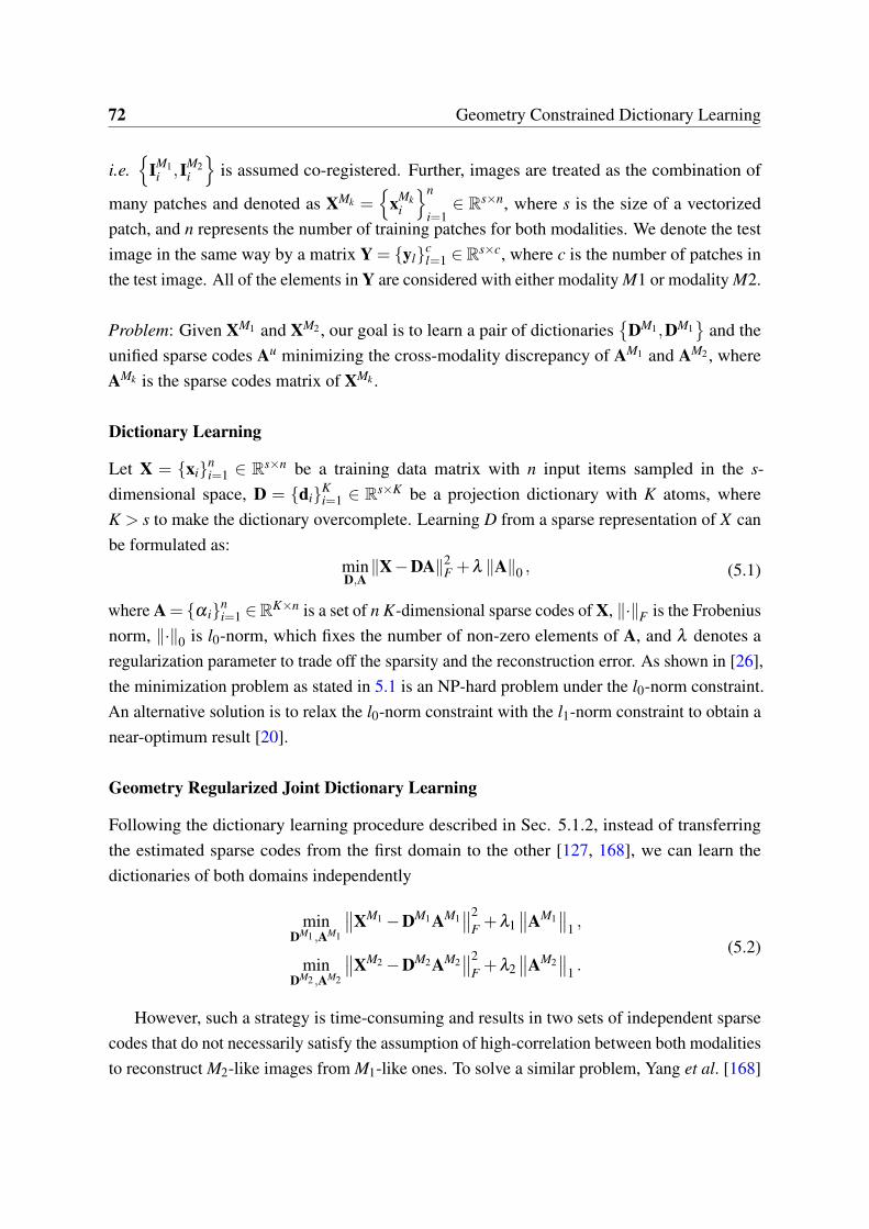
72 Geometry Constrained Dictionary Learning
i.e.
IM1i ,IM2
i
is assumed co-registered. Further, images are treated as the combination of
many patches and denoted as XMk =
xMki
n
i=1∈ Rs×n, where s is the size of a vectorized
patch, and n represents the number of training patches for both modalities. We denote the testimage in the same way by a matrix Y = ylc
l=1 ∈ Rs×c, where c is the number of patches inthe test image. All of the elements in Y are considered with either modality M1 or modality M2.
Problem: Given XM1 and XM2 , our goal is to learn a pair of dictionaries
DM1 ,DM1
and theunified sparse codes Au minimizing the cross-modality discrepancy of AM1 and AM2 , whereAMk is the sparse codes matrix of XMk .
Dictionary Learning
Let X = xini=1 ∈ Rs×n be a training data matrix with n input items sampled in the s-
dimensional space, D = diKi=1 ∈ Rs×K be a projection dictionary with K atoms, where
K > s to make the dictionary overcomplete. Learning D from a sparse representation of X canbe formulated as:
minD,A∥X−DA∥2
F +λ ∥A∥0 , (5.1)
where A = α ini=1 ∈RK×n is a set of n K-dimensional sparse codes of X, ∥·∥F is the Frobenius
norm, ∥·∥0 is l0-norm, which fixes the number of non-zero elements of A, and λ denotes aregularization parameter to trade off the sparsity and the reconstruction error. As shown in [26],the minimization problem as stated in 5.1 is an NP-hard problem under the l0-norm constraint.An alternative solution is to relax the l0-norm constraint with the l1-norm constraint to obtain anear-optimum result [20].
Geometry Regularized Joint Dictionary Learning
Following the dictionary learning procedure described in Sec. 5.1.2, instead of transferringthe estimated sparse codes from the first domain to the other [127, 168], we can learn thedictionaries of both domains independently
minDM1 ,AM1
∥∥XM1−DM1AM1∥∥2
F +λ1∥∥AM1
∥∥1 ,
minDM2 ,AM2
∥∥XM2−DM2AM2∥∥2
F +λ2∥∥AM2
∥∥1 .
(5.2)
However, such a strategy is time-consuming and results in two sets of independent sparsecodes that do not necessarily satisfy the assumption of high-correlation between both modalitiesto reconstruct M2-like images from M1-like ones. To solve a similar problem, Yang et al. [168]
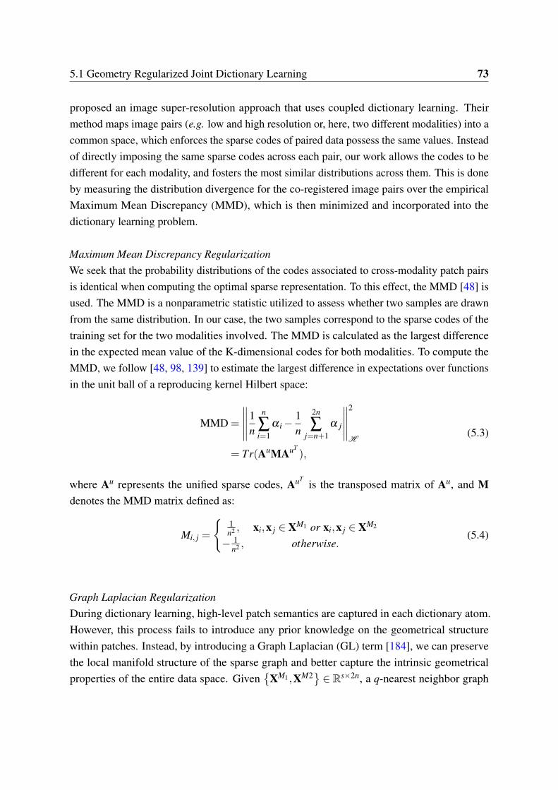
5.1 Geometry Regularized Joint Dictionary Learning 73
proposed an image super-resolution approach that uses coupled dictionary learning. Theirmethod maps image pairs (e.g. low and high resolution or, here, two different modalities) into acommon space, which enforces the sparse codes of paired data possess the same values. Insteadof directly imposing the same sparse codes across each pair, our work allows the codes to bedifferent for each modality, and fosters the most similar distributions across them. This is doneby measuring the distribution divergence for the co-registered image pairs over the empiricalMaximum Mean Discrepancy (MMD), which is then minimized and incorporated into thedictionary learning problem.
Maximum Mean Discrepancy RegularizationWe seek that the probability distributions of the codes associated to cross-modality patch pairsis identical when computing the optimal sparse representation. To this effect, the MMD [48] isused. The MMD is a nonparametric statistic utilized to assess whether two samples are drawnfrom the same distribution. In our case, the two samples correspond to the sparse codes of thetraining set for the two modalities involved. The MMD is calculated as the largest differencein the expected mean value of the K-dimensional codes for both modalities. To compute theMMD, we follow [48, 98, 139] to estimate the largest difference in expectations over functionsin the unit ball of a reproducing kernel Hilbert space:
MMD =
∥∥∥∥∥1n
n
∑i=1
α i−1n
2n
∑j=n+1
α j
∥∥∥∥∥2
H
= Tr(AuMAuT),
(5.3)
where Au represents the unified sparse codes, AuTis the transposed matrix of Au, and M
denotes the MMD matrix defined as:
Mi, j =
1n2 , xi,x j ∈ XM1 or xi,x j ∈ XM2
− 1n2 , otherwise.
(5.4)
Graph Laplacian RegularizationDuring dictionary learning, high-level patch semantics are captured in each dictionary atom.However, this process fails to introduce any prior knowledge on the geometrical structurewithin patches. Instead, by introducing a Graph Laplacian (GL) term [184], we can preservethe local manifold structure of the sparse graph and better capture the intrinsic geometricalproperties of the entire data space. Given
XM1,XM2 ∈ Rs×2n, a q-nearest neighbor graph
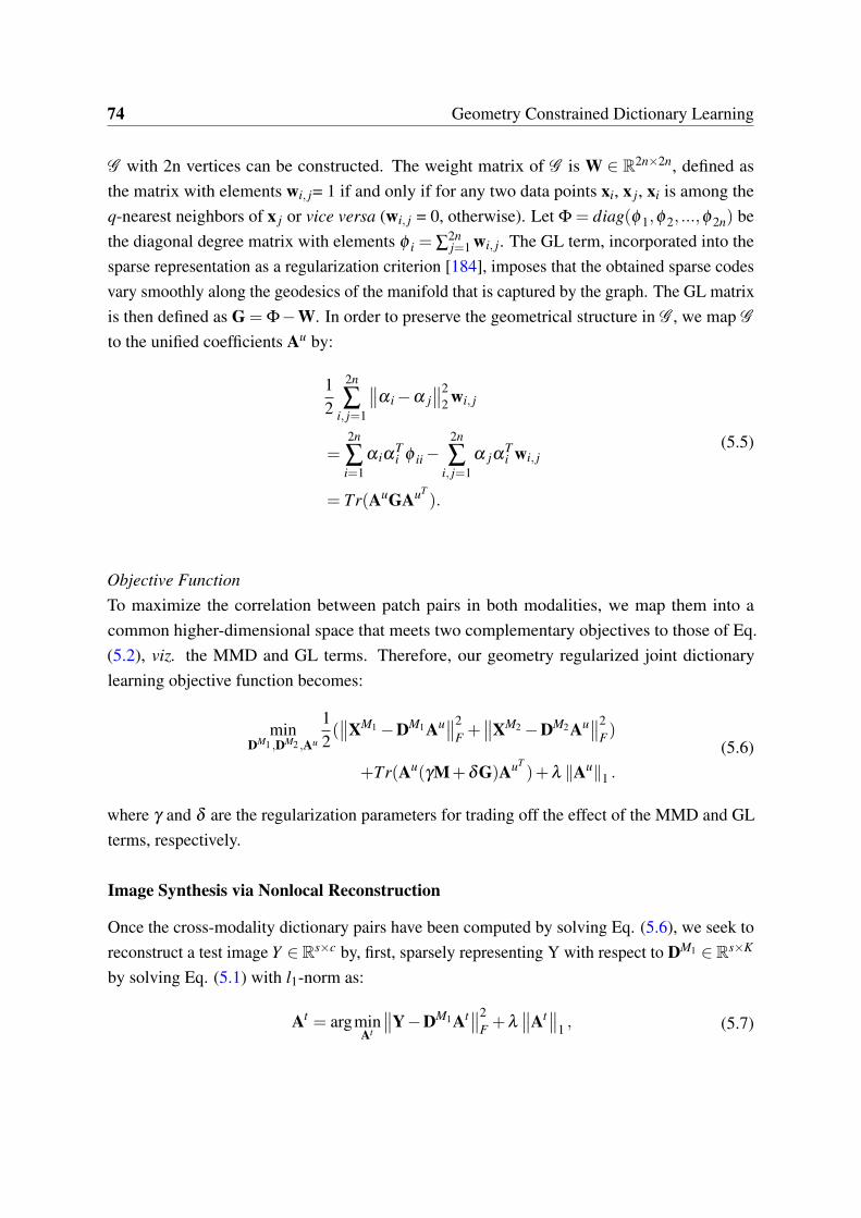
74 Geometry Constrained Dictionary Learning
G with 2n vertices can be constructed. The weight matrix of G is W ∈ R2n×2n, defined asthe matrix with elements wi, j= 1 if and only if for any two data points xi, x j, xi is among theq-nearest neighbors of x j or vice versa (wi, j = 0, otherwise). Let Φ = diag(φ 1,φ 2, ...,φ 2n) bethe diagonal degree matrix with elements φ i = ∑
2nj=1 wi, j. The GL term, incorporated into the
sparse representation as a regularization criterion [184], imposes that the obtained sparse codesvary smoothly along the geodesics of the manifold that is captured by the graph. The GL matrixis then defined as G = Φ−W. In order to preserve the geometrical structure in G , we map G
to the unified coefficients Au by:
12
2n
∑i, j=1
∥∥α i−α j∥∥2
2 wi, j
=2n
∑i=1
α iαTi φ ii−
2n
∑i, j=1
α jαTi wi, j
= Tr(AuGAuT).
(5.5)
Objective FunctionTo maximize the correlation between patch pairs in both modalities, we map them into acommon higher-dimensional space that meets two complementary objectives to those of Eq.(5.2), viz. the MMD and GL terms. Therefore, our geometry regularized joint dictionarylearning objective function becomes:
minDM1 ,DM2 ,Au
12(∥∥XM1−DM1Au∥∥2
F +∥∥XM2−DM2Au∥∥2
F)
+Tr(Au(γM+δG)AuT)+λ ∥Au∥1 .
(5.6)
where γ and δ are the regularization parameters for trading off the effect of the MMD and GLterms, respectively.
Image Synthesis via Nonlocal Reconstruction
Once the cross-modality dictionary pairs have been computed by solving Eq. (5.6), we seek toreconstruct a test image Y ∈Rs×c by, first, sparsely representing Y with respect to DM1 ∈Rs×K
by solving Eq. (5.1) with l1-norm as:
At = argminAt
∥∥Y−DM1At∥∥2F +λ
∥∥At∥∥1 , (5.7)
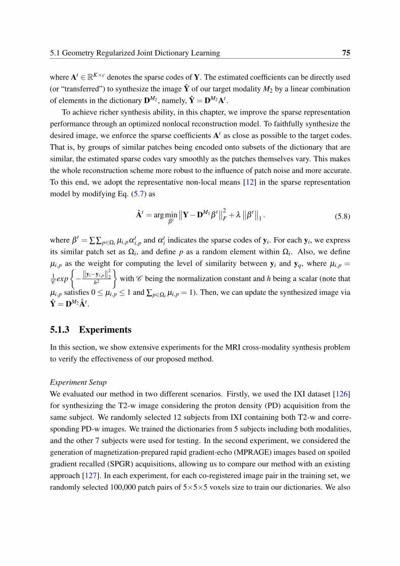
5.1 Geometry Regularized Joint Dictionary Learning 75
where At ∈RK×c denotes the sparse codes of Y. The estimated coefficients can be directly used(or “transferred”) to synthesize the image Y of our target modality M2 by a linear combinationof elements in the dictionary DM2 , namely, Y = DM2At .
To achieve richer synthesis ability, in this chapter, we improve the sparse representationperformance through an optimized nonlocal reconstruction model. To faithfully synthesize thedesired image, we enforce the sparse coefficients At as close as possible to the target codes.That is, by groups of similar patches being encoded onto subsets of the dictionary that aresimilar, the estimated sparse codes vary smoothly as the patches themselves vary. This makesthe whole reconstruction scheme more robust to the influence of patch noise and more accurate.To this end, we adopt the representative non-local means [12] in the sparse representationmodel by modifying Eq. (5.7) as
At = argminβ t
∥∥Y−DM1βt∥∥2
F +λ∥∥β
t∥∥1 . (5.8)
where βt = ∑∑p∈Ωi µi,pα t
i,p and α ti indicates the sparse codes of yi. For each yi, we express
its similar patch set as Ωi, and define p as a random element within Ωi. Also, we defineµi,p as the weight for computing the level of similarity between yi and yq, where µi,p =
1C exp
−∥yi−yi,p∥2
2h2
with C being the normalization constant and h being a scalar (note that
µi,p satisfies 0≤ µi,p ≤ 1 and ∑p∈Ωi µi,p = 1). Then, we can update the synthesized image viaY = DM2At .
5.1.3 Experiments
In this section, we show extensive experiments for the MRI cross-modality synthesis problemto verify the effectiveness of our proposed method.
Experiment SetupWe evaluated our method in two different scenarios. Firstly, we used the IXI dataset [126]for synthesizing the T2-w image considering the proton density (PD) acquisition from thesame subject. We randomly selected 12 subjects from IXI containing both T2-w and corre-sponding PD-w images. We trained the dictionaries from 5 subjects including both modalities,and the other 7 subjects were used for testing. In the second experiment, we considered thegeneration of magnetization-prepared rapid gradient-echo (MPRAGE) images based on spoiledgradient recalled (SPGR) acquisitions, allowing us to compare our method with an existingapproach [127]. In each experiment, for each co-registered image pair in the training set, werandomly selected 100,000 patch pairs of 5×5×5 voxels size to train our dictionaries. We also
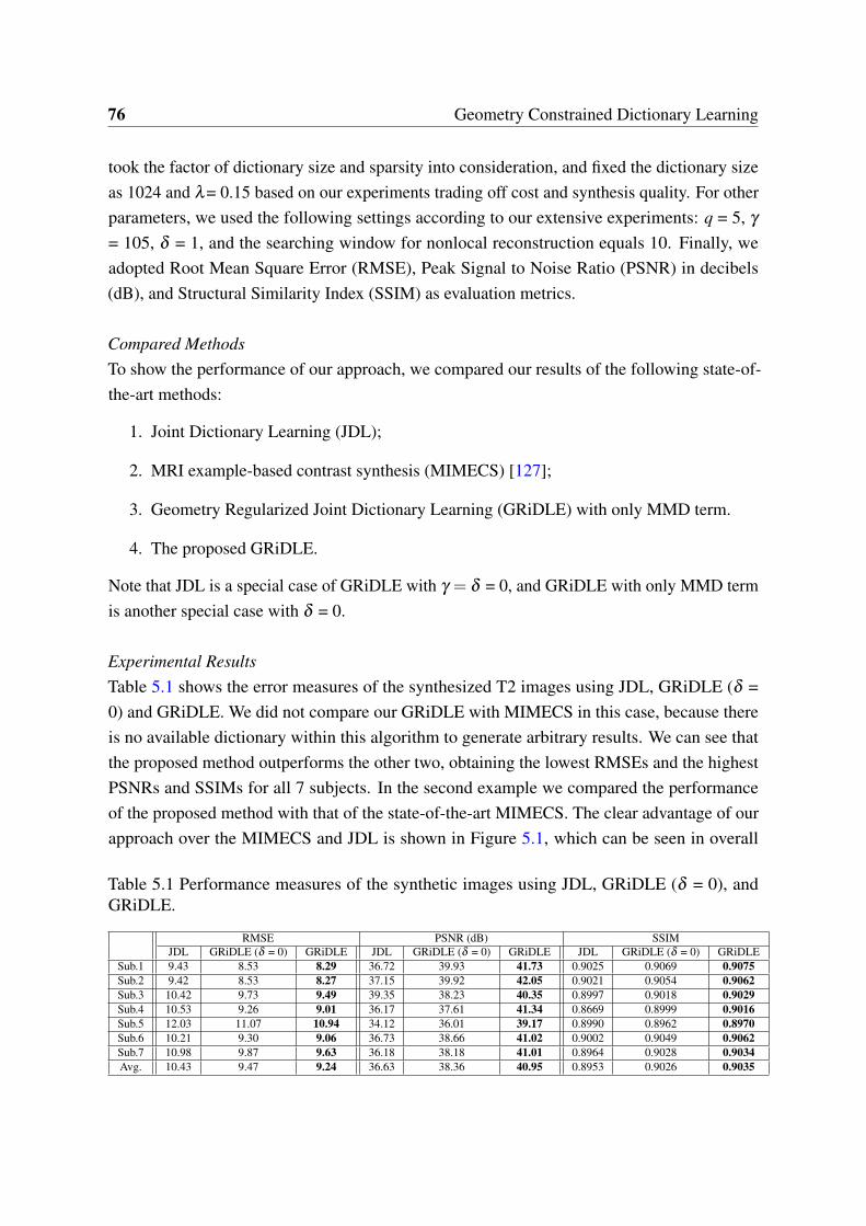
76 Geometry Constrained Dictionary Learning
took the factor of dictionary size and sparsity into consideration, and fixed the dictionary sizeas 1024 and λ= 0.15 based on our experiments trading off cost and synthesis quality. For otherparameters, we used the following settings according to our extensive experiments: q = 5, γ
= 105, δ = 1, and the searching window for nonlocal reconstruction equals 10. Finally, weadopted Root Mean Square Error (RMSE), Peak Signal to Noise Ratio (PSNR) in decibels(dB), and Structural Similarity Index (SSIM) as evaluation metrics.
Compared MethodsTo show the performance of our approach, we compared our results of the following state-of-the-art methods:
1. Joint Dictionary Learning (JDL);
2. MRI example-based contrast synthesis (MIMECS) [127];
3. Geometry Regularized Joint Dictionary Learning (GRiDLE) with only MMD term.
4. The proposed GRiDLE.
Note that JDL is a special case of GRiDLE with γ = δ = 0, and GRiDLE with only MMD termis another special case with δ = 0.
Experimental ResultsTable 5.1 shows the error measures of the synthesized T2 images using JDL, GRiDLE (δ =0) and GRiDLE. We did not compare our GRiDLE with MIMECS in this case, because thereis no available dictionary within this algorithm to generate arbitrary results. We can see thatthe proposed method outperforms the other two, obtaining the lowest RMSEs and the highestPSNRs and SSIMs for all 7 subjects. In the second example we compared the performanceof the proposed method with that of the state-of-the-art MIMECS. The clear advantage of ourapproach over the MIMECS and JDL is shown in Figure 5.1, which can be seen in overall
Table 5.1 Performance measures of the synthetic images using JDL, GRiDLE (δ = 0), andGRiDLE.
RMSE PSNR (dB) SSIMJDL GRiDLE (δ = 0) GRiDLE JDL GRiDLE (δ = 0) GRiDLE JDL GRiDLE (δ = 0) GRiDLE
Sub.1 9.43 8.53 8.29 36.72 39.93 41.73 0.9025 0.9069 0.9075Sub.2 9.42 8.53 8.27 37.15 39.92 42.05 0.9021 0.9054 0.9062Sub.3 10.42 9.73 9.49 39.35 38.23 40.35 0.8997 0.9018 0.9029Sub.4 10.53 9.26 9.01 36.17 37.61 41.34 0.8669 0.8999 0.9016Sub.5 12.03 11.07 10.94 34.12 36.01 39.17 0.8990 0.8962 0.8970Sub.6 10.21 9.30 9.06 36.73 38.66 41.02 0.9002 0.9049 0.9062Sub.7 10.98 9.87 9.63 36.18 38.18 41.01 0.8964 0.9028 0.9034Avg. 10.43 9.47 9.24 36.63 38.36 40.95 0.8953 0.9026 0.9035
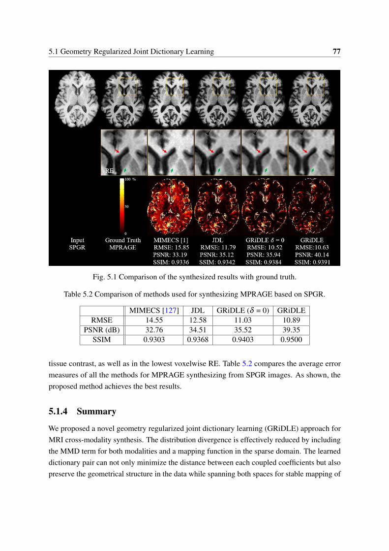
5.1 Geometry Regularized Joint Dictionary Learning 77
Fig. 5.1 Comparison of the synthesized results with ground truth.
Table 5.2 Comparison of methods used for synthesizing MPRAGE based on SPGR.
MIMECS [127] JDL GRiDLE (δ = 0) GRiDLERMSE 14.55 12.58 11.03 10.89
PSNR (dB) 32.76 34.51 35.52 39.35SSIM 0.9303 0.9368 0.9403 0.9500
tissue contrast, as well as in the lowest voxelwise RE. Table 5.2 compares the average errormeasures of all the methods for MPRAGE synthesizing from SPGR images. As shown, theproposed method achieves the best results.
5.1.4 Summary
We proposed a novel geometry regularized joint dictionary learning (GRiDLE) approach forMRI cross-modality synthesis. The distribution divergence is effectively reduced by includingthe MMD term for both modalities and a mapping function in the sparse domain. The learneddictionary pair can not only minimize the distance between each coupled coefficients but alsopreserve the geometrical structure in the data while spanning both spaces for stable mapping of
78 Geometry Constrained Dictionary Learning
image details. Extensive experiments have demonstrated that GRiDLE can achieve superiorperformance over the state-of-the-art methods. Future work will focus on the simultaneousgeneration of multimodality images.
5.2 Weakly-Coupled and Geometry Co-Regularized Joint Dic-tionary Learning
In this work, we propose a Weakly-coupled And Geometry co-regularized (WAG) joint dictio-nary learning method to address the problem of cross-modality synthesis while consideringthe fact that collecting large amounts of training data is often impractical. Our learning stagerequires only a few registered multi-modality image pairs as training data. To employ bothpaired images and a large set of unpaired data, a cross-modality image matching criterionis proposed. We then propose a unified model by integrating such a criterion into the jointdictionary learning and the observed common feature space for associating cross-modality datafor the purpose of synthesis. Furthermore, two regularization terms are added to constructrobust sparse representations. Our experimental results demonstrate superior performance ofthe proposed model over state-of-the-art methods.
5.2.1 Introduction
Magnetic Resonance Imaging (MRI) is a versatile and noninvasive imaging technique exten-sively used in neuroimaging studies. MRI comes in several modalities, for example, ProtonDensity (PD)-weighted images distinguish between fluid and fat, whereas T1-weighted scanshave good tissue contrast between gray matter and white matter. Each modality offers diverseand complementary image contrast mechanisms unraveling structural and functional informa-tion about brain tissue. Due to variations in the brain images across modalities, multi-modalityMRI is preferred in many pharmaceutical clinical trials, in research studies of neurosciences, orin population imaging cohorts targeting to understand neurodegeneration and cognitive decline.However, the acquisitions of a full battery of all these MR images can face constraints associatedwith their cost, limited availability of scanning time, patient comfort or safety considerations.In large scale studies, it is not uncommon to face incomplete datasets since the presence ofimaging artifacts, acquisition errors or corrupted data. While various post-processing solutionssuch as image imputation [152] and histogram matching [100, 112] have been proposed tocompensate for these latter issues, this is usually only at the level of derived imaging biomarkersbut not of the data itself [62, 127]. Finally, in longitudinal imaging studies where images arecollected over several years, evolution of imaging technology may lead to the appearance of
5.2 Weakly-Coupled and Geometry Co-Regularized Joint Dictionary Learning 79
new MRI sequences added to an existing imaging protocol in time, which were not availableas part of the imaging battery acquired at earlier time points. In these and other applications,it would be desirable to have a cross-modality image synthesis method that can generate thetarget modality images from the source modality scans. The ability to synthesize differentmodalities of the same anatomy can benefit various practical image analysis tasks includingmulti-modal registration [15, 160], segmentation [68], and atlas construction [25, 115].
In the last few years, cross-modality image synthesis has attracted the attention of themedical image computing community. Most techniques assume such mapping exists betweensource and target imaging modalities. The problem is then formulated as that of learning themost efficient mapping representation. To synthesize the target from a source modality, somemethods have been proposed that construct a dictionary from patches extracted from a singleimage or from image pairs [59, 72, 95, 127] or that learn the mapping from a large set oftraining image pairs [14, 150, 153, 172]. Although these approaches have shown great promise,they are supervised and require labeled data sets.
In this work, instead, we propose a single-image cross-modality synthesis method with anapplication to T1-w, T2-w and PD-w brain MRI that utilizes a few registered multi-modalityimage pairs2 while employing a larger set of unpaired data for synthesizing the target imagemodality from an available source image modality. Our method extracts the common latentfeatures that map different image features of the underlying tissues, preserves global statisticalimage properties across modalities, and simultaneously, refines extracted features to preservethe local geometrical structure in each modality. In addition, the proposed approach requiresonly a few registered image pairs to find the mapping between the appearances in differentimage modalities and employs auxiliary unpaired training images to further exploit the modality-specific geometric structure and obtain a robust sparse representation. To complement theunpaired data with the original training pairs, manifold ranking-based cross-modality imagematching is employed as a criterion to pick up features of the target domain from most similarsubjects in the source domain. The mapping between multi-modality data can be complexand highly nonlinear. To provide the needed flexibility to map image structures in differentmodalities, we determine a common feature space by an association function that describesand relates cross-modality data. We call the proposed method Weakly-coupled And Geometry(WAG) co-regularized joint dictionary learning, and perform extensive experiments to verify itsperformance.
The contributions of this work are threefold:2Paired data requires data in both source and target domains from the same subject and registered with each
other. Unpaired data means data in the source and target domains are from different subjects without registration.
80 Geometry Constrained Dictionary Learning
1. WAG is a unified model, which learns a pair of (not coupled) dictionaries with a commonfeature space for medical imaging cross-modality synthesis. WAG automatically trainsdictionary pairs and computes an association function between source and target modalitydata based on only a few registered image pairs;
2. To enrich this model, we design a cross-modality image matching criterion that acts col-laboratively with a larger set of unpaired images. This allows identifying correspondencesacross source and target domains that are invariant to pose transformations;
3. We deal with the considerable difference in data distributions from different modali-ties (i.e. T1-w, T2-w and PD-w MRI) by simultaneously minimizing the distributiondiscrepancy of similar instances and preserving geometric structures in each domain.
A preliminary version [62] of this work was presented earlier at the SASHIMI Workshopin MICCAI 2016 (www.cistib.org/sashimi2016). This work adds to the seminal version insignificant ways. First, we improve the synthesis model by introducing a cross-modality image-matching criterion to connect and integrate all information from both registered and unregistereddata in different modalities to describe the diversity of human brain imaging. Second, we extendthe single geometry regularization by preserving modality-specific local geometric propertiesto penalize undesired loss of information. Third, we consider the flexibility of domain-specificinformation and construct a common feature space by a mapping function that describes andassociates cross-modality data. Fourth, we also extend the original experiments from onlycomparing with one baseline method to several recently published approaches involving bothsupervised and unsupervised settings. The proposed method demonstrates state-of-the-artsynthesis results using two evaluation metrics in all of our experiments.
5.2.2 Method
In this section, we first formulate the problem formally. Then, we propose a general frameworkfor cross-modality image synthesis. Our approach extends the conventional dictionary learningapproach by jointly learning a pair of dictionaries from the constructed common feature spacethat describes and associates cross-modality data. We also consider the minimization ofthe distribution divergence between both modalities while preserving modality-specific localgeometric properties that penalize undesired loss of information. Finally, we utilize unpairedimages in both domains as auxiliary training data that enhances the supervised learning process.This additional unsupervised step collaborates with and complements the registered trainingimage pairs. An overview of our proposed method is depicted in Fig. 5.2.
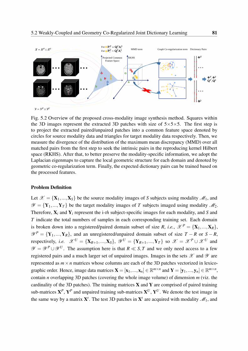
5.2 Weakly-Coupled and Geometry Co-Regularized Joint Dictionary Learning 81
GR
Projected Common
Feature Space
RKHS
For
ForMMD term Graph Co-regularization term Dictionary Pairs
Fig. 5.2 Overview of the proposed cross-modality image synthesis method. Squares withinthe 3D images represent the extracted 3D patches with size of 5×5×5. The first step isto project the extracted paired/unpaired patches into a common feature space denoted bycircles for source modality data and triangles for target modality data respectively. Then, wemeasure the divergence of the distribution of the maximum mean discrepancy (MMD) over allmatched pairs from the first step to seek the intrinsic pairs in the reproducing kernel Hilbertspace (RKHS). After that, to better preserve the modality-specific information, we adopt theLaplacian eigenmaps to capture the local geometric structure for each domain and denoted bygeometric co-regularization term. Finally, the expected dictionary pairs can be trained based onthe processed features.
Problem Definition
Let X = X1, ...,XS be the source modality images of S subjects using modality M1, andY = Y1, ...,YT be the target modality images of T subjects imaged using modality M2.Therefore, Xi and Yi represent the i-th subject-specific images for each modality, and S andT indicate the total numbers of samples in each corresponding training set. Each domainis broken down into a registered/paired domain subset of size R, i.e., X P = X1, ...,XR,Y P = Y1, ...,YR, and an unregistered/unpaired domain subset of size T − R or S− R,respectively, i.e. X U = XR+1, ...,XS, Y U = YR+1, ...,YT so X = X P ∪X U andY = Y P ∪Y U . The assumption here is that R≪ S,T and we only need access to a fewregistered pairs and a much larger set of unpaired images. Images in the sets X and Y arerepresented as m×n matrices whose columns are each of the 3D patches vectorized in lexico-graphic order. Hence, image data matrices X = [x1, ...,xn] ∈Rm×n and Y = [y1, ...,yn] ∈Rm×n,contain n overlapping 3D patches (covering the whole image volume) of dimension m (viz. thecardinality of the 3D patches). The training matrices X and Y are comprised of paired trainingsub-matrices XP, YP and unpaired training sub-matrices XU , YU . We denote the test image inthe same way by a matrix Xt . The test 3D patches in Xt are acquired with modality M1, and
82 Geometry Constrained Dictionary Learning
will be the input to synthesize the corresponding 3D patches in modality M2.
Problem Statement: We first denote the coding coefficients AX , AY of X, Y over the learneddictionaries Φ
X , ΦY , the projected data PX , PY of X, Y in a defined common space, and a
mapping function F (·) to represent the relationship between the sparse codes AX , AY of twodomains, where the detailed descriptions and the corresponding mathematical formulationsare provided in the following subsections. Given a pair of training matrices X and Y withX =
[XP XU] and Y =
[YP YU], our goal is: 1) to learn a pair of dictionaries
Φ
X ,ΦY
, theirsparse codes
AX ,AY
, and an association function F (·) : M1→M2 using the projected
data PX and PY ; and 2) to minimize the inter-modality divergence between PX and PY , and3) to preserve the domain-specific local geometric structure.
Dictionary Learning
Assume that X = [x1, ...,xn] ∈ Rm×n is a training dataset, which can be reconstructed bythe linear combination of a set of n coefficients that lie on a k-dimensional sparse space,AX =
[αX
1 , ...,αXn]∈ Rk×n is associated to the dictionary Φ
X =[φ
X1 , ...,φX
k]∈ Rm×k.
Here, k > m to make the dictionary over-complete [1]. Considering the reconstruction error foreach data point, the problem of learning a dictionary Φ
X for sparse representation of X can beformulated as
minΦ
X ,AX
∥∥∥X−ΦX AX
∥∥∥2
F+λ
∥∥∥AX∥∥∥
0, (5.9)
where ∥·∥F is the Frobenius norm, ∥·∥0 is the l0-norm that penalizes non-zero elements in A,and λ denotes a regularization parameter to trade off sparsity vs. reconstruction error. Asshown in [26], the minimization problem in Eq. (5.9) is, in general, NP-hard under the l0-norm.An alternative solution is to relax the l0-norm with the l1-norm and obtain a near-optimal result[20]. The dictionary learning problem in Eq. (5.9) can be reformulated as
minΦ
X ,AX
∥∥∥X−ΦX AX
∥∥∥2
F+λ
∥∥∥AX∥∥∥
1. (5.10)
The above objective function is not simultaneously convex over Φ and A. A practicalsolution is to alternate between optimizing for the dictionary Φ and for the sparse codes Afixing the other degree of freedom. This makes the problem convex and the solution convergesto a local minimum [86]. When the dictionary is fixed, the algorithm is known as Lasso/LARS[146] with an l1 penalty over the coefficients and can be solved by the feature-sign searchapproach [86]. When sparse codes are fixed, such an optimization problem is reduced to a leastsquares optimization with quadratic constraints, and can be solved using a Lagrange dual [86].
5.2 Weakly-Coupled and Geometry Co-Regularized Joint Dictionary Learning 83
When dealing with multi-modality data, one can simply construct two independent dic-tionaries using conventional dictionary learning. Specifically, given two training data sets Xand Y, following the dictionary learning procedure described in [1, 104] and Eq. (5.10), wecan learn the dictionaries separately to obtain the two dictionaries, Φ
X and ΦY , and the two
corresponding sparse coefficients, AX and AY , respectively. The data of each modality can bereconstructed using the respective dictionary and associated sparse coefficients.
Cross-Modality Dictionary Learning
Cross-modality image synthesis is based on learning a joint sparse representation [168] with acommon set of sparse codes shared between source and target image modalities, i.e. AX ≡AY . These sparse codes act on independent dictionaries for each modality, viz. Φ
X andΦ
Y , to reconstruct the corresponding source and target images. To this effect, both 3Dpatches in the source and target modalities must be perfectly co-registered. To map the tissueappearance across modalities, the joint dictionary learning strategy groups two independentreconstruction errors (viz.
∥∥X−ΦX AX
∥∥2F and
∥∥Y−ΦY AY
∥∥2F ) in a single objective function
to be optimized:
minΦ
X ,ΦY ,A
∥∥∥X−ΦX A
∥∥∥2
F+∥∥∥Y−Φ
Y A∥∥∥2
F+λ ∥A∥1
s.t.∥∥∥φ
Xi
∥∥∥2
2≤ 1,
∥∥∥φYi
∥∥∥2
2≤ 1 ∀i = 1, ...,k,
(5.11)
where A denotes the same coefficients to be enforced of registered data pairs projected in acommon feature space. As in the single dictionary learning optimization problem, the jointoptimization function in Eq. (5.11) is convex regarding the learned dictionaries, Φ
X and ΦY ,
for fixed sparse codes A. Therefore, the computation of A and of the dictionary pairs can bealternated. Analyzing (5.11), we note that this objective function is suitable to collaborativelylearn a pair of dictionaries, so the sparse codes in the source modality space M1 can directlyreconstruct the target modality image M2 in a transferable feature space.
Although joint dictionary learning achieves very good results, it assumes that source andtarget images, when represented with jointly learned dictionary pairs, Φ
X and ΦY , must
share the same sparse codes. In addition, all previous work requires that the training datasetcontains registered image pairs, which imposes additional demands. In this work, we addressthe above problems by relaxing the need for a common sparse representation and providingmore flexibility in reducing the registration requirement to a small training dataset only.

84 Geometry Constrained Dictionary Learning
Weak Coupling and Geometry Co-regularization
To make the proposed method effective for generalized cross-modality synthesis, we combinethe following ideas:
1. We integrate paired and unpaired training data in both modalities into a unified frame-work.
2. We relax the need for a shared sparse code in source and target domains.
3. We allow for dissimilar data distributions as required when dealing with very differentimage modalities.
4. We include a mechanism that preserves the local geometric structure specific to themodalities of the source and target images.
In the following, we introduce each component, and then summarize our overall approach.
Cross-Modality Image MatchingTo relate and integrate the information from the paired and unpaired training data subsets ofeach modality, we introduce a criterion called cross-modality image matching (CMIM) forincorporating the information from the unpaired training data into dictionary learning andcross-modality image synthesis.
In visually matching cross-modality data, it is common to identify the same features acrosssource and target imaging modalities. In this work, we extract High-Frequency (HF) featuresfrom source and target images where the resolutions of both modalities are similar. This isbased on the assumption that tissues may present different visual appearances one each modalitybut they share similar high order edge/texture characteristics while modality-specific detailsaffect primarily Low-Frequency (LF) properties [168].
In this chapter, we follow [16, 168] and adopt first- and second- order derivatives involvinghorizontal and vertical gradients as the HF features for each training data by Xh = H ∗X,Yh =H ∗Y. Generally, H is a high-pass filter operator used to extract derivatives, Consideringfirst and second order derivatives, H is one of the following operators: H1
1,H21,H
12,H
22, where
H11 =
−1 0 1−1 0 1−1 0 1
, H21 = H1
1T , and H1
2 =
−2 −1 0 1 2−2 −1 0 1 2−2 −1 0 1 2−2 −1 0 1 2−2 −1 0 1 2
, H22 = H1
2T . Once the features
in both domains are computed, we can use them to optimize CMIM and define a mapping

5.2 Weakly-Coupled and Geometry Co-Regularized Joint Dictionary Learning 85
C (·) : X → Y . In particular, CMIM can be thought of as a unilateral matching metric (i.e.,the weighted regression) that focuses on a particular goal (e.g. matching across resolutions,modalities, or domains. [66, 183, 186]). Given associated HF image feature sets, Xh and Yh,corresponding to both paired and unpaired training image data sets, X P, X U , Y P and Y U ,CMIM represents an ensemble of paired and unpaired cross-modality matching sub-problems.Images in X P and Y P are endowed with a natural correspondence, X P Y P. In contrast,CMIM finds a mapping for multi-modality unpaired image data for X U and Y U . Since X P
and Y P are already registered/paired, we can assume a perfect matching between them. Byintegrating the unpaired image data, we can establish a final affinity matrix TTT ∈ Rn×n such thatC (X ,Y ) =
∥∥Xh−TTTYh∥∥2
2:
TTT=
D(xh1,y
h1) · · · D(xh
1,yhn)
... . . . ...D(xh
n,yh1) · · · D(xh
n,yhn)
, (5.12)
where D(xhi ,y
hj) is a distance function generally designed to measure the distances between
each pair of HF feature vectors in X and Y using an g-dimensional Gaussian kernel
D(xhi ,y
hj) =
1(√
2πσ)ge−∥xh
i −yhj∥
2
2σ2 , (5.13)
where σ = 0 denotes the kernel bandwidth. TTT establishes a one-to-one correspondence foreach source domain 3D patch. We preserve the most relevant features with the largest D valueswithin Y while discarding other 3D patches. In this way, from TTT we define TTT as:
TTT(i, j) =
1, if j = ji,0, otherwise.
(5.14)
where ji = max j (TTT(i, j)) is the maximum element of the i-th row in TTT. Furthermore, we setthe maximum element TTT(i, ji) to be 1 where all other values are set to 0 resulting in a binaryassignment matrix TTT. Given TTT, each source patch is only mapped to one target patch withthe most similar tissue texture. Hence, patches across different domains can be treated as theregistered pairs after such a processing, i.e., X Y for each xi paired with y ji denoted asPi = xi,y ji for i = 1 . . .n.
Computing the mapping functionStarting off by Eq. (5.10), by minimizing the reconstruction error, the corresponding sparse

86 Geometry Constrained Dictionary Learning
codes AX and AY for each modality can be computed, respectively. To allow these codes todiffer for the paired examples and unpaired data matched via CMIM, we assume there exists amapping function F : M1 →M2 with Y = F (X). Accordingly, the sparse codes of X andY over the dictionaries will be related by such a mapping function F
(AX ,AY
). To build a
stable mapping between two domains, Wang et al. [155] assumed that the sparse codes fromthe source domain had to be identical to those for the target domain via a linear projection W.As suggested in [60], projecting both source and target domain data into a common featurespace can better describe and associate cross-modality data. Inspired by this strategy, we firstdefine the cross-modality relationship in the projected data PX , PY of X, Y, and replaceF (AX ,AY ) by F (PX ,PY ), and then incorporate the projected features into CMIM-drivencoupled dictionary learning. The objective function based on the pre-determined CMIM term∥∥∥Xh−TTTYh
∥∥∥2
2of this learning model is:
minΦ
X ,ΦY ,AX ,AY
∥∥∥X−ΦX AX
∥∥∥2
F+∥∥∥Y−Φ
Y AY∥∥∥2
F
+λ
(∥∥∥AX∥∥∥
1+∥∥∥AY
∥∥∥1
)+νF
(PX ,PY
),
(5.15)
where PX = QX AX ∈ Rk×n and PY = QY AY ∈ Rk×n denote the projected data of X andY, respectively, in the common feature space. Here, λ and ν are regularization parameters.The projection matrices, QX ∈ Rk×k and QY ∈ Rk×k are the projection matrices for AX
and AY , respectively. Generally, F (PX ,PY ) can be applied to any joint dictionary learn-ing scheme with F (PX ,PY ) =
∥∥PX −PY∥∥2
F =∥∥QX AX −QY AY
∥∥2F . For example, in
Eq. (5.11) of [168], F is defined with an infinitely large ν having QX = QY = I, whilein [155] F is defined so QX = I and QY = W, where I is the identity matrix. The solu-tions of QX and QY are not unique. Following [60], an additional regularization constraintshould be added to ensure the uniqueness of these solutions. Moreover, to guarantee theprojected data lands in a common space and we can synthesize data of the target modality fromprojected data of the source modality, an additional regularization constraint is provided tomake the function separately convex with respect to each variable. Given PX and PY , weminimize their distance in the projected common space considering the projections separately,viz. ν
(∥∥AX QX −PY∥∥2
F +∥∥AY QY −PX
∥∥2F
). Solving this objective function, we obtain
AX = QX −1PY and AY = QY −1PX , where PX = QX AX and PY = QY AY denote theprojected data of X and Y, respectively, in the constructed common feature space.
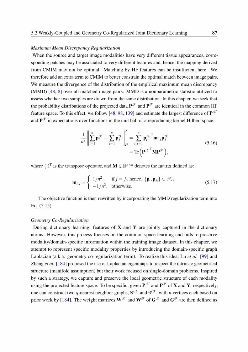
5.2 Weakly-Coupled and Geometry Co-Regularized Joint Dictionary Learning 87
Maximum Mean Discrepancy RegularizationWhen the source and target image modalities have very different tissue appearances, corre-
sponding patches may be associated to very different features and, hence, the mapping derivedfrom CMIM may not be optimal. Matching by HF features can be insufficient here. Wetherefore add an extra term to CMIM to better constrain the optimal match between image pairs.We measure the divergence of the distribution of the empirical maximum mean discrepancy(MMD) [48, 8] over all matched image pairs. MMD is a nonparametric statistic utilized toassess whether two samples are drawn from the same distribution. In this chapter, we seek thatthe probability distributions of the projected data PX and PY are identical in the common HFfeature space. To this effect, we follow [48, 98, 139] and estimate the largest difference of PX
and PY in expectations over functions in the unit ball of a reproducing kernel Hilbert space:
1n2
∥∥∥∥∥ n
∑i=1
pXi −
n
∑j=1
pYj
∥∥∥∥∥2
H
=n
∑i, j=1
pXi
Tmi, jpYj
= Tr(
PX TMPY),
(5.16)
where (·)T is the transpose operator, and M ∈ Rn×n denotes the matrix defined as:
mi, j =
1/n2, if j = ji, hence, pi,p ji ∈Pi,
−1/n2, otherwise.(5.17)
The objective function is then rewritten by incorporating the MMD regularization term intoEq. (5.15).
Geometry Co-RegularizationDuring dictionary learning, features of X and Y are jointly captured in the dictionary
atoms. However, this process focuses on the common space learning and fails to preservemodality/domain-specific information within the training image dataset. In this chapter, weattempt to represent specific modality properties by introducing the domain-specific graphLaplacian (a.k.a. geometry co-regularization term). To realize this idea, Lu et al. [99] andZheng et al. [184] proposed the use of Laplacian eigenmaps to respect the intrinsic geometricalstructure (manifold assumption) but their work focused on single-domain problems. Inspiredby such a strategy, we capture and preserve the local geometric structure of each modalityusing the projected feature space. To be specific, given PX and PY of X and Y, respectively,one can construct two q-nearest neighbor graphs, G X and G Y , with n vertices each based onprior work by [184]. The weight matrices WX and WY of GX and GY are then defined as
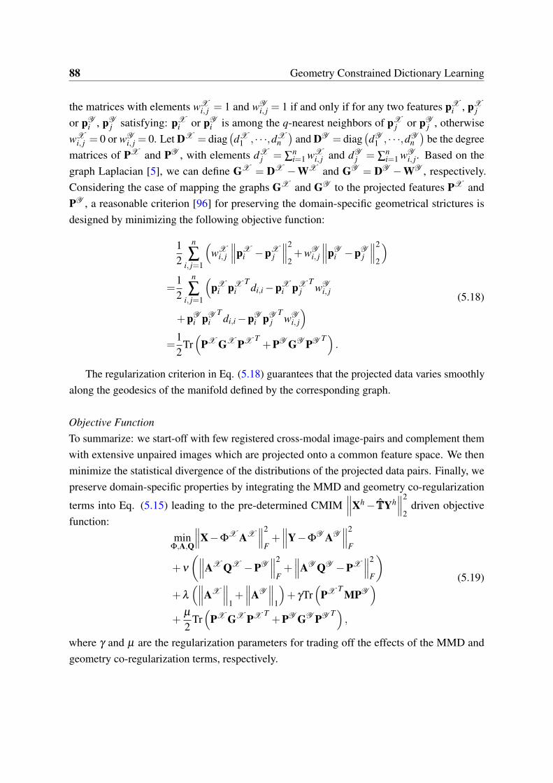
88 Geometry Constrained Dictionary Learning
the matrices with elements wXi, j = 1 and wY
i, j = 1 if and only if for any two features pXi , pX
j
or pYi , pY
j satisfying: pXi or pY
i is among the q-nearest neighbors of pXj or pY
j , otherwisewX
i, j = 0 or wYi, j = 0. Let DX = diag
(dX
1 , · · ·,dXn)
and DY = diag(dY
1 , · · ·,dYn)
be the degreematrices of PX and PY , with elements dX
j = ∑ni=1 wX
i, j and dYj = ∑
ni=1 wY
i, j. Based on thegraph Laplacian [5], we can define GX = DX −WX and GY = DY −WY , respectively.Considering the case of mapping the graphs GX and GY to the projected features PX andPY , a reasonable criterion [96] for preserving the domain-specific geometrical strictures isdesigned by minimizing the following objective function:
12
n
∑i, j=1
(wX
i, j
∥∥∥pXi −pX
j
∥∥∥2
2+wY
i, j
∥∥∥pYi −pY
j
∥∥∥2
2
)=
12
n
∑i, j=1
(pX
i pXi
Tdi,i−pX
i pXj
TwY
i, j
+pYi pY
iT
di,i−pYi pY
jT
wYi, j
)=
12
Tr(
PX GX PX T+PY GY PY T
).
(5.18)
The regularization criterion in Eq. (5.18) guarantees that the projected data varies smoothlyalong the geodesics of the manifold defined by the corresponding graph.
Objective FunctionTo summarize: we start-off with few registered cross-modal image-pairs and complement themwith extensive unpaired images which are projected onto a common feature space. We thenminimize the statistical divergence of the distributions of the projected data pairs. Finally, wepreserve domain-specific properties by integrating the MMD and geometry co-regularization
terms into Eq. (5.15) leading to the pre-determined CMIM∥∥∥Xh−TTTYh
∥∥∥2
2driven objective
function:min
Φ,A,Q
∥∥∥X−ΦX AX
∥∥∥2
F+∥∥∥Y−Φ
Y AY∥∥∥2
F
+ν
(∥∥∥AX QX −PY∥∥∥2
F+∥∥∥AY QY −PX
∥∥∥2
F
)+λ
(∥∥∥AX∥∥∥
1+∥∥∥AY
∥∥∥1
)+ γTr
(PX T MPY
)+
µ
2Tr(
PX GX PX T+PY GY PY T
),
(5.19)
where γ and µ are the regularization parameters for trading off the effects of the MMD andgeometry co-regularization terms, respectively.
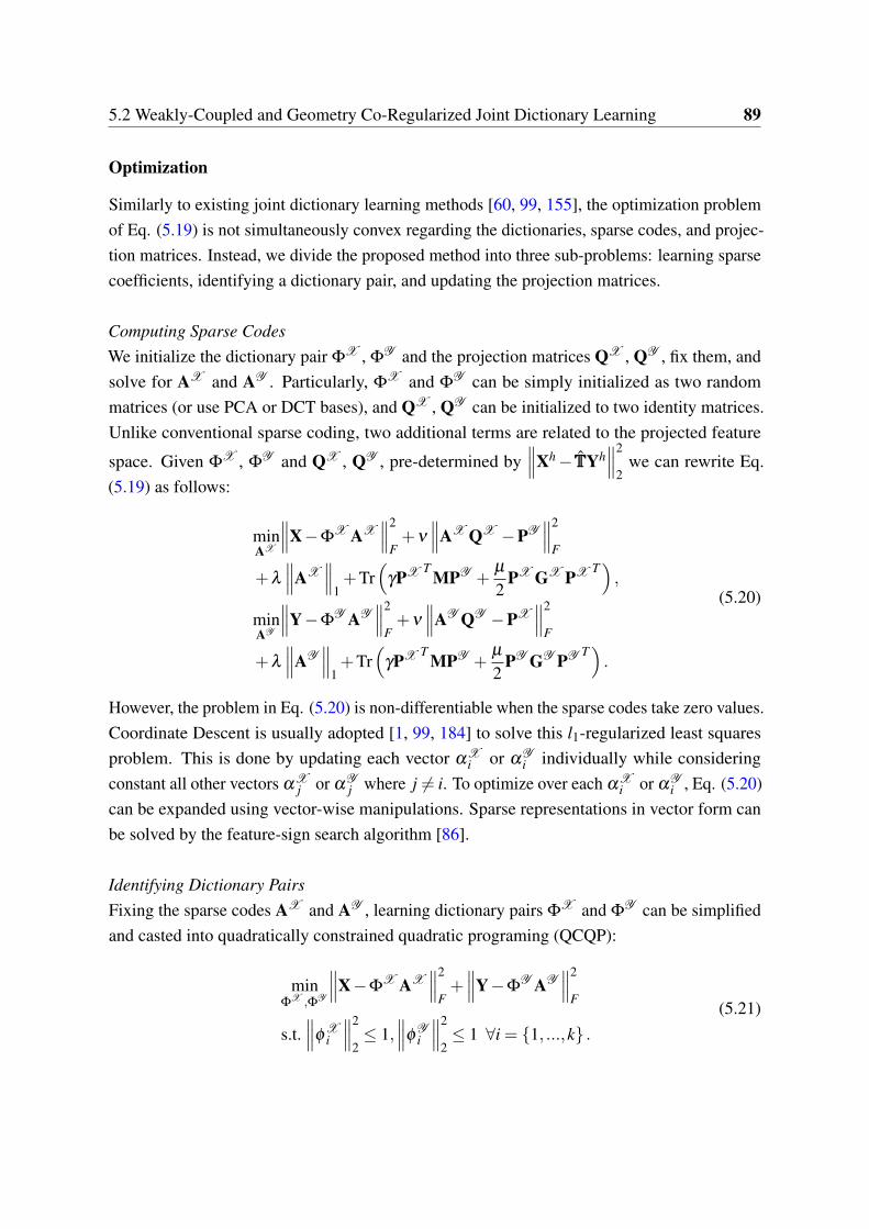
5.2 Weakly-Coupled and Geometry Co-Regularized Joint Dictionary Learning 89
Optimization
Similarly to existing joint dictionary learning methods [60, 99, 155], the optimization problemof Eq. (5.19) is not simultaneously convex regarding the dictionaries, sparse codes, and projec-tion matrices. Instead, we divide the proposed method into three sub-problems: learning sparsecoefficients, identifying a dictionary pair, and updating the projection matrices.
Computing Sparse CodesWe initialize the dictionary pair Φ
X , ΦY and the projection matrices QX , QY , fix them, and
solve for AX and AY . Particularly, ΦX and Φ
Y can be simply initialized as two randommatrices (or use PCA or DCT bases), and QX , QY can be initialized to two identity matrices.Unlike conventional sparse coding, two additional terms are related to the projected feature
space. Given ΦX , Φ
Y and QX , QY , pre-determined by∥∥∥Xh−TTTYh
∥∥∥2
2we can rewrite Eq.
(5.19) as follows:
minAX
∥∥∥X−ΦX AX
∥∥∥2
F+ν
∥∥∥AX QX −PY∥∥∥2
F
+λ
∥∥∥AX∥∥∥
1+Tr
(γPX T MPY +
µ
2PX GX PX T
),
minAY
∥∥∥Y−ΦY AY
∥∥∥2
F+ν
∥∥∥AY QY −PX∥∥∥2
F
+λ
∥∥∥AY∥∥∥
1+Tr
(γPX T MPY +
µ
2PY GY PY T
).
(5.20)
However, the problem in Eq. (5.20) is non-differentiable when the sparse codes take zero values.Coordinate Descent is usually adopted [1, 99, 184] to solve this l1-regularized least squaresproblem. This is done by updating each vector αX
i or αYi individually while considering
constant all other vectors αXj or αY
j where j = i. To optimize over each αXi or αY
i , Eq. (5.20)can be expanded using vector-wise manipulations. Sparse representations in vector form canbe solved by the feature-sign search algorithm [86].
Identifying Dictionary PairsFixing the sparse codes AX and AY , learning dictionary pairs Φ
X and ΦY can be simplified
and casted into quadratically constrained quadratic programing (QCQP):
minΦ
X ,ΦY
∥∥∥X−ΦX AX
∥∥∥2
F+∥∥∥Y−Φ
Y AY∥∥∥2
F
s.t.∥∥∥φ
Xi
∥∥∥2
2≤ 1,
∥∥∥φYi
∥∥∥2
2≤ 1 ∀i = 1, ...,k .
(5.21)
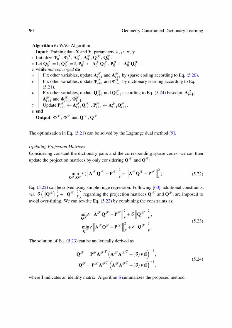
90 Geometry Constrained Dictionary Learning
Algorithm 6: WAG AlgorithmInput: Training data X and Y, parameters λ , µ , σ , γ .
1 Initialize ΦX0 , Φ
Y0 , AX
0 , AY0 , QX
0 , QY0 .
2 Let QX0 = I, QY
0 = I, PX0 ← AX
0 QX0 , PY
0 ← AY0 QY
0 .3 while not converged do4 Fix other variables, update AX
i+1 and AYi+1 by sparse coding according to Eq. (5.20).
5 Fix other variables, update ΦXi+1 and Φ
Yi+1 by dictionary learning according to Eq.
(5.21).6 Fix other variables, update QX
i+1 and QYi+1 according to Eq. (5.24) based on AX
i+1,AY
i+1 and ΦXi+1, Φ
Yi+1.
7 Update PXi+1← AX
i+1QXi+1, PY
i+1← AYi+1QY
i+1.8 end
Output: ΦX , Φ
Y and QX , QY .
The optimization in Eq. (5.21) can be solved by the Lagrange dual method [9].
Updating Projection MatricesConsidering constant the dictionary pairs and the corresponding sparse codes, we can thenupdate the projection matrices by only considering QX and QY :
minQX ,QY
ν(∥∥∥AX QX −PY
∥∥∥2
F+∥∥∥AY QY −PX
∥∥∥2
F). (5.22)
Eq. (5.22) can be solved using simple ridge regression. Following [60], additional constraints,viz. δ
(∥∥QX∥∥2
F +∥∥QY
∥∥2F
)regarding the projection matrices QX and QY , are imposed to
avoid over-fitting. We can rewrite Eq. (5.22) by combining the constraints as:
minQX
ν
∥∥∥AX QX −PY∥∥∥2
F+δ
∥∥∥QX∥∥∥2
F,
minQY
ν
∥∥∥AY QY −PX∥∥∥2
F+δ
∥∥∥QY∥∥∥2
F.
(5.23)
The solution of Eq. (5.23) can be analytically derived as
QX = PY AX T(
AX AX T+(δ/ν)I
)−1,
QY = PX AY T(
AY AY T+(δ/ν)I
)−1,
(5.24)
where I indicates an identity matrix. Algorithm 6 summarizes the proposed method.
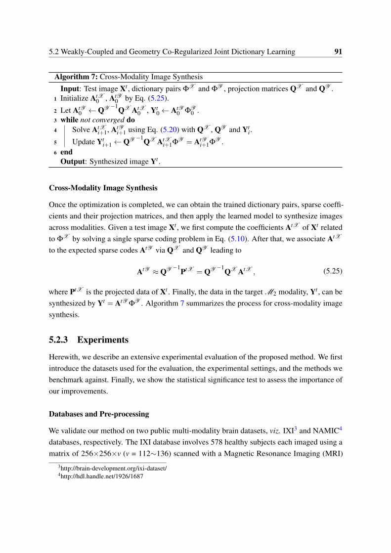
5.2 Weakly-Coupled and Geometry Co-Regularized Joint Dictionary Learning 91
Algorithm 7: Cross-Modality Image Synthesis
Input: Test image Xt , dictionary pairs ΦX and Φ
Y , projection matrices QX and QY .1 Initialize AtX
0 , AtY0 by Eq. (5.25).
2 Let AtY0 ←QY −1QX AtX
0 , Yt0← AtY
0 ΦY0 .
3 while not converged do4 Solve AtX
i+1, AtYi+1 using Eq. (5.20) with QX , QY and Yt
i.
5 Update Yti+1←QY −1QX AtX
i+1ΦY = AtY
i+1ΦY .
6 endOutput: Synthesized image Yt .
Cross-Modality Image Synthesis
Once the optimization is completed, we can obtain the trained dictionary pairs, sparse coeffi-cients and their projection matrices, and then apply the learned model to synthesize imagesacross modalities. Given a test image Xt , we first compute the coefficients AtX of Xt relatedto Φ
X by solving a single sparse coding problem in Eq. (5.10). After that, we associate AtX
to the expected sparse codes AtY via QX and QY leading to
AtY ≈QY −1PtX = QY −1QX AtX , (5.25)
where PtX is the projected data of Xt . Finally, the data in the target M2 modality, Yt , can besynthesized by Yt = AtY Φ
Y . Algorithm 7 summarizes the process for cross-modality imagesynthesis.
5.2.3 Experiments
Herewith, we describe an extensive experimental evaluation of the proposed method. We firstintroduce the datasets used for the evaluation, the experimental settings, and the methods webenchmark against. Finally, we show the statistical significance test to assess the importance ofour improvements.
Databases and Pre-processing
We validate our method on two public multi-modality brain datasets, viz. IXI3 and NAMIC4
databases, respectively. The IXI database involves 578 healthy subjects each imaged using amatrix of 256×256×v (v = 112∼136) scanned with a Magnetic Resonance Imaging (MRI)
3http://brain-development.org/ixi-dataset/4http://hdl.handle.net/1926/1687
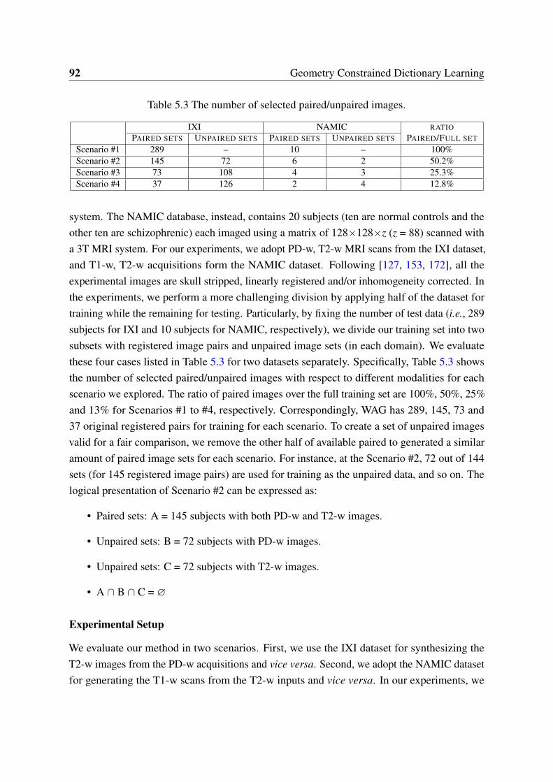
92 Geometry Constrained Dictionary Learning
Table 5.3 The number of selected paired/unpaired images.
IXI NAMIC RATIOPAIRED SETS UNPAIRED SETS PAIRED SETS UNPAIRED SETS PAIRED/FULL SET
Scenario #1 289 – 10 – 100%Scenario #2 145 72 6 2 50.2%Scenario #3 73 108 4 3 25.3%Scenario #4 37 126 2 4 12.8%
system. The NAMIC database, instead, contains 20 subjects (ten are normal controls and theother ten are schizophrenic) each imaged using a matrix of 128×128×z (z = 88) scanned witha 3T MRI system. For our experiments, we adopt PD-w, T2-w MRI scans from the IXI dataset,and T1-w, T2-w acquisitions form the NAMIC dataset. Following [127, 153, 172], all theexperimental images are skull stripped, linearly registered and/or inhomogeneity corrected. Inthe experiments, we perform a more challenging division by applying half of the dataset fortraining while the remaining for testing. Particularly, by fixing the number of test data (i.e., 289subjects for IXI and 10 subjects for NAMIC, respectively), we divide our training set into twosubsets with registered image pairs and unpaired image sets (in each domain). We evaluatethese four cases listed in Table 5.3 for two datasets separately. Specifically, Table 5.3 showsthe number of selected paired/unpaired images with respect to different modalities for eachscenario we explored. The ratio of paired images over the full training set are 100%, 50%, 25%and 13% for Scenarios #1 to #4, respectively. Correspondingly, WAG has 289, 145, 73 and37 original registered pairs for training for each scenario. To create a set of unpaired imagesvalid for a fair comparison, we remove the other half of available paired to generated a similaramount of paired image sets for each scenario. For instance, at the Scenario #2, 72 out of 144sets (for 145 registered image pairs) are used for training as the unpaired data, and so on. Thelogical presentation of Scenario #2 can be expressed as:
• Paired sets: A = 145 subjects with both PD-w and T2-w images.
• Unpaired sets: B = 72 subjects with PD-w images.
• Unpaired sets: C = 72 subjects with T2-w images.
• A ∩ B ∩ C = ∅
Experimental Setup
We evaluate our method in two scenarios. First, we use the IXI dataset for synthesizing theT2-w images from the PD-w acquisitions and vice versa. Second, we adopt the NAMIC datasetfor generating the T1-w scans from the T2-w inputs and vice versa. In our experiments, we

5.2 Weakly-Coupled and Geometry Co-Regularized Joint Dictionary Learning 93
Input PD-w
SC T2-w (32.14, 0.7622) MIMECS T2-w (32.10, 0.7214) WAG-0 T2-w (32.30, 0.7767)
Ground Truth T2-w (PSNR, SSIM)
WAG-GC T2-w (32.87, 0.7913) WAG-MMD T2-w (33.32, 0.8263) WAG T2-w (36.24, 0.9100)
Fig. 5.3 Synthesized results generated using SC, MIMECS, WAG-0, WAG-GC, WAG-MMDand WAG (zoom in for details).
randomly select 100 thousand training patch pairs from both datasets respectively, which haveno relation with the test images used in our experiments. We consider patches of dimension5×5×5 voxels. Following [60, 98], the regularization parameters γ , λ , µ , and ν are empiricallyset to be 105, 0.15, 1, 0.01, respectively. The number of atoms in the learned dictionary isset as 1024 according to [168]. Correspondingly, matrix P has n items in the k dimensionalspace, Q has k elements in the k dimensional space, G and T have n items in the n dimensionalspace, where n is the size of the training set and k is the size of the trained dictionary. Unlessotherwise explicitly stated, we always use scenario #4 in all our experiments, which is a morechallenging case between paired training data and unpaired training data (we will examine theeffects of all scenarios in Section 5.2.3). For the evaluation metrics, we adopt the widely usedPeak Signal to Noise Ratio (PSNR) and Structural Similarity Index (SSIM) [159] to objectivelyassess the quality of the synthesized images.
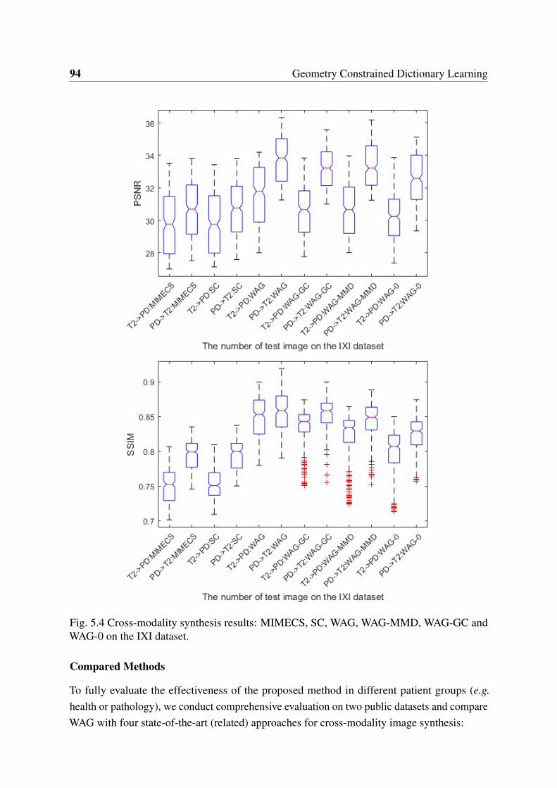
94 Geometry Constrained Dictionary Learning
Fig. 5.4 Cross-modality synthesis results: MIMECS, SC, WAG, WAG-MMD, WAG-GC andWAG-0 on the IXI dataset.
Compared Methods
To fully evaluate the effectiveness of the proposed method in different patient groups (e.g.health or pathology), we conduct comprehensive evaluation on two public datasets and compareWAG with four state-of-the-art (related) approaches for cross-modality image synthesis:
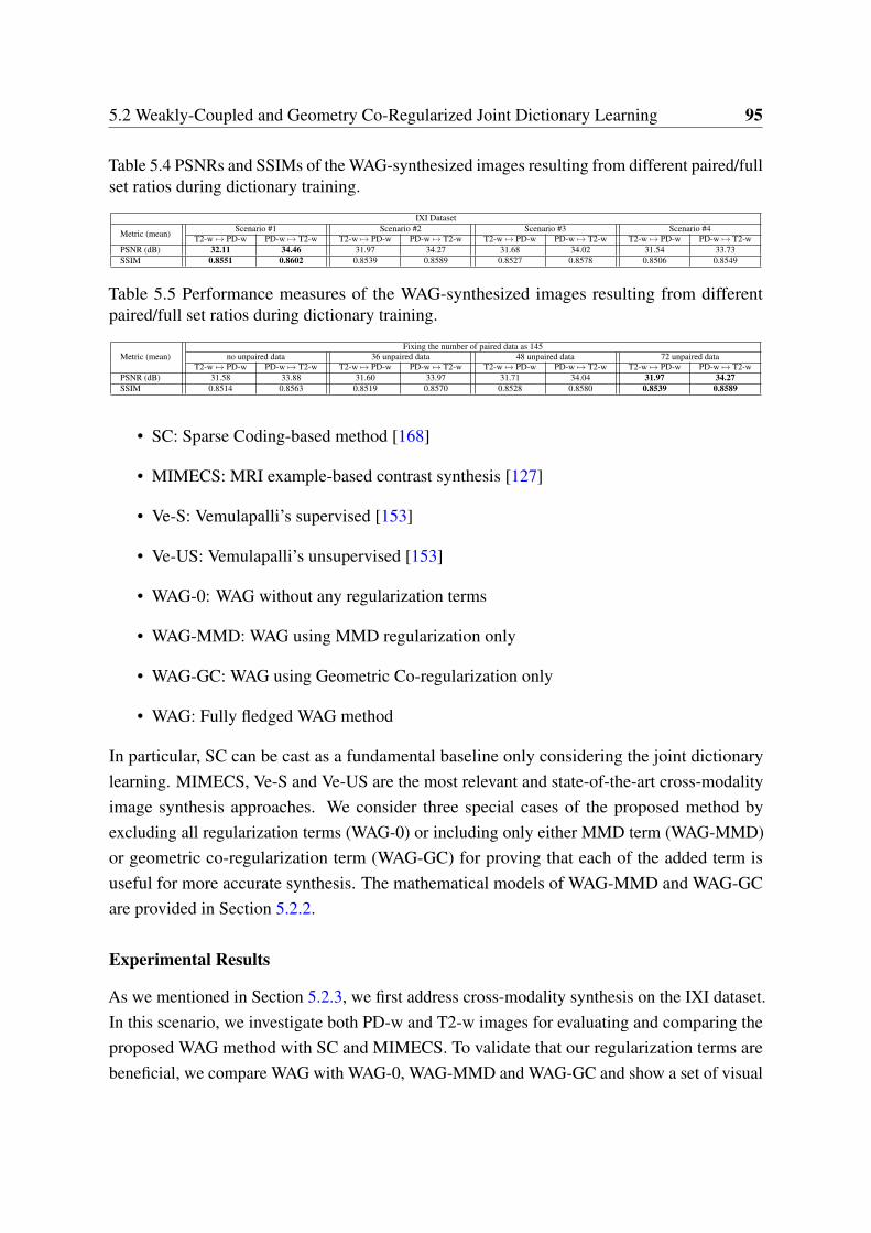
5.2 Weakly-Coupled and Geometry Co-Regularized Joint Dictionary Learning 95
Table 5.4 PSNRs and SSIMs of the WAG-synthesized images resulting from different paired/fullset ratios during dictionary training.
IXI Dataset
Metric (mean) Scenario #1 Scenario #2 Scenario #3 Scenario #4T2-w 7→ PD-w PD-w 7→ T2-w T2-w 7→ PD-w PD-w 7→ T2-w T2-w 7→ PD-w PD-w 7→ T2-w T2-w 7→ PD-w PD-w 7→ T2-w
PSNR (dB) 32.11 34.46 31.97 34.27 31.68 34.02 31.54 33.73SSIM 0.8551 0.8602 0.8539 0.8589 0.8527 0.8578 0.8506 0.8549
Table 5.5 Performance measures of the WAG-synthesized images resulting from differentpaired/full set ratios during dictionary training.
Metric (mean)Fixing the number of paired data as 145
no unpaired data 36 unpaired data 48 unpaired data 72 unpaired dataT2-w 7→ PD-w PD-w 7→ T2-w T2-w 7→ PD-w PD-w 7→ T2-w T2-w 7→ PD-w PD-w 7→ T2-w T2-w 7→ PD-w PD-w 7→ T2-w
PSNR (dB) 31.58 33.88 31.60 33.97 31.71 34.04 31.97 34.27SSIM 0.8514 0.8563 0.8519 0.8570 0.8528 0.8580 0.8539 0.8589
• SC: Sparse Coding-based method [168]
• MIMECS: MRI example-based contrast synthesis [127]
• Ve-S: Vemulapalli’s supervised [153]
• Ve-US: Vemulapalli’s unsupervised [153]
• WAG-0: WAG without any regularization terms
• WAG-MMD: WAG using MMD regularization only
• WAG-GC: WAG using Geometric Co-regularization only
• WAG: Fully fledged WAG method
In particular, SC can be cast as a fundamental baseline only considering the joint dictionarylearning. MIMECS, Ve-S and Ve-US are the most relevant and state-of-the-art cross-modalityimage synthesis approaches. We consider three special cases of the proposed method byexcluding all regularization terms (WAG-0) or including only either MMD term (WAG-MMD)or geometric co-regularization term (WAG-GC) for proving that each of the added term isuseful for more accurate synthesis. The mathematical models of WAG-MMD and WAG-GCare provided in Section 5.2.2.
Experimental Results
As we mentioned in Section 5.2.3, we first address cross-modality synthesis on the IXI dataset.In this scenario, we investigate both PD-w and T2-w images for evaluating and comparing theproposed WAG method with SC and MIMECS. To validate that our regularization terms arebeneficial, we compare WAG with WAG-0, WAG-MMD and WAG-GC and show a set of visual
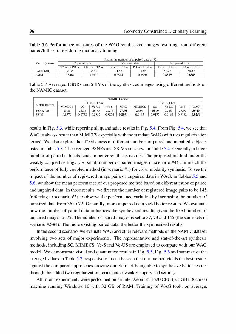
96 Geometry Constrained Dictionary Learning
Table 5.6 Performance measures of the WAG-synthesized images resulting from differentpaired/full set ratios during dictionary training.
Metric (mean)Fixing the number of unpaired data as 72
37 paired data 73 paired data 145 paired dataT2-w 7→ PD-w PD-w 7→ T2-w T2-w 7→ PD-w PD-w 7→ T2-w T2-w 7→ PD-w PD-w 7→ T2-w
PSNR (dB) 31.35 33.54 31.57 33.86 31.97 34.27SSIM 0.8487 0.8532 0.8514 0.8560 0.8539 0.8589
Table 5.7 Averaged PSNRs and SSIMs of the synthesized images using different methods onthe NAMIC dataset.
NAMIC Dataset
Metric (mean) T1-w 7→ T2-w T2w 7→ T1-wMIMECS SC Ve-US Ve-S WAG MIMECS SC Ve-US Ve-S WAG
PSNR (dB) 23.88 24.58 26.70 27.76 27.96 27.05 26.90 27.66 29.40 30.40SSIM 0.8779 0.8778 0.8832 0.8874 0.8991 0.9165 0.9177 0.9168 0.9182 0.9259
results in Fig. 5.3, while reporting all quantitative results in Fig. 5.4. From Fig. 5.4, we see thatWAG is always better than MIMECS especially with the standard WAG (with two regularizationterms). We also explore the effectiveness of different numbers of paired and unpaired subjectslisted in Table 5.3. The averaged PSNRs and SSIMs are shown in Table 5.4. Generally, a largernumber of paired subjects leads to better synthesis results. The proposed method under theweakly coupled settings (i.e. small number of paired images in scenario #4) can match theperformance of fully coupled method (in scenario #1) for cross-modality synthesis. To see theimpact of the number of registered image pairs or unpaired data in WAG, in Tables 5.5 and5.6, we show the mean performance of our proposed method based on different ratios of pairedand unpaired data. In those results, we first fix the number of registered image pairs to be 145(referring to scenario #2) to observe the performance variation by increasing the number ofunpaired data from 36 to 72. Generally, more unpaired data yield better results. We evaluatehow the number of paired data influences the synthesized results given the fixed number ofunpaired images as 72. The number of paired images is set to 37, 73 and 145 (the same sets inscenario #2-#4). The more existing paired data, the better the synthesized results.
In the second scenario, we evaluate WAG and other relevant methods on the NAMIC datasetinvolving two sets of major experiments. The representative and stat-of-the-art synthesismethods, including SC, MIMECS, Ve-S and Ve-US are employed to compare with our WAGmodel. We demonstrate visual and quantitative results in Fig. 5.5, Fig. 5.6 and summarize theaveraged values in Table 5.7, respectively. It can be seen that our method yields the best resultsagainst the compared approaches proving our claim of being able to synthesize better resultsthrough the added two regularization terms under weakly-supervised setting.
All of our experiments were performed on an Intel Xeon E5-1620 CPU (3.5 GHz, 8 cores)machine running Windows 10 with 32 GB of RAM. Training of WAG took, on average,
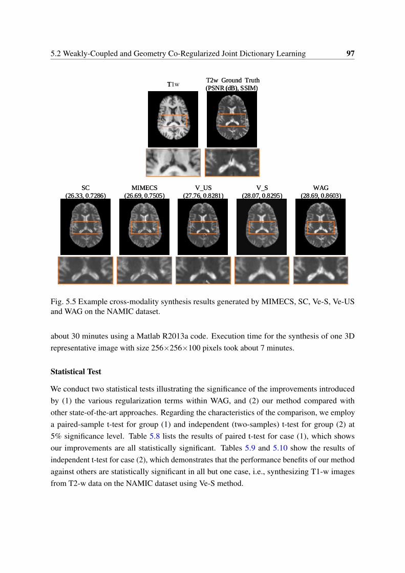
5.2 Weakly-Coupled and Geometry Co-Regularized Joint Dictionary Learning 97
T2T2ww GGrorouunndd TTrurutthh
(P(PSSNNR R d((d ,B)B), SSSS MIIM))T1T1w
SCSC
(2(266..3333,, 00..77228866))
MMIMIMEECSCS
(2(266..6699,, 00..77550055))
VV__UUSS
(2(277..7766,, 00..88228811))
VV__SS
(2(288..0077,, 00..88229955))
WWAAGG
(2(288..6699,, 00..88660033))
Fig. 5.5 Example cross-modality synthesis results generated by MIMECS, SC, Ve-S, Ve-USand WAG on the NAMIC dataset.
about 30 minutes using a Matlab R2013a code. Execution time for the synthesis of one 3Drepresentative image with size 256×256×100 pixels took about 7 minutes.
Statistical Test
We conduct two statistical tests illustrating the significance of the improvements introducedby (1) the various regularization terms within WAG, and (2) our method compared withother state-of-the-art approaches. Regarding the characteristics of the comparison, we employa paired-sample t-test for group (1) and independent (two-samples) t-test for group (2) at5% significance level. Table 5.8 lists the results of paired t-test for case (1), which showsour improvements are all statistically significant. Tables 5.9 and 5.10 show the results ofindependent t-test for case (2), which demonstrates that the performance benefits of our methodagainst others are statistically significant in all but one case, i.e., synthesizing T1-w imagesfrom T2-w data on the NAMIC dataset using Ve-S method.
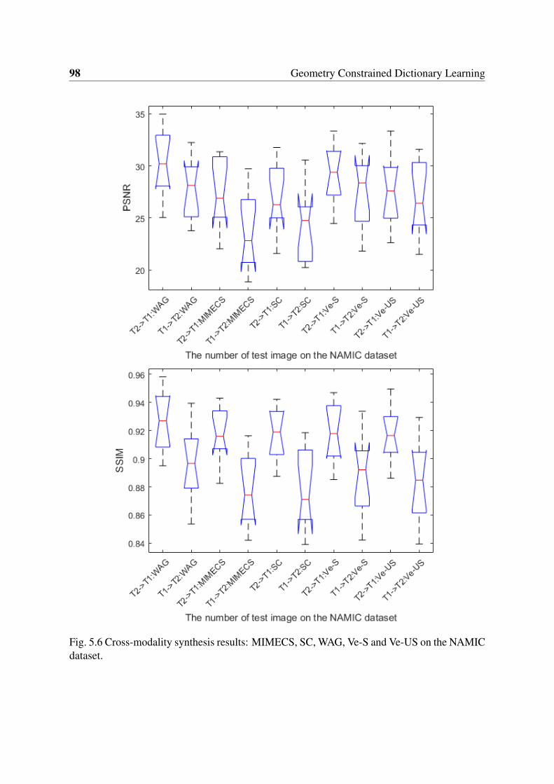
98 Geometry Constrained Dictionary Learning
Fig. 5.6 Cross-modality synthesis results: MIMECS, SC, WAG, Ve-S and Ve-US on the NAMICdataset.
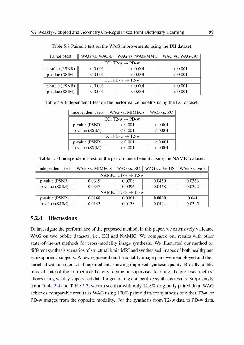
5.2 Weakly-Coupled and Geometry Co-Regularized Joint Dictionary Learning 99
Table 5.8 Paired t-test on the WAG improvements using the IXI dataset.
Paired t-test WAG vs. WAG-0 WAG vs. WAG-MMD WAG vs. WAG-GCIXI: T2-w 7→ PD-w
p-value (PSNR) < 0.001 < 0.001 < 0.001p-value (SSIM) < 0.001 < 0.001 < 0.001
IXI: PD-w 7→ T2-wp-value (PSNR) < 0.001 < 0.001 < 0.001p-value (SSIM) < 0.001 < 0.001 < 0.001
Table 5.9 Independent t-test on the performance benefits using the IXI dataset.
Independent t-test WAG vs. MIMECS WAG vs. SCIXI: T2-w 7→ PD-w
p-value (PSNR) < 0.001 < 0.001p-value (SSIM) < 0.001 < 0.001
IXI: PD-w 7→ T2-wp-value (PSNR) < 0.001 < 0.001p-value (SSIM) < 0.001 < 0.001
Table 5.10 Independent t-test on the performance benefits using the NAMIC dataset.
Independent t-test WAG vs. MIMECS WAG vs. SC WAG vs. Ve-US WAG vs. Ve-SNAMIC: T1-w 7→ T2-w
p-value (PSNR) 0.0319 0.0308 0.0450 0.0363p-value (SSIM) 0.0347 0.0396 0.0468 0.0392
NAMIC: T2-w 7→ T1-wp-value (PSNR) 0.0168 0.0361 0.0809 0.041p-value (SSIM) 0.0143 0.0138 0.0464 0.0345
5.2.4 Discussions
To investigate the performance of the proposed method, in this paper, we extensively validatedWAG on two public datasets, i.e., IXI and NAMIC. We compared our results with otherstate-of-the-art methods for cross-modality image synthesis. We illustrated our method ondifferent synthesis scenarios of structural brain MRI and synthesized images of both healthy andschizophrenic subjects. A few registered multi-modality image pairs were employed and thenenriched with a larger set of unpaired data showing improved synthesis quality. Broadly, unlikemost of state-of-the-art methods heavily relying on supervised learning, the proposed methodallows using weakly-supervised data for generating competitive synthesis results. Surprisingly,from Table 5.4 and Table 5.7, we can see that with only 12.8% originally paired data, WAGachieves comparable results as WAG using 100% paired data for synthesis of either T2-w orPD-w images from the opposite modality. For the synthesis from T2-w data to PD-w data,
100 Geometry Constrained Dictionary Learning
WAG (#1) with 100% registered image pairs outperforms WAG (#4) with 12.8% registeredimage pairs by 0.57 dB for PSNR and 0.0045 for SSIM, on average. For the synthesis fromPD-w data to T2-w data, WAG (#1) outperforms WAG (#4) by 0.73 dB for PSNR and 0.0053for SSIM, on average. By using 12.8% paired data, WAG offers an excellent performancein two evaluation metrics in all experiments compared with MIMECS, SC, Ve-US and Ve-Swhile the compared methods required 100% registered image pairs for training. Specifically, asshown in Fig. 5.5, 5.6 and Table 5.7, for generating T2-w from T1-w data, the average gains onPSNR and SSIM achieved by WAG are 4.08 dB and 0.0212 higher than the worst performingapproach on the NAMIC dataset. Also, for synthesizing T1-w images from T2-w data, theaverage gains on PSNR and SSIM achieved by WAG are 3.35 dB and 0.0094 higher than theworst performing approach on the NAMIC dataset as well. WAG achieves the best performanceamong all supervised state-of-the-art methods under a weakly-supervised setting (with only12.8% registered data) in both healthy and pathological scenarios. This reveals its capability ineffectively leveraging data to boost the learning system. Therefore, the proposed method isusable in clinical practice considering the fact that collecting parallel image pairs is costly andusually limited in many situations.
WAG achieves compelling synthesis results in this paper for the specific MRI modalitiesinvestigated here. However, our method could be potentially applied to other imaging modalitieshaving the assumption that images with similar high order edge/texture characteristics andresolutions. It remains to be demonstrated the synthesis quality in more complex settings like,for instance, for the synthesis of PET images from MRI data, for the synthesis of MRI data fromCT images, and for the more challenging cases such as the synthesis of a tumor case. In addition,to address multi-modality image synthesis involving more than two modalities, the naturalextension of the proposed method would currently required that all source modalities would beavailable at once at the input. We are aware of very recent work by other researchers that handlemulti-modality image synthesis even in the absence of one of some source modalities [17].In our future work, we plan to explore extensions to our framework based on multi-modalityimage fusion of the source modalities before the synthesis. Fused features can better expressmultiple source modalities and thus synthesize the target image modality even with only partialinput sources.
5.2.5 Conclusions
We proposed a weakly-coupled and geometry co-regularized joint dictionary learning (WAG)method for cross-modality synthesis of MRI images. Most conventional joint dictionarylearning methods with sparse representations assume a fully supervised setting. Instead,our method only requires a small subset of registered image pairs and automatically finds
5.2 Weakly-Coupled and Geometry Co-Regularized Joint Dictionary Learning 101
correspondences for a much larger set of unpaired images. This process assists and enrichesthe supervised learning on the smaller subset while booting synthesis performance. Withthe proposed cross-modality image matching criterion, the derived common feature spaceassociates cross-modality data effectively by updating a pair of dictionaries in both domains.We integrated our model with both MMD and modality-specific geometric co-regularizationterms to further improve image synthesis quality. The proposed WAG approach was appliedto cross-modality image synthesis of brain MRI and experimental results demonstrated thatWAG significantly outperforms competing state-of-the-art methods on two public databaseswith healthy and schizophrenic subjects.

Chapter 6
Task-Driven Bidirectional Fault-AwareAdversarial Networks
Different imaging modalities present valuable and complementary anatomical informationabout the underlying organ for medical image analysis. However, a full battery of multi-modality data is often scarce, costly and even impossible to obtain. The ability to automaticallygenerate meaningful synthetic information is highly desirable for many computer-aided medicalapplications. With recent progress in generative adversarial networks (GANs) particularly onnatural images, instead of collecting acquisitions relying on the scanner, an appealing alternativeis to generate highly compelling subject-specific images, such as structural magnetic resonanceimaging. Inspired by the framework of adversarial learning, we propose the task-drivenbidirectional fault-aware adversarial networks (T-GAN) for volumetric neuroimage processingin an unsupervised manner. T-GAN provides a generic way of learning a dual mapping betweensource and target domains while considering both visually high-fidelity synthesis and task-practicability. Through combining the bidirectional adversarial loss, the cycle-consistencyloss and domain adapted loss in volumetric space, T-GAN is robust for medical images undermultiple conditions. In addition to generating the desirable modality data, we complement bothdiscriminators conditioned on the performance of any optional post-processing which balancessynthesis fidelity and task performance. Experiments evaluated on several cross-modalitysynthesis tasks show that T-GAN not only produces visually impressive results but also cansubstitute real acquisitions for the clinical post-processing, and also outperforms some relatedstate-of-the-art methods.
104 Task-Driven Bidirectional Fault-Aware Adversarial Networks
6.1 Introduction
Medical imaging enjoys a multitude of imaging modalities such as Computed Tomography(CT), Magnetic Resonance Imaging (MRI) and Positron-Emission Tomography, and opensup the opportunity to gain insights into diverse tissues’ characteristics via different physicalacquisition principles or parameters. The simultaneous availability of multi-modal imaging hasbenefited a wide range of brain image analysis tasks, for example, providing complementaryinformation to discriminate specific tissues, anatomies and pathologies in image segmenta-tion [54], or improved cross-modal image registration under the great variability of tissue ororgan appearance [136].
Despite that neuroimaging such as MRI can produce highly detailed images with greatsoft tissue contrast, one practical problem remains largely unsolved: imaging has notoriouslylong acquisition times, which hampers multi-protocol MRI acquisitions at high-resolution.Additional complications arise when imaging patients with some specific medical conditions,for instance, Alzheimer’s Disease and Parkinson’s Disease, require that the acquisitions arecollected in even short times resulting in very low-quality images.
Automatic generation of synthesized images for recovering corrupt/missing modality dataor extending a dataset to additional modalities has been shown to be an effective way inseveral applications of the medical community [65, 150, 153]. Especially in recent years,for auxiliary diagnosis and scientific research, propagating and synthesizing non-acquiredor higher-resolution imaging modalities has seen rapid progress, fueled increasingly by thedevelopment of the machine learning and computer vision techniques. This problem can bemore broadly casted as cross-modality image synthesis [64, 75], which is closely related totexture transfer [3, 32, 35, 59], also known as image-to-image translation or image style transferin the context of computer vision. That is, we seek to render a source modality image intoa target modality, for instance, to synthesize a CT image as an MRI image, or a PD-w MRIimage as a T2-w MRI image, or a structural MRI image as the corresponding diffusion tensorMRI image.
Among techniques for addressing such cross-modality synthesis tasks, sparse representa-tion [42, 127] and deep learning-based approaches [44, 69] particularly favor the scenarios inwhich fully paired images in different modalities are available and have shown their promisingresults. However, collecting a large amount of paired data is impractical in the medical imag-ining community. To cope with cases where paired data are scarce or even unavailable, semi-supervised [21, 155], weakly-supervised [65] and unsupervised methods [93, 119, 173, 189]are developed respectively, aiming at learning a joint representation or distribution of imagesin different modalities of source and target domains. Due to lack of paired information, the
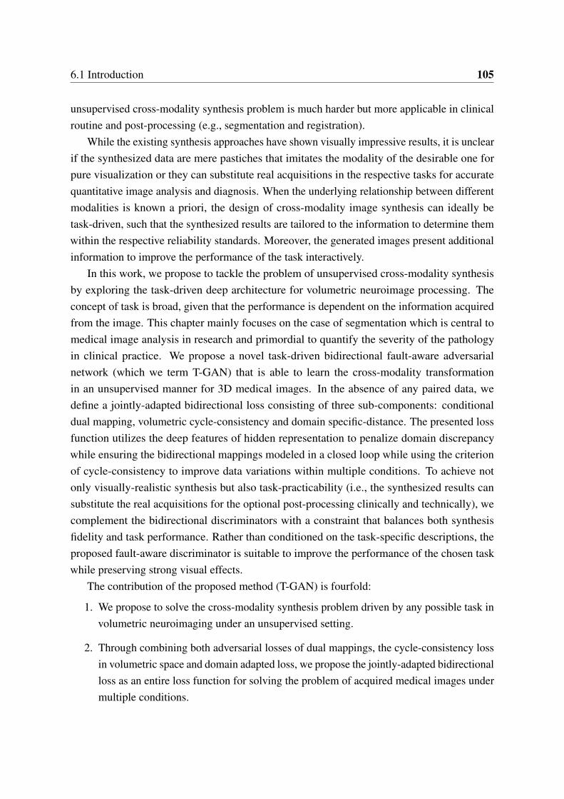
6.1 Introduction 105
unsupervised cross-modality synthesis problem is much harder but more applicable in clinicalroutine and post-processing (e.g., segmentation and registration).
While the existing synthesis approaches have shown visually impressive results, it is unclearif the synthesized data are mere pastiches that imitates the modality of the desirable one forpure visualization or they can substitute real acquisitions in the respective tasks for accuratequantitative image analysis and diagnosis. When the underlying relationship between differentmodalities is known a priori, the design of cross-modality image synthesis can ideally betask-driven, such that the synthesized results are tailored to the information to determine themwithin the respective reliability standards. Moreover, the generated images present additionalinformation to improve the performance of the task interactively.
In this work, we propose to tackle the problem of unsupervised cross-modality synthesisby exploring the task-driven deep architecture for volumetric neuroimage processing. Theconcept of task is broad, given that the performance is dependent on the information acquiredfrom the image. This chapter mainly focuses on the case of segmentation which is central tomedical image analysis in research and primordial to quantify the severity of the pathologyin clinical practice. We propose a novel task-driven bidirectional fault-aware adversarialnetwork (which we term T-GAN) that is able to learn the cross-modality transformationin an unsupervised manner for 3D medical images. In the absence of any paired data, wedefine a jointly-adapted bidirectional loss consisting of three sub-components: conditionaldual mapping, volumetric cycle-consistency and domain specific-distance. The presented lossfunction utilizes the deep features of hidden representation to penalize domain discrepancywhile ensuring the bidirectional mappings modeled in a closed loop while using the criterionof cycle-consistency to improve data variations within multiple conditions. To achieve notonly visually-realistic synthesis but also task-practicability (i.e., the synthesized results cansubstitute the real acquisitions for the optional post-processing clinically and technically), wecomplement the bidirectional discriminators with a constraint that balances both synthesisfidelity and task performance. Rather than conditioned on the task-specific descriptions, theproposed fault-aware discriminator is suitable to improve the performance of the chosen taskwhile preserving strong visual effects.
The contribution of the proposed method (T-GAN) is fourfold:
1. We propose to solve the cross-modality synthesis problem driven by any possible task involumetric neuroimaging under an unsupervised setting.
2. Through combining both adversarial losses of dual mappings, the cycle-consistency lossin volumetric space and domain adapted loss, we propose the jointly-adapted bidirectionalloss as an entire loss function for solving the problem of acquired medical images undermultiple conditions.
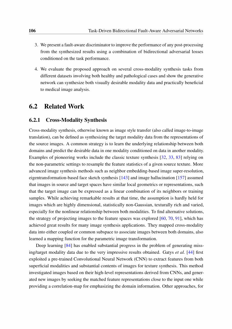
106 Task-Driven Bidirectional Fault-Aware Adversarial Networks
3. We present a fault-aware discriminator to improve the performance of any post-processingfrom the synthesized results using a combination of bidirectional adversarial lossesconditioned on the task performance.
4. We evaluate the proposed approach on several cross-modality synthesis tasks fromdifferent datasets involving both healthy and pathological cases and show the generativenetwork can synthesize both visually desirable modality data and practically beneficialto medical image analysis.
6.2 Related Work
6.2.1 Cross-Modality Synthesis
Cross-modality synthesis, otherwise known as image style transfer (also called image-to-imagetranslation), can be defined as synthesizing the target modality data from the representations ofthe source images. A common strategy is to learn the underlying relationship between bothdomains and predict the desirable data in one modality conditioned on data in another modality.Examples of pioneering works include the classic texture synthesis [32, 33, 83] relying onthe non-parametric settings to resample the feature statistics of a given source texture. Moreadvanced image synthesis methods such as neighbor embedding-based image super-resolution,eigentransformation-based face sketch synthesis [143] and image hallucination [157] assumedthat images in source and target spaces have similar local geometrics or representations, suchthat the target image can be expressed as a linear combination of its neighbors or trainingsamples. While achieving remarkable results at that time, the assumption is hardly held forimages which are highly dimensional, statistically non-Gaussian, texturally rich and varied,especially for the nonlinear relationship between both modalities. To find alternative solutions,the strategy of projecting images to the feature spaces was explored [60, 70, 91], which hasachieved great results for many image synthesis applications. They mapped cross-modalitydata into either coupled or common subspace to associate images between both domains, alsolearned a mapping function for the parametric image transformation.
Deep learning [84] has enabled substantial progress in the problem of generating miss-ing/target modality data due to the very impressive results obtained. Gatys et al. [44] firstexploited a pre-trained Convolutional Neural Network (CNN) to extract features from bothsuperficial modalities and substantial contents of images for texture synthesis. This methodinvestigated images based on their high-level representations derived from CNNs, and gener-ated new images by seeking the matched feature representations close to the input one whileproviding a correlation-map for emphasizing the domain information. Other approaches, for
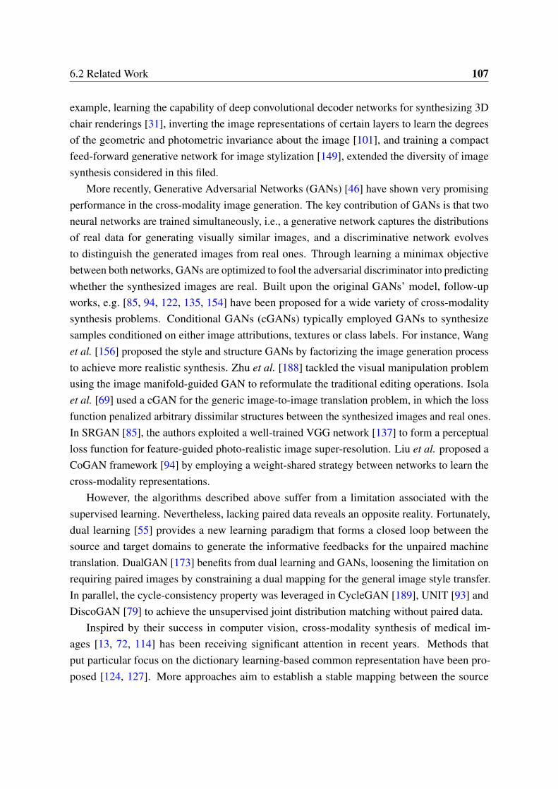
6.2 Related Work 107
example, learning the capability of deep convolutional decoder networks for synthesizing 3Dchair renderings [31], inverting the image representations of certain layers to learn the degreesof the geometric and photometric invariance about the image [101], and training a compactfeed-forward generative network for image stylization [149], extended the diversity of imagesynthesis considered in this filed.
More recently, Generative Adversarial Networks (GANs) [46] have shown very promisingperformance in the cross-modality image generation. The key contribution of GANs is that twoneural networks are trained simultaneously, i.e., a generative network captures the distributionsof real data for generating visually similar images, and a discriminative network evolvesto distinguish the generated images from real ones. Through learning a minimax objectivebetween both networks, GANs are optimized to fool the adversarial discriminator into predictingwhether the synthesized images are real. Built upon the original GANs’ model, follow-upworks, e.g. [85, 94, 122, 135, 154] have been proposed for a wide variety of cross-modalitysynthesis problems. Conditional GANs (cGANs) typically employed GANs to synthesizesamples conditioned on either image attributions, textures or class labels. For instance, Wanget al. [156] proposed the style and structure GANs by factorizing the image generation processto achieve more realistic synthesis. Zhu et al. [188] tackled the visual manipulation problemusing the image manifold-guided GAN to reformulate the traditional editing operations. Isolaet al. [69] used a cGAN for the generic image-to-image translation problem, in which the lossfunction penalized arbitrary dissimilar structures between the synthesized images and real ones.In SRGAN [85], the authors exploited a well-trained VGG network [137] to form a perceptualloss function for feature-guided photo-realistic image super-resolution. Liu et al. proposed aCoGAN framework [94] by employing a weight-shared strategy between networks to learn thecross-modality representations.
However, the algorithms described above suffer from a limitation associated with thesupervised learning. Nevertheless, lacking paired data reveals an opposite reality. Fortunately,dual learning [55] provides a new learning paradigm that forms a closed loop between thesource and target domains to generate the informative feedbacks for the unpaired machinetranslation. DualGAN [173] benefits from dual learning and GANs, loosening the limitation onrequiring paired images by constraining a dual mapping for the general image style transfer.In parallel, the cycle-consistency property was leveraged in CycleGAN [189], UNIT [93] andDiscoGAN [79] to achieve the unsupervised joint distribution matching without paired data.
Inspired by their success in computer vision, cross-modality synthesis of medical im-ages [13, 72, 114] has been receiving significant attention in recent years. Methods thatput particular focus on the dictionary learning-based common representation have been pro-posed [124, 127]. More approaches aim to establish a stable mapping between the source
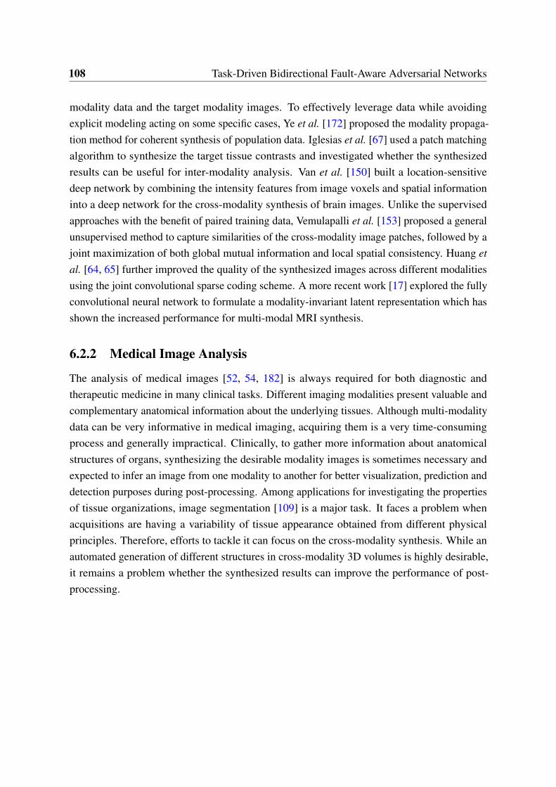
108 Task-Driven Bidirectional Fault-Aware Adversarial Networks
modality data and the target modality images. To effectively leverage data while avoidingexplicit modeling acting on some specific cases, Ye et al. [172] proposed the modality propaga-tion method for coherent synthesis of population data. Iglesias et al. [67] used a patch matchingalgorithm to synthesize the target tissue contrasts and investigated whether the synthesizedresults can be useful for inter-modality analysis. Van et al. [150] built a location-sensitivedeep network by combining the intensity features from image voxels and spatial informationinto a deep network for the cross-modality synthesis of brain images. Unlike the supervisedapproaches with the benefit of paired training data, Vemulapalli et al. [153] proposed a generalunsupervised method to capture similarities of the cross-modality image patches, followed by ajoint maximization of both global mutual information and local spatial consistency. Huang etal. [64, 65] further improved the quality of the synthesized images across different modalitiesusing the joint convolutional sparse coding scheme. A more recent work [17] explored the fullyconvolutional neural network to formulate a modality-invariant latent representation which hasshown the increased performance for multi-modal MRI synthesis.
6.2.2 Medical Image Analysis
The analysis of medical images [52, 54, 182] is always required for both diagnostic andtherapeutic medicine in many clinical tasks. Different imaging modalities present valuable andcomplementary anatomical information about the underlying tissues. Although multi-modalitydata can be very informative in medical imaging, acquiring them is a very time-consumingprocess and generally impractical. Clinically, to gather more information about anatomicalstructures of organs, synthesizing the desirable modality images is sometimes necessary andexpected to infer an image from one modality to another for better visualization, prediction anddetection purposes during post-processing. Among applications for investigating the propertiesof tissue organizations, image segmentation [109] is a major task. It faces a problem whenacquisitions are having a variability of tissue appearance obtained from different physicalprinciples. Therefore, efforts to tackle it can focus on the cross-modality synthesis. While anautomated generation of different structures in cross-modality 3D volumes is highly desirable,it remains a problem whether the synthesized results can improve the performance of post-processing.
6.3 Task-Driven Bidirectional Fault-Aware Adversarial Networks 109
6.3 Task-Driven Bidirectional Fault-Aware Adversarial Net-works
6.3.1 Preliminaries
Generative Adversarial Networks (GANs) [46] are composed of two models: generator G anddiscriminator D. G is trained to imitate the real image by mapping a latent random vectorz sampled from the uniform noise distribution pz to the real data distribution pdata. D isoptimized to distinguish whether an image is the generated counterpart G(z)∼ pg or the realone x ∼ pdata. Concretely, given the vectorized image x, G and D are defined to solve thefollowing adversarial minimax objective on V (D,G):
minG
maxD
V (D,G) =Ex∼pdata [logD(x)]+
Ez∼pz [log(1−D(G(z)))] .(6.1)
Eq. (6.1) can be solved in an alternative manner over generator G and discriminator D. Thatis, by fixing the parameters of G, we can optimize D and vice versa. There exists a globaloptimality when pg = pdata with a mild condition that G and D have enough capacity to makepg converges to pdata.
CycleGAN [189], DualGAN [173], DiscoGAN [79] and UNIT [93] are the extensions ofGANs where the cycle-consistency property Lcyc(G,F) is combined with the dual mappingfunctions G : X→ Y and F : Y→ X into the GANs’ objective for unpaired cross-modalitysynthesis. X and Y are two sets of training samples as X = (x1,x2, ...xs) and Y = (y1,y2, ...yt).
6.3.2 Problem Formulation
Instead of working with 2D image stacks of original volumetric neuroimaging, we input3D volumes (i.e., X and Y) directly to ensure the intrinsic sequential information betweenconsecutive slices. Given training samples X = XiS
i=1 ∈ Rm×n×t×S in the source domainand Y = YiT
i=1 ∈ Rm×n×t×T in the target domain, our goal is to form a closed loop betweenthe dual tasks, i.e. X ↔ Y without supervision of paired examples. Here, m and n are thedimensions of the axial view of the volumetric image, t denotes the size of an image along the z-axis, while S and T are the numbers of elements in the source and target training sets respectively.As with the existing dual GANs’ learning, we construct two mappings: G : X → Y andF : Y →X in the volumetric space, therefore the generation of G and F can be represented asY = G(X) and X = F(Y) respectively. Two adversarial discriminators DG and DF are modeledto distinguish the fake products corresponding to G and F . The difficulties of our synthesis work

110 Task-Driven Bidirectional Fault-Aware Adversarial Networks
Fig. 6.1 Flowchart of the proposed method (T-GAN) for cross-modality synthesis. G andF are the dual mapping functions which are used to establish domain exchange among thesource domain X and the target domain Y , X and Y are the 3D volumes belongs to X andY respectively, X and Y represent the first generated results while X and Y are their dualgenerations, DCG and DCF are the discriminators corresponding to G and F , Lc denotes thecycle-consistent GAN, dk is the MK-MMD-based jointly-adapted regularizer, CX and CY arethe task-driven results.
vary with multiple conditions, e.g., the volumetric representations, an unsupervised setting,different imaging modalities, imaging angles and even systems (such as Philips, Siemensand GE). To encourage the synthesized results actually leading to the improvement of anypossible post-processing, we generate visually-realistic images conditioned on performingapplication specific task. Therefore, we address the task-driven cross-modality synthesis byfirst building two GANs in a dual manner with the bidirectional loss, then minimizing themisaligned representations, while conditioning the whole model on performing the selectedpost-processing task. In this chapter, we attempt to synthesize MRI of human brains withsegmentation. The proposed method is diagrammed in Fig. 6.1.
6.3.3 Jointly-Adapted Bidirectional Loss
To translate an image Xi in X to an image in Y through applying GANs’ model, we canlearn a function G : X → Y with the expected output Yi = G(Xi). The generator G is thenargued by a discriminator DG giving the likelihood that the input image Xi has been sampledfrom the target domain. Similarly, to map an image Yi in Y to an image in X which can bethe dual task of G by training an inverse generator F : Y →X having Xi = F(Yi) with thecorresponding discriminator DF . Following the standard GAN [46], the adversarial losses of
6.3 Task-Driven Bidirectional Fault-Aware Adversarial Networks 111
both mapping functions are jointly expressed in the volumetric space:
Ld(DG,DF ,G,F) =EY∼pdata(Y) [logDG(Y)]+
EX∼pdata(X) [log(1−DG(G(X)))]+
EX∼pdata(X) [logDF(X)]+
EY∼pdata(Y) [log(1−DF(F(Y)))] ,
(6.2)
where Ld is the dual loss. The function in Eq. (6.2) forms a simple closed loop between twolosses which extends the volumetric GANs into a dual learning manner and joint representationsinto a unified framework. In the unsupervised dual learning problem, one typical property is toforce both learnings from each other to produce the pseudo-input. This is done by generatingX′ for task X → Y and Y′ for task Y →X respectively, where X′ = F(Y) = F(G(X))
and Y′ = G(X) = G(F(Y)). We note that some contemporary works [79, 93, 173, 189] inferthe pseudo-input by involving the cycle-consistency constraint to regularize both mappings.Inspired by such a strategy, we enforce a volumetric cycle-consistency with GANs’ modelusing
Lc(X ,G,Y ,F) =EX∼pdata(X) ∥X−F(G(X))∥1+
EY∼pdata(Y) ∥Y−G(F(Y))∥1 ,(6.3)
where ∥·∥1 means we adopt l1 distance1 to quantitatively compare the input data and recon-structed pseudo.
Although the modeled image distributions over the latent feature space are adopted in theunsupervised cross-modality synthesis problem, a potential assumption is implied that therepresentations of both modalities are almost domain invariant. Some recent approaches [97,174] reveal a fact that deep features can disentangle explanatory factors of variations inthe data distributions [6], but the cross-modality distribution discrepancy is still remnant.Motivated by the requirement of boosting unpaired cross-modality data (underlying the samedistributions) to be close to each other, especially in the medical images under multipleconditions, we define a jointly-adapted regularization term that intrinsically manifests invariantstructures across modalities. To achieve this effect, recent work [49, 65, 183] employed eitherthe traditional Maximum Mean Discrepancy (MMD) or the extended Multi-Kernel MMD(MK-MMD) criterion to explore the data statistics of different domains. The jointly-adaptedregularizer is proposed to release the assumption of domain invariance which was exploredin [174]. We follow such an idea and make use of the MK-MMD in our method. MK-MMD isemployed for the two-sample matching, along with other components of T-GAN, to align the’real’ paired data. Specifically, we use the unbiased estimate of MK-MMD to reduce the domain
1l1-based loss has been explored in [173, 189] to avoid blurriness and show promising results.
112 Task-Driven Bidirectional Fault-Aware Adversarial Networks
discrepancy, hence our model is independent of the assumption of ’same latent variables’. Thisis done by adding the MK-MMD-based jointly-adapted regularizer to our bidirectional GANmodel:
dk(AX ,A Y ) =
∥∥∥Epdata(X)ψ(AX )−Epdata(Y)
ψ(AY )∥∥∥2
Hk, (6.4)
where dk is interpreted as matching all orders of statistics which can be performed by stochasticgradient descent with the gradient calculated by back-propagation through the generativenetwork, and k is the characteristic kernel defined on the vectorized element A combining a setof positive definite kernels kud
u=1:
k ∈K :=
d
∑u=1
βuku :d
∑u=1
βu = 1,βu ≥ 0,∀u ∈ 1, ...,d
, (6.5)
where βudu=1 is the coefficient for constraining the characteristic of each ku. ψ(·) denotes
the nonlinear mapping with k(AX ,AY ) =⟨ψ(AX ),ψ(AY )
⟩, A X =
AX
iS
i=1 and A Y =AY
iT
i=1 are the deep features of Xi and Yi for source and target domains respectively, andHk indicates the reproducing kernel Hilbert space (RKHS) induced by k and ψ .
We then integrate the volumetric cycle-consistency and joint adaptation into Eq. (6.1),yielding the proposed jointly-adapted bidirectional loss:
Lb(X ,Y ) =Ld(DG,DF ,G,F)+
Lc(X ,G,Y ,F)+dk(AX ,A Y ).
(6.6)
6.3.4 Fault-Aware Discriminator
Rather than only encouraging the visually-realistic synthesis to approximate the ground truthin an unsupervised bidirectional learning manner, we instead encourage them to have betterperformance in an optional post-processing as used by the real image. As we introducedin Section 6.3.3, jointly-adapted bidirectional loss penalizes both generators and domaindiscrepancy in the latent space, while the corresponding discriminators simply distinguishwhether the generation is real or fake. To ensure the synthesized results can satisfy therequirement of later processing, e.g., image segmentation or registration, and substitute the realacquisitions for medical image analysis, we need to bridge the gap of task performance betweenthe distributions of generated and real ones. The ideal discriminator has an explicit notion thatwhether the image is real or synthesized and also match the task performance. To achieve this,we propose the fault-aware discriminator to meet the additional condition on the selected task.
6.3 Task-Driven Bidirectional Fault-Aware Adversarial Networks 113
Given the solution C2 of an arbitrary task, and the input data X, the result of X for the chosentask can be denoted as CX. More precisely, the responsibility of the proposed discriminator is tojudge two major tasks (i.e., the performance of synthesis and possible task) derived an obviousdiscriminant: real data & right performance. Similar concept has been explored in some recentworks [122, 177] conditioned on the embedded text for text-to-image translation. Instead ofrelying on the task-specific (e.g. text, label and even image) descriptions, we build on theideas but in theory more general and suitable for an application. Conditioned on the result ofC, the mapping functions G : X → Y and F : Y →X are updated to G : X ,C→ Y andF : Y ,C→X with the corresponding outputs Y = G(X,C) and X = F(Y,C), respectively.The fault-aware discriminators LDCG and LDCF for the mappings G and F are then expressedas
LDCG =E(Y,C)∼pdata(Y) [logDCG(Y,C)]+
E(X,C)∼pdata(X) [log(1−DCG(G(X),C))] ,
LDCF =E(X,C)∼pdata(X) [logDCF(X,C)]+
E(Y,C)∼pdata(Y) [log(1−DCF(F(Y),C))] .
(6.7)
We can then update the parameters of the discriminative network by minimizing the abovelosses in Eq. (6.7).
6.3.5 Objective Function
Essentially, the properties of dual mapping, visual similarity and task performance form thewhole adversarial loss that enforces associations between similar contents conditioned on anextra fault (i.e. the quantification of an optional application) of both domains. We thus updatethe adversarial loss in Eq. (6.2) based on the fault-aware discriminator, which is given below:
Lcd(DCG,DCG,G,F) =
E(Y,C)∼pdata(Y) [logDCG(Y,C)]+
E(X,C)∼pdata(X) [log(1−DCG(G(X),C))]+
E(X,C)∼pdata(X) [logDCF(X,C)]+
E(Y,C)∼pdata(Y) [log(1−DCF(F(Y),C))] .
(6.8)
where Lcd is the conditional dual mapping loss. Correspondingly, the overall loss func-tion for the proposed model can be further updated as Lb(X ,Y ) = Lcd(DCG,DCF ,G,F)+
2C can be treated as performing any task measured by an appropriate quantification such as dice score.
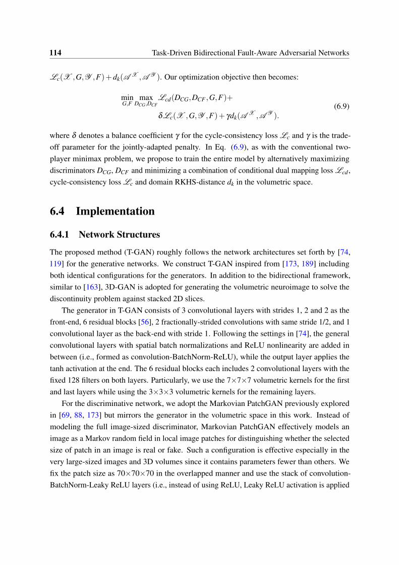
114 Task-Driven Bidirectional Fault-Aware Adversarial Networks
Lc(X ,G,Y ,F)+dk(AX ,A Y ). Our optimization objective then becomes:
minG,F
maxDCG,DCF
Lcd(DCG,DCF ,G,F)+
δLc(X ,G,Y ,F)+ γdk(AX ,A Y ).
(6.9)
where δ denotes a balance coefficient γ for the cycle-consistency loss Lc and γ is the trade-off parameter for the jointly-adapted penalty. In Eq. (6.9), as with the conventional two-player minimax problem, we propose to train the entire model by alternatively maximizingdiscriminators DCG, DCF and minimizing a combination of conditional dual mapping loss Lcd ,cycle-consistency loss Lc and domain RKHS-distance dk in the volumetric space.
6.4 Implementation
6.4.1 Network Structures
The proposed method (T-GAN) roughly follows the network architectures set forth by [74,119] for the generative networks. We construct T-GAN inspired from [173, 189] includingboth identical configurations for the generators. In addition to the bidirectional framework,similar to [163], 3D-GAN is adopted for generating the volumetric neuroimage to solve thediscontinuity problem against stacked 2D slices.
The generator in T-GAN consists of 3 convolutional layers with strides 1, 2 and 2 as thefront-end, 6 residual blocks [56], 2 fractionally-strided convolutions with same stride 1/2, and 1convolutional layer as the back-end with stride 1. Following the settings in [74], the generalconvolutional layers with spatial batch normalizations and ReLU nonlinearity are added inbetween (i.e., formed as convolution-BatchNorm-ReLU), while the output layer applies thetanh activation at the end. The 6 residual blocks each includes 2 convolutional layers with thefixed 128 filters on both layers. Particularly, we use the 7×7×7 volumetric kernels for the firstand last layers while using the 3×3×3 volumetric kernels for the remaining layers.
For the discriminative network, we adopt the Markovian PatchGAN previously exploredin [69, 88, 173] but mirrors the generator in the volumetric space in this work. Instead ofmodeling the full image-sized discriminator, Markovian PatchGAN effectively models animage as a Markov random field in local image patches for distinguishing whether the selectedsize of patch in an image is real or fake. Such a configuration is effective especially in thevery large-sized images and 3D volumes since it contains parameters fewer than others. Wefix the patch size as 70×70×70 in the overlapped manner and use the stack of convolution-BatchNorm-Leaky ReLU layers (i.e., instead of using ReLU, Leaky ReLU activation is applied
6.5 Experiments 115
here) to train the discriminative network. Similar to [55, 69, 173], our discriminator is runconvolutionally across the volumes and finally averaging all responses to give the ultimateresults.
6.4.2 Training Details
To train the proposed method (T-GAN), a common procedure is to take alternating steps ofupdating the generator and discriminator in every batch. We set the learning rate of 0.0002, em-ploy the Stochastic Gradient Descent with mini-batch of size 1 and apply the Adam solver [80]for optimization. Empirically, to control the influence between G and F , we follow [97, 189]and set the balance coefficient δ =10, the trade-off parameter γ =0.3. However, with 3Dgeneration, a potential problem can be exposed that synthesizing 3D voxels is harder thandifferentiating between the synthesized result and ground truth, easily leading to faster learningprogress of the discriminator than the generator. The proposed discriminator is conditionedon the extra criteria that the performance of both synthesis and its application need to bebalanced and satisfied. As the suggestion in [163], to make the training of both generatorand discriminator in pace meanwhile taking account of the task performance, we update thediscriminator when its accuracy and dice scores 3 in the last batch are less than 0.8.
6.5 Experiments
6.5.1 Experimental Setup
Datasets
Our T-GAN is evaluated on two brain datasets: IXI 4 and NAMIC Multimodality 5 datasets.The IXI dataset involves 578 healthy subjects, each was imaged using a matrix of 256×256×pscanned with either Philips 3T system, Philips 1.5T system, or GE 3T system having 0.94×0.94×1.2mm3 voxel dimensions. The NAMIC dataset includes 20 subjects (10 normal controls and 10schizophrenics), each was imaged using a matrix of 128×128×q scanned with a 3T GE systemhaving 1x1x1 mm3 voxel dimensions.
3The Dice overlap is commonly used as a proxy for evaluating the quality of segmentation and registration formedical image analysis.
4http://brain-development.org/ixi-dataset/5http://hdl.handle.net/1926/1687
116 Task-Driven Bidirectional Fault-Aware Adversarial Networks
Experiments
We evaluate our method in two scenarios: (1) synthesizing the T2-w images from the PD-wacquisitions and vice versa in the IXI dataset, (2) generating the T1-w images from the T2-winputs and vice versa in the NAMIC dataset. However, we note that only a few groups ofunpaired data are available in the NAMIC dataset. To deal with this problem, the images inthe IXI dataset are scaled to 128×128×p voxels for extending the size of training data inthis scenario. For quantitative evaluation, we perform two-fold cross-validation to test ourmethod. By selecting 230 unpaired Proton Density-weighted (PD-w) and T2-weighted (T2-w)MRI scans from the IXI dataset and 7 unpaired T1-w, T2-w acquisitions form the NAMICdataset for training, while the remaining data i.e., 118 (IXI) and 6 (NAMIC) for testing. Inthe segmentation experiments, we feed the real scans and the synthesized results to the fully-automatic FreeSurfer (i.e., a structural MRI analysis software with default parameters) [38]pipeline. It should work independently of the primary training procedure. Once the regulartraining (i.e., GAN) has done, we input the first generated result into the task, e.g. segmentation,and collect the segmented results to ’reboot’ our T-GAN for judging two major tasks (synthesisand segmentation) derived two discriminants. The segmentation (carried out by FreeSurfer)produces several major brain tissue classes, i.e., Cerebrospinal fluid (CSF), (GM) and (WM),yielding the averaged quantification of a whole brain volume. The tissue prior probabilitytemplates used in FreeSurfer are based on averaging multiple automatically segmented imagesin standard space of images from either the IXI or the NAMIC dataset in this chapter, so thereis no guarantee that CSF, GM and WM classes will exactly follow other methods. In addition,this work provides a reliable synthesis mechanism for generating both visually-realistic andtask-effective products, and we focus on our synthesized results in these experiments.
Baselines
We compare our results against several state-of-the-art cross-modality synthesis algorithmsincluding MR image exampled-based contrast synthesis (MIMECS) [127], Vemulapalli’s super-vised cross-modal synthesis of subject-specific scans (V-s) [153], Vemulapalli’s unsupervisedsynthesis method (V-us) [153], dual convolutional filter learning (DOTE) [64], GAN [46] andCycleGAN [189]. Specifically, MIMECS, V-s, DOTE and GAN have supervision in form ofpaired data, while V-us, CycleGAN and our method are unsupervised. The implementationsare mostly from the available codes provided by the authors, except Vemulapalli’s methods thatthe results are provided by the authors and only available on the NAMIC dataset. Moreover,following [64, 127, 153], the brain MRI scans are skull-stripped, bias-field corrected andlinearly registered. To demonstrate the robustness of our method, we skip the skull stripping
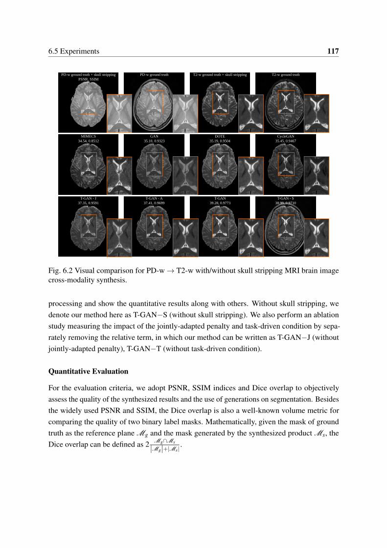
6.5 Experiments 117
PD-w ground truth + skull stripping PD-w ground truth T2-w ground truth + skull stripping T2-w ground truth
MIMECS GAN DOTE CycleGAN
T-GAN - J T-GAN - A T-GAN T-GAN - S
PSNR, SSIM
34.54, 0.8512 35.10, 0.9323 35.19, 0.9504 35.45, 0.9467
37.35, 0.9591 37.41, 0.9699 39.28, 0.9773 38.99, 0.9710
Fig. 6.2 Visual comparison for PD-w→ T2-w with/without skull stripping MRI brain imagecross-modality synthesis.
processing and show the quantitative results along with others. Without skull stripping, wedenote our method here as T-GAN−S (without skull stripping). We also perform an ablationstudy measuring the impact of the jointly-adapted penalty and task-driven condition by sepa-rately removing the relative term, in which our method can be written as T-GAN−J (withoutjointly-adapted penalty), T-GAN−T (without task-driven condition).
Quantitative Evaluation
For the evaluation criteria, we adopt PSNR, SSIM indices and Dice overlap to objectivelyassess the quality of the synthesized results and the use of generations on segmentation. Besidesthe widely used PSNR and SSIM, the Dice overlap is also a well-known volume metric forcomparing the quality of two binary label masks. Mathematically, given the mask of groundtruth as the reference plane Mg and the mask generated by the synthesized product Ms, theDice overlap can be defined as 2 Mg∩Ms
|Mg|+|Ms|.
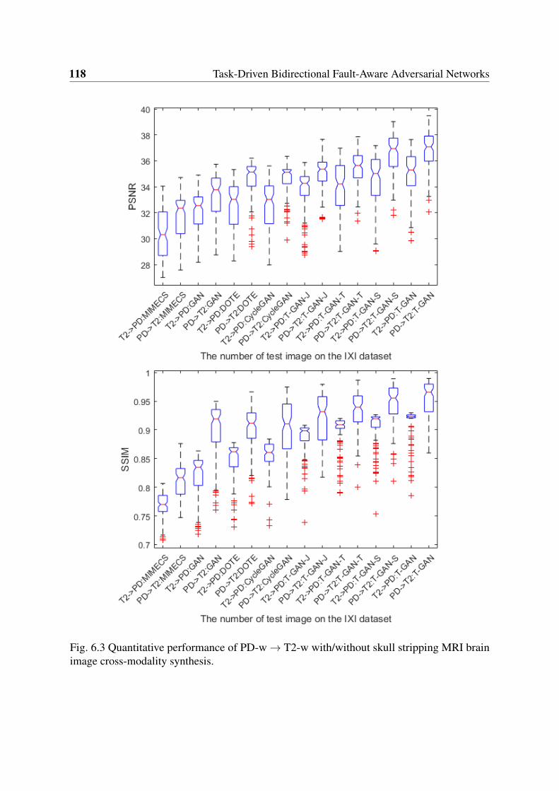
118 Task-Driven Bidirectional Fault-Aware Adversarial Networks
Fig. 6.3 Quantitative performance of PD-w→ T2-w with/without skull stripping MRI brainimage cross-modality synthesis.
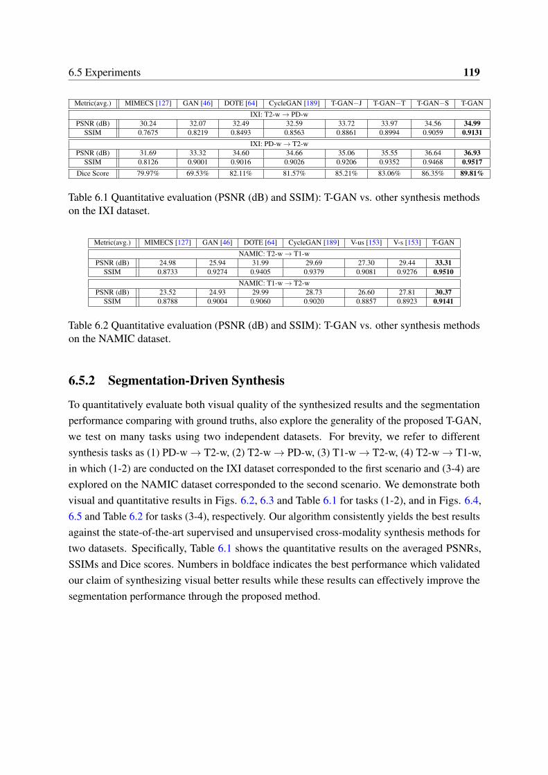
6.5 Experiments 119
Metric(avg.) MIMECS [127] GAN [46] DOTE [64] CycleGAN [189] T-GAN−J T-GAN−T T-GAN−S T-GAN
IXI: T2-w→ PD-wPSNR (dB) 30.24 32.07 32.49 32.59 33.72 33.97 34.56 34.99
SSIM 0.7675 0.8219 0.8493 0.8563 0.8861 0.8994 0.9059 0.9131IXI: PD-w→ T2-w
PSNR (dB) 31.69 33.32 34.60 34.66 35.06 35.55 36.64 36.93SSIM 0.8126 0.9001 0.9016 0.9026 0.9206 0.9352 0.9468 0.9517
Dice Score 79.97% 69.53% 82.11% 81.57% 85.21% 83.06% 86.35% 89.81%
Table 6.1 Quantitative evaluation (PSNR (dB) and SSIM): T-GAN vs. other synthesis methodson the IXI dataset.
Metric(avg.) MIMECS [127] GAN [46] DOTE [64] CycleGAN [189] V-us [153] V-s [153] T-GAN
NAMIC: T2-w→ T1-wPSNR (dB) 24.98 25.94 31.99 29.69 27.30 29.44 33.31
SSIM 0.8733 0.9274 0.9405 0.9379 0.9081 0.9276 0.9510NAMIC: T1-w→ T2-w
PSNR (dB) 23.52 24.93 29.99 28.73 26.60 27.81 30.37SSIM 0.8788 0.9004 0.9060 0.9020 0.8857 0.8923 0.9141
Table 6.2 Quantitative evaluation (PSNR (dB) and SSIM): T-GAN vs. other synthesis methodson the NAMIC dataset.
6.5.2 Segmentation-Driven Synthesis
To quantitatively evaluate both visual quality of the synthesized results and the segmentationperformance comparing with ground truths, also explore the generality of the proposed T-GAN,we test on many tasks using two independent datasets. For brevity, we refer to differentsynthesis tasks as (1) PD-w→ T2-w, (2) T2-w→ PD-w, (3) T1-w→ T2-w, (4) T2-w→ T1-w,in which (1-2) are conducted on the IXI dataset corresponded to the first scenario and (3-4) areexplored on the NAMIC dataset corresponded to the second scenario. We demonstrate bothvisual and quantitative results in Figs. 6.2, 6.3 and Table 6.1 for tasks (1-2), and in Figs. 6.4,6.5 and Table 6.2 for tasks (3-4), respectively. Our algorithm consistently yields the best resultsagainst the state-of-the-art supervised and unsupervised cross-modality synthesis methods fortwo datasets. Specifically, Table 6.1 shows the quantitative results on the averaged PSNRs,SSIMs and Dice scores. Numbers in boldface indicates the best performance which validatedour claim of synthesizing visual better results while these results can effectively improve thesegmentation performance through the proposed method.
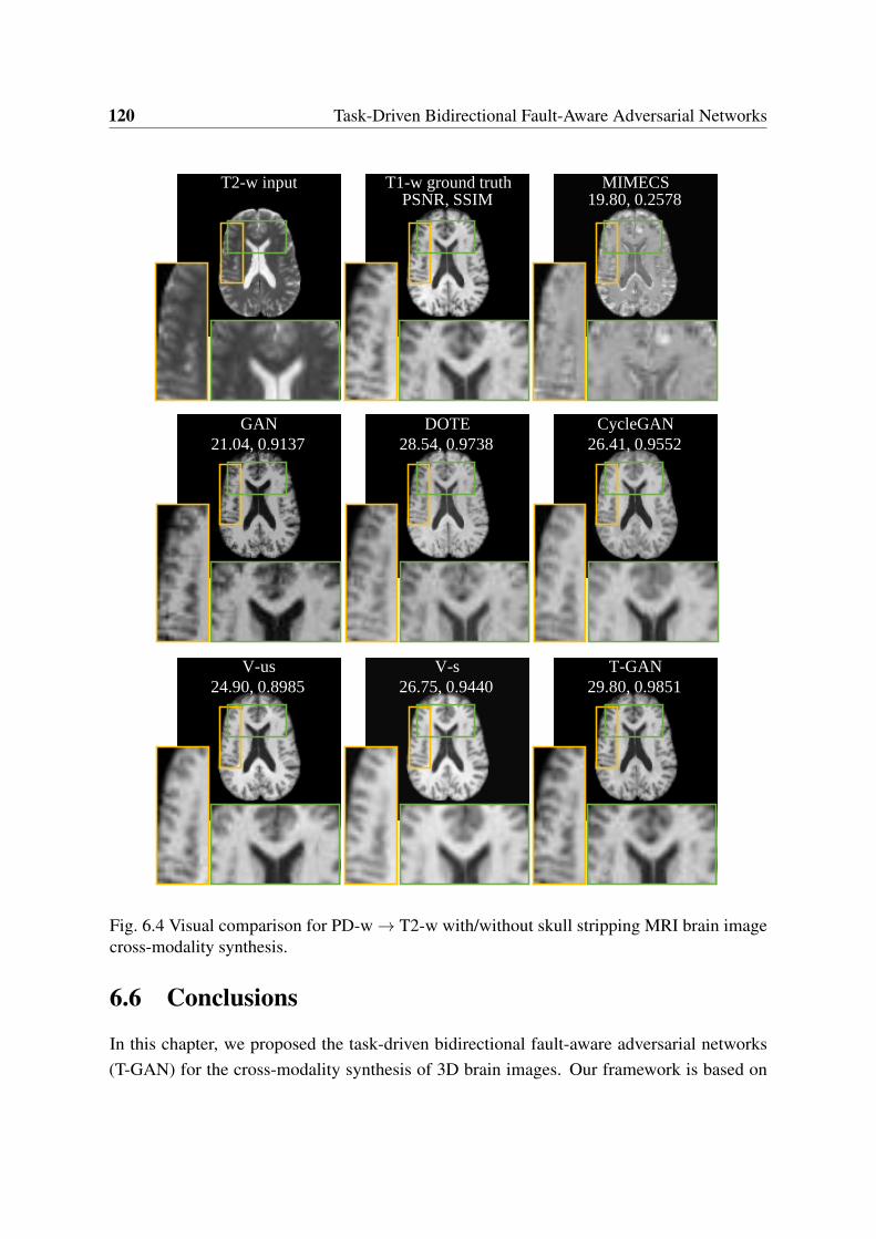
120 Task-Driven Bidirectional Fault-Aware Adversarial Networks
T2-w input T1-w ground truth MIMECS
GAN DOTE CycleGAN
V-us V-s T-GAN
PSNR, SSIM 19.80, 0.2578
21.04, 0.9137 28.54, 0.9738 26.41, 0.9552
24.90, 0.8985 26.75, 0.9440 29.80, 0.9851
Fig. 6.4 Visual comparison for PD-w→ T2-w with/without skull stripping MRI brain imagecross-modality synthesis.
6.6 Conclusions
In this chapter, we proposed the task-driven bidirectional fault-aware adversarial networks(T-GAN) for the cross-modality synthesis of 3D brain images. Our framework is based on
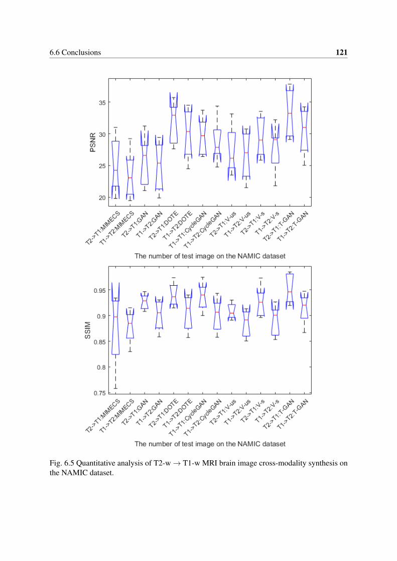
6.6 Conclusions 121
Fig. 6.5 Quantitative analysis of T2-w→ T1-w MRI brain image cross-modality synthesis onthe NAMIC dataset.

122 Task-Driven Bidirectional Fault-Aware Adversarial Networks
GANs’ model using high-level representations over both generative and discriminative networksacross image spaces. To learn the mapping relations between both modalities, we exploited thejointly-adapted bidirectional loss for simultaneously minimizing the domain divergence andproviding volumetric consistency mappings in a dual manner. Imposing the task-effectivenessconstraint in the synthesis provides a segmentation that achieves better results with visualinteraction compared to a separate synthesis and segmentation process. In future work, wehope to explore the use of T-GAN for other medical image synthesis tasks such as the morechallenging 4D cardiac images.
Chapter 7
Conclusions and Future Directions
7.1 Conclusions
This dissertation has focused on the problem of learning cross-modality features for three-dimensional brain image synthesis. Specifically, we have addressed two major problemsincluding image super-resolution and cross-modality synthesis. We first explored the supervisedmodels which rely on a large number well-processed (i.e., skull-stripped and strictly registered)multi-modality brain images. In contrast to the fully supervised methods, we also learn from afew registered multi-modality image pairs which are weakly supervised. We attempt to resolvethe modality divergence associated with weak pairs through constructing a common spaceprocessed by the rigorous mathematical constraints on the features. We demonstrated thatthe resulting approaches for the general cross-modality synthesis task could be trained in aweakly-supervised manner. Further, we addressed the problem of unsupervised cross-modalitysynthesis by exploring the task-driven deep architecture for volumetric neuroimage processing.
Concretely, in Chapter 2 we developed a region-character clustering model that can matchcross-modality images in the sparse feature space. This allowed us to synthesize the desiredmodality data with normalized domain specific property. We represented a general approachfor bringing transitional independent sparse representations of two domains for cross-modalityimage synthesis into joint learning, leveraging freely available pairwise data for training ourmodel. This method projected the sparse codes of both domains into a common feature space,which was used to describe the correspondence between two modalities and generate thenormalized target modality data via inputting the source modality image.
In Chapter 3, we addressed the problem of cross-modality synthesis for MR brain images.We introduced an approach which constructs a closed loop joint filter learning strategy togenerate informative feedback for model self-optimization. The proposed method can efficientlyleverage data and therefore reducing the size of the required training set. We presented dual
124 Conclusions and Future Directions
learning and interaction based features which are informative about modality characteristics.The features were used in a convolutional sparse coding space where the role assignmentsand modality-specific feature weights were jointly inferred through a dual convolutionalfilter learning algorithm. The proposed method was evaluated against multiple baselines intwo challenging tasks and demonstrated the superior performance over other state-of-the-artapproaches.
In Chapters 4 and 5 we presented two models for automatically learning different modalityfeatures for image super-resolution and cross-modality synthesis. Both works had the benefitsof improved synthesis performance via hetero-domain alignment without requiring fully pairedtraining data, making synthesis more flexible. The proposed models can take a source modalityimage and generate the corresponding target modality image without being constrained tomerely training from a finite collection of strictly pairwise data pre-processed by an extra tool(e.g., FSL, AFNI, and ANTs for brain image registration). Our models generate both visuallyand quantitatively impressive results, and we showed in experimental evaluations that theproposed models outperform previous cross-modality synthesis methods based on the rankingresults.
Finally, in Chapter 6, we presented an image synthesis model even more scalable byremoving the requirement of either fully or weakly-supervised setting at training stage. Thismodel made use of freely and publicly available brain dataset from the web, realizing thatdata is fundamentally a limiting factor in learning-based methods for cross-modality synthesis.As a result, we introduced the task-driven bidirectional fault-aware adversarial networks forvolumetric neuroimage processing in an unsupervised manner. This method is related to thewell-studied problem of the adversarial model in computer vision and machine learning. Inparticular, we defined a jointly-adapted bidirectional loss which utilizes the deep featuresof hidden representation to penalize domain discrepancy. The bidirectional mappings weremodeled in a closed loop with the criterion of cycle-consistency to improve data variationswithin multiple conditions. We also introduced the fault-aware discriminator with a constrainton the task-specific descriptions to balance both synthesis fidelity and task performance. Onthe algorithmic side, our approach is suitable to improve the performance of the chosen taskwhile preserving strong visual effects.
7.2 Future Works
Due to the large amount of progress on image synthesis made in recent years, caused onlypartially by the contributions included in this dissertation, it is challenging to say that somefuture work can be directed towards achieving better performance in brain image synthesis.
7.2 Future Works 125
Nonetheless, based on the potential extensions of our works, there are some open questionslead for future research.
7.2.1 Discrimination Capability
Cross-modality synthesis has thus far focused on the missing/target data reconstruction problem.What advances need to be made to push only cross-modality synthesis into other problems,e.g. segmentation, detection of lesion area, diagnosis, or prognosis. The key limiting factor forthese problems is the discrimination capability of the learned model. Most existing approachestreat the learning procedure and classifier training as two separate processes since it is easier toconsider a one-way operation rather than mixing reconstructive and discriminative formulationinto a unified whole. Some previous methods which are patch-based mechanism learn adictionary and a classifier simultaneously, however, they might not scale well to a large numberof data/classes. Learning a discriminative model while guaranteeing the modality-specificfeatures tend to be required. Thus, one interesting research direction along these lines is tocombine cross-modality synthesis with image classification, and doing so with transfer learningor domain adaption strategy.
7.2.2 Conditional GAN
GAN learns a generative network jointly with a corresponding discriminative adversarialnetwork in a mini-max objective, which enables a wide variety of applications, particularlyin image synthesis task. Unfortunately in practice, GAN does not provide a stable trainingprocess, and thus people suggested that adversarial training might be unstable and prone tofailure even for single-modality image reconstruction problem. As GAN continues to improve,some works explore GAN in the conditional setting making the yielded conditional GAN(cGAN) suitable for both image reconstruction and image-to-image translation tasks. It makessense to start reasoning about even more complex cases since cGAN can be extended in aprincipled way. While this has been partially addressed in Chapter 6, more work remains,such as leveraging the perceptual similarity between the source and target modality imageswith GAN to produce high-quality results. On the other hand, although the proposed methodintroduced in Chapter 6 can achieve compelling results in cross-modality synthesis, the resultsare far from uniformly positive. A more general and promising demonstration can be exploredto perform cross-modality synthesis between an inexpensive modality and one that is expensiveeither monetarily or concerning exposure to ionizing radiation such as CT or PET. Therefore,handling more varied and extreme synthesis problems, especially a great changes in geometry,is an interesting direction for our future work.
126 Conclusions and Future Directions
7.2.3 4D Cardiac Data
A limitation of the proposed synthesis method is its flexibility to handle different subjects(e.g. brain, bone, and heart), and complicated situations (e.g. abnormalities affecting themorphology). As no close match exists in the currently explored datasets, the synthesis ofvarious subjects is limited and cannot be compensated by the utilized datasets. In this situation,finding several appropriate datasets is preferential. Fortunately, UK Biobank1 as a national andinternational health resource provides unparalleled research opportunities for improving theprevention, diagnosis, and treatment of a wide range of serious and life-threatening illnesses. Asimple solution can then be to apply the proposed synthesis method to these subjects. However,it is worth noting that none of the sequence data (like 4D cardiac images) is used in thisthesis as an input for the synthesis purpose. We can potentially design a method which canact on the four-dimensional sequences to generate good quality data while providing thecomplementary/required modality information.
1http://www.ukbiobank.ac.uk/
References
[1] Aharon, M., Elad, M., and Bruckstein, A. (2006). K-SVD: An algorithm for designingovercomplete dictionaries for sparse representation. IEEE Transactions on Signal Processing,54(11):4311–4322.
[2] Akhtar, N., Shafait, F., and Mian, A. (2014). Bayesian sparse representation for hyper-spectral image super resolution. IEEE Transactions on Geoscience and Remote Sensing,52(3):1693–1704.
[3] Ashikhmin, N. (2003). Fast texture transfer. IEEE Computer Graphics and Applications,23(4):38–43.
[4] Bahrami, K., Shi, F., Zong, X., Shin, H. W., An, H., and Shen, D. (2015). Hierarchicalreconstruction of 7t-like images from 3t mri using multi-level cca and group sparsity. InInternational Conference on Medical Image Computing and Computer-Assisted Intervention,pages 659–666. Springer.
[5] Belkin, M. and Niyogi, P. (2001). Laplacian eigenmaps and spectral techniques forembedding and clustering. In Neural Information Processing Systems, volume 14, pages585–591.
[6] Bengio, Y., Courville, A., and Vincent, P. (2013). Representation learning: A reviewand new perspectives. IEEE Transactions on Pattern Analysis and Machine Intelligence,35(8):1798–1828.
[7] Bogunovic, H., Pozo, J. M., Villa-Uriol, M. C., Majoie, C. B., van den Berg, R., van Andel,H. A. G., Macho, J. M., Blasco, J., San Román, L., and Frangi, A. F. (2011). Automatedsegmentation of cerebral vasculature with aneurysms in 3dra and tof-mra using geodesicactive regions: an evaluation study. Medical Physics, 38(1):210–222.
[8] Borgwardt, K. M., Gretton, A., Rasch, M. J., Kriegel, H.-P., Schölkopf, B., and Smola,A. J. (2006). Integrating structured biological data by kernel maximum mean discrepancy.Bioinformatics, 22(14):e49–e57.
[9] Boyd, S. and Vandenberghe, L. (2004). Convex optimization. Cambridge university press.
[10] Bristow, H., Eriksson, A., and Lucey, S. (2013). Fast convolutional sparse coding. InProceedings of the IEEE Conference on Computer Vision and Pattern Recognition, pages391–398.
[11] Bruckstein, A. M., Donoho, D. L., and Elad, M. (2009). From sparse solutions of systemsof equations to sparse modeling of signals and images. SIAM Review, 51(1):34–81.
128 References
[12] Buades, A., Coll, B., and Morel, J.-M. (2010). Image denoising methods. a new nonlocalprinciple. SIAM Review, 52(1):113–147.
[13] Burgos, N., Cardoso, M. J., Modat, M., Pedemonte, S., Dickson, J., Barnes, A., Duncan,J. S., Atkinson, D., Arridge, S. R., Hutton, B. F., et al. (2013). Attenuation correctionsynthesis for hybrid PET-MR scanners. In International Conference on Medical ImageComputing and Computer-Assisted Intervention, pages 147–154. Springer.
[14] Burgos, N., Cardoso, M. J., Thielemans, K., Modat, M., Pedemonte, S., Dickson, J.,Barnes, A., Ahmed, R., Mahoney, C. J., Schott, J. M., et al. (2014). Attenuation correctionsynthesis for hybrid pet-mr scanners: application to brain studies. IEEE Transactions onMedical Imaging, 33(12):2332–2341.
[15] Cao, T., Zach, C., Modla, S., Powell, D., Czymmek, K., and Niethammer, M. (2014).Multi-modal registration for correlative microscopy using image analogies. Medical ImageAnalysis, 18(6):914–926.
[16] Chang, H., Yeung, D.-Y., and Xiong, Y. (2004). Super-resolution through neighborembedding. In Computer Vision and Pattern Recognition, 2004. CVPR 2004. Proceedingsof the 2004 IEEE Computer Society Conference on, volume 1, pages I–I. IEEE.
[17] Chartsias, A., Joyce, T., Giuffrida, M. V., and Tsaftaris, S. A. (2017). Multimodalmr synthesis via modality-invariant latent representation. IEEE Transactions on MedicalImaging.
[18] Chen, B., Polatkan, G., Sapiro, G., Blei, D., Dunson, D., and Carin, L. (2013). Deeplearning with hierarchical convolutional factor analysis. IEEE Transactions on PatternAnalysis and Machine Intelligence, 35(8):1887–1901.
[19] Chen, L., Li, W., and Xu, D. (2014). Recognizing rgb images by learning from rgb-d data.In Proceedings of the IEEE Conference on Computer Vision and Pattern Recognition, pages1418–1425.
[20] Chen, S. S., Donoho, D. L., and Saunders, M. A. (2001). Atomic decomposition by basispursuit. SIAM Review, 43(1):129–159.
[21] Cheng, L., Vishwanathan, S. N., and Zhang, X. (2008). Consistent image analogies usingsemi-supervised learning. In Computer Vision and Pattern Recognition (CVPR), 2008 IEEEConference on, pages 1–8. IEEE.
[22] Cho, D., Lee, M., Kim, S., and Tai, Y.-W. (2013). Modeling the calibration pipeline of thelytro camera for high quality light-field image reconstruction. In Computer Vision (ICCV),2013 IEEE International Conference on, pages 3280–3287. IEEE.
[23] Choudhury, B., Swanson, R., Heide, F., Wetzstein, G., and Heidrich, W. (2017). Consensusconvolutional sparse coding. IEEE International Conference on Computer Vision.
[24] Christensen, J. D. (2003). Normalization of brain magnetic resonance images usinghistogram even-order derivative analysis. Magnetic Resonance Imaging, 21(7):817–820.
References 129
[25] Cordier, N., Delingette, H., Lê, M., and Ayache, N. (2016). Extended modality prop-agation: Image synthesis of pathological cases. IEEE Transactions on Medical Imaging,35(12):2598–2608.
[26] Davis, G., Mallat, S., and Avellaneda, M. (1997). Adaptive greedy approximations.Constructive Approximation, 13(1):57–98.
[27] Dong, C., Loy, C. C., He, K., and Tang, X. (2016). Image super-resolution using deepconvolutional networks. IEEE Transactions on Pattern Analysis and Machine Intelligence,38(2):295–307.
[28] Dong, W., Li, X., Zhang, L., and Shi, G. (2011). Sparsity-based image denoising viadictionary learning and structural clustering. In Computer Vision and Pattern Recognition(CVPR), 2011 IEEE Conference on, pages 457–464. IEEE.
[29] Dong, W., Zhang, L., Shi, G., and Li, X. (2013). Nonlocally centralized sparse represen-tation for image restoration. IEEE Transactions on Image Processing, 22(4):1620–1630.
[30] Donoho, D. L. (2006). For most large underdetermined systems of linear equations theminimal l1-norm solution is also the sparsest solution. Communications on Pure and AppliedMathematics, 59(6):797–829.
[31] Dosovitskiy, A., Tobias Springenberg, J., and Brox, T. (2015). Learning to generate chairswith convolutional neural networks. In Proceedings of the IEEE Conference on ComputerVision and Pattern Recognition, pages 1538–1546.
[32] Efros, A. A. and Freeman, W. T. (2001). Image quilting for texture synthesis andtransfer. In Proceedings of the 28th annual conference on Computer graphics and interactivetechniques, pages 341–346. ACM.
[33] Efros, A. A. and Leung, T. K. (1999). Texture synthesis by non-parametric sampling. InComputer Vision, 1999. The Proceedings of the Seventh IEEE International Conference on,volume 2, pages 1033–1038. IEEE.
[34] Elad, M. and Aharon, M. (2006). Image denoising via sparse and redundant representa-tions over learned dictionaries. IEEE Transactions on Image Processing, 15(12):3736–3745.
[35] Elad, M. and Milanfar, P. (2017). Style transfer via texture synthesis. IEEE Transactionson Image Processing, 26(5):2338–2351.
[36] Elhamifar, E. and Vidal, R. (2013). Sparse subspace clustering: Algorithm, theory, andapplications. IEEE Transactions on Pattern Analysis and Machine Intelligence, 35(11):2765–2781.
[37] Engan, K., Aase, S. O., and Husoy, J. H. (1999). Method of optimal directions forframe design. In Acoustics, Speech, and Signal Processing, 1999. Proceedings., 1999 IEEEInternational Conference on, volume 5, pages 2443–2446. IEEE.
[38] Fischl, B., Salat, D. H., Busa, E., Albert, M., Dieterich, M., Haselgrove, C., VanDer Kouwe, A., Killiany, R., Kennedy, D., Klaveness, S., et al. (2002). Whole brainsegmentation: automated labeling of neuroanatomical structures in the human brain. Neuron,33(3):341–355.
130 References
[39] Frangi, A. F., Niessen, W. J., Vincken, K. L., and Viergever, M. A. (1998). Multiscalevessel enhancement filtering. In International Conference on Medical Image Computingand Computer-Assisted Intervention, pages 130–137. Springer.
[40] Freeman, W. T., Jones, T. R., and Pasztor, E. C. (2002). Example-based super-resolution.IEEE Computer Graphics and Applications, 22(2):56–65.
[41] Freeman, W. T., Pasztor, E. C., and Carmichael, O. T. (2000). Learning low-level vision.International Journal of Computer Vision, 40(1):25–47.
[42] Gao, X., Wang, N., Tao, D., and Li, X. (2012a). Face sketch–photo synthesis andretrieval using sparse representation. IEEE Transactions on Circuits and Systems for VideoTechnology, 22(8):1213–1226.
[43] Gao, X., Zhang, K., Tao, D., and Li, X. (2012b). Image super-resolution with sparseneighbor embedding. IEEE Transactions on Image Processing, 21(7):3194–3205.
[44] Gatys, L. A., Ecker, A. S., and Bethge, M. (2016). Image style transfer using convolutionalneural networks. In Proceedings of the IEEE Conference on Computer Vision and PatternRecognition, pages 2414–2423.
[45] Gersho, A. and Gray, R. M. (2012). Vector quantization and signal compression, volume159. Springer Science & Business Media.
[46] Goodfellow, I., Pouget-Abadie, J., Mirza, M., Xu, B., Warde-Farley, D., Ozair, S.,Courville, A., and Bengio, Y. (2014). Generative adversarial nets. In Advances in NeuralInformation Processing Systems, pages 2672–2680.
[47] Greenspan, H., Oz, G., Kiryati, N., and Peled, S. (2002). Mri inter-slice reconstructionusing super-resolution. Magnetic Resonance Imaging, 20(5):437–446.
[48] Gretton, A., Borgwardt, K. M., Rasch, M. J., Schölkopf, B., and Smola, A. (2012a). Akernel two-sample test. Journal of Machine Learning Research, 13(Mar):723–773.
[49] Gretton, A., Sejdinovic, D., Strathmann, H., Balakrishnan, S., Pontil, M., Fukumizu, K.,and Sriperumbudur, B. K. (2012b). Optimal kernel choice for large-scale two-sample tests.In Advances in Neural Information Processing Systems, pages 1205–1213.
[50] Grevera, G. J. and Udupa, J. K. (1998). An objective comparison of 3d image interpolationmethods. IEEE Transactions on Medical Imaging, 17(4):642–652.
[51] Gu, S., Zuo, W., Xie, Q., Meng, D., Feng, X., and Zhang, L. (2015). Convolutional sparsecoding for image super-resolution. In Proceedings of the IEEE International Conference onComputer Vision, pages 1823–1831.
[52] Han, J., Chen, C., Shao, L., Hu, X., Han, J., and Liu, T. (2015). Learning computationalmodels of video memorability from fmri brain imaging. IEEE Transactions on Cybernetics,45(8):1692–1703.
[53] Hartigan, J. A. and Wong, M. A. (1979). Algorithm as 136: A k-means clusteringalgorithm. Journal of the Royal Statistical Society. Series C (Applied Statistics), 28(1):100–108.
References 131
[54] Havaei, M., Guizard, N., Chapados, N., and Bengio, Y. (2016). Hemis: Hetero-modal im-age segmentation. In International Conference on Medical Image Computing and Computer-Assisted Intervention, pages 469–477. Springer.
[55] He, D., Xia, Y., Qin, T., Wang, L., Yu, N., Liu, T., and Ma, W.-Y. (2016a). Dual learningfor machine translation. In Advances in Neural Information Processing Systems, pages820–828.
[56] He, K., Zhang, X., Ren, S., and Sun, J. (2016b). Deep residual learning for imagerecognition. In The IEEE Conference on Computer Vision and Pattern Recognition (CVPR).
[57] Heide, F., Heidrich, W., and Wetzstein, G. (2015). Fast and flexible convolutional sparsecoding. In 2015 IEEE Conference on Computer Vision and Pattern Recognition (CVPR),pages 5135–5143. IEEE.
[58] Herman, G. T., Rowland, S. W., and Yau, M.-m. (1979). A comparative study of the use oflinear and modified cubic spline interpolation for image reconstruction. IEEE Transactionson Nuclear Science, 26(2):2879–2894.
[59] Hertzmann, A., Jacobs, C. E., Oliver, N., Curless, B., and Salesin, D. H. (2001). Im-age analogies. In Proceedings of the 28th annual conference on Computer graphics andinteractive techniques, pages 327–340. ACM.
[60] Huang, D.-A. and Frank Wang, Y.-C. (2013). Coupled dictionary and feature spacelearning with applications to cross-domain image synthesis and recognition. In Proceedingsof the IEEE international conference on computer vision, pages 2496–2503.
[61] Huang, J.-B., Singh, A., and Ahuja, N. (2015). Single image super-resolution fromtransformed self-exemplars. In 2015 IEEE Conference on Computer Vision and PatternRecognition (CVPR), pages 5197–5206. IEEE.
[62] Huang, Y., Beltrachini, L., Shao, L., and Frangi, A. F. (2016a). Geometry regularizedjoint dictionary learning for cross-modality image synthesis in magnetic resonance imaging.In International Workshop on Simulation and Synthesis in Medical Imaging, pages 118–126.Springer.
[63] Huang, Y., Shao, L., and Frangi, A. F. (2017a). Cross-modality image synthesis viaweakly-coupled and geometry co-regularized joint dictionary learning. IEEE Transactionson Medical Imaging.
[64] Huang, Y., Shao, L., and Frangi, A. F. (2017b). Dote: Dual convolutional filter learningfor super-resolution and cross-modality synthesis in MRI. pages 89–98.
[65] Huang, Y., Shao, L., and Frangi, A. F. (2017c). Simultaneous super-resolution andcross-modality synthesis of 3D medical images using weakly-supervised joint convolutionalsparse coding. In IEEE Computer Vision and Pattern Recognition.
[66] Huang, Y., Zhu, F., Shao, L., and Frangi, A. F. (2016b). Color object recognition viacross-domain learning on rgb-d images. In Robotics and Automation (ICRA), 2016 IEEEInternational Conference on, pages 1672–1677. IEEE.
132 References
[67] Iglesias, J. E., Konukoglu, E., Zikic, D., Glocker, B., Van Leemput, K., and Fischl, B.(2013). Is synthesizing mri contrast useful for inter-modality analysis? In InternationalConference on Medical Image Computing and Computer-Assisted Intervention, pages 631–638. Springer.
[68] Iglesias, J. E. and Sabuncu, M. R. (2015). Multi-atlas segmentation of biomedical images:a survey. Medical Image Analysis, 24(1):205–219.
[69] Isola, P., Zhu, J.-Y., Zhou, T., and Efros, A. A. (2016). Image-to-image translation withconditional adversarial networks. arXiv preprint arXiv:1611.07004.
[70] Jia, K., Wang, X., and Tang, X. (2013). Image transformation based on learning dictionar-ies across image spaces. IEEE Transactions on Pattern Analysis and Machine Intelligence,35(2):367–380.
[71] Jiang, Z., Lin, Z., and Davis, L. S. (2013). Label consistent k-svd: Learning a discrim-inative dictionary for recognition. IEEE Transactions on Pattern Analysis and MachineIntelligence, 35(11):2651–2664.
[72] Jog, A., Carass, A., Roy, S., Pham, D. L., and Prince, J. L. (2017). Random forestregression for magnetic resonance image synthesis. Medical Image Analysis, 35:475–488.
[73] Jog, A., Roy, S., Carass, A., and Prince, J. L. (2013). Magnetic resonance image synthesisthrough patch regression. In 2013 IEEE 10th International Symposium on BiomedicalImaging, pages 350–353. IEEE.
[74] Johnson, J., Alahi, A., and Fei-Fei, L. (2016). Perceptual losses for real-time styletransfer and super-resolution. In European Conference on Computer Vision, pages 694–711.Springer.
[75] Joyce, T., Chartsias, A., and Tsaftaris, S. A. (2017). Robust multi-modal MR imagesynthesis. In International Conference on Medical Image Computing and Computer-AssistedIntervention, pages 347–355. Springer.
[76] Kainz, B., Steinberger, M., Wein, W., Kuklisova-Murgasova, M., Malamateniou, C.,Keraudren, K., Torsney-Weir, T., Rutherford, M., Aljabar, P., Hajnal, J. V., et al. (2015). Fastvolume reconstruction from motion corrupted stacks of 2d slices. IEEE Transactions onMedical Imaging, 34(9):1901–1913.
[77] Kavukcuoglu, K., Sermanet, P., Boureau, Y.-L., Gregor, K., Mathieu, M., and Cun, Y. L.(2010). Learning convolutional feature hierarchies for visual recognition. In Advances inNeural Information Processing Systems, pages 1090–1098.
[78] Keys, R. (1981). Cubic convolution interpolation for digital image processing. IEEETransactions on Acoustics, Speech, and Signal Processing, 29(6):1153–1160.
[79] Kim, T., Cha, M., Kim, H., Lee, J., and Kim, J. (2017). Learning to discover cross-domainrelations with generative adversarial networks. arXiv preprint arXiv:1703.05192.
[80] Kinga, D. and Adam, J. B. (2015). A method for stochastic optimization. In InternationalConference on Learning Representations (ICLR).
References 133
[81] Kong, S. and Wang, D. (2012). A dictionary learning approach for classification: separat-ing the particularity and the commonality. In European Conference on Computer Vision,pages 186–199. Springer.
[82] Kroon, D.-J. and Slump, C. H. (2009). MRI modalitiy transformation in demon registra-tion. In IEEE International Symposium on Biomedical Imaging, pages 963–966. IEEE.
[83] Kwatra, V., Schödl, A., Essa, I., Turk, G., and Bobick, A. (2003). Graphcut textures:image and video synthesis using graph cuts. In ACM Transactions on Graphics (ToG),volume 22, pages 277–286. ACM.
[84] LeCun, Y., Bengio, Y., and Hinton, G. (2015). Deep learning. Nature, 521(7553):436–444.
[85] Ledig, C., Theis, L., Huszár, F., Caballero, J., Cunningham, A., Acosta, A., Aitken, A.,Tejani, A., Totz, J., Wang, Z., et al. (2016). Photo-realistic single image super-resolutionusing a generative adversarial network. arXiv preprint arXiv:1609.04802.
[86] Lee, H., Battle, A., Raina, R., and Ng, A. Y. (2007). Efficient sparse coding algorithms.Neural Information Processing Systems, 19:801.
[87] Lehmann, T. M., Gonner, C., and Spitzer, K. (1999). Survey: Interpolation methods inmedical image processing. IEEE Transactions on Medical Imaging, 18(11):1049–1075.
[88] Li, C. and Wand, M. (2016). Precomputed real-time texture synthesis with markoviangenerative adversarial networks. In European Conference on Computer Vision, pages702–716. Springer.
[89] Li, S., Yin, H., and Fang, L. (2012). Group-sparse representation with dictionary learningfor medical image denoising and fusion. IEEE Transactions on Biomedical Engineering,59(12):3450–3459.
[90] Li, X. and Orchard, M. T. (2001). New edge-directed interpolation. IEEE Transactionson Image Processing, 10(10):1521–1527.
[91] Lin, D. and Tang, X. (2005). Coupled space learning of image style transformation. InComputer Vision, 2005. ICCV 2005. Tenth IEEE International Conference on, volume 2,pages 1699–1706. IEEE.
[92] Lin, X., Liu, Y., Wu, J., and Dai, Q. (2014). Spatial-spectral encoded compressivehyperspectral imaging. ACM Transactions on Graphics (TOG), 33(6):233.
[93] Liu, M.-Y., Breuel, T., and Kautz, J. (2017). Unsupervised image-to-image translationnetworks. arXiv preprint arXiv:1703.00848.
[94] Liu, M.-Y. and Tuzel, O. (2016). Coupled generative adversarial networks. In Advancesin Neural Information Processing Systems, pages 469–477.
[95] Liu, Z., Zhang, Z., and Shan, Y. (2004). Image-based surface detail transfer. IEEEComputer Graphics and Applications, 24(3):30–35.
[96] Long, M., Ding, G., Wang, J., Sun, J., Guo, Y., and Yu, P. S. (2013). Transfer sparsecoding for robust image representation. In Proceedings of the IEEE conference on computervision and pattern recognition, pages 407–414.

134 References
[97] Long, M., Wang, J., Cao, Y., Sun, J., and Philip, S. Y. (2016). Deep learning of transferablerepresentation for scalable domain adaptation. IEEE Transactions on Knowledge and DataEngineering, 28(8):2027–2040.
[98] Long, M., Wang, J., Ding, G., Shen, D., and Yang, Q. (2014). Transfer learning with graphco-regularization. IEEE Transactions on Knowledge and Data Engineering, 26(7):1805–1818.
[99] Lu, X., Yuan, H., Yan, P., Yuan, Y., and Li, X. (2012). Geometry constrained sparsecoding for single image super-resolution. In IEEE Computer Vision and Pattern Recognition,pages 1648–1655.
[100] Madabhushi, A. and Udupa, J. K. (2006). New methods of mr image intensity standard-ization via generalized scale. Medical Physics, 33(9):3426–3434.
[101] Mahendran, A. and Vedaldi, A. (2015). Understanding deep image representations byinverting them. In Proceedings of the IEEE conference on computer vision and patternrecognition, pages 5188–5196.
[102] Mairal, J., Bach, F., Ponce, J., and Sapiro, G. (2009a). Online dictionary learning forsparse coding. In Proceedings of the 26th annual international conference on machinelearning, pages 689–696. ACM.
[103] Mairal, J., Bach, F., Ponce, J., Sapiro, G., and Zisserman, A. (2008a). Discriminativelearned dictionaries for local image analysis. In Computer Vision and Pattern Recognition,2008. CVPR 2008. IEEE Conference on, pages 1–8. IEEE.
[104] Mairal, J., Elad, M., and Sapiro, G. (2008b). Sparse representation for color imagerestoration. IEEE Transactions on Image Processing, 17(1):53–69.
[105] Mairal, J., Ponce, J., Sapiro, G., Zisserman, A., and Bach, F. R. (2009b). Superviseddictionary learning. In Advances in Neural Information Processing Systems, pages 1033–1040.
[106] Manjón, J. V., Carbonell-Caballero, J., Lull, J. J., García-Martí, G., Martí-Bonmatí, L.,and Robles, M. (2008). Mri denoising using non-local means. Medical Image Analysis,12(4):514–523.
[107] Manjón, J. V., Coupé, P., Buades, A., Fonov, V., Collins, D. L., and Robles, M. (2010).Non-local mri upsampling. Medical Image Analysis, 14(6):784–792.
[108] Marwah, K., Wetzstein, G., Bando, Y., and Raskar, R. (2013). Compressive light fieldphotography using overcomplete dictionaries and optimized projections. ACM Transactionson Graphics (TOG), 32(4):46.
[109] Menze, B. H., Van Leemput, K., Lashkari, D., Riklin-Raviv, T., Geremia, E., Alberts, E.,Gruber, P., Wegener, S., Weber, M.-A., Szekely, G., et al. (2016). A generative probabilisticmodel and discriminative extensions for brain lesion segmentation—with application totumor and stroke. IEEE Transactions on Medical Imaging, 35(4):933–946.
References 135
[110] Monay, F. and Gatica-Perez, D. (2007). Modeling semantic aspects for cross-media im-age indexing. IEEE Transactions on Pattern Analysis and Machine Intelligence, 29(10):1802–1817.
[111] Mueller, S. G., Weiner, M. W., Thal, L. J., Petersen, R. C., Jack, C., Jagust, W., Tro-janowski, J. Q., Toga, A. W., and Beckett, L. (2005). The alzheimer’s disease neuroimaginginitiative. Neuroimaging Clinics of North America, 15(4):869–877.
[112] Nyúl, L. G., Udupa, J. K., et al. (1999). On standardizing the mr image intensity scale.Image, 1081.
[113] Nyúl, L. G., Udupa, J. K., and Zhang, X. (2000). New variants of a method of mri scalestandardization. IEEE Transactions on Medical Imaging, 19(2):143–150.
[114] Oktay, O., Bai, W., Lee, M., Guerrero, R., Kamnitsas, K., Caballero, J., de Marvao,A., Cook, S., O’Regan, D., and Rueckert, D. (2016). Multi-input cardiac image super-resolution using convolutional neural networks. In International Conference on MedicalImage Computing and Computer-Assisted Intervention, pages 246–254. Springer.
[115] Olivier Commowick, S. K. W. and Malandain, G. (2009). Using Frankenstein’s creatureparadigm to build a patient specific atlas. In International Conference On Medical ImageComputing and Computer Assisted Intervention, pages 993–1000. Springer.
[116] Olshausen, B. A. and Field, D. J. (1997). Sparse coding with an overcomplete basis set:A strategy employed by v1? Vision Research, 37(23):3311–3325.
[117] Ongie, G. and Jacob, M. (2015). Recovery of discontinuous signals using group sparsehigher degree total variation. IEEE Signal Processing Letters, 22:1414–1418.
[118] Pan, S. J. and Yang, Q. (2010). A survey on transfer learning. IEEE Transactions onKnowledge and Data Engineering, 22(10):1345–1359.
[119] Radford, A., Metz, L., and Chintala, S. (2015). Unsupervised representation learningwith deep convolutional generative adversarial networks. arXiv preprint arXiv:1511.06434.
[120] Rao, S. R., Tron, R., Vidal, R., and Ma, Y. (2008). Motion segmentation via robustsubspace separation in the presence of outlying, incomplete, or corrupted trajectories. InComputer Vision and Pattern Recognition, 2008. CVPR 2008. IEEE Conference on, pages1–8. IEEE.
[121] Ravishankar, S. and Bresler, Y. (2011). Mr image reconstruction from highly under-sampled k-space data by dictionary learning. IEEE Transactions on Medical Imaging,30(5):1028–1041.
[122] Reed, S., Akata, Z., Yan, X., Logeswaran, L., Schiele, B., and Lee, H. (2016). Generativeadversarial text to image synthesis. arXiv preprint arXiv:1605.05396.
[123] Robitaille, N., Mouiha, A., Crépeault, B., Valdivia, F., and Duchesne, S. (2012). Tissue-based mri intensity standardization: application to multicentric datasets. InternationalJournal of Biomedical Imaging, 2012:4.
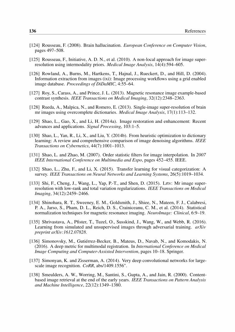
136 References
[124] Rousseau, F. (2008). Brain hallucination. European Conference on Computer Vision,pages 497–508.
[125] Rousseau, F., Initiative, A. D. N., et al. (2010). A non-local approach for image super-resolution using intermodality priors. Medical Image Analysis, 14(4):594–605.
[126] Rowland, A., Burns, M., Hartkens, T., Hajnal, J., Rueckert, D., and Hill, D. (2004).Information extraction from images (ixi): Image processing workflows using a grid enabledimage database. Proceedings of DiDaMIC, 4:55–64.
[127] Roy, S., Carass, A., and Prince, J. L. (2013). Magnetic resonance image example-basedcontrast synthesis. IEEE Transactions on Medical Imaging, 32(12):2348–2363.
[128] Rueda, A., Malpica, N., and Romero, E. (2013). Single-image super-resolution of brainmr images using overcomplete dictionaries. Medical Image Analysis, 17(1):113–132.
[129] Shao, L., Gao, X., and Li, H. (2014a). Image restoration and enhancement: Recentadvances and applications. Signal Processing, 103:1–5.
[130] Shao, L., Yan, R., Li, X., and Liu, Y. (2014b). From heuristic optimization to dictionarylearning: A review and comprehensive comparison of image denoising algorithms. IEEETransactions on Cybernetics, 44(7):1001–1013.
[131] Shao, L. and Zhao, M. (2007). Order statistic filters for image interpolation. In 2007IEEE International Conference on Multimedia and Expo, pages 452–455. IEEE.
[132] Shao, L., Zhu, F., and Li, X. (2015). Transfer learning for visual categorization: Asurvey. IEEE Transactions on Neural Networks and Learning Systems, 26(5):1019–1034.
[133] Shi, F., Cheng, J., Wang, L., Yap, P.-T., and Shen, D. (2015). Lrtv: Mr image super-resolution with low-rank and total variation regularizations. IEEE Transactions on MedicalImaging, 34(12):2459–2466.
[134] Shinohara, R. T., Sweeney, E. M., Goldsmith, J., Shiee, N., Mateen, F. J., Calabresi,P. A., Jarso, S., Pham, D. L., Reich, D. S., Crainiceanu, C. M., et al. (2014). Statisticalnormalization techniques for magnetic resonance imaging. NeuroImage: Clinical, 6:9–19.
[135] Shrivastava, A., Pfister, T., Tuzel, O., Susskind, J., Wang, W., and Webb, R. (2016).Learning from simulated and unsupervised images through adversarial training. arXivpreprint arXiv:1612.07828.
[136] Simonovsky, M., Gutiérrez-Becker, B., Mateus, D., Navab, N., and Komodakis, N.(2016). A deep metric for multimodal registration. In International Conference on MedicalImage Computing and Computer-Assisted Intervention, pages 10–18. Springer.
[137] Simonyan, K. and Zisserman, A. (2014). Very deep convolutional networks for large-scale image recognition. CoRR, abs/1409.1556".
[138] Smeulders, A. W., Worring, M., Santini, S., Gupta, A., and Jain, R. (2000). Content-based image retrieval at the end of the early years. IEEE Transactions on Pattern Analysisand Machine Intelligence, 22(12):1349–1380.
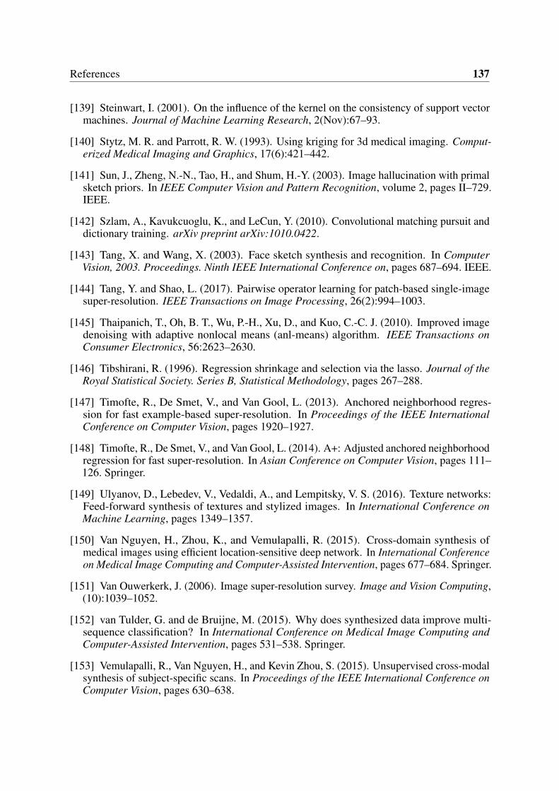
References 137
[139] Steinwart, I. (2001). On the influence of the kernel on the consistency of support vectormachines. Journal of Machine Learning Research, 2(Nov):67–93.
[140] Stytz, M. R. and Parrott, R. W. (1993). Using kriging for 3d medical imaging. Comput-erized Medical Imaging and Graphics, 17(6):421–442.
[141] Sun, J., Zheng, N.-N., Tao, H., and Shum, H.-Y. (2003). Image hallucination with primalsketch priors. In IEEE Computer Vision and Pattern Recognition, volume 2, pages II–729.IEEE.
[142] Szlam, A., Kavukcuoglu, K., and LeCun, Y. (2010). Convolutional matching pursuit anddictionary training. arXiv preprint arXiv:1010.0422.
[143] Tang, X. and Wang, X. (2003). Face sketch synthesis and recognition. In ComputerVision, 2003. Proceedings. Ninth IEEE International Conference on, pages 687–694. IEEE.
[144] Tang, Y. and Shao, L. (2017). Pairwise operator learning for patch-based single-imagesuper-resolution. IEEE Transactions on Image Processing, 26(2):994–1003.
[145] Thaipanich, T., Oh, B. T., Wu, P.-H., Xu, D., and Kuo, C.-C. J. (2010). Improved imagedenoising with adaptive nonlocal means (anl-means) algorithm. IEEE Transactions onConsumer Electronics, 56:2623–2630.
[146] Tibshirani, R. (1996). Regression shrinkage and selection via the lasso. Journal of theRoyal Statistical Society. Series B, Statistical Methodology, pages 267–288.
[147] Timofte, R., De Smet, V., and Van Gool, L. (2013). Anchored neighborhood regres-sion for fast example-based super-resolution. In Proceedings of the IEEE InternationalConference on Computer Vision, pages 1920–1927.
[148] Timofte, R., De Smet, V., and Van Gool, L. (2014). A+: Adjusted anchored neighborhoodregression for fast super-resolution. In Asian Conference on Computer Vision, pages 111–126. Springer.
[149] Ulyanov, D., Lebedev, V., Vedaldi, A., and Lempitsky, V. S. (2016). Texture networks:Feed-forward synthesis of textures and stylized images. In International Conference onMachine Learning, pages 1349–1357.
[150] Van Nguyen, H., Zhou, K., and Vemulapalli, R. (2015). Cross-domain synthesis ofmedical images using efficient location-sensitive deep network. In International Conferenceon Medical Image Computing and Computer-Assisted Intervention, pages 677–684. Springer.
[151] Van Ouwerkerk, J. (2006). Image super-resolution survey. Image and Vision Computing,(10):1039–1052.
[152] van Tulder, G. and de Bruijne, M. (2015). Why does synthesized data improve multi-sequence classification? In International Conference on Medical Image Computing andComputer-Assisted Intervention, pages 531–538. Springer.
[153] Vemulapalli, R., Van Nguyen, H., and Kevin Zhou, S. (2015). Unsupervised cross-modalsynthesis of subject-specific scans. In Proceedings of the IEEE International Conference onComputer Vision, pages 630–638.
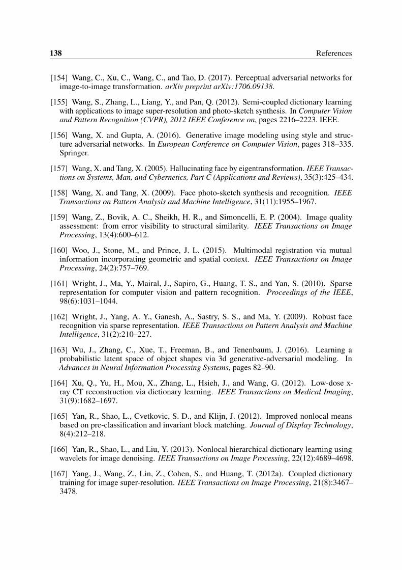
138 References
[154] Wang, C., Xu, C., Wang, C., and Tao, D. (2017). Perceptual adversarial networks forimage-to-image transformation. arXiv preprint arXiv:1706.09138.
[155] Wang, S., Zhang, L., Liang, Y., and Pan, Q. (2012). Semi-coupled dictionary learningwith applications to image super-resolution and photo-sketch synthesis. In Computer Visionand Pattern Recognition (CVPR), 2012 IEEE Conference on, pages 2216–2223. IEEE.
[156] Wang, X. and Gupta, A. (2016). Generative image modeling using style and struc-ture adversarial networks. In European Conference on Computer Vision, pages 318–335.Springer.
[157] Wang, X. and Tang, X. (2005). Hallucinating face by eigentransformation. IEEE Transac-tions on Systems, Man, and Cybernetics, Part C (Applications and Reviews), 35(3):425–434.
[158] Wang, X. and Tang, X. (2009). Face photo-sketch synthesis and recognition. IEEETransactions on Pattern Analysis and Machine Intelligence, 31(11):1955–1967.
[159] Wang, Z., Bovik, A. C., Sheikh, H. R., and Simoncelli, E. P. (2004). Image qualityassessment: from error visibility to structural similarity. IEEE Transactions on ImageProcessing, 13(4):600–612.
[160] Woo, J., Stone, M., and Prince, J. L. (2015). Multimodal registration via mutualinformation incorporating geometric and spatial context. IEEE Transactions on ImageProcessing, 24(2):757–769.
[161] Wright, J., Ma, Y., Mairal, J., Sapiro, G., Huang, T. S., and Yan, S. (2010). Sparserepresentation for computer vision and pattern recognition. Proceedings of the IEEE,98(6):1031–1044.
[162] Wright, J., Yang, A. Y., Ganesh, A., Sastry, S. S., and Ma, Y. (2009). Robust facerecognition via sparse representation. IEEE Transactions on Pattern Analysis and MachineIntelligence, 31(2):210–227.
[163] Wu, J., Zhang, C., Xue, T., Freeman, B., and Tenenbaum, J. (2016). Learning aprobabilistic latent space of object shapes via 3d generative-adversarial modeling. InAdvances in Neural Information Processing Systems, pages 82–90.
[164] Xu, Q., Yu, H., Mou, X., Zhang, L., Hsieh, J., and Wang, G. (2012). Low-dose x-ray CT reconstruction via dictionary learning. IEEE Transactions on Medical Imaging,31(9):1682–1697.
[165] Yan, R., Shao, L., Cvetkovic, S. D., and Klijn, J. (2012). Improved nonlocal meansbased on pre-classification and invariant block matching. Journal of Display Technology,8(4):212–218.
[166] Yan, R., Shao, L., and Liu, Y. (2013). Nonlocal hierarchical dictionary learning usingwavelets for image denoising. IEEE Transactions on Image Processing, 22(12):4689–4698.
[167] Yang, J., Wang, Z., Lin, Z., Cohen, S., and Huang, T. (2012a). Coupled dictionarytraining for image super-resolution. IEEE Transactions on Image Processing, 21(8):3467–3478.
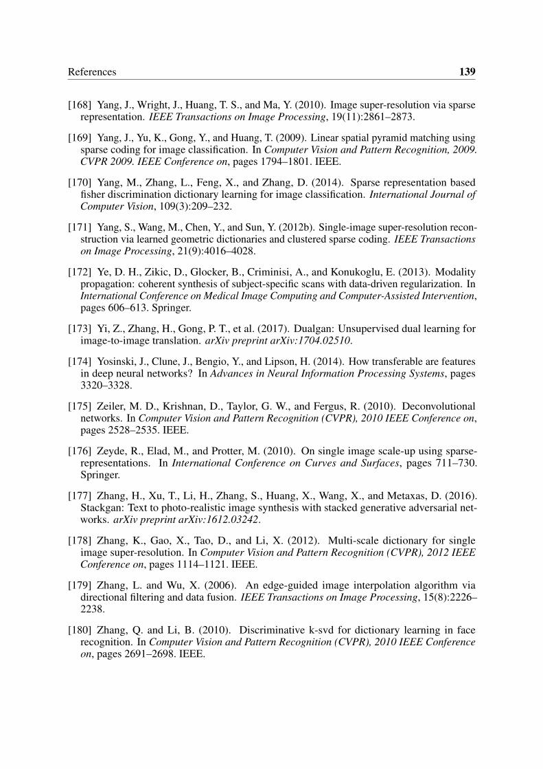
References 139
[168] Yang, J., Wright, J., Huang, T. S., and Ma, Y. (2010). Image super-resolution via sparserepresentation. IEEE Transactions on Image Processing, 19(11):2861–2873.
[169] Yang, J., Yu, K., Gong, Y., and Huang, T. (2009). Linear spatial pyramid matching usingsparse coding for image classification. In Computer Vision and Pattern Recognition, 2009.CVPR 2009. IEEE Conference on, pages 1794–1801. IEEE.
[170] Yang, M., Zhang, L., Feng, X., and Zhang, D. (2014). Sparse representation basedfisher discrimination dictionary learning for image classification. International Journal ofComputer Vision, 109(3):209–232.
[171] Yang, S., Wang, M., Chen, Y., and Sun, Y. (2012b). Single-image super-resolution recon-struction via learned geometric dictionaries and clustered sparse coding. IEEE Transactionson Image Processing, 21(9):4016–4028.
[172] Ye, D. H., Zikic, D., Glocker, B., Criminisi, A., and Konukoglu, E. (2013). Modalitypropagation: coherent synthesis of subject-specific scans with data-driven regularization. InInternational Conference on Medical Image Computing and Computer-Assisted Intervention,pages 606–613. Springer.
[173] Yi, Z., Zhang, H., Gong, P. T., et al. (2017). Dualgan: Unsupervised dual learning forimage-to-image translation. arXiv preprint arXiv:1704.02510.
[174] Yosinski, J., Clune, J., Bengio, Y., and Lipson, H. (2014). How transferable are featuresin deep neural networks? In Advances in Neural Information Processing Systems, pages3320–3328.
[175] Zeiler, M. D., Krishnan, D., Taylor, G. W., and Fergus, R. (2010). Deconvolutionalnetworks. In Computer Vision and Pattern Recognition (CVPR), 2010 IEEE Conference on,pages 2528–2535. IEEE.
[176] Zeyde, R., Elad, M., and Protter, M. (2010). On single image scale-up using sparse-representations. In International Conference on Curves and Surfaces, pages 711–730.Springer.
[177] Zhang, H., Xu, T., Li, H., Zhang, S., Huang, X., Wang, X., and Metaxas, D. (2016).Stackgan: Text to photo-realistic image synthesis with stacked generative adversarial net-works. arXiv preprint arXiv:1612.03242.
[178] Zhang, K., Gao, X., Tao, D., and Li, X. (2012). Multi-scale dictionary for singleimage super-resolution. In Computer Vision and Pattern Recognition (CVPR), 2012 IEEEConference on, pages 1114–1121. IEEE.
[179] Zhang, L. and Wu, X. (2006). An edge-guided image interpolation algorithm viadirectional filtering and data fusion. IEEE Transactions on Image Processing, 15(8):2226–2238.
[180] Zhang, Q. and Li, B. (2010). Discriminative k-svd for dictionary learning in facerecognition. In Computer Vision and Pattern Recognition (CVPR), 2010 IEEE Conferenceon, pages 2691–2698. IEEE.
140 References
[181] Zhang, Y., Jiang, Z., and Davis, L. S. (2013). Learning structured low-rank representa-tions for image classification. In Computer Vision and Pattern Recognition (CVPR), 2013IEEE Conference on, pages 676–683. IEEE.
[182] Zhen, X., Zhang, H., Islam, A., Bhaduri, M., Chan, I., and Li, S. (2017). Direct andsimultaneous estimation of cardiac four chamber volumes by multioutput sparse regression.Medical Image Analysis, 36:184–196.
[183] Zheng, F., Tang, Y., and Shao, L. (2016). Hetero-manifold regularisation for cross-modalhashing. IEEE Transactions on Pattern Analysis and Machine Intelligence.
[184] Zheng, M., Bu, J., Chen, C., Wang, C., Zhang, L., Qiu, G., and Cai, D. (2011). Graphregularized sparse coding for image representation. IEEE Transactions on Image Processing,20(5):1327–1336.
[185] Zhou, N., Shen, Y., Peng, J., and Fan, J. (2012). Learning inter-related visual dictionaryfor object recognition. In Computer Vision and Pattern Recognition (CVPR), 2012 IEEEConference on, pages 3490–3497. IEEE.
[186] Zhu, F. and Shao, L. (2014). Weakly-supervised cross-domain dictionary learning forvisual recognition. International Journal of Computer Vision, 109(1-2):42–59.
[187] Zhu, F., Shao, L., and Lin, M. (2013). Multi-view action recognition using localsimilarity random forests and sensor fusion. Pattern Recognition Letters, 34(1):20–24.
[188] Zhu, J.-Y., Krähenbühl, P., Shechtman, E., and Efros, A. A. (2016). Generative visualmanipulation on the natural image manifold. In European Conference on Computer Vision,pages 597–613. Springer.
[189] Zhu, J.-Y., Park, T., Isola, P., and Efros, A. A. (2017). Unpaired image-to-imagetranslation using cycle-consistent adversarial networks. arXiv preprint arXiv:1703.10593.
[190] Zoran, D. and Weiss, Y. (2011). From learning models of natural image patches to wholeimage restoration. In Computer Vision (ICCV), 2011 IEEE International Conference on,pages 479–486. IEEE.
Appendix A
Parallel Contrast Experiment
To quantitatively evaluate all proposed methods in this thesis, we further examine the per-formance of our methods including SiSCS, DOTE, WEENIE, WAG, and T-GAN for imagesynthesis from the IXI dataset of the selected subjects using PSNR (dB) and SSIM. Specifi-cally, we utilize the same experimental settings trained with the identical data for the parallelcomparison.
Implementation details: The models are evaluated on whole subject of brain MR imagesacquired from the IXI dataset. We randomly select 100 subjects involving pairwise PD-w andT2-w data for training, and then divide the reminding 478 subjects into two parts: 400 subjectsand 78 subjects. To verify the effectiveness of the weakly-supervised approaches, we simplyseparate 400 pairwise data to 200 unpaired images. That is, for each method, four groups ofexperiments (i.e., PD-w -> T2-w and T2-w -> PD-w training on the fixed 100 subject pairs;PD-w -> T2-w and T2-w -> PD-w training on the 100 subject pairs + 200 enhancing subjects)are performed. In particular, the proposed supervised algorithms cannot handle the imagealignment procedure. We keep the original pairs and input them for the enhancement.
We generate 20 groups of experiments corresponding to various proposed methods in twocases (i.e., PD-w -> T2-w and T2-w -> PD-w). The algorithms we used are signed as: SiSCS-100, SiSCS-300, DOTE-100, DOTE-300, WEENIE-100, WEENIE-300, WAG-100, WAG-300,T-GAN-100, and T-GAN-300. Models are trained using 100 subjects are represented as’-100’,and ’-300’ denotes that the enhanced 200 subjects are included in the training data. Table A.1shows the quantitative results (averaged PSNR and SSIM) on the IXI dataset. The proposedmethod T-GAN yields the best quantitative results for all cases, 4.51 dB (training with 100subjects for T2-w -> PD-w), 3.42 dB (training with 100 subjects for PD-w -> T2-w), 3.67 dB(training with 300 subjects for T2-w -> PD-w), and 3.06 dB (training with 300 subjects forPD-w -> T2-w) PSNR better than the worst case; 0.0578 (training with 100 subjects for T2-w-> PD-w), 0.0893 (training with 100 subjects for PD-w -> T2-w), 0.0637 (training with 300

142 Parallel Contrast Experiment
Metric(avg.) SiSCS-100 DOTE-100 WEENIE-100 WAG-100 T-GAN-100PD-w→ T2-w
PSNR (dB) 33.25 34.43 34.89 34.32 36.67SSIM 0.8611 0.8786 0.8801 0.8599 0.9492
T2-w→ PD-wPSNR (dB) 30.27 32.91 33.00 32.03 34.78
SSIM 0.8523 0.8614 0.8617 0.8549 0.9098Metric(avg.) SiSCS-300 DOTE-300 WEENIE-300 WAG-300 T-GAN-300
PD-w→ T2-wPSNR (dB) 33.98 37.09 37.02 35.01 37.04
SSIM 0.8700 0.9100 0.8927 0.8612 0.9523T2-w→ PD-w
PSNR (dB) 31.45 35.07 34.93 32.96 35.12SSIM 0.8597 0.9178 0.9050 0.8578 0.9215
Table A.1 Quantitative evaluation (PSNR (dB) and SSIM): SiSCS, DOTE, WEENIE, WAG,and T-GAN on the IXI dataset.
subjects for T2-w -> PD-w), and 0.0911 (training with 300 subjects for PD-w -> T2-w) SSIMbetter than the worst case.