Radiomics as Biomarker in Multi-Modality Treatment of Locally ...
275
Zurich Open Repository and Archive University of Zurich University Library Strickhofstrasse 39 CH-8057 Zurich www.zora.uzh.ch Year: 2021 Radiomics as Biomarker in Multi-Modality Treatment of Locally Advanced Non-Small Cell Lung Cancer Vuong, Diem Posted at the Zurich Open Repository and Archive, University of Zurich ZORA URL: https://doi.org/10.5167/uzh-211927 Dissertation Published Version Originally published at: Vuong, Diem. Radiomics as Biomarker in Multi-Modality Treatment of Locally Advanced Non-Small Cell Lung Cancer. 2021, University of Zurich, Faculty of Science.
-
Upload
khangminh22 -
Category
Documents
-
view
0 -
download
0
Transcript of Radiomics as Biomarker in Multi-Modality Treatment of Locally ...
Zurich Open Repository andArchiveUniversity of ZurichUniversity LibraryStrickhofstrasse 39CH-8057 Zurichwww.zora.uzh.ch
Year: 2021
Radiomics as Biomarker in Multi-Modality Treatment of Locally AdvancedNon-Small Cell Lung Cancer
Vuong, Diem
Posted at the Zurich Open Repository and Archive, University of ZurichZORA URL: https://doi.org/10.5167/uzh-211927DissertationPublished Version
Originally published at:Vuong, Diem. Radiomics as Biomarker in Multi-Modality Treatment of Locally Advanced Non-SmallCell Lung Cancer. 2021, University of Zurich, Faculty of Science.
Radiomics as Biomarker in Multi-Modality Treatment of Locally Advanced
Non-Small Cell Lung Cancer
Dissertation
zur
Erlangung der naturwissenschaftlichen Doktorwürde
(Dr. sc. nat.)
vorgelegt der
Mathematisch-naturwissenschaftlichen Fakultät
der
Universität Zürich
von
Diem Vuong
von
Basel BS
Promotionskommission
Prof. Dr. Jan Unkelbach (Vorsitz)
Dr. Stephanie Tanadini-Lang (Leitung der Dissertation)
Prof. Dr. Jürg Osterwalder
Zürich, 2021


Radiomics as Biomarker in Multi-Modality Treatment of Locally
Advanced Non-Small Cell Lung Cancer

Abstract
In 2018, more than 1.7 million deaths worldwide were caused by lung cancer, of which approxi-mately 80-85% were classified as non-small-cell lung cancer (NSCLC).1 Stage III locally advancedNSCLC is known for its heterogeneous tumor representations, i.e. primary tumor extension andsizes (T1-T4), involvement of hilar or mediastinal lymph nodes (N1-N3)2,3 as well as variabilityat the genetic level4. Despite multi-modal treatment, these patients have a poor prognosis (from10-30% at 5 years).2 Understanding and quantifying the heterogeneous tumor phenotype canhelp guide treatment decisions for individual patients.
Today, the accelerated growth of data mining strategies is fueled by the large amount of BigData being collected in cancer research.5 Within the course of treatment, patient data rangingfrom electronic records to genomic sequencing are readily collected5 which in turn imposes thechallenge of appropriately, efficiently, and reliably incorporating this vast, primarily unstructureddata into an informed treatment decision. In this context, medical imaging has been recognizedas a resource that is used in a limited and mostly qualitative manner.
Imaging biomarkers based on radiomics have attracted considerable interest in cancer research,with the number of publications increasing exponentially over the past six years.2 Unlike con-ventional radiological image analysis, this methodology is considered more objective and allowsfor a comprehensive description of all available 3D spatial information in medical images, suchas shape, intensity, texture, and filter-based properties of a given region of interest. Radiomics istherefore assumed to potentially complement current efforts in the field of precision medicine: toachieve a comprehensive analysis of the cancer phenotype in order to tailor treatment to patient-specific cancer characteristics. Nevertheless, this young research field has only sporadically madethe transition into clinical practice.6 Limited generalizability of the models, the lack of multi-centric datasets, the sensitivity of the features to imaging settings, and the interpretability ofthe features have been identified as hurdles for its incorporation into clinics.
This dissertation addresses these challenges using locally advanced NSCLC as an example whileproviding a multifaceted quantitative view of the disease. For this purpose, I collected computedtomography (CT) and positron emission tomography (PET) imaging data originating from aprospective Swiss multicentric randomized trial (SAKK-16/007). The prospective clinical natureof this trial provided an ideal real-world scenario to examine the challenges in implementingradiomics into a clinical setting. This thesis is divided into four parts.
In a first part, I studied the tumor location in the lung as a prognostic factor and developedfrequency weighted cumulative status maps as a novel methodology to define regions of worsetwo years overall survival (OS). I developed a software solution to map the primary tumor spatialextent from a patient to a reference patient CT scans, by performing deformable image registra-tion. The decreased survival areas were found to be located centrally close to the mediastinum.These regions were found to be differ between treatment regimens (radiochemotherapy aloneor with surgery). Closer distance of the primary tumor to a high-risk region was found to beassociated with worse outcome in the radiochemotherapy cohort.
In a second part, I evaluated the sensitivity of radiomics to variability in imaging settings that arecommon in a multicentric imaging dataset. I found that only a subset of PET radiomic featureswas stable across PET images from PET/CT and PET/MR scans. Shape and intensity features
were found more stable compared to texture and wavelet features (only 50% and 28%, respec-tively). In CT radiomics, I examined the effect of convolution kernel variation and found thatfeature stability was influenced more by tissue type and to a lesser extent by lung disease type,with 50% of features being transferable across all three lung diseases. For NSCLC, I includedthen further three effects from chest CT imaging relevant for radiomics (delineation variability,motion, contrast). The highest feature stability was observed for delineation variability whereaslowest stability was found when using different convolution kernels. In addition, I observed thatonly 10% of the features were considered stable across all four effects.These low robustness rates pose the challenge to optimally incorporate robustness studies intomulticentric radiomics models. Two approaches are commonly found in the literature: a) dis-carding unstable features but using all patients and b) including all features but using a smallerpatient subcohort imaged with similar imaging settings. In the third part, these two approacheswere compared for the first time. Although I could not find a statistically significant differencein model performance on the validation set (AUC = 0.72 [0.48-0.95] and AUC = 0.79 [0.63-0.95],respectively, p = 0.59), the model with the standardized imaging settings was preferred becauseits lower range 95% confidence interval was above 0.5 (random predictor). The fact that its finalmodel consisted of features previously identified as unstable suggests that excluding featuresbased on their robustness may result in suboptimal models.Nowadays, features are becoming more complex to quantify tumor phenotype more accuratelyat the expense of poor interpretability. In part four, I introduced radiomics feature activationmaps as a new tool to identify the spatial region where a particular feature is activated withina region of interest, thus supporting feature interpretation. Using the example of peritumoralradiomics to predict histology of NSCLC, I showed that the rim region (the region adjacent tothe tumor) was more informative compared to the tumor region for histology prediction.
In summary, in this dissertation I presented a multifaceted approach to study image-based fea-tures as prognostic factors for locally advanced NSCLC disease, a heterogeneous disease withpoor prognosis. I extended current findings in the radiomics literature by analyzing a patientcohort treated multimodally with surgery, in contrast to previous studies of patients treated withradiochemotherapy alone. The model performances I observed were comparable to reported mod-els. Furthermore, I showed that image-based heterogeneity was associated with poorer prognosis.At the same time, I addressed important key issues in multicentric radiomics modeling such asrobustness of CT and PET radiomics and optimal inclusion technique of robustness results in arobust multicenter radiomics model. Further, I introduced voxelized cumulative status maps aswell as radiomics features activation maps as novel methods to quantify tumor location withinthe lung and help interpret radiomics signatures, respectively.
6

Preface
This cumulative dissertation was carried out at the Department of Radiation Oncology of theUniversity Hospital Zurich. It begins with an introduction to the topics of lung cancer and medi-cal imaging. Both chapters convey the understanding of the radiomics chapter which describes itsprinciple and technical aspects. This is followed by two review articles that provide an overviewof the current state of the art in CT and PET radiomics and the correlation of radiomics withbiological biomarkers (Chapter 4 and 5, respectively). I am shared first author of the reviewin Chapter 4 published in the Quarterly Journal of Nuclear Medicine and Molecular Imagingand was co-author on the review in Chapter 5 which was written in the last half a year of myPhD and has not been published yet. Next, the aims and outline of this thesis are presentedfollowed by my original research. Chapter 7 represents my research recently submitted to Scien-tific Reports. In Chapter 8, my work is presented which was published in the Medical PhysicsJournal. In Chapter 9, a dissertation for the degree of Doctor of Medicine was conducted undermy supervision and was published in the British Journal of Radiology. Chapter 10 representsmy work published in the Medical Physics Journal while my study in Chapter 11 was publishedin Frontiers in Oncology. A discussion and outlook chapter concludes this thesis.My original research has been presented at national and international conferences. My workin Chapter 10 and 11 were selected for oral presentations at national conferences. In addition,the work in Chapter 10 also won the Best Poster Award at the 2019 European Lung CancerCongress.

Contributions
First-author publications included in this dissertation
• Chapter 8: Vuong D, Tanadini-Lang S, Huellner MW, Veit-Haibach P, Unkelbach J, An-dratschke N, et al. Interchangeability of radiomic features between [18F]-FDG PET/CT and[18F]-FDG PET/MR. Med Phys. 2019;46(4):1677-1685. doi: 10.1002/mp.13422
• Chapter 10: Vuong D, Bogowicz M, Denzler S, Oliveira C, Foerster R, Amstutz F, et al.Comparison of robust to standardized CT radiomics models to predict overall survival fornon-small cell lung cancer patients. Med Phys. 2020;47(9):4045-4053. doi: 10.1002/mp.14224
• Chapter 11: Vuong D, Tanadini-Lang S, Wu Z, Marks R, Unkelbach J, Hillinger S, etal. Radiomics Feature Activation Maps as a New Tool for Signature Interpretability. FrontOncol. 2020;10:578895. doi: 10.3389/fonc.2020.578895
Shared first-author publication included in this dissertation
• Chapter 4: Bogowicz M*, Vuong D*, Huellner MW, Pavic M, Andratschke N, Gabrys HS,et al. CT radiomics and PET radiomics: Ready for clinical implementation? Q J Nucl MedMol Imaging. 2019;63(4):355-370. doi: 10.23736/S1824-4785.19.03192-3
Co-authored publication included in this dissertation
• Chapter 9: Denzler S, Vuong D, Bogowicz M, Pavic M, Frauenfelder T, Thierstein S, etal. Impact of CT convolution kernel on robustness of radiomic features for different lungdiseases and tissue types. Br J Radiol. 2021;94(1120):20200947. doi: 10.1259/bjr.20200947
Publications not included in this dissertation
• Vils A, Bogowicz M, Tanadini-Lang S, Vuong D, Saltybaeva N, Kraft J, et al. Radiomic Anal-ysis to Predict Outcome in Recurrent Glioblastoma Based on Multi-Center MR Imaging Fromthe Prospective DIRECTOR Trial. Front Oncol. 2021;11. doi: 10.3389/fonc.2021.636672
• Pavic M, Bogowicz M, Kraft J, Vuong D, Mayinger M, Kroeze SGC, et al. FDG PET versusCT radiomics to predict outcome in malignant pleural mesothelioma patients. EJNMMI Res.2020;10(1):81. doi: 10.1186/s13550-020-00669-3
• Basler L, Gabryś HS, Hogan SA, Pavic M, Bogowicz M, Vuong D, et al. Radiomics, Tu-mor Volume, and Blood Biomarkers for Early Prediction of Pseudoprogression in Patientswith Metastatic Melanoma Treated with Immune Checkpoint Inhibition. Clin Cancer Res.2020;26(16):4414-4425. doi: 10.1158/1078-0432.CCR-20-0020
• Tanadini-Lang S, Balermpas P, Guckenberger M, Pavic M, Riesterer O, Vuong D, et al.Radiomic biomarkers for head and neck squamous cell carcinoma. Strahlentherapie undOnkol. 2020;196(10):868-878. doi: 10.1007/s00066-020-01638-4
8

Acknowledgements
I would like to take this opportunity to thank the people who have supported, guided, andmentored me in whole or in part during this time.I would like to thank my advisor, Dr. Stephanie Tanadini-Lang, for her continuous supportthroughout my PhD and for suggesting the topic. I would also like to thank the other membersof my PhD committee, Prof. Jan Unkelbach and Prof. Jürg Osterwalder, for their inputs duringproject discussions. I would like to thank all physicists, clinicians, biologists, and RTTs in theDepartment of Radiation Oncology at the University Hospital Zurich for their contributions tothe project. In particular, I would like to mention: Dr. med. Matea Pavic and Verena Waller fortheir feedback on the clinical and biological part of the dissertation. I would also like to thankall members of our growing radiomics group for their support and discussions. In particular, Iwould like to mention the students who chose one of our projects and gave me the opportunityto supervise and mentor them: Florian Amstutz, Sarah Denzler, Carol Oliveira, Robert Marks,and Ze Wu. Certainly, I learned at least as much as they did.I would also like to thank Prof. Carsten Brink for his support and dedication during my 6-monthresearch stay at Odense University Hospital in Denmark. Strange times can sometimes lead togreat collaborations. It was always a pleasure to work with and learn from you. I would also liketo thank everyone in the Department of Oncology at Odense University Hospital for collaboratingon this research project.I would like to especially thank my direct supervisor, Dr. Marta Bogowicz. There are almost nowords to describe how grateful I am to have had the opportunity to work closely with her formore than 3.5 years. Her passion and dedication were always a real inspiration to me and I couldnot have asked for a better person to share all the ups and downs of this PhD project with.Finally, I would like to thank my friends and family for their support during all stages of myPhD. I would like to mention a few in particular: Jonas for our weekly lunch conversations aboutR and modeling, Rita for designing the cover of my PhD thesis, Alex for parsing through theraw text and Simon for his continuous support and encouragement over all these years. Last butnot least, to my mother, who taught me important soft skills: Be brave, be respectful, be kind.She is the quiet, selfless fighter who did everything she could that I can pursue my interests. Forall her sacrifices, I will be forever grateful to her.
9


Contents
Abstract 5
Preface 7
1 Lung cancer 15
1.1 The lungs: anatomy and physiology . . . . . . . . . . . . . . . . . . . . . . . . 15
1.2 Hallmarks of cancer . . . . . . . . . . . . . . . . . . . . . . . . . . . . . . . . . 16
1.3 Epidemiology . . . . . . . . . . . . . . . . . . . . . . . . . . . . . . . . . . . . . 16
1.4 Diagnosis and staging . . . . . . . . . . . . . . . . . . . . . . . . . . . . . . . . 17
1.5 Therapy options . . . . . . . . . . . . . . . . . . . . . . . . . . . . . . . . . . . 18
2 Medical imaging 21
2.1 Photon-matter interactions . . . . . . . . . . . . . . . . . . . . . . . . . . . . . 22
2.2 Computed tomography . . . . . . . . . . . . . . . . . . . . . . . . . . . . . . . 22
2.3 Positron emission tomography . . . . . . . . . . . . . . . . . . . . . . . . . . . 23
2.4 Hybrid imaging system . . . . . . . . . . . . . . . . . . . . . . . . . . . . . . . 24
2.5 Image registration . . . . . . . . . . . . . . . . . . . . . . . . . . . . . . . . . . 24
3 Radiomics 25
3.1 Imaging and delineation . . . . . . . . . . . . . . . . . . . . . . . . . . . . . . . 26
3.2 Image processing . . . . . . . . . . . . . . . . . . . . . . . . . . . . . . . . . . . 26
3.3 Feature extraction . . . . . . . . . . . . . . . . . . . . . . . . . . . . . . . . . . 26
3.4 Modeling . . . . . . . . . . . . . . . . . . . . . . . . . . . . . . . . . . . . . . . 26
3.4.1 Feature reduction . . . . . . . . . . . . . . . . . . . . . . . . . . . . . . . 26
3.4.2 Feature selection . . . . . . . . . . . . . . . . . . . . . . . . . . . . . . . 27
3.4.3 Classification . . . . . . . . . . . . . . . . . . . . . . . . . . . . . . . . . 27
3.5 Validation . . . . . . . . . . . . . . . . . . . . . . . . . . . . . . . . . . . . . . 28
3.6 Challenges . . . . . . . . . . . . . . . . . . . . . . . . . . . . . . . . . . . . . . 29
4 CT radiomics and PET radiomics: ready for clinical implementation? 31
4.1 Abstract . . . . . . . . . . . . . . . . . . . . . . . . . . . . . . . . . . . . . . . 32
4.2 Introduction . . . . . . . . . . . . . . . . . . . . . . . . . . . . . . . . . . . . . 32
4.3 Radiomics . . . . . . . . . . . . . . . . . . . . . . . . . . . . . . . . . . . . . . 34
4.4 Materials and methods . . . . . . . . . . . . . . . . . . . . . . . . . . . . . . . 34
4.4.1 Robustness of radiomic features . . . . . . . . . . . . . . . . . . . . . . . 34
4.4.2 Factor influencing image quality . . . . . . . . . . . . . . . . . . . . . . 35
4.4.3 Clinical models . . . . . . . . . . . . . . . . . . . . . . . . . . . . . . . . 36
4.4.4 CT models . . . . . . . . . . . . . . . . . . . . . . . . . . . . . . . . . . 36
4.4.5 PET models . . . . . . . . . . . . . . . . . . . . . . . . . . . . . . . . . . 41
4.4.6 Combined image modalities . . . . . . . . . . . . . . . . . . . . . . . . . 45
4.5 Discussion . . . . . . . . . . . . . . . . . . . . . . . . . . . . . . . . . . . . . . 45
11
4.6 Conclusion . . . . . . . . . . . . . . . . . . . . . . . . . . . . . . . . . . . . . . 47
4.7 Supplement A: Overview of CT based robustness studies . . . . . . . . . . . . 48
4.8 Supplement B: Overview of PET based robustness studies . . . . . . . . . . . . 51
4.9 Supplement C: Phantom radiomics robustness studies . . . . . . . . . . . . . . 54
4.10 Supplement D: CT outcome models . . . . . . . . . . . . . . . . . . . . . . . . 55
4.11 Supplement E: PET outcome models . . . . . . . . . . . . . . . . . . . . . . . 57
5 Systematic review on the correlation of radiomics with tumor biomarker 59
5.1 Abstract . . . . . . . . . . . . . . . . . . . . . . . . . . . . . . . . . . . . . . . 60
5.2 Introduction . . . . . . . . . . . . . . . . . . . . . . . . . . . . . . . . . . . . . 60
5.3 Materials and methods . . . . . . . . . . . . . . . . . . . . . . . . . . . . . . . 60
5.3.1 Literature search . . . . . . . . . . . . . . . . . . . . . . . . . . . . . . . 61
5.3.2 Eligibility criteria . . . . . . . . . . . . . . . . . . . . . . . . . . . . . . . 61
5.3.3 Analysis . . . . . . . . . . . . . . . . . . . . . . . . . . . . . . . . . . . . 62
5.4 Results . . . . . . . . . . . . . . . . . . . . . . . . . . . . . . . . . . . . . . . . 62
5.4.1 Literature search, eligibility criteria and study selection . . . . . . . . . 62
5.4.2 CNS . . . . . . . . . . . . . . . . . . . . . . . . . . . . . . . . . . . . . . 63
5.4.3 Breast cancer . . . . . . . . . . . . . . . . . . . . . . . . . . . . . . . . . 70
5.4.4 Lung cancer . . . . . . . . . . . . . . . . . . . . . . . . . . . . . . . . . . 75
5.4.5 Gastrointestinal cancer . . . . . . . . . . . . . . . . . . . . . . . . . . . . 82
5.4.6 Liver cancer . . . . . . . . . . . . . . . . . . . . . . . . . . . . . . . . . . 87
5.4.7 Other cancers . . . . . . . . . . . . . . . . . . . . . . . . . . . . . . . . . 90
5.4.8 Feature interpretation . . . . . . . . . . . . . . . . . . . . . . . . . . . . 92
5.5 Discussion . . . . . . . . . . . . . . . . . . . . . . . . . . . . . . . . . . . . . . 95
5.6 Conclusion . . . . . . . . . . . . . . . . . . . . . . . . . . . . . . . . . . . . . . 95
5.7 Supplement: Query list . . . . . . . . . . . . . . . . . . . . . . . . . . . . . . . 96
5.8 Supplement: PRISMA checklist . . . . . . . . . . . . . . . . . . . . . . . . . . 97
5.9 Supplement: Interpretation table . . . . . . . . . . . . . . . . . . . . . . . . . . 100
6 Aims and outline 113
6.1 Aims . . . . . . . . . . . . . . . . . . . . . . . . . . . . . . . . . . . . . . . . . 114
6.2 Outline . . . . . . . . . . . . . . . . . . . . . . . . . . . . . . . . . . . . . . . . 114
7 Quantification of spatial distribution of primary tumors in the lung todevelop new prognostic biomarkers for locally advanced NSCLC 117
7.1 Abstract . . . . . . . . . . . . . . . . . . . . . . . . . . . . . . . . . . . . . . . 118
7.2 Introduction . . . . . . . . . . . . . . . . . . . . . . . . . . . . . . . . . . . . . 118
7.3 Materials and methods . . . . . . . . . . . . . . . . . . . . . . . . . . . . . . . 119
7.3.1 Patient and imaging data . . . . . . . . . . . . . . . . . . . . . . . . . . 119
7.3.2 Mapping of patient to reference . . . . . . . . . . . . . . . . . . . . . . . 119
7.3.3 Generation of decreased survival areas and outcome prediction . . . . . 120
7.4 Results . . . . . . . . . . . . . . . . . . . . . . . . . . . . . . . . . . . . . . . . 122
7.4.1 From fwCS map to decreased survival areas . . . . . . . . . . . . . . . . 122
7.4.2 Comparison between treatment regimens . . . . . . . . . . . . . . . . . . 122
7.4.3 Outcome prediction . . . . . . . . . . . . . . . . . . . . . . . . . . . . . 123
7.5 Discussion . . . . . . . . . . . . . . . . . . . . . . . . . . . . . . . . . . . . . . 124
7.6 Conclusion . . . . . . . . . . . . . . . . . . . . . . . . . . . . . . . . . . . . . . 125
7.7 Supplement A: Patient characteristics . . . . . . . . . . . . . . . . . . . . . . . 126
7.8 Supplement B: Frequency maps . . . . . . . . . . . . . . . . . . . . . . . . . . 127
7.9 Supplement C: Correlation distance with volume, T and N stage . . . . . . . . 128
12

CONTENTS
8 Interchangeability of radiomic features between [18F]–FDG PET/CT and[18F]–FDG PET/MR 129
8.1 Abstract . . . . . . . . . . . . . . . . . . . . . . . . . . . . . . . . . . . . . . . 130
8.2 Introduction . . . . . . . . . . . . . . . . . . . . . . . . . . . . . . . . . . . . . 130
8.3 Materials and methods . . . . . . . . . . . . . . . . . . . . . . . . . . . . . . . 132
8.3.1 Study population . . . . . . . . . . . . . . . . . . . . . . . . . . . . . . . 132
8.3.2 Image acquisition . . . . . . . . . . . . . . . . . . . . . . . . . . . . . . . 132
8.3.3 Segmentation . . . . . . . . . . . . . . . . . . . . . . . . . . . . . . . . . 132
8.3.4 Radiomic features and statistical analysis . . . . . . . . . . . . . . . . . 132
8.4 Results . . . . . . . . . . . . . . . . . . . . . . . . . . . . . . . . . . . . . . . . 133
8.4.1 Segmentation . . . . . . . . . . . . . . . . . . . . . . . . . . . . . . . . . 133
8.4.2 Stable features of 4DPETMR and PETCT–PETMR . . . . . . . . . . . 133
8.4.3 Shared stable radiomic features between 4DPETMR and PETCT–PETMR 134
8.5 Discussion . . . . . . . . . . . . . . . . . . . . . . . . . . . . . . . . . . . . . . 135
8.5.1 4DPETMR and PETCT–PETMR . . . . . . . . . . . . . . . . . . . . . 136
8.5.2 Feature stability influences in PETCT–PETMR . . . . . . . . . . . . . . 136
8.5.3 Comparison of 4DPETMR and PETCT–PETMR . . . . . . . . . . . . . 137
8.5.4 Limitations . . . . . . . . . . . . . . . . . . . . . . . . . . . . . . . . . . 137
8.5.5 Recommendation . . . . . . . . . . . . . . . . . . . . . . . . . . . . . . . 138
8.6 Conclusion . . . . . . . . . . . . . . . . . . . . . . . . . . . . . . . . . . . . . . 138
8.7 Supplement A: Radiomic features robustness ICC results . . . . . . . . . . . . 139
8.8 Supplement B: Discretization method analysis . . . . . . . . . . . . . . . . . . 151
9 Impact of CT convolution kernel on robustness of radiomic features fordifferent lung diseases and tissue types 153
9.1 Abstract . . . . . . . . . . . . . . . . . . . . . . . . . . . . . . . . . . . . . . . 154
9.2 Introduction . . . . . . . . . . . . . . . . . . . . . . . . . . . . . . . . . . . . . 154
9.3 Materials and methods . . . . . . . . . . . . . . . . . . . . . . . . . . . . . . . 155
9.3.1 Studied cohorts of patients . . . . . . . . . . . . . . . . . . . . . . . . . 155
9.3.2 Image acquisition . . . . . . . . . . . . . . . . . . . . . . . . . . . . . . . 155
9.3.3 Delineation . . . . . . . . . . . . . . . . . . . . . . . . . . . . . . . . . . 156
9.3.4 Radiomics analysis and image pre-processing . . . . . . . . . . . . . . . 156
9.4 Results . . . . . . . . . . . . . . . . . . . . . . . . . . . . . . . . . . . . . . . . 157
9.4.1 Delineation . . . . . . . . . . . . . . . . . . . . . . . . . . . . . . . . . . 157
9.4.2 Stability of radiomic features within same disease . . . . . . . . . . . . . 159
9.4.3 Transferability of stable features across tissue types . . . . . . . . . . . . 159
9.4.4 Transferability of stable features across disease types . . . . . . . . . . . 160
9.5 Discussion . . . . . . . . . . . . . . . . . . . . . . . . . . . . . . . . . . . . . . 161
9.6 Conclusion . . . . . . . . . . . . . . . . . . . . . . . . . . . . . . . . . . . . . . 162
9.7 Supplement A: Volume correlation of stable features . . . . . . . . . . . . . . . 163
9.8 Supplement B: ICC Results . . . . . . . . . . . . . . . . . . . . . . . . . . . . . 164
10 Comparison of robust to standardized CT radiomics models to predictoverall survival for non-small cell lung cancer patients 201
10.1 Abstract . . . . . . . . . . . . . . . . . . . . . . . . . . . . . . . . . . . . . . . 202
10.2 Introduction . . . . . . . . . . . . . . . . . . . . . . . . . . . . . . . . . . . . . 202
10.3 Materials and methods . . . . . . . . . . . . . . . . . . . . . . . . . . . . . . . 203
10.3.1 Workflow . . . . . . . . . . . . . . . . . . . . . . . . . . . . . . . . . . . 203
10.3.2 Study cohort . . . . . . . . . . . . . . . . . . . . . . . . . . . . . . . . . 204
10.3.3 Imaging data . . . . . . . . . . . . . . . . . . . . . . . . . . . . . . . . . 204
10.3.4 Robustness studies . . . . . . . . . . . . . . . . . . . . . . . . . . . . . . 204
13
10.3.5 Delineation, data preprocessing, and radiomics calculation . . . . . . . . 20510.3.6 Statistical analysis . . . . . . . . . . . . . . . . . . . . . . . . . . . . . . 206
10.4 Results . . . . . . . . . . . . . . . . . . . . . . . . . . . . . . . . . . . . . . . . 20610.4.1 Robustness studies . . . . . . . . . . . . . . . . . . . . . . . . . . . . . . 20610.4.2 Model comparison . . . . . . . . . . . . . . . . . . . . . . . . . . . . . . 206
10.5 Discussion . . . . . . . . . . . . . . . . . . . . . . . . . . . . . . . . . . . . . . 20810.6 Conclusion . . . . . . . . . . . . . . . . . . . . . . . . . . . . . . . . . . . . . . 20910.7 Supplement A: Model data characteristics . . . . . . . . . . . . . . . . . . . . . 21010.8 Supplement B: Robustness studies . . . . . . . . . . . . . . . . . . . . . . . . . 21110.9 Supplement C: ICC Results . . . . . . . . . . . . . . . . . . . . . . . . . . . . . 21310.10 Supplement D: Validation with different imaging setting . . . . . . . . . . . . . 225
11 Radiomics feature activation maps as a new tool for signature interpretability 227
11.1 Abstract . . . . . . . . . . . . . . . . . . . . . . . . . . . . . . . . . . . . . . . 22811.2 Introduction . . . . . . . . . . . . . . . . . . . . . . . . . . . . . . . . . . . . . 22811.3 Materials and methods . . . . . . . . . . . . . . . . . . . . . . . . . . . . . . . 229
11.3.1 Patient and imaging characteristics . . . . . . . . . . . . . . . . . . . . . 22911.3.2 Delineation . . . . . . . . . . . . . . . . . . . . . . . . . . . . . . . . . . 23011.3.3 Robustness study . . . . . . . . . . . . . . . . . . . . . . . . . . . . . . . 23011.3.4 Radiomics . . . . . . . . . . . . . . . . . . . . . . . . . . . . . . . . . . . 23011.3.5 Statistical analysis for global radiomics . . . . . . . . . . . . . . . . . . . 23011.3.6 Creation of activation maps based on local radiomics . . . . . . . . . . . 231
11.4 Results . . . . . . . . . . . . . . . . . . . . . . . . . . . . . . . . . . . . . . . . 23211.4.1 Modeling and validation . . . . . . . . . . . . . . . . . . . . . . . . . . . 23211.4.2 Model features . . . . . . . . . . . . . . . . . . . . . . . . . . . . . . . . 23311.4.3 Analysis of radiomics feature activation maps . . . . . . . . . . . . . . . 233
11.5 Discussion . . . . . . . . . . . . . . . . . . . . . . . . . . . . . . . . . . . . . . 23411.6 Conclusion . . . . . . . . . . . . . . . . . . . . . . . . . . . . . . . . . . . . . . 23611.7 Supplement A: Patient characteristics . . . . . . . . . . . . . . . . . . . . . . . 23711.8 Supplement B: Robustness studies . . . . . . . . . . . . . . . . . . . . . . . . . 23811.9 Supplement C: Comparison of feature selection methods . . . . . . . . . . . . . 23811.10 Supplement D: Creation of radiomics activation maps . . . . . . . . . . . . . . 240
12 Discussion and outlook 243
12.1 Main findings . . . . . . . . . . . . . . . . . . . . . . . . . . . . . . . . . . . . . 24312.1.1 Clinical aspects . . . . . . . . . . . . . . . . . . . . . . . . . . . . . . . . 24312.1.2 Technical aspects . . . . . . . . . . . . . . . . . . . . . . . . . . . . . . . 243
12.2 Quantification of primary lung tumor location as a prognostic factor . . . . . . 24412.3 Radiomics to predict outcome in locally advanced NSCLC . . . . . . . . . . . . 24512.4 Robustness of radiomic features . . . . . . . . . . . . . . . . . . . . . . . . . . 24612.5 Incorporation of robustness results in multicentric radiomic models . . . . . . . 24712.6 Interpretability of radiomics features . . . . . . . . . . . . . . . . . . . . . . . . 24712.7 Introduction of radiomics into the clinical routine . . . . . . . . . . . . . . . . 24812.8 Outlook . . . . . . . . . . . . . . . . . . . . . . . . . . . . . . . . . . . . . . . . 249
References 251
Curriculum Vitae 274
14
1Lung cancer
In this chapter, a short overview of the anatomy and physiology of the lungs is provided. Thehallmarks of cancer are introduced, and epidemiology of lung cancer is discussed. The chapterends with a summary of the current treatment options for lung cancer patients with a focus onadvanced stage NSCLC patients.
1.1 The lungs: anatomy and physiology
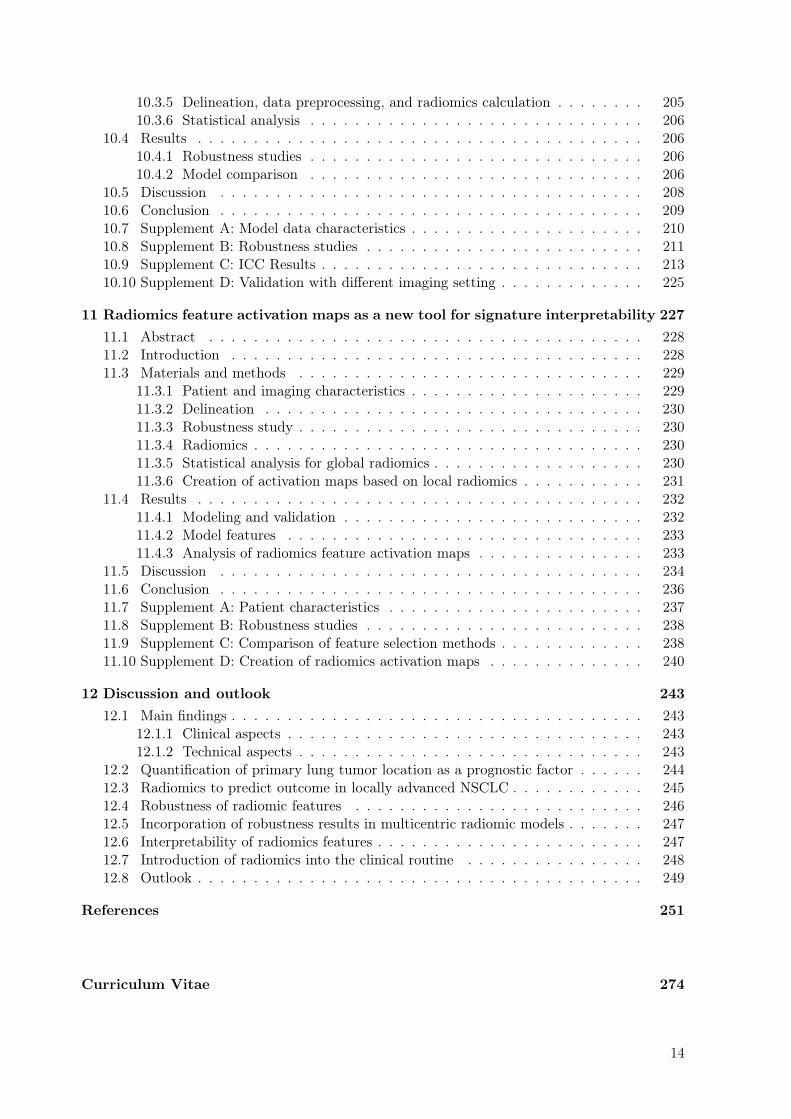
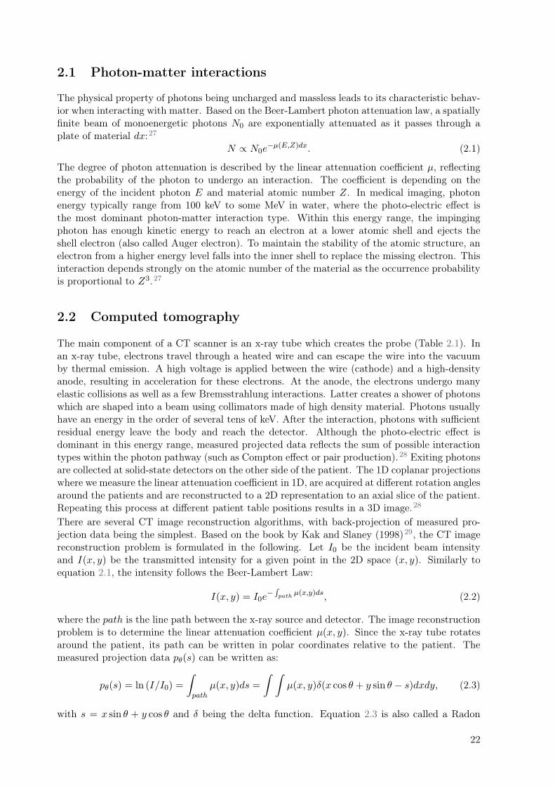
Figure 1.1: Anatomy of the lungs. Scheme from Anatomy andPhysiology.8
The main function of the lung isthe exchange of respiratory gases inthe blood system. They supply oxy-gen to the oxygen-depleted bloodand release resulting carbon dioxidefrom the body. Air flows through ahighly complex hierarchically struc-tured air-cavity system. From theoral cavities through the trachea viathe two main bronchi, which are con-nected to the two pyramid-shapedlungs. The lungs can be divided byfive subregions (lobes), three in theright lung and two in the left lung.They are spatially separated by fis-sures. From the bronchi, the gaspasses through the secondary and
tertiary bronchi to the bronchioles. As the air flows deeper into the lungs, the cavities be-come smaller and finer and finally reach the alveolus, the smallest instance of the respiratorysystem. The shape and size of the alveoli facilitates an extended surface area for efficient gasexchange (Figure 1.1).8
The movement of the lung is controlled by the diaphragm and the thoracic wall, which in turnis controlled by thoracic muscles. Pleura is the connective tissue between the lungs and otherorgans. The pleura consiss of two layers: the parietal and the visceral layer. The parietal layerforms the outer layer to the ribs and the visceratis layer borders the lung tissue. The latter layerconnects to the chest wall, the mediastinum (anatomical area containing the main organs besidesthe lung, i.e. heart, esophagus, trachea, etc.) and the diaphragm. The space between the twolayers is called the pleural cavity, in which the mesothelial cells of both pleural layers secretea pleural fluid that lubricates the surfaces of the two layers to reduce friction between the twolayers and creates a surface tension that maintains the position of the lungs against the thoracicwall. This adhesive property of the pleural fluid causes the lungs to expand as the chest wallexpands during ventilation, allowing the lungs to fill with air.8
Owing to its direct connection to the outside world, the lung is susceptible to pathogens thatcan cause development of lung diseases. The immune system has the task of protecting thebody from these external influences. The accessibility of the immune system is facilitated bya complex lymphatic system of vessels, cells, and organs, which transports excess body fluidsinto the bloodstream and filters pathogens from the blood. Therefore, damage in the lymphaticsystem such as caused by cancerous cells can elevate the risk of disease spread. Further, in thelymph (interstitial fluid), cells of the immune systems are transported. Cells of the immunesystem not only use lymphatic vessels to make their way from interstitial spaces back into thecirculation, but they also use lymph nodes as major staging areas for the development of criticalimmune responses.8
1.2 Hallmarks of cancer
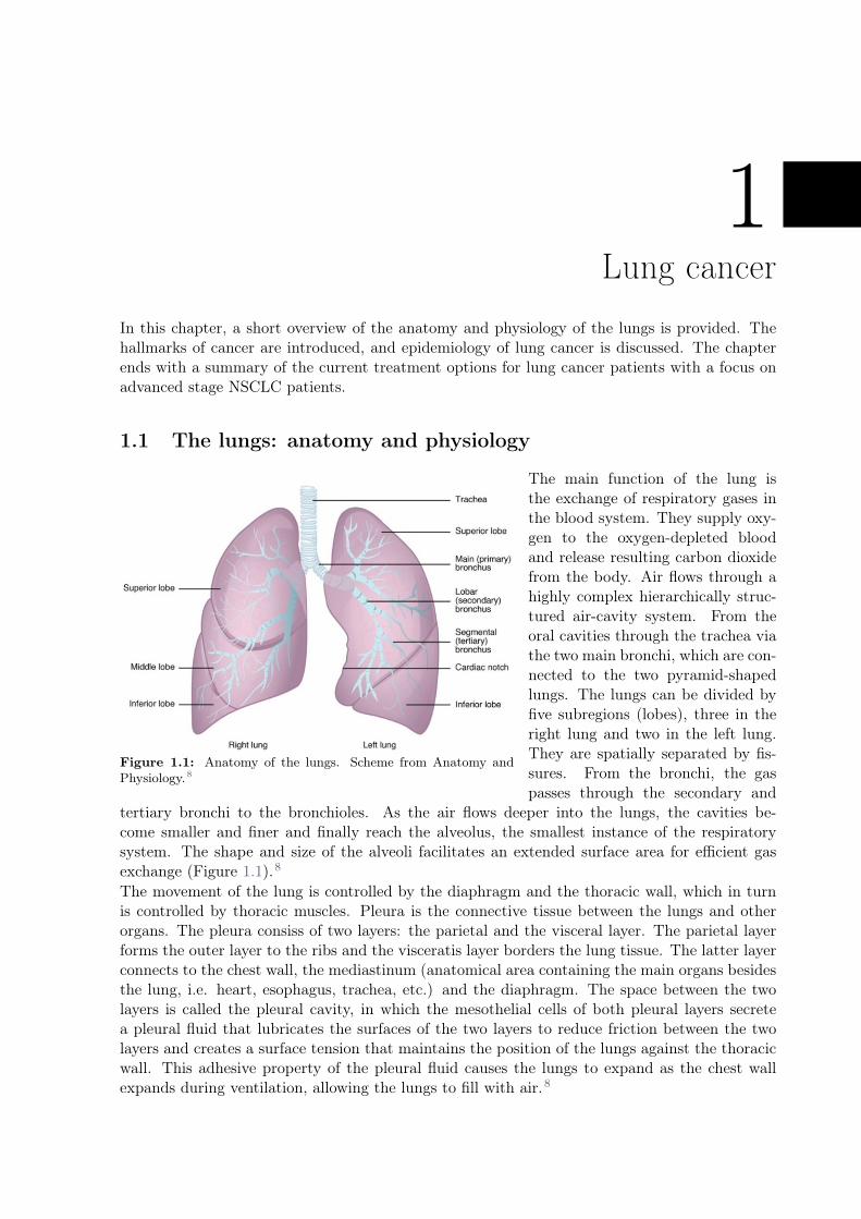
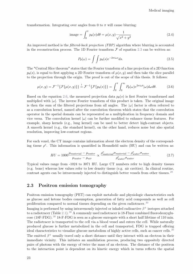
Figure 1.2: Hallmarks of cancer, taken fromHanahan and Weinberg et al.9
Carcinogenesis is a genetic or epigenetic process thatleads to the transformation of normal cells into cancercells.9 Extra- or intracellular influences can lead to ge-netic instability of the cells, which can cause furthermutations and eventually lead to cancer. Insufficientlyrepaired genetic defects carry the risk of an altered cellcycle pathway and thus of extensive malignant prolifera-tion.9 This process is not straightforward, i.e. a healthycell can develop into cancer cells in many ways. Thisis one of the reasons for the variety of cancer types andsubtypes9 This high intra- and inter-tumor heterogene-ity poses a challenge for the treatment of cancer. Hana-han and Weinberg proposed a catalog of the manifesta-tion of six traits common to most cancers and subtypes,also known as hallmarks of cancer (Figure 1.2).9
In healthy cells, a control system protects the cell fromuncontrolled proliferation facilitated by antigrowth sig-nals. Cancer cells have the tenacious ability to blockthese mechanisms and at the same time resist from ex-tracellular and intracellular signals to enforce cell death (apoptosis). Their uncontrolled rapidcell growth is fuelled by their ability of increased growth of vessels in the proximal vicinity (an-giogenesis) and their invasion of other tissues to gain access to nutrient- and oxygen-rich areasand thereby metastasize into distant anatomical locations. Hanahan and Weinberg have added ina revised version two hallmarks: list-reprogramming of energy metabolism and evading immunedestruction.10
1.3 Epidemiology
Lung cancer is particularly common in higher developed countries.1 In 2018, worldwide morethan two million new incidence of lung cancer were estimated, 1.7 million died of lung cancer.1
The predominant risk factor for the development of lung cancer is cigarette smoking, whichis responsible for 90% of cases.11 In addition, ionizing radiation, environmental toxins suchas asbestos, human immunodeficiency virus (HIV) infection, genetic factors have identified asrelevant risk factors.11
The patients’ symptoms may vary depending on the stage of the disease and its spread path.Typical symptoms such as coughing, haemoptysis, chest pain or shortness of breath (dyspnoea)are cancer non-specific and are therefore often initially associated with other lung diseases such
16

Lung cancer
as chronic obstructive pulmonary disease (COPD).12 As a result, lung cancer patients are oftendiagnosed at a late, more advanced stage13,14 which leads to additional challenges for a successfultreatment.
If cancer cells can freely pass the lymph nodes station, they can further travel to other distantanatomical location. Invasion into lymph nodes is easier to do than into blood vessels due tothe thinner thickness of the walls of the lymph vessels.15 However, when in the lymph system,cancer cells are faced with the immune system, which they can avoid in the blood vessels. Thetype of vascular invasion can also dictate where the metastasis will set – along with the lymphnodes or the blood vessels.15
1.4 Diagnosis and staging
Primary tumor (T)T1 tumor diameter < 3 cm diameter invasion more proximal than lobar
bronchusT2 Tumor > 3 cm diameter or tumor with pleural invasion or partial lung
atelectasis or proximal extent < 2 cm from the carinaT3 large tumor extension > 7 cm or invades one of the following: parietal
pleura, chest wall, diaphragm, phrenic nerve, mediastinal pleura, parietalpericardium; or tumour in the main bronchus less than 2 cm distal to thecarinal but without involvement of the carina; or associated atelectasis orobstructive pneumonitis of the entire lung or separate tumour nodule(s)in the same lobe as the primary
Lymph nodes (N)N1 Ipsilateral hilar and/or ipsilateral peribronchial nodal involvementN2 Ipsilateral mediastinal and/or subcarinal nodal
Table 1.1: Overview of 6th edition of the TNM classification (taken from Greene et al.16).
Different options are available to diagnose the patients. However, predominantly medical imaging-based approaches are used in clinical routine. X-ray and computed tomography (CT) scans areinitially used to identify suspicious tissues and are commonly used in screening programs17.Screening programs are not yet routine in Switzerland. This imaging is often followed by apositron emission tomography (PET) scan to find tumorous cluster in distant anatomical lo-cation. Invasive surgical tissue samples (biopsies) are then collected to investigate the type ofcancer cells. This surgical intervention is usually performed with a bronchoscopy, i.e. extractionof tissue samples through the air pathways. Lung cancer is categorized into two main histologicalgroups: small cell lung cancer (SCLC, 15% of all lung cancers) and non-small cell lung cancer(NSCLC, 85% of all lung cancers).18 NSCLCs are generally subcategorized into adenocarcinoma(ADC), squamous cell carcinoma (SCC), and large cell carcinoma.18 Owing to the late diagnosisof lung cancer, in advanced stage lung cancer a brain MRI scan is performed to reassure thatno cancerous clusters have developed in distant locations.19,20 Imaging is a key component ofstaging the disease of the patient and different imaging modalities have specific advantages fora given disease stage.
In the next step, the patient’s tumor is staged, reflecting the degree severity of the tumor.The conventional staging, also referred to as the TNM staging system, enables the clinician tocategorize the patient and decide on which treatment scheme to be offered. It is based on threemain parameters:
• T: spatial extent of the primary tumor (often maximal diameter) (1/2/3/4)
• N: lymph node involvement (0/1/2)
17
• M: presence of distant metastasis (0/1)
Based on the 6th edition of the TNM staging, locally advanced NSCLC have the following stagingT1N2M0, T2N2M0, T3N1M0, and T3N2M0 (see Table 1.1) which are aggregated into stage IIIdisease. Despite being outdated, the 6th edition is used in this project, because large part of theanalysed data comes from a prospective multicentric Swiss clinical study which based patientclassification on that edition (SAKK-16/007).
1.5 Therapy options
This section describes treatment options for stage III NSCLC patients since this was the patientselection criteria of this thesis. Stage III NSCLC patients are treated with multimodal therapyincluding surgery, radiation therapy and chemotherapy to provide the best chance of concurringthe advanced disease.
The goal of surgery in cancer treatment is the complete removal of cancer tissue. Due to thehierarchical structure of the lung, standard procedure is lobectomy, i.e. the removal of individuallung lobes.21 The limitations of surgery are accessibility to the cancer site but also patient relatedcomorbidities to undergo anaesthesia and surgery.21 Radiation therapy is a less invasive localtherapy option where patients are irradiated with ionizing radiation. Delivered ionizing radiationcan generate ions of the water molecules in the body. These so-called water radicals are highlyreactive and can potentially damage the deoxyribonucleic acid (DNA) coding cell genetic infor-mation and in result induce a cell death. Therefore, the aim of radiation therapy is to deliver theionizing radiation to the cancerous tissue only and spare healthy tissue. This is not trivial and islimited by the anatomically difficult, superimposed position of tumor and organs at risk withinthe beam direction. The third treatment type is chemotherapy. This systemic treatment canbe used in a neoadjuvant or adjuvant setting (before or after local therapy). Chemotherapeuticagents injected into the body aim to eradicate fast-growing cells, which is a typical characteristicof tumor cells. Therefore it can be used to remove micro-metastases and reduce tumor sizesbefore or remove remaining cancer cells after local therapy, as well as to prevent the disease frommetastasizing further to other anatomical regions.22
Only selected locally advanced NSCLC patients are offered surgery at the stage of diagnosisas 30%-50% of patients are considered inoperable.21 Therefore, treatment of locally advancedNSCLC patients is typically distinguished whether the primary tumor can be resected.
A purely surgical approach for locally advanced NSCLC patients has shown limited success (30%-70%, death or recurrence)21, therefore it is often combined with chemotherapy. Chemotherapycan be offered in a neoadjuvant or adjuvant setting showing both similar improvements comparedto surgery alone for OS and progression-free survival (PFS).23 Neoadjuvant chemotherapy canincrease the probability of full resection, however it also delays surgery, and if ineffective, tumorscan become inoperable, i.e., preoperative chemotherapy showed non-significant outcome differ-ence compared with surgery alone.21 In contrast, post-operative chemotherapy can kill remainingcancer cells and improved PFS and OS outcome. However, a large proportion of patients areat risk of tumor recurrence (40%).22 Hence, radiation therapy can be offered to improve localcontrol and survival to intensify local therapy.21
To summarize, for operable NSCLC patients, surgery has shown best local control with improve-ments by managing the development of distant metastasis by pre- or post-systemic therapy.However, OS and local control remains low.21
For inoperable patients, definitive chemoradiation has been the standard treatment for stage IIINSCLC patients until 2020.24 Radiation therapy serves as a local therapy and chemotherapyreduces micro-metastatic spread of the disease, and also acts as a radiosensitizer to increase the
18

Lung cancer
therapeutic index of radiation therapy, resulting in improvement of survival over supportive careor radiation therapy alone.21
Response to treatment varies widely between individuals, partially due to the observed hetero-geneity in tumor biology.21 Current research in cancer therapy has therefore focused on personal-izing treatment to the individual patient by incorporating knowledge of the tumor phenotype.21
Advances in genetic sequencing allow identification of prognostic biomarkers differentiating in-dividual patients. Driver mutations such as EGFR, ELM4-ALK, and KRAS, characteristic toelevate certain cancer hallmarks, have been identified and are actively integrated into the man-agement of advanced stage IV NSCLC patients and has been recently studied in stage III diseasewhere cetuximab in addition to chemotherapy showed significant increased survival compared tochemotherapy alone (p = 0.04).21 So far, these treatments tried to directly block mutations whichupregulate uncontrolled cancer growth. Additionally, cancer cells have the viscous ability to hidefrom the immune system making them invisible and therefore difficult to treat. Immunotherapy,and in particular immune-checkpoint inhibitors targeting the PD-1/PD-L1 axis, have gainedgreat importance especially in combination with radiochemotherapy.21 In 2020, the EuropeanSociety For Medical Oncology (ESMO) clinical practice guidelines were updated recommendingimmunotherapy after chemotherapy in unresectable locally advanced NSCLC patients with PD-L1 tumors and whose disease has not yet progressed.25
These personalized therapies often come along with side effects and rely on invasive biopsieswhich are pin-point measurements at a given timepoint. To date, it is still challenging to identifypatients that will benefit from these therapies. Considering the side effects that these therapiesindividually have, such as COPD, asthma, chronic bronchitis, pneumonitis, and fibrosis, it wouldbe highly desired to identify patients benefiting from the therapy and help clinicians to guidetreatment decisions.26
19

20

2Medical imaging
Advances in non-invasive medical imaging techniques to map morphological and functional fea-tures of a human body with higher resolution have enabled more precise and accurate diagnosisand therapies.20 Different modalities exist, such as CT, ultrasound, MRI, or PET. For lung can-cer treatment CT and PET imaging plays a critical role in the diagnosis and staging of patients.20
CT provides excellent spatial image resolution whereas PET imaging depicts the functional in-formation. Often these are acquired in combination, i.e. as PET/CT imaging.
Figure 2.1: Coronal slice of a patient CT, PET and MRI scans of a locally advanced stage lung cancer patientwith an irregularity in the right upper lung.
Medical imaging can be divided into four components: Probe, physical interaction, detection,and image formation. To image an object of interest, a probe must interact with matter (patient),triggering change in the probe as a result, which in turn is detected and converted into an image.
This chapter begins with a short overview of physical interactions of photons with matter, fol-lowed by introduction of CT and PET imaging structured in these four components. Finally,this chapter ends with hybrid imaging and image registration.
CT PET
Probe X-ray photons <1 MeV Radiopharmaceuticals, e.g. 18F FDGMatter interaction Photo electric effect Positron-electron annihilationDetection Measure cumulative sum of interac-
tion linear attenuation coefficientCoincidence detection
Image formation Filtered-back projection, iterative Iterative
Table 2.1: Overview of properties of medical imaging used in this thesis.
2.1 Photon-matter interactions
The physical property of photons being uncharged and massless leads to its characteristic behav-ior when interacting with matter. Based on the Beer-Lambert photon attenuation law, a spatiallyfinite beam of monoenergetic photons N0 are exponentially attenuated as it passes through aplate of material dx:27
N ∝ N0e−µ(E,Z)dx. (2.1)
The degree of photon attenuation is described by the linear attenuation coefficient µ, reflectingthe probability of the photon to undergo an interaction. The coefficient is depending on theenergy of the incident photon E and material atomic number Z. In medical imaging, photonenergy typically range from 100 keV to some MeV in water, where the photo-electric effect isthe most dominant photon-matter interaction type. Within this energy range, the impingingphoton has enough kinetic energy to reach an electron at a lower atomic shell and ejects theshell electron (also called Auger electron). To maintain the stability of the atomic structure, anelectron from a higher energy level falls into the inner shell to replace the missing electron. Thisinteraction depends strongly on the atomic number of the material as the occurrence probabilityis proportional to Z3.27
2.2 Computed tomography
The main component of a CT scanner is an x-ray tube which creates the probe (Table 2.1). Inan x-ray tube, electrons travel through a heated wire and can escape the wire into the vacuumby thermal emission. A high voltage is applied between the wire (cathode) and a high-densityanode, resulting in acceleration for these electrons. At the anode, the electrons undergo manyelastic collisions as well as a few Bremsstrahlung interactions. Latter creates a shower of photonswhich are shaped into a beam using collimators made of high density material. Photons usuallyhave an energy in the order of several tens of keV. After the interaction, photons with sufficientresidual energy leave the body and reach the detector. Although the photo-electric effect isdominant in this energy range, measured projected data reflects the sum of possible interactiontypes within the photon pathway (such as Compton effect or pair production).28 Exiting photonsare collected at solid-state detectors on the other side of the patient. The 1D coplanar projectionswhere we measure the linear attenuation coefficient in 1D, are acquired at different rotation anglesaround the patients and are reconstructed to a 2D representation to an axial slice of the patient.Repeating this process at different patient table positions results in a 3D image.28
There are several CT image reconstruction algorithms, with back-projection of measured pro-jection data being the simplest. Based on the book by Kak and Slaney (1998)29, the CT imagereconstruction problem is formulated in the following. Let I0 be the incident beam intensityand I(x, y) be the transmitted intensity for a given point in the 2D space (x, y). Similarly toequation 2.1, the intensity follows the Beer-Lambert Law:
I(x, y) = I0e−
∫path
µ(x,y)ds, (2.2)
where the path is the line path between the x-ray source and detector. The image reconstructionproblem is to determine the linear attenuation coefficient µ(x, y). Since the x-ray tube rotatesaround the patient, its path can be written in polar coordinates relative to the patient. Themeasured projection data pθ(s) can be written as:
pθ(s) = ln (I/I0) =
∫
path
µ(x, y)ds =
∫ ∫
µ(x, y)δ(x cos θ + y sin θ − s)dxdy, (2.3)
with s = x sin θ + y cos θ and δ being the delta function. Equation 2.3 is also called a Radon
22
Medical imaging
transformation. Integrating over angles from 0 to π will cause blurring:
image =
∫ π
0pθ(s)dθ = µ(x, y)
1√
x2 + y2(2.4)
An improved method is the filtered-back projection (FBP) algorithm where blurring is accountedin the reconstruction process. The 1D Fourier transform F of equation 2.3 can be written as:
Pθ(ω) =
∫ ∫
pθ(s)e−2πiωsds. (2.5)
The "Central Slice theorem" states that the Fourier transform of a line projection of a 2D functionpθ(s), is equal to first applying a 2D Fourier transform of µ(x, y) and then take the slice parallelto the projection through the origin. The proof is out of the scope of this thesis. It follows:
µ(x, y) = F−1{F{µ(x, y)}}!= F−1{F{pθ(s)}} =
∫ π
0
∫ ∞
0Pθ(ω)e
2πiωt|ω|dωdθ. (2.6)
Based on the equation 2.6, the measured projection data pθ(s) is first Fourier transformed andmultiplied with |ω|. The inverse Fourier transform of this product is taken. The original imageis then the sum of the filtered projections from all angles. The |ω| factor is often referred toas a convolution kernel, named after the convolution theorem which states that the convolutionoperator in the spatial domain can be represented as a multiplication in frequency domain andvice versa. The convolution kernel |ω| can be further modified to enhance tissue features. Forexample, sharp kernels (e.g., lung kernel) can be used to better detect high-contrast objects.A smooth kernel (e.g., the standard kernel), on the other hand, reduces noise but also spatialresolution, improving low-contrast regions.
For each voxel, the CT image contains information about the electron density of the correspond-ing tissue ρe. This information is quantified in Hounsfield units (HU) and can be written as:
HU = 1000µmaterial − µwater
µwater − µair∝
ρematerialσmaterial − ρewaterσwater
ρewaterσwater. (2.7)
Typical values range from -1024 to 3071 HU. Large CT numbers refer to high density tissues(e.g. bone) whereas low values refer to low density tissue (e.g. air cavities). In clinical routine,contrast agents can be intravenously injected to distinguish better vessels from other tissues.28
2.3 Positron emission tomography
Positron emission tomography (PET) can exploit metabolic and physiologic characteristics suchas glucose and ketone bodies consumption, generation of fatty acid compounds as well as cellproliferation compared to normal tissues depending on the given radiotracer.30
Imaging is performed by using intravenously injected or inhaled radioactive β+ isotopes attachedto a radiotracer (Table 2.1).30 A commonly used radiotracer is 18-Fluor combined fluorodeoxyglu-cose (18F-FDG).30 18-F-FDG is seen as a glucose surrogate with a short half lifetime of 110 min.The radiotracer is transported to the cell via a blood vessel and enters the cell. While naturallyproduced glucose is further metabolized in the cell and transported, FDG is trapped offeringideal characteristics to visualize glucose metabolism of highly active cells, such as cancer cells.30
The emitted β+ usually travel only a short distance until they interact with an electron in theirimmediate vicinity. This initiates an annihilation process, producing two oppositely directedpairs of photons with the energy of twice the mass of an electron. The distance of the positronto the interaction point is dependent on its kinetic energy which in turns reflects the spatial
23
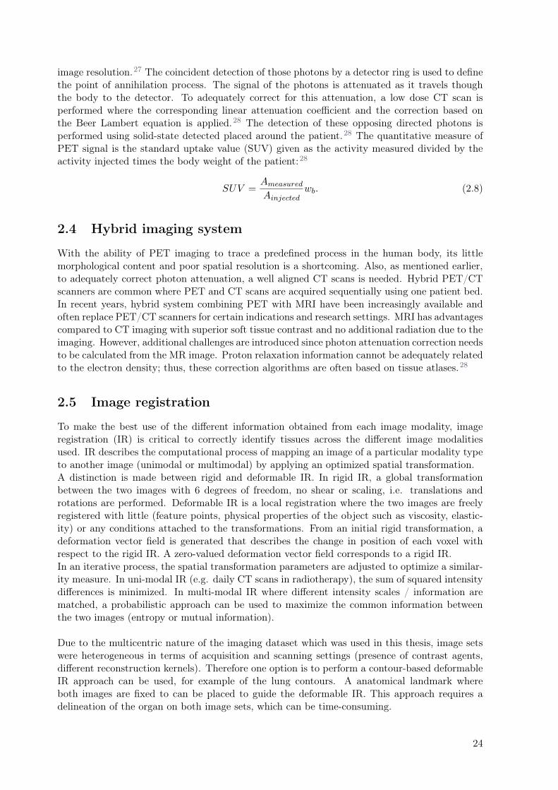
image resolution.27 The coincident detection of those photons by a detector ring is used to definethe point of annihilation process. The signal of the photons is attenuated as it travels thoughthe body to the detector. To adequately correct for this attenuation, a low dose CT scan isperformed where the corresponding linear attenuation coefficient and the correction based onthe Beer Lambert equation is applied.28 The detection of these opposing directed photons isperformed using solid-state detected placed around the patient.28 The quantitative measure ofPET signal is the standard uptake value (SUV) given as the activity measured divided by theactivity injected times the body weight of the patient:28
SUV =Ameasured
Ainjected
wb. (2.8)
2.4 Hybrid imaging system
With the ability of PET imaging to trace a predefined process in the human body, its littlemorphological content and poor spatial resolution is a shortcoming. Also, as mentioned earlier,to adequately correct photon attenuation, a well aligned CT scans is needed. Hybrid PET/CTscanners are common where PET and CT scans are acquired sequentially using one patient bed.In recent years, hybrid system combining PET with MRI have been increasingly available andoften replace PET/CT scanners for certain indications and research settings. MRI has advantagescompared to CT imaging with superior soft tissue contrast and no additional radiation due to theimaging. However, additional challenges are introduced since photon attenuation correction needsto be calculated from the MR image. Proton relaxation information cannot be adequately relatedto the electron density; thus, these correction algorithms are often based on tissue atlases.28
2.5 Image registration
To make the best use of the different information obtained from each image modality, imageregistration (IR) is critical to correctly identify tissues across the different image modalitiesused. IR describes the computational process of mapping an image of a particular modality typeto another image (unimodal or multimodal) by applying an optimized spatial transformation.A distinction is made between rigid and deformable IR. In rigid IR, a global transformationbetween the two images with 6 degrees of freedom, no shear or scaling, i.e. translations androtations are performed. Deformable IR is a local registration where the two images are freelyregistered with little (feature points, physical properties of the object such as viscosity, elastic-ity) or any conditions attached to the transformations. From an initial rigid transformation, adeformation vector field is generated that describes the change in position of each voxel withrespect to the rigid IR. A zero-valued deformation vector field corresponds to a rigid IR.In an iterative process, the spatial transformation parameters are adjusted to optimize a similar-ity measure. In uni-modal IR (e.g. daily CT scans in radiotherapy), the sum of squared intensitydifferences is minimized. In multi-modal IR where different intensity scales / information arematched, a probabilistic approach can be used to maximize the common information betweenthe two images (entropy or mutual information).
Due to the multicentric nature of the imaging dataset which was used in this thesis, image setswere heterogeneous in terms of acquisition and scanning settings (presence of contrast agents,different reconstruction kernels). Therefore one option is to perform a contour-based deformableIR approach can be used, for example of the lung contours. A anatomical landmark whereboth images are fixed to can be placed to guide the deformable IR. This approach requires adelineation of the organ on both image sets, which can be time-consuming.
24
3Radiomics
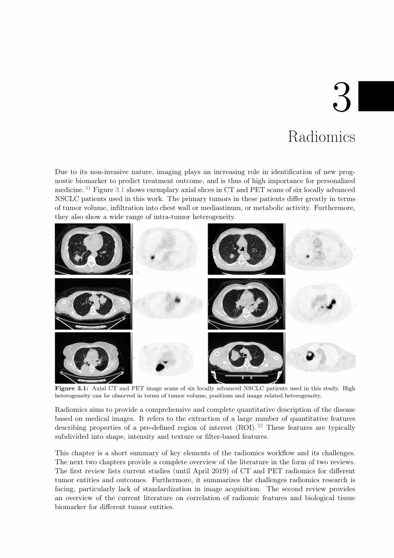
Due to its non-invasive nature, imaging plays an increasing role in identification of new prog-nostic biomarker to predict treatment outcome, and is thus of high importance for personalizedmedicine.31 Figure 3.1 shows exemplary axial slices in CT and PET scans of six locally advancedNSCLC patients used in this work. The primary tumors in these patients differ greatly in termsof tumor volume, infiltration into chest wall or mediastinum, or metabolic activity. Furthermore,they also show a wide range of intra-tumor heterogeneity.
Figure 3.1: Axial CT and PET image scans of six locally advanced NSCLC patients used in this study. Highheterogeneity can be observed in terms of tumor volume, positions and image related heterogeneity.
Radiomics aims to provide a comprehensive and complete quantitative description of the diseasebased on medical images. It refers to the extraction of a large number of quantitative featuresdescribing properties of a pre-defined region of interest (ROI).32 These features are typicallysubdivided into shape, intensity and texture or filter-based features.
This chapter is a short summary of key elements of the radiomics workflow and its challenges.The next two chapters provide a complete overview of the literature in the form of two reviews.The first review lists current studies (until April 2019) of CT and PET radiomics for differenttumor entities and outcomes. Furthermore, it summarizes the challenges radiomics research isfacing, particularly lack of standardization in image acquisition. The second review providesan overview of the current literature on correlation of radiomic features and biological tissuebiomarker for different tumor entities.

3.1 Imaging and delineation
Virtually any type of medical imaging can be used. Radiomics are often based on CT, PET orMR imaging as they are the modality of choice for diagnosis and staging in lung cancer. As a firststep, the ROI is to be identified. This is often the primary tumor, but other tissue types can beanalysed as well, such as lymph node metastasis or healthy lung tissue. Delineations are mainlyperformed manually. However they can be time consuming and susceptible to inter-observervariability.33 Therefore semi- or fully automated segmentation tools can be used.34
3.2 Image processing
Prior to the feature extraction, the image scans can be pre-processed to harmonize them within acohort. These processing steps have shown to elevate the robustness of radiomics features in test-retest studies, i.e. image scans from the same patient within a short time interval.35,36 Typicalexamples for preprocessing steps are interpolation to uniform voxel size, grey-level intensities,bins of the grey-level histogram.
3.3 Feature extraction
From the defined ROI, radiomic features are extracted. Currently, different software solutionsexist.37 In this work, I used our in-house developed radiomics implementation (see https://
medical-physics-usz.github.io/). This implementation has been tested against internationalstandards of feature definitions (image biomarker standardization initiative IBSI38).
3.4 Modeling
Radiomics can offer the possibility for complex tumor classification via hundreds of potentiallyuseful and prognostic features. Including all features in a clinical model often results in sup-optimal models, e.g., models that are not generalizable, not robust, and not interpretable. Thischapter summarizes some of the commonly used techniques to address the "small n, large p"problem in radiomics research, focusing on the techniques used in this thesis.
3.4.1 Feature reduction
Radiomic features are often highly correlated with each other which can be a result of similaritiesin their mathematical definitions (i.e. GLCM inverse difference and GLCM inverse difference mo-ment) or biological process (i.e. heterogeneity tends to increase with tumor volume).39 Includingthese correlated features in a model can lead to suboptimal models due to multicollinearity ofthe features.40 Optimally, a feature reduction method reduces the number of features while min-imizing the information loss. The main method used in this work was the principal componentanalysis (PCA).41 Intuitively, PCA can be interpreted as an orthogonal linear transformation(Hauptachsentransformation) of the n-dimensional feature space with its eigenvectors being in-dependent. These eigenvectors are also referred to as principcal components. As a first step,the eigenvalues and eigenvectors of the covariance matrix are determined. To reduce the n-dimensional feature space to a k dimensional feature subspace (i.e. k < n), the eigenvectors withthe kth largest eigenvalues are selected.
Since the covariance matrix is based on the variances of the features, PCA is strongly influencedby the feature value scales. For example, given two features with an order of magnitude 2 timesgreater difference, the feature with the lower feature values is considered to have lower datavariance. Therefore, feature values are normalized (e.g. using the z-score) prior to PCA.41 In
26

Radiomics
this work, the main method for selecting a subset of retained components k was to determinethe minimum number of principal components that still retained 95% of the data variance.The principal components are a linear combination of the original features, which affects theirinterpretability. Therefore, the feature that correlated most strongly with a selected principalcomponent was used as a surrogate (the largest Pearson correlation coefficient). This allows tomaintain an interpretability of the features while still reducing the number of features.42
3.4.2 Feature selection
Even after feature reduction, remaining features may be redundant or not informative to themodeling task. Feature selection can be applied to further reduce the number of features. Meth-ods are commonly divided into three different types: filter-based, wrapper-based or embedded.43
Filter-based methods differ from the other two methods, because they are independent of theclassification task. They select features based on scores that reflect the relationship with theoutcome (i.e. correlation). As selected features may be correlated with each other, popularmethods incorporate the feature correlation into the score. For example, a subset of features isselected that correlate most strongly with the class (relevance) and most weakly with the otherpredictors (redundancy). Relevance can be evaluated using mutual information, as in MinimumRedundancy Maximum Relevance (mRMR).42
Wrapper-based methods search the entire feature space and identify a relevant and non-redundantfeature subset based on the performance of candidate models in training/validation cohorts.Common methods are forward and backward selection, where the algorithm starts from all/nofeatures and then removes/adds new features, resulting in new candidate models. These methodscan be highly overfitted to the given task and are computationally demanding.43
Embedded methods include feature selection as part of the training process and are computation-ally more efficient compared to wrapper-based methods. A popular method is the Least AbsoluteShrinkage and Selection Operator (LASSO), which attempts to fit the data by regularizing thepredictor coefficients using an L1 norm penalty term. This shrinks the feature coefficients andideally results in less overfitted models. Further, due to the L1 norm penalty function, somefeatures may have zero-valued coefficients and will be removed.40,43
All three types have advantages and disadvantages in terms of computational efficiency, simplic-ity, and generalizability. Finding the optimal feature selection method depends on the task andoften requires an iterative exploration in the training set.
3.4.3 Classification
Survival analysis aims to model time-to-event data. Survival data in clinical trials are often(right-) censored, i.e. lost patient follow-up until the end of the trails.44
Cox proportional-hazard model
A popular regression model in survival analysis and most often used is the Cox proportionalhazard (Cox PH) regression model. We define the hazard ratio h(t) as the instantaneous potentialper unit time for the event to occur that the individual has survived up to time t:44
h(t, ~X) = h0(t)e∑p
i=1βiXi , (3.1)
where βi to the coefficients of the corresponding radiomic features and Xi the linear predictor.The Cox PH regression model is a semi-parametric and has two assumptions:
1. the baseline hazard function h0(t) contains all time-dependent information and
27

2. the exponential contains all time-independent properties, i.e. the hazards of the predictorsstays constant over time.44
These assumptions are often difficult to fulfill, therefore a fixed timepoint analysis can serve asan alternative.
Logistic regression
Several classifiers can be used to predict survival for a given time point after therapy initiation(event / no event) the simplest being logistic regression. In contrast to the Cox PH model,logistic regression aims to model the odds (relative risk to have an event) rather than the hazardratio. The logit function can be described as follows:41
logit = ln (p
1− p) = β0 + ~xi
T ~β = β0 + β1x1 + β2x2 + · · ·+ βnxn, (3.2)
where β0 refers to the intercept of the fit and β1−n to the coefficients of the correspondingradiomic features and p the probability of having an event. Re-formulating equation 3.2 resultsin a predicted probability for an event:
P (Y = 1|x1, x2, x3, . . . , xn) =exp(β0 + ~xi
T ~β)
1 + exp(β0 + ~xiT ~β)
. (3.3)
Using these predicted probabilities, a receiver operating characteristic (ROC) curve can be ex-tracted, indicating the ability of a given logistic model to discriminate between patients with anevent or no event.
Performance measure
The quantitative measure of discriminatory power is the area under the ROC curve (AUC). Amodel that achieves an AUC of 1 is considered a perfect model, capable of perfectly classifyingeach patient into his correct class. In contrast, a poor model achieves an AUC of 0.5 and is asgood as a random predictor.41
3.5 Validation
Due to the exploratory nature of radiomics modelling, where often no clear hypothesis is given,it is critical to separate the data into an exploratory dataset for training and a separate datasetfor validation.
In the training cohort, the combination of feature reduction, feature selection, and modelingtechnique can be tested. Due to limited resources, a model’s tendency to overfit can be evaluatedin bootstrapped resampled cross-validation.40 In a k-fold cross-validation, the given data aredivided into k equally sized patient subsets (also called folds). There are k iterations, whereeach fold is a hold-out set once and the remaining folds are merged into a training set on whichthe model is trained. Cross-validation can be used to test the generalizability of the modelon different fold sets, where stable performance across fold sets is considered optimal. Cross-validated performances tend to yield overly optimistic results because patients are re-used fordifferent folds.40 Therefore external validation on new unseen data, preferably from anotherinstitution, is highly recommended by the Transparent reporting of a multivariable predictionmodel for individual prognosis or diagnosis (TRIPOD) statement.45
28
Radiomics
3.6 Challenges
Challenges in radiomics are often related the lack of standardization in feature definition orimaging settings. This results in limited generalization of the models.37 Sensitivity of radiomicfeatures to imaging settings is particularly important with respect to imaging data collected frommultiple centers. Medical images acquired in clinical routine aim for the best diagnostic quality,and hence imaging settings may vary from center to center. Generalizable radiomics modelsideally model patient- or tumor-specific characteristics only. Signatures obscured by variation inimaging settings should be excluded from the modeling.The robustness of radiomic features has been studied extensively for both CT and PET radiomics.A complete summary can be found in the first review (Chapter 4). Little is known about thetranslation of robustness results across disease sites or across tissue types. In Chapter 9, imagepairs reconstructed with different convolution kernels were collected from three different diseasesand four different tissue types. Often radiomics robustness studies are limited to one or twofactors. In Chapter 10, four main factors were investigated relevant in lung cancer radiomics(delineation, convolution kernel, motion, contrast).Last but not least, interpretability of radiomic features can complicate its introduction to theclinic. Therefore different studies have investigated the correlation of radiomics with biologi-cal tissue biomarker for clinically relevant tumor entities and biomarkers. A full summary ispresented in a second review (Chapter 5).
29

30

4CT radiomics and PET radiomics: ready for
clinical implementation?
Marta Bogowicz1,†, Diem Vuong1,†, Martin W. Huellner2, Matea Pavic1, Nicolaus Andratschke1,Hubert S. Gabryś1, Matthias Guckenberger1, Stephanie Tanadini–Lang1
1Department of Radiation Oncology, University Hospital Zurich and University of Zurich, Zurich, Switzer-land2Department of Nuclear Medicine, University Hospital Zurich and University of Zurich, Zurich, Switzer-land
† authors contributed equally
Status:Published in Quarterly Journal of NuclearMedicine and Molecular Imaging, 2019doi: 10.23736/S1824-4785.19.03192-3
Copyright: This is a preprint version of thearticle submitted to Quarterly Journal of Nu-clear Medicine and Molecular Imaging underpeer review. This version is free to view anddownload to private research and study only.Not for redistribution or re-use. ©EdizioniMinerva Medica.
My contribution: I summarized studies on CT radiomics robustness, phantoms and publically avail-able datasets (section 4.4.1 including the Tables 4.5 and 4.6 in the supplement). Further, I wrote thesection on factors influencing the image quality in CT (section 4.4.2) and created the Figure 4.1. Fur-thermore, I contributed largely on the discussion.
4.1 Abstract
Introduction: Today, rapid technical and clinical developments result in an increasing number of treat-ment options for oncological diseases. Thus, decision support systems are needed to offer the righttreatment to the right patient. Imaging biomarkers hold great promise in patient-individual treatmentguidance. Routinely performed for diagnosis and staging, imaging datasets are expected to hold moreinformation than used in the clinical practice. Radiomics describes the extraction of a large number ofmeaningful quantitative features from medical images, such as computed tomography (CT) and positronemission tomography (PET). Due to the non-invasive nature and ability to capture 3D image-based het-erogeneity, radiomic features are potential surrogate markers of the cancer phenotype. Several radiomicstudies are published per day, owing to encouraging results of many radiomics-based patient outcomemodels. Despite this comparably large number of studies, radiomics is mainly studied in proof of prin-ciple concept. Hence, a translation of radiomics from a hot topic research field into an essential clinicaldecision-making tool is lacking, but of high clinical interest.
Evidence acquisition: Herein, we present a literature review addressing the clinical evidence of CT andPET radiomics. An extensive literature review was conducted in PubMed, including papers on robustnessand clinical applications.
Evidence synthesis: We summarize image-modality related influences on the robustness of radiomicfeatures and provide an overview of clinical evidence reported in the literature. Today, more evidence hasbeen provided for CT imaging, however, PET imaging offers the promise of direct imaging of biologicalprocesses and functions. We provide a summary of future research directions, which needs to be addressedin order to successfully introduce radiomics into clinical medicine. In comparison to CT, more focus shouldbe directed towards harmonization of PET acquisition and reconstruction protocols, which is importantfor transferable modelling.
Conclusions: Both CT and PET radiomics are promising pre-treatment and intra-treatment biomarkersfor outcome prediction. Most studies are performed in retrospective setting, however their validation inprospective data collections is ongoing.
4.2 Introduction
Precision medicine aims to tailor treatment to intra-disease specific traits. In cancer it is a rapidlygrowing field of research with genomics, proteomics, metabolomics and studies of cellular assays beingmajor drivers in understanding the complexity of the disease. In the era of precision medicine, anidentification of biomarkers, which help guide treatment decisions, is important. Medical imaging isan interesting biomarker in oncology, as it allows capturing the spatial and temporal changes in tumorphenotype. Medical imaging already plays an important role in the management of cancer patients.46 Ithas a wide range of applications from screening and diagnosis to tailoring treatment decisions.47 Overthe years, the development in medical imaging techniques allowed for more precise staging, and lead toan optimization of treatment and to an earlier detection of treatment failure.Introduction of computed tomography (CT) imaging in 1980s triggered a change in target definitionin radiotherapy.48 CT is readily available, may provide reasonable soft tissue contrast, particularly ifcontrast agents are used and if different phases of contrast passages are exploited. It is a widely usedimage modality for anatomical recognition in hybrid imaging. Particularly, in the chest, CT remains theimage modality of choice for thoracic malignancies owing to its high native contrast for lung tissue49
and for situations where bone or cartilage involvement needs to be assessed in the absence of magneticresonance imaging.50 Recently, it has also shown its value in lung cancer screening in a high-risk smokerpopulation.51,52 Additionally, native CT showed very good diagnostic accuracy (97%) of cancer relatedfindings (mass or neoplasm, metastatic disease, organ wall thickening, effusion) for different locations inthe abdomen.53 Although the current routine assessment is still mostly qualitative and descriptive innature, it has proven valuable and achieves a reasonable sensitivity and specificity for the detection ofprimary lung cancer as well as liver, bone, adrenal, and lymph node metastases. Quantitative assessmentis mostly performed by the measurement of diameter or volume of lesions, and by determining theHounsfield units in specific circumstances in order to differentiate solid lesions from effusing. Tumorvolume is a strong predictor of overall survival (OS), e.g. in head and neck cancer (HNC)54, early55 andadvanced stage non-small cell lung cancer (NSCLC)56. The diameter of tumor and lymph nodes is a part
32
CT radiomics and PET radiomics: ready for clinical implementation?
of the TNM staging of virtually all solid tumors. In addition, the anatomic tumor volume correlates withradiocurability and is therefore highly predictive of local control (LC).57
While CT images basically represents a function of tissue density, positron emission tomography (PET)images represent different cellular, tissue, or organ functions. These different functions are addressedwith different radiopharmaceuticals (radiotracers), with the most commonly used radiotracer (18F-fluorodeoxyglucose [18F-FDG]) serving as a surrogate biomarker for glucose consumption, and hencemetabolism. PET allows for a quantification of radiotracer uptake, and therefore is able to non-invasivelyassess biological processes. The traditional approach to obtain PET biomarkers is by determining themaximum standardized uptake (SUVmax) value of a target lesion using a simple volume of interest (VOI)on PET images. The SUVmax is the single most important PET-derived parameter that is used for theinitial assessment and follow-up of lesions in oncological imaging. Besides the SUVmax, other measureswere proposed to predict tumor response to therapy, such as the SUVpeak or SULpeak.58 However, theseparameters are more difficult to obtain than the SUVmax and are therefore not widely used outsidespecialized academic centers. Other approaches use a target-to-background ratio (TBR) that relates theSUVmax to physiologic uptake in blood pool and liver, as done for the therapy response assessmentof lymphoma with 18F-FDG-PET. Simply the dichotomy positive/negative 18F-FDG-PET scan carriesimportant prognostic information, as shown for patients with follicular lymphoma, where subjects withpositive scans after first-line therapy had a shorter progression-free survival (PFS) and OS comparedto subjects with negative scans, outperforming contrast-enhanced CT.59 For prognostication with 18F-FDG-PET, often the total lesion glycolysis (TLG) or the metabolically active tumor volume (MTV) areused besides the SUVmax. Several such PET-derived quantifiable parameters were shown able to predictresponse and survival in cancer patients. Pre-treatment TLG was reported to prognosticate OS of pa-tients with malignant pleural mesothelioma.60 In multiple myeloma patients, the SUVmax may predictthe success of allogeneic hematopoietic cell transplantation.61 Pre-treatment MTV might predict OS inpatients with anal carcinoma.62 In NSCLC, high SUVmax, TLG, and MTV predicted a higher risk oftumor recurrence or death.63 In the restaging of pancreatic cancer, 18F-FDG-PET is able to identifypatients with worse OS.64 High TLG predicts a poor clinical outcome in subjects with colorectal cancerafter surgical resection with curative intent.65 In HNC, low SUV predicts higher LC rates after 2 yearsand higher disease-free survival (DFS).66
To summarize, due to the non-invasive nature and the possibility for high spatial and temporal resolu-tion, imaging has gained increasing influence in the identification of new prognostic biomarkers to predicttreatment outcome.67 However, currently cancer staging and response assessment based on imaging relyon image analyses performed by diagnostic radiology, nuclear medicine or radiation oncology, which inferssubstantial inter- and intra-observer variability.68 Additionally, current radiological cancer characteriza-tion largely lacks to incorporate the heterogeneous phenotypes that most oncological diseases have.69
Hence, despite large efforts in improving imaging quality, only limited information from the medical im-ages are used for staging in current clinical routine assessment. Therefore, so-called radiomic featureswere proposed as new prognostic image based-biomarkers.32,70–76 Radiomics is defined as the extractionof a large amount of quantitative image features, aiming to provide a comprehensive quantification ofcancer phenotypes. These features can potentially be used to build prognostic outcome models, therebyenabling treatment intensity tailored to individual cancers. However, before radiomic signatures are usedin a clinical setting, several aspects need to be considered. First, radiomic features depend on imaging-specific uncertainties. To assess the sensitivity of radiomic features against these uncertainties, robustnessstudies should be performed to assure model transferability to a different cohort of patients. Further, theevidence of a link between radiomics and treatment outcome needs to be established in order to transferthem into clinical routine.
This review investigates the possibility of translating CT-based and PET-based radiomics models into aclinical setting. First, a short overview of the radiomics workflow is provided, followed by a descriptionof the performed literature review searches. Second, a short overview of the most relevant radiomicsrobustness studies is provided, along with the most influencing factors and uncertainties in CT and PETimaging. Third, CT, PET, and combined image modality based radiomics studies are provided. Finally,we compare the stage of the radiomics research in both modalities and indicate gaps that need to bebridged before radiomics can be considered a clinical decision support system.
33
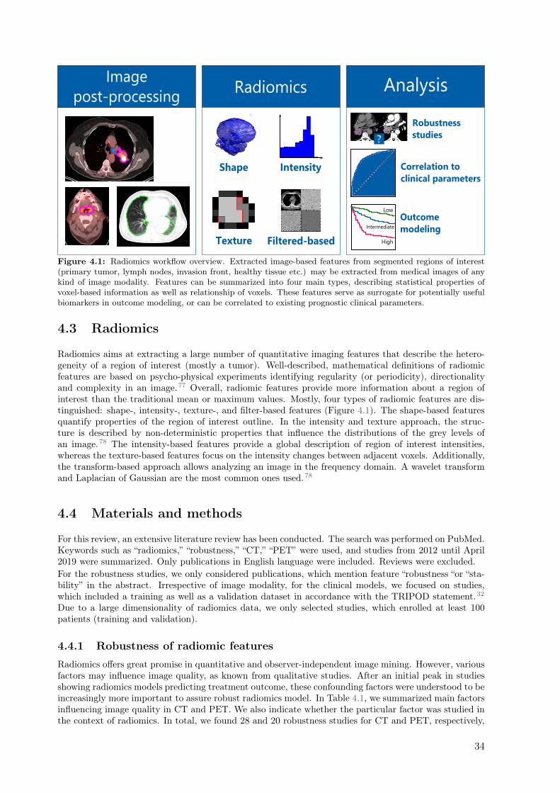
Radiomics
Shape
Texture Filtered-based
Intensity
AnalysisImage
post-processing
?
Robustness
studies
High
Intermediate
Low
Outcome
modeling
Correlation to
clinical parameters
Figure 4.1: Radiomics workflow overview. Extracted image-based features from segmented regions of interest(primary tumor, lymph nodes, invasion front, healthy tissue etc.) may be extracted from medical images of anykind of image modality. Features can be summarized into four main types, describing statistical properties ofvoxel-based information as well as relationship of voxels. These features serve as surrogate for potentially usefulbiomarkers in outcome modeling, or can be correlated to existing prognostic clinical parameters.
4.3 Radiomics
Radiomics aims at extracting a large number of quantitative imaging features that describe the hetero-geneity of a region of interest (mostly a tumor). Well-described, mathematical definitions of radiomicfeatures are based on psycho-physical experiments identifying regularity (or periodicity), directionalityand complexity in an image.77 Overall, radiomic features provide more information about a region ofinterest than the traditional mean or maximum values. Mostly, four types of radiomic features are dis-tinguished: shape-, intensity-, texture-, and filter-based features (Figure 4.1). The shape-based featuresquantify properties of the region of interest outline. In the intensity and texture approach, the struc-ture is described by non-deterministic properties that influence the distributions of the grey levels ofan image.78 The intensity-based features provide a global description of region of interest intensities,whereas the texture-based features focus on the intensity changes between adjacent voxels. Additionally,the transform-based approach allows analyzing an image in the frequency domain. A wavelet transformand Laplacian of Gaussian are the most common ones used.78
4.4 Materials and methods
For this review, an extensive literature review has been conducted. The search was performed on PubMed.Keywords such as “radiomics,” “robustness,” “CT,” “PET” were used, and studies from 2012 until April2019 were summarized. Only publications in English language were included. Reviews were excluded.
For the robustness studies, we only considered publications, which mention feature “robustness “or “sta-bility” in the abstract. Irrespective of image modality, for the clinical models, we focused on studies,which included a training as well as a validation dataset in accordance with the TRIPOD statement.32
Due to a large dimensionality of radiomics data, we only selected studies, which enrolled at least 100patients (training and validation).
4.4.1 Robustness of radiomic features
Radiomics offers great promise in quantitative and observer-independent image mining. However, variousfactors may influence image quality, as known from qualitative studies. After an initial peak in studiesshowing radiomics models predicting treatment outcome, these confounding factors were understood to beincreasingly more important to assure robust radiomics model. In Table 4.1, we summarized main factorsinfluencing image quality in CT and PET. We also indicate whether the particular factor was studied inthe context of radiomics. In total, we found 28 and 20 robustness studies for CT and PET, respectively,
34

CT radiomics and PET radiomics: ready for clinical implementation?
which investigated 10 different sources of feature instability. A higher number of robustness studies wasfound in CT imaging, both in human and phantom studies. However, newly published PET studiesattempt to bridge this gap.79 Nevertheless, based on the literature research it is difficult to pinpoint,which source of instability is the most pronounced one, as most studies investigate only a small subsetof factors (e.g., reconstruction method) and/or are limited to a single tumor site. This section providesan overview of the recent research on the robustness of radiomic features of CT and PET imaging andin the discussion section we indicate areas for further research.
4.4.2 Factor influencing image quality
Influence on image quality Stable features (%)CT FDG-PET CT FDG-PET
Test-retest ! ! 74%-93%80–83 53%-71%84,85
Spatial resolution ! ! 70%35,86 52%87*
Reconstruction method ! ! 50%-80%88 1%-41%89–91
Scanner type ! ! 68%-83%92,93 36%94
Scanner calibration ! ! - -
Respiratory motion ! ! 27%85,72%-83%81 26%85
Contrast administration ! - -
Tube voltage ! - -
Tube current ! 8%-95%95 -
Pitch ! 90%88 -
Attenuation correction ! -
Time of flight !
Dosage of radionuclide !
Uptake time !
Table 4.1: Overview of robustness studies and the most relevant factors influencing the image quality. The firstpart shows the factors affecting both CT and PET (indicated by check symbol), then modality-specific factorsare shown. *Results are given for a combined influence of voxel sizes, filters and discretization bins, stability ratefor specific parameters not reported.
From the 28 CT robustness studies, the majority of the studies investigated test-retest uncertainties(n = 4), followed by respiratory motion (n = 3) and reconstruction (n = 3). Less often investigated weretube current, tube voltage and pitch (each once). In PET imaging, 20 studies investigated robustness ofPET radiomics, i.e. delineation (n = 7) and reconstruction (n = 6), followed by optimal bin size (n = 4)and respiratory motion (n = 2). A list of all the robustness studies is given in the Supplement 4.5 and4.6. The reconstruction method showed a large impact on radiomic features in both image modalities. InCT imaging, the largest variation in reconstruction originates from different kernel choices (e.g. smoothor sharp).83,88 In the case of PET, instability of up to 99% features was observed, when a large varietyof algorithms was studied (ranging from filtered back projection to different iterative reconstructions).91
Additionally, the spatial resolution (i.e., voxel size) was a frequently studied influence. CT robustnessstudies have concluded that voxel size variation had the largest effect on the robustness of radiomicfeatures and was more relevant than other CT-related scanning parameters (kVp, exposure, focal point,tube current).35 We have not found a study reporting specifically on stability of PET radiomic featuresin the context of voxel size, however earlier studies reported on its large influence on a limited set oftextual features.96 On the other hand, the highest stability rate was observed in test-retest studies (74-93% and 53-71% in CT and PET, respectively). This is a promising result, as test-retest studies targetthe quantification of random effects, which cannot be controlled.
Not only the acquisition and reconstruction parameters, but also radiomics workflow-related steps canaffect the stability of radiomics features. The first workflow step is the delineation of the region of in-terest. Three studies were identified investigating the impact of delineation in CT and seven in PET.Manual delineation was shown to have considerable effect on the robustness of CT radiomic features,33,83
and this effect was tumor entity dependent (36-90%).33 To reduce delineation variability, semiautomaticsegmentation has been proposed, and has shown to improve the stability rate of the radiomic features inCT imaging.34 In PET imaging, semiautomatic segmentation is more commonly used clinically, however,
35
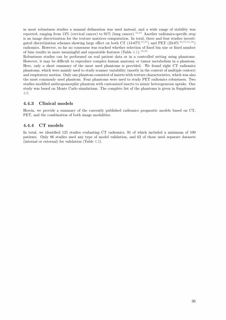
in most robustness studies a manual delineation was used instead, and a wide range of stability wasreported, ranging from 13% (cervical cancer) to 91% (lung cancer).84,91 Another radiomics-specific stepis an image discretization for the texture matrices computation. In total, three and four studies investi-gated discretization schemes showing large effect on both CT (13-67%35,97) and PET (23-6%36,87,91,98)radiomics. However, so far no consensus was reached whether selection of fixed bin size or fixed numberof bins results in more meaningful and repeatable features (Table 4.1).36,99
Robustness studies can be performed on real patient data or in a controlled setting using phantoms.However, it may be difficult to reproduce complex human anatomy or tumor metabolism in a phantom.Here, only a short summary of the most used phantoms is provided. We found eight CT radiomicsphantoms, which were mainly used to study scanner variability (mostly in the context of multiple centers)and respiratory motion. Only one phantom consisted of inserts with texture characteristics, which was alsothe most commonly used phantom. Four phantoms were used to study PET radiomics robustness. Twostudies modified anthropomorphic phantom with customized inserts to mimic heterogeneous uptake. Onestudy was based on Monte Carlo simulations. The complete list of the phantoms is given in Supplement4.9.
4.4.3 Clinical models
Herein, we provide a summary of the currently published radiomics prognostic models based on CT,PET, and the combination of both image modalities.
4.4.4 CT models
In total, we identified 125 studies evaluating CT radiomics, 91 of which included a minimum of 100patients. Only 86 studies used any type of model validation, and 62 of those used separate datasets(internal or external) for validation (Table 4.2).
36
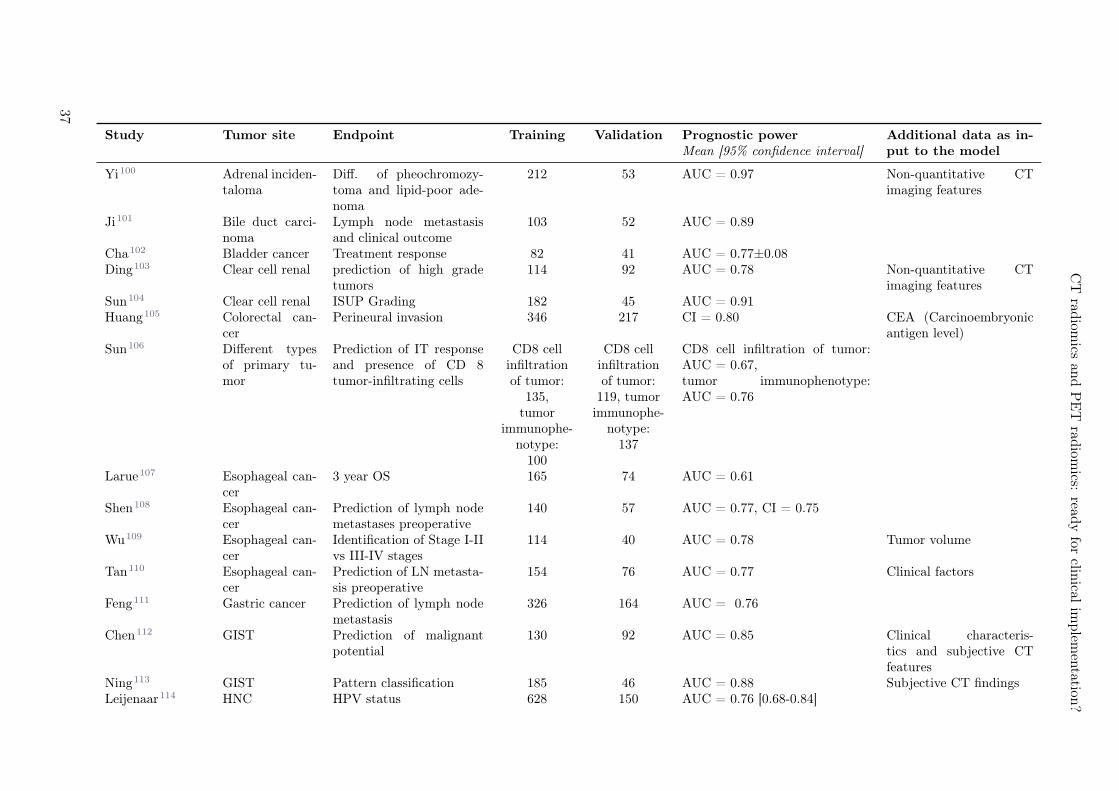
CT
radiom
icsan
dP
ET
radiom
ics:read
yfor
clinical
implem
entation
?
Study Tumor site Endpoint Training Validation Prognostic powerMean [95% confidence interval]
Additional data as in-put to the model
Yi100 Adrenal inciden-taloma
Diff. of pheochromozy-toma and lipid-poor ade-noma
212 53 AUC = 0.97 Non-quantitative CTimaging features
Ji101 Bile duct carci-noma
Lymph node metastasisand clinical outcome
103 52 AUC = 0.89
Cha102 Bladder cancer Treatment response 82 41 AUC = 0.77±0.08Ding103 Clear cell renal prediction of high grade
tumors114 92 AUC = 0.78 Non-quantitative CT
imaging featuresSun104 Clear cell renal ISUP Grading 182 45 AUC = 0.91Huang105 Colorectal can-
cerPerineural invasion 346 217 CI = 0.80 CEA (Carcinoembryonic
antigen level)Sun106 Different types
of primary tu-mor
Prediction of IT responseand presence of CD 8tumor-infiltrating cells
CD8 cellinfiltrationof tumor:
135,tumor
immunophe-notype:
100
CD8 cellinfiltrationof tumor:
119, tumorimmunophe-
notype:137
CD8 cell infiltration of tumor:AUC = 0.67,tumor immunophenotype:AUC = 0.76
Larue107 Esophageal can-cer
3 year OS 165 74 AUC = 0.61
Shen108 Esophageal can-cer
Prediction of lymph nodemetastases preoperative
140 57 AUC = 0.77, CI = 0.75
Wu109 Esophageal can-cer
Identification of Stage I-IIvs III-IV stages
114 40 AUC = 0.78 Tumor volume
Tan110 Esophageal can-cer
Prediction of LN metasta-sis preoperative
154 76 AUC = 0.77 Clinical factors
Feng111 Gastric cancer Prediction of lymph nodemetastasis
326 164 AUC = 0.76
Chen112 GIST Prediction of malignantpotential
130 92 AUC = 0.85 Clinical characteris-tics and subjective CTfeatures
Ning113 GIST Pattern classification 185 46 AUC = 0.88 Subjective CT findingsLeijenaar114 HNC HPV status 628 150 AUC = 0.76 [0.68-0.84]
37
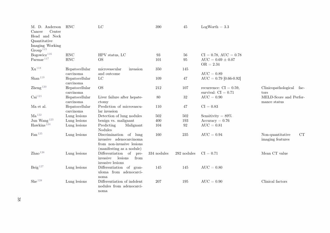
M. D. AndersonCancer CenterHead and NeckQuantitativeImaging WorkingGroup115
HNC LC 390 45 LogWorth = 3.3
Bogowicz116 HNC HPV status, LC 93 56 CI = 0.78, AUC = 0.78Parmar117 HNC OS 101 95 AUC = 0.69 ± 0.07
Xu118 Hepatocellularcarcinoma
microvascular invasionand outcome
350 145OR = 2.34
AUC = 0.89Shan119 Hepatocellular
carcinomaLC 109 47 AUC = 0.79 [0.66-0.92]
Zheng120 Hepatocellularcarcinoma
OS 212 107 recurrence: CI = 0.59,survival: CI = 0.71
Clinicopathological fac-tors
Cai121 Hepatocellularcarcinoma
Liver failure after hepate-ctomy
80 32 AUC = 0.90 MELD-Score and Perfor-mance status
Ma et al. Hepatocellularcarcinoma
Prediction of microvascu-lar invasion
110 47 CI = 0.83
Ma122 Lung lesions Detection of lung nodules 502 502 Sensitivity = 89%Jun Wang123 Lung lesions benign vs. malignant 400 193 Accuracy = 0.76Hawkins124 Lung lesions Predicting Malignant
Nodules104 92 AUC = 0.81
Fan125 Lung lesions Discrimination of lunginvasive adenocarcinomafrom non-invasive lesions(manifesting as a nodule)
160 235 AUC = 0.94 Non-quantitative CTimaging features
Zhao126 Lung lesions Differentiation of pre-invasive lesions frominvasive lesions
334 nodules 292 nodules CI = 0.71 Mean CT value
Beig127 Lung lesions Differentiation of gran-uloma from adenocarci-noma
145 145 AUC = 0.80
She128 Lung lesions Differentiation of indolentnodules from adenocarci-noma
207 195 AUC = 0.90 Clinical factors
38
CT
radiom
icsan
dP
ET
radiom
ics:read
yfor
clinical
implem
entation
?
Yang129 Lung lesions Differentiation of gran-uloma from adenocarci-noma
211 91 AUC = 0.84 Clinical factors
Wu130 NSCLC Tumor histological sub-types
198 152 AUC = 0.72
Parmar43 NSCLC OS 310 154 AUC = 0.66Coroller131 NSCLC DM 98 84 CI = 0.61Wang132 NSCLC Lymph node metastasis 242 124 AUC = 0.84Hosny133 NSCLC OS 463 307 AUC = 0.71 [0.60-0.82]Yang134 NSCLC EGFR mutation status 306 161 AUC = 0.78 Clinical factorsJia135 NSCLC EGFR mutations status 345 158 AUC = 0.83 Clinical factorsLi136 NSCLC EGFR mutations status 810 200 AUC = 0.83 Clinical factorsYang137 NSCLC OS 239 132 CI = 0.71 Clinical factorsDou138 NSCLC DM 100 100 CI = 0.63 Clinical factorsHe139 NSCLC OS 223 75 AUC = 0.93Xue140 NSCLC Invasiveness of tumors ap-
pearing as nodules453 117 AUC = 0.79 Clinical factors
Yang141 NSCLC LN Metastasis prediction 106 53 AUC = 0.86 Clinical factorsFan142 NSCLC DM 243 161 CI = 0.36 [0.27-0.44] Clinicopathological fac-
tors and CT imagingfeatures
Tunali143 NSCLC OS 61 47 HR = 0.40Shen144 NSCLC OS 463 125 AUC = 0.66, CI = 0.63van Timmeren145 NSCLC OS 132 156 CI = 0.66Parmar117 NSCLC and
HNCStage (AUC), prognosis(CI)
558 320 AUC = 0.77 ± 0.02,CI = 0.68 ± 0.01
Trebeschi146 Melanoma andlung cancer
Response to immunother-apy
133 70 AUC = 0.76 (p < 0.001)
Cozzi147 Pancreatic can-cer
OS, LC 60 40 OS: AUC = 0.73 [0.53-0.93],CI = 0.75 ± 0.03,LC: AUC = 0.70 [0.52-0.89],CI = 0.75 ± 0.10
Liang148 Pancreatic neu-roendocrine tu-mors
Prediction of histologicgrade
86 51 AUC = 0.89 Clinical factors
Huang149 Discrimination of high-grade from low-grade can-cer
222 144 0.74 [0.64-0.83]
39
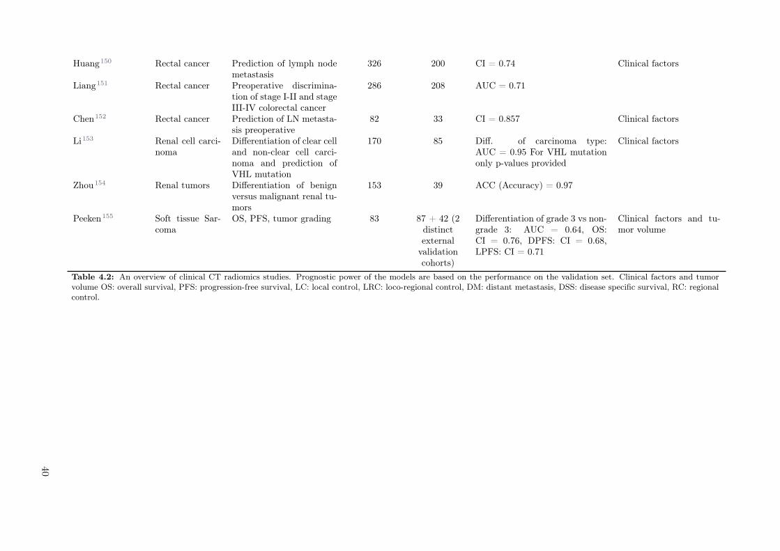
Huang150 Rectal cancer Prediction of lymph nodemetastasis
326 200 CI = 0.74 Clinical factors
Liang151 Rectal cancer Preoperative discrimina-tion of stage I-II and stageIII-IV colorectal cancer
286 208 AUC = 0.71
Chen152 Rectal cancer Prediction of LN metasta-sis preoperative
82 33 CI = 0.857 Clinical factors
Li153 Renal cell carci-noma
Differentiation of clear celland non-clear cell carci-noma and prediction ofVHL mutation
170 85 Diff. of carcinoma type:AUC = 0.95 For VHL mutationonly p-values provided
Clinical factors
Zhou154 Renal tumors Differentiation of benignversus malignant renal tu-mors
153 39 ACC (Accuracy) = 0.97
Peeken155 Soft tissue Sar-coma
OS, PFS, tumor grading 83 87 + 42 (2distinctexternal
validationcohorts)
Differentiation of grade 3 vs non-grade 3: AUC = 0.64, OS:CI = 0.76, DPFS: CI = 0.68,LPFS: CI = 0.71
Clinical factors and tu-mor volume
Table 4.2: An overview of clinical CT radiomics studies. Prognostic power of the models are based on the performance on the validation set. Clinical factors and tumorvolume OS: overall survival, PFS: progression-free survival, LC: local control, LRC: loco-regional control, DM: distant metastasis, DSS: disease specific survival, RC: regionalcontrol.
40
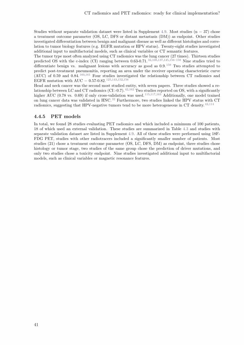
CT radiomics and PET radiomics: ready for clinical implementation?
Studies without separate validation dataset were listed in Supplement 4.9. Most studies (n = 37) chosea treatment outcome parameter (OS, LC, DFS or distant metastasis (DM)) as endpoint. Other studiesinvestigated differentiation between benign and malignant disease as well as different histologies and corre-lation to tumor biology features (e.g. EGFR mutation or HPV status). Twenty-eight studies investigatedadditional input to multifactorial models, such as clinical variables or CT semantic features.The tumor type most often analyzed using CT radiomics was the lung cancer (27 times). Thirteen studiespredicted OS with the c-index (CI) ranging between 0.63-0.71.32,108,137,145,156–158 Nine studies tried todifferentiate benign vs. malignant lesions with accuracy as good as 0.9.159 Two studies attempted topredict post-treatment pneumonitis, reporting an area under the receiver operating characteristic curve(AUC) of 0.59 and 0.84.160,161 Four studies investigated the relationship between CT radiomics andEGFR mutation with AUC = 0.57-0.82.125,143,152,156
Head and neck cancer was the second most studied entity, with seven papers. Three studies showed a re-lationship between LC and CT radiomics (CI>0.7).42,162 Two studies reported on OS, with a significantlyhigher AUC (0.78 vs. 0.69) if only cross-validation was used.115,117,163 Additionally, one model trainedon lung cancer data was validated in HNC.32 Furthermore, two studies linked the HPV status with CTradiomics, suggesting that HPV-negative tumors tend to be more heterogeneous in CT density.42,114
4.4.5 PET models
In total, we found 28 studies evaluating PET radiomics and which included a minimum of 100 patients,18 of which used an external validation. These studies are summarized in Table 4.3 and studies withseparate validation dataset are listed in Supplement 4.9. All of these studies were performed using 18F-FDG PET, studies with other radiotracers included a significantly smaller number of patients. Moststudies (21) chose a treatment outcome parameter (OS, LC, DFS, DM) as endpoint, three studies chosehistology or tumor stage, two studies of the same group chose the prediction of driver mutations, andonly two studies chose a toxicity endpoint. Nine studies investigated additional input to multifactorialmodels, such as clinical variables or magnetic resonance features.
41
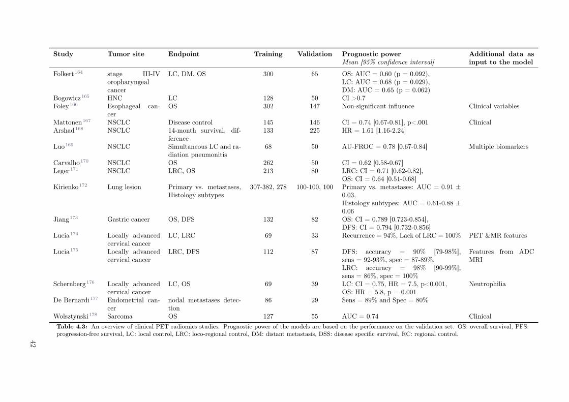
Study Tumor site Endpoint Training Validation Prognostic powerMean [95% confidence interval]
Additional data asinput to the model
Folkert164 stage III-IVoropharyngealcancer
LC, DM, OS 300 65 OS: AUC = 0.60 (p = 0.092),LC: AUC = 0.68 (p = 0.029),DM: AUC = 0.65 (p = 0.062)
Bogowicz165 HNC LC 128 50 CI >0.7Foley166 Esophageal can-
cerOS 302 147 Non-significant influence Clinical variables
Mattonen167 NSCLC Disease control 145 146 CI = 0.74 [0.67-0.81], p<.001 ClinicalArshad168 NSCLC 14-month survival, dif-
ference133 225 HR = 1.61 [1.16-2.24]
Luo169 NSCLC Simultaneous LC and ra-diation pneumonitis
68 50 AU-FROC = 0.78 [0.67-0.84] Multiple biomarkers
Carvalho170 NSCLC OS 262 50 CI = 0.62 [0.58-0.67]Leger171 NSCLC LRC, OS 213 80 LRC: CI = 0.71 [0.62-0.82],
OS: CI = 0.64 [0.51-0.68]Kirienko172 Lung lesion Primary vs. metastases,
Histology subtypes307-382, 278 100-100, 100 Primary vs. metastases: AUC = 0.91 ±
0.03,Histology subtypes: AUC = 0.61-0.88 ±0.06
Jiang173 Gastric cancer OS, DFS 132 82 OS: CI = 0.789 [0.723-0.854],DFS: CI = 0.794 [0.732-0.856]
Lucia174 Locally advancedcervical cancer
LC, LRC 69 33 Recurrence = 94%, Lack of LRC = 100% PET &MR features
Lucia175 Locally advancedcervical cancer
LRC, DFS 112 87 DFS: accuracy = 90% [79-98%],sens = 92-93%, spec = 87-89%,LRC: accuracy = 98% [90-99%],sens = 86%, spec = 100%
Features from ADCMRI
Schernberg176 Locally advancedcervical cancer
LC, OS 69 39 LC: CI = 0.75, HR = 7.5, p<0.001,OS: HR = 5.8, p = 0.001
Neutrophilia
De Bernardi177 Endometrial can-cer
nodal metastases detec-tion
86 29 Sens = 89% and Spec = 80%
Wolsztynski178 Sarcoma OS 127 55 AUC = 0.74 Clinical
Table 4.3: An overview of clinical PET radiomics studies. Prognostic power of the models are based on the performance on the validation set. OS: overall survival, PFS:progression-free survival, LC: local control, LRC: loco-regional control, DM: distant metastasis, DSS: disease specific survival, RC: regional control.
42
CT radiomics and PET radiomics: ready for clinical implementation?
The tumor type that was the most often analyzed using PET radiomics was NSCLC (n = 12). In total,seven studies built a model for NSCLC to predict treatment outcome (most often OS (n = 4)). Modelperformance for the prediction of OS was in agreement between the studies (CI = 0.62-0.66).169–171 Luoet al. successfully developed a model for simultaneous prediction of LC and radiation pneumonitis.169
Five studies analyzed radiomics biomarkers for HNC. Most of these studies focused on the predictionof LC (n = 3). Additionally, the value of radiomics was shown for gastric cancer, cervical cancer,endometrical cancer, sarcoma, and esophageal cancers. Only two studies reported a negative outcome,one for the prediction of OS in esophageal cancer166 and one for the prediction of the thymidylate synthaseexpression status in NSCLC (Table 4.3).179
43
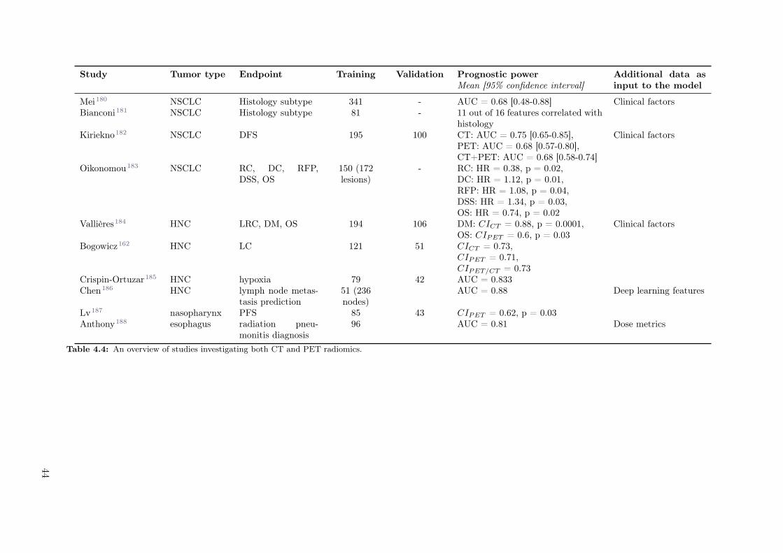
Study Tumor type Endpoint Training Validation Prognostic powerMean [95% confidence interval]
Additional data asinput to the model
Mei180 NSCLC Histology subtype 341 - AUC = 0.68 [0.48-0.88] Clinical factorsBianconi181 NSCLC Histology subtype 81 - 11 out of 16 features correlated with
histologyKiriekno182 NSCLC DFS 195 100 CT: AUC = 0.75 [0.65-0.85],
PET: AUC = 0.68 [0.57-0.80],CT+PET: AUC = 0.68 [0.58-0.74]
Clinical factors
Oikonomou183 NSCLC RC, DC, RFP,DSS, OS
150 (172lesions)
- RC: HR = 0.38, p = 0.02,DC: HR = 1.12, p = 0.01,RFP: HR = 1.08, p = 0.04,DSS: HR = 1.34, p = 0.03,OS: HR = 0.74, p = 0.02
Vallières184 HNC LRC, DM, OS 194 106 DM: CICT = 0.88, p = 0.0001,OS: CIPET = 0.6, p = 0.03
Clinical factors
Bogowicz162 HNC LC 121 51 CICT = 0.73,CIPET = 0.71,CIPET/CT = 0.73
Crispin-Ortuzar185 HNC hypoxia 79 42 AUC = 0.833Chen186 HNC lymph node metas-
tasis prediction51 (236nodes)
AUC = 0.88 Deep learning features
Lv187 nasopharynx PFS 85 43 CIPET = 0.62, p = 0.03Anthony188 esophagus radiation pneu-
monitis diagnosis96 AUC = 0.81 Dose metrics
Table 4.4: An overview of studies investigating both CT and PET radiomics.
44
CT radiomics and PET radiomics: ready for clinical implementation?
4.4.6 Combined image modalities
We identified ten papers, which used both CT and PET for the radiomics analysis. One focused on themethodology for model training and two enrolled less than 100 patients. Three studies analyzed data oflung cancer patients. Two studies investigated DFS as endpoint. One study indicated better performanceof CT features182, whereas the other one emphasized complementary value of both modalities, however,pointing out that several CT features were correlated with SUVmax.183 Further, features from mergedCT and PET images predicted histology in lung cancer with an accuracy of 0.89.189 None of thesestudies showed statistically significant superiority of one of the image modalities for prognostic modellingin lung cancer. Four studies were conducted in HNC. For outcome prediction (LRC, DM and LC), nosignificant difference was observed in the performance of models based on CT or PET184, however, themodel evaluating LC showed better calibration for PET imaging.162 In nasopharyngeal cancer, clinicalparameters (staging and standard blood lab analysis) outperformed both CT and PET.187 CT and PETradiomics were also used to predict the hypoxia status with 18F-MISO PET imaging as reference.185 Inthe validation set, the combined model performed best (AUC = 0.83), significantly better than the modelbased on the 90th percentile of 18F-FDG uptake (Table 4.4).
4.5 Discussion
In 21st century medicine, with wide variety of treatment options, the development of reliable and acces-sible decision support systems is of high importance. According to the TRIPOD statement, models andbiomarkers should be extensively validated before introduction into clinical routine in order to assuretheir reliability.45 The wide accessibility of a decision support system can be achieved by the use ofcost-effective parameters, such as results of analysis of routinely collected blood samples or imaging data.Additionally, repetitive monitoring is important in oncology, where tumors may technically be consideredas continuously evolving structures that change their properties over time. In recent decades, medicalimaging has become an important pillar in the diagnosis and management of cancer. More recently,quantitative, high-throughput image analysis, such as radiomics, promise fast, comprehensive and repet-itive tumor monitoring, and thus its clinical incorporation into decision support systems is appealing.During the last five years, more than 400 studies were published with a keyword “CT radiomics” or “PETradiomics”. In this section we discuss the existing evidence on CT and PET radiomics prognostic powerand indicate directions for further research.
PET imaging serves as a 3D surrogate of tumor biology, depicting different biological processes or featuresdepending on the injected radiotracer. Different PET measures were shown to correlate with treatmentoutcomes for several tumor entities,60–66 in many instances outperforming morphological imaging-basedassessment, such as CT.59,190–192 PET imaging is therefore an obvious candidate for biomarkers extractionusing radiomics. However, in clinical routine, larger databases of annotated and segmented CTs areavailable, due to its larger availability and its integration into the radiotherapy planning process, wheresegmentation is necessary. This is reflected in the number of papers reporting on clinical prognosticmodels, with separate validation cohorts, which is three times larger for CT compared to PET. Moreover,we have identified only ten papers analyzing both modalities. None of these papers reported superiorityof one or the other image modality, but rather emphasized their complementary value. Regardless of theimage modality, the most studied tumor types were lung and head and neck. The most studied endpointwas OS in lung cancer and LC in head and neck cancer.
In a decision support system, a prospective validation should be performed to control for confoundingfactors, after an initial model testing in a separate cohort. Most of the radiomics studies were con-ducted in a retrospective setting. We have searched the US National Library of Medicine for registered,prospective clinical trials including radiomics. We found 55 entries, 18 of which included CT radiomicsand 9 PET radiomics. Two CT studies (NCT01302626, NCT03872362) and one PET (NCT01764217)study completed patient accrual. CT studies focused on lung cancer and diagnosis of pulmonary nodules,whereas PET imaging was used to predict outcome in cervical cancer. No results of these studies have yetbeen published. A proof of radiomics-based model validity in a prospective setting will be a convincingargument for the clinical introduction of radiomics.
Alternative approach to corroborate validity of radiomic signatures is the correlation of radiomic featuresto tumor biology (e.g. gene expression or blood serum biomarkers). Also, in this domain we identifiedlarger number of published CT studies than PET studies (13 and 2, respectively). Based on standard CTchest imaging, several studies demonstrated that radiomic features are correlated with histopathological
45
cancer characteristics, such as GLUT-1 expression193, a marker for hypoxia, EGFR expression194 or K-ras mutational status195 in NSCLC. However, the main purpose of these studies is not to replace biopsybut to provide a proof that CT imaging offers more than volumetric and anatomical assessment. In PETimaging, this type of studies is of lower relevance, as a proof of link between PET imaging and tumorbiology is obtained by specific design of radiopharmaceutical (e.g. FDG is an analog of glucose).
Regardless of the image modality, radiomics studies suffer from a lack of standardization. A recent exper-imental study on CT radiomics showed that many CT radiomic features might actually be redundant andnon-reproducible, owing to non-standardized CT acquisition parameters.196,197 Only 10 out of 177 (5.6%)radiomic features were regarded as non-redundant, if all acquisition parameters except tube voltage, mAand field of view would be fixed.196 The lack of standardization appears even to be a larger problem withPET, where different uptake time or attenuation correction may largely influence simple measures suchas the SUVmax.198,199
Little attention has been paid to harmonization of PET acquisition and reconstruction methods amongdifferent scans, scanners and institutions. In our opinion, initiatives such as the Dutch multicenter trialprotocol should be encouraged and extended.200 The standardization of radiotracer dosage, standardizedscan delay after injection, standardized correction of emission data, and standardized reconstructiontechniques (with or without time of flight information; type of iterative reconstruction, e.g. the use ofpoint spread function modelling or penalized iterative reconstruction techniques)199,201–203 is of greatimportance to build reproducible SUV-based metrics in radiomics studies.
Recommendations for future studies
Due to this lack of standardization of imaging parameters, robustness studies are needed to assess thesensitivity of radiomic features. A document with standardized feature definition was recently providedby the biomarker standardization initiative (IBSI).38 It contains detailed information on radiomics stan-dardization across different radiomics research groups. Introduction of these standardized features leadsto more comparable results. Nevertheless, a clear comparison of importance of standardization of dif-ferent acquisition parameters is currently not possible based on published literature. It is caused by alarge number of influencing factors, limitation to single tumor types as well as use of different stabilitymeasures and thresholds. Therefore, a large study on features following IBSI guidelines an includingdifferent robustness factors is desired.
Despite the large number of robustness studies for both image modalities, still several important imagequality-affecting factors have not been studied (Table 4.1). For example, contrast-enhanced CT scansare regularly performed in clinical practice, but the influence of contrast agent dosage on stability ofthe features has not yet been studied. It is worth to mention that some studies did not even separatecontrast-enhanced and non-enhanced CTs in the model training (e.g. publicly available LUNG1 dataset).In clinical PET imaging, uptake times usually may vary, and are sometimes longer than the proposed 60min after radiotracer injection. Different uptake times may influence the SUV metric. Post-harmonizationof the features is challenging since relevant information are inconsistently reported. In the ideal case,post-harmonization techniques reduce the image related variability, while preserving information on pa-tient characteristics. First feature post-harmonization techniques (such as ComBat method) have beensuccessfully introduced for a limited number of features. Both in CT and PET imaging, studies haveshown that this technique can produce more reproducible and repeatable features.204,205 However, theclinical meaning of the processed features remains unclear since the post-harmonization techniques maysignificantly change feature values, resulting in e.g. negative volume values.
Most radiomics models are trained and validated in a single study and by the same group. Only one sig-nature was validated additionally in a different ethnic population.32,206 In the future, more effort shouldbe undertaken to validate or disproof the already proposed models in large cohorts. Furthermore, vali-dation of retrospective models should be performed in cohorts with standardized imaging protocols. Inorder to fairly judge the potential added value of radiomics for clinical assessment, multifactorial modelsneed to be studied. Few studies attempted to combine radiomics with clinical factors, and few nomo-grams have been published.108,207,208 Clinical prognostic factors such as TNM stage, patient performancestatus, smoking history or hypoxia influence survival of both lung and head and neck cancer and thesefactors should be combined with radiomics in future studies. Additionally, lung cancer cohorts should bestratified based on EGFR and ALK mutations (14.6% vs. 4.5% 5-year survival rates in EGFR-mutantand EGFR unselected advanced lung cancer, respectively209). In head and neck cancer, major knownprognostic factors are HPV status (HR = 0.38) and alcohol consumption (HR = 1.73).210,211 However,with increasing model complexity, more data is required to prove its validity. Further development of
46

CT radiomics and PET radiomics: ready for clinical implementation?
infrastructures enabling distributed learning (learning on data without data sharing) may help facilitatethis approach.212
In-line with efforts for large cohort recruitment would be a multicenter initiative for collecting 100+patients for studies on other PET radiotracers. This review was restricted to 18F-FDG due to sparsityof other data. The radiomics evaluation of processes such as perfusion (e.g., H215O), receptor expres-sion (e.g., 68Ga-DOTATATE for somatostatin type 2 receptors expressed in neuroendocrine tumors),amino acid metabolism (e.g., 18F-fluoroethyltyrosin [18F-FET]), cell membrane turnover (18F-choline)or cellular activity (e.g., 18F-NaF for osteoblasts),213,214 may further emphasize the value of PET imag-ing. Such non-FDG radiotracers may offer new radiomics models targeting different physiological andpathophysiological aspects than 18F-FDG.Most of the published studies focused on identification of prognostic radiomic biomarkers. However, tooffer a patient the best possible treatment predictive biomarkers are needed. One predictive radiomicsignature was successfully established in head and neck cancer, pointing at a group of patients receivingcetuximab with locoregional control as high as in patients receiving cisplatin.154 This is a promisingresult nevertheless, the study lacks an external validation.Finally, we would like to encourage publishing negative results. In our literature review, we have noticeda clear publication bias with a very limited amount of negative results. Publishing negative results wouldhelp avoiding repetitive analysis. Additionally, it would help focus on the relevant models, which may beshifted to next levels of validation, such as the prospective validation.
4.6 Conclusion
In summary, both CT and PET radiomics are promising pre-treatment and intra-treatment biomarkersfor outcome prediction. Studies reporting on both image modalities indicated their complementary value.Radiomics enables decoding of biological information even from morphological imaging (CT), which wasshown in studies evaluating correlation to histopathology. Today, more evidence has been providedfor CT imaging, however, PET imaging offers the promise of direct imaging of biological processes andfunctions. In comparison to CT, more focus should be directed towards harmonization of PET acquisitionand reconstruction protocols, which is important for transferable modelling. However, newly developed,sophisticated PET phantoms, specific for radiomics evaluation, have been introduced into the field, andmay help to bridge this gap. A few prospective studies incorporating radiomics are currently runningand the community eagerly awaits the first results.
47
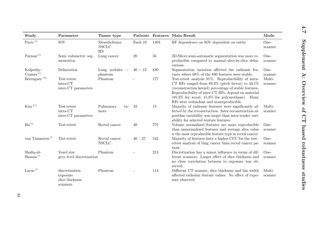
4.7
Supple
men
tA
:O
verv
iewofC
Tbased
robustn
essstu
dies
Study Parameter Tumor type Patients Features Main Result Mode
Pavic33 IOV MesotheliomaNSCLCHN
Each 10 1404 RF dependence on IOV dependent on entity One-scanner
Parmar34 Semi volumetric seg-mentation
Lung cancer 20 56 3D-Slicer semi-automatic segmentation was more re-producible compared to manual slice-by-slice delin-eations.
One-scanner
Kalpathy-Cramer92
Delineation Lung nodules +phantom
40 + 12 830 Segmentation variation affected the radiomic fea-tures where 68% of the 830 features were stable.
One-scanner
Berenguer196 Test-retestintra-CTinter-CT parameters
Phantom - 177 Test-retest analysis 91%. Reproducibility of intra-CT RFs ranged from 89.3% (pitch factor) to 43.1%(reconstruction kernel) percentage of stable features.Reproducibility of inter-CT RFs, depend on material(85.3% for wood, 15.8% for polyurethane). ManyRFs were redundant and nonreproducible.
Multi-scanner
Kim215 Test-retestintra-CTinter-CT parameters
Pulmonary tu-mors
42 15 Majority of radiomic features were significantly af-fected by the reconstruction. Inter-reconstruction al-gorithm variability was larger than inter-reader vari-ability for selected texture features
Multi-scanner
Hu82 Test-retest Rectal cancer 40 775 Volume normalized features are more reproduciblethan unnormalized features and average slice valueis the most reproducible feature type in rectal cancer.
One-scanner
van Timmeren58 Test-retest Rectal cancerNSCLC
40 / 27 542 Majority of features have a higher CCC for the test–retest analysis of lung cancer than rectal cancer pa-tient.
One-scanner
Shafiq-ul-Hassan35
Voxel sizegrey level discretization
Phantom - 213 Discretization has a minor influence in terms of dif-ferent scanners. Larger effect of slice thickness andno clear correlation between to exposure was ob-served.
One-scanner
Larue97 discretizationexposureslice thicknessscanners
Phantom - 114 Different CT scanner, slice thickness and bin widthaffected radiomic feature values. No effect of expo-sure observed.
Multi-scanner
48
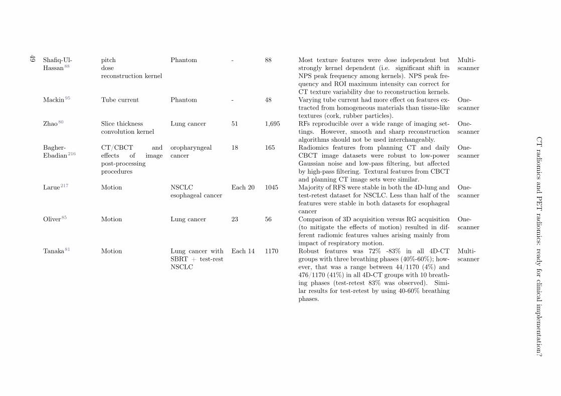
CT
radiom
icsan
dP
ET
radiom
ics:read
yfor
clinical
implem
entation
?
Shafiq-Ul-Hassan88
pitchdosereconstruction kernel
Phantom - 88 Most texture features were dose independent butstrongly kernel dependent (i.e. significant shift inNPS peak frequency among kernels). NPS peak fre-quency and ROI maximum intensity can correct forCT texture variability due to reconstruction kernels.
Multi-scanner
Mackin95 Tube current Phantom - 48 Varying tube current had more effect on features ex-tracted from homogeneous materials than tissue-liketextures (cork, rubber particles).
One-scanner
Zhao80 Slice thicknessconvolution kernel
Lung cancer 51 1,695 RFs reproducible over a wide range of imaging set-tings. However, smooth and sharp reconstructionalgorithms should not be used interchangeably.
One-scanner
Bagher-Ebadian216
CT/CBCT andeffects of imagepost-processingprocedures
oropharyngealcancer
18 165 Radiomics features from planning CT and dailyCBCT image datasets were robust to low-powerGaussian noise and low-pass filtering, but affectedby high-pass filtering. Textural features from CBCTand planning CT image sets were similar.
One-scanner
Larue217 Motion NSCLCesophageal cancer
Each 20 1045 Majority of RFS were stable in both the 4D-lung andtest-retest dataset for NSCLC. Less than half of thefeatures were stable in both datasets for esophagealcancer
One-scanner
Oliver85 Motion Lung cancer 23 56 Comparison of 3D acquisition versus RG acquisition(to mitigate the effects of motion) resulted in dif-ferent radiomic features values arising mainly fromimpact of respiratory motion.
One-scanner
Tanaka81 Motion Lung cancer withSBRT + test-restNSCLC
Each 14 1170 Robust features was 72% -83% in all 4D-CTgroups with three breathing phases (40%-60%); how-ever, that was a range between 44/1170 (4%) and476/1170 (41%) in all 4D-CT groups with 10 breath-ing phases (test-retest 83% was observed). Simi-lar results for test-retest by using 40-60% breathingphases.
Multi-scanner
49

Hunter218 Scanner and Imagetype
NSCLC 56 328 Image feature reproducibility and redundancy de-pended on both the CT machine and the CT im-age type. For each image type, cross-machine re-producible, non-redundant, and informative imagefeatures were found. Compared to end-exhale 4D-CT and breath-hold 3D-CT, average 4D-CT derivedimage features showed superior multi-machine repro-ducibility.
Multi-scanner
Mackin219 Scanner variabilityslice thickness
lung cancer +phantom
20 + 1 150 Combination of image resampling with Butterworthfiltering in the frequency was applied to CT recon-structed with 0.59 to 0.98 mm. Strongly affected fea-tures by pixel size variability reduced from 79% to10%. In the phantom, post processing substantiallyreduced variability in 61% of the radiomics featuresand substantially increased variability in only 6% ofthe features.
Multi-scanner
Bogowicz86 Perfusion CT Dis-cretization
oropharyngealcarcinoma,NSCLC
Each 11 315 Discretization method using fixed number of bins orfixed intervals similar number of stable radiomic pa-rameters (40%).
One-scanner
Ger93 Scanner variability Phantom - 49 Imaging variability of radiomics feature values wasevaluated on 100 CT scanners at 35 clinics. The con-trolled protocol reduces the variability up to 50% forchest and head protocols and also reduces the relativecontribution of the manufacturer to the total vari-ability. For majority of variabilities (manufacturer,scanner, residual with different pre-processsing), thecontrolled protocol had a significantly smaller vari-ability than the local protocol. Using controlledscans can reduce the feature variability.
Multi-scanner
Table 4.5: Overview of CT based robustness studies.
50
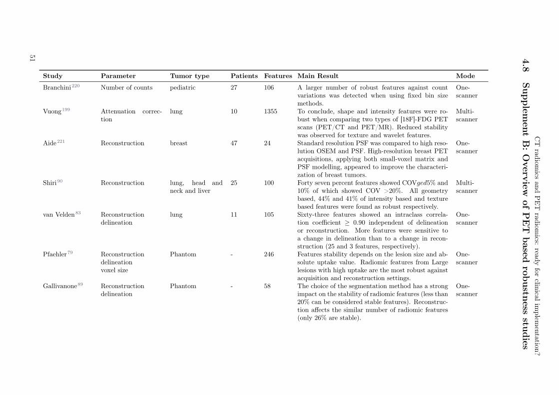
CT
radiom
icsan
dP
ET
radiom
ics:read
yfor
clinical
implem
entation
?
4.8
Supple
men
tB
:O
verv
iewofP
ET
based
robustn
essstu
dies
Study Parameter Tumor type Patients Features Main Result Mode
Branchini220 Number of counts pediatric 27 106 A larger number of robust features against countvariations was detected when using fixed bin sizemethods.
One-scanner
Vuong199 Attenuation correc-tion
lung 10 1355 To conclude, shape and intensity features were ro-bust when comparing two types of [18F]-FDG PETscans (PET/CT and PET/MR). Reduced stabilitywas observed for texture and wavelet features.
Multi-scanner
Aide221 Reconstruction breast 47 24 Standard resolution PSF was compared to high reso-lution OSEM and PSF. High-resolution breast PETacquisitions, applying both small-voxel matrix andPSF modelling, appeared to improve the characteri-zation of breast tumors.
One-scanner
Shiri90 Reconstruction lung, head andneck and liver
25 100 Forty seven percent features showed COVged5% and10% of which showed COV >20%. All geometrybased, 44% and 41% of intensity based and texturebased features were found as robust respectively.
Multi-scanner
van Velden83 Reconstructiondelineation
lung 11 105 Sixty-three features showed an intraclass correla-tion coefficient ≥ 0.90 independent of delineationor reconstruction. More features were sensitive toa change in delineation than to a change in recon-struction (25 and 3 features, respectively).
One-scanner
Pfaehler79 Reconstructiondelineationvoxel size
Phantom - 246 Features stability depends on the lesion size and ab-solute uptake value. Radiomic features from Largelesions with high uptake are the most robust againstacquisition and reconstruction settings.
One-scanner
Gallivanone89 Reconstructiondelineation
Phantom - 58 The choice of the segmentation method has a strongimpact on the stability of radiomic features (less than20% can be considered stable features). Reconstruc-tion affects the similar number of radiomic features(only 26% are stable).
One-scanner
51

Hatt222 Delineation Lung, head andneck and simu-lated lesions
176 1 Five segmentation methods were considered: twothresholds (40% and 50% of SUVmax), antcolony optimization, fuzzy locally adaptive Bayesian(FLAB), and gradient-aided region-based active con-tour. Tumour functional sphericity was found to bedependent on the segmentation method, althoughthe accuracy in retrieving the true sphericity wasnot dependent on tumour volume. In addition, evenaccurate segmentation can lead to an inaccuratesphericity value, and vice versa. Sphericity had simi-lar or lower prognostic value than volume alone in thepatients with lung cancer, except when determinedusing the FLAB method for which there was a smallimprovement in stratification when the parameterswere combined.
Multi-scanner
Leijenaar36 Delineationtest-retest
Lung 11 106 Results showed that the majority of assessed featureshad both a high test-retest (71%) and inter-observer(91%) stability in terms of their ICC. Overall, fea-tures more stable in repeated PET imaging were alsofound to be more robust against inter-observer vari-ability.
One-scanner
Altazi91 Delineation, recon-struction discretiza-tion
cervix 88 79 The number of radiomic features that showed insen-sitivity to variations in segmentation methods, gray-level discretization, and reconstruction algorithmswas 10 (13%), 4 (5%), and 1 (1%), respectively.
One-scanner
Yip87 Discretizationvoxel
size lung 348 66 The majority of features (85%) were significantlypredictive for EGFR mutation status (AUC ≥ 0.61).29 radiomic features significantly predicted EGFRmutations and were robust to experimental settings.The experimental settings had the greatest impacton the predictive power of GLSZM features. Formost of the feature groups voxel size had a largerimpact than bin size.
Multi-scanner
Leijenaar84 Discretization lung 35 44 None of the observed pairwise ICCs was higher than0.85, meaning that textural features and their as-cribed value depend on the intensity resolution usedfor SUV discretization.
One-scanner
52

CT
radiom
icsan
dP
ET
radiom
ics:read
yfor
clinical
implem
entation
?
Presotto98 Noisediscretization
phantom - 39 Fixed bin number was also less influenced by the ac-quisition and reconstruction setup; 95% features sta-ble in comparison to only 51% for fixed bin size.
One-scanner
Grootjans223 Gating lung 60 4 In the lower lung lobes, respiratory motion signifi-cantly affected quantification of intratumor hetero-geneity for all textural parameters (P <0.007) ex-cept entropy (P >0.007). No significant differenceswere observed for lesions in the upper lung lobes (P>0.007), significance threshold adjusted for multipletesting.
One-scanner
Oliver85 Gating lung 23 56 Overall, 26.2% of total features demonstrated lessthan 5% difference between 3D and gated protocolsfor CT and PET, respectively. Between 10 respira-tory gated phases in PET, 53.4% of features demon-strated percent differences less than 5%.
One-scanner
Desseroit207 Test-retest lung 74 40 Features were more reliable in PET when discretizedwith fixed number of bins
Multi-scanner
Reuze94 Scanner type cervix 118 11 Four features were significantly different betweenscanner when computed in a healthy organ (liver).Spatial resampling was not sufficient to explain thestratification effect.
Multi-scanner
Table 4.6: Overview of PET based robustness studies.
53

4.9 Supplement C: Phantom radiomics robustness studies
Phantom Name Vendor Studies
CT
Nonanatomic in-house phantom* -224
American College of Radiology (ACR)with germanium (Ge)-68 cylindrical insert
Gammex-RMI, Middleton, WI,USA
225
Catphan 700 Phantom Laboratory, Greenwich,NY, USA
226
COPDGene Lung Phantom II Phantom Laboratory, Greenwich,NY, USA
226
Triple modality 3D Abdominal Phantom CIRS, Norfolk, VA, USA226
Credence Cartridge Radiomics phantom(CCR)*
-35,93,205,227
Anthropomorphic thorax phantom KYOTO KAGAKU co., Kyoto,Japan
228
Voxel-based 3D printed textured phantoms -229
FDG-PETNEMA
79,230
RSD Alderson Thorax phantom* Radiology Support Devices INC89
Digital phantom used in Monte Carlo sim-ulation*
231
Table 4.7: Overview of existing phantoms and the radiomics robustness studies they were used in. Stars indicatephantom including heterogeneous materials.
54

CT
radiom
icsan
dP
ET
radiom
ics:read
yfor
clinical
implem
entation
?
4.1
0Supple
men
tD
:C
Toutco
me
models
Study Tumor type Endpoint PatientsPrognostic powerAUC/CI (95% confidence interval)
Additional data used asinput to the model
Cha102 Bladder can-cer
treatment response toneoadj chemotherapy /assessment of pathologicalT0 disease
123 AUC = 0.80
Shu232 Clear cell re-nal cancer
Prediction of fuhrmanngrade
260 AUC = 0.82
Fan233 Colorectalcancer
Prediction of MSI Status 119 AUC = 0.75 Clinical factors
Ou163 Head neckcancer
OS, PFS, 5-year survival 120OS: HR=0.3 PFS: HR=0.35-year survival: AUC = 0.78 [0.68-0.88]
Clinical factors
Zhou234 Hepatocellularcarcinoma
early recurrence (≤ 1year)
215 AUC = 0.84 [0.78-0.88]
Akai235 Hepatocellularcarcinoma
OS, DFS 127DFS: CI = 61.1 %OS: CI = 70.1 %
Clinical factors
Chakraborty236IPMN pan-creas
predict high-risk intra-ductal papillary mucinousneoplasms
103 AUC = 0.81 Clinical factors
Mei180 NSCLC EGFR status 296 AUC = 0.664 Clinical factorsChaddad237 NSCLC survival time 315 AUR = 0.76
Zhang238 NSCLC recurrence, death, RFS 112
Recurrence: AUC = 0.76Death: AUC = 0.77Recurrence free survival: AUC =0.73
Huynh156 NSCLC distant metastasis 112 CI = 0.67Starkov239 NSCLC OS after SBRT 116 p-value = 0.04Wang158 NSCLC OS 118 CI = 0.74 Clinical factors and hema-
tological featuresSun157 NSCLC OS 283 CI = 0.68Krafft160 Lung Development of pneu-
monitis after RT192 AUC = 0.68 Clinical and dosimetric
parametersLee179 NSCLC Thymidylate Synthase
Expression169 AUC = 0.62 Clinical factors
55
Zhong240 NSCLC Occult LN metastasis me-diastinal
492 AUC = 0.97 Clinical factors
Zhou159 Lung andbreast lesion
Classification of lesion ma-lignancy
1010 AUC = 0.94
Zhang241 Lung lesions Differentiation of pneumo-nia and peripheral adeno-carcinoma
226 AUC = 0.96 Clinical and radiologicalfeatures
Zhou242 Lung cancer Prediction of Ki-67 110 AUC = 0.77
Linning243 Lung cancer Classification of histologi-cal subtypes
229
Adeno vs scc: AUC = 0.86 (venous)0.83 (arterial)0.80 (non-enhanced)Adeno vs sclc: AUC = 0.86 (venous)0.86 (arterial)0.86 (non-enhanced)Scc vs sclc:AUC = 0.66 (venous)0.62 (arterial)0.66 (non-enhanced)
Rizzo244 Ovarian Can-cer
disease progression at 12months
101 AUC 0.73 Clinical factors
Kunapuli245 Renal masses Classification of renalmasses
150 AUC = 0.82
Coy246 Renal car-cinoma /Oncocytoma
Classification of renal le-sions into either clearcell renal cell carcinoma(ccRCC) or benign onco-cytoma (ONC)
179 PPV (positive predictive value) = 82.5%
Cunliffe161 Esophagealcancer
Radiation pneumonitis AUC = 0.75
Huynh247 NSCLC OS CI = 0.67Yuan248 NSCLC Visceral pleura invasion 327 CI = 0.90
56
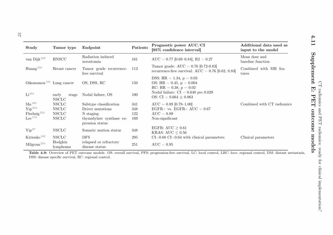
CT
radiom
icsan
dP
ET
radiom
ics:read
yfor
clinical
implem
entation
?
4.1
1Supple
men
tE:P
ET
outco
me
models
Study Tumor type Endpoint PatientsPrognostic power AUC/CI[95% confidence interval]
Additional data used asinput to the model
van Dijk249 HNSCCRadiation inducedxerostomia
161 AUC = 0.77 [0.69–0.84], R2 = 0.27Mean dose andbaseline function
Huang250 Breast cancer Tumor grade recurrence-free survival
113Tumor grade: AUC = 0.76 [0.72-0.83]recurrence-free survival: AUC = 0.76 [0.62, 0.83]
Combined with MR fea-tures
Oikonomou183 Lung cancer OS, DSS, RC 150DSS: HR = 1.34, p = 0.03OS: HR = 0.45, p = 0.004RC: HR = 0.38, p = 0.02
Li251 early stageNSCLC
Nodal failure, OS 100Nodal failure: CI = 0.640 pm 0.029OS: CI = 0.664 ± 0.063
Ma189 NSCLC Subtype classification 341 AUC = 0.89 [0.78–1.00] Combined with CT radiomicsYip252 NSCLC Driver mutations 348 EGFR+ vs. EGFR-: AUC = 0.67Flechsig253 NSCLC N staging 122 AUC = 0.89Lee179 NSCLC thymidylate synthase ex-
pression status169 Non-significant
Yip87 NSCLC Somatic mution status 348EGFR: AUC ≥ 0.61KRAS: AUC ≤ 0.56
Kirienko182 NSCLC DFS 295 CI=0.68 CI=0.64 with clinical parameters Clinical parameters
Milgrom254 Hodgkinlymphoma
relapsed or refractorydisease status
251 AUC = 0.95
Table 4.9: Overview of PET outcome models. OS: overall survival, PFS: progression-free survival, LC: local control, LRC: loco- regional control, DM: distant metastasis,DSS: disease specific survival, RC: regional control.
57

58

5Systematic review on the correlation of
radiomics with tumor biomarker
Agustina La Greca1, Diem Vuong1, Fabienne Tschanz2, Janita E. van Timmeren1, Ricardo Dal Bello1,
Verena Waller2, Martin Pruschy2, Matthias Guckenberger1, Stephanie Tanadini–Lang1
1Department of Radiation Oncology, University Hospital Zurich and University of Zurich, Zurich, Switzer-land2Laboratory of Applied Radiobiology, Department of Radiation Oncology, University of Zurich, Zurich,Switzerland
Status:Not yet published. It is planned to submitthis study to Cancers in the form presentedhere with only minor non-content changes.
Copyright: Authors retained the copyright totheir articles.
My contribution: In the literature search, I identified papers with keywords "ALK", "EGFR","KRAS". I summarized all papers investigating lung cancer radiomics (section 5.4.4). Further, I extractedmodel features of all found studies and created the feature interpretation tables (Table 5.8, 5.9, 5.10 aswell as the Supplement Tables 5.12, 5.13, 5.14). I included the feature interpretation if provided in therespective study, otherwise I noted a potential interpretation of the features.
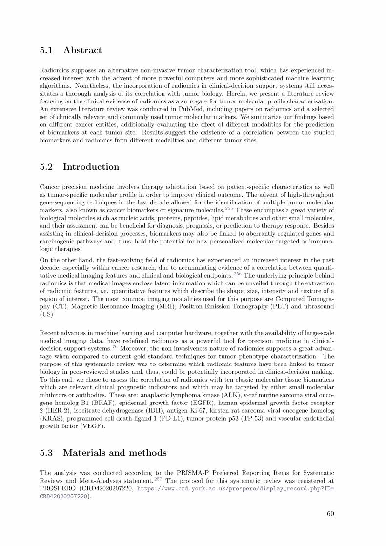
5.1 Abstract
Radiomics supposes an alternative non-invasive tumor characterization tool, which has experienced in-creased interest with the advent of more powerful computers and more sophisticated machine learningalgorithms. Nonetheless, the incorporation of radiomics in clinical-decision support systems still neces-sitates a thorough analysis of its correlation with tumor biology. Herein, we present a literature reviewfocusing on the clinical evidence of radiomics as a surrogate for tumor molecular profile characterization.An extensive literature review was conducted in PubMed, including papers on radiomics and a selectedset of clinically relevant and commonly used tumor molecular markers. We summarize our findings basedon different cancer entities, additionally evaluating the effect of different modalities for the predictionof biomarkers at each tumor site. Results suggest the existence of a correlation between the studiedbiomarkers and radiomics from different modalities and different tumor sites.
5.2 Introduction
Cancer precision medicine involves therapy adaptation based on patient-specific characteristics as wellas tumor-specific molecular profile in order to improve clinical outcome. The advent of high-throughputgene-sequencing techniques in the last decade allowed for the identification of multiple tumor molecularmarkers, also known as cancer biomarkers or signature molecules.255 These encompass a great variety ofbiological molecules such as nucleic acids, proteins, peptides, lipid metabolites and other small molecules,and their assessment can be beneficial for diagnosis, prognosis, or prediction to therapy response. Besidesassisting in clinical-decision processes, biomarkers may also be linked to aberrantly regulated genes andcarcinogenic pathways and, thus, hold the potential for new personalized molecular targeted or immuno-logic therapies.
On the other hand, the fast-evolving field of radiomics has experienced an increased interest in the pastdecade, especially within cancer research, due to accumulating evidence of a correlation between quanti-tative medical imaging features and clinical and biological endpoints.256 The underlying principle behindradiomics is that medical images enclose latent information which can be unveiled through the extractionof radiomic features, i.e. quantitative features which describe the shape, size, intensity and texture of aregion of interest. The most common imaging modalities used for this purpose are Computed Tomogra-phy (CT), Magnetic Resonance Imaging (MRI), Positron Emission Tomography (PET) and ultrasound(US).
Recent advances in machine learning and computer hardware, together with the availability of large-scalemedical imaging data, have redefined radiomics as a powerful tool for precision medicine in clinical-decision support systems.76 Moreover, the non-invasiveness nature of radiomics supposes a great advan-tage when compared to current gold-standard techniques for tumor phenotype characterization. Thepurpose of this systematic review was to determine which radiomic features have been linked to tumorbiology in peer-reviewed studies and, thus, could be potentially incorporated in clinical-decision making.To this end, we chose to assess the correlation of radiomics with ten classic molecular tissue biomarkerswhich are relevant clinical prognostic indicators and which may be targeted by either small molecularinhibitors or antibodies. These are: anaplastic lymphoma kinase (ALK), v-raf murine sarcoma viral onco-gene homolog B1 (BRAF), epidermal growth factor (EGFR), human epidermal growth factor receptor2 (HER-2), isocitrate dehydrogenase (IDH), antigen Ki-67, kirsten rat sarcoma viral oncogene homolog(KRAS), programmed cell death ligand 1 (PD-L1), tumor protein p53 (TP-53) and vascular endothelialgrowth factor (VEGF).
5.3 Materials and methods
The analysis was conducted according to the PRISMA-P Preferred Reporting Items for SystematicReviews and Meta-Analyses statement.257 The protocol for this systematic review was registered atPROSPERO (CRD42020207220, https://www.crd.york.ac.uk/prospero/display_record.php?ID=
CRD42020207220).
60

Systematic review on the correlation of radiomics with tumor biomarker
Records identified through
database searching
(n = 304 ) S
cre
en
ing
In
clu
de
d
Eli
gib
ilit
y
Ide
nti
fica
tio
n
Additional records identified
through other sources
(n = 0 )
Records after duplicates removed
(n = 121 )
Records screened
(n = 183 )
Records excluded
(n = 33 )
Full-text articles assessed
for eligibility
(n = 150 )
Full-text articles excluded,
with reasons
(n = 50 )
Studies included in
qualitative synthesis
(n = 100 )
Studies included in
quantitative synthesis
(meta-analysis)
(n = 100 )
Figure 5.1: Flow diagram of the study selection process according to PRISMA guidelines.
5.3.1 Literature search
The search was conducted on the PubMed database. According to PRISMA guidelines, article selectionwas carried out in multiple steps. The literature search was performed using the query “Radiomics[AllFields] AND keyword[All Fields]”, where keyword corresponded to one of the ten classic molecular tissuebiomarkers under study (i.e. ALK, BRAF, EGFR, HER-2, IDH-1, Ki-67, KRAS, TP-53, PD-L1 andVEGF) and the possible variations in its naming (e.g. HER2 and HER-2). The full list of queries isprovided in the supplementary material. In total, twenty independent searches were performed. Norecords were included from other sources such as direct correspondence with authors. The search had nostart date limit and was concluded on March 31st, 2020.The total number of studies retrieved in the independent PubMed searches was collected, from whichduplicates were identified with the open-source reference management software Zotero258 and removedfrom the following analysis.
5.3.2 Eligibility criteria
During the first screening, those studies which did not fulfil the following requirements were excluded: 1)the article had to be written in English, 2) the study had to be a scientific article excluding reviews, and3) the topic had to be related to biomarkers in cancer. Following this step, every article was assignedto one of the following categories, depending on the cancer site: breast, central nervous system (CNS),gastrointestinal, liver, lung and others.The full-text articles were then assessed for eligibility. If at least one of the following criteria applied,the article was excluded from the final analysis: 1) only one of the two groups, biomarker-negative orbiomarker-positive, patients were included in the study, 2) the total number of patients was less than 40,
61
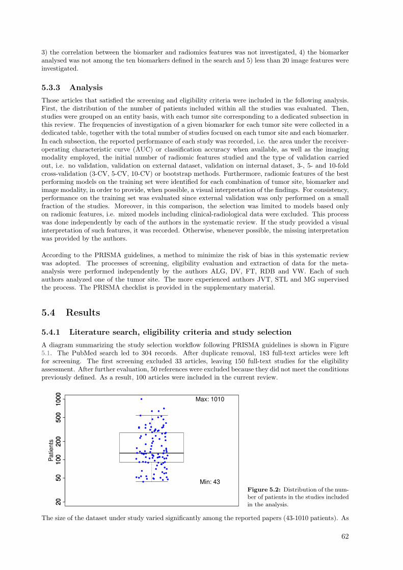
3) the correlation between the biomarker and radiomics features was not investigated, 4) the biomarkeranalysed was not among the ten biomarkers defined in the search and 5) less than 20 image features wereinvestigated.
5.3.3 Analysis
Those articles that satisfied the screening and eligibility criteria were included in the following analysis.First, the distribution of the number of patients included within all the studies was evaluated. Then,studies were grouped on an entity basis, with each tumor site corresponding to a dedicated subsection inthis review. The frequencies of investigation of a given biomarker for each tumor site were collected in adedicated table, together with the total number of studies focused on each tumor site and each biomarker.In each subsection, the reported performance of each study was recorded, i.e. the area under the receiver-operating characteristic curve (AUC) or classification accuracy when available, as well as the imagingmodality employed, the initial number of radiomic features studied and the type of validation carriedout, i.e. no validation, validation on external dataset, validation on internal dataset, 3-, 5- and 10-foldcross-validation (3-CV, 5-CV, 10-CV) or bootstrap methods. Furthermore, radiomic features of the bestperforming models on the training set were identified for each combination of tumor site, biomarker andimage modality, in order to provide, when possible, a visual interpretation of the findings. For consistency,performance on the training set was evaluated since external validation was only performed on a smallfraction of the studies. Moreover, in this comparison, the selection was limited to models based onlyon radiomic features, i.e. mixed models including clinical-radiological data were excluded. This processwas done independently by each of the authors in the systematic review. If the study provided a visualinterpretation of such features, it was recorded. Otherwise, whenever possible, the missing interpretationwas provided by the authors.
According to the PRISMA guidelines, a method to minimize the risk of bias in this systematic reviewwas adopted. The processes of screening, eligibility evaluation and extraction of data for the meta-analysis were performed independently by the authors ALG, DV, FT, RDB and VW. Each of suchauthors analyzed one of the tumor site. The more experienced authors JVT, STL and MG supervisedthe process. The PRISMA checklist is provided in the supplementary material.
5.4 Results
5.4.1 Literature search, eligibility criteria and study selection
A diagram summarizing the study selection workflow following PRISMA guidelines is shown in Figure5.1. The PubMed search led to 304 records. After duplicate removal, 183 full-text articles were leftfor screening. The first screening excluded 33 articles, leaving 150 full-text studies for the eligibilityassessment. After further evaluation, 50 references were excluded because they did not meet the conditionspreviously defined. As a result, 100 articles were included in the current review.
20
50
10
02
00
50
01
00
0
●
●
●
●
●
●
●
●
●
●
●
●
● ●
●
●
●
●
●
●●
●
●
●
●●
●
●
●
●
●
●
●
●
●
●
●
●
●
●
●
●
●
●
●
●
●
●
●
●
●
●●
●
●
●
●
●
●
●
●
●
●
●
●
●
●
●
●
●
●
●
●
●
●●
●
●
●
●
●
●
●
●
●
● ●
●
● ●
●
●
●
●
●
●
●
●
●
●
●
●
●
●
●
20
50
10
02
00
50
01
00
0
●
●
●
●
●
●
●
●
●
●
●
●
●●
●
●
●
●
●
● ●
●
●
●
● ●
●
●
●
●
●
●
●
●
●
●
●
●
●
●
●
●
●
●
●
●
●
●
●
●
●
● ●
●
●
●
●
●
●
●
●
●
●
●
●
●
●
●
●
●
●
●
●
●
●●
●
●
●
●
●
●
●
●
●
●●
●
●●
●
●
●
●
●
●
●
●
●
●
●
●
●
●
●
Pa
tie
nts
Min: 43
Max: 1010
Figure 5.2: Distribution of the num-ber of patients in the studies includedin the analysis.
The size of the dataset under study varied significantly among the reported papers (43-1010 patients). As
62
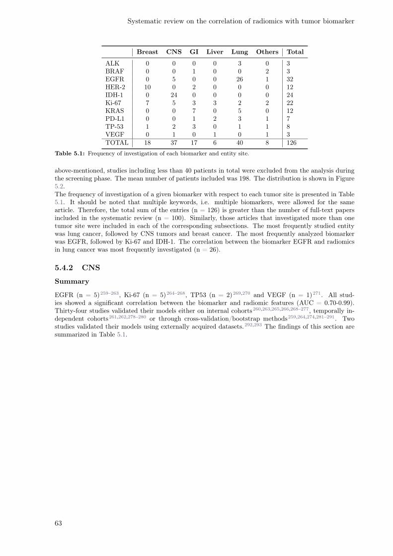
Systematic review on the correlation of radiomics with tumor biomarker
Breast CNS GI Liver Lung Others Total
ALK 0 0 0 0 3 0 3BRAF 0 0 1 0 0 2 3EGFR 0 5 0 0 26 1 32HER-2 10 0 2 0 0 0 12IDH-1 0 24 0 0 0 0 24Ki-67 7 5 3 3 2 2 22KRAS 0 0 7 0 5 0 12PD-L1 0 0 1 2 3 1 7TP-53 1 2 3 0 1 1 8VEGF 0 1 0 1 0 1 3TOTAL 18 37 17 6 40 8 126
Table 5.1: Frequency of investigation of each biomarker and entity site.
above-mentioned, studies including less than 40 patients in total were excluded from the analysis duringthe screening phase. The mean number of patients included was 198. The distribution is shown in Figure5.2.The frequency of investigation of a given biomarker with respect to each tumor site is presented in Table5.1. It should be noted that multiple keywords, i.e. multiple biomarkers, were allowed for the samearticle. Therefore, the total sum of the entries (n = 126) is greater than the number of full-text papersincluded in the systematic review (n = 100). Similarly, those articles that investigated more than onetumor site were included in each of the corresponding subsections. The most frequently studied entitywas lung cancer, followed by CNS tumors and breast cancer. The most frequently analyzed biomarkerwas EGFR, followed by Ki-67 and IDH-1. The correlation between the biomarker EGFR and radiomicsin lung cancer was most frequently investigated (n = 26).
5.4.2 CNS
Summary
EGFR (n = 5)259–263, Ki-67 (n = 5)264–268, TP53 (n = 2)269,270 and VEGF (n = 1)271. All stud-ies showed a significant correlation between the biomarker and radiomic features (AUC = 0.70-0.99).Thirty-four studies validated their models either on internal cohorts260,263,265,266,268–277, temporally in-dependent cohorts261,262,278–280 or through cross-validation/bootstrap methods259,264,274,281–291. Twostudies validated their models using externally acquired datasets.292,293 The findings of this section aresummarized in Table 5.1.
63
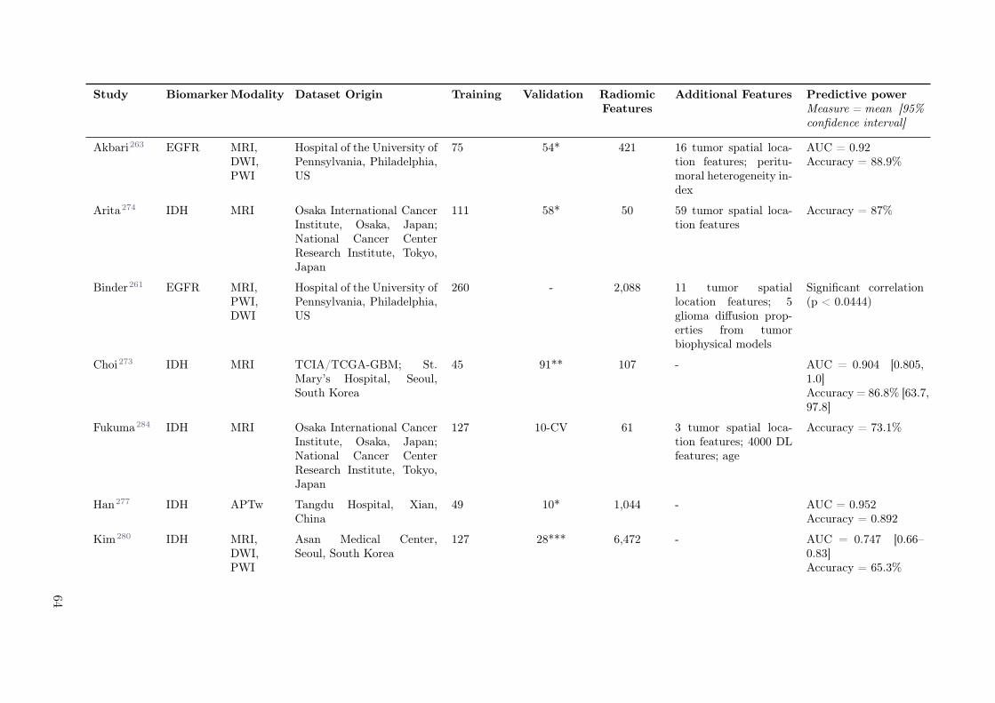
Study BiomarkerModality Dataset Origin Training Validation RadiomicFeatures
Additional Features Predictive powerMeasure = mean [95%confidence interval]
Akbari263 EGFR MRI,DWI,PWI
Hospital of the University ofPennsylvania, Philadelphia,US
75 54* 421 16 tumor spatial loca-tion features; peritu-moral heterogeneity in-dex
AUC = 0.92Accuracy = 88.9%
Arita274 IDH MRI Osaka International CancerInstitute, Osaka, Japan;National Cancer CenterResearch Institute, Tokyo,Japan
111 58* 50 59 tumor spatial loca-tion features
Accuracy = 87%
Binder261 EGFR MRI,PWI,DWI
Hospital of the University ofPennsylvania, Philadelphia,US
260 - 2,088 11 tumor spatiallocation features; 5glioma diffusion prop-erties from tumorbiophysical models
Significant correlation(p < 0.0444)
Choi273 IDH MRI TCIA/TCGA-GBM; St.Mary’s Hospital, Seoul,South Korea
45 91** 107 - AUC = 0.904 [0.805,1.0]Accuracy = 86.8% [63.7,97.8]
Fukuma284 IDH MRI Osaka International CancerInstitute, Osaka, Japan;National Cancer CenterResearch Institute, Tokyo,Japan
127 10-CV 61 3 tumor spatial loca-tion features; 4000 DLfeatures; age
Accuracy = 73.1%
Han277 IDH APTw Tangdu Hospital, Xian,China
49 10* 1,044 - AUC = 0.952Accuracy = 0.892
Kim280 IDH MRI,DWI,PWI
Asan Medical Center,Seoul, South Korea
127 28*** 6,472 - AUC = 0.747 [0.66–0.83]Accuracy = 65.3%
64
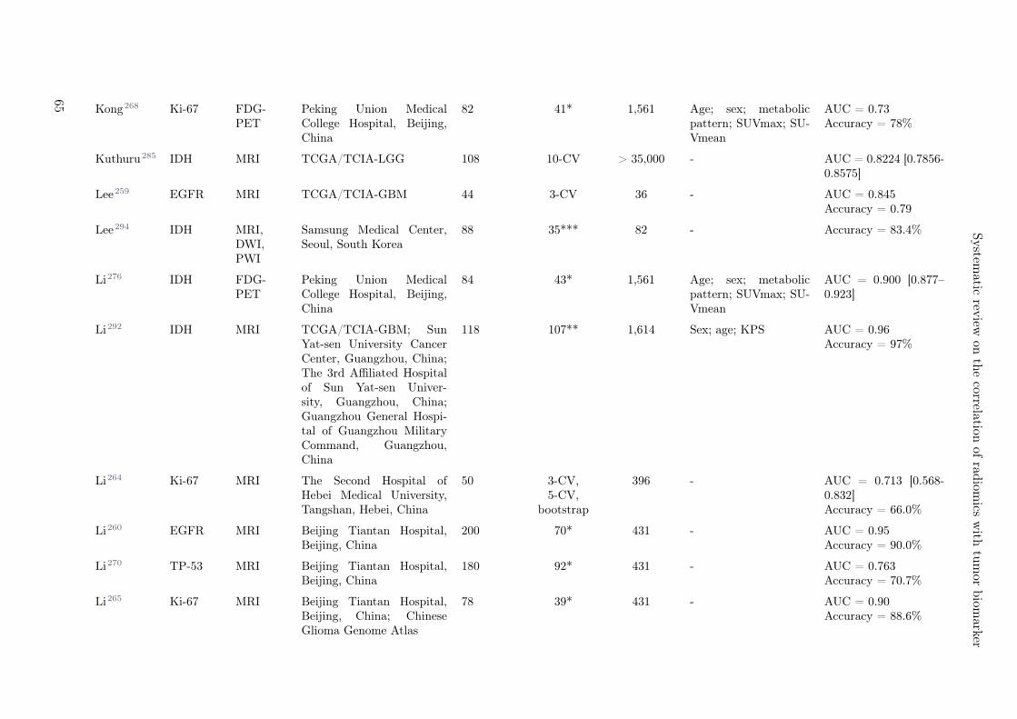
System
aticrev
iewon
the
correlationof
radiom
icsw
ithtu
mor
biom
arker
Kong268 Ki-67 FDG-PET
Peking Union MedicalCollege Hospital, Beijing,China
82 41* 1,561 Age; sex; metabolicpattern; SUVmax; SU-Vmean
AUC = 0.73Accuracy = 78%
Kuthuru285 IDH MRI TCGA/TCIA-LGG 108 10-CV > 35,000 - AUC = 0.8224 [0.7856-0.8575]
Lee259 EGFR MRI TCGA/TCIA-GBM 44 3-CV 36 - AUC = 0.845Accuracy = 0.79
Lee294 IDH MRI,DWI,PWI
Samsung Medical Center,Seoul, South Korea
88 35*** 82 - Accuracy = 83.4%
Li276 IDH FDG-PET
Peking Union MedicalCollege Hospital, Beijing,China
84 43* 1,561 Age; sex; metabolicpattern; SUVmax; SU-Vmean
AUC = 0.900 [0.877–0.923]
Li292 IDH MRI TCGA/TCIA-GBM; SunYat-sen University CancerCenter, Guangzhou, China;The 3rd Affiliated Hospitalof Sun Yat-sen Univer-sity, Guangzhou, China;Guangzhou General Hospi-tal of Guangzhou MilitaryCommand, Guangzhou,China
118 107** 1,614 Sex; age; KPS AUC = 0.96Accuracy = 97%
Li264 Ki-67 MRI The Second Hospital ofHebei Medical University,Tangshan, Hebei, China
50 3-CV,5-CV,
bootstrap
396 - AUC = 0.713 [0.568-0.832]Accuracy = 66.0%
Li260 EGFR MRI Beijing Tiantan Hospital,Beijing, China
200 70* 431 - AUC = 0.95Accuracy = 90.0%
Li270 TP-53 MRI Beijing Tiantan Hospital,Beijing, China
180 92* 431 - AUC = 0.763Accuracy = 70.7%
Li265 Ki-67 MRI Beijing Tiantan Hospital,Beijing, China; ChineseGlioma Genome Atlas
78 39* 431 - AUC = 0.90Accuracy = 88.6%
65
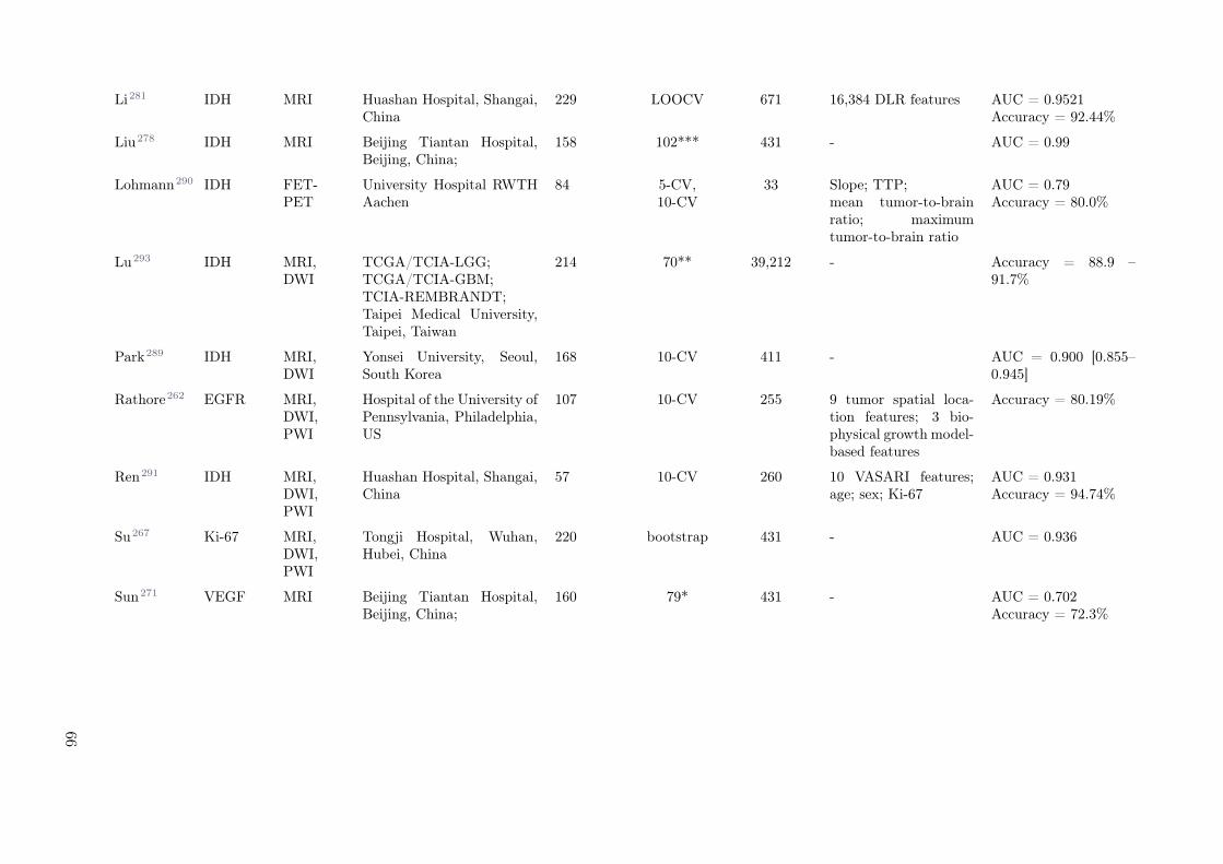
Li281 IDH MRI Huashan Hospital, Shangai,China
229 LOOCV 671 16,384 DLR features AUC = 0.9521Accuracy = 92.44%
Liu278 IDH MRI Beijing Tiantan Hospital,Beijing, China;
158 102*** 431 - AUC = 0.99
Lohmann290 IDH FET-PET
University Hospital RWTHAachen
84 5-CV,10-CV
33 Slope; TTP;mean tumor-to-brainratio; maximumtumor-to-brain ratio
AUC = 0.79Accuracy = 80.0%
Lu293 IDH MRI,DWI
TCGA/TCIA-LGG;TCGA/TCIA-GBM;TCIA-REMBRANDT;Taipei Medical University,Taipei, Taiwan
214 70** 39,212 - Accuracy = 88.9 –91.7%
Park289 IDH MRI,DWI
Yonsei University, Seoul,South Korea
168 10-CV 411 - AUC = 0.900 [0.855–0.945]
Rathore262 EGFR MRI,DWI,PWI
Hospital of the University ofPennsylvania, Philadelphia,US
107 10-CV 255 9 tumor spatial loca-tion features; 3 bio-physical growth model-based features
Accuracy = 80.19%
Ren291 IDH MRI,DWI,PWI
Huashan Hospital, Shangai,China
57 10-CV 260 10 VASARI features;age; sex; Ki-67
AUC = 0.931Accuracy = 94.74%
Su267 Ki-67 MRI,DWI,PWI
Tongji Hospital, Wuhan,Hubei, China
220 bootstrap 431 - AUC = 0.936
Sun271 VEGF MRI Beijing Tiantan Hospital,Beijing, China;
160 79* 431 - AUC = 0.702Accuracy = 72.3%
66
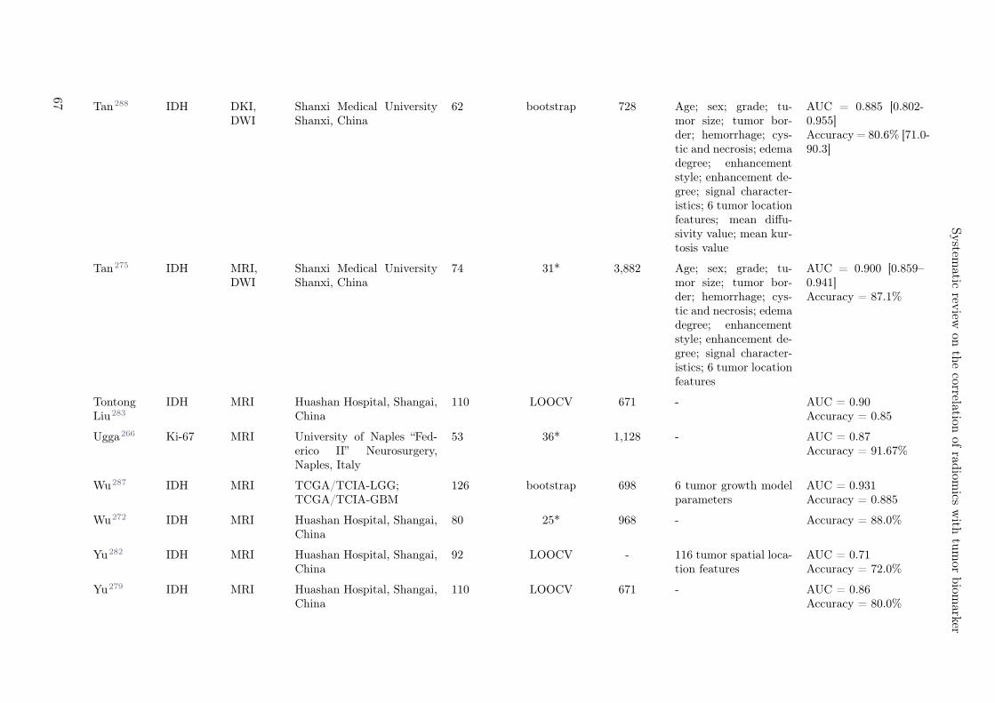
System
aticrev
iewon
the
correlationof
radiom
icsw
ithtu
mor
biom
arker
Tan288 IDH DKI,DWI
Shanxi Medical UniversityShanxi, China
62 bootstrap 728 Age; sex; grade; tu-mor size; tumor bor-der; hemorrhage; cys-tic and necrosis; edemadegree; enhancementstyle; enhancement de-gree; signal character-istics; 6 tumor locationfeatures; mean diffu-sivity value; mean kur-tosis value
AUC = 0.885 [0.802-0.955]Accuracy = 80.6% [71.0-90.3]
Tan275 IDH MRI,DWI
Shanxi Medical UniversityShanxi, China
74 31* 3,882 Age; sex; grade; tu-mor size; tumor bor-der; hemorrhage; cys-tic and necrosis; edemadegree; enhancementstyle; enhancement de-gree; signal character-istics; 6 tumor locationfeatures
AUC = 0.900 [0.859–0.941]Accuracy = 87.1%
TontongLiu283
IDH MRI Huashan Hospital, Shangai,China
110 LOOCV 671 - AUC = 0.90Accuracy = 0.85
Ugga266 Ki-67 MRI University of Naples “Fed-erico II” Neurosurgery,Naples, Italy
53 36* 1,128 - AUC = 0.87Accuracy = 91.67%
Wu287 IDH MRI TCGA/TCIA-LGG;TCGA/TCIA-GBM
126 bootstrap 698 6 tumor growth modelparameters
AUC = 0.931Accuracy = 0.885
Wu272 IDH MRI Huashan Hospital, Shangai,China
80 25* 968 - Accuracy = 88.0%
Yu282 IDH MRI Huashan Hospital, Shangai,China
92 LOOCV - 116 tumor spatial loca-tion features
AUC = 0.71Accuracy = 72.0%
Yu279 IDH MRI Huashan Hospital, Shangai,China
110 LOOCV 671 - AUC = 0.86Accuracy = 80.0%
67

Zhang269 IDH, TP-53
MRI TCGA/TCIA-LGG 73 30* 260 16 VASARI features IDH: AUC = 0.792Accuracy = 80.0%TP-53: AUC = 0.869Accuracy = 85.0%
Zhou286 IDH MRI TCGA/TCIA-LGG 84 bootstrap 3,360 30 VASARI features;age; sex; KPS; histo-logical type; grade; lat-erality; location
AUC = 0.86
Table 5.2: An overview of the radiomic studies included in the CNS cancer section. * internal validation; ** external validation; *** temporally independent internalvalidation. Acronyms: epidermal growth factor (EGFR), isocitrate dehydrogenase 1 (IDH-1), antigen Ki-67 (Ki-67), tumor protein p53 (TP-53), vascular endothelial growthfactor (VEGF), fluorodeoxyglucose positron emission tomogrpahy (FDG-PET), fluoro-ethyl-tyrosine positron emission tomography (FET-PET), perfusion weighted imaging(PWI), magnetic resonance imaging (MRI), diffusion weighted imaging (DWI), amide proton transfer-weighted imaging (APTw), max and mean standardized uptake value(SUVmax, SUVmean), The Cancer Imaging Archive / The Cancer Genome Atlas (TCIA/TCGA), glioblastoma (GBM), lower-grade glioma (LGG), Karnofsky PerformanceStatus (KPS), The Repository of Molecular Brain Neoplasia Data (REMBRANDT), Vissualy AccesSAble Rembrandt Images (VASARI), deep learning (DL), deep learningradiomics (DLR), time-to-peak (TTP), leave-one-out cross-validation (LOOCV), 3-, 5- and 10-fold cross-validation (3-, 5- and 10-CV), area under the curve (AUC).
68

Systematic review on the correlation of radiomics with tumor biomarker
IDH
A total of fifteen studies were found which investigated the power of MR radiomics to predict IDHgenotype in glioma (AUC = 0.70-0.99, accuracy = 73.1-97%).269,272–274,278,279,281,283–287,292 Four studiesexclusively employed MR radiomics273,278,279,283, whereas eight studies used a combination of traditionalradiomic features with other types of imaging features such as location parameters (n = 5)274,279,282,283,Visually AcceSAble Rembrandt Images (VASARI) features (n = 3)269,286,292, deep learning radiomics(DLR, n = 2)274,281, and tumor growth model parameters (n = 1)287. Three studies based their modelscompletely on non-conventional radiomics: one of them employed purely anatomical location features282,another one used histogram of oriented gradients (HoGs), raw voxel intensities and scale-invariant fea-ture transform (SIFT) descriptors285, and the third one used fine texture features obtained by k-meanssingular value decomposition (K-SVD), a dictionary learning algorithm.272 Three of the fifteen studiesalso incorporated clinical-radiological parameters into their models.274,286,292
The best predictive performance was achieved by Li et al. on glioblastoma patients by means of arandom forests (RF) model based on gray-level co-occurrence matrix (GLCM), grey-level run-lengthmatrix (GLRLM) and grey-level size zone matrix (GLSZM) textural features together with patient age(AUC = 0.96, external validation).292 Among MR radiomics in both, lower- and higher-grade gliomas,relevant features for IDH mutation status prediction were associated with textural heterogeneity, suggest-ing that IDH wild-type tumors are more heterogeneous and more structurally complex than IDH-mutantones.273,274,292 Another feature that significantly correlated with IDH mutation status was tumor meansurface-to-volume ratio, which was lower in IDH-mutant cases.273,279 Moreover, IDH-mutant gliomaswere found to occur more frequently in the frontal, insular and temporal lobes.274,282
A total of seven studies were found which combined MR radiomics with diffusion weighted imaging(DWI), perfusion weighted imaging (PWI) and/or diffusion kinetic imaging (DKI) features to predict IDHmutation status in glioma patients (AUC = 0.747-0.931).275,280,288,289,291,293,294 Among these studies,three of them incorporated clinical-radiological parameters in their modelling275,289,293 and one employedadditional VASARI imaging features.291 The best performance on an external cohort was achieved byLu et al., who proposed two support vector machine (SVM) models based on MR and DWI featurestogether with patient age and sex to predict IDH mutation status in GBM and LGG patients separately(accuracy = 88.9-91.7%, external validation).293 As opposed to MRI, DWI and PWI textural and intensityfeatures describing increased tumor heterogeneity were associated with IDH wild-type tumors. Moreover,IDH wild-type LGGs were found to have smaller minimum Apparent Diffusion Coefficient (ADC) andCerebral Blood Volume (CBV) values, which could indicate an increased tumor proliferation index andincreased malignancy.280,291
Two studies were found which used PET radiomics in conjunction with clinical-radiological parametersto predict IDH status in gliomas. One of them used fluoro-ethyl-tyrosine (FET)-PET standard param-eter slope and one texture feature (accuracy = 80.0%, 10-fold cross-validation)290, while the other onecombined fluorodeoxyglucose (FDG)-PET radiomics with age and tumor metabolism to achieve an AUCof 0.90 on an internal validation set276. Among FDG-PET radiomics, the feature sphericity was foundto play a significant role in IDH mutation status prediction, indicating that IDH-mutant gliomas are lessspherical than IDH wild-type in FDG-PET scans. Lastly, one study used APTw radiomics to predictIDH status in LGG patients (AUC = 0.84, internal validation).277 GLCM and GLRLM radiomic fea-tures describing tumor heterogeneity were identified as main contributors of IDH genotype prediction,with IDH-mutant tumors being more homogeneous.
EGFR
In total, two studies were found which investigated the correlation between MR radiomics and EGFRalterations in glioma, more precisely, between EGFR over-expression in LGG patients and EGFR mu-tation in GBM patients, respectively.259,260 The former proposed a logistic regression model based on41 radiomics features (AUC = 0.95, internal validation)260, and the latter study employed a symbolicregression method based on non-conventional MR spatial diversity descriptors (AUC = 0.845, cross-validation).259 In both cases, MR features describing tumor textural heterogeneity and shape irregularitywere found to correlate to EGFR, suggesting increased diversity in EGFR-mutated and EGFR-amplifiedtumors. Three studies were found which employed MR radiomics together with DWI and PWI radiomicsto predict EGFR mutation status in GBM patients. Binder et al. studied a variety of EGFR missensemutations and concluded that EGFR mutation at alanine 289 presented a unique radiographic phenotype.Authors reported significantly lower average T1 signal, higher relative cerebral blood volume and longer
69

major axis in EGFR-A289D/T/V-mutant tumors among other features.261 The two remaining studiesinvestigated the prediction of EGFR mutation at exons 2-7 (EGFRvIII) and incorporated additionalimaging features on their modelling such as location parameters, tumor growth model parameters andthe peritumoral heterogeneity index. Authors reported predictive accuracies of 73.58%262 and 87%263
on a temporally independent and on an internal validation cohort, respectively. Authors of the threeabove-mentioned studies suggested that EGFR-mutant tumors present an increase in shape variabilityand water concentration as well as a decreased cell density.
Ki-67
Three studies were found which investigated the correlation between Ki-67 expression and MR radiomicsin CNS tumors; one in glioblastoma (AUC = 0.9, accuracy = 88.6%, internal validation), one in both,lower and higher-grade gliomas (AUC = 0.713, accuracy = 66%, cross-validation) and one in pituitarymacroadenoma (accuracy = 96.7%, internal validation). In the three studies, Ki-67 expression wasassociated with increased textural heterogeneity. One study was found which combined MR, DWI andPWI radiomics to predict Ki-67 expression in grade I-IV gliomas (AUC = 0.936, training cohort).267
Authors reported that DWI features were more strongly correlated to Ki-67 than the other two imagingmodalities. Another study focused on Ki-67 prediction using FDG-PET radiomics (AUC = 0.76, internalvalidation).268
TP-53
Two studies evaluated the power of MR radiomics for TP-53 mutation status prediction in LGGs witha varying performance (AUC = 0.763-0.869, internal validation).269,269,270 One of them also includedVASARI imaging features in the modelling. Authors concluded that TP-53 mutant gliomas are moreheterogeneous and present higher water content.
VEGF
One study was found which investigated the use of conventional MR radiomics to predict VEGF expressionin LGGs (AUC = 0.702, internal validation).271
5.4.3 Breast cancer
Summary
Sixteen studies which correlated breast tumor molecular markers with clinical imaging radiomic fea-tures were identified. The imaging modalities studied were PWI (n = 9)295–303, conventional MRI(n = 2)304,305, DWI (n = 1)306, DWI+ PWI307, Digital Breast Tomography (DBT, n = 1)308, PET/CT(n = 1)309 or standard 2D digital mammography (DMG, n = 1)310. Most studies focused on invasivebreast cancer (n = 13)295–301,304–308,310,311, while three studies investigated non-invasive breast cancertypes302,303,309. HER-2 was the most frequently investigated biomarker (n = 10), and all studies showed asignificant correlation between HER-2 status and radiomic features (AUC = 0.65-0.95).295,297–301,303,305,309,310
Eight studies examined Ki-67, and all except one study found a significant correlation to radiomics fea-tures (AUC = 0.70-0.81).297,298,303,304,306–310 One study investigated TP-53 status (n = 1).296 Thirteenstudies employed internal validation sets or cross-validation and bootstrap methods datasets. The findingsof this section are summarized in Table 5.3.
70

System
aticrev
iewon
the
correlationof
radiom
icsw
ithtu
mor
biom
arker
Study BiomarkerModality Dataset Origin Training Validation RadiomicFeatures
Additional Features Predictive powerMeasure = mean [95%confidence interval]
Antunovic309 HER-2,Ki-67
FDG-PET/CT
Humanitas Hospital,Milan, Italy
43 - 20 MTV, SUVmean and TLG HER-2: Significantcorrelation (p = 0.021- 0.046)Ki-67: No significantcorrelation
Braman302 HER-2 PWI Cleveland Medi-cal Center, Cleveland,Ohio, US; City of HopeComprehensive Can-cer Center, Duarte,California, US; YaleCancer Center, NewHaven, Connecticut,US; Brown UniversityOncology ResearchGroup, Providence,Rhode Island, US;TCIA/TCGA-BRCA
117 3-CV 495 - AUC = 0.71 [0.63-0.79]
Castaldo301 HER-2 PWI TCIA/TCGA-BRCA 55 36* 36 - AUC = 0.91Accuracy = 81-88%
Fan300 HER-2 PWI Zhejiang CancerHospital, Hangzhou,China
60 36* 65 Age, menopausal status;29 dynamic features fromBPE and the lesion; 9 bi-lateral differences in BPE
AUC = 0.947
Fan307 Ki-67 PWI,DWI
First Affiliated Hospi-tal of Zhejiang Chi-nese Medical Univer-sity, Hangzhou, China
144 LOOCV 97 - AUC = 0.811
71
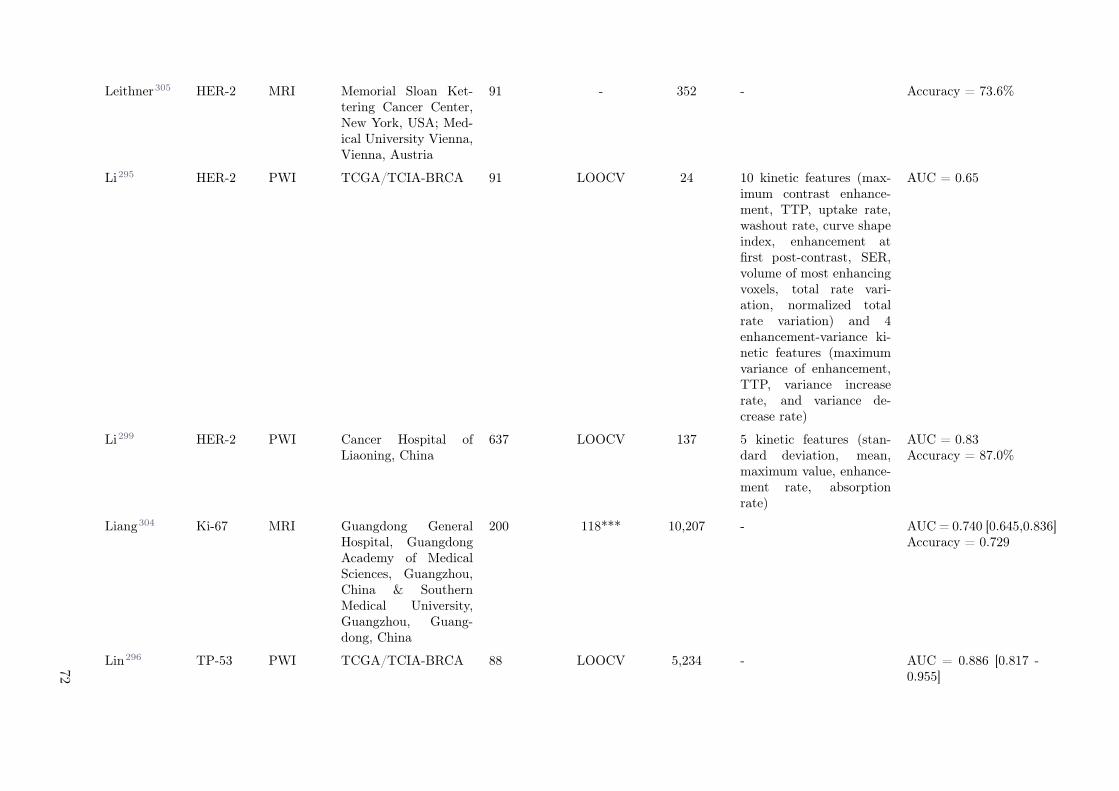
Leithner305 HER-2 MRI Memorial Sloan Ket-tering Cancer Center,New York, USA; Med-ical University Vienna,Vienna, Austria
91 - 352 - Accuracy = 73.6%
Li295 HER-2 PWI TCGA/TCIA-BRCA 91 LOOCV 24 10 kinetic features (max-imum contrast enhance-ment, TTP, uptake rate,washout rate, curve shapeindex, enhancement atfirst post-contrast, SER,volume of most enhancingvoxels, total rate vari-ation, normalized totalrate variation) and 4enhancement-variance ki-netic features (maximumvariance of enhancement,TTP, variance increaserate, and variance de-crease rate)
AUC = 0.65
Li299 HER-2 PWI Cancer Hospital ofLiaoning, China
637 LOOCV 137 5 kinetic features (stan-dard deviation, mean,maximum value, enhance-ment rate, absorptionrate)
AUC = 0.83Accuracy = 87.0%
Liang304 Ki-67 MRI Guangdong GeneralHospital, GuangdongAcademy of MedicalSciences, Guangzhou,China & SouthernMedical University,Guangzhou, Guang-dong, China
200 118*** 10,207 - AUC = 0.740 [0.645,0.836]Accuracy = 0.729
Lin296 TP-53 PWI TCGA/TCIA-BRCA 88 LOOCV 5,234 - AUC = 0.886 [0.817 -0.955]
72

System
aticrev
iewon
the
correlationof
radiom
icsw
ithtu
mor
biom
arker
Ma297 Ki-67 PWI Tianjin MedicalUniversity CancerInstitute and Hospi-tal, National ClinicalResearch Center forCancer, Tianjin, China
159 10-CV 56 - AUC = 0.773Accuracy = 0.757
Monti298 HER-2,Ki-67
PWI Hospital of Moscati,Avellino, Italy; Insti-tute for Hospitaliza-tion and HealthcareSDN, Naples, Italy
HER-2: 48Ki-67: 49
bootstrap 163 - HER-2: AUC = 0.838Accuracy = 0.785Ki-67: AUC = 0.811Accuracy = 0.677
Tagliafico308 Ki-67 DBT Emergency Radiology,IRCCS Policlinico SanMartino, Genoa, Italy
70 bootstrap 106 - AUC = 0.698
Zhang306 Ki-67 DWI The Second Hospital,Dalian Medical Uni-versity, Dalian, China
101 27* 1,029 - AUC = 0.72 [0.495 -0.857]Accuracy = 0.70
Zhou310 HER-2 DMG Henan Provincial Peo-ple’s Hospital, Henan,China
244 62* 186 - AUC = 0.787 [0.673-0.885]Accuracy = 77.00%
Zhou303 HER-2,Ki-67
PWI The Affiliated HuaianNo. 1 People’s Hospi-tal of Nanjing MedicalUniversity, China
126 5-CV 386 - HER-2: AUC = 0.68Accuracy = 0.60Ki-67: AUC = 0.74Accuracy = 0.69
Table 5.3: An overview of the radiomic studies included in the breast cancer section. * internal validation; ** external validation; *** temporally independent internalvalidation. Acronyms: human epidermal growth factor receptor 2 (HER-2), antigen Ki-67 (Ki-67), tumor protein p53 (TP-53), fluorodeoxyglucose positron emission tomo-grpahy / computed tomogrpahy (FDG-PET/CT), perfusion weighted imaging (PWI), magnetic resonance imaging (MRI), diffusion weighted imaging (DWI), digital breasttomosynthesis (DBT), digital mammography (DMG), metabolic tumor volume (MTV), mean standardized uptake value (SUVmean), The Cancer Imaging Archive / TheCancer Genome Atlas (TCIA/TCGA), BRCA (BReast invasive CArcinoma), total lesion glycolysis (TLG), background parenchymal enhancement (BPE), signal enhancementratio (SER), time-to-peak (TTP), leave-one-out cross-validation (LOOCV), 3-, 5- and 10-fold cross-validation (3-, 5- and 10-CV), area under the curve (AUC).
73

HER-2
The most frequently investigated biomarker was HER-2, with seven studies correlating HER-2 statusto radiomics data derived from PWI295,298–[51], one study to DMG310, another study to PET/CT(n = 1)[57], and one study to conventional MRI305. In the study using PET/CT, only mean standardizeduptake value (SUVmean) and total lesion glycolysis (TLG) were independently associated with HER-2status (p = 0.021 and p = 0.046, respectively).309 The predictive model constructed by Monti et al.using PWI-extracted radiomics, could discriminate between HER-2+ versus HER-2- with an AUC of0.838 (accuracy: 0.785).298 Zhou et al. applied pharmacokinetic dynamic contrast-enhanced (Pk-DCE)MRI on the Tofts model to non-invasively diagnose molecular breast cancer subtypes (AUC = 0.61-0.68,cross validation).303
One group investigated the prediction performance of radiomic features derived from contrast enhanced(CE)-MRI images (accuracy=73.6%, training).305 Fan et al. trained a multi-class classifier using 15radiomics features extracted from PWI, which achieved an AUC of 0.947±0.053 for the prediction of theHER-2 molecular subtype.300 By combining PWI features from peritumoral and intratumoral regions,Braman et al. developed a model to distinguish HER-2+ molecular subtypes from other receptor subtypes(AUC = 0.71, cross validation).302
One group compared four traditional recursive feature elimination (RFE) models with a novel multi-model RFE algorithm to select the feature subset derived from PWI images.299 The gradient boostingdecision tree (GBDT) model obtained the best result on both classification and imbalance performancefor prediction of HER-2+ with a recognition precision of 0.83. Li et al. extracted 38 descriptors from PWIthat were able to distinguish between molecular subtypes with AUC values of 0.65 for the differentiationbetween HER-2+ versus HER-2-.295 By correlating quantitative radiomics with genomic signatures onegroup identified three advanced machine learning techniques (SVM, RF, and Naïve Bayesian) that coulddistinguish between HER-2-/HER-2+ as a prognostic indicator with AUC of 91%.301 One group usedradiomic features derived from DMG images for the prediction of HER-2 status.310 Zhou et al. obtainedhigher prediction performance when applying the logistic regression model using a combination of bilat-eral craniocaudal and mediolateral oblique view images derived from 2D MG (AUC = 0.787, internalvalidation), compared to the SVM model or using radiomic features from each view alone.
Ki-67
In total, eight studies correlated the Ki-67 status to radiomic features derived from PWI (n = 4)297,298,303,307,DWI (n = 2)306,307, MRI (n = 1)304, PET/CT (n = 1)309, and DBT (n = 1)308. One study associated 11features extracted from ADC maps to the Ki-67 index of 128 invasive ductal breast cancer patients, whichresulted in an AUC of 0.72 in the test set306. The study using PET/CT could not find any radiomicfeature that were significantly correlated to Ki-67.309 Two studies using PWI-extracted radiomic featuresfound AUCs of 0.811286 and 0.67-0.74271. Fan et al. proposed a multi-task learning model for the pre-diction of Ki-67 expression level.307 Applying the multi-task model on PWI and ADC images separately,improved the Ki-67 prediction performance for all image series. The S50-based predictive model per-formed the best with an AUC of 0.810 (p = 0.011), followed by ADC (AUC: 0.805; p = 0.028), S0 (AUC:0.795; p = 0.105), and S20 (AUC: 0.768; p = 0.032). Moreover, applying this model on radiomics datafrom PWI and DWI images combined, increased the AUC to 0.805-0.821. One group used 13 PWI ra-diomic features for the differentiation between low versus high Ki-67 expression levels (AUC = 0.773).297
Three features entropy, contrast and line likeness showing the highest prediction performance, indicatingthat more heterogeneous tumors had higher Ki-67 expression levels. One study used DBT images andshowed that a combination of the five most predictive features yielded an AUC of 0.698 for low- versushigh Ki-67 expression.308 Liang et al. applied MRI-based radiomics with the aim to identify the mostsuitable classifier and compared T2-weighted (T2W) with T1-weighted with contrast (T1+C).304 Theanalysis revealed that the T2W image-based radiomics classifier could significantly predict Ki-67 in thevalidation cohorts (AUC: 0.740 [95% CI: 0.645 - 0.836), whereas T1+C-based radiomics failed for thevalidation dataset.
TP-53
The highest correlation for breast cancer was found between TP-53 mutations and PWI radiomics of88 patients in which 13 radiomic features predicted TP-53 alterations with an AUC of 0.886 (95% CI:
74

Systematic review on the correlation of radiomics with tumor biomarker
0.817-0.955) on the internal validation dataset.296
In conclusion, the radiomic features extracted from breast cancer MRI are rather heterogeneous for theproliferation marker Ki-67 and the proto-oncogene HER-2. Since only one study investigated radiomicdescriptors for TP-53 together with a large variety of features, it is difficult to interpret the data.
5.4.4 Lung cancer
Summary
In total, we identified 33 studies investigating radiomics and tissue biomarkers for lung lesions, using CT(n = 22)134–136,180,242,312–327, PET/CT (n = 8)328–335, PET (n = 2)87,336 or MRI (n = 1)337. One studyinvestigated radiomics from metastases, all other studies correlated tissue biomarkers with radiomics ofthe primary tumor. Almost half of the studies selected histological subtypes and used adenocarcinomapatients only (n = 15) whereas the other half used a mix of histologies. Research has predominantlyfocused on EGFR (n = 26)87,134–136,180,312–323,328–333,336,337, followed by KRAS (n = 5)87,320,333,336,337,ALK (n = 3)324,334,337, PD-L1 (n = 3)325,326,335, Ki-67 (n = 2)242,327, and TP53 (n = 1)321. All studiesshowed a significant correlation between EGFR and radiomic features (AUC = 0.66-0.95). Two studiesthat could not find a significant correlation for KRAS, but all remaining studies found a significantcorrelation between radiomics and the respective biomarker (AUC = 0.66-0.99). In total, 21 studiesvalidated their predictive models, two of which were external validation. A summary of the findings ofthis section can be found in Table 5.4.
EGFR
The predictive power of CT radiomics with EGFR mutations status reported by studies using valida-tion strongly varied from acceptable to good performance (AUC = 0.69-0.851)134–136,314–323,338. AcrossCT radiomics studies, relevant features for EGFR mutation status prediction were associated to textureheterogeneity suggesting that mutated tumors were more heterogeneous. Further, two studies observedgood correlation of CT radiomics with subtypes of EGFR mutation, i.e. differentiation subtype to wild-type (AUC = 0.655-0.727)180,316 and within subtypes (AUC = 0.708-0.87)331,338. While PET radiomicsalso showed potential for EGFR mutation status prediction (AUC = 0.67, internal validation)87,336,combining CT and PET were reported similar or better compared to single modal radiomics mod-els328,328–332. Two studies examined radiomics at different time points other than pre-treatment.312,313
In contrast to three-week post-treatment CT radiomics, one delta radiomic feature (i.e. change of fea-ture value over time) was found predictive for EGFR mutation status (AUC = 0.74, weakly corrected todelta volume and diameter).312 Multiple studies were found using CE CT315,321,322, non-CE CT imag-ing134,135,180,180,312,314,317–319,338 or a mix of thereof136,320. In a recent study, it was shown for EGFRmutation status prediction that a model based CE CT did not significantly performed different to a modelbased non-CE CT.322
KRAS
In contrast to EGFR, CT radiomics was weakly predictive for KRAS mutation status in 763 lung adeno-carcinoma patients from four institutions (AUC = 0.63, temporally independent validation).320 KRASmutant tumors were found to be more homogeneous.320 PET radiomics was reported non-predictive forKRAS mutation status (AUC < 0.56, no validation).87,336 Radiomics was further shown to better differ-entiate between EGFR and KRAS mutated tumors in CT (AUC = 0.80, internal validation)320 than inPET (AUC = 0.65)336.
ALK
For ALK mutation status, CT radiomics showed excellent performance (AUC = 0.80, temporally inde-pendent validation).324 Selected radiomic features inferred that ALK mutated tumors were associatedwith denser tumors. One study observed that PET-based radiomics combined with tumor stage and agewas able to differentiate ALK/ROS1/RET fusion-positive and fusion negative tumors (sensitivity=0.73,specificity=0.70).334 A study on 110 patients evaluated if MR radiomics from brain metastasis origi-nated from lung cancer correlated with EGFR, ALK and KRAS mutations and reported excellent modelperformances for all three tissue biomarkers (AUC > 0.9, leave-one out cross validation).337
75

Study BiomarkerModality Dataset Origin Training Validation RadiomicFeatures
Additional Features Predictive powerMeasure = mean [95%confidence interval]
Aerts312 EGFR CT Memorial Sloan-KetteringCancer Center, New YorkCity, New York, US
47 - 183 - AUC = 0.91
Chen337 EGFR;KRAS;ALK
MR City of Hope Medical Cen-ter, Duarte, California,US
110 LOOCV 2,786 Age; sex; ethnicity; his-tory of smoking; histol-ogy type; other metastaticsites
EGFR: AUC = 0.912Accuracy = 77.7%ALK: AUC = 0.915Accuracy = 86.7%KRAS: AUC = 0.985Accuracy = 96.7%
Gu327 Ki-67 CT The Third Xiangya Hospi-tal of Central South Uni-versity, Hunan, China
245 10-CV 103 Lobulation sign; spiculesign; cavitation; cysticnecrosis; pleural indenta-tion; pleural effusion
AUC = 0.782
Hong322 EGFR CT The First Hospital ofChina Medical University,Shenyang, China
140 61* 396 Age; sex; history of smok-ing
AUC = 0.851 [0.750-0.951], CI = 0.835[0.825-0.845]
Huang313 EGFR CT The University of TexasMD Anderson CancerCenter, Houston, Texas
46 - 89 - AUC = 0.88
Jia135 EGFR CT Shanghai Chest Hospital,Shanghai, China
345 158* 440 Age; sex; smoking history;TNM stage
AUC = 0.828 [0.764-0.892]
Jiang335 PD-L1 PET/CT Shanghai Institute ofMedical Imaging, Zhong-shan Hospital of FudanUniversity, Shanghai,China
266 133* 1,744 SUVmax; age; sex; smok-ing status; TNM stage;histology type
AUC = 0.97
76

System
aticrev
iewon
the
correlationof
radiom
icsw
ithtu
mor
biom
arker
Jiang328 EGFR PET/CT Shanghai Institute ofMedical Imaging, Zhong-shan Hospital of FudanUniversity, Shanghai,China
80 10-CV 512 12 semantic features AUC = 0.953
Koyasu329 EGFR PET/CT TCIA- NSCLC Radio-genomics
138 10-CV Notdisclosed
SUVmax; SUVmean;TLG; MTV
AUC = 0.659Accuracy = 81.2%
Li330 EGFR PET/CT Tianjin Medical Univer-sity Cancer Hospital,Tianjin, China
115 10-CV 38 SUVmax; SUVmean; SU-Vpeak; TLG; MTV; age;sex; smoking status; TNMstage; lesion location
AUC = 0.822Accuracy = 82.65%
Li315 EGFR CT Second Xiangya Hospitalof Central South Univer-sity, Hunan, China
51 10-CV 1,695 - AUC = 0.83 [0.68-0.92]
Li136 EGFR CT Shanghai Chest Hospital,Shanghai, China
810 200* 440 DL prediction; age; sex;smoking history; patho-logical stage
AUC = 0.834 [0.776–0.892]
Li316 EGFR CT Shengjing Hospital ofChina Medical University,Liaoning, China
236 76*** 580 Age; sex; tumor grade;lobe; smoking history; in-trapulmonary metastasis
AUC = 0.7750-0.7925
Liu323 EGFR CT Tianjin Medical Univer-sity Cancer Institute andHospital, Tianjin, China
298 bootstrap 209 10 tumor spatial locationfeatures; age; sex; histo-logical subtype; pathologi-cal stage; smoking history
AUC = 0.709 [0.654 -0.766]
77

Lu314 EGFR CT The First Hospital of JilinUniversity, China
83 21* 1,025 45 categorical variables in-cluding: age, sex, smok-ing status, CEA level, vas-cular infiltration, visceralpleural infiltration, lymphnode metastasis, histolog-ical subtype, pathologi-cal stage, type of le-sion, tumor location, tu-mor size, tumor necro-sis, lobulation, spicula-tion, vacuolization, etc.
AUC = 0.894
Mei180 EGFR CT Shenzhen People’s Hospi-tal, Guangdong, China
296 - 94 Age; sex; smoking status AUC = 0.75
Nair331 EGFR PET/CT McGill University HealthCentre, 2011 and 2015
50 LOOCV 326 - AUC = 0.8713
Rios Ve-lazquez320
EGFR;KRAS
CT Profile and Harvard-RT(Dana-Farber/HarvardCancer Center IRB,Boston, MA), Tianjin(Tianjin Medical Univer-sity IRB, Tianjin, China),Moffitt (IRB MoffittCancer Center, Tampa,FL)
353 352*** 635 Age; sex; smoking status;ethnicity; clinical stage
EGFR:AUC = 0.75 [0.69-0.81]Accuracy = 65.0%KRAS:AUC = 0.75 [0.69-080]Accuracy = 66.0%EGFR+ vs. KRAS+:0.86 [0.80 – 0.91]Accuracy = 79.0%
Shiri333 EGFR;KRAS
PET/CT TCIA 82 68* 109 MTV, SUVmax, SUV-peak, SULmax, SULpeak
EGFR: AUC = 0.82KRAS: AUC = 0.83
78

System
aticrev
iewon
the
correlationof
radiom
icsw
ithtu
mor
biom
arker
Song324 ALK CT Peking Union MedicalCollege Hospital, ChineseAcademy of Medical Sci-ences and Peking UnionMedical College, Novem-ber 2015 to October2018
268 67* 1,218 Age; sex; smoking his-tory; smoking index; clin-ical stage; distal metas-tasis; pathological inva-siveness of tumor; maxi-mum diameter; mean CTattenuation; lesion loca-tion; involved lobe; den-sity; margin; cavity; calci-fication; pleural retractionsign; pleural effusion; peri-cardial effusion; local lym-phadenopathy
AUC = 0.88 [0.77-0.94]Accuracy = 79.0%
Sun325 PD-L1 CT The First Affiliated Hospi-tal of Soochow University,Suzhou City, China
260 130* 200 Age; sex; tumor location;CEA level; TNM stage;smoking status; histologictype; histologic grade
AUC = 0.848
Tu317 EGFR CT Changzheng Hospital,Second Military MedicalUniversity, Shanghai,China
243 130* 234 Age; sex; smoking sta-tus; CEA level; clinicalstage; maximum diame-ter; density; tumor lo-cation; interface; shape;lobulation; pleural inden-tation; spiculation; cuspangle; spine-like process;vacuole sign; cavity sign;air bronchograms; vascu-lar convergence; pleurathickening; pleural effu-sion; lymphoadenopathy
AUC = 0.818 [0.751-0885]Accuracy = 75.8%
Wang321 EGFR;TP-53
CT Nanjing Medical Univer-sity Affiliated Cancer Hos-pital, Nanjing, China
41 20* 718 78 clinical and patholog-ical features (age, sex,smoking status, histologi-cal subtypes, pathologicalstages, etc.)
EGFR: AUC = 0.697TP-53: AUC = 0.656
79
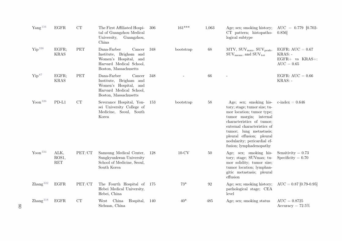
Yang134 EGFR CT The First Affiliated Hospi-tal of Guangzhou MedicalUniversity, Guangzhou,China
306 161*** 1,063 Age; sex; smoking history;CT pattern; histopatho-logical subtype
AUC = 0.779 [0.702-0.856]
Yip336 EGFR;KRAS
PET Dana-Farber CancerInstitute, Brigham andWomen’s Hospital, andHarvard Medical School,Boston, Massachusetts
348 bootstrap 68 MTV, SUVmax, SUVpeak,SUVmean, and SUVtot
EGFR: AUC = 0.67KRAS: -EGFR+ vs KRAS+:AUC = 0.65
Yip87 EGFR;KRAS
PET Dana-Farber CancerInstitute, Brigham andWomen’s Hospital, andHarvard Medical School,Boston, Massachusetts
348 - 66 - EGFR: AUC = 0.66KRAS: -
Yoon326 PD-L1 CT Severance Hospital, Yon-sei University College ofMedicine, Seoul, SouthKorea
153 bootstrap 58 Age; sex; smoking his-tory; stage; tumor size; tu-mor location; tumor type;tumor margin; internalcharacteristics of tumor;external characteristics oftumor; lung metastasis;pleural effusion; pleuralnodularity; pericardial ef-fusion; lymphadenopathy
c-index = 0.646
Yoon334 ALK,ROS1,RET
PET/CT Samsung Medical Center,Sungkyunkwan UniversitySchool of Medicine, Seoul,South Korea
128 10-CV 50 Age; sex; smoking his-tory; stage; SUVmax; tu-mor solidity; tumor size;tumor location; lymphan-gitic metastasis; pleuraleffusion
Sensitivity = 0.73Specificity = 0.70
Zhang332 EGFR PET/CT The Fourth Hospital ofHebei Medical University,Hebei, China
175 73* 92 Age; sex; smoking history;pathological stage; CEAlevel
AUC = 0.87 [0.79-0.95]
Zhang318 EGFR CT West China Hospital,Sichuan, China
140 40* 485 Age; sex; smoking status AUC = 0.8725Accuracy = 72.5%
80
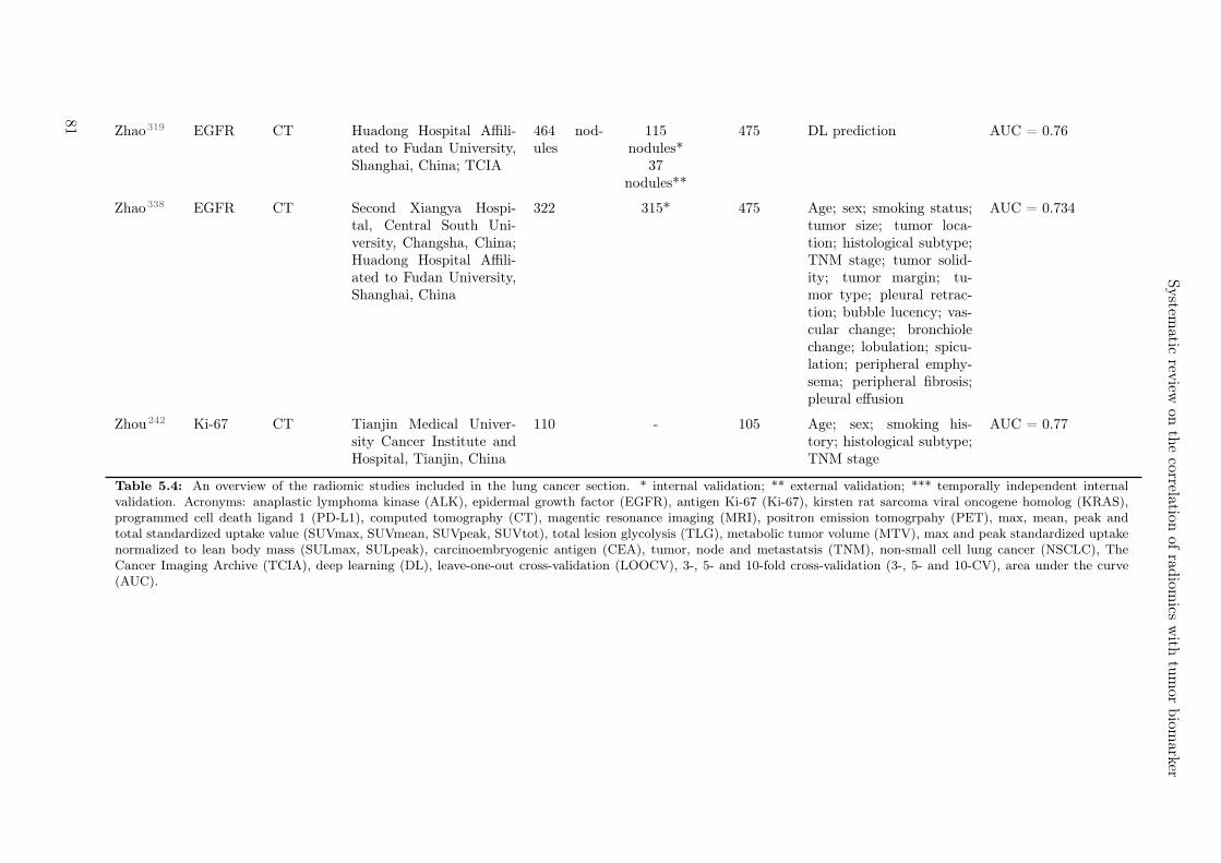
System
aticrev
iewon
the
correlationof
radiom
icsw
ithtu
mor
biom
arker
Zhao319 EGFR CT Huadong Hospital Affili-ated to Fudan University,Shanghai, China; TCIA
464 nod-ules
115nodules*
37nodules**
475 DL prediction AUC = 0.76
Zhao338 EGFR CT Second Xiangya Hospi-tal, Central South Uni-versity, Changsha, China;Huadong Hospital Affili-ated to Fudan University,Shanghai, China
322 315* 475 Age; sex; smoking status;tumor size; tumor loca-tion; histological subtype;TNM stage; tumor solid-ity; tumor margin; tu-mor type; pleural retrac-tion; bubble lucency; vas-cular change; bronchiolechange; lobulation; spicu-lation; peripheral emphy-sema; peripheral fibrosis;pleural effusion
AUC = 0.734
Zhou242 Ki-67 CT Tianjin Medical Univer-sity Cancer Institute andHospital, Tianjin, China
110 - 105 Age; sex; smoking his-tory; histological subtype;TNM stage
AUC = 0.77
Table 5.4: An overview of the radiomic studies included in the lung cancer section. * internal validation; ** external validation; *** temporally independent internalvalidation. Acronyms: anaplastic lymphoma kinase (ALK), epidermal growth factor (EGFR), antigen Ki-67 (Ki-67), kirsten rat sarcoma viral oncogene homolog (KRAS),programmed cell death ligand 1 (PD-L1), computed tomography (CT), magentic resonance imaging (MRI), positron emission tomogrpahy (PET), max, mean, peak andtotal standardized uptake value (SUVmax, SUVmean, SUVpeak, SUVtot), total lesion glycolysis (TLG), metabolic tumor volume (MTV), max and peak standardized uptakenormalized to lean body mass (SULmax, SULpeak), carcinoembryogenic antigen (CEA), tumor, node and metastatsis (TNM), non-small cell lung cancer (NSCLC), TheCancer Imaging Archive (TCIA), deep learning (DL), leave-one-out cross-validation (LOOCV), 3-, 5- and 10-fold cross-validation (3-, 5- and 10-CV), area under the curve(AUC).
81

PD-L1
PD-L1 expression levels were observed to be correlated with CT radiomic features in two studies (AUC = 0.661326
and AUC = 0.848325, internal validations), indicating that dense and homogeneous tumors (withoutground-glass opacity (GGO), necrosis, cavitation or calcification) were more likely PD-L1 positive inlung adenocarcinoma326. Radiomics from PET/CT imaging was found to be similarly strongly predic-tive as CT but outperformed PET in PD-L1 expression level prediction for 399 stage I-IV non-small celllung cancer (NSCLC) patients (AUC > 0.8, internal validation).335
Ki-67
CT radiomics was found significantly predictive for Ki-67 (best performing feature: inverse variance,AUC = 0.77)242,327, however less relevant for TP53 and TMB (AUC = 0.604 and 0.586, respectively)321.In total, 24 studies incorporated clinical data. CT radiomics was reported to outperform individualclinical parameters such as tumor volume, axial diameter, sex, age, smoking, clinical stage and loca-tion for EGFR and KRAS mutation status prediction.134,312,314,317,318,320,337,338 Conventional clinicalPET measures such as SUVmax (AUC = 0.621), SUVmean (AUC = 0.624), SUVpeak (AUC = 0.615),MTV (non-significant) or TLG (non-significant) could not achieve the same performance as PET ra-diomics (AUC = 0.805).330,333 Although some studies reported inferiority of radiomics models com-pared to multivariate clinical models320,332, combining both was found beneficial for all imaging modali-ties135,317,320,323,325,330,332.
5.4.5 Gastrointestinal cancer
Summary
A total of ten studies addressing the correlation of radiomics and biological tissue markers in gastroin-testinal cancers were identified, which used CT (n = 6)148,339–343, combined PET/CT (n = 2)344,345 orMRI (n = 3)346–348. The tumor types analysed belong to gastric cancers (n = 3)339–341, rectal cancers(n = 3)346–348, pancreatic cancers (n = 2)148,344, colorectal cancer (CRC) and colorectal liver metastases(n = 3)342,343,345. The most frequent biomarker analysed was KRAS mutation (n = 7)342–348 followed byTP-53 mutation (n = 2)344,345, Ki-67 (n = 3)148,340,348 and HER-2 expression status (n = 3)339,341,348.One group analysed BRAF (n = 1)342 together with KRAS and NRAS as one mutation signature. Allexcept one study on TP-53 showed a significant correlation between the respective biomarker and ra-diomic features (AUC = 0.65-0.88). All studies were set up retrospectively and used internal data. Tworesearch groups validated their results on external datasets148,346 (Table 5.5).
KRAS
KRAS mutations in gastrointestinal cancers were analysed the most often for a potential correlation withradiomic signatures. The highest correlation was found in CRC patients for which the mutation signature(KRAS, NRAS or BRAF) was significantly associated with the radiomic signature consisting of threeGLCM features extracted from contrast-enhanced CT (CE-CT): energy, maximum probability and sumaverage342, which have been associated with homogeneity (AUC = 0.829, internal validation). One groupfocused on the association of KRAS mutation to FDG-PET-based radiomics acquired from pancreaticductal adenocarcinoma patients.344 Low-intensity textural features were significantly correlated to KRASgene status (AUC = 0.794-0.82).Another research group extracted radiomic features from FDG-PET but from patients with CRC.345 Fortumors with mutated KRAS the value at the 25th percentile of SUVmax of the metabolic tumor volume(MTV) and contrast derived from the GLCM were significantly increased. Hence, KRAS mutated tumorswere more likely to have an increase in PET contrast. A similar correlation was acquired by a modelthat incorporated hand-crafted radiomics and deep radiomics derived from CT of CRC patients.343 Thecombined model achieved the highest performance (c-index = 0.831 [95% CI, 0.762-0.905], external vali-dation).
Coherent results were obtained by extracting radiomic features from MRI. One study used minimumredundancy maximum relevance (mRMR) combined with LASSO regression for KRAS prediction(AUC = 0.651 [95% CI: 0.539-0.763], temporally independent validation).348 Another group extractedimaging features from T2W MR-images of patients with primary rectal cancer to differentiate mutant
82
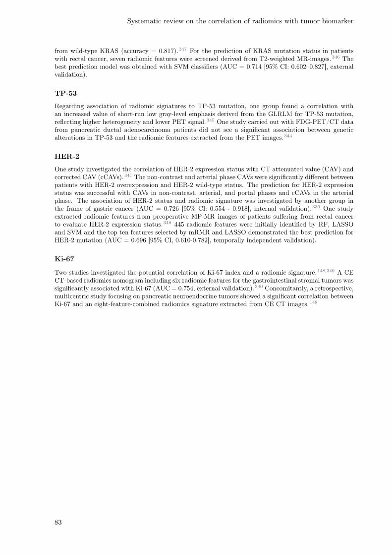
Systematic review on the correlation of radiomics with tumor biomarker
from wild-type KRAS (accuracy = 0.817).347 For the prediction of KRAS mutation status in patientswith rectal cancer, seven radiomic features were screened derived from T2-weighted MR-images.346 Thebest prediction model was obtained with SVM classifiers (AUC = 0.714 [95% CI: 0.602–0.827], externalvalidation).
TP-53
Regarding association of radiomic signatures to TP-53 mutation, one group found a correlation withan increased value of short-run low gray-level emphasis derived from the GLRLM for TP-53 mutation,reflecting higher heterogeneity and lower PET signal.345 One study carried out with FDG-PET/CT datafrom pancreatic ductal adenocarcinoma patients did not see a significant association between geneticalterations in TP-53 and the radiomic features extracted from the PET images.344
HER-2
One study investigated the correlation of HER-2 expression status with CT attenuated value (CAV) andcorrected CAV (cCAVs).341 The non-contrast and arterial phase CAVs were significantly different betweenpatients with HER-2 overexpression and HER-2 wild-type status. The prediction for HER-2 expressionstatus was successful with CAVs in non-contrast, arterial, and portal phases and cCAVs in the arterialphase. The association of HER-2 status and radiomic signature was investigated by another group inthe frame of gastric cancer (AUC = 0.726 [95% CI: 0.554 - 0.918], internal validation).339 One studyextracted radiomic features from preoperative MP-MR images of patients suffering from rectal cancerto evaluate HER-2 expression status.348 445 radiomic features were initially identified by RF, LASSOand SVM and the top ten features selected by mRMR and LASSO demonstrated the best prediction forHER-2 mutation (AUC = 0.696 [95% CI, 0.610-0.782], temporally independent validation).
Ki-67
Two studies investigated the potential correlation of Ki-67 index and a radiomic signature.148,340 A CECT-based radiomics nomogram including six radiomic features for the gastrointestinal stromal tumors wassignificantly associated with Ki-67 (AUC = 0.754, external validation).340 Concomitantly, a retrospective,multicentric study focusing on pancreatic neuroendocrine tumors showed a significant correlation betweenKi-67 and an eight-feature-combined radiomics signature extracted from CE CT images.148
83
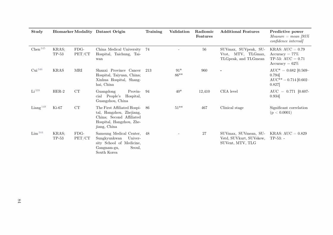
Study BiomarkerModality Dataset Origin Training Validation RadiomicFeatures
Additional Features Predictive powerMeasure = mean [95%confidence interval]
Chen345 KRAS;TP-53
FDG-PET/CT
China Medical UniversityHospital, Taichung, Tai-wan
74 - 56 SUVmax, SUVpeak, SU-Vtot, MTV, TLGmax,TLGpeak, and TLGmean
KRAS: AUC = 0.79Accuracy = 77%TP-53: AUC = 0.71Accuracy = 62%
Cui346 KRAS MRI Shanxi Province CancerHospital, Taiyuan, China;Xinhua Hospital, Shang-hai, China
213 91*86**
960 - AUC* = 0.682 [0.569–0.794]AUC** = 0.714 [0.602–0.827]
Li339 HER-2 CT Guangdong Provin-cial People’s Hospital,Guangzhou, China
94 40* 12,410 CEA level AUC = 0.771 [0.607-0.934]
Liang148 Ki-67 CT The First Affiliated Hospi-tal, Hangzhou, Zhejiang,China; Second AffiliatedHospital, Hangzhou, Zhe-jiang, China
86 51** 467 Clinical stage Significant correlation(p < 0.0001)
Lim344 KRAS;TP-53
FDG-PET/CT
Samsung Medical Center,Sungkyunkwan Univer-sity School of Medicine,Gangnam-gu, Seoul,South Korea
48 - 27 SUVmax, SUVmean, SU-Vstd, SUVkurt, SUVskew,SUVent, MTV, TLG
KRAS: AUC = 0.829TP-53: -
84

System
aticrev
iewon
the
correlationof
radiom
icsw
ithtu
mor
biom
arker
Meng348 Ki-67,KRAS,HER-2
MRI,DWI,PWI
Sixth Affiliated Hospitalof Sun Yat-sen University.Guangzhou, China
197 148*** 2,534 - HER-2:AUC = 0.696 [0.610 -0.782]Accuracy = 0.621Ki-67:AUC = 0.699 [0.611 -0.788]Accuracy = 0.582KRAS:AUC = 0.651 [0.539 -0.763]Accuracy = 0.616
Oh347 KRAS MRI Research Institute andHospital, National CancerCenter, Goyang„ Korea
60 - 44 - AUC = 0.884Accuracy = 81.7%
Wu343 KRAS CT South China University ofTechnology, Guangzhou,Guangdong Province,China
279 119*** 2,634 2,208 DL features c-index = 0.832 [0.762–0.905]
Yang342 KRAS;BRAF
CT National Cancer Cen-ter/Cancer Hospital,Chinese Academy of Med-ical Sciences and PekingUnion Medical College,Beijing, China
61 57*** 346 - AUC = 0.829 [0.718–0.939]Accuracy = 0.750 [0.623–0.845]
Zhang340 Ki-67 CT Renji Hospital, Huangpu,Shanghai, China; Zhong-shan Hospital, Shanghai,China; Sir Run Run ShawHospital, Hangzhou, Zhe-jiang, China and First Af-filiated Hospital of Wen-zhou Medical University,Wenzhou, China
148 41*150**
833 Tumor size AUC* = 0.828 [0.681–0.974]AUC** = 0.784 [0.701–0.868]Accuracy* = 68.29%Accuracy** = 73.33%
85
Table 5.5: An overview of the radiomic studies included in the gastrointestinal cancer section. * internal validation; ** external validation; *** temporally independentinternal validation. Acronyms: v-raf murine sarcoma viral oncogene homolog B1 (BRAF), antigen Ki-67 (Ki-67), kirsten rat sarcoma viral oncogene homolog (KRAS), tumorprotein p53 (TP-53), fluorodeoxyglucose positron emission tomography (FDG-PET), computed tomography (CT), perfusion weighted imaging (PWI), magnetic resonanceimaging (MRI), diffusion weighted imaging (DWI), carcinoembryonic antigen (CEA), metabolic tumor volume (MTV), max, mean, peak, standard deviation, skewness,kurtosis, entropy and total standardized uptake value (SUVmax, SUVmean, SUVpeak, SUVstd, SUVskew, SUVkurt, SUVent, SUVtot), max, peak and min of total lesionglycolysis (TLGmax, TLGmin, TLGpeak), deep learning (DL), area under the curve (AUC).
86
Systematic review on the correlation of radiomics with tumor biomarker
5.4.6 Liver cancer
Summary
Four studies were found to correlate radiomics and tissue biomarkers for liver patients, using eitherMR with contrast agents (n = 2) or US (n = 2). The most common tumor type was hepatocellularcarcinoma (HCC, n=3)349–351 followed by cholangiocarcinoma (CCA, n=1)352. Three tissue biomarkerswere investigated: Ki-67 (n = 3), PD-L1 (n = 2) and VEGF (n = 1) and all were shown to be significantlycorrelated to radiomics (AUC = 0.85-0.97). All studies employed a dataset limited to a single center; onestudy separated the dataset into a training and a validation cohort352 (Table 5.6).
PD-L1
The best predictive performance overall for liver studies was obtained for PD-L1 in US images (AUC = 0.97).351
The expression of PD-L1 was also predicted from MRI where the best correlation was found with thetexture feature ADC variance, which can be interpreted with higher heterogeneity associated with higherPD-L1 expression levels.349
Ki-67
The best AUC for Ki-67 was 0.94, employing the trained SVM model from US images.351 Slightly worseperformances (AUC = 0.804, internal validation) were obtained with wavelet features for CCA patientsimaged also with US.352 Finally, texture features were extracted from MR images of HCC patients.350
The authors combined 13 features from the T2W, PRE, AP and PVP scans into a multiparametrictexture signature (Harrell’s C = 0.878).350 The features included by the authors share the interpretation,which is that higher intra-tumor heterogeneity correlates to higher expression of the biomarker. Thelatter may reflect the cell proliferation status and therefore the aggressiveness.
VEGF
The expression of VEGF was analyzed only in CCA patients with US images.352 The wavelet featureswere found to be the most promising method to predict the biomarker expression (AUC = 0.864, internalvalidation). The features investigated by the authors are correlated to the heterogeneity of the tumorvolume.
87
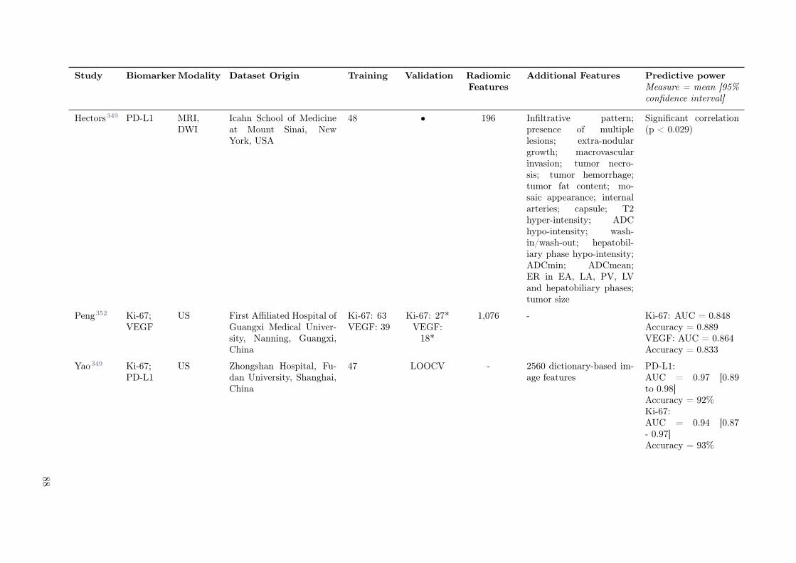
Study BiomarkerModality Dataset Origin Training Validation RadiomicFeatures
Additional Features Predictive powerMeasure = mean [95%confidence interval]
Hectors349 PD-L1 MRI,DWI
Icahn School of Medicineat Mount Sinai, NewYork, USA
48 • 196 Infiltrative pattern;presence of multiplelesions; extra-nodulargrowth; macrovascularinvasion; tumor necro-sis; tumor hemorrhage;tumor fat content; mo-saic appearance; internalarteries; capsule; T2hyper-intensity; ADChypo-intensity; wash-in/wash-out; hepatobil-iary phase hypo-intensity;ADCmin; ADCmean;ER in EA, LA, PV, LVand hepatobiliary phases;tumor size
Significant correlation(p < 0.029)
Peng352 Ki-67;VEGF
US First Affiliated Hospital ofGuangxi Medical Univer-sity, Nanning, Guangxi,China
Ki-67: 63VEGF: 39
Ki-67: 27*VEGF:
18*
1,076 - Ki-67: AUC = 0.848Accuracy = 0.889VEGF: AUC = 0.864Accuracy = 0.833
Yao349 Ki-67;PD-L1
US Zhongshan Hospital, Fu-dan University, Shanghai,China
47 LOOCV - 2560 dictionary-based im-age features
PD-L1:AUC = 0.97 [0.89to 0.98]Accuracy = 92%Ki-67:AUC = 0.94 [0.87- 0.97]Accuracy = 93%
88

System
aticrev
iewon
the
correlationof
radiom
icsw
ithtu
mor
biom
arker
Ye350 Ki-67 MRI West China Hospital,Sichuan, China
89 10-CV 396 Serum level of alpha-fetoprotein; hepatitisB surface antigen;hepatitis C antibody;Barcelona-Clinic LiverCancer classification;cirrhosis; multifocality;arterial phase hyper-enhancement; washout,capsule integrity, in-ternal arteries, tumormargin, enhancing cap-sule, hepato-biliary phasehypo-intensity
c-index: 0.936 [0.863-0.977]
Table 5.6: An overview of the radiomic studies included in the liver cancer section. * internal validation; ** external validation; *** temporally independent internalvalidation. Acronyms: antigen Ki-67 (Ki-67), programmed cell death ligand 1 (PD-L1), vascular endothelial growth factor (VEGF), magnetic resonance imaging (MRI),diffusion weighted imaging (DWI), ultrasound (US), apparent diffusion coefficient (ADC), enhancement ratio (ER), early arterial (EA), late arterial (LA), early venous (EV),late venous (LV), area under the curve (AUC), leave-one-out cross-validation (LOOCV), 10-fold cross-validation (10-CV).
89
5.4.7 Other cancers
Summary
In total, five studies were found which investigated the correlation between radiomics and molecularmarkers in other entities not included in the sections above: melanoma (n = 1), thyroid cancer (n = 1),head and neck cancer (n = 2), adrenal gland carcinoma (n = 1). All studies showed a significant correlationbetween the biomarker and radiomics (AUC = 0.62-0.78). None of the studies used external validation(Table 5.7).
Details
One study explored the use of FDG-PET/CT radiomics to predict BRAFv600 mutation status in melanomapatients (AUC = 0.62, 10-fold cross-validation).353 Another study investigated the use of US radiomicsto predict BRAFv600 mutation of thyroid cancer patients with a limited predictive performance on atemporally independent validation cohort (c-statistics = 0.629).354 Two studies explored the correlationof different biomarkers and imaging features in head and neck squamous cell carcinoma patients. One ofthem reported a moderate predictive power of CT radiomics for TP53 mutation prediction (AUC = 0.641,5-fold cross-validation)355, while the other study reported a limited correlation between PD-L1, VEGF,Ki-67 and EGFR expression and FDG-PET radiomics on their training cohort356. The latter also showeda positive correlation between PD-L1 and Ki-67 expression. Correlation from GLCM was found to be anegative predictor of PD-L1 expression, while it was positively associated with VEGF expression. Onestudy investigated the efficacy of CE CT radiomics to predict Ki-67 expression in adrenal gland carci-noma patients.357 The authors reported final AUCs of 0.7-0.78 on the training cohort after using logisticregression models based on two shape features, suggesting that high Ki-67 expression is associated withflatter and more elongated tumors.
90
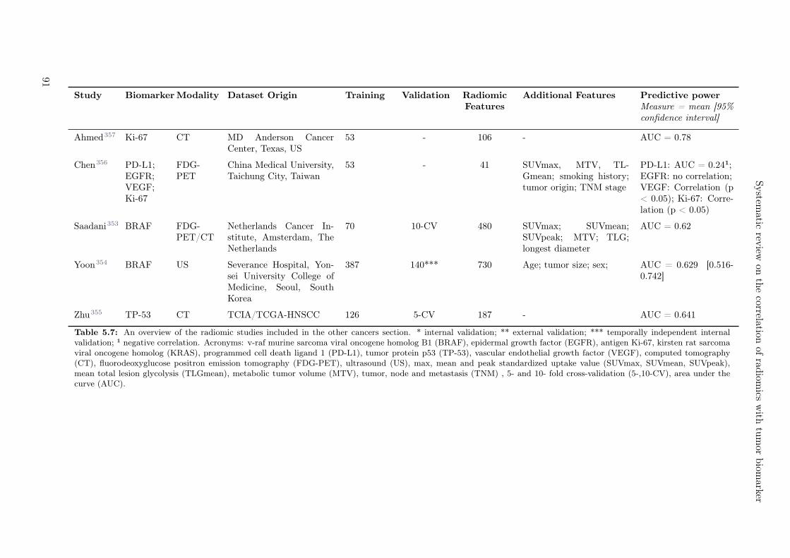
System
aticrev
iewon
the
correlationof
radiom
icsw
ithtu
mor
biom
arker
Study BiomarkerModality Dataset Origin Training Validation RadiomicFeatures
Additional Features Predictive powerMeasure = mean [95%confidence interval]
Ahmed357 Ki-67 CT MD Anderson CancerCenter, Texas, US
53 - 106 - AUC = 0.78
Chen356 PD-L1;EGFR;VEGF;Ki-67
FDG-PET
China Medical University,Taichung City, Taiwan
53 - 41 SUVmax, MTV, TL-Gmean; smoking history;tumor origin; TNM stage
PD-L1: AUC = 0.24¹;EGFR: no correlation;VEGF: Correlation (p< 0.05); Ki-67: Corre-lation (p < 0.05)
Saadani353 BRAF FDG-PET/CT
Netherlands Cancer In-stitute, Amsterdam, TheNetherlands
70 10-CV 480 SUVmax; SUVmean;SUVpeak; MTV; TLG;longest diameter
AUC = 0.62
Yoon354 BRAF US Severance Hospital, Yon-sei University College ofMedicine, Seoul, SouthKorea
387 140*** 730 Age; tumor size; sex; AUC = 0.629 [0.516-0.742]
Zhu355 TP-53 CT TCIA/TCGA-HNSCC 126 5-CV 187 - AUC = 0.641
Table 5.7: An overview of the radiomic studies included in the other cancers section. * internal validation; ** external validation; *** temporally independent internalvalidation; ¹ negative correlation. Acronyms: v-raf murine sarcoma viral oncogene homolog B1 (BRAF), epidermal growth factor (EGFR), antigen Ki-67, kirsten rat sarcomaviral oncogene homolog (KRAS), programmed cell death ligand 1 (PD-L1), tumor protein p53 (TP-53), vascular endothelial growth factor (VEGF), computed tomography(CT), fluorodeoxyglucose positron emission tomography (FDG-PET), ultrasound (US), max, mean and peak standardized uptake value (SUVmax, SUVmean, SUVpeak),mean total lesion glycolysis (TLGmean), metabolic tumor volume (MTV), tumor, node and metastasis (TNM) , 5- and 10- fold cross-validation (5-,10-CV), area under thecurve (AUC).
91
5.4.8 Feature interpretation
In Table 5.8, 5.9, and 5.10, we gathered those radiomic features employed in the best performing modelsfor each combination of biomarker and tumor site, for MRI, CT and PET, respectively. Detailed tables in-cluding feature names and additional modalities (e.g. US or non-conventional MRI sequences) are shownin Supplementary Tables 5.11, 5.12, 5.13, and 5.14. Out of 29 studies, 15 provided an interpretation fortheir models, whereas we derived the interpretation using the features and their values for the remainingseven studies. For seven studies, no interpretation was possible due to lack of information.
Oftentimes, dysregulation of one specific biomarker led to similar tumor phenotype across entities andimaging modalities. This was the case for EGFR-mutant tumors, which exhibited greater textural hetero-geneity in CNS MRI, PWI and DWI, as well as in lung CT and PET. Similarly, alteration of TP-53 statuswas associated with increased heterogeneity in CT of HN and PET of colorectal cancer. IDH-mutanttumors were reported to have greater textural homogeneity in MRI, DWI, PWI, DKI and FDG-PET inCNS. Hence, high Ki-67-expressing tumors were reported to be more homogeneous in CT for lung cancerbut more heterogeneous for gynecological tumors and head and neck tumors. KRAS+ was shown to bemore homogeneous for CT in lung, but more heterogeneous for gastrointestinal cancer.
92
System
aticrev
iewon
the
correlationof
radiom
icsw
ithtu
mor
biom
arker
MRI EGFR Ki-67 KRAS TP-53 VEGF IDH
CNS EGFR+ more hetero-geneous, less spheri-cal260
Ki-67 high expres-sion more heteroge-neous265
TP-53+ higher inten-sity270
VEGF+ more hetero-geneous271
IDH+ more homoge-neous, more regularlyshaped278
GI KRAS+ more hetero-geneous346
Liver Ki-67 high expres-sion more heteroge-neous350
Table 5.8: Interpretation of the best performing models on the training dataset for T2-weighted magnetic resonance imaging (MRI). Acronyms: central nervous system(CNS), gastrointestinal (GI), epidermal growth factor (EGFR), isocitrate dehydrogenase (IDH), kirsten rat sarcoma viral oncogene homolog (KRAS), programmed cell deathligand (PD-L1), tumor protein p53 (TP-53), vascular endothelial growth factor (VEGF).
CT EGFR Ki-67 KRAS/BRAF TP-53 HER-2 ALK PD-L1
HNC TP-53+ moreheterogeneous355
Lung EGFR+ moreheterogeneous,smaller320
Ki-67 high expressionmore homogeneous,more elongated242
KRAS+ more ho-mogeneous320
ALK+ higherdensity324
PD-L1+ more ho-mogeneous326
GI Ki-67 high expressionmore heterogeneous340
KRAS/BRAF+more heteroge-neous342
HER-2+ moreheterogeneous339
Table 5.9: Interpretation of the best performing models on the training dataset for computer tomography (CT). Acronyms: head and neck cancer (HNC), gastrointestinal(GI), anaplastic lymphoma kinase (ALK), v-raf murine sarcoma viral oncogene homolog B1 (BRAF), epidermal growth factor (EGFR), human epidermal growth factorreceptor 2 (HER-2), kirsten rat sarcoma viral oncogene homolog (KRAS), programmed cell death ligand 1 (PD-L1), tumor protein p53 (TP-53).
93
PET EGFR Ki-67 KRAS TP-53 VEGF IDH PD-L1
CNS IDH+ more ho-mogeneous, lessspherical276
HNC Ki-67 high expres-sion more heteroge-neous356
VEGF+ moreheterogeneous356
PD-L1+ moreheterogeneous356
Lung EGFR+ more het-erogeneous, morecompact336
GI KRAS+ lower in-tensity344
TP-53+ more het-erogeneous345
Adrenalglandcarci-noma
Ki-67 high expres-sion more elongatedand flatter357
Table 5.10: Interpretation of the best performing models on the training dataset for positron emission tomography (PET). Acronyms: head and neck cancer (HNC),central nervous system (CNS), gastrointestinal (GI), epidermal growth factor (EGFR), isocitrate dehydrogenase (IDH), kirsten rat sarcoma viral oncogene homolog (KRAS),programmed cell death ligand 1 (PD-L1), tumor protein p53 (TP-53), vascular endothelial growth factor (VEGF).
94

Systematic review on the correlation of radiomics with tumor biomarker
5.5 Discussion
In the recent decades, extensive genomic studies have leveraged our understanding of cancer biology andpathophysiology. The identification of key genetic alterations that drive oncogenesis and their subsequentmolecular markers has led to a different classification of tumor entities as defined by the World HealthOrganization (WHO) and to a more accurate and comprehensive patient-specific treatment planning andadaptation. Furthermore, the field of radiomics, i.e. the quantitative, high-throughput analysis of medicalimages, has emerged as a potential diagnostic, prognostic and predictive tool in clinical decision-supportsystems. This is especially true in cancer treatment, where medical imaging is routinely performed withdiagnostic and monitoring purposes. The primary objective of this review was to identify key radiomicfeatures shown to correlate with specific tumor molecular markers through an electronic search of peer-reviewed journal publications.For this purpose, we limited our search to ten cancer biomarkers commonly investigated and used inclinical practice, which apply to a broad range of cancer types. Other, even though valid, biomarkers,such as methylation status or indicators for virus-born cancers were deliberately excluded as their originand/or mechanism leading to malignant transformation of healthy cells is not simply comparable. Otherexamples of biomarkers excluded in this review are the loss of tumor suppressors in cancer such asbreast cancer genes 1 and 2 (BRCA-1, BRCA-2), RNAs, proteins such as prostate-specific antigen (PSA)or circulating tumor DNA (ct-DNA).255 By focusing on this compact set of biomarkers, we aimed tosummarize revealed correlations between radiomics and signature molecules and eventually contributeto promote radiomics as a valid diagnostic, prognostic and predictive tool in cancer treatment. We areaware that the selection of biomarkers is not complete but due to the sheer amount of biomarkers andthe variability thereof, the search had to be narrowed in order to make a meaningful systematic review.Most of the studies reported some correlation between the assessed biomarkers and radiomics, suggestingthat mutated and non-mutated tumors have different growth patterns, identifiable in high-throughputimaging. In total, 96 out of 100 studies found a significant correlation between at least one of the studiedbiomarkers and one or more radiomic features. However, only 6 studies validated their models on externalvalidation cohorts, and an additonal 11 on temporally independent validation cohorts. Fourteen studiesdid not use any form of validation. Imbalance of Ki-67, PD-L1 and KRAS biomarkers resulted in a smallerdegree of phenotype agreement across different entities and same/different modalities. This could be ex-plained by the lack of standardization of immunohistochemistry techniques for biomarker staining andscoring systems, leading to moderate intra/inter-laboratory and intra/inter-observer variabilities.255,358
Moreover, different studies employed different biomarker expression levels as cutoffs to stratify patients,hindering results reproducibility and interpretation. Nonetheless and, as previously explained, it shouldbe noted that the studies were included on the interpretation table based on their performance on thetraining set, and, for the vast majority, external validation remains to be accomplished. Along theselines, we believe greater effort should be made to employ larger, multi-institutional cohorts, either bymeans of new data-sharing agreements among research groups or through distributed learning.
Regardless of the imaging modality and selected biomarker, radiomic studies suffer from lack of standardperformance and clinical utility evaluations. Moreover, differences in image acquisition, pre-processing,as well as feature nomenclature, definition and software implementation significantly affect results re-producibility and robustness, along with hindering a direct comparison of studies. Therefore, we wouldlike to encourage projects such as the image biomarker standardisation initiative (IBSI)38, which workstowards the homogenization of image feature extraction and analysis.
Finally, the correlation of textural, intensity, shape, size and wavelet image features with tumor biomark-ers entails an advance in feature interpretability, as summarized in Tables 5.8, 5.9, and 5.10, which bringsradiomics closer to its application in a clinical setting. Nonetheless, more evidence by external validationis still required to validate the reported findings and establish a true relationship between image featuresand tumor biology.
5.6 Conclusion
In summary, radiomics from different modalities and cancer entities is a promising tool for tumor biologyassessment. Further multi-center studies are required to validate the results reported in this review.
95
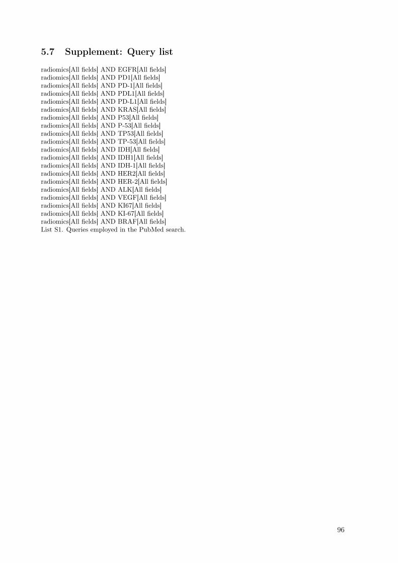
5.7 Supplement: Query list
radiomics[All fields] AND EGFR[All fields]radiomics[All fields] AND PD1[All fields]radiomics[All fields] AND PD-1[All fields]radiomics[All fields] AND PDL1[All fields]radiomics[All fields] AND PD-L1[All fields]radiomics[All fields] AND KRAS[All fields]radiomics[All fields] AND P53[All fields]radiomics[All fields] AND P-53[All fields]radiomics[All fields] AND TP53[All fields]radiomics[All fields] AND TP-53[All fields]radiomics[All fields] AND IDH[All fields]radiomics[All fields] AND IDH1[All fields]radiomics[All fields] AND IDH-1[All fields]radiomics[All fields] AND HER2[All fields]radiomics[All fields] AND HER-2[All fields]radiomics[All fields] AND ALK[All fields]radiomics[All fields] AND VEGF[All fields]radiomics[All fields] AND KI67[All fields]radiomics[All fields] AND KI-67[All fields]radiomics[All fields] AND BRAF[All fields]List S1. Queries employed in the PubMed search.
96
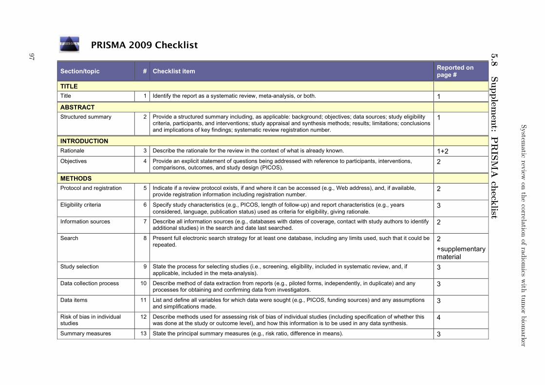
PRISMA 2009 Checklist
Section/topic # Checklist item Reported on page #
TITLE Title 1 Identify the report as a systematic review, meta-analysis, or both. 1 ABSTRACT Structured summary 2 Provide a structured summary including, as applicable: background; objectives; data sources; study eligibility
criteria, participants, and interventions; study appraisal and synthesis methods; results; limitations; conclusions and implications of key findings; systematic review registration number.
1
INTRODUCTION Rationale 3 Describe the rationale for the review in the context of what is already known. 1+2 Objectives 4 Provide an explicit statement of questions being addressed with reference to participants, interventions,
comparisons, outcomes, and study design (PICOS). 2
METHODS Protocol and registration 5 Indicate if a review protocol exists, if and where it can be accessed (e.g., Web address), and, if available,
provide registration information including registration number. 2
Eligibility criteria 6 Specify study characteristics (e.g., PICOS, length of follow-up) and report characteristics (e.g., years considered, language, publication status) used as criteria for eligibility, giving rationale.
3
Information sources 7 Describe all information sources (e.g., databases with dates of coverage, contact with study authors to identify additional studies) in the search and date last searched.
2
Search 8 Present full electronic search strategy for at least one database, including any limits used, such that it could be repeated.
2 +supplementary material
Study selection 9 State the process for selecting studies (i.e., screening, eligibility, included in systematic review, and, if applicable, included in the meta-analysis).
3
Data collection process 10 Describe method of data extraction from reports (e.g., piloted forms, independently, in duplicate) and any processes for obtaining and confirming data from investigators.
3
Data items 11 List and define all variables for which data were sought (e.g., PICOS, funding sources) and any assumptions and simplifications made.
3
Risk of bias in individual studies
12 Describe methods used for assessing risk of bias of individual studies (including specification of whether this was done at the study or outcome level), and how this information is to be used in any data synthesis.
4
Summary measures 13 State the principal summary measures (e.g., risk ratio, difference in means). 3
System
aticrev
iewon
the
correlationof
radiom
icsw
ithtu
mor
biom
arker
5.8
Supple
men
t:P
RIS
MA
check
list
97

PRISMA 2009 Checklist
Synthesis of results 14 Describe the methods of handling data and combining results of studies, if done, including measures of consistency (e.g., I2) for each meta-analysis.
Not applicable
Page 1 of 2
Section/topic # Checklist item Reported on page #
Risk of bias across studies 15 Specify any assessment of risk of bias that may affect the cumulative evidence (e.g., publication bias, selective reporting within studies).
4
Additional analyses 16 Describe methods of additional analyses (e.g., sensitivity or subgroup analyses, meta-regression), if done, indicating which were pre-specified.
Not applicable
RESULTS Study selection 17 Give numbers of studies screened, assessed for eligibility, and included in the review, with reasons for exclusions at
each stage, ideally with a flow diagram. 4
Study characteristics 18 For each study, present characteristics for which data were extracted (e.g., study size, PICOS, follow-up period) and provide the citations.
34 - 46
Risk of bias within studies 19 Present data on risk of bias of each study and, if available, any outcome level assessment (see item 12). Not applicable
Results of individual studies 20 For all outcomes considered (benefits or harms), present, for each study: (a) simple summary data for each intervention group (b) effect estimates and confidence intervals, ideally with a forest plot.
6-31
Synthesis of results 21 Present results of each meta-analysis done, including confidence intervals and measures of consistency. Tables at pages 5 9-12 16-18 21-25 27-28 30 32
Risk of bias across studies 22 Present results of any assessment of risk of bias across studies (see Item 15). ?? Additional analysis 23 Give results of additional analyses, if done (e.g., sensitivity or subgroup analyses, meta-regression [see Item 16]). Not
applicable DISCUSSION
98
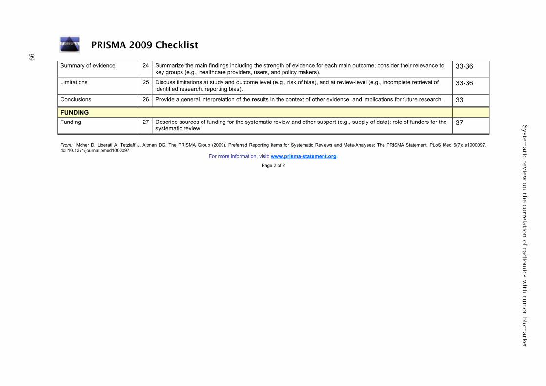
PRISMA 2009 Checklist
Summary of evidence 24 Summarize the main findings including the strength of evidence for each main outcome; consider their relevance to key groups (e.g., healthcare providers, users, and policy makers).
33-36
Limitations 25 Discuss limitations at study and outcome level (e.g., risk of bias), and at review-level (e.g., incomplete retrieval of identified research, reporting bias).
33-36
Conclusions 26 Provide a general interpretation of the results in the context of other evidence, and implications for future research. 33
FUNDING Funding 27 Describe sources of funding for the systematic review and other support (e.g., supply of data); role of funders for the
systematic review. 37
From: Moher D, Liberati A, Tetzlaff J, Altman DG, The PRISMA Group (2009). Preferred Reporting Items for Systematic Reviews and Meta-Analyses: The PRISMA Statement. PLoS Med 6(7): e1000097. doi:10.1371/journal.pmed1000097
For more information, visit: www.prisma-statement.org.
Page 2 of 2
System
aticrev
iewon
the
correlationof
radiom
icsw
ithtu
mor
biom
arker
99
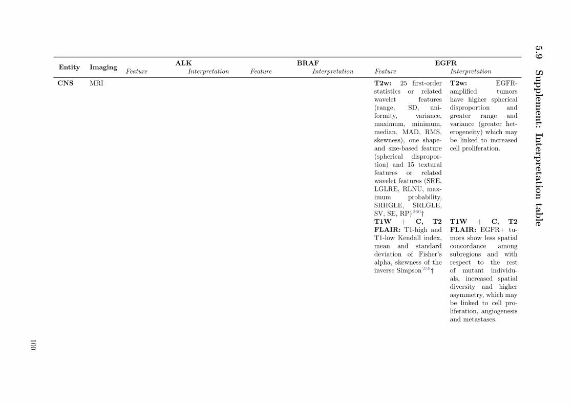
5.9
Supple
men
t:In
terpreta
tion
table
Entity ImagingALK BRAF EGFR
Feature Interpretation Feature Interpretation Feature Interpretation
CNS MRI T2w: 25 first-orderstatistics or relatedwavelet features(range, SD, uni-formity, variance,maximum, minimum,median, MAD, RMS,skewness), one shape-and size-based feature(spherical dispropor-tion) and 15 texturalfeatures or relatedwavelet features (SRE,LGLRE, RLNU, max-imum probability,SRHGLE, SRLGLE,SV, SE, RP)260†
T2w: EGFR-amplified tumorshave higher sphericaldisproportion andgreater range andvariance (greater het-erogeneity) which maybe linked to increasedcell proliferation.
T1W + C, T2FLAIR: T1-high andT1-low Kendall index,mean and standarddeviation of Fisher’salpha, skewness of theinverse Simpson259†
T1W + C, T2FLAIR: EGFR+ tu-mors show less spatialconcordance amongsubregions and withrespect to the restof mutant individu-als, increased spatialdiversity and higherasymmetry, which maybe linked to cell pro-liferation, angiogenesisand metastases.
100

System
aticrev
iewon
the
correlationof
radiom
icsw
ithtu
mor
biom
arker
T1W, T1W + C,T2W, T2 FLAIR,DWI, PWI: SD ofthe non-ET intensityin T2W, 3rd and 4thbins of the non-ETintensity distributionin ADC maps and twoatlas-based spatial dis-tribution parametersof the tumor core263†
T1W, T1W + C,T2W, T2 FLAIR,DWI, PWI: EGFR+tumors showed highervalues for rCBV andFA, and lower valuesfor ADC and T2-FLAIR, which maybe linked to increasedhypervascularity, cel-lularity, anisotropictissue and decreasedwater concentration.EGFR+ tumors alsopresented a distinctivespatial pattern (morefrequent in the frontaland parietal lobes).
Lung CT 90th percentile,maximum,LHH_GLDM_LDHGLE324†
ALK+ tumorsare more likelyto have higherdensity
Homogeneity, in-verse variance,HLL_GLCM_SE,LoG_SRLGLE, Vol-ume320*
EGFR+ are smallerand more heteroge-neous, potentiallydue to increasedvascularization.
PET Compactness, busy-ness, SUVmax,GLRLM_LGLRE,GLSZM_LGSZE,GLSZM_SZV,GLCM_IDM_normalized336†
EGFR+ are more com-pact and more hetero-geneous.
Other PET/CT Melanoma Melanoma
101
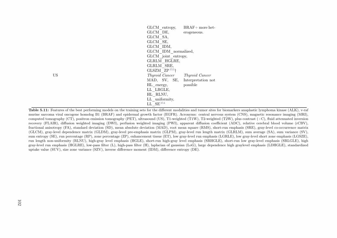
GLCM_entropy,GLCM_DE,GLCM_SA,GLCM_SE,GLCM_IDM,GLCM_IDM_normalized,GLCM_joint_entropy,GLRLM_HGLRE,GLRLM_SRE,GLSZM_ZP353†
BRAF+ more het-erogeneous.
US Thyroid Cancer Thyroid CancerMAD, SV, SE,HL_energy,LL_LRGLE,HL_RLNU,LL_uniformity,LL_SE354
Interpretation notpossible
Table 5.11: Features of the best performing models on the training sets for the different modalities and tumor sites for biomarkers anaplastic lymphoma kinase (ALK), v-rafmurine sarcoma viral oncogene homolog B1 (BRAF) and epidermal growth factor (EGFR). Acronyms: central nervous system (CNS), magnetic resonance imaging (MRI),computed tomography (CT), positron emission tomography (PET), ultrasound (US), T1-weighted (T1W), T2-weighted (T2W), plus contrast (+C), fluid attenuated inversionrecovery (FLAIR), diffusion weighted imaging (DWI), perfusion weighted imaging (PWI), apparent diffusion coefficient (ADC), relative cerebral blood volume (rCBV),fractional anisotropy (FA), standard deviation (SD), mean absolute deviation (MAD), root mean square (RMS), short-run emphasis (SRE), gray-level co-occurrence matrix(GLCM), gray-level dependence matrix (GLDM), gray-level pre-emphasis matrix (GLPM), gray-level run length matrix (GLRLM), sum average (SA), sum variance (SV),sum entropy (SE), run percentage (RP), zone percentage (ZP), enhancement tissue (ET), low gray-level run emphasis (LGRLE), low gray-level short zone emphasis (LGSZE),run length non-uniformity (RLNU), high-gray level emphasis (HGLE), short-run high-gray level emphasis (SRHGLE), short-run low gray-level emphasis (SRLGLE), highgray-level run emphasis (HGLRE), low-pass filter (L), high-pass filter (H), laplacian of gaussian (LoG), large dependence high graylevel emphasis (LDHGLE), standardizeduptake value (SUV), size zone variance (SZV), inverse difference moment (IDM), difference entropy (DE).
102
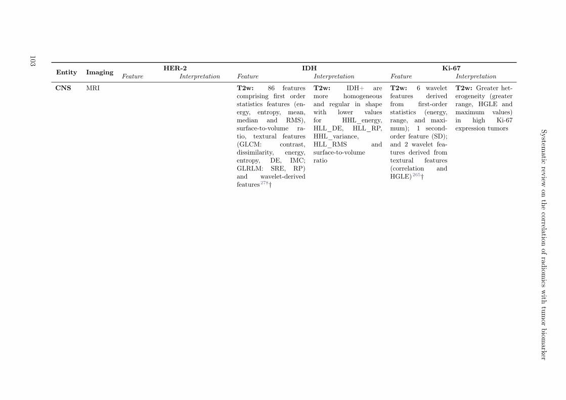
System
aticrev
iewon
the
correlationof
radiom
icsw
ithtu
mor
biom
arker
Entity ImagingHER-2 IDH Ki-67
Feature Interpretation Feature Interpretation Feature Interpretation
CNS MRI T2w: 86 featurescomprising first orderstatistics features (en-ergy, entropy, mean,median and RMS),surface-to-volume ra-tio, textural features(GLCM: contrast,dissimilarity, energy,entropy, DE, IMC;GLRLM: SRE, RP)and wavelet-derivedfeatures278†
T2w: IDH+ aremore homogeneousand regular in shapewith lower valuesfor HHL_energy,HLL_DE, HLL_RP,HHL_variance,HLL_RMS andsurface-to-volumeratio
T2w: 6 waveletfeatures derivedfrom first-orderstatistics (energy,range, and maxi-mum); 1 second-order feature (SD);and 2 wavelet fea-tures derived fromtextural features(correlation andHGLE)265†
T2w: Greater het-erogeneity (greaterrange, HGLE andmaximum values)in high Ki-67expression tumors
103

T1W + C, T1FLAIR, T2BLADE, T2FLAIR, PWI-CBF,DWI-ADC, DWI-eADC, PWI-ASL:eADC_GLRLM_SRE,eADC_GLCM_energy,eADC_GLRLM_LRE,eADC_GLGCM_energy,eADC_GLRLM_RLNU,eADC_hist_mode,eADC_hist_entropy,eADC_GLGCM_contrast,eADC_GLGCM_correlation,eADC_GLGCM_variance,eADC_GLRLM_GLNU,eADC_GLSZM_GLNU,eADC_GLSZM_LGZE,eADC_GLCM_contrast,eADC_GLGCM_IDM,eADC_GLCM_correlation,ADC_hist_max,ADC_hist_min,ADC_NGTDM_coarseness,ADC_GLRLM_LGLRE,ADC_GLSZM_HGLZE,CBF_GLSZM_SZE,CBF_GLSZM_ZSNU,FLAIR_GLSZM_LZE,FLAIR_GLRLM_RP,FLAIR_GLSZM_ZP,FLAIR_GLGCM_SA,FLAIR_hist_entropy291†
T1W + C, T1FLAIR, T2 BLADE,T2 FLAIR, DWI-CBF, DWI-ADC,DWI-eADC, PWI-ASL: IDH+ morehomogeneous with acoarser zone texture,lower energy, RLNU,variance and higherADC minimum values,IDM, contrast, GLNU
T1 FLAIR,T1W + C, T2FLAIR, T2FSE, DWI-CBF,DWI-ADC,DWI-eADC,DWI-B0, DWI-B1000, PWI-CBF, PWI-ASL: Waveletfeatures derivedfrom eADC_SD,eADC_MAD,eADC_ClusterTendency,eADC_homogeneity,eADC_InverseVariance,eADC_RP,B1000_MAD,B1000_energy,surface-to volumeratio, compactness,volume, spheri-cal disproportion,ClusterPromi-nence267†
T1 FLAIR,T1W + C, T2FLAIR, T2FSE, DWI-CBF,DWI-ADC,DWI-eADC,DWI-B0, DWI-B1000, PWI-CBF, PWI-ASL:Interpretation notpossible
DWI, DKI:MK_90th,MD_elongation,MK_E5R5L5288†
DWI, DKI: IDH+more homogeneous
104
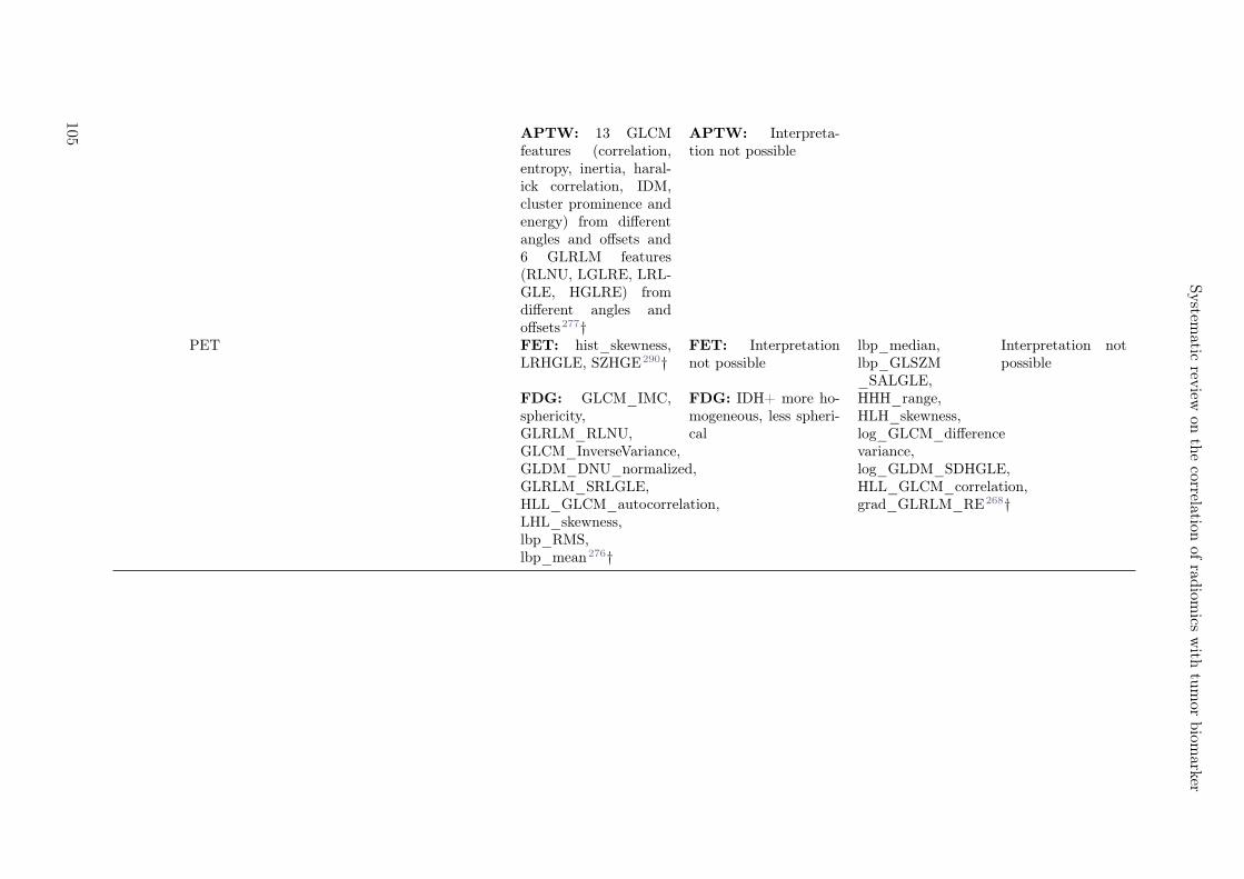
System
aticrev
iewon
the
correlationof
radiom
icsw
ithtu
mor
biom
arker
APTW: 13 GLCMfeatures (correlation,entropy, inertia, haral-ick correlation, IDM,cluster prominence andenergy) from differentangles and offsets and6 GLRLM features(RLNU, LGLRE, LRL-GLE, HGLRE) fromdifferent angles andoffsets277†
APTW: Interpreta-tion not possible
PET FET: hist_skewness,LRHGLE, SZHGE290†
FET: Interpretationnot possible
lbp_median,lbp_GLSZM_SALGLE,
Interpretation notpossible
FDG: GLCM_IMC,sphericity,GLRLM_RLNU,GLCM_InverseVariance,GLDM_DNU_normalized,GLRLM_SRLGLE,HLL_GLCM_autocorrelation,LHL_skewness,lbp_RMS,lbp_mean276†
FDG: IDH+ more ho-mogeneous, less spheri-cal
HHH_range,HLH_skewness,log_GLCM_differencevariance,log_GLDM_SDHGLE,HLL_GLCM_correlation,grad_GLRLM_RE268†
105

Breast MRI PWI: skewness,kurtosis, dy-namic featuresin BPE and inbreast lesions,two bilateralasymmetryfeatures300†
PWI: HER-2+tumors had thehighest enhance-ment valuesin the normalbreasts poten-tially linked toincreased neo-angiogenesis,and higherskewness andkurtosis, po-tentially linkedto higher het-erogeneity andworse prognosis
PWI: area,perimeter, ef-fective diameter,GSS_kurtosis,GSS_entropy,GSS_skewness,GLCM_homogeneity,GLCM_contrast,GLCM_IDM,GLDS_mean,GLDS_entropy,Tamura_coarseness,Tamura_line_likeliness297*
PWI: High-Ki-67 tumors havehigher values forarea, perimeter,effective diameter,entropy, homo-geneity, kurtosisand coarseness,and lower val-ues for contrast,IDM, skewnessline likeliness andGLDS_mean
DWI+PWI:DE307*
DWI+PWI: DEis lower in PWI ofhigh-Ki-67 express-ing tumors, andhigher in DWI ofhigh-Ki-67 express-ing tumors.
GI CT 2 db wavelet-derived features(skewness, andGLSZM_LALGLE),2 bior wavelet-derived features(GLDM_SDHGLEand kurto-sis) and 3rbio wavelet-derived features(GLCM_correlation,GLSZM_SALGLE,GLDM_DE)264†
HER-2+ moreheterogeneous
HHH_GLCM_IMC,HLL_GLDM_LDE,LLL_NGTDM_Busyness,HHH_GLSZM_LALGLE,HLL_GLCM_maxProbability,LLL_firstorder_TotalEnergy340‡
High-Ki-67 moreheterogeneous
106
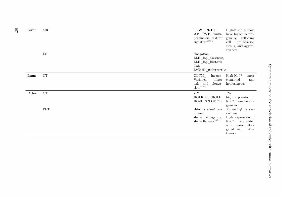
System
aticrev
iewon
the
correlationof
radiom
icsw
ithtu
mor
biom
arker
Liver MRI T2W+PRE+AP+PVP: multi-parametric texturesignature350*
High-Ki-67 tumorshave higher hetero-geneity, reflectingcell proliferationstatus, and aggres-siveness
US elongation,LLH_lbp_skewness,LLH_lbp_kurtosis,CoL-IAGe2D_90Percentile
Lung CT GLCM_ Inverse-Variance, minoraxis and elonga-tion242*
High-Ki-67 moreelongated andhomogeneous
Other CT HN HNHGLRE, SRHGLE,HGZE, SZLGE356†
high expression ofKi-67 more hetero-geneous
PET Adrenal gland car-cinoma
Adrenal gland car-cinoma
shape elongation,shape flatness357†
High expression ofKi-67 correlatedwith more elon-gated and flattertumors
107
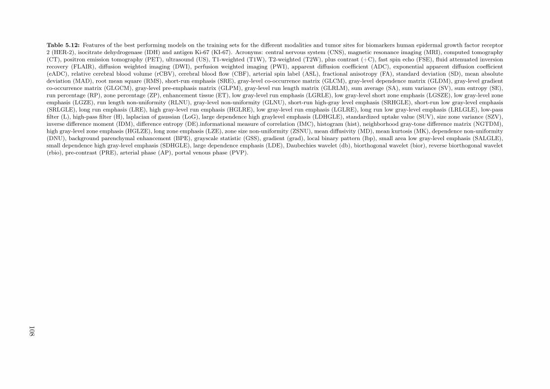
Table 5.12: Features of the best performing models on the training sets for the different modalities and tumor sites for biomarkers human epidermal growth factor receptor2 (HER-2), isocitrate dehydrogenase (IDH) and antigen Ki-67 (KI-67). Acronyms: central nervous system (CNS), magnetic resonance imaging (MRI), computed tomography(CT), positron emission tomography (PET), ultrasound (US), T1-weighted (T1W), T2-weighted (T2W), plus contrast (+C), fast spin echo (FSE), fluid attenuated inversionrecovery (FLAIR), diffusion weighted imaging (DWI), perfusion weighted imaging (PWI), apparent diffusion coefficient (ADC), exponential apparent diffusion coefficient(eADC), relative cerebral blood volume (rCBV), cerebral blood flow (CBF), arterial spin label (ASL), fractional anisotropy (FA), standard deviation (SD), mean absolutedeviation (MAD), root mean square (RMS), short-run emphasis (SRE), gray-level co-occurrence matrix (GLCM), gray-level dependence matrix (GLDM), gray-level gradientco-occurrence matrix (GLGCM), gray-level pre-emphasis matrix (GLPM), gray-level run length matrix (GLRLM), sum average (SA), sum variance (SV), sum entropy (SE),run percentage (RP), zone percentage (ZP), enhancement tissue (ET), low gray-level run emphasis (LGRLE), low gray-level short zone emphasis (LGSZE), low gray-level zoneemphasis (LGZE), run length non-uniformity (RLNU), gray-level non-uniformity (GLNU), short-run high-gray level emphasis (SRHGLE), short-run low gray-level emphasis(SRLGLE), long run emphasis (LRE), high gray-level run emphasis (HGLRE), low gray-level run emphasis (LGLRE), long run low gray-level emphasis (LRLGLE), low-passfilter (L), high-pass filter (H), laplacian of gaussian (LoG), large dependence high graylevel emphasis (LDHGLE), standardized uptake value (SUV), size zone variance (SZV),inverse difference moment (IDM), difference entropy (DE).informational measure of correlation (IMC), histogram (hist), neighborhood gray-tone difference matrix (NGTDM),high gray-level zone emphasis (HGLZE), long zone emphasis (LZE), zone size non-uniformity (ZSNU), mean diffusivity (MD), mean kurtosis (MK), dependence non-uniformity(DNU), background parenchymal enhancement (BPE), grayscale statistic (GSS), gradient (grad), local binary pattern (lbp), small area low gray-level emphasis (SALGLE),small dependence high gray-level emphasis (SDHGLE), large dependence emphasis (LDE), Daubechies wavelet (db), biorthogonal wavelet (bior), reverse biorthogonal wavelet(rbio), pre-contrast (PRE), arterial phase (AP), portal venous phase (PVP).
108
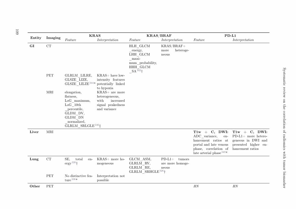
System
aticrev
iewon
the
correlationof
radiom
icsw
ithtu
mor
biom
arker
Entity ImagingKRAS KRAS/BRAF PD-L1
Feature Interpretation Feature Interpretation Feature Interpretation
GI CT HLH_GLCM_energy,LHH_GLCM_maxi-mum_probability,HHH_GLCM_SA342†
KRAS/BRAF+more heteroge-neous
PET GLRLM_LILRE,GLSZE_LIZE,GLSZE_LILZE344*
KRAS+ have low-intensity featurespotentially linkedto hypoxia
MRI elongation,flatness,LoG_maximum,LoG_10th_percentile,GLDM_DV,GLDM_DN_normalized,GLRLM_SRLGLE346‡
KRAS+ are moreheterogeneous,with increasedsignal peakednessand variance
Liver MRI T1w + C, DWI:ADC_variance, en-hancement ratios atportal and late venousphase, correlation oflate arterial phase349*
T1w + C, DWI:PD-L1+ more hetero-geneous in DWI andpresented higher en-hancement ratios
Lung CT SE, total en-ergy320†
KRAS+ more ho-mogeneous
GLCM_ASM,GLRLM_RV,GLRLM_RE,GLRLM_SRHGLE326†
PD-L1+ tumorsare more homoge-neous
PET No distinctive fea-ture336*
Interpretation notpossible
Other PET HN HN
109

GLRLM_GLNUr,GLRLM_RP,GLSZM_SZLGE,GLCM_correlation356*
PD-L1+ tumors havelower textural coarse-ness and are more het-erogeneous
Table 5.13: Features of the best performing models on the training sets for the different modalities and tumor sites for biomarkers kirsten rat sarcoma viral oncogene homolog(KRAS), KRAS together with v-raf murine sarcoma viral oncogene homolog B1 (BRAF), and programmed cell death ligand 1 (PD-L1). Acronyms: gastrointestinal (GI), headand neck (HN), magnetic resonance imaging (MRI), computed tomography (CT), positron emission tomography (PET), ultrasound (US), T1-weighted (T1W), T2-weighted(T2W), plus contrast (+C), fluid attenuated inversion recovery (FLAIR), diffusion weighted imaging (DWI), perfusion weighted imaging (PWI), apparent diffusion coefficient(ADC), relative cerebral blood volume (rCBV), fractional anisotropy (FA), standard deviation (SD), mean absolute deviation (MAD), root mean square (RMS), short-runemphasis (SRE), gray-level co-occurrence matrix (GLCM), gray-level dependence matrix (GLDM), gray-level pre-emphasis matrix (GLPM), gray-level run length matrix(GLRLM), sum average (SA), sum variance (SV), sum entropy (SE), run percentage (RP), zone percentage (ZP), enhancement tissue (ET), low gray-level run emphasis(LGRLE), low gray-level short zone emphasis (LGSZE), run length non-uniformity (RLNU), high-gray level emphasis (HGLE), short-run high-gray level emphasis (SRHGLE),short-run low gray-level emphasis (SRLGLE), high gray-level run emphasis (HGLRE), low-pass filter (L), high-pass filter (H), laplacian of gaussian (LoG), large dependencehigh graylevel emphasis (LDHGLE), standardized uptake value (SUV), size zone variance (SZV), inverse difference moment (IDM), difference entropy (DE), difference variance(DV), difference normalized (DN), run variance (RV), run entropy (RE).
110
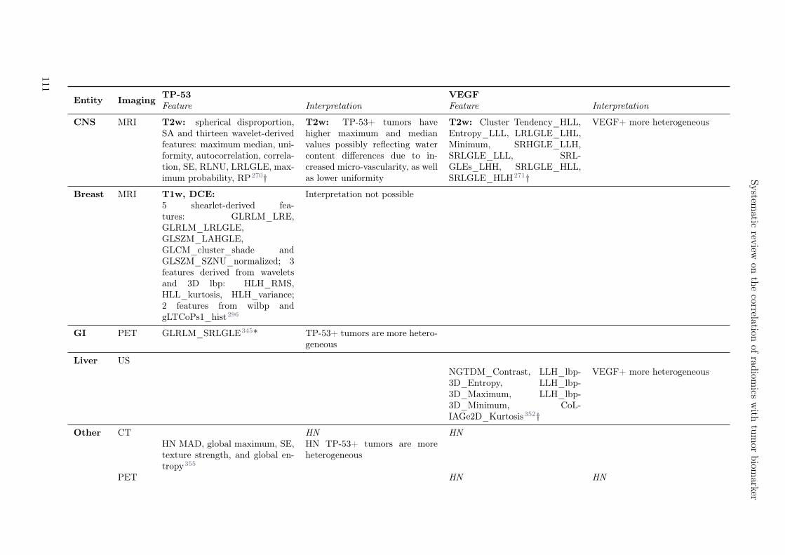
System
aticrev
iewon
the
correlationof
radiom
icsw
ithtu
mor
biom
arker
Entity ImagingTP-53 VEGFFeature Interpretation Feature Interpretation
CNS MRI T2w: spherical disproportion,SA and thirteen wavelet-derivedfeatures: maximum median, uni-formity, autocorrelation, correla-tion, SE, RLNU, LRLGLE, max-imum probability, RP270†
T2w: TP-53+ tumors havehigher maximum and medianvalues possibly reflecting watercontent differences due to in-creased micro-vascularity, as wellas lower uniformity
T2w: Cluster Tendency_HLL,Entropy_LLL, LRLGLE_LHL,Minimum, SRHGLE_LLH,SRLGLE_LLL, SRL-GLEs_LHH, SRLGLE_HLL,SRLGLE_HLH271†
VEGF+ more heterogeneous
Breast MRI T1w, DCE: Interpretation not possible5 shearlet-derived fea-tures: GLRLM_LRE,GLRLM_LRLGLE,GLSZM_LAHGLE,GLCM_cluster_shade andGLSZM_SZNU_normalized; 3features derived from waveletsand 3D lbp: HLH_RMS,HLL_kurtosis, HLH_variance;2 features from wilbp andgLTCoPs1_hist296
GI PET GLRLM_SRLGLE345* TP-53+ tumors are more hetero-geneous
Liver USNGTDM_Contrast, LLH_lbp-3D_Entropy, LLH_lbp-3D_Maximum, LLH_lbp-3D_Minimum, CoL-IAGe2D_Kurtosis352†
VEGF+ more heterogeneous
Other CT HN HNHN MAD, global maximum, SE,texture strength, and global en-tropy355
HN TP-53+ tumors are moreheterogeneous
PET HN HN
111
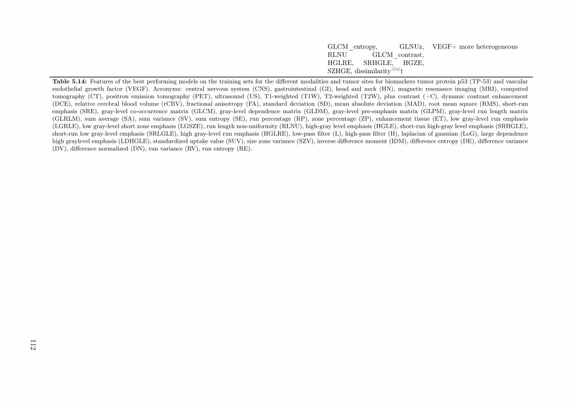
GLCM_entropy, GLNUz,RLNU GLCM_contrast,HGLRE, SRHGLE, HGZE,SZHGE, dissimilarity356†
VEGF+ more heterogeneous
Table 5.14: Features of the best performing models on the training sets for the different modalities and tumor sites for biomarkers tumor protein p53 (TP-53) and vascularendothelial growth factor (VEGF). Acronyms: central nervous system (CNS), gastrointestinal (GI), head and neck (HN), magnetic resonance imaging (MRI), computedtomography (CT), positron emission tomography (PET), ultrasound (US), T1-weighted (T1W), T2-weighted (T2W), plus contrast (+C), dynamic contrast enhancement(DCE), relative cerebral blood volume (rCBV), fractional anisotropy (FA), standard deviation (SD), mean absolute deviation (MAD), root mean square (RMS), short-runemphasis (SRE), gray-level co-occurrence matrix (GLCM), gray-level dependence matrix (GLDM), gray-level pre-emphasis matrix (GLPM), gray-level run length matrix(GLRLM), sum average (SA), sum variance (SV), sum entropy (SE), run percentage (RP), zone percentage (ZP), enhancement tissue (ET), low gray-level run emphasis(LGRLE), low gray-level short zone emphasis (LGSZE), run length non-uniformity (RLNU), high-gray level emphasis (HGLE), short-run high-gray level emphasis (SRHGLE),short-run low gray-level emphasis (SRLGLE), high gray-level run emphasis (HGLRE), low-pass filter (L), high-pass filter (H), laplacian of gaussian (LoG), large dependencehigh graylevel emphasis (LDHGLE), standardized uptake value (SUV), size zone variance (SZV), inverse difference moment (IDM), difference entropy (DE), difference variance(DV), difference normalized (DN), run variance (RV), run entropy (RE).
112
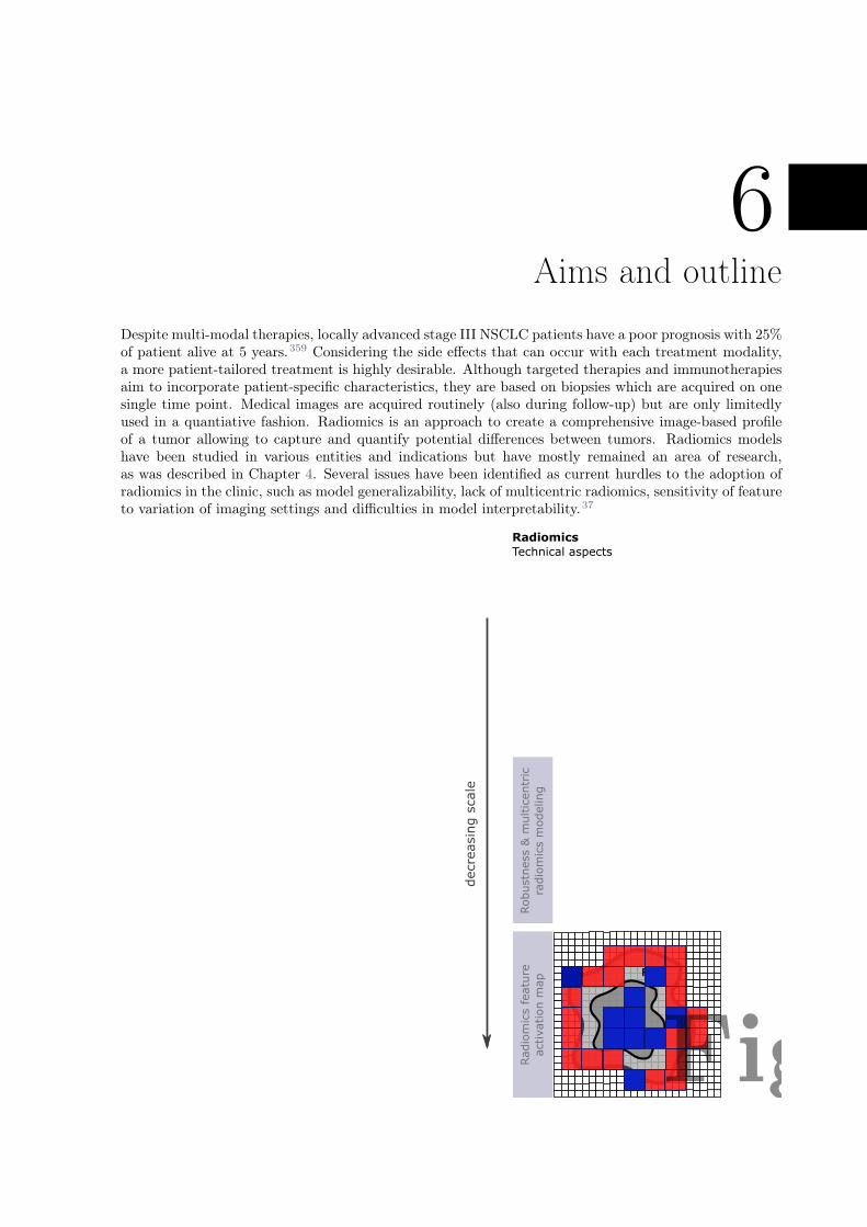
6Aims and outline
Despite multi-modal therapies, locally advanced stage III NSCLC patients have a poor prognosis with 25%of patient alive at 5 years.359 Considering the side effects that can occur with each treatment modality,a more patient-tailored treatment is highly desirable. Although targeted therapies and immunotherapiesaim to incorporate patient-specific characteristics, they are based on biopsies which are acquired on onesingle time point. Medical images are acquired routinely (also during follow-up) but are only limitedlyused in a quantiative fashion. Radiomics is an approach to create a comprehensive image-based profileof a tumor allowing to capture and quantify potential differences between tumors. Radiomics modelshave been studied in various entities and indications but have mostly remained an area of research,as was described in Chapter 4. Several issues have been identified as current hurdles to the adoption ofradiomics in the clinic, such as model generalizability, lack of multicentric radiomics, sensitivity of featureto variation of imaging settings and difficulties in model interpretability.37
decre
asin
g s
cale
Radiomics
Technical aspects
GTV
Rim
Radio
mic
s featu
re
activation m
ap
Robustn
ess &
multic
entr
ic
radio
mic
s m
odeling
Fig

6.1 Aims
This PhD thesis aims to address these challenges for the example of locally advanced stage III NSCLCpatients treated with multi-modal therapy. For this purpose, pre-treatment PET/CT imaging data wascollected from a prospective phase 3 multi-centric Swiss trial (SAKK–16/007), where patients were treatedwith neoadjuvant chemotherapy followed by surgery versus neoadjuvant radiation chemotherapy followedby surgery. In the same time, a quantitative description of the locally advanced NSCLC on differentlength scales is studied. An illustration is presented in Figure 6.1.
6.2 Outline
The remainder of this PhD thesis can be divided into four main parts.
Part I In the first part, I analyzed the anatomic spatial location of the tumor within the lung. Theproximity of the tumor to other organs at risk can lead to difficulties in local therapy such as radiotherapyor surgery and can be prognostic for patient outcome. Until now, tumor location was often defined inrelation to a pre-defined anatomical region (e.g. lung lobe location) or was based on the distance topre-selected critical organs (e.g. distance of tumor to the carina).3 Both have limited ability to integratethe entire spatial extent of the primary tumor and are prone to interobserver variability. In Chapter7, I proposed a data mining approach to investigate the association between tumor location and 2-yearoverall survival of locally advanced NSCLC patients. Using displacement data obtained from deformableimage registration, the initial spatial extent of primary tumors were mapped onto a reference patientanatomy and assigned a patient status. Thus, a given cohort can be represented as a spatial voxelizedmap in which each voxel contains the cumulative patient status. Within this map, high-risk lung regionscan be identified and used to further investigate the location of the primary tumor as a prognostic factorfor survival (Figure 6.1, first row).
Part II To be able to assess the value of radiomics in outcome prediction in locally advanced NSCLCpatients, an in-depth analysis was performed to assess the feature robustness to the variability in imagingsettings often found in multicenter datasets. In Chapter 8, I studied the feature robustness in PETimaging when PET scans are acquired as a PET/CT or PET/MR combination. With the increasedavailability of PET/MR, a mixture of PET/CT and PET/MR scanners may be encountered in clinicalstudies, and question arises whether PET radiomic features are interchangeable between these typesof scanners. In Chapter 9, I studied the effect using two convolution kernels in FBP algorithm forCT reconstructions commonly used in chest imaging. In addition to NSCLC patients, different pleuralmalignant mesothelioma and systemic sclerosis interstitial lung disease were studied. In addition to theprimary tumor region, radiomics of the largest lymph node and the lungs were also studied, which to ourknowledge is one of the most comprehensive robustness analysis for kernel robustness in lung imaging(Figure 6.1, second row).
Part III The best approach to incorporate robustness results into radiomic modeling has yet to befound. Identified unstable features should not be included in radiomic models because they may representnot only image-based heterogeneity of tumor phenotype but also variations in imaging settings betweenpatients.37 Because the primary goal of routinely acquired medical imaging is to optimize these settingsfor the best quality diagnosis, it is nearly impossible to control imaging and scanner settings betweencenters in large clinical trials. There are two main approaches for robust multi-centric radiomics models:a) Either discard features based solely on their sensitivity to differences in imaging settings, which mayresult in the removal of potentially useful and informative features360 or b) discard patients by selectingthe largest subset of patients with homogeneous imaging settings. This facilitates the use of all featuresbut given the limited clinical data that are already problematic for radiomic research, this approach woulddiscard many patients. Since these two approaches have not yet been directly compared, I set up a studyin the third part of this thesis to perform this comparison (Chapter 10).To this end, I analyzed the robustness of radiomic features for four different settings in CT lung radiomics,namely interobserver delineation variability, CT reconstruction kernel, contrast enhancement, and res-piratory motion. Using these identified robust features in conjunction with the multicentric imagingdataset, I generated a first model that pre-selected the robust features before modeling. For the second
114
Aims and outline
model, I identified the largest patient subcohort that had homogeneous imaging and scanning settings inwhich I could use all features. These two models were validated on a separate validation cohort and theirperformance was compared (Figure 6.1, second row).
Part IV In recent years, many efforts have been made to find the most powerful radiomic model andhave begun to introduce more complex features that aim to describe finer and more detailed aspects of theROI. Interpretability of model features is a relevant property for quality assurance and introduction intothe clinic. The goal of this last part of this thesis was to improve the interpretability of radiomic signaturesby spatially localizing the activation of features in a model. In Chapter 11, I introduced the concept ofradiomic feature activation maps. These maps were based on a local radiomic approach, where insteadof extracting radiomic features from the entire ROI, features are computed from smaller ROI subregions(also called patches). This allows detection of the spatial location of a given feature within the globalROI (extreme feature values). Peritumoral radiomics (radiomics including microscopic extension nearthe visible primary tumor) to predict histology in NSCLC patients served as a case study. The goal wasto identify which region (rim or primary tumor) was most responsible region for the predicting histology(Figure 6.1, third row).
115

116
7Quantification of spatial distribution of
primary tumors in the lung to develop newprognostic biomarkers for locally advanced
NSCLC
Diem Vuong1, Marta Bogowicz1, Leonard Wee2, Oliver Riesterer1,3, Eugenia Vlaskou Badra1, Louisa
D’Cruz4, Panagiotis Balermpas1, Janita E. van Timmeren1, Simon Burgermeister1, André Dekker2, DirkDe Ruysscher2, Jan Unkelbach1, Sandra Thierstein5, Eric Innocents Eboulet5, Solange Peters6, MiklosPless7, Matthias Guckenberger1, Stephanie Tanadini-Lang1
1Department of Radiation Oncology, University Hospital Zurich and University of Zurich, Zurich, Switzer-land2Department of Radiation Oncology (MAASTRO), GROW School for Oncology and DevelopmentalBiology, Maastricht University Medical Centre+, Maastricht, The Netherlands3Center for Radiation-Oncology KSA-KSB, Kantonsspital Aarau AG, Aarau, Switzerland4Strahlentherapie und Onkologie, Universitätsklinikum Frankfurt, Frankfurt, Germany5Swiss Group for Clinical Cancer Research (SAKK), Coordinating Center, Bern, Switzerland6Department of Oncology, Centre Hospitalier Universitaire Vaudois (CHUV), Lausanne, Switzerland7Department of Medical Oncology, Kantonsspital Winterthur, Winterthur, Switzerland
Status:Submitted to Scientific Reports, 2021
Copyright: Authors retained the copyright totheir articles.
My contribution: I collected imaging and contour data from all institutions and performed thedeformable image registrations for each patient to the reference patient. I implemented the softwaresolution to transfer the primary tumors to the reference patient, to create the maps, and to calculate thedistances. I interpreted the results and wrote the manuscript.
7.1 Abstract
Purpose: The anatomical location and extent of primary lung tumors have shown prognostic value foroverall survival (OS). However, its manual assessment is prone to interobserver variability. This studyaims at data driven identification of image characteristics for OS in locally advanced non-small cell lungcancer (NSCLC) patients.
Materials and Methods: Five stage IIIA/IIIB NSCLC patient cohorts were retrospectively collected.Patients were treated either with radiochemotherapy (RCT): RCT1* (n = 107), RCT2 (n = 95), RCT3(n = 37) or with surgery combined with radiotherapy or chemotherapy: S1* (n = 135), S2 (n = 55).Based on a deformable image registration (MIM Vista, 6.9.2.), an in-house software transferred eachprimary tumor to the CT scan of a reference patient while maintaining the original primary tumorshape. A frequency-weighted cumulative status (fwCS) map was created for both exploratory cohorts(indicated with an asterisk), where primary tumor spatial extent was uni-labeled with 2 years OS. Forthose exploratory cohorts, a permutation test with random assignment of patient status to the primarytumor was performed to identify regions with statistically significant worse OS (referred to as decreasedsurvival areas (DSA)). The minimal Euclidean distance between primary tumor to DSA was extractedfrom the validation cohorts (negative distance in case of overlap). To account for the primary tumorextent, the distance was scaled with the radius of the volume-equivalent sphere.
Results: For the S1 cohort, DSA were located at the right main bronchus whereas for the RCT1 cohortthey further extended in cranio-caudal direction. In the validation cohorts, the model based on distanceto DSA achieved performance: AUCRCT2 [95% CI] = 0.67 [0.55-0.78] and AUCRCT3 = 0.59 [0.39-0.79]for RCT patients, but showed bad performance for surgery cohort (AUCS2 = 0.52 [0.30-0.74]). Shorterdistance to DSA was associated with worse outcome.
Conclusions: This explanatory analysis quantifies the value of primary tumor location for OS predictionbased on cumulative status maps. Smaller distance of primary tumor to a high-risk region was associatedwith worse prognosis in the RCT cohort.
7.2 Introduction
Locally advanced non-small cell lung cancer (NSCLC) is the most advanced stage treated with curativeintent to date, but patient outcome remains poor with a 5-year overall survival (OS) rate of approximately5-35% despite multimodality treatment.21
In local treatments such as radiotherapy or surgery, the anatomical location of the primary tumor is ofimportance as anatomical obstacles may compromise treatment success. Primary tumors located eitherin the lower lobe361,362, more centrally363, or with chest wall invasion364,365 have been associated withpoorer prognosis for different stages of NSCLC. However, these studies associate tumor location to pre-defined anatomic regions that only partially reflect the full 3D location within the lung.
In recent years, more data is being collected, accelerating data mining approaches in cancer research.An excellent example to illustrate the additive value of data mining in cancer research is a study on therole of cardiac irradiation on OS of lung cancer patients.366 Using a voxelized dosimetric comparison toidentify regions of poor patient survival, they demonstrated that dose delivered at the base of the heartwas more prognostic than previously used metrics.366
Here, we propose for the first time a data mining approach to investigate the association between tumorlocation and 2-year OS of locally advanced NSCLC patients. The extent of patient tumors is mapped toa reference patient anatomy and assigned with patient status. Thus, a given cohort can be representedby a voxelized spatial distribution of the cumulative status. This mapping approach has been previouslyused in brain lesions e.g. to study the impact of primary tumor entity on the spatial distribution of brainmetastases.367,368 In contrast to other studies, here the primary tumors are mapped while preserving theoriginal shape of the primary tumors.The aim of the study was two-fold. First, we identify areas in these maps with statistically significant de-creased survival (DSA) to examine differences in outcome between surgical or radiochemotherapy (RCT)regimens. Second, the smallest distance of the primary tumor to the DSA is extracted to quantify thespatial distribution and perform outcome modeling on independent patient cohorts.
118

Quantification of spatial distribution of primary tumors in the lung to develop new prognosticbiomarkers for locally advanced NSCLC
7.3 Materials and methods
7.3.1 Patient and imaging data
Name RCT1* RCT2 RCT3 S1* S2
Center MaastroClinic(LUNG1)
MaastroClinic(LUNG4)
KantonsspitalAarau
Swiss multi-centric trial(SAKK 16/00)
UniversityHospitalZurich
Patients 107 95 37 135 55Treatment RCT RCT RCT RCT followed
by surgeryRCT followedby surgery
OS events at 2 years 69.2% 50.5% 56.8% 37.8% 21.9%Imaging Single-
institutionSingle-institution
Single-institution
Multi-centric Single-institution
In-plane resolution (mm) 0.98 (0) 0.98 (0) 0.98 (0) 0.98 (0.19) 1.04 (0.12)Slice thickness (mm) 3.00 (0) 2.98 (0.15) 2.84 (1.04) 3.17 (1.18) 3.05 (0.45)No. CT reconstructionmethods
8 6 2 16 6
Primary tumor volume(ml)
79.24 (94.4) 95.38(102.12)
129.19(124.60)
49.82 (56.81) 76.27 (99.44)
TNM edition 7 7 6 6 6
Table 7.1: Overview of stage III NSCLC patient cohorts used in this study. Cohorts indicated with an asteriskare referred to as exploratory cohorts and the remaining cohorts as validation cohorts. Exploratory cohorts wereused to identify the decreased survival areas and the validation cohorts to extract the smallest distance to thedecreased survival areas. Values are reported with mean (standard deviation).
Computed tomography (CT) scans were collected retrospectively from five locally advanced stage IIIA/IIIBNSCLC cohorts (Table 7.1). Three patient cohorts were treated curatively with concurrent or sequentialRCT (RCT1, RCT2, RCT3) and two with a combination of radiotherapy and chemotherapy and surgery(S1 and S2, more details can be found in the Supplement 7.7). The RCT1 cohort is a publically availabledataset that has been previously published32,369,370. The S1 cohort was collected from a multi-centricclinical trial (SAKK 16/007), part of whose imaging data has been described elsewhere.371 All remainingcohorts were based on single institution data.Radiation therapy planning CT scans were collected along with contours from each institution in theRCT cohorts, whereas diagnostic CT scans were collected and contoured at our institution in the surgicalcohorts. Informed consent was obtained from all patients.
Cohorts RCT1 and S1 (indicated with an asterisk in Table 7.1) are referred to as exploratory cohorts,whereas the remaining cohorts are the validation cohorts. Based on the exploratory cohorts, maps ofboth spatial distribution and DSA are created. The validation cohorts will be used to extract the primarytumor distance to DSA and to test its prognostic value.
7.3.2 Mapping of patient to reference
Reference patient
One head and neck cancer patient with two healthy lungs was selected as a reference patient frame.This patient had an age and body weight within 10% of the average patients in the S1 cohort. Hispatient characteristics were: male, 59 years, 65 kg, and 4710.28 ml lung volume (2544.42 ml right lungand 2165.86 left lung). The pre-treatment non-contrast CT scan had a resolution of 0.98 x 0.98 x 3.27mm and was reconstructed with filtered-back projection and standard convolution kernel (GE MedicalSystem, Discovery STE).
Mapping of patient tumor to reference patient
Due to the multi-centric setting of this study, image sets were heterogeneous in terms of acquisitionand scanning settings (i.e., presence of contrast agents, different reconstruction kernels). Therefore, anintensity independent contour-only based deformable image registration was performed. The ipsilateral
119
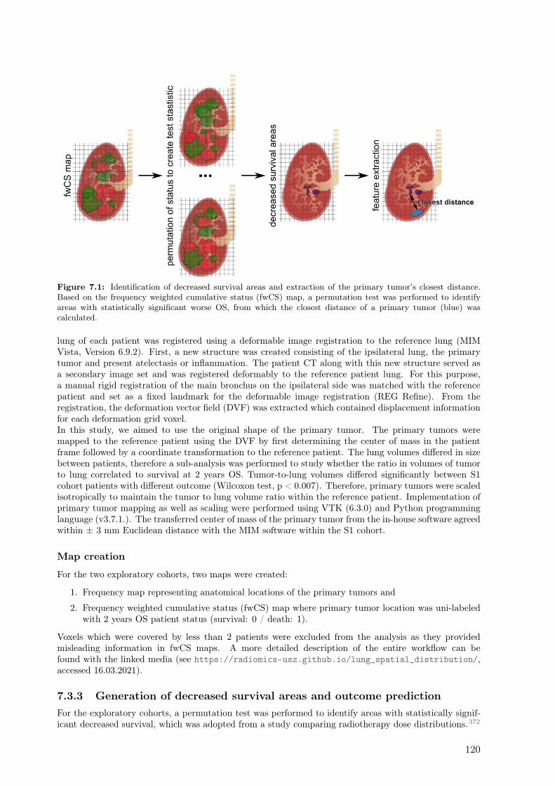
Figure 7.1: Identification of decreased survival areas and extraction of the primary tumor’s closest distance.Based on the frequency weighted cumulative status (fwCS) map, a permutation test was performed to identifyareas with statistically significant worse OS, from which the closest distance of a primary tumor (blue) wascalculated.
lung of each patient was registered using a deformable image registration to the reference lung (MIMVista, Version 6.9.2). First, a new structure was created consisting of the ipsilateral lung, the primarytumor and present atelectasis or inflammation. The patient CT along with this new structure served asa secondary image set and was registered deformably to the reference patient lung. For this purpose,a manual rigid registration of the main bronchus on the ipsilateral side was matched with the referencepatient and set as a fixed landmark for the deformable image registration (REG Refine). From theregistration, the deformation vector field (DVF) was extracted which contained displacement informationfor each deformation grid voxel.In this study, we aimed to use the original shape of the primary tumor. The primary tumors weremapped to the reference patient using the DVF by first determining the center of mass in the patientframe followed by a coordinate transformation to the reference patient. The lung volumes differed in sizebetween patients, therefore a sub-analysis was performed to study whether the ratio in volumes of tumorto lung correlated to survival at 2 years OS. Tumor-to-lung volumes differed significantly between S1cohort patients with different outcome (Wilcoxon test, p < 0.007). Therefore, primary tumors were scaledisotropically to maintain the tumor to lung volume ratio within the reference patient. Implementation ofprimary tumor mapping as well as scaling were performed using VTK (6.3.0) and Python programminglanguage (v3.7.1.). The transferred center of mass of the primary tumor from the in-house software agreedwithin ± 3 mm Euclidean distance with the MIM software within the S1 cohort.
Map creation
For the two exploratory cohorts, two maps were created:
1. Frequency map representing anatomical locations of the primary tumors and
2. Frequency weighted cumulative status (fwCS) map where primary tumor location was uni-labeledwith 2 years OS patient status (survival: 0 / death: 1).
Voxels which were covered by less than 2 patients were excluded from the analysis as they providedmisleading information in fwCS maps. A more detailed description of the entire workflow can befound with the linked media (see https://radiomics-usz.github.io/lung_spatial_distribution/,accessed 16.03.2021).
7.3.3 Generation of decreased survival areas and outcome prediction
For the exploratory cohorts, a permutation test was performed to identify areas with statistically signif-icant decreased survival, which was adopted from a study comparing radiotherapy dose distributions.372
120
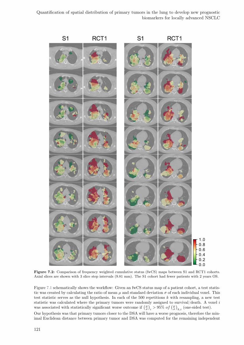
Quantification of spatial distribution of primary tumors in the lung to develop new prognosticbiomarkers for locally advanced NSCLC
Figure 7.2: Comparison of frequency weighted cumulative status (fwCS) maps between S1 and RCT1 cohorts.Axial slices are shown with 3 slice step intervals (9.81 mm). The S1 cohort had fewer patients with 2 years OS.
Figure 7.1 schematically shows the workflow: Given an fwCS status map of a patient cohort, a test statis-tic was created by calculating the ratio of mean µ and standard deviation σ of each individual voxel. Thistest statistic serves as the null hypothesis. In each of the 500 repetitions k with resampling, a new teststatistic was calculated where the primary tumors were randomly assigned to survival/death. A voxel iwas associated with statistically significant worse outcome if
(
µσ
)
i> 95% of
(
µσ
)
k,i(one-sided test).
Our hypothesis was that primary tumors closer to the DSA will have a worse prognosis, therefore the min-imal Euclidean distance between primary tumor and DSA was computed for the remaining independent
121
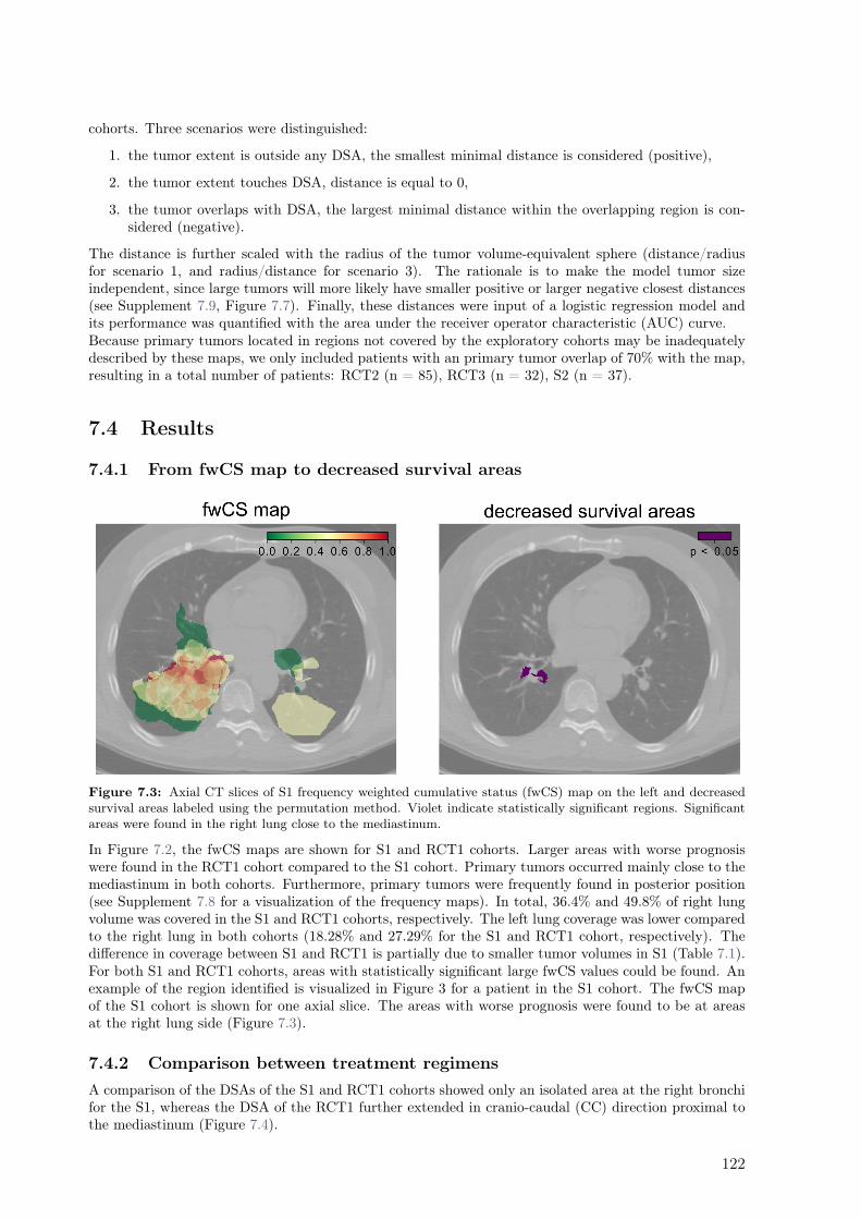
cohorts. Three scenarios were distinguished:
1. the tumor extent is outside any DSA, the smallest minimal distance is considered (positive),
2. the tumor extent touches DSA, distance is equal to 0,
3. the tumor overlaps with DSA, the largest minimal distance within the overlapping region is con-sidered (negative).
The distance is further scaled with the radius of the tumor volume-equivalent sphere (distance/radiusfor scenario 1, and radius/distance for scenario 3). The rationale is to make the model tumor sizeindependent, since large tumors will more likely have smaller positive or larger negative closest distances(see Supplement 7.9, Figure 7.7). Finally, these distances were input of a logistic regression model andits performance was quantified with the area under the receiver operator characteristic (AUC) curve.Because primary tumors located in regions not covered by the exploratory cohorts may be inadequatelydescribed by these maps, we only included patients with an primary tumor overlap of 70% with the map,resulting in a total number of patients: RCT2 (n = 85), RCT3 (n = 32), S2 (n = 37).
7.4 Results
7.4.1 From fwCS map to decreased survival areas
Figure 7.3: Axial CT slices of S1 frequency weighted cumulative status (fwCS) map on the left and decreasedsurvival areas labeled using the permutation method. Violet indicate statistically significant regions. Significantareas were found in the right lung close to the mediastinum.
In Figure 7.2, the fwCS maps are shown for S1 and RCT1 cohorts. Larger areas with worse prognosiswere found in the RCT1 cohort compared to the S1 cohort. Primary tumors occurred mainly close to themediastinum in both cohorts. Furthermore, primary tumors were frequently found in posterior position(see Supplement 7.8 for a visualization of the frequency maps). In total, 36.4% and 49.8% of right lungvolume was covered in the S1 and RCT1 cohorts, respectively. The left lung coverage was lower comparedto the right lung in both cohorts (18.28% and 27.29% for the S1 and RCT1 cohort, respectively). Thedifference in coverage between S1 and RCT1 is partially due to smaller tumor volumes in S1 (Table 7.1).For both S1 and RCT1 cohorts, areas with statistically significant large fwCS values could be found. Anexample of the region identified is visualized in Figure 3 for a patient in the S1 cohort. The fwCS mapof the S1 cohort is shown for one axial slice. The areas with worse prognosis were found to be at areasat the right lung side (Figure 7.3).
7.4.2 Comparison between treatment regimens
A comparison of the DSAs of the S1 and RCT1 cohorts showed only an isolated area at the right bronchifor the S1, whereas the DSA of the RCT1 further extended in cranio-caudal (CC) direction proximal tothe mediastinum (Figure 7.4).
122

Quantification of spatial distribution of primary tumors in the lung to develop new prognosticbiomarkers for locally advanced NSCLC
Figure 7.4: Comparison of decreased survival areas (violet) between S1 andRCT1 cohorts. Axial slices areshown with 3 slice step intervals (9.81 mm). S1 cohort shows an isolated location on the right lung side, whereasthe decreased survival areas are spread in superior and inferior direction for RCT1.
7.4.3 Outcome prediction
The model performances for predicting 2 years OS were AUCRCT2 = 0.67 [95%CI: 0.55-0.78] and AUCRCT3=0.59 [0.39-0.79] for RCT patients, but showed bad performance for the surgery cohort (AUCS2 = 0.52 [0.30-0.74]). Smaller distance to DSA was associated with worse outcome.Since T and N stage definition is related to invasion and extent of the tumor into the carina, a sub-analysis was performed to test the distances against T and N stages. A statistically significant difference
123
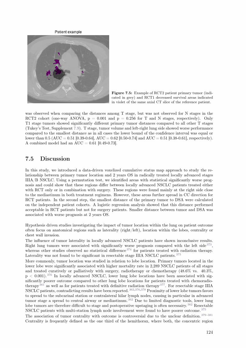
Figure 7.5: Example of RCT2 patient primary tumor (indi-cated in grey) and RCT1 decreased survival areas indicatedin violet of the same axial CT slice of the reference patient.
was observed when comparing the distances among T stage, but was not observed for N stages in theRCT2 cohort (one-way ANOVA, p = 0.001 and p = 0.256 for T and N stages, respectively). OnlyT1 stage tumors showed significantly different primary tumor distances compared to all other T stages(Tukey’s Test, Supplement 7.9). T stage, tumor volume and left-right lung side showed worse performancecompared to the smallest distance as in all cases the lower bound of the confidence interval was equal orlower than 0.5 (AUC = 0.51 [0.39-0.64], AUC = 0.62 [0.50-0.74] and AUC = 0.51 [0.38-0.61], respectively).A combined model had an AUC = 0.61 [0.49-0.73].
7.5 Discussion
In this study, we introduced a data-driven voxelized cumulative status map approach to study the re-lationship between primary tumor location and 2 years OS in radically treated locally advanced stagesIIIA/B NSCLC. Using a permutation test, we identified areas with statistical significantly worse prog-nosis and could show that these regions differ between locally advanced NSCLC patients treated eitherwith RCT only or in combination with surgery. These regions were found mainly at the right side closeto the mediastinum in both treatment regimens. However, these areas further spread in CC direction forRCT patients. In the second step, the smallest distance of the primary tumor to DSA were calculatedon the independent patient cohorts. A logistic regression analysis showed that this distance performedacceptable in RCT patients but not for surgery patients. Smaller distance between tumor and DSA wasassociated with worse prognosis at 2 years OS.
Hypothesis driven studies investigating the impact of tumor location within the lung on patient outcomeoften focus on anatomical regions such as laterality (right/left), location within the lobes, centrality orchest wall invasion.
The influence of tumor laterality in locally advanced NSCLC patients have shown inconclusive results.Right lung tumors were associated with significantly worse prognosis compared with the left side373,whereas other studies observed no statistical difference374 for patients treated with radiation therapy.Laterality was not found to be significant in resectable stage IIIA NSCLC patients.375
More commonly, tumor location was studied in relation to lobe location. Primary tumors located in thelower lobe were significantly associated with higher mortality rate in 2,289 NSCLC patients of all stagesand treated curatively or palliatively with surgery, radiotherapy or chemotherapy (48.6% vs. 40.3%,p < 0.001).376 In locally advanced NSCLC, lower lung lobe locations have been associated with sig-nificantly poorer outcome compared to other lung lobe locations for patients treated with chemoradio-therapy361 as well as for patients treated with definitive radiation therapy377. For resectable stage IIIANSCLC patients, contradicting results have been reported.362,376,378 Proximity of lower lobe tumors favorsto spread to the subcarinal station or contralateral hilar lymph nodes, causing in particular in advancedtumor stage a spread to central airway or mediastinum.362 Due to limited diagnostic tools, lower lunglobe tumors are therefore difficult to stage and postoperative upstaging is often necessairy.362 ResectableNSCLC patients with multi-station lymph node involvement were found to have poorer outcome.375
The association of tumor centrality with outcome is controversial due to the unclear definition.379–381
Centrality is frequently defined as the one third of the hemithorax, where both, the concentric region
124
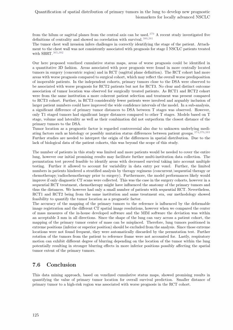
Quantification of spatial distribution of primary tumors in the lung to develop new prognosticbiomarkers for locally advanced NSCLC
from the hilum or sagittal planes from the central axis can be used.379 A recent study investigated fivedefinitions of centrality and showed no correlation with survival.380,381
The tumor chest wall invasion infers challenges in correctly identifying the stage of the patient. Attach-ment to the chest wall was not consistently associated with prognosis for stage I NSCLC patients treatedwith SBRT.365,382
Our here proposed voxelized cumulative status maps, areas of worse prognosis could be identified ina quantitative 3D fashion. Areas associated with poor prognosis were found in more centrally locatedtumors in surgery (concentric region) and in RCT (sagittal plane definition). The RCT cohort had moreareas with worse prognosis compared to surgical cohort, which may reflect the overall worse predispositionof inoperable patients. In the independent cohorts, primary tumors close to the DSA were observed tobe associated with worse prognosis for RCT2 patients but not for RCT3. No clear and distinct outcomeassociation of tumor location was observed for surgically treated patients. As RCT1 and RCT2 cohortwere from the same institution a more coherent patient selection and treatment was present comparedto RCT3 cohort. Further, in RCT3 considerably fewer patients were involved and arguably inclusion oflarger patient numbers could have improved the wide confidence intervals of the model. In a sub-analysis,a significant difference of primary tumor distances to DSA between T stages was observed. However,only T1 staged tumors had significant larger distances compared to other T stages. Models based on Tstage, volume and laterality as well as their combination did not outperform the closest distance of theprimary tumors to the DSA.Tumor location as a prognostic factor is regarded controversial also due to unknown underlying medi-ating factors such as histology or possibly mutation status differences between patient groups.374,376,383
Further studies are needed to interpret the origin of the differences in spatial distribution. Due to thelack of biological data of the patient cohorts, this was beyond the scope of this study.
The number of patients in this study was limited and more patients would be needed to cover the entirelung, however our initial promising results may facilitate further multi-institution data collection. Thepermutation test proved feasible to identify areas with decreased survival taking into account multipletesting. Further it allowed to account for variability in data entry per voxel. Further, the limitednumbers in patients hindered a stratified analysis by therapy regimens (concurrent/sequential therapy orchemotherapy/radiochemotherapy prior to surgery). Furthermore, the model performances likely wouldimprove if only diagnostic CT scans were collected. This was the case in the surgery cohorts, however in asequential RCT treatment, chemotherapy might have influenced the anatomy of the primary tumors andthus the distances. We however had only a small number of patients with sequential RCT. Nevertheless,RCT1 and RCT2 being from the same institution and same treatment era, our methodology showedfeasibility to quantify the tumor location as a prognostic factor.The accuracy of the mapping of the primary tumors to the reference is influenced by the deformableimage registration and the different CT spatial image resolutions, however when we compared the centerof mass measures of the in-house developed software and the MIM software the deviation was withinan acceptable 3 mm in all directions. Since the shape of the lung can vary across a patient cohort, themapping of the primary tumor center of mass can be misplaced. Therefore, lung tumors positioned inextreme positions (inferior or superior position) should be excluded from the analysis. Since those extremelocations were not found frequent, they were automatically discarded by the permutation test. Furtherrotation of the tumors from the patient to reference frame were not accounted for. Lastly, respiratorymotion can exhibit different degree of blurring depending on the location of the tumor within the lungpotentially resulting in stronger blurring effects in more inferior positions possibly affecting the spatialtumor extent of the primary tumors.
7.6 Conclusion
This data mining approach, based on voxelized cumulative status maps, showed promising results inquantifying the value of primary tumor location for overall survival prediction. Smaller distance ofprimary tumor to a high-risk region was associated with worse prognosis in the RCT cohort.
125

7.7 Supplement A: Patient characteristics
RCT1 RCT2 RCT3 S1 S2
Number of Patients 107 95 37 135 55Sex
Female 39 37 13 48 26Male 68 58 24 87 29
Age (Median (IQR) 65.5 (42.6) 68 (47) 66 (43) 60 (39) 67 (33)Tumor Histology
Adenocarcinoma 13 * 16 58 17Squamous cell carcinoma 38 * 16 43 3Large cell carcinoma 56 * 8Poorly diff./Unknown * 26 3
Tumor StageT1 12 8 2 21 5T2 44 28 13 78 23T3 8 18 11 34 12T4 43 41 11 2 15
Nodal StageN0 14 7 3 5N1 3 4 2 1 8N2 56 46 14 134 41N3 34 37 18 1
Metastasis StageM0 105 95 32 132 54M1 4 3 1M2 2Unknown 1
TreatmentConcurrent RCT * 86 32 2Sequential RCT * 9 5 70 6Adj. Chemotherapy Therapy * 6Chemotherapy * 65 41
Survival DataOS events at 2 years 69.2% 50.5% 56.8% 37.8% 69.2%
Table 7.2: Patient characteristics. Asterisks indicate insufficiently reported data.
126

Quantification of spatial distribution of primary tumors in the lung to develop new prognosticbiomarkers for locally advanced NSCLC
7.8 Supplement B: Frequency maps
Figure 7.6: Comparison of frequency maps between S1 and RCT1 cohorts. Axial slices are shown with 3 slicestep intervals (9.81 mm).
127
7.9 Supplement C: Correlation distance with volume, T and Nstage
Figure 7.7: Scatterplot of distances and tumor volume for RCT2 cohort.
In a sub-analysis we performed a one-way ANOVA test to study the difference in distance betweenprimary tumor distance and decreased survival areas for different T and N stages. For the T stages, theaverage distance was 14.48 mm (±8.88), 1.67 mm (±5.69), 4.5 mm (±13.18) and 1.27 mm (±5.54) forincreasing T stage. There was a statistically significant difference between the primary tumor distancesof different the T stage (F = 5.88, p-value = 0.001). The distances of T1 stage tumors were significantlydifferent any other T stage (p-values = 0.002, 0.0319, 0.001 for T2, T3 and T4, respectively, Tukey test).For N stage, the closest tumor-to-DSA distance was 0.19 mm (±1.51), -0.23 mm (±0.12), 2.13 mm(±6.35), 5.34 mm (±11.42) for increasing N stage. No statistically difference was found between theprimary tumor PT distances of different the N stages (F = 1.37, p-value = 0.256).
128
8Interchangeability of radiomic features
between [18F]–FDG PET/CT and[18F]–FDG PET/MR
Diem Vuong1, Stephanie Tanadini–Lang1, Martin W. Huellner2, Patrick Veit-Haibach2, Jan Unkelbach1,
Nicolaus Andratschke1, Johannes Kraft1, Matthias Guckenberger1, Marta Bogowicz1
1Department of Radiation Oncology, University Hospital Zurich and University of Zurich, Zurich, Switzer-land2Department of Nuclear Medicine, University Hospital Zurich and University of Zurich, Zurich, Switzer-land
Status:Published in Medical Physics Journal, 2019doi: 10.1002/mp.13422
Copyright: ©American Association of Physi-cists in Medicine. Reproduced with permis-sion. All rights reserved.
My contribution: I identified eligible patients and collected the corresponding PET imaging data. Idelineated the tumor region with two segmentation methods. I performed the radiomics calculation androbustness analysis. Further, I wrote, revised, and proof-read the manuscript.
8.1 Abstract
Purpose Radiomics is a promising tool for identification of new prognostic biomarkers. However, imagereconstruction settings and test–retest variability may influence the absolute values of radiomic features.Unstable radiomic features cannot be used as reliable biomarkers. PET/MR is becoming increasinglyavailable and often replaces PET/CT for different indications. The aim of this study was to quantifyto what extend [18F]–FDG PET/CT radiomics models can be transferred to [18F]–FDG PET/MR andthereby to investigate the feasibility of combined PET/CT–PET/MR models. For this purpose, wecompared PET radiomic features calculated on PET/MR and PET/CT and on a 4D-gated PET/MRdataset to select radiomic features that are robust to attenuation correction differences and test–retestvariability, respectively.
Methods Two cohorts of patients with lung lesions were studied. In the first cohort (n = 10), inhaleand exhale phases of a 4D [18F]–FDG PET/MR (4DPETMR) scan were used as a surrogate for a test–retest dataset. In the second cohort (n = 9), patients underwent first an [18F]–FDG PET/MR scan(SIGNA PET/MR, GE Healthcare, Waukesha) followed by an [18F]–FDG PET/CT scan (Discovery690, GE Healthcare) with a delay of 33 ± 5 min (PETCT–PETMR). Lesions were segmented on inhaleand exhale 4D–PET phases and on the individual PET scans from PET/CT and PET/MR with twosemi–automated methods (gradient–based and threshold–based). The scan resolution was 2.73 x 2.73x 3.27 mm and 2.34 x 2.34 x 2.78 mm for the PET/CT and PET/MR, respectively. In total, 1355radiomic features were calculated, i.e. shape (n = 18), intensity (n = 17), texture (n = 136), and wavelet(n = 1184). The intraclass correlation coefficient (ICC) was calculated to compare the radiomic featuresof the 4DPETMR (ICC(1,1)) and PETCT–PETMR (ICC(3,1)) datasets. An ICC > 0.9 was consideredstable among both types of PET scans.
Results and conclusion The 4DPETMR showed highest stability for shape, intensity, and texture(>80%) and lower stability for wavelet features (40%). Gradient–based method showed higher stabilitycompared to threshold–based method except from shape features. In PETC–PETMR, more than 61%of shape and intensity features were stable for both segmentation methods. However, a reduced stabilitywas observed for texture (50%) and wavelet (<30%) features. More wavelet features were robust inthe smoothed images (low–pass filtering) compared to images with emphasized heterogeneity (high–passfiltering). Comparing stable features of both investigations, highest agreement was found for intensityand lower agreement for shape, texture, and wavelet features. Only 53.6% of stable texture featuresin 4DPETMR were also stable in PETCT–PETMR, and even less in case of wavelet features (40.4%).Approximately 16.9% (texture) and 43.2% (wavelet) of stable PETCT–PETMR features are unstable in4DPETMR.
To conclude, shape and intensity features were robust when comparing two types of [18F]–FDG PET scans(PET/CT and PET/MR). Reduced stability was observed for texture and wavelet features. We identifiedmultiple origins of instability of radiomic features, such as attenuation correction differences, differentuptake times, and spatial resolution. This needs to be considered when models based on PET/CT aretransferred PET/MR models or when combined models are used.
8.2 Introduction
Due to its noninvasive nature, imaging has gained an increasing role in identification of new prognosticbiomarkers to predict treatment outcome.384 Pretreatment [18F]–FDG positron emission tomography(PET) scans have been investigated intensively and have shown good prognostic value in multiple onco-logical diseases.385,386 Numerous studies have proposed and investigated so–called radiomic features asnew prognostic biomarkers.32,70,72
Radiomics refers to the process of extracting a large number of quantitative imaging features that describethe intratumoral heterogeneity noninvasively using medical images and were partially shown superior toconventional voxel–based standard-uptake value (SUV) metrics in research settings.69 Radiomic featurescan be categorized into four types: shape, intensity, texture, and wavelet. Shape and intensity featureshave shown good predictive power.75,387 However, it is known that tumors are spatial and temporal het-erogeneous.388 Therefore, particularly interesting are texture and wavelet features, which focus not onlyon the individual voxels but also the relation between voxels. Texture features describe the relationship
130
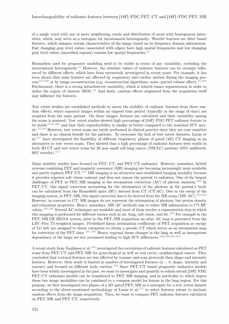
Interchangeability of radiomic features between [18F]–FDG PET/CT and [18F]–FDG PET/MR
of a single voxel with one or more neighboring voxels and distribution of areas with homogenous inten-sities, which, may serve as a surrogate for intratumoral heterogeneity. Wavelet features are filter–basedfeatures, which enhance certain characteristics of the image based on its frequency domain information.Fast changing gray level values (associated with edges) have high spatial frequencies and low changinggray level values (smoothed regions) contain low spatial frequencies.32
Biomarkers used for prognostic modeling need to be stable in terms of any variability, excluding theintratumoral heterogeneity.67 However, the absolute values of radiomic features can be strongly influ-enced by different effects, which have been extensively investigated in recent years. For example, it hasbeen shown that some features are affected by respiratory and cardiac motion during the imaging pro-cess223,389 or by image reconstruction (e.g. reconstruction algorithms, noise, partial volume effect).84,389
Furthermore, there is a strong intraobserver variability, which is related tumor segmentation in order todefine the region–of–interest (ROI).83 And lastly, random effects originated from the acquisition itselfmay influence the features.
Test–retest studies are established methods to assess the stability of radiomic features from those ran-dom effects, where repeated images within an elapsed time period (typically in the range of days) areacquired from the same patient. On those images, features are calculated and their variability amongthe scans is assessed. Test–retest studies showed high percentage of [18F]–FDG PET radiomic feature tobe stable83,84,390 and that their reproducibility is similar or better compared to the standard SUV met-ric.72,390 However, test–retest scans are rarely performed in clinical practice since they are cost–sensitiveand there is no clinical benefit for the patients. To overcome the lack of test–retest datasets, Larue etal.217 have investigated the feasibility of different respiratory phases of gated (4D) CT imaging as analternative to test–retest scans. They showed that a high percentage of radiomic features were stable inboth 4D CT and test–retest scans for 20 non–small cell lung cancer (NSCLC) patients (85% unfiltered,90% wavelet).217
Many stability studies have focused on PET, CT, and PET/CT radiomics. However, nowadays, hybridsystems combining PET and magnetic resonance (MR) imaging are becoming increasingly more availableand partly replaces PET/CT.391 MR imaging is an attractive and established imaging modality becauseit provides superior soft–tissue contrast and does not expose the patient to radiation. One of the largestchallenges of PET in PET/MR imaging is the attenuation correction (AC) of photon emission.392 InPET/CT, this signal correction accounting for the attenuation of the photons in the patient’s bodycan be calculated from the Hounsfield units (HU) derived from CT (CT-AC). Due to the setup of theimaging system, in PET/MR, this signal correction has to be derived from the MR scans (MR–AC).392,393
However, in contrast to CT, MR images do not represent the attenuation of photons, but proton densityand relaxation properties. Hence, nowadays, MR–AC methods aim to relate MR information to CT HUvalues.394,395 Several AC techniques are available and most of them involve a segmentation step in whichthis mapping is performed for different tissues such as air, lung, soft tissue, and fat.396 For example in thePET/MR GE SIGNA system, prior to the PET/MR acquisition an atlas–AC map is generated from theLAV–Flex T1-weighted images. Predefined linear attenuation coefficients of PET acquisition at energyof 511 keV are assigned to tissue categories to obtain a pseudo–CT which serves as an attenuation mapfor correction of the PET data.397–399 Hence, regional tissue changes in the lung as well as interpatientdependency of the lungs are not accounted leading to high SUV differences.392,396,400,401
A recent study from Tsujikawa et al.402 investigated the correlation of radiomic features calculated on PETscans from PET/CT and PET/MR for gynecological as well as oral cavity/oropharyngeal cancer. Theyconcluded that textural features are less affected by scanner and scan protocols than shape and intensityfeatures. However, their study is limited in number of investigated features (n = 8, shape, intensity andtexture) and focused on different body entities.402 Since PET/CT–based prognostic radiomics modelshave been widely investigated in the past, we want to investigate and quantify to which extend [18F]–FDGPET/CT radiomics models can be transferred to PET/MR imaging, and in particular to which degreethose two image modalities can be combined to a common model for lesions in the lung region. For thispurpose, we first investigated two phases of a 4D–gated PET/MR as a surrogate for a test–retest datasetaccording to the above-mentioned methodology of Larue et al.217 to select features robust to intrinsicrandom effects from the image acquisition. Then, we want to compare PET radiomic features calculatedon PET/MR and PET/CT, respectively.
131

8.3 Materials and methods
8.3.1 Study population
Similar to the study of Larue et al.217, ten patients with lung lesions, who underwent a respiratory-gatedPET/MR scan (hereon called 4DPETMR), were selected retrospectively as a surrogate for a test–retestdataset. Seven patients had suspected NSCLC and three patients had primary head and neck cancer,thyroid cancer, or lymphoma. An additional dataset of nine patients with proven or suspected NSCLCfrom a diagnostic comparison trial (2014-2016) between PET/CT and PET/MR was included in ourinvestigation (PETCT–PETMR). Three out of those ten patients were identical to the participants ofthe 4DPETMR comparison. Both observational studies were approved by the local ethic commission(Kantonale Ethikkomission Zürich) and written consent was obtained from all individual participants.Patients with a lung lesion volume of >1 cc were enrolled.
8.3.2 Image acquisition
In 4DPETMR, a 4D [18F]–FDG PET/MR scan was acquired with six phases of the respiratory cycle,phase–gated triggered, where first and fourth phase are maximum inhale and exhale (standard non peakinspiration), respectively. Retrospective gating was performed using bellows. [18F]–FDG (203 ± 38 MBq)was injected 66 ± 24 min prior to the acquisition. Maximum inhale and exhale phases were chosen, sincethe exhale phase is the most stable phase in the respiratory cycle in contrast to the inhale phase wherewe expect more motion artefacts.
In PETCT–PETMR, first a [18F]–FDG 3D PET/MR scan was acquired followed by a [18F]–FDG 3DPET/CT with a delay time of 33 ± 5 min. [18F]–FDG (220 ± 23 MBq) was injected once for bothscans 60 ± 24 min before the first scan. Forty minutes after the injection, patients were transferred tothe PET/MR scanner and the MR scan was acquired within 20 min, followed by a PET scan of 10 min.After a transfer time of 15 min, the PET/CT scan was acquired within 12–16 min. Image acquisition wasperformed with arms up for PET/CT and arms down for PET/MR. SUV were corrected for the injectiontime by normalizing voxel activity concentration to the injected dose and the patient’s body weight.
8.3.3 Segmentation
In 4DPETMR, the largest thoracic lesion was segmented independently in the maximum inhale and exhalephase using MIM VISTA (Version 6.7.4.). In PETCT–PETMR, only the primary tumor was includedinto the ROI. The segmentation was performed separately on the PET scans from both PET/CT andPET/MR. For both investigations, the segmentation was performed using two semi-automated methods:gradient–based and threshold–based segmentation. Threshold level was set patient specific and the samelevel was set for both PET scans, ranging from 16% to 44% and 27% to 41% for 4DPETMR and PETCT–PETMR, respectively. Segmented ROIs were approved by an experienced physician. The respiratorymotion of the lesion was determined using the Euclidean distance of the ROI center of mass of inhale andexhale phases.
8.3.4 Radiomic features and statistical analysis
Resampling of the images was performed to 3.27 mm using linear interpolation, which is the largestresolution among the studied datasets. Radiomics calculation was performed with an in–house developedradiomics software Z–Rad implemented in Python programming language (Version 2.7.10). The Z–Rad software has been validated according to the image biomarker standardization initiative (IBSI)Zwanenburg et al.38 A fixed bin size of 0.25 SUV was chosen according to IBSI (Supplement 8.8). Intotal, 1355 radiomic features were calculated, i.e. shape (n = 18), intensity (n = 17), texture (n = 136),and wavelets (n = 1184) (Supplement 8.6). Statistical analysis was performed using R (Version 3.3.2). Tocompare the radiomic features, the intraclass correlation coefficient (ICC) was calculated. An one–wayrandom (ICC(1,1)) and two–way mixed single model (ICC(3,1)) for the variance estimates were used for4DPETMR and PETCT–PETMR, respectively.403 In formulas:
ICC(3, 1) =BMS − EMS
BMS + (κ− 1)EMS, (8.1)
132
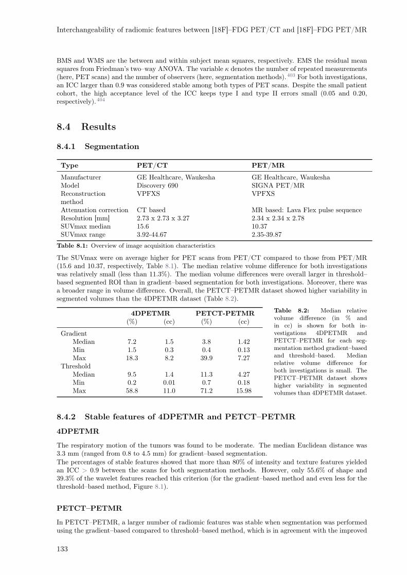
Interchangeability of radiomic features between [18F]–FDG PET/CT and [18F]–FDG PET/MR
BMS and WMS are the between and within subject mean squares, respectively. EMS the residual meansquares from Friedman’s two–way ANOVA. The variable κ denotes the number of repeated measurements(here, PET scans) and the number of observers (here, segmentation methods).403 For both investigations,an ICC larger than 0.9 was considered stable among both types of PET scans. Despite the small patientcohort, the high acceptance level of the ICC keeps type I and type II errors small (0.05 and 0.20,respectively).404
8.4 Results
8.4.1 Segmentation
Type PET/CT PET/MR
Manufacturer GE Healthcare, Waukesha GE Healthcare, WaukeshaModel Discovery 690 SIGNA PET/MRReconstructionmethod
VPFXS VPFXS
Attenuation correction CT based MR based: Lava Flex pulse sequenceResolution [mm] 2.73 x 2.73 x 3.27 2.34 x 2.34 x 2.78SUVmax median 15.6 10.37SUVmax range 3.92-44.67 2.35-39.87
Table 8.1: Overview of image acquisition characteristics
The SUVmax were on average higher for PET scans from PET/CT compared to those from PET/MR(15.6 and 10.37, respectively, Table 8.1). The median relative volume difference for both investigationswas relatively small (less than 11.3%). The median volume differences were overall larger in threshold–based segmented ROI than in gradient–based segmentation for both investigations. Moreover, there wasa broader range in volume difference. Overall, the PETCT–PETMR dataset showed higher variability insegmented volumes than the 4DPETMR dataset (Table 8.2).
4DPETMR PETCT-PETMR(%) (cc) (%) (cc)
GradientMedian 7.2 1.5 3.8 1.42Min 1.5 0.3 0.4 0.13Max 18.3 8.2 39.9 7.27
ThresholdMedian 9.5 1.4 11.3 4.27Min 0.2 0.01 0.7 0.18Max 58.8 11.0 71.2 15.98
Table 8.2: Median relativevolume difference (in % andin cc) is shown for both in-vestigations 4DPETMR andPETCT–PETMR for each seg-mentation method gradient–basedand threshold–based. Medianrelative volume difference forboth investigations is small. ThePETCT–PETMR dataset showshigher variability in segmentedvolumes than 4DPETMR dataset.
8.4.2 Stable features of 4DPETMR and PETCT–PETMR
4DPETMR
The respiratory motion of the tumors was found to be moderate. The median Euclidean distance was3.3 mm (ranged from 0.8 to 4.5 mm) for gradient–based segmentation.The percentages of stable features showed that more than 80% of intensity and texture features yieldedan ICC > 0.9 between the scans for both segmentation methods. However, only 55.6% of shape and39.3% of the wavelet features reached this criterion (for the gradient–based method and even less for thethreshold–based method, Figure 8.1).
PETCT–PETMR
In PETCT–PETMR, a larger number of radiomic features was stable when segmentation was performedusing the gradient–based compared to threshold–based method, which is in agreement with the improved
133
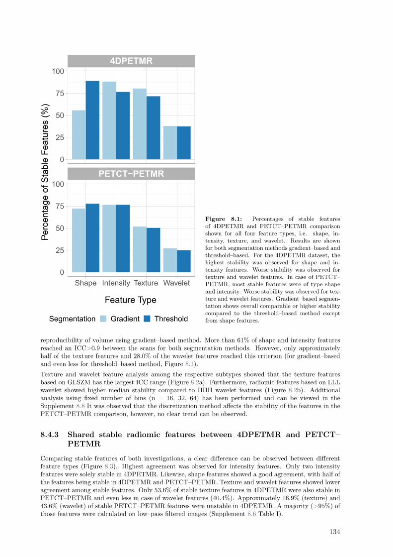
PETCT−PETMR
4DPETMR
Shape Intensity Texture Wavelet
0
25
50
75
100
0
25
50
75
100
Feature Type
Perc
enta
ge o
f S
table
Featu
res (
%)
Segmentation Gradient Threshold
Figure 8.1: Percentages of stable featuresof 4DPETMR and PETCT–PETMR comparisonshown for all four feature types, i.e. shape, in-tensity, texture, and wavelet. Results are shownfor both segmentation methods gradient–based andthreshold–based. For the 4DPETMR dataset, thehighest stability was observed for shape and in-tensity features. Worse stability was observed fortexture and wavelet features. In case of PETCT–PETMR, most stable features were of type shapeand intensity. Worse stability was observed for tex-ture and wavelet features. Gradient–based segmen-tation shows overall comparable or higher stabilitycompared to the threshold–based method exceptfrom shape features.
reproducibility of volume using gradient–based method. More than 61% of shape and intensity featuresreached an ICC>0.9 between the scans for both segmentation methods. However, only approximatelyhalf of the texture features and 28.0% of the wavelet features reached this criterion (for gradient–basedand even less for threshold–based method, Figure 8.1).
Texture and wavelet feature analysis among the respective subtypes showed that the texture featuresbased on GLSZM has the largest ICC range (Figure 8.2a). Furthermore, radiomic features based on LLLwavelet showed higher median stability compared to HHH wavelet features (Figure 8.2b). Additionalanalysis using fixed number of bins (n = 16, 32, 64) has been performed and can be viewed in theSupplement 8.8 It was observed that the discretization method affects the stability of the features in thePETCT–PETMR comparison, however, no clear trend can be observed.
8.4.3 Shared stable radiomic features between 4DPETMR and PETCT–
PETMR
Comparing stable features of both investigations, a clear difference can be observed between differentfeature types (Figure 8.3). Highest agreement was observed for intensity features. Only two intensityfeatures were solely stable in 4DPETMR. Likewise, shape features showed a good agreement, with half ofthe features being stable in 4DPETMR and PETCT–PETMR. Texture and wavelet features showed loweragreement among stable features. Only 53.6% of stable texture features in 4DPETMR were also stable inPETCT–PETMR and even less in case of wavelet features (40.4%). Approximately 16.9% (texture) and43.6% (wavelet) of stable PETCT–PETMR features were unstable in 4DPETMR. A majority (>95%) ofthose features were calculated on low–pass filtered images (Supplement 8.6 Table I).
134
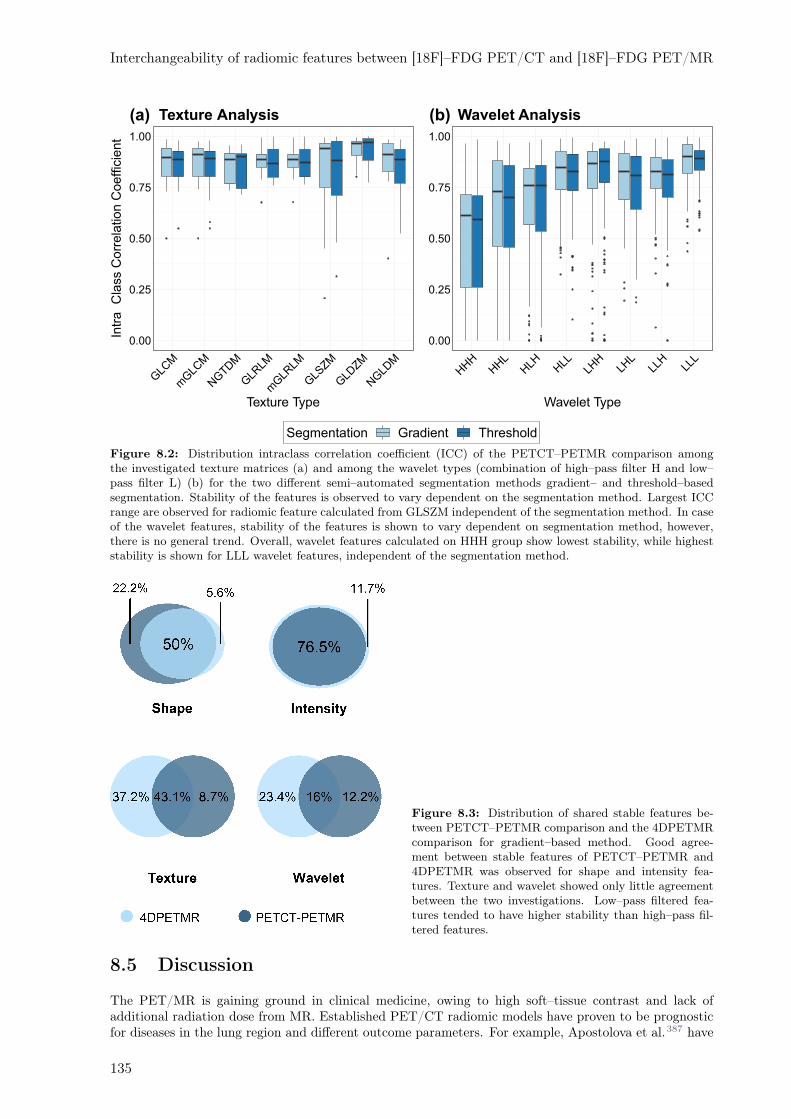
Interchangeability of radiomic features between [18F]–FDG PET/CT and [18F]–FDG PET/MR
Segmentation Gradient Threshold
Texture Analysis(a)
0.00
0.25
0.50
0.75
1.00
Intr
aC
lass C
orr
ela
tion C
oeffic
ient
GLC
M
mGLC
M
NGTD
M
GLR
LM
mGLR
LM
GLS
ZM
GLD
ZM
NGLD
M
Texture Type
(b)
0.00
0.25
0.50
0.75
1.00
HHH
HHL
HLH H
LLLH
HLH
LLL
HLL
L
Wavelet Type
Wavelet Analysis
Figure 8.2: Distribution intraclass correlation coefficient (ICC) of the PETCT–PETMR comparison amongthe investigated texture matrices (a) and among the wavelet types (combination of high–pass filter H and low–pass filter L) (b) for the two different semi–automated segmentation methods gradient– and threshold–basedsegmentation. Stability of the features is observed to vary dependent on the segmentation method. Largest ICCrange are observed for radiomic feature calculated from GLSZM independent of the segmentation method. In caseof the wavelet features, stability of the features is shown to vary dependent on segmentation method, however,there is no general trend. Overall, wavelet features calculated on HHH group show lowest stability, while higheststability is shown for LLL wavelet features, independent of the segmentation method.
Figure 8.3: Distribution of shared stable features be-tween PETCT–PETMR comparison and the 4DPETMRcomparison for gradient–based method. Good agree-ment between stable features of PETCT–PETMR and4DPETMR was observed for shape and intensity fea-tures. Texture and wavelet showed only little agreementbetween the two investigations. Low–pass filtered fea-tures tended to have higher stability than high–pass fil-tered features.
8.5 Discussion
The PET/MR is gaining ground in clinical medicine, owing to high soft–tissue contrast and lack ofadditional radiation dose from MR. Established PET/CT radiomic models have proven to be prognosticfor diseases in the lung region and different outcome parameters. For example, Apostolova et al.387 have
135
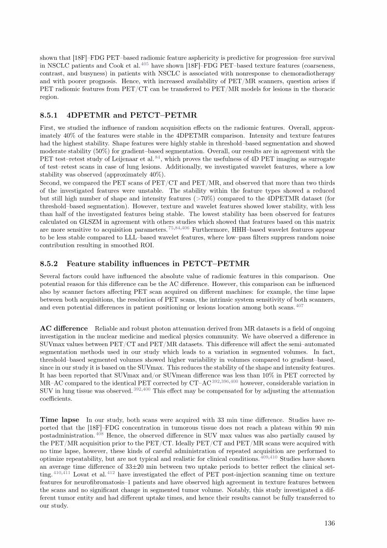
shown that [18F]–FDG PET–based radiomic feature asphericity is predictive for progression–free survivalin NSCLC patients and Cook et al.405 have shown [18F]–FDG PET–based texture features (coarseness,contrast, and busyness) in patients with NSCLC is associated with nonresponse to chemoradiotherapyand with poorer prognosis. Hence, with increased availability of PET/MR scanners, question arises ifPET radiomic features from PET/CT can be transferred to PET/MR models for lesions in the thoracicregion.
8.5.1 4DPETMR and PETCT–PETMR
First, we studied the influence of random acquisition effects on the radiomic features. Overall, approx-imately 40% of the features were stable in the 4DPETMR comparison. Intensity and texture featureshad the highest stability. Shape features were highly stable in threshold–based segmentation and showedmoderate stability (50%) for gradient–based segmentation. Overall, our results are in agreement with thePET test–retest study of Leijenaar et al.84, which proves the usefulness of 4D PET imaging as surrogateof test–retest scans in case of lung lesions. Additionally, we investigated wavelet features, where a lowstability was observed (approximately 40%).
Second, we compared the PET scans of PET/CT and PET/MR, and observed that more than two thirdsof the investigated features were unstable. The stability within the feature types showed a reducedbut still high number of shape and intensity features (>70%) compared to the 4DPETMR dataset (forthreshold–based segmentation). However, texture and wavelet features showed lower stability, with lessthan half of the investigated features being stable. The lowest stability has been observed for featurescalculated on GLSZM in agreement with others studies which showed that features based on this matrixare more sensitive to acquisition parameters.75,84,406 Furthermore, HHH–based wavelet features appearto be less stable compared to LLL–based wavelet features, where low–pass filters suppress random noisecontribution resulting in smoothed ROI.
8.5.2 Feature stability influences in PETCT–PETMR
Several factors could have influenced the absolute value of radiomic features in this comparison. Onepotential reason for this difference can be the AC difference. However, this comparison can be influencedalso by scanner factors affecting PET scan acquired on different machines: for example, the time lapsebetween both acquisitions, the resolution of PET scans, the intrinsic system sensitivity of both scanners,and even potential differences in patient positioning or lesions location among both scans.407
AC difference Reliable and robust photon attenuation derived from MR datasets is a field of ongoinginvestigation in the nuclear medicine and medical physics community. We have observed a difference inSUVmax values between PET/CT and PET/MR datasets. This difference will affect the semi–automatedsegmentation methods used in our study which leads to a variation in segmented volumes. In fact,threshold–based segmented volumes showed higher variability in volumes compared to gradient–based,since in our study it is based on the SUVmax. This reduces the stability of the shape and intensity features.It has been reported that SUVmax and/or SUVmean difference was less than 10% in PET corrected byMR–AC compared to the identical PET corrected by CT–AC392,396,400 however, considerable variation inSUV in lung tissue was observed.392,400 This effect may be compensated for by adjusting the attenuationcoefficients.
Time lapse In our study, both scans were acquired with 33 min time difference. Studies have re-ported that the [18F]–FDG concentration in tumorous tissue does not reach a plateau within 90 minpostadministration.408 Hence, the observed difference in SUV max values was also partially caused bythe PET/MR acquisition prior to the PET/CT. Ideally PET/CT and PET/MR scans were acquired withno time lapse, however, these kinds of careful administration of repeated acquisition are performed tooptimize repeatability, but are not typical and realistic for clinical conditions.409,410 Studies have shownan average time difference of 33±20 min between two uptake periods to better reflect the clinical set-ting.410,411 Lovat et al.412 have investigated the effect of PET post-injection scanning time on texturefeatures for neurofibromatosis–1 patients and have observed high agreement in texture features betweenthe scans and no significant change in segmented tumor volume. Notably, this study investigated a dif-ferent tumor entity and had different uptake times, and hence their results cannot be fully transferred toour study.
136
Interchangeability of radiomic features between [18F]–FDG PET/CT and [18F]–FDG PET/MR
Spatial image resolution Furthermore, variation in SUV can also originate from the differencein spatial image resolution of the compared PET scans. Shafiq-Ul-Hassan et al.35 have shown that 63of 213 investigated shape and first–order radiomics were unstable with varying voxel size. Stability ofthose could be improved using resampling to the same voxel size. To address this uncertainty, the imageswere resampled to the same spatial resolution. However, resampling alters the SUV413 and introducesadditional variation among PET image datasets derived from PET/CT and PET/MR.
Intrinsic scanner sensitivity Moreover, also both scanner types used in our study have a differentsensitivity, as was shown by Zeimpekis et al.414
8.5.3 Comparison of 4DPETMR and PETCT–PETMR
Nevertheless, the intersection of shape and intensity features of 4DPETMR and PETCT–PETMR remainshigh in our study. We have observed 100% agreement for intensity features, indicating that time lapseand AC affected the absolute SUV value but not its distribution within the lesions. Few of the texturewere found to be stable in PETCT–PETMR comparison but not stable in 4DPETMR study. In termsof texture feature types, these features are associated with low gray level–enhanced features, which arelikely to be less sensitive to blurring sourced from the respiratory motion during the long acquisition timein conventional 3D PET images.85
In case of wavelet features, a poor stability was observed for both 4DPETMR and PETCT–PETMR. Forboth investigations, more features were stable in the smoothed images (low–pass filtering) in comparisonto images with emphasized heterogeneity (high–pass filtering) (Supplement 8.6 Table). This may beexplained by the impact of high–pass filters applied on the images, enhancing fast varying gray levels.Similar to texture features, two thirds of the stable wavelet features from the 4DPETMR study wereaffected by the differences in AC, time lapse or resolution differences. One third of wavelet featuresstable in 4DPETMR dataset were also stable in PETCT–PETMR comparison. Approximately 16% ofwavelet features stable in PETCT–PETMR were not stable in the 4DPETMR dataset. Most of themwere wavelet features calculated on low–pass filtered images, which have a reduced noise impact.
8.5.4 Limitations
In our study, we have shown that a high extent of shape and intensity features are stable among PET/CTand PET/MR and can be thus used interchangeably between PET/CT and PET/MR radiomic modelsfor patients with lung lesions. In wavelet and texture features, only a few selected features are stableamong both modalities. However, some limitations of our investigation need to be considered.First, in our study, features calculated on PET scans of (3D) PET/CT and PET/MR were comparedand stable features were set in agreement with a 4D–gated PET/MR phase comparison to account formodality–intrinsic random effects from the image acquisition. Oliver et al.85 have investigated the impactof respiratory motion on the stability of the 3D and 4D imaging radiomic features. They have compared3D and 4D PET shape, intensity and first–order radiomics and they showed that features calculatedon 3D and 4D PET scans differ. Differences were attributed to both ROI motion and count statistics(noise).85 Adams et al.415 investigated the factors affecting SUV measurements. They showed SUV variesup to 30% due to an averaging effect of motion during acquisition in 3D PET which causes blurring inthe images. This results in higher susceptibility of 4D acquisition to noise. Additionally, Oliver et al.85
observed that PET features were more stable compared to CT features when comparing 3D and 4Dacquisition. Conventional PET scans usually have longer acquisition times that can impact the radiomicfeature stability particularly in the lung region, where image acquisition is influenced considerably byrespiratory motion. One main conclusion refers to the reduced stability of CT compared to PET due tothe higher spatial image resolution and therefore higher impact from respiratory motion. This is a riskof using 4D PET acquisition as a surrogate of test–retest study.Second, uptake time correction was shown not capable to fully account for the SUV changes over time.Additionally, we assumed the FDG kinetics to be irreversible. To our knowledge, the impact of FDGkinetics on SUV heterogeneity pattern within the tumor has only been investigated by Lovat et al.412
However, since they investigated a different tumor entity and different uptake times, conclusion drawnfrom their observation are limited. Therefore, further investigations are needed to fully account for thetime lapse observed in our study.Third, partial volume effects are affecting segmenting volumes. Further investigations are needed toexplore the influence of image resampling on the partial volume effect.
137
Fourth, limitation of this study is the small sample size of ten and nine patients for 4DPETMR andPETCT–PETMR dataset, respectively, as well as the small investigated volumes that show to influencethe intratumoral uptake heterogeneity.416,417
Finally, respiratory motion was assumed to be regular, but irregularities can introduce uncertainties infeature stability.
8.5.5 Recommendation
In this work we have shown a majority of radiomic features calculated on PET from PET/CT andPET/MR to be nonstable and hence, these features should not be used for outcome modeling of combinedPET/CT–PET/MR models. Several approaches were investigated to overcome this inherent problem.One approach, used in a majority of radiomics–based models, is to discard all unstable features prior tothe development of outcome models. However, as seen in this work, this results in a major number offeatures to be discarded solely due to their scanner variability, despite their potential prognostic power asbiomarker. Another approach is to postprocess the PET scans to harmonize the variability. For example,effects from different pixel sizes can be addressed using resampling combined with additional low–passfilters.219 However, it has be ensured that the harmonization addresses the scanner and image acquisitionvariability only and preserve the patient variability. In a recent publication, a PET reconstructionharmonization method ComBat, first introduced in genomic studies, was suggested to correct for centervariability.204 They reported for nine investigated features (three SUV based and six texture based)that tissue dependent variability could be preserved and that they could correct for imaging protocoldifferences.204 Nevertheless, as we have shown, uptake time differences in PET acquisition affect thePET scans strongly, which has to be considered for any type (single- or multimodality) of PET models.
8.6 Conclusion
In this study, we have investigated the interchangeability of [18F]–FDG PET/CT–based radiomic featuresto [18F]–FDG PET/MR for lung lesions. Despite differences in imaging techniques and influences on theSUV (time lapse, spatial resolution differences, and motion), there are radiomic features which showedhigh stability. Shape and intensity features were stable between both image modalities. However, onlya few selected texture and wavelet features were stable (51.5% and 28%, respectively). Only a reducednumber of radiomics features can be used when models from PET/CT are transferred to PET/MRor when combined image modality models for lung lesion are determined. A more detailed study toinvestigate impact of time lapse on stability of the features is needed. Additional investigations shouldbe performed to draw conclusion for other entities.
138
Supplement A: Radiomic Features ICC Results
Table 1: The intra-class correlation coefficients (ICC) of the investigated radiomic features in our study. Stablefeatures are shown in bold. Nomenclature according to Zwanenburg et al. (2016) ”Image biomarker standardi-sation initiative.”
Radiomic Feature 4DPETMR PETCT-PETMR
Gradient Threshold Gradient Threshold
Shape Shape volume 1.00 0.95 1.00 0.99
Shape Shape surface 1.00 0.97 0.99 0.99
Shape Shape compactness 1 0.86 0.99 0.90 0.97
Shape Shape compactness 2 0.86 0.99 0.91 0.97
Shape Shape spherical disproportion 0.86 1.00 0.88 0.96
Shape Shape sphericity 0.86 0.99 0.90 0.97
Shape Shape asphericity 0.86 1.00 0.88 0.96
Shape Shape surface to volume ratio 0.99 0.92 0.98 0.98
Shape Shape median thickness 0.99 0.98 0.98 0.99
Shape Shape standard deviation thickness 1.00 0.98 0.99 0.98
Shape Shape euclidian distance 0.99 0.95 0.99 1.00
Shape Shape major axis length 1.00 0.99 1.00 0.99
Shape Shape minor axis length 0.98 0.99 1.00 0.99
Shape Shape least axis length 1.00 0.97 0.99 0.99
Shape Shape elongation 0.89 0.96 0.96 0.86Shape Shape flatness 0.95 0.96 0.87 0.83Shape Shape fractal dimension -0.12 0.73 0.17 0.45Shape Shape center of mass shift 0.86 0.29 0.89 0.70Unfiltered Intensity mean 0.95 0.97 0.93 0.93
Unfiltered Intensity standard deviation 0.96 0.95 0.93 0.93
Unfiltered Intensity coefficient of variation 0.81 0.49 0.89 0.97
Unfiltered Intensity skewness 0.92 0.89 0.98 0.95
Unfiltered Intensity kurtosis 0.95 0.87 0.92 0.85Unfiltered Intensity variance 0.93 0.91 0.81 0.82Unfiltered Intensity median 0.93 0.97 0.93 0.92
Unfiltered Intensity percentile 10th 0.73 0.82 0.82 0.87Unfiltered Intensity percentile 90th 0.97 0.98 0.93 0.93
Unfiltered Intensity interquartile range 0.93 0.94 0.92 0.93
Unfiltered Intensity range 0.99 0.98 0.93 0.91
Unfiltered Intensity mean absolut deviation 0.96 0.95 0.93 0.93
Unfiltered Intensity robust mean absolut deviation 0.94 0.94 0.92 0.93
Unfiltered Intensity energy 0.99 0.98 0.89 0.89Unfiltered Intensity entropy 0.99 0.97 0.98 0.98
Unfiltered Intensity root mean square 0.96 0.97 0.93 0.93
Unfiltered Intensity uniformity 0.98 0.97 0.93 0.92
Unfiltered GLCM energy 0.95 0.95 0.80 0.73Unfiltered GLCM entropy 0.99 0.98 0.98 0.98
Unfiltered GLCM contrast 0.99 0.99 0.81 0.81Unfiltered GLCM correlation 0.55 0.27 0.91 0.86Unfiltered GLCM homogeneity 0.97 0.93 0.95 0.93
Unfiltered GLCM homogeneity normalized 0.88 0.80 0.91 0.91
Unfiltered GLCM inverese difference 0.97 0.95 0.96 0.95
Unfiltered GLCM inverese difference normalized 0.93 0.79 0.94 0.93
Unfiltered GLCM variance 0.94 0.91 0.80 0.82Unfiltered GLCM sum of average 0.97 0.97 0.94 0.91
Unfiltered GLCM sum of entropy 0.99 0.95 0.98 0.98
Unfiltered GLCM sum of variance 0.91 0.83 0.80 0.83Unfiltered GLCM difference entropy 0.99 0.99 0.97 0.97
Unfiltered GLCM difference variance 0.98 0.99 0.80 0.80Continued on next page
1
Table 1 – Continued
Unfiltered GLCM information measures of correlation 1 0.99 0.99 0.73 0.75Unfiltered GLCM information measures of correlation 2 0.95 0.98 0.88 0.94
Unfiltered GLCM maximal correlation coefficient 0.95 0.97 0.81 0.73Unfiltered GLCM joint maximum 0.90 0.90 0.88 0.82Unfiltered GLCM joint average 0.97 0.97 0.94 0.91
Unfiltered GLCM difference average 0.99 0.99 0.92 0.92
Unfiltered GLCM dissimilarity 0.99 0.99 0.92 0.92
Unfiltered GLCM inverse variance 0.98 0.94 0.95 0.95
Unfiltered GLCM autocorrelation 0.94 0.94 0.85 0.78Unfiltered GLCM cluster tendency 0.91 0.83 0.80 0.83Unfiltered GLCM cluster shade 0.96 0.71 0.83 0.78Unfiltered GLCM cluster prominence 0.80 0.63 0.48 0.53Unfiltered m GLCM energy 0.94 0.91 0.74 0.69Unfiltered m GLCM entropy 0.99 0.97 0.98 0.98
Unfiltered m GLCM contrast 0.99 0.99 0.81 0.81Unfiltered m GLCM correlation 0.57 0.24 0.91 0.85Unfiltered m GLCM homogeneity 0.97 0.93 0.95 0.93
Unfiltered m GLCM homogeneity normalized 0.89 0.79 0.91 0.91
Unfiltered m GLCM inverese difference 0.98 0.95 0.96 0.95
Unfiltered m GLCM inverese difference normalized 0.93 0.78 0.94 0.92
Unfiltered m GLCM variance 0.94 0.91 0.80 0.82Unfiltered m GLCM sum of average 0.97 0.97 0.94 0.91
Unfiltered m GLCM sum of entropy 0.98 0.96 0.97 0.98
Unfiltered m GLCM sum of variance 0.91 0.84 0.80 0.83Unfiltered m GLCM difference entropy 0.99 0.99 0.97 0.96
Unfiltered m GLCM difference variance 0.99 0.99 0.80 0.80Unfiltered m GLCM information measures of correlation 1 0.85 0.84 0.74 0.58Unfiltered m GLCM information measures of correlation 2 0.92 0.85 0.93 0.93
Unfiltered m GLCM maximal correlation coefficient 0.76 0.12 0.91 0.88Unfiltered m GLCM joint maximum 0.86 0.45 0.86 0.70Unfiltered m GLCM joint average 0.97 0.97 0.94 0.91
Unfiltered m GLCM difference average 0.99 0.99 0.92 0.92
Unfiltered m GLCM dissimilarity 0.99 0.99 0.92 0.92
Unfiltered m GLCM inverse variance 0.98 0.94 0.95 0.96
Unfiltered m GLCM autocorrelation 0.94 0.94 0.85 0.78Unfiltered m GLCM cluster tendency 0.91 0.84 0.80 0.83Unfiltered m GLCM cluster shade 0.96 0.72 0.83 0.77Unfiltered m GLCM cluster prominence 0.80 0.65 0.49 0.53Unfiltered NGTDM coarseness 0.91 0.91 0.95 0.91
Unfiltered NGTDM contrast 0.99 1.00 0.88 0.90
Unfiltered NGTDM busyness 0.77 0.59 0.92 0.96
Unfiltered NGTDM complexity 0.96 0.92 0.72 0.71Unfiltered NGTDM strength 0.82 0.87 0.77 0.74Unfiltered GRLM grey level non-uniformity 0.99 0.99 0.91 0.88Unfiltered GRLM grey level non-uniformity normalized 0.99 0.98 0.93 0.93
Unfiltered GRLM zone size non-uniformity 0.99 0.95 1.00 1.00
Unfiltered GRLM zone size non-uniformity normalized 0.97 0.94 0.92 0.90
Unfiltered GRLM short runs emphasis 0.98 0.93 0.89 0.87Unfiltered GRLM long runs emphasis 0.99 0.93 0.89 0.78Unfiltered GRLM low grey level run emphasis 0.36 0.80 0.79 0.94
Unfiltered GRLM high grey level run emphasis 0.94 0.95 0.85 0.78Unfiltered GRLM short run low grey level emphasis 0.37 0.81 0.82 0.96
Unfiltered GRLM short run high grey level emphasis 0.94 0.95 0.85 0.77Unfiltered GRLM long run low grey level emphasis 0.64 0.77 0.68 0.84Unfiltered GRLM long run high grey level emphasis 0.95 0.95 0.86 0.79Unfiltered GRLM run percentage 0.98 0.93 0.91 0.87Unfiltered GRLM grey level variance 0.93 0.91 0.80 0.82Unfiltered GRLM run length variance 0.99 0.93 0.89 0.76Unfiltered GRLM run entropy 0.99 0.97 0.98 0.98
Continued on next page
2
Interch
angeab
ilityof
radiom
icfeatu
resbetw
een[18F
]–FD
GP
ET
/CT
and
[18F]–F
DG
PE
T/M
R
8.7
Supple
men
tA
:R
adio
mic
featu
resro
bustn
essIC
Cresu
lts
139
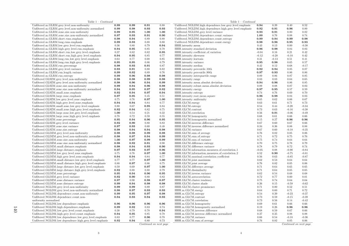
Table 1 – Continued
Unfiltered m GLRM grey level non-uniformity 0.99 0.99 0.91 0.88Unfiltered m GLRM grey level non-uniformity normalized 0.99 0.98 0.93 0.93
Unfiltered m GLRM zone size non-uniformity 0.99 0.95 1.00 1.00
Unfiltered m GLRM zone size non-uniformity normalized 0.97 0.93 0.91 0.90
Unfiltered m GLRM short runs emphasis 0.98 0.94 0.89 0.88Unfiltered m GLRM long runs emphasis 0.99 0.93 0.88 0.80Unfiltered m GLRM low grey level run emphasis 0.36 0.80 0.79 0.94
Unfiltered m GLRM high grey level run emphasis 0.94 0.95 0.85 0.78Unfiltered m GLRM short run low grey level emphasis 0.37 0.82 0.82 0.95
Unfiltered m GLRM short run high grey level emphasis 0.94 0.95 0.85 0.77Unfiltered m GLRM long run low grey level emphasis 0.64 0.77 0.68 0.85Unfiltered m GLRM long run high grey level emphasis 0.95 0.95 0.86 0.79Unfiltered m GLRM run percentage 0.98 0.93 0.91 0.87Unfiltered m GLRM grey level variance 0.93 0.91 0.80 0.82Unfiltered m GLRM run length variance 0.99 0.92 0.89 0.76Unfiltered m GLRM run entropy 0.99 0.96 0.98 0.98
Unfiltered GLSZM grey level non-uniformity 0.98 0.98 0.99 0.98
Unfiltered GLSZM grey level non-uniformity normalized 0.98 0.96 0.94 0.99
Unfiltered GLSZM zone size non-uniformity 0.99 0.94 0.96 0.98
Unfiltered GLSZM zone size non-uniformity normalized 0.94 0.95 0.97 0.92
Unfiltered GLSZM small zone emphasis 0.92 0.94 0.97 0.94
Unfiltered GLSZM large zone emphasis 0.97 0.95 0.45 0.51Unfiltered GLSZM low grey level zone emphasis 0.75 0.76 0.97 1.00
Unfiltered GLSZM high grey level zone emphasis 0.94 0.94 0.84 0.77Unfiltered GLSZM small zone low grey level emphasis 0.80 0.67 0.95 0.84Unfiltered GLSZM small zone high grey level emphasis 0.92 0.94 0.82 0.75Unfiltered GLSZM large zone low grey level emphasis 1.00 0.54 0.21 0.32Unfiltered GLSZM large zone high grey level emphasis 0.78 0.72 0.59 0.55Unfiltered GLSZM zone percentage 0.95 0.94 0.96 0.95
Unfiltered GLSZM grey level variance 0.92 0.90 0.80 0.82Unfiltered GLSZM zone size variance 0.97 0.93 0.60 0.48Unfiltered GLSZM zone size entropy 0.98 0.94 0.94 0.98
Unfiltered GLDZM grey level non-uniformity 0.98 0.98 0.99 0.98
Unfiltered GLDZM grey level non-uniformity normalized 0.98 0.97 0.94 0.99
Unfiltered GLDZM zone size non-uniformity 1.00 0.97 0.99 0.99
Unfiltered GLDZM zone size non-uniformity normalized 0.98 0.92 0.91 0.90Unfiltered GLDZM small distance emphasis 0.98 0.94 0.93 0.90
Unfiltered GLDZM large distance emphasis 0.97 0.93 0.97 0.96
Unfiltered GLDZM low grey level zone emphasis 0.75 0.76 0.97 1.00
Unfiltered GLDZM high grey level zone emphasis 0.94 0.94 0.84 0.77Unfiltered GLDZM small distance low grey level emphasis 0.77 0.77 0.97 1.00
Unfiltered GLDZM small distance high grey level emphasis 0.88 0.97 0.86 0.75Unfiltered GLDZM large distance low grey level emphasis 0.59 0.69 0.97 1.00
Unfiltered GLDZM large distance high grey level emphasis 0.92 0.88 0.80 0.79Unfiltered GLDZM zone percentage 0.95 0.94 0.96 0.95
Unfiltered GLDZM grey level variance 0.92 0.90 0.80 0.82Unfiltered GLDZM zone distance variance 0.97 0.90 0.98 0.97
Unfiltered GLDZM zone distance entropy 0.99 0.94 0.98 0.98
Unfiltered NGLDM grey level non-uniformity 0.99 0.99 0.89 0.87Unfiltered NGLDM grey level non-uniformity normalized 0.98 0.97 0.93 0.93
Unfiltered NGLDM dependence count non-uniformity 0.99 0.95 0.97 0.98
Unfiltered NGLDM dependence count non-uniformity normalized
0.94 0.93 0.94 0.93
Unfiltered NGLDM low dependence emphasis 0.96 0.96 0.96 0.96
Unfiltered NGLDM high dependence emphasis 0.99 0.92 0.83 0.74Unfiltered NGLDM low grey level count emphasis 0.38 0.79 0.78 0.94
Unfiltered NGLDM high grey level count emphasis 0.94 0.95 0.85 0.78Unfiltered NGLDM low dependence low grey level emphasis 0.83 0.77 0.96 0.78Unfiltered NGLDM low dependence high grey level emphasis 0.92 0.94 0.80 0.73
Continued on next page
3
Table 1 – Continued
Unfiltered NGLDM high dependence low grey level emphasis 0.94 0.39 0.40 0.52Unfiltered NGLDM high dependence high grey level emphasis 0.92 0.91 0.96 0.89Unfiltered NGLDM grey level variance 0.93 0.91 0.80 0.82Unfiltered NGLDM dependence count variance 1.00 0.76 0.88 0.74Unfiltered NGLDM dependence count entropy 0.99 0.94 0.99 0.98
Unfiltered NGLDM dependence count energy 0.98 0.96 0.95 0.93
HHH intensity mean 0.43 0.13 0.00 -0.38HHH intensity standard deviation 0.96 0.98 0.84 0.83HHH intensity coefficient of variation -0.04 0.16 0.21 0.42HHH intensity skewness -0.12 -0.20 -0.10 0.42HHH intensity kurtosis 0.31 -0.13 0.51 0.41HHH intensity variance 0.95 0.98 0.65 0.57HHH intensity median 0.42 0.12 0.68 -0.17HHH intensity percentile 10th 0.92 0.94 0.85 0.87HHH intensity percentile 90th 0.97 0.93 0.86 0.86HHH intensity interquartile range 0.89 0.86 0.87 0.85HHH intensity range 0.83 0.83 0.64 0.65HHH intensity mean absolut deviation 0.94 0.96 0.86 0.85HHH intensity robust mean absolut deviation 0.89 0.88 0.87 0.83HHH intensity energy 0.97 0.95 0.57 0.59HHH intensity entropy 0.74 0.76 0.69 0.70HHH intensity root mean square 0.96 0.98 0.84 0.83HHH intensity uniformity 0.65 0.62 0.66 0.67HHH GLCM energy 0.63 0.61 0.71 0.73HHH GLCM entropy 0.54 0.44 -0.20 -0.34HHH GLCM contrast 0.73 0.63 -0.16 -0.38HHH GLCM correlation 0.56 0.91 -0.06 -0.49HHH GLCM homogeneity 0.68 0.61 0.66 0.66HHH GLCM homogeneity normalized 0.15 0.27 0.96 0.96
HHH GLCM inverese difference 0.67 0.60 0.67 0.66HHH GLCM inverese difference normalized 0.34 0.36 0.88 0.88HHH GLCM variance 0.67 0.60 -0.18 -0.35HHH GLCM sum of average 0.76 0.82 0.05 0.06HHH GLCM sum of entropy 0.71 0.72 0.75 0.76HHH GLCM sum of variance 0.75 0.74 0.64 0.64HHH GLCM difference entropy 0.70 0.75 0.78 0.79HHH GLCM difference variance 0.78 0.79 0.72 0.74HHH GLCM information measures of correlation 1 -0.05 0.88 -0.90 -0.84HHH GLCM information measures of correlation 2 0.52 0.90 -0.75 -0.81HHH GLCM maximal correlation coefficient 0.56 0.63 -0.85 -0.87HHH GLCM joint maximum 0.62 0.53 0.64 0.64HHH GLCM joint average 0.76 0.82 0.05 0.06HHH GLCM difference average 0.71 0.64 0.65 0.65HHH GLCM dissimilarity 0.71 0.64 0.65 0.65HHH GLCM inverse variance 0.62 0.54 0.68 0.68HHH GLCM autocorrelation 0.72 0.77 0.00 0.01HHH GLCM cluster tendency 0.75 0.74 0.64 0.64HHH GLCM cluster shade 0.26 0.15 -0.59 -0.62HHH GLCM cluster prominence 0.71 0.80 0.52 0.51HHH m GLCM energy 0.64 0.60 0.71 0.72HHH m GLCM entropy 0.54 0.39 -0.23 -0.37HHH m GLCM contrast 0.73 0.59 -0.15 -0.39HHH m GLCM correlation 0.73 0.56 0.14 -0.42HHH m GLCM homogeneity 0.69 0.61 0.66 0.66HHH m GLCM homogeneity normalized 0.19 0.26 0.96 0.96
HHH m GLCM inverese difference 0.68 0.59 0.67 0.66HHH m GLCM inverese difference normalized 0.37 0.35 0.88 0.88HHH m GLCM variance 0.66 0.54 -0.18 -0.36HHH m GLCM sum of average 0.76 0.82 0.05 0.06
Continued on next page
4
140
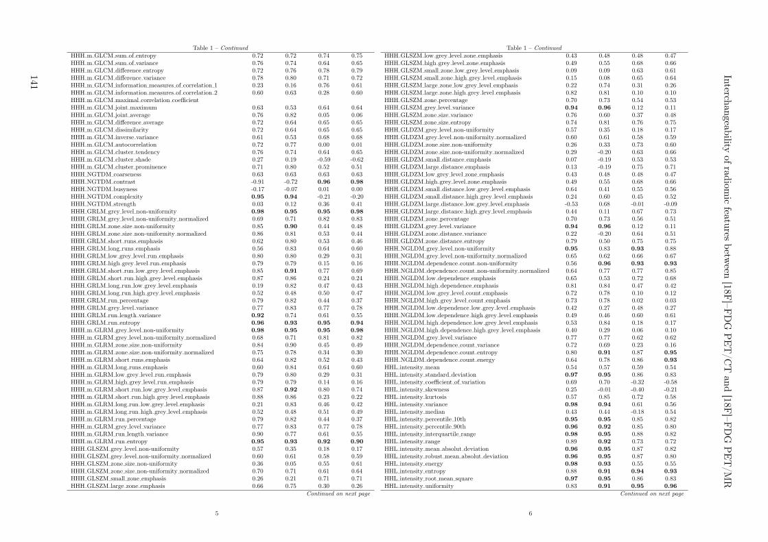
Table 1 – Continued
HHH m GLCM sum of entropy 0.72 0.72 0.74 0.75HHH m GLCM sum of variance 0.76 0.74 0.64 0.65HHH m GLCM difference entropy 0.72 0.76 0.78 0.79HHH m GLCM difference variance 0.78 0.80 0.71 0.72HHH m GLCM information measures of correlation 1 0.23 0.16 0.76 0.61HHH m GLCM information measures of correlation 2 0.60 0.63 0.28 0.60HHH m GLCM maximal correlation coefficientHHH m GLCM joint maximum 0.63 0.53 0.64 0.64HHH m GLCM joint average 0.76 0.82 0.05 0.06HHH m GLCM difference average 0.72 0.64 0.65 0.65HHH m GLCM dissimilarity 0.72 0.64 0.65 0.65HHH m GLCM inverse variance 0.61 0.53 0.68 0.68HHH m GLCM autocorrelation 0.72 0.77 0.00 0.01HHH m GLCM cluster tendency 0.76 0.74 0.64 0.65HHH m GLCM cluster shade 0.27 0.19 -0.59 -0.62HHH m GLCM cluster prominence 0.71 0.80 0.52 0.51HHH NGTDM coarseness 0.63 0.63 0.63 0.63HHH NGTDM contrast -0.91 -0.72 0.96 0.98
HHH NGTDM busyness -0.17 -0.07 0.01 0.00HHH NGTDM complexity 0.95 0.94 -0.21 -0.20HHH NGTDM strength 0.03 0.12 0.36 0.41HHH GRLM grey level non-uniformity 0.98 0.95 0.95 0.98
HHH GRLM grey level non-uniformity normalized 0.69 0.71 0.82 0.83HHH GRLM zone size non-uniformity 0.85 0.90 0.44 0.48HHH GRLM zone size non-uniformity normalized 0.86 0.81 0.53 0.44HHH GRLM short runs emphasis 0.62 0.80 0.53 0.46HHH GRLM long runs emphasis 0.56 0.83 0.64 0.60HHH GRLM low grey level run emphasis 0.80 0.80 0.29 0.31HHH GRLM high grey level run emphasis 0.79 0.79 0.15 0.16HHH GRLM short run low grey level emphasis 0.85 0.91 0.77 0.69HHH GRLM short run high grey level emphasis 0.87 0.86 0.24 0.24HHH GRLM long run low grey level emphasis 0.19 0.82 0.47 0.43HHH GRLM long run high grey level emphasis 0.52 0.48 0.50 0.47HHH GRLM run percentage 0.79 0.82 0.44 0.37HHH GRLM grey level variance 0.77 0.83 0.77 0.78HHH GRLM run length variance 0.92 0.74 0.61 0.55HHH GRLM run entropy 0.96 0.93 0.95 0.94
HHH m GLRM grey level non-uniformity 0.98 0.95 0.95 0.98
HHH m GLRM grey level non-uniformity normalized 0.68 0.71 0.81 0.82HHH m GLRM zone size non-uniformity 0.84 0.90 0.45 0.49HHH m GLRM zone size non-uniformity normalized 0.75 0.78 0.34 0.30HHH m GLRM short runs emphasis 0.64 0.82 0.52 0.43HHH m GLRM long runs emphasis 0.60 0.84 0.64 0.60HHH m GLRM low grey level run emphasis 0.79 0.80 0.29 0.31HHH m GLRM high grey level run emphasis 0.79 0.79 0.14 0.16HHH m GLRM short run low grey level emphasis 0.87 0.92 0.80 0.74HHH m GLRM short run high grey level emphasis 0.88 0.86 0.23 0.22HHH m GLRM long run low grey level emphasis 0.21 0.83 0.46 0.42HHH m GLRM long run high grey level emphasis 0.52 0.48 0.51 0.49HHH m GLRM run percentage 0.79 0.82 0.44 0.37HHH m GLRM grey level variance 0.77 0.83 0.77 0.78HHH m GLRM run length variance 0.90 0.77 0.61 0.55HHH m GLRM run entropy 0.95 0.93 0.92 0.90
HHH GLSZM grey level non-uniformity 0.57 0.35 0.18 0.17HHH GLSZM grey level non-uniformity normalized 0.60 0.61 0.58 0.59HHH GLSZM zone size non-uniformity 0.36 0.05 0.55 0.61HHH GLSZM zone size non-uniformity normalized 0.70 0.71 0.61 0.64HHH GLSZM small zone emphasis 0.26 0.21 0.71 0.71HHH GLSZM large zone emphasis 0.66 0.75 0.30 0.26
Continued on next page
5
Table 1 – Continued
HHH GLSZM low grey level zone emphasis 0.43 0.48 0.48 0.47HHH GLSZM high grey level zone emphasis 0.49 0.55 0.68 0.66HHH GLSZM small zone low grey level emphasis 0.09 0.09 0.63 0.61HHH GLSZM small zone high grey level emphasis 0.15 0.08 0.65 0.64HHH GLSZM large zone low grey level emphasis 0.22 0.74 0.31 0.26HHH GLSZM large zone high grey level emphasis 0.82 0.81 0.10 0.10HHH GLSZM zone percentage 0.70 0.73 0.54 0.53HHH GLSZM grey level variance 0.94 0.96 0.12 0.11HHH GLSZM zone size variance 0.76 0.60 0.37 0.48HHH GLSZM zone size entropy 0.74 0.81 0.76 0.75HHH GLDZM grey level non-uniformity 0.57 0.35 0.18 0.17HHH GLDZM grey level non-uniformity normalized 0.60 0.61 0.58 0.59HHH GLDZM zone size non-uniformity 0.26 0.33 0.73 0.60HHH GLDZM zone size non-uniformity normalized 0.29 -0.20 0.63 0.66HHH GLDZM small distance emphasis 0.07 -0.19 0.53 0.53HHH GLDZM large distance emphasis 0.13 -0.19 0.75 0.71HHH GLDZM low grey level zone emphasis 0.43 0.48 0.48 0.47HHH GLDZM high grey level zone emphasis 0.49 0.55 0.68 0.66HHH GLDZM small distance low grey level emphasis 0.64 0.41 0.55 0.56HHH GLDZM small distance high grey level emphasis 0.24 0.60 0.45 0.52HHH GLDZM large distance low grey level emphasis -0.53 0.68 -0.01 -0.09HHH GLDZM large distance high grey level emphasis 0.44 0.11 0.67 0.73HHH GLDZM zone percentage 0.70 0.73 0.56 0.51HHH GLDZM grey level variance 0.94 0.96 0.12 0.11HHH GLDZM zone distance variance 0.22 -0.20 0.64 0.51HHH GLDZM zone distance entropy 0.79 0.50 0.75 0.75HHH NGLDM grey level non-uniformity 0.95 0.83 0.93 0.88HHH NGLDM grey level non-uniformity normalized 0.65 0.62 0.66 0.67HHH NGLDM dependence count non-uniformity 0.56 0.96 0.93 0.93
HHH NGLDM dependence count non-uniformity normalized 0.64 0.77 0.77 0.85HHH NGLDM low dependence emphasis 0.65 0.53 0.72 0.68HHH NGLDM high dependence emphasis 0.81 0.84 0.47 0.42HHH NGLDM low grey level count emphasis 0.72 0.78 0.10 0.12HHH NGLDM high grey level count emphasis 0.73 0.78 0.02 0.03HHH NGLDM low dependence low grey level emphasis 0.42 0.27 0.48 0.27HHH NGLDM low dependence high grey level emphasis 0.49 0.46 0.60 0.61HHH NGLDM high dependence low grey level emphasis 0.53 0.84 0.18 0.17HHH NGLDM high dependence high grey level emphasis 0.40 0.29 0.06 0.10HHH NGLDM grey level variance 0.77 0.77 0.62 0.62HHH NGLDM dependence count variance 0.72 0.69 0.23 0.16HHH NGLDM dependence count entropy 0.80 0.91 0.87 0.95
HHH NGLDM dependence count energy 0.64 0.78 0.86 0.93
HHL intensity mean 0.54 0.57 0.59 0.54HHL intensity standard deviation 0.97 0.95 0.86 0.83HHL intensity coefficient of variation 0.69 0.70 -0.32 -0.58HHL intensity skewness 0.25 -0.01 -0.40 -0.21HHL intensity kurtosis 0.57 0.85 0.72 0.58HHL intensity variance 0.98 0.94 0.61 0.56HHL intensity median 0.43 0.44 -0.18 0.54HHL intensity percentile 10th 0.95 0.95 0.85 0.82HHL intensity percentile 90th 0.96 0.92 0.85 0.80HHL intensity interquartile range 0.98 0.95 0.88 0.82HHL intensity range 0.89 0.92 0.73 0.72HHL intensity mean absolut deviation 0.96 0.95 0.87 0.82HHL intensity robust mean absolut deviation 0.96 0.95 0.87 0.80HHL intensity energy 0.98 0.93 0.55 0.55HHL intensity entropy 0.88 0.91 0.94 0.93
HHL intensity root mean square 0.97 0.95 0.86 0.83HHL intensity uniformity 0.83 0.91 0.95 0.96
Continued on next page
6
Interch
angeab
ilityof
radiom
icfeatu
resbetw
een[18F
]–FD
GP
ET
/CT
and
[18F]–F
DG
PE
T/M
R
141

Table 1 – Continued
HHL GLCM energy 0.67 0.82 0.93 0.95
HHL GLCM entropy 0.95 0.83 0.82 0.77HHL GLCM contrast 0.96 0.87 0.43 0.35HHL GLCM correlation 0.62 0.67 0.27 -0.03HHL GLCM homogeneity 0.88 0.90 0.94 0.93
HHL GLCM homogeneity normalized 0.02 0.68 0.38 0.49HHL GLCM inverese difference 0.86 0.89 0.94 0.94
HHL GLCM inverese difference normalized 0.42 0.76 0.79 0.85HHL GLCM variance 0.96 0.86 0.44 0.36HHL GLCM sum of average 0.80 0.82 0.67 0.64HHL GLCM sum of entropy 0.81 0.88 0.94 0.94
HHL GLCM sum of variance 0.96 0.86 0.65 0.60HHL GLCM difference entropy 0.77 0.86 0.92 0.92
HHL GLCM difference variance 0.98 0.95 0.66 0.64HHL GLCM information measures of correlation 1 0.97 0.91 0.50 0.46HHL GLCM information measures of correlation 2 0.94 0.93 0.70 0.62HHL GLCM maximal correlation coefficient 0.90 0.90 0.68 0.68HHL GLCM joint maximum 0.83 0.88 0.96 0.96
HHL GLCM joint average 0.80 0.82 0.67 0.64HHL GLCM difference average 0.93 0.91 0.88 0.85HHL GLCM dissimilarity 0.93 0.91 0.88 0.85HHL GLCM inverse variance 0.48 0.74 0.90 0.93
HHL GLCM autocorrelation 0.83 0.82 0.37 0.34HHL GLCM cluster tendency 0.96 0.86 0.65 0.60HHL GLCM cluster shade 0.98 0.46 0.28 0.26HHL GLCM cluster prominence 0.96 0.80 0.18 0.15HHL m GLCM energy 0.62 0.82 0.93 0.95
HHL m GLCM entropy 0.94 0.90 0.90 0.88HHL m GLCM contrast 0.97 0.89 0.53 0.47HHL m GLCM correlation 0.63 0.62 0.46 0.32HHL m GLCM homogeneity 0.86 0.91 0.94 0.93
HHL m GLCM homogeneity normalized -0.08 0.69 0.38 0.51HHL m GLCM inverese difference 0.83 0.90 0.94 0.94
HHL m GLCM inverese difference normalized 0.34 0.77 0.79 0.86HHL m GLCM variance 0.97 0.89 0.54 0.47HHL m GLCM sum of average 0.82 0.82 0.67 0.64HHL m GLCM sum of entropy 0.79 0.89 0.93 0.93
HHL m GLCM sum of variance 0.96 0.91 0.65 0.60HHL m GLCM difference entropy 0.74 0.87 0.92 0.92
HHL m GLCM difference variance 0.97 0.96 0.65 0.63HHL m GLCM information measures of correlation 1 0.55 0.65 -0.61 -0.47HHL m GLCM information measures of correlation 2 0.83 0.74 0.14 0.13HHL m GLCM maximal correlation coefficient 0.65 0.53 -0.10 -0.08HHL m GLCM joint maximum 0.80 0.89 0.96 0.96
HHL m GLCM joint average 0.82 0.82 0.67 0.64HHL m GLCM difference average 0.92 0.92 0.88 0.85HHL m GLCM dissimilarity 0.92 0.92 0.88 0.85HHL m GLCM inverse variance 0.48 0.74 0.90 0.93
HHL m GLCM autocorrelation 0.84 0.84 0.37 0.34HHL m GLCM cluster tendency 0.96 0.91 0.65 0.60HHL m GLCM cluster shade 0.98 1.00 0.27 0.26HHL m GLCM cluster prominence 0.97 0.85 0.18 0.14HHL NGTDM coarseness -0.06 -0.06 0.75 0.75HHL NGTDM contrast 0.67 0.94 0.01 0.25HHL NGTDM busyness -0.07 -0.09 0.05 0.06HHL NGTDM complexity 0.93 0.85 0.23 0.18HHL NGTDM strength 0.83 0.68 0.11 0.37HHL GRLM grey level non-uniformity 0.99 0.94 0.96 0.91
HHL GRLM grey level non-uniformity normalized 0.75 0.88 0.94 0.95
Continued on next page
7
Table 1 – Continued
HHL GRLM zone size non-uniformity 0.99 0.95 0.92 0.93
HHL GRLM zone size non-uniformity normalized 0.90 0.94 0.84 0.78HHL GRLM short runs emphasis 0.58 0.94 0.84 0.84HHL GRLM long runs emphasis 0.70 0.96 0.72 0.72HHL GRLM low grey level run emphasis 0.73 0.76 0.90 0.90HHL GRLM high grey level run emphasis 0.86 0.86 0.39 0.37HHL GRLM short run low grey level emphasis 0.72 0.82 0.80 0.80HHL GRLM short run high grey level emphasis 0.88 0.88 0.38 0.34HHL GRLM long run low grey level emphasis 0.37 0.73 0.67 0.72HHL GRLM long run high grey level emphasis 0.80 0.57 0.44 0.44HHL GRLM run percentage 0.81 0.95 0.83 0.78HHL GRLM grey level variance 0.98 0.93 0.67 0.62HHL GRLM run length variance 0.98 0.95 0.88 0.82HHL GRLM run entropy 0.92 0.93 0.97 0.96
HHL m GLRM grey level non-uniformity 0.99 0.94 0.96 0.91
HHL m GLRM grey level non-uniformity normalized 0.76 0.88 0.94 0.95
HHL m GLRM zone size non-uniformity 0.99 0.95 0.92 0.93
HHL m GLRM zone size non-uniformity normalized 0.86 0.94 0.87 0.82HHL m GLRM short runs emphasis 0.60 0.95 0.83 0.82HHL m GLRM long runs emphasis 0.77 0.96 0.71 0.70HHL m GLRM low grey level run emphasis 0.73 0.76 0.90 0.90HHL m GLRM high grey level run emphasis 0.86 0.86 0.39 0.37HHL m GLRM short run low grey level emphasis 0.74 0.83 0.84 0.84HHL m GLRM short run high grey level emphasis 0.88 0.88 0.38 0.34HHL m GLRM long run low grey level emphasis 0.37 0.70 0.63 0.67HHL m GLRM long run high grey level emphasis 0.81 0.60 0.46 0.45HHL m GLRM run percentage 0.81 0.95 0.83 0.78HHL m GLRM grey level variance 0.98 0.93 0.67 0.62HHL m GLRM run length variance 0.97 0.95 0.86 0.79HHL m GLRM run entropy 0.91 0.94 0.97 0.95
HHL GLSZM grey level non-uniformity 0.86 0.77 0.82 0.85HHL GLSZM grey level non-uniformity normalized 0.39 0.47 0.88 0.83HHL GLSZM zone size non-uniformity 0.93 0.87 0.58 0.57HHL GLSZM zone size non-uniformity normalized 0.37 0.23 0.74 0.84HHL GLSZM small zone emphasis 0.53 0.23 0.71 0.83HHL GLSZM large zone emphasis 0.73 0.28 0.32 0.35HHL GLSZM low grey level zone emphasis 0.53 0.55 0.77 0.79HHL GLSZM high grey level zone emphasis 0.87 0.90 0.40 0.37HHL GLSZM small zone low grey level emphasis 0.42 0.25 0.01 0.11HHL GLSZM small zone high grey level emphasis 0.74 0.72 0.36 0.30HHL GLSZM large zone low grey level emphasis 0.09 0.06 0.08 0.09HHL GLSZM large zone high grey level emphasis 0.97 0.88 0.83 0.87HHL GLSZM zone percentage 0.90 0.82 0.65 0.49HHL GLSZM grey level variance 0.81 0.88 0.70 0.70HHL GLSZM zone size variance 0.95 0.86 0.47 0.48HHL GLSZM zone size entropy 0.71 0.74 0.94 0.94
HHL GLDZM grey level non-uniformity 0.86 0.77 0.82 0.85HHL GLDZM grey level non-uniformity normalized 0.39 0.47 0.88 0.83HHL GLDZM zone size non-uniformity 0.79 0.92 0.91 0.83HHL GLDZM zone size non-uniformity normalized 0.52 0.75 0.73 0.64HHL GLDZM small distance emphasis 0.54 0.81 0.77 0.60HHL GLDZM large distance emphasis 0.51 0.81 0.63 0.38HHL GLDZM low grey level zone emphasis 0.53 0.55 0.77 0.79HHL GLDZM high grey level zone emphasis 0.87 0.90 0.40 0.37HHL GLDZM small distance low grey level emphasis 0.62 0.56 0.87 0.90HHL GLDZM small distance high grey level emphasis 0.70 0.90 0.47 0.44HHL GLDZM large distance low grey level emphasis 0.19 0.48 -0.17 -0.25HHL GLDZM large distance high grey level emphasis 0.53 0.88 0.22 0.25HHL GLDZM zone percentage 0.91 0.82 0.64 0.49
Continued on next page
8
142

Table 1 – Continued
HHL GLDZM grey level variance 0.81 0.88 0.70 0.70HHL GLDZM zone distance variance 0.39 0.75 0.47 0.22HHL GLDZM zone distance entropy 0.74 0.73 0.87 0.86HHL NGLDM grey level non-uniformity 1.00 0.95 0.95 0.89HHL NGLDM grey level non-uniformity normalized 0.83 0.91 0.95 0.96
HHL NGLDM dependence count non-uniformity 0.98 0.93 0.96 0.93
HHL NGLDM dependence count non-uniformity normalized 0.74 0.97 0.88 0.76HHL NGLDM low dependence emphasis 0.91 0.59 0.79 0.70HHL NGLDM high dependence emphasis 0.77 0.97 0.79 0.75HHL NGLDM low grey level count emphasis 0.70 0.69 0.84 0.84HHL NGLDM high grey level count emphasis 0.87 0.86 0.39 0.36HHL NGLDM low dependence low grey level emphasis 0.50 0.44 -0.06 0.16HHL NGLDM low dependence high grey level emphasis 0.87 0.59 0.21 0.17HHL NGLDM high dependence low grey level emphasis 0.41 0.69 0.67 0.66HHL NGLDM high dependence high grey level emphasis 0.77 0.45 0.52 0.51HHL NGLDM grey level variance 0.99 0.93 0.65 0.58HHL NGLDM dependence count variance 0.96 0.90 0.84 0.60HHL NGLDM dependence count entropy 0.93 0.98 0.98 0.96
HHL NGLDM dependence count energy 0.77 1.00 0.97 0.96
HLH intensity mean 0.66 -0.03 0.17 0.24HLH intensity standard deviation 0.89 0.84 0.91 0.90HLH intensity coefficient of variation 0.14 0.00 -0.07 0.02HLH intensity skewness 0.43 0.72 0.36 0.36HLH intensity kurtosis 0.74 0.81 0.34 0.35HLH intensity variance 0.86 0.83 0.79 0.76HLH intensity median -0.02 0.10 0.52 -0.00HLH intensity percentile 10th 0.88 0.84 0.89 0.88HLH intensity percentile 90th 0.82 0.82 0.91 0.89HLH intensity interquartile range 0.75 0.64 0.93 0.92
HLH intensity range 0.95 0.91 0.83 0.83HLH intensity mean absolut deviation 0.85 0.80 0.91 0.91
HLH intensity robust mean absolut deviation 0.86 0.78 0.92 0.91
HLH intensity energy 0.98 0.98 0.68 0.69HLH intensity entropy 0.88 0.82 0.89 0.90
HLH intensity root mean square 0.89 0.84 0.91 0.90HLH intensity uniformity 0.81 0.73 0.80 0.83HLH GLCM energy 0.81 0.81 0.74 0.77HLH GLCM entropy 0.92 0.80 0.78 0.75HLH GLCM contrast 0.89 0.75 0.58 0.51HLH GLCM correlation 0.82 0.96 0.12 -0.02HLH GLCM homogeneity 0.87 0.79 0.85 0.88HLH GLCM homogeneity normalized 0.55 0.17 0.03 -0.02HLH GLCM inverese difference 0.85 0.78 0.83 0.86HLH GLCM inverese difference normalized 0.61 0.44 0.38 0.37HLH GLCM variance 0.89 0.77 0.58 0.51HLH GLCM sum of average 0.85 0.83 0.83 0.83HLH GLCM sum of entropy 0.89 0.90 0.86 0.89HLH GLCM sum of variance 0.92 0.86 0.79 0.77HLH GLCM difference entropy 0.85 0.88 0.89 0.90
HLH GLCM difference variance 0.95 0.91 0.82 0.81HLH GLCM information measures of correlation 1 0.85 0.87 0.54 0.60HLH GLCM information measures of correlation 2 0.86 0.72 0.68 0.69HLH GLCM maximal correlation coefficient 0.73 0.68 0.43 0.47HLH GLCM joint maximum 0.79 0.74 0.73 0.77HLH GLCM joint average 0.85 0.83 0.83 0.83HLH GLCM difference average 0.89 0.81 0.87 0.88HLH GLCM dissimilarity 0.89 0.81 0.87 0.88HLH GLCM inverse variance 0.53 0.65 0.57 0.60HLH GLCM autocorrelation 0.75 0.74 0.65 0.65
Continued on next page
9
Table 1 – Continued
HLH GLCM cluster tendency 0.92 0.86 0.79 0.77HLH GLCM cluster shade 0.54 0.74 0.31 0.30HLH GLCM cluster prominence 0.81 0.79 0.36 0.31HLH m GLCM energy 0.64 0.67 0.73 0.76HLH m GLCM entropy 0.91 0.76 0.82 0.85HLH m GLCM contrast 0.89 0.75 0.70 0.66HLH m GLCM correlation 0.62 0.96 0.52 0.47HLH m GLCM homogeneity 0.80 0.76 0.85 0.87HLH m GLCM homogeneity normalized 0.29 0.11 0.04 -0.02HLH m GLCM inverese difference 0.77 0.74 0.83 0.86HLH m GLCM inverese difference normalized 0.34 0.37 0.38 0.36HLH m GLCM variance 0.89 0.77 0.70 0.66HLH m GLCM sum of average 0.87 0.83 0.83 0.83HLH m GLCM sum of entropy 0.80 0.79 0.86 0.88HLH m GLCM sum of variance 0.92 0.84 0.79 0.77HLH m GLCM difference entropy 0.76 0.80 0.88 0.90HLH m GLCM difference variance 0.94 0.89 0.82 0.80HLH m GLCM information measures of correlation 1 0.80 0.76 0.51 0.47HLH m GLCM information measures of correlation 2 0.89 0.85 0.67 0.74HLH m GLCM maximal correlation coefficient 0.89 0.89 0.54 0.57HLH m GLCM joint maximum 0.70 0.66 0.73 0.76HLH m GLCM joint average 0.87 0.83 0.83 0.83HLH m GLCM difference average 0.85 0.79 0.87 0.87HLH m GLCM dissimilarity 0.85 0.79 0.87 0.87HLH m GLCM inverse variance 0.52 0.58 0.56 0.59HLH m GLCM autocorrelation 0.78 0.74 0.65 0.65HLH m GLCM cluster tendency 0.92 0.84 0.79 0.77HLH m GLCM cluster shade 0.65 0.69 0.30 0.29HLH m GLCM cluster prominence 0.83 0.79 0.36 0.31HLH NGTDM coarseness -0.06 -0.06 0.75 0.75HLH NGTDM contrast 0.52 0.17 -0.45 -0.67HLH NGTDM busyness 0.20 0.17 0.00 -0.00HLH NGTDM complexity 0.76 0.77 0.29 0.28HLH NGTDM strength 0.90 0.47 0.22 0.12HLH GRLM grey level non-uniformity 0.99 0.93 0.96 0.92
HLH GRLM grey level non-uniformity normalized 0.80 0.73 0.83 0.84HLH GRLM zone size non-uniformity 0.97 0.96 0.93 0.95
HLH GRLM zone size non-uniformity normalized 0.82 0.83 0.59 0.65HLH GRLM short runs emphasis 0.77 0.71 0.61 0.67HLH GRLM long runs emphasis 0.83 0.68 0.41 0.52HLH GRLM low grey level run emphasis 0.95 0.93 0.93 0.93
HLH GRLM high grey level run emphasis 0.80 0.76 0.66 0.66HLH GRLM short run low grey level emphasis 0.95 0.93 0.75 0.81HLH GRLM short run high grey level emphasis 0.78 0.74 0.64 0.63HLH GRLM long run low grey level emphasis 0.85 0.88 0.68 0.72HLH GRLM long run high grey level emphasis 0.91 0.86 0.77 0.78HLH GRLM run percentage 0.83 0.74 0.52 0.58HLH GRLM grey level variance 0.95 0.89 0.83 0.80HLH GRLM run length variance 0.90 0.73 0.51 0.47HLH GRLM run entropy 0.89 0.92 0.97 0.97
HLH m GLRM grey level non-uniformity 0.99 0.93 0.96 0.92
HLH m GLRM grey level non-uniformity normalized 0.80 0.73 0.83 0.84HLH m GLRM zone size non-uniformity 0.97 0.96 0.93 0.95
HLH m GLRM zone size non-uniformity normalized 0.83 0.77 0.66 0.69HLH m GLRM short runs emphasis 0.80 0.73 0.57 0.65HLH m GLRM long runs emphasis 0.86 0.73 0.34 0.49HLH m GLRM low grey level run emphasis 0.95 0.93 0.93 0.93
HLH m GLRM high grey level run emphasis 0.80 0.76 0.66 0.66HLH m GLRM short run low grey level emphasis 0.94 0.93 0.80 0.85
Continued on next page
10
Interch
angeab
ilityof
radiom
icfeatu
resbetw
een[18F
]–FD
GP
ET
/CT
and
[18F]–F
DG
PE
T/M
R
143

Table 1 – Continued
HLH m GLRM short run high grey level emphasis 0.78 0.74 0.64 0.63HLH m GLRM long run low grey level emphasis 0.88 0.90 0.67 0.72HLH m GLRM long run high grey level emphasis 0.91 0.86 0.77 0.78HLH m GLRM run percentage 0.83 0.74 0.52 0.59HLH m GLRM grey level variance 0.95 0.89 0.83 0.80HLH m GLRM run length variance 0.90 0.72 0.38 0.40HLH m GLRM run entropy 0.90 0.91 0.97 0.96
HLH GLSZM grey level non-uniformity 0.98 0.95 0.76 0.81HLH GLSZM grey level non-uniformity normalized 0.61 0.53 0.88 0.89HLH GLSZM zone size non-uniformity 0.96 0.93 0.56 0.54HLH GLSZM zone size non-uniformity normalized 0.47 0.34 0.83 0.74HLH GLSZM small zone emphasis 0.68 0.46 0.59 0.64HLH GLSZM large zone emphasis 0.97 0.73 0.12 0.10HLH GLSZM low grey level zone emphasis 0.58 0.62 0.93 0.88HLH GLSZM high grey level zone emphasis 0.89 0.83 0.79 0.78HLH GLSZM small zone low grey level emphasis 0.21 0.60 0.12 0.09HLH GLSZM small zone high grey level emphasis 0.86 0.81 0.78 0.79HLH GLSZM large zone low grey level emphasis 0.88 0.79 0.03 0.02HLH GLSZM large zone high grey level emphasis 0.92 0.71 0.38 0.33HLH GLSZM zone percentage 0.82 0.86 0.57 0.41HLH GLSZM grey level variance 0.96 0.92 0.82 0.82HLH GLSZM zone size variance 0.97 0.97 0.85 0.73HLH GLSZM zone size entropy 0.91 0.88 0.88 0.87HLH GLDZM grey level non-uniformity 0.98 0.95 0.76 0.81HLH GLDZM grey level non-uniformity normalized 0.61 0.53 0.88 0.89HLH GLDZM zone size non-uniformity 0.94 0.94 0.75 0.61HLH GLDZM zone size non-uniformity normalized 0.52 -0.14 0.77 0.79HLH GLDZM small distance emphasis 0.51 -0.18 0.73 0.74HLH GLDZM large distance emphasis 0.42 -0.11 0.74 0.58HLH GLDZM low grey level zone emphasis 0.57 0.62 0.93 0.88HLH GLDZM high grey level zone emphasis 0.89 0.83 0.79 0.78HLH GLDZM small distance low grey level emphasis 0.62 0.62 0.94 0.90HLH GLDZM small distance high grey level emphasis 0.91 0.82 0.81 0.78HLH GLDZM large distance low grey level emphasis 0.56 0.57 0.33 0.41HLH GLDZM large distance high grey level emphasis 0.82 0.65 0.67 0.72HLH GLDZM zone percentage 0.82 0.86 0.58 0.40HLH GLDZM grey level variance 0.96 0.92 0.82 0.82HLH GLDZM zone distance variance 0.38 0.01 0.66 0.53HLH GLDZM zone distance entropy 0.90 0.80 0.91 0.91
HLH NGLDM grey level non-uniformity 0.98 0.91 0.95 0.89HLH NGLDM grey level non-uniformity normalized 0.81 0.73 0.80 0.83HLH NGLDM dependence count non-uniformity 0.94 0.93 0.86 0.89HLH NGLDM dependence count non-uniformity normalized 0.82 0.82 0.65 0.55HLH NGLDM low dependence emphasis 0.73 0.84 0.81 0.69HLH NGLDM high dependence emphasis 0.81 0.71 0.39 0.51HLH NGLDM low grey level count emphasis 0.95 0.95 0.92 0.92
HLH NGLDM high grey level count emphasis 0.79 0.75 0.66 0.65HLH NGLDM low dependence low grey level emphasis 0.50 0.68 0.07 -0.04HLH NGLDM low dependence high grey level emphasis 0.81 0.73 0.52 0.45HLH NGLDM high dependence low grey level emphasis 0.82 0.88 0.66 0.69HLH NGLDM high dependence high grey level emphasis 0.88 0.87 0.82 0.85HLH NGLDM grey level variance 0.92 0.85 0.79 0.77HLH NGLDM dependence count variance 0.71 0.34 0.08 0.03HLH NGLDM dependence count entropy 0.96 0.90 0.97 0.98
HLH NGLDM dependence count energy 0.87 0.74 0.96 0.97
HLL intensity mean 0.62 0.67 0.71 0.78HLL intensity standard deviation 0.91 0.96 0.93 0.92
HLL intensity coefficient of variation 0.66 0.24 0.79 0.58HLL intensity skewness 0.66 0.82 0.91 0.89
Continued on next page
11
Table 1 – Continued
HLL intensity kurtosis 0.63 0.89 0.93 0.87HLL intensity variance 0.87 0.98 0.82 0.77HLL intensity median 0.89 0.21 0.44 0.06HLL intensity percentile 10th 0.76 0.89 0.91 0.90HLL intensity percentile 90th 0.93 0.95 0.94 0.91
HLL intensity interquartile range 0.89 0.93 0.94 0.89HLL intensity range 0.96 0.98 0.91 0.90HLL intensity mean absolut deviation 0.89 0.96 0.93 0.91
HLL intensity robust mean absolut deviation 0.85 0.95 0.93 0.88HLL intensity energy 0.97 0.99 0.75 0.75HLL intensity entropy 0.94 0.92 0.97 0.97
HLL intensity root mean square 0.90 0.95 0.93 0.91
HLL intensity uniformity 0.89 0.89 0.92 0.94
HLL GLCM energy 0.88 0.80 0.88 0.89HLL GLCM entropy 0.97 0.96 0.97 0.97
HLL GLCM contrast 0.98 0.96 0.80 0.76HLL GLCM correlation 0.85 0.87 0.47 0.31HLL GLCM homogeneity 0.94 0.95 0.94 0.93
HLL GLCM homogeneity normalized 0.76 0.86 0.71 0.71HLL GLCM inverese difference 0.96 0.95 0.94 0.93
HLL GLCM inverese difference normalized 0.86 0.88 0.60 0.49HLL GLCM variance 0.97 0.99 0.81 0.77HLL GLCM sum of average 0.94 0.98 0.90 0.90HLL GLCM sum of entropy 0.98 0.95 0.97 0.97
HLL GLCM sum of variance 0.96 0.98 0.81 0.78HLL GLCM difference entropy 0.96 0.90 0.96 0.96
HLL GLCM difference variance 0.96 0.97 0.81 0.78HLL GLCM information measures of correlation 1 0.96 0.98 0.86 0.79HLL GLCM information measures of correlation 2 0.96 0.95 0.89 0.91
HLL GLCM maximal correlation coefficient 0.95 0.96 0.93 0.90HLL GLCM joint maximum 0.83 0.80 0.79 0.82HLL GLCM joint average 0.94 0.98 0.90 0.90HLL GLCM difference average 0.98 0.96 0.92 0.90HLL GLCM dissimilarity 0.98 0.96 0.92 0.90HLL GLCM inverse variance 0.75 0.88 0.84 0.85HLL GLCM autocorrelation 0.87 0.98 0.71 0.72HLL GLCM cluster tendency 0.96 0.98 0.81 0.78HLL GLCM cluster shade 0.80 0.93 0.61 0.63HLL GLCM cluster prominence 0.93 0.99 0.46 0.41HLL m GLCM energy 0.86 0.87 0.85 0.89HLL m GLCM entropy 0.97 0.95 0.97 0.96
HLL m GLCM contrast 0.94 0.96 0.80 0.76HLL m GLCM correlation 0.74 0.83 0.51 0.36HLL m GLCM homogeneity 0.91 0.96 0.94 0.93
HLL m GLCM homogeneity normalized 0.81 0.86 0.71 0.72HLL m GLCM inverese difference 0.92 0.96 0.95 0.93
HLL m GLCM inverese difference normalized 0.86 0.88 0.58 0.50HLL m GLCM variance 0.96 0.98 0.81 0.77HLL m GLCM sum of average 0.93 0.99 0.90 0.90HLL m GLCM sum of entropy 0.98 0.97 0.97 0.97
HLL m GLCM sum of variance 0.96 0.98 0.81 0.78HLL m GLCM difference entropy 0.96 0.96 0.96 0.95
HLL m GLCM difference variance 0.94 0.98 0.81 0.78HLL m GLCM information measures of correlation 1 0.23 0.59 0.91 0.63HLL m GLCM information measures of correlation 2 0.47 0.75 0.94 0.92
HLL m GLCM maximal correlation coefficient 0.10 0.37 0.95 0.88HLL m GLCM joint maximum 0.77 0.69 0.69 0.76HLL m GLCM joint average 0.93 0.99 0.90 0.90HLL m GLCM difference average 0.93 0.96 0.92 0.90
Continued on next page
12
144
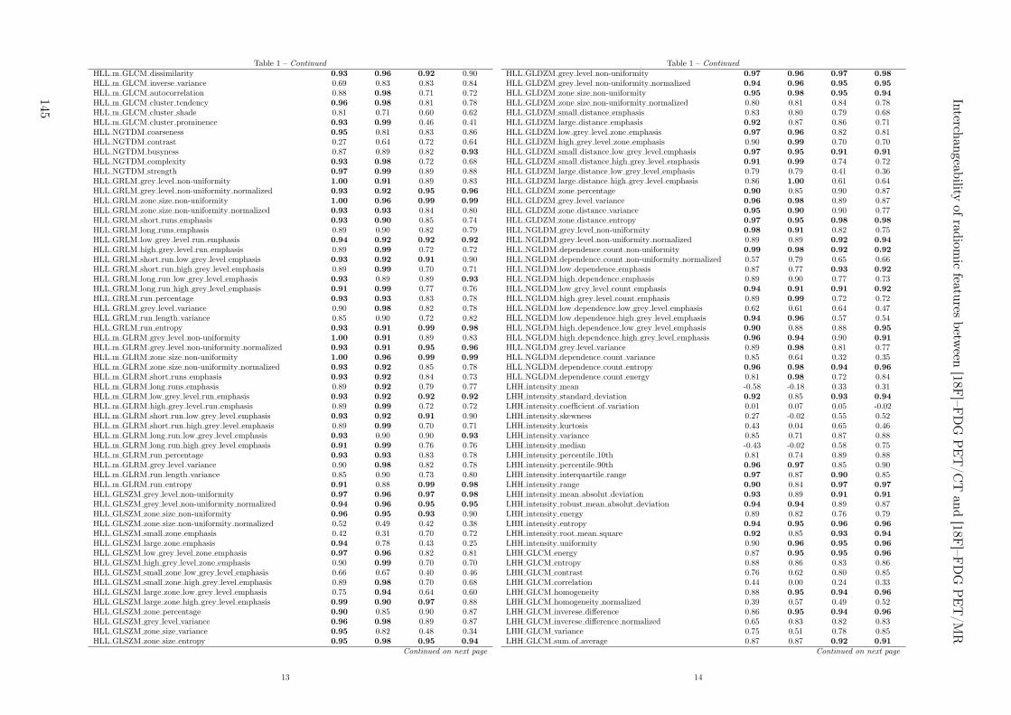
Table 1 – Continued
HLL m GLCM dissimilarity 0.93 0.96 0.92 0.90HLL m GLCM inverse variance 0.69 0.83 0.83 0.84HLL m GLCM autocorrelation 0.88 0.98 0.71 0.72HLL m GLCM cluster tendency 0.96 0.98 0.81 0.78HLL m GLCM cluster shade 0.81 0.71 0.60 0.62HLL m GLCM cluster prominence 0.93 0.99 0.46 0.41HLL NGTDM coarseness 0.95 0.81 0.83 0.86HLL NGTDM contrast 0.27 0.64 0.72 0.64HLL NGTDM busyness 0.87 0.89 0.82 0.93
HLL NGTDM complexity 0.93 0.98 0.72 0.68HLL NGTDM strength 0.97 0.99 0.89 0.88HLL GRLM grey level non-uniformity 1.00 0.91 0.89 0.83HLL GRLM grey level non-uniformity normalized 0.93 0.92 0.95 0.96
HLL GRLM zone size non-uniformity 1.00 0.96 0.99 0.99
HLL GRLM zone size non-uniformity normalized 0.93 0.93 0.84 0.80HLL GRLM short runs emphasis 0.93 0.90 0.85 0.74HLL GRLM long runs emphasis 0.89 0.90 0.82 0.79HLL GRLM low grey level run emphasis 0.94 0.92 0.92 0.92
HLL GRLM high grey level run emphasis 0.89 0.99 0.72 0.72HLL GRLM short run low grey level emphasis 0.93 0.92 0.91 0.90HLL GRLM short run high grey level emphasis 0.89 0.99 0.70 0.71HLL GRLM long run low grey level emphasis 0.93 0.89 0.89 0.93
HLL GRLM long run high grey level emphasis 0.91 0.99 0.77 0.76HLL GRLM run percentage 0.93 0.93 0.83 0.78HLL GRLM grey level variance 0.90 0.98 0.82 0.78HLL GRLM run length variance 0.85 0.90 0.72 0.82HLL GRLM run entropy 0.93 0.91 0.99 0.98
HLL m GLRM grey level non-uniformity 1.00 0.91 0.89 0.83HLL m GLRM grey level non-uniformity normalized 0.93 0.91 0.95 0.96
HLL m GLRM zone size non-uniformity 1.00 0.96 0.99 0.99
HLL m GLRM zone size non-uniformity normalized 0.93 0.92 0.85 0.78HLL m GLRM short runs emphasis 0.93 0.92 0.84 0.73HLL m GLRM long runs emphasis 0.89 0.92 0.79 0.77HLL m GLRM low grey level run emphasis 0.93 0.92 0.92 0.92
HLL m GLRM high grey level run emphasis 0.89 0.99 0.72 0.72HLL m GLRM short run low grey level emphasis 0.93 0.92 0.91 0.90HLL m GLRM short run high grey level emphasis 0.89 0.99 0.70 0.71HLL m GLRM long run low grey level emphasis 0.93 0.90 0.90 0.93
HLL m GLRM long run high grey level emphasis 0.91 0.99 0.76 0.76HLL m GLRM run percentage 0.93 0.93 0.83 0.78HLL m GLRM grey level variance 0.90 0.98 0.82 0.78HLL m GLRM run length variance 0.85 0.90 0.73 0.80HLL m GLRM run entropy 0.91 0.88 0.99 0.98
HLL GLSZM grey level non-uniformity 0.97 0.96 0.97 0.98
HLL GLSZM grey level non-uniformity normalized 0.94 0.96 0.95 0.95
HLL GLSZM zone size non-uniformity 0.96 0.95 0.93 0.90HLL GLSZM zone size non-uniformity normalized 0.52 0.49 0.42 0.38HLL GLSZM small zone emphasis 0.42 0.31 0.70 0.72HLL GLSZM large zone emphasis 0.94 0.78 0.43 0.25HLL GLSZM low grey level zone emphasis 0.97 0.96 0.82 0.81HLL GLSZM high grey level zone emphasis 0.90 0.99 0.70 0.70HLL GLSZM small zone low grey level emphasis 0.66 0.67 0.40 0.46HLL GLSZM small zone high grey level emphasis 0.89 0.98 0.70 0.68HLL GLSZM large zone low grey level emphasis 0.75 0.94 0.64 0.60HLL GLSZM large zone high grey level emphasis 0.99 0.90 0.97 0.88HLL GLSZM zone percentage 0.90 0.85 0.90 0.87HLL GLSZM grey level variance 0.96 0.98 0.89 0.87HLL GLSZM zone size variance 0.95 0.82 0.48 0.34HLL GLSZM zone size entropy 0.95 0.98 0.95 0.94
Continued on next page
13
Table 1 – Continued
HLL GLDZM grey level non-uniformity 0.97 0.96 0.97 0.98
HLL GLDZM grey level non-uniformity normalized 0.94 0.96 0.95 0.95
HLL GLDZM zone size non-uniformity 0.95 0.98 0.95 0.94
HLL GLDZM zone size non-uniformity normalized 0.80 0.81 0.84 0.78HLL GLDZM small distance emphasis 0.83 0.80 0.79 0.68HLL GLDZM large distance emphasis 0.92 0.87 0.86 0.71HLL GLDZM low grey level zone emphasis 0.97 0.96 0.82 0.81HLL GLDZM high grey level zone emphasis 0.90 0.99 0.70 0.70HLL GLDZM small distance low grey level emphasis 0.97 0.95 0.91 0.91
HLL GLDZM small distance high grey level emphasis 0.91 0.99 0.74 0.72HLL GLDZM large distance low grey level emphasis 0.79 0.79 0.41 0.36HLL GLDZM large distance high grey level emphasis 0.86 1.00 0.61 0.64HLL GLDZM zone percentage 0.90 0.85 0.90 0.87HLL GLDZM grey level variance 0.96 0.98 0.89 0.87HLL GLDZM zone distance variance 0.95 0.90 0.90 0.77HLL GLDZM zone distance entropy 0.97 0.95 0.98 0.98
HLL NGLDM grey level non-uniformity 0.98 0.91 0.82 0.75HLL NGLDM grey level non-uniformity normalized 0.89 0.89 0.92 0.94
HLL NGLDM dependence count non-uniformity 0.99 0.98 0.92 0.92
HLL NGLDM dependence count non-uniformity normalized 0.57 0.79 0.65 0.66HLL NGLDM low dependence emphasis 0.87 0.77 0.93 0.92
HLL NGLDM high dependence emphasis 0.89 0.90 0.77 0.73HLL NGLDM low grey level count emphasis 0.94 0.91 0.91 0.92
HLL NGLDM high grey level count emphasis 0.89 0.99 0.72 0.72HLL NGLDM low dependence low grey level emphasis 0.62 0.61 0.64 0.47HLL NGLDM low dependence high grey level emphasis 0.94 0.96 0.57 0.54HLL NGLDM high dependence low grey level emphasis 0.90 0.88 0.88 0.95
HLL NGLDM high dependence high grey level emphasis 0.96 0.94 0.90 0.91
HLL NGLDM grey level variance 0.89 0.98 0.81 0.77HLL NGLDM dependence count variance 0.85 0.64 0.32 0.35HLL NGLDM dependence count entropy 0.96 0.98 0.94 0.96
HLL NGLDM dependence count energy 0.81 0.98 0.72 0.84LHH intensity mean -0.58 -0.18 0.33 0.31LHH intensity standard deviation 0.92 0.85 0.93 0.94
LHH intensity coefficient of variation 0.01 0.07 0.05 -0.02LHH intensity skewness 0.27 -0.02 0.55 0.52LHH intensity kurtosis 0.43 0.04 0.65 0.46LHH intensity variance 0.85 0.71 0.87 0.88LHH intensity median -0.43 -0.02 0.58 0.75LHH intensity percentile 10th 0.81 0.74 0.89 0.88LHH intensity percentile 90th 0.96 0.97 0.85 0.90LHH intensity interquartile range 0.97 0.87 0.90 0.85LHH intensity range 0.90 0.84 0.97 0.97
LHH intensity mean absolut deviation 0.93 0.89 0.91 0.91
LHH intensity robust mean absolut deviation 0.94 0.94 0.89 0.87LHH intensity energy 0.89 0.82 0.76 0.79LHH intensity entropy 0.94 0.95 0.96 0.96
LHH intensity root mean square 0.92 0.85 0.93 0.94
LHH intensity uniformity 0.90 0.96 0.95 0.96
LHH GLCM energy 0.87 0.95 0.95 0.96
LHH GLCM entropy 0.88 0.86 0.83 0.86LHH GLCM contrast 0.76 0.62 0.80 0.85LHH GLCM correlation 0.44 0.00 0.24 0.33LHH GLCM homogeneity 0.88 0.95 0.94 0.96
LHH GLCM homogeneity normalized 0.39 0.57 0.49 0.52LHH GLCM inverese difference 0.86 0.95 0.94 0.96
LHH GLCM inverese difference normalized 0.65 0.83 0.82 0.83LHH GLCM variance 0.75 0.51 0.78 0.85LHH GLCM sum of average 0.87 0.87 0.92 0.91
Continued on next page
14
Interch
angeab
ilityof
radiom
icfeatu
resbetw
een[18F
]–FD
GP
ET
/CT
and
[18F]–F
DG
PE
T/M
R
145
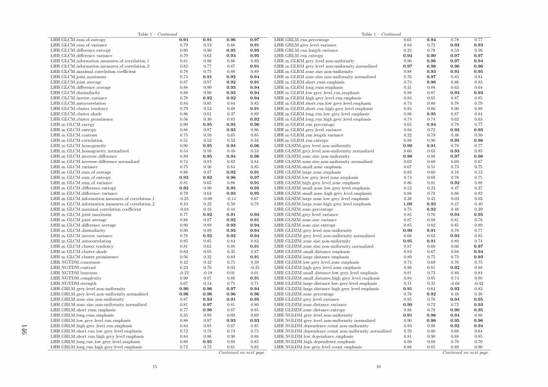
Table 1 – Continued
LHH GLCM sum of entropy 0.91 0.91 0.96 0.97
LHH GLCM sum of variance 0.79 0.53 0.88 0.91
LHH GLCM difference entropy 0.90 0.90 0.95 0.95
LHH GLCM difference variance 0.79 0.63 0.93 0.95
LHH GLCM information measures of correlation 1 0.81 0.86 0.86 0.89LHH GLCM information measures of correlation 2 0.82 0.77 0.87 0.91
LHH GLCM maximal correlation coefficient 0.78 0.75 0.88 0.89LHH GLCM joint maximum 0.74 0.91 0.92 0.94
LHH GLCM joint average 0.87 0.87 0.92 0.91
LHH GLCM difference average 0.88 0.90 0.93 0.94
LHH GLCM dissimilarity 0.88 0.90 0.93 0.94
LHH GLCM inverse variance 0.78 0.92 0.92 0.94
LHH GLCM autocorrelation 0.84 0.85 0.84 0.82LHH GLCM cluster tendency 0.79 0.53 0.88 0.91
LHH GLCM cluster shade 0.86 0.01 0.37 0.89LHH GLCM cluster prominence 0.56 0.30 0.83 0.92
LHH m GLCM energy 0.90 0.95 0.95 0.96
LHH m GLCM entropy 0.88 0.87 0.93 0.86LHH m GLCM contrast 0.75 0.59 0.85 0.85LHH m GLCM correlation 0.51 0.52 0.52 0.34LHH m GLCM homogeneity 0.90 0.95 0.94 0.96
LHH m GLCM homogeneity normalized 0.54 0.59 0.49 0.53LHH m GLCM inverese difference 0.89 0.95 0.94 0.96
LHH m GLCM inverese difference normalized 0.74 0.83 0.82 0.84LHH m GLCM variance 0.75 0.56 0.84 0.85LHH m GLCM sum of average 0.88 0.87 0.92 0.91
LHH m GLCM sum of entropy 0.93 0.92 0.96 0.97
LHH m GLCM sum of variance 0.81 0.65 0.88 0.91
LHH m GLCM difference entropy 0.92 0.90 0.95 0.95
LHH m GLCM difference variance 0.79 0.63 0.93 0.95
LHH m GLCM information measures of correlation 1 -0.25 -0.08 -0.14 0.67LHH m GLCM information measures of correlation 2 0.10 0.32 0.59 0.78LHH m GLCM maximal correlation coefficient -0.04 0.16 0.44LHH m GLCM joint maximum 0.77 0.92 0.91 0.93
LHH m GLCM joint average 0.88 0.87 0.92 0.91
LHH m GLCM difference average 0.90 0.89 0.93 0.94
LHH m GLCM dissimilarity 0.90 0.89 0.93 0.94
LHH m GLCM inverse variance 0.78 0.92 0.92 0.94
LHH m GLCM autocorrelation 0.85 0.85 0.84 0.82LHH m GLCM cluster tendency 0.81 0.65 0.88 0.91
LHH m GLCM cluster shade 0.83 0.05 0.35 0.87LHH m GLCM cluster prominence 0.56 0.32 0.83 0.91
LHH NGTDM coarseness 0.42 0.42 0.75 0.59LHH NGTDM contrast 0.23 0.70 0.03 -0.35LHH NGTDM busyness -0.23 -0.18 0.01 0.01LHH NGTDM complexity 0.90 0.87 0.86 0.91
LHH NGTDM strength 0.67 0.14 0.75 0.71LHH GRLM grey level non-uniformity 0.90 0.96 0.97 0.94
LHH GRLM grey level non-uniformity normalized 0.96 0.96 0.96 0.96
LHH GRLM zone size non-uniformity 0.87 0.93 0.91 0.95
LHH GRLM zone size non-uniformity normalized 0.81 0.97 0.81 0.80LHH GRLM short runs emphasis 0.77 0.96 0.87 0.85LHH GRLM long runs emphasis 0.35 0.89 0.69 0.69LHH GRLM low grey level run emphasis 0.88 0.87 0.93 0.93
LHH GRLM high grey level run emphasis 0.84 0.85 0.87 0.85LHH GRLM short run low grey level emphasis 0.72 0.78 0.74 0.75LHH GRLM short run high grey level emphasis 0.84 0.86 0.90 0.88LHH GRLM long run low grey level emphasis 0.88 0.95 0.88 0.85LHH GRLM long run high grey level emphasis 0.72 0.73 0.61 0.62
Continued on next page
15
Table 1 – Continued
LHH GRLM run percentage 0.65 0.94 0.78 0.77LHH GRLM grey level variance 0.84 0.72 0.93 0.93
LHH GRLM run length variance 0.24 0.78 0.53 0.56LHH GRLM run entropy 0.94 0.90 0.97 0.97
LHH m GLRM grey level non-uniformity 0.90 0.96 0.97 0.94
LHH m GLRM grey level non-uniformity normalized 0.97 0.96 0.96 0.96
LHH m GLRM zone size non-uniformity 0.88 0.93 0.91 0.95
LHH m GLRM zone size non-uniformity normalized 0.76 0.97 0.85 0.84LHH m GLRM short runs emphasis 0.74 0.96 0.86 0.83LHH m GLRM long runs emphasis 0.31 0.88 0.63 0.64LHH m GLRM low grey level run emphasis 0.88 0.87 0.93 0.93
LHH m GLRM high grey level run emphasis 0.84 0.85 0.87 0.85LHH m GLRM short run low grey level emphasis 0.74 0.80 0.78 0.79LHH m GLRM short run high grey level emphasis 0.84 0.86 0.90 0.88LHH m GLRM long run low grey level emphasis 0.86 0.95 0.87 0.84LHH m GLRM long run high grey level emphasis 0.74 0.74 0.62 0.63LHH m GLRM run percentage 0.65 0.94 0.78 0.77LHH m GLRM grey level variance 0.84 0.72 0.93 0.93
LHH m GLRM run length variance 0.22 0.79 0.46 0.50LHH m GLRM run entropy 0.89 0.90 0.95 0.96
LHH GLSZM grey level non-uniformity 0.90 0.91 0.78 0.77LHH GLSZM grey level non-uniformity normalized 0.66 0.63 0.93 0.85LHH GLSZM zone size non-uniformity 0.98 0.88 0.97 0.96
LHH GLSZM zone size non-uniformity normalized 0.63 0.60 0.69 0.67LHH GLSZM small zone emphasis 0.67 0.51 0.73 0.75LHH GLSZM large zone emphasis 0.83 0.60 0.16 0.13LHH GLSZM low grey level zone emphasis 0.74 0.69 0.76 0.75LHH GLSZM high grey level zone emphasis 0.86 0.81 0.92 0.88LHH GLSZM small zone low grey level emphasis 0.53 0.23 0.47 0.37LHH GLSZM small zone high grey level emphasis 0.88 0.78 0.86 0.82LHH GLSZM large zone low grey level emphasis 0.38 0.45 0.03 0.03LHH GLSZM large zone high grey level emphasis 1.00 0.93 0.47 0.40LHH GLSZM zone percentage 0.75 0.92 0.48 0.39LHH GLSZM grey level variance 0.85 0.76 0.94 0.95
LHH GLSZM zone size variance 0.87 0.88 0.81 0.78LHH GLSZM zone size entropy 0.85 0.82 0.85 0.89LHH GLDZM grey level non-uniformity 0.90 0.91 0.78 0.77LHH GLDZM grey level non-uniformity normalized 0.66 0.63 0.93 0.85LHH GLDZM zone size non-uniformity 0.95 0.91 0.80 0.74LHH GLDZM zone size non-uniformity normalized 0.87 0.69 0.66 0.97
LHH GLDZM small distance emphasis 0.83 0.67 0.68 0.94
LHH GLDZM large distance emphasis 0.89 0.75 0.73 0.93
LHH GLDZM low grey level zone emphasis 0.74 0.69 0.76 0.75LHH GLDZM high grey level zone emphasis 0.86 0.81 0.92 0.88LHH GLDZM small distance low grey level emphasis 0.81 0.73 0.80 0.84LHH GLDZM small distance high grey level emphasis 0.84 0.85 0.74 0.88LHH GLDZM large distance low grey level emphasis 0.11 0.31 -0.68 -0.32LHH GLDZM large distance high grey level emphasis 0.91 0.64 0.92 0.83LHH GLDZM zone percentage 0.76 0.92 0.48 0.38LHH GLDZM grey level variance 0.85 0.76 0.94 0.95
LHH GLDZM zone distance variance 0.90 0.72 0.72 0.93
LHH GLDZM zone distance entropy 0.88 0.76 0.90 0.95
LHH NGLDM grey level non-uniformity 0.91 0.96 0.94 0.88LHH NGLDM grey level non-uniformity normalized 0.90 0.96 0.95 0.96
LHH NGLDM dependence count non-uniformity 0.83 0.88 0.92 0.94
LHH NGLDM dependence count non-uniformity normalized 0.70 0.80 0.68 0.64LHH NGLDM low dependence emphasis 0.81 0.90 0.88 0.85LHH NGLDM high dependence emphasis 0.50 0.88 0.70 0.70LHH NGLDM low grey level count emphasis 0.88 0.85 0.89 0.90
Continued on next page
16
146
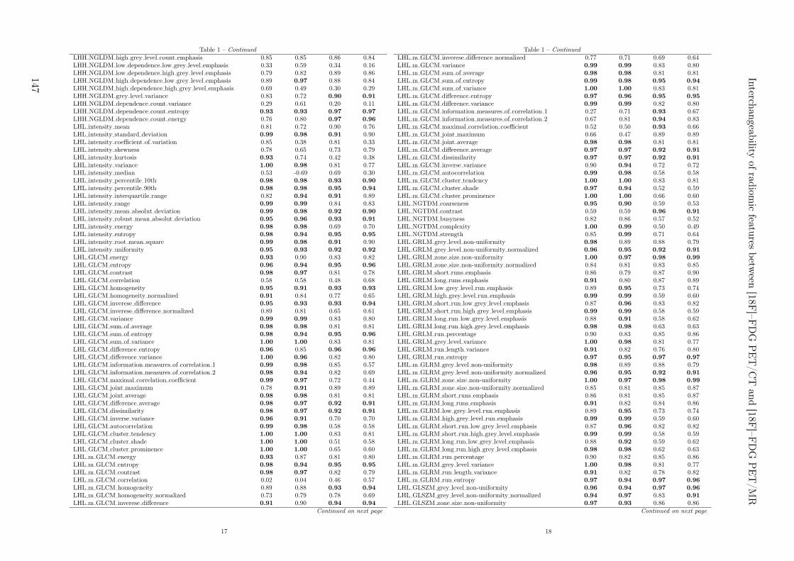
Table 1 – Continued
LHH NGLDM high grey level count emphasis 0.85 0.85 0.86 0.84LHH NGLDM low dependence low grey level emphasis 0.33 0.59 0.34 0.16LHH NGLDM low dependence high grey level emphasis 0.79 0.82 0.89 0.86LHH NGLDM high dependence low grey level emphasis 0.89 0.97 0.88 0.84LHH NGLDM high dependence high grey level emphasis 0.69 0.49 0.30 0.29LHH NGLDM grey level variance 0.83 0.72 0.90 0.91
LHH NGLDM dependence count variance 0.29 0.61 0.20 0.11LHH NGLDM dependence count entropy 0.93 0.93 0.97 0.97
LHH NGLDM dependence count energy 0.76 0.80 0.97 0.96
LHL intensity mean 0.81 0.72 0.90 0.76LHL intensity standard deviation 0.99 0.98 0.91 0.90LHL intensity coefficient of variation 0.85 0.38 0.81 0.33LHL intensity skewness 0.78 0.65 0.73 0.79LHL intensity kurtosis 0.93 0.74 0.42 0.38LHL intensity variance 1.00 0.98 0.81 0.77LHL intensity median 0.53 -0.69 0.69 0.30LHL intensity percentile 10th 0.98 0.98 0.93 0.90
LHL intensity percentile 90th 0.98 0.98 0.95 0.94
LHL intensity interquartile range 0.82 0.94 0.91 0.89LHL intensity range 0.99 0.99 0.84 0.83LHL intensity mean absolut deviation 0.99 0.98 0.92 0.90
LHL intensity robust mean absolut deviation 0.95 0.96 0.93 0.91
LHL intensity energy 0.98 0.98 0.69 0.70LHL intensity entropy 0.98 0.94 0.95 0.95
LHL intensity root mean square 0.99 0.98 0.91 0.90LHL intensity uniformity 0.95 0.93 0.92 0.92
LHL GLCM energy 0.93 0.90 0.83 0.82LHL GLCM entropy 0.96 0.94 0.95 0.96
LHL GLCM contrast 0.98 0.97 0.81 0.78LHL GLCM correlation 0.58 0.58 0.48 0.68LHL GLCM homogeneity 0.95 0.91 0.93 0.93
LHL GLCM homogeneity normalized 0.91 0.84 0.77 0.65LHL GLCM inverese difference 0.95 0.93 0.93 0.94
LHL GLCM inverese difference normalized 0.89 0.81 0.65 0.61LHL GLCM variance 0.99 0.99 0.83 0.80LHL GLCM sum of average 0.98 0.98 0.81 0.81LHL GLCM sum of entropy 0.98 0.94 0.95 0.96
LHL GLCM sum of variance 1.00 1.00 0.83 0.81LHL GLCM difference entropy 0.96 0.85 0.96 0.96
LHL GLCM difference variance 1.00 0.96 0.82 0.80LHL GLCM information measures of correlation 1 0.99 0.98 0.85 0.57LHL GLCM information measures of correlation 2 0.98 0.94 0.82 0.69LHL GLCM maximal correlation coefficient 0.99 0.97 0.72 0.44LHL GLCM joint maximum 0.78 0.91 0.89 0.89LHL GLCM joint average 0.98 0.98 0.81 0.81LHL GLCM difference average 0.98 0.97 0.92 0.91
LHL GLCM dissimilarity 0.98 0.97 0.92 0.91
LHL GLCM inverse variance 0.96 0.91 0.70 0.70LHL GLCM autocorrelation 0.99 0.98 0.58 0.58LHL GLCM cluster tendency 1.00 1.00 0.83 0.81LHL GLCM cluster shade 1.00 1.00 0.51 0.58LHL GLCM cluster prominence 1.00 1.00 0.65 0.60LHL m GLCM energy 0.93 0.87 0.81 0.80LHL m GLCM entropy 0.98 0.94 0.95 0.95
LHL m GLCM contrast 0.98 0.97 0.82 0.79LHL m GLCM correlation 0.02 0.04 0.46 0.57LHL m GLCM homogeneity 0.89 0.88 0.93 0.94
LHL m GLCM homogeneity normalized 0.73 0.79 0.78 0.69LHL m GLCM inverese difference 0.91 0.90 0.94 0.94
Continued on next page
17
Table 1 – Continued
LHL m GLCM inverese difference normalized 0.77 0.71 0.69 0.64LHL m GLCM variance 0.99 0.99 0.83 0.80LHL m GLCM sum of average 0.98 0.98 0.81 0.81LHL m GLCM sum of entropy 0.99 0.98 0.95 0.94
LHL m GLCM sum of variance 1.00 1.00 0.83 0.81LHL m GLCM difference entropy 0.97 0.96 0.95 0.95
LHL m GLCM difference variance 0.99 0.99 0.82 0.80LHL m GLCM information measures of correlation 1 0.27 0.71 0.93 0.67LHL m GLCM information measures of correlation 2 0.67 0.81 0.94 0.83LHL m GLCM maximal correlation coefficient 0.52 0.50 0.93 0.66LHL m GLCM joint maximum 0.66 0.47 0.89 0.89LHL m GLCM joint average 0.98 0.98 0.81 0.81LHL m GLCM difference average 0.97 0.97 0.92 0.91
LHL m GLCM dissimilarity 0.97 0.97 0.92 0.91
LHL m GLCM inverse variance 0.90 0.94 0.72 0.72LHL m GLCM autocorrelation 0.99 0.98 0.58 0.58LHL m GLCM cluster tendency 1.00 1.00 0.83 0.81LHL m GLCM cluster shade 0.97 0.94 0.52 0.59LHL m GLCM cluster prominence 1.00 1.00 0.66 0.60LHL NGTDM coarseness 0.95 0.90 0.59 0.53LHL NGTDM contrast 0.59 0.59 0.96 0.91
LHL NGTDM busyness 0.82 0.86 0.57 0.52LHL NGTDM complexity 1.00 0.99 0.50 0.49LHL NGTDM strength 0.85 0.99 0.71 0.64LHL GRLM grey level non-uniformity 0.98 0.89 0.88 0.79LHL GRLM grey level non-uniformity normalized 0.96 0.95 0.92 0.91
LHL GRLM zone size non-uniformity 1.00 0.97 0.98 0.99
LHL GRLM zone size non-uniformity normalized 0.84 0.81 0.83 0.85LHL GRLM short runs emphasis 0.86 0.79 0.87 0.90LHL GRLM long runs emphasis 0.91 0.80 0.87 0.89LHL GRLM low grey level run emphasis 0.89 0.95 0.73 0.74LHL GRLM high grey level run emphasis 0.99 0.99 0.59 0.60LHL GRLM short run low grey level emphasis 0.87 0.96 0.83 0.82LHL GRLM short run high grey level emphasis 0.99 0.99 0.58 0.59LHL GRLM long run low grey level emphasis 0.88 0.91 0.58 0.62LHL GRLM long run high grey level emphasis 0.98 0.98 0.63 0.63LHL GRLM run percentage 0.90 0.83 0.85 0.86LHL GRLM grey level variance 1.00 0.98 0.81 0.77LHL GRLM run length variance 0.91 0.82 0.76 0.80LHL GRLM run entropy 0.97 0.95 0.97 0.97
LHL m GLRM grey level non-uniformity 0.98 0.89 0.88 0.79LHL m GLRM grey level non-uniformity normalized 0.96 0.95 0.92 0.91
LHL m GLRM zone size non-uniformity 1.00 0.97 0.98 0.99
LHL m GLRM zone size non-uniformity normalized 0.85 0.81 0.85 0.87LHL m GLRM short runs emphasis 0.86 0.81 0.85 0.87LHL m GLRM long runs emphasis 0.91 0.82 0.84 0.86LHL m GLRM low grey level run emphasis 0.89 0.95 0.73 0.74LHL m GLRM high grey level run emphasis 0.99 0.99 0.59 0.60LHL m GLRM short run low grey level emphasis 0.87 0.96 0.82 0.82LHL m GLRM short run high grey level emphasis 0.99 0.99 0.58 0.59LHL m GLRM long run low grey level emphasis 0.88 0.92 0.59 0.62LHL m GLRM long run high grey level emphasis 0.98 0.98 0.62 0.63LHL m GLRM run percentage 0.90 0.82 0.85 0.86LHL m GLRM grey level variance 1.00 0.98 0.81 0.77LHL m GLRM run length variance 0.91 0.82 0.78 0.82LHL m GLRM run entropy 0.97 0.94 0.97 0.96
LHL GLSZM grey level non-uniformity 0.96 0.94 0.97 0.96
LHL GLSZM grey level non-uniformity normalized 0.94 0.97 0.83 0.91
LHL GLSZM zone size non-uniformity 0.97 0.93 0.86 0.86Continued on next page
18
Interch
angeab
ilityof
radiom
icfeatu
resbetw
een[18F
]–FD
GP
ET
/CT
and
[18F]–F
DG
PE
T/M
R
147

Table 1 – Continued
LHL GLSZM zone size non-uniformity normalized 0.77 0.89 0.46 0.55LHL GLSZM small zone emphasis 0.65 0.87 0.78 0.83LHL GLSZM large zone emphasis 0.85 0.72 0.26 0.19LHL GLSZM low grey level zone emphasis 0.84 0.84 0.84 0.90
LHL GLSZM high grey level zone emphasis 0.98 0.98 0.56 0.58LHL GLSZM small zone low grey level emphasis 0.67 0.51 0.58 0.73LHL GLSZM small zone high grey level emphasis 0.97 0.98 0.49 0.52LHL GLSZM large zone low grey level emphasis 0.55 0.72 0.19 0.33LHL GLSZM large zone high grey level emphasis 0.95 0.89 0.75 0.47LHL GLSZM zone percentage 0.95 0.94 0.86 0.85LHL GLSZM grey level variance 1.00 0.99 0.77 0.75LHL GLSZM zone size variance 0.90 0.77 0.28 0.21LHL GLSZM zone size entropy 0.94 0.94 0.95 0.95
LHL GLDZM grey level non-uniformity 0.96 0.94 0.97 0.96
LHL GLDZM grey level non-uniformity normalized 0.94 0.97 0.83 0.91
LHL GLDZM zone size non-uniformity 0.99 0.98 0.94 0.95
LHL GLDZM zone size non-uniformity normalized 0.75 0.80 0.92 0.91
LHL GLDZM small distance emphasis 0.75 0.75 0.91 0.90
LHL GLDZM large distance emphasis 0.86 0.68 0.89 0.93
LHL GLDZM low grey level zone emphasis 0.84 0.84 0.84 0.90
LHL GLDZM high grey level zone emphasis 0.98 0.98 0.56 0.58LHL GLDZM small distance low grey level emphasis 0.89 0.87 0.88 0.90LHL GLDZM small distance high grey level emphasis 0.97 0.99 0.61 0.61LHL GLDZM large distance low grey level emphasis 0.54 0.79 0.60 0.82LHL GLDZM large distance high grey level emphasis 0.96 0.95 0.46 0.46LHL GLDZM zone percentage 0.95 0.94 0.86 0.85LHL GLDZM grey level variance 1.00 0.99 0.77 0.75LHL GLDZM zone distance variance 0.91 0.72 0.92 0.94
LHL GLDZM zone distance entropy 0.94 0.94 0.97 0.97
LHL NGLDM grey level non-uniformity 0.99 0.88 0.79 0.69LHL NGLDM grey level non-uniformity normalized 0.94 0.93 0.93 0.92
LHL NGLDM dependence count non-uniformity 0.99 0.98 0.93 0.94
LHL NGLDM dependence count non-uniformity normalized 0.78 0.91 0.53 0.63LHL NGLDM low dependence emphasis 0.96 0.95 0.88 0.88LHL NGLDM high dependence emphasis 0.91 0.79 0.84 0.87LHL NGLDM low grey level count emphasis 0.87 0.94 0.69 0.70LHL NGLDM high grey level count emphasis 0.99 0.99 0.59 0.60LHL NGLDM low dependence low grey level emphasis 0.91 0.91 0.80 0.83LHL NGLDM low dependence high grey level emphasis 1.00 0.99 0.44 0.44LHL NGLDM high dependence low grey level emphasis 0.72 0.74 0.46 0.49LHL NGLDM high dependence high grey level emphasis 0.98 0.81 0.79 0.78LHL NGLDM grey level variance 1.00 0.98 0.81 0.77LHL NGLDM dependence count variance 0.90 0.64 0.67 0.73LHL NGLDM dependence count entropy 0.96 0.97 0.96 0.96
LHL NGLDM dependence count energy 0.80 0.93 0.84 0.84LLH intensity mean 0.63 0.27 0.74 0.66LLH intensity standard deviation 0.85 0.72 0.90 0.90LLH intensity coefficient of variation 0.36 0.14 0.46 0.65LLH intensity skewness 0.73 0.68 0.01 -0.09LLH intensity kurtosis 0.55 0.38 0.64 -0.03LLH intensity variance 0.89 0.67 0.78 0.78LLH intensity median 0.40 -0.07 0.50 0.22LLH intensity percentile 10th 0.72 0.61 0.90 0.87LLH intensity percentile 90th 0.60 0.51 0.90 0.92
LLH intensity interquartile range 0.64 0.72 0.94 0.92
LLH intensity range 0.93 0.87 0.88 0.88LLH intensity mean absolut deviation 0.79 0.67 0.91 0.90
LLH intensity robust mean absolut deviation 0.73 0.66 0.92 0.91
LLH intensity energy 0.93 0.92 0.72 0.74Continued on next page
19
Table 1 – Continued
LLH intensity entropy 0.76 0.75 0.94 0.90
LLH intensity root mean square 0.86 0.72 0.90 0.89LLH intensity uniformity 0.54 0.60 0.90 0.82LLH GLCM energy 0.92 0.64 0.68 0.59LLH GLCM entropy 0.98 0.93 0.94 0.91
LLH GLCM contrast 0.89 0.55 0.76 0.78LLH GLCM correlation 0.33 0.05 0.63 0.69LLH GLCM homogeneity 0.89 0.36 0.88 0.84LLH GLCM homogeneity normalized 0.73 0.60 0.60 0.63LLH GLCM inverese difference 0.89 0.39 0.88 0.85LLH GLCM inverese difference normalized 0.71 0.52 0.55 0.39LLH GLCM variance 0.92 0.66 0.77 0.80LLH GLCM sum of average 0.93 0.88 0.91 0.91
LLH GLCM sum of entropy 0.98 0.90 0.94 0.92
LLH GLCM sum of variance 0.93 0.76 0.79 0.81LLH GLCM difference entropy 0.96 0.77 0.92 0.91
LLH GLCM difference variance 0.92 0.64 0.76 0.78LLH GLCM information measures of correlation 1 0.92 0.99 0.77 0.62LLH GLCM information measures of correlation 2 0.84 0.87 0.78 0.64LLH GLCM maximal correlation coefficient 0.86 0.81 0.77 0.44LLH GLCM joint maximum 0.71 0.62 0.76 0.65LLH GLCM joint average 0.93 0.88 0.91 0.91
LLH GLCM difference average 0.91 0.51 0.88 0.88LLH GLCM dissimilarity 0.91 0.51 0.88 0.88LLH GLCM inverse variance 0.90 0.29 0.93 0.92
LLH GLCM autocorrelation 0.92 0.91 0.83 0.83LLH GLCM cluster tendency 0.93 0.76 0.79 0.81LLH GLCM cluster shade 0.75 0.72 0.88 0.87LLH GLCM cluster prominence 0.77 0.66 0.54 0.56LLH m GLCM energy 0.34 0.36 0.66 0.53LLH m GLCM entropy 0.75 0.76 0.92 0.89LLH m GLCM contrast 0.83 0.51 0.76 0.78LLH m GLCM correlation 0.46 -0.08 0.50 0.45LLH m GLCM homogeneity 0.40 0.46 0.88 0.85LLH m GLCM homogeneity normalized 0.81 0.65 0.58 0.62LLH m GLCM inverese difference 0.44 0.49 0.89 0.85LLH m GLCM inverese difference normalized 0.73 0.58 0.46 0.32LLH m GLCM variance 0.86 0.62 0.77 0.80LLH m GLCM sum of average 0.92 0.88 0.91 0.91
LLH m GLCM sum of entropy 0.71 0.67 0.93 0.89LLH m GLCM sum of variance 0.88 0.73 0.79 0.81LLH m GLCM difference entropy 0.68 0.60 0.91 0.90LLH m GLCM difference variance 0.88 0.57 0.76 0.78LLH m GLCM information measures of correlation 1 0.70 0.38 0.72 0.28LLH m GLCM information measures of correlation 2 0.66 0.55 0.81 0.63LLH m GLCM maximal correlation coefficient 0.76 0.50 0.62 0.52LLH m GLCM joint maximum 0.43 0.46 0.79 0.63LLH m GLCM joint average 0.92 0.88 0.91 0.91
LLH m GLCM difference average 0.71 0.55 0.88 0.89LLH m GLCM dissimilarity 0.71 0.55 0.88 0.89LLH m GLCM inverse variance 0.47 0.41 0.90 0.90
LLH m GLCM autocorrelation 0.92 0.91 0.83 0.83LLH m GLCM cluster tendency 0.88 0.73 0.79 0.81LLH m GLCM cluster shade 0.73 0.73 0.89 0.87LLH m GLCM cluster prominence 0.77 0.65 0.55 0.57LLH NGTDM coarseness 0.79 0.79 0.96 0.80LLH NGTDM contrast 0.63 0.45 0.60 0.61LLH NGTDM busyness 0.37 0.70 0.55 0.55LLH NGTDM complexity 0.97 0.91 0.60 0.59
Continued on next page
20
148
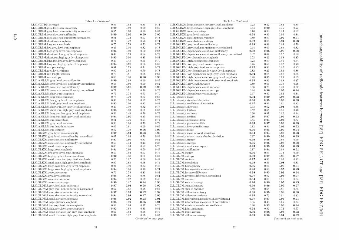
Table 1 – Continued
LLH NGTDM strength 0.86 0.62 0.81 0.74LLH GRLM grey level non-uniformity 0.99 0.89 0.90 0.85LLH GRLM grey level non-uniformity normalized 0.55 0.60 0.90 0.82LLH GRLM zone size non-uniformity 0.99 0.96 0.99 0.99
LLH GRLM zone size non-uniformity normalized 0.81 0.73 0.77 0.73LLH GRLM short runs emphasis 0.74 0.72 0.76 0.74LLH GRLM long runs emphasis 0.75 0.79 0.73 0.72LLH GRLM low grey level run emphasis 0.46 0.56 0.82 0.78LLH GRLM high grey level run emphasis 0.93 0.90 0.82 0.83LLH GRLM short run low grey level emphasis 0.49 0.59 0.84 0.79LLH GRLM short run high grey level emphasis 0.93 0.90 0.81 0.82LLH GRLM long run low grey level emphasis 0.39 0.48 0.71 0.70LLH GRLM long run high grey level emphasis 0.94 0.90 0.85 0.85LLH GRLM run percentage 0.81 0.75 0.74 0.72LLH GRLM grey level variance 0.90 0.68 0.79 0.78LLH GRLM run length variance 0.70 0.81 0.66 0.61LLH GRLM run entropy 0.80 0.80 0.96 0.93
LLH m GLRM grey level non-uniformity 0.99 0.89 0.90 0.85LLH m GLRM grey level non-uniformity normalized 0.55 0.60 0.90 0.82LLH m GLRM zone size non-uniformity 0.99 0.96 0.99 0.99
LLH m GLRM zone size non-uniformity normalized 0.77 0.71 0.78 0.75LLH m GLRM short runs emphasis 0.76 0.73 0.73 0.70LLH m GLRM long runs emphasis 0.76 0.79 0.67 0.66LLH m GLRM low grey level run emphasis 0.46 0.56 0.82 0.77LLH m GLRM high grey level run emphasis 0.93 0.90 0.82 0.83LLH m GLRM short run low grey level emphasis 0.49 0.59 0.82 0.77LLH m GLRM short run high grey level emphasis 0.93 0.90 0.81 0.82LLH m GLRM long run low grey level emphasis 0.39 0.48 0.76 0.73LLH m GLRM long run high grey level emphasis 0.94 0.90 0.85 0.85LLH m GLRM run percentage 0.81 0.76 0.74 0.72LLH m GLRM grey level variance 0.90 0.68 0.79 0.78LLH m GLRM run length variance 0.69 0.81 0.69 0.66LLH m GLRM run entropy 0.82 0.79 0.96 0.93
LLH GLSZM grey level non-uniformity 0.97 0.91 0.98 0.99
LLH GLSZM grey level non-uniformity normalized 0.67 0.68 0.78 0.81LLH GLSZM zone size non-uniformity 0.97 0.95 0.83 0.82LLH GLSZM zone size non-uniformity normalized 0.50 0.54 0.43 0.37LLH GLSZM small zone emphasis 0.63 0.24 0.82 0.76LLH GLSZM large zone emphasis 0.91 0.66 0.50 0.47LLH GLSZM low grey level zone emphasis 0.59 0.64 0.77 0.76LLH GLSZM high grey level zone emphasis 0.92 0.88 0.81 0.82LLH GLSZM small zone low grey level emphasis 0.23 0.07 0.66 0.41LLH GLSZM small zone high grey level emphasis 0.90 0.88 0.78 0.75LLH GLSZM large zone low grey level emphasis 0.24 0.40 0.33 0.46LLH GLSZM large zone high grey level emphasis 0.94 0.68 0.70 0.74LLH GLSZM zone percentage 0.76 0.58 0.83 0.82LLH GLSZM grey level variance 0.95 0.86 0.86 0.84LLH GLSZM zone size variance 0.94 0.62 0.52 0.48LLH GLSZM zone size entropy 0.90 0.87 0.94 0.93
LLH GLDZM grey level non-uniformity 0.97 0.91 0.98 0.99
LLH GLDZM grey level non-uniformity normalized 0.67 0.68 0.78 0.81LLH GLDZM zone size non-uniformity 0.97 0.97 0.92 0.92
LLH GLDZM zone size non-uniformity normalized 0.94 0.91 0.97 0.93
LLH GLDZM small distance emphasis 0.95 0.92 0.93 0.91
LLH GLDZM large distance emphasis 0.93 0.89 0.95 0.91
LLH GLDZM low grey level zone emphasis 0.59 0.64 0.77 0.76LLH GLDZM high grey level zone emphasis 0.92 0.88 0.81 0.82LLH GLDZM small distance low grey level emphasis 0.67 0.64 0.76 0.75LLH GLDZM small distance high grey level emphasis 0.92 0.87 0.85 0.83
Continued on next page
21
Table 1 – Continued
LLH GLDZM large distance low grey level emphasis 0.22 0.42 0.84 0.85LLH GLDZM large distance high grey level emphasis 0.84 0.90 0.75 0.77LLH GLDZM zone percentage 0.76 0.58 0.83 0.82LLH GLDZM grey level variance 0.95 0.86 0.86 0.84LLH GLDZM zone distance variance 0.89 0.80 0.97 0.91
LLH GLDZM zone distance entropy 0.92 0.85 0.94 0.93
LLH NGLDM grey level non-uniformity 0.99 0.88 0.84 0.79LLH NGLDM grey level non-uniformity normalized 0.54 0.60 0.89 0.82LLH NGLDM dependence count non-uniformity 0.98 0.96 0.95 0.98
LLH NGLDM dependence count non-uniformity normalized 0.82 0.64 0.57 0.68LLH NGLDM low dependence emphasis 0.52 0.46 0.88 0.85LLH NGLDM high dependence emphasis 0.73 0.80 0.56 0.54LLH NGLDM low grey level count emphasis 0.45 0.56 0.82 0.78LLH NGLDM high grey level count emphasis 0.92 0.90 0.82 0.83LLH NGLDM low dependence low grey level emphasis 0.82 0.27 0.83 0.86LLH NGLDM low dependence high grey level emphasis 0.92 0.85 0.68 0.65LLH NGLDM high dependence low grey level emphasis 0.28 0.35 0.69 0.69LLH NGLDM high dependence high grey level emphasis 0.95 0.89 0.88 0.87LLH NGLDM grey level variance 0.89 0.66 0.78 0.78LLH NGLDM dependence count variance 0.66 0.78 0.40 0.27LLH NGLDM dependence count entropy 0.84 0.96 0.95 0.94
LLH NGLDM dependence count energy 0.37 0.80 0.82 0.84LLL intensity mean 0.92 0.99 0.95 0.93
LLL intensity standard deviation 0.96 0.95 0.93 0.93
LLL intensity coefficient of variation 0.97 0.86 0.81 0.82LLL intensity skewness 0.53 0.62 0.91 0.86LLL intensity kurtosis 0.52 0.65 0.88 0.76LLL intensity variance 0.90 0.87 0.82 0.84LLL intensity median 0.86 0.97 0.95 0.93
LLL intensity percentile 10th 0.85 0.91 0.93 0.87LLL intensity percentile 90th 0.93 0.97 0.93 0.93
LLL intensity interquartile range 0.82 0.84 0.93 0.92
LLL intensity range 0.96 0.95 0.95 0.94
LLL intensity mean absolut deviation 0.94 0.94 0.93 0.93
LLL intensity robust mean absolut deviation 0.87 0.90 0.93 0.93
LLL intensity energy 0.99 0.98 0.89 0.90LLL intensity entropy 0.95 0.96 0.98 0.98
LLL intensity root mean square 0.93 0.99 0.94 0.93
LLL intensity uniformity 0.87 0.94 0.89 0.91
LLL GLCM energy 0.96 0.84 0.72 0.69LLL GLCM entropy 0.99 0.97 0.98 0.97
LLL GLCM contrast 0.97 0.90 0.80 0.82LLL GLCM correlation 0.98 0.86 0.98 0.83LLL GLCM homogeneity 0.95 0.84 0.90 0.91
LLL GLCM homogeneity normalized 0.96 0.86 0.95 0.93
LLL GLCM inverese difference 0.98 0.93 0.93 0.94
LLL GLCM inverese difference normalized 0.97 0.87 0.95 0.97
LLL GLCM variance 0.94 0.80 0.81 0.84LLL GLCM sum of average 0.96 0.98 0.95 0.93
LLL GLCM sum of entropy 0.99 0.96 0.99 0.97
LLL GLCM sum of variance 0.89 0.68 0.81 0.85LLL GLCM difference entropy 0.98 0.95 0.98 0.98
LLL GLCM difference variance 0.95 0.73 0.81 0.83LLL GLCM information measures of correlation 1 0.97 0.97 0.95 0.91
LLL GLCM information measures of correlation 2 0.85 0.48 0.65 0.54LLL GLCM maximal correlation coefficient 0.90 0.92 0.96 0.94
LLL GLCM joint maximum 0.94 0.82 0.72 0.77LLL GLCM joint average 0.96 0.98 0.95 0.93
LLL GLCM difference average 0.99 0.96 0.91 0.92
Continued on next page
22
Interch
angeab
ilityof
radiom
icfeatu
resbetw
een[18F
]–FD
GP
ET
/CT
and
[18F]–F
DG
PE
T/M
R
149

Table 1 – Continued
LLL GLCM dissimilarity 0.99 0.96 0.91 0.92
LLL GLCM inverse variance 0.98 0.64 0.98 0.93
LLL GLCM autocorrelation 0.88 0.98 0.88 0.83LLL GLCM cluster tendency 0.89 0.68 0.81 0.85LLL GLCM cluster shade 0.94 0.96 0.88 0.80LLL GLCM cluster prominence 0.74 0.51 0.53 0.59LLL m GLCM energy 0.60 0.93 0.59 0.61LLL m GLCM entropy 0.95 0.97 0.98 0.97
LLL m GLCM contrast 0.98 0.91 0.80 0.82LLL m GLCM correlation 0.90 0.76 0.98 0.81LLL m GLCM homogeneity 0.94 0.88 0.91 0.92
LLL m GLCM homogeneity normalized 0.95 0.84 0.94 0.93
LLL m GLCM inverese difference 0.97 0.94 0.94 0.95
LLL m GLCM inverese difference normalized 0.96 0.84 0.95 0.98
LLL m GLCM variance 0.94 0.83 0.81 0.84LLL m GLCM sum of average 0.96 0.99 0.95 0.93
LLL m GLCM sum of entropy 0.91 0.90 0.98 0.97
LLL m GLCM sum of variance 0.89 0.75 0.81 0.85LLL m GLCM difference entropy 0.92 0.91 0.97 0.97
LLL m GLCM difference variance 0.96 0.88 0.81 0.83LLL m GLCM information measures of correlation 1 0.80 0.64 0.91 0.82LLL m GLCM information measures of correlation 2 0.90 0.70 0.98 0.95
LLL m GLCM maximal correlation coefficient 0.75 0.86 0.91 0.51LLL m GLCM joint maximum 0.48 0.67 0.48 0.68LLL m GLCM joint average 0.96 0.99 0.95 0.93
LLL m GLCM difference average 0.99 0.97 0.91 0.92
LLL m GLCM dissimilarity 0.99 0.97 0.91 0.92
LLL m GLCM inverse variance 0.91 0.79 0.98 0.94
LLL m GLCM autocorrelation 0.88 0.98 0.88 0.83LLL m GLCM cluster tendency 0.89 0.75 0.81 0.85LLL m GLCM cluster shade 0.88 0.97 0.88 0.80LLL m GLCM cluster prominence 0.72 0.52 0.53 0.59LLL NGTDM coarseness 0.90 0.97 0.84 0.84LLL NGTDM contrast 0.68 0.95 0.81 0.84LLL NGTDM busyness 0.80 0.86 0.90 0.91
LLL NGTDM complexity 0.92 0.82 0.70 0.75LLL NGTDM strength 0.83 0.93 0.86 0.80LLL GRLM grey level non-uniformity 0.99 0.94 0.85 0.84LLL GRLM grey level non-uniformity normalized 0.87 0.94 0.90 0.90LLL GRLM zone size non-uniformity 1.00 0.96 1.00 0.99
LLL GRLM zone size non-uniformity normalized 0.90 0.92 0.80 0.91
LLL GRLM short runs emphasis 0.89 0.92 0.74 0.88LLL GRLM long runs emphasis 0.91 0.89 0.73 0.85LLL GRLM low grey level run emphasis 0.79 0.86 0.96 0.88LLL GRLM high grey level run emphasis 0.87 0.98 0.88 0.83LLL GRLM short run low grey level emphasis 0.78 0.87 0.96 0.88LLL GRLM short run high grey level emphasis 0.87 0.98 0.88 0.82LLL GRLM long run low grey level emphasis 0.85 0.84 0.95 0.87LLL GRLM long run high grey level emphasis 0.88 0.99 0.89 0.84LLL GRLM run percentage 0.91 0.91 0.78 0.89LLL GRLM grey level variance 0.90 0.88 0.82 0.84LLL GRLM run length variance 0.93 0.89 0.75 0.85LLL GRLM run entropy 0.96 0.96 0.99 0.98
LLL m GLRM grey level non-uniformity 0.99 0.94 0.85 0.84LLL m GLRM grey level non-uniformity normalized 0.86 0.94 0.90 0.90
LLL m GLRM zone size non-uniformity 1.00 0.96 1.00 0.99
LLL m GLRM zone size non-uniformity normalized 0.90 0.92 0.79 0.90
LLL m GLRM short runs emphasis 0.90 0.92 0.77 0.89LLL m GLRM long runs emphasis 0.92 0.90 0.75 0.87
Continued on next page
23
Table 1 – Continued
LLL m GLRM low grey level run emphasis 0.79 0.86 0.96 0.88LLL m GLRM high grey level run emphasis 0.87 0.98 0.88 0.83LLL m GLRM short run low grey level emphasis 0.79 0.87 0.96 0.88LLL m GLRM short run high grey level emphasis 0.87 0.98 0.88 0.82LLL m GLRM long run low grey level emphasis 0.85 0.84 0.95 0.87LLL m GLRM long run high grey level emphasis 0.87 0.99 0.89 0.84LLL m GLRM run percentage 0.91 0.91 0.78 0.89LLL m GLRM grey level variance 0.90 0.88 0.82 0.84LLL m GLRM run length variance 0.93 0.88 0.75 0.85LLL m GLRM run entropy 0.95 0.96 0.99 0.98
LLL GLSZM grey level non-uniformity 0.99 0.95 0.93 0.92
LLL GLSZM grey level non-uniformity normalized 0.84 0.93 0.96 0.90LLL GLSZM zone size non-uniformity 0.99 0.96 0.96 0.99
LLL GLSZM zone size non-uniformity normalized 0.89 0.72 0.91 0.94
LLL GLSZM small zone emphasis 0.86 0.61 0.90 0.80LLL GLSZM large zone emphasis 0.97 0.95 0.69 0.83LLL GLSZM low grey level zone emphasis 0.78 0.91 0.97 0.92
LLL GLSZM high grey level zone emphasis 0.83 0.98 0.86 0.82LLL GLSZM small zone low grey level emphasis 0.77 0.82 0.79 0.83LLL GLSZM small zone high grey level emphasis 0.79 0.95 0.82 0.80LLL GLSZM large zone low grey level emphasis 1.00 0.69 0.76 0.69LLL GLSZM large zone high grey level emphasis 0.92 0.97 0.96 0.95
LLL GLSZM zone percentage 0.92 0.93 0.89 0.93
LLL GLSZM grey level variance 0.87 0.91 0.81 0.85LLL GLSZM zone size variance 0.99 0.67 0.58 0.60LLL GLSZM zone size entropy 0.96 0.95 0.97 0.96
LLL GLDZM grey level non-uniformity 0.99 0.95 0.93 0.92
LLL GLDZM grey level non-uniformity normalized 0.83 0.93 0.96 0.89LLL GLDZM zone size non-uniformity 0.99 0.96 1.00 1.00
LLL GLDZM zone size non-uniformity normalized 0.85 0.95 0.96 0.93
LLL GLDZM small distance emphasis 0.89 0.95 0.96 0.95
LLL GLDZM large distance emphasis 0.95 0.96 0.98 0.96
LLL GLDZM low grey level zone emphasis 0.78 0.91 0.97 0.92
LLL GLDZM high grey level zone emphasis 0.83 0.98 0.86 0.82LLL GLDZM small distance low grey level emphasis 0.79 0.91 0.96 0.92
LLL GLDZM small distance high grey level emphasis 0.64 0.99 0.94 0.81LLL GLDZM large distance low grey level emphasis 0.67 0.90 0.97 0.92
LLL GLDZM large distance high grey level emphasis 0.98 0.94 0.83 0.86LLL GLDZM zone percentage 0.92 0.93 0.89 0.93
LLL GLDZM grey level variance 0.87 0.91 0.81 0.85LLL GLDZM zone distance variance 0.96 0.95 0.99 0.95
LLL GLDZM zone distance entropy 0.97 0.97 0.98 0.98
LLL NGLDM grey level non-uniformity 0.99 0.94 0.85 0.83LLL NGLDM grey level non-uniformity normalized 0.87 0.94 0.89 0.91
LLL NGLDM dependence count non-uniformity 1.00 0.97 0.97 0.99
LLL NGLDM dependence count non-uniformity normalized 0.92 0.94 0.79 0.84LLL NGLDM low dependence emphasis 0.92 0.86 0.90 0.93
LLL NGLDM high dependence emphasis 0.96 0.80 0.63 0.83LLL NGLDM low grey level count emphasis 0.80 0.86 0.96 0.88LLL NGLDM high grey level count emphasis 0.87 0.98 0.88 0.83LLL NGLDM low dependence low grey level emphasis 0.76 0.89 0.82 0.91
LLL NGLDM low dependence high grey level emphasis 0.81 0.95 0.81 0.78LLL NGLDM high dependence low grey level emphasis 0.92 0.55 0.82 0.91
LLL NGLDM high dependence high grey level emphasis 0.94 0.92 0.97 0.94
LLL NGLDM grey level variance 0.90 0.88 0.82 0.84LLL NGLDM dependence count variance 0.98 0.45 0.44 0.70LLL NGLDM dependence count entropy 0.98 0.96 0.98 0.94
LLL NGLDM dependence count energy 0.88 0.94 0.89 0.63
24
150
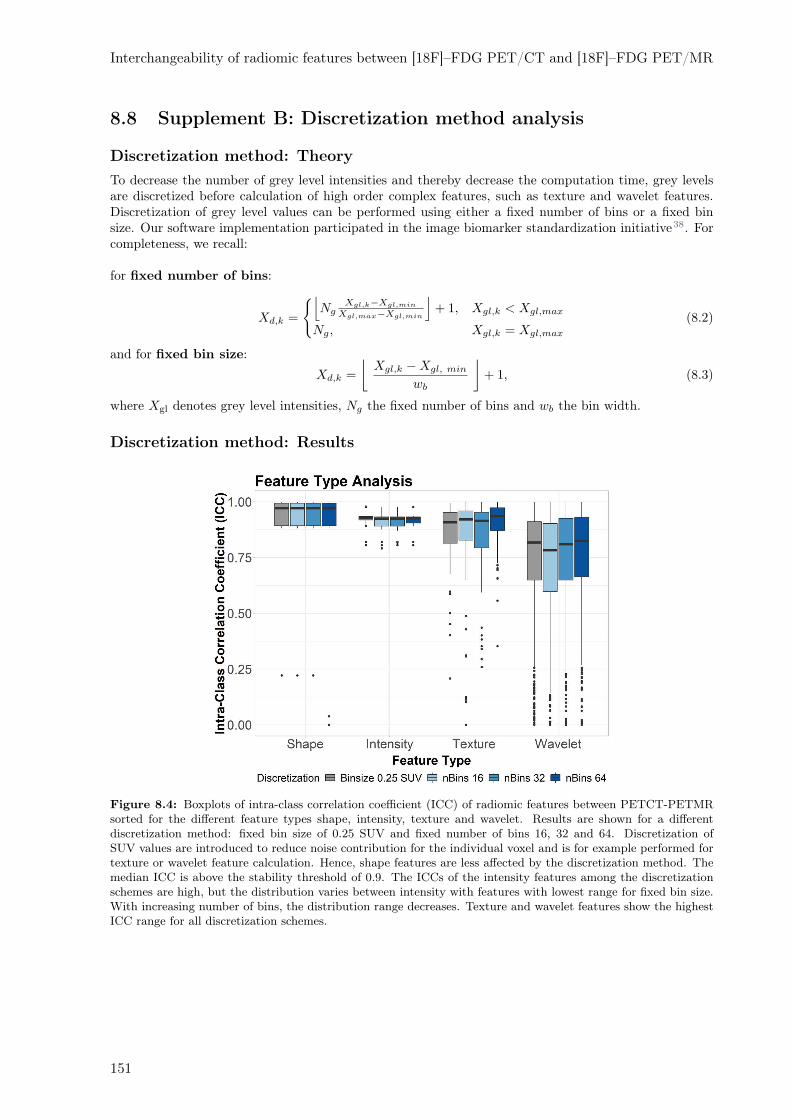
Interchangeability of radiomic features between [18F]–FDG PET/CT and [18F]–FDG PET/MR
8.8 Supplement B: Discretization method analysis
Discretization method: Theory
To decrease the number of grey level intensities and thereby decrease the computation time, grey levelsare discretized before calculation of high order complex features, such as texture and wavelet features.Discretization of grey level values can be performed using either a fixed number of bins or a fixed binsize. Our software implementation participated in the image biomarker standardization initiative38. Forcompleteness, we recall:
for fixed number of bins:
Xd,k =
{
⌊
NgXgl,k−Xgl,min
Xgl,max−Xgl,min
⌋
+ 1, Xgl,k < Xgl,max
Ng, Xgl,k = Xgl,max
(8.2)
and for fixed bin size:
Xd,k =
⌊
Xgl,k −Xgl, min
wb
⌋
+ 1, (8.3)
where Xgl denotes grey level intensities, Ng the fixed number of bins and wb the bin width.
Discretization method: Results
Figure 8.4: Boxplots of intra-class correlation coefficient (ICC) of radiomic features between PETCT-PETMRsorted for the different feature types shape, intensity, texture and wavelet. Results are shown for a differentdiscretization method: fixed bin size of 0.25 SUV and fixed number of bins 16, 32 and 64. Discretization ofSUV values are introduced to reduce noise contribution for the individual voxel and is for example performed fortexture or wavelet feature calculation. Hence, shape features are less affected by the discretization method. Themedian ICC is above the stability threshold of 0.9. The ICCs of the intensity features among the discretizationschemes are high, but the distribution varies between intensity with features with lowest range for fixed bin size.With increasing number of bins, the distribution range decreases. Texture and wavelet features show the highestICC range for all discretization schemes.
151
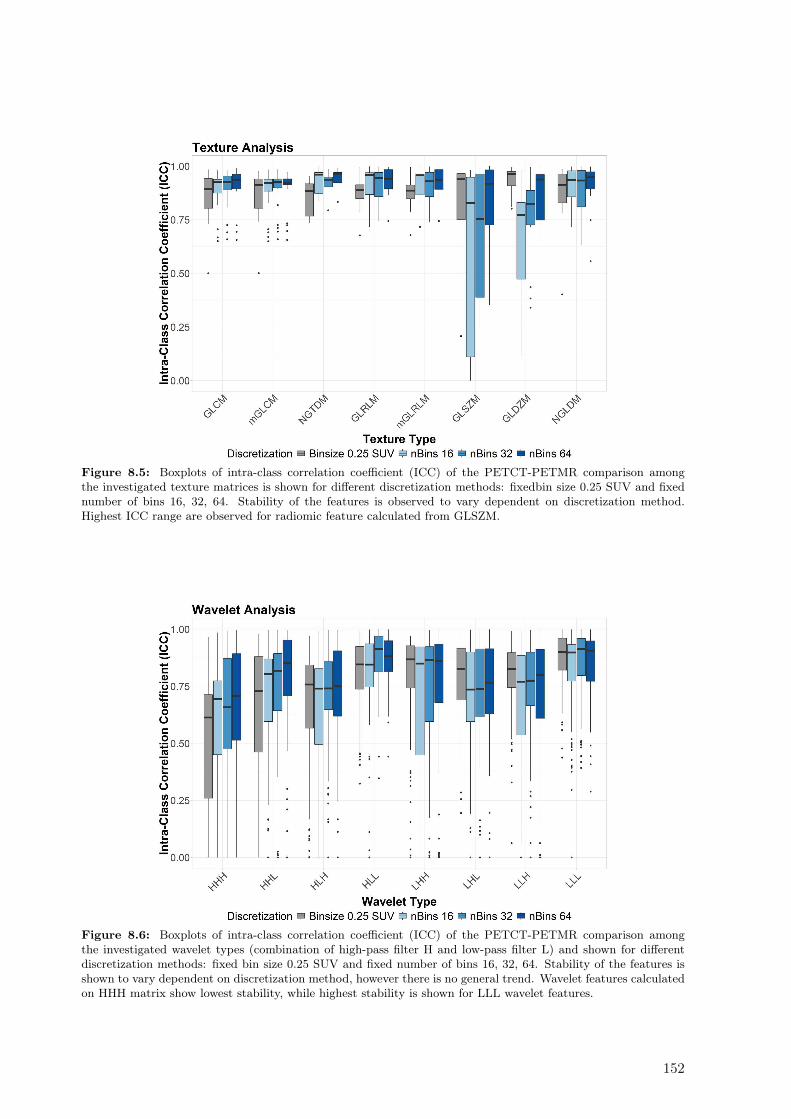
Figure 8.5: Boxplots of intra-class correlation coefficient (ICC) of the PETCT-PETMR comparison amongthe investigated texture matrices is shown for different discretization methods: fixedbin size 0.25 SUV and fixednumber of bins 16, 32, 64. Stability of the features is observed to vary dependent on discretization method.Highest ICC range are observed for radiomic feature calculated from GLSZM.
Figure 8.6: Boxplots of intra-class correlation coefficient (ICC) of the PETCT-PETMR comparison amongthe investigated wavelet types (combination of high-pass filter H and low-pass filter L) and shown for differentdiscretization methods: fixed bin size 0.25 SUV and fixed number of bins 16, 32, 64. Stability of the features isshown to vary dependent on discretization method, however there is no general trend. Wavelet features calculatedon HHH matrix show lowest stability, while highest stability is shown for LLL wavelet features.
152
9Impact of CT convolution kernel on
robustness of radiomic features for differentlung diseases and tissue types
Sarah Denzler1, Diem Vuong1, Marta Bogowicz1, Matea Pavic1, Thomas Frauenfelder2, Sandra Thier-
stein 3, Eric I. Eboulet 3, Britta Maurer4, Janine Schniering4, Hubert S. Gabrys1, Isabelle Schmitt-Opitz,Miklos Pless6, Robert Foerster1, Matthias Guckenberger1, Stephanie Tanadini–Lang1
1Department of Radiation Oncology, University Hospital Zurich and University of Zurich, Zurich, Switzer-land2Institute of Diagnostic and Interventional Radiology, University Hospital Zurich and University of Zurich,Zurich, Switzerland3Swiss Group for Clinical Cancer Research (SAKK) Coordinating Center, Bern, Switzerland4Department of Rheumatology, Center of Experimental Rheumatology, University Hospital Zurich andUniversity of Zurich, Zurich, Switzerland5Department of Thoracic Surgery, University Hospital Zurich and University of Zurich, Zurich, Switzer-land6Department of Medical Oncology, Kantonsspital Winterthur, Winterthur, Switzerland
Status:Published to British Journal of Radiology,2021doi: 10.1259/bjr.20200947
Copyright: Authors retained the copyright totheir articles.
My contribution: I supervised Sarah Denzler. I identified eligible patients for this study and col-lected the respective CT image scans. I developed the robustness analysis code and helped interpretingthe robustness results. Further, I wrote the result section (section 9.4) and prepared all figures and thesupplementary data.
9.1 Abstract
Objectives: In this study, we aimed to assess the impact of different CT reconstruction kernels on thestability of radiomic features and the transferability between different diseases and tissue types. Threelung diseases were evaluated, i.e. non-small cell lung cancer (NSCLC), malignant pleural mesothelioma(MPM) and interstitial lung disease related to systemic sclerosis (SSc-ILD) as well as four different tissuetypes, i.e. primary tumor, largest involved lymph node ipsilateral and contralateral lung.
Methods: Pre-treatment non-contrast enhanced CT scans from 23 NSCLC, 10 MPM and 12 SSc-ILDpatients were collected retrospectively. For each patient, CT scans were reconstructed using smooth andsharp kernel in filtered back projection. The regions of interest (ROIs) were contoured on the smoothkernel-based CT and transferred to the sharp kernel-based CT. The scans were resized to the largest voxeldimension of each cohort. In total, 1386 features were analyzed. Feature stability was assessed using theintraclass correlation coefficient. Features above the stability threshold >0.9 were considered stable.
Results: We observed a strong impact of the reconstruction method on stability of the features (atmaximum 26% of the 1386 features were stable). Intensity features were the most stable followed bytexture and wavelet features. The wavelet features showed a positive correlation between percentage ofstable features and size of the ROI (R2 = 0.79, p = 0.005). Lymph node radiomics showed poorest stability(<10%) and lung radiomics the largest stability (26%). Robustness analysis done on the contralaterallung could to a large extent be transferred to the ipsilateral lung, and the overlap of stable lung featuresbetween different lung diseases was more than 50%. However, results of robustness studies cannot betransferred between tissue types, which was investigated in NSCLC and MPM patients; the overlap ofstable features for lymph node and lung, as well as for primary tumor and lymph node was very small inboth disease types.
Conclusion: The robustness of radiomic features is strongly affected by different reconstruction kernels.The effect is largely influenced by the tissue type and less by the disease type.
Advances in knowledge: The study presents to our knowledge the most complete analysis on theimpact of convolution kernel on the robustness of CT-based radiomics for four relevant tissue types inthree different lung diseases.
9.2 Introduction
Malfunction of the lung has a strong impact on the quality of life. Patients with lung diseases frequentlysuffer from dyspnea, coughing and general weakness. Various diseases originate from the lung tissue.Lung cancer is one of the leading causes of cancer worldwide and the leading cause for cancer-relateddeath,418 with non-small cell lung cancer (NSCLC) being the most common type.419,420 Malignant pleuralmesothelioma (MPM) is a rare but even more aggressive cancer with a dismal prognosis.421 Besidescancer, there are also other forms of lung diseases with strong impact on the patient’s life and well-being.For example, interstitial lung disease is the leading cause of death in patients with systemic sclerosis(SSc-ILD) and is characterized by various degrees of lung inflammation and fibrosis.
Various options to treat these lung diseases exists, however, the selection of the right treatment for theright patient is challenging. There is consequently a strong clinical need for decision-support systems toguide the optimal treatment.422 Biomarker identification has increasingly gained importance in precisionmedicine to deliver the optimal treatment to every individual patient. Quantitative imaging biomarkerswere proposed to provide an observer-independent, non-invasive and comprehensive characterization ofthe region of interest (ROI). Medical imaging technologies are increasingly used to identify prognosticand predictive biomarkers for decision-support systems32: they can provide a 3D profile without the riskof sampling errors, allow assessment with high temporal resolution, are acquired non-invasively and useexisting resources for data acquisition, analysis and storage. The extraction of quantitative image featuresis also referred to as radiomics116 and can be classified in shape, intensity, texture and filtered-based fea-tures.423 Radiomics has been successfully applied to characterize lung cancer and lung fibrosis424–426 andseveral CT radiomics studies have shown that these markers could be linked to treatment outcome.384,427
Despite their potential prognostic power, radiomic features show high scanner and image acquisitiondependency,389 including image reconstruction, intra- and interobserver variability in image segmentation,respiratory and cardiac motion during imaging process and other random effects,99,252,428 hampering the
154

Impact of CT convolution kernel on robustness of radiomic features for different lung diseasesand tissue types
clinical implementation. Several studies have investigated the feature stability against reconstructiontechniques in different cancer types83,96,429 and have shown the choice of convolution kernel in filteredback projection (FBP) CT reconstruction to be of major impact. Convolution kernel is often appliedon the raw projection data to account for the limitation of the conventional back-propagation algorithmwhich tends to provide blurred images. Different convolution kernels are available to additionally exploitand enhance the underlying information of the specific tissue. For lung imaging examination, smoothand sharp convolution kernel are the most often used. A smooth kernel aims to suppress high frequencydomain information to reduce noise and leads to more smoothed images. A sharp kernel enhancesstructure heterogeneity leading to more clearly visible brightness details or textures of the lung structures,such as small vessels and bronchi. However, these images do contain more noise. Different groups haveinvestigated the robustness of radiomic features for the two most often used convolution kernels for FBPin chest CT imaging.430,431 They concluded that reconstruction method and slice thickness significantlyaffected different features. Their phantom-based study evaluated the robustness of a low number offeatures (14 features) and focused on the primary tumor only.
In this study, we aimed to assess the robustness of radiomic features in two different CT reconstructionkernels (smooth and sharp kernel) for three different lung diseases: NSCLC, MPM as well as for SSc-ILDpatients. Further, a complete robustness analysis of the relevant tissue types (primary tumor, lymph node,ipsilateral and contralateral lung) was performed. Finally, we assessed if robustness studies performedfor a specific tissue and disease type can be transferred to other disease or tissue types.
9.3 Materials and methods
9.3.1 Studied cohorts of patients
In total, 45 patients of 3 different lung disease were included. The first cohort (denoted as NSCLC)consisted of 23 retrospectively collected patients with locally advanced Stage IIIA/N2 NSCLC cancer(sixth TNM edition) from a Swiss multi centric prospective Phase III randomized trial (SAKK 16/007).The second cohort consisted of 10 Stage III MPM patients treated at the University Hospital Zurich(USZ).33 The third cohort consisted of 12 patients with proven systemic sclerosis and mild stage offibrosis (denoted as SSc-ILD cohort) treated at the USZ. MPM and SSc-ILD patients were retrospectivelycollected from our institution University Hospital Zurich, (USZ). Written consent was obtained from allpatients and this study was accepted by the local ethical committee (KEK ZH PB_2018–0026).
9.3.2 Image acquisition
Type NSCLC MPM SSc-ILD
GE Medical Systems GE Medical Systems SIEMENSModel Discovery STE, Discovery 690 Discovery 690 SOMATOM Definition AS
Reconstructionsmooth sharp smooth sharp smooth sharpSTANDARD LUNG STANDARD DETAIL B30f I70f
Resolution(mm)
0.98-1.370.98-1.371.25-3.27
0.94-1.370.94-1.371.25-3.27
0.98-1.170.98-1.173.27
0.59-0.760.59-0.761.25
0.62-0.850.62-0.850.8-1.6
0.54-0.840.54-0.840.8-1.0
Table 9.1: Overview of image acquisition characteristics. NSCLC cohort was retrospectively collected from amulticentric clinical trial and a large variation with in image spatial resolution can be observed in contrast toMPM and SSc-ILD which were imaged in one single institution.
For each patient with oncological disease, a native pre-treatment CT was collected as a part of standardPET/CT examination. For the SSc-ILD cohort, a high-resolution CT was collected. The images werereconstructed using FBP once with a sharp and once with a smooth kernel from the same raw data. Asit was a retrospective study, we assessed the kernels that were available, which were standard and lungkernel. The phantom study of Mackin et al. compared which kernel of a different vendor matched closestto GE standard kernel and showed that Siemens B30f had the closest match, i.e. features were the mostsimilar to the features calculation on a CT using GE standard kernel.432 They further stated that B60fwas most similar to the GE lung kernel. Our selection for I70f was also based on the availability of thekernel. Detailed information on the CT images can be found in Table 9.1.
155

Figure 9.1: CT axial slices for three pa-tients showing the delineated tissue types inthe two kernel CT. NSCLC in smooth (a)and in sharp kernel (b), MPM in smooth(c) and in sharp kernel (d), SSc-ILD insmooth (e) and in sharp kernel (f). Rightlung (green), left lung (blue), GTV_prim(red) and GTV_LN_max (pink) are shown.MPM, malignant pleural mesothelioma;NSCLC, non-small cell lung cancer; SSc-ILD, interstitial lung disease related to sys-temic sclerosis.
9.3.3 Delineation
We considered for each patient at maximum four tissue types: primary tumor (GTV_prim), largestlymph node involved (GTV_LN_max), ipsilateral (lung_ipsi) and contralateral lung (lung_contra). InSSc-ILD patients, only lung_ipsi and lung_contra were considered. All tissue types were delineated onthe smooth kernel-based CT and contours were transferred to the corresponding registered sharp kernelbased CT. GTV_prim and GTV_LN_max were delineated manually, lung_ipsi and lung_contra usingan automatic threshold segmentation. The NSCLC cohort was contoured according to the institutionalprotocol for routine radiotherapy practice.371 For the MPM cohort, a special study protocol was definedwhere primary tumor comprised pleural thickening as well as lung nodules, infiltrated pericard andmediastinal extensions. For NSCLC and MPM, the lung and mediastinal windows were set for thedelineation and the corresponding [18F]-FDG PET scans were used to assist in contouring. Pleuraleffusion and atelectasis were excluded from lung, tumor and lymph node contours. For the contouringof the lungs, a semi-automated method based on the HU thresholding was used. In SSc-ILD, the rightlung was used for further analysis. Delineation was performed in MIMVista (MIM software Inc., v. 6.7.9,Cleveland, OH). An example of the delineation can be found in Figure 9.1.
9.3.4 Radiomics analysis and image pre-processing
For the radiomics calculations, we used an in-house developed software (Z-Rad) written in Python pro-gramming language (v. 2.7.14.). In total, 1386 features were extracted:
• Intensity distribution (n=17)
• Texture (n=37): the Gray Level Co-occurrence Matrix (n=52), the Neighborhood Gray ToneDifference Matrix (n=5), the Gray Level Run Length Matrix (n=32), the Gray Level Size ZoneMatrix (n=16) and the Neighboring Gray Level Dependence Matrix (n=16)
• Wavelet transform (n=1232).
No shape features were analyzed since a high stability was assumed as the same contours were used inboth image sets. Definition of intensity and texture features were standardized according to the imagebiomarker standardization initiative (IBSI, v.11).38 For further details on the feature calculations, consult:https://medical-physics-usz.github.io.Due to the retrospective nature of this study, image resolution differed between the patients. Therefore,CT images of both convolution kernels were resized to cubic voxels of 3.27 mm for NSCLC and 3.27 mm
156
Impact of CT convolution kernel on robustness of radiomic features for different lung diseasesand tissue types
for MPM and 1.6 mm for SSc-ILD using linear interpolation. These voxel sizes correspond to the lowestimage resolution in the CT scans in the respective cohort. A bin size of 10 HU for all texture and waveletanalyses was chosen. For the analysis of the primary tumor and the lymph nodes, a Hounsfield unit (HU)range of -300 to 200 was set to exclude bone, air and lung tissue. For the lung analysis, a HU range of-1024 to 50 was set to exclude non-lung tissue structures.Statistical analysis was performed using R (v. 3.3.2.). Intraclass correlation coefficient (ICC) was calcu-lated according to Shrout et al.403
ICC(3, 1) =BMS − EMS
BMS + (κ− 1)EMS, (9.1)
where BMS is the between subject mean squares and EMS is the residual mean squares from Friedman’stwo-way ANOVA. The variable denotes the number of observers, i.e. the number of repeated measure-ments (here, scans with different convolution kernels). For both investigations, an ICC larger than 0.9 wasconsidered stable among both types of CT scans. Despite the small patient cohort, the high acceptancelevel of the ICC kept Type I and Type II errors small.404
9.4 Results
9.4.1 Delineation
Table 9.2 shows median volume and HU ranges for all three lung diseases. The relative range of volumewas largest for GTV_prim for both NSCLC and MPM. Accordingly, there was a large range for lung_ipsibecause tumorous tissue was not included in the lung_ipsi. Primary tumors had more homogeneous HUcompared to LN structures.
157
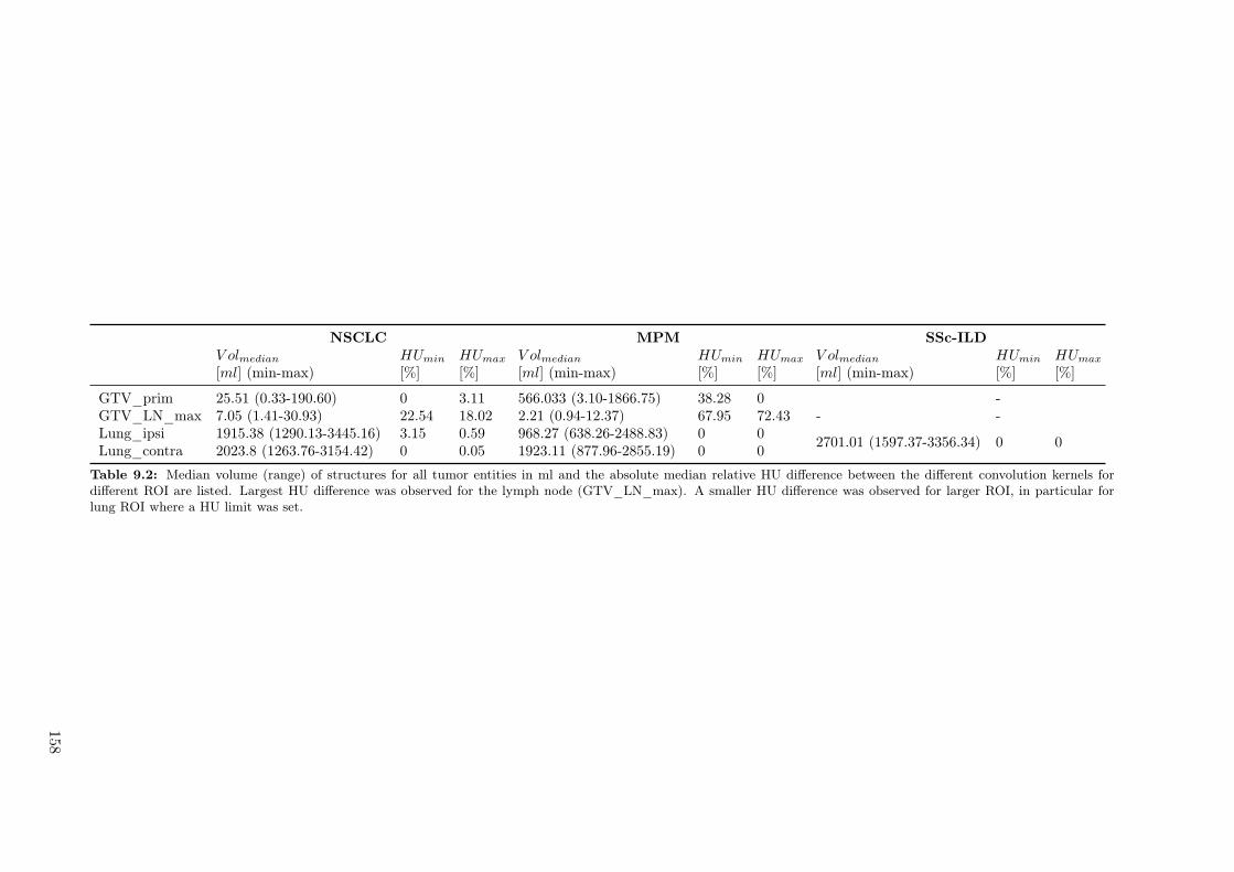
NSCLC MPM SSc-ILDV olmedian HUmin HUmax V olmedian HUmin HUmax V olmedian HUmin HUmax
[ml] (min-max) [%] [%] [ml] (min-max) [%] [%] [ml] (min-max) [%] [%]
GTV_prim 25.51 (0.33-190.60) 0 3.11 566.033 (3.10-1866.75) 38.28 0 -GTV_LN_max 7.05 (1.41-30.93) 22.54 18.02 2.21 (0.94-12.37) 67.95 72.43 - -Lung_ipsi 1915.38 (1290.13-3445.16) 3.15 0.59 968.27 (638.26-2488.83) 0 0
2701.01 (1597.37-3356.34) 0 0Lung_contra 2023.8 (1263.76-3154.42) 0 0.05 1923.11 (877.96-2855.19) 0 0
Table 9.2: Median volume (range) of structures for all tumor entities in ml and the absolute median relative HU difference between the different convolution kernels fordifferent ROI are listed. Largest HU difference was observed for the lymph node (GTV_LN_max). A smaller HU difference was observed for larger ROI, in particular forlung ROI where a HU limit was set.
158

Impact of CT convolution kernel on robustness of radiomic features for different lung diseasesand tissue types
MPM NSCLC SSc−ILD
Intensity Texture Wavelet Intensity Texture Wavelet Intensity Texture Wavelet
0
25
50
75
100
Pe
rce
nta
ge
of sta
ble
fe
atu
res (
%)
Tissue types GTV_prim GTV_LN_max lung_ipsi lung_contra
Figure 9.2: Percentage of stable features for NSCLC, MPM and SSc-ILD patients subdivided into feature types.Results of SSc-ILD are shown for one lung. MPM, malignant pleural mesothelioma; NSCLC, non-small cell lungcancer; SSc-ILD, interstitial lung disease related to systemic sclerosis.
9.4.2 Stability of radiomic features within same disease
Lung disease Tissue type Stable features
NSCLC
GTV_prim 23%GTV_LN_max 8%Lung_ipsi 20%Lung_contra 19%
MPM
GTV_prim 26%GTV_LN_max 3%Lung_ipsi 26%Lung_contra 19%
SSc-ILD Lung 19%
Table 9.3: Percentages of stable features in NSCLC, MPMand SSc-ILD for different tissue types. Overall, the stabil-ity of the features is poor for all disease types. Lung tissueshowed highest stability and lymph nodes radiomics the poor-est stability.
Overall, there was a large influence of the con-volution kernel on the robustness of radiomicfeatures Table 9.3. The percentage of sta-ble features was low (<26%) and strongly de-pended on the tissue type. 3% of featureswere stable for GTV_LN_max in MPM, andthe highest stability (26%) was observed forlung_ipsi and GTV_prim in MPM. In gen-eral, high stability was observed for lung tis-sue and GTV_prim, and low stability for theGTV_LN_max. A positive correlation was ob-served for the subset of intensity features, butnot other feature types (R2=0.79, p = 0.005,Supplement A Figure 9.7).The ipsi- and contralateral lung had the highestpercentage of stable features in intensity, tex-ture and wavelet compared to the other studiedtissue types. Lowest feature stability was observed for GTV_LN_max. The GTV_prim structure hadmore robust features than GTV_LN_max in MPM and NSCLC. Wavelet features had the highest per-centage of stable features for GTV_prim (27.11%). Stable features of lung_ipsi and lung_contra hadhigh agreement among all feature types. In SSc-ILD, there was the highest percentage of stable featuresin intensity features, followed by texture and wavelet features (Figure 9.2). A complete list of all ICCvalues of each feature can be found in Supplement 9.7.
9.4.3 Transferability of stable features across tissue types
The low feature stability rate in tissue types translate into a low number of features transferable acrossthe tissue types for both NSCLC (39 features, 2.8%) and MPM (5 features, 0.4%). Considering excludingthe tissue type with the lowest stability rate, i.e. GTV_LN_max the overlap increased to 130 (9.4%)and 105 (7.6%) features for NSCLC and MPM, respectively (Figure 9.3).Interestingly was the overlap of ipsi- and contralateral lung radiomics in NSCLC and MPM. There were208 (15%) features that were stable in the ipsi- and the contralateral lung in NSCLC and MPM. Overall,in the ipsilateral lung there were more stable features than in the contralateral lung (Figure 9.4). InNSCLC, 75% of the features that were stable in the ipsilateral lung were also stable in the contralaterallung, for MPM this overlap was smaller (57.6%).
159
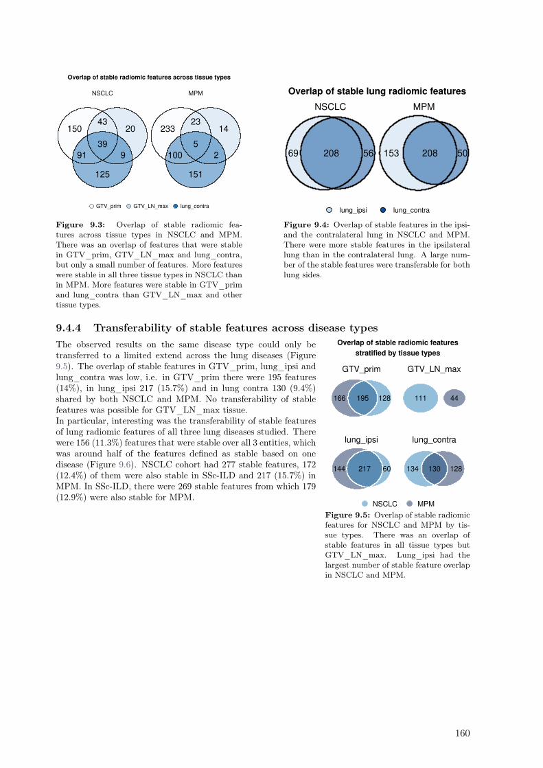
15043
20
91
39
9
125
NSCLC
23323
14
100
5
2
151
MPM
GTV_prim GTV_LN_max lung_contra
Overlap of stable radiomic features across tissue types
Figure 9.3: Overlap of stable radiomic fea-tures across tissue types in NSCLC and MPM.There was an overlap of features that were stablein GTV_prim, GTV_LN_max and lung_contra,but only a small number of features. More featureswere stable in all three tissue types in NSCLC thanin MPM. More features were stable in GTV_primand lung_contra than GTV_LN_max and othertissue types.
69 56208
NSCLC
153 50208
MPM
lung_ipsi lung_contra
Overlap of stable lung radiomic features
Figure 9.4: Overlap of stable features in the ipsi-and the contralateral lung in NSCLC and MPM.There were more stable features in the ipsilaterallung than in the contralateral lung. A large num-ber of the stable features were transferable for bothlung sides.
9.4.4 Transferability of stable features across disease types
166 128195
GTV_prim
111 44
GTV_LN_max
144 60217
lung_ipsi
134 128130
lung_contra
NSCLC MPM
Overlap of stable radiomic features
stratified by tissue types
Figure 9.5: Overlap of stable radiomicfeatures for NSCLC and MPM by tis-sue types. There was an overlap ofstable features in all tissue types butGTV_LN_max. Lung_ipsi had thelargest number of stable feature overlapin NSCLC and MPM.
The observed results on the same disease type could only betransferred to a limited extend across the lung diseases (Figure9.5). The overlap of stable features in GTV_prim, lung_ipsi andlung_contra was low, i.e. in GTV_prim there were 195 features(14%), in lung_ipsi 217 (15.7%) and in lung contra 130 (9.4%)shared by both NSCLC and MPM. No transferability of stablefeatures was possible for GTV_LN_max tissue.In particular, interesting was the transferability of stable featuresof lung radiomic features of all three lung diseases studied. Therewere 156 (11.3%) features that were stable over all 3 entities, whichwas around half of the features defined as stable based on onedisease (Figure 9.6). NSCLC cohort had 277 stable features, 172(12.4%) of them were also stable in SSc-ILD and 217 (15.7%) inMPM. In SSc-ILD, there were 269 stable features from which 179(12.9%) were also stable for MPM.
160
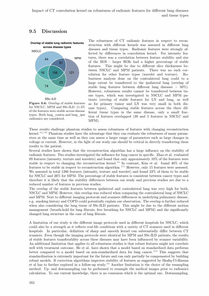
Impact of CT convolution kernel on robustness of radiomic features for different lung diseasesand tissue types
9.5 Discussion
4461
12116 156
2374
NSCLC
MPM
SSc−ILD
Overlap of stable lung radiomic features
across disease types
Figure 9.6: Overlap of stable featuresfor NSCLC, MPM and SSc-ILD. 11.3%of the features were stable across diseasetypes. Both lung_contra and lung_ipsiradiomics are considered.
The robustness of CT radiomic features in respect to recon-struction with different kernels was assessed in different lungdiseases and tissue types. Radiomic features were strongly af-fected by differences in convolution kernel. For intensity fea-tures, there was a correlation between feature stability and sizeof the ROI – larger ROIs had a higher percentage of stablefeatures. This might be due to different slice thicknesses be-tween NSCLC and MPM patients. There was no such cor-relation for other feature types (wavelet and texture). Ro-bustness analysis done on the contralateral lung could to alarge extent be transferred to the ipsilateral lung (overlap ofstable lung features between different lung diseases > 50%).However, robustness results cannot be transferred between tis-sue types, which was investigated in NSCLC and MPM pa-tients (overlap of stable features for LN and lung, as wellas for primary tumor and LN was very small in both dis-ease types). Comparing stable features across the three dif-ferent tissue types in the same disease, only a small frac-tion of features overlapped (39 and 5 features in NSCLC andMPM).
These results challenge phantom studies to assess robustness of features with changing reconstructionkernel.35,196 Phantom studies have the advantage that they can evaluate the robustness of many param-eters at the same time as well as they can assess a larger range of parameters such as large changes involtage or current. However, in the light of our study one should be critical in directly transferring theseresults to the patient.Several studies have shown that the reconstruction algorithm has a large influence on the stability ofradiomic features. Two studies investigated the influence for lung cancer in specific. Zhao et al. evaluated89 features (intensity, texture and wavelets) and found that only approximately 10% of the features werestable in respect to changing the reconstruction kernel.80 In contrast, Kim et al. found 40% of thefeatures to be stable in respect to reconstruction algorithm.215 However, only 15 features were assessed.We assessed in total 1386 features (intensity, texture and wavelet) and found 23% of them to be stablefor NSCLC and 26% for MPM. The percentage of stable features is consistent between cancer types andtherefore it is likely that the stability differences between our study and previous studies are due to areduced number of features in previous studies.The overlap of the stable features between ipsilateral and contralateral lung was very high for both,NSCLC and MPM. However, this overlap was reduced when comparing the contralateral lung of NSCLCand MPM. Next to different imaging protocols and scanners differences in underlying pulmonary disease,e.g. smoking history and COPD could potentially explain our observation. The overlap is further reducedwhen also considering the lung tissue of SSc-ILD patients. This might be due to the different motionmanagement (breath-hold for lung fibrosis, free breathing for NSCLC and MPM) and the significantlychanged lung structure in the case of lung fibrosis.
A limitation of our study is the different image protocols used in different hospitals for NSCLC, whichcould also be a strength as it reflects real-life conditions with a variety of CT scanners used in differenthospitals. In particular, definition of sharp and smooth kernel can substantially differ between CTscanners. Even though the imaging protocols were identical for MPM and SSc-ILD patients, the resultsof stable features transferability across these diseases may have been influenced by scanner variability.An additional limitation that applies to all robustness studies is that robust features might not correlatewell with treatment outcome. He et al. have shown that a model based on standardized data performsbetter compared to a model based on non-standardized data for lung cancer.433 This suggests thatstandardization is extremely important for the future and can only partially be compensated by buildingrobust models. If correction algorithms improves stability of features as suggested by Shafiq-Ul-Hassanet al has to further explored in a follow-up study.88 Another limitation is the choice of the resamplingmethod. Up- and downsampling can be performed to resample the medical images prior to radiomicscalculation. To our current knowledge, there is no consensus which is the optimal one. Downsampling,
161
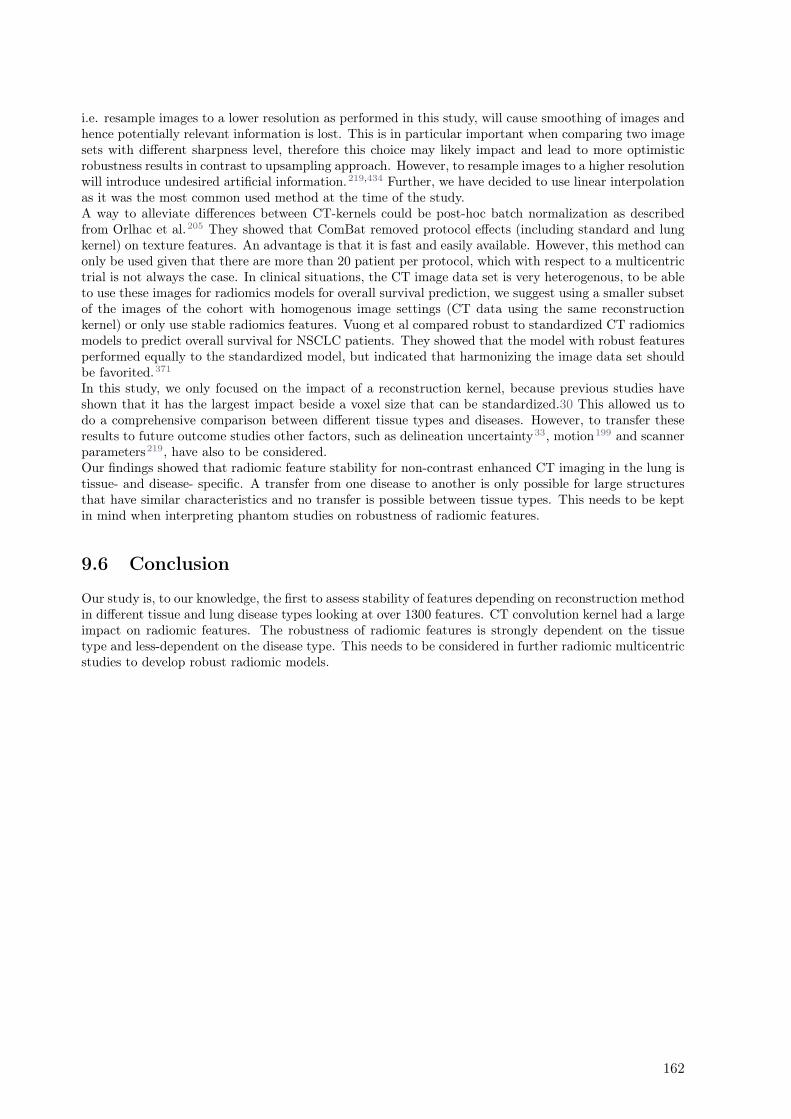
i.e. resample images to a lower resolution as performed in this study, will cause smoothing of images andhence potentially relevant information is lost. This is in particular important when comparing two imagesets with different sharpness level, therefore this choice may likely impact and lead to more optimisticrobustness results in contrast to upsampling approach. However, to resample images to a higher resolutionwill introduce undesired artificial information.219,434 Further, we have decided to use linear interpolationas it was the most common used method at the time of the study.A way to alleviate differences between CT-kernels could be post-hoc batch normalization as describedfrom Orlhac et al.205 They showed that ComBat removed protocol effects (including standard and lungkernel) on texture features. An advantage is that it is fast and easily available. However, this method canonly be used given that there are more than 20 patient per protocol, which with respect to a multicentrictrial is not always the case. In clinical situations, the CT image data set is very heterogenous, to be ableto use these images for radiomics models for overall survival prediction, we suggest using a smaller subsetof the images of the cohort with homogenous image settings (CT data using the same reconstructionkernel) or only use stable radiomics features. Vuong et al compared robust to standardized CT radiomicsmodels to predict overall survival for NSCLC patients. They showed that the model with robust featuresperformed equally to the standardized model, but indicated that harmonizing the image data set shouldbe favorited.371
In this study, we only focused on the impact of a reconstruction kernel, because previous studies haveshown that it has the largest impact beside a voxel size that can be standardized.30 This allowed us todo a comprehensive comparison between different tissue types and diseases. However, to transfer theseresults to future outcome studies other factors, such as delineation uncertainty33, motion199 and scannerparameters219, have also to be considered.Our findings showed that radiomic feature stability for non-contrast enhanced CT imaging in the lung istissue- and disease- specific. A transfer from one disease to another is only possible for large structuresthat have similar characteristics and no transfer is possible between tissue types. This needs to be keptin mind when interpreting phantom studies on robustness of radiomic features.
9.6 Conclusion
Our study is, to our knowledge, the first to assess stability of features depending on reconstruction methodin different tissue and lung disease types looking at over 1300 features. CT convolution kernel had a largeimpact on radiomic features. The robustness of radiomic features is strongly dependent on the tissuetype and less-dependent on the disease type. This needs to be considered in further radiomic multicentricstudies to develop robust radiomic models.
162
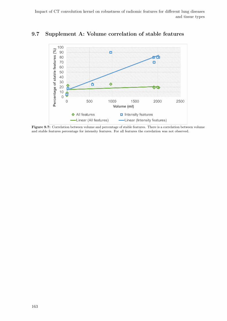
Impact of CT convolution kernel on robustness of radiomic features for different lung diseasesand tissue types
9.7 Supplement A: Volume correlation of stable features
Figure 9.7: Correlation between volume and percentage of stable features. There is a correlation between volumeand stable features percentage for intensity features. For all features the correlation was not observed.
163
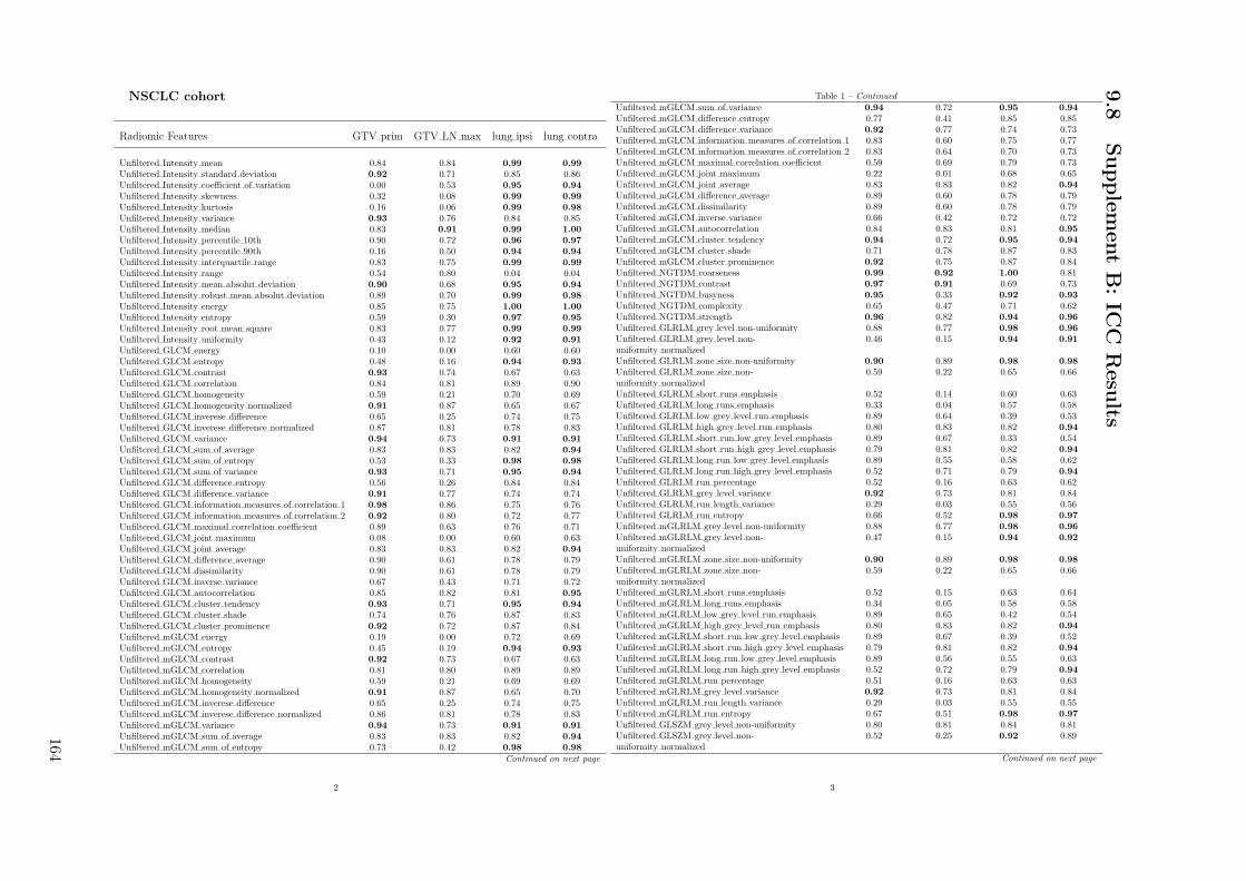
NSCLC cohort
Radiomic Features GTV prim GTV LN max lung ipsi lung contra
Unfiltered Intensity mean 0.84 0.84 0.99 0.99
Unfiltered Intensity standard deviation 0.92 0.71 0.85 0.86Unfiltered Intensity coefficient of variation 0.00 0.53 0.95 0.94
Unfiltered Intensity skewness 0.32 0.08 0.99 0.99
Unfiltered Intensity kurtosis 0.16 0.06 0.99 0.98
Unfiltered Intensity variance 0.93 0.76 0.84 0.85Unfiltered Intensity median 0.83 0.91 0.99 1.00
Unfiltered Intensity percentile 10th 0.90 0.72 0.96 0.97
Unfiltered Intensity percentile 90th 0.16 0.50 0.94 0.94
Unfiltered Intensity interquartile range 0.83 0.75 0.99 0.99
Unfiltered Intensity range 0.54 0.80 0.04 0.04Unfiltered Intensity mean absolut deviation 0.90 0.68 0.95 0.94
Unfiltered Intensity robust mean absolut deviation 0.89 0.70 0.99 0.98
Unfiltered Intensity energy 0.85 0.75 1.00 1.00
Unfiltered Intensity entropy 0.59 0.30 0.97 0.95
Unfiltered Intensity root mean square 0.83 0.77 0.99 0.99
Unfiltered Intensity uniformity 0.43 0.12 0.92 0.91
Unfiltered GLCM energy 0.10 0.00 0.60 0.60Unfiltered GLCM entropy 0.48 0.16 0.94 0.93
Unfiltered GLCM contrast 0.93 0.74 0.67 0.63Unfiltered GLCM correlation 0.84 0.81 0.89 0.90Unfiltered GLCM homogeneity 0.59 0.21 0.70 0.69Unfiltered GLCM homogeneity normalized 0.91 0.87 0.65 0.67Unfiltered GLCM inverese difference 0.65 0.25 0.74 0.75Unfiltered GLCM inverese difference normalized 0.87 0.81 0.78 0.83Unfiltered GLCM variance 0.94 0.73 0.91 0.91
Unfiltered GLCM sum of average 0.83 0.83 0.82 0.94
Unfiltered GLCM sum of entropy 0.53 0.33 0.98 0.98
Unfiltered GLCM sum of variance 0.93 0.71 0.95 0.94
Unfiltered GLCM difference entropy 0.56 0.26 0.84 0.84Unfiltered GLCM difference variance 0.91 0.77 0.74 0.74Unfiltered GLCM information measures of correlation 1 0.98 0.86 0.75 0.76Unfiltered GLCM information measures of correlation 2 0.92 0.80 0.72 0.77Unfiltered GLCM maximal correlation coefficient 0.89 0.63 0.76 0.71Unfiltered GLCM joint maximum 0.08 0.00 0.60 0.63Unfiltered GLCM joint average 0.83 0.83 0.82 0.94
Unfiltered GLCM difference average 0.90 0.61 0.78 0.79Unfiltered GLCM dissimilarity 0.90 0.61 0.78 0.79Unfiltered GLCM inverse variance 0.67 0.43 0.71 0.72Unfiltered GLCM autocorrelation 0.85 0.82 0.81 0.95
Unfiltered GLCM cluster tendency 0.93 0.71 0.95 0.94
Unfiltered GLCM cluster shade 0.74 0.76 0.87 0.83Unfiltered GLCM cluster prominence 0.92 0.72 0.87 0.84Unfiltered mGLCM energy 0.19 0.00 0.72 0.69Unfiltered mGLCM entropy 0.45 0.19 0.94 0.93
Unfiltered mGLCM contrast 0.92 0.73 0.67 0.63Unfiltered mGLCM correlation 0.81 0.80 0.89 0.89Unfiltered mGLCM homogeneity 0.59 0.21 0.69 0.69Unfiltered mGLCM homogeneity normalized 0.91 0.87 0.65 0.70Unfiltered mGLCM inverese difference 0.65 0.25 0.74 0.75Unfiltered mGLCM inverese difference normalized 0.86 0.81 0.78 0.83Unfiltered mGLCM variance 0.94 0.73 0.91 0.91
Unfiltered mGLCM sum of average 0.83 0.83 0.82 0.94
Unfiltered mGLCM sum of entropy 0.73 0.42 0.98 0.98
Continued on next page
2
Table 1 – Continued
Unfiltered mGLCM sum of variance 0.94 0.72 0.95 0.94
Unfiltered mGLCM difference entropy 0.77 0.41 0.85 0.85Unfiltered mGLCM difference variance 0.92 0.77 0.74 0.73Unfiltered mGLCM information measures of correlation 1 0.83 0.60 0.75 0.77Unfiltered mGLCM information measures of correlation 2 0.83 0.64 0.70 0.73Unfiltered mGLCM maximal correlation coefficient 0.59 0.69 0.79 0.73Unfiltered mGLCM joint maximum 0.22 0.01 0.68 0.65Unfiltered mGLCM joint average 0.83 0.83 0.82 0.94
Unfiltered mGLCM difference average 0.89 0.60 0.78 0.79Unfiltered mGLCM dissimilarity 0.89 0.60 0.78 0.79Unfiltered mGLCM inverse variance 0.66 0.42 0.72 0.72Unfiltered mGLCM autocorrelation 0.84 0.83 0.81 0.95
Unfiltered mGLCM cluster tendency 0.94 0.72 0.95 0.94
Unfiltered mGLCM cluster shade 0.71 0.78 0.87 0.83Unfiltered mGLCM cluster prominence 0.92 0.75 0.87 0.84Unfiltered NGTDM coarseness 0.99 0.92 1.00 0.81Unfiltered NGTDM contrast 0.97 0.91 0.69 0.73Unfiltered NGTDM busyness 0.95 0.33 0.92 0.93
Unfiltered NGTDM complexity 0.65 0.47 0.71 0.62Unfiltered NGTDM strength 0.96 0.82 0.94 0.96
Unfiltered GLRLM grey level non-uniformity 0.88 0.77 0.98 0.96
Unfiltered GLRLM grey level non-uniformity normalized
0.46 0.15 0.94 0.91
Unfiltered GLRLM zone size non-uniformity 0.90 0.89 0.98 0.98
Unfiltered GLRLM zone size non-uniformity normalized
0.59 0.22 0.65 0.66
Unfiltered GLRLM short runs emphasis 0.52 0.14 0.60 0.63Unfiltered GLRLM long runs emphasis 0.33 0.04 0.57 0.58Unfiltered GLRLM low grey level run emphasis 0.89 0.64 0.39 0.53Unfiltered GLRLM high grey level run emphasis 0.80 0.83 0.82 0.94
Unfiltered GLRLM short run low grey level emphasis 0.89 0.67 0.33 0.54Unfiltered GLRLM short run high grey level emphasis 0.79 0.81 0.82 0.94
Unfiltered GLRLM long run low grey level emphasis 0.89 0.55 0.58 0.62Unfiltered GLRLM long run high grey level emphasis 0.52 0.71 0.79 0.94
Unfiltered GLRLM run percentage 0.52 0.16 0.63 0.62Unfiltered GLRLM grey level variance 0.92 0.73 0.81 0.84Unfiltered GLRLM run length variance 0.29 0.03 0.55 0.56Unfiltered GLRLM run entropy 0.66 0.52 0.98 0.97
Unfiltered mGLRLM grey level non-uniformity 0.88 0.77 0.98 0.96
Unfiltered mGLRLM grey level non-uniformity normalized
0.47 0.15 0.94 0.92
Unfiltered mGLRLM zone size non-uniformity 0.90 0.89 0.98 0.98
Unfiltered mGLRLM zone size non-uniformity normalized
0.59 0.22 0.65 0.66
Unfiltered mGLRLM short runs emphasis 0.52 0.15 0.63 0.64Unfiltered mGLRLM long runs emphasis 0.34 0.05 0.58 0.58Unfiltered mGLRLM low grey level run emphasis 0.89 0.65 0.42 0.54Unfiltered mGLRLM high grey level run emphasis 0.80 0.83 0.82 0.94
Unfiltered mGLRLM short run low grey level emphasis 0.89 0.67 0.39 0.52Unfiltered mGLRLM short run high grey level emphasis 0.79 0.81 0.82 0.94
Unfiltered mGLRLM long run low grey level emphasis 0.89 0.56 0.55 0.63Unfiltered mGLRLM long run high grey level emphasis 0.52 0.72 0.79 0.94
Unfiltered mGLRLM run percentage 0.51 0.16 0.63 0.63Unfiltered mGLRLM grey level variance 0.92 0.73 0.81 0.84Unfiltered mGLRLM run length variance 0.29 0.03 0.55 0.55Unfiltered mGLRLM run entropy 0.67 0.51 0.98 0.97
Unfiltered GLSZM grey level non-uniformity 0.80 0.81 0.84 0.81Unfiltered GLSZM grey level non-uniformity normalized
0.52 0.25 0.92 0.89
Continued on next page
3
9.8
Supplem
ent
B:IC
CR
esults
164
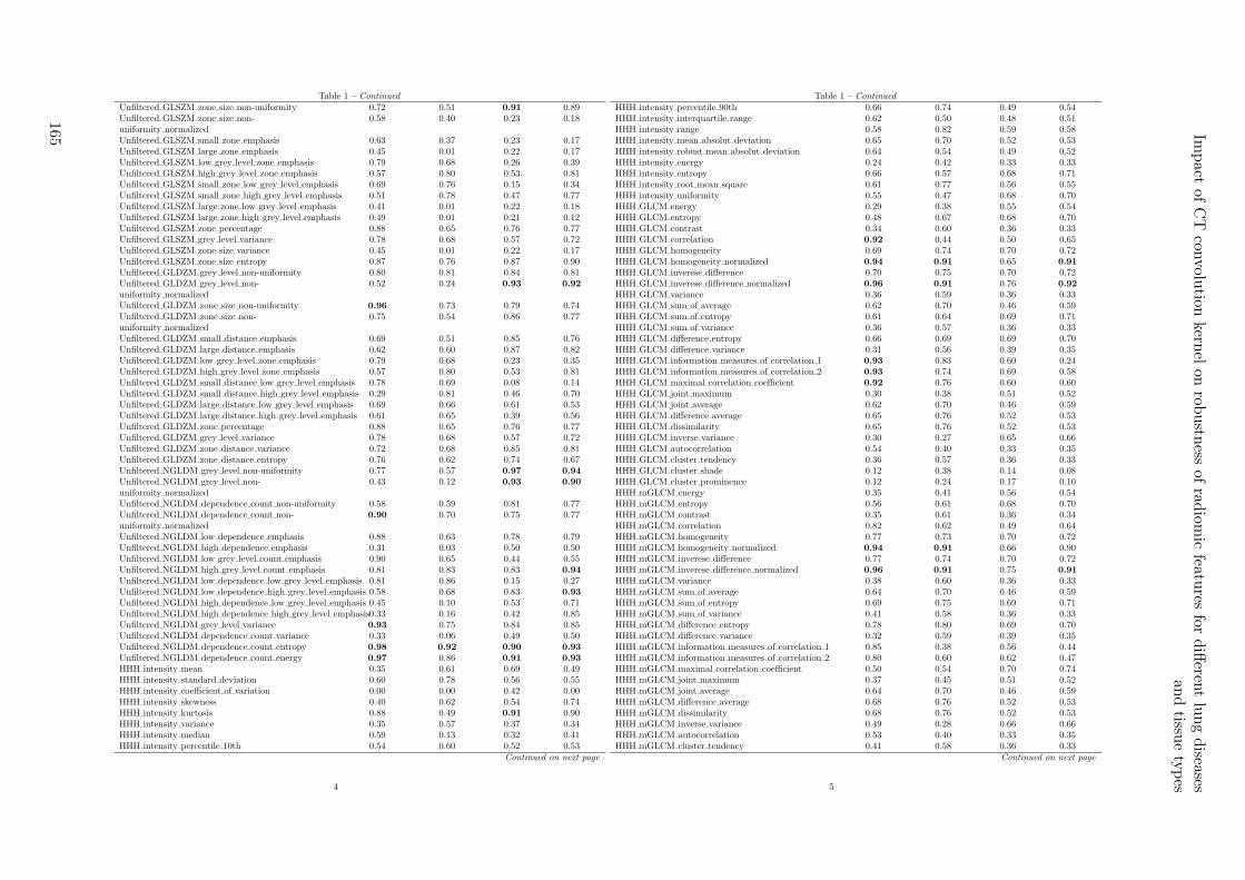
Table 1 – Continued
Unfiltered GLSZM zone size non-uniformity 0.72 0.51 0.91 0.89Unfiltered GLSZM zone size non-uniformity normalized
0.58 0.40 0.23 0.18
Unfiltered GLSZM small zone emphasis 0.63 0.37 0.23 0.17Unfiltered GLSZM large zone emphasis 0.45 0.01 0.22 0.17Unfiltered GLSZM low grey level zone emphasis 0.79 0.68 0.26 0.39Unfiltered GLSZM high grey level zone emphasis 0.57 0.80 0.53 0.81Unfiltered GLSZM small zone low grey level emphasis 0.69 0.76 0.15 0.34Unfiltered GLSZM small zone high grey level emphasis 0.51 0.78 0.47 0.77Unfiltered GLSZM large zone low grey level emphasis 0.41 0.01 0.22 0.18Unfiltered GLSZM large zone high grey level emphasis 0.49 0.01 0.21 0.12Unfiltered GLSZM zone percentage 0.88 0.65 0.76 0.77Unfiltered GLSZM grey level variance 0.78 0.68 0.57 0.72Unfiltered GLSZM zone size variance 0.45 0.01 0.22 0.17Unfiltered GLSZM zone size entropy 0.87 0.76 0.87 0.90Unfiltered GLDZM grey level non-uniformity 0.80 0.81 0.84 0.81Unfiltered GLDZM grey level non-uniformity normalized
0.52 0.24 0.93 0.92
Unfiltered GLDZM zone size non-uniformity 0.96 0.73 0.79 0.74Unfiltered GLDZM zone size non-uniformity normalized
0.75 0.54 0.86 0.77
Unfiltered GLDZM small distance emphasis 0.69 0.51 0.85 0.76Unfiltered GLDZM large distance emphasis 0.62 0.60 0.87 0.82Unfiltered GLDZM low grey level zone emphasis 0.79 0.68 0.23 0.35Unfiltered GLDZM high grey level zone emphasis 0.57 0.80 0.53 0.81Unfiltered GLDZM small distance low grey level emphasis 0.78 0.69 0.08 0.14Unfiltered GLDZM small distance high grey level emphasis 0.29 0.81 0.46 0.70Unfiltered GLDZM large distance low grey level emphasis 0.69 0.66 0.61 0.53Unfiltered GLDZM large distance high grey level emphasis 0.61 0.65 0.39 0.56Unfiltered GLDZM zone percentage 0.88 0.65 0.76 0.77Unfiltered GLDZM grey level variance 0.78 0.68 0.57 0.72Unfiltered GLDZM zone distance variance 0.72 0.68 0.85 0.81Unfiltered GLDZM zone distance entropy 0.76 0.62 0.74 0.67Unfiltered NGLDM grey level non-uniformity 0.77 0.57 0.97 0.94
Unfiltered NGLDM grey level non-uniformity normalized
0.43 0.12 0.93 0.90
Unfiltered NGLDM dependence count non-uniformity 0.58 0.59 0.81 0.77Unfiltered NGLDM dependence count non-uniformity normalized
0.90 0.70 0.75 0.77
Unfiltered NGLDM low dependence emphasis 0.88 0.63 0.78 0.79Unfiltered NGLDM high dependence emphasis 0.31 0.03 0.50 0.50Unfiltered NGLDM low grey level count emphasis 0.90 0.65 0.44 0.55Unfiltered NGLDM high grey level count emphasis 0.81 0.83 0.83 0.94
Unfiltered NGLDM low dependence low grey level emphasis 0.81 0.86 0.15 0.27Unfiltered NGLDM low dependence high grey level emphasis 0.58 0.68 0.83 0.93
Unfiltered NGLDM high dependence low grey level emphasis 0.45 0.10 0.53 0.71Unfiltered NGLDM high dependence high grey level emphasis0.33 0.16 0.42 0.85Unfiltered NGLDM grey level variance 0.93 0.75 0.84 0.85Unfiltered NGLDM dependence count variance 0.33 0.06 0.49 0.50Unfiltered NGLDM dependence count entropy 0.98 0.92 0.90 0.93
Unfiltered NGLDM dependence count energy 0.97 0.86 0.91 0.93
HHH intensity mean 0.35 0.61 0.69 0.49HHH intensity standard deviation 0.60 0.78 0.56 0.55HHH intensity coefficient of variation 0.00 0.00 0.42 0.00HHH intensity skewness 0.40 0.62 0.54 0.74HHH intensity kurtosis 0.88 0.49 0.91 0.90HHH intensity variance 0.35 0.57 0.37 0.34HHH intensity median 0.59 0.13 0.32 0.41HHH intensity percentile 10th 0.54 0.60 0.52 0.53
Continued on next page
4
Table 1 – Continued
HHH intensity percentile 90th 0.66 0.74 0.49 0.54HHH intensity interquartile range 0.62 0.50 0.48 0.51HHH intensity range 0.58 0.82 0.59 0.58HHH intensity mean absolut deviation 0.65 0.70 0.52 0.53HHH intensity robust mean absolut deviation 0.64 0.54 0.49 0.52HHH intensity energy 0.24 0.42 0.33 0.33HHH intensity entropy 0.66 0.57 0.68 0.71HHH intensity root mean square 0.61 0.77 0.56 0.55HHH intensity uniformity 0.55 0.47 0.68 0.70HHH GLCM energy 0.29 0.38 0.55 0.54HHH GLCM entropy 0.48 0.67 0.68 0.70HHH GLCM contrast 0.34 0.60 0.36 0.33HHH GLCM correlation 0.92 0.44 0.50 0.65HHH GLCM homogeneity 0.69 0.74 0.70 0.72HHH GLCM homogeneity normalized 0.94 0.91 0.65 0.91
HHH GLCM inverese difference 0.70 0.75 0.70 0.72HHH GLCM inverese difference normalized 0.96 0.91 0.76 0.92
HHH GLCM variance 0.36 0.59 0.36 0.33HHH GLCM sum of average 0.62 0.70 0.46 0.59HHH GLCM sum of entropy 0.61 0.64 0.69 0.71HHH GLCM sum of variance 0.36 0.57 0.36 0.33HHH GLCM difference entropy 0.66 0.69 0.69 0.70HHH GLCM difference variance 0.31 0.56 0.39 0.35HHH GLCM information measures of correlation 1 0.93 0.83 0.60 0.24HHH GLCM information measures of correlation 2 0.93 0.74 0.69 0.58HHH GLCM maximal correlation coefficient 0.92 0.76 0.60 0.60HHH GLCM joint maximum 0.30 0.38 0.51 0.52HHH GLCM joint average 0.62 0.70 0.46 0.59HHH GLCM difference average 0.65 0.76 0.52 0.53HHH GLCM dissimilarity 0.65 0.76 0.52 0.53HHH GLCM inverse variance 0.30 0.27 0.65 0.66HHH GLCM autocorrelation 0.54 0.40 0.33 0.35HHH GLCM cluster tendency 0.36 0.57 0.36 0.33HHH GLCM cluster shade 0.12 0.38 0.14 0.08HHH GLCM cluster prominence 0.12 0.24 0.17 0.10HHH mGLCM energy 0.35 0.41 0.56 0.54HHH mGLCM entropy 0.56 0.61 0.68 0.70HHH mGLCM contrast 0.35 0.61 0.36 0.34HHH mGLCM correlation 0.82 0.62 0.49 0.64HHH mGLCM homogeneity 0.77 0.73 0.70 0.72HHH mGLCM homogeneity normalized 0.94 0.91 0.66 0.90HHH mGLCM inverese difference 0.77 0.74 0.70 0.72HHH mGLCM inverese difference normalized 0.96 0.91 0.75 0.91
HHH mGLCM variance 0.38 0.60 0.36 0.33HHH mGLCM sum of average 0.64 0.70 0.46 0.59HHH mGLCM sum of entropy 0.69 0.75 0.69 0.71HHH mGLCM sum of variance 0.41 0.58 0.36 0.33HHH mGLCM difference entropy 0.78 0.80 0.69 0.70HHH mGLCM difference variance 0.32 0.59 0.39 0.35HHH mGLCM information measures of correlation 1 0.85 0.38 0.56 0.44HHH mGLCM information measures of correlation 2 0.80 0.60 0.62 0.47HHH mGLCM maximal correlation coefficient 0.50 0.54 0.70 0.74HHH mGLCM joint maximum 0.37 0.45 0.51 0.52HHH mGLCM joint average 0.64 0.70 0.46 0.59HHH mGLCM difference average 0.68 0.76 0.52 0.53HHH mGLCM dissimilarity 0.68 0.76 0.52 0.53HHH mGLCM inverse variance 0.49 0.28 0.66 0.66HHH mGLCM autocorrelation 0.53 0.40 0.33 0.35HHH mGLCM cluster tendency 0.41 0.58 0.36 0.33
Continued on next page
5
Impact
ofC
Tcon
volution
kernel
onrob
ustn
essof
radiom
icfeatu
resfo
rdiff
erent
lung
diseases
and
tissue
types
165
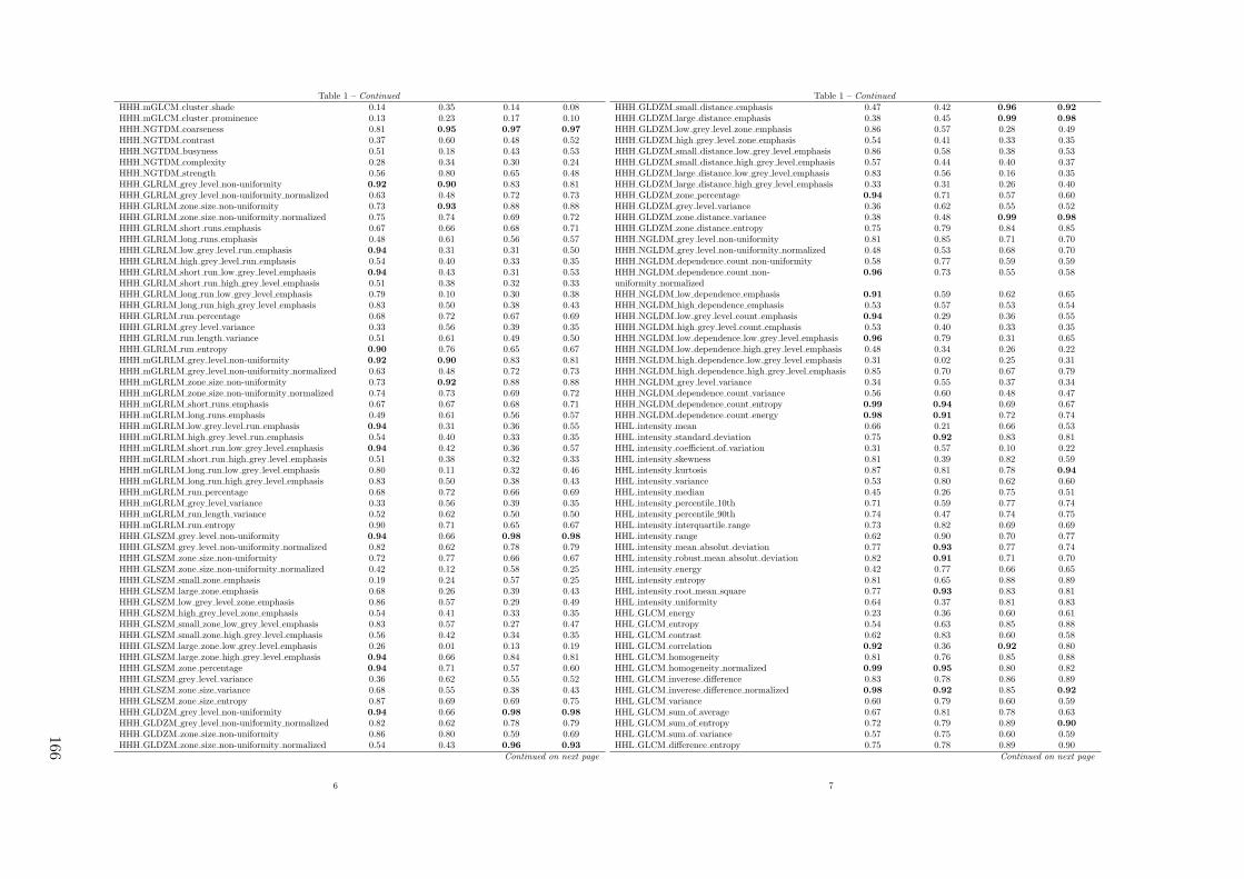
Table 1 – Continued
HHH mGLCM cluster shade 0.14 0.35 0.14 0.08HHH mGLCM cluster prominence 0.13 0.23 0.17 0.10HHH NGTDM coarseness 0.81 0.95 0.97 0.97
HHH NGTDM contrast 0.37 0.60 0.48 0.52HHH NGTDM busyness 0.51 0.18 0.43 0.53HHH NGTDM complexity 0.28 0.34 0.30 0.24HHH NGTDM strength 0.56 0.80 0.65 0.48HHH GLRLM grey level non-uniformity 0.92 0.90 0.83 0.81HHH GLRLM grey level non-uniformity normalized 0.63 0.48 0.72 0.73HHH GLRLM zone size non-uniformity 0.73 0.93 0.88 0.88HHH GLRLM zone size non-uniformity normalized 0.75 0.74 0.69 0.72HHH GLRLM short runs emphasis 0.67 0.66 0.68 0.71HHH GLRLM long runs emphasis 0.48 0.61 0.56 0.57HHH GLRLM low grey level run emphasis 0.94 0.31 0.31 0.50HHH GLRLM high grey level run emphasis 0.54 0.40 0.33 0.35HHH GLRLM short run low grey level emphasis 0.94 0.43 0.31 0.53HHH GLRLM short run high grey level emphasis 0.51 0.38 0.32 0.33HHH GLRLM long run low grey level emphasis 0.79 0.10 0.30 0.38HHH GLRLM long run high grey level emphasis 0.83 0.50 0.38 0.43HHH GLRLM run percentage 0.68 0.72 0.67 0.69HHH GLRLM grey level variance 0.33 0.56 0.39 0.35HHH GLRLM run length variance 0.51 0.61 0.49 0.50HHH GLRLM run entropy 0.90 0.76 0.65 0.67HHH mGLRLM grey level non-uniformity 0.92 0.90 0.83 0.81HHH mGLRLM grey level non-uniformity normalized 0.63 0.48 0.72 0.73HHH mGLRLM zone size non-uniformity 0.73 0.92 0.88 0.88HHH mGLRLM zone size non-uniformity normalized 0.74 0.73 0.69 0.72HHH mGLRLM short runs emphasis 0.67 0.67 0.68 0.71HHH mGLRLM long runs emphasis 0.49 0.61 0.56 0.57HHH mGLRLM low grey level run emphasis 0.94 0.31 0.36 0.55HHH mGLRLM high grey level run emphasis 0.54 0.40 0.33 0.35HHH mGLRLM short run low grey level emphasis 0.94 0.42 0.36 0.57HHH mGLRLM short run high grey level emphasis 0.51 0.38 0.32 0.33HHH mGLRLM long run low grey level emphasis 0.80 0.11 0.32 0.46HHH mGLRLM long run high grey level emphasis 0.83 0.50 0.38 0.43HHH mGLRLM run percentage 0.68 0.72 0.66 0.69HHH mGLRLM grey level variance 0.33 0.56 0.39 0.35HHH mGLRLM run length variance 0.52 0.62 0.50 0.50HHH mGLRLM run entropy 0.90 0.71 0.65 0.67HHH GLSZM grey level non-uniformity 0.94 0.66 0.98 0.98
HHH GLSZM grey level non-uniformity normalized 0.82 0.62 0.78 0.79HHH GLSZM zone size non-uniformity 0.72 0.77 0.66 0.67HHH GLSZM zone size non-uniformity normalized 0.42 0.12 0.58 0.25HHH GLSZM small zone emphasis 0.19 0.24 0.57 0.25HHH GLSZM large zone emphasis 0.68 0.26 0.39 0.43HHH GLSZM low grey level zone emphasis 0.86 0.57 0.29 0.49HHH GLSZM high grey level zone emphasis 0.54 0.41 0.33 0.35HHH GLSZM small zone low grey level emphasis 0.83 0.57 0.27 0.47HHH GLSZM small zone high grey level emphasis 0.56 0.42 0.34 0.35HHH GLSZM large zone low grey level emphasis 0.26 0.01 0.13 0.19HHH GLSZM large zone high grey level emphasis 0.94 0.66 0.84 0.81HHH GLSZM zone percentage 0.94 0.71 0.57 0.60HHH GLSZM grey level variance 0.36 0.62 0.55 0.52HHH GLSZM zone size variance 0.68 0.55 0.38 0.43HHH GLSZM zone size entropy 0.87 0.69 0.69 0.75HHH GLDZM grey level non-uniformity 0.94 0.66 0.98 0.98
HHH GLDZM grey level non-uniformity normalized 0.82 0.62 0.78 0.79HHH GLDZM zone size non-uniformity 0.86 0.80 0.59 0.69HHH GLDZM zone size non-uniformity normalized 0.54 0.43 0.96 0.93
Continued on next page
6
Table 1 – Continued
HHH GLDZM small distance emphasis 0.47 0.42 0.96 0.92
HHH GLDZM large distance emphasis 0.38 0.45 0.99 0.98
HHH GLDZM low grey level zone emphasis 0.86 0.57 0.28 0.49HHH GLDZM high grey level zone emphasis 0.54 0.41 0.33 0.35HHH GLDZM small distance low grey level emphasis 0.86 0.58 0.38 0.53HHH GLDZM small distance high grey level emphasis 0.57 0.44 0.40 0.37HHH GLDZM large distance low grey level emphasis 0.83 0.56 0.16 0.35HHH GLDZM large distance high grey level emphasis 0.33 0.31 0.26 0.40HHH GLDZM zone percentage 0.94 0.71 0.57 0.60HHH GLDZM grey level variance 0.36 0.62 0.55 0.52HHH GLDZM zone distance variance 0.38 0.48 0.99 0.98
HHH GLDZM zone distance entropy 0.75 0.79 0.84 0.85HHH NGLDM grey level non-uniformity 0.81 0.85 0.71 0.70HHH NGLDM grey level non-uniformity normalized 0.48 0.53 0.68 0.70HHH NGLDM dependence count non-uniformity 0.58 0.77 0.59 0.59HHH NGLDM dependence count non-uniformity normalized
0.96 0.73 0.55 0.58
HHH NGLDM low dependence emphasis 0.91 0.59 0.62 0.65HHH NGLDM high dependence emphasis 0.53 0.57 0.53 0.54HHH NGLDM low grey level count emphasis 0.94 0.29 0.36 0.55HHH NGLDM high grey level count emphasis 0.53 0.40 0.33 0.35HHH NGLDM low dependence low grey level emphasis 0.96 0.79 0.31 0.65HHH NGLDM low dependence high grey level emphasis 0.48 0.34 0.26 0.22HHH NGLDM high dependence low grey level emphasis 0.31 0.02 0.25 0.31HHH NGLDM high dependence high grey level emphasis 0.85 0.70 0.67 0.79HHH NGLDM grey level variance 0.34 0.55 0.37 0.34HHH NGLDM dependence count variance 0.56 0.60 0.48 0.47HHH NGLDM dependence count entropy 0.99 0.94 0.69 0.67HHH NGLDM dependence count energy 0.98 0.91 0.72 0.74HHL intensity mean 0.66 0.21 0.66 0.53HHL intensity standard deviation 0.75 0.92 0.83 0.81HHL intensity coefficient of variation 0.31 0.57 0.10 0.22HHL intensity skewness 0.81 0.39 0.82 0.59HHL intensity kurtosis 0.87 0.81 0.78 0.94
HHL intensity variance 0.53 0.80 0.62 0.60HHL intensity median 0.45 0.26 0.75 0.51HHL intensity percentile 10th 0.71 0.59 0.77 0.74HHL intensity percentile 90th 0.74 0.47 0.74 0.75HHL intensity interquartile range 0.73 0.82 0.69 0.69HHL intensity range 0.62 0.90 0.70 0.77HHL intensity mean absolut deviation 0.77 0.93 0.77 0.74HHL intensity robust mean absolut deviation 0.82 0.91 0.71 0.70HHL intensity energy 0.42 0.77 0.66 0.65HHL intensity entropy 0.81 0.65 0.88 0.89HHL intensity root mean square 0.77 0.93 0.83 0.81HHL intensity uniformity 0.64 0.37 0.81 0.83HHL GLCM energy 0.23 0.36 0.60 0.61HHL GLCM entropy 0.54 0.63 0.85 0.88HHL GLCM contrast 0.62 0.83 0.60 0.58HHL GLCM correlation 0.92 0.36 0.92 0.80HHL GLCM homogeneity 0.81 0.76 0.85 0.88HHL GLCM homogeneity normalized 0.99 0.95 0.80 0.82HHL GLCM inverese difference 0.83 0.78 0.86 0.89HHL GLCM inverese difference normalized 0.98 0.92 0.85 0.92
HHL GLCM variance 0.60 0.79 0.60 0.59HHL GLCM sum of average 0.67 0.81 0.78 0.63HHL GLCM sum of entropy 0.72 0.79 0.89 0.90
HHL GLCM sum of variance 0.57 0.75 0.60 0.59HHL GLCM difference entropy 0.75 0.78 0.89 0.90
Continued on next page
7
166
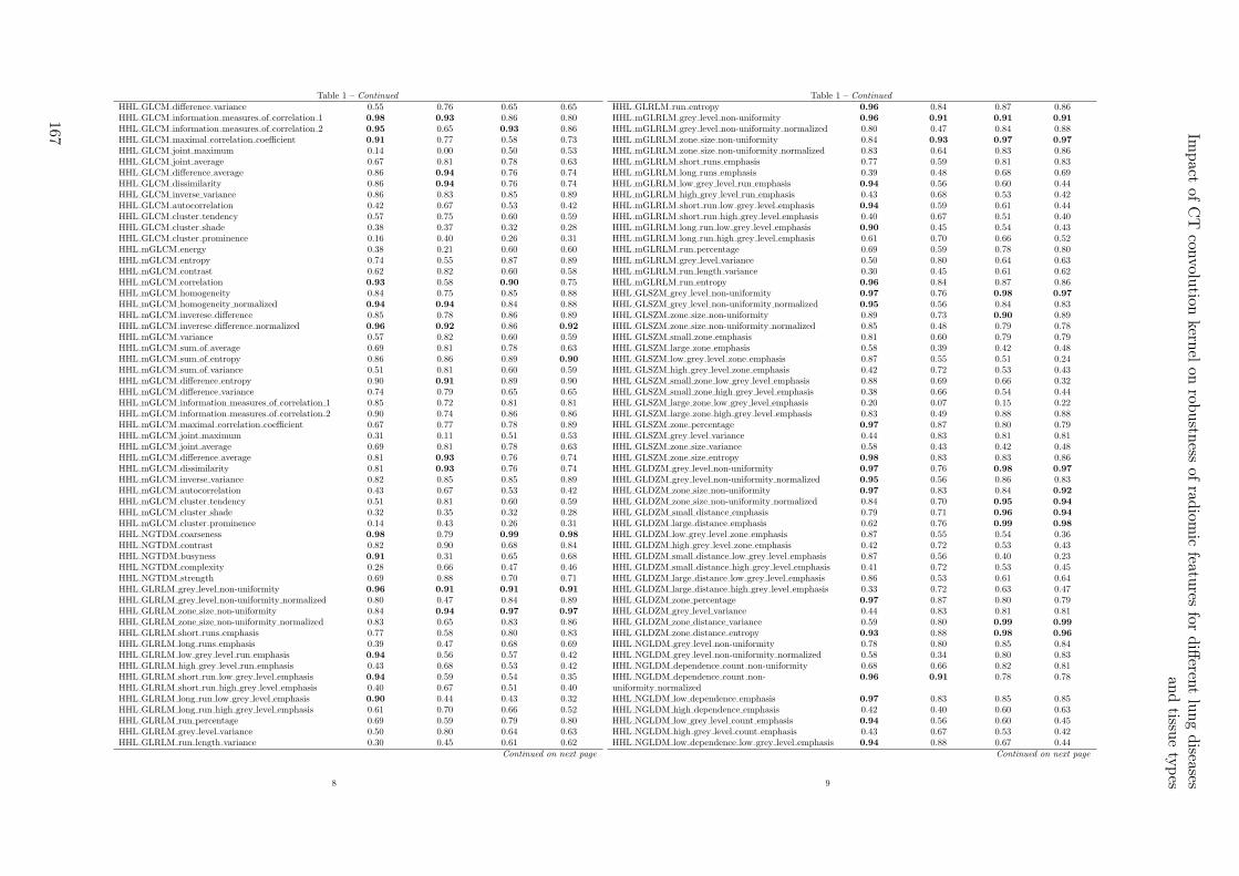
Table 1 – Continued
HHL GLCM difference variance 0.55 0.76 0.65 0.65HHL GLCM information measures of correlation 1 0.98 0.93 0.86 0.80HHL GLCM information measures of correlation 2 0.95 0.65 0.93 0.86HHL GLCM maximal correlation coefficient 0.91 0.77 0.58 0.73HHL GLCM joint maximum 0.14 0.00 0.50 0.53HHL GLCM joint average 0.67 0.81 0.78 0.63HHL GLCM difference average 0.86 0.94 0.76 0.74HHL GLCM dissimilarity 0.86 0.94 0.76 0.74HHL GLCM inverse variance 0.86 0.83 0.85 0.89HHL GLCM autocorrelation 0.42 0.67 0.53 0.42HHL GLCM cluster tendency 0.57 0.75 0.60 0.59HHL GLCM cluster shade 0.38 0.37 0.32 0.28HHL GLCM cluster prominence 0.16 0.40 0.26 0.31HHL mGLCM energy 0.38 0.21 0.60 0.60HHL mGLCM entropy 0.74 0.55 0.87 0.89HHL mGLCM contrast 0.62 0.82 0.60 0.58HHL mGLCM correlation 0.93 0.58 0.90 0.75HHL mGLCM homogeneity 0.84 0.75 0.85 0.88HHL mGLCM homogeneity normalized 0.94 0.94 0.84 0.88HHL mGLCM inverese difference 0.85 0.78 0.86 0.89HHL mGLCM inverese difference normalized 0.96 0.92 0.86 0.92
HHL mGLCM variance 0.57 0.82 0.60 0.59HHL mGLCM sum of average 0.69 0.81 0.78 0.63HHL mGLCM sum of entropy 0.86 0.86 0.89 0.90
HHL mGLCM sum of variance 0.51 0.81 0.60 0.59HHL mGLCM difference entropy 0.90 0.91 0.89 0.90HHL mGLCM difference variance 0.74 0.79 0.65 0.65HHL mGLCM information measures of correlation 1 0.85 0.72 0.81 0.81HHL mGLCM information measures of correlation 2 0.90 0.74 0.86 0.86HHL mGLCM maximal correlation coefficient 0.67 0.77 0.78 0.89HHL mGLCM joint maximum 0.31 0.11 0.51 0.53HHL mGLCM joint average 0.69 0.81 0.78 0.63HHL mGLCM difference average 0.81 0.93 0.76 0.74HHL mGLCM dissimilarity 0.81 0.93 0.76 0.74HHL mGLCM inverse variance 0.82 0.85 0.85 0.89HHL mGLCM autocorrelation 0.43 0.67 0.53 0.42HHL mGLCM cluster tendency 0.51 0.81 0.60 0.59HHL mGLCM cluster shade 0.32 0.35 0.32 0.28HHL mGLCM cluster prominence 0.14 0.43 0.26 0.31HHL NGTDM coarseness 0.98 0.79 0.99 0.98
HHL NGTDM contrast 0.82 0.90 0.68 0.84HHL NGTDM busyness 0.91 0.31 0.65 0.68HHL NGTDM complexity 0.28 0.66 0.47 0.46HHL NGTDM strength 0.69 0.88 0.70 0.71HHL GLRLM grey level non-uniformity 0.96 0.91 0.91 0.91
HHL GLRLM grey level non-uniformity normalized 0.80 0.47 0.84 0.89HHL GLRLM zone size non-uniformity 0.84 0.94 0.97 0.97
HHL GLRLM zone size non-uniformity normalized 0.83 0.65 0.83 0.86HHL GLRLM short runs emphasis 0.77 0.58 0.80 0.83HHL GLRLM long runs emphasis 0.39 0.47 0.68 0.69HHL GLRLM low grey level run emphasis 0.94 0.56 0.57 0.42HHL GLRLM high grey level run emphasis 0.43 0.68 0.53 0.42HHL GLRLM short run low grey level emphasis 0.94 0.59 0.54 0.35HHL GLRLM short run high grey level emphasis 0.40 0.67 0.51 0.40HHL GLRLM long run low grey level emphasis 0.90 0.44 0.43 0.32HHL GLRLM long run high grey level emphasis 0.61 0.70 0.66 0.52HHL GLRLM run percentage 0.69 0.59 0.79 0.80HHL GLRLM grey level variance 0.50 0.80 0.64 0.63HHL GLRLM run length variance 0.30 0.45 0.61 0.62
Continued on next page
8
Table 1 – Continued
HHL GLRLM run entropy 0.96 0.84 0.87 0.86HHL mGLRLM grey level non-uniformity 0.96 0.91 0.91 0.91
HHL mGLRLM grey level non-uniformity normalized 0.80 0.47 0.84 0.88HHL mGLRLM zone size non-uniformity 0.84 0.93 0.97 0.97
HHL mGLRLM zone size non-uniformity normalized 0.83 0.64 0.83 0.86HHL mGLRLM short runs emphasis 0.77 0.59 0.81 0.83HHL mGLRLM long runs emphasis 0.39 0.48 0.68 0.69HHL mGLRLM low grey level run emphasis 0.94 0.56 0.60 0.44HHL mGLRLM high grey level run emphasis 0.43 0.68 0.53 0.42HHL mGLRLM short run low grey level emphasis 0.94 0.59 0.61 0.44HHL mGLRLM short run high grey level emphasis 0.40 0.67 0.51 0.40HHL mGLRLM long run low grey level emphasis 0.90 0.45 0.54 0.43HHL mGLRLM long run high grey level emphasis 0.61 0.70 0.66 0.52HHL mGLRLM run percentage 0.69 0.59 0.78 0.80HHL mGLRLM grey level variance 0.50 0.80 0.64 0.63HHL mGLRLM run length variance 0.30 0.45 0.61 0.62HHL mGLRLM run entropy 0.96 0.84 0.87 0.86HHL GLSZM grey level non-uniformity 0.97 0.76 0.98 0.97
HHL GLSZM grey level non-uniformity normalized 0.95 0.56 0.84 0.83HHL GLSZM zone size non-uniformity 0.89 0.73 0.90 0.89HHL GLSZM zone size non-uniformity normalized 0.85 0.48 0.79 0.78HHL GLSZM small zone emphasis 0.81 0.60 0.79 0.79HHL GLSZM large zone emphasis 0.58 0.39 0.42 0.48HHL GLSZM low grey level zone emphasis 0.87 0.55 0.51 0.24HHL GLSZM high grey level zone emphasis 0.42 0.72 0.53 0.43HHL GLSZM small zone low grey level emphasis 0.88 0.69 0.66 0.32HHL GLSZM small zone high grey level emphasis 0.38 0.66 0.54 0.44HHL GLSZM large zone low grey level emphasis 0.20 0.07 0.15 0.22HHL GLSZM large zone high grey level emphasis 0.83 0.49 0.88 0.88HHL GLSZM zone percentage 0.97 0.87 0.80 0.79HHL GLSZM grey level variance 0.44 0.83 0.81 0.81HHL GLSZM zone size variance 0.58 0.43 0.42 0.48HHL GLSZM zone size entropy 0.98 0.83 0.83 0.86HHL GLDZM grey level non-uniformity 0.97 0.76 0.98 0.97
HHL GLDZM grey level non-uniformity normalized 0.95 0.56 0.86 0.83HHL GLDZM zone size non-uniformity 0.97 0.83 0.84 0.92
HHL GLDZM zone size non-uniformity normalized 0.84 0.70 0.95 0.94
HHL GLDZM small distance emphasis 0.79 0.71 0.96 0.94
HHL GLDZM large distance emphasis 0.62 0.76 0.99 0.98
HHL GLDZM low grey level zone emphasis 0.87 0.55 0.54 0.36HHL GLDZM high grey level zone emphasis 0.42 0.72 0.53 0.43HHL GLDZM small distance low grey level emphasis 0.87 0.56 0.40 0.23HHL GLDZM small distance high grey level emphasis 0.41 0.72 0.53 0.45HHL GLDZM large distance low grey level emphasis 0.86 0.53 0.61 0.64HHL GLDZM large distance high grey level emphasis 0.33 0.72 0.63 0.47HHL GLDZM zone percentage 0.97 0.87 0.80 0.79HHL GLDZM grey level variance 0.44 0.83 0.81 0.81HHL GLDZM zone distance variance 0.59 0.80 0.99 0.99
HHL GLDZM zone distance entropy 0.93 0.88 0.98 0.96
HHL NGLDM grey level non-uniformity 0.78 0.80 0.85 0.84HHL NGLDM grey level non-uniformity normalized 0.58 0.34 0.80 0.83HHL NGLDM dependence count non-uniformity 0.68 0.66 0.82 0.81HHL NGLDM dependence count non-uniformity normalized
0.96 0.91 0.78 0.78
HHL NGLDM low dependence emphasis 0.97 0.83 0.85 0.85HHL NGLDM high dependence emphasis 0.42 0.40 0.60 0.63HHL NGLDM low grey level count emphasis 0.94 0.56 0.60 0.45HHL NGLDM high grey level count emphasis 0.43 0.67 0.53 0.42HHL NGLDM low dependence low grey level emphasis 0.94 0.88 0.67 0.44
Continued on next page
9
Impact
ofC
Tcon
volution
kernel
onrob
ustn
essof
radiom
icfeatu
resfo
rdiff
erent
lung
diseases
and
tissue
types
167
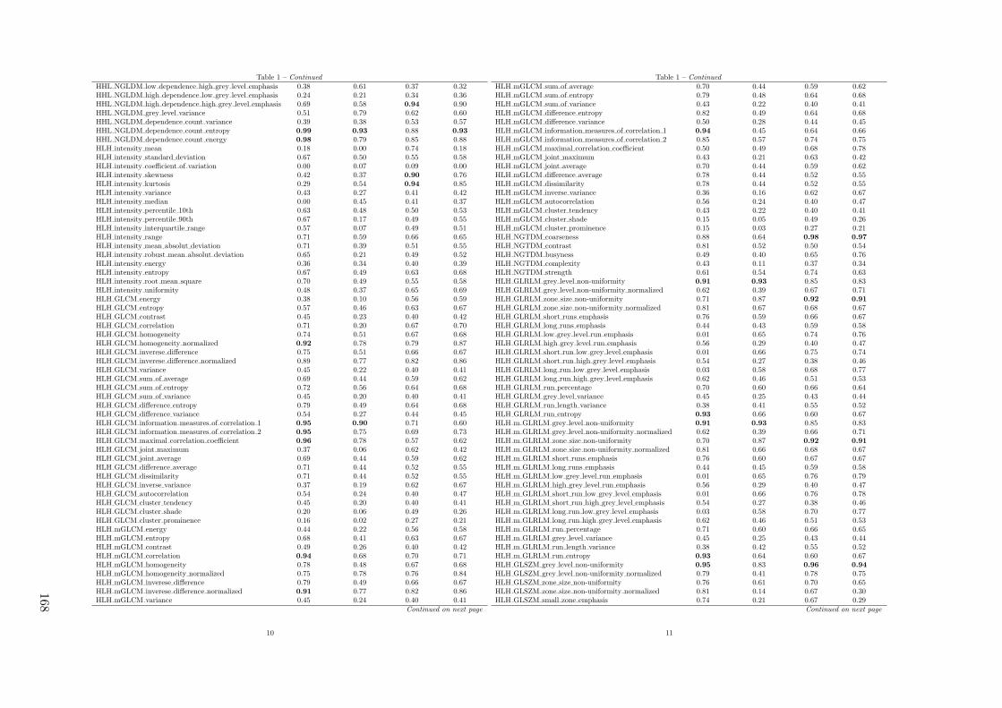
Table 1 – Continued
HHL NGLDM low dependence high grey level emphasis 0.38 0.61 0.37 0.32HHL NGLDM high dependence low grey level emphasis 0.24 0.21 0.34 0.36HHL NGLDM high dependence high grey level emphasis 0.69 0.58 0.94 0.90HHL NGLDM grey level variance 0.51 0.79 0.62 0.60HHL NGLDM dependence count variance 0.39 0.38 0.53 0.57HHL NGLDM dependence count entropy 0.99 0.93 0.88 0.93
HHL NGLDM dependence count energy 0.98 0.79 0.85 0.88HLH intensity mean 0.18 0.00 0.74 0.18HLH intensity standard deviation 0.67 0.50 0.55 0.58HLH intensity coefficient of variation 0.00 0.07 0.09 0.00HLH intensity skewness 0.42 0.37 0.90 0.76HLH intensity kurtosis 0.29 0.54 0.94 0.85HLH intensity variance 0.43 0.27 0.41 0.42HLH intensity median 0.00 0.45 0.41 0.37HLH intensity percentile 10th 0.63 0.48 0.50 0.53HLH intensity percentile 90th 0.67 0.17 0.49 0.55HLH intensity interquartile range 0.57 0.07 0.49 0.51HLH intensity range 0.71 0.59 0.66 0.65HLH intensity mean absolut deviation 0.71 0.39 0.51 0.55HLH intensity robust mean absolut deviation 0.65 0.21 0.49 0.52HLH intensity energy 0.36 0.34 0.40 0.39HLH intensity entropy 0.67 0.49 0.63 0.68HLH intensity root mean square 0.70 0.49 0.55 0.58HLH intensity uniformity 0.48 0.37 0.65 0.69HLH GLCM energy 0.38 0.10 0.56 0.59HLH GLCM entropy 0.57 0.46 0.63 0.67HLH GLCM contrast 0.45 0.23 0.40 0.42HLH GLCM correlation 0.71 0.20 0.67 0.70HLH GLCM homogeneity 0.74 0.51 0.67 0.68HLH GLCM homogeneity normalized 0.92 0.78 0.79 0.87HLH GLCM inverese difference 0.75 0.51 0.66 0.67HLH GLCM inverese difference normalized 0.89 0.77 0.82 0.86HLH GLCM variance 0.45 0.22 0.40 0.41HLH GLCM sum of average 0.69 0.44 0.59 0.62HLH GLCM sum of entropy 0.72 0.56 0.64 0.68HLH GLCM sum of variance 0.45 0.20 0.40 0.41HLH GLCM difference entropy 0.79 0.49 0.64 0.68HLH GLCM difference variance 0.54 0.27 0.44 0.45HLH GLCM information measures of correlation 1 0.95 0.90 0.71 0.60HLH GLCM information measures of correlation 2 0.95 0.75 0.69 0.73HLH GLCM maximal correlation coefficient 0.96 0.78 0.57 0.62HLH GLCM joint maximum 0.37 0.06 0.62 0.42HLH GLCM joint average 0.69 0.44 0.59 0.62HLH GLCM difference average 0.71 0.44 0.52 0.55HLH GLCM dissimilarity 0.71 0.44 0.52 0.55HLH GLCM inverse variance 0.37 0.19 0.62 0.67HLH GLCM autocorrelation 0.54 0.24 0.40 0.47HLH GLCM cluster tendency 0.45 0.20 0.40 0.41HLH GLCM cluster shade 0.20 0.06 0.49 0.26HLH GLCM cluster prominence 0.16 0.02 0.27 0.21HLH mGLCM energy 0.44 0.22 0.56 0.58HLH mGLCM entropy 0.68 0.41 0.63 0.67HLH mGLCM contrast 0.49 0.26 0.40 0.42HLH mGLCM correlation 0.94 0.68 0.70 0.71HLH mGLCM homogeneity 0.78 0.48 0.67 0.68HLH mGLCM homogeneity normalized 0.75 0.78 0.76 0.84HLH mGLCM inverese difference 0.79 0.49 0.66 0.67HLH mGLCM inverese difference normalized 0.91 0.77 0.82 0.86HLH mGLCM variance 0.45 0.24 0.40 0.41
Continued on next page
10
Table 1 – Continued
HLH mGLCM sum of average 0.70 0.44 0.59 0.62HLH mGLCM sum of entropy 0.79 0.48 0.64 0.68HLH mGLCM sum of variance 0.43 0.22 0.40 0.41HLH mGLCM difference entropy 0.82 0.49 0.64 0.68HLH mGLCM difference variance 0.50 0.28 0.44 0.45HLH mGLCM information measures of correlation 1 0.94 0.45 0.64 0.66HLH mGLCM information measures of correlation 2 0.85 0.57 0.74 0.75HLH mGLCM maximal correlation coefficient 0.50 0.49 0.68 0.78HLH mGLCM joint maximum 0.43 0.21 0.63 0.42HLH mGLCM joint average 0.70 0.44 0.59 0.62HLH mGLCM difference average 0.78 0.44 0.52 0.55HLH mGLCM dissimilarity 0.78 0.44 0.52 0.55HLH mGLCM inverse variance 0.36 0.16 0.62 0.67HLH mGLCM autocorrelation 0.56 0.24 0.40 0.47HLH mGLCM cluster tendency 0.43 0.22 0.40 0.41HLH mGLCM cluster shade 0.15 0.05 0.49 0.26HLH mGLCM cluster prominence 0.15 0.03 0.27 0.21HLH NGTDM coarseness 0.88 0.64 0.98 0.97
HLH NGTDM contrast 0.81 0.52 0.50 0.54HLH NGTDM busyness 0.49 0.40 0.65 0.76HLH NGTDM complexity 0.43 0.11 0.37 0.34HLH NGTDM strength 0.61 0.54 0.74 0.63HLH GLRLM grey level non-uniformity 0.91 0.93 0.85 0.83HLH GLRLM grey level non-uniformity normalized 0.62 0.39 0.67 0.71HLH GLRLM zone size non-uniformity 0.71 0.87 0.92 0.91
HLH GLRLM zone size non-uniformity normalized 0.81 0.67 0.68 0.67HLH GLRLM short runs emphasis 0.76 0.59 0.66 0.67HLH GLRLM long runs emphasis 0.44 0.43 0.59 0.58HLH GLRLM low grey level run emphasis 0.01 0.65 0.74 0.76HLH GLRLM high grey level run emphasis 0.56 0.29 0.40 0.47HLH GLRLM short run low grey level emphasis 0.01 0.66 0.75 0.74HLH GLRLM short run high grey level emphasis 0.54 0.27 0.38 0.46HLH GLRLM long run low grey level emphasis 0.03 0.58 0.68 0.77HLH GLRLM long run high grey level emphasis 0.62 0.46 0.51 0.53HLH GLRLM run percentage 0.70 0.60 0.66 0.64HLH GLRLM grey level variance 0.45 0.25 0.43 0.44HLH GLRLM run length variance 0.38 0.41 0.55 0.52HLH GLRLM run entropy 0.93 0.66 0.60 0.67HLH m GLRLM grey level non-uniformity 0.91 0.93 0.85 0.83HLH m GLRLM grey level non-uniformity normalized 0.62 0.39 0.66 0.71HLH m GLRLM zone size non-uniformity 0.70 0.87 0.92 0.91
HLH m GLRLM zone size non-uniformity normalized 0.81 0.66 0.68 0.67HLH m GLRLM short runs emphasis 0.76 0.60 0.67 0.67HLH m GLRLM long runs emphasis 0.44 0.45 0.59 0.58HLH m GLRLM low grey level run emphasis 0.01 0.65 0.76 0.79HLH m GLRLM high grey level run emphasis 0.56 0.29 0.40 0.47HLH m GLRLM short run low grey level emphasis 0.01 0.66 0.76 0.78HLH m GLRLM short run high grey level emphasis 0.54 0.27 0.38 0.46HLH m GLRLM long run low grey level emphasis 0.03 0.58 0.70 0.77HLH m GLRLM long run high grey level emphasis 0.62 0.46 0.51 0.53HLH m GLRLM run percentage 0.71 0.60 0.66 0.65HLH m GLRLM grey level variance 0.45 0.25 0.43 0.44HLH m GLRLM run length variance 0.38 0.42 0.55 0.52HLH m GLRLM run entropy 0.93 0.64 0.60 0.67HLH GLSZM grey level non-uniformity 0.95 0.83 0.96 0.94
HLH GLSZM grey level non-uniformity normalized 0.79 0.41 0.78 0.75HLH GLSZM zone size non-uniformity 0.76 0.61 0.70 0.65HLH GLSZM zone size non-uniformity normalized 0.81 0.14 0.67 0.30HLH GLSZM small zone emphasis 0.74 0.21 0.67 0.29
Continued on next page
11
168

Table 1 – Continued
HLH GLSZM large zone emphasis 0.66 0.56 0.44 0.48HLH GLSZM low grey level zone emphasis 0.00 0.61 0.67 0.73HLH GLSZM high grey level zone emphasis 0.58 0.45 0.40 0.47HLH GLSZM small zone low grey level emphasis 0.00 0.47 0.64 0.73HLH GLSZM small zone high grey level emphasis 0.57 0.46 0.41 0.47HLH GLSZM large zone low grey level emphasis 0.40 0.32 0.21 0.42HLH GLSZM large zone high grey level emphasis 0.75 0.87 0.78 0.60HLH GLSZM zone percentage 0.96 0.70 0.55 0.58HLH GLSZM grey level variance 0.58 0.36 0.60 0.59HLH GLSZM zone size variance 0.66 0.57 0.44 0.48HLH GLSZM zone size entropy 0.91 0.63 0.63 0.70HLH GLDZM grey level non-uniformity 0.95 0.83 0.96 0.94
HLH GLDZM grey level non-uniformity normalized 0.79 0.41 0.78 0.74HLH GLDZM zone size non-uniformity 0.91 0.80 0.66 0.67HLH GLDZM zone size non-uniformity normalized 0.67 0.02 0.96 0.92
HLH GLDZM small distance emphasis 0.64 0.00 0.94 0.91
HLH GLDZM large distance emphasis 0.60 0.03 0.99 0.98
HLH GLDZM low grey level zone emphasis 0.00 0.61 0.69 0.76HLH GLDZM high grey level zone emphasis 0.58 0.45 0.40 0.47HLH GLDZM small distance low grey level emphasis 0.00 0.65 0.71 0.75HLH GLDZM small distance high grey level emphasis 0.58 0.46 0.41 0.48HLH GLDZM large distance low grey level emphasis 0.00 0.33 0.50 0.76HLH GLDZM large distance high grey level emphasis 0.49 0.39 0.47 0.58HLH GLDZM zone percentage 0.96 0.70 0.55 0.58HLH GLDZM grey level variance 0.58 0.36 0.60 0.59HLH GLDZM zone distance variance 0.58 0.10 0.99 0.99
HLH GLDZM zone distance entropy 0.82 0.64 0.83 0.81HLH NGLDM grey level non-uniformity 0.78 0.79 0.75 0.74HLH NGLDM grey level non-uniformity normalized 0.54 0.34 0.66 0.68HLH NGLDM dependence count non-uniformity 0.65 0.65 0.64 0.59HLH NGLDM dependence count non-uniformity normalized
0.95 0.67 0.56 0.55
HLH NGLDM low dependence emphasis 0.94 0.51 0.59 0.61HLH NGLDM high dependence emphasis 0.53 0.41 0.57 0.54HLH NGLDM low grey level count emphasis 0.01 0.65 0.76 0.79HLH NGLDM high grey level count emphasis 0.55 0.27 0.40 0.47HLH NGLDM low dependence low grey level emphasis 0.04 0.56 0.70 0.72HLH NGLDM low dependence high grey level emphasis 0.42 0.22 0.27 0.34HLH NGLDM high dependence low grey level emphasis 0.64 0.37 0.54 0.62HLH NGLDM high dependence high grey level emphasis 0.56 0.64 0.85 0.79HLH NGLDM grey level variance 0.43 0.24 0.41 0.42HLH NGLDM dependence count variance 0.50 0.39 0.55 0.44HLH NGLDM dependence count entropy 0.98 0.86 0.57 0.72HLH NGLDM dependence count energy 1.00 0.72 0.59 0.74HLL intensity mean 0.79 0.43 0.89 0.82HLL intensity standard deviation 0.83 0.73 0.93 0.92
HLL intensity coefficient of variation 0.25 0.00 0.92 0.81HLL intensity skewness 0.89 0.59 0.97 0.87HLL intensity kurtosis 0.51 0.58 0.79 0.82HLL intensity variance 0.76 0.65 0.84 0.81HLL intensity median 0.62 0.63 0.93 0.90HLL intensity percentile 10th 0.92 0.79 0.89 0.85HLL intensity percentile 90th 0.77 0.29 0.87 0.89HLL intensity interquartile range 0.91 0.83 0.87 0.82HLL intensity range 0.76 0.66 0.80 0.69HLL intensity mean absolut deviation 0.87 0.77 0.90 0.87HLL intensity robust mean absolut deviation 0.96 0.88 0.87 0.84HLL intensity energy 0.86 0.82 0.86 0.85HLL intensity entropy 0.90 0.73 0.92 0.92
Continued on next page
12
Table 1 – Continued
HLL intensity root mean square 0.84 0.70 0.93 0.92
HLL intensity uniformity 0.83 0.48 0.82 0.85HLL GLCM energy 0.48 0.44 0.61 0.64HLL GLCM entropy 0.76 0.67 0.88 0.89HLL GLCM contrast 0.76 0.71 0.85 0.81HLL GLCM correlation 0.71 0.72 0.66 0.77HLL GLCM homogeneity 0.83 0.80 0.86 0.86HLL GLCM homogeneity normalized 0.93 0.85 0.70 0.91
HLL GLCM inverese difference 0.85 0.84 0.88 0.88HLL GLCM inverese difference normalized 0.94 0.84 0.83 0.91
HLL GLCM variance 0.74 0.69 0.84 0.81HLL GLCM sum of average 0.88 0.85 0.71 0.74HLL GLCM sum of entropy 0.89 0.85 0.92 0.92
HLL GLCM sum of variance 0.71 0.68 0.83 0.80HLL GLCM difference entropy 0.88 0.83 0.92 0.93
HLL GLCM difference variance 0.74 0.70 0.87 0.86HLL GLCM information measures of correlation 1 0.97 0.97 0.96 0.89HLL GLCM information measures of correlation 2 0.98 0.76 0.98 0.96
HLL GLCM maximal correlation coefficient 0.96 0.86 0.60 0.48HLL GLCM joint maximum 0.51 0.05 0.54 0.59HLL GLCM joint average 0.88 0.85 0.71 0.74HLL GLCM difference average 0.92 0.89 0.89 0.87HLL GLCM dissimilarity 0.92 0.89 0.89 0.87HLL GLCM inverse variance 0.71 0.83 0.87 0.88HLL GLCM autocorrelation 0.80 0.75 0.59 0.57HLL GLCM cluster tendency 0.71 0.68 0.83 0.80HLL GLCM cluster shade 0.64 0.57 0.63 0.67HLL GLCM cluster prominence 0.49 0.44 0.51 0.55HLL mGLCM energy 0.74 0.16 0.65 0.69HLL mGLCM entropy 0.85 0.63 0.90 0.91
HLL mGLCM contrast 0.78 0.70 0.84 0.81HLL mGLCM correlation 0.90 0.86 0.38 0.70HLL mGLCM homogeneity 0.83 0.75 0.86 0.86HLL mGLCM homogeneity normalized 0.72 0.83 0.77 0.89HLL mGLCM inverese difference 0.85 0.79 0.88 0.88HLL mGLCM inverese difference normalized 0.88 0.81 0.81 0.91
HLL mGLCM variance 0.79 0.68 0.84 0.81HLL mGLCM sum of average 0.86 0.85 0.71 0.74HLL mGLCM sum of entropy 0.91 0.87 0.92 0.93
HLL mGLCM sum of variance 0.79 0.67 0.83 0.80HLL mGLCM difference entropy 0.93 0.92 0.92 0.93
HLL mGLCM difference variance 0.71 0.67 0.87 0.86HLL mGLCM information measures of correlation 1 0.98 0.62 0.93 0.77HLL mGLCM information measures of correlation 2 0.94 0.77 0.93 0.84HLL mGLCM maximal correlation coefficient 0.87 0.59 0.92 0.85HLL mGLCM joint maximum 0.60 0.12 0.57 0.60HLL mGLCM joint average 0.86 0.85 0.71 0.74HLL mGLCM difference average 0.89 0.88 0.89 0.87HLL mGLCM dissimilarity 0.89 0.88 0.89 0.87HLL mGLCM inverse variance 0.81 0.81 0.87 0.88HLL mGLCM autocorrelation 0.80 0.75 0.59 0.57HLL mGLCM cluster tendency 0.79 0.67 0.83 0.80HLL mGLCM cluster shade 0.47 0.52 0.64 0.67HLL mGLCM cluster prominence 0.54 0.42 0.51 0.55HLL NGTDM coarseness 0.92 0.82 1.00 1.00
HLL NGTDM contrast 0.41 0.20 0.85 0.88HLL NGTDM busyness 0.97 0.40 0.82 0.82HLL NGTDM complexity 0.79 0.64 0.68 0.63HLL NGTDM strength 0.73 0.50 0.80 0.74
Continued on next page
13
Impact
ofC
Tcon
volution
kernel
onrob
ustn
essof
radiom
icfeatu
resfo
rdiff
erent
lung
diseases
and
tissue
types
169
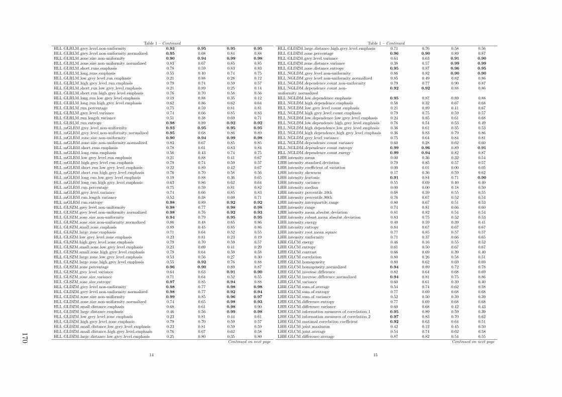
Table 1 – Continued
HLL GLRLM grey level non-uniformity 0.93 0.95 0.95 0.95
HLL GLRLM grey level non-uniformity normalized 0.95 0.68 0.84 0.88HLL GLRLM zone size non-uniformity 0.90 0.94 0.99 0.98
HLL GLRLM zone size non-uniformity normalized 0.83 0.67 0.85 0.85HLL GLRLM short runs emphasis 0.78 0.59 0.83 0.83HLL GLRLM long runs emphasis 0.55 0.40 0.74 0.75HLL GLRLM low grey level run emphasis 0.21 0.88 0.28 0.12HLL GLRLM high grey level run emphasis 0.79 0.74 0.59 0.57HLL GLRLM short run low grey level emphasis 0.21 0.89 0.25 0.14HLL GLRLM short run high grey level emphasis 0.76 0.70 0.58 0.56HLL GLRLM long run low grey level emphasis 0.19 0.88 0.35 0.12HLL GLRLM long run high grey level emphasis 0.62 0.86 0.62 0.64HLL GLRLM run percentage 0.75 0.59 0.81 0.81HLL GLRLM grey level variance 0.74 0.66 0.85 0.83HLL GLRLM run length variance 0.51 0.38 0.69 0.71HLL GLRLM run entropy 0.98 0.89 0.92 0.92
HLL mGLRM grey level non-uniformity 0.93 0.95 0.95 0.95
HLL mGLRM grey level non-uniformity normalized 0.95 0.68 0.86 0.89HLL mGLRM zone size non-uniformity 0.90 0.94 0.99 0.98
HLL mGLRM zone size non-uniformity normalized 0.83 0.67 0.85 0.85HLL mGLRM short runs emphasis 0.78 0.61 0.83 0.84HLL mGLRM long runs emphasis 0.56 0.43 0.74 0.75HLL mGLRM low grey level run emphasis 0.21 0.88 0.41 0.67HLL mGLRM high grey level run emphasis 0.79 0.74 0.59 0.57HLL mGLRM short run low grey level emphasis 0.22 0.89 0.42 0.67HLL mGLRM short run high grey level emphasis 0.76 0.70 0.58 0.56HLL mGLRM long run low grey level emphasis 0.19 0.88 0.36 0.65HLL mGLRM long run high grey level emphasis 0.63 0.86 0.62 0.64HLL mGLRM run percentage 0.75 0.59 0.81 0.82HLL mGLRM grey level variance 0.74 0.66 0.85 0.83HLL mGLRM run length variance 0.52 0.38 0.69 0.71HLL mGLRM run entropy 0.98 0.89 0.92 0.92
HLL GLSZM grey level non-uniformity 0.98 0.77 0.98 0.98
HLL GLSZM grey level non-uniformity normalized 0.98 0.76 0.92 0.93
HLL GLSZM zone size non-uniformity 0.94 0.79 0.95 0.95
HLL GLSZM zone size non-uniformity normalized 0.86 0.48 0.85 0.86HLL GLSZM small zone emphasis 0.89 0.45 0.85 0.86HLL GLSZM large zone emphasis 0.71 0.64 0.52 0.55HLL GLSZM low grey level zone emphasis 0.23 0.81 0.23 0.19HLL GLSZM high grey level zone emphasis 0.79 0.70 0.59 0.57HLL GLSZM small zone low grey level emphasis 0.23 0.69 0.41 0.29HLL GLSZM small zone high grey level emphasis 0.79 0.64 0.59 0.58HLL GLSZM large zone low grey level emphasis 0.53 0.56 0.27 0.30HLL GLSZM large zone high grey level emphasis 0.55 0.92 0.76 0.88HLL GLSZM zone percentage 0.96 0.90 0.89 0.87HLL GLSZM grey level variance 0.64 0.63 0.91 0.90
HLL GLSZM zone size variance 0.71 0.64 0.52 0.55HLL GLSZM zone size entropy 0.97 0.85 0.94 0.88HLL GLDZM grey level non-uniformity 0.98 0.77 0.98 0.98
HLL GLDZM grey level non-uniformity normalized 0.98 0.77 0.92 0.94
HLL GLDZM zone size non-uniformity 0.99 0.85 0.96 0.97
HLL GLDZM zone size non-uniformity normalized 0.74 0.65 0.98 0.93
HLL GLDZM small distance emphasis 0.68 0.61 0.98 0.90HLL GLDZM large distance emphasis 0.46 0.56 0.99 0.98
HLL GLDZM low grey level zone emphasis 0.23 0.81 0.44 0.61HLL GLDZM high grey level zone emphasis 0.79 0.70 0.59 0.57HLL GLDZM small distance low grey level emphasis 0.23 0.81 0.59 0.59HLL GLDZM small distance high grey level emphasis 0.76 0.67 0.62 0.58HLL GLDZM large distance low grey level emphasis 0.25 0.80 0.35 0.80
Continued on next page
14
Table 1 – Continued
HLL GLDZM large distance high grey level emphasis 0.71 0.76 0.58 0.56HLL GLDZM zone percentage 0.96 0.90 0.89 0.87HLL GLDZM grey level variance 0.64 0.63 0.91 0.90
HLL GLDZM zone distance variance 0.38 0.57 0.99 0.99
HLL GLDZM zone distance entropy 0.95 0.87 0.96 0.95
HLL NGLDM grey level non-uniformity 0.86 0.82 0.90 0.90
HLL NGLDM grey level non-uniformity normalized 0.85 0.49 0.82 0.86HLL NGLDM dependence count non-uniformity 0.79 0.77 0.90 0.87HLL NGLDM dependence count non-uniformity normalized
0.92 0.92 0.88 0.86
HLL NGLDM low dependence emphasis 0.95 0.87 0.89 0.88HLL NGLDM high dependence emphasis 0.58 0.32 0.67 0.68HLL NGLDM low grey level count emphasis 0.21 0.89 0.41 0.67HLL NGLDM high grey level count emphasis 0.79 0.75 0.59 0.57HLL NGLDM low dependence low grey level emphasis 0.24 0.85 0.61 0.68HLL NGLDM low dependence high grey level emphasis 0.76 0.54 0.53 0.49HLL NGLDM high dependence low grey level emphasis 0.36 0.61 0.35 0.53HLL NGLDM high dependence high grey level emphasis 0.36 0.83 0.79 0.86HLL NGLDM grey level variance 0.75 0.64 0.84 0.81HLL NGLDM dependence count variance 0.60 0.28 0.62 0.60HLL NGLDM dependence count entropy 0.99 0.96 0.89 0.91
HLL NGLDM dependence count energy 0.99 0.94 0.82 0.87LHH intensity mean 0.00 0.36 0.32 0.54LHH intensity standard deviation 0.79 0.85 0.57 0.57LHH intensity coefficient of variation 0.00 0.01 0.00 0.05LHH intensity skewness 0.17 0.36 0.59 0.62LHH intensity kurtosis 0.91 0.84 0.71 0.90
LHH intensity variance 0.55 0.69 0.40 0.40LHH intensity median 0.00 0.00 0.18 0.50LHH intensity percentile 10th 0.68 0.59 0.55 0.55LHH intensity percentile 90th 0.76 0.67 0.52 0.54LHH intensity interquartile range 0.80 0.67 0.51 0.53LHH intensity range 0.74 0.81 0.66 0.60LHH intensity mean absolut deviation 0.81 0.82 0.54 0.54LHH intensity robust mean absolut deviation 0.83 0.75 0.52 0.53LHH intensity energy 0.40 0.59 0.39 0.41LHH intensity entropy 0.84 0.67 0.67 0.67LHH intensity root mean square 0.77 0.85 0.57 0.57LHH intensity uniformity 0.71 0.37 0.66 0.65LHH GLCM energy 0.46 0.16 0.55 0.52LHH GLCM entropy 0.61 0.50 0.67 0.67LHH GLCM contrast 0.66 0.69 0.39 0.40LHH GLCM correlation 0.80 0.26 0.58 0.51LHH GLCM homogeneity 0.80 0.62 0.69 0.69LHH GLCM homogeneity normalized 0.94 0.89 0.72 0.78LHH GLCM inverese difference 0.82 0.64 0.68 0.69LHH GLCM inverese difference normalized 0.94 0.81 0.75 0.86LHH GLCM variance 0.60 0.61 0.39 0.40LHH GLCM sum of average 0.54 0.74 0.62 0.58LHH GLCM sum of entropy 0.77 0.69 0.68 0.68LHH GLCM sum of variance 0.52 0.50 0.39 0.39LHH GLCM difference entropy 0.77 0.69 0.68 0.68LHH GLCM difference variance 0.60 0.68 0.42 0.43LHH GLCM information measures of correlation 1 0.95 0.89 0.59 0.39LHH GLCM information measures of correlation 2 0.97 0.83 0.70 0.62LHH GLCM maximal correlation coefficient 0.92 0.63 0.64 0.51LHH GLCM joint maximum 0.42 0.12 0.45 0.50LHH GLCM joint average 0.54 0.74 0.62 0.58LHH GLCM difference average 0.87 0.82 0.54 0.55
Continued on next page
15
170

Table 1 – Continued
LHH GLCM dissimilarity 0.87 0.82 0.54 0.55LHH GLCM inverse variance 0.68 0.27 0.66 0.67LHH GLCM autocorrelation 0.39 0.67 0.46 0.42LHH GLCM cluster tendency 0.52 0.50 0.39 0.39LHH GLCM cluster shade 0.38 0.39 0.30 0.22LHH GLCM cluster prominence 0.17 0.22 0.18 0.20LHH mGLCM energy 0.61 0.11 0.53 0.52LHH mGLCM entropy 0.79 0.58 0.67 0.67LHH mGLCM contrast 0.55 0.71 0.39 0.40LHH mGLCM correlation 0.94 0.87 0.59 0.50LHH mGLCM homogeneity 0.83 0.61 0.69 0.69LHH mGLCM homogeneity normalized 0.90 0.89 0.71 0.82LHH mGLCM inverese difference 0.84 0.63 0.68 0.69LHH mGLCM inverese difference normalized 0.93 0.80 0.73 0.87LHH mGLCM variance 0.54 0.69 0.39 0.40LHH mGLCM sum of average 0.58 0.74 0.62 0.58LHH mGLCM sum of entropy 0.89 0.69 0.68 0.68LHH mGLCM sum of variance 0.52 0.66 0.39 0.39LHH mGLCM difference entropy 0.90 0.77 0.68 0.68LHH mGLCM difference variance 0.49 0.72 0.42 0.43LHH mGLCM information measures of correlation 1 0.77 0.56 0.59 0.66LHH mGLCM information measures of correlation 2 0.79 0.69 0.66 0.73LHH mGLCM maximal correlation coefficient 0.51 0.42 0.69 0.85LHH mGLCM joint maximum 0.52 0.19 0.45 0.51LHH mGLCM joint average 0.58 0.74 0.62 0.58LHH mGLCM difference average 0.79 0.82 0.54 0.55LHH mGLCM dissimilarity 0.79 0.82 0.54 0.55LHH mGLCM inverse variance 0.82 0.40 0.66 0.67LHH mGLCM autocorrelation 0.42 0.67 0.46 0.42LHH mGLCM cluster tendency 0.52 0.66 0.39 0.39LHH mGLCM cluster shade 0.35 0.39 0.30 0.22LHH mGLCM cluster prominence 0.18 0.28 0.18 0.20LHH NGTDM coarseness 0.78 0.50 0.98 0.98
LHH NGTDM contrast 0.52 0.60 0.43 0.53LHH NGTDM busyness 0.62 0.33 0.50 0.49LHH NGTDM complexity 0.43 0.43 0.34 0.33LHH NGTDM strength 0.67 0.78 0.67 0.55LHH GLRLM grey level non-uniformity 0.94 0.93 0.85 0.83LHH GLRLM grey level non-uniformity normalized 0.78 0.38 0.68 0.68LHH GLRLM zone size non-uniformity 0.83 0.90 0.92 0.91
LHH GLRLM zone size non-uniformity normalized 0.85 0.68 0.67 0.68LHH GLRLM short runs emphasis 0.81 0.54 0.67 0.67LHH GLRLM long runs emphasis 0.65 0.46 0.57 0.59LHH GLRLM low grey level run emphasis 0.74 0.21 0.35 0.54LHH GLRLM high grey level run emphasis 0.44 0.67 0.46 0.42LHH GLRLM short run low grey level emphasis 0.76 0.30 0.41 0.47LHH GLRLM short run high grey level emphasis 0.43 0.65 0.44 0.40LHH GLRLM long run low grey level emphasis 0.61 0.07 0.38 0.39LHH GLRLM long run high grey level emphasis 0.64 0.69 0.54 0.52LHH GLRLM run percentage 0.79 0.63 0.65 0.67LHH GLRLM grey level variance 0.54 0.71 0.41 0.41LHH GLRLM run length variance 0.59 0.50 0.51 0.54LHH GLRLM run entropy 0.96 0.80 0.65 0.65LHH mGLRLM grey level non-uniformity 0.94 0.93 0.85 0.83LHH mGLRLM grey level non-uniformity normalized 0.78 0.37 0.69 0.68LHH mGLRLM zone size non-uniformity 0.83 0.90 0.92 0.91
LHH mGLRLM zone size non-uniformity normalized 0.85 0.66 0.68 0.68LHH mGLRLM short runs emphasis 0.81 0.56 0.67 0.67LHH mGLRLM long runs emphasis 0.65 0.48 0.57 0.59
Continued on next page
16
Table 1 – Continued
LHH mGLRLM low grey level run emphasis 0.74 0.21 0.45 0.51LHH mGLRLM high grey level run emphasis 0.44 0.67 0.46 0.42LHH mGLRLM short run low grey level emphasis 0.75 0.29 0.47 0.53LHH mGLRLM short run high grey level emphasis 0.43 0.65 0.44 0.40LHH mGLRLM long run low grey level emphasis 0.61 0.08 0.38 0.42LHH mGLRLM long run high grey level emphasis 0.64 0.69 0.54 0.52LHH mGLRLM run percentage 0.79 0.63 0.65 0.66LHH mGLRLM grey level variance 0.54 0.71 0.41 0.41LHH mGLRLM run length variance 0.59 0.50 0.51 0.54LHH mGLRLM run entropy 0.96 0.79 0.65 0.65LHH GLSZM grey level non-uniformity 0.95 0.54 0.98 0.97
LHH GLSZM grey level non-uniformity normalized 0.86 0.48 0.71 0.74LHH GLSZM zone size non-uniformity 0.76 0.87 0.72 0.72LHH GLSZM zone size non-uniformity normalized 0.23 0.32 0.65 0.67LHH GLSZM small zone emphasis 0.07 0.23 0.63 0.66LHH GLSZM large zone emphasis 0.65 0.56 0.42 0.43LHH GLSZM low grey level zone emphasis 0.82 0.32 0.47 0.36LHH GLSZM high grey level zone emphasis 0.48 0.68 0.46 0.42LHH GLSZM small zone low grey level emphasis 0.90 0.29 0.39 0.31LHH GLSZM small zone high grey level emphasis 0.44 0.66 0.47 0.43LHH GLSZM large zone low grey level emphasis 0.17 0.05 0.16 0.12LHH GLSZM large zone high grey level emphasis 0.93 0.68 0.54 0.76LHH GLSZM zone percentage 0.93 0.77 0.59 0.57LHH GLSZM grey level variance 0.60 0.70 0.55 0.57LHH GLSZM zone size variance 0.66 0.54 0.42 0.43LHH GLSZM zone size entropy 0.97 0.72 0.70 0.72LHH GLDZM grey level non-uniformity 0.95 0.54 0.98 0.97
LHH GLDZM grey level non-uniformity normalized 0.86 0.48 0.71 0.74LHH GLDZM zone size non-uniformity 0.94 0.91 0.62 0.66LHH GLDZM zone size non-uniformity normalized 0.59 0.25 0.94 0.90
LHH GLDZM small distance emphasis 0.50 0.23 0.94 0.89LHH GLDZM large distance emphasis 0.49 0.23 0.98 0.98
LHH GLDZM low grey level zone emphasis 0.82 0.32 0.43 0.37LHH GLDZM high grey level zone emphasis 0.48 0.68 0.46 0.42LHH GLDZM small distance low grey level emphasis 0.82 0.33 0.48 0.40LHH GLDZM small distance high grey level emphasis 0.51 0.66 0.48 0.42LHH GLDZM large distance low grey level emphasis 0.81 0.27 0.34 0.20LHH GLDZM large distance high grey level emphasis 0.23 0.74 0.50 0.56LHH GLDZM zone percentage 0.93 0.77 0.59 0.57LHH GLDZM grey level variance 0.60 0.70 0.55 0.57LHH GLDZM zone distance variance 0.60 0.25 0.99 0.98
LHH GLDZM zone distance entropy 0.87 0.77 0.84 0.84LHH NGLDM grey level non-uniformity 0.84 0.79 0.74 0.73LHH NGLDM grey level non-uniformity normalized 0.71 0.35 0.66 0.65LHH NGLDM dependence count non-uniformity 0.62 0.77 0.63 0.62LHH NGLDM dependence count non-uniformity normalized
0.83 0.86 0.56 0.57
LHH NGLDM low dependence emphasis 0.85 0.72 0.63 0.61LHH NGLDM high dependence emphasis 0.64 0.44 0.53 0.55LHH NGLDM low grey level count emphasis 0.73 0.20 0.46 0.52LHH NGLDM high grey level count emphasis 0.43 0.67 0.46 0.42LHH NGLDM low dependence low grey level emphasis 0.94 0.67 0.61 0.47LHH NGLDM low dependence high grey level emphasis 0.40 0.59 0.32 0.28LHH NGLDM high dependence low grey level emphasis 0.06 0.00 0.25 0.27LHH NGLDM high dependence high grey level emphasis 0.87 0.49 0.76 0.87LHH NGLDM grey level variance 0.54 0.69 0.40 0.40LHH NGLDM dependence count variance 0.59 0.50 0.48 0.53LHH NGLDM dependence count entropy 0.99 0.93 0.69 0.62LHH NGLDM dependence count energy 0.88 0.83 0.68 0.60
Continued on next page
17
Impact
ofC
Tcon
volution
kernel
onrob
ustn
essof
radiom
icfeatu
resfo
rdiff
erent
lung
diseases
and
tissue
types
171

Table 1 – Continued
LHL intensity mean 0.95 0.58 0.95 0.97
LHL intensity standard deviation 0.85 0.90 0.92 0.91
LHL intensity coefficient of variation 0.22 0.05 0.90 0.90
LHL intensity skewness 0.77 0.52 0.90 0.95
LHL intensity kurtosis 0.94 0.81 0.94 0.92
LHL intensity variance 0.76 0.76 0.81 0.80LHL intensity median 0.91 0.78 0.92 0.91
LHL intensity percentile 10th 0.89 0.64 0.83 0.80LHL intensity percentile 90th 0.67 0.85 0.91 0.89LHL intensity interquartile range 0.86 0.94 0.79 0.77LHL intensity range 0.84 0.91 0.89 0.88LHL intensity mean absolut deviation 0.87 0.91 0.87 0.85LHL intensity robust mean absolut deviation 0.86 0.89 0.82 0.79LHL intensity energy 0.84 0.86 0.84 0.83LHL intensity entropy 0.90 0.77 0.91 0.90LHL intensity root mean square 0.89 0.92 0.92 0.91
LHL intensity uniformity 0.74 0.47 0.82 0.84LHL GLCM energy 0.44 0.38 0.54 0.64LHL GLCM entropy 0.79 0.79 0.87 0.86LHL GLCM contrast 0.82 0.74 0.78 0.76LHL GLCM correlation 0.92 0.57 0.90 0.87LHL GLCM homogeneity 0.86 0.87 0.84 0.86LHL GLCM homogeneity normalized 0.96 0.85 0.87 0.86LHL GLCM inverese difference 0.89 0.89 0.86 0.87LHL GLCM inverese difference normalized 0.98 0.91 0.93 0.90LHL GLCM variance 0.80 0.74 0.79 0.78LHL GLCM sum of average 0.77 0.83 0.91 0.82LHL GLCM sum of entropy 0.89 0.84 0.91 0.90LHL GLCM sum of variance 0.78 0.70 0.80 0.79LHL GLCM difference entropy 0.92 0.85 0.91 0.89LHL GLCM difference variance 0.83 0.69 0.84 0.83LHL GLCM information measures of correlation 1 0.98 0.96 0.92 0.89LHL GLCM information measures of correlation 2 0.99 0.71 0.96 0.92
LHL GLCM maximal correlation coefficient 0.96 0.84 0.61 0.74LHL GLCM joint maximum 0.42 0.11 0.58 0.62LHL GLCM joint average 0.77 0.83 0.91 0.82LHL GLCM difference average 0.95 0.92 0.84 0.82LHL GLCM dissimilarity 0.95 0.92 0.84 0.82LHL GLCM inverse variance 0.77 0.87 0.86 0.86LHL GLCM autocorrelation 0.61 0.70 0.82 0.68LHL GLCM cluster tendency 0.78 0.70 0.80 0.79LHL GLCM cluster shade 0.66 0.44 0.49 0.58LHL GLCM cluster prominence 0.46 0.43 0.56 0.58LHL mGLCM energy 0.52 0.15 0.63 0.67LHL mGLCM entropy 0.87 0.72 0.89 0.88LHL mGLCM contrast 0.74 0.73 0.78 0.76LHL mGLCM correlation 0.92 0.79 0.89 0.83LHL mGLCM homogeneity 0.78 0.86 0.84 0.86LHL mGLCM homogeneity normalized 0.73 0.85 0.89 0.87LHL mGLCM inverese difference 0.81 0.88 0.86 0.87LHL mGLCM inverese difference normalized 0.82 0.92 0.93 0.90
LHL mGLCM variance 0.73 0.74 0.79 0.78LHL mGLCM sum of average 0.80 0.83 0.91 0.82LHL mGLCM sum of entropy 0.92 0.89 0.91 0.90
LHL mGLCM sum of variance 0.72 0.73 0.80 0.79LHL mGLCM difference entropy 0.93 0.94 0.91 0.89LHL mGLCM difference variance 0.74 0.67 0.84 0.83LHL mGLCM information measures of correlation 1 0.93 0.77 0.83 0.83LHL mGLCM information measures of correlation 2 0.89 0.80 0.87 0.89
Continued on next page
18
Table 1 – Continued
LHL mGLCM maximal correlation coefficient 0.79 0.74 0.89 0.87LHL mGLCM joint maximum 0.46 0.23 0.58 0.63LHL mGLCM joint average 0.80 0.83 0.91 0.82LHL mGLCM difference average 0.84 0.91 0.84 0.82LHL mGLCM dissimilarity 0.84 0.91 0.84 0.82LHL mGLCM inverse variance 0.54 0.85 0.86 0.86LHL mGLCM autocorrelation 0.63 0.70 0.82 0.68LHL mGLCM cluster tendency 0.72 0.73 0.80 0.79LHL mGLCM cluster shade 0.67 0.35 0.49 0.58LHL mGLCM cluster prominence 0.44 0.37 0.56 0.58LHL NGTDM coarseness 0.46 0.93 0.99 0.99
LHL NGTDM contrast 0.60 0.35 0.82 0.73LHL NGTDM busyness 0.91 0.85 0.80 0.78LHL NGTDM complexity 0.75 0.83 0.69 0.68LHL NGTDM strength 0.84 0.80 0.88 0.82LHL GLRLM grey level non-uniformity 0.95 0.97 0.94 0.94
LHL GLRLM grey level non-uniformity normalized 0.86 0.64 0.85 0.87LHL GLRLM zone size non-uniformity 0.92 0.94 0.99 0.98
LHL GLRLM zone size non-uniformity normalized 0.85 0.78 0.81 0.86LHL GLRLM short runs emphasis 0.81 0.70 0.79 0.84LHL GLRLM long runs emphasis 0.50 0.44 0.73 0.77LHL GLRLM low grey level run emphasis 0.93 0.92 0.41 0.33LHL GLRLM high grey level run emphasis 0.63 0.73 0.82 0.68LHL GLRLM short run low grey level emphasis 0.93 0.93 0.19 0.29LHL GLRLM short run high grey level emphasis 0.63 0.74 0.81 0.67LHL GLRLM long run low grey level emphasis 0.93 0.90 0.32 0.43LHL GLRLM long run high grey level emphasis 0.73 0.58 0.87 0.75LHL GLRLM run percentage 0.76 0.68 0.79 0.82LHL GLRLM grey level variance 0.74 0.75 0.83 0.82LHL GLRLM run length variance 0.43 0.39 0.69 0.73LHL GLRLM run entropy 0.96 0.85 0.93 0.90
LHL mGLRLM grey level non-uniformity 0.95 0.97 0.94 0.94
LHL mGLRLM grey level non-uniformity normalized 0.86 0.64 0.85 0.86LHL mGLRLM zone size non-uniformity 0.92 0.94 0.99 0.98
LHL mGLRLM zone size non-uniformity normalized 0.85 0.78 0.81 0.86LHL mGLRLM short runs emphasis 0.81 0.70 0.79 0.84LHL mGLRLM long runs emphasis 0.51 0.45 0.73 0.77LHL mGLRLM low grey level run emphasis 0.93 0.93 0.69 0.56LHL mGLRLM high grey level run emphasis 0.63 0.73 0.82 0.68LHL mGLRLM short run low grey level emphasis 0.93 0.93 0.69 0.55LHL mGLRLM short run high grey level emphasis 0.63 0.74 0.81 0.67LHL mGLRLM long run low grey level emphasis 0.93 0.91 0.68 0.58LHL mGLRLM long run high grey level emphasis 0.73 0.58 0.87 0.75LHL mGLRLM run percentage 0.76 0.68 0.78 0.83LHL mGLRLM grey level variance 0.74 0.75 0.83 0.82LHL mGLRLM run length variance 0.44 0.40 0.70 0.73LHL mGLRLM run entropy 0.97 0.85 0.93 0.90
LHL GLSZM grey level non-uniformity 0.98 0.82 0.98 0.98
LHL GLSZM grey level non-uniformity normalized 0.97 0.69 0.92 0.87LHL GLSZM zone size non-uniformity 0.96 0.87 0.93 0.93
LHL GLSZM zone size non-uniformity normalized 0.57 0.52 0.84 0.84LHL GLSZM small zone emphasis 0.55 0.56 0.84 0.85LHL GLSZM large zone emphasis 0.68 0.69 0.49 0.53LHL GLSZM low grey level zone emphasis 0.92 0.90 0.27 0.37LHL GLSZM high grey level zone emphasis 0.60 0.71 0.83 0.68LHL GLSZM small zone low grey level emphasis 0.92 0.78 0.30 0.00LHL GLSZM small zone high grey level emphasis 0.59 0.69 0.83 0.69LHL GLSZM large zone low grey level emphasis 0.20 0.56 0.18 0.32LHL GLSZM large zone high grey level emphasis 0.87 0.59 0.80 0.82
Continued on next page
19
172
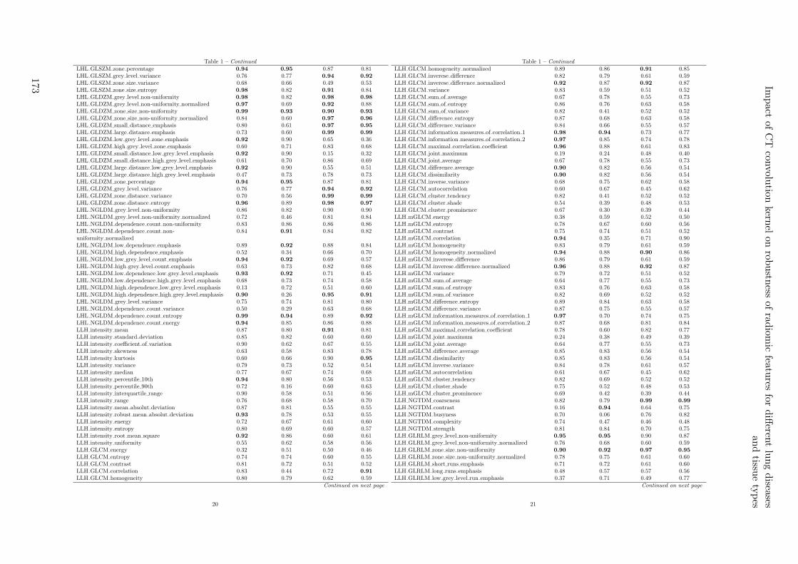
Table 1 – Continued
LHL GLSZM zone percentage 0.94 0.95 0.87 0.81LHL GLSZM grey level variance 0.76 0.77 0.94 0.92
LHL GLSZM zone size variance 0.68 0.66 0.49 0.53LHL GLSZM zone size entropy 0.98 0.82 0.91 0.84LHL GLDZM grey level non-uniformity 0.98 0.82 0.98 0.98
LHL GLDZM grey level non-uniformity normalized 0.97 0.69 0.92 0.88LHL GLDZM zone size non-uniformity 0.99 0.93 0.90 0.93
LHL GLDZM zone size non-uniformity normalized 0.84 0.60 0.97 0.96
LHL GLDZM small distance emphasis 0.80 0.61 0.97 0.95
LHL GLDZM large distance emphasis 0.73 0.60 0.99 0.99
LHL GLDZM low grey level zone emphasis 0.92 0.90 0.65 0.36LHL GLDZM high grey level zone emphasis 0.60 0.71 0.83 0.68LHL GLDZM small distance low grey level emphasis 0.92 0.90 0.15 0.32LHL GLDZM small distance high grey level emphasis 0.61 0.70 0.86 0.69LHL GLDZM large distance low grey level emphasis 0.92 0.90 0.55 0.51LHL GLDZM large distance high grey level emphasis 0.47 0.73 0.78 0.73LHL GLDZM zone percentage 0.94 0.95 0.87 0.81LHL GLDZM grey level variance 0.76 0.77 0.94 0.92
LHL GLDZM zone distance variance 0.70 0.56 0.99 0.99
LHL GLDZM zone distance entropy 0.96 0.89 0.98 0.97
LHL NGLDM grey level non-uniformity 0.86 0.82 0.90 0.90LHL NGLDM grey level non-uniformity normalized 0.72 0.46 0.81 0.84LHL NGLDM dependence count non-uniformity 0.83 0.86 0.86 0.86LHL NGLDM dependence count non-uniformity normalized
0.84 0.91 0.84 0.82
LHL NGLDM low dependence emphasis 0.89 0.92 0.88 0.84LHL NGLDM high dependence emphasis 0.52 0.34 0.66 0.70LHL NGLDM low grey level count emphasis 0.94 0.92 0.69 0.57LHL NGLDM high grey level count emphasis 0.63 0.73 0.82 0.68LHL NGLDM low dependence low grey level emphasis 0.93 0.92 0.71 0.45LHL NGLDM low dependence high grey level emphasis 0.68 0.73 0.74 0.58LHL NGLDM high dependence low grey level emphasis 0.13 0.72 0.51 0.60LHL NGLDM high dependence high grey level emphasis 0.90 0.26 0.95 0.91
LHL NGLDM grey level variance 0.75 0.74 0.81 0.80LHL NGLDM dependence count variance 0.50 0.29 0.63 0.68LHL NGLDM dependence count entropy 0.99 0.94 0.89 0.92
LHL NGLDM dependence count energy 0.94 0.85 0.86 0.88LLH intensity mean 0.87 0.80 0.91 0.81LLH intensity standard deviation 0.85 0.82 0.60 0.60LLH intensity coefficient of variation 0.90 0.62 0.67 0.55LLH intensity skewness 0.63 0.58 0.83 0.78LLH intensity kurtosis 0.60 0.66 0.90 0.95
LLH intensity variance 0.79 0.73 0.52 0.54LLH intensity median 0.77 0.67 0.74 0.68LLH intensity percentile 10th 0.94 0.80 0.56 0.53LLH intensity percentile 90th 0.72 0.16 0.60 0.63LLH intensity interquartile range 0.90 0.58 0.51 0.56LLH intensity range 0.76 0.68 0.58 0.70LLH intensity mean absolut deviation 0.87 0.81 0.55 0.55LLH intensity robust mean absolut deviation 0.93 0.78 0.53 0.55LLH intensity energy 0.72 0.67 0.61 0.60LLH intensity entropy 0.80 0.69 0.60 0.57LLH intensity root mean square 0.92 0.86 0.60 0.61LLH intensity uniformity 0.55 0.62 0.58 0.56LLH GLCM energy 0.32 0.51 0.50 0.46LLH GLCM entropy 0.74 0.74 0.60 0.55LLH GLCM contrast 0.81 0.72 0.51 0.52LLH GLCM correlation 0.83 0.44 0.72 0.91
LLH GLCM homogeneity 0.80 0.79 0.62 0.59Continued on next page
20
Table 1 – Continued
LLH GLCM homogeneity normalized 0.89 0.86 0.91 0.85LLH GLCM inverese difference 0.82 0.79 0.61 0.59LLH GLCM inverese difference normalized 0.92 0.87 0.92 0.87LLH GLCM variance 0.83 0.59 0.51 0.52LLH GLCM sum of average 0.67 0.78 0.55 0.73LLH GLCM sum of entropy 0.86 0.76 0.63 0.58LLH GLCM sum of variance 0.82 0.41 0.52 0.52LLH GLCM difference entropy 0.87 0.68 0.63 0.58LLH GLCM difference variance 0.84 0.66 0.55 0.57LLH GLCM information measures of correlation 1 0.98 0.94 0.73 0.77LLH GLCM information measures of correlation 2 0.97 0.85 0.74 0.78LLH GLCM maximal correlation coefficient 0.96 0.88 0.61 0.83LLH GLCM joint maximum 0.19 0.24 0.48 0.40LLH GLCM joint average 0.67 0.78 0.55 0.73LLH GLCM difference average 0.90 0.82 0.56 0.54LLH GLCM dissimilarity 0.90 0.82 0.56 0.54LLH GLCM inverse variance 0.68 0.75 0.62 0.58LLH GLCM autocorrelation 0.60 0.67 0.45 0.62LLH GLCM cluster tendency 0.82 0.41 0.52 0.52LLH GLCM cluster shade 0.54 0.39 0.48 0.53LLH GLCM cluster prominence 0.67 0.30 0.39 0.44LLH mGLCM energy 0.38 0.59 0.52 0.50LLH mGLCM entropy 0.78 0.67 0.60 0.56LLH mGLCM contrast 0.75 0.74 0.51 0.52LLH mGLCM correlation 0.94 0.35 0.71 0.90LLH mGLCM homogeneity 0.83 0.79 0.61 0.59LLH mGLCM homogeneity normalized 0.94 0.88 0.90 0.86LLH mGLCM inverese difference 0.86 0.79 0.61 0.59LLH mGLCM inverese difference normalized 0.96 0.88 0.92 0.87LLH mGLCM variance 0.79 0.72 0.51 0.52LLH mGLCM sum of average 0.64 0.77 0.55 0.73LLH mGLCM sum of entropy 0.83 0.76 0.63 0.58LLH mGLCM sum of variance 0.82 0.69 0.52 0.52LLH mGLCM difference entropy 0.89 0.84 0.63 0.58LLH mGLCM difference variance 0.87 0.75 0.55 0.57LLH mGLCM information measures of correlation 1 0.97 0.70 0.74 0.75LLH mGLCM information measures of correlation 2 0.87 0.68 0.81 0.84LLH mGLCM maximal correlation coefficient 0.78 0.60 0.82 0.77LLH mGLCM joint maximum 0.24 0.38 0.49 0.39LLH mGLCM joint average 0.64 0.77 0.55 0.73LLH mGLCM difference average 0.85 0.83 0.56 0.54LLH mGLCM dissimilarity 0.85 0.83 0.56 0.54LLH mGLCM inverse variance 0.84 0.78 0.61 0.57LLH mGLCM autocorrelation 0.61 0.67 0.45 0.62LLH mGLCM cluster tendency 0.82 0.69 0.52 0.52LLH mGLCM cluster shade 0.75 0.52 0.48 0.53LLH mGLCM cluster prominence 0.69 0.42 0.39 0.44LLH NGTDM coarseness 0.82 0.79 0.99 0.99
LLH NGTDM contrast 0.16 0.94 0.64 0.75LLH NGTDM busyness 0.70 0.06 0.76 0.82LLH NGTDM complexity 0.74 0.47 0.46 0.48LLH NGTDM strength 0.81 0.84 0.70 0.75LLH GLRLM grey level non-uniformity 0.95 0.95 0.90 0.87LLH GLRLM grey level non-uniformity normalized 0.76 0.68 0.60 0.59LLH GLRLM zone size non-uniformity 0.90 0.92 0.97 0.95
LLH GLRLM zone size non-uniformity normalized 0.78 0.75 0.61 0.60LLH GLRLM short runs emphasis 0.71 0.72 0.61 0.60LLH GLRLM long runs emphasis 0.48 0.57 0.57 0.56LLH GLRLM low grey level run emphasis 0.37 0.71 0.49 0.77
Continued on next page
21
Impact
ofC
Tcon
volution
kernel
onrob
ustn
essof
radiom
icfeatu
resfo
rdiff
erent
lung
diseases
and
tissue
types
173

Table 1 – Continued
LLH GLRLM high grey level run emphasis 0.60 0.68 0.45 0.62LLH GLRLM short run low grey level emphasis 0.37 0.73 0.25 0.79LLH GLRLM short run high grey level emphasis 0.59 0.68 0.43 0.60LLH GLRLM long run low grey level emphasis 0.36 0.64 0.48 0.86LLH GLRLM long run high grey level emphasis 0.73 0.57 0.54 0.70LLH GLRLM run percentage 0.70 0.69 0.61 0.59LLH GLRLM grey level variance 0.76 0.69 0.53 0.55LLH GLRLM run length variance 0.45 0.50 0.55 0.54LLH GLRLM run entropy 0.93 0.80 0.62 0.58LLH mGLRLM grey level non-uniformity 0.95 0.95 0.90 0.87LLH mGLRLM grey level non-uniformity normalized 0.77 0.68 0.60 0.58LLH mGLRLM zone size non-uniformity 0.90 0.92 0.97 0.95
LLH mGLRLM zone size non-uniformity normalized 0.78 0.75 0.62 0.60LLH mGLRLM short runs emphasis 0.72 0.73 0.61 0.59LLH mGLRLM long runs emphasis 0.48 0.59 0.57 0.56LLH mGLRLM low grey level run emphasis 0.37 0.71 0.75 0.89LLH mGLRLM high grey level run emphasis 0.60 0.68 0.45 0.62LLH mGLRLM short run low grey level emphasis 0.37 0.72 0.76 0.88LLH mGLRLM short run high grey level emphasis 0.59 0.68 0.43 0.60LLH mGLRLM long run low grey level emphasis 0.36 0.67 0.72 0.89LLH mGLRLM long run high grey level emphasis 0.72 0.57 0.54 0.70LLH mGLRLM run percentage 0.70 0.69 0.60 0.59LLH mGLRLM grey level variance 0.76 0.69 0.53 0.55LLH mGLRLM run length variance 0.45 0.51 0.55 0.54LLH mGLRLM run entropy 0.94 0.79 0.62 0.58LLH GLSZM grey level non-uniformity 0.96 0.70 0.99 0.97
LLH GLSZM grey level non-uniformity normalized 0.96 0.67 0.71 0.59LLH GLSZM zone size non-uniformity 0.93 0.81 0.82 0.82LLH GLSZM zone size non-uniformity normalized 0.61 0.48 0.59 0.77LLH GLSZM small zone emphasis 0.51 0.40 0.59 0.77LLH GLSZM large zone emphasis 0.59 0.68 0.50 0.49LLH GLSZM low grey level zone emphasis 0.36 0.69 0.63 0.76LLH GLSZM high grey level zone emphasis 0.60 0.68 0.45 0.63LLH GLSZM small zone low grey level emphasis 0.22 0.08 0.56 0.63LLH GLSZM small zone high grey level emphasis 0.64 0.69 0.46 0.64LLH GLSZM large zone low grey level emphasis 0.35 0.35 0.35 0.47LLH GLSZM large zone high grey level emphasis 0.91 0.56 0.84 0.60LLH GLSZM zone percentage 0.93 0.90 0.60 0.62LLH GLSZM grey level variance 0.75 0.68 0.64 0.70LLH GLSZM zone size variance 0.59 0.69 0.50 0.49LLH GLSZM zone size entropy 0.96 0.81 0.55 0.44LLH GLDZM grey level non-uniformity 0.96 0.74 0.99 0.97
LLH GLDZM grey level non-uniformity normalized 0.96 0.67 0.71 0.60LLH GLDZM zone size non-uniformity 0.98 0.88 0.84 0.86LLH GLDZM zone size non-uniformity normalized 0.79 0.04 0.95 0.90LLH GLDZM small distance emphasis 0.75 0.04 0.92 0.87LLH GLDZM large distance emphasis 0.57 0.04 0.99 0.98
LLH GLDZM low grey level zone emphasis 0.36 0.69 0.67 0.82LLH GLDZM high grey level zone emphasis 0.60 0.68 0.45 0.63LLH GLDZM small distance low grey level emphasis 0.37 0.69 0.61 0.70LLH GLDZM small distance high grey level emphasis 0.64 0.66 0.49 0.64LLH GLDZM large distance low grey level emphasis 0.34 0.66 0.72 0.87LLH GLDZM large distance high grey level emphasis 0.37 0.74 0.54 0.71LLH GLDZM zone percentage 0.93 0.90 0.60 0.62LLH GLDZM grey level variance 0.75 0.68 0.64 0.70LLH GLDZM zone distance variance 0.49 0.04 0.99 0.99
LLH GLDZM zone distance entropy 0.91 0.79 0.85 0.77LLH NGLDM grey level non-uniformity 0.82 0.85 0.83 0.80LLH NGLDM grey level non-uniformity normalized 0.59 0.61 0.58 0.56
Continued on next page
22
Table 1 – Continued
LLH NGLDM dependence count non-uniformity 0.75 0.73 0.74 0.66LLH NGLDM dependence count non-uniformity normalized
0.87 0.87 0.58 0.60
LLH NGLDM low dependence emphasis 0.88 0.85 0.62 0.64LLH NGLDM high dependence emphasis 0.48 0.50 0.54 0.53LLH NGLDM low grey level count emphasis 0.37 0.69 0.76 0.89LLH NGLDM high grey level count emphasis 0.60 0.68 0.45 0.62LLH NGLDM low dependence low grey level emphasis 0.19 0.51 0.70 0.78LLH NGLDM low dependence high grey level emphasis 0.71 0.67 0.35 0.48LLH NGLDM high dependence low grey level emphasis 0.13 0.48 0.54 0.74LLH NGLDM high dependence high grey level emphasis 0.76 0.26 0.84 0.75LLH NGLDM grey level variance 0.76 0.69 0.52 0.54LLH NGLDM dependence count variance 0.45 0.35 0.51 0.51LLH NGLDM dependence count entropy 0.99 0.93 0.55 0.55LLH NGLDM dependence count energy 0.98 0.85 0.50 0.50LLL intensity mean 0.97 0.73 0.99 0.99
LLL intensity standard deviation 0.95 0.58 0.91 0.91
LLL intensity coefficient of variation 0.00 0.41 0.97 0.96
LLL intensity skewness 0.91 0.75 0.99 0.99
LLL intensity kurtosis 0.98 0.61 0.99 0.99
LLL intensity variance 0.94 0.44 0.91 0.91
LLL intensity median 0.97 0.93 1.00 1.00
LLL intensity percentile 10th 0.95 0.30 0.99 1.00
LLL intensity percentile 90th 0.96 0.90 0.95 0.91
LLL intensity interquartile range 0.93 0.90 0.99 0.99
LLL intensity range 0.87 0.73 0.78 0.75LLL intensity mean absolut deviation 0.97 0.58 0.95 0.94
LLL intensity robust mean absolut deviation 0.97 0.82 0.97 0.97
LLL intensity energy 0.99 0.87 1.00 1.00
LLL intensity entropy 0.89 0.74 0.98 0.98
LLL intensity root mean square 0.96 0.47 1.00 1.00
LLL intensity uniformity 0.76 0.55 0.96 0.95
LLL GLCM energy 0.88 0.73 0.72 0.75LLL GLCM entropy 0.91 0.92 0.96 0.96
LLL GLCM contrast 0.95 0.63 0.93 0.89LLL GLCM correlation 0.89 0.63 0.99 0.98
LLL GLCM homogeneity 0.85 0.77 0.91 0.90
LLL GLCM homogeneity normalized 0.92 0.82 0.94 0.78LLL GLCM inverese difference 0.88 0.80 0.93 0.93
LLL GLCM inverese difference normalized 0.95 0.84 0.97 0.95
LLL GLCM variance 0.95 0.49 0.93 0.94
LLL GLCM sum of average 0.65 0.73 0.81 0.88LLL GLCM sum of entropy 0.97 0.91 0.99 0.98
LLL GLCM sum of variance 0.95 0.34 0.95 0.95
LLL GLCM difference entropy 0.96 0.83 0.95 0.95
LLL GLCM difference variance 0.90 0.61 0.97 0.94
LLL GLCM information measures of correlation 1 0.99 0.98 0.98 0.97
LLL GLCM information measures of correlation 2 1.00 0.89 0.98 0.98
LLL GLCM maximal correlation coefficient 0.93 0.79 0.92 0.90LLL GLCM joint maximum 0.51 0.51 0.82 0.87LLL GLCM joint average 0.65 0.73 0.81 0.88LLL GLCM difference average 0.97 0.79 0.94 0.94
LLL GLCM dissimilarity 0.97 0.79 0.94 0.94
LLL GLCM inverse variance 0.86 0.91 0.92 0.91
LLL GLCM autocorrelation 0.67 0.71 0.84 0.91
LLL GLCM cluster tendency 0.95 0.34 0.95 0.95
LLL GLCM cluster shade 0.89 0.58 0.97 0.95
LLL GLCM cluster prominence 0.91 0.46 0.95 0.94
LLL mGLCM energy 0.82 0.25 0.90 0.87Continued on next page
23
174
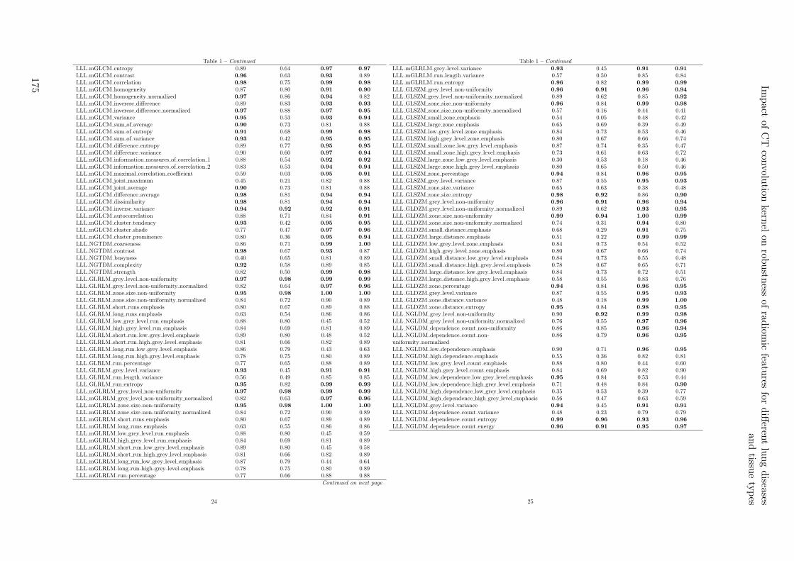
Table 1 – Continued
LLL mGLCM entropy 0.89 0.64 0.97 0.97
LLL mGLCM contrast 0.96 0.63 0.93 0.89LLL mGLCM correlation 0.98 0.75 0.99 0.98
LLL mGLCM homogeneity 0.87 0.80 0.91 0.90
LLL mGLCM homogeneity normalized 0.97 0.86 0.94 0.82LLL mGLCM inverese difference 0.89 0.83 0.93 0.93
LLL mGLCM inverese difference normalized 0.97 0.88 0.97 0.95
LLL mGLCM variance 0.95 0.53 0.93 0.94
LLL mGLCM sum of average 0.90 0.73 0.81 0.88LLL mGLCM sum of entropy 0.91 0.68 0.99 0.98
LLL mGLCM sum of variance 0.93 0.42 0.95 0.95
LLL mGLCM difference entropy 0.89 0.77 0.95 0.95
LLL mGLCM difference variance 0.90 0.60 0.97 0.94
LLL mGLCM information measures of correlation 1 0.88 0.54 0.92 0.92
LLL mGLCM information measures of correlation 2 0.83 0.53 0.94 0.94
LLL mGLCM maximal correlation coefficient 0.59 0.03 0.95 0.91
LLL mGLCM joint maximum 0.45 0.21 0.82 0.88LLL mGLCM joint average 0.90 0.73 0.81 0.88LLL mGLCM difference average 0.98 0.81 0.94 0.94
LLL mGLCM dissimilarity 0.98 0.81 0.94 0.94
LLL mGLCM inverse variance 0.94 0.92 0.92 0.91
LLL mGLCM autocorrelation 0.88 0.71 0.84 0.91
LLL mGLCM cluster tendency 0.93 0.42 0.95 0.95
LLL mGLCM cluster shade 0.77 0.47 0.97 0.96
LLL mGLCM cluster prominence 0.80 0.36 0.95 0.94
LLL NGTDM coarseness 0.86 0.71 0.99 1.00
LLL NGTDM contrast 0.98 0.67 0.93 0.87LLL NGTDM busyness 0.40 0.65 0.81 0.89LLL NGTDM complexity 0.92 0.58 0.89 0.85LLL NGTDM strength 0.82 0.50 0.99 0.98
LLL GLRLM grey level non-uniformity 0.97 0.98 0.99 0.99
LLL GLRLM grey level non-uniformity normalized 0.82 0.64 0.97 0.96
LLL GLRLM zone size non-uniformity 0.95 0.98 1.00 1.00
LLL GLRLM zone size non-uniformity normalized 0.84 0.72 0.90 0.89LLL GLRLM short runs emphasis 0.80 0.67 0.89 0.88LLL GLRLM long runs emphasis 0.63 0.54 0.86 0.86LLL GLRLM low grey level run emphasis 0.88 0.80 0.45 0.52LLL GLRLM high grey level run emphasis 0.84 0.69 0.81 0.89LLL GLRLM short run low grey level emphasis 0.89 0.80 0.48 0.52LLL GLRLM short run high grey level emphasis 0.81 0.66 0.82 0.89LLL GLRLM long run low grey level emphasis 0.86 0.79 0.43 0.63LLL GLRLM long run high grey level emphasis 0.78 0.75 0.80 0.89LLL GLRLM run percentage 0.77 0.65 0.88 0.89LLL GLRLM grey level variance 0.93 0.45 0.91 0.91
LLL GLRLM run length variance 0.56 0.49 0.85 0.85LLL GLRLM run entropy 0.95 0.82 0.99 0.99
LLL mGLRLM grey level non-uniformity 0.97 0.98 0.99 0.99
LLL mGLRLM grey level non-uniformity normalized 0.82 0.63 0.97 0.96
LLL mGLRLM zone size non-uniformity 0.95 0.98 1.00 1.00
LLL mGLRLM zone size non-uniformity normalized 0.84 0.72 0.90 0.89LLL mGLRLM short runs emphasis 0.80 0.67 0.89 0.89LLL mGLRLM long runs emphasis 0.63 0.55 0.86 0.86LLL mGLRLM low grey level run emphasis 0.88 0.80 0.45 0.59LLL mGLRLM high grey level run emphasis 0.84 0.69 0.81 0.89LLL mGLRLM short run low grey level emphasis 0.89 0.80 0.45 0.58LLL mGLRLM short run high grey level emphasis 0.81 0.66 0.82 0.89LLL mGLRLM long run low grey level emphasis 0.87 0.79 0.44 0.64LLL mGLRLM long run high grey level emphasis 0.78 0.75 0.80 0.89LLL mGLRLM run percentage 0.77 0.66 0.88 0.88
Continued on next page
24
Table 1 – Continued
LLL mGLRLM grey level variance 0.93 0.45 0.91 0.91
LLL mGLRLM run length variance 0.57 0.50 0.85 0.84LLL mGLRLM run entropy 0.96 0.82 0.99 0.99
LLL GLSZM grey level non-uniformity 0.96 0.91 0.96 0.94
LLL GLSZM grey level non-uniformity normalized 0.89 0.62 0.85 0.92
LLL GLSZM zone size non-uniformity 0.96 0.84 0.99 0.98
LLL GLSZM zone size non-uniformity normalized 0.57 0.16 0.44 0.41LLL GLSZM small zone emphasis 0.54 0.05 0.48 0.42LLL GLSZM large zone emphasis 0.65 0.69 0.39 0.49LLL GLSZM low grey level zone emphasis 0.84 0.73 0.53 0.46LLL GLSZM high grey level zone emphasis 0.80 0.67 0.66 0.74LLL GLSZM small zone low grey level emphasis 0.87 0.74 0.35 0.47LLL GLSZM small zone high grey level emphasis 0.73 0.61 0.63 0.72LLL GLSZM large zone low grey level emphasis 0.30 0.53 0.18 0.46LLL GLSZM large zone high grey level emphasis 0.80 0.65 0.50 0.46LLL GLSZM zone percentage 0.94 0.84 0.96 0.95
LLL GLSZM grey level variance 0.87 0.55 0.95 0.93
LLL GLSZM zone size variance 0.65 0.63 0.38 0.48LLL GLSZM zone size entropy 0.98 0.92 0.86 0.90
LLL GLDZM grey level non-uniformity 0.96 0.91 0.96 0.94
LLL GLDZM grey level non-uniformity normalized 0.89 0.62 0.93 0.95
LLL GLDZM zone size non-uniformity 0.99 0.94 1.00 0.99
LLL GLDZM zone size non-uniformity normalized 0.74 0.31 0.94 0.80LLL GLDZM small distance emphasis 0.68 0.29 0.91 0.75LLL GLDZM large distance emphasis 0.51 0.22 0.99 0.99
LLL GLDZM low grey level zone emphasis 0.84 0.73 0.54 0.52LLL GLDZM high grey level zone emphasis 0.80 0.67 0.66 0.74LLL GLDZM small distance low grey level emphasis 0.84 0.73 0.55 0.48LLL GLDZM small distance high grey level emphasis 0.78 0.67 0.65 0.71LLL GLDZM large distance low grey level emphasis 0.84 0.73 0.72 0.51LLL GLDZM large distance high grey level emphasis 0.58 0.55 0.83 0.76LLL GLDZM zone percentage 0.94 0.84 0.96 0.95
LLL GLDZM grey level variance 0.87 0.55 0.95 0.93
LLL GLDZM zone distance variance 0.48 0.18 0.99 1.00
LLL GLDZM zone distance entropy 0.95 0.84 0.98 0.95
LLL NGLDM grey level non-uniformity 0.90 0.92 0.99 0.98
LLL NGLDM grey level non-uniformity normalized 0.76 0.55 0.97 0.96
LLL NGLDM dependence count non-uniformity 0.86 0.85 0.96 0.94
LLL NGLDM dependence count non-uniformity normalized
0.86 0.79 0.96 0.95
LLL NGLDM low dependence emphasis 0.90 0.71 0.96 0.95
LLL NGLDM high dependence emphasis 0.55 0.36 0.82 0.81LLL NGLDM low grey level count emphasis 0.88 0.80 0.44 0.60LLL NGLDM high grey level count emphasis 0.84 0.69 0.82 0.90LLL NGLDM low dependence low grey level emphasis 0.95 0.84 0.53 0.44LLL NGLDM low dependence high grey level emphasis 0.71 0.48 0.84 0.90
LLL NGLDM high dependence low grey level emphasis 0.35 0.53 0.39 0.77LLL NGLDM high dependence high grey level emphasis 0.56 0.47 0.63 0.59LLL NGLDM grey level variance 0.94 0.45 0.91 0.91
LLL NGLDM dependence count variance 0.48 0.23 0.79 0.79LLL NGLDM dependence count entropy 0.99 0.96 0.93 0.96
LLL NGLDM dependence count energy 0.96 0.91 0.95 0.97
25
Impact
ofC
Tcon
volution
kernel
onrob
ustn
essof
radiom
icfeatu
resfo
rdiff
erent
lung
diseases
and
tissue
types
175
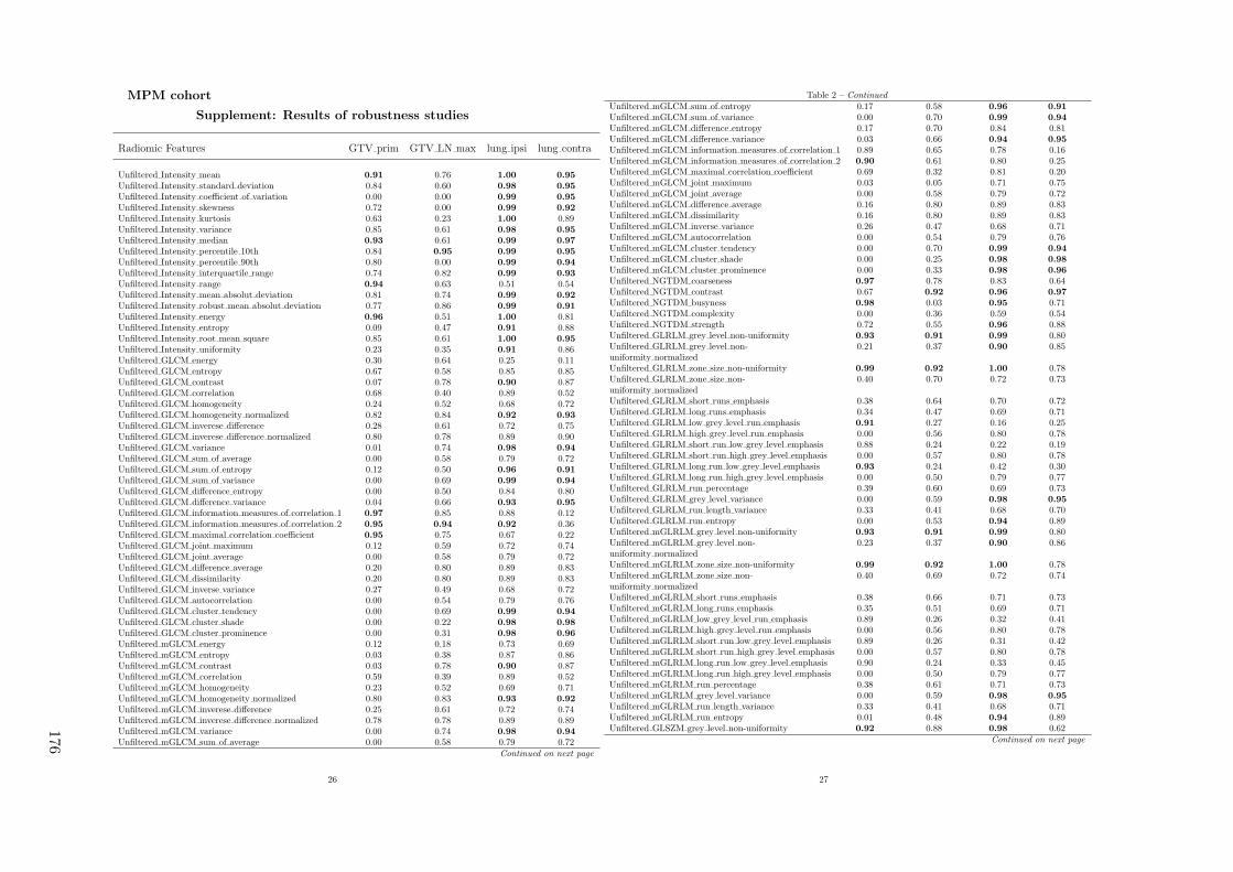
MPM cohort
Supplement: Results of robustness studies
Radiomic Features GTV prim GTV LN max lung ipsi lung contra
Unfiltered Intensity mean 0.91 0.76 1.00 0.95
Unfiltered Intensity standard deviation 0.84 0.60 0.98 0.95
Unfiltered Intensity coefficient of variation 0.00 0.00 0.99 0.95
Unfiltered Intensity skewness 0.72 0.00 0.99 0.92
Unfiltered Intensity kurtosis 0.63 0.23 1.00 0.89Unfiltered Intensity variance 0.85 0.61 0.98 0.95
Unfiltered Intensity median 0.93 0.61 0.99 0.97
Unfiltered Intensity percentile 10th 0.84 0.95 0.99 0.95
Unfiltered Intensity percentile 90th 0.80 0.00 0.99 0.94
Unfiltered Intensity interquartile range 0.74 0.82 0.99 0.93
Unfiltered Intensity range 0.94 0.63 0.51 0.54Unfiltered Intensity mean absolut deviation 0.81 0.74 0.99 0.92
Unfiltered Intensity robust mean absolut deviation 0.77 0.86 0.99 0.91
Unfiltered Intensity energy 0.96 0.51 1.00 0.81Unfiltered Intensity entropy 0.09 0.47 0.91 0.88Unfiltered Intensity root mean square 0.85 0.61 1.00 0.95
Unfiltered Intensity uniformity 0.23 0.35 0.91 0.86Unfiltered GLCM energy 0.30 0.64 0.25 0.11Unfiltered GLCM entropy 0.67 0.58 0.85 0.85Unfiltered GLCM contrast 0.07 0.78 0.90 0.87Unfiltered GLCM correlation 0.68 0.40 0.89 0.52Unfiltered GLCM homogeneity 0.24 0.52 0.68 0.72Unfiltered GLCM homogeneity normalized 0.82 0.84 0.92 0.93
Unfiltered GLCM inverese difference 0.28 0.61 0.72 0.75Unfiltered GLCM inverese difference normalized 0.80 0.78 0.89 0.90Unfiltered GLCM variance 0.01 0.74 0.98 0.94
Unfiltered GLCM sum of average 0.00 0.58 0.79 0.72Unfiltered GLCM sum of entropy 0.12 0.50 0.96 0.91
Unfiltered GLCM sum of variance 0.00 0.69 0.99 0.94
Unfiltered GLCM difference entropy 0.00 0.50 0.84 0.80Unfiltered GLCM difference variance 0.04 0.66 0.93 0.95
Unfiltered GLCM information measures of correlation 1 0.97 0.85 0.88 0.12Unfiltered GLCM information measures of correlation 2 0.95 0.94 0.92 0.36Unfiltered GLCM maximal correlation coefficient 0.95 0.75 0.67 0.22Unfiltered GLCM joint maximum 0.12 0.59 0.72 0.74Unfiltered GLCM joint average 0.00 0.58 0.79 0.72Unfiltered GLCM difference average 0.20 0.80 0.89 0.83Unfiltered GLCM dissimilarity 0.20 0.80 0.89 0.83Unfiltered GLCM inverse variance 0.27 0.49 0.68 0.72Unfiltered GLCM autocorrelation 0.00 0.54 0.79 0.76Unfiltered GLCM cluster tendency 0.00 0.69 0.99 0.94
Unfiltered GLCM cluster shade 0.00 0.22 0.98 0.98
Unfiltered GLCM cluster prominence 0.00 0.31 0.98 0.96
Unfiltered mGLCM energy 0.12 0.18 0.73 0.69Unfiltered mGLCM entropy 0.03 0.38 0.87 0.86Unfiltered mGLCM contrast 0.03 0.78 0.90 0.87Unfiltered mGLCM correlation 0.59 0.39 0.89 0.52Unfiltered mGLCM homogeneity 0.23 0.52 0.69 0.71Unfiltered mGLCM homogeneity normalized 0.80 0.83 0.93 0.92
Unfiltered mGLCM inverese difference 0.25 0.61 0.72 0.74Unfiltered mGLCM inverese difference normalized 0.78 0.78 0.89 0.89Unfiltered mGLCM variance 0.00 0.74 0.98 0.94
Unfiltered mGLCM sum of average 0.00 0.58 0.79 0.72Continued on next page
26
Table 2 – Continued
Unfiltered mGLCM sum of entropy 0.17 0.58 0.96 0.91
Unfiltered mGLCM sum of variance 0.00 0.70 0.99 0.94
Unfiltered mGLCM difference entropy 0.17 0.70 0.84 0.81Unfiltered mGLCM difference variance 0.03 0.66 0.94 0.95
Unfiltered mGLCM information measures of correlation 1 0.89 0.65 0.78 0.16Unfiltered mGLCM information measures of correlation 2 0.90 0.61 0.80 0.25Unfiltered mGLCM maximal correlation coefficient 0.69 0.32 0.81 0.20Unfiltered mGLCM joint maximum 0.03 0.05 0.71 0.75Unfiltered mGLCM joint average 0.00 0.58 0.79 0.72Unfiltered mGLCM difference average 0.16 0.80 0.89 0.83Unfiltered mGLCM dissimilarity 0.16 0.80 0.89 0.83Unfiltered mGLCM inverse variance 0.26 0.47 0.68 0.71Unfiltered mGLCM autocorrelation 0.00 0.54 0.79 0.76Unfiltered mGLCM cluster tendency 0.00 0.70 0.99 0.94
Unfiltered mGLCM cluster shade 0.00 0.25 0.98 0.98
Unfiltered mGLCM cluster prominence 0.00 0.33 0.98 0.96
Unfiltered NGTDM coarseness 0.97 0.78 0.83 0.64Unfiltered NGTDM contrast 0.67 0.92 0.96 0.97
Unfiltered NGTDM busyness 0.98 0.03 0.95 0.71Unfiltered NGTDM complexity 0.00 0.36 0.59 0.54Unfiltered NGTDM strength 0.72 0.55 0.96 0.88Unfiltered GLRLM grey level non-uniformity 0.93 0.91 0.99 0.80Unfiltered GLRLM grey level non-uniformity normalized
0.21 0.37 0.90 0.85
Unfiltered GLRLM zone size non-uniformity 0.99 0.92 1.00 0.78Unfiltered GLRLM zone size non-uniformity normalized
0.40 0.70 0.72 0.73
Unfiltered GLRLM short runs emphasis 0.38 0.64 0.70 0.72Unfiltered GLRLM long runs emphasis 0.34 0.47 0.69 0.71Unfiltered GLRLM low grey level run emphasis 0.91 0.27 0.16 0.25Unfiltered GLRLM high grey level run emphasis 0.00 0.56 0.80 0.78Unfiltered GLRLM short run low grey level emphasis 0.88 0.24 0.22 0.19Unfiltered GLRLM short run high grey level emphasis 0.00 0.57 0.80 0.78Unfiltered GLRLM long run low grey level emphasis 0.93 0.24 0.42 0.30Unfiltered GLRLM long run high grey level emphasis 0.00 0.50 0.79 0.77Unfiltered GLRLM run percentage 0.39 0.60 0.69 0.73Unfiltered GLRLM grey level variance 0.00 0.59 0.98 0.95
Unfiltered GLRLM run length variance 0.33 0.41 0.68 0.70Unfiltered GLRLM run entropy 0.00 0.53 0.94 0.89Unfiltered mGLRLM grey level non-uniformity 0.93 0.91 0.99 0.80Unfiltered mGLRLM grey level non-uniformity normalized
0.23 0.37 0.90 0.86
Unfiltered mGLRLM zone size non-uniformity 0.99 0.92 1.00 0.78Unfiltered mGLRLM zone size non-uniformity normalized
0.40 0.69 0.72 0.74
Unfiltered mGLRLM short runs emphasis 0.38 0.66 0.71 0.73Unfiltered mGLRLM long runs emphasis 0.35 0.51 0.69 0.71Unfiltered mGLRLM low grey level run emphasis 0.89 0.26 0.32 0.41Unfiltered mGLRLM high grey level run emphasis 0.00 0.56 0.80 0.78Unfiltered mGLRLM short run low grey level emphasis 0.89 0.26 0.31 0.42Unfiltered mGLRLM short run high grey level emphasis 0.00 0.57 0.80 0.78Unfiltered mGLRLM long run low grey level emphasis 0.90 0.24 0.33 0.45Unfiltered mGLRLM long run high grey level emphasis 0.00 0.50 0.79 0.77Unfiltered mGLRLM run percentage 0.38 0.61 0.71 0.73Unfiltered mGLRLM grey level variance 0.00 0.59 0.98 0.95
Unfiltered mGLRLM run length variance 0.33 0.41 0.68 0.71Unfiltered mGLRLM run entropy 0.01 0.48 0.94 0.89Unfiltered GLSZM grey level non-uniformity 0.92 0.88 0.98 0.62
Continued on next page
27
176
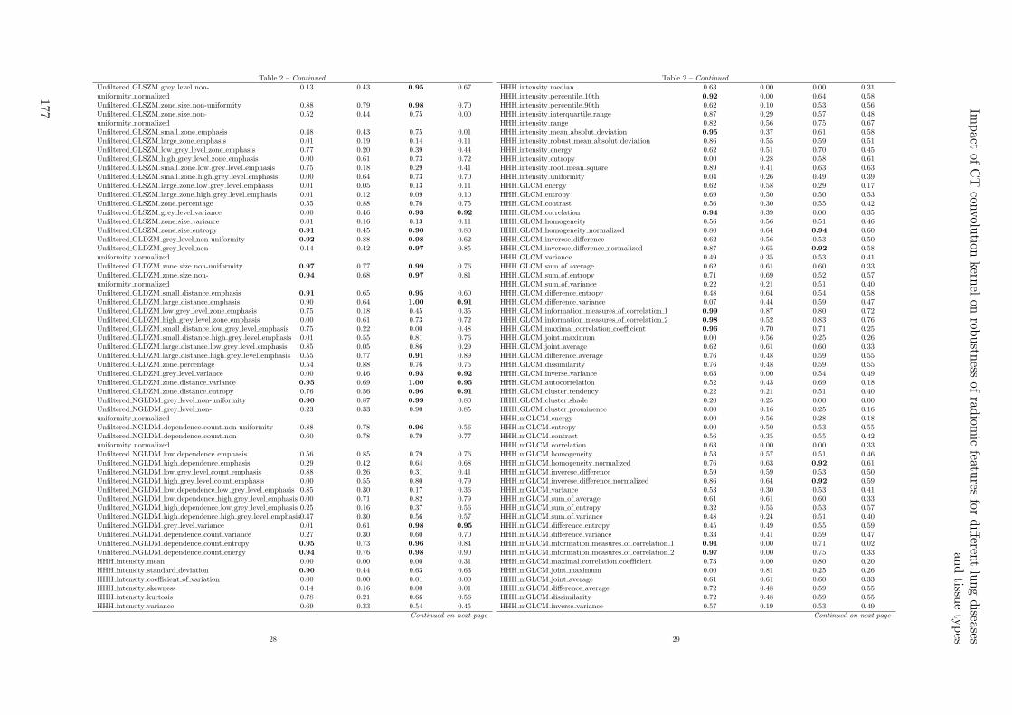
Table 2 – Continued
Unfiltered GLSZM grey level non-uniformity normalized
0.13 0.43 0.95 0.67
Unfiltered GLSZM zone size non-uniformity 0.88 0.79 0.98 0.70Unfiltered GLSZM zone size non-uniformity normalized
0.52 0.44 0.75 0.00
Unfiltered GLSZM small zone emphasis 0.48 0.43 0.75 0.01Unfiltered GLSZM large zone emphasis 0.01 0.19 0.14 0.11Unfiltered GLSZM low grey level zone emphasis 0.77 0.20 0.39 0.44Unfiltered GLSZM high grey level zone emphasis 0.00 0.61 0.73 0.72Unfiltered GLSZM small zone low grey level emphasis 0.75 0.18 0.29 0.41Unfiltered GLSZM small zone high grey level emphasis 0.00 0.64 0.73 0.70Unfiltered GLSZM large zone low grey level emphasis 0.01 0.05 0.13 0.11Unfiltered GLSZM large zone high grey level emphasis 0.01 0.12 0.09 0.10Unfiltered GLSZM zone percentage 0.55 0.88 0.76 0.75Unfiltered GLSZM grey level variance 0.00 0.46 0.93 0.92
Unfiltered GLSZM zone size variance 0.01 0.16 0.13 0.11Unfiltered GLSZM zone size entropy 0.91 0.45 0.90 0.80Unfiltered GLDZM grey level non-uniformity 0.92 0.88 0.98 0.62Unfiltered GLDZM grey level non-uniformity normalized
0.14 0.42 0.97 0.85
Unfiltered GLDZM zone size non-uniformity 0.97 0.77 0.99 0.76Unfiltered GLDZM zone size non-uniformity normalized
0.94 0.68 0.97 0.81
Unfiltered GLDZM small distance emphasis 0.91 0.65 0.95 0.60Unfiltered GLDZM large distance emphasis 0.90 0.64 1.00 0.91
Unfiltered GLDZM low grey level zone emphasis 0.75 0.18 0.45 0.35Unfiltered GLDZM high grey level zone emphasis 0.00 0.61 0.73 0.72Unfiltered GLDZM small distance low grey level emphasis 0.75 0.22 0.00 0.48Unfiltered GLDZM small distance high grey level emphasis 0.01 0.55 0.81 0.76Unfiltered GLDZM large distance low grey level emphasis 0.85 0.05 0.86 0.29Unfiltered GLDZM large distance high grey level emphasis 0.55 0.77 0.91 0.89Unfiltered GLDZM zone percentage 0.54 0.88 0.76 0.75Unfiltered GLDZM grey level variance 0.00 0.46 0.93 0.92
Unfiltered GLDZM zone distance variance 0.95 0.69 1.00 0.95
Unfiltered GLDZM zone distance entropy 0.76 0.56 0.96 0.91
Unfiltered NGLDM grey level non-uniformity 0.90 0.87 0.99 0.80Unfiltered NGLDM grey level non-uniformity normalized
0.23 0.33 0.90 0.85
Unfiltered NGLDM dependence count non-uniformity 0.88 0.78 0.96 0.56Unfiltered NGLDM dependence count non-uniformity normalized
0.60 0.78 0.79 0.77
Unfiltered NGLDM low dependence emphasis 0.56 0.85 0.79 0.76Unfiltered NGLDM high dependence emphasis 0.29 0.42 0.64 0.68Unfiltered NGLDM low grey level count emphasis 0.88 0.26 0.31 0.41Unfiltered NGLDM high grey level count emphasis 0.00 0.55 0.80 0.79Unfiltered NGLDM low dependence low grey level emphasis 0.85 0.30 0.17 0.36Unfiltered NGLDM low dependence high grey level emphasis 0.00 0.71 0.82 0.79Unfiltered NGLDM high dependence low grey level emphasis 0.25 0.16 0.37 0.56Unfiltered NGLDM high dependence high grey level emphasis0.47 0.30 0.56 0.57Unfiltered NGLDM grey level variance 0.01 0.61 0.98 0.95
Unfiltered NGLDM dependence count variance 0.27 0.30 0.60 0.70Unfiltered NGLDM dependence count entropy 0.95 0.73 0.96 0.84Unfiltered NGLDM dependence count energy 0.94 0.76 0.98 0.90HHH intensity mean 0.00 0.00 0.00 0.31HHH intensity standard deviation 0.90 0.44 0.63 0.63HHH intensity coefficient of variation 0.00 0.00 0.01 0.00HHH intensity skewness 0.14 0.16 0.00 0.01HHH intensity kurtosis 0.78 0.21 0.66 0.56HHH intensity variance 0.69 0.33 0.54 0.45
Continued on next page
28
Table 2 – Continued
HHH intensity median 0.63 0.00 0.00 0.31HHH intensity percentile 10th 0.92 0.00 0.64 0.58HHH intensity percentile 90th 0.62 0.10 0.53 0.56HHH intensity interquartile range 0.87 0.29 0.57 0.48HHH intensity range 0.82 0.56 0.75 0.67HHH intensity mean absolut deviation 0.95 0.37 0.61 0.58HHH intensity robust mean absolut deviation 0.86 0.55 0.59 0.51HHH intensity energy 0.62 0.51 0.70 0.45HHH intensity entropy 0.00 0.28 0.58 0.61HHH intensity root mean square 0.89 0.41 0.63 0.63HHH intensity uniformity 0.04 0.26 0.49 0.39HHH GLCM energy 0.62 0.58 0.29 0.17HHH GLCM entropy 0.69 0.50 0.50 0.53HHH GLCM contrast 0.56 0.30 0.55 0.42HHH GLCM correlation 0.94 0.39 0.00 0.35HHH GLCM homogeneity 0.56 0.56 0.51 0.46HHH GLCM homogeneity normalized 0.80 0.64 0.94 0.60HHH GLCM inverese difference 0.62 0.56 0.53 0.50HHH GLCM inverese difference normalized 0.87 0.65 0.92 0.58HHH GLCM variance 0.49 0.35 0.53 0.41HHH GLCM sum of average 0.62 0.61 0.60 0.33HHH GLCM sum of entropy 0.71 0.69 0.52 0.57HHH GLCM sum of variance 0.22 0.21 0.51 0.40HHH GLCM difference entropy 0.48 0.64 0.54 0.58HHH GLCM difference variance 0.07 0.44 0.59 0.47HHH GLCM information measures of correlation 1 0.99 0.87 0.80 0.72HHH GLCM information measures of correlation 2 0.98 0.52 0.83 0.76HHH GLCM maximal correlation coefficient 0.96 0.70 0.71 0.25HHH GLCM joint maximum 0.00 0.56 0.25 0.26HHH GLCM joint average 0.62 0.61 0.60 0.33HHH GLCM difference average 0.76 0.48 0.59 0.55HHH GLCM dissimilarity 0.76 0.48 0.59 0.55HHH GLCM inverse variance 0.63 0.00 0.54 0.49HHH GLCM autocorrelation 0.52 0.43 0.69 0.18HHH GLCM cluster tendency 0.22 0.21 0.51 0.40HHH GLCM cluster shade 0.20 0.25 0.00 0.00HHH GLCM cluster prominence 0.00 0.16 0.25 0.16HHH mGLCM energy 0.00 0.56 0.28 0.18HHH mGLCM entropy 0.00 0.50 0.53 0.55HHH mGLCM contrast 0.56 0.35 0.55 0.42HHH mGLCM correlation 0.63 0.00 0.00 0.33HHH mGLCM homogeneity 0.53 0.57 0.51 0.46HHH mGLCM homogeneity normalized 0.76 0.63 0.92 0.61HHH mGLCM inverese difference 0.59 0.59 0.53 0.50HHH mGLCM inverese difference normalized 0.86 0.64 0.92 0.59HHH mGLCM variance 0.53 0.30 0.53 0.41HHH mGLCM sum of average 0.61 0.61 0.60 0.33HHH mGLCM sum of entropy 0.32 0.55 0.53 0.57HHH mGLCM sum of variance 0.48 0.24 0.51 0.40HHH mGLCM difference entropy 0.45 0.49 0.55 0.59HHH mGLCM difference variance 0.33 0.41 0.59 0.47HHH mGLCM information measures of correlation 1 0.91 0.00 0.71 0.02HHH mGLCM information measures of correlation 2 0.97 0.00 0.75 0.33HHH mGLCM maximal correlation coefficient 0.73 0.00 0.80 0.20HHH mGLCM joint maximum 0.00 0.81 0.25 0.26HHH mGLCM joint average 0.61 0.61 0.60 0.33HHH mGLCM difference average 0.72 0.48 0.59 0.55HHH mGLCM dissimilarity 0.72 0.48 0.59 0.55HHH mGLCM inverse variance 0.57 0.19 0.53 0.49
Continued on next page
29
Impact
ofC
Tcon
volution
kernel
onrob
ustn
essof
radiom
icfeatu
resfo
rdiff
erent
lung
diseases
and
tissue
types
177
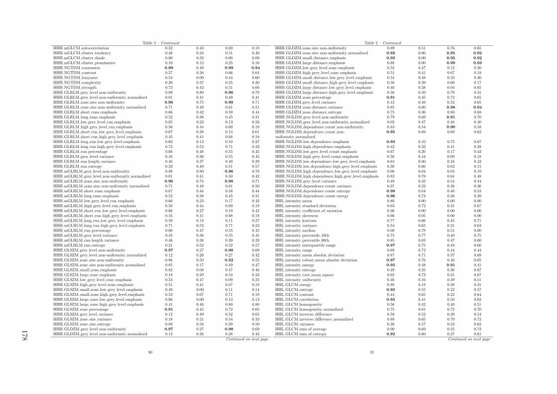
Table 2 – Continued
HHH mGLCM autocorrelation 0.52 0.43 0.69 0.18HHH mGLCM cluster tendency 0.48 0.24 0.51 0.40HHH mGLCM cluster shade 0.00 0.32 0.00 0.00HHH mGLCM cluster prominence 0.10 0.12 0.25 0.16HHH NGTDM coarseness 0.99 0.49 0.99 0.94
HHH NGTDM contrast 0.57 0.38 0.66 0.64HHH NGTDM busyness 0.54 0.00 0.44 0.60HHH NGTDM complexity 0.20 0.37 0.35 0.30HHH NGTDM strength 0.73 0.42 0.51 0.66HHH GLRLM grey level non-uniformity 0.89 0.80 0.96 0.78HHH GLRLM grey level non-uniformity normalized 0.01 0.41 0.49 0.41HHH GLRLM zone size non-uniformity 0.96 0.75 0.98 0.71HHH GLRLM zone size non-uniformity normalized 0.71 0.49 0.61 0.51HHH GLRLM short runs emphasis 0.66 0.42 0.59 0.44HHH GLRLM long runs emphasis 0.52 0.36 0.45 0.31HHH GLRLM low grey level run emphasis 0.65 0.23 0.13 0.56HHH GLRLM high grey level run emphasis 0.50 0.44 0.69 0.18HHH GLRLM short run low grey level emphasis 0.67 0.28 0.14 0.61HHH GLRLM short run high grey level emphasis 0.45 0.41 0.68 0.18HHH GLRLM long run low grey level emphasis 0.60 0.13 0.10 0.27HHH GLRLM long run high grey level emphasis 0.72 0.53 0.71 0.23HHH GLRLM run percentage 0.66 0.48 0.55 0.45HHH GLRLM grey level variance 0.45 0.36 0.55 0.45HHH GLRLM run length variance 0.46 0.37 0.40 0.29HHH GLRLM run entropy 0.33 0.49 0.51 0.57HHH mGLRLM grey level non-uniformity 0.89 0.80 0.96 0.78HHH mGLRLM grey level non-uniformity normalized 0.01 0.41 0.50 0.42HHH mGLRLM zone size non-uniformity 0.96 0.74 0.98 0.71HHH mGLRLM zone size non-uniformity normalized 0.71 0.49 0.61 0.50HHH mGLRLM short runs emphasis 0.67 0.44 0.58 0.44HHH mGLRLM long runs emphasis 0.52 0.38 0.45 0.31HHH mGLRLM low grey level run emphasis 0.66 0.23 0.17 0.42HHH mGLRLM high grey level run emphasis 0.50 0.44 0.69 0.18HHH mGLRLM short run low grey level emphasis 0.66 0.27 0.19 0.42HHH mGLRLM short run high grey level emphasis 0.45 0.41 0.68 0.18HHH mGLRLM long run low grey level emphasis 0.59 0.13 0.11 0.37HHH mGLRLM long run high grey level emphasis 0.71 0.53 0.71 0.23HHH mGLRLM run percentage 0.66 0.47 0.55 0.45HHH mGLRLM grey level variance 0.45 0.36 0.55 0.45HHH mGLRLM run length variance 0.46 0.38 0.39 0.29HHH mGLRLM run entropy 0.21 0.52 0.52 0.57HHH GLSZM grey level non-uniformity 0.97 0.27 0.98 0.69HHH GLSZM grey level non-uniformity normalized 0.12 0.26 0.27 0.42HHH GLSZM zone size non-uniformity 0.86 0.50 0.92 0.55HHH GLSZM zone size non-uniformity normalized 0.85 0.17 0.49 0.47HHH GLSZM small zone emphasis 0.82 0.08 0.47 0.46HHH GLSZM large zone emphasis 0.18 0.20 0.54 0.33HHH GLSZM low grey level zone emphasis 0.53 0.47 0.09 0.25HHH GLSZM high grey level zone emphasis 0.51 0.41 0.67 0.18HHH GLSZM small zone low grey level emphasis 0.49 0.00 0.11 0.14HHH GLSZM small zone high grey level emphasis 0.53 0.67 0.71 0.19HHH GLSZM large zone low grey level emphasis 0.06 0.00 0.13 0.13HHH GLSZM large zone high grey level emphasis 0.41 0.46 0.80 0.80HHH GLSZM zone percentage 0.91 0.45 0.72 0.65HHH GLSZM grey level variance 0.12 0.49 0.52 0.65HHH GLSZM zone size variance 0.18 0.21 0.54 0.33HHH GLSZM zone size entropy 0.89 0.58 0.29 0.50HHH GLDZM grey level non-uniformity 0.97 0.27 0.98 0.69HHH GLDZM grey level non-uniformity normalized 0.12 0.26 0.28 0.43
Continued on next page
30
Table 2 – Continued
HHH GLDZM zone size non-uniformity 0.89 0.51 0.76 0.65HHH GLDZM zone size non-uniformity normalized 0.93 0.00 0.95 0.92
HHH GLDZM small distance emphasis 0.93 0.00 0.95 0.92
HHH GLDZM large distance emphasis 0.88 0.00 0.99 0.93
HHH GLDZM low grey level zone emphasis 0.52 0.47 0.12 0.30HHH GLDZM high grey level zone emphasis 0.51 0.41 0.67 0.18HHH GLDZM small distance low grey level emphasis 0.54 0.48 0.23 0.30HHH GLDZM small distance high grey level emphasis 0.50 0.39 0.69 0.17HHH GLDZM large distance low grey level emphasis 0.40 0.38 0.04 0.65HHH GLDZM large distance high grey level emphasis 0.50 0.50 0.79 0.31HHH GLDZM zone percentage 0.91 0.45 0.72 0.65HHH GLDZM grey level variance 0.12 0.49 0.52 0.65HHH GLDZM zone distance variance 0.85 0.00 0.98 0.94
HHH GLDZM zone distance entropy 0.75 0.36 0.80 0.68HHH NGLDM grey level non-uniformity 0.79 0.69 0.91 0.70HHH NGLDM grey level non-uniformity normalized 0.02 0.47 0.48 0.40HHH NGLDM dependence count non-uniformity 0.83 0.54 0.90 0.58HHH NGLDM dependence count non-uniformity normalized
0.95 0.69 0.69 0.62
HHH NGLDM low dependence emphasis 0.93 0.10 0.75 0.67HHH NGLDM high dependence emphasis 0.43 0.32 0.41 0.28HHH NGLDM low grey level count emphasis 0.67 0.20 0.17 0.43HHH NGLDM high grey level count emphasis 0.50 0.44 0.69 0.18HHH NGLDM low dependence low grey level emphasis 0.64 0.00 0.34 0.42HHH NGLDM low dependence high grey level emphasis 0.30 0.66 0.62 0.15HHH NGLDM high dependence low grey level emphasis 0.00 0.04 0.04 0.19HHH NGLDM high dependence high grey level emphasis 0.83 0.78 0.64 0.48HHH NGLDM grey level variance 0.49 0.33 0.54 0.44HHH NGLDM dependence count variance 0.37 0.22 0.38 0.36HHH NGLDM dependence count entropy 0.98 0.84 0.46 0.53HHH NGLDM dependence count energy 0.96 0.73 0.38 0.39HHL intensity mean 0.80 0.00 0.00 0.00HHL intensity standard deviation 0.63 0.72 0.31 0.67HHL intensity coefficient of variation 0.36 0.00 0.00 0.00HHL intensity skewness 0.66 0.05 0.00 0.00HHL intensity kurtosis 0.77 0.66 0.45 0.71HHL intensity variance 0.54 0.65 0.31 0.63HHL intensity median 0.00 0.78 0.51 0.00HHL intensity percentile 10th 0.75 0.77 0.40 0.75HHL intensity percentile 90th 0.85 0.03 0.47 0.60HHL intensity interquartile range 0.97 0.75 0.49 0.60HHL intensity range 0.69 0.72 0.44 0.44HHL intensity mean absolut deviation 0.87 0.71 0.37 0.69HHL intensity robust mean absolut deviation 0.97 0.76 0.46 0.65HHL intensity energy 0.93 0.48 0.91 0.41HHL intensity entropy 0.49 0.25 0.36 0.67HHL intensity root mean square 0.62 0.73 0.31 0.67HHL intensity uniformity 0.46 0.16 0.39 0.51HHL GLCM energy 0.88 0.18 0.38 0.31HHL GLCM entropy 0.93 0.55 0.22 0.57HHL GLCM contrast 0.44 0.65 0.22 0.64HHL GLCM correlation 0.93 0.41 0.50 0.62HHL GLCM homogeneity 0.56 0.42 0.40 0.51HHL GLCM homogeneity normalized 0.75 0.61 0.72 0.70HHL GLCM inverese difference 0.59 0.52 0.39 0.54HHL GLCM inverese difference normalized 0.88 0.65 0.70 0.72HHL GLCM variance 0.38 0.57 0.23 0.62HHL GLCM sum of average 0.00 0.69 0.25 0.72HHL GLCM sum of entropy 0.92 0.60 0.27 0.61
Continued on next page
31
178
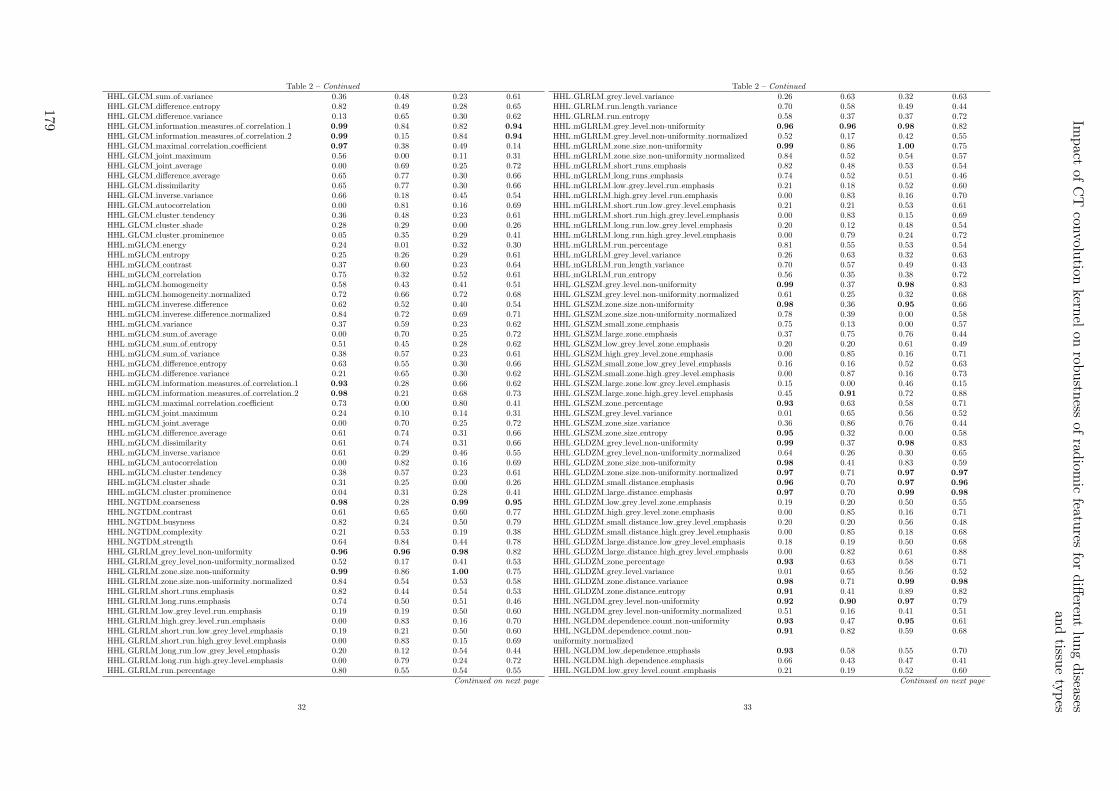
Table 2 – Continued
HHL GLCM sum of variance 0.36 0.48 0.23 0.61HHL GLCM difference entropy 0.82 0.49 0.28 0.65HHL GLCM difference variance 0.13 0.65 0.30 0.62HHL GLCM information measures of correlation 1 0.99 0.84 0.82 0.94
HHL GLCM information measures of correlation 2 0.99 0.15 0.84 0.94
HHL GLCM maximal correlation coefficient 0.97 0.38 0.49 0.14HHL GLCM joint maximum 0.56 0.00 0.11 0.31HHL GLCM joint average 0.00 0.69 0.25 0.72HHL GLCM difference average 0.65 0.77 0.30 0.66HHL GLCM dissimilarity 0.65 0.77 0.30 0.66HHL GLCM inverse variance 0.66 0.18 0.45 0.54HHL GLCM autocorrelation 0.00 0.81 0.16 0.69HHL GLCM cluster tendency 0.36 0.48 0.23 0.61HHL GLCM cluster shade 0.28 0.29 0.00 0.26HHL GLCM cluster prominence 0.05 0.35 0.29 0.41HHL mGLCM energy 0.24 0.01 0.32 0.30HHL mGLCM entropy 0.25 0.26 0.29 0.61HHL mGLCM contrast 0.37 0.60 0.23 0.64HHL mGLCM correlation 0.75 0.32 0.52 0.61HHL mGLCM homogeneity 0.58 0.43 0.41 0.51HHL mGLCM homogeneity normalized 0.72 0.66 0.72 0.68HHL mGLCM inverese difference 0.62 0.52 0.40 0.54HHL mGLCM inverese difference normalized 0.84 0.72 0.69 0.71HHL mGLCM variance 0.37 0.59 0.23 0.62HHL mGLCM sum of average 0.00 0.70 0.25 0.72HHL mGLCM sum of entropy 0.51 0.45 0.28 0.62HHL mGLCM sum of variance 0.38 0.57 0.23 0.61HHL mGLCM difference entropy 0.63 0.55 0.30 0.66HHL mGLCM difference variance 0.21 0.65 0.30 0.62HHL mGLCM information measures of correlation 1 0.93 0.28 0.66 0.62HHL mGLCM information measures of correlation 2 0.98 0.21 0.68 0.73HHL mGLCM maximal correlation coefficient 0.73 0.00 0.80 0.41HHL mGLCM joint maximum 0.24 0.10 0.14 0.31HHL mGLCM joint average 0.00 0.70 0.25 0.72HHL mGLCM difference average 0.61 0.74 0.31 0.66HHL mGLCM dissimilarity 0.61 0.74 0.31 0.66HHL mGLCM inverse variance 0.61 0.29 0.46 0.55HHL mGLCM autocorrelation 0.00 0.82 0.16 0.69HHL mGLCM cluster tendency 0.38 0.57 0.23 0.61HHL mGLCM cluster shade 0.31 0.25 0.00 0.26HHL mGLCM cluster prominence 0.04 0.31 0.28 0.41HHL NGTDM coarseness 0.98 0.28 0.99 0.95
HHL NGTDM contrast 0.61 0.65 0.60 0.77HHL NGTDM busyness 0.82 0.24 0.50 0.79HHL NGTDM complexity 0.21 0.53 0.19 0.38HHL NGTDM strength 0.64 0.84 0.44 0.78HHL GLRLM grey level non-uniformity 0.96 0.96 0.98 0.82HHL GLRLM grey level non-uniformity normalized 0.52 0.17 0.41 0.53HHL GLRLM zone size non-uniformity 0.99 0.86 1.00 0.75HHL GLRLM zone size non-uniformity normalized 0.84 0.54 0.53 0.58HHL GLRLM short runs emphasis 0.82 0.44 0.54 0.53HHL GLRLM long runs emphasis 0.74 0.50 0.51 0.46HHL GLRLM low grey level run emphasis 0.19 0.19 0.50 0.60HHL GLRLM high grey level run emphasis 0.00 0.83 0.16 0.70HHL GLRLM short run low grey level emphasis 0.19 0.21 0.50 0.60HHL GLRLM short run high grey level emphasis 0.00 0.83 0.15 0.69HHL GLRLM long run low grey level emphasis 0.20 0.12 0.54 0.44HHL GLRLM long run high grey level emphasis 0.00 0.79 0.24 0.72HHL GLRLM run percentage 0.80 0.55 0.54 0.55
Continued on next page
32
Table 2 – Continued
HHL GLRLM grey level variance 0.26 0.63 0.32 0.63HHL GLRLM run length variance 0.70 0.58 0.49 0.44HHL GLRLM run entropy 0.58 0.37 0.37 0.72HHL mGLRLM grey level non-uniformity 0.96 0.96 0.98 0.82HHL mGLRLM grey level non-uniformity normalized 0.52 0.17 0.42 0.55HHL mGLRLM zone size non-uniformity 0.99 0.86 1.00 0.75HHL mGLRLM zone size non-uniformity normalized 0.84 0.52 0.54 0.57HHL mGLRLM short runs emphasis 0.82 0.48 0.53 0.54HHL mGLRLM long runs emphasis 0.74 0.52 0.51 0.46HHL mGLRLM low grey level run emphasis 0.21 0.18 0.52 0.60HHL mGLRLM high grey level run emphasis 0.00 0.83 0.16 0.70HHL mGLRLM short run low grey level emphasis 0.21 0.21 0.53 0.61HHL mGLRLM short run high grey level emphasis 0.00 0.83 0.15 0.69HHL mGLRLM long run low grey level emphasis 0.20 0.12 0.48 0.54HHL mGLRLM long run high grey level emphasis 0.00 0.79 0.24 0.72HHL mGLRLM run percentage 0.81 0.55 0.53 0.54HHL mGLRLM grey level variance 0.26 0.63 0.32 0.63HHL mGLRLM run length variance 0.70 0.57 0.49 0.43HHL mGLRLM run entropy 0.56 0.35 0.38 0.72HHL GLSZM grey level non-uniformity 0.99 0.37 0.98 0.83HHL GLSZM grey level non-uniformity normalized 0.61 0.25 0.32 0.68HHL GLSZM zone size non-uniformity 0.98 0.36 0.95 0.66HHL GLSZM zone size non-uniformity normalized 0.78 0.39 0.00 0.58HHL GLSZM small zone emphasis 0.75 0.13 0.00 0.57HHL GLSZM large zone emphasis 0.37 0.75 0.76 0.44HHL GLSZM low grey level zone emphasis 0.20 0.20 0.61 0.49HHL GLSZM high grey level zone emphasis 0.00 0.85 0.16 0.71HHL GLSZM small zone low grey level emphasis 0.16 0.16 0.52 0.63HHL GLSZM small zone high grey level emphasis 0.00 0.87 0.16 0.73HHL GLSZM large zone low grey level emphasis 0.15 0.00 0.46 0.15HHL GLSZM large zone high grey level emphasis 0.45 0.91 0.72 0.88HHL GLSZM zone percentage 0.93 0.63 0.58 0.71HHL GLSZM grey level variance 0.01 0.65 0.56 0.52HHL GLSZM zone size variance 0.36 0.86 0.76 0.44HHL GLSZM zone size entropy 0.95 0.32 0.00 0.58HHL GLDZM grey level non-uniformity 0.99 0.37 0.98 0.83HHL GLDZM grey level non-uniformity normalized 0.64 0.26 0.30 0.65HHL GLDZM zone size non-uniformity 0.98 0.41 0.83 0.59HHL GLDZM zone size non-uniformity normalized 0.97 0.71 0.97 0.97
HHL GLDZM small distance emphasis 0.96 0.70 0.97 0.96
HHL GLDZM large distance emphasis 0.97 0.70 0.99 0.98
HHL GLDZM low grey level zone emphasis 0.19 0.20 0.50 0.55HHL GLDZM high grey level zone emphasis 0.00 0.85 0.16 0.71HHL GLDZM small distance low grey level emphasis 0.20 0.20 0.56 0.48HHL GLDZM small distance high grey level emphasis 0.00 0.85 0.18 0.68HHL GLDZM large distance low grey level emphasis 0.18 0.19 0.50 0.68HHL GLDZM large distance high grey level emphasis 0.00 0.82 0.61 0.88HHL GLDZM zone percentage 0.93 0.63 0.58 0.71HHL GLDZM grey level variance 0.01 0.65 0.56 0.52HHL GLDZM zone distance variance 0.98 0.71 0.99 0.98
HHL GLDZM zone distance entropy 0.91 0.41 0.89 0.82HHL NGLDM grey level non-uniformity 0.92 0.90 0.97 0.79HHL NGLDM grey level non-uniformity normalized 0.51 0.16 0.41 0.51HHL NGLDM dependence count non-uniformity 0.93 0.47 0.95 0.61HHL NGLDM dependence count non-uniformity normalized
0.91 0.82 0.59 0.68
HHL NGLDM low dependence emphasis 0.93 0.58 0.55 0.70HHL NGLDM high dependence emphasis 0.66 0.43 0.47 0.41HHL NGLDM low grey level count emphasis 0.21 0.19 0.52 0.60
Continued on next page
33
Impact
ofC
Tcon
volution
kernel
onrob
ustn
essof
radiom
icfeatu
resfo
rdiff
erent
lung
diseases
and
tissue
types
179

Table 2 – Continued
HHL NGLDM high grey level count emphasis 0.00 0.83 0.16 0.70HHL NGLDM low dependence low grey level emphasis 0.19 0.64 0.53 0.69HHL NGLDM low dependence high grey level emphasis 0.00 0.86 0.09 0.60HHL NGLDM high dependence low grey level emphasis 0.00 0.00 0.08 0.30HHL NGLDM high dependence high grey level emphasis 0.67 0.53 0.38 0.78HHL NGLDM grey level variance 0.28 0.64 0.31 0.64HHL NGLDM dependence count variance 0.59 0.38 0.42 0.39HHL NGLDM dependence count entropy 0.99 0.79 0.56 0.75HHL NGLDM dependence count energy 0.99 0.76 0.55 0.65HLH intensity mean 0.01 0.14 0.00 0.35HLH intensity standard deviation 0.92 0.27 0.74 0.64HLH intensity coefficient of variation 0.00 0.00 0.02 0.32HLH intensity skewness 0.00 0.00 0.42 0.78HLH intensity kurtosis 0.77 0.93 0.76 0.00HLH intensity variance 0.93 0.10 0.63 0.53HLH intensity median 0.92 0.00 0.42 0.31HLH intensity percentile 10th 0.74 0.12 0.77 0.69HLH intensity percentile 90th 0.66 0.09 0.74 0.72HLH intensity interquartile range 0.89 0.09 0.62 0.61HLH intensity range 0.66 0.60 0.72 0.15HLH intensity mean absolut deviation 0.93 0.04 0.71 0.68HLH intensity robust mean absolut deviation 0.90 0.26 0.67 0.63HLH intensity energy 0.70 0.50 0.76 0.23HLH intensity entropy 0.26 0.22 0.73 0.66HLH intensity root mean square 0.94 0.22 0.75 0.64HLH intensity uniformity 0.17 0.04 0.58 0.41HLH GLCM energy 0.69 0.52 0.38 0.22HLH GLCM entropy 0.76 0.43 0.67 0.61HLH GLCM contrast 0.89 0.02 0.64 0.53HLH GLCM correlation 0.71 0.64 0.54 0.00HLH GLCM homogeneity 0.48 0.00 0.63 0.50HLH GLCM homogeneity normalized 0.95 0.61 0.84 0.23HLH GLCM inverese difference 0.55 0.00 0.66 0.54HLH GLCM inverese difference normalized 0.92 0.73 0.83 0.19HLH GLCM variance 0.81 0.00 0.63 0.53HLH GLCM sum of average 0.48 0.56 0.55 0.16HLH GLCM sum of entropy 0.71 0.68 0.71 0.64HLH GLCM sum of variance 0.68 0.26 0.62 0.53HLH GLCM difference entropy 0.53 0.63 0.73 0.68HLH GLCM difference variance 0.38 0.41 0.65 0.47HLH GLCM information measures of correlation 1 0.97 0.83 0.79 0.69HLH GLCM information measures of correlation 2 0.95 0.42 0.88 0.78HLH GLCM maximal correlation coefficient 0.95 0.38 0.16 0.00HLH GLCM joint maximum 0.02 0.15 0.32 0.08HLH GLCM joint average 0.48 0.56 0.55 0.16HLH GLCM difference average 0.84 0.04 0.72 0.68HLH GLCM dissimilarity 0.84 0.04 0.72 0.68HLH GLCM inverse variance 0.63 0.15 0.67 0.65HLH GLCM autocorrelation 0.40 0.41 0.43 0.11HLH GLCM cluster tendency 0.68 0.26 0.62 0.53HLH GLCM cluster shade 0.51 0.00 0.20 0.37HLH GLCM cluster prominence 0.31 0.18 0.34 0.14HLH mGLCM energy 0.00 0.03 0.40 0.19HLH mGLCM entropy 0.00 0.18 0.70 0.64HLH mGLCM contrast 0.88 0.06 0.64 0.53HLH mGLCM correlation 0.49 0.39 0.53 0.00HLH mGLCM homogeneity 0.53 0.03 0.63 0.50HLH mGLCM homogeneity normalized 0.94 0.60 0.80 0.27HLH mGLCM inverese difference 0.59 0.04 0.66 0.54
Continued on next page
34
Table 2 – Continued
HLH mGLCM inverese difference normalized 0.92 0.72 0.83 0.19HLH mGLCM variance 0.86 0.06 0.63 0.53HLH mGLCM sum of average 0.47 0.56 0.55 0.16HLH mGLCM sum of entropy 0.35 0.22 0.72 0.64HLH mGLCM sum of variance 0.81 0.06 0.62 0.53HLH mGLCM difference entropy 0.47 0.21 0.74 0.68HLH mGLCM difference variance 0.64 0.31 0.65 0.48HLH mGLCM information measures of correlation 1 0.82 0.10 0.33 0.00HLH mGLCM information measures of correlation 2 0.90 0.09 0.45 0.00HLH mGLCM maximal correlation coefficient 0.69 0.05 0.53 0.00HLH mGLCM joint maximum 0.02 0.00 0.34 0.08HLH mGLCM joint average 0.47 0.56 0.55 0.16HLH mGLCM difference average 0.84 0.04 0.72 0.68HLH mGLCM dissimilarity 0.84 0.04 0.72 0.68HLH mGLCM inverse variance 0.62 0.00 0.67 0.64HLH mGLCM autocorrelation 0.39 0.41 0.43 0.11HLH mGLCM cluster tendency 0.81 0.06 0.62 0.53HLH mGLCM cluster shade 0.00 0.00 0.20 0.37HLH mGLCM cluster prominence 0.56 0.14 0.34 0.14HLH NGTDM coarseness 0.97 0.53 0.98 0.95
HLH NGTDM contrast 0.98 0.00 0.77 0.63HLH NGTDM busyness 0.56 0.00 0.79 0.58HLH NGTDM complexity 0.39 0.22 0.51 0.09HLH NGTDM strength 0.95 0.33 0.57 0.51HLH GLRLM grey level non-uniformity 0.90 0.94 0.96 0.80HLH GLRLM grey level non-uniformity normalized 0.06 0.00 0.63 0.51HLH GLRLM zone size non-uniformity 0.95 0.70 0.98 0.72HLH GLRLM zone size non-uniformity normalized 0.70 0.47 0.66 0.54HLH GLRLM short runs emphasis 0.64 0.31 0.64 0.49HLH GLRLM long runs emphasis 0.46 0.30 0.57 0.29HLH GLRLM low grey level run emphasis 0.80 0.11 0.34 0.21HLH GLRLM high grey level run emphasis 0.38 0.43 0.43 0.11HLH GLRLM short run low grey level emphasis 0.81 0.13 0.41 0.22HLH GLRLM short run high grey level emphasis 0.33 0.37 0.41 0.10HLH GLRLM long run low grey level emphasis 0.74 0.04 0.40 0.20HLH GLRLM long run high grey level emphasis 0.56 0.69 0.53 0.12HLH GLRLM run percentage 0.61 0.42 0.63 0.46HLH GLRLM grey level variance 0.82 0.22 0.64 0.52HLH GLRLM run length variance 0.39 0.34 0.54 0.24HLH GLRLM run entropy 0.40 0.42 0.72 0.68HLH m GLRLM grey level non-uniformity 0.91 0.94 0.96 0.80HLH m GLRLM grey level non-uniformity normalized 0.07 0.00 0.62 0.51HLH m GLRLM zone size non-uniformity 0.95 0.70 0.98 0.72HLH m GLRLM zone size non-uniformity normalized 0.70 0.41 0.67 0.54HLH m GLRLM short runs emphasis 0.65 0.36 0.64 0.49HLH m GLRLM long runs emphasis 0.46 0.33 0.57 0.30HLH m GLRLM low grey level run emphasis 0.80 0.11 0.51 0.09HLH m GLRLM high grey level run emphasis 0.38 0.43 0.43 0.11HLH m GLRLM short run low grey level emphasis 0.81 0.13 0.53 0.07HLH m GLRLM short run high grey level emphasis 0.33 0.37 0.41 0.10HLH m GLRLM long run low grey level emphasis 0.74 0.04 0.41 0.21HLH m GLRLM long run high grey level emphasis 0.56 0.69 0.53 0.12HLH m GLRLM run percentage 0.62 0.41 0.64 0.45HLH m GLRLM grey level variance 0.82 0.21 0.64 0.52HLH m GLRLM run length variance 0.39 0.34 0.54 0.24HLH m GLRLM run entropy 0.35 0.40 0.73 0.69HLH GLSZM grey level non-uniformity 0.98 0.60 0.99 0.85HLH GLSZM grey level non-uniformity normalized 0.34 0.14 0.51 0.45HLH GLSZM zone size non-uniformity 0.93 0.42 0.94 0.58
Continued on next page
35
180
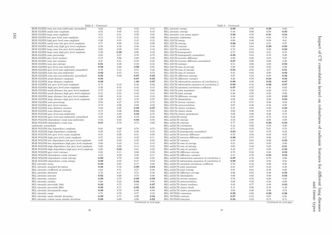
Table 2 – Continued
HLH GLSZM zone size non-uniformity normalized 0.62 0.02 0.52 0.12HLH GLSZM small zone emphasis 0.55 0.05 0.52 0.10HLH GLSZM large zone emphasis 0.21 0.51 0.59 0.35HLH GLSZM low grey level zone emphasis 0.74 0.18 0.41 0.00HLH GLSZM high grey level zone emphasis 0.39 0.55 0.45 0.12HLH GLSZM small zone low grey level emphasis 0.77 0.00 0.40 0.00HLH GLSZM small zone high grey level emphasis 0.38 0.56 0.49 0.16HLH GLSZM large zone low grey level emphasis 0.05 0.00 0.25 0.16HLH GLSZM large zone high grey level emphasis 0.59 0.98 0.86 0.43HLH GLSZM zone percentage 0.85 0.27 0.76 0.73HLH GLSZM grey level variance 0.73 0.66 0.69 0.32HLH GLSZM zone size variance 0.21 0.51 0.58 0.35HLH GLSZM zone size entropy 0.91 0.38 0.49 0.42HLH GLDZM grey level non-uniformity 0.98 0.60 0.99 0.85HLH GLDZM grey level non-uniformity normalized 0.33 0.14 0.51 0.46HLH GLDZM zone size non-uniformity 0.92 0.55 0.81 0.52HLH GLDZM zone size non-uniformity normalized 0.95 0.89 0.97 0.95
HLH GLDZM small distance emphasis 0.95 0.97 0.95
HLH GLDZM large distance emphasis 0.90 1.00 0.97
HLH GLDZM low grey level zone emphasis 0.74 0.18 0.46 0.02HLH GLDZM high grey level zone emphasis 0.39 0.55 0.45 0.12HLH GLDZM small distance low grey level emphasis 0.75 0.18 0.42 0.06HLH GLDZM small distance high grey level emphasis 0.41 0.55 0.43 0.14HLH GLDZM large distance low grey level emphasis 0.69 0.18 0.48 0.24HLH GLDZM large distance high grey level emphasis 0.29 0.55 0.79 0.37HLH GLDZM zone percentage 0.85 0.27 0.76 0.73HLH GLDZM grey level variance 0.73 0.66 0.69 0.32HLH GLDZM zone distance variance 0.88 0.00 0.99 0.97
HLH GLDZM zone distance entropy 0.75 0.36 0.94 0.62HLH NGLDM grey level non-uniformity 0.79 0.80 0.92 0.72HLH NGLDM grey level non-uniformity normalized 0.07 0.00 0.59 0.42HLH NGLDM dependence count non-uniformity 0.82 0.33 0.93 0.56HLH NGLDM dependence count non-uniformity normalized
0.91 0.76 0.74 0.63
HLH NGLDM low dependence emphasis 0.85 0.00 0.78 0.74HLH NGLDM high dependence emphasis 0.39 0.27 0.49 0.24HLH NGLDM low grey level count emphasis 0.81 0.09 0.51 0.09HLH NGLDM high grey level count emphasis 0.37 0.42 0.43 0.11HLH NGLDM low dependence low grey level emphasis 0.86 0.50 0.70 0.02HLH NGLDM low dependence high grey level emphasis 0.08 0.24 0.41 0.10HLH NGLDM high dependence low grey level emphasis 0.00 0.00 0.14 0.18HLH NGLDM high dependence high grey level emphasis 0.65 0.95 0.81 0.32HLH NGLDM grey level variance 0.82 0.11 0.63 0.53HLH NGLDM dependence count variance 0.34 0.26 0.40 0.17HLH NGLDM dependence count entropy 0.99 0.70 0.68 0.56HLH NGLDM dependence count energy 0.99 0.35 0.57 0.53HLL intensity mean 0.93 0.65 0.77 0.38HLL intensity standard deviation 0.98 0.76 0.90 0.94
HLL intensity coefficient of variation 0.64 0.71 0.57 0.56HLL intensity skewness 0.76 0.17 0.75 0.49HLL intensity kurtosis 0.92 0.00 0.78 0.08HLL intensity variance 0.99 0.73 0.90 0.93
HLL intensity median 0.00 0.42 0.94 0.90HLL intensity percentile 10th 0.93 0.75 0.83 0.97
HLL intensity percentile 90th 0.99 0.71 0.95 0.91
HLL intensity interquartile range 0.99 0.70 0.90 0.89HLL intensity range 0.75 0.78 0.57 0.32HLL intensity mean absolut deviation 0.99 0.77 0.90 0.94
HLL intensity robust mean absolut deviation 0.99 0.69 0.90 0.92
Continued on next page
36
Table 2 – Continued
HLL intensity energy 0.98 0.59 0.99 0.60HLL intensity entropy 0.48 0.06 0.88 0.92
HLL intensity root mean square 0.98 0.76 0.91 0.94
HLL intensity uniformity 0.48 0.05 0.84 0.78HLL GLCM energy 0.90 0.46 0.59 0.61HLL GLCM entropy 0.96 0.63 0.81 0.87HLL GLCM contrast 0.80 0.84 0.90 0.93
HLL GLCM correlation 0.75 0.54 0.86 0.93
HLL GLCM homogeneity 0.75 0.52 0.81 0.78HLL GLCM homogeneity normalized 0.95 0.84 0.78 0.20HLL GLCM inverese difference 0.80 0.60 0.84 0.82HLL GLCM inverese difference normalized 0.97 0.80 0.80 0.26HLL GLCM variance 0.51 0.86 0.89 0.92
HLL GLCM sum of average 0.20 0.59 0.50 0.00HLL GLCM sum of entropy 0.94 0.62 0.87 0.91
HLL GLCM sum of variance 0.21 0.84 0.88 0.92
HLL GLCM difference entropy 0.87 0.52 0.88 0.92
HLL GLCM difference variance 0.30 0.76 0.94 0.92
HLL GLCM information measures of correlation 1 0.99 0.62 0.92 0.97
HLL GLCM information measures of correlation 2 0.99 0.16 0.96 0.97
HLL GLCM maximal correlation coefficient 0.97 0.37 0.40 0.63HLL GLCM joint maximum 0.56 0.20 0.46 0.52HLL GLCM joint average 0.20 0.59 0.50 0.00HLL GLCM difference average 0.89 0.85 0.89 0.93
HLL GLCM dissimilarity 0.89 0.85 0.89 0.93
HLL GLCM inverse variance 0.78 0.57 0.80 0.82HLL GLCM autocorrelation 0.07 0.40 0.48 0.00HLL GLCM cluster tendency 0.21 0.84 0.88 0.92
HLL GLCM cluster shade 0.09 0.00 0.70 0.48HLL GLCM cluster prominence 0.02 0.69 0.90 0.72HLL mGLCM energy 0.23 0.07 0.72 0.58HLL mGLCM entropy 0.53 0.09 0.86 0.89HLL mGLCM contrast 0.77 0.85 0.90 0.93
HLL mGLCM correlation 0.44 0.00 0.83 0.86HLL mGLCM homogeneity 0.71 0.53 0.81 0.78HLL mGLCM homogeneity normalized 0.93 0.81 0.79 0.22HLL mGLCM inverese difference 0.76 0.59 0.83 0.82HLL mGLCM inverese difference normalized 0.96 0.75 0.80 0.27HLL mGLCM variance 0.58 0.81 0.89 0.93
HLL mGLCM sum of average 0.21 0.61 0.50 0.00HLL mGLCM sum of entropy 0.62 0.34 0.88 0.91
HLL mGLCM sum of variance 0.42 0.77 0.88 0.92
HLL mGLCM difference entropy 0.73 0.53 0.88 0.92
HLL mGLCM difference variance 0.51 0.76 0.95 0.92
HLL mGLCM information measures of correlation 1 0.97 0.16 0.79 0.60HLL mGLCM information measures of correlation 2 0.99 0.23 0.82 0.81HLL mGLCM maximal correlation coefficient 0.78 0.23 0.90 0.56HLL mGLCM joint maximum 0.27 0.27 0.43 0.49HLL mGLCM joint average 0.21 0.61 0.50 0.00HLL mGLCM difference average 0.86 0.85 0.89 0.93
HLL mGLCM dissimilarity 0.86 0.85 0.89 0.93
HLL mGLCM inverse variance 0.76 0.53 0.80 0.82HLL mGLCM autocorrelation 0.08 0.43 0.48 0.00HLL mGLCM cluster tendency 0.42 0.77 0.88 0.92
HLL mGLCM cluster shade 0.15 0.00 0.70 0.48HLL mGLCM cluster prominence 0.04 0.46 0.90 0.72HLL NGTDM coarseness 0.99 0.68 0.99 0.96
HLL NGTDM contrast 0.97 0.53 0.87 0.85HLL NGTDM busyness 0.94 0.24 0.74 0.71
Continued on next page
37
Impact
ofC
Tcon
volution
kernel
onrob
ustn
essof
radiom
icfeatu
resfo
rdiff
erent
lung
diseases
and
tissue
types
181
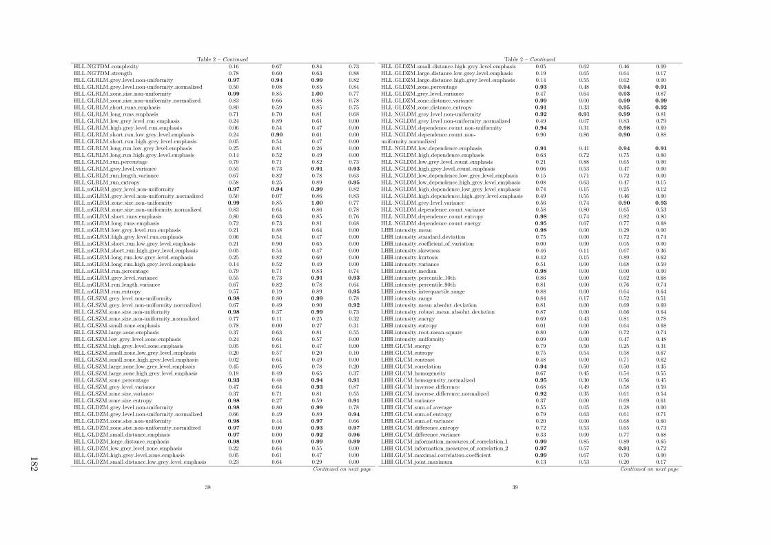
Table 2 – Continued
HLL NGTDM complexity 0.16 0.67 0.84 0.73HLL NGTDM strength 0.78 0.60 0.63 0.88HLL GLRLM grey level non-uniformity 0.97 0.94 0.99 0.82HLL GLRLM grey level non-uniformity normalized 0.50 0.08 0.85 0.84HLL GLRLM zone size non-uniformity 0.99 0.85 1.00 0.77HLL GLRLM zone size non-uniformity normalized 0.83 0.66 0.86 0.78HLL GLRLM short runs emphasis 0.80 0.59 0.85 0.75HLL GLRLM long runs emphasis 0.71 0.70 0.81 0.68HLL GLRLM low grey level run emphasis 0.24 0.89 0.61 0.00HLL GLRLM high grey level run emphasis 0.06 0.54 0.47 0.00HLL GLRLM short run low grey level emphasis 0.24 0.90 0.61 0.00HLL GLRLM short run high grey level emphasis 0.05 0.54 0.47 0.00HLL GLRLM long run low grey level emphasis 0.25 0.81 0.26 0.00HLL GLRLM long run high grey level emphasis 0.14 0.52 0.49 0.00HLL GLRLM run percentage 0.79 0.71 0.82 0.73HLL GLRLM grey level variance 0.55 0.73 0.91 0.93
HLL GLRLM run length variance 0.67 0.82 0.78 0.63HLL GLRLM run entropy 0.58 0.25 0.89 0.95
HLL mGLRM grey level non-uniformity 0.97 0.94 0.99 0.82HLL mGLRM grey level non-uniformity normalized 0.50 0.07 0.86 0.83HLL mGLRM zone size non-uniformity 0.99 0.85 1.00 0.77HLL mGLRM zone size non-uniformity normalized 0.83 0.64 0.86 0.78HLL mGLRM short runs emphasis 0.80 0.63 0.85 0.76HLL mGLRM long runs emphasis 0.72 0.73 0.81 0.68HLL mGLRM low grey level run emphasis 0.21 0.88 0.64 0.00HLL mGLRM high grey level run emphasis 0.06 0.54 0.47 0.00HLL mGLRM short run low grey level emphasis 0.21 0.90 0.65 0.00HLL mGLRM short run high grey level emphasis 0.05 0.54 0.47 0.00HLL mGLRM long run low grey level emphasis 0.25 0.82 0.60 0.00HLL mGLRM long run high grey level emphasis 0.14 0.52 0.49 0.00HLL mGLRM run percentage 0.79 0.71 0.83 0.74HLL mGLRM grey level variance 0.55 0.73 0.91 0.93
HLL mGLRM run length variance 0.67 0.82 0.78 0.64HLL mGLRM run entropy 0.57 0.19 0.89 0.95
HLL GLSZM grey level non-uniformity 0.98 0.80 0.99 0.78HLL GLSZM grey level non-uniformity normalized 0.67 0.49 0.90 0.92
HLL GLSZM zone size non-uniformity 0.98 0.37 0.99 0.73HLL GLSZM zone size non-uniformity normalized 0.77 0.11 0.25 0.32HLL GLSZM small zone emphasis 0.78 0.00 0.27 0.31HLL GLSZM large zone emphasis 0.37 0.63 0.81 0.55HLL GLSZM low grey level zone emphasis 0.24 0.64 0.57 0.00HLL GLSZM high grey level zone emphasis 0.05 0.61 0.47 0.00HLL GLSZM small zone low grey level emphasis 0.20 0.57 0.20 0.10HLL GLSZM small zone high grey level emphasis 0.02 0.64 0.49 0.00HLL GLSZM large zone low grey level emphasis 0.45 0.05 0.78 0.20HLL GLSZM large zone high grey level emphasis 0.18 0.49 0.65 0.37HLL GLSZM zone percentage 0.93 0.48 0.94 0.91
HLL GLSZM grey level variance 0.47 0.64 0.93 0.87HLL GLSZM zone size variance 0.37 0.71 0.81 0.55HLL GLSZM zone size entropy 0.98 0.27 0.59 0.91
HLL GLDZM grey level non-uniformity 0.98 0.80 0.99 0.78HLL GLDZM grey level non-uniformity normalized 0.66 0.49 0.89 0.94
HLL GLDZM zone size non-uniformity 0.98 0.44 0.97 0.66HLL GLDZM zone size non-uniformity normalized 0.97 0.00 0.93 0.97
HLL GLDZM small distance emphasis 0.97 0.00 0.92 0.96
HLL GLDZM large distance emphasis 0.98 0.00 0.99 0.99
HLL GLDZM low grey level zone emphasis 0.22 0.64 0.55 0.00HLL GLDZM high grey level zone emphasis 0.05 0.61 0.47 0.00HLL GLDZM small distance low grey level emphasis 0.23 0.64 0.29 0.00
Continued on next page
38
Table 2 – Continued
HLL GLDZM small distance high grey level emphasis 0.05 0.62 0.46 0.09HLL GLDZM large distance low grey level emphasis 0.19 0.65 0.64 0.17HLL GLDZM large distance high grey level emphasis 0.14 0.55 0.62 0.00HLL GLDZM zone percentage 0.93 0.48 0.94 0.91
HLL GLDZM grey level variance 0.47 0.64 0.93 0.87HLL GLDZM zone distance variance 0.99 0.00 0.99 0.99
HLL GLDZM zone distance entropy 0.91 0.33 0.95 0.92
HLL NGLDM grey level non-uniformity 0.92 0.91 0.99 0.81HLL NGLDM grey level non-uniformity normalized 0.49 0.07 0.83 0.79HLL NGLDM dependence count non-uniformity 0.94 0.31 0.98 0.69HLL NGLDM dependence count non-uniformity normalized
0.90 0.86 0.90 0.88
HLL NGLDM low dependence emphasis 0.91 0.41 0.94 0.91
HLL NGLDM high dependence emphasis 0.63 0.72 0.75 0.60HLL NGLDM low grey level count emphasis 0.21 0.88 0.65 0.00HLL NGLDM high grey level count emphasis 0.06 0.53 0.47 0.00HLL NGLDM low dependence low grey level emphasis 0.15 0.71 0.72 0.00HLL NGLDM low dependence high grey level emphasis 0.08 0.63 0.47 0.15HLL NGLDM high dependence low grey level emphasis 0.74 0.15 0.25 0.12HLL NGLDM high dependence high grey level emphasis 0.49 0.55 0.46 0.00HLL NGLDM grey level variance 0.56 0.74 0.90 0.93
HLL NGLDM dependence count variance 0.58 0.80 0.65 0.53HLL NGLDM dependence count entropy 0.98 0.74 0.82 0.80HLL NGLDM dependence count energy 0.95 0.67 0.77 0.68LHH intensity mean 0.98 0.00 0.29 0.00LHH intensity standard deviation 0.75 0.00 0.72 0.74LHH intensity coefficient of variation 0.00 0.00 0.05 0.00LHH intensity skewness 0.46 0.11 0.67 0.36LHH intensity kurtosis 0.42 0.15 0.89 0.62LHH intensity variance 0.51 0.00 0.68 0.59LHH intensity median 0.98 0.00 0.00 0.00LHH intensity percentile 10th 0.86 0.00 0.62 0.68LHH intensity percentile 90th 0.81 0.00 0.76 0.74LHH intensity interquartile range 0.88 0.00 0.64 0.64LHH intensity range 0.84 0.17 0.52 0.51LHH intensity mean absolut deviation 0.81 0.00 0.69 0.69LHH intensity robust mean absolut deviation 0.87 0.00 0.66 0.64LHH intensity energy 0.69 0.43 0.81 0.78LHH intensity entropy 0.01 0.00 0.64 0.68LHH intensity root mean square 0.80 0.00 0.72 0.74LHH intensity uniformity 0.09 0.00 0.47 0.48LHH GLCM energy 0.79 0.50 0.25 0.31LHH GLCM entropy 0.75 0.54 0.58 0.67LHH GLCM contrast 0.48 0.00 0.71 0.62LHH GLCM correlation 0.94 0.50 0.50 0.35LHH GLCM homogeneity 0.67 0.45 0.54 0.55LHH GLCM homogeneity normalized 0.95 0.30 0.56 0.45LHH GLCM inverese difference 0.68 0.49 0.58 0.59LHH GLCM inverese difference normalized 0.92 0.35 0.61 0.54LHH GLCM variance 0.37 0.00 0.69 0.61LHH GLCM sum of average 0.55 0.05 0.28 0.00LHH GLCM sum of entropy 0.79 0.63 0.61 0.71LHH GLCM sum of variance 0.20 0.00 0.68 0.60LHH GLCM difference entropy 0.72 0.53 0.65 0.73LHH GLCM difference variance 0.33 0.00 0.77 0.68LHH GLCM information measures of correlation 1 0.99 0.85 0.89 0.65LHH GLCM information measures of correlation 2 0.97 0.57 0.91 0.72LHH GLCM maximal correlation coefficient 0.99 0.67 0.70 0.00LHH GLCM joint maximum 0.13 0.53 0.20 0.17
Continued on next page
39
182

Table 2 – Continued
LHH GLCM joint average 0.55 0.05 0.28 0.00LHH GLCM difference average 0.70 0.09 0.71 0.72LHH GLCM dissimilarity 0.70 0.09 0.71 0.72LHH GLCM inverse variance 0.78 0.00 0.56 0.62LHH GLCM autocorrelation 0.53 0.04 0.26 0.00LHH GLCM cluster tendency 0.20 0.00 0.68 0.60LHH GLCM cluster shade 0.35 0.10 0.38 0.04LHH GLCM cluster prominence 0.00 0.00 0.53 0.29LHH mGLCM energy 0.11 0.00 0.29 0.27LHH mGLCM entropy 0.00 0.00 0.62 0.69LHH mGLCM contrast 0.39 0.00 0.71 0.62LHH mGLCM correlation 0.29 0.52 0.61 0.34LHH mGLCM homogeneity 0.60 0.18 0.55 0.55LHH mGLCM homogeneity normalized 0.96 0.12 0.53 0.44LHH mGLCM inverese difference 0.61 0.23 0.58 0.60LHH mGLCM inverese difference normalized 0.92 0.08 0.60 0.54LHH mGLCM variance 0.33 0.00 0.69 0.61LHH mGLCM sum of average 0.56 0.01 0.28 0.00LHH mGLCM sum of entropy 0.40 0.00 0.62 0.71LHH mGLCM sum of variance 0.26 0.00 0.67 0.60LHH mGLCM difference entropy 0.56 0.00 0.66 0.74LHH mGLCM difference variance 0.38 0.00 0.77 0.68LHH mGLCM information measures of correlation 1 0.93 0.00 0.52 0.00LHH mGLCM information measures of correlation 2 0.97 0.00 0.62 0.16LHH mGLCM maximal correlation coefficient 0.84 0.00 0.53 0.00LHH mGLCM joint maximum 0.10 0.07 0.18 0.17LHH mGLCM joint average 0.56 0.01 0.28 0.00LHH mGLCM difference average 0.58 0.02 0.71 0.72LHH mGLCM dissimilarity 0.58 0.02 0.71 0.72LHH mGLCM inverse variance 0.71 0.00 0.55 0.63LHH mGLCM autocorrelation 0.53 0.01 0.26 0.00LHH mGLCM cluster tendency 0.26 0.00 0.67 0.60LHH mGLCM cluster shade 0.38 0.08 0.38 0.04LHH mGLCM cluster prominence 0.00 0.00 0.53 0.29LHH NGTDM coarseness 0.98 0.82 0.99 0.94
LHH NGTDM contrast 0.49 0.20 0.55 0.72LHH NGTDM busyness 0.78 0.00 0.71 0.41LHH NGTDM complexity 0.49 0.00 0.63 0.39LHH NGTDM strength 0.65 0.00 0.73 0.37LHH GLRLM grey level non-uniformity 0.91 0.89 0.95 0.75LHH GLRLM grey level non-uniformity normalized 0.07 0.00 0.51 0.49LHH GLRLM zone size non-uniformity 0.96 0.86 0.99 0.77LHH GLRLM zone size non-uniformity normalized 0.78 0.48 0.64 0.56LHH GLRLM short runs emphasis 0.75 0.36 0.62 0.53LHH GLRLM long runs emphasis 0.60 0.49 0.52 0.39LHH GLRLM low grey level run emphasis 0.92 0.00 0.16 0.19LHH GLRLM high grey level run emphasis 0.51 0.00 0.27 0.00LHH GLRLM short run low grey level emphasis 0.92 0.00 0.14 0.00LHH GLRLM short run high grey level emphasis 0.46 0.00 0.27 0.00LHH GLRLM long run low grey level emphasis 0.88 0.00 0.18 0.00LHH GLRLM long run high grey level emphasis 0.70 0.04 0.28 0.00LHH GLRLM run percentage 0.73 0.52 0.60 0.51LHH GLRLM grey level variance 0.18 0.00 0.68 0.60LHH GLRLM run length variance 0.54 0.61 0.49 0.35LHH GLRLM run entropy 0.19 0.18 0.64 0.69LHH mGLRLM grey level non-uniformity 0.91 0.89 0.95 0.75LHH mGLRLM grey level non-uniformity normalized 0.08 0.00 0.51 0.50LHH mGLRLM zone size non-uniformity 0.96 0.86 0.99 0.77LHH mGLRLM zone size non-uniformity normalized 0.78 0.45 0.64 0.57
Continued on next page
40
Table 2 – Continued
LHH mGLRLM short runs emphasis 0.75 0.43 0.61 0.52LHH mGLRLM long runs emphasis 0.60 0.52 0.52 0.39LHH mGLRLM low grey level run emphasis 0.92 0.00 0.15 0.00LHH mGLRLM high grey level run emphasis 0.51 0.00 0.27 0.00LHH mGLRLM short run low grey level emphasis 0.92 0.00 0.14 0.00LHH mGLRLM short run high grey level emphasis 0.46 0.00 0.27 0.00LHH mGLRLM long run low grey level emphasis 0.89 0.00 0.19 0.00LHH mGLRLM long run high grey level emphasis 0.70 0.04 0.28 0.00LHH mGLRLM run percentage 0.73 0.52 0.60 0.51LHH mGLRLM grey level variance 0.18 0.00 0.68 0.60LHH mGLRLM run length variance 0.54 0.60 0.49 0.35LHH mGLRLM run entropy 0.06 0.11 0.64 0.70LHH GLSZM grey level non-uniformity 0.99 0.84 0.99 0.80LHH GLSZM grey level non-uniformity normalized 0.16 0.00 0.44 0.54LHH GLSZM zone size non-uniformity 0.90 0.89 0.94 0.81LHH GLSZM zone size non-uniformity normalized 0.00 0.52 0.46 0.62LHH GLSZM small zone emphasis 0.00 0.42 0.44 0.64LHH GLSZM large zone emphasis 0.23 0.56 0.54 0.30LHH GLSZM low grey level zone emphasis 0.90 0.00 0.14 0.00LHH GLSZM high grey level zone emphasis 0.53 0.00 0.27 0.00LHH GLSZM small zone low grey level emphasis 0.93 0.00 0.11 0.00LHH GLSZM small zone high grey level emphasis 0.50 0.00 0.32 0.03LHH GLSZM large zone low grey level emphasis 0.08 0.00 0.30 0.10LHH GLSZM large zone high grey level emphasis 0.52 0.29 0.75 0.55LHH GLSZM zone percentage 0.92 0.49 0.80 0.71LHH GLSZM grey level variance 0.02 0.00 0.78 0.82LHH GLSZM zone size variance 0.23 0.51 0.54 0.30LHH GLSZM zone size entropy 0.93 0.50 0.30 0.67LHH GLDZM grey level non-uniformity 0.99 0.84 0.99 0.80LHH GLDZM grey level non-uniformity normalized 0.15 0.00 0.39 0.55LHH GLDZM zone size non-uniformity 0.91 0.71 0.90 0.75LHH GLDZM zone size non-uniformity normalized 0.94 0.00 0.94 0.88LHH GLDZM small distance emphasis 0.93 0.00 0.94 0.84LHH GLDZM large distance emphasis 0.95 0.00 0.99 0.88LHH GLDZM low grey level zone emphasis 0.90 0.00 0.08 0.00LHH GLDZM high grey level zone emphasis 0.53 0.00 0.27 0.00LHH GLDZM small distance low grey level emphasis 0.90 0.00 0.04 0.07LHH GLDZM small distance high grey level emphasis 0.55 0.00 0.39 0.00LHH GLDZM large distance low grey level emphasis 0.89 0.00 0.49 0.06LHH GLDZM large distance high grey level emphasis 0.46 0.00 0.45 0.38LHH GLDZM zone percentage 0.92 0.49 0.80 0.71LHH GLDZM grey level variance 0.02 0.00 0.78 0.82LHH GLDZM zone distance variance 0.98 0.00 0.99 0.92
LHH GLDZM zone distance entropy 0.82 0.04 0.88 0.89LHH NGLDM grey level non-uniformity 0.82 0.81 0.92 0.70LHH NGLDM grey level non-uniformity normalized 0.16 0.00 0.48 0.47LHH NGLDM dependence count non-uniformity 0.84 0.64 0.93 0.67LHH NGLDM dependence count non-uniformity normalized
0.88 0.77 0.77 0.70
LHH NGLDM low dependence emphasis 0.85 0.28 0.81 0.72LHH NGLDM high dependence emphasis 0.51 0.45 0.42 0.33LHH NGLDM low grey level count emphasis 0.92 0.00 0.15 0.00LHH NGLDM high grey level count emphasis 0.51 0.00 0.27 0.00LHH NGLDM low dependence low grey level emphasis 0.95 0.00 0.07 0.00LHH NGLDM low dependence high grey level emphasis 0.00 0.00 0.37 0.10LHH NGLDM high dependence low grey level emphasis 0.00 0.01 0.21 0.06LHH NGLDM high dependence high grey level emphasis 0.77 0.19 0.37 0.27LHH NGLDM grey level variance 0.22 0.00 0.68 0.59LHH NGLDM dependence count variance 0.47 0.55 0.29 0.31
Continued on next page
41
Impact
ofC
Tcon
volution
kernel
onrob
ustn
essof
radiom
icfeatu
resfo
rdiff
erent
lung
diseases
and
tissue
types
183

Table 2 – Continued
LHH NGLDM dependence count entropy 0.99 0.82 0.45 0.79LHH NGLDM dependence count energy 0.99 0.65 0.50 0.60LHL intensity mean 0.00 0.44 0.96 0.62LHL intensity standard deviation 0.94 0.75 0.89 0.94
LHL intensity coefficient of variation 0.00 0.00 0.85 0.35LHL intensity skewness 0.83 0.51 0.82 0.61LHL intensity kurtosis 0.92 0.47 0.83 0.88LHL intensity variance 0.97 0.67 0.91 0.95
LHL intensity median 0.63 0.40 0.73 0.79LHL intensity percentile 10th 0.89 0.66 0.91 0.88LHL intensity percentile 90th 1.00 0.02 0.93 0.94
LHL intensity interquartile range 0.94 0.59 0.90 0.85LHL intensity range 0.91 0.72 0.67 0.71LHL intensity mean absolut deviation 0.98 0.79 0.89 0.90LHL intensity robust mean absolut deviation 1.00 0.66 0.90 0.85LHL intensity energy 0.96 0.89 0.99 0.81LHL intensity entropy 0.75 0.39 0.85 0.85LHL intensity root mean square 0.94 0.75 0.89 0.94
LHL intensity uniformity 0.63 0.25 0.80 0.71LHL GLCM energy 0.85 0.54 0.63 0.57LHL GLCM entropy 0.94 0.80 0.82 0.83LHL GLCM contrast 0.44 0.62 0.90 0.93
LHL GLCM correlation 0.00 0.94 0.91 0.76LHL GLCM homogeneity 0.67 0.62 0.78 0.75LHL GLCM homogeneity normalized 0.94 0.82 0.85 0.51LHL GLCM inverese difference 0.70 0.65 0.81 0.78LHL GLCM inverese difference normalized 0.96 0.74 0.86 0.69LHL GLCM variance 0.43 0.73 0.91 0.94
LHL GLCM sum of average 0.55 0.32 0.60 0.60LHL GLCM sum of entropy 0.96 0.79 0.86 0.88LHL GLCM sum of variance 0.42 0.72 0.92 0.95
LHL GLCM difference entropy 0.96 0.71 0.85 0.88LHL GLCM difference variance 0.53 0.67 0.91 0.94
LHL GLCM information measures of correlation 1 0.99 0.93 0.89 0.96
LHL GLCM information measures of correlation 2 0.99 0.11 0.94 0.97
LHL GLCM maximal correlation coefficient 0.97 0.42 0.22 0.00LHL GLCM joint maximum 0.68 0.44 0.56 0.54LHL GLCM joint average 0.55 0.32 0.60 0.60LHL GLCM difference average 0.65 0.78 0.88 0.90
LHL GLCM dissimilarity 0.65 0.78 0.88 0.90
LHL GLCM inverse variance 0.85 0.67 0.81 0.73LHL GLCM autocorrelation 0.44 0.10 0.53 0.60LHL GLCM cluster tendency 0.42 0.72 0.92 0.95
LHL GLCM cluster shade 0.32 0.27 0.82 0.62LHL GLCM cluster prominence 0.13 0.52 0.93 0.93
LHL mGLCM energy 0.45 0.16 0.69 0.54LHL mGLCM entropy 0.70 0.36 0.85 0.85LHL mGLCM contrast 0.45 0.76 0.90 0.93
LHL mGLCM correlation 0.44 0.63 0.92 0.83LHL mGLCM homogeneity 0.77 0.56 0.78 0.75LHL mGLCM homogeneity normalized 0.99 0.89 0.86 0.55LHL mGLCM inverese difference 0.78 0.61 0.80 0.78LHL mGLCM inverese difference normalized 0.98 0.81 0.86 0.72LHL mGLCM variance 0.43 0.74 0.91 0.94
LHL mGLCM sum of average 0.53 0.32 0.60 0.60LHL mGLCM sum of entropy 0.78 0.60 0.86 0.88LHL mGLCM sum of variance 0.43 0.70 0.92 0.95
LHL mGLCM difference entropy 0.78 0.68 0.86 0.88LHL mGLCM difference variance 0.49 0.60 0.91 0.94
Continued on next page
42
Table 2 – Continued
LHL mGLCM information measures of correlation 1 0.97 0.13 0.69 0.77LHL mGLCM information measures of correlation 2 0.99 0.22 0.76 0.88LHL mGLCM maximal correlation coefficient 0.95 0.54 0.78 0.78LHL mGLCM joint maximum 0.36 0.00 0.58 0.53LHL mGLCM joint average 0.53 0.32 0.60 0.60LHL mGLCM difference average 0.66 0.81 0.88 0.90
LHL mGLCM dissimilarity 0.66 0.81 0.88 0.90
LHL mGLCM inverse variance 0.82 0.50 0.80 0.73LHL mGLCM autocorrelation 0.42 0.11 0.53 0.60LHL mGLCM cluster tendency 0.43 0.70 0.92 0.95
LHL mGLCM cluster shade 0.37 0.25 0.82 0.63LHL mGLCM cluster prominence 0.14 0.40 0.93 0.93
LHL NGTDM coarseness 0.94 0.79 0.98 0.96
LHL NGTDM contrast 0.45 0.55 0.93 0.94
LHL NGTDM busyness 0.91 0.91 0.57 0.70LHL NGTDM complexity 0.33 0.81 0.81 0.92
LHL NGTDM strength 0.67 0.54 0.61 0.81LHL GLRLM grey level non-uniformity 0.97 0.87 0.99 0.79LHL GLRLM grey level non-uniformity normalized 0.64 0.32 0.81 0.74LHL GLRLM zone size non-uniformity 0.99 0.90 1.00 0.78LHL GLRLM zone size non-uniformity normalized 0.89 0.50 0.83 0.80LHL GLRLM short runs emphasis 0.87 0.46 0.84 0.78LHL GLRLM long runs emphasis 0.82 0.45 0.78 0.72LHL GLRLM low grey level run emphasis 0.92 0.81 0.65 0.14LHL GLRLM high grey level run emphasis 0.36 0.12 0.53 0.61LHL GLRLM short run low grey level emphasis 0.92 0.79 0.22 0.14LHL GLRLM short run high grey level emphasis 0.32 0.12 0.53 0.61LHL GLRLM long run low grey level emphasis 0.93 0.87 0.76 0.00LHL GLRLM long run high grey level emphasis 0.54 0.12 0.53 0.63LHL GLRLM run percentage 0.87 0.50 0.81 0.76LHL GLRLM grey level variance 0.45 0.66 0.91 0.95
LHL GLRLM run length variance 0.79 0.53 0.78 0.70LHL GLRLM run entropy 0.80 0.54 0.88 0.91
LHL mGLRLM grey level non-uniformity 0.97 0.87 0.99 0.79LHL mGLRLM grey level non-uniformity normalized 0.64 0.32 0.82 0.73LHL mGLRLM zone size non-uniformity 0.99 0.90 1.00 0.78LHL mGLRLM zone size non-uniformity normalized 0.89 0.50 0.83 0.80LHL mGLRLM short runs emphasis 0.88 0.49 0.82 0.78LHL mGLRLM long runs emphasis 0.82 0.49 0.78 0.72LHL mGLRLM low grey level run emphasis 0.92 0.81 0.67 0.20LHL mGLRLM high grey level run emphasis 0.36 0.12 0.53 0.61LHL mGLRLM short run low grey level emphasis 0.92 0.79 0.68 0.20LHL mGLRLM short run high grey level emphasis 0.32 0.12 0.53 0.61LHL mGLRLM long run low grey level emphasis 0.92 0.87 0.64 0.21LHL mGLRLM long run high grey level emphasis 0.54 0.12 0.53 0.63LHL mGLRLM run percentage 0.87 0.50 0.81 0.77LHL mGLRLM grey level variance 0.45 0.66 0.91 0.95
LHL mGLRLM run length variance 0.79 0.52 0.76 0.69LHL mGLRLM run entropy 0.79 0.53 0.88 0.91
LHL GLSZM grey level non-uniformity 0.99 0.60 0.99 0.78LHL GLSZM grey level non-uniformity normalized 0.83 0.50 0.90 0.92
LHL GLSZM zone size non-uniformity 0.99 0.63 0.99 0.81LHL GLSZM zone size non-uniformity normalized 0.73 0.42 0.39 0.81LHL GLSZM small zone emphasis 0.76 0.63 0.39 0.80LHL GLSZM large zone emphasis 0.50 0.38 0.69 0.51LHL GLSZM low grey level zone emphasis 0.92 0.45 0.65 0.00LHL GLSZM high grey level zone emphasis 0.34 0.11 0.54 0.63LHL GLSZM small zone low grey level emphasis 0.91 0.04 0.82 0.00LHL GLSZM small zone high grey level emphasis 0.24 0.13 0.55 0.65
Continued on next page
43
184

Table 2 – Continued
LHL GLSZM large zone low grey level emphasis 0.34 0.96 0.18 0.26LHL GLSZM large zone high grey level emphasis 0.71 0.16 0.51 0.55LHL GLSZM zone percentage 0.95 0.52 0.90 0.92
LHL GLSZM grey level variance 0.38 0.51 0.93 0.94
LHL GLSZM zone size variance 0.50 0.44 0.69 0.50LHL GLSZM zone size entropy 0.98 0.62 0.62 0.79LHL GLDZM grey level non-uniformity 0.99 0.60 0.99 0.78LHL GLDZM grey level non-uniformity normalized 0.83 0.49 0.90 0.92
LHL GLDZM zone size non-uniformity 0.99 0.72 0.98 0.80LHL GLDZM zone size non-uniformity normalized 0.96 0.99 0.98 0.93
LHL GLDZM small distance emphasis 0.96 0.98 0.98 0.92
LHL GLDZM large distance emphasis 0.98 0.98 0.99 0.93
LHL GLDZM low grey level zone emphasis 0.92 0.45 0.64 0.12LHL GLDZM high grey level zone emphasis 0.34 0.11 0.54 0.63LHL GLDZM small distance low grey level emphasis 0.92 0.45 0.78 0.14LHL GLDZM small distance high grey level emphasis 0.32 0.11 0.58 0.58LHL GLDZM large distance low grey level emphasis 0.92 0.45 0.11 0.30LHL GLDZM large distance high grey level emphasis 0.46 0.10 0.67 0.73LHL GLDZM zone percentage 0.95 0.52 0.90 0.92
LHL GLDZM grey level variance 0.38 0.51 0.93 0.94
LHL GLDZM zone distance variance 0.99 0.99 1.00 0.95
LHL GLDZM zone distance entropy 0.91 0.65 0.97 0.94
LHL NGLDM grey level non-uniformity 0.95 0.84 0.99 0.78LHL NGLDM grey level non-uniformity normalized 0.63 0.27 0.80 0.69LHL NGLDM dependence count non-uniformity 0.95 0.56 0.99 0.72LHL NGLDM dependence count non-uniformity normalized
0.86 0.53 0.88 0.89
LHL NGLDM low dependence emphasis 0.92 0.53 0.90 0.91
LHL NGLDM high dependence emphasis 0.75 0.44 0.74 0.67LHL NGLDM low grey level count emphasis 0.92 0.83 0.68 0.21LHL NGLDM high grey level count emphasis 0.36 0.13 0.53 0.61LHL NGLDM low dependence low grey level emphasis 0.91 0.34 0.78 0.24LHL NGLDM low dependence high grey level emphasis 0.19 0.11 0.54 0.63LHL NGLDM high dependence low grey level emphasis 0.59 0.99 0.41 0.28LHL NGLDM high dependence high grey level emphasis 0.93 0.11 0.50 0.73LHL NGLDM grey level variance 0.46 0.67 0.91 0.95
LHL NGLDM dependence count variance 0.70 0.52 0.69 0.68LHL NGLDM dependence count entropy 0.99 0.78 0.89 0.82LHL NGLDM dependence count energy 0.99 0.60 0.91 0.68LLH intensity mean 0.97 0.00 0.53 0.81LLH intensity standard deviation 0.99 0.09 0.94 0.91
LLH intensity coefficient of variation 0.69 0.27 0.18 0.67LLH intensity skewness 0.27 0.53 0.71 0.65LLH intensity kurtosis 0.90 0.53 0.94 0.69LLH intensity variance 0.93 0.04 0.84 0.83LLH intensity median 0.92 0.00 0.44 0.91
LLH intensity percentile 10th 0.95 0.00 0.93 0.88LLH intensity percentile 90th 0.97 0.29 0.96 0.94
LLH intensity interquartile range 0.89 0.16 0.94 0.90LLH intensity range 0.91 0.26 0.72 0.51LLH intensity mean absolut deviation 0.98 0.00 0.95 0.93
LLH intensity robust mean absolut deviation 0.91 0.24 0.94 0.91
LLH intensity energy 0.84 0.33 0.88 0.64LLH intensity entropy 0.09 0.00 0.95 0.92
LLH intensity root mean square 0.99 0.12 0.94 0.92
LLH intensity uniformity 0.11 0.00 0.83 0.70LLH GLCM energy 0.82 0.44 0.69 0.45LLH GLCM entropy 0.88 0.57 0.93 0.90LLH GLCM contrast 0.85 0.00 0.85 0.85
Continued on next page
44
Table 2 – Continued
LLH GLCM correlation 0.91 0.57 0.85 0.57LLH GLCM homogeneity 0.68 0.00 0.84 0.76LLH GLCM homogeneity normalized 0.99 0.43 0.66 0.65LLH GLCM inverese difference 0.73 0.00 0.88 0.82LLH GLCM inverese difference normalized 0.99 0.41 0.75 0.75LLH GLCM variance 0.75 0.01 0.84 0.84LLH GLCM sum of average 0.59 0.23 0.76 0.48LLH GLCM sum of entropy 0.92 0.57 0.96 0.93
LLH GLCM sum of variance 0.49 0.04 0.83 0.83LLH GLCM difference entropy 0.84 0.38 0.96 0.94
LLH GLCM difference variance 0.66 0.05 0.85 0.83LLH GLCM information measures of correlation 1 0.98 0.51 0.92 0.87LLH GLCM information measures of correlation 2 0.98 0.04 0.96 0.92
LLH GLCM maximal correlation coefficient 0.97 0.22 0.80 0.26LLH GLCM joint maximum 0.24 0.14 0.50 0.35LLH GLCM joint average 0.59 0.23 0.76 0.48LLH GLCM difference average 0.89 0.00 0.94 0.93
LLH GLCM dissimilarity 0.89 0.00 0.94 0.93
LLH GLCM inverse variance 0.82 0.76 0.88 0.84LLH GLCM autocorrelation 0.51 0.37 0.77 0.46LLH GLCM cluster tendency 0.49 0.04 0.83 0.83LLH GLCM cluster shade 0.73 0.62 0.68 0.72LLH GLCM cluster prominence 0.55 0.01 0.53 0.54LLH mGLCM energy 0.07 0.00 0.64 0.46LLH mGLCM entropy 0.07 0.00 0.95 0.91
LLH mGLCM contrast 0.86 0.01 0.85 0.85LLH mGLCM correlation 0.32 0.38 0.76 0.53LLH mGLCM homogeneity 0.65 0.00 0.84 0.76LLH mGLCM homogeneity normalized 1.00 0.38 0.66 0.67LLH mGLCM inverese difference 0.69 0.00 0.88 0.82LLH mGLCM inverese difference normalized 0.99 0.36 0.75 0.74LLH mGLCM variance 0.82 0.04 0.84 0.84LLH mGLCM sum of average 0.58 0.24 0.76 0.48LLH mGLCM sum of entropy 0.39 0.00 0.96 0.93
LLH mGLCM sum of variance 0.77 0.07 0.83 0.83LLH mGLCM difference entropy 0.60 0.00 0.96 0.94
LLH mGLCM difference variance 0.76 0.05 0.85 0.83LLH mGLCM information measures of correlation 1 0.98 0.42 0.73 0.34LLH mGLCM information measures of correlation 2 0.98 0.28 0.81 0.40LLH mGLCM maximal correlation coefficient 0.86 0.50 0.87 0.28LLH mGLCM joint maximum 0.00 0.00 0.55 0.33LLH mGLCM joint average 0.58 0.24 0.76 0.48LLH mGLCM difference average 0.87 0.00 0.94 0.93
LLH mGLCM dissimilarity 0.87 0.00 0.94 0.93
LLH mGLCM inverse variance 0.78 0.81 0.88 0.83LLH mGLCM autocorrelation 0.51 0.37 0.77 0.46LLH mGLCM cluster tendency 0.77 0.07 0.83 0.83LLH mGLCM cluster shade 0.75 0.57 0.68 0.71LLH mGLCM cluster prominence 0.67 0.02 0.53 0.54LLH NGTDM coarseness 1.00 0.47 1.00 0.96
LLH NGTDM contrast 0.64 0.42 0.95 0.88LLH NGTDM busyness 0.80 0.00 0.70 0.62LLH NGTDM complexity 0.68 0.04 0.60 0.52LLH NGTDM strength 0.90 0.02 0.44 0.48LLH GLRLM grey level non-uniformity 0.94 0.92 0.97 0.81LLH GLRLM grey level non-uniformity normalized 0.11 0.00 0.85 0.79LLH GLRLM zone size non-uniformity 0.97 0.84 0.99 0.77LLH GLRLM zone size non-uniformity normalized 0.75 0.20 0.84 0.74LLH GLRLM short runs emphasis 0.72 0.09 0.82 0.69
Continued on next page
45
Impact
ofC
Tcon
volution
kernel
onrob
ustn
essof
radiom
icfeatu
resfo
rdiff
erent
lung
diseases
and
tissue
types
185
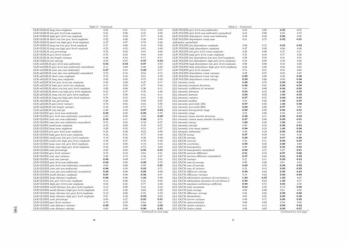
Table 2 – Continued
LLH GLRLM long runs emphasis 0.56 0.21 0.74 0.56LLH GLRLM low grey level run emphasis 0.21 0.00 0.37 0.00LLH GLRLM high grey level run emphasis 0.51 0.33 0.77 0.46LLH GLRLM short run low grey level emphasis 0.22 0.00 0.40 0.00LLH GLRLM short run high grey level emphasis 0.47 0.27 0.76 0.46LLH GLRLM long run low grey level emphasis 0.17 0.00 0.19 0.00LLH GLRLM long run high grey level emphasis 0.70 0.55 0.81 0.49LLH GLRLM run percentage 0.70 0.23 0.81 0.68LLH GLRLM grey level variance 0.73 0.04 0.84 0.82LLH GLRLM run length variance 0.48 0.44 0.71 0.51LLH GLRLM run entropy 0.53 0.05 0.97 0.94
LLH mGLRLM grey level non-uniformity 0.94 0.92 0.97 0.82LLH mGLRLM grey level non-uniformity normalized 0.11 0.00 0.86 0.80LLH mGLRLM zone size non-uniformity 0.97 0.84 0.99 0.77LLH mGLRLM zone size non-uniformity normalized 0.75 0.16 0.84 0.74LLH mGLRLM short runs emphasis 0.72 0.16 0.81 0.70LLH mGLRLM long runs emphasis 0.56 0.28 0.75 0.56LLH mGLRLM low grey level run emphasis 0.20 0.00 0.37 0.11LLH mGLRLM high grey level run emphasis 0.51 0.33 0.77 0.46LLH mGLRLM short run low grey level emphasis 0.20 0.00 0.36 0.11LLH mGLRLM short run high grey level emphasis 0.47 0.27 0.76 0.46LLH mGLRLM long run low grey level emphasis 0.17 0.00 0.41 0.11LLH mGLRLM long run high grey level emphasis 0.70 0.55 0.81 0.49LLH mGLRLM run percentage 0.69 0.23 0.80 0.67LLH mGLRLM grey level variance 0.73 0.04 0.84 0.82LLH mGLRLM run length variance 0.48 0.40 0.71 0.51LLH mGLRLM run entropy 0.49 0.02 0.97 0.94
LLH GLSZM grey level non-uniformity 0.98 0.80 0.99 0.78LLH GLSZM grey level non-uniformity normalized 0.62 0.00 0.88 0.90
LLH GLSZM zone size non-uniformity 0.95 0.37 0.96 0.74LLH GLSZM zone size non-uniformity normalized 0.75 0.34 0.43 0.57LLH GLSZM small zone emphasis 0.72 0.00 0.45 0.57LLH GLSZM large zone emphasis 0.29 0.55 0.51 0.47LLH GLSZM low grey level zone emphasis 0.16 0.00 0.22 0.00LLH GLSZM high grey level zone emphasis 0.52 0.25 0.77 0.46LLH GLSZM small zone low grey level emphasis 0.13 0.32 0.30 0.00LLH GLSZM small zone high grey level emphasis 0.49 0.27 0.76 0.49LLH GLSZM large zone low grey level emphasis 0.12 0.00 0.18 0.25LLH GLSZM large zone high grey level emphasis 0.53 0.89 0.73 0.63LLH GLSZM zone percentage 0.88 0.36 0.95 0.91
LLH GLSZM grey level variance 0.73 0.19 0.84 0.81LLH GLSZM zone size variance 0.29 0.72 0.50 0.47LLH GLSZM zone size entropy 0.96 0.09 0.47 0.84LLH GLDZM grey level non-uniformity 0.98 0.80 0.99 0.78LLH GLDZM grey level non-uniformity normalized 0.63 0.00 0.88 0.91
LLH GLDZM zone size non-uniformity 0.96 0.50 0.95 0.71LLH GLDZM zone size non-uniformity normalized 0.98 0.00 0.98 0.90LLH GLDZM small distance emphasis 0.97 0.00 0.98 0.87LLH GLDZM large distance emphasis 0.96 0.00 1.00 0.89LLH GLDZM low grey level zone emphasis 0.14 0.00 0.31 0.05LLH GLDZM high grey level zone emphasis 0.52 0.25 0.77 0.46LLH GLDZM small distance low grey level emphasis 0.14 0.00 0.34 0.16LLH GLDZM small distance high grey level emphasis 0.51 0.26 0.62 0.39LLH GLDZM large distance low grey level emphasis 0.12 0.00 0.35 0.22LLH GLDZM large distance high grey level emphasis 0.51 0.23 0.93 0.63LLH GLDZM zone percentage 0.88 0.37 0.95 0.91
LLH GLDZM grey level variance 0.73 0.19 0.84 0.81LLH GLDZM zone distance variance 0.96 0.00 1.00 0.92
LLH GLDZM zone distance entropy 0.89 0.00 0.98 0.91
Continued on next page
46
Table 2 – Continued
LLH NGLDM grey level non-uniformity 0.84 0.90 0.95 0.78LLH NGLDM grey level non-uniformity normalized 0.15 0.00 0.83 0.72LLH NGLDM dependence count non-uniformity 0.88 0.39 0.96 0.68LLH NGLDM dependence count non-uniformity normalized
0.81 0.75 0.92 0.91
LLH NGLDM low dependence emphasis 0.86 0.12 0.95 0.93
LLH NGLDM high dependence emphasis 0.47 0.28 0.66 0.46LLH NGLDM low grey level count emphasis 0.20 0.00 0.37 0.11LLH NGLDM high grey level count emphasis 0.51 0.34 0.77 0.46LLH NGLDM low dependence low grey level emphasis 0.20 0.35 0.21 0.21LLH NGLDM low dependence high grey level emphasis 0.24 0.00 0.59 0.46LLH NGLDM high dependence low grey level emphasis 0.00 0.00 0.48 0.20LLH NGLDM high dependence high grey level emphasis 0.86 0.86 0.88 0.63LLH NGLDM grey level variance 0.74 0.01 0.84 0.83LLH NGLDM dependence count variance 0.39 0.37 0.58 0.37LLH NGLDM dependence count entropy 0.99 0.68 0.88 0.90
LLH NGLDM dependence count energy 0.99 0.66 0.89 0.96
LLL intensity mean 0.98 0.70 0.99 0.96
LLL intensity standard deviation 0.98 0.31 0.98 0.95
LLL intensity coefficient of variation 0.00 0.00 0.98 0.95
LLL intensity skewness 0.94 0.19 1.00 0.95
LLL intensity kurtosis 0.98 0.33 1.00 0.93
LLL intensity variance 0.97 0.27 0.98 0.95
LLL intensity median 0.88 0.62 1.00 0.97
LLL intensity percentile 10th 0.97 0.20 1.00 0.96
LLL intensity percentile 90th 0.92 0.68 0.97 0.90LLL intensity interquartile range 0.99 0.00 0.99 0.91
LLL intensity range 0.52 0.60 0.56 0.74LLL intensity mean absolut deviation 0.99 0.11 0.99 0.92
LLL intensity robust mean absolut deviation 0.97 0.00 0.99 0.91
LLL intensity energy 1.00 0.46 1.00 0.81LLL intensity entropy 0.88 0.18 0.99 0.94
LLL intensity root mean square 0.98 0.24 1.00 0.96
LLL intensity uniformity 0.88 0.10 0.98 0.94
LLL GLCM energy 0.97 0.59 0.06 0.56LLL GLCM entropy 0.99 0.85 0.97 0.96
LLL GLCM contrast 0.35 0.11 0.99 0.97
LLL GLCM correlation 0.98 0.38 0.99 0.89LLL GLCM homogeneity 0.90 0.39 0.95 0.95
LLL GLCM homogeneity normalized 0.96 0.75 0.87 0.91
LLL GLCM inverese difference 0.91 0.34 0.97 0.96
LLL GLCM inverese difference normalized 0.97 0.68 0.94 0.93
LLL GLCM variance 0.27 0.11 0.99 0.94
LLL GLCM sum of average 0.00 0.69 0.61 0.32LLL GLCM sum of entropy 0.99 0.76 0.99 0.92
LLL GLCM sum of variance 0.21 0.14 0.99 0.92
LLL GLCM difference entropy 0.99 0.63 0.99 0.94
LLL GLCM difference variance 0.19 0.23 0.98 0.95
LLL GLCM information measures of correlation 1 1.00 0.97 1.00 0.85LLL GLCM information measures of correlation 2 0.99 0.24 1.00 0.77LLL GLCM maximal correlation coefficient 0.99 0.75 0.95 0.78LLL GLCM joint maximum 0.94 0.56 0.73 0.98
LLL GLCM joint average 0.00 0.69 0.61 0.32LLL GLCM difference average 0.65 0.05 0.99 0.96
LLL GLCM dissimilarity 0.65 0.05 0.99 0.96
LLL GLCM inverse variance 0.86 0.17 0.96 0.95
LLL GLCM autocorrelation 0.00 0.69 0.56 0.32LLL GLCM cluster tendency 0.21 0.14 0.99 0.92
LLL GLCM cluster shade 0.00 0.62 0.99 0.97
Continued on next page
47
186

Table 2 – Continued
LLL GLCM cluster prominence 0.01 0.35 0.98 0.96
LLL mGLCM energy 0.73 0.10 0.95 0.94
LLL mGLCM entropy 0.94 0.20 0.99 0.95
LLL mGLCM contrast 0.32 0.07 0.99 0.97
LLL mGLCM correlation 0.94 0.50 0.99 0.89LLL mGLCM homogeneity 0.88 0.08 0.95 0.95
LLL mGLCM homogeneity normalized 0.97 0.68 0.88 0.91
LLL mGLCM inverese difference 0.89 0.07 0.97 0.96
LLL mGLCM inverese difference normalized 0.98 0.57 0.94 0.93
LLL mGLCM variance 0.29 0.12 0.99 0.94
LLL mGLCM sum of average 0.00 0.68 0.61 0.32LLL mGLCM sum of entropy 0.74 0.00 0.99 0.92
LLL mGLCM sum of variance 0.27 0.18 0.99 0.92
LLL mGLCM difference entropy 0.78 0.00 0.99 0.94
LLL mGLCM difference variance 0.21 0.24 0.98 0.95
LLL mGLCM information measures of correlation 1 0.95 0.41 0.97 0.47LLL mGLCM information measures of correlation 2 0.99 0.28 0.98 0.54LLL mGLCM maximal correlation coefficient 0.94 0.11 0.98 0.84LLL mGLCM joint maximum 0.57 0.00 0.77 0.91
LLL mGLCM joint average 0.00 0.68 0.61 0.32LLL mGLCM difference average 0.64 0.01 0.99 0.96
LLL mGLCM dissimilarity 0.64 0.01 0.99 0.96
LLL mGLCM inverse variance 0.86 0.01 0.96 0.95
LLL mGLCM autocorrelation 0.00 0.68 0.56 0.32LLL mGLCM cluster tendency 0.27 0.18 0.99 0.92
LLL mGLCM cluster shade 0.00 0.62 0.99 0.97
LLL mGLCM cluster prominence 0.03 0.39 0.98 0.96
LLL NGTDM coarseness 0.96 0.52 1.00 0.96
LLL NGTDM contrast 0.66 0.49 0.96 0.95
LLL NGTDM busyness 1.00 0.85 0.95 0.55LLL NGTDM complexity 0.06 0.10 0.82 0.85LLL NGTDM strength 0.72 0.43 0.98 0.89LLL GLRLM grey level non-uniformity 0.99 0.90 1.00 0.79LLL GLRLM grey level non-uniformity normalized 0.90 0.10 0.97 0.93
LLL GLRLM zone size non-uniformity 1.00 0.91 1.00 0.80LLL GLRLM zone size non-uniformity normalized 0.92 0.50 0.93 0.96
LLL GLRLM short runs emphasis 0.91 0.46 0.92 0.96
LLL GLRLM long runs emphasis 0.86 0.50 0.91 0.94
LLL GLRLM low grey level run emphasis 0.70 0.91 0.36 0.05LLL GLRLM high grey level run emphasis 0.00 0.66 0.61 0.44LLL GLRLM short run low grey level emphasis 0.70 0.91 0.43 0.40LLL GLRLM short run high grey level emphasis 0.00 0.65 0.61 0.45LLL GLRLM long run low grey level emphasis 0.70 0.90 0.41 0.24LLL GLRLM long run high grey level emphasis 0.00 0.70 0.59 0.41LLL GLRLM run percentage 0.90 0.52 0.93 0.95
LLL GLRLM grey level variance 0.21 0.27 0.98 0.95
LLL GLRLM run length variance 0.82 0.56 0.89 0.94
LLL GLRLM run entropy 0.93 0.37 0.98 0.92
LLL mGLRLM grey level non-uniformity 0.99 0.90 1.00 0.79LLL mGLRLM grey level non-uniformity normalized 0.90 0.12 0.98 0.93
LLL mGLRLM zone size non-uniformity 1.00 0.91 1.00 0.80LLL mGLRLM zone size non-uniformity normalized 0.92 0.49 0.93 0.96
LLL mGLRLM short runs emphasis 0.91 0.50 0.93 0.95
LLL mGLRLM long runs emphasis 0.86 0.53 0.91 0.94
LLL mGLRLM low grey level run emphasis 0.69 0.91 0.34 0.26LLL mGLRLM high grey level run emphasis 0.00 0.66 0.61 0.44LLL mGLRLM short run low grey level emphasis 0.69 0.91 0.33 0.26LLL mGLRLM short run high grey level emphasis 0.00 0.65 0.61 0.45LLL mGLRLM long run low grey level emphasis 0.69 0.90 0.39 0.23
Continued on next page
48
Table 2 – Continued
LLL mGLRLM long run high grey level emphasis 0.00 0.70 0.59 0.41LLL mGLRLM run percentage 0.90 0.52 0.92 0.95
LLL mGLRLM grey level variance 0.21 0.27 0.98 0.95
LLL mGLRLM run length variance 0.83 0.55 0.90 0.93
LLL mGLRLM run entropy 0.93 0.44 0.98 0.92
LLL GLSZM grey level non-uniformity 0.98 0.90 0.99 0.78LLL GLSZM grey level non-uniformity normalized 0.88 0.37 0.92 0.88LLL GLSZM zone size non-uniformity 1.00 0.21 0.99 0.80LLL GLSZM zone size non-uniformity normalized 0.88 0.39 0.84 0.63LLL GLSZM small zone emphasis 0.91 0.20 0.86 0.64LLL GLSZM large zone emphasis 0.39 0.79 0.67 0.68LLL GLSZM low grey level zone emphasis 0.69 0.72 0.22 0.22LLL GLSZM high grey level zone emphasis 0.00 0.60 0.49 0.41LLL GLSZM small zone low grey level emphasis 0.69 0.56 0.21 0.23LLL GLSZM small zone high grey level emphasis 0.00 0.38 0.51 0.43LLL GLSZM large zone low grey level emphasis 0.36 0.70 0.57 0.56LLL GLSZM large zone high grey level emphasis 0.40 0.87 0.46 0.31LLL GLSZM zone percentage 0.97 0.57 0.95 0.95
LLL GLSZM grey level variance 0.06 0.48 0.97 0.93
LLL GLSZM zone size variance 0.38 0.83 0.64 0.67LLL GLSZM zone size entropy 0.97 0.71 0.89 0.69LLL GLDZM grey level non-uniformity 0.98 0.90 0.99 0.78LLL GLDZM grey level non-uniformity normalized 0.89 0.37 0.96 0.89LLL GLDZM zone size non-uniformity 1.00 0.74 1.00 0.79LLL GLDZM zone size non-uniformity normalized 0.97 0.00 0.97 0.95
LLL GLDZM small distance emphasis 0.97 0.00 0.95 0.93
LLL GLDZM large distance emphasis 0.98 0.00 0.99 0.94
LLL GLDZM low grey level zone emphasis 0.69 0.72 0.28 0.32LLL GLDZM high grey level zone emphasis 0.00 0.60 0.49 0.41LLL GLDZM small distance low grey level emphasis 0.69 0.72 0.58 0.34LLL GLDZM small distance high grey level emphasis 0.00 0.58 0.58 0.50LLL GLDZM large distance low grey level emphasis 0.68 0.71 0.40 0.37LLL GLDZM large distance high grey level emphasis 0.00 0.62 0.63 0.64LLL GLDZM zone percentage 0.97 0.57 0.95 0.95
LLL GLDZM grey level variance 0.06 0.48 0.97 0.93
LLL GLDZM zone distance variance 0.99 0.00 1.00 0.95
LLL GLDZM zone distance entropy 0.95 0.45 0.99 0.97
LLL NGLDM grey level non-uniformity 0.98 0.87 1.00 0.80LLL NGLDM grey level non-uniformity normalized 0.88 0.10 0.98 0.94
LLL NGLDM dependence count non-uniformity 0.98 0.61 0.99 0.76LLL NGLDM dependence count non-uniformity normalized
0.91 0.58 0.96 0.97
LLL NGLDM low dependence emphasis 0.96 0.46 0.96 0.95
LLL NGLDM high dependence emphasis 0.77 0.43 0.89 0.93
LLL NGLDM low grey level count emphasis 0.69 0.90 0.34 0.25LLL NGLDM high grey level count emphasis 0.00 0.67 0.61 0.46LLL NGLDM low dependence low grey level emphasis 0.70 0.85 0.26 0.40LLL NGLDM low dependence high grey level emphasis 0.07 0.41 0.67 0.57LLL NGLDM high dependence low grey level emphasis 0.55 0.31 0.66 0.24LLL NGLDM high dependence high grey level emphasis 0.81 0.68 0.32 0.15LLL NGLDM grey level variance 0.22 0.26 0.98 0.95
LLL NGLDM dependence count variance 0.67 0.27 0.85 0.89LLL NGLDM dependence count entropy 0.99 0.77 0.84 0.72LLL NGLDM dependence count energy 0.92 0.62 0.85 0.81
49
Impact
ofC
Tcon
volution
kernel
onrob
ustn
essof
radiom
icfeatu
resfo
rdiff
erent
lung
diseases
and
tissue
types
187
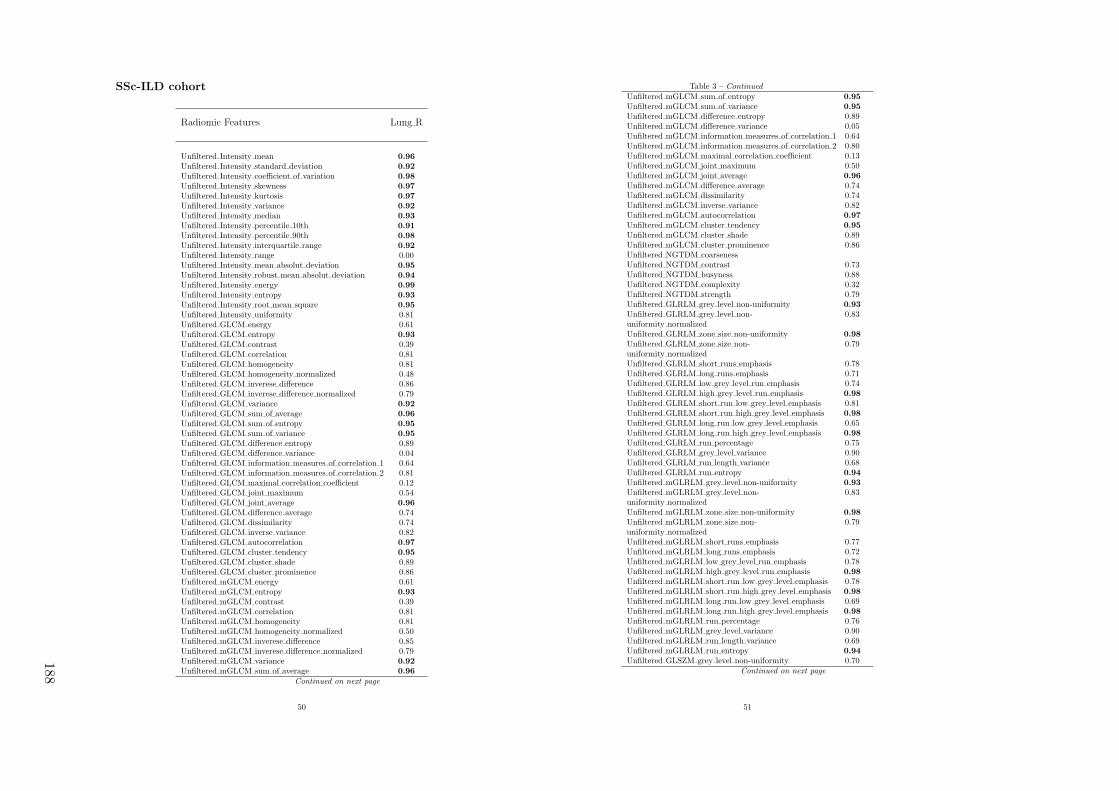
SSc-ILD cohort
Radiomic Features Lung R
Unfiltered Intensity mean 0.96
Unfiltered Intensity standard deviation 0.92
Unfiltered Intensity coefficient of variation 0.98
Unfiltered Intensity skewness 0.97
Unfiltered Intensity kurtosis 0.97
Unfiltered Intensity variance 0.92
Unfiltered Intensity median 0.93
Unfiltered Intensity percentile 10th 0.91
Unfiltered Intensity percentile 90th 0.98
Unfiltered Intensity interquartile range 0.92
Unfiltered Intensity range 0.00Unfiltered Intensity mean absolut deviation 0.95
Unfiltered Intensity robust mean absolut deviation 0.94
Unfiltered Intensity energy 0.99
Unfiltered Intensity entropy 0.93
Unfiltered Intensity root mean square 0.95
Unfiltered Intensity uniformity 0.81Unfiltered GLCM energy 0.61Unfiltered GLCM entropy 0.93
Unfiltered GLCM contrast 0.39Unfiltered GLCM correlation 0.81Unfiltered GLCM homogeneity 0.81Unfiltered GLCM homogeneity normalized 0.48Unfiltered GLCM inverese difference 0.86Unfiltered GLCM inverese difference normalized 0.79Unfiltered GLCM variance 0.92
Unfiltered GLCM sum of average 0.96
Unfiltered GLCM sum of entropy 0.95
Unfiltered GLCM sum of variance 0.95
Unfiltered GLCM difference entropy 0.89Unfiltered GLCM difference variance 0.04Unfiltered GLCM information measures of correlation 1 0.64Unfiltered GLCM information measures of correlation 2 0.81Unfiltered GLCM maximal correlation coefficient 0.12Unfiltered GLCM joint maximum 0.54Unfiltered GLCM joint average 0.96
Unfiltered GLCM difference average 0.74Unfiltered GLCM dissimilarity 0.74Unfiltered GLCM inverse variance 0.82Unfiltered GLCM autocorrelation 0.97
Unfiltered GLCM cluster tendency 0.95
Unfiltered GLCM cluster shade 0.89Unfiltered GLCM cluster prominence 0.86Unfiltered mGLCM energy 0.61Unfiltered mGLCM entropy 0.93
Unfiltered mGLCM contrast 0.39Unfiltered mGLCM correlation 0.81Unfiltered mGLCM homogeneity 0.81Unfiltered mGLCM homogeneity normalized 0.50Unfiltered mGLCM inverese difference 0.85Unfiltered mGLCM inverese difference normalized 0.79Unfiltered mGLCM variance 0.92
Unfiltered mGLCM sum of average 0.96
Continued on next page
50
Table 3 – Continued
Unfiltered mGLCM sum of entropy 0.95
Unfiltered mGLCM sum of variance 0.95
Unfiltered mGLCM difference entropy 0.89Unfiltered mGLCM difference variance 0.05Unfiltered mGLCM information measures of correlation 1 0.64Unfiltered mGLCM information measures of correlation 2 0.80Unfiltered mGLCM maximal correlation coefficient 0.13Unfiltered mGLCM joint maximum 0.50Unfiltered mGLCM joint average 0.96
Unfiltered mGLCM difference average 0.74Unfiltered mGLCM dissimilarity 0.74Unfiltered mGLCM inverse variance 0.82Unfiltered mGLCM autocorrelation 0.97
Unfiltered mGLCM cluster tendency 0.95
Unfiltered mGLCM cluster shade 0.89Unfiltered mGLCM cluster prominence 0.86Unfiltered NGTDM coarsenessUnfiltered NGTDM contrast 0.73Unfiltered NGTDM busyness 0.88Unfiltered NGTDM complexity 0.32Unfiltered NGTDM strength 0.79Unfiltered GLRLM grey level non-uniformity 0.93
Unfiltered GLRLM grey level non-uniformity normalized
0.83
Unfiltered GLRLM zone size non-uniformity 0.98
Unfiltered GLRLM zone size non-uniformity normalized
0.79
Unfiltered GLRLM short runs emphasis 0.78Unfiltered GLRLM long runs emphasis 0.71Unfiltered GLRLM low grey level run emphasis 0.74Unfiltered GLRLM high grey level run emphasis 0.98
Unfiltered GLRLM short run low grey level emphasis 0.81Unfiltered GLRLM short run high grey level emphasis 0.98
Unfiltered GLRLM long run low grey level emphasis 0.65Unfiltered GLRLM long run high grey level emphasis 0.98
Unfiltered GLRLM run percentage 0.75Unfiltered GLRLM grey level variance 0.90Unfiltered GLRLM run length variance 0.68Unfiltered GLRLM run entropy 0.94
Unfiltered mGLRLM grey level non-uniformity 0.93
Unfiltered mGLRLM grey level non-uniformity normalized
0.83
Unfiltered mGLRLM zone size non-uniformity 0.98
Unfiltered mGLRLM zone size non-uniformity normalized
0.79
Unfiltered mGLRLM short runs emphasis 0.77Unfiltered mGLRLM long runs emphasis 0.72Unfiltered mGLRLM low grey level run emphasis 0.78Unfiltered mGLRLM high grey level run emphasis 0.98
Unfiltered mGLRLM short run low grey level emphasis 0.78Unfiltered mGLRLM short run high grey level emphasis 0.98
Unfiltered mGLRLM long run low grey level emphasis 0.69Unfiltered mGLRLM long run high grey level emphasis 0.98
Unfiltered mGLRLM run percentage 0.76Unfiltered mGLRLM grey level variance 0.90Unfiltered mGLRLM run length variance 0.69Unfiltered mGLRLM run entropy 0.94
Unfiltered GLSZM grey level non-uniformity 0.70Continued on next page
51
188

Table 3 – Continued
Unfiltered GLSZM grey level non-uniformity normalized
0.88
Unfiltered GLSZM zone size non-uniformity 0.84Unfiltered GLSZM zone size non-uniformity normalized
0.00
Unfiltered GLSZM small zone emphasis 0.00Unfiltered GLSZM large zone emphasis 0.01Unfiltered GLSZM low grey level zone emphasis 0.76Unfiltered GLSZM high grey level zone emphasis 0.95
Unfiltered GLSZM small zone low grey level emphasis 0.70Unfiltered GLSZM small zone high grey level emphasis 0.92
Unfiltered GLSZM large zone low grey level emphasis 0.01Unfiltered GLSZM large zone high grey level emphasis 0.01Unfiltered GLSZM zone percentage 0.84Unfiltered GLSZM grey level variance 0.50Unfiltered GLSZM zone size variance 0.01Unfiltered GLSZM zone size entropy 0.85Unfiltered GLDZM grey level non-uniformity 0.70Unfiltered GLDZM grey level non-uniformity normalized
0.87
Unfiltered GLDZM zone size non-uniformity 0.72Unfiltered GLDZM zone size non-uniformity normalized
0.35
Unfiltered GLDZM small distance emphasis 0.00Unfiltered GLDZM large distance emphasis 0.91
Unfiltered GLDZM low grey level zone emphasis 0.77Unfiltered GLDZM high grey level zone emphasis 0.95
Unfiltered GLDZM small distance low grey level emphasis 0.28Unfiltered GLDZM small distance high grey level emphasis 0.46Unfiltered GLDZM large distance low grey level emphasis 0.93
Unfiltered GLDZM large distance high grey level emphasis 0.62Unfiltered GLDZM zone percentage 0.84Unfiltered GLDZM grey level variance 0.50Unfiltered GLDZM zone distance variance 0.91
Unfiltered GLDZM zone distance entropy 0.84Unfiltered NGLDM grey level non-uniformity 0.90
Unfiltered NGLDM grey level non-uniformity normalized
0.81
Unfiltered NGLDM dependence count non-uniformity 0.81Unfiltered NGLDM dependence count non-uniformity normalized
0.80
Unfiltered NGLDM low dependence emphasis 0.85Unfiltered NGLDM high dependence emphasis 0.62Unfiltered NGLDM low grey level count emphasis 0.76Unfiltered NGLDM high grey level count emphasis 0.98
Unfiltered NGLDM low dependence low grey level emphasis0.53Unfiltered NGLDM low dependence high grey level emphasis0.95Unfiltered NGLDM high dependence low grey level emphasis0.15Unfiltered NGLDM high dependence high grey level emphasis0.72Unfiltered NGLDM grey level variance 0.92
Unfiltered NGLDM dependence count variance 0.58Unfiltered NGLDM dependence count entropy 0.93
Unfiltered NGLDM dependence count energy 0.94
HHH intensity mean 0.04HHH intensity standard deviation 0.05HHH intensity coefficient of variation 0.00HHH intensity skewness 0.72HHH intensity kurtosis 0.87HHH intensity variance 0.01
Continued on next page
52
Table 3 – Continued
HHH intensity median 0.09HHH intensity percentile 10th 0.18HHH intensity percentile 90th 0.17HHH intensity interquartile range 0.20HHH intensity range 0.47HHH intensity mean absolut deviation 0.14HHH intensity robust mean absolut deviation 0.20HHH intensity energy 0.02HHH intensity entropy 0.31HHH intensity root mean square 0.05HHH intensity uniformity 0.40HHH GLCM energy 0.13HHH GLCM entropy 0.35HHH GLCM contrast 0.02HHH GLCM correlation 0.00HHH GLCM homogeneity 0.51HHH GLCM homogeneity normalized 0.86HHH GLCM inverese difference 0.51HHH GLCM inverese difference normalized 0.94
HHH GLCM variance 0.02HHH GLCM sum of average 0.41HHH GLCM sum of entropy 0.29HHH GLCM sum of variance 0.02HHH GLCM difference entropy 0.21HHH GLCM difference variance 0.00HHH GLCM information measures of correlation 1 0.64HHH GLCM information measures of correlation 2 0.90
HHH GLCM maximal correlation coefficient 0.41HHH GLCM joint maximum 0.16HHH GLCM joint average 0.41HHH GLCM difference average 0.14HHH GLCM dissimilarity 0.14HHH GLCM inverse variance 0.00HHH GLCM autocorrelation 0.09HHH GLCM cluster tendency 0.02HHH GLCM cluster shade 0.01HHH GLCM cluster prominence 0.00HHH mGLCM energy 0.14HHH mGLCM entropy 0.35HHH mGLCM contrast 0.02HHH mGLCM correlation 0.00HHH mGLCM homogeneity 0.51HHH mGLCM homogeneity normalized 0.87HHH mGLCM inverese difference 0.51HHH mGLCM inverese difference normalized 0.94
HHH mGLCM variance 0.02HHH mGLCM sum of average 0.41HHH mGLCM sum of entropy 0.30HHH mGLCM sum of variance 0.02HHH mGLCM difference entropy 0.22HHH mGLCM difference variance 0.00HHH mGLCM information measures of correlation 1 0.66HHH mGLCM information measures of correlation 2 0.89HHH mGLCM maximal correlation coefficient 0.65HHH mGLCM joint maximum 0.16HHH mGLCM joint average 0.41HHH mGLCM difference average 0.15HHH mGLCM dissimilarity 0.15HHH mGLCM inverse variance 0.00
Continued on next page
53
Impact
ofC
Tcon
volution
kernel
onrob
ustn
essof
radiom
icfeatu
resfo
rdiff
erent
lung
diseases
and
tissue
types
189
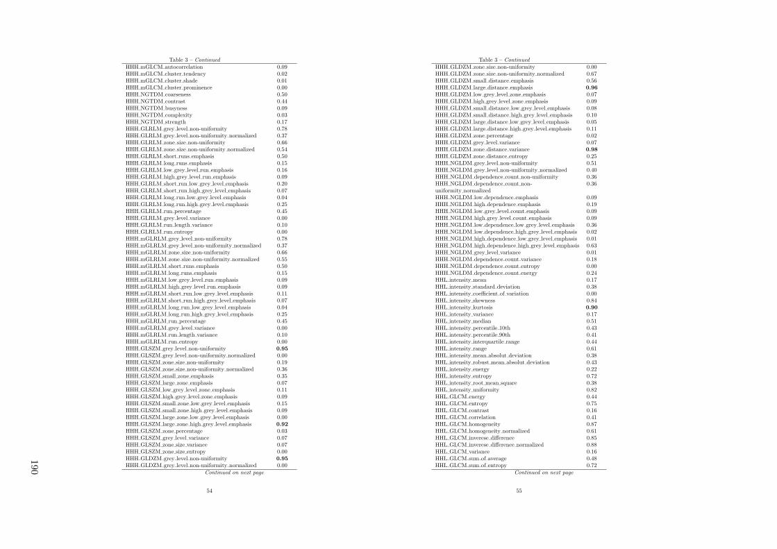
Table 3 – Continued
HHH mGLCM autocorrelation 0.09HHH mGLCM cluster tendency 0.02HHH mGLCM cluster shade 0.01HHH mGLCM cluster prominence 0.00HHH NGTDM coarseness 0.50HHH NGTDM contrast 0.44HHH NGTDM busyness 0.09HHH NGTDM complexity 0.03HHH NGTDM strength 0.17HHH GLRLM grey level non-uniformity 0.78HHH GLRLM grey level non-uniformity normalized 0.37HHH GLRLM zone size non-uniformity 0.66HHH GLRLM zone size non-uniformity normalized 0.54HHH GLRLM short runs emphasis 0.50HHH GLRLM long runs emphasis 0.15HHH GLRLM low grey level run emphasis 0.16HHH GLRLM high grey level run emphasis 0.09HHH GLRLM short run low grey level emphasis 0.20HHH GLRLM short run high grey level emphasis 0.07HHH GLRLM long run low grey level emphasis 0.04HHH GLRLM long run high grey level emphasis 0.25HHH GLRLM run percentage 0.45HHH GLRLM grey level variance 0.00HHH GLRLM run length variance 0.10HHH GLRLM run entropy 0.00HHH mGLRLM grey level non-uniformity 0.78HHH mGLRLM grey level non-uniformity normalized 0.37HHH mGLRLM zone size non-uniformity 0.66HHH mGLRLM zone size non-uniformity normalized 0.55HHH mGLRLM short runs emphasis 0.50HHH mGLRLM long runs emphasis 0.15HHH mGLRLM low grey level run emphasis 0.09HHH mGLRLM high grey level run emphasis 0.09HHH mGLRLM short run low grey level emphasis 0.11HHH mGLRLM short run high grey level emphasis 0.07HHH mGLRLM long run low grey level emphasis 0.04HHH mGLRLM long run high grey level emphasis 0.25HHH mGLRLM run percentage 0.45HHH mGLRLM grey level variance 0.00HHH mGLRLM run length variance 0.10HHH mGLRLM run entropy 0.00HHH GLSZM grey level non-uniformity 0.95
HHH GLSZM grey level non-uniformity normalized 0.00HHH GLSZM zone size non-uniformity 0.19HHH GLSZM zone size non-uniformity normalized 0.36HHH GLSZM small zone emphasis 0.35HHH GLSZM large zone emphasis 0.07HHH GLSZM low grey level zone emphasis 0.11HHH GLSZM high grey level zone emphasis 0.09HHH GLSZM small zone low grey level emphasis 0.15HHH GLSZM small zone high grey level emphasis 0.09HHH GLSZM large zone low grey level emphasis 0.00HHH GLSZM large zone high grey level emphasis 0.92
HHH GLSZM zone percentage 0.03HHH GLSZM grey level variance 0.07HHH GLSZM zone size variance 0.07HHH GLSZM zone size entropy 0.00HHH GLDZM grey level non-uniformity 0.95
HHH GLDZM grey level non-uniformity normalized 0.00Continued on next page
54
Table 3 – Continued
HHH GLDZM zone size non-uniformity 0.00HHH GLDZM zone size non-uniformity normalized 0.67HHH GLDZM small distance emphasis 0.56HHH GLDZM large distance emphasis 0.96
HHH GLDZM low grey level zone emphasis 0.07HHH GLDZM high grey level zone emphasis 0.09HHH GLDZM small distance low grey level emphasis 0.08HHH GLDZM small distance high grey level emphasis 0.10HHH GLDZM large distance low grey level emphasis 0.05HHH GLDZM large distance high grey level emphasis 0.11HHH GLDZM zone percentage 0.02HHH GLDZM grey level variance 0.07HHH GLDZM zone distance variance 0.98
HHH GLDZM zone distance entropy 0.25HHH NGLDM grey level non-uniformity 0.51HHH NGLDM grey level non-uniformity normalized 0.40HHH NGLDM dependence count non-uniformity 0.36HHH NGLDM dependence count non-uniformity normalized
0.36
HHH NGLDM low dependence emphasis 0.09HHH NGLDM high dependence emphasis 0.19HHH NGLDM low grey level count emphasis 0.09HHH NGLDM high grey level count emphasis 0.09HHH NGLDM low dependence low grey level emphasis 0.36HHH NGLDM low dependence high grey level emphasis 0.02HHH NGLDM high dependence low grey level emphasis 0.01HHH NGLDM high dependence high grey level emphasis 0.63HHH NGLDM grey level variance 0.01HHH NGLDM dependence count variance 0.18HHH NGLDM dependence count entropy 0.00HHH NGLDM dependence count energy 0.24HHL intensity mean 0.17HHL intensity standard deviation 0.38HHL intensity coefficient of variation 0.00HHL intensity skewness 0.84HHL intensity kurtosis 0.90
HHL intensity variance 0.17HHL intensity median 0.51HHL intensity percentile 10th 0.43HHL intensity percentile 90th 0.41HHL intensity interquartile range 0.44HHL intensity range 0.61HHL intensity mean absolut deviation 0.38HHL intensity robust mean absolut deviation 0.43HHL intensity energy 0.22HHL intensity entropy 0.72HHL intensity root mean square 0.38HHL intensity uniformity 0.82HHL GLCM energy 0.44HHL GLCM entropy 0.75HHL GLCM contrast 0.16HHL GLCM correlation 0.41HHL GLCM homogeneity 0.87HHL GLCM homogeneity normalized 0.61HHL GLCM inverese difference 0.85HHL GLCM inverese difference normalized 0.88HHL GLCM variance 0.16HHL GLCM sum of average 0.48HHL GLCM sum of entropy 0.72
Continued on next page
55
190

Table 3 – Continued
HHL GLCM sum of variance 0.15HHL GLCM difference entropy 0.67HHL GLCM difference variance 0.24HHL GLCM information measures of correlation 1 0.78HHL GLCM information measures of correlation 2 0.91
HHL GLCM maximal correlation coefficient 0.66HHL GLCM joint maximum 0.40HHL GLCM joint average 0.48HHL GLCM difference average 0.39HHL GLCM dissimilarity 0.39HHL GLCM inverse variance 0.76HHL GLCM autocorrelation 0.22HHL GLCM cluster tendency 0.15HHL GLCM cluster shade 0.08HHL GLCM cluster prominence 0.04HHL mGLCM energy 0.46HHL mGLCM entropy 0.74HHL mGLCM contrast 0.16HHL mGLCM correlation 0.42HHL mGLCM homogeneity 0.87HHL mGLCM homogeneity normalized 0.73HHL mGLCM inverese difference 0.85HHL mGLCM inverese difference normalized 0.89HHL mGLCM variance 0.16HHL mGLCM sum of average 0.48HHL mGLCM sum of entropy 0.72HHL mGLCM sum of variance 0.15HHL mGLCM difference entropy 0.68HHL mGLCM difference variance 0.24HHL mGLCM information measures of correlation 1 0.82HHL mGLCM information measures of correlation 2 0.94
HHL mGLCM maximal correlation coefficient 0.84HHL mGLCM joint maximum 0.41HHL mGLCM joint average 0.48HHL mGLCM difference average 0.39HHL mGLCM dissimilarity 0.39HHL mGLCM inverse variance 0.76HHL mGLCM autocorrelation 0.22HHL mGLCM cluster tendency 0.15HHL mGLCM cluster shade 0.07HHL mGLCM cluster prominence 0.04HHL NGTDM coarseness 0.50HHL NGTDM contrast 0.52HHL NGTDM busyness 0.38HHL NGTDM complexity 0.12HHL NGTDM strength 0.31HHL GLRLM grey level non-uniformity 0.86HHL GLRLM grey level non-uniformity normalized 0.87HHL GLRLM zone size non-uniformity 0.91
HHL GLRLM zone size non-uniformity normalized 0.87HHL GLRLM short runs emphasis 0.84HHL GLRLM long runs emphasis 0.61HHL GLRLM low grey level run emphasis 0.00HHL GLRLM high grey level run emphasis 0.22HHL GLRLM short run low grey level emphasis 0.11HHL GLRLM short run high grey level emphasis 0.19HHL GLRLM long run low grey level emphasis 0.37HHL GLRLM long run high grey level emphasis 0.36HHL GLRLM run percentage 0.82
Continued on next page
56
Table 3 – Continued
HHL GLRLM grey level variance 0.17HHL GLRLM run length variance 0.52HHL GLRLM run entropy 0.23HHL mGLRLM grey level non-uniformity 0.86HHL mGLRLM grey level non-uniformity normalized 0.87HHL mGLRLM zone size non-uniformity 0.91
HHL mGLRLM zone size non-uniformity normalized 0.87HHL mGLRLM short runs emphasis 0.84HHL mGLRLM long runs emphasis 0.61HHL mGLRLM low grey level run emphasis 0.18HHL mGLRLM high grey level run emphasis 0.22HHL mGLRLM short run low grey level emphasis 0.20HHL mGLRLM short run high grey level emphasis 0.19HHL mGLRLM long run low grey level emphasis 0.13HHL mGLRLM long run high grey level emphasis 0.36HHL mGLRLM run percentage 0.81HHL mGLRLM grey level variance 0.17HHL mGLRLM run length variance 0.52HHL mGLRLM run entropy 0.23HHL GLSZM grey level non-uniformity 0.97
HHL GLSZM grey level non-uniformity normalized 0.27HHL GLSZM zone size non-uniformity 0.59HHL GLSZM zone size non-uniformity normalized 0.74HHL GLSZM small zone emphasis 0.74HHL GLSZM large zone emphasis 0.30HHL GLSZM low grey level zone emphasis 0.00HHL GLSZM high grey level zone emphasis 0.22HHL GLSZM small zone low grey level emphasis 0.00HHL GLSZM small zone high grey level emphasis 0.23HHL GLSZM large zone low grey level emphasis 0.04HHL GLSZM large zone high grey level emphasis 0.81HHL GLSZM zone percentage 0.32HHL GLSZM grey level variance 0.53HHL GLSZM zone size variance 0.30HHL GLSZM zone size entropy 0.39HHL GLDZM grey level non-uniformity 0.97
HHL GLDZM grey level non-uniformity normalized 0.21HHL GLDZM zone size non-uniformity 0.46HHL GLDZM zone size non-uniformity normalized 0.81HHL GLDZM small distance emphasis 0.77HHL GLDZM large distance emphasis 0.98
HHL GLDZM low grey level zone emphasis 0.14HHL GLDZM high grey level zone emphasis 0.22HHL GLDZM small distance low grey level emphasis 0.11HHL GLDZM small distance high grey level emphasis 0.27HHL GLDZM large distance low grey level emphasis 0.20HHL GLDZM large distance high grey level emphasis 0.25HHL GLDZM zone percentage 0.32HHL GLDZM grey level variance 0.53HHL GLDZM zone distance variance 0.98
HHL GLDZM zone distance entropy 0.83HHL NGLDM grey level non-uniformity 0.75HHL NGLDM grey level non-uniformity normalized 0.82HHL NGLDM dependence count non-uniformity 0.65HHL NGLDM dependence count non-uniformity normalized
0.56
HHL NGLDM low dependence emphasis 0.46HHL NGLDM high dependence emphasis 0.54HHL NGLDM low grey level count emphasis 0.19
Continued on next page
57
Impact
ofC
Tcon
volution
kernel
onrob
ustn
essof
radiom
icfeatu
resfo
rdiff
erent
lung
diseases
and
tissue
types
191
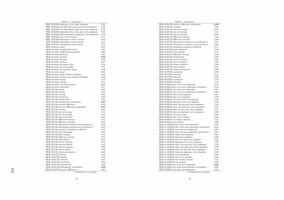
Table 3 – Continued
HHL NGLDM high grey level count emphasis 0.22HHL NGLDM low dependence low grey level emphasis 0.39HHL NGLDM low dependence high grey level emphasis 0.08HHL NGLDM high dependence low grey level emphasis 0.06HHL NGLDM high dependence high grey level emphasis 0.78HHL NGLDM grey level variance 0.17HHL NGLDM dependence count variance 0.53HHL NGLDM dependence count entropy 0.47HHL NGLDM dependence count energy 0.79HLH intensity mean 0.36HLH intensity standard deviation 0.08HLH intensity coefficient of variation 0.06HLH intensity skewness 0.87HLH intensity kurtosis 0.92
HLH intensity variance 0.03HLH intensity median 0.27HLH intensity percentile 10th 0.38HLH intensity percentile 90th 0.41HLH intensity interquartile range 0.40HLH intensity range 0.56HLH intensity mean absolut deviation 0.31HLH intensity robust mean absolut deviation 0.40HLH intensity energy 0.10HLH intensity entropy 0.55HLH intensity root mean square 0.08HLH intensity uniformity 0.57HLH GLCM energy 0.27HLH GLCM entropy 0.58HLH GLCM contrast 0.07HLH GLCM correlation 0.00HLH GLCM homogeneity 0.69HLH GLCM homogeneity normalized 0.91
HLH GLCM inverese difference 0.68HLH GLCM inverese difference normalized 0.94
HLH GLCM variance 0.06HLH GLCM sum of average 0.54HLH GLCM sum of entropy 0.51HLH GLCM sum of variance 0.06HLH GLCM difference entropy 0.47HLH GLCM difference variance 0.00HLH GLCM information measures of correlation 1 0.49HLH GLCM information measures of correlation 2 0.83HLH GLCM maximal correlation coefficient 0.43HLH GLCM joint maximum 0.32HLH GLCM joint average 0.54HLH GLCM difference average 0.33HLH GLCM dissimilarity 0.33HLH GLCM inverse variance 0.35HLH GLCM autocorrelation 0.22HLH GLCM cluster tendency 0.06HLH GLCM cluster shade 0.04HLH GLCM cluster prominence 0.00HLH mGLCM energy 0.28HLH mGLCM entropy 0.59HLH mGLCM contrast 0.07HLH mGLCM correlation 0.00HLH mGLCM homogeneity 0.68HLH mGLCM homogeneity normalized 0.92
HLH mGLCM inverese difference 0.68Continued on next page
58
Table 3 – Continued
HLH mGLCM inverese difference normalized 0.94
HLH mGLCM variance 0.06HLH mGLCM sum of average 0.54HLH mGLCM sum of entropy 0.52HLH mGLCM sum of variance 0.06HLH mGLCM difference entropy 0.48HLH mGLCM difference variance 0.00HLH mGLCM information measures of correlation 1 0.65HLH mGLCM information measures of correlation 2 0.83HLH mGLCM maximal correlation coefficient 0.75HLH mGLCM joint maximum 0.32HLH mGLCM joint average 0.54HLH mGLCM difference average 0.33HLH mGLCM dissimilarity 0.33HLH mGLCM inverse variance 0.35HLH mGLCM autocorrelation 0.22HLH mGLCM cluster tendency 0.06HLH mGLCM cluster shade 0.04HLH mGLCM cluster prominence 0.00HLH NGTDM coarseness 0.00HLH NGTDM contrast 0.54HLH NGTDM busyness 0.23HLH NGTDM complexity 0.04HLH NGTDM strength 0.33HLH GLRLM grey level non-uniformity 0.84HLH GLRLM grey level non-uniformity normalized 0.58HLH GLRLM zone size non-uniformity 0.81HLH GLRLM zone size non-uniformity normalized 0.66HLH GLRLM short runs emphasis 0.61HLH GLRLM long runs emphasis 0.33HLH GLRLM low grey level run emphasis 0.19HLH GLRLM high grey level run emphasis 0.22HLH GLRLM short run low grey level emphasis 0.40HLH GLRLM short run high grey level emphasis 0.18HLH GLRLM long run low grey level emphasis 0.27HLH GLRLM long run high grey level emphasis 0.49HLH GLRLM run percentage 0.60HLH GLRLM grey level variance 0.00HLH GLRLM run length variance 0.25HLH GLRLM run entropy 0.00HLH m GLRLM grey level non-uniformity 0.84HLH m GLRLM grey level non-uniformity normalized 0.58HLH m GLRLM zone size non-uniformity 0.81HLH m GLRLM zone size non-uniformity normalized 0.67HLH m GLRLM short runs emphasis 0.62HLH m GLRLM long runs emphasis 0.33HLH m GLRLM low grey level run emphasis 0.27HLH m GLRLM high grey level run emphasis 0.22HLH m GLRLM short run low grey level emphasis 0.29HLH m GLRLM short run high grey level emphasis 0.18HLH m GLRLM long run low grey level emphasis 0.18HLH m GLRLM long run high grey level emphasis 0.49HLH m GLRLM run percentage 0.60HLH m GLRLM grey level variance 0.00HLH m GLRLM run length variance 0.25HLH m GLRLM run entropy 0.00HLH GLSZM grey level non-uniformity 0.96
HLH GLSZM grey level non-uniformity normalized 0.00HLH GLSZM zone size non-uniformity 0.44
Continued on next page
59
192

Table 3 – Continued
HLH GLSZM zone size non-uniformity normalized 0.66HLH GLSZM small zone emphasis 0.65HLH GLSZM large zone emphasis 0.28HLH GLSZM low grey level zone emphasis 0.13HLH GLSZM high grey level zone emphasis 0.22HLH GLSZM small zone low grey level emphasis 0.40HLH GLSZM small zone high grey level emphasis 0.23HLH GLSZM large zone low grey level emphasis 0.03HLH GLSZM large zone high grey level emphasis 0.86HLH GLSZM zone percentage 0.25HLH GLSZM grey level variance 0.11HLH GLSZM zone size variance 0.28HLH GLSZM zone size entropy 0.05HLH GLDZM grey level non-uniformity 0.96
HLH GLDZM grey level non-uniformity normalized 0.00HLH GLDZM zone size non-uniformity 0.33HLH GLDZM zone size non-uniformity normalized 0.89HLH GLDZM small distance emphasis 0.84HLH GLDZM large distance emphasis 0.99
HLH GLDZM low grey level zone emphasis 0.22HLH GLDZM high grey level zone emphasis 0.22HLH GLDZM small distance low grey level emphasis 0.20HLH GLDZM small distance high grey level emphasis 0.22HLH GLDZM large distance low grey level emphasis 0.20HLH GLDZM large distance high grey level emphasis 0.29HLH GLDZM zone percentage 0.25HLH GLDZM grey level variance 0.11HLH GLDZM zone distance variance 0.99
HLH GLDZM zone distance entropy 0.56HLH NGLDM grey level non-uniformity 0.68HLH NGLDM grey level non-uniformity normalized 0.57HLH NGLDM dependence count non-uniformity 0.59HLH NGLDM dependence count non-uniformity normalized
0.47
HLH NGLDM low dependence emphasis 0.35HLH NGLDM high dependence emphasis 0.35HLH NGLDM low grey level count emphasis 0.27HLH NGLDM high grey level count emphasis 0.22HLH NGLDM low dependence low grey level emphasis 0.56HLH NGLDM low dependence high grey level emphasis 0.07HLH NGLDM high dependence low grey level emphasis 0.07HLH NGLDM high dependence high grey level emphasis 0.81HLH NGLDM grey level variance 0.04HLH NGLDM dependence count variance 0.32HLH NGLDM dependence count entropy 0.25HLH NGLDM dependence count energy 0.43HLL intensity mean 0.64HLL intensity standard deviation 0.70HLL intensity coefficient of variation 0.44HLL intensity skewness 0.61HLL intensity kurtosis 0.77HLL intensity variance 0.52HLL intensity median 0.87HLL intensity percentile 10th 0.78HLL intensity percentile 90th 0.84HLL intensity interquartile range 0.77HLL intensity range 0.66HLL intensity mean absolut deviation 0.71HLL intensity robust mean absolut deviation 0.78
Continued on next page
60
Table 3 – Continued
HLL intensity energy 0.68HLL intensity entropy 0.91
HLL intensity root mean square 0.70HLL intensity uniformity 0.90HLL GLCM energy 0.69HLL GLCM entropy 0.91
HLL GLCM contrast 0.50HLL GLCM correlation 0.66HLL GLCM homogeneity 0.92
HLL GLCM homogeneity normalized 0.70HLL GLCM inverese difference 0.92
HLL GLCM inverese difference normalized 0.96
HLL GLCM variance 0.50HLL GLCM sum of average 0.69HLL GLCM sum of entropy 0.91
HLL GLCM sum of variance 0.50HLL GLCM difference entropy 0.89HLL GLCM difference variance 0.63HLL GLCM information measures of correlation 1 0.89HLL GLCM information measures of correlation 2 0.95
HLL GLCM maximal correlation coefficient 0.75HLL GLCM joint maximum 0.71HLL GLCM joint average 0.69HLL GLCM difference average 0.71HLL GLCM dissimilarity 0.71HLL GLCM inverse variance 0.91
HLL GLCM autocorrelation 0.41HLL GLCM cluster tendency 0.50HLL GLCM cluster shade 0.14HLL GLCM cluster prominence 0.19HLL mGLCM energy 0.70HLL mGLCM entropy 0.91
HLL mGLCM contrast 0.50HLL mGLCM correlation 0.87HLL mGLCM homogeneity 0.92
HLL mGLCM homogeneity normalized 0.88HLL mGLCM inverese difference 0.92
HLL mGLCM inverese difference normalized 0.97
HLL mGLCM variance 0.50HLL mGLCM sum of average 0.69HLL mGLCM sum of entropy 0.91
HLL mGLCM sum of variance 0.50HLL mGLCM difference entropy 0.89HLL mGLCM difference variance 0.63HLL mGLCM information measures of correlation 1 0.83HLL mGLCM information measures of correlation 2 0.94
HLL mGLCM maximal correlation coefficient 0.94
HLL mGLCM joint maximum 0.70HLL mGLCM joint average 0.69HLL mGLCM difference average 0.71HLL mGLCM dissimilarity 0.71HLL mGLCM inverse variance 0.91
HLL mGLCM autocorrelation 0.41HLL mGLCM cluster tendency 0.50HLL mGLCM cluster shade 0.14HLL mGLCM cluster prominence 0.19HLL NGTDM coarseness 0.50HLL NGTDM contrast 0.88HLL NGTDM busyness 0.54
Continued on next page
61
Impact
ofC
Tcon
volution
kernel
onrob
ustn
essof
radiom
icfeatu
resfo
rdiff
erent
lung
diseases
and
tissue
types
193
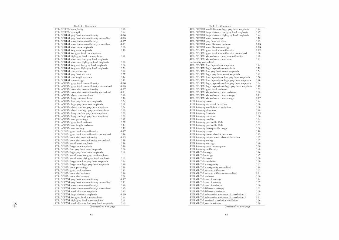
Table 3 – Continued
HLL NGTDM complexity 0.25HLL NGTDM strength 0.44HLL GLRLM grey level non-uniformity 0.96
HLL GLRLM grey level non-uniformity normalized 0.93
HLL GLRLM zone size non-uniformity 0.97
HLL GLRLM zone size non-uniformity normalized 0.91
HLL GLRLM short runs emphasis 0.89HLL GLRLM long runs emphasis 0.79HLL GLRLM low grey level run emphasisHLL GLRLM high grey level run emphasis 0.41HLL GLRLM short run low grey level emphasisHLL GLRLM short run high grey level emphasis 0.39HLL GLRLM long run low grey level emphasis 0.00HLL GLRLM long run high grey level emphasis 0.53HLL GLRLM run percentage 0.88HLL GLRLM grey level variance 0.57HLL GLRLM run length variance 0.74HLL GLRLM run entropy 0.72HLL mGLRM grey level non-uniformity 0.96
HLL mGLRM grey level non-uniformity normalized 0.93
HLL mGLRM zone size non-uniformity 0.97
HLL mGLRM zone size non-uniformity normalized 0.91
HLL mGLRM short runs emphasis 0.89HLL mGLRM long runs emphasis 0.79HLL mGLRM low grey level run emphasis 0.54HLL mGLRM high grey level run emphasis 0.41HLL mGLRM short run low grey level emphasis 0.54HLL mGLRM short run high grey level emphasis 0.39HLL mGLRM long run low grey level emphasis 0.53HLL mGLRM long run high grey level emphasis 0.53HLL mGLRM run percentage 0.87HLL mGLRM grey level variance 0.57HLL mGLRM run length variance 0.74HLL mGLRM run entropy 0.72HLL GLSZM grey level non-uniformity 0.97
HLL GLSZM grey level non-uniformity normalized 0.76HLL GLSZM zone size non-uniformity 0.92
HLL GLSZM zone size non-uniformity normalized 0.76HLL GLSZM small zone emphasis 0.76HLL GLSZM large zone emphasis 0.70HLL GLSZM low grey level zone emphasis 0.00HLL GLSZM high grey level zone emphasis 0.41HLL GLSZM small zone low grey level emphasisHLL GLSZM small zone high grey level emphasis 0.42HLL GLSZM large zone low grey level emphasis 0.24HLL GLSZM large zone high grey level emphasis 0.80HLL GLSZM zone percentage 0.78HLL GLSZM grey level variance 0.82HLL GLSZM zone size variance 0.70HLL GLSZM zone size entropy 0.58HLL GLDZM grey level non-uniformity 0.97
HLL GLDZM grey level non-uniformity normalized 0.73HLL GLDZM zone size non-uniformity 0.89HLL GLDZM zone size non-uniformity normalized 0.85HLL GLDZM small distance emphasis 0.82HLL GLDZM large distance emphasis 0.99
HLL GLDZM low grey level zone emphasis 0.44HLL GLDZM high grey level zone emphasis 0.41HLL GLDZM small distance low grey level emphasis 0.43
Continued on next page
62
Table 3 – Continued
HLL GLDZM small distance high grey level emphasis 0.44HLL GLDZM large distance low grey level emphasis 0.47HLL GLDZM large distance high grey level emphasis 0.44HLL GLDZM zone percentage 0.78HLL GLDZM grey level variance 0.82HLL GLDZM zone distance variance 0.99
HLL GLDZM zone distance entropy 0.93
HLL NGLDM grey level non-uniformity 0.92
HLL NGLDM grey level non-uniformity normalized 0.90HLL NGLDM dependence count non-uniformity 0.85HLL NGLDM dependence count non-uniformity normalized
0.81
HLL NGLDM low dependence emphasis 0.84HLL NGLDM high dependence emphasis 0.73HLL NGLDM low grey level count emphasis 0.54HLL NGLDM high grey level count emphasis 0.41HLL NGLDM low dependence low grey level emphasis 0.56HLL NGLDM low dependence high grey level emphasis 0.26HLL NGLDM high dependence low grey level emphasis 0.34HLL NGLDM high dependence high grey level emphasis 0.75HLL NGLDM grey level variance 0.52HLL NGLDM dependence count variance 0.69HLL NGLDM dependence count entropy 0.91
HLL NGLDM dependence count energy 0.97
LHH intensity mean 0.44LHH intensity standard deviation 0.00LHH intensity coefficient of variation 0.00LHH intensity skewness 0.88LHH intensity kurtosis 0.92
LHH intensity variance 0.00LHH intensity median 0.34LHH intensity percentile 10th 0.32LHH intensity percentile 90th 0.32LHH intensity interquartile range 0.38LHH intensity range 0.18LHH intensity mean absolut deviation 0.23LHH intensity robust mean absolut deviation 0.37LHH intensity energy 0.07LHH intensity entropy 0.40LHH intensity root mean square 0.00LHH intensity uniformity 0.49LHH GLCM energy 0.26LHH GLCM entropy 0.47LHH GLCM contrast 0.00LHH GLCM correlation 0.00LHH GLCM homogeneity 0.62LHH GLCM homogeneity normalized 0.88LHH GLCM inverese difference 0.62LHH GLCM inverese difference normalized 0.91
LHH GLCM variance 0.00LHH GLCM sum of average 0.24LHH GLCM sum of entropy 0.37LHH GLCM sum of variance 0.00LHH GLCM difference entropy 0.31LHH GLCM difference variance 0.00LHH GLCM information measures of correlation 1 0.64LHH GLCM information measures of correlation 2 0.91
LHH GLCM maximal correlation coefficient 0.66LHH GLCM joint maximum 0.29
Continued on next page
63
194
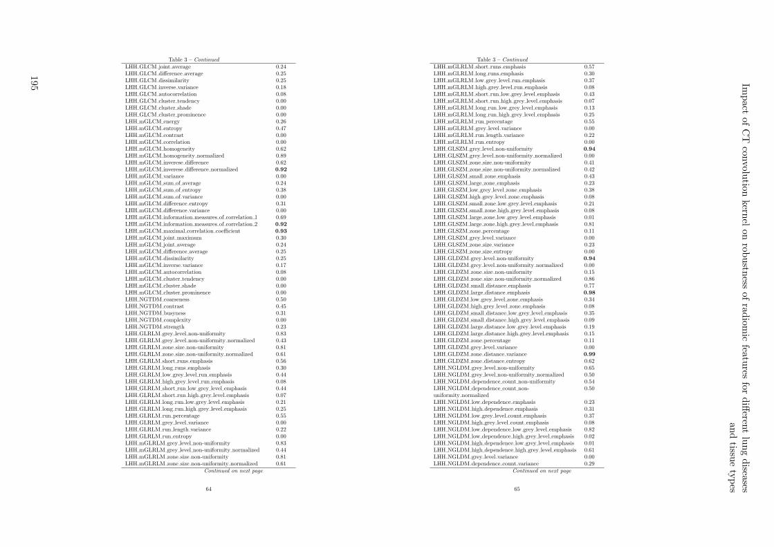
Table 3 – Continued
LHH GLCM joint average 0.24LHH GLCM difference average 0.25LHH GLCM dissimilarity 0.25LHH GLCM inverse variance 0.18LHH GLCM autocorrelation 0.08LHH GLCM cluster tendency 0.00LHH GLCM cluster shade 0.00LHH GLCM cluster prominence 0.00LHH mGLCM energy 0.26LHH mGLCM entropy 0.47LHH mGLCM contrast 0.00LHH mGLCM correlation 0.00LHH mGLCM homogeneity 0.62LHH mGLCM homogeneity normalized 0.89LHH mGLCM inverese difference 0.62LHH mGLCM inverese difference normalized 0.92
LHH mGLCM variance 0.00LHH mGLCM sum of average 0.24LHH mGLCM sum of entropy 0.38LHH mGLCM sum of variance 0.00LHH mGLCM difference entropy 0.31LHH mGLCM difference variance 0.00LHH mGLCM information measures of correlation 1 0.69LHH mGLCM information measures of correlation 2 0.92
LHH mGLCM maximal correlation coefficient 0.93
LHH mGLCM joint maximum 0.30LHH mGLCM joint average 0.24LHH mGLCM difference average 0.25LHH mGLCM dissimilarity 0.25LHH mGLCM inverse variance 0.17LHH mGLCM autocorrelation 0.08LHH mGLCM cluster tendency 0.00LHH mGLCM cluster shade 0.00LHH mGLCM cluster prominence 0.00LHH NGTDM coarseness 0.50LHH NGTDM contrast 0.45LHH NGTDM busyness 0.31LHH NGTDM complexity 0.00LHH NGTDM strength 0.23LHH GLRLM grey level non-uniformity 0.83LHH GLRLM grey level non-uniformity normalized 0.43LHH GLRLM zone size non-uniformity 0.81LHH GLRLM zone size non-uniformity normalized 0.61LHH GLRLM short runs emphasis 0.56LHH GLRLM long runs emphasis 0.30LHH GLRLM low grey level run emphasis 0.44LHH GLRLM high grey level run emphasis 0.08LHH GLRLM short run low grey level emphasis 0.44LHH GLRLM short run high grey level emphasis 0.07LHH GLRLM long run low grey level emphasis 0.21LHH GLRLM long run high grey level emphasis 0.25LHH GLRLM run percentage 0.55LHH GLRLM grey level variance 0.00LHH GLRLM run length variance 0.22LHH GLRLM run entropy 0.00LHH mGLRLM grey level non-uniformity 0.83LHH mGLRLM grey level non-uniformity normalized 0.44LHH mGLRLM zone size non-uniformity 0.81LHH mGLRLM zone size non-uniformity normalized 0.61
Continued on next page
64
Table 3 – Continued
LHH mGLRLM short runs emphasis 0.57LHH mGLRLM long runs emphasis 0.30LHH mGLRLM low grey level run emphasis 0.37LHH mGLRLM high grey level run emphasis 0.08LHH mGLRLM short run low grey level emphasis 0.43LHH mGLRLM short run high grey level emphasis 0.07LHH mGLRLM long run low grey level emphasis 0.13LHH mGLRLM long run high grey level emphasis 0.25LHH mGLRLM run percentage 0.55LHH mGLRLM grey level variance 0.00LHH mGLRLM run length variance 0.22LHH mGLRLM run entropy 0.00LHH GLSZM grey level non-uniformity 0.94
LHH GLSZM grey level non-uniformity normalized 0.00LHH GLSZM zone size non-uniformity 0.41LHH GLSZM zone size non-uniformity normalized 0.42LHH GLSZM small zone emphasis 0.43LHH GLSZM large zone emphasis 0.23LHH GLSZM low grey level zone emphasis 0.38LHH GLSZM high grey level zone emphasis 0.08LHH GLSZM small zone low grey level emphasis 0.21LHH GLSZM small zone high grey level emphasis 0.08LHH GLSZM large zone low grey level emphasis 0.01LHH GLSZM large zone high grey level emphasis 0.81LHH GLSZM zone percentage 0.11LHH GLSZM grey level variance 0.00LHH GLSZM zone size variance 0.23LHH GLSZM zone size entropy 0.00LHH GLDZM grey level non-uniformity 0.94
LHH GLDZM grey level non-uniformity normalized 0.00LHH GLDZM zone size non-uniformity 0.15LHH GLDZM zone size non-uniformity normalized 0.86LHH GLDZM small distance emphasis 0.77LHH GLDZM large distance emphasis 0.98
LHH GLDZM low grey level zone emphasis 0.34LHH GLDZM high grey level zone emphasis 0.08LHH GLDZM small distance low grey level emphasis 0.35LHH GLDZM small distance high grey level emphasis 0.09LHH GLDZM large distance low grey level emphasis 0.19LHH GLDZM large distance high grey level emphasis 0.15LHH GLDZM zone percentage 0.11LHH GLDZM grey level variance 0.00LHH GLDZM zone distance variance 0.99
LHH GLDZM zone distance entropy 0.62LHH NGLDM grey level non-uniformity 0.65LHH NGLDM grey level non-uniformity normalized 0.50LHH NGLDM dependence count non-uniformity 0.54LHH NGLDM dependence count non-uniformity normalized
0.50
LHH NGLDM low dependence emphasis 0.23LHH NGLDM high dependence emphasis 0.31LHH NGLDM low grey level count emphasis 0.37LHH NGLDM high grey level count emphasis 0.08LHH NGLDM low dependence low grey level emphasis 0.82LHH NGLDM low dependence high grey level emphasis 0.02LHH NGLDM high dependence low grey level emphasis 0.01LHH NGLDM high dependence high grey level emphasis 0.61LHH NGLDM grey level variance 0.00LHH NGLDM dependence count variance 0.29
Continued on next page
65
Impact
ofC
Tcon
volution
kernel
onrob
ustn
essof
radiom
icfeatu
resfo
rdiff
erent
lung
diseases
and
tissue
types
195

Table 3 – Continued
LHH NGLDM dependence count entropy 0.00LHH NGLDM dependence count energy 0.12LHL intensity mean 0.94
LHL intensity standard deviation 0.63LHL intensity coefficient of variation 0.79LHL intensity skewness 0.50LHL intensity kurtosis 0.85LHL intensity variance 0.55LHL intensity median 0.85LHL intensity percentile 10th 0.76LHL intensity percentile 90th 0.72LHL intensity interquartile range 0.75LHL intensity range 0.91
LHL intensity mean absolut deviation 0.70LHL intensity robust mean absolut deviation 0.75LHL intensity energy 0.70LHL intensity entropy 0.85LHL intensity root mean square 0.64LHL intensity uniformity 0.86LHL GLCM energy 0.73LHL GLCM entropy 0.87LHL GLCM contrast 0.53LHL GLCM correlation 0.52LHL GLCM homogeneity 0.89LHL GLCM homogeneity normalized 0.68LHL GLCM inverese difference 0.90LHL GLCM inverese difference normalized 0.85LHL GLCM variance 0.52LHL GLCM sum of average 0.61LHL GLCM sum of entropy 0.85LHL GLCM sum of variance 0.51LHL GLCM difference entropy 0.84LHL GLCM difference variance 0.61LHL GLCM information measures of correlation 1 0.87LHL GLCM information measures of correlation 2 0.86LHL GLCM maximal correlation coefficient 0.61LHL GLCM joint maximum 0.72LHL GLCM joint average 0.61LHL GLCM difference average 0.72LHL GLCM dissimilarity 0.72LHL GLCM inverse variance 0.87LHL GLCM autocorrelation 0.45LHL GLCM cluster tendency 0.51LHL GLCM cluster shade 0.00LHL GLCM cluster prominence 0.27LHL mGLCM energy 0.70LHL mGLCM entropy 0.87LHL mGLCM contrast 0.53LHL mGLCM correlation 0.51LHL mGLCM homogeneity 0.89LHL mGLCM homogeneity normalized 0.70LHL mGLCM inverese difference 0.90LHL mGLCM inverese difference normalized 0.85LHL mGLCM variance 0.52LHL mGLCM sum of average 0.61LHL mGLCM sum of entropy 0.86LHL mGLCM sum of variance 0.51LHL mGLCM difference entropy 0.84LHL mGLCM difference variance 0.61
Continued on next page
66
Table 3 – Continued
LHL mGLCM information measures of correlation 1 0.87LHL mGLCM information measures of correlation 2 0.91
LHL mGLCM maximal correlation coefficient 0.92
LHL mGLCM joint maximum 0.73LHL mGLCM joint average 0.61LHL mGLCM difference average 0.72LHL mGLCM dissimilarity 0.72LHL mGLCM inverse variance 0.87LHL mGLCM autocorrelation 0.45LHL mGLCM cluster tendency 0.51LHL mGLCM cluster shade 0.00LHL mGLCM cluster prominence 0.27LHL NGTDM coarseness 0.50LHL NGTDM contrast 0.77LHL NGTDM busyness 0.54LHL NGTDM complexity 0.50LHL NGTDM strength 0.60LHL GLRLM grey level non-uniformity 0.95
LHL GLRLM grey level non-uniformity normalized 0.86LHL GLRLM zone size non-uniformity 0.97
LHL GLRLM zone size non-uniformity normalized 0.89LHL GLRLM short runs emphasis 0.87LHL GLRLM long runs emphasis 0.80LHL GLRLM low grey level run emphasis 0.00LHL GLRLM high grey level run emphasis 0.45LHL GLRLM short run low grey level emphasis 0.00LHL GLRLM short run high grey level emphasis 0.42LHL GLRLM long run low grey level emphasis 0.00LHL GLRLM long run high grey level emphasis 0.59LHL GLRLM run percentage 0.87LHL GLRLM grey level variance 0.56LHL GLRLM run length variance 0.76LHL GLRLM run entropy 0.56LHL mGLRLM grey level non-uniformity 0.95
LHL mGLRLM grey level non-uniformity normalized 0.87LHL mGLRLM zone size non-uniformity 0.97
LHL mGLRLM zone size non-uniformity normalized 0.89LHL mGLRLM short runs emphasis 0.87LHL mGLRLM long runs emphasis 0.80LHL mGLRLM low grey level run emphasis 0.31LHL mGLRLM high grey level run emphasis 0.45LHL mGLRLM short run low grey level emphasis 0.31LHL mGLRLM short run high grey level emphasis 0.42LHL mGLRLM long run low grey level emphasis 0.27LHL mGLRLM long run high grey level emphasis 0.59LHL mGLRLM run percentage 0.87LHL mGLRLM grey level variance 0.56LHL mGLRLM run length variance 0.76LHL mGLRLM run entropy 0.56LHL GLSZM grey level non-uniformity 0.95
LHL GLSZM grey level non-uniformity normalized 0.45LHL GLSZM zone size non-uniformity 0.88LHL GLSZM zone size non-uniformity normalized 0.59LHL GLSZM small zone emphasis 0.60LHL GLSZM large zone emphasis 0.68LHL GLSZM low grey level zone emphasis 0.00LHL GLSZM high grey level zone emphasis 0.45LHL GLSZM small zone low grey level emphasis 0.00LHL GLSZM small zone high grey level emphasis 0.46
Continued on next page
67
196

Table 3 – Continued
LHL GLSZM large zone low grey level emphasis 0.14LHL GLSZM large zone high grey level emphasis 0.93
LHL GLSZM zone percentage 0.71LHL GLSZM grey level variance 0.72LHL GLSZM zone size variance 0.68LHL GLSZM zone size entropy 0.33LHL GLDZM grey level non-uniformity 0.95
LHL GLDZM grey level non-uniformity normalized 0.52LHL GLDZM zone size non-uniformity 0.80LHL GLDZM zone size non-uniformity normalized 0.88LHL GLDZM small distance emphasis 0.85LHL GLDZM large distance emphasis 0.98
LHL GLDZM low grey level zone emphasis 0.25LHL GLDZM high grey level zone emphasis 0.45LHL GLDZM small distance low grey level emphasis 0.28LHL GLDZM small distance high grey level emphasis 0.52LHL GLDZM large distance low grey level emphasis 0.19LHL GLDZM large distance high grey level emphasis 0.48LHL GLDZM zone percentage 0.70LHL GLDZM grey level variance 0.72LHL GLDZM zone distance variance 0.99
LHL GLDZM zone distance entropy 0.95
LHL NGLDM grey level non-uniformity 0.91
LHL NGLDM grey level non-uniformity normalized 0.86LHL NGLDM dependence count non-uniformity 0.84LHL NGLDM dependence count non-uniformity normalized
0.80
LHL NGLDM low dependence emphasis 0.78LHL NGLDM high dependence emphasis 0.75LHL NGLDM low grey level count emphasis 0.31LHL NGLDM high grey level count emphasis 0.45LHL NGLDM low dependence low grey level emphasis 0.35LHL NGLDM low dependence high grey level emphasis 0.27LHL NGLDM high dependence low grey level emphasis 0.14LHL NGLDM high dependence high grey level emphasis 0.88LHL NGLDM grey level variance 0.55LHL NGLDM dependence count variance 0.72LHL NGLDM dependence count entropy 0.70LHL NGLDM dependence count energy 0.80LLH intensity mean 0.91
LLH intensity standard deviation 0.30LLH intensity coefficient of variation 0.84LLH intensity skewness 0.77LLH intensity kurtosis 0.92
LLH intensity variance 0.25LLH intensity median 0.70LLH intensity percentile 10th 0.76LLH intensity percentile 90th 0.72LLH intensity interquartile range 0.72LLH intensity range 0.21LLH intensity mean absolut deviation 0.65LLH intensity robust mean absolut deviation 0.73LLH intensity energy 0.42LLH intensity entropy 0.75LLH intensity root mean square 0.30LLH intensity uniformity 0.72LLH GLCM energy 0.52LLH GLCM entropy 0.77LLH GLCM contrast 0.38
Continued on next page
68
Table 3 – Continued
LLH GLCM correlation 0.65LLH GLCM homogeneity 0.78LLH GLCM homogeneity normalized 0.93
LLH GLCM inverese difference 0.79LLH GLCM inverese difference normalized 0.93
LLH GLCM variance 0.36LLH GLCM sum of average 0.38LLH GLCM sum of entropy 0.73LLH GLCM sum of variance 0.33LLH GLCM difference entropy 0.74LLH GLCM difference variance 0.00LLH GLCM information measures of correlation 1 0.80LLH GLCM information measures of correlation 2 0.92
LLH GLCM maximal correlation coefficient 0.69LLH GLCM joint maximum 0.49LLH GLCM joint average 0.38LLH GLCM difference average 0.67LLH GLCM dissimilarity 0.67LLH GLCM inverse variance 0.77LLH GLCM autocorrelation 0.29LLH GLCM cluster tendency 0.33LLH GLCM cluster shade 0.26LLH GLCM cluster prominence 0.00LLH mGLCM energy 0.54LLH mGLCM entropy 0.77LLH mGLCM contrast 0.38LLH mGLCM correlation 0.66LLH mGLCM homogeneity 0.78LLH mGLCM homogeneity normalized 0.92
LLH mGLCM inverese difference 0.79LLH mGLCM inverese difference normalized 0.93
LLH mGLCM variance 0.36LLH mGLCM sum of average 0.38LLH mGLCM sum of entropy 0.74LLH mGLCM sum of variance 0.33LLH mGLCM difference entropy 0.75LLH mGLCM difference variance 0.00LLH mGLCM information measures of correlation 1 0.83LLH mGLCM information measures of correlation 2 0.90
LLH mGLCM maximal correlation coefficient 0.87LLH mGLCM joint maximum 0.50LLH mGLCM joint average 0.38LLH mGLCM difference average 0.67LLH mGLCM dissimilarity 0.67LLH mGLCM inverse variance 0.77LLH mGLCM autocorrelation 0.29LLH mGLCM cluster tendency 0.33LLH mGLCM cluster shade 0.26LLH mGLCM cluster prominence 0.00LLH NGTDM coarseness 0.50LLH NGTDM contrast 0.80LLH NGTDM busyness 0.44LLH NGTDM complexity 0.00LLH NGTDM strength 0.45LLH GLRLM grey level non-uniformity 0.94
LLH GLRLM grey level non-uniformity normalized 0.75LLH GLRLM zone size non-uniformity 0.92
LLH GLRLM zone size non-uniformity normalized 0.77LLH GLRLM short runs emphasis 0.75
Continued on next page
69
Impact
ofC
Tcon
volution
kernel
onrob
ustn
essof
radiom
icfeatu
resfo
rdiff
erent
lung
diseases
and
tissue
types
197
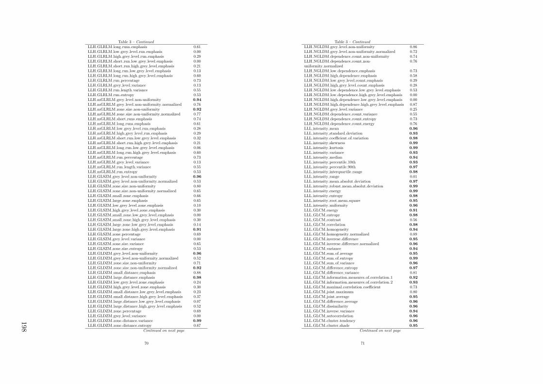
Table 3 – Continued
LLH GLRLM long runs emphasis 0.61LLH GLRLM low grey level run emphasis 0.00LLH GLRLM high grey level run emphasis 0.29LLH GLRLM short run low grey level emphasis 0.00LLH GLRLM short run high grey level emphasis 0.21LLH GLRLM long run low grey level emphasis 0.13LLH GLRLM long run high grey level emphasis 0.60LLH GLRLM run percentage 0.73LLH GLRLM grey level variance 0.13LLH GLRLM run length variance 0.55LLH GLRLM run entropy 0.53LLH mGLRLM grey level non-uniformity 0.94
LLH mGLRLM grey level non-uniformity normalized 0.76LLH mGLRLM zone size non-uniformity 0.92
LLH mGLRLM zone size non-uniformity normalized 0.77LLH mGLRLM short runs emphasis 0.74LLH mGLRLM long runs emphasis 0.61LLH mGLRLM low grey level run emphasis 0.28LLH mGLRLM high grey level run emphasis 0.29LLH mGLRLM short run low grey level emphasis 0.32LLH mGLRLM short run high grey level emphasis 0.21LLH mGLRLM long run low grey level emphasis 0.06LLH mGLRLM long run high grey level emphasis 0.60LLH mGLRLM run percentage 0.73LLH mGLRLM grey level variance 0.13LLH mGLRLM run length variance 0.55LLH mGLRLM run entropy 0.53LLH GLSZM grey level non-uniformity 0.96
LLH GLSZM grey level non-uniformity normalized 0.53LLH GLSZM zone size non-uniformity 0.80LLH GLSZM zone size non-uniformity normalized 0.65LLH GLSZM small zone emphasis 0.66LLH GLSZM large zone emphasis 0.65LLH GLSZM low grey level zone emphasis 0.10LLH GLSZM high grey level zone emphasis 0.30LLH GLSZM small zone low grey level emphasis 0.00LLH GLSZM small zone high grey level emphasis 0.30LLH GLSZM large zone low grey level emphasis 0.14LLH GLSZM large zone high grey level emphasis 0.91
LLH GLSZM zone percentage 0.69LLH GLSZM grey level variance 0.00LLH GLSZM zone size variance 0.65LLH GLSZM zone size entropy 0.53LLH GLDZM grey level non-uniformity 0.96
LLH GLDZM grey level non-uniformity normalized 0.52LLH GLDZM zone size non-uniformity 0.71LLH GLDZM zone size non-uniformity normalized 0.92
LLH GLDZM small distance emphasis 0.88LLH GLDZM large distance emphasis 0.98
LLH GLDZM low grey level zone emphasis 0.24LLH GLDZM high grey level zone emphasis 0.30LLH GLDZM small distance low grey level emphasis 0.23LLH GLDZM small distance high grey level emphasis 0.37LLH GLDZM large distance low grey level emphasis 0.07LLH GLDZM large distance high grey level emphasis 0.52LLH GLDZM zone percentage 0.69LLH GLDZM grey level variance 0.00LLH GLDZM zone distance variance 0.99
LLH GLDZM zone distance entropy 0.67Continued on next page
70
Table 3 – Continued
LLH NGLDM grey level non-uniformity 0.86LLH NGLDM grey level non-uniformity normalized 0.72LLH NGLDM dependence count non-uniformity 0.74LLH NGLDM dependence count non-uniformity normalized
0.76
LLH NGLDM low dependence emphasis 0.73LLH NGLDM high dependence emphasis 0.58LLH NGLDM low grey level count emphasis 0.29LLH NGLDM high grey level count emphasis 0.28LLH NGLDM low dependence low grey level emphasis 0.53LLH NGLDM low dependence high grey level emphasis 0.00LLH NGLDM high dependence low grey level emphasis 0.00LLH NGLDM high dependence high grey level emphasis 0.87LLH NGLDM grey level variance 0.25LLH NGLDM dependence count variance 0.55LLH NGLDM dependence count entropy 0.73LLH NGLDM dependence count energy 0.76LLL intensity mean 0.96
LLL intensity standard deviation 0.93
LLL intensity coefficient of variation 0.98
LLL intensity skewness 0.99
LLL intensity kurtosis 0.99
LLL intensity variance 0.93
LLL intensity median 0.94
LLL intensity percentile 10th 0.93
LLL intensity percentile 90th 0.97
LLL intensity interquartile range 0.98
LLL intensity range 0.01LLL intensity mean absolut deviation 0.97
LLL intensity robust mean absolut deviation 0.99
LLL intensity energy 0.99
LLL intensity entropy 0.98
LLL intensity root mean square 0.95
LLL intensity uniformity 0.96
LLL GLCM energy 0.91
LLL GLCM entropy 0.98
LLL GLCM contrast 0.56LLL GLCM correlation 0.98
LLL GLCM homogeneity 0.94
LLL GLCM homogeneity normalized 0.89LLL GLCM inverese difference 0.95
LLL GLCM inverese difference normalized 0.96
LLL GLCM variance 0.94
LLL GLCM sum of average 0.95
LLL GLCM sum of entropy 0.99
LLL GLCM sum of variance 0.96
LLL GLCM difference entropy 0.97
LLL GLCM difference variance 0.81LLL GLCM information measures of correlation 1 0.92
LLL GLCM information measures of correlation 2 0.93
LLL GLCM maximal correlation coefficient 0.73LLL GLCM joint maximum 0.80LLL GLCM joint average 0.95
LLL GLCM difference average 0.96
LLL GLCM dissimilarity 0.96
LLL GLCM inverse variance 0.94
LLL GLCM autocorrelation 0.96
LLL GLCM cluster tendency 0.96
LLL GLCM cluster shade 0.95
Continued on next page
71
198
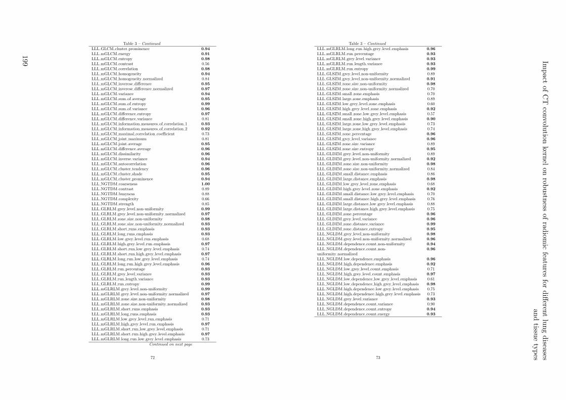
Table 3 – Continued
LLL GLCM cluster prominence 0.94
LLL mGLCM energy 0.91
LLL mGLCM entropy 0.98
LLL mGLCM contrast 0.56LLL mGLCM correlation 0.98
LLL mGLCM homogeneity 0.94
LLL mGLCM homogeneity normalized 0.84LLL mGLCM inverese difference 0.95
LLL mGLCM inverese difference normalized 0.97
LLL mGLCM variance 0.94
LLL mGLCM sum of average 0.95
LLL mGLCM sum of entropy 0.99
LLL mGLCM sum of variance 0.96
LLL mGLCM difference entropy 0.97
LLL mGLCM difference variance 0.81LLL mGLCM information measures of correlation 1 0.93
LLL mGLCM information measures of correlation 2 0.92
LLL mGLCM maximal correlation coefficient 0.73LLL mGLCM joint maximum 0.81LLL mGLCM joint average 0.95
LLL mGLCM difference average 0.96
LLL mGLCM dissimilarity 0.96
LLL mGLCM inverse variance 0.94
LLL mGLCM autocorrelation 0.96
LLL mGLCM cluster tendency 0.96
LLL mGLCM cluster shade 0.95
LLL mGLCM cluster prominence 0.94
LLL NGTDM coarseness 1.00
LLL NGTDM contrast 0.89LLL NGTDM busyness 0.88LLL NGTDM complexity 0.66LLL NGTDM strength 0.85LLL GLRLM grey level non-uniformity 0.99
LLL GLRLM grey level non-uniformity normalized 0.97
LLL GLRLM zone size non-uniformity 0.98
LLL GLRLM zone size non-uniformity normalized 0.93
LLL GLRLM short runs emphasis 0.93
LLL GLRLM long runs emphasis 0.93
LLL GLRLM low grey level run emphasis 0.68LLL GLRLM high grey level run emphasis 0.97
LLL GLRLM short run low grey level emphasis 0.74LLL GLRLM short run high grey level emphasis 0.97
LLL GLRLM long run low grey level emphasis 0.74LLL GLRLM long run high grey level emphasis 0.96
LLL GLRLM run percentage 0.93
LLL GLRLM grey level variance 0.93
LLL GLRLM run length variance 0.93
LLL GLRLM run entropy 0.99
LLL mGLRLM grey level non-uniformity 0.99
LLL mGLRLM grey level non-uniformity normalized 0.97
LLL mGLRLM zone size non-uniformity 0.98
LLL mGLRLM zone size non-uniformity normalized 0.93
LLL mGLRLM short runs emphasis 0.93
LLL mGLRLM long runs emphasis 0.93
LLL mGLRLM low grey level run emphasis 0.71LLL mGLRLM high grey level run emphasis 0.97
LLL mGLRLM short run low grey level emphasis 0.71LLL mGLRLM short run high grey level emphasis 0.97
LLL mGLRLM long run low grey level emphasis 0.73Continued on next page
72
Table 3 – Continued
LLL mGLRLM long run high grey level emphasis 0.96
LLL mGLRLM run percentage 0.93
LLL mGLRLM grey level variance 0.93
LLL mGLRLM run length variance 0.93
LLL mGLRLM run entropy 0.99
LLL GLSZM grey level non-uniformity 0.89LLL GLSZM grey level non-uniformity normalized 0.91
LLL GLSZM zone size non-uniformity 0.98
LLL GLSZM zone size non-uniformity normalized 0.70LLL GLSZM small zone emphasis 0.70LLL GLSZM large zone emphasis 0.89LLL GLSZM low grey level zone emphasis 0.60LLL GLSZM high grey level zone emphasis 0.92
LLL GLSZM small zone low grey level emphasis 0.57LLL GLSZM small zone high grey level emphasis 0.90
LLL GLSZM large zone low grey level emphasis 0.73LLL GLSZM large zone high grey level emphasis 0.74LLL GLSZM zone percentage 0.96
LLL GLSZM grey level variance 0.96
LLL GLSZM zone size variance 0.89LLL GLSZM zone size entropy 0.95
LLL GLDZM grey level non-uniformity 0.89LLL GLDZM grey level non-uniformity normalized 0.92
LLL GLDZM zone size non-uniformity 0.98
LLL GLDZM zone size non-uniformity normalized 0.84LLL GLDZM small distance emphasis 0.86LLL GLDZM large distance emphasis 0.98
LLL GLDZM low grey level zone emphasis 0.68LLL GLDZM high grey level zone emphasis 0.92
LLL GLDZM small distance low grey level emphasis 0.70LLL GLDZM small distance high grey level emphasis 0.76LLL GLDZM large distance low grey level emphasis 0.88LLL GLDZM large distance high grey level emphasis 0.75LLL GLDZM zone percentage 0.96
LLL GLDZM grey level variance 0.96
LLL GLDZM zone distance variance 0.99
LLL GLDZM zone distance entropy 0.95
LLL NGLDM grey level non-uniformity 0.98
LLL NGLDM grey level non-uniformity normalized 0.96
LLL NGLDM dependence count non-uniformity 0.94
LLL NGLDM dependence count non-uniformity normalized
0.96
LLL NGLDM low dependence emphasis 0.96
LLL NGLDM high dependence emphasis 0.92
LLL NGLDM low grey level count emphasis 0.71LLL NGLDM high grey level count emphasis 0.97
LLL NGLDM low dependence low grey level emphasis 0.61LLL NGLDM low dependence high grey level emphasis 0.98
LLL NGLDM high dependence low grey level emphasis 0.75LLL NGLDM high dependence high grey level emphasis 0.73LLL NGLDM grey level variance 0.93
LLL NGLDM dependence count variance 0.90LLL NGLDM dependence count entropy 0.94
LLL NGLDM dependence count energy 0.93
73
Impact
ofC
Tcon
volution
kernel
onrob
ustn
essof
radiom
icfeatu
resfo
rdiff
erent
lung
diseases
and
tissue
types
199

200

10Comparison of robust to standardized CT
radiomics models to predict overall survivalfor non-small cell lung cancer patients
Diem Vuong1, Marta Bogowicz1, Sarah Denzler1, Carol Oliveira2, Robert Foerster1, Florian Amstutz1,
Hubert S. Gabryś1, Jan Unkelbach1, Sven Hillinger3, Sandra Thierstein4, Alexandros Xyrafas4, SolangePeters5, Miklos Pless6, Matthias Guckenberger1, Stephanie Tanadini-Lang1
1Department of Radiation Oncology, University Hospital Zurich and University of Zurich, Zurich, Switzer-land2Department of Oncology and Cancer Center of Southeastern Ontario, Queen’s University, Kingston,Ontario, Canada3Department of Thoracic Surgery, University Hospital Zurich and University of Zurich, Zurich, Switzer-land4Swiss Group for Clinical Cancer Research (SAKK) Coordinating Center, Bern, Switzerland5Department of Oncology, Centre Hospitalier Universitaire Vaudois (CHUV), Lausanne, Switzerland6Department of Medical Oncology, Kantonsspital Winterthur, Winterthur, Switzerland
Status:Published in Medical Physics Journal, 2020doi: 10.1002/mp.14224
Copyright: ©American Association of Physi-cists in Medicine. Reproduced with permis-sion. All rights reserved.
My contribution: For this study, I collected PET/CT imaging data from Swiss institutions con-tributing to the SAKK–16/00 trial. Further, I identified eligible patients and collected the respectiveimaging data for the robustness study. I performed the image processing, radiomics calculation, model-ing, validation, analysis, and interpretation of the results. I wrote, revised, and proof-read the manuscript.
10.1 Abstract
Background: Radiomics is a promising tool for the identification of new prognostic biomarkers. Ra-diomic features can be affected by different scanning protocols, often present in retrospective and prospec-tive clinical data. We compared a computed tomography (CT) based radiomics model based on a largebut highly heterogeneous multicentric image dataset with robust feature pre-selection to a model basedon a smaller but standardized image dataset without pre-selection.
Materials and methods: Primary tumor radiomics was extracted from pre-treatment CT scans ofIIIA/N2/IIIB NSCLC patients from a prospective Swiss multicentric randomized trial (npatient = 124,ninstitution = 14, SAKK–16/00) and a validation dataset (npatient = 31, ninstitution = 1). Four robustnessstudies investigating inter-observer delineation variation, motion, convolution kernel, and contrast wereconducted to identify robust features using an intraclass correlation coefficient threshold > 0.9. Two12–months overall survival (OS) logistic regression models were trained: (a) on the entire multicentricheterogeneous dataset but with robust feature pre-selection (MCR) and (b) on a smaller standardizedsubset using all features (STD). Both models were validated on the validation dataset acquired withsimilar reconstruction parameters as the STD dataset. The model performances were compared usingthe DeLong test.
Results: In total, 113 stable features were identified (nshape = 8, nintensity = 0, ntexture = 7, nwavelet = 98).The convolution kernel had the strongest influence on the feature robustness (<20% stable features). Thefinal models of MCR and STD consisted of one and two features respectively. The features of STD wereidentified both as non-robust. MCR did not show performance significantly different from STD on thevalidation cohort (AUC [95%CI] = 0.72 [0.48–0.95] and 0.79 [0.63–0.95], p = 0.59).
Conclusion: Prognostic OS CT radiomics model for NSCLC based on a heterogeneous multicentricimaging dataset with robust feature pre-selection performed equally well as a model on a standardizeddataset.
10.2 Introduction
Imaging based biomarkers are gaining ground in the development of prognostic models for patient outcomeprediction. Radiomics refers to the extraction of a large number of quantitative features from medicalimages.32 These features can be subdivided into shape, intensity, texture, and filter–based (wavelet)features, describing tissue characteristics such as grey–value distribution and intra–pixel relationships.These radiomic features have shown good prognostic power for different entities for several researchsettings.42,162,238,424,435,436
Radiomic models are often based on single institution imaging datasets. However, radiomic modelsbased on large multicentric imaging datasets are desired since they better reflect the clinical reality.45
The increased heterogeneity in terms of scanner and acquisition settings in the imaging data has shownto differentially affect radiomic features.116 Robustness studies are often performed to identify robustradiomic features where features from two image sets of the same patient are compared. Numerousinvestigations have been performed to quantify the robustness of computed tomography (CT) basedradiomic features. Voxel size, grey level discretization, mAs, and tube voltage in CT imaging haveshown to be an important influence on the feature stability.35,80,97,219,437 Furthermore, two recent studiesinvestigated the reproducibility of CT radiomic features of CT scans reconstructed using different slicethicknesses and two filtered back projection (FBP) convolution kernel (standard and lung). They showedhigh feature reproducibility among the CT scans for varying slice thicknesses, however, observed a lowreproducibility when comparing standard and lung kernel based CT radiomics.80,438 Another source ofnoise in CT imaging in the thorax region is respiratory motion. Oliver et al.85 showed using three–dimensional (3D) and four–dimensional (4D) CT imaging that respiratory motion can influence radiomicfeatures. Pavic et al.33 investigated the inter-observer variability (IOV) of manual delineated primarytumors from three tumor sites and showed that the feature stability was site–dependent, with non-smallcell lung cancer (NSCLC) being the most stable.
Since unstable features should not be used for outcome modeling, current multicentric models often involvea robust feature selection step prior to modeling to remove features sensitive to, for example, scanningparameters. So far there is however, a lack of insights on how robust pre-selection affects the modeling
202
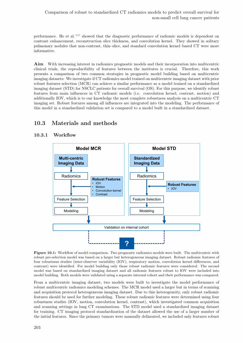
Comparison of robust to standardized CT radiomics models to predict overall survival fornon-small cell lung cancer patients
performance. He et al.433 showed that the diagnostic performance of radiomic models is dependent oncontrast–enhancement, reconstruction slice thickness, and convolution kernel. They showed in solitarypulmonary nodules that non-contrast, thin–slice, and standard convolution kernel–based CT were moreinformative.
Aim With increasing interest in radiomics prognostic models and their incorporation into multicentricclinical trials, the reproducibility of features between the institutes is crucial. Therefore, this workpresents a comparison of two common strategies in prognostic model building based on multicentricimaging datasets: We investigate if CT radiomics model trained on multicentric imaging dataset with priorrobust features selection (MCR) can achieve a similar performance as a model trained on a standardizedimaging dataset (STD) for NSCLC patients for overall survival (OS). For this purpose, we identify robustfeatures from main influences in CT radiomic models (i.e. convolution kernel, contrast, motion) andadditionally IOV, which is to our knowledge the most complete robustness analysis on a multicentric CTimaging set. Robust features among all influences are integrated into the modeling. The performance ofthis model in a standardized validation set is compared to a model built in a standardized dataset.
10.3 Materials and methods
10.3.1 Workflow
Multi-centric
Imaging Data
Feature Selection
Radiomics
Modeling
Robust Features• IOV
• Motion
• Convolution kernel
• Contrast
Model MCR
Validation on internal cohort
Model STD
Standardized
Imaging Data
Feature Selection
Radiomics
Modeling
Robust Features • IOV
?Figure 10.1: Workflow of model comparison. Two prognostic radiomics models were built. The multicentric withrobust pre-selection model was based on a larger but heterogeneous imaging dataset. Robust radiomic features offour robustness studies (inter-observer variability (IOV), respiratory motion, convolution kernel differences, andcontrast) were identified. For model building only those robust radiomic features were considered. The secondmodel was based on standardized imaging dataset and all radiomic features robust to IOV were included intomodel building. Both models were validated using a separate internal cohort and their performance was compared.
From a multicentric imaging dataset, two models were built to investigate the model performance ofrobust multicentric radiomics modeling schemes. The MCR model used a larger but in terms of scanningand acquisition protocol heterogeneous imaging dataset. Due to this heterogeneity, only robust radiomicfeatures should be used for further modeling. These robust radiomic features were determined using fourrobustness studies (IOV, motion, convolution kernel, contrast), which investigated common acquisitionand scanning settings in lung CT examinations. The STD model used a standardized imaging datasetfor training. CT imaging protocol standardization of the dataset allowed the use of a larger number ofthe initial features. Since the primary tumors were manually delineated, we included only features robust
203
against IOV. Both models were then validated on the same single–institution based validation cohort.Finally, the model performances were compared (Figure 10.1).
10.3.2 Study cohort
For the training cohort, pre-treatment CT scans were collected from 124 IIIA/N2 NSCLC from a prospec-tive Swiss multicentric randomized phase 3 trial (SAKK 16/007). In this multimodality treatment com-parison trial, patients underwent neoadjuvant chemotherapy or radiochemotherapy prior to surgery. Forthe validation cohort, CT scans of 31 IIIA/N2 or IIIB NSCLC patients were included. Patients weretreated curatively at University Hospital Zurich (USZ) with induction radiochemotherapy or chemother-apy only prior to surgery. Median follow–up time were 82 and 32 months for training and validation co-hort, respectively. Ethics amendment were received from all contributed Swiss Kanton ethics committeesand informed consent was obtained from all individual participants (for training (EKNZ PB_2016–01071,KEK ZH PB_201–00412, KEK Bern PB_2016–01072, CER–VD PB_201–01078, CCER PB_2016–01073, EKOS PB_201–01075, Comitato Etico Cantonale Bellinzona PB_2016–01077) and for validation(KEK ZH 2018–02405)). Outcome endpoint OS as well as patient staging (6th edition of the TNMclassification) were defined according to the SAKK–16/00 protocol7 (Supplement 10.7).
10.3.3 Imaging data
The entire heterogeneous imaging dataset was included for the MCR model which consisted of contrastCTs scans (n = 25), large range of slice thicknesses and different convolution kernels (Supplement 10.7).A subset of 84 CT scans from the MCR dataset with standardized imaging protocol was used for the STDmodel. We defined standardized imaging protocol as the largest homogeneous subset in the multicentricdataset, i.e.:
• non-contrast enhanced CT
• FBP using standard convolution kernel
• non-gated CT acquisition.
Mackin et al.227 identified in their radiomics phantom study, reconstruction kernels from different man-ufacturer which produced similar radiomic feature values. In a follow–up study of Ger et al.93, 100 CTscanner at 35 institutions were analyzed using a controlled chest and head imaging protocols. Theyshowed that controlled protocols can reduce feature variability up to 57% and the imaging variabilitywas small relative to the interpatient feature variability for NSCLC and head and neck squamous cellcarcinoma patients.93 Therefore, we defined standard convolution kernel as follows: GE – STANDARD,Siemens – B30f/B31f, Toshiba – FC18, and Philips – B.From the patients of the validation cohort, non-contrast enhanced average CT imaging were acquired onthe following CT scanners: Discovery RX, STE, 690 (GE MEDICAL SYSTEMS); Biograph 128 Edge,128, 40, 6 (SIEMENS); SOMATOM Definition AS (SOMATOM Definition AS). Scans were reconstructedwith FBP and a smooth kernel (STANDARD, I30f, B31f). CT spatial resolution was 0.98, 1.17, 1.37 mmin–plane and 2 and 3.27 mm in slice thickness.Only patients with a tumor volume of larger than 1 cm3 were included into further analysis, since theyallowed meaningful wavelet calculations.
10.3.4 Robustness studies
Four distinct robustness studies were conducted to investigate the IOV and three major acquisition andscanner parameters (motion, convolution kernel, and contrast) in chest–CT imaging data from patientswith primary tumors or malignant lung lesions (Figure 10.2). Table 10.1 shows characteristics of therobustness studies. Further information on the imaging data used for the robustness studies can be foundin the Supplement 10.8.Stability measure was the intraclass correlation coefficient (ICC). A two–way mixed single model (ICC(3,1))for the variance estimates was used403:
ICC(3, 1) =BMS − EMS
BMS + (κ− 1)EMS(10.1)
where BMS is between subject mean squares, respectively. EMS is the residual mean squares fromFriedman’s two–way ANOVA. The variable denotes the number of repeated measurements (here, CT
204
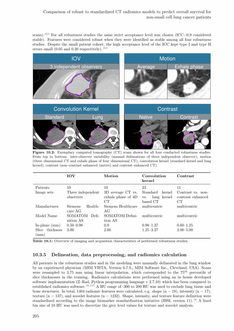
Comparison of robust to standardized CT radiomics models to predict overall survival fornon-small cell lung cancer patients
scans).403 For all robustness studies the same strict acceptance level was chosen (ICC>0.9 consideredstable). Features were considered robust when they were identified as stable among all four robustnessstudies. Despite the small patient cohort, the high acceptance level of the ICC kept type I and type IIerrors small (0.05 and 0.20 respectively).404
3 independent observers
IOV
Average Exhale phase
Motion
Standard Lung
Convolution Kernel
ContrastNative
Contrast
Figure 10.2: Exemplary computed tomography (CT) scans shown for all four conducted robustness studies.From top to bottom: inter-observer variability (manual delineations of three independent observer), motion(three–dimensional CT and exhale phase of four–dimensional CT), convolution kernel (standard kernel and lungkernel), contrast (non–contrast enhanced (native) and contrast–enhanced CT).
IOV Motion Convolutionkernel
Contrast
Patients 10 10 23 11Image sets Three independent
observers3D average CT vs.exhale phase of 4DCT
Standard kernelvs. lung kernelbased CT
Contrast vs. non-contrast enhancedCT
Manufacturer Siemens Health-care AG
Siemens HealthcareAG
multicentric multicentric
Model Name SOMATOM Defi-nition AS
SOMATOM Defini-tion AS
multicentric multicentric
In-plane (mm) 0.50–0.98 0.9 0.98–1.37 0.60–1.25Slice thickness(mm)
3.00 2.00 1.25–3.27 2.00–5.00
Table 10.1: Overview of imaging and acquisition characteristics of performed robustness studies.
10.3.5 Delineation, data preprocessing, and radiomics calculation
All patients in the robustness studies and in the modeling were manually delineated in the lung windowby an experienced physician (MIM VISTA, Version 6.7.9., MIM Software Inc., Cleveland, USA). Scanswere resampled to 3.75 mm using linear interpolation, which corresponded to the 75th percentile ofslice thicknesses in the training. Radiomics calculations were performed using an in–house developedsoftware implementation (Z–Rad, Python programming language v 2.7.10) which has been compared toestablished radiomics software.38,165 A HU range of -300 to 200 HU was used to exclude lung tissue andbone structures. In total, 1404 radiomic features were calculated, e.g. shape (n = 18), intensity (n = 17),texture (n = 137), and wavelet features (n = 1232). Shape, intensity, and texture feature definition werestandardized according to the image biomarker standardization initiative (IBSI, version 11).38 A fixedbin size of 10 HU was used to discretize the grey level values for texture and wavelet analysis.
205
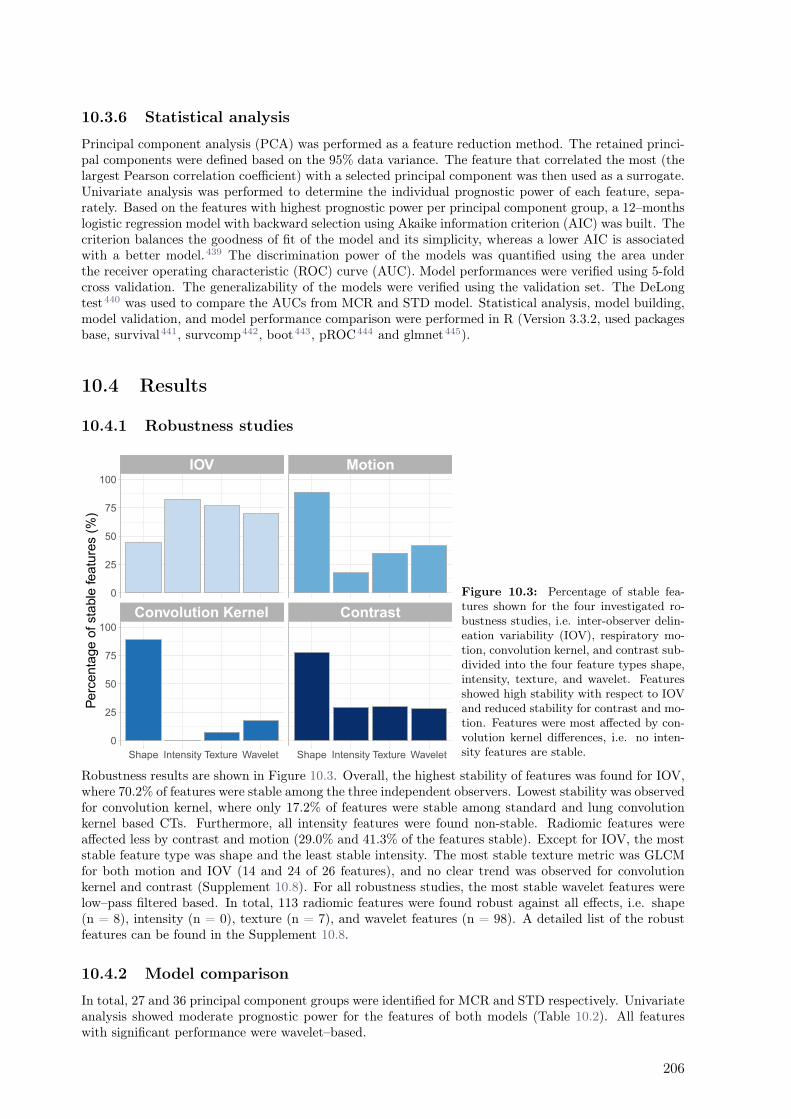
10.3.6 Statistical analysis
Principal component analysis (PCA) was performed as a feature reduction method. The retained princi-pal components were defined based on the 95% data variance. The feature that correlated the most (thelargest Pearson correlation coefficient) with a selected principal component was then used as a surrogate.Univariate analysis was performed to determine the individual prognostic power of each feature, sepa-rately. Based on the features with highest prognostic power per principal component group, a 12–monthslogistic regression model with backward selection using Akaike information criterion (AIC) was built. Thecriterion balances the goodness of fit of the model and its simplicity, whereas a lower AIC is associatedwith a better model.439 The discrimination power of the models was quantified using the area underthe receiver operating characteristic (ROC) curve (AUC). Model performances were verified using 5-foldcross validation. The generalizability of the models were verified using the validation set. The DeLongtest440 was used to compare the AUCs from MCR and STD model. Statistical analysis, model building,model validation, and model performance comparison were performed in R (Version 3.3.2, used packagesbase, survival441, survcomp442, boot443, pROC444 and glmnet445).
10.4 Results
10.4.1 Robustness studies
Figure 10.3: Percentage of stable fea-tures shown for the four investigated ro-bustness studies, i.e. inter-observer delin-eation variability (IOV), respiratory mo-tion, convolution kernel, and contrast sub-divided into the four feature types shape,intensity, texture, and wavelet. Featuresshowed high stability with respect to IOVand reduced stability for contrast and mo-tion. Features were most affected by con-volution kernel differences, i.e. no inten-sity features are stable.
Robustness results are shown in Figure 10.3. Overall, the highest stability of features was found for IOV,where 70.2% of features were stable among the three independent observers. Lowest stability was observedfor convolution kernel, where only 17.2% of features were stable among standard and lung convolutionkernel based CTs. Furthermore, all intensity features were found non-stable. Radiomic features wereaffected less by contrast and motion (29.0% and 41.3% of the features stable). Except for IOV, the moststable feature type was shape and the least stable intensity. The most stable texture metric was GLCMfor both motion and IOV (14 and 24 of 26 features), and no clear trend was observed for convolutionkernel and contrast (Supplement 10.8). For all robustness studies, the most stable wavelet features werelow–pass filtered based. In total, 113 radiomic features were found robust against all effects, i.e. shape(n = 8), intensity (n = 0), texture (n = 7), and wavelet features (n = 98). A detailed list of the robustfeatures can be found in the Supplement 10.8.
10.4.2 Model comparison
In total, 27 and 36 principal component groups were identified for MCR and STD respectively. Univariateanalysis showed moderate prognostic power for the features of both models (Table 10.2). All featureswith significant performance were wavelet–based.
206
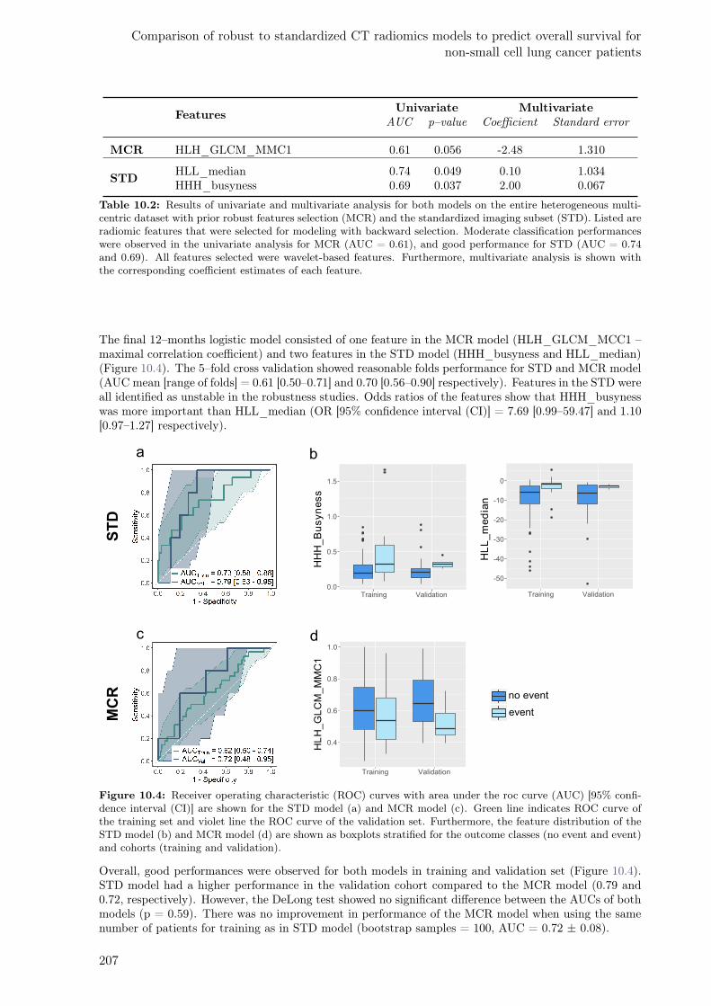
Comparison of robust to standardized CT radiomics models to predict overall survival fornon-small cell lung cancer patients
FeaturesUnivariate Multivariate
AUC p–value Coefficient Standard error
MCR HLH_GLCM_MMC1 0.61 0.056 -2.48 1.310
STDHLL_median 0.74 0.049 0.10 1.034HHH_busyness 0.69 0.037 2.00 0.067
Table 10.2: Results of univariate and multivariate analysis for both models on the entire heterogeneous multi-centric dataset with prior robust features selection (MCR) and the standardized imaging subset (STD). Listed areradiomic features that were selected for modeling with backward selection. Moderate classification performanceswere observed in the univariate analysis for MCR (AUC = 0.61), and good performance for STD (AUC = 0.74and 0.69). All features selected were wavelet-based features. Furthermore, multivariate analysis is shown withthe corresponding coefficient estimates of each feature.
The final 12–months logistic model consisted of one feature in the MCR model (HLH_GLCM_MCC1 –maximal correlation coefficient) and two features in the STD model (HHH_busyness and HLL_median)(Figure 10.4). The 5–fold cross validation showed reasonable folds performance for STD and MCR model(AUC mean [range of folds] = 0.61 [0.50–0.71] and 0.70 [0.56–0.90] respectively). Features in the STD wereall identified as unstable in the robustness studies. Odds ratios of the features show that HHH_busynesswas more important than HLL_median (OR [95% confidence interval (CI)] = 7.69 [0.99–59.47] and 1.10[0.97–1.27] respectively).
0.0
0.5
1.0
1.5
Training Validation
HH
H_B
usyn
ess
-50
-40
-30
-20
-10
0
Training Validation
HL
L_
me
dia
n
0.4
0.6
0.8
1.0
Training Validation
HL
H_G
LC
M_M
MC
1
no event
event
a b
c d
MCR
STD
Figure 10.4: Receiver operating characteristic (ROC) curves with area under the roc curve (AUC) [95% confi-dence interval (CI)] are shown for the STD model (a) and MCR model (c). Green line indicates ROC curve ofthe training set and violet line the ROC curve of the validation set. Furthermore, the feature distribution of theSTD model (b) and MCR model (d) are shown as boxplots stratified for the outcome classes (no event and event)and cohorts (training and validation).
Overall, good performances were observed for both models in training and validation set (Figure 10.4).STD model had a higher performance in the validation cohort compared to the MCR model (0.79 and0.72, respectively). However, the DeLong test showed no significant difference between the AUCs of bothmodels (p = 0.59). There was no improvement in performance of the MCR model when using the samenumber of patients for training as in STD model (bootstrap samples = 100, AUC = 0.72 ± 0.08).
207

10.5 Discussion
Randomized prospective multicentric clinical trials are considered the gold standard of clinical investiga-tion and aim to reflect the real world scenario. In terms of radiomic models, multicentric clinical trialsare preferred to counteract the “large–P, small–N” problem where a large number of predictors face smallsample sizes.238 In prospective multicentric trials, patient follow–up data are carefully collected. However,so far imaging data are rarely collected prospectively and often lack of standardized imaging protocols.For radiomics prognostic models, this infers additional challenges since features may be influenced notonly by the tumor phenotype but also from the used acquisition and scanner settings.Acquisition and scanner settings allow improving diagnostic accuracy. For example, filtered–back pro-jection can be performed with different convolution kernels, which exploit the underlying information ofthe specific tissue and structures. Standard (smooth) kernel suppresses high frequency domain informa-tion (including noise) leading to smoother but also more blurred images. Lung (sharp) kernel enhancesstructure heterogeneity leading to clearer visible brightness details or textures.Differentiation of vessel structures from mediastinal structures and tumorous tissue can be achievedusing contrast agent administration. And furthermore, respiratory motion can influence image quality,so that phase–gated imaging can achieve less motion affected scans to better distinguish the bordersof tumorous tissue. In our robustness studies we showed that CT radiomic features are differentlyaffected by scanner and acquisition parameters. The largest impact on radiomic features robustness wereconvolution kernel differences (<20% of the features stable). Intensity, texture, and wavelet featuresshowed poor stability, i.e. no stable intensity features and only two features stable for each texturemetric. Our findings are in agreement with several investigations.80,196,438 The second highest impact onrobustness of radiomic features was seen while comparing contrast with non-contrast enhanced CT scans(29.0%). The low feature stability may result from the different information provided by non-contrast andcontrast–enhanced CT, i.e. morphological tumor heterogeneity and the differential contrast agent uptakeof vessel inside the tissue.446 Furthermore, in agreement to Oliver et al., we found that intensity andtexture features were affected strongly by respiratory motion.85 Most stable texture metric was GLCM— unfiltered and with one or more low pass filters.Despite the high sensitivity of radiomic features, still around 100 features were stable against all effects(including IOV). These features were investigated on their prognostic power by development of the MCRmodel. MCR indicated worse estimated AUC performance on the validation cohort compared to theSTD model, despite the reduced number of patients in the STD model for training (AUC = 0.72 and 0.79for MCR and STD respectively). Both models consisted of a combination of wavelet features, i.e. morecomplex, higher order radiomic features. DeLong test showed no significant difference of the AUCs ofboth models. However, since the 95%CI of the MCR model overlaps with 0.5 (performance of a randompredictor), we would still suggest using the STD model. The broad confidence intervals result from thesmall patient number in the validation. Moreover, the selected features of the STD model were statis-tically significant in the univariate analysis (p < 0.05, Table 10.2). The final STD model consisted oftwo features: HHH_busyness and HLL_median. In particular, the HHH_busyness feature representstextures with fast changes in grey levels between neighboring voxels438 based on edge–enhanced scans(HHH). In this model, higher HHH_busyness feature value was associated with worse prognosis, which isin agreement with other studies indicating that patients with more heterogeneous tumor structure showedworse prognosis.447,448 Although the performance measure of the STD model on the validation cohortwas within the 95% CI, it is worth noting that the model performed better on the validation compared tothe training. Next to the small sample size, one explanation might be the interscanner variability. Bothphantom studies, Mackin et al.432 and the larger follow–up study by Ger et al.93, showed that interscan-ner variability can have an effect on the radiomic features196 despite controlled protocols (similar to theSTD model) and that it can be comparable to interpatient feature variability in NSCLC and head andneck cancer patients. This might introduce an additional variability in the training cohort compared tothe validation cohort.
This study had several limitations. First, we studied only a subset of CT imaging parameters. Otherparameters such as tube voltage or mAs also considerable influence radiomic features196 and hence theshown performances might be affected when using different scanning conditions. However, the conductedrobustness studies assessed the most important aspect for lung imaging examination in multicentricdataset and additionally IOV. In a substudy, we could show that both models failed to be validated onthe same validation patient cohort, but with different scanning setting (contrast–enhanced CT recon-structed with lung kernel, Supplement 10.10). Furthermore, the robustness study of both convolution
208

Comparison of robust to standardized CT radiomics models to predict overall survival fornon-small cell lung cancer patients
kernel differences, and contrast–agent administration were based on the multicentric dataset. Moreover,the patient dataset for the motion robustness studies was limited to patients with small motion amplitudewith mean Euclidean distance of 2.4 mm ranging from 0.68 to 7.01 mm. Different robustness results areexpected for patients with larger tumor motion. Ideally, CT scans would be acquired on the same scan-ner with same reconstruction and slice thickness. In terms of slice thickness and resolution, it has beenshown that the sensitivity of radiomic features to spatial imaging resolution variations can be reduced byresampling.35,219,438 Lastly, the sample sizes used in our study were small for training, validation, androbustness studies. For the robustness studies, we therefore set a strict acceptance level to avoid sam-ple fluctuation to cause misleading conclusions. However, recently PET and CT radiomic models werepublished which failed to consistently predict OS using 600 head and neck cancer patients of two institu-tions even within patients with the same imaging protocol (using the same methodology as in the STDmodel).93 They hypothesized that the negative results may originate in differences in patient populationand suggested that radiomics signatures may not always be transferrable due to unseen differences in pa-tient populations. Hence, it is a good practice to first test a model on the cohort from your own instituteand perhaps perform model recalibration before its use in a prospective cohort. Toward multicentric basedradiomics models, one possibility to preserve the number of potential biomarkers is to use a standardizedimaging protocol for all centers. Convolution kernel differences, contrast administration (with or without)and motion (4D gated CT imaging) can be controlled prior to clinical studies using standardized imagingprotocols. However, convolution kernel and reconstruction algorithms are vendor–specific and differ in forexample, noise and smoothing enhancement.438 Mackin et al.227 studied the comparability of radiomicfeatures from phantom CT scans acquired at 17 scanners from the four most common vendors. Thoughlimited in the number of investigated features, they showed that texture features were scanner dependent.Contrast agent influence can be controlled by selection of only contrast–enhanced CTs. However, carefuladministration of the agent, which is dependent not only on the substrate but also on the patient–specificuptake or scan delay time needs to be considered and is therefore difficult to perform in clinical routine.In a recent study, radiomic feature values from diagnostic contrast–enhanced and non-contrast enhancedCT in NSCLC patients were shown to be affected by the contrast enhancement and in particular maydepend largely on the patient characteristics, for example, patient weight, tumor volume or performancestatus.449 Therefore, additional analysis is needed to define robust radiomic features for different levels ofcontrast–agent uptake, which to our current knowledge has not been performed. To overcome IOV, stan-dardized contouring protocols or alternatively semi– or full–automatized segmentation software solutionscan be helpful.33 Regardless of imaging protocol standardization among clinics, these suggestions are lim-ited to the availability of the hardware and software equipment at the individual centers. Hence, severalgroups are studying postprocessing methods to compensate for multicentric effect. Ideally, postprocessingmethods should sufficiently harmonize multicentric variations while preserving patient–specific variation.A recent study from Orlhac et al.205 showed a method to compensate multicentric effects affecting CTradiomics for 74 lung cancer patients involving 10 texture patterns. Initially used in genomic datasetsto overcome lab and scanner variation, this compensation method (ComBat) entered the radiomics fieldand showed good results for PET scanner variation while preserving patient–specific texture patternsvariation.204 Recently, they additionally showed feasibility of this method for CT imaging.205 However,they only received satisfactory harmonization results with at least 20 patients per protocol205, which wasnot fulfilled in our study (number of patients per center ranging from 1 to 30).
10.6 Conclusion
CT radiomic features based on malignant lung lesions show differential sensitivity to inter-observer delin-eation variability, respiratory motion, convolution kernel, and contrast. A small number of investigatedfeatures (10%) were robust to all effects. Our model comparison study indicated that the prognostic CTradiomics model to predict OS for locally advanced NSCLC patients based on a larger, heterogeneousmulticentric imaging dataset with prior robust features pre-selection can perform equally well as a modeltrained on a standardized imaging protocol. However, considering low robustness rate, imaging protocolstandardization in combination with postharmonization of features should be considered in multicentricradiomics models to improve their performance and reproducibility. Further investigations are needed toverify the generalizability of the models on external validation datasets.
209
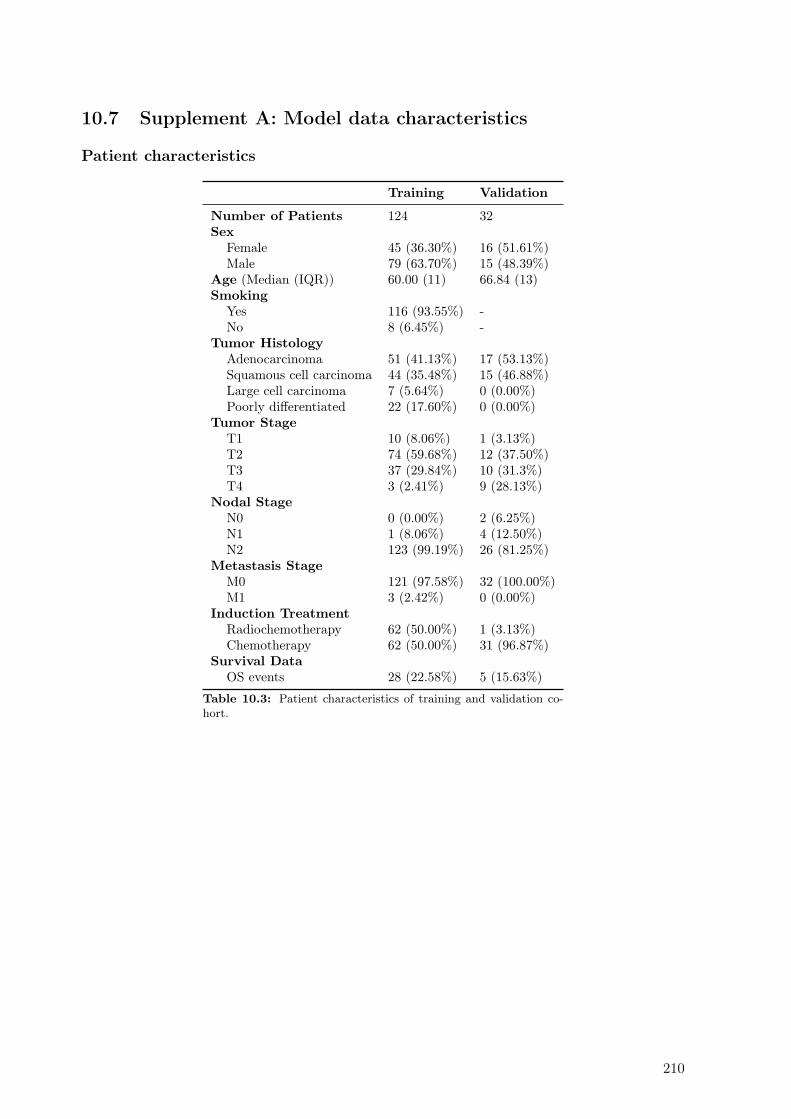
10.7 Supplement A: Model data characteristics
Patient characteristics
Training Validation
Number of Patients 124 32Sex
Female 45 (36.30%) 16 (51.61%)Male 79 (63.70%) 15 (48.39%)
Age (Median (IQR)) 60.00 (11) 66.84 (13)Smoking
Yes 116 (93.55%) -No 8 (6.45%) -
Tumor HistologyAdenocarcinoma 51 (41.13%) 17 (53.13%)Squamous cell carcinoma 44 (35.48%) 15 (46.88%)Large cell carcinoma 7 (5.64%) 0 (0.00%)Poorly differentiated 22 (17.60%) 0 (0.00%)
Tumor StageT1 10 (8.06%) 1 (3.13%)T2 74 (59.68%) 12 (37.50%)T3 37 (29.84%) 10 (31.3%)T4 3 (2.41%) 9 (28.13%)
Nodal StageN0 0 (0.00%) 2 (6.25%)N1 1 (8.06%) 4 (12.50%)N2 123 (99.19%) 26 (81.25%)
Metastasis StageM0 121 (97.58%) 32 (100.00%)M1 3 (2.42%) 0 (0.00%)
Induction TreatmentRadiochemotherapy 62 (50.00%) 1 (3.13%)Chemotherapy 62 (50.00%) 31 (96.87%)
Survival DataOS events 28 (22.58%) 5 (15.63%)
Table 10.3: Patient characteristics of training and validation co-hort.
210

Comparison of robust to standardized CT radiomics models to predict overall survival fornon-small cell lung cancer patients
Imaging variability of training cohort
0.75 1.00 1.25 1.50 1.75 2.00 2.25 2.50 2.75 3.00 3.25 3.50 3.75 4.00 4.25 4.50 4.75 5.00
Slice thickness (m m )
0
10
20
30
40
Fre
qu
en
cy
Sl ice Th ick n ess
STANDARD B
B30f
SOFT
B31f
B19f
B20f
B31s
FC02
B10f
B41s
FC12
B25f
LUNG L C
0
20
40
60
80
Fre
qu
en
cy
Con v o lu t ion Ker n e l
Figure 10.5: Data variability of imaging dataset of the multicentric training cohort is shown as frequency barplots. High imaging protocol variability can be found in the dataset, i.e. slice thickness ranges from 0.6 to5.0 mm. Similar observation are found for convolution kernel, various convolution kernel with a majority beingSTANDARD kernel (84 patients).
10.8 Supplement B: Robustness studies
Patient selection and delineation
Convolution Kernel A subset of the multicentric training dataset was retrospectively. Patientswere selected if they received pre-treatment non-contrast enhanced CT reconstructed once with FBPusing a standard convolution kernel as well as a lung convolution kernel on the same day using the sameprojection raw data. Primary tumors were delineated on standard convolution kernel image set and thecontours were transferred to the corresponding lung convolution kernel image set.
Contrast A patient subset of multicentric training dataset was retrospectively selected. Patients wereselected if they received a contrast-enhanced and non-contrast enhanced CT on the same day prior totreatment. CTs were registered deformably when necessary. Primary tumours were delineated on thenon-contrast enhanced CT and structures were transferred to the corresponding contrast-enhanced CT.
Motion To investigate motion effects on the stability of the radiomics features, patients treated at theUniversity Hospital Zurich with lung lesions were retrospectively selected. A pre-treatment 3D CT aswell as a pre-treatment 4D (gated) CT (10 phases, phase-triggered) were acquired on the same day foreach patients. The CT scans were reconstructed with FBP B30fs. Largest lesions in the lung region weremanually delineated independently on the 3D CT scan as well as on the exhale phase of the 4D CT scanwhich is considered the most stable phase. Motion displacement were determined using the Euclideandistance of the center of mass of the lesion. Median motion displacement was found to be moderate with2.4 mm (0.68 - 7.01).
211

Delineation To investigate the interobserver variability, we used the same dataset as Pavic et al.33
NSCLC patients treated at the University Hospital Zurich were retrospectively selected. The primarytumors on the pre-treatment CT were manually delineated by three experienced radiation oncologists.Radiomic features were calculated on the contours of each individual observers. CT imaging data werereconstructed with FBP standard convolution kernel.
Stable features
Features identified as stable across all four robustness studies:
• shape (n = 8): volume, surface, median thickness, standard deviation thickness, Euclidean distance,major and minor axis length, least axis length
• intensity (n = 0)
• texture (n = 7): information measures of correlation 1 and 2, coarseness, zone size non-uniformitycalculated from GLRLM, m_GLRLM and GLDZM, dependence count entropy
• wavelet (n = 98): HHH (8), HHL (13), HLH (5), HLL (13), LHH (6), LHL (18), LLH (13), LLL(22).
212

Supplement C: Results of robustness studies
Table 1: The intra-class correlation coefficients (ICC) of the investigated radiomic features in our four ro-bustness studies: inter-observer delineation variability (IOV), motion, convolution kernel (kernel) and contrast.Stable features (ICC > 0.9) are shown in bold. Nomenclature according to Zwanenburg et al. (2016) ”Imagebiomarker standardisation initiative.”
Radiomic Features IOV Motion Kernel Contrast
Shape volume 1.00 0.99 1.00 1.00
Shape surface 0.99 0.99 1.00 1.00
Shape compactness 1 0.80 0.97 0.97 0.93
Shape compactness 2 0.82 0.96 0.96 0.93
Shape spherical disproportion 0.73 0.98 0.97 0.89Shape sphericity 0.79 0.97 0.97 0.93
Shape asphericity 0.73 0.98 0.97 0.89Shape surface to volume ratio 0.90 0.95 0.99 0.99
Shape median thickness 0.96 0.98 1.00 1.00
Shape standard deviation thickness 0.97 0.99 1.00 1.00
Shape euclidian distance 0.95 0.99 1.00 1.00
Shape major axis length 0.93 0.99 1.00 1.00
Shape minor axis length 0.99 1.00 1.00 1.00
Shape least axis length 0.98 0.99 1.00 1.00
Shape elongation 0.58 0.95 0.99 0.91
Shape flatness 0.73 0.94 0.99 0.94
Shape fractal dimension 0.48 0.65 0.58 0.89Shape center of mass shift 0.50 0.03 0.00 0.00Unfiltered Intensity mean 0.95 0.91 0.80 0.87Unfiltered Intensity standard deviation 0.91 0.45 0.83 0.71Unfiltered Intensity coefficient of variation 0.62 0.00 0.00 0.00Unfiltered Intensity skewness 0.97 0.92 0.35 0.92
Unfiltered Intensity kurtosis 0.94 0.83 0.27 0.89Unfiltered Intensity variance 0.92 0.43 0.80 0.70Unfiltered Intensity median 0.97 0.85 0.75 0.87Unfiltered Intensity percentile 10th 0.89 0.75 0.90 0.92
Unfiltered Intensity percentile 90th 0.95 0.69 0.00 0.37Unfiltered Intensity interquartile range 0.92 0.62 0.86 0.96
Unfiltered Intensity range 0.50 0.70 0.66 0.60Unfiltered Intensity mean absolut deviation 0.92 0.57 0.85 0.86Unfiltered Intensity robust mean absolut deviation 0.93 0.62 0.85 0.92
Unfiltered Intensity energy 0.99 0.97 0.81 0.90
Unfiltered Intensity entropy 0.96 0.85 0.52 0.48Unfiltered Intensity root mean square 0.94 0.88 0.88 0.82Unfiltered Intensity uniformity 0.98 0.71 0.34 0.60Unfiltered GLCM energy 0.95 0.88 0.63 0.63Unfiltered GLCM entropy 0.93 0.96 0.66 0.83Unfiltered GLCM contrast 0.98 0.90 0.82 0.87Unfiltered GLCM correlation 0.93 0.64 0.39 0.95
Unfiltered GLCM homogeneity 0.99 0.80 0.50 0.84Unfiltered GLCM homogeneity normalized 0.90 0.95 0.77 0.99
Unfiltered GLCM inverese difference 0.99 0.83 0.57 0.87Unfiltered GLCM inverese difference normalized 0.93 0.94 0.74 0.99
Unfiltered GLCM variance 0.95 0.51 0.83 0.76Unfiltered GLCM sum of average 0.96 0.91 0.82 0.90Unfiltered GLCM sum of entropy 0.92 0.97 0.74 0.77Unfiltered GLCM sum of variance 0.90 0.14 0.80 0.63Unfiltered GLCM difference entropy 0.98 0.98 0.55 0.59Unfiltered GLCM difference variance 0.96 0.40 0.80 0.73Unfiltered GLCM information measures of correlation 1 0.99 0.97 0.98 0.99
Continued on next page
1
Table 1 – Continued
Unfiltered GLCM information measures of correlation 2 1.00 0.98 0.92 0.94
Unfiltered GLCM maximal correlation coefficient 0.96 0.98 0.89 0.98
Unfiltered GLCM joint maximum 0.91 0.51 0.15 0.69Unfiltered GLCM joint average 0.96 0.91 0.82 0.90Unfiltered GLCM difference average 0.98 0.96 0.81 0.94
Unfiltered GLCM dissimilarity 0.98 0.96 0.81 0.94
Unfiltered GLCM inverse variance 0.99 0.87 0.55 0.88Unfiltered GLCM autocorrelation 0.96 0.93 0.84 0.87Unfiltered GLCM cluster tendency 0.90 0.14 0.80 0.63Unfiltered GLCM cluster shade 0.93 0.71 0.54 0.36Unfiltered GLCM cluster prominence 0.89 0.00 0.55 0.05Unfiltered mGLCM energy 0.98 0.47 0.10 0.60Unfiltered mGLCM entropy 0.96 0.81 0.33 0.55Unfiltered mGLCM contrast 0.98 0.90 0.81 0.87Unfiltered mGLCM correlation 0.93 0.80 0.43 0.93
Unfiltered mGLCM homogeneity 0.99 0.81 0.50 0.84Unfiltered mGLCM homogeneity normalized 0.90 0.95 0.79 0.98
Unfiltered mGLCM inverese difference 0.99 0.84 0.57 0.87Unfiltered mGLCM inverese difference normalized 0.92 0.95 0.75 0.99
Unfiltered mGLCM variance 0.95 0.62 0.84 0.77Unfiltered mGLCM sum of average 0.96 0.91 0.82 0.90Unfiltered mGLCM sum of entropy 0.96 0.79 0.64 0.74Unfiltered mGLCM sum of variance 0.90 0.28 0.84 0.66Unfiltered mGLCM difference entropy 0.99 0.94 0.69 0.87Unfiltered mGLCM difference variance 0.96 0.47 0.82 0.72Unfiltered mGLCM information measures of correlation 1 0.95 0.86 0.74 0.94
Unfiltered mGLCM information measures of correlation 2 0.94 0.84 0.76 0.92
Unfiltered mGLCM maximal correlation coefficient 0.90 0.69 0.35 0.56Unfiltered mGLCM joint maximum 0.92 0.35 0.07 0.68Unfiltered mGLCM joint average 0.96 0.91 0.82 0.90Unfiltered mGLCM difference average 0.98 0.96 0.81 0.94
Unfiltered mGLCM dissimilarity 0.98 0.96 0.81 0.94
Unfiltered mGLCM inverse variance 0.99 0.87 0.55 0.88Unfiltered mGLCM autocorrelation 0.96 0.93 0.84 0.87Unfiltered mGLCM cluster tendency 0.90 0.28 0.84 0.66Unfiltered mGLCM cluster shade 0.93 0.71 0.64 0.35Unfiltered mGLCM cluster prominence 0.89 0.00 0.64 0.07Unfiltered NGTDM coarseness 0.98 0.96 0.90 0.91
Unfiltered NGTDM contrast 0.94 0.96 0.65 0.78Unfiltered NGTDM busyness 0.99 0.73 0.91 0.93
Unfiltered NGTDM complexity 0.86 0.75 0.51 0.05Unfiltered NGTDM strength 0.97 0.84 0.77 0.96
Unfiltered GLRLM grey level non-uniformity 1.00 0.98 0.84 0.99
Unfiltered GLRLM grey level non-uniformity normalized 0.98 0.85 0.39 0.56Unfiltered GLRLM zone size non-uniformity 1.00 0.98 0.91 0.99
Unfiltered GLRLM zone size non-uniformity normalized 0.99 0.82 0.54 0.86Unfiltered GLRLM short runs emphasis 0.99 0.79 0.47 0.85Unfiltered GLRLM long runs emphasis 0.99 0.63 0.28 0.83Unfiltered GLRLM low grey level run emphasis 0.81 0.63 0.61 0.60Unfiltered GLRLM high grey level run emphasis 0.95 0.92 0.81 0.85Unfiltered GLRLM short run low grey level emphasis 0.81 0.63 0.64 0.60Unfiltered GLRLM short run high grey level emphasis 0.93 0.88 0.78 0.80Unfiltered GLRLM long run low grey level emphasis 0.78 0.61 0.54 0.56Unfiltered GLRLM long run high grey level emphasis 0.97 0.88 0.58 0.94
Unfiltered GLRLM run percentage 0.99 0.76 0.45 0.86Unfiltered GLRLM grey level variance 0.91 0.32 0.77 0.66Unfiltered GLRLM run length variance 0.99 0.53 0.22 0.84Unfiltered GLRLM run entropy 0.86 0.95 0.67 0.70Unfiltered mGLRLM grey level non-uniformity 1.00 0.98 0.84 0.99
Continued on next page
2
Com
parison
ofrob
ust
tostan
dard
izedC
Trad
iomics
models
topred
ictoverall
surv
ivalfor
non
-small
celllu
ng
cancer
patien
ts
10.9
Supplem
ent
C:IC
CR
esults
213
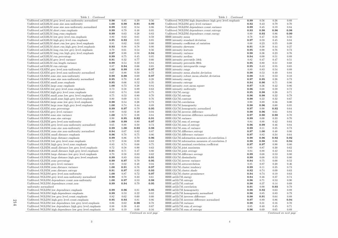
Table 1 – Continued
Unfiltered mGLRLM grey level non-uniformity normalized 0.98 0.85 0.39 0.56Unfiltered mGLRLM zone size non-uniformity 1.00 0.98 0.91 0.99
Unfiltered mGLRLM zone size non-uniformity normalized 0.99 0.82 0.54 0.86Unfiltered mGLRLM short runs emphasis 0.99 0.79 0.48 0.85Unfiltered mGLRLM long runs emphasis 0.99 0.63 0.28 0.83Unfiltered mGLRLM low grey level run emphasis 0.80 0.62 0.61 0.59Unfiltered mGLRLM high grey level run emphasis 0.95 0.92 0.81 0.85Unfiltered mGLRLM short run low grey level emphasis 0.81 0.62 0.63 0.60Unfiltered mGLRLM short run high grey level emphasis 0.93 0.88 0.78 0.80Unfiltered mGLRLM long run low grey level emphasis 0.79 0.61 0.54 0.56Unfiltered mGLRLM long run high grey level emphasis 0.97 0.88 0.58 0.94
Unfiltered mGLRLM run percentage 0.99 0.75 0.45 0.85Unfiltered mGLRLM grey level variance 0.91 0.32 0.77 0.66Unfiltered mGLRLM run length variance 0.99 0.54 0.22 0.84Unfiltered mGLRLM run entropy 0.87 0.94 0.66 0.65Unfiltered GLSZM grey level non-uniformity 1.00 0.99 0.80 0.97
Unfiltered GLSZM grey level non-uniformity normalized 0.67 0.88 0.50 0.72Unfiltered GLSZM zone size non-uniformity 0.99 0.98 0.69 0.97
Unfiltered GLSZM zone size non-uniformity normalized 0.95 0.70 0.49 0.28Unfiltered GLSZM small zone emphasis 0.95 0.66 0.52 0.35Unfiltered GLSZM large zone emphasis 1.00 0.73 0.38 0.84Unfiltered GLSZM low grey level zone emphasis 0.73 0.58 0.89 0.63Unfiltered GLSZM high grey level zone emphasis 0.83 0.74 0.68 0.75Unfiltered GLSZM small zone low grey level emphasis 0.75 0.53 0.80 0.70Unfiltered GLSZM small zone high grey level emphasis 0.80 0.69 0.51 0.76Unfiltered GLSZM large zone low grey level emphasis 0.98 0.54 0.26 0.73Unfiltered GLSZM large zone high grey level emphasis 1.00 0.74 0.44 0.89Unfiltered GLSZM zone percentage 0.99 0.97 0.79 0.95
Unfiltered GLSZM grey level variance 0.88 0.02 0.48 0.04Unfiltered GLSZM zone size variance 1.00 0.72 0.38 0.84Unfiltered GLSZM zone size entropy 0.90 0.95 0.92 0.91
Unfiltered GLDZM grey level non-uniformity 1.00 0.99 0.80 0.97
Unfiltered GLDZM grey level non-uniformity normalized 0.65 0.88 0.50 0.73Unfiltered GLDZM zone size non-uniformity 0.99 1.00 0.93 0.98
Unfiltered GLDZM zone size non-uniformity normalized 0.94 0.67 0.82 0.87Unfiltered GLDZM small distance emphasis 0.96 0.70 0.75 0.86Unfiltered GLDZM large distance emphasis 0.99 0.86 0.70 0.96
Unfiltered GLDZM low grey level zone emphasis 0.72 0.58 0.89 0.63Unfiltered GLDZM high grey level zone emphasis 0.83 0.74 0.68 0.75Unfiltered GLDZM small distance low grey level emphasis 0.72 0.58 0.90 0.63Unfiltered GLDZM small distance high grey level emphasis 0.91 0.71 0.47 0.80Unfiltered GLDZM large distance low grey level emphasis 0.70 0.58 0.83 0.62Unfiltered GLDZM large distance high grey level emphasis 0.99 0.83 0.64 0.91
Unfiltered GLDZM zone percentage 0.99 0.97 0.79 0.95
Unfiltered GLDZM grey level variance 0.88 0.02 0.48 0.04Unfiltered GLDZM zone distance variance 1.00 0.91 0.76 0.97
Unfiltered GLDZM zone distance entropy 0.91 0.97 0.83 0.93
Unfiltered NGLDM grey level non-uniformity 1.00 0.87 0.72 0.97
Unfiltered NGLDM grey level non-uniformity normalized 0.98 0.70 0.33 0.61Unfiltered NGLDM dependence count non-uniformity 1.00 0.97 0.53 0.98
Unfiltered NGLDM dependence count non-uniformity normalized
0.99 0.94 0.79 0.95
Unfiltered NGLDM low dependence emphasis 0.99 0.96 0.81 0.95
Unfiltered NGLDM high dependence emphasis 0.99 0.53 0.22 0.82Unfiltered NGLDM low grey level count emphasis 0.82 0.62 0.60 0.60Unfiltered NGLDM high grey level count emphasis 0.95 0.93 0.81 0.86Unfiltered NGLDM low dependence low grey level emphasis 0.86 0.62 0.98 0.78Unfiltered NGLDM low dependence high grey level emphasis 0.88 0.30 0.40 0.67Unfiltered NGLDM high dependence low grey level emphasis 0.29 0.19 0.09 0.16
Continued on next page
3
Table 1 – Continued
Unfiltered NGLDM high dependence high grey level emphasis 0.99 0.56 0.26 0.89Unfiltered NGLDM grey level variance 0.92 0.43 0.79 0.70Unfiltered NGLDM dependence count variance 0.99 0.45 0.19 0.84Unfiltered NGLDM dependence count entropy 0.93 0.98 0.96 0.98
Unfiltered NGLDM dependence count energy 0.89 0.93 0.86 0.99
HHH intensity mean 0.78 0.47 0.58 0.50HHH intensity standard deviation 0.97 0.59 0.45 0.84HHH intensity coefficient of variation 0.00 0.23 0.55 0.09HHH intensity skewness 0.91 0.38 0.44 0.27HHH intensity kurtosis 0.95 0.90 0.76 0.73HHH intensity variance 0.98 0.36 0.23 0.76HHH intensity median 0.94 0.00 0.51 0.89HHH intensity percentile 10th 0.82 0.47 0.47 0.51HHH intensity percentile 90th 0.95 0.80 0.51 0.68HHH intensity interquartile range 0.95 0.43 0.55 0.65HHH intensity range 0.89 0.83 0.54 0.89HHH intensity mean absolut deviation 0.98 0.53 0.49 0.84HHH intensity robust mean absolut deviation 0.98 0.31 0.53 0.10HHH intensity energy 0.97 0.95 0.26 0.73HHH intensity entropy 0.94 0.90 0.71 0.86HHH intensity root mean square 0.97 0.36 0.42 0.86HHH intensity uniformity 0.96 0.68 0.59 0.72HHH GLCM energy 0.95 0.98 0.26 0.71HHH GLCM entropy 0.96 0.98 0.32 0.79HHH GLCM contrast 0.98 0.22 0.32 0.67HHH GLCM correlation 0.90 0.89 0.56 0.00HHH GLCM homogeneity 0.98 0.96 0.60 0.85HHH GLCM homogeneity normalized 0.97 0.90 0.92 0.64HHH GLCM inverese difference 0.98 0.96 0.61 0.84HHH GLCM inverese difference normalized 0.97 0.90 0.90 0.70HHH GLCM variance 0.99 0.00 0.33 0.70HHH GLCM sum of average 0.84 0.88 0.42 0.64HHH GLCM sum of entropy 0.96 0.99 0.46 0.84HHH GLCM sum of variance 0.99 0.11 0.35 0.73HHH GLCM difference entropy 0.97 1.00 0.48 0.86HHH GLCM difference variance 0.97 0.82 0.34 0.64HHH GLCM information measures of correlation 1 0.98 0.96 0.92 0.92
HHH GLCM information measures of correlation 2 0.98 0.98 0.86 0.94
HHH GLCM maximal correlation coefficient 0.97 0.97 0.90 0.80HHH GLCM joint maximum 0.89 0.87 0.30 0.62HHH GLCM joint average 0.84 0.88 0.42 0.64HHH GLCM difference average 0.99 0.68 0.53 0.80HHH GLCM dissimilarity 0.99 0.68 0.53 0.80HHH GLCM inverse variance 0.94 0.75 0.00 0.52HHH GLCM autocorrelation 0.85 0.87 0.20 0.46HHH GLCM cluster tendency 0.99 0.11 0.35 0.73HHH GLCM cluster shade 0.92 0.74 0.09 0.63HHH GLCM cluster prominence 0.94 0.74 0.19 0.63HHH mGLCM energy 0.94 0.46 0.37 0.74HHH mGLCM entropy 0.96 0.71 0.53 0.90HHH mGLCM contrast 0.98 0.37 0.14 0.69HHH mGLCM correlation 0.91 0.90 0.93 0.79HHH mGLCM homogeneity 0.98 0.92 0.63 0.89HHH mGLCM homogeneity normalized 0.96 0.85 0.83 0.79HHH mGLCM inverese difference 0.98 0.91 0.64 0.89HHH mGLCM inverese difference normalized 0.97 0.89 0.86 0.94
HHH mGLCM variance 0.98 0.31 0.16 0.70HHH mGLCM sum of average 0.85 0.40 0.45 0.71HHH mGLCM sum of entropy 0.96 0.69 0.65 0.89
Continued on next page
4
214
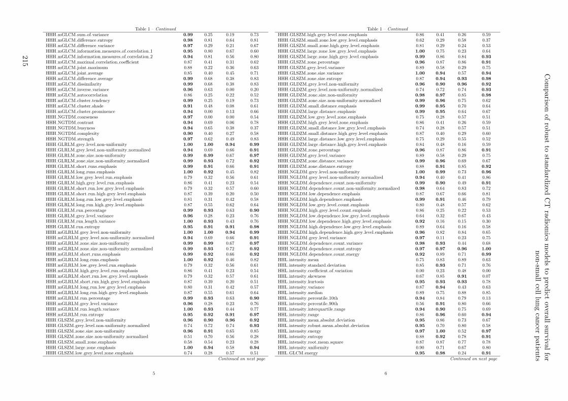
Table 1 – Continued
HHH mGLCM sum of variance 0.99 0.25 0.19 0.73HHH mGLCM difference entropy 0.98 0.81 0.64 0.81HHH mGLCM difference variance 0.97 0.29 0.21 0.67HHH mGLCM information measures of correlation 1 0.95 0.80 0.67 0.60HHH mGLCM information measures of correlation 2 0.94 0.81 0.56 0.80HHH mGLCM maximal correlation coefficient 0.87 0.41 0.31 0.62HHH mGLCM joint maximum 0.88 0.22 0.36 0.63HHH mGLCM joint average 0.85 0.40 0.45 0.71HHH mGLCM difference average 0.99 0.68 0.38 0.83HHH mGLCM dissimilarity 0.99 0.68 0.38 0.83HHH mGLCM inverse variance 0.96 0.63 0.00 0.20HHH mGLCM autocorrelation 0.86 0.25 0.22 0.52HHH mGLCM cluster tendency 0.99 0.25 0.19 0.73HHH mGLCM cluster shade 0.91 0.48 0.08 0.61HHH mGLCM cluster prominence 0.94 0.00 0.13 0.66HHH NGTDM coarseness 0.97 0.00 0.00 0.54HHH NGTDM contrast 0.94 0.69 0.06 0.78HHH NGTDM busyness 0.94 0.65 0.38 0.37HHH NGTDM complexity 0.90 0.40 0.27 0.58HHH NGTDM strength 0.97 0.62 0.49 0.83HHH GLRLM grey level non-uniformity 1.00 1.00 0.94 0.99
HHH GLRLM grey level non-uniformity normalized 0.94 0.69 0.66 0.91
HHH GLRLM zone size non-uniformity 0.99 0.99 0.67 0.97
HHH GLRLM zone size non-uniformity normalized 0.99 0.93 0.72 0.92
HHH GLRLM short runs emphasis 0.99 0.91 0.66 0.91
HHH GLRLM long runs emphasis 1.00 0.92 0.45 0.82HHH GLRLM low grey level run emphasis 0.79 0.32 0.56 0.61HHH GLRLM high grey level run emphasis 0.86 0.41 0.23 0.54HHH GLRLM short run low grey level emphasis 0.79 0.32 0.57 0.60HHH GLRLM short run high grey level emphasis 0.87 0.39 0.20 0.50HHH GLRLM long run low grey level emphasis 0.81 0.31 0.42 0.58HHH GLRLM long run high grey level emphasis 0.87 0.55 0.62 0.64HHH GLRLM run percentage 0.99 0.93 0.63 0.90
HHH GLRLM grey level variance 0.96 0.28 0.23 0.76HHH GLRLM run length variance 1.00 0.93 0.43 0.76HHH GLRLM run entropy 0.95 0.91 0.91 0.98
HHH mGLRLM grey level non-uniformity 1.00 1.00 0.94 0.99
HHH mGLRLM grey level non-uniformity normalized 0.94 0.69 0.66 0.91
HHH mGLRLM zone size non-uniformity 0.99 0.99 0.67 0.97
HHH mGLRLM zone size non-uniformity normalized 0.99 0.93 0.72 0.92
HHH mGLRLM short runs emphasis 0.99 0.92 0.66 0.92
HHH mGLRLM long runs emphasis 1.00 0.92 0.46 0.82HHH mGLRLM low grey level run emphasis 0.79 0.32 0.56 0.61HHH mGLRLM high grey level run emphasis 0.86 0.41 0.23 0.54HHH mGLRLM short run low grey level emphasis 0.79 0.32 0.57 0.61HHH mGLRLM short run high grey level emphasis 0.87 0.39 0.20 0.51HHH mGLRLM long run low grey level emphasis 0.80 0.31 0.42 0.57HHH mGLRLM long run high grey level emphasis 0.87 0.55 0.61 0.64HHH mGLRLM run percentage 0.99 0.93 0.63 0.90
HHH mGLRLM grey level variance 0.96 0.28 0.23 0.76HHH mGLRLM run length variance 1.00 0.93 0.44 0.77HHH mGLRLM run entropy 0.95 0.92 0.91 0.97
HHH GLSZM grey level non-uniformity 0.96 0.90 0.96 0.92
HHH GLSZM grey level non-uniformity normalized 0.74 0.72 0.74 0.93
HHH GLSZM zone size non-uniformity 0.96 0.91 0.65 0.85HHH GLSZM zone size non-uniformity normalized 0.51 0.70 0.56 0.28HHH GLSZM small zone emphasis 0.58 0.54 0.23 0.28HHH GLSZM large zone emphasis 1.00 0.94 0.58 0.94
HHH GLSZM low grey level zone emphasis 0.74 0.28 0.57 0.51Continued on next page
5
Table 1 – Continued
HHH GLSZM high grey level zone emphasis 0.86 0.41 0.26 0.59HHH GLSZM small zone low grey level emphasis 0.62 0.29 0.58 0.37HHH GLSZM small zone high grey level emphasis 0.81 0.29 0.24 0.53HHH GLSZM large zone low grey level emphasis 1.00 0.75 0.23 0.64HHH GLSZM large zone high grey level emphasis 0.99 0.86 0.84 0.93
HHH GLSZM zone percentage 0.96 0.87 0.86 0.91
HHH GLSZM grey level variance 0.89 0.58 0.29 0.75HHH GLSZM zone size variance 1.00 0.94 0.57 0.94
HHH GLSZM zone size entropy 0.87 0.94 0.93 0.98
HHH GLDZM grey level non-uniformity 0.96 0.90 0.96 0.92
HHH GLDZM grey level non-uniformity normalized 0.74 0.72 0.74 0.93
HHH GLDZM zone size non-uniformity 0.98 0.97 0.85 0.98
HHH GLDZM zone size non-uniformity normalized 0.99 0.96 0.75 0.62HHH GLDZM small distance emphasis 0.99 0.95 0.70 0.64HHH GLDZM large distance emphasis 0.99 0.95 0.64 0.67HHH GLDZM low grey level zone emphasis 0.75 0.28 0.57 0.51HHH GLDZM high grey level zone emphasis 0.86 0.41 0.26 0.59HHH GLDZM small distance low grey level emphasis 0.74 0.28 0.57 0.51HHH GLDZM small distance high grey level emphasis 0.87 0.40 0.29 0.60HHH GLDZM large distance low grey level emphasis 0.75 0.29 0.55 0.52HHH GLDZM large distance high grey level emphasis 0.84 0.48 0.16 0.59HHH GLDZM zone percentage 0.96 0.87 0.86 0.91
HHH GLDZM grey level variance 0.89 0.58 0.29 0.75HHH GLDZM zone distance variance 0.99 0.96 0.69 0.67HHH GLDZM zone distance entropy 0.88 0.91 0.85 0.92
HHH NGLDM grey level non-uniformity 1.00 0.99 0.73 0.96
HHH NGLDM grey level non-uniformity normalized 0.94 0.40 0.41 0.86HHH NGLDM dependence count non-uniformity 0.99 0.90 0.49 0.91
HHH NGLDM dependence count non-uniformity normalized 0.98 0.64 0.83 0.72HHH NGLDM low dependence emphasis 0.87 0.67 0.66 0.81HHH NGLDM high dependence emphasis 0.99 0.91 0.46 0.79HHH NGLDM low grey level count emphasis 0.80 0.48 0.57 0.62HHH NGLDM high grey level count emphasis 0.86 0.25 0.22 0.53HHH NGLDM low dependence low grey level emphasis 0.64 0.32 0.67 0.43HHH NGLDM low dependence high grey level emphasis 0.92 0.16 0.15 0.30HHH NGLDM high dependence low grey level emphasis 0.89 0.64 0.16 0.58HHH NGLDM high dependence high grey level emphasis 0.96 0.82 0.84 0.65HHH NGLDM grey level variance 0.97 0.11 0.23 0.75HHH NGLDM dependence count variance 0.98 0.93 0.44 0.68HHH NGLDM dependence count entropy 0.97 0.97 0.96 1.00
HHH NGLDM dependence count energy 0.92 0.89 0.71 0.99
HHL intensity mean 0.75 0.83 0.89 0.63HHL intensity standard deviation 0.85 0.93 0.71 0.76HHL intensity coefficient of variation 0.00 0.23 0.48 0.00HHL intensity skewness 0.67 0.85 0.91 0.07HHL intensity kurtosis 0.95 0.93 0.93 0.78HHL intensity variance 0.87 0.94 0.43 0.63HHL intensity median 0.89 0.75 0.88 0.85HHL intensity percentile 10th 0.94 0.84 0.79 0.13HHL intensity percentile 90th 0.56 0.91 0.80 0.66HHL intensity interquartile range 0.94 0.90 0.75 0.69HHL intensity range 0.86 0.96 0.60 0.94
HHL intensity mean absolut deviation 0.95 0.86 0.73 0.67HHL intensity robust mean absolut deviation 0.95 0.70 0.80 0.58HHL intensity energy 0.97 1.00 0.52 0.97
HHL intensity entropy 0.88 0.92 0.78 0.91
HHL intensity root mean square 0.87 0.87 0.77 0.78HHL intensity uniformity 0.90 0.71 0.67 0.80HHL GLCM energy 0.95 0.98 0.24 0.91
Continued on next page
6
Com
parison
ofrob
ust
tostan
dard
izedC
Trad
iomics
models
topred
ictoverall
surv
ivalfor
non
-small
celllu
ng
cancer
patien
ts
215
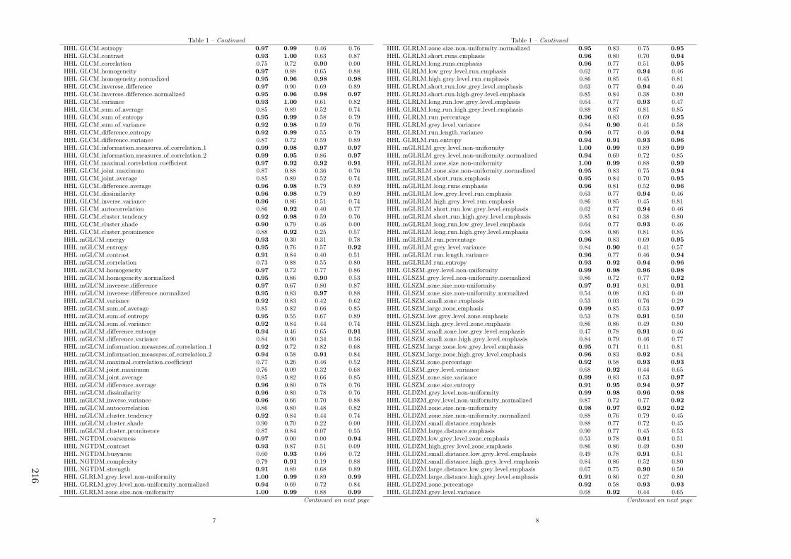
Table 1 – Continued
HHL GLCM entropy 0.97 0.99 0.46 0.76HHL GLCM contrast 0.93 1.00 0.63 0.87HHL GLCM correlation 0.75 0.72 0.90 0.00HHL GLCM homogeneity 0.97 0.88 0.65 0.88HHL GLCM homogeneity normalized 0.95 0.96 0.98 0.98
HHL GLCM inverese difference 0.97 0.90 0.69 0.89HHL GLCM inverese difference normalized 0.95 0.96 0.98 0.97
HHL GLCM variance 0.93 1.00 0.61 0.82HHL GLCM sum of average 0.85 0.89 0.52 0.74HHL GLCM sum of entropy 0.95 0.99 0.58 0.79HHL GLCM sum of variance 0.92 0.98 0.59 0.76HHL GLCM difference entropy 0.92 0.99 0.55 0.79HHL GLCM difference variance 0.87 0.72 0.59 0.89HHL GLCM information measures of correlation 1 0.99 0.98 0.97 0.97
HHL GLCM information measures of correlation 2 0.99 0.95 0.86 0.97
HHL GLCM maximal correlation coefficient 0.97 0.92 0.92 0.91
HHL GLCM joint maximum 0.87 0.88 0.36 0.76HHL GLCM joint average 0.85 0.89 0.52 0.74HHL GLCM difference average 0.96 0.98 0.79 0.89HHL GLCM dissimilarity 0.96 0.98 0.79 0.89HHL GLCM inverse variance 0.96 0.86 0.51 0.74HHL GLCM autocorrelation 0.86 0.92 0.40 0.77HHL GLCM cluster tendency 0.92 0.98 0.59 0.76HHL GLCM cluster shade 0.90 0.79 0.46 0.00HHL GLCM cluster prominence 0.88 0.92 0.25 0.57HHL mGLCM energy 0.93 0.30 0.31 0.78HHL mGLCM entropy 0.95 0.76 0.57 0.92
HHL mGLCM contrast 0.91 0.84 0.40 0.51HHL mGLCM correlation 0.73 0.88 0.55 0.80HHL mGLCM homogeneity 0.97 0.72 0.77 0.86HHL mGLCM homogeneity normalized 0.95 0.86 0.90 0.53HHL mGLCM inverese difference 0.97 0.67 0.80 0.87HHL mGLCM inverese difference normalized 0.95 0.83 0.97 0.88HHL mGLCM variance 0.92 0.83 0.42 0.62HHL mGLCM sum of average 0.85 0.82 0.66 0.85HHL mGLCM sum of entropy 0.95 0.55 0.67 0.89HHL mGLCM sum of variance 0.92 0.84 0.44 0.74HHL mGLCM difference entropy 0.94 0.46 0.65 0.91
HHL mGLCM difference variance 0.84 0.90 0.34 0.56HHL mGLCM information measures of correlation 1 0.92 0.72 0.82 0.68HHL mGLCM information measures of correlation 2 0.94 0.58 0.91 0.84HHL mGLCM maximal correlation coefficient 0.77 0.26 0.46 0.52HHL mGLCM joint maximum 0.76 0.09 0.32 0.68HHL mGLCM joint average 0.85 0.82 0.66 0.85HHL mGLCM difference average 0.96 0.80 0.78 0.76HHL mGLCM dissimilarity 0.96 0.80 0.78 0.76HHL mGLCM inverse variance 0.96 0.66 0.70 0.88HHL mGLCM autocorrelation 0.86 0.80 0.48 0.82HHL mGLCM cluster tendency 0.92 0.84 0.44 0.74HHL mGLCM cluster shade 0.90 0.70 0.22 0.00HHL mGLCM cluster prominence 0.87 0.84 0.07 0.55HHL NGTDM coarseness 0.97 0.00 0.00 0.94
HHL NGTDM contrast 0.93 0.87 0.51 0.09HHL NGTDM busyness 0.60 0.93 0.66 0.72HHL NGTDM complexity 0.79 0.91 0.19 0.88HHL NGTDM strength 0.91 0.89 0.68 0.89HHL GLRLM grey level non-uniformity 1.00 0.99 0.89 0.99
HHL GLRLM grey level non-uniformity normalized 0.94 0.69 0.72 0.84HHL GLRLM zone size non-uniformity 1.00 0.99 0.88 0.99
Continued on next page
7
Table 1 – Continued
HHL GLRLM zone size non-uniformity normalized 0.95 0.83 0.75 0.95
HHL GLRLM short runs emphasis 0.96 0.80 0.70 0.94
HHL GLRLM long runs emphasis 0.96 0.77 0.51 0.95
HHL GLRLM low grey level run emphasis 0.62 0.77 0.94 0.46HHL GLRLM high grey level run emphasis 0.86 0.85 0.45 0.81HHL GLRLM short run low grey level emphasis 0.63 0.77 0.94 0.46HHL GLRLM short run high grey level emphasis 0.85 0.84 0.38 0.80HHL GLRLM long run low grey level emphasis 0.64 0.77 0.93 0.47HHL GLRLM long run high grey level emphasis 0.88 0.87 0.81 0.85HHL GLRLM run percentage 0.96 0.83 0.69 0.95
HHL GLRLM grey level variance 0.84 0.90 0.41 0.58HHL GLRLM run length variance 0.96 0.77 0.46 0.94
HHL GLRLM run entropy 0.94 0.91 0.93 0.96
HHL mGLRLM grey level non-uniformity 1.00 0.99 0.89 0.99
HHL mGLRLM grey level non-uniformity normalized 0.94 0.69 0.72 0.85HHL mGLRLM zone size non-uniformity 1.00 0.99 0.88 0.99
HHL mGLRLM zone size non-uniformity normalized 0.95 0.83 0.75 0.94
HHL mGLRLM short runs emphasis 0.95 0.84 0.70 0.95
HHL mGLRLM long runs emphasis 0.96 0.81 0.52 0.96
HHL mGLRLM low grey level run emphasis 0.63 0.77 0.94 0.46HHL mGLRLM high grey level run emphasis 0.86 0.85 0.45 0.81HHL mGLRLM short run low grey level emphasis 0.62 0.77 0.94 0.46HHL mGLRLM short run high grey level emphasis 0.85 0.84 0.38 0.80HHL mGLRLM long run low grey level emphasis 0.64 0.77 0.93 0.46HHL mGLRLM long run high grey level emphasis 0.88 0.86 0.81 0.85HHL mGLRLM run percentage 0.96 0.83 0.69 0.95
HHL mGLRLM grey level variance 0.84 0.90 0.41 0.57HHL mGLRLM run length variance 0.96 0.77 0.46 0.94
HHL mGLRLM run entropy 0.93 0.92 0.94 0.96
HHL GLSZM grey level non-uniformity 0.99 0.98 0.96 0.98
HHL GLSZM grey level non-uniformity normalized 0.86 0.72 0.77 0.92
HHL GLSZM zone size non-uniformity 0.97 0.91 0.81 0.91
HHL GLSZM zone size non-uniformity normalized 0.54 0.08 0.83 0.40HHL GLSZM small zone emphasis 0.53 0.03 0.76 0.29HHL GLSZM large zone emphasis 0.99 0.85 0.53 0.97
HHL GLSZM low grey level zone emphasis 0.53 0.78 0.91 0.50HHL GLSZM high grey level zone emphasis 0.86 0.86 0.49 0.80HHL GLSZM small zone low grey level emphasis 0.47 0.78 0.91 0.46HHL GLSZM small zone high grey level emphasis 0.84 0.79 0.46 0.77HHL GLSZM large zone low grey level emphasis 0.95 0.71 0.11 0.81HHL GLSZM large zone high grey level emphasis 0.96 0.83 0.92 0.84HHL GLSZM zone percentage 0.92 0.58 0.93 0.93
HHL GLSZM grey level variance 0.68 0.92 0.44 0.65HHL GLSZM zone size variance 0.99 0.83 0.53 0.97
HHL GLSZM zone size entropy 0.91 0.95 0.94 0.97
HHL GLDZM grey level non-uniformity 0.99 0.98 0.96 0.98
HHL GLDZM grey level non-uniformity normalized 0.87 0.72 0.77 0.92
HHL GLDZM zone size non-uniformity 0.98 0.97 0.92 0.92
HHL GLDZM zone size non-uniformity normalized 0.88 0.76 0.79 0.45HHL GLDZM small distance emphasis 0.88 0.77 0.72 0.45HHL GLDZM large distance emphasis 0.90 0.77 0.45 0.53HHL GLDZM low grey level zone emphasis 0.53 0.78 0.91 0.51HHL GLDZM high grey level zone emphasis 0.86 0.86 0.49 0.80HHL GLDZM small distance low grey level emphasis 0.49 0.78 0.91 0.51HHL GLDZM small distance high grey level emphasis 0.84 0.86 0.52 0.80HHL GLDZM large distance low grey level emphasis 0.67 0.75 0.90 0.50HHL GLDZM large distance high grey level emphasis 0.91 0.86 0.27 0.80HHL GLDZM zone percentage 0.92 0.58 0.93 0.93
HHL GLDZM grey level variance 0.68 0.92 0.44 0.65Continued on next page
8
216

Table 1 – Continued
HHL GLDZM zone distance variance 0.92 0.76 0.36 0.58HHL GLDZM zone distance entropy 0.92 0.92 0.92 0.97
HHL NGLDM grey level non-uniformity 1.00 0.98 0.78 0.99
HHL NGLDM grey level non-uniformity normalized 0.94 0.50 0.43 0.84HHL NGLDM dependence count non-uniformity 0.98 0.88 0.63 0.94
HHL NGLDM dependence count non-uniformity normalized 0.93 0.25 0.94 0.87HHL NGLDM low dependence emphasis 0.85 0.24 0.93 0.88HHL NGLDM high dependence emphasis 0.95 0.79 0.50 0.93
HHL NGLDM low grey level count emphasis 0.63 0.90 0.94 0.45HHL NGLDM high grey level count emphasis 0.86 0.82 0.43 0.81HHL NGLDM low dependence low grey level emphasis 0.53 0.89 0.94 0.39HHL NGLDM low dependence high grey level emphasis 0.73 0.63 0.37 0.70HHL NGLDM high dependence low grey level emphasis 0.86 0.82 0.01 0.59HHL NGLDM high dependence high grey level emphasis 0.91 0.80 0.90 0.86HHL NGLDM grey level variance 0.87 0.85 0.40 0.58HHL NGLDM dependence count variance 0.92 0.73 0.50 0.85HHL NGLDM dependence count entropy 0.93 0.98 0.98 0.98
HHL NGLDM dependence count energy 0.91 0.91 0.96 0.93
HLH intensity mean 0.76 0.83 0.00 0.58HLH intensity standard deviation 0.87 0.00 0.49 0.75HLH intensity coefficient of variation 0.00 0.18 0.01 0.04HLH intensity skewness 0.92 0.36 0.21 0.28HLH intensity kurtosis 0.85 0.79 0.80 0.71HLH intensity variance 0.86 0.02 0.44 0.53HLH intensity median 0.93 0.79 0.00 0.00HLH intensity percentile 10th 0.93 0.81 0.66 0.53HLH intensity percentile 90th 0.81 0.38 0.43 0.78HLH intensity interquartile range 0.90 0.36 0.41 0.77HLH intensity range 0.87 0.72 0.57 0.68HLH intensity mean absolut deviation 0.91 0.00 0.40 0.80HLH intensity robust mean absolut deviation 0.94 0.88 0.45 0.00HLH intensity energy 0.98 0.87 0.35 0.89HLH intensity entropy 0.93 0.90 0.71 0.86HLH intensity root mean square 0.86 0.22 0.57 0.75HLH intensity uniformity 0.93 0.70 0.65 0.78HLH GLCM energy 0.90 1.00 0.20 0.86HLH GLCM entropy 0.96 1.00 0.37 0.82HLH GLCM contrast 0.97 0.91 0.49 0.81HLH GLCM correlation 0.12 0.96 0.61 0.40HLH GLCM homogeneity 0.97 0.98 0.58 0.87HLH GLCM homogeneity normalized 0.90 0.99 0.89 0.39HLH GLCM inverese difference 0.96 0.99 0.59 0.88HLH GLCM inverese difference normalized 0.91 0.98 0.89 0.59HLH GLCM variance 0.97 0.88 0.49 0.78HLH GLCM sum of average 0.58 0.90 0.59 0.75HLH GLCM sum of entropy 0.96 1.00 0.51 0.83HLH GLCM sum of variance 0.97 0.83 0.49 0.75HLH GLCM difference entropy 0.98 0.97 0.55 0.84HLH GLCM difference variance 0.95 0.45 0.52 0.84HLH GLCM information measures of correlation 1 0.99 0.98 0.92 0.90
HLH GLCM information measures of correlation 2 0.99 0.93 0.81 0.95
HLH GLCM maximal correlation coefficient 0.96 0.95 0.90 0.97
HLH GLCM joint maximum 0.78 0.97 0.19 0.85HLH GLCM joint average 0.58 0.90 0.59 0.75HLH GLCM difference average 0.98 0.95 0.63 0.81HLH GLCM dissimilarity 0.98 0.95 0.63 0.81HLH GLCM inverse variance 0.87 0.75 0.22 0.39HLH GLCM autocorrelation 0.60 0.81 0.50 0.62HLH GLCM cluster tendency 0.97 0.83 0.49 0.75
Continued on next page
9
Table 1 – Continued
HLH GLCM cluster shade 0.85 0.21 0.17 0.24HLH GLCM cluster prominence 0.97 0.60 0.16 0.57HLH mGLCM energy 0.91 0.70 0.23 0.73HLH mGLCM entropy 0.96 0.83 0.53 0.85HLH mGLCM contrast 0.95 0.93 0.49 0.64HLH mGLCM correlation 0.46 0.44 0.79 0.80HLH mGLCM homogeneity 0.96 0.93 0.65 0.79HLH mGLCM homogeneity normalized 0.91 0.94 0.97 0.76HLH mGLCM inverese difference 0.96 0.93 0.67 0.85HLH mGLCM inverese difference normalized 0.91 0.94 0.96 0.78HLH mGLCM variance 0.96 0.94 0.47 0.53HLH mGLCM sum of average 0.58 0.85 0.57 0.68HLH mGLCM sum of entropy 0.97 0.79 0.56 0.75HLH mGLCM sum of variance 0.97 0.91 0.45 0.34HLH mGLCM difference entropy 0.98 0.80 0.52 0.68HLH mGLCM difference variance 0.91 0.84 0.50 0.25HLH mGLCM information measures of correlation 1 0.90 0.84 0.65 0.71HLH mGLCM information measures of correlation 2 0.92 0.77 0.66 0.88HLH mGLCM maximal correlation coefficient 0.87 0.50 0.45 0.83HLH mGLCM joint maximum 0.79 0.65 0.24 0.79HLH mGLCM joint average 0.58 0.85 0.57 0.68HLH mGLCM difference average 0.97 0.95 0.66 0.88HLH mGLCM dissimilarity 0.97 0.95 0.66 0.88HLH mGLCM inverse variance 0.86 0.61 0.46 0.47HLH mGLCM autocorrelation 0.60 0.78 0.50 0.52HLH mGLCM cluster tendency 0.97 0.91 0.45 0.34HLH mGLCM cluster shade 0.84 0.00 0.17 0.51HLH mGLCM cluster prominence 0.97 0.76 0.16 0.04HLH NGTDM coarseness 0.98 0.00 0.00 0.95
HLH NGTDM contrast 0.94 0.64 0.59 0.98
HLH NGTDM busyness 0.75 0.39 0.26 0.82HLH NGTDM complexity 0.91 0.71 0.44 0.58HLH NGTDM strength 0.84 0.59 0.58 0.66HLH GLRLM grey level non-uniformity 1.00 0.99 0.87 0.98
HLH GLRLM grey level non-uniformity normalized 0.91 0.71 0.66 0.78HLH GLRLM zone size non-uniformity 0.99 1.00 0.78 0.99
HLH GLRLM zone size non-uniformity normalized 0.96 0.96 0.73 0.96
HLH GLRLM short runs emphasis 0.96 0.96 0.66 0.96
HLH GLRLM long runs emphasis 0.96 0.98 0.36 0.92
HLH GLRLM low grey level run emphasis 0.51 0.50 0.50 0.13HLH GLRLM high grey level run emphasis 0.61 0.71 0.51 0.52HLH GLRLM short run low grey level emphasis 0.53 0.50 0.52 0.14HLH GLRLM short run high grey level emphasis 0.62 0.70 0.50 0.53HLH GLRLM long run low grey level emphasis 0.42 0.50 0.35 0.12HLH GLRLM long run high grey level emphasis 0.64 0.73 0.54 0.54HLH GLRLM run percentage 0.96 0.97 0.63 0.96
HLH GLRLM grey level variance 0.86 0.01 0.45 0.54HLH GLRLM run length variance 0.97 0.99 0.30 0.88HLH GLRLM run entropy 0.91 0.91 0.85 0.95
HLH m GLRLM grey level non-uniformity 1.00 0.99 0.87 0.98
HLH m GLRLM grey level non-uniformity normalized 0.91 0.71 0.66 0.78HLH m GLRLM zone size non-uniformity 0.99 1.00 0.78 0.99
HLH m GLRLM zone size non-uniformity normalized 0.96 0.95 0.73 0.96
HLH m GLRLM short runs emphasis 0.96 0.96 0.66 0.97
HLH m GLRLM long runs emphasis 0.96 0.98 0.37 0.92
HLH m GLRLM low grey level run emphasis 0.51 0.50 0.50 0.13HLH m GLRLM high grey level run emphasis 0.61 0.71 0.51 0.52HLH m GLRLM short run low grey level emphasis 0.53 0.50 0.51 0.14HLH m GLRLM short run high grey level emphasis 0.62 0.71 0.50 0.53
Continued on next page
10
Com
parison
ofrob
ust
tostan
dard
izedC
Trad
iomics
models
topred
ictoverall
surv
ivalfor
non
-small
celllu
ng
cancer
patien
ts
217

Table 1 – Continued
HLH m GLRLM long run low grey level emphasis 0.42 0.50 0.35 0.12HLH m GLRLM long run high grey level emphasis 0.64 0.73 0.54 0.54HLH m GLRLM run percentage 0.96 0.97 0.63 0.96
HLH m GLRLM grey level variance 0.86 0.01 0.45 0.54HLH m GLRLM run length variance 0.97 0.98 0.31 0.89HLH m GLRLM run entropy 0.90 0.93 0.86 0.95
HLH GLSZM grey level non-uniformity 0.99 0.93 0.96 0.94
HLH GLSZM grey level non-uniformity normalized 0.70 0.73 0.71 0.86HLH GLSZM zone size non-uniformity 0.98 0.93 0.65 0.91
HLH GLSZM zone size non-uniformity normalized 0.59 0.33 0.71 0.66HLH GLSZM small zone emphasis 0.55 0.25 0.63 0.60HLH GLSZM large zone emphasis 0.97 0.89 0.54 0.98
HLH GLSZM low grey level zone emphasis 0.64 0.39 0.45 0.19HLH GLSZM high grey level zone emphasis 0.64 0.69 0.53 0.57HLH GLSZM small zone low grey level emphasis 0.66 0.35 0.58 0.15HLH GLSZM small zone high grey level emphasis 0.68 0.63 0.46 0.56HLH GLSZM large zone low grey level emphasis 0.79 0.97 0.10 0.95
HLH GLSZM large zone high grey level emphasis 0.76 0.71 0.94 0.95
HLH GLSZM zone percentage 0.97 0.78 0.92 0.95
HLH GLSZM grey level variance 0.80 0.00 0.52 0.49HLH GLSZM zone size variance 0.97 0.90 0.55 0.98
HLH GLSZM zone size entropy 0.84 0.94 0.91 0.94
HLH GLDZM grey level non-uniformity 0.99 0.93 0.96 0.94
HLH GLDZM grey level non-uniformity normalized 0.71 0.73 0.71 0.86HLH GLDZM zone size non-uniformity 0.98 0.97 0.88 0.98
HLH GLDZM zone size non-uniformity normalized 0.81 0.53 0.48 0.27HLH GLDZM small distance emphasis 0.82 0.52 0.43 0.24HLH GLDZM large distance emphasis 0.82 0.52 0.31 0.28HLH GLDZM low grey level zone emphasis 0.64 0.38 0.46 0.20HLH GLDZM high grey level zone emphasis 0.64 0.69 0.53 0.57HLH GLDZM small distance low grey level emphasis 0.62 0.39 0.46 0.18HLH GLDZM small distance high grey level emphasis 0.65 0.69 0.56 0.57HLH GLDZM large distance low grey level emphasis 0.70 0.38 0.43 0.22HLH GLDZM large distance high grey level emphasis 0.63 0.71 0.35 0.56HLH GLDZM zone percentage 0.97 0.78 0.92 0.95
HLH GLDZM grey level variance 0.80 0.00 0.52 0.49HLH GLDZM zone distance variance 0.81 0.53 0.27 0.39HLH GLDZM zone distance entropy 0.83 0.92 0.76 0.93
HLH NGLDM grey level non-uniformity 0.99 1.00 0.76 0.99
HLH NGLDM grey level non-uniformity normalized 0.91 0.70 0.36 0.79HLH NGLDM dependence count non-uniformity 0.99 0.93 0.57 0.97
HLH NGLDM dependence count non-uniformity normalized 0.97 0.51 0.92 0.88HLH NGLDM low dependence emphasis 0.92 0.54 0.87 0.90
HLH NGLDM high dependence emphasis 0.95 0.99 0.39 0.91
HLH NGLDM low grey level count emphasis 0.51 0.52 0.56 0.14HLH NGLDM high grey level count emphasis 0.60 0.78 0.49 0.51HLH NGLDM low dependence low grey level emphasis 0.67 0.47 0.74 0.15HLH NGLDM low dependence high grey level emphasis 0.78 0.65 0.33 0.56HLH NGLDM high dependence low grey level emphasis 0.66 0.77 0.11 0.85HLH NGLDM high dependence high grey level emphasis 0.76 0.91 0.69 0.82HLH NGLDM grey level variance 0.88 0.89 0.47 0.55HLH NGLDM dependence count variance 0.92 0.96 0.34 0.83HLH NGLDM dependence count entropy 0.96 0.97 0.97 0.99
HLH NGLDM dependence count energy 0.95 0.88 0.91 0.93
HLL intensity mean 0.94 0.90 0.83 0.64HLL intensity standard deviation 0.92 0.84 0.57 0.53HLL intensity coefficient of variation 0.54 0.00 0.36 0.35HLL intensity skewness 0.90 0.41 0.71 0.30HLL intensity kurtosis 0.94 0.79 0.88 0.88
Continued on next page
11
Table 1 – Continued
HLL intensity variance 0.91 0.89 0.62 0.57HLL intensity median 0.92 0.85 0.75 0.95
HLL intensity percentile 10th 0.97 0.88 0.91 0.97
HLL intensity percentile 90th 0.91 0.91 0.75 0.00HLL intensity interquartile range 0.81 0.72 0.83 0.55HLL intensity range 0.90 0.93 0.84 0.53HLL intensity mean absolut deviation 0.94 0.80 0.60 0.51HLL intensity robust mean absolut deviation 0.92 0.74 0.94 0.01HLL intensity energy 0.97 0.99 0.81 0.90
HLL intensity entropy 0.91 0.95 0.88 0.94
HLL intensity root mean square 0.93 0.94 0.83 0.94
HLL intensity uniformity 0.93 0.74 0.73 0.81HLL GLCM energy 0.95 1.00 0.15 0.78HLL GLCM entropy 0.98 1.00 0.60 0.74HLL GLCM contrast 0.96 0.99 0.80 0.68HLL GLCM correlation 0.91 0.78 0.77 0.23HLL GLCM homogeneity 0.97 0.92 0.67 0.84HLL GLCM homogeneity normalized 0.98 0.99 0.97 0.85HLL GLCM inverese difference 0.97 0.93 0.72 0.85HLL GLCM inverese difference normalized 0.99 0.99 0.97 0.90HLL GLCM variance 0.96 0.98 0.81 0.66HLL GLCM sum of average 0.92 0.75 0.71 0.40HLL GLCM sum of entropy 0.97 1.00 0.75 0.68HLL GLCM sum of variance 0.97 0.94 0.82 0.63HLL GLCM difference entropy 0.97 0.99 0.69 0.69HLL GLCM difference variance 0.95 0.99 0.73 0.41HLL GLCM information measures of correlation 1 0.99 0.98 0.96 0.96
HLL GLCM information measures of correlation 2 0.99 0.91 0.92 0.93
HLL GLCM maximal correlation coefficient 0.98 1.00 0.95 0.90
HLL GLCM joint maximum 0.88 0.94 0.01 0.81HLL GLCM joint average 0.92 0.75 0.71 0.40HLL GLCM difference average 0.96 0.98 0.91 0.89HLL GLCM dissimilarity 0.96 0.98 0.91 0.89HLL GLCM inverse variance 0.95 0.73 0.68 0.81HLL GLCM autocorrelation 0.93 0.82 0.56 0.34HLL GLCM cluster tendency 0.97 0.94 0.82 0.63HLL GLCM cluster shade 0.97 0.94 0.70 0.00HLL GLCM cluster prominence 0.96 0.97 0.58 0.15HLL mGLCM energy 0.84 0.83 0.25 0.62HLL mGLCM entropy 0.81 0.94 0.69 0.92
HLL mGLCM contrast 0.96 0.90 0.83 0.41HLL mGLCM correlation 0.92 0.65 0.84 0.72HLL mGLCM homogeneity 0.98 0.77 0.77 0.83HLL mGLCM homogeneity normalized 0.98 0.96 0.99 0.49HLL mGLCM inverese difference 0.98 0.86 0.82 0.84HLL mGLCM inverese difference normalized 0.99 0.97 0.99 0.70HLL mGLCM variance 0.96 0.88 0.76 0.50HLL mGLCM sum of average 0.92 0.91 0.71 0.53HLL mGLCM sum of entropy 0.95 0.97 0.80 0.89HLL mGLCM sum of variance 0.97 0.84 0.62 0.64HLL mGLCM difference entropy 0.95 0.96 0.78 0.88HLL mGLCM difference variance 0.95 0.91 0.65 0.09HLL mGLCM information measures of correlation 1 0.93 0.80 0.81 0.73HLL mGLCM information measures of correlation 2 0.95 0.89 0.87 0.84HLL mGLCM maximal correlation coefficient 0.84 0.65 0.56 0.45HLL mGLCM joint maximum 0.79 0.41 0.11 0.70HLL mGLCM joint average 0.92 0.91 0.71 0.53HLL mGLCM difference average 0.96 0.91 0.94 0.53HLL mGLCM dissimilarity 0.96 0.91 0.94 0.53
Continued on next page
12
218

Table 1 – Continued
HLL mGLCM inverse variance 0.95 0.64 0.81 0.10HLL mGLCM autocorrelation 0.93 0.92 0.58 0.63HLL mGLCM cluster tendency 0.97 0.84 0.62 0.64HLL mGLCM cluster shade 0.97 0.87 0.65 0.00HLL mGLCM cluster prominence 0.96 0.95 0.42 0.28HLL NGTDM coarseness 0.95 0.00 0.00 0.28HLL NGTDM contrast 0.95 0.80 0.95 0.14HLL NGTDM busyness 0.92 0.96 0.82 0.76HLL NGTDM complexity 0.89 0.99 0.67 0.60HLL NGTDM strength 0.93 0.70 0.77 0.75HLL GLRLM grey level non-uniformity 1.00 0.99 0.94 0.99
HLL GLRLM grey level non-uniformity normalized 0.74 0.75 0.74 0.86HLL GLRLM zone size non-uniformity 1.00 1.00 0.90 0.98
HLL GLRLM zone size non-uniformity normalized 0.97 0.91 0.78 0.94
HLL GLRLM short runs emphasis 0.97 0.90 0.72 0.93
HLL GLRLM long runs emphasis 0.98 0.93 0.44 0.91
HLL GLRLM low grey level run emphasis 0.48 0.73 0.93 0.58HLL GLRLM high grey level run emphasis 0.92 0.92 0.55 0.33HLL GLRLM short run low grey level emphasis 0.45 0.73 0.94 0.58HLL GLRLM short run high grey level emphasis 0.92 0.92 0.53 0.28HLL GLRLM long run low grey level emphasis 0.46 0.72 0.88 0.58HLL GLRLM long run high grey level emphasis 0.92 0.92 0.75 0.70HLL GLRLM run percentage 0.98 0.93 0.66 0.93
HLL GLRLM grey level variance 0.90 0.90 0.57 0.51HLL GLRLM run length variance 0.98 0.95 0.36 0.89HLL GLRLM run entropy 0.90 0.96 0.95 0.97
HLL mGLRM grey level non-uniformity 1.00 0.99 0.94 0.99
HLL mGLRM grey level non-uniformity normalized 0.74 0.75 0.74 0.86HLL mGLRM zone size non-uniformity 1.00 1.00 0.90 0.98
HLL mGLRM zone size non-uniformity normalized 0.97 0.91 0.78 0.94
HLL mGLRM short runs emphasis 0.98 0.91 0.72 0.94
HLL mGLRM long runs emphasis 0.98 0.94 0.45 0.91
HLL mGLRM low grey level run emphasis 0.45 0.73 0.92 0.58HLL mGLRM high grey level run emphasis 0.92 0.92 0.55 0.33HLL mGLRM short run low grey level emphasis 0.46 0.73 0.93 0.58HLL mGLRM short run high grey level emphasis 0.92 0.92 0.53 0.28HLL mGLRM long run low grey level emphasis 0.45 0.72 0.88 0.58HLL mGLRM long run high grey level emphasis 0.92 0.92 0.75 0.70HLL mGLRM run percentage 0.98 0.92 0.66 0.93
HLL mGLRM grey level variance 0.90 0.90 0.57 0.51HLL mGLRM run length variance 0.98 0.95 0.36 0.89HLL mGLRM run entropy 0.90 0.96 0.95 0.97
HLL GLSZM grey level non-uniformity 0.99 0.99 0.97 0.96
HLL GLSZM grey level non-uniformity normalized 0.84 0.75 0.78 0.88HLL GLSZM zone size non-uniformity 0.98 0.92 0.92 0.96
HLL GLSZM zone size non-uniformity normalized 0.93 0.44 0.84 0.95
HLL GLSZM small zone emphasis 0.90 0.40 0.76 0.93
HLL GLSZM large zone emphasis 0.99 0.98 0.51 0.99
HLL GLSZM low grey level zone emphasis 0.31 0.67 0.98 0.57HLL GLSZM high grey level zone emphasis 0.90 0.92 0.56 0.36HLL GLSZM small zone low grey level emphasis 0.34 0.69 0.97 0.59HLL GLSZM small zone high grey level emphasis 0.86 0.87 0.55 0.26HLL GLSZM large zone low grey level emphasis 0.86 0.57 0.25 0.51HLL GLSZM large zone high grey level emphasis 0.99 0.97 0.74 0.92
HLL GLSZM zone percentage 0.97 0.80 0.95 0.98
HLL GLSZM grey level variance 0.84 0.86 0.41 0.35HLL GLSZM zone size variance 0.99 0.98 0.51 0.99
HLL GLSZM zone size entropy 0.96 0.97 0.96 0.97
HLL GLDZM grey level non-uniformity 0.99 0.99 0.97 0.96
Continued on next page
13
Table 1 – Continued
HLL GLDZM grey level non-uniformity normalized 0.84 0.75 0.78 0.88HLL GLDZM zone size non-uniformity 0.99 0.99 0.98 0.98
HLL GLDZM zone size non-uniformity normalized 0.87 0.69 0.75 0.62HLL GLDZM small distance emphasis 0.88 0.70 0.70 0.63HLL GLDZM large distance emphasis 0.92 0.70 0.50 0.75HLL GLDZM low grey level zone emphasis 0.31 0.68 0.98 0.57HLL GLDZM high grey level zone emphasis 0.90 0.92 0.56 0.36HLL GLDZM small distance low grey level emphasis 0.31 0.67 0.95 0.57HLL GLDZM small distance high grey level emphasis 0.90 0.92 0.59 0.30HLL GLDZM large distance low grey level emphasis 0.31 0.67 0.93 0.57HLL GLDZM large distance high grey level emphasis 0.90 0.93 0.36 0.62HLL GLDZM zone percentage 0.97 0.80 0.95 0.98
HLL GLDZM grey level variance 0.84 0.86 0.41 0.35HLL GLDZM zone distance variance 0.93 0.69 0.43 0.78HLL GLDZM zone distance entropy 0.95 0.96 0.95 0.96
HLL NGLDM grey level non-uniformity 1.00 0.99 0.78 0.99
HLL NGLDM grey level non-uniformity normalized 0.78 0.87 0.48 0.83HLL NGLDM dependence count non-uniformity 0.99 0.88 0.76 0.97
HLL NGLDM dependence count non-uniformity normalized 0.99 0.51 0.95 1.00
HLL NGLDM low dependence emphasis 0.96 0.59 0.93 0.99
HLL NGLDM high dependence emphasis 0.98 0.88 0.37 0.90
HLL NGLDM low grey level count emphasis 0.48 0.72 0.92 0.58HLL NGLDM high grey level count emphasis 0.92 0.93 0.57 0.33HLL NGLDM low dependence low grey level emphasis 0.52 0.77 0.99 0.60HLL NGLDM low dependence high grey level emphasis 0.90 0.84 0.68 0.20HLL NGLDM high dependence low grey level emphasis 0.70 0.46 0.09 0.27HLL NGLDM high dependence high grey level emphasis 0.92 0.90 0.72 0.97
HLL NGLDM grey level variance 0.91 0.88 0.75 0.53HLL NGLDM dependence count variance 0.97 0.80 0.30 0.89HLL NGLDM dependence count entropy 0.98 0.99 0.99 0.99
HLL NGLDM dependence count energy 0.96 0.91 0.98 0.91
LHH intensity mean 0.51 0.20 0.00 0.00LHH intensity standard deviation 0.89 0.95 0.60 0.49LHH intensity coefficient of variation 0.09 0.09 0.64 0.00LHH intensity skewness 0.68 0.55 0.28 0.08LHH intensity kurtosis 0.86 0.81 0.76 0.83LHH intensity variance 0.86 0.87 0.36 0.46LHH intensity median 0.73 0.50 0.00 0.00LHH intensity percentile 10th 0.53 0.78 0.46 0.73LHH intensity percentile 90th 0.91 0.90 0.35 0.39LHH intensity interquartile range 0.97 0.93 0.57 0.25LHH intensity range 0.84 0.92 0.61 0.76LHH intensity mean absolut deviation 0.96 0.98 0.60 0.34LHH intensity robust mean absolut deviation 0.97 0.88 0.50 0.21LHH intensity energy 0.97 0.95 0.38 0.79LHH intensity entropy 0.89 0.94 0.85 0.79LHH intensity root mean square 0.90 0.95 0.47 0.53LHH intensity uniformity 0.93 0.72 0.71 0.45LHH GLCM energy 0.93 0.99 0.32 0.73LHH GLCM entropy 0.97 0.99 0.57 0.80LHH GLCM contrast 0.93 0.92 0.44 0.59LHH GLCM correlation 0.96 0.95 0.88 0.63LHH GLCM homogeneity 0.97 0.90 0.73 0.84LHH GLCM homogeneity normalized 0.94 0.97 0.91 0.78LHH GLCM inverese difference 0.97 0.91 0.73 0.84LHH GLCM inverese difference normalized 0.94 0.99 0.92 0.78LHH GLCM variance 0.94 0.94 0.44 0.60LHH GLCM sum of average 0.89 0.90 0.53 0.60LHH GLCM sum of entropy 0.96 1.00 0.68 0.86
Continued on next page
14
Com
parison
ofrob
ust
tostan
dard
izedC
Trad
iomics
models
topred
ictoverall
surv
ivalfor
non
-small
celllu
ng
cancer
patien
ts
219
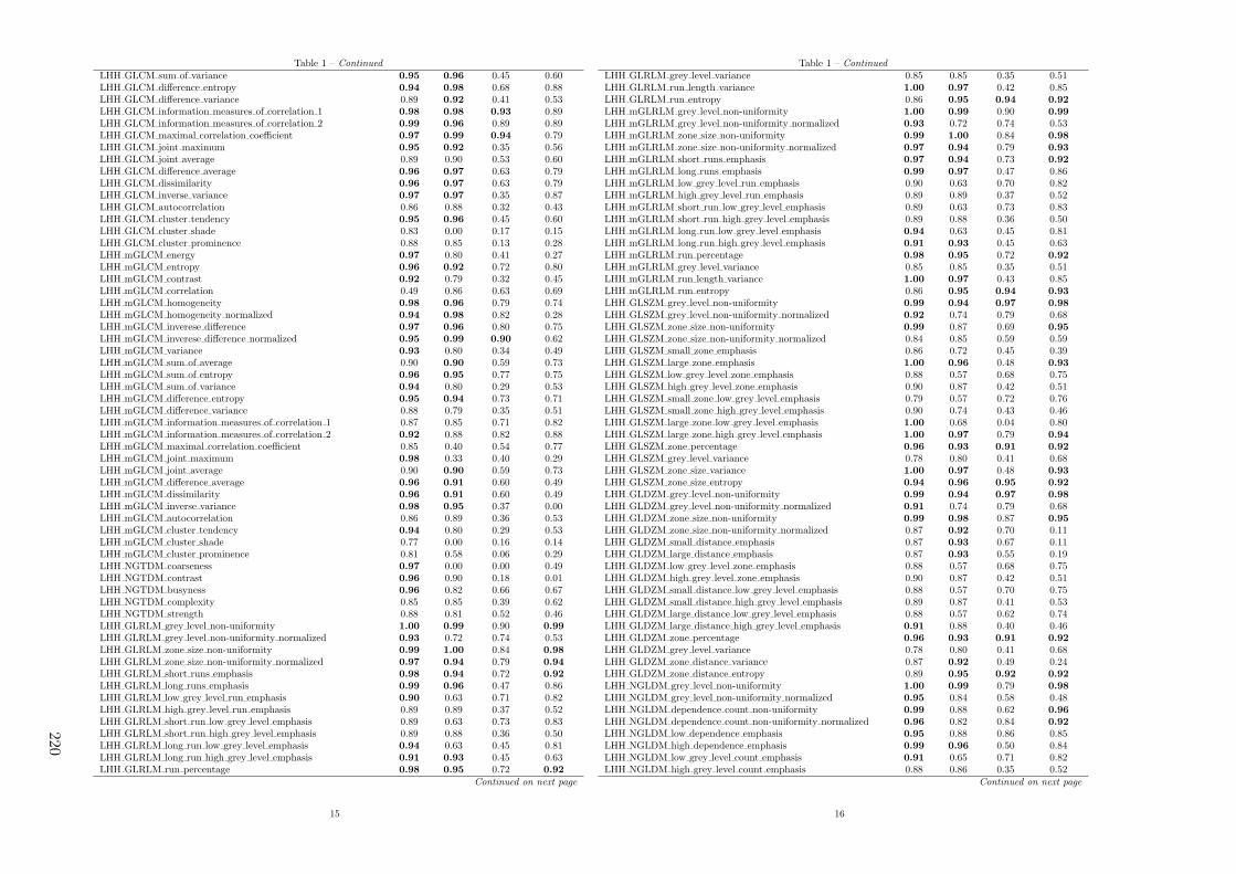
Table 1 – Continued
LHH GLCM sum of variance 0.95 0.96 0.45 0.60LHH GLCM difference entropy 0.94 0.98 0.68 0.88LHH GLCM difference variance 0.89 0.92 0.41 0.53LHH GLCM information measures of correlation 1 0.98 0.98 0.93 0.89LHH GLCM information measures of correlation 2 0.99 0.96 0.89 0.89LHH GLCM maximal correlation coefficient 0.97 0.99 0.94 0.79LHH GLCM joint maximum 0.95 0.92 0.35 0.56LHH GLCM joint average 0.89 0.90 0.53 0.60LHH GLCM difference average 0.96 0.97 0.63 0.79LHH GLCM dissimilarity 0.96 0.97 0.63 0.79LHH GLCM inverse variance 0.97 0.97 0.35 0.87LHH GLCM autocorrelation 0.86 0.88 0.32 0.43LHH GLCM cluster tendency 0.95 0.96 0.45 0.60LHH GLCM cluster shade 0.83 0.00 0.17 0.15LHH GLCM cluster prominence 0.88 0.85 0.13 0.28LHH mGLCM energy 0.97 0.80 0.41 0.27LHH mGLCM entropy 0.96 0.92 0.72 0.80LHH mGLCM contrast 0.92 0.79 0.32 0.45LHH mGLCM correlation 0.49 0.86 0.63 0.69LHH mGLCM homogeneity 0.98 0.96 0.79 0.74LHH mGLCM homogeneity normalized 0.94 0.98 0.82 0.28LHH mGLCM inverese difference 0.97 0.96 0.80 0.75LHH mGLCM inverese difference normalized 0.95 0.99 0.90 0.62LHH mGLCM variance 0.93 0.80 0.34 0.49LHH mGLCM sum of average 0.90 0.90 0.59 0.73LHH mGLCM sum of entropy 0.96 0.95 0.77 0.75LHH mGLCM sum of variance 0.94 0.80 0.29 0.53LHH mGLCM difference entropy 0.95 0.94 0.73 0.71LHH mGLCM difference variance 0.88 0.79 0.35 0.51LHH mGLCM information measures of correlation 1 0.87 0.85 0.71 0.82LHH mGLCM information measures of correlation 2 0.92 0.88 0.82 0.88LHH mGLCM maximal correlation coefficient 0.85 0.40 0.54 0.77LHH mGLCM joint maximum 0.98 0.33 0.40 0.29LHH mGLCM joint average 0.90 0.90 0.59 0.73LHH mGLCM difference average 0.96 0.91 0.60 0.49LHH mGLCM dissimilarity 0.96 0.91 0.60 0.49LHH mGLCM inverse variance 0.98 0.95 0.37 0.00LHH mGLCM autocorrelation 0.86 0.89 0.36 0.53LHH mGLCM cluster tendency 0.94 0.80 0.29 0.53LHH mGLCM cluster shade 0.77 0.00 0.16 0.14LHH mGLCM cluster prominence 0.81 0.58 0.06 0.29LHH NGTDM coarseness 0.97 0.00 0.00 0.49LHH NGTDM contrast 0.96 0.90 0.18 0.01LHH NGTDM busyness 0.96 0.82 0.66 0.67LHH NGTDM complexity 0.85 0.85 0.39 0.62LHH NGTDM strength 0.88 0.81 0.52 0.46LHH GLRLM grey level non-uniformity 1.00 0.99 0.90 0.99
LHH GLRLM grey level non-uniformity normalized 0.93 0.72 0.74 0.53LHH GLRLM zone size non-uniformity 0.99 1.00 0.84 0.98
LHH GLRLM zone size non-uniformity normalized 0.97 0.94 0.79 0.94
LHH GLRLM short runs emphasis 0.98 0.94 0.72 0.92
LHH GLRLM long runs emphasis 0.99 0.96 0.47 0.86LHH GLRLM low grey level run emphasis 0.90 0.63 0.71 0.82LHH GLRLM high grey level run emphasis 0.89 0.89 0.37 0.52LHH GLRLM short run low grey level emphasis 0.89 0.63 0.73 0.83LHH GLRLM short run high grey level emphasis 0.89 0.88 0.36 0.50LHH GLRLM long run low grey level emphasis 0.94 0.63 0.45 0.81LHH GLRLM long run high grey level emphasis 0.91 0.93 0.45 0.63LHH GLRLM run percentage 0.98 0.95 0.72 0.92
Continued on next page
15
Table 1 – Continued
LHH GLRLM grey level variance 0.85 0.85 0.35 0.51LHH GLRLM run length variance 1.00 0.97 0.42 0.85LHH GLRLM run entropy 0.86 0.95 0.94 0.92
LHH mGLRLM grey level non-uniformity 1.00 0.99 0.90 0.99
LHH mGLRLM grey level non-uniformity normalized 0.93 0.72 0.74 0.53LHH mGLRLM zone size non-uniformity 0.99 1.00 0.84 0.98
LHH mGLRLM zone size non-uniformity normalized 0.97 0.94 0.79 0.93
LHH mGLRLM short runs emphasis 0.97 0.94 0.73 0.92
LHH mGLRLM long runs emphasis 0.99 0.97 0.47 0.86LHH mGLRLM low grey level run emphasis 0.90 0.63 0.70 0.82LHH mGLRLM high grey level run emphasis 0.89 0.89 0.37 0.52LHH mGLRLM short run low grey level emphasis 0.89 0.63 0.73 0.83LHH mGLRLM short run high grey level emphasis 0.89 0.88 0.36 0.50LHH mGLRLM long run low grey level emphasis 0.94 0.63 0.45 0.81LHH mGLRLM long run high grey level emphasis 0.91 0.93 0.45 0.63LHH mGLRLM run percentage 0.98 0.95 0.72 0.92
LHH mGLRLM grey level variance 0.85 0.85 0.35 0.51LHH mGLRLM run length variance 1.00 0.97 0.43 0.85LHH mGLRLM run entropy 0.86 0.95 0.94 0.93
LHH GLSZM grey level non-uniformity 0.99 0.94 0.97 0.98
LHH GLSZM grey level non-uniformity normalized 0.92 0.74 0.79 0.68LHH GLSZM zone size non-uniformity 0.99 0.87 0.69 0.95
LHH GLSZM zone size non-uniformity normalized 0.84 0.85 0.59 0.59LHH GLSZM small zone emphasis 0.86 0.72 0.45 0.39LHH GLSZM large zone emphasis 1.00 0.96 0.48 0.93
LHH GLSZM low grey level zone emphasis 0.88 0.57 0.68 0.75LHH GLSZM high grey level zone emphasis 0.90 0.87 0.42 0.51LHH GLSZM small zone low grey level emphasis 0.79 0.57 0.72 0.76LHH GLSZM small zone high grey level emphasis 0.90 0.74 0.43 0.46LHH GLSZM large zone low grey level emphasis 1.00 0.68 0.04 0.80LHH GLSZM large zone high grey level emphasis 1.00 0.97 0.79 0.94
LHH GLSZM zone percentage 0.96 0.93 0.91 0.92
LHH GLSZM grey level variance 0.78 0.80 0.41 0.68LHH GLSZM zone size variance 1.00 0.97 0.48 0.93
LHH GLSZM zone size entropy 0.94 0.96 0.95 0.92
LHH GLDZM grey level non-uniformity 0.99 0.94 0.97 0.98
LHH GLDZM grey level non-uniformity normalized 0.91 0.74 0.79 0.68LHH GLDZM zone size non-uniformity 0.99 0.98 0.87 0.95
LHH GLDZM zone size non-uniformity normalized 0.87 0.92 0.70 0.11LHH GLDZM small distance emphasis 0.87 0.93 0.67 0.11LHH GLDZM large distance emphasis 0.87 0.93 0.55 0.19LHH GLDZM low grey level zone emphasis 0.88 0.57 0.68 0.75LHH GLDZM high grey level zone emphasis 0.90 0.87 0.42 0.51LHH GLDZM small distance low grey level emphasis 0.88 0.57 0.70 0.75LHH GLDZM small distance high grey level emphasis 0.89 0.87 0.41 0.53LHH GLDZM large distance low grey level emphasis 0.88 0.57 0.62 0.74LHH GLDZM large distance high grey level emphasis 0.91 0.88 0.40 0.46LHH GLDZM zone percentage 0.96 0.93 0.91 0.92
LHH GLDZM grey level variance 0.78 0.80 0.41 0.68LHH GLDZM zone distance variance 0.87 0.92 0.49 0.24LHH GLDZM zone distance entropy 0.89 0.95 0.92 0.92
LHH NGLDM grey level non-uniformity 1.00 0.99 0.79 0.98
LHH NGLDM grey level non-uniformity normalized 0.95 0.84 0.58 0.48LHH NGLDM dependence count non-uniformity 0.99 0.88 0.62 0.96
LHH NGLDM dependence count non-uniformity normalized 0.96 0.82 0.84 0.92
LHH NGLDM low dependence emphasis 0.95 0.88 0.86 0.85LHH NGLDM high dependence emphasis 0.99 0.96 0.50 0.84LHH NGLDM low grey level count emphasis 0.91 0.65 0.71 0.82LHH NGLDM high grey level count emphasis 0.88 0.86 0.35 0.52
Continued on next page
16
220

Table 1 – Continued
LHH NGLDM low dependence low grey level emphasis 0.67 0.65 0.88 0.83LHH NGLDM low dependence high grey level emphasis 0.92 0.71 0.38 0.37LHH NGLDM high dependence low grey level emphasis 0.99 0.44 0.05 0.84LHH NGLDM high dependence high grey level emphasis 0.99 0.99 0.63 0.76LHH NGLDM grey level variance 0.86 0.83 0.33 0.49LHH NGLDM dependence count variance 0.99 0.90 0.50 0.76LHH NGLDM dependence count entropy 0.98 0.99 0.99 0.97
LHH NGLDM dependence count energy 0.95 0.96 0.93 0.75LHL intensity mean 0.96 0.66 0.83 0.07LHL intensity standard deviation 0.99 0.92 0.75 0.93
LHL intensity coefficient of variation 0.56 0.49 0.00 0.00LHL intensity skewness 0.92 0.97 0.62 0.48LHL intensity kurtosis 0.93 0.99 0.66 0.84LHL intensity variance 0.99 0.83 0.77 0.88LHL intensity median 0.95 0.64 0.46 0.46LHL intensity percentile 10th 0.95 0.77 0.85 0.75LHL intensity percentile 90th 0.97 0.87 0.67 0.77LHL intensity interquartile range 0.97 0.70 0.84 0.25LHL intensity range 0.94 0.96 0.82 0.59LHL intensity mean absolut deviation 0.99 0.88 0.67 0.89LHL intensity robust mean absolut deviation 0.97 0.76 0.84 0.00LHL intensity energy 0.97 0.99 0.80 0.87LHL intensity entropy 0.93 0.98 0.90 0.92
LHL intensity root mean square 0.98 0.73 0.83 0.94
LHL intensity uniformity 0.90 0.99 0.71 0.65LHL GLCM energy 0.94 0.99 0.38 0.98
LHL GLCM entropy 0.97 1.00 0.71 0.94
LHL GLCM contrast 1.00 0.97 0.79 0.83LHL GLCM correlation 0.96 0.94 0.68 0.58LHL GLCM homogeneity 0.99 0.98 0.76 0.97
LHL GLCM homogeneity normalized 0.70 0.99 0.95 0.72LHL GLCM inverese difference 0.99 0.98 0.79 0.97
LHL GLCM inverese difference normalized 0.78 0.99 0.94 0.83LHL GLCM variance 0.99 0.96 0.81 0.76LHL GLCM sum of average 0.74 0.97 0.64 0.81LHL GLCM sum of entropy 0.97 1.00 0.80 0.90
LHL GLCM sum of variance 0.99 0.95 0.82 0.69LHL GLCM difference entropy 0.97 1.00 0.78 0.91
LHL GLCM difference variance 0.99 0.97 0.81 0.80LHL GLCM information measures of correlation 1 0.99 0.92 0.99 0.96
LHL GLCM information measures of correlation 2 0.99 0.75 0.91 0.98
LHL GLCM maximal correlation coefficient 0.98 0.94 0.91 0.92
LHL GLCM joint maximum 0.89 0.95 0.25 0.92
LHL GLCM joint average 0.74 0.97 0.64 0.81LHL GLCM difference average 1.00 0.99 0.90 0.91
LHL GLCM dissimilarity 1.00 0.99 0.90 0.91
LHL GLCM inverse variance 0.98 0.91 0.75 0.87LHL GLCM autocorrelation 0.83 0.98 0.51 0.88LHL GLCM cluster tendency 0.99 0.95 0.82 0.69LHL GLCM cluster shade 0.94 0.95 0.70 0.00LHL GLCM cluster prominence 0.98 0.91 0.52 0.40LHL mGLCM energy 0.92 0.76 0.54 0.41LHL mGLCM entropy 0.94 0.93 0.82 0.91
LHL mGLCM contrast 1.00 0.92 0.83 0.68LHL mGLCM correlation 0.88 0.52 0.91 0.72LHL mGLCM homogeneity 0.99 0.61 0.66 0.70LHL mGLCM homogeneity normalized 0.70 0.89 0.95 0.96
LHL mGLCM inverese difference 1.00 0.70 0.72 0.74LHL mGLCM inverese difference normalized 0.79 0.89 0.96 0.93
Continued on next page
17
Table 1 – Continued
LHL mGLCM variance 0.99 0.87 0.82 0.81LHL mGLCM sum of average 0.73 0.87 0.70 0.69LHL mGLCM sum of entropy 0.97 0.92 0.90 0.83LHL mGLCM sum of variance 0.99 0.79 0.80 0.95
LHL mGLCM difference entropy 1.00 0.94 0.91 0.75LHL mGLCM difference variance 0.99 0.94 0.75 0.96
LHL mGLCM information measures of correlation 1 0.94 0.83 0.80 0.77LHL mGLCM information measures of correlation 2 0.96 0.80 0.84 0.83LHL mGLCM maximal correlation coefficient 0.84 0.67 0.64 0.31LHL mGLCM joint maximum 0.90 0.37 0.37 0.49LHL mGLCM joint average 0.73 0.87 0.70 0.69LHL mGLCM difference average 1.00 0.92 0.95 0.75LHL mGLCM dissimilarity 1.00 0.92 0.95 0.75LHL mGLCM inverse variance 0.99 0.60 0.85 0.72LHL mGLCM autocorrelation 0.83 0.90 0.52 0.77LHL mGLCM cluster tendency 0.99 0.79 0.80 0.95
LHL mGLCM cluster shade 0.93 0.43 0.70 0.00LHL mGLCM cluster prominence 0.98 0.60 0.49 0.82LHL NGTDM coarseness 0.96 1.00 0.00 0.70LHL NGTDM contrast 0.94 0.82 0.85 0.20LHL NGTDM busyness 0.62 0.80 0.19 0.34LHL NGTDM complexity 0.96 0.95 0.59 0.61LHL NGTDM strength 0.96 0.79 0.93 0.92
LHL GLRLM grey level non-uniformity 1.00 0.99 0.94 0.99
LHL GLRLM grey level non-uniformity normalized 0.96 0.99 0.72 0.65LHL GLRLM zone size non-uniformity 1.00 1.00 0.91 0.99
LHL GLRLM zone size non-uniformity normalized 0.99 0.91 0.79 0.98
LHL GLRLM short runs emphasis 0.99 0.56 0.74 0.97
LHL GLRLM long runs emphasis 0.99 0.67 0.53 0.98
LHL GLRLM low grey level run emphasis 0.46 0.00 0.09 0.19LHL GLRLM high grey level run emphasis 0.84 0.87 0.53 0.72LHL GLRLM short run low grey level emphasis 0.46 0.00 0.10 0.20LHL GLRLM short run high grey level emphasis 0.83 0.85 0.54 0.69LHL GLRLM long run low grey level emphasis 0.45 0.00 0.05 0.16LHL GLRLM long run high grey level emphasis 0.89 0.92 0.67 0.83LHL GLRLM run percentage 0.99 0.82 0.70 0.98
LHL GLRLM grey level variance 0.99 0.84 0.75 0.87LHL GLRLM run length variance 0.99 0.94 0.46 0.97
LHL GLRLM run entropy 0.98 0.98 0.95 0.94
LHL mGLRLM grey level non-uniformity 1.00 0.99 0.94 0.99
LHL mGLRLM grey level non-uniformity normalized 0.96 0.99 0.72 0.65LHL mGLRLM zone size non-uniformity 1.00 1.00 0.91 0.99
LHL mGLRLM zone size non-uniformity normalized 0.99 0.78 0.79 0.98
LHL mGLRLM short runs emphasis 0.99 0.80 0.75 0.98
LHL mGLRLM long runs emphasis 0.99 0.85 0.54 0.98
LHL mGLRLM low grey level run emphasis 0.46 0.00 0.09 0.19LHL mGLRLM high grey level run emphasis 0.84 0.87 0.53 0.72LHL mGLRLM short run low grey level emphasis 0.46 0.00 0.10 0.20LHL mGLRLM short run high grey level emphasis 0.83 0.85 0.54 0.69LHL mGLRLM long run low grey level emphasis 0.45 0.00 0.06 0.17LHL mGLRLM long run high grey level emphasis 0.89 0.92 0.67 0.83LHL mGLRLM run percentage 0.99 0.81 0.70 0.98
LHL mGLRLM grey level variance 0.99 0.84 0.75 0.87LHL mGLRLM run length variance 0.99 0.87 0.46 0.97
LHL mGLRLM run entropy 0.98 0.99 0.96 0.95
LHL GLSZM grey level non-uniformity 0.99 1.00 0.96 0.95
LHL GLSZM grey level non-uniformity normalized 0.94 1.00 0.77 0.76LHL GLSZM zone size non-uniformity 0.96 0.96 0.91 0.97
LHL GLSZM zone size non-uniformity normalized 0.74 0.43 0.69 0.37Continued on next page
18
Com
parison
ofrob
ust
tostan
dard
izedC
Trad
iomics
models
topred
ictoverall
surv
ivalfor
non
-small
celllu
ng
cancer
patien
ts
221
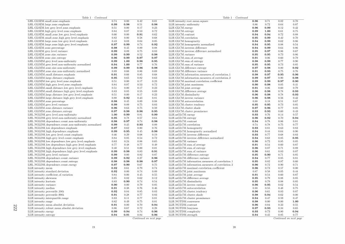
Table 1 – Continued
LHL GLSZM small zone emphasis 0.74 0.00 0.42 0.01LHL GLSZM large zone emphasis 0.99 0.98 0.51 0.98
LHL GLSZM low grey level zone emphasis 0.51 0.00 0.17 0.23LHL GLSZM high grey level zone emphasis 0.84 0.87 0.53 0.72LHL GLSZM small zone low grey level emphasis 0.66 0.00 0.91 0.62LHL GLSZM small zone high grey level emphasis 0.82 0.80 0.58 0.68LHL GLSZM large zone low grey level emphasis 0.43 0.03 0.04 0.05LHL GLSZM large zone high grey level emphasis 0.97 0.99 0.74 0.92
LHL GLSZM zone percentage 0.98 0.45 0.89 0.88LHL GLSZM grey level variance 0.99 0.89 0.75 0.83LHL GLSZM zone size variance 0.99 0.99 0.52 0.98
LHL GLSZM zone size entropy 0.96 0.99 0.97 0.97
LHL GLDZM grey level non-uniformity 0.99 1.00 0.96 0.95
LHL GLDZM grey level non-uniformity normalized 0.94 1.00 0.77 0.76LHL GLDZM zone size non-uniformity 0.99 0.99 0.96 0.98
LHL GLDZM zone size non-uniformity normalized 0.89 0.66 0.86 0.69LHL GLDZM small distance emphasis 0.91 0.66 0.85 0.68LHL GLDZM large distance emphasis 0.95 0.65 0.82 0.63LHL GLDZM low grey level zone emphasis 0.51 0.00 0.17 0.23LHL GLDZM high grey level zone emphasis 0.84 0.87 0.53 0.72LHL GLDZM small distance low grey level emphasis 0.51 0.00 0.17 0.23LHL GLDZM small distance high grey level emphasis 0.83 0.85 0.55 0.69LHL GLDZM large distance low grey level emphasis 0.51 0.00 0.17 0.23LHL GLDZM large distance high grey level emphasis 0.88 0.92 0.43 0.81LHL GLDZM zone percentage 0.98 0.45 0.89 0.88LHL GLDZM grey level variance 0.99 0.89 0.75 0.83LHL GLDZM zone distance variance 0.96 0.63 0.75 0.59LHL GLDZM zone distance entropy 0.97 0.98 0.96 0.95
LHL NGLDM grey level non-uniformity 1.00 0.99 0.81 0.99
LHL NGLDM grey level non-uniformity normalized 0.95 0.78 0.57 0.64LHL NGLDM dependence count non-uniformity 0.98 0.97 0.74 0.98
LHL NGLDM dependence count non-uniformity normalized 0.99 0.45 0.93 0.89LHL NGLDM low dependence emphasis 0.97 0.62 0.80 0.76LHL NGLDM high dependence emphasis 0.99 0.95 0.45 0.98
LHL NGLDM low grey level count emphasis 0.46 0.29 0.08 0.19LHL NGLDM high grey level count emphasis 0.84 0.85 0.54 0.72LHL NGLDM low dependence low grey level emphasis 0.63 0.24 0.88 0.65LHL NGLDM low dependence high grey level emphasis 0.77 0.48 0.77 0.49LHL NGLDM high dependence low grey level emphasis 0.40 0.51 0.00 0.01LHL NGLDM high dependence high grey level emphasis 0.99 0.98 0.83 0.91
LHL NGLDM grey level variance 0.99 0.80 0.82 0.87LHL NGLDM dependence count variance 0.99 0.92 0.37 0.96
LHL NGLDM dependence count entropy 0.98 0.98 0.98 0.97
LHL NGLDM dependence count energy 0.97 0.90 0.67 0.75LLH intensity mean 0.92 0.61 0.79 0.74LLH intensity standard deviation 0.92 0.00 0.74 0.89LLH intensity coefficient of variation 0.84 0.00 0.45 0.55LLH intensity skewness 0.85 0.82 0.62 0.12LLH intensity kurtosis 0.83 0.90 0.74 0.54LLH intensity variance 0.90 0.00 0.79 0.85LLH intensity median 0.91 0.38 0.76 0.46LLH intensity percentile 10th 0.92 0.84 0.85 0.83LLH intensity percentile 90th 0.91 0.28 0.77 0.83LLH intensity interquartile range 0.83 0.11 0.77 0.81LLH intensity range 0.82 0.49 0.75 0.81LLH intensity mean absolut deviation 0.91 0.00 0.70 0.94
LLH intensity robust mean absolut deviation 0.86 0.67 0.72 0.28LLH intensity energy 0.99 0.94 0.74 0.96
LLH intensity entropy 0.94 0.91 0.84 0.96
Continued on next page
19
Table 1 – Continued
LLH intensity root mean square 0.96 0.71 0.82 0.70LLH intensity uniformity 0.86 0.72 0.64 0.87LLH GLCM energy 0.96 0.99 0.12 0.42LLH GLCM entropy 0.99 1.00 0.61 0.75LLH GLCM contrast 0.94 0.94 0.72 0.88LLH GLCM correlation 0.95 0.99 0.42 0.70LLH GLCM homogeneity 0.94 0.99 0.62 0.86LLH GLCM homogeneity normalized 0.94 0.95 0.88 0.54LLH GLCM inverese difference 0.94 0.99 0.64 0.86LLH GLCM inverese difference normalized 0.95 0.97 0.86 0.67LLH GLCM variance 0.95 0.95 0.73 0.86LLH GLCM sum of average 0.91 0.06 0.60 0.79LLH GLCM sum of entropy 0.98 0.99 0.77 0.90LLH GLCM sum of variance 0.95 0.95 0.73 0.85LLH GLCM difference entropy 0.97 0.98 0.80 0.92
LLH GLCM difference variance 0.91 0.93 0.75 0.76LLH GLCM information measures of correlation 1 0.98 0.97 0.95 0.96
LLH GLCM information measures of correlation 2 0.99 0.97 0.90 0.98
LLH GLCM maximal correlation coefficient 0.99 0.99 0.97 0.90
LLH GLCM joint maximum 0.90 0.98 0.05 0.41LLH GLCM joint average 0.91 0.06 0.60 0.79LLH GLCM difference average 0.96 0.98 0.78 0.93
LLH GLCM dissimilarity 0.96 0.98 0.78 0.93
LLH GLCM inverse variance 0.96 0.98 0.56 0.42LLH GLCM autocorrelation 0.88 0.18 0.51 0.67LLH GLCM cluster tendency 0.95 0.95 0.73 0.85LLH GLCM cluster shade 0.97 0.96 0.77 0.05LLH GLCM cluster prominence 0.93 0.93 0.60 0.43LLH mGLCM energy 0.93 0.76 0.14 0.57LLH mGLCM entropy 0.96 0.92 0.70 0.94
LLH mGLCM contrast 0.94 0.78 0.86 0.81LLH mGLCM correlation 0.74 0.78 0.75 0.77LLH mGLCM homogeneity 0.93 0.81 0.63 0.83LLH mGLCM homogeneity normalized 0.94 0.44 0.64 0.90LLH mGLCM inverese difference 0.93 0.77 0.68 0.83LLH mGLCM inverese difference normalized 0.94 0.62 0.85 0.95
LLH mGLCM variance 0.96 0.72 0.85 0.85LLH mGLCM sum of average 0.91 0.54 0.60 0.87LLH mGLCM sum of entropy 0.96 0.87 0.71 0.89LLH mGLCM sum of variance 0.96 0.61 0.83 0.87LLH mGLCM difference entropy 0.95 0.90 0.71 0.85LLH mGLCM difference variance 0.94 0.77 0.85 0.81LLH mGLCM information measures of correlation 1 0.95 0.82 0.87 0.60LLH mGLCM information measures of correlation 2 0.96 0.72 0.90 0.71LLH mGLCM maximal correlation coefficient 0.96 0.73 0.57 0.00LLH mGLCM joint maximum 0.87 0.58 0.05 0.44LLH mGLCM joint average 0.91 0.54 0.60 0.87LLH mGLCM difference average 0.95 0.79 0.88 0.85LLH mGLCM dissimilarity 0.95 0.79 0.88 0.85LLH mGLCM inverse variance 0.96 0.95 0.62 0.54LLH mGLCM autocorrelation 0.88 0.55 0.48 0.75LLH mGLCM cluster tendency 0.96 0.61 0.83 0.87LLH mGLCM cluster shade 0.98 0.94 0.62 0.00LLH mGLCM cluster prominence 0.94 0.47 0.59 0.47LLH NGTDM coarseness 0.98 0.00 0.00 1.00
LLH NGTDM contrast 0.96 0.84 0.33 0.55LLH NGTDM busyness 0.97 0.93 0.34 0.65LLH NGTDM complexity 0.93 0.73 0.80 0.94
LLH NGTDM strength 0.94 0.45 0.85 0.77Continued on next page
20
222

Table 1 – Continued
LLH GLRLM grey level non-uniformity 0.99 0.99 0.96 0.98
LLH GLRLM grey level non-uniformity normalized 0.82 0.73 0.72 0.94
LLH GLRLM zone size non-uniformity 1.00 1.00 0.87 0.97
LLH GLRLM zone size non-uniformity normalized 0.95 0.95 0.68 0.91
LLH GLRLM short runs emphasis 0.95 0.94 0.59 0.89LLH GLRLM long runs emphasis 0.96 0.96 0.30 0.68LLH GLRLM low grey level run emphasis 0.98 0.73 0.79 0.46LLH GLRLM high grey level run emphasis 0.87 0.37 0.52 0.78LLH GLRLM short run low grey level emphasis 0.98 0.73 0.79 0.46LLH GLRLM short run high grey level emphasis 0.86 0.36 0.52 0.77LLH GLRLM long run low grey level emphasis 0.98 0.72 0.77 0.45LLH GLRLM long run high grey level emphasis 0.91 0.43 0.47 0.80LLH GLRLM run percentage 0.96 0.96 0.55 0.84LLH GLRLM grey level variance 0.89 0.00 0.77 0.84LLH GLRLM run length variance 0.97 0.98 0.24 0.61LLH GLRLM run entropy 0.99 0.94 0.94 0.98
LLH mGLRLM grey level non-uniformity 1.00 0.99 0.96 0.98
LLH mGLRLM grey level non-uniformity normalized 0.82 0.73 0.72 0.93
LLH mGLRLM zone size non-uniformity 1.00 1.00 0.87 0.97
LLH mGLRLM zone size non-uniformity normalized 0.95 0.94 0.67 0.91
LLH mGLRLM short runs emphasis 0.95 0.95 0.60 0.89LLH mGLRLM long runs emphasis 0.97 0.97 0.30 0.69LLH mGLRLM low grey level run emphasis 0.98 0.73 0.79 0.46LLH mGLRLM high grey level run emphasis 0.87 0.37 0.52 0.78LLH mGLRLM short run low grey level emphasis 0.98 0.73 0.79 0.47LLH mGLRLM short run high grey level emphasis 0.86 0.36 0.52 0.77LLH mGLRLM long run low grey level emphasis 0.98 0.72 0.77 0.45LLH mGLRLM long run high grey level emphasis 0.91 0.43 0.47 0.80LLH mGLRLM run percentage 0.96 0.96 0.55 0.84LLH mGLRLM grey level variance 0.89 0.00 0.77 0.84LLH mGLRLM run length variance 0.97 0.97 0.25 0.61LLH mGLRLM run entropy 0.98 0.94 0.94 0.97
LLH GLSZM grey level non-uniformity 0.98 0.98 0.94 0.99
LLH GLSZM grey level non-uniformity normalized 0.93 0.74 0.76 0.93
LLH GLSZM zone size non-uniformity 0.99 0.92 0.82 0.95
LLH GLSZM zone size non-uniformity normalized 0.93 0.57 0.61 0.72LLH GLSZM small zone emphasis 0.91 0.60 0.47 0.73LLH GLSZM large zone emphasis 0.99 0.98 0.45 0.97
LLH GLSZM low grey level zone emphasis 0.98 0.74 0.80 0.42LLH GLSZM high grey level zone emphasis 0.86 0.39 0.52 0.78LLH GLSZM small zone low grey level emphasis 0.99 0.77 0.78 0.43LLH GLSZM small zone high grey level emphasis 0.87 0.34 0.53 0.79LLH GLSZM large zone low grey level emphasis 0.99 0.54 0.14 0.91
LLH GLSZM large zone high grey level emphasis 0.95 0.64 0.69 0.94
LLH GLSZM zone percentage 0.95 0.81 0.89 0.95
LLH GLSZM grey level variance 0.76 0.00 0.73 0.86LLH GLSZM zone size variance 0.99 0.99 0.45 0.97
LLH GLSZM zone size entropy 0.95 0.96 0.96 0.98
LLH GLDZM grey level non-uniformity 0.98 0.98 0.94 0.99
LLH GLDZM grey level non-uniformity normalized 0.93 0.74 0.76 0.93
LLH GLDZM zone size non-uniformity 0.99 0.98 0.96 0.98
LLH GLDZM zone size non-uniformity normalized 0.95 0.96 0.70 0.28LLH GLDZM small distance emphasis 0.94 0.97 0.65 0.24LLH GLDZM large distance emphasis 0.92 0.97 0.50 0.22LLH GLDZM low grey level zone emphasis 0.98 0.74 0.80 0.42LLH GLDZM high grey level zone emphasis 0.86 0.39 0.52 0.78LLH GLDZM small distance low grey level emphasis 0.98 0.74 0.80 0.43LLH GLDZM small distance high grey level emphasis 0.84 0.37 0.50 0.76LLH GLDZM large distance low grey level emphasis 0.98 0.74 0.80 0.40
Continued on next page
21
Table 1 – Continued
LLH GLDZM large distance high grey level emphasis 0.94 0.51 0.53 0.78LLH GLDZM zone percentage 0.95 0.80 0.89 0.95
LLH GLDZM grey level variance 0.76 0.00 0.73 0.86LLH GLDZM zone distance variance 0.92 0.96 0.47 0.23LLH GLDZM zone distance entropy 0.97 0.94 0.92 0.96
LLH NGLDM grey level non-uniformity 1.00 0.99 0.74 0.96
LLH NGLDM grey level non-uniformity normalized 0.82 0.75 0.39 0.86LLH NGLDM dependence count non-uniformity 0.99 0.98 0.66 0.96
LLH NGLDM dependence count non-uniformity normalized 0.95 0.62 0.83 0.88LLH NGLDM low dependence emphasis 0.94 0.67 0.81 0.92
LLH NGLDM high dependence emphasis 0.98 0.99 0.27 0.60LLH NGLDM low grey level count emphasis 0.98 0.00 0.81 0.47LLH NGLDM high grey level count emphasis 0.88 0.62 0.48 0.77LLH NGLDM low dependence low grey level emphasis 0.98 0.15 0.81 0.48LLH NGLDM low dependence high grey level emphasis 0.85 0.74 0.58 0.75LLH NGLDM high dependence low grey level emphasis 0.93 0.00 0.00 0.58LLH NGLDM high dependence high grey level emphasis 0.95 0.77 0.32 0.71LLH NGLDM grey level variance 0.90 0.66 0.81 0.85LLH NGLDM dependence count variance 0.98 1.00 0.22 0.50LLH NGLDM dependence count entropy 0.97 0.98 0.98 0.99
LLH NGLDM dependence count energy 0.96 0.91 0.91 0.97
LLL intensity mean 0.96 0.82 0.90 0.89LLL intensity standard deviation 0.95 0.40 0.78 0.80LLL intensity coefficient of variation 0.84 0.83 0.00 0.00LLL intensity skewness 0.96 0.86 0.86 0.78LLL intensity kurtosis 0.94 0.73 0.68 0.87LLL intensity variance 0.95 0.43 0.83 0.89LLL intensity median 0.99 0.81 0.88 0.97
LLL intensity percentile 10th 0.96 0.57 0.88 0.82LLL intensity percentile 90th 0.84 0.84 0.84 0.50LLL intensity interquartile range 0.85 0.65 0.95 0.69LLL intensity range 0.84 0.79 0.83 0.66LLL intensity mean absolut deviation 0.93 0.25 0.81 0.87LLL intensity robust mean absolut deviation 0.87 0.14 0.95 0.00LLL intensity energy 0.99 0.99 0.99 0.92
LLL intensity entropy 0.95 0.96 0.94 0.98
LLL intensity root mean square 0.96 0.51 0.90 0.94
LLL intensity uniformity 0.92 0.76 0.77 0.94
LLL GLCM energy 0.96 0.99 0.75 0.36LLL GLCM entropy 0.98 1.00 0.86 0.84LLL GLCM contrast 0.94 0.86 0.94 0.65LLL GLCM correlation 0.97 0.98 0.96 0.61LLL GLCM homogeneity 0.99 0.92 0.77 0.76LLL GLCM homogeneity normalized 0.94 0.98 0.94 0.87LLL GLCM inverese difference 0.99 0.92 0.82 0.79LLL GLCM inverese difference normalized 0.96 0.99 0.96 0.96
LLL GLCM variance 0.95 0.82 0.95 0.62LLL GLCM sum of average 0.98 0.96 0.73 0.58LLL GLCM sum of entropy 0.98 1.00 0.94 0.90
LLL GLCM sum of variance 0.95 0.88 0.96 0.58LLL GLCM difference entropy 0.98 1.00 0.91 0.85LLL GLCM difference variance 0.96 0.91 0.89 0.45LLL GLCM information measures of correlation 1 0.98 0.99 0.99 0.95
LLL GLCM information measures of correlation 2 0.99 0.82 0.97 0.97
LLL GLCM maximal correlation coefficient 0.98 0.79 0.95 0.94
LLL GLCM joint maximum 0.93 0.97 0.18 0.45LLL GLCM joint average 0.98 0.96 0.73 0.58LLL GLCM difference average 0.96 0.91 0.96 0.81LLL GLCM dissimilarity 0.96 0.91 0.96 0.81
Continued on next page
22
Com
parison
ofrob
ust
tostan
dard
izedC
Trad
iomics
models
topred
ictoverall
surv
ivalfor
non
-small
celllu
ng
cancer
patien
ts
223

Table 1 – Continued
LLL GLCM inverse variance 1.00 0.97 0.88 0.95
LLL GLCM autocorrelation 0.97 0.97 0.76 0.54LLL GLCM cluster tendency 0.95 0.88 0.96 0.58LLL GLCM cluster shade 0.98 0.98 0.94 0.28LLL GLCM cluster prominence 0.96 0.89 0.92 0.23LLL mGLCM energy 0.96 0.96 0.70 0.78LLL mGLCM entropy 0.96 0.99 0.87 0.97
LLL mGLCM contrast 0.94 0.18 0.79 0.91
LLL mGLCM correlation 0.96 0.70 0.91 0.95
LLL mGLCM homogeneity 0.99 0.91 0.83 0.72LLL mGLCM homogeneity normalized 0.94 0.86 0.93 0.97
LLL mGLCM inverese difference 0.99 0.91 0.88 0.75LLL mGLCM inverese difference normalized 0.97 0.96 0.97 0.93
LLL mGLCM variance 0.95 0.05 0.85 0.91
LLL mGLCM sum of average 0.98 0.82 0.79 0.91
LLL mGLCM sum of entropy 0.97 0.98 0.93 0.96
LLL mGLCM sum of variance 0.96 0.11 0.95 0.83LLL mGLCM difference entropy 0.98 0.95 0.92 0.95
LLL mGLCM difference variance 0.94 0.21 0.83 0.94
LLL mGLCM information measures of correlation 1 0.97 0.75 0.85 0.71LLL mGLCM information measures of correlation 2 0.96 0.72 0.92 0.72LLL mGLCM maximal correlation coefficient 0.93 0.66 0.61 0.40LLL mGLCM joint maximum 0.99 0.43 0.29 0.57LLL mGLCM joint average 0.98 0.82 0.79 0.91
LLL mGLCM difference average 0.97 0.46 0.86 0.84LLL mGLCM dissimilarity 0.97 0.46 0.86 0.84LLL mGLCM inverse variance 1.00 0.93 0.92 0.33LLL mGLCM autocorrelation 0.97 0.86 0.85 0.91
LLL mGLCM cluster tendency 0.96 0.11 0.95 0.83LLL mGLCM cluster shade 0.98 0.96 0.91 0.00LLL mGLCM cluster prominence 0.96 0.18 0.93 0.55LLL NGTDM coarseness 0.99 0.00 0.00 0.68LLL NGTDM contrast 0.84 0.39 0.32 0.68LLL NGTDM busyness 0.96 0.81 0.90 0.96
LLL NGTDM complexity 0.95 0.97 0.90 0.84LLL NGTDM strength 0.96 0.62 0.87 0.82LLL GLRLM grey level non-uniformity 1.00 0.98 0.96 0.97
LLL GLRLM grey level non-uniformity normalized 0.91 0.76 0.77 0.96
LLL GLRLM zone size non-uniformity 1.00 1.00 0.95 0.98
LLL GLRLM zone size non-uniformity normalized 0.99 0.95 0.78 0.83LLL GLRLM short runs emphasis 0.99 0.94 0.74 0.81LLL GLRLM long runs emphasis 0.99 0.95 0.61 0.77LLL GLRLM low grey level run emphasis 0.92 0.75 0.81 0.97
LLL GLRLM high grey level run emphasis 0.96 0.79 0.83 0.73LLL GLRLM short run low grey level emphasis 0.92 0.75 0.81 0.97
LLL GLRLM short run high grey level emphasis 0.96 0.77 0.81 0.63LLL GLRLM long run low grey level emphasis 0.92 0.74 0.81 0.97
LLL GLRLM long run high grey level emphasis 0.97 0.85 0.76 0.91
LLL GLRLM run percentage 0.99 0.95 0.72 0.81LLL GLRLM grey level variance 0.95 0.47 0.82 0.88LLL GLRLM run length variance 0.99 0.96 0.55 0.78LLL GLRLM run entropy 0.97 0.97 0.97 0.99
LLL mGLRLM grey level non-uniformity 1.00 0.98 0.96 0.97
LLL mGLRLM grey level non-uniformity normalized 0.91 0.76 0.77 0.96
LLL mGLRLM zone size non-uniformity 1.00 1.00 0.95 0.98
LLL mGLRLM zone size non-uniformity normalized 0.99 0.95 0.78 0.83LLL mGLRLM short runs emphasis 0.99 0.95 0.74 0.81LLL mGLRLM long runs emphasis 0.99 0.96 0.61 0.77LLL mGLRLM low grey level run emphasis 0.92 0.75 0.81 0.97
Continued on next page
23
Table 1 – Continued
LLL mGLRLM high grey level run emphasis 0.96 0.79 0.83 0.73LLL mGLRLM short run low grey level emphasis 0.92 0.75 0.81 0.97
LLL mGLRLM short run high grey level emphasis 0.96 0.77 0.81 0.63LLL mGLRLM long run low grey level emphasis 0.92 0.74 0.81 0.97
LLL mGLRLM long run high grey level emphasis 0.97 0.85 0.76 0.91
LLL mGLRLM run percentage 0.99 0.96 0.72 0.81LLL mGLRLM grey level variance 0.95 0.47 0.82 0.88LLL mGLRLM run length variance 0.99 0.96 0.56 0.78LLL mGLRLM run entropy 0.97 0.97 0.97 0.99
LLL GLSZM grey level non-uniformity 0.99 0.97 0.92 0.98
LLL GLSZM grey level non-uniformity normalized 0.93 0.76 0.79 0.97
LLL GLSZM zone size non-uniformity 1.00 0.94 0.98 0.98
LLL GLSZM zone size non-uniformity normalized 0.82 0.62 0.90 0.79LLL GLSZM small zone emphasis 0.83 0.65 0.87 0.72LLL GLSZM large zone emphasis 1.00 0.95 0.49 0.76LLL GLSZM low grey level zone emphasis 0.93 0.76 0.80 0.96
LLL GLSZM high grey level zone emphasis 0.96 0.76 0.74 0.54LLL GLSZM small zone low grey level emphasis 0.91 0.77 0.80 0.96
LLL GLSZM small zone high grey level emphasis 0.94 0.69 0.58 0.56LLL GLSZM large zone low grey level emphasis 0.95 0.66 0.73 0.91
LLL GLSZM large zone high grey level emphasis 1.00 0.96 0.41 0.81LLL GLSZM zone percentage 0.97 0.89 0.94 0.97
LLL GLSZM grey level variance 0.97 0.48 0.78 0.85LLL GLSZM zone size variance 1.00 0.95 0.49 0.74LLL GLSZM zone size entropy 0.97 0.97 0.98 0.99
LLL GLDZM grey level non-uniformity 0.99 0.97 0.92 0.98
LLL GLDZM grey level non-uniformity normalized 0.93 0.76 0.79 0.97
LLL GLDZM zone size non-uniformity 0.99 1.00 0.98 0.99
LLL GLDZM zone size non-uniformity normalized 0.94 0.82 0.72 0.80LLL GLDZM small distance emphasis 0.94 0.81 0.65 0.79LLL GLDZM large distance emphasis 0.95 0.81 0.50 0.76LLL GLDZM low grey level zone emphasis 0.93 0.76 0.80 0.96
LLL GLDZM high grey level zone emphasis 0.96 0.76 0.74 0.54LLL GLDZM small distance low grey level emphasis 0.93 0.76 0.80 0.96
LLL GLDZM small distance high grey level emphasis 0.97 0.73 0.69 0.55LLL GLDZM large distance low grey level emphasis 0.93 0.76 0.80 0.96
LLL GLDZM large distance high grey level emphasis 0.95 0.80 0.65 0.55LLL GLDZM zone percentage 0.97 0.89 0.94 0.97
LLL GLDZM grey level variance 0.97 0.48 0.78 0.85LLL GLDZM zone distance variance 0.96 0.82 0.47 0.70LLL GLDZM zone distance entropy 0.98 0.97 0.97 0.99
LLL NGLDM grey level non-uniformity 1.00 0.98 0.87 0.93
LLL NGLDM grey level non-uniformity normalized 0.92 0.94 0.80 0.94
LLL NGLDM dependence count non-uniformity 0.99 0.97 0.87 0.97
LLL NGLDM dependence count non-uniformity normalized 0.97 0.73 0.96 0.99
LLL NGLDM low dependence emphasis 0.96 0.81 0.94 0.98
LLL NGLDM high dependence emphasis 1.00 0.95 0.50 0.72LLL NGLDM low grey level count emphasis 0.92 0.77 0.96 0.97
LLL NGLDM high grey level count emphasis 0.96 0.73 0.79 0.75LLL NGLDM low dependence low grey level emphasis 0.93 0.87 0.96 0.97
LLL NGLDM low dependence high grey level emphasis 0.96 0.26 0.47 0.60LLL NGLDM high dependence low grey level emphasis 0.93 0.29 0.96 0.94
LLL NGLDM high dependence high grey level emphasis 1.00 0.96 0.48 0.76LLL NGLDM grey level variance 0.95 0.13 0.83 0.88LLL NGLDM dependence count variance 1.00 0.92 0.44 0.75LLL NGLDM dependence count entropy 0.99 0.99 0.99 1.00
LLL NGLDM dependence count energy 0.97 0.96 0.98 0.97
24
224

Comparison of robust to standardized CT radiomics models to predict overall survival fornon-small cell lung cancer patients
10.10 Supplement D: Validation with different imaging setting
We have collected from each patient of the validation cohort an additional image set consisting of pre-treatment contrast-enhanced CT which were reconstructed using a LUNG kernel. Those new CTs wererigidly registered the CT scans of our main analysis (native CT reconstructed with standard convolutionkernel). Each primary tumor delineation was transferred to the corresponding CT with new acquisitionand imaging setting.
Figure 10.6: Receiver operating characteristic (ROC) curves of STD model (a) and MCR model (c). Green lineindicates the ROC curve of the models on the training set and violet line the ROC curve of the models on thevalidation set. Further, the feature distribution of the STD model (b) and MCR model (d) are shown as boxplotsstratified by outcome (no event and event) and cohorts (training and validation). Here, the validation patientsreceived a contrast-enhanced CT reconstructed using FBP with LUNG kernel.
The performance of the STD model (based on uniform image settings) failed successfully validated onthe validation set under the new imaging and scanning settings (AUC = 0.58 compared to AUC = 0.79).One explanation is that the feature with the largest coefficient in the model (HHH_busyness) fails tosplit the patients. The MCR model also fails to predict on this new validation cohort (see Figure 10.6).One possible explanation that the MCR model also fails might originate from the imaging data used. Inthis validation cohort, patients received a CT scan with a combination of contrast enhancement and lungreconstruction, whereas in the training these effects were separate. Moreover, the majority of the trainingimaging data in the MCR model were standardized (native CT with standard convolution kernel).
225

226
11Radiomics feature activation maps as a new
tool for signature interpretability
Diem Vuong1, Stephanie Tanadini-Lang1, Ze Wu1, Robert Marks1, Jan Unkelbach, Sven Hillinger2, Eric I.
Eboulet3, Sandra Thierstein3, Solange Peters4, Miklos Pless5, Matthias Guckenberger1, Marta Bogowicz1
1Department of Radiation Oncology, University Hospital Zurich and University of Zurich, Zurich, Switzer-land2Department of Thoracic Surgery, University Hospital Zurich and University of Zurich, Zurich, Switzer-land3Swiss Group for Clinical Cancer Research (SAKK) Coordinating Center, Bern, Switzerland4Department of Oncology, Centre Hospitalier Universitaire Vaudois (CHUV), Lausanne, Switzerland5Department of Medical Oncology, Kantonsspital Winterthur, Winterthur, Switzerland
Status:Published in Frontiers in Oncology, 2020doi: 10.3389/fonc.2020.578895
Copyright: Authors retained the copyright totheir articles.
My contribution: I developed the radiomics feature activation maps. I performed the image pro-cessing, global and local radiomics calculation, validation of the radiomics activation maps, analysis andinterpretation of the results. I wrote, revised, and proof-read the manuscript.
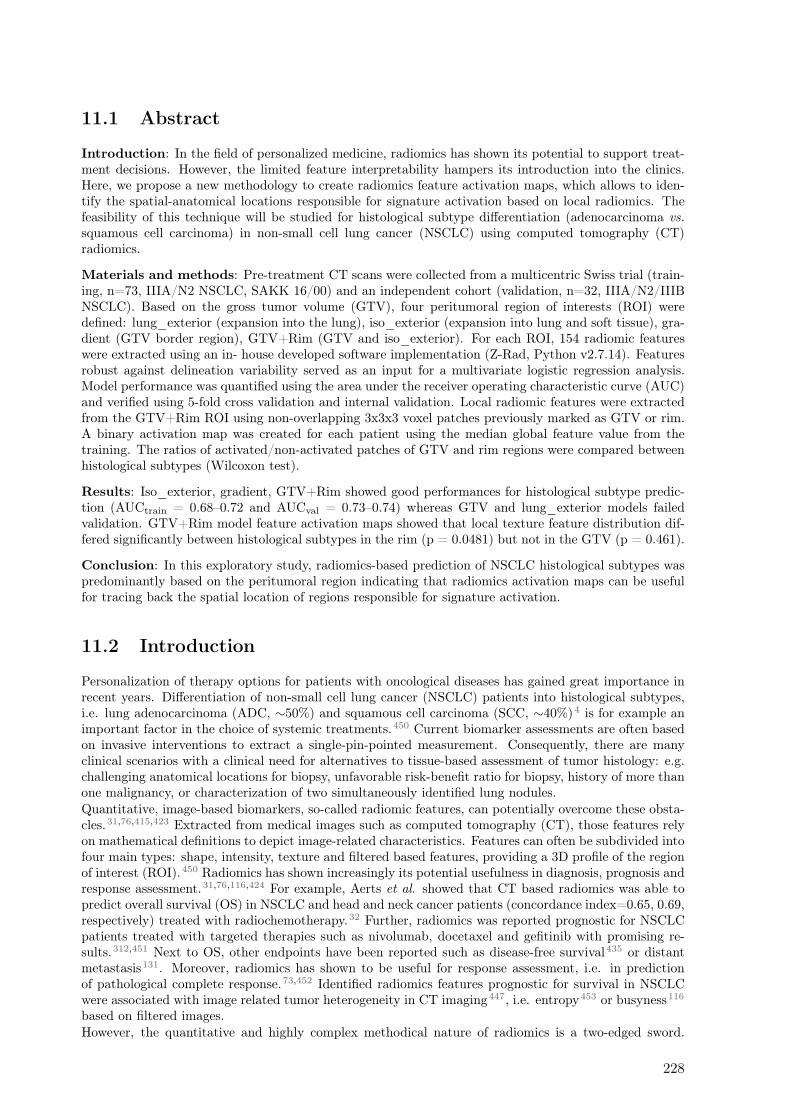
11.1 Abstract
Introduction: In the field of personalized medicine, radiomics has shown its potential to support treat-ment decisions. However, the limited feature interpretability hampers its introduction into the clinics.Here, we propose a new methodology to create radiomics feature activation maps, which allows to iden-tify the spatial-anatomical locations responsible for signature activation based on local radiomics. Thefeasibility of this technique will be studied for histological subtype differentiation (adenocarcinoma vs.squamous cell carcinoma) in non-small cell lung cancer (NSCLC) using computed tomography (CT)radiomics.
Materials and methods: Pre-treatment CT scans were collected from a multicentric Swiss trial (train-ing, n=73, IIIA/N2 NSCLC, SAKK 16/00) and an independent cohort (validation, n=32, IIIA/N2/IIIBNSCLC). Based on the gross tumor volume (GTV), four peritumoral region of interests (ROI) weredefined: lung_exterior (expansion into the lung), iso_exterior (expansion into lung and soft tissue), gra-dient (GTV border region), GTV+Rim (GTV and iso_exterior). For each ROI, 154 radiomic featureswere extracted using an in- house developed software implementation (Z-Rad, Python v2.7.14). Featuresrobust against delineation variability served as an input for a multivariate logistic regression analysis.Model performance was quantified using the area under the receiver operating characteristic curve (AUC)and verified using 5-fold cross validation and internal validation. Local radiomic features were extractedfrom the GTV+Rim ROI using non-overlapping 3x3x3 voxel patches previously marked as GTV or rim.A binary activation map was created for each patient using the median global feature value from thetraining. The ratios of activated/non-activated patches of GTV and rim regions were compared betweenhistological subtypes (Wilcoxon test).
Results: Iso_exterior, gradient, GTV+Rim showed good performances for histological subtype predic-tion (AUCtrain = 0.68–0.72 and AUCval = 0.73–0.74) whereas GTV and lung_exterior models failedvalidation. GTV+Rim model feature activation maps showed that local texture feature distribution dif-fered significantly between histological subtypes in the rim (p = 0.0481) but not in the GTV (p = 0.461).
Conclusion: In this exploratory study, radiomics-based prediction of NSCLC histological subtypes waspredominantly based on the peritumoral region indicating that radiomics activation maps can be usefulfor tracing back the spatial location of regions responsible for signature activation.
11.2 Introduction
Personalization of therapy options for patients with oncological diseases has gained great importance inrecent years. Differentiation of non-small cell lung cancer (NSCLC) patients into histological subtypes,i.e. lung adenocarcinoma (ADC, ∼50%) and squamous cell carcinoma (SCC, ∼40%)4 is for example animportant factor in the choice of systemic treatments.450 Current biomarker assessments are often basedon invasive interventions to extract a single-pin-pointed measurement. Consequently, there are manyclinical scenarios with a clinical need for alternatives to tissue-based assessment of tumor histology: e.g.challenging anatomical locations for biopsy, unfavorable risk-benefit ratio for biopsy, history of more thanone malignancy, or characterization of two simultaneously identified lung nodules.Quantitative, image-based biomarkers, so-called radiomic features, can potentially overcome these obsta-cles.31,76,415,423 Extracted from medical images such as computed tomography (CT), those features relyon mathematical definitions to depict image-related characteristics. Features can often be subdivided intofour main types: shape, intensity, texture and filtered based features, providing a 3D profile of the regionof interest (ROI).450 Radiomics has shown increasingly its potential usefulness in diagnosis, prognosis andresponse assessment.31,76,116,424 For example, Aerts et al. showed that CT based radiomics was able topredict overall survival (OS) in NSCLC and head and neck cancer patients (concordance index=0.65, 0.69,respectively) treated with radiochemotherapy.32 Further, radiomics was reported prognostic for NSCLCpatients treated with targeted therapies such as nivolumab, docetaxel and gefitinib with promising re-sults.312,451 Next to OS, other endpoints have been reported such as disease-free survival435 or distantmetastasis131. Moreover, radiomics has shown to be useful for response assessment, i.e. in predictionof pathological complete response.73,452 Identified radiomics features prognostic for survival in NSCLCwere associated with image related tumor heterogeneity in CT imaging447, i.e. entropy453 or busyness116
based on filtered images.However, the quantitative and highly complex methodical nature of radiomics is a two-edged sword.
228
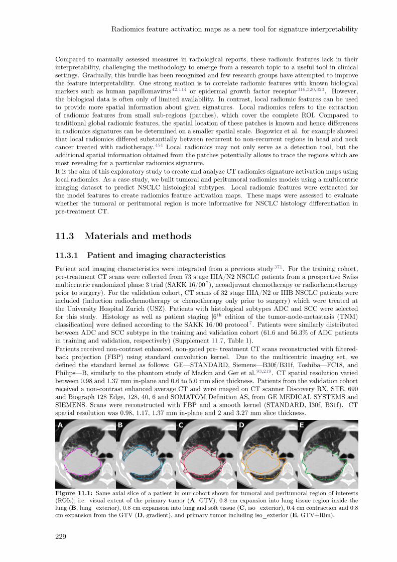
Radiomics feature activation maps as a new tool for signature interpretability
Compared to manually assessed measures in radiological reports, these radiomic features lack in theirinterpretability, challenging the methodology to emerge from a research topic to a useful tool in clinicalsettings. Gradually, this hurdle has been recognized and few research groups have attempted to improvethe feature interpretability. One strong motion is to correlate radiomic features with known biologicalmarkers such as human papillomavirus42,114 or epidermal growth factor receptor316,320,323. However,the biological data is often only of limited availability. In contrast, local radiomic features can be usedto provide more spatial information about given signatures. Local radiomics refers to the extractionof radiomic features from small sub-regions (patches), which cover the complete ROI. Compared totraditional global radiomic features, the spatial location of these patches is known and hence differencesin radiomics signatures can be determined on a smaller spatial scale. Bogowicz et al. for example showedthat local radiomics differed substantially between recurrent to non-recurrent regions in head and neckcancer treated with radiotherapy.454 Local radiomics may not only serve as a detection tool, but theadditional spatial information obtained from the patches potentially allows to trace the regions which aremost revealing for a particular radiomics signature.It is the aim of this exploratory study to create and analyze CT radiomics signature activation maps usinglocal radiomics. As a case-study, we built tumoral and peritumoral radiomics models using a multicentricimaging dataset to predict NSCLC histological subtypes. Local radiomic features were extracted forthe model features to create radiomics feature activation maps. These maps were assessed to evaluatewhether the tumoral or peritumoral region is more informative for NSCLC histology differentiation inpre-treatment CT.
11.3 Materials and methods
11.3.1 Patient and imaging characteristics
Patient and imaging characteristics were integrated from a previous study371. For the training cohort,pre-treatment CT scans were collected from 73 stage IIIA/N2 NSCLC patients from a prospective Swissmulticentric randomized phase 3 trial (SAKK 16/007), neoadjuvant chemotherapy or radiochemotherapyprior to surgery). For the validation cohort, CT scans of 32 stage IIIA/N2 or IIIB NSCLC patients wereincluded (induction radiochemotherapy or chemotherapy only prior to surgery) which were treated atthe University Hospital Zurich (USZ). Patients with histological subtypes ADC and SCC were selectedfor this study. Histology as well as patient staging [6th edition of the tumor-node-metastasis (TNM)classification] were defined according to the SAKK 16/00 protocol7. Patients were similarly distributedbetween ADC and SCC subtype in the training and validation cohort (61.6 and 56.3% of ADC patientsin training and validation, respectively) (Supplement 11.7, Table 1).Patients received non-contrast enhanced, non-gated pre- treatment CT scans reconstructed with filtered-back projection (FBP) using standard convolution kernel. Due to the multicentric imaging set, wedefined the standard kernel as follows: GE—STANDARD, Siemens—B30f/B31f, Toshiba—FC18, andPhilips—B, similarly to the phantom study of Mackin and Ger et al.93,219. CT spatial resolution variedbetween 0.98 and 1.37 mm in-plane and 0.6 to 5.0 mm slice thickness. Patients from the validation cohortreceived a non-contrast enhanced average CT and were imaged on CT scanner Discovery RX, STE, 690and Biograph 128 Edge, 128, 40, 6 and SOMATOM Definition AS, from GE MEDICAL SYSTEMS andSIEMENS. Scans were reconstructed with FBP and a smooth kernel (STANDARD, I30f, B31f). CTspatial resolution was 0.98, 1.17, 1.37 mm in-plane and 2 and 3.27 mm slice thickness.
Figure 11.1: Same axial slice of a patient in our cohort shown for tumoral and peritumoral region of interests(ROIs), i.e. visual extent of the primary tumor (A, GTV), 0.8 cm expansion into lung tissue region inside thelung (B, lung_exterior), 0.8 cm expansion into lung and soft tissue (C, iso_exterior), 0.4 cm contraction and 0.8cm expansion from the GTV (D, gradient), and primary tumor including iso_exterior (E, GTV+Rim).
229
11.3.2 Delineation
Five ROIs were defined for this study (Figure 11.1):
A. GTV: visual extent of the gross tumor volume (GTV)
B. lung_exterior: 0.8 cm expansion from the GTV into lung tissue only
C. iso_exterior: 0.8 cm expansion from the GTV into lung and soft tissue
D. gradient: 0.4 cm contraction and 0.8 cm expansion from the GTV
E. GTV+Rim: union of GTV and 0.8 cm expansion from GTV (iso_exterior).
The GTV ROI was manually delineated on the CT scans by an experienced physician using MIM VISTA(Version 6.7.9., MIM Software Inc., Cleveland, USA) with the lung window level and the support ofregistered PET images. All ROIs except for the GTV will be referred to as peritumoral ROIs. Theseperitumoral ROIs were created using an in-house developed MIM workflow. Anatomical structures whichwould strongly disturb the analysis, e.g. consisting of large air cavities (bronchi) or dense structures(bones) were manually excluded from all ROIs. Further, patients were excluded from the gradient analysisif the gradient regions comprised the entire GTV (Figure 11.1D).
11.3.3 Robustness study
The creation of the peritumoral ROIs was based on the manual delineation of the GTV, therefore arobustness study was performed to study the impact of inter-observer delineation variability on theradiomic features. A separate set of eleven patients were used as described in the study of Pavic et al.33
Three independent observers from USZ manually delineated the GTV. The same MIM workflow wasused to create the peritumoral ROIs with the GTV of the three observers as an input. The intra-classcorrelation coefficient (ICC) was used as stability measure as described in Pavic et al.33 However, astricter acceptance level of 0.9 was chosen, i.e. radiomic features with ICC > 0.9 were considered stable.
11.3.4 Radiomics
Pre-treatment CT scans were resampled to 3.75 mm cubic voxels, the 75th percentile of slice thicknesses inthe training dataset using linear interpolation. Radiomic calculations were performed using an in-housedeveloped software implementation (Z-Rad) based on Python programming language v 2.7.14 (for detailson the software and features, please consult: https://medical-physics-usz.github.io). A Hounsfield unit(HU) range of -1,024 to 200 HU was chosen to exclude bone structures which could not be accounted formanually. Since the expansion and contraction parameters for the peritumoral ROIs were fixed, no shapefeatures were considered for the analysis. Further, due to the small number of voxels in each direction,no wavelet features were included. Hence, a total of 154 radiomic features were calculated, i.e. intensity(n = 17) and texture (n = 137). Feature definitions were standardized according to the image biomarkerstandardization initiative (IBSI, version 11).38 A fixed bin size of 20 HU was used to discretize the greylevel values for texture analysis, resulting in approximately 60 bins, which has been shown to reduceintrinsic noise in the images while preserving essential texture.97
11.3.5 Statistical analysis for global radiomics
To reduce the number of features, principal component analysis (PCA) was performed as a featurereduction method.455 The retained principal components were defined based on the 95% data variance.The feature which correlated the most with the selected principal component was used as a surrogate (thelargest Pearson correlation coefficient). Univariate logistic regression analysis was performed to determineindividual prognostic power of each features, separately. The significance level was 0.05, with no correctionfor multiple testing. Based on features with highest prognostic power per principal component group, amultivariate logistic regression model was built with backward selection using Akaike information criterion(AIC) which balances the goodness of fit of the model and its simplicity.439 The discriminatory powerof the models was quantified using the area under the receiver operating characteristic curve (AUC)along with its 95% confidence interval (CI). Model performance was verified using 5-fold cross validation.Folds were chosen randomly without repetition. The generalizability of the models was verified in thevalidation cohort. Statistical analysis, model building and validation were performed with R (Version3.5.1, packages: base, survival441, survcomp442, boot456, pROC444, and glmnet445).
230

Radiomics feature activation maps as a new tool for signature interpretability
11.3.6 Creation of activation maps based on local radiomics
Figure 11.2: Scheme of radiomics feature activation map creation. Patches were optimally placed and patcheswith few informative voxels (< 9) were discarded (1), patches were labeled according to their overlap with thegross tumor volume (GTV) contour (2), and patches with mixed overlap were discarded (3). Patches were labeledactivated (red) if their feature value was larger than the global median and were labeled non-activated (blue)if their feature value was smaller than the global median. The activation ratio was analyzed per region andhistological subtype (5).
Local radiomic features were extracted from the GTV+Rim ROI using non-overlapping patches of size3x3x3 voxels. This size of the patches allowed a meaningful calculation of the texture features (minimumnumber of voxels in each direction) as well as a meaningful overlap with the rim region (0.8 cm marginin each direction and 3.75 mm voxel size). The placement of the patches was automatically optimized tocover the entire ROI with a minimum number of patches. Patches with a low number of informative voxels(< 9 voxels) of the ROI were discarded. The overlap of the patches with the GTV was assessed, i.e. 100%referred to patches comprising only the GTV and 0% to patches comprising only normal tissue. Thistool is intended to determine whether the radiomics signature for the prediction of histological subtypesoriginates from a certain predefined region. The signatures of patches with mixed overlap (10% to90%) contain ambiguous information and were therefore discarded to clearly distinguish patches spatiallyassigned rim or GTV. Finally, patches with overlap lower than 10% or larger than 90% were labeledas rim and GTV, respectively. A binary feature activation map was created for each individual patientusing the respective median of the global (standard) feature value in the training cohort, i.e. patches withfeature value larger than the median were considered activated. The ratios of activated/non-activatedpatches for the normal tissue and the GTV were compared in the validation cohort between the histologytypes (Wilcoxon test), considering only patients with at least 27 patches and a minimum 3 patches perregion (Figure 11.2), a more detailed description can be found in Supplement 11.10.
231

11.4 Results
11.4.1 Modeling and validation
Univariate MultivariateROI Feature AUC p-value Coefficient p-value
GTV GLRLM_run entropy 0.64 0.034GLCM inverse variance* 0.65 0.035 -10.83 0.035
lung_exterior GLSZM_zone percentage 0.63 0.046GLCM_contrast 0.65 0.043GLCM_homogeneity normalized* 0.72 0.004 52.51 0.004NGLDM_low dependence emphasis 0.66 0.025
iso_exterior Intensity_median 0.65 0.028GLCM_correlation 0.61 0.043GLSZM_zone size non-uniformity normalized* 0.68 0.015 -12.84 0.112Intensity_percentile_90* 0.68 0.025 -0.01 0.072
gradient GLSZM_zone size non-uniformity normalized* 0.68 0.046 -20.26 0.046GTV+Rim Intensity_median* 0.63 0.026 0.002 0.144
GLSZM_zone size non-uniformity normalized* 0.69 0.010 -16.75 0.026
Table 11.1: Overview of univariate and multivariate analysis shown for all region of interests (ROIs) considered.Only features are listed which had a significant performance in the univariate analysis per principal componentgroup. Features with an asterisk were retained in the final models after backward selection and their coefficientsand p-values in the multivariate analysis are listed.
Robust features were identified from the inter-observer variability robustness studies. Overall, the numberof stable features for each ROIs were found to be moderate, i.e. GTV (49.7%), lung_exterior (57.6%),iso_exterior (57.6%), gradient (55.8%), and GTV+Rim (74.5%). The analysis can be found in the Sup-plement 11.8. Results of the univariate analysis of the robust features selected in the feature selection stepare shown in Table 11.1. Features marked with an asterisk were the final features retained after backwardselection. Overall good univariate performances on the training set were observed (AUC = 0.61 – 0.72).
Different methods of feature selection were tested. The PCA+univariate logistic regression feature selec-tion method led to simpler models. For majority of the ROIs, the models using PCA+univariate logisticregression performed best compared to other feature selection methods (Supplement 11.9).
Figure 11.3: Receiver operating characteristic curve (ROC) curves and corresponding mean AUC [95% confi-dence interval] of the analyzed ROIs shown for training (blue) and validation cohort (red). The radiomic modelsbased on GTV and lung_exterior could not be successfully validated in the validation cohort. Iso_exterior,gradient and GTV+Rim models had good performances in both cohorts.
For all regions, a logistic regression model could be built. The 5-fold cross validation performance was[mean AUC (range)]: GTV [0.625 (0.23–1.00)], lung_exterior [0.72 (0.68–0.78)], iso_exterior [0.67 (0.46–0.84)], gradient [0.70 (0.48–0.82)], GTV+Rim [0.67 (0.48–0.84)]. The models based on the GTV andlung_exterior ROI were the only models which could not be validated on the validation cohort with95% CI covering AUC = 0.5, i.e. a performance of a random predictor. Iso_exterior, gradient and theGTV+Rim showed acceptable performances in the range of 0.68–0.72 in the training and 0.73–0.74 inthe validation cohort (Figure 11.3).
232

Radiomics feature activation maps as a new tool for signature interpretability
11.4.2 Model features
Histology Squamous cell carcinomaAdenocarcinoma
0.3
0.4
0.5
Training Validation
GL
CM
_in
ve
rse
va
ria
nc
e
GTV
0.90
0.92
0.94
0.96
0.98
Training Validation
GL
CM
_h
om
og
en
eit
y n
orm
lung_exterior
0.50
0.55
0.60
Training Validation
GL
SZ
M_
zo
ne
siz
e n
on−u
nifo
rmity n
orm
gradient
−400
−300
−200
−100
0
Training Validation
Inte
ns
ity
_p
erc
en
tile
90
th
0.40
0.45
0.50
0.55
0.60
0.65
Training Validation
GLS
ZM
_zone s
ize n
on−u
niform
ity n
orm
iso_exterior
−600
−400
−200
0
Training Validation
Inte
nsit
y_m
ed
ian
0.4
0.5
0.6
0.7
Training Validation
GLS
ZM
_zone s
ize n
on−u
niform
ity n
orm
GTV+Rim
Figure 11.4: Boxplots of each studied region of interest (ROI) stratified by histological subtype (adenocarcinoma,squamous cell carcinoma) and dataset (training, validation) for the final model features.
In Table 11.1, the coefficients of the final model features are listed. The final models consisted of one ortwo features. Each model consisted of one texture features. These texture features can be associated withthe texture heterogeneity in the ROI. For example, the gray level co-ocurrence matrix (GLCM) inversevariance in the GTV model is small if there is higher variance (Figure 11.4). The median GLCM inversevariance was lower for ADC compared to SCC, i.e. ADC were more likely to have heterogeneous and SCCmore homogeneous patterns (Figure 11.4). For all regions, iso_exterior, gradient and the GTV+Rim,one texture feature (GLSZM_zone size non-uniformity normalized) was present in all three models. Thisfeature counts the homogeneous zones of the same size over the different zone sizes and is low in patternswhere zone counts are equally distributed along zone sizes, i.e. more heterogeneous patterns (Figure11.4). In the models, the higher texture value (more homogeneous pattern) was associated more withSCC patients. Further, since this feature was present in the all three models, this feature will most likelybe associated in the tumor adjacent region within the stable performing GTV+Rim model. Using theactivation maps we further validate this assumption (see next section). Interestingly, the iso_exteriorthe 90% percentile intensity feature was significant more relevant in the model compared to the texturefeatures whereas in the GTV+Rim model the opposite was observed (Figure 11.4).
11.4.3 Analysis of radiomics feature activation maps
The activation map analysis of the full radiomics signature indicated a greater importance of the rimregion compared to the GTV (p = 0.0541 and p = 0.302 for rim and GTV, respectively). A closeranalysis on the individual features showed that visually the texture feature was more activated on theadjacent region of the tumor, the intensity median more in the tumoral region. The median split values
233
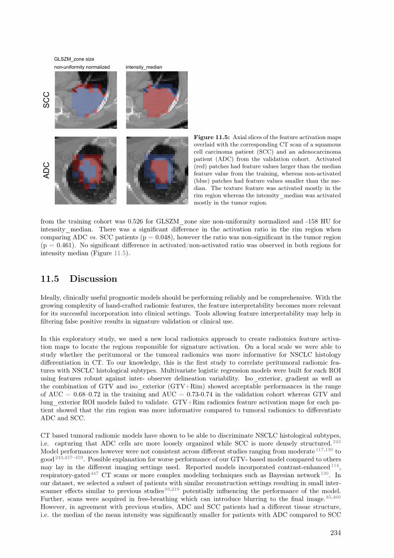
SC
CA
DC
intensity_median
GLSZM_zone size
non-uniformity normalized
Figure 11.5: Axial slices of the feature activation mapsoverlaid with the corresponding CT scan of a squamouscell carcinoma patient (SCC) and an adenocarcinomapatient (ADC) from the validation cohort. Activated(red) patches had feature values larger than the medianfeature value from the training, whereas non-activated(blue) patches had feature values smaller than the me-dian. The texture feature was activated mostly in therim region whereas the intensity_median was activatedmostly in the tumor region.
from the training cohort was 0.526 for GLSZM_zone size non-uniformity normalized and -158 HU forintensity_median. There was a significant difference in the activation ratio in the rim region whencomparing ADC vs. SCC patients (p = 0.048), however the ratio was non-significant in the tumor region(p = 0.461). No significant difference in activated/non-activated ratio was observed in both regions forintensity median (Figure 11.5).
11.5 Discussion
Ideally, clinically useful prognostic models should be performing reliably and be comprehensive. With thegrowing complexity of hand-crafted radiomic features, the feature interpretability becomes more relevantfor its successful incorporation into clinical settings. Tools allowing feature interpretability may help infiltering false positive results in signature validation or clinical use.
In this exploratory study, we used a new local radiomics approach to create radiomics feature activa-tion maps to locate the regions responsible for signature activation. On a local scale we were able tostudy whether the peritumoral or the tumoral radiomics was more informative for NSCLC histologydifferentiation in CT. To our knowledge, this is the first study to correlate peritumoral radiomic fea-tures with NSCLC histological subtypes. Multivariate logistic regression models were built for each ROIusing features robust against inter- observer delineation variability. Iso_exterior, gradient as well asthe combination of GTV and iso_exterior (GTV+Rim) showed acceptable performances in the rangeof AUC = 0.68–0.72 in the training and AUC = 0.73-0.74 in the validation cohort whereas GTV andlung_exterior ROI models failed to validate. GTV+Rim radiomics feature activation maps for each pa-tient showed that the rim region was more informative compared to tumoral radiomics to differentiateADC and SCC.
CT based tumoral radiomic models have shown to be able to discriminate NSCLC histological subtypes,i.e. capturing that ADC cells are more loosely organized while SCC is more densely structured.243
Model performances however were not consistent across different studies ranging from moderate117,130 togood243,457–459. Possible explanation for worse performance of our GTV- based model compared to othersmay lay in the different imaging settings used. Reported models incorporated contrast-enhanced114,respiratory-gated447 CT scans or more complex modeling techniques such as Bayesian network130. Inour dataset, we selected a subset of patients with similar reconstruction settings resulting in small inter-scanner effects similar to previous studies93,219 potentially influencing the performance of the model.Further, scans were acquired in free-breathing which can introduce blurring to the final image.85,460
However, in agreement with previous studies, ADC and SCC patients had a different tissue structure,i.e. the median of the mean intensity was significantly smaller for patients with ADC compared to SCC
234

Radiomics feature activation maps as a new tool for signature interpretability
(p < 0.05). The final GTV model feature (GLCM_inverse variance) was lower for ADC patients comparedto SCC patients, reflecting the more loosely structured tumor in ADC patients compared to more denselystructured tissue of SCC patients. Lower GLCM_inverse variance feature can be associated with higherheterogeneity in the tissue in agreement with other studies459, i.e. higher entropy values (associated withhigher tumor heterogeneity) were observed to be associated with ADC tumors.458
We hypothesized that peritumoral radiomics can depict better the known association between the anatom-ical tumor location and histological subtypes, i.e. ADC occur in more peripheral regions while SCC areoften located centrally.4 This association is assumed to be most evident in iso_exterior ROI where thecaptured adjacent soft tissue structures can reflect the periphery or centrality of the primary tumor lo-cation. Indeed, the median 90% percentile in ADC was lower compared to SCC indicating less densestructures in the ROI. Further, it has been shown that the microscopic tumor extension in the peritu-moral region differs between ADC and SCC. As a result, it has been suggested to use different marginsizes when treating ADC and SCC tumors to cover 95% of the microscopic tumor extension (8 and 6 mmmargin for ADC and SCC, respectively).461 With the chosen 8 mm margin for the iso_exterior region,this peritumoral model may depict this difference in the cell distribution.
The presence of the GLSZM_zone size non-uniformity normalized feature in the peritumoral ROI modelsindicated that this feature varies stronger between different histologies in the rim rather than in the GTVregion in the GTV+Rim model. The activation maps of the GTV+Rim model confirmed this observation,i.e. the distribution of local texture feature of ADC differed significantly from SCC for the rim (p = 0.048)but not for the GTV (p = 0.461), irrespective that the feature threshold was based on the global featurevalues and no feature scaling was applied.
To account for the inter-observer delineation variability, a robustness study was performed for the primarytumor and peritumoral ROIs. The peritumoral feature stability was moderate, interestingly however, sim-ilar or even more stable than the primary tumor radiomics. A possible reason can be a different amount oflung tissue in the primary tumor delineation, which can result in higher sensitivity to manual delineationsof the primary tumor compared to peritumoral regions where substantial lung tissue was a priori present.Further, an increased stability for larger ROI sizes can be observed. This observation is in agreementwith Tunali et al.’s inter-observer variability study, where, however, the initial primary tumor contourswere delineated using three semi-automatic segmentation methods.462 Arguably, the strict acceptancelevel ICC > 0.9, could have discarded potential useful features. However, due to the small cohort of11 patients for the robustness analysis, the strict acceptance level helps ensuring that results were notaffected by the small sample size. Recently, it has been shown that discarding features based on theirrobustness will lead to different models compared to modeling using a standardized imaging allowing toinclude all features.371
The localization of signature relevant regions in the context of activation maps has been established indeep learning methods. Activation maps are pre-dominantly used to identify areas of interest used fromthe neural network to perform its class prediction. Introduction of such activation maps into the fieldof radiomics may provide an addition for clinical interpretability of radiomic models. In the context ofperitumoral radiomics for example, where various peritumoral region definitions were reported in differentsites463, no clear strategy was available to determine the most promising region other than to model andvalidate each region individually. Therefore the tool presented in this study may guide the user to selectthe most relevant region in a more efficient way. Further, the presented tool can be not only applied onindividual features but could be useful to interpret a complete signature for example by combining theactivation maps of the model features. However, in our case, the texture feature had a more importantrole for the modeling compared to the intensity feature, therefore we did not include an analysis combin-ing both activation maps.
It is important to study the link between local and global features. For intensity features, the globalfeatures do not necessary have to reflect the spatial saliency on a local scale, as they are not scale-invariant. For texture features, the distribution of discretized intensities need to be preserved betweenthe local and global approach. For example, in our study, the same discretization for local and globalradiomics was used (fixed bin size of 20 HU with bin 0 corresponding to minimum intensity in the entireROI). For majority of texture features the link between global and local can be argued on the basisthat they are calculated on the relationship of a single voxel to its immediate neighbor (e.g. GLCM,NGTDM) consistent with the definition of our patches (3x3x3 voxels). The patch size should be ad-justed in situations where larger distances are used for the texture metrics calculation. In more complexmetrics (e.g. GLSZM, GLRLM), further analysis is required to study the main driving factor of the
235

feature values. However, in our study both iso_exterior and the GTV+Rim model shared the samefeature (GLSZM_zone_size_non-uniformity_normalized) indicating a close link of that feature to therim region, further also observed on the local scale. Similarly, another study showed that CT based localradiomics was useful to identifying subregions of head and neck tumors associated with different degreesof radiation curability, i.e. local features differed significantly between recurrent region and controlled(non-recurrent) region.454 In that study, heterogeneity on both global and local scale was linked to worseprognosis. Irrespectively, a closer investigation is needed to identify the optimal activation threshold.
This study has its limitations. Higher complexity features such as wavelet features were not included,since a minimum number of voxels in each direction is needed to provide a meaningful analysis. Thepublished tumoral radiomic models consisted of filter-based features such as law-features or waveletfeatures. However, these features were also more sensitive to delineation variability.462 Further, strictcut-off values were chosen to differentiate patches originated from the GTV and rim (10% and 90%).These results will likely change when using different cut-off values. Out of the scope of this exploratorystudy was the use of different margin sizes for the definition of peritumoral ROI as well as the inclusionof clinical known prognostic factors which might have improved the presented model performances. Afurther limitation is our assumption that the tumor spreads isotropically radial from the primary tumorcenter of mass. However, we distinguished a tumor spread into the lung-only regions with an isotropicspread. Lastly, the small sample size could have impacted the results, further analysis incorporating moreimaging data would be desired.
11.6 Conclusion
In this exploratory study we have shown that feature activation maps using local radiomics proved tobe useful for tracing back the spatial location of regions responsible for signature activation. Radiomicsfeature activation map analysis indicated that the rim region, which is anatomically the tumor invasionfront, was more relevant for histological subtype prediction than the GTV in CT imaging.
236
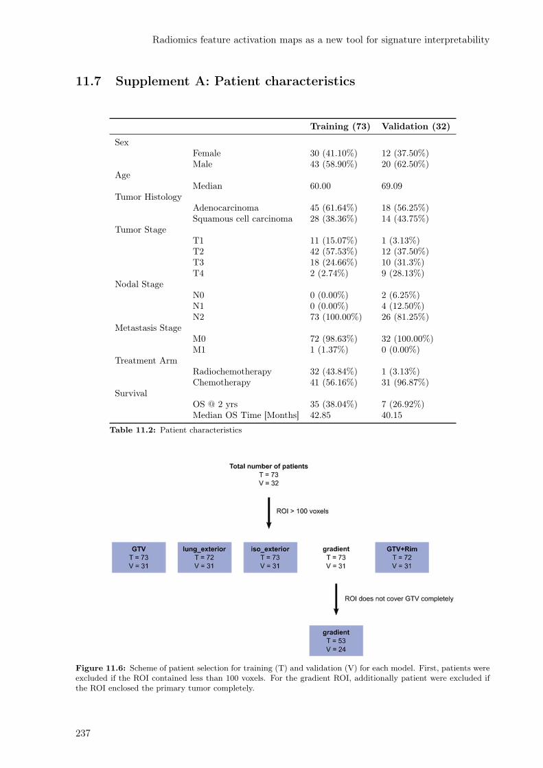
Radiomics feature activation maps as a new tool for signature interpretability
11.7 Supplement A: Patient characteristics
Training (73) Validation (32)
SexFemale 30 (41.10%) 12 (37.50%)Male 43 (58.90%) 20 (62.50%)
AgeMedian 60.00 69.09
Tumor HistologyAdenocarcinoma 45 (61.64%) 18 (56.25%)Squamous cell carcinoma 28 (38.36%) 14 (43.75%)
Tumor StageT1 11 (15.07%) 1 (3.13%)T2 42 (57.53%) 12 (37.50%)T3 18 (24.66%) 10 (31.3%)T4 2 (2.74%) 9 (28.13%)
Nodal StageN0 0 (0.00%) 2 (6.25%)N1 0 (0.00%) 4 (12.50%)N2 73 (100.00%) 26 (81.25%)
Metastasis StageM0 72 (98.63%) 32 (100.00%)M1 1 (1.37%) 0 (0.00%)
Treatment ArmRadiochemotherapy 32 (43.84%) 1 (3.13%)Chemotherapy 41 (56.16%) 31 (96.87%)
SurvivalOS @ 2 yrs 35 (38.04%) 7 (26.92%)Median OS Time [Months] 42.85 40.15
Table 11.2: Patient characteristics
Figure 11.6: Scheme of patient selection for training (T) and validation (V) for each model. First, patients wereexcluded if the ROI contained less than 100 voxels. For the gradient ROI, additionally patient were excluded ifthe ROI enclosed the primary tumor completely.
237

11.8 Supplement B: Robustness studies
Figure 11.7: Robustnessstudy on inter-observer delin-eation variability. Barplots ofpercentage of stable featuresfor considered ROIs (GTV,lung_exterior, iso_exterior,gradient and GTV+Rim) strat-ified for intensity and texturefeatures.
Initial inter-observer delineation variability of the primary tumor can influence the stability of radiomicfeatures extracted from the peritumoral ROIs. Overall, the number of stable features for each ROIswere found to be moderate, i.e. GTV (49.7%), lung_exterior (57.6%), iso_exterior (57.6%), gradient(55.8%) and GTV+Rim (74.5%). Interestingly, the overall stability of the peritumoral features waslarger compared to the GTV. This observation was evident in particular for intensity features, where theGTV+Rim ROI was the most stable (94.1%). In terms of texture features, the stability of the features wasvery similar among GTV, iso_exterior, lung_exterior and gradient. Similarly to the intensity features,texture features from GTV+Rim was the most stable ROI (75% of stable features, Figure 11.7).
11.9 Supplement C: Comparison of feature selection methods
This supplement summarizes different feature selection methods used in a sub-analysis. We have per-formed three different feature selection methods, i.e. PCA + univariate logistic regression, Least Abso-lute Shrinkage Selection Operator (LASSO) and Minimum Redundancy Maximum Relevance (mRmR),and two classifiers (multivariate logistic regression and LASSO). In mRmR, an ensemble approach wasused.464 It was partiality combined with the principal component analysis. The feature count was definedas the number of principal components, which explains 95% of data variance. The mRmR was repeated1000 randomly selecting samples using bootstrap procedure. The redundancy between the features wasdefined as the Pearson correlation. Features, which achieved at least 80% selection rate, were includedin the final set. Table 1 lists the 5-fold cross validation results as well as the features in the final models.More details on the specific modeling technique were reported and illustrated in a previous article fromour group.162
238
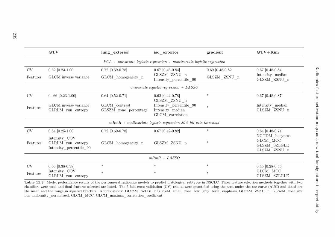
Rad
iomics
feature
activationm
aps
asa
new
tool
forsign
ature
interp
retability
GTV lung_exterior iso_exterior gradient GTV+Rim
PCA + univariate logistic regression + multivariate logistic regression
CV 0.62 [0.23-1.00] 0.72 [0.69-0.78] 0.67 [0.46-0.84] 0.69 [0.48-0.82] 0.67 [0.48-0.84]
Features GLCM inverse variance GLCM_homogeneity_nGLSZM_ZSNU_nIntensity_percentile_90
GLSZM_ZSNU_nIntensity_medianGLSZM_ZSNU_n
univariate logistic regression + LASSO
CV 0. 66 [0.23-1.00] 0.64 [0.52-0.71] 0.62 [0.44-0.78] * 0.67 [0.48-0.87]
FeaturesGLCM inverse varianceGLRLM_run_entropy
GLCM_contrastGLSZM_zone_percentage
GLSZM_ZSNU_nIntensity_percentile_90Intensity_medianGLCM_correlation
*Intensity_medianGLSZM_ZSNU_n
mRmR + multivariate logistic regression 80% hit rate threshold
CV 0.64 [0.25-1.00] 0.72 [0.69-0.78] 0.67 [0.42-0.82] * 0.64 [0.48-0.74]
FeaturesIntensity_COVGLRLM_run_entropyIntensity_percentile_90
GLCM_homogeneity_n GLSZM_ZSNU_n *
NGTDM_busynessGLCM_MCCGLSZM_SZLGLEGLSZM_ZSNU_n
mRmR + LASSO
CV 0.66 [0.38-0.98] * * * 0.45 [0.28-0.55]
FeaturesIntensity_COVGLRLM_run_entropy
* * *GLCM_MCCGLSZM_SZLGLE
Table 11.3: Model performance results of the peritumoral radiomics models to predict histological subtypes in NSCLC. Three feature selection methods together with twoclassifiers were used and final features selected are listed. The 5-fold cross validation (CV) results were quantified using the area under the roc curve (AUC) and listed arethe mean and the range in squared brackets. Abbreviations: GLSZM_SZLGLE: GLSZM_small_zone_low_grey_level_emphasis, GLSZM_ZSNU_n: GLSZM_zone sizenon-uniformity_normalized, GLCM_MCC: GLCM_maximal_correlation_coefficient.
239

11.10 Supplement D: Creation of radiomics activation maps
In the following, we present the detailed pipeline workflow to create radiomics activation maps. Thereare two distinct parts: the first part involves the global, traditional radiomics and the second the newlocal radiomics approach.First, the region of interest (ROI) was contoured (1). The ROI used for the radiomics activation mapcomputation was a union of the GTV (contoured manually) and a rim (defined as a 0.8 cm isotropicexpansion of the GTV), also referred to as GTV+Rim. From this ROI, radiomic features of type intensityand texture were extracted for each patient (2). Feature selection, modeling and validation was performedas described in the manuscript (3). From here on, we move to a local radiomics approach to createradiomics feature activation maps. The new local approach starts by optimizing the patch placement tominimize the total number of patches (in our study 3x3x3 voxel patches were used, 4). Next, patcheswith few informative voxels (n<3), i.e. no overlap with the ROI contour were discarded (5). To assign thepatches to GTV or the rim region, patches were labeled based on their overlap with the GTV contour.A patch with 1.0 was completely within the GTV and a patch with 0.0 completely within the rim (6). Itis clear that patches can have a mixed overlap of GTV and rim. In this case, we discard these patcheswith mixed overlap (between 10% – 90%) to ensure distinct differentiation of the activation signatureoriginating from the GTV and the one from the rim (7). The selected radiomic feature is then calculatedfor each individual patch resulting in a parametric feature map (8). To create an activation map, eachindividual patch will be labeled as activated or non-activated based on its feature value and globalthreshold. The global threshold is defined the median of the global radiomic feature (extracted fromentire GTV+Rim) over the training cohort. This is the step where radiomics on a global scale is linkedwith radiomics on a local scale (9). Lastly, the activation ratio (#activated / #non-activated patches)in the rim and in the GTV are compared between adenocarcinoma and squamous cell carcinoma usingstatistical testing (10).
240
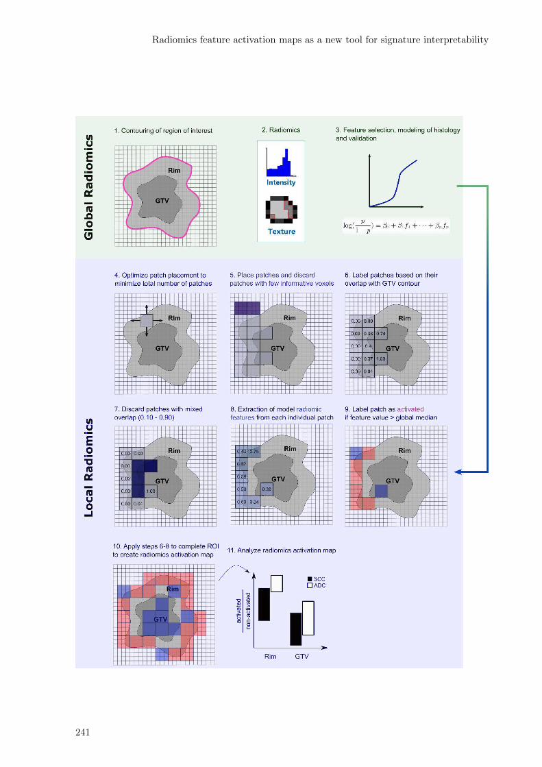
Radiomics feature activation maps as a new tool for signature interpretability
241

242
12Discussion and outlook
Imaging biomarkers based on radiomics have seen tremendous interest in cancer research.465 Neverthe-less, to date, there are only a few active registered prospective clinical trials that incorporate radiomicsinto clinical trials for the treatment of oncological diseases.116 Until March 2021, only one trial was com-pleted however no results have been published yet (Radiomics: a Study of Outcome in Lung Cancer,NCT01302626466). The aim of the study was to collect multifactorial patient data (including CT andPET image characteristics) that potentially improve and validate the predictive model for survival andlong-term toxicity in lung cancer through multicentric prospective data collection. Factors identified ashurdles to the incorporation of radiomics into the clinics include: limited generalizability of models, lackof multicenter data sets, sensitivity of features to imaging settings, and interpretability.37
This PhD thesis examined these factors for the example of locally advanced NSCLC disease while pro-viding a multi-faceted view of the disease. This chapter begins with a summary of the main findingsfollowed by a discussion of these various aspects and future prospects.
12.1 Main findings
In this section I summarize the main findings of this PhD thesis. It is divided into clinical and technicalaspects.
12.1.1 Clinical aspects
The main clinical findings can be divided into different length scales. On a large scale, I studiedthe anatomical tumor location within the lung as a prognostic factor for overall survival. I collectedpatients from five centers who were treated with radiochemotherapy only or in combination with surgery.I developed a voxelized cumulative status map of the spatial distribution of the primary tumors. Forthis purpose, the center of mass of the patient tumor was mapped to a reference patient lung using theregistration data of a deformable image registration. To identify areas of statistically significant worseprognosis, I performed a permutation test. These areas were located at central sites near the mediastinum(Chapter 7). The minimal distance of primary tumors to these areas was observed to be correlated withworse outcome in patients receiving radiochemotherapy but not in surgical patients.On an intermediate scale, I examined the image-based heterogeneity of each tumor using radiomicsand found that CT radiomics showed good prognostic power for modeling of 12 months OS. I furtherobserved that tumors with more heterogeneous textures were associated with an event (Chapter 10).In a small scale, I studied the region adjacent to the tumor (peritumoral region). This region is oftenincluded in the treatment volume as microscopic cancer cells may be present but not adequately imaged.I could show that peritumoral CT radiomics could predict histologic subtype in NSCLC (Chapter 11).
12.1.2 Technical aspects
As expected, I was confronted with a wide variety of imaging settings after collection of the CT andPET imaging data from the multicentric trial (SAKK-16/007). Therefore, I first investigated the impactof this variability in settings on the robustness of PET and CT radiomics. I found that only a fractionof PET radiomic features was stable across PET images from PET/CT and PET/MR scans. Whileshape and intensity features were highly stable (> 60%), lower feature stability was observed for textureand wavelet features (50% and 28%, respectively). I identified different attenuation corrections andtime differences between injection and acquisition between PET/CT and PET/MR scans as sources of

variability (Chapter 8). In CT radiomics, I examined the effect of convolution kernel variation and foundthat feature stability was influenced more by tissue type (lung, tumor, lymph node) and to a lesser extentby disease type (NSCLC, MPM, SSc-ILD), with 50% of features being transferable across all three diseases(Chapter 9). In a follow-up study, I included three additional effects from chest CT imaging relevantfor radiomics (delineation variability, motion, contrast). The highest feature stability was observed fordelineation variability whereas lowest stability was found when using different convolution kernels, i.e. nointensity features were found stable. In addition, I observed that only 10% of the features were consideredstable across all four main effects (Chapter 10).This observed result imposes the challenge to optimally include robustness studies into robust multicentricradiomics models. I compared two common approaches: a) discarding unstable features but using allpatients versus b) including all features but using a smaller subcohort of patients all imaged with similarimaging settings. Although I could not find a statistically significant difference in model performancebetween the two models, the model with the standardized imaging settings was preferred because itslower range 95% confidence interval was above 0.5 (random predictor). Interestingly, the final modelconsisted of features that were all previously identified as unstable. This suggests that excluding featuresbased on their robustness may result in suboptimal models (Chapter 10).Nowadays, features are becoming increasingly complex to describe and quantify tumor phenotype inmore detail, with the shortcoming of poor interpretability. In Chapter 11, I introduced radiomics featureactivation maps as a new tool to identify the spatial region where a particular feature is activated withina region of interest, thus supporting feature interpretation. Using the example of peritumoral radiomicsfor predicting the histology of NSCLC, I have shown with the radiomics activation maps that the rimregion was more informative compared to the tumor region for histology prediction.I will further discuss these main findings together with the relevant literature in the following order:
• Quantification of primary lung tumor location as a prognostic factor
• Radiomics to predict locally advanced NSCLC
• Robustness in multicentric radiomics studies
• Incorporation of robustness results into clinical modelling
• Interpretability of radiomic features
• Introduction of radiomics into the clinical routine.
12.2 Quantification of primary lung tumor location as a prognos-tic factor
The current literature inconsistently reports an association of tumor location and survival, mainly assign-ing tumor location within the lung to predefined anatomic regions, such as laterality (right or left lungside)373,374, centrality363,467 or lobe location361,362. These studies however only associate tumor locationwith respect to predefined anatomic regions that only partially reflect the full 3D tumor location withinthe lung. So far, the tumor location has not been studied in the context of a fully data driven method.In Chapter 7, I proposed a novel data mining approach to study the association of 3D tumor locationwith survival based on voxelized cumulative status maps.For this purpose, I first performed deformable image registration to a reference patient lung for eachpatient. From the deformation vector field data I mapped the center of mass of the primary tumor tothe reference lung. Compared to other spatial distribution maps368, I implemented a software solutionto retain the original shape of the primary tumor instead of a shape surrogate, which provides a betterestimate of the true spatial extent of the tumor. I performed a permutation test to identify regionsof statistically significant poorer prognosis. This allowed me to validate current literature findings thatcentrally located regions were associated with worse prognosis in radiochemotherapy and surgery cohorts.Additionally, patients with better performance status tend to be allocated to surgery group, this fact wasvisualized in my maps by larger areas of decreased survival in radiochemotherapy cohort. Based onexternal validation cohorts, I observed that tumors spatially closer to the decreased survival areas hadworse outcome in radiochemotherapy patients. Since the distances were corrected for the primary tumorextent, the model was not confounded by tumor volume. My model based on the distances outperformedtraditional models of T stage, tumor volume or laterality.
244
Discussion and outlook
In this use case, the voxelized cumulative status maps validated hypothesis that centrality is linked toworse outcome. However, this methodology can be used for other research questions and potentiallyreveal unknown aspects on existing hypotheses.372
Nonetheless, this study allows only to assess the survival of patients on a large scale. Reported associationof tumor location and survival may have been mediated by underlying biology. For example, lower lobelocation was observed to be mediated by EGFR mutation.376 Cancer patients are increasingly geneticallysequenced to assess potential genetic predisposition prior to therapy. Genomic sequencing is rarelyperformed in a retrospective cohort. Further, in contrast to today24,25, it was rarely performed routinelyat the time of the SAKK 16/007 trial. Thus, an in-depth analysis on the biological level was not possible.
12.3 Radiomics to predict outcome in locally advanced NSCLC
As summarized in the review in Chapter 4, many radiomics studies have investigated the prognosticvalue of radiomics in predicting survival in lung cancer. Aerts et al. developed a four-feature radiomicssignature including descriptors of intratumor heterogeneity and tested and validated it in more than 1000lung cancer and head and neck cancer patients.32 Their model showed an acceptable performance foroverall survival prediction (CI = 0.65), which performed better than tumor volume alone.32
In this PhD thesis, I studied patients treated with multimodality treatment including surgery, whereasmost radiomics studies treated locally advanced NSCLC patients with radiochemotherapy alone.32,158,468
Nevertheless, I was able to develop an OS model with similar model performance. I also observed thattumors with more heterogeneous CT image density were associated with poorer prognosis.447,451,453 Thisfinding suggests that the CT radiomics signature represents an overall prognostic tumor phenotype whichis independent of the received therapy. Radiomics models may be vulnerable if their signature is influ-enced by hidden confounding factors, such as tumor volume. On one hand, it is important to assess theadditional value of radiomics to existing clinical models. On the other hand, hidden confounding factorsmay increase the risk of multicollinearity, which could lead to suboptimal combined clinical and radiomicsmodels.39,469 My radiomics signature was not correlated with tumor volume.
In recent years, lung cancer radiomics research have expanded to regions other than the gross tumor.Peritumoral radiomics has experienced increasing interest over the past two years. Recent studies reportedsuccessful demonstration of peritumoral radiomics to predict distant metastasis138 and survival470. How-ever, because of the inconsistent clinical definition of microscopic extent, the peritumoral definition in theliterature varied across studies.132,138,302,471 Therefore results are difficult to compare with each other. Ina recent publication, tumor and peritumoral radiomics was used to predict survival and thereby stratifyearly stage NSCLC patients into high and low risk groups based on low dose CT scans used in lung cancerscreening.470 Two features were found highly informative, which was peritumoral NGTDM busyness (ratein intensity density change) and tumoral statistical RMS (root mean square of voxel intensities).470
Due to the advanced stage, the disease has often metastasized to lymph nodes at time of diagnosis.2
Lymph nodes involvement in locally advanced NSCLC disease has been reported relevant for patientoutcome.472 In resectable locally advanced NSCLC patients, Coroller et al. demonstrated the feasibilityof CT radiomics of primary tumor and lymph nodes to predict pathological complete response priorto the surgery treatment. Larger homogeneous texture in lymph nodes were predictive (AUC = 0.67,p < 0.05), outperforming tumor radiomics.452 Furthermore, healthy lung radiomics showed predictivevalue in prediction of radiation-induced pneumonitis and just recently immunotherapy-induced pneu-monitis.160,161,473 Next to the expansion to other region of interest, radiomics has also been studied asa treatment response assessment tool. Time-resolved longitudinal-radiomics (also referred to as deltaradiomics) in CT imaging are mostly based on cone-beam CT scans, which are routinely performedwithin the course of radiation therapy. Radiomics from daily cone-beam CT scans however did not showprognostic value for prediction of survival in three external validation sets.474
Radiomics depicts potential tumor phenotype differences on a macroscopic imaging level. Large studiescorrelating biology with radiomics are sparse. Pre-clinical models are completely missing. With recentintroduction of target therapy and immunotherapy, more studies are published investigating radiomicspredictive value for driver mutations. Models published are mainly proof of concepts, where externalvalidation is missing. Image-based biomarker were found to correlate to EGFR mutated tumors, i.e.being more heterogeneous than its wildtype pendant, whereas KRAS mutated tumors seem to show amore homogeneous texture in CT radiomics.320 Further Ki-67 proliferation index has been studied in
245

the context of radiomics with good predictive performance (AUC = 0.76, cross validation).475 It is thehope that larger studies are being published to improve the trustworthiness of the results. With geneticsequencing becoming more frequently performed for immunotherapy, we could expect newer larger studiesbeing published in the near future.
12.4 Robustness of radiomic features
As shown in the previous chapters, radiomic features can be differentially sensitive to variation in imagingsettings within one center (Chapter 8) as well as in multiple centers (Chapter 9 and 10). Two aspectsof model robustness are distinguished, namely repeatability and reproducibility. Clinical models shouldbe repeatable, i.e. assessment of biomarkers should remain the same when repeated multiple times.476
In radiomics, repeatability can be assessed in so-called test-retest studies. An example was included inChapter 8 where I used PET images of two respiratory phases of 4D PET/MR scans. On the other hand,features should be reproducible, i.e. they remain the same when imagined with different imaging settingssuch as commonly present in multicentric studies.471 This was investigated in Chapters 10, 9, where Itested the reproducibility of CT and PET features.With PET/MR scanner becoming more available in the clinics, question arises whether current PETradiomics models based on PET/CT scanners are transferrable to PET/MR scanners. In Chapter 8,I have shown for the first time that a large fraction of shape and intensity features can be transferredbetween PET scans from PET/CT and PET/MR scanners in contrast to texture and wavelet features(<50%). I further showed that PET features were less stable when comparing PET scans of PET/CTand PET/MR compared to the test-retest sub study.Reported robustness studies are often difficult to compare with each other because they examine in-dividual effects separately or consider different aspects such as disease type, tissue type, single- andmulti-institutional data. In both Chapters 9 and 10, I studied a set of multiple effects. In Chapter 9, Iinvestigated the robustness of CT radiomics across three lung diseases and four tissue types. In agreementwith other studies88,228,315, only a small fraction of features was stable across sharp and smooth kernelCT scans. Interestingly, the disease type had a lower impact on the robustness than the tissue type.A volume effect was observed where lymph nodes radiomics showed lowest stability and lung radiomicshighest stability. In a second CT robustness analysis, I studied the reproducibility of radiomics featuresfrom different delineations as well as relevant in lung CT imaging settings (convolution kernel, motionand contrast). Delineation variability affect the robustness of features to a smaller extent compared toother imaging settings. In agreement with other studies88,228,315, variation in convolution kernels showedstrongest impact. For example, no intensity feature was stable in scans reconstructed with differentkernels. Respiratory motion as well as contrast enhancement have shown less strong impact on the ro-bustness of radiomic features. Oliver et al. showed similar results.85 Motion artefacts can be substantiallyreduced in respiratory gated imaging. To date, the robustness study on comparing contrast enhancedand non-contrast enhanced CT scans was the first to study impact of contrast of the robustness of ra-diomic features. Contrast-enhanced CT scans are difficult to control due to varying injection dose andacquisition time across patients. In total, only 10% of the initial features were stable across all four effects.
Robustness studies rely on pairwise image sets. Test-retest studies of image modalities using ionizingradiation are difficult to perform because imaging patients twice within a short time frame is neitherpart of routine clinical practice nor ethical. I used PET scans of respiratory phases from 4D PETscans as a surrogate for test-retest studies, which has been previously shown to be feasible for 4D CTscans.217 A recent study in NSCLC and head and neck cancer patients showed that certain chains ofimage perturbation transformations resulted in similar robustness rates compared to test-retest studiesin CT radiomics, making them an acceptable alternative.434
To that end, a phantom study provides a controlled environment for assessment of radiomics’ robustness.Often however they are being criticized for being far from the realistic patient situation and only limitedlyresolve intra-tumor heterogeneity. A patient-specific CT quality assurance phantom is currently beingdeveloped for radiomics research as part of the Swiss Personalized Health Network (SPHN)477, whichaims to build the infrastructure for health data exchange within Switzerland. Unlike other phantoms,it is 3D printed with iodine ink where iodine concentrations can reflect the density variations visiblein CT imaging. These 3D-printed phantoms were first introduced to assess the diagnostic detectabilityin different CT scanners478 but in the long term, this type of phantoms could enable a patient-specificquality assurance tool for radiomics research.
246

Discussion and outlook
As a consequence of these observed low robustness rates, an ideal data set for the robustness study inlung cancer patients must be multi-layered (separate image scans is needed for each factor), e.g.
• Test-retest
• Delineated by multiple observers for each region of interest
• Respiratory gated
• Sequence of CT scans with time-resolved contrast injection-acquisition time
• Raw projection data to assess reconstruction differences. Availability of this raw data allows testingof feature robustness as new reconstruction methods are introduced to the market.
12.5 Incorporation of robustness results in multicentric radiomicmodels
Prospective trials are considered as the gold standard of clinical trials, where follow-up data of patientsare carefully collected in pre-set time intervals. However, to date it is difficult to convince institutions touse a standardized protocol for prospective data collection, which impose challenges for the robustnessof image-based biomarker models. Features that are sensitive to imaging-related variations should beremoved from model development because they reflect not only the differential tumor phenotype butalso where the patient was imaged. For the first time, I studied two strategies to incorporate radiomicsrobustness studies. My model achieved good model performance of AUC = 0.73 in the training andAUC = 0.79 in the validation set.The model was based on a subset of the initial multicentric imaging clinical trial.7 The dataset usedfor training was in terms of imaging settings homogeneous, i.e. non-contrast CT scans reconstructedwith FBP and standard convolution kernel (Chapter 10). Careful consideration is needed when dataof different settings are mixed which provide different patient information. In a CT radiomics studyof solitary pulmonary nodules, He et al. could demonstrate that non-contrast, thin-slice and standardconvolution kernel-based CT is more informative compared to their counterpart CT scans.433
The results I obtained illustrate well the challenge of heterogeneous imaging data sets in multicentricradiomic models. The inclusion of only four effects (delineation, respiratory motion, contrast, and recon-struction kernel) drastically decreases the number of stable features to 10% of the original 1400+ features.Including more robustness studies to fully account for all variety of imaging settings would potentiallyresult in no stable features, i.e. no model.Feature post-processing methods aim to adequately remove center based effects while maintaining thesubject effects and thereby retain more features. One method which has been recently introduced toradiomics is the ComBat method.175,205 Originally introduced in genetic sequencing where center effectsfrom different laboratories were aimed to remove effects on the results by different laboratories.474 A sim-ulation study suggests optimal results of the ComBat method if each center has at least 20 subjects.204
In smaller multicentric trials such as present in this thesis, this criteria can often not be fulfilled. Alter-natively, the lack of data for robustness of models can be overcome by data augmentations.479 Furtherinvestigations are needed to assess which feature removal and post-processing method performs optimally.
12.6 Interpretability of radiomics features
Image based biomarker development has evolved from simple shape measures and intensity descriptorsto texture and filtered based features. One option to improve interpretability of features is to correlatethem with known clinical and biological prognostic markers, such as EGFR or KRAS mutation status.320
Despite becoming frequently assessed and collected, the biological data is sparse and are based on pin-point measures. In Chapter 11, I introduced radiomics feature activation maps as a new approach tointerpret model features based on their spatial activation. These maps were based on local radiomics.Local radiomics refers to the radiomics calculation on a set of subvolumes of the entire region of interest.This allows to maintain the spatial information as to where the feature was calculated from. On theexample of peritumoral radiomics, different regions are being analysed (tumor, rim, tumor+rim).132,462
My exploratory analysis of radiomics activation maps may help selectively choose the region of interest
247
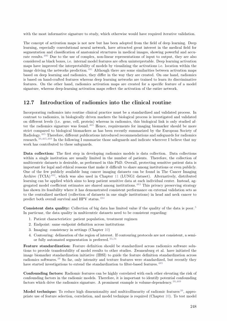
with the most informative signature to study, which otherwise would have required iterative validation.
The concept of activation maps is not new but has been adopted from the field of deep learning. Deeplearning, especially convolutional neural network, have attracted great interest in the medical field forsegmentation and classification of anatomical structures in medical images, showing powerful and accu-rate results.480 Due to the use of complex, non-linear representations of input to output, they are alsoconsidered as black boxes, i.e. internal model features are often uninterpretable. Deep learning activationmaps have improved the interpretability of models by visualizing the activations i.e. location within theimage driving the networks prediction.481 Although there are some similarities between activation mapsbased on deep learning and radiomics, they differ in the way they are created. On one hand, radiomicsis based on hand-crafted features whereas deep learning networks are trained to learn its discriminativefeatures. On the other hand, radiomics activation maps are created for a specific feature of a modelsignature, whereas deep-learning activation maps reflect the activation of the entire network.
12.7 Introduction of radiomics into the clinical routine
Incorporating radiomics into routine clinical practice must be a standardized and validated process. Incontrast to radiomics, in biologically driven markers the biological process is investigated and validatedon different levels (i.e. gene, cell, protein) whereas in radiomics, this biological link is only studied af-ter the radiomics signature was found.465 Hence, requirements for imaging biomarker should be morestrict compared to biological biomarkers as has been recently summarized by the European Society ofRadiology.465 Therefore, different publications introduced recommendations and safeguards for radiomicsresearch.39,465,469 In the following I summarize those safeguards and indicate wherever I believe that mywork has contributed to these safeguards.
Data collection: The first step in developing radiomics models is data collection. Data collectionswithin a single institution are usually limited in the number of patients. Therefore, the collection ofmulticentric datasets is desirable, as performed in this PhD. Overall, protecting sensitive patient data isimportant for legal and ethical reasons that make it difficult to share among institutions or even publicly.One of the few publicly available lung cancer imaging datasets can be found in The Cancer ImagingArchive (TCIA)482, which was also used in Chapter 11 (LUNG1 dataset). Alternatively, distributedlearning can be applied which aims to keep patient sensitive data at each individual center. Instead, ag-gregated model coefficient estimates are shared among institutions.483 This privacy preserving strategyhas shown its feasibility where it has demonstrated consistent performance on external validation sets asto the centralized method (collection of datasets in one single institutions) in head and neck cancer topredict both overall survival and HPV status.484
Consistent data quality: Collection of big data has limited value if the quality of the data is poor.5
In particuar, the data quality in multicentric datasets need to be consistent regarding:
1. Patient characteristics: patient population, treatment regimen
2. Endpoint: same endpoint definition across institutions
3. Imaging: consistency in settings (Chapter 10)
4. Contouring: delineation of the region of interest. If contouring protocols are not consistent, a semi-or fully automated segmentation is preferred.33,34
Feature standardization: Feature definition should be standardized across radiomics software solu-tions to provide transferability of model results to other studies. Zwanenburg et al. have initiated theimage biomarker standardization initiative (IBSI) to guide the feature definition standardization acrossradiomics softwares.38 So far, only intensity and texture features were standardized, but recently theyhave started investigations to extend the standardization to filter-based features.485
Confounding factors: Radiomic features can be highly correlated with each other elevating the risk ofconfounding factors in the radiomic models. Therefore, it is important to identify potential confoundingfactors which drive the radiomics signature. A prominent example is volume-dependency.39,469
Model technique: To reduce high dimensionality and multicollinearity of radiomic features39, appro-priate use of feature selection, correlation, and model technique is required (Chapter 10). To test model
248
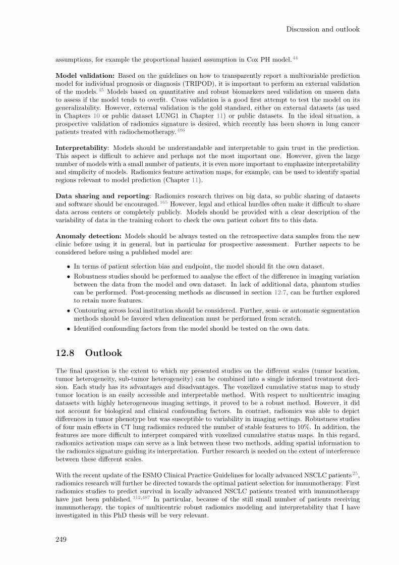
Discussion and outlook
assumptions, for example the proportional hazard assumption in Cox PH model.44
Model validation: Based on the guidelines on how to transparently report a multivariable predictionmodel for individual prognosis or diagnosis (TRIPOD), it is important to perform an external validationof the models.45 Models based on quantitative and robust biomarkers need validation on unseen datato assess if the model tends to overfit. Cross validation is a good first attempt to test the model on itsgeneralizability. However, external validation is the gold standard, either on external datasets (as usedin Chapters 10 or public dataset LUNG1 in Chapter 11) or public datasets. In the ideal situation, aprospective validation of radiomics signature is desired, which recently has been shown in lung cancerpatients treated with radiochemotherapy.486
Interpretability: Models should be understandable and interpretable to gain trust in the prediction.This aspect is difficult to achieve and perhaps not the most important one. However, given the largenumber of models with a small number of patients, it is even more important to emphasize interpretabilityand simplicity of models. Radiomics feature activation maps, for example, can be used to identify spatialregions relevant to model prediction (Chapter 11).
Data sharing and reporting: Radiomics research thrives on big data, so public sharing of datasetsand software should be encouraged.165 However, legal and ethical hurdles often make it difficult to sharedata across centers or completely publicly. Models should be provided with a clear description of thevariability of data in the training cohort to check the own patient cohort fits to this data.
Anomaly detection: Models should be always tested on the retrospective data samples from the newclinic before using it in general, but in particular for prospective assessment. Further aspects to beconsidered before using a published model are:
• In terms of patient selection bias and endpoint, the model should fit the own dataset.
• Robustness studies should be performed to analyse the effect of the difference in imaging variationbetween the data from the model and own dataset. In lack of additional data, phantom studiescan be performed. Post-processing methods as discussed in section 12.7, can be further exploredto retain more features.
• Contouring across local institution should be considered. Further, semi- or automatic segmentationmethods should be favored when delineation must be performed from scratch.
• Identified confounding factors from the model should be tested on the own data.
12.8 Outlook
The final question is the extent to which my presented studies on the different scales (tumor location,tumor heterogeneity, sub-tumor heterogeneity) can be combined into a single informed treatment deci-sion. Each study has its advantages and disadvantages. The voxelized cumulative status map to studytumor location is an easily accessible and interpretable method. With respect to multicentric imagingdatasets with highly heterogeneous imaging settings, it proved to be a robust method. However, it didnot account for biological and clinical confounding factors. In contrast, radiomics was able to depictdifferences in tumor phenotype but was susceptible to variability in imaging settings. Robustness studiesof four main effects in CT lung radiomics reduced the number of stable features to 10%. In addition, thefeatures are more difficult to interpret compared with voxelized cumulative status maps. In this regard,radiomics activation maps can serve as a link between these two methods, adding spatial information tothe radiomics signature guiding its interpretation. Further research is needed on the extent of interferencebetween these different scales.
With the recent update of the ESMO Clinical Practice Guidelines for locally advanced NSCLC patients25,radiomics research will further be directed towards the optimal patient selection for immunotherapy. Firstradiomics studies to predict survival in locally advanced NSCLC patients treated with immunotherapyhave just been published.312,487 In particular, because of the still small number of patients receivingimmunotherapy, the topics of multicentric robust radiomics modeling and interpretability that I haveinvestigated in this PhD thesis will be very relevant.
249

250

References
[1] Ferlay J, Colombet M, Soerjomataram I, etal. Estimating the global cancer incidenceand mortality in 2018: GLOBOCAN sourcesand methods. International Journal of Can-cer. 2019;144(8):1941–1953. 5, 16
[2] Huber RM, Ruysscher DD, Hoffmann H,Reu S, Tufman A. Interdisciplinary multi-modality management of stage III nonsmallcell lung cancer. European Respiratory Re-view. 2019;28(152):190024. 5, 245
[3] Goldstraw P, Chansky K, Crowley J, et al.The IASLC Lung Cancer Staging Project:Proposals for Revision of the TNM StageGroupings in the Forthcoming (Eighth)Edition of the TNM Classification forLung Cancer. Journal of Thoracic Oncology.2016;11(1):39–51. 5, 114
[4] Chen Z, Fillmore CM, Hammerman PS, KimCF, Wong KK. Non-small-cell lung cancers:A heterogeneous set of diseases. Nature Re-views Cancer. 2014;14(8):535–546. 5, 228, 235
[5] Tsai CJ, Riaz N, Gomez SL. Big Data inCancer Research: Real-World Resources forPrecision Oncology to Improve Cancer CareDelivery. Seminars in Radiation Oncology.2019;29(4):306–310. 5, 248
[6] Vallières M, Zwanenburg A, Badic B, ChezeLe Rest C, Visvikis D, Hatt M. Respon-sible Radiomics Research for Faster Clini-cal Translation. Journal of Nuclear Medicine.2018;59(2):189–193. 5
[7] Pless M, Stupp R, Ris HB, et al. Inductionchemoradiation in stage IIIA/N2 non-small-cell lung cancer: A phase 3 randomised trial.The Lancet. 2015;386(9998):1049–1056. 5, 18,114, 119, 155, 204, 229, 243, 245, 247
[8] Edition TE. Anatomy and Physiology Volume3 of 3. Lulu.com; 2014. 15, 16
[9] Hanahan D, Weinberg RA. The hallmarks ofcancer. Cell. 2000;100(1):57–70. 16
[10] Hanahan D, Weinberg RA. Hallmarksof cancer: The next generation. Cell.2011;144(5):646–674. 16
[11] Bender E. Epidemiology: The dominant ma-lignancy.. Nature. 2014;513(7517):S2—-3. 16
[12] Balekian AA, Fisher JM, Gould MK. BrainImaging for Staging of Patients With Clin-ical Stage IA Non-small Cell Lung Cancerin the National Lung Screening Trial. Chest.2016;149(4):1–37. 17
[13] Rami-Porta R, Bolejack V, Giroux DJ, et al.The IASLC lung cancer staging project: Thenew database to inform the eighth edition ofthe TNM classification of lung cancer. Jour-nal of Thoracic Oncology. 2014;9(11):1618–1624. 17
[14] Jones CM, Brunelli A, Callister ME, FranksKN. Multimodality treatment of advancednon-small cell lung cancer: Where are wewith the evidence?. Current Surgery Reports.2018;6(2):1–11. 17
[15] Popper HH. Progression and metastasis oflung cancer. Cancer and Metastasis Reviews.2016;35(1):75–91. 17
[16] Greene FL, Page D, Fleming ID, et al. AJCCCancer Staging Handbook: TNM Classifica-tion of Malignant Tumors, 6th ed. New York:Springer-Verlag. Springer Science & BusinessMedia; 2002. 17
[17] Frille A, Hardavella G, Lee R. Lung Can-cer Incidence and Mortality with ExtendedFollow-up in the National Lung Screen-ing Trial. Journal of Thoracic Oncology.2019;14(10):1732–1742. 17
[18] Zappa C, Mousa SA. Non-small cell lungcancer: Current treatment and future ad-vances. Translational Lung Cancer Research.2016;5(3):288–300. 17
[19] Schoenmaekers J, Hofman P, Bootsma G,et al. Screening for brain metastases in pa-tients with stage III non–small-cell lung can-cer, magnetic resonance imaging or computedtomography? A prospective study. EuropeanJournal of Cancer. 2019;115:88–96. 17
[20] Purandare NC, Rangarajan V. Imaging oflung cancer: Implications on staging andmanagement. Indian Journal of Radiologyand Imaging. 2015;25(2):109–120. 17, 21
[21] Yoon S, Shaikh T, Hallman M. Therapeuticmanagement options for stage III non-smallcell lung cancer. World Journal of ClinicalOncology. 2017;8(1):1–20. 18, 19, 118
[22] Burdett S. Preoperative chemotherapy fornon-small-cell lung cancer: A systematic re-view and meta-analysis of individual partici-pant data. The Lancet. 2014;383(9928):1561–1571. 18
[23] R A, A A, S B, et al. Adjuvant chemotherapy,with or without postoperative radiotherapy,in operable non-small-cell lung cancer: twometa-analyses of individual patient data. TheLancet. 2010;375(9722):1267–1277. 18
[24] Postmus PE, Kerr KM, Oudkerk M, et al.Early and locally advanced non-small-celllung cancer (NSCLC): ESMO Clinical Prac-tice Guidelines for diagnosis, treatment andfollow-up. Annals of Oncology. 2017;28:iv1–iv21. 18, 245
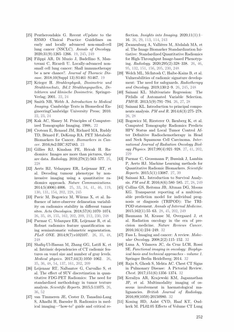
[25] Pentheroudakis G. Recent eUpdate to theESMO Clinical Practice Guidelines onearly and locally advanced non-small-celllung cancer (NSCLC). Annals of Oncology.2020;31(9):1265–1266. 19, 245, 249
[26] Filippi AR, Di Muzio J, Badellino S, Man-tovani C, Ricardi U. Locally-advanced non-small cell lung cancer: Shall immunotherapybe a new chance?. Journal of Thoracic Dis-ease. 2018;10(Suppl 13):S1461–S1467. 19
[27] Krieger H. Strahlenphysik, Dosimetrie undStrahlenschutz, Bd.2 Strahlungsquellen, De-tektoren und klinische Dosimetrie. Springer-Verlag; 2001. 22, 24
[28] Smith NB, Webb A. Introduction to MedicalImaging. Cambridge Texts in Biomedical En-gineeringCambridge University Press; 2010.22, 23, 24
[29] Kak AC, Slaney M. Principles of Computer-ized Tomographic Imaging. 1988;. 22
[30] Croteau E, Renaud JM, Richard MA, RuddyTD, Bénard F, DeKemp RA. PET MetabolicBiomarkers for Cancer. Biomarkers in Can-cer. 2016;8s2:BIC.S27483. 23
[31] Gillies RJ, Kinahan PE, Hricak H. Ra-diomics: Images are more than pictures, theyare data. Radiology. 2016;278(2):563–577. 25,228
[32] Aerts HJ, Velazquez ER, Leijenaar RT, etal. Decoding tumour phenotype by non-invasive imaging using a quantitative ra-diomics approach. Nature Communications.2014;5(4006):4006. 25, 33, 34, 41, 46, 119,130, 131, 154, 202, 228, 245
[33] Pavic M, Bogowicz M, Würms X, et al. In-fluence of inter-observer delineation variabil-ity on radiomics stability in different tumorsites. Acta Oncologica. 2018;57(8):1070–1074.26, 35, 48, 155, 162, 202, 209, 212, 230, 248
[34] Parmar C, Velazquez ER, Leijenaar R, et al.Robust radiomics feature quantification us-ing semiautomatic volumetric segmentation.PLoS ONE. 2014;9(7):e102107. 26, 35, 48,248
[35] Shafiq-Ul-Hassan M, Zhang GG, Latifi K, etal. Intrinsic dependencies of CT radiomic fea-tures on voxel size and number of gray levels.Medical physics. 2017;44(3):1050–1062. 26,35, 36, 48, 54, 137, 161, 202, 209
[36] Leijenaar RT, Nalbantov G, Carvalho S, etal. The effect of SUV discretization in quan-titative FDG-PET Radiomics: The need forstandardized methodology in tumor textureanalysis. Scientific Reports. 2015;5:11075. 26,36, 52
[37] van Timmeren JE, Cester D, Tanadini-LangS, Alkadhi H, Baessler B. Radiomics in med-ical imaging—“how-to” guide and critical re-
flection. Insights into Imaging. 2020;11(1):1–16. 26, 29, 113, 114, 243
[38] Zwanenburg A, Vallières M, Abdalah MA, etal. The Image Biomarker Standardization Ini-tiative: Standardized Quantitative Radiomicsfor High-Throughput Image-based Phenotyp-ing. Radiology. 2020;295(2):328–338. 26, 46,95, 132, 151, 156, 205, 230, 248
[39] Welch ML, McIntosh C, Haibe-Kains B, et al.Vulnerabilities of radiomic signature develop-ment: The need for safeguards. Radiotherapyand Oncology. 2019;130:2–9. 26, 245, 248
[40] Sainani KL. Multivariate Regression: ThePitfalls of Automated Variable Selection.PM&R. 2013;5(9):791–794. 26, 27, 28
[41] Sainani KL. Introduction to principal compo-nents analysis. PM and R. 2014;6(3):275–278.26, 28
[42] Bogowicz M, Riesterer O, Ikenberg K, et al.Computed Tomography Radiomics PredictsHPV Status and Local Tumor Control Af-ter Definitive Radiochemotherapy in Headand Neck Squamous Cell Carcinoma. Inter-national Journal of Radiation Oncology Biol-ogy Physics. 2017;99(4):921–928. 27, 41, 202,229
[43] Parmar C, Grossmann P, Bussink J, LambinP, Aerts HJ. Machine Learning methods forQuantitative Radiomic Biomarkers. ScientificReports. 2015;5(1):13087. 27, 39
[44] Sainani KL. Introduction to Survival Analy-sis. PM and R. 2016;8(6):580–585. 27, 28, 249
[45] Collins GS, Reitsma JB, Altman DG, MoonsKG. Transparent reporting of a multivari-able prediction model for individual prog-nosis or diagnosis (TRIPOD): The TRI-POD statement. Annals of Internal Medicine.2015;162(1):55–63. 28, 45, 202, 249
[46] Baumann M, Krause M, Overgaard J, etal. Radiation oncology in the era of pre-cision medicine. Nature Reviews Cancer.2016;16(4):234–249. 32
[47] Fass L. Imaging and cancer: A review. Molec-ular Oncology. 2008;2(2):115–152. 32
[48] Luna A, Vilanova JC, da Cruz LCH, RossiSE. Functional imaging in oncology: Biophys-ical basis and technical approaches - volume 1.Springer Berlin Heidelberg; 2014. 32
[49] Raju S, Ghosh S, Mehta AC. Chest CT Signsin Pulmonary Disease: A Pictorial Review.Chest. 2017;151(6):1356–1374. 32
[50] Keraliya AR, Krajewski KM, JagannathanJP, et al. Multimodality imaging of os-seous involvement in haematological ma-lignancies. British Journal of Radiology.2016;89(1059):20150980. 32
[51] Koning HD, Aalst CVD, Haaf KT, Oud-kerk M. PL02.05 Effects of Volume CT Lung
252

REFERENCES
Cancer Screening: Mortality Results of theNELSON Randomised-Controlled PopulationBased Trial. Journal of Thoracic Oncology.2018;13(10):S185. 32
[52] Jemal A, Fedewa SA. Lung cancer screeningwith low-dose computed tomography in theUnited States - 2010 to 2015. JAMA Oncol-ogy. 2017;3(9):1278–1281. 32
[53] Semaan H, Bazerbashi MF, Siesel G, AldingerP, Obri T. Diagnostic accuracy of non-contrast abdominal CT scans performed asfollow-up for patients with an established can-cer diagnosis: a retrospective study. Acta On-cologica. 2018;57(3):426–430. 32
[54] Dejaco D, Steinbichler T, Schartinger VH, etal. Prognostic value of tumor volume in pa-tients with head and neck squamous cell car-cinoma treated with primary surgery. Headand Neck. 2018;40(4):728–739. 32
[55] Takenaka T, Yamazaki K, Miura N, Mori R,Takeo S. The prognostic impact of tumor vol-ume in patients with clinical stage IA non-small cell lung cancer. Journal of ThoracicOncology. 2016;11(7):1074–1080. 32
[56] Kuo CFJ, Ke BH, Wu NY, Kuo J, Hsu HH.Prognostic value of tumor volume for pa-tients with advanced lung cancer treated withchemotherapy. Computer Methods and Pro-grams in Biomedicine. 2017;144:165–177. 32
[57] Dubben HH, Thames HD, Beck-BornholdtHP. Tumor volume: A basic and specific re-sponse predictor in radiotherapy. Radiother-apy and Oncology. 1998;47(2):167–174. 33
[58] van Timmeren JE, Leijenaar RTH, van ElmptW, et al. Test–Retest Data for RadiomicsFeature Stability Analysis: Generalizable orStudy-Specific?. Tomography. 2016;2(4):361–365. 33, 48
[59] Trotman J, Luminari S, Boussetta S, et al.Prognostic value of PET-CT after fi rst-linetherapy in patients with follicular lymphoma:A pooled analysis of central scan review inthree multicentre studies. The Lancet Haema-tology. 2014;1(1):e17–e27. 33, 45
[60] Kitajima K, Doi H, Kuribayashi K, et al.Prognostic value of pretreatment volume-based quantitative 18F-FDG PET/CT pa-rameters in patients with malignant pleuralmesothelioma. European Journal of Radiol-ogy. 2017;86:176–183. 33, 45
[61] Stolzenburg A, Lückerath K, Samnick S, etal. Prognostic value of [18F]FDG-PET/CTin multiple myeloma patients before and af-ter allogeneic hematopoietic cell transplanta-tion. European Journal of Nuclear Medicineand Molecular Imaging. 2018;45(10):1694–1704. 33
[62] Lawal IO, Ankrah AO, Mokoala KM, et al.
Prognostic Value of Pre-treatment F-18 FDGPET Metabolic Metrics in Patients with Lo-cally Advanced Carcinoma of the Anus withand without HIV Infection. NuklearMedizin.2018;57(5):190–197. 33
[63] Liu J, Dong M, Sun X, Li W, Xing L, YuJ. Prognostic value of 18F-FDG PET/CT insurgical non-small cell lung cancer: A meta-analysis. PLoS ONE. 2016;11(1):e0146195. 33
[64] Albano D, Familiari D, Gentile R, etal. Clinical and prognostic value of 18F-FDG-PET/CT in restaging of pancreaticcancer. Nuclear Medicine Communications.2018;39(8):741–746. 33
[65] Ogawa S, Itabashi M, Kondo C, Momose M,Sakai S, Kameoka S. Prognostic Value of To-tal Lesion Glycolysis Measured by 18F-FDG-PET/CT in Patients with Colorectal Cancer.Anticancer research. 2015;35(6):3495—3500.33
[66] Torizuka T, Tanizaki Y, Kanno T, et al.Prognostic Value ofl8F-FDG PET in pa-tients with head and neck squamous cellcancer. American Journal of Roentgenology.2009;192(4):W156—-60. 33, 45
[67] Moons KG, Royston P, Vergouwe Y, GrobbeeDE, Altman DG. Prognosis and prognosticresearch: What, why, and how?. BMJ (On-line). 2009;338(7706):1317–1320. 33, 131
[68] Steenbakkers RJHM, Duppen JC, Fitton I,et al. Reduction of observer variation us-ing matched CT-PET for lung cancer delin-eation: A three-dimensional analysis. Inter-national Journal of Radiation Oncology Biol-ogy Physics. 2006;64(2):435–448. 33
[69] Burrell RA, McGranahan N, Bartek J, Swan-ton C. The causes and consequences of ge-netic heterogeneity in cancer evolution. Na-ture. 2013;501(7467):338–345. 33, 130
[70] Chicklore S, Goh V, Siddique M, Roy A,Marsden PK, Cook GJ. Quantifying tumourheterogeneity in 18F-FDG PET/CT imag-ing by texture analysis. European Journalof Nuclear Medicine and Molecular Imaging.2013;40(1):133–140. 33, 130
[71] Toma-Dasu I, Uhrdin J, Lazzeroni M,et al. Evaluating tumor response of non-small cell lung cancer patients with 18F-fludeoxyglucose positron emission tomogra-phy: Potential for treatment individualiza-tion. International Journal of Radiation On-cology Biology Physics. 2015;91(2):376–384.
[72] Lee G, Lee HY, Park H, et al. Radiomicsand its emerging role in lung cancer research,imaging biomarkers and clinical management:State of the art. European Journal of Radiol-ogy. 2017;86:297–307. 130, 131
[73] Coroller TP, Agrawal V, Narayan V, et al.
253

Radiomic phenotype features predict patho-logical response in non-small cell Radiomicpredicts pathological response lung cancer.Radiotherapy and Oncology. 2016;119(3):480–486. 228
[74] Thakur MK, Gadgeel SM. Predictive andPrognostic Biomarkers in Non-Small CellLung Cancer. Seminars in Respiratory andCritical Care Medicine. 2016;37(5):760–770.
[75] Sollini M, Cozzi L, Antunovic L, Chiti A,Kirienko M. PET Radiomics in NSCLC:State of the art and a proposal for harmo-nization of methodology. Scientific Reports.2017;7(1):358. 130, 136
[76] Lambin P, Leijenaar RT, Deist TM, et al.Radiomics: The bridge between medicalimaging and personalized medicine. NatureReviews Clinical Oncology. 2017;14(12):749–762. number: 12 publisher: Nature Publish-ing Group. 33, 60, 228
[77] Rao AR, Lohse GL. Identifying High LevelFeatures of Texture Perception. CVGIP:Graphical Models and Image Processing.1993;55(3):218–233. 34
[78] Materka A. Texture analysis methodologiesfor magnetic resonance imaging. Dialogues inClinical Neuroscience. 2004;6(2):243–250. 34
[79] Pfaehler E, Beukinga RJ, de Jong JR, et al.Repeatability of 18F-FDG PET radiomic fea-tures: A phantom study to explore sensitiv-ity to image reconstruction settings, noise,and delineation method. Medical Physics.2019;46(2):665–678. 35, 51, 54
[80] Zhao B, Tan Y, Tsai WY, et al. Repro-ducibility of radiomics for deciphering tumorphenotype with imaging. Scientific Reports.2016;6:23428. 35, 49, 161, 202, 208
[81] Tanaka S, Kadoya N, Kajikawa T, et al. In-vestigation of thoracic four-dimensional CT-based dimension reduction technique for ex-tracting the robust radiomic features. PhysicaMedica. 2019;58:141–148. 35, 49
[82] Hu P, Wang J, Zhong H, et al. Reproducibilitywith repeat CT in radiomics study for rectalcancer. Oncotarget. 2016;7(44):71440–71446.48
[83] van Velden FH, Kramer GM, Frings V, et al.Repeatability of Radiomic Features in Non-Small-Cell Lung Cancer [18F]FDG-PET/CTStudies: Impact of Reconstruction and De-lineation. Molecular Imaging and Biology.2016;18(5):788–795. 35, 51, 131, 155
[84] Leijenaar RT, Carvalho S, Velazquez ER,et al. Stability of FDG-PET Radiomics fea-tures: An integrated analysis of test-retestand inter-observer variability. Acta Oncolog-ica. 2013;52(7):1391–1397. 35, 36, 52, 131,136
[85] Oliver JA, Budzevich M, Zhang GG, DillingTJ, Latifi K, Moros EG. Variability ofimage features computed from conven-tional and respiratory-gated PET/CT im-ages of lung cancer. Translational Oncology.2015;8(6):524–534. 35, 49, 53, 137, 202, 208,234, 246
[86] Bogowicz M, Riesterer O, Bundschuh RA, etal. Stability of radiomic features in CT perfu-sion maps. Physics in Medicine and Biology.2016;61(24):8736–8749. 35, 50
[87] Yip SS, Parmar C, Kim J, Huynh E, MakRH, Aerts HJ. Impact of experimental designon PET radiomics in predicting somatic mu-tation status. European Journal of Radiology.2017;97:8–15. PMID: 29153372. 35, 36, 52,57, 75, 80
[88] Shafiq-ul Hassan M, Zhang GG, Hunt DC,et al. Accounting for reconstruction kernel-induced variability in CT radiomic featuresusing noise power spectra. Journal of MedicalImaging. 2017;5(01):1. 35, 49, 161, 246
[89] Gallivanone F, Interlenghi M, D’AmbrosioD, Trifirò G, Castiglioni I. Parameters Influ-encing PET Imaging Features: A PhantomStudy with Irregular and Heterogeneous Syn-thetic Lesions. Contrast Media & MolecularImaging. 2018;2018:1-12. 35, 51, 54
[90] Shiri I, Rahmim A, Ghaffarian P, GeramifarP, Abdollahi H, Bitarafan-Rajabi A. The im-pact of image reconstruction settings on 18F-FDG PET radiomic features: multi-scannerphantom and patient studies. European Radi-ology. 2017;27(11):4498–4509. 51
[91] Altazi BA, Zhang GG, Fernandez DC, et al.Reproducibility of F18-FDG PET radiomicfeatures for different cervical tumor segmen-tation methods, gray-level discretization, andreconstruction algorithms. Journal of AppliedClinical Medical Physics. 2017;18(6):32–48.35, 36, 52
[92] Kalpathy-Cramer J, Mamomov A, Zhao B,et al. Radiomics of Lung Nodules: A Multi-Institutional Study of Robustness and Agree-ment of Quantitative Imaging Features. To-mography. 2016;2(4):430–437. 35, 48
[93] Ger RB, Zhou S, Chi PCM, et al. Compre-hensive Investigation on Controlling for CTImaging Variabilities in Radiomics Studies.Scientific Reports. 2018;8(1):13047. 35, 50,54, 204, 208, 209, 229, 234
[94] Reuzé S, Orlhac F, Chargari C, et al. Predic-tion of cervical cancer recurrence using tex-tural features extracted from 18F-FDG PETimages acquired with different scanners. On-cotarget. 2017;8(26):43169–43179. 35, 53
[95] MacKin D, Ger R, Dodge C, et al. Ef-fect of tube current on computed tomog-
254

REFERENCES
raphy radiomic features. Scientific Reports.2018;8(1):2354. 35, 49
[96] Galavis PE, Hollensen C, Jallow N, PaliwalB, Jeraj R. Variability of textural features inFDG PET images due to different acquisitionmodes and reconstruction parameters. ActaOncologica. 2010;49(7):1012–1016. 35, 155
[97] Larue RT, van Timmeren JE, de Jong EE, etal. Influence of gray level discretization on ra-diomic feature stability for different CT scan-ners, tube currents and slice thicknesses: acomprehensive phantom study. Acta Oncolog-ica. 2017;56(11):1544–1553. 36, 48, 202, 230
[98] Presotto L, Bettinardi V, De Bernardi E, etal. PET textural features stability and pat-tern discrimination power for radiomics anal-ysis: An “ad-hoc” phantoms study. PhysicaMedica. 2018;50:66–74. 36, 53
[99] Hatt M, Tixier F, Pierce L, Kinahan PE,Rest CCL, Visvikis D. Characterization ofPET/CT images using texture analysis: thepast, the present. . . any future?. EuropeanJournal of Nuclear Medicine and MolecularImaging. 2017;44(1):151–165. 36, 154
[100] Yi X, Guan X, Zhang Y, et al. Radiomics im-proves efficiency for differentiating subclini-cal pheochromocytoma from lipid-poor ade-noma: a predictive, preventive and personal-ized medical approach in adrenal incidentalo-mas. EPMA Journal. 2018;9(4):421–429. 37
[101] Ji GW, Zhu FP, Zhang YD, et al. A radiomicsapproach to predict lymph node metastasisand clinical outcome of intrahepatic cholan-giocarcinoma. European Radiology. 2019;. 37
[102] Cha KH, Hadjiiski L, Chan HP, et al. Blad-der Cancer Treatment Response Assessmentin CT using Radiomics with Deep-Learning.Scientific Reports. 2017;7(1):8738. 37, 55
[103] Ding J, Xing Z, Jiang Z, et al. CT-based ra-diomic model predicts high grade of clear cellrenal cell carcinoma. European Journal of Ra-diology. 2018;103:51–56. 37
[104] Sun X, Liu L, Xu K, et al. Prediction ofISUP grading of clear cell renal cell carcinomausing support vector machine model basedon CT images. Medicine (United States).2019;98(14):e15022. 37
[105] Huang Y, He L, Dong D, et al. Individualizedprediction of perineural invasion in colorectalcancer: development and validation of a ra-diomics prediction model. Chinese Journal ofCancer Research. 2018;30(1):40–50. 37
[106] Sun R, Limkin EJ, Vakalopoulou M, et al.A radiomics approach to assess tumour-infiltrating CD8 cells and response toanti-PD-1 or anti-PD-L1 immunother-apy: an imaging biomarker, retrospective
multicohort study. The Lancet Oncology.2018;19(9):1180–1191. 37
[107] Larue RT, Klaassen R, Jochems A, et al.Pre-treatment CT radiomics to predict 3-year overall survival following chemoradio-therapy of esophageal cancer. Acta Oncolog-ica. 2018;57(11):1475–1481. 37
[108] Shen C, Liu Z, Wang Z, et al. Building CTRadiomics Based Nomogram for Preopera-tive Esophageal Cancer Patients Lymph NodeMetastasis Prediction. Translational Oncol-ogy. 2018;11(3):815–824. 37, 41, 46
[109] Wu L, Wang C, Tan X, et al. Radiomicsapproach for preoperative identification ofstages I-II and III-IV of esophageal can-cer. Chinese Journal of Cancer Research.2018;30(4):396–405. 37
[110] Tan X, Ma Z, Yan L, Ye W, Liu Z, Liang C.Radiomics nomogram outperforms size crite-ria in discriminating lymph node metastasisin resectable esophageal squamous cell car-cinoma. European Radiology. 2019;29(1):392–400. 37
[111] Feng QX, Liu C, Qi L, et al. An IntelligentClinical Decision Support System for Preop-erative Prediction of Lymph Node Metastasisin Gastric Cancer. Journal of the AmericanCollege of Radiology. 2019;16(7):952–960. 37
[112] Chen T, Ning Z, Xu L, et al. Radiomics nomo-gram for predicting the malignant potentialof gastrointestinal stromal tumours preopera-tively. European Radiology. 2019;29(3):1074–1082. 37
[113] Ning Z, Luo J, Li Y, et al. Pattern classi-fication for gastrointestinal stromal tumorsby integration of radiomics and deep convo-lutional features. IEEE Journal of Biomedi-cal and Health Informatics. 2019;23(3):1181–1191. 37
[114] Leijenaar RT, Bogowicz M, Jochems A, etal. Development and validation of a ra-diomic signature to predict HPV (p16) sta-tus from standard CT imaging: A multi-center study. British Journal of Radiology.2018;91(1086):20170498. 37, 41, 229, 234
[115] Head MDACC, Reports NQIWG%S. Investi-gation of radiomic signatures for local recur-rence using primary tumor texture analysis inoropharyngeal head and neck cancer patients.Scientific Reports. 2018;8(1):1524. 38, 41
[116] Bogowicz M, Vuong D, Huellner MW, et al.CT radiomics and PET radiomics: Ready forclinical implementation?. Quarterly Journalof Nuclear Medicine and Molecular Imaging.2019;63(4):355–370. 38, 154, 202, 228, 243
[117] Parmar C, Leijenaar RT, Grossmann P, etal. Radiomic feature clusters and PrognosticSignatures specific for Lung and Head &neck
255
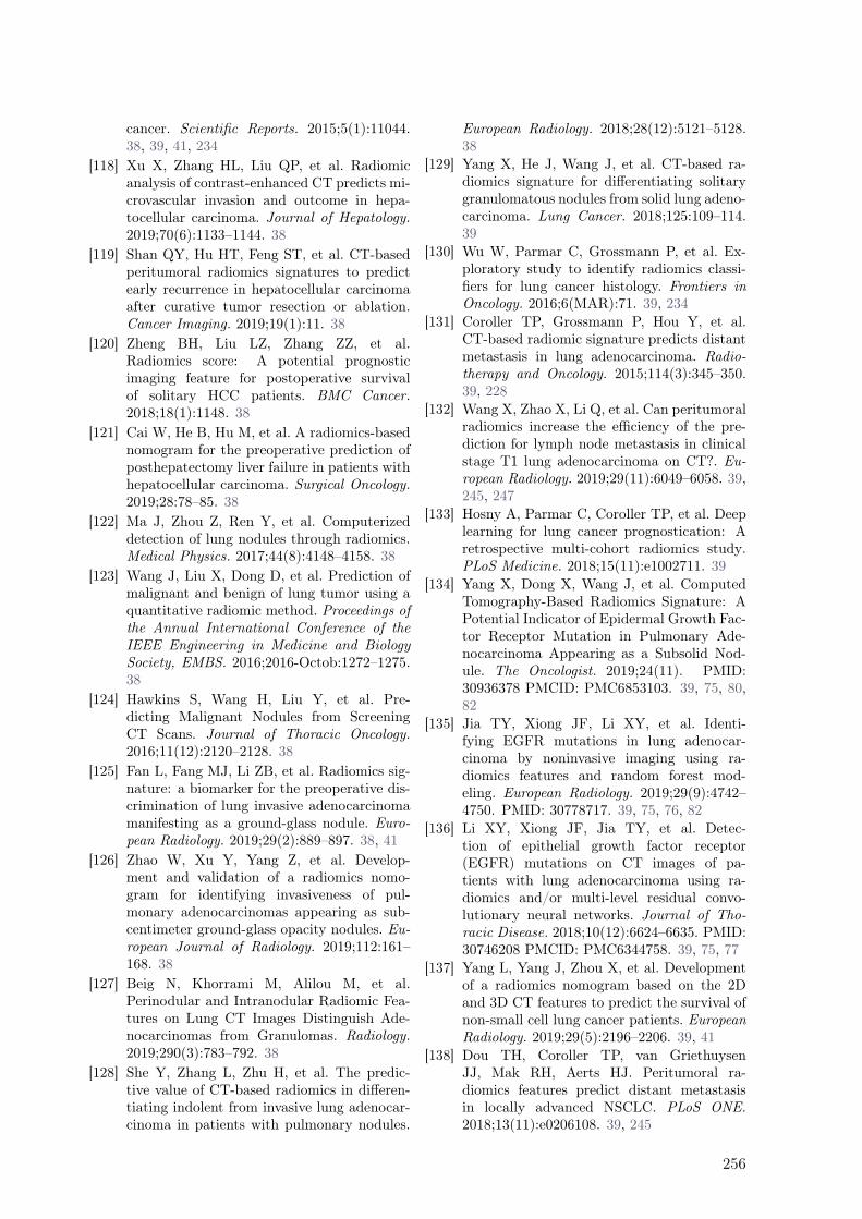
cancer. Scientific Reports. 2015;5(1):11044.38, 39, 41, 234
[118] Xu X, Zhang HL, Liu QP, et al. Radiomicanalysis of contrast-enhanced CT predicts mi-crovascular invasion and outcome in hepa-tocellular carcinoma. Journal of Hepatology.2019;70(6):1133–1144. 38
[119] Shan QY, Hu HT, Feng ST, et al. CT-basedperitumoral radiomics signatures to predictearly recurrence in hepatocellular carcinomaafter curative tumor resection or ablation.Cancer Imaging. 2019;19(1):11. 38
[120] Zheng BH, Liu LZ, Zhang ZZ, et al.Radiomics score: A potential prognosticimaging feature for postoperative survivalof solitary HCC patients. BMC Cancer.2018;18(1):1148. 38
[121] Cai W, He B, Hu M, et al. A radiomics-basednomogram for the preoperative prediction ofposthepatectomy liver failure in patients withhepatocellular carcinoma. Surgical Oncology.2019;28:78–85. 38
[122] Ma J, Zhou Z, Ren Y, et al. Computerizeddetection of lung nodules through radiomics.Medical Physics. 2017;44(8):4148–4158. 38
[123] Wang J, Liu X, Dong D, et al. Prediction ofmalignant and benign of lung tumor using aquantitative radiomic method. Proceedings ofthe Annual International Conference of theIEEE Engineering in Medicine and BiologySociety, EMBS. 2016;2016-Octob:1272–1275.38
[124] Hawkins S, Wang H, Liu Y, et al. Pre-dicting Malignant Nodules from ScreeningCT Scans. Journal of Thoracic Oncology.2016;11(12):2120–2128. 38
[125] Fan L, Fang MJ, Li ZB, et al. Radiomics sig-nature: a biomarker for the preoperative dis-crimination of lung invasive adenocarcinomamanifesting as a ground-glass nodule. Euro-pean Radiology. 2019;29(2):889–897. 38, 41
[126] Zhao W, Xu Y, Yang Z, et al. Develop-ment and validation of a radiomics nomo-gram for identifying invasiveness of pul-monary adenocarcinomas appearing as sub-centimeter ground-glass opacity nodules. Eu-ropean Journal of Radiology. 2019;112:161–168. 38
[127] Beig N, Khorrami M, Alilou M, et al.Perinodular and Intranodular Radiomic Fea-tures on Lung CT Images Distinguish Ade-nocarcinomas from Granulomas. Radiology.2019;290(3):783–792. 38
[128] She Y, Zhang L, Zhu H, et al. The predic-tive value of CT-based radiomics in differen-tiating indolent from invasive lung adenocar-cinoma in patients with pulmonary nodules.
European Radiology. 2018;28(12):5121–5128.38
[129] Yang X, He J, Wang J, et al. CT-based ra-diomics signature for differentiating solitarygranulomatous nodules from solid lung adeno-carcinoma. Lung Cancer. 2018;125:109–114.39
[130] Wu W, Parmar C, Grossmann P, et al. Ex-ploratory study to identify radiomics classi-fiers for lung cancer histology. Frontiers inOncology. 2016;6(MAR):71. 39, 234
[131] Coroller TP, Grossmann P, Hou Y, et al.CT-based radiomic signature predicts distantmetastasis in lung adenocarcinoma. Radio-therapy and Oncology. 2015;114(3):345–350.39, 228
[132] Wang X, Zhao X, Li Q, et al. Can peritumoralradiomics increase the efficiency of the pre-diction for lymph node metastasis in clinicalstage T1 lung adenocarcinoma on CT?. Eu-ropean Radiology. 2019;29(11):6049–6058. 39,245, 247
[133] Hosny A, Parmar C, Coroller TP, et al. Deeplearning for lung cancer prognostication: Aretrospective multi-cohort radiomics study.PLoS Medicine. 2018;15(11):e1002711. 39
[134] Yang X, Dong X, Wang J, et al. ComputedTomography-Based Radiomics Signature: APotential Indicator of Epidermal Growth Fac-tor Receptor Mutation in Pulmonary Ade-nocarcinoma Appearing as a Subsolid Nod-ule. The Oncologist. 2019;24(11). PMID:30936378 PMCID: PMC6853103. 39, 75, 80,82
[135] Jia TY, Xiong JF, Li XY, et al. Identi-fying EGFR mutations in lung adenocar-cinoma by noninvasive imaging using ra-diomics features and random forest mod-eling. European Radiology. 2019;29(9):4742–4750. PMID: 30778717. 39, 75, 76, 82
[136] Li XY, Xiong JF, Jia TY, et al. Detec-tion of epithelial growth factor receptor(EGFR) mutations on CT images of pa-tients with lung adenocarcinoma using ra-diomics and/or multi-level residual convo-lutionary neural networks. Journal of Tho-racic Disease. 2018;10(12):6624–6635. PMID:30746208 PMCID: PMC6344758. 39, 75, 77
[137] Yang L, Yang J, Zhou X, et al. Developmentof a radiomics nomogram based on the 2Dand 3D CT features to predict the survival ofnon-small cell lung cancer patients. EuropeanRadiology. 2019;29(5):2196–2206. 39, 41
[138] Dou TH, Coroller TP, van GriethuysenJJ, Mak RH, Aerts HJ. Peritumoral ra-diomics features predict distant metastasisin locally advanced NSCLC. PLoS ONE.2018;13(11):e0206108. 39, 245
256
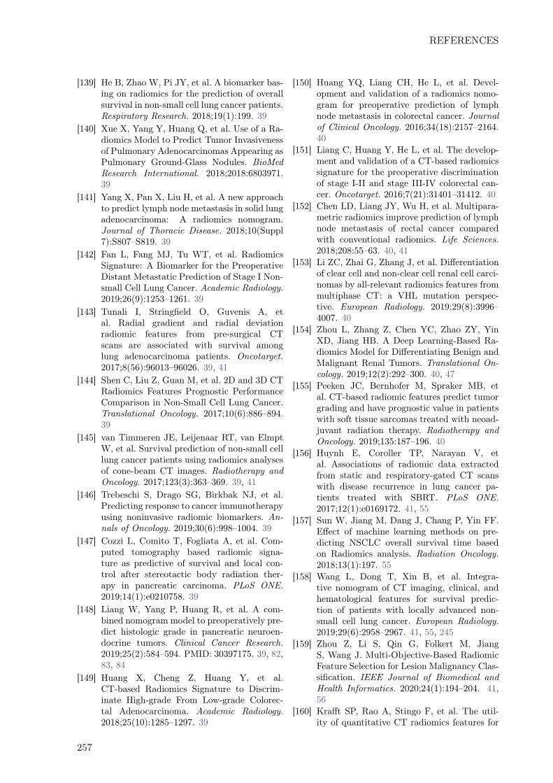
REFERENCES
[139] He B, Zhao W, Pi JY, et al. A biomarker bas-ing on radiomics for the prediction of overallsurvival in non-small cell lung cancer patients.Respiratory Research. 2018;19(1):199. 39
[140] Xue X, Yang Y, Huang Q, et al. Use of a Ra-diomics Model to Predict Tumor Invasivenessof Pulmonary Adenocarcinomas Appearing asPulmonary Ground-Glass Nodules. BioMedResearch International. 2018;2018:6803971.39
[141] Yang X, Pan X, Liu H, et al. A new approachto predict lymph node metastasis in solid lungadenocarcinoma: A radiomics nomogram.Journal of Thoracic Disease. 2018;10(Suppl7):S807–S819. 39
[142] Fan L, Fang MJ, Tu WT, et al. RadiomicsSignature: A Biomarker for the PreoperativeDistant Metastatic Prediction of Stage I Non-small Cell Lung Cancer. Academic Radiology.2019;26(9):1253–1261. 39
[143] Tunali I, Stringfield O, Guvenis A, etal. Radial gradient and radial deviationradiomic features from pre-surgical CTscans are associated with survival amonglung adenocarcinoma patients. Oncotarget.2017;8(56):96013–96026. 39, 41
[144] Shen C, Liu Z, Guan M, et al. 2D and 3D CTRadiomics Features Prognostic PerformanceComparison in Non-Small Cell Lung Cancer.Translational Oncology. 2017;10(6):886–894.39
[145] van Timmeren JE, Leijenaar RT, van ElmptW, et al. Survival prediction of non-small celllung cancer patients using radiomics analysesof cone-beam CT images. Radiotherapy andOncology. 2017;123(3):363–369. 39, 41
[146] Trebeschi S, Drago SG, Birkbak NJ, et al.Predicting response to cancer immunotherapyusing noninvasive radiomic biomarkers. An-nals of Oncology. 2019;30(6):998–1004. 39
[147] Cozzi L, Comito T, Fogliata A, et al. Com-puted tomography based radiomic signa-ture as predictive of survival and local con-trol after stereotactic body radiation ther-apy in pancreatic carcinoma. PLoS ONE.2019;14(1):e0210758. 39
[148] Liang W, Yang P, Huang R, et al. A com-bined nomogram model to preoperatively pre-dict histologic grade in pancreatic neuroen-docrine tumors. Clinical Cancer Research.2019;25(2):584–594. PMID: 30397175. 39, 82,83, 84
[149] Huang X, Cheng Z, Huang Y, et al.CT-based Radiomics Signature to Discrim-inate High-grade From Low-grade Colorec-tal Adenocarcinoma. Academic Radiology.2018;25(10):1285–1297. 39
[150] Huang YQ, Liang CH, He L, et al. Devel-opment and validation of a radiomics nomo-gram for preoperative prediction of lymphnode metastasis in colorectal cancer. Journalof Clinical Oncology. 2016;34(18):2157–2164.40
[151] Liang C, Huang Y, He L, et al. The develop-ment and validation of a CT-based radiomicssignature for the preoperative discriminationof stage I-II and stage III-IV colorectal can-cer. Oncotarget. 2016;7(21):31401–31412. 40
[152] Chen LD, Liang JY, Wu H, et al. Multipara-metric radiomics improve prediction of lymphnode metastasis of rectal cancer comparedwith conventional radiomics. Life Sciences.2018;208:55–63. 40, 41
[153] Li ZC, Zhai G, Zhang J, et al. Differentiationof clear cell and non-clear cell renal cell carci-nomas by all-relevant radiomics features frommultiphase CT: a VHL mutation perspec-tive. European Radiology. 2019;29(8):3996–4007. 40
[154] Zhou L, Zhang Z, Chen YC, Zhao ZY, YinXD, Jiang HB. A Deep Learning-Based Ra-diomics Model for Differentiating Benign andMalignant Renal Tumors. Translational On-cology. 2019;12(2):292–300. 40, 47
[155] Peeken JC, Bernhofer M, Spraker MB, etal. CT-based radiomic features predict tumorgrading and have prognostic value in patientswith soft tissue sarcomas treated with neoad-juvant radiation therapy. Radiotherapy andOncology. 2019;135:187–196. 40
[156] Huynh E, Coroller TP, Narayan V, etal. Associations of radiomic data extractedfrom static and respiratory-gated CT scanswith disease recurrence in lung cancer pa-tients treated with SBRT. PLoS ONE.2017;12(1):e0169172. 41, 55
[157] Sun W, Jiang M, Dang J, Chang P, Yin FF.Effect of machine learning methods on pre-dicting NSCLC overall survival time basedon Radiomics analysis. Radiation Oncology.2018;13(1):197. 55
[158] Wang L, Dong T, Xin B, et al. Integra-tive nomogram of CT imaging, clinical, andhematological features for survival predic-tion of patients with locally advanced non-small cell lung cancer. European Radiology.2019;29(6):2958–2967. 41, 55, 245
[159] Zhou Z, Li S, Qin G, Folkert M, JiangS, Wang J. Multi-Objective-Based RadiomicFeature Selection for Lesion Malignancy Clas-sification. IEEE Journal of Biomedical andHealth Informatics. 2020;24(1):194–204. 41,56
[160] Krafft SP, Rao A, Stingo F, et al. The util-ity of quantitative CT radiomics features for
257

improved prediction of radiation pneumoni-tis. Medical Physics. 2018;45(11):5317–5324.41, 55, 245
[161] Cunliffe A, Armato SG, Castillo R, PhamN, Guerrero T, Al-Hallaq HA. Lung tex-ture in serial thoracic computed tomographyscans: Correlation of radiomics-based fea-tures with radiation therapy dose and ra-diation pneumonitis development. Interna-tional Journal of Radiation Oncology BiologyPhysics. 2015;91(5):1048–1056. 41, 56, 245
[162] Bogowicz M, Riesterer O, Stark LS, et al.Comparison of PET and CT radiomics forprediction of local tumor control in head andneck squamous cell carcinoma. Acta Oncolog-ica. 2017;56(11):1531–1536. 41, 44, 45, 202,238
[163] Ou D, Blanchard P, Rosellini S, et al. Pre-dictive and prognostic value of CT based ra-diomics signature in locally advanced headand neck cancers patients treated with con-current chemoradiotherapy or bioradiother-apy and its added value to Human Papillo-mavirus status. Oral Oncology. 2017;71:150–155. 41, 55
[164] Folkert MR, Setton J, Apte AP, et al.Predictive modeling of outcomes followingdefinitive chemoradiotherapy for oropharyn-geal cancer based on FDG-PET image char-acteristics. Physics in Medicine and Biology.2017;62(13):5327–5343. 42
[165] Bogowicz M, Leijenaar RT, Tanadini-Lang S,et al. Post-radiochemotherapy PET radiomicsin head and neck cancer – The influence of ra-diomics implementation on the reproducibil-ity of local control tumor models. Radiother-apy and Oncology. 2017;125(3):385–391. 42,205, 249
[166] Foley KG, Shi Z, Whybra P, et al. Exter-nal validation of a prognostic model incor-porating quantitative PET image features inoesophageal cancer. Radiotherapy and Oncol-ogy. 2019;133:205–212. 42, 43
[167] Mattonen SA, Davidzon GA, Bakr S, etal. 18F] FDG Positron Emission Tomogra-phy (PET) Tumor and Penumbra ImagingFeatures Predict Recurrence in Non-SmallCell Lung Cancer. Tomography (Ann Arbor,Mich.). 2019;5(1):145–153. 42
[168] Arshad MA, Thornton A, Lu H, et al. Discov-ery of pre-therapy 2-deoxy-2- 18 F-fluoro-D-glucose positron emission tomography-basedradiomics classifiers of survival outcome innon-small-cell lung cancer patients. EuropeanJournal of Nuclear Medicine and MolecularImaging. 2019;46(2):455–466. 42
[169] Luo Y, McShan DL, Matuszak MM, et al.A multiobjective Bayesian networks approach
for joint prediction of tumor local control andradiation pneumonitis in nonsmall-cell lungcancer (NSCLC) for response-adapted radio-therapy. Medical Physics. 2018;45(8):3980–3995. 42, 43
[170] Carvalho S, Leijenaar RTH, Troost EGC, etal. 18F-fluorodeoxyglucose positron-emissiontomography (FDG- PET)-Radiomics ofmetastatic lymph nodes and primary tumorin non-small cell lung cancer (NSCLC) – Aprospective externally validated study. PLoSONE. 2018;13(3):e0192859. 42
[171] Leger S, Zwanenburg A, Pilz K, et al. Acomparative study of machine learning meth-ods for time-To-event survival data for ra-diomics risk modelling. Scientific Reports.2017;7(1):13206. 42, 43
[172] Kirienko M, Cozzi L, Rossi A, et al. Abil-ity of FDG PET and CT radiomics fea-tures to differentiate between primary andmetastatic lung lesions. European Journalof Nuclear Medicine and Molecular Imaging.2018;45(10):1649–1660. 42
[173] Jiang Y, Yuan Q, Lv W, et al. Radiomic sig-nature of 18F fluorodeoxyglucose PET/CTfor prediction of gastric cancer survivaland chemotherapeutic benefits. Theranostics.2018;8(21):5915–5928. 42
[174] Lucia F, Visvikis D, Desseroit MC, etal. Prediction of outcome using pretreat-ment 18F-FDG PET/CT and MRI radiomicsin locally advanced cervical cancer treatedwith chemoradiotherapy. European Journalof Nuclear Medicine and Molecular Imaging.2018;45(5):768–786. 42
[175] Lucia F, Visvikis D, Vallières M, et al. Ex-ternal validation of a combined PET andMRI radiomics model for prediction of re-currence in cervical cancer patients treatedwith chemoradiotherapy. European Journalof Nuclear Medicine and Molecular Imaging.2019;46(4):864–877. 42, 247
[176] Schernberg A, Reuze S, Orlhac F, et al. Ascore combining baseline neutrophilia and pri-mary tumor SUVpeak measured from FDGPET is associated with outcome in locallyadvanced cervical cancer. European Journalof Nuclear Medicine and Molecular Imaging.2018;45(2):187–195. 42
[177] De Bernardi E, Buda A, Guerra L, et al. Ra-diomics of the primary tumour as a tool toimprove 18F-FDG-PET sensitivity in detect-ing nodal metastases in endometrial cancer.EJNMMI Research. 2018;8(1):86. 42
[178] Wolsztynski E, O’Sullivan F, Keyes E,O’Sullivan J, Eary JF. Positron emissiontomography-based assessment of metabolicgradient and other prognostic features
258
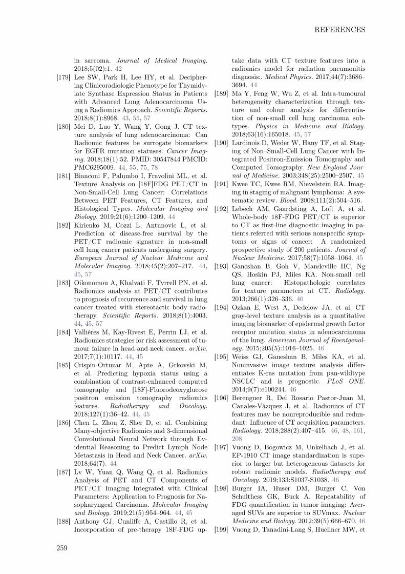
REFERENCES
in sarcoma. Journal of Medical Imaging.2018;5(02):1. 42
[179] Lee SW, Park H, Lee HY, et al. Decipher-ing Clinicoradiologic Phenotype for Thymidy-late Synthase Expression Status in Patientswith Advanced Lung Adenocarcinoma Us-ing a Radiomics Approach. Scientific Reports.2018;8(1):8968. 43, 55, 57
[180] Mei D, Luo Y, Wang Y, Gong J. CT tex-ture analysis of lung adenocarcinoma: CanRadiomic features be surrogate biomarkersfor EGFR mutation statuses. Cancer Imag-ing. 2018;18(1):52. PMID: 30547844 PMCID:PMC6295009. 44, 55, 75, 78
[181] Bianconi F, Palumbo I, Fravolini ML, et al.Texture Analysis on [18F]FDG PET/CT inNon-Small-Cell Lung Cancer: CorrelationsBetween PET Features, CT Features, andHistological Types. Molecular Imaging andBiology. 2019;21(6):1200–1209. 44
[182] Kirienko M, Cozzi L, Antunovic L, et al.Prediction of disease-free survival by thePET/CT radiomic signature in non-smallcell lung cancer patients undergoing surgery.European Journal of Nuclear Medicine andMolecular Imaging. 2018;45(2):207–217. 44,45, 57
[183] Oikonomou A, Khalvati F, Tyrrell PN, et al.Radiomics analysis at PET/CT contributesto prognosis of recurrence and survival in lungcancer treated with stereotactic body radio-therapy. Scientific Reports. 2018;8(1):4003.44, 45, 57
[184] Vallières M, Kay-Rivest E, Perrin LJ, et al.Radiomics strategies for risk assessment of tu-mour failure in head-and-neck cancer. arXiv.2017;7(1):10117. 44, 45
[185] Crispin-Ortuzar M, Apte A, Grkovski M,et al. Predicting hypoxia status using acombination of contrast-enhanced computedtomography and [18F]-Fluorodeoxyglucosepositron emission tomography radiomicsfeatures. Radiotherapy and Oncology.2018;127(1):36–42. 44, 45
[186] Chen L, Zhou Z, Sher D, et al. CombiningMany-objective Radiomics and 3-dimensionalConvolutional Neural Network through Ev-idential Reasoning to Predict Lymph NodeMetastasis in Head and Neck Cancer. arXiv.2018;64(7). 44
[187] Lv W, Yuan Q, Wang Q, et al. RadiomicsAnalysis of PET and CT Components ofPET/CT Imaging Integrated with ClinicalParameters: Application to Prognosis for Na-sopharyngeal Carcinoma. Molecular Imagingand Biology. 2019;21(5):954–964. 44, 45
[188] Anthony GJ, Cunliffe A, Castillo R, et al.Incorporation of pre-therapy 18F-FDG up-
take data with CT texture features into aradiomics model for radiation pneumonitisdiagnosis:. Medical Physics. 2017;44(7):3686–3694. 44
[189] Ma Y, Feng W, Wu Z, et al. Intra-tumouralheterogeneity characterization through tex-ture and colour analysis for differentia-tion of non-small cell lung carcinoma sub-types. Physics in Medicine and Biology.2018;63(16):165018. 45, 57
[190] Lardinois D, Weder W, Hany TF, et al. Stag-ing of Non–Small-Cell Lung Cancer with In-tegrated Positron-Emission Tomography andComputed Tomography. New England Jour-nal of Medicine. 2003;348(25):2500–2507. 45
[191] Kwee TC, Kwee RM, Nievelstein RA. Imag-ing in staging of malignant lymphoma: A sys-tematic review. Blood. 2008;111(2):504–516.
[192] Lebech AM, Gaardsting A, Loft A, et al.Whole-body 18F-FDG PET/CT is superiorto CT as first-line diagnostic imaging in pa-tients referred with serious nonspecific symp-toms or signs of cancer: A randomizedprospective study of 200 patients. Journal ofNuclear Medicine. 2017;58(7):1058–1064. 45
[193] Ganeshan B, Goh V, Mandeville HC, NgQS, Hoskin PJ, Miles KA. Non-small celllung cancer: Histopathologic correlatesfor texture parameters at CT. Radiology.2013;266(1):326–336. 46
[194] Ozkan E, West A, Dedelow JA, et al. CTgray-level texture analysis as a quantitativeimaging biomarker of epidermal growth factorreceptor mutation status in adenocarcinomaof the lung. American Journal of Roentgenol-ogy. 2015;205(5):1016–1025. 46
[195] Weiss GJ, Ganeshan B, Miles KA, et al.Noninvasive image texture analysis differ-entiates K-ras mutation from pan-wildtypeNSCLC and is prognostic. PLoS ONE.2014;9(7):e100244. 46
[196] Berenguer R, Del Rosario Pastor-Juan M,Canales-Vázquez J, et al. Radiomics of CTfeatures may be nonreproducible and redun-dant: Influence of CT acquisition parameters.Radiology. 2018;288(2):407–415. 46, 48, 161,208
[197] Vuong D, Bogowicz M, Unkelbach J, et al.EP-1910 CT image standardization is supe-rior to larger but heterogeneous datasets forrobust radiomic models. Radiotherapy andOncology. 2019;133:S1037-S1038. 46
[198] Burger IA, Huser DM, Burger C, VonSchulthess GK, Buck A. Repeatability ofFDG quantification in tumor imaging: Aver-aged SUVs are superior to SUVmax. NuclearMedicine and Biology. 2012;39(5):666–670. 46
[199] Vuong D, Tanadini-Lang S, Huellner MW, et
259
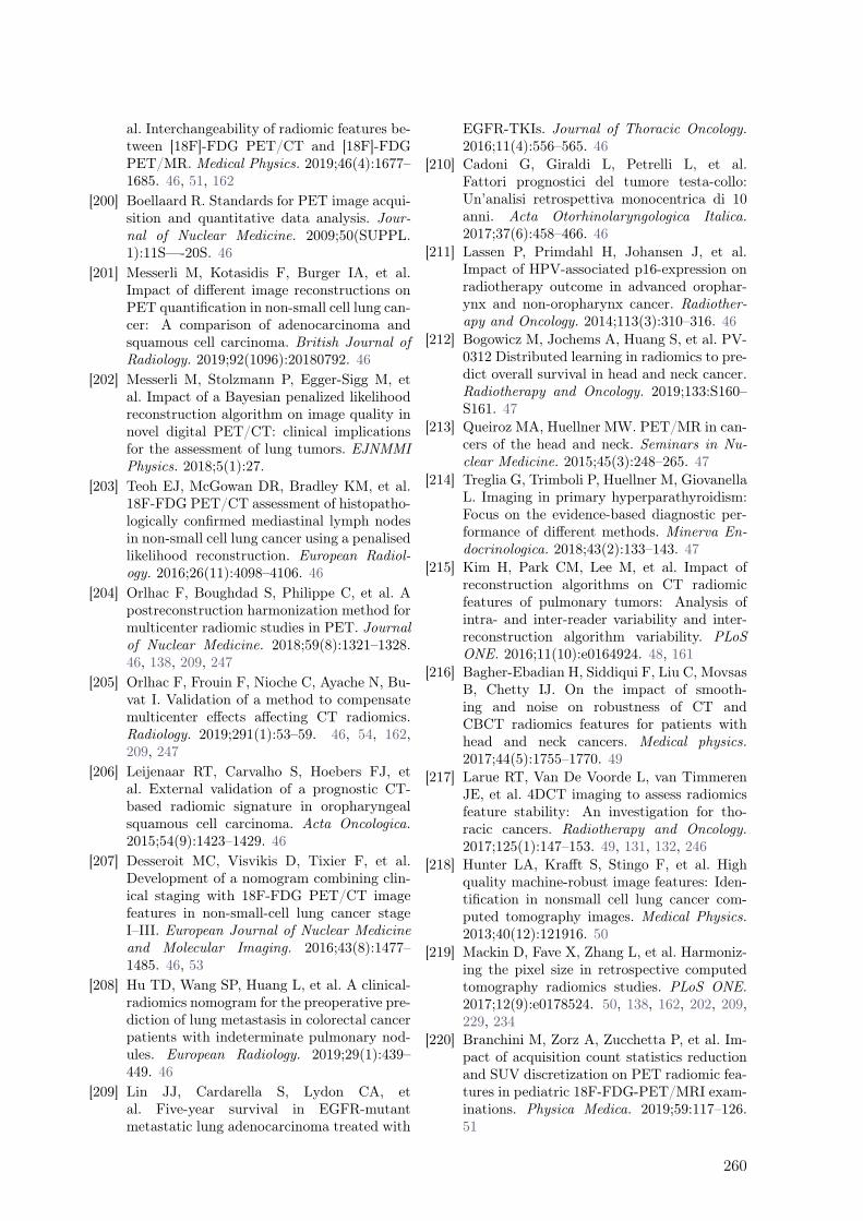
al. Interchangeability of radiomic features be-tween [18F]-FDG PET/CT and [18F]-FDGPET/MR. Medical Physics. 2019;46(4):1677–1685. 46, 51, 162
[200] Boellaard R. Standards for PET image acqui-sition and quantitative data analysis. Jour-nal of Nuclear Medicine. 2009;50(SUPPL.1):11S—-20S. 46
[201] Messerli M, Kotasidis F, Burger IA, et al.Impact of different image reconstructions onPET quantification in non-small cell lung can-cer: A comparison of adenocarcinoma andsquamous cell carcinoma. British Journal ofRadiology. 2019;92(1096):20180792. 46
[202] Messerli M, Stolzmann P, Egger-Sigg M, etal. Impact of a Bayesian penalized likelihoodreconstruction algorithm on image quality innovel digital PET/CT: clinical implicationsfor the assessment of lung tumors. EJNMMIPhysics. 2018;5(1):27.
[203] Teoh EJ, McGowan DR, Bradley KM, et al.18F-FDG PET/CT assessment of histopatho-logically confirmed mediastinal lymph nodesin non-small cell lung cancer using a penalisedlikelihood reconstruction. European Radiol-ogy. 2016;26(11):4098–4106. 46
[204] Orlhac F, Boughdad S, Philippe C, et al. Apostreconstruction harmonization method formulticenter radiomic studies in PET. Journalof Nuclear Medicine. 2018;59(8):1321–1328.46, 138, 209, 247
[205] Orlhac F, Frouin F, Nioche C, Ayache N, Bu-vat I. Validation of a method to compensatemulticenter effects affecting CT radiomics.Radiology. 2019;291(1):53–59. 46, 54, 162,209, 247
[206] Leijenaar RT, Carvalho S, Hoebers FJ, etal. External validation of a prognostic CT-based radiomic signature in oropharyngealsquamous cell carcinoma. Acta Oncologica.2015;54(9):1423–1429. 46
[207] Desseroit MC, Visvikis D, Tixier F, et al.Development of a nomogram combining clin-ical staging with 18F-FDG PET/CT imagefeatures in non-small-cell lung cancer stageI–III. European Journal of Nuclear Medicineand Molecular Imaging. 2016;43(8):1477–1485. 46, 53
[208] Hu TD, Wang SP, Huang L, et al. A clinical-radiomics nomogram for the preoperative pre-diction of lung metastasis in colorectal cancerpatients with indeterminate pulmonary nod-ules. European Radiology. 2019;29(1):439–449. 46
[209] Lin JJ, Cardarella S, Lydon CA, etal. Five-year survival in EGFR-mutantmetastatic lung adenocarcinoma treated with
EGFR-TKIs. Journal of Thoracic Oncology.2016;11(4):556–565. 46
[210] Cadoni G, Giraldi L, Petrelli L, et al.Fattori prognostici del tumore testa-collo:Un’analisi retrospettiva monocentrica di 10anni. Acta Otorhinolaryngologica Italica.2017;37(6):458–466. 46
[211] Lassen P, Primdahl H, Johansen J, et al.Impact of HPV-associated p16-expression onradiotherapy outcome in advanced orophar-ynx and non-oropharynx cancer. Radiother-apy and Oncology. 2014;113(3):310–316. 46
[212] Bogowicz M, Jochems A, Huang S, et al. PV-0312 Distributed learning in radiomics to pre-dict overall survival in head and neck cancer.Radiotherapy and Oncology. 2019;133:S160–S161. 47
[213] Queiroz MA, Huellner MW. PET/MR in can-cers of the head and neck. Seminars in Nu-clear Medicine. 2015;45(3):248–265. 47
[214] Treglia G, Trimboli P, Huellner M, GiovanellaL. Imaging in primary hyperparathyroidism:Focus on the evidence-based diagnostic per-formance of different methods. Minerva En-docrinologica. 2018;43(2):133–143. 47
[215] Kim H, Park CM, Lee M, et al. Impact ofreconstruction algorithms on CT radiomicfeatures of pulmonary tumors: Analysis ofintra- and inter-reader variability and inter-reconstruction algorithm variability. PLoSONE. 2016;11(10):e0164924. 48, 161
[216] Bagher-Ebadian H, Siddiqui F, Liu C, MovsasB, Chetty IJ. On the impact of smooth-ing and noise on robustness of CT andCBCT radiomics features for patients withhead and neck cancers. Medical physics.2017;44(5):1755–1770. 49
[217] Larue RT, Van De Voorde L, van TimmerenJE, et al. 4DCT imaging to assess radiomicsfeature stability: An investigation for tho-racic cancers. Radiotherapy and Oncology.2017;125(1):147–153. 49, 131, 132, 246
[218] Hunter LA, Krafft S, Stingo F, et al. Highquality machine-robust image features: Iden-tification in nonsmall cell lung cancer com-puted tomography images. Medical Physics.2013;40(12):121916. 50
[219] Mackin D, Fave X, Zhang L, et al. Harmoniz-ing the pixel size in retrospective computedtomography radiomics studies. PLoS ONE.2017;12(9):e0178524. 50, 138, 162, 202, 209,229, 234
[220] Branchini M, Zorz A, Zucchetta P, et al. Im-pact of acquisition count statistics reductionand SUV discretization on PET radiomic fea-tures in pediatric 18F-FDG-PET/MRI exam-inations. Physica Medica. 2019;59:117–126.51
260

REFERENCES
[221] Aide N, Salomon T, Blanc-Fournier C,Grellard JM, Levy C, Lasnon C. Implica-tions of reconstruction protocol for histo-biological characterisation of breast cancersusing FDG-PET radiomics. EJNMMI Re-search. 2018;8(1):114. 51
[222] Hatt M, Laurent B, Fayad H, Jaouen V,Visvikis D, Le Rest CC. Tumour functionalsphericity from PET images: prognostic valuein NSCLC and impact of delineation method.European Journal of Nuclear Medicine andMolecular Imaging. 2018;45(4):630–641. 52
[223] Grootjans W, Tixier F, Van Der Vos CS, etal. The impact of optimal respiratory gat-ing and image noise on evaluation of intratu-mor heterogeneity on 18F-FDG pet imagingof lung cancer. Journal of Nuclear Medicine.2016;57(11):1692–1698. 53, 131
[224] Buch K, Li B, Qureshi MM, Kuno H, An-derson SW, Sakai O. Quantitative assessmentof variation in CT parameters on texturefeatures: Pilot study using a nonanatomicphantom. American Journal of Neuroradiol-ogy. 2017;38(5):981–985. 54
[225] Oliver JA, Budzevich M, Hunt D, et al. Sensi-tivity of Image Features to Noise in Conven-tional and Respiratory-Gated PET/CT Im-ages of Lung Cancer: Uncorrelated NoiseEffects. Technology in Cancer Research andTreatment. 2017;16(5):595–608. 54
[226] Kalendralis P, Traverso A, Shi Z, et al.Multicenter CT phantoms public datasetfor radiomics reproducibility tests. MedicalPhysics. 2019;46(3):1512–1518. 54
[227] Mackin D, Fave X, Zhang L, et al. Measur-ing computed tomography scanner variabilityof radiomics features. Investigative Radiology.2015;50(11):757–765. 54, 204, 209
[228] Kim YJ, Lee HJ, Kim KG, Lee SH. The Effectof CT Scan Parameters on the Measurementof CT Radiomic Features: A Lung NodulePhantom Study. Computational and Mathe-matical Methods in Medicine. 2019;2019. 54,246
[229] Plautz TE, Zheng C, Noid G, Li XA. Timestability of delta-radiomics features and theimpact on patient analysis in longitudinal CTimages. Medical Physics. 2019;46(4):1663–1676. 54
[230] Papp L, Rausch I, Grahovac M, Hacker M,Beyer T. Optimized feature extraction for ra-diomics analysis of 18F-FDG PET imaging.Journal of Nuclear Medicine. 2019;60(6):864–872. 54
[231] Yang F, Young LA, Johnson PB. Quanti-tative radiomics: Validating image texturalfeatures for oncological PET in lung cancer.
Radiotherapy and Oncology. 2018;129(2):209–217. 54
[232] Shu J, Tang Y, Cui J, et al. Clear cell renalcell carcinoma: CT-based radiomics featuresfor the prediction of Fuhrman grade. Euro-pean Journal of Radiology. 2018;109:8–12. 55
[233] Fan S, Li X, Cui X, et al. ComputedTomography-Based Radiomic Features CouldPotentially Predict Microsatellite Instabil-ity Status in Stage II Colorectal Cancer:A Preliminary Study. Academic Radiology.2019;26(12):1633–1640. 55
[234] Zhou Y, He L, Huang Y, et al. CT-based ra-diomics signature: a potential biomarker forpreoperative prediction of early recurrence inhepatocellular carcinoma. Abdominal Radiol-ogy. 2017;42(6):1695–1704. 55
[235] Akai H, Yasaka K, Kunimatsu A, et al. Pre-dicting prognosis of resected hepatocellularcarcinoma by radiomics analysis with randomsurvival forest. Diagnostic and InterventionalImaging. 2018;99(10):643–651. 55
[236] Chakraborty J, Midya A, Gazit L, et al.CT radiomics to predict high-risk intra-ductal papillary mucinous neoplasms of thepancreas. Medical Physics. 2018;45(11):5019–5029. 55
[237] Chaddad A, Desrosiers C, Toews M, Abdulka-rim B. Predicting survival time of lung cancerpatients using radiomic analysis. Oncotarget.2017;8(61):104393–104407. 55
[238] Zhang Y, Oikonomou A, Wong A, HaiderMA, Khalvati F. Radiomics-based Progno-sis Analysis for Non-Small Cell Lung Cancer.Scientific Reports. 2017;7(1):46349. 55, 202,208
[239] Starkov P, Aguilera TA, Golden DI, et al. Theuse of texture-based radiomics CT analysisto predict outcomes in early-stage non-smallcell lung cancer treated with stereotactic ab-lative radiotherapy. British Journal of Radi-ology. 2019;92(1094). 55
[240] Zhong Y, Yuan M, Zhang T, Zhang YD, LiH, Yu TF. Radiomics approach to predictionof occult mediastinal lymph node metastasisof lung adenocarcinoma. American Journal ofRoentgenology. 2018;211(1):109–113. 56
[241] Zhang T, Yuan M, Zhong Y, et al. Differenti-ation of focal organising pneumonia and pe-ripheral adenocarcinoma in solid lung lesionsusing thin-section CT-based radiomics. Clin-ical Radiology. 2019;74(1):78.e23–78.e30. 56
[242] Zhou B, Xu J, Tian Y, Yuan S, Li X. Cor-relation between radiomic features based oncontrast-enhanced computed tomography im-ages and Ki-67 proliferation index in lungcancer: A preliminary study. Thoracic Can-
261
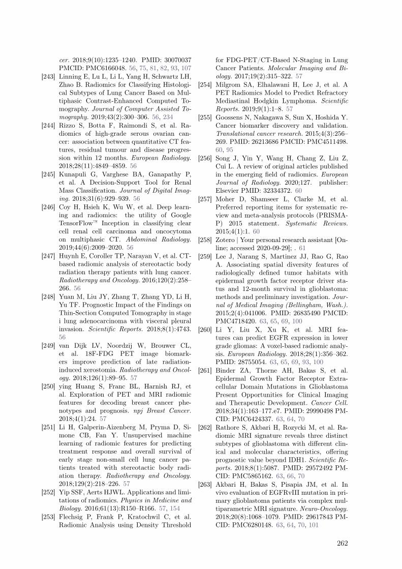
cer. 2018;9(10):1235–1240. PMID: 30070037PMCID: PMC6166048. 56, 75, 81, 82, 93, 107
[243] Linning E, Lu L, Li L, Yang H, Schwartz LH,Zhao B. Radiomics for Classifying Histologi-cal Subtypes of Lung Cancer Based on Mul-tiphasic Contrast-Enhanced Computed To-mography. Journal of Computer Assisted To-mography. 2019;43(2):300–306. 56, 234
[244] Rizzo S, Botta F, Raimondi S, et al. Ra-diomics of high-grade serous ovarian can-cer: association between quantitative CT fea-tures, residual tumour and disease progres-sion within 12 months. European Radiology.2018;28(11):4849–4859. 56
[245] Kunapuli G, Varghese BA, Ganapathy P,et al. A Decision-Support Tool for RenalMass Classification. Journal of Digital Imag-ing. 2018;31(6):929–939. 56
[246] Coy H, Hsieh K, Wu W, et al. Deep learn-ing and radiomics: the utility of GoogleTensorFlow™ Inception in classifying clearcell renal cell carcinoma and oncocytomaon multiphasic CT. Abdominal Radiology.2019;44(6):2009–2020. 56
[247] Huynh E, Coroller TP, Narayan V, et al. CT-based radiomic analysis of stereotactic bodyradiation therapy patients with lung cancer.Radiotherapy and Oncology. 2016;120(2):258–266. 56
[248] Yuan M, Liu JY, Zhang T, Zhang YD, Li H,Yu TF. Prognostic Impact of the Findings onThin-Section Computed Tomography in stagei lung adenocarcinoma with visceral pleuralinvasion. Scientific Reports. 2018;8(1):4743.56
[249] van Dijk LV, Noordzij W, Brouwer CL,et al. 18F-FDG PET image biomark-ers improve prediction of late radiation-induced xerostomia. Radiotherapy and Oncol-ogy. 2018;126(1):89–95. 57
[250] ying Huang S, Franc BL, Harnish RJ, etal. Exploration of PET and MRI radiomicfeatures for decoding breast cancer phe-notypes and prognosis. npj Breast Cancer.2018;4(1):24. 57
[251] Li H, Galperin-Aizenberg M, Pryma D, Si-mone CB, Fan Y. Unsupervised machinelearning of radiomic features for predictingtreatment response and overall survival ofearly stage non-small cell lung cancer pa-tients treated with stereotactic body radi-ation therapy. Radiotherapy and Oncology.2018;129(2):218–226. 57
[252] Yip SSF, Aerts HJWL. Applications and limi-tations of radiomics. Physics in Medicine andBiology. 2016;61(13):R150–R166. 57, 154
[253] Flechsig P, Frank P, Kratochwil C, et al.Radiomic Analysis using Density Threshold
for FDG-PET/CT-Based N-Staging in LungCancer Patients. Molecular Imaging and Bi-ology. 2017;19(2):315–322. 57
[254] Milgrom SA, Elhalawani H, Lee J, et al. APET Radiomics Model to Predict RefractoryMediastinal Hodgkin Lymphoma. ScientificReports. 2019;9(1):1–8. 57
[255] Goossens N, Nakagawa S, Sun X, Hoshida Y.Cancer biomarker discovery and validation.Translational cancer research. 2015;4(3):256–269. PMID: 26213686 PMCID: PMC4511498.60, 95
[256] Song J, Yin Y, Wang H, Chang Z, Liu Z,Cui L. A review of original articles publishedin the emerging field of radiomics. EuropeanJournal of Radiology. 2020;127. publisher:Elsevier PMID: 32334372. 60
[257] Moher D, Shamseer L, Clarke M, et al.Preferred reporting items for systematic re-view and meta-analysis protocols (PRISMA-P) 2015 statement. Systematic Reviews.2015;4(1):1. 60
[258] Zotero | Your personal research assistant [On-line; accessed 2020-09-29]; . 61
[259] Lee J, Narang S, Martinez JJ, Rao G, RaoA. Associating spatial diversity features ofradiologically defined tumor habitats withepidermal growth factor receptor driver sta-tus and 12-month survival in glioblastoma:methods and preliminary investigation. Jour-nal of Medical Imaging (Bellingham, Wash.).2015;2(4):041006. PMID: 26835490 PMCID:PMC4718420. 63, 65, 69, 100
[260] Li Y, Liu X, Xu K, et al. MRI fea-tures can predict EGFR expression in lowergrade gliomas: A voxel-based radiomic analy-sis. European Radiology. 2018;28(1):356–362.PMID: 28755054. 63, 65, 69, 93, 100
[261] Binder ZA, Thorne AH, Bakas S, et al.Epidermal Growth Factor Receptor Extra-cellular Domain Mutations in GlioblastomaPresent Opportunities for Clinical Imagingand Therapeutic Development. Cancer Cell.2018;34(1):163–177.e7. PMID: 29990498 PM-CID: PMC6424337. 63, 64, 70
[262] Rathore S, Akbari H, Rozycki M, et al. Ra-diomic MRI signature reveals three distinctsubtypes of glioblastoma with different clin-ical and molecular characteristics, offeringprognostic value beyond IDH1. Scientific Re-ports. 2018;8(1):5087. PMID: 29572492 PM-CID: PMC5865162. 63, 66, 70
[263] Akbari H, Bakas S, Pisapia JM, et al. Invivo evaluation of EGFRvIII mutation in pri-mary glioblastoma patients via complex mul-tiparametric MRI signature. Neuro-Oncology.2018;20(8):1068–1079. PMID: 29617843 PM-CID: PMC6280148. 63, 64, 70, 101
262

REFERENCES
[264] Li J, Liu S, Qin Y, Zhang Y, Wang N, LiuH. High-order radiomics features based on T2FLAIR MRI predict multiple glioma immuno-histochemical features: A more precise andpersonalized gliomas management. PloS One.2020;15(1):e0227703. PMID: 31968004 PM-CID: PMC6975558. 63, 65, 106
[265] Li Y, Qian Z, Xu K, et al. Radiomic featurespredict Ki-67 expression level and survivalin lower grade gliomas. Journal of Neuro-Oncology. 2017;135(2):317–324. PMID:28900812. 63, 65, 93, 103
[266] Ugga L, Cuocolo R, Solari D, et al. Pre-diction of high proliferative index in pi-tuitary macroadenomas using MRI-basedradiomics and machine learning. Neuro-radiology. 2019;61(12):1365–1373. PMID:31375883. 63, 67
[267] Su C, Jiang J, Zhang S, et al. Ra-diomics based on multicontrast MRI can pre-cisely differentiate among glioma subtypesand predict tumour-proliferative behaviour.European Radiology. 2019;29(4):1986–1996.PMID: 30315419. 66, 70, 104
[268] Kong Z, Li J, Liu Z, et al. Radiomics signa-ture based on FDG-PET predicts prolifera-tive activity in primary glioma. Clinical Ra-diology. 2019;74(10):815.e15–815.e23. PMID:31376917. 63, 65, 70, 105
[269] Zhang X, Tian Q, Wang L, et al. RadiomicsStrategy for Molecular Subtype Stratifica-tion of Lower-Grade Glioma: Detecting IDHand TP53 Mutations Based on MultimodalMRI. Journal of magnetic resonance imaging:JMRI. 2018;48(4):916–926. PMID: 29394005.63, 68, 69, 70
[270] Li Y, Qian Z, Xu K, et al. MRI features pre-dict p53 status in lower-grade gliomas viaa machine-learning approach. NeuroImage.Clinical. 2018;17:306–311. PMID: 29527478PMCID: PMC5842645. 63, 65, 70, 93, 111
[271] Sun Z, Li Y, Wang Y, et al. Radiogenomicanalysis of vascular endothelial growth factorin patients with diffuse gliomas. Cancer Imag-ing: The Official Publication of the Interna-tional Cancer Imaging Society. 2019;19(1):68.PMID: 31639060 PMCID: PMC6805458. 63,66, 70, 74, 93, 111
[272] Wu G, Chen Y, Wang Y, et al. SparseRepresentation-Based Radiomics for the Di-agnosis of Brain Tumors. IEEE transac-tions on medical imaging. 2018;37(4):893–905. PMID: 29610069. 67, 69
[273] Choi Y, Nam Y, Lee YS, et al. IDH1 mu-tation prediction using MR-based radiomicsin glioblastoma: comparison between man-ual and fully automated deep learning-based approach of tumor segmentation. Euro-
pean Journal of Radiology. 2020;128:109031.PMID: 32417712. 64, 69
[274] Arita H, Kinoshita M, Kawaguchi A, etal. Lesion location implemented magneticresonance imaging radiomics for predict-ing IDH and TERT promoter mutationsin grade II/III gliomas. Scientific Reports.2018;8(1):11773. PMID: 30082856 PMCID:PMC6078954. 63, 64, 69
[275] Tan Y, tong Zhang S, wei Wei J, et al.A radiomics nomogram may improve theprediction of IDH genotype for astrocy-toma before surgery. European Radiology.2019;29(7):3325–3337. PMID: 30972543. 67,69
[276] Li L, Mu W, Wang Y, et al. A Non-invasiveRadiomic Method Using 18F-FDG PET Pre-dicts Isocitrate Dehydrogenase Genotype andPrognosis in Patients With Glioma. Frontiersin Oncology. 2019;9:1183. PMID: 31803608PMCID: PMC6869373. 65, 69, 94, 105
[277] Han Y, Wang W, Yang Y, et al. Amide Pro-ton Transfer Imaging in Predicting IsocitrateDehydrogenase 1 Mutation Status of GradeII/III Gliomas Based on Support Vector Ma-chine. Frontiers in Neuroscience. 2020;14:144.PMID: 32153362 PMCID: PMC7047712. 63,64, 69, 105
[278] Liu X, Li Y, Li S, et al. IDH mutation-specificradiomic signature in lower-grade gliomas.Aging. 2019;11(2):673–696. PMID: 30696801PMCID: PMC6366985. 63, 66, 69, 93, 103
[279] Yu J, Shi Z, Lian Y, et al. Noninvasive IDH1mutation estimation based on a quantita-tive radiomics approach for grade II glioma.European Radiology. 2017;27(8):3509–3522.PMID: 28004160. 67, 69
[280] Kim M, Jung SY, Park JE, et al. Diffusion-and perfusion-weighted MRI radiomics modelmay predict isocitrate dehydrogenase (IDH)mutation and tumor aggressiveness in dif-fuse lower grade glioma. European Radiology.2020;30(4):2142–2151. PMID: 31828414. 63,64, 69
[281] Li Z, Wang Y, Yu J, Guo Y, Cao W.Deep Learning based Radiomics (DLR) andits usage in noninvasive IDH1 predictionfor low grade glioma. Scientific Reports.2017;7(1):5467. PMID: 28710497 PMCID:PMC5511238. 63, 66, 69
[282] Yu J, Shi Z, Ji C, et al. Anatomical loca-tion differences between mutated and wild-type isocitrate dehydrogenase 1 in low-gradegliomas. The International Journal of Neu-roscience. 2017;127(10):873–880. PMID:27929688. 67, 69
[283] Tongtong Liu n, Guoqing Wu n, Jinhua Yun, et al. A mRMRMSRC feature selec-
263
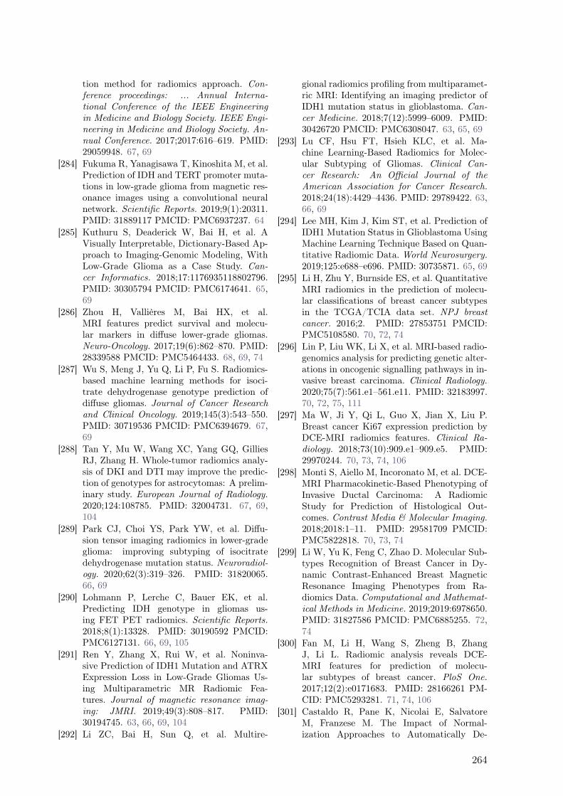
tion method for radiomics approach. Con-ference proceedings: ... Annual Interna-tional Conference of the IEEE Engineeringin Medicine and Biology Society. IEEE Engi-neering in Medicine and Biology Society. An-nual Conference. 2017;2017:616–619. PMID:29059948. 67, 69
[284] Fukuma R, Yanagisawa T, Kinoshita M, et al.Prediction of IDH and TERT promoter muta-tions in low-grade glioma from magnetic res-onance images using a convolutional neuralnetwork. Scientific Reports. 2019;9(1):20311.PMID: 31889117 PMCID: PMC6937237. 64
[285] Kuthuru S, Deaderick W, Bai H, et al. AVisually Interpretable, Dictionary-Based Ap-proach to Imaging-Genomic Modeling, WithLow-Grade Glioma as a Case Study. Can-cer Informatics. 2018;17:1176935118802796.PMID: 30305794 PMCID: PMC6174641. 65,69
[286] Zhou H, Vallières M, Bai HX, et al.MRI features predict survival and molecu-lar markers in diffuse lower-grade gliomas.Neuro-Oncology. 2017;19(6):862–870. PMID:28339588 PMCID: PMC5464433. 68, 69, 74
[287] Wu S, Meng J, Yu Q, Li P, Fu S. Radiomics-based machine learning methods for isoci-trate dehydrogenase genotype prediction ofdiffuse gliomas. Journal of Cancer Researchand Clinical Oncology. 2019;145(3):543–550.PMID: 30719536 PMCID: PMC6394679. 67,69
[288] Tan Y, Mu W, Wang XC, Yang GQ, GilliesRJ, Zhang H. Whole-tumor radiomics analy-sis of DKI and DTI may improve the predic-tion of genotypes for astrocytomas: A prelim-inary study. European Journal of Radiology.2020;124:108785. PMID: 32004731. 67, 69,104
[289] Park CJ, Choi YS, Park YW, et al. Diffu-sion tensor imaging radiomics in lower-gradeglioma: improving subtyping of isocitratedehydrogenase mutation status. Neuroradiol-ogy. 2020;62(3):319–326. PMID: 31820065.66, 69
[290] Lohmann P, Lerche C, Bauer EK, et al.Predicting IDH genotype in gliomas us-ing FET PET radiomics. Scientific Reports.2018;8(1):13328. PMID: 30190592 PMCID:PMC6127131. 66, 69, 105
[291] Ren Y, Zhang X, Rui W, et al. Noninva-sive Prediction of IDH1 Mutation and ATRXExpression Loss in Low-Grade Gliomas Us-ing Multiparametric MR Radiomic Fea-tures. Journal of magnetic resonance imag-ing: JMRI. 2019;49(3):808–817. PMID:30194745. 63, 66, 69, 104
[292] Li ZC, Bai H, Sun Q, et al. Multire-
gional radiomics profiling from multiparamet-ric MRI: Identifying an imaging predictor ofIDH1 mutation status in glioblastoma. Can-cer Medicine. 2018;7(12):5999–6009. PMID:30426720 PMCID: PMC6308047. 63, 65, 69
[293] Lu CF, Hsu FT, Hsieh KLC, et al. Ma-chine Learning-Based Radiomics for Molec-ular Subtyping of Gliomas. Clinical Can-cer Research: An Official Journal of theAmerican Association for Cancer Research.2018;24(18):4429–4436. PMID: 29789422. 63,66, 69
[294] Lee MH, Kim J, Kim ST, et al. Prediction ofIDH1 Mutation Status in Glioblastoma UsingMachine Learning Technique Based on Quan-titative Radiomic Data. World Neurosurgery.2019;125:e688–e696. PMID: 30735871. 65, 69
[295] Li H, Zhu Y, Burnside ES, et al. QuantitativeMRI radiomics in the prediction of molecu-lar classifications of breast cancer subtypesin the TCGA/TCIA data set. NPJ breastcancer. 2016;2. PMID: 27853751 PMCID:PMC5108580. 70, 72, 74
[296] Lin P, Liu WK, Li X, et al. MRI-based radio-genomics analysis for predicting genetic alter-ations in oncogenic signalling pathways in in-vasive breast carcinoma. Clinical Radiology.2020;75(7):561.e1–561.e11. PMID: 32183997.70, 72, 75, 111
[297] Ma W, Ji Y, Qi L, Guo X, Jian X, Liu P.Breast cancer Ki67 expression prediction byDCE-MRI radiomics features. Clinical Ra-diology. 2018;73(10):909.e1–909.e5. PMID:29970244. 70, 73, 74, 106
[298] Monti S, Aiello M, Incoronato M, et al. DCE-MRI Pharmacokinetic-Based Phenotyping ofInvasive Ductal Carcinoma: A RadiomicStudy for Prediction of Histological Out-comes. Contrast Media & Molecular Imaging.2018;2018:1–11. PMID: 29581709 PMCID:PMC5822818. 70, 73, 74
[299] Li W, Yu K, Feng C, Zhao D. Molecular Sub-types Recognition of Breast Cancer in Dy-namic Contrast-Enhanced Breast MagneticResonance Imaging Phenotypes from Ra-diomics Data. Computational and Mathemat-ical Methods in Medicine. 2019;2019:6978650.PMID: 31827586 PMCID: PMC6885255. 72,74
[300] Fan M, Li H, Wang S, Zheng B, ZhangJ, Li L. Radiomic analysis reveals DCE-MRI features for prediction of molecu-lar subtypes of breast cancer. PloS One.2017;12(2):e0171683. PMID: 28166261 PM-CID: PMC5293281. 71, 74, 106
[301] Castaldo R, Pane K, Nicolai E, SalvatoreM, Franzese M. The Impact of Normal-ization Approaches to Automatically De-
264
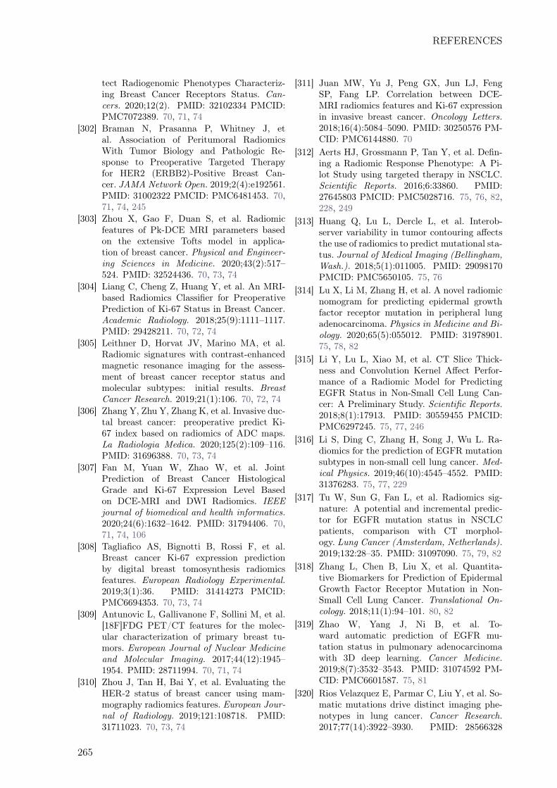
REFERENCES
tect Radiogenomic Phenotypes Characteriz-ing Breast Cancer Receptors Status. Can-cers. 2020;12(2). PMID: 32102334 PMCID:PMC7072389. 70, 71, 74
[302] Braman N, Prasanna P, Whitney J, etal. Association of Peritumoral RadiomicsWith Tumor Biology and Pathologic Re-sponse to Preoperative Targeted Therapyfor HER2 (ERBB2)-Positive Breast Can-cer. JAMA Network Open. 2019;2(4):e192561.PMID: 31002322 PMCID: PMC6481453. 70,71, 74, 245
[303] Zhou X, Gao F, Duan S, et al. Radiomicfeatures of Pk-DCE MRI parameters basedon the extensive Tofts model in applica-tion of breast cancer. Physical and Engineer-ing Sciences in Medicine. 2020;43(2):517–524. PMID: 32524436. 70, 73, 74
[304] Liang C, Cheng Z, Huang Y, et al. An MRI-based Radiomics Classifier for PreoperativePrediction of Ki-67 Status in Breast Cancer.Academic Radiology. 2018;25(9):1111–1117.PMID: 29428211. 70, 72, 74
[305] Leithner D, Horvat JV, Marino MA, et al.Radiomic signatures with contrast-enhancedmagnetic resonance imaging for the assess-ment of breast cancer receptor status andmolecular subtypes: initial results. BreastCancer Research. 2019;21(1):106. 70, 72, 74
[306] Zhang Y, Zhu Y, Zhang K, et al. Invasive duc-tal breast cancer: preoperative predict Ki-67 index based on radiomics of ADC maps.La Radiologia Medica. 2020;125(2):109–116.PMID: 31696388. 70, 73, 74
[307] Fan M, Yuan W, Zhao W, et al. JointPrediction of Breast Cancer HistologicalGrade and Ki-67 Expression Level Basedon DCE-MRI and DWI Radiomics. IEEEjournal of biomedical and health informatics.2020;24(6):1632–1642. PMID: 31794406. 70,71, 74, 106
[308] Tagliafico AS, Bignotti B, Rossi F, et al.Breast cancer Ki-67 expression predictionby digital breast tomosynthesis radiomicsfeatures. European Radiology Experimental.2019;3(1):36. PMID: 31414273 PMCID:PMC6694353. 70, 73, 74
[309] Antunovic L, Gallivanone F, Sollini M, et al.[18F]FDG PET/CT features for the molec-ular characterization of primary breast tu-mors. European Journal of Nuclear Medicineand Molecular Imaging. 2017;44(12):1945–1954. PMID: 28711994. 70, 71, 74
[310] Zhou J, Tan H, Bai Y, et al. Evaluating theHER-2 status of breast cancer using mam-mography radiomics features. European Jour-nal of Radiology. 2019;121:108718. PMID:31711023. 70, 73, 74
[311] Juan MW, Yu J, Peng GX, Jun LJ, FengSP, Fang LP. Correlation between DCE-MRI radiomics features and Ki-67 expressionin invasive breast cancer. Oncology Letters.2018;16(4):5084–5090. PMID: 30250576 PM-CID: PMC6144880. 70
[312] Aerts HJ, Grossmann P, Tan Y, et al. Defin-ing a Radiomic Response Phenotype: A Pi-lot Study using targeted therapy in NSCLC.Scientific Reports. 2016;6:33860. PMID:27645803 PMCID: PMC5028716. 75, 76, 82,228, 249
[313] Huang Q, Lu L, Dercle L, et al. Interob-server variability in tumor contouring affectsthe use of radiomics to predict mutational sta-tus. Journal of Medical Imaging (Bellingham,Wash.). 2018;5(1):011005. PMID: 29098170PMCID: PMC5650105. 75, 76
[314] Lu X, Li M, Zhang H, et al. A novel radiomicnomogram for predicting epidermal growthfactor receptor mutation in peripheral lungadenocarcinoma. Physics in Medicine and Bi-ology. 2020;65(5):055012. PMID: 31978901.75, 78, 82
[315] Li Y, Lu L, Xiao M, et al. CT Slice Thick-ness and Convolution Kernel Affect Perfor-mance of a Radiomic Model for PredictingEGFR Status in Non-Small Cell Lung Can-cer: A Preliminary Study. Scientific Reports.2018;8(1):17913. PMID: 30559455 PMCID:PMC6297245. 75, 77, 246
[316] Li S, Ding C, Zhang H, Song J, Wu L. Ra-diomics for the prediction of EGFR mutationsubtypes in non-small cell lung cancer. Med-ical Physics. 2019;46(10):4545–4552. PMID:31376283. 75, 77, 229
[317] Tu W, Sun G, Fan L, et al. Radiomics sig-nature: A potential and incremental predic-tor for EGFR mutation status in NSCLCpatients, comparison with CT morphol-ogy. Lung Cancer (Amsterdam, Netherlands).2019;132:28–35. PMID: 31097090. 75, 79, 82
[318] Zhang L, Chen B, Liu X, et al. Quantita-tive Biomarkers for Prediction of EpidermalGrowth Factor Receptor Mutation in Non-Small Cell Lung Cancer. Translational On-cology. 2018;11(1):94–101. 80, 82
[319] Zhao W, Yang J, Ni B, et al. To-ward automatic prediction of EGFR mu-tation status in pulmonary adenocarcinomawith 3D deep learning. Cancer Medicine.2019;8(7):3532–3543. PMID: 31074592 PM-CID: PMC6601587. 75, 81
[320] Rios Velazquez E, Parmar C, Liu Y, et al. So-matic mutations drive distinct imaging phe-notypes in lung cancer. Cancer Research.2017;77(14):3922–3930. PMID: 28566328
265

PMCID: PMC5528160. 75, 78, 82, 93, 101,109, 229, 245, 247
[321] Wang X, Kong C, Xu W, et al. Decoding tu-mor mutation burden and driver mutationsin early stage lung adenocarcinoma usingCT-based radiomics signature. Thoracic Can-cer. 2019;10(10):1904–1912. PMID: 31414580PMCID: PMC6775017. 75, 79, 82
[322] Hong D, Xu K, Zhang L, Wan X, Guo Y. Ra-diomics Signature as a Predictive Factor forEGFR Mutations in Advanced Lung Adeno-carcinoma. Frontiers in Oncology. 2020;10:28.PMID: 32082997 PMCID: PMC7005234. 75,76
[323] Liu Y, Kim J, Balagurunathan Y, et al. Ra-diomic Features Are Associated With EGFRMutation Status in Lung Adenocarcinomas.Clinical Lung Cancer. 2016;17(5):441–448.e6.PMID: 27017476 PMCID: PMC5548419. 75,77, 82, 229
[324] Song L, Zhu Z, Mao L, et al. Clinical,Conventional CT and Radiomic Feature-Based Machine Learning Models for Predict-ing ALK Rearrangement Status in Lung Ade-nocarcinoma Patients. Frontiers in Oncology.2020;10. 75, 79, 93, 101
[325] Sun Z, Hu S, Ge Y, et al. Radiomics study forpredicting the expression of PD-L1 in non-small cell lung cancer based on CT imagesand clinicopathologic features. Journal of X-Ray Science and Technology. 2020;. PMID:32176676. 75, 79, 82
[326] Yoon J, Suh YJ, Han K, et al. Utility ofCT radiomics for prediction of PD-L1 expres-sion in advanced lung adenocarcinomas. Tho-racic Cancer. 2020;11(4):993–1004. PMID:32043309. 75, 80, 82, 93, 109
[327] Gu Q, Feng Z, Liang Q, et al. Machinelearning-based radiomics strategy for predic-tion of cell proliferation in non-small celllung cancer. European Journal of Radiology.2019;118:32–37. PMID: 31439255. 75, 76, 82
[328] Jiang M, Zhang Y, Xu J, et al. Assess-ing EGFR gene mutation status in non-small cell lung cancer with imaging fea-tures from PET/CT. Nuclear Medicine Com-munications. 2019;40(8):842–849. PMID:31290849. 75, 77
[329] Koyasu S, Nishio M, Isoda H, NakamotoY, Togashi K. Usefulness of gradient treeboosting for predicting histological subtypeand EGFR mutation status of non-small celllung cancer on 18F FDG-PET/CT. Annals ofNuclear Medicine. 2020;34(1):49–57. PMID:31659591. 77
[330] Li X, Yin G, Zhang Y, et al. PredictivePower of a Radiomic Signature Based on18F-FDG PET/CT Images for EGFR Muta-
tional Status in NSCLC. Frontiers in Oncol-ogy. 2019;9:1062. PMID: 31681597 PMCID:PMC6803612. 77, 82
[331] Nair JKR, Saeed UA, McDougall CC, et al.Radiogenomic Models Using Machine Learn-ing Techniques to Predict EGFR Muta-tions in Non-Small Cell Lung Cancer. Cana-dian Association of Radiologists Journal =Journal l’Association Canadienne Des Ra-diologistes. 2020;:846537119899526. PMID:32063026. 75, 78
[332] Zhang J, Zhao X, Zhao Y, et al. Value ofpre-therapy 18F-FDG PET/CT radiomics inpredicting EGFR mutation status in patientswith non-small cell lung cancer. EuropeanJournal of Nuclear Medicine and Molecu-lar Imaging. 2020;47(5):1137–1146. PMID:31728587. 75, 80, 82
[333] Shiri I, Maleki H, Hajianfar G, et al. Next-Generation Radiogenomics Sequencing forPrediction of EGFR and KRAS MutationStatus in NSCLC Patients Using Multi-modal Imaging and Machine Learning Al-gorithms. Molecular Imaging and Biology.2020;. PMID: 32185618. 75, 78, 82
[334] Yoon HJ, Sohn I, Cho JH, et al. Decod-ing Tumor Phenotypes for ALK, ROS1,and RET Fusions in Lung AdenocarcinomaUsing a Radiomics Approach. Medicine.2015;94(41):e1753. PMID: 26469915 PMCID:PMC4616787. 75, 80
[335] Jiang M, Sun D, Guo Y, et al. Assessing PD-L1 Expression Level by Radiomic FeaturesFrom PET/CT in Nonsmall Cell Lung CancerPatients: An Initial Result. Academic Radi-ology. 2020;27(2):171–179. PMID: 31147234.75, 76, 82
[336] Yip SSF, Kim J, Coroller TP, et al. As-sociations Between Somatic Mutations andMetabolic Imaging Phenotypes in Non-Small Cell Lung Cancer. Journal of NuclearMedicine: Official Publication, Society of Nu-clear Medicine. 2017;58(4):569–576. PMID:27688480 PMCID: PMC5373502. 75, 80, 94,101, 109
[337] Chen BT, Jin T, Ye N, et al. Radiomic pre-diction of mutation status based on MR imag-ing of lung cancer brain metastases. MagneticResonance Imaging. 2020;69:49–56. PMID:32179095. 75, 76, 82
[338] Zhao W, Wu Y, Xu Y, et al. The Potentialof Radiomics Nomogram in Non-invasivelyPrediction of Epidermal Growth Factor Re-ceptor Mutation Status and Subtypes inLung Adenocarcinoma. Frontiers in Oncol-ogy. 2019;9:1485. PMID: 31993370 PMCID:PMC6962353. 75, 81, 82
[339] Li Y, Cheng Z, Gevaert O, et al. A CT-based
266

REFERENCES
radiomics nomogram for prediction of humanepidermal growth factor receptor 2 status inpatients with gastric cancer. Chinese Jour-nal of Cancer Research = Chung-Kuo YenCheng Yen Chiu. 2020;32(1):62–71. PMID:32194306 PMCID: PMC7072015. 82, 83, 84,93
[340] Zhang QW, Gao YJ, Zhang RY, et al. Per-sonalized CT-based radiomics nomogram pre-operative predicting Ki-67 expression in gas-trointestinal stromal tumors: a multicen-ter development and validation cohort. Clini-cal and Translational Medicine. 2020;9(1):12.PMID: 32006200 PMCID: PMC6994569. 82,83, 85, 93, 106
[341] Wang N, Wang X, Li W, et al. Contrast-Enhanced CT Parameters of Gastric Adeno-carcinoma: Can Radiomic Features Be Surro-gate Biomarkers for HER2 Over-ExpressionStatus?. Cancer Management and Research.2020;12:1211–1219. PMID: 32110095 PM-CID: PMC7035892. 82, 83
[342] Yang L, Dong D, Fang M, et al. CanCT-based radiomics signature predictKRAS/NRAS/BRAF mutations in col-orectal cancer?. European Radiology.2018;28(5):2058–2067. PMID: 29335867.82, 85, 93, 109
[343] Wu X, Li Y, Chen X, et al. Deep LearningFeatures Improve the Performance of a Ra-diomics Signature for Predicting KRAS Sta-tus in Patients with Colorectal Cancer. Aca-demic Radiology. 2020;. PMID: 31982342. 82,85
[344] Lim CH, Cho YS, Choi JY, et al. Imag-ing phenotype using 18F-fluorodeoxyglucosepositron emission tomography-based ra-diomics and genetic alterations of pancre-atic ductal adenocarcinoma. European Jour-nal of Nuclear Medicine and Molecular Imag-ing. 2020;47(9):2113–2122. PMID: 32002592.82, 83, 84, 94, 109
[345] Chen SW, Shen WC, Chen WTL, etal. Metabolic Imaging Phenotype UsingRadiomics of [18F]FDG PET/CT Associ-ated with Genetic Alterations of Colorec-tal Cancer. Molecular Imaging and Biology.2019;21(1):183–190. PMID: 29948642. 82, 83,84, 94, 111
[346] Cui Y, Liu H, Ren J, et al. Developmentand validation of a MRI-based radiomicssignature for prediction of KRAS muta-tion in rectal cancer. European Radiology.2020;30(4):1948–1958. PMID: 31942672. 82,83, 84, 93, 109
[347] Oh JE, Kim MJ, Lee J, et al. MagneticResonance-Based Texture Analysis Differen-tiating KRAS Mutation Status in Rectal Can-
cer. Cancer Research and Treatment: Offi-cial Journal of Korean Cancer Association.2020;52(1):51–59. PMID: 31096736 PMCID:PMC6962487. 83, 85
[348] Meng X, Xia W, Xie P, et al. Preopera-tive radiomic signature based on multipara-metric magnetic resonance imaging for non-invasive evaluation of biological character-istics in rectal cancer. European Radiology.2019;29(6):3200–3209. PMID: 30413959. 82,83, 85
[349] Hectors SJ, Lewis S, Besa C, et al. MRI ra-diomics features predict immuno-oncologicalcharacteristics of hepatocellular carcinoma.European Radiology. 2020;. PMID: 32086577.87, 88, 109
[350] Ye Z, Jiang H, Chen J, et al. Texture analysison gadoxetic acid enhanced-MRI for predict-ing Ki-67 status in hepatocellular carcinoma:A prospective study. Chinese Journal of Can-cer Research = Chung-Kuo Yen Cheng YenChiu. 2019;31(5):806–817. PMID: 31814684PMCID: PMC6856708. 87, 89, 93, 107
[351] Yao Z, Dong Y, Wu G, et al. Preopera-tive diagnosis and prediction of hepatocellu-lar carcinoma: Radiomics analysis based onmulti-modal ultrasound images. BMC cancer.2018;18(1):1089. PMID: 30419849 PMCID:PMC6233500. 87
[352] Peng YT, Zhou CY, Lin P, et al. PreoperativeUltrasound Radiomics Signatures for Nonin-vasive Evaluation of Biological Characteris-tics of Intrahepatic Cholangiocarcinoma. Aca-demic Radiology. 2019;. PMID: 31494003. 87,88, 111
[353] Saadani H, van der Hiel B, Aalbers-berg EA, et al. Metabolic Biomarker-Based BRAFV600 Mutation Association andPrediction in Melanoma. Journal of Nu-clear Medicine: Official Publication, Societyof Nuclear Medicine. 2019;60(11):1545–1552.PMID: 31481581. 90, 91, 102
[354] Yoon JH, Han K, Lee E, et al. Radiomics inpredicting mutation status for thyroid can-cer: A preliminary study using radiomics fea-tures for predicting BRAFV600E mutationsin papillary thyroid carcinoma. PloS One.2020;15(2):e0228968. PMID: 32053670 PM-CID: PMC7018006. 90, 91, 102
[355] Zhu Y, Mohamed ASR, Lai SY, et al.Imaging-Genomic Study of Head and NeckSquamous Cell Carcinoma: Associations Be-tween Radiomic Phenotypes and GenomicMechanisms via Integration of The Can-cer Genome Atlas and The Cancer Imag-ing Archive. JCO clinical cancer informat-ics. 2019;3:1–9. PMID: 30730765 PMCID:PMC6874020. 90, 91, 93, 111
267
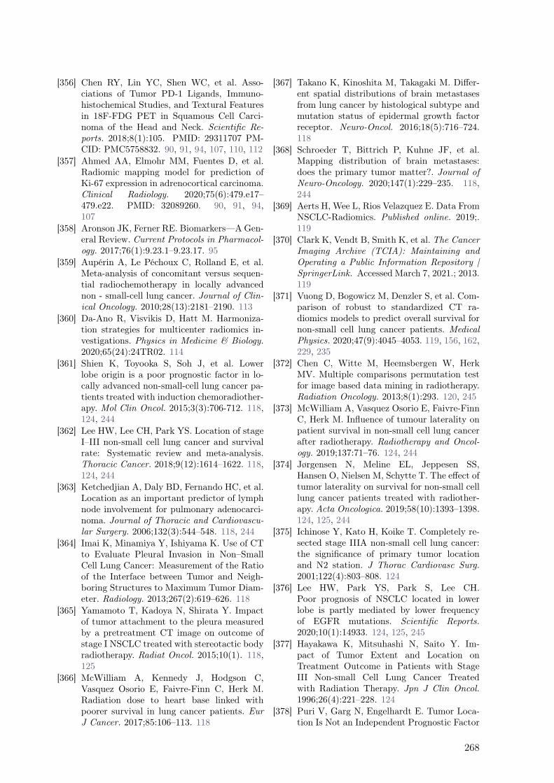
[356] Chen RY, Lin YC, Shen WC, et al. Asso-ciations of Tumor PD-1 Ligands, Immuno-histochemical Studies, and Textural Featuresin 18F-FDG PET in Squamous Cell Carci-noma of the Head and Neck. Scientific Re-ports. 2018;8(1):105. PMID: 29311707 PM-CID: PMC5758832. 90, 91, 94, 107, 110, 112
[357] Ahmed AA, Elmohr MM, Fuentes D, et al.Radiomic mapping model for prediction ofKi-67 expression in adrenocortical carcinoma.Clinical Radiology. 2020;75(6):479.e17–479.e22. PMID: 32089260. 90, 91, 94,107
[358] Aronson JK, Ferner RE. Biomarkers—A Gen-eral Review. Current Protocols in Pharmacol-ogy. 2017;76(1):9.23.1–9.23.17. 95
[359] Aupérin A, Le Péchoux C, Rolland E, et al.Meta-analysis of concomitant versus sequen-tial radiochemotherapy in locally advancednon - small-cell lung cancer. Journal of Clin-ical Oncology. 2010;28(13):2181–2190. 113
[360] Da-Ano R, Visvikis D, Hatt M. Harmoniza-tion strategies for multicenter radiomics in-vestigations. Physics in Medicine & Biology.2020;65(24):24TR02. 114
[361] Shien K, Toyooka S, Soh J, et al. Lowerlobe origin is a poor prognostic factor in lo-cally advanced non-small-cell lung cancer pa-tients treated with induction chemoradiother-apy. Mol Clin Oncol. 2015;3(3):706-712. 118,124, 244
[362] Lee HW, Lee CH, Park YS. Location of stageI–III non-small cell lung cancer and survivalrate: Systematic review and meta-analysis.Thoracic Cancer. 2018;9(12):1614–1622. 118,124, 244
[363] Ketchedjian A, Daly BD, Fernando HC, et al.Location as an important predictor of lymphnode involvement for pulmonary adenocarci-noma. Journal of Thoracic and Cardiovascu-lar Surgery. 2006;132(3):544–548. 118, 244
[364] Imai K, Minamiya Y, Ishiyama K. Use of CTto Evaluate Pleural Invasion in Non–SmallCell Lung Cancer: Measurement of the Ratioof the Interface between Tumor and Neigh-boring Structures to Maximum Tumor Diam-eter. Radiology. 2013;267(2):619–626. 118
[365] Yamamoto T, Kadoya N, Shirata Y. Impactof tumor attachment to the pleura measuredby a pretreatment CT image on outcome ofstage I NSCLC treated with stereotactic bodyradiotherapy. Radiat Oncol. 2015;10(1). 118,125
[366] McWilliam A, Kennedy J, Hodgson C,Vasquez Osorio E, Faivre-Finn C, Herk M.Radiation dose to heart base linked withpoorer survival in lung cancer patients. EurJ Cancer. 2017;85:106–113. 118
[367] Takano K, Kinoshita M, Takagaki M. Differ-ent spatial distributions of brain metastasesfrom lung cancer by histological subtype andmutation status of epidermal growth factorreceptor. Neuro-Oncol. 2016;18(5):716–724.118
[368] Schroeder T, Bittrich P, Kuhne JF, et al.Mapping distribution of brain metastases:does the primary tumor matter?. Journal ofNeuro-Oncology. 2020;147(1):229–235. 118,244
[369] Aerts H, Wee L, Rios Velazquez E. Data FromNSCLC-Radiomics. Published online. 2019;.119
[370] Clark K, Vendt B, Smith K, et al. The CancerImaging Archive (TCIA): Maintaining andOperating a Public Information Repository |SpringerLink. Accessed March 7, 2021.; 2013.119
[371] Vuong D, Bogowicz M, Denzler S, et al. Com-parison of robust to standardized CT ra-diomics models to predict overall survival fornon-small cell lung cancer patients. MedicalPhysics. 2020;47(9):4045–4053. 119, 156, 162,229, 235
[372] Chen C, Witte M, Heemsbergen W, HerkMV. Multiple comparisons permutation testfor image based data mining in radiotherapy.Radiation Oncology. 2013;8(1):293. 120, 245
[373] McWilliam A, Vasquez Osorio E, Faivre-FinnC, Herk M. Influence of tumour laterality onpatient survival in non-small cell lung cancerafter radiotherapy. Radiotherapy and Oncol-ogy. 2019;137:71–76. 124, 244
[374] Jørgensen N, Meline EL, Jeppesen SS,Hansen O, Nielsen M, Schytte T. The effect oftumor laterality on survival for non-small celllung cancer patients treated with radiother-apy. Acta Oncologica. 2019;58(10):1393–1398.124, 125, 244
[375] Ichinose Y, Kato H, Koike T. Completely re-sected stage IIIA non-small cell lung cancer:the significance of primary tumor locationand N2 station. J Thorac Cardiovasc Surg.2001;122(4):803–808. 124
[376] Lee HW, Park YS, Park S, Lee CH.Poor prognosis of NSCLC located in lowerlobe is partly mediated by lower frequencyof EGFR mutations. Scientific Reports.2020;10(1):14933. 124, 125, 245
[377] Hayakawa K, Mitsuhashi N, Saito Y. Im-pact of Tumor Extent and Location onTreatment Outcome in Patients with StageIII Non-small Cell Lung Cancer Treatedwith Radiation Therapy. Jpn J Clin Oncol.1996;26(4):221–228. 124
[378] Puri V, Garg N, Engelhardt E. Tumor Loca-tion Is Not an Independent Prognostic Factor
268

REFERENCES
in Early Stage Non-Small Cell Lung Cancer.Ann Thorac Surg. 2010;89(4):1053–1059. 124
[379] Casal R, Vial M, Miller R. What Exactly Isa Centrally Located Lung Tumor? Results ofan Online Survey. Ann Am Thorac Soc. Pub-lished online December. 2016;30. 124, 125
[380] Decaluwé H, Moons J, Fieuws S. Is centrallung tumour location really predictive for oc-cult mediastinal nodal disease in (suspected)non-small-cell lung cancer staged cN0 on 18F-fluorodeoxyglucose positron emission tomog-raphy–computed tomography?. Eur J Cardio-thorac Surg. 2018;54(1):134–140. 125
[381] Decaluwé H, Petersen R, Brunelli A. Mul-ticentric evaluation of the impact of cen-tral tumour location when comparing ratesof N1 upstaging in patients undergoing video-assisted and open surgery for clinical Stage Inon-small-cell lung cancer†. Eur J Cardiotho-rac Surg. 2018;53(2):359–365. 124, 125
[382] Wink K, Löck S, Rossi M. Contact of atumour with the pleura is not associatedwith regional recurrence following stereo-tactic ablative radiotherapy for early stagenon-small cell lung cancer. Radiother Oncol.2019;131:120–126. 125
[383] Whitson B, Groth S, Andrade R, Haber-mann E, Maddaus M, D’Cunha J. T1/T2non–small-cell lung cancer treated by lobec-tomy: Does tumor anatomic location mat-ter?. J Surg Res. 2012;177(2):185–190. 125
[384] O’Connor JP, Aboagye EO, Adams JE, etal. Imaging biomarker roadmap for cancerstudies. Nature Reviews Clinical Oncology.2017;14(3):169–186. 130, 154
[385] Higashi K, Ueda Y, Arisaka Y, et al. 18F-FDG uptake as a biologic prognostic factorfor recurrence in patients with surgically re-sected non-small cell lung cancer. Journal ofNuclear Medicine. 2002;43(1):39–45. 130
[386] Tixier F, Hatt M, Le Rest CC, Le PogamA, Corcos L, Visvikis D. Reproducibility oftumor uptake heterogeneity characterizationthrough textural feature analysis in 18F-FDG PET. Journal of Nuclear Medicine.2012;53(5):693–700. 130
[387] Apostolova I, Rogasch J, Buchert R, et al.Quantitative assessment of the asphericity ofpretherapeutic FDG uptake as an indepen-dent predictor of outcome in NSCLC. BMCCancer. 2014;14(1):896. 130, 135
[388] Marusyk A, Almendro V, Polyak K.Intra-tumour heterogeneity: A lookingglass for cancer?. Nature Reviews Cancer.2012;12(5):323–334. 130
[389] Kumar V, Gu Y, Basu S, et al. Radiomics:The process and the challenges. Magnetic
Resonance Imaging. 2012;30(9):1234–1248.131, 154
[390] Weber WA, Gatsonis CA, David Mozley P, etal. Repeatability of 18F-FDG PET/CT in ad-vanced non-small cell lung cancer: Prospec-tive assessment in 2 multicenter trials. Jour-nal of Nuclear Medicine. 2015;56(8):1137–1143. 131
[391] Ehman EC, Johnson GB, Villanueva-MeyerJE, et al. PET/MRI: Where might it replacePET/CT?. Journal of Magnetic ResonanceImaging. 2017;46(5):1247–1262. 131
[392] Keereman V, Mollet P, Berker Y, SchulzV, Vandenberghe S. Challenges and cur-rent methods for attenuation correctionin PET/MR. Magnetic Resonance Mate-rials in Physics, Biology and Medicine.2013;26(1):81–98. 131, 136
[393] Vandenberghe S, Marsden PK. PET-MRI:A review of challenges and solutions inthe development of integrated multimodal-ity imaging. Physics in Medicine and Biology.2015;60(4):R115–R154. 131
[394] Hofmann M, Pichler B, Schölkopf B, Beyer T.Towards quantitative PET/MRI: A review ofMR-based attenuation correction techniques.European Journal of Nuclear Medicine andMolecular Imaging. 2009;36(SUPPL. 1):93–104. 131
[395] Wagenknecht G, Kaiser HJ, Mottaghy FM,Herzog H. MRI for attenuation correctionin PET: Methods and challenges. MagneticResonance Materials in Physics, Biology andMedicine. 2013;26(1):99–113. 131
[396] Izquierdo-Garcia D, Sawiak SJ, Knesaurek K,et al. Comparison of MR-based attenuationcorrection and CT-based attenuation correc-tion of whole-body PET/MR imaging. Euro-pean Journal of Nuclear Medicine and Molec-ular Imaging. 2014;41(8):1574–1584. 131, 136
[397] Spick C, Herrmann K, Czernin J. 18F-FDGPET/CT and PET/MRI perform equallywell in cancer: Evidence from studies onmore than 2,300 patients. Journal of NuclearMedicine. 2016;57(3):420–430. 131
[398] Boellaard R, Quick HH. Current image ac-quisition options in PET/MR. Seminars inNuclear Medicine. 2015;45(3):192–200.
[399] Sekine T, Ter Voert EE, Warnock G, etal. Clinical evaluation of zero-echo-time at-tenuation correction for brain 18F-FDGPET/MRI: Comparison with atlas attenua-tion correction. Journal of Nuclear Medicine.2016;57(12):1927–1932. 131
[400] Seith F, Schmidt H, Gatidis S, et al. SUV-quantification of physiological lung tissue inan integrated PET/MR-system: Impact of
269

lung density and bone tissue. PLoS ONE.2017;12(5):e0177856. 131, 136
[401] Keereman V, Holen RV, Mollet P, Vanden-berghe S. The effect of errors in segmented at-tenuation maps on PET quantification. Med-ical Physics. 2011;38(11):6010–6019. 131
[402] Tsujikawa T, Tsuyoshi H, Kanno M, et al.Selected PET radiomic features remain thesame. Oncotarget. 2018;9(29):20734–20746.131
[403] Shrout PE, Fleiss JL. Intraclass correlations:Uses in assessing rater reliability. Psycholog-ical Bulletin. 1979;86(2):420–428. 132, 133,157, 204, 205
[404] Walter SD, Eliasziw M, Donner A. Samplesize and optimal designs for reliability stud-ies. Statistics in Medicine. 1998;17(1):101–110. 133, 157, 205
[405] Cook GJ, Yip C, Siddique M, et al. Are pre-treatment 18F-FDG PET tumor textural fea-tures in non-small cell lung cancer associatedwith response and survival after chemora-diotherapy?. Journal of Nuclear Medicine.2013;54(1):19–26. 136
[406] Orlhac F, Soussan M, Maisonobe JA, GarciaCA, Vanderlinden B, Buvat I. Tumor textureanalysis in 18F-FDG PET: Relationships be-tween texture parameters, histogram indices,standardized uptake values, metabolic vol-umes, and total lesion glycolysis. Journal ofNuclear Medicine. 2014;55(3):414–422. 136
[407] Lee SM, Goo JM, Park CM, et al.Preoperative staging of non-small celllung cancer: prospective comparison ofPET/MR and PET/CT. European Radiol-ogy. 2016;26(11):3850–3857. 136
[408] Hamberg LM, Hunter GJ, Alpert NM,Choi NC, Babich JW, Fischman AJ. Thedose uptake ratio as an index of glucosemetabolism: Useful parameter or oversim-plification?. Journal of Nuclear Medicine.1994;35(8):1308–1312. 136
[409] Kurland BF, Muzi M, Peterson LM, et al.Multicenter clinical trials using 18F-FDGPET to measure early response to oncologictherapy: Effects of injection-to-acquisitiontime variability on required sample size. Jour-nal of Nuclear Medicine. 2016;57(2):226–230.136
[410] Kumar V, Nath K, Berman CG, et al.Variance of SUVs for FDG-PET/CT isgreater in clinical practice than under idealstudy settings. Clinical Nuclear Medicine.2013;38(3):175–182. 136
[411] Hristova I, Boellaard R, Vogel W, et al.Retrospective quality control review of FDGscans in the imaging sub-study of PALETTEEORTC 62072/VEG110727: a randomized,
double-blind, placebo-controlled phase IIItrial. European Journal of Nuclear Medicineand Molecular Imaging. 2015;42(6):848–857.136
[412] Lovat E, Siddique M, Goh V, Ferner RE,Cook GJ, Warbey VS. The effect of post-injection 18F-FDG PET scanning time ontexture analysis of peripheral nerve sheath tu-mours in neurofibromatosis-1. EJNMMI Re-search. 2017;7(1):35. 136, 137
[413] Gonzalez RC, Wintz P. Digital image process-ing(Book). Reading, Mass., Addison-WesleyPublishing Co., Inc.(Applied Mathematicsand Computation. 1977;14(13):451. 137
[414] Zeimpekis KG, Barbosa F, Hüllner M, etal. Clinical Evaluation of PET Image Qual-ity as a Function of Acquisition Time ina New TOF-PET/MRI Compared to TOF-PET/CT—Initial Results. Molecular Imagingand Biology. 2015;17(5):735–744. 137
[415] Adams MC, Turkington TG, Wilson JM,Wong TZ. A systematic review of the fac-tors affecting accuracy of SUV measure-ments. American Journal of Roentgenology.2010;195(2):310–320. 137, 228
[416] Brooks FJ, Grigsby PW. The effect of smalltumor volumes on studies of intratumoral het-erogeneity of tracer uptake. Journal of Nu-clear Medicine. 2014;55(1):37–42. 138
[417] Hatt M, Majdoub M, Vallières M, et al. 18F-FDG PET uptake characterization throughtexture analysis: Investigating the comple-mentary nature of heterogeneity and func-tional tumor volume in a multi-cancer sitepatient cohort. Journal of Nuclear Medicine.2015;56(1):38–44. 138
[418] Bray F, Ferlay J, Soerjomataram I, Siegel RL,Torre LA, Jemal A. Erratum: Global cancerstatistics 2018: GLOBOCAN estimates of in-cidence and mortality worldwide for 36 can-cers in 185 countries. CA: A Cancer Journalfor Clinicians. 2020;70(4):313–313. 154
[419] Cruz CSD, Tanoue LT, Matthay RA.Lung Cancer: Epidemiology, Etiology,and Prevention. Clinics in Chest Medicine.2011;32(4):605–644. 154
[420] Van Baardwijk A, Wanders S, Boersma L, etal. Mature results of an individualized radia-tion dose prescription study based on normaltissue constraints in stages I to III non-small-cell lung cancer. Journal of Clinical Oncology.2010;28(8):1380–1386. 154
[421] Yang H, Testa JR, Carbone M. Mesotheliomaepidemiology, carcinogenesis, and pathogene-sis. Current Treatment Options in Oncology.2008;9(2-3):147–157. 154
[422] Ley B, Collard H. Epidemiology of idio-
270
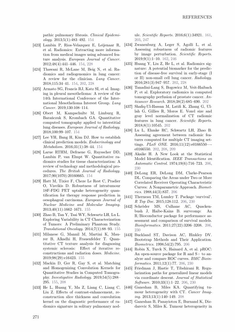
REFERENCES
pathic pulmonary fibrosis. Clinical Epidemi-ology. 2013;5(1):483–492. 154
[423] Lambin P, Rios-Velazquez E, Leijenaar R,et al. Radiomics: Extracting more informa-tion from medical images using advanced fea-ture analysis. European Journal of Cancer.2012;48(4):441–446. 154, 228
[424] Thawani R, McLane M, Beig N, et al. Ra-diomics and radiogenomics in lung cancer:A review for the clinician. Lung Cancer.2018;115:34–41. 154, 202, 228
[425] Armato SG, Francis RJ, Katz SI, et al. Imag-ing in pleural mesothelioma: A review of the14th International Conference of the Inter-national Mesothelioma Interest Group. LungCancer. 2019;130:108–114.
[426] Obert M, Kampschulte M, Limburg R,Barańczuk S, Krombach GA. Quantitativecomputed tomography applied to interstitiallung diseases. European Journal of Radiology.2018;100:99–107. 154
[427] Lee YH, Bang H, Kim DJ. How to establishclinical prediction models. Endocrinology andMetabolism. 2016;31(1):38–44. 154
[428] Larue RTHM, Defraene G, Ruysscher DD,Lambin P, van Elmpt W. Quantitative ra-diomics studies for tissue characterization: Areview of technology and methodological pro-cedures. The British Journal of Radiology.2017;90(1070):20160665. 154
[429] Hatt M, Tixier F, Cheze Le Rest C, PradierO, Visvikis D. Robustness of intratumour18F-FDG PET uptake heterogeneity quan-tification for therapy response prediction inoesophageal carcinoma. European Journal ofNuclear Medicine and Molecular Imaging.2013;40(11):1662–1671. 155
[430] Zhao B, Tan Y, Tsai WY, Schwartz LH, Lu L.Exploring Variability in CT Characterizationof Tumors: A Preliminary Phantom Study.Translational Oncology. 2014;7(1):88–93. 155
[431] Milanese G, Mannil M, Martini K, Mau-rer B, Alkadhi H, Frauenfelder T. Quan-titative CT texture analysis for diagnosingsystemic sclerosis: Effect of iterative re-constructions and radiation doses. Medicine.2019;98(29):e16423. 155
[432] Mackin D, Ger R, Gay S, et al. Matchingand Homogenizing Convolution Kernels forQuantitative Studies in Computed Tomogra-phy. Investigative Radiology. 2019;54(5):288–295. 155, 208
[433] He L, Huang Y, Ma Z, Liang C, Liang C,Liu Z. Effects of contrast-enhancement, re-construction slice thickness and convolutionkernel on the diagnostic performance of ra-diomics signature in solitary pulmonary nod-
ule. Scientific Reports. 2016;6(1):34921. 161,203, 247
[434] Zwanenburg A, Leger S, Agolli L, et al.Assessing robustness of radiomic featuresby image perturbation. Scientific Reports.2019;9(1):1–10. 162, 246
[435] Huang Y, Liu Z, He L, et al. Radiomics sig-nature: A potential biomarker for the predic-tion of disease-free survival in early-stage (Ior II) non-small cell lung cancer. Radiology.2016;281(3):947–957. 202, 228
[436] Tanadini-Lang S, Bogowicz M, Veit-HaibachP, et al. Exploratory radiomics in computedtomography perfusion of prostate cancer. An-ticancer Research. 2018;38(2):685–690. 202
[437] Shafiq-Ul-Hassan M, Latifi K, Zhang G, Ul-lah G, Gillies R, Moros E. Voxel size andgray level normalization of CT radiomicfeatures in lung cancer. Scientific Reports.2018;8(1):10545. 202
[438] Lu L, Ehmke RC, Schwartz LH, Zhao B.Assessing agreement between radiomic fea-tures computed for multiple CT imaging set-tings. PLoS ONE. 2016;11(12):e0166550—-e0166550. 202, 208, 209
[439] Akaike H. A New Look at the StatisticalModel Identification. IEEE Transactions onAutomatic Control. 1974;19(6):716–723. 206,230
[440] DeLong ER, DeLong DM, Clarke-PearsonDL. Comparing the Areas under Two or MoreCorrelated Receiver Operating CharacteristicCurves: A Nonparametric Approach. Biomet-rics. 1988;44(3):837. 206
[441] Therneau TM, Lumley T. Package ‘survival’.R Top Doc. 2015;128:112. 206, 230
[442] Schröder MS, Culhane AC, Quacken-bush J, Haibe-Kains B. survcomp: AnR/Bioconductor package for performance as-sessment and comparison of survival models.Bioinformatics. 2011;27(22):3206–3208. 206,230
[443] Buckland ST, Davison AC, Hinkley DV.Bootstrap Methods and Their Application.Biometrics. 1998;54(2):795. 206
[444] Robin X, Turck N, Hainard A, et al. pROC:An open-source package for R and S+ to an-alyze and compare ROC curves. BMC Bioin-formatics. 2011;12(1):77. 206, 230
[445] Friedman J, Hastie T, Tibshirani R. Regu-larization paths for generalized linear modelsvia coordinate descent. Journal of StatisticalSoftware. 2010;33(1):1–22. 206, 230
[446] Ganeshan B, Miles KA. Quantifying tu-mour heterogeneity with CT. Cancer Imag-ing. 2013;13(1):140–149. 208
[447] Ganeshan B, Panayiotou E, Burnand K, Diz-darevic S, Miles K. Tumour heterogeneity in
271

non-small cell lung carcinoma assessed by CTtexture analysis: A potential marker of sur-vival. European Radiology. 2012;22(4):796–802. 208, 228, 234, 245
[448] Grove O, Berglund AE, Schabath MB, etal. Quantitative computed tomographic de-scriptors associate tumor shape complex-ity and intratumor heterogeneity with prog-nosis in lung adenocarcinoma. PLoS ONE.2015;10(3):e0118261. 208
[449] Kakino R, Nakamura M, Mitsuyoshi T, et al.Comparison of radiomic features in diagnos-tic CT images with and without contrast en-hancement in the delayed phase for NSCLCpatients. Physica Medica. 2020;69:176–182.209
[450] Standfield L, Weston AR, Barraclough H,Van Kooten M, Pavlakis N. Histology as atreatment effect modifier in advanced non-small cell lung cancer: A systematic reviewof the evidence. Respirology. 2011;16(8):1210–1220. 228
[451] Dercle L, Fronheiser M, Lu L, et al. Iden-tification of Non-Small Cell Lung CancerSensitive to Systemic Cancer Therapies Us-ing Radiomics. Clinical Cancer Research.2020;26(9):2151–2162. 228, 245
[452] Coroller TP, Agrawal V, Huynh E, et al.Radiomic-Based Pathological Response Pre-diction from Primary Tumors and LymphNodes in NSCLC. Journal of Thoracic On-cology. 2017;12(3):467–476. 228, 245
[453] Dercle L, Ammari S, Bateson M, et al. Lim-its of radiomic-based entropy as a surrogateof tumor heterogeneity: ROI-area, acquisi-tion protocol and tissue site exert substantialinfluence. Scientific Reports. 2017;7(1):7952.228, 245
[454] Bogowicz M, Pavic M, Riesterer O, et al. PD-0429: CT radiomics differentiates levels ofradiocurability in tumor subvolumes in headand neck cancer. Radiotherapy and Oncology.2020;152:S235. 229, 236
[455] Jollife IT, Cadima J. Principal componentanalysis: A review and recent developments.Philosophical Transactions of the Royal Soci-ety A: Mathematical, Physical and Engineer-ing Sciences. 2016;374(2065):20150202. 230
[456] Canty A, Ripley B. boot: {B}ootstrap {R}({S}-Plus) Functions. R package version.2006;1:3–20. 230
[457] Ferreira Junior JR, Koenigkam-Santos M,Cipriano FEG, Fabro AT, de Azevedo-Marques PM. Radiomics-based featuresfor pattern recognition of lung cancerhistopathology and metastases. ComputerMethods and Programs in Biomedicine.2018;159:23–30. 234
[458] Digumarthy SR, Padole AM, Gullo RL, Seq-uist LV, Kalra MK. Can CT radiomic analysisin NSCLC predict histology and EGFR mu-tation status?. Medicine. 2019;98(1):e13963.235
[459] Zhu X, Dong D, Chen Z, et al. Radiomic sig-nature as a diagnostic factor for histologicsubtype classification of non-small cell lungcancer. European Radiology. 2018;28(7):2772–2778. 234, 235
[460] Lafata K, Cai J, Wang C, Hong J, Kelsey CR,Yin FF. Spatialoral variability of radiomicfeatures and its effect on the classificationof lung cancer histology. Physics in Medicineand Biology. 2018;63(22):225003. 234
[461] Giraud P, Antoine M, Larrouy A, et al. Eval-uation of microscopic tumor extension in non-small-cell lung cancer for three-dimensionalconformal radiotherapy planning. Interna-tional Journal of Radiation Oncology BiologyPhysics. 2000;48(4):1015–1024. 235
[462] Tunali I, Hall LO, Napel S, et al. Stabil-ity and reproducibility of computed tomog-raphy radiomic features extracted from peri-tumoral regions of lung cancer lesions. Medi-cal Physics. 2019;46(11):5075–5085. 235, 236,247
[463] Keek S, Sanduleanu S, Wesseling F, et al.Computed tomography-derived radiomic sig-nature of head and neck squamous cell car-cinoma (peri)tumoral tissue for the predic-tion of locoregional recurrence and distantmetastasis after concurrent chemoradiother-apy. PLoS ONE. 2020;15(5):e0232639. 235
[464] De Jay N, Papillon-Cavanagh S, Olsen C,El-Hachem N, Bontempi G, Haibe-Kains B.MRMRe: An R package for parallelizedmRMR ensemble feature selection. Bioinfor-matics. 2013;29(18):2365–2368. 238
[465] Fournier L, Costaridou L, Bidaut L, etal. Incorporating radiomics into clinical tri-als: expert consensus on considerations fordata-driven compared to biologically drivenquantitative biomarkers. European Radiology.2021;:1–12. 243, 248
[466] Radiomics: a Study of Outcome in Lung Can-cer . 243
[467] Decaluwé H, Stanzi A, Dooms C, et al. Cen-tral tumour location should be consideredwhen comparing N1 upstaging between thora-coscopic and open surgery for clinical stage Inon-small-cell lung cancer. European Journalof Cardio-thoracic Surgery. 2016;50(1):110–117. 244
[468] Shi L, Rong Y, Daly M, et al. Cone-beamcomputed tomography-based delta-radiomicsfor early response assessment in radiotherapy
272

REFERENCES
for locally advanced lung cancer. Physics inMedicine and Biology. 2020;65(1). 245
[469] Traverso A, Kazmierski M, Zhovannik I, etal. Machine learning helps identifying volume-confounding effects in radiomics. PhysicaMedica. 2020;71:24–30. 245, 248
[470] Pérez-Morales J, Tunali I, Stringfield O, et al.Peritumoral and intratumoral radiomic fea-tures predict survival outcomes among pa-tients diagnosed in lung cancer screening. Sci-entific Reports. 2020;10(1). 245
[471] Braman NM, Etesami M, Prasanna P, et al.Intratumoral and peritumoral radiomics forthe pretreatment prediction of pathologicalcomplete response to neoadjuvant chemother-apy based on breast DCE-MRI. Breast Can-cer Research. 2017;19(1):57. 245, 246
[472] Brascia D, Iaco GD, Schiavone M, et al. Re-sectable IIIA-N2 non-small-cell lung cancer(NSCLC): In search for the proper treatment.Cancers. 2020;12(8):1–31. 245
[473] aki Hirose T, Arimura H, Ninomiya K, Yoshi-take T, ichi Fukunaga J, Shioyama Y. Ra-diomic prediction of radiation pneumonitison pretreatment planning computed tomog-raphy images prior to lung cancer stereotac-tic body radiation therapy. Scientific Reports.2020;10(1):1–9. 245
[474] van Timmeren JE, van Elmpt W, LeijenaarRT, et al. Longitudinal radiomics of cone-beam CT images from non-small cell lungcancer patients: Evaluation of the addedprognostic value for overall survival and lo-coregional recurrence. Radiotherapy and On-cology. 2019;136:78–85. 245, 247
[475] Gu Q, Feng Z, Hu X, et al. Radiomicsin predicting tumor molecular marker P63for non-small cell lung cancer. Journal ofCentral South University (Medical Sciences).2019;44(9):1055–1062. 246
[476] Traverso A, Wee L, Dekker A, Gillies R. Re-peatability and Reproducibility of RadiomicFeatures: A Systematic Review. Interna-tional Journal of Radiation Oncology BiologyPhysics. 2018;102(4):1143–1158. 246
[477] Network SPH. Swiss Personalized Health Net-work. 2019. 246
[478] Ardila Pardo GL, Conzelmann J, Genske U,Hamm B, Scheel M, Jahnke P. 3D printingof anatomically realistic phantoms with de-tection tasks to assess the diagnostic perfor-mance of CT images. European Radiology.2020;30(8):4557–4563. 246
[479] Parmar C, Barry JD, Hosny A, Quacken-bush J, Aerts HJ. Data Analysis Strategies inMedical Imaging. Clinical Cancer Research.2018;24(15):3492–3499. 247
[480] Yamashita R, Nishio M, Do RKG, Togashi K.Convolutional neural networks: an overviewand application in radiology. Insights intoImaging. 2018;9(4):611–629. 248
[481] Zhou B, Khosla A, Lapedriza A, Oliva A, Tor-ralba A. Learning Deep Features for Discrim-inative Localization. 2016. 248
[482] University of Arkansas for Medical Sciences(UAMS). Cancer Imaging Archive. 2017. 248
[483] Deist TM, Jochems A, van Soest J, etal. Infrastructure and distributed learningmethodology for privacy-preserving multi-centric rapid learning health care: euroCAT.Clinical and Translational Radiation Oncol-ogy. 2017;4:24–31. 248
[484] Bogowicz M, Jochems A, Deist TM, et al.Privacy-preserving distributed learning of ra-diomics to predict overall survival and HPVstatus in head and neck cancer. Scientific Re-ports. 2020;10(1):1–10. 248
[485] Fontaine P, Acosta O, Castelli J, CrevoisierRD, Müller H, Depeursinge A. Standardisedconvolutional filtering for radiomics. Scien-tific Reports. 2020;10(1). 248
[486] Leijenaar R, Zerka F, Vaidyanathan A, et al.5MO Prospective validation of a radiomicssignature for chemoradiotherapy lung cancerpatients. Annals of Oncology. 2020;31:S246.249
[487] Nardone V, Reginelli A, Guida C, et al. Delta-radiomics increases multicentre reproducibil-ity: a phantom study. Medical Oncology.2020;37(5). 249
273

Curriculum Vitae
Diem VuongBorn November 10, 1992 in Basel-Stadt, Switzerland.
Education
2017–2021* Ph.D., Physics, University of Zurich
2018–2021 Master of Advanced Studies ETH in Medical Physics, ETH Zurich
2015–2017 Master of Science ETH in Physics, ETH Zurich
2011–2014 Bachelor of Science ETH in Physics, ETH Zurich
2006–2011 Matura, Wirtschaftsgymnasium Basel
*Indicates expected
Professional Experience
2017 Internship ionising radiation Federal Institute of Metrology METAS, Bern-Wabern
2015–2016 Mathematics tutor Schule für Förderkurse, Zurich
2013–2014 Internship acoustics laboratory Swiss Federal Laboratories for Materials Science andTechnology (EMPA), Dübendorf
Teaching Assistant
FS2019 PHY125 Scientific Computing University of Zurich
HS2018 PHY114 Computing Physics University of Zurich
FS2018 PHY125 Scientific Computing University of Zurich
Grants and Awards
2020 SNF Mobility Grant. 6-month research stay at Odense University Hospital, Odense,Denmark
2019 Best Poster Award. European Lung Cancer Congress (ELCC), Geneva, Switzerland