Dual modality tomography for the monitoring of constituent ...

Dual modality tomography for the monitoring of constituent volumes in multi-component flows.

DANIELS, A. R.

Available from Sheffield Hallam University Research Archive (SHURA) at:

http://shura.shu.ac.uk/19533/

This document is the author deposited version. You are advised to consult the publisher's version if you wish to cite from it.

Published version

DANIELS, A. R. (1996). Dual modality tomography for the monitoring of constituent volumes in multi-component flows. Doctoral, Sheffield Hallam University (United Kingdom)..

Copyright and re-use policy

See http://shura.shu.ac.uk/information.html

Sheffield Hallam University Research Archivehttp://shura.shu.ac.uk

http://shura.shu.ac.uk/

http://shura.shu.ac.uk/information.html

Sheffield Hallam University

REFERENCE ONLY

ProQuest Number: 10694414

All rights reserved

INFORMATION TO ALL USERS The quality of this reproduction is dependent upon the quality of the copy submitted.

In the unlikely event that the author did not send a com ple te manuscript and there are missing pages, these will be noted. Also, if material had to be removed,

a note will indicate the deletion.

uestProQuest 10694414

Published by ProQuest LLC(2017). Copyright of the Dissertation is held by the Author.

All rights reserved.This work is protected against unauthorized copying under Title 17, United States C ode

Microform Edition © ProQuest LLC.

ProQuest LLC.789 East Eisenhower Parkway

P.O. Box 1346 Ann Arbor, Ml 48106- 1346

DUAL MODALITY TOMOGRAPHY FOR THE

MONITORING OF CONSTITUENT VOLUMES IN

MULTI-COMPONENT FLOWS

A R DANIELS (B(Eng.) AMIEE)

Thesis submitted to satisfy the

requirements of Sheffield Hallam University for the degree

of Doctor of Philosophy (PhD)

School of Engineering Information Technology


Pond Street

Sheffield

S1 1WB

February 1996

Acknowledgements

ACKNOWLEDGEMENTSThe concept for this project came from my supervisor Professor R G Green

without whose immense knowledge, gentle encouragement and eternal

patience little progress would have been possible. Many thanks also to my

second supervisor Dr I Basarab for his support and patient reading of draft

papers/thesis and to Dr F Dicken and his process tomography team at UMIST

for their advice and help, especially in the construction of phantoms etc. I

would also like to thank all the technicians in the department of EIT at Sheffield

Hallam University for their assistance in constructing circuits and hardware etc.

I am also grateful to the other researchers with whom I had the pleasure of

working: Neil, Marshall, Joe, Jas, Fu’ad, Ruzairi and Jan, whose support and

friendship was invaluable throughout my three and a half years.

My biggest debt is to Valerie, my wife, for her patience and understanding

during my time as a researcher and when writing my thesis.

Abstract

ABSTRACTThis thesis describes an investigation into the use of dual modality tomography

to monitor multi-component flows. The concept of combining two modalities for

this purpose evolved from a desire by the Water Research Council to

determine volume flow rates of the major components of sewage. No single

sensing method is capable of detecting all suspended solids in sewage flows

therefore a decision was taken to combine the technologies of electrical

resistance and optical tomography to produce a single measurement system.

Sensors for both were positioned around the periphery of a static, circular

phantom to allow comparisons between dual and single modalities.

Modelling was carried out to determine the behaviour of the electrical

impedance and optical tomography technologies in a three dimensional

situation, where a variety of flow components exist. This provided a greater

understanding of the problems involved in combining these technologies and

an appreciation of the potential benefits.

The remainder of the work can be divided into three areas. Firstly, hardware

was constructed to make voltage measurements for both modalities. Secondly,

software was written to perform data acquisition, data manipulation and image

reconstruction using a simple back projection algorithm developed for this

purpose. Finally, an integration of the individual hardware and software

components was performed to produce a dual modality system on which tests

were carried out to determine the resulting benefits over single modality

alternatives.

II

i aD ie ot uomenis

TABLE OF CONTENTSC h a p t e r 1

In t r o d u c t io n

1.1 Sewage Flow s .................................................................................................................... 1

1.1.1 The Changing Boundary..........................................................................................................2

1.1.2 Safety as a Consideration.........................................................................................................3

1.1.3 The Environment Within a Sewer............................................................................................ 4

1.1.4 Physical Properties of the Conveying Liquid........................................................................ 4

1.2 Existing Flow Measurement A pproaches ................................................................. 5

1.2.1 Commercial Flow Measurement Techniques........................................................................ 5

1.2.1.1 Variable A rea Flo w M eter .....................................................................................................................5

1.2.1.2 Turbine Fl o w M eter ................................................................................................................................. 6

1.2.1.3 D ifferential Pressure Fl o w M e te r s ................................................................................................. 6

1.2.1.4 Vo rtex Shedding Flo w M eter ...............................................................................................................6

1.2.1.5 Electromagnetic Fl o w M e t e r ..............................................................................................................71.2.1.6 Ultrasonic Flo w M e t e r ..........................................................................................................................71.2.1.6 Coriolis F o rce Fl o w Me ter ...................................................................................................................7

1.2.2 Tomographic Techniques Under Development.................................................................... 8

1.2.2.1 Electrical Im pedance To m o g r a p h y ....................................................................................................8

1.2.2.2 Electrical Capacitance Tom o g raphy ................................................................................................9

1.2.2.3 Electrical Charge Tomography ........................................................................................................10

1.2.2.4 Electromagnetic To m o g raphy .......................................................................................................... 10

1.2.2.5 Optical Tom o g raphy ..............................................................................................................................11

1.2.2.6 Ultrasonic A coustic Tomography ....................................................................................................11

1.2.2.7 O ther Tomographic M eth o d s .............................................................................................................12

1.3 T he Dual Modality Measurement Sy s t e m ............................................................... 12

1.4 A ims of the pr o je c t .......................................................................................................14

1.5 O rganisation of the thesis ..........................................................................................15

C h a p te r 2

Im a g e R e c o n s t r u c t io n a n d S y s t e m S o f t w a r e

2.1 Five ERT Reconstruction Metho do lo g ies ............................................................17

2.1.1 Back Projection Along Equipotential Lines.........................................................................17

2.1.2 Iterative Back Projection Along Equipotential Lines..........................................................18

2.1.3 The Sensitivity Method........................................................................................................... 19

2.1.4 The Newton Raphson Algorithm............................................................................................19

i c iu ie u i o u m e i i i i

2.1.5 The Double Constraint Method............................................................................................. 19

2.2 Ba ck Projectio n of ERT Da t a ........................................................................................ 20

2.3 'B a ck Pro jectio n ' of O ptical Da ta ................................................................................25

2.4 Dual Modality T o m o g ra ph y Image R e c o n s tr u c tio n ...............................................27

2.5 So ftw a r e ..................................................................................................................................29

2.5.1 Electrical Resistance Tomography Software...................................................................... 29

2.5.2 Optical Tomography Software.............................................................................................. 32

2.5.3 Dual Modality Tomography Software...................................................................................34

C h a p t e r 3

E lec tr ic a l R esistance To m o g raphy

3.1 M ethods of Modelling C o m plex Im p e d a n c e ...............................................................35

3.1.1 Two Dimensional Modelling Using 'Teledeltos' Paper......................................................36

3.1.2 Results of Teledeltos Modelling........................................................................................... 38

3.1.3 Two Dimensional Modelling Using ’HSPICE'..................................................................... 41

3.1.4 Results of Two Dimensional HSPICE Modelling................................................................. 43

3.1.5 Three Dimensional Modelling Using 'HSPICE'................................................................... 45

3.1.6 Results of Three Dimensional HSPICE Modelling..............................................................46

3.1.7 Modelling Conclusions...........................................................................................................47

3.2 Ha r d w a r e .................................................................................................................................49

3.2.1 Electrode Construction..........................................................................................................50

3.2.2 Oscillator..................................................................................................................................52

3.2.3 Constant Current Source........................................................................................................52

3.2.4 Multiplexer................................................................................................................................54

3.2.5 High Impedance Buffer...........................................................................................................56

3.2.6 Instrumentation Amplifier.......................................................................................................57

3.2.7 R.M.S. To D.C. Converter........................................................................................................58

3.2.8 Analogue To Digital Converter...............................................................................................60

3.2.9 Computer Interface................................................................................................................. 62

3.3 Re s u l t s .....................................................................................................................................62

3.3.1 Varying Background Conductivity........................................................................................ 63

3.3.2 Three Dimensional Analysis...................................................................................................64

3.3.3 Image Reconstructions for Five Samples.............................................................................66

3.3.4 Image Reconstructions for Multiple Substances................................................................ 67

3.3.5 Conclusions from Measured Results.................................................................................... 68

3.3.6 Discussion of Data Acquisition Speed..................................................................................70

IV

i auie ui ouiiitsiiii)

C h a p te r 4

O ptical T om o g raphy

4.1 Modelling of O ptical D isco ntinuities ......................................................................72

4.1.1 Attenuation of Light................................................................................................................ 73

4.1.2 Refraction and Reflection At a 'Bubble' Interface...............................................................74

4.1.3 Divergence Due To 'Bubble' Interfaces................................................................................77

4.1.4 Refraction Due To a Variable Liquid Depth......................................................................... 78

4.1.5 Modelling Conclusions...........................................................................................................79

4.2 Hardw are .......................................................................................................................... 80

4.2.1 Optical Transducers............................................................................................................... 81

4.2.2 Logic Decoding / Data Latches............................................................................................. 85

4.2.3 LED Drivers..............................................................................................................................87

4.2.4 Analogue Switches................................................................................................................. 89

4.2.5 Signal Conditioning................................................................................................................ 91

4.2.6 Data Capture.............................................................................................................................92

4.2.7 Computer Interface................................................................................................................. 94

4.3 Re s u l t s ..............................................................................................................................94

4.3.1 Determination of 'a' for Air and Water..................................................................................95

4.3.2 Air Bubbles in Water............................................................................................................... 97

4.3.3 Variable Depth Liquids in Pipes............................................................................................ 99

4.3.4 Image Reconstructions for Five Samples...........................................................................101

4.3.5 Image Reconstructions for Multiple Substances.............................................................. 102

4.3.6 Conclusions from Measured Results.................................................................................. 103

C h a p te r 5

D ual M o dality T om o g raphy

5.1 Dual Modality Configuration...................................................................................106

5.2 Dual Modality Re s u l t s ...............................................................................................107

5.2.1 Dual Modality Image Combination Techniques................................................................ 107

5.2.1.1 A verag ing F u n c tio n s .......................................................................................................................... 108

5.2.1.2 Criteria Based Decision F unction ................................................................................................... 109

5.2.1.3 Log ical Combination F u n c tio n ......................................................................................................... 110

5.2.2 Image Reconstructions for Five Samples...........................................................................111

5.2.3 Image Reconstructions of Multiple Substances............................................................... 113

5.3 Conclusions ................................................................................................................... 114

v

i auie or uoruenis

C h a p te r 6

C o nclusio ns and Future W o r k

6.1 Conclusions ................................................................................................................... 116

6.1.1 Models for the Optical and Electrical Modalities (Aim *1').................................................116

6.1.2 Hardware for the Optical and Electrical Resistance Modalities (Aim ‘2’)....................... 117

6.1.3 Combination of Sensors for Both Modalities on the Same Section of Pipe (Aim ‘3’).. 117

6.1.4 Windows Based Software for Image Reconstruction and Data Acquisition (Aim ‘4’).. 117

6.1.5 The Comparison of Measured and Modelled Data (aim ‘5’).............................................. 117

6.1.5.1 Electrical Resistance To m o g raphy ..............................................................................................118

6.1.5.2 Optical To m ography ........................................................................................................................... 118

6.1.6 Image Combination Techniques to Produce Dual Modality Images (Aim *6’) ................119

6.1.7 Determining the Advantages of a Dual Modality Approach (Aim ‘7’)..............................119

6.1.7.1 Electrical R esistance Tomography R e su lts .............................................................................119

6.1.7.2 Optical To mography R esu lts .......................................................................................................... 120

6.1.7.3 D ual M odality Re s u lts ...................................................................................................................... 120

6.2 Future W o rk .................................................................................................................. 121

6.2.1 Faster Data Acquisition........................................................................................................121

6.2.1.1 Impro ved Data A cquisition Te c h n o lo g y .......................................................................................122

6.2.1.2 D irect Wave Sampling (ERT).............................................................................................................122

6.2.1.3 S witched d .c . Operation (ERT)........................................................................................................123

6.2.2 Electrical Resistance Tomography Sensors..................................................................... 125

6.2.2.1 Electrode Leng th ................................................................................................................................ 125

6.2.2.2 Compound El e c tr o d e s ...................................................................................................................... 126

6.2.2.3 M ulti-Layer Electrode Configurations.......................................................................................126

6.2 .2A Alternative Electrode N um bers .................................................................................................... 127

6.2.3 Optical Tomography Sensors............................................................................................. 128

6.2.3.1 Increased View s and Projections...................................................................................................128

6.2.3.2 O ther Lig ht S o u r c es .......................................................................................................................... 130

6.2.3.3 Alternative Lig ht Freq uencies ........................................................................................................131

6.2.4 Further Mathematical Modelling......................................................................................... 131

6.2.4.1 A n Impro ved H SPICE M o d e l ............................................................................................................131

6.2.4.2 Optical M odelling S oftware Development ................................................................................ 132

6.2.5 Other Possibilities for Future Work.................................................................................... 133

6.2.5.1 Timing Betw een M odalities................................................................................................................ 133

6.2.5.2 Impro ved Image Reconstruction and Alternatives ..................................................................133

6.2.5.4 Fl o w M odelling and Environmental M o nitoring .......................................................................134

References............................................................................................................................ 136

VI

Chapter 1: Introduction

CHAPTER 1 INTRODUCTIONThis chapter introduces work carried out to investigate the use of tomographic

imaging to monitor volume flows of individual sewage components. Current

monitoring technology is introduced and the options chosen for final

investigation are also presented. Finally, the aims of the project are described

followed by a description of how the thesis is organised.

1.1 S e w a g e F lo w s

The problems associated with monitoring sewage flows are similar to those that

arise when developing technology for other multi-component processes [44].

There are several reasons for monitoring sewage flows:

(1) To obtain daily on-line quantitative measurements from sewers which

can be used to verify mathematical modelling of this type of flow [45].

(2) Mechanical screens are used to remove solids from sewage flows but

present designs vary in efficiency (% of solid removed) from about 15% to

50% [47]. Because the development process for these processes is

empirical, two tomographic systems, one upstream and the other

downstream of a screen would provide a convenient method of monitoring

effectiveness and as a result help optimise designs.

(3) During periods of heavy rainfall many sewers are unable to handle the

volume of sewage flowing. Weirs inside the sewers permit any excess to

overflow and be diverted through storm drains into rivers or special settling

tanks [2]. Quantifying these flows would be useful for environmental

1


monitoring of the rivers at storm outlets and help enforce new European

pollution legislation.

The main components of sewage are: cellulose material (paper, sanitary

towels, rags etc.); rubber/plastic (condoms, plastic associated with sanitary

towels etc.); solids (faeces) and the conveying liquid (mainly water based).

Each have different physical properties making detection difficult using a single

measurement technique. There have been various investigations in the field of

two component flows including Dugdale [16] who applied optical methods to the

problem of liquid/air interactions and attempted to identify the types of flow that

occur. Govier [22] introduces theory to explain the interaction between

different phases for flows in pipes and Geraets [20] uses capacitance sensors

to identify flow patterns for two phase flows. This type of approach attempts

initially to explain the modes of flow caused by varying combinations of both

phases and then design hardware capable of identifying these. The work

presented here takes an alternative approach and investigates the feasibility of

designing a system capable of identifying the presence of each major

component of sewage and their volumes, rather than the physical behaviour of

the flow. Much of the work presented in this thesis concentrates on the type of

problems unique to the sewage application, although the technology developed

could successfully be applied to any situation where multi-component flows

exist. Typical problems associated with sewage flows are described in the

following sections.

1.1.1 T he C hanging Boundary

A problem particular to horizontal flows of the type found in sewers is the

changing boundary which results from the variation in flow depth, Fig.1.1. At

2


times of low flow levels Fig.1.1 (C) several sensors may not make contact with

the conveying liquid. Consequently any measurement system must be capable

of adapting to this, otherwise a significant amount of data will be lost. This is

especially important for a design using impedance tomography (Section 1.2.2)

where electrodes should be in contact with the conveying liquid.

Pipe Wall Sewage Flow

(a) (b) (c)

Fig.1.1 The Changing Boundary.

1.1.2 Sa fety as a Co nsideratio n .

Equipment designed to work in a sewer must be intrinsically safe due to the

presence of flammable gases, such as methane, in explosive concentrations.

For many forms of tomographic imaging this is not a problem as it is possible to

electrically isolate sensors. Careful consideration is required for designs using

electrical impedance or resistance tomography (Section 1.2.2) in order to

prevent the possibility of gaseous ignition resulting from the application of

electric currents across the flow regime. Brant et. al. [12] discuss the issue of

intrinsic safety with particular reference to explosive hazards in the oil and gas

industry and describe methods of optimising circuit design. Intrinsic safety is

an issue more correctly dealt with when a particular application has been

decided and it will be left for future work to address this aspect more fully.

3


1.1.3 The E nvironm ent W ith in a S ew er

Another important consideration for designers of hardware that operates within

a sewer is the internal environment. Sewers are extremely unclean areas

resulting in the requirement that all sensors be non-intrusive to reduce the

soiling of surfaces and degradation of measurement accuracy over time.

Sensors that require regular cleaning will result in a system that is inefficient

and costly to maintain. This is an issue that should be fully addressed during

the production process, although it should be apparent at the design stage that

a problem is not inherent when choosing a technique to monitor sewage flows.

1.1.4 P h ys ica l P ro p e r t ie s o f th e Conveying Liquid

The depth of the conveying liquid will affect the boundary conditions of a

measurement system, although the physical properties of the liquid may alter

due to a variety of reasons:

a) Mineral Seepage - to or from surrounding strata may affect the

electrical, optical and chemical properties as well as the relative density of

the conveying liquid.

b) Temperature Variations - occur due to seasonal changes in the

discharge temperature of fluids entering the sewage affecting the electrical

properties of the conveying liquid.

c) Influxes of Suspended Soil Material - during heavy rain will affect the

electrical, optical and chemical properties of the liquid.

d) Wide Variations in Discharge - from industrial and domestic outflows

will affect the depth, temperature, electrical, optical, and chemical

characteristics of the liquid.

4


1.2 Existing Flo w M easurem ent A ppro aches

Many measurement techniques are available to monitor liquid flows and some

for liquid/solid flows, but none exists that has been designed specifically for

multi-phase applications where components have vastly different physical

properties. ‘Flow’ measurement is a general term that can be defined as

having three distinct definitions:

(1) Volumetric Flow is the total volume that passes a measurement cross-

section per unit of time.

(2) Mass Flow is the total mass passing a measurement cross-section per

unit time.

(3) Velocity of Flow is the linear velocity past a measurement cross-section.

It is useful to define an additional category, that of Constituent Flow, as this is

more appropriate for multi-component processes and measures either the

Volumetric, Mass or Velocity flow of each distinct constituent within the flow.

An overview of existing commercial flow measurement technologies and

tomographic techniques currently under development is discussed below.

1.2.1 C om m ercial Flo w M easurem ent T echniques

Beck et. al. [6] define the concept of true mass flow measurement of a single

phase and explain the difficulties of relating liquid mass flow-rate to a single

direct on-line measurement. Single phase methods [37], [18] and [35] usually

relate to liquid or gas flows and include the following technologies [37]:

1.2.1.1 Variable Area FlowMeter

One type of variable area meter introduces a restriction into a section of pipe

which increases in diameter along the length of the pipe. An increase in fluid

5


velocity produces an increasing force on the restriction, causing it to move in

the direction of the flow. The area around the restriction increases as it moves,

due to the pipe’s taper, reducing the pressure drop across it. As a result the

restriction settles in a position where the opposite force applied to it (e.g. by a

spring) exactly matches the force produced by the differential pressure. A

typical design [3] inserts a magnet in the restriction and a Hall effect sensing

device connected to a micro-controller interface is used to determine flow-

rates.

1.2.1.2 Turbine FlowMeter

The turbine flow-meter utilises a ‘propeller’ situated in the flow and measures

the flow rate by counting the number of revolutions induced per second, as the

angular velocity is proportional to the rate of flow. Rotations are detected

‘electronically’ using a proximity detector within the pipe wall close to the

propeller.

1.2.1.3 Differential Pressure Flow Meters

Known more commonly as ‘orifice plate’ or ‘venturi’ meters these introduce a

restriction or gradual narrowing of the pipe into the flow causing a pressure

drop. Pressure is measured either side of the restriction and the difference

calculated. Flow rate is proportional to the square root of the measured

differential pressure, but at low flows inaccuracy increases as low differential

pressure values are difficult to measure.

1.2.1.4 Vortex Shedding Flow Meter

If a ‘bluff body is placed in a slow moving liquid it passes smoothly around the

outside. As the fluid velocity increases the liquid separates alternately from the

sides of the bluff body and swirls to form ‘vortices’. Pressure sensors, such as

6


Piezo electric cells, can be used to measure these oscillations which are then

used to determine the flow rate.

1.2.1.5 Electromagnetic Flow Meter

This type of flow-meter applies an electromagnetic field across the flow. When

a conducting liquid passes through this field a small electric current is induced

which can be detected by measuring the induced voltage between two

electrodes. Flow rate is proportional to the measured voltage for a conveying

liquid with constant electrical properties, which is an important consideration

because if the electrical properties are subject to change this technology will

not produce accurate results.

1.2.1.6 Ultrasonic FlowMeter

The ultrasonic flow meter has two standard categories, the ‘Doppler effect’ and

the ‘time of flight’ meters. The Doppler effect flow-meter transmits ultrasonic

pulses into the flow and measures levels of ‘reflected’ energy, which are then

related to flow rate. Time of flight meters measure the time taken for an

ultrasonic pulse to travel a set distance and then convert this a to flow rate. A

major problem with the Doppler effect meter is that it relies on the presence of

acoustic discontinuities within the flow otherwise little change in reflected

energy levels occurs. The time of flight approach is more accurate but because

only small changes in transit time occur these tend to be difficult to measure

accurately.

1.2.1.6 Coriolis Force Flow Meter

The Coriolis meter utilises the forces exerted by liquids as they flow around

bends in a vibrating pipe (Blickley [10]). As liquid approaches such a bend it

7


experiences an acceleration producing a force F-, and as it leaves it

experiences a deceleration resulting in an equal and opposite force F2.

Because and F2 occur at different positions the result is a twisting of the

pipe, which can be measured and converted to a mass flow rate. This

technique is accurate (1-2%) and can be implemented on dual phase flows

such as liquid/solid and liquid/liquid (i.e. oil and water). In general it is

expensive and only available for pipe diameters up to 100mm.

1.2.2 T om o graphic T echniques Under Develo pm en t

There is currently a wide variety of tomographic techniques under development

that are capable of measuring flow rates when used in conjunction with cross

correlation algorithms. Some techniques can also distinguish individual

materials in multi-component flows by using mathematical image reconstruction

algorithms. The main drawback of any tomographic technique is the cost of

associated hardware and software.

1.2.2.1 Electrical Impedance Tomography

Electrical impedance tomography (EIT) produces a cross-sectional image of

the impedance profile of a process. The origins of this technique can be traced

to medical computed tomography, [28] and [4] where a lower cost and less

harmful alternative to existing computed methods based on radiation was

required. If a potential difference is induced between two electrodes on the

external boundary of a conductive medium an electric field is produced within.

Other electrodes positioned around the boundary measure the intensity of this

field which is a function of the impedance profile of the enclosed medium.

Sheffield University EIT hardware [4] uses 16 electrodes located around the

outside of a patient’s

8


body. A constant current is injected between two electrodes and the voltage

potential induced is measured between all remaining adjacent electrode pairs.

These measurements are repeated for a series of current injection positions

and the resulting data are used to produce an impedance cross-section of the

patient’s body. This is achieved using a reconstruction algorithm to solve

Laplace’s field equations in two dimensions. This method has also been used

to monitor industrial processes such as the concentration profile measurements

made by Grootveld et. al. [24]. A distinction should be made between electrical

impedance tomography (EIT) and electrical resistance tomography (ERT), EIT

[42] uses both magnitude and phase components of the measured electrode

waveforms, while ERT [46] uses only the magnitudes.

1.2.2.2 Electrical Capacitance Tomography

Electrical capacitance tomography (ECT) is based on the principle that as a

substance moves through a measurement plane its specific permittivity alters

the overall capacitance of the plane. Most capacitance systems use up to

twelve measurement electrodes positioned around the outside of the

measurement volume. Yang et. al. [53] present circuitry to measure low levels

of capacitance with high accuracy (1 %) requiring resolutions of 0.1 /F. A series

of capacitance values can be determined by measuring between combinations

of two electrodes. The resulting data are used by a reconstruction algorithm

such as that used by Huang et. al. [26] to image two component process flows.

Consequently, ECT is a viable technology but the resolution is limited due to

the length of electrodes necessary to produce measurable capacitances. This

produces the ‘smearing’ and ‘averaging’ effect associated with this technology.

9


1.2.2.3 Electrical Charge Tomography

Most of the work to date in this area of process monitoring has been carried out

by Shackleton and Bidin et. al. [8, 9] using insulated electrodes fitted into the

wall of a steel pipe. Dry particulates, passing these electrodes induce charge

into them which is detected by either converting it to a voltage (charging a

capacitor) or passing it to a charge amplifier. Currently, neural networks are

used to identify the flow regime and velocity information is obtained by using

two arrays of sensors at different positions along the pipe. This technique has

the potential to monitor processes containing dry particulate flows and non

conducting liquids. However, it is not applicable to conducting liquids such as

those found in sewage flows.

1.2.2.4 Electromagnetic Tomography

Electromagnetic tomography (EMT) is a new area of investigation instigated

after a feasibility study carried out by Yu et. al. [56] with an experimental

system using 21 sensors. The basis of this approach is to energise a

measurement section using a sinusoidal magnetic field created using copper

coils. The conductivity and permeability of a material within the measurement

section produces a unique magnetic field, which is detected by separate

measurement coils. Current work conducted by Yu et. al. [56] concerns the

detection of electrically conductive and ferromagnetic material and it is not

possible at this stage to determine the potential for detecting other substances.

One consideration is the high cost of hardware required to generate high

intensity magnetic fields capable of penetrating large objects.

10


1.2.2.5 Optical TomographyOptical tomography is an established imaging technique used by Saeed et. al.

[40] and Dugdale [16] for the identification of two component flows. As light

travels through space it suffers attenuation for a variety of reasons, including

scattering and absorption. Different materials cause varying levels of

attenuation and it is this fact that forms the basis of optical tomography. If an

optical emitter and detector pair, termed a 'view', are positioned either side of

the measurement volume, information about its optical characteristics can be

obtained. If the light is 'collimated' into thin 'pencils' and several views are

grouped together to form a 'projection' then a larger area can be interrogated.

If several different projections are used then it is possible to reconstruct an

image of the materials optical attenuation cross-section.

1.2.2.6 Ultrasonic Acoustic Tomography

Ultrasonic tomography is an established medical imaging technique which has

achieved a reputation as a useful method for the measurement of velocities in

process flows. Xu et. al. [52] used ultrasonic tomography to measure bubble

velocities in two phase flows. Transducers are excited using extremely short

duration voltage pulses causing ultrasonic energy to propagate through the

flow medium. This energy is attenuated by an amount dependent on the flow’s

physical composition. The detected signal is a train of amplitude modulated

pulses which can be buffered, signal processed and low-pass filtered to

produce an analogue voltage waveform. If two sets of detector/emitter pairs

are used, at separate positions along the flow pipe, then cross-correlation [52]

of the resulting data allows velocity information to be derived. The major

drawback with this technique is that ultrasonic waves are difficult to collimate

11


and problems occur due to reflections within enclosed spaces, such as metal

pipes etc. A Water Research Council report [48] concluded that the use of

ultrasonic methods to detect solids within sewage flows was impractical due to

the lack of contrast between the conveying liquid and some of the solid

material, such as paper and rubber.

1.2.2.7 Other Tomographic Methods

A variety of other measurement techniques exists such as microwave

tomography which utilises the varying attenuation characteristics of different

materials at high frequencies. The main problem with microwave tomography

is that of sensor design [11], as components have only recently emerged that

allow spatial resolutions of less than 1cm at the detector. Microwave

technology requires complex control circuitry but is capable of producing good

discrimination between materials. Nuclear Magnetic Resonance (NMR)

tomography is currently used as a medical imaging tool. NMR has been used

by King et. al. [29] to monitor the flow of pneumatically conveyed coal but the

major drawback for process applications is the development cost of the high

power, high speed magnetic coils required to induce a uniform magnetic field

through the whole of a measurement section.

1.3 T he D ual M o dality M ea su r em en t System

After reviewing the various options it was decided that a dual modality system

would provide the best approach for the detection of all the major components

within sewage. Xie et. al. [51] used the dual modalities of electrodynamic and

capacitance tomography to make mass flow calculations of gravity fed solids.

Cross-correlation techniques were used in conjunction with one modality to

12


obtain velocity information while the second modality determined volume

profiles. For the purposes of this work a cost effective approach was

necessary and consequently the modalities of optical and electrical resistance

tomography were chosen for investigation. Sensors for both are low cost and

the design of associated circuitry can be made intrinsically safe. The electrical

and optical characteristics of the major components of sewage are:

a) Cellulose Materials tend to be absorbent and consequently assume the

same electrical properties as the conveying liquid. They are usually

optically opaque.

b) Rubber/Plastic materials have a high electrical resistance and vary

between opaque and clear in their optical properties.

c) Solids generally have a resistivity higher than the conveying liquid and

are opaque.

d) The Conveying liquid can vary in respect of both optical and electrical

properties but is mostly water in content.

Many fluids are opaque to visible light, but optical wavelengths are used to

prove that the technique is viable. Wavelengths can then be modified to suite

particular applications. An outline of the dual modality measurement system is

shown in Fig. 1.2 which illustrates sensors for both optical and ERT tomography

mounted on a section of pipe. In reality both sets of transducers will have to be

positioned close together to reduce the possibility of an image offset when the

data sets are combined. All measurements were made using an 8cm (internal

diameter) pipe, designed to fit directly into a flow rig. Optical hardware was

designed using two ‘projections’ of 8 transducer pairs (views) allowing image

13


reconstruction to be applied to the acquired data. The ERT hardware was

designed using 16 electrodes positioned equidistantly around the periphery of

the pipe wall.

Pipe

Analogue to Digital

Conversion

Analogue to Digital

Conversion

LED and Sensor

ElectronicsData Analysis

and Image Production

E ITSensors

OpticalSensors

Current Injection and

Voltage Measurement

Direction of Flow

Fig.1.2 The proposed measurement system.

1.4 A ims OF THE PROJECT

The main project aim was to design and investigate the benefits of a dual

modality (optical an electrical resistance) tomography system for the

measurement of constituent volumetric flows (Section 1.2) in sewers. The

overall dual modality design was analysed and any possible improvements

recorded, in terms of image 'quality' and the range of materials detected. Other

research in this field tends to show that multi-component processes

incorporating solids, liquids and possibly gases are unlikely to be imaged using

a single modality due to the limited capabilities of any one process [16, 24, 26].

The original project objectives were:

1. Devise models for both the electrical resistance and optical tomography

methodologies and where appropriate, investigate in two and three

dimensions their potential performance in multi-component flows.

14


2. Design and build sixteen electrode, electrical resistance and two

projection, eight view optical tomography hardware. Both systems must be

compatible with the same computer input/output hardware to allow simple

data combination.

3. Combine the sensor hardware for both modalities on a single section of

pipe to allow dual modality data to be acquired.

4. Write 'Windows' based software to implement back projection algorithms

for both the electrical resistance and optical tomography designs and use

this to implement a dual modality imaging system.

5. Compare measured and modelled data for both modalities.

6. Make measurements and reconstruct images for a wide range of

materials within a liquid conveyor, including bubbles, and draw conclusions

about the benefits of dual modality tomography.

1.5 O rganisation of the thesis

An outline of the contents of each thesis chapter is given below:

Chapter 1: A general introduction to the topic of tomography and its

application to the monitoring of process flows is presented.

Chapter 2: Image reconstruction theory and methodology are presented

and an algorithm capable of producing images for optical, electrical

resistance and dual modality tomography is described. Also, Windows

software designed to control the system hardware, carry out image

reconstruction and produce a graphical display is described.

15


Chapter 3: A detailed description of the hardware designed, built and

tested to implement electrical impedance tomography is given. Modelling

carried out in two and three dimensions and test results carried out on a

static phantom are also presented.

Chapter 4: Similar in content to chapter three but with reference to the

optical hardware. Modelling carried out to determine the behaviour of

certain aspects of optical theory is also presented.

Chapter 5: Describes how the hardware outlined in chapters three and four

is combined to produce a dual modality system. Results are also

presented for various image reconstructions.

Chapter 6: This chapter presents conclusions relating to previous chapters

and makes suggestions for future work.

16

Chapter 2: Image Reconstruction and System Software

CHAPTER 2IMAGE RECONSTRUCTION AND SYSTEM SOFTWAREThis chapter presents theory relating to the reconstruction of tomographic

images and the system software written to achieve this. It can be divided into

five sections: firstly, five major electrical resistance reconstruction algorithms

are introduced; secondly, implementation of the back projection method used in

this thesis is described; thirdly a method for the reconstruction of optical

tomography data is presented; next, there is a description of how both

techniques can be combined to produce dual modality tomograms and finally

Windows software written to implement image reconstruction and hardware

control is discussed.

2.1 F ive ER T R e c o n s t r u c t io n M e t h o d o l o g ie s

The purpose of an electrical resistance tomography reconstruction algorithm is

to produce a graphical representation of the resistance cross-section bounded

by the measurement electrodes. A major difficulty when designing algorithms

for electrical resistance tomography lies in the behaviour of electric currents,

which follow a path of least resistance. Consequently, the equipotentials within

a measurement volume tend to form complex three dimensional shapes that

are a function of the internal resistivity profile. This is in contrast to optical

tomography where light beams, when fully collimated, follow an extremely

predictable path unless absorbed or deflected by some object.

2.1.1 Back Pro jectio n A long Eq uipo tential L ines

This was proposed by Barber et al [4] and uses the principle that if lines of

equipotential are traced between electrodes then any change in resistivity

17


within the measurement cross-section produces a corresponding voltage

change at the originating electrodes. This is due to the Ohmic relationship

between the measured voltages and the internal resistivity profile of the

measurement section. Back Projection Along Equipotential Lines is limited by

the assumption that the back projected equipotential lines remain a constant

shape, when modelling in chapter 3 demonstrates that this is not the case. The

result is that for large objects (relative to the measurement section) and for

objects of high resistance (relative to the surrounding medium) image

distortions occur. Barber and Browne [5] describe a fast, one step

implementation of this method and a variation of this is used for image

reconstructions throughout this thesis.

2.1.2 I te ra t iv e Back P ro je c t io n A lo n g E q u ip o te n tia l Lines

One step back projection reconstruction algorithms often produce large errors,

due to the reasons outlined above, and because of this an iterative variation

was developed. The 'forward' problem (that of finding boundary voltages due

to resistivity changes within the measurement section) is solved using a two

dimensional finite element approach. The 'backward' or inverse problem (that

of re-calculating the resistivity profile of the measurement section) is then

solved by a back projection which combines error values from the previous

solution to the forward problem and the actual measured boundary voltages.

After several iterations an improved image is produced, assuming that

convergence occurs which may require a relatively accurate first 'guess’ of the

resistance profile.

18


2.1.3 T he S ensitiv ity M ethod

Geselowitz [21] proposed the sensitivity theorem used by Gadd et al [19] to

reconstruct ERT images resulting from the adjacent electrode drive strategy.

For every projection, using adjacent current injection, sensitivity coefficients for

each pixel location are established which are then grouped together into

sensitivity regions. Back projection of measurement data is performed using

these coefficients as the basis for the image reconstruction, with the less

sensitive measurement pairs beingignored. Therefore, this approach is a

variation of the original Barber and Brown technique in that the sensitivity

regions are similar in shape to those produced by back projection.

2.1.4 T he N ew ton Raphson A lgorithm

This algorithm uses a regularised linear ‘approximation’ to improve the estimate

of conductivity for the 'backward' solution iteratively. In contrast to one step

methods this approach requires that the large matrix of potentials, and its

inverse, be calculated repeatedly producing an inflated computational

overhead. Computational speed can be improved by using parallel processors

[13] and dedicated matrix algebra co-processors. Yorkey et al [54] stated that

this method is guaranteed to converge to the optimal solution, although

variations of the algorithm often require a relatively accurate initial ‘guess’ of

the average resistivity.

2.1.5 T he D ouble C onstraint M ethod

This was proposed by Wexler et al [50] in which the finite element mesh is

constrained with known current source values and the current density is then

19


calculated for the computer model elements. The finite element mesh is then

constrained with the measured voltages and current source value allowing the

voltage gradient in each element to be calculated. Finally, the resistivity in

each element can be determined. Wexler demonstrated an improved accuracy

for the double constraint method over conventional iterative approaches but

this has to be weighed against the added computation required.

2.2 Ba c k P r o je c t io n o f ERT Da ta

Back projection along equipotential lines using a single step was implemented

to produce the image reconstructions presented in this thesis. This approach

was chosen because of its speed and ease of implementation, although Yorkey

[55] showed it to be the least accurate of the five methods outlined above.

Absolute accuracy was less important than speed and simplicity of design for

the purposes of this thesis because the reconstructed images are used as a

method of comparing sets of results. Although the algorithm presented here is

classified as 'back projection along equipotential lines' it also shares many

similarities with other reconstruction techniques such as the sensitivity

algorithm and may be more accurately described as a combination of the two.

As an introduction, the theory underlying this type of approach is outlined

below.

To produce accurate image reconstruction of an electrical resistance

measurement section involves the solution of a three dimensional problem. To

simplify the computational complexity that this entails most algorithms

approximate to two dimensions. Using Maxwell's equations {1-4} as a starting

20


point, formulae may be derived [49] that provide quantitative information about

the 'real' and 'imaginary' components of an electrical signal injected into a

circular phantom (radius ‘r’) containing a homogeneous liquid.

Where p = volume charge density; D = electric flux density; B = magnetic flux

density; H = magnetic field density; E = electric field density; J = current density

and t = time. Given that J = crE {3} can be re-written as:

Where a = conductivity, % = permittivity and co=27cf (f = frequency). If the values

of a and £ for water are substituted in {5}, for a frequency of 8kHz (the

operating frequency of the experimental system) then:

V .H = ( l + ( j8 .854 x 10~n x 1 6 n x l ( f ))E

The imaginary component of the electric field induced in an isotropic water

based phantom {6} is approximately 2200000 times smaller than the real part of

the signal at this frequency. If these measurements were resolved into

voltages by a phase sensitive detector then it would be difficult to make

measurements of the imaginary (phase) component due to background noise

V.D= p {1}

V .£ = 0 {2}

{3}

{4}

V x H = ( <j + j%co)E {5}

V .H = (1 + j0.445xl0~6)E {6}

21


levels. Therefore, it was decided to concentrate on the real (magnitude)

component to produce electrical resistance (ERT) rather than electrical

impedance (EIT) tomograms.

The region within a phantom of any size bounded by the measurement

electrodes can be represented by Laplaces’ equation {7}, which can be written

using cylindrical polar co-ordinates {8} to describe a circular phantom in 3

dimensions.

&V <?V t f v _ 2l+ ^T T + ^T 7 = - K ( X >Y,Z) = V'V = 0 {7}

# x 2 c?y2 (?z

Where p is the radial axis, z the axis of symmetry to the pipe and 0 the angular

component. Approximating to two dimensions by making z a constant

simplifies {8} to {9}, where K is a constant. Similarly, if the problem is one that

uses boundary potentials then p is also a constant, for a circular phantom, as

all the electrodes are positioned at a constant radius.

w = f (0 ) = K ^ p - = O ( 0 a e < 2 x ) {9}

The solution to {9} will produce boundary potentials for a circular phantom

which can be approximated by a finite set of data readings made at equidistant

electrode locations around the periphery of the phantom. Consequently, for

any two adjacent electrodes having potentials Vj and Mi the boundary voltage

can be described as {10}.

22


1 1 8${10}

Gauss' equation for an enclosed region {11} states that the change in surface

potential integrates to zero over a conservative path 's'.

j£ .5S = 0 {11}

For a finite set of adjacent electrode potentials V. and V, this equates to:

Z ( v i - v (i- l ) ) = oi=0

{12}

Where n is the number of electrodes. Fig.2.1 shows a phantom having 8

electrodes and therefore 8 possible adjacent potentials, which when summed

will equal zero (according to equation {12}).

Equipotentials

Current Source

Electrodes

Largest change in conductivity ( SC)

Fig.2.1 Sensitivity region map for an 8 electrode phantom

Fig.2.1 also shows the sensitivity regions (Sn) produced by the equipotentials

originating from the measurement electrodes. Changes in the magnitude of the

measured gradients (Vn = Vj - Vj) between these electrodes can be related to

the corresponding sensitivity region. This is because an increase in the

measured gradient Vn is assumed to be due (by a process of back projection)

23


to an increase in the conductivity within Sn. A calculation of relative

conductivity within one sensitivity region (Sn) for a particular current injection

position can be obtained by taking two voltage gradient measurements at the

location associated with Sn, as described by equation {13}.

V - VSC = - ^ —± {13}

V>+Va

Where Va is for a homogenous phantom and Vb is for a phantom containing a

resistive discontinuity. Fig.2.1 shows that the greatest conductivity change (5

C) produces the largest voltage gradient change at location V4 - V3. Because

Gauss' equation {11} equates to zero it is possible to superimpose the resulting

'summed' voltage gradients (from all the possible current injection positions) as

the net effect will be zero. This action will also superimpose the sensitivity

region maps to provide a 'picture' of the total relative conductivity change and

accordingly the total relative resistivity change.

A practical application of this algorithm, for a 16 electrode phantom, produces

16 voltage gradients and therefore 16 sensitivity regions. If a 32x32 array is

used to map these sensitivity regions (Fig.2.2) the voltage gradient values for

each region can be stored in the corresponding array locations. For example,

the value V4 - V3 is stored in the locations marked with an ‘X’ in Fig.2.2. Using

this approach, a unique 32x32 array can be formed for each current injection

position. If this is carried out for a homogenous and then a non-homogeneous

phantom, equation {13} can be applied to produce a ‘picture’ of the relative

conductivity change (5C) for each current injection position.

24


Electrode 1ode 1 s.

■f <5 ■■ ' 5

Electrode 9

Fig.2.2 ERT sensitivity regions mapped onto a 32x32 array

These can then be superimposed to form a final 32 x 32 array representing a

reconstruction of the change in conductivity over the measurement cross-

section with a 32x32 pixel resolution. The disadvantage of this approach is that

the final image is relative to the initial homogenous data set and therefore not

an ’absolute' conductivity map. However, the algorithm is extremely fast and

acceptable as a tool to compare data sets.

2.3 'B a c k P r o je c t io n ' o f O p tic a l Da ta

If it assumed that pencils of 'collimated' light travel in straight lines and that the

effect of reflection and refraction is ignored, then the major effect on a light

beam is the optical attenuation as it passes through a medium:

Where I is the light intensity after a distance ds, l0 is the initial light intensity

and as is the attenuation constant of the medium through which the light is

travelling. Therefore, for a constant distance across a circular phantom and a

I = /0 x e asds {14}

25


constant light source intensity the received light intensity is a function of the

average attenuation coefficient over the path. If a similar approach is used for

light as is used for ERT back projection, then it is possible to say that for a

particular optical emitter/sensor pair there exists a sensitivity region (Sn),

Fig.2.3. It can also be stated that any change in the received light intensity is

due to a change in the optical attenuation constant within the associated

sensitivity region.

Sensitivity RegionsPhantom

Optical SensorLarge change in attenuation

Smaller change in attenuation'

- Optical Discontinuity

Optical Source

Fig.2.3 Sensitivity regions for an 8 view optical system

If two projections are used then it is possible to superimpose both sensitivity

maps to form a 'picture' of the relative change in optical attenuation constant

over the phantom cross-section (Fig.2.4). The major problem with using only 2

projections is the lack of information, producing aliasing and a resultant lack of

image resolution.

Optical.Sensors

OpticalDiscontinuity

OpticalSources

m E3 ! i m es m m

Fig.2.4 Two sensitivity maps overlaid

26


Consequently, if the change in optical intensity is measured for each view in a

single projection the values can be stored in the appropriate positions within a

32x32 array (Fig.2.5). For example, the change in attenuation constant

measured between emitter TV and sensor ‘A’ is stored in each of the locations

marked with a cross in Fig.2.5. For two projections two 32x32 arrays are

produced which can be superimposed to produce a final 32x32 array

representing the change in optical attenuation constant across the

measurement cross-section.

Fig.2.5 Optical Sensitivity regions mapped onto a 32x32 array

In reality, a resolution of 32x32 pixels is not required as only 8x8

emitter/detector pairs are used, but this approach was taken to allow

compatibility with the ERT reconstruction.

2.4 D u al M o d a lity T o m o g r a p h y Im a g e R e c o n s t r u c t io n

Image reconstruction of both ERT and optical data in this thesis is based on the

back projection of measured data using sensitivity maps. Both techniques

produce a 32 x 32 location image array with values representing changes in

resistivity and optical attenuation constant. To produce a dual modality image

OpticalEmitter

‘A’

OpticalSensor

‘A’

27


the data within these two arrays are converted to percentage values. 100%

represents the largest resistivity change (for ERT) or the largest change in

optical attenuation constant (for optical tomography), while 0% represents no

change. The resulting percentage values for each modality can then be

combined using an algorithm (section 1.2).

The requirement for, and idea behind a dual modality approach is illustrated in

Fig.2.6 where simulated image reconstructions for three substances: opaque

rubber; saturated paper and an air bubble are presented for the optical;

electrical resistance and dual modality techniques. The electrical resistance

tomogram (ie) only shows rubber and air bubbles; the optical tomogram (i0)

shows rubber and saturated paper while the dual modality tomogram, by a

process of ‘data fusion’ (f{i0, ie}), produces an image that identifies the position

of all three materials.

EITImage

Air Bubble

Opaque Rubber

OpticalImage

Opaque Rubber

Saturated Paper

Dual Modality ImageAir Bubble

Opaque Rubber

laturated Paper

Fig.2.6 Production of the dual modality image

28


2.5 S o ftw a r e

Sections 2.1 to 2.4 detail the theory behind the process of image reconstruction

for both optical and electrical resistance tomography data. Image

reconstruction is used in this thesis to compare data from these modalities with

that of a dual modality system. Consequently, reconstruction software was

written for both technologies separately and this code was combined to

produce dual modality images. Three major pieces of software resulted for

'optical', 'electrical resistance' and 'dual modality' tomography, written using

‘Windows’ development tools within Visual C++. This section outlines the

structure behind this software and explains how to interpret image

reconstructions.

2.5.1 E lectrical R esistance T o m o g raphy S o ftw are

Software developed for electrical resistance tomography performs basic tasks

which includes: multiplexer control, application of a constant current to selected

electrodes; control of the MAX180 data acquisition IC and image

reconstruction. Fig.2.7 presents a flow diagram of the software which acquires

a full set of data, as outlined earlier in this chapter, and also performs the

following tasks:

1. Reconstruction of an image of the resistance contour bounded by the

system electrodes.

2. Saving of the reconstructed image to disk in the form of a 32 x 32 array.

3. Printing of image reconstructions.

4. Copying of image reconstructions to the 'Windows' Clipboard, allowing

pasting to other software packages.

29


5. Saving the acquired data to disk in the form of a 16x16 voltage array.

(s ta r t )-->Update

Homogenous Matrix ?

Read Electrode

Voltages ?Print

Image ?

Set COUNT = 1

Set COUNT n 1

Current Injection Position = COUNT

TRead All Adjacent Electrode Voltages

' Store 'In^ltrix:/HOMOGV

COUNT = COUNT +1

COUNT »17?

/ Current \ Injection Position ■ COUNT

Read All Adjacent Electrode Voltages

' StoreIn^itrix:

READINGS)

COUNT = COUNT +1

COUNT = 11 ?

Save Image ?

Copy Image to

Clipboard ?Save

Data? EXIT?

f Open Windows'

. Clipboard

( Setup N File I/O

I Gateway )

r r( Save \ NMAGE1' To ^Clipboard^

File Opened ?

TerminateProgram

Execution

Setup File I/O

Gateway

CloseWindows'Clipboard

FileOSucces

r

pened sfully ?

Yr

/ \ Save

'IMAGE 1'\ /

Save 'HOMOG' And

'READINGS'

SetupPrinter

Gateway

ConstructImage

Store ImageN As 32x32 Array: 'IMAGE 1'

pPrinter N /

Successfully ------------ MInitialised ? \

Yr

Display rinter Errc Message

Print'IMAGE 1' As A Windows

Bitmap

I

Display File Error Message

< * ------

Fig.2.7 Flow diagram of ERT software

Descriptions of the 'Windows' operating system and programming terminology

are found in the 'Windows user guide' [31] and 'Microsoft Visual C'

programming manual [33]. The software developed provides a large amount of

versatility, as it allows both data and reconstructed images to be saved to disk,

in a format that can be imported directly into spreadsheets such as Microsoft

Excel [32] and also the matrix manipulation software 'Mathcad'. Initially, data

sets for a homogenous phantom are acquired and stored in a reference matrix

30


which may be updated at any time. Non-homogenous data sets are then

acquired and subtracted from these homogenous readings before being

processed by the image reconstruction software.

CurrentInjectionPosition

v 1.1 v u V 1,3 VM . . . . V 1,16

V 2.1

CM

>" ^2,3 V 2.4 V 2.16

v « v w V 3.4 ■ ^3,16

V V V V16,1 16,2 16,3 16,4 V16,16

►Measurement Position

Fig.2.8 Format of 16 x 16 ERT array of measured potentials

Reconstructed images are stored in the form of 32x32 arrays, the principle of

which is outlined in section 2.4. A 16 x 16 array is used to store acquired

electrode voltages as shown in Fig.2.8. Consequently, V2 4 represents the

potential at measurement position 4 produced when current injection position 2

is used. Fig.2.9 shows this numbering convention which can be used to

describe both adjacent current injection (Fig.2.9 (a)) and adjacent voltage

measurement positions (Fig.2.9 (b)).

Po? 1 Pos 2

Pos3

etc... A

Pos 1

(a)

Pos 2

Pos 3

^ " etc.

(b)

Fig.2.9 Opposite numbering convention (a) and adjacent numbering convention (b)

31


2.5.2 O ptical To m o g raphy S oftw are

The core of the optical tomography software is identical to that presented in the

previous section, for electrical resistance tomography. Fig.2.11 presents a flow

diagram of the software illustrating this similarity. Consequently, a discussion

of the differences between the two programs is presented here. The image

reconstruction process discussed earlier in this chapter produces a 32 x 32

array in exactly the same way as the resistance tomography software except

that the stored data sets represent changes in optical attenuation.

I v,. v,,I 1,1 1,2 1,3 1,4

1 V ,, V V VX 2,1 2,2 2,3 2,4

V ,8

°Ptical I V V V V VProjection + 2,1 W2,2 w2,3 w2 , 4 ................ 2,8

Measurement Position

Fig.2.10 The 8 x 2 array used to store optical sensor voltages

The voltages produced by the 16 sensors (2 projections of 8 views) are stored

in an 8 x 2 array prior to image reconstruction and the format of this is

illustrated in Fig.2.10. There are 8 sensor voltages for both projections and

therefore V2 3 of Fig.2.10 represents the voltage obtained for view '3' of

projection '2'.

Fig.2.12 illustrates the numbering convention, used by the optical software, for

each of the projections/views. This can be superimposed over Fig.2.9 (b) to

illustrate how both sets of readings relate to each other. Remaining details

concerning the optical software (such as image/data saving, pasting and

printing) are identical to the resistance software.

32


Read Sensor

Voltages ?

Copy Image to

Clipboard ?Print

Image ?Save

Image ?Save

Data ? EXIT?

Setup File I/O

Gateway

TerminateProgram

Execution

OpenWindows'Clipboard

Set COUNT = 1

( Save IMAGE? To

Clipboard ,

Display File Error Message

File Opened ?

Source Position

V = COUNT/

Setup File I/O

Gateway

CloseWindows'Clipboard

Save•LIGHTS'

Opposite Sensor

\ Voltage /

StoreIn ^ ltn x :•LIGHTS'

File Opened ?

COUNT= COUNT +1

Save 'IMAGE 2'

SetupPrinter

GatewayCOUNT = 17 ?

Printer Successfully Initialised ?

' Display ' Printer Error l Message >

ConstructImage

/ Store Image As 32x32

Arrav: k 'IMAGE21'

Print'IMAGE 2' As A Windows

Bitmap

Fig.2.11 Flow diagram for the optical software

LED'S

Row1

-4 .....11...1......i

1 N......i.__ I

i

11

..... J__ i1 1 1 1

"T.....1

“ T...... 1 T

1 1...r — r1 1“ t.....

1 1..... t~ ~ t1 |

- t ...|1 1

..... i — i1

-4 .....i J /

.... 4 ^ 4

View

/•-•■•I t — ri IV I •»—- I

..|..

W l i i S I .1 2 3 4 5 6 7 8

Row 2

Sensors

Fig.2.12 The sensor numbering convention used

33


2.5.3 D ual M o dality To m o g raphy S oftw are

A third software package, which is a synthesis of code developed for both

optical and resistance tomography, was developed for dual modality

applications. Separate image reconstructions are performed for each individual

modality, using the code described in sections 2.5.1 and 2.5.2. Fig.2.13

illustrates how the sensors for both modalities, and consequently their image

reconstructions, overlap when viewed from above. This software package

performs either of the image merging techniques described in section 2.4.

LED'sEIT Electrodes

T . . . r

Projection 14-

J .

Q I 3

Projection 2

Fig.2.13 Mapping of the Sensors for Both Modalities in Space.

A detailed description of the data output, file and image formats can be found in

sections 2.5.1 and 2.5.2. A full listing of the dual modality software (Fig.2.14) is

included in Appendix 4 and a summary of its operation follows:

1. The user can update the homogenous matrix or acquire a full set of

optical and resistance tomography readings.

2. A dual modality reconstruction is then produced by combining the

individual resistance and optical image reconstructions (Chapter 2).

3. The reconstructed image data can be saved to disk as an array, in a

format that can be imported into spreadsheets such as 'EXCEL'.

4. The reconstructed image data can also be printed within Windows.

34


5. Both sets of acquired data, resistance and optical, can be saved to disk in

a format that can be imported into 'EXCEL'.

6. Previous data sets can be loaded from file and an image reconstructed.

7. Graphs of the acquired optical and resistance data can be viewed

separately.

Tomeorapmc ImagingView System Data Set Color Window Help

EJ3T ittjactiofl Popftittft t . * E

x_rdng\bubbles\2_75_t.txt

2 25 Ltxt I c : \2_5_t.txt i tonywoik2_75_t.txt 2 cm t.txt & x_idng3 25 Ltxt fl^ bubbles3 5 Ltxt3 75 Ltxt3 Ltxt

fis t F8e* of I#pe:Data Files (Mxt] @ c: tonyl *!

Fig.2.14 A typical screen shot of the dual modality software

35

Chapter 3: Electrical Resistance Tomography

CHAPTER 3ELECTRICAL RESISTANCE TOMOGRAPHYThis chapter consists of four parts. Firstly, modelling carried out prior to

evaluation of the hardware is described along with results for specific cases;

secondly, the electrode and circuit designs are presented; thirdly, experimental

results are presented that were designed to test the validity of the modelling

carried out and finally there is an analysis and discussion of the results.

3.1 M e th o d s o f M o d e l l in g C o m p l e x Im p e d a n c e

In this section three methods are presented that are used to model boundary

voltage changes due to complex internal impedance variations in a 16

electrode phantom. Initially, resistive 'Teledeltos' paper was used to model a

cross-section of the phantom but this has limitations because impedance

changes can only be simulated by removing segments of the paper at

appropriate locations. A second approach used created a two dimensional

model using the circuit simulation package 'HSPICE', which was then

developed to produce a three dimensional model.

3.1.1 Two Dimensional M o d e llin g Using 'T e le d e lto s ' P ap er

Teledeltos paper can be used to physically ‘plot’ the equipotentials within any

two dimensional shape. The concept of 'the flow of flux' assumes three

dimensions and in the absence of sources or sinks of flux between the

boundary surfaces it can be described by Laplaces' equation, {3.1}.

d2w d2v d2v . . . . .

+ T T + r T = 0 {3-1}c fx 2 d2y2 d2z2

36


Where V is the function of potential with X ,Y, and Z: the conventional co

ordinate directions. When sources of flux are involved Poisson’s equation can

be used which, when combined with {3.1} produces equation {3.2}.

o+ 4rXr + 4rTr = - K(X,Y,Z) = V2V {3.2}

rfx2 cfy2 ( fz 2

Where K is a function of X, Y, and Z in the sense that numerical values can be

assigned to K at known points in the field. Under certain conditions there is no

change in the field strength in one direction, e.g. the field within a long straight

coaxial cable. Consequently, if the field in this direction is denoted by Fz then

{3.3} applies allowing equation {3.1} to be reduced to {3.4}.

-dsfF =

dL

cN2dz2

= C (a constant) {3.3}

= 0 and.

H r—- = 0c?x2 <¥y

{3.4}

The solution of equation {3.4} depends upon boundary conditions and is

obtainable mathematically only in relatively simple cases e.g. the measured

potential at the periphery of a homogeneous static phantom.

A O ConstantCurrentSourceGalvanometer

Probe

B O

Fig.3.1 Circuitry used for field plotting

37

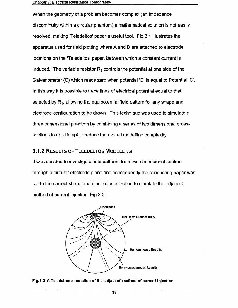
Chapter 3: Electrical Resistance Tomography___________________________________________

When the geometry of a problem becomes complex (an impedance

discontinuity within a circular phantom) a mathematical solution is not easily

resolved, making 'Teledeltos' paper a useful tool. Fig.3.1 illustrates the

apparatus used for field plotting where A and B are attached to electrode

locations on the 'Teledeltos' paper, between which a constant current is

induced. The variable resistor R-j controls the potential at one side of the

Galvanometer (C) which reads zero when potential ‘D’ is equal to Potential ‘C\

In this way it is possible to trace lines of electrical potential equal to that

selected by R-j, allowing the equipotential field pattern for any shape and

electrode configuration to be drawn. This technique was used to simulate a

three dimensional phantom by combining a series of two dimensional cross-

sections in an attempt to reduce the overall modelling complexity.

3.1.2 R e s u lts o f T e le d e lto s M o d e llin g

It was decided to investigate field patterns for a two dimensional section

through a circular electrode plane and consequently the conducting paper was

cut to the correct shape and electrodes attached to simulate the adjacent

method of current injection, Fig.3.2.

Electrodes

Resistive Discontinuity

Homogeneous Results

Non-Homogeneous Results

Fig.3.2 A Teledeltos simulation of the 'adjacent' method of current injection

38


Fig.3.2 illustrates two sets of results, one for a uniform homogeneous circle of

Teledeltos paper and another produced after a circular hole was cut in the

paper (non-homogeneous). A problem with this technique, other than the two

dimensional limitation, is that it is difficult to alter the resistivity of the circular

discontinuity. A hole cut into the Teledeltos paper represents an object with an

infinite resistance, which in practice is unlikely to occur. However, this

technique is of use when mapping equipotential lines for various electrode and

current injection positions. The solid lines of Fig.3.2 represent equipotentials

produced when a constant current source is connected to both electrodes for a

homogenous phantom. The plot is repeated for the non-homogenous

simulation and the results are also marked (by dotted lines in Fig.3.2). In a

practical ERT design the changes in position of equipotentials illustrated in

Fig.3.2 would be recorded as variations in measured electrode potentials.

Electrode

'Pipe' Wall

(A) (B)

Fig.3.3 A Teledeltos simulation of the 'three dimensional' effect

Fig.3.3 (a) illustrates a vertical section through a homogenous phantom

simulated using Teledeltos paper, where each of the dotted lines represent a

10% change in the measured potential. Fig.3.3 (b) repeats this approach for a

Discontinuity

39


non-homogenous phantom using a rectangular hole to produce a resistive

discontinuity. It can be noted from Fig.3.3 (a) and (b) that the equipotentials

are affected significantly by the applied resistive discontinuity. By utilising this

technique for several varying two dimensional views it is possible to

approximate three dimensions and the next step is to compare results for an

object moving through the phantom.

Fig.3.4 (a) represents a homogenous section and (b) - (e) represent the results

obtained for a circular discontinuity moving a distance of 0.9cm per image

towards the electrode plane. Fig.3.4 shows the point of contact between the

phantom wall and the 10%, 20%, 30% and 40% equipotentials.

(A) (B) (C) (D) (E)

Fig.3.4 Teledeltos simulation of a moving object

The distances moved by these points of contact are measured for (a) - (e) and

the results plotted in Fig.3.5. This graph illustrates large non-linear changes

for the 30% and 40% equipotentials that are not linear. Significant alterations

in the points of contact occur for resistance discontinuities outside of the

electrode plane, Fig.3.4 (b) and (c). The Teledeltos plan and side elevations

(Fig.3.2 and Fig.3.4) when viewed together suggest that objects outside the

40


measurement section do affect the measured electrode potentials. However,

this approach confines the electric current to two dimensions making it more

sensitive to smaller objects than a three dimensional evaluation.

Consequently, a three dimensional model was developed to investigate this

further.

1,6 T1.4 ■■

~ 1.2 ■ ■

| 0.8 ■ ■

jl 0.6 • • ° 0 . 4 -

0.2 ■ '

(B) (C) (D) (E)Discontinuity Position

Fig.3.5 Change in equipotential positions with discontinuity movement.

3.1.3 Two Dimensional M o d e llin g Using 'HSPICE'

Griffiths [23] introduced a method of constructing phantoms for electrical

impedance tomography using a mesh of resistors soldered to pins on a matrix

board. To simulate changing conductivities, resistors in the mesh are shunted

at selected locations using other resistors and capacitors.

1

•A’

3

’A’

Fig.3.6 The resistive building block

41


Dines et. al. [15] also uses the resistor analogy to model cross-sections of core

samples in an attempt to analyse the possible benefits of electrical resistance

tomography for the incorporation into a dual modality imaging system.

Fig.3.6 illustrates a basic ‘building block’ that is used to implement Griffiths’

technique (the actual resistance values R and R" are determined by the

physical distance they cover). The phantom used for this thesis is 8cm in

diameter and therefore if 20 x 20 ‘building blocks’ are used in the model

(Fig.3.7) one block will be equivalent to a distance of 0.4cm ('A' marked on

Fig.3.6). Consequently the resistor R will equate to a distance of 0.2cm and R"

to a distance of 0.282cm, allowing any resistivity (Ocm) to be selected.

Griffiths [23] physically constructed the phantom to gain the electrode voltage

readings while Dines et. al. [15] derived sets of network equations to achieve

this. Other research groups including Curtis et. al. [14] have presented

equations to calculate either the internal resistance given specific electrode

voltages or electrode voltages given specific resistance values.

16

15

m14

13

12

11

10

1

ISI

EL

XTa l

Inner Phantom

4

■ Electrodes

Fig.3.7 A circular cross-section using 'basic' building blocks

The circuit simulation package 'HSPICE' is an alternative to these approaches

42


which are based on the calculation of voltages at nodes which connect various

types of linear components. Appendix 2 presents the HSPICE listing used to

implement the configuration illustrated in Fig.3.7. Separate constant current

sources, controlled by the HSPICE 'pulse' function, are used for each current

injection position to produce 5mA output pulses at different points in time. In

this way each current injection position is pulsed sequentially, during which

time a full set of adjacent electrode voltages is calculated (Fig.3.8).

Adjacent Current Injection Electrode Curren, . 0N. Curren, . 0 FP

/ /1-2

2-3

3 4

4-5

5-6

6-7

Tetc.. \ \ i /

Calculate Adjacent Voltages Here etc...

Fig.3.8 Timing diagram for HSPICE constant current sources

This technique is able to construct complex models of two dimensional

resistivity profiles and has the potential to be a useful tool when testing image

reconstruction algorithms.

3.1.4 R e s u lts o f Two Dimensional HSPICE M o d e llin g

The two dimensional HSPICE model uses copies of a single building block of

resistors (Fig.3.6) duplicated 370 times and connected together to simulate a

circular phantom (Fig.3.7). Results presented in this section are designed to

test the performance of the model for various resistive discontinuity values.

The background resistance was set to 50 Ocm and simulations carried out for

43


building block resistances of 500 flcm, 5000 flcm and 50,000 Qcm in the

position marked in Fig.3.9.

3 Resistive Discontinuity

Electrodes

Fig.3.9 Position of resistive discontinuity (2D test)

Image reconstructions were generated from these simulated voltages using a

simplified back-projection algorithm (Chapter 2). These are illustrated in

Fig.3.10 and show a noticeable change in shape of the image reconstruction

between 500 and 5000 Hem but this is less obvious between 5000 and 50000

Hem.

(a)10x (b)100x (c) 1000x

Fig.3.10 Increasing discontinuity resistivity

44


3.1.5 T hree D im ensional M o d e llin g Using 'HSPICE'

The three dimensional HSPICE model is an extension of the two dimensional

model and allows complex impedance profiles to be simulated. The model is

defined textually rather than using a graphical interface, which simplifies the

construction of a large three dimensional resistor mesh. The three dimensional

model is actually an interconnection of several two dimensional 'planes'

separated by vertical connecting resistors whose values are a function of the

distance between each plane. Initial experiments on large volumes required a

large amount of processing time due to the excessive number of nodes

required. Consequently the number of nodes in each plane was reduced to

less than 100 from the original two dimensional design (Fig.3.11).

Electrode PositionsExternal Resistors

NodesInternal Resistors

Fig.3.11 The resistor net used in 3 dimensional HSPICE modelling

Appendix 3 presents the HSPICE listing for a simulation using four layers

(Fig.3.12). The constant current source and resistive building block

descriptions are identical to those used in the two dimensional model. By a

suitable choice of resistors in a localised area, it is possible to model three

dimensional objects within the conducting liquid for a static phantom, and if

multiple sets of results are combined it is possible to simulate flows.

45


Plane 4 (Nodes 400-499)

Plane 3 (Nodes 300 - 399)

Plane 2 (Nodes 200-299)

Plane 1 (Nodes 100-199) (Electrode Plane)

Fig.3.12 Node/Plane numbering convention

3.1.6 R e s u lts o f T h ree D imensional HSPICE M o d e llin g

This section presents results for the three dimensional model when used to

simulate objects moving through the electrode plane. Initially, plane 4

(Fig.3.12) with discontinuity ‘1’ (Fig.3.13) is simulated with planes 3, 2 and 1

having a uniform distribution. Discontinuity T is then moved through planes 3

to 1 to gain information about how objects transported by a flow will affect the

image reconstruction when they move towards the electrode plane.

ResistiveDiscontinuities

Electrodes

Fig.3.13 Position of resistive discontinuity (2D test)

Results are presented for discontinuities in position ‘1’ (Fig.3.14) and position

‘2’ (Fig.3.15) for each of the four planes, using a 50n/cm background

resistivity, a simulated phantom diameter of 8cm and a distance between

planes of 1cm. For a phantom of this size the discontinuities equate to

cylindrical shapes of 2cm diameter and 1cm in height.

46


(a) Plane 1 (b) Plane 2

(c) Plane 3Fig.3.14 3D modelling for discontinuity '1'

(d) Plane 4

(a) Plane 1 (b) Plane 2

(c) Plane 3

Fig.3.15 3D modelling for discontinuity '2'

(d) Plane 4

47


Both sets of results (Fig.3.14 and Fig.3.15) show that discontinuities within the

electrode plane (Plane T ) produce the greatest resistivity changes, but those

within planes 2 and 3 are also significant.

3.1.7 M o d e llin g C o nc lu s io ns

Results have been presented for electrical impedance tomography modelling in

two and three dimensions using ‘Teledeltos’ and HSPICE techniques. Fig.3.4

illustrates how ‘Teledeltos’ paper was used to ‘simulate’ three dimensions using

a combination of two dimensional cross-sections. From these results and the

corresponding graphical tabulation in Fig.3.5 it can be seen that measurable

distortions occur in the voltage profile around the phantom wall as an object

moves towards the electrode plane. However, a more versatile modelling

technique is required to quantify this in three dimensions and for this an

HSPICE model was developed.

Fig.3.10 illustrates a set of image reconstructions gained from the two

dimensional HSPICE model for a discontinuity of increasing resistivity. From

this it may be seen that as the resistivity of the discontinuity increases there is

a corresponding increase in image contrast. This is due mainly to the

associated increase in potential gradient between adjacent electrodes and the

resulting increase in signal to noise ratio. Fig.3.14 and Fig.3.15 illustrate

image reconstructions using the three dimensional HSPICE model configured

to simulate an object ‘flowing’ toward the electrode plane at two different radial

positions. These results show that the object’s radial position with respect to

the phantoms’ centre influences the data set and hence the image

48


reconstruction. This is due to the three dimensional flow of current flux in this

type of environment. The closer the object is to the phantom wall, the more

closely packed the current flux is around each electrode (i.e. the greater the

current density). This hypothesis is tested in section 3.3, which introduces

measured results.

3.2 Ha r d w a r e

For test purposes, an 8cm diameter vertical section of pipe (the phantom),

sealed at the bottom and having 16 stainless steel electrodes positioned

around the periphery is used. Fig.3.16 illustrates the Electrical Resistance

Tomography hardware constructed to inject an alternating current (of constant

frequency and peak to peak amplitude) into the phantom via two selected

electrodes and measure the voltage at each remaining adjacent pair.

m MULTIPLEXER

= n channels

= single channel

OSCILLATOR

RMS. TO DC CONVERTER

PERSONALCOMPUTERINTERFACE

A/DCONVERTER

INSTRUMENTAMPLIFIERS

HIGHIMPEDANCE

BUFFERS

VOLTAGECONTROLLED

CURRENTSOURCE

Fig.3.16 Schematic diagram of an Electrical Resistance Tomography system.

The magnitude of injected current is a function of the oscillator amplitude and

an internal reference resistor. The oscillator provides a sine-wave of pre-set

amplitude and frequency to the constant current source where any d.c. offset is

removed to prevent electrolysis occurring. Selection of electrodes, between

49


which current is injected, is implemented by an analogue multiplexer

arrangement under software control. The resultant voltages induced at the

remaining electrodes are transferred to unity gain, high impedance buffers

which subsequently connect to instrumentation amplifiers. The output of the

instrumentation amplifiers is a difference wave-form which is converted to a d.c.

signal by an r.m.s. to d.c. converter and finally passed to a personal computer

interface by a 12 bit analogue to digital converter. Inputs to individual

instrumentation amplifiers are from adjacent electrode sources and therefore

the high impedance buffers prior to this must be able to cope with the large

voltages that occur at current injection electrodes.

3.2.1 E lec tr o d e C onstruction

The design chosen for this thesis uses 16 electrodes positioned halfway along

the vertical height and equidistantly around the inside of a circular phantom

(Fig.3.17). These provide electrical contact between the constant current

source and the conveying liquid. All measurements presented in this thesis

use a phantom filled with saline solution (of controlled conductivity) and

consequently stainless steel was used as the electrode material to prevent

corrosion. The phantom is of plastic tubing with an internal diameter of 8 cm, a

5mm wall thickness and rectangular electrodes of size 16mm high x 8 mm wide.

Gold plated SMB connectors link the electrodes to coaxial cable which then

joins to the current injection circuit board. Current injection electrodes are not

used for voltage measurement [49], because a two electrode system is affected

by the impedance between electrode and medium, and the impedance across

50


the electrodes (Fig.3.18). A four electrode configuration eliminates this

problem.

Jubilee ClipEarthed Shield

MB Connector

Electrode

Jubilee Clip!

Phantom'

Fig.3.17 Electrode positioning within the 'phantom'

The major limitation of four electrode designs is that the total number of

readings is reduced because any adjacent measurement pair containing a

current injection electrode must be discounted. For the polar current injection

approach this produces a loss of 4 data points per injection position and 64 for

a full set of readings.

Constant Current Source Voltage Measurement

Fig.3.18 The two and four electrode methods

Hau et. al. [25] overcome this problem of a reduction in data points by using

compound electrodes (Fig.3.19) which permit voltage to be measured and

51


current to be injected at the same electrode position, while retaining a four

electrode configuration. This is achieved using a separate, smaller voltage

measurement electrode which is bounded by the current injection electrode.

Current Injection

Voltage Measurement

Fig.3.19 Compound electrodes

Using compound electrodes allows more voltage readings to be made in total,

for the same number of electrodes, but also increases circuit complexity. For

this reason compound electrodes are not used in the final design.

3.2.2 O scillato r

In order to provide a low noise wave-form it was decided to use a HAMEG

HM8030 function generator as this removed the necessity of designing and

building such a complex device. The oscillator wave-form must be stable as its

amplitude controls the magnitude of the injected current. The HAMEG HM8030

varies in amplitude by less than 0.05% at a frequency of 8 kHz and a voltage

setting of 5V (r.m.s.), allowing it to be used in 12 bit resolution systems.

3.2.3 C o nstant C urrent S ource

A design based on Nowicki [36] was chosen due to its reliable design and

integrated capacitative compensation for the coaxial cable used to connect the

phantom to the system hardware (Fig.3.20).

52


100 a

in O [690 n AD847JN

"H 5 pF- r °c ,— _ L . 3 Coaxial Cable

220 nTT R------

100 a

15 nF

1.3 KQ 50 Cl Electrodesvia

Multiplexer

Fig.3.20 A single operational amplifier current source.

This design incorporates a d.c. blocking capacitor within Z3 and is designed to

provide 12 bit resolution for a load of between 39f2 and 1000H, with a

maximum 1 0 % reactive component. Capacitor Cs is the equivalent cable

capacitance when its shield is grounded to earth and Z4 eliminates effects of

load voltage on the output current. Adjustment of the component values

contained in this reactive combination reduces any phase or gain errors

produced by the operational amplifier. Under ideal conditions the load current

supplied by the circuit is given by the equation:

j ____________ ~ ^ i n - ^ 2 ^ 4 ____________

R,z 3z 4 + ZL (R,Z3 - R2Z4 )

When the condition R1Z3 = R2Z4 is met this simplifies to equation 3.5.

I L= ^ {3.5}4

Z4 can be simplified (Fig.3.21) when the equivalent capacitance of the coaxial

cable (Cs) is also taken into account. Equation {3.6} gives the overall maximum

53


and minimum impedances of Z4 due to changes in the value of Rv. For the

selected oscillator frequency of 8 kHz and with Cs assumed to be 1 0 0 pF (a im

length of cable), the resultant minimum and maximum values for Z4 are shown

in equations {3.6a} and {3.6b}. An 8 kHz oscillator frequency was chosen due

to bandwidth limitations of the r.m.s./d.c. converter design (Section 3.2.6). To

produce a constant current of 5mA an input voltage of 6 V (r.m.s.) is required.

50 Q

15 nF1.3 kQ

Fig.3.21 Equivalent circuit diagram for Z4.

Y = j° 3 SinF) + Y ^ a (Minimum) (3-6a}

Y - ja (\S \nF) + i3son (Maximum) {3.6b}

3.2.4 M ultiplexer

Voltage measurement utilises a parallel approach with circuitry repeated for

each of the 16 electrode positions to facilitate faster data acquisition by

reducing the amount of time required for the signal conditioning circuitry to

settle. However, this approach is not applied to the current injection circuitry as

this would only remove the multiplexer switching delays, which are less than 1 p

s per operation. The hardware designed allows only two electrodes to be

54


selected for current injection via a single, multiplexed voltage controlled current

source and two DG526, 16 way analogue switches (Fig.3.22).

DG526CJ o ENW R(1)

outDG526CJ D ENWR (2)RS A , A , A j A,

To l\0 Port

|?> To Electrodes

Fig.3.22 Multiplexing of the constant current source.

One analogue switch input is connected to the constant current source and the

other to zero volts. Both devices are address decoded using two separate TTL

control lines of the 40 way digital I/O port (Section 3.2.8), with all other

connections identical.

a3 a2 Al Ao Channel0 0 0 0 10 0 0 1 20 0 1 0 30 0 1 1 40 1 0 0 50 1 0 1 60 1 1 0 70 1 1 1 81 0 0 0 91 0 0 1 101 0 1 0 111 0 1 1 121 1 0 0 131 1 0 1 141 1 1 0 151 1 1 1 16

Table.1 Address decoding for the DG526

55


To connect an electrode to the current source both £7Vand RS are set to logic

HIGH, and WK(1) is set to LOW. Then, the correct digital value (Table. 1) is

applied to the four address lines (A0- A 3) and after WR is pulsed HIGH, the

correct electrode is connected. The same principle is applied to the electrode

connected to earth, but this time WR (2) is used. Both multiplexers can be reset

to provide a high impedance connection to all 16 electrodes by pulsing RS

LOW.

3.2.5 High Impedance B u f fe r

The design of the buffer (Fig.3.23) provides a high input impedance, over a

wide range of frequencies and incorporates d.c. blocking to prevent saturation

of the high gain instrumentation amplifier that follows. Included in the design is

a unity gain amplifier to drive the coaxial-cable shield at the same potential as

Vout, thus reducing the capacitative loading that would occur if the shield were

connected directly to earth [34].

Coaxial Cable

084

out100 nF

75 kQ

100 nF55 kQ

084

Fig.3.23 High input impedance voltage buffer.

A minimal design for the high impedance buffer is desirable to reduce the

amount of noise that would be induced by the use of excessive component

numbers. The input impedance, when tested over the range 1Hz-100kHz , has

56


a peak between 1kHz and 10kHz (Fig.3.24) making it suitable for use at the

selected oscillator frequency of 8kHz. A high impedance buffer is desirable at

this point in order to reduce the loading effect on each of the measurement

electrodes and sixteen are required, one connected to each electrode.

10000000

«| 1000000 •o 01 a E3a.c 100000

1000010Hz 100Hz 1kHz 10kHz 100kHz

Frequency

Fig.3.24 Input Impedance versus frequency for the voltage buffer.

3.2.6 Instrum entatio n A mplifier

The buffered voltages from each electrode (1 -16) are connected in adjacent

pairs (1-2, 2-3, 3-4, ...) to the dual inputs of stable, high accuracy

instrumentation amplifiers (Fig.3.25).

100 kQ

INA 110

(n+1)

1uF 1uF i)0V + 15V-15V

Fig.3.25 Connection details of the INA110 instrumentation amplifier

An output equal to the differential voltage between each electrode pair is

provided by the circuit in Fig.3.25, which is the format required by the image

reconstruction algorithm used (Chapter 2). The INA110 instrumentation

57


amplifier is a monolithic FET input device having a settling time of 4ps (to an

accuracy of 0.01%) and several gain options (1, 10, 100, 200, 500) which are

set by internal laser trimmed resistors. For an 8cm diameter phantom, an

injection current of 5mA and a 20mS saline solution the maximum electrode

difference voltage produced is 10mV. If a gain of 500 is selected for each

instrumentation amplifier a maximum output voltage of 5V results, for

measurement positions other than those used for current injection.

3.2.7 R.M.S. To D.C. CONVERTER

The amplified a.c. difference signal is converted to an equivalent r.m.s. voltage

via an AD736 r.m.s. to d.c. converter device. This is a low cost, true r.m.s.

device which can be connected in an averaging mode to provide fast operation,

as illustrated in Fig.3.26. In true r.m.s. mode an averaging capacitor is

connected between Cav and the negative supply rail, producing conversion

times that are a function of the input voltage magnitude.

10nFhi-

+15 V 0 V -15 V9 9 9

oVM

COM

v,„AD736 v

s

VoUT

■Vs C AV

H M h

Fig.3.26 Connection details of the AD736 r.m.s. to d.c. converter (Averaging mode)

The faster averaging mode results in settling times that are determined solely

by the RC time constant of CF and an internal 8kH resistor. Fig.3.27 illustrates

58


this dependency on CF, which also provides low-pass filtering of the output

voltage. Consequently, to achieve a settling time of approximately 3ms a value

for CF of 0.2pF is used, which yields a total time of 48ms when summed over all

16 current injection positions .

10000 t

1000 -E100 - -v

EFO)c

10 -

oV)

0.1 J ■---- ■—0.01 uF 0.1 uF 1uF 10uF 100uF

Capacitance

Fig.3.27 Settling time versus CF for the averaging mode

Another important design aspect is the frequency response of the AD736, as

this will affect design considerations for the other system components. Fig.3.28

shows the measured frequency response when the averaging mode is used

and clearly identifies the reduction in gain at frequencies above 10kHz, which

is compatible with a sinusoidal oscillator frequency of 8kHz.

10

1

1Hz 10Hz 100Hz 1kHz 10kHz 100kHz

Source Frequency

Fig.3.28 Frequency response of the AD736 r.m.s./d.c. converter

59


Output voltages from each AD736 contain both a.c. and d.c. error components

which although relatively small may affect the reconstruction algorithm.

Compensation for both of these error components can be provided by including

a correction factor in the system software, although for the purposes of this

thesis they are ignored.

3.2.8 A nalogue To D igital Converter

The d.c. signal produced by the AD736 is converted into a digital format

allowing it to be transferred, via an interface, to the system software running on

a computer. This interface is a MAX180 [30] 12-bit, 8 channel data acquisition

device is used that incorporates internal track and hold circuitry, a low drift

zener reference and flexible microprocessor interfacing (Fig.3.29). The time

required by the internal track and hold circuitry to acquire an input signal is a

function of the input capacitance and can be calculated using equation {3.7}.

acq = 10x (Rs +R|n) x20/?F {3.7}

Where RiN is the output resistance of the previous stage and Rs is 1 kQ.

Therefore the acquisition time is a function of the output resistance of the

previous r.m.s./d.c. converter stage, which in this case is 0.2£2 producing a

theoretical acquisition time of 0.2ps. However, the internal characteristics of

the MAX180 allow the minimum conversion time to be tCOnv=1.875ps, preceded

by a delay of three clock cycles (Fig.3.30). Individual conversion times for all 8

channels are summed to produce an overall A/D conversion time. As the

MAX180 is a 12 bit device a facility exists to read an initial 8 bits of the digital

conversion and then the remaining 4 bits as separate operations.

60


+5V

DC Signals

REFADJ OFFADJ vDD

REFOUT1REFIN

AIN8AIN7AIN6AIN5AIN4AIN3AIN2AIN1

ZW ClMMAX180

CLKIN HBEN MODE

CS RD

WR BUSY

DIFF BIP

D0-D11AOA2A1

AGND DGND Vss

0.1mfC jTT47mF

X I0.1 fiF ■—j - 47 pF

^ Data Lines

- Address Lines

_-15V

0.1pF L-j- 1 47 pF

Fig.3.29 The MAX180 data acquisition device

The option used for the design presented here reads all 12 data bits in a single

step to reduce data transfer and hence acquisition times.

csWR

RD

BUSY

Data In

Data Out

Va r

j r^ a

I j * _ t _ * i! conv y

N—

X d a t a v a u d X ! XD A TA VALID

i I X n e w d a t a X

HOLDTRACK

3CLK

Fig.3.30 Timing diagram for the MAX180 data acquisition device

61


3.2.9 Computer Interface

All digital control signals required/supplied by the electrical resistance

tomography hardware are provided by personal computer software via an

Arcom PCIB40, 40 channel digital I/O board.

B O AR D 2

t> r i \Chan 1

£>— ^

Chan 8

Chan 9

BO AR D 1

(X 8) |High Impedance Buffers

Chan 1Instrumentation Amplifiei

BO AR D 3

ConstantCurrentSource

Oscillator

RMS/DCConverter

RMS/DCConverter

RMS/DCConverter

RMS/DCConverter

1-16 Channel Multiplexer

1-16 Channel Multiplexer

Including Interface Card

486 PC

MAX 180

MAX 180

Fig.3.31 Component positioning and interconnection over 3 printed circuit boards

The PCIB40 provides 40 TTL lines which can be configured as input or output

and is positioned in a spare expansion slot of a personal computer. Full details

of the I/O board including software design considerations and memory

addresses are presented in Appendix 1. All the electronic hardware

constructed for this project is located on three printed circuit boards as

illustrated in Fig.3.31. One circuit board is used for the current injection and

driven shield components and the other two provide the 16 channels of data

acquisition hardware. All connections between these three boards and

62


peripheral components is via a 64 way Eurocard 'backplane' as described in

Appendix 1.

3.3 R esu lts

Results for three areas of investigation are presented in this chapter. Firstly,

the 'background resistivity' is varied to test the resulting effect on image quality

for a particular resistive discontinuity position. Secondly, measured data are

presented for three dimensional experimentation including sets for liquid/solid

flows. Finally, image reconstructions are presented (using the algorithm

outlined in chapter 2) for single and multiple substance combinations. All

experiments were carried out using an 8cm diameter phantom having 16

equidistantly spaced radial electrodes. An oscillator frequency of 8kHz coupled

to a 5mA (r.m.s.) constant current source was used and the background

conductivity was set to 11.5mS. The main purpose of these results are to verify

the validity of earlier modelling and to investigate the ability of electrical

impedance tomography to detect five substances: paper; plastic; gas bubbles;

perspex and rubber singularly and in multiple combinations. Fig.3.32 illustrates

a plan view of the labelling convention used for the different material positions.

Phantom (8cm Dia')

Position '4' (2cm Dia')

Position '3', (2cm Dia')

tPosition '1'(2cm Dia')

Position '2' (2cm Dia')

Position '2/3' ' (2cm Dia*)

Fig.3.32 Positioning of substances

62


3.3.1 V arying Background Conductivity

A link between background resistivity and image quality was investigated

producing the results presented in Fig.3.33. A tubular rubber discontinuity of

2cm diameter was placed in position ‘3’ (Fig.3.32), i.e. directly in the centre of

the phantoms. Six simulations were caried out, each using different

background conductivity values: (a) 217pS (b) 4.5mS (c) 7.9mS (d) 11.5mS

(e) 14.4mS and (f) 17.45mS.

(a) (b) (c)

(d) (e) (f)

Fig.3.33 Various background conductivities: (a)217^S (b) 4.5mS (c) 7.9mS(d)11.5mS (e) 14.4mS (f) 17.45mS

The system software reconstructs a resistivity profile, in the form of a 32x32

pixel array, using the reconstruction algorithm and software outlined in Chapter

2, and analyses the data to select the set having the highest individual

resistivity value (Rmax)- This value is then used to convert all other values (RN)

from each set into percentages (R.*):

63


R%= - ^ - x 100 {3.8}n MAX

These percentage values are displayed in Fig.3.33 for each data set. Although

Fig.3.33 (d) does not contain the largest reconstructed resistivity value (R max) it

is the image with least noise interference. Consequently 11.5mS is used for all

the data acquisitions in this chapter and those in chapter 5 which present

details of a dual modality tomography system.

3.3.2 Three Dim ensional A n a lys is

A potential problem associated with implementing an electrical impedance

tomography system to measure flow rates of suspended solids is the three

dimensional effect. It is not possible to limit current flow to two dimensions in a

three dimensional flow, as is illustrated by the HSPICE modelling outlined

earlier in this chapter.

Results presented in Fig.3.34 detail the effect that various lengths of tubular

plastic (2cm diameter) have on the measured adjacent electrode potentials

when using polar current injection over a single projection. The plastic tubing

is moved, in 1cm steps, toward the electrode plane while remaining at

discontinuity position ‘4’ (Fig.3.32). Fig.3.34 illustrates how the voltage profile

changes as the tube moves towards the electrode plane, where the data at the

back of each graph is for the tube within the electrode plane. The results

shown in Fig.3.35 repeat the steps presented above but for different radial

substance positions (Fig.3.32): (a) position ‘2’ (b) position ‘2/3’ (c) position ‘3’.

This provides information on how the radial position of a material affects the

results as a function of its distance from the electrode plane.

64


1200 1000 - 1000 -

E 800 -E 800 -S. 600 . £. 600 -

5 400 - = 400 -200 -200 -

15°* '» o n

(a) 2cm Length (b) 4cm Length

£ 800 S. 600

o 400 > 200

(c) 6cm Length (d) 8cm Length

Fig.3.34 Varying lengths of 2cm diameter tube moved through the electrode plane

The modelling presented earlier in this chapter suggested that the closer an

object is to the wall of the phantom the closer it has to be to the electrode plane

before it affects the acquired data.

_ 300 % 250

' 200600“ 800o> 600 £ n 150-= 400> 200

(a) Substance Position ‘2’ (b) Substance Position ‘2/3’ (c) Substance Position ‘3’

Fig.3.35 The 2cm Plastic pipe, in varying substance positions

It can be seen that the absolute measured potentials are higher for objects

closer to the phantom wall (Fig.3.35 (a)), while objects nearer the centre

(Fig.3.35 (c)) have a greater relative affect on the measured potentials at

65


distances further from the electrode plane. The latter can be seen more clearly

when comparing voltage plots for vertical positions ‘X’ and ‘Y* (Fig.3.35 (a - c)).

3.3.3 Image R e c o n s tru c tio n s f o r Five Samples

This section presents image reconstructions for five substances that have

differing physical properties. 2cm diameter cylinders of each material are used

and Fig.3.36 presents the resulting image reconstructions for:

(a) Paper tube (b) Plastic tube (c) Bubble

(d) Perspex bar (e) Rubber tube

(a) (b) (c)

(d) (e)

Fig.3.36 Image reconstructions for: (a) Paper tube, (b) Plastic tube, (c) Bubble,(d) Perspex bar, (e) Rubber tube

None of the image reconstructions shown in Fig.3.36 is filtered and therefore

noise degradation is visible. This is because the relatively low signal to noise

ratio present in the measured voltages has a bearing on image reconstructions

for materials having low levels of contrast. The same approach was taken as

66


that detailed in section 3.3.1 when producing the image reconstructions, where

each pixel location is converted to a percentage value of the largest overall

resistivity (R max). Using a percentage scale in this way allows a qualitative

comparison of results and is employed in all situations where image

reconstructions are compared. These results are discussed in the concluding

section of this chapter (section 3.3.5).

3.3.4 Image R e c o n s tru c tio n s f o r M u lt ip le S ubstances

This section presents image reconstructions for three combinations of two

substances to allow comparison of the reconstructed images produced.

Fig.3.37 shows image reconstructions for: (a) Paper (position T ) and perspex

(position ‘2’); (b) Rubber (position ‘1’) and perspex (position ‘2’) and (c) Rubber

(position T ) and paper (position ‘2’). Each object is 2cm in diameter and

Fig.3.32 illustrates where each is positioned within the phantom. These results

are discussed in section.3.3.5.

RubberPerspex Paper Rubber

(a)

Fig.3.37 Image reconstructions for:

(b) (c)

(a) perspex and paper (b) perspex and rubber (c) rubber and paper

3.3.5 C o nc lus io ns fro m M easured R e s u lts

The results presented in this chapter have demonstrated the operation of

hardware designed and constructed to carry out electrical resistance

67


tomography. Fig.3.33 illustrates how the background conductivity affects the

final image reconstruction, with a value of 11.5mS found to produce the best

results. These changes are due to the physical limitations placed on the

hardware when extremes of resistivity are present in the phantom. For low

conductivities a high voltage is required to maintain a constant 5mA injection

current and this may produce saturation in certain situations. For high

conductivities a low voltage is required, producing results that are susceptible

to a low signal to noise ratio.

Fig.3.34 presents measured voltages for a three dimensional situation where

varying lengths of 2cm diameter plastic pipe are gradually lowered into a

vertical phantom, from a point above the electrode plane. From these results it

is evident that long objects produce larger measured voltage changes in

relative terms at distances further from the electrode plane than shorter length

objects.

Fig.3.35 repeats the test described for Fig.3.34 but lowers a plastic tube of 2cm

diameter and length into the phantom. Three radial positions are used: one at

the phantom’s centre; one at the edge and one in an intermediate position.

The results indicate that positions closest to the phantom wall produce the

highest absolute measured electrode voltage disturbance while positions

closest to the centre are more sensitive, in relative terms, to objects further

from the electrode plane. This confirms the modelling presented earlier in this

chapter which can be explained using Fig.3.38.

68


A B

V6.lH3 'V3

'V5'H2

lV2

(a) (b)Fig.3.38 Three dimensional current paths

Two views of a three dimensional phantom are presented in Fig.3.38 for objects

at radial positions ‘A’ and ‘B\ Fig.3.38 (a) shows a plan view which represents

both objects within the electrode plane. From this it can be seen that the

current density due to the applied electrode voltage is greater for objects closer

to the phantom wall. This is illustrated in Fig.3.38 (a) by three current paths

(Im, Ih2 and lH3) intercepting the object at radial position ‘A’ while only two (lHi

and lH2) intercept the object at radial position ‘B’. Consequently, for objects at a

particular distance from the electrode plane those closest to the phantom wall

will produce the greatest absolute electrode voltage disturbance. However, as

the object at position ‘B’ moves towards the electrode plane maintaining a

constant radial position (Fig.3.38 (b)) it intercepts current path lVs, earlier than

the object at radial position ‘B\ This results in image reconstructions for

position ‘B’ being more sensitive to objects further from the electrode plane, in

relative terms, than position ‘A’. Fig.3.36 and Fig.3.37 present image

reconstructions for five materials, both singularly and in selected pairings.

These results indicate that saturated paper is not visible to electrical resistance

69


tomography; perspex is only partially visible and bubbles, plastic and rubber

are all highly visible.

3.3.6 Discussion o f D a ta A cq u is itio n Speed.

One important aspect of any tomographic equipment design is the question of

an acceptable data acquisition speed. Equation {3.9} presents a formula that

illustrates this point:

d = n x v x t a {3.9}

Where ‘d’ is the measurement distance that a single object moves during the

time taken to acquire a full set of readings; 'n' is the number of voltages that are

acquired for a full set of data; V is the flow velocity and 'ta' is the time taken for

one voltage to be acquired. For the opposite method of data collection 96

unique voltage measurements are required to produce a full set of data.

The time taken to acquire this amount of data using the hardware presented in

this chapter is approximately 80ms (eight unique current injection positions)

when the r.m.s./d.c. converter settling time due to ripple voltages is taken into

account. This produces a ‘measurement length,’ from equation {3.9}, of:

d = vx80.1x10-3tw {3.10}

Fig.39 draws this graphically as measurement length (d) 'vs.' velocity (v) for a

variety of data acquisition speeds. From Fig.39 it can be seen that a flow

having a velocity of 0.3ms'1, monitored by a tomographic system that acquires a

full set of data in 80.1ms will have a measurement length of 24mm. The

hardware presented in this thesis is intended for use on a prototype system

70


with a flow velocity of less than 0.3ms-1- This example illustrates the

importance of fast data acquisition in commercial systems and this is

addressed in chapter 7.

10

v(m/s)

Fig.39 Distance 'df vs. velocity V for various data acquisition times

71

Chapter 4: Optical Tomography

CHAPTER 4 OPTICAL TOMOGRAPHYThis chapter is divided into four parts. Firstly, models verifying the behaviour

of light in liquid flows are developed; secondly, system hardware is discussed

and circuit diagrams presented; thirdly, experimental results are presented to

test the validity of modelled data and finally there is an analysis of the results.

4.1 M o d e l l in g o f O ptical D is c o n tin u it ie s

This section describes optical modelling carried out to characterise certain

aspects of liquid flows. Formulae are presented that illustrate the attenuation

of light passing through various materials and multiple media combinations; the

behaviour of light passing through a bubble within the conveying 'liquid' and

refraction of light due to a variable depth conveying liquid. All of these

situations affect the level of detected light and give an indication of the

potential difficulties involved in using optical tomography for the

characterisation of multi-component flows. Dugdale [17] describes several flow

regimes that can occur in a two component liquid/gas flow but for the purposes

of this thesis multi-component flows are assumed to be mainly liquid/solid. Gas

bubbles are therefore optically modelled to asses the possible adverse affect

that they may have on an optical tomography system.

When light passes through any non-opaque substance its intensity suffers

attenuation due to many factors such as scattering, absorption and refraction.

Scattering of light is complex to describe mathematically due to the random

positioning of the particles responsible, but absorption and refraction may be

72


quantified by relatively simple mathematical models. Absorption occurs when

incident light energy is converted to heat causing attenuation, and some

materials exhibit selective absorption to specific frequencies of light.

Refraction happens at boundaries between optically different materials as the

speed of light increases or decreases when moving from one to the other.

Refraction is a result of materials having different optical densities, a measure

of which is provided by the refractive index of a material. Laws of refraction are

available to describe general aspects of liquid/gas interfaces and these are

used to construct more specific models related to bubbles.

4.1.1 A tte n u a tio n o f L ig h t

The attenuation of light in any isotropic optical material can be described by the

following equation:

ln(l) = ln(l0) - andn {1}

Where T is the intensity of light received over a distance dn, for an initial light

intensity l0 and an attenuation constant an. The attenuation constant is

frequency dependent and therefore quoted for a particular wavelength (>.).

Over a particular light path there may be several substances having differing

attenuation constants:

= lo* " (2}

Where 'n' is the number of materials negotiated by the light path, an is the

attenuation constant and dn is the distance travelled in each material.

Consequently, if dn is summed for all possible values of n this will produce the

73

Chapter 4: Optical Tomography_______________________________________________________

total path length. If this is applied to a phantom where light passes vertically

through air and water (of variable depth), as illustrated in Fig.4.1 then only two

attenuation constants are involved:

Fig.4.1 Variable water air boundary for a constant total path length

Where (da + dw = phantom diameter). At 930nm aa and are 0.142cm"1 and

0.287cnrr1 respectively [16], producing maximum and minimum values for T for

an 8cm phantom of 0.321 x l0 (maximum) and 0.101 x l0 (minimum).

4.1.2 R e fra c t io n and R e fle c t io n A t a 'Bubble* In te r fa c e

Consider the situation of a light 'pencil' incident upon an air bubble, Snells' law

states that:

Where 0j is the angle of incidence, 0r is the refracted angle after entering the

bubble (Fig.4.2) and the refractive indexes of air and water are tjair and rjwater

respectively. For a horizontal pencil of light incident at a point ‘A’ above the

optical axis of the bubble (Fig.4.2):

| g - ( a ada+ a wdw) {3}

Pipe Wall

Light Patl

Watt

Air d

sin(flj) V air sin(0r ) '/water

{4}

74


Where 'r' is the radius of the spherical bubble.

Bubble

Ught

’Iwater

Fig.4.2 Refraction of light at a spherical water/air ‘bubble’ interface

Substituting in {4} and using values for rjair and r|water of 1 and 1.3 respectively

Therefore light pencils passing through this type of interface will diverge

upwards, relative to the optical axis (Fig.4.2). Further diffraction occurs until

the point of total internal reflection is reached, which happens when 0r equals

90°:

Therefore:

Consequently, when the value of 'h' exceeds approximately 77% of 'r', total

internal reflection takes place and any light striking above this point will not

enter the bubble. Consider the three situations illustrated in Fig.4.3 where light

pencils of differing sizes, relative to a bubble, are depicted. Equations {5} and

[16]:

75


{6} allow an estimate of the refractive/reflective effect to be calculated for a

bubble and light pencil of known dimensions.

Light Pencil

(a) (b)

Fig.4.3 Light pencils of varying relative size

They also allow generalisations to be applied, for example Fig.4.3 (a) shows a

bubble that is large (in relative terms) to the light pencil and under certain

circumstances no light will be transmitted towards the initial point of aim.

Fig.4.3 (b) shows a smaller bubble, in relative terms, and here a proportion of

the light pencil is totally deflected; most is partially deflected and a fragment

passing along the central bubble axis suffers no deviation. Fig.4.3 (c)

represents a very small bubble within a light pencil and because most of the

light passes around the bubble there is a minimal affect on sensors positioned

at the point of aim.

For these reasons it is not adequate to model only the attenuation

characteristics of the two component water/air interface of a bubble, equation

{3}. This is because refraction and reflection may have a more significant

affect than attenuation on the light intensity detected at a sensor as a diverging

beam will produce a reduced light intensity per unit area. Consequently, an

important consideration is the bubble’s size and distance from any light sensor

as this is the controlling factor in the level of divergence that occurs, and the

next section models this.

76


4.1.3 D ive rgence Due To 'B u b b le ' In te r fa c e s

Fig.4.4 (a) illustrates the divergent effect of a bubble suspended in liquid on a

thin, incident light pencil where 'Disp' is the total deviation of the beam from its

original path. The triangle 'abc' is isosceles and therefore 0X = 0n. Using

equation {4} and values for rjair and r|water of 1 and 1.3 respectively:

From Fig.4.4 (a):

0t =18O-0r -0 .. and 0X = 180- 0t - 9i

Tlv

Fig.4.4 (a) Divergence at a bubble interface

It is also possible to deduce the height 'hh':

hh = r x sin(0x) = r x sin(20r - 0\)

From Fig.4.4 (a) and equations {7} and {8}:

{8}

Bubble

m m


The portion of Fig.4.4 (a) referring to the displacement ‘Disp’ can be redrawn

as Fig.4.4 (b).

Disp

hh-h

Fig.4.4 (b) Derivation of the displacement ‘Disp’

From this: x= dx tan(0d), giving a total displacement of:

isp = (h h - h) + d tan(#d) {10}

Therefore if the bubble were to move along the axis of the light pencil, towards

the light source, <9d, ‘hh’ and ‘h’ would remain constant and the distance ‘d’

would be the only variable. Under these conditions the displacement (Disp)

would be linearly proportional to the change in ‘d’.

4.1.4 R efraction D ue To a V ariable L iquid D epth

A major characteristic of some suspended solid flows, such as those found in

sewer outflows etc., is the variable depth of the conveying liquid. This

introduces added complexity for optical hardware design, as at certain times,

there will exist a water/air interface for non horizontal light beams, as illustrated

in Fig.4.5. In order to simplify the model the assumption is made that the water

depth is only 50% of the maximum allowing the radial displacement 'a' to be

calculated. The circumference of a circle is 27ir and the angle of deviation that

produces 'a' can be stated as Deviation = 0r - 0 j . Therefore:

a = ^ e v *a t *o n x Circumference = — — ~ l ^ x t c t { 1 1 }360 180

78


Pipe Wall

Air

Light..Pencil

Watei

Fig.4.5 Refraction due to a variable conveying liquid depth

using Snells’ law to determine 0r from 0j {4} this can be rewritten as:

sin-1 [1.3 x sin#/] - 0 \180

Which is plotted graphically in Fig.4.6.

nr {12}

a 25

0.5 • -

0 5 10 15 20 25 30 35 40 45 50

e,Fig.4.6 Graph of 0, versus, 'a' for equation {12}

4.1.5 M o d e llin g Conclusions

Modelling described in this chapter investigates the behaviour of light for two

possible situations, for air bubbles present in liquid flows and for liquid/air

boundaries in variable depth flows. Section 4.1.1 examines the equations

governing attenuation of light and Fig.4.1 relates this to conditions where light

moves from liquid to air with an angle of incidence of 90°. Fig.4.2 illustrates the

effect of refraction due to bubbles in liquids and Fig.4.3 links this to bubble and

79


light beams of various sizes. The main conclusion that can be drawn is that

light pencils with a width significantly less than the bubble diameter will pass

unaffected through a bubble centre. For other paths through the bubble it will

be reflected, refracted and deviated to varying degrees up to the point of total

internal reflection, after which point the beam is deviated only.

Fig.4.4 (a) progresses a stage further by examining the level of displacement

that a light pencil receives when a bubble moves along different optical paths.

This displacement is significant for all circumstances other than when a

relatively ‘thin’ light pencil passes through the bubble centre, producing the

relationship described in equation {10}.

Finally, Fig.4.5 illustrates how far a light pencil is displaced from its original

target point when passing through an air/liquid boundary with varying angles of

incidence. It appears to be non-linear and significant for relatively small angles

of incidence.

4 .2 Ha r d w a r e

Hardware designed for the optical tomography system falls into three

categories. Firstly, control of the optical sources for the selected projection is

required; secondly, buffering, amplification and conversion to a digital format of

the optical sensor voltages is carried out and finally a personal computer

interface is utilised to acquire the digital data and supply the necessary control

signals. The design in Fig.4.7 uses the spare channels from the 40 channel

digital I/O board described in chapter 3. Logic decoding of the four address

lines supplied by the I/O port (Appendix. 1) is carried out, to allow expansion of

80


the system to eight optical projections. Two 8-bit data latches store (in a digital

format) control bits for the selected LEDs and present them to an 8-bit LED

driver device, which uses them to select specific combinations of LEDs for

application of the 15V supply voltage.

Computer

i l ----w

LogicDecoding

I/O Interface Board

Data Capture 1C

2 x 8 Bit Data

Latches

LEDDrivers

LED (x8) Arrays

SignalConditioning

mAnalogueSwitches

Optical Sensor (x8) Arrays

Fig.4.7 Schematic diagram of an Optical Tomography system.

Analogue switches are used as multiplexers to connect the eight analogue

sensor currents associated with a particular optical projection to signal

conditioning circuitry, which converts them to voltages and amplifies the result.

These amplified voltages are then transferred to a data capture integrated

circuit which converts them to a digital format. Finally, these digital values are

passed to a personal computer via a 40 way digital I/O port (Appendix 1) for

processing by the system software (Chapter 2).

4.2.1 O ptical T ransducers

The circuitry presented in this chapter switches an optical source on,

configures the signal conditioning circuitry, takes a set of readings and

81


switches the optical source off. The choice of what type of light emitter and

sensor to use depends on the application, as some situations demand light at a

specific frequency to gain full advantage of an optical window in the attenuation

spectrum of the conveying medium [7].

Various forms of emitters and sensors exist including filament light sources,

LEDs, laser-diodes, photo-diodes, photo-transistors and light dependent

resistors. Choice of emitter is usually constrained by the requirement to

collimate the radiated light pencil in order to maximise incident light intensity

and reduce the magnification of reconstructed images. To achieve good

collimation the choice of light source would be a laser-diode due to its

excellent coherence, low spectral width, high optical intensity and fast switching

times. The main drawback of this type of device is its cost, at £20+ per device

(excluding lenses). Most filament light sources are extremely incoherent when

focused and have very slow turn on/off times leaving LEDs as the most cost

effective option for the prototype design.

There are various categories of LED each having differing characteristics, but

for the prototype system a Siemens SFH484-2 was chosen due to its low cost

(less than £1.00 each), small half angle and a peak wavelength that is readilly

matched to a standard photo-diode detector. This device has a peak

wavelength of 880nm and a half angle of 8° allowing it to be collimated in a

phantom of a radius of 8cm without gross degradation of optical intensity at the

sensor. Collimation is achieved using a mounting arrangement that restricts

82


the light to a narrow ‘pencil’ (Fig.4.8). Table 4.1 lists the major characteristics

of the Siemens SFH484-2 LED [41].

Phantom Wall

•Collimated'Light

LED 4mm

PerspexScreen

LED Positioning Assembly

Fig.4.8 A collimated light source

Types of sensor available are more numerous than types of emitter and include

the families of photo diodes, photo voltaic cells, photo transistors and photo

multipliers. Here also the choice of sensor is application and budget

dependent. Ideally it has a linear characteristic, generates an electric current

as a function of incident light and has a fast response time.

Light Output (@ 100 mA) 15 mWHalf Angle 8°Peak Wavelength 880 nmTurn 'ON' Time (tr) 0.6 psTurn 'OFF' Time (tf) 0.5 ps

Table.4.1 Characteristics of the Siemens SFH484-2 LED

Equation {13} is an outline response function, where l( is the current produced

due to the light intensity, Lj, incident on the sensor which has a constant of

proportionality <D.

I, = O x Lj {13}

83


The photo multiplier is a complex device in which the incident light on a

particular material causes the emission of charged particles (usually electrons)

which are increased in velocity by the application of an electric field. Several

such sections can be connected in series with the final device producing an

image on a coated screen which phosphoresces when the charged particles

strike.

The photo voltaic cell, more commonly known as the light dependent resistor

(LDR), is the simplest of all the light sensing devices. Incident light photons

provide the extra energy required for charge carrying particles to bridge the

depletion region of a PN junction, thus reducing the resistance 'seen' by an

applied voltage. These types of device are usually non-linear, have extremely

slow response times and require a large surface area to sense very low levels

of light.

The photo diode also uses a PN junction to generate free charge carriers in

the presence of light creating an increase in reverse current, known as photo

current, proportional to the incident light intensity. This photo current is usually

in the order of nA and occurs when the device is connected in reverse bias

mode. The main disadvantage of the photo diode is the necessity of a large

gain amplifier to convert these very small photo currents into measurable

voltages.

The photo transistor partially overcomes this limitation by using the current

generated by a PN junction as the base current of an adjoining transistor

therefore effectively amplifying the signal. This added complexity produces

84


drawbacks as the resulting devices are less linear than a photo diode, slower

and also more sensitive to temperature variations.

A Siemens SFH2030 Photo-diode was chosen due to its fast switching speed,

excellent linearity and a peak spectral response close to that of the emitter.

Table.4.2 illustrates the main characteristics of this device [41].

Sensitivity (@ =850 nm) 0.62 A/WHalf Angle 40°Peak Response 850 nmTurn 'ON' Time (tr) 0.002 psTurn 'OFF' Time (tf) 0.002 ps

Table.4.2 Characteristics of the Siemens SFH2030 Photo-diode

In order to reduce the effect of reflections on the SFH2030 due to its large half

angle acceptance cone, it was positioned away from the conveying liquid, in a

hollow circular section fronted by a clear plastic film. This is illustrated in

Fig.4.9.

Phantom Wall

Positioning Assembly

Acceptance Cone

Photodiode

Perspex Screen

Fig.4.9 Positioning of the photo diode within the phantom cross section

4.2.2 Logic Decoding I D a ta Latches

The complete optical tomography system is designed to provide two

‘projections’, each having eight 'views', although expansion to a maximum of

eight separate projections is possible. More than one optical projection is

85


achieved by decoding the three available address lines (A0, Ai and A2), using a

74LS138 3 to eight line digital decoder, as shown in Fig.4.10. Table.4.3

illustrates how the address bus is decoded to allow selection of the correct

projection, although for two projections only T and ‘2’ are used.

Ao Ai a2 Selected Projection0 0 0 10 0 1 20 1 0 30 1 1 41 0 0 51 0 1 61 1 0 71 1 1 8

Table.4.3 Selection of 'Projection' by address decoding

Consequently, to make projection T the active projection address 000 is

selected, and CS (OPTICAL -1) is set ‘HIGH’.

LEDDrivers

ProjectionRSDO ♦5V-

D2D3D4D5D6D7

DATABUS

♦5V-

A0A1A2

ADDRESSBUS

0VCS (OPTICAL-1)

♦5V

^ LED Drivers

Projection0V

GND

G2BG1

74138 ^ Y4 Y5 Y6

VccY0

3D4D4QGND

CLR 1Q 1D 2D 2Q3Q 74LS273 6Q

6D 5D 5Q

CLK

8Q8D7D7Q

CLR1Q1D2D2Q3Q3D4D4QGND

Vcc 8Q 8D 7D

74LS273 ™ 6D 6D 5Q

CLK

Fig.4.10 Address decoding and data latching circuit (2 projections)

On the positive going edge of CS (OPTICAL -1) the current value on the data

bus is transferred to the outputs of the 74LS273 8-bit latch associated with the

86


active projection. For example, if LED 3 of the active projection is to be turned

on then the data bus is set to 00000100. Fig.4.11 illustrates the delay, ^ (of

5ns) taken for the 74LS138 to respond to a particular address and the time t2

(of 15ns) taken for the 74LS273 to latch.

Fig.4.11 Timing diagram for the decoding circuit

The selected LED remains ‘ON’ for a time t3 (Fig.4.11) which is variable and

controlled by the system software and t4 is the time taken for the Siemens

SFH484-2 LED (section 4.2.1) to switch ‘OFF’ after RS (the reset pin) is pulsed

4.2.3 LED D rivers

The outputs from the data latching circuits are used to control a specialised

LED driver, the ULN2803 (Fig.4.12), which is TTL compatible and capable of

switching 0.5A per channel and 2.2W (@50V) over all eight channels if

selected concurrently. Two ULN2803 devices are required, one for each

optical projection, with the output pins (Oi - 0 8) connected to eight LEDs via

current limiting resistors.

.wait

CLK

RS

1Q

LOW’

87


The suggested operating current [41] for the Siemens SFH484-2 LEDs is

20mA. This can be increased to 100mA if the devices are pulsed on for less

than 1ms, which is well within the limits of the ULN2803 drivers.

From Data

Latches View 1

From Data

Latches View 2

11 0112 0213 0314 0415 ULN2803 0516 0617 0718 08

GND Vcc

VR.

- i X8 Y

=

11 0112 0213 0314 0415 ULN2803 0516 0617 0718 08

GND Vcc

VR«

— i xs y

ov

Fig.4.12 LED driver circuit

An LED current range of 10mA to 70mA was chosen to allow the brightness

levels to be varied if required, producing resistor values for VRi and R2 of 200H

and 1200Q respectively. Variation of VRi causes the brightness of each LED

to change.

Vcc

Load (Q)

Input (I)

2.7kQ

Ground

Fig.4.13 Internal structure for single channel of the ULN2803

The ULN2803 comprises a single Darlington driver per channel (Fig.4.13) to

allow switching of relatively large currents. This type of configuration acts in

88


the same way as a single transistor but has a total current gain (p) equal to the

product of those of both transistors and a high input resistance to allow safe

connection to TTL logic circuitry. The 3kQ. resistor acts to improve the turn

on/off speed of the circuit.

4.2.4 A nalogue Sw itches

Measurements are made for a single optical 'projection' at a time and therefore

only one data acquisition device is required. Consequently, some form of

sensor multiplexing is required and this is achieved by using two DG309 (quad)

analogue switches, per projection (Fig.4.14). To permit future expansion a 3 to

8 line address decoder device (74LS138) is used to decode the 3 available

address lines allowing a total of 8 projections to be monitored. A block diagram

of the complete circuit for two projections is illustrated in Fig.4.15. The DG309

produces a low resistance between its inputs (Dn) and outputs (Sn) when a

logic LOW is applied to the corresponding control pins (INn), returning them to

a high resistance when a logic HIGH is applied.

Outputs FromTo Projection '2 Projection T

Outputs From Projection *1’

+5V.Optical --------Sensor ^ZZZ

Inputs (x8) Projection ‘1’ -------

AOADORESS BUS A1

A2

OVCS (OPT1CAL-2)

-15VOV

+15VGNDIN8D8S8

IN5D5S5

INSDG309 9®

56 Vcc

> NCIN7 D757

GNDIN4D4S4

INI IN2DG309 9252

Vcc' NC

IN3 D353

g5XG 2B

G1Y7GND

Vcc

Y2Y3Y4Y5Y6

Fig.4.14 Analogue switches (1 projection only)


Two DG309s are used in parallel providing 8 analogue channels with inputs

derived from the optical sensors and outputs connected to the eight input

channels of a data acquisition device (section 4.2.6). The control inputs to the

analogue switches for a particular projection are all supplied by a single output

of the address decoder.

To Signal Conditioning

Circuitry Projection *1*

mm

m

To Signal Conditioning

Circuitry Projection ‘2’

m

AddressDecoding

4-Channel Analogue Switch ‘2’

4-Channel Analogue Switch ‘ V

4-Channel Analogue Switch *1'

4-Channel Analogue Switch ‘2’

Optical Sensors

Projection ‘1’ (x8)

Optical Sensors

Projection ‘2’ (x8)

Fig.4.15 A block diagram of the total analogue switch circuit for 2 ‘projections’

Projection ‘1’ is selected by setting the address bus (A0j Ai and A2) to 000 and

pulsing CS ‘LOW’ (Fig.4.16). Following a delay (t.,) of 5ns, IN-, - IN8 also go

LOW connecting the individual cathodes of the optical sensors (section 4.2.1),

for projection T , to the signal conditioning circuit.

c s ^

lNn — H ____________________ II t 1 | t2 Connection Made

Fig.4.16 Connection of channel 1 sensors to the signal conditioning circuit

The analogue switching time (t2) taken to make this connection is

approximately 130ns which is a relatively long delay compared to those

90


involved in TTL logic circuitry, but as this only occurs once per channel this is

not significant.

4.2.5 S ignal C onditioning

Incident light falling on a reverse biased SFH2030 pin photo-diode causes a

current to flow with a magnitude that is a function of the light intensity. To

interface this signal to a computer it has to be converted to a voltage in the

range 0-5V (compatible with the data acquisition device of section 4.2.6),

requiring a current to voltage converter with a high gain (Fig.4.17).

■c=>400kQ

Yc/v

(Photodiode)

100Q

(Sensitivity)

Fig.4.17 Signal conditioning circuit (single channel) and amplifier

The output voltage of A1f described by equation {14}, has a magnitude

proportional to the current produced by the photo-diode and resistance A2

is a non-inverting amplifier supplying secondary gain to reduce the size of

feedback resistor required in the first stage. Consequently, two stages are

used to minimise noise levels that would occur with very high gain, single stage

operational amplifiers. Equation {15} describes the output voltage of Fig.4.17.

Ve/v = i| X R, {14}

V„ = ( l + ^ ) x il x R1 {15}

91


The Siemens SFH2030 photo-diode produces a current of approximately

120nA when positioned 8cm away from a Siemens SFH484-2 LED in distilled

water. Therefore the following resistor values are required for this current

magnitude, to produce an output voltage of 5V (a variable resistor (R3) is used

to allow fine tuning of the output level for sensor/emitter separations other than

8cm):

Rj = 400k£l, R2 =100Q., R3 = WkQ (var)

4.2.6 D a ta C a p tu re

Once the sensors associated with a particular optical 'projection' are selected

the resulting amplified voltages are passed directly to a MAX155 [30] 8

channel, 8 bit data acquisition device (Fig.4.18).

From Signal Conditioning

From I/O Board

Fig.4.18 8 channel data capture using the MAX155

This device contains eight parallel sample and hold circuits that are internally

multiplexed to an 8-bit A/D converter which stores the resulting eight

conversions in internal 8X8 RAM. The MAX155 has a conversion time of 3.6ps

per channel, an internal 2.5V reference and a single +5V operation.

AIN3 AIN4AIN2 AIN5AIN1 AIN6AINO AIN7MODE VddVss AGNDCS REFINRD REFOUTWR DOBUSY D1CLK D2D7 MAX155 03D6 D4DGND D5

U—T -3 " r r■+5V

92

Chapter 4: Optical Tomography________________________________________________________

Conversions are initiated by a pulse to the WR pin and data sets are accessed

from the onboard RAM with a pulse to the D pin. A digital output is provided

via an 8-bit tri-state buffered data bus and this is also used to configure internal

registers which control operations such as addressing the internal RAM, power

down, inhibit and conversion polarity. However, the design illustrated in

Fig.4.18 uses the MAX155s hardwired mode of operation requiring no initial

register configuration.

To make a full set of readings all 8 channels are sampled by the internal

sample and hold circuitry when CS and WR go LOW (Fig.4.19), and A/D

conversion commences when these return HIGH. The sample and hold

acquisition time is between 800ns and 1 ps and the A/D conversion time ( t COn v )

can be calculated using equation {16}, where 'N' is the number of channels to

be converted (which for single ended 8-bit mode is 8).

With a clock frequency of 5MHz a total conversion time (including sample and

hold delays) of 29.8ps can be achieved allowing both optical projections to be

sampled in less than 60ps.

RD ■\ — \ _ ^BUSY

All 8 Channels Sampled

Fig.4.19 Hard-wired mode timing, eight single ended conversions

93


Once conversion is complete USY returns HIGH allowing data for each

channel to be placed on the data bus once D has been taken LOW. The data

is supplied to the data bus in sequential order from CHO to CH7.

4.2.7 C om pute r In te r fa c e

All digital control signals and data lines required by the hardware are supplied

via a 40 channel digital input/output (I/O) board. The I/O board is positioned in

a spare expansion slot of an IBM compatible computer and mapped into two

vacant memory locations allowing access by the system software. A full outline

of the system software is given in chapter 2 and a description of the I/O board

is presented in Appendix 1. The circuitry described in sections 4.2.2 - 4.2.6 of

this chapter is constructed on two printed circuit boards. On the first board is

the circuitry to control the LED switching and on the second are the optical

sensor signal conditioning and A/D conversion components. Each board

connects to a common 'backplane' via a Eurocard connector (as described in

Appendix 1).

4 .3 R esu lts

Results presented in this chapter test the validity of the modelling outlined

earlier and demonstrate reconstructed images for five different materials using

the back-projection reconstruction algorithm described in chapter 2. These

reconstructions are for each of the five substances in isolation and also for

selected multiple combinations. The voltage scale used to present all the

results in this section originates from the digital value obtained from the

94


analogue to digital (A/D) converter. Therefore, maximum attenuation of the

light source is represented by a value of 255 and minimum by 0 (8 bit).

4.3.1 D ete rm ina tion o f V f o r A ir and W a te r

Fig.4.20 is a graph of sensor voltage (Vd) for a partially collimated light beam in

air for an increasing path length d. The LED emitter was pulsed with a current

of 20mA, using a supply voltage of +15V. The PIN photo-diode sensor was

sampled using a single channel of the data acquisition circuit outlined in

section 4.2 of this chapter.

1.6

1.4

1.2Ln (Vd)

1

0.8

0.63 4 5 6 7 8 9

dtpm)Fig.4.20 Attenuation in AIR as a function of sensor - emitter separation

For a high degree of collimation Fig.4.20 would have been a straight line but

the technique used for the results presented in this thesis only partially

collimates the beam (Fig.4.21). Fig.4.21 also shows that the smallest value

that can be obtained for'd' is 3cm (2.5cm + 0.5cm).

Partially Collimated2.5cm l ! 0.5cm

I

Fig.4.21 Optical sensor - emitter separation'd'

95


Attenuation of a collimated light beam as it passes through a medium over a

known distance can be described as:

/n(Va)=/A7(V0) - a ada {17}

Where Va is the voltage detected by the sensor for a finite distance'd' and V0 is

the voltage detected by the sensor when d = 0 for a medium having an

attenuation constant of a. Consequently aa, the value for 'air1, is the negative

gradient of the graph in Fig.4.20 (when approximated to a straight line) where:

aa = -gradient = / ° '6^3~146^ = 0.128 cnr1 {18}

This experiment was repeated for water and the results plotted in Fig.4.22

allowing the gradient '0^ ' to be calculated:

« w = -gradient = = cm"1 {19}

1 ;......;......;......:...... ;....... :...... r..... :..... :...... ;...... :0.5 ......I .....

0 ... !.... i.... :........................ \. .... ....Ln (Vd) .0 .5 j i i j .... | ...^ |..

, i-1 ....... j....... ............................. r........... . ! K

-1.5 -I— j— j— i— j— j— i— i— j— i— i— j— i3 4 5 6 7 8 9

'd' (cm)

Fig.4.22 Attenuation in 'WATER' as a function of sensor - emitter separation

In a practical situation, for example inside a sewer, there will be a constant

separation'd' but a varying liquid level.

.....! * - >

<— ><— S

.....I.... : >1 h 1 h 1----1

96


0.8 y 0.6 — ■

0 .4 -

-0 .2 -

: : : ; ............ : .; : :- 0 . 6 - i - ........... ; ............. ............. ................• ............... ; .............. ' .............................‘ ............. '

6 5 4 3 2 1 0

’Water Depth’ (cm)

■0.4

Fig.4.23 Variable water depth for separation, d=9cm

Fig.4.23 presents results for d=9cm, the effective diameter of the sewer, when

the water depth is varied between 6cm (the maximum possible with the

equipment used) and 0cm. When no water is present the sensor voltage is

three times the magnitude of readings when the whole space between sensor

and emitter is filled with water.

4.3.2 A ir B ubbles in W ater

A potentially important component of any liquid based flow is gas in bubble

form which, from modelling presented earlier in this chapter, exhibits complex

behaviour. In order to verify this modelling work and gain further information,

these effects were investigated experimentally. The main problem when

making measurements involving air bubbles in water is the difficulty involved in

controlling the experiment.

Top Seal

0.05mm Perspex

Bottom Seal

Fig.4.24 Bubble constructed from 0.05mm flexible perspex

97


To simplify this 'pseudo' bubbles were constructed using 0.05mm thick flexible

perspex sheet rolled into tubes and the ends sealed (Fig.4.24).

This section presents two sets of results, both obtained using the 8x8 sensor

and detector pairs described in section 4.2. The optical transducers were

mounted on the 8cm diameter pipe and the bubble was constructed to have a

diameter of 2cm. The optical system produces collimated light pencils of

approximately 3mm diameter which are 1 cm apart. The complete system, when

constructed was initially calibrated in air. Fig.4.25 (a) shows a side elevation

and Fig.4.25 (b) a plan view of the experiment using the ‘pseudo’ bubble.

Bubble

Sideways Movement Lengthways Movement

* 1 cm2 cm

BubbleLight Beams

(a) (b)

Fig.4.25 (a) Sideways movement (b) Lengthways movement

Fig.4.26 presents the results obtained from one sensor/emitter pair for the

bubble moving sideways through the light pencil.

Position of Emitter/Detector Axisat 300o>

01 I 1.50.5 2.50 2

Distance Sideways (cm)

Fig.4.26 Voltage readings for sideways movement

98


The first reading, for a sideways distance of Ocm, represents the bubble before

it enters the light pencil's path and by the 2.5cm mark it has passed through

completely. Attenuation occurs initially due to reflection and refraction as the

edge of the bubble begins to intercept the light pencil however, when the

bubble is positioned centrally along the emitter/detector axis (Fig.4.26) it is

mainly unattenuated. If this experiment is repeated for a bubble moving along

the emitter/detector axis of the light pencil (Fig.4.25 (b)) the graph illustrated in

Fig.4.27 results. In this case the distances marked are those between the

sensor and the bubble centre. The measured light intensity is a function of

distance from the bubble to the sensor and this relationship appears to be non

linear.

Fig.4.27 Voltage readings for lengthways movement

4.3.3 V a ria b le D epth Liquids in Pipes

This section presents analytical results for liquids in horizontal pipes, where the

depth varies. Section 4.1.1 dealt with the effect that a variable depth liquid has

on the overall attenuation of a light beam and section 4.1.4 outlined the effect

of refraction at a liquid/gas interface on a light pencil for various angles of

incidence. Both of these phenomena have relevance for optical tomography

hardware that is to be implemented in a variable depth liquid based flow.

190

VoltageChange

110 . l - i - i . i I i i i I i I i I i - i - i - i . i i i I

4.75 4.25 3.75 3.25 2.75 2.25

Distance From Sensor (cm)

99


When three or more projections are required one of these will produce an

angle of incidence (0j) at the liquid surface of between 0 and 90 degrees

depending on the systems design (Fig.4.28).

Un-Ref racted / PathsOptical

Transducers

Refracted Path ~

Water

Fig.4.28 Refraction due to an acute angle of incidence 0|

Identical hardware was used to that in section 4.3.2, with results presented for

the central sensor/emitter pair, highlighted on Fig.4.28. For this experiment the

phantom was sealed at the top using a clear perspex plug and positioned

horizontally. It was then filled to a depth of 4cm (50%), through a hole drilled at

one end, and rotated anticlockwise to simulate various angles of incidence (0f).

The results of detected voltage (Vd) vs’0j are illustrated in Fig.4.29 over the

range 0° to 14° (for 0j), as angles of incidence greater than this produced no

response at the sensor.

60

Vd *>-- 20 - -

40 2 6 8 10 12 14

0.

Fig.4.29 Optical sensor voltage (Vd) versus 0j

100



This section presents image reconstructions, using the back projection method

outlined in chapter 2, for five physically different substances of 2cm diameter.

(a) (b)

Fig.4.30 Calibrations for (a) water and (b) air.

Fig.4.30 illustrates two image reconstructions, the first is for transducers

calibrated in water when only air is present (a) and the second is for

transducers calibrated in air when only water is present in the phantom (b). In

each graph the vertical axis represents, in relative terms, the optical

attenuation at a particular location on the phantom cross-section (the x-y axis).

For the purposes of this experiment the system was calibrated in air. Fig.4.31

illustrates the labelling of material positions used when looking at a plan view

of the pipe.

Substance '1' ' (2cm Dia')Phantom

(8cm Dia') Substance '2' (2cm Dia')

4>; 1cm

Fig.4.31 Positioning of substances

101


(a) (b) (c)

(d) (e)Fig.4.32 Image reconstructions for: (a) Paper tube, (b) Plastic tube, (c) Bubble,

(d) Perspex bar, (e) Rubber tube

Fig.4.32 presents the resulting image reconstructions for: (a) Paper tube; (b)

Plastic tube; (c) Bubble; (d) Perspex bar and (e) Rubber tube.

4.3.5 Image R e c o n s tru c tio n s f o r M u lt ip le S ubstances

This section presents image reconstructions for three combinations of two

substances, to test the resulting image contrast (Fig.4.33). The combinations

used were: (a) Paper (position ‘1’) and perspex (position ‘2’); (b) Rubber

(position ‘1’) and perspex (position ‘2’) and (c) Rubber (position *1’) and paper

(position ‘2’). Fig.4.31 illustrates positions ‘1’ and ‘2’ within the phantom.

Because the system design presented earlier in this chapter only uses two

optical projections the image reconstructions shown in Fig.4.33 are the result of

superimposing reconstructions obtained for each material in isolation. The

102


reason for this is that reconstructions for multiple substances using optical

tomography require more than two projections (chapter 2).

PerspexPaper Rubber Perspex Paper Rubber

(a) (b) (c)

Fig.4.33 Image reconstructions for: (a) paper and perspex (b) rubber and perspex(c) rubber and paper

The results presented in Fig.4.33 illustrate that opaque substances such as

paper and rubber produce approximately 100% attenuation and that clear

substances such as perspex produce less than 20% attenuation of the

sensor/emitter light pencils.

4.3.6 C o n c lu s io n s fro m M easured R e s u lts

Section 4.2 determined the optical attenuation constants of water and air and

also investigated how optical attenuation is affected when the proportions of

water and air between the sensor and emitter vary. Fig.4.26 shows a graph of

received light intensity for a single sensor/emitter pair as a simulated bubble

passes across the light path. The results illustrate that total internal reflection

occurs when the light path connects with the edge of the bubble and that the

beam is largely unattenuated when passing through the bubble centre. This

agrees well with modelling presented in section 4.1.

103


Fig.4.27 presents results for a bubble moving along a light pencil, when slightly

offset from its centre. Again, the light intensity attenuation due to divergence

matches the modelling results presented in section 4.1.3. Fig.4.29 presents

measured light intensity results for a single sensor/emitter pair when a light

pencil passes through a water/air boundary for a range of angles of incidence.

These results match the modelling carried out in section 4.1.4.

Fig.4.32 presents image reconstructions of acquired data for five different

substances. From these it is apparent that paper, plastic and rubber are easily

detected, as the samples used were all opaque. Clear perspex appeared

largely invisible to the reconstruction algorithm and bubbles are only detected

when light is significantly refracted or caused to diverge, as explained by the

modelling of section 4.1.

Finally, Fig.4.33 introduces reconstructions for selected substance pairings.

When perspex and paper are imaged together only paper is visible; when

perspex and rubber are together only the rubber is visible and when rubber and

paper are placed in the phantom together they are both equally detectable.

From the results presented in this chapter it can be seen that the simulated

bubbles attenuate the incident light pencils more than the background water.

Theoretically, air attenuates light less than water but as simulated bubbles

were used a water/perspex/air interface is produced rather than a water/air

interface. This may account for any discrepancy, as may the physical size of

the simulated bubble (2cm diameter) which, when used in conjunction with light

pencils of 2mm diameter (section 4.2.1) may cause refraction.

104

Chapter 5: Dual Modality Tomography

CHAPTER 5DUAL MODALITY TOMOGRAPHYChapters 3 and 4 present hardware designed to implement both optical and

electrical resistance tomography in conjunction with modelling and physical

results relating to both. This chapter will present aspects of hardware design

detailing a combination of both modalities and discuss the implications of such

a process. Also included are results of single/dual modality analysis relating to

five materials:

1. Paper 2. Plastic

3. Bubbles 4. Clear Perspex

5. Rubber

When saturated with the conveying liquid, paper acquires a very similar

resistivity making it virtually undetectable to resistance tomography. However,

this saturation will not grossly affect its opaque optical properties. Plastic has a

high resistivity making it detectable by resistance tomography and being

opaque it can also be detected by optical tomography. Bubbles have a high

resistivity but optical properties that are difficult to define which complicates

optical image reconstruction. Clear perspex has a high resistivity but similar

optical properties to water (saline solution) and rubber is detectable by both

resistance and optical tomography as it is highly resistive but transmits no light

(if totally opaque).

Testing these materials illustrates the advantages of a dual modality system in

situations where multi-component flows are diverse and not easily resolved by

105

Chapters: Dual Modality Tomography

a single tomographic technique. Reconstructions are presented for each

material using each modality in isolation and also combining both. This

illustrates improvements in system performance that can be achieved between

single and dual modality technologies.

5.1 D u a l M o d a lity C o n fig u ra tio n

The hardware used for dual modality readings is identical to that described

separately in chapters 3 and 4 but with both modalities’ sensors mounted in the

same section of pipe. Ideally, both the optical and electrical resistance sensors

should be positioned in the same two dimensional plane however, they are

actually slightly offset, as illustrated in Fig.5.1 (a).

Optical Sensors

(a)

ilectrodes

Phantom

(b)

Fig.5.1 Combination of sensors for two modalities

Fig.5.1 (b) shows how both sets of sensors are superimposed using a plan

view. Because a flow will move suspended solids through both sets of sensors

in sequence, measurements on a moving liquid will require some form of timing

to ensure that both sets of data refer to the same two dimensional section. For

106


measurements made on a static phantom this is not a problem as objects of

sufficient length to span both sets of transducers are used.

5.2 D ual M o d a l it y R esu lts

Investigations are described using the dual modality hardware outlined in

section 5.1 and reconstruction software described in chapter 2. Initially, the

methods used to combine reconstructed images for both optical and electrical

resistance modalities are discussed and then results are presented for each of

these using a combination of materials. Fig.5.2 illustrates the labelling

convention used when positioning materials in the phantom.

1cm £ Substance '1' (2cm Dia')Phantom

(8cm Dia') Substance '2' (2cm Dia')

jOi 1cm

Fig.5.2 Position of substances (Plan view)

5.2.1 D u a l M o d a lity Image Combination Techniques

Paper and clear perspex are used to demonstrate several approaches used to

produce dual modality image reconstructions. Results presented in chapters 3

and 4 illustrate the difficulties experienced by electrical resistance tomography

in detecting saturated paper and by optical tomography in detecting perspex. A

saline solution with a background conductivity of 11mS; an oscillator frequency

of 8kHz and an injection current of 5mA are used. To allow comparison the

107


paper (substance ‘1’) and perspex (substance ‘2’) cylinders are placed in the

test phantom in the positions shown in Fig.5.2.

The optical and electrical resistance tomography software written for this

project (Appendix 4) allows image reconstructions to be saved to disk in a tab

delimited text format. The dual modality image reconstructions presented in

this chapter are the result of manipulations performed on individual optical and

electrical resistance tomograms by the spreadsheet package Excel [32]. This

approach was used because most of the data had already been imported into

Excel to produce the three dimensional images presented in chapters 3 and 4.

Possible ‘data fusion’ techniques include:

(a) Superimposing the primary images using an ‘averaging’ function

(b) Using a software based test function to select one of the original

images using criteria such as contrast etc.

(c) Combining both using a 'logical' function to choose the highest

contrast on a pixel by pixel basis.

Results for each of these approaches are presented in un-filtered and filtered

formats. For the filtered results a threshold filter is used which establishes the

threshold value as the average non-zero pixel value. In this way any spurious

data can be removed from the image reconstructions producing an improved

contrast at an object’s border.

5.2.1.1 Averaging Functions

An averaging function, within Excel, was applied to corresponding pixel pairs

for both the 32x32 optical and EIT image arrays producing a combined 32x32

108

Chapter 5: Dual Modality Tomography

dual modality array. Both of the initial arrays contain percentage values

relating to the relative electrical and optical properties at individual pixel

locations and therefore the final array also has values in the range 0-100%.

The averaging function sums each optical and electrical image matrix at

individual pixel locations, and divides the result by two, as described by

equation {1}.

_ 'sp\Pn,m + En,m\ mU n,m ~ Z u ry 1 ' J

n,m

Where On/m and En/m are the individual pixel values of the optical and electrical

reconstruction arrays at row n, column m and Dn/m is the value produced for the

dual modality array. Fig.5.3 (a) shows results for an un-filtered image and

Fig.5.3 (b) shows the corresponding filtered results where the threshold value

is computed to be 40%.

Perspex

(a) (b)

Fig.5.3 Dual modality image reconstructions using an averaging function

5.2.1.2 Criteria Based Decision Function

The design of this technique depends on the type of reconstruction acceptable

to the user. One approach would be to choose either of the single modality

109


reconstructions depending on which has the highest contrast. Fig.5.4 (a)

illustrates an electrical resistance reconstruction and Fig.5.4 (b) an optical

reconstruction for the objects shown in Fig.5.2. From this, it is not apparent

which of the two images should be chosen, as neither fully describes both the

paper and perspex discontinuities, although Fig.5.4 (b) does identify the

position of both. Therefore assuming that Fig.5.4 (b) is the most useful image

then a technique for deciding this mathematically is required. This must be

applied after both reconstructions are performed, otherwise improvements and

alterations in the individual reconstruction algorithms used may invalidate the

choice. This topic will be discussed further in chapter 7.

'erspex

(a) (b)

Fig.5.4 Image reconstructions using (a) ERT (b) Optical tomography

5.2.1.3 Logical Combination Function

The 'logical combination' function is a variation of the 'criteria based decision'

function described in section 5.2.1.2, but the decision is made at a pixel level

rather than a whole image level. In the case of Fig.5.4 choosing either of the

images (a) or (b) will result in the loss of data. The following function

implements such an approach:

110


E n,m ~ On,m

E n,m ~ E n,m

(On,m > E n,m)

(On,m - ^n,m ){2}

Where On/m and En/m are the individual pixel values of the 32x32 optical and

EIT image reconstruction arrays at row n, column m and Dn/m is the value

produced for the dual modality array. Therefore if array position n=3, m=5 is

used this function can be rewritten as equation {3}.

A ? ,5 = A , 5 ( ° 3 ,5 > E 3,5)

D \ 5 = E 3,5 ( ° 3 ,5 ^ E 3,5){3}

This function {3} chooses the highest of the two original array components to

be placed in the dual modality array. Fig.5.5 (a) shows an un-filtered image

using this method and Fig.5.5 (b) shows the corresponding filtered image

where the threshold computes to 70%.Perspex Perspex

Paper Paper

(a) (b)

Fig.5.5 Dual modality image reconstructions using a logical combination function


Using the logical combination function described in section 5.2.1.3 dual

modality image reconstructions for five different materials are presented in

Fig.5.6. Each sample is the same size and they are all placed in position ‘1’ of

111


Fig.5.2. The threshold values that compute for each sample shown in Fig.5.6

are:

paper = 60% plastic = 70%

bubble = 50% perspex = 35%

rubber = 70%.

The electrical resistance tomography data used to produce each of the dual

modality images is scaled (in % units) relative to the highest pixel value (100%)

computed for all five substances, as outlined in chapter 3. This approach is

utilised because the back projection algorithm used (chapter 2) produces

results that represent changes in resistivity rather than absolute values.

(a) (b) (c)

(d) (e)

Fig.5.6 Image reconstructions using the 'logical combination function' for:(a) Paper Tube (b) Plastic Tube (c) Bubble (d) Perspex Rod (e) Rubber Tube

1 1 2


5.2.3 Image R e c o n s tru c tio n s o f M u lt ip le S ubstances

This section presents image reconstructions for more than one substance

placed in the phantom at a time. This poses an extremely non-linear problem

for the EIT image reconstruction algorithm used, due to the wide range of

resistivities, and consequently only combinations of two substances are

presented in order to minimise image overlapping. Both substances are

positioned as illustrated in Fig.5.2 and the ‘logical combination function’ is used

to produce a dual modality image. Fig.5.7 shows results for perspex (position

‘2) and paper (position ‘1). Fig.5.7(a) is a filtered image and Fig.5.7 (b) is

unfiltered.

Fig.5.7 Perspex and paper reconstructions, (a) un-filtered (b) filtered

When this is repeated for rubber (position ‘1’) and perspex (position ’2’) Fig.5.8

(a) and (b) are the resulting images.

Perspex Perspex

(a) (b)

Perspex PerspexPaper, Paper

100806040200-20

(a)

Fig.5.8 Rubber and perspex reconstructions, (a) un-filtered (b) filtered

113


PerspexPaper Paper

Perspex

(a) (b)

Fig.5.9 Paper and rubber reconstructions, (a) un-filtered (b) filtered

Finally results for paper (position ‘1’) and rubber (position ‘2’) are presented in

Fig.5.9.

5.3 C o n c l u s io n s

Three methods of combining single modality data to produce a dual modality

tomogram have been demonstrated in conjunction with one filtering technique.

The ‘averaging’ function produces an image similar in shape to the logical

combination function, however the averaging function Fig.5.3 results in a

degraded ‘compromise’ image. Averaging images for a substance hardly

visible to one modality, but highly visible to the other produces a dual modality

tomogram which is a compromise between the images produced by the two

modalities in isolation.

The ‘criteria based decision’ function is useful when only a single material is

being monitored at a time as the most appropriate image for one substance (for

a particular modality) may not be the best for the other and the dominant

substance overrides the other. When more than one substance is present one

option for this method could be to display both ‘single modality’ images side by

side.

114


The logical combination method in conjunction with some form of filtering is the

most effective (Fig5.6, Fig.5.7, Fig.5.8 and Fig.5.9), although it may introduce

complications if the individual substances have to be identified. This problem

may be overcome if each of the substances has a unique set of characteristics.

For example, rubber is highly visible to both optical and electrical modalities

while perspex and paper are only visible to one. It would be possible to

incorporate a subroutine within the system software to utilise this knowledge

and decide what each material is. Consequently, if prior knowledge of a multi-

component flow were available then dual modality tomography, using some

form of ‘logical combination’ reconstruction algorithm, would be capable of flow

component identification. If multiple sensor sets were used in conjunction with

some form of cross correlation, velocity profile information could also be

synthesised.

115

i> n a p ie i o: o o h u u s io i is a n u r u iu ie v v u ik

CHAPTER 6CONCLUSIONS AND FUTURE WORKThis chapter consists of two parts. Firstly, general conclusions are presented

resulting from work outlined in chapters 2 to 5. This is followed by a discussion

of possible options for future work. The nature of the project undertaken covers

two areas of tomography and consequently a large amount of design was

required to produce both systems before a unified dual modality system could

be produced. As a result many ideas for future work have emerged.

6.1 C o n c l u s io n s

Chapters 2 to 5 present conclusions for electrical resistance, optical and dual

modality tomography modelled and acquired data. This section will summarise

these and comment on progress made towards achieving the project aims

outlined in section 1.4 of chapter 1.

6.1.1 D eve lopm ent o f M o d e ls f o r th e O p tic a l and E le c t r ic a l M o d a lit ie s (Aim T )

Chapter 3 (sections 3.1.1 to 3.1.6) presents theory and results of modelling for

the electrical resistance tomography modality. Conclusions for these are drawn

in section 3.1.7. Chapter 4 (sections 4.1.1 to 4.1.4) presents corresponding

results for the optical modality with conclusions presented in section 4.1.5.

Consequently, two and three dimensional models have been developed for the

electrical resistance modality and the attenuation, refraction, reflection and

divergent properties of light at liquid/air interfaces were also successfully

modelled for the optical tomography modality.

116

i / n a p ie r o . c o n c lu s io n s a n a r u iu r e v v u ik .

6.1.2 D eve lopm ent o f H a rd w a re f o r th e O p tic a l and E le c t r ic a l R esis tance M o d a lit ie s (Aim ‘2 ’)

Chapter 3 (sections 3.2.1 to 3.2.9) outlines the hardware developed for the

electrical resistance modality and chapter 4 (sections 4.2.1 to 4.2.7) presents

corresponding information for the optical modality. This hardware was

constructed and successfully tested using a static phantom and used to

produce the measurement data presented in chapters 3, 4 and 5.

6.1.3 The Com bination o f S e nso rs f o r B o th M o d a lit ie s on th e Same S e c tio n o f Pipe (Aim ‘3 ’)

Chapter 5, section 5.1 describes how sensors for the two modalities of

electrical resistance and optical tomography were mounted on the same

section of pipe. Section 5.2 presents results gained using this configuration

and therefore dual modality hardware was successfully developed and

employed to produce measured data.

6.1.4 The D evelopm ent o f W indow s Based S o ftw a re f o r Image R e c o n s tru c tio n and D a ta A cq u is itio n (Aim ‘4 ’)

Chapter 2 describes software developed, using the Windows programming

environment, to control the hardware presented in chapters 3, 4 and 5. This

software implements a back projection algorithm (chapter 2) to produce image

reconstructions for both modalities. Consequently, aim ‘4’ was achieved in full.

6.1.5 The Com parison o f M easured and M o d e lle d D a ta (aim ‘5 ’)

Chapters 3 and 4 present results for modelled and measured electrical and

optical tomography data. The validity of the modelling approaches used, with

reference to measured results, is examined below using an example from

117

i /n a p ie r o : c o n c lu s io n s a n a r u iu r e w o r n

chapter 3 (electrical resistance tomography) and chapter 4 (optical

tomography).

6.1.5.1 Electrical Resistance TomographyFig.3.14 and Fig.3.15, of chapter 3, show image reconstructions using the three

dimensional HSPICE model configured to simulate an object ‘flowing’ toward

the electrode plane for two different radial positions. These results suggest

that an object’s radial position, with respect to the pipe’s centre, influences the

image reconstruction algorithm. This is confirmed by measured results, as

illustrated in Fig.3.35, which suggests that positions closest to the phantom wall

produce the highest absolute measured electrode voltage disturbance, but

positions closest to the centre are more sensitive (relative to the electrode

plane image) to objects further from the electrode plane.

6.1.5.2 Optical TomographyFig.4.6 of chapter 4 illustrates the modelled displacement (a) of a light pencil

due to a changing angle of incidence (0j) at a water air boundary. This

indicates that a increases as a function of 0 j . If a sensor were to be positioned

at the initial point of aim of the light pencil (in Fig.4.6) then its output would

reduce as 0j increases. Fig.4.29 illustrates the results of an experiment to test

this and clearly shows the modelled prediction to be accurate. Consequently,

these examples demonstrate the validity of each modelling approach used.

Chapters 3 and 4 provide a complete set of results and individual conclusions.

118

u n a p ie i o . i^ u n u iu s iu n s a n u r u iu ie v v u in

6.1.6 D eve lopm ent o f Image Combination Techniques t o P rod uce D u a l M o d a lity Images (Aim ‘6 ’)

Chapter 5, section 5.2.1 introduces three possible image combination

techniques capable of producing dual modality tomograms from the individual

images produced by the electrical resistance and optical modalities. The

Logical Combination Function was selected for incorporation into the final

Windows based dual modality software. Consequently, the original single

modality software was upgraded to produce dual modality images resulting in

the development of a complete dual modality system.

6.1.7 D eterm in ing th e A dvan tages o f a D u a l M o d a lity A p p ro a ch (Aim T )

To determine whether the dual modality system described in this thesis

produces benefits over individual single modality approaches two sets of

measurements were made for the electrical resistance, optical and dual

modality configurations. These first produced image reconstructions for five

physically different substances (paper, opaque plastic, bubbles, clear perspex

and opaque rubber) and the second used selected combinations of these

(perspex/paper; perspex/rubber and rubber/paper). The relevant sections are:

chapter 3 (sections 3.3.3 and 3.3.4); chapter 4 (sections 4.3.4 and 4.3.5) and

chapter 5 (sections 5.2.1 and 5.2.2). The results of these tests for each

modality are discussed below.

6.1.7.1 Electrical Resistance Tomography ResuitsFig.3.36 of chapter 3 presents image reconstructions for the five individual

substances using the electrical resistance modality. These show a good image

contrast for plastic and rubber and illustrate that bubbles and perspex are also

119

onapiero: ounuiusiuns arm ruiure vvutK,

detected. However, these results also indicate that electrical methods are

incapable of detecting fibrous materials (such as paper) which , when

saturated, assume a resistivity that is similar to the surrounding liquid. Fig.37

presents image reconstructions for the three substance pairings. In each of

these three tomograms the substance with the highest resistivity tends to

overwhelm its pair. Only in the case of the perspex/rubber combination is it

obvious that two substances are present in the tomogram, as both have very

high resistivities.

6.1.7.2 Optical Tomography ResultsFig.4 .32 of chapter 4 presents tomograms for the five materials. Here again

the plastic and rubber tubing produces a good contrast as they are both

opaque. Paper and bubbles are also detectable but clear perspex produces a

similar response to that produced by paper for the electrical resistance images.

Fig.4.33 presents the image reconstructions for the three substance pairings.

For Fig.4.33 (a) and (b) the opaque substances (paper and rubber) dominate

and only in Fig.4.33 (c) where two opaque materials are used is it possible to

clearly identify two objects.

6.1.7.3 Dual Modality ResultsFig.5.6 of chapter 5 presents the dual modality image reconstructions using the

logical combination function for the five individual substances. In each of the

five tomograms of Fig.5.6 a high image contrast is produced. For the three

substance pairings (Fig.5.7 - Fig.5.9) two object positions are clearly visible.

Consequently it can be concluded that the original aims of the research project

were achieved. Also, there are advantages in using a dual modality approach

120

^ n a p ie r o: c o n c lu s io n s a n a r u iu r e w o r n

when no single modality is capable of detecting all materials present in multi-

component flows.

6.2 F u tu r e W o r k

Suggestions presented here for future work fall into four main categories:

hardware design, software development, mathematical modelling and

investigative experimentation.

Electrical resistance tomography (ERT) hardware can be broken down into four

main areas: sensor design, hardware control, signal conditioning, and data

acquisition. The first section presented below deals with improvements in the

data acquisition hardware, followed by sections on sensor design, software

development and further mathematical modelling work.

6.2.1 F a s te r D a ta A cq u is itio n

The ultimate purpose of any process tomography system is to provide

measurement data on component flow rates. Section 3.3.5, of chapter 3,

presents formulae to describe how far an object moves when travelling at a

specific velocity for a given data acquisition time. Fig.39 illustrates this

graphically and shows that for a flow velocity of 1 ms'1 and using the data

acquisition hardware described in chapter 3 an object would move 8cm during

data acquisition. This would be unacceptable for small objects and

consequently fast data acquisition systems are important for certain

applications. This section suggests ways of improving the data acquisition time

of the hardware presented in chapters 3, 4 and 5.

121

V . / I n a y tc i u . o m i o i u a i i n i o a i m r u i u i c v v i h i v

6.2.1.11mproved Data Acquisition TechnologyThe WIN/30D data acquisition board [1], with a sampling rate of 1 MHz (for a

single channel) and 16 configurable input channels, should be considered.

When all 16 channels are in use it acquires data at a rate of 62.5kHz per

channel, allowing a full set of 16 readings to be made in 25ps. Using the

opposite method of current injection, described in chapter 3, an EIT system with

16 electrodes could acquire a full set of data in approximately 130ps. This is

more than five times faster than the system presented in chapter 3 but presents

a relatively high cost at £1000. The WIN/30D is capable of Direct Memory

Access (DMA) which allows data to be transferred to a personal computer’s

memory at a rate of 900k words per second, which is independent of the

computer’s central processor. Consequently, image reconstruction could be

implemented at the same time as data is being transferred, producing further

time savings.

6.2.1.2 Direct Wave Sampling (ERT)The limiting factor when designing a fast Electrical Resistance Tomography

(ERT) system using r.m.s./d.c. converters is their settling time. Consequently,

methods of eliminating the rectification process should be investigated. One

example is the approach of Grootvelt et. al. [24] who presents results for a

general EIT system that does not require any form of voltage rectification, but

more can be done.

Firstly, after the electrode potentials are buffered and amplified they could be

sampled using a very fast 16 channel data acquisition card, such as that

suggested in section 6.2.1.1. Timing problems can be simplified by using a

1 2 2

i / i ia p ic i o . v -/u iiu u a iu iis d iiu r u iu ie w o r n

voltage controlled oscillator that produces a trigger pulse connected directly to

the data acquisition card to initiate operation.

.Sampling Points

Electrode Waveform

Period

Fig.6.1 Four sampling points per cycle for a 20kHz wave form

The trigger pulse is set to occur when the oscillator is at a peak producing a

single voltage reading. Using this technique, a full set of 96 readings would

take approximately 4.8ms (for an oscillator frequency of 20kHz). This time

could be further reduced if the voltage wave-form were more efficiently

sampled, for example making readings at points other than the oscillator

voltage amplitude peaks and troughs (Fig.6.1).

Finally, another possibility would be to use a sample and hold circuit at the

input to the data acquisition channels to sample the peak voltage of all the

electrode wave forms. Both of these final approaches introduce further

complexity into the circuit design and may introduce errors due to noise when

sampling very small voltages.

6.2.1.3 Switched d.c. Operation (ERT)A more radical approach is to use d.c. voltages. There are two main reasons

for using a.c. voltages in electrical tomography designs: firstly, to prevent

electrolysis when using liquid solutions and secondly, to allow both phase and

123

o n a p ie i o: i /u n u u s iu n s a n u r u iu ie v v u iis ,

magnitude data to be extracted from the sampled electrode voltages. The

hardware presented in this thesis, for Electrical Resistance Tomography (ERT),

utilises only magnitude information and if a short d.c. pulse were used, of the

type illustrated in Fig.6.2, then electrolysis could be prevented as the overall

d.c. component of this waveform is zero. Fig.6.2 illustrates the result of

connecting a 100kHz square wave to opposite electrodes of a 10cm radius,

circular phantom (containing a 11mS saline solution) via a constant current

source and measuring the voltage at separate electrodes.

Measured Electrode Voltage True Square Wave i

M--------- 10jiS----------- ►;

Fig.6.2 Measured 5ps voltage pulse compared to a 'true' square wave

The measured result (perforated line) was a waveform with a short rise time

(less that 1ps) followed by a shorter fall time (approximately 0.5ps).

Consequently, if such a d.c. voltage were used to replace the usual sinewave

source in an ERT design there would be a rise time delay of 1 ps before the

electrode voltages could be sampled. For hardware such as the WIN-30/D,

introduced in section 6.2.1.1, data acquisition would take approximately 16ps

for 16 electrodes and utilising eight unique projections (opposite current

injection) a total acquisition time of 140ps would result. Allowing 20-40ps for

digital logic propagation delays elsewhere in the system this would allow an

124

oiidF-iici u . ^ u n o iu s iu iia cniu r u iu ic v v u in

ERT design, based on this concept, to acquired over 2000 sets of data per

second. If this were the case then flows of 2m/s could be interrogated with a

measurement length of 1mm (Section 6.2.1).

6.2.2 E le c t r ic a l R esistance Tom ography S e n so rs

An important area of electrical tomography system development is that of

electrode design and positioning. Electrical Resistance Tomography (ERT)

interrogates a three dimensional space and subsequent reconstruction

algorithms approximate the resulting data to two dimensions. For process

flows this will produce problems (Section 6.1) as objects outside the two

dimensional electrode plane will interfere with image reconstructions, under

certain conditions. Outlined below are some approaches that may reduce or

overcome this problem along with other electrode improvement possibilities.

6.2.2.1 Electrode LengthWith Electrical Resistance Tomography the electrodes are the physical means

by which an electric field is induced in a phantom or pipe. For this reason an

investigation into the effect of varying electrode lengths may be beneficial. A

large electrode length, relative to the pipe diameter, may confine most of the

electric field to the measurement section, Fig.6.3. However, a relatively large

volume of the conveyor will be interrogated.

E le c tro d e s

S u s p e n d e d S o lid

r4------------------- L en g th ►

Fig.6.3 The use of longer electrodes

125

u n a p t e r s : u o n c iu s io n s a n a r u iu r e w o r n

An alternative approach is to use end guard electrodes as used in capacitance

methods, to prevent current from flowing away from the measurement section.

Also, if the guard electrodes are wide compared with the injection electrode the

result may be very significant in obtaining a two dimensional measurement.

6.2.2.2 Compound Electrodes

Hau et. al. [25] use a compound electrode design to improve the sensitivity of

an EIT system. Chapter 3, section 3.2 introduces this concept which allows all

electrodes to be used for data acquisition, as separate electrodes are used for

current injection and voltage measurement. It may be useful to investigate

whether any other benefits would result from this approach, such as an

improved image reconstruction resolution due to the increased number of

voltage measurements per current injection position. The main drawback of

compound electrodes is that the same cable cannot be used by the current

injection and voltage measurement electrodes, further complicating the design

and increasing construction costs.

6.2.2.3 Multi-Layer Electrode ConfigurationsAn alternative method of reducing the three dimensional effect may be to use it

positively. Ilyas et. al. [27] describe a multi-plane impedance tomography

design utilising four sets of sixteen electrodes positioned at different positions

along a mixing vessel. The information derived from these four electrode

planes is used to construct a pseudo three dimensional image of the

processes.

126

o iia p it i i o . o u m u u s iu m s a n u r u iu ic v v u ik ,

Flow

Fig.6.4 A multi-plane electrode

One possibility with suspended solid flows may be to use three sets of sensors

along the pipe, Fig.6.4. In this way weighted images from the left and right

hand electrode planes could be combined with the central image to produce a

more accurate two dimensional representation. The mechanism for achieving

this combination of images would require investigation, and it may be possible

to combine the data at a voltage level to minimise the computational

overheads. Also, this type of electrode architecture would provide the

opportunity for cross-correlation to be implemented to produce velocity

information.

6.2.2.4 Alternative Electrode NumbersImage resolution may be improved by the use of more electrodes in a single

plane. 16 electrodes restrict the image resolution to some finite value which,

for pipes of a relatively large diameter, may not be adequate. Using 32

electrodes would produce improvements in image resolution which would have

to be offset against increased circuit complexity and software overheads. A 16

electrode system employing polar current injection requires a minimum of 96

voltage readings before repetition occurs while a 32 electrode design requires

448.

Electrode Planes

An n II

A

\ ) U I U UPipe

configuration

127

u n a p ie r o : c o n c lu s io n s a n a r u iu r e w o r n

6.2.3 O ptical Tomography S ensors

The optical tomography hardware presented in this thesis uses only two

projections of eight views. This would not be adequate for a practical design

due to aliasing effects. Also, LEDs were chosen as a source due to their low

cost and adequate light intensities for the diameter of pipe used in chapter 4.

When designing a system that uses optical tomography methods then the

choice of correct light source is essential in order that acceptable light

intensities reach the sensors. Outlined below are suggestions for

improvements that can be made to the optical tomography system described in

chapter 4.

6.2.3.1 increased Views and ProjectionsDugdale [16] designed an optical tomographic system to image two component

gas/liquid flows and describes the limiting factor (with respect to the maximum

number of optical views that can be used per projection) as their physical size.

The typical diameter of a pin photodiode package, Fig.6.5 (a) is 6mm restricting

the number that can be used per projection, Fig.6.5 (b) to:

AX = — = —— {1}dia 6mm

where'd' and 'dia' are the pipe diameter and LED diameters respectively. One

approach to solving this problem is currently being investigated by the process

tomography group at Sheffield Hallam University and uses optical fibres to

couple transmitters and receivers to the pipe [38].

128

u n a p te r o: u o n c iu s io n s a n a r-u iu re w o r n

'PIN' Photodiode

dia

Pipe(b)(a)

Fig.6.5 Maximum resolution limitation

Due to the relatively small diameter of modern optical fibres this allows many

more views per projection than the approach illustrated in Fig.6.5 (b).

ProjectionProjection

A i

PipeProjection

Fig.6.6 A three projection optical arrangement

The main drawbacks of using optical fibres include complexities associated

with coupling light sources and detectors to the fibre and also the problem of

collimating light emerging from a fibre. The main benefit is that greatly

enhanced resolutions become possible allowing much better images to be

reconstructed than those presented in chapters 4 and 5.

Another method of improving optical resolution and reducing the aliasing

effects, documented by Dugdale [16], is the use of more projections (Fig.6.6).

Using more than two projections introduces the problem of how to mount the

129

i / i ia p ie i o . ^ u m u u s iu i is a n u r u iu ie v v u in

transducers in the same two dimensional plane. It is possible to use two or

more transducer planes but these would have to be offset by a minimum

distance of 6mm, along the flow axis, using the current LEDs. Therefore, an

investigation into the consequences of axial displacement is required.

6.2.3.2 Other Light SourcesA light source with a superior specification to a high intensity LED is the laser

diode. A typical device, the SLD1131 VS [43], can be obtained for

approximately £23 which is ten times more expensive than an average LED.

The SLD1131VS has an optical output power of 6mW, an operating wavelength

of 670nm and a response time of less than 5ns, making it ideal for high speed

data acquisition. This particular device operates in a single longitudinal mode

and is extremely stable over a wide temperature range. The light emitted has a

radiation angle of approximately 10° (Fig.6.7 (a)) and therefore some form of

collimation is required which is simplified by the devices’ high coherence.

Another feature of this device is an internal PIN photodiode with an external

connection (Fig.6.7(b)) and this can be used to monitor optical power output,

allowing calibration to be performed automatically.

'Laser-diode'

Fig.6.7 A laser diode - (a) Beam Divergence (b) Electrical connections

130

i/iia p ie i o. ouiluiubnjiio anu ru iu ic vvuirs.

In an industrial environment where accuracy and ease of calibration is

important then a system using laser diodes may be necessary and therefore

further investigation in this area would be beneficial.

6.2.3.3 Alternative Light FrequenciesSaeed [39] demonstrated that infra-red light frequencies produce better

transmission results through oil, water and gas mixtures. The LEDs outlined in

chapter 4 operate at a peak frequency of 880nm which produces 'red' light. For

future applications it would be useful to conduct an investigation into the optical

transmission properties of the conveying medium over a wide range of source

frequencies to determine an optimum value.

6.2.4 Further Mathematical M odelling

The mathematical modelling presented in chapters 3 and 4 of this thesis was

carried out as part of a study into the use of optical and electrical resistance

tomography for the monitoring of multi-component flows. There remains further

scope for the development of these models. This is especially true when

designing high resolution systems where component costs are high, as

preliminary modelling may highlight problems that were not initially obvious.

This section of the thesis presents ideas for further modelling work and

improvements of existing techniques.

6.2.4.1 An Improved HSPICE ModelHSPICE was chosen as a modelling tool for electrical resistance tomography

because of its ease of use and availability. It is possible to construct large

three dimensional models in HSPICE to represent the complex impedance

bounded by the measurement electrodes. One problem with HSPICE is the

131

v-/iiapit:i o. ouinjiuaiuna anu ruiuic v v u i n

user interface since to describe a circuit, only two options are available: a

textual description or a graphical interface. Both methods present their own

limitations when describing three dimensional component meshes: textual

descriptions become complex and difficult to interpret at a later date and using

a graphical interface circuit descriptions in three dimensions are extremely

difficult. One solution to this would be to write software that produces the initial

HSPICE listing, allowing the user to choose from a variety of options:

1. Shape of pipe and size

2. Number of electrodes

3. Resolution required (number of nodes)

4. Position, size and electrical properties of any impedance

discontinuity

5. Source frequency, frequency sweeps etc.

6. Definition of noise sources

7. Format of output etc.

A graphical package using EIT terminology could produce an optimised

HSPICE input listing and it would also be possible to embed the HSPICE

software within this package, and allow the user to choose an image

reconstruction algorithm that would use the HSPICE output file as its

reference.

6.2.4.2 Optical Modelling Software DevelopmentThe optical modelling work carried out in chapter 4 did not use any form of

computational analysis. One possible use for any mathematical model is the

production of data which can be used to test a reconstruction algorithm. This

would be particularly useful for a dual modality design when experimenting with

132

o n a p i c i o . o u i i u i u a i m i a a i m r u i u i c vvu itv .

methods of data combination. Section 6.2.4.1 outlines the possibilities for

impedance modelling and although optical methods are commercially available

they are usually designed for specific applications and are therefore expensive.

It would be possible to write a basic software based optical modelling system

and therefore further investigation in this area may be useful.

6.2.5 O th er Po ssib ilities fo r Future W ork

The following sections describe further ideas for future work.

6.2.5.1 Timing Between ModalitiesThe dual modality hardware presented in this thesis needs to be developed

further before flow monitoring can be implemented. An area requiring attention

is the timing between the sensor sets of each modality. Section 6.2.3.1

illustrated the difficulties involved in mounting all the sensor sets on the same

two dimensional plane. The hardware in chapter 5, takes an alternative

approach and positions the sensors from each modality on different planes. To

do this and avoid sampling different flow positions with each modality would

require an accurate method of co-ordinating both sets of data acquisition

hardware. This would have to take into account changes in flow velocity and

consequently further investigation of this problem is required.

6.2.5.2 Improved Image Reconstruction and AlternativesChapter 2 introduced the concept of image reconstruction and described the

back-projection algorithm used to produce tomograms for this thesis. Yorkey

et. al. [55] outline the possible methods of image reconstruction and conclude

that the most accurate approach is the modified Newton Raphson algorithm,

133

o n a p ie r o : c o n c lu s io n s arm r u iu r e v v u ik

which requires an iterative solution. Therefore any future development may

benefit from investigating iterative methods of image reconstruction.

One consideration that may also be useful is whether image reconstructions

are actually required and whether some other form of flow identification may be

possible. This may take the form of a statistical analysis of electrode and

optical sensor voltages or some form of neural network flow recognition. Image

reconstructions alone do not provide information about volume flow rates but

do require large amounts of computation.

6.2.5.4 Flow Modelling and Environmental MonitoringThere are many applications that would benefit from a dual modality

tomographic approach and two suggestions are described here. First is the

environmental monitoring of gross solids for combined sewer overflows. A

water research council publication [48] outlines a method by which this is

currently achieved. In operation storm sewage is pumped into a viewing cell

and images are recorded on tape Fig.6.8. Analysis consists of manually

counting the number of objects that pass the window per minute. This system

would benefit from some form of automation and a dual modality tomography

system with a relatively low resolution may be capable of performing this task.

Video Camera

Flow In

Infra Red ’LED* Array

Fig.6.8 WRc gross solids monitor

Flow Out

134

^ n a p te r o : c o n c lu s io n s a n a r u iu r e w o r n

A second possibility for dual modality tomography is in the design and analysis

of sewage systems [47, 2]. Often, sewage component behaviours have to be

modelled in order to improve a system’s efficiency and, at present, there are

few ways of verifying the results with measured data. Methods of sampling

sewage flows do exist [45] but irrespective of their accuracy they provide little

information regarding velocity and lateral drift of individual sewage

components. To achieve this a flow has to be sampled without being disturbed,

making tomographic techniques suitable. One specific application could be the

investigation of ‘sewage rake’ efficiency. These rakes are used to remove

gross solids from sewage flows, are empirically designed and tend to have low

efficiencies. New designs could be investigated using an upstream and

downstream dual tomography system with high speed data capture. In this way

different designs could be analysed quickly.

135

rceierences

REFERENCES1 . Amplicon Liveline summer 1994 catalogue, p84

2. Balmforth D J, 1991, “Model testing of the park road storm sewage

overflow", Report on behalf of Calderdale Metropolitan Borough Council,

Department of Civil Engineering, Sheffield Hallam University

3. Bamford (Instruments) LTD, “Series 2000 electronic ‘smart’ flowmeter”,

Company literature, F Bamford (Instruments) LTD, Stockport

4. Barber D C, Brown B H and Freeston I L, 1983, "Imaging spatial

distributions of resistivity using applied potential tomography", Electron.

Lett, 19, p933-5

5. Barber D C and Brown B H, 1987, "Fast reconstruction of resistive

images", Clin.Phys.Physiol.Meas, 8 (Suppl A), p47-54

6. Beck M S, Green R G and Thorn R, 1987, "Non-intrusive measurement of

solids mass flow in pneumatic conveying”, J.Phys.E. E:Sci.Instrum., Vol.

20, p835-40

7. Beck M.S. et al, "Flow imaging for the complete characterisation and

measurement of multi-component flows", Trans.lnst Measurement

Control, April - June 1987, vol. 9, no.2, p113-122

8. Bidin A R, Green R G and Shackleton M E, 1992, “A prototype

electrodynamic imaging system for pneumatic conveyors”, First Meeting

of the European Concerted Action on Process Tomography, 26-29 March,

Manchester, p60-73

9. Bidin A R, Green R G, Shackleton M E, Stott A L and Taylor R W, 1993,

"Process tomography using electrodynamic sensors”, Process

Tomography - A strategy for industrial exploitation, Karlesruhe, 25-27

March, p229-32

10. Blickley G J, April 1991, "Mass flow measurement aided by Coriolis

methods", Control Engineering, p53-6

136

Keierences

11. Bolomey J C, Joachimowicz N and Pichot C, 1993, "Microwave imaging

techniques for non-destructive testing of industrial materials: from

projections to tomography", Process Tomography - A strategy for

industrial exploitation, Karlesruhe, 25-27 March, p233-7

12. Brant M R, Yang W Q and Beck M S, 1993, "Safety aspects in instrument

design - explosive hazards”, Process Tomography - A strategy for


13. Breckon W R, Paulson K S, Pidcock M K, 1991, "Parallelism in EIT, in

information processing in medical imaging", Edited by: Ortendahl D A and

LacerJ, Wiley-Liss, p 187-96

14. Curtis E, Thaddeus E, Morrow J, 1989, "Calculating resistors in a

network", IEEE Engineering in Medicine & Biology Society, 1989, Images

of the 21st century, Vol. 9 (Part 2/6), p451-2

15. Dines K A, Lytle R J, July 1981, "Analysis of electrical conductivity

imaging", Geophysics, Vol. 46, No. 7, p1025-36

16. Dugdale W P, 1994, "An optical instrumentation system for the imaging of

two component flow”, PhD thesis, Bolton Institute

17. Dugdale W P, Green R G, Hartley A J, Jackson R G, Landauro J, 1994,

“Characterisation of single bubbles by an optical tomographic system”,

Process Tomography - A strategy for industrial exploitation, Norway, p229-

32

18. Furness, A R, 1989, "Fluid flow measurement", Longman, ISBN: 0-582-

03165-6

19. Gadd R, Record P, Rolfe P, 1992, "A sensitivity region reconstruction

algorithm using adjacent drive current injection strategy",

Clin.Phys.Physiol.Meas., 13 (Suppl A), p101 -5

20. Garaets J J and Borst J C, 1987, "A capacitance sensor for two phase

void fraction measurement and flow pattern recognition”, Int.J. Multiphase

Flow, Vol. 14, No. 3, p305-20

137

Kererences

21. Geselowitz D B, 1971, "An application of electrocardiographic lead theory

to impedance plethsmography", IEEE Trans.Biomed.Eng., BME-18, p38-

41

22. Govier G W and Aziz K, 1970, "The flow of complex mixtures in pipes”,

Robert Krieger

23. Griffiths H, 1988, "A phantom for electrical impedance tomography",

Clin.Phys.Physiol.Meas, Vol. 9 (Suppl A), p5-14

24. Grootveld C J, van Weert G and Scarlett B, 1993, "Concentration profiles

measurement using EIT”, Process Tomography - A strategy for industrial

exploitation, Karlesruhe, 25-27 March, p335-7

25. Hua P, Eung J W, Webster J G Tompkins W J, "An electrical impedance

tomograph using compound electrodes", IEEE Engineering in Medicine &

Biology Society, 1989, Images of the 21st century, Vol. 9 (Part 2/6), p472-

3

26. Huang S M, Plaskowski A B, Xie C G and Beck M S, 1989, "Tomographic

imaging of two-component flow using capacitance sensors”,

J.Phys.E.Sci.lnstrum., Vol. 22, p173-7

27. Ilyas O M, Williams R A, Mann R, Ying P, Rushton A and Edwards R B,

1993, "Investigation of batch mixing using multi-plane impedance

tomography", Process Tomography - A strategy for industrial exploitation,

Karlesruhe, 25-27 March, p316-21

28. Kim Y and Woo H W, 1987, "A prototype system and reconstruction

algorithms for the electrical impedance technique in medical body

imaging”, Clin.Phys.Physiol.Meas., Vol. 8, Suppl. A, p63-70

29. King J D and Rollowitz W L, 1983, "Magnetic resonance measurement of

flowing coal", ISA Trans., Vol. 22, p69-76

30. MAXIM, 1992, “New releases data book”

31. Microsoft Corporation, Windows users guide (3.1), 1990 -1992

32. Microsoft Corporation, Microsoft Excel users guide (Ver. 4), 1991

138

KeTerences__________________________________________________________________________

33. Microsoft Corporation, Microsoft Visual C++ (Manuals), 1994

34. Murphy D and Rolfe P, "Aspects of instrumentation design for impedance

imaging", Clin.Phys.Physiol.Meas., 1988, Vol. 9 (Suppl. A), p5-14

35. Mylroi M G and Calvert G, 1986, "Measurement and instrumentation for

control", Peter Peregrinus, ISBN: 0-86341-024-3

36. Nowicki. D. J., Webster. J. G., "A one op-amp current source for electrical

impedance tomography", IEEE Engineering in Medicine and Biology

Society, 11th International Conference, 1989, p457-8

37. Parr A, 1991, "Hydraulics and Pneumatics, a Technician's and Engineer's

guide", Newnes, ISBN: 0-7506-0015-2

38. Ruzairie M F, 1995, “Ph.D. conversion report”, Department of EIT,


39. Saeed N, 1987, "Two component flow measurement using digital

processing of optical signals", MSc Thesis, CNAA

40. Saeed N, Browne M A, Green R G and Martin P, 16-21 October 1988,

"Two component flow regime identification and imaging with optical

sensors", IMEKO XI, Houston Texas

41. Siemens, 1993, “Optoelectronics data book”

42. Smith R W M, Brown B H, Freeston I L and McArdle F J, 1991, "Real-time

electrical impedance imaging”, Trans.Inst.MC., Vol. 13, No. 3, p125-8

43. Sony Optical Devices Data Book, Sony Electronics, 1994

44. Southern P W and Deloughry, 1993, “Imaging of oil/gas/water/sand

interface levels in an oil separation vessel”, Process Tomography - A

strategy for industrial exploitation, Karlesruhe, 25-27 March, p335-37

45. Walsh A M, 1990, "The gross solids sampler - development of a sampler

for combined sewer overflows", WRc Internal Report, WRc, Swindon

139

Keie re rices______________________________________________________________________________ _

46. Wang M, Dickin F J and Williams R A, 1994, "Electrical resistance

tomography of metal walled vessels and pipelines”, Electronics Letters,

12 May, Vol. 30, No. 10, p771-3.

47. Wardle J, 1980, "Development work in vortex sewage separation",

Internal report, Department of Civil Engineering, Sheffield Hallam

University

48. Water Research Council Internal Report, "An Investigation into Applying

Ultrasonic Techniques to Gross Solids Monitoring in Combined Sewer

Outflows”, Water Research Council, UM1171, November, 1990.

49. Webster J G (Editor), "Electrical impedance tomography", Adam Hilger,

1990

50. Wexler A, Fry B and Neuman M R, 1985, "Impedance computed

tomography algorithm and system", Appl.Opt., 24, p3985-92

51. Xie C G, Stott A L, Huang S M, Plaskowski A and Beck M S, 1989, "Mass

flow measurement of solids using electrodynamic and capacitance

sensors", J.Phys., E:Sci.Instrum., Vol. 22, p712-9

52. Xu L A, Green R G, Plaskowski A and Beck M S, 1988, "The pulsed

ultrasonic cross-correlation flometer for two phase flow measurement",

J.Phys., E:Sci.Instrum., Vol.21, p406-14

53. Yang W Q and Stott A L, 1992, "Low value capacitance measurements

for process tomography”, First Meeting of the European Concerted Action

on Process Tomography, 26-29 March, Manchester, p60-73

54. Yorkey T J, Webster J G and Tompkins W J, 1986, "An optimal

impedance tomographic reconstruction algorithm", Proceedings of the 8th

annual conference, IEEE Eng. Med. bioisoc., p339-42

55. Yorkey T J, Webster J G, 1987, "A comparison of impedance tomographic

reconstruction algorithms", Clin.Phys.Physiol.Meas, 8 (Suppl. A), p55-62

56. Yu Z Z, Peyton A J and Beck M S, 1993, “A feasability study of

Electromagnetic Tomography”, Process Tomography - A strategy for


140

List of Appendixes

LIST OF APPENDIXES

TITLE PAGE40 Channel Digital I/O Port and ‘Backplane’ A1

SPICE Listing for the 2 Dimensional Impedance Model A3

SPICE Listing for the 3 Dimensional Impedance Model A10

Dual Modality Tomography Software A18

Publications A51

Appendix 1: 40 Channel Digital I/O Port and •Backplane*

APPENDIX 140 CHANNEL DIGITAL I/O PORT AND ‘BACKPLANE’All digital control signals required by system hardware are provided via an

Arcom PCIB40, 40 channel digital I/O board, positioned in a spare expansion

slot of an IBM compatible personal computer. It provides 40 TTL level lines

which can be configured as either input or output using five 8-bit registers

mapped into vacant bytes of the computer's memory. The first of the addresses

sets a pointer to one of the 5 I/O ports or control registers on the I/O board

(Table.A.1) and the second address allows an 8-bit read/write operation to be

performed to/from the selected port/register. Also included on the Arcom board

are 3 counters/timers, two test addresses and an output enable control, which

has to be set to 255 to allow data to be written to the ports.

Pointer Value Register Name Read/Write Comments13 Control W Counter/Timer Control12 CT2 R/W Counter 2 Count11 CT1 R/W Counter 1 Count10 CTO R/W Counter 0 Count05-0F Not used - -

04 G4 R/W I/O Port 403 G3 R/W I/O Port 302 G2 R/W I/O Port 201 G1 R/W I/O Port 100 GO R/W I/O Port 090 Output Enable W Enables Outputs of Certain Ports81 Board Ident R Returns a Zero for PCIB4080 User LED W '01' Switches Board LED on

Table.A.1 Pointer values for the 40 way digital I/O ports’ register locations

Connections to the port are made via a 40 way D-type socket. On the

hardware designed for this project the port is connected to a ‘backplane’, which

has eight 62 way sockets for attachment of each circuit board. The

A1

Appendix 1: 40 Channel Digital I/O Port and ‘Backplane’

connections to the 62 way sockets (Table.A.1) fall into three areas. Firstly the

40 digital I/O lines have connections to 40 of the pins; secondly, the 16

electrical impedance electrode connections are required by three boards and

this is achieved by passing them over via the ‘backplane’ board and finally the

(+15V, 0V, -15V) and (0V, 5V) power supply rails occupy five spaces.

I/O Pin Connection I/O Pin Connection1 A1 D2 (OPT1/2) (EIT1/2) 2 B1 A2 (EIT1/2) (OPT2)3 A2 D3 (OPT1/2) (EIT1/2) 4 B2 A1 (EIT1/2) (OPT2)5 A3 D4 (OPT1/2) (EIT1/2) 6 B3 A0 (EIT1/2) (OPT2)7 A4 D5 (OPT1/2) (EIT1/2) 8 B4 BIP (EIT1/2)9 A5 D6 (OPT1/2) (EIT1/2) 10 B5 DIFF (EIT1/2)11 A6 D7 (OPT1/2) (EIT1/2) 12 B6 N_BSY (EIT1/2)13 A7 D8 (EIT1/2) 14 B715 A8 D9 (EIT1/2) 16 B817 A9 D10 (EIT1/2) 18 B9 N_WR (EIT1/2)19 A10 D11 (EIT1/2) 20 B10 N_RD (EIT1/2)21 A11 MODE (EIT1/2) 22 B11 HBEN (EIT1/2)23 A12 CS(1) (EIT1/2) ♦ B12 CLKIN (OPT2) (EIT1/2)24 A13 CS(2) (EIT1/2) 25 B13 DO (OPT1/2) (EIT1/2)26 A14 SPARE 27 B14 D1 (OPT1/2) (EIT1/2)28 A15 SPARE 29 B15 N_RS (OPT1) (EIT1)30 A16 N_BUSY (OPT2) 31 B16 N_WR_1 (EIT1)32 A17 N_CS (OPT2) 33 B17 A3 (EIT1)34 A18 N_CS (1) (OPT1) 35 B18 A2 (EIT1) (OPT1)36 A19 N_CS (2) (OPT2) 37 B19 A1 (EIT1) (OPT1)♦ A20 Electrode 10 39 B20 A0 (EIT1) (OPT1)♦ A21 Electrode 9 40 B21 EN (EIT1)♦ A22 Electrode 8 38 B22 N_WR_2 (EIT1)♦ A23 Electrode 7 ♦ B23 Electrode 16♦ A24 Electrode 6 ♦ B24 Electrode 15♦ A25 Electrode 5 ♦ B25 Electrode 14♦ A26 Electrode 4 ♦ B26 Electrode 13♦ A27 Electrode 3 ♦ B27 Electrode 12♦ A28 Electrode 2 ♦ B28 Electrode 11♦ A29 Electrode 1 ♦ B29 -15 V♦ A30 +5 V ♦ B30 AGND♦ A31 DGND ♦ B31 +15 V♦ A32 Spare ♦ B32 Spare

Table.A.2 Connections to the ‘backplane’

A2

n^pPIIUIA 4.. L/IMIPIIOIUMQI W flV L IVIUUUI

APPENDIX 2SPICE LISTING FOR THE 2 DIMENSIONAL IMPEDANCE MODEL* The initial cross-piece subcircuit .SUBCKT BLOCK 12 3 4R1 1 5 25 R2 2 5 25 R3 3 5 25 R4 4 5 25 .ENDS

* The insert cross-piece subcircuit .SUBCKT INSBLOCK 12 3 4R1 1 5 25 R2 2 5 25 R3 3 5 25 R4 4 5 25 .ENDS

* The cubed building block, 4 cross pieces .SUBCKT CUBE 1 2 3 4 5 6 7 8X1 1 9 12 8 BLOCK X2 2 3 10 9 BLOCK X3 10 4 5 11 BLOCK X4 1211 6 7 BLOCK .ENDS* The insert building block, 4 cross-pieces .SUBCKT INSERT 1 2 3 4 5 6 7 8X1 1 9 12 8 INSBLOCK X2 2 3 10 9 INSBLOCK X3 10 4 5 11 INSBLOCK X4 12 11 6 7 INSBLOCK .ENDS

* 2 building blocks in an oblong, for unusual shapes .SUBCKT STRIP2 1 2 3 4 5 6X1 1 2 7 6 BLOCK X2 7 3 4 5 BLOCK .ENDS

A3

Mppenaix z: z uimensiunai o r iu c iviuuei

* 6 building blocks in an oblong, for unusual shapes .SUBCKT STRIP6 1 2 3 4 5 6 7 8 9 10 11 12 13 14 X1 1 2 15 14 BLOCKX2 15 3 16 13 BLOCK X3 16 4 17 12 BLOCK X4 17 5 18 11 BLOCK X5 18 6 19 10 BLOCK X6 19 7 8 9 BLOCK .ENDS

* The listing. Firstly the cubes XMOD1 31 32 13 8 2 1 7 12 CUBE XMOD2 33 34 14 9 4 3 8 13 CUBE XMOD3 35 36 15 10 6 5 9 14 CUBE XMOD4 51 52 23 12 18 17 11 22 CUBE XMOD5 53 54 27 16 20 19 15 26 CUBE XMOD6 65 66 43 22 30 29 21 42 CUBE XMOD7 67 68 45 24 32 31 23 44 CUBE XMOD8 69 70 46 25 34 33 24 45 CUBE XMOD9 71 72 47 26 36 35 25 46 CUBE XMOD10 73 74 49 28 38 37 27 48 CUBE XMOD11 87 88 58 44 52 51 43 57 CUBE XMOD12 89 90 62 48 54 53 47 61 CUBE XMOD13 103 104 77 57 66 65 56 76 CUBE XMOD14 105 106 79 59 68 67 58 78 CUBE XMOD15 107 108 80 60 70 69 59 79 CUBE XMOD16 109 110 81 61 72 71 60 80 CUBE XMOD17 111 112 83 63 74 73 62 82 CUBE XMOD18 114 115 94 76 86 85 75 93 CUBE XMOD19 116 117 96 78 88 87 77 95 CUBE XMOD20 118 119 100 82 90 89 81 99 CUBE XMOD21 120 121 102 84 92 91 83 101 CUBE XMOD22 135 136 126 95 104 103 94 125 CUBE XMOD23 137 138 128 97 106 105 96 127 CUBE XMOD24 139 140 129 98 108 107 97 128 CUBE XMOD25 141 142 130 99 110 109 98 129 CUBE XMOD26 143 144 132 101 112 111 100 131 CUBE XMOD27 157 158 147 125 115 114 124 146 CUBE XMOD28 159 160 149 127 117 116 126 148 CUBE

A4

Mppenuix /l. umieiisiunai o n o c iviuuci

XMOD29 161 162 153 131 119 118 130 152 CUBE XMOD30 163 164 155 133 121 120 132 154 CUBE XMOD31 177 178 168 148 136 135 147 167 CUBE XMOD32 179 180 170 150 138 137 149 169 INSERT XMOD33 181 182 171 151 140 139 150 170 INSERT XMOD34 183 184 172 152 142 141 151 171 INSERT XMOD35 185 186 174 154 144 143 153 173 CUBE XMOD36 199 200 189 167 158 157 166 188 CUBE XMOD37 201 202 191 169 160 159 168 190 CUBE XMOD38 203 204 195 173 162 161 172 194 CUBE XMOD39 205 206 197 175 164 163 174 196 CUBE XMOD40 219 220 210 190 178 177 189 209 CUBE XMOD41 221 222 212 192 180 179 191 211 INSERT XMOD42 223 224 213 193 182 181 192 212 INSERT XMOD43 225 226 214 194 184 183 193 213 INSERT XMOD44 227 228 216 196 186 185 195 215 CUBE XMOD45 241 242 231 209 200 199 208 230 CUBE XMOD46 243 244 233 211 202 201 210 232 CUBE XMOD47 245 246 237 215 204 203 214 236 CUBE XMOD48 247 248 239 216 206 205 216 238 CUBE XMOD49 261 262 253 232 220 219 231 252 CUBE XMOD50 263 264 255 234 222 221 233 254 CUBE XMOD51 265 266 256 235 224 223 234 255 CUBE XMOD52 267 268 257 236 226 225 235 256 CUBE XMOD53 269 270 259 238 228 227 237 258 CUBE XMOD54 281 282 272 252 242 241 251 271 CUBE XMOD55 283 284 274 254 244 243 253 273 CUBE XMOD56 285 286 278 258 246 245 257 277 CUBE XMOD57 287 288 280 260 248 247 259 279 CUBE XMOD58 299 300 291 273 262 261 272 290 CUBE XMOD59 301 302 293 275 264 263 274 292 CUBE XMOD60 303 304 294 276 266 265 275 293 CUBE XMOD61 305 306 295 277 268 267 276 294 CUBE XMOD62 307 308 297 279 270 269 278 296 CUBE XMOD63 320 321 312 292 284 283 291 311 CUBE XMOD64 322 323 316 296 286 285 295 315 CUBE XMOD65 333 334 326 311 300 299 310 325 CUBE XMOD66 335 336 328 313 302 301 312 327 CUBE XMOD67 337 338 329 314 304 303 313 328 CUBE XMOD68 339 340 330 315 306 305 314 329 CUBE

A5

ryyyCIIUIA £- L/IHICIIOIUIIC1I o r IOL IVIUUCI

XMOD69 341 342 332 317 308 307 316 331 CUBE XMOD70 349 350 344 327 321 320 326 343 CUBE XMOD71 351 352 348 331 323 322 330 347 CUBE XMOD72 357 358 354 345 336 335 344 353 CUBE XMOD73 359 360 355 346 338 337 345 354 CUBE XMOD74 361 362 356 347 340 339 346 355 CUBE

* The 2x1 blocksXMOD75 91 64 50 40 49 63 STRIP2 XMOD76 324 318 298 287 297 317 STRIP2 XMOD77 319 310 290 282 289 309 STRIP2 XMOD78 86 56 42 39 41 55 STRIP2

* The 6x1 blocksXMOD79 250 240 218 198 176 156 134 122 133 155 175 197 216 239 STRIP6 XMOD80 249 230 208 188 166 146 124 113 123 145 165 187 207 229 STRIP6

* The low value resistors that provide the electrodes RE1 3 4 1URE2 10 19 1U RE3 28 40 1U RE4 102 122 1U RE5 176 198 1U RE6 250 260 1U RE7 324 332 1U RE8 351 356 1U RE9 359 360 1U RE10 350 353 1U RE11 319 325 1U RE12 249 251 1U RE131651871U RE14 113 93 1U RE15 39 21 1U RE16 18 7 1U

* Resistors to compensate for single connections to a node R1 7 1 142R2 1 2 100 R3 2 3 100 R5 4 5 100

A6

A|J>JgllUIA £. U>IIIICIIOIUIiai o r IOC- IVIUUCI

R6 5 6 100 R7 6 10 142 R9 19 20 100 R10 20 16 142 R11 16 37 142 R12 37 38 100 R13 38 28 142 R15 40 50 142 R16 50 64 100 R17 64 92 142 R18 92 84 142 R19 84 102 100 R21 122 134 142 R22 134 156 100 R23 156 176 100 R25 198 218 100 R26 218 240 100 R27 240 250 142 R29 260 280 100 R30 280 288 142 R31 288 298 142 R32 298 318100 R33 318 324 142 R35 332 342 142 R36 342 341 100 R37 341 348 142 R38 348 352 142 R39 352 351 100 R41 356 362 142 R42 362 361 100 R43 361 360 100 R45 359 358 100 R46 358 357 100 R47 357 353 142 R49 350 349 100 R50 349 343 142 R51 343 334 142 R52 334 333 100 R53 333 325 142 R55 319 309 142

A7

rvpyciiuiA £. L^micnaiuiicii o r i o l iviuuci

R56 309 289 100 R57 289 281 142 R58 281 271 142 R59 271 251 100 R61 249 229 142 R62 229 207 100 R63 207 187 100 R65 165 145 100 R66 145 123 100 R67 123 113 142 R69 93 75 100 R70 75 85 142 R71 85 55 142 R72 55 41 100 R73 41 39 142 R75 21 29 142 R76 29 30 100 R77 30 11 142 R78 11 17 142 R79 17 18 100

* Now for the resistors to connect the ZERO node to the correct electrode:* These will not need to be duplicated in a 3D model.RZEROI 0 187 100MEGRZER02 0 113 100MEG RZER03 0 39 100MEG RZER04 0 18 100MEG RZER05 0 3 100MEG RZER06 0 10 100MEG RZER07 0 28 100MEG RZER08 0 102 100MEG RZER09 0 176 100MEG RZERO10 0 250 100MEG RZER011 0 324 100MEG RZER012 0 351 100MEG RZER013 0 360 100MEG RZER014 0 353 100MEG RZER015 0 325 100MEG RZER016 0 251 100MEG

A8

Appenaix c. £ uimensionai o r io c iviuuei

* The Constant Current Sources:

ICON1 3 359 PULSE(0 5M 0 0.0001 M 0.0001 M 1.5M 50M)

ICON2 10 350 PULSE(0 5M 2M 0.0001 M 0.0001 M 1.5M 50M)




ICON6 250 93 PULSE(0 5M10M 0.0001 M 0.0001 M1.5M50M)



♦CONTROL

.tran 2M 17M 1M

.print tran v(113,165) v(39,93) v(18,21) v(3,7) v(10,4)

.print tran v(28,19) v(102,40) v(176,122) v(250,198) v(324,260)

.print tran v(351t332) v(360,356) v(353,359) v(325,350) v(251,319)

.print tran v(187,249)

.END

A9

i v i i i i w i i o i u i i c i i w r i u l . i v i u u c i

APPENDIX 3SPICE LISTING FOR THE 3 DIMENSIONAL IMPEDANCE MODEL* Subcircuit 1 .SUBCKT UNIT1 1 2 3 R1 1 2 62.8R2 2 3 102.85 R3 3 1 42.8 .ENDS

* Subcircuit 2 .SUBCKT UNIT2 1 2 3 R1 1 2 42.8R2 2 3 62.8 R3 3 1 71.4 .ENDS

* Subcircuit 3 .SUBCKT UNIT3 1 2 3 R1 1 2 31.4R2 2 3 91.4 R3 3 1 42.8 .ENDS

* Subcircuit 4 .SUBCKT UNIT4 1 2 3 R1 1 2114.2R2 2 3 31.4 R3 3 1 71.4 .ENDS

* Subcircuit 5 .SUBCKT UNIT5 12 3 4 R1 1 2 71.4R2 2 3 71.4 R3 3 4 71.4 R4 4 1 71.4 R5 1 3 200 R6 2 4 200 .ENDS

* Subcircuit 6 .SUBCKT UNIT6 1 2 3 R1 1 2 50R2 2 3 100 R3 3 1 71.4 .ENDS

* Insert subcircuit .SUBCKT INS 1 2 3 4 R1 1 2 714R2 2 3 714 R3 3 4 714 R4 4 1 714 R5 1 3 2000 R6 2 4 2000 .ENDS

A10

Mppenuix o. o uimensiuiiai o r iu c iviuuei

* Vertical connector subcircuit .SUBCKT HEIGHT 1 2R1 1 2 100 .ENDS

* Vertical connector insert subcircuit .SUBCKT HINS 1 2R1 1 21000 .ENDS

* Connections to the electrode plane XE1 37 34 32 33 UNIT5XE2 38 35 17 34 UNIT5 XE3 41 37 33 36 UNIT5 XE4 42 38 34 37 UNIT5 XE5 43 39 35 38 UNIT5 XE6 45 41 36 40 UNIT5 XE7 46 42 37 41 INS XE8 47 43 38 42 INS XE9 48 44 39 43 UNIT5 XE10 49 45 40 29 UNIT5 XE11 50 46 41 45 INS XE12 51 47 42 46 INS XE13 52 48 43 47 INS XE14 53 20 44 48 UNIT5 XE15 54 50 45 49 UNIT5 XE16 55 51 46 50 INS XE17 56 52 47 51 INS XE18 57 53 48 52 UNIT5 XE19 58 54 49 28 UNIT5 XE20 59 55 50 54 INS XE21 60 56 51 55 INS XE22 61 57 52 56 INS XE23 62 21 53 57 UNIT5 XE24 63 59 54 58 UNIT5 XE25 64 60 55 59 INS XE26 65 61 56 60 INS XE27 66 62 57 61 UNIT5 XE28 67 64 59 63 UNIT5 XE29 68 65 60 64 UNIT5 XE30 69 66 61 65 UNIT5 XE31 25 68 64 67 UNIT5 XE32 24 69 65 68 UNIT5 XE34 34 1 32 UNIT6 XE35 34 1 17UNIT6 XE52 53 5 20 UNIT6 XE54 53 5 21 UNIT6 XE71 68 9 25 UNIT6 XE72 68 9 24 UNIT6 XE51 49 13 29 UNIT6 XE53 49 13 28 UNIT6 XE42 39 18 3 UNIT1 XE44 39 19 3 UNIT1 XE64 66 23 7 UNIT1 XE62 66 22 7 UNIT1 XE61 63 27 11 UNIT1 XE63 63 26 11 UNIT1 XE43 36 30 15 UNIT1 XE41 36 31 15UNIT1 XE46 44 19 39 UNIT2 XE40 35 18 39 UNIT2

A11

n p p c u u i A o . %j u i i i i g i i o i u i i Q i v j r i v l i v i v / v i ^ i

XE60 62 22 66 UNIT2 XE66 69 23 66 UNIT2 XE59 58 27 63 UNIT2 XE65 67 26 63 UNIT2 XE45 40 30 36 UNIT2 XE39 33 31 36 UNIT2 XE48 44 4 19 UNIT3 XE38 35 2 18 UNIT3 XE58 62 6 22 UNIT3 XE68 69 8 23 UNIT3 XE67 67 10 26 UNIT3 XE57 58 12 27 UNIT3 XE47 40 14 30 UNIT3 XE37 33 16 31 UNIT3 XE36 17 2 35 UNIT4 XE50 20 4 44 UNIT4 XE56 21 6 62 UNIT4 XE70 24 8 69 UNIT4 XE69 25 10 67 UNIT4 XE55 28 12 58 UNIT4 XE49 29 14 40 UNIT4 XE33 32 16 33 UNIT4

* The resistors to connect the 'zero' node to the correct electrode:RE1 0 1 100MEGRE2 0 2 100MEGRE3 0 3 100MEGRE4 0 4 100MEGRE5 0 5 100MEGRE6 0 6 100MEGRE7 0 7100MEGRE8 0 8 100MEGRE9 0 9 100MEGRE10 0 10 100MEGRE11 0 11 100MEGRE12 0 12 100MEGRE13 0 13 100MEGRE14 0 14 100MEGRE15 0 15 100MEGRE16 0 16 100MEG

* Connections to the upper plane(1) XU1 137 134 132 133 UNIT5 XU2 138 135 117 134 UNIT5 XU3 141 137 133 136 UNIT5 XU4 142 138 134 137 UNIT5 XU5 143 139 135 138 UNIT5 XU6 145 141 136 140 UNIT5 XU7 146 142137141 UNIT5 XU8 147 143 138 142 UNIT5 XU9 148 144 139 143 UNIT5 XU10 149 145 140 129 UNIT5 XU11 150 146 141 145 UNIT5 XU12 151 147142146 UNIT5 XU13 152 148 143 147 UNIT5 XU14 153 120 144 148 UNIT5 XU15 154 150 145 149 UNIT5 XU16 155 151 146 150 UNIT5 XU17 156 152 147 151 UNIT5 XU18 157 153 148 152 UNIT5 XU19 158 154 149 128 UNIT5

A12

n p p p u u i A v j . %j l , / i i i i o i i o i w i i q i w r i w l i v i v / u ^ i

XU20 159 155 150 154 UNIT5 XU21 160 156 151 155 UNIT5 XU22 161 157 152 156 UNIT5 XU23 162 121 153 157 UNIT5 XU24 163 159 154 158 UNIT5 XU25 164 160 155 159 UNIT5 XU26 165 161 156 160 UNIT5 XU27 166 162 157 161 UNIT5 XU28 167 164 159 163 UNIT5 XU29 168 165 160 164 UNIT5 XU30 169 166 161 165 UNIT5 XU31 125 168 164 167 UNIT5 XU32 124 169 165 168 UNIT5 XU34 134 101 132 UNIT6 XU35 134 101 117 UNIT6 XU52 153 105 120 UNIT6 XU54 153 105 121 UNIT6 XU71 168 109 125 UNIT6 XU72 168 109 124 UNIT6 XU51 149 113 129 UNIT6 XU53 149 113 128 UNIT6 XU42 139 118 103 UNIT1 XU44 139 119 103 UNIT1 XU64 166 123 107 UNIT1 XU62 166 122 107 UNIT1 XU61 163 127111 UNIT1 XU63 163 126 111 UNIT1 XU43 136 130 115 UNIT1 XU41 136 131 115 UNIT1 XU46 144 119 139 UNIT2 XU40 135 118 139 UNIT2 XU60 162 122 166 UNIT2 XU66 169 123 166 UNIT2 XU59 158 127 163 UNIT2 XU65 167 126 163 UNIT2 XU45 140 130 136 UNIT2 XU39 133 131 136 UNIT2 XU48 144 104 119 UNIT3 XU38 135 102 118 UNIT3 XU58 162 106 122 UNIT3 XU68 169 108 123 UNIT3 XU67 167 110 126 UNIT3 XU57 158 112 127 UNIT3 XU47 140 114 130 UNIT3 XU37 133 116 131 UNIT3 XU36 117 102 135 UNIT4 XU50 120 104 144 UNIT4 XU56 121 106 162 UNIT4 XU70 124 108 169 UNIT4 XU69 125 110 167 UNIT4 XU55 128 112 158 UNIT4 XU49 129 114 140 UNIT4 XU33 132 116 133 UNIT4

* Connections between the upper plane(1) and the electrode planeXUR1 1 101 HEIGHTXUR2 2 102 HEIGHTXUR3 3 103 HEIGHTXUR4 4 104 HEIGHTXUR5 5 105 HEIGHTXUR6 6 106 HEIGHT

A13

XUR7 7 107 HEIGHT XUR8 8 108 HEIGHT XUR9 9 109 HEIGHT XUR10 10 110 HEIGHT XUR11 11 111 HEIGHT XUR12 12 112 HEIGHT XUR13 13 113 HEIGHT XUR14 14 114 HEIGHT XUR15 15 115 HEIGHT XUR16 16 116 HEIGHT XUR17 17 117 HEIGHT XUR18 18 118 HEIGHT XUR19 19 119 HEIGHT XUR20 20 120 HEIGHT XUR21 21 121 HEIGHT XUR22 22 122 HEIGHT XUR23 23 123 HEIGHT XUR24 24 124 HEIGHT XUR25 25 125 HEIGHT XUR26 26 126 HEIGHT XUR27 27 127 HEIGHT XUR28 28 128 HEIGHT XUR29 29 129 HEIGHT XUR30 30 130 HEIGHT XUR31 31 131 HEIGHT XUR32 32 132 HEIGHT XUR33 33 133 HEIGHT XUR34 34 134 HEIGHT XUR35 35 135 HEIGHT XUR36 36 136 HEIGHT XUR37 37 137 HEIGHT XUR38 38 138 HEIGHT XUR39 39 139 HEIGHT XUR40 40 140 HEIGHT XUR41 41 141 HEIGHT XUR42 42 142 HEIGHT XUR43 43 143 HEIGHT XUR44 44 144 HEIGHT XUR45 45 145 HEIGHT XUR46 46 146 HEIGHT XUR47 47 147 HEIGHT XUR48 48 148 HEIGHT XUR49 49 149 HEIGHT XUR50 50 150 HEIGHT XUR51 51 151 HEIGHT XUR52 52152 HEIGHT XUR53 53 153 HEIGHT XUR54 54 154 HEIGHT XUR55 55 155 HEIGHT XUR56 56 156 HEIGHT XUR57 57 157 HEIGHT XUR58 58 158 HEIGHT XUR59 59 159 HEIGHT XUR60 60 160 HEIGHT XUR61 61 161 HEIGHT XUR62 62 162 HEIGHT XUR63 63 163 HEIGHT XUR64 64 164 HEIGHT XUR65 65 165 HEIGHT XUR66 66 166 HEIGHT XUR67 67 167 HEIGHT

XUR68 68 168 HEIGHT XUR69 69 169 HEIGHT * Connections to the upper plane(2) XL1 237 234 232 233 UNIT5 XL2 238 235 217 234 UNIT5 XL3 241 237 233 236 UNIT5 XL4 242 238 234 237 UNIT5 XL5 243 239 235 238 UNIT5 XL6 245 241 236 240 UNIT5 XL7 246 242 237 241 UNIT5 XL8 247 243 238 242 UNIT5 XL9 248 244 239 243 UNIT5 XL10 249 245 240 229 UNIT5 XL11 250 246 241 245 UNIT5 XL12 251 247 242 246 UNIT5 XL13 252 248 243 247 UNIT5 XL14 253 220 244 248 UNIT5 XL15 254 250 245 249 UNIT5 XL16 255 251 246 250 UNIT5 XL17 256 252 247 251 UNIT5 XL18 257 253 248 252 UNIT5 XL19 258 254 249 228 UNIT5 XL20 259 255 250 254 UNIT5 XL21 260 256 251 255 UNIT5 XL22 261 257 252 256 UNIT5 XL23 262 221 253 257 UNIT5 XL24 263 259 254 258 UNIT5 XL25 264 260 255 259 UNIT5 XL26 265 261 256 260 UNIT5 XL27 266 262 257 261 UNIT5 XL28 267 264 259 263 UNIT5 XL29 268 265 260 264 UNIT5 XL30 269 266 261 265 UNIT5 XL31 225 268 264 267 UNIT5 XL32 224 269 265 268 UNIT5 XL34 234 201 232 UNIT6 XL35 234 201 217UNIT6 XL52 253 205 220 UNIT6 XL54 253 205 221 UNIT6 XL71 268 209 225 UNIT6 XL72 268 209 224 UNIT6 XL51 249 213 229 UNIT6 XL53 249 213 228 UNIT6 XL42 239 218 203 UNIT1 XL44 239 219 203 UNIT1 XL64 266 223 207 UNIT1 XL62 266 222 207 UNIT1 XL61 263 227 211 UNIT1 XL63 263 226 211 UNIT1 XL43 236 230 215 UNIT1 XL41 236 231 215UNIT1 XL46 244 219 239 UNIT2 XL40 235 218 239 UNIT2 XL60 262 222 266 UNIT2 XL66 269 223 266 UNIT2 XL59 258 227 263 UNIT2 XL65 267 226 263 UNIT2 XL45 240 230 236 UNIT2 XL39 233 231 236 UNIT2 XL48 244 204 219 UNIT3 XL38 235 202 218 UNIT3

MypciiuiA o. o uimeiiMunai oriv^c iviuuci

XL58 262 206 222 UNIT3 XL68 269 208 223 UNIT3 XL67 267 210 226 UNIT3 XL57 258 212 227 UNIT3 XL47 240 214 230 UNIT3 XL37 233 216 231 UNIT3 XL36 217 202 235 UNIT4 XL50 220 204 244 UNIT4 XL56 221 206 262 UNIT4 XL70 224 208 269 UNIT4 XL69 225 210 267 UNIT4 XL55 228 212 258 UNIT4 XL49 229 214 240 UNIT4 XL33 232 216 233 UNIT4

* Connection between upper layer(1) and upper layer(2)XLR1 201 101 HEIGHTXLR2 202 102 HEIGHTXLR3 203 103 HEIGHTXLR4 204 104 HEIGHTXLR5 205 105 HEIGHTXLR6 206 106 HEIGHTXLR7 207 107 HEIGHTXLR8 208 108 HEIGHTXLR9 209 109 HEIGHTXLR10 210 110 HEIGHTXLR11 211 111 HEIGHTXLR12 212 112 HEIGHTXLR13 213 113 HEIGHTXLR14 214 114 HEIGHTXLR15 215 115 HEIGHTXLR16 216 116 HEIGHTXLR17 217 117 HEIGHTXLR18 218 118 HEIGHTXLR19 219 119 HEIGHTXLR20 220 120 HEIGHTXLR21 221 121 HEIGHTXLR22 222 122 HEIGHTXLR23 223 123 HEIGHTXLR24 224 124 HEIGHTXLR25 225 125 HEIGHTXLR26 226 126 HEIGHTXLR27 227 127 HEIGHTXLR28 228 128 HEIGHTXLR29 229 129 HEIGHTXLR30 230 130 HEIGHTXLR31 231 131 HEIGHTXLR32 232 132 HEIGHTXLR33 233 133 HEIGHTXLR34 234 134 HEIGHTXLR35 235 135 HEIGHTXLR36 236 136 HEIGHTXLR37 237 137 HEIGHTXLR38 238 138 HEIGHTXLR39 239 139 HEIGHTXLR40 240 140 HEIGHTXLR41 241 141 HEIGHTXLR42 242 142 HEIGHTXLR43 243 143 HEIGHTXLR44 244 144 HEIGHTXLR45 245 145 HEIGHT

A16

nppwiiuiA u. uuuoium uqi m i v l iviuuui

XLR46 246 146 HEIGHT XLR47 247 147 HEIGHT XLR48 248 148 HEIGHT XLR49 249 149 HEIGHT XLR50 250 150 HEIGHT XLR51 251 151 HEIGHT XLR52 252 152 HEIGHT XLR53 253 153 HEIGHT XLR54 254 154 HEIGHT XLR55 255 155 HEIGHT XLR56 256 156 HEIGHT XLR57 257 157 HEIGHT XLR58 258 158 HEIGHT XLR59 259 159 HEIGHT XLR60 260 160 HEIGHT XLR61 261 161 HEIGHT XLR62 262 162 HEIGHT XLR63 263 163 HEIGHT XLR64 264 164 HEIGHT XLR65 265 165 HEIGHT XLR66 266 166 HEIGHT XLR67 267 167 HEIGHT XLR68 268 168 HEIGHT XLR69 269 169 HEIGHT

The Constant Current Sources, each pulsed at a different time:9 PULSE(0 5M 0 0.0001 M 0.0001 M 1.5M 50M)10 PULSE(0 5M 2M 0.0001 M 0.0001 M 1.5M 50M)11 PULSE(0 5M 4M 0.0001 M 0.0001 M 1.5M 50M)12 PULSE(0 5M 6M 0.0001 M 0.0001 M 1.5M 50M)13 PULSE(0 5M 8M 0.0001 M 0.0001 M 1.5M 50M)14 PULSE(0 5M 10M 0.0001M 0.0001M 1.5M 50M)15 PULSE(0 5M 12M 0.0001M 0.0001M 1.5M 50M)16 PULSE(0 5M 14M 0.0001M 0.0001M 1.5M 50M)1 PULSE(0 5M 16M 0.0001 M 0.0001 M 1.5M 50M)2 PULSE(0 5M 18M 0.0001 M 0.0001 M 1.5M 50M)3 PULSE(0 5M 20M 0.0001 M 0.0001 M 1.5M 50M)4 PULSE(0 5M 22M 0.0001 M 0.0001 M 1.5M 50M)5 PULSE(0 5M 24M 0.0001 M 0.0001 M 1.5M 50M)6 PULSE(0 5M 26M 0.0001 M 0.0001 M 1.5M 50M)7 PULSE(0 5M 28M 0.0001 M 0.0001 M 1.5M 50M)8 PULSE(0 5M 30M 0.0001 M 0.0001 M 1.5M 50M)

ICON1 ICON2 ICON3 ICON4 ICON5 ICON6 ICON7 ICON8 ICON9 ICON10 ICON11 ICON12 12 ICON13 13 ICON14 14 ICON15 15 ICON16 16

12345678910 11

* SPICE control instructions .tran 2M 33M 1M.print tran v(1,2) v(2,3) v(3,4) v(4,5) v(5,6).print tran v(6,7) v(7,8) v(8,9) v(9,10) v(10,11).print tran v(11,12) v(12,13) v(13,14) v(14,15) v(15,16) .print tran v(16,1).END

A17

n p p w i i u i A u u a i i w i u u a m j i u i i « | * n \ y w v / i i v v a i ^

APPENDIX 4DUAL MODALITY TOMOGRAPHY SOFTWARE

A.4.1 Main P rogram F ile// Windows/DOS headers:#include <fcntl.h>#include <io.h>#include <dos.h>#include <string.h>#include <commdlg.h>#include <conio.h>#include <stdio.h>#include <math.h>#include <stdlib.h>#include <windows.h>// My headers, containing subroutines and definitions #include <tomog_e.h>#include <optrec_l.h>#include <eitrec__e.h>#include <eitinj_e.h>#include <eitcap_e.h>#include <fileio.h>

int PASCAL WinMain (HANDLE hlnstance, HANDLE hPrevlnstance,LPSTR IpszCmdParam, int nCmdShow)

{char szAppName[] = "Tomography";HWND hwnd;MSG msg;WNDCLASS wndclass; ipszCmdParam+=0;

if(ihPrevlnstance){wndclass.style =CS_HREDRAW | CS_VREDRAW; wndclass.IpfnWndProc =(WNDPROC)WndProc; wndclass.cbClsExtra =0; wndclass.cbWndExtra =0; wndclass.hlnstance =hlnstance; wndclass.hlcon =Loadlcon(hlnstance, "iconT'); wndclass.hCursor =LoadCursor(NULL, IDC_ARROW); wndclass.hbrBackground =GetStockObject(WHITE_BRUSH); wndclass.IpszMenuName ="Menu1 wndclass.IpszClassName =szAppName;RegisterClass (&wndclass);}

hAccTable=LoadAccelerators(hlnstance, "ACCELERATORS_1"); hwnd=CreateWindow(szAppName, //window class name "EIT Tomography Reconstruction", //window caption WS_OVERLAPPEDWINDOW, //WINDOW STYLE 0, //INIT X POS0, //INIT Y POSGetSystemMetrics(SM_CXSCREEN), //INIT X SIZE GetSystemMetrics(SM_CYSCREEN), //INIT Y SIZE NULL, //PARENT WINDOW HANDLENULL, //WINDOW MENU HANDLE

A 18

MfJfJCiiuiA uutA\ iviuuoiiiy luniuyiayiiy ounwaic

hlnstance, //PROGRAM INSTANCE HANDLE NULL); //CREATION PARAMETERS ShowWindow(hwnd, nCmdShow);Update Window(hwnd);

while (GetMessage(&msg, NULL, NULL, NULL)){// Only translate message if it is not an accelerator message if (!TranslateAccelerator(hwnd, hAccTable, &msg))

{T ranslateMessage(&msg);DispatchMessage(&msg);}

}return msg.wParam;

}

//## This is a simple, basic ABOUT box routine ##BOOL FAR PASCAL AboutDlgProc(HWND hwnd, WORD message, WORD wParam, LONG IParam){

switch(message){case WMJNITDIALOG:IParam+=0; return TRUE;

case WM_COMMAND:

switch(wParam){case IDCANCEL: case IDOK:EndDialog(hwnd, TRUE); return(TRUE);}

break;}return(FALSE);

}

long FAR PASCAL WndProc(HWND hwnd, WORD message,WORD wParam, LONG IParam) {static HANDLE hlnstance; static FARPROC IpfnAboutDlgProc;HDC hDC, hMemoryDC;HBITMAP hOldBitmap;BITMAP Bitmap;PAINTSTRUCT ps; int inc, cnt1, cnt2;

switch(message){case WM_CREATE:

lpfnAboutDlgProc=MakeProclnstance((FARPROC)AboutDlgProc, hlnstance); hlnstance=((LPCREATESTRUCT)IParam)->hlnstance; bitmapX=800; //## This is used in printing the image ## bitmapY=600;

A 19

/AfJfJciiuiA *t. uucti iviuudiuy i u m u yid fjiiy o u u w d ic

hDC=GetDC(hwnd);hBitmap=CreateCompatibleBitmap(hDC, bitmapX, bitmapY); hFontl =CreateFont(18, //## Size of font ##0,0,0,FW_MEDIUM,0,0,0,ANSI_CHARSET,OUT_DEFAULT_PRECIS,CLIP DEFAULT_PRECIS,PROOF_QUALITY,VARIABLE_PITCH,"Times New Roman");//## The brushes used to draw the coloured x-section ## hPen0= CreatePen(PS_NULL,0, RGB(0,0,0)); hBrush0= CreateSolidBrush(RGB(250,250,250)); h Brush 1 = CreateSolidBrush(RGB(225,225I225)); hBrush2= CreateSolidBrush(RGB(200,200>200)); hBrush3= CreateSolidBrush(RGB(175,175,175)); hBrush4= CreateSolidBrush(RGB(150,150,150)); hBrush5= CreateSolidBrush(RGB(125,125,125)); hBrush6= CreateSolidBrush(RGB(100,100,100)); hBrush7= CreateSolidBrush(RGB( 75, 75, 75)); hBrush8= CreateSolidBrush(RGB( 50, 50, 50)); hBrush9= CreateSolidBrush(RGB( 25, 25, 25)); hBrush10=CreateSolidBrush(RGB( 0, 0, 0)); hWidePen=CreatePen(PS_SOLID, 17, RGB(0, 0, 0)); DeleteDC(hDC);InitialiselOPort(hwnd);FillMatsO; return 0;

case WM_SIZE:cxClient=LOWORD(IParam);cyClient=HIWORD(IParam);lnvalidateRect(hwnd, NULL, TRUE); //## Repaint Workspace ## return 0; //## Update 2 parameters and repaint if size changes ##

//## Monitor the menu bar for any selections ## case WM_COMMAND:GetMenu(hwnd); //## Has the menu provided the command ## //## and if so what is it ## switch (wParam)

{case IDM_ABOUT: //## The about dialog box ##DialogBox(hInstance, "About2", hwnd, IpfnAboutDlgProc); return 0;

case IDM_SETUP__HOMOG: for(cnt1=0; cnt1<=15; cnt1++)

{for(cnt2=0; cnt2<=15; cnt2++)

{readings[cnt1 ][cnt2]=0;}

}// First injection position = 1 -> 9 // This is the 1'st set of readings

A 20

Mppenuix uuai iviuuaiuy mmuyiapiiy ouitwaic

// It refers to injectlSetupSwitches(hwnd, eElectrodel, eElectrode9); ReadElectrodes(hwnd, 0);SetupSwitches(hwnd, eElectrode2, eElectrodel 0); ReadElectrodes(hwnd, 1);SetupSwitches(hwnd, eElectrode3, eElectrodel 1); ReadElectrodes(hwnd, 2);SetupSwitches(hwnd, eElectrode4, eElectrodel2); ReadElectrodes(hwnd, 3);SetupSwitches(hwnd, eElectrode5, eElectrodel 3); ReadElectrodes(hwnd, 4);SetupSwitches(hwnd, eElectrode6, eElectrodel 4); ReadElectrodes(hwnd, 5);SetupSwitches(hwnd, eElectrode7, eElectrodel 5); ReadElectrodes(hwnd, 6);SetupSwitches(hwnd, eElectrode8, eElectrodel6); ReadElectrodes(hwnd, 7);// Only 1/2 the readings are required for 'opposite'

for(cnt1=0; cnt1<=15; cnt1++){for(cnt2=0; cnt2<=15; cnt2++)

{homog[cnt1][cnt2]=readings[cnt1][cnt2]/ave;}

}

// Inform the user that its over // via a message boxMessageBox(hwnd, "Homogenous Update Finished", "Finished Update",MB_OK | MBJCONINFORMATION); return 0;

case IDM_START_READINGS: for(cnt1=0; cnt1<=15; cnt1++)


{readings[cnt1 ][cnt2]=0;}

}SetupSwitches(hwnd, eElectrodel, eElectrode9); ReadElectrodes(hwnd, 0);SetupSwitches(hwnd, eElectrode2, eElectrodel 0); ReadElectrodes(hwnd, 1);SetupSwitches(hwnd, eElectrode3, eElectrodel 1); ReadElectrodes(hwnd, 2);SetupSwitches(hwnd, eElectrode4, eElectrodel2); ReadElectrodes(hwnd, 3);SetupSwitches(hwnd, eElectrode5, eElectrodel 3); ReadElectrodes(hwnd, 4);SetupSwitches(hwnd, eElectrode6, eElectrodel4); ReadElectrodes(hwnd, 5);SetupSwitches(hwnd, eElectrode7, eElectrodel 5); ReadElectrodes(hwnd, 6);SetupSwitches(hwnd, eElectrode8, eElectrodel 6); ReadElectrodes(hwnd, 7);// Only 1/2 the readings are required for 'opposite'

A 21

Appendix h : uuai iviuuamy i umuyiafjiiy ounwaic


{readings[cnt1][cnt2]=readings[cnt1][cnt2]/ave;}

}

DifferenceO;AverageO;lnvalidateRect(hwnd, NULL, TRUE);//## Repaint Workspace ##

// **** Now the OPTICAL Readings: ****// First set up the port for(cnt1=0; cnt1<=7; cnt1++)

{iowrite(BOTTOMDATA, bits[cnt1]); // D1 = 1 // RESET=1... AND ABus = 000 iowrite(GROUP3, 255-A0-A1-A2); // LED Set 'O' iowrite(GROUP4, 255-BIT6); // CS low iowrite(GROUP4, 255); // CS back high iowrite(BOTTOMDATA, 255); // DBus =11111111

// Now read the port// CONTROL1 is either 0 or 1 to read each of // the two sets of sensors iowrite(CONTROL1, 255-BIT2-BIT3); //ABus iowrite(GROUP4, 255-BIT7); // Set BIT7 (CS) = 0 wait(1);ReadSensors(cntl); //Take readings iowrite(CONTROL1,255); iowrite(GROUP4, 255);iowrite(GROUP3, 255-BIT6); // reset (RS=0) LED's iowrite(GROUP3, 255); // Back to 255 }

// Now for port2// CONTROL1 is either 0 or 1 to read each of // the two sets of sensors for(cnt1=0; cnt1<=7; cnt1++)

{iowrite(BOTTOMDATA, bits2[cnt1]); // D1 = 1 // RESET=1... AND ABus = 000 iowrite(GROUP3, 255-A1-A2); // LED Set 'O' iowrite(GROUP4, 255-BIT6); // CS low iowrite(GROUP4, 255); // CS back high iowrite(BOTTOMDATA, 255); // DBus =11111111

// Now read the port// CONTROL1 is either 0 or 1 to read each of // the two sets of sensorsiowrite(CONTROL1, 255-BIT1-BIT2-BIT3); //ABus iowrite(GROUP4, 255-BIT7); // Set BIT7 (CS) = 0 wait(1);ReadSensors(cnt1+8); //Take readings iowrite(CONTROL1,255); iowrite(GROUP4, 255);iowrite(GROUP3, 255-BIT6); // reset (RS=0) LED's iowrite(GROUP3, 255); // Back to 255 }

A 22

Mppenuix uuai iviuuamy i uuiuyiapny ouuwaie

iowrite(BOTTOMDATA, 255); // DBus =11111111 lnvalidateRect(hwnd, NULL, TRUE);

// Now set the correct Variables for(cnt2=0; cnt2<=7; cnt2++)

{optreadings[0][cnt2]=OPTDATA[cnt2][cnt2];optreadings[1][cnt2]=OPTDATA[cnt2+8][cnt2];}

OptDifferenceO;OptAverageO;lnvalidateRect(hwnd, NULL, TRUE);//## Repaint Workspace ## return 0;

case IDM__SAVE_IMAGE: //## Copy presently displayed image to Clipboard ##CMUFileSavelmg(hwnd);break;

case IDM_SAVE_DUAL_DATA: //## Copy presently displayed image to Clipboard ##CMUFileSaveDualDat(hwnd);break;

case IDM_SAVE_EIT_DATA: //## Copy presently displayed image to Clipboard ##CMUFileSaveEitDat(hwnd);break;

case IDM_SAVE_OPTICAL_DATA: //## Copy presently displayed image to Clipboard ##CMUFileSaveOptDat(hwnd);break;case IDM_COPY_IMAGE: //## Copy presently displayed image to Clipboard ##hGMem=GlobalAlloc(GHND, (DWORD)sizeof(METAFILEPICT));lpMFP=(LPMETAFILEPICT)GlobalLock(hGMem); //##Allocate memory and set##lpMFP->mm = MMJSOTROPIC; //## size constants etc.. ##lpMFP->xExt=600;lpMFP->yExt=450;lpMFP->hMF=hmf;GlobalUnlock(hGMem);OpenClipboard(hwnd); //## Open and clear Clipboard ##EmptyClipboardO;SetClipboardData(CF_METAFILEPICT, hGMem);CloseClipboardO; //## Save memory to Clipboard ## return 0;

case IDM_EXIT: // User wants to exitDestroyWindow(hwnd);break;

}return 0;

case WM_PAINT: //## Now we paint the screen in response to an ## combineO; //## invalidaterect command ## hDC=BeginPaint(hwnd, &ps);SetMapMode(hDC, MMJSOTROPIC);SetWindowExt(hDC, 750, 475);SetViewportExt(hDC, 600, 400); //## Set size of screen viewport ##SetWindowOrg(hDC, -20, -35); //## Set the Play Position, middle= 0,0 ## PlayMetaFile(hDC, hmf); //## Play the Metafile on screen ##EndPaint(hwnd, &ps); //## This removes the DC and rounds things off ##

A 23

nppeiiuix h. uuai iviuuamy i uinuyia|jiiy ouitwctic

return 0;

case WM_DESTROY: //## When finished delete all new handles ## DeleteObject(hFontl);DeleteObject(hPenO);DeleteObject(hBrushO);DeleteObject(hBrushl);DeleteObject(hBrush2);DeleteObject(hBrush3);DeleteObject(hBrush4);DeleteObject(hBrush5);DeleteObject(hBrush6);DeleteObject(hBrush7);DeleteObject(hBrush8);DeleteObject(hBrush9);DeleteObject(hBrush10);DeleteObject(hWidePen);MessageBeep(MBJCONHAND);PostQuitMessage(O); return (0);}

return DefWindowProc(hwnd, message, wParam, IParam);}

// This routine takes the individual 'Metafile' routines for both// Optical and EIT and combines them to produce a dual modality image.// This 'Control' routine can be refined or completely rewritten in // order to provide a more scietific method of data combination.// It uses 'equip' and 'optequip', storing the final values in equip //forthe time being: void combine(void){int cnt1, cnt2;for(cnt1=0; cnt1<=31; cnt1++)


{equip[cnt1 ][cnt2]=(equip[cnt1 ][cnt2]+optequip[cnt1 ][cnt2])/2;}

}SetUpMetaO;

}

// These are the paint instructions that set up the Metafiles hmfl and hmf2 // They are only updated when the readings are updated and therefore switching // between images on screen doesn't waste processor time void SetUpMeta(void){HDC hDCMeta; int cnt1, cnt2, x, y; char buffer[40]; float varl, var2; int d1, d2, d3, d4, d5;hDCMeta=CreateMetaFile(NULL); //## Can onle have one Metafile open at once ##x=15;y=15;hOldPen=SelectObject(hDCMeta, hPenO);hOldBrush=SelectObject(hDCMeta, hBrushO); //## Select our own pen/brush ## SelectObject(hDCMeta, hFontl);

A 24

nppciluiA *t. uuai muuciiiiy i umuyiapiiy wuuvvai^


{if(equip[cnt1][cnt2]==0) //## Equip = 0 means leave blanc (white) ##

goto nodraw;if(equip[cnt1][cnt2]==1) //## Equip = 1 means paint that square with brushO ##

{SelectObject(hDCMeta, hPenO);SelectObject(hDCMeta, hBrushl);>

if(equip[cnt1][cnt2]==2) //## etc ##{SelectObject(hDCMeta, hPenO);SelectObject(hDCMeta, hBrush2);}

if(equip[cnt1][cnt2]==3) //## N.B. hDCMeta = handle to present Metafiles Displaycontext##

{SelectObject(hDCMeta, hPenO);SelectObject(hDCMeta, hBrush3);}

if(equip[cnt1 ][cnt2]==4){SelectObject(hDCMeta, hPenO);SelectObject(hDCMeta, hBrush4);}

if(equip[cnt1 ][cnt2]==5){SelectObject(hDCMeta, hPenO);SelectObject(hDCMeta, hBrushS);>


if(equip[cnt1][cnt2]==7){SelectObject(hDCMeta, hPenO);SelectObject(hDCMeta, hBrush7);}



if(equip[cnt1 ][cnt2]==10){SelectObject(hDCMeta, hPenO);SelectObject(hDCMeta, hBrushl 0);}

SetBkMode(hDCMeta, OPAQUE);Rectangle(hDCMeta, x, y, x+15, y+15); nodraw: x+=13;

A 25

nppenuix uuai iviuuamy i umuyiapny ouiivvaic

}y+=13;x=15;}

SelectObject(hDCMeta, hWidePen);SelectObject(hDCMeta, GetStockObject(HOLLOW__BRUSH));Ellipse(hDCMeta, 15,15, 431, 431);//## Draw circular boundary ##SetBkMode(hDCMeta, OPAQUE);TextOut(hDCMeta, 480, 70 , "INJECTION: OPPOSITE", 19);TextOut(hDCMeta, 480,100, "MODALITY: EIT", 13);x=0; //## Add text##y=0;SelectObject(hDCMeta, hOldPen);SelectObject(hDCMeta, hOldBrush); //## Restore old pen/brush to DC ## hmf=CloseMetaFile(hDCMeta); //## hmfl now points to the details/info for this Metafile ##}

//## Merely sets Finalnet to ZERO ## void ClearReadings(void){int cnt1 ,cnt2;for(cnt1=0; cnt1 <=31; cnt1++)

{for(cnt2=0; cnt2 <=31; cnt2++)

{finalnet[cnt1 ][cnt2]=0.00;}

}}

//## This converts 'float' numbers to 'int' numbers ##//## as long as there values are less than 10, which they are ##//## in the routine that calls this ## int mag(float val){int cnt1, ret;

for(cnt1=0; cnt1<=9; cnt1++){if(cnt1 <= val)

ret=cnt1;}

return(ret);}

//## This routine sets up the I/O port ## int lnitialiselOPort(HWND hwnd){if (ioread(IDREG) == 0) /* Check I/O boards' ID code */

iowrite(OPENABLE.OxFF); //## Enable buffers - VERY IMPORTANT ## else

{MessageBox(hwnd, "No PCIB40 Port Found", NULL, MB_OK | MBJCONEXCLAMATION); return(FALSE);}

//## Now set all the ZERO control bits to their correct values ## iowrite(CONTROL1 ,0); iowrite(GROUP4, NOT_CS1+NOT_CS2); iowrite(TOPDATA_CONTROL2, 0);

A 26

MpptJliuix h: uuai iviuuamy i umuyiapny ouuwaic

iowrite(BOTTOMDATA , 0); //## Set everything to zero ##iowrite(GROUP3, 255-BIT6); // Reset the logic chips at setup//## Now set all the Readable BITS to '1' to enable them for reading ##iowrite(BOTTOMDATA, 255); //## Enable reading of DO - D7 ##iowrite(TOPDATA_CONTROL2, D8 + D9 + D10 + D11 + MODE + NOT_BUSY_EIT);//## Rest of data bus plus MODE=HIGH (i/o port mode)iowrite(CONTROL1, NOT_WR + NOT_RD); //## Unipolar##//## Other control bits that must start in a high state ## return (TRUE);}

//IftltltllttftlftttlUlllltlttlllttNlttlttlttftttttllllftlittftftttfttifltlffftt //##### This resets all the LED's //////////////// ////////////////#////////////////////////////#//////////////////////////■//////# void Resetleds(HWND hwnd){iowrite(GROUP3, 0); //## GROUP3 includes the DG526 reset bit ## lnvalidateRect(hwnd, NULL, TRUE); return; //## Easy or what 11! ##}

//tiiiiitiiiiitttfiitiittttittifiititftmmmtiifiiiiiiittmtmiiimiiiitfitttftiitittiitiiiiitm void ReadSensors(int where) //## The HWND is for MessageBox calls ## {int inc, oldval, newval;

// Find state of CONTROL1 oldval=ioread(CONTROL1);// Set NOT_WR low newval=oldval-NOT_WR;// Keeping N_CS(OPT2) LOW take N_CS(MAX) LOW also iowrite(GROUP4, 255-N_CS_OPT2-N_CS_MAX);// Send new value of CONTROL1 to port iowrite(CONTROL1, newval);// Now, keeping N_CS(OPT2) LOW send N_CS(MAX) back HIGH iowrite(GROUP4, 255-N_CS_OPT2);//Send NOT.WR back HIGH as well iowrite(CONTROL1, oldval);// Conversion is now instigated therefore loop round until // BUSY goes back high loop: oldval=ioread(GROUP4); if(oldval==255-NOT_BUSY_OPT-N_CS_OPT2)

goto loop;

for(inc=0; inc<=7; inc++){// Find state of CONTROL1 oldval=ioread(CONTROL1);// Set NOT_RD low newval=oldval-NOT_RD; iowrite(CONTROL1, newval);// Keeping N_CS(OPT2) LOW take N_CS(MAX) LOW also iowrite(GROUP4, 255-N_CS_OPT2-N_CS_MAX);// Read bottom 8 bitsOPTDATA[where][inc]=ioread(BOTTOMDATA);// Restore RD, CS bit to HIGH iowrite(CONTROL1, oldval);// Now, keeping N_CS(OPT2) LOW send N_CS(MAX) back HIGH iowrite(GROUP4, 255-N_CS_OPT2);}

A 27

/Appciiuia H. uucji iviuucmiy lumuyiapny ounwaic

return;}

A .4.2 H eader F ile : tom og_e.h//## Define Bit Values###define BIT1 1 //## Bit/s 1----- ###define BIT2 2 //## Bit/s-1----- ###define BIT3 4 //## Bit/s -1---- ###define BIT4 8 //## Bit/s —1—###define BIT5 16 //## Bit/s —-1—###define BIT6 32 //## Bit/s----1- ###define BIT7 64 //## Bit/s-----1-###define BIT8 128 //## Bit/s------1 ###define ALLPLUS 255 //## Bit/s 11111111 ##//# STE addresses ###define OFFSET 0x180 //# Address of PCIB40 offset register ###define DATA OFFSET+1 //# data registers###define BOTTOMDATA 0x00 //# GROUPO offset ###defineTOPDATA_CONTROL2 0x01 //#GROUP1 offset###define CONTROL1 0x02 //# GROUP2 offset ###define GROUP3 0x03 //# " " " ###define GROUP4 0x04 //# GROUP4 offset ###define TOP4 BIT5+BIT6+BIT7+BIT8 //# Multiplexed I/O addresses ###define TIMER0 0x10 //# TimerO in timer IC ###define CWREG 0x13 //# Timer command word reg ###define INJECT 0x03 //# Group 3 offset ###define OPENABLE 0x90 //# O/P buffer enable register, standard address. ## #define USRLED 0x80 //# User LED standard address ###define IDREG 0x81 //# Board type identification code address ##//## Define Bits of Port 0: all used for Analogue Mult' ###define AMO 1 //## Bit/s 1-----###define AM1 2 //## Bit/s -1-----###define AM2 4 //## Bit/s-1----###define AM3 8 //## Bit/s ~ 1 - ###define Writel 16 //## Bit/s —1— ###define Reset 32 //## Bit/s — 1- ###define Enable 64 //## Bit/s-----1-###define Write2 128 //## Bit/s-----1 ###define ReadReady 255 //## Bit/s 11111111 ###define A2 BIT3#define A1 BIT2#define A0 BIT1#define DO BIT1#define D1 BIT2#define D2 BIT3#define D3 BIT4#define D4 BIT5#define D5 BIT6#define D6 BIT7#define D7 BIT8 //## All port 0 ##define D8 BIT1#define D9 BIT2#define D10 BIT3#define D11 BIT4

//## The 8-bit words to identify the electrode position ## //## for the analogue switches ###define eElectrodel 0

A 28

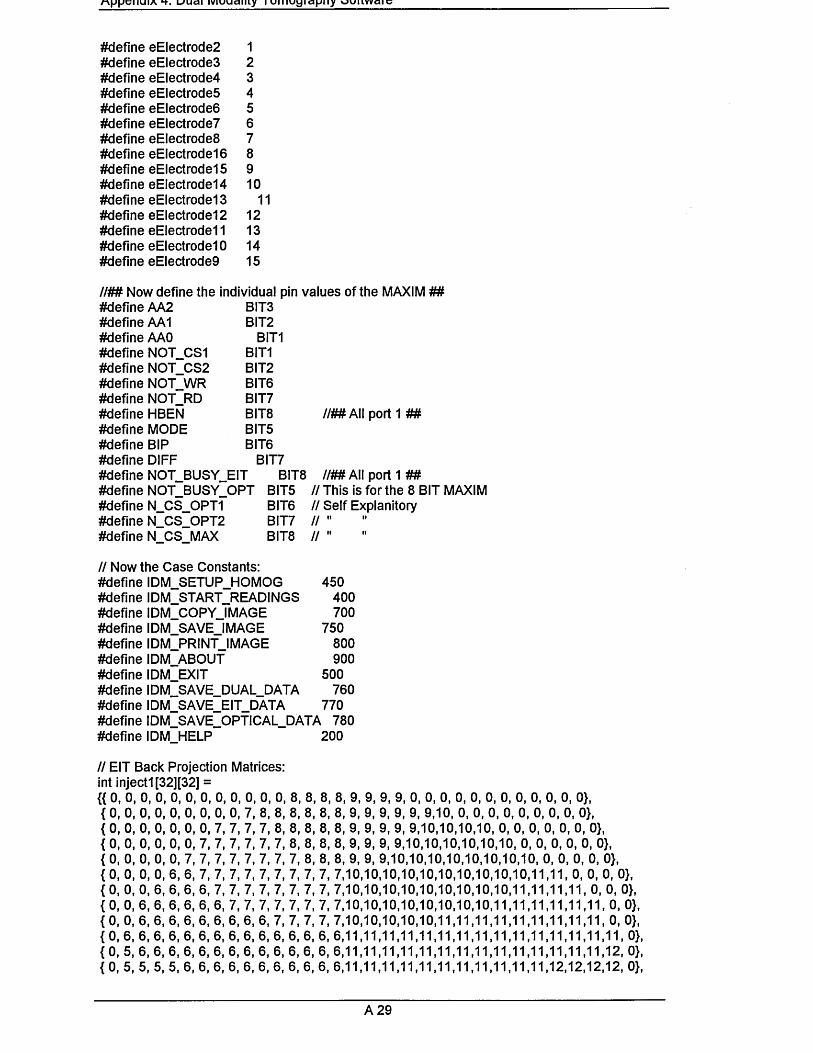
MppeiiuiA iviuuaiiiy i uinuyiapny ouuwaic

#define eElectrode2 1#define eElectrode3 2#define eElectrode4 3#define eElectrode5 4#define eElectrode6 5#define eElectrode7 6#define eElectrode8 7#define eElectrode16 8#define eElectrode15 9#define eElectrode14 10#define eElectrode13 11#define eElectrode12 12#define eElectrodel 1 13#define eElectrodel 0 14#define eElectrode9 15

//## Now define the individual pin values of the MAXIM ## #define AA2 BIT3#define AA1 BIT2#defineAAO BIT1#define NOT_CS1 BIT1#define NOT_CS2 BIT2#define NOT_WR BIT6#define NOT_RD BIT7#define HBEN BIT8#define MODE BIT5#define BIP BIT6#define DIFF BIT7#define NOT_BUSY_EIT BIT8 #define NOT_BUSY_OPT BIT5 #define N_CS_OPT1 BIT6#define N_CS_OPT2 BIT7#define N CS MAX BIT8

//## All port 1 ##

//## All port 1 ##// This is for the 8 BIT MAXIM // Self Explanitory // "// "

// Now the Case Constants:#define IDM_SETUP_HOMOG 450#define IDM_START_READINGS 400 #define IDM_COPYJMAGE 700#define IDM_SAVE_IMAGE 750#define IDM_PRINTJMAGE 800#define IDM_ABOUT 900#define IDM_EXIT 500#define IDM_SAVE_DUAL_DATA 760 #define IDM_SAVE_EIT_DATA 770#define IDM_SAVE_OPTICAL_DATA 780 #define IDM HELP 200

// EIT Back Projection int injecti [32][32] = {{0, 0, 0, 0, 0, 0, 0,0 (0, 0, 0, 0, 0, 0, 0,0 {0 , 0, 0, 0, 0, 0, 0 ,7 {0 , 0, 0, 0, 0, 0, 7 ,7 {0 , 0, 0, 0, 0, 7, 7 ,7 {0 , 0, 0, 0, 6, 6, 7 ,7 (0 , 0, 0, 6, 6, 6, 6 ,7 {0, 0, 6, 6, 6, 6, 6,6 (0, 0, 6, 6, 6, 6, 6,6 {0, 6, 6, 6, 6, 6, 6,6 {0 , 5, 6, 6, 6, 6, 6 ,6 { 0, 5, 5, 5, 5, 6, 6, 6

Matrices:

0 ,0 0, 0 ,80 ,7 8, 8 ,87 ,7 7, 8 ,87 ,7 7, 7 ,87 ,7 7, 7 ,77 ,7 7, 7 ,77 ,7 7, 7 ,77 ,7 7, 7 ,76 ,6 6, 7 ,76 ,6 6, 6 ,66 ,6 6, 6 ,66 ,6 6, 6 ,6

8, 8, 8, 9, 9, 9, 9, 0, 0, 0, 0, 0, 0, 0, 0, 0, 0, 0, 0),8, 8, 8, 9, 9, 9, 9, 9, 9,10, 0, 0, 0, 0, 0, 0, 0, 0, 0},8, 8, 8, 9, 9, 9, 9, 9,10,10,10,10, 0, 0, 0, 0, 0, 0, 0},8, 8, 8, 9, 9, 9, 9,10,10,10,10,10,10, 0, 0, 0, 0, 0, 0),8, 8, 8, 9, 9, 9,10,10,10,10,10,10,10,10, 0, 0, 0, 0, 0},7, 7, 7,10,10,10,10,10,10,10,10,10,10 7, 7, 7,10,10,10,10,10,10,10,10,10,1 7, 7, 7,10,10,10,10,10,10,10,10,11,1 7, 7, 7,10,10,10,10,10,11,11,11,11,1 6, 6, 6,11,11,11,11,11,11,11,11,11,1 6, 6, 6,11,11,11,11,11,11,11,11,11,1 6, 6, 6,11,11,11,11,11,11,11,11,11,1

,11,11,0, 0, 0, 0}, 1,11,11,11,0, 0, 0}, 1,11,11,11,11,0, 0}, 1,11,11,11,11,0, 0}, 1,11,11,11,11,11, 0}, 1,11,11,11,11,12, 0), 1,11,12,12,12,12, 0),

A 29

A p p e n d ix 4 : u u a i iv io a a iity i o m o g ra p n y s o n w a re

{ 5 ,5 5 5 5 5 5 5 5 5 6 6 6 6 6 6,11,11,11,11,11,11,12,12,12,12,12,12,12,12,12,12},{5 ,5 5 5 5 5 5 5 5 5 5 5 5 5 5 5,12,12,12,12,12,12,12,12,12,12,12,12,12,12,12,12},{5 ,5 5 5 5 5 5 5 5 5 5 5 5 5 5 5,12,12,12,12,12,12,12,12,12,12,12,12,12,12,12,12},{ 5 ,5 5 5 5 5 5 5 5 5 5 5 5 5 5 5,12,12,12,12,12,12,12,12,12,12,12,12,12,12,12,12},{ 4 ,4 4 4 4 4 4 4 4 4 4 4 4 4 4 4,13,13,13,13,13,13,13,13,13,13,13,13,13,13,13,13},{ 4 ,4 4 4 4 4 4 4 4 4 4 4 4 4 4 4,13,13,13,13,13,13,13,13,13,13,13,13,13,13,13,13},{ 4 ,4 4 4 4 4 4 4 4 4 4 4 4 4 4 4,13,13,13,13,13,13,13,13,13,13,13,13,13,13,13,13},{4 ,4 4 4 4 4 4 4 4 4 3 3 3 3 3 3,14,14,14,14,14,14,13,13,13,13,13,13,13,13,13,13},{ 0 ,4 4 4 4 3 3 3 3 3 3 3 3 3 3 3,14,14,14,14,14,14,14,14,14,14,14,13,13,13,13, 0},{0 ,4 3 3 3 3 3 3 3 3 3 3 3 3 3 3,14,14,14,14,14,14,14,14,14,14,14,14,14,14,13, 0},{0 ,3 3 3 3 3 3 3 3 3 3 3 3 3 3 3,14,14,14,14,14,14,14,14,14,14,14,14,14,14,14, 0},{ 0 ,0 3 3 3 3 3 3 3 3 3 2 2 2 2 2,15,15,15,15,15,14,14,14,14,14,14,14,14,14, 0, 0},{ 0 ,0 3 3 3 3 3 3 2 2 2 2 2 2 2 2,15,15,15,15,15,15,15,15,14,14,14,14,14,14, 0, 0},{ 0 ,0 0 3 3 3 3 2 2 2 2 2 2 2 2 2,15,15,15,15,15,15,15,15,15,14,14,14,14, 0, 0, 0},{ 0 ,0 0 0 3 3 2 2 2 2 2 2 2 2 2 2,15,15,15,15,15,15,15,15,15,15,14,14, 0, 0, 0, 0},{ 0 ,0 0 0 0 2 2 2 2 2 2 2 2 1 1 1,16,16,16,15,15,15,15,15,15,15,15, 0, 0, 0, 0, 0},{ 0 ,0 0 0 0 0 2 2 2 2 2 2 1 1 1 1,16,16,16,16,15,15,15,15,15,15, 0, 0, 0, 0, 0, 0},{0 ,0 0 0 0 0 0 2 2 2 2 1 1 1 1 1,16,16,16,16,16,15,15,15,15, 0, 0, 0, 0, 0, 0, 0},{0 ,0 0 0 0 0 0 0 0 2 1 1 1 1 1 1,16,16,16,16,16,16,15, 0, 0, 0, 0, 0, 0, 0, 0, 0},{0 ,0 0 0 0 0 0 0 0 0 0 0 1 1 1 1,16,16,16,16, 0, 0, 0, 0, 0, 0, 0, 0, 0, 0, 0, 0}};

t injectl 6[32][32] =0, 8, 8, 8, 8, 9, 9, 9, 9, 0, 0, 0, 0, 0, 0, 0, 0, 0, 0, 0, 0},8, 8, 8, 8, 8, 9, 9, 9, 9, 9, 9,10, 0, 0, 0, 0, 0, 0, 0, 0, 0},8, 8, 8, 8, 8, 9, 9, 9, 9, 9, 9,10,10,10, 0, 0, 0, 0, 0, 0, 0},8, 8, 8, 8, 9, 9, 9, 9, 9, 9,10,10,10,10,10, 0, 0, 0, 0, 0, 0},8, 8, 8, 9, 9, 9, 9, 9, 9,10,10,10,10,10,10,10, 0, 0, 0, 0, 0},7, 8, 9, 9, 9, 9, 9, 9, 9,10,10,10,10,10,10,10,11, 0, 0, 0, 0},6, 9, 9, 9, 9, 9, 9, 9,10,10,10,10,10,10,11,11,11,11, 0, 0, 0},6, 6, 9, 9, 9, 9, 9,10,10,10,10,10,10,10,11,11,11,11,11, 0, 0},6, 6, 9, 9, 9,10,10,10,10,10,10,10,11,11,11,11,11,11,11, 0, 0},6, 6, 9,10,10,10,10,10,10,10,10,11,11,11,11,11,11,11,11,11, 0}, 6, 5, 5,10,10,10,10,10,10,11,11,11,11,11,11,11,11,11,11,12, 0}, 5, 5, 5,10,10,10,10,10,11,11,11,11,11,11,11,11,12,12,12,12, 0}, 5, 5, 5, 5,10,10,11,11,11,11,11,11,11,11,12,12,12,12,12,12,12}, 5, 5, 5, 5,11,11,11,11,11,11,11,12,12,12,12,12,12,12,12,12,12}, 5, 4, 4, 4,11,11,11,11,11,12,12,12,12,12,12,12,12,12,12,12,12}, 4, 4, 4, 4, 4,11,12,12,12,12,12,12,12,12,12,12,12,12,12,12,12}, 4, 4, 4, 4, 3,12,12,12,12,12,12,12,12,13,13,13,13,13,13,13,13}, 4, 3, 3, 3, 3, 3,12,12,12,13,13,13,13,13,13,13,13,13,13,13,13}, 3, 3, 3, 3, 3, 3,13,13,13,13,13,13,13,13,13,13,13,13,13,13,13}, 3, 3, 3, 3, 2, 2,13,13,13,13,13,13,13,13,13,13,13,13,13,13,13}, 3, 3, 2, 2, 2, 2, 2,13,13,13,13,13,13,13,13,13,13,13,13,13, 0},3, 2, 2, 2, 2, 2, 2,13,13,14,14,14,14,14,14,14,14,14,13,13, 0},2, 2, 2, 2, 2, 2, 2, 1,14,14,14,14,14,14,14,14,14,14,14,14, 0},2, 2, 2, 2, 2, 1, 1, 1,14,14,14,14,14,14,14,14,14,14,14, 0, 0},2, 2, 2, 1, 1, 1,1, 1,14,14,14,14,14,14,14,14,14,14,14, 0, 0},2, 2, 1, 1, 1, 1, 1, 1, 1,14,14,14,14,14,14,14,14,14, 0, 0, 0},2 ,1 ,1 ,1 , 1, 1,1, 1,16,15,15,15,15,15,15,14,14, 0, 0, 0, 0},2, 1, 1, 1, 1, 1, 1,16,16,16,15,15,15,15,15,15, 0, 0, 0, 0, 0},1, 1, 1, 1, 1, 1,16,16,16,16,15,15,15,15,15, 0, 0, 0, 0, 0, 0},1, 1, 1, 1, 1,16,16,16,16,16,15,15,15,15, 0, 0, 0, 0, 0, 0, 0},1, 1, 1, 1, 1,16,16,16,16,16,16,15, 0, 0, 0, 0, 0, 0, 0, 0, 0},0,1,1,1,1,16,16,16,16, 0, 0, 0, 0, 0, 0, 0, 0, 0, 0, 0, 0}};

int injectl 5[32][32] ={{ 0, 0, 0, 0, 0, 0, 0, 0, 0, 0, 0, 0, 8, 8, 8, 8, 9, 9, 9, 9, 0, 0, 0, 0, 0, 0, 0, 0, 0, 0, 0, 0},

0, 0, 0, 0, 0, 0, 0, 0, 0, 7, 8, 8, 8, 8, 8, 8, 9, 9, 9, 9, 9, 9,10, 0, 0, 0, 0, 0, 0, 0, 0, 0},0, 0, 0, 0, 0, 0, 0, 7, 7, 7, 8, 8, 8, 8, 8, 8, 9, 9, 9, 9, 9,10,10,10,10, 0, 0, 0, 0, 0, 0, 0},0, 0, 0, 0, 0, 0, 7, 7, 7, 7, 7, 8, 8, 8, 8, 8, 9, 9, 9, 9, 9,10,10,10,10,10, 0, 0, 0, 0, 0, 0},0, 0, 0, 0, 0, 7, 7, 7, 7, 7, 7, 8, 8, 8, 8, 9, 9, 9, 9, 9, 9,10,10,10,10,10,10, 0, 0, 0, 0, 0},

0 0 0 0 0 0 0 0 0 0 00 0 0 0 0 0 0 0 0 7 80 0 0 0 0 0 0 7 7 7 70 0 0 0 0 0 7 7 7 7 70 0 0 0 0 7 7 7 7 7 70 0 0 0 6 6 7 7 7 7 70 0 0 6 6 6 6 6 6 6 60 0 6 6 6 6 6 6 6 6 60 0 6 6 6 6 6 6 6 6 60 6 6 6 6 6 6 6 6 6 60 5 5 6 6 6 6 6 6 6 60 5 5 5 5 5 5 5 5 5 55 5 5 5 5 5 5 5 5 5 55 5 5 5 5 5 5 5 5 5 55 5 5 5 5 5 5 5 5 5 55 5 5 5 5 5 5 5 4 4 44 4 4 4 4 4 4 4 4 4 44 4 4 4 4 4 4 4 4 4 44 4 4 4 4 4 4 4 4 4 34 4 4 4 4 4 4 3 3 3 30 4 4 4 4 3 3 3 3 3 30 4 3 3 3 3 3 3 3 3 30 3 3 3 3 3 3 3 3 3 20 0 3 3 3 3 3 3 3 2 20 0 3 3 3 3 3 2 2 2 20 0 0 3 3 3 3 2 2 2 20 0 0 0 3 2 2 2 2 2 20 0 0 0 0 2 2 2 2 2 20 0 0 0 0 0 2 2 2 2 20 0 0 0 0 0 0 2 2 2 10 0 0 0 0 0 0 0 0 2 10 0 0 0 0 0 0 0 0 0 0

A 30

MJJ|JCIiuia *t. u'ucti iviuuamy i unm^ia^njf «Jinivyciio

{0 , 0 0 0 6, 6, 7, 7, 7 7 8, 8, 8, 8, 8, 9, 9, 9, 9, 9,10,10,10,10,10,10,11,11, 0, 0, 0, 0},{0 , 0 0 6 6, 6, 7, 7, 7 7 8, 8, 8, 8, 8, 9, 9, 9, 9, 9,10,10,10,10,10,10,11,11,11, 0, 0, 0},{0, 0 6 6 6, 6, 6, 6, 7 7 8, 8, 8, 8, 9, 9, 9, 9, 9,10,10,10,10,10,11,11,11,11,11,11, 0, 0},{0, 0 6 6 6, 6, 6, 6, 8 8 8, 8, 8, 8, 9, 9, 9, 9,10,10,10,10,10,10,11,11,11,11,11,11, 0, 0},{0 , 6 6 6 6, 6, 6, 6, 5 5 8, 8, 8, 9, 9, 9, 9, 9,10,10,10,10,11,11,11,11,11,11,11,11,11, 0},{0 , 5 5 6 6, 5, 5, 5, 5 5 8, 8, 9, 9, 9, 9, 9,10,10,10,10,10,11,11,11,11,11,11,11,11,12, 0},{0 , 5 5 5 5, 5, 5, 5, 5 5 5, 5, 9, 9, 9, 9,10,10,10,10,11,11,11,11,11,11,11,11,12,12,12, 0},{5, 5 5 5 5, 5, 5, 5, 5 5 4, 4, 4, 9, 9, 9,10,10,10,10,11,11,11,11,11,11,12,12,12,12,12,12},{ 5, 5 5 5 5, 5, 5, 5, 5 4 4, 4, 4, 9,10,10,10,10,11,11,11,11,11,11,12,12,12,12,12,12,12,12},{ 5, 5 5 5 5, 5, 5, 4, 4 4 4, 4, 4, 4, 3,10,10,10,11,11,11,11,11,12,12,12,12,12,12,12,12,12},{ 5, 5 5 5 4, 4, 4, 4, 4 4 4, 4, 3, 3, 3,10,11,11,11,11,11,12,12,12,12,12,12,12,12,12,12,12},(4 , 4 4 4 4, 4, 4, 4, 4 4 4, 3, 3, 3, 3, 3, 2,11,11,11,12,12,12,12,12,12,12,12,13,13,13,13},{4 , 4 4 4 4, 4, 4, 4, 4 3 3, 3, 3, 3, 2, 2, 2,11,12,12,12,12,12,12,12,13,13,13,13,13,13,13},{4, 4 4 4 4, 4, 4, 4, 3 3 3, 3, 3, 3, 2, 2, 2, 2, 1,12,12,12,12,13,13,13,13,13,13,13,13,13},{4 , 4 4 4 4, 4, 3, 3, 3 3 3, 3, 2, 2, 2, 2, 1, 1, 1,12,12,12,13,13,13,13,13,13,13,13,13,13},{0 , 4 4 4 3, 3, 3, 3, 3 3 3, 3, 2, 2, 2, 2, 1, 1, 1, 1,13,13,13,13,13,13,13,13,13,13,13, 0},{0 , 4 3 3 3, 3, 3, 3, 3 3 2, 2, 2, 2, 2,1,1,1,1,1,16,16,13,13,13,13,13,14,14,13,13, 0},(0 , 3 3 3 3, 3, 3, 3, 3 3 2, 2, 2, 2, 1, 1, 1, 1, 1,16,16,16,13,13,14,14,14,14,14,14,14, 0},{0 , 0 3 3 3, 3, 3, 3, 2 2 2, 2, 2, 2, 1, 1, 1, 1,16,16,16,16,16,16,14,14,14,14,14,14, 0, 0},{0, 0 3 3 3, 3, 3, 3, 2 2 2, 2, 2, 1, 1, 1, 1, 1,16,16,16,16,15,15,14,14,14,14,14,14, 0, 0},{0, 0 0 3 3, 3, 2, 2, 2 2 2, 2, 1, 1, 1, 1, 1,16,16,16,16,16,15,15,15,15,14,14,14, 0, 0, 0},(0 , 0 0 0 3, 3, 2, 2, 2 2 2, 2, 1, 1, 1, 1, 1,16,16,16,16,16,15,15,15,15,14,14, 0, 0, 0, 0},(0 , 0 0 0 0, 2, 2, 2, 2 2 2, 1, 1, 1, 1, 1, 1,16,16,16,16,15,15,15,15,15,15, 0, 0, 0, 0, 0},(0 , 0 0 0 0, 0, 2, 2, 2 2 2, 1, 1, 1, 1, 1,16,16,16,16,16,15,15,15,15,15, 0, 0, 0, 0, 0, 0},{0, 0 0 0 0, 0, 0, 2, 2 2 2, 1, 1, 1, 1, 1,16,16,16,16,16,16,15,15,15, 0, 0, 0, 0, 0, 0, 0},{0, 0 0 0 0, 0, 0, 0, 0 2 1, 1, 1, 1, 1, 1,16,16,16,16,16,16,15, 0, 0, 0, 0, 0, 0, 0, 0, 0},{0 , 0 0 0 0, 0, 0, 0, 0 0 0, 0, 1, 1, 1, 1,16,16,16,16, 0, 0, 0, 0, 0, 0, 0, 0, 0, 0, 0, 0}};

int inject2[32][32] int inject3[32][32] int inject4[32][32] int inject5[32][32] int inject6[32][32] int inject7[32][32] int inject8[32][32]//int//int//int//int//int//int

nject9[32][32]; nject10[32][32] njectl 1 [32][32] nject12[32][32] njectl 3[32][32] njectl 4[32][32]

// Optical Back Projection Matrices int Iight1[32][32] ={{0, 0, 0, 0 {0, 0, 0, 0 { 0, 0, 0, 0 { 0, 0, 0, 0 { 0, 0, 0, 0 { 0, 0, 0, 0 {0, 0, 0,1{0, 0, ,1{0, 0, ,1{0,1, ,1{0,1, ,1{0,1, ,1{1.1, ,1{1,1. ,1{1.1, ,1{1,1, ,1{1,1, ,1

,0, 0, 0, 0, 0, 0, 0, 0, 4, 4, 4, 4, 5, 5, 5, 5, 0, 0, 0, 0, 0, 0 0 0 0,0, 0, 0},,0, 0, 0, 0, 0, 3, 3, 3, 4, 4, 4, 4, 5, 5, 5, 5, 6, 6, 6, 0, 0, 0 0 0 0,0, 0, 0},,0, 0, 0, 2, 3, 3, 3, 3, 4, 4, 4, 4, 5, 5, 5, 5, 6, 6, 6, 6, 7, 0 0 0 0,0, 0, 0},,0, 0, 2, 2, 3, 3, 3, 3, 4, 4, 4, 4, 5, 5, 5, 5, 6, 6, 6, 6, 7, 7 0 0 0,0, 0, 0},,0, 2, 2, 2, 3, 3, 3, 3, 4, 4, 4, 4, 5, 5, 5, 5, 6, 6, 6, 6, 7, 7 7 0 0,0, 0, 0},,2, 2, 2, 2, 3, 3, 3, 3, 4, 4, 4, 4, 5, 5, 5, 5, 6, 6, 6, 6, 7, 7 7 7 0,0, 0, 0},,2, 2, 2, 2, 3, 3, 3, 3, 4, 4, 4, 4, 5, 5, 5, 5, 6, 6, 6, 6, 7, 7 7 7 8, 0, 0, 0},,2, 2, 2, 2, 3, 3, 3, 3, 4, 4, 4, 4, 5, 5, 5, 5, 6, 6, 6, 6, 7, 7 7 7 8, 8, 0, 0},,2, 2, 2, 2, 3, 3, 3, 3, 4, 4, 4, 4, 5, 5, 5, 5, 6, 6, 6, 6, 7, 7 7 7 8, 8, 0, 0},,2 , 2, 2, 2, 3, 3, 3, 3, 4, 4, 4, 4, 5, 5, 5, 5, 6, 6, 6, 6, 7, 7 7 7 8, 8, 8, 0},,2, 2, 2, 2, 3, 3, 3, 3, 4, 4, 4, 4, 5, 5, 5, 5, 6, 6, 6, 6, 7, 7 7 7 8, 8, 8, 0},,2, 2, 2, 2, 3, 3, 3, 3, 4, 4, 4, 4, 5, 5, 5, 5, 6, 6, 6, 6, 7, 7 7 7 8, 8, 8, 0},,2, 2, 2, 2, 3, 3, 3, 3, 4, 4, 4, 4, 5, 5, 5, 5, 6, 6, 6, 6, 7, 7 7 7 8, 8, 8, 8},, 2, 2, 2, 2, 3, 3, 3, 3, 4, 4, 4, 4, 5, 5, 5, 5, 6, 6, 6, 6, 7, 7 7 7 8, 8, 8, 8},,2, 2, 2, 2, 3, 3, 3, 3, 4, 4, 4, 4, 5, 5, 5, 5, 6, 6, 6, 6, 7, 7 7 7 8, 8, 8, 8},,2, 2, 2, 2, 3, 3, 3, 3, 4, 4, 4, 4, 5, 5, 5, 5, 6, 6, 6, 6, 7, 7 7 7 8, 8, 8, 8},,2, 2, 2, 2, 3, 3, 3, 3, 4, 4, 4, 4, 5, 5, 5, 5, 6, 6, 6, 6, 7, 7 7 7 8, 8, 8, 8},

A 31

/AfJfJCiiuiA *t. umcii iviuudiuy i umujjiafJiiy ounwdic

1 ,1 ,1 ,1 2, 2, 2, 2, 3, 3, 3, 3, 4, 4 4, 4, 5, 5, 5, 5, 6, 6, 6, 6, 7, 7, 7 7, 8, 8, 8, 8},1 .1 .1 .1 2, 2, 2, 2, 3, 3, 3, 3, 4, 4 4, 4, 5, 5, 5, 5, 6, 6, 6, 6, 7, 7, 7 7, 8, 8, 8, 8},1 ,1 .1 ,1 2, 2, 2, 2, 3, 3, 3, 3, 4, 4 4, 4, 5, 5, 5, 5, 6, 6, 6, 6, 7, 7, 7 7, 8, 8, 8, 8},0 ,1, 1,1 2, 2, 2, 2, 3, 3, 3, 3, 4, 4 4, 4, 5, 5, 5, 5, 6, 6, 6, 6, 7, 7, 7 7, 8, 8, 8, 0},0 ,1 ,1 ,1 2, 2, 2, 2, 3, 3, 3, 3, 4, 4 4, 4, 5, 5, 5, 5, 6, 6, 6, 6, 7, 7, 7 7, 8, 8, 8, 0},0 ,1 ,1 ,1 2, 2, 2, 2, 3, 3, 3, 3, 4, 4 4, 4, 5, 5, 5, 5, 6, 6, 6, 6, 7, 7, 7 7, 8, 8, 8, 0},0 ,0 ,1 ,1 2, 2, 2, 2, 3, 3, 3, 3, 4, 4 4, 4, 5, 5, 5, 5, 6, 6, 6, 6, 7, 7, 7 7, 8, 8, 0, 0},0, 0 ,1 ,1 2, 2, 2, 2, 3, 3, 3, 3, 4, 4 4, 4, 5, 5, 5, 5, 6, 6, 6, 6, 7, 7, 7 7, 8, 8, 0, 0},0 ,0, 0, 1 2, 2, 2, 2, 3, 3, 3, 3, 4, 4 4, 4, 5, 5, 5, 5, 6, 6, 6, 6, 7, 7, 7 7, 8, 0, 0, 0},0, 0, 0, 0 2, 2, 2, 2, 3, 3, 3, 3, 4, 4 4, 4, 5, 5, 5, 5, 6, 6, 6, 6, 7, 7, 7 7, 0, 0, 0, 0},0, 0, 0, 0 0, 2, 2, 2, 3, 3, 3, 3, 4, 4 4, 4, 5, 5, 5, 5, 6, 6, 6, 6, 7, 7, 7 0, 0, 0, 0, 0},0, 0, 0, 0 0, 0, 2, 2, 3, 3, 3, 3, 4, 4 4, 4, 5, 5, 5, 5, 6, 6, 6, 6, 7, 7, 0 0, 0, 0, 0, 0},0, 0, 0, 0 0, 0, 0, 2, 3, 3, 3, 3, 4 ,4 4, 4, 5, 5, 5, 5, 6, 6, 6, 6, 7, 0, 0 0, 0, 0, 0, 0},0, 0, 0, 0 0, 0, 0, 0, 0, 3, 3, 3, 4, 4 4, 4, 5, 5, 5, 5, 6, 6, 6, 0, 0, 0, 0 0, 0, 0, 0, 0),0, 0, 0, 0 0, 0, 0, 0, 0, 0, 0, 0, 4, 4 4, 4, 5, 5, 5, 5, 0, 0, 0, 0, 0, 0, 0 0, 0, 0, 0, 0}};

Iight2[32][32] =0 0 0 0 0 0 0 0 0 0 0 0 8 8 8 8 8 8 8 8 0 0 0 0 0 0 0 0 0 0 0 0},0 0 0 0 0 0 0 0 0 8 8 8 8 8 8 8 8 8 8 8 8 8 8 0 0 0 0 0 0 0 0 0},0 0 0 0 0 0 0 8 8 8 8 8 8 8 8 8 8 8 8 8 8 8 8 8 8 0 0 0 0 0 0 0},0 0 0 0 0 0 8 8 8 8 8 8 8 8 8 8 8 8 8 8 8 8 8 8 8 8 0 0 0 0 0 0},0 0 0 0 0 7 7 7 7 7 7 7 7 7 7 7 7 7 7 7 7 7 7 7 7 7 7 0 0 0 0 0},0 0 0 0 7 7 7 7 7 7 7 7 7 7 7 7 7 7 7 7 7 7 7 7 7 7 7 7 0 0 0 0},0 0 0 7 7 7 7 7 7 7 7 7 7 7 7 7 7 7 7 7 7 7 7 7 7 7 7 7 7 0 0 0},0 0 7 7 7 7 7 7 7 7 7 7 7 7 7 7 7 7 7 7 7 7 7 7 7 7 7 7 7 7 0 0},0 0 6 6 6 6 6 6 6 6 6 6 6 6 6 6 6 6 6 6 6 6 6 6 6 6 6 6 6 6 0 0},0 6 6 6 6 6 6 6 6 6 6 6 6 6 6 6 6 6 6 6 6 6 6 6 6 6 6 6 6 6 6 0},0 6 6 6 6 6 6 6 6 6 6 6 6 6 6 6 6 6 6 6 6 6 6 6 6 6 6 6 6 6 6 0),0 6 6 6 6 6 6 6 6 6 6 6 6 6 6 6 6 6 6 6 6 6 6 6 6 6 6 6 6 6 6 0},5 5 5 5 5 5 5 5 5 5 5 5 5 5 5 5 5 5 5 5 5 5 5 5 5 5 5 5 5 5 5 5},5 5 5 5 5 5 5 5 5 5 5 5 5 5 5 5 5 5 5 5 5 5 5 5 5 5 5 5 5 5 5 5},5 5 5 5 5 5 5 5 5 5 5 5 5 5 5 5 5 5 5 5 5 5 5 5 5 5 5 5 5 5 5 5},5 5 5 5 5 5 5 5 5 5 5 5 5 5 5 5 5 5 5 5 5 5 5 5 5 5 5 5 5 5 5 5},4 4 4 4 4 4 4 4 4 4 4 4 4 4 4 4 4 4 4 4 4 4 4 4 4 4 4 4 4 4 4 4},4 4 4 4 4 4 4 4 4 4 4 4 4 4 4 4 4 4 4 4 4 4 4 4 4 4 4 4 4 4 4 4},4 4 4 4 4 4 4 4 4 4 4 4 4 4 4 4 4 4 4 4 4 4 4 4 4 4 4 4 4 4 4 4},4 4 4 4 4 4 4 4 4 4 4 4 4 4 4 4 4 4 4 4 4 4 4 4 4 4 4 4 4 4 4 4},0 3 3 3 3 3 3 3 3 3 3 3 3 3 3 3 3 3 3 3 3 3 3 3 3 3 3 3 3 3 3 0},0 3 3 3 3 3 3 3 3 3 3 3 3 3 3 3 3 3 3 3 3 3 3 3 3 3 3 3 3 3 3 0},0 3 3 3 3 3 3 3 3 3 3 3 3 3 3 3 3 3 3 3 3 3 3 3 3 3 3 3 3 3 3 0},0 0 3 3 3 3 3 3 3 3 3 3 3 3 3 3 3 3 3 3 3 3 3 3 3 3 3 3 3 3 0 0},0 0 2 2 2 2 2 2 2 2 2 2 2 2 2 2 2 2 2 2 2 2 2 2 2 2 2 2 2 2 0 0},0 0 0 2 2 2 2 2 2 2 2 2 2 2 2 2 2 2 2 2 2 2 2 2 2 2 2 2 2 2 0 0},0 0 0 0 2 2 2 2 2 2 2 2 2 2 2 2 2 2 2 2 2 2 2 2 2 2 2 2 0 0 0 0},0 0 0 0 0 2 2 2 2 2 2 2 2 2 2 2 2 2 2 2 2 2 2 2 2 2 2 0 0 0 0 0},0 0 0 0 0 0 1 1 1 1 1 1 1 1 1 1 1 1 1 1 1 1 1 1 1 1 0 0 0 0 0 0},0 0 0 0 0 0 0 1 1 1 1 1 1 1 1 1 1 1 1 1 1 1 1 1 1 0 0 0 0 0 0 0},0 0 0 0 0 0 0 0 0 1 1 1 1 1 1 1 1 1 1 1 1 1 1 0 0 0 0 0 0 0 0 0),0 0 0 0 0 0 0 0 0 0 0 0 1 1 1 1 1 1 1 1 0 0 0 0 0 0 0 0 0 0 0 0}};

// EIT Constants: float homog[16][16]={0.0}; float readings[16][16]={0.0}; float finalnet[32][32]={0.0>; int equip[32][32]={0>; float bufferh=0.0; float bufferl=10000.0; int injectpos=1;int injectneg=2; //# set up the 2 static injection electrodes ## int ave=2;

A 32

luiA *t. l/ ucji iviuucuuy i umuyiapiiy vjunwaic

// Optical Constants: int optreadings[2][8]; int OPTDATA[16][8]; float optfinalnet[32][32]; int optfinalnet1[32][32]; int optequip[32][32]={0};int oppzero[16][16]= {{1,1.0,0,0,0,0,0,1,1,0,0,0,0,0,0},

{0,1,1,0,0,0,0,0,0,1,1,0,0,0,0,0},{0,0,1,1,0,0,0,0,0,0,1,1,0,0,0,0},{0,0,0,1,1,0,0,0,0,0,0,1,1,0,0,0},{0,0,0,0,1,1,0,0,0,0,0,0,1,1,0,0},{0,0,0,0,0,1,1,0,0,0,0,0,0,1,1,0},{0,0,0,0,0,0,1,1,0,0,0,0,0,0,1,1},{1,0,0,0,0,0,0,1,1,0,0,0,0,0,0,1},{1,1,0,0,0,0,0,0,1,1,0,0,0,0,0,0},{0,1,1,0,0,0,0,0,0,1,1,0,0,0,0,0},{0,0,1,1,0,0,0,0,0,0,1,1,0,0,0,0},{0,0,0,1,1,0,0,0,0,0,0,1,1,0,0,0},{0,0,0,0,1,1,0,0,0,0,0,0,1,1,0,0},{0,0,0,0,0,1,1,0,0,0,0,0,0,1,1,0},{0,0,0,0,0,0,1,1,0,0,0,0,0,0,1,1},{1,0,0,0,0,0,0,1,1,0,0,0,0,0,0,1}};

int bits2[8]={BIT8, BIT7, BIT6, BIT5, BIT4, BIT3, BIT2, BIT1}; int bits[8]={BIT1, BIT2, BIT3, BIT4, BIT5, BIT6, BIT7, BIT8};

// General Constants: int hX, hY;int bitmapX, bitmapY, cxClient, cyClient; char *blanc="\xDB";HBITMAP hBitmap;HPEN hPenO, hWidePen, hOldPen;HBRUSH hBrushO, hBrushl, hBrush2, hOldBrush;HBRUSH hBrush3, hBrush4, hBrush5, hBrush6, hBrush7;HBRUSH hBrush8, hBrush9, hBrushl 0; static HANDLE hmf = NULL;GLOBALHANDLE hGMem;LPMETAFILEPICT IpMFP;HANDLE hPr, hAccTable;HFONT hFontl, hFont2;

// EIT Subroutines: void FillMats(void); void Rotate16_2(void);void FirstClock(int eit1[32][32], int eit2[32][32]);void Difference(void);void Average(void);int ReadElectrodes(HWND, int);void CalcFinalNet(int array[32][32], int);int InitialiselOPort(HWND); //## Check the I/O port and set it up ##void SetupSwitches(HWND, int, int); //## Set the groups up with their values ##void ResetElectrodes(void); //## Reset the electrodes to o/c ##void ClearReadings(void); void SetUpMeta(void);

// Optical Subroutines:void OptDifference(void);void OptAverage(void);void OptCalcFinalNet(int array[32][32], int);void ReadSensors(int);

A 33

ANfJfJCIIUIA *r. U U d l IV IU U c llliy I U l I iu y I d fJ Iiy O U llW d lC

void FAR Setuplnjection(HWND, int, int); void ResetLeds(HWND);

// File Save Subroutines: void CMUFileSavelmg(HWND); void CMUFileSaveDualData(HWND); void CMUFileSaveEitData(HWND); void CMUFileSaveOptData(HWND);

// General Subroutines:long FAR PASCAL WndProc(HWND, WORD.WORD, LONG); int mag(float);void wait(int); //## Rather complicated delay procedure ##void iowrite( int, int); //## I/O Port write procedure ## int ioread( int); //## I/O Port read procedure ##void combine(void);

A.4.3 H eader F il e : o ptr ec_ l .h// Optrec.h: The code for Optical Reconstruction of Data //## This routine calculates the difference between the ##//## hardware readings stored in thw global variable readings[][] ## //## and the homogenous values stored in homog[][] ## void OptDifference(void){int indxl, indx2;for(indx1=0; indxl <=1; indxl++)

{for(indx2=0; indx2<=7; indx2++){optreadings[indx1][indx2]=255-optreadings[indx1][indx2];}

}for(indx1=0; indxl <=31; indxl++)

{for(indx2=0; indx2<=31; indx2++){optfinalnet[indx1 ][indx2]=0;}

}OptCalcFinalNet(light1, 0); for(indx1=0; indxl <=31; indxl++)

{for(indx2=0; indx2<=31; indx2++)

{optfinalnet1[indx1][indx2]=optfinalnet[indx1][indx2];}

}OptCalcFinalNet(light2,1); for(indx1=0; indxl <=31; indxl++)


{optfinalnet[indx1][indx2]*=optfinalnet1[indx1][indx2];}

}}

//## This routine calculates the value of the final array ##//## finalnet[][] before the color array associted with these ##//## values is calculated ##

A 34

MyycuuiA LJUdi iviuudiiiy i umuyidf-niy ouuwdic

void OptCalcFinalNet(int array[32][32], int row){int indxl, indx2;for(indx1=0; indxl <=31; indxl++)


{// if it's == 1 then this means it wants readings for // electrode2 - electrodel. These are stored in row 0-15, // but in colum 1 - NOT 0!!! if(array[indx1][indx2]==1)

{optfinalnet[indx1][indx2]=optreadings[row][0]; goto finish;}

if(array[indx1][indx2]==2){optfinalnet[indx1][indx2]=optreadings[row][1]; goto finish;}

if(array[indx1 ][indx2]==3){optfinalnet[indx1][indx2]=optreadings[row][2]; goto finish;}

if(array[indx1][indx2]==4){optfinalnet[indx1][indx2]=optreadings[row][3]; goto finish;}





finish:;}

}}

//## This routine calculates the average values of those in ## //## finalnet[][] with respect to the maximum value therin ## void OptAverage(void){int indxl, indx2;for(indx1=0; indxl <=31; indxl++)

A 35

/AjjycnuiA *t. l/ uoi iviuuamy i uuujyiapiiy vjuiivvciig


{// Max Value for 2 Projections = 2*255=510: optfinalnet[indx1][indx2]=((optfinalnet[indx1][indx2]

/65025)*100); if(optfinalnet[indx1 ][indx2]==0)

{optequip[indx1 ][indx2]=0; goto finish;}

if(optfinalnet[indx1][indx2]>=90){optequip[indx1][indx2]=10;//## 1 = Most significant, darkest ## goto finish;}

if((optfinalnet[indx1][indx2]<=90)&(optfinalnet[indx1][indx2]>=80)){optequip[indx1 ][indx2]=9; goto finish;}


if((optfinalnet[indx1][indx2]<=70)&(optfinalnet[indx1][indx2]>=60)){optequip[indx1][indx2]=7; goto finish;}

if((optfinalnet[indx1][indx2]<=60)&(optfinalnet[indx1 ][indx2]>=50)){optequip[indx1 ][indx2]=6; goto finish;}

if((optfinalnet[indx1][indx2]<=50)&(optfinalnet[indx1][indx2]>=40)){optequip[indx1][indx2]=5; goto finish;}



if((optfinalnet[indx1][indx2]<=20)&(optfinalnet[indx1][indx2]>=10)){

A 36

Mppenuix h: uuai iviuuaniy i uinuyiapiiy ouuwaie

optequip[indx1 ][indx2]=2; goto finish;}

if((optfinalnet[indx1][indx2]<=10)&(optfinalnet[indx1 j[indx2]>=9)){optequip[indx1][indx2]=1; goto finish;}

optequip[indx1][indx2]=0; finish:;}

}}

A.4.4 H eader F ile : e itre c_e .h//## This rotates eit1 by 90 degrees to produce eit2 ## void FirstClock(int eit1[32][32], int eit2[32][32]){float buff;int slowplus, fastplus, slowminus;//## Rotate by 90 degrees an renumber to maintain there##//## correct positions in the colour scheme ## for(slowplus=0; slowplus<=31; slowplus++)

{for(fastpius=0; fastplus<=31; fastplus++)

{slowminus=31 -slowplus;eit2[fastplus][slowminus]=eit1[slowplus][fastplus];if(eit2[fastplus][slowminus]==0)

buff=0;if(eit2[fastplus][slowminus]>4)

buff=eit2[fastplus][slowminus]-4;if((eit2[fastplus][slowminus]<=4)&(eit2[fastplus][slowminus]>0))

buff=eit2[fastplus][slowminus]+12;eit2[fastplus][slowminus]=buff;>

}}

//## This creates the other 13 matrices using FirstClock ##//## by rotating the three defined matrices through 90 ##//## degrees, and the using the result to produce the next ##//## etc.. It also uses another routine to produce inject2 ##//## before it can be rotated as it doesn't exist and can ##//## easilly be formed from injectl6 by flipping through ##//## 180 degrees. ## void FillMats(void){int indxl, indx2;

FirstClock(inject1, injects);FirstClock(inject5, inject9);FirstClock(inject9, injectl 3);FirstClock(inject16, inject4);FirstClock(inject4, inject8);FirstClock(inject8, inject12);FirstClock(inject15, inject3);FirstCiock(inject3, inject7);FirstClock(inject7, injectl 1);

A 37

Appendix uuai iviuuamy lumuyiapny ounwaie

Rotate16_20; //## Produce Inject2 from injectl 6 ## FirstClock(inject2, inject6);FirstClock(inject6, injectl0);FirstClock(inject10, inject14);}

void Rotate”! 6_2(void){int indxl, indx2, val; for(indx1=0; indxl <=31; indxl++)


{val=31-indx2;inject2[indx1 ][val]=inject16[indx1 ][indx2]; if(inject2[indx1][val]==1)

{inject2[indx1][val]=16; goto finish;}

if(inject2[indx1 ][val]==2){inject2[indx1][val]=15; goto finish;}

if(inject2[indx1][val]==3){inject2[indx1 ][val]=14; goto finish;}

if(inject2[indx1][val]==4){inject2[indx1][val]=13; goto finish;}






if(inject2[indx1][val]==10)

A 38

A p p e n d ix u u a i iv iou aiu y i o m c g ra p n y o u n w a ie

{inject2[indx1][val]=7; goto finish;}



if(inject2[indx1 ][val]==13){inject2[indx1 ][val]=4; goto finish;}




finish:;}

}}

//## This routine calculates the difference between the ##//## hardware readings stored in thw global variable readings[][] ##//## and the homogenous values stored in homog[][] ## void Difference(void){int indxl, indx2;for(indx1=0; indxl <=15; indxl++)


{if((readings[indx1][indx2]!=0)&&(homog[indx1][indx2]!=0))

{readings[indx1][indx2]=(readings[indx1][indx2]-homog[indx1][indx2]);// (readings[indx1 j[indx2]+homog[indx1 ][indx2]);}

else{readings[indx1][indx2]=0;}

}}

for(indx1=0; indxl <=31; indxl++)

A 39

rsppeiiuiA *+. uuai iviuuamy luiuuyiapuy ouuwaic


{finalnet[indx1 ][indx2]=0;}

}CalcFinalNet(inject1, 0);CalcFinalNet(inject2, 1);CalcFinalNet(inject3, 2);CalcFinalNet(inject4, 3);CalcFinalNet(inject5, 4);CalcFinalNet(inject6, 5);CalcFinalNet(inject7, 6);CalcFinalNet(inject8, 7);CalcFinalNet(inject9, 8);CalcFinalNet(inject10, 9);CalcFinalNet(inject11,10);CalcFinalNet(inject12,11);CalcFinalNet(inject13, 12);CalcFinalNet(inject14, 13);CalcFinalNet(inject15,14);CalcFinalNet(inject16, 15);}

//## This routine calculates the value of the final array ##//## finalnetDH before the color array associted with these ##//## values is calculated ##void CalcFinalNet(int array[32][32],int row){int indxl, indx2;for(indx1=0; indxl <=31; indxl++)


{// if it's == 1 then this means it wants readings for // electrode2 - electrodel. These are stored in row 0-15,// but in colum 1 - NOT 0!!! if(array[indx1][indx2]==1)

{finalnet[indx1][indx2]=finalnet[indx1][indx2]+readings[row][1]; goto finish;}

if(array[indx1 ][indx2]==2){finalnet[indx1][indx2]=finalnet[indx1][indx2]+readings[row][2]; goto finish;}


if(array[indx1 ][indx2]==4){finalnet[indx1 ][indx2]=finalnet[indx1 ][indx2]+readings[row][4]; goto finish;}

if(array[indx1 ][indx2]==5){finalnet[indx1][indx2]=finalnet[indx1][indx2]+readings[row][5]; goto finish;

A 40

SAppcnuiA *t. uuoi iviuuamy i uinuvjiapiiy owuvvaic

}if(array[indx1 ][indx2]==6)

{finalnet[indx1][indx2]=finalnet[indx1][indx2]+readings[row][6]; goto finish;}

if(array[indx1][indx2]==7){finalnet[indx1][indx2]=finalnet[indx1][indx2]+readings[row][7]; goto finish;}

if(array[indx1 ][indx2]==8){finalnet[indx1 ][indx2]=finalnet[indx1 ][indx2]+readings[row][8]; goto finish;}


if(array[indx1][indx2]==10){finalnet[indx1 ][indx2]=finalnet[indx1 ][indx2]+readings[row][10]; goto finish;}






if(array[indx1 ][indx2]==16){finalnet[indx1][indx2]=finalnet[indx1][indx2]+readings[row][0];}

finish:;}

}}

//## This routine calculates the average values of those in ##

A 41

A p p e n d ix 4: u u a i M o a a m y i o m o g ra p n y ^ o n w a re

//## finalnet[][] with respect to the maximum value therin ## void Average(void){int indxl, indx2; float bufferh, bufferl; bufferl=0.0; bufferh=0.0;for(indx1=0; indxl <=31; indxl++)


{if(finalnet[indx1][indx2]>=bufferh)

{bufferh=finalnet[indx1][indx2];}

if(finalnet[indx1][indx2]<=bufferl){bufferl=finalnet[indx1][indx2];}

}}

if(bufferl<=0) // Find value of largest magnitude bufferl=bufferl*-1; // If bufferl=-ve then make +ve

if(bufferl>=bufferh) bufferh=bufferl; // Only keep largest value for'%' calculations

for(indx1=0; indxl <=31; indxl++){for(indx2=0; indx2<=31; indx2++)

{finalnet[indx1][indx2]=((finalnet[indx1][indx2]/bufferh)*100); if(finalnet[indx1 ][indx2]==0)

{equip[indx1 ][indx2]=0; goto finish;}

if((finalnet[indx1 ][indx2]<=100)&(finalnet[indx1 ][indx2]>=90)){equip[indx1][indx2]=10; //## 1 = Most significant, darkest ## goto finish;}

if((finalnet[indx1 ][indx2]<=90)&(finalnetfindxl ][indx2]>=80)){equip[indx1 ][indx2]=9; goto finish;}

if((finalnet[indx1 ][indx2]<=80)&(finalnetfindxl ][indx2]>=70)){equip[indx1 ][indx2]=8; goto finish;

if((finalnet[indx1 ][indx2]<=70)&(finalnetfindxl ][indx2]>=60)){equip[indx1][indx2]=7; goto finish;}

if((finalnet[indx1 ][indx2]<=60)&(finalnetfindxl ][indx2]>=50)){

A 42

m j j j j c iiu ia u u a i iv iuu aiu y i u i i iuy i a \ J i ly o u u w c i i e

equip[indx1 ][indx2]=6; goto finish;}

if((finalnet[indx1][indx2]<=50)&(finalnetfindxl ][indx2]>=40)){equip[indx1 ][indx2]=5; goto finish;}

if((finalnet[indx1 ][indx2]<=40)&(finalnet[indx1][indx2]>=30)){equip[indx1 ][indx2]=4; goto finish;}

if((finalnet[indx1 ][indx2]<=30)&(finalnet[indx1 ][indx2]>=20)){equip[indx1 ][indx2]=3; goto finish;}

if((finalnet[indx1 ][indx2]<=20)&(finalnet[indx1][indx2]>=10)){equip[indx1 ][indx2]=2; goto finish;}

if((finalnet[indx1 ][indx2]<=10)&(finalnetfindxl ][indx2]>=0)){equip[indx1][indx2]=1; goto finish;}

equip[indx1 ][indx2]=0; finish:;}

}}

A.4.5 Header F ile : e itinj_ e .h//## This Setups up both the '+' and Electrodes and ##//## then pulses (NOT)Write HIGH ##void SetupSwitches(HWND hwnd, int eElectrodeP, int eElectrodeN){if(eElectrodeP == eElectrodeN)

{MessageBox(hwnd, "This Would Connect'+' to Cancel??.", NULL, MB_OK |MBJCONEXCLAMATION);return;}

// Note: INJECT == GROUP3; iowrite(INJECT, eElectrodeP + Enable + Reset); iowrite(INJECT, eElectrodeP + Enable + Reset + Writel); iowrite(INJECT, eElectrodeP + Reset + Writel);iowrite(INJECT, eElectrodeN + Enable + Reset + Writel); //## Keep Writel HIGH ##iowrite(INJECT, eElectrodeN + Enable + Reset + Writel + Write2);iowrite(INJECT, eElectrodeN + Reset + Writel + Write2);iowrite(GROUP3, 255-BIT6); // Reset the logic chips as a precautionwait(12);}

A 43

M p p e n u ix h: u u a i iv iuu am y i u m u y ia p n y o u i iw a ie

//ittitm m m ifttiiiittititiifitttiitiiiiitiiittiiiiitiiiiiiitifiiiiifiiiiiitiifm iiiiiiiiiitiitiim //##### This resets all the electrodes to open cct # ttIfIIItIIIIII//Mm m um iifiiiiiiiiiiitiiiMuifiiiifHtiititiifiiittiitifiiitiiiiitititiiiiiiiiiiiiiiiiitiiiiHm #void ResetElectrodes(void){iowrite(INJECTf 0); return;}

//## This is a wait procedure that came with the io port ## //tlllllllllllllllltllllllfllllllltllHftfHllillfimiflHtlUIHIHHflfHIHHIIIIIMIfiflllllfflllllllMM void wait(int period) /* A rather over-complicated delay routine that*//* demonstrates the timer of the PCIB40.*/{int ctr = OxFF;iowrite(CWREG,0x26); /* Timer 0, mode 3, decimal, load MSB only */ iowrite(TIMER0,0); /* MSB of count, counter starts */ while(period-)

{/* 2 x 'WHILE' loops wait for counter MSB transition 0-$FF */ while(ctr != 0) /* Wait for counter = 0 */

{iowrite(CWREG.OxOO); /* Latch count */ ctr = ioread(TIMERO);}

while(ctr != 10) /* Wait for counter =10 7 {iowrite(CWREG,OxOO); /* Latch count */ ctr= ioread(TIMERO);}

}}

//##### This converts the single line command into the #### //######### format required by the C compiler ############# //M//////#//////////////////////////////////////////////////////////////////////////////////////////////////## void iowrite( int ioaddr, int value){outportb(OFFSET,ioaddr); /* Set up I/O address */ outportb((DATA),value); /* Write value to I/O address */}

iim m m m m m m m m m m m m m m m m m m m m m m m m m m m//MflUNt This converts the single line command into the #### //######### format required by the C compiler #############

int ioread( int ioaddr){outportb(OFFSET,ioaddr); /* Set up I/O address */ return (inportb(DATA)); /* Read back value */}

A .4.6 Header Fil e : e itcap_ e .hint ReadElectrodes(HWND hwnd, int where){int inc, oldval, newval, incaverage; hwnd+=0;

A 44

M p p e n u ix q . u u a i iv iou am y m m u y ia p i iy o u u w a ie

for(incaverage=1; incaverage<=ave; incaverage++){for(inc=0; inc<=7; inc++)

{//## First job = set up Control logic, ie which input ? ## oldval=ioread(CONTROL1 );//## Find state of CONTROL1 ## newval=oldval-NOT_WR+inc; //## Set WRITE bit low and choose an ##//## anlogue input ## iowrite(GROUP4, 0+NOT.CS1);iowrite(CONTROL1, newval); //## Send new value to port ##iowrite(CONTROL1, newval+NOT_WR); //## Now set write high.. ## iowrite(CONTROL1, oldval); //##..and then restore most of old value ## loop: oldval=ioread(TOPDATA_CONTROL2); if(oldval<128)

goto loop; //## Loop until BUSY goes HIGH ## oldval=ioread(CONTROL1 );//## Find state of CONTROL1 ## newval=oldval-NOT_RD; //## Set READ bit low ## iowrite(CONTROL1, newval); //## Send new value to port ##//## Read top 4 bits##readings[where][inc]+=ioread(BOTTOMDATA); //## Read bottom 8 bits ## readings[where][inc]+=(ioread(TOPDATA_CONTROL2)-MODE-NOT_BUSY_EIT)*255; iowrite(CONTROL1, oldval); //## Restore RD, CS bit to HIGH ## iowrite(GROUP4, NOT_CS1+NOT_CS2);}

for(inc=0; inc<=7; inc++){//## First job = set up Control logic, ie which input ? ## oldval=ioread(CONTROL1);//## Find state of CONTROL1 ## newval=oldval-NOT_WR+inc; //## Set WRITE bit low and choose an ##//## anlogue input ## iowrite(GROUP4, 0+NOT_CS2);iowrite(CONTROL1, newval); //## Send new value to port ## iowrite(CONTROL1, newval+NOT_WR); //## Now set write high.. ## iowrite(CONTROL1, oldval); //## ..and then restore most of old value ## loop2: oldval=ioread(TOPDATA_CONTROL2);if(oldval<128)

goto loop2; //## Loop until BUSY goes HIGH ## oldval=ioread(CONTROL1);//## Find state of CONTROL1 ## newval=oldval-NOT_RD; //## Set READ bit low ## iowrite(CONTROL1, newval); //## Send new value to port ##//## Read top 4 bits##readings[where][inc+8]+=ioread(BOTTOMDATA); //## Read bottom 8 bits## readings[where][inc+8]+=(ioread(TOPDATA__CONTROL2)-MODE-NOT_BUSY_EIT)*255; iowrite(CONTROL1, oldval); //## Restore RD, CS bit to HIGH ## iowrite(GROUP4, NOT_CS1+NOT_CS2);} //## And then do until all 8 ports are read ##

}for(inc=0; inc<=15; inc++)

{if(oppzero[where][inc]==1)

{readings[where][inc]=0;}

}return (TRUE);}

A .4.7 H eader F il e : eit_ e .h/*** Global Variables ***! charszName[256j;

A 45

M fJ fJ tJ I IU IA H. Uuai IV IU U c ll l iy I U I I I U y i d | J l i y O U H W d l C

//## Save the image to disk ## void CMUFileSavelmg( HWND hWnd){OPENFILENAME ofnTemp;DWORD Errval; // Error value char buf[5]; // Error bufferchar Errstr[50]="GetOpenFileName returned Error #"; charszTempD = "Image Files (*.img)\0*.img\0AII Files (*.*)\0*.*\0";FILE *stream; int cnt1 ,cnt2;ofnTemp.IStructSize = sizeof( OPENFILENAME); ofnTemp.hwndOwner = hWnd; //An invalid hWnd causes non-modality ofnTemp.hlnstance = 0;ofnTemp.IpstrFilter = (LPSTR)szTemp; // See previous note concerning string ofnTemp.IpstrCustomFilter = NULL; ofnTemp.nMaxCustFilter = 0; ofnTemp.nFilterlndex = 1;ofnTemp.IpstrFile = (LPSTR)szName; // Stores the result in this variableofnTemp.nMaxFile = sizeof( szName);ofnTemp.IpstrFileTitle = NULL;ofnTemp.nMaxFileTitle = 0;ofnTemp.IpstrlnitialDir = NULL;ofnTemp.IpstrTitle = "Save Dual Modality Image..."; //Title for dialogofnTemp.Flags = OFN_FILEMUSTEXIST | OFNJHIDEREADONLY | OFN_PATHMUSTEXIST;ofnTemp.nFileOffset = 0;ofnTemp.nFileExtension = 0;ofnTemp.IpstrDefExt =ofnTemp.ICustData = NULL;ofnTemp.IpfnHook = NULL;ofnTemp.IpTemplateName = NULL;/ *If the call to GetOpenFileNameO fails you can call CommDlgExtendedErrorO to retrieve the type of error that occured.7if(GetSaveFileName( &ofnTemp) != TRUE)

{Errval=CommDlgExtendedErrorO; if(Errval!=0) // 0 value means user selected Cancel

{sprintf(buf,"%ld",Errval); strcat(Errstr.buf);MessageBox(hWnd,Errstr, "WARNING",MB_OK|MB_ICONSTOP);}

}if ((stream = fopen(ofnTemp.lpstrFile, "wt")) == NULL) /* open file TEST.$$$ 7

{//fprintf(stderr, "Cannot open output fileAn");MessageBeep(MBJCONASTERISK);return;}

fprintf(stream, "Dual Modality Image DataAn\n"); for(cnt1=0; cnt1<=31; cnt1++)


{fprintf(stream, "%d\t", equip[cnt1][cnt2]); /* write struct s to file 7 }

fprintf(stream, "\n");}

fclose(stream); /* close file 7

A 46

A p p e n d ix u u a i iv iuu an iy lo m u y ia p n y o u n w a ie

return;}

//## Save dual modality data ##void CMUFileSaveDualDat( HWND hWnd){OPENFILENAME ofnTemp;DWORD Errval; // Error value char buf[5]; // Error bufferchar Errstr[50]="GetOpenFileName returned Error #"; charszTempQ = "Dual' Data Files (*.dal)\0*.dal\0AII Files (*.*)\0*.*\0";FILE *stream; int cnt1 ,cnt2;ofnTemp.IStructSize = sizeof( OPENFILENAME); ofnTemp.hwndOwner = hWnd; //An invalid hWnd causes non-modality ofnTemp.hlnstance = 0;ofnTemp.IpstrFilter = (LPSTR)szTemp; // See previous note concerning string ofnTemp.IpstrCustomFilter = NULL; ofnTemp.nMaxCustFilter = 0; ofnTemp.nFilterlndex = 1;ofnTemp.IpstrFile = (LPSTR)szName; // Stores the result in this variableofnTemp.nMaxFile = sizeof( szName);ofnTemp.IpstrFileTitle = NULL;ofnTemp.nMaxFileTitle = 0;ofnTemp.IpstrlnitialDir = NULL;ofnTemp.IpstrTitle = "Save Dual Modality Data..."; //Title for dialogofnTemp.Flags = OFN_FILEMUSTEXIST | OFN_HIDEREADONLY | OFN_PATHMUSTEXIST;ofnTemp.nFileOffset = 0;ofnTemp.nFileExtension = 0;ofnTemp.IpstrDefExt =ofnTemp.ICustData = NULL;ofnTemp.IpfnHook = NULL;ofnTemp.IpTemplateName = NULL;/ *If the call to GetOpenFileNameO fails you can call CommDlgExtendedErrorO to retrieve the type of error that occured.* /if(GetSaveFileName( &ofnTemp) != TRUE)


sprintf(bufI"%ld", Errval); strcat(Errstr.buf);MessageBox(hWnd,Errstr, "WARNING",MB__OK|MB_ICONSTOP);}

}if ((stream = fopen(ofnTemp.lpstrFile, "wt")) == NULL) /* open file TEST.$$$ */

{fprintf(stderr, "Cannot open output fileAn"); return;}

fprintf(stream, "EIT ReadingsAn\n"); for(cnt1=0; cnt1<=15; cnt1++)


{fprintf(stream, "%5.2ftt", readings[cnt1][cnt2]); /* write struct s to file */}


fprintf(stream, "\n\n");

A 47

A p p e n d ix u u a i iv io aa in y i o m o g ra p n y caoiiw are

fprintf(stream, "Optical Readings:\n\n"); for(cnt1=0; cnt1<=1; cnt1++)


{fprintf(stream, "%d\t", optreadings[cnt1][cnt2]); /* write struct s to file */}


fclose(stream); /* close file */ return;}

//## Save EIT data to disk ##void CMUFileSaveEitDat( HWND hWnd){OPENFILENAME ofnTemp;DWORD Errval; // Error value char buf[5]; // Error bufferchar Errstr[50]="GetOpenFileName returned Error#"; charszTemp[] = "EIT Data Files (*.dae)\0*.dae\0AII Files (*.*)\0*.*\0";FILE *stream; int cnt1 ,cnt2;ofnTemp.IStructSize = sizeof( OPENFILENAME); ofnTemp.hwndOwner = hWnd; //An invalid hWnd causes non-modality ofnTemp.hlnstance = 0;ofnTemp.IpstrFilter = (LPSTR)szTemp;// See previous note concerning string ofnTemp. IpstrCustomFilter = NULL; ofnTemp.nMaxCustFilter = 0; ofnTemp.nFilterlndex = 1;ofnTemp.IpstrFile = (LPSTR)szName; // Stores the result in this variableofnTemp.nMaxFile = sizeof( szName);ofnTemp.IpstrFileTitle = NULL;ofnTemp.nMaxFileTitle = 0;ofnTemp.IpstrlnitialDir = NULL;ofnTemp.IpstrTitle = "Save EIT Data..."; // Title for dialogofnTemp.Flags = OFN_FILEMUSTEXIST | OFN_HIDEREADONLY | OFN_PATHMUSTEXIST;ofnTemp.nFileOffset = 0;ofnTemp.nFileExtension = 0;ofnTemp.IpstrDefExt =ofnTemp. ICustData = NULL;ofnTemp.IpfnHook = NULL;ofnTemp.IpTemplateName = NULL;/*If the call to GetOpenFileNameO fails you can call CommDlgExtendedErrorO to retrieve the type of error that occured.* /if(GetSaveFileName( &ofnTemp) != TRUE)


{sprintf(buf,"%ld",Errval); strcat(Errstr.buf);MessageBox(hWnd,Errstr,"WARNING",MB_OK|MB_ICONSTOP);}


{fprintf(stderr, "Cannot open output fileAn"); return;

A 48

Mppenuix h . uuai iviuucuuy i uiiiuyictpuy ouuwoic

}fprintf(stream, "EIT Readings:\n\n"); for(cnt1=0; cnt1<=15; cnt1++)


{fprintf(stream, "%5.2f\t", readings[cnt1][cnt2]); /* write struct s to file */}


fclose(stream); /* close file */ return;}//## Save optical data to disk ##void CMUFileSaveOptDat( HWND hWnd){OPENFILENAME ofnTemp;DWORD Errval; // Error value char buf[5]; // Error bufferchar Errstr[50]="GetOpenFileName returned Error#";charszTemp[] = "Optical Data Files (*.dao)\0*.dao\0AII Files (*.*)\0*.*\0";FILE *stream; int cnt1 ,cnt2;ofnTemp.IStructSize = sizeof( OPENFILENAME); ofnTemp.hwndOwner = hWnd; //An invalid hWnd causes non-modality ofnTemp.hlnstance = 0;ofnTemp.IpstrFilter = (LPSTR)szTemp; // See previous note concerning string ofnTemp.IpstrCustomFilter = NULL; ofnTemp.nMaxCustFilter = 0; ofnTemp.nFilterlndex = 1;ofnTemp.IpstrFile = (LPSTR)szName; // Stores the result in this variableofnTemp.nMaxFile = sizeof( szName);ofnTemp.IpstrFileTitle = NULL;ofnTemp.nMaxFileTitle = 0;ofnTemp.IpstrlnitialDir = NULL;ofnTemp.IpstrTitle = "Save Optical Data As...";//Title for dialogofnTemp.Flags = OFN_FILEMUSTEXIST | OFN_HIDEREADONLY | OFN_PATHMUSTEXIST;ofnTemp.nFileOffset = 0;ofnTemp.nFileExtension = 0;ofnTemp.IpstrDefExt = "*";ofnTemp. ICustData = NULL;ofnTemp.IpfnHook = NULL;ofnTemp.IpTemplateName = NULL;/ *

If the call to GetOpenFileNameO fails you can call CommDlgExtendedErrorO to retrieve the type of error that occured.* /if(GetSaveFileName( &ofnTemp) != TRUE)


{sprintf(buf,"%ld", Errval); strcat(Errstr.buf);MessageBox(hWnd,Errstr,"WARNING"IMB_OK|MB_ICONSTOP);}


{fprintf(stderr, "Cannot open output fileAn"); return;

A 49

Mppenuixq-. uuai iviuuaiuy mmugiapiiy ouuwaie

}fprintf(stream, "Optical Readings:\n\n"); for(cnt1=0; cnt1<=1; cnt1++)


{fprintf(stream, "%d\t", optreadings[cnt1][cnt2]); /* write struct s to file 7 >

fprint^stream, "\n");}

fclose(stream); /* close file 7

return;}

A 50

Publications

APPENDIX 5 PUBLICATIONSPublications, to date, resulting from this work are:

1. Daniels A R, Basarab-Horwath I, Dickin F and Green R G, "A

proposed measurement system using dual modality tomography."

ECAPT 92: First Meeting of BRITE-EURAM Concerted Action on

Process Tomography, 26-29 March, 1992, Manchester.

2. Daniels A R, Basarab-Horwath I, Dickin F and Green R G, "Initial

Findings on an EIT Imaging System for Sewers."

ECAPT 93: Second Meeting of BRITE-EURAM Concerted Action on

Process Tomography, Karlesruhe, 25-27 March, 1993.

3. Daniels A R, Green R G and Basarab-Horwath I, “Modelling of three

dimensional resistive discontinuities using ‘HSPICE'“,

IOP, Measurement Science and Technology, March 1996.

4. Daniels A R, Green R G and Basarab-Horwath I, “Dual-Modality Image

Reconstruction from 'Optical' and 'Electric Resistance' Data”, Currently

Under Consideration by the journal ‘Electronic Letters'

A 51

Dual modality tomography for the monitoring of constituent ...

Documents

Transcript of Dual modality tomography for the monitoring of constituent ...