sustainability

Article

Crop Parameters for Modeling Sugarcane underRainfed Conditions in Mexico

Alma Delia Baez-Gonzalez 1,*, James R. Kiniry 2, Manyowa N. Meki 3, Jimmy Williams 3,Marcelino Alvarez-Cilva 4, Jose L. Ramos-Gonzalez 1, Agustin Magallanes-Estala 5

and Gonzalo Zapata-Buenfil 6

1 Campo Experimental Pabellon, Instituto Nacional de Investigaciones Forestales,Agricolas y Pecuarias (INIFAP), km 32.5 Carr, Aguascalientes-Zacatecas, Pabellon de Arteaga 20660,Aguascalientes, Mexico; ramos.jose@inifap.gob.mx

2 USDA, Agricultural Research Service, Grassland Soil and Water Research Laboratory, 808 E. Blackland Rd.,Temple, TX 76502, USA; jim.kiniry@ars.usda.gov

3 AgriLife Research, Blackland Research and Extension Center, 720 E. Blackland Rd., Temple, TX 76502, USA;nmeki@brc.tamus.edu (M.N.M.); jwilliams@brc.tamus.edu (J.W.)

4 Campo Experimental Tecoman, Instituto Nacional de Investigaciones Forestales, Agricolas y Pecuarias,km. 35, Carr, Colima-Manzanillo, Tecoman 28930, Colima, Mexico; alvarez.marcelino@inifap.gob.mx

5 Campo Experimental Rio Bravo, Instituto Nacional de Investigaciones Forestales, Agricolas y Pecuarias,km 61 Carr, Matamoros-Reynosa, Rio Bravo 88900, Tamaulipas, Mexico; magallanes.agustin@inifap.gob.mx

6 Campo Experimental Chetumal, INIFAP, km 25.2 Carr. Chetumal-Bacalar, Ejido Juan Sarabia,Municipio Othon P. Blanco 77900, Quintana Roo, Mexico; zapata.gonzalo@inifap.gob.mx

* Correspondence: baez.alma@inifap.gob.mx; Tel.: +52-55-387-187-00 (ext. 82503)

Received: 21 May 2017; Accepted: 27 July 2017; Published: 31 July 2017

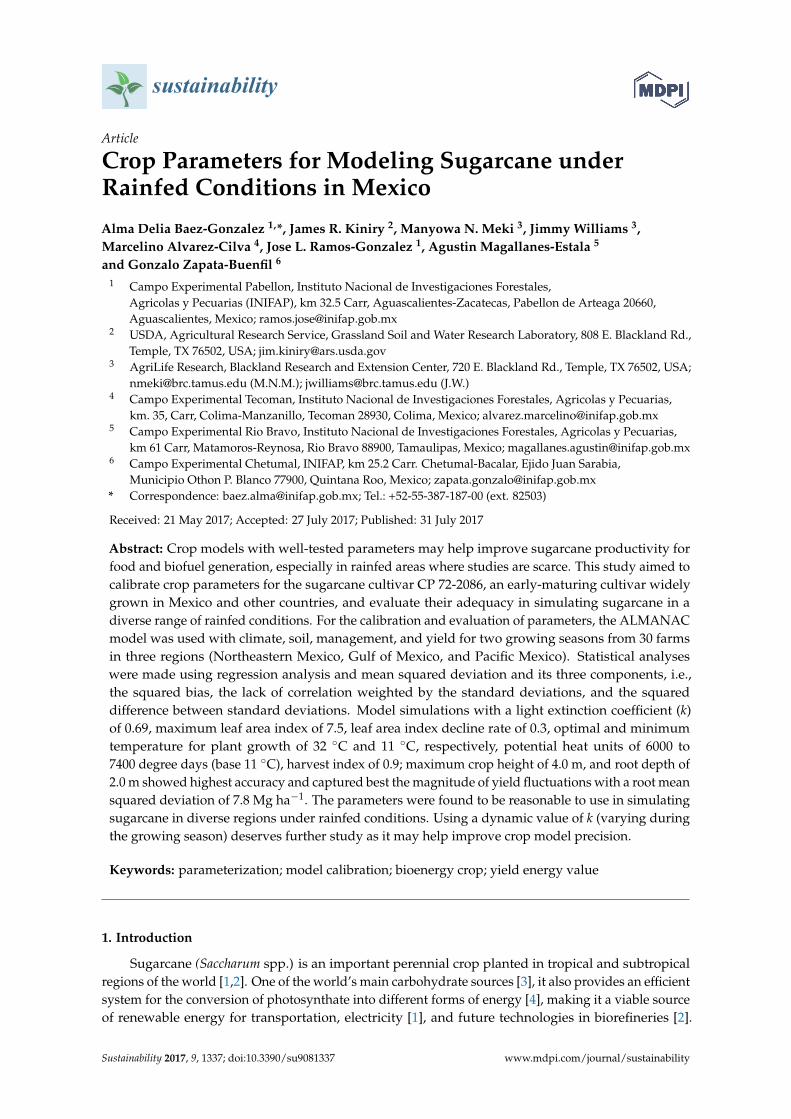
Abstract: Crop models with well-tested parameters may help improve sugarcane productivity forfood and biofuel generation, especially in rainfed areas where studies are scarce. This study aimed tocalibrate crop parameters for the sugarcane cultivar CP 72-2086, an early-maturing cultivar widelygrown in Mexico and other countries, and evaluate their adequacy in simulating sugarcane in adiverse range of rainfed conditions. For the calibration and evaluation of parameters, the ALMANACmodel was used with climate, soil, management, and yield for two growing seasons from 30 farmsin three regions (Northeastern Mexico, Gulf of Mexico, and Pacific Mexico). Statistical analyseswere made using regression analysis and mean squared deviation and its three components, i.e.,the squared bias, the lack of correlation weighted by the standard deviations, and the squareddifference between standard deviations. Model simulations with a light extinction coefficient (k)of 0.69, maximum leaf area index of 7.5, leaf area index decline rate of 0.3, optimal and minimumtemperature for plant growth of 32 ◦C and 11 ◦C, respectively, potential heat units of 6000 to7400 degree days (base 11 ◦C), harvest index of 0.9; maximum crop height of 4.0 m, and root depth of2.0 m showed highest accuracy and captured best the magnitude of yield fluctuations with a root meansquared deviation of 7.8 Mg ha−1. The parameters were found to be reasonable to use in simulatingsugarcane in diverse regions under rainfed conditions. Using a dynamic value of k (varying duringthe growing season) deserves further study as it may help improve crop model precision.

Keywords: parameterization; model calibration; bioenergy crop; yield energy value

1. Introduction

Sugarcane (Saccharum spp.) is an important perennial crop planted in tropical and subtropicalregions of the world [1,2]. One of the world’s main carbohydrate sources [3], it also provides an efficientsystem for the conversion of photosynthate into different forms of energy [4], making it a viable sourceof renewable energy for transportation, electricity [1], and future technologies in biorefineries [2].

Sustainability 2017, 9, 1337; doi:10.3390/su9081337 www.mdpi.com/journal/sustainability

Sustainability 2017, 9, 1337 2 of 19

Thus far, the sugarcane crop is considered to have the best potential for the production of ethanol toreplace fossil fuels as it shows the highest energy ratio (energy delivered per energy spent) amongthe biofuels [5]. Its use is expected to help mitigate the harmful effects of the petroleum-based energysystem [2]. The growing pressure to increase productivity of sugarcane [4] for food production [3] andbiofuel generation [1,6] has resulted in a worldwide increase in sugarcane area from 23.7 million ha in2010 to 27.1 million ha in 2014 [6,7] and a greater interest in researching sugarcane and its industrialexploitation [2]. This expansion of sugarcane cultivation, which, in some cases is on marginal landsand vulnerable to the potential impacts of climate change, presents farmers with multiple challenges,especially in countries like Mexico and Brazil, where the sugarcane industry has both social andeconomic impact, being the source of livelihood for many rural families [8,9].

Crop models are helpful tools in improving sugarcane productivity as they aid in the synthesis andapplication of knowledge and in yield forecasting [10]. Field-scale models, such as ALMANAC [11],EPIC [12], CANEGRO [3,13], and APSIM [3,14], as well as regional-scale ones, such as Agro-IBIS [15]and LPJmL [16], have been applied to energy crops under a wide range of environments. These modelsdiffer in the degree of parameterization needed and in their ability to simulate different cultivars anddifferent stress conditions [8,17]. These complexities can be a hindrance to the application of cropmodels for sugarcane, possibly because of the lack of understanding of their capabilities and limitationsand also because of the difficulties in using them. Another problem seems to be the general lack ofmodel credibility [8]. For crop simulations to be reliable, high-quality field data is required for modeldevelopment, and more effort is needed in the parameterization and validation of models [10,18].Some of the physiological development and growth parameters that appear in model functions varyamong sugarcane cultivars and therefore need to be estimated from data in order to predict growthand yield [8]. Region-specific calibrations of models are also essential [10].

Well-tested parameters are required for the development of robust crop models for reliable yieldpredictions [19]. Unfortunately, recent literature holds little information on parameter estimation forcrop models [20]. Hence, there continues to be uncertainty regarding the allocation of parametersto sugarcane species, ecotype, and cultivar categories [21]. Parameters related to photosynthesisare particularly important to sugarcane simulation as biomass production is dependent on theamount of photosynthetically active radiation (PAR) intercepted by the crop canopy [21–23]. The lightextinction coefficient (k), a key parameter in sugarcane yield simulation, describes the efficiency oflight interception for the canopy [4,24–26]. Studies have been done [24,27] to compare the relationshipof different k values and yield of sugarcane cultivars. However, there is insufficient information onthe cultivar chosen for this study, CP 72-2086, which is widely grown in Mexico and other countries.Modeling studies of sugarcane under rainfed conditions are particularly scarce. Hence, this studycalibrated crop parameters for the sugarcane cultivar CP 72-2086 under rainfed conditions using theALMANAC model and evaluated their adequacy in simulating sugarcane in a diverse range of rainfedconditions in Mexico.

2. Materials and Methods

2.1. The ALMANAC Model

This study used the ALMANAC (Agricultural Land Management Alternatives with NumericalAssessment Criteria) model, which has simulated the productivity of crops such as maize (Zea mays L.),sorghum (Sorghum bicolor L. Moench), dry bean (Phaseolus vulgaris L.) [19,28,29], rice (Oryza sativa L.),wheat (Triticum aestivum L.), and sunflower (Helianthus annuus L.) [11,30], as well as native grasses andimproved pastures [31]. The model has been successfully applied to biomass simulation of bioenergycrops such as switchgrass (Panicum virgatum L.) [32–35] and sugarcane [36]. It has also been used instudies for forecasting climatic change impact on native grasses [37].

The ALMANAC model was developed for use in field management; several individual fieldsmay be simulated to comprise a whole farm up to about 100 ha. Model input consists of weather

Sustainability 2017, 9, 1337 3 of 19

(daily maximum and minimum temperatures, rainfall, and solar radiation), soils and managementdata. In cases where weather data or portions of weather data are missing from available databases,realistic values can be generated within the model itself [38].

The model runs on a daily time step and contains the following detailed functions to simulategrowth: light interception, competition for water and nutrients among plants, biomass production,and biomass partitioning [39]. Light interception is simulated by Beer’s Law and considers total leafarea and height of the canopy [39]. The water and nutrient balance subroutines are from the ErosionProductivity Impact Calculator (EPIC) model [40]. Radiation interception and radiation use efficiency(RUE) are the drivers of plant growth or biomass accumulation, which are in turn a function of the LAIand k for FIPAR, as described by Monsi and Saeki’s (1953) Beer’s Law. RUE is a function of the vaporpressure deficit and atmospheric CO2 [41,42], while LAI evolution is simulated with a daily heat unitsystem that correlates plant growth with temperature. Detailed information on the main processessimulated by ALMANAC, including the equations and requisite input parameters, is provided byKiniry [38].

The ALMANAC model can be used to compare management systems and their effects on yields,nitrogen, phosphorus, carbon, pesticides, and sediment. Among the management components thatcan be changed are irrigation scheduling, crop rotations, and tillage operations.

2.2. Study Area

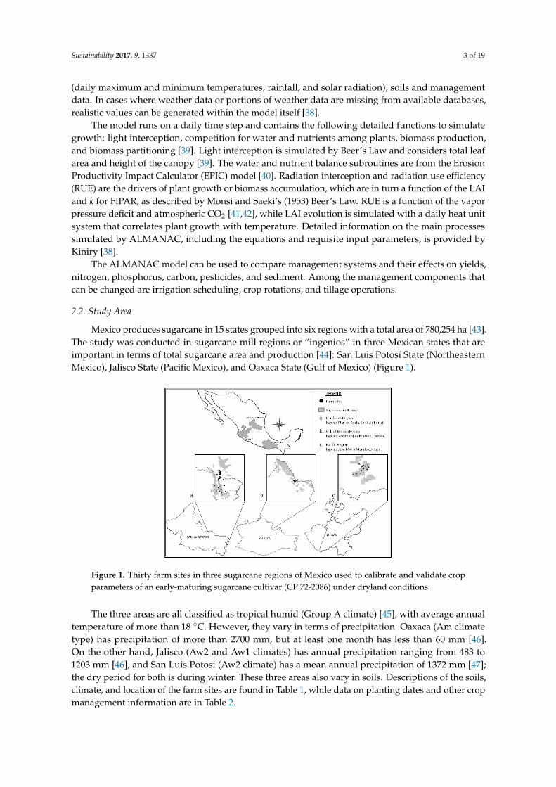
Mexico produces sugarcane in 15 states grouped into six regions with a total area of 780,254 ha [43].The study was conducted in sugarcane mill regions or “ingenios” in three Mexican states that areimportant in terms of total sugarcane area and production [44]: San Luis Potosí State (NortheasternMexico), Jalisco State (Pacific Mexico), and Oaxaca State (Gulf of Mexico) (Figure 1).

Sustainability 2017, 9, 1337 3 of 19

(daily maximum and minimum temperatures, rainfall, and solar radiation), soils and management data. In cases where weather data or portions of weather data are missing from available databases, realistic values can be generated within the model itself [38].

The model runs on a daily time step and contains the following detailed functions to simulate growth: light interception, competition for water and nutrients among plants, biomass production, and biomass partitioning [39]. Light interception is simulated by Beer’s Law and considers total leaf area and height of the canopy [39]. The water and nutrient balance subroutines are from the Erosion Productivity Impact Calculator (EPIC) model [40]. Radiation interception and radiation use efficiency (RUE) are the drivers of plant growth or biomass accumulation, which are in turn a function of the LAI and k for FIPAR, as described by Monsi and Saeki’s (1953) Beer’s Law. RUE is a function of the vapor pressure deficit and atmospheric CO2 [41,42], while LAI evolution is simulated with a daily heat unit system that correlates plant growth with temperature. Detailed information on the main processes simulated by ALMANAC, including the equations and requisite input parameters, is provided by Kiniry [38].

The ALMANAC model can be used to compare management systems and their effects on yields, nitrogen, phosphorus, carbon, pesticides, and sediment. Among the management components that can be changed are irrigation scheduling, crop rotations, and tillage operations.

2.2. Study Area

Mexico produces sugarcane in 15 states grouped into six regions with a total area of 780,254 ha [43]. The study was conducted in sugarcane mill regions or “ingenios” in three Mexican states that are important in terms of total sugarcane area and production [44]: San Luis Potosí State (Northeastern Mexico), Jalisco State (Pacific Mexico), and Oaxaca State (Gulf of Mexico) (Figure 1).

Figure 1. Thirty farm sites in three sugarcane regions of Mexico used to calibrate and validate crop parameters of an early-maturing sugarcane cultivar (CP 72-2086) under dryland conditions.

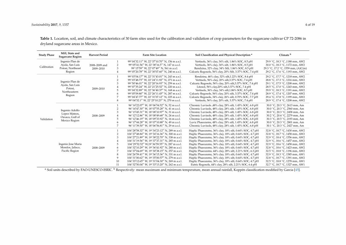
The three areas are all classified as tropical humid (Group A climate) [45], with average annual temperature of more than 18 °C. However, they vary in terms of precipitation. Oaxaca (Am climate type) has precipitation of more than 2700 mm, but at least one month has less than 60 mm [46]. On the other hand, Jalisco (Aw2 and Aw1 climates) has annual precipitation ranging from 483 to 1203 mm [46], and San Luis Potosi (Aw2 climate) has a mean annual precipitation of 1372 mm [47]; the dry period for both is during winter. These three areas also vary in soils. Descriptions of the soils, climate, and location of the farm sites are found in Table 1, while data on planting dates and other crop management information are in Table 2.

Figure 1. Thirty farm sites in three sugarcane regions of Mexico used to calibrate and validate cropparameters of an early-maturing sugarcane cultivar (CP 72-2086) under dryland conditions.

The three areas are all classified as tropical humid (Group A climate) [45], with average annualtemperature of more than 18 ◦C. However, they vary in terms of precipitation. Oaxaca (Am climatetype) has precipitation of more than 2700 mm, but at least one month has less than 60 mm [46].On the other hand, Jalisco (Aw2 and Aw1 climates) has annual precipitation ranging from 483 to1203 mm [46], and San Luis Potosi (Aw2 climate) has a mean annual precipitation of 1372 mm [47];the dry period for both is during winter. These three areas also vary in soils. Descriptions of the soils,climate, and location of the farm sites are found in Table 1, while data on planting dates and other cropmanagement information are in Table 2.

Sustainability 2017, 9, 1337 4 of 19

Table 1. Location, soil, and climate characteristics of 30 farm sites used for the calibration and validation of crop parameters for the sugarcane cultivar CP 72-2086 indryland sugarcane areas in Mexico.

Study Phase Mill, State andSugarcane Region Harvest Period Farm Site Location Soil Classification and Physical Description a Climate b

Calibration

Ingenio Plan deAyala, San Luis

Potosi, NortheastRegion

2008–2009 and2009–2010

1 99◦04′32.11′ ′ W, 22◦37′10.70′ ′ N, 156 m a.s.l. Vertisols, 36% clay, 34% silt, 1.86% SOC, 8.5 pH 29.9 ◦C, 18.3 ◦C ,1188 mm, AW22 99◦05′41.56′ ′ W, 22◦38′16.5′ ′ N, 147 m a.s.l. Vertisols, 36% clay, 34% silt, 1.86% SOC, 8.5 pH 30.0 ◦C, 18.3 ◦C, 1172 mm, AW23 99◦15′59′ ′ W, 22◦07′49′ ′ N, 561 m a.s.l. Rendzina, 32% clay, 34% Silt, 1.86% SOC, 8.5 pH 29.3 ◦C, 17.2 ◦C, 1559 mm, (A)C(m)4 99◦05′20.78′ ′ W, 22◦30′07.60′ ′ N, 240 m a.s.l. Calcaric Regosols, 56% clay, 20% Silt, 3.37% SOC, 7.4 pH 29.2 ◦C, 17.6 ◦C, 1193 mm, AW2

Validation

Ingenio Plan deAyala, San Luis

Potosi,Northeastern

Region

2009–2010

1 99◦03′04.17′ ′ W, 22◦31′43.01′ ′ N, 243 m a.s.l. Rendzina, 46% clay, 32% silt,1.22% SOC, 8.4 pH 29.2 ◦C, 17.7 ◦C, 1218 mm, AW22 99◦03′48.73′ ′ W, 22◦24′11.92′ ′ N, 271 m a.s.l. Vertisols, 56% clay, 20% silt,3.37% SOC, 7.4 pH 28.8 ◦C, 17.3 ◦C, 1216 mm, AW23 99◦50′46.01′ ′ W, 22◦20′16.93′ ′ N, 259 m a.s.l. Calcaric Regosols, 56% clay, 20% silt,3.37% SOC, 7.4 pH 29.1 ◦C, 17.5 ◦C, 1208 mm, AW24 99◦07′35.24′ ′ W, 22◦21′25.52′ ′ N, 220 m a.s.l. Litosol, 56% clay,20% silt,3.37% SOC, 7.4 pH 28.5 ◦C, 17.0 ◦C, 1243 mm, AW25 99◦04′32.89′ ′ W, 22◦36′40.37′ ′ N, 168 m a.s.l. Vertisols, 36% clay, 34% silt,1.86% SOC, 8.5 pH 29.9 ◦C, 18.3 ◦C, 1191 mm, AW26 99◦05′09.80′ ′ W, 22◦26′11.45′ ′ N, 287 m a.s.l. Calcaric Regosols, 56% clay, 20% silt, 3.37% SOC, 7.4 pH 28.9 ◦C, 17.4 ◦C, 1207 mm, AW27 99◦04′47.77′ ′ W, 22◦31′07.12′ ′ N, 225 m a.s.l. Calcaric Regosols, 34% clay, 26% silt, 0.70% SOC, 7.7 pH 29.4 ◦C, 17.8 ◦C, 1199 mm, AW28 99◦04′32.1′ ′ W, 22◦25′10.23′ ′ N, 270 m a.s.l. Vertisols, 56% clay, 20% silt, 3.37% SOC, 7.4 pH 28.9 ◦C, 17.4 ◦C, 1208 mm, AW2

Ingenio AdolfoLopez Mateos,

Oaxaca, Gulf ofMexico Region

2008–2009

1 96◦14′22.07′ ′ W, 18◦06′54.52′ ′ N, 52 m a.s.l. Chromic Luvisols ,48% clay, 28% silt, 1.45% SOC, 6.8 pH 30.0 ◦C, 20.3 ◦C, 2613 mm, Am2 96◦14′47.30′ ′ W, 18◦07′55.28′ ′ N, 41 m a.s.l. Chromic Luvisols, 48% clay, 28% silt, 1.45% SOC, 6.8 pH 30.0 ◦C, 20.3 ◦C, 2560 mm, Am3 96◦13′45.31′ ′ W, 18◦08′10.97′ ′ N, 31 m a.s.l. Chromic Luvisols, 48% clay, 28% silt, 1.45% SOC, 6.8 pH 30.0 ◦C, 20.3 ◦C, 2458 mm, Am4 96◦12′12.86′ ′ W, 18◦08′49.68′ ′ N, 24 m a.s.l. Chromic Luvisols, 48% clay, 28% silt, 1.45% SOC, 6.8 pH 30.2 ◦C, 20.4 ◦C, 2279 mm, Am5 96◦12′46.19′ ′ W, 18◦09′33.92′ ′ N, 16 m a.s.l. Chromic Luvisols, 48% clay, 28% silt, 1.45% SOC, 6.8 pH 30.3 ◦C, 20.5 ◦C, 2193 mm, Am6 96◦17′44.28′ ′ W, 18◦07′10.88′ ′ N, 49 m a.s.l. Luvic Phaeozems, 48% clay, 28% silt, 1.45% SOC, 6.8 pH 30.0 ◦C, 20.3 ◦C, 2801 mm, Am7 96◦11′39.50′ ′ W, 18◦06′56.81′ ′ N, 29 m a.s.l. Chromic Luvisols, 48% clay, 28% silt, 1.45% SOC, 6.8 pH 30.1 ◦C, 20.3 ◦C, 2427 mm, Am

Ingenio Jose MariaMorelos, Jalisco,Pacific Region

2008–2009

1 104◦28′58.32′ ′ W, 19◦34′23.12′ ′ N, 289 m a.s.l. Haplic Phaeozems, 36% clay, 18% silt, 0.64% SOC, 4.7 pH 32.8 ◦C, 18.7 ◦C, 1430 mm, AW22 104◦27′48.84′ ′ W, 19◦34′16.36′ ′ N, 300 m a.s.l. Haplic Phaeozems, 36% clay, 18% silt, 0.64% SOC, 4.7 pH 32.8 ◦C, 18.7 ◦C, 1458 mm, AW23 104◦27′21.89′ ′ W, 19◦38′22.70′ ′ N, 338 m a.s.l. Haplic Phaeozems, 36% clay, 18% silt, 0.64% SOC, 4.7 pH 32.9 ◦C, 18.4 ◦C, 1556 mm, AW24 104◦31′19.56′ ′ W, 19◦37′37.31′ ′ N, 285 m a.s.l. Haplic Phaeozems, 36% clay, 18% silt, 0.64% SOC, 4.7 pH 32.9 ◦C, 18.6 ◦C, 1457 mm, AW25 104◦29′52.52′ ′ W,19◦36′59.55′ ′ N, 287 m a.s.l. Haplic Phaeozems, 36% clay, 18% silt, 0.64% SOC, 4.7 pH 32.9 ◦C, 18.6 ◦C, 1458 mm, AW26 104◦32′10.29′ ′ W, 19◦36′41.92′ ′ N, 280 m a.s.l. Haplic Phaeozems, 36% clay, 18% silt, 0.64% SOC, 4.7 pH 32.8 ◦C, 18.6 ◦C, 1423 mm, AW27 104◦37′04.69′ ′ W, 19◦30′38.15′ ′ N, 257 m a.s.l. Haplic Phaeozems, 44% clay, 28% silt, 2.21% SOC, 6.3 pH 32.5 ◦C, 18.8 ◦C, 1196 mm, AW28 104◦26′59.41′ ′ W, 19◦36′15.36′ ′ N, 331 m a.s.l. Haplic Phaeozems, 36% clay, 18% silt, 0.64% SOC, 4.7 pH 32.9 ◦C, 18.3 ◦C, 1585 mm, AW19 104◦31′00.62′ ′ W, 19◦35′00.57′ ′ N, 279 m a.s.l. Haplic Phaeozems, 36% clay, 18% silt, 0.64% SOC, 4.7 pH 32.8 ◦C, 18.7 ◦C, 1391 mm, AW2

10 104◦33′12.65′ ′ W, 19◦31′04.30′ ′ N, 269 m a.s.l. Haplic Phaeozems, 36% clay, 18% silt, 0.64% SOC, 4.7 pH 32.5 ◦C, 18.8 ◦C, 1278 mm, AW111 104◦32′50.04′ ′ W, 19◦33′13.20′ ′ N, 262 m a.s.l. Eutric Regosols, 44% clay, 28% silt, 2.21% SOC, 6.4 pH 32.7 ◦C, 18.7 ◦C, 1327 mm, AW1

a Soil units described by FAO-UNESCO-ISRIC. b Respectively: mean maximum and minimum temperature, mean annual rainfall, Koppën classification modified by Garcia [45].

Sustainability 2017, 9, 1337 5 of 19

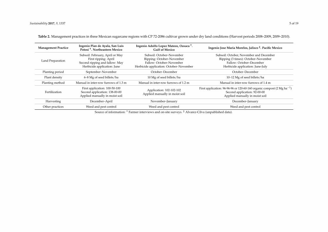
Table 2. Management practices in three Mexican sugarcane regions with CP 72-2086 cultivar grown under dry land conditions (Harvest periods 2008–2009, 2009–2010).

Management Practice Ingenio Plan de Ayala, San LuisPotosi †. Northeastern Mexico

Ingenio Adolfo Lopez Mateos, Oaxaca †.Gulf of Mexico Ingenio Jose Maria Morelos, Jalisco ‡. Pacific Mexico

Land Preparation

Subsoil: February, April or May Subsoil: October–November Subsoil: October, November and DecemberFirst ripping: April Ripping: October–November Ripping (3 times): October–November

Second ripping and fallow: May Fallow: October–November Fallow: October–DecemberHerbicide application: June Herbicide application: October–November Herbicide application: June-July

Planting period September–November October–December October–December

Plant density 6–8 Mg of seed billets/ha 10 Mg of seed billets/ha 10–12 Mg of seed billets/ha

Planting method Manual in inter-row furrows of 1.3 m Manual in inter-row furrows of 1.2 m Manual in inter-row furrows of 1.4 m

FertilizationFirst application: 100-50-100

Second application: 138-00-00Applied manually in moist soil

Application: 102-102-102Applied manually in moist soil

First application: 96-96-96 or 120-60-160 organic compost (2 Mg ha−1)Second application: 92-00-00

Applied manually in moist soil

Harvesting December–April November–January December–January

Other practices Weed and pest control Weed and pest control Weed and pest control

Source of information: † Farmer interviews and on-site surveys. ‡ Alvarez-Cilva (unpublished data).

Sustainability 2017, 9, 1337 6 of 19

The majority of producers in the studied areas are “ejidatarios” (shareholders in common lands).The rest are small farm owners and tenants [46]. Government loans and subsidies are made available tofarmers to enable them to adopt recommended management practices for the sugarcane mill regions.

2.3. Sugarcane Crop-Management Databases

The sugarcane crop-management information used in this study (Table 2) was derived from threedatabases. The San Luis Potosi and Oaxaca databases consist of crop information for two growingseasons (2008–2009 and 2009–2010) obtained through interviews of sugarcane growers in the millregions of Ingenio Plan de Ayala (San Luis Potosi State) and Ingenio Adolfo Lopez Mateos (OaxacaState). The crop-management information (Table 2) from planting to harvest for the two growingseasons include the following: land preparation, planting period, planting density (quantity of seedbillets; sections of stems that are planted), planting method, distance between furrows, sugarcanevariety, application of bud-sprouting promoters, fertilization (period, dosage, type of fertilizer),pest control (type of insecticide, dosage, number of applications, time of application), weed control(type of weed, control method, type of herbicide, dosage, period of application), disease control, date ofharvesting, and yield production (previous and current growing season).

The Jalisco database holds the following information obtained from sugarcane mill reports ofIngenio Jose Maria Morelos for the growing season 2008–2009: sugarcane variety, total harvested area,yield production, date of harvest, fertilization date, soil type, crop age, crop maturity, type of harvest(manual or machinery), irrigated or rainfed condition, farm site identification, type of land tenancy,sugarcane farmer organization, owners name and locality, and sugarcane inspector ID. The followingadditional field information was from Alvarez-Cilva (unpublished) of INIFAP (Instituto Nacional deInvestigaciones Forestales, Agricolas y Pecuarias): land preparation, planting period, planting density(quantity of seeds), planting method, distance between furrows, sugarcane variety, pest control (typeof insecticide and dosage), and weed control (type of weed, control method, type of herbicide, dosage).

Four farm sites from the San Luis Potosi database were used for calibration. Eight additionalsites from this database were used for validation, along with seven and 11 sites from the databases ofOaxaca and Jalisco, respectively.

2.4. Climate and Soil Databases

The climate information used in the study (Table 1) was obtained from a climate databasecontaining monthly “normal means” of the following parameters, derived from weather stations of theNational Meteorological Service of Mexico: monthly mean maximum and minimum air temperature(◦C), monthly mean standard deviation of daily maximum and minimum temperatures (◦C), monthlymean precipitation (mm), monthly standard deviation of daily precipitation (mm), monthly skewcoefficient for daily precipitation, monthly probability of wet day after dry day, monthly probability ofwet day after wet day, and average number days of rain per month (days).

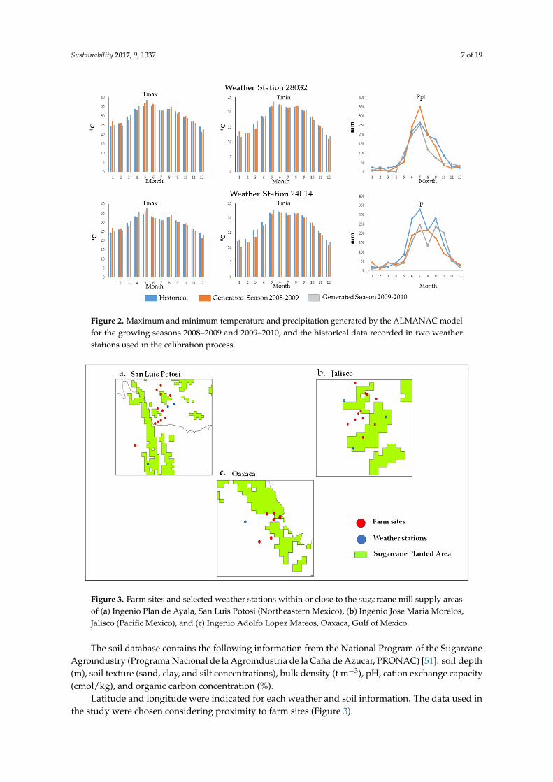
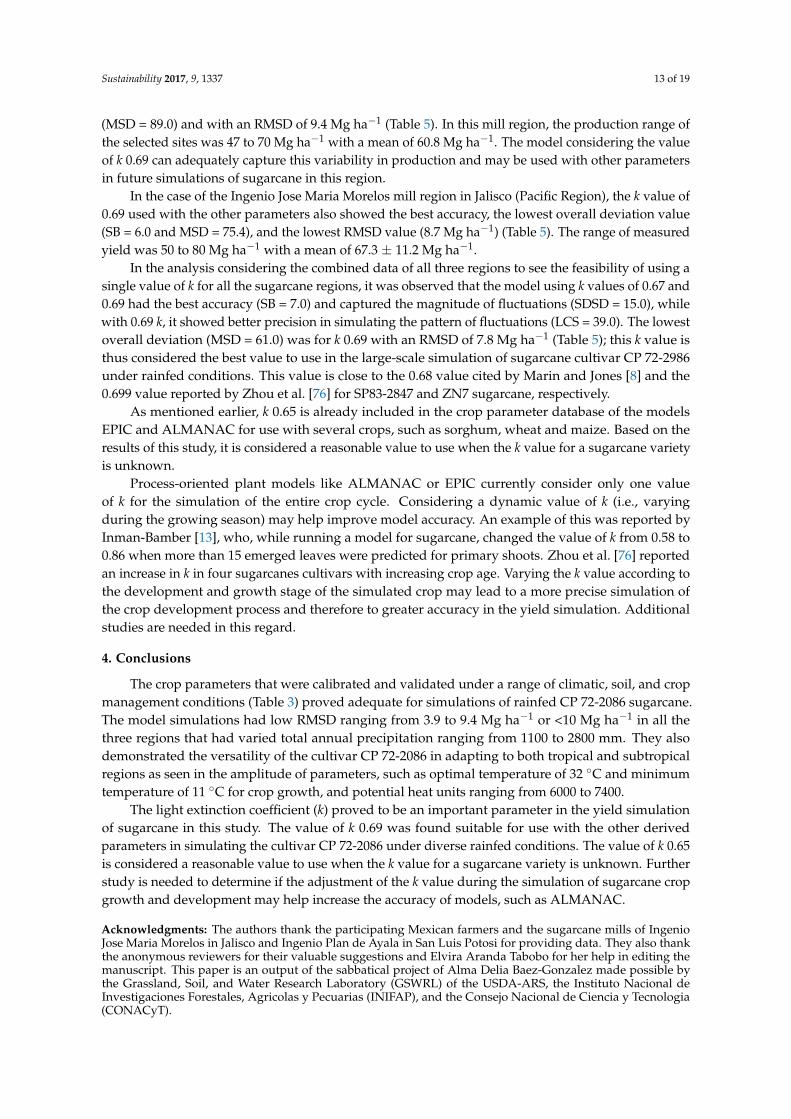
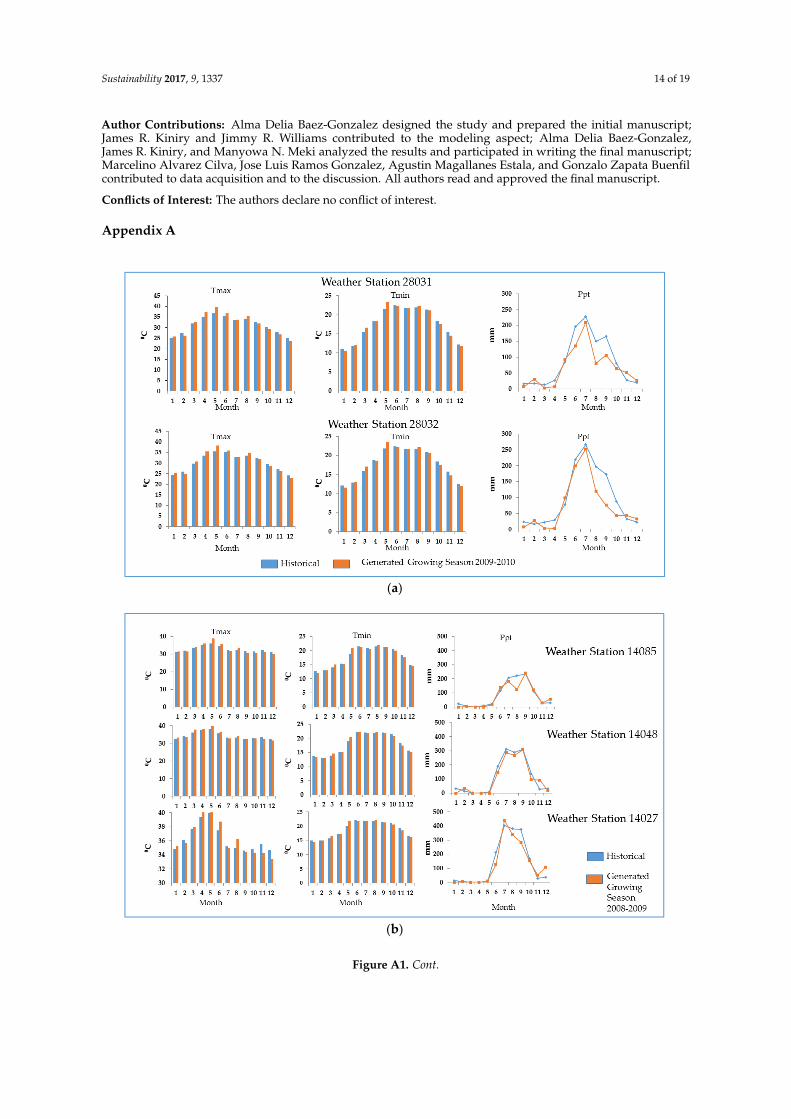
The weather generator in the ALMANAC model was used to create the daily weather dataneeded to run the model. This model component generates daily information on the occurrence andamount of precipitation, maximum and minimum temperatures, and total solar radiation by usingFourier coefficients and parameters that govern these weather variables [48]. It offers a convenientand adequate method of obtaining the numerous long sequences of weather data that are required formodels such as EPIC and ALMANAC [48,49]. A full description of the weather generator is given inSharpley and Williams [50]. Figure 2 shows the maximum temperature, minimum temperature andprecipitation generated by the model versus the historical data recorded at the two weather stationsused during the calibration process. The historical and generated data for each of the weather stationsused during the validation process of the model are shown in Appendix A. The weather stations werewithin or close to (average distance of 33 km for San Luis Potosi, 23 km for Jalisco and 50 km forOaxaca) the sugarcane mill supply areas under study (Figure 3).

Sustainability 2017, 9, 1337 7 of 19Sustainability 2017, 9, 1337 7 of 19

Figure 2. Maximum and minimum temperature and precipitation generated by the ALMANAC model for the growing seasons 2008–2009 and 2009–2010, and the historical data recorded in two weather stations used in the calibration process.

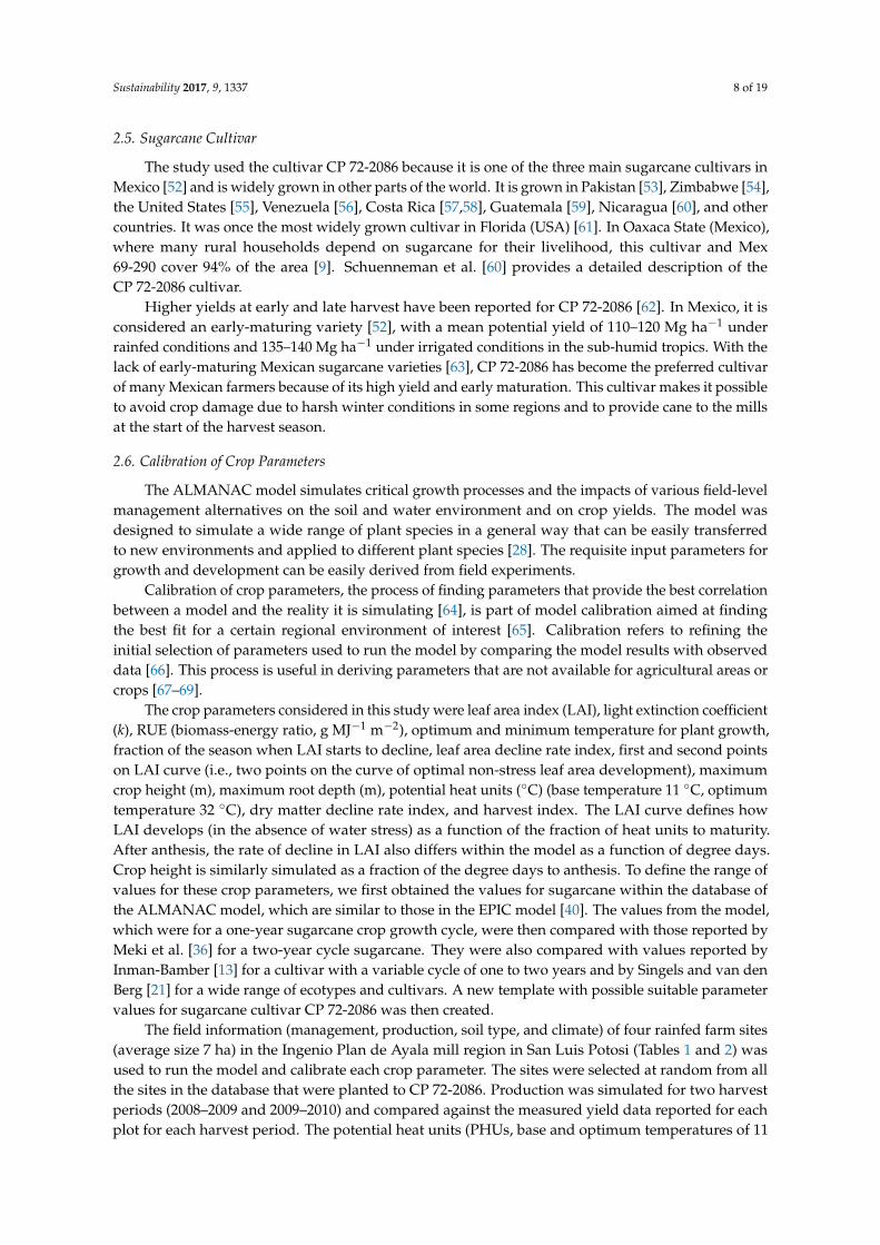
Figure 3. Farm sites and selected weather stations within or close to the sugarcane mill supply areas of (a) Ingenio Plan de Ayala, San Luis Potosi (Northeastern Mexico), (b) Ingenio Jose Maria Morelos, Jalisco (Pacific Mexico), and (c) Ingenio Adolfo Lopez Mateos, Oaxaca, Gulf of Mexico.

The soil database contains the following information from the National Program of the Sugarcane Agroindustry (Programa Nacional de la Agroindustria de la Caña de Azucar, PRONAC) [51]: soil depth (m), soil texture (sand, clay, and silt concentrations), bulk density (t m−3), pH, cation exchange capacity (cmol/kg), and organic carbon concentration (%).

Figure 2. Maximum and minimum temperature and precipitation generated by the ALMANAC modelfor the growing seasons 2008–2009 and 2009–2010, and the historical data recorded in two weatherstations used in the calibration process.

Sustainability 2017, 9, 1337 7 of 19

Figure 2. Maximum and minimum temperature and precipitation generated by the ALMANAC model for the growing seasons 2008–2009 and 2009–2010, and the historical data recorded in two weather stations used in the calibration process.

Figure 3. Farm sites and selected weather stations within or close to the sugarcane mill supply areas of (a) Ingenio Plan de Ayala, San Luis Potosi (Northeastern Mexico), (b) Ingenio Jose Maria Morelos, Jalisco (Pacific Mexico), and (c) Ingenio Adolfo Lopez Mateos, Oaxaca, Gulf of Mexico.

The soil database contains the following information from the National Program of the Sugarcane Agroindustry (Programa Nacional de la Agroindustria de la Caña de Azucar, PRONAC) [51]: soil depth (m), soil texture (sand, clay, and silt concentrations), bulk density (t m−3), pH, cation exchange capacity (cmol/kg), and organic carbon concentration (%).

Figure 3. Farm sites and selected weather stations within or close to the sugarcane mill supply areasof (a) Ingenio Plan de Ayala, San Luis Potosi (Northeastern Mexico), (b) Ingenio Jose Maria Morelos,Jalisco (Pacific Mexico), and (c) Ingenio Adolfo Lopez Mateos, Oaxaca, Gulf of Mexico.

The soil database contains the following information from the National Program of the SugarcaneAgroindustry (Programa Nacional de la Agroindustria de la Caña de Azucar, PRONAC) [51]: soil depth(m), soil texture (sand, clay, and silt concentrations), bulk density (t m−3), pH, cation exchange capacity(cmol/kg), and organic carbon concentration (%).

Latitude and longitude were indicated for each weather and soil information. The data used inthe study were chosen considering proximity to farm sites (Figure 3).

Sustainability 2017, 9, 1337 8 of 19

2.5. Sugarcane Cultivar

The study used the cultivar CP 72-2086 because it is one of the three main sugarcane cultivars inMexico [52] and is widely grown in other parts of the world. It is grown in Pakistan [53], Zimbabwe [54],the United States [55], Venezuela [56], Costa Rica [57,58], Guatemala [59], Nicaragua [60], and othercountries. It was once the most widely grown cultivar in Florida (USA) [61]. In Oaxaca State (Mexico),where many rural households depend on sugarcane for their livelihood, this cultivar and Mex69-290 cover 94% of the area [9]. Schuenneman et al. [60] provides a detailed description of theCP 72-2086 cultivar.

Higher yields at early and late harvest have been reported for CP 72-2086 [62]. In Mexico, it isconsidered an early-maturing variety [52], with a mean potential yield of 110–120 Mg ha−1 underrainfed conditions and 135–140 Mg ha−1 under irrigated conditions in the sub-humid tropics. With thelack of early-maturing Mexican sugarcane varieties [63], CP 72-2086 has become the preferred cultivarof many Mexican farmers because of its high yield and early maturation. This cultivar makes it possibleto avoid crop damage due to harsh winter conditions in some regions and to provide cane to the millsat the start of the harvest season.

2.6. Calibration of Crop Parameters

The ALMANAC model simulates critical growth processes and the impacts of various field-levelmanagement alternatives on the soil and water environment and on crop yields. The model wasdesigned to simulate a wide range of plant species in a general way that can be easily transferredto new environments and applied to different plant species [28]. The requisite input parameters forgrowth and development can be easily derived from field experiments.

Calibration of crop parameters, the process of finding parameters that provide the best correlationbetween a model and the reality it is simulating [64], is part of model calibration aimed at findingthe best fit for a certain regional environment of interest [65]. Calibration refers to refining theinitial selection of parameters used to run the model by comparing the model results with observeddata [66]. This process is useful in deriving parameters that are not available for agricultural areas orcrops [67–69].

The crop parameters considered in this study were leaf area index (LAI), light extinction coefficient(k), RUE (biomass-energy ratio, g MJ−1 m−2), optimum and minimum temperature for plant growth,fraction of the season when LAI starts to decline, leaf area decline rate index, first and second pointson LAI curve (i.e., two points on the curve of optimal non-stress leaf area development), maximumcrop height (m), maximum root depth (m), potential heat units (◦C) (base temperature 11 ◦C, optimumtemperature 32 ◦C), dry matter decline rate index, and harvest index. The LAI curve defines howLAI develops (in the absence of water stress) as a function of the fraction of heat units to maturity.After anthesis, the rate of decline in LAI also differs within the model as a function of degree days.Crop height is similarly simulated as a fraction of the degree days to anthesis. To define the range ofvalues for these crop parameters, we first obtained the values for sugarcane within the database ofthe ALMANAC model, which are similar to those in the EPIC model [40]. The values from the model,which were for a one-year sugarcane crop growth cycle, were then compared with those reported byMeki et al. [36] for a two-year cycle sugarcane. They were also compared with values reported byInman-Bamber [13] for a cultivar with a variable cycle of one to two years and by Singels and van denBerg [21] for a wide range of ecotypes and cultivars. A new template with possible suitable parametervalues for sugarcane cultivar CP 72-2086 was then created.

The field information (management, production, soil type, and climate) of four rainfed farm sites(average size 7 ha) in the Ingenio Plan de Ayala mill region in San Luis Potosi (Tables 1 and 2) wasused to run the model and calibrate each crop parameter. The sites were selected at random from allthe sites in the database that were planted to CP 72-2086. Production was simulated for two harvestperiods (2008–2009 and 2009–2010) and compared against the measured yield data reported for eachplot for each harvest period. The potential heat units (PHUs, base and optimum temperatures of 11

Sustainability 2017, 9, 1337 9 of 19

and 32 ◦C) value was defined in the model according to the management schedule while consideringinformation from farmers. The crop parameters were adjusted iteratively, i.e., the model was runnumerous times, the simulated aboveground dry biomass yields were compared with actual data, andcrop parameter values were adjusted until there was a good match between predicted and measureddry matter yield values.

The modeling process provides a better understanding of the complex interaction betweenleaves and their environment [70]. In this study, the importance of light extinction coefficient (k) indetermining canopy photosynthesis [25] became evident during the initial parameterization phase,presenting a strong influence on the simulation of sugarcane. Hence, we also made a sensitivityanalysis of k. The model was run again 40 times (four farm sites × five k values × two growingseasons); in each run, the value of k was changed while the values of all other parameters were keptconstant. The k values that were used were 0.53, 0.56, 0.65, 0.67, and 0.69 because they had beenpreviously reported in other studies for sugarcane cultivars [8,13,21,36,40,71].

2.7. Validation of Crop Parameters in Three Regions

The validation of the performance of a model is usually done by running the model under thesame conditions used for its calibration, but with a different set of data. In this study, we used anotherset of farm sites from the database of San Luis Potosi (the region considered in the calibration) for thevalidation. In addition, we also evaluated model performance and the stability of the parameters inrainfed areas with diverse climate and soil conditions. For this, we used rainfed farm sites from SanLuis Potosi and also from sugarcane mill regions in Jalisco State (Pacific Mexico) and Oaxaca (Gulfof Mexico). A total of 26 randomly selected rainfed farms were used in the evaluation of the cropparameters to establish their usefulness in simulating CP 72-2086 sugarcane under rainfed conditions:eight farms (average size 7 ha) in San Luis Potosi (Northeastern Mexico), 11 farms (average size 5 ha)in Jalisco (Pacific Region), and seven farms (average size 8 ha) in Oaxaca (Gulf of Mexico Region)(Figure 1, Tables 1 and 2).

The model was run 104 times (26 farm sites × four k values) using the different k values thatperformed well during the sensitivity analysis and all the other crop parameters resulting from thecalibration process. In each run, only the k value was modified, and all other crop parameters werekept constant. All the previously selected k values were considered, except 0.56. The criterion for theselection of k values to be included in the validation process was that they present the lowest value inat least one of the three components of MSD. In the case of k 0.56, its values in all the MSD componentswere higher than those of the other four k values (0.53, 0.65, 0.67, and 0.69).

2.8. Statistical Analysis

A regression analysis was made to simulate sugarcane dry matter yield as a function of measureddry matter yield and to determine the significance of the regression model. However, combiningan R2 analysis with other statistical analyses—in this case, the three components of MSD—made itpossible to measure model efficiency from different angles. For further comparison of the modelperformance, the three components of mean squared deviation (MSD = RMSD2) were calculated, i.e.,the squared bias (SB), the squared difference between standard deviations (SDSD), and the lack ofcorrelation weighted by the standard deviations (LCS) [72]. SDSD and LCS were calculated using thefollowing equations:

SDSD = (SDs − SDm)2 (1)

LCS = 2SDsSDm (1 − r) (2)

where SDs and SDm are the standard deviation of the simulation and the measurement respectively;r is the correlation coefficient.

The SB represents the bias of the simulation from the measurement. The LCS shows the lack ofpositive correlation weighted by the standard deviations. The SDSD is the difference in the magnitude

Sustainability 2017, 9, 1337 10 of 19

of fluctuation between the simulation and measurement [72]. As mentioned by Kobayashi andSalam [72] and Bellocchi et al. [73], the MSD test is better suited to the x-y comparison and easier tointerpret than regression. The correlation-regression approach tends to focus on the contrast witha lower correlation and regression line far from the equality line, while the analysis of MSD clearlyidentifies the simulation vs. measurements contrast with larger deviation than others [72]. In thisstudy, we decided to use both approaches.

3. Results

3.1. Sugarcane Crop Parameters

Fourteen crop parameters based on the values for sugarcane contained in the ALMANAC databaseand those reported by Meki et al. [36], Inman-Bamber [13], and Singels and van den Berg [21] werecalibrated for the one-year cycle sugarcane cultivar CP 72-2086 under rainfed conditions. Table 3shows the parameter values that had the best fit with the cultivar under study. The model usingthe following crop parameters showed highest accuracy and captured best the magnitude of yieldfluctuations: maximum leaf area index of 7.5, leaf area index decline rate of 0.3, optimal and minimumtemperature for plant growth of 32 ◦C and 11 ◦C, respectively, potential heat units 6000 to 7400 degreedays base 11 ◦C, harvest index 0.9, maximum crop height of 4.0 m, root depth of 2.0 m, and a k of 0.69.Other parameters are in Table 3.

Table 3. Crop parameters calibrated for an early maturing, one-year growth cycle sugarcane cultivar(CP 72-2086) under dryland conditions in Mexico. The biomass-energy ratio is equivalent to radiationuse efficiency.

Parameter Name Units Value

Biomass-energy ratio g MJ−1 m−2 3.4Optimal temperature ◦C 32

Minimum temperature ◦C 11Maximum Leaf Area Index 7.5

Fraction of season when LAI starts to decline 0.9Leaf area decline rate index 0.3

Light extinction coefficient for Beer’s Law 0.69First point on optimal LAI curve 25; 25 *

Second point on optimal LAI curve 90; 95 *Potential heat units ◦C 6000–7400

Maximum crop height m 4Maximum root depth m 2

Dry matter decline rate index 0.1Harvest index 0.9

* Two points on optimal (nonstress) leaf area development curve. Numbers before semicolon are % of growingseason. Numbers after semicolon are fractions of maximum potential leaf area index (LAI).

The resulting values for maximum leaf area index (7.5), leaf area decline rate index (0.30),and maximum root depth (2.0) were similar to those of Meki et al. [36]. As for the biomass-energyratio, which represents the potential (unstressed) growth rate (including roots), the value of3.4 g MJ−1 m−2 [36] proved suitable for use with CP 72-2086. For the dry matter decline rate index,which indicates reduction in the efficiency of conversion of intercepted photosynthetically activeradiation to biomass due to production of high energy products like seeds and/or translocation of Nfrom leaves to seeds [40], the default value of 0.1 in the ALMANAC model proved to be adequate inthis study. The minimum temperature value of 11 ◦C is close to the 12 ◦C value reported by Marin andJones [8] for sugarcane in Brazil, while the value of 32 ◦C for optimal temperature is similar to thatreported by NeTafim [74] for sugarcane.

Sustainability 2017, 9, 1337 11 of 19

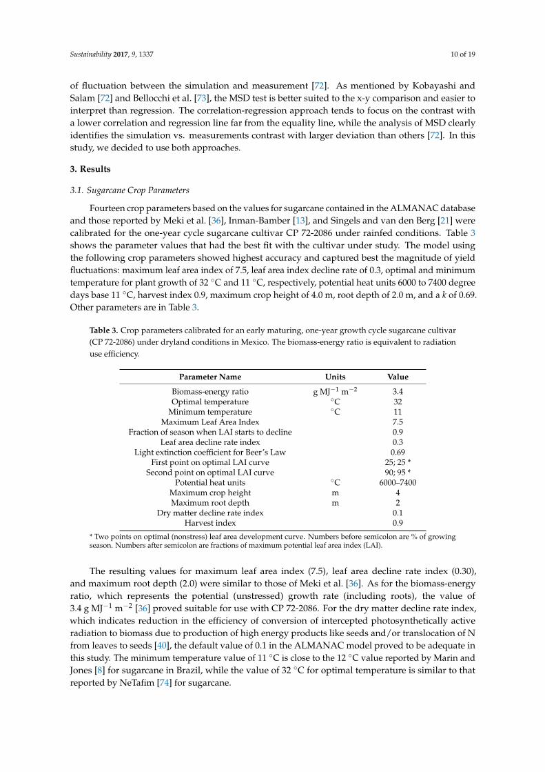
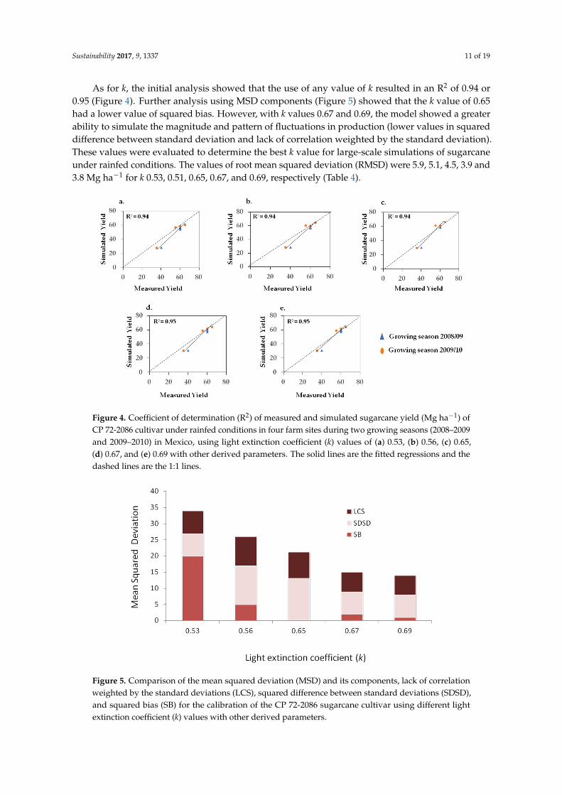
As for k, the initial analysis showed that the use of any value of k resulted in an R2 of 0.94 or0.95 (Figure 4). Further analysis using MSD components (Figure 5) showed that the k value of 0.65had a lower value of squared bias. However, with k values 0.67 and 0.69, the model showed a greaterability to simulate the magnitude and pattern of fluctuations in production (lower values in squareddifference between standard deviation and lack of correlation weighted by the standard deviation).These values were evaluated to determine the best k value for large-scale simulations of sugarcaneunder rainfed conditions. The values of root mean squared deviation (RMSD) were 5.9, 5.1, 4.5, 3.9 and3.8 Mg ha−1 for k 0.53, 0.51, 0.65, 0.67, and 0.69, respectively (Table 4).

Sustainability 2017, 9, 1337 11 of 19

As for k, the initial analysis showed that the use of any value of k resulted in an R2 of 0.94 or 0.95 (Figure 4). Further analysis using MSD components (Figure 5) showed that the k value of 0.65 had a lower value of squared bias. However, with k values 0.67 and 0.69, the model showed a greater ability to simulate the magnitude and pattern of fluctuations in production (lower values in squared difference between standard deviation and lack of correlation weighted by the standard deviation). These values were evaluated to determine the best k value for large-scale simulations of sugarcane under rainfed conditions. The values of root mean squared deviation (RMSD) were 5.9, 5.1, 4.5, 3.9 and 3.8 Mg ha−1 for k 0.53, 0.51, 0.65, 0.67, and 0.69, respectively (Table 4).

Figure 4. Coefficient of determination (R2) of measured and simulated sugarcane yield (Mg ha−1) of CP 72-2086 cultivar under rainfed conditions in four farm sites during two growing seasons (2008–2009 and 2009–2010) in Mexico, using light extinction coefficient (k) values of (a) 0.53, (b) 0.56, (c) 0.65, (d) 0.67, and (e) 0.69 with other derived parameters. The solid lines are the fitted regressions and the dashed lines are the 1:1 lines.

Figure 5. Comparison of the mean squared deviation (MSD) and its components, lack of correlation weighted by the standard deviations (LCS), squared difference between standard deviations (SDSD), and squared bias (SB) for the calibration of the CP 72-2086 sugarcane cultivar using different light extinction coefficient (k) values with other derived parameters.

Figure 4. Coefficient of determination (R2) of measured and simulated sugarcane yield (Mg ha−1) ofCP 72-2086 cultivar under rainfed conditions in four farm sites during two growing seasons (2008–2009and 2009–2010) in Mexico, using light extinction coefficient (k) values of (a) 0.53, (b) 0.56, (c) 0.65,(d) 0.67, and (e) 0.69 with other derived parameters. The solid lines are the fitted regressions and thedashed lines are the 1:1 lines.

Sustainability 2017, 9, 1337 11 of 19

As for k, the initial analysis showed that the use of any value of k resulted in an R2 of 0.94 or 0.95 (Figure 4). Further analysis using MSD components (Figure 5) showed that the k value of 0.65 had a lower value of squared bias. However, with k values 0.67 and 0.69, the model showed a greater ability to simulate the magnitude and pattern of fluctuations in production (lower values in squared difference between standard deviation and lack of correlation weighted by the standard deviation). These values were evaluated to determine the best k value for large-scale simulations of sugarcane under rainfed conditions. The values of root mean squared deviation (RMSD) were 5.9, 5.1, 4.5, 3.9 and 3.8 Mg ha−1 for k 0.53, 0.51, 0.65, 0.67, and 0.69, respectively (Table 4).

Figure 4. Coefficient of determination (R2) of measured and simulated sugarcane yield (Mg ha−1) of CP 72-2086 cultivar under rainfed conditions in four farm sites during two growing seasons (2008–2009 and 2009–2010) in Mexico, using light extinction coefficient (k) values of (a) 0.53, (b) 0.56, (c) 0.65, (d) 0.67, and (e) 0.69 with other derived parameters. The solid lines are the fitted regressions and the dashed lines are the 1:1 lines.

Figure 5. Comparison of the mean squared deviation (MSD) and its components, lack of correlation weighted by the standard deviations (LCS), squared difference between standard deviations (SDSD), and squared bias (SB) for the calibration of the CP 72-2086 sugarcane cultivar using different light extinction coefficient (k) values with other derived parameters.

Figure 5. Comparison of the mean squared deviation (MSD) and its components, lack of correlationweighted by the standard deviations (LCS), squared difference between standard deviations (SDSD),and squared bias (SB) for the calibration of the CP 72-2086 sugarcane cultivar using different lightextinction coefficient (k) values with other derived parameters.

Sustainability 2017, 9, 1337 12 of 19

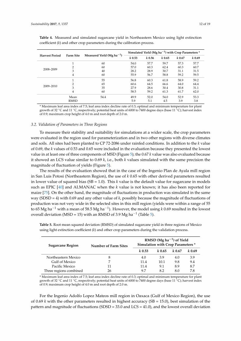
Table 4. Measured and simulated sugarcane yield in Northeastern Mexico using light extinctioncoefficient (k) and other crop parameters during the calibration process.

Harvest Period Farm Site Measured Yield (Mg ha−1)Simulated Yield (Mg ha−1) with Crop Parameters *

k 0.53 k 0.56 k 0.65 k 0.67 k 0.69

2008–2009

1 60 54.0 57.7 59.7 57.3 57.72 60 57.0 60.3 62.4 60.3 60.73 40 28.2 28.9 30.7 31.1 31.54 60 55.9 56.7 58.8 59.2 59.5

2009–2010

1 55 56.8 60.3 61.8 58.9 59.22 65 60.6 64.5 66.6 64.0 64.43 35 27.9 28.6 30.4 30.8 31.14 60 58.5 59.2 61.3 61.7 62.0

Mean 54.4 49.9 52.0 54.0 52.9 53.3RMSD 5.9 5.1 4.5 3.9 3.8

* Maximum leaf area index of 7.5; leaf area index decline rate of 0.3; optimal and minimum temperature for plantgrowth of 32 ◦C and 11 ◦C, respectively; potential heat units of 6000 to 7400 degree days (base 11 ◦C); harvest indexof 0.9; maximum crop height of 4.0 m and root depth of 2.0 m.

3.2. Validation of Parameters in Three Regions

To measure their stability and suitability for simulations at a wider scale, the crop parameterswere evaluated in the region used for parameterization and in two other regions with diverse climatesand soils. All sites had been planted to CP 72-2086 under rainfed conditions. In addition to the k valueof 0.69, the k values of 0.53 and 0.65 were included in the evaluation because they presented the lowestvalue in at least one of three components of MSD (Figure 5); the 0.67 k value was also evaluated becauseit showed an LCS value similar to 0.69 k, i.e., both k values simulated with the same precision themagnitude of fluctuation of yields (Figure 5).

The results of the evaluation showed that in the case of the Ingenio Plan de Ayala mill regionin San Luis Potosi (Northeastern Region), the use of k 0.65 with other derived parameters resultedin lower value of squared bias (SB = 1.0). This k value is the default value for sugarcane in modelssuch as EPIC [40] and ALMANAC when the k value is not known; it has also been reported formaize [75]. On the other hand, the magnitude of fluctuations in production was simulated in the sameway (SDSD = 4) with 0.69 and any other value of k, possibly because the magnitude of fluctuations ofproduction was not very wide in the selected sites in this mill region (yields were within a range of 55to 65 Mg ha−1 with a mean of 58.5 Mg ha−1). However, the model using k 0.69 resulted in the lowestoverall deviation (MSD = 15) with an RMSD of 3.9 Mg ha−1 (Table 5).

Table 5. Root mean squared deviation (RMSD) of simulated sugarcane yield in three regions of Mexicousing light extinction coefficient (k) and other crop parameters during the validation process.

Sugarcane Region Number of Farm Sites

RMSD (Mg ha−1) of YieldSimulation with Crop Parameters *

k 0.53 k 0.65 k 0.67 k 0.69

Northeastern Mexico 8 4.0 3.9 4.0 3.9Gulf of Mexico 7 11.4 10.1 9.8 9.4Pacific Mexico 11 11.4 9.1 8.9 8.7

Three regions combined 26 9.7 8.2 8.0 7.8

* Maximum leaf area index of 7.5; leaf area index decline rate of 0.3; optimal and minimum temperature for plantgrowth of 32 ◦C and 11 ◦C, respectively; potential heat units of 6000 to 7400 degree days (base 11 ◦C); harvest indexof 0.9; maximum crop height of 4.0 m and root depth of 2.0 m.

For the Ingenio Adolfo Lopez Mateos mill region in Oaxaca (Gulf of Mexico Region), the useof 0.69 k with the other parameters resulted in highest accuracy (SB = 15.0), best simulation of thepattern and magnitude of fluctuations (SDSD = 33.0 and LCS = 41.0), and the lowest overall deviation

Sustainability 2017, 9, 1337 13 of 19

(MSD = 89.0) and with an RMSD of 9.4 Mg ha−1 (Table 5). In this mill region, the production range ofthe selected sites was 47 to 70 Mg ha−1 with a mean of 60.8 Mg ha−1. The model considering the valueof k 0.69 can adequately capture this variability in production and may be used with other parametersin future simulations of sugarcane in this region.

In the case of the Ingenio Jose Maria Morelos mill region in Jalisco (Pacific Region), the k value of0.69 used with the other parameters also showed the best accuracy, the lowest overall deviation value(SB = 6.0 and MSD = 75.4), and the lowest RMSD value (8.7 Mg ha−1) (Table 5). The range of measuredyield was 50 to 80 Mg ha−1 with a mean of 67.3 ± 11.2 Mg ha−1.

In the analysis considering the combined data of all three regions to see the feasibility of using asingle value of k for all the sugarcane regions, it was observed that the model using k values of 0.67 and0.69 had the best accuracy (SB = 7.0) and captured the magnitude of fluctuations (SDSD = 15.0), whilewith 0.69 k, it showed better precision in simulating the pattern of fluctuations (LCS = 39.0). The lowestoverall deviation (MSD = 61.0) was for k 0.69 with an RMSD of 7.8 Mg ha−1 (Table 5); this k value isthus considered the best value to use in the large-scale simulation of sugarcane cultivar CP 72-2986under rainfed conditions. This value is close to the 0.68 value cited by Marin and Jones [8] and the0.699 value reported by Zhou et al. [76] for SP83-2847 and ZN7 sugarcane, respectively.

As mentioned earlier, k 0.65 is already included in the crop parameter database of the modelsEPIC and ALMANAC for use with several crops, such as sorghum, wheat and maize. Based on theresults of this study, it is considered a reasonable value to use when the k value for a sugarcane varietyis unknown.

Process-oriented plant models like ALMANAC or EPIC currently consider only one valueof k for the simulation of the entire crop cycle. Considering a dynamic value of k (i.e., varyingduring the growing season) may help improve model accuracy. An example of this was reported byInman-Bamber [13], who, while running a model for sugarcane, changed the value of k from 0.58 to0.86 when more than 15 emerged leaves were predicted for primary shoots. Zhou et al. [76] reportedan increase in k in four sugarcanes cultivars with increasing crop age. Varying the k value according tothe development and growth stage of the simulated crop may lead to a more precise simulation ofthe crop development process and therefore to greater accuracy in the yield simulation. Additionalstudies are needed in this regard.

4. Conclusions

The crop parameters that were calibrated and validated under a range of climatic, soil, and cropmanagement conditions (Table 3) proved adequate for simulations of rainfed CP 72-2086 sugarcane.The model simulations had low RMSD ranging from 3.9 to 9.4 Mg ha−1 or <10 Mg ha−1 in all thethree regions that had varied total annual precipitation ranging from 1100 to 2800 mm. They alsodemonstrated the versatility of the cultivar CP 72-2086 in adapting to both tropical and subtropicalregions as seen in the amplitude of parameters, such as optimal temperature of 32 ◦C and minimumtemperature of 11 ◦C for crop growth, and potential heat units ranging from 6000 to 7400.

The light extinction coefficient (k) proved to be an important parameter in the yield simulationof sugarcane in this study. The value of k 0.69 was found suitable for use with the other derivedparameters in simulating the cultivar CP 72-2086 under diverse rainfed conditions. The value of k 0.65is considered a reasonable value to use when the k value for a sugarcane variety is unknown. Furtherstudy is needed to determine if the adjustment of the k value during the simulation of sugarcane cropgrowth and development may help increase the accuracy of models, such as ALMANAC.

Acknowledgments: The authors thank the participating Mexican farmers and the sugarcane mills of IngenioJose Maria Morelos in Jalisco and Ingenio Plan de Ayala in San Luis Potosi for providing data. They also thankthe anonymous reviewers for their valuable suggestions and Elvira Aranda Tabobo for her help in editing themanuscript. This paper is an output of the sabbatical project of Alma Delia Baez-Gonzalez made possible bythe Grassland, Soil, and Water Research Laboratory (GSWRL) of the USDA-ARS, the Instituto Nacional deInvestigaciones Forestales, Agricolas y Pecuarias (INIFAP), and the Consejo Nacional de Ciencia y Tecnologia(CONACyT).

Sustainability 2017, 9, 1337 14 of 19

Author Contributions: Alma Delia Baez-Gonzalez designed the study and prepared the initial manuscript;James R. Kiniry and Jimmy R. Williams contributed to the modeling aspect; Alma Delia Baez-Gonzalez,James R. Kiniry, and Manyowa N. Meki analyzed the results and participated in writing the final manuscript;Marcelino Alvarez Cilva, Jose Luis Ramos Gonzalez, Agustin Magallanes Estala, and Gonzalo Zapata Buenfilcontributed to data acquisition and to the discussion. All authors read and approved the final manuscript.

Conflicts of Interest: The authors declare no conflict of interest.

Appendix A

Sustainability 2017, 9, 1337 14 of 19

Investigaciones Forestales, Agricolas y Pecuarias (INIFAP), and the Consejo Nacional de Ciencia y Tecnologia (CONACyT).

Author Contributions: Alma Delia Baez-Gonzalez designed the study and prepared the initial manuscript; James R. Kiniry and Jimmy R. Williams contributed to the modeling aspect; Alma Delia Baez-Gonzalez, James R. Kiniry, and Manyowa N. Meki analyzed the results and participated in writing the final manuscript; Marcelino Alvarez Cilva, Jose Luis Ramos Gonzalez, Agustin Magallanes Estala, and Gonzalo Zapata Buenfil contributed to data acquisition and to the discussion. All authors read and approved the final manuscript.

Conflicts of Interest: The authors declare no conflict of interest.

Appendix A

(a)

(b)

Figure A1. Cont.

Sustainability 2017, 9, 1337 15 of 19

Sustainability 2017, 9, 1337 15 of 19

(c)

Figure A1. Historical and ALMANAC-generated weather data used for validation of sugarcane parameters in (a) Ingenio Plan de Ayala, San Luis Potosi (Northeastern Mexico), (b) Ingenio Jose Maria Morelos, Jalisco (Pacific Mexico), and (c) Ingenio Adolfo Lopez Mateos, Oaxaca, Gulf of Mexico.

References

1. Lin, H.; Chen, J.; Pei, Z.; Zhang, S.; Hu, X. Monitoring sugarcane growth using ENVISAT ASAR data. Geoscience and Remote Sensing. IEEE Trans. 2009, 47, 2572–2580, doi:10.1109/TGRS.2009.2015769.

2. Matsuoka, S.; Stolf, R. Sugarcane tillering and ratooning: Key factors for a profitable cropping. In Sugarcane: Production, Cultivation and Uses; Goncalves, J., Correia, K., Eds.; Nova Science Publishers Inc.: Hauppauge, NY, USA, 2012; pp. 137–157.

3. Marin, F.R.; Thorburn, P.J.; Nassif, D.S.; Costa, L.G. Sugarcane model intercomparison: Structural differences and uncertainties under current and potential future climates. Environ. Model. Softw. 2015, 72, 372–386, doi:10.1016/j.ensoft.2015.02.019.

4. Ascencio, J.; Lazo, J.V. The Shade Avoidance Syndrome under the Sugarcane Crop; Intech Open Access Publisher: Rijeka, Croatia, 2012.

5. Valade, A.; Ciais, P.; Vuichard, N.; Viovy, N.; Caubel, A.; Huth, N.; Marin, F.; Martiné, J.-F. Modeling sugarcane yield with a process-based model from site to continental scale: Uncertainties arising from model structure and parameter values. Geosci. Model Dev. 2014, 7, 1225–1245, doi:10.519/gmd-7-1225-2014.

6. Valade, A.; Vuichard, N.; Ciais, P.; Ruget, F.; Viovy, N.; Gabrielle, B.; Huth, N.; Martiné, J.F. ORCHIDEE-STICS, a process-based model of sugarcane biomass production: Calibration of model parameters governing phenology. GCB Bioenergy 2014, 6, 606–620, doi:10.111/gcbb.12074.

7. Food and Agriculture Organization of the United Nations. FAO Statistics. Available online: http://www.fao.org/faostate (accessed on 12 July 2016).

8. Marin, F.R.; Jones, J.W. Process-based simple model for simulating sugarcane growth and production. Scientia Agricola 2014, 7, 11–16, doi:10.1590/SO103-90162014.

9. Bravo-Mosqueda, E.; Baez-Gonzalez, A.D.; Tinoco-Alfaro, C.A.; Mariles-Flores, V.; Osuna-Ceja, E. Yield-gap analysis of a homogenous area and zonification of a sugarcane mill region in Oaxaca, Mexico. J. Crop Improv. 2014, 28, 772–794, doi:10.1080/15427528.2014.942762.

10. Andrade, A.S.; Santos, P.M.; Pezzopane, J.R.M.; de Araujo, L.C.; Pedreira, B.C.; Pedreira, C.G.S.; Marin, F.R.; Lara, M.A.S. Simulating tropical forage growth and biomass accumulation: An overview of model development and application. Grass Forage Sci. 2015, 71, 54–65, doi:10.111/gfs.12177.

11. Kiniry, J.R.; Williams, J.R.; Gassman, P.W.; Debaeke, P. A General, Process-Oriented Model for Two Competing Plant Species. TASAE 1992, 3, 801–810.

Figure A1. Historical and ALMANAC-generated weather data used for validation of sugarcaneparameters in (a) Ingenio Plan de Ayala, San Luis Potosi (Northeastern Mexico), (b) Ingenio Jose MariaMorelos, Jalisco (Pacific Mexico), and (c) Ingenio Adolfo Lopez Mateos, Oaxaca, Gulf of Mexico.

References

1. Lin, H.; Chen, J.; Pei, Z.; Zhang, S.; Hu, X. Monitoring sugarcane growth using ENVISAT ASAR data.Geoscience and Remote Sensing. IEEE Trans. Geosci. Remote Sens. 2009, 47, 2572–2580. [CrossRef]

2. Matsuoka, S.; Stolf, R. Sugarcane tillering and ratooning: Key factors for a profitable cropping. In Sugarcane:Production, Cultivation and Uses; Goncalves, J., Correia, K., Eds.; Nova Science Publishers Inc.: Hauppauge,NY, USA, 2012; pp. 137–157.

3. Marin, F.R.; Thorburn, P.J.; Nassif, D.S.; Costa, L.G. Sugarcane model intercomparison: Structural differencesand uncertainties under current and potential future climates. Environ. Model. Softw. 2015, 72, 372–386.[CrossRef]

4. Ascencio, J.; Lazo, J.V. The Shade Avoidance Syndrome under the Sugarcane Crop; Intech Open Access Publisher:Rijeka, Croatia, 2012.

5. Valade, A.; Ciais, P.; Vuichard, N.; Viovy, N.; Caubel, A.; Huth, N.; Marin, F.; Martiné, J.-F. Modelingsugarcane yield with a process-based model from site to continental scale: Uncertainties arising from modelstructure and parameter values. Geosci. Model Dev. 2014, 7, 1225–1245. [CrossRef]

6. Valade, A.; Vuichard, N.; Ciais, P.; Ruget, F.; Viovy, N.; Gabrielle, B.; Huth, N.; Martiné, J.F. ORCHIDEE-STICS,a process-based model of sugarcane biomass production: Calibration of model parameters governingphenology. GCB Bioenergy 2014, 6, 606–620. [CrossRef]

7. Food and Agriculture Organization of the United Nations. FAO Statistics. Available online: http://www.fao.org/faostate (accessed on 12 July 2016).

8. Marin, F.R.; Jones, J.W. Process-based simple model for simulating sugarcane growth and production.Sci. Agric. 2014, 7, 11–16. [CrossRef]

9. Bravo-Mosqueda, E.; Baez-Gonzalez, A.D.; Tinoco-Alfaro, C.A.; Mariles-Flores, V.; Osuna-Ceja, E. Yield-gapanalysis of a homogenous area and zonification of a sugarcane mill region in Oaxaca, Mexico. J. Crop Improv.2014, 28, 772–794. [CrossRef]

10. Andrade, A.S.; Santos, P.M.; Pezzopane, J.R.M.; de Araujo, L.C.; Pedreira, B.C.; Pedreira, C.G.S.; Marin, F.R.;Lara, M.A.S. Simulating tropical forage growth and biomass accumulation: An overview of modeldevelopment and application. Grass Forage Sci. 2015, 71, 54–65. [CrossRef]

Sustainability 2017, 9, 1337 16 of 19

11. Kiniry, J.R.; Williams, J.R.; Gassman, P.W.; Debaeke, P. A General, Process-Oriented Model for Two CompetingPlant Species. Trans. ASAE 1992, 3, 801–810.

12. Williams, J.R.; Jones, C.A.; Dyke, P.T. The EPIC Model and Its Application. In Proceedings of the InternationalSymposium on Minimum Data Sets for Agrotechnology Transfer, Andhra Pradeshe, India, 21–26 March 1983.

13. Inman-Bamber, N. A growth model for sugar-cane based on a simple carbon balance and the CERES-Maizewater balance. S. Afr. J. Plant Soil 1991, 8, 93–99. [CrossRef]

14. Keating, B.A.; Robertson, M.J.; Muchow, R.C.; Huth, N.I. Modelling sugarcane production systems I.Development and performance of the sugarcane module. Field Crops Res. 1999, 61, 253–271. [CrossRef]

15. Kucharik, C.J. Evaluation of a process-based agro-ecosystem model (Agro-IBIS) across the US corn belt:Simulations of the interannual variability in maize yield. Earth Interact. 2003, 7, 1–33. [CrossRef]

16. Bondea, U.A.; Smith, P.C.; Zaehle, S.; Schaphof, S.; Lucht, W.; Cramer, W.; Gerten, D.; Lotze-Campen, H.;Muller, C.; Reichstein, M.; et al. Modelling the role of agriculture for the 20th century global terrestrialcarbon balance. Glob. Chang. Biol. 2007, 13, 679–706. [CrossRef]

17. O’Leary, G.J. A review of three sugarcane simulation models with respect to their prediction of sucrose yield.Field Crops Res. 2000, 68, 97–111. [CrossRef]

18. Surendran, N.S.; Kang, S.; Zhang, X.; Miguez, F.E.; Izaurralde, R.C.; Post, W.M.; Dietze, M.C.; Lynd, L.R.;Wullschleger, S.D. Bioenergy crop models: Descriptions, data requirements, and future challenges.GCB Bioenergy 2012, 4, 620–633. [CrossRef]

19. Baez-Gonzalez, A.D.; Kiniry, J.R.; Padilla, R.J.S.; Medina, G.G.; Ramos, G.J.L.; Osuna, C.E.S. Parametrizationof ALMANAC Crop Simulation Model for Non-Irrigated Dry Bean in Semi-Arid Temperate Areas in Mexico.Interciencia 2015, 40, 185–189.

20. Ahuja, L.R.; Ma, L. A synthesis of current parameterization approaches and needs for further improvements.In Methods of Introducing System Models into Agricultural Research; Ahuja, L.R., Ma, L., Eds.; American Societyof Agronomy Inc.: Madison, WI, USA; Crop Science Society of America Inc.: Madison, WI, USA; Soil ScienceSociety of America Inc.: Madison, WI, USA, 2011; pp. 427–440.

21. Singels, M.J.; van den Berg, M. DSSAT v4.5—Canegro Sugarcane Plan Module. Scientific Documentation.International Consortium for Sugarcane Modelling (ICSM). Available online: http://sasri.sasa.org.za/misc/icsm.html (accessed on 14 November 2015).

22. Ma, L.; Ahuja, L.R.; Saseendran, S.A.; Malone, R.W.; Green, T.R.; Nolan, B.T.; Bartling, P.N.S.;Flerchinger, G.N.; Boote, K.J.; Hoogenboom, G.A. Protocol for parameterization and calibration of RZWQM2in field research. In Methods of Introducing System Models into Agricultural Research; Ahuja, L.R., Ma, L., Eds.;American Society of Agronomy Inc.: Madison, WI, USA; Crop Science Society of America Inc.: Madison, WI,USA; Soil Science Society of America, Inc.: Madison, WI, USA, 2011; pp. 1–64.

23. Guo, L.P.; Kang, H.J.; Ouyang, Z.; Zhuang, W.; Yu, Q. Photosynthetic parameters estimations by consideringinteractive effects of light, temperature and CO2 concentration. Int. J. Plant Prod. 2015, 9, 321–345.

24. Shimabuku, M. Studies on the yield of sugarcane varieties with particular reference to the efficiency structureand light extinction coefficient of communities of some sugarcane varieties. Jpn. J. Trop. Agric 1976, 19,151–155.

25. Hikosaka, K.; Hirose, T. Leaf angle as a strategy for light competition: Optimal and evolutionarilystable-extinction coefficient within a leaf canopy. Ecoscience 1997, 4, 501–507. [CrossRef]

26. Singels, A.; Donaldson, R.A. A Simple Model of Unstressed Sugarcane Canopy Development. Proc. S. Afr.Sugar Technol. Assoc. 2000, 74, 151–154.

27. Shimabuku, M.; Higa, K. Studies on the yield of sugarcane varieties with particular reference to the efficiencyof the utilization on sunlight. Part 3. The effects of light extinction coefficient on some yield components insome sugarcane varieties. Congress of the International Society of Sugar Cane Technologists. Plant Breed.1977, 16, 177–185.

28. Xie, Y.; Kiniry, J.R.; Nedbalek, V.; Rosenthal, W.D. Maize and sorghum simulation with CEREs-Maize,SORKAM, and ALMANAC under water-limiting conditions. Agron. J. 2001, 93, 1148–1155. [CrossRef]

29. Meki, M.N.; Snider, L.J.; Kiniry, J.R.; Raper, L.R.; Rocateli, C.A. Energy sorghum biomass harvest thresholdsand tillage effects on soil organic carbon and bulk density. Ind. Crops Prod. 2013, 43, 172–182. [CrossRef]

30. Kiniry, J.R.; Jones, C.A.; O’toole, J.C.; Blanchet, R.; Cabelguenne, M.; Spanel, D.A. Radiation-use efficiencyin biomass accumulation prior to grain-filling for five grain-crops species. Field Crops Res. 1989, 20, 51–64.[CrossRef]

Sustainability 2017, 9, 1337 17 of 19

31. Kiniry, J.R.; Burson, B.L.; Evers, G.W.; Williams, L.R.; Sanchez, H.; Wade, C.; Featherson, J.W.; Greenwade, J.Coastal bermudagrass, bahiagrass, and native range simulation at diverse sites in Texas. Agron. J. 2007, 99,450–461. [CrossRef]

32. Kiniry, J.R.; Lynd, L.; Greene, N.; Johnson, M.V.; Casler, M.; Laster, M.S. Biofuels and water use: Comparisonof maize and switchgrass and general perspectives. In New Research on Biofuels; Wright, J.H., Evans, D.A.,Eds.; Nova Science Publishers Inc.: Hauppauge, NY, USA, 2008; pp. 1–14.

33. Kiniry, J.R.; Schmer, M.R.; Vogel, K.P.; Mitchell, R.B. Switchgrass biomass simulation at diverse sites in theNorthern Great Plains of the U.S. Bioenergy Res. 2008, 1, 259–264. [CrossRef]

34. Mclaughlin, B.S.; Kiniry, J.R.; Taliaferro, C.M.; De La Torre, U.D. Projecting yield and utilization potential ofswitch grass as an energy crop. Adv. Agron. 2006, 90, 267–297. [CrossRef]

35. Woli, P.; Paz, J.O.; Lang, D.J.; Baldwin, B.S.; Kiniry, J.R. Soil and variety effects on the energy and carbonbalances of switchgrass-derived ethanol. J. Sustain. Bionergy Syst. 2012, 2, 65–74. [CrossRef]

36. Meki, M.N.; Kiniry, J.R.; Youkkhana, A.H.; Crow, S.E.; Ogashi, R.M.; Nakahata, M.H.; Tirado-Corba, L.R.;Anderson, R.G.; Osorio, J.; Jeong, J. Two-year growth cycle sugarcane crop parameters attributes and theirapplication in modelling. Agron. J. 2015, 107, 1310–1320. [CrossRef]

37. Behrman, D.K.; Kiniry, J.R.; Winchell, M.; Juenger, T.E.; Keitt, T.H. Spatial forecasting of switchgrassproductivity under current and future climate change scenarios. Ecol. Appl. 2013, 23, 73–83. [CrossRef][PubMed]

38. Kiniry, J.R. A general crop model. In Modeling and Remote Sensing Applied to Agriculture (U.S. and Mexico);Richardson, W.C., Baez-Gonzalez, A.D., Tiscareno-Lopez, M., Eds.; USDA-ARS: Washington, DC, USA;INIFAP Ciudad de Mexico, Mexico, 2006; pp. 1–12.

39. Kiniry, J.R.; Blanchet, R.; Williams, J.R.; Texier, V.; Jones, C.A.; Cabelguenne, M. Simulating sunflower withthe EPIC and ALMANAC models. Field Crops Res. 1992, 30, 403–423. [CrossRef]

40. Williams, J.R.; Jones, C.A.; Kiniry, J.R.; Spanel, D.A. The EPIC crop growth model. Trans. ASAE 1989, 32,497–511. [CrossRef]

41. Kemanian, A.R.; Stockle, C.O.; Huggins, D.R. Variability of barley radiation-use efficiency. Crop Sci. 2004, 44,1662–1672. [CrossRef]

42. Stockle, C.A.; Kiniry, J.R. Variability in crop radiation use efficiency associated with vapor pressure deficit.Field Crops Res. 1990, 21, 171–181. [CrossRef]

43. Official Journal of The Federation (Diario Oficial de la Federacion). Programa Nacional de la Agroindustria de laCaña de Azucar 2014–2018; Edicion Vespertina Mexico: Mexico City, Mexico, 2014. (In Spanish)

44. SIAP (Servicio De Información Agroailmentaria Y Pesquera) Cierre de la Producción Agrícola Por Cultivo2012. Available online: http://www.siap.gob.mx/index.php?option=com_wrapper&view=wrapper&Itemid=350 (accessed 21 November 2015). (In Spanish)

45. Garcia, E. Modificaciones al Sistema de Clasificación Climática de Köppen, 2nd ed.; Instituto de Geografía, UNAM:Ciudad de Mexico, Mexico, 1973; p. 246.

46. Mexican Sugarcane Manual (Manual Azucarero Mexicano). Cuadragésima Séptima Edición, 47th ed.; CompañíaEditora del Manual Azucarero, S.A. de C.V.: Ciudad de Mexico, Mexico, 2004. (In Spanish)

47. Magallanes, E.A.; Lopez, L.A.; Ramirez, G.R.A. Caracterizacion del Ingenio Plan de Ayala, San Luis Potosi.In Caracteristicas Climaticas y Edaficas de las Zonas de Abastecimiento de Ingenios Cañeros en Mexico. Climaticand Soil Characteristics of the Sugarcane Mill Supply Zones in Mexico; Baez-Gonzalez, A.D., Medina-Garcia, G.,Ruiz-Corral, J.A., Ramos-Gonzalez, J.L., Eds.; Libro Tecnico No. 13; INIFAP-SAGARPA: Ciudad de Mexico,Mexico, 2012; pp. 269–302. (In Spanish)

48. Richardson, C.W.; Nicks, A.D. Weather generator description. In EPIC—Erosion/Productivity Impact Calculator.1. Model Documentation; Sharpley, A.N., Williams, J.R., Eds.; Technical Bulletin No. 1768; U.S. Department ofAgriculture: Washington, DC, USA, 1990; pp. 93–103.

49. Nicks, A.D.; Richardson, C.W.; Williams, J.R. Evaluation of the EPIC model generator. InEPIC—Erosion/Productivity Impact Calculator. 1. Model Documentation; Sharpley, A.N., Williams, J.R., Eds.;Technical Bulletin No. 1768; U.S. Department of Agriculture: Washington, DC, USA, 1990; pp. 105–124.

50. Sharpley, A.N.; Williams, J.R. EPIC—Erosion/Productivity Impact Calculator. 1. Model Documentation; TechnicalBulletin No. 1768; U.S. Department of Agriculture: Washington, DC, USA, 1990; p. 235.

Sustainability 2017, 9, 1337 18 of 19

51. PRONAC (Programa Nacional de la Agroindustria de la Caña de Azucar). Digitalizacion del Campo Cañeroen Mexico para Alcanzar la Agricultura de Precision de la Caña de Azucar. Desarrollo de un ModeloIntegral de Sistema de Informacion Geografica y Edafica como Fundamento de la Agricultura de Precisionen la Caña de Azucar en Mexico. Formato Digital. 2009. Digital Format. Available online: http://www.intechopen.com/books/crop-plant/the-shade-avoidance-syndrome-under-the-sugarcane-crop (accessedon 16 June 2015).

52. Milanes-Ramos, N.; Ruvalcaba, V.E.; Caredo, M.B.; Barahona, P.O. Effects of Location and Time of Harveston Yields of the Three Main Sugarcane Varieties in Mexico. Proc. Int. Soc. Sugar Cane Technol. 2010, 27, 1–10.

53. Hussnain, S.-Z.; Afghan, S.; Road, T.; Haq, M.-I.; Mughal, S.-M.; Shahazad, A.; Hussain, K.; Nawaz, K.;Pan, Y.-B.; Batool, A.; et al. First report of ratoon stunt of sugarcane caused by Leifsoni xyli subsp. xyli inPakistan. Plant Dis. 2011, 95, 1581. [CrossRef]

54. Shoko, M.D.; Zhou, M.; Pieterse, P.J. The use of Soybean (Glycine max) as a break crop affect the cane andsugar yield of sugarcane (Saccharum officinarum) variety CP 72-2086 in Zimbabwe. World J. Agric. Sci. 2009, 5,567–571.

55. Sinclair, T.R.; Gilbert, R.A.; Perdomo, R.E.; Shine, J.M., Jr.; Powell, G.; Montes, G. Sugarcane leaf areadevelopment under field conditions in Florida, USA. Field Crops Res. 2004, 88, 171–178. [CrossRef]

56. Rea, R.; De Souza, O.; Gonzalez, V. Caracterizacion de catorce variedades promisoras de caña de azucar enVenezuela Characterization of fourteen promising sugarcane varieties in Venezuela. Revista Cana de Azucar1994, 12, 3–45. (In Spanish)

57. Fermin, S.J. Calidad del jugo y contenido de fibra de tres variedades de caña de azucar en un ciclo decrecimiento en Guanacaste, Costa Rica Juice quality and fiber content of three varieties of sugarcane in onegrowth cycle in Guanacaste, Costa Rica. Agronomia Costarriciense 1998, 22, 173–184. (In Spanish)

58. Chavarria, E.F.; Vega, S.J.; Ralda, G.; Glynn, N.C.; Comstock, J.C.; Castlebury, A. First report of orange rust ofsugarcane caused by Puccinia kuehnii in Costa Rica and Nicaragua. Plant Dis. 2009, 93, 425. [CrossRef]

59. Ovalle, W.; Comstock, J.C.; Glynn, N.C.; Castlebury, L.A. First Report of Puccinia kuehnii, Causau Agent ofOrange Rust of Sugarcane, in Guatemala. Plant Dis. 2008, 92, 973. [CrossRef]

60. Schuenneman, T.J.; Miller, J.D.; Gilbert, R.A.; Harrison, N.L. Sugarcane Cultivar CP 72-2086 Descriptive FactSheet; University of Florida Cooperative Extension Service, Institute of Food and Agricultural Sciences:Gainesville, FL, USA, 2008; SSAG115; pp. 1–4.

61. Todd, J.; Glaz, B.; Burner, D.; Kimbeng, C. Historical use of cultivars as parents in Florida and Louisianasugarcane breeding programs. Hindawi Publishing Corporation. Int. Sch. Res. 2015, 2015, 257417. [CrossRef]

62. Miller, J.D.; Tai, P.Y.P.; Glaz, B.; Dean, J.L.; Kang, M.S. Registration of CP 72-2086 sugarcane. Crop Sci. 1984,24, 210. [CrossRef]

63. Aguilar, N.; Debernardi, L. Efecto de la floracion en la calidad agroindustrial de la variedad de caña deazucar CP 72-2086 en Mexico. Effect of flowering on the agroindustrial quality of CP 72-2086 sugarcane inMexico. Caña de Azucar 2004, 22, 19–37. (In Spanish)

64. Skrehota, O. Quantitative Structure-Property Relationship Modeling Algorithms, Challenges and ITSolutions. Ph.D. Thesis, Masaryk University Faculty of Informatics, Brno, Czechoslovakia, 2010.

65. Ko, J.; Piccinn, G.; Guo, W.; Steglich, E. Parameterization of EPIC crop model for simulation of cotton growthin South Texas. J. Agric. Sci. 2009, 147, 169–178. [CrossRef]

66. Ahuja, L.R.; Ma, L. Parameterization of agricultural system models: Current approaches and future needs.In Agricultural Systems Models in Field Research and Technology Transfer; Ahuja, L.R., Ma, L., Howell, T.A., Eds.;Lewis Publishers: Boca Raton, FL, USA, 2002; pp. 273–316.

67. Driessen, P.M.; Konijn, N.T. Land-Use Systems Analysis; Wageningen Agricultural University, Department ofSoil Science & Geology: Wageningen, The Netherlands, 1992; p. 230.

68. Monteiro, L.A.; Sentelhas, P.C. Potential and actual sugarcane yields in southern Brazil as a function ofclimate conditions and crop management. Sugar Technol. 2013, 16, 264–276. [CrossRef]

69. Odongo, V.; Onyando, J.; Mutua, B.; van Oel, P.R.; Becht, R. Sensitivity analysis and calibration of theModified Universal Soil Loss Equation (MUSLE) for the Upper Malewa Catchment, Kenya. Int. J. SedimentRes. 2013, 28, 368–383. [CrossRef]

70. Harley, P.C.; Tenhunen, J.D. Modeling the photosynthetic response of C3 leaves to environmental factors.In Modeling Crop Photosynthesis—From Biochemistry to Canopy; CSSA special publication No. 19; AmericanSociety of Agronomy and Crop Science of America: Madison, WI, USA, 1991; pp. 17–39.

Sustainability 2017, 9, 1337 19 of 19

71. Inman-Bamber, N.G.; Thompson, G.D. Models of Dry Matter Accumulation by Sugarcane. Proc. S. Afr. SugarTechnol. Assoc. 1989, 63, 212–216.

72. Kobayashi, K.; Salam, M.U. Comparing simulated and measured values using mean squared deviation andits components. Agron. J. 2000, 92, 345–352. [CrossRef]

73. Bellocchi, G.; Rivington, M.; Donatelli, M.; Matthews, K. Validation of biophysical models: Issues andmethodologies. A review. Agron. Sustain. Dev. 2010, 30, 109–130. [CrossRef]

74. Netafim. Sugarcane. Available online: http://www.sugarcanecrops.com/climate/ (accessed on15 July 2015).

75. Jones, C.A.; Kiniry, J.R. CERES-Maize Model: A Simulation Model of Maize Growth and Development; Texas A&MUniversity Press: College Station, TX, USA, 1986.

76. Zhou, M.M.; Singels, A.; Savage, M.J. Physiological Parameters for Modeling Differences in CanopyDevelopment between Sugarcane Cultivars. Proc. S. Afr. Sugar Technol. Assoc. 2002, 7, 610–621.

© 2017 by the authors. Licensee MDPI, Basel, Switzerland. This article is an open accessarticle distributed under the terms and conditions of the Creative Commons Attribution(CC BY) license (http://creativecommons.org/licenses/by/4.0/).