1  

Critical Ambient Pressure and Critical Cooling Rate in Optomechanics of Electromagnetically Levitated Nanoparticles

AMIR M. JAZAYERI

Department of Electrical Engineering, Sharif University of Technology, Tehran 145888-9694, Iran amirjazaayeri@gmail.com

Abstract: The concept of critical ambient pressure is introduced in this paper. The particle escapes from its trap when the ambient pressure becomes comparable with or smaller than a critical value, even if the particle motion is cooled by one of the feedback cooling (or cavity cooling) schemes realized so far. The critical ambient pressure may be so small that it is not a limiting factor in ground-state cooling, but critical feedback cooling rates, which are also introduced in this paper, are limiting factors. The particle escapes from its trap if any of the feedback cooling rates (corresponding to the components of the particle motion) becomes comparable with or larger than its critical value. Critical feedback cooling rate is different from the well-known manifestation of the measurement noise. The critical feedback cooling rate corresponding to a certain component of the particle motion is usually smaller than the optimum feedback cooling rate at which the standard quantum limit happens unless that component is cooled by the Coulomb force (instead of the optical gradient force). Also, given that the measurement noise for the z component of the particle motion is smaller than the measurement noises for the other two components (assuming that the beam illuminating the particle for photodetection propagates parallel to the z axis), the feedback scheme in which the z component of the particle motion is cooled by the Coulomb force has the best performance. This conclusion is in agreement with the experimental results published after writing the first version of this paper. The dependence of the critical ambient pressure, the critical feedback cooling rates, and the minimum achievable mean phonon numbers on the parameters of the system is derived in this paper, and can be verified experimentally. The insights into and the subtle points about the EM force (including the gradient force, radiation pressure, and recoil force), the EM force fluctuations, and the measurement noise that are presented in this paper are all of theoretical and practical importance, and might be useful in many systems besides those examined in this paper.

1. Introduction

Cavity optomechanics of non-levitated objects examines the interaction between the EM fields of a resonator and the vibrations of its body [1-11]. The vibrations are usually a standing wave [1-4,7-11], and sometimes a travelling wave [5,6]. Some conceivable applications of cavity optomechanics are amplification of microwave signals [12], mechanical memory [13], synchronization of mechanical oscillators [14,15], induced transparency [16], and optical frequency conversion [17]. However, such applications are subject to slow response of mechanical oscillators. Still, cavity optomechanics offers unique opportunities in the quantum regime [18-20], which necessitate cooling the mechanical vibrations to near their ground state [3,4]. Cavity cooling of mechanical oscillations parallels Doppler cooling in atomic physics; the former is thanks to the frequency-selective EM response of resonators, and the latter is thanks to the frequency-selective EM response of atoms. The other way of cooling the mechanical vibrations is to use feedback [21]; the idea is to continuously measure the velocity of the vibrating wall, and exert an optical force proportional to and in the

2  

opposite direction of its velocity on it. The minimum mean phonon number (in steady state) achieved by cavity cooling or feedback cooling is a decreasing function of the intrinsic damping rate of the mechanical vibrations, because, as a manifestation of the fluctuation-dissipation theorem, the spectral density of the exerted thermal force on the vibrating part is proportional to the intrinsic damping rate of its vibrations. Design and fabrication of structures with mechanical modes of extremely small intrinsic damping rates is in fact a major challenge in optomechanics of non-levitated objects.

To avoid the challenge of engineering the mechanical characteristics of the system, one idea is to use an electromagnetically levitated particle as the mechanical part of the system, because the intrinsic damping rate of its oscillations around the trapping point can be made arbitrarily small simply by reducing the ambient pressure [22]. In cavity cooling systems, the cavity mode supposed to cool the particle motion may be excited directly by a laser [23-25], or excited by the photons scattered by the particle [26-28]. In feedback cooling systems, the force cooling the particle motion may be an optical force [29-33], or a combination of an optical force and a Coulomb force [34-36] (in the latter case, the particle has to have a net charge).

In Section 3, it will be shown that the particle escapes from its trap if the intrinsic damping rate (or, equivalently, the ambient pressure) becomes comparable with or smaller than a critical value. The critical value comes from the inherent uncertainty in the emission of photons by the laser trapping the particle, and the resulting fluctuations in the trapping force, which is linear in the position of the particle (viz., its corresponding Hamiltonian is quadratic in the position of the particle). It is worth noting that the usual Hamiltonian in optomechanics is linear in the position of the mechanical part of the system [1-4,8-10,23-28], and this is why the Heisenberg equations (which are always non-linear) is usually linearized in optomechanics, whether in the weak [1,2,4,23-28] or strong optomechanical interaction regime [3,8-10]. However, the Hamiltonian corresponding to the trapping force in our problem is quadratic in the position operator, and the resulting Heisenberg equations cannot be linearized. To derive the critical value of the intrinsic damping rate, we use a quantum noise approach like the one in [11]; however, unlike [11], a simple closed-form solution to the steady-state mean phonon number will be found in our problem. After writing this paper, we realized that a similar (and not exactly the same) analysis of the trapping force fluctuations had previously been presented in the context of atom traps [37,38], which has seldom been cited by papers on optomechanics. What is called ‘heating rate’ in [37,38] is similar to the rate ,8 g i derived in Section 3, where we will argue that the term ‘heating rate’ might be

misleading.

The dependence of the critical intrinsic damping rate (and its corresponding critical ambient pressure) on the parameters of the system will be derived in this paper. Also, it will be argued that the cavity cooling and feedback cooling schemes realized so far cannot counteract the particle’s escape at ambient pressures comparable with or smaller than the critical value. It should be noted that the critical ambient pressure may be so small that it is not a limiting factor in ground-state cooling, but critical feedback cooling rates (which have the same origin as the critical ambient pressure, and will be derived in Section 4) are limiting factors. The concept of critical feedback cooling rate has not so far been introduced in the literature.

In Section 4, the parametric feedback cooling scheme [31-33] (which cools the particle motion by the optical gradient force) and the hybrid feedback cooling scheme [34-36] (which cools two components of the particle motion by the optical gradient force, and the other component by the Coulomb force) will be analyzed. It will be discussed that the measurement noise coming from the uncertainty in the emission of photons by the laser illuminating the particle for photodetection (which is usually the same as the laser trapping the particle) have

3  

two manifestations. One manifestation is well-known, and is relevant to feedback cooling systems of levitated particles [34] and non-levitated objects [21] both. The other manifestation, which is relevant only to feedback cooling systems of levitated particles, and has not so far been investigated in the literature, is the existence of critical feedback cooling rates. The particle escapes from its trap if any of the feedback cooling rates (corresponding to the components of the particle motion) becomes comparable with or larger than its critical value. The critical feedback cooling rates will be derived by using a novel self-consistent method.

In section 4, it will also be derived how the minimum achievable mean phonon number (for each component of the particle motion) depends on the parameters of the system, especially on the mean laser power used to illuminate the particle for photodetection (which is usually the same as the mean laser power used to trap the particle), the radius of the particle, and the numerical aperture of the lens employed to generate the beam illuminating the particle for photodetection (which is usually the same as the beam trapping the particle). In Section 5, by giving some numerical examples, it will be demonstrated whether the parametric feedback cooling scheme and the hybrid feedback cooling scheme are able to cool the components of the particle motion to near their ground states. Our conclusions are in agreement with the experimental results reported in the literature.

It should be noted that there is a realization of feedback cooling of levitated particles which was reported in [30], and will not be analyzed in Section 4. This feedback cooling scheme can be analyzed in a way similar to the analyses presented in Section 4, but it should be noted that the expressions of the critical feedback cooling rates for this scheme are completely different from the expressions given in Section 4. The analysis of this feedback cooling scheme was removed from the current version of the paper, because this scheme is affected by practical issues, and is no longer used; in this scheme, the components of the cooling force are generated by three lasers distinct from the laser trapping the particle (and illuminating it for photodetection), and therefore, the misalignment of the axes of the cooling beams with respect to the coordinate axes (defined by the trapping beam) is a serious issue.

Finally, it is worth noting that the points which will be made in the main text as well as the appendices about the EM force (including the gradient force, radiation pressure, and recoil force), the EM force fluctuations, and the measurement noise might be useful in any system employing levitated particles (e.g. the system reported in [39]). Also, we note that not only a systematic study of the EM force fluctuations has not so far been presented in the literature, but also there even exist misconceptions about the classical EM force (e.g. see [40] which tries to clear up some of those misconceptions).

2. Effects of gas molecules

Let us consider a small dielectric particle of mass M levitated by the optical gradient force around the focal point of a lens whose axis is defined as the z axis. I denote the position (or position operator) of the particle center with respect to the focal point of the lens by

1 2 3( , , )r x x x

. The gas molecules surrounding the particle exert a damping force M r

on it, where the coefficient , which will hereafter be called ‘the intrinsic damping rate’, is proportional to the ambient pressure Pam (see [41] and Appendix C). As a manifestation of the

fluctuation-dissipation theorem, the gas molecules also exert a random force thf

on the

particle, where the spectral density of ,th if is proportional to (see [42] for the definition of

4  

spectral density). Ignoring the laser power fluctuations for the moment, the variance of ix

(see [43] for the definition of variance) can be written as ,(2 1) / (2 )th i im M , where

the mechanical oscillation frequency i is determined by the optical gradient force, and the

mean phonon number ,th im , which reads 1[exp( ) 1]i

Bk T

, can be approximated by

/ ( )B ik T for B ik T . The temperature T in the expression of ,th im has a value

between the ambient temperature and the surface temperature of the particle (see [44,45] and Appendix C). It is noteworthy that the photophoretic force, which is a result of temperature gradient over the particle surface [46,47], is negligible in our problem.

3. EM force and its fluctuations

The exerted EM force on the particle can be written as the sum of three terms called gradient force, radiation pressure, and recoil force (see Appendices A and B). The gradient force comes from the dependence of the EM energy on the position of the particle. In other words, the gradient force is exerted on the particle by the EM modes included in the Hamiltonian. In contrast, interaction between the system (consisting of the particle and the EM modes included in the Hamiltonian) and the EM modes excluded from the Hamiltonian leads to radiation pressure and the recoil force. Radiation pressure comes from the initial momentum of the photons scattered or absorbed by the particle, while the recoil force comes from their final momentum. Since our dielectric particle has a low loss, we can ignore the contribution of the initial momentum of the photons absorbed by the particle in radiation pressure.

It is noteworthy that in cavity optomechanics of levitated particles [23-28], the force trapping the particle as well as the force cooling the particle motion is in fact a gradient force. Also, in cavity optomechanics of non-levitated objects [1,2], where the EM fields of a resonator interact with the vibrations of the body of the resonator, the force cooling the vibrations is usually called ‘radiation pressure’, but it is in fact a conservative force (viz., it is exerted by the EM modes included in the Hamiltonian), and is therefore similar to the gradient force in this paper.

In this section, I examine quantum fluctuations in the exerted trapping force on the particle, and show how they lead to a critical value for the ambient pressure. It should be noted that unlike the usual Hamiltonian in optomechanics [1-4,8-10,23-28], which is linear in the position of the movable part of the system, the Hamiltonian corresponding to the trapping force is quadratic in the position of the particle. Also, it should be noted that the trapping EM field in our problem is non-resonant, but a similar critical ambient pressure can be derived for the schemes whose trapping EM field is resonant. The to-be-derived critical ambient pressure is usually so small that it is not a limiting factor in ground-state cooling, but we shall see in the next section that fluctuations in the gradient force also lead to a critical feedback cooling rate which is a limiting factor. In the following, I also take into account quantum fluctuations in the exerted radiation pressure and recoil force on the particle.

Our system consists of the particle and a Gaussian beam. The Gaussian beam around the focal point of the lens can be considered as a valid EM mode satisfying Maxwell’s equations

[48,49]. The exerted gradient force 1 2 3( , , )g g g on the particle acts as a spring force

1 1 2 2 3 3( , , )K x K x K x around the focal point of the lens, and allows us to define

5  

mechanical modes with the oscillation frequencies /i iK M . Let us write iK as

i LA P , where LP denotes the power carried by the Gaussian beam, and iA are coefficients

given in Appendix A. We can infer from the expression i i L ig A P x , which is derived in

the framework of classical electrodynamics, that the Hamiltonian corresponding to the

gradient force component ig reads 2 / 2i L iA P x , in which LP and ix are interpreted as

operators. In Appendix B, I will discuss that this inference is not exactly accurate, but can be used in our problem (and similar problems), where we can ignore the effect of the particle motion on the evolution of the non-resonant EM mode included in the Hamiltonian. However, that inference would be exactly accurate if the EM mode was resonant, and the expression of the gradient force was written in terms of the energy of the EM mode.

Assuming that the laser power fluctuations are solely due to inherent uncertainty in the

emission of photons by the laser, the spectral density of LP (more accurately, the spectral

density of LP in the absence of the particle) is the constant function 0( )LP LS P ,

where LP denotes the expectation value of LP (see [42] for the definition of spectral

density). It is noteworthy that if the EM mode was resonant, its energy would appear in the gradient force and the corresponding Hamiltonian; however, the spectral density of the EM mode energy (in the absence of the particle) would not be a constant function of .

The exerted radiation pressure on the particle around the focal point of the lens can be written

as 3 3x (viz., 1 2, 0 ), where 3x denotes the unit vector parallel to the z axis. Also, 3

is almost insensitive to the position of the particle (see Appendices A and B). The expectation

value of 3 can be derived in the framework of classical electrodynamics, and written as

LBP , where B is a coefficient given in Appendix A, and LP was defined above.

Interestingly, the quantum treatment of radiation pressure also yields exactly the same result

for the expectation value of 3 (see Appendix B). However, we can never infer from

3 LBP that the Hamiltonian corresponding to radiation pressure reads 3LBP x , because

3LBP x does not capture the role of the EM modes excluded from the system. As a result,

the spectral density of 3 is not equal to 2 ( )LPB S . Rather, the spectral density of 3 can

be written as 2 ( )LPB S , where B , which is given in Appendix B, is not equal to B . It

should be noted that if the laser power fluctuations were mainly due to fluctuations in the electric current applied to the laser [viz., if ( )

LPS , apart from a coefficient, was equal to

the spectral density of the electric current applied to the laser], the spectral density of 3

would be equal to 2 ( )LPB S . We will return to this point when we discuss feedback

cooling in the next section.

Unlike radiation pressure, the recoil force has a zero expectation value. In other words, the presence of the recoil force is not deducible from classical electrodynamics. The recoil force

has three components ˆi ix (for i=1,2,3), and is almost insensitive to the position of the

particle. The spectral density of i reads 20i LC P , where iC is given in Appendix B. As

6  

is discussed therein, even if there were fluctuations in the electric current applied to the laser,

the spectral density of i could still be approximated by 20i LC P . This point will be used

when we discuss feedback cooling in the next section. It is noteworthy that as a manifestation of the fluctuation-dissipation theorem, the radiation pressure and recoil force fluctuations are accompanied by a damping force. However, this damping force, which can also be explained by the Doppler effect [50,51], is negligible (at least in our problem).

To examine the time evolution of the mechanical state of the system, let us use a quantum noise approach similar to the one in cavity optomechanics of non-levitated objects in the

weak optomechanical coupling regime [1,2,11]. We assume that the spectral density of ix

can be approximated by a Lorentzian function whose central frequency is i (viz., with

peaks at i ). Also, let us assume that the particle motion does not significantly

change the spectral density of the power carried by the EM mode (viz., the Gaussian beam) interacting with the particle. Fermi’s golden rule can then be used to find the transition rates between the mechanical Fock states. It is noteworthy that the use of Fermi’s golden rule is in fact equivalent to expanding the time evolution of the reduced density matrix (viz., the density matrix after tracing over the Gaussian beam and the thermal bath) to second order in

L LP P and ,th if . The quantum noise approach leads to the following rate equation:

, , 2 , , 1, , , ,

, , , ,, , , ,

, ,, , , ,

, , 1 , 2, , , ,

( 1) ( )

( )( 1) [ ]

( 2)( 1) ( 1)

[ ]( 1) ( 1)( 2) ,

i m i m th i i mg i r i

th i i m th i i mr i r i

i m i mg i g i

th i i m i mr i g i

P m m P m mP

m m P m mP

m m P m mP

m m P m m P

(1)

where , ( )i mP t denotes the probability that the mean phonon number im (for the ith

component of the particle motion) at t equals m. The ith component of the thermal force

fluctuations (viz., ,th if ) leads to a transition rate , ( 1)th in m from the mechanical Fock

state i

m to 1i

m , and a transition rate ,th in m from i

m to 1i

m . The ith

component of the damping force (viz., ˆi ix M x ) leads to a transition rate m from i

m

to 1i

m only. The ith components of the radiation pressure fluctuations (viz., i i )

and the recoil force fluctuations (viz., i ) lead to a transition rate , ,( 1)

r im from

im

to 1i

m , and a transition rate , ,r im from

im to 1

im , where , ,r i and , ,r i

read [ ( ) ( )] / (2 )i i ii iS S M and [ ( ) ( )] / (2 )i i ii i

S S M ,

respectively, in terms of the spectral densities of i and i calculated at i and i .

Since , ,r i and , ,r i are equal, they will hereafter be denoted by ,r i . The ith component

of the trapping force fluctuations [viz., ( )i L L iA P P x ] leads to a transition rate

, ,( 1)( 2)

g im m from

im to 2

im , and a transition rate , ,

( 1)g i

m m from

7  

im to 2

im , where , ,g i and , ,g i read

2 2( 2 ) / (4 )Li P i iA S M and

2 2(2 ) / (4 )Li P i iA S M , respectively, in terms of the spectral density of LP calculated at

2 i and 2 i , respectively. Since , ,g i and , ,g i are equal, they will hereafter be

denoted by ,g i . It is noteworthy that , ,g i and , ,g i would not be equal if the EM mode

was resonant (viz., if it was supported by a resonator).

The mean phonon number is by definition equal to ,( ) ( )i i m

m

m t mP t . We are interested

in steady state, viz., at large enough t, where , ( )i mP t all vanish, and the spectral density of

ix is definable. By using Eq. (1), we find that the steady-state mean phonon number, which

is usually shortened to ‘mean phonon number’, has the following closed-form solution

, , , ,( 4 ) / ( 8 )i th i r i g i g im m . (2)

The three terms in the numerator of im are due to the thermal force fluctuations, the recoil

force fluctuations (together with the radiation pressure fluctuations), and the trapping force

fluctuations, respectively. The first term in the denominator of im is thanks to the damping

force ˆi ix M x , which counteracts the effect of the force fluctuations. Note that, in the

absence of the EM force fluctuations, im reduces to ,th im . The second term in the

denominator of im is due to the renormalization of the susceptibility of ix by the trapping

force fluctuations. The expression of im indicates that the intrinsic damping rate () must be

kept well above the critical value ,max(8 )cr g ii

– otherwise, the renormalization effect

becomes so strong that the particle escapes from the trap. Therefore, it is impossible to trap the particle in vacuum even by an ideal laser whose field fluctuations are solely due to inherent uncertainty in the emission of photons. After writing this paper, we realized that a similar (and not exactly the same) analysis of the trapping force fluctuations had previously been presented in the context of atom traps [37,38], which has seldom been cited in papers on optomechanics. The mean phonon number has not been derived in [37,38], but what is called ‘heating rate’ in [37,38] is similar to the rate ,8 g i derived above. The term ‘heating rate’

might be misleading, because one might mistakenly think that the ‘heating rate’ in [37,38] leads to terms such as those that appeared in the ‘numerator’ of the mean phonon number in Eq. (2), whereas the ‘heating rate’ in [37,38] in fact acts as a negative damping rate.

Unlike the usual renormalization effect in cavity optomechanics [1,2,4], which is mainly due to an asymmetry in the spectral density of the energy of a resonant EM mode (and the resultant asymmetry in the spectral density of an EM force which has no explicit dependency on the position operator), the renormalization effect discussed above is due to the explicit

dependency of the trapping force on ix . Also, it should be noted that the spectral density of

ix can no longer be approximated by a Lorentzian function with a well-defined central

frequency when becomes comparable to (or smaller than) cr , because the trapping force

fluctuations directly affect the stiffness of the spring defining the mechanical mode of the

8  

oscillation frequency i . In other words, when becomes comparable to (or smaller than)

cr , at least one of the mechanical modes disappears. This destruction of the mechanical

modes by the trapping force fluctuations is to some extent similar to the destruction of the Higgs mode [52] in the magnetically ordered phase of the quantum rotor model in low dimensions.

In deriving Eq. (2), the intrinsic damping force M r has been assumed to be the only

force cooling the particle motion. If an ideal cooling force whose ith component reads

,i c i iF M x was also exerted on the particle, in the denominator of im would be

replaced by ,c i . In such a case, if ,c i cr , we would not need to keep well

above cr . However, the cooling schemes which have been realized so far do not produce

the ideal cooling force, and do not allow us to remove the constraint that must be kept well

above cr , whether they are cavity-based or feedback-based. Cavity cooling in general [1-

4,8-10] and cavity cooling of levitated particles in particular [23-28] can only cool well-

defined mechanical modes efficiently – in other words, the spectral density of ix has to be a

function with a well-defined and specific central frequency, which is not the case when

becomes comparable with (or smaller than) cr . As to the feedback cooling schemes which

have been realized so far [31-36], we will discuss in the next section that they require that the

spectral densities of 2jx and 2

ix (for i j ) do not overlap with each other, which is not the

case when becomes comparable with (or smaller than) cr . It is worth emphasizing that

‘spectral density’, which is a steady state quantity, is not definable in the first place when

becomes comparable with (or smaller than) cr , whether the particle motion is cooled by

one the cooling schemes which have been realized so far or not.

Interestingly, cr is insensitive to LP and also to the radius (R) of the particle, because ,g i

(for all i) is insensitive to LP and R. Also, cr is an increasing function of the numerical

aperture (NA) of the lens employed to generate the trapping beam. The critical ambient

pressure ,am crP corresponding to cr is (almost) insensitive to LP , but is proportional to R,

and is an increasing function of NA (see Appendix C). As is usually the case in the feedback systems of levitated particles [31,32,34-36], let us assume that the beam trapping the particle illuminates it for photodetection as well – otherwise [33], the contribution of the illuminating

beam in the rates ,r i and ,g i (and the critical value cr ) can be simply taken into

account.

4. Feedback cooling

The idea of feedback cooling is to measure r , and generate a cooling force whose ith

component is ,i fb i iF M x [21]. This section examines the parametric feedback cooling

scheme [31-33] as well as the hybrid feedback cooling scheme [34-36]. In the parametric feedback cooling scheme, the electric currents carrying the necessary information about the

9  

particle motion are applied to the laser trapping the particle. In the hybrid feedback cooling scheme, the electric current carrying the necessary information about one component of the particle motion is applied to a capacitor, while the electric currents carrying the necessary information about the other two components are applied to the laser trapping the particle.

Two major issues are to be discussed in this section. The first one is what I name the issue of ‘unwanted force components’. We will see that each component of the cooling force is accompanied by unwanted force components which disable feedback cooling if there are overlaps between the spectral densities of the components of the particle motion. This is why neither parametric feedback cooling nor hybrid feedback cooling can counteract the destruction of the mechanical modes by the trapping force fluctuations discussed in the previous section. In other words, the intrinsic damping rate must be kept well above the

critical value cr (derived in the previous section) even in the presence of feedback cooling.

It is worth emphasizing that the issue of unwanted force components is not relevant to feedback systems of non-levitated objects (e.g. the feedback system reported in [21]).

The second issue to be discussed in this section is the measurement noise. We saw in the previous section that inherent uncertainty in the emission of photons by the laser trapping the particle as well as the laser illuminating the particle for photodetection (which are usually the

same) leads to the rates ,r i and ,g i (and the critical value cr ). However, the uncertainty

in the emission of photons by the laser illuminating the particle also leads to the measurement

noise: the photodetector intended to measure ix (for i=1,2,3) generates a photocurrent iI

whose spectral density, apart from an unimportant coefficient, can be written as

( ) ( )i ix nS S . We can interpret iI (apart from the unimportant coefficient) as an

incoherent sum of ix and in , and write it as i ix n . In Appendix D, subtle assumptions

and approximations involved in deriving ( )inS are discussed. Also, ( )

inS , which is a

constant function of , is derived in terms of the parameters I name ‘effective distance’ and

‘effective area’. It is noteworthy that the variance of in is much larger than the variance of

ix , but the variance of in as seen by the particle (viz., considering the small linewidth of the

susceptibility of ix ) is usually much smaller than the variance of ix – hence the name

‘noise’ for in .

The measurement noise is not peculiar to feedback systems of levitated particles. Feedback systems of non-levitated objects (e.g. the feedback system reported in [21]) are also afflicted by the measurement noise. However, the measurement noise in feedback systems of levitated particles has two manifestations. The first manifestation, which is also common to feedback systems of non-levitated objects, is an increase in the numerator of Eq. (2). The second manifestation, which is the one that is absent in feedback systems of non-levitated objects, is

a decrease in the denominator of Eq. (2). More precisely, the mean phonon number im (for

i=1,2,3) in the presence of feedback cooling can be written as

, , , , , , , ,( 4 4 ) / ( 8 8 )i th i r i g i r i g i fb i g i g im m , (3)

where ,g i and ,r i were derived in the previous section, and ,g i and ,r i will be derived

in this section for different realizations of the feedback system.

10  

In view of Eq. (3), one might think that ,fb i is the quantity which must be kept well

above , ,8 8g i g i . However, due to the first issue (viz., the issue of ‘unwanted force

components’), neither parametric feedback cooling nor hybrid feedback cooling can counteract the destruction of the mechanical modes. In other words, the intrinsic damping rate

(not ,fb i ) is the quantity which must kept well above , ,8 8g i g i . The condition

that must be kept well above ,8 g i (for all i) means that the feedback cooling rates must be

kept well below critical values which will be derived in this section. Assuming that is

much larger than , ,8 8g i g i , Eq. (3) can be simplified to

, , , ,( ) / ( )i th i r i r i fb im m . (4)

4.1 Parametric feedback cooling

We now examine the parametric feedback cooling scheme [31-33], in which the cooling force

is generated by the laser trapping the particle. The electric current cI which carries the

necessary information about the velocity of the particle, and is to be applied to the laser, can

be written as c cI I , where the electric current fluctuations cI contain the useful

information and the measurement noise both. Since cI is much smaller than the current BI

that provides the laser power used to trap (and illuminate) the particle, we can ignore the uncertainty in the emission of photons by the laser when we consider the laser power

fluctuations coming from cI . In other words, unlike the laser power fluctuations coming

from BI , which was discussed in Section 3 and is due to the uncertainty in the emission of

photons by the laser, we can assume that the laser power fluctuations coming from cI is

linearly proportional to cI . In short, we can write the laser power operator as

L L l cP P P P , where the spectral density of the power fluctuations lP reads

0 LP , and the power fluctuations cP is linearly proportional to the electric current

fluctuations cI .

The ith component of the gradient force operator can be readily written as

( )i L l c iA P P P x in terms of the operators lP , cP , and ix , where the

coefficient iA was defined in Section 3, and is given in Appendix A. We saw in Section 3

that the radiation pressure operator and the recoil force operator (which are insensitive to the position of the particle) cannot be written solely in terms of the EM modes included in the Hamiltonian (viz., the Gaussian beam in our system). We saw that the spectral density of the

radiation pressure fluctuations coming from lP reads 20 LB P (viz., is proportional to

the spectral density of lP with the proportionality constant 2B ), and the spectral density

of the ith component of the recoil force fluctuations coming from lP reads 20i LC P

11  

(viz., is proportional to the spectral density of lP with the proportionality constant 2iC ),

where the coefficients B and iC are given in Appendix B. However, as is discussed in

Appendix B, the spectral density of the radiation pressure fluctuations coming from cP is

proportional to the spectral density of cP with the proportionality constant 2B , where the

coefficients B and B are unequal. Also, as is discussed in Appendix B, we can ignore the

recoil force fluctuations coming from cP .

The photodetector intended to measure jx (for j=1,2,3) generates a photocurrent jI which

(apart from an unimportant coefficient) can be interpreted as an incoherent sum j jx n ,

where the spectral density ( )inS of the unwanted term jn is a constant function of , and

is derived in Appendix D.

To generate the jth component of the cooling force (viz., ,fb j jM x ), one might think that

we have to apply the current jI (viz., the derivative of jI ) to the laser. However, since the

exerted gradient force on the particle is linear in the position of the particle, the resulting

force component would be of the form j j jx x , which does not cool the particle motion

because its sign depends on jx . Therefore, we have to multiply jI by jI before applying it

to the laser. The resulting force component is now of the form 2j j jx x , which is a cooling

force, but not of the desired form ,fb j jM x . Let us now introduce an approximation. Let

us write j as 2, /fb j jM x , and approximate 2

j j jx x by ,fb j jM x , where, in

general, 2jx (viz., the expectation value of 2

jx ) must be calculated self-consistently.

The cooling force component 2j j jx x (for each j) is accompanied by a gradient force i jix g

(for i j ), another gradient force ,ˆi n jix g (for all i), and a radiation pressure

3 3 , 3ˆ ( )j n jx , where jig , ,n jig , 3j , and , 3n j read ( / )( )i j j j j iA A x x x ,

( / ) ( )i j j j j j j iA A x n x n x , ( / )j j j jB A x x , and ( / ) ( )j j j j j jB A x n x n ,

respectively, and the coefficients iA and B were defined in Section 3, and are given in

Appendix A. The forces which are proportional to j jn n have been ignored. For simplicity,

let us define /ji i ja A A and /j jb B A .

The forces i jix g (for i j ) and 3 3ˆ jx , which are in fact what I named ‘unwanted force

components’ at the beginning of this section, can potentially disable feedback cooling. Given

that the unwanted force i jix g (for i j ) reads i ji j j j ix a x x x , it is crucial that the spectral

density of j j ix x x (for i j ) does not overlap with the susceptibility of ix . In other words,

the spectral densities of 2jx and 2

ix (for i j ) must not overlap with each other. Also, given

12  

that the unwanted force 3 3ˆ jx reads 3ˆ j j j jx b x x , it is crucial that the spectral densities of

2jx (for all j) and 3x do not overlap with each other. The unwanted force components are

what make parametric feedback cooling unable to counteract the destruction of the mechanical modes (discussed in Section 3). Therefore, the intrinsic damping rate must be

kept well above the critical value cr (derived in Section 3) even in the presence of

parametric feedback cooling. In short, we can say that the unwanted force ˆjiig (for i j )

does not affect parametric feedback cooling if the conditions cr and

2 2 2 2j i j i are met, where ,( ) / 2fb ii is the linewidth of ( )ixS

. Also, the unwanted force 3ˆ jz does not affect parametric feedback cooling if the conditions

cr and 3 32 2j j are met.

Let us now examine the effect of ,ˆi n jix g , which reads ˆ ( )i ji j j j j j ix a x n x n x . Unlike

i jix g (for i j ), ,ˆi n jix g has a spectral density which always overlaps with the susceptibility

of ix , because ( )jnS is a constant function of . However, given the small linewidth of

the susceptibility of ix , the variance of in as seen by the particle is much smaller than the

variance of ix (unless the mechanical mode is cooled to near its ground state). Therefore, we

can consider ,ˆi n jix g as fluctuations, and use the quantum noise approach discussed in Section

3 to derive the rate ,g i associated with ,ˆi n jij

x g in the same way as the rate ,g i was

derived. If we write j as 2, /fb j jM x , and also approximate ( )

j j j jx n x nS (viz., the

spectral density of j j j jx n x n ) by 2 2j jnx S , the rate ,g i is found to be equal to

2 2 2, / (4 )ji fb j j

jjna S x , where 2

jx has yet to be found. We note that the intrinsic damping

rate must be kept well above ,8 g i for the same reason that it must be kept well above

,8 g i . This condition means that ,fb j (for each j) must be kept well below a critical value

, ,fb cr j .

The force 3 , 3ˆ n jx , which reads

3ˆ ( )j j j j j jx b x n x n , can be considered as fluctuations as

well. Therefore, we can use the quantum noise approach discussed in Section 3 to derive the

rate ,3r associated with 3 , 3ˆ n jj

x in the same way as the rates ,r i were derived. If we

write j as 2, /fb j jM x , and also approximate ( )

j j j jx n x nS by 2 2j jnx S , the rate

,3r is found to be equal to 2 2 23 , / (2 )j fb j j

jjnM b S x , where 2

jx has yet to be found.

13  

The rates ,1r and ,2r are zero. It should be noted that, due to the recoil force fluctuations,

the rates ,1r and ,2r derived in Section 3 were not zero.

Having derived the rates ,g i and ,r i , we can now find the mean phonon number im via

Eq. (3) [or Eq. (4)]. However, we note that the rates ,g i and ,r i themselves depend on the

mean phonon number im , because they depend on 2ix , which is equal to

2(2 1) / (2 ) / ( )i i i i ix m M m M . The rates ,g i and ,r i also depend on

the mean phonon number jm (for j i ), because they depend on 2 / ( )j j jx m M .

Therefore, the mean phonon numbers must be calculated self-consistently.

One can improve the performance of the system by filtering the electric current jI (or the

electric current j jI I ) in a way that the information about jx (or

j jx x ) remains intact while

jn (or j j j jx n x n ) converts into fluctuations whose spectral density is localized within a

small enough linewidth around j (or 2 j ). If such filtering is employed,

not only the rate ,3r becomes zero, the rate ,g i also decreases and becomes equal to

2 2, / (4 )fb i iinS x . As a result, the condition that ,8 g i (for all i) must be kept well below

becomes equivalent to the condition that 3

,fb i must be kept well below a critical value

3, ,fb cr i equal to , ,( ) / (2 )th i r i i inm M S . In the derivation of the critical value

3, ,fb cr i , Eq. (4) has been used. Also, ,fb i has been assumed to be much larger than (but

,fb i is much smaller than , ,fb cr i ).

In short, we can say that in the parametric feedback cooling scheme, the conditions (i)

j i j i (for j i ), (ii) 3 32 2i i , (iii) cr , and (iv)

3 3, , ,fb i fb cr i must be met. Assuming that ,fb i , the mean phonon number im is

simplified to , , ,( ) /th i r i fb im for i=1,2, and to ,3 ,3 ,3 ,3( ) /th r r fbm for i=3.

If the filtering described above is employed, ,3r is zero, and 3

, ,fb cr i (for each i) is equal to

, ,( ) / (2 )th i r i i inm M S . To minimize im , we have to choose the maximum

possible value well below , ,fb cr i for ,fb i (note that , ,fb cr i depends on ).

4.2 Hybrid feedback cooling

More recently, the Coulomb force has been used in feedback systems of levitated particles [34-36]. In such systems, one component of the particle motion is cooled by the Coulomb force while the other two components are cooled by the optical gradient force in the way

14  

described in the previous subsection. To be specific, let us assume that the kth component of the particle motion is to be cooled by the Coulomb force.

Let us first examine the jth component of the cooling force, where j k . This component,

which is of the form 2j j jx x , is accompanied by a gradient force i jix g (for i j ),

another gradient force ,ˆi n jix g (for all i), and a radiation pressure 3 3 , 3ˆ ( )j n jx , where

the expressions of jig , ,n jig , 3j , and , 3n j were given in the previous subsection. We saw

that, to prevent jig (for i j ) and 3j from disabling feedback cooling, (i) the intrinsic

damping rate must be kept well above the critical value cr derived in Section 3, and (ii)

the conditions 2 2 2 2j i j i (for i j ) and 3 32 2j j must

be met. Also, according to the previous subsection, the effect of ,ˆi n ji

j k

x g on the mean

phonon number im (for each i) is determined by the rate ,g i , which is equal to

2 2 2, / (4 )ji fb j j

j kjna S x

, while the effect of 3 , 3ˆ n jj k

x on the mean phonon number 3m is

determined by the rate ,3r , which is equal to 2 2 23 , / (2 )j fb j j

j kjnM b S x

. We note that

the intrinsic damping rate must be kept well above ,8 g i (for all i).

According to the previous subsection, if we filter the electric current jI in a way that the

spectral density of the resulting current is localized around j , (i) the rate ,g k

becomes zero, (ii) the rate ,g i (for i k ) is reduced to 2 2, / (4 )fb i iinS x , and (iii) the rate

,3r becomes zero. In such a case, the condition that ,8 g i (for all i) must be kept well below

becomes equivalent to the condition that 3

,fb i (for i k ) must be kept well below the

critical value 3, , , ,( ) / (2 )fb cr i th i r i i inm M S . Also, to minimize

, , ,( ) /i th i r i fb im m (for i k ), we have to choose the maximum possible value

well below , ,fb cr i for ,fb i .

Let us now examine the kth component of the cooling force. This component is supposed to be the Coulomb force, and therefore, requires that the particle has a net charge, and is trapped between the plates of a capacitor whose plates are perpendicular to the kth coordinate axis.

Also, the second time-derivative of kI has to be applied to the capacitor, because the voltage

of the capacitor and the resultant Coulomb force are proportional to the time-integral of the

electric current applied to it ( kI denotes the electric current generated by the photodetector

intended to measure kx ). An implicit assumption is that the EM fields generated by the

capacitor are quasi-static. This is a valid assumption especially if kI is filtered in a way that

the spectral density of the resulting current is localized around k , because the

15  

dimensions of the capacitor are much smaller than the wavelength 2 /k kc

corresponding to the mechanical angular frequency k (c denotes the speed of light in free

space).

The kth component of the cooling force (viz., the component that is a Coulomb force) can be

written as ,fb k kM x . This component is only accompanied by the force fluctuations

,ˆk fb k kx M n . Therefore, the kth component of the cooling force is not accompanied by any

force fluctuations that can contribute to ,g i (for any i). In other words, there is no critical

value , ,fb cr k for ,fb k (viz., , ,fb cr k is infinite). Also, the kth component of the cooling

force is not accompanied by any force fluctuations that can contribute to ,3r . However, the

Coulomb force fluctuations ,ˆk fb k kx M n lead to a non-zero ,r k , which is equal to

2, / (2 )k fb k knM S . Although ,r k comes from the Coulomb force fluctuations (neither

radiation pressure fluctuations nor recoil force fluctuations), we have used the subscript ‘r’

for ,r k in order that we do not rewrite Eqs. (3) and (4) for the mean phonon number km .

It should be noted that the Coulomb force has been assumed to be parallel to the kth coordinate axis. This is a valid assumption because the particle is far from the edges of the plates. However, even if the kth component of the cooling force was also accompanied by a

Coulomb force ˆ ( )i ki k kx x n along other coordinate axes (viz., for i k ), where ki are

certain coefficients, then (i) the force ˆi ki kx x would not disable feedback cooling because the

conditions cr and k i ik have already been met, and (ii) the force

fluctuations ˆi ki kx n could be converted into fluctuations which would not increase im (by

filtering the electric current kI ).

In short, we can say that in the hybrid feedback cooling scheme, where the kth component of

the cooling force is the Coulomb force, the conditions (i) j i j i (for j i ),

(ii) 3 32 2j j , (for j k ) (iii) cr , and (iv) 3 3

, , ,fb i fb cr i (for

i k ) must be met. There is no critical value , ,fb cr k for ,fb k (viz., , ,fb cr k ).

Assuming that the electric currents are filtered, 3

, ,fb cr i (for i k ) is equal to

, ,( ) / (2 )th i r i i inm M S . Assuming that ,fb i , the mean phonon number im

is simplified to , , ,( ) /th i r i fb im for i k , and to , , , ,( ) /th k r k r k fb km for

i k . To minimize im for i k , we have to choose the maximum possible value well

below , ,fb cr i for ,fb i . However, to minimize km , we have to choose the optimum value

, , , ,( )2 / ( )fb opt k th k r k k knm M S for ,fb k .

The critical value , ,fb cr i (for i k ) as well as the optimum value , ,fb opt k are both

manifestations of the fact that, due to the measurement noise, we cannot choose arbitrarily

16  

large values for the feedback cooling rates. While the existence of optimum feedback cooling rates in feedback systems (viz., feedback systems of non-levitated objects [21] as well as feedback systems of levitated particles [34]) has been underscored in other papers, the existence of critical feedback cooling rates, which is peculiar to feedback systems of levitated particles, has not so far been investigated.

We saw in Section 3 that the critical intrinsic damping rate cr is insensitive to the mean

power LP of the Gaussian beam trapping the particle (and illuminating the particle for

photodetection), and is also insensitive to the radius R of the particle, but is an increasing function of the numerical aperture NA of the lens employed to generate the Gaussian beam. Let us now see how the minimum mean phonon number

min, , ,2 ( ) / (2 )k th k r k k knm m M S (viz., km evaluated at , , ,fb k fb opt k )

varies with LP , R, and NA. The minimum mean phonon number min,km is a decreasing

function of LP , because (i) ,th k k k kn nm M S TS is a decreasing function of LP

(although T is an increasing function of LP ), and (ii) ,r k k Lk kn nM S P S is insensitive

to LP (see Appendices C and D for the expressions of T and knS , respectively). The

minimum mean phonon number min,km is also a decreasing function of R, because (i)

,th k k k kn nm M S TMS is a decreasing function of R (although M is an increasing

function of R), and (ii) 2 2, ( )r k k k kk kn nM S B C S is insensitive to R (see Appendix B

for the expressions of kB and kC ). The minimum mean phonon number min,km is a

decreasing function of NA, because (i) ,th k k k kn nm M S TS is a decreasing function of

NA, and (ii) 2 2, ( )r k k k kk kn nM S B C S is insensitive to or a decreasing function of

NA (depending on k). However, if we choose to be equal to cr (where is a certain

number less than unity), we have to take into account the dependence of cr on NA. In such

a case, the minimum mean phonon number min,km is still a decreasing function of NA when

k=3, but is an increasing function of NA when k=1 or k=2. When choosing LP , R, and NA, it

should be noted that the surface temperature of the particle must remain below the melting point.

5. Numerical examples

Let us assume that the wavelength and the mean power of the Gaussian beam trapping the

particle (and illuminating it for photodetection) are 0 =1064 nm and LP =100 mW. The

numerical aperture of the lens employed to generate the Gaussian beam is NA=0.8. The Gaussian beam propagates parallel to the z axis, and its electric field is polarized parallel to the x axis. The particle is of fused silica with a mass density of 2.2 gr/cm3 and relative permittivity of 2.1+j10-5.

17  

The calculated mechanical oscillation frequencies 1 (and 2 ) and 3 are equal to

2π×367 KHz and 2π×208 KHz, respectively. We saw in the previous section that parametric

feedback cooling and hybrid feedback cooling both require that i and j (for j i ) are

not exactly equal, whereas the calculated 1 and 2 are equal because the Gaussian beam

is symmetrical. Fortunately, in practice 1 and 2 are not exactly equal, because (i) the

lens (and the resulting Gaussian beam) is not exactly symmetrical, and (ii) a Gaussian beam is not an exact solution to Maxwell’s equations in the first place.

For a particle of radius R=70 nm, the calculated critical intrinsic damping rate cr and its

corresponding critical ambient pressure ,am crP are equal to 2π×791 nHz and 7×10-10 mbar,

respectively. We saw in Sections 3 and 4 that the ambient pressure ( amP ) must be kept well

above ,am crP . Let us assume that amP is equal to ,10 am crP =7×10-9 mbar. It is noteworthy that

the ambient pressure chosen in a very recent experiment (where 0 =1064 nm, LP =130 mW,

NA=0.85, and R=68 nm) is equal to 7.5×10-9 mbar [36].

The calculated surface temperature Ts and the calculated temperature T (which determines

,th im ) are equal to 1467 K and 697 K, respectively (note that they have been calculated at

,10am am crP P =7×10-9 mbar). If we employ a larger particle of radius 180 nm, the

calculated 1 , 2 , 3 , and cr remain unchanged, but the calculated ,am crP , Ts, and T

are now equal to 2×10-9 mbar, 1857 K, and 866 K, respectively (note that Ts and T have been

now calculated at ,10am am crP P =2×10-8 mbar). The values 1467 K and 1857 K for Ts are

smaller than the melting point of fused silica, which is equal to 1873 K.

In Appendix D, the spectral density of the measurement noise has been derived in terms of parameters I named ‘effective distance’ (Z) and ‘effective area’ ( da ). Let us assume that (i)

the effective areas of the photodetectors are equal to their maximum allowable values [viz.,

0 / (45 )Z for the photodetectors intended to measure 1x and 2x , and 0 / (5 )Z for

the photodetector intended to measure 3x ], (ii) the effective distance between the

photodetectors and the particle is as small as 010 , and (iii) the electric current generated by

the photodetector intended to measure ix (for each i) is filtered in a way that the spectral

density of the resulting current is localized around i .

To examine the parametric feedback cooling scheme, let us first consider the particle of

radius 70 nm at the ambient pressure of 7×10-9 mbar. The calculated critical values 3

, ,1fb cr

and 3

, ,3fb cr are equal to (2π×0.02 Hz)3 and (2π×0.3 Hz)3, respectively. We saw that in the

parametric feedback cooling scheme, 3

,fb i (for each i) must be kept well below 3

, ,fb cr i . Let

us assume that 3

,fb i (for each i) is equal to 3

, ,0.1 fb cr i . In such a case, the calculated mean

phonon numbers 1m and 3m are equal to 3×104 and 5×103, respectively. For the larger

18  

particle of radius 180 nm at the ambient pressure of 2×10-8 mbar, the calculated 3

, ,1fb cr and

3, ,3fb cr are equal to (2π×0.06 Hz)3 and (2π×0.8 Hz)3, respectively, and the calculated 1m

and 3m are equal to 2×104 and 2×103, respectively.

The calculated 3m is considerably smaller than 1m (and 2m ), because the Gaussian beam

illuminating the particle for photodetection propagates parallel to the z axis, and therefore, the

spectral density of the measurement noise for 3x is smaller than the corresponding values for

1x (and 2x ). Also, it should be noted that the calculated 1m and 2m are almost equal,

because the only difference between the x and y components of the particle motion in our calculations is that, given the polarization of the Gaussian beam, the spectral density of the x component of the recoil force fluctuations is equal to half the corresponding value for the y

component, and therefore, the rate ,1r is equal to half the rate ,2r .

Let us now examine the hybrid feedback cooling scheme, and focus our attention on the kth component of the particle motion, which is the component to be cooled by the Coulomb force. For the particle of radius 70 nm at the ambient pressure of 7×10-9 mbar, the calculated

optimum feedback cooling rate , ,fb opt k and the calculated minimum mean phonon number

min,km are equal to 2π×2 Hz and 3×102 if k=1, and equal to 2π×94 Hz and 12 if k=3. For the

particle of radius 180 nm at the ambient pressure of 2×10-8 mbar, the calculated , ,fb opt k and

min,km are equal to 2π×10 Hz and 88 if k=1, and equal to 2π×465 Hz and 3 if k=3. For the

same reasons as those given in the previous paragraph, (i) the calculated min,3m is

considerably smaller than min,1m and min,2m , and (ii) the calculated min,1m and min,2m are

almost equal.

Our results suggest that the parametric feedback cooling scheme is not able to cool any component of the particle motion to near its ground state. Also, our results suggest that the hybrid feedback cooling scheme is able to cool the z component of the particle motion to near its ground state if the z component is cooled by the Coulomb force (viz., if k=3), but is not able to cool the x (or y) component to near its ground state even if the x (or y) component is cooled by Coulomb force (viz., even if k=1 or k=2). This is in agreement with the

experimental results reported in [36] (where k=3) and [34] (where 3k ).

6. Concluding remarks

The true meaning of the optical gradient force and its corresponding operator was discussed in Section 3 (and Appendices A and B). Also, the spectral densities of radiation pressure and the recoil force were derived. In particular, it was shown that the approach used to derive the spectral densities leads to the same expectation value for radiation pressure as the result coming from the classical electrodynamics (viz., from the Maxwell stress tensor). Moreover, it was discussed how the spectral densities of radiation pressure and the recoil force depend on whether the laser power fluctuations are mainly due to the inherent uncertainty in the emission of photons by the laser or due to fluctuations in the electric current applied to the

19  

laser; the former case is relevant to the light trapping the particle, and the latter case is relevant to the light cooling the particle motion in the feedback cooling schemes.

It was shown that due to the inherent uncertainty in the emission of photons by the laser trapping the particle, and the resulting quantum fluctuations in the trapping force (which is a gradient force linear in the position of the particle), the particle escapes from its trap if the intrinsic damping rate (or, equivalently, the ambient pressure) becomes comparable with or smaller than a critical value. It was discussed how the renormalization effect leading to the particle’s escape differs from the usual renormalization effect in cavity optomechanics. Also, it was argued that the cavity cooling and feedback cooling schemes realized so far cannot counteract that particle’s escape at ambient pressures comparable with or smaller than the critical value. It was derived how the critical ambient pressure depends on the parameters of the system, especially on the mean laser power used to trap the particle, the radius of the particle, and the numerical aperture of the lens employed to generate the trapping beam.

Two main feedback cooling schemes (viz., parametric feedback cooling and hybrid feedback cooling) were analyzed in Section 4. To this end, the measurement noise coming from the uncertainty in the emission of photons by the laser illuminating the particle for photodetection (which is usually the same as the laser trapping the particle) was derived in terms of the parameters of the system, and the subtleties of the derivation were highlighted. It was then discussed that the measurement noise has two manifestations; one is well-known, and is relevant to feedback cooling systems of levitated particles and non-levitated objects both, and the other has not so far been investigated in the literature, and is relevant only to feedback cooling systems of levitated particles. The latter manifestation is that the particle escapes from its trap if any of the feedback cooling rates (corresponding to the three components of the particle motion in the parametric feedback cooling scheme, and corresponding to two components of the particle motion in the hybrid feedback cooling scheme) become comparable with or larger than critical values. The critical feedback cooling rates were derived by using a novel self-consistent method.

By giving some numerical examples, it was demonstrated that the parametric feedback cooling scheme is not able to cool any component of the particle motion to near its ground state. Also, it was shown that the hybrid feedback cooling scheme is able to cool the z component of the particle motion to near its ground state if the z component is cooled by the Coulomb force, but is not able to cool the x (or y) component to near its ground state even if the x (or y) component is cooled by Coulomb force, where we have assumed that the beam illuminating the particle for photodetection (which is usually the same as the beam trapping the particle) propagates parallel to the z axis. These conclusions are in full agreement with the experimental results reported in the literature.

Finally, it was derived how the minimum mean phonon number (which is achieved in the hybrid feedback cooling scheme) for each component of the particle motion depends on the parameters of the system, especially on the mean laser power used to illuminate the particle for photodetection (which is usually the same as the mean laser power used to trap the particle), the radius of the particle, and the numerical aperture of the lens employed to generate the beam illuminating the particle for photodetection (which is usually the same as the beam trapping the particle).

Appendix A: Classical EM force

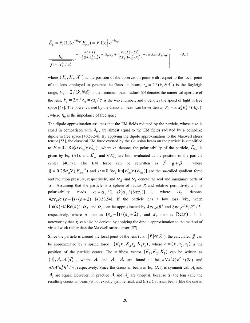
The electric field of the Gaussian beam trapping the particle (and illuminating it for photodetection) reads

20  

0

2 2

3 0

1 10 0

2 22 20 1 21 2

0 3 3 02 2 2 2 20 3 0 3 0 3

( ) arctan( / )

(1 / ) 2 (1 / )

1 /

ˆ ˆRe( ) ReL inc

i t i t

k X XX Xik X i i X z

w X z X z XE

X z

E x E xe e

e

(A1)

where 1 2 3( , , )X X X is the position of the observation point with respect to the focal point

of the lens employed to generate the Gaussian beam, 20 02 / ( )z k NA is the Rayleigh

range, 0 02 / ( )w k NA is the minimum beam radius, NA denotes the numerical aperture of

the lens, 0 0 02 / /k c is the wavenumber, and c denotes the speed of light in free

space [48]. The power carried by the Gaussian beam can be written as 2 20 0 0/ (4 )LP w E

, where 0 is the impedance of free space.

The dipole approximation assumes that the EM fields radiated by the particle, whose size is

small in comparison with 0 , are almost equal to the EM fields radiated by a point-like

dipole in free space [40,53,54]. By applying the dipole approximation to the Maxwell stress tensor [55], the classical EM force exerted by the Gaussian beam on the particle is simplified

to 0.5Re( )inc incF E E

, where denotes the polarizability of the particle, incE is

given by Eq. (A1), and incE and incE are both evaluated at the position of the particle

center [40,57]. The EM force can be rewritten as F g

, where 2

0.25 ( )R incg E

and 0.5 Im[ ( )]I inc incE E

are the so-called gradient force

and radiation pressure, respectively, and R and I denote the real and imaginary parts of

. Assuming that the particle is a sphere of radius R and relative permittivity , its

polarizability reads 30 0 0 0/ [1 / (6 )]ik , where 0 denotes

304 ( 1) / ( 2)R [40,53,54]. If the particle has a low loss [viz., when

Im( ) Re( ) ], R and I can be approximated by 304 aR and 2 3 6

0 08 / 3a k R ,

respectively, where a denotes ( 1) / ( 2)R R , and R denotes Re( ) . It is

noteworthy that g

can also be derived by applying the dipole approximation to the method of

virtual work rather than the Maxwell stress tensor [57].

Since the particle is around the focal point of the lens (viz., 0| |r ), the calculated g

can

be approximated by a spring force 1 1 2 2 3 3( , , )K x K x K x , where 1 2 3( , , )r x x x

is the

position of the particle center. The stiffness vector 1 2 3( , , )K K K can be written as

1 2 3( , , ) LA A A P , where 3A and 1 2A A are found to be 6 4 30 / (2 )aNA k R c and

4 4 30 /aNA k R c , respectively. Since the Gaussian beam in Eq. (A1) is symmetrical, 1A and

2A are equal. However, in practice 1A and 2A are unequal, because (i) the lens (and the

resulting Gaussian beam) is not exactly symmetrical, and (ii) a Gaussian beam [like the one in

21  

Eq. (A1)] is not an exact solution to Maxwell’s equations in the first place. The fact that 1A

and 2A are unequal is fortunate, because, as is discussed in Section 4, what I name

‘unwanted force components’ disable parametric feedback cooling and hybrid feedback

cooling if the oscillation frequencies /i iK M and /j jK M (for any j i )

are equal.

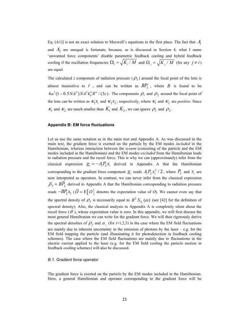
The calculated z component of radiation pressure ( 3 ) around the focal point of the lens is

almost insensitive to r

, and can be written as LBP , where B is found to be

2 2 2 6 604 (1 0.5 ) / (3 )a NA NA k R c . The components 1 and 2 around the focal point of

the lens can be written as 1 1x and 2 2x , respectively, where 1 and 2 are positive. Since

1 and 2 are much smaller than 1K and 2K , we can ignore 1 and 2 .

Appendix B: EM force fluctuations

Let us use the same notation as in the main text and Appendix A. As was discussed in the main text, the gradient force is exerted on the particle by the EM modes included in the Hamiltonian, whereas interaction between the system (consisting of the particle and the EM modes included in the Hamiltonian) and the EM modes excluded from the Hamiltonian leads to radiation pressure and the recoil force. This is why we can (approximately) infer from the

classical expression i i L ig A P x derived in Appendix A that the Hamiltonian

corresponding to the gradient force component ig reads 2 / 2i L iA P x , where LP and ix are

now interpreted as operators. In contrast, we can never infer from the classical expression

3 LBP derived in Appendix A that the Hamiltonian corresponding to radiation pressure

reads 3LBP x ( O O denotes the expectation value of O). We cannot even say that

the spectral density of 3 is necessarily equal to 2 ( )LPB S (see [42] for the definition of

spectral density). Also, the classical analysis in Appendix A is completely silent about the recoil force ( ), whose expectation value is zero. In this appendix, we will first discuss the most general Hamiltonian we can write for the gradient force. We will then rigorously derive

the spectral densities of 3 and i (for i=1,2,3) in the case where the EM field fluctuations

are mainly due to inherent uncertainty in the emission of photons by the laser – e.g. for the EM field trapping the particle (and illuminating it for photodetection in feedback cooling schemes). The case where the EM field fluctuations are mainly due to fluctuations in the electric current applied to the laser (e.g. for the EM field cooling the particle motion in feedback cooling schemes) will also be discussed.

B.1. Gradient force operator

The gradient force is exerted on the particle by the EM modes included in the Hamiltonian. Here, a general Hamiltonian and operator corresponding to the gradient force will be

22  

presented. The Hamiltonians used in the literature on cavity optomechanics of levitated particles [23-28] are in fact special cases of the Hamiltonian to be presented.

Let us assume that our system consists of a certain number of EM modes (with bosonic

operators ma ) which linearly interacts with each other and with the particle, whose position

operator is denoted by r

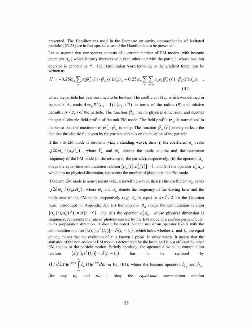
. The Hamiltonian ‘corresponding to the gradient force’ can be written as

2 † †0.25 ( ) ( ) 0.25 ( ) ( )R m m m m m R m n m n m nm m n m

H e r r a a e e r r a a

,

(B1)

where the particle has been assumed to be lossless. The coefficient R , which was defined in

Appendix A, reads 304 ( 1) / ( 2)R RR in terms of the radius (R) and relative

permittivity ( R ) of the particle. The function m has no physical dimension, and denotes

the spatial electric field profile of the mth EM mode. The field profile m is normalized in

the sense that the maximum of m m

is unity. The function ( )m r merely reflects the

fact that the electric field seen by the particle depends on the position of the particle.

If the mth EM mode is resonant (viz., a standing wave), then (i) the coefficient me reads

02 / ( )m mV , where mV and m denote the mode volume and the resonance

frequency of the EM mode (in the absence of the particle), respectively, (ii) the operator ma

obeys the equal-time commutation relation †[ ( ), ( )] 1m ma t a t , and (iii) the operator †m ma a ,

which has no physical dimension, represents the number of photons in the EM mode.

If the mth EM mode is non-resonant (viz., a travelling wave), then (i) the coefficient me reads

02 / ( )L mcA , where L and mA denote the frequency of the driving laser and the

mode area of the EM mode, respectively (e.g. mA is equal to 20 / 2w for the Gaussian

beam introduced in Appendix A), (ii) the operator ma obeys the commutation relation †[ ( ), ( )] ( )m ma t a t t t , and (iii) the operator †

m ma a , whose physical dimension is

frequency, represents the rate of photons carried by the EM mode at a surface perpendicular to its propagation direction. It should be noted that the use of an operator like s with the

commutation relation †1 2 1 2[ ( ), ( )] ( )s t s t t t , which holds whether 1t and 2t are equal

or not, means that the evolution of s is known a priori. In other words, it means that the statistics of the non-resonant EM mode is determined by the laser, and is not affected by other EM modes or the particle motion. Strictly speaking, the operator s with the commutation

relation †1 2 1 2[ ( ), ( )] ( )s t s t t t has to be replaced by

(1 / 2 ) ( )Li t i te b t e d

in Eq. (B1), where the bosonic operators

1b and

2b

(for any 1 and 2 ) obey the equal-time commutation relation

23  

1 2

†1 2[ ( ), ( )] ( )b t b t . The operator s with the commutation relation

†1 2 1 2[ ( ), ( )] ( )s t s t t t is in fact equal to (1 / 2 ) (0)Li t i te b e d

in terms

of the operators b , where 0t is the time at which we know the state of the system.

However, for problems such as those discussed in this paper, we can use operators like s

with the commutation relation †1 2 1 2[ ( ), ( )] ( )s t s t t t for non-resonant EM modes in

Eq. (B1), because in such problems we ignore the effect of the particle motion on the evolution of the non-resonant EM modes included in the system.

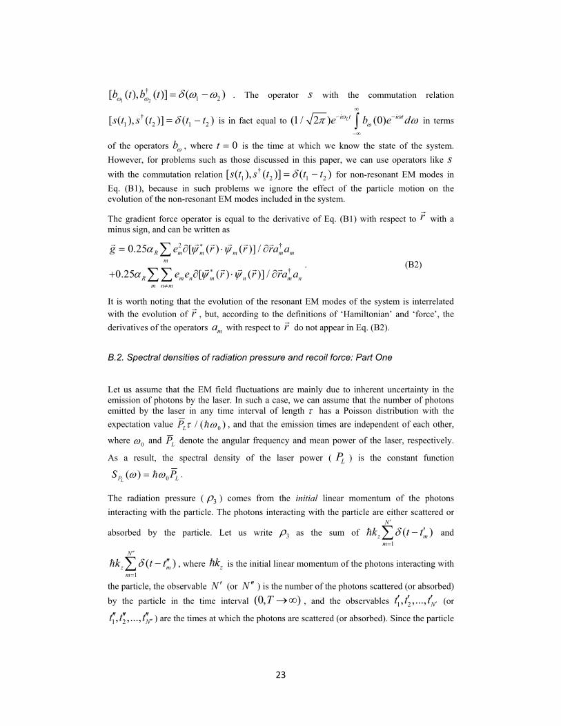
The gradient force operator is equal to the derivative of Eq. (B1) with respect to r

with a minus sign, and can be written as

2 †

†

0.25 [ ( ) ( )] /

0.25 [ ( ) ( )] /

R m m m m mm

R m n m n m nm n m

g e r r ra a

e e r r ra a

. (B2)

It is worth noting that the evolution of the resonant EM modes of the system is interrelated with the evolution of r

, but, according to the definitions of ‘Hamiltonian’ and ‘force’, the

derivatives of the operators ma with respect to r

do not appear in Eq. (B2).

B.2. Spectral densities of radiation pressure and recoil force: Part One

Let us assume that the EM field fluctuations are mainly due to inherent uncertainty in the emission of photons by the laser. In such a case, we can assume that the number of photons emitted by the laser in any time interval of length has a Poisson distribution with the

expectation value 0/ ( )LP , and that the emission times are independent of each other,

where 0 and LP denote the angular frequency and mean power of the laser, respectively.

As a result, the spectral density of the laser power ( LP ) is the constant function

0( )LP LS P .

The radiation pressure ( 3 ) comes from the initial linear momentum of the photons

interacting with the particle. The photons interacting with the particle are either scattered or

absorbed by the particle. Let us write 3 as the sum of 1

( )N

z mm

k t t

and

1

( )N

z mm

k t t

, where zk is the initial linear momentum of the photons interacting with

the particle, the observable N (or N ) is the number of the photons scattered (or absorbed)

by the particle in the time interval (0, )T , and the observables 1 2, ,..., Nt t t (or

1 2, ,..., Nt t t ) are the times at which the photons are scattered (or absorbed). Since the particle

24  

is around the focal point of the lens (viz., the expectation value of | |r

is much smaller than

0 ), Eq. (A1) indicates that zk is equal to 20 0 01 / (1 0.5 )k z k NA . Since the number

of photons emitted by the laser in any time interval of length has a Poisson distribution

with the expectation value 0/ ( )LP , and since the emission times are independent of

each other, we can say that: (i) N and N , which are independent of each other, have

Poisson distributions with the expectation values 0/ ( )sP T and 0/ ( )aP T ,

respectively, where s sP P and a aP P are the mean optical powers scattered

and absorbed by the particle, respectively, (ii) for a given N , the observables mt and nt

(for n m ) are independent of each other, (iii) for a given N , the observables mt and nt

(for n m ) are independent of each other, (iv) for a given N and N , the observables

mt and nt are independent of each other, and (v) for a given N and N , the observables

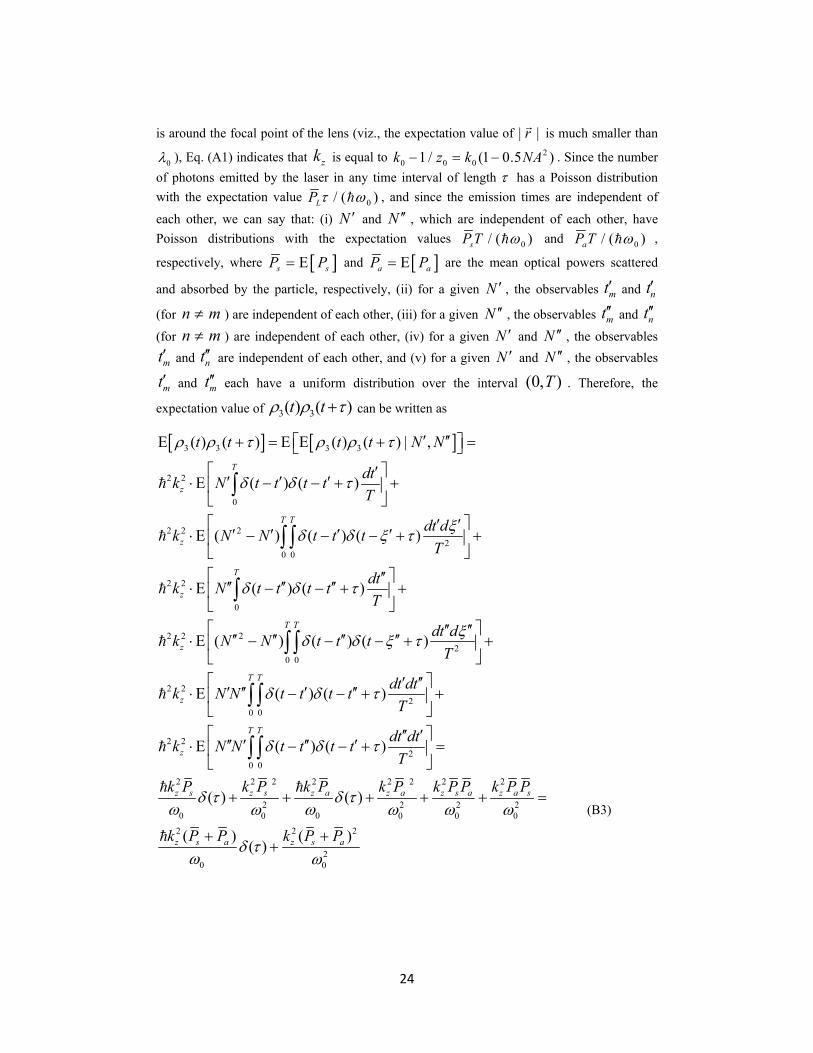
mt and mt each have a uniform distribution over the interval (0, )T . Therefore, the

expectation value of 3 3( ) ( )t t can be written as

3 3 3 3

2 2

0

2 2 22

0 0

2 2

0

2 2 2

( ) ( ) ( ) ( ) | ,

( ) ( )

( ) ( ) ( )

( ) ( )

( ) ( )

T

z

T T

z

T

z

z

t t t t N N

dtk N t t t t

T

dt dk N N t t t

T

dtk N t t t t

T

k N N t t

2

0 0

2 22

0 0

2 22

0 0

2 2 2 2 2 2 2 2

2 2 20 00 0 0

( )

( ) ( )

( ) ( )

( ) ( )

T T

T T

z

T T

z

z s z s z a z a z s a z a s

dt dt

T

dt dtk N N t t t t

T

dt dtk N N t t t t

T

k P k P k P k P k P P k P P

20

2 2 2

20 0

( ) ( )( )z s a z s ak P P k P P

(B3)

25  

where 3 3( ) ( ) | ,t t N N denotes the conditional expectation value of

3 3( ) ( )t t given N and N . The square root of the second term on the right hand

side of Eq. (B3) is in fact the expectation value of 3 . Moreover, the Fourier transform of the

first term on the right hand side of Eq. (B3) with respect to is the spectral density of 3 .

To derive sP and aP , which appeared in Eq. (B3), we note that under the dipole

approximation [40,53,54], the electric field radiated by the particle ( rE

) is equal to the

electric field radiated by a point-like dipole with the electric dipole moment 0

1 Re[ ( )]i tincx e E r

, where denotes the polarizability of the particle, and was given in

Appendix A, and ( )incE r

is the function given by Eq. (A1) and evaluated at

1 2 3( , , )r x x x

. Since the particle is around the focal point of the lens (viz., the expectation

value of | |r

is much smaller than 0 ), its dipole moment can be approximated by

0 31 0ˆ Re[ ]zi t ik xx e E e

, where zk reads 0 01/k z . For a given r

, r rE H

in the

far-field is found to be 2 2 6 2 3 2 2

0 0ˆsin ( ) / (32 )LNA k P r r , where †0 0E E has

been replaced by 20 04 / ( )LP w , and ( , , )r denotes the position of the observation

point with respect to the particle center in the spherical coordinate system whose zenith

direction is parallel to the x axis. Therefore, sP , which is equal to the flux of r rE H

over any closed surface enclosing the particle, reads 2 2 6 2 2

0 0/ (12 )LNA k P . Also, aP

is equal to †0 0 0( / 2)I sE E P , where I denotes the imaginary part of .

Therefore, if the particle has a low loss [viz., when I R ], sP and aP can be

approximated by 2 2 6 604 / 3La NA k R P and 2 3 3 2

06 / ( 2)I L RNA k R P , respectively,

where R Ii is the relative permittivity of the particle, and a denotes

( 1) / ( 2)R R . In such a case, aP is much smaller than sP , and can be ignored.

Interestingly, the square root of the second term on the right hand side of Eq. (B3) is in

agreement with 2 2 2 6 63 04 (1 0.5 ) / (3 )L LBP a NA NA k R P c , which was derived in

Appendix A by applying the dipole approximation to the Maxwell stress tensor. Moreover,

the spectral density of 3 [viz., the Fourier transform of the first term on the right hand side

of Eq. (B3) with respect to ], can be written as 2 ( )LPB S , where 0( )

LP LS P is

the spectral density of LP , and B is equal to 2 3 302 (1 0.5 ) / ( 3 )a NA NAk R c . It

should be noted that B is not equal to B . Also, it should be noted that the expectation value

and spectral density of 3 are insensitive of the position of the particle in that the phase 3zk x

in the expression of the dipole moment does not appear in r rE H

. However, the phase

26  

3zk x will be important in deriving the spectral density of the measurement noise in Appendix

D.

The spectral densities of the components of the recoil force ( ) can be found in [32], but the derivation to be presented here, which is along the lines of Eq. (B3), allows us to make some important points. The recoil force ( ) comes from the final linear momentum of the photons

scattered by the particle. Let us write ( )i t as ,1

( )N

m i mm

k t t

, where the observable

N is the number of photons scattered by the particle in the time interval (0, )T , the

observables 1 2, ,..., Nt t t are the times at which the photons are scattered, and the observable

,m ik is the ith component of the final wave vector ( mk

) of the mth photon scattered by the

particle. One can write ,1mk

, ,2mk

, and ,3mk

as 0 cos( )mk , 0 sin( )cos( )m mk , and

0 sin( )sin( )m mk , respectively, where the observables m and m are the zenith and

azimuth angles of mk

in a spherical coordinate system whose zenith direction is parallel to

the x axis. The observable ,m ik is independent of nt (for all n), and is independent of ,n ik

(for n m ). The observable N has a Poisson distribution with the expectation value

0/ ( )sP T . Also, for a given N , the observables mt and nt (for n m ) are

independent of each other, and have uniform distributions over the interval (0, )T .

Therefore, the expectation value of ( ) ( )i it t can be written as

2 2

,

0

2 2 2, 2

0 0

2 2 2, ,

20 0

( ) ( ) ( ) ( ) |

( ) ( )

( ) ( ) ( )

( )

i i i i

T

m i

T T

m i

m i s m i s

t t t t N

dtk N t t t t

T

dt dk N N t t t

T

k P k P

(B4)

Since ,m ik is zero, the second term on the right side of Eq. (B4) is zero, and therefore,

the expectation value of i is zero. To calculate the spectral density of i [viz., the Fourier

transform of the first term on the right hand side of Eq. (B4) with respect to ], 2,m ik

must be found. The spatial variation 2sin ( ) of r rE H

, which was discussed below

Eq. (B3), means that the joint probably density function of m and m in the expression of

mk

reads 33sin ( ) / (8 )m , and, as a result, 2,m ik is equal to 2

0 / 5k for i=1, and to

27  

202 / 5k for i=2,3. Therefore, the spectral density of i reads 2

0i LC P , where iC is

equal to 3 302 / ( 15 )aNAk R c for i=1, and to 3 3

02 2 / ( 15 )aNAk R c for i=2,3. It

should be noted that even if ,m ik was not zero, the second term on the right hand side of

Eq. (B4) would not contribute to the spectral density of i , because that term would still be

independent of . Therefore, it might seem that the fact , 0m ik is always unimportant

in deriving the spectral density of i , but below we will see otherwise.

B.2. Spectral densities of radiation pressure and recoil force: Part Two

Let us now assume that the EM field fluctuations are mainly due to fluctuations in the electric current applied to the laser. This is the case for the EM field cooling the particle motion in the feedback cooling schemes discussed in Section 4. Let us denote the laser power used to cool a

certain component of the particle motion by cP , and denote the corresponding current

applied to the laser by cI (it is noteworthy that c cI I , which is here considered as

fluctuations, is in fact the sum of the signal needed for feedback cooling and the measurement

noise). We can derive an equation similar to Eq. (B3) for ( ) ( )c ct t , where ˆ cz

denotes the radiation pressure associated with the EM field supposed to cool that component of the particle motion. The first term on the right hand side of the equation for

( ) ( )c ct t will be similar to the first term on the right hand side of Eq. (B3), but

can be ignored because cP is small (viz., much smaller than LP ). Unlike the second term on

the right hand side of Eq. (B3), the second term on the right hand side of the equation for

( ) ( )c ct t will not be independent of . To derive the second term, let us ignore

absorption and make three assumptions: (i) the proportionality constant between ( )cPR and

( )cIR is equal to the proportionality constant between 2

cP and 2cI , where ( )OR

denotes 2[ ( ) ( )]O t O t O , (ii) ( )

cPR is real, and (iii) the joint probability density

function of ,c mt and ,c nt (for a given N , and for n m ) over the interval (0, )T is

equal to 2 2, ,1 / [ ( )]

cc P c m c nT P R t t , where ,1 ,2 ,, ,...,c c c Nt t t denote the times at

which photons of the cooling EM field are scattered by the particle, and

2

0

1 / [ (1 / ) ( ) ]c

T

c PP T R d is a normalizing constant [it is noteworthy that the joint

probability density function which led to the second term on the right hand side of Eq. (B3)

was 21 / T ]. Under these assumptions, we can say that the proportionality constant

between ( )c

R and ( )cPR is equal to the proportionality constant between 2

c and

2cP . Also, the proportionality constant reads 2 2 2 2 6 6 2

0[4 (1 0.5 ) / (3 )]B a NA NA k R c

. Therefore, unlike the radiation pressure operator 3 for the trapping EM field, which

28  

cannot be written as LBP in terms of the operator LP , the radiation pressure operator c for

the cooling EM field can be approximated by cBP in terms of the operator cP .

We can derive an equation similar to Eq. (B4) for , ,( ) ( )c i c it t , where ,c i (for

i=1,2,3) denote the components of the recoil force associated with the cooling EM field. The

first term on the right hand side of the equation for , ,( ) ( )c i c it t will be similar to

the first term on the right hand side of Eq. (B4), but can be ignored because cP is small (viz.,

much smaller than LP ). Unlike the second term on the right hand side of Eq. (B4), the second

term on the right hand side of the equation for , ,( ) ( )c i c it t has factors dependent

on , but still does not contribute to the spectral density of ,c i because , ,c m ik is zero,

where , ,c m ik denotes the ith component of the final wave vector of the mth photon scattered

by the particle. Therefore, the fact , , 0c m ik is very important in allowing us to ignore

the spectral density of ,c i .

Appendix C: Thermal damping force and thermal random force

Let us first derive the surface temperature of the particle ( sT ). Since the particle is very small

and is around the focal point of the lens (viz., R and the expectation value of | |r

are much

smaller than 0 ), and is also of rather high thermal conductivity, its surface temperature ( sT )

is almost uniform, and is the solution to . . . .a c c r cP P P , where aP denotes the mean optical

power absorbed by the particle, . .c cP denotes the rate of heat conduction by the gas, and . .r cP

denotes thermal radiation. The mean optical power absorbed by the particle ( aP ), which was

derived in Appendix B, is equal to 2 3 3 206 / ( 2)I L RNA k R P . The rate of heat

conduction by the gas ( . .c cP ) is equal to ( 1)

( )8( 1)

a am imacc P s am

a am

P va T T

T

, where acc and

24Pa R are the thermal accommodation coefficient and surface area of the particle,

respectively, a , amP , and amT denote the heat capacity ratio, ambient pressure, and

ambient temperature of the gas, respectively, and 8 / ( )im B amv k T m is the mean

velocity of the gas molecules impinging on the particle (m denotes the mass of the gas

molecules) [58,59]. The rate of thermal radiation ( . .r cP ) is equal to 4 40 ( )P s ama T T , where

0 denotes the Stefan-Boltzmann constant, and the emissivity of the particle has been

assumed to be unity.

29  

The gas molecules surrounding the particle exert a damping force M v

on the particle, where M and v

denote the mass and velocity of the particle, respectively. The intrinsic

damping rate ( ) is not given by Stokes’ law, and is derived by using the kinetic theory of gases. According to Epstein’s seminal paper [41], the intrinsic damping rate ( ) for the motion of a spherical particle of radius R in a rarefied gas can be written as the sum of

/ (3 )im a im Pv a M , which is the contribution of the gas molecules impinging on the

particle, and / (24 )em a em Pv a M , which is the contribution of the gas molecules

emerging from the particle, where / ( )a a am B amm P k T is the gas density, and

8 / ( )em B emv k T m is the mean velocity of the gas molecules emerging from the

particle in terms of their temperature ( emT ). Epstein’s formula is applicable whenever the

temperature emT is definable. The temperature emT can be written as ( )am acc s amT T T

[58,59].

Epstein’s formula shows that the intrinsic damping rate ( ) is almost insensitive to the mean

laser power used to trap the particle ( LP ), and is almost proportional to the ambient pressure (

amP ) and the inverse of the particle’s radius (1/ R ). I say ‘almost’ because the temperature

of the emerging molecules ( emT ) itself depends on the surface temperature of the particle ( sT

), and therefore depends on LP , amP , and R.

The gas molecules also exert a random force f

on the particle. This force is random even in

the classical limit and even if the position and velocity of the particle are known. Also, this force is almost insensitive to the position and velocity of the particle. When the temperature

of the emerging molecules ( emT ) is equal to the ambient temperature ( amT ), the spectral

densities of the components of f

, which are equal to each other, can be derived by using the

Caldeira-Leggett model, and written as a function ( ; , )amG T of amT and [60]. The

function ( ; , )amG T can be rewritten as the sum of ( ; , )am imG T and

( ; , )am emG T , where im em , and the expressions of im and em were given

above.

When the temperature of the emerging molecules ( emT ) is not equal to the ambient

temperature ( amT ), the spectral density of the components of f

can be written as the sum of

( ; , )am imG T and ( ; , )em emG T , and simplified to ( ; , )G T , where T is defined as

( ) /im am em emT T [44,45]. The temperature T is what appears in the expressions of

,th im and im (for all i) in the main text.

Appendix D: Measurement noise

30  

As is usually the case in experiments [31,32,34-36], let us assume that the beam trapping the particle illuminates it for photodetection as well. Let us use the same notations as in Appendix A and Appendix B. The measurement of the position of the particle is carried out by the measurement of the EM field intensity [31-36]. The electric field is the sum of the incident

electric field ( LE

) given by Eq. (A1) and the electric field radiated by the particle ( rE

).

Under the dipole approximation [40,53,54], rE

is equal to the electric field radiated by a

point-like dipole with the electric dipole moment 01 Re[ ( )]i t

incx e E r , where denotes

the polarizability of the particle, and ( )incE r

is the function given by Eq. (A1) and evaluated

at the particle center (viz., at r

). Since the particle is around the focal point of the lens (viz., the expectation value of | |r

is much smaller than 0 ), its dipole moment can be

approximated by 0 31 0ˆ Re[ ]zi t ik xx e E e

, where r

has been written as 1 2 3( , , )x x x , and

zk reads 0 01/k z . It is noteworthy that the phase 3zk x in the expression of the dipole

moment was not important in deriving the spectral densities of 3 and 3 , but it is now

important in deriving 3nS (viz., the spectral density of the measurement noise corresponding

to the measurement of 3x ).

At an observation point ( , , )X Y Z far enough from the particle and close enough to the axis

of the beam [viz., 010Z and 2 20, / (20 )X Y Z ], the sum of LE

and rE

can be

written as

01 0

3 3 2 3 3 2 2 30 0 1 0 2 0 3 0

ˆ Re ( )

/ / / / ( )

i tdE x e i E

z Z ak R Xx Z ak R Yx Z ak R x z Z

(D1)

where a and R denote ( 1) / ( 2)R R and the radius of the particle, respectively, and 0z

denotes the Rayleigh range of the Gaussian beam illuminating the particle. It should be noted

that ( , , )X Y Z and 1 2 3( , , )r x x x

have been defined with respect to the focal point of the

lens employed to generate the Gaussian beam. Equation (D1) is in fact the electric field calculated within the dipole approximation, the far-field approximation, the paraxial approximation, and the assumption that the particle is around the focal point of the lens.

The electric field operator at ( , , )X Y Z is also given by Eq. (D1) if 1 2 3( , , )r x x x

and

0E are interpreted as operators. The operator corresponding to the optical power carried by

the beam can be written as 2 †0 0 0 0/ (4 )LP w E E in terms of the operator 0E , where 0w

denotes the minimum beam radius of the beam, and 0 denotes the impedance of free space.

The spectral density of the photocurrent iI generated by a small enough photodetector

centered at ( , , )i i iX Y Z can be written as the sum of ( )iMS and ( )Ni

S , where

31  

( )NiS , which is independent of over the detection bandwidth, is equal to

2 †i d di iq E E , and ( )

iMS is equal to the Fourier transform of

2 2 † † 2 2 † †( ) ( ) ( ) ( ) ( )M i d d d d i d d d di i i i i i i i iR q E t E t E t E t q E E E E

(D2)

with respect to ( O denotes the expectation value of O) [61]. The subscript ‘i’

emphasizes that the photodetector is intended to measure ix . The role of the second term on

the right hand side of Eq. (D2) is to eliminate the -independent part of the first term. The

coefficient q denotes the elementary charge, and the coefficient i reads 0 0/ (2 )dia in

terms of the area dia of the photodetector. The detection efficiency has been assumed to be

unity, and the detection bandwidth has been assumed to be large in comparison with the

mechanical oscillation frequency i . Given that ( )IiS is the sum of ( )

iMS and

( )iNS , we can interpret the fluctuations i iI I as an incoherent sum of a signal iM with

the spectral density ( )iMS and a noise iN with the spectral density ( )

iNS . Let us write

i iI I as i iM N .

Given Eq. (D1) and the fact that the expectation value of | |r

is much smaller than 0 ,

( )iNS , which is independent of , is found to be 2 † 2

0 0 0( / )i iq E E z Z . Let us now

derive ( )iMS for each i.

The photodetector intended to measure 3x is centered at 3 3 3( , , ) (0,0, )X Y Z Z , and thus

we can ignore any signature of 1x and 2x in 3M . Ignoring

2 3 4 2 40 0 3 3 3 3( / ( )) ( ) ( ) ( )ak R z Z x t x t x t x , we find that

3( )MS can be written as

3 3( )xS , where the coefficient 3 reads 2 3 2 2 †2 2

3 0 0 0(2 / )qak R Z E E . Therefore,

3nS , defined in the main text, is found to be

2 2 20 0 0

3 2 4 60

3 33

/8 L d

n Nw z Z

S Sa k R P a

. (D3)

The expression of 3nS indicates that it is advantageous to increase

3da . However, in view of

the paraxial approximation, the maximum allowable value of 3da is around 0 / (5 )Z at a

given Z . If we assume that 3da is equal to its maximum allowable value for any given Z ,

3nS is proportional to Z . Therefore, it is advantageous to decrease Z . However, in view of

the far-field approximation, Z must be kept well above 0 (viz., 010Z ).

32  

To measure 1x , the photocurrents 1 1 1 1I I M N and 1 1 1 1I I M N generated

by two photodetectors centered at 1 1 1( , , ) ( ,0, )X Y Z X Z and

1 1 1( , , ) ( ,0, )X Y Z X Z , respectively, are subtracted from each other [31]. Such a

balanced detection allows us to ignore any signature of 3x (and 2x ) in 1 1I I . It should be

noted that 1 1I I cannot be written as 1 1 1 1 1 1( ) ( ) ( )I I M M N N . In fact, 1M

and 1M are added coherently (viz., they are perfectly correlated) while 1N and 1N are

added incoherently (viz., they are uncorrelated). Therefore, let us write 1 1I I as

1 1 1 1 1 1( ) ( ) [ ( )]I I M M N N . The spectral density of 1 1( )N N is equal

to 1

2 ( )NS . Ignoring 3 3 2 4 2 40 1 1 1 1( / ) ( ) ( ) ( )ak R X Z x t x t x t x , we find that the

spectral density of 1 1( )M M can be written as 1 14 ( )xS , where 1 reads

3 3 3 2 †2 21 0 0 0 0(2 / )qak R z X Z E E . Therefore,

1nS , defined in the main text, reads

2 40 0

1 2 6 6 20

1 11

0.5 / 0.58 L d

n Nw Z

S Sa k R P X a

. (D4)

The expression of 1nS indicates that it is advantageous to increase 2

1dX a . However, in view

of the paraxial approximation, the maximum allowable value of 2

1dX a is around

20[ / (45 )]Z at a given Z . It happens when 2

01& / (45 )dX a Z . If we assume that

201

& / (45 )dX a Z for any given Z , 1nS is proportional to 2Z . Therefore, it is

advantageous to decrease Z . However, in view of the far-field approximation, Z must be

kept well above 0 (viz., 010Z ).

To measure 2x , the photocurrents generated by two photodetectors centered at

2 2 2( , , ) (0, , )X Y Z Y Z and 2 2 2( , , ) (0, , )X Y Z Y Z are subtracted from each other.

The term 2nS , defined in the main text, is derived in the same way as

1nS was derived. It

reads

2 40 0

2 2 6 6 20

2 22

0.5 / 0.58 L d

n Nw Z

S Sa k R P Y a

. (D5)

In view of the paraxial approximation, the maximum allowable value of 2

2dY a is around

20[ / (45 )]Z at a given Z . It happens when 2

02& / (45 )dY a Z . If we assume that

202

& / (45 )dY a Z for any given Z , 2nS is proportional to 2Z .

33  

It is noteworthy that there was a subtle approximation involved in deriving ( )iMS for each

i. The correlation ( ) ( )i ix t x t has been approximated by its real part. In other words,

† †( ) ( ) ( ) ( )d d d di i i iE t E t E t E t has been approximated by

† †( ) ( ) ( ) ( )d d d di i i iE t E t E t E t . The latter is in fact proportional to

( ) ( )d di iP t P t , where di

P denotes the optical power received by the photodetector i.

This approximation was necessary in deriving the relations ( ) ( )i ii xMS S .

Finally, it should be noted that in practice the photodetectors cannot be placed at a small

distance of 010 from the particle – rather, they are at a distance of 6 70 010 10 from the

particle. The effect of such a long distance on inS can be compensated to some extent by

employing a collimating lens with a large enough numerical aperture to collect a large enough amount of light before we direct the light to the photodetectors. The focal point of the collimating lens must coincide with the focal point of the lens employed to generate the beam illuminating the particle. Also, each photodetector must be placed at the focal plane of a converging lens supposed to compensate the Fourier transforming effect of the collimating lens. In such a detection scheme, the results derived in this appendix all remain valid, but Z no longer denotes the actual distance between the photodetectors and the focal point of the

lens employed to generate the beam illuminating the particle. Also, dia no longer denotes the

actual area of the photodetector intended to measure ix . Rather, Z is a parameter

determined by the characteristics of the collimating lens, the converging lens, and other optical devices between them (e.g., beam splitters and mirrors), hence the name ‘effective

distance’ for Z in the main text. The parameter Z must still meet the condition 0Z .

Also, the maximum allowable values of the parameters 3da , 2

1dX a , and 2

2dY a are still

around 0 / (5 )Z , 20[ / (45 )]Z , and 2

0[ / (45 )]Z , respectively, at a given Z . If we

assume that 03/ (5 )da Z for any given Z ,

3nS is still proportional to Z . If we

assume that 2 201 2

& & & / (45 )d dX Y a a Z for any given Z , 1nS and

2nS are still

proportional to 2Z .

Appendix E: Summary of important symbols

Table 1. Definitions of important symbols used in the article

1 2 3( , , )r x x x

The position (or position operator) of the particle

center with respect to the focal point of the lens

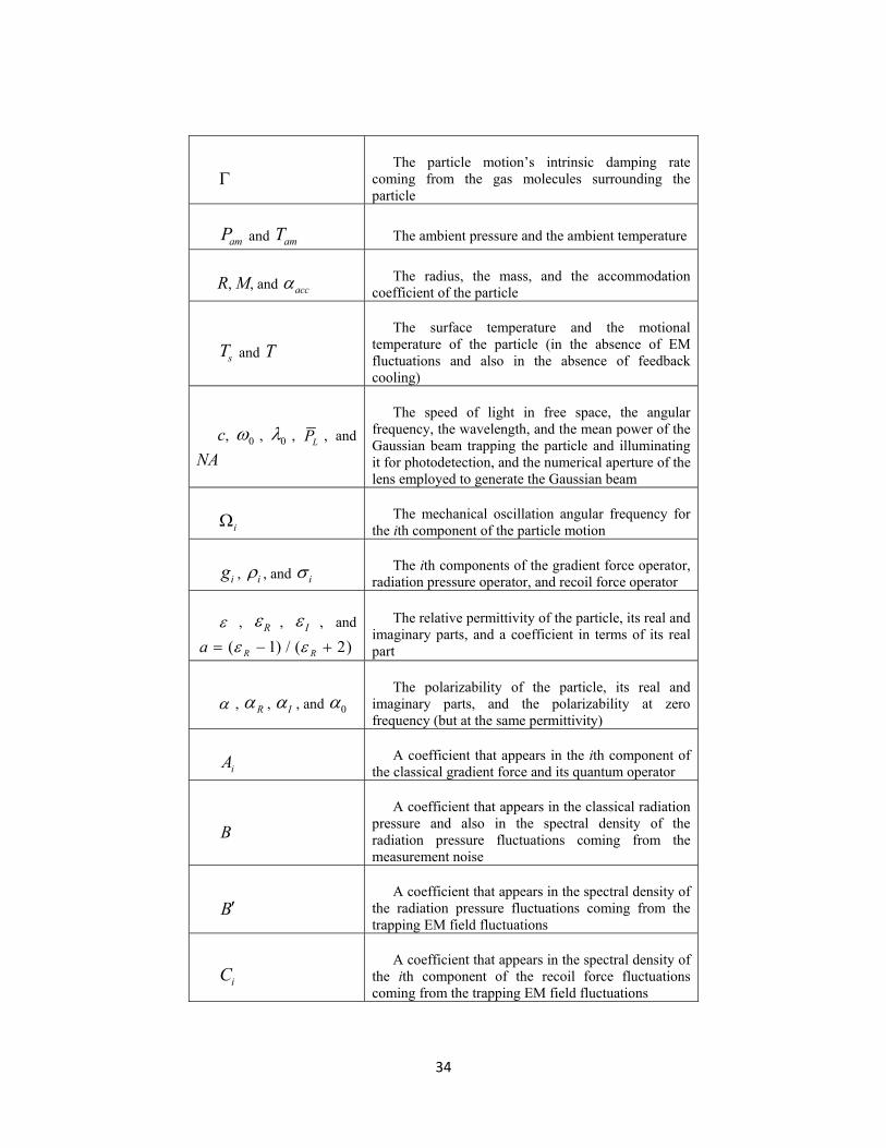
34  

The particle motion’s intrinsic damping rate

coming from the gas molecules surrounding the particle

amP and amT The ambient pressure and the ambient temperature

R, M, and acc The radius, the mass, and the accommodation coefficient of the particle

sT and T

The surface temperature and the motional temperature of the particle (in the absence of EM fluctuations and also in the absence of feedback cooling)

c, 0 , 0 , LP , and

NA

The speed of light in free space, the angular frequency, the wavelength, and the mean power of the Gaussian beam trapping the particle and illuminating it for photodetection, and the numerical aperture of the lens employed to generate the Gaussian beam

i The mechanical oscillation angular frequency for the ith component of the particle motion

ig , i , and i The ith components of the gradient force operator,

radiation pressure operator, and recoil force operator

, R , I , and

( 1) / ( 2) R Ra

The relative permittivity of the particle, its real and imaginary parts, and a coefficient in terms of its real part

, R , I , and 0 The polarizability of the particle, its real and

imaginary parts, and the polarizability at zero frequency (but at the same permittivity)

iA A coefficient that appears in the ith component of the classical gradient force and its quantum operator

B

A coefficient that appears in the classical radiation pressure and also in the spectral density of the radiation pressure fluctuations coming from the measurement noise

B A coefficient that appears in the spectral density of

the radiation pressure fluctuations coming from the trapping EM field fluctuations

iC A coefficient that appears in the spectral density of

the ith component of the recoil force fluctuations coming from the trapping EM field fluctuations

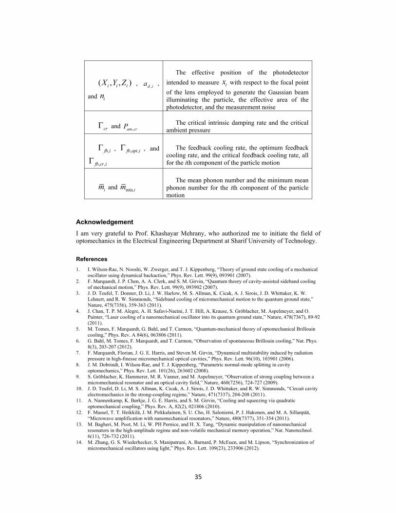
35  

( , , )i i iX Y Z , ,d ia ,

and in

The effective position of the photodetector

intended to measure ix with respect to the focal point

of the lens employed to generate the Gaussian beam illuminating the particle, the effective area of the photodetector, and the measurement noise

cr and ,am crP The critical intrinsic damping rate and the critical ambient pressure

, fb i , , , fb opt i , and

, , fb cr i

The feedback cooling rate, the optimum feedback cooling rate, and the critical feedback cooling rate, all for the ith component of the particle motion

im and min,im The mean phonon number and the minimum mean

phonon number for the ith component of the particle motion

Acknowledgement

I am very grateful to Prof. Khashayar Mehrany, who authorized me to initiate the field of optomechanics in the Electrical Engineering Department at Sharif University of Technology.

References

1. I. Wilson-Rae, N. Nooshi, W. Zwerger, and T. J. Kippenberg, “Theory of ground state cooling of a mechanical oscillator using dynamical backaction,” Phys. Rev. Lett. 99(9), 093901 (2007).

2. F. Marquardt, J. P. Chen, A. A. Clerk, and S. M. Girvin, “Quantum theory of cavity-assisted sideband cooling of mechanical motion,” Phys. Rev. Lett. 99(9), 093902 (2007).

3. J. D. Teufel, T. Donner, D. Li, J. W. Harlow, M. S. Allman, K. Cicak, A. J. Sirois, J. D. Whittaker, K. W. Lehnert, and R. W. Simmonds, “Sideband cooling of micromechanical motion to the quantum ground state,” Nature, 475(7356), 359-363 (2011).

4. J. Chan, T. P. M. Alegre, A. H. Safavi-Naeini, J. T. Hill, A. Krause, S. Gröblacher, M. Aspelmeyer, and O. Painter, “Laser cooling of a nanomechanical oscillator into its quantum ground state,” Nature, 478(7367), 89-92 (2011).

5. M. Tomes, F. Marquardt, G. Bahl, and T. Carmon, “Quantum-mechanical theory of optomechanical Brillouin cooling,” Phys. Rev. A 84(6), 063806 (2011).

6. G. Bahl, M. Tomes, F. Marquardt, and T. Carmon, “Observation of spontaneous Brillouin cooling,” Nat. Phys. 8(3), 203-207 (2012).

7. F. Marquardt, Florian, J. G. E. Harris, and Steven M. Girvin, “Dynamical multistability induced by radiation pressure in high-finesse micromechanical optical cavities,” Phys. Rev. Lett. 96(10), 103901 (2006).

8. J. M. Dobrindt, I. Wilson-Rae, and T. J. Kippenberg, “Parametric normal-mode splitting in cavity optomechanics,” Phys. Rev. Lett. 101(26), 263602 (2008).

9. S. Gröblacher, K. Hammerer, M. R. Vanner, and M. Aspelmeyer, “Observation of strong coupling between a micromechanical resonator and an optical cavity field,” Nature, 460(7256), 724-727 (2009).

10. J. D. Teufel, D. Li, M. S. Allman, K. Cicak, A. J. Sirois, J. D. Whittaker, and R. W. Simmonds, “Circuit cavity electromechanics in the strong-coupling regime,” Nature, 471(7337), 204-208 (2011).

11. A. Nunnenkamp, K. Børkje, J. G. E. Harris, and S. M. Girvin, “Cooling and squeezing via quadratic optomechanical coupling,” Phys. Rev. A, 82(2), 021806 (2010).

12. F. Massel, T. T. Heikkilä, J. M. Pirkkalainen, S. U. Cho, H. Saloniemi, P. J. Hakonen, and M. A. Sillanpää, “Microwave amplification with nanomechanical resonators,” Nature, 480(7377), 351-354 (2011).

13. M. Bagheri, M. Poot, M. Li, W. PH Pernice, and H. X. Tang, “Dynamic manipulation of nanomechanical resonators in the high-amplitude regime and non-volatile mechanical memory operation,” Nat. Nanotechnol. 6(11), 726-732 (2011).

14. M. Zhang, G. S. Wiederhecker, S. Manipatruni, A. Barnard, P. McEuen, and M. Lipson, “Synchronization of micromechanical oscillators using light,” Phys. Rev. Lett. 109(23), 233906 (2012).

36  

15. M. Bagheri, M. Poot, L. Fan, F. Marquardt, and H. X. Tang, “Photonic cavity synchronization of nanomechanical oscillators,” Phys. Rev. Lett. 111(21), 213902 (2013).

16. S. Weis, R. Rivière, S. Deléglise, E. Gavartin, O. Arcizet, A. Schliesser, and T. J. Kippenberg, “Optomechanically induced transparency,” Science, 330(6010), 1520-1523 (2010).

17. J. T. Hill, A. H. Safavi-Naeini, J. Chan, and O. Painter, “Coherent optical wavelength conversion via cavity optomechanics,” Nature Commun. 3(1), 1-7 (2012).

18. M. J. Hartmann and M. B. Plenio, “Steady state entanglement in the mechanical vibrations of two dielectric membranes,” Phys. Rev. Lett. 101(20), 200503 (2008).

19. Y. D. Wang and A. A. Clerk, “Using interference for high fidelity quantum state transfer in optomechanics,” Phys. Rev. Lett. 108(15), 153603 (2012).

20. T. A. Palomaki, J. W. Harlow, J. D. Teufel, R. W. Simmonds, and K. W. Lehnert, “Coherent state transfer between itinerant microwave fields and a mechanical oscillator,” Nature, 495(7440), 210-214 (2013).

21. M. Poggio, C. L. Degen, H. J. Mamin, and D. Rugar, “Feedback cooling of a cantilever’s fundamental mode below 5 mK,” Phys. Rev. Lett. 99(1), 017201 (2007).

22. 27. S. Singh, G. A. Phelps, D. S. Goldbaum, E. M. Wright, and P. Meystre, “All-optical optomechanics: An optical spring mirror,” Phys. Rev. Lett. 105(21), 213602 (2010).

23. D. E. Chang, C. A. Regal, S. B. Papp, D. J. Wilson, J. Ye, O. Painter, H. J. Kimble, and P. Zoller, “Cavity opto-mechanics using an optically levitated nanosphere,” Proc. Natl. Acad. Sci. U.S.A. 107(3), 1005-1010 (2010).

24. N. Kiesel, F. Blaser, U. Delić, D. Grass, R. Kaltenbaek, and M. Aspelmeyer, “Cavity cooling of an optically levitated submicron particle,” Proc. Natl. Acad. Sci. U.S.A. 110(35), 14180-14185 (2013).

25. N. Meyer, A. Sommer, P. Mestres, J. Gieseler, V. Jain, L. Novotny, and R. Quidant, “Resolved-sideband cooling of a levitated nanoparticle in the presence of laser phase noise,” Phys. Review Lett. 123(15), 153601 (2019).

26. U. Delić, M. Reisenbauer, D. Grass, N. Kiesel, V. Vuletić, and M. Aspelmeyer, “Cavity cooling of a levitated nanosphere by coherent scattering,” Phys. Rev. Lett. 122(12), 123602 (2019).

27. D. Windey, C. Gonzalez-Ballestero, P. Maurer, L. Novotny, O. Romero-Isart, and R. Reimann, “Cavity-based 3D cooling of a levitated nanoparticle via coherent scattering,” Phys. Rev. Lett. 122(12), 123601 (2019).

28. U. Delić, M. Reisenbauer, K. Dare, D. Grass, V. Vuletić, N. Kiesel, and M. Aspelmeyer, “Cooling of a levitated nanoparticle to the motional quantum ground state,” Science, 367(6480), 892-895 (2020).

29. A. Ashkin and J. M. Dziedzic, “Feedback stabilization of optically levitated particles,” Appl. Phys. Lett. 30(4), 202-204 (1977).

30. T. Li, S. Kheifets and M. G. Raizen, “Millikelvin cooling of an optically trapped microsphere in vacuum,” Nat. Phys. 7(7), 527-530, (2011).

31. J. Gieseler, B. Deutsch, R. Quidant, and L. Novotny, “Subkelvin parametric feedback cooling of a laser-trapped nanoparticle” Phys. Rev. Lett. 109(10), 103603 (2012).

32. V. Jain, J. Gieseler, C. Moritz, C. Dellago, R. Quidant, and L. Novotny, “Direct measurement of photon recoil from a levitated nanoparticle,” Phys. Rev. Lett. 116(24), 243601 (2016).

33. B. Rodenburg, L. P. Neukirch, A. N. Vamivakas, and M. Bhattacharya, “Quantum model of cooling and force sensing with an optically trapped nanoparticle,” Optica, 3(3), 318-323 (2016).

34. F. Tebbenjohanns, M. Frimmer, A. Militaru, V. Jain, and L. Novotny, “Cold damping of an optically levitated nanoparticle to microkelvin temperatures,” Phys. Rev. Lett. 122(22), 223601 (2019).

35. G. P. Conangla, F. Ricci, M. T. Cuairan, A. W. Schell, N. Meyer, and R. Quidant, “Optimal feedback cooling of a charged levitated nanoparticle with adaptive control,” Phys. Rev. Lett. 122(22), 223602 (2019).

36. F. Tebbenjohanns, M. Frimmer, V. Jain, D. Windey, and L. Novotny, “Motional sideband asymmetry of a nanoparticle optically levitated in free space,” Phys. Rev. Lett. 124(1), 013603 (2020).

37. T. A. Savard, K. M. O’hara, and J. E. Thomas, “Laser-noise-induced heating in far-off resonance optical traps,” Phys. Rev. A 56(2), R1095 (1997).

38. M. E. Gehm, K. M. O’hara, T. A. Savard, and J. E. Thomas, “Dynamics of noise-induced heating in atom traps,” Phys. Rev. A 58 (5), 3914 (1998).

39. F. Monteiro, W. Li, G. Afek, C. Li, M .Mossman, and D. C. Moore, “Force and acceleration sensing with optically levitated nanogram masses at microkelvin temperatures,” Phys. Rev. A, 101(5), 053835 (2020).

40. A. M. Jazayeri, arXiv preprint arXiv:1905.11168 (2019). 41. P. S. Epstein, “On the resistance experienced by spheres in their motion through gases,” Phys. Rev. 23(6), 710

(1924): Equation (29).

42. The spectral density of an observable O is defined as the Fourier transform of 2[ ( ) ( )] [ ( )]O t O t O t

with respect to τ, provided that the expectation values, denoted by [ ] , are independent of t. The spectral

density is a real function, and sometimes an even function. It is always an even function in the classical limit.

43. The variance of an observable O is defined as 22[ ( )] [ ( )]O t O t , provided that the expectation values,

denoted by [ ] , are independent of t.

44. J. Millen, T. Deesuwan, P. Barker, and J. Anders, “Nanoscale temperature measurements using non-equilibrium Brownian dynamics of a levitated nanosphere,” Nat. Nanotechnol. 9(6), 425 (2014).

37  

45. E. Hebestreit, R. Reimann, M. Frimmer, and L. Novotny, “Measuring the internal temperature of a levitated nanoparticle in high vacuum,” Phys. Rev. A 97(4), 043803 (2018).

46. D. W. Keith, “Photophoretic levitation of engineered aerosols for geoengineering,” Proc. Natl. Acad. Sci. U.S.A. 107(38), 16428-16431 (2010).

47. V. G. Shvedov, A. V. Rode, Y. V. Izdebskaya, A. S. Desyatnikov, W. Krolikowski, and Y. S. Kivshar, “Giant optical manipulation,” Phys. Rev. Lett. 105(11), 118103 (2010).

48. B. E. A. Saleh and M. C. Teich, Fundamentals of Photonics (John Wiley & Sons, New York, 1991). 49. D. F. Walls and G. J. Milburn, Quantum Optics (Springer Science & Business Media, 2007). 50. K. Karrai, I. Favero, and C. Metzger, “Doppler optomechanics of a photonic crystal,” Phys. Rev. Lett. 100(24),

240801 (2008). 51. L. Novotny, “Radiation damping of a polarizable particle,” Phys. Rev. A 96(3), 032108 (2017). 52. S. Sachdev, Quantum Phase Transitions (Cambridge University Press, New York, 2011). 53. C. F. Bohren and D. R. Huffman, Absorption and Scattering of Light by Small Particles (John Wiley & Sons,

New York, 1998). 54. B. T. Draine, “The discrete-dipole approximation and its application to interstellar graphite grains,” Astrophy.

J. 333, 848-872 (1988). 55. A. M. Jazayeri and K. Mehrany, “Critical study and discrimination of different formulations of electromagnetic

force density and consequent stress tensors inside matter,” Phys. Rev. A, 89(4), 043845 (2014). 56. P. C. Chaumet and A. Rahmani, “Electromagnetic force and torque on magnetic and negative-index scatterers,”

Opt. Express 17(4), 2224-2234 (2009). 57. A. M. Jazayeri and K. Mehrany, “All-dielectric structure for trapping nanoparticles via light funneling and

nanofocusing,” J. Opt. Soc. Am. B 34(10), 2179-2184 (2017). 58. M. Knudsen, “Die molekulare Wärmeleitung der Gase und der Akkommodationskoeffizient,” Ann. Phys.

339(4), 593-656 (1911). 59. E. H. Kennard, Kinetic Theory of Gases (McGraw-Hill, New York, 1938). 60. A. O. Caldeira and A. J. Leggett, “Influence of dissipation on quantum tunneling in macroscopic systems,”

Phys. Rev. Lett. 46(4), 211 (1981). 61. H. J. Carmichael, “Spectrum of squeezing and photocurrent shot noise: a normally ordered treatment,” J. Opt.

Soc. Am. B 4(10), 1588-1603 (1987).