Cray XT4: An Early Evaluation for Petascale Scientific Simulation

Sadaf R. Alam Oak Ridge National Laboratory

Oak Ridge, Tennessee alamsr@ornl.gov

Jeffery A. Kuehn ‡ Oak Ridge National Laboratory

Oak Ridge, Tennessee kuehn@ornl.gov

Richard F. Barrett Oak Ridge National Laboratory

Oak Ridge, Tennessee rbarrett@ornl.gov

Jeff M. Larkin

Cray Inc Seattle, Washington

larkin@cray.com

Patrick H. Worley Oak Ridge National Laboratory

Oak Ridge, Tennessee worleyph@ornl.gov

Mark R. Fahey Oak Ridge National Laboratory

Oak Ridge, Tennessee faheymr@ornl.gov

Ramanan Sankaran Oak Ridge National Laboratory

Oak Ridge, Tennessee sankaranr@ornl.gov

ABSTRACT

The scientific simulation capabilities of next generation high-end

computing technology will depend on striking a balance among

memory, processor, I/O, and local and global network

performance across the breadth of the scientific simulation space.

The Cray XT4 combines commodity AMD dual core Opteron

processor technology with the second generation of Cray’s custom

communication accelerator in a system design whose balance is

claimed to be driven by the demands of scientific simulation. This

paper presents an evaluation of the Cray XT4 using micro-

benchmarks to develop a controlled understanding of individual

system components, providing the context for analyzing and

comprehending the performance of several petascale-ready

applications. Results gathered from several strategic application

domains are compared with observations on the previous

generation Cray XT3 and other high-end computing systems,

demonstrating performance improvements across a wide variety

of application benchmark problems.

Categories and Subject Descriptors

C.4 [Performance of Systems] Measurement techniques &

Performance attributes. C.5.1 [Large and Medium (―Mainframe‖)

Computers] Supercomputers.

General Terms

Measurement, Performance.

Keywords

Cray XT4, HPCC, IOR, AORSA, CAM, NAMD, POP, S3D.

1. INTRODUCTION In our quest to develop the capability for petascale scientific

simulation for both long-term strategic and economic advantage,

we face numerous challenges. The suitability of next generation

high performance computing technology for petascale simulations

will depend on balance among memory, processor, I/O, and local

and global network performance. As we approach technological

―event horizons‖ in memory latency, processor core performance,

I/O bandwidth, and network latency and bandwidth, achieving

system balance becomes ever more difficult. In this context, we

present an evaluation of the Cray XT4 computer system. We use

micro-benchmarks to develop a controlled understanding of

individual system components, and then use this understanding to

analyze and interpret the performance of several petascale-ready

applications.

2. CRAY XT4 COMPUTER SYSTEM AND

SOFTWARE OVERVIEW The Cray XT4 is an evolutionary descendant of the Cray XT3 line

of supercomputers, upgrading the processor, memory, and

network technologies and preparing the architecture for additional

on-site technology upgrades. We begin with a description of the

XT3.

Designed in collaboration with Sandia National Laboratory under

the RedStorm project [1][2], the Cray XT3 [3][4][5] has been

called Cray’s third generation of massively parallel processor

(MPP) supercomputers, following the lineage of the Cray T3D

and T3E systems. The machine was designed around the AMD

Opteron processor, a scalable custom interconnect (Cray SeaStar),

and a light-weight kernel (LWK) operating system, Catamount.

The AMD Opteron 100-series processor was selected for the Cray

XT3 system because it provides good floating point performance

with high memory bandwidth and low memory latency. A

compelling feature of the AMD Opteron architecture over

competing processors is AMD’s HyperTransport (HT)

specification. HT technology is an open standard for

communicating directly with the CPU, which allows Cray to

©2007 Association for Computing Machinery. ACM acknowledges that

this contribution was authored or co-authored by a contractor or affiliate

of the [U.S.] Government. As such, the Government retains a nonexclusive, royalty-free right to publish or reproduce this article, or to

allow others to do so, for Government purposes only.

SC07, November 10–16, 2007, Reno, Nevada, USA.

© 2007 ACM 978-1-59593-764-3/07/0011…$5.00.

connect the Opteron processor directly to the SeaStar network.

AMD also moved the memory controller from a separate

NorthBridge chip to the CPU die, which reduces both complexity

and latency. By choosing the 100-series (single CPU) parts rather

than the 200- (dual CPU SMP) or 800- (quad CPU SMP) series

parts, Cray was able to further reduce the memory latency to less

than 60ns by removing the added latency of memory coherency.

[5][6]

The Cray SeaStar interconnect is a custom, 3D toroidal network

designed to provide very high bandwidth and reliability. The

SeaStar NIC has a PowerPC 440 processor with a DMA engine

onboard to reduce the network load on the Opteron processor.

Each NIC has six links with a peak bidirectional bandwidth of

7.6GB/s and a sustained bidirectional bandwidth of more than

6GB/s. The network links actually exceed the HT bandwidth with

the Opteron processors, ensuring that one node is not capable of

completely saturating the network bandwidth.

It was deemed critical when designing the Cray XT3 system that

the OS should minimize interruptions to the running applications

(―OS jitter‖). Thus, while the XT3 service and login nodes run a

complete Linux-based OS, the compute nodes run a microkernel

OS. This combination of operating systems is called UNICOS/lc

(Linux-Catamount). Catamount was initially developed by Sandia

National Laboratory to support scaling the Cray XT3/RedStorm

system to many thousands of processors. RedStorm’s Catamount

supported just one thread of execution per node and reduced

signal handling to minimize interrupts. Additionally, it took

advantage of the single thread of execution to streamline memory

management. To enable the use of dual-core Opterons, ―virtual

node‖ (VN) support was added. In VN mode, the node’s memory

is divided evenly between the cores. However, the VN mode

design is inherently asymmetric, with only one core handling

system interrupts and NIC access, leading to the potential for

imbalance in per-core performance. In particular, in the current

MPI [7] implementation, one core is responsible for all message

passing, with the other core interrupting it to handle messages on

its behalf. Messages between two cores on the same socket are

handled through a memory copy. The XT nodes can also be run in

―single/serial node‖ (SN) mode, in which only one core is used

but has full access to all of the node’s memory and the NIC.

Cray XT4 compute blades fit into the same cabinet and connect to

the same underlying Cray SeaStar network as the Cray XT3,

allowing both XT3 and XT4 compute blades to co-exist within the

same system. Three major differences exist between the XT3 and

XT4 systems. First, the AMD Socket 939 Revision E Opteron

processors have been replaced with the newer AMD AM2 Socket

Revision F Opteron. This socket change was critical to ensure that

dual-core XT4 systems can be site-upgraded to quad-core

processors, just as the original single-core XT3 could be site-

upgraded to dual core. The AMD Revision F Opteron includes a

new integrated memory controller with support for DDR2 RAM.

The upgrade from DDR to DDR2 memory is the second major

difference between the XT3 and XT4 systems. When the Cray

XT3 migrated from single to dual core, there was no change to

memory bandwidth to match the additional processor core. By

upgrading to DDR2 memory, the effective memory bandwidth to

each processor core improves from 6.4GB/s for DDR-400

memory to 10.6GB/s for DDR2-667 memory and 12.8GB/s for

DDR2-800 memory. Finally, XT4 introduces the SeaStar2

network chip to replace the original SeaStar. The SeaStar and

SeaStar2 networks are link-compatible, meaning that Seastar and

SeaStar2 NICs can co-exist on the same network. The SeaStar2

increases the network injection bandwidth of each node from

2.2GB/s to 4GB/s and increases the sustained network

performance from 4GB/s to 6GB/s. This increased injection

bandwidth corresponds with the increased memory bandwidth of

DDR2 RAM. Our study demonstrates the overall impact of the

combination of these new features on system balance in the XT4.

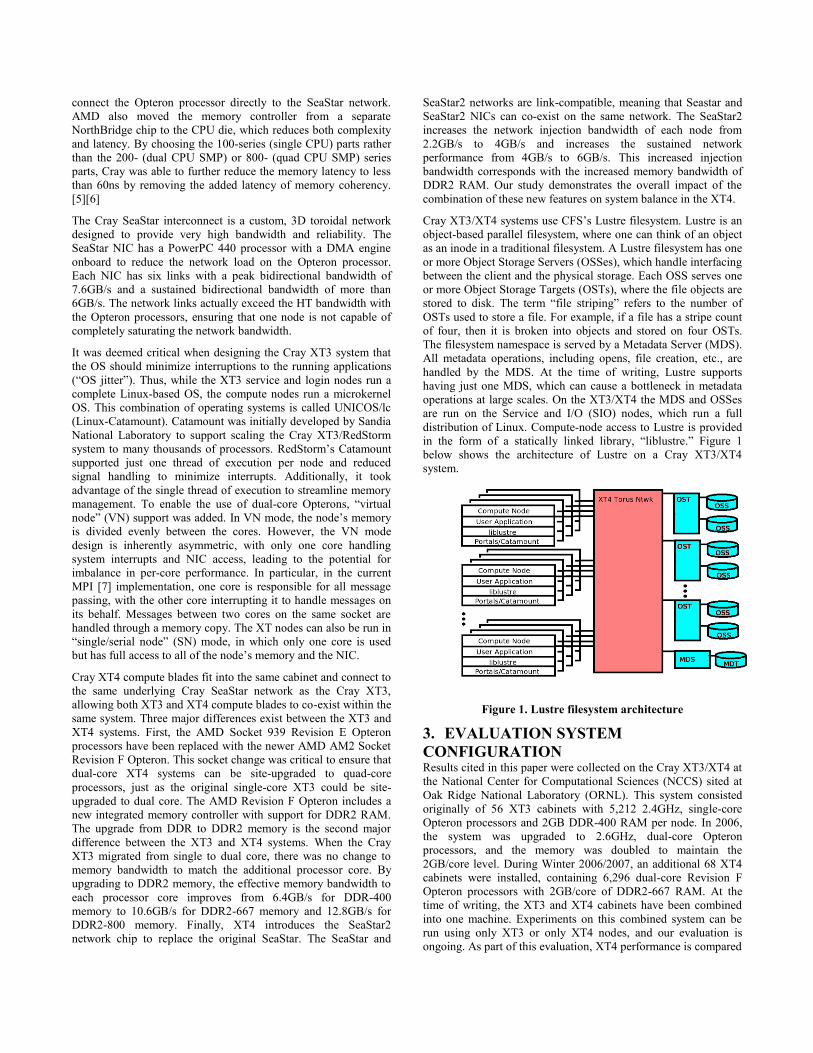
Cray XT3/XT4 systems use CFS’s Lustre filesystem. Lustre is an

object-based parallel filesystem, where one can think of an object

as an inode in a traditional filesystem. A Lustre filesystem has one

or more Object Storage Servers (OSSes), which handle interfacing

between the client and the physical storage. Each OSS serves one

or more Object Storage Targets (OSTs), where the file objects are

stored to disk. The term ―file striping‖ refers to the number of

OSTs used to store a file. For example, if a file has a stripe count

of four, then it is broken into objects and stored on four OSTs.

The filesystem namespace is served by a Metadata Server (MDS).

All metadata operations, including opens, file creation, etc., are

handled by the MDS. At the time of writing, Lustre supports

having just one MDS, which can cause a bottleneck in metadata

operations at large scales. On the XT3/XT4 the MDS and OSSes

are run on the Service and I/O (SIO) nodes, which run a full

distribution of Linux. Compute-node access to Lustre is provided

in the form of a statically linked library, ―liblustre.‖ Figure 1

below shows the architecture of Lustre on a Cray XT3/XT4

system.

Figure 1. Lustre filesystem architecture

3. EVALUATION SYSTEM

CONFIGURATION Results cited in this paper were collected on the Cray XT3/XT4 at

the National Center for Computational Sciences (NCCS) sited at

Oak Ridge National Laboratory (ORNL). This system consisted

originally of 56 XT3 cabinets with 5,212 2.4GHz, single-core

Opteron processors and 2GB DDR-400 RAM per node. In 2006,

the system was upgraded to 2.6GHz, dual-core Opteron

processors, and the memory was doubled to maintain the

2GB/core level. During Winter 2006/2007, an additional 68 XT4

cabinets were installed, containing 6,296 dual-core Revision F

Opteron processors with 2GB/core of DDR2-667 RAM. At the

time of writing, the XT3 and XT4 cabinets have been combined

into one machine. Experiments on this combined system can be

run using only XT3 or only XT4 nodes, and our evaluation is

ongoing. As part of this evaluation, XT4 performance is compared

both with the original XT3 system using single-core 2.4GHz

Opteron processors and with the dual-core XT3 system when

results are available. System details are summarized in Table 1.

Other systems used for comparison include the IBM SP and IBM

p575 clusters at the National Energy Research Scientific

Computing Center (NERSC) sited at Lawrence Berkeley National

Laboratory, the IBM p690 cluster at ORNL, the Cray X1E at the

NCCS, and the Japanese Earth Simulator.

Table 1. Comparison of XT3, XT3 dual core, and XT4 systems

at ORNL

Cray provides three compiler options on its XT4 supercomputers:

the Portland Group compiler, the GNU Compiler Collection, and

the PathScale compiler. Unless otherwise noted, results in this

paper were obtained using the Portland Group v6.2 compilers with

Message Passing ToolKit (MPT) v1.5 and scientific/math library

functionality provided by Cray’s ―libsci‖ library (which includes

Cray FFT, LAPACK, and ScaLAPACK interfaces) and the AMD

Core Math Library (ACML).

4. METHODOLOGY Our system evaluation approach recognizes that application

performance is the ultimate measure of system capability, but that

understanding an application’s interaction with a system requires

a detailed map of the performance of the system components.

Thus, we begin with micro-benchmarks that measure processor,

memory subsystem, and network capabilities of the system at a

low level. We then use the insights gained from the micro-

benchmarks to guide and interpret the performance analysis of

several key applications.

5. MICRO-BENCHMARKS

5.1 High Performance Computing Challenge

Benchmark Suite The High Performance Computing Challenge (HPCC) benchmark

suite [9][10][11][12] is composed of benchmarks measuring

network performance, node-local performance, and global

performance. Network performance is characterized by measuring

the network latency and bandwidth for three communication

patterns: naturally ordered ring, which represents an idealized

analogue to nearest neighbor communication; randomly ordered

ring, which represents non-local communication patterns; and

point-to-point or ping-pong patterns, which exhibit low

contention. The node local and global performance are

characterized by considering four algorithm sets, which represent

four combinations of minimal and maximal spatial and temporal

locality: DGEMM/HPL for high temporal and spatial locality,

FFT for high temporal and low spatial locality, Stream/Transpose

(PTRANS) for low temporal and high spatial locality, and

RandomAccess (RA) for low temporal and spatial locality. The

performance of these four algorithm sets are measured in

single/serial process mode (SP) in which only one processor is

used, embarrassingly parallel mode (EP) in which all of the

processors repeat the same computation in parallel without

communicating, and global mode in which each processor

provides a unique contribution to the overall computation

requiring communication. XT4 results are compared to the

original XT3 based on the 2.4GHz single core Opteron.

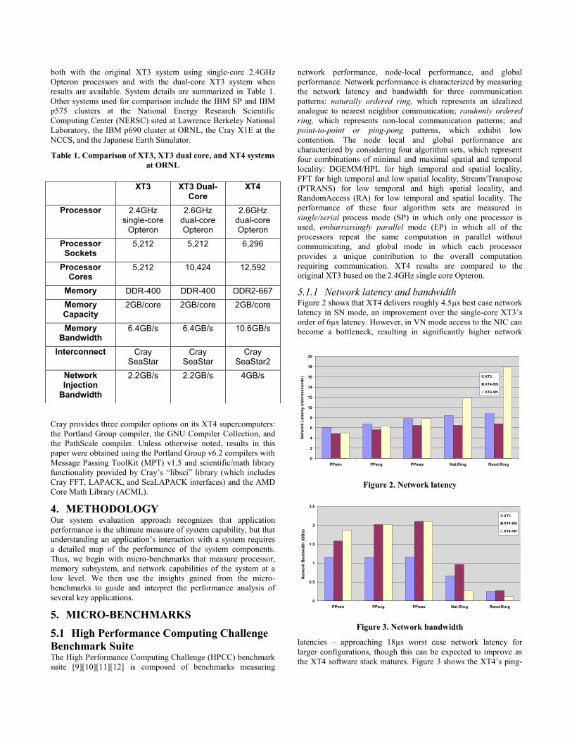
5.1.1 Network latency and bandwidth Figure 2 shows that XT4 delivers roughly 4.5µs best case network

latency in SN mode, an improvement over the single-core XT3’s

order of 6µs latency. However, in VN mode access to the NIC can

become a bottleneck, resulting in significantly higher network

0

2

4

6

8

10

12

14

16

18

20

PPmin PPavg PPmax Nat.Ring Rand.Ring

Ne

two

rk L

ate

nc

y (

mic

ros

ec

on

ds

) XT3

XT4-SN

XT4-VN

Figure 2. Network latency

0

0.5

1

1.5

2

2.5

PPmin PPavg PPmax Nat.Ring Rand.Ring

Ne

two

rk B

an

dw

idth

(G

B/s

)

XT3

XT4-SN

XT4-VN

Figure 3. Network bandwidth

latencies – approaching 18µs worst case network latency for

larger configurations, though this can be expected to improve as

the XT4 software stack matures. Figure 3 shows the XT4’s ping-

XT3 XT3 Dual-Core

XT4

Processor 2.4GHz single-core

Opteron

2.6GHz dual-core Opteron

2.6GHz dual-core Opteron

Processor Sockets

5,212 5,212 6,296

Processor Cores

5,212 10,424 12,592

Memory DDR-400 DDR-400 DDR2-667

Memory Capacity

2GB/core 2GB/core 2GB/core

Memory Bandwidth

6.4GB/s 6.4GB/s 10.6GB/s

Interconnect Cray SeaStar

Cray SeaStar

Cray SeaStar2

Network Injection

Bandwidth

2.2GB/s 2.2GB/s 4GB/s

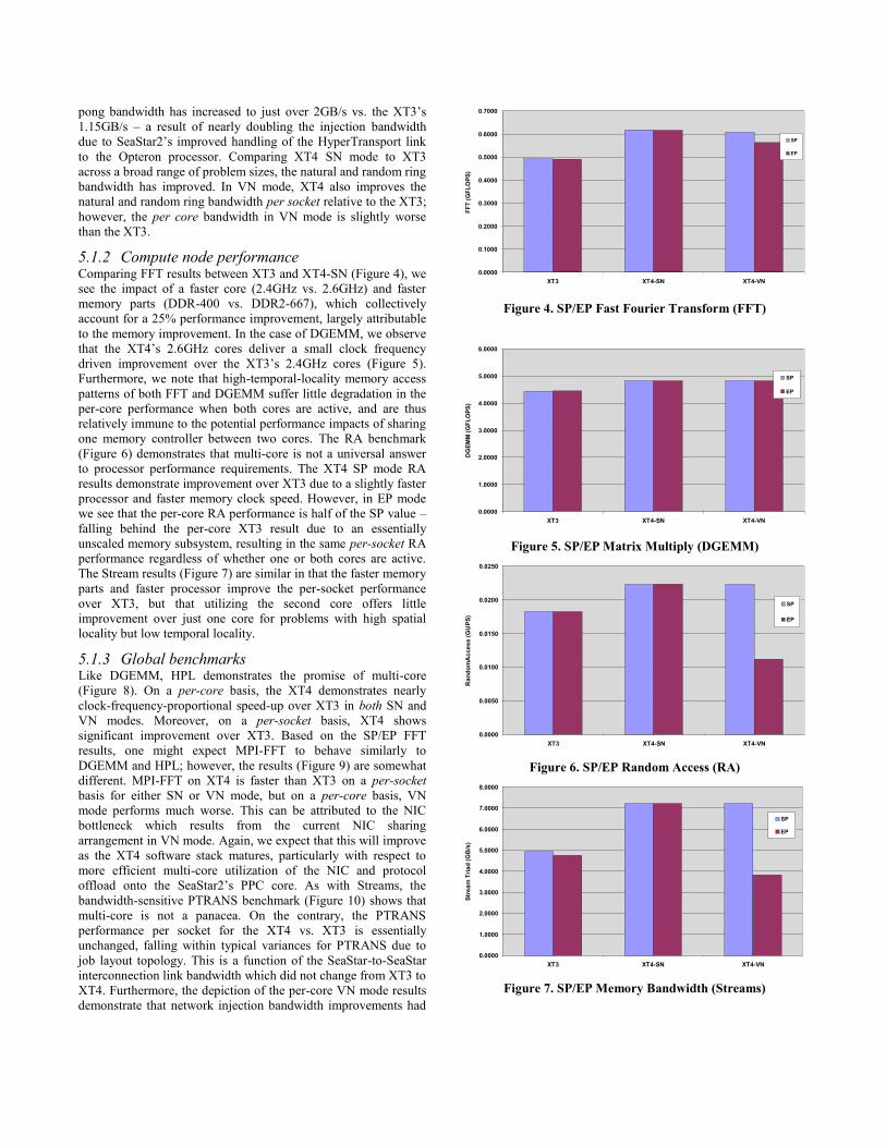
pong bandwidth has increased to just over 2GB/s vs. the XT3’s

1.15GB/s – a result of nearly doubling the injection bandwidth

due to SeaStar2’s improved handling of the HyperTransport link

to the Opteron processor. Comparing XT4 SN mode to XT3

across a broad range of problem sizes, the natural and random ring

bandwidth has improved. In VN mode, XT4 also improves the

natural and random ring bandwidth per socket relative to the XT3;

however, the per core bandwidth in VN mode is slightly worse

than the XT3.

5.1.2 Compute node performance Comparing FFT results between XT3 and XT4-SN (Figure 4), we

see the impact of a faster core (2.4GHz vs. 2.6GHz) and faster

memory parts (DDR-400 vs. DDR2-667), which collectively

account for a 25% performance improvement, largely attributable

to the memory improvement. In the case of DGEMM, we observe

that the XT4’s 2.6GHz cores deliver a small clock frequency

driven improvement over the XT3’s 2.4GHz cores (Figure 5).

Furthermore, we note that high-temporal-locality memory access

patterns of both FFT and DGEMM suffer little degradation in the

per-core performance when both cores are active, and are thus

relatively immune to the potential performance impacts of sharing

one memory controller between two cores. The RA benchmark

(Figure 6) demonstrates that multi-core is not a universal answer

to processor performance requirements. The XT4 SP mode RA

results demonstrate improvement over XT3 due to a slightly faster

processor and faster memory clock speed. However, in EP mode

we see that the per-core RA performance is half of the SP value –

falling behind the per-core XT3 result due to an essentially

unscaled memory subsystem, resulting in the same per-socket RA

performance regardless of whether one or both cores are active.

The Stream results (Figure 7) are similar in that the faster memory

parts and faster processor improve the per-socket performance

over XT3, but that utilizing the second core offers little

improvement over just one core for problems with high spatial

locality but low temporal locality.

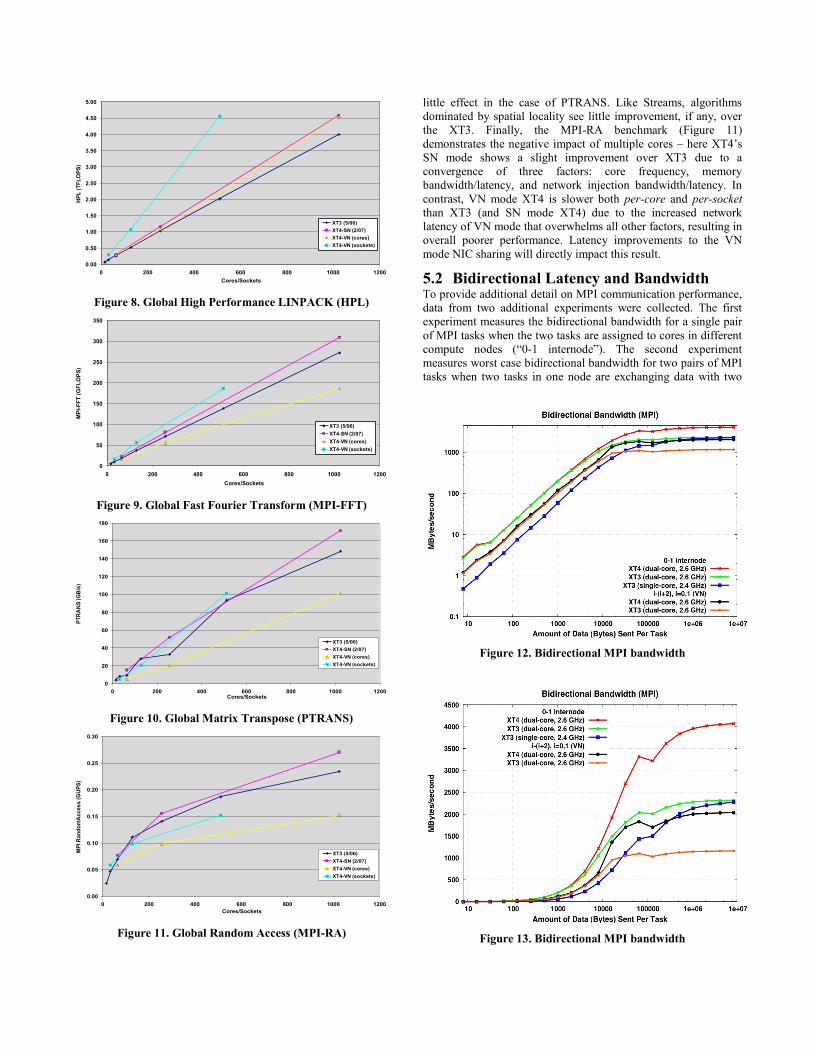
5.1.3 Global benchmarks Like DGEMM, HPL demonstrates the promise of multi-core

(Figure 8). On a per-core basis, the XT4 demonstrates nearly

clock-frequency-proportional speed-up over XT3 in both SN and

VN modes. Moreover, on a per-socket basis, XT4 shows

significant improvement over XT3. Based on the SP/EP FFT

results, one might expect MPI-FFT to behave similarly to

DGEMM and HPL; however, the results (Figure 9) are somewhat

different. MPI-FFT on XT4 is faster than XT3 on a per-socket

basis for either SN or VN mode, but on a per-core basis, VN

mode performs much worse. This can be attributed to the NIC

bottleneck which results from the current NIC sharing

arrangement in VN mode. Again, we expect that this will improve

as the XT4 software stack matures, particularly with respect to

more efficient multi-core utilization of the NIC and protocol

offload onto the SeaStar2’s PPC core. As with Streams, the

bandwidth-sensitive PTRANS benchmark (Figure 10) shows that

multi-core is not a panacea. On the contrary, the PTRANS

performance per socket for the XT4 vs. XT3 is essentially

unchanged, falling within typical variances for PTRANS due to

job layout topology. This is a function of the SeaStar-to-SeaStar

interconnection link bandwidth which did not change from XT3 to

XT4. Furthermore, the depiction of the per-core VN mode results

demonstrate that network injection bandwidth improvements had

0.0000

0.1000

0.2000

0.3000

0.4000

0.5000

0.6000

0.7000

XT3 XT4-SN XT4-VN

FF

T (

GF

LO

PS

)

SP

EP

Figure 4. SP/EP Fast Fourier Transform (FFT)

0.0000

1.0000

2.0000

3.0000

4.0000

5.0000

6.0000

XT3 XT4-SN XT4-VN

DG

EM

M (

GF

LO

PS

)

SP

EP

Figure 5. SP/EP Matrix Multiply (DGEMM)

0.0000

0.0050

0.0100

0.0150

0.0200

0.0250

XT3 XT4-SN XT4-VN

Ra

nd

om

Ac

ce

ss

(G

UP

S)

SP

EP

Figure 6. SP/EP Random Access (RA)

0.0000

1.0000

2.0000

3.0000

4.0000

5.0000

6.0000

7.0000

8.0000

XT3 XT4-SN XT4-VN

Str

ea

m T

ria

d (

GB

/s)

SP

EP

Figure 7. SP/EP Memory Bandwidth (Streams)

0.00

0.50

1.00

1.50

2.00

2.50

3.00

3.50

4.00

4.50

5.00

0 200 400 600 800 1000 1200

Cores/Sockets

HP

L (

TF

LO

PS

)

XT3 (5/06)

XT4-SN (2/07)

XT4-VN (cores)

XT4-VN (sockets)

Figure 8. Global High Performance LINPACK (HPL)

0

50

100

150

200

250

300

350

0 200 400 600 800 1000 1200

Cores/Sockets

MP

I-F

FT

(G

FL

OP

S)

XT3 (5/06)

XT4-SN (2/07)

XT4-VN (cores)

XT4-VN (sockets)

Figure 9. Global Fast Fourier Transform (MPI-FFT)

0

20

40

60

80

100

120

140

160

180

0 200 400 600 800 1000 1200Cores/Sockets

PT

RA

NS

(G

B/s

)

XT3 (5/06)

XT4-SN (2/07)

XT4-VN (cores)

XT4-VN (sockets)

Figure 10. Global Matrix Transpose (PTRANS)

0.00

0.05

0.10

0.15

0.20

0.25

0.30

0 200 400 600 800 1000 1200

Cores/Sockets

MP

I R

an

do

mA

cc

es

s (

GU

PS

)

XT3 (5/06)

XT4-SN (2/07)

XT4-VN (cores)

XT4-VN (sockets)

Figure 11. Global Random Access (MPI-RA)

little effect in the case of PTRANS. Like Streams, algorithms

dominated by spatial locality see little improvement, if any, over

the XT3. Finally, the MPI-RA benchmark (Figure 11)

demonstrates the negative impact of multiple cores – here XT4’s

SN mode shows a slight improvement over XT3 due to a

convergence of three factors: core frequency, memory

bandwidth/latency, and network injection bandwidth/latency. In

contrast, VN mode XT4 is slower both per-core and per-socket

than XT3 (and SN mode XT4) due to the increased network

latency of VN mode that overwhelms all other factors, resulting in

overall poorer performance. Latency improvements to the VN

mode NIC sharing will directly impact this result.

5.2 Bidirectional Latency and Bandwidth To provide additional detail on MPI communication performance,

data from two additional experiments were collected. The first

experiment measures the bidirectional bandwidth for a single pair

of MPI tasks when the two tasks are assigned to cores in different

compute nodes (―0-1 internode‖). The second experiment

measures worst case bidirectional bandwidth for two pairs of MPI

tasks when two tasks in one node are exchanging data with two

Figure 12. Bidirectional MPI bandwidth

Figure 13. Bidirectional MPI bandwidth

tasks in a different node simultaneously (―i-(i+2), i=0,1 (VN)‖).

Figure 12 and Figure 13 are plots of the MPI bidirectional

bandwidth as a function of message size, where Figure 12 uses a

log-log scale to emphasize the performance for small message

sizes and Figure 13 uses a log-linear scale to emphasize the

performance for large message sizes. From these data, the dual-

core XT4 bidirectional bandwidth is at least 1.8 times that of the

dual-core XT3 for message sizes over 100,000 Bytes. For large

messages, the two-pair experiments achieve exactly half the per

pair bidirectional bandwidth as the single-pair experiments,

representing identical compute node bandwidths. Bandwidth for

the single-core XT3 lags that of the dual-core XT3 for all but the

largest messages, but it achieves the same peak performance. For

small message sizes, dual-core XT3 performance and dual-core

XT4 performance are identical. However, latency for the two-pair

experiments on the dual-core systems is over twice that of the

single-pair experiments. This sensitivity of MPI latency to

simultaneous communication by both cores will be evident in

some of the application benchmark results. Finally, single-core

XT3 latency is much worse than that on the dual-core systems.

However, data for the single-core experiments were collected

more than two years ago, and the performance differences are

likely to be, at least partly, due to changes in the system software.

6. APPLICATION BENCHMARKS The following application benchmarks are drawn from the current

NCCS workload. These codes are large with complex

performance characteristics and numerous production

configurations that cannot be captured or characterized adequately

in the current study. The intent is, rather, to provide a qualitative

view of system performance using these benchmarks. In

particular, despite the importance, I/O performance is explicitly

ignored in these application benchmarks for the practical reason

that I/O would be overemphasized in the relatively short, but

numerous, benchmark runs that we employed in this study.

6.1 Atmospheric Modeling The Community Atmosphere Model (CAM) is a global

atmosphere circulation model developed at the National Science

Foundation’s National Center for Atmospheric Research (NCAR)

with contributions from researchers funded by the Department of

Energy (DOE) and by the National Aeronautics and Space

Administration [16][17]. CAM is used in both weather and

climate research. In particular, CAM serves as the atmosphere

component of the Community Climate System Model (CCSM)

[18][19].

For this evaluation, we ported and optimized CAM version 3.1

(available for download from the CCSM website at

http://www.ccsm.ucar.edu/) as described in [20]. CAM is a

mixed-mode parallel application code using both MPI and

OpenMP protocols [21]. CAM’s performance is characterized by

two phases: ―dynamics‖ and ―physics.‖ The dynamics phase

advances the evolution equations for the atmospheric flow, while

the physics phase approximates subgrid phenomena, including

precipitation processes, clouds, long- and short-wave radiation,

and turbulent mixing [16]. Control moves between the dynamics

and the physics at least once during each model simulation

timestep. The number and order of these transitions depend on the

configuration of numerical algorithm for the dynamics.

CAM implements three dynamical cores (dycores), one of which

is selected at compile-time: a spectral Eulerian solver [22], a

spectral semi-Lagrangian solver [23], and a finite volume semi-

Lagrangian solver [24]. Our benchmark problem is based on using

the finite volume (FV) dycore over a 361×576 horizontal

computational grid with 26 vertical levels. This resolution is

referred to as the ―D-grid,‖ and while it is greater than that used in

current computational climate experiments, it represents a

resolution of interest for future experiments. The FV dycore

supports both a one-dimensional (1D) latitude decomposition and

a two-dimensional (2D) decomposition of the computational grid.

The 2D decomposition is over latitude and longitude during one

phase of the dynamics and over latitude and the vertical in another

phase, requiring two remaps of the domain decomposition each

timestep. For small processor counts, the 1D decomposition is

faster than the 2D decomposition, but the 1D decomposition must

have at least three latitudes per MPI task and so is limited to a

maximum of 120 MPI tasks for the D-grid benchmark. Using a

2D decomposition requires at least three latitudes and three

vertical layers per MPI task, so is limited to 120×8, or 960, MPI

tasks for the D-grid benchmark. OpenMP can also be used to

exploit multiple processors per MPI task. While OpenMP

parallelism is used on the Earth Simulator and IBM systems for

the results described in Figure , it is not used on the Cray systems.

Figure 14. CAM throughput on XT4 vs. XT3

Figure 14 is a comparison of CAM throughput for the D-grid

benchmark problem on the single-core XT3 and on the dual-core

XT3 and XT4. Comparing throughput between the single-core

XT3 and the dual-core XT3 and XT4 when running in SN mode,

the impact of the improved processor, memory, and network

performance is clear, though software improvements may also

play a role in the performance differences between the single-core

and dual-core XT3 results. Comparing performance between the

dual-core XT3 and XT4 when running in VN mode demonstrates

a similar performance improvement due to the higher memory

performance and network injection bandwidth for the XT4. As

indicated in the micro-benchmarks, contention for memory and

for network access can degrade performance in VN mode as

compared to SN mode, on a per task basis. However, SN mode is

―wasting‖ as many processor cores as it is using, so the 10%

improvement in throughput compared to VN mode comes at a

significant cost in computer resources. For example, comparing

performance using 504 MPI tasks in SN mode with using 960

MPI tasks in VN mode, thus using approximately the same

number of compute nodes, VN mode achieves approximately 30%

better throughput.

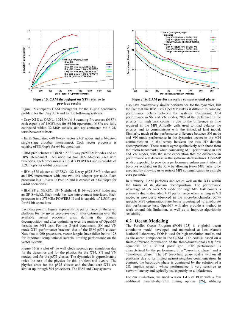
Figure 15. CAM throughput on XT4 relative to

previous results

Figure 15 compares CAM throughput for the D-grid benchmark

problem for the Cray XT4 and for the following systems:

• Cray X1E at ORNL: 1024 Multi-Streaming Processors (MSP),

each capable of 18GFlop/s for 64-bit operations. MSPs are fully

connected within 32-MSP subsets, and are connected via a 2D

torus between subsets.

• Earth Simulator: 640 8-way vector SMP nodes and a 640x640

single-stage crossbar interconnect. Each vector processor is

capable of 8GFlop/s for 64-bit operations.

• IBM p690 cluster at ORNL: 27 32-way p690 SMP nodes and an

HPS interconnect. Each node has two HPS adapters, each with

two ports. Each processor is a 1.3GHz POWER4 and is capable of

5.2GFlop/s for 64-bit operations.

• IBM p575 cluster at NERSC: 122 8-way p575 SMP nodes and

an HPS interconnect with one two-link adapter per node. Each

processor is a 1.9GHz POWER5 and is capable of 7.6GFlop/s for

64-bit operations.

• IBM SP at NERSC: 184 Nighthawk II 16-way SMP nodes and

an SP Switch2. Each node has two interconnect interfaces. Each

processor is a 375MHz POWER3-II and is capable of 1.5GFlop/s

for 64-bit operations.

Each data point in Figure represents the performance on the given

platform for the given processor count after optimizing over the

available virtual processor grids defining the domain

decomposition and after optimizing over the number of OpenMP

threads per MPI task. For the D-grid benchmark, SN and VN

mode XT4 performance brackets that of the IBM p575 cluster.

Note that at 960 processors, vector lengths have fallen below 128

for important computational kernels, limiting performance on the

vector systems.

Figure 16 is a plot of the wall clock seconds per simulation day

for the dynamics and for the physics for the XT4, SN and VN

modes, and for the p575 cluster. The dynamics is approximately

twice the cost of the physics for this problem and dycore. The

physics costs for the p575 cluster and the dual-core XT4 are

similar up through 504 processors. The IBM and Cray systems

Figure 16. CAM performance by computational phase

also have qualitatively similar performance for the dynamics, but

the fact that the IBM uses OpenMP makes it difficult to compare

performance details between the systems. Comparing XT4

performance in SN and VN modes, 70% of the difference in the

physics for high task counts is due to the difference in time

required in the MPI_Alltoallv calls used to load balance the

physics and to communicate with the imbedded land model.

Similarly, much of the performance difference between SN mode

and VN mode performance in the dynamics occurs in the MPI

communication in the remap between the two 2D domain

decompositions. These results agree qualitatively with those from

the micro-benchmarks when comparing MPI performance in SN

and VN modes, with the same expectation that the difference in

performance will decrease as the software stack matures. OpenMP

is also expected to provide a performance enhancement when it

becomes available on the XT4 by allowing fewer MPI tasks to be

used and by allowing us to restrict MPI communication to a single

core per node.

In summary, CAM performs and scales well on the XT4 within

the limits of its domain decomposition. The performance

advantage of SN over VN mode for large MPI task counts is

primarily due to degraded MPI performance when running in VN

mode, as previously observed in the micro-benchmarks. XT4-

specific MPI optimizations are being investigated to ameliorate

this performance loss. OpenMP will also provide a method to

work around this limitation, as well as to improve algorithmic

scalability.

6.2 Ocean Modeling The Parallel Ocean Program (POP) [25] is a global ocean

circulation model developed and maintained at Los Alamos

National Laboratory. POP is used for high-resolution studies and

as the ocean component in the CCSM. The code is based on a

finite-difference formulation of the three-dimensional (3D) flow

equations on a shifted polar grid. POP performance is

characterized by the performance of a ―baroclinic phase‖ and a

―barotropic phase.‖ The 3D baroclinic phase scales well on all

platforms due to its limited nearest-neighbor communication. In

contrast, the barotropic phase is dominated by the solution of a

2D, implicit system, whose performance is very sensitive to

network latency and typically scales poorly on all platforms.

For our evaluation, we used version 1.4.3 of POP with a few

additional parallel-algorithm tuning options [26], utilizing

historical performance data based on this version to provide a

context for the current results. The current production version of

POP is version 2.0.1. While version 1.4.3 and version 2.0.1 have

similar performance characteristics, the intent here is to use

version 1.4.3 to evaluate system performance, not to evaluate the

performance of POP.

We consider results for the 1/10-degree benchmark problem,

referred to as ―0.1.‖ The pole of the latitude-longitude grid is

shifted into Greenland to avoid computations near the singular

pole point. The grid resolution is 1/10 degree (10km) around the

equator, increasing to 2.5km near the poles, utilizing a 3600x2400

horizontal grid and 40 vertical levels. This grid resolution resolves

eddies for effective heat transport and is used for ocean-only or

ocean and sea-ice experiments.

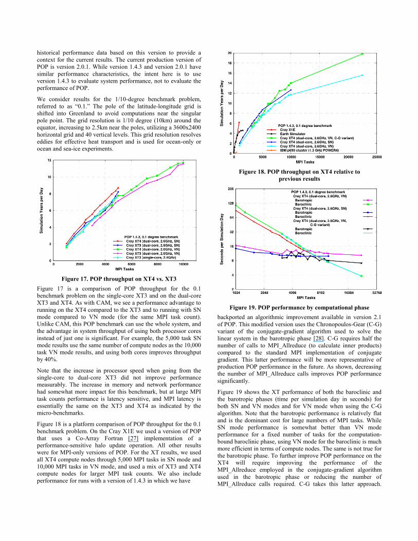
Figure 17. POP throughput on XT4 vs. XT3

Figure 17 is a comparison of POP throughput for the 0.1

benchmark problem on the single-core XT3 and on the dual-core

XT3 and XT4. As with CAM, we see a performance advantage to

running on the XT4 compared to the XT3 and to running with SN

mode compared to VN mode (for the same MPI task count).

Unlike CAM, this POP benchmark can use the whole system, and

the advantage in system throughput of using both processor cores

instead of just one is significant. For example, the 5,000 task SN

mode results use the same number of compute nodes as the 10,000

task VN mode results, and using both cores improves throughput

by 40%.

Note that the increase in processor speed when going from the

single-core to dual-core XT3 did not improve performance

measurably. The increase in memory and network performance

had somewhat more impact for this benchmark, but at large MPI

task counts performance is latency sensitive, and MPI latency is

essentially the same on the XT3 and XT4 as indicated by the

micro-benchmarks.

Figure 18 is a platform comparison of POP throughput for the 0.1

benchmark problem. On the Cray X1E we used a version of POP

that uses a Co-Array Fortran [27] implementation of a

performance-sensitive halo update operation. All other results

were for MPI-only versions of POP. For the XT results, we used

all XT4 compute nodes through 5,000 MPI tasks in SN mode and

10,000 MPI tasks in VN mode, and used a mix of XT3 and XT4

compute nodes for larger MPI task counts. We also include

performance for runs with a version of 1.4.3 in which we have

Figure 18. POP throughput on XT4 relative to

previous results

Figure 19. POP performance by computational phase

backported an algorithmic improvement available in version 2.1

of POP. This modified version uses the Chronopoulos-Gear (C-G)

variant of the conjugate-gradient algorithm used to solve the

linear system in the barotropic phase [28]. C-G requires half the

number of calls to MPI_Allreduce (to calculate inner products)

compared to the standard MPI implementation of conjugate

gradient. This latter performance will be more representative of

production POP performance in the future. As shown, decreasing

the number of MPI_Allreduce calls improves POP performance

significantly.

Figure 19 shows the XT performance of both the baroclinic and

the barotropic phases (time per simulation day in seconds) for

both SN and VN modes and for VN mode when using the C-G

algorithm. Note that the barotropic performance is relatively flat

and is the dominant cost for large numbers of MPI tasks. While

SN mode performance is somewhat better than VN mode

performance for a fixed number of tasks for the computation-

bound baroclinic phase, using VN mode for the baroclinic is much

more efficient in terms of compute nodes. The same is not true for

the barotropic phase. To further improve POP performance on the

XT4 will require improving the performance of the

MPI_Allreduce employed in the conjugate-gradient algorithm

used in the barotropic phase or reducing the number of

MPI_Allreduce calls required. C-G takes this latter approach.

More-efficient pre-conditioners, to decrease the number of

iterations required by conjugate gradient to solve the linear

system, are also being examined. It is worth noting that the VN

mode performance of the Cray-supplied MPI_Allreduce improved

significantly recently, eliminating much of the contention between

the processor cores. This optimization is reflected in the data here.

Additional VN optimization is feasible, as there is little reason for

latency-dominated collectives to run significantly slower in VN

mode than in SN mode. The VN mode performance variability in

the barotropic phase apparent in Figure also indicates the

possibility for further performance improvements.

In summary, the 0.1-degree POP benchmark scales very well on

the XT4, achieving excellent performance out to 22,000 MPI

tasks. The performance analysis indicates that performance will

not scale further unless the cost of the conjugate-gradient

algorithm used in the barotropic phase can be further decreased.

Both algorithmic and MPI collective optimizations are currently

being investigated for this purpose.

6.3 Biomolecular Simulations Nanoscale Molecular Dynamics (NAMD) is a scalable, object-

oriented molecular dynamics (MD) application designed for

simulation of large biomolecular systems [29]. It employs the

prioritized message-driven execution model of the

Charm++/Converse parallel runtime system, in which collections

of C++ objects remotely invoke methods on other objects with

messages, allowing parallel scaling on both MPP supercomputers

and workstation clusters [30].

Biomolecular simulation improves our understanding of novel

biochemical functions and essential life processes. Biomolecular

problems are computationally difficult, engendering high

complexity and time scales spanning more than 15 orders of

magnitude to represent the dynamics and functions of

biomolecules. Biomolecular simulations are based on the

principles of molecular dynamics (MD), which model the time

evolution of a wide variety of complex chemical problems as a set

of interacting particles, simulated by integrating the equations of

motion defined by classical mechanics — most notably Newton’s

second law, ∑F=ma. Several commercial and open source MD

software frameworks are in use by a large community of

biologists, and differ primarily in the form of their potential

functions and force-field parameters.

0.001

0.01

0.1

1

64 128 256 512 1024 2048 4096 8192 12000

MP I T as ks

Tim

e (

seco

nd

s)

per

NA

MD

Sim

ula

tio

n T

imeste

p

XT3(1M)

XT4(1M)

XT3(3M)

XT4(3M)

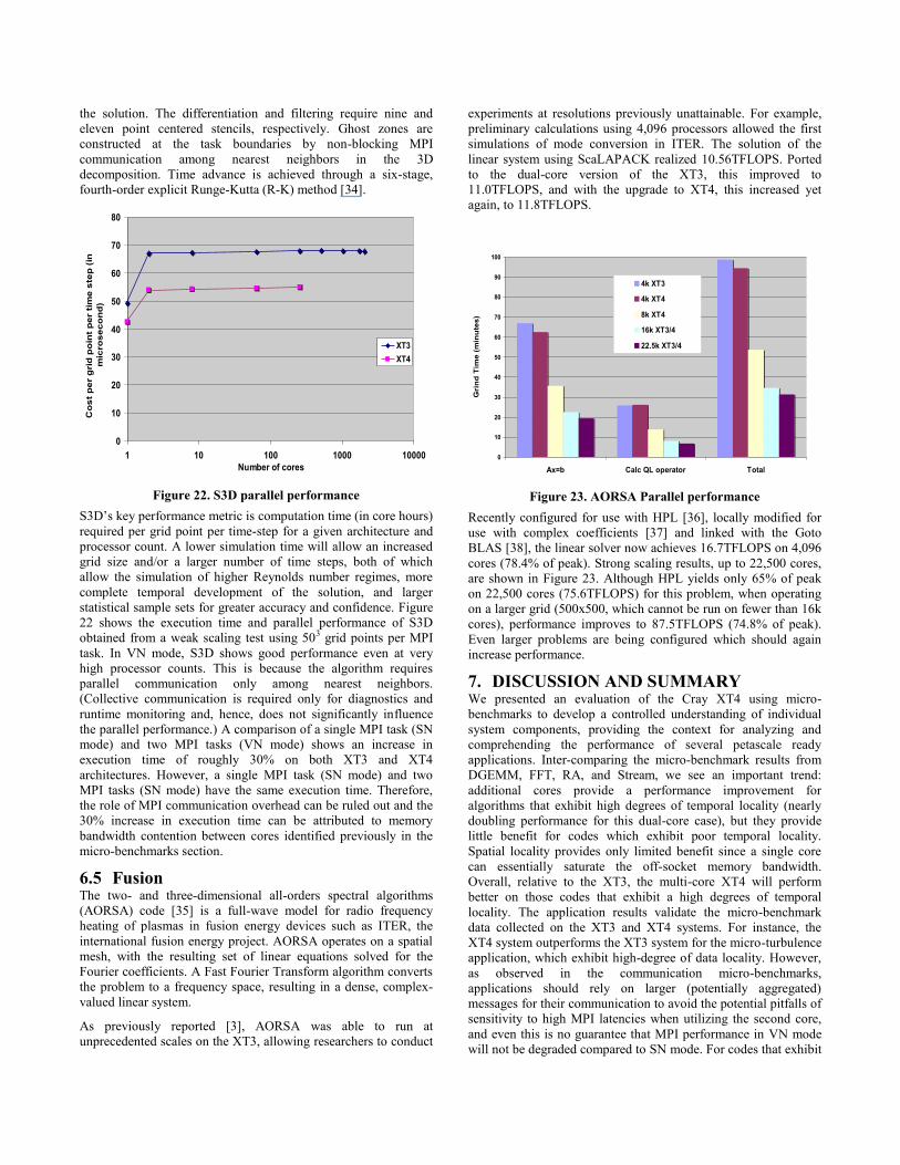
Figure 20. NAMD performance on XT4 vs. XT3

0.001

0.01

0.1

1

64 128 256 512 1024 2048 4096 8192 12000

MP I T as ks

Tim

e (

seco

nd

s)

per

NA

MD

Sim

ula

tio

n T

imeste

p

1M(S N)1M(VN)3M(S N)3M(VN)

Figure 21. NAMD performance impact of SN vs. VN

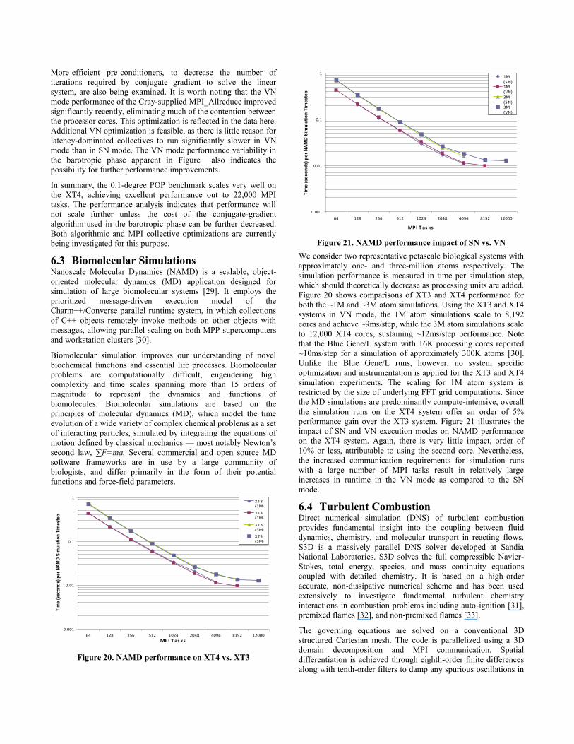
We consider two representative petascale biological systems with

approximately one- and three-million atoms respectively. The

simulation performance is measured in time per simulation step,

which should theoretically decrease as processing units are added.

Figure 20 shows comparisons of XT3 and XT4 performance for

both the ~1M and ~3M atom simulations. Using the XT3 and XT4

systems in VN mode, the 1M atom simulations scale to 8,192

cores and achieve ~9ms/step, while the 3M atom simulations scale

to 12,000 XT4 cores, sustaining ~12ms/step performance. Note

that the Blue Gene/L system with 16K processing cores reported

~10ms/step for a simulation of approximately 300K atoms [30].

Unlike the Blue Gene/L runs, however, no system specific

optimization and instrumentation is applied for the XT3 and XT4

simulation experiments. The scaling for 1M atom system is

restricted by the size of underlying FFT grid computations. Since

the MD simulations are predominantly compute-intensive, overall

the simulation runs on the XT4 system offer an order of 5%

performance gain over the XT3 system. Figure 21 illustrates the

impact of SN and VN execution modes on NAMD performance

on the XT4 system. Again, there is very little impact, order of

10% or less, attributable to using the second core. Nevertheless,

the increased communication requirements for simulation runs

with a large number of MPI tasks result in relatively large

increases in runtime in the VN mode as compared to the SN

mode.

6.4 Turbulent Combustion Direct numerical simulation (DNS) of turbulent combustion

provides fundamental insight into the coupling between fluid

dynamics, chemistry, and molecular transport in reacting flows.

S3D is a massively parallel DNS solver developed at Sandia

National Laboratories. S3D solves the full compressible Navier-

Stokes, total energy, species, and mass continuity equations

coupled with detailed chemistry. It is based on a high-order

accurate, non-dissipative numerical scheme and has been used

extensively to investigate fundamental turbulent chemistry

interactions in combustion problems including auto-ignition [31],

premixed flames [32], and non-premixed flames [33].

The governing equations are solved on a conventional 3D

structured Cartesian mesh. The code is parallelized using a 3D

domain decomposition and MPI communication. Spatial

differentiation is achieved through eighth-order finite differences

along with tenth-order filters to damp any spurious oscillations in

the solution. The differentiation and filtering require nine and

eleven point centered stencils, respectively. Ghost zones are

constructed at the task boundaries by non-blocking MPI

communication among nearest neighbors in the 3D

decomposition. Time advance is achieved through a six-stage,

fourth-order explicit Runge-Kutta (R-K) method [34].

0

10

20

30

40

50

60

70

80

1 10 100 1000 10000

Number of cores

Co

st

pe

r g

rid

po

int

pe

r ti

me

ste

p (

in

mic

ros

ec

on

d)

XT3

XT4

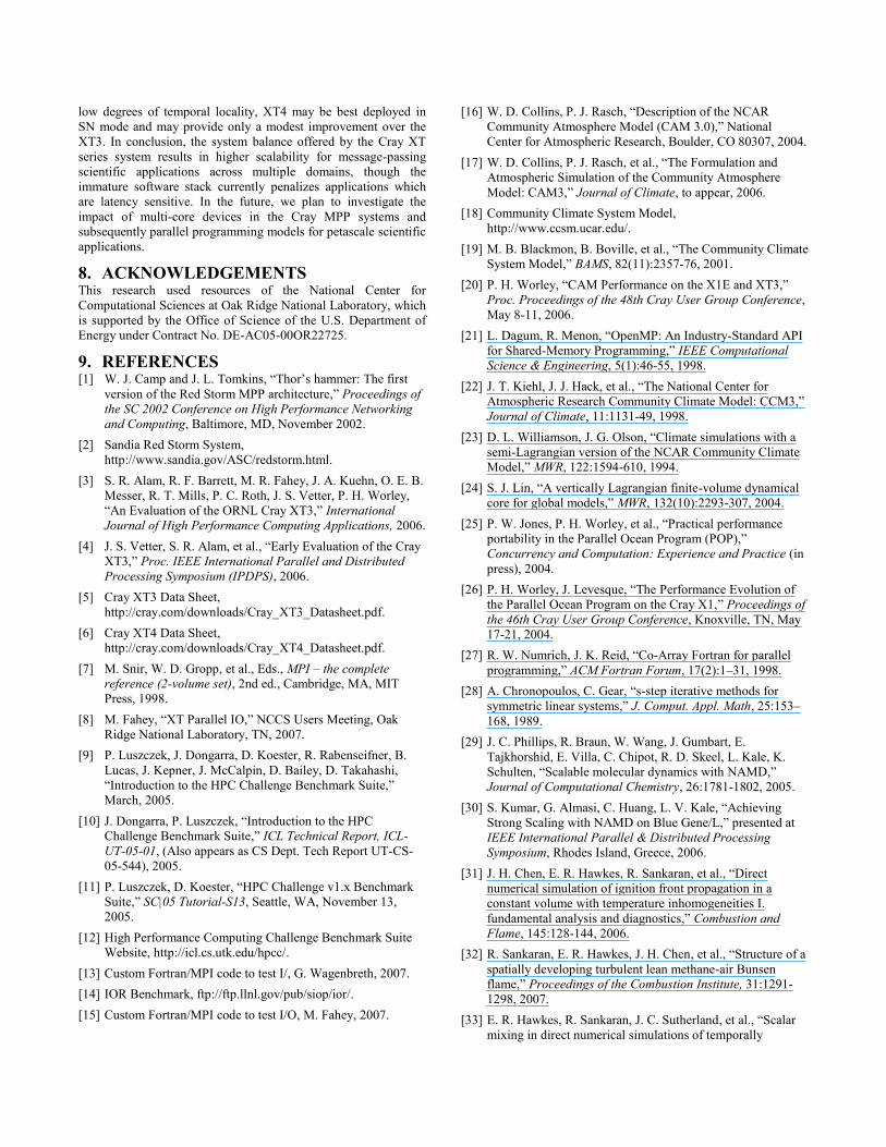
Figure 22. S3D parallel performance

S3D’s key performance metric is computation time (in core hours)

required per grid point per time-step for a given architecture and

processor count. A lower simulation time will allow an increased

grid size and/or a larger number of time steps, both of which

allow the simulation of higher Reynolds number regimes, more

complete temporal development of the solution, and larger

statistical sample sets for greater accuracy and confidence. Figure

22 shows the execution time and parallel performance of S3D

obtained from a weak scaling test using 503 grid points per MPI

task. In VN mode, S3D shows good performance even at very

high processor counts. This is because the algorithm requires

parallel communication only among nearest neighbors.

(Collective communication is required only for diagnostics and

runtime monitoring and, hence, does not significantly influence

the parallel performance.) A comparison of a single MPI task (SN

mode) and two MPI tasks (VN mode) shows an increase in

execution time of roughly 30% on both XT3 and XT4

architectures. However, a single MPI task (SN mode) and two

MPI tasks (SN mode) have the same execution time. Therefore,

the role of MPI communication overhead can be ruled out and the

30% increase in execution time can be attributed to memory

bandwidth contention between cores identified previously in the

micro-benchmarks section.

6.5 Fusion The two- and three-dimensional all-orders spectral algorithms

(AORSA) code [35] is a full-wave model for radio frequency

heating of plasmas in fusion energy devices such as ITER, the

international fusion energy project. AORSA operates on a spatial

mesh, with the resulting set of linear equations solved for the

Fourier coefficients. A Fast Fourier Transform algorithm converts

the problem to a frequency space, resulting in a dense, complex-

valued linear system.

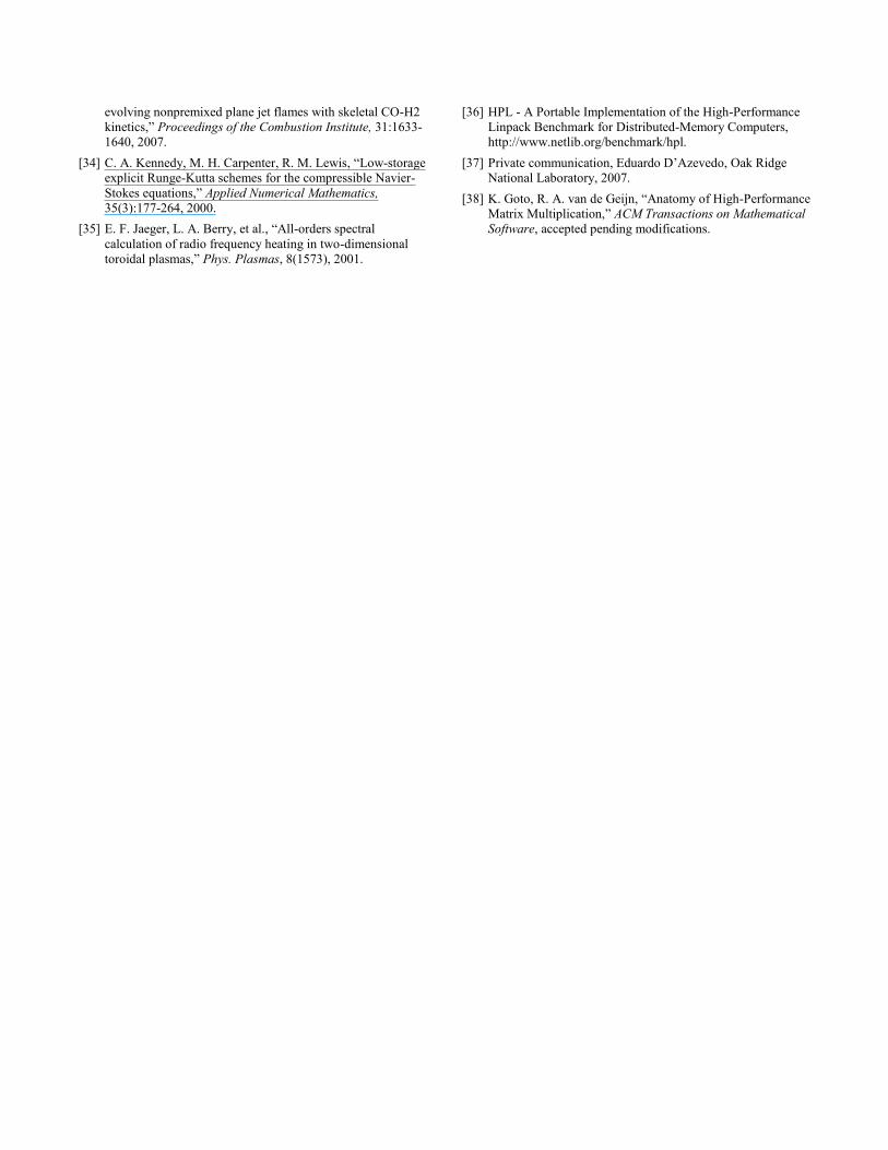
As previously reported [3], AORSA was able to run at

unprecedented scales on the XT3, allowing researchers to conduct

experiments at resolutions previously unattainable. For example,

preliminary calculations using 4,096 processors allowed the first

simulations of mode conversion in ITER. The solution of the

linear system using ScaLAPACK realized 10.56TFLOPS. Ported

to the dual-core version of the XT3, this improved to

11.0TFLOPS, and with the upgrade to XT4, this increased yet

again, to 11.8TFLOPS.

0

10

20

30

40

50

60

70

80

90

100

Ax=b Calc QL operator TotalG

rin

d T

ime

(m

inu

tes

)

4k XT3

4k XT4

8k XT4

16k XT3/4

22.5k XT3/4

Figure 23. AORSA Parallel performance

Recently configured for use with HPL [36], locally modified for

use with complex coefficients [37] and linked with the Goto

BLAS [38], the linear solver now achieves 16.7TFLOPS on 4,096

cores (78.4% of peak). Strong scaling results, up to 22,500 cores,

are shown in Figure 23. Although HPL yields only 65% of peak

on 22,500 cores (75.6TFLOPS) for this problem, when operating

on a larger grid (500x500, which cannot be run on fewer than 16k

cores), performance improves to 87.5TFLOPS (74.8% of peak).

Even larger problems are being configured which should again

increase performance.

7. DISCUSSION AND SUMMARY We presented an evaluation of the Cray XT4 using micro-

benchmarks to develop a controlled understanding of individual

system components, providing the context for analyzing and

comprehending the performance of several petascale ready

applications. Inter-comparing the micro-benchmark results from

DGEMM, FFT, RA, and Stream, we see an important trend:

additional cores provide a performance improvement for

algorithms that exhibit high degrees of temporal locality (nearly

doubling performance for this dual-core case), but they provide

little benefit for codes which exhibit poor temporal locality.

Spatial locality provides only limited benefit since a single core

can essentially saturate the off-socket memory bandwidth.

Overall, relative to the XT3, the multi-core XT4 will perform

better on those codes that exhibit a high degrees of temporal

locality. The application results validate the micro-benchmark

data collected on the XT3 and XT4 systems. For instance, the

XT4 system outperforms the XT3 system for the micro-turbulence

application, which exhibit high-degree of data locality. However,

as observed in the communication micro-benchmarks,

applications should rely on larger (potentially aggregated)

messages for their communication to avoid the potential pitfalls of

sensitivity to high MPI latencies when utilizing the second core,

and even this is no guarantee that MPI performance in VN mode

will not be degraded compared to SN mode. For codes that exhibit

low degrees of temporal locality, XT4 may be best deployed in

SN mode and may provide only a modest improvement over the

XT3. In conclusion, the system balance offered by the Cray XT

series system results in higher scalability for message-passing

scientific applications across multiple domains, though the

immature software stack currently penalizes applications which

are latency sensitive. In the future, we plan to investigate the

impact of multi-core devices in the Cray MPP systems and

subsequently parallel programming models for petascale scientific

applications.

8. ACKNOWLEDGEMENTS This research used resources of the National Center for

Computational Sciences at Oak Ridge National Laboratory, which

is supported by the Office of Science of the U.S. Department of

Energy under Contract No. DE-AC05-00OR22725.

9. REFERENCES [1] W. J. Camp and J. L. Tomkins, ―Thor’s hammer: The first

version of the Red Storm MPP architecture,‖ Proceedings of

the SC 2002 Conference on High Performance Networking

and Computing, Baltimore, MD, November 2002.

[2] Sandia Red Storm System,

http://www.sandia.gov/ASC/redstorm.html.

[3] S. R. Alam, R. F. Barrett, M. R. Fahey, J. A. Kuehn, O. E. B.

Messer, R. T. Mills, P. C. Roth, J. S. Vetter, P. H. Worley,

―An Evaluation of the ORNL Cray XT3,‖ International

Journal of High Performance Computing Applications, 2006.

[4] J. S. Vetter, S. R. Alam, et al., ―Early Evaluation of the Cray

XT3,‖ Proc. IEEE International Parallel and Distributed

Processing Symposium (IPDPS), 2006.

[5] Cray XT3 Data Sheet,

http://cray.com/downloads/Cray_XT3_Datasheet.pdf.

[6] Cray XT4 Data Sheet,

http://cray.com/downloads/Cray_XT4_Datasheet.pdf.

[7] M. Snir, W. D. Gropp, et al., Eds., MPI – the complete

reference (2-volume set), 2nd ed., Cambridge, MA, MIT

Press, 1998.

[8] M. Fahey, ―XT Parallel IO,‖ NCCS Users Meeting, Oak

Ridge National Laboratory, TN, 2007.

[9] P. Luszczek, J. Dongarra, D. Koester, R. Rabenseifner, B.

Lucas, J. Kepner, J. McCalpin, D. Bailey, D. Takahashi,

―Introduction to the HPC Challenge Benchmark Suite,‖

March, 2005.

[10] J. Dongarra, P. Luszczek, ―Introduction to the HPC

Challenge Benchmark Suite,‖ ICL Technical Report, ICL-

UT-05-01, (Also appears as CS Dept. Tech Report UT-CS-

05-544), 2005.

[11] P. Luszczek, D. Koester, ―HPC Challenge v1.x Benchmark

Suite,‖ SC|05 Tutorial-S13, Seattle, WA, November 13,

2005.

[12] High Performance Computing Challenge Benchmark Suite

Website, http://icl.cs.utk.edu/hpcc/.

[13] Custom Fortran/MPI code to test I/, G. Wagenbreth, 2007.

[14] IOR Benchmark, ftp://ftp.llnl.gov/pub/siop/ior/.

[15] Custom Fortran/MPI code to test I/O, M. Fahey, 2007.

[16] W. D. Collins, P. J. Rasch, ―Description of the NCAR

Community Atmosphere Model (CAM 3.0),‖ National

Center for Atmospheric Research, Boulder, CO 80307, 2004.

[17] W. D. Collins, P. J. Rasch, et al., ―The Formulation and

Atmospheric Simulation of the Community Atmosphere

Model: CAM3,‖ Journal of Climate, to appear, 2006.

[18] Community Climate System Model,

http://www.ccsm.ucar.edu/.

[19] M. B. Blackmon, B. Boville, et al., ―The Community Climate

System Model,‖ BAMS, 82(11):2357-76, 2001.

[20] P. H. Worley, ―CAM Performance on the X1E and XT3,‖

Proc. Proceedings of the 48th Cray User Group Conference,

May 8-11, 2006.

[21] L. Dagum, R. Menon, ―OpenMP: An Industry-Standard API

for Shared-Memory Programming,‖ IEEE Computational

Science & Engineering, 5(1):46-55, 1998.

[22] J. T. Kiehl, J. J. Hack, et al., ―The National Center for

Atmospheric Research Community Climate Model: CCM3,‖

Journal of Climate, 11:1131-49, 1998.

[23] D. L. Williamson, J. G. Olson, ―Climate simulations with a

semi-Lagrangian version of the NCAR Community Climate

Model,‖ MWR, 122:1594-610, 1994.

[24] S. J. Lin, ―A vertically Lagrangian finite-volume dynamical

core for global models,‖ MWR, 132(10):2293-307, 2004.

[25] P. W. Jones, P. H. Worley, et al., ―Practical performance

portability in the Parallel Ocean Program (POP),‖

Concurrency and Computation: Experience and Practice (in

press), 2004.

[26] P. H. Worley, J. Levesque, ―The Performance Evolution of

the Parallel Ocean Program on the Cray X1,‖ Proceedings of

the 46th Cray User Group Conference, Knoxville, TN, May

17-21, 2004.

[27] R. W. Numrich, J. K. Reid, ―Co-Array Fortran for parallel

programming,‖ ACM Fortran Forum, 17(2):1–31, 1998.

[28] A. Chronopoulos, C. Gear, ―s-step iterative methods for

symmetric linear systems,‖ J. Comput. Appl. Math, 25:153–

168, 1989.

[29] J. C. Phillips, R. Braun, W. Wang, J. Gumbart, E.

Tajkhorshid, E. Villa, C. Chipot, R. D. Skeel, L. Kale, K.

Schulten, ―Scalable molecular dynamics with NAMD,‖

Journal of Computational Chemistry, 26:1781-1802, 2005.

[30] S. Kumar, G. Almasi, C. Huang, L. V. Kale, ―Achieving

Strong Scaling with NAMD on Blue Gene/L,‖ presented at

IEEE International Parallel & Distributed Processing

Symposium, Rhodes Island, Greece, 2006.

[31] J. H. Chen, E. R. Hawkes, R. Sankaran, et al., ―Direct

numerical simulation of ignition front propagation in a

constant volume with temperature inhomogeneities I.

fundamental analysis and diagnostics,‖ Combustion and

Flame, 145:128-144, 2006.

[32] R. Sankaran, E. R. Hawkes, J. H. Chen, et al., ―Structure of a

spatially developing turbulent lean methane-air Bunsen

flame,‖ Proceedings of the Combustion Institute, 31:1291-

1298, 2007.

[33] E. R. Hawkes, R. Sankaran, J. C. Sutherland, et al., ―Scalar

mixing in direct numerical simulations of temporally

evolving nonpremixed plane jet flames with skeletal CO-H2

kinetics,‖ Proceedings of the Combustion Institute, 31:1633-

1640, 2007.

[34] C. A. Kennedy, M. H. Carpenter, R. M. Lewis, ―Low-storage

explicit Runge-Kutta schemes for the compressible Navier-

Stokes equations,‖ Applied Numerical Mathematics,

35(3):177-264, 2000.

[35] E. F. Jaeger, L. A. Berry, et al., ―All-orders spectral

calculation of radio frequency heating in two-dimensional

toroidal plasmas,‖ Phys. Plasmas, 8(1573), 2001.

[36] HPL - A Portable Implementation of the High-Performance

Linpack Benchmark for Distributed-Memory Computers,

http://www.netlib.org/benchmark/hpl.

[37] Private communication, Eduardo D’Azevedo, Oak Ridge

National Laboratory, 2007.

[38] K. Goto, R. A. van de Geijn, ―Anatomy of High-Performance

Matrix Multiplication,‖ ACM Transactions on Mathematical

Software, accepted pending modifications.