Cray® XC™ Advanced Power Management Updates

Steven J. Martin, Greg J. Koprowski, Dr. Sean J. Wallace

Cray Inc.

{stevem,gkoprowski,swallace}@cray.com

Abstract—This paper will highlight the power managementfeatures of the newest blades for Cray® XC50™ and updatesto the Cray PMDB (Power Management Database). The paperwill first highlight the power monitoring and control featuresof the compute blades. The paper will then highlight powermanagement changes in the SMW 8.0.UP06 release for thePMDB. These database implementation changes enhance thePMDB performance, configuration and management. Thispaper targets system administrators along with researchersinvolved in advanced power monitoring and management,power aware computing, and energy efficiency.

Keywords-Cray Advanced Power Management; Power mon-itoring; power capping;

I. INTRODUCTION

In previous work and Cray publications, we have shown

details of, and documentation for power monitoring and

management features of Cray XC systems [1]–[5]. In this

paper we add to that work with details for Cray XC50

blades, PMDB updates in the SMW 8.0UP06 release, and

new examples using power monitoring and control on Cray

XC50 hardware.

This paper is organized as follows. In Section II we give a

blade agnostic description of Cray XC compute blade power

management features. In Section III some implementation

details are given for the Intel Xeon Scalable Processors

blade for Cray XC50. In Section IV we dive into PMDB

enhancements delivered in the SMW 8.0.UP06 release. Last

in Section V example experiments are shown to illustrate

some of the power management features in use on Cray

XC50 hardware in the Cray Lab in Chippewa Falls, WI.

II. CRAY XC50 COMPUTE BLADE POWER

MANAGEMENT FEATURES

In this section we describe Cray XC50 compute blade

power monitoring and management features. The Cray XC50

supercomputer supports compute blades featuring the newest

generation of CPU and GPU processors:

• NVIDIA® Tesla® P100 PCIe GPUs

• Intel® Xeon® Scalable processors

• Cavium ThunderX2™ processors

The following power management (power and energy

monitoring and control) features will be discussed in some

detail in this section:

• Total node power and energy monitoring

• Aggregate CPU power and energy monitoring

• Aggregate Memory power and energy monitoring

• Publishing of collected power and energy data:

– Out-Of-Band (OOB) via the PMDB

– In-band via /sys/cray/pm counters sysfs files

• Power capping controls

• P-state and C-state controls

A. Total Node Power and Energy Monitoring

All blades developed for the Cray XC platform support

OOB collection of total node power and energy at the blade

level. Data collection is enabled by default on all blade types

with a default collect rate of 1Hz. Collected data feeds into

the data publishing paths described in Subsection II-C below.

B. Aggregate CPU and Memory; Power and Energy Moni-

toring

First introduced in [1], aggregate CPU-domain and

memory-domain power telemetry is supported on blades

with Intel Xeon Scalable processors, and on blades support-

ing the Cavium ThunderX2 processors. As with the design

for the Cray® XC40™ blades supporting the Intel® Xeon

Phi™ processor, XC50™ blade designs have multiple power

rails. Some power rails support only the CPU-domain, some

only the memory-domain, and others are shared. Power for

shared rails is assigned to the dominant consumer. Collection

of aggregate power and energy telemetry data is enabled by

default on blades that support its collection with a default

collection rate of 10Hz. Collected data is published using

the same paths as the node-level telemetry data, which are

described next.

C. Publishing of Collected Power and Energy Data

There are two primary paths for publishing power and

energy telemetry data collected OOB at the blade level.

First, we will describe the OOB path used to publish all the

telemetry collected at the blade level into the Cray PMDB.

This path supports the “High Speed” node-level, and ag-

gregate CPU-domain and memory-domain data described in

Subsections II-A and II-B, as well as blade-level HSS power

and energy, and all System Environment Data Collection

(SEDC) telemetry. The default rate for publishing collected

power and energy data is 1Hz. A maximum rate of 5Hz

is allowed on up-to 48 blades (192 nodes) in a system. The

control is at the blade granularity, and can be changed at the

SMW command line using the xtpmaction utility. By default,

the PMDB is resident on the SMW, but Cray supports

the ability to move the PMDB to an “External PMDB

Node” [4]. Node level energy data, as well as cabinet and

system level power data in the Cray PMDB are exposed via

Cray Advanced Platform Monitoring and Control (CAPMC)

REST interfaces to our workload manager (WLM) vendor

partners. More about CAPMC in subsection II-D.

The second way that power and energy data col-

lected OOB on Cray XC blades is published is the

CLE:/sys/cray/PM counters/ “sysfs” path, which has been

described and used in previous works. [6]–[8] Here are some

details about this path, including some actual counter data

collected from some Cray XC50 compute nodes.

Table I lists all the counter “filenames” you may find

on a given compute node. The table is divided into three

groupings for the purposes of this description: “Metadata

Counters”, “Base Telemetry Counters”, and “Feature Spe-

cific Counters.”

The “Metadata Counters” provide consumers of the raw

sysfs data the ability to insure the counters are working as

expected and to detect event and conditions that are not

communicated by the basic and feature-specific telemetry

counters. For example, a common use case is to read all

of the counters, do some computational work, reread the

counters, then compute values based on those readings, such

as average power or total energy used. The change in the

“freshness” counter can be used to validate the counters have

updated between the first and second reads. If a change in

the “generation” counter is observed, the caller can detect

that the power cap was changed between the first and second

read, even if the power cap was changed and restored to the

original value. A change in the “startup” counter indicates

that the OOB controller was restarted (an extremely rare

edge case), and that no comparisons of other counters can

be considered valid. The “raw scan hz” counter informs the

user of the rate at which all counters should be updating.

It can be used along with an accurate elapsed time when

evaluating the “freshness” counter. The “Metadata Counters”

are present on all Cray XC50 compute blade types.

The “Base Telemetry Counters” provide power, energy,

and power cap data. These counters are present on all

Cray XC50 compute blade types. As noted in the table, a

power cap value of “0” watts is the special case for “NOT

CAPPED”.

The “Feature Specific Counters” are populated

only where the OOB hardware collection of and/or

the feature is present. For example, only nodes

that support an Accelerator will populate the

CLE:/sys/cray/PM counters/accel power cap sysfs file.

Likewise, only select blade types support the Aggregate

CPU and Memory counters.

Next we show the use of grep -v ”not”

/sys/cray/pm counters/* to do the dirty work of printing

the counter filenames and contents with minimal developer

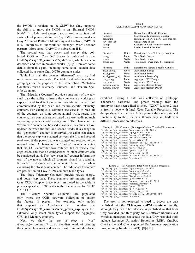
Table ICLE:/SYS/CRAY/PM COUNTERS/ (SYSFS)

Filename Description: Metadata Countersfreshness Monotonically increasing countergeneration Increments on OOB power cap changesraw scan hz Update Rate in Hzstartup Changes on OOB controller restartversion Protocol Version Number

Filename Units Description: Base Telemetry Countersenergy Joules Total Node Energypower Watts Total Node Powerpower cap Watts Total Node Power Cap, 0 is uncapped

Filename Units Description: Feature Specific Countersaccel energy Joules Accelerator Energyaccel power Watts Accelerator Poweraccel power cap Watts Accelerator Power Capcpu energy Joules Aggregate CPU Energycpu power Watts Aggregate CPU Powermemory energy Joules Aggregate Memory Energymemory power Watts Aggregate Memory Power

overhead. Listing 1 data was collected on prototype

ThunderX2 hardware. The power readings from the

prototype have been edited to show “XXX.” Listing 2 data

is from a node with Intel Xeon Scalable Processors. The

dumps show that the two blades present the same data and

functionality to the user even though they are built with

different processor architectures.

Listing 1. PM Counters: (Prototype) Cavium ThunderX2 processors/ s y s / c r a y / pm coun te r s / cpu ene rgy :4921323 J/ s y s / c r a y / pm coun te r s / cpu power :XXX W/ s y s / c r a y / pm coun te r s / e ne r gy :85627470 J/ s y s / c r a y / pm coun te r s / f r e s h n e s s :305224/ s y s / c r a y / pm coun te r s / g e n e r a t i o n : 2 7/ s y s / c r a y / pm coun te r s / memory energy :13529865 J/ s y s / c r a y / pm coun te r s / memory power :XXX W/ s y s / c r a y / pm coun te r s / power :XXX W/ s y s / c r a y / pm coun te r s / power cap : 0 W/ s y s / c r a y / pm coun te r s / raw scan hz : 1 0/ s y s / c r a y / pm coun te r s / s t a r t u p :1524167761885522/ s y s / c r a y / pm coun te r s / v e r s i o n : 2

Listing 2. PM Counters: Intel Xeon Scalable processors/ s y s / c r a y / pm coun te r s / cpu ene rgy :1243834 J/ s y s / c r a y / pm coun te r s / cpu power : 6 6 W/ s y s / c r a y / pm coun te r s / e ne r gy :3186024 J/ s y s / c r a y / pm coun te r s / f r e s h n e s s :326845/ s y s / c r a y / pm coun te r s / g e n e r a t i o n : 1 2/ s y s / c r a y / pm coun te r s / memory energy :409128 J/ s y s / c r a y / pm coun te r s / memory power : 4 W/ s y s / c r a y / pm coun te r s / power : 7 2 W/ s y s / c r a y / pm coun te r s / power cap : 0 W/ s y s / c r a y / pm coun te r s / raw scan hz : 1 0/ s y s / c r a y / pm coun te r s / s t a r t u p :1524658189863550/ s y s / c r a y / pm coun te r s / v e r s i o n : 2

The user is not expected to need to access the data

published into the CLE:/sys/cray/PM counters/ directly,

although they can. The interface is published so that both

Cray provided, and third party, tools, software libraries, and

workload managers can access the data. Cray provided tools

include Resource Utilization Reporting (RUR), CrayPat,

CrayPat-lite and Cray supported Performance Application

Programming Interface (PAPI). [9]–[12]

D. Power Capping Controls

Cray supports power capping on all Cray XC blade types,

including the latest Cray XC50 blades. The base capability

for all blade types is OOB “Node-Level Power Capping.”

Higher level power capping constructs, such as “Job-Level”

and “System-Level” power capping, are built on top of this

basic capability. At the lowest level, the implementation

of node-level power capping is hardware dependent. The

controls available to manage power caps are common and

consistent for all blade types.

The suggested interface for managing power capping on

all Cray XC systems is CAPMC. CAPMC is a RESTful

web service with a published API. Cray provides capmc, a

command line utility that implements CAPMC’s API, along

with the CAPMC service to make it easier for administra-

tors, operators, and processes to use CAPMC. Access to

CAPMC is controlled using X.509 certificates. Setup and

maintenance of the SSL infrastructure is facilitated on the

SMW using the xtmake ca utility. Access and distribution

of certificates must be tightly controlled in accordance with

site security policy. On systems with a properly setup SSL

infrastructure, authorized CAPMC users can typically inter-

act with CAPMC by first setting up their environment using

module load capmc, then using the capmc utility. Third-

party workload manager (WLM) vendors can use CAPMC

to integrate with Cray XC’s advanced platform capabilities,

including power capping.

The other supported method to access power capping on

Cray XC systems is using the xtpmaction utility. This is

an older access method developed to manage static system

power capping. Although this interface is still supported,

sites should only use it to control power capping if CAPMC

is not being used for power capping.

Official Cray documentation for CAPMC, capmc, and

xtpmaction can be found on Cray’s new online documen-

tation server https://pubs.cray.com/ [4], [5], [13].

E. P-state and C-state Controls

Cray supports P-state and C-state controls via native

Linux capabilities under Cray Linux Environment (CLE),

and more specifically under Compute Node Linux (CNL)

running on compute nodes. In addition to the expected

native Linux support that requires escalated privileges, Cray

supports job launch at fixed P-state with the aprun –p-

state=kHz command line for Customers running a WLM

that utilizes the Cray Application Level Placement Scheduler

(ALPS) software suite.

Cray also enables P-state and C-state limiting with

CAPMC. This enables WLM software to dynamically man-

age upper and lower P-state limits and C-state limits at node-

and job-level granularity. This capability provides WLM

software (and other authorized actors) additional tools to

manage power and energy consumption.

Figure 1: Cray XC50 Scalable Processors Blade

Figure 2: Cray XC50 SPDC Block Diagram

III. CRAY XC50 BLADE FEATURING INTEL XEON

SCALABLE PROCESSORS

The Cray XC50 blade that features the Intel Xeon Scal-

able Processors shown in Figure 1 uses two SPDC boards

and a Cray® Aries™ Network Card (ANC) to build a four-

node compute blade. Each Cray XC50 cabinet can support

48 blades (192 Nodes) for a total of 384 processor sockets.

The Cray Scalable Processors Daughter Card (SPDC) is

Cray’s custom designed board to support the Intel Xeon

Scalable Processors in the XC50 blade form factor. The

SPDC block diagram is shown in Figure 2.

Each SPDC comprises two nodes, with two processor

sockets each, and eight DDR4 memory slots in a 2-1-1

configuration across the six memory channels per socket.

Cray supports processor SKUs with varying core counts and

thermal design power (TDP) up to 165 watts.

The SPDC is the first Cray design to use a Vicor [14]

Vcore [15] solution. With this design, the Vcore power rail

is stepped down from the node input at 52 VDC to the socket

input at point of load voltage in one stage. This solution is

beneficial in several ways, but arguably the biggest benefit

is the higher power density it offers with the lower board

space it uses.

The following is a more complete list of benefits:

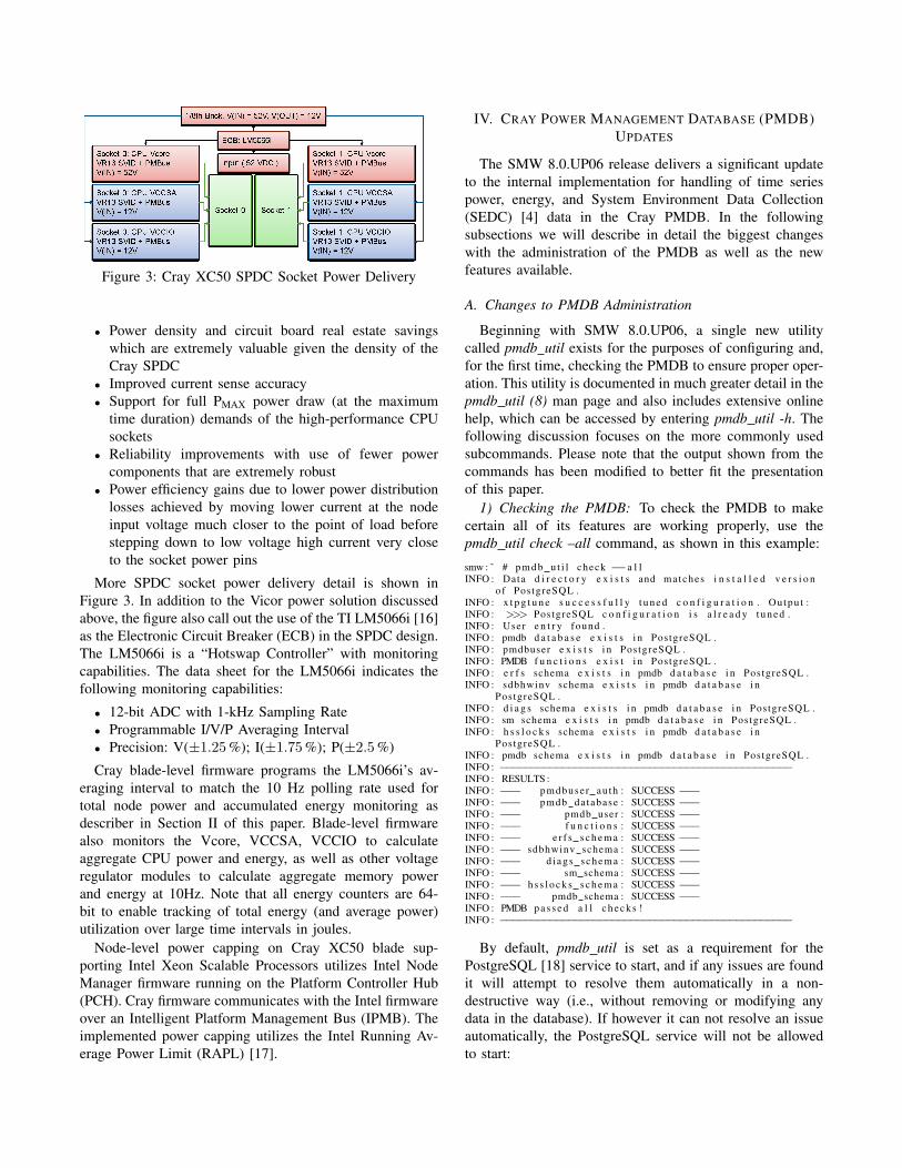
Figure 3: Cray XC50 SPDC Socket Power Delivery

• Power density and circuit board real estate savings

which are extremely valuable given the density of the

Cray SPDC

• Improved current sense accuracy

• Support for full PMAX power draw (at the maximum

time duration) demands of the high-performance CPU

sockets

• Reliability improvements with use of fewer power

components that are extremely robust

• Power efficiency gains due to lower power distribution

losses achieved by moving lower current at the node

input voltage much closer to the point of load before

stepping down to low voltage high current very close

to the socket power pins

More SPDC socket power delivery detail is shown in

Figure 3. In addition to the Vicor power solution discussed

above, the figure also call out the use of the TI LM5066i [16]

as the Electronic Circuit Breaker (ECB) in the SPDC design.

The LM5066i is a “Hotswap Controller” with monitoring

capabilities. The data sheet for the LM5066i indicates the

following monitoring capabilities:

• 12-bit ADC with 1-kHz Sampling Rate

• Programmable I/V/P Averaging Interval

• Precision: V(±1.25%); I(±1.75%); P(±2.5%)

Cray blade-level firmware programs the LM5066i’s av-

eraging interval to match the 10 Hz polling rate used for

total node power and accumulated energy monitoring as

describer in Section II of this paper. Blade-level firmware

also monitors the Vcore, VCCSA, VCCIO to calculate

aggregate CPU power and energy, as well as other voltage

regulator modules to calculate aggregate memory power

and energy at 10Hz. Note that all energy counters are 64-

bit to enable tracking of total energy (and average power)

utilization over large time intervals in joules.

Node-level power capping on Cray XC50 blade sup-

porting Intel Xeon Scalable Processors utilizes Intel Node

Manager firmware running on the Platform Controller Hub

(PCH). Cray firmware communicates with the Intel firmware

over an Intelligent Platform Management Bus (IPMB). The

implemented power capping utilizes the Intel Running Av-

erage Power Limit (RAPL) [17].

IV. CRAY POWER MANAGEMENT DATABASE (PMDB)

UPDATES

The SMW 8.0.UP06 release delivers a significant update

to the internal implementation for handling of time series

power, energy, and System Environment Data Collection

(SEDC) [4] data in the Cray PMDB. In the following

subsections we will describe in detail the biggest changes

with the administration of the PMDB as well as the new

features available.

A. Changes to PMDB Administration

Beginning with SMW 8.0.UP06, a single new utility

called pmdb util exists for the purposes of configuring and,

for the first time, checking the PMDB to ensure proper oper-

ation. This utility is documented in much greater detail in the

pmdb util (8) man page and also includes extensive online

help, which can be accessed by entering pmdb util -h. The

following discussion focuses on the more commonly used

subcommands. Please note that the output shown from the

commands has been modified to better fit the presentation

of this paper.

1) Checking the PMDB: To check the PMDB to make

certain all of its features are working properly, use the

pmdb util check –all command, as shown in this example:

smw : ˜ # p m d b u t i l check −−a l lINFO : Data d i r e c t o r y e x i s t s and matches i n s t a l l e d v e r s i o n

o f PostgreSQL .INFO : x t p g t u n e s u c c e s s f u l l y t u n e d c o n f i g u r a t i o n . Outpu t :INFO : >>> PostgreSQL c o n f i g u r a t i o n i s a l r e a d y t u n e d .INFO : User e n t r y found .INFO : pmdb d a t a b a s e e x i s t s i n PostgreSQL .INFO : pmdbuser e x i s t s i n PostgreSQL .INFO : PMDB f u n c t i o n s e x i s t i n PostgreSQL .INFO : e r f s schema e x i s t s i n pmdb d a t a b a s e i n PostgreSQL .INFO : sdbhwinv schema e x i s t s i n pmdb d a t a b a s e i n

PostgreSQL .INFO : d i a g s schema e x i s t s i n pmdb d a t a b a s e i n PostgreSQL .INFO : sm schema e x i s t s i n pmdb d a t a b a s e i n PostgreSQL .INFO : h s s l o c k s schema e x i s t s i n pmdb d a t a b a s e i n

PostgreSQL .INFO : pmdb schema e x i s t s i n pmdb d a t a b a s e i n PostgreSQL .INFO : −−−−−−−−−−−−−−−−−−−−−−−−−−−−−−−−−−−−−−−−−−−−−−−INFO : RESULTS :INFO : −−− pmdbuser au th : SUCCESS −−−INFO : −−− pmdb database : SUCCESS −−−INFO : −−− pmdb user : SUCCESS −−−INFO : −−− f u n c t i o n s : SUCCESS −−−INFO : −−− e r f s s c h e m a : SUCCESS −−−INFO : −−− sdbhwinv schema : SUCCESS −−−INFO : −−− d iags schema : SUCCESS −−−INFO : −−− sm schema : SUCCESS −−−INFO : −−− h s s l o c k s s c h e m a : SUCCESS −−−INFO : −−− pmdb schema : SUCCESS −−−INFO : PMDB p a s s e d a l l c he c ks !INFO : −−−−−−−−−−−−−−−−−−−−−−−−−−−−−−−−−−−−−−−−−−−−−−−

By default, pmdb util is set as a requirement for the

PostgreSQL [18] service to start, and if any issues are found

it will attempt to resolve them automatically in a non-

destructive way (i.e., without removing or modifying any

data in the database). If however it can not resolve an issue

automatically, the PostgreSQL service will not be allowed

to start:

smw : ˜ # s y s t e m c t l s t a r t p o s t g r e s q lA dependency j o b f o r p o s t g r e s q l . s e r v i c e f a i l e d . See ’

j o u r n a l c t l −xe ’ f o r d e t a i l s .

There are several ways to diagnose the problem, but per-

haps the easiest is to investigate the journalctl -u pmdb util

output. The last start attempt will always be recorded at the

bottom of that output and will include a list of problems that

could not be resolved.

2) Configuring the PMDB: To start fresh and reinitialize

the PMDB, run the pmdb util config –init command. For

example:

smw : ˜ # p m d b u t i l c o n f i g −− i n i tINFO : C o n f i g u r i n g PostgreSQL d a t a d i r e c t o r y . . .INFO : Old d a t a d i r e c t o r y removed .INFO : New d a t a d i r e c t o r y s u c c e s s f u l l y c r e a t e d .INFO : x t p g t u n e s u c c e s s f u l l y t u n e d c o n f i g u r a t i o n . Outpu t :INFO : >>> Wrote backup of / v a r / l i b / p g s q l / d a t a / p o s t g r e s q l .

c on f t o / v a r / l i b / p g s q l / d a t a / p o s t g r e s q l . c on f . bakINFO : >>> Wrote c o n f i g u r a t i o n t o / v a r / l i b / p g s q l / d a t a /

p o s t g r e s q l . c on fINFO : C o n f i g u r i n g pmdbuser a u t h e n t r y . . .INFO : Adding pmdbuser e n t r y t o pg hba . c on f f i l e . . .INFO : User e n t r y added .INFO : C r e a t i n g pmdbuser i n PostgreSQL . . .INFO : C r e a t e d d a t a b a s e u s e r s u c c e s s f u l l y .INFO : C o n f i g u r i n g t h e pmdb d a t a b a s e i n PostgreSQL . . .INFO : C r e a t e d t h e pmdb d a t a b a s e s u c c e s s f u l l y .INFO : I n s t a l l i n g t h e XTPMD schema . . .INFO : XTPMD schema s u c c e s s f u l l y i n s t a l l e d .INFO : I n s t a l l i n g e x t e n s i o n s . . .INFO : xtpmd e x t e n s i o n s i n s t a l l e d .INFO : e r f s e x t e n s i o n s i n s t a l l e d .INFO : I n s t a l l a t i o n o f d i r f d w e x t e n s i o n and t h e d i a g s

schema s u c c e e d e d .INFO : sbdhwinv e x t e n s i o n i n s t a l l e d .INFO : h s s l o c k s e x t e n s i o n i n s t a l l e d .INFO : −−−−−−−−−−−−−−−−−−−−−−−−−−−−−−−−−−−−−−−−−−−−−−−INFO : PMDB I n i t i a l i z a t i o n SUCCEEDEDINFO : −−−−−−−−−−−−−−−−−−−−−−−−−−−−−−−−−−−−−−−−−−−−−−−

Any facet of the PMDB can be configured by using

pmdb util config with one or more of the specific options.

For more information, enter the pmdb util config -h com-

mand.

After configuration, there are additional ”runtime” options

that can be found in the file pmdb migration.conf in the

/var/adm/cray/pmdb migration/ directory. Most are self ex-

planatory, but there are a few that deserve special mention.

The first is PMDB MAX SIZE, which is the new method

by which data retention is controlled. Rather than having to

compute estimated storage requirements, the power manage-

ment daemons now monitor the total size of the PMDB. If

the size reaches this value or higher, data from the PMDB

will be dropped in increments of the chunk time interval

starting from the oldest data until the total size is less than

this value.

In the previous generation of PMDB jobs data

would be dropped when there was no remaining power

data that it could be related to. A new setting,

PMDB JOBS NUM DAYS, changes this behavior so that

jobs information is kept for the number of specified days (or

forever is this is set to 0). If the system administrator sets

PMDB JOBS NUM DAYS=0, they must then take on the

responsibility of pruning data from the pmdb.job info and

pmdb.job timing tables to prevent job data from growing so

large that disk space is not available for other telemetry. The

default setting is to keep 30 days of job related data.

B. Integration of TimescaleDB

PostgreSQL is an object-relational database management

system (ORDBMS) that is used by the PMDB to store data.

It is best suited towards a high frequency update workload.

Database engines of this type have poor write performance

for large tables with indexes, and as these tables grow this

problem worsens as table indexes no longer fit into memory.

This results in every table insert performing many disk

fetches swapping in and out portions of an index’s B-Tree.

Indexing is a necessity otherwise every query targeting any

portion of the database would require a sequential scan of

the entire database, a potentially very wasteful action when

only a subset of the data is required.

Time-series databases are very regularly used as a solution

to this problem. They are designed for fast ingest and

fast analytical queries over almost always a single column

(hence, key/value). This works very well for analytics on a

single metric or some aggregate metric, but this leads to a

lack of a rich query language or secondary index support. A

lack of secondary index support means that queries targeting

multiple fields are much less efficient and often result in

entire tables being scanned.

One of the major functions of the PMDB is the storage

of time-series power data, and one of the most common

use cases is the joining of raw power data along with job

info. As a result, we have been continually faced with the

challenge of optimizing for the efficient ingest of potentially

large collections of data as well as efficient querying of that

data in multiple contexts.

Up to this point, our solution to the ingest problem was

relatively simple; it’s a non-trivial task to generate an index

on a very large table, whereas smaller tables take much less

effort to generate indexes. In this way, we set up the database

to abstract the idea of a single large continuous table into

smaller partitions that made index generation not only much

faster, but also an action that could be performed in the

background. This approach worked well to solve the scaling

issues, however it still relied entirely on indexing for efficient

querying.

TimescaleDB [19]–[21] is an open-source project that

aims to approach this problem differently. Instead of try-

ing to build yet another time-series database, they instead

focused on extending PostgreSQL providing time-series

features while retaining all of the PostgreSQL features and

reliability that has been built up over the past 20 years. In a

similar fashion as our previous implementation, Timescale

partitions data into smaller chunks to abstract the idea of a

single continuous table. Unlike our approach, however, this

partitioning is done by time instead of a maximal number

of rows.

This time based partitioning offers a number of potential

advantages with one of the most immediately beneficial of

them being aggressive query optimization. Since Timescale

integrates with PostgreSQL at the extension level, it has the

ability to better inform the query planner where data resides.

Essentially, since Timescale knows exactly what time range

each partition holds, any query that targets a specific range

of time can be optimized to only scan those chunks that

could possibly contain the data.

To demonstrate the potential of this approach, consider

the following query which counts the number of samples

per minute over a several day period for a specific sensor:

SELECT d a t e t r u n c ( ’ minu te ’ , t s ) a s t ime , COUNT( * )FROM pmdb . b c d a t aWHERE t s BETWEEN ’2017−07−11 0 0 : 0 0 : 0 0 ’

AND ’2017−07−13 0 0 : 0 0 : 0 0 ’AND i d = 16GROUP BY t ime ORDER BY t ime DESC ;

Because Timescale knows exactly where the data resides

for this block of time and this sensor, it only has to do a

sequential scan on 8 chunks. A system without Timescale

would have to do an index scan on over 1,000 child table

indexes and then sequentially scan each applicable partition

to match on the id. For this query and data set, this

optimization resulted in a savings of nearly 3.5 minutes or

a speedup of 6.86x.

This optimization is possible with or without indexing,

meaning most queries that target ranges of time can expect

a 2x speedup in query execution time with certain queries

seeing much more than that.

1) Determining Database Contents: With the previous

partition method, it was rather simple to compute what data

resided in the PMDB. With Timescale, it’s still possible

to figure this out, but the process is slightly less straight

forward. It has always been possible to determine the total

size of the database:

pmdb=> SELECT p g s i z e p r e t t y ( p g d a t a b a s e s i z e ( ’pmdb ’ ) ) ;p g s i z e p r e t t y−−−−−−−−−−−−−−−−500 GB(1 row )

It is also easy to check the size of each table:

pmdb=> s e l e c t * frompmdb−> h y p e r t a b l e r e l a t i o n s i z e p r e t t y ( ’pmdb . b c d a t a ’ ) ;

t a b l e s i z e | i n d e x s i z e | t o a s t s i z e | t o t a l s i z e−−−−−−−−−−−−+−−−−−−−−−−−−+−−−−−−−−−−−−+−−−−−−−−−−−−

234 GB | 101 GB | | 335 GB(1 row )

All of the metadata that Timescale uses to deter-

mine which chunks data belongs to is housed in the

timescaledb catalog table schema. For example, one can

use the information in these child tables to figure out exactly

what range of time each chunk contains (full timestamps are

abbreviated to save space):

smw:˜> p s q l pmdb pmdbuser −c ”> s e l e c t h y p e r t a b l e . t a b l e n a m e as pmdb table ,> chunk . t a b l e n a m e as t i m e s c a l e t a b l e ,> t o c h a r ( t o t i m e s t a m p ( r a n g e s t a r t / 1 0 0 0 0 0 0 ) , ’HH: MI ’ )> as s t a r t ,> t o c h a r ( t o t i m e s t a m p ( range end / 1000000) , ’HH: MI ’ )> as end> from t i m e s c a l e d b c a t a l o g . chunk> i n n e r j o i n t i m e s c a l e d b c a t a l o g . c h u n k c o n s t r a i n t> on chunk . i d = c h u n k c o n s t r a i n t . chunk id> i n n e r j o i n t i m e s c a l e d b c a t a l o g . d i m e n s i o n s l i c e> on c h u n k c o n s t r a i n t . d i m e n s i o n s l i c e i d => d i m e n s i o n s l i c e . i d> i n n e r j o i n t i m e s c a l e d b c a t a l o g . h y p e r t a b l e> on chunk . h y p e r t a b l e i d = h y p e r t a b l e . i d> o r d e r by r a n g e s t a r t de sc l i m i t 8 ;> ” ;

pmdb tab le | t i m e s c a l e t a b l e | s t a r t | end−−−−−−−−−−−−−−+−−−−−−−−−−−−−−−−−−−−−−+−−−−−−−+−−−−−−−

b c d a t a | hyper 1 16546 chunk | 05 :30 | 06 :00c c s e d c d a t a | hyper 4 16548 chunk | 05 :30 | 06 :00b c s e d c d a t a | hyper 3 16545 chunk | 05 :30 | 06 :00c c d a t a | hyper 2 16547 chunk | 05 :30 | 06 :00c c s e d c d a t a | hyper 4 16542 chunk | 05 :00 | 05 :30b c s e d c d a t a | hyper 3 16541 chunk | 05 :00 | 05 :30c c d a t a | hyper 2 16543 chunk | 05 :00 | 05 :30b c d a t a | hyper 1 16544 chunk | 05 :00 | 05 :30

(8 rows )

The above output shows the last two chunks of time

(05:00 - 06:00 and 05:30 to 06:00) for each of the four

tables that house power data. The actual data for each of

these chunks resides in the timescaledb internal schema,

and these tables can be treated as any other normal table.

For example, to find out how many rows there are in the

first chunk of the last result:

pmdb=# s e l e c t c o u n t ( * )pmdb−# from t i m e s c a l e d b i n t e r n a l . hyper 1 16546 chunk ;c o u n t−−−−−−−−544842(1 row )

V. CRAY POWER MANAGEMENT USAGE EXAMPLES

The previous sections in this paper have described many

of the power monitoring and control features of the Cray

XC50 system. In this section we show some examples of

using some of the monitoring and control features. In Sub-

section V-A we show and example with some experimenta-

tion running an unoptimized version of the industry standard

stream memory benchmark over the range of supported

frequencies of the Cray XC50 test system featuring Intel

Xeon Scalable Processors. Then in Subsection V-B we use

the same test system and nodes to show the use of power

capping controls to modify the power ramp rate at job startup

for nodes running a Cray diagnostics build of xhpl.

A. Stream examples using P-States

In this subsection, we show two simple examples of run-

ning stream with different “P-State” (or frequency) settings.

The two examples will differ in how the frequency is set,

and we also show some different ways of looking at power

profiles collected for the test runs.

First, we show the use of selecting a “P-State” at job

launch. The test system was configured to support the qsub.

We used the qsub command to launch a scrip that makes use

of the Cray aprun command, which is part if the Cray Ap-

plication Level Placement Scheduler (ALPS) software suite.

Listing 3 shows the simple bash script used in this experi-

ment. The script first uses gcc to compile stream.c as down-

loaded from https://github.com/jeffhammond/STREAM. The

option -DNTIMES=2048 is used extend the time of each test

iteration to just under two minutes. The script then iterates

over a list for supported processor frequencies for the nodes

in the test system passing the requested frequency (in kHz)

via the aprun –p-state=kHz option. The script then injects

a 20 second delay between iterations.

This experiment could also be implemented on a system

using SLURM job launch, using the –cpu-freq option.

Listing 3. do run streamu s e r : ˜ / STREAM> c a t d o r u n s t r e a m# ! / b i n / bash## qsub −l n o d e s =12: ppn=1 . / d o r u n s t r e a m

cd / home / u s e r s / u s e r /STREAM

gcc −O −DSTREAM ARRAY SIZE=100000000 \−DNTIMES=2048 \−fopenmp s t r e a m . c \−o stream omp DNT 2048

f o r xxx i n 2101000 2100000 2000000 \1900000 1800000 1700000 \1600000 1500000 1400000 \1300000 1200000 1100000 1000000

do

aprun −n 12 −N 1 −cc none −−p−s t a t e =$xxx \. / stream omp DNT 2048 | t e e sweep . $$ . $xxx . SK48 stream

s l e e p 20done

Figure 4 shows the power profile for stream on our test

system, running on 12 Cray XC50 nodes with Intel Xeon

Scalable Processors. The power profile was generated from

data in the Cray PMDB. The blue lines in Figure 4 show (at

1Hz) total node power data average of 12 nodes, maximum

node power, and minimum node power for each of the 13

stream iterations. The red lines are minimum-, average-, and

maximum-CPU power, and the green lines show the same

for memory power. One observation that stands out from this

data is that the memory power is consistently high over all of

the tested CPU frequencies. And unlike the memory power,

the CPU and total node power decrease as the frequency is

reduced.

This is not a performance paper, but when we look at

the stream output files, the results are in line with the

memory power, in that they are not highly correlated with the

CPU frequency. Figure 5 shows that the “Best Rate MB/s”

performance data output from the (unoptimized) stream test

is flat over the supported CPU frequency range.

Figure 4: Stream Power Profile (ALPS)

Figure 5: Relative (Best Rate MB/s) performance

Figure 6: Example 1: Stream Power Profile (CAPMC)

In Listing 4 we show test script that supports the use of

CAPMC to iterate over supported frequency settings. The

script starts with the maximum Turbo Frequency (2101000),

lowers frequencies by iterating over the $FREQ H2L list,

and then from minimum frequency back to the maximum

iterating over the $FREQ L2H list. The underlying work

is done by the call to capmc set freq limits -n $NIDS -m

1000000 -M $xxx. The script was run on the test system’s

SMW as user:crayadm, it could be run on properly con-

figured service nodes by an authorized user. This CAPMC

functional is targeted at third party WLM vendors, or

researchers with escalated privileges.

Listing 4. CAPMC Frequency Walking Script# ! / b i n / bashSLEEP TIME=20FREQ H2L=” 2101000 2100000 2000000 1900000 \

1800000 1700000 1600000 1500000 1400000 \1300000 1201000 1100000 1000000 ” ;

FREQ L2H=” 1000000 1100000 1200000 1300000 \1400000 1500000 1600000 1700000 1800000 \1900000 2000000 2100000 2101000 ” ;

NIDS=” 2 8 , 2 9 , 3 0 , 3 1 , 6 8 , 6 9 , 7 0 , 7 1 , 1 0 4 , 1 0 5 , 1 0 6 , 1 0 7 ”

d o i t ( ) {s l e e p $SLEEP TIME ;f o r xxx i n $FREQ H2L $FREQ L2H ;do

echo −n ” $xxx : ” ; d a t e ;capmc s e t f r e q l i m i t s −n $NIDS −m 1000000 −M $xxx ;s l e e p $SLEEP TIME

done}{ l s t : SK48 PCAP walk}module l o a d capmc ;

In Figure 6 we show the resulting power profile for a

test run where the test script described above was run after

the test started. As with the previous runs using “P-State”

at job launch, the memory power and streams performance

are not lowered as the frequency is changed, but the total

node power and CPU power are reduced. Stream is designed

to be memory bandwidth bound, so these findings are not

unexpected. This example shows how power and frequency

profiling can be done on the Cray XC systems.

B. Xhpl examples using Power Capping

Next, we show an example of using the CAPMC API

to do power capping. The goal in this example is to show

how power capping controls work in general by shaping

the power consumption of a compute intensive application

job launch. The test binary selected is the Cray xhpl binary

distributed with the Cray diagnostics package. The script

shown in Listing 5 was run on the test system’s SMW as

user:crayadm. The script first applies the minimum power

cap and then prompts the user to “Enter to continue: ”, then

after the user hits enter it steps the power cap up in 5 watt

increments, with a 5 second delay at each step.

We used the following test procedure:

1) login-node: Using qsub -I get an interactive allocation

of test nodes that matches the “$NIDS” list in the

power capping script.

2) SMW-crayadm: After the qsub -I completes, start

the power capping script and wait for the “Enter to

continue: ” prompt. Do not hit enter yet.

3) login-node: Start the xhpl job from inside the alloca-

tion from the call to qsub -I in step 1.

4) SMW-crayadm: Now hit enter at the “Enter to con-

tinue: ” prompt. The power capping script should

complete about half way through the xhpl test run.

Listing 5. CAPMC Power Cap Ramp Up Script# ! / b i n / bash: ${SLEEP TIME=5} ; : ${PCAP STEP=5} ;: ${PCAP MIN=240} ; : ${PCAP MAX=425} ;: ${NIDS=” 2 8 , 2 9 , 3 0 , 3 1 , 6 8 , 6 9 , 7 0 , 7 1 , 1 0 4 , 1 0 5 , 1 0 6 , 1 0 7 ” } ;

s e t c a p ( ) {echo −n ” $1 , $2 : ” ; d a t e ;capmc s e t p o w e r c a p −n $1 −−node $2s l e e p $SLEEP TIME

}

d o i t ( ) {s e t c a p $NIDS $PCAP MIN ;echo −n ” E n t e r t o c o n t i n u e : ” ; r e a df o r ( ( xxx=PCAP MIN ; xxx <= PCAP MAX; xxx += PCAP STEP ) )do

s e t c a p $NIDS $xxxdones e t c a p $NIDS 0 ;

}

module l o a d capmc ;d o i t

Figure 7 shows an aggregate view of data from all 12

nodes running xhpl with the power capping script modifying

the the job power up ramp rate. The data from PMDB

is averaged for all nodes in 6 second time buckets, and

average power, maximum power, and minimum power are

shown using gnuplot “errorlines”, the group by time bucket

function provided by the PostgreSQL extension is used

by the SQL query from PMDB. We think this graphic

representation shows interesting insight into data, especially

when looking at jobs with much larger node counts.

Figure 8 gives a different view of the same data, this

time displaying the 1Hz data directly out of PMDB but

selectively showing only the data for three of the twelve

nodes. The three selected nodes were selected by the script

that generated the plots by first sorting the nodes by total

energy used, then picking the the nodes from the top, bottom,

and middle of the list.

The node-minimum and node-maximum data shown using

the gnuplot “errorlines” in Figure 7 and again in the node-

level data in Figure 8 both seem to show regions with more

and less noisy behavior in the power ramp up. This might

me an interesting subject for additional research on power

capping.

Finally, Figure 9 shows the xhpl test program running on

the same nodes of the test system, this time without power

capping. This shows the near instantaneous per-node power

ramp up from less then 50 watts per node to over 400 watts

per node.

The examples shown in this paper are simple, and in-

tended to show some Cray XC50 power management ca-

pabilities in a way that can be useful to a wide audience.

We believe the real-world use cases that these capabilities

support are very important to the Cray user community.

Figure 7: Xhpl Power Profile (aggregate view)

Figure 8: Xhpl Power Profile (node view)

Figure 9: Xhpl Power Profile (no capping)

VI. CONCLUSION

This paper has provided an overview and updated descrip-

tion of the power management features of the Cray XC50

system, focusing mostly on the Cray XC50 compute blades.

The paper started with a general description of features, then

focusing in more detail on the features of the Cray XC50

blade that supports the Intel Xeon Scalable Processors. An

update was then provided for the Cray PMDB with some

details on how the design was changed to leverage the Time

Scale extension for PostgreSQL, and related PMDB configu-

ration management tool changes. Finally the paper provided

two examples of using power management monitoring and

control features on a Cray XC50 system. We are committed

to providing the power and energy monitoring and control

features needed for leadership class HPC systems. We en-

courage the user community to use these features and give

us feedback on how we can improve, add new capabilities,

and together solve new challenges.

REFERENCES

[1] S. Martin, D. Rush, M. Kappel, M. Sandstedt, andJ. Williams, “Cray XC40 Power Monitoring and Controlfor Knights Landing,” Proceedings of the Cray UserGroup (CUG), 2016, (Accessed 22.March.17). [Online].Available: https://cug.org/proceedings/cug2016 proceedings/includes/files/pap112s2-file1.pdf

[2] S. Martin, D. Rush, and M. Kappel, “Cray Advanced PlatformMonitoring and Control (CAPMC),” Proceedings of the CrayUser Group (CUG), 2015, (Accessed 24.Aprl.18). [Online].Available: https://cug.org/proceedings/cug2015 proceedings/includes/files/pap132.pdf

[3] S. Martin, C. Whitney, D. Rush, and M. Kappel, “How towrite a plugin to export job, power, energy, and systemenvironmental data from your cray xc system,” Concurrencyand Computation: Practice and Experience, vol. 30, no. 1,p. e4299. [Online]. Available: https://onlinelibrary.wiley.com/doi/abs/10.1002/cpe.4299

[4] “XC Series Power Management and SEDCAdministration Guide (CLE 6.0.UP06) S-0043,” (Accessed 6.April.18). [Online]. Avail-able: https://pubs.cray.com/pdf-attachments/attachment?pubId=00529040-DB&attachmentId=pub 00529040-DB.pdf

[5] CAPMC API Documentation, (CLE 6.0UP06) S-2553, Cray Inc., (Accessed 9.May.18). [Online].Available: https://pubs.cray.com/content/S-2553/CLE%206.0.UP06/capmc-api-documentation

[6] G. Fourestey, B. Cumming, L. Gilly, and T. C. Schulthess,“First experiences with validating and using the cray powermanagement database tool,” arXiv preprint arXiv:1408.2657,2014, (Accessed 24.Aprl.18). [Online]. Available: http://arxiv.org/pdf/1408.2657v1.pdf

[7] A. Hart, H. Richardson, J. Doleschal, T. Ilsche, M. Bielert,and M. Kappel, “User-level power monitoring andapplication performance on cray xc30 supercomputers,”Proceedings of the Cray User Group (CUG), 2014,(Accessed 31.March.16). [Online]. Available: https://cug.org/proceedings/cug2014 proceedings/includes/files/pap136.pdf

[8] S. Martin and M. Kappel, “Cray XC30 Power Monitoringand Management,” Proceedings of the Cray UserGroup (CUG), 2014, (Accessed 24.Aprl.18). [Online].Available: https://cug.org/proceedings/cug2014 proceedings/includes/files/pap130.pdf

[9] “CrayPAT: Cray Performance Measurement and Anal-ysis,” Cray Inc., (Accessed 29.Apr.18). [Online].Available: https://pubs.cray.com/pdf-attachments/attachment?pubId=00505504-DA&attachmentId=pub 00505504-DA.pdf

[10] “PAPI: Performance Application Programming Interface,”(Accessed 25.Apr.18). [Online]. Available: http://icl.cs.utk.edu/papi/

[11] M. Bareford, “Monitoring the Cray XC30 power managementhardware counters,” Proceedings of the Cray UserGroup (CUG), 2015, (Accessed 29.Apr.18). [Online].Available: https://cug.org/proceedings/cug2015 proceedings/includes/files/pap125.pdf

[12] S. P. Jammy, C. T. Jacobs, D. J. Lusher, and N. D. Sandham,“Energy efficiency of finite difference algorithms on multicorecpus, gpus, and intel xeon phi processors,” arXiv preprintarXiv:1709.09713, 2017.

[13] “Cray technical documentation,” (Accessed 26.April.18).[Online]. Available: https://pubs.cray.com/

[14] “Vicorpower,” (Accessed 17.Apr.18). [Online]. Available:http://www.vicorpower.com

[15] “High Current, Low Voltage Solution For MicroprocessorApplications from 48V Input,” (Accessed 17.Apr.18).[Online]. Available: http://www.vicorpower.com/documents/whitepapers/whitepaper2.pdf

[16] “LM5066I 10 to 80 V Hotswap Controller WithI/V/P Monitoring and PMBus Interface,” (Accessed28.April.18). [Online]. Available: http://www.ti.com/lit/ds/symlink/lm5066i.pdf

[17] “Intel 64 and IA-32 architectures software developer’smanual, volume 3b: System programming guide,part 2, order number: 253669-047US,” (Accessed11.Apr.14). [Online]. Available: http://download.intel.com/products/processor/manual/253669.pdf

[18] “PostgreSQL,” (Accessed 12.May.18). [Online]. Available:http://www.postgresql.org/

[19] “Timescaledb GitHub,” (Accessed 12.Apr.18). [Online].Available: https://github.com/timescale/timescaledb

[20] “TimescaleDB Documentation,” (Accessed 12.Apr.18).[Online]. Available: https://docs.timescale.com/v0.9/main

[21] “Timescale,” (Accessed 12.Apr.18). [Online]. Available: