ARTICLE IN PRESS

Available at www.sciencedirect.com

B I O M A S S A N D B I O E N E R G Y 3 2 ( 2 0 0 8 ) 3 1 4 – 3 2 5

0961-9534/$ - see frodoi:10.1016/j.biomb

�Corresponding autE-mail address: r

http://www.elsevier.com/locate/biombioe

Cotton logistics as a model for a biomasstransportation system

Poorna P. Ravula, Robert D. Grisso�, John S. Cundiff

Biological Systems Engineering, Virginia Tech, Blacksburg, VA 24061-0303, USA

a r t i c l e i n f o

Article history:

Received 15 August 2006

Received in revised form

24 October 2007

Accepted 30 October 2007

Available online 20 December 2007

Keywords:

Cotton

Modules

Discrete event

Simulation

Optimization

Knapsack

Biomass logistics

Greedy algorithm

Inventory control

nt matter & 2007 Elsevieioe.2007.10.016

hor. Tel.: +1 540 231 6538;grisso@vt.edu (R.D. Griss

a b s t r a c t

To reach the US Department of Energy’s goal of replacing 30% of current petroleum

consumption by biomass and its products by year 2030, various systems capable

of harvesting, storing and transporting biomass efficiently, at a low cost, need to

be designed. The transportation system of a cotton gin, which shares several key

components with a biomass transportation system, was simulated using a discrete event

simulation procedure, to determine the operating parameters under various management

practices.

The cotton module transportation system, when operating under a FIFO management

plan, was found to operate at 77% utilization factor, while the actual ginning

process operated at 69%. Two greedy algorithm-based management policies were

simulated, which increased the gin operational factor to 100%, but doing so required

an increase in gin inventory level. A knapsack model, with travel times, was constructed

and solved to obtain the lower bound for the transportation system. The significance of

these operating parameters and their links to a biomass transportation system are

presented.

Using the new management strategies, the utilization factor for the transportation

system was increased to 99%. To achieve this improvement, the transportation manager

must know where all modules are located and have the ability to dispatch a hauler to any

location.

& 2007 Elsevier Ltd. All rights reserved.

1. Background

The United State’s economic growth depends on continuous

availability of low-cost energy. This need for lower cost energy

has assumed increased significance in the current economic

and political environment. More than 85% of energy con-

sumed in year 2005 in the United States was from fossil fuels,

namely coal, petroleum, and natural gas. Six percent of

energy was produced from renewable resources, of which

alcohol fuel was a mere 6% of the renewable energy total [1].

The US Department of Energy’s Biomass Research and

Development Committee has set a goal of replacing 30% of

r Ltd. All rights reserved.

fax: +1 540 231 3199.o).

the current petroleum consumption with fuel created from

biomass by the year 2030 [2]. To achieve this goal, various

systems capable of harvesting, storing, and transporting large

quantities of biomass have to be designed and built.

The supply logistics of an agricultural commodity consists

of multiple harvesting, storage, pre-processing, and transport

operations. Supply logistics are characterized by a randomly

distributed raw material; time and weather-sensitive crop

maturity; variable moisture content; low bulk density of

agricultural materials and a short time window for collection

with competition from concurrent harvest operations. An

optimized collection, storage and transport network ensures

ARTICLE IN PRESS

B I O M A S S A N D B I O E N E R G Y 3 2 ( 2 0 0 8 ) 3 1 4 – 3 2 5 315

timely supply at minimum cost. To this end, many have used

simulation models to analyze and optimize these complex

systems. These models have been successfully applied to

commodities such as sugar [3–7], cotton [8,9], energy crops

[9–27], grains/forage [28,29], and wood products [30–33]. These

results provide needed estimates for business planning and to

attract investment capital required for a biorefinery.

There are no commercial fiber-to-ethanol conversion plants

in operation today, which can be used as a baseline model

for the transportation system. However, the transportation

system of a cotton gin uses several components, or sub-

systems, that a fiber-to-ethanol system envisioned in this

study will use. Most notably, both systems use trucks capable

of road speeds to haul modularized loads. Therefore, a study

was developed to review the current transportation system of

a gin in Southeastern Virginia to gather operating parameters

for a fiber-to-ethanol conversion system.

1.1. Cotton collection and harvest

Cotton is usually harvested with a machine that pulls the

fiber from the plant. Seeds, parts of the bole, and pieces of

stalk and leaves are also collected during harvest. This

material is collected in a dump bin on the harvester and is

emptied into a dump trailer as needed. The dump trailer

transports this material to a module builder, usually located

at the edge of a field. The module builder compresses this

material into 2.4 m wide�2.4 m high�6.1 m long blocks

known as cotton modules, with each module weighing

anywhere from 4.5 to 8.2 Mg, depending on moisture content

and other factors.

These modules rest on the ground and are covered with a

fitted canvas or plastic cover to protect against rain. The

Fig. 1 – Location of cotton fields shown as dots an

modules remain on the farm until they are transported to the

gin by module haulers.

1.2. Cotton module transport

Module haulers are ‘‘live-bottom’’ trucks designed to pull the

truck bed back under the module, thus lifting it up onto the

bed. The bed is then lowered to the horizontal position and

the truck transports the module to the gin for processing.

With the current transportation system, the gin owns and

operates these module haulers. Typically, when farmers have

several modules built, they notify the gin and request pickup.

The gin then schedules the module haulers to transport these

new modules as soon as all previously scheduled modules are

transported. That is, all modules are picked up on a first-in,

first-out (FIFO) basis.

An average ginning season in southeast Virginia ranges

from 75 to 85 days, typically running from October 1 to

December 15. This case study [34] was conducted at

Mid-Atlantic Gin located in Emporia, VA (36141015.100N,

7713305.4700W). The gin gathered modules harvested from

5929 cotton fields in the surrounding region during the 2001

ginning season. Fig. 1 shows the location of the cotton fields

with dots and the location of the cotton gin with a star.

2. Simulation of cotton-ginning operations

2.1. Module arrival rate

After the cotton modules are built, the farmer typically calls

the gin during morning hours for a cotton module pickup.

However, a small percentage of these calls occur during

d cotton gin as a star located in Emporia, VA.

ARTICLE IN PRESS

0

20

40

60

80

100

120

0 5 10 15 20 25 30 35 40 45 50 55 60 65 70 75

Day

No

. o

f M

od

ule

s C

all

ed

-in

Fig. 2 – Time series for module call-in rate at the gin for year 2001 (day 0 ¼ 10/1/2001).

B I O M A S S A N D B I O E N E R G Y 3 2 ( 2 0 0 8 ) 3 1 4 – 3 2 5316

afternoon. The gin records the date, time and module

numbers on a call-in sheet. This information was used to

compile a time series showing the number of modules that

were called in during each day (Fig. 2). During 2001, 2141

modules were called in to the gin. The simulation model was

constructed to terminate when the total number of call-ins

exceeded 2000.

In the simulation model constructed for this study, multiple

module call-ins throughout the workday were replaced by a

single module call-in at the beginning of a workday, a model

simplification that has negligible impact on the desired

results. This was done to simplify the simulation model

without loss of information that the model can produce.

These modules were assumed available for pickup at the

beginning of each workday in which the call-in occurred.

Fig. 3 shows the frequency distribution of observed number of

modules called in and the beta distribution that was used to

model that data. The number shown beneath the bar on the

horizontal scale is the value of the derived distribution at

the midpoint of the bar. The daily mean for the number

of modules called in was 27 with a 6.6 variance. Both a

Kolmogorov–Smirnov test and a chi-square goodness-of-fit

test (r ¼ 0.89) were performed on this data and beta distribu-

tion and the differences were found to be statistically

insignificant (a ¼ 0.05).

2.2. Truck cycle time

Module haulers are sent to pickup modules from the fields on

a FIFO basis. That is, module trucks will transport all modules

from a single farmer before they transport modules from the

next farmer on the list. This policy is disregarded only when

the gin is running short on inventory and there are modules

available at shorter distances than the next location in the

FIFO queue. Farmers do not like this practice, and the gin

management avoids this strategy, if possible.

Truck cycle time consists of travel time from the gin to the

field, module load time, travel time from the field to the gin,

and module weigh-in time. Time lost due to driver breaks and

maintenance factors were not considered explicitly in this

model, as they were incorporated in the travel time measured

for each load. The gin maintains a record of module arrival

times when the truck weighs in, but does not record its

corresponding departure times. Typically, the module haulers

operated continuously during the day; therefore, the truck

departure time was assumed to be same as the time records

when the empty truck is weighed as it departs the gin. These

data, with the exception of the first trip of the day, were used

to estimate a frequency distribution of truck travel times

(Fig. 4). The number shown beneath the bar on the horizontal

scale is the value of the derived distribution at the midpoint

of the range.

Currently, the gin owns and operates six trucks and all are

assumed to be identical. Of these six trucks, one truck is

exclusively used to load modules from the gin storage yard

onto the conveyor that feeds modules into the gin for

processing. The remaining five trucks are used to transport

modules from the fields to the gin storage yard. Although the

sixth truck is sometimes used to transport modules very close

to the gin, such an event is rare and was not modeled in this

simulation.

The trucks operate 10 h d�1, 7 d wk�1 during ginning season.

The distribution of truck travel times (Fig. 4) has a long right

tail with a mean of 95.6 min trip�1 and a standard deviation of

42.4 min. Due to the possibility of a truck breaking down or

becoming inoperable for long periods of time, a beta

distribution with a long, but finite, right tail, was estimated

with parameters of a1 ¼ 3.6, a2 ¼ 11.5, and a scale factor of

400. Truck breakdown, resulting in travel time of 6 h or more,

was very rare and these events were not considered.

Fig. 4 shows this distribution superimposed over actual truck

travel times. A Kolmogorov–Smirnov test and chi-square

ARTICLE IN PRESS

0

0.05

0.1

0.15

0.2

0.25

0.3

0.35

3.5 8.4 13.4 18.3 23.3 28.2 33.2 38.1 43.1 48.0 53.0 57.9 62.9 67.8 72.8 77.7 82.7 87.6 92.6 97.5

No. of Modules Called-in

Fre

qu

en

cy

Observed frequency

Predicted frequency

Fig. 3 – Predicted vs. actual frequency distribution of daily module call-in.

0

0.02

0.04

0.06

0.08

0.1

0.12

0.14

0.16

0.18

0.2

11.4 28.2 45 61.8 78.6 95.4 112 129 146 163 179 196 213 230 247 263 280 297 314 331

Travel Time (min)

Pro

bab

ilit

y

Observed frequency

Beta, fitted frequency

Fig. 4 – Truck travel time histogram and beta fitted distribution.

Table 1 – Probability models considered for truck traveltimes

Distribution Mean(min)

Strategy

400 Beta

[3.6,11.5]

95.6 Current truck travel times

at the gin

10+400 Beta

[3.6,11.5]

105.6 Increased mean truck travel

time by 10 min

20+400 Beta

[3.6,11.5]

115.6 Increased mean truck travel

time by 20 min

�10+400 Beta

[3.6,11.5]

85.6 Decreased mean truck travel

time by 10 min

B I O M A S S A N D B I O E N E R G Y 3 2 ( 2 0 0 8 ) 3 1 4 – 3 2 5 317

goodness-of-fit test (r ¼ 0.98) were performed on this data and

beta distribution, and the differences were found to be

statistically insignificant (a ¼ 0.05).

The shape of this beta distribution (for the truck travel time)

is not expected to vary significantly from one season to the

next, because the number of farmers who switch from one

gin to another is small. On the other hand, weather or other

annual road/field conditions may significantly impact travel

times. Impact of such a change will be uniform, irrespective

of travel times. To account for these seasonal differences, the

mean travel time was increased by 10 and 20 min and

decreased by 10 min to simulate its impact on gin operation.

Table 1 shows these distributions and corresponding means.

ARTICLE IN PRESS

B I O M A S S A N D B I O E N E R G Y 3 2 ( 2 0 0 8 ) 3 1 4 – 3 2 5318

2.3. Cotton gin

Information on when the modules were processed by the gin

was not available. A gamma distribution, based on expert

advice of the gin manager [34], was used to model processing

times for each module. In the worst-case scenario, the gin will

process 20 modules d�1. On a ‘‘good’’ day, the gin will process

50 modules d�1. In a typical day, the gin processes 45 modules.

The gin operates for two shifts per day; each shift operates for

12 h; thus, the gin operates for 24 h d�1 during ginning season.

These data was used to calculate the distribution of module

processing times by the gin. In the worst-case scenario, the

gin will need a module every 72 min. In the best-case

scenario, the gin will need a module every 28.8 min. In the

typical day, the gin will need a module every 32 min.

A gamma distribution with l ¼ 0.4 hrs and a constant 0.2

was used to generate module processing times. An inventory

of 100 or more modules was needed for the gin to start its

initial processing.

3. Simulation

Fig. 5 shows the actual discrete event model used to simulate

the cotton gin operations. Discrete event simulation software

Sigmas (Custom Simulations, 1178 Laurel St., Berkeley,

CA 94708) was used to run this model. The first event scheduled

Fig. 5 – Sigmas discrete event model of c

is ‘‘Start’’. This event starts the simulation model and initializes

the state variables. Next, an event ‘‘Day’’, signifying the start of

a workday, is scheduled. This event is set to repeat itself every

24 h until the simulation is terminated. The event ‘‘Day’’ was

set to activate events ‘‘MCall’’, which schedules module call-in

and event ‘‘Gin’’, which starts the gin processing.

Module call-in event (MCall) is the first daily event and

occurs once a day till 2000 or more modules are called in.

Once the number of call-ins exceeds 2000, event ‘‘Day’’ will

not activate event ‘‘MCall’’. The module call-in distribution

determined the number of modules that were daily called.

The event ‘‘Day’’ schedules the event ‘‘Gin’’ through event

‘‘P1’’. Event ‘‘P1’’ prevents duplicate scheduling of event ‘‘Gin’’

and keeps track of gin-operating status. Activating event

‘‘Gin’’ from event ‘‘Day’’ occurs only once if one of the two

following conditions is satisfied:

1.

ott

the gin is currently not running and current inventory is

more than 100 modules, or

2.

the gin is currently not running and all modules expected

for this ginning season were called in. That is, event

‘‘MCall’’ is no longer scheduled.

Event ‘‘MCall’’ activates ‘‘Truck1’’ to ‘‘Truck5,’’ where each

event represents an individual truck in the logistic system, in

that order. Each truck event was incrementally delayed by

1 min during this initial scheduling to prevent two or more

trucks being scheduled for the same module. These truck

on logistics using a FIFO strategy.

ARTICLE IN PRESS

B I O M A S S A N D B I O E N E R G Y 3 2 ( 2 0 0 8 ) 3 1 4 – 3 2 5 319

events were activated by event ‘‘Day’’ when event ‘‘MCall’’ is

no longer scheduled. This was done to ensure that all

modules are picked up. Depending on the number of modules

waiting in the fields, trucks were assigned and the modules

transported to gin storage.

When a truck event was scheduled, the number of modules

waiting for pickup were reduced by one to eliminate any

chance of multiple trucks assigned to pickup the same

module. The truck travel time distribution determined the

time required to pickup a module and return to the gin. This

travel time was coded into the time delay between ‘‘Truckx’’

and ‘‘T1x’’ events of each truck. At the end of this delay, the

inventory at the gin was increased by one. The trucks were

scheduled to terminate their last trip after 10 h of service

every day and this was controlled by ‘‘T1x’’ events.

Ginning was the last operation to start and was not

activated until the at-plant inventory reached 100 modules.

The cotton ginning distribution was used to determine the

time to gin a module. Once the ginning process started, it did

not stop until all modules in the gin’s storage were processed.

At this point, if there are more modules waiting to be

transported, the gin shuts down until the inventory level is

built to 100 modules. Event ‘‘P2’’ was used to record the gin’s

operating status. If there are no more modules in the fields,

the event ‘‘Gin’’ activates event ‘‘Stop’’, which terminates the

simulation. A fail-safe event ‘‘Stop’’ was coded from event

‘‘Day’’. This fail-safe was activated if the gin had completed

processing all modules but failed to activate event ‘‘Stop’’.

Five replications were run for each travel time distribution

and the results were averaged. Gin utilization factor was

defined as the ratio between the sum of all module-proces-

sing times and the time difference between processing the

first module and the last module. Truck utilization factor for

any truck was defined as the sum of all travel times divided by

that total available truck time, where the total available truck

time was defined as 10 h d�1 times the number of days

available in the hauling season.

4. Results and discussion

Table 2 compares the truck utilization factors under four

conditions. When the mean truck cycle time was increased

Table 2 – Average truck and gin utilization rates and predicted

Module arrivalrates

Truck traveltimes (min)

Number oftrucks used

Tru

Beta

[0.5,1.49] � 101

400 Beta [3.6,11.5] 5 0.7

Beta

[0.5,1.49]a101

10+400 Beta

[3.6,11.5]

5 0.

Beta

[0.5,1.49] � 101

20+400 Beta

[3.6,11.5]

5 0

Beta

[0.5,1.49] � 101

�10+400 Beta

[3.6,11.5]

5 0.

a Average values of 5 trucks and 5 replications and the range of simulate

from 95.6 to 105.6 min (an increase of 10 min per trip), the

average truck utilization went up by 3.2% for the five trucks.

This small change in utilization factor occurs because when

all five trucks are operated under normal conditions the

maximum number of modules that can be hauled per day is

limited by availability of modules in the fields to be hauled

and the restriction on truck operating time. But, when the

truck travel times were increased, the number of modules

hauled per day did decrease. Since there is no change in the

number of operating hours or the number of modules called

in, the trucks will have more modules waiting to be hauled

and the truck can operate longer, causing an increase in truck

utilization factor.

When the mean truck cycle time was increased to

115.6 min, there was a corresponding increase in truck

utilization factor to 89%, with no change in simulation length.

This increase is due to increased module availability during

the simulation run caused by larger truck cycle times. As the

truck cycle time was decreased to 85.6 min, the number of

modules available for pickup on any given day decreased, and

there was a drop in truck utilization factor from 77% to 73%.

With decreased truck cycle times, the gin was able to build up

its inventory faster, and the effect was reflected in its

increased utilization factor of 74% vs. 69% under normal

truck cycle times.

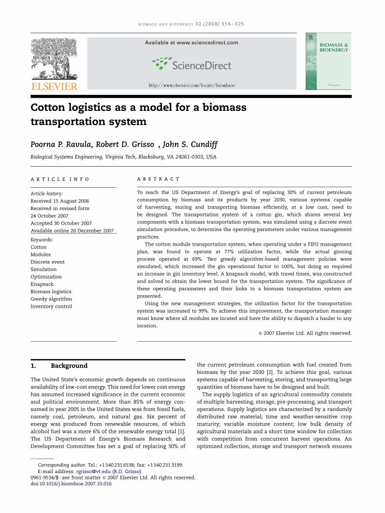
Fig. 6 shows the number of modules processed by the gin on

any given day. Once the inventory level reached zero, the gin

stopped processing modules and the gin did not restart until

the inventory level reached 100 modules. A time interval when

both inventory and module call-in rates were low is repre-

sented by a long delay before ginning started (days 41–46).

There were 5 days in which the gin did better than expected

and processed in excess of 50 modules (Max ¼ 55 modules).

Although this is not a common occurrence, the gin had in the

past processed at these high numbers, especially with low

moisture content modules. The last day for this ginning

season, as predicted by this simulation run, was day 74, and

29 modules were ginned on this last day. The gin was operating

from day 8 until day 74, for a total of 67 d, during which it was

shut down three times, for a total of 14 d.

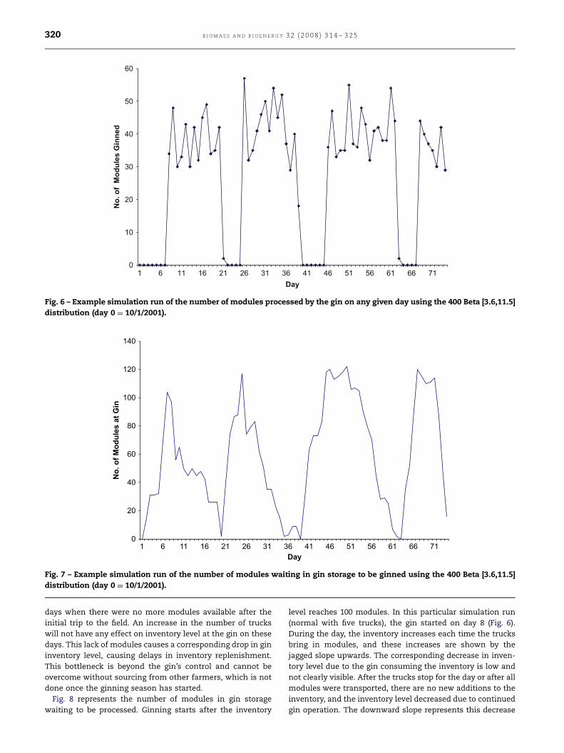
Fig. 7 represents the number of modules waiting in the

fields to be hauled under normal conditions by using five

trucks operating. As the figure shows, there are numerous

processing season under different travel strategies

ck utilizationfactor

Average ginutilization factor

Simulation length(days)

7a (0.63–0.85) 0.69 80a (74–95)

80 (0.71–0.87) 0.66 83 (77–93)

.89 (0.81–1.0) 0.67 83 (73–91)

73 (0.67–0.86) 0.74 74 (64–79)

d values are listed below the average.

ARTICLE IN PRESS

0

10

20

30

40

50

60

1 6 11 16 21 26 31 36 41 46 51 56 61 66 71

Day

No

. o

f M

od

ule

s G

inn

ed

Fig. 6 – Example simulation run of the number of modules processed by the gin on any given day using the 400 Beta [3.6,11.5]

distribution (day 0 ¼ 10/1/2001).

0

20

40

60

80

100

120

140

1 6 11 16 21 26 31 36 41 46 51 56 61 66 71

Day

No

. o

f M

od

ule

s a

t G

in

Fig. 7 – Example simulation run of the number of modules waiting in gin storage to be ginned using the 400 Beta [3.6,11.5]

distribution (day 0 ¼ 10/1/2001).

B I O M A S S A N D B I O E N E R G Y 3 2 ( 2 0 0 8 ) 3 1 4 – 3 2 5320

days when there were no more modules available after the

initial trip to the field. An increase in the number of trucks

will not have any effect on inventory level at the gin on these

days. This lack of modules causes a corresponding drop in gin

inventory level, causing delays in inventory replenishment.

This bottleneck is beyond the gin’s control and cannot be

overcome without sourcing from other farmers, which is not

done once the ginning season has started.

Fig. 8 represents the number of modules in gin storage

waiting to be processed. Ginning starts after the inventory

level reaches 100 modules. In this particular simulation run

(normal with five trucks), the gin started on day 8 (Fig. 6).

During the day, the inventory increases each time the trucks

bring in modules, and these increases are shown by the

jagged slope upwards. The corresponding decrease in inven-

tory level due to the gin consuming the inventory is low and

not clearly visible. After the trucks stop for the day or after all

modules were transported, there are no new additions to the

inventory, and the inventory level decreased due to continued

gin operation. The downward slope represents this decrease

ARTICLE IN PRESS

0

20

40

60

80

100

120

1 6 11 16 21 26 31 36 41 46 51 56 61 66 71

Day

No

. o

f M

od

ule

s

Fig. 8 – One of the simulation runs of the number of modules waiting in the fields to be hauled (end of workday) using the 400

Beta [3.6,11.5] distribution (day 0 ¼ 10/1/2001).

B I O M A S S A N D B I O E N E R G Y 3 2 ( 2 0 0 8 ) 3 1 4 – 3 2 5 321

in inventory at the gin. The flat lines represent days in which

no ginning took place as the inventory level was below 100

modules.

5. Knapsack formulations

Fig. 6 shows long periods of time when there were no modules

to be hauled from the fields. All five module haulers remain

idle during this time. This bottleneck should not exist in a

biomass transportation system. To understand the effect of a

process without this bottleneck, a knapsack model [35] was

constructed and solved to optimality. The model assumed

that all 2000 modules were available for pickup at the

beginning of ginning season (t ¼ 0). The optimal transporta-

tion schedule, and minimum number of days module haulers

needed to move all 2000 modules into gin storage, was

calculated.

Variables used:

yi ¼ 1, if truck is scheduled to haul load on day 1

¼ 0 otherwise

n ¼ total number of modules

wj ¼ travel time to pickup module j, j ¼ 1yn

xij ¼ 1, if module i is picked up on day j

¼ 0, otherwise

C ¼ total time available on any given day for hauling

modules

¼ 600 min/day

Objective function: MinPn

j¼1yi

The objective function is to minimize the total number of

days that trucks are scheduled to move modules from the

fields to the gin.

Constraints:

Xn

j¼1

wixijpCyi; i ¼ 1 . . .n. (1)

This constraint forces the total travel time for any day by

the truck to be less than or equal to 600 min if a truck is being

used for that day, or equal to 0 min if no truck is scheduled for

that day:

Xn

j¼1

xij ¼ 1; j ¼ 1 . . .n. (2)

This constraint forces each module to be transported from

the field to the gin exactly once:

xij 2 f0; 1g; i ¼ 1 . . .n; j ¼ 1 . . .n. (3)

This constraint is used to define this variable as binary

yi 2 f0;1g; i ¼ 1 . . .n. (4)

This particular model was constructed for one single truck.

Since all five trucks are identical, the results for one truck can

be used to construct optimal solution for any number of

trucks. Vector xi will provide a list of all modules transported

on day j, with xijwj providing the total travel time on any given

day. This model was coded in AMPL/CPLEX (ILOG, Inc.,

Washington DC Office, 4350 North Fairfax Drive, Suite 800,

Arlington, VA) and run on an IBM machine. Fifty-four days

were needed to transport all 2000 modules from the fields to

the gin in this model when compared to 74 days needed by

the simulation model.

6. Greedy transportation strategies

In a ‘‘greedy’’ algorithm, the algorithm chooses the locally

optimum choice at each stage with the hope of finding

the global optimum [36]. In this management policy, the

ARTICLE IN PRESS

B I O M A S S A N D B I O E N E R G Y 3 2 ( 2 0 0 8 ) 3 1 4 – 3 2 5322

algorithm tries to satisfy inventory demand at the gin by

moving modules that have lowest cycle time. The average

number of modules a truck can deliver to the gin per day is

approximately six. With all five trucks operating, the gin

receives approximately 30–35 modules d�1, depending on

travel times. The gin, on the other hand, processes around

45 modules d�1. This mismatch between these two processes

will quickly deplete the initial 100-module buffer at the

beginning of the season, and the buffer will eventually reach

zero. To reduce the chances of this happening, the threshold

limit at which the gin starts operating was increased. The

cotton-ginning model was simulated with 100, 200, 300, 400

and 500-module threshold before the start of ginning. Of

these different threshold levels, only 500 modules in initial

storage operated the gin without running out of modules. Five

hundred modules are around 25% of the total number of

modules processed per season. Maintaining such a large

inventory, although feasible, is expensive. One way to reduce

this inventory storage requirement is by using a greedy

algorithm-based transport strategy.

6.1. Greedy algorithm, ‘‘shortest first’’

In a greedy transportation plan, modules with the smallest

travel times are transported first. This allows the gin to reach

its operating threshold of 100 modules quickly and maintain

that level early in the season without much trouble.

Eventually, the inventory level drops off as modules have

longer transport time and the gin runs out of modules.

However, this event will occur during the latter part of the

season, where the management can adopt a better policy to

reduce gin shutdown (for example, operate gin for 12 h d�1

instead of 24 h d�1). The simulation model was modified to

Fig. 9 – Module inventory level at the g

remove event ‘‘MCall’’ and was replaced by a dataset contain-

ing modules, sorted in ascending order by their travel times.

Each time a truck was scheduled, the module with the

smallest travel time was assigned to the truck.

Fig. 9 shows a graph of inventory level at the gin for a greedy

transportation plan. As expected, the number of modules

rises very quickly and the gin operates at 100% efficiency.

During the end of processing season, the gin’s inventory is

depleted twice. Both times, the gin waits until inventory

reaches 100 modules before it restarts. Fig. 10 shows the

number of modules ginned when using this policy.

6.2. Greedy algorithm, ‘‘longest first, shortest second’’

An alternate greedy algorithm, in which modules with

the largest travel time were moved first to satisfy some part

of the gin’s initial inventory, was also examined. That is, if the

ginning threshold is set at 250 modules, move those 100

modules with the largest travel time first and then start

moving based on ‘‘Shortest First’’ policy. It was expected that

by rescheduling the smaller travel time module pickups later

in the simulation run, the transportation system should not

have any problems transporting enough modules to keep the

inventory level above zero. The simulation model’s dataset

was rearranged such that the initial 100 modules were

modules with highest travel times and the rest of the order

was left unchanged, the ‘‘Shortest First’’ model was used.

Fig. 11 shows the gin’s inventory level when the threshold

was moved to 250 modules and the greedy policy modified.

With this strategy, the gin has sufficient modules to operate at

100%. Fig. 12 shows the number of modules ginned per day

using this policy. The gin starts processing modules later

(15 vs. 3 d) than under any other management policy and

in, Greedy Policy, ‘‘Shortest First’’.

ARTICLE IN PRESS

0

10

20

30

40

50

60

1 3 5 7 9 11 13 15 17 19 21 23 25 27 29 31 33 35 37 39 41 43 45 47 49 51 53 55 57 59 61 63

Day

Mo

du

les

Pro

ce

ss

ed

Fig. 10 – Number of modules processed by the gin on any given day, Greedy Policy, ‘‘Shortest First’’.

Fig. 11 – Module inventory level at the gin, Greedy Policy, ‘‘Longest First, Shortest Second’’.

B I O M A S S A N D B I O E N E R G Y 3 2 ( 2 0 0 8 ) 3 1 4 – 3 2 5 323

finishes ginning at the same time as ‘‘Shortest First’’ manage-

ment policy.

7. Cotton logistics correlated with biomasslogistics

Biomass logistics involves hauling baled grasses from

on-farm storage to a central plant which uses several compo-

nents or subsystems that are similar to the transportation

system for cotton modules. A concept has been proposed [37]

whereby multiple round bales of grass hay are compacted into a

module, which becomes the handling/transportation unit. The

round bales are modularized to produce a package that

achieves the same handling advantages as the cotton module.

But, there are four key differences that need to be considered

when drawing inferences between the two logistics systems.

1.

In cotton logistics, one cotton module is considered as one

unit load and each truck can transport one unit, thus, one

module and one truck can be used interchangeably. In the

case of biomass, there may be more than one module

ARTICLE IN PRESS

0

10

20

30

40

50

60

1 3 5 7 9 11 13 15 17 19 21 23 25 27 29 31 33 35 37 39 41 43 45 47 49 51 53 55 57 59 61 63

Day

Mo

du

les g

inn

ed

Fig. 12 – Number of modules processed by the gin on any given day under Greedy Policy, ‘‘Longest First, Shortest Second’’.

B I O M A S S A N D B I O E N E R G Y 3 2 ( 2 0 0 8 ) 3 1 4 – 3 2 5324

loaded onto a single truck and therefore one unit load is

not the same as seen in cotton logistics. For simulating

biomass transport, it will suffice to model one truckload as

one unit and not consider individual bales of hay except

during load/unload. Current biomass logistics systems

load/unload bales individually. This process is cumber-

some and on-going research is investigating concepts

that will reduce the load/unload times. The proposed

concept [37] calls for the multi-bale module to be loaded

and ready for the truck when it arrives at the temporary

storage site. The goal is to load the truck in 10 min,

which compares with a load/unload time of less than

5 min for a cotton module. The cotton gin data includes

this load/unload time in the truck travel time. No effort

was made to separate on-road time and load/unload time

because this step takes so little time and does not affect

simulation results in any significant way. But, the load/

unload time is significant in biomass logistics due to large

volume of trucks and could lead to a potential bottleneck.

2.

Current simulation of cotton logistics shows that, when

operating under ideal conditions, truck utilization and

therefore gin utilization are constrained by module call-in

rates (FIFO strategy), as this dictates availability of modules

to be hauled. Fig. 7 shows that the hauling operation

‘‘catches-up’’ with modules waiting to be hauled and no

modules are available to be transported. Under a biomass

system, the amount of biomass accumulated in the

temporary storage will be known, and hauling optimization

can be achieved. The hauling operation will not ‘‘catch-up’’

and trucks can be operated at maximum utilization. This

characteristic may help schedule trucks efficiently and has

to be explored when simulating biomass systems.

3.

This simulation model assumes that there are no limita-

tions on the number of modules that can be stored at

the gin. When considering a biomass system, there are

practical and economic limits on the size of storage at the

conversion plant, which will dictate maximum storage

(inventory) level. The advantages of ‘‘just-in-time’’ feed-

stock delivery are substantial.

4.

A cotton gin is a mechanical process in that it can be started

and stopped without significant effort or economic penalty.

A biomass conversion plant is a chemical process. The cost

penalty for starting and stopping the production flow is much

greater; therefore, the penalty for running out of feedstock is

much higher for a biomass plant than a cotton gin.

8. Conclusion

A case study was done on a gin in Emporia, VA, which uses

five trucks to haul modules. Using current practices, the truck

utilization factor was 77% and the gin utilization factor was

69%. Cost figures from the gin are not available, but the cost of

operating the gin is believed to be significantly greater than

the cost to operate the fleet of trucks, therefore, a reduction of

truck fleet was not recommended.

The current gin logistics are constrained by the FIFO policy,

and there is limited opportunity to increase truck utilization

percentages during the harvest season. If there was an

opportunity to select which modules to haul, then a knapsack

model can be formulated and the solution would increase the

truck utilization and reduce overall truck requirements.

Decreasing truck cycle time did not increase the truck

utilization factor significantly, since module call-in rates

currently constrain truck utilization rates. To achieve an

increase in the utilization factor, more modules have to be

available. This means that the customer base has to be

increased from current levels, or the gin waits until sufficient

modules are available before hauling starts. In general,

greater annual throughout reduces per-bale ginning costs.

ARTICLE IN PRESS

B I O M A S S A N D B I O E N E R G Y 3 2 ( 2 0 0 8 ) 3 1 4 – 3 2 5 325

The modified greedy algorithm provided a better gin utiliza-

tion factor than any other management plan. The modified

greedy algorithm also reduced the initial at-plant storage to

operate the gin continuously, from 500 to 250 modules.

There are several components or subsystems of the trans-

portation system for a cotton gin that a biomass system can

emulate. While differences do exist, the system analysis of

cotton gin operations can be useful for determining operating

parameters for potential biomass transportation systems.

R E F E R E N C E S

[1] Department of Energy. Annual energy review. Superinten-dent of Documents, Pittsburgh, PA.

[2] Department of Energy. Billion tons program. Office of Scientificand Technical Information, Oak Ridge, TN. Online at: /http://www1.eere.energy.gov/biomass/pdfs/final_billionton_vision_report2.pdfS (19/10/07).

[3] Dıaz JA, Perez IG. Simulation and optimization of sugar canetransportation in harvest season. In: Winter simulationconference, proceedings of the 32nd conference on wintersimulation, vol. 3, 2000. p. 1114–7.

[4] Semezato R. A simulation study of sugar cane harvesting.Agricultural Systems 1995;47:427–37.

[5] Semezato R, Lozano S, Valero R. A discrete event simulationof sugar cane harvesting operations. Journal of the Opera-tional Research Society 1995;46:1073–8.

[6] Salassi ME, Garcia M, Breaux JB, No SC. Impact of sugarcanedelivery schedule on product value at raw sugar factories.Journal of Agribusiness 2004;22(1):61–75.

[7] Hansen AC, Barnes AJ, Lyne PWL. Simulation modeling ofsugarcane harvest-to-mill delivery systems. Transactions ofthe ASAE 2002;45(3):531–8.

[8] Harrison D, Johnson J. How many? How far? A study ofmodule truck costs. In: 2007 Beltwide cotton conference, NewOrleans, LA, January 9–12, 2007.

[9] Tatsiopoulos IP, Tolis AJ. Economic aspects of the cotton-stalkbiomass logistics and comparison of supply chain methods.Biomass and Bioenergy 2003;24(3):199–214.

[10] Allen J, Browne M, Hunter A, Boyd J, Palmer H. Logisticsmanagement and costs of biomass fuel supply. InternationalJournal of Physical Distribution and Logistics Management1998;28(6):463–77.

[11] De Mol RM, Jogems MAH, Van Beek P, Gigler JK. Simulationand optimization of the logistics of biomass fuel collection.Netherlands Journal of Agricultural Science 1997;45:219–28.

[12] Dunnett A, Agjiman C, Shah N. Biomass to heat supplychains applications of process optimization. Transactions ofthe Institution of Chemical Engineers: Process Safety andEnvironmental Protection 2007;85(B5):419–29.

[13] Mukunda A, Ileleji KE, Wan H. Simulation of corn stoverlogistics from on-farm storage to an ethanol plant. ASABEmeeting paper no. 066177. St. Joseph, MI: ASABE; 2006.

[14] Kumar A, Sokhansanj S. Switchgrass (Ppanicum vigratum, L.)delivery to a biorenery using integrated biomass supplyanalysis and logistics (IBSAL) model. Bioresource Technology2007;98:1033–44.

[15] Sokhansanj S, Turhollow AF. Baseline cost for corn stovercollection. Applied Engineering in Agriculture2002;18(5):525–30.

[16] Sokhansanj S, Kumar A, Turhollow AF. Development andimplementation of integrated biomass supply analysis andlogistics model (IBSAL). Biomass and Bioenergy 2006;30:838–47.

[17] Cundiff JS. Simulation of five large round bale harvestingsystems for biomass. Bioresource Technology 1996;56:77–82.

[18] Cundiff JS, Dias N, Sherali H. A liner programming approachfor designing an herbaceous biomass delivery system.Bioresource Technology 1997;59:47–55.

[19] Epplin FM. Cost to produce and deliver switchgrass biomassto an ethanol-conversion facility in the southern plains ofthe United States. Biomass and Bioenergy 1996;11(6):459–67.

[20] Nilsson D. Dynamic simulation of straw harvesting systems:influence of climatic, geographical factors on performanceand costs. Journal of Agricultural Engineering Research2000;76(1):27–36.

[21] Nilsson D, Hansson PA. Influence of various machinerycombinations, fuel proportions and storage capacitieson costs for co handling of straw and reed canary grassto district heating plants. Biomass and Bioenergy2001;20(4):247–60.

[22] Nilsson D. Dynamic simulation of the harvest operations offlax straw for short fibre production—part 1: model descrip-tion. Journal of Natural Fibers 2006;3(4):23–34.

[23] Nilsson D. Dynamic simulation of the harvest operations offlax straw for short fibre production—part 2: simulationresults. Journal of Natural Fibers 2006;3(4):43–57.

[24] Popp M, Hogan R. Assessment of two alternative switchgrassharvest and transport methods. Farm foundation confer-ence, St. Louis, Missouri, April 12–13, 2007. /http://www.farmfoundation.org/projects/documents/PoppSwitchgrassModulesSSnonumbers.pdfS (accessedon 18/10/07).

[25] McLaughlin SB, Kszos LA. Development of switchgrass(Panicum virgatum, L.) as a bioenergy feedstock in the UnitedStates. Biomass and Bioenergy 2005;28:515–35.

[26] Bransby DI, Smith HA, Taylor CR, Duffy PA. Switchgrassbudget model: an interactive budget model for producing anddelivering switchgrass to a bioprocessing plant. IndustrialBiotechnology 2005;1(2):122–5.

[27] Raula PR, Grisso RD, Cunduff JC. Comparison between two policystrategies for scheduling in a biomass logistic system. Biore-source Technology, in press, doi:10.1016/j.biortech.2007.10.044.

[28] Berruto R, Ess D, Maier DE, Dooley F. Network simulation ofcrop harvesting and delivery from farm field to commercialelevator. In: Quick GR, editor. Electronic proceedings of theinternational conference on crop harvesting and processing,Louisville, Kentucky, USA: ASAE Publication #701P1103e; 9–11February 2003.

[29] Kumar A, Cameron JB, Flynn PC. Pipeline transport andsimultaneous saccharification of cover stover. BioresourcesTechnology 2005;96:819–29.

[30] Maseraa O, Ghilardia A, Drigob R, Trosserob MA. WISDOM:a GIS-based supply demand mapping tool for woodfuelmanagement. Biomass and Bioenergy 2006;30:618–37.

[31] Moller B, Nielsen PS. Analysing transport costs of Danishforest wood chip resources by means of continuous costsurfaces. Biomass and Bioenergy 2007;31:291–8.

[32] Polagyea BL, Hodgson KT, Malte PC. An economic analysis ofbio-energy options using thinnings from overstocked forests.Biomass and Bioenergy 2007;31:105–25.

[33] Simsa REH, Venturi P. All-year-round harvesting of shortrotation coppice eucalyptus compared with the deliveredcosts of biomass from more conventional short season,harvesting systems. Biomass and Bioenergy 2004;26:27–37.

[34] Hartman E. Personal communication (01/08/05), Mid AtlanticGin, 1378 Southampton Pkwy, Emporia, VA.

[35] Bazarra MS, Jarvis JJ, Sherali HD. Linear programming andnetwork flows. 2nd ed. New York: Wiley; 1990.

[36] Cormen TH, Leiserson CE, Rivest RL, et al. Introduction toalgorithms. 2nd ed. New York: McGraw-Hill Companies; 2001.

[37] Cundiff, JS, Grisso RD, Ravula PP. Management system forbiomass delivery at a conversion plant. ASAE/CSAE meetingpaper no. 046169. St. Joseph, MI: ASAE; 2004.